A Revisit of Internet of Things Technologies for Monitoring and ...
Upload
khangminh22Category
view
4download
0
Correlation Management and Search
for the Internet of Things
Ali Shemshadi
School of Computer Science
The University of Adelaide
This dissertation is submitted for the degree of
Doctor of Philosophy
Supervisors: Prof. Michael Sheng
September 2016

© Copyright by
Ali Shemshadi
September 2016
All rights reserved.
No part of the publication may be reproduced in any form by print, photoprint, microfilm or
any other means without written permission from the author.

To my mother and father,
my wife and my two little princes,
my brother and sister,
who made all of this possible,
for their endless encouragement and patience.


Declaration
I certify that this work contains no material which has been accepted for the award of any
other degree or diploma in my name, in any university or other tertiary institution and, to the
best of my knowledge and belief, contains no material previously published or written by
another person, except where due reference has been made in the text. In addition, I certify
that no part of this work will, in the future, be used in a submission in my name, for any other
degree or diploma in any university or other tertiary institution without the prior approval
of the University of Adelaide and where applicable, any partner institution responsible for
the joint-award of this degree. I give consent to this copy of my thesis, when deposited
in the University Library, being made available for loan and photocopying, subject to the
provisions of the Copyright Act 1968. I also give permission for the digital version of my
thesis to be made available on the web, via the University’s digital research repository, the
Library Search and also through web search engines, unless permission has been granted by
the University to restrict access for a period of time.
Ali Shemshadi
September 2016


Acknowledgements
I could not have arrived at this point without the help and support of my peers, supervisors,
instructors, friends and of course, my family. I found the experience of working with the
school, staff and students at the University of Adelaide to be both joyful and fruitful and
thus, I would like to thank all of these people, who made my PhD journey such a great
experience. Firstly, I owe a sincere gratitude towards my supervisor, Prof. Michael Sheng,
a compassionate teacher, a hard-working researcher and an outstanding supervisor. His
motto from the early days of my graduate study was “aim high and never compromise"
keeps me inspired and motivated. This success was due to his devotion to his students,
which is exemplary and unique. His kind personality made me rethink about the offers from
other institutions and thoroughly changed my life and career path towards a highly positive
direction. Secondly, I would like to thank my co-supervisors, Prof. Zbigniew Michalewicz
and Prof. Hong Shen for their supports before and throughout my post-graduate study.
I am blessed to find the opportunity to befriend with many fellow colleagues in our
research group. I appreciate every minute that I had the opportunity to be with them. In
particular, I would like to acknowledge Dr. Yongrui Qin, Dr. Lina Yao and Ms. Wei Emma
Zhang. It was such a pleasure for me to collaborate with and learn from them. Furthermore,
I would like to thank the staff at Xively, the IoT platform for sharing their data.
Lastly, but not the least, I owe a huge debt of gratitude to my mother, my father, my wife,
my both princes, my brother and my sister for their patience, encouragement and support
without which, I could not be successful at any point of time in the past, present and future.


Abstract
The Internet of Things (IoT) is a compelling paradigm, which aims to enable everyday
physical things embedded with electronics, software, sensors, and network connectivity to
collect and exchange data on the Internet. It is anticipated that by 2020, billions of things get
connected to the Internet. Creating future IoT search engines is a key step towards unlocking
answering the above question. Future search engines can potentially in revolutionise various
applications in different domains. Existing approaches for searching the IoT use simple
techniques to obtain a list of things for a query. The state of the art needs to be improved
in different aspects. For instance, it is often disregarded that in the context of IoT, we have
two types of users including machines and human users. In addition, many have complained
about the absence of the real-world IoT data. Unsurprisingly, a common question that arises
regularly nowadays is “Does the IoT already exist?”. So far, little has been known about
the real-world situation on IoT, its attributes, the presentation of data and user interests.
Moreover, existing approaches also disregard the attribute based correlations between things
in the real-world. In this dissertation, we review the state of the art in IoT search domain and
propose a novel framework to collect and analyse IoT data. Our system is also able to resolve
IoT queries based on the knowledge that is acquired from the IoT data sources. Furthermore,
we introduce a novel technique to extract the correlations between things. Our framework is
capable of using the correlations to improve the quality of search results for both types of
users. We investigate the scalability and the effectiveness of our approach using large scale
and real-world datasets. Moreover, we investigate two case studies in transport systems in

x
our research. The first case study, challenges the complex problem of taxi ridesharing in the
context of smart cities. The second case study, involves a real-time prediction method for
flight delays based on the IoT sourced data.

Table of contents
List of figures xvii
List of tables xxi
1 Introduction 1
1.1 Motivating Scenario . . . . . . . . . . . . . . . . . . . . . . . . . . . . . . 3
1.2 Research Issues . . . . . . . . . . . . . . . . . . . . . . . . . . . . . . . . 7
1.3 Contributions Overview . . . . . . . . . . . . . . . . . . . . . . . . . . . . 9
1.3.1 Data Collection . . . . . . . . . . . . . . . . . . . . . . . . . . . . 10
1.3.2 Correlation Discovery . . . . . . . . . . . . . . . . . . . . . . . . 10
1.3.3 Diversified Query Resolution . . . . . . . . . . . . . . . . . . . . . 11
1.3.4 Pattern Matching for Correlation Graphs . . . . . . . . . . . . . . 11
1.3.5 Intent-Oriented Search:Taxi Ridesharing . . . . . . . . . . . . . . 12
1.3.6 A Crawling and Search Engine . . . . . . . . . . . . . . . . . . . . 12
1.4 Dissertation Publications . . . . . . . . . . . . . . . . . . . . . . . . . . . 12
1.5 Dissertation Organization . . . . . . . . . . . . . . . . . . . . . . . . . . . 15
2 Crawling the IoT Data 19
2.1 Where is the IoT? . . . . . . . . . . . . . . . . . . . . . . . . . . . . . . . 22
2.1.1 Cloud Based IoT Platforms . . . . . . . . . . . . . . . . . . . . . . 22
2.1.2 WoT Enabled Platforms . . . . . . . . . . . . . . . . . . . . . . . 24
xii Table of contents
2.1.3 Web Mapping Enabled Data Sources . . . . . . . . . . . . . . . . 24
2.2 IoT Data Acquisition . . . . . . . . . . . . . . . . . . . . . . . . . . . . . 25
2.2.1 Identification of Data Sources . . . . . . . . . . . . . . . . . . . . 27
2.2.2 IoT Data Collection . . . . . . . . . . . . . . . . . . . . . . . . . . 28
2.3 IoT Data Analysis . . . . . . . . . . . . . . . . . . . . . . . . . . . . . . . 30
2.3.1 User Interests . . . . . . . . . . . . . . . . . . . . . . . . . . . . . 30
2.3.2 IoT Data Characteristics . . . . . . . . . . . . . . . . . . . . . . . 32
2.3.3 IoT vs. User Interests . . . . . . . . . . . . . . . . . . . . . . . . . 44
2.4 Discussions . . . . . . . . . . . . . . . . . . . . . . . . . . . . . . . . . . 45
2.4.1 Challenges in IoT Data Discovery . . . . . . . . . . . . . . . . . . 45
2.4.2 Information Retrieval in IoT . . . . . . . . . . . . . . . . . . . . . 46
2.4.3 Other Challenges . . . . . . . . . . . . . . . . . . . . . . . . . . . 47
2.5 Related Work . . . . . . . . . . . . . . . . . . . . . . . . . . . . . . . . . 49
2.6 Summary . . . . . . . . . . . . . . . . . . . . . . . . . . . . . . . . . . . 51
3 Interlinking IoT Resources 53
3.1 The CEIoT Approach . . . . . . . . . . . . . . . . . . . . . . . . . . . . . 56
3.1.1 Correlation Discovery Process . . . . . . . . . . . . . . . . . . . . 57
3.1.2 Framework Architecture and System Entities . . . . . . . . . . . . 57
3.1.3 Correlation Extraction . . . . . . . . . . . . . . . . . . . . . . . . 61
3.1.4 Correlation Representation . . . . . . . . . . . . . . . . . . . . . . 64
3.2 Experimental Results . . . . . . . . . . . . . . . . . . . . . . . . . . . . . 66
3.2.1 System Performance . . . . . . . . . . . . . . . . . . . . . . . . . 68
3.2.2 Things Correlation Graph . . . . . . . . . . . . . . . . . . . . . . 72
3.2.3 Message Volume . . . . . . . . . . . . . . . . . . . . . . . . . . . 72
3.3 Related Work . . . . . . . . . . . . . . . . . . . . . . . . . . . . . . . . . 73
3.4 Summary . . . . . . . . . . . . . . . . . . . . . . . . . . . . . . . . . . . 74

Table of contents xiii
4 Pattern Matching for Things Correlation Graphs 77
4.1 Problem Formulation . . . . . . . . . . . . . . . . . . . . . . . . . . . . . 82
4.2 The Naive Approach . . . . . . . . . . . . . . . . . . . . . . . . . . . . . 83
4.3 Background . . . . . . . . . . . . . . . . . . . . . . . . . . . . . . . . . . 85
4.3.1 Markov Chains . . . . . . . . . . . . . . . . . . . . . . . . . . . . 85
4.3.2 Markov Chain Monte-Carlo . . . . . . . . . . . . . . . . . . . . . 87
4.4 Pattern Matching . . . . . . . . . . . . . . . . . . . . . . . . . . . . . . . 88
4.4.1 Identifying Matches . . . . . . . . . . . . . . . . . . . . . . . . . 89
4.4.2 Top-k Matches . . . . . . . . . . . . . . . . . . . . . . . . . . . . 93
4.5 Experimental Evaluation . . . . . . . . . . . . . . . . . . . . . . . . . . . 96
4.5.1 Experimental Setting . . . . . . . . . . . . . . . . . . . . . . . . . 96
4.5.2 Efficiency . . . . . . . . . . . . . . . . . . . . . . . . . . . . . . . 100
4.5.3 Discussion . . . . . . . . . . . . . . . . . . . . . . . . . . . . . . 105
4.6 Related Work . . . . . . . . . . . . . . . . . . . . . . . . . . . . . . . . . 107
4.7 Summary . . . . . . . . . . . . . . . . . . . . . . . . . . . . . . . . . . . 109
5 Diversifying Top-k Query Matches 111
5.1 Problem Statement . . . . . . . . . . . . . . . . . . . . . . . . . . . . . . 114
5.1.1 Problem Formulation . . . . . . . . . . . . . . . . . . . . . . . . . 114
5.1.2 Methodology . . . . . . . . . . . . . . . . . . . . . . . . . . . . . 116
5.2 ECS Approach . . . . . . . . . . . . . . . . . . . . . . . . . . . . . . . . 117
5.2.1 TCG Construction . . . . . . . . . . . . . . . . . . . . . . . . . . 117
5.2.2 Clustering . . . . . . . . . . . . . . . . . . . . . . . . . . . . . . . 118
5.2.3 Selection . . . . . . . . . . . . . . . . . . . . . . . . . . . . . . . 120
5.3 Experimental Results . . . . . . . . . . . . . . . . . . . . . . . . . . . . . 122
5.3.1 Datasets . . . . . . . . . . . . . . . . . . . . . . . . . . . . . . . . 123
5.3.2 Results . . . . . . . . . . . . . . . . . . . . . . . . . . . . . . . . 130
xiv Table of contents
5.4 Related Work . . . . . . . . . . . . . . . . . . . . . . . . . . . . . . . . . 133
5.4.1 Search Based on Social Relationships . . . . . . . . . . . . . . . . 133
5.4.2 IoT Search Engines . . . . . . . . . . . . . . . . . . . . . . . . . . 134
5.5 Summary . . . . . . . . . . . . . . . . . . . . . . . . . . . . . . . . . . . 136
6 Intent Based Search: A Case Study in Taxi Ridesharing 137
6.1 Preliminaries . . . . . . . . . . . . . . . . . . . . . . . . . . . . . . . . . 143
6.1.1 Problem Definition . . . . . . . . . . . . . . . . . . . . . . . . . . 143
6.1.2 Design Basics . . . . . . . . . . . . . . . . . . . . . . . . . . . . . 145
6.2 Background: IS vs. DS Approach . . . . . . . . . . . . . . . . . . . . . . 151
6.3 The TRIPS Framework . . . . . . . . . . . . . . . . . . . . . . . . . . . . 153
6.3.1 Traffic Modeling Layer . . . . . . . . . . . . . . . . . . . . . . . . 156
6.3.2 TRIPS Application Layer . . . . . . . . . . . . . . . . . . . . . . 157
6.3.3 Distribution Management Layer . . . . . . . . . . . . . . . . . . . 162
6.4 Experiment . . . . . . . . . . . . . . . . . . . . . . . . . . . . . . . . . . 163
6.4.1 The Dataset . . . . . . . . . . . . . . . . . . . . . . . . . . . . . . 163
6.4.2 Performance . . . . . . . . . . . . . . . . . . . . . . . . . . . . . 164
6.4.3 Cost Savings . . . . . . . . . . . . . . . . . . . . . . . . . . . . . 167
6.4.4 Comparison with Other Solutions . . . . . . . . . . . . . . . . . . 169
6.5 Related Work . . . . . . . . . . . . . . . . . . . . . . . . . . . . . . . . . 170
6.5.1 Dynamic Ridesharing . . . . . . . . . . . . . . . . . . . . . . . . . 170
6.5.2 Travel Time Estimation . . . . . . . . . . . . . . . . . . . . . . . . 172
6.5.3 Uncertainty in Spatio-Temporal Data . . . . . . . . . . . . . . . . 173
6.6 Summary . . . . . . . . . . . . . . . . . . . . . . . . . . . . . . . . . . . 174
7 ThingSeek: An Enriched Interface for IoT Search Engine 177
7.1 ThingSeek: An Overview . . . . . . . . . . . . . . . . . . . . . . . . . . . 179
Table of contents xv
7.1.1 ThingSeek Crawler Engine . . . . . . . . . . . . . . . . . . . . . . 179
7.1.2 Query Results Preparation . . . . . . . . . . . . . . . . . . . . . . 182
7.2 Demonstration . . . . . . . . . . . . . . . . . . . . . . . . . . . . . . . . . 184
7.2.1 Crawling an IoT Data Source . . . . . . . . . . . . . . . . . . . . 185
7.2.2 IoT Search by Human Users . . . . . . . . . . . . . . . . . . . . . 185
7.2.3 IoT Search by Smart Machines . . . . . . . . . . . . . . . . . . . . 186
7.3 ThingSeek in Application: Flight Delay Analysis . . . . . . . . . . . . . . 187
7.3.1 Model Features . . . . . . . . . . . . . . . . . . . . . . . . . . . . 187
7.3.2 Feature Analysis Results . . . . . . . . . . . . . . . . . . . . . . . 187
7.4 Related Work . . . . . . . . . . . . . . . . . . . . . . . . . . . . . . . . . 192
7.5 Summary . . . . . . . . . . . . . . . . . . . . . . . . . . . . . . . . . . . 196
8 Conclusion 199
8.1 Summary . . . . . . . . . . . . . . . . . . . . . . . . . . . . . . . . . . . 199
8.2 Future Research . . . . . . . . . . . . . . . . . . . . . . . . . . . . . . . . 202
References 205
Appendix A Curriculum Vitae 223


List of figures
1.1 Motivating scenario for IoT search . . . . . . . . . . . . . . . . . . . . . . 4
2.1 Illustration of the sequential-spatial access to things data . . . . . . . . . . 26
2.2 Ranking of the popular IoT services . . . . . . . . . . . . . . . . . . . . . 31
2.3 Query frequency per day in Thingful . . . . . . . . . . . . . . . . . . . . . 31
2.4 The distribution of things trajectories on a map . . . . . . . . . . . . . . . 33
2.5 The distribution of IoT queries on a map . . . . . . . . . . . . . . . . . . . 34
2.6 Technologies used by IoT platforms . . . . . . . . . . . . . . . . . . . . . 36
2.7 Comparison of the densities of the query logs and IoT data . . . . . . . . . 37
2.8 EMD through time for IoT data sources . . . . . . . . . . . . . . . . . . . 38
2.9 Sensor update percentage . . . . . . . . . . . . . . . . . . . . . . . . . . . 41
3.1 ThingSpeak mashup example . . . . . . . . . . . . . . . . . . . . . . . . . 54
3.2 Correlation discovery process for IoT . . . . . . . . . . . . . . . . . . . . 58
3.3 CEIoT Framework . . . . . . . . . . . . . . . . . . . . . . . . . . . . . . 59
3.4 Search area breakdown . . . . . . . . . . . . . . . . . . . . . . . . . . . . 62
3.5 Multiple correlations example . . . . . . . . . . . . . . . . . . . . . . . . 66
3.6 CEIoT system view . . . . . . . . . . . . . . . . . . . . . . . . . . . . . . 69
3.7 Characteristics of the data set and the final results . . . . . . . . . . . . . . 70
3.8 CLOR graphs for connections with different thresholds . . . . . . . . . . . 71

xviii List of figures
4.1 Example query and data graph . . . . . . . . . . . . . . . . . . . . . . . . 79
4.2 Graphs after removing non-matching edges . . . . . . . . . . . . . . . . . 92
4.3 Visualization of pattern graphs . . . . . . . . . . . . . . . . . . . . . . . . 98
4.4 Results for the total runtime . . . . . . . . . . . . . . . . . . . . . . . . . 100
4.5 Matching results for the first experiment . . . . . . . . . . . . . . . . . . . 101
4.6 Matching results for the second experiment . . . . . . . . . . . . . . . . . 102
4.7 Matching results for the third experiment . . . . . . . . . . . . . . . . . . 103
4.8 Matching results for the synthetic datasets . . . . . . . . . . . . . . . . . . 104
4.9 Comparison with the baseline . . . . . . . . . . . . . . . . . . . . . . . . . 106
5.1 Correlations in IoT . . . . . . . . . . . . . . . . . . . . . . . . . . . . . . 112
5.2 ECS Components . . . . . . . . . . . . . . . . . . . . . . . . . . . . . . . 116
5.3 Distribution of query keywords from Thingful dataset . . . . . . . . . . . . 122
5.4 Visualization of two TCGs . . . . . . . . . . . . . . . . . . . . . . . . . . 126
5.5 Visualization of different selection methods on the trajectory dataset . . . . 127
5.6 Results for weather stations dataset . . . . . . . . . . . . . . . . . . . . . . 128
5.7 Distribution of 3D location data for weather stations . . . . . . . . . . . . . 129
5.8 Experimental results for IoT search results diversification . . . . . . . . . . 131
6.1 Intent-based search in ridesharing scenario . . . . . . . . . . . . . . . . . . 140
6.2 Extended search areas for a query . . . . . . . . . . . . . . . . . . . . . . 145
6.3 Possible schedule sequences for a query . . . . . . . . . . . . . . . . . . . 147
6.4 TRIPS Framework . . . . . . . . . . . . . . . . . . . . . . . . . . . . . . 155
6.5 Symmetric vs. asymmetric extensions of search . . . . . . . . . . . . . . . 158
6.6 Availability of the index for all origins and destinations . . . . . . . . . . . 164
6.7 The results of the experimental evaluation . . . . . . . . . . . . . . . . . . 165
6.8 Effectiveness results . . . . . . . . . . . . . . . . . . . . . . . . . . . . . . 168
List of figures xix
7.1 Architecture of the ThingSeek crawler engine . . . . . . . . . . . . . . . . 180
7.2 Query resolution in ThingSeek . . . . . . . . . . . . . . . . . . . . . . . . 183
7.3 Query resolution for smart things in ThingSeek framework . . . . . . . . . 185
7.4 ThingSeek Web based visualization . . . . . . . . . . . . . . . . . . . . . 186
7.5 Features affecting flight delays from each source . . . . . . . . . . . . . . 188
7.6 Example of the flight records . . . . . . . . . . . . . . . . . . . . . . . . . 190
7.7 Example of the weather records . . . . . . . . . . . . . . . . . . . . . . . 191
7.8 Example of the air quality records . . . . . . . . . . . . . . . . . . . . . . 191
7.9 Delay at departure performance for airlines . . . . . . . . . . . . . . . . . 192
7.10 Delay at departure performance for airports . . . . . . . . . . . . . . . . . 193
7.11 Results of the correlation analysis . . . . . . . . . . . . . . . . . . . . . . 193

List of tables
2.1 Examples of IoT cloud services . . . . . . . . . . . . . . . . . . . . . . . . 24
2.2 Most popular keywords and their categories . . . . . . . . . . . . . . . . . 35
2.3 WoT vs. IoT cloud services . . . . . . . . . . . . . . . . . . . . . . . . . . 36
2.4 Sensor readings from Xively platform . . . . . . . . . . . . . . . . . . . . 39
2.5 Transportation data sources with overlapping set of objects . . . . . . . . . 43
3.1 Requirements of traditional WWW hyperlinks vs. novel IoT-links . . . . . 54
4.1 The set of label assignments . . . . . . . . . . . . . . . . . . . . . . . . . 79
4.2 Nodes with label similarity above threshold . . . . . . . . . . . . . . . . . 80
4.3 Mapping of the edges of G to edges in the query graph Q . . . . . . . . . . 93
4.4 Index construction summary for different datasets . . . . . . . . . . . . . . 99
5.1 Object data structure for taxi trajectories dataset . . . . . . . . . . . . . . . 124
5.2 Object data structure for weather stations dataset . . . . . . . . . . . . . . 124
6.1 List of important notations . . . . . . . . . . . . . . . . . . . . . . . . . . 146
6.2 Taxi speed estimation based on GPS reading analysis . . . . . . . . . . . . 170
7.1 Feature description for flight delay search . . . . . . . . . . . . . . . . . . 189


Chapter 1
Introduction
The Internet of Things (IoT) is a novel paradigm which escalates the data transfer on the
Internet by interconnecting the sensors and actuators of physical things in a global scale.
The IoT has progressively evolved over recent years in terms of enabling technologies,
applications, architectures and scope. Due to its broad spectrum of applications, there are
many visions for the IoT paradigm in the literature. Kevin Ashton, a co-founder of MIT
Auto-ID Center, coined the name IoT by imagining on extension of the Internet to the
physical world [1]. In the last decade, a variety of novel visions have been depicted for IoT
applications [2]. Atzori et al. [3] distinguish three types of categories for IoT visions including
things oriented, Internet oriented and semantic oriented approaches. As reviewed by other
surveys in this area, the IoT concept definition revolves around its two main keywords, Things
and the Internet [4–6, 2]. Thus, overall, we view the IoT concept as Internet connected
swarm of uniquely identifiable virtual and physical sensors, where each sensor belongs to a
physical object.
Observations and predictions demonstrate promising growth for IoT in the near future. In
2015, Gartner placed IoT on the peak of its Hype Cycle [7], predicting that it will reach the
Plateau of Productivity of the cycle within 5-10 years. McKinsey Global Institute identifies
IoT as one of the top twelve technologies whose solid disruptive economic impact will trigger

2 Introduction
profound changes in our daily lives, as well as the global economy [8]. Nowadays, IoT
is growing at a dazzling speed, as predictions show that billions of devices will become
connected to the Internet by 2020 [9, 10]. Progressively, IoT is gaining attention in many
application domains such as the Industrial Internet [11–15], Environmental Monitoring [16,
17], Smart Cities [18–20] and Health Management [21].
Given the accelerated adoption of the IoT, effective searching is still considered as one of
the key challenges for the deployment of IoT in real-world application domains. Efficient and
effective discovery of things is described as one of the main challenges in the establishment
of the IoT [22, 2]. The heterogeneity of the things, highly dynamic environment and the
lack of standards increase the complexity of IoT search. Based on Chen et al. [23], with
the emergence of IoT, people will no longer be the only producers and consumers of the
big data on the Internet. As a result, current online platforms must transform to effectively
and efficiently support the emerging network of heterogeneous network of people and
things. In particular, a number of important strategies need to be devised to provide useful
results from searching the IoT. According to Yao et al. [24] the traditional postactive search
paradigms would no longer be sufficiently effective to fully utilize the potential of the IoT
to extract useful information from sensory data. Thus, rather than traditional postactive
approaches, a proactive approach will be more suitable. Due to the scale, heterogeneity and
the complexity of IoT, devising effective proactive discovery strategies requires enormous
computing infrastructure in addition to significant user contribution, which cannot be justified
in terms of costs and benefits. Ultimately, the goal is to enable machines to seamlessly
facilitate the so called self adaptable zero-touch management and analysis of the streaming
IoT data [25].
An efficient and effective platform for crawling, processing and searching the IoT data
should: (i) extract data from heterogeneous sensory data sources on the Internet; (ii) load,
transform and interpret the data according to its context [26]; (iii) extract and manipulate
1.1 Motivating Scenario 3
correlations between things [27]; and (iv) be scalable to enable real-time processing of IoT
data.
This chapter is organized as follows. In Section 1.1, we illustrate a motivating sce-
nario, from which we will draw sub-scenarios as examples throughout this dissertation. In
Section 1.2, we outline research issues that are tackled in our dissertation. In Section 1.3,
we summarize our contributions in addressing the research issues and in Section 1.4, we
enumerate the publications by the author that are related to this work. Finally, in Section 1.5,
we describe the structure of this dissertation.
1.1 Motivating Scenario
In this dissertation, we work on tackling a number of research issues in searching and
management of IoT with focus on transport systems and environmental monitoring. Although
different parts of our approach are deployed for different scenarios and case studies in our
work, we use this motivating scenario as a generic example, from which we define sub-
scenarios in each chapter of this dissertation.
Figure 1.1 illustrates our motivating scenario. In our scenario, we focus on two types of
users including smart devices and human users. Specifically, two types of search queries can
be identified in this scenario, which are described as follows:
• Correlation based search: based on Yao et al. [24], searching and recommending
things using heterogeneous correlations is a promising and interesting trend in IoT
research. This type of search queries can be used by both smart devices and human
clients to find the things of interest.
• Intent based search: another trend in IoT research emphasizes the role of the knowl-
edge that is acquired from things in real-world applications. Ragget proposes intent
based search as a promising research opportunity for IoT search [28]. Accordingly, this

4 Introduction
Text
Identifying IoT data sources
IoT Data aquisation
Resource management
Users
Interface
Analytics
Crawling
Physical
things
Interface
REST World Wide Web
Indexing Location Ownership Service Descriptions
TCG Pattern Matching Index based search
Intent based indexing
Correlation based search Intent based search
IoT PlatformWeb mapping
Smart devices Human client Bob John
1
2
3
46}
Results diversificationResults
enhancementProbabilistic ordeing5
7
Web of Things
Fig. 1.1 Motivating scenario for IoT search
1.1 Motivating Scenario 5
would provide the footpath for smarter search in IoT. Thus, application specific search
queries can be manipulated to improve the effectiveness of IoT search in application.
Yet, this type of query is mainly useful for human clients only as the knowledge or
domain specific applications cannot be easily deployed by things.
We describe each part of the motivating scenario of Figure 1.1 as follows:
1. Initially, sensor enabled physical things propagate their data such as sensor readings
and meta-data through different mediums on the Internet. This includes, real-time
maps, real time Web pages which use Web of Things (WoT) technology and IoT
platforms such as Xively [29]. A crawler engine in the next level would only have
access to the visible IoT data sources on the Internet. The following steps are all
activated by a user’s request, which is submitted to the system as a search query. The
format of the search query can be different based on the particular application.
2. A crawler engine identifies IoT data sources and crawls them based on a pre-constructed
crawling pattern. The purpose of the crawling pattern is to specify the amount of
resources required to crawl the data. In addition, due to the heterogeneity of the data
sources and deployed technologies, the crawler must be tuned to support, then integrate
the used data formats.
3. Due to the lack of interconnection between IoT data sources on the Internet, hetero-
geneous correlations are identified and used to construct networks of things. The
key elements in the data, which enable us to create edges, are location, ownership
meta-data and descriptive tags.
4. Pattern matching is the core of our analytic engine. It has a number of applications
in our scenario. For example, it can be used to find matches for complex queries on
correlation graphs. Furthermore, given the Things Correlations Graphs (TCG) from

6 Introduction
the previous steps, pattern matching can be applied to identify matching nodes from
different data sources to form a larger enterprise TCG.
5. Smart devices have limited resources in terms of processing power and memory. In
addition, providing unprocessed sets of all existing things that match a query, is not
useful for human clients. Thus, in our scenario, the size of the search result is limited
to contain k things only. Due to the ambiguity in the purpose of the search, we can
select either a set of k closest things, k things with closest owners, k things that have
the closest set of tags or a diversified result set. Results diversification can improve the
quality of results in this stage, before they are presented to the users.
6. Alternatively, human users may use the search engine to either find things or search
the knowledge that is acquired by the sensory data over the Internet. In this scenario,
considering a case where a client is looking for things, a human user (John) searches for
the nearest booked taxi to get a rideshare instead of booking a separate taxi. However,
the ridesharing request must be agreed by Bob who has previously booked the same
taxi. A sub-set of processing steps needs to be redesigned to serve the desired purpose
in this scenario. In this case, we focus on getting the best taxi which is not only the
closest, has the highest opportunity of success in the process of booking the request.
7. Final results can be tailored and presented to the users based on their type. For instance,
a smart device receives a message that contains the list of top k things and a human
client can receive a visualized result set instead.
This motivating scenario poses several major concerns including: (i) due to the limited
capacity of machine users, the size of the response should be limited to k and thus, preparing
the best response may require finding the most relevant and/or diversifying the things in
the result set; (ii) based on the previous issue, given that the IoT resources are presented in
singular form and are not correlated to each other, we are interested in digging the correlations
1.2 Research Issues 7
and establishing a heterogeneous network of things using a scalable approach; and (iii) we are
specifically interested to deploy the role of the IoT search engine in two use cases including
taxi ridesharing and flight delay analysis.
1.2 Research Issues
Based on the observation in the aforementioned motivating scenario, correlation based search
for IoT search and data management services should tackle the following issues:
• Discovery. Indeed, there is no universal directory of IoT connected devices due to a
number of reasons. Firstly, IoT is not a unified network or platform as heterogeneous
types of sensory data are publicized using a variety of technologies and thus, it is not
straightforward to identify IoT data sources on the Internet. Secondly, most works
on IoT search have used simulated or small scale datasets and, as yet, the current
status of IoT is not investigated by other works [30]. Thirdly, given the security and
privacy concerns of the IoT, the majority of sensory data sources are kept private and
not revealed to the public, making it impossible to collect and process that data.
• Correlation extraction. The heterogeneity of the nodes of the IoT network implies
a variety of correlations which can be defined across those nodes. However, unlike
the traditional Web documents, which are correlated using hyperlinks, all of the
correlations in IoT are implicit and none is explicitly demonstrated. Given the scale
of the streaming sensory data in IoT, it would be very complex to capture all types of
correlations on the fly. Moreover, in correlation based IoT search the correlation of the
querying user with other nodes is required to provide the best results.
• Network matching. It is defined as finding the top-k matches in a data graph for
a given subgraph. Network matching is a core function that lies at the heart of IoT
data management and querying due to a number of reasons. Firstly, open linked data

8 Introduction
and service descriptions are widely deployed for Wireless Sensor Network as well
as the IoT [31, 32]. Resource Description Framework (RDF) descriptions are useful
in providing semantic foundations for the dynamic networks of things, where each
node is provided with a set of descriptions [33]. Secondly, merging different networks
to create an enterprise correlation graph is a challenging task. Having the network
of networks where each sub-network is a collection of things in IoT, finding the best
matches to integrate all networks is NP-Hard. Thirdly, in the IoT, things may have
more than one service description and very often, different things can share the same
description. Thus, assigning unique labels to things based on their service description
in a semantic network is not viable in the real-world.
• Query resolution for smart machines. Due to the limits in the processing power and
memory of the smart machines, the size of the response to the query made by a smart
machine should be limited. Thus, only a subset of the result set should be returned to
the machine user. In this case, as well as other scenarios when the user is a human
being, a good result subset is a subset of correlated things. One example is the search
locality concept where only things in the same area are returned as a result. However,
due to the heterogeneity of the correlations in the IoT, a combination of the correlations
can be selected to prepare the result set. In this case, rather than returning the things
that are locally correlated with the query maker, we need to balance the correlations in
order to get the best result set. However, due to the lack of IoT data, this problem yet
has not been studied in detail.
• Intent based search. Intent based search is proposed as one of the strong application
areas for searching the IoT [28]. It is difficult to identify the users’ search intention only
by using the query keywords and the ambiguity can cause high degree of fuzziness in
the result set [34]. Modelling the user’s intention can vary significantly across different
applications. Given a sub-scenario of taxi ridesharing, taxi search engines, which are

1.3 Contributions Overview 9
equivalent to ridesharing applications, are designed to find the nearest taxi. However,
the intention of users in this case is not only to find the nearest taxi, but rather find
the most economical taxi which can be booked conveniently, while traditionally it
is assumed that when the nearest taxi is found, it is then booked. Considering the
consequences of selecting taxis that cannot be easily booked can change the solution
fundamentally and thus, increase the complexity of finding the optimal taxi.
• Knowledge acquisition from IoT data. In addition to acquiring the most relevant
things in query results or finding the most optimal solution for an intention search,
from the motivating scenario we know that users are more interested in acquiring
knowledge from sensory data. In the case of flight tracking and management, one of
the major intentions of flight data analysis is to understand the parameters that affect
flight delays in order to predict flight delays beforehand. However, previous work
in this area either consider only one dataset and/or rely on using historical data [35].
Nowadays there are a variety of online tools available. For instance, flight tracking
software such as the website FlightRadar24 [36] are currently very popular. Using the
real-time sensory data from heterogeneous data sources requires more complex and
deeper analysis of the parameters that affect flight delays.
1.3 Contributions Overview
We propose a framework for collecting, managing correlations and querying the IoT data
according to the set of edges between heterogeneous things. We also provide an implementa-
tion of our approach in the ThingSeek prototype [37]. In ThingSeek, we identify and crawl
publicly available IoT data sources with millions of objects. Correlations are extracted and
used for query resolution to limit the size of the response to k most correlated objects. We
propose a novel framework for identifying correlations and diversify the result set based on

10 Introduction
different types of correlations. Finally, we consider query handling in two sub-scenarios of
IoT in application. The first sub-scenario, aims at benefit maximisation in taxi ridesharing
applications. We use a novel approach to extend traditional models by considering new
decision parameters such as companion users’ decisions. This implies intent based IoT
search, where the search result is presented based on the users’ intentions (finding the best
taxi to get a rideshare) rather than aimlessly querying them (finding local taxis). We also
propose a novel model for the analysis of the features that affect flight delays. In particular,
our main contributions in this work are focused on the following:
1.3.1 Data Collection
IoT is increasingly gaining popularity amongst the industry and academia. Yet, due to
security and privacy concerns, the majority of the sensory data on the Web is not accessible
to the public. Thus, research on the real-world applications of IoT remains limited in terms
of scope and effectiveness. In our study, we include IoT data from different resources that
are already available on the Internet. We collect a real-world dataset of publicly available
IoT data for millions of things. We analyse the collected IoT data to gain some insights on
the patterns and changes in the IoT data over a 24 hour timeframe. Furthermore, we present
our findings from the analysis of real-world queries from a popular IoT search engine to get
some insights about user interests in IoT. Based on the results of the analyses, we discuss
the future challenges and opportunities for research in IoT search. We provide the evidence
of return cycles in sensor readings, which significantly improves our ability to archive and
analyse IoT data.
1.3.2 Correlation Discovery
In order to address the heterogeneity of the correlations between things, we propose a novel
approach to identify three types of correlations including Object Ownership Relationship

1.3 Contributions Overview 11
(OOR), Category Based Object Relationship (CBOR) and Co-Location Object Relationship
(CLOR). We conduct experiments on real-world data and demonstrate the performance of
our approach. Our approach automates the process of extracting correlations from IoT data.
1.3.3 Diversified Query Resolution
The diversity of the correlations between things can result in the ambiguity of the search
queries where the type of the desired correlation is not normally stated in the query. Moreover,
given the limitations in the processing power and the memory of the smart IoT connected
things and considering the fact that the user may not need all of the result set, we propose to
limit the size of the response to include only k-most correlated things. Thus, a challenging
issue is how to prepare the best results for a given IoT search query. We propose a novel
approach which identifies correlations and forms multiple Things Correlation Graphs (TCG),
integrates the TCGs and and diversifies the selection of the objects in the response. We define
and use a measure to estimate the quality of the result. Moreover, we conduct experiments
using real-world and synthetic datasets and demonstrate the effectiveness and efficiency of
our approach [38].
1.3.4 Pattern Matching for Correlation Graphs
Digging further into TCG analysis and also given that the Open Linked Data is popular for
representing the dynamic IoT data, a core process is subgraph pattern matching. Furthermore,
with the emergence of the Social Internet of Things (SIoT) [39–41], the significance of the
application of graph pattern matching for IoT increases. In particular, we target integrating
TCGs and matching patterns for owners in the graph heterogeneous things and users. We
redefine the pattern matching problem (MULTIMATCH) to be used for IoT data. We use
multiple labels for nodes instead of the traditional single label. We propose a novel approach
for identifying top-k patterns in the data graph with vertices with multiple labels. Moreover,

12 Introduction
we conduct experiments using both real-world and synthetic patterns and data graphs and
analyse the time and space complexity of our approach.
1.3.5 Intent-Oriented Search:Taxi Ridesharing
In order to address intent based search, we focus on a specific application scenario where
a user shares a ride with companion users to reduce the cost of the ride. Considering the
intention of users in a taxi ridesharing scenario, we redefine the purpose of the taxi search in
order to find the “nearest and the easiest-to-book taxi". Due to the complexity of the new
problem, we propose a novel and scalable approach. We conduct extensive experiments
using real-world data and demonstrate the efficiency and the effectiveness of our approach to
find the best taxi.
1.3.6 A Crawling and Search Engine
Building future generation of crawlers and search engines is critical for research on IoT. We
demonstrate our implementation of ThingSeek, a search engine with a crawler to hunt for
IoT data on the Web. We mainly focus on the sensor data that is disseminated through Web
Mapping. Our ThingSeek framework contains a crawler and two querying interfaces to cover
both human and machine users, e.g., smart devices. We crawl IoT data and demonstrate two
types of outputs: knowledge and things for each type of user. We use a flight delay analysis
scenario as our case study.
1.4 Dissertation Publications
In the following, we include the papers from my work related to this dissertation. The list of
the papers, including all accepted, revised and submitted manuscripts is a follows:

1.4 Dissertation Publications 13
Journals
1. Shemshadi, A., Sheng, Q.Z., Zhang, W. E., Sun, A., Qin, Y., Yao, L. (2016) Personal
and Ubiquitous Computing, to appear.[Impact:1.498]
2. Shemshadi, A., Sheng, Q.Z., Qin, Y. (2016) Efficient Pattern Matching for Graphs
with Multi-Labeled Nodes. Knowledge Based Systems, 38(10), 12160-12167. [ISI,
Impact:3.32]
3. Shemshadi, A., Sheng, Q. Z., Zhang, E. W. TRIPS: Scalable and Dynamic Taxi
Ridesharing with Uncertain Data. Under review by IEEE Computer.
4. Shemshadi, A., Sheng, Q. Z., Qin, Y., Dustdar, S. An Empirical Investigation of the
Internet of Things on the Web. Under preparation.
5. Zhang, W. E., Sheng, Q. Z., Taylor, K., Shemshadi, A., Qin, Y. A Learning Based
Caching Framework for Enhanced SPARQL Endpoint Query Answering. Revision
under review by Information Systems. [CORE A∗ Rank, Impact:1.832]
Conferences
1. Shemshadi, A., Sheng, Q. Z., Qin, Y., Alzubaidi, A. CEIoT: A Framework for Interlink-
ing Things in the Internet of Things. Submitted to the 12th International Conference
on Advanced Data Mining and Applications (ADMA), 2016.
2. Shemshadi, A., Aljubairy, A., Sheng, Q. Z. An Analytical Investigation of Flight Delays
Based on the Internet of Things. Submitted to the 12th International Conference on
Advanced Data Mining and Applications (ADMA), 2016.
3. Shemshadi, A., Sheng, Q. Z., Qin, Y. ThingSeek: A Framework for Crawling and
Searching the Internet of Things. In Proceedings of the 39th ACM SIGIR Conference

14 Introduction
on Research and Development in Information Retrieval (SIGIR 2016), 2016. to appear.
[demo - CORE rank: A∗- top 3 downloaded papers from SIGIR 2016]
4. Zhang, WE, Sheng, QZ, Qin, Y, Yao, L, Shemshadi, A, Taylor, K. (2016) SECF:
improving SPARQL querying performance with proactive fetching and caching. Pro-
ceedings of the 31st Annual ACM Symposium on Applied Computing, 362-367. [Full
paper - CORE rank: B]
5. Shemshadi, A., Yao, L., Qin, Y., Sheng, Q. Z., and Zhang, Y. ECS: A Framework for
Diversified and Relevant Searching for the Internet of Things. In Proceedings of the
16th International Conference on Web Information System Engineering (WISE 2015),
2015. to appear. [Full paper - CORE rank: A]
6. Yao, L., Sheng, Q. Z., Qin, Y., Wang, X., Shemshadi, A., and He, Q. Context-aware
Point-of-Interest Recommendation Using Tensor Factorization with Social Regulariza-
tion. In Proceedings of the 38th International ACM SIGIR Conference on Research
and Development in Information Retrieval (SIGIR 2015), 2015. pp. 1007-1010. ACM.
[CORE rank: A∗]
7. Qin, Y., Sheng, Q. Z., Falkner, N. J., Shemshadi, A., and Curry, E. Batch matching
of conjunctive triple patterns over linked data streams in the internet of things. In
Proceedings of the 27th International Conference on Scientific and Statistical Database
Management (SSDBM 2015), 2015. pp. 41. ACM. [CORE rank: A]
8. Qin, Y., Sheng, Q. Z., Falkner, N., Shemshadi, A. and Curry, E. Towards Efficient
Dissemination of Linked Data in the Internet of Things. The 23rd ACM Conference on
Information and Knowledge Management (CIKM 2014). Shanghai, China, November
3-7, 2014. [CORE rank: A]
1.5 Dissertation Organization 15
9. Shemshadi, A., Sheng, Q. Z., Zhang, E. W. (2014) A Decremental Search Approach for
Large Scale Dynamic Ridesharing. 15th International Conference on Web Information
Systems Engineering (WISE). [full paper - CORE rank: A]
10. Ma, J., Sheng, Q. Z., Yao, L., Xu, Y. and Shemshadi, A. (2014) Keyword Search over
Web Documents based on Earth Mover’s Distance, The 15th International Conference
on Web Information Systems Engineering (WISE). Thessaloniki, Greece, October
12-14. [CORE rank: A]
11. Peng, Y., Xie, D., & Shemshadi, A. (2013). A Network Storage Framework for Internet
of Things. The 3rd International Symposium on Internet of Ubiquitous and Pervasive
Things, 2013. IUPT 2013, 1136-1141.
1.5 Dissertation Organization
The remainder of this dissertation is organized as follows.
Chapter 2 corresponds to steps 1 and 2 in the motivating scenario. In this chapter, we
identify and crawl IoT data sources on the Internet. We analyse the critical characteristics
of IoT data including its volume, dynamics, formats and used technologies. We provide the
details of our findings based on an empirical analysis of the the IoT data.
Chapter 3 provides the details of our approach, namely CEIoT, for automated interlinking
of things in IoT. Based on the set of features that are obtained from the real-world IoT
data in the previous section, our approach focuses on three types of correlations including
Co-location Object Relationship, Ownership Object Relationship and Category Based Object
Relationship. We use Open Linked Data to Represent Correlations. We use autonomous
agents in our agent-based architecture to enable smart objects and IoT platforms to identify
and represent their correlations without external intervention. This is a novel approach for

16 Introduction
constructing the TCGs in step 3 of the motivating scenario, where TCGs of different types
are constructed. Finally, we evaluate our approach using a real-world IoT data set.
Chapter 4 covers further TCG processing in our research. It corresponds to step 4 in the
aforementioned scenario. Graph pattern matching is core to a number of purposes which
involve TCG processing including (i) knowledge processing; and (ii) merging information
from different data sources. However, due to the complexity of the sub-graph matching
problem, accommodating nodes with a single label is applied to enable pattern matching in
polynomial time. However, based on our observation, due to the lack of standards for service
description which leads to the huge overlap between the nodes’ meta-data, we cannot define
single labels for the nodes in TCGs. Thus, we propose a new approach for approximating the
top-k matches of a query node in query graph Q from a given data graph G. We evaluate our
approach using real-world datasets and show that our approach can perform more efficiently
than existing approaches in terms of processing time and memory use.
In Chapter 5 we address the problem of search query ambiguity when the type of
correlations are not specified in the search query. Based on our dataset of IoT query logs, we
observe that this problem is common in real world scenarios. In addition, we address the
needs of users by limiting the size of the result set to include k objects. Moreover, we need
to integrate the TCGs of different types to be able to process the queries. Thus, we propose a
framework that consists of an integration mechanism of TCGs of different types and a search
diversification that improves the quality of search results by diversifying the query results.
Chapter 5 addresses step 5 in the aforementioned scenario. We use a number of real-world
datasets to evaluate the effectiveness of our approach.
We focus on an intent based IoT search scenario in Chapter 6. In this chapter, we target
taxi ridesharing, which is an application of IoT in the context of urban areas. We propose
a novel indexing, searching and ranking approach, namely TRIPS, for the taxi ridesharing
problem which improves the probability of ridesharing request acceptance by companion

1.5 Dissertation Organization 17
passengers. While existing solutions focus on finding the nearest taxi, our approach improves
the effectiveness of the search by considering new parameters. In addition, using an intent
oriented search limit, we improve the performance of the search algorithm significantly.
Finally, we use a real-world dataset consisting of taxi trajectories to validate our approach.
This chapter corresponds to step 6 in our motivating scenario.
We demonstrate the details of our ThingSeek implementation in Chapter 7. This chapter
mainly addresses step 7 of the aforementioned scenario, where the search results are presented
to the final user. More specifically, in this chapter we focus on a flight data analysis and show
a number of search results that enable value added search experience in IoT.
We conclude this dissertation in Chapter 8. We summarize the key points of each chapter
of this dissertation, then describe their relationship with the publications from this thesis.
Finally, we finish this dissertation by discussing the directions for future research.


Chapter 2
Crawling the IoT Data
Finding, crawling and knowing the IoT data sources over the Web is the first step in our
research. IoT is a generic concept while as an emerging paradigm, it can be applied a
variety of applications including but not limited to healthcare, mining industry, environmental
sensing, transportation and logistics, and etc [42, 43]. For instance, through the use of an
IoT infrastructure, in-home healthcare terminals can be developed to continuously check
a patient’s heart rate [43]. Various definitions of the IoT are traceable within the research
community, and each of them targets at some strong interest to a specific type of applications
or technologies. The very first definitions of IoT consider simple objects and RFID technology
only. Later, IoT definitions broaden the purpose, perspective and the enabling technologies
[3]. In a broader sense, it is hard to limit the boundaries of IoT to specific applications or
specific technologies. Thus, we envisage IoT as the set of initiations that publish the data
generated by embedded and non-embedded sensors that are publicly available on the Web.
The status of IoT is indeed similar to an iceberg as only a small part of it is visible to
the public. Due to its novelty, its visibility is still very limited to the extent that a common
question for many people is that “Does the IoT already exist?" [44]. Crawling and analyzing
real-world IoT data may help to answer this question. In the context of World Wide Web,
this is usually carried out by existing search engines such as Google. However, in the context

20 Crawling the IoT Data
of IoT, very little work has been carried out in this regard. To the best of our knowledge, the
only working example of the IoT search engine is Thingful [45] and none of the IoT search
engines in the literature have been deployed for real-world or large-scale data. Furthermore,
the Thingful initiation itself is still limited and significant progress is needed to expand this
area. One instance of such limitations is the public availability of the collected data. For
example, Thingful provides access to its data only via a dedicated User Interface. Another
example of the limitations is the fast expiration of the data due to the highly dynamic nature
of the IoT [46, 47]. Graph of Things [48] is another interesting project which aims to provide
live IoT data in real-time, which is still limited and can be potentially expanded in terms of
scope and capabilities.
There is another search engine, namely Shodan [49] which also claims to be a search
engine for IoT. The main difference between Shodan and IoT search engines such as Thingful,
is that Shodan is basically designed as a search engine for hackers. It identifies and hacks
into password protected devices connected to the Internet. Servers and routers as well as
other Internet-connected devices have been archived with their IP addresses in its database.
The website itself does not process sensor outputs. Due to its large and broad scope, catching
everyday objects on this website is still difficult while servers and network devices constitute
the majority of the things in its database. Due to ethical issues and scope matters, we do not
include Shodan in our study.
Given the lack of powerful IoT search engines and the unavailability of large-scale IoT
data, the visibility of IoT and its data is far from satisfying. This creates notable gaps in the
IoT research and development [44] and still leaves many questions without answers. We list
some of them as follows:
1. Does IoT already exist on the Web?
2. What technologies are used to make IoT visible?
3. Which aspects of IoT are more interesting to users?
21
4. What are the characteristics of the large-scale IoT data?
In this chapter, we conduct an extensive study on publicly available IoT data sources and
the current status of the real-world IoT. Studying the characteristics of IoT data is crucial for
designing a proper crawling and analysis strategy. Our main contributions are summarized as
follows:
• We identify and classify IoT data sources into three categorizations, including Cloud
based IoT platforms, Web of Things enabled platforms, and Web Mapping. Our
practical experience provides strong evidence that IoT does exist on the Web nowadays
and we suggest that more IoT research efforts are needed to take advantage of this
availability.
• We design and implement a novel IoT crawling platform, to collect and analyze IoT
data. Using our crawler, we capture publicly available data from the major IoT data
sources that we identify over the Web. We make the collected IoT dataset available to
the public in order to boost the research related to IoT.
• We study the general user interests on IoT data by using a real world query log dataset
from an IoT search engine. We also analyze the characteristics of the collected IoT
data including spatio-temporal distributions of things, data dynamics, and data quality.
• Based on the collected real-world IoT data and our analysis, we discuss future research
challenges and identify open research problems to shed light on the future IoT research
and development.
The rest of this chapter is organized as follows. We discuss the potential places to look for
IoT over the Web in Section 2.1. In Section 2.2, we discuss the best practices that we learn in
IoT data acquisition. Then in Section 2.3, we present the analytical results of the collected
IoT data and search logs. We discuss some of the observed opportunities for IoT research in

22 Crawling the IoT Data
Section 2.4. In Section 2.5, we overview the related works and Section 2.6 summarizes this
chapter.
2.1 Where is the IoT?
The interactions with IoT can be realized in Machine-to-Machine (M2M) as well as Machine-
to-Human (M2H) [50]. The M2M approach is mainly used for smart things and enabled
by predefined APIs, e.g., RESTful APIs [51, 52]. In contrast, M2H can include almost
every object that are connected to the Internet and enabled using current Web protocols and
existing IoT middleware. Pioneering IoT cloud services such as Xively [29], Paraimpu [53],
ThingSpeak [54] and Sen.se [55] are some of the examples of IoT dedicated cloud services
which provide infrastructure to store and share things data for various types of sensors.
Nowadays, there are numerous examples of websites which focus on a specific type of
applications such as tracking aircrafts [36], marine traffic [56], traffic jams [57] or Raspberry
Pi board [58] In the rest of this chapter, we refer to these two types of IoT services as general
and niche IoT services, respectively.
In our work, we categorize IoT data sources into three groups, namely the cloud based
IoT platforms, the WoT enabled platforms, and the Web Mapping enabled data sources.
2.1.1 Cloud Based IoT Platforms
Cloud computing is a very popular demand-based Internet computing paradigm in which,
shared resources, data and information are provided to computers and other devices on-
demand. Since the introduction of the concept, numerous cloud services have been launched
where each service is designed specifically for certain applications such as web hosting, file
sharing, programming and etc.

2.1 Where is the IoT? 23
With the growth of the idea of connecting things to the Internet, one of the dominant
visions for developing the IoT is to use cloud computing technologies to develop cloud
services which facilitate the utilities for storing, sharing and visualizing IoT data through the
conventional tools of the World Wide Web [10, 59]. For this purpose, many services have
been developed where Table 2.1 enlists some of them.
One of the main features of this category, is that the platforms have been designed with
the idea of enabling any object of any kind to be connected to the IoT rather than being a
solution designed specifically for a certain application. Furthermore, the service model of the
cloud platforms, can provide more details about cloud based platforms for IoT. Infrastructure
as a Service (Iaas), Platform as a Service (Paas) and Software as a Service (SaaS) are the
prevalent service models for cloud services. These models provide services at different
levels from basic access to infrastructure to complete service via online application software
and database, respectively. IoT cloud platforms in this category, such as the services in
Table 2.1, may follow a SaaS model for connecting devices to IoT. All of the mentioned
services provide dashboard, API, M2M communication, middleware and the infrastructure to
facilitate the IoT connection of the devices. In addition, many of the popular cloud services
which follow other models, such as Amazon Web Services and Google Cloud, have recently
provided tools for IoT integration.
Basically, cloud platforms for heterogeneous IoT devices are considered as the primary
means of sharing IoT data [10]. The data ownership policy of these platforms is typically
set to be private with a few exceptions such as Xively that provides a public sharing option.
Public IoT data, if available, can be generally retrieved through a pre-designed API such as
Xively API [60].

24 Crawling the IoT Data
Table 2.1 Examples of IoT cloud services
Platform DescriptionXively Popular IoT cloud with open dataParaimpu Social network with IoT cloudTheThings.io IoT cloud with open dataAyla Networks IoT cloud with smartphone appJasper Scalable IoT cloud with predefined business applicationsCloud Plugs IoT cloud with variety of development librariesThingSpeak One of the earliest IoT cloudsCovisint Enterprise purpose built IoT cloudparticle.io IoT cloud with hardware development kitsThingWorx IoT cloud with machine learning
2.1.2 WoT Enabled Platforms
The WoT concept describes approaches, frameworks and programming patterns that allow
things to share their data through the World Wide Web. Currently, WoT is an active research
area with a range of challenges and opportunities including security, resilience, intent oriented
search, legal implications and so on [28]. Backed by existing WoT packages [61], these
data sources create mashups to publish IoT data. One of the most popular WoT packages is
the WoTKit [62]. Although some WoT packages have been used by IoT cloud services, we
distinguish them from other cloud services (e.g., Xively) that are not developed based on the
WoT. WoT can be applied in both of the traditional server (such as WeIO examples [63]) and
the cloud based (such as SenseTecnic [64]) environments.
2.1.3 Web Mapping Enabled Data Sources
Web Mapping is the process of using online maps to browse and visualize geospatial data in a
Web environment (e.g., Google Maps) [65]. Web Mapping is more than just Web cartography.
There exist a wide variety of use cases for Web Mapping presentation of the data. In fact,
we realize that a considerable number of Web pages with maps are providing IoT data and
2.2 IoT Data Acquisition 25
thus, include them in our list of data sources. The main categories of such data sources are as
follows:
• Real-time Transportation Information Services: Real-time tracking services (e.g.,
FlightRadar24 [36] and Arrivebus [66]) are designed to process and share the coor-
dination of public transport services generated by embedded GPS devices. Unlike
IoT cloud platforms, these services are often publicly available and data is visualized
via Web Mapping. The most dynamic attributes of the objects in these networks are
location-related including latitude and longitude.
• Urban Crowdsensing Services: Urban crowdsourcing services provide a platform for
people to report and share their observations of things around them. For example,
Waze [57] provides a mobile phone application for users to report their locations, traffic
jams, roadworks or police attendances. Although the collected data from this type of
platforms is not originated from embedded physical sensors, the information is still
related to physical or virtual things that people observe around themselves. Most often,
the data is available through a Web based map.
• Public Environmental Sensing Services: These services include platforms that share
the data originated by environmental sensors such as weather stations and pollution
metrics. The data is available through a Web based map interface available to public.
2.2 IoT Data Acquisition
In this section we provide details on identifying the data sources of things and collecting the
things dataset. We focus on the general idea of the IoT which is composed of two main words:
Internet and Things. As every object occupies a space and the location is one of the key
features of things, we limit the scope of our search to the sources which necessarily contain,
or at least consider, the location data. The location data is usually represented as a unique
26 Crawling the IoT Data
tuple (latitude, longitude) such that latitude ∈ [−90,90] and longitude ∈ [−180,180]. On
top of the location information, we also need to focus on specific features to identify the
relevant sources of things data. We include some of the available WoT and IoT platforms to
our search queries to cover popular IoT implementation techniques. We also consider Web
Mapping as an IoT data sharing interface to identify more IoT data sources. Thus, we limit
our search scope to the sources which contain a map.
Scanned Area
1 2
3 4
Existing Object
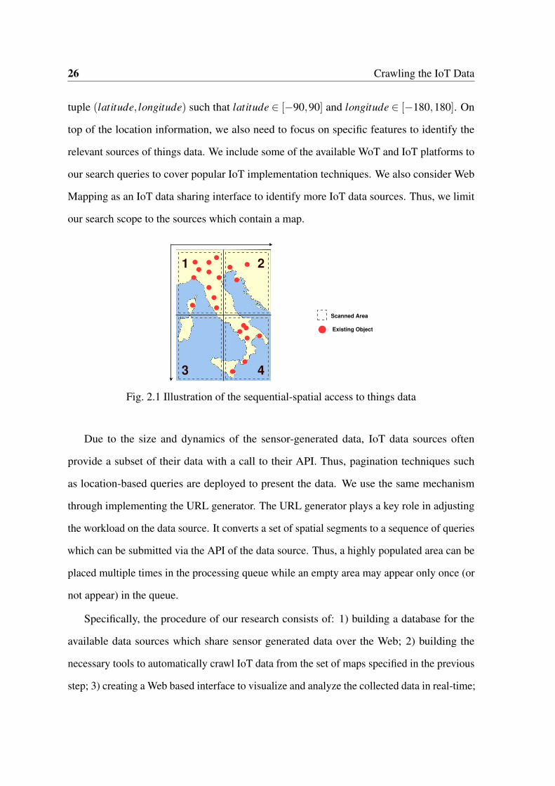
Fig. 2.1 Illustration of the sequential-spatial access to things data
Due to the size and dynamics of the sensor-generated data, IoT data sources often
provide a subset of their data with a call to their API. Thus, pagination techniques such
as location-based queries are deployed to present the data. We use the same mechanism
through implementing the URL generator. The URL generator plays a key role in adjusting
the workload on the data source. It converts a set of spatial segments to a sequence of queries
which can be submitted via the API of the data source. Thus, a highly populated area can be
placed multiple times in the processing queue while an empty area may appear only once (or
not appear) in the queue.
Specifically, the procedure of our research consists of: 1) building a database for the
available data sources which share sensor generated data over the Web; 2) building the
necessary tools to automatically crawl IoT data from the set of maps specified in the previous
step; 3) creating a Web based interface to visualize and analyze the collected data in real-time;
2.2 IoT Data Acquisition 27
4) analyzing the data sources based on their architecture, reliability and technologies used; 5)
analyzing the retrieved IoT data based on key attributes such as location, volume, redundancy
and distribution; and 6) identifying and overcoming the challenges in data collection step.
2.2.1 Identification of Data Sources
The number of cloud IoT platforms with open access data is limited and thus, identifying
them is not difficult. For WoT enabled data sources, one can check the traces of existing
WoT packages such as the ones from WeIO [67], WoT Code Forge [61] and WoT Project
Directory [68].
In principle, not all IoT data appears in the form of Web Mapping and not every Web
based map is related to IoT data. Web based maps have been used for a variety of purposes
including presenting IoT data. From our experience, those Web pages that visualize IoT
data have the following requirements: 1) containing an interactive map; 2) being publicly
available; 3) being real-time; 4) being real-world; and 5) being within valid ranges.
Relying on the spatial characteristics of things, we observe that Web based maps are key
features to discover IoT data. Interactive Web based maps often contain a RESTful back end
[51, 52] and a script on the front end, thus the RESTful API can be used to collect the data.
If a map is not interactive, then no general approach can be found to collect the data. If the
map is not publicly available, then the access to the data will be restricted.
IoT is usually updated in real-time and vintage maps are not very useful in this case. The
real-world data is a key to find real physical things, thus, maps of virtual worlds such as
game maps do not provide IoT data. Finally, key features of the data should contain proper
values. Maps with encrypted data cannot be very useful for IoT data collection.
Based on the features of IoT data, which are mentioned above, we use the following
procedure to identify the data sources: 1) the Web page should contain an interactive map;
2) data is presented inside the XMLHttpRequest (XHR) response of the requests that the

28 Crawling the IoT Data
page makes; 3) the response in the XHR may continuously be updated; and 4) data contains
coordinates which are within the valid boundaries.
2.2.2 IoT Data Collection
We design a distributed crawler which can automate the process of IoT data collection. Firstly,
we identify a set of potential sources and categorize them based on the pre-specified features
and criteria. Then from the result set, we use around 20 data sources from which many
are partially included in Thingsful as well. The datasets include Xively, Air Quality Egg,
Raspberri Pi, Air Quality Index, ThingSpeak, Flight tracking (three different sources), Ocean
(underwater) things tracking, WUnderground (weather stations), Weatherlink, Waze (three
different datasets for traffic jams, users and alerts), University buses (4 universities), London
subway tracking, Bus tracking in UK, Vessel tracking and Cruise ship tracking.
As we need to further process Thingful queries with our crawled things dataset, the
sources are selected to represent the Thingful data. We crawl the selected data sources in two
hour intervals for a period of one week between 25/8/2015 and 1/9/2015. In this study, our
goal is to monitor daily changes and patterns in the IoT data sources. As we use the whole
dataset, no bias can be involved. Wherever a selection is made, it is done randomly, which
alleviates the bias in data sampling [69]. The crawling resulted in two million things from
the selected IoT data sources. We distribute the crawler over 4 machines where each machine
has the maximum of 2.5 GHz Intel core-i5 CPU, 8 GB memory.
We observe that the majority of data sources use pagination to limit the output size. Thus,
capturing the whole dataset through a single request using API would be impractical. For
example, the length of the resultset of a query from a Web Mapping enabled website such
as a flight tracker would be limited to a few hundred aircrafts. For this reason, we need to
construct a spacial or paginated query and process it through the API. As shown in Figure 2.1,
a larger area will be segmented into a grid of smaller segments and then we capture things

2.2 IoT Data Acquisition 29
data in a sub-area of each segment. In this regards, small margin will be considered to avoid
capturing duplicate things. Duplicate things will be created if a single object is captured twice
as it is moving from one segment to its neighbour. However, using the above technique will
result in sequential access to the whole data. In the example shown in Figure 2.1, Segment 4
may only be accessed after screening the other segments such as 1,2 and 3. Considering the
high rate of updates as well as the size of data, this could make a problem as other segments
such as 2 and 3 are not as populated as Segment 4. Thus, a considerable amount of resources
is not used properly and a long delay in data refreshing is triggered by this mechanism.
Due to the frequent sensor reading updates, the volume of IoT data can be huge. Based
on our observation, storing IoT data requires more than 0.25 GB of space per second. Thus,
we can estimate that to store the data in 24 hours, we need approximately 21 TB of space.
Obtaining this amount of information from a data source can be time consuming and bear
a high cost. However, in order to save the processing cost and reduce the distortion of the
captured things dataset, one option is to analyze the density of things in each area and put
more effort on the areas with more things. For instance, in Figure 2.1, Segment 3 on average
has the least density of things, thus it can be removed from the queue. Another option, which
can be taken at the same time, is to consider the distribution of the retrieval queries. For
instance in Figure 2.1, if user queries specify the Segment 2 more than Segment 4, more
resources can be devoted to scan Segment 2 data.
In our dataset, we have identified nearly two million objects. The number of records
for each object deviates between 10 and 1,933 based on the fact that the time for scanning
different data sources varies between 30 seconds to more than 50 minutes. In average, the
readings per object in our data set are 32. On top of the crawled things dataset, we use a
real-world query set consisting of 136,746 queries between 12/2/2014 to 27/1/2015 from the
Thingful search engine. We use the query set to investigate user interests. A query in our
query set is structured as follows: {"timestamp":"2015-01-27T09:33:06+00:00",
30 Crawling the IoT Data
"query":{"lat":"51.55", "lng":".03", "zoom":"8", "what":"speed camera"}}
2.3 IoT Data Analysis
In this section, we present the result and statistical analysis of IoT data and queries collected
during multiple routine crawling rounds. We investigate the results from user-related and
things-related points of view and then we compare the distribution of IoT and queries data.
2.3.1 User Interests
We investigate user interests from different angles including Popularity Trends, Search
Queries Statistics and comparing the Things vs Query Distribution.
Popularity Trends
A glimpse into IoT keyword trends over Google Trends [70], suggests that the public interest
towards IoT with its most popular abbreviations has been steadily increasing over the past
few years.
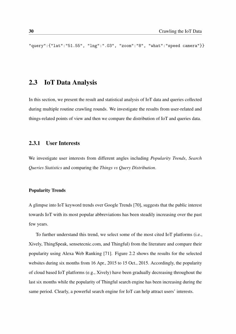
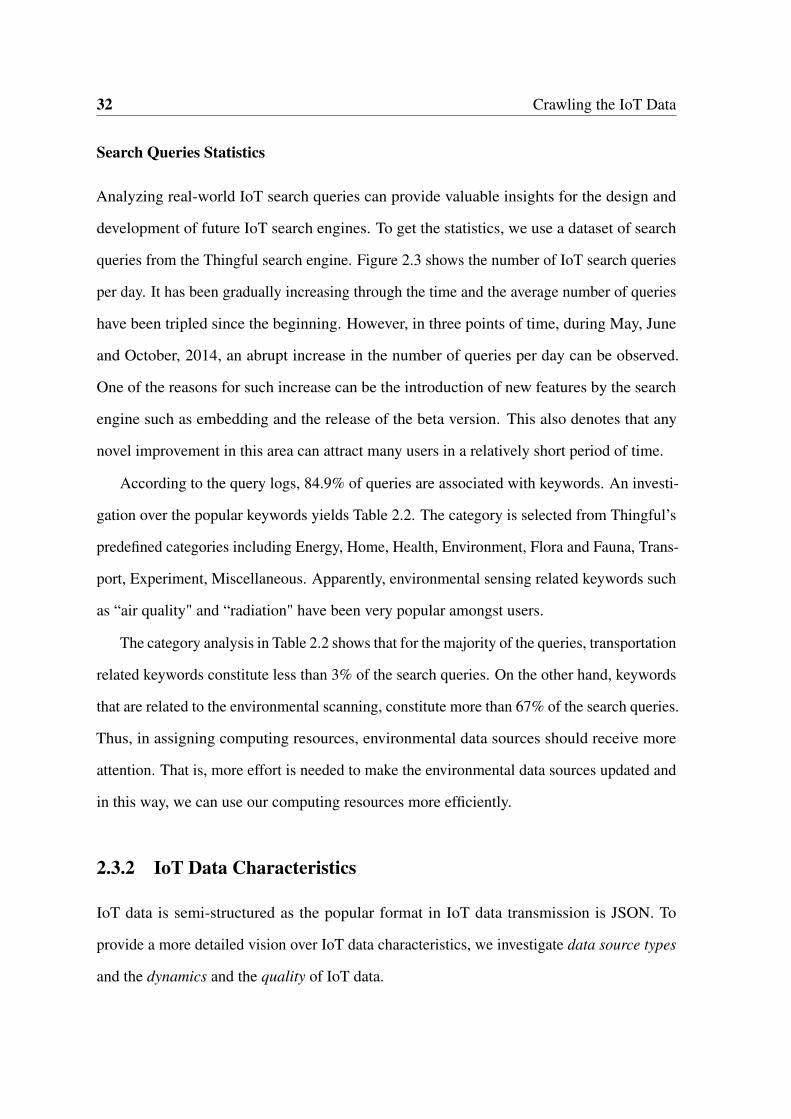
To further understand this trend, we select some of the most cited IoT platforms (i.e.,
Xively, ThingSpeak, sensetecnic.com, and Thingful) from the literature and compare their
popularity using Alexa Web Ranking [71]. Figure 2.2 shows the results for the selected
websites during six months from 16 Apr., 2015 to 15 Oct., 2015. Accordingly, the popularity
of cloud based IoT platforms (e.g., Xively) have been gradually decreasing throughout the
last six months while the popularity of Thingful search engine has been increasing during the
same period. Clearly, a powerful search engine for IoT can help attract users’ interests.
2.3 IoT Data Analysis 31
Time (Apr. 2015−Oct. 2015)Ran
k (d
ista
nce
from
the
1st w
ebsi
te)
May Jun Jul Aug Sep Oct100,
000
10,0
00,0
00
xively.comthingful.netsensetecnic.comthingspeak.com
Fig. 2.2 Ranking of the popular IoT services
Mar May Jul Sep Nov Jan
Time (month)
Fre
qu
en
cy (
pe
r d
ay)
10
10
01
00
0
Fig. 2.3 Query frequency per day in Thingful
32 Crawling the IoT Data
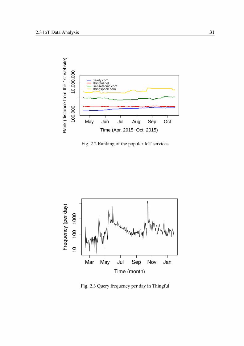
Search Queries Statistics
Analyzing real-world IoT search queries can provide valuable insights for the design and
development of future IoT search engines. To get the statistics, we use a dataset of search
queries from the Thingful search engine. Figure 2.3 shows the number of IoT search queries
per day. It has been gradually increasing through the time and the average number of queries
have been tripled since the beginning. However, in three points of time, during May, June
and October, 2014, an abrupt increase in the number of queries per day can be observed.
One of the reasons for such increase can be the introduction of new features by the search
engine such as embedding and the release of the beta version. This also denotes that any
novel improvement in this area can attract many users in a relatively short period of time.
According to the query logs, 84.9% of queries are associated with keywords. An investi-
gation over the popular keywords yields Table 2.2. The category is selected from Thingful’s
predefined categories including Energy, Home, Health, Environment, Flora and Fauna, Trans-
port, Experiment, Miscellaneous. Apparently, environmental sensing related keywords such
as “air quality" and “radiation" have been very popular amongst users.
The category analysis in Table 2.2 shows that for the majority of the queries, transportation
related keywords constitute less than 3% of the search queries. On the other hand, keywords
that are related to the environmental scanning, constitute more than 67% of the search queries.
Thus, in assigning computing resources, environmental data sources should receive more
attention. That is, more effort is needed to make the environmental data sources updated and
in this way, we can use our computing resources more efficiently.
2.3.2 IoT Data Characteristics
IoT data is semi-structured as the popular format in IoT data transmission is JSON. To
provide a more detailed vision over IoT data characteristics, we investigate data source types
and the dynamics and the quality of IoT data.

2.3 IoT Data Analysis 33
(a) 6pm ACST (b) 12am ACST (c) 6am ACST
(d) 6pm ACST (e) 12am ACST (f) 6am ACST
(g) 6pm ACST (h) 12am ACST (i) 6am ACST
(j) 6pm ACST (k) 12am ACST (l) 6am ACST
Fig. 2.4 The distribution of things trajectories on a map

34 Crawling the IoT Data
(a) all the time (b) all the time (c) all the time
(d) all the time
Fig. 2.5 The distribution of IoT queries on a map
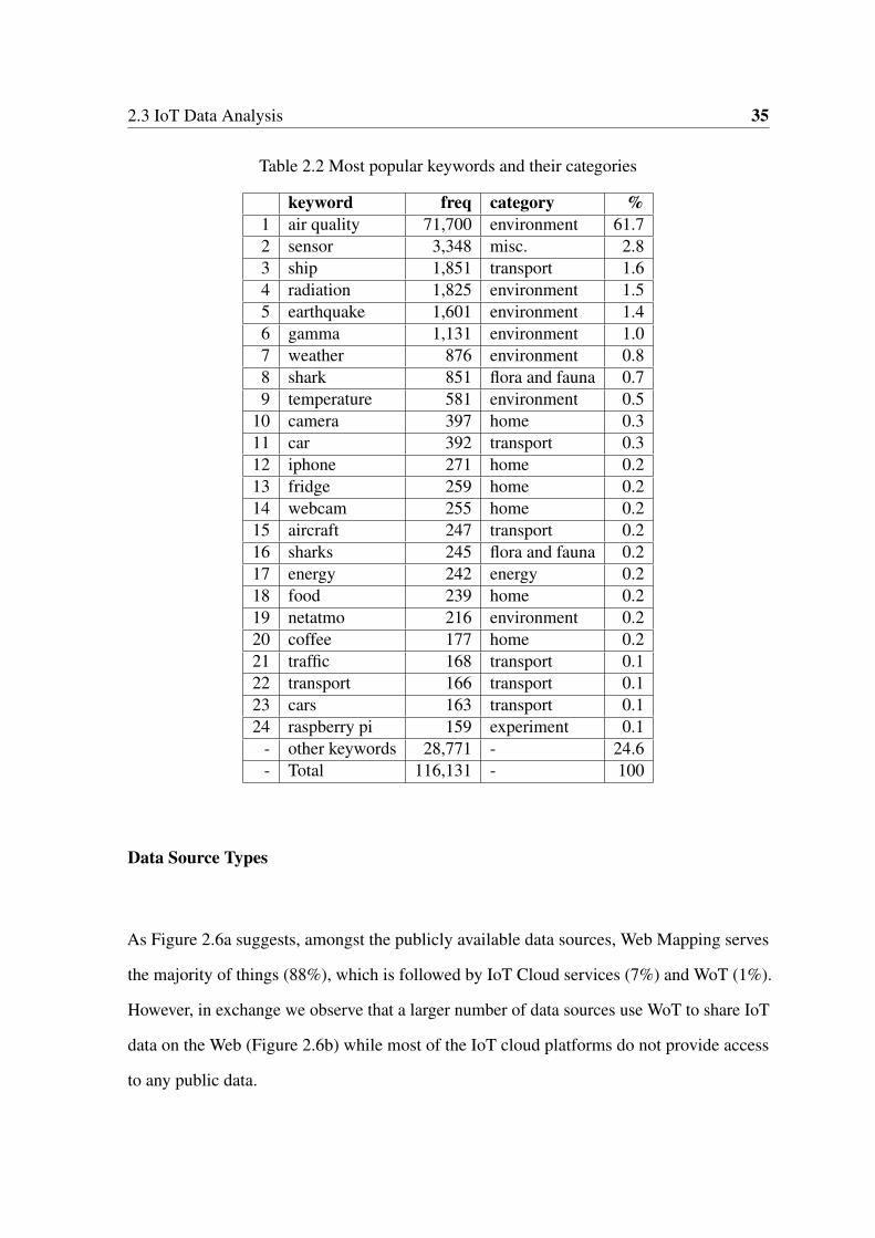
2.3 IoT Data Analysis 35
Table 2.2 Most popular keywords and their categories
keyword freq category %1 air quality 71,700 environment 61.72 sensor 3,348 misc. 2.83 ship 1,851 transport 1.64 radiation 1,825 environment 1.55 earthquake 1,601 environment 1.46 gamma 1,131 environment 1.07 weather 876 environment 0.88 shark 851 flora and fauna 0.79 temperature 581 environment 0.5
10 camera 397 home 0.311 car 392 transport 0.312 iphone 271 home 0.213 fridge 259 home 0.214 webcam 255 home 0.215 aircraft 247 transport 0.216 sharks 245 flora and fauna 0.217 energy 242 energy 0.218 food 239 home 0.219 netatmo 216 environment 0.220 coffee 177 home 0.221 traffic 168 transport 0.122 transport 166 transport 0.123 cars 163 transport 0.124 raspberry pi 159 experiment 0.1
- other keywords 28,771 - 24.6- Total 116,131 - 100
Data Source Types
As Figure 2.6a suggests, amongst the publicly available data sources, Web Mapping serves
the majority of things (88%), which is followed by IoT Cloud services (7%) and WoT (1%).
However, in exchange we observe that a larger number of data sources use WoT to share IoT
data on the Web (Figure 2.6b) while most of the IoT cloud platforms do not provide access
to any public data.

36 Crawling the IoT Data
WoTIoT Cloud
Web Mapping
(a) Number of things by each technology
WoT
IoT Cloud
Web Mapping
(b) Number of websites by each technology
Fig. 2.6 Major provider technologies for public IoT data
Table 2.3 WoT vs. IoT cloud services
Data Source Public Sensors (Things) TypeXively 67,000 IoT CloudWoTkit 4,065 WoTThingSpeak 3,571 WoTWikiBeacon 30,052 WoTISMN* 2,080 WoT*International Soil Moisture Network
To grasp a more detailed image of IoT clouds and WoT, Table 2.3 shows WoT and IoT
clouds and the number of non-private things which use these technologies.
Spatial and Temporal Distribution of Things
Understanding the spatial and temporal distribution of IoT and query updates is valuable for
identifying the existing gaps, which can help in predicting the trends of searches and updates.
To model the spatial gaps between IoT and queries, we use the Earth Mover’s Distance
(EMD) measure. EMD describes the normalized minimum amount of work required to
transform one distribution to the other. In our case, given the two distributions matrices of
things, d1 and di, which have been taken in timestamps t1 and ti respectively, we want to
measure the amount of changes in the latter distribution (di) from the initial distribution d1
using EMD(d1,di) measure. Therefore, we can monitor the changes in distribution over the
time.

2.3 IoT Data Analysis 37
We summarized the two datasets into a list of density indices shown in Figure 2.7. The
length and width of each record density index is 5 degrees of longitude and 5 degrees of
latitude, respectively. The EMD yields 0.4338619 for an image of IoT data and the whole
queries dataset.
0 100 200 300 400 500
040
000
Index
Den
sity IoT
Queries
Fig. 2.7 Comparison of the densities of the query logs and IoT data
In the next step, we want to know whether the patterns in Figure 2.5 and changes in the
distribution of things recur over the time. Thus, we perform the same analysis over a period
of time on how the spatial distribution of things changes through the time. In particular,
we use the emdist [72] implementation to approximate the EMD score for each transition.
Figure 2.8 shows the EMD score for a given period of time in 48 timetamps which we have
collected within 48 hours. The curve shows that in each given timestamp ti, the value of
EMD(t1, ti) ∈ [0,1]. Thus, the EMD score for t1 is 0 since there is no difference between the
distribution matrix in t1 and itself.
Shortly, a huge amount of change is observed between t2 to t5 and later the EMD score
continuously decreases as the distribution returns to its initial status. The very same pattern
recurs on the next period of time. As a result, we understand that the geospatial distribution of
things goes back to its original state over a period of time (in this case, after 24 hours). This
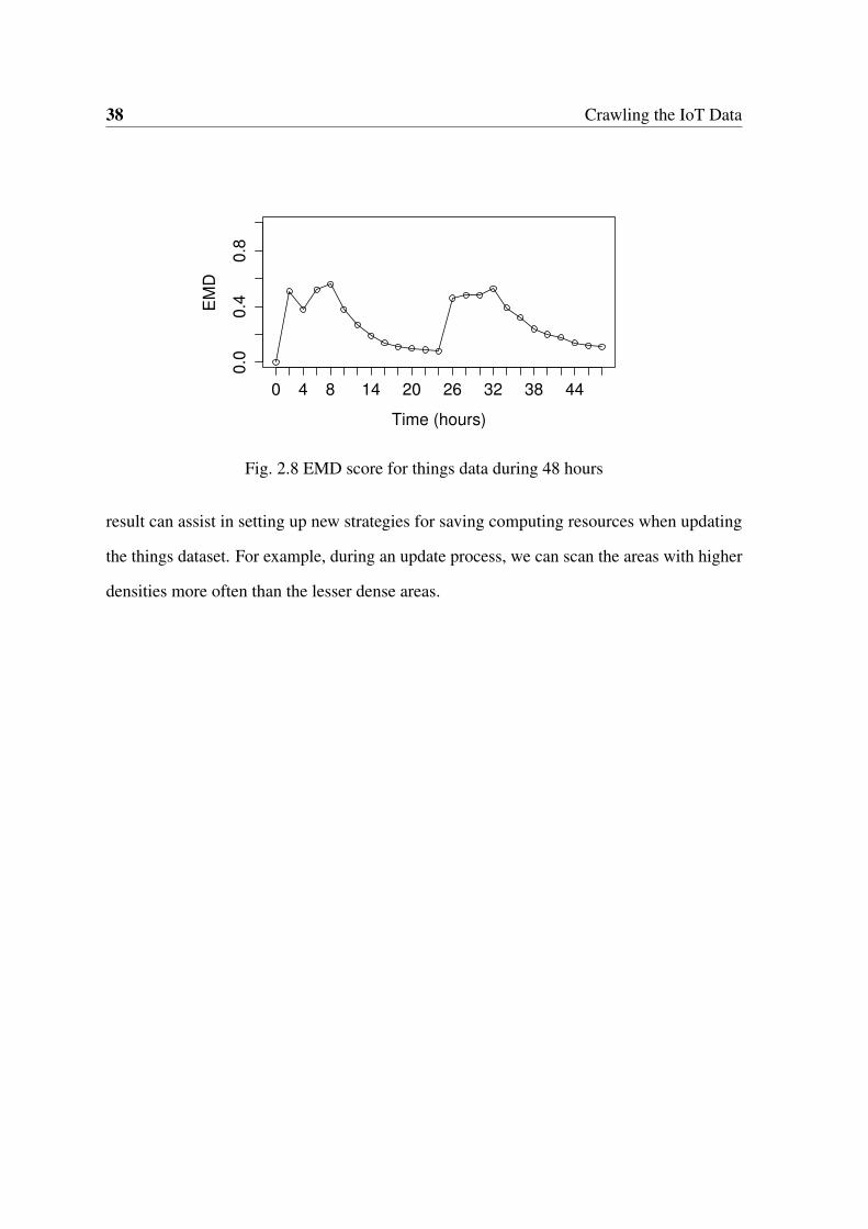
38 Crawling the IoT Data
0.0
0.4
0.8
Time (hours)
EM
D
0 4 8 14 20 26 32 38 44
Fig. 2.8 EMD score for things data during 48 hours
result can assist in setting up new strategies for saving computing resources when updating
the things dataset. For example, during an update process, we can scan the areas with higher
densities more often than the lesser dense areas.
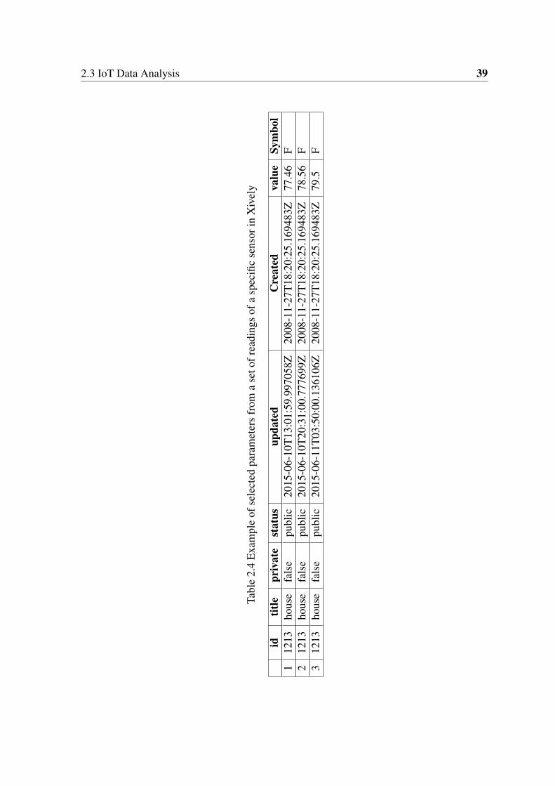
2.3 IoT Data Analysis 39
Tabl
e2.
4E
xam
ple
ofse
lect
edpa
ram
eter
sfr
oma
seto
frea
ding
sof
asp
ecifi
cse
nsor
inX
ivel
y
idtit
lepr
ivat
est
atus
upda
ted
Cre
ated
valu
eSy
mbo
l1
1213
hous
efa
lse
publ
ic20
15-0
6-10
T13
:01:
59.9
9705
8Z20
08-1
1-27
T18
:20:
25.1
6948
3Z77
.46
F2
1213
hous
efa
lse
publ
ic20
15-0
6-10
T20
:31:
00.7
7769
9Z20
08-1
1-27
T18
:20:
25.1
6948
3Z78
.56
F3
1213
hous
efa
lse
publ
ic20
15-0
6-11
T03
:50:
00.1
3610
6Z20
08-1
1-27
T18
:20:
25.1
6948
3Z79
.5F
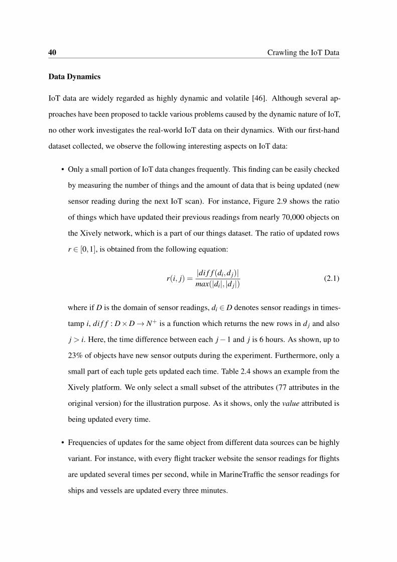
40 Crawling the IoT Data
Data Dynamics
IoT data are widely regarded as highly dynamic and volatile [46]. Although several ap-
proaches have been proposed to tackle various problems caused by the dynamic nature of IoT,
no other work investigates the real-world IoT data on their dynamics. With our first-hand
dataset collected, we observe the following interesting aspects on IoT data:
• Only a small portion of IoT data changes frequently. This finding can be easily checked
by measuring the number of things and the amount of data that is being updated (new
sensor reading during the next IoT scan). For instance, Figure 2.9 shows the ratio
of things which have updated their previous readings from nearly 70,000 objects on
the Xively network, which is a part of our things dataset. The ratio of updated rows
r ∈ [0,1], is obtained from the following equation:
r(i, j) =|di f f (di,d j)|max(|di|, |d j|)
(2.1)
where if D is the domain of sensor readings, di ∈ D denotes sensor readings in times-
tamp i, di f f : D×D→ N+ is a function which returns the new rows in d j and also
j > i. Here, the time difference between each j−1 and j is 6 hours. As shown, up to
23% of objects have new sensor outputs during the experiment. Furthermore, only a
small part of each tuple gets updated each time. Table 2.4 shows an example from the
Xively platform. We only select a small subset of the attributes (77 attributes in the
original version) for the illustration purpose. As it shows, only the value attributed is
being updated every time.
• Frequencies of updates for the same object from different data sources can be highly
variant. For instance, with every flight tracker website the sensor readings for flights
are updated several times per second, while in MarineTraffic the sensor readings for
ships and vessels are updated every three minutes.
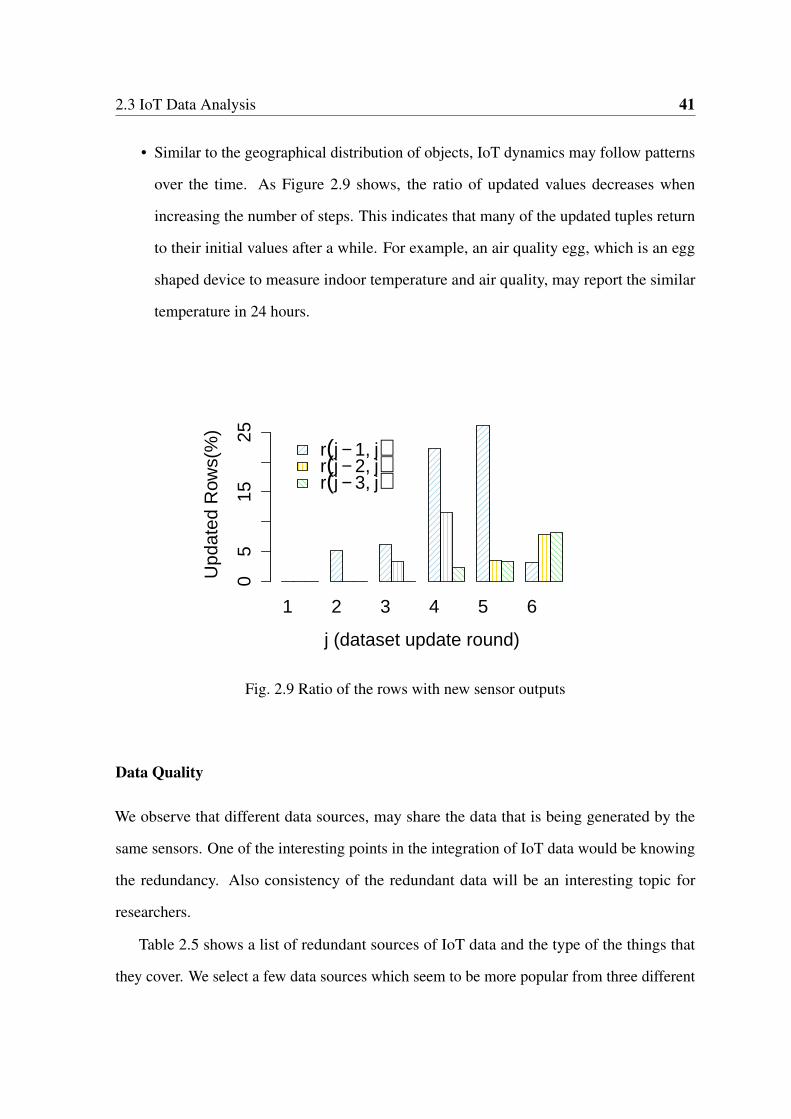
2.3 IoT Data Analysis 41
• Similar to the geographical distribution of objects, IoT dynamics may follow patterns
over the time. As Figure 2.9 shows, the ratio of updated values decreases when
increasing the number of steps. This indicates that many of the updated tuples return
to their initial values after a while. For example, an air quality egg, which is an egg
shaped device to measure indoor temperature and air quality, may report the similar
temperature in 24 hours.
1 2 3 4 5 6
j (dataset update round)
Upd
ated
Row
s(%
)
05
1525
r(j − 1, j)r(j − 2, j)r(j − 3, j)
Fig. 2.9 Ratio of the rows with new sensor outputs
Data Quality
We observe that different data sources, may share the data that is being generated by the
same sensors. One of the interesting points in the integration of IoT data would be knowing
the redundancy. Also consistency of the redundant data will be an interesting topic for
researchers.
Table 2.5 shows a list of redundant sources of IoT data and the type of the things that
they cover. We select a few data sources which seem to be more popular from three different
42 Crawling the IoT Data
categories: flight tracking and marine traffic tracking. Every object from these sources is
associated with an identifier which can distinguish it from other objects. We merge the data
from all websites in each category to get the ratio of inclusiveness. This measure denotes
the rate of the objects which exist in the data source and the union set of objects for the
corresponding category.
For the captured flight data, the objects information from different sources is quite
different. There are two main reasons associated with this issue. The first reason is the delay
in updating the information. The second reason is the loss of some values for some flights.
For example, the flight registration is provided by a data source while the same attribute
for the same flight is not set in other websites. For the marine traffic tracking websites, we
observe that the majority of niche websites are using the same techniques and data as the
source website. No delay is observed while the ratio of overlapped data is higher than flight
trackers.

2.3 IoT Data Analysis 43
Tabl
e2.
5Tr
ansp
orta
tion
data
sour
ces
with
over
lapp
ing
seto
fobj
ects
App
licat
ion
UR
LSc
ope
Nov
elD
ata
Incl
usiv
enes
sD
elay
Flig
httr
acki
ng
http
://w
ww
.flig
htra
dar2
4.co
m
Wor
ldw
ide
✓99
.99%
-ht
tps:
//flig
htaw
are.
com
/live
/✓
0.01
%✓
http
s://p
lane
finde
r.net
✓0.
01%
✓ht
tp://
ww
w.ra
darb
ox24
.com
✓0.
01%
✓ht
tp://
ww
w.ra
darv
irtu
el.c
om✓
0.01
%✓
http
://tin
yurl
.com
/klm
livA
irlin
e✓
0.01
%✓
http
://tin
yurl
.com
/per
thliv
Air
port
✓0.
01%
✓
Mar
ine
traf
fictr
acki
ng
http
://w
ww
.mar
inet
raffi
c.co
mW
orld
wid
e✓
100%
-ht
tp://
ww
w.s
hips
potti
ng.c
om/a
is/
✓0.
01%
✓ht
tp://
ship
.gr/
map
/inde
x.ht
m×
100%
×ht
tp://
ww
w.c
ruis
emap
per.c
omC
ruis
e✓
0.01
%×
http
://w
ww
.cru
isin
.me/
crui
se-s
hip-
trac
ker/
×10
0%×

44 Crawling the IoT Data
2.3.3 IoT vs. User Interests
As mentioned, the analysis of the distribution of things and queries can lead to finding more
efficient strategies for storing and retrieving IoT data.
Our observation shows that in many cases, there is a huge difference between the dis-
tribution of the queries and the distribution of the things data. Figures 2.5a, 2.5b and 2.5d
show the local distribution of the queries from Thingful in Asia, Australia and the Europe,
respectively. We do not include other continents such as the Americas and the Africa as their
results do not add new information on top of the selected regions. As the figures show, in
each region most of the queries are focused on specific regions such as India, East Coast of
Australia and London.
We also investigate the distribution of the things and its changes over the time in each
region separately. We randomly pick a 12-hour time frame and conduct the analysis over
three snapshots all over the world. Due to the space limit, we select three snapshots and
investigate the distribution of the things in each region. The first snapshot is during evening,
the second is during early morning and the third is around noon. The snapshots are all
based on the Australian Central Standard Time (ACST). In Asia, during the afternoon most
of the things are concentrated on East Asia (Figure 2.4a) while later in the morning the
concentration of the things transfers to the South West Asia (Figure 2.4b). In the next
snapshot, the concentration moves towards South East Asia again (Figure 2.4c). A large part
of this change is due to the existing large ratio of flight data comparing to the other types of
things data in Asia. However, in Asia, no record demonstrates a good match between the
distribution of things and the distribution of the queries, while most queries are concentrated
on India (see Figure 2.5a).
In Australia, things are mostly concentrated on the east coast of Australia during evening
time (Figure 2.4d) which is a good match for the distribution of the queries (Figure 2.5b).
Later as Figures 2.4e and 2.4f show, many things are present in other places as well as around

2.4 Discussions 45
the capital cities of Sydney and Melbourne. Thus, a huge gap exists between the distribution
of things and queries in this region. However, unlike Asia, the distribution of the things
partially matches with the distribution of the queries over the two cities.
In the US, the snapshots demonstrate the change of distribution throughout the time
during daylight. The distribution of things continuously spreads from the east coast to the
west coast as Figures 2.4g, 2.4h and 2.4i illustrate. However, there is a loose connection
between the queries distribution 2.5c and things distribution over the New York.
The situation is quite different in Europe. As Figures 2.4j, 2.4k and 2.4l show, a large
number of things are constantly concentrated over London area and partially over Germany
which is a very good match with the distribution of the queries in this part of the world
(Figure 2.5d).
2.4 Discussions
In this section, we provide further discussions on the challenges and opportunities for IoT
research and development.
2.4.1 Challenges in IoT Data Discovery
IoT data discovery is important towards establishing the next step in the life of the Internet.
Since the early days of IoT, several technologies have been specifically proposed to share
IoT data. There have been several successful stories for cloud based IoT platforms such as
Xively and Paraimpu. They are often designed to provide global support for almost any type
of sensors or actuators.
However, the community of users does not restrict themselves to what these IoT platforms
provide. An increasing number of techniques are being used to publish sensory data on
the Web. The number of sensors, various types of applications and the increasing demand
46 Crawling the IoT Data
for real time data have driven to reinvent various techniques which are previously used for
other purposes (e.g., Web Mapping). In this case, a large number of niche websites have
been developed to publish the data that are generated by specific sensors or for specific
applications. In fact, the volume of the publicly available information provided by these
websites is much more than the general purpose IoT cloud platforms. However, identifying
these websites is similar to finding a needle in haystack as there is no comprehensive list
of such websites, many of which have been created recently after the success of similar
applications such as the flight trackers.
Another challenge is the structure of the data that is provided on the Web. For a large
portion of the websites, the data should be collected from the deep Web. For example, to
obtain the results from a flight tracker website, several parameters need to be set and passed.
Otherwise, a small subset of the data or an empty set will be provided by the server. In some
cases, authentication may also be required as a part of the process when accessing the data.
Unlike other types of the information on the Web, IoT data mostly are presented in a
structured or semi-structured format. The structure of the data widely varies from one website
to another. In addition, in many cases, the parameter names are not self descriptive and these
parameters need to be demystified manually.
2.4.2 Information Retrieval in IoT
Currently, IoT search is quickly evolving to address the needs of users and leverage the
benefits of deploying IoT. This includes preserving accuracy, speed, consistency and ease of
use for IoT search engines in future. Thus, new search forms such as searching the retrieving
knowledge from things data, intent-based search are emerging which in turn require proper
data source selection, tackling query ambiguity [38].
We consider a simple example to further explain this point. For example, a user may
search for air quality in a specific area rather than a specific air sensor. To answer her query,

2.4 Discussions 47
firstly, the documents containing air quality sensors in that area should be retrieved. Secondly,
sensors which also provide contextual information about the air quality should be retrieved as
well. Thirdly, knowledge about air quality can be extracted from the selected documents. We
should note that due to the high uncertainty in IoT data, some estimation or prediction (in case
of data unavailability) techniques may be used to fill the empty pieces of the puzzle. Finally,
result diversification would be very important to address issues such as query ambiguity.
Due to the highly dynamic nature of IoT, documents containing IoT information can
change drastically from the time when they are crawled to the time when their data are
presented. Thus, effective and efficient indexing techniques would be required to retrieve
information from IoT data.
Furthermore, IoT will leverage Temporal Information Retrieval more [73]. We observe
that the content of a large number of documents as well as the data sources, may variate
between 1% to 100% in a very short period of time. With the high rate of changes in IoT
data sources, document selection as well as the user query results will require novel temporal
techniques to tackle the issues.
2.4.3 Other Challenges
Our dataset can be used for a variety of purposes in the IoT research and development,
including correlation discovery between things [74], IoT data storage [75, 59], context
aware computing for IoT [76] by merging sensor readings from different sources such as
environmental and transportation sensors, point of interest recommendation [77] and other
active IoT research areas which may need real-world data.
Data Integration
Continuous retrieval of IoT data is very challenging. Some of the sources demand authenti-
cation before providing the access. In many cases, data for the same object (e.g., an aircraft)
48 Crawling the IoT Data
is being broadcasted by different data sources. Furthermore, in some cases, each available
source may only provide partial information for an object. The similar issue affects merging
data for the same resource. For example, the results of parsing objects data for a single
resource have different length and parameters which need to be integrated at the end. Lastly,
many data sources limit their response length due to load balancing concerns. We do not fully
resolve all challenges in the integration but rather, we use an efficient approach to integrate
the data from different sources for the purpose of our research. However, the integration of
IoT data is more challenging than what is believed and more research in this area is required
in the future.
Scalability
Collecting, processing and storing IoT data can be a time consuming procedure, particularly
if the size of the dataset is large. As the number of sources and objects increases, which
might count in billions, using one instance of the crawler would be very inefficient. In
particular, dramatic difference between the update rate of different data sources which also
partially depends on their size, can be challenging. Furthermore, technical failures of one
resource may affect collecting data from other data sources in the same chain. Thus, we use
a distribution strategy to coordinate different instances of the crawler running on different
machines.
Archiving IoT Data
IoT fully interprets the Big Data. The volume, velocity and the variety of the data generated
by things are enormous. The amount of the data that is already being published from 20
IoT data sources on the Web, which we estimate to be more than 100 TB a day, is already
comparable to the amount of data that is being generated by users on social networks. With
2.5 Related Work 49
the rapid growth of the IoT, in the near future, new techniques will be required to effectively
and efficiently process and store IoT data.
Currently, to the best of our knowledge, there is no popular website for archiving the
publicly available IoT data. In this regard, the traditional approaches need to be revised for
the new era of the IoT. The result can be valuable to many core applications such as IoT
search while we compromise on some issues to make the impossibles possible. For instance,
we discover that based on the changes in the geographical distribution of objects, a crawling
strategy can be issued to capture the most updated data in the least amount of time. Through
creating spatial and per resource indexes, the process can also become more optimized.
2.5 Related Work
Over the past few years, the IoT has received increasing attention from researchers and
practitioners. In the earlier days, Atzori et al.[3] offers an initial survey on the IoT research.
Accordingly, there exist manifold definitions of the IoT paradigm within the research commu-
nity. Each definition may view this paradigm from a specific angle including things oriented,
Internet oriented and semantic oriented definitions. More specifically, based on all these
definitions, a wide variety of networking and sharing technologies have been used to enable
the future IoT including but not limited to the Web of Things (WoT) [28], RFID, Near-Field
Communication (NFC), middleware and the Wireless Identification and Sensing Platform
(WISP) [78].
Some researchers have claimed that the IoT is implemented with the technologies specifi-
cally designed for the purpose of being deployed in IoT [44]. Thus, it is argued that the IoT
already exists but only a small number of experiments and as a result, yet many researchers
consider as inaccessible [44]. Restricting IoT with this point of view is contrary to the
spirit of open systems at the heart of the original Internet standards. Moreover, within the
technologies which have been applied to facilitate IoT, open Web technologies including

50 Crawling the IoT Data
HTML, Ajax, HTTPS, OpenID and structured data apply equally well to IoT. However, yet
there is no advanced mechanism to be able to effectively search and retrieve things from the
Web.
The very diverse range of the objects, approaches and technologies used to implement IoT
have contributed in broadening the definition of this paradigm. For instance, the IoT can be
realized through deploying an RFID ecosystem consisting of objects tagged with numerous
RFID labels [79]. Another option is to build the IoT using smart objects [80] which in turn
can be divided into activity-aware, policy-aware and process-aware smart objects.
Cloud based platforms such as Paraimpu [53, 81] and Xively provide environments which
have been considerably discussed in the literature. In the literature, WoT is not the only,
but is one of the mostly adopted technologies to facilitate the future IoT. The WoT concept
describes approaches, software architectures, frameworks and programming patterns that
allow things to share their data with human beings through the World Wide Web. Currently,
WoT is an active research area with a wide range of challenges and opportunities including
security, resilience, intent oriented search, legal implications and so on [28].
Currently IoT search is a trending research direction [82] with stress over some major
goals such as real-time search [83], context-awareness [76] and relationship support [84].
Researchers have complained about the lack of real-world IoT data in the past [74].
Although some of the previous works have claimed testing their proposed solutions for large
scale IoT data, such as meta-heuristic [85] or context aware sensor search [76], all these
previous works mainly deal with small or simulated datasets. To the best of our knowledge,
no work has ever collected or analyzed large scale things data. In addition, none of the
existing works use real IoT search query dataset. Moreover, we could not find any other work
that has deployed or analyzed a large real-world IoT query dataset for mining user interests
in the IoT domain. By combining the user interests and the IoT data, we can analyze the gap
of what people look for and what currently the IoT presents on the Web. Our work is the

2.6 Summary 51
very first that investigates IoT in large scale and the dataset released from our study is the
first real-life, large IoT dataset that is publicly available for the research community.
2.6 Summary
The unique characteristics of IoT require that the future search engines provide support for
a variety of new requirements. Firstly, IoT is no longer solely attached to the public cloud
based solutions, and IoT indeed has been spreading by all means throughout the World Wide
Web. Secondly, due to the dynamics of IoT, future search engines need to provide real-time
results. In this work, we conduct an in-depth analytical investigation on IoT data that exists
on the Web. Based on our real-life IoT data, we investigate the current status of the IoT
and identify open research and development issues. Our findings show that conventional
geospatial data presentation techniques such as Web Mapping play an important role in
disseminating IoT data. We also discover that the environmental scanning is the most popular
application of IoT followed by transportation while transportation data sources require the
majority of the resources. We also show that we can find patterns on the updates and the
distribution of things. Moreover, our observation shows that the presentation of things data is
limited and very isolated. Thus, in the next chapter, we focus on correlating things from a
bottom-up perspective. In a bottom up perspective, data sources can process the data of the
things which belong to them then extract and present the correlations to an external viewer
such as a search engine.


Chapter 3
Interlinking IoT Resources
Our observation in the previous chapter shows that IoT data is widely visualized and presented
through Web mashups. For instance, Figure 3.1 shows an example of Web of Things mashup
from the ThingSpeak platform [86]. As shown, none of the parts of the present mashup is
referring to other mashups or correlated things on the Web. As a result, correlations remain
implicit and IoT resources may remain isolated from each other. Interlinking relevant smart
things will trigger improved user navigation as well as providing a solid foundation for
crawling WoT. This is a very critical issue which resembles the role of hyperlinks in the
traditional Web.
A hyperlink is a reference to Web resources that the reader can directly follow either
by clicking or by hovering. Usually, hyperlinks are associated with a textual description
about their target, which is called hypertext. Hyperlinks play a key role in interlinking Web
resources and provide navigation between different Web pages for users. Web crawlers
which are deployed by search engines are navigated based on the existing hyperlinks in a
Web-based document [87].
To enable the interlinking between resources in the context of interconnected networks
of things, one eminent issue is that the traditional approach of interlinking Web documents,
cannot fully unravel the benefits of interlinking IoT. In this regard, IoT-specific requirements
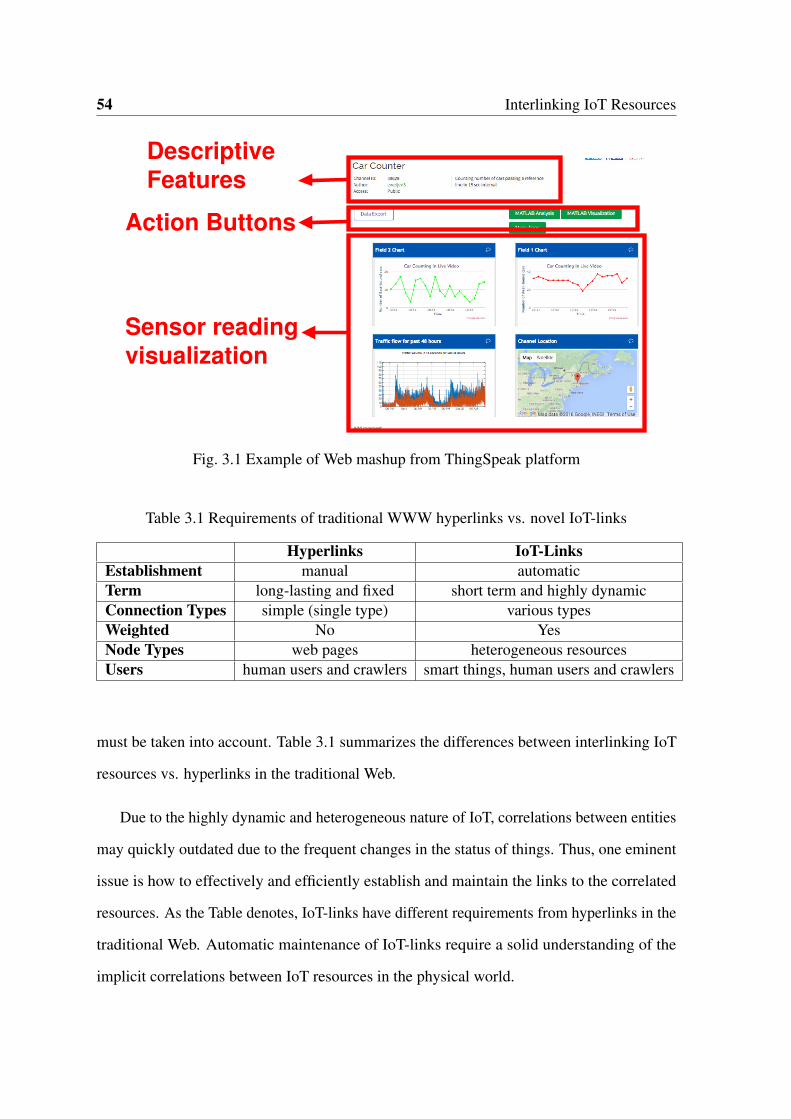
54 Interlinking IoT Resources
Descriptive
Features
Sensor reading
visualization
Action Buttons
Fig. 3.1 Example of Web mashup from ThingSpeak platform
Table 3.1 Requirements of traditional WWW hyperlinks vs. novel IoT-links
Hyperlinks IoT-LinksEstablishment manual automaticTerm long-lasting and fixed short term and highly dynamicConnection Types simple (single type) various typesWeighted No YesNode Types web pages heterogeneous resourcesUsers human users and crawlers smart things, human users and crawlers
must be taken into account. Table 3.1 summarizes the differences between interlinking IoT
resources vs. hyperlinks in the traditional Web.
Due to the highly dynamic and heterogeneous nature of IoT, correlations between entities
may quickly outdated due to the frequent changes in the status of things. Thus, one eminent
issue is how to effectively and efficiently establish and maintain the links to the correlated
resources. As the Table denotes, IoT-links have different requirements from hyperlinks in the
traditional Web. Automatic maintenance of IoT-links require a solid understanding of the
implicit correlations between IoT resources in the physical world.

55
Although every pair of smart things around the world could potentially be correlated,
in the context of IoT, correlations may not necessarily share the same type or the same
weight.Thus, several types of correlations can be identified between interconnected things
[40]. For instance, the type of the correlation that exists between two things that belong
to the same person (owned by correlation) can be different from the correlation between
two objects that are present in the same physical area (co-located correlation). Moreover,
correlations of the same type, may not necessarily have the same weight. For example, the
weight of co-located things may vary based on their distance from each other.
In this chapter we propose the CEIoT (Correlations Extractor for IoT), a framework
to facilitate automated correlation extraction for smart things in IoT. We use Multi-Agent
System (MAS) architecture to design and implement our approach in order to be able to
simulate the behaviours of smart things in real-world. Our framework regulates the extraction
of different types of correlations. The correlation types that we cover in this chapter are
defined as follows [40]:
• Ownership object relationship (OOR): correlates objects with the same owner.
• Co-location object relationship (CLOR): correlates objects that are physically close to
each other.
• Category based object relationship (CBOR): correlates objects which have the same
describing tags.
In our CEIoT framework, we provide correlations with normalized weights to enable
our model to represent more details from the real-world. Thus, our approach employs a
weighted undirected graph to model the heterogeneous network of things. In this chapter, we
assume that each thing is registered only to one network and belongs only to maximum of
one user. We only focus on the publicly available things. We design a distributed and scalable

56 Interlinking IoT Resources
framework to support the correlation extraction and use Open Linked Data to present the
extracted correlations. Our contributions are summarized as follows:
• We propose our CEIoT framework to extract things correlations in IoT. Our approach
can support correlations with different types including CBOR, CLOR and OOR. We
use a distributed architecture to enable our CEIoT framework to estimate the weights
of the correlations. To the best of our knowledge, other approaches focus on one type
correlation or have only been deployed in small scales.
• We define the process of correlation discovery for IoT. We propose two novel algo-
rithms for extracting and one algorithm for integrating the extracted correlations. In
the CEIoT framework, we localize CBORs and estimate the weights of correlations for
CLORs to increase the efficiency of the correlation extraction process. We increase the
efficiency of correlation extraction and integration using a distributed architecture.
• We conduct extensive experiments to evaluate our approach. We use both synthetic
and real-world datasets to and demonstrate the efficiency and effectiveness of our
framework based on measures including system performance and number of messages.
The remainder of this chapter is organized as follows. We describe the CEIoT frame-
work in Section 3.1. We present the results from the implementation of the framework in
Section 3.2. Section 3.3 reviews the research activities that are relevant to our work. Finally,
we summarize the chapter in Section 3.4.
3.1 The CEIoT Approach
In this section, we present the details of our CEIoT architecture for automated extraction and
representation of the correlations between things in IoT.

3.1 The CEIoT Approach 57
3.1.1 Correlation Discovery Process
Today, there are many online IoT platforms such as Xively [29] and Paraimpu [53, 81].
Despite of their large scale and complexity, no means has been deployed to analyze or present
the correlations between things. This includes the correlations of things of both inter and
intra data sources.
We define correlation discovery as the process of extraction and representation of cor-
relations of any types that exist between the resources in the IoT. Figure 3.2 illustrates the
process of correlation discovery for the IoT consisting of four different phases: Collection,
Extraction, Integration and Presentation. In the first phase, things’ data is collected via
RESTful application interfaces and maintained on a server. In the next step, Extraction,
the similarity of given object pairs is examined based on different measures and criteria to
extract the correlations. During the Integration phase, all of the extracted correlations are
integrated to form a Things Correlations Graph (TCG) [38], which resembles the graphs in
the traditional social networks. Finally, in the last phase, the edges of the TCG are converted
into IoT hyperlinks.
3.1.2 Framework Architecture and System Entities
Our CEIoT framework architecture is inspired by MAS framework. We design and implement
a set of agent classes with built-in behaviors which facilitate the simulation of important
entity types and their interactions in IoT correlation extraction problem. In the next step,
agents are instantiated and deploy pre-designed communication protocols to interact and
submit/receive messages. An overview of the CEIoT framework is shown in Figure 3.3. Each
platform in our framework operates independently from other platforms as IoT platforms
operate in the real-world. The figure shows the main types of agents in each platform and
how their instances interact with other parts of the system such as smart things, database and
other platforms. Each platform maintains its own correlation database and Data Facilitator
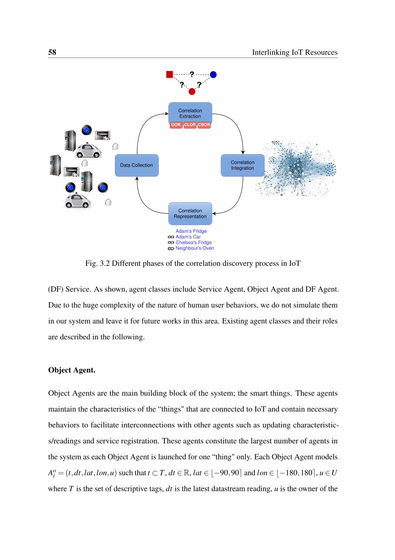
58 Interlinking IoT Resources
Data Collection
CorrelationExtraction
Correlation Integration
Correlation Representation
Adam's FridgeAdam's CarChelsea's FridgeNeighbour's Oven
OOR CLOR CBOR
Fig. 3.2 Different phases of the correlation discovery process in IoT
(DF) Service. As shown, agent classes include Service Agent, Object Agent and DF Agent.
Due to the huge complexity of the nature of human user behaviors, we do not simulate them
in our system and leave it for future works in this area. Existing agent classes and their roles
are described in the following.
Object Agent.
Object Agents are the main building block of the system; the smart things. These agents
maintain the characteristics of the “things" that are connected to IoT and contain necessary
behaviors to facilitate interconnections with other agents such as updating characteristic-
s/readings and service registration. These agents constitute the largest number of agents in
the system as each Object Agent is launched for one “thing" only. Each Object Agent models
Aoi = (t,dt, lat, lon,u) such that t ⊂ T , dt ∈R, lat ∈ ⌊−90,90⌉ and lon∈ ⌊−180,180⌉, u∈U
where T is the set of descriptive tags, dt is the latest datastream reading, u is the owner of the

3.1 The CEIoT Approach 59
sensors actuators Low powered device
Restful APIRestful APIRestful API
manages/negotiates
service descriptionstores
Service Agent
service description
Object Agent Object Agent
IoT Cloud Service
Directory Facilitator
Correlations Database
CorrelationManagement Behaviour
+ OOR.TCG: Graph+CLOR.TCG: Graph+ CBR.TCG: Graph
service description
Other platforms
Network
Federation
Fig. 3.3 A general overview of the CEIoT framework

60 Interlinking IoT Resources
smart thing and lat, lon are the latitude and longitude of the object, respectively. Also, the
Object Agent contains at least three default behaviors. One is to register their descriptive tags
(t) into DF service. Two other behaviors are for updating location and other characteristics.
Service Agent.
A Service Agent represents an IoT service provider (IoT platform) which facilitates the
management of Object Agents. There is only one service agent per platform. It is responsible
for coordinating and managing all agents present in its container as well as correlation
discovery. These agents maintain all of the necessary information about their corresponding
IoT platform. This includes host URL, port, Agent Communication Channel’s address,
platform ID and the DF Agent. Moreover, the Service Agent can launch, suspend or destroy
Object Agents if required. It can directly communicate with the IoT cloud and transfer data
when required. However, the main responsibility of the Service Agent is to enquire other
agents and update the correlation database frequently.
DF Agent.
DF service facilitates the address book of each platform. Intra-platform agents can enquire
the DF service to find agents with the specified services. The DF Agent stores tuples of
services and agent URIs in the form of {(t,a)} such that t ∈ T and a ∈ A where T is the
set of descriptive tags and A is the set of all agents in the platform. Usually, DF service
is provided only for the platform agents internally and is not designed to be shared across
multiple platforms. Hence, inter-platform agent communication cannot be established in
this situation. To avoid having a number of isolated MAS platforms, we devise a medium to
share DF data across authorized platforms.

3.1 The CEIoT Approach 61
3.1.3 Correlation Extraction
Correlation extraction is the key step in the IoT correlation discovery process. In this step,
our aim is to set up an efficient approach to extract the three types of correlations discussed
earlier. As each type of correlation is discovered independently, firstly, we propose a separate
approach for each correlation type. Then secondly, we investigate how we can integrate the
process and the results.
CLOR.
Given a pair of Object Agents (Aoi ,A
oj) and a threshold t ∈ [0,1], CLOR can be defined as
follows:
clor(Aoi ,A
oj) =
∆(Ao
i .l,Aoj .l)
max{∆(Ao.l,Ao.l)} i f ∆(Aoi .l,A
oj .l)≥ t;
0 otherwise
where ∆ : (latitude, longitude)2→ R returns the distance between two points (Manhattan,
Euclidean, Haversine and etc.).
Unlike OOR, extracting CLORs among objects can be very complex if a naive approach
is used. A naive approach would require mutual comparison between every pair of things.
Thus, at least two for loops are required to trace all pairs of Object Agents. Therefore, the
complexity for extracting the CLORs for N things using a naive approach is O(N2), which is
not suitable for a large number of things as in IoT.
To overcome the complexity of naive approach, we introduce a weight estimation strategy
for CLORs. Our estimation strategy uses R-Tree data structure along with capping the
distance granularity to construct weighted CLOR edges between a number of Object Agents.
To describe the idea of limiting distance granularity, consider the area of the parent rectangle
(T ) with a diagonal length D(T ). Any given pair of objects in this rectangular area will have a
distance 0≥ d ≤ D(T ). In this case, if we limit the granularity of the distance to D(T ) (means
that the distance can only be 0 or D(T )), then the CLOR between all objects located in T

62 Interlinking IoT Resources
forms a complete graph GT = (V,E,w) where V is the set of objects, E =V ×V is the set of
edges defined between all objects in T and w = D(T ). In order to increase the precision of the
correlation weights w, we can fragment the rectangular area T and strengthen the weights of
the correlations between objects in the same sub-areas. This initiates a new level with higher
precision. In this case, objects in the same sub-area t ∈ T ′, will have a maximum distance
of D(t) yielding a correlation which is D(T )D(t) stronger than the previous step. For example,
objects surrounded by a rectangle with 1km diagonal have a correlation twice stronger than
objects surrounded by a larger rectangle with a 2km diagonal. Figure 3.4 depicts this idea.
Fig. 3.4 The surrounding rectangular area recursively breaks down into smaller sub areas
Algorithm 1 describes our approach in further details. The Extract_CLOR is a recursive
algorithm to estimate the strength of correlations between object agents. In the first level, the
algorithm is launched with initial adjacency matrix M = {0}m,m where m is the number of
object agents. In each recursion round (level l), the algorithm assigns correlation weights
to all object agents included in the target area T . Thereafter, the algorithm would stop
recursion for empty areas or if it reaches to the maximum level of granularity. The order of
the algorithm would mainly depend on the distance granularity level rather than the number
of object agents.
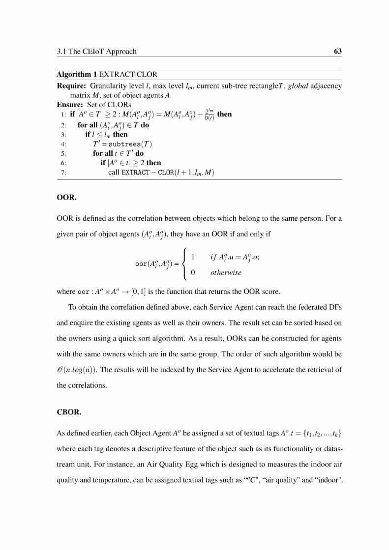
3.1 The CEIoT Approach 63
Algorithm 1 EXTRACT-CLORRequire: Granularity level l, max level lm, current sub-tree rectangleT , global adjacency
matrix M, set of object agents AEnsure: Set of CLORs
1: if |Ao ∈ T | ≥ 2 : M(Aoi ,A
oj) = M(Ao
i ,Aoj)+
2lm
D(t) then2: for all (Ao
i ,Aoj) ∈ T do
3: if l ≤ lm then4: T ′ = subtrees(T )5: for all t ∈ T ′ do6: if |Ao ∈ t| ≥ 2 then7: call EXTRACT−CLOR(l +1, lm,M)
OOR.
OOR is defined as the correlation between objects which belong to the same person. For a
given pair of object agents (Aoi ,A
oj), they have an OOR if and only if
oor(Aoi ,A
oj) =
1 i f Aoi .u = Ao
j .o;
0 otherwise
where oor : Ao×Ao→ [0,1] is the function that returns the OOR score.
To obtain the correlation defined above, each Service Agent can reach the federated DFs
and enquire the existing agents as well as their owners. The result set can be sorted based on
the owners using a quick sort algorithm. As a result, OORs can be constructed for agents
with the same owners which are in the same group. The order of such algorithm would be
O(n.log(n)). The results will be indexed by the Service Agent to accelerate the retrieval of
the correlations.
CBOR.
As defined earlier, each Object Agent Ao be assigned a set of textual tags Ao.t = {t1, t2, ..., tk}
where each tag denotes a descriptive feature of the object such as its functionality or datas-
tream unit. For instance, an Air Quality Egg which is designed to measures the indoor air
quality and temperature, can be assigned textual tags such as “oC", “air quality" and “indoor".

64 Interlinking IoT Resources
The tags are assigned by the users of the IoT platform and thus, can vary significantly based
on their count, keyword selection, dictation and used symbols. We assume that the tag set for
each object can be used for the purpose of categorization. For a given pair of Object Agents
(Aoi ,A
oj), a text similarity function σ : T 2→ [0,1] and a similarity threshold τ ∈ [0,1] we
define the CBOR as follows:
cbor(Aoi ,A
oj) =
∏σ(Aoi .t,A
oj .t) i f σ(Ao
i .t,Aoj .t)> τ;
0 otherwise
where cbor : A2→ [0,1] is the weight function of the CBOR correlation between (Aoi ,A
oj).
Algorithm 2 shows our approach to identify and extract CBORs amongst a set of given
Object Agents. Using a naive approach for finding the similarity between all pairs of object
agents is time consuming and complex. Thereupon, the three scenarios of searching for
similar objects using CBOR are:
• There is no matching result and a Null value returned.
• The number of objects in the list ≤ Max_results. Thus, all objects in the list are
returned.
• The number of objects exceeds the max criterion. Provided that the list is descendingly
sorted, a sub list with size of Max_results is cut from the first element and retrieved as
an answer for the query indicating that there is high potentiality to connect, correlate,
cooperate, and any action can be taken with these objects.
3.1.4 Correlation Representation
Correlation representation is a part of correlation discovery process in which all of the
extracted correlations are presented based on a standard format. We use RDF to represent
correlations in IoT. Thus, we can maintain the connections between things while a large

3.1 The CEIoT Approach 65
Algorithm 2 EXTRACTCBORRequire: Requester ID, Type, Sensor_ set, Actuators_ set, Max_ resultsEnsure: resultsList : List of relevant objects agents
1: if Results = /0 then2: for all Ob ject ∈ result do3: if Sensors = /0 || Actuators = /0 then4: S = {Sensors}5: A = {Actuators}6: S_SIM(Sensor_set,S) = ⌈Sensor_set ∩S⌉/⌈Sensor_set ∪S⌉7: A_SIM(Actuators_set,A) = ⌈Actuators_set ∩A⌉/⌈Actuators_set ∪A⌉8: Similarity = SIM.S+SIM.A9: Assign Similarity to Object
10: Add Object to resultsList11: Sort resultsList descendingly12: if {Results− list} ≥Max_results then13: Shrink the result by excluding elements from Max_ results until the end of the list14: return resultsList
portion of them are quickly evolving. Through the use of specifically designed ontologies
along with RDF correlations, our approach can be deployed to empower pattern queries for
IoT search engines. In this regard, we use triple space computing (TSC) to facilitate the
communication and store relationships triples.
Figure 3.5 depicts an example of how things can be correlated using RDF triples, where
each object is considered as a resource. Each statement is identified via a unique URI. A
statement consists of three elements: subject, predicate, and object. A subject (a thing)
is linked with an object (another thing). The connection between two objects is called a
predicate. The predicate explains the relationship between the subject and the object of the
statement.
Two objects will have OOR if and only if they have the same owner. In this type of
relationships, we point out the possibility of connecting objects under different regimes based
on a criterion such as a common owner. The result is retrieved from federated DFs as graph
of RDF triples similar to the following.
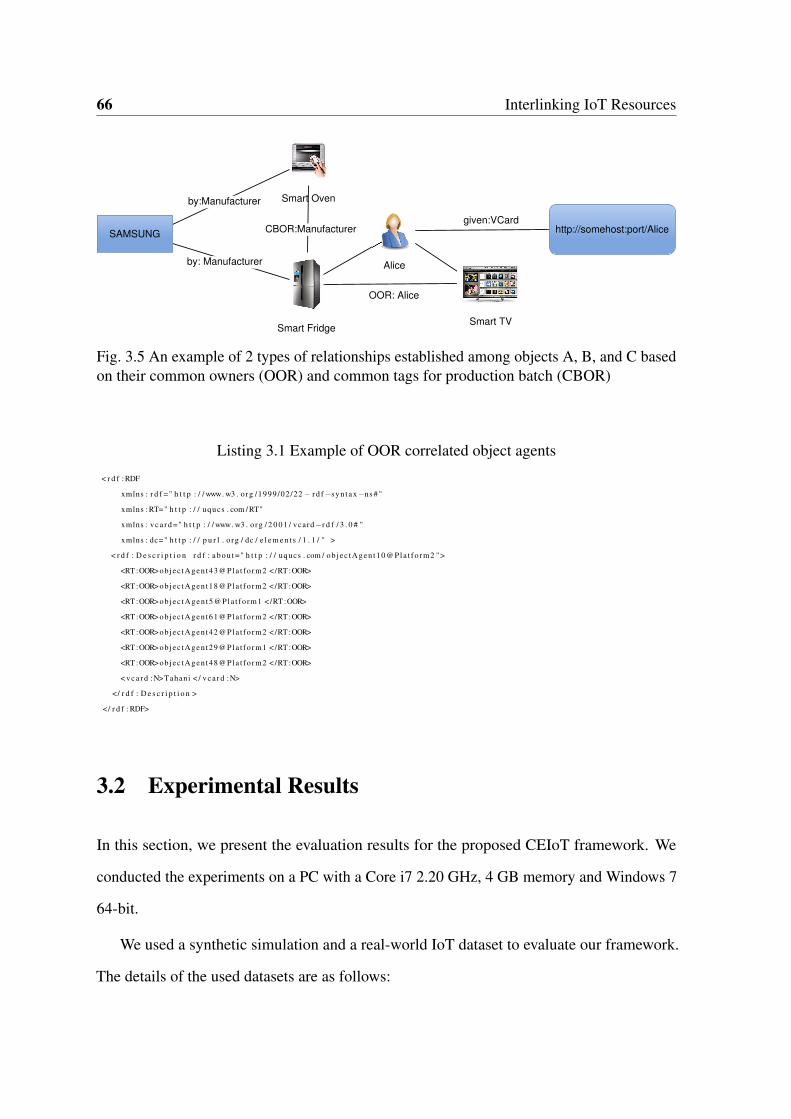
66 Interlinking IoT Resources
given:VCard
Aliceby: Manufacturer
CBOR:Manufacturer
OOR: Alice
Smart Fridge
by:Manufacturer Smart Oven
Smart TV
SAMSUNG http://somehost:port/Alice
Fig. 3.5 An example of 2 types of relationships established among objects A, B, and C basedon their common owners (OOR) and common tags for production batch (CBOR)
Listing 3.1 Example of OOR correlated object agents
< r d f :RDF
xmlns : r d f =" h t t p : / / www. w3 . org /1999/02 /22− r d f−syn t ax−ns # "
xmlns : RT=" h t t p : / / uqucs . com / RT"
xmlns : v c a r d =" h t t p : / / www. w3 . org / 2 0 0 1 / vcard−r d f / 3 . 0 # "
xmlns : dc=" h t t p : / / p u r l . o rg / dc / e l e m e n t s / 1 . 1 / " >
< r d f : D e s c r i p t i o n r d f : a b o u t =" h t t p : / / uqucs . com / ob j ec tAgen t10@Pla t fo rm2 ">
<RT :OOR> objec tAgen t43@Pla t fo rm2 </RT :OOR>
<RT :OOR> objec tAgen t18@Pla t fo rm2 </RT :OOR>
<RT :OOR> objec tAgen t5@Pla t fo rm1 </RT :OOR>
<RT :OOR> objec tAgen t61@Pla t fo rm2 </RT :OOR>
<RT :OOR> objec tAgen t42@Pla t fo rm2 </RT :OOR>
<RT :OOR> objec tAgen t29@Pla t fo rm1 </RT :OOR>
<RT :OOR> objec tAgen t48@Pla t fo rm2 </RT :OOR>
< v c a r d :N>Tahani < / v c a r d :N>
</ r d f : D e s c r i p t i o n >
</ r d f : RDF>
3.2 Experimental Results
In this section, we present the evaluation results for the proposed CEIoT framework. We
conducted the experiments on a PC with a Core i7 2.20 GHz, 4 GB memory and Windows 7
64-bit.
We used a synthetic simulation and a real-world IoT dataset to evaluate our framework.
The details of the used datasets are as follows:

3.2 Experimental Results 67
1. Synthetic dataset: we simulated a set of four IoT service providers where each service
provider is supplied with one Service Agents and 1,000 Object Agents. Furthermore,
each service provider was initialized on a separate platform, which can run on an
independent machine or share the same machine with other service providers. We
use this simulation to evaluate the framework on a distributed infrastructure and for
multiple service providers. Figure 3.6a shows four RMA GUIs visualizing all four
platform and their agents. We used this dataset only for the purpose of examining
the effect of decentralization of our approach. As all other characteristics are already
featured in the real-world dataset, there is no merit in reporting the results on the
synthetic approach, separately. Thus, the rest of the results are acquired from the
experiment on the real-world dataset as described below.
2. Real-world dataset: we used our dataset from the previous chapter. We randomly
picked the data from one of the crawling rounds from Xively [29]. The dataset contains
around 67,000 things and their most recent sensor readings. However, after filtering
records with incomplete data, only 11,894 records remain in our dataset. A primary
analysis of the tag sets reveals that the tags are scattered (Figure 3.7a) but densely
focused on some tags (Figure 3.7b). Moreover, only less than 10% of the tags have
been assigned to more than 60% of things (Figure 3.7c). Thus, a single label based
without considering location based correlations will not be helpful in application.
We used tools provided by RMA GUI such as Sniffer and Dummy for debugging and
testing purposes. Dummy agent is used to communicate with agents in the platform and
command them to execute specific behaviors. We prepared the agents with Cyclic behaviors
that are responsible for receiving these commands and their execution. Otherwise, these
behaviors are blocked until a command is received to prevent infinite loop. Blocking the
behaviors in agents does not block the entire agent. Additional aim of implementing agents
behaviors and communication is to use them as self-explained examples of how agents can

68 Interlinking IoT Resources
be communicated and commanded by end users of the framework using third-party agent
such as Dummy agent.
3.2.1 System Performance
One concern is the overall performance of the framework including all aspects discussed
except the relationships extraction and establishment. Mainly, the framework does the
following: i) launches all independent platforms; ii) launches all agents mentioned above; iii)
federates DF service; iv) communication for exchanging stetting information; v) generating
RDFs and message de/serialization; and vi) R-tree insertion. Using the fixed parameters with
an RMA launched for each platform, it takes the system roughly 25 seconds to perform all
the mentioned key tasks. This is due to that each Service Agent waits for about 10 seconds to
ensure all platforms are established, as well as additional 10 seconds for federation. These
20 seconds were introduced to avoid racing conditions.
The experiment was conducted on 4,000 object agents which were distributed over four
independent platforms. In the worst scenario, for all objects agents, we took them under the
same owner, the same sensors, the same actuators. These values were set to make them all
similar in order to be able to observe the performance. Thus, when an object searches for
other objects, all other 3,999 should be retrieved from the DF to an object agent requesting
OOR relationships. For the experiment, each object agent has a cycle behavior that receives
a message with a Request per-formative act. It recognizes commands OOR, and CBOR.
Otherwise, it responses with a non-understood message associated with which commands it
can understand. If the commands are understood, it complies with them to search for other
agents matching the type in the command.
The communication with Object Agent was performed as expected (Figure 3.6b). The
figure shows the UML sequence for sending relationship requests by the dummy agent (d0)
to an object agent. Agent d0 was used in our experiment for requesting object agents to

3.2 Experimental Results 69
(a) RMA view of launched platforms for each service agent
(b) Sniffed communications between two object agents
Fig. 3.6 CEIoT System View
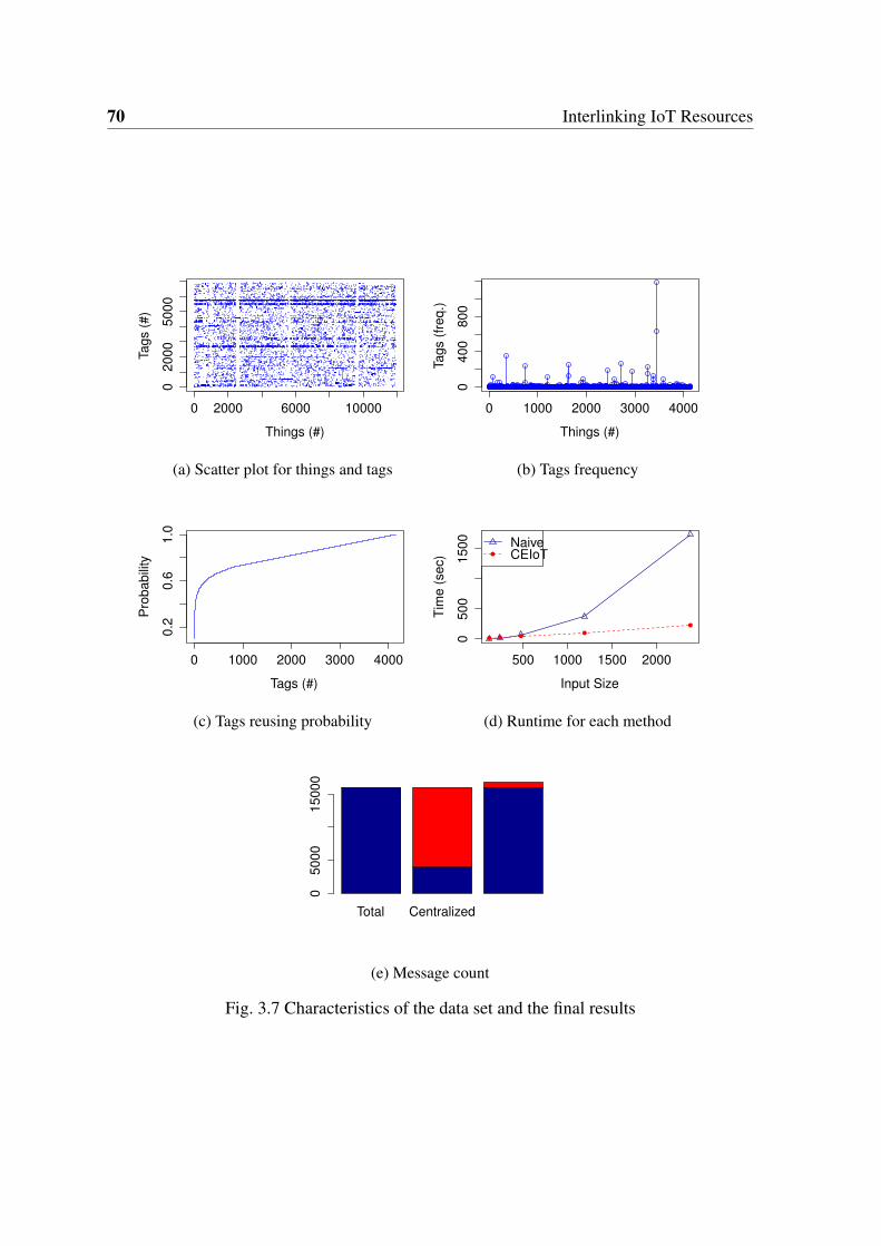
70 Interlinking IoT Resources
0 2000 6000 10000
02000
5000
Things (#)
Tags (
#)
(a) Scatter plot for things and tags
0 1000 2000 3000 4000
0400
800
Things (#)Tags (
freq.)
(b) Tags frequency
0 1000 2000 3000 4000
0.2
0.6
1.0
Tags (#)
Pro
babili
ty
(c) Tags reusing probability
500 1000 1500 2000
0500
1500
Input Size
Tim
e (
sec)
NaiveCEIoT
(d) Runtime for each method
Total Centralized
05000
15000
(e) Message count
Fig. 3.7 Characteristics of the data set and the final results
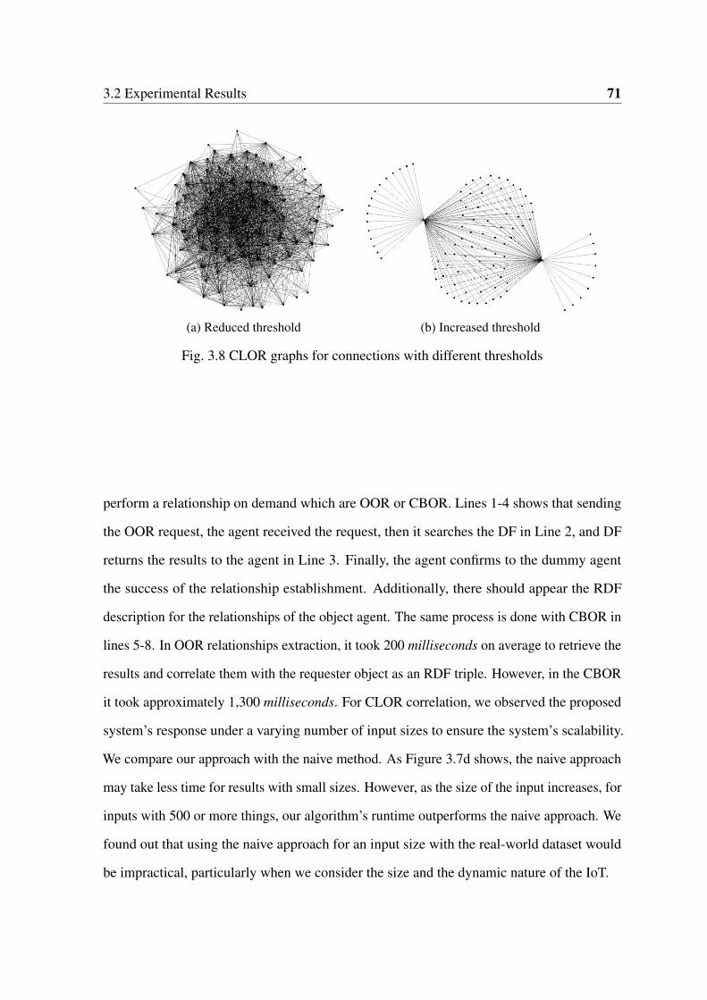
3.2 Experimental Results 71
(a) Reduced threshold (b) Increased threshold
Fig. 3.8 CLOR graphs for connections with different thresholds
perform a relationship on demand which are OOR or CBOR. Lines 1-4 shows that sending
the OOR request, the agent received the request, then it searches the DF in Line 2, and DF
returns the results to the agent in Line 3. Finally, the agent confirms to the dummy agent
the success of the relationship establishment. Additionally, there should appear the RDF
description for the relationships of the object agent. The same process is done with CBOR in
lines 5-8. In OOR relationships extraction, it took 200 milliseconds on average to retrieve the
results and correlate them with the requester object as an RDF triple. However, in the CBOR
it took approximately 1,300 milliseconds. For CLOR correlation, we observed the proposed
system’s response under a varying number of input sizes to ensure the system’s scalability.
We compare our approach with the naive method. As Figure 3.7d shows, the naive approach
may take less time for results with small sizes. However, as the size of the input increases, for
inputs with 500 or more things, our algorithm’s runtime outperforms the naive approach. We
found out that using the naive approach for an input size with the real-world dataset would
be impractical, particularly when we consider the size and the dynamic nature of the IoT.

72 Interlinking IoT Resources
3.2.2 Things Correlation Graph
For Algorithm 1, we applied different thresholds to simulate a search engine harvesting the
graph. For example, it can be interesting in relationship matching a certain criteria. Thus, the
threshold was used to reduce the search space and to limit it to connections with values equal
or larger than the threshold. We visualized this by passing the symmetric weighted graph to
the GraphVis class. The graph is the file holding all CLOR relationships among the Object
Agents resulted from Algorithm 1. The higher the value of a threshold, the smaller search
space is. Figures 3.8a and 3.8b illustrate the samples of graphs produced based on different
thresholds, respectively.
3.2.3 Message Volume
One of the key factors is to minimize the number of transacted messages between the
machines. In our CEIoT framework, the messages that should be transacted between different
platforms are summarized. Thus, we expect a dramatic reduction in the number of transacted
messaged compare to a centralized scenario. Figure 3.7e shows the number of both internal
and external messages which were transacted between agents during the experiment on the
synthetic dataset. In this Figure, the As it is shown, although the red stack (top) shows the
number of inter-platform messages and the blue (bottom) shows the number of intra-platform
messages in our experiment. As shown, despite the fact that using the CEIoT approach
in a distributed mode increases the number of transacted messages by a small amount, it
may enhance the total throughput of the system by reducing the ratio of inter-platform
messages which are quite expensive. Moreover, in the distributed mode the messages are
being processed by a larger number of machines than the centralized approach.

3.3 Related Work 73
3.3 Related Work
There are some studies which promote that the IoT can be implemented as the Internet
of agents [88]. This is due to the ability of agents to mimic human activities such as
willingness to achieve certain goals, and the social ability to interact with each other and
with human as well. In a proposal by Fortino et al [89], MAS is also considered to perfectly
help developing a smart environment for objects without direct human intervention. The
heterogeneity and disparity can intensify the problem of dealing with smart things in an
effective way. Things data is never under centralized control. Hence, datasets are usually
stored in distributed locations. Using central location for data storage is an obstacle for
materializing an effective solution. The diversity of sensors infrastructures means that, data
are structured and documented in different ways, which complicates combining their datasets
in an easy way. Thus, one of the solutions called Concinnity [90] takes the advantage of
Semantic Web technologies such as RDF, Ontology, and SPARQL.
There is an interesting paradigm called Triple Space Computing [91] that has the potential
to facilitate storage and communication in the Internet of Things context. It is basically a
dedicated Web for machines, which is combined of space-based computing and the Semantic
Web. It uses RDF triples for data representation to exchange knowledge using shared space,
just like HTML representation in human-driven Web [92]. TSC provides asynchronous
communication such that consumers neither need to recognize each other through identifiers,
nor need to concurrently consume data.
A provisional approach is the Social Internet of Things (SIoT) [40, 39, 93]. To socialize
things in the IoT, unlike the solutions for socializing smart things that depend totally on their
owners’ relationships, this approach seeks a solution to enable smart things to be interlinked
by themselves. Objects have their own profiles and IDs, so they can discover other objects
of interest and establish a friendship with each other according to their owners’ constraints.
Additionally, this approach defines some types of relationships established among objects.

74 Interlinking IoT Resources
For instance, Parental Object Relationship (POR), Co-Location Object relationship (CLOR),
Co-work Object Relationship (C-WOR), and Social Object Relationship (SOR). However,
no realistic and scalable solution given on how to identify and extract these relationships.
Correlating things in IoT has various benefits such as better navigability experience, query
result diversification and matters of an interest can be effectively discovered with the least
effort possible [38]. As discussed before, Atzori et al. [40] discuss the characteristics of
Social Internet of Things and define polices for relationships establishment among connected
things. Unlike the approaches that socializes things according to what relationships their
owners [93, 94], this approach is more focused on things as key players in relationships
establishment, which limits the roles of their owners to managing them and setting appropriate
rules for their relationships. However, to the best of our knowledge, this vision has not been
implemented yet. Additionally, currently no technical details have been given on how to
automate the establishment of relationships between objects when they are aware of each
other. Automated correlation extraction is limited to one type of correlation for a small
number of objects [27, 74].
3.4 Summary
One of the missing components in the IoT is something similar to hyperlinks in the World
Wide Web. Unlike the traditional Web, establishing correlations in IoT can be challenging as
it must be automated. In this chapter, we have proposed the CEIoT framework for extraction
and representation of correlations between things in the IoT. We have used a distributed
architecture and local correlation filtering to stabilize the performance of the library in
different conditions. Our framework can be used in parallel with the crawler and enable it to
improve its navigation through the WoT resources.
However, given the pool of correlations and/or sensor data in the form of Open Linked
Data (using RDF), there are a number of challenges that need to be tackled. Firstly, to

3.4 Summary 75
merge/integrate the networks of things that are acquired from multiple data sources, we need
to find the matches of the given nodes in different graphs. Secondly, it is crucial to an IoT
search engine to be able to process subgraph queries. To identify the answers to a given
query, it is critical to find the best matches for a given pattern that is extracted from the
query, similar to the Graph Search in Facebook [95]. We address this key function in the next
chapter and tackle the associated technical challenges of pattern matching by proposing a
novel approach that can address the requirements of the IoT data.

Chapter 4
Pattern Matching for Things Correlation
Graphs
Graph pattern matching is already a fundamental method for various applications in many
domains including, but not limited to, social computing [96], computer vision [97] and
computational chemistry[98]. Existing variations of this method is extensively studied in
different contexts in the past few years. Given the Things Correlation Graphs (TCGs) from
correlating the objects, we can apply pattern matching for the following purposes:
• Knowledge processing: linked sensor data is a popular format for presenting and
modeling IoT data on the Web [99–105]. Due to the fundamental role of pattern
matching in processing sensor data in RDF format [106, 107], it is necessary to
develop efficient approaches.
• TCG merging: Sensors can provide data on different networks simultaneously. The
analysis of IoT data in Chapter 2 confirms this claim by showing that in some cases,
the ratio of the overlapping things between different networks are high. Given the
distributed bottom-up interlinking approach from Chapter 3, a number of distinct TCGs

78 Pattern Matching for Things Correlation Graphs
are extracted from different networks. Thus, a pattern matching approach is required to
process the data for a given node from a TCG and find the matches in the other TCGs.
Assorted types of conditions and requirements impose different constraints on pattern
matching techniques. In general, pattern matching aims to solve the problem of finding
subgraphs of a given data graph G, which match a given pattern graph Q. One of the partic-
ular conditions, i.e., processing graphs with labeled nodes [108], is increasingly receiving
attention.
The existing approaches for labeled graph pattern matching use a particular definition of
labeled nodes where each node is associated with a single label [96]. Thus, for the pattern
Q and the data graph G, the nodes of G can be categorized based on the set of labels of
nodes in Q without any conflict. This approach is useful for many applications in social
computing but does not cover some of the new domains, such as the IoT [3], and some
sophisticated problems in social networks, i.e., when the labels are uncertain or when the data
is incomplete. In any of these cases, assigning a single label to each node could be unrealistic
and we need to define graphs with multi-labeled nodes. However, using multi-labeled graphs
compared to the single-labeled graphs can potentially increase the complexity of the problem.
In this case, revising the current pattern matching approaches for multi-labeled graphs is
beneficial.
Example 1. To provide a clear image of the problem, in this chapter we explain an applica-
tion in the context of the Internet of Things. For example, a search service extracts the pattern
graph from one network of things and the data graph from another. Figure 4.1 illustrates
two graphs that are obtained from these two networks. Each edge represents a relationship
between two nodes in the same network.
Each node (i.e., a thing) is described with a set of metadata about its sensors and
actuators. We can take each tag as a label due to some reasons including (1) there is
not universal description for things connected to the network, and (2) each node can be

79
Fig. 4.1 Querying two networks of things (a) the pattern graph, (b) the data graph
Table 4.1 The set of label assignments
Node Labelsu1 l.s0, l.s1, l.a0, l.a3u2 l.s2, l.s3, l.a1, l.a3u3 l.s1, l.s3, l.a2, l.a3u4 l.s0, l.s1, l.a0, l.a1v1 l.s2, l.s3, l.a1, l.a3v2 l.s0, l.s1, l.a0, l.a2v3 l.s1, l.s2, l.s3, l.a1, l.a2v4 l.s2, l.a0, l.a1, l.a2v5 l.s3, l.a0, l.a1, l.a3v6 l.s0, l.s1, l.a0, l.a1v7 l.s1, l.s2, l.s3, l.a3v8 l.s0, l.s2, l.a0, l.a1v9 l.s1, l.s2, l.s3, l.a0v10 l.s0, l.s2, l.a0, l.a1, l.a2v11 l.s1, l.s2, l.a1, l.a2v12 l.s0, l.s1
registered partially on different networks. The labels are selected from a language Σ.s =
{sensor/thermal, sensor/weather, sensor/signal, sensor/current, sensor/motion} and Σ.a =

80 Pattern Matching for Things Correlation Graphs
{actuator/screen, actuator/switch, actuator/fan, actuator/speaker, actuator/alarm}. Table
4.1 shows the labels assigned to each node.
To examine the similarity between two nodes, we use a similarity ratio as follows:
s(vi,v j) =|L(vi)∩L(v j)||L(vi)∪L(v j)|
(4.1)
where |L(vi)∩Ł(v j)| denotes the number of common labels between two nodes and |L(vi)|
denotes the number of the labels of vi. We can compare the similarity score with a threshold
t.
Based on the present model, if we set the similarity threshold as 0.5, for each node ui ∈Q,
Table 4.2 lists the nodes vi ∈ G that can be a match. All of the nodes from the data graph
appear more than once in the set of similarity lists. Due to this conflict, no unique label can
be associated with any of the nodes. For instance, although v2 is specified a match of the
query node (u1), it can match node u4 as well. The set of similarity lists is more complex than
the case when each node is assigned only one table. This is because in that case, each node
of the data graph would appear only once in the final list. Therefore, the pattern matching
process can be more complex and new situations must be considered.
Table 4.2 Nodes with label similarity above threshold
Query Graph Node Similar Data Graph Nodeu1 v2,v6,v12u2 v1,v3,v5,v7u3 v3,v7u4 v2,v6,v8,v10,v12
With the increasing complexity and volume of graphs in new contexts such as social
networks and the Internet of Things, performance will be the main issue that we should tackle
when we revise graph pattern matching for multi-labeled graphs. The typical definitions of

81
graph simulation are generally too restrictive to be applied for this purpose. Nonetheless,
computing all of the possible simulations will result in the inefficiency of any solution. In
order to tackle these challenges, we propose a novel approach for graph pattern matching for
multi-labeled graphs. Our contributions in this chapter are as follows:
• We introduce the concept of surjective simulation, which is more flexible than graph
simulation and bounded simulation. Through the use of surjective simulation, the
proposed approach can notably reduce the complexity of simulation creation step to
|Vp||V |. With this concept, we can optimize the process via removing the simulations
that do not contain any match of the query nodes.
• To avoid going through the computation of each simulation to get its size, we propose
an approximation procedure based on the Metropolis-Hastings Algorithm. We also
devise an early stop mechanism when (1) we have at least k nodes in the results and
(2) the size of the smallest simulation is equal to or greater than the rest of surjective
simulations.
• We evaluate the proposed approach via extensive experimental studies. The results
show the efficiency of our approach and verify the superiority of our approach over
existing approaches.
The rest of this chapter is organized as follows. In Section 4.1 we define the problem. A
naive approach based on a very recent work is provided in Section 4.2. We provide necessary
background in Section 4.3. Then in Section 4.4 we show how we can compute the set of
the top-k results using the proposed concept of surjective simulation with the Metropolis-
Hastings algorithm. Section 4.5 presents the experimental results. Finally, Section 4.6
reviews the related works and Section 4.7 provides some concluding remarks.

82 Pattern Matching for Things Correlation Graphs
4.1 Problem Formulation
Before presenting our approach for graph pattern matching, we first formally define the
problem that we are going to investigate. Multi-labeled graph pattern matching is the task
of matching the nodes of a given pattern graph Q with a data graph G based on structural
similarity, where each node is given a set of labels.
Definition 1 (Graph). A graph is represented as G = (V,E,L) where (1) V = {v1,v2, ...,vn}
is a set of nodes; (2) E ⊆V ×V is a set of edges; and (3) L = {li : li ∈V ×Σ} is a mapping
that relates each node to a set of assigned labels from language Σ. □
Definition 2 (Pattern Graph [109, 108]). A pattern graph is a directed and connected graph
Q = (Vp,Ep,Lp,u∗), where (1) Vp is a set of query nodes; (2) Ep is a set of query edges; (3)
Lp ⊆Vp×Σ is a mapping that links every node u ∈Vp to a set of labels in Σp ⊆ Σ; and (4)
u∗ ∈Vp that specifies the query node. □
Definition 3 (Graph Simulation [109]). A graph G matches a pattern Q iff there exists a
binary relation S⊆Vp×V such that (1) for each node u ∈Vp, there exists a node v ∈V such
that (u,v) ∈ S, referred to as a match of u; (2) for each pair (u,v) ∈ S, L(u) = L(v), and for
each edge (u,u′) in Ep, there exists an edge (v,v′) in G such that (u′,v′) ∈ S. □
A top-k problem can be defined in the following. Given a surface Γ(x,y), a function
f (x,y) : x,y→ D, a scoring function δ ( f ), and a positive integer k, it is to find a subset
φ ⊆ D, such that |φ |= k and
φ = argmaxφ⊆Γ,|φ |=k
∑x,y∈Γ
δ ( f ) (4.2)
In the rest of this chapter, we refer to the following problem as MULTIMATCH. Given a
data graph G and a query graph Q with the query node u∗, assuming that there are at least
k subgraphs in G that match the query graph (i.e., containing the nodes, edges and labels
in Q), we want to find the top-k matches Mk = {m1,m2, ...,mk} of u∗ in G such that (1) for
4.2 The Naive Approach 83
every mi ∈ M, there exists at least one simulation Si that contains (u∗,mi), and (2) i < j
iff |Si| ≥ |S j| and Si,S j represent the largest simulations containing (u∗,mi) and (u∗,m j),
respectively. In the case that we do not have k matches of the query graph in the subsets of
the data graph, we look for all matches instead. In other words, we want to compute the
following equation:
M = argmaxM⊆V,|M|=k
∑v∈V|S = (Vs,Es,Ls,Ms)| (4.3)
where S denotes a simulation of pattern Q = (Vp,Ep,Lp) in data graph G = (V,E,L) and
|(Vs,Es,Ls,Ms)| denotes the size of the simulation.
Example 2. For the pattern Q and the data graph G in Figure 4.1, we can retrieve simulation
S = {(u1,v6),(u2,v11),(u3,v7),(u4,v10)}. S is one of the possible simulations. Definition 3
is strict and does not include other subsets of S.
4.2 The Naive Approach
The naive approach explores the whole set of possible permutations for the answers. To the
best of our knowledge, one of the closest efforts that only works for single-labeled nodes is
the diversified graph pattern matching in [110].
As mentioned, high complexity is the first critical issue that we encounter when employing
the graph simulation to deal with graphs containing multi-labeled nodes. This is mainly
the result of the restrictions imposed by the graph simulation definition. A more flexible
definition that is used in naive approaches is the bounded simulation.
Definition 4 (Strong (Bounded) Simulation [111]). A pattern graph Q matches a data graph
G via strong simulation, denoted by Q≺LD G, if there exists a node v in G and a connected
subgraph Gs of G such that (1) Q≺DGs, with the maximum match relation S; (2) Gs is exactly

84 Pattern Matching for Things Correlation Graphs
the match graph w.r.t. S; and (3) Gs is contained in the ball G[v,d(Q)], where d(Q) is the
diameter of Q. □
We take the gist of this work (which work? Any reference?) to develop a naive approach.
We use two algorithms for both Directed Acyclic Graphs (Algorithm 3) but modify them to
support the possible worlds of multi-labeled nodes.
Algorithm 3 works as follows. The underlying idea of this algorithm is to execute
TopKDAG [110] for all possible label assignments of the both graphs (i.e., Q and G). We first
compute the possible worlds for label assignment with ∏i L(vi) for G in line 1 and ∏ j Lp(u j)
for Q in line 2. Then, for every possible combination, we use the following process to get the
biggest possible simulation S∗. We initialize the min-heap S that is used to store the simulation
and the termination variable (line 5). The topological rank r(u) is used to keep track of the
distance from the starting point. We define r(u) for u ∈ G as (a) r(u) = 0 if the mapped node
of u is a leaf in GSCC; and otherwise (b) r(u) = max{(1+ r(u′))|(uSCC,u′SCC) ∈ ESCC}. This
algorithm dynamically maintains a vector v.T , which contains (1) a Boolean equation v.b f of
the form Xv = f , where f is a Boolean formula that indicates whether v is a match of u; (2)
a subset v.R of its relevant set R(u,v); and (3) integers v.l and v.h to estimate the lower and
upper bounds of δr(u,v), respectively. The algorithm iteratively computes the set of matches
and updates the vectors of other candidates by “propagating” the partially evaluated results.
Algorithm 3 supports directed acyclic graphs (DAGs) only. For other types of graphs that
contain cyclic paths, the complexity of the solution could rise and naive approaches could be
developed based on running the SccProcess [110] for all label permutations. Otherwise, we
can convert the graph with cyclic paths to a set of DAGs [112] and use Algorithm 3 for all
subgraphs. However, due to the complexity and poor connection with our contribution, in
this chapter we do not cover this situation and leave it for future research.
Theorem 4.2.1. Given a pattern graph P(VP,EP,LP) and a data graph G(V,E,L), the com-
plexity of the naive approach for computing the top-k matches for u∗ ∈Q is O(|V ||Vp||E||EP|).

4.3 Background 85
Proof. We can prove the complexity of the given problem via computing the upper and the
lower bounds for the complexity. To compute the upper bound, we suppose that for each
node v ∈ G, |Σ|= |V | and |V | different labels have been assigned. In other words, all of the
nodes have the same set of assigned labels. Respectively, let us suppose |Σp|= |Vp| and for
each node u ∈ Q, |Vp| labels have been assigned.
This means that in the worst case, we have to go through a search space of all possible
matches. In the ith iteration for matching ui and v j, |V | possible cases are available. Thus, by
the last iteration, |Vp||V | matches have been traced.
On the other hand, the lower bound for the complexity of the mentioned problem occurs
when each node in G is assigned with only one label. All of the nodes u ∈ Q except one
(e.g., u∗) are assigned with only one label while u∗ owns n labels. Therefore, by running the
TopKDAG [110] for the two possible cases, we end up with O(n∗ (|Q||G|+ |V |(|V |+ |E|)+
|V | log(k))) time to compute the top-k matches where |G|= |V |+ |E| and |Q|= |VP|+ |EP|.
Thus, the time order of the NAIVE-DAG approach is O(V 2VP).
4.3 Background
In this section, we review some of the necessary background materials before we propose
our approach in the next section.
4.3.1 Markov Chains
Here we provide a concise description of the theory of Markov chains. Interested readers may
refer to [113] for more details. Briefly, a Markov chain is a sequence of random variables
x1,x2,x3, . . . ,xn with the Markov property, namely that, given the present state, the future
and past states are independent.

86 Pattern Matching for Things Correlation Graphs
Algorithm 3 NAIVE-DAG
Require: Q = (Vp,Ep,Lp,u∗) the DAG pattern, G the data graph, t node similarity thresholdEnsure: S∗ the biggest set of simulations
1: Let L ⊆∏i L(vi) and Lp ⊆∏ j Lp(u j) be the set of possible permutations of the labelsof G and Q
2: for all l ∈L do3: for all lp ∈Lp do4: Let min-heap S←∅ and termination← f alse5: for all u ∈Vp do6: get topological rank r(u) and initialize can(u)7: for all v ∈ can(u) do8: initialize v.T9: while termination = f alse do
10: select a set of unvisited candidates Sc ⊆ can(u) of query nodes u in Q, wherer(u) = 0
11: if Sc =∅ then12: Let ⟨G,S⟩ ← AcyclicProp(Q,Sc,G,S)13: check the termination condition and update termination14: else15: termination← true16: Update S∗
17: return S∗

4.3 Background 87
To be more specific, let x be a random variable, where x(t) denotes the value of x at time
t. Let S = {s1, . . . ,sn} be the set of possible x values, denoted the state space of x. If x moves
from the current state to a next state based only on its current state, then x follows a Markov
process. That is, Pr(x(t + 1) = si|x(0) = sm, . . . ,x(t) = s j) = Pr(x(t + 1) = si|x(t) = s j),
here sm is the initial state. The process starts in one of these states sm and moves successively
from one state to another. Each move is called a step. A Markov chain is a state sequence
generated by a Markov process. The transition probability between a pair of states si and s j
can be denoted by Pr(si→ s j). If the chain is currently in state si, then it moves to state s j at
the next step with a probability specified by Pr(si→ s j).
A Markov chain may reach a stationary distribution π over its state space S, where the
probability of being at a particular state is independent from the initial state of the chain.
There are two conditions of reaching a stationary distribution, including (1) irreducibility
(i.e., any state is reachable from any other state), and (2) aperiodicity (i.e., the chain does not
cycle between states in a deterministic number of steps). A unique stationary distribution is
reachable if the following balance equation holds for every pair of states si and s j :
Pr(si→ s j)π(si) = Pr(s j→ si)π(s j) (4.4)
4.3.2 Markov Chain Monte-Carlo
The concepts of Monte-Carlo method and Markov chains are combined in the Markov Chain
Monte-Carlo (MCMC) method [113] to simulate a complex distribution using a Markovian
sampling process, where each sample depends only on the previous sample. A Markov
chain is normally to start with some transition distribution (a transition matrix in the discrete
case) modelling some process of interest, to determine conditions under which there is an
invariant or stationary distribution and then to identify the form of that limiting distribution.
By contrast, MCMC methods involve the solution of the inverse of this problem whereby the

88 Pattern Matching for Things Correlation Graphs
stationary distribution is known, and it is the transition distribution that needs to be identified,
though in practice there may be many distributions to choose from.
A standard MCMC algorithm is the Metropolis-Hastings (M-H) sampling algorithm
[114]. Suppose that we are interested in drawing samples from a target distribution π(x).
The (M-H) algorithm generates a sequence of random draws of samples that follow π(x). A
more detailed process is shown as follows: (1) start from an initial sample x0, (2) generate
a candidate sample x1 from an arbitrary proposal distribution q(x1|x0), (3) accept the new
sample x1 with probability α = min(
π(x1)·q(x0|x1)π(x0)·q(x1|x0)
,1)
, (4) if x1 is accepted, then set x0 = x1,
and (5) repeat from step (2).
The (M-H) algorithm draws samples biased by their probabilities. At each step, a
candidate sample x1 is generated given the current sample x0. The ratio α compares π(x1)
and π(x0) to decide on accepting x1. The (M-H) algorithm satisfies the balance condition
(Eq. 4.4) with arbitrary proposal distributions [114]. Hence, the algorithm converges to the
target distribution π . The number of times a sample is visited is proportional to its probability,
and hence the relative frequency of visiting a sample x is an estimate of π(x). The (M-H)
algorithm is typically used to compute distribution summaries (e.g., average) or estimate a
function of interest on π .
4.4 Pattern Matching
The high complexity of the naive approach affects the performance of the solution, particularly
when the graphs become large. In this section, we describe the details of our approach to
resolve the mentioned problem, which consists of two steps: identifying matches and ranking
matches.

4.4 Pattern Matching 89
4.4.1 Identifying Matches
Bounded simulation has shown to be useful for graphs containing nodes with single label
assigned. But when it comes to multiple labels, the use of bounded simulation does not
scale well. Thus, we need to define a more flexible definition of graph simulation. In
addition, the main criteria that can be used in ranking matches is the number of connected
nodes in the simulation. A graph simulation by definition demands that the nodes in the
generated simulation remain connected if the nodes in the pattern graph are already connected.
Regarding the fact that a bounded simulation does not ensure the connectivity of nodes of
the simulation, it increases the complexity of estimating the mentioned criteria. Furthermore,
this can increase the complexity of the pattern matching step. Thus, in this chapter we use a
more flexible definition of graph simulation as follows:
Definition 5 (Surjective Simulation). For a pattern graph Q = (Vp,Ep,Lp,u∗) and a data
graph G = (V,E,L), a surjective simulation S = (Vs,Es,Ls,Ms) is defined as a graph with the
following conditions: (1) ∀vs ∈Vs⇒∃(v ∈ G) such that v = vs and there exists a nonempty
path ρ in G which connects every pair of nodes in Vs; (2) Es = {(vs,v′s)|vs,v′s ∈Vs} and for
all of its edges there exists a (vp,v′p) ∈ Ep s.t. s(vp,vs)≥ t and s(v′p,v′s)≥ t; (3) Labels Ls
are the set of common labels from (2); (4)Ms = {(u,v)⊆Vp×Vs∧ s(u,v)≥ t} where t is a
threshold for the degree of labels similarity; and (5) S is connected and d(S)≤ d(P) where d
denotes diameter. □
We call our proposed graph simulation surjective since it covers any part of bounded
simulations that exists in a strongly connected component after mapping edges of the pattern
and the data graphs. One important difference between the proposed surjective simulation
and the graph simulation is that it does not oblige the neighbors’ nodes to remain as neighbors
after being simulated. Very similar to the bounded simulation, for every neighbor nodes um
and un, it is sufficient to remain connected after being simulated. The idea behind introducing
the concept of surjective simulation is to reduce the complexity of finding simulation stage.

90 Pattern Matching for Things Correlation Graphs
Based on the Lemma 1, it is possible to use the concept of surjective simulation in domains
where simulation has been adopted.
Example 3. Based on the given graphs Q and G in example 1, a surjective simulation can
be obtained as shown in Figure 4.2. The surjective simulation can be shown as a graph and
each node is mapped to a set of nodes in Q. It is composed of several simulations and all of
the nodes similar to the query node can be identified with "*" sign.
Lemma 1. If S denotes the set of all possible surjective simulations and SB denotes the set of
all bounded simulations for data graph G and pattern Q, for every {s∈ SB|s = (Vs,Es)} there
exists a set of surjective simulations Ss = {s1,s2, ...,sn|si = (V ′s ,E′s)∈S ,∑iV ′s =Vs∧∑i E ′s =
Es}.
Theorem 4.4.1. The MULTIMATCH problem is NP-Hard.
Proof. We prove the above theorem as follows. First, we show that any solution to this
problem can be verified in polynomial time. In order to verify an answer consisting of k given
subgraphs, we show that all of the steps can be accomplished in polynomial time and space.
For verifying each given subgraph, the set of nodes and edges could be sorted and matched
against the pattern graph in polynomial time. In addition, to verify that the subgraphs are
maximal, we can verify the extensions of each subgraph by matching the added node against
the pattern. In this regards, to generate each extension, a new edge from the original graph is
added to the subgraph. This part of the process can also be done in polynomial time, either.
Second, we show that this problem is a reduction of a NP problem. Since in the least
complex form, where all nodes in the data graph have unqiue labels, e.g., each node v ∈V
has only one label but there does not exist a u ∈V where L(u) = L(v), the MULTIMATCH
problem is similar to topKDP problem[110] that is shown to be NP-Hard. If we increase
the number of labels for all nodes v and assume that for all nodes v ∈V the labels are the
same s.t. ∀u ∈ V and u = v, L(u) = L(v), the MULTIMATCH problem is a reduction of

4.4 Pattern Matching 91
subgraph isomorphism [115] which is NP-complete. Graph pattern matching is very costly.
It is NP-complete for subgraph isomorphism [115], cubic-time for bounded simulation [96],
and quadratic-time for simulation [109].
Taking the advantage of the surjective simulation, we can avoid processing the nodes
which may not be a part of the maximum unique simulation and will be eliminated from
the pool of alternatives for further processing. To achieve this goal, we propose an index
for surjective simulation with a simple structure in the following: Iu = {(u,v)|u ∈ Q,v ∈
G∧σ(Lp(u),L(v))≥ t}.
Algorithm 4 provides the steps to create and maintain the set of surjective simulations.
The algorithm returns a set of surjective simulations S based on the given data graph G, the
given pattern graph Q and a given threshold for node similarity t. At the first step, matrix
M = {(MV ,ME)|u ∈ Q,v ∈ G} denotes a mapping from Q to G. For every edge ep ∈ Q
and e ∈ G, we iteratively (1) compare all labels and compute the corresponding degree of
similarity based on the number of common labels, and (2) add the new nodes and the new
edge to M . In the next step, we update the indexes including the set of query nodes (s.q),
the size of connected component (s.s). The new surjective simulation is then added to S .
One strength of Algorithm 4 is its low complexity without losing too much matching
quality. In the proposed algorithm, for the two for loops in steps 2-7, if we use an index to
get the mapped nodes in G, the complexity will be O(|E||Ep|). Based on the fact that getting
the connected components in step 8 is performed in a polynomial time O(|G|), the whole
process runs in O(|V ||Vp|+ |G|) time.
Example 4. Figure 4.2 shows the outcome of passing parameters Q, G, and the threshold
from previous example to the Algorithm 4. The set of mappings of the edges is shown in
Table 4.3. During the edge matching procedure, some of the edges in the data graph are
omitted when no corresponding edge is found in the query graph for them. Thus, one of the
first things that can be observed is that the data graph is divided into multiple connected

92 Pattern Matching for Things Correlation Graphs
Algorithm 4 GET-SURJECTIVE-SIMULATIONSRequire: Q the pattern graph, G the data graph, t node similarity thresholdEnsure: S the set of surjective simulations
1: Let M be the set mapped nodes in G2: for all ep = (up,vp) ∈ Q do3: for all e = (u,v) ∈ G do4: Let simu be the degree similarity of u and up based on the set of their labels5: Let simv be the degree similarity of v and vp based on the set of their labels6: if simu > t and simv > t then7: Add (u,v) to M8: for all Connected component C ∈M do9: Let s.q point to the set of query nodes in C
10: Let s.s point to the size of C11: if |s.q|> 0 and d(S)≥ d(Q) then12: Add surjective simulation S with specifications s.s and s.q to the S13: Sort S based on s.s value for each set14: return S
Fig. 4.2 The query and data graphs after removing non-matching edges
components as shown. Thus, connected components with lesser nodes than the query graph
can be removed from the result set. As a result, in the next step, we can limit our search
only to the connected components with greater number of nodes. In this example, we have
only one large connected component and other nodes including v4, v9, v11 and v12 will no
longer be considered to match any node in the query graph. In the next step, we observe that
each query edges ε2 and ε3 are mapped to only one corresponding data edge each. On the
other hand, there are multiple data graph nodes that match query nodes ε1 and ε4. Based on

4.4 Pattern Matching 93
this example, no match can be retrieved using simulation and strong simulation definitions.
However, based on the surjective simulation definition, different subgraphs exist in the main
connected component which contain nodes and edges that match nodes and edges in the Q.
These surjective matches include any connected subgraph with diameter 3 that contains e6
and e7.
Table 4.3 Mapping of the edges of G to edges in the query graph Q
Query Graph Edge Matching Data Graph Edgeε1 e1,e2,e3,e4,e5,e9ε2 e6ε3 e7ε4 e1,e2,e3,e4,e8
4.4.2 Top-k Matches
We propose a new approach, which approximates the maximum-sized match so as to reduce
the complexity introduced by the naive approach. The main idea is to employ the set of
surjective simulations to start the ranking procedure with an inter-simulations approach
that first gets sufficient candidates. Then it further ranks and sorts the intra-simulations.
To provide an efficient solution for finding top-k matches, we divide this step into two
sub-problems. In the first step, we look for the suitable surjective simulations within the
identified set of surjective simulations from Algorithm 4. In the second step, we approximate
the scores and rank of each match of the query node until we obtain the top-k nodes.
Algorithm 5 details the second step to obtain the top-k results. Unlike Algorithms 3, we
can process the both kinds of input (directed acyclic graphs and graphs with cycles) using the
same procedure. In this algorithm, similar to TopKDAG and SccProcss[110], we use an early
termination strategy by employing a termination variable. This variable gets updated after
each iteration by checking the conditions where (1) we still have more simulations in the
S to process, and (2) if the top k list is filled, the approximation of the size of the smallest
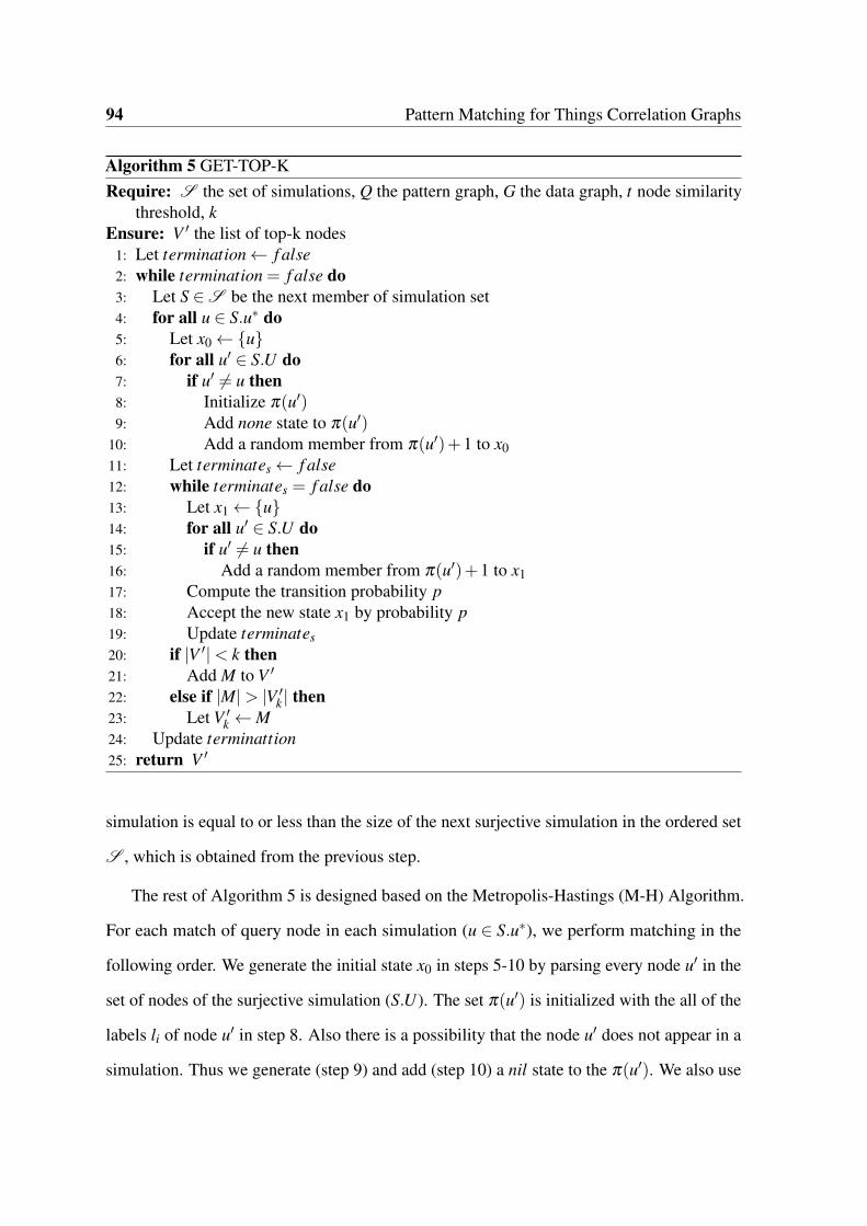
94 Pattern Matching for Things Correlation Graphs
Algorithm 5 GET-TOP-KRequire: S the set of simulations, Q the pattern graph, G the data graph, t node similarity
threshold, kEnsure: V ′ the list of top-k nodes
1: Let termination← f alse2: while termination = f alse do3: Let S ∈S be the next member of simulation set4: for all u ∈ S.u∗ do5: Let x0←{u}6: for all u′ ∈ S.U do7: if u′ = u then8: Initialize π(u′)9: Add none state to π(u′)
10: Add a random member from π(u′)+1 to x011: Let terminates← f alse12: while terminates = f alse do13: Let x1←{u}14: for all u′ ∈ S.U do15: if u′ = u then16: Add a random member from π(u′)+1 to x117: Compute the transition probability p18: Accept the new state x1 by probability p19: Update terminates20: if |V ′|< k then21: Add M to V ′
22: else if |M|> |V ′k | then23: Let V ′k ←M24: Update terminattion25: return V ′
simulation is equal to or less than the size of the next surjective simulation in the ordered set
S , which is obtained from the previous step.
The rest of Algorithm 5 is designed based on the Metropolis-Hastings (M-H) Algorithm.
For each match of query node in each simulation (u ∈ S.u∗), we perform matching in the
following order. We generate the initial state x0 in steps 5-10 by parsing every node u′ in the
set of nodes of the surjective simulation (S.U). The set π(u′) is initialized with the all of the
labels li of node u′ in step 8. Also there is a possibility that the node u′ does not appear in a
simulation. Thus we generate (step 9) and add (step 10) a nil state to the π(u′). We also use

4.4 Pattern Matching 95
a termination mechanism for the next steps by using the terminations variable. The variable
can be changed to true (step 19) after we get a certain number of iterations with no change in
the approximate size of simulation S. In steps 14-16 we generate a new random state x1 in a
process similar to x0 initiation. In the next steps (steps 17,18), we compute the probability of
accepting the new state x1 by the following equation:
p = min(π(x1).q(x0|x1)
π(x0).q(x1|x0) (4.5)
The early termination strategy is implemented afterwards in steps 20-23. Finally, the top
k matches are returned in step 25.
To calculate the values of π(xn) and q(xm|xn), we can use the following approach:
Supposing that to create π(xn) a procedure f in i = 1, ...,N steps is executed. In each step, a
new node is selected and added to the graph simulation. Based on the fact that the probability
of state xi+1 in the step i+1 is independent from the states 1,2, ..., i−1 and only depends on
the state i, we assume that the sequence is a Markov chain. Thus, for the step i+1, we have:
π(xi+1) =1
P(xi+1)(4.6)
Similarly, to calculate q(xm|xn), we can compute the cost of converting xn to xm. In step
i, we can convert xn to xm by converting the selected element to the new selection. In other
words, to make it simple, we can use the following equation:
q(xm|xn) =π(xm∩ xn)
π(xm− xn)(4.7)
where xm∩xn denotes the sequence of common selections between xm and xn and xm−xn
denotes the sequence of difference of selections in xm.

96 Pattern Matching for Things Correlation Graphs
4.5 Experimental Evaluation
We have implemented the proposed approach and conducted extensive experiments to study
its performance.
4.5.1 Experimental Setting
We used Java 1.6 and graphstream [116] 1.2 in the implementation. The experiments were
conducted on a computer with a 3.4 GHz Intel Core i7 processor and 8 GB of memory
running Ubuntu 14.04. We used the following datasets:
• Facebook dataset [117]: an anonymized social circles graph from Facebook with 4,039
nodes and 88,234 edges. Each node is associated with a set of features which are
dynamically defined and mapped.
• Twitter dataset [117]: an anonymized social circles graph from Twitter with 81,306
nodes and 1,768,149 edges. Each node is associated with a set of features which are
dynamically defined and mapped.
• Two synthetic datasets: we created a graph generator which takes the size of the nodes
and the size of the edges, and then generates a graph with randomly selected labels
for its nodes. We generated two graphs: one with 1,000 nodes and 10,000 edges and
the other with 1,000 nodes and 100,000 edges. Each node is associated with a set of
features which are randomly selected from a set of 40 labels similarly defined as the
ones in Example 1.
Although the main topic of this research is focused on IoT, due to the wide application
of pattern matching, the application of the proposed work in this chapter is not limited to
IoT. Thus, the main reason for selecting a social network graph is due to the lack of existing
established graphs in the domain of IoT. In other words, to avoid the questionableness of the

4.5 Experimental Evaluation 97
proposed approach, we use datasets from a well established area, which is social networks.
However, in the context of IoT, we need to process social graphs in processing correlations
that are related to social networks.
We also implemented a pattern generator for generating the graph Q = (Vp,Ep,Lp,u∗)
based on a given set of parameters such as graph Gp = (V,E,L), which is the source graph
for generating patterns, and an integer number r, which is the Euclidean radius of the pattern
graph starting from the query node.
The pattern’s label assignment process is carried out in the same way as for data graphs
label assignment. For this purpose, to maintain the closeness of the problem with reality, we
used the set of tags and features for each node provided by each dataset. At the beginning,
each node is associated with the set of its own labels. To compare the similarity of the labels
of two nodes, we used the Jaro Winkler method [118]. To optimize the proficiency of the
solution, we developed an index which stores the nodes that have similar labels for a given
node ui using the process shown in Algorithm 6.
To generate the pattern, a random node from Qs is picked as the query node u∗ and for
the rest of the nodes, only nodes within a certain distance from u∗ (≤ r), are picked out with
related edges and added to form Q. Jaro-Winkler is a measure of similarity between two
string based on the Jaro distance metric. The Jaro-Winkler score is normalized in the range
of [0,1] as the higher score denotes the higher similarity between strings. It is well suited for
short strings and a good option for comparing features of different nodes.
Algorithm 6 INITIALIZE-INDEXRequire: Qs the source graph for pattern, G the data graph, t node similarity thresholdEnsure: I nodes similarity index
1: for all Node u ∈ Qs and v ∈ G do2: Let su,v← Jaro-Winkler(L(u),L(v)) be the similarity score of u and v3: if su,v ≥ t then4: Add v to Iu5: return I

98 Pattern Matching for Things Correlation Graphs
(a) Example of larger pattern (b) Example of smaller pattern
Fig. 4.3 Visualization of pattern graphs
Table 4.4 provides a summary for the construction of the proposed index for each pair of
used datasets. Technically, the amount of time and the size of index highly depend on the
similarity threshold, or the degree of similarity for the set of nodes, in each test case.

4.5 Experimental Evaluation 99
Tabl
e4.
4In
dex
cons
truc
tion
sum
mar
yfo
rdiff
eren
tdat
aset
s
Firs
tDat
aset
Seco
ndD
atas
etT
hres
hold
Tim
e(s
)C
ompa
riso
nsE
ntri
esSi
ze(M
B)
Synt
hetic
Synt
hetic
0.7
1,47
2.29
610
,000
,000
236,
491
1.5
Face
book
Face
book
0.99
82,
426.
721
16,0
00,0
0033
0,73
91.
6Fa
cebo
okTw
itter
0.7
7,83
2.82
132
4,00
0,00
04,
585,
485
21.7
Twitt
erTw
itter
0.75
19,3
97.4
616,
561,
000,
000
9,56
2,74
889
.1

100 Pattern Matching for Things Correlation Graphs
However, the results show that although the amount of time and space are still high, using
the proposed index can significantly decrease the query processing time (see Figure 4.4).
Q:Syn/G:Syn Q:Fb/G:Fb Q:Fb/G:Twr
Datasets
Query
Tim
e(s
ec)
05000
15000
With IndexWithout Index
Fig. 4.4 Results for the total runtime
4.5.2 Efficiency
To assure the efficiency of our approach, we performed several tests using each of the datasets
mentioned above. Each efficiency test requires a pattern source graph Qs and a data graph
G. In the following figures, the efficiency test results are depicted as scatter plots along
with their regression (red) lines. From all datasets, we use a number of scenarios, which are
presented in the following.
Facebook as both the pattern source and the data graph
In this scenario, we used the node similarity threshold t = 0.97 due to the high similarity
of the metadata of features. The pattern was generated randomly by the Elucidian radius
r = 2. The size of the set of matching nodes for a given node deviates between 0 and 3,500
(Figure 4.5c). We ran this test 100 times with 100 M-H iterations. The results are shown in

4.5 Experimental Evaluation 101
0 50 100 150 200 250
04000
8000
Pattern nodes
Tim
e (
sec)
(a) Varying nodes count
0 50 100 150 200
04000
8000
Pattern edges
Tim
e (
sec)
(b) Varying number of edges
0 200 400 600 800
04000
8000
Average similarity degree
Tim
e (
sec)
(c) Varying average similarity
Fig. 4.5 The results for Qs :Facebook and G :Facebook
Figure 4.5a and 4.5b. Regression lines show the linear increment in the average processing
time as the number of pattern nodes, pattern edges and the average similarity degree increase.
Facebook as the pattern source and Twitter as the data graph
In this scenario, we used the node similarity threshold t = 0.7. The pattern was generated
randomly by the Elucidian radius r = 2. The average size of the set of matching nodes for a
given node deviates between 25 to 462 (Figure 4.6c). We ran this test 200 times. The results
are shown in Figures 4.6a and 4.6b. Figure 4.3a shows an example of a large pattern graph
generated from the Facebook dataset and Figure 4.3b smaller patterns through breaking down
larger patterns. The decreasing regression line in the pattern nodes increment is due to the

102 Pattern Matching for Things Correlation Graphs
0 500 1000 1500
0500
1000
Pattern nodes
Tim
e (
sec)
(a) Varying nodes count
0 5000 10000 15000 20000
0500
1000
Pattern edges
Tim
e (
sec)
(b) Varying edges count
100 200 300 400
0500
1000
Average similarity degree
Tim
e (
sec)
(c) Varying average similarity
Fig. 4.6 The results for Qs :Facebook and G :Twitter
special nature of the patterns extracted from Facebook dataset and the cross domain pattern
matching.
Twitter as both the pattern source and the data graph
In this scenario, we used the node similarity threshold t = 0.75. The pattern was generated
randomly by the Elucidian radius r = 1. The average size of the set of matching nodes for a
given node deviates between 0 and 3,512 (Figure 4.7c). We ran this test 100 times with 100
M-H iterations. The results are shown in Figures 4.7b and 4.7a. As the Figures show, there is
a linear increment in processing time as the number of edges and nodes increase. However,
the average similarity degree does not show a strong impact on the processing time.

4.5 Experimental Evaluation 103
0 50 100 150 200 250
0100
200
300
Pattern nodes
Tim
e (
sec)
(a) Varying nodes count
0 50 100 150 200 250 300 350
0100
200
300
Pattern edges
Tim
e (
sec)
(b) Varying edges count
0 500 1500 2500 3500
0100
200
300
Average similarity degree
Tim
e (
sec)
(c) Varying average similarity
Fig. 4.7 The results for Qs :Twitter and G :Twitter
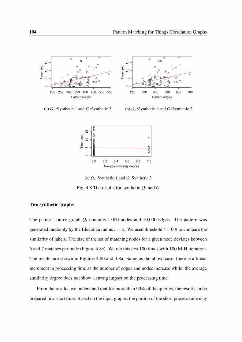
104 Pattern Matching for Things Correlation Graphs
200 250 300 350 400 450 500 550
05
10
15
Pattern nodes
Tim
e (
sec)
(a) Qs :Synthetic 1 and G :Synthetic 2
200 300 400 500 600 700
05
10
15
Pattern edges
Tim
e (
sec)
(b) Qs :Synthetic 1 and G :Synthetic 2
6.0 6.2 6.4 6.6 6.8 7.0
05
10
15
Average similarity degree
Tim
e (
sec)
(c) Qs :Synthetic 1 and G :Synthetic 2
Fig. 4.8 The results for synthetic Qs and G
Two synthetic graphs
The pattern source graph Qs contains 1,000 nodes and 10,000 edges. The pattern was
generated randomly by the Elucidian radius r = 2. We used threshold t = 0.9 to compare the
similarity of labels. The size of the set of matching nodes for a given node deviates between
6 and 7 matches per node (Figure 4.8c). We ran this test 100 times with 100 M-H iterations.
The results are shown in Figures 4.8b and 4.8a. Same as the above case, there is a linear
increment in processing time as the number of edges and nodes increase while, the average
similarity degree does not show a strong impact on the processing time.
From the results, we understand that for more than 90% of the queries, the result can be
prepared in a short time. Based on the input graphs, the portion of the short process time may

4.5 Experimental Evaluation 105
vary, but it deviates in a limited interval for the social networks datasets. To have a better
estimation of the impact of the proposed approach, we can estimate the time required by the
naive approach based on Theorem 4.2.1.
4.5.3 Discussion
To examine our approach, we used a different mix of the datasets. We designed a new test,
in which we take the same dataset as the pattern source Qs and data graph G with the same
label setting. In other words, we selected the following dataset matches for this test:
• Facebook as both the pattern source and the data graph: In this scenario, we used the
node similarity threshold t = 0.97 for Jaro-Winkler label similarity due to the high
similarity of the metadata of features.
• Twitter as both the pattern source and the data graph: In this scenario, we used the
node similarity threshold t = 0.75 for Jaro-Winkler label similarity.
Time Complexity
The reduced complexity of relaxed pattern matching and the proposed approximation tech-
nique does not come without any price. The precision of the estimated scores for each
match depends on the ratio of the explored possible worlds in the universal set of possible
matchings.
The range of approximation error can change from 1.0, which results in low precision, to
very small values based on the traversed portion of possible worlds. With fixed number of
iterations for Metropolis Hastings, the accuracy of the result depends on the nature of the
problem. For example, for an extreme case in which all nodes have similar labels, the result
from our approach will be approximated by a relatively low precision while finding a precise
answer will be Np-Complete.
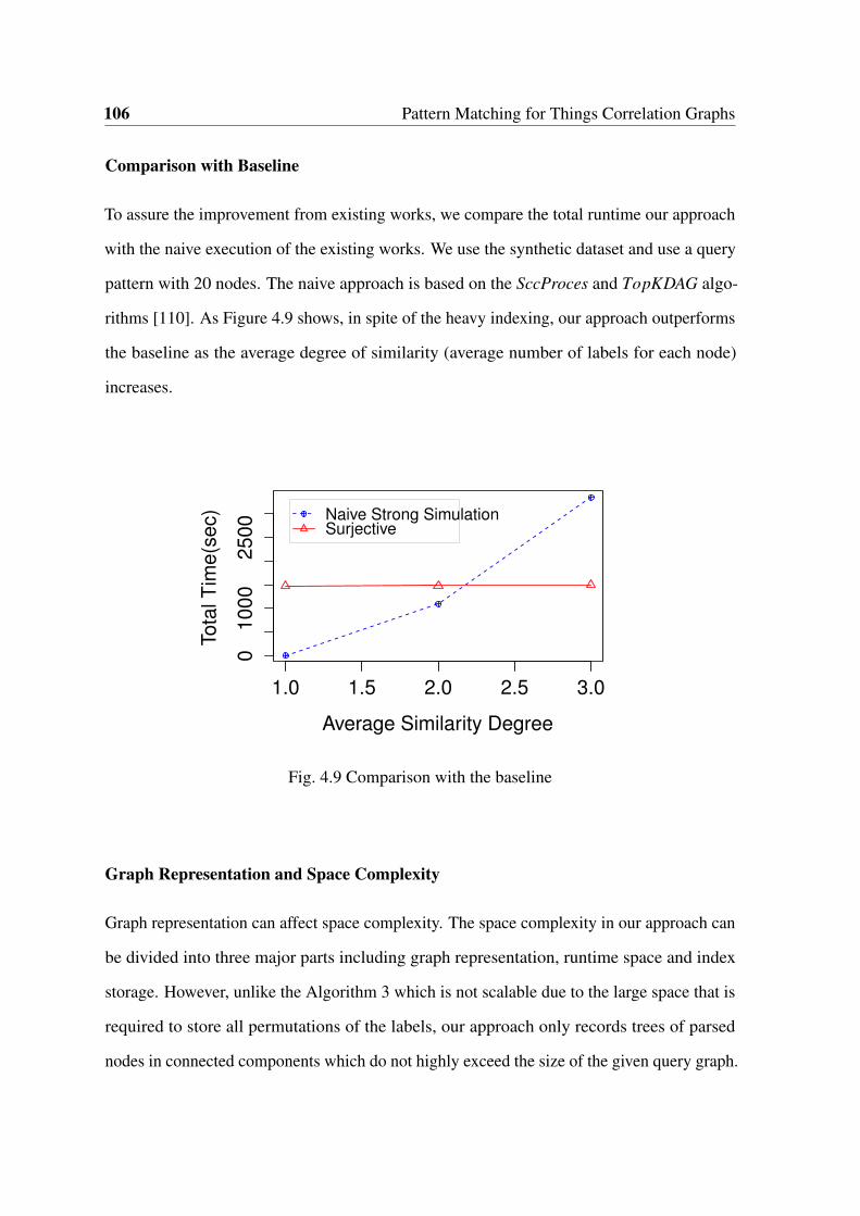
106 Pattern Matching for Things Correlation Graphs
Comparison with Baseline
To assure the improvement from existing works, we compare the total runtime our approach
with the naive execution of the existing works. We use the synthetic dataset and use a query
pattern with 20 nodes. The naive approach is based on the SccProces and TopKDAG algo-
rithms [110]. As Figure 4.9 shows, in spite of the heavy indexing, our approach outperforms
the baseline as the average degree of similarity (average number of labels for each node)
increases.
1.0 1.5 2.0 2.5 3.0
01
00
02
50
0
Average Similarity Degree
To
tal T
ime
(se
c) Naive Strong Simulation
Surjective
Fig. 4.9 Comparison with the baseline
Graph Representation and Space Complexity
Graph representation can affect space complexity. The space complexity in our approach can
be divided into three major parts including graph representation, runtime space and index
storage. However, unlike the Algorithm 3 which is not scalable due to the large space that is
required to store all permutations of the labels, our approach only records trees of parsed
nodes in connected components which do not highly exceed the size of the given query graph.

4.6 Related Work 107
There are two different approaches to store graph data including Adjacency List and
Matrix representation. The first approach normally reduces the file size while the second
approach can potentially reduce the runtime of the process. The original version of the
real-world data sets that we have used, are stored using adjacency list format. However, due
to the heavy processing workload in our experiment, we convert the graphs to adjacency
matrices as we import them into our application. Through the use of scalable libraries, our
approach can handle graphs with millions of nodes on one machine.
As Table 4.4 shows, the size of the index increases when we process larger graphs or use
smaller thresholds. As shown, the size of the index can take up 1.6 MB for around 330,000
entries or up to 89.1 MB for 9.5 million entries. Thus, our approach is scalable in terms of
space and time.
4.6 Related Work
Graph pattern matching has been extensively studied and employed in various domains.
Typically, two main approaches are often used for this purpose: subgraph isomorphism [119–
122] and graph simulation [123–125]. When it comes to new applications such as social
computing, none of these approaches can meet the applications’ requirements. Recently, there
has been a trend towards revising pattern matching for new domains, e.g., social networks
[108]. The main problem in deploying the mentioned approaches is their too much restrictive
definition. This reduces the efficiency and scalability of matching process. In addition, in
the case of social networks analysis, these approaches will fail to obtain many useful and
meaningful solutions [108].
One of the problems which recently has been discussed along with graph pattern matching
is querying top-k nodes in a data graph by matching a query node from a pattern graph [110].
In the previous works both of the pattern graph and data graph use a single tag for each node
[108]. The top-k query processing is challenging and an ongoing issue particularly under

108 Pattern Matching for Things Correlation Graphs
special conditions such as uncertainty. For instance, in a distinct approach, given a noisy
or uncertain dataset, Song et al. propose to return Top-k Oracle instead of returning only
k tuples [126]. Users can later sub-query the results oracle to get the best answers based
on their choice. However, so far this approach has not been examined for graphs, thus this
approach needs further investigations to be applied on graph shaped data. In more graph
oriented applications, Top-k exploration has been applied to efficient graph search on RDF
data, which is represented using basic graph patterns [127].
Due to the frequently changing nature of social networks, it is often too costly to recom-
pute all of the matches of a given pattern starting from scratch. To respond to this issue, the
incremental graph pattern matching [128] can be adopted in many cases [129]. This approach
identifies the changes in the data graph once they are made and corrects the pre-computed
match set regardless of the complexity of batch algorithms.
The trend towards reforming the concept of graph simulation and graph isomorphism
has continued to form new definitions such as bounded graph simulation [96], edges rela-
tionship simulation [130], strong simulation [111, 131] and strict simulation [132]. The
strict simulation has been accompanied with distributed computing to tackle the performance
obstacle. Using on-the-fly ranked lists and spanning trees is another approach that can
optimize the solution [133]. One of the most important factors in this evolution process is
the specifications of the application context. However, none of these efforts has applied
graphs with multi-labeled nodes. Nonetheless, the size of pattern in most cases is very
small. Efficient processing of probabilistic graphs has also been discussed by previous works
[134]. Although dealing with probabilistic graphs to some extent can have similarities with
analyzing graphs with multiple node labels, their purpose and definition are quite different.

4.7 Summary 109
4.7 Summary
Graph matching is a fundamental method which is applied in many important areas, such
as social computing, image processing and computational chemistry. In IoT search, graph
pattern matching can be applied for many purposes including RDF sensor data processing
and correlation graph merge. Considering the results of the previous chapters, we identify
that each node in TCGs can carry multiple labels based on the specifications of their sensors
and actuators.
In this chapter, we propose a novel approach to efficiently match graphs with nodes that
can take multiple labels. The aspects of the novelty of our approach include: (1) we address
pattern graphs that are much larger than pattern graphs used by previous approaches, (2) in
our approach each node can be associated with multiple labels while previous approaches
only accept one label for each node, (3) we propose the concept of surjective simulation
that is more flexible than graph simulation and strong simulations, and we have shown how
it can greatly improve the efficiency of the graph matching process. We conduct several
experiments to examine the efficiency of our approach and demonstrate the superiority of our
approach over existing methods.
For the future research, we plan to extend our approach to support several new specifica-
tions, such as matching probabilistic graphs with multi-labeled and graph based processing
for large-scale distributed pattern matching.
However, finding the best matches for a given user query is a different process. Based
on the intention of search, users may look for things that are either locally, semantically or
socially correlated with them. Thus, different TCGs are produced in correlation extraction.
Unfortunately, in most cases the desired type of correlation is not reflected in the query and
remains implicit. Thus, on challenge is how to integrate the TCGs of different types. On
the other hand, presenting all of the matching results is not a suitable approach due to the
interests of human users and the limitations of the machine users of an IoT search engine.

110 Pattern Matching for Things Correlation Graphs
Thus, we cannot use the approach presented in this chapter for the purpose of user query
processing. In Chapter 5, we propose a novel approach to address the above challenges. We
use diversification the address the different needs/intentions of the users by diversifying the
search results of the query.
Chapter 5
Diversifying Top-k Query Matches
The formation of Social IoT [40] and the Semantic IoT [135] triggered the idea of establishing
correlation graphs for things similar to social networks analysis. Technically, it bears a good
potential to support more complex queries and design more effective search approaches by
adopting the correlation graphs between things. Although this idea may seem similar to
making connections between people through social networks, correlations in IoT are not
established in the same way. In Chapter 3, we proposed a novel approach, namely CEIoT, for
extracting and presenting the correlations graphs (TCGs). As we show, in IoT, correlations
are extracted based on the attributes of things while in social networks users contribute in
establishing their relationships. Different correlations between things are expressed and
understood differently and thus, can fall into different categories based on their definition
and scope. For example, a correlation that is defined based on location attributes is different
than a correlation which is defined based on ownership attributes. In the CEIoT approach,
IoT services collaborate to establish the TCGs with minimized human intervention.
We consider TCGs to represent things correlation networks. Each vertex in a TCG
represents a thing in IoT and each pair of vertices may be connected through an edge of
a specific type, which represents a correlation of that type. Establishing correlations of
different types can improve the depth of our model from the real world. It becomes possible

112 Diversifying Top-k Query Matches
to apply more filters to get the related things from the huge pool of things. Each type of
edge is formed based on a specific type of correlation. A non-exhaustive list of correlation
types include Co-location Object Relationship, Parental Object Relationship, Social Object
Relationship, Co-Working Object Relationship and Ownership Object Relationship [40].
However, in the last step for preparing the query results, a challenging problem is to find an
approach to integrate TCGs of different types. Furthermore, given the limitations of smart
devices and the interests human users demand that the length of the result set should be
limited and maintain high quality.
Fig. 5.1 Example of various relationships between things and users in IoT
An important problem is how we can effectively manipulate correlations in the IoT to
obtain better search results when it is not clear that what kind of correlations are more
important for users’ search? If we pick only one type of correlation, would it harm the
diversity of the search results? Example 5 describes this in more details.
Example 5. Assume a user simply enters a query such as <"air","USA">. As shown in
Figure 5.1, keyword filtering can yield four different types of things such as an oil rig (v1)
and a Buoy (v2) close to each other in the gulf of the Mexico as well as two air quality eggs
(v3 and v4) in two different places. We can see that v1 and v2 are almost in the same location

113
and thus they are connected through a co-location edge. This indicates a CLOR relationship
between them. Meanwhile, v3 and v4 belong to same type of sensors, and thus they are
connected through a parental relationship edge. This indicates a POR relationship between
them. Now, if we want to limit the number of things in the result to two items only, how can
we select them to best balance coherence and diversity? A selection of {v3,v4} or {v1,v2}
will improve the coherence, but the search result is limited to just one type of correlation,
leading to less diversity. In contrast, the selection of {v1,v3} or other similar combinations
will increase the diversity of the final result but with less coherence. Thus, there will be a
tradeoff between coherence and diversity in the selection process.
In response to the above challenge, we propose a novel framework to answer search
queries by maintaining different types of correlations. Our main contributions are as follows:
• We formally define the characteristics of search results (coherence and diversity) and
use them to increase the quality of search in IoT. To the best of our knowledge, our
work is the first piece of research that investigates and formulates different types of
relationships.
• We propose a new framework, the ECS (Extract, Cluster, Select) framework, to manage
the coherence and diversity of search results. Our framework contains a novel approach
to extract and integrate different types of correlation graphs with a spectral clustering
method and a selection method to improve the coherence and the diversity of top-k
results for a given search query.
• We conduct extensive experiments to validate the effectiveness of our approach using
real-world datasets.
The rest of this chapter is organized as follows: In Section 5.1 we use a graph based
data structure to formally define the problem and provide an overview of our methodology.
Section 5.2 presents the technical details for our ECS approach. We describe the results of
114 Diversifying Top-k Query Matches
experimental evaluation in Section 5.3. In Section 5.4 we review the related works. Finally,
we summarize the chapter in Section 5.5.
5.1 Problem Statement
5.1.1 Problem Formulation
In this section we formally define various types of correlations and then the problem. In
this chapter we focus mainly on two types of correlations: Co-Location Object Relationship
(CLOR) and Parental Object Relationship (POR).
Definition 6 (Thing). Suppose that V is the universal set of things and a thing v ∈ V is
an object connected to IoT where (1) (v.lat,v.lon) = v.l denotes the location of the object
composed of latitude v.lat and longitude v.lon; (2) v.dt = {dti}mi=1 and dti ∈ Td denotes a
set of descriptive tags about v, where Td is an alphabet consisting of descriptive tags; (3)
v.lt = {lti}ni=1 and lti ∈ Tl where Tl is an alphabet consisting of location tags such as road
and/or grid cell IDs. □
Definition 7 (Parental Object Relationship – POR). For every given pair of objects v,v′ ∈V ,
they have a POR if the following equation is satisfied:
σP(v,v′) =
|v.dt ∩ v′.dt||v.dt ∪ v′.dt|
≥ τ (5.1)
where σP(v,v′) ∈ [0,1] denotes the strength of POR and τ ∈ [0,1] is the similarity threshold.
□
Definition 8 (Co-Location Object Relationship – CLOR). For every given pair of objects
o,o′ ∈V , they have a CLOR if the following equation is satisfied:
σL(v,v′) =
|v.lt ∩ v′.lt||v.lt ∪ v′.lt|
≥ τ (5.2)

5.1 Problem Statement 115
where σL(v,v′) ∈ [0,1] denotes the strength of CLOR and τ is the similarity threshold. □
Definition 9 (Things Correlation Graph (TCG)). A TCG is an undirected graph denoted as
G = (V,E,w) where (1) V is the universal set of things; (2) E ⊆V ×V is the set of edges and
each edge (v1,v2) ∈ E indicates a correlation (either POR or CLOR) between v1 and v2; and
(3) w : E→ [0,1] is the weight function and w(v1,v2) represents the weight of relationship
of edge (v1,v2). □
Our goal is that given the set of TCGs for two types of relationships (POR and CLOR),
retrieve the most coherent and diverse results for a search query issued by a user. The problem
is formally defined as:
For a given query Q =<keyword,location>, we need to select the ordered set of Things
(V ⊆V ) with highest coherence and diversity which are ordered non decreasingly by their
matching scores. We compute the matching score from the following:
µ(Q,v) = w1|Q.dt ∩ v.dt||Q.dt ∪ v.dt|
+w2|Q.lt ∩ v.lt||Q.lt ∪ v.lt|
(5.3)
where Q.dt and Q.lt refer to the descriptive and location tags, respectively.
We obtain the coherence of the result set from the following equation:
φ(V ) =1|V |2 ∑
v,v′∈Vw1σ
L(v,v′)+w2σP(v,v′) (5.4)
We define search results diversity based on the selection size as follows:
δ (V ) =k×|C∗|n×|C|
(5.5)
where C∗ denotes the clusters with selected nodes, C denotes the set of all clusters and n
denotes the number of selected nodes.

116 Diversifying Top-k Query Matches
The objective function is defined as follows:
f = α×φ(V )+β ×δ (V ) (5.6)
where α,β ∈ [0,1].
5.1.2 Methodology
We design a novel framework to answer search queries based on the correlations between
things. Figure 5.2 shows the general structure of our framework and how it is evolved from
the traditional approach.
Fig. 5.2 Components of the ECS framework
As mentioned, current IoT search engines deploy a simple keyword based search strategy
based on the crawled data from the IoT. The initial steps are TCG Construction and then
Clustering. The next step is Selection which is performed on clusters. In our framework, we
integrate different types of TCGs and cluster the vertices into a set of different clusters. Then,
in the next step, we prepare the top-k results for a given search query.
5.2 ECS Approach 117
5.2 ECS Approach
In this section, we introduce the details of our approach. The TCG construction covers
Extracting Correlations in ECS framework followed by Clustering and Selection.
5.2.1 TCG Construction
Given a set of things represented by V = {vni=1} ∈ Rm, their correlation graph TCG (Defini-
tion 5) is an undirected weighted graph TCG =<V,E,W >, where V denotes all the things,
E ⊆ V ×V is the edges of TCG, the weighted matrix W can be obtained using ℓ1-based
one-to-all sparse graph based reconstruction, in which each thing can be considered as a
linear span of other things in the dataset.
Given a set of things V = {vni=1} ∈Rm, for each thing vi, its similarity/affinity with other
things can be obtained by vi = Viw, where vi ∈Rm is the sample to be reconstructed, w ∈Rn
is the reconstruction coefficients, Vi = V \vi = [v1, ...,vi−1,vi+1, ...,vn] ∈ Rm×(n−1), which is
formed by other objects in the dataset except for object vi. The reconstruction coefficients of
vi can be computed using the objective function:
minw||w||1, s.t. vi = Viw (5.7)
where || · ||1 is the ℓ1 norm, tending to minimize the ℓ1 norm of reconstruction error. Since the
relations of nodes on a graph is supposed to be non-negative, we impose an extra constraints
on Equation 5.7, which is formulated as:
minw||w||1, ,s.t. vi = Viw, w j
i ≥ 0 (5.8)
The construction process is summarized in Algorithm 7. Algorithm 8 summarizes the
clustering process using the weighted matrix generated by Algorithm 7. Under this way, the

118 Diversifying Top-k Query Matches
algorithm can adaptively select the neighbors for each data point, and at the same time the
similarity matrix indicating pointwise similarity is automatically derived from the calculation
of these sparse representations. It automatically leads to a sparse solutions, which means the
thing correlation graph would be a sparse graph.
Algorithm 7 ℓ1-based Thing Correlation Graph Construction
Require: A collection of feature vectors of things V = {v1, ..,vn},vi ∈ Rm
Ensure: Similarity matrix W ∈ Rn×n
1: Each vi is normalized to be vi =vi
||v||222: for i = 1→ n do3: Vi = [V \vi|I] ∈ Rm×(m+(n−1))
4: minwi ||w||1 s.t., ||vi−Bwi||2 = 0, w≥ 05: for j = 1→ i−1 do6: if 1≤ j ≤ i−1 then7: W(i, j) = w j
i8: if i+1≤ j ≤ n then9: W(i, j) = w j−1
i10: return W
5.2.2 Clustering
After solving the proposed optimization program in Equation 5.8, we obtain a sparse rep-
resentation for each data points whose nonzero elements ideally correspond to points from
the same subspace. To infer the cluster of each data points on TCG into different subspaces
using the sparse coefficients w ∈W, we first employ spectral clustering techniques to extract
more informative structures by computing the first K eigenvectors of graph Laplacian of W,
the graph Laplacian can be computed as
L = I−D−1/2WD−1/2 (5.9)
where D = [di j] is a diagonal matrix with dii = ∑ j wi j. D−1/2 indicates the inverse square
root of D. The Laplacian is symmetric positive semidefinite, and its first K eigenvectors

5.2 ECS Approach 119
corresponding to K smallest eigenvalues can be computed. Thus, we can perform kmeans to
cluster all the data points.
Algorithm 8 Subspace Clustering on Weighted Matrix W of TCGRequire: Weighted matrix W of TCGEnsure: Clustering membership for each data point vi
1: Normalizing columns of W as W(:, i)← W(:, i)||W(:, i)||∞
2: Symmetrizing W =12(W+WT )
3: Computing graph Laplacian matrix L= I−D−1/2WD−1/2, where D= [di j] is a diagonalmatrix with dii = ∑ j wi j
4: Computing K eigenvectors of L corresponding to K largest eigenvalues, and form thematrix C = [c1, ...,cK]
5: Performing K-means using C6: Assign each data point vi to cluster j if the i-th row of the matrix C is assigned to the
cluster j7: return the set of clusters
Time Complexity Analysis. Sparse similarity W construction and k-means based spec-
tral clustering would be two main stages of consuming computational resource. As we know,
efficiency is crucial, especially we will deal with a large amount of ubiquitous things. We
briefly draw some analysis of time complexity of our method and how to adapt our proposed
approach in a scalable way to match the needs of IoT.
We adopt the ℓ1 sparse representation to decode the similarity of queries and the training
dataset, which is the most expensive part of our proposed method. Given a collection of data
points (i.e., each object can be considered as a virtual data point), ℓ1-graph finds a sparse
representation for the object using all other objects in the dataset and builds a similarity graph
using the representation coefficients. Although the sparse similarity graph performs well, it
needs an iterative optimization process for respective objective function, and has no closed
form like ℓ2 norm. In our implementation, we adopt Homotopy algorithm based fast solver,
where each step of the algorithm involves the rank-one update of a linear system. If the
whole procedure stops in K steps, yielding a solution with K nonzeros, its overall complexity

120 Diversifying Top-k Query Matches
is bounded by 4Kd′2/3+Kd′n+O(Kn), where d′ is the dimension of the reduced features
and n is the number of the training samples. To further reduce the computational cost, we
can sparsely reconstruct each data point from its k nearest neighbors in feature space instead
of using all the other samples to improve the efficiency while maintaining its effectiveness.
In this way, the searching space of constructing TCG will be reduced from n−1 to k (k < n).
On the other hand, k-means algorithm employs an iterative procedure. At each iteration,
one finds each data point’s nearest center and assigns it to the corresponding cluster. Cluster
centers are then recalculated. The procedure stops after reaching a stable error function
value. Since the algorithm evaluates the distances between any point and the current k cluster
centers, the time complexity of k-means is O(nk2), where n is the number of data points and
k number of clusters. However, since its weight matrix W is a sparse similarity matrix as
well, we can use sparse eigensolvers to accelerate the computation of top K eigenvectors
from Laplacian matrix L, e.g., ARPACK [136], which can reduce the time complexity of
computing eigenvectors from O(m3) to ∼O(nm).
5.2.3 Selection
To make this selection, we can pick a single node from each cluster and add it to the result set.
We can use different strategies in the selection step. For example, one can choose elements
based on their similarity values, or the medoid element of each cluster. However, the quality
of the final results highly depends on the quality of the selection strategy [137]. We propose
an approach to implement a selection strategy in such a way that can satisfy the following
conditions:
1. The set of things in each cluster have the most similarity to each other while the
inter-cluster similarity is minimized; and

5.2 ECS Approach 121
2. The returned results maximize the objective function which aggregates the coherence
and the diversity of the result set. We select the nodes with maximum similarity index
to intra-cluster nodes.
Algorithm 9 Node Selection
Require: A collection of Clusters C = {Ci}Ni=0; k the size of the result set; Query Q; and α ,
β
Ensure: An ordered set of things V for which |V |= k1: Filter the nodes in clusters set C based on the features specified in the query Q2: for i = 1→ |C| do3: m = random(vx) ∈Ci4: for vz ∈Ci do5: if ∑vy∈Ci W(z,y)> ∑vy∈Ci W(z,y) then6: m = v7: V ← V +m8: Ci←Ci\m9: if |V |< k then
10: Add select(updated C,k−|V |,Q,α,β ) to V11: return V
Algorithm 9 summarizes the steps of our selection strategy. The algorithm takes a set of
parameters including the clusters from the clustering step, the expected size of the result k,
the query Q and the tradeoff coefficients α and β . The algorithm initializes V in the first
turn (Lines 1-8) to cover conditions (1) and (2). First, the set of nodes are filtered based on
the keywords from the query (line 1). Then the algorithm iterates through all of the clusters
with a for loop (line 2), picks a random node from the cluster Ci as its medoid (line 3), and
iterates through the remaining nodes in the cluster (line 4) to find nodes which have less
intra-cluster dissimilarity with other nodes. Once a new optimal node is found, it is replaced
by the selected medoid (lines 5-8). Later the medoid is added to V and removed from
Ci(lines 9, 10). The algorithm recursively calls itself with subtracted V from the clusters k
is greater than k in lines 12-14. Finally, set V is returned. The order of execution for the
Algorithm 9 for a small k is n+ KO(kn)k as it is mainly composed of keyword based filtering,
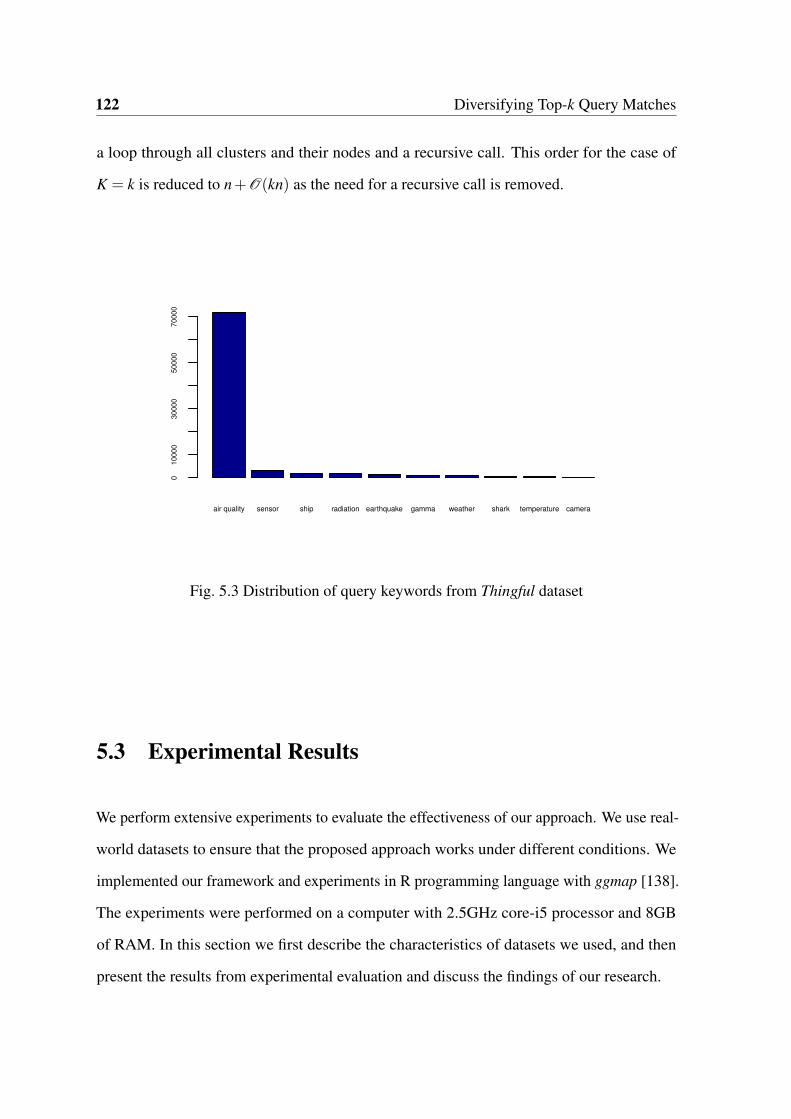
122 Diversifying Top-k Query Matches
a loop through all clusters and their nodes and a recursive call. This order for the case of
K = k is reduced to n+O(kn) as the need for a recursive call is removed.
air quality sensor ship radiation earthquake gamma weather shark temperature camera
01
00
00
30
00
05
00
00
70
00
0
Fig. 5.3 Distribution of query keywords from Thingful dataset
5.3 Experimental Results
We perform extensive experiments to evaluate the effectiveness of our approach. We use real-
world datasets to ensure that the proposed approach works under different conditions. We
implemented our framework and experiments in R programming language with ggmap [138].
The experiments were performed on a computer with 2.5GHz core-i5 processor and 8GB
of RAM. In this section we first describe the characteristics of datasets we used, and then
present the results from experimental evaluation and discuss the findings of our research.

5.3 Experimental Results 123
5.3.1 Datasets
Nowadays, many of IoT applications such as smart cities, intelligent transport systems,
environmental sensing and etc. are publishing their data on the Internet. IoT search engines
such as Thingful, rely on this type of data. We take this opportunity to create a large scale
dataset of IoT data.
We use the following real-world datasets to evaluate our work:
1. Vehicle Trajectory Data: It contains nearly 16,000,000 trajectories for 10,357 taxicabs
in the city of Beijing in a one week period [139]. The sampling frequency for each taxi
differs from a few seconds to a couple of hours. In order to prepare the data to be used
in the experiment, we performed some preprocessing. We first divided the city into
76 parts in length and 76 parts in height, which means that we have 5,776 segments.
We specified the average speed between each pair of subsequent records to find the
vehicle’s status.
2. Weather Sensor Data: We also used a dataset known as LinkedSensorData [99, 140],
which is an RDF dataset containing expressive descriptions of nearly 10,000 weather
stations in the United States. The data originated at MesoWest, a project within
the Department of Meterology at the University of Utah that has been aggregating
weather data since 2002 [141]. It contains the observations from weather sensor
measurements of phenomena such as temperature, visibility, precipitation, pressure,
wind speed, humidity, etc. The dataset includes observations during the time periods
that several major storms were active. This includes Hurricane Katrina, Ike, Bill,
Bertha, Wilma, Charley, Gustav, and a major blizzard in Nevada in 2003. The dataset
contains 1,730,284,735 triples from 159,460,500 observations. We accompanied every
sensor’s data with location tags from GeoNames [142].

124 Diversifying Top-k Query Matches
3. Query Data: we used a real-world dataset consisting of 136,746 queries between Feb,
2014 to Feb, 2015 from Thingful search engine. This dataset is not IoT data, but we
used it for query generation and analysis. We random selections from key features
such as location, related keywords and timestamp to generate the queries for each of
the above datasets. Figure 5.3 shows distribution of most popular keywords in the
queries dataset.
Table 5.1 describes the thing data structure and the dimensionality of each category of
properties for the taxis dataset. Furthermore, Table 5.2 describes the thing data structure and
the dimensionality of each category of properties for the weather dataset.
Table 5.1 Object data structure for taxi trajectories dataset
Category Dim. StructureLocation 2 v.lat, v.lonDescriptive tags 2 v.type ∈ {taxi,ordinary,bus}, v.status ∈
{moving,stopped}Location tags 2 v.cell = (si,s j) and si,s j ∈ [0,76], v.rd the road idOwner 1 v.u
Table 5.2 Object data structure for weather stations dataset
Category Dim. StructureLocation 3 v.lat, v.lon, v.altDescriptive tags 16 v. f eat ⊆ D where D is the universal set of feature tagsLocation tags 2 v.state and v.county which refer to the name of the state
and the name of the county in which the weather stationis located, respectively
First we perform a dataset analysis on each dataset we have used. After computing the
weights matrix W, we normalized the matrices and obtained the graph for the two real-world
datasets. Figure 5.4a shows a partition of the integrated TCG for the vehicles trajectory

5.3 Experimental Results 125
dataset. Comparing with Figure 5.4b which shows a partition from weather stations dataset,
the graph of the first dataset is far more scarce than the graph for the first dataset.

126 Diversifying Top-k Query Matches
(a) The trajectory dataset
(b) The weather stations dataset
Fig. 5.4 Visualization of two TCGs
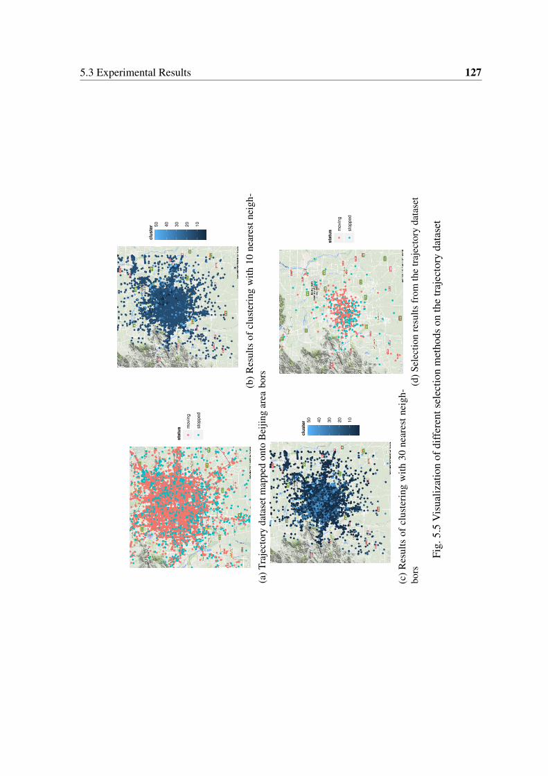
5.3 Experimental Results 127
sta
tus m
ovin
g
sto
pped
(a)T
raje
ctor
yda
tase
tmap
ped
onto
Bei
jing
area
10
20
30
40
50
clu
ste
r
(b)
Res
ults
ofcl
uste
ring
with
10ne
ares
tnei
gh-
bors
10
20
30
40
50
clu
ste
r
(c)
Res
ults
ofcl
uste
ring
with
30ne
ares
tnei
gh-
bors
sta
tus m
ovin
g
sto
pped
(d)S
elec
tion
resu
ltsfr
omth
etr
ajec
tory
data
set
Fig.
5.5
Vis
ualiz
atio
nof
diff
eren
tsel
ectio
nm
etho
dson
the
traj
ecto
ryda
tase
t

128 Diversifying Top-k Query Matches
05000
10000
Alt
(a)W
eath
erst
atio
nsda
tase
tmap
ped
onto
Nor
thA
mer
ica
10
20
30
40
50
clu
ste
r
(b)R
esul
tsof
clus
terin
gw
ith5
near
estn
eigh
bors
10
20
30
40
50
clu
ste
r
(c)R
esul
tsof
clus
teri
ngw
ith20
0ne
ares
tnei
gh-
bors
(d)
Sele
ctio
nre
sult
from
the
wea
ther
stat
ions
data
set
Fig.
5.6
Vis
ualiz
atio
nof
diff
eren
tsel
ectio
nm
etho
dson
the
wea
ther
stat
ions
data
set
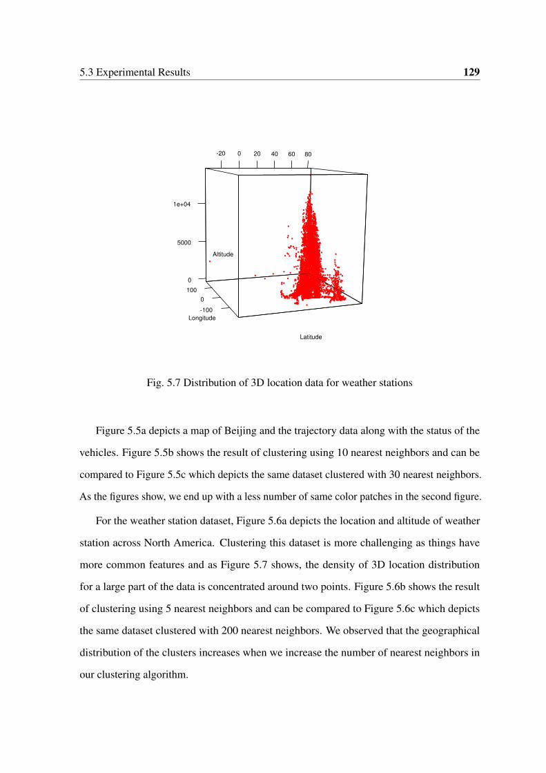
5.3 Experimental Results 129
Latitude
Longitude
-100
0
100
0
5000
1e+04
Altitude
-20 0 20 40 60 80
Fig. 5.7 Distribution of 3D location data for weather stations
Figure 5.5a depicts a map of Beijing and the trajectory data along with the status of the
vehicles. Figure 5.5b shows the result of clustering using 10 nearest neighbors and can be
compared to Figure 5.5c which depicts the same dataset clustered with 30 nearest neighbors.
As the figures show, we end up with a less number of same color patches in the second figure.
For the weather station dataset, Figure 5.6a depicts the location and altitude of weather
station across North America. Clustering this dataset is more challenging as things have
more common features and as Figure 5.7 shows, the density of 3D location distribution
for a large part of the data is concentrated around two points. Figure 5.6b shows the result
of clustering using 5 nearest neighbors and can be compared to Figure 5.6c which depicts
the same dataset clustered with 200 nearest neighbors. We observed that the geographical
distribution of the clusters increases when we increase the number of nearest neighbors in
our clustering algorithm.

130 Diversifying Top-k Query Matches
5.3.2 Results
In our experiments, our target is to investigate the answers to the following questions: (i)
How do different methods react to different ratios between α and β? (ii) What would be the
outcome for different amount of k in the initial clustering? (iii) Which selection approach
would be more effective?
In the following we present the experimental results from our work. We compare our
approach with other thing selection approaches including Fixed Length Selection (FLS -
selecting random k nodes), Maximum Similarity Selection (MSS - selecting things with
highest augmented µ), k-Medoids Selection (KMS - our approach) and Plain Selection(PS)
which is the current approach used by Thingful and other works.
Varying α and β
In Figure 5.8a, we compare the final ranking scores for different ratios of α and β between
different other selection approaches. As we increase the ratio from 1 to 10, the final score for
MSS approach increases to meet FLS score. As FLS and KMS strategies both experience a
slight increase in their final scores for greater amounts of α , it shows that the MSS is better
in providing more coherent results but the KMS performs stronger in overall distribution of
diversity and coherence.
Varying k
To answer the last question, we investigate the coherence and diversity of results for each
one of the object selection strategies. Figure 5.8b compares the coherence of the outcomes
for varying k. As shown, the KMS method outperforms other methods in terms of results
coherence. While the coherence scores of PS are quite steady, MSS and FLS methods
fluctuate dramatically.
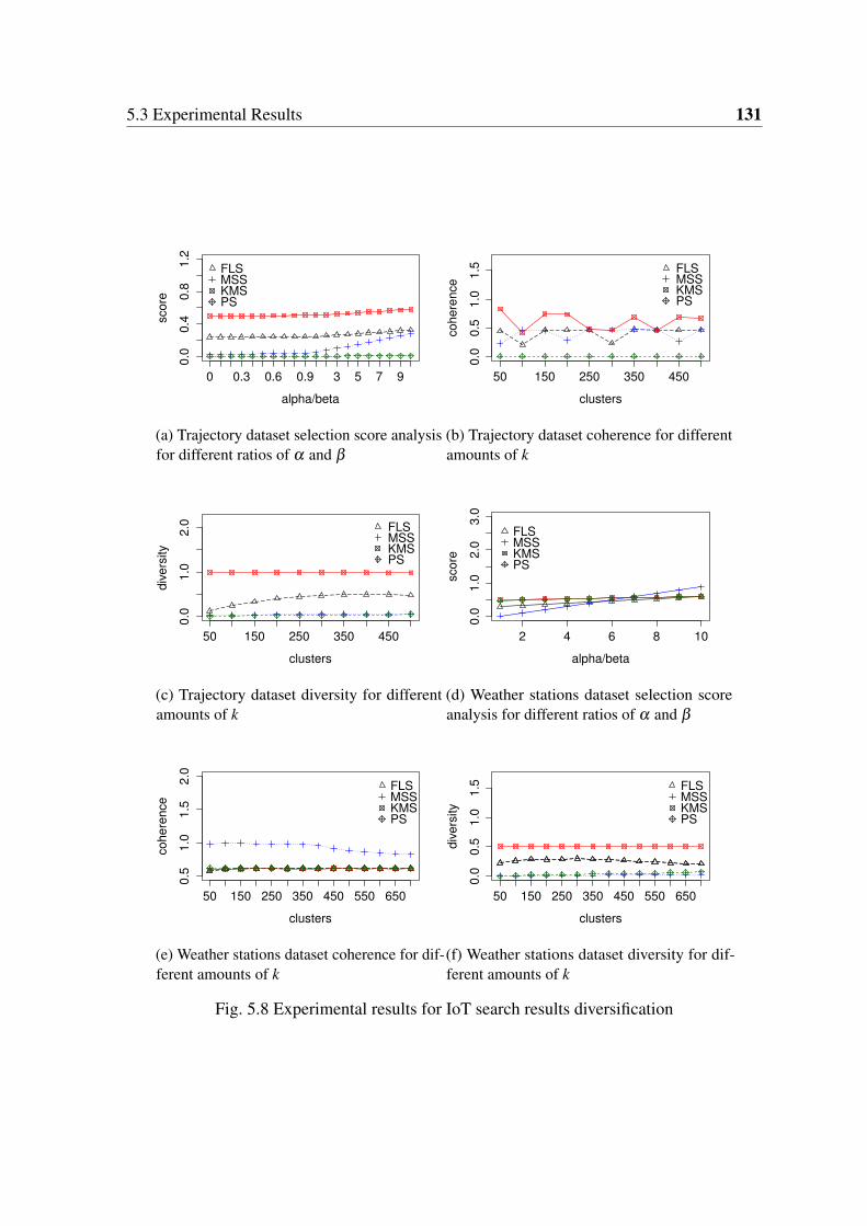
5.3 Experimental Results 131
0.0
0.4
0.8
1.2
alpha/beta
sco
re
FLSMSSKMSPS
0 0.3 0.6 0.9 3 5 7 9
(a) Trajectory dataset selection score analysisfor different ratios of α and β
0.0
0.5
1.0
1.5
clusters
co
he
ren
ce
50 150 250 350 450
FLSMSSKMSPS
(b) Trajectory dataset coherence for differentamounts of k
0.0
1.0
2.0
clusters
div
ers
ity
50 150 250 350 450
FLSMSSKMSPS
(c) Trajectory dataset diversity for differentamounts of k
2 4 6 8 10
0.0
1.0
2.0
3.0
alpha/beta
sco
re
FLSMSSKMSPS
(d) Weather stations dataset selection scoreanalysis for different ratios of α and β
0.5
1.0
1.5
2.0
clusters
co
he
ren
ce
50 150 250 350 450 550 650
FLSMSSKMSPS
(e) Weather stations dataset coherence for dif-ferent amounts of k
0.0
0.5
1.0
1.5
clusters
div
ers
ity
50 150 250 350 450 550 650
FLSMSSKMSPS
(f) Weather stations dataset diversity for dif-ferent amounts of k
Fig. 5.8 Experimental results for IoT search results diversification

132 Diversifying Top-k Query Matches
Finally, Figure 5.8c compares the diversity of the outcomes for different methods. The
diversity index for the results of KMS method constantly remains as 1.00 for varying amounts
of k as one vertex is selected from each cluster. For MMS method, the diversity of results
improves to a limit as k is increased. As the figure shows, both of the PS and FLS methods
perform very poor in terms of diversity.
Due to the fact that the weather sensors dataset generates a much denser graph than the
trajectory dataset, it is more challenging for our approach to improve the coherence, the
diversity and as a result the overall score of the selected k things. However, as Figure 5.8d
shows, the KMS method outperforms other methods when the coherence has a higher weight
(≥ 1/7β ). For higher values of α , the MSS method outperforms KMS as the graph is very
dense and its nodes have a very strong correlation.
Figure 5.8e compares the coherence of the results for a varying amount of k. As shown,
the MSS approach outperforms other approaches in terms of coherence but their difference
decreases as as k is increased. Figure 5.8e compares the diversity of the outcomes for
different methods. The diversity index for the results of KMS method remains 1.00 for
varying amounts of k as one vertex is selected from each cluster.
Methods Analysis
To conclude, the experimental results show that our approach improves the coherence and
diversity compared to the current and baseline approaches. Our findings show that our
approach performs better on sparse graphs although it improves the overall results score from
dense graphs as well.
In our design, we feature the nodes along with filtering criteria based on different types
of correlations to simplify the final filtering for users (Figures 5.5d and 5.6d).
5.4 Related Work 133
5.4 Related Work
As the idea of WoT implementation in large scale keeps flourishing and gains more popularity
everyday, provisioning of its future structure, components, functionality and challenges
becomes clearer. As a matter of fact, the implementation of IoT, in the first place does
not require unknown technologies that are still unborn, as numerous academic and non-
academic initiations have been carried out in this area. In advance, search engines in
the context of IoT will play a significant part as they are doing today. Accordingly, the
current structure will no longer support large scale IoT implementation sufficiently. Major
technical challenges and changes in needs of users will require search engines to undertake
new approaches for their query processes. To illustrate the future of search engines, [143]
identified some of the challenging issues for searching within IoT as search locality and real-
time search. Furthermore, based on IoT characteristics such as networked interconnection,
real-time, semantic coherence and spontaneous interaction will result in raising issues such as
architectural design, search locality, scalability and real-time for designing and implementing
IoT search engines [144]. However, due to the existing differences in the nature of WoT with
the IoT, WoT may even strike additional different challenges.
5.4.1 Search Based on Social Relationships
Some of the notable works in this area are as follows [30]: (1) Snoogle/Microsearch [145,
146]; (2) Dyser [83]; and (3) SPITFIRE [147]. Current search engines perform the search
using keyword based filtering. This kind of approaches have limited applications in the
context of the IoT due to the dynamic nature of IoT. Some other recent approaches such as
Context Aware Search [76] and Sensor Similarity Search [148] provide more functionality
to search in the IoT. However, a glimpse into IoT applications reveals that supporting the
correlations between things yet remains undiscovered in the IoT search.
134 Diversifying Top-k Query Matches
The library paradigm constitutes the basis of traditional information retrieval and based
on this paradigm, traditional search engines perform search and rank results using keywords.
Another approach that is so called the library paradigm [144] in which knowledge dissem-
ination is achieved socially and the search should aim finding the right person rather than
finding the right document.
In [144] the details of anatomy of a social search engine, namely Aardvark, have been
discussed. The search process in Aardvark is based on the village search paradigm in which
people use natural language to ask questions and answers are generated in real-time by
someone from the village and trust is based on intimacy. Main components of Aardvark
are as follows: Crawler and indexer, Query analyzer, Ranking function, UI. To index the
relationships and affiliation of users, social graph structure has been deployed. Aardvark
is a social search engine designed to index people and propose the best users to answer a
question given by a user and the results are ranked based on factors such as topic expertise,
intimacy (connectedness) and activity (availability).
5.4.2 IoT Search Engines
Microsoft SensorMap [149] and linked sensor middleware [150] support search for sensors
based on textual metadata that describes the sensors (e.g., type and location of a sensor,
measurement unit, object to which the sensor is attached). Such metadata is often manually
entered by the person who deploy the sensors. Other users can then search for sensors
with certain metadata by entering appropriate keywords. There are efforts to provide a
standardized vocabulary to describe sensors and their properties such as SensorML [151]
or the Semantic Sensor Network Ontology (SSN) [152]. Unfortunately, these ontologies
and their use are rather complex. It is problematic that end users are able to provide correct
descriptions of sensors and their deployment context without the help from experts. In other
words, this type of solutions require the time-consuming prior and expertise knowledge, e.g.,
5.4 Related Work 135
define the descriptions of things and their corresponding characteristics under a uniform
format such as Resource Description Framework (RDF). Furthermore, these solutions do
not exploit the rich information about user’s historical interactions with things, containing
implicit relations of different entities, e.g., if some users have the similar usage pattern on
some things, which may indicate close connection of these things.
Another alternative approach for searching things is based on search-by-example. The
work in [148] adopts this approach to sensors, i.e., a user provides a sensor, respectively a
fraction of its past output as an example, and requests sensors that produced similar output
in the past. Ostermaier et al. [83] propose a real-time search engine for Web of Things,
which allows searching real-world entities having certain properties. They associate a Web
page to a real-world entity (e.g., a meeting room) containing additional structured metadata
about the sensors connected to it. This method takes care of the valuable information of
historical data, but misses the relations among contextual information. Maekawa et al. [153]
propose a context-aware web search in ubiquitous sensor environments, Brown and Jones
[154] explore a new environment for information retrieval and information filtering, and Yao
et al. [155, 156] construct the models that captures the pairwise relations between things via
mapping the contextual information into separate graphs. However, more complex relations
between heterogeneous objects can not be captured in these works. In addition, some useful
information and structure might be lost when flating the multi-dimensional information into
graphs. [157] propose a hypergraph-based model to capture the high-order and complex
relations among things, however it suffers from the scalability issue and heavy computational
cost resulted from hypergraph calculations.
136 Diversifying Top-k Query Matches
5.5 Summary
Building enterprise search services is considered as one of the most significant steps in IoT
research area. Being inspired by social networks, in this chapter we proposed a framework
for diversified query result preparation for IoT.
TCGs of different types are generated by the CEIoT framework in Chapter 3. In Chapter 4,
we merged those TCGs by using a novel approach to find the top matches for the given
nodes in the TCGs. In this chapter, we focus on integrating the merged TCGs of different
types. Furthermore, we propose a diversification method for search results. Our aim is to
maintain the quality of the search results whilst we limit the size of the search results. We
measure the quality in terms of coherence and diversity. We use a number of techniques
including k-Nearest Neighbors, Spectral Clustering and k-Medoids Clustering for query
results preparation. We assess our approach using real-world datasets and show that our
approach can improve the coherence and diversity compared to the current and possible
substitute approaches.
One of the future directions for this research is to extend the framework to support other
types of correlations such as Social Object Relationship. We also target to extend the solution
over time series and uncertain IoT data to provide more accurate search results.
The work presented in this chapter, is the final step before presenting the raw results
that include a list of things to the user(s). However, the results can be further enriched
using further analytical plots when they are presented. We present details and a showcase
in aviation industry in Chapter 7. However, query resolution for intent-based search can be
customized if the intention of the search is already known. Instances of customized systems
in different fields of application can serve as examples for intention-oriented IoT search. In
particular, we use a taxi ridesharing example in Chapter 6. In order to maintain the flow of
the motivating scenario in Chapter 1, we present the taxi ridesharing case study first.
Chapter 6
Intent Based Search: A Case Study in
Taxi Ridesharing
Automated dynamic ridesharing is a promising approach to relieve the problem of traffic
lines which are overwhelmingly growing in our cities. In general, ridesharing provides us
with various benefits such as economical (e.g., reduced total mileage and fuel consumption),
environmental (e.g., less air pollution) and social benefits (e.g., passenger waiting time) [158,
159]. With the growth of newly introduced networking paradigms such as the IoT, nowadays
we are able to derive knowledge in real-time from large and heterogeneous data collected by
sensors from urban spaces [160]. In the recent years, various propositions have been made
to facilitate ridesharing where each proposition focuses on particular types of results. For
instance, a ridesharing application designed to minimize the effect of stochastic time frames
(delays) [161] has different effects than a solution that is designed to minimize the mileage
of the vehicles [159, 162].
Given the above details, taxi ridesharing can serve as a suitable example of intention-
oriented search in IoT. In particular, a search query that is issued by the end user of the
system is not issued to find the list of the taxis that are spatially or semantically correlated,
but rather to find a convenient and economic taxicab for a shared ride. Thus, the architecture
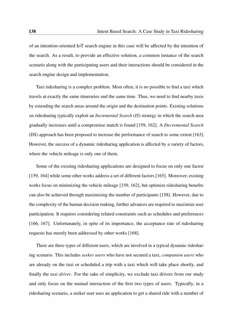
138 Intent Based Search: A Case Study in Taxi Ridesharing
of an intention-oriented IoT search engine in this case will be affected by the intention of
the search. As a result, to provide an effective solution, a common instance of the search
scenario along with the participating users and their interactions should be considered in the
search engine design and implementation.
Taxi ridesharing is a complex problem. Most often, it is no possible to find a taxi which
travels at exactly the same itineraries and the same time. Thus, we need to find nearby taxis
by extending the search areas around the origin and the destination points. Existing solutions
on ridesharing typically exploit an Incremental Search (IS) strategy in which the search area
gradually increases until a compromise match is found [159, 162]. A Decremental Search
(DS) approach has been proposed to increase the performance of search to some extent [163].
However, the success of a dynamic ridesharing application is affected by a variety of factors,
where the vehicle mileage is only one of them.
Some of the existing ridesharing applications are designed to focus on only one factor
[159, 164] while some other works address a set of different factors [165]. Moreover, existing
works focus on minimizing the vehicle mileage [159, 162], but optimize ridesharing benefits
can also be achieved through maximizing the number of participants [158]. However, due to
the complexity of the human decision making, further advances are required to maximize user
participation. It requires considering related constraints such as schedules and preferences
[166, 167]. Unfortunately, in spite of its importance, the acceptance rate of ridesharing
requests has merely been addressed by other works [168].
There are three types of different users, which are involved in a typical dynamic rideshar-
ing scenario. This includes seeker users who have not secured a taxi, companion users who
are already on the taxi or scheduled a trip with a taxi which will take place shortly, and
finally the taxi driver. For the sake of simplicity, we exclude taxi drivers from our study
and only focus on the mutual interaction of the first two types of users. Typically, in a
ridesharing scenario, a seeker user uses an application to get a shared ride with a number of

139
companion passengers or passengers who may have already booked the taxi [159]. In the real
world, the companion passengers may accept or reject the ridesharing request based on their
desired criteria. If the seeker users cannot efficiently and effectively find a good match for
ridesharing, they might no longer continue to use the system. Thus, considering companion
users is crucial for the success of the ridesharing application. For instance, unaccompanied
female travelers may reject the requests made by stranger male travelers. However, due to the
complexity in the nature of human decision making, it is too difficult to predict the outcome
of this decision at this stage. Thus, in this study we focus only the economical criterion and
leave the rest of criteria for future research. We rely on the mutual benefit principle, which is
a basic concept that demands almost anyone who is participating in the ridesharing process,
mainly is looking for financial benefits.
We particularly consider three scenarios in dynamic ridesharing context, which are related
to the outcome of the decisions of companion travelers. Those scenarios are explained in the
following.

140 Intent Based Search: A Case Study in Taxi Ridesharing
(a)C
ompa
nion
pass
enge
r’s
phon
e(b
)Ord
ered
bypr
oxim
ity(c
)Ord
ered
byac
cept
ing
chan
ce
Fig.
6.1
Inte
nt-b
ased
sear
chin
ride
shar
ing
scen
ario

141
Firstly, as the Figure 6.1a shows the list of rideshare requests on the screen of the mobile
device of a companion passenger. Based on the savings from each request, the user may pick
the second request and reject the first as the second option provides better savings. However,
in many cases, if the amount of savings is very low compared to the total cost of the private
ride, the companion passenger may reject all requests and accept none of them as well.
Secondly, Figure 6.1b shows an example of the results of an existing ridesharing applica-
tion on the seeker passenger’s mobile device. The application orders the results based their
from the seeker user’s pickup point. As shown, it is not far from reality if several attempts by
the seeker user get declined due to the preferences of the companion passengers. Only after
several attempts the user have found a shared ride with taxi8 successfully while the taxi is not
very far from the first (nearest) taxi. If the users of the ridesharing application need to make
numerous retries to get a taxi, they may cease using the application due to the hassle it takes.
Thirdly, along with the second scenario, we suggest to develop a new application or
extend the existing solutions to consider the probability of accepting the user’s rideshare
request. As shown in Figure 6.1c, this time the list is ordered by a score that includes the
probability of request acceptance. As a result, the taxi8 which had the most opportunity and
savings, will sit on the top of the list.
In this chapter, we propose the TRIPS framework which maximizes the real-world savings
from dynamic ridesharing by combining two important parameters: vehicle mileage and
users’ acceptance. Unlike current works which suppose that the ridesharing request gets
accepted and select the nearest taxi, we consider the probability of rejection in our design
and propose a new search approach. We design a framework, named TRIPS, which provides
a layered architecture with modules to provide support for handling the uncertainty of end
users’ decisions. Our framework is based on search-once-and-rank strategy rather than
extending [162] or shrinking [163] the search area in each step. For the search step, by
extending the decremental search idea, we propose a fixed search approach which runs only

142 Intent Based Search: A Case Study in Taxi Ridesharing
one time per each user query. We further optimize our search using an indexing approach.
For the ranking step, we propose a ranking algorithm which exploits probabilistic partial
orders. Finally, the sorted result set will be ordered by the combination of extra mileage and
acceptance probability.
A review by [169] divides the paradigm of trajectory data mining into sub-areas with
different directions. Our work in this chapter uses segmentation in preprocessing as a part
of its model. We also target the uncertainty in ridesharing problem, which is different from
trajectory uncertainty in [169]. The main contributions of our work are as follows:
• We propose a novel scalable approach which improves the query results considering the
uncertainty in the decisions made by companion passengers. We propose a new search
algorithm which utilizes a search-once-and-rank strategy instead of IS [162, 159] and
DS [163] approaches. The new approach facilitates the support for criteria that is
associated with probability such as companion passengers decisions. To the best of
our knowledge, our work is the first that incorporates the rideshare request acceptance
possibility into the dynamic ridesharing problem.
• We develop an indexing scheme based on scheduled trips and their corresponding seg-
ments. Through incorporating interval estimates instead of crisp values, our approach
is able to respond to the queries where no historical estimates are available. Our system
can also incorporate travel time estimation and routes prediction, which have been
addressed elsewhere [170–172], to improve the accuracy of time and cost estimation.
• We conduct extensive experimental studies to examine the effectiveness and the effi-
ciency of our approach and we compare it with other approaches using a real-world
dataset which includes 15,784,344 trajectories of 10,357 taxis in Beijing.
The remainder of the chapter is organized as follows. Section 6.1 defines the problem and
basic concepts that we use to develop our solution. Section 6.3 presents the technical details
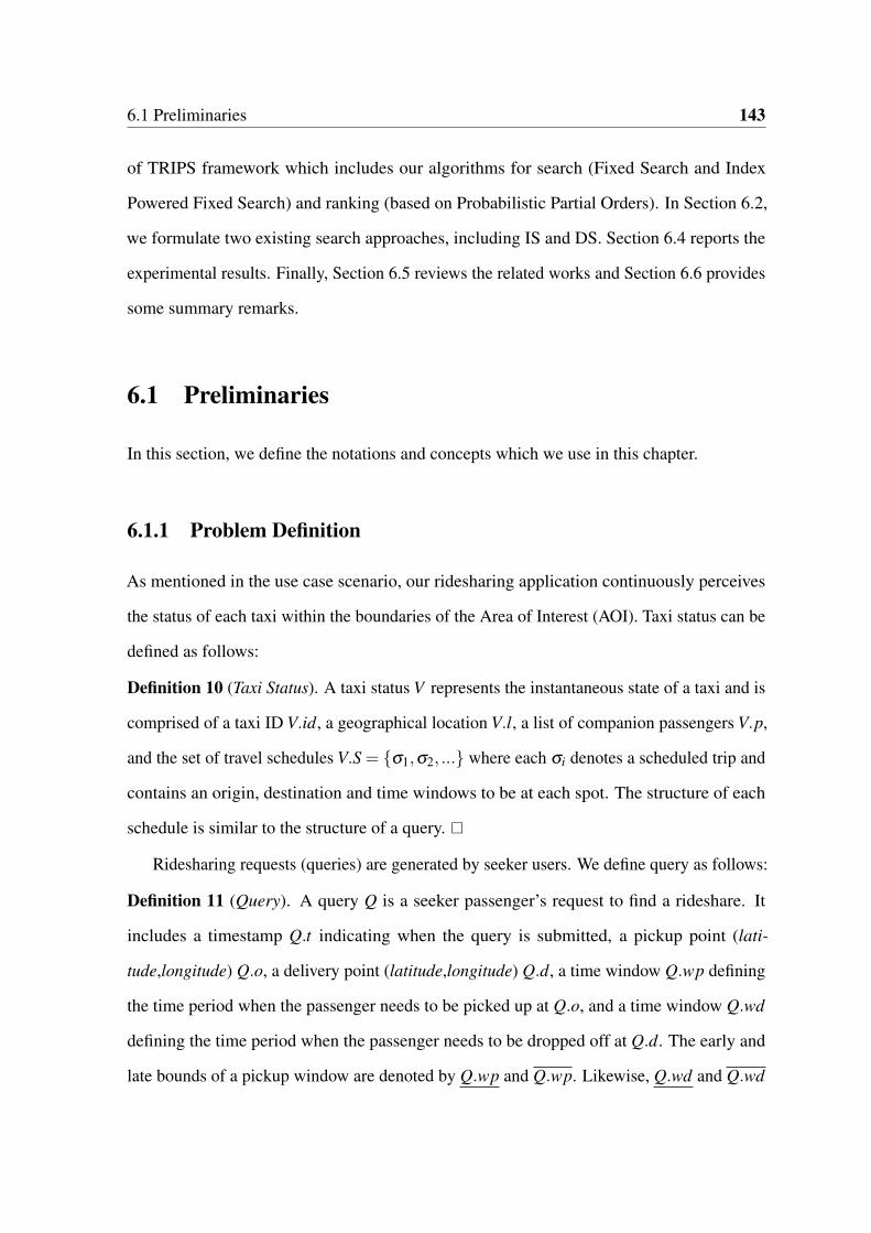
6.1 Preliminaries 143
of TRIPS framework which includes our algorithms for search (Fixed Search and Index
Powered Fixed Search) and ranking (based on Probabilistic Partial Orders). In Section 6.2,
we formulate two existing search approaches, including IS and DS. Section 6.4 reports the
experimental results. Finally, Section 6.5 reviews the related works and Section 6.6 provides
some summary remarks.
6.1 Preliminaries
In this section, we define the notations and concepts which we use in this chapter.
6.1.1 Problem Definition
As mentioned in the use case scenario, our ridesharing application continuously perceives
the status of each taxi within the boundaries of the Area of Interest (AOI). Taxi status can be
defined as follows:
Definition 10 (Taxi Status). A taxi status V represents the instantaneous state of a taxi and is
comprised of a taxi ID V.id, a geographical location V.l, a list of companion passengers V.p,
and the set of travel schedules V.S = {σ1,σ2, ...} where each σi denotes a scheduled trip and
contains an origin, destination and time windows to be at each spot. The structure of each
schedule is similar to the structure of a query. □
Ridesharing requests (queries) are generated by seeker users. We define query as follows:
Definition 11 (Query). A query Q is a seeker passenger’s request to find a rideshare. It
includes a timestamp Q.t indicating when the query is submitted, a pickup point (lati-
tude,longitude) Q.o, a delivery point (latitude,longitude) Q.d, a time window Q.wp defining
the time period when the passenger needs to be picked up at Q.o, and a time window Q.wd
defining the time period when the passenger needs to be dropped off at Q.d. The early and
late bounds of a pickup window are denoted by Q.wp and Q.wp. Likewise, Q.wd and Q.wd

144 Intent Based Search: A Case Study in Taxi Ridesharing
denote the bounds of the delivery window. Also Q.u represents the user u who have made
the query. For the sake of simplicity, each query indicates one passenger’s request, but the
approach can readily support multi-passengers’ requests. □
Given a query Q, we would like to find the alternatives which can satisfy Q such that
they can maximize the benefits for both companion and seeker users while the effort to get a
rideshare is minimized. A taxi, with the corresponding status V , satisfies Q if and only if (i)
size(V.p) is smaller than the seat capacity of the taxi; (ii) the taxi can pick up the passenger
of Q at Q.o within Q.wp and delivers her at Q.d within Q.wd; (iii) the taxi can pick up and
drop off the existing passengers in V.s no later than the late bound of their corresponding
pickup and delivery time windows.
In this chapter we use a cost function which depends on three main parameters: distance,
time and taxi fares. The fee that is paid for the distance roughly is a constant number while
the time variable is accountable for the extra costs that are incurred in during the waits in
traffic or similar reasons. We define these two variables first and then we define the cost
function. The distance between two points o and d is denoted as δod ∈ R+, which refers
to the length of the shortest path in the roads network between the two points. The travel
time estimate for the same points is denoted as θod ∈ R+, which is a measure in seconds that
approximates the time required to travel from o to d. Taxi fares are positive real numbers
fc, fd and ft that are used to calculate the final cost. Thus, we define the cost function as
follows:
Definition 12 (Cost Function). Cost function cost(δ ,θ) approximates the cost of a taxi
based on the distance δod and the trip time estimate θod using:
cost(δod,θod) = fc +δod fd +θod ft (6.1)
cost(δod,θod) = fc +δod fd (6.2)
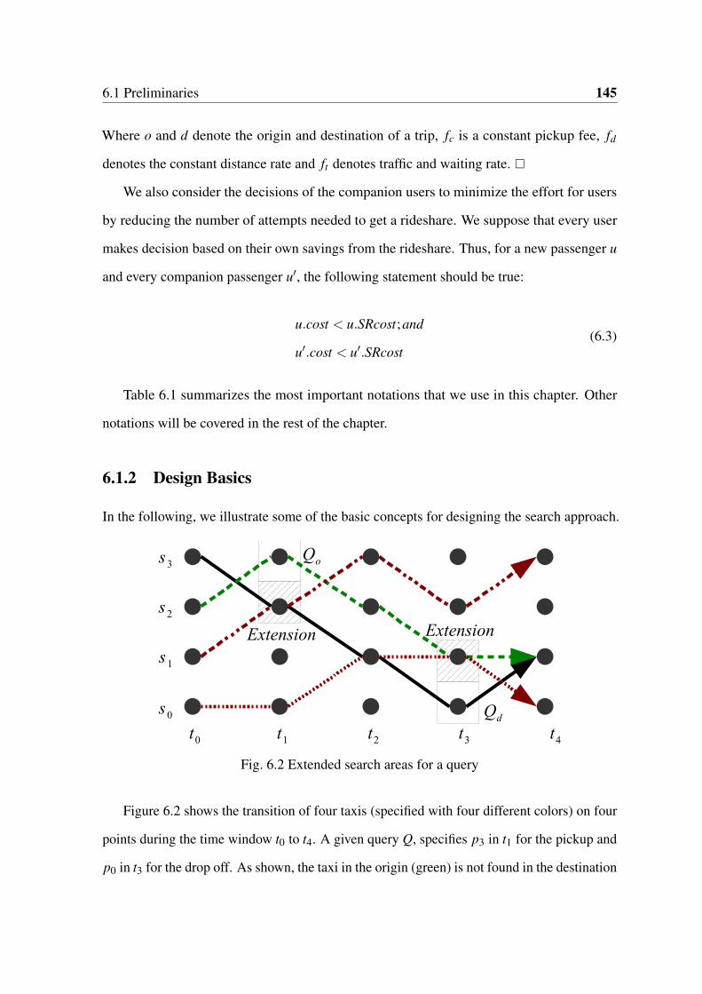
6.1 Preliminaries 145
Where o and d denote the origin and destination of a trip, fc is a constant pickup fee, fd
denotes the constant distance rate and ft denotes traffic and waiting rate. □
We also consider the decisions of the companion users to minimize the effort for users
by reducing the number of attempts needed to get a rideshare. We suppose that every user
makes decision based on their own savings from the rideshare. Thus, for a new passenger u
and every companion passenger u′, the following statement should be true:
u.cost < u.SRcost;and
u′.cost < u′.SRcost(6.3)
Table 6.1 summarizes the most important notations that we use in this chapter. Other
notations will be covered in the rest of the chapter.
6.1.2 Design Basics
In the following, we illustrate some of the basic concepts for designing the search approach.
Fig. 6.2 Extended search areas for a query
Figure 6.2 shows the transition of four taxis (specified with four different colors) on four
points during the time window t0 to t4. A given query Q, specifies p3 in t1 for the pickup and
p0 in t3 for the drop off. As shown, the taxi in the origin (green) is not found in the destination

146 Intent Based Search: A Case Study in Taxi Ridesharing
Table 6.1 List of important notations
Notation DefinitionAOI The area of interestpi Point i in AOIδpi p j The distance between points pi and p j
[i, i] Any interval value i with the minimum bound i and maximum bound iθpi p j The trip time estimate between points pi and p j at time tcost(δ ,θ) Travel cost estimation functionQ A query made by the seeker usersQ.o The pickup point (latitude,longitude) of query QQ.d The delivery point (latitude,longitude) of query QQ.wp The pickup time window of query QQ.wd The delivery time window of query QQ.dur Defined as [Q.wp,Q.wd] is the duration of a trip for QV Taxi statusV.S Set of scheduled trips for the given taxi Vσ A scheduled tripA The set of alternatives which are displayed to the userR∗ Maximum range of economically justifiable alternativesidx The segments indexu Useru.cost Ridesharing cost for user uu.SRcost Sole ride cost for user uV Any set of taxi trajectoriesP(u′,Q) The probability of user u′ accepting a rideshare offer based on Q
(only the black taxi is there), if the exact points in the query are used. In this situation, to find
a compromise solution, we need to apply some extension to the search area to find the nearest
taxi that satisfies the query. Only after extending the origin and/or destination, two taxis
are found. The IS approach [159, 162] proposes applying extension after each unsuccessful
search. For the given example in the figure, after applying two extensions taxis starting from
p2 and p3 are found as the closest alternatives. Following the IS approach, one of the taxis
will be selected based on the extra distance required by taxis to get to the points Q.o and
Q.d. Previous works aim at finding the nearest taxi while it may not necessarily be the best
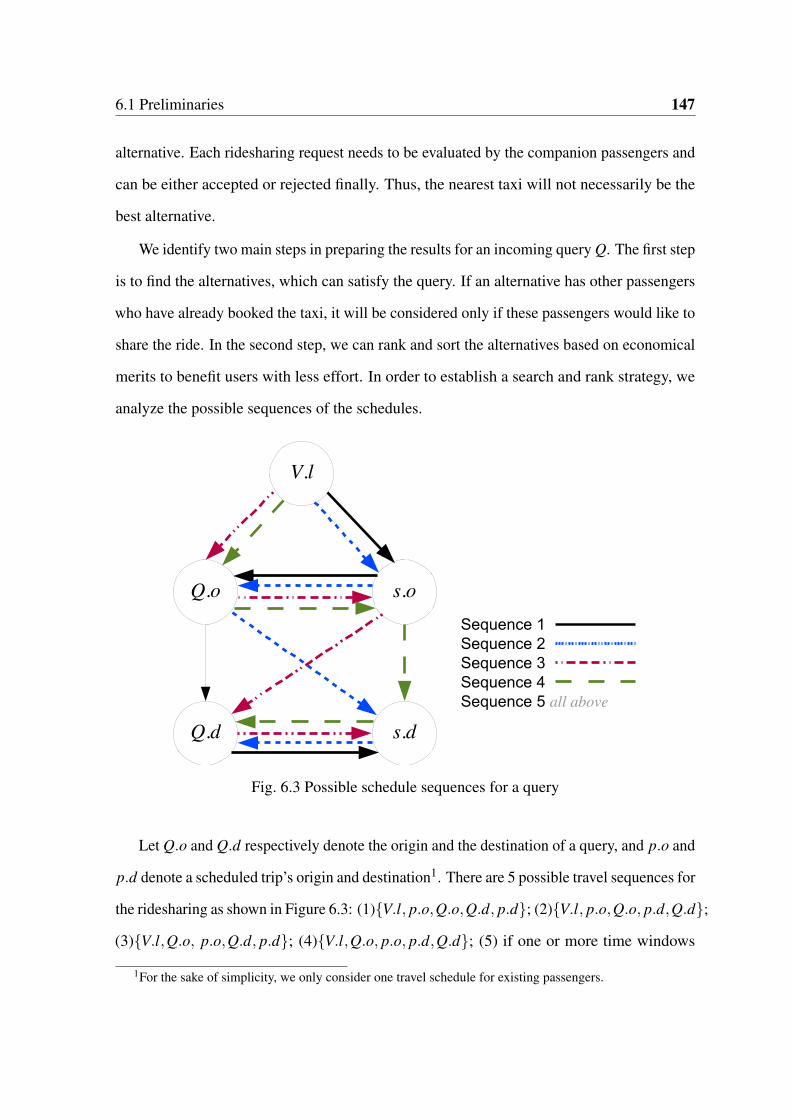
6.1 Preliminaries 147
alternative. Each ridesharing request needs to be evaluated by the companion passengers and
can be either accepted or rejected finally. Thus, the nearest taxi will not necessarily be the
best alternative.
We identify two main steps in preparing the results for an incoming query Q. The first step
is to find the alternatives, which can satisfy the query. If an alternative has other passengers
who have already booked the taxi, it will be considered only if these passengers would like to
share the ride. In the second step, we can rank and sort the alternatives based on economical
merits to benefit users with less effort. In order to establish a search and rank strategy, we
analyze the possible sequences of the schedules.
Fig. 6.3 Possible schedule sequences for a query
Let Q.o and Q.d respectively denote the origin and the destination of a query, and p.o and
p.d denote a scheduled trip’s origin and destination1. There are 5 possible travel sequences for
the ridesharing as shown in Figure 6.3: (1){V.l, p.o,Q.o,Q.d, p.d}; (2){V.l, p.o,Q.o, p.d,Q.d};
(3){V.l,Q.o, p.o,Q.d, p.d}; (4){V.l,Q.o, p.o, p.d,Q.d}; (5) if one or more time windows
1For the sake of simplicity, we only consider one travel schedule for existing passengers.

148 Intent Based Search: A Case Study in Taxi Ridesharing
overlap, any order for pick up/delivery is possible; and (6) if the companion traveler is already
on the taxi.
For the sake of simplicity, we consider two sets of users but the approach can be general-
ized to support sequences with multiple pickup/drops. The following sequences are possible
for the taxi (see Figure 6.3):
Sequence 1: Respectively, pre-scheduled pickup, new user pickup, new user delivery, pre-
scheduled delivery. The riding cost can be formulated as follows:
u.cost =cost(δod,θod)
(m+1)(6.4)
u′.cost =cost(δio,θio)
m+
cost(δod,θod)
m+1+
cost(δd j,θd j)
m(6.5)
Sequence 2: Respectively, pre-scheduled pickup, new user pickup, pre-scheduled delivery,
new user delivery. The riding cost can be formulated as follows:
u.cost =cost(δo j,θo j)
m+1+ cost(δ jd,θ jd) (6.6)
u′.cost =cost(δio,θio)
m+
cost(δo j,θo j)
m+1(6.7)
Sequence 3: Respectively, new user pickup, pre-scheduled pickup, new user delivery, pre-
scheduled delivery. The riding cost can be formulated as follows:
u.cost = cost(δoi,θoi)+cost(δid,θid)
m+1(6.8)
u′.cost =cost(δid,θid)
m+1+
cost(δd j,θd j)
m(6.9)
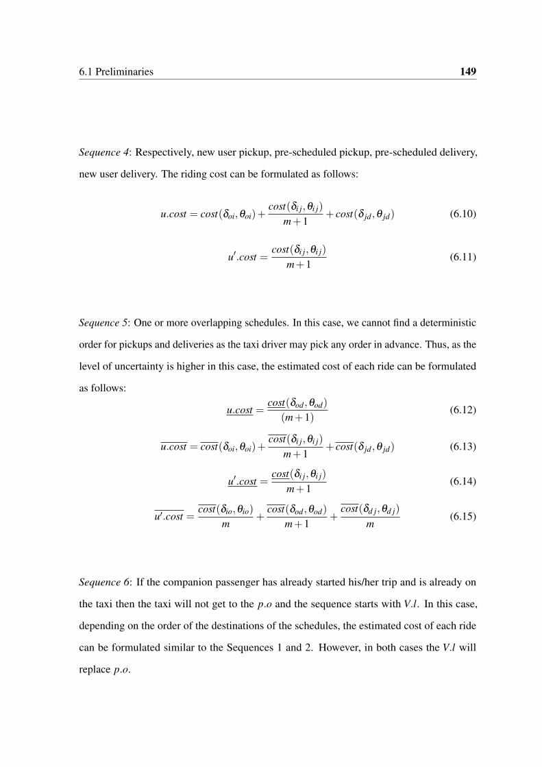
6.1 Preliminaries 149
Sequence 4: Respectively, new user pickup, pre-scheduled pickup, pre-scheduled delivery,
new user delivery. The riding cost can be formulated as follows:
u.cost = cost(δoi,θoi)+cost(δi j,θi j)
m+1+ cost(δ jd,θ jd) (6.10)
u′.cost =cost(δi j,θi j)
m+1(6.11)
Sequence 5: One or more overlapping schedules. In this case, we cannot find a deterministic
order for pickups and deliveries as the taxi driver may pick any order in advance. Thus, as the
level of uncertainty is higher in this case, the estimated cost of each ride can be formulated
as follows:
u.cost =cost(δod,θod)
(m+1)(6.12)
u.cost = cost(δoi,θoi)+cost(δi j,θi j)
m+1+ cost(δ jd,θ jd) (6.13)
u′.cost =cost(δi j,θi j)
m+1(6.14)
u′.cost =cost(δio,θio)
m+
cost(δod,θod)
m+1+
cost(δd j,θd j)
m(6.15)
Sequence 6: If the companion passenger has already started his/her trip and is already on
the taxi then the taxi will not get to the p.o and the sequence starts with V.l. In this case,
depending on the order of the destinations of the schedules, the estimated cost of each ride
can be formulated similar to the Sequences 1 and 2. However, in both cases the V.l will
replace p.o.

150 Intent Based Search: A Case Study in Taxi Ridesharing
Economic Search Margin
One of the problems that is associated with the IS approach is that the search area is gradually
extended until the nearest taxi with enough space is found. Thus, it is possible that for a
number of searches, we get results which should travel a long distance to reach the seeker
user making it is not efficient for the companion passengers. We use the following theorem
to set up this concept.
Theorem 6.1.1. Given the Query Q, where the user intends to travel from o to d, a taxi that
can pick the user iff it does not have any other trip with the origin and destination further
than the following distance from the points o and d:
R∗ = δod (6.16)
where δod denotes the distance that the user wants to travel and R∗ is the economically justi-
fiable radius. A taxi with scheduled trips further this distance is not within the economically
justifiable range.
Proof. We can prove the above theorem by using costs and benefits analysis for all possible
schedule sequences. Based on the mutual benefit principle, by summing up the total cost for
all users (e.g., all passengers), we have:
u.cost +m∗u′.cost < u.SRcost +m∗u′.SRcost (6.17)
This statement holds for all of the possible schedule sequences. For instance, for Sequence
1, we have:
u.cost +m∗u′.cost = cost(δoi,θoi)+ cost(δi j,θi j)+ cost(δ jd,θ jd) (6.18)

6.2 Background: IS vs. DS Approach 151
If we make a false assumption that R∗ > δod , we will have the following:
u.cost +m∗u′.cost ≥ SRcost (6.19)
where SRcost denotes u.SRcost +m ∗ u′.SRcost. Equation (6.19) in fact contradicts the
mutual benefit principle and cannot be correct. Theorem 1 is therefore proved.
6.2 Background: IS vs. DS Approach
Area extensions are applied to the origin and destination areas in order to find the taxis
with the least extra distance for taxis because for most of the queries no taxi is found to
exactly match the specified requirements. As mentioned before, one of the recent taxi search
approaches is exploiting an incremental search approach. Using the R∗ concept, instead of
increasing the search area, we can decrease the search area in each step. This will lead to the
decremental search approach. The details of each approach are as follows.
Incremental Search (IS)
It has been used in designing dynamic ridesharing applications such as T-Share [159].
Algorithm 10 shows a procedure based on this approach.
The steps of the Algorithm 10 take place in the following order. The input of the algorithm
is the given query Q and the extended areas of origin and destination, which in the first
round would be equal to Q.o and Q.d. First, the taxis at extended origin area and extended
destination area are queried and stored in T1 and T2 respectively (lines 1-2). The getTaxis
function loops through all taxis to find the right ones. The list of the common taxis in the two
sets are stored in the T set (lines 3-5). Then, if T is empty (lines 6-9), the area is expanded
and search is recursively called with the expanded origin and/or destination areas and the

152 Intent Based Search: A Case Study in Taxi Ridesharing
Algorithm 10 INCREMENTAL-SEARCHRequire: Q,origin,destEnsure: T set of taxis which satisfy the query
1: Let T1←getTaxis(origin,Q.wp)2: Let T2←getTaxis(dest,Q.wd)3: for all taxi ∈ T1 do4: if taxi ∈ T2 then5: Let T ← T ∪ taxi add taxi to output list.6: if T is empty then7: Let origin←expand(origin,Q.o) extending the search area.8: Let dest←expand(dest,Q.d) extending the search area.9: return INCREMENTAL-SEARCH(Q,origin,dest)
10: else11: return T
same query. Otherwise, if a common taxi is found in the same area, it is returned (lines
10-11).
The complexity of this algorithm depends mainly on three factors: the number of segments
(|AOI|) in AOI, the number of taxis (|taxis|), and the number of scheduled trips n. Thus the
order is O(n.|AOI|.|taxis|2).
The IS approach, as proposed [159], does not support the economical search margin and
continues extension until the first taxi is found. However, if this approach is extended to
support this margin, it still will continue to expand to fill the whole area within the boundaries
of the margin even if no taxi is found. Thus, a decremental strategy can be developed [163]
to fill this gap.
Decremental Search (DS)
The decremental search approach is proposed to decrease the cost of the search procedure
[163]. The details of this approach are shown in Algorithm 11. To initialize, the decremental
search requires the total extended area that includes all of the economically justifiable taxis.
We call it Economic Search Margin and denote the radius with R∗ (Figure 6.5).
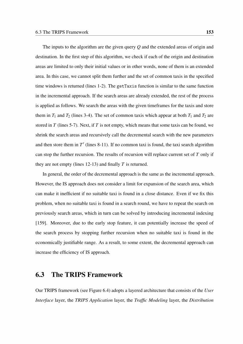
6.3 The TRIPS Framework 153
The inputs to the algorithm are the given query Q and the extended areas of origin and
destination. In the first step of this algorithm, we check if each of the origin and destination
areas are limited to only their initial values or in other words, none of them is an extended
area. In this case, we cannot split them further and the set of common taxis in the specified
time windows is returned (lines 1-2). The getTaxis function is similar to the same function
in the incremental approach. If the search areas are already extended, the rest of the process
is applied as follows. We search the areas with the given timeframes for the taxis and store
them in T1 and T2 (lines 3-4). The set of common taxis which appear at both T1 and T2 are
stored in T (lines 5-7). Next, if T is not empty, which means that some taxis can be found, we
shrink the search areas and recursively call the decremental search with the new parameters
and then store them in T ′ (lines 8-11). If no common taxi is found, the taxi search algorithm
can stop the further recursion. The results of recursion will replace current set of T only if
they are not empty (lines 12-13) and finally T is returned.
In general, the order of the decremental approach is the same as the incremental approach.
However, the IS approach does not consider a limit for expansion of the search area, which
can make it inefficient if no suitable taxi is found in a close distance. Even if we fix this
problem, when no suitable taxi is found in a search round, we have to repeat the search on
previously search areas, which in turn can be solved by introducing incremental indexing
[159]. Moreover, due to the early stop feature, it can potentially increase the speed of
the search process by stopping further recursion when no suitable taxi is found in the
economically justifiable range. As a result, to some extent, the decremental approach can
increase the efficiency of IS approach.
6.3 The TRIPS Framework
Our TRIPS framework (see Figure 6.4) adopts a layered architecture that consists of the User
Interface layer, the TRIPS Application layer, the Traffic Modeling layer, the Distribution

154 Intent Based Search: A Case Study in Taxi Ridesharing
Algorithm 11 DECREMENTAL-SEARCHRequire: Q,origin,destEnsure: T set of taxis which satisfy the query
1: if origin equals Q.o and dest equals Q.d then2: return T ← getTaxis(origin,dest,Q.wp,Q.wd)3: Let T1←getTaxis(origin,Q.wp)4: Let T2←getTaxis(dest,Q.wd)5: for all taxi ∈ T1 do6: if taxi ∈ T2 then7: Let T ← T ∪ taxi add taxi to output list.8: if T is not empty then9: Let origin←shrink(origin,Q.o) shrinking the search area.
10: Let dest←shrink(dest,Q.d) shrinking the search area.11: Let T ′←DECREMENTAL-SEARCH(Q,origin,dest)12: if T ′ is not empty then13: Let T ← T ′
14: return T
Management layer, and the Data Storage layer. The data storage layer facilitates the storage
and retrieval of TRIPS data, including the spatio-temporal index of taxis, the routes index,
and the traffic data. Parts of the work in previous section can be reused in this section.
Accordingly, we use the design basics for limiting the search area. Also, The search
algorithms in previous section can be used for comparison and the application layer. In the
following, we focus on the technical details of the other layers in the TRIPS framework.
Our framework supports a novel combination of functional factors as follows:
1. Minimizing the end user’s attempt to get a rideshare: The preferences of the companion
passenger(s) is an important factor for the success of ridesharing. For instance, some
studies suggest that behavioral parameters—such as the low rate of acceptance to the
requests from male strangers by female participants who travel alone [173] and issues
related with e.g., smoking [168] can affect the final decision of other riders on the
same taxi. However, in this chapter we do not aim to address all behavioral factors. In
our model, we assume that users only decide based on their own economical benefits.
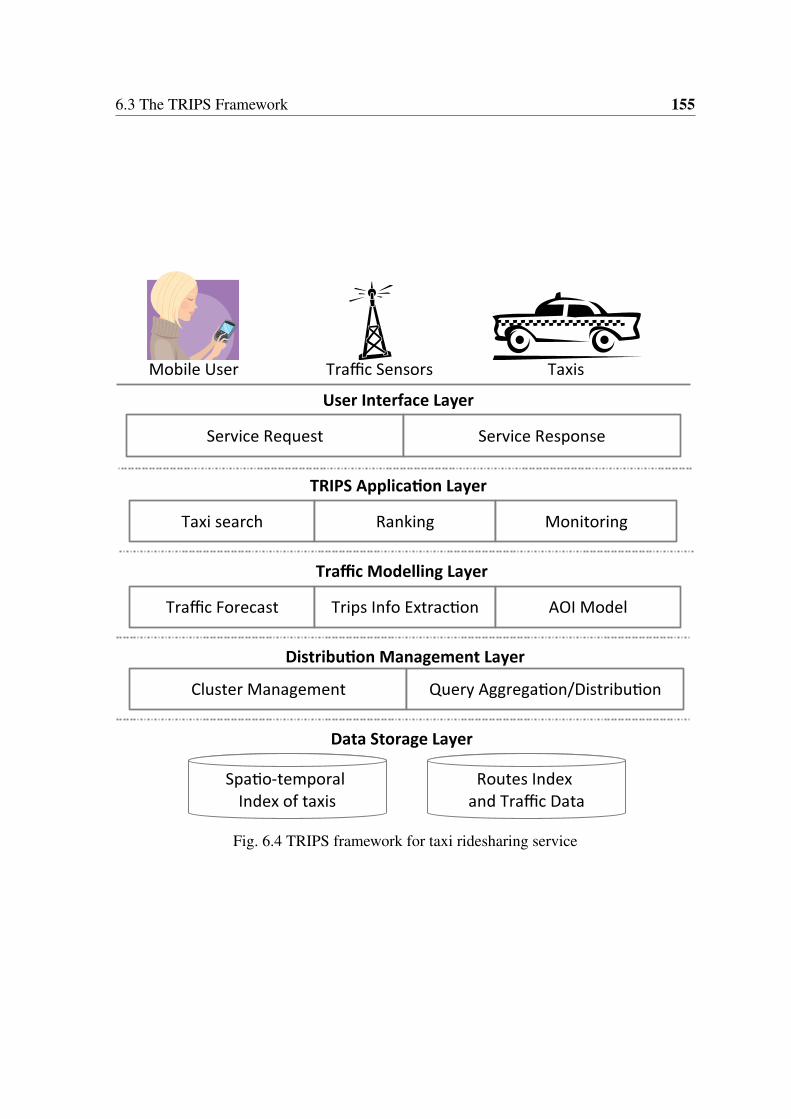
6.3 The TRIPS Framework 155
Fig. 6.4 TRIPS framework for taxi ridesharing service

156 Intent Based Search: A Case Study in Taxi Ridesharing
2. Maximizing the performance of the application: Computationally, matching finding
the best taxi is a complex problem. In Moreover, in particular, including uncertain user
decisions and processing the distances of all taxis from all users are complex processes.
In this chapter, we particularly focus on the uncertain end users decisions and avoid
duplicate rounds for performing the search when the ridesharing requests get rejected.
3. Maximizing overall savings from using the application: The savings from ridesharing
is the primary goal of users when they use a the application. To maximize the savings,
we improve the rate of accepted requests and the amount of savings (by reducing
vehicle mileage) for the accepted queries.
6.3.1 Traffic Modeling Layer
The traffic modeling layer operates in parallel to the TRIPS application layer (details in
Section 6.3.2) in order to provide the application layer with the needed traffic forecasts and
identified common trips model. The AOI model, the trips information extraction, and the
traffic forecast are the three main modules of this layer.
AOI Model: The underlying roads network can be modeled via different approaches such as
R-tree and partitioning using a grid network. In our work, a grid partitioning system similar
to [159] is developed in order to avoid high cost indexing level. However, the indexing
system can easily be upgraded if needed.
Trips Information Extraction: Trips information extraction module is designed to obtain
the regular trips that taxis undertake within different locations in a certain period of time.
For this purpose, we use the same algorithm as in [163] which provides the actual upper and
lower bounds from the historical data. In our study we use these results to avoid dealing with
technical complexity over the accuracy of predicted travel times. However, in application it
can simply be replaced by prediction algorithms such as [172].

6.3 The TRIPS Framework 157
Traffic Forecast: The traffic forecast module can exploit several techniques to forecast
traffic because many approaches have been proposed for this task in the literature [174, 175].
Although the traffic forecast model is not the focus of this study, we briefly discuss in the
following on how traffic index is generated in our work.
To generate a traffic index, the speed of taxis moving along a specified trip is taken as an
index. The traffic load in a route between two points can have direct relationship with the
speed of cars passing over that route if they are moving. A query over historical data record
can easily provide the margins of each entry in traffic index and trip time matrices. Thus
θpi p j = max{θpi,p j}, θpi,p j = min{θpi,p j}.
6.3.2 TRIPS Application Layer
In the proposed framework, TRIPS application layer runs on top of the traffic modeling
layer, facilitating modules for responding user queries, ranking and monitoring the successful
requests.
Taxi Search: Upon receiving a query from a user, the taxi search module returns all possible
taxis which can satisfy the query by considering uncertainty. Since every taxi that can satisfy
user’s query could be an option for the user, instead of gradually increasing search area (IS)
such as T-Share [159, 162] or gradually decreasing it (DS approach), in TRIPS we develop a
new strategy, namely Fixed Search (FS), to perform search once to get all of the available
taxis.
Based on the FS approach, to find the alternatives we calculate all taxis’ locations at the
pickup and delivery time windows specified by the user’s query. However, this approach
requires traversing all scheduled trips for all taxis which makes it very inefficient for large
scale applications. In order to increase the efficiency, the search area can be limited to R∗
(Figure 6.5). In Theorem 1, we have showed that any taxi beyond the economic search

158 Intent Based Search: A Case Study in Taxi Ridesharing
Fig. 6.5 Symmetric (solid) and asymmetric (dashed) extended search areas
margin will not be suitable. As Figure 6.5 shows, the margins can grow symmetrically or in
an asymmetric manner. However, the total added distance should exceed the R∗ limit.
Based on this approach, we propose a novel search algorithm (see Algorithm 12). The
algorithm has several steps as follows. First, R∗ is initialized to prevent searching unnecessary
locations (line 1). Then the algorithm loops through every scheduled trip of each taxi (lines
2-3) and checks if the duration of trips overlap at pickup point, the taxi is added to T1 . Also,
if they overlap at destination, it is added to the T2 set (lines 4-7). Later, common taxis in T1
and T2 are added to the set of alternatives (lines 8-10). As a result set consisting of numerous
taxis is not suitable for users, due to the fact that only one needs to be selected, the taxis in
the result set need to be ranked and sorted based on the gain and the possible acceptance rate
by other users to get the best result. Thus, we call the RANK function and return the best
taxi as a result (lines 11-12). The details of RANK algorithm will be discussed later in this
section.
The complexity of the FS algorithm depends on two factors the number of taxis (|taxis|)
and the number of scheduled trips (n). Thus the order of FS approach is O(|taxis|.n). As
a result, with the growth of the number of taxi schedules, the FS approach will become
inefficient as it is shown by our experiments (Section 6.4).

6.3 The TRIPS Framework 159
Algorithm 12 FIXED-SEARCHRequire: Q user’s queryEnsure: T set of available taxis
1: Let R∗← δod Setting the R∗ to avoid searching the unnecessary area2: for all taxi ∈ taxis do3: for all σ ∈ taxi.V.S do4: if i = σ .pickup and δio ≤ R∗ and Q.dur overlaps(σ .dur) then5: Add taxi to T16: if j = σ .destination and δ jd ≤ R∗ and Q.dur overlaps(σ .dur) then7: Add taxi to T28: for all taxi ∈ T1 do9: if taxi ∈ T2 then
10: Add taxi to T11: T ← RANK(T )12: return T. f irst
We also design a new algorithm, namely Index Powered Fixed Search (IPFS), to use the
index in the search procedure.
First, we set up the indexing scheme and then we present the new algorithm. For creating
the index, similar to T-Share [159], we divide the spatial domain of moving taxis, which
we refer to as the AOI, into a finite set of rectangular cells. Each cell is called a segment
and is denoted by s. The number of segments in an AOI is often limited and constant. Also,
the number of scheduled trips which begin from or end to a segment are limited as well.
Therefore, we introduce a segment based index denoted by s.idx, which keeps the set of
schedules relevant (pick up or delivery) to s.
The index contains two sets of entries. The first set is the scheduled trips from the
segment and the second contains the scheduled trips to the segment. The records in the index
are updated whenever a new trip is scheduled and removed whenever a trip is finished. Thus,
the index is updated during schedule set up and schedule removal steps without notable extra
workload on the system. The complexity order of the index update algorithm, if implemented
separately, is O(∑ |V.S).

160 Intent Based Search: A Case Study in Taxi Ridesharing
The new search approach is presented in Algorithm 13. Similar to the FS algorithm, the
IPFS algorithm starts with initializing R∗ (line 1). The algorithm loops through the index
entries for each segment within the range of R∗ instead of the schedules of each taxi (lines
2-4). Then for each segment within the economical search margin (i.e., the area that includes
all of the economically justifiable taxis), if a scheduled trip is found in the segment index
entry, the corresponding taxi will be added to the set of found taxis at origin denoted by T1
and/or destination denoted by T2 (lines 5-8). Only taxis appearing in both sets (T1 and T2)
are included in the output (T ), ranked similar to the FS algorithm and finally returned (lines
9-13).
The complexity of the IPFS algorithm depends on two factors: the number of index
entries (n) and the number of segments (|AOI|). Thus the order of FS approach however
depends on the number of taxis as well. However, the execution cost of this algorithm will
be lower than the FS algorithm due to the fact that only a small portion of the scheduled trips
are processed in each round.
Algorithm 13 INDEX-POWERED-FIXED-SEARCHRequire: Q user’s query, AOI list of segments in AOIEnsure: T set of available alternatives
1: Let R∗← δod Initializing the R∗ to avoid searching the unnecessary area2: for all segment s ∈ AOI do3: if δseg,o ≤ R∗ then4: for all trip ∈ s.idx do5: if δseg,o ≤ R∗ and Q.dur overlaps(trip.dur) then6: Add idx.taxi to T17: if δseg,d ≤ R∗ and Q.dur overlaps(trip.dur) then8: Add idx.taxi to T29: for all taxi ∈ T1 do
10: if taxi ∈ T2 then11: Add taxi to T12: T ← RANK(T )13: return T. f irst

6.3 The TRIPS Framework 161
Ranking: Ranking can be challenging when it comes to uncertain data. The score for
each alternative will be represented as an interval. Hence, to rank and sort them, different
possible orders must be considered. We propose the RANK algorithm (see Algorithm 14)
which works in the following order: 1) the algorithm starts by calculating the score for each
alternative. For each active scheduled trip (line 2) of each alternative (line 1) we determine
the sequence (seq) of the new user’s trip and the previously scheduled trip (see Figure 6.3)
in line 3 and update users sole ride cost (u.SRcost), shared ride cost (u.cost), the amount of
saving (u.saving) and the possibility of accepting the rideshare request (P(u,Q)) based on
the savings in lines 4-9; 2) In the next step (line 10), we pass the query (Q) and the set of
scored alternatives (A) to BUILD-TREE algorithm (Algorithm 15) which updates the global
tree of possible worlds; 3) Then, the alternatives will be sorted based on the tree of possible
worlds and the result will be returned (lines 11 and 12).
The complexity of RANK algorithm in the worst case is O(|taxis|.n) if |taxis| and n
represent the number of the taxis and the number of scheduled trips. However, due to the fact
that usually only a small subset of the taxis set is received from the search algorithm, the
runtime and order of RANK algorithm are negligible. Moreover, using segment schedules
index can also improve this algorithm by reducing the number of accessed schedules.
We design the BUILD-TREE using the probabilistic partial order as follows.
Definition 13 (Probabilistic Partial Order [176]). Let A = {a1, ...,an} be the set of the
alternatives with their scores, and O be the set of orders of alternatives. The probabilistic
partial order PPO(A,O) is a set with (ai,a j) ∈ O iff ai precedes a j. □
Algorithm BUILD-TREE recursively builds the tree of possible worlds, which is a
globally defined variable, and can stop at the specified level (if any) in line 1. Building each
level starts by finding sources (lines 2-4), which are alternatives that dominate others by their
scores, and ends up with passing the generated probabilistic partial order to the next level
(line 5). The complexity of this algorithm only depends on the number of taxis received from

162 Intent Based Search: A Case Study in Taxi Ridesharing
Algorithm 14 RANKRequire: Q user’s query, T the set of taxisEnsure: Ar ranked list of alternatives
1: for all taxi ∈ T do2: for all σ ∈ taxi.V.S do3: Let seq be the sequence of Q.wp and Q.wd comparing with σ .wp and σ .wd4: Calculate Q.u.SRcost, Q.u.cost, Q.u.saving based on seq5: Calculate σ .u.SRcost, σ .u.cost, σ .u.saving based on seq6: Update P(σ .u,Q) based on seq7: Update Q.u.totalSRcost, Q.u.totalCost and Q.u.totalSaving8: Update σ .SRcost, σ .cost and σ .saving9: Set the saving and possibility to taxi
10: Update global tree of possibilities T by BUILD-TREE(Q,A,nil,nil,0)11: Let Ar← sort( A,T ) be the set of sorted alternatives12: return Ar
the RANK algorithm, and as there are usually a small number of taxis, we expect that the
complexity and runtime of the BUILD-TREE algorithm would be negligible.
Algorithm 15 BUILD-TREERequire: PPO(A,O), Treenode n, level
1: if level ≤ max− level then2: for all sources taxi ∈ A do3: Add taxi as a new child to children4: Let PPO← PPO(A,O) after removing taxi5: BUILD-TREE(Q,A,PPO,child,level +1)
6.3.3 Distribution Management Layer
The distribution management layer handles two main tasks: the cluster management and the
query distribution/aggregation.
The cluster management module maintains taxis in a set of object clusters. Formally, an
object cluster is defined in the following:
Definition 14 (Object Cluster). Object cluster is a set of tables containing the data of moving
objects (taxis) {taxisi|i ∈ D(taxis)}, where the member items share one or more common
values in their status V such as their location or corresponding ID. The set of clusters can be
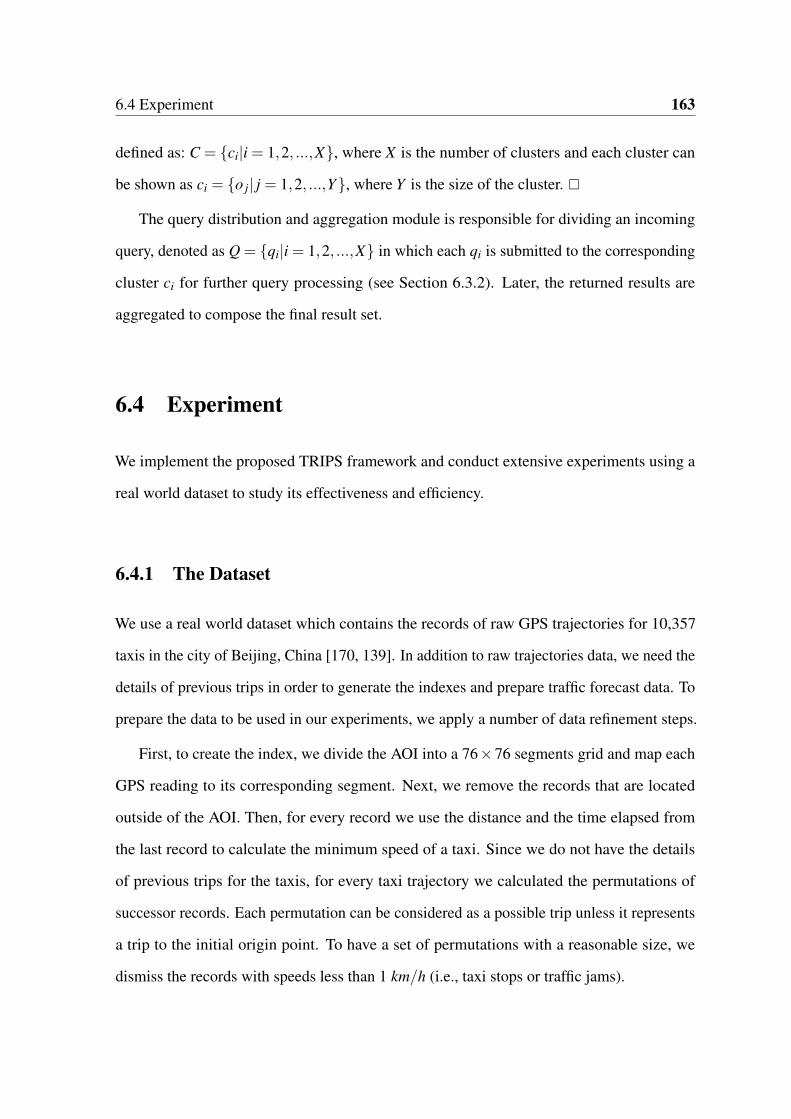
6.4 Experiment 163
defined as: C = {ci|i = 1,2, ...,X}, where X is the number of clusters and each cluster can
be shown as ci = {o j| j = 1,2, ...,Y}, where Y is the size of the cluster. □
The query distribution and aggregation module is responsible for dividing an incoming
query, denoted as Q = {qi|i = 1,2, ...,X} in which each qi is submitted to the corresponding
cluster ci for further query processing (see Section 6.3.2). Later, the returned results are
aggregated to compose the final result set.
6.4 Experiment
We implement the proposed TRIPS framework and conduct extensive experiments using a
real world dataset to study its effectiveness and efficiency.
6.4.1 The Dataset
We use a real world dataset which contains the records of raw GPS trajectories for 10,357
taxis in the city of Beijing, China [170, 139]. In addition to raw trajectories data, we need the
details of previous trips in order to generate the indexes and prepare traffic forecast data. To
prepare the data to be used in our experiments, we apply a number of data refinement steps.
First, to create the index, we divide the AOI into a 76×76 segments grid and map each
GPS reading to its corresponding segment. Next, we remove the records that are located
outside of the AOI. Then, for every record we use the distance and the time elapsed from
the last record to calculate the minimum speed of a taxi. Since we do not have the details
of previous trips for the taxis, for every taxi trajectory we calculated the permutations of
successor records. Each permutation can be considered as a possible trip unless it represents
a trip to the initial origin point. To have a set of permutations with a reasonable size, we
dismiss the records with speeds less than 1 km/h (i.e., taxi stops or traffic jams).

164 Intent Based Search: A Case Study in Taxi Ridesharing
Fig. 6.6 Availability of the index for all origins and destinations
Figure 6.6 shows the index availability for all origins and destinations in the AOI. Each
dark point indicates that the time estimation for the corresponding segments pair is existing.
The density in the central areas is higher than the density of indexed data in the surrounding
areas while some of the segment pairs have no data.
Then, we conduct two separate experiments to examine the effect of the proposed
approach on efficiency (performance) and effectiveness (cost saving).
6.4.2 Performance
We analyze two measures for the performance and the scalability of our system: i) search
space, and ii) its ability to respond to a heavy workload. The size of search space can greatly
affect the performance of a search procedure. One of the advantages of using segments index
is that it fixes the maximum size of search space. For any number of given trips data in
the input, the size of trip information index is equal to or less than |AOI|2 (e.g., 33,362,176
records). Figure 6.7b shows the size of the dataset in each step of the dataset preparation.

6.4 Experiment 165
02
46
8
Query Count
Tim
e (
se
c)
Incremental SearchDecremental SearchFixed SearchIndex Powered Fixed Search
0 1000 2000 3000 4000 5000 6000
(a) Index availability
5 10 15 20
0.0
e+
00
6.0
e+
06
1.2
e+
07
Cluster
Record
s
All GPS recordsFiltered recordsPermutations (tens)Filtered permutations
(b) Processing time
0.1
0.2
0.3
0.4
0.5
Query count
Tim
e (
sec)
FSIPFS
500 1500 2500 3500 4500 5500
(c) Dataset size
0.0
05
0.0
15
Query count
Tim
e (
sec)
FSIPFS
500 1500 2500 3500 4500 5500
(d) Search time
24
68
Query count
Pro
cessed a
ltern
atives
IS and DSFSIPFS
500 1500 2500 3500 4500 5500
(e) Rank time
37.5
38.5
39.5
Query count
Ave
rage d
elta (
seg) IS
DSFSIPFS
1000 2000 3000 4000 5000 6000
(f) Average delta
Fig. 6.7 The results of the experimental evaluation
166 Intent Based Search: A Case Study in Taxi Ridesharing
For the second indicator, we implement a simulation, in which we use a set of entities
such as a 76×76 grid of segments (same as AOI), using key parts of a random taxi query
generator [159]. We also use 10,000 taxis with limited capacity (up to 4 people) to represent
a realistic scenario.
In our experiments, we use 6,000 queries which are processed by the system. For the
baseline, we use an improved version of T-Share which uses the IS approach. The improved
version applies extension to the search area by adding all the surrounding segments (instead
of one by one segment strategy used by e.g., T-Share) in each iteration. Figure 6.7a compares
the total query processing time among IS, DS, FS and IPFS approaches. As the Figure
shows, the IFPS algorithm is the most efficient one. We also measure the amount of time
spent on search and rank stages separately and for each of them, we compare the runtime
between using and not using the segments index. Figure 6.7c compares the average search
time between FS and IPFS for the same number of queries. As it shows, while the IPFS takes
less than 0.1 second until the end of the experiment, the FS search time gradually increases
and reaches to 1.4 seconds. This is mainly due to the constant size of the search space in the
IPFS algorithm.
The RANK function can benefit from the segments index as well. Figure 6.7d compares
the execution time for two versions of the RANK function. The use of segments index
reduces the increment in average ranking time by nearly 50%. The average ranking time for
index powered approach is nearly 15 milliseconds per query where without using the index,
it can take up nearly 30 milliseconds for the last set of queries.
Another interesting feature found in our performance analysis is the number of index
access times. While in the incremental approaches same segments may be accessed several
times [159, 162], in our TRIPS framework, the same segment index is accessed only twice in
maximum.

6.4 Experiment 167
To have a deeper analysis of the changes in conditions between the two experiments
(index-powered and FS approach), we deploy two more parameters. The first parameter is the
average number of alternatives found by the FS algorithm. This can be useful to assure that
the two ranking approaches have not been affected by the number of their input (processed
alternatives). Figure 6.7e shows that the enhanced RANK algorithm has processed more
alternatives while it has a better performance. Except a slight difference for a number of
queries, the number of processed alternatives is almost the same.
The second parameter is δod , which also can affect the performance of the search step.
As shown in Figure 6.7f, the average amount of δod from the two experiments are very close
to each other most of the time. As a result, we have a good evidence that the IPFS and
FS approaches have been examined in a fairly comparable condition. However the index
powered approach shows to be more efficient.
6.4.3 Cost Savings
The second experiment investigates the effect of considering uncertainty in the total savings
of the ridesharing process. In this experiment, we enable the riders who have booked earlier
to accept or reject the incoming ridesharing requests. The decision is made based on the ratio
of their own savings from the rideshare to their initial cost:
P(u′,Q) ∝u′.SRcost−u′.cost
u′.SRcost(6.20)
Where u′ is a user who has previously booked the taxi for a time which overlaps with
[Q.wp,Q.wd], possibility is the possibility of accepting the new user, u′.cost is the cost after
accepting the rideshare and u′.SRcost denotes the sole ride cost for u′ before accepting the
rideshare.

168 Intent Based Search: A Case Study in Taxi Ridesharing
10
03
00
All requests
Acce
pte
d r
eq
ue
sts
Without acceptance possibilityWith acceptance possiblity
100 200 300 400 500 600 700 800 900
(a) Accepted requests
10
00
03
00
00
50
00
0
Rideshare requests (#)
To
tal savin
gs (
CN
Y) without acceptance possibility (max)
without acceptance possiblity (min)with acceptance possiblity (max)with acceptance possiblity (min)
100 200 300 400 500 600 700 800 900
(b) Bounds of savings
10
00
03
00
00
Rideshare requests (#)
To
tal savin
gs (
CN
Y) without acceptance possibility (mean)
with acceptance possiblity (mean)
100 200 300 400 500 600 700 800 900
(c) Mean Savings
Fig. 6.8 Effectiveness results

6.4 Experiment 169
In a similar setting to the previous experiments, we develop two implementations of the
RANK algorithm to the same number of ridesharing requests. Nearly 1,000 ridesharing
requests were successful in finding a set of suitable alternatives. The result (see Figure 6.8a)
shows that considering the companion passenger decision factor increases the acceptance
rate of the companion users. To assess the amount of financial benefits for users, we use the
following formula to calculate the taxi fares in Chinese Yuan (CNY)2:
cost(δ ,θ) = 12+δ ∗ (2.2)+(θ −θ)∗ (0.01)
cost(δ ,θ) = 12+δ ∗ (2.2)(6.21)
Figure 6.8b shows the upper and lower bounds for the estimated cumulative savings.
The possible amount of savings increases due to the increment in acceptance rate. As the
amount of uncertainty increases throughout the time, the upper and lower bounds of the two
estimations may interfere. Figure 6.8c shows the average amount of cumulative savings for
users in each approach. From the experimental results, we conclude that the total savings
remarkably increase by using our TRIPS framework. This is due to the reason that our
approach considers the most probable and most efficient alternatives rather than the most
efficient ones only.
6.4.4 Comparison with Other Solutions
In this section, we compare our approach with other existing approaches. T-Share’s search
approach [159, 162] is the main work comparable with our search approach. It is not
designed to support the effect of users’ decisions, it does not have any component similar
to the taxi ranking part of our framework. Thus, we can only compare the searching part.
After customizing the approach to find all possible taxis, the customized code does not stop
with finding the first taxi. We realize that in this case, the performance of this approach is
2http://www.numbeo.com
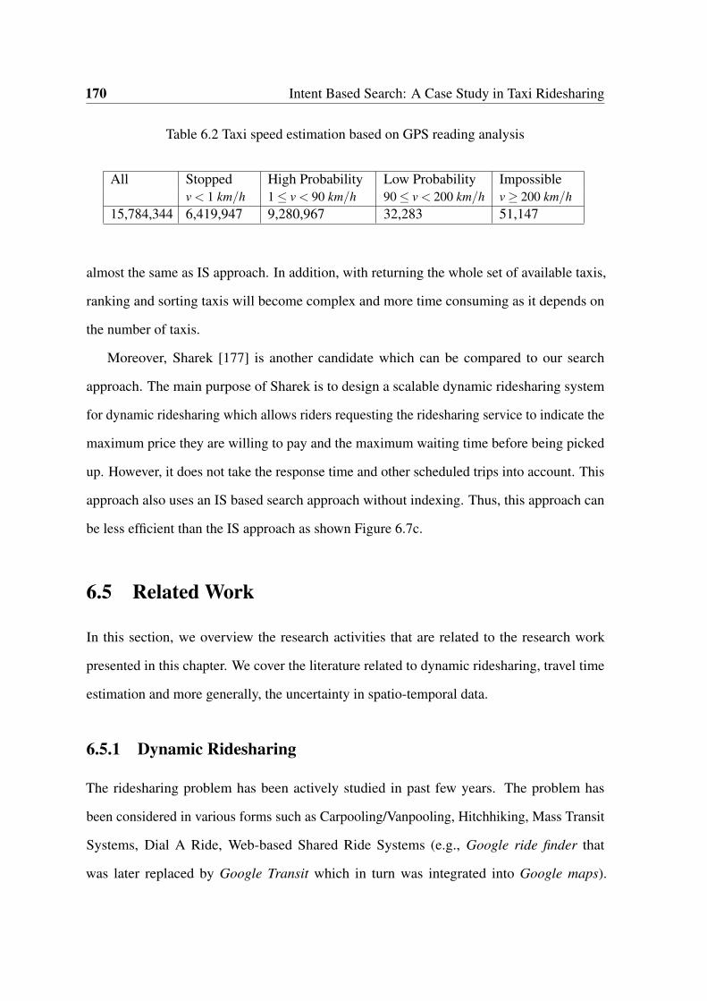
170 Intent Based Search: A Case Study in Taxi Ridesharing
Table 6.2 Taxi speed estimation based on GPS reading analysis
All Stopped High Probability Low Probability Impossiblev < 1 km/h 1≤ v < 90 km/h 90≤ v < 200 km/h v≥ 200 km/h
15,784,344 6,419,947 9,280,967 32,283 51,147
almost the same as IS approach. In addition, with returning the whole set of available taxis,
ranking and sorting taxis will become complex and more time consuming as it depends on
the number of taxis.
Moreover, Sharek [177] is another candidate which can be compared to our search
approach. The main purpose of Sharek is to design a scalable dynamic ridesharing system
for dynamic ridesharing which allows riders requesting the ridesharing service to indicate the
maximum price they are willing to pay and the maximum waiting time before being picked
up. However, it does not take the response time and other scheduled trips into account. This
approach also uses an IS based search approach without indexing. Thus, this approach can
be less efficient than the IS approach as shown Figure 6.7c.
6.5 Related Work
In this section, we overview the research activities that are related to the research work
presented in this chapter. We cover the literature related to dynamic ridesharing, travel time
estimation and more generally, the uncertainty in spatio-temporal data.
6.5.1 Dynamic Ridesharing
The ridesharing problem has been actively studied in past few years. The problem has
been considered in various forms such as Carpooling/Vanpooling, Hitchhiking, Mass Transit
Systems, Dial A Ride, Web-based Shared Ride Systems (e.g., Google ride finder that
was later replaced by Google Transit which in turn was integrated into Google maps).

6.5 Related Work 171
Dynamic ridesharing is generally described as an automated system that facilitates drivers and
riders to share one-time trips close to their departure times/places and can be characterized
with features like dynamic, independent, cost-sharing, non-recurring trips, prearranged
and automated matching [158]. A survey over Trajectory Data Mining [169], which is
a more comprehensive research area, divides this paradigm into different sub-paradigms
including trajectory preprocessing, trajectory indexing and retrieval, trajectory pattern mining,
trajectory classification, trajectory outlier/anomaly detection and uncertainty. However, the
uncertainty sub-paradigm is more focused on the uncertainty of the trajectory data rather
than the uncertainty in the application context. The use of contextual information and user
centered trajectory data mining, which is the main direction of this chapter, have been
mentioned as the areas of future research in the same survey. Inferring gas consumption
and pollution emission from the trajectory data is an example of contextual information
processing in this paradigm [178].
Most of the proposed applications have not been examined for either real-life and/or
large-scale datasets. These solutions are developed based on a variety of techniques and
approaches such as auction negotiation [179, 164], analyzing social connections in SRSS
[180], and multi source-destination path planning [181].
Some other recent solutions such as T-Share [159, 162], Noah [182] and kinetic tree
algorithm [183] treat dynamic taxi ridesharing as finding k-nearest neighbors (kNN) problem
although it does not cover the whole challenges and minimizing the system wide travel
time and travel distance. However, although using this approach can enormously reduce the
complexity of the problem, using kNN for dynamic ridesharing is not a suitable approach as
k is unclear. CallCab [184] deploys a generic MapreduceMeasure to tackle the raw dataset
of 14,000 taxis efficiently. However, the dominating approach is the IS approach while in
real world scenarios, this approach does not find all suitable taxis and leaves search iterations
right after finding the first taxi.

172 Intent Based Search: A Case Study in Taxi Ridesharing
Some of the related works such as [164] take companion users willingness for ridesharing
into account and develop a multi-agent system to support dynamic ridehsaring in real-time.
However, the scalability of the framework has not been evaluated for real-world or large
scale data. The proposed approach is still too simplistic. Other works in this area often focus
on different criteria and do not address uncertainty or scalability. For instance, [165] propose
a solution based on genetic algorithms to achieve the following goals:
1. Minimize the total distance of vehicles’ trips
2. Minimize the total time of vehicles’ trips
3. Minimize the total time to successfully get a ride
4. Maximize the number of accepted (served) requests
The work by [161] considers time window restrictions and models them as a soft con-
straint, where for instance, a reasonable delay might be acceptable. They consider the
problem as an on-line continual planning problem, in which additional ride requests may
arrive while plans for previous ride-matching are being executed. The success of this model
depends on other uncertain parameters such as routes selected by drivers and travel time
estimate.
6.5.2 Travel Time Estimation
In addition, estimating the travel time is a sub-problem of dynamic taxi ridesharing. It is a
highly challenging problem because it deals with different factors such as traffic fluctuations,
demand and supply, traffic signals, weather conditions and seasonal changes [139, 170]. One
of the existing approaches proposes a real-time travel time estimation using sparse trajectories
[172]. The requirements for this method is knowing the path for which a part of the path is
not associated with previous values. One of the recent works proposes an approach for travel

6.5 Related Work 173
time estimation using large-scale taxi data with partial information [185]. The proposed
model focuses on uncertainty in path choices. It infers the possible paths for each trip and
then estimates the link travel times by minimizing the error between the expected path travel
times and the observed path travel times. This model uses only the current time data and
does not support historical data.
6.5.3 Uncertainty in Spatio-Temporal Data
Many applications such as monitoring and querying moving objects over traceability net-
works, querying and searching objects in the IoT, and querying uncertain and incomplete
spatio-temporal data. In many cases, these applications deploy the RFID technology to
identify and locate the moving objects. The main characteristics of RFID data are simplic-
ity [186, 187], large volumes [188, 189], uncertainty and inaccuracy [190, 191], spatial,
temporality and distribution [192].
Another example for static uncertain data [193] makes use of a method called probabilistic
inverse ranking. In the proposed model, a probabilistic threshold top k query is used to find
the set of records in which, each one takes a probability of at least p, a given probability
threshold, to appear in the top k lists in the possible worlds. Uncertain spatial data also has
been discussed in the literature.
Many studies discuss spatial data in a time snapshot [194–196]. Thus, the spatial data is
treated as static data while it can easily change in the matter of time especially in the case of
enterprise traceability networks. On the other hand, several studies focus on temporal data.
For instance, [197] discusses the problem of ranking top-k query results of temporal data in
an instance of time and develop a SEB-Tree, which is more efficient than R-Tree indexing
scheme.
In spite of its applicability, the problem of uncertain spatio-temporal data has been rarely
discussed. One of the studies that takes this type of data into account is [198]. In that study,
174 Intent Based Search: A Case Study in Taxi Ridesharing
the problem of analyzing a moving object’s data has been modeled as a Markovian chain and
impossible states are pruned based on previous status of that object. Hence, the search area
is reduced to possible states.
Uncertain data streams also have attracted researchers recently. For instance, Tran
et al. [199] discuss conditioning and aggregation operations on uncertain data streams.
Furthermore, some studies consider high-volume uncertain streams specifically. In [200],
the proposed system employs probabilistic inference to generate uncertainty description for
its input (raw data), then a set of statistical methods are deployed to capture changes of
uncertainty as data propagates through query operators. The proposed system is inspired by
two case studies, namely i) object tracking and monitoring using RFID and ii) hazardous
weather monitoring using radar networks.
6.6 Summary
Taxi ridesharing is an interesting example of intention-oriented search in IoT. The intention
of using a search engine in this case is to find a convenient and economic option for a shared
ride rather than finding a list of correlated taxis. In this chapter, we present the details of
the TRIPS, an intention-oriented search engine for taxi ridesharing. We use this example
to emphasize the impacts of the search intention on query resolution in IoT search. Our
approach improves the results by considering the probability of users decisions, which is not
previously addressed by the proposed systems in this area. We describe the details of three
novel approaches including the DS, FS and IPFS, to search for the suitable alternatives.
Unlike other state-of-the-art ridesharing solutions which use the IS approach, our ap-
proach focuses on finding the maximum number of taxis that match the query and then rank
them based on certainty and closeness (i.e., the search once and rank strategy). We also
reformulate the criteria for searching and ranking ridesharing alternatives to optimize the
process. We conduct extensive experiments using a real-world dataset of taxi trajectories

6.6 Summary 175
collected in Beijing, China to evaluate the proposed search approach. The experimental
results show not only the efficiency and scalability of the proposed approach, but also the
financial benefits brought by the approach.
There are several interesting directions for the future research. First, the nature of
uncertainty in dynamic ridesharing is very complex. We plan to further investigate the
modeling of different sources of uncertainty and analyze their impacts on taxi ridesharing.
For instance, our observation of the real-world dataset shows that the validity of sensor
readings are contaminated with a high level of uncertainty. Table 6.2 shows the speeds of
taxis in the dataset that we have used. There are 51,147 records showing taxis traveling with
high speed of 200 km/h or more, which are most likely due to errors in GPS readings for
some taxis. Sensor uncertainty, which is likely to increase during the operation of the system,
can result in incorrect and non optimal query results. Therefore, extending uncertainty factor
is one of our future research directions. Finally, we also will target automating decision
making and optimized stochastic planning for the cases in which, taxi or passenger(s) get
missed due to the external factors such as predictable delays and traffic.
In Chapter 7, we present the final stage of the query resolution process for our IoT search
engine. Independently from how the query results have been prepared, the interface of our
IoT search engine can prepare the results for the users. Considering the requirements of
different groups of users, the results can be presented in different ways. Furthermore, the
results can be enriched through the use of additional analytical plots particularly for human
users.

Chapter 7
ThingSeek: An Enriched Interface for
IoT Search Engine
IoT is a generic paradigm that can be deployed in various sectors of our society. Some
interesting examples are smart cities, smart homes, healthcare, security and surveillance [201].
Web services are now mature enough to enable sensors to automatically publish their data on
the Internet. Unfortunately, traditional Web search engines currently do not cover existing
IoT data on the Web. Therefore, a major milestone in boosting this area is to create tools to
search IoT.
Given the variety of the IoT systems and their purposes, we provide a number of ap-
proaches for query result resolution in previous chapters. In this chapter, we focus on our
points of contact with the users and the data sources. This includes the crawling engine
and the user interface. Some of the notable works in this area are as follows [30]: (1)
Snoogle/Microsearch [145, 146]; (2) Dyser [83]; and (3) SPITFIRE [147]. Currently, to the
best of our knowledge, all of the existing search engines have been examined only for small
and/or unreal data. Furthermore, all of these search engines have been designed for human
users only and it is neglected that smart objects may also require this service.

178 ThingSeek: An Enriched Interface for IoT Search Engine
There are a number of tangible results of initiations for IoT search such as Thingful
project [45] and the Graph of Things [48]. Thingful is a search engine for the IoT, providing
a geographical index of connected objects around the world, including energy, radiation,
weather, and air quality devices as well as seismographs, beacons, ships, aircraft and even
wildlife trackers. The search engine indexes the data which is generated by publicly available
sensors from different data sources. However, handling the data that should be indexed is
a huge technical problem and the data on Thingful is mostly outdated. Moreover, the data
collected by Thingful cannot be extracted by any means and the interface of the website
presents raw data only. Thus, further improvements are required to convert the existing work
to a good infrastructure for future works in this area. On the other hand, Graph of Things,
which originally launched in 2015, is designed to provide a visualization of sensor readings
in real-time for its users. Quite recently, the interface was improved to add a map of things
distribution. However, it cannot be regarded as a search engine due to its limited functionality
and no further analytical results are used to enrich the search experience.
Meanwhile, there is another search engine, namely Shodan [49] which also claims to
be a search engine for IoT. Shodan is basically designed as a search engine for hackers as
it identifies and hacks password protected devices such as servers and routers as well as
any other object that is connected to the Internet. Shodan itself does not process sensor
outputs and despite the size of its dataset, catching everyday objects on Shodan is still not
straightforward as servers, routers and network devices constitute the majority of devices on
its database.
We develop a data discovery engine to extract, analyze, visualize and export IoT data
from publicly available data sources on the Internet. In our design, we focus on collecting
publicly available real-time IoT data. The result of our work includes integrated tools for
managing IoT data sources, a crawler engine to collect highly dynamic IoT data and two
novel user interfaces to serve both human and machine users.

7.1 ThingSeek: An Overview 179
7.1 ThingSeek: An Overview
In this section, we present the framework of the ThingSeek crawler engine and specifications
of the collected dataset.
7.1.1 ThingSeek Crawler Engine
ThingSeek Framework
To minimize the required amount of work when collecting data from a new source, we have
broken down the crawling procedure into a certain set of steps in a unified framework.

180 ThingSeek: An Enriched Interface for IoT Search Engine
Fig.
7.1
Arc
hite
ctur
eof
the
Thi
ngSe
ekcr
awle
reng
ine
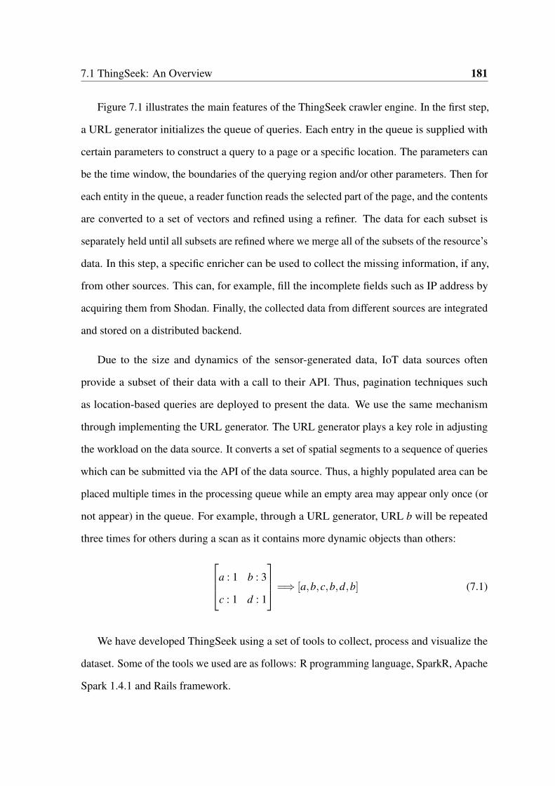
7.1 ThingSeek: An Overview 181
Figure 7.1 illustrates the main features of the ThingSeek crawler engine. In the first step,
a URL generator initializes the queue of queries. Each entry in the queue is supplied with
certain parameters to construct a query to a page or a specific location. The parameters can
be the time window, the boundaries of the querying region and/or other parameters. Then for
each entity in the queue, a reader function reads the selected part of the page, and the contents
are converted to a set of vectors and refined using a refiner. The data for each subset is
separately held until all subsets are refined where we merge all of the subsets of the resource’s
data. In this step, a specific enricher can be used to collect the missing information, if any,
from other sources. This can, for example, fill the incomplete fields such as IP address by
acquiring them from Shodan. Finally, the collected data from different sources are integrated
and stored on a distributed backend.
Due to the size and dynamics of the sensor-generated data, IoT data sources often
provide a subset of their data with a call to their API. Thus, pagination techniques such
as location-based queries are deployed to present the data. We use the same mechanism
through implementing the URL generator. The URL generator plays a key role in adjusting
the workload on the data source. It converts a set of spatial segments to a sequence of queries
which can be submitted via the API of the data source. Thus, a highly populated area can be
placed multiple times in the processing queue while an empty area may appear only once (or
not appear) in the queue. For example, through a URL generator, URL b will be repeated
three times for others during a scan as it contains more dynamic objects than others:
a : 1 b : 3
c : 1 d : 1
=⇒ [a,b,c,b,d,b] (7.1)
We have developed ThingSeek using a set of tools to collect, process and visualize the
dataset. Some of the tools we used are as follows: R programming language, SparkR, Apache
Spark 1.4.1 and Rails framework.

182 ThingSeek: An Enriched Interface for IoT Search Engine
Adding IoT data sources
We leverage Web Mapping such as Google Maps which is the most dominant way of
visualizing spatial data on the Web, to achieve the goal. Thus, we limit our search scope
to the sources which contain a map. We use a set of keywords to narrow our search results
to find such sources such as “real-time map of [application]", “live map of [application]"
and “tracker map of [application]". In the search query, the term “application" can be
replaced with any application of IoT such as flight. We also include some of the available
IoT platforms such as Xively1 to the initial set of data sources.
7.1.2 Query Results Preparation
Human User
In this section, we propose our approach for query resolution and the indexing approach to
enable large-scale search for IoT. Figure 7.2 shows the procedure of retrieving query results
in ThingSeek. As the figure shows, the query processing workflow works as follows.
1. Queries, which are formed as pairs of keywords and locations, are fed into the system.
The query structure is inspired from the Thingful search engine.
2. The Queries are processed in two steps: location based filtering and keyword based
filtering and finally the results are updated with the most recent values before being
presented to the user.
3. We use approximate values based on indexed data in the location filtering step. The
location filtering is facilitated using the R-Tree data structure to enhance the flexibility
and the performance of the system.
1https://xively.com/
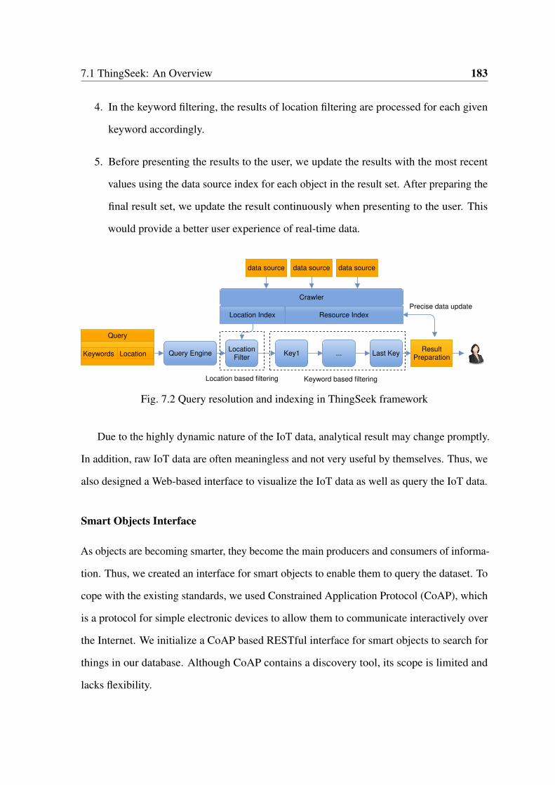
7.1 ThingSeek: An Overview 183
4. In the keyword filtering, the results of location filtering are processed for each given
keyword accordingly.
5. Before presenting the results to the user, we update the results with the most recent
values using the data source index for each object in the result set. After preparing the
final result set, we update the result continuously when presenting to the user. This
would provide a better user experience of real-time data.
Keywords Location
Query
Query EngineLocation
FilterKey1 ... Last Key
ResultPreparation
Location based filtering Keyword based filtering
data source data source data source
Crawler
Precise data update
Resource IndexLocation Index
Fig. 7.2 Query resolution and indexing in ThingSeek framework
Due to the highly dynamic nature of the IoT data, analytical result may change promptly.
In addition, raw IoT data are often meaningless and not very useful by themselves. Thus, we
also designed a Web-based interface to visualize the IoT data as well as query the IoT data.
Smart Objects Interface
As objects are becoming smarter, they become the main producers and consumers of informa-
tion. Thus, we created an interface for smart objects to enable them to query the dataset. To
cope with the existing standards, we used Constrained Application Protocol (CoAP), which
is a protocol for simple electronic devices to allow them to communicate interactively over
the Internet. We initialize a CoAP based RESTful interface for smart objects to search for
things in our database. Although CoAP contains a discovery tool, its scope is limited and
lacks flexibility.

184 ThingSeek: An Enriched Interface for IoT Search Engine
Figure 7.3 compares our architecture with CoAP discovery and illustrates how the
ThingSeek’s machine interface serves queries. For example, a smart air conditioning system
searches objects related to air or weather to plan its cooling strategy. As shown, with
the use of CoAP, a querying object can only enquire objects on the same network via
distributing discovery messages to all objects on the network. Following this, the issuer
gets objects’ responses if they match to the query. However, this approach can limit the
scope and effectiveness of the search. To resolve this issue, in our ThingSeek architecture,
the smart object uses a service to send its query directly to the search engine with a POST
or GET message. Due to the power, network and computing limits of things, ThingSeek
should respond the query with a number of messages containing only a small number of
results. In this regard, we use the ECS approach [38] (Extract-Cluster-Select) to provide
the best response with limited size. The ECS approach extracts co-location (objects in the
same location or very close to each other) and co-ownered (objects with the same owner)
correlations between things and forms a unified Things Correlation Graph. Then, the nodes
are clustered into k groups and finally a number of things from each cluster are selected and
returned. It is designed to rank objects based on their correlations and responds the query
with a limited number of the top-k results based on the weight of their correlations with the
query issuer. Finally, the URI of the corresponding data source is located and crawled to get
the latest sensor readings. If the object is not found in the index, the latest cached records
will be supplied.
7.2 Demonstration
In this section, we demonstrate the functionality of the proposed ThingSeek framework.
ThingSeek can extract IoT data from desired data sources by providing separate simple inter-
faces and effective search algorithms for users and machines. In particular, we demonstrate
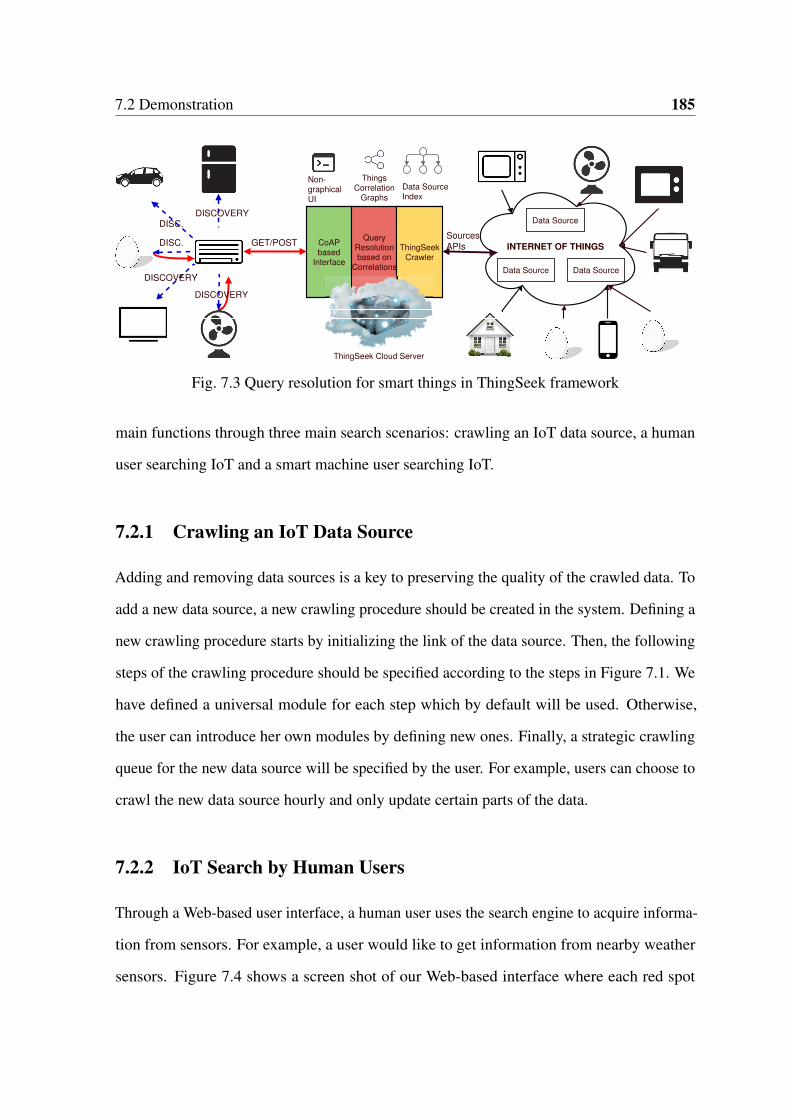
7.2 Demonstration 185
INTERNET OF THINGSCoAPbased
Interface
QueryResolutionbased on
Correlations
ThingSeekCrawler
ThingSeek Cloud Server
ThingsCorrelation
Graphs
Non-graphicalUI
Data SourceIndex
Data Source Data Source
Data Source
DISCOVERY
DISCOVERY
DISC.DISCOVERY
DISC. GET/POSTSources
APIs
Fig. 7.3 Query resolution for smart things in ThingSeek framework
main functions through three main search scenarios: crawling an IoT data source, a human
user searching IoT and a smart machine user searching IoT.
7.2.1 Crawling an IoT Data Source
Adding and removing data sources is a key to preserving the quality of the crawled data. To
add a new data source, a new crawling procedure should be created in the system. Defining a
new crawling procedure starts by initializing the link of the data source. Then, the following
steps of the crawling procedure should be specified according to the steps in Figure 7.1. We
have defined a universal module for each step which by default will be used. Otherwise,
the user can introduce her own modules by defining new ones. Finally, a strategic crawling
queue for the new data source will be specified by the user. For example, users can choose to
crawl the new data source hourly and only update certain parts of the data.
7.2.2 IoT Search by Human Users
Through a Web-based user interface, a human user uses the search engine to acquire informa-
tion from sensors. For example, a user would like to get information from nearby weather
sensors. Figure 7.4 shows a screen shot of our Web-based interface where each red spot

186 ThingSeek: An Enriched Interface for IoT Search Engine
denotes an object in the result set. Users can use the query panel to generate new queries and
the result can be shown as a list of sensors or through an interactive map as shown. However,
users would be more interested in acquiring knowledge from the data streams rather than
finding the sensors. Thus, we added an interactive plot maker to generate real-time plots.
Fig. 7.4 ThingSeek Web based visualization
7.2.3 IoT Search by Smart Machines
In this scenario, we consider a smart object querying our search engine. We developed
a Machine-to-Machine (M2M) interface based on the architecture in Figure 7.3 to enable
things to use CoAP to connect to our server and submit their queries. To use the interface,
on the client side, users can use any of CoAP implementations on CoAP website2 to send a
GET or POST message to our server. The message payload contains keywords followed the
desired number of the result set at the end. The server would provide the results in response.
2http://coap.technology/
7.3 ThingSeek in Application: Flight Delay Analysis 187
7.3 ThingSeek in Application: Flight Delay Analysis
In the previous chapters we already presented a number of examples of the search results for
searching things. In this chapter, we present results for a novel application in the aviation
industry. Specifically we focus on flight delay analysis. For our case study, we use three
different data sources including a real-time flight data, air quality index and real-time weather
data. While finding the trajectories of aeroplanes in real-time can be interesting for aviation
professional, value added results such as flight delay predictions can be widely used.
The results of our study fall into two categories. First, a search result can provide the list
of contextual features that can be identified based on the selected IoT data sources. Secondly,
additional results can precisely show that the extent of effectiveness for a given feature such
as temperature. We briefly present the results as follows.
7.3.1 Model Features
Due to the heterogeneity of IoT data, the semi-structured or unstructured sensor reading
data that is provided by different data sources can widely vary based on our selection of
the dataset. An intra-source feature model is an interesting showcase to demonstrate the
correlation between different data sources. Accordingly, Figure 7.5 shows the list of the
features that we have extracted from our case study.
In order to provide a clearer image, we describe the characteristics of each feature in
Table 7.1.
7.3.2 Feature Analysis Results
For this case study, we select seven airports from the largest cities of China. The cities
are: Beijing (PEK), Shanghai (SHA), Guangzhou (CAN), Wuhan (WUH), Chengdu (CTU),
Harbin (HRB), and Dalian (DLC). In our case study, we collect the data of all flights between

188 ThingSeek: An Enriched Interface for IoT Search Engine
Fig. 7.5 Features affecting flight delays from each source
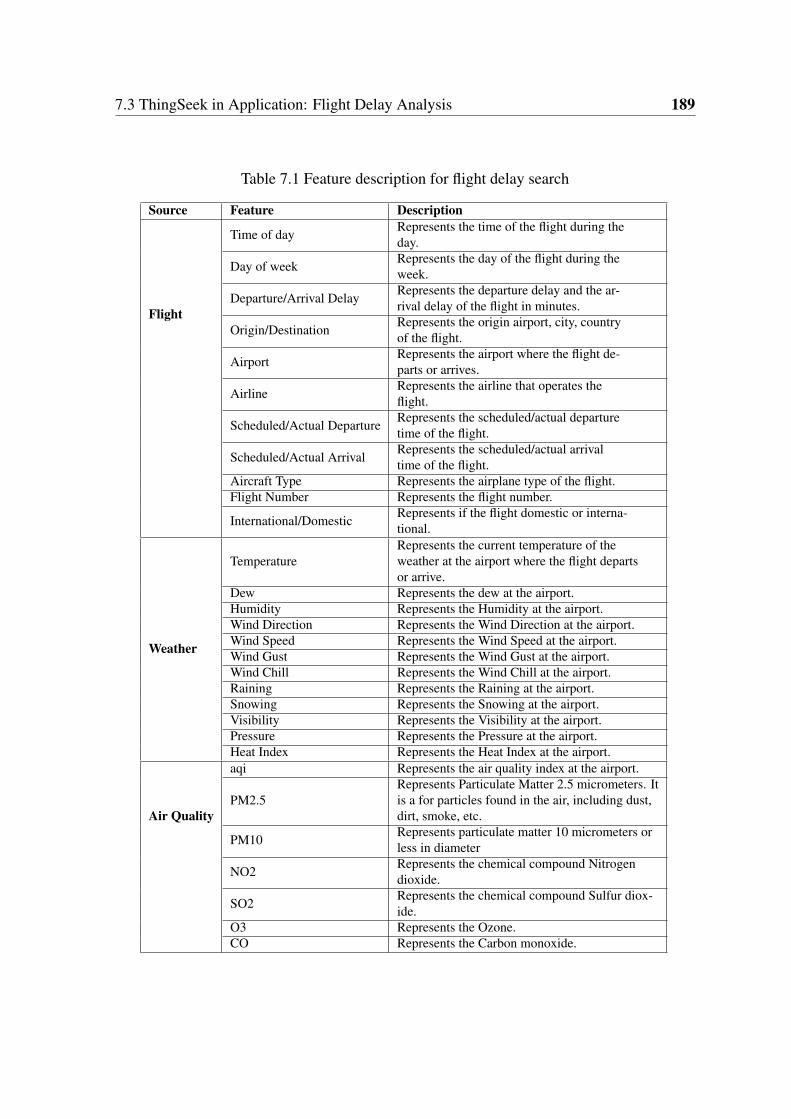
7.3 ThingSeek in Application: Flight Delay Analysis 189
Table 7.1 Feature description for flight delay search
Source Feature Description
Flight
Time of dayRepresents the time of the flight during theday.
Day of weekRepresents the day of the flight during theweek.
Departure/Arrival DelayRepresents the departure delay and the ar-rival delay of the flight in minutes.
Origin/DestinationRepresents the origin airport, city, countryof the flight.
AirportRepresents the airport where the flight de-parts or arrives.
AirlineRepresents the airline that operates theflight.
Scheduled/Actual DepartureRepresents the scheduled/actual departuretime of the flight.
Scheduled/Actual ArrivalRepresents the scheduled/actual arrivaltime of the flight.
Aircraft Type Represents the airplane type of the flight.Flight Number Represents the flight number.
International/DomesticRepresents if the flight domestic or interna-tional.
Weather
TemperatureRepresents the current temperature of theweather at the airport where the flight departsor arrive.
Dew Represents the dew at the airport.Humidity Represents the Humidity at the airport.Wind Direction Represents the Wind Direction at the airport.Wind Speed Represents the Wind Speed at the airport.Wind Gust Represents the Wind Gust at the airport.Wind Chill Represents the Wind Chill at the airport.Raining Represents the Raining at the airport.Snowing Represents the Snowing at the airport.Visibility Represents the Visibility at the airport.Pressure Represents the Pressure at the airport.Heat Index Represents the Heat Index at the airport.
Air Quality
aqi Represents the air quality index at the airport.
PM2.5Represents Particulate Matter 2.5 micrometers. Itis a for particles found in the air, including dust,dirt, smoke, etc.
PM10Represents particulate matter 10 micrometers orless in diameter
NO2Represents the chemical compound Nitrogendioxide.
SO2Represents the chemical compound Sulfur diox-ide.
O3 Represents the Ozone.CO Represents the Carbon monoxide.

190 ThingSeek: An Enriched Interface for IoT Search Engine
these cities. The distribution of the number of flights varies according to the city size and
the population number. The airlines operate the flight between these cities are: China Air
(CA), Shanghai Airlines (FM), China Eastern Airlines (MU), China Southern Airlines (CZ),
Juneyao Airlines (HO), Hainan Airlines (HU), Xiamen Airlines (MF), Sichuan Airlines (3U),
Shandong Airlines (SC), Chongqing Airlines(OQ), Grand China Air (CN), Shenzhen Airlines
(ZH), Spring Airlines (9C), Tibet Airlines (TV), Beijing Capital Airlines (JD), Chengdu
Airlines (EU).
In our study we focus on China, where environmental factors can be concerning due to
the industrial development. We get around 14,000 records for more than 800 flights between
the selected cities. Figure 7.6 shows a screenshot of a few records from the flights dataset.
Fig. 7.6 Example of the flight records
We also crawl 2,091 records for weather data from public and private weather stations.
Figure 7.7 shows a screenshot from a number of records in our dataset.
We also collect 3,084 records for air quality data near the airports. Figure 7.8 shows a
screenshot from a number of records.
The following results would be shown to the user after a search for the flights data.
Figure 7.9 compares the delay at departure for different airlines. Therefore, the user can
easily identify the airlines which have the least and the most delay in real-time.
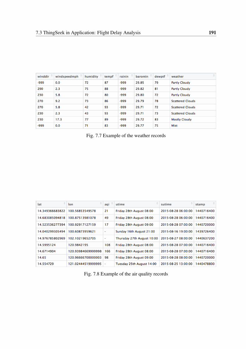
7.3 ThingSeek in Application: Flight Delay Analysis 191
Fig. 7.7 Example of the weather records
Fig. 7.8 Example of the air quality records
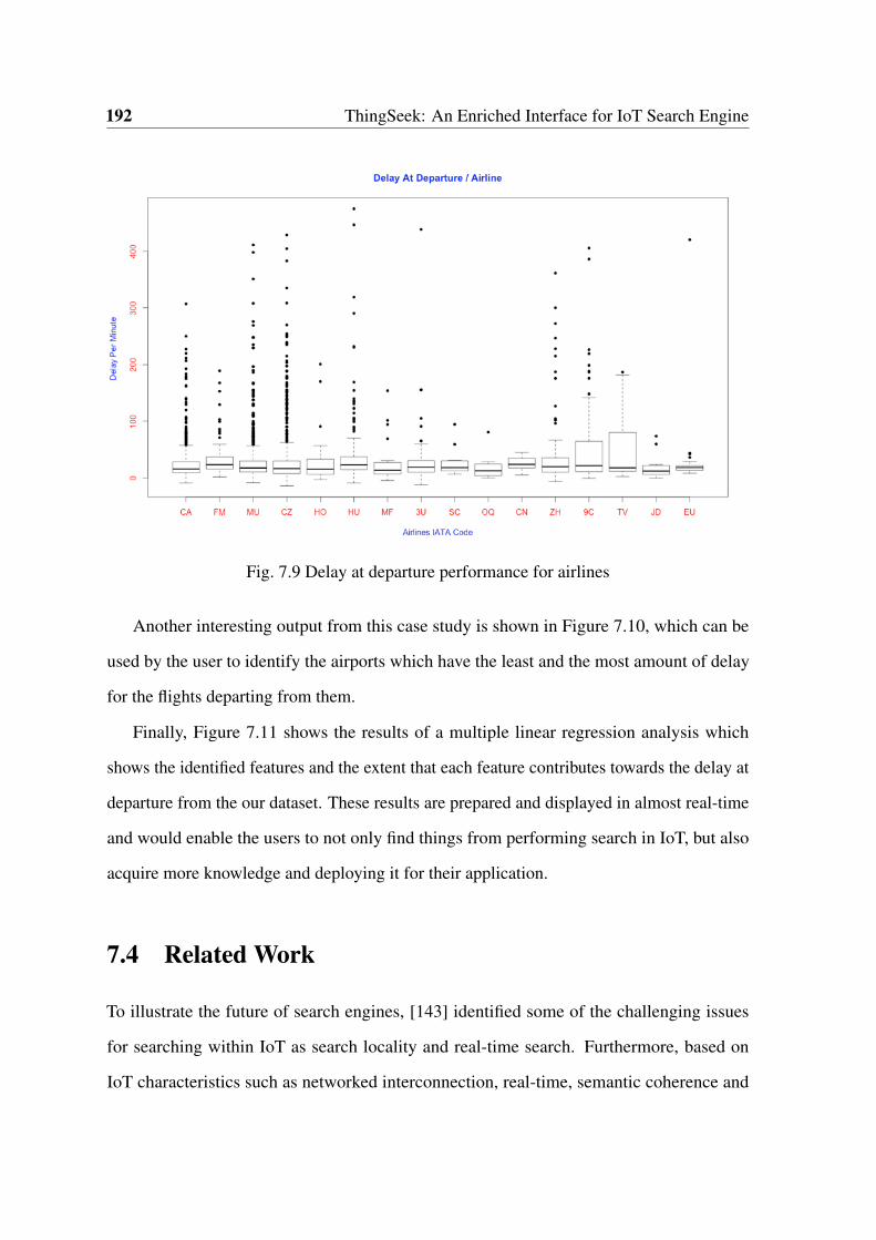
192 ThingSeek: An Enriched Interface for IoT Search Engine
Fig. 7.9 Delay at departure performance for airlines
Another interesting output from this case study is shown in Figure 7.10, which can be
used by the user to identify the airports which have the least and the most amount of delay
for the flights departing from them.
Finally, Figure 7.11 shows the results of a multiple linear regression analysis which
shows the identified features and the extent that each feature contributes towards the delay at
departure from the our dataset. These results are prepared and displayed in almost real-time
and would enable the users to not only find things from performing search in IoT, but also
acquire more knowledge and deploying it for their application.
7.4 Related Work
To illustrate the future of search engines, [143] identified some of the challenging issues
for searching within IoT as search locality and real-time search. Furthermore, based on
IoT characteristics such as networked interconnection, real-time, semantic coherence and
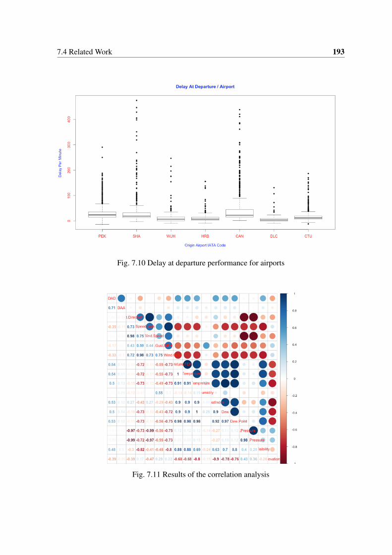
7.4 Related Work 193
Fig. 7.10 Delay at departure performance for airports
Fig. 7.11 Results of the correlation analysis

194 ThingSeek: An Enriched Interface for IoT Search Engine
spontaneous interaction will result in raising issues such as architectural design, search
locality, scalability and real-time for designing and implementing IoT search engines [144].
However, due to the existing differences in the nature of Web of Things (WoT) with the IoT,
WoT may even strike additional different challenges.
In order to design the next generation of search engines, many components of current
search engines from data collection methods to user experience and semantics should be
redesigned. In this section, some of the previous initiations in this area are categorized and
reviewed. MAX [202], Microsearch [203] and Snoogle [146] are developed based on this
idea. In keyword search approach, keywords are extracted from a given term and top query
results are ranked based on a score derived from the percentage of similarity between the
given query term and the keyword-based description on sensors. The result is a list of sensors
and thus, it might not be very useful particularly for human users.
In the following, we also address the works that are related to flight delay analysis. Flight
delay is not a new problem, and it has been considered by many researchers. In [204] the
authors analyzed the time factor influence of the flight delay in twenty airports in the US.
They observed the changes of the delay rate using historical data. Their investigation aim
was to predict the delay of each period based on their mode. They used ANOVA and k-means
clustering model in order to demonstrate the periodic of the delay rate. After that they applied
the Fast Furious Transform to find the period of the delay. Although their model was able to
predict accurately for the first airport they were studying, they found out that their model
should be improved in order to be applied to the other 19 airports. However, they did not
consider the airline influence.
Liu and Yang studied in [205] the flight delay propagation in the flight chain. So they
proposed a new algorithm that could estimate the delay from the beginning in order to to
determine how much time the flights in chain could be delayed. Authors of [205] did not
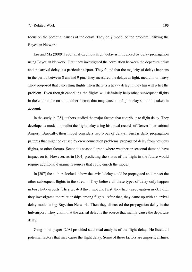
7.4 Related Work 195
focus on the potential causes of the delay. They only modelled the problem utilizing the
Bayesian Network.
Liu and Ma (2009) [206] analyzed how flight delay is influenced by delay propagation
using Bayesian Network. First, they investigated the correlation between the departure delay
and the arrival delay at a particular airport. They found that the majority of delays happens
in the period between 8 am and 9 pm. They measured the delays as light, medium, or heavy.
They proposed that cancelling flights when there is a heavy delay in the chin will relief the
problem. Even though cancelling the flights will definitely help other subsequent flights
in the chain to be on-time, other factors that may cause the flight delay should be taken in
account.
In the study in [35], authors studied the major factors that contribute to flight delay. They
developed a model to predict the flight delay using historical records of Denver International
Airport. Basically, their model considers two types of delays. First is daily propagation
patterns that might be caused by crew connection problems, propagated delay from previous
flights, or other factors. Second is seasonal trend where weather or seasonal demand have
impact on it. However, as in [204] predicting the status of the flight in the future would
require additional dynamic resources that could enrich the model.
In [207] the authors looked at how the arrival delay could be propagated and impact the
other subsequent flights in the stream. They believe all these types of delay only happen
in busy hub-airports. They created three models. First, they had a propagation model after
they investigated the relationships among flights. After that, they came up with an arrival
delay model using Bayesian Network. Then they discussed the propagation delay in the
hub-airport. They claim that the arrival delay is the source that mainly cause the departure
delay.
Geng in his paper [208] provided statistical analysis of the flight delay. He listed all
potential factors that may cause the flight delay. Some of these factors are airports, airlines,

196 ThingSeek: An Enriched Interface for IoT Search Engine
passengers, public safety, weather, fuel, departure control system, and air force. All these
factors are actually play a role on the flight delay. Then he discussed some countermeasures
in order to deal with the flight delay.
Another study [209] focused on study the flight delay problem based on the random flight
point delays. They used series analysis on airline data and presented an influence factor
model of the random flight points. The basic idea of this model is to combine the Bayesian
Network with the Gaussian Matrix Model using expectation maximization algorithm. This
model can predict the delay of the downstream.
As the best of our knowledge, there is no study has considered the real-time data to
investigate the flight delay. In [204] the authors recommend for the future work to combine
the analysis of historical data with real time data. That would predict the on-time performance
of any airport. Our work will consider the real time data to predict the performance of
individual flights.
Rebollo and Balakrishnan [210] presented a new model to predict the flight delay. They
consider the temporal and the spatial delay states as explanatory variables. Their approach
is to predict the delay sometime in the future between 2 to 24 hours. They use the Random
Forest algorithm to do so. Although this model predicts the flight status in the future, the
aforementioned interval seems too short because people require time more than that when
they book their flights.
7.5 Summary
In this paper, we demonstrate ThingSeek, a search interface with a crawler to hunt IoT data
on the Web. We mainly focus on the sensor data that is published through Web Mapping.
Our ThingSeek framework contains a crawler and two querying interfaces to cover both
human and machine users, e.g., smart things. In our crawler engine, we deploy a number of
technologies and a multi-layered approach to prepare the data for correlation analysis. In

7.5 Summary 197
our search interface, we demonstrate the details of the two interfaces, which are develop to
serve different groups of users. The machines interface of our engine complies with COAP
technology that is developed for machine-to-machine interaction.
Furthermore, we showcase an application of our search engine in the aviation industry.
In particular, we target flight delay analysis, which has a significant impact and depends on a
variety of environmental and operational factors that change in real time. Specifically, in our
showcase, we use two other data sets for assessing the air quality and weather data from the
identified data sources using our crawler engine. We use the real-time data of seven cities in
China, mainly due to the environmental circumstances, which affect flight schedules in many
cases. We initiate our model based on our data then investigate the correlation between the
collected datasets and the delay at departure. We use multiple linear regression analysis to
assess the weight of each feature and attach the final results to the search results for flights
data. In this case, our records show a relatively effective correlation between the delay at
departure and some features including dew and altitude. However, we hope thatr further
development of our method can lead to precise flight delay prediction, which can enrich the
experience of IoT search in future.
We conclude the dissertation in Chapter 8 and discuss some of the possible directions for
our research in future.


Chapter 8
Conclusion
In this chapter, we summarize the contributions of this dissertation and propose the directions
for future research in intent oriented and correlation aware IoT search.
8.1 Summary
The IoT paradigm is increasingly attracting a wide spectrum of researchers and professionals,
mainly due to its tremendous potential in impacting on our daily lives in the near future. IoT
search and related topics have attracted a large number of researchers in the last few years.
However, in IoT, with the highly dynamic, large volume and loosely interconnected data
sources, correlation based and intent oriented search have not been sufficiently developed.
Further research on application oriented interconnection of IoT resources is essential for
establishing the future search engines and recommender systems for IoT.
In this dissertation, we propose a novel framework for a context aware and correlation
based IoT discovery service. We also provide an implementation of our approach in the
ThingSeek prototype. Our framework incorporates a number of subcomponents where each
is devised to serve a specific purpose in the steps of the given motivating scenario. In the
ThingSeek architecture, we consider two types of users including human clients and smart
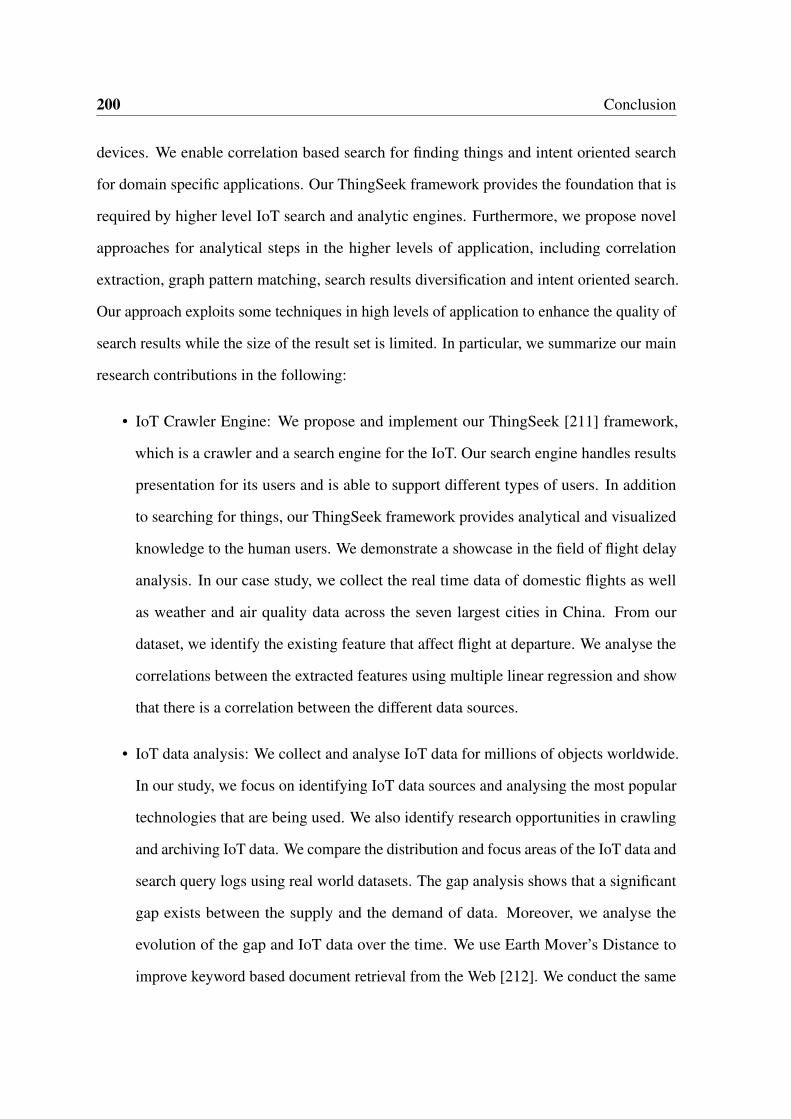
200 Conclusion
devices. We enable correlation based search for finding things and intent oriented search
for domain specific applications. Our ThingSeek framework provides the foundation that is
required by higher level IoT search and analytic engines. Furthermore, we propose novel
approaches for analytical steps in the higher levels of application, including correlation
extraction, graph pattern matching, search results diversification and intent oriented search.
Our approach exploits some techniques in high levels of application to enhance the quality of
search results while the size of the result set is limited. In particular, we summarize our main
research contributions in the following:
• IoT Crawler Engine: We propose and implement our ThingSeek [211] framework,
which is a crawler and a search engine for the IoT. Our search engine handles results
presentation for its users and is able to support different types of users. In addition
to searching for things, our ThingSeek framework provides analytical and visualized
knowledge to the human users. We demonstrate a showcase in the field of flight delay
analysis. In our case study, we collect the real time data of domestic flights as well
as weather and air quality data across the seven largest cities in China. From our
dataset, we identify the existing feature that affect flight at departure. We analyse the
correlations between the extracted features using multiple linear regression and show
that there is a correlation between the different data sources.
• IoT data analysis: We collect and analyse IoT data for millions of objects worldwide.
In our study, we focus on identifying IoT data sources and analysing the most popular
technologies that are being used. We also identify research opportunities in crawling
and archiving IoT data. We compare the distribution and focus areas of the IoT data and
search query logs using real world datasets. The gap analysis shows that a significant
gap exists between the supply and the demand of data. Moreover, we analyse the
evolution of the gap and IoT data over the time. We use Earth Mover’s Distance to
improve keyword based document retrieval from the Web [212]. We conduct the same

8.1 Summary 201
analysis over IoT data and identify the patterns of the recurring sensory data around
the world. Our results show that traditional technologies are a trend in sensor data
dissemination and Web mapping is playing a key role in IoT [213].
• Automatic correlation extraction: We propose a novel framework, namely CEIoT,
for extracting correlations from IoT data. Specifically, we focus on three types of
correlations between objects, based on the features that we extract from IoT data. In
particular we focus on the location based correlations. Our framework represents
correlations using RDF triples and R-Tree to extract the co-location correlations. We
use a Multi Agent System architecture to implement our approach and use a real world
dataset to verify its efficiency [214]. Moreover, we provide a novel method for batch
matching of conjunctive triple patterns over linked data streams, which can be used by
the Service Agents in our architecture to match the features of sensory data [106].
• Pattern matching for IoT data: We provide an efficient approach for integrating Linked
Data streams from various data collectors. Our approach disseminates matched data
to relevant data consumers based on conjunctive triple pattern queries registered in
the system by the consumers [106, 107]. Moreover, we redefine the graph pattern
matching problem for the context of IoT and form the MULTIMATCH problem, which
increases the cardinality of the labels that are assigned to each node compared with
the previous work. We use Monte Carlo Markov Chain to approximate the matches in
polynomial time. We validate all of the proposed methods and show that our approach
is efficient in terms of processing time and space allocation [215].
• High quality query results: Given the limits of end users, in particular, smart devices
with limited processing power and memory, we propose a novel solution to select
the top-k results from the things dataset [38]. Our proposed method constitutes three
different layers to Extract correlations, Cluster objects and Select the results (ECS)
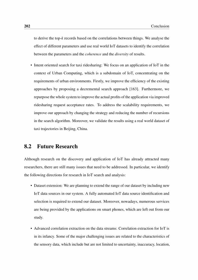
202 Conclusion
to derive the top-k records based on the correlations between things. We analyse the
effect of different parameters and use real world IoT datasets to identify the correlation
between the parameters and the coherence and the diversity of results.
• Intent oriented search for taxi ridesharing: We focus on an application of IoT in the
context of Urban Computing, which is a subdomain of IoT, concentrating on the
requirements of urban environments. Firstly, we improve the efficiency of the existing
approaches by proposing a decremental search approach [163]. Furthermore, we
repurpose the whole system to improve the actual profits of the application via improved
ridesharing request acceptance rates. To address the scalability requirements, we
improve our approach by changing the strategy and reducing the number of recursions
in the search algorithm. Moreover, we validate the results using a real world dataset of
taxi trajectories in Beijing, China.
8.2 Future Research
Although research on the discovery and application of IoT has already attracted many
researchers, there are still many issues that need to be addressed. In particular, we identify
the following directions for research in IoT search and analysis:
• Dataset extension: We are planning to extend the range of our dataset by including new
IoT data sources in our system. A fully automated IoT data source identification and
selection is required to extend our dataset. Moreover, nowadays, numerous services
are being provided by the applications on smart phones, which are left out from our
study.
• Advanced correlation extraction on the data streams: Correlation extraction for IoT is
in its infancy. Some of the major challenging issues are related to the characteristics of
the sensory data, which include but are not limited to uncertainty, inaccuracy, location,

8.2 Future Research 203
dynamics and security. Further developments are required in order to provide a solid
basis for correlation analysis on IoT. Deployment of the existing approaches in the
existing applications can escalate the amount of knowledge that is acquired from the
worldwide sensory data of IoT.
• Enhanced intent based search: We plan to develop the intent based search further in
two areas. Firstly, we will develop our progress on flight delay analysis to enable
the prediction of flight delays in real time. Furthermore, we can build up a context
aware real time flight recommender system which can potentially reduce the amount
of the losses that are caused by flight delays. Secondly, we plan to improve the current
search experience of taxi ridesharing to include more contextual features based on the
historical social and sensory data in the city.
• Dynamic graph pattern matching: Graph pattern matching is key to many applications
including IoT sensory data analysis. We plan to develop our method further in two
directions. Firstly, given the high dynamics of the IoT, we will revise the graph pattern
matching analysis problem to include dynamic data graphs with dynamic patterns.
Considering the fact that the pattern matching has relied on the static pattern graphs
so far, dynamic patterns can extend the range and applications of graph based queries
significantly. Secondly, we are planning to introduce context aware pattern matching
with a focus on the applications in IoT. The context of a given pattern matching problem
may vary widely, based on the intent of the search. However, this is not covered in
the existing pattern matching approaches which return the same set of patterns for all
contexts.
• Archiving IoT data: Nowadays existing WWW archives are playing significant roles
both in research and application. The recording of the contents of the documents
on the Internet started shortly after the emergence of the WWW. However, due to

204 Conclusion
the technical challenges of handling sensory data in its current form, to the best of
our knowledge, there is no initiative on archiving the IoT data. We are planning to
introduce an archival service for IoT by tackling these challenges based on our results
and observations. For instance, through a thorough pattern analysis, we can reduce the
size of the data significantly.
References
[1] David L Brock. The electronic product code (epc). Auto-ID Center White PaperMIT-AUTOID-WH-002, 2001.
[2] Eleonora Borgia. The internet of things vision: Key features, applications and openissues. Computer Communications, 54:1–31, 2014.
[3] Luigi Atzori, Antonio Iera, and Giacomo Morabito. The internet of things: A survey.Computer networks, 54(15):2787–2805, 2010.
[4] Shancang Li, Li Da Xu, and Shanshan Zhao. The internet of things: a survey.Information Systems Frontiers, 17(2):243–259, 2015.
[5] Charith Perera, Arkady Zaslavsky, Peter Christen, and Dimitrios Georgakopoulos.Context aware computing for the internet of things: A survey. IEEE CommunicationsSurveys & Tutorials, 16(1):414–454, 2014.
[6] SK Anithaa, S Arunaa, M Dheepthika, S Kalaivani, M Nagammai, M Aasha, andS Sivakumari. The internet of things-a survey. World Scientific News, 41:150, 2016.
[7] Janessa Rivera and Rob van der Meulen. The gartner hype cycle 2015. http://www.gartner.com/newsroom/id/3114217. Accessed: 2016-07-1.
[8] James Manyika, Michael Chui, Jacques Bughin, Richard Dobbs, Peter Bisson, andAlex Marrs. Disruptive technologies: Advances that will transform life, business, andthe global economy, volume 12. McKinsey Global Institute San Francisco, CA, 2013.
[9] F. Khodadadi, A.V. Dastjerdi, and R. Buyya. Chapter 1 - internet of things: anoverview. In Rajkumar Buyya and Amir Vahid Dastjerdi, editors, Internet of Things,pages 3 – 27. Morgan Kaufmann, 2016.
[10] Jayavardhana Gubbi, Rajkumar Buyya, Slaven Marusic, and Marimuthu Palaniswami.Internet of things (iot): A vision, architectural elements, and future directions. FutureGeneration Computer Systems, 29(7):1645–1660, 2013.
[11] Diego Dujovne, Thomas Watteyne, Xavier Vilajosana, and Pascal Thubert. 6tisch: de-terministic ip-enabled industrial internet (of things). IEEE Communications Magazine,52(12):36–41, 2014.
[12] Gheorghe H Popescu. The economic value of the industrial internet of things. Psy-chosociological Issues in Human Resource Management, 3(2):86–92, 2015.

206 References
[13] Hao Wang, Ottar L Osen, Guoyuan Li, Wei Li, Hong-Ning Dai, and Wei Zeng. Bigdata and industrial internet of things for the maritime industry in northwestern norway.In TENCON 2015-2015 IEEE Region 10 Conference, pages 1–5. IEEE, 2015.
[14] Athanasios S Voulodimos, Charalampos Z Patrikakis, Alexander B Sideridis,Vasileios A Ntafis, and Eftychia M Xylouri. A complete farm management sys-tem based on animal identification using rfid technology. Computers and Electronicsin Agriculture, 70(2):380–388, 2010.
[15] Shanshan Li, Shaoliang Peng, Weifeng Chen, and Xiaopei Lu. Income: Practical landmonitoring in precision agriculture with sensor networks. Computer Communications,36(4):459–467, 2013.
[16] Fadi M Al-Turjman, Hossam S Hassanein, and Mohamed A Ibnkahla. Efficientdeployment of wireless sensor networks targeting environment monitoring applications.Computer Communications, 36(2):135–148, 2013.
[17] Gayathri Tilak Singh and Fadi M Al-Turjman. A data delivery framework for cog-nitive information-centric sensor networks in smart outdoor monitoring. ComputerCommunications, 74:38–51, 2016.
[18] Raghu K Ganti, Fan Ye, and Hui Lei. Mobile crowdsensing: current state and futurechallenges. IEEE Communications Magazine, 49(11):32–39, 2011.
[19] Elena Polycarpou, Lambros Lambrinos, and Eftychios Protopapadakis. Smart parkingsolutions for urban areas. In World of Wireless, Mobile and Multimedia Networks(WoWMoM), 2013 IEEE 14th International Symposium and Workshops on a, pages1–6. IEEE, 2013.
[20] Giuseppe Amato, Fabrizio Falchi, and Fausto Rabitti. Landmark recognition in visitotuscany. In Multimedia for Cultural Heritage, pages 1–13. Springer, 2012.
[21] Franca Delmastro. Pervasive communications in healthcare. Computer Communica-tions, 35(11):1284–1295, 2012.
[22] Friedemann Mattern and Christian Floerkemeier. From the internet of computers tothe internet of things. In From active data management to event-based systems andmore, pages 242–259. Springer, 2010.
[23] Min Chen, Shiwen Mao, and Yunhao Liu. Big data: a survey. Mobile Networks andApplications, 19(2):171–209, 2014.
[24] Lina Yao, Quan Z Sheng, Anne HH Ngu, and Xue Li. Things of interest recommenda-tion by leveraging heterogeneous relations in the internet of things. ACM Transactionson Internet Technology (TOIT), 16(2):9, 2016.
[25] Yen-Kuang Chen. Challenges and opportunities of internet of things. In Proc. ofthe 17th Asia and South Pacific Design Automation Conf. (ASP-DAC 2012), pages383–388. IEEE, 2012.
References 207
[26] Charith Perera, Arkady Zaslavsky, Chi Harold Liu, Michael Compton, Peter Christen,and Dimitrios Georgakopoulos. Sensor search techniques for sensing as a servicearchitecture for the internet of things. IEEE Sensors Journal, 14(2):406–420, 2014.
[27] Lina Yao, Quan Z Sheng, Byron J Gao, Anne HH Ngu, and Xue Li. A model fordiscovering correlations of ubiquitous things. In Proceedings of 13th InternationalConference on Data Mining (ICDM 2013), pages 1253–1258. IEEE, 2013.
[28] Dave Raggett. The web of things: Challenges and opportunities. Computer, 48(5):26–32, 2015.
[29] Xively: A platform for the internet of things. https://www.xively.com. Accessed:2016-07-1.
[30] Daqiang Zhang, Laurence Tianruo Yang, and Hongyu Huang. Searching in internet ofthings: Vision and challenges. In Proceedings of the 9th International Symposium onParallel and Distributed Processing with Applications (ISPA), pages 201–206. IEEE,May 2011.
[31] Matthias Thoma, Klaus Sperner, and Torsten Braun. Service descriptions and linkeddata for integrating wsns into enterprise it. In Proceedings of the Third InternationalWorkshop on Software Engineering for Sensor Network Applications (SESENA), pages43–48. IEEE, 2012.
[32] Henning Hasemann, Alexander Kröller, and Max Pagel. Rdf provisioning for theinternet of things. In Internet of Things (IOT), 2012 3rd International Conference onthe, pages 143–150. IEEE, 2012.
[33] Debasis Bandyopadhyay and Jaydip Sen. Internet of things: Applications andchallenges in technology and standardization. Wireless Personal Communications,58(1):49–69, 2011.
[34] Xiaoou Tang, Ke Liu, Jingyu Cui, Fang Wen, and Xiaogang Wang. Intentsearch:Capturing user intention for one-click internet image search. IEEE transactions onpattern analysis and machine intelligence, 34(7):1342–1353, 2012.
[35] Yufeng Tu, Michael O Ball, and Wolfgang S Jank. Estimating flight departure delaydistributions—a statistical approach with long-term trend and short-term pattern.Journal of the American Statistical Association, 103(481):112–125, 2008.
[36] Flight radar 24 live air traffic. https://www.flightradar24.com. Accessed: 2016-07-1.
[37] ThingSeek: A Crawler and Search Engine for the Internet of Things. ACM, 2016.
[38] Ali Shemshadi, Lina Yao, Yongrui Qin, Quan Z Sheng, and Yihong Zhang. Ecs:A framework for diversified and relevant search in the internet of things. In WebInformation Systems Engineering–WISE 2015, pages 448–462. 2015.
[39] Luigi Atzori, Antonio Iera, and Giacomo Morabito. Siot: Giving a social structure tothe internet of things. Communications Letters, 15(11):1193–1195, 2011.

208 References
[40] Luigi Atzori, Antonio Iera, Giacomo Morabito, and Michele Nitti. The social internetof things (siot)–when social networks meet the internet of things: Concept, architectureand network characterization. Computer Networks, 56(16):3594–3608, 2012.
[41] S Geetha. Social internet of things. World Scientific News, 41:76, 2016.
[42] Li Da Xu, Wu He, and Shancang Li. Internet of things in industries: A survey. IEEETransactions on Industrial Informatics, 10(4):2233–2243, 2014.
[43] Zhibo Pang, Qiang Chen, Junzhe Tian, Lirong Zheng, and Elena Dubrova. Ecosystemanalysis in the design of open platform-based in-home healthcare terminals towardsthe internet-of-things. In Proc. of the 15th Intl. Conf. on Advanced CommunicationTechnology (ICACT 2013), pages 529–534, 2013.
[44] Roy Want, Bill N Schilit, and Scott Jenson. Enabling the internet of things. Computer,48(1):28–35, 2015.
[45] Thingful: A search engine for the internet of things. http://www.thingful.net. Accessed:2016-07-1.
[46] Yongrui Qin, Quan Z. Sheng, and Wei Emma Zhang. SIEF: Efficiently AnsweringDistance Queries for Failure Prone Graphs. In Proc. of the 18th Intl. Conf. on ExtendingDatabase Technology (EDBT), pages 145–156, 2015.
[47] Yongrui Qin, Quan Z. Sheng, Nickolas J. G. Falkner, Schahram Dustdar, Hua Wang,and Athanasios V. Vasilakos. When Things Matter: A Survey on Data-Centric Internetof Things. Journal Network and Computer Applications, 64:137–153, 2016.
[48] Graph of things: A real-time search engine for the internet of things. http://graphofthings.org. Accessed: 2016-07-1.
[49] Shodan: A search engine for hackers and the internet of things. https://www.shodan.io.Accessed: 2016-07-1.
[50] Geng Wu, Shilpa Talwar, Kerstin Johnsson, Nageen Himayat, and Kevin D Johnson.M2m: From mobile to embedded internet. IEEE Communications Magazine, 49(4):36–43, 2011.
[51] Jaewoo Kim, Jaiyong Lee, Jaeho Kim, and Jaeseok Yun. M2m service platforms:survey, issues, and enabling technologies. Communications Surveys & Tutorials, IEEE,16(1):61–76, 2014.
[52] Miguel Castro, Antonio J Jara, and Antonio F Skarmeta. An analysis of m2m platforms:challenges and opportunities for the internet of things. In Proc. of the 6th Intl. Conf.on Innovative Mobile and Internet Services in Ubiquitous Computing (IMIS 2012),pages 757–762. IEEE, 2012.
[53] Antonio Pintus, Davide Carboni, and Andrea Piras. Paraimpu: a platform for a socialweb of things. In Proc. of the 21st Intl. Companion Conf. on World Wide Web (WWW2012), pages 401–404, 2012.
[54] Thingspeak: Internet of things. https://thingspeak.com. Accessed: 2016-07-1.
References 209
[55] Mother • sen.se. https://www.sen.se/mother/. Accessed: 2016-07-1.
[56] Marinetraffic.com. http://www.marinetraffic.com. Accessed: 2016-07-1.
[57] Traffic jam news, updates from the road - waze live map. https://www.waze.com/livemap. Accessed: 2016-07-1.
[58] Rastrack.co.uk - home. http://rastrack.co.uk. Accessed: 2016-07-1.
[59] Lihong Jiang, Li Da Xu, Hongming Cai, Zuhai Jiang, Fenglin Bu, and Boyi Xu. Aniot-oriented data storage framework in cloud computing platform. IEEE Transactionson Industrial Informatics, 10(2):1443–1451, 2014.
[60] Xively rest api. https://personal.xively.com/dev/docs/api/. Accessed: 2016-07-1.
[61] Web of things code forge. https://github.com/webofthings. Accessed: 2016-07-1.
[62] Michael Blackstock and Rodger Lea. Iot mashups with the wotkit. In Proc. of the 3rdIntl. Conf. on the Internet of Things (IOT 2012), pages 159–166. IEEE, 2012.
[63] Weio on github. https://github.com/nodesign/weio/tree/master/examples. Accessed:2016-07-1.
[64] Sense tecnic | aggregating real world data. https://wotkit.sensetecnic.com/wotkit/.Accessed: 2015-09-1.
[65] Muki Haklay, Alex Singleton, and Chris Parker. Web mapping 2.0: The neogeographyof the geoweb. Geography Compass, 2(6):2011–2039, 2008.
[66] Arrivebus live map. http://www.arrivabus.co.uk/journeyplanner/help/en?tpl=livemap.Accessed: 2016-07-1.
[67] Weio - the web of things platform - the web of things for creators. http://we-io.net.Accessed: 2016-07-1.
[68] Web of things projects directory. https://github.com/webofthings/webofthings-projects-directory/wiki/Web-of-Things-Projects-Directory. Ac-cessed: 2016-07-1.
[69] Christopher J Pannucci and Edwin G Wilkins. Identifying and avoiding bias inresearch. Plastic and reconstructive surgery, 126(2):619, 2010.
[70] Google trends. https://www.google.com/trends/. Accessed: 2016-07-1.
[71] Alexa - actionable analytics for the web. http://www.alexa.com. Accessed: 2016-07-1.
[72] Simon Urbanek and Yossi Rubner. emdist: Earth Mover’s Distance, 2012. R packageversion 0.3-1.
[73] Nattiya Kanhabua, Roi Blanco, Kjetil Nørvåg, et al. Temporal information retrieval.Foundations and Trends® in Information Retrieval, 9(2):91–208, 2015.

210 References
[74] Lina Yao and Quan Z Sheng. Correlation discovery in web of things. In Proc. of the22nd Intl. Comp. Conf. on World Wide Web (WWW 2013), pages 215–216, 2013.
[75] Youzhong Ma, Jia Rao, Weisong Hu, Xiaofeng Meng, Xu Han, Yu Zhang, YunpengChai, and Chunqiu Liu. An efficient index for massive iot data in cloud environment.In Proc. of the 21st ACM Intl. Conf. on Information and Knowledge Management(CIKM 2012), pages 2129–2133, 2012.
[76] Charith Perera, Arkady Zaslavsky, Peter Christen, Michael Compton, and DimitriosGeorgakopoulos. Context-aware sensor search, selection and ranking model forinternet of things middleware. In Proc. of the 14th IEEE Intl. Conf. on Mobile DataManagement (MDM 2013), volume 1, pages 314–322. IEEE, 2013.
[77] Lina Yao, Quan Z. Sheng, Yongrui Qin, Xianzhi Wang, Ali Shemshadi, and Qi He.Context-aware Point-of-Interest Recommendation Using Tensor Factorization withSocial Regularization. In Proc. of the 38th Intl. ACM SIGIR Conf. on Research andDevelopment in Inf. Retrieval (SIGIR), pages 1007–1010, 2015.
[78] Wisp - home - wikispaces. http://wisp.wikispaces.com. Accessed: 2016-07-1.
[79] Evan Welbourne, Leilani Battle, Gregory Cole, Kyle Gould, Kyle Rector, SamuelRaymer, Magdalena Balazinska, and Gaetano Borriello. Building the internet of thingsusing rfid: the rfid ecosystem experience. IEEE Internet Computing, 13(3):48–55,2009.
[80] Gerd Kortuem, Fahim Kawsar, Daniel Fitton, and Vasughi Sundramoorthy. Smartobjects as building blocks for the internet of things. IEEE Internet Computing,14(1):44–51, 2010.
[81] Andrea Piras, Davide Carboni, Antonio Pintus, and DMT Features. A platform tocollect, manage and share heterogeneous sensor data. In Proc. of 9th Intl. Conf. onNetworked Sensing Systems (INSS 2012), pages 1–2, 2012.
[82] Andrew Whitmore, Anurag Agarwal, and Li Da Xu. The internet of things–a surveyof topics and trends. Information Systems Frontiers, 17(2):261–274, 2014.
[83] Benedikt Ostermaier, Kay Romer, Friedemann Mattern, Michael Fahrmair, and Wolf-gang Kellerer. A real-time search engine for the web of things. In Proc. of the 2ndInternet of Things Conf. (IOT 2010), pages 1–8. IEEE, 2010.
[84] M. Nitti, L. Atzori, and I.P. Cvijikj. Friendship selection in the social internet of things:Challenges and possible strategies. Internet of Things Journal, IEEE, 2(3):240–247,June 2015.
[85] Mohammad Ebrahimi, Elaheh Shafieibavani, Raymond K Wong, and Chi-Hung Chi.A new meta-heuristic approach for efficient search in the internet of things. InProceedinsg of the 12th IEEE Intl. Conf. on Services Computing (SCC 2015), pages264–270. IEEE, 2015.
[86] Car counter - thingspeak. https://thingspeak.com/channels/38629. Accessed: 2016-07-1.

References 211
[87] Sergey Brin and Larry Page. The anatomy of a large-scale hypertextual web searchengine. In Proceedings of the 7th International World-Wide Web Conference (WWW1998), 1998.
[88] Han Yu, Zhiqi Shen, and Cyril Leung. From internet of things to internet of agents.In Proceedings of the 2013 IEEE International Conference on Green Computing andCommunications (GreenCom), pages 1054–1057. IEEE, 2013.
[89] Giancarlo Fortino, Antonio Guerrieri, and Wilma Russo. Agent-oriented smart objectsdevelopment. In Proceedings of the 16th International Conference onComputerSupported Cooperative Work in Design (CSCWD 2012), pages 907–912. IEEE, 2012.
[90] Chun-Hsiang Lee, David Birch, Chao Wu, Dilshan Silva, Orestis Tsinalis, Yang Li,Shulin Yan, Moustafa Ghanem, and Yike Guo. Building a generic platform for bigsensor data application. In Proceedings of 2013 IEEE International Conference onBig Data (IEEE BigData), pages 94–102. IEEE, 2013.
[91] Dieter Fensel, Reto Krummenacher, Omair Shafiq, Eva Kuehn, Johannes Riemer,Ying Ding, and Bernd Draxler. Tsc–triple space computing. e & i Elektrotechnik undInformationstechnik, 124(1-2):31–38, 2007.
[92] Aitor Gómez-Goiri and Diego López-de Ipiña. On the complementarity of triplespaces and the web of things. In Proceedings of the 2nd International Workshop onWeb of Things, page 12. ACM, 2011.
[93] Dominique Guinard, Mathias Fischer, and Vlad Trifa. Sharing using social networks ina composable web of things. In Proceedings of the 8th IEEE International Conferenceon Pervasive Computing and Communications Workshops (PERCOM 2010), pages702–707. IEEE, 2010.
[94] Antonio Pintus, Davide Carboni, and Andrea Piras. The anatomy of a large scale socialweb for internet enabled objects. In Proceedings of the 2nd International Workshopon Web of Things, page 6. ACM, 2011.
[95] Nikita V Spirin, Junfeng He, Mike Develin, Karrie G Karahalios, and Maxime Boucher.People search within an online social network: Large scale analysis of facebook graphsearch query logs. In Proceedings of the 23rd acm international conference onconference on information and knowledge management, pages 1009–1018. ACM,2014.
[96] Wenfei Fan, Jianzhong Li, Shuai Ma, Hongzhi Wang, and Yinghui Wu. Graphhomomorphism revisited for graph matching. Proceedings of the VLDB Endowment,3(1-2):1161–1172, 2010.
[97] Minsu Cho, Jungmin Lee, and Kyoung Mu Lee. Reweighted random walks for graphmatching. In Proceedings of the 11th European Conference on Computer Vision(ECCV), pages 492–505, Crete, Greece, 2010. Springer.
[98] Lorenzo Livi and Antonello Rizzi. The graph matching problem. Pattern Analysisand Applications, 16(3):253–283, 2013.

212 References
[99] Harshal Patni, Cory Henson, and Amit Sheth. Linked sensor data. In CollaborativeTechnologies and Systems (CTS), 2010 International Symposium on, pages 362–370.IEEE, 2010.
[100] Payam Barnaghi and Mirko Presser. Publishing linked sensor data. In Proceedings ofthe 3rd International Conference on Semantic Sensor Networks-Volume 668, pages1–16. CEUR-WS. org, 2010.
[101] Kevin R Page, David C De Roure, Kirk Martinez, Jason D Sadler, and Oles YKit. Linked sensor data: Restfully serving rdf and gml. In Proceedings of the 2ndInternational Conference on Semantic Sensor Networks-Volume 522, pages 49–63.CEUR-WS. org, 2009.
[102] Krzysztof Janowicz, Arne Bröring, Christoph Stasch, Sven Schade, Thomas Everd-ing, and Alejandro Llaves. A restful proxy and data model for linked sensor data.International Journal of Digital Earth, 6(3):233–254, 2013.
[103] Danh Le-Phuoc and Manfred Hauswirth. Linked open data in sensor data mashups. InProceedings of the 2nd International Conference on Semantic Sensor Networks, pages1–16. CEUR-WS. org, 2009.
[104] Danh Le-Phuoc, Minh Dao-Tran, Josiane Xavier Parreira, and Manfred Hauswirth. Anative and adaptive approach for unified processing of linked streams and linked data.In Proceedings of the 2011 International Semantic Web Conference (ICWS), pages370–388. Springer, 2011.
[105] Juan F Sequeda and Oscar Corcho. Linked stream data: A position paper. InProceedings of the 2nd International Conference on Semantic Sensor Networks, pages148–157. CEUR-WS. org, 2009.
[106] Yongrui Qin, Quan Z Sheng, Nickolas JG Falkner, Ali Shemshadi, and Edward Curry.Batch matching of conjunctive triple patterns over linked data streams in the internetof things. In Proceedings of the 27th International Conference on Scientific andStatistical Database Management, page 41. ACM, 2015.
[107] Yongrui Qin, Quan Z Sheng, Nickolas JG Falkner, Ali Shemshadi, and EdwardCurry. Towards efficient dissemination of linked data in the internet of things. InProceedings of the 23rd ACM International Conference on Conference on Informationand Knowledge Management, pages 1779–1782. ACM, 2014.
[108] Wenfei Fan. Graph pattern matching revised for social network analysis. In Proceed-ings of the 15th International Conference on Database Theory, pages 8–21. ACM,2012.
[109] Monika Rauch Henzinger, Thomas A Henzinger, and Peter W Kopke. Computingsimulations on finite and infinite graphs. In Proceedings of the 36th Annual Symposiumon Foundations of Computer Science, pages 453–462, Milwaukee, USA, 1995. IEEE.
[110] Wenfei Fan, Xin Wang, and Yinghui Wu. Diversified top-k graph pattern matching.Proceedings of the VLDB Endowment, 6(13):1510–1521, 2013.

References 213
[111] Shuai Ma, Yang Cao, Wenfei Fan, Jinpeng Huai, and Tianyu Wo. Capturing topologyin graph pattern matching. Proceedings of the VLDB Endowment, 5(4):310–321, 2011.
[112] Jun Gao, Chang Zhou, Jiashuai Zhou, and Jeffrey Xu Yu. Continuous pattern detectionover billion-edge graph using distributed framework. In Data Engineering (ICDE),2014 IEEE 30th International Conference on, pages 556–567. IEEE, 2014.
[113] Mark Jerrum and Alistair Sinclair. The markov chain monte carlo method: an approachto approximate counting and integration. Approximation Algorithms for NP-hardProblems, pages 482–520, 1996.
[114] W.K. Hastings. Monte carlo samping methods using markov chains and their applica-tions. Biometrika, 57(1):97–109, 1970.
[115] Michael R. Garey and David S. Johnson. Computers and Intractability; A Guide tothe Theory of NP-Completeness. W. H. Freeman & Co., New York, NY, USA, 1990.
[116] Graphstream - graphstream - a dynamic graph library. http://graphstream-project.org.Accessed: 2016-07-1.
[117] Jure Leskovec and Julian J Mcauley. Learning to discover social circles in egonetworks. In Advances in neural information processing systems, pages 539–547,2012.
[118] William Cohen, Pradeep Ravikumar, and Stephen Fienberg. A comparison of stringmetrics for matching names and records. In KDD Workshop on Data Cleaning andObject Consolidation, volume 3, pages 73–78, Washington DC, USA, 2003.
[119] Charu C Aggarwal and Haixun Wang. Managing and Mining Graph Data, volume 40.Springer, 2010.
[120] Donatello Conte, Pasquale Foggia, Carlo Sansone, and Mario Vento. Thirty years ofgraph matching in pattern recognition. International Journal of Pattern Recognitionand Artificial Intelligence, 18(03):265–298, 2004.
[121] Brian Gallagher. Matching structure and semantics: A survey on graph-based patternmatching. AAAI Fall Symposia, 6:45–53, 2006.
[122] Dennis Shasha, Jason TL Wang, and Rosalba Giugno. Algorithmics and applicationsof tree and graph searching. In Proceedings of the 21st ACM Symposium on Principlesof Database Systems (PODS), pages 39–52, Madison, USA, 2002. ACM.
[123] Joel Brynielsson, Johanna Hogberg, Lisa Kaati, Christian Mårtenson, and PontusSvenson. Detecting social positions using simulation. In Proceedings of the 2010 Inter-national Conference on Advances in Social Networks Analysis and Mining (ASONAM),pages 48–55, Odense, Denmark, 2010. IEEE.
[124] Junghoo Cho, Narayanan Shivakumar, and Hector Garcia-Molina. Finding replicatedweb collections. In Proceedings of the 2000 ACM International Conference onManagement of Data (SIGMOD), pages 355–366, Dallas, Texas, 2000. ACM.

214 References
[125] Lorenzo De Nardo, Francesco Ranzato, and Francesco Tapparo. The subgraph sim-ilarity problem. IEEE Transactions on Knowledge and Data Engineering (TKDE),21(5):748–749, 2009.
[126] Chunyao Song, Zheng Li, and Tingjian Ge. Top-k oracle: A new way to present top-ktuples for uncertain data. In Proceedings of the 29th International Conference on DataEngineering (ICDE), pages 146–157, Brisbane, Australia, 2013. IEEE.
[127] Thanh Tran, Haofen Wang, Sebastian Rudolph, and Philipp Cimiano. Top-k explo-ration of query candidates for efficient keyword search on graph-shaped (rdf) data. InProceedings of the 25th International Conference on Data Engineering (ICDE), pages405–416, Shanghai, China, 2009. IEEE.
[128] Wenfei Fan, Xin Wang, and Yinghui Wu. Incremental graph pattern matching. ACMTransactions on Database Systems (TODS), 38(3):18, 2013.
[129] Alexandros Ntoulas, Junghoo Cho, and Christopher Olston. What’s new on the web?:the evolution of the web from a search engine perspective. In Proceedings of the 13thinternational conference on World Wide Web (WWW), pages 1–12, New York, USA,2004. ACM.
[130] Wenfei Fan, Jianzhong Li, Shuai Ma, Nan Tang, and Yinghui Wu. Adding regularexpressions to graph reachability and pattern queries. In Proceedings of the 27thInternational Conference on Data Engineering (ICDE), pages 39–50, Hannover,Germany, 2011. IEEE.
[131] Shuai Ma, Yang Cao, Wenfei Fan, Jinpeng Huai, and Tianyu Wo. Strong simulation:Capturing topology in graph pattern matching. ACM Transactions on DatabaseSystems (TODS), 39(1):4, 2014.
[132] Arash Fard, M Usman Nisar, Lakshmish Ramaswamy, John A Miller, and MatthewSaltz. A distributed vertex-centric approach for pattern matching in massive graphs.In Big Data, 2013 IEEE International Conference on Big Data (IEEE BigData), pages403–411, Santa Clara, USA, 2013. IEEE.
[133] Jiefeng Cheng, Xianggang Zeng, and Jeffrey Xu Yu. Top-k graph pattern matchingover large graphs. In Proceedings of the 29th IEEE International Conference on DataEngineering (ICDE), pages 1033–1044, Brisbane, Australia, 2013. IEEE.
[134] Ye Yuan, Guoren Wang, Lei Chen, and Haixun Wang. Efficient subgraph similaritysearch on large probabilistic graph databases. Proceedings of the VLDB Endowment,5(9):800–811, 2012.
[135] Zhexuan Song, Alvaro A Cárdenas, and Ryusuke Masuoka. Semantic middleware forthe internet of things. In Proceedings of the Internet of Things Conference (IoT 2010),2010.
[136] Richard B Lehoucq, Danny C Sorensen, and Chao Yang. ARPACK users’ guide:solution of large-scale eigenvalue problems with implicitly restarted Arnoldi methods,volume 6. SIAM, 1998.

References 215
[137] Marcos R Vieira, Humberto Luiz Razente, Maria Camila Nardini Barioni, MariosHadjieleftheriou, Divesh Srivastava, AJM Traina, and Vassilis J Tsotras. On queryresult diversification. In Proceedings of the 27th IEEE International Conference onData Engineering (ICDE), pages 1163–1174. IEEE, April 2011.
[138] David Kahle and Hadley Wickham. ggmap: Spatial visualization with ggplot2. The RJournal, 5(1):144–161, 2013.
[139] Jing Yuan, Yu Zheng, Xing Xie, and Guangzhong Sun. Driving with knowledge fromthe physical world. In Proc. of the 17th Intl. Conf. on Knowledge Discovery and DataMining (SIGKDD), pages 316–324, San Diego, USA, Aug. 2011.
[140] Harshal Patni, Satya S. Sahoo, Cory Henson, and Amit Sheth. Provenance awarelinked sensor data. Proceedings of the 2nd Workshop on Trust and Privacy on theSocial and Semantic Web, 2010.
[141] Mesowest data - university of utah. http://mesowest.utah.edu/index.html. Accessed:2016-07-1.
[142] Geonames. http://www.geonames.org/. Accessed: 2016-07-1.
[143] Benoit Christophe, Vincent Verdot, and Vincent Toubiana. Searching the’web ofthings’. In Proceedings of the 5th IEEE International Conference on Semantic Com-puting (ICSC), pages 308–315. IEEE, September 2011.
[144] D. Horowitz and S.D. Kamvar. The anatomy of a large-scale social search engine. InProceedings of the 19th International Conference on World Wide Web, pages 431–440.ACM, April 2010.
[145] Chiu C Tan, Bo Sheng, Haodong Wang, and Qun Li. Microsearch: A search enginefor embedded devices used in pervasive computing. ACM Transactions on EmbeddedComputing Systems (TECS), 9(4):43, 2010.
[146] Haodong Wang, C.C. Tan, and Qun Li. Snoogle: A search engine for pervasiveenvironments. IEEE Transactions on Parallel and Distributed Systems, 21(8):1188–1202, August 2010.
[147] Dennis Pfisterer, Kay Romer, Daniel Bimschas, Oliver Kleine, Richard Mietz, CuongTruong, Henning Hasemann, Alexander Kroller, Max Pagel, Manfred Hauswirth, et al.Spitfire: toward a semantic web of things. Communications Magazine, 49(11):40–48,2011.
[148] Cuong Truong, Kay Romer, and Kai Chen. Sensor similarity search in the web ofthings. In Proceedings of the 13th International Symposium on a World of Wireless,Mobile and Multimedia Networks (WoWMoM), pages 1–6. IEEE, June 2012.
[149] Suman Nath, Jie Liu, and Feng Zhao. Sensormap for wide-area sensor webs. Computer,40(7):0090–93, 2007.
[150] Danh Le-Phuoc, Hoan Nguyen Mau Quoc, Josiane Xavier Parreira, and ManfredHauswirth. The linked sensor middleware–connecting the real world and the semanticweb. 2011.
216 References
[151] Sensor model language (sensorml) | ogc. http://www.opengeospatial.org/standards/sensorml. Accessed: 2016-07-1.
[152] Semantic sensor network ontology. http://www.w3.org/2005/Incubator/ssn/ssnx/ssn.Accessed: 2016-07-1.
[153] Takuya Maekawa, Yutaka Yanagisawa, Yasushi Sakurai, Yasue Kishino, Koji Kamei,and Takeshi Okadome. Context-aware web search in ubiquitous sensor environments.ACM Transactions on Internet Technology (TOIT), 11(3):12, 2012.
[154] Peter J Brown and Gareth JF Jones. Context-aware retrieval: Exploring a new envi-ronment for information retrieval and information filtering. Personal and UbiquitousComputing, 5(4):253–263, 2001.
[155] Lina Yao and Quan Z Sheng. Exploiting latent relevance for relational learning ofubiquitous things. In Proceedings of the 21st ACM International Conference onInformation and Knowledge Management (CIKM), pages 1547–1551. ACM, October2012.
[156] Lina Yao, Quan Z. Sheng, Byron Gao, Anne. H. H. Ngu, and Xue Li. A Model forDiscovering Correlations of Ubiquitous Things. In Proceedings of the 2013 IEEEInternational Conference on Data Mining (ICDM), December 2013.
[157] Lina Yao, Quan Z Sheng, Nickolas JG Falkner, and Anne HH Ngu. Thingsnavi: findingmost-related things via multi-dimensional modeling of human-thing interactions. InProceedings of the 11th International Conference on Mobile and Ubiquitous Systems:Computing, Networking and Services (Mobiquitous), pages 20–29. ICST, July 2014.
[158] Niels Agatz, Alan Erera, Martin Savelsbergh, and Xing Wang. Optimization for dy-namic ride-sharing: A review. European Journal of Operational Research, 223(2):295–303, 2012.
[159] Shuo Ma, Yu Zheng, and Ouri Wolfson. T-share: A large-scale dynamic taxi rideshar-ing service. In Proceedings of 29th International Conference on Data Engineering(ICDE 2013), pages 410–421, Brisbane, Australia, April 2013.
[160] Yu Zheng, Licia Capra, Ouri Wolfson, and Hai Yang. Urban computing: concepts,methodologies, and applications. ACM Transactions on Intelligent Systems andTechnology (TIST), 5(3):38, 2014.
[161] Carlo Manna and Steve Prestwich. Online stochastic planning for taxi and ridesharing.In Proc. of the 26th International Conference on Tools with Artificial Intelligence(ICTAI 2014), pages 906–913, Limassol, Cyprus, November 2014.
[162] Shuo Ma, Yu Zheng, and O. Wolfson. Real-time city-scale taxi ridesharing. IEEETransactions on Knowledge and Data Engineering (TKDE), 27(7):1782–1795, July2015.
[163] Ali Shemshadi, Quan Z Sheng, and Wei Emma Zhang. A decremental search ap-proach for large scale dynamic ridesharing. In Proceedings of the 15th InternationalConference on Web Information Systems Engineering (WISE 2014), pages 202–217,Thessaloniki, Greece, October 2014. Springer.

References 217
[164] Alexander Kleiner, Bernhard Nebel, and V Ziparo. A mechanism for dynamic ridesharing based on parallel auctions. In Proceedings of the 22th International JointConference on Artificial Intelligence (IJCAI 2011), pages 266–272, Barcelona, Spain,July 2011.
[165] Wesam Herbawi and Matthias Weber. Modeling the multihop ridematching problemwith time windows and solving it using genetic algorithms. In Proceedings of the 24thInternational Conference on Tools with Artificial Intelligence (ICTAI 2012), pages89–96, Athens, Greece, Athens, Greece 2012. IEEE.
[166] Niels Agatz, Alan L Erera, Martin WP Savelsbergh, and Xing Wang. Dynamicride-sharing: A simulation study in metro atlanta. Procedia-Social and BehavioralSciences, 17:532–550, 2011.
[167] Roberto Baldacci, Vittorio Maniezzo, and Aristide Mingozzi. An exact method for thecar pooling problem based on lagrangean column generation. Operations Research,52(3):422–439, 2004.
[168] Keivan Ghoseiri, Ali Haghani, and Masoud Hamedi. Real-time rideshare matchingproblem. University of Maryland, 2011.
[169] Yu Zheng. Trajectory data mining: an overview. ACM Transactions on IntelligentSystems and Technology (TIST), 6(3):29, 2015.
[170] Jing Yuan, Yu Zheng, Chengyang Zhang, Wenlei Xie, Xing Xie, Guangzhong Sun,and Yan Huang. T-drive: driving directions based on taxi trajectories. In Proc. ofthe 18th International Conference on Advances in Geographic Information Systems(SIGSPATIAL 2010), pages 99–108, San Jose, USA, November 2010. ACM.
[171] John Krumm, Robert Gruen, and Daniel Delling. From destination prediction to routeprediction. Journal of Location Based Services, 7(2):98–120, 2013.
[172] Yilun Wang, Yu Zheng, and Yexiang Xue. Travel time estimation of a path usingsparse trajectories. In Proc. of the 20th ACM SIGKDD International Conference onKnowledge Discovery and Data Mining (KDD 2014), pages 25–34. ACM, 2014.
[173] Irwin P Levin, MK Mosell, CM Lamka, BE Savage, and MJ Gray. Measurementof psychological factors and their role in travel behavior. Transportation ResearchRecord, 649:1–7, 1977.
[174] Roland Chrobok, O. Kaumann, Joachim Wahle, and Michael Schreckenberg. Differentmethods of traffic forecast based on real data. European Journal of OperationalResearch, 155(3):558 – 568, 2004.
[175] Tobias Pohlmann and Bernhard Friedrich. A combined method to forecast andestimate traffic demand in urban networks. Transportation Research Part C: EmergingTechnologies, 31:131–144, 2013.
[176] Mohamed A. Soliman, Ihab F. Ilyas, and Shalev Ben-David. Supporting rankingqueries on uncertain and incomplete data. The VLDB Journal, 19(4):477–501, 2010.

218 References
[177] Bin Cao, Louai Alarabi, Mohamed F. Mokbel, and Anas Basalamah. Sharek: Ascalable dynamic ride sharing system. In Proc. of the 16th IEEE Intl. Conf. on MobileData Management (MDM 2015), Pittsburgh, June 2015.
[178] Jingbo Shang, Yu Zheng, Wenzhu Tong, Eric Chang, and Yong Yu. Inferring gasconsumption and pollution emission of vehicles throughout a city. In Proc. of the 20thACM SIGKDD International Conference on Knowledge Discovery and Data Mining(KDD 2014), pages 1027–1036. ACM, 2014.
[179] Sameh Abdel-Naby, Stefano Fante, and Paolo Giorgini. Auctions Negotiation forMobile Rideshare Service. In Proc. of the 2nd Intl. Conf. on Pervasive Computingand Applications (ICPCA 2007), Birmengham, UK, July 2007.
[180] Gyözö Gidófalvi, Gergely Herenyi, and Torben Bach Pedersen. Instant Social Ride-Sharing. In Proc. of the 15th World Congress on Intelligent Transport Systems, page 8,New York, NY, USA, November 2008.
[181] Jamal Yousaf, Juanzi Li, Lu Chen, Jie Tang, Xiaowen Dai, and John Du. Ride-Sharing:A Multi Source-Destination Path Planning Approach. In Proc. 25th Intl. AustralasianJoint Conf. (AI 2012), Sydney., 2012.
[182] Charls Tian, Yan Huang, Zhi Liu, Favyen Bastani, and Ruoming Jin. Noah: ADynamic Ridesharing System. In Proc. of the 2013 ACM SIGMOD Intl. Conf. onManagement of Data (SIGMOD 2013), New York, USA, June 2013.
[183] Yan Huang, Ruoming Jin, Favyen Bastani, and Xiaoyang Sean Wang. Large Scale Real-time Ridesharing with Service Guarantee on Road Networks. Computing ResearchRepository, 2013.
[184] Desheng Zhang, Tian He, Yunhuai Liu, and John A Stankovic. Callcab: A unifiedrecommendation system for carpooling and regular taxicab services. In 2013 IEEEInternational Conference on Big Data (IEEE Big Data 2013), pages 439–447, SantaClara, USA, October 2013. IEEE.
[185] Xianyuan Zhan, Samiul Hasan, Satish V Ukkusuri, and Camille Kamga. Urban linktravel time estimation using large-scale taxi data with partial information. Transporta-tion Research Part C: Emerging Technologies, 33:37–49, 2013.
[186] Hector Gonzalez, Jiawei Han, Xiaolei Li, and Diego Klabjan. Warehousing andanalyzing massive RFID data sets. In Proc. of the 22nd International Conference onData Engineering (ICDE 2006), pages 83–83, Atlanta, GA, USA, April 2006.
[187] Dong Xie, Quan Z. Sheng, Jiangang Ma, Yun Cheng, Yongrui Qin, and Rui Zeng. Aframework for processing uncertain rfid data in supply chain management. In The14th International Conference on Web Information Systems Engineering (WISE 2013),pages 396–409, 2013.
[188] Roozbeh Derakhshan, Maria E. Orlowska, and Xue Li. Rfid data management:challenges and opportunities. In Proc. of IEEE International Conference on RFID(RFID 2007), pages 175–182, Grapevine, TX, USA, March 2007.

References 219
[189] Fusheng Wang and Peiya Liu. Temporal management of RFID data. In Proc. ofthe 31st International Conference on Very Large Databases (VLDB 2005), pages1128–1139, Trondheim, Norway, August 2005.
[190] Shawn R. Jeffery, Minos Garofalakis, and Michael J. Franklin. Adaptive cleaningfor RFID data streams. In Proc. of the 32nd International Conference on Very LargeDatabases (VLDB 2006), pages 163–174, Seoul, Korea, September 2006.
[191] C. Floerkemeier and M. Lampe. Issues with RFID usage in ubiquitous computingapplications. In Proc. of the 2nd International Conference on Pervasive Computing(PERVASIVE 2004), pages 188–193, Vienna, Austria, April 2004.
[192] Quan Z. Sheng, Xue Li, and Sherali Zeadally. Enabling Next-Generation RFIDApplications: Solutions and Challenges. IEEE Computer, 41(9):21–28, September2008.
[193] M. Hua, J. Pei, W. Zhang, and X. Lin. Ranking queries on uncertain data: A probabilis-tic threshold approach. In Proc. of the 28th ACM SIGMOD International Conferenceon Management of Data (SIGMOD 2008), pages 673–686, Vancouver, BC, Canada,June 2008.
[194] Y. Tao, R. Cheng, X. Xiao, W.K. Ngai, B. Kao, and S. Prabhakar. Indexing multi-dimensional uncertain data with arbitrary probability density functions. In Proc. of the31st International Conference on Very Large Databases (VLDB 2005), pages 922–933,Trondheim, Norway, August 2005.
[195] C. Bohm, A. Pryakhin, and M. Schubert. The Gauss-tree: Efficient object identificationin databases of probabilistic feature vectors. In Proc. of the 22nd InternationalConference on Data Engineering (ICDE 2006), pages 9–9, Atlanta, GA, USA, April2006.
[196] G. Cormode, F. Li, and K. Yi. Semantics of ranking queries for probabilistic data andexpected ranks. In Proc. of the 25th International Conference on Data Engineering(ICDE 2009), pages 305–316, Shanghai, China, March 2009.
[197] F. Li, K. Yi, and W. Le. Top-k queries on temporal data. The VLDB Journal, 19(5):715–733, 2010.
[198] T. Emrich, H. Kriegel, N. Mamoulis, M. Renz, and A. Zufle. Querying UncertainSpatio-Temporal Data. In Proc. of the 28th International Conference on Data Engi-neering (ICDE 2012), pages 354–365, Washington, DC, USA, April 2012.
[199] T.T.L. Tran, A. McGregor, Y. Diao, L. Peng, and A. Liu. Conditioning and aggregat-ing uncertain data streams: Going beyond expectations. Proceedings of the VLDBEndowment, 3(1-2):1302–1313, 2010.
[200] Y. Diao, B. Li, A. Liu, L. Peng, C. Sutton, T. Tran, and M. Zink. Capturing datauncertainty in high-volume stream processing. In Proc. of 4th Biennial Conf. onInnovative Data Systems Research (CIDR), Asilomar, USA, January 2009.

220 References
[201] Daniele Miorandi, Sabrina Sicari, Francesco De Pellegrini, and Imrich Chlamtac.Internet of things: Vision, applications and research challenges. Ad Hoc Networks,10(7):1497–1516, 2012.
[202] Kok-Kiong Yap, Vikram Srinivasan, and Mehul Motani. Max: human-centric searchof the physical world. In Proceedings of the 3rd international conference on Embeddednetworked sensor systems, SenSys ’05, pages 166–179, New York, NY, USA, 2005.ACM.
[203] ChiuC. Tan, Bo Sheng, Haodong Wang, and Qun Li. Microsearch: When search en-gines meet small devices. In Jadwiga Indulska, DonaldJ. Patterson, Tom Rodden, andMax Ott, editors, Pervasive Computing, volume 5013 of Lecture Notes in ComputerScience, pages 93–110. Springer Berlin Heidelberg, 2008.
[204] Q. L. Qin and Hai Yu. A statistical analysis on the periodicity of flight delay rate ofthe airports in the us. Advances in Transportation Studies, 2014.
[205] Yujie Liu and Fan Yang. Initial flight delay modeling and estimating based on animproved bayesian network structure learning algorithm. In 2009 Fifth InternationalConference on Natural Computation, volume 6, pages 72–76. IEEE, 2009.
[206] Yu-Jie Liu and Song Ma. Flight delay and delay propagation analysis based onbayesian network. In Knowledge Acquisition and Modeling, 2008. KAM’08. Interna-tional Symposium on, pages 318–322. IEEE, 2008.
[207] Yu-Jie Liu, Wei-Dong Cao, and Song Ma. Estimation of arrival flight delay anddelay propagation in a busy hub-airport. In 2008 Fourth International Conference onNatural Computation, volume 4, pages 500–505. IEEE, 2008.
[208] Xi Geng. Analysis and countermeasures to flight delay based on statistical data. InIntelligent Human-Machine Systems and Cybernetics (IHMSC), 2013 5th InternationalConference on, volume 2, pages 535–537. IEEE, 2013.
[209] Fei Rong, Li Qianya, Hu Bo, Zhang Jing, and Yang Dongdong. The prediction offlight delays based the analysis of random flight points. In Control Conference (CCC),2015 34th Chinese, pages 3992–3997. IEEE, 2015.
[210] Juan Jose Rebollo and Hamsa Balakrishnan. Characterization and prediction of airtraffic delays. Transportation Research Part C: Emerging Technologies, 44:231–241,2014.
[211] Ali Shemshadi, Quan Z Sheng, and Yongrui Qin. Thingseek: A crawler and searchengine for the internet of things. In Proceedings of the 39th International ACM SIGIRconference on Research and Development in Information Retrieval, pages 1149–1152.ACM, 2016.
[212] Jiangang Ma, Quan Z Sheng, Lina Yao, Yong Xu, and Ali Shemshadi. Keyword searchover web documents based on earth mover’s distance. In International Conference onWeb Information Systems Engineering, pages 256–265. Springer, 2014.

References 221
[213] Ali Shemshadi, Quan Z Sheng, Wei Emma Zhang, Aixin Sun, Yongrui Qin, and LinaYao. Searching for the internet of things on the web: Where it is and what it lookslike. arXiv preprint arXiv:1607.06884, 2016.
[214] Ali Shemshadi, Quan Z Sheng, Yongrui Qin, and Ali Alzubaidi. Ceiot: A frameworkfor interlinking smart things in the internet of things. arXiv preprint arXiv:1607.06884,2016.
[215] Ali Shemshadi, Quan Z Sheng, and Yongrui Qin. Efficient pattern matching for graphswith multi-labeled nodes. Knowledge-Based Systems, 2016.


Appendix A
Curriculum Vitae
Personal Information
Name: Ali ShemshadiTel: +61 41 081 0378Email: [email protected]: http://cs.adelaide.edu.au/∼ali/Visa status: Permanent Resident of Australia
Research Interests
Internet of Things, Industrial Internet, Big Data, Cloud Computing, Parallel Graph Processing,
Multi-Agent Systems, Machine Learning, Supply Chain Management, Urban Computing

224 Curriculum Vitae
2012-2016
Ph.D. in Computer ScienceThe University of Adelaide, Adelaide, Australia1
Supervisors: Michael ShengHong ShenZbigniew Michalewicz
2009-2011
M.Sc. in I.T. engineering - E-commerceK. N. Toosi University of Technology, Tehran, Iran2
Dissertation: A Supplier Selection Approach for Real-time Supply Chain Coordination SystemsSupervisor: M. J. TarokhGPA: 3.7/4 (top 10%)
2004-2008
B.Sc. in I.T. engineeringShiraz University of Technology, Shiraz, Iran3
Dissertation: A Multi-Agent System for Real-time Supply Chain CoordinationSupervisor: Javad SoroorGPA: 3.4/4 (top 5%)
Education
Honours and Awards
Author of one of the top 1% papers
2016
Identified as the author of one of the top 1% most highly cited papers in my field by the
Council of Canadian Academics.
Higher Degree Research Fellows for Computer Science PhD Candidates
2014
Offered by the University of Adelaide. Fellows will be involved in a range of academic
experiences to complement the research training provided as part of the School of Computer
Science HDR program. The salary can be up to A$61,880 p.a. + superannuation.

225
Adelaide Scholarship International
2012-2015
Awarded by the University of Adelaide in midyear round. This award for midyear round is
highly competitive and only 9 applications were successful. The award covers tuition fees
(∼ A$28,000 p.a.), living stipend (∼ A$24,000 p.a.) for three years and the total amount of
required Overseas Students Healthcare insurance.
Commended Research Poster Award, ADC PhD School
2014
Selected by the committee during the PhD school, Australian Database Conference 2014,
Brisbane, Australia.
International Postgraduate Research Scholarship
2012
I got offers from some other universities such as the University of New South Wales. The
amount of award was equal to ASI.
DR Stranks Travel Fellowship
2014
Was offered by the University of Adelaide. The amount of award was equal to A$5,000.
International Khwarizmi Award
2008
Ranked 3rd among more than 2,500 proposals in the 10th Khwarizmi Awards for Youth
in Tehran, Iran. This is a very prestigious science and technology award offered by http:

226 Curriculum Vitae
//www.irost.org/en/IROST that provides the winners with highly regarded merits including
but not limited to membership in the National Elite Foundation, a research grant equal to
$3,000, several loans and supports from the foundation and exemption from the compulsory
military service. My bachelors research project had to compete with many PhD proposals to
win this prize.
Tuition Waiver
2004-2008 Based on the academic excellence, several tuition waivers and prizes were offered
by Shiraz University of Technology in Shiraz, Iran. The total amount of the awards was more
than $2,000.
Excellence in Academic Records
I was the top %10 student in Masters and top %5 student in my undergraduate studies. The
track of academic excellence even goes back to my high school when I was the only student
in my city and one of very few students in Fars province for National Physics Olympiad.
Publications
Book Chapter
• Soroor, J. Tarokh, M. J., Shemshadi, A., & Shemshadi, J. (2009). Decentralized
Manufacturing via Autonomous Multi-Agent Modules: Case of a Distributed Control
Architecture in a Real-time Coordinated Supply Chain. Supply Chain Performance
Management Current Approaches, Part IV: Supply chain optimization, 217-238. [cita-
tion:5]

227
Journal
• Shemshadi, A., Sheng, Q.Z., Zhang, W. E., Sun, A., Qin, Y., Yao, L. (2016) Personal
and Ubiquitous Computing, to appear.
• Shemshadi, A., Sheng, Q.Z., Qin, Y. (2016) Efficient Pattern Matching for Graphs
with Multi-Labeled Nodes. Knowledge Based Systems, 38(10), 12160-12167. [ISI,
Impact:3.32]
• Shemshadi, A., Shirazi, H., Toreihi, M., & Tarokh, M. J. (2011). A fuzzy VIKOR
method for supplier selection based on entropy measure for objective weighting. Expert
Systems with Applications, 38(10), 12160-12167. [ISI, Impact:1.85, citation:143]
• Soroor, J., Tarokh, M. J., & Shemshadi, A. (2009). Initiating a state of the art system
for real-time supply chain coordination. European Journal of Operational Research,
196(2), 635-650. [ISI, Impact:2, citation:46]
• Ali Shemshadi, M. Toreihi, H. Shirazi, & M. J. Tarokh. (2011). Supplier Selection
Based on Supplier Risk: An ANP and Fuzzy TOPSIS Approach. The Journal of
Mathematics and Computer Science, 2(1), 111-121. [citation:9]
• Ali. Shemshadi, H. Shirazi, M. J. Tarokh. (2010). Simulating A State of the Art Agent
Based System with Fuzzy Reasoning for Supply Chain Coordination. The Journal of
Mathematics and Computer Science, 1(4), 293-30.
Conference
• Shemshadi, A.; Sheng, Q. Z.; Qin, Y. ThingSeek: A Framework for Crawling and
Searching the Internet of Things. In Proceedings of the 39th ACM SIGIR Conference
on Research and Development in Information Retrieval (SIGIR 2016), 2016. to appear.
[demo - CORE rank: A∗- top 3 downloaded papers from SIGIR 2016]

228 Curriculum Vitae
• Zhang, WE, Sheng, QZ, Qin, Y, Yao, L, Shemshadi, A, Taylor, K. (2016) SECF:
improving SPARQL querying performance with proactive fetching and caching. Pro-
ceedings of the 31st Annual ACM Symposium on Applied Computing, 362-367. [Full
paper - CORE rank: B]
• Shemshadi, A.; Yao, L.; Qin, Y.; Sheng, Q. Z.; and Zhang, Y. ECS: A Framework for
Diversified and Relevant Searching for the Internet of Things. In Proceedings of the
16th International Conference on Web Information System Engineering (WISE 2015),
2015. to appear. [Full paper - CORE rank: A]
• Yao, L., Sheng, Q. Z., Qin, Y., Wang, X., Shemshadi, A., and He, Q. Context-aware
Point-of-Interest Recommendation Using Tensor Factorization with Social Regulariza-
tion. In Proceedings of the 38th International ACM SIGIR Conference on Research
and Development in Information Retrieval (SIGIR 2015), 2015. pp. 1007-1010. ACM.
[poster - CORE rank: A∗]
• Qin, Y., Sheng, Q. Z., Falkner, N. J., Shemshadi, A., and Curry, E. Batch matching
of conjunctive triple patterns over linked data streams in the internet of things. In
Proceedings of the 27th International Conference on Scientific and Statistical Database
Management (SSDBM 2015), 2015. pp. 41. ACM. [poster - CORE rank: A]
• Qin, Y., Sheng, Q. Z., Falkner, N., Shemshadi, A. and Curry, E. Towards Efficient
Dissemination of Linked Data in the Internet of Things. The 23rd ACM Conference on
Information and Knowledge Management (CIKM 2014). Shanghai, China, November
3-7, 2014. [poster - CORE rank: A]
• Shemshadi, A., Sheng, Q. Z., Zhang, E. W. (2014) A Decremental Search Approach for
Large Scale Dynamic Ridesharing. 15th International Conference on Web Information
Systems Engineering (WISE). [full paper - CORE rank: A]
229
• Ma, J., Sheng, Q. Z., Yao, L., Xu, Y. and Shemshadi, A. (2014) Keyword Search over
Web Documents based on Earth Mover’s Distance, The 15th International Conference
on Web Information Systems Engineering (WISE). Thessaloniki, Greece, October
12-14. [poster - CORE rank: A]
• Peng, Y., Xie, D., & Shemshadi, A. (2013). A Network Storage Framework for Internet
of Things. The 3rd International Symposium on Internet of Ubiquitous and Pervasive
Things, 2013. IUPT 2013, 1136-1141.
• Shemshadi, A., Soroor, J., & Tarokh, M. J. (2008, June). Implementing a multi-
agent system for the real-time coordination of a typical supply chain based on the
JADE technology. In Proc. of IEEE International Conference on System of Systems
Engineering, 2008. SoSE’08. (pp. 1-6). [citation:17]
• Shemshadi, A., Soroor, J., & Tarokh, M. J. (2008, April). An Innovative Framework
for the New Generation of SCORM 2004 Conformant E-Learning Systems. In Proc.
of Fifth International Conference on Information Technology: New Generations, 2008.
ITNG 2008. (pp. 949-954). [citation:7]
Under review
• Shemshadi, A., Sheng, Q. Z., & Zhang, E. W. TRIPS: Scalable and Dynamic Taxi
Ridesharing with Uncertain Data. Under review by a top tier journal.
• Co-authored 3 other works which are under review.
Teaching Experience
• Associate lecturer at the University of Adelaide, Australia. (2016)
• Casual lecturer and Course Coordinator at the University of Adelaide, Australia. (2016)

230 Curriculum Vitae
• Teacher at the College of Bradford, Australia. (2016)
• Tutor and casual Lecturer at the University of Adelaide, Australia. (2016)
• Supervised two master students project in the University of Adelaide, Australia. (2014)
• Tutoring Introduction to Programming (Python) in Adelaide University, Australia.
(2014)
• Practical supervision for Object Oriented Programming (C++) in Adelaide University,
Australia. (2013)
• Practical supervision for Internet Computing (PHP) in Adelaide University, Australia.
(2013)
• Teaching assistance for Data Structure (in Java) in Shiraz University of Technology,
Iran.
Work Experience
Bradford College
ADELAIDE, AUSTRALIA
Tutor/Lecturer
Feb ’16 – Jun’16
Responsible for lecturing and tutoring for several courses such as Programming and Object
Oriented Programming.
The University of Adelaide
ADELAIDE, AUSTRALIA

231
Associate Lecturer/Course Cooriator
Jun ’16 – Nov ’16
Responsible for lecturing and coordinating a number of courses including Introduction
to Programming for Engineers, Algorithm and Data Structure Analysis and Small Group
Discovery Experience.
HDR Teaching Fellow/Lecturer
Feb ’14 – ’16
Responsible for lecturing and tutoring for a number of courses including Introduction to
Programming and Object Oriented Programming.
Senior Developer
Sep ’12-Feb ’16
Designed and developed a number of software projects for different customers in the Uni-
versity. These projects include a data sharing website for geological data, an integration
software for large scale data.
Architects of Communication Age co.
TEHRAN, IRAN
Programmer Developer
Sep ’10 – Sep ’12
Architects of Communication Age is a software development company which has been
operating for 15 years with focus on enterprise software for universities, news agencies and
foreign industries such as Renault. I was included developer teams for several web-based and

232 Curriculum Vitae
application projects for companies such as Renault Iran, organizations such as Geological
Survey of Iran. Following the successes as a developer and I was called in to solve several
technical design and implementation challenges and assist in proposing new solutions for
businesses. The most common challenges were information security, data consistency and
DBMS performance. Used multiple approaches from architectural corrections to deploying
NoSQL for addressing these challenges.
Tejarat Bank
TEHRAN, IRAN
Researcher and Data Analyst
Sep ’09 – Sep ’10
One of the largest banks in Iran with more than 3,000 branches. Researching into a proper
model for assessment of the bank’s software systems which were already more than 300.
Later, using PHP (Joomla) and MySQL, developed a website (which is only accessible from
Intranet) which implements intelligent and real time handling of the assessment procedure.
Shiraz City Council
SHIRAZ, IRAN
IT Consultant
Sep ’07 – Sep ’8
Researching for proper system design and implementation of Automated Vehicle Location
(AVL) system for Shiraz public transport. After the success of the first project, finished

233
working on two other contracts for the same organisation. The first was related to the
intelligent traffic cameras and the second was related to e-learning for physicians across the
Fars province.
Skills
Programming:
Java (Spring, Maven, JBeans), C++, Ruby on Rails, Python, PHP, Scala, R
Starting with Java and C++ more than 10 years ago, I have always enthusiastically worked
on a variety of programming projects both in academia and industry. I have worked with
PHP and Ruby on Rails as a professional Web developer and am able to provide a number of
professional work examples in my portfolio. During my PhD, I gained extensive experience
with Scala and R in developing a number of innovative projects including a real-time crawler
and search engine for the Internet of Things.
Data Analytics: Hadoop, Giraph, Spark, MLib, R, SparkR
I have extensively used Big Data technologies for analysing large scale sensor data from the
Internet of Things and large scale graphs from social networks (twitter). However, I have
used Spark with SparkR (development phase) and physical machines (configured Hadoop
and Spark myself) but am very confident in using the Scala based Spark shell in production
mode and on a cloud infrastructure if required. I have extensively used R for my research
and data analysis. Shortly, I will be able to provide certificates for any of above.
Cloud: Heroku, Digital Ocean, AWS
I have used a number of academic cloud services (ERSA) and popular cloud services such
as Heroku and Digital Ocean. I am familiar with SOA and RESTful Web services and have

234 Curriculum Vitae
some working examples on each cloud service. Also, I have some familiarity with AWS
but have not used it so far. Furthermore, I have also worked with lots of dedicated servers
which were mainly Linux (Ubuntu, Red Hat and Cent OS) but also have some experience
with Windows based servers, as well.
IDEs and Build Tools and Development Management: Eclipse, NetBeans,
Aptana, IntelliJ, TypeSafe stack, Ardunio IDE, SBT, ANT, Maven, Git
I have worked with variety of IDEs such as Eclipse, Aptana and NetBeans for Java, Python,
RoR and C++. I have worked with variety of add-ons and plug-ins for those. Am very
interested in Typesafe stack despite its limitations. Moreover, I am also experienced very
fond of using Linux/Mac shell and simple editors for development. Am also experienced in
using Git. Furthermore, I am also experienced in using package managers along with IDEs
to deploy TDD.
Design and Documentation: MS Visio, Enterprise Architect, MS Project,
IBM Rational Rose
As an analyst developer and a solution designer, I have designed the architecture of many
projects from scratch for international and local clients using the above software. I have
experience in UML, UI, DFD, Database Schema and Project Management Charts and many
other designs for different projects.
Natural languages:
Farsi (mother tongue), English (fluent), Arabic (fluent).

235
Services
• Program Co-Chair in the 7th International Symposium on Internet of Ubiquitous and
Pervasive Things (IUPT 2017)
• Program Co-Chair in the 6th International Symposium on Internet of Ubiquitous and
Pervasive Things (IUPT 2016), Madrid, Spain
• Program Co-Chair in the 5th International Symposium on Internet of Ubiquitous and
Pervasive Things (IUPT 2015), London, UK
• Reviewer for IEEE Transactions on Emerging Topics in Computing
• Reviewer for Information Systems Frontiers
• Reviewer for Journal of Computer and System Sciences
• Reviewer for International Journal of Production Research
• Reviewer for World Wide Web Journal
• Reviewer for Journal of Ambient Intelligence and Humanized Computing
• Reviewer for IEEE International Conf. on Service Oriented Computing and Applica-
tions (SOCA 2014)
• Reviewer for the 10th International Conf. on Advanced Data Mining and Applications
(ADMA 2014)
Membership
• Australian Computer Society

236 Curriculum Vitae
• Iranian National Elite Foundation4
• Honorary member of BPJ (Young Researchers Club)
• ACM
• IEEE
References
Available upon request.
4Only a small number of people (less than 3,000 in more than 3,000,000 uni students to the date) areaccepted based on the academic merits.
Copyright © 2022 FDOKUMEN