Correcting Propagation Effects in C-Band Polarimetric Radar Observations of Tropical Convection...
29
VOLUME 39 SEPTEMBER 2000 JOURNAL OF APPLIED METEOROLOGY q 2000 American Meteorological Society 1405 Correcting Propagation Effects in C-Band Polarimetric Radar Observations of Tropical Convection Using Differential Propagation Phase LAWRENCE D. CAREY,STEVEN A. RUTLEDGE, AND DAVID A. AHIJEVYCH Department of Atmospheric Science, Colorado State University, Fort Collins, Colorado TOM D. KEENAN Bureau of Meteorology Research Centre, Melbourne, Australia (Manuscript received 21 April 1999, in final form 11 October 1999) ABSTRACT A propagation correction algorithm utilizing the differential propagation phase (f dp ) was developed and tested on C-band polarimetric radar observations of tropical convection obtained during the Maritime Continent Thun- derstorm Experiment. An empirical procedure was refined to estimate the mean coefficient of proportionality a (b) in the linear relationship between f dp and the horizontal (differential) attenuation throughout each radar volume. The empirical estimates of these coefficients were a factor of 1.5–2 times larger than predicted by prior scattering simulations. This discrepancy was attributed to the routine presence of large drops [e.g., differential reflectivity Z dr $ 3 dB] within the tropical convection that were not included in prior theoretical studies. Scattering simulations demonstrated that the coefficients a and b are nearly constant for small to moderate sized drops (e.g., 0.5 # Z dr # 2 dB; 1 # diameter D 0 , 2.5 mm) but actually increase with the differential reflectivity for drop size distributions characterized by Z dr . 2 dB. As a result, large drops 1) bias the mean coefficients upward and 2) increase the standard error associated with the mean empirical coefficients down range of convective cores that contain large drops. To reduce this error, the authors implemented a ‘‘large drop correction’’ that utilizes enhanced coefficients a* and b* in large drop cores. Validation of the propagation correction algorithm was accomplished with cumulative rain gauge data and internal consistency among the polarimetric variables. The bias and standard error of the cumulative radar rainfall estimator R(Z h )[R(K dp , Z dr )], where Z h is horizontal reflectivity and K dp is specific differential phase, were substantially reduced after the application of the attenuation (differential attenuation) correction procedure uti- lizing f dp . Similarly, scatterplots of uncorrected Z h (Z dr ) versus K dp substantially underestimated theoretical expectations. After application of the propagation correction algorithm, the bias present in observations of both Z h (K dp ) and Z dr (K dp ) was removed and the standard errors relative to scattering simulation results were significantly reduced. 1. Introduction a. Background material The need to correct higher-frequency (e.g., C band) radar reflectivity for attenuation effects has long been recognized (Ryde 1946; Atlas and Banks 1951; Hitsch- feld and Bordan 1954; Gunn and East 1954). There are many examples in the scientific literature of severe at- tenuation effects at C band that render the radar reflec- tivity data nearly useless for quantitative and even qual- itative interpretation (e.g., Johnson and Brandes 1987; Shepherd et al. 1995). A reliable empirical estimate of attenuation has prov- Corresponding author address: Dr. Lawrence D. Carey, Depart- ment of Atmospheric Science, Colorado State University, Fort Col- lins, CO 80521. E-mail: [email protected] en elusive. Hitschfeld and Bordan (1954) demonstrated that an indirect estimate of the specific attenuation A can be obtained from empirical Z–R (reflectivity vs rain rate) and A–R (attenuation vs rain rate) relationships. In their technique, the correction for attenuation at the nth gate is accomplished using the reflectivity measure- ments made at all preceding n 2 1 gates, beginning with the gate closest to the radar. Hitschfeld and Bordan (1954) concluded that even a small error in the radar power calibration could cause a large error in the cor- rected reflectivity. Indeed, this error, which accumulates as the correction is successively carried out in range, can be larger than the original error caused by attenu- ation, rendering reflectivity-based attenuation correction futile (e.g., Hitschfeld and Bordan 1954; Hildebrand 1978; Johnson and Brandes 1987). With the development of polarization diverse radars (e.g., Bringi and Hendry 1990), a better estimate of attenuation is possible than with reflectivity alone. Ay-
-
Upload
independent -
Category
Documents
-
view
3 -
download
0
Transcript of Correcting Propagation Effects in C-Band Polarimetric Radar Observations of Tropical Convection...
VOLUME 39 SEPTEMBER 2000J O U R N A L O F A P P L I E D M E T E O R O L O G Y
q 2000 American Meteorological Society 1405
Correcting Propagation Effects in C-Band Polarimetric Radar Observations ofTropical Convection Using Differential Propagation Phase
LAWRENCE D. CAREY, STEVEN A. RUTLEDGE, AND DAVID A. AHIJEVYCH
Department of Atmospheric Science, Colorado State University, Fort Collins, Colorado
TOM D. KEENAN
Bureau of Meteorology Research Centre, Melbourne, Australia
(Manuscript received 21 April 1999, in final form 11 October 1999)
ABSTRACT
A propagation correction algorithm utilizing the differential propagation phase (f dp) was developed and testedon C-band polarimetric radar observations of tropical convection obtained during the Maritime Continent Thun-derstorm Experiment. An empirical procedure was refined to estimate the mean coefficient of proportionality a(b) in the linear relationship between f dp and the horizontal (differential) attenuation throughout each radarvolume. The empirical estimates of these coefficients were a factor of 1.5–2 times larger than predicted by priorscattering simulations. This discrepancy was attributed to the routine presence of large drops [e.g., differentialreflectivity Zdr $ 3 dB] within the tropical convection that were not included in prior theoretical studies.
Scattering simulations demonstrated that the coefficients a and b are nearly constant for small to moderatesized drops (e.g., 0.5 # Zdr # 2 dB; 1 # diameter D0 , 2.5 mm) but actually increase with the differentialreflectivity for drop size distributions characterized by Zdr . 2 dB. As a result, large drops 1) bias the meancoefficients upward and 2) increase the standard error associated with the mean empirical coefficients downrange of convective cores that contain large drops. To reduce this error, the authors implemented a ‘‘large dropcorrection’’ that utilizes enhanced coefficients a* and b* in large drop cores.
Validation of the propagation correction algorithm was accomplished with cumulative rain gauge data andinternal consistency among the polarimetric variables. The bias and standard error of the cumulative radar rainfallestimator R(Zh) [R(Kdp, Zdr)], where Zh is horizontal reflectivity and Kdp is specific differential phase, weresubstantially reduced after the application of the attenuation (differential attenuation) correction procedure uti-lizing f dp. Similarly, scatterplots of uncorrected Zh (Zdr) versus Kdp substantially underestimated theoreticalexpectations. After application of the propagation correction algorithm, the bias present in observations of bothZh(Kdp) and Zdr(Kdp) was removed and the standard errors relative to scattering simulation results were significantlyreduced.
1. Introduction
a. Background material
The need to correct higher-frequency (e.g., C band)radar reflectivity for attenuation effects has long beenrecognized (Ryde 1946; Atlas and Banks 1951; Hitsch-feld and Bordan 1954; Gunn and East 1954). There aremany examples in the scientific literature of severe at-tenuation effects at C band that render the radar reflec-tivity data nearly useless for quantitative and even qual-itative interpretation (e.g., Johnson and Brandes 1987;Shepherd et al. 1995).
A reliable empirical estimate of attenuation has prov-
Corresponding author address: Dr. Lawrence D. Carey, Depart-ment of Atmospheric Science, Colorado State University, Fort Col-lins, CO 80521.E-mail: [email protected]
en elusive. Hitschfeld and Bordan (1954) demonstratedthat an indirect estimate of the specific attenuation Acan be obtained from empirical Z–R (reflectivity vs rainrate) and A–R (attenuation vs rain rate) relationships. Intheir technique, the correction for attenuation at the nthgate is accomplished using the reflectivity measure-ments made at all preceding n 2 1 gates, beginning withthe gate closest to the radar. Hitschfeld and Bordan(1954) concluded that even a small error in the radarpower calibration could cause a large error in the cor-rected reflectivity. Indeed, this error, which accumulatesas the correction is successively carried out in range,can be larger than the original error caused by attenu-ation, rendering reflectivity-based attenuation correctionfutile (e.g., Hitschfeld and Bordan 1954; Hildebrand1978; Johnson and Brandes 1987).
With the development of polarization diverse radars(e.g., Bringi and Hendry 1990), a better estimate ofattenuation is possible than with reflectivity alone. Ay-

1406 VOLUME 39J O U R N A L O F A P P L I E D M E T E O R O L O G Y
din et al. (1989) derived an empirical relationship toestimate the specific horizontal attenuation (Ah, dBkm21) based on the horizontal reflectivity (Zh, dBZ) andthe differential reflectivity (Zdr, dB), which is less sen-sitive to variations in the drop size distribution (DSD)than past relationships relying on Zh alone. Gorgucci etal. (1996, 1998) recently modified and extended thismethod to include a correction for the differential at-tenuation (ahv 5 ah 2 ay, dB) at C band, where ah anday are the attenuation at horizontal and vertical polar-izations, respectively, through a rain medium. Exceptfor the empirical relationship relating ah (or ahv) to theradar measurements, attenuation (or differential atten-uation) correction schemes utilizing Zh and Zdr are sim-ilar to the original procedure of Hitschfeld and Bordan(1954) and therefore suffer from some of the same sen-sitivities and biases, including power calibration errors(Aydin et al. 1989; Gorgucci 1996, 1998).
Holt (1988) and Bringi et al. (1990) proposed an al-ternative approach to correct Zh (Zdr) for the deleteriouseffects of ah (ahv) that utilizes an estimate of the dif-ferential propagation phase (f dp) through rain. The dif-ferential propagation phase represents the difference inthe phase shift between horizontally and vertically po-larized waves as they propagate through a rain medium(e.g., Oguchi 1983). Holt (1988) and Bringi et al. (1990)demonstrated that ahv and ah are approximately linearlyproportional to f dp at precipitation radar frequencies(3–10 GHz). This approach has two distinct advantagesover the power-based methods discussed above. Thedifferential propagation phase is 1) unaffected by at-tenuation as long as the returned power is above thenoise power and 2) independent of radar calibration er-rors (e.g., Zrnic and Ryzhkov 1996).
The accuracy of the correction procedure is affectedby 1) variability in the drop size distribution (Bringi etal. 1990; Jameson 1991a; Zrnic et al. 2000; Keenan etal. 2000, hereinafter KCZM), 2) deviations from theassumed temperature (Jameson 1992; Aydin and Giri-dhar 1992), 3) departures from the postulated drop shapeversus size relationship (KCZM) 4) nonzero values ofthe backscatter differential phase (d) between horizontaland vertical polarization (Jameson and Mueller 1985;Aydin and Giridhar 1992), and 5) errors in the esti-mation of f dp due to measurement fluctuations (Bringiet al. 1990). These sensitivities limit the physical dis-tance (or accumulated propagation phase shift) overwhich the correction can be applied successfully (Bringiet al. 1990; Jameson 1991a, 1992).
Based on scattering simulations, Bringi et al. (1990)estimated the correction accuracy for horizontal atten-uation and differential attenuation to be within 30% and35%, respectively, of the mean at C band. This impliesthat the horizontal reflectivity and differential reflectiv-ity could be estimated to within acceptable error limits,of 1 and 0.3 dB, respectively, if f dp # 608. Jameson(1991a) clearly demonstrated the sensitivity of the meth-od to variations in the DSD. Jameson (1991a) concluded
that the specific differential phase (Kdp; range derivativeof f dp) could be used to extend the range over whichuseful measurements of Zh and Zdr can be obtained atC band. However, because of residual errors in the meth-od, Jameson (1991a) also concluded that the correctedZh and Zdr are more suitable for qualitative microphys-ical applications than quantitative rainfall estimation,except at short ranges (e.g., ,40 km) or in light rain.Because attenuation is dominated by temperature sen-sitive molecular absorption at C band for typical dropsizes whereas differential phase shift is not strongly de-pendent on temperature, the relationship between f dp
and ah (or ahv) is temperature sensitive (Jameson 1992).Using disdrometer measurements of drop size distri-
butions from Boulder, Colorado, Aydin and Giridhar(1992) developed power law equations for estimatingthe specific horizontal attenuation (Ah) and the specificdifferential attenuation (Ahv) from Kdp at C band. Theyalso noted significant sensitivity to raindrop tempera-ture. They emphasized the need to separate the back-scatter differential phase (d) from the measured, totaldifferential phase (Cdp) before calculating Kdp (fromf dp) because d can be significant at C band (e.g., Hub-bert et al. 1993; Hubbert and Bringi 1995). Using dis-drometer measurements of tropical DSDs collected nearDarwin, Australia, KCZM and Zrnic et al. (2000) con-ducted sensitivity analyses of C-band polarimetric var-iables in tropical rainfall. KCZM showed that theKdp-based estimation of attenuation and differential at-tenuation is a function of the assumed drop size versusdrop shape relationship. Both Zrnic et al. (2000) andKCZM demonstrate that propagation effects are verysensitive to the presence of large drops and assumptionsin the analytical parameterization of the large drop tailat C band.
b. Motivation and purpose
Initially, we intended to use published relationshipsat C band for Ah(Kdp) and Ahv(Kdp) (e.g., Scarchilli etal. 1993; Gorgucci et al. 1998) to correct Zh and Zdr,respectively. However, it readily became apparent thatchoosing a relationship was not a simple matter andrequired knowledge regarding the DSD, raindrop tem-perature, and drop shape versus size relationship. Figure1 depicts a sample of Ah(Kdp) and Ahv(Kdp) relationshipsavailable in the literature for C band (Balakrishnan andZrnic 1989; Bringi et al. 1990; Jameson 1991a, 1992;Aydin and Giridhar 1992; Tan et al. 1995; Gorgucci etal. 1998; KCZM). For a given value of the specificdifferential phase, there is at least a factor of 2 vari-ability in the estimate or Ah and Ahv (Fig. 1). As dis-cussed in section 1a, this variability and hence potentialerror in the estimates of attenuation and differential at-tenuation are the result of varying temperatures, DSDs,and drop shape relationships utilized in the scatteringsimulation studies represented by Fig. 1.
As a result, we adapted an empirical correction meth-
SEPTEMBER 2000 1407C A R E Y E T A L .
FIG. 1. Plot of specific horizontal attenuation (Ah, dB km21) andspecific differential attenuation (Ahv, dB km21) vs specific differentialphase (Kdp, 8 km21) in rain as taken from published scattering sim-ulations at C-band (Balakrishnan and Zrnic 1989; Bringi et al. 1990;Jameson 1991a, 1992; Aydin and Giridhar 1992; Tan et al. 1995;Gorgucci et al. 1998; KCZM) that used various drop size distributionsand temperatures (2108 to 308C).
od utilizing the slope of the linear relationship betweenthe observed differential propagation phase (f dp) andthe propagation affected Zh (Zdr) to estimate ‘‘correctionfactors’’ that were then used to estimate ah (ahv)throughout the radar echo volume. This empirical pro-cedure was first proposed by Ryzhkov and Zrnic (1994)for S-band radar observations. The correction schemewas further refined in Ryzhkov and Zrnic (1995a) andapplied in several S-band polarimetric radar studies ofmidlatitude convection (Ryzhkov and Zrnic 1995a;1996a,b; Ryzhkov et al. 1997). This method has theadvantage of determining the mean linear relationshipbetween f dp and ah (or ahv) first proposed by Holt(1988) and Bringi et al. (1990) for a particular convec-tive complex without prior knowledge of the appropriatetemperature, DSD, or drop shape versus size relation-ship. As will be demonstrated, this property of the em-pirical approach eliminates any potential bias and likelymitigates the resultant error in the correction procedurethat might have occurred if inappropriate attenuationrelationships from Fig. 1 had been chosen instead. Inthis study, we adapt, improve, and validate the empiricalmethod proposed by Ryzhkov and Zrnic (1995a) at Sband for use at C band in the Tropics. An alternateempirical procedure to estimate ahv ray by ray at S bandusing the negative Zdr in light precipitation behind theattenuation region was proposed recently by Smyth andIllingworth (1998).
The value of ah (or ahv) for a given f dp increaseswith both D0 and Dmax for a gamma drop-size distri-bution (Holt 1988; Jameson 1991a; Ryzhkov and Zrnic1994; Smyth and Illingworth 1998; KCZM 1999).Therefore, the error associated with using a single re-lationship between f dp and ah (or ahv) in the correctionprocedure becomes larger as both median volume di-
ameter and maximum drop diameter (D0 and Dmax) in-crease above mean values. This ‘‘large drop’’ effect isparticularly important at C band (KCZM). As a result,we have extended the Ryzhkov and Zrnic (1994, 1995a)empirical method to include a simple, large drop cor-rection that extends the conditions over which a usefulcorrection can be applied for the qualitative interpre-tation of Zh and Zdr at C band.
2. Mean empirical correction using differentialpropagation phase
a. Polarization radar data and theoretical basis
During the Maritime Continent Thunderstorm Ex-periment (MCTEX; Keenan et al. 1994, 1996), obser-vations of tropical rainfall over the Tiwi Islands (Bath-urst and Melville Islands, which are centered at about11.68S, 130.88E) were obtained with the Bureau of Me-teorology Research Centre C-band (5.3 cm) dual-po-larimetric radar (C-pol; Keenan et al. 1998) from 13November to 10 December 1995. We focus on an intensetropical convective complex with heavy rain that oc-curred on 28 November 1995. An examination of thecomplete life cycle of the horizontal and vertical struc-ture of this storm as observed by the C-pol radar canbe found in Carey and Rutledge (2000). We supplementthese data with additional observations of tropical rain-fall on 23 and 27 November 1995.
For C-pol radar specifications and definitions of allobserved quantities, see Keenan et al. (1998). We willreview herein those definitions required to develop theempirical attenuation correction scheme that utilizes thedifferential propagation phase. The theoretical basis forattenuation correction schemes using the differentialpropagation phase (f dp) derives from the finding thatspecific attenuation (Ah) and specific differential atten-uation (Ahv) are approximately linearly proportional tothe specific differential phase (Kdp) at precipitation radarwavelengths (e.g., Bringi et al. 1990):
A ø aK (1)h dp
A ø bK . (2)hv dp
By definition, the two-way horizontal attenuation (ah)and the two-way differential propagation phase (f dp)can be expressed as
r2
a 5 2 A (r) dr (3)h E h
r1
r2
f 5 2 K (r) dr. (4)dp E dp
r1
By combining (1), (3), and (4), we find that ah 5 af dp.This result is then substituted into the definition for the
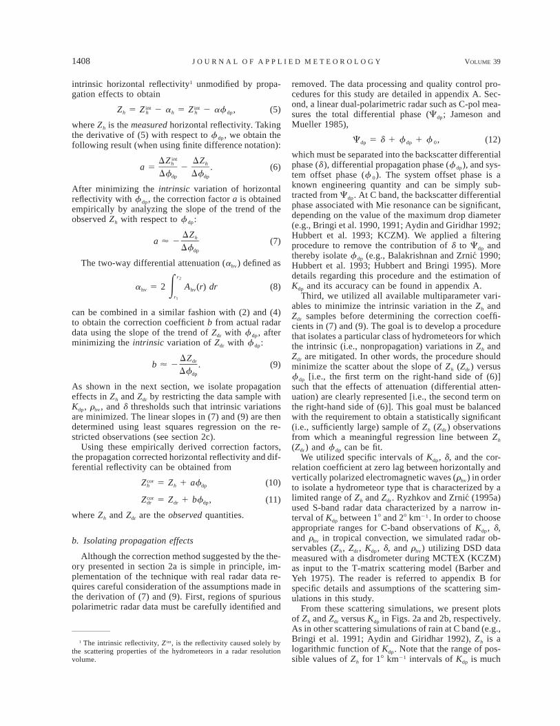
1408 VOLUME 39J O U R N A L O F A P P L I E D M E T E O R O L O G Y
intrinsic horizontal reflectivity1 unmodified by propa-gation effects to obtain
Zh 5 2 ah 5 2 af dp,int intZ Zh h (5)
where Zh is the measured horizontal reflectivity. Takingthe derivative of (5) with respect to f dp, we obtain thefollowing result (when using finite difference notation):
intDZ DZh ha 5 2 . (6)Df Dfdp dp
After minimizing the intrinsic variation of horizontalreflectivity with f dp, the correction factor a is obtainedempirically by analyzing the slope of the trend of theobserved Zh with respect to f dp:
DZha ø 2 (7)Dfdp
The two-way differential attenuation (ahv) defined asr2
a 5 2 A (r) dr (8)hv E hv
r1
can be combined in a similar fashion with (2) and (4)to obtain the correction coefficient b from actual radardata using the slope of the trend of Zdr with f dp, afterminimizing the intrinsic variation of Zdr with f dp:
DZdrb ø 2 . (9)Dfdp
As shown in the next section, we isolate propagationeffects in Zh and Zdr by restricting the data sample withKdp, rhv, and d thresholds such that intrinsic variationsare minimized. The linear slopes in (7) and (9) are thendetermined using least squares regression on the re-stricted observations (see section 2c).
Using these empirically derived correction factors,the propagation corrected horizontal reflectivity and dif-ferential reflectivity can be obtained from
corZ 5 Z 1 af (10)h h dp
corZ 5 Z 1 bf , (11)dr dr dp
where Zh and Zdr are the observed quantities.
b. Isolating propagation effects
Although the correction method suggested by the the-ory presented in section 2a is simple in principle, im-plementation of the technique with real radar data re-quires careful consideration of the assumptions made inthe derivation of (7) and (9). First, regions of spuriouspolarimetric radar data must be carefully identified and
1 The intrinsic reflectivity, Z int, is the reflectivity caused solely bythe scattering properties of the hydrometeors in a radar resolutionvolume.
removed. The data processing and quality control pro-cedures for this study are detailed in appendix A. Sec-ond, a linear dual-polarimetric radar such as C-pol mea-sures the total differential phase (Cdp; Jameson andMueller 1985),
Cdp 5 d 1 f dp 1 f 0, (12)
which must be separated into the backscatter differentialphase (d), differential propagation phase (f dp), and sys-tem offset phase (f 0). The system offset phase is aknown engineering quantity and can be simply sub-tracted from Cdp. At C band, the backscatter differentialphase associated with Mie resonance can be significant,depending on the value of the maximum drop diameter(e.g., Bringi et al. 1990, 1991; Aydin and Giridhar 1992;Hubbert et al. 1993; KCZM). We applied a filteringprocedure to remove the contribution of d to Cdp andthereby isolate f dp (e.g., Balakrishnan and Zrnic 1990;Hubbert et al. 1993; Hubbert and Bringi 1995). Moredetails regarding this procedure and the estimation ofKdp and its accuracy can be found in appendix A.
Third, we utilized all available multiparameter vari-ables to minimize the intrinsic variation in the Zh andZdr samples before determining the correction coeffi-cients in (7) and (9). The goal is to develop a procedurethat isolates a particular class of hydrometeors for whichthe intrinsic (i.e., nonpropagation) variations in Zh andZdr are mitigated. In other words, the procedure shouldminimize the scatter about the slope of Zh (Zdr) versusf dp [i.e., the first term on the right-hand side of (6)]such that the effects of attenuation (differential atten-uation) are clearly represented [i.e., the second term onthe right-hand side of (6)]. This goal must be balancedwith the requirement to obtain a statistically significant(i.e., sufficiently large) sample of Zh (Zdr) observationsfrom which a meaningful regression line between Zh
(Zdr) and f dp can be fit.We utilized specific intervals of Kdp, d, and the cor-
relation coefficient at zero lag between horizontally andvertically polarized electromagnetic waves (rhv) in orderto isolate a hydrometeor type that is characterized by alimited range of Zh and Zdr. Ryzhkov and Zrnic (1995a)used S-band radar data characterized by a narrow in-terval of Kdp between 18 and 28 km21. In order to chooseappropriate ranges for C-band observations of Kdp, d,and rhv in tropical convection, we simulated radar ob-servables (Zh, Zdr, Kdp, d, and rhv) utilizing DSD datameasured with a disdrometer during MCTEX (KCZM)as input to the T-matrix scattering model (Barber andYeh 1975). The reader is referred to appendix B forspecific details and assumptions of the scattering sim-ulations in this study.
From these scattering simulations, we present plotsof Zh and Zdr versus Kdp in Figs. 2a and 2b, respectively.As in other scattering simulations of rain at C band (e.g.,Bringi et al. 1991; Aydin and Giridhar 1992), Zh is alogarithmic function of Kdp. Note that the range of pos-sible values of Zh for 18 km21 intervals of Kdp is much
SEPTEMBER 2000 1409C A R E Y E T A L .
FIG. 2. Plots of (a) horizontal reflectivity (Zh, dBZ ) and (b) differential reflectivity (Zdr, dB) vs the specific differential phase (Kdp, 8 km21)as obtained from scattering simulations. Solid squares (open squares) are drop size distributions characterized by rhv . 0.97 and |d| , 18(rhv # 0.97 and |d| $ 18). Details regarding scattering simulations are described in appendix B.
larger at the low end of Kdp. This is especially true ifwe partition the scatterplot in Fig. 2a using rhv and d.The solid (open) squares in Figs. 2a,b are characterizedby rhv . 0.97 and d , 18 (rhv # 0.97 and d $ 18). Asshown in Bringi et al. (1991) and Aydin and Giridhar(1992), DSDs distinguished by lowered values of rhv
and large d have large values of the median volumediameter (D0) and hence large Zdr. As shown in Fig. 2b,the open (solid) squares are characterized by a mean Zdr
of 4 dB (0.7 dB) with a range of 2.5–5.4 dB (0.2–2.6dB). By removing those DSDs characterized by loweredrhv and significant d (i.e., removing DSDs with largeD0), the scatter of Zh for a given interval of Kdp issignificantly reduced. Using this restricted sample, therange of Zh values for a given Kdp interval decreaseswith increasing Kdp. Similarly, the range of Zdr valuesthat have been restricted by rhv . 0.97 and d , 18 alsodecreases with increasing Kdp (Fig. 2b).
Therefore, the use of a 18 km21 interval of Kdp aboveKdp 5 28 km21 would minimize the scatter of Zh and Zdr
about f dp. However, the need to minimize the intrinsicscatter must be balanced by the need for a sufficientlylarge sample to obtain a representative slope describedby (7) and (9). These values of Kdp would correspondto rain rates in excess of 40 mm h21 at C band (e.g.,Carey and Rutledge 2000). Our experience indicates thatthere are often insufficient grid points characterized bythese high rain rates to obtain a good regression. Ingeneral, the Kdp interval utilized by Ryzhkov and Zrnic(1995a) at S band of 18–28 km21 is typically a goodcompromise at C band as well. Inspection of Figs. 2a,bsuggest that most values of Zh (Zdr) should be between41 and 45 dBZ (0.75 and 1.5 dB).
Unlike Ryzhkov and Zrnic (1995a), Kdp thresholdsalone did not isolate propagation effects in our study.Because of the increased intrinsic scatter of Zh and Zdr
versus Kdp at C band, we found it necessary to applyrhv and d thresholds. The thresholds for rhv and d shouldbe governed by the performance of the radar. Based onthe performance of the C-pol radar (Keenan et al. 1998)and a detailed inspection of the data, we chose to restrictthe regression using rhv . 0.95, |d| , 58, and 1 # Kdp
# 28 km21 at grid levels between 0.5 and 2.0 km aboveground level (AGL). The effect of varying the regres-sion sample by changing the Kdp, rhv, d, and altitudethresholds was explored in sensitivity tests. The abovepolarimetric and height thresholds provided the mostreliable and statistically superior (i.e., low standard er-ror, high coefficient of correlation, and large samplesize) least squares fit to the data. A detailed descriptionof the sensitivity tests can be found in Carey (1999).
c. Estimating the mean correction coefficients
Using these thresholds, regression samples for Zh andZdr versus f dp are shown in Figs. 3a and 3b, respectively,for 0416 UTC (all times UTC hereafter) on 28 Novem-ber 1995. In both Figs. 3a and 3b, there is an unmis-takably decreasing trend of Zh and Zdr with f dp due tothe effects of horizontal and differential attenuation, re-spectively. The slope of Zh (Zdr) versus f dp for the un-restricted sample (N 5 1099) is 20.071 dB (8)21
(20.0199 dB (8)21). There is significant scatter of Zh
(4.4 dBZ) and Zdr (0.5 dB) about a least squares fit tothe data. This scatter is generally consistent with thesimulated data presented in Figs. 2a,b. In addition, thereare obvious outliers from the linear fits. For example,the low values of Zh (,32 dBZ) at relatively low f dp
(,208) in Fig. 3a are inconsistent with the theoreticalexpectations (cf. Fig. 2a) for Zh at these ranges of Kdp.Enhanced attenuation due to the presence of large rain-drops may have caused the presence of these outliers
1410 VOLUME 39J O U R N A L O F A P P L I E D M E T E O R O L O G Y
FIG. 3. Least squares linear regression results for (a) horizontal reflectivity (Zh, dBZ ) and (b) differentialreflectivity (Zdr, dB) vs the differential propagation phase (f dp, 8) taken from 0416 UTC on 28 Nov 1995.The original data sample (1) originated from 0.5 to 2 km and met the following polarimetric radar criteria:1 , Kdp , 28 km21, rhv . 0.95, and |d| , 58. The sample was further restricted by the standard error ofthe least squares estimate (M). Least square regression slopes for both samples are shown (original sample:short dash; restricted sample: dot).
(cf. sections 3a–c). However, it is also possible thaterrors in the estimated Kdp due to partial beam filling(Ryzhkov and Zrnic 1998a) resulted in the erroneousinclusion of these data points into the regression sample.In Fig. 3b, there are also obvious outliers from the gen-
eral decreasing trend of Zdr with f dp (e.g., Zdr , 0.5 dBand Zdr . 2.5 dB for f dp , 158). The presence of outlierssuch as these can seriously bias the inferred correctioncoefficient.
In order to avoid biasing the mean correction coef-
SEPTEMBER 2000 1411C A R E Y E T A L .
ficients for each radar volume, the final step in deter-mining the correction coefficients a and b is to eliminateoutliers from the linear assumption implicit in the der-ivation of (7) and (9) using simple statistics. We utilizedthe standard error of the estimate (S) of Zh (Zdr) on f dp
from a least squares regression line to restrict the sam-ple. We began by removing data outside of 2S from theregression line if r , 0.9.2 We continued to restrict thesample incrementally by 0.2S until r $ 0.9 or the datawas restricted to within S of the original regression line.Once the restricted sample was obtained, we recalcu-lated the best fit slope to the data using least squaresregression. An example of the restricted datasets from0416 and their associated regression lines are presentedin Figs. 3a,b for Zh versus f dp and Zdr versus f dp, re-spectively.
Frequently, the slope resulting from the least squaresfit to the restricted sample is somewhat different fromthe original slope. This was the case for Zh versus f dp
at 0416 as shown in Fig. 3a. The final slope of 20.081dB (8)21 is 14% lower than the original slope of Zh versusf dp. When a good slope could be determined, the finalslope Zh/f dp differed by no more than 18% from theinitial, unrestricted slope. The mean change in Zh/f dp
due to restricting the sample was 9%. Sometimes out-liers did not bias the least squares fit and the regressionslope did not change significantly after restricting thesample, as for Zdr versus f dp in Fig. 3b. For the entiredataset, retrieved slopes of Zdr/f dp changed by up to16% with a mean change of 5%. Once the final regres-sion slopes are determined as in Figs. 3a,b, the correc-tion coefficients a and b in (7) and (9) are simply thenegative of these two respective slopes.
In order to eliminate significant errors in the propa-gation corrected Zh and Zdr, it is important to assess therepresentativeness of each a and b. The y intercepts fromthe restricted datasets in Figs. 3a,b should be represen-tative of the propagation-free, intrinsic value of Zh andZdr, respectively. The y intercept for Zh (Zdr) is approx-imately 42 dBZ (1.3 dB), which is generally consistentwith the median value of the scattering simulation re-sults in Fig. 2a (Fig. 2b) for 1 # Kdp # 28 km21. Beforeutilizing the correction coefficients, we required the co-efficient of correlation (r), the number of data points inthe final regression sample (N), the standard error (S),and the maximum observed f dp to meet the followingthresholds: r2 $ 0.25 for a (r2 $ 0.6 for b), N $ 200,S # 5.5 dBZ for a (S # 0.55 dB for b), and f dp(max)$ 158. If all of these conditions were met, then theinferred a and b were used. Otherwise, alternate cor-rection coefficients were determined. If possible, we uti-lized an interpolation of a and b from adjacent times.
2 The coefficient of correlation (r) of a least squares regressionline should not be confused with rhv, which is the correlation coef-ficient at zero lag between horizontally and vertically polarized back-scattered electromagnetic radiation measured by the radar.
As a last resort, we used the median of all successfullydetermined correction coefficients for the day.
Once correction coefficients a and b were identifiedfor each radar volume, the correction was applied to Zh
and Zdr at each radar gate (or Cartesian grid point) asspecified in (10) and (11), respectively. A summary ofthis propagation correction procedure in the form of aflow-chart can be found in steps 1–4 in Fig. 4. Thisportion of the algorithm is referred to as the ‘‘meancorrection’’ because it is equivalent to assuming a sin-gle, mean D0 for the radar volume.
d. Results
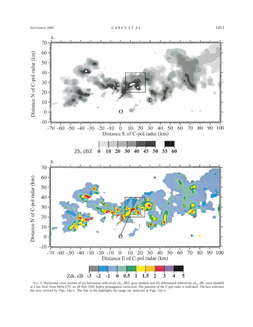
Horizontal cross sections of uncorrected Zh and Zdr at2 km associated with Figs. 3a,b are presented in Figs.5a and 5b, respectively. We chose data from 0416 on28 November 1995 because the convection was wide-spread and intense. By this time, precipitation hadmerged on the mesoscale (Carey and Rutledge 2000)with intense convective cores embedded within the com-plex. Even prior to propagation correction, peak reflec-tivities and differential reflectivities in these coresranged from 50 to 55 dBZ and from 2.5 to 4 dB, re-spectively.
Typically, the effects of attenuation on Zh are notreadily apparent at C band via visual inspection (Fig.5a). However, differential attenuation visibly decreasesthe differential reflectivity in range (Fig. 5b). Large ar-eas of negative Zdr, sometimes as low as 22 dB, areapparent down range of convection. Note that the lowestvalues of Zdr on the back edge of the convection are notnecessarily farthest from the radar, nor are they alwaysbehind the largest precipitation echo path. Typically, thegreatest propagation effects discernible in Zdr are down-range from intense convective cores characterized bylarge values of reflectivity (Zh . 50 dBZ) and differ-ential reflectivity (Zdr . 2 dB), suggesting the presenceof large raindrops. These ‘‘large drop cores’’ createreadily apparent range ‘‘shadows’’ of lowered Zdr rel-ative to their immediate surroundings. One example ofa shadow in Zdr down range of an intense convectivecore is highlighted in Figs. 5b, 14a, and 15b.
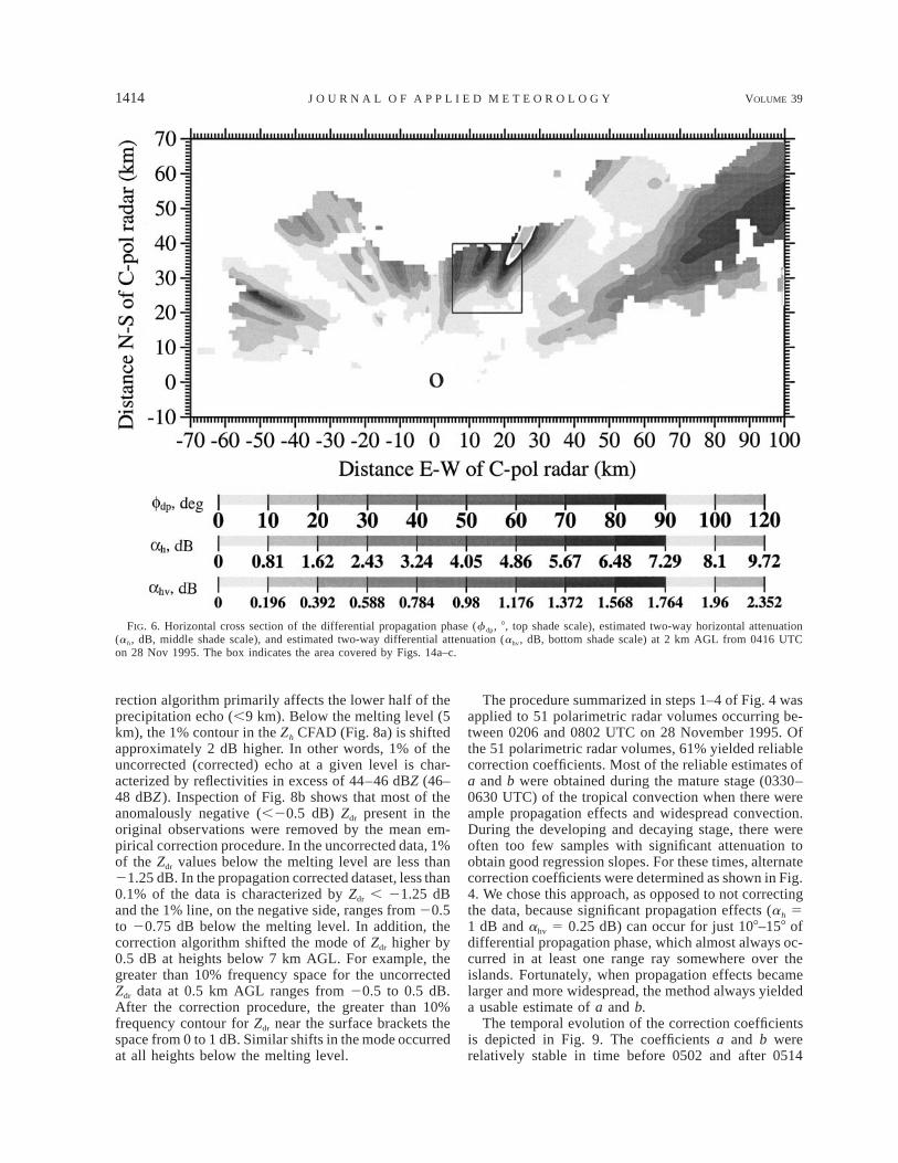
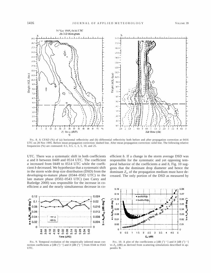
A horizontal cross section at 2 km of differential prop-agation phase for 0416 UTC is shown in Fig. 6. Com-parison of Figs. 5b and 6 further demonstrates the an-ticorrelation between f dp and Zdr. As shown earlier inFig. 3b, increasing values of f dp are generally associatedwith decreasing Zdr as a result of differential attenuation.Maximum f dp exceeds 1208 at this time. Interestingly,this peak occurs less than 50 km in range from the radar.During 28 November 1995, the maximum f dp exceeded2008 several times.
As shown in section 2a, the differential propagationphase is linearly proportional to both the path integratedhorizontal and differential attenuation where a and b,respectively, are the constants of proportionality. Bymultiplying f dp by a 5 0.081 and b 5 0.0196 (as de-
1412 VOLUME 39J O U R N A L O F A P P L I E D M E T E O R O L O G Y
FIG. 4. Flow chart summary of the propagation correction algorithm. Steps 1–4 summarize themean empirical correction procedure (sections 2a–d) and steps 5–6 depict the big drop correctiondescribed in sections 3a–c.
termined in Figs. 3a,b), estimates of ah and ahv wereobtained (Fig. 6). Maximum estimates of ah and ahv at2 km exceed 9 and 2 dB, respectively. Approximately26% of the echo is characterized by significant atten-uation (ah . 1 dB) and differential attenuation (ahv .0.25 dB). Five percent of the precipitation echo expe-rienced severe propagation effects (e.g., defined here asah . 4 dB and ahv . 1 dB).
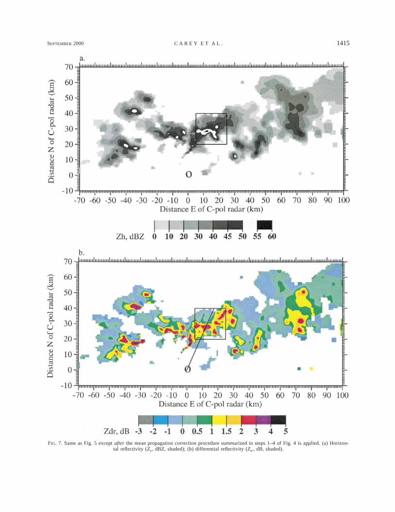
Using the above estimates of propagation effects at0416 UTC, the corrected Zh and Zdr were calculatedaccording to (10) and (11) (Figs. 7a and 7b, respec-tively). As expected, a comparison of Figs. 5a,b to Figs.7a,b reveals significant differences between observedZh/Zdr and propagation corrected Zh/Zdr in regions of
significant f dp (Fig. 6). Most notable is the eliminationof most negative values of Zdr in Fig. 7b. Another strik-ing difference is the increased area of precipitation echocharacterized by Zdr . 1 dB, particularly in the north–south-oriented complex centered on x 5 75 km and inthe cells located 20–50 km to the north-northeast of theradar (Fig. 7b). Similarly, the precipitation echo areacharacterized by Zh . 40 dBZ also has been substan-tially increased (Fig. 7a).
To examine the effects of the correction algorithm inthree dimensions at 0416 UTC, contoured frequency byaltitude diagrams (CFADs; Yuter and Houze 1995) ofthe uncorrected and corrected Zh and Zdr are presentedin Figs. 8a and 8b, respectively. As expected, the cor-
SEPTEMBER 2000 1413C A R E Y E T A L .
FIG. 5. Horizontal cross section of (a) horizontal reflectivity (Zh, dBZ, gray shaded) and (b) differential reflectivity (Zdr, dB, color shaded)at 2 km AGL from 0416 UTC on 28 Nov 1995 before propagation correction. The position of the C-pol radar is indicated. The box indicatesthe area covered by Figs. 14a–c. The line in (b) highlights the range ray analyzed in Figs. 15a–c.
1414 VOLUME 39J O U R N A L O F A P P L I E D M E T E O R O L O G Y
FIG. 6. Horizontal cross section of the differential propagation phase (f dp, 8, top shade scale), estimated two-way horizontal attenuation(ah, dB, middle shade scale), and estimated two-way differential attenuation (ahv, dB, bottom shade scale) at 2 km AGL from 0416 UTCon 28 Nov 1995. The box indicates the area covered by Figs. 14a–c.
rection algorithm primarily affects the lower half of theprecipitation echo (,9 km). Below the melting level (5km), the 1% contour in the Zh CFAD (Fig. 8a) is shiftedapproximately 2 dB higher. In other words, 1% of theuncorrected (corrected) echo at a given level is char-acterized by reflectivities in excess of 44–46 dBZ (46–48 dBZ). Inspection of Fig. 8b shows that most of theanomalously negative (,20.5 dB) Zdr present in theoriginal observations were removed by the mean em-pirical correction procedure. In the uncorrected data, 1%of the Zdr values below the melting level are less than21.25 dB. In the propagation corrected dataset, less than0.1% of the data is characterized by Zdr , 21.25 dBand the 1% line, on the negative side, ranges from 20.5to 20.75 dB below the melting level. In addition, thecorrection algorithm shifted the mode of Zdr higher by0.5 dB at heights below 7 km AGL. For example, thegreater than 10% frequency space for the uncorrectedZdr data at 0.5 km AGL ranges from 20.5 to 0.5 dB.After the correction procedure, the greater than 10%frequency contour for Zdr near the surface brackets thespace from 0 to 1 dB. Similar shifts in the mode occurredat all heights below the melting level.
The procedure summarized in steps 1–4 of Fig. 4 wasapplied to 51 polarimetric radar volumes occurring be-tween 0206 and 0802 UTC on 28 November 1995. Ofthe 51 polarimetric radar volumes, 61% yielded reliablecorrection coefficients. Most of the reliable estimates ofa and b were obtained during the mature stage (0330–0630 UTC) of the tropical convection when there wereample propagation effects and widespread convection.During the developing and decaying stage, there wereoften too few samples with significant attenuation toobtain good regression slopes. For these times, alternatecorrection coefficients were determined as shown in Fig.4. We chose this approach, as opposed to not correctingthe data, because significant propagation effects (ah 51 dB and ahv 5 0.25 dB) can occur for just 108–158 ofdifferential propagation phase, which almost always oc-curred in at least one range ray somewhere over theislands. Fortunately, when propagation effects becamelarger and more widespread, the method always yieldeda usable estimate of a and b.
The temporal evolution of the correction coefficientsis depicted in Fig. 9. The coefficients a and b wererelatively stable in time before 0502 and after 0514
SEPTEMBER 2000 1415C A R E Y E T A L .
FIG. 7. Same as Fig. 5 except after the mean propagation correction procedure summarized in steps 1–4 of Fig. 4 is applied. (a) Horizon-tal reflectivity (Zh, dBZ, shaded); (b) differential reflectivity (Zdr, dB, shaded).
1416 VOLUME 39J O U R N A L O F A P P L I E D M E T E O R O L O G Y
FIG. 8. A CFAD (%) of (a) horizontal reflectivity and (b) differential reflectivity both before and after propagation correction at 0416UTC on 28 Nov 1995. Before mean propagation correction: dashed line. After mean propagation correction: solid line. The following relativefrequencies (%) are contoured: 0.1, 0.5, 1, 3, 5, 10, and 25.
FIG. 10. A plot of the coefficients a [dB (8)21] and b [dB (8)21]vs Zdr (dB) as derived from scattering simulations described in ap-pendix B.
FIG. 9. Temporal evolution of the empirically inferred mean cor-rection coefficients a [dB (8)21] and b [dB (8)21] from 0344 to 0543UTC.
UTC. There was a systematic shift in both coefficientsa and b between 0449 and 0514 UTC. The coefficienta increased from 0449 to 0514 UTC while the coeffi-cient b decreased. We hypothesize that a systematic shiftin the storm wide drop size distribution (DSD) from thedeveloping-to-mature phase (0344–0502 UTC) to thelate mature phase (0502–0543 UTC) (see Carey andRutledge 2000) was responsible for the increase in co-efficient a and the nearly simultaneous decrease in co-
efficient b. If a change in the storm average DSD wasresponsible for the systematic and yet opposing tem-poral behavior of the coefficients a and b, Fig. 10 sug-gests that the dominant drop diameter and hence thedominant Zdr of the propagation medium must have de-creased. The only portion of the DSD as measured by
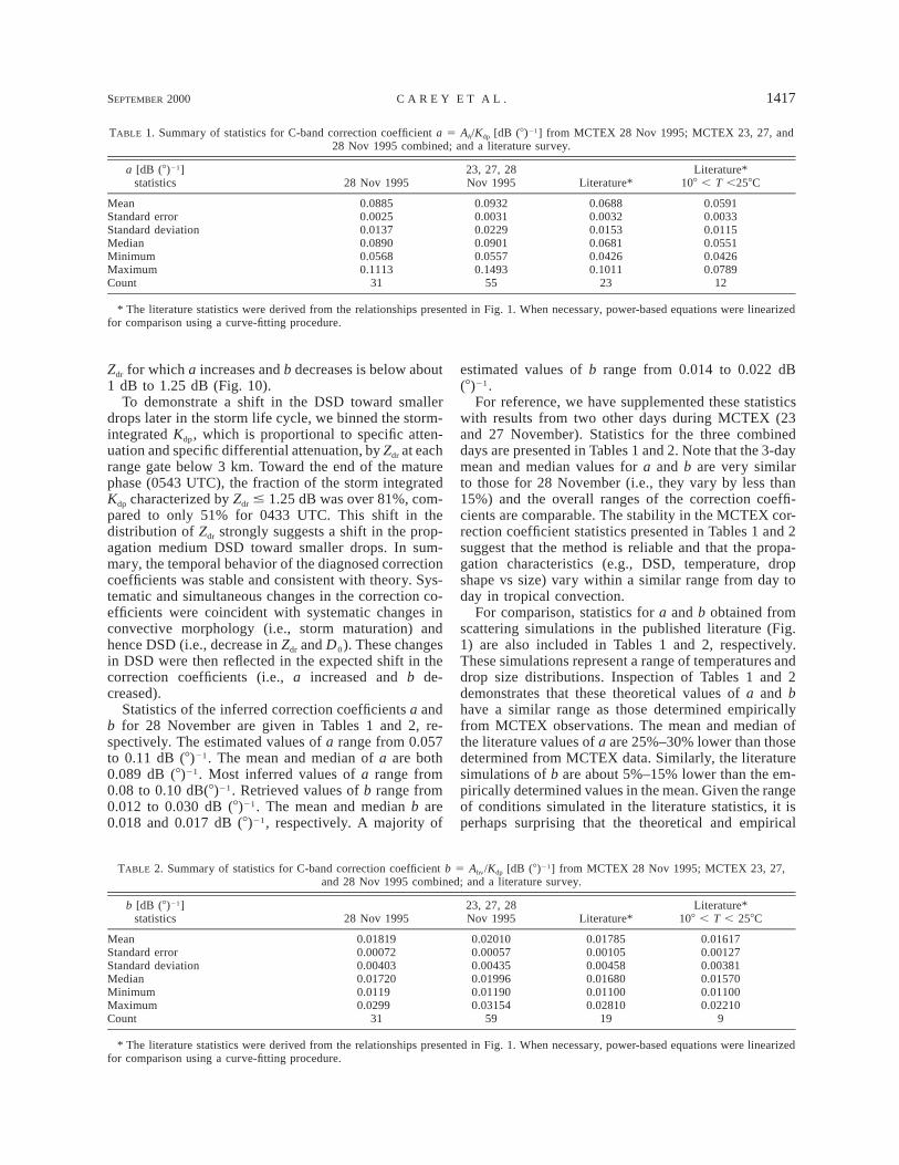
SEPTEMBER 2000 1417C A R E Y E T A L .
TABLE 1. Summary of statistics for C-band correction coefficient a 5 Ah/Kdp [dB (8)21] from MCTEX 28 Nov 1995; MCTEX 23, 27, and28 Nov 1995 combined; and a literature survey.
a [dB (8)21]statistics 28 Nov 1995
23, 27, 28Nov 1995 Literature*
Literature*108 , T ,258C
MeanStandard errorStandard deviationMedianMinimumMaximumCount
0.08850.00250.01370.08900.05680.1113
31
0.09320.00310.02290.09010.05570.1493
55
0.06880.00320.01530.06810.04260.1011
23
0.05910.00330.01150.05510.04260.0789
12
* The literature statistics were derived from the relationships presented in Fig. 1. When necessary, power-based equations were linearizedfor comparison using a curve-fitting procedure.
TABLE 2. Summary of statistics for C-band correction coefficient b 5 Ahv/Kdp [dB (8)21] from MCTEX 28 Nov 1995; MCTEX 23, 27,and 28 Nov 1995 combined; and a literature survey.
b [dB (8)21]statistics 28 Nov 1995
23, 27, 28Nov 1995 Literature*
Literature*108 , T , 258C
MeanStandard errorStandard deviationMedianMinimumMaximumCount
0.018190.000720.004030.017200.01190.0299
31
0.020100.000570.004350.019960.011900.03154
59
0.017850.001050.004580.016800.011000.02810
19
0.016170.001270.003810.015700.011000.02210
9
* The literature statistics were derived from the relationships presented in Fig. 1. When necessary, power-based equations were linearizedfor comparison using a curve-fitting procedure.
Zdr for which a increases and b decreases is below about1 dB to 1.25 dB (Fig. 10).
To demonstrate a shift in the DSD toward smallerdrops later in the storm life cycle, we binned the storm-integrated Kdp, which is proportional to specific atten-uation and specific differential attenuation, by Zdr at eachrange gate below 3 km. Toward the end of the maturephase (0543 UTC), the fraction of the storm integratedKdp characterized by Zdr # 1.25 dB was over 81%, com-pared to only 51% for 0433 UTC. This shift in thedistribution of Zdr strongly suggests a shift in the prop-agation medium DSD toward smaller drops. In sum-mary, the temporal behavior of the diagnosed correctioncoefficients was stable and consistent with theory. Sys-tematic and simultaneous changes in the correction co-efficients were coincident with systematic changes inconvective morphology (i.e., storm maturation) andhence DSD (i.e., decrease in Zdr and D0). These changesin DSD were then reflected in the expected shift in thecorrection coefficients (i.e., a increased and b de-creased).
Statistics of the inferred correction coefficients a andb for 28 November are given in Tables 1 and 2, re-spectively. The estimated values of a range from 0.057to 0.11 dB (8)21. The mean and median of a are both0.089 dB (8)21. Most inferred values of a range from0.08 to 0.10 dB(8)21. Retrieved values of b range from0.012 to 0.030 dB (8)21. The mean and median b are0.018 and 0.017 dB (8)21, respectively. A majority of
estimated values of b range from 0.014 to 0.022 dB(8)21.
For reference, we have supplemented these statisticswith results from two other days during MCTEX (23and 27 November). Statistics for the three combineddays are presented in Tables 1 and 2. Note that the 3-daymean and median values for a and b are very similarto those for 28 November (i.e., they vary by less than15%) and the overall ranges of the correction coeffi-cients are comparable. The stability in the MCTEX cor-rection coefficient statistics presented in Tables 1 and 2suggest that the method is reliable and that the propa-gation characteristics (e.g., DSD, temperature, dropshape vs size) vary within a similar range from day today in tropical convection.
For comparison, statistics for a and b obtained fromscattering simulations in the published literature (Fig.1) are also included in Tables 1 and 2, respectively.These simulations represent a range of temperatures anddrop size distributions. Inspection of Tables 1 and 2demonstrates that these theoretical values of a and bhave a similar range as those determined empiricallyfrom MCTEX observations. The mean and median ofthe literature values of a are 25%–30% lower than thosedetermined from MCTEX data. Similarly, the literaturesimulations of b are about 5%–15% lower than the em-pirically determined values in the mean. Given the rangeof conditions simulated in the literature statistics, it isperhaps surprising that the theoretical and empirical
1418 VOLUME 39J O U R N A L O F A P P L I E D M E T E O R O L O G Y
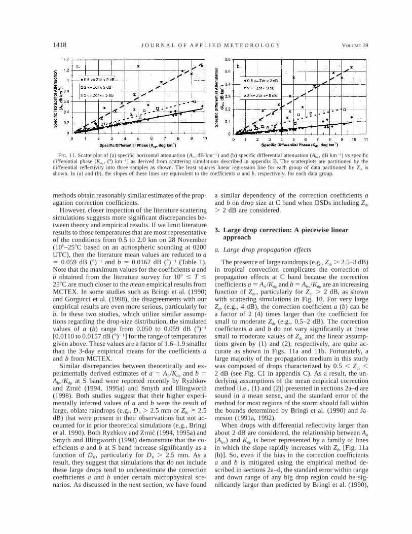
FIG. 11. Scatterplot of (a) specific horizontal attenuation (Ah, dB km21) and (b) specific differential attenuation (Ahv, dB km21) vs specificdifferential phase [Kdp, (8) km21] as derived from scattering simulations described in appendix B. The scatterplots are partitioned by thedifferential reflectivity into three samples as shown. The least squares linear regression line for each group of data partitioned by Zdr isshown. In (a) and (b), the slopes of these lines are equivalent to the coefficients a and b, respectively, for each data group.
methods obtain reasonably similar estimates of the prop-agation correction coefficients.
However, closer inspection of the literature scatteringsimulations suggests more significant discrepancies be-tween theory and empirical results. If we limit literatureresults to those temperatures that are most representativeof the conditions from 0.5 to 2.0 km on 28 November(108–258C based on an atmospheric sounding at 0200UTC), then the literature mean values are reduced to a5 0.059 dB (8)21 and b 5 0.0162 dB (8)21 (Table 1).Note that the maximum values for the coefficients a andb obtained from the literature survey for 108 # T #258C are much closer to the mean empirical results fromMCTEX. In some studies such as Bringi et al. (1990)and Gorgucci et al. (1998), the disagreements with ourempirical results are even more serious, particularly forb. In these two studies, which utilize similar assump-tions regarding the drop-size distribution, the simulatedvalues of a (b) range from 0.050 to 0.059 dB (8)21
[0.0110 to 0.0157 dB (8)21] for the range of temperaturesgiven above. These values are a factor of 1.6–1.9 smallerthan the 3-day empirical means for the coefficients aand b from MCTEX.
Similar discrepancies between theoretically and ex-perimentally derived estimates of a 5 Ah/Kdp and b 5Ahv/Kdp at S band were reported recently by Ryzhkovand Zrnic (1994, 1995a) and Smyth and Illingworth(1998). Both studies suggest that their higher experi-mentally inferred values of a and b were the result oflarge, oblate raindrops (e.g., D0 . 2.5 mm or Zdr $ 2.5dB) that were present in their observations but not ac-counted for in prior theoretical simulations (e.g., Bringiet al. 1990). Both Ryzhkov and Zrnic (1994, 1995a) andSmyth and Illingworth (1998) demonstrate that the co-efficients a and b at S band increase significantly as afunction of D0, particularly for D0 . 2.5 mm. As aresult, they suggest that simulations that do not includethese large drops tend to underestimate the correctioncoefficients a and b under certain microphysical sce-narios. As discussed in the next section, we have found
a similar dependency of the correction coefficients aand b on drop size at C band when DSDs including Zdr
. 2 dB are considered.
3. Large drop correction: A piecewise linearapproach
a. Large drop propagation effects
The presence of large raindrops (e.g., Zdr . 2.5–3 dB)in tropical convection complicates the correction ofpropagation effects at C band because the correctioncoefficients a 5 Ah/Kdp and b 5 Ahv/Kdp are an increasingfunction of Zdr, particularly for Zdr . 2 dB, as shownwith scattering simulations in Fig. 10. For very largeZdr (e.g., 4 dB), the correction coefficient a (b) can bea factor of 2 (4) times larger than the coefficient forsmall to moderate Zdr (e.g., 0.5–2 dB). The correctioncoefficients a and b do not vary significantly at thesesmall to moderate values of Zdr and the linear assump-tions given by (1) and (2), respectively, are quite ac-curate as shown in Figs. 11a and 11b. Fortunately, alarge majority of the propagation medium in this studywas composed of drops characterized by 0.5 , Zdr ,2 dB (see Fig. C1 in appendix C). As a result, the un-derlying assumptions of the mean empirical correctionmethod [i.e., (1) and (2)] presented in sections 2a–d aresound in a mean sense, and the standard error of themethod for most regions of the storm should fall withinthe bounds determined by Bringi et al. (1990) and Ja-meson (1991a, 1992).
When drops with differential reflectivity larger thanabout 2 dB are considered, the relationship between Ah
(Ahv) and Kdp is better represented by a family of linesin which the slope rapidly increases with Zdr [Fig. 11a(b)]. So, even if the bias in the correction coefficientsa and b is mitigated using the empirical method de-scribed in sections 2a–d, the standard error within rangeand down range of any big drop region could be sig-nificantly larger than predicted by Bringi et al. (1990),
SEPTEMBER 2000 1419C A R E Y E T A L .
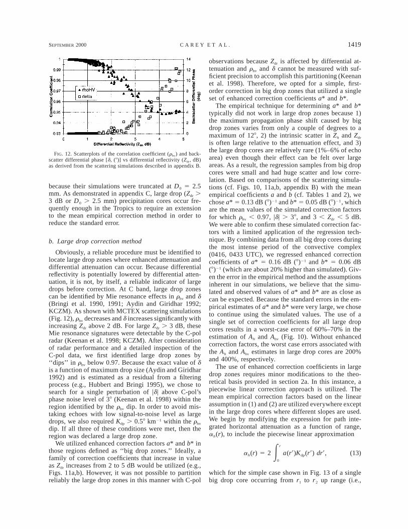
FIG. 12. Scatterplots of the correlation coefficient (rhv) and back-scatter differential phase [d, (8)] vs differential reflectivity (Zdr, dB)as derived from the scattering simulations described in appendix B.
because their simulations were truncated at D0 5 2.5mm. As demonstrated in appendix C, large drop (Zdr .3 dB or D0 . 2.5 mm) precipitation cores occur fre-quently enough in the Tropics to require an extensionto the mean empirical correction method in order toreduce the standard error.
b. Large drop correction method
Obviously, a reliable procedure must be identified tolocate large drop zones where enhanced attenuation anddifferential attenuation can occur. Because differentialreflectivity is potentially lowered by differential atten-uation, it is not, by itself, a reliable indicator of largedrops before correction. At C band, large drop zonescan be identified by Mie resonance effects in rhv and d(Bringi et al. 1990, 1991; Aydin and Giridhar 1992;KCZM). As shown with MCTEX scattering simulations(Fig. 12), rhv decreases and d increases significantly withincreasing Zdr above 2 dB. For large Zdr . 3 dB, theseMie resonance signatures were detectable by the C-polradar (Keenan et al. 1998; KCZM). After considerationof radar performance and a detailed inspection of theC-pol data, we first identified large drop zones by‘‘dips’’ in rhv below 0.97. Because the exact value of dis a function of maximum drop size (Aydin and Giridhar1992) and is estimated as a residual from a filteringprocess (e.g., Hubbert and Bringi 1995), we chose tosearch for a single perturbation of |d| above C-pol’sphase noise level of 38 (Keenan et al. 1998) within theregion identified by the rhv dip. In order to avoid mis-taking echoes with low signal-to-noise level as largedrops, we also required Kdp . 0.58 km21 within the rhv
dip. If all three of these conditions were met, then theregion was declared a large drop zone.
We utilized enhanced correction factors a* and b* inthose regions defined as ‘‘big drop zones.’’ Ideally, afamily of correction coefficients that increase in valueas Zdr increases from 2 to 5 dB would be utilized (e.g.,Figs. 11a,b). However, it was not possible to partitionreliably the large drop zones in this manner with C-pol
observations because Zdr is affected by differential at-tenuation and rhv and d cannot be measured with suf-ficient precision to accomplish this partitioning (Keenanet al. 1998). Therefore, we opted for a simple, first-order correction in big drop zones that utilized a singleset of enhanced correction coefficients a* and b*.
The empirical technique for determining a* and b*typically did not work in large drop zones because 1)the maximum propagation phase shift caused by bigdrop zones varies from only a couple of degrees to amaximum of 128, 2) the intrinsic scatter in Zh and Zdr
is often large relative to the attenuation effect, and 3)the large drop cores are relatively rare (1%–6% of echoarea) even though their effect can be felt over largeareas. As a result, the regression samples from big dropcores were small and had huge scatter and low corre-lation. Based on comparisons of the scattering simula-tions (cf. Figs. 10, 11a,b, appendix B) with the meanempirical coefficients a and b (cf. Tables 1 and 2), wechose a* 5 0.13 dB (8)21 and b* 5 0.05 dB (8)21, whichare the mean values of the simulated correction factorsfor which rhv , 0.97, |d| . 38, and 3 , Zdr , 5 dB.We were able to confirm these simulated correction fac-tors with a limited application of the regression tech-nique. By combining data from all big drop cores duringthe most intense period of the convective complex(0416, 0433 UTC), we regressed enhanced correctioncoefficients of a* 5 0.16 dB (8)21 and b* 5 0.06 dB(8)21 (which are about 20% higher than simulated). Giv-en the error in the empirical method and the assumptionsinherent in our simulations, we believe that the simu-lated and observed values of a* and b* are as close ascan be expected. Because the standard errors in the em-pirical estimates of a* and b* were very large, we choseto continue using the simulated values. The use of asingle set of correction coefficients for all large dropcores results in a worst-case error of 60%–70% in theestimation of Ah and Ahv (Fig. 10). Without enhancedcorrection factors, the worst case errors associated withthe Ah and Ahv estimates in large drop cores are 200%and 400%, respectively.
The use of enhanced correction coefficients in largedrop zones requires minor modifications to the theo-retical basis provided in section 2a. In this instance, apiecewise linear correction approach is utilized. Themean empirical correction factors based on the linearassumption in (1) and (2) are utilized everywhere exceptin the large drop cores where different slopes are used.We begin by modifying the expression for path inte-grated horizontal attenuation as a function of range,ah(r), to include the piecewise linear approximation
r
a (r) 5 2 a(r9)K (r9) dr9, (13)h E dp
0
which for the simple case shown in Fig. 13 of a singlebig drop core occurring from r1 to r2 up range (i.e.,
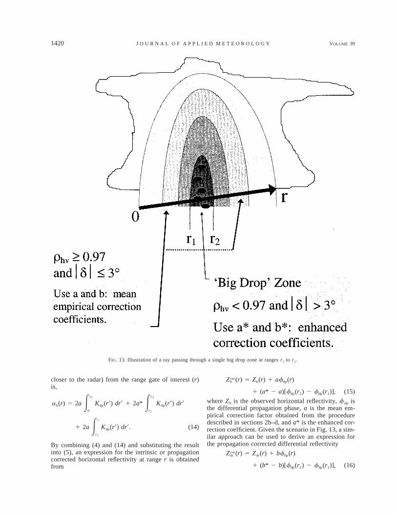
1420 VOLUME 39J O U R N A L O F A P P L I E D M E T E O R O L O G Y
FIG. 13. Illustration of a ray passing through a single big drop zone at ranges r1 to r2.
closer to the radar) from the range gate of interest (r)is,
r r1 2
a (r) 5 2a K (r9) dr9 1 2a* K (r9) dr9h E dp E dp
0 r1
r
1 2a K (r9) dr9. (14)E dp
r2
By combining (4) and (14) and substituting the resultinto (5), an expression for the intrinsic or propagationcorrected horizontal reflectivity at range r is obtainedfrom
corZ (r) 5 Z (r) 1 af (r)h h dp
1 (a* 2 a)[f (r ) 2 f (r )], (15)dp 2 dp 1
where Zh is the observed horizontal reflectivity, f dp isthe differential propagation phase, a is the mean em-pirical correction factor obtained from the proceduredescribed in sections 2b–d, and a* is the enhanced cor-rection coefficient. Given the scenario in Fig. 13, a sim-ilar approach can be used to derive an expression forthe propagation corrected differential reflectivity
corZ (r) 5 Z (r) 1 bf (r)dr dr dp
1 (b* 2 b)[f (r ) 2 f (r )], (16)dp 2 dp 1
SEPTEMBER 2000 1421C A R E Y E T A L .
where Zdr is the observed differential reflectivity, b isthe mean empirical correction factor obtained from theprocedure described in sections 2b–d, and b* is the en-hanced correction coefficient. The above derivation canbe easily extended to include any number of big dropcores in a given range ray. The complete propagationcorrection technique utilized in this study, including thebig drop correction (steps 5, 6), is summarized in flow-chart form in Fig. 4.
c. Results
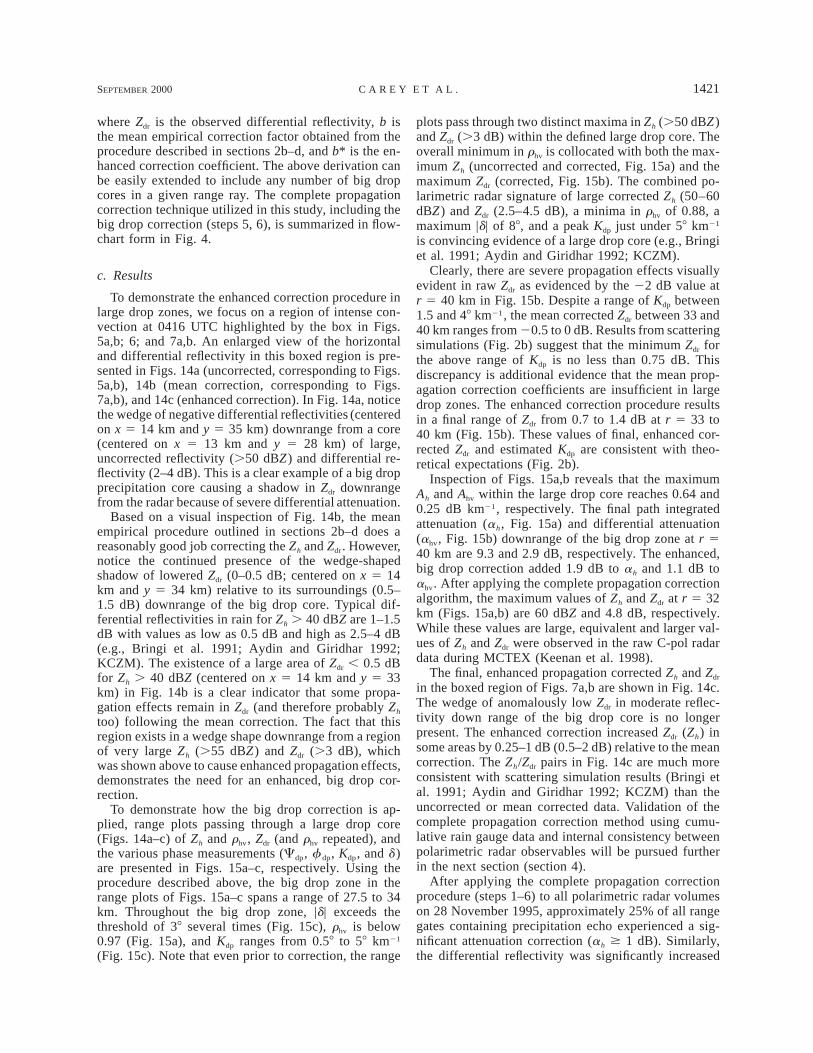
To demonstrate the enhanced correction procedure inlarge drop zones, we focus on a region of intense con-vection at 0416 UTC highlighted by the box in Figs.5a,b; 6; and 7a,b. An enlarged view of the horizontaland differential reflectivity in this boxed region is pre-sented in Figs. 14a (uncorrected, corresponding to Figs.5a,b), 14b (mean correction, corresponding to Figs.7a,b), and 14c (enhanced correction). In Fig. 14a, noticethe wedge of negative differential reflectivities (centeredon x 5 14 km and y 5 35 km) downrange from a core(centered on x 5 13 km and y 5 28 km) of large,uncorrected reflectivity (.50 dBZ) and differential re-flectivity (2–4 dB). This is a clear example of a big dropprecipitation core causing a shadow in Zdr downrangefrom the radar because of severe differential attenuation.
Based on a visual inspection of Fig. 14b, the meanempirical procedure outlined in sections 2b–d does areasonably good job correcting the Zh and Zdr. However,notice the continued presence of the wedge-shapedshadow of lowered Zdr (0–0.5 dB; centered on x 5 14km and y 5 34 km) relative to its surroundings (0.5–1.5 dB) downrange of the big drop core. Typical dif-ferential reflectivities in rain for Zh . 40 dBZ are 1–1.5dB with values as low as 0.5 dB and high as 2.5–4 dB(e.g., Bringi et al. 1991; Aydin and Giridhar 1992;KCZM). The existence of a large area of Zdr , 0.5 dBfor Zh . 40 dBZ (centered on x 5 14 km and y 5 33km) in Fig. 14b is a clear indicator that some propa-gation effects remain in Zdr (and therefore probably Zh
too) following the mean correction. The fact that thisregion exists in a wedge shape downrange from a regionof very large Zh (.55 dBZ) and Zdr (.3 dB), whichwas shown above to cause enhanced propagation effects,demonstrates the need for an enhanced, big drop cor-rection.
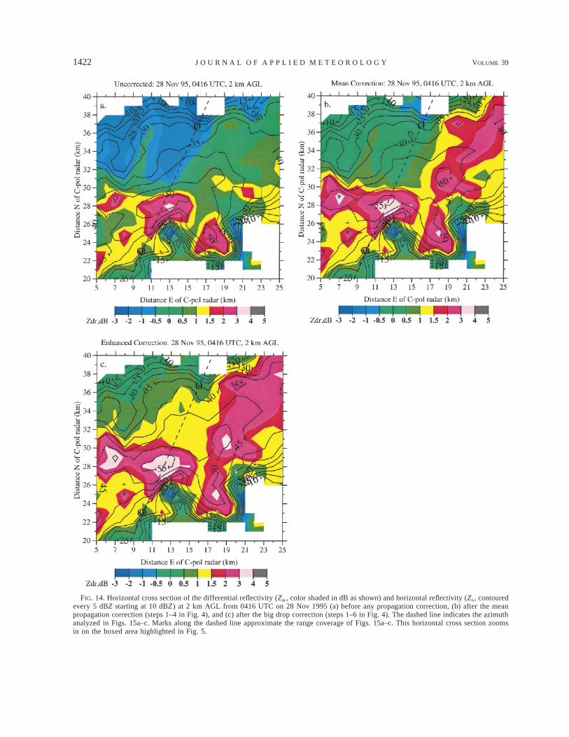
To demonstrate how the big drop correction is ap-plied, range plots passing through a large drop core(Figs. 14a–c) of Zh and rhv, Zdr (and rhv repeated), andthe various phase measurements (Cdp, f dp, Kdp, and d)are presented in Figs. 15a–c, respectively. Using theprocedure described above, the big drop zone in therange plots of Figs. 15a–c spans a range of 27.5 to 34km. Throughout the big drop zone, |d| exceeds thethreshold of 38 several times (Fig. 15c), rhv is below0.97 (Fig. 15a), and Kdp ranges from 0.58 to 58 km21
(Fig. 15c). Note that even prior to correction, the range
plots pass through two distinct maxima in Zh (.50 dBZ)and Zdr (.3 dB) within the defined large drop core. Theoverall minimum in rhv is collocated with both the max-imum Zh (uncorrected and corrected, Fig. 15a) and themaximum Zdr (corrected, Fig. 15b). The combined po-larimetric radar signature of large corrected Zh (50–60dBZ) and Zdr (2.5–4.5 dB), a minima in rhv of 0.88, amaximum |d| of 88, and a peak Kdp just under 58 km21
is convincing evidence of a large drop core (e.g., Bringiet al. 1991; Aydin and Giridhar 1992; KCZM).
Clearly, there are severe propagation effects visuallyevident in raw Zdr as evidenced by the 22 dB value atr 5 40 km in Fig. 15b. Despite a range of Kdp between1.5 and 48 km21, the mean corrected Zdr between 33 and40 km ranges from 20.5 to 0 dB. Results from scatteringsimulations (Fig. 2b) suggest that the minimum Zdr forthe above range of Kdp is no less than 0.75 dB. Thisdiscrepancy is additional evidence that the mean prop-agation correction coefficients are insufficient in largedrop zones. The enhanced correction procedure resultsin a final range of Zdr from 0.7 to 1.4 dB at r 5 33 to40 km (Fig. 15b). These values of final, enhanced cor-rected Zdr and estimated Kdp are consistent with theo-retical expectations (Fig. 2b).
Inspection of Figs. 15a,b reveals that the maximumAh and Ahv within the large drop core reaches 0.64 and0.25 dB km21, respectively. The final path integratedattenuation (ah, Fig. 15a) and differential attenuation(ahv, Fig. 15b) downrange of the big drop zone at r 540 km are 9.3 and 2.9 dB, respectively. The enhanced,big drop correction added 1.9 dB to ah and 1.1 dB toahv. After applying the complete propagation correctionalgorithm, the maximum values of Zh and Zdr at r 5 32km (Figs. 15a,b) are 60 dBZ and 4.8 dB, respectively.While these values are large, equivalent and larger val-ues of Zh and Zdr were observed in the raw C-pol radardata during MCTEX (Keenan et al. 1998).
The final, enhanced propagation corrected Zh and Zdr
in the boxed region of Figs. 7a,b are shown in Fig. 14c.The wedge of anomalously low Zdr in moderate reflec-tivity down range of the big drop core is no longerpresent. The enhanced correction increased Zdr (Zh) insome areas by 0.25–1 dB (0.5–2 dB) relative to the meancorrection. The Zh/Zdr pairs in Fig. 14c are much moreconsistent with scattering simulation results (Bringi etal. 1991; Aydin and Giridhar 1992; KCZM) than theuncorrected or mean corrected data. Validation of thecomplete propagation correction method using cumu-lative rain gauge data and internal consistency betweenpolarimetric radar observables will be pursued furtherin the next section (section 4).
After applying the complete propagation correctionprocedure (steps 1–6) to all polarimetric radar volumeson 28 November 1995, approximately 25% of all rangegates containing precipitation echo experienced a sig-nificant attenuation correction (ah $ 1 dB). Similarly,the differential reflectivity was significantly increased
1422 VOLUME 39J O U R N A L O F A P P L I E D M E T E O R O L O G Y
FIG. 14. Horizontal cross section of the differential reflectivity (Zdr, color shaded in dB as shown) and horizontal reflectivity (Zh, contouredevery 5 dBZ starting at 10 dBZ ) at 2 km AGL from 0416 UTC on 28 Nov 1995 (a) before any propagation correction, (b) after the meanpropagation correction (steps 1–4 in Fig. 4), and (c) after the big drop correction (steps 1–6 in Fig. 4). The dashed line indicates the azimuthanalyzed in Figs. 15a–c. Marks along the dashed line approximate the range coverage of Figs. 15a–c. This horizontal cross section zoomsin on the boxed area highlighted in Fig. 5.
SEPTEMBER 2000 1423C A R E Y E T A L .
FIG. 15. Range plots of (a) correlation coefficient (rhv) and horizontal reflectivity (Zh, dBZ) before correction (raw), after the meanpropagation correction (cor), and after the enhanced correction (enhanced cor.). (b) Correlation coefficient and differential reflectivity (Zdr,dB) before correction (raw), after the mean propagation correction (cor), and after the enhanced correction (enhanced cor.). (c) Total differentialphase (Cdp, 8), propagation differential phase (f dp, 8), backscatter differential phase (d, 8), and specific differential phase (Kdp, 8 km21). Therange plots display ray 387 (azimuth angle 5 23.218, elevation angle 5 3.88) from r 5 25 km to r 5 40 km. Range resolution is 0.30 km.The big drop zone as defined in the text is highlighted. Refer to Figs. 5b and 14a–c to place this range ray in the context of the entireconvective complex.
(ahv $ 0.25 dB) about 22% of the time. In about 7%(6%) of the precipitation echo during 28 November1995, there were massive propagation corrections to Zh
(Zdr) defined as ah $ 5 dB (ahv $ 1 dB). Clearly, prop-agation effects at C band in the Tropics are significantand must be corrected before using the data either qual-itatively or quantitatively. This premise will be testedfurther in the next section.
4. Validation
a. Comparison with rain gauge data
Fourteen tipping bucket rain gauges distributedthroughout the Tiwi Islands at ranges of 15–88 km fromthe radar during MCTEX (Keenan et al. 1994) provided
an independent dataset from which to judge the efficacyof the above propagation correction algorithm. The timeof each bucket tip was logged, each tip representing 0.2mm of rainfall. The accuracy of the gauge rain rateswas typically better than 5%. Quality control of thegauge data included pre- and post-MCTEX rain rate andaccumulation calibrations on each gauge.
Our approach was to estimate the cumulative rainfallamount at each gauge while polarimetric data wereavailable (0206–0802 UTC) on 28 November 1995. Wechose two independent radar rainfall algorithms to com-pare to the gauges before and after steps 1–6 (Fig. 4)of the propagation correction algorithm were applied tothe C-pol radar data: R(Zh), and R(Kdp, Zdr). The equa-tions for these two radar rainfall estimators,
1424 VOLUME 39J O U R N A L O F A P P L I E D M E T E O R O L O G Y
FIG. 16. Scatterplot of the radar cumulative rainfall (mm) [as determined from both R(Zh) and R(Kdp, Zdr)] vs the gauge cumulative rain-fall (mm) for both (a) uncorrected Zh and Zdr data and (b) propagation-corrected (steps 1–6 in Fig. 4) Zh and Zdr data.
23 0.862R(Z ) 5 5.865 3 10 (Z ) (17)h h
0.988 20.583R(K , Z ) 5 25.00(K ) (Z ) , (18)dp dr dp dr
were derived using a curve-fitting procedure on R (mmh21), Zh (mm6 m23), Kdp (8 km21), and Zdr (dB) datafrom scattering simulations described in appendix B.We compared each gauge rainfall total with the radarcumulative rainfall estimates at the closest 1 km 3 1km grid point.
Comparing the cumulative rainfall amounts over eachgauge from R(Zh), before and after correction, to theassociated gauge estimates is intended to assess the per-formance of the attenuation correction method. BecauseKdp is unaffected by horizontal or differential attenuation(e.g., Zrnic and Ryzhkov 1996), the relative comparisonof the cumulative R(Kdp, Zdr) rainfall estimates to raingauge totals before and after correction provides an op-portunity to evaluate the results of the differential at-tenuation correction algorithm. Of course, many otherphysical and engineering factors enter into the absolutecomparison of radar and gauge rainfall estimations (e.g.,Zawadzki 1975, 1984). As a result, the use of radarversus gauge rainfall results to substantiate the propa-gation correction method above is only valid in a rel-ative sense. In other words, our only objective was tocompare the relative performance of the uncorrected andcorrected radar rainfall estimators to the rain gauge to-tals. A similar approach was taken by Gorgucci et al.(1996). Other studies have focused on the absolute per-formance of R(Kdp, Zdr) and R(Zh) versus rain gauges(e.g., Ryzhkov and Zrnic 1995a; Bolen et al. 1998).
We utilized the normalized bias (NB) and the nor-malized standard error (NSE) to evaluate the perfor-mance of various estimators relative to some reference
data or ‘‘truth’’ (e.g., rain gauge data). The normalizedbias is defined as
(X 2 X )O e tNB 5 X (19)t@[ ]n
and the normalized standard error is defined as1/22NSE 5 (X 2 X 2 X 1 X ) /n X , (20)3 4 @O e e t t t
where Xe is the estimated variable, Xt is the referencedparameter or truth, the overbar indicates a mean, and nis the number of samples.
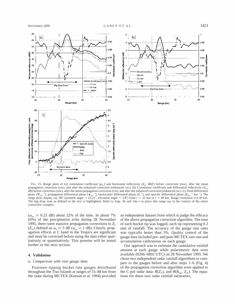
Results of the polarization radar versus gauge cu-mulative rainfall comparison before and after the ap-plication of the empirical propagation correction methodwith large drop adjustment are shown in Figs. 16a and16b, respectively. The NB and NSE for the uncorrectedand corrected cumulative R(Zh) and R(Kdp, Zdr) relativeto the rain gauges are summarized in Tables 3 and 4,respectively.
Before propagation correction, the scatter between thepolarization radar and gauge cumulative rainfallamounts is very large (Fig. 16a). This scatter is reflectedin very large NSEs of 74% and 83% for uncorrectedR(Zh) and R(Kdp, Zdr), respectively. As expected, the un-corrected cumulative R(Zh) significantly underestimatedthe rain gauge totals (NB 5 256%). Since the differ-ential reflectivity is lowered from its intrinsic value bydifferential attenuation and R is inversely proportionalto Zdr [e.g., (18)], the overestimation (NB 5 112%) ofthe uncorrected cumulative R(Kdp, Zdr) is consistent withtheoretical expectations.
After the propagation correction algorithm summa-rized in Fig. 4 is applied to Zh and Zdr, the scatter be-tween the radar and gauge cumulative rainfall totals is
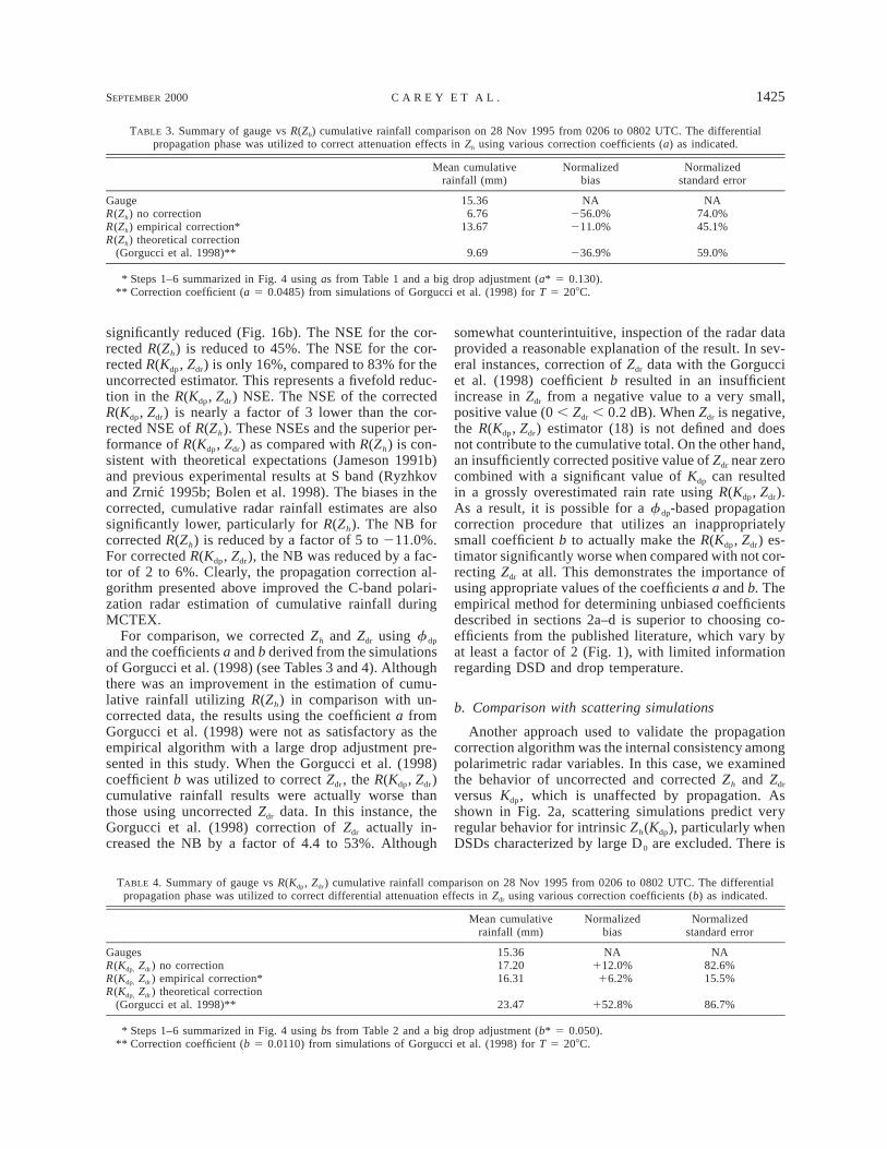
SEPTEMBER 2000 1425C A R E Y E T A L .
TABLE 3. Summary of gauge vs R(Zh) cumulative rainfall comparison on 28 Nov 1995 from 0206 to 0802 UTC. The differentialpropagation phase was utilized to correct attenuation effects in Zh using various correction coefficients (a) as indicated.
Mean cumulativerainfall (mm)
Normalizedbias
Normalizedstandard error
GaugeR(Zh) no correctionR(Zh) empirical correction*R(Zh) theoretical correction
(Gorgucci et al. 1998)**
15.366.76
13.67
9.69
NA256.0%211.0%
236.9%
NA74.0%45.1%
59.0%
* Steps 1–6 summarized in Fig. 4 using as from Table 1 and a big drop adjustment (a* 5 0.130).** Correction coefficient (a 5 0.0485) from simulations of Gorgucci et al. (1998) for T 5 208C.
TABLE 4. Summary of gauge vs R(Kdp, Zdr) cumulative rainfall comparison on 28 Nov 1995 from 0206 to 0802 UTC. The differentialpropagation phase was utilized to correct differential attenuation effects in Zdr using various correction coefficients (b) as indicated.
Mean cumulativerainfall (mm)
Normalizedbias
Normalizedstandard error
GaugesR(Kdp, Zdr) no correctionR(Kdp, Zdr) empirical correction*R(Kdp, Zdr) theoretical correction
(Gorgucci et al. 1998)**
15.3617.2016.31
23.47
NA112.0%16.2%
152.8%
NA82.6%15.5%
86.7%
* Steps 1–6 summarized in Fig. 4 using bs from Table 2 and a big drop adjustment (b* 5 0.050).** Correction coefficient (b 5 0.0110) from simulations of Gorgucci et al. (1998) for T 5 208C.
significantly reduced (Fig. 16b). The NSE for the cor-rected R(Zh) is reduced to 45%. The NSE for the cor-rected R(Kdp, Zdr) is only 16%, compared to 83% for theuncorrected estimator. This represents a fivefold reduc-tion in the R(Kdp, Zdr) NSE. The NSE of the correctedR(Kdp, Zdr) is nearly a factor of 3 lower than the cor-rected NSE of R(Zh). These NSEs and the superior per-formance of R(Kdp, Zdr) as compared with R(Zh) is con-sistent with theoretical expectations (Jameson 1991b)and previous experimental results at S band (Ryzhkovand Zrnic 1995b; Bolen et al. 1998). The biases in thecorrected, cumulative radar rainfall estimates are alsosignificantly lower, particularly for R(Zh). The NB forcorrected R(Zh) is reduced by a factor of 5 to 211.0%.For corrected R(Kdp, Zdr), the NB was reduced by a fac-tor of 2 to 6%. Clearly, the propagation correction al-gorithm presented above improved the C-band polari-zation radar estimation of cumulative rainfall duringMCTEX.
For comparison, we corrected Zh and Zdr using f dp
and the coefficients a and b derived from the simulationsof Gorgucci et al. (1998) (see Tables 3 and 4). Althoughthere was an improvement in the estimation of cumu-lative rainfall utilizing R(Zh) in comparison with un-corrected data, the results using the coefficient a fromGorgucci et al. (1998) were not as satisfactory as theempirical algorithm with a large drop adjustment pre-sented in this study. When the Gorgucci et al. (1998)coefficient b was utilized to correct Zdr, the R(Kdp, Zdr)cumulative rainfall results were actually worse thanthose using uncorrected Zdr data. In this instance, theGorgucci et al. (1998) correction of Zdr actually in-creased the NB by a factor of 4.4 to 53%. Although
somewhat counterintuitive, inspection of the radar dataprovided a reasonable explanation of the result. In sev-eral instances, correction of Zdr data with the Gorgucciet al. (1998) coefficient b resulted in an insufficientincrease in Zdr from a negative value to a very small,positive value (0 , Zdr , 0.2 dB). When Zdr is negative,the R(Kdp, Zdr) estimator (18) is not defined and doesnot contribute to the cumulative total. On the other hand,an insufficiently corrected positive value of Zdr near zerocombined with a significant value of Kdp can resultedin a grossly overestimated rain rate using R(Kdp, Zdr).As a result, it is possible for a f dp-based propagationcorrection procedure that utilizes an inappropriatelysmall coefficient b to actually make the R(Kdp, Zdr) es-timator significantly worse when compared with not cor-recting Zdr at all. This demonstrates the importance ofusing appropriate values of the coefficients a and b. Theempirical method for determining unbiased coefficientsdescribed in sections 2a–d is superior to choosing co-efficients from the published literature, which vary byat least a factor of 2 (Fig. 1), with limited informationregarding DSD and drop temperature.
b. Comparison with scattering simulations
Another approach used to validate the propagationcorrection algorithm was the internal consistency amongpolarimetric radar variables. In this case, we examinedthe behavior of uncorrected and corrected Zh and Zdr
versus Kdp, which is unaffected by propagation. Asshown in Fig. 2a, scattering simulations predict veryregular behavior for intrinsic Zh(Kdp), particularly whenDSDs characterized by large D0 are excluded. There is
1426 VOLUME 39J O U R N A L O F A P P L I E D M E T E O R O L O G Y
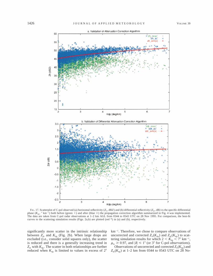
FIG. 17. Scatterplot of C-pol observed (a) horizontal reflectivity (Zh, dBZ ) and (b) differential reflectivity (Zdr, dB) vs the specific differentialphase (Kdp, 8 km21) both before (green 1) and after (blue 3) the propagation correction algorithm summarized in Fig. 4 was implemented.The data are taken from C-pol radar observations at 1–2 km AGL from 0344 to 0543 UTC on 28 Nov 1995. For comparison, the best-fitcurves to the scattering simulation results (Figs. 2a,b) are plotted (red *) in (a) and (b), respectively.
significantly more scatter in the intrinsic relationshipbetween Zdr and Kdp (Fig. 2b). When large drops areexcluded (i.e., consider solid squares only), the scatteris reduced and there is a generally increasing trend inZdr with Kdp. The scatter in both relationships are furtherreduced when Kdp is limited to values in excess of 28
km21. Therefore, we chose to compare observations ofuncorrected and corrected Zh(Kdp) and Zdr(Kdp) to scat-tering simulation results for which 2 , Kdp , 78 km21,rhv $ 0.97, and |d| # 18 (or 38 for C-pol observations).
Observations of uncorrected and corrected Zh(Kdp) andZdr(Kdp) at 1–2 km from 0344 to 0543 UTC on 28 No-
SEPTEMBER 2000 1427C A R E Y E T A L .
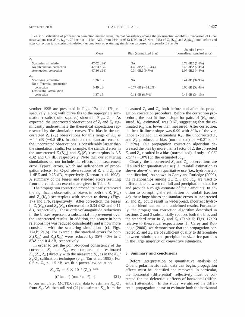
TABLE 5. Validation of propagation correction method using internal consistency among the polarimetric variables. Comparison of C-polobservations (for 28 , Kdp , 78 km21 at 1–2 km AGL from 0344 to 0543 UTC on 28 Nov 1995) of Zh (Kdp) and Zdr(Kdp) both before andafter correction to scattering simulation (assumptions of scattering simulation discussed in appendix B) results.
Mean Bias (normalized bias)Standard error
(normalized standard error)
Zh
Scattering simulationNo attenuation correctionAttenuation correction
47.02 dBZ42.63 dBZ47.36 dBZ
NA24.40 dBZ (29.4%)
0.34 dBZ (0.7%)
0.78 dBZ (1.6%)3.46 dBZ (7.4%)2.07 dBZ (4.4%)
Zdr
Scattering simulationNo differential attenuation
correctionDifferential attenuation
correction
1.26 dB
0.49 dB
1.37 dB
NA
20.77 dB (261.2%)
0.11 dB (8.7%)
0.44 dB (34.9%)
0.66 dB (52.4%)
0.43 dB (34.1%)
vember 1995 are presented in Figs. 17a and 17b, re-spectively, along with curve fits to the appropriate sim-ulation results (solid squares) shown in Figs. 2a,b. Asexpected, the uncorrected observations of Zh and Zdr sig-nificantly underestimate the theoretical expectation rep-resented by the simulation curves. The bias in the un-corrected Zh (Zdr) observations for this range of Kdp is24.4 dB (20.8 dB). In addition, the standard error ofthe uncorrected observations is considerably larger thanthe simulation results. For example, the standard error inthe uncorrected Zh(Kdp) and Zdr(Kdp) scatterplots is 3.5dBZ and 0.7 dB, respectively. Note that our scatteringsimulations do not include the effects of measurementerror. Typical errors, which are independent of propa-gation effects, for C-pol observations of Zh and Zdr are1 dBZ and 0.25 dB, respectively (Keenan et al. 1998).A summary of the biases and standard errors resultingfrom the validation exercise are given in Table 5.
The propagation correction procedure nearly removedthe significant observational biases in both the Zh(Kdp)and Zdr(Kdp) scatterplots with respect to theory (Figs.17a and 17b, respectively). After correction, the biasesin Zh(Kdp) and Zdr(Kdp) decreased to 0.34 dBZ and 0.11dB, respectively. These order-of-magnitude reductionsin the biases represent a substantial improvement overthe uncorrected results. In addition, the scatter in bothrelationships was reduced considerably and is now moreconsistent with the scattering simulations (cf. Figs.17a,b; 2a,b). For example, the standard errors for bothZh(Kdp) and Zdr(Kdp) were reduced by 35%–40% to 2dBZ and 0.4 dB, respectively.
In order to test the point-to-point consistency of thecorrected Zh and Zdr, we compared the estimatedKdp(Zh, Zdr) directly with the measured Kdp as in the Kdp/Zdr/Zh calibration technique (e.g., Tan et al. 1995). For0.5 # Zdr # 1.5 dB, we fit a power-law equation
Kdp/Zh 5 6 3 1025 (Zdr)20.636
[(8 km21) (mm6 m23)21] (21)
to our simulated MCTEX radar data to estimate Kdp/Zh
from Zdr. We then utilized (21) to estimate Kdp from the
measured Zh and Zdr both before and after the propa-gation correction procedure. Before the correction pro-cedure, the best-fit linear slope for pairs of (Kdp mea-sured, Kdp estimated) was 0.67, suggesting that the es-timated Kdp was lower than measured. After correction,the best-fit linear slope was 0.99 with 80% of the var-iance explained. In estimating Kdp, the uncorrected Zh
and Zdr produced a bias (normalized) of 20.28 km21
(225%). Our propagation correction algorithm de-creased the bias by more than a factor of 2; the correctedZh and Zdr resulted in a bias (normalized) of only 20.088km21 (210%) in the estimated Kdp.
Clearly, the uncorrected Zh and Zdr observations areill suited for quantitative use (i.e., rainfall estimation asshown above) or even qualitative use (i.e., hydrometeoridentification). As shown in Carey and Rutledge (2000),the relationships among Zh, Zdr, and Kdp are used todifferentiate between rainfall and precipitation-sized iceand provide a rough estimate of their amounts. In ad-dition to corrupting the estimation of rainfall (section4a), these huge biases and standard errors in uncorrectedZh and Zdr could result in widespread, incorrect hydro-meteor identifications and undefined results. Fortunate-ly, the propagation correction algorithm described insections 2 and 3 substantially reduces both the bias andthe standard error in Zh and Zdr (Table 5; Figs. 17a,b)relative to theoretical expectations. In Carey and Rut-ledge (2000), we demonstrate that the propagation-cor-rected Zh and Zdr are of sufficient quality to differentiatebetween raindrops and precipitation-sized ice particlesin the large majority of convective situations.
5. Summary and conclusions
Before interpretation or quantitative analysis ofC-band polarimetric radar data can begin, propagationeffects must be identified and removed. In particular,the horizontal (differential) reflectivity must be cor-rected for the deleterious effects of horizontal (differ-ential) attenuation. In this study, we utilized the differ-ential propagation phase to estimate both the horizontal
1428 VOLUME 39J O U R N A L O F A P P L I E D M E T E O R O L O G Y
and differential attenuation at C band. This phase-basedapproach has several advantages over traditional power-based algorithms. The specific differential phase 1) isimmune to power calibration errors (e.g., Zrnic andRyzhkov 1996), 2) is not adversely affected by atten-uation (e.g., Zrnic and Ryzhkov 1996), and yet 3) isapproximately linearly proportional to both the specifichorizontal and differential attenuation (e.g., Bringi et al.1990).
The relationship between Ah or Ahv and Kdp is depen-dent on temperature, DSD, and the drop shape versussize relationship (e.g., Bringi et al. 1990; Jameson1991a, 1992; KCZM). As a result, the calculated valuesof Ah and Ahv for a specific Kdp vary by a factor of 2 ormore for relevant precipitation characteristics in pub-lished scattering simulations (see Fig. 1). Without spe-cific information on DSD, temperature, and drop shapethroughout each radar echo volume, an unbiased esti-mate of a 5 Ah/Kdp and b 5 Ahv/Kdp cannot be chosenfrom these published simulations. Therefore, we adaptedand modified the empirical approach of Ryzhkov andZrnic (1995a) to estimate unbiased correction coeffi-cients a and b for each radar volume.
The coefficients a and b are estimated from the ob-served decreasing trends of Zh and Zdr, respectively, withf dp. A least squares regression technique was appliedto observed data to estimate the linear slope of this trend.The theoretical basis for this procedure was reviewedand the regression method was presented and tested us-ing C-pol radar observations taken during MCTEX. Inorder to extract the effects of propagation, the intrinsicvariations in Zh and Zdr must be minimized. As in Ryzh-kov and Zrnic (1995a), we utilized a specific range ofKdp to mitigate intrinsic differences in Zh and Zdr. How-ever, we found it also necessary to use rhv, d, and heightto restrict the sample from which a and b were esti-mated. These polarimetric radar thresholds were chosenusing scattering simulation results as a guide. Tropicaldrop-size distributions observed during MCTEX wereused as input for these scattering simulations. Statisticalprocedures to minimize biases in the inferred coeffi-cients a and b were proposed and demonstrated. Last,a mechanism to test the representativeness of the esti-mated correction coefficients was presented.
During the mature phase of a tropical convective sys-tem on 28 November 1995, the empirical regressiontechnique reliably produced statistically acceptable cor-rection coefficients. The temporal behavior of the di-agnosed correction coefficients was stable and consis-tent with theory. Systematic and simultaneous changesin the correction coefficients were coincident with sys-tematic changes in convective morphology (i.e., stormmaturation) and hence DSD (i.e., decrease in Zdr andD0). These changes in DSD were then reflected in theexpected shift in the correction coefficients (i.e., a in-creased and b decreased).
The range of empirically estimated coefficients wasgenerally consistent with theoretical expectations. How-
ever, the coefficients a and b determined from priorscattering simulations tended to be 10%–30% lowerthan the empirical results from MCTEX. When consid-ering appropriate temperatures (108 , T , 258C) fortropical rainfall at 0.5 to 2 km AGL, the empiricallyinferred coefficients from MCTEX are 1.5–2 times larg-er than prior scattering simulations. This significant dis-crepancy between observations and theory at C band inthe Tropics is similar to midlatitude results at S bandby Ryzhkov and Zrnic (1994, 1995a) and Smyth andIllingworth (1998).
Using scattering simulations, we demonstrated that a(Ah/Kdp) and b (Ahv/Kdp) are sensitive functions of thedrop size if large raindrops are present. For small tomoderate values of Zdr (0.5–2 dB), the coefficients a andb are relatively insensitive to drop size. For Zdr . 2 dB,the coefficients a and b increase rapidly as a functionof Zdr. As a result, the value of a (b) for large drops(e.g., Zdr 5 4 dB) is a factor of 2 (4) times larger thanthe coefficient for small- to moderate-sized drops. Thereare two implications for this large drop sensitivity: 1)as also determined by Ryzhkov and Zrnic (1994, 1995a)and Smyth and Illingworth (1998), the presence of largedrops can bias the mean coefficients higher than priorscattering simulations (e.g., Bringi et al. 1990); and 2)the standard error for corrected Zh and Zdr in precipi-tation downrange from large drop cores can be signif-icantly larger than predicted by Bringi et al. (1990) ifthe mean coefficients are utilized. Because in situ andradar observations during MCTEX confirmed the pres-ence of large raindrops in tropical convection, theseeffects were deemed to be significant. The mean em-pirical method automatically eliminates any bias causedby the presence of large drops because no assumptionsregarding DSD are made. Without some extension tothis procedure however, the error down range from bigdrop cores was unacceptably large.
To minimize this error, we proposed the use of en-hanced correction coefficients in so-called big dropzones. The enhanced correction coefficients a* and b*were determined from scattering simulations of largedrops and were confirmed by a limited application ofthe empirical regression technique in large drop zones.To locate large drop zones (D0 . 2.5 mm) in the ob-served C-band data, we searched for dips in rhv accom-panied by significant perturbations in d caused by Mieresonance effects. The method was demonstrated on ob-servations of intense MCTEX convection containing aclear-cut example of enhanced propagation effects downrange from big drop cores. The big drop correction sig-nificantly improved the qualitative results of the cor-rection procedure.
To validate the overall propagation correction algo-rithm utilizing the differential propagation phase, cu-mulative rain gauge amounts were compared with cu-mulative radar rainfall estimates using R(Zh) andR(Kdp, Zdr) before and after correction. The correctionprocedure significantly reduced both the bias and stan-
SEPTEMBER 2000 1429C A R E Y E T A L .
dard error of both cumulative radar rainfall estimates towithin expected ranges given typical measurement er-rors other than propagation. To verify further the pro-cedure, we compared the behavior of Zh and Zdr withKdp both before and after correction to theoretical ex-pectations generated with scattering simulations. Theuncorrected Zh(Kdp) and Zdr(Kdp) significantly underes-timated the simulation results. The correction procedurereduced these negative biases by nearly an order of mag-nitude and substantially reduced the standard error ofthe observations relative to scattering simulations. Fi-nally, we compared the estimated Kdp(Zh, Zdr) to themeasured Kdp. The propagation correction algorithm re-duced the bias in the estimated mean Kdp(Zh, Zdr) by afactor of 2.5 to only 210% (20.088 km21). This vali-dation result provides additional confidence in the mu-tual consistency between the corrected Zh and Zdr.
Given these validation results, we proceeded to qual-itatively interpret and quantitatively analyze the prop-agation corrected Zh and Zdr with confidence in Careyand Rutledge (2000). The repeated correlation betweenradar-inferred precipitation characteristics and cloudelectrification and lightning demonstrated in Carey andRutledge (2000) provide additional indirect support forour propagation correction algorithm. Because the pro-cedure was only tested on three case studies duringMCTEX, continued testing of the procedure on othercase studies and with other C-band radars would bebeneficial. Moreover, a long-term, quantitative study inan operational setting on a large amount of data wouldbe required to determine if the algorithm could be im-plemented reliably on an operational radar.
Because many radar meteorologists utilize precipi-tation radar wavelengths other than C band (e.g., S bandand X band), a few words regarding the application ofthis correction algorithm to other wavelengths is war-ranted. Given the modeling studies of Bringi et al.(1990) and Jameson (1991a, 1992) and the empiricalresults of Ryzhkov and Zrnic (1995a), we are confidentthat the mean correction coefficients can be determinedat X band and S band using empirical regression tech-niques similar to those used in this study. The correctiontechnique is sensitive to fluctuations in the DSD at bothS band (Bringi et al. 1990) and X band (Bringi et al.1990; Jameson 1991a). Therefore a big drop correctionis warranted at these wavelengths too. At X band, thebackscatter differential phase is large and measurablein large drop cores. Assuming the iterative filtering tech-nique of Hubbert and Bringi (1995) can accurately es-timate significant values of the backscatter phase (e.g.,d . 38) at X band, large drop cores should be identifiableand a large drop correction could be applied. Giventypical radar performance, rhv and LDR would not de-viate measurably in rain, even for large drops at X band.At S band, the same is true for d, rhv, and LDR. There-fore, the identification of large drop cores at S band iscomplicated compared to C and X bands. We suggestusing the propagation-affected Zdr and Zh for identifying
large drop cores at S band. Because the overall prop-agation effects are less at S band in comparison withlower wavelengths, we believe that most large dropcores should still be identifiable from the uncorrectedZh and Zdr at S band.
Acknowledgments. We wish to thank Mr. Ken Glassonof the Bureau of Meteorology Research Centre for hissuperlative engineering work in developing and de-ploying the C-pol radar for the Maritime ContinentThunderstorm Experiment. We also thank Mr. John Lutzand Dr. Jeffrey Keeler of the National Center for At-mospheric Research for their efforts in improving theperformance of the C-pol radar. We acknowledge Dr.Tsutomu Takahashi for providing the analyzed video-sonde data. The support of the Tiwi Land Council inundertaking MCTEX is acknowledged. We would liketo recognize helpful discussions regarding propagationeffects in polarimetric radar data with Drs. Peter May,Dusan Zrnic, V. N. Bringi, and Anthony Illingworth.This research was supported by NASA TRMM GrantsNAG 5-2692 and NAG5-4754 and NSF Grant ATM-9726464.
APPENDIX A
Polarimetric Radar Data Processing
Before analyzing any C-pol radar observations, alldata were carefully edited using the Research Data Sup-port System (RDSS) software developed at the NationalCenter for Atmospheric Research (NCAR) (Oye andCarbone 1981). First, all polarimetric radar data (Zh,Zdr, Cdp, and rhv) at range gates characterized by rhv ,0.7 were removed. This rhv thresholding technique re-moves range gates in which the returned power is dom-inated by unacceptably low signal-to-noise ratios or byground clutter (Ryzhkov and Zrnic 1998b). Any re-maining ground clutter was manually removed since ithas a deleterious effect on the quality of polarimetricradar measurements at low elevation angles. Spuriousvalues of horizontal reflectivity and differential reflec-tivity caused by three-body scattering effects (Zrnic1987; Hubbert and Bringi 1997) were removed manu-ally. In regions of large reflectivity gradients, antennapattern–induced errors can bias the estimates of Zdr, rhv,and to a lesser extent Cdp (Pointin et al. 1988). In orderto remove spurious data, we manually examined all re-gions of large =Zh (.20 dBZ km21) in azimuth andelevation and deleted the data if it appeared suspect.During MCTEX, the C-pol differential phase data wererecorded between 2328 and 1328 with folding occur-ring for values outside of these bounds (Keenan et al.1998). A dealiasing algorithm in the RDSS softwarepackage was used to unfold the Cdp data. Next, thehorizontal reflectivity data at low elevation angles (,48)were corrected for partial beam blocking according tothe procedure described in May et al. (1999). We then
1430 VOLUME 39J O U R N A L O F A P P L I E D M E T E O R O L O G Y
removed the bias in Zdr of 10.1 dB as determined froma vertically pointing scan in stratiform precipitation on29 November 95 (Keenan et al. 1998).
Because the differential phase at C band is a com-bination of both the backscatter differential phase,which can be significant at C band (e.g., Bringi et al.1990, 1991; Aydin and Giridhar 1992), and the (for-ward) propagation differential phase, it was necessaryto apply an iterative filtering technique (Hubbert andBringi 1995) to the differential phase data. We utilizeda 13-point (over 3.9 km) running mean filter. The it-erative application of this filter was designed to removegate-to-gate fluctuations caused by significant d or sys-tem phase noise while preserving the physically mean-ingful trends caused by f dp. The specific differentialphase was then calculated from the filtered differentialphase using a finite differencing approximation accord-ing to (4). The accuracy or standard deviation of Kdp
can be estimated from the expression given by Balak-rishnan and Zrnic (1990)
Ï3sdps 5 , (A1)Kdp 3/2N Dr
where sdp is the standard deviation of the differentialphase, N is the number of range gates in the filter, andDr is the range gate spacing. Given a standard deviationof the differential phase of about 38–48 (Keenan et al.1998), 13 points in the filter, and a range gate spacingof 0.3 km, the accuracy of Kdp is estimated as 0.4–0.58km21. For the dwell times used in this study (128 sam-ples and azimuthal rotation rates from 68 to 88 s21),typical standard errors of measurement for the othervariables are: 1 dBZ for Zh, 0.25 dB for Zdr, and 0.01for rhv (Keenan et al. 1998).
Some analysis applications in this study required grid-ded Cartesian radar data. Therefore, we interpolated allpolarimetric radar variables to a Cartesian grid usingthe NCAR REORDER software package (Mohr 1986).The grid was centered on the Tiwi Islands with a hor-izontal and vertical spacing of 1.0 and 0.5 km, respec-tively. Variable radii of influence consistent with thescanning strategies during MCTEX (Keenan et al. 1994)were utilized in order to maximize the resolution of thedata in range from the radar. The radius of influence inthe azimuthal (elevational) direction was 1.28 (28). Inrange, the radius of influence was equal to the productof the range and the azimuthal radius of influence inradians.
APPENDIX B
Scattering Simulations of C-Band PolarimetricRadar Parameters in Rain
During MCTEX, a Joss and Waldvogel (1967) dis-drometer collected raindrop size distribution informa-tion as described in Keenan et al. (1999). The disdro-meter data were fit to gamma drop size distributions
according to Ulbrich (1983). As discussed in KCZM,empirical linear relationships between the gamma DSDparameters were determined. The empirical relationswere then used to obtain physically realistic domainsfor the fitted gamma DSD parameters that were used asinput to the T-matrix (Barber and Yeh 1975) scatteringsimulations of rainfall at C band (5.33 cm).
In the T-matrix scattering simulations, raindrops weremodeled as oblate spheroids with a shape versus sizerelationship defined by Green (1975). The dielectric ofwater was obtained from Ray (1972) using a temperatureof 208C, consistent with typical wet-bulb temperaturesnear the surface over the Tiwi Islands as analyzed fromsounding data during MCTEX. Based on in situ andradar observations of large drops during MCTEX andprior evidence for the presence of large drops in tropicalconvection (reference summary in appendix C), themaximum drop diameter Dmax was set at 8 mm and themedian volume diameter D0 was allowed to vary from0.8 to 5 mm. As discussed above, the other DSD pa-rameters (N0, m) of a gamma distribution were variedaccording to empirical relationships determined byKCZM.
Using the resulting T matrices as input to a Mueller-matrix scattering model (e.g., Vivekanandan et al.1991), C-band backscatter and propagation character-istics as described by various polarimetric radar param-eters (Zh, Zdr, Kdp, d, rhv, Ah, and Ahv) were simulated.Following Vivekanandan et al. (1991), hydrometeorcanting angle and radar elevation angle effects wereconsidered. Rainfall orientation distributions were mod-eled by a quasi-Gaussian distribution (e.g., Vivekan-andan et al. 1991) with a mean of zero and a standarddeviation of 58. For the results in this study, the sim-ulated radar elevation angle was held fixed in a plane0.58 above the local surface.
APPENDIX C
In situ and Radar Evidence ofLarge Drops during MCTEX
Before offering observational evidence supportingthe presence of large (i.e., D . 3 mm) drops in thetropical island convection observed during MCTEX, itis important to review some potential hypotheses fortheir production. In tropical maritime air masses, thepresence of exceptionally large aerosol particles actingas nuclei for drops near cloud base may allow drops toreach giant size (5–8 mm) as they accrete smaller drops(e.g., Johnson 1982; Rauber et al. 1991; Szumowski etal. 1999). Alternatively in the Tropics, an active coa-lescence process in a cloud environment nearly devoidof smaller raindrops, hence limiting collisional breakup,but rich in cloud liquid water can result in large dropproduction (e.g., Rauber et al. 1991; Szumowski et al.1998). Although it is beyond the scope of this study toinvestigate these hypotheses further, it is possible that
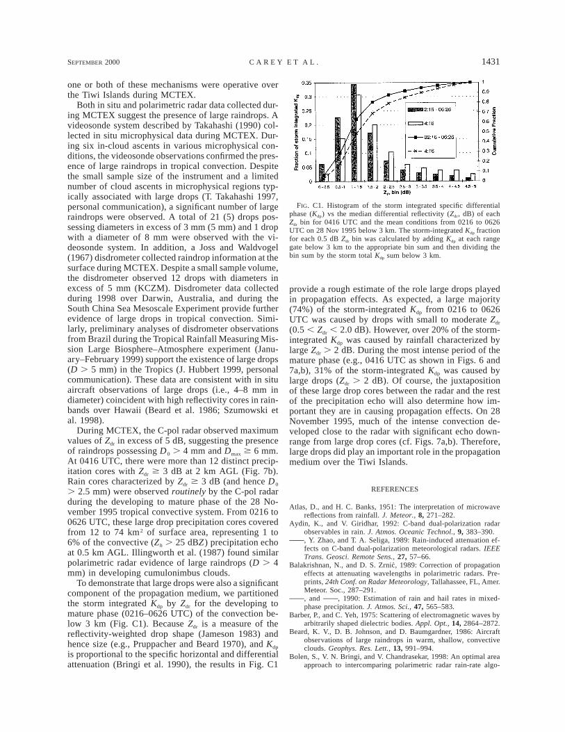
SEPTEMBER 2000 1431C A R E Y E T A L .
FIG. C1. Histogram of the storm integrated specific differentialphase (Kdp) vs the median differential reflectivity (Zdr, dB) of eachZdr bin for 0416 UTC and the mean conditions from 0216 to 0626UTC on 28 Nov 1995 below 3 km. The storm-integrated Kdp fractionfor each 0.5 dB Zdr bin was calculated by adding Kdp at each rangegate below 3 km to the appropriate bin sum and then dividing thebin sum by the storm total Kdp sum below 3 km.
one or both of these mechanisms were operative overthe Tiwi Islands during MCTEX.
Both in situ and polarimetric radar data collected dur-ing MCTEX suggest the presence of large raindrops. Avideosonde system described by Takahashi (1990) col-lected in situ microphysical data during MCTEX. Dur-ing six in-cloud ascents in various microphysical con-ditions, the videosonde observations confirmed the pres-ence of large raindrops in tropical convection. Despitethe small sample size of the instrument and a limitednumber of cloud ascents in microphysical regions typ-ically associated with large drops (T. Takahashi 1997,personal communication), a significant number of largeraindrops were observed. A total of 21 (5) drops pos-sessing diameters in excess of 3 mm (5 mm) and 1 dropwith a diameter of 8 mm were observed with the vi-deosonde system. In addition, a Joss and Waldvogel(1967) disdrometer collected raindrop information at thesurface during MCTEX. Despite a small sample volume,the disdrometer observed 12 drops with diameters inexcess of 5 mm (KCZM). Disdrometer data collectedduring 1998 over Darwin, Australia, and during theSouth China Sea Mesoscale Experiment provide furtherevidence of large drops in tropical convection. Simi-larly, preliminary analyses of disdrometer observationsfrom Brazil during the Tropical Rainfall Measuring Mis-sion Large Biosphere–Atmosphere experiment (Janu-ary–February 1999) support the existence of large drops(D . 5 mm) in the Tropics (J. Hubbert 1999, personalcommunication). These data are consistent with in situaircraft observations of large drops (i.e., 4–8 mm indiameter) coincident with high reflectivity cores in rain-bands over Hawaii (Beard et al. 1986; Szumowski etal. 1998).
During MCTEX, the C-pol radar observed maximumvalues of Zdr in excess of 5 dB, suggesting the presenceof raindrops possessing D0 . 4 mm and Dmax $ 6 mm.At 0416 UTC, there were more than 12 distinct precip-itation cores with Zdr $ 3 dB at 2 km AGL (Fig. 7b).Rain cores characterized by Zdr $ 3 dB (and hence D0
. 2.5 mm) were observed routinely by the C-pol radarduring the developing to mature phase of the 28 No-vember 1995 tropical convective system. From 0216 to0626 UTC, these large drop precipitation cores coveredfrom 12 to 74 km2 of surface area, representing 1 to6% of the convective (Zh . 25 dBZ) precipitation echoat 0.5 km AGL. Illingworth et al. (1987) found similarpolarimetric radar evidence of large raindrops (D . 4mm) in developing cumulonimbus clouds.
To demonstrate that large drops were also a significantcomponent of the propagation medium, we partitionedthe storm integrated Kdp by Zdr for the developing tomature phase (0216–0626 UTC) of the convection be-low 3 km (Fig. C1). Because Zdr is a measure of thereflectivity-weighted drop shape (Jameson 1983) andhence size (e.g., Pruppacher and Beard 1970), and Kdp
is proportional to the specific horizontal and differentialattenuation (Bringi et al. 1990), the results in Fig. C1
provide a rough estimate of the role large drops playedin propagation effects. As expected, a large majority(74%) of the storm-integrated Kdp from 0216 to 0626UTC was caused by drops with small to moderate Zdr
(0.5 , Zdr , 2.0 dB). However, over 20% of the storm-integrated Kdp was caused by rainfall characterized bylarge Zdr . 2 dB. During the most intense period of themature phase (e.g., 0416 UTC as shown in Figs. 6 and7a,b), 31% of the storm-integrated Kdp was caused bylarge drops (Zdr . 2 dB). Of course, the juxtapositionof these large drop cores between the radar and the restof the precipitation echo will also determine how im-portant they are in causing propagation effects. On 28November 1995, much of the intense convection de-veloped close to the radar with significant echo down-range from large drop cores (cf. Figs. 7a,b). Therefore,large drops did play an important role in the propagationmedium over the Tiwi Islands.
REFERENCES
Atlas, D., and H. C. Banks, 1951: The interpretation of microwavereflections from rainfall. J. Meteor., 8, 271–282.
Aydin, K., and V. Giridhar, 1992: C-band dual-polarization radarobservables in rain. J. Atmos. Oceanic Technol., 9, 383–390., Y. Zhao, and T. A. Seliga, 1989: Rain-induced attenuation ef-fects on C-band dual-polarization meteorological radars. IEEETrans. Geosci. Remote Sens., 27, 57–66.
Balakrishnan, N., and D. S. Zrnic, 1989: Correction of propagationeffects at attenuating wavelengths in polarimetric radars. Pre-prints, 24th Conf. on Radar Meteorology, Tallahassee, FL, Amer.Meteor. Soc., 287–291., and , 1990: Estimation of rain and hail rates in mixed-phase precipitation. J. Atmos. Sci., 47, 565–583.
Barber, P., and C. Yeh, 1975: Scattering of electromagnetic waves byarbitrarily shaped dielectric bodies. Appl. Opt., 14, 2864–2872.
Beard, K. V., D. B. Johnson, and D. Baumgardner, 1986: Aircraftobservations of large raindrops in warm, shallow, convectiveclouds. Geophys. Res. Lett., 13, 991–994.
Bolen, S., V. N. Bringi, and V. Chandrasekar, 1998: An optimal areaapproach to intercomparing polarimetric radar rain-rate algo-
1432 VOLUME 39J O U R N A L O F A P P L I E D M E T E O R O L O G Y
rithms with gauge data. J. Atmos. Oceanic Technol., 15, 605–623.
Bringi, V. N., and A. Hendry, 1990: Technology of polarization di-versity radars for meteorology. Radar in Meteorology: BattanMemorial and 40th Anniversary Radar Meteorology Conference,D. Atlas, Ed., Amer. Meteor. Soc., 153–190., V. Chandrasekar, N. Balakrishnan, and D. S. Zrnic, 1990: Anexamination of propagation effects in rainfall on radar mea-surements at microwave frequencies. J. Atmos. Oceanic Tech-nol., 7, 829–840., , P. Meischner, J. Hubbert, and Y. Golestani, 1991: Po-larimetric radar signatures of precipitation at S- and C-bands.IEE Proc. F, 138, 109–119.
Carey, L. D., 1999: On the relationship between precipitation andlightning as revealed by multiparameter radar observations.Ph.D. dissertation, Colorado State University, 238 pp., and S. A. Rutledge, 2000: The relationship between precipi-tation and lightning in tropical island convection: A C-band po-larimetric radar study. Mon. Wea. Rev., 128, 2687–2710.
Gorgucci, E., G. Scarchilli, and V. Chandrasekar, 1996: Error structureof radar rainfall measurement at C-band frequencies with dualpolarization algorithm for attenuation correction. J. Geophys.Res., 101, 26 461–26 472., , , P. F. Meischner, and M. Hagen, 1998: Intercom-parison of techniques to correct for attenuation of C-band weath-er radar signals. J. Appl. Meteor., 37, 845–853.
Green, A. W., 1975: An approximation for the shape of large rain-drops. J. Appl. Meteor., 14, 1578–1583.
Gunn, K. L. S., and T. W. R. East, 1954: The microwave propertiesof precipitation particles. Quart. J. Roy. Meteor. Soc., 80, 522–545.
Hildebrand, P. H., 1978: Iterative correction for attenuation of 5 cmradar in rain. J. Appl. Meteor., 17, 508–514.
Hitschfeld, W., and J. Bordan, 1954: Errors inherent in the radarmeasurement of rainfall at attenuating wavelengths. J. Meteor.,11, 58–67.
Holt, A. R., 1988: Extraction of differential propagation phase fromdata from S-band circularly polarized radars. Electron. Lett., 24,1241–1242.
Hubbert, J., and V. N. Bringi, 1995: An iterative filtering techniquefor the analysis of copolar differential phase and dual-frequencyradar measurements. J. Atmos. Oceanic Technol., 12, 643–648., and , 1997: The effects of 3-body scattering on differentialreflectivity. Preprints, 28th Conf. on Radar Meteorology, Austin,TX, Amer. Meteor. Soc., 11–12., V. Chandrasekar, V. N. Bringi, P. Meischner, 1993: Processingand interpretation of coherent dual-polarized radar measure-ments. J. Atmos. Oceanic Technol., 10, 155–164.
Illingworth, A. J., J. W. Goddard, and S. M. Cherry, 1987: Polarizationradar studies of precipitation development in convective storms.Quart. J. Roy. Meteor. Soc., 113, 469–489.
Jameson, A. R., 1991a: Polarization radar measurements in rain at 5and 9 GHz. J. Appl. Meteor., 30, 1500–1513., 1991b: A comparison of microwave techniques for measuringrainfall. J. Appl. Meteor., 30, 32–54., 1992: The effect of temperature on attenuation-correctionschemes in rain using polarization propagation differential phaseshift. J. Appl. Meteor., 31, 1106–1118., and E. A. Mueller, 1985: Estimation of differential phase shiftfrom sequential orthogonal linear polarization radar measure-ments. J. Atmos. Oceanic Technol., 2, 133–137.
Johnson, B. C., and E. A. Brandes, 1987: Attenuation of a 5-cmwavelength radar signal in the Lahoma–Orienta storms. J. Atmos.Oceanic Technol., 4, 512–517.
Johnson, D. B., 1982: The role of giant and ultragiant aerosol particlesin warm rain initiation. J. Atmos. Sci., 39, 448–460.
Joss, V. J., and A. Waldvogel, 1967: Ein spectograph fur Nieder-schlagstropher mit automatischer auswertung. Pure Appl. Geo-phys., 68, 240–246.
Keenan, T. D., and Coauthors, 1994: Science Plan—Maritime Con-
tinent Thunderstorm Experiment. BMRC Research Rep. 44, 61pp. [Available from Bureau of Meteorology Research Centre,P.O. Box 1289K, Melbourne, Victoria 3001, Australia.], R. Carbone, S. Rutledge, J. Wilson, G. Holland, and P. May,1996: The Maritime Continent Thunderstorm Experiment(MCTEX): Overview and initial results. Preprints, Seventh Conf.on Mesoscale Processes, Reading, United Kingdom, Amer. Me-teor. Soc., 326–328., K. Glasson, F. Cummings, T. S. Bird, J. Keeler, and J. Lutz,1998: The BMRC/NCAR C-band polarimetric (C-POL) radarsystem. J. Atmos. Oceanic Technol., 15, 871–886., L. D. Carey, D. S. Zrnic, and P. T. May, 2000: Sensitivity of5-cm wavelength polarimetric radar variables to raindrop axialratio and drop size distribution. J. Appl. Meteor., in press.
May, P. T., T. D. Keenan, D. S. Zrnic, L. D. Carey, and S. A. Rutledge,1999: Polarimetric radar measurements of tropical rain at a 5-cm wavelength. J. Appl. Meteor., 38, 750–765.
Mohr, C. G., 1986: Merger of mesoscale data sets into a commonCartesian format for efficient and systematic analyses. J. Atmos.Oceanic. Technol., 3, 143–161.
Oguchi, T., 1983: Electromagnetic wave propagation and scatteringin rain and other hydrometeors. IEEE Proc., 71, 1029–1078.
Oye, R., and R. E. Carbone, 1981: Interactive Doppler editing soft-ware. Proc. 20th Conf. on Radar Meteorology, Boston, MA,Amer. Meteor. Soc., 683–689.
Pointin, Y. C., C. Ramond, and J. Fournet-Fayard, 1988: Radar dif-ferential reflectivity Zdr: A real case evaluation of errors inducedby antenna characteristic. J. Atmos. Oceanic Technol., 5, 416–423.
Pruppacher, H. R., and K. V. Beard, 1970: A wind tunnel investigationof the internal circulation and shape of water drops falling atterminal velocity in air. Quart. J. Roy. Meteor. Soc., 96, 247–256.
Rauber, R. M., K. V. Beard, and B. M. Andrews, 1991: A mechanismfor giant raindrop formation in warm, shallow, convectiveclouds. J. Atmos. Sci., 48, 1791–1797.
Ray, P. S., 1972: Broad-band complex refractive indices of ice andwater. Appl. Opt., 11, 1836–1844.
Ryde, J. W., 1946: The attenuation and radar echoes produced atcentimetre wavelengths by various meteorological phenomena.Meteorological Factors in Radio Wave Propagation, PhysicalSociety, 169–189.
Ryzhkov, A. V., and D. S. Zrnic, 1994: Precipitation observed inOklahoma mesoscale convective systems with a polarimetric ra-dar. J. Appl. Meteor., 33, 455–464., and , 1995a: Precipitation and attenuation measurementsat a 10-cm wavelength. J. Appl. Meteor., 34, 2121–2134., and , 1995b: Comparison of dual-polarization radar esti-mators of rain. J. Atmos. Oceanic Technol., 12, 249–256., and , 1996a: Rain in shallow and deep convection mea-sured with a polarimetric radar. J. Atmos. Sci., 53, 2989–2995., and , 1996b: Assessment of rainfall measurement that usesspecific differential phase. J. Appl. Meteor., 35, 2080–2090., and , 1998a: Beamwidth effects on the differential phasemeasurements of rain. J. Atmos. Oceanic Technol., 15, 624–634., and , 1998b: Polarimetric rainfall estimation in the pres-ence of anomalous propagation. J. Atmos. Oceanic Technol., 15,1320–1330., , and D. Atlas, 1997: Polarimetrically tuned R(Z ) relationsand comparisons of radar rainfall methods. J. Appl. Meteor., 36,340–349.
Scarchilli, G., E. Gorgucci, V. Chandrasekar, and T. A. Seliga, 1993:Rainfall estimation using polarimetric techniques at C-band fre-quencies. J. Appl. Meteor., 32, 1150–1160.
Shepherd, G. W., J. Searson, A. Pallot, and C. G. Collier, 1995: Theperformance of a C-band weather radar during a line convectionevent. Meteor. Appl., 2, 65–69.
Smyth, T. J., and A. J. Illingworth, 1998: Correction for attenuationof radar reflectivity using polarisation data. Quart. J. Roy. Me-teor. Soc., 124, 2393–2415.
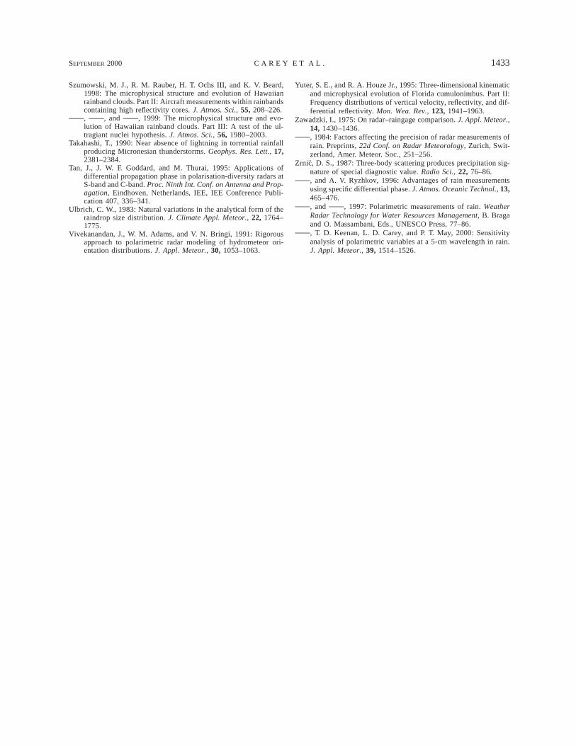
SEPTEMBER 2000 1433C A R E Y E T A L .
Szumowski, M. J., R. M. Rauber, H. T. Ochs III, and K. V. Beard,1998: The microphysical structure and evolution of Hawaiianrainband clouds. Part II: Aircraft measurements within rainbandscontaining high reflectivity cores. J. Atmos. Sci., 55, 208–226., , and , 1999: The microphysical structure and evo-lution of Hawaiian rainband clouds. Part III: A test of the ul-tragiant nuclei hypothesis. J. Atmos. Sci., 56, 1980–2003.
Takahashi, T., 1990: Near absence of lightning in torrential rainfallproducing Micronesian thunderstorms. Geophys. Res. Lett., 17,2381–2384.
Tan, J., J. W. F. Goddard, and M. Thurai, 1995: Applications ofdifferential propagation phase in polarisation-diversity radars atS-band and C-band. Proc. Ninth Int. Conf. on Antenna and Prop-agation, Eindhoven, Netherlands, IEE, IEE Conference Publi-cation 407, 336–341.
Ulbrich, C. W., 1983: Natural variations in the analytical form of theraindrop size distribution. J. Climate Appl. Meteor., 22, 1764–1775.
Vivekanandan, J., W. M. Adams, and V. N. Bringi, 1991: Rigorousapproach to polarimetric radar modeling of hydrometeor ori-entation distributions. J. Appl. Meteor., 30, 1053–1063.
Yuter, S. E., and R. A. Houze Jr., 1995: Three-dimensional kinematicand microphysical evolution of Florida cumulonimbus. Part II:Frequency distributions of vertical velocity, reflectivity, and dif-ferential reflectivity. Mon. Wea. Rev., 123, 1941–1963.
Zawadzki, I., 1975: On radar–raingage comparison. J. Appl. Meteor.,14, 1430–1436., 1984: Factors affecting the precision of radar measurements ofrain. Preprints, 22d Conf. on Radar Meteorology, Zurich, Swit-zerland, Amer. Meteor. Soc., 251–256.
Zrnic, D. S., 1987: Three-body scattering produces precipitation sig-nature of special diagnostic value. Radio Sci., 22, 76–86., and A. V. Ryzhkov, 1996: Advantages of rain measurementsusing specific differential phase. J. Atmos. Oceanic Technol., 13,465–476., and , 1997: Polarimetric measurements of rain. WeatherRadar Technology for Water Resources Management, B. Bragaand O. Massambani, Eds., UNESCO Press, 77–86., T. D. Keenan, L. D. Carey, and P. T. May, 2000: Sensitivityanalysis of polarimetric variables at a 5-cm wavelength in rain.J. Appl. Meteor., 39, 1514–1526.