Copyright by Raymond Edward Lane III 2016 - The University ...
226
Copyright by Raymond Edward Lane III 2016
-
Upload
khangminh22 -
Category
Documents
-
view
2 -
download
0
Transcript of Copyright by Raymond Edward Lane III 2016 - The University ...

Copyright
by
Raymond Edward Lane III
2016
The Thesis Committee for Raymond Edward Lane IIICertifies that this is the approved version of the following thesis:
Modeling and Integration of Steam Accumulators in
Nuclear Steam Supply Systems
APPROVED BY
SUPERVISING COMMITTEE:
Erich Schneider, Supervisor
Sheldon Landsberger

Modeling and Integration of Steam Accumulators in
Nuclear Steam Supply Systems
by
Raymond Edward Lane III, B.S.M.E
THESIS
Presented to the Faculty of the Graduate School of
The University of Texas at Austin
in Partial Fulfillment
of the Requirements
for the Degree of
MASTER OF SCIENCE IN ENGINEERING
THE UNIVERSITY OF TEXAS AT AUSTIN
December 2016

Dedicated to my son Rhys
Acknowledgments
I would like to thank the Nuclear and Radiation Engineering faculty at
the University of Texas at Austin; especially my thesis Supervisor, Dr. Erich
Schneider, whose support and mentorship has driven me to challenge myself
and pursue areas of study that were initially daunting to me. I would also like
to specifically thank Dr. Sheldon Landsberger for championing the distance
learning program and encouraging me to take this journey.
v
Modeling and Integration of Steam Accumulators in
Nuclear Steam Supply Systems
Raymond Edward Lane III, M.S.E.
The University of Texas at Austin, 2016
Supervisor: Erich Schneider
Nuclear power plants in deregulated markets need to leverage thermal
energy storage to take advantage of peak demand pricing to improve their
profitability in an increasingly competitive landscape. Substantial research
has been conducted to integrate steam accumulators into concentrated solar
power plants and they present a viable solution for the commercial nuclear
fleet. Prior work in this field has concentrated mainly on the installation
of separate turbine-generators to generate electricity from the stored thermal
energy. This work demonstrates that the use of stored thermal energy to
augment feedwater heaters and moisture separator reheaters, in lieu of using
separate electrical generating equipment, can result in sizable increases in elec-
trical power production for a significant period of time provided that a suitably
sized main steam turbine, main generator, and support systems are present.
Additionally, a model was constructed using prior work to reliably demonstrate
the time response of an accumulator to charge and discharge operations.
vi
Table of Contents
Acknowledgments v
Abstract vi
List of Tables x
List of Figures xi
Chapter 1. Introduction 1
Chapter 2. Literature Review 4
2.1 Steam Accumulators . . . . . . . . . . . . . . . . . . . . . . . 4
2.2 Approximations in Modeling . . . . . . . . . . . . . . . . . . . 6
2.3 Equilibrium versus Non-equilibrium Models . . . . . . . . . . . 7
2.4 Existing Models . . . . . . . . . . . . . . . . . . . . . . . . . . 8
2.4.1 Steinmann and Eck . . . . . . . . . . . . . . . . . . . . 8
2.4.2 Schnaider et al. . . . . . . . . . . . . . . . . . . . . . . . 11
2.4.3 Stevanovic et al. . . . . . . . . . . . . . . . . . . . . . . 15
2.4.3.1 Equilibrium Model . . . . . . . . . . . . . . . . 16
2.4.3.2 Non-equilibrium Model . . . . . . . . . . . . . . 19
2.4.3.3 Equilibrium versus Non-equilibrium PredictionDifferences . . . . . . . . . . . . . . . . . . . . . 26
2.4.3.4 Derivation of Condensation and Evaporation Re-laxation Times . . . . . . . . . . . . . . . . . . 29
Chapter 3. Methodology 30
3.1 Steam Plant Configurations . . . . . . . . . . . . . . . . . . . 31
3.1.1 General Plant Designs . . . . . . . . . . . . . . . . . . . 31
3.1.2 Selection of Plant Design for Analysis . . . . . . . . . . 34
vii
3.1.3 Integration . . . . . . . . . . . . . . . . . . . . . . . . . 35
3.1.4 Analyzed Plant Designs . . . . . . . . . . . . . . . . . . 41
3.1.5 Integration Assessment . . . . . . . . . . . . . . . . . . 43
3.1.6 Accumulator Efficiency . . . . . . . . . . . . . . . . . . 44
3.2 Steam Accumulator Model . . . . . . . . . . . . . . . . . . . . 44
3.2.1 Model Selection . . . . . . . . . . . . . . . . . . . . . . 44
3.2.2 Model Design . . . . . . . . . . . . . . . . . . . . . . . . 46
3.2.2.1 Solution Method . . . . . . . . . . . . . . . . . 46
3.2.2.2 Accumulator Capacity . . . . . . . . . . . . . . 48
Chapter 4. Results 50
4.1 Steam Accumulator Model . . . . . . . . . . . . . . . . . . . . 50
4.1.1 Validation and Verification . . . . . . . . . . . . . . . . 50
4.1.2 Charge/Discharge Simulation . . . . . . . . . . . . . . . 50
4.1.2.1 Conservation of Volume . . . . . . . . . . . . . 51
4.1.2.2 Pressure . . . . . . . . . . . . . . . . . . . . . . 52
4.1.2.3 Phase Mass . . . . . . . . . . . . . . . . . . . . 53
4.1.2.4 Phase Specific Enthalpy . . . . . . . . . . . . . 55
4.1.2.5 Phase Temperature . . . . . . . . . . . . . . . . 55
4.2 Steam Plant Integration . . . . . . . . . . . . . . . . . . . . . 56
4.2.1 Recommendation . . . . . . . . . . . . . . . . . . . . . . 57
4.2.2 Key Considerations . . . . . . . . . . . . . . . . . . . . 65
4.2.2.1 Inadvertent Loss of the Steam Accumulator Sys-tem During Charging or Discharging Operations 65
4.2.2.2 Additional Heat Sink . . . . . . . . . . . . . . . 66
4.2.2.3 Increased Hotwell Capacity . . . . . . . . . . . 66
Chapter 5. Conclusions 67
Appendices 69
viii
Appendix A. Validation and Verification of the Non-EquilibriumSteam Accumulator Model 70
A.1 Discussion . . . . . . . . . . . . . . . . . . . . . . . . . . . . . 70
A.2 Results . . . . . . . . . . . . . . . . . . . . . . . . . . . . . . . 73
A.2.1 Test Number 1 . . . . . . . . . . . . . . . . . . . . . . . 73
A.2.2 Test Number 2 . . . . . . . . . . . . . . . . . . . . . . . 73
A.3 Summary . . . . . . . . . . . . . . . . . . . . . . . . . . . . . . 73
Appendix B. Accumulator Model Time Sensitivity Evaluation 76
Appendix C. MATLAB Code 81
C.1 Steam Accumulator . . . . . . . . . . . . . . . . . . . . . . . . 81
C.1.1 Steam Accumulator Model . . . . . . . . . . . . . . . . 81
C.1.2 Validation and Verification Model . . . . . . . . . . . . 113
C.1.3 Steam Accumulator Charge and Discharge Evolutions . 146
C.1.4 Validation and Verification Scripts . . . . . . . . . . . . 148
C.1.4.1 Validation 1 . . . . . . . . . . . . . . . . . . . . 148
C.1.4.2 Validation 2 . . . . . . . . . . . . . . . . . . . . 150
C.2 Steam Plant Heat and Mass Balances . . . . . . . . . . . . . . 152
C.2.1 Non-regenerative Cycle . . . . . . . . . . . . . . . . . . 152
C.2.2 Regenerative Cycle (Feedwater Heater) . . . . . . . . . 155
C.2.3 Regenerative Cycle (Feedwater Heater and AccumulatorDischarging) . . . . . . . . . . . . . . . . . . . . . . . . 162
C.2.4 Regenerative Cycle (Feedwater Heater and AccumulatorCharging) . . . . . . . . . . . . . . . . . . . . . . . . . . 169
C.2.5 Regenerative Cycle (Feedwater Heater and Reheater) . . 177
C.2.6 Regenerative Cycle (Feedwater Heater, Reheater, and Ac-cumulator Discharging) . . . . . . . . . . . . . . . . . . 186
C.2.7 Regenerative Cycle (Feedwater Heater, Reheater, and Ac-cumulator Charging) . . . . . . . . . . . . . . . . . . . . 196
C.2.8 Cycle Evaluation Script . . . . . . . . . . . . . . . . . . 206
C.2.9 Accumulator Discharge Rates versus Pressure . . . . . . 209
Bibliography 212
ix
List of Tables
4.1 Ideal cycle electrical output for analyzed cycles . . . . . . . . 57
x
List of Figures
2.1 Steam accumulator layout . . . . . . . . . . . . . . . . . . . . 5
2.2 Equilibrium versus non-equilibrium model prediction (charging) 27
2.3 Equilibrium versus non-equilibrium model prediction (discharg-ing) . . . . . . . . . . . . . . . . . . . . . . . . . . . . . . . . 28
3.1 Non-regnerative plant layout . . . . . . . . . . . . . . . . . . . 31
3.2 Regenerative plant layout . . . . . . . . . . . . . . . . . . . . 33
3.3 Non-regenerative plant with steam accumulator layout . . . . 35
3.4 Regenerative plant with steam accumulator layout . . . . . . . 36
3.5 Non-regenerative plant design with parameters . . . . . . . . . 40
3.6 Regenerative plant design with parameters (feedwater heater) 42
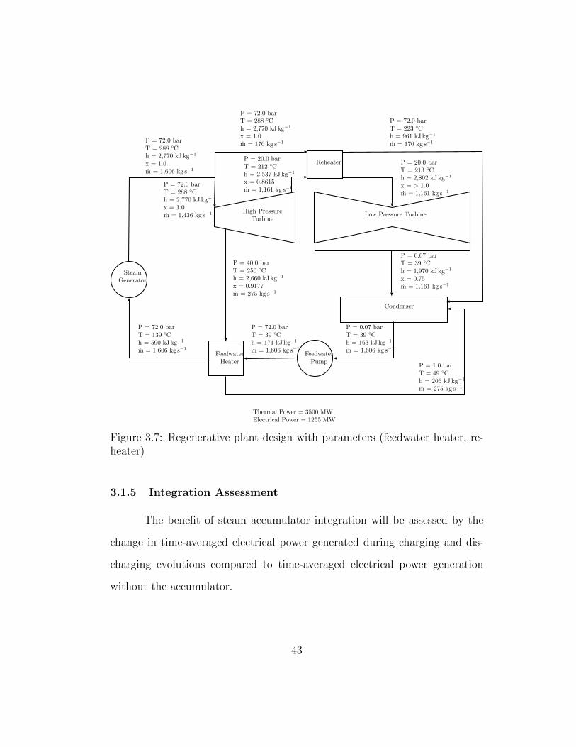
3.7 Regenerative plant design with parameters (feedwater heater,reheater) . . . . . . . . . . . . . . . . . . . . . . . . . . . . . . 43
3.8 Accumulator mass flow rate versus accumulator pressure (feed-water heater, accumulator discharging and charging) . . . . . 48
3.9 Accumulator mass flow rate versus accumulator pressure (feed-water heater, reheater, accumulator discharging and charging) 49
4.1 Accumulator pressure versus time (multiple charge and discharge) 51
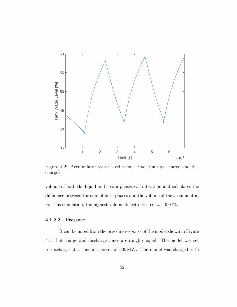
4.2 Accumulator water level versus time (multiple charge and dis-charge) . . . . . . . . . . . . . . . . . . . . . . . . . . . . . . . 52
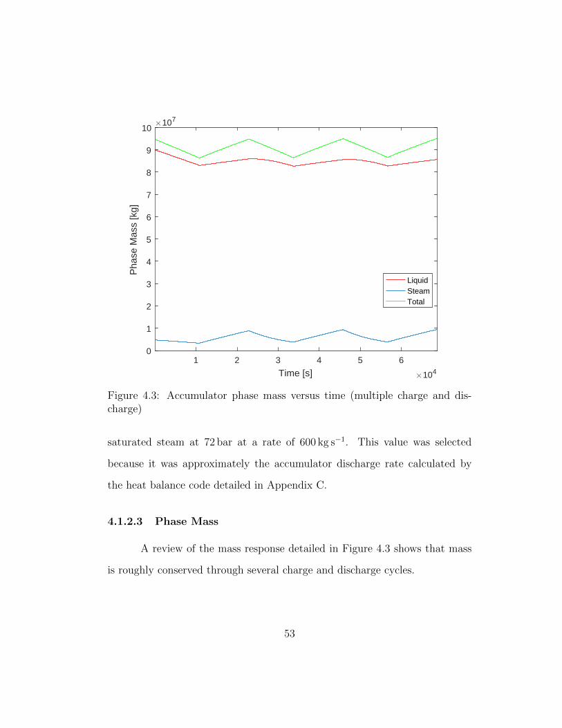
4.3 Accumulator phase mass versus time (multiple charge and dis-charge) . . . . . . . . . . . . . . . . . . . . . . . . . . . . . . . 53
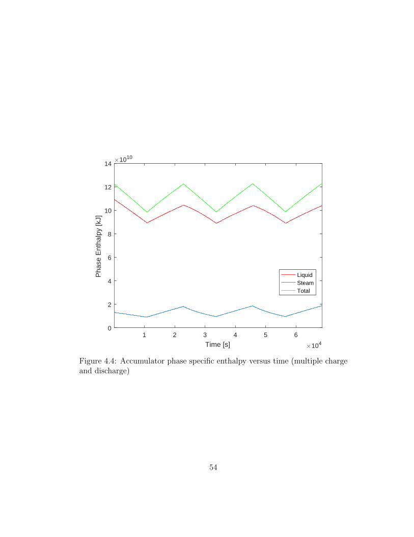
4.4 Accumulator phase specific enthalpy versus time (multiple chargeand discharge) . . . . . . . . . . . . . . . . . . . . . . . . . . . 54
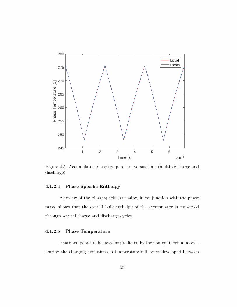
4.5 Accumulator phase temperature versus time (multiple chargeand discharge) . . . . . . . . . . . . . . . . . . . . . . . . . . . 55
4.6 Saturation temperature versus pressure . . . . . . . . . . . . . 58
4.7 Specific enthalpy versus pressure . . . . . . . . . . . . . . . . . 59
4.8 Apparent efficiency versus accumulator pressure (feedwater heater) 60
xi
4.9 Apparent efficiency versus accumulator pressure (feedwater heaterand reheater) . . . . . . . . . . . . . . . . . . . . . . . . . . . 60
4.10 Regenerative plant design with parameters (feedwater heater,accumulator discharging) . . . . . . . . . . . . . . . . . . . . . 61
4.11 Regenerative plant design with parameters (feedwater heater,accumulator charging) . . . . . . . . . . . . . . . . . . . . . . 62
4.12 Regenerative plant design with parameters (feedwater heater,reheater, accumulator discharging) . . . . . . . . . . . . . . . 63
4.13 Regenerative plant design with parameters (feedwater heater,reheater, accumulator charging) . . . . . . . . . . . . . . . . . 64
A.1 Pressure versus time for test 1 . . . . . . . . . . . . . . . . . . 71
A.2 Pressure versus time for test 1 (Stevanovic et al.) . . . . . . . 72
A.3 Pressure versus time for test 2 . . . . . . . . . . . . . . . . . . 74
A.4 Pressure versus time for test 2 (Stevanovic et al.) . . . . . . . 75
B.1 Volume defect versus time for selected values of time step . . . 78
B.2 Pressure versus time for selected values of time step . . . . . . 78
B.3 Pressure versus time for selected values of time step (detail) . 79
xii
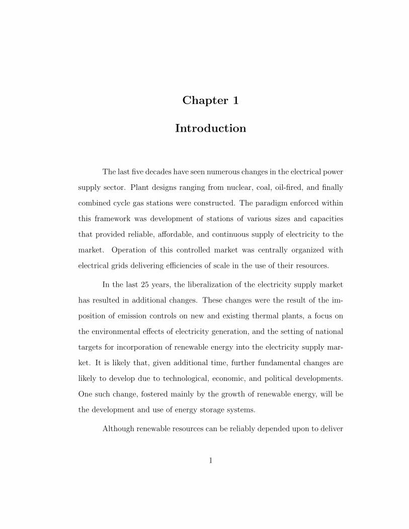
Chapter 1
Introduction
The last five decades have seen numerous changes in the electrical power
supply sector. Plant designs ranging from nuclear, coal, oil-fired, and finally
combined cycle gas stations were constructed. The paradigm enforced within
this framework was development of stations of various sizes and capacities
that provided reliable, affordable, and continuous supply of electricity to the
market. Operation of this controlled market was centrally organized with
electrical grids delivering efficiencies of scale in the use of their resources.
In the last 25 years, the liberalization of the electricity supply market
has resulted in additional changes. These changes were the result of the im-
position of emission controls on new and existing thermal plants, a focus on
the environmental effects of electricity generation, and the setting of national
targets for incorporation of renewable energy into the electricity supply mar-
ket. It is likely that, given additional time, further fundamental changes are
likely to develop due to technological, economic, and political developments.
One such change, fostered mainly by the growth of renewable energy, will be
the development and use of energy storage systems.
Although renewable resources can be reliably depended upon to deliver
1
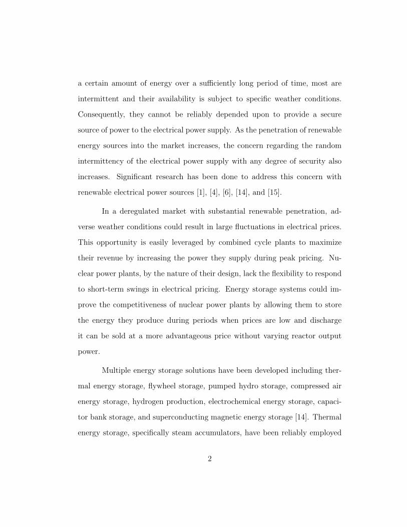
a certain amount of energy over a sufficiently long period of time, most are
intermittent and their availability is subject to specific weather conditions.
Consequently, they cannot be reliably depended upon to provide a secure
source of power to the electrical power supply. As the penetration of renewable
energy sources into the market increases, the concern regarding the random
intermittency of the electrical power supply with any degree of security also
increases. Significant research has been done to address this concern with
renewable electrical power sources [1], [4], [6], [14], and [15].
In a deregulated market with substantial renewable penetration, ad-
verse weather conditions could result in large fluctuations in electrical prices.
This opportunity is easily leveraged by combined cycle plants to maximize
their revenue by increasing the power they supply during peak pricing. Nu-
clear power plants, by the nature of their design, lack the flexibility to respond
to short-term swings in electrical pricing. Energy storage systems could im-
prove the competitiveness of nuclear power plants by allowing them to store
the energy they produce during periods when prices are low and discharge
it can be sold at a more advantageous price without varying reactor output
power.
Multiple energy storage solutions have been developed including ther-
mal energy storage, flywheel storage, pumped hydro storage, compressed air
energy storage, hydrogen production, electrochemical energy storage, capaci-
tor bank storage, and superconducting magnetic energy storage [14]. Thermal
energy storage, specifically steam accumulators, have been reliably employed
2
in fossil-based electrical power production facilities for over 60 years [2] [14].
Steam accumulators could be integrated into new reactor designs to increase
flexibility. The incorporation of steam accumulators into reactor plant designs
introduces new benefits and liabilities. In order to assess these benefits and
vulnerabilities associated with the integration of steam accumulators with re-
actor plant systems, it is necessary to model the thermodynamic behavior of
steam accumulators and their response to various scenarios. This work an-
alyzes the integration of steam accumulators with reactor plant systems and
the potential benefits and liabilities introduced by that integration.
Chapter 2 provides an overview of existing literature, including prior
attempts to thermodynamically model steam accumulators. Chapter 3 pro-
vides the analysis methods used in this study. Chapter 4 presents the results
of the analysis.
3
Chapter 2
Literature Review
2.1 Steam Accumulators
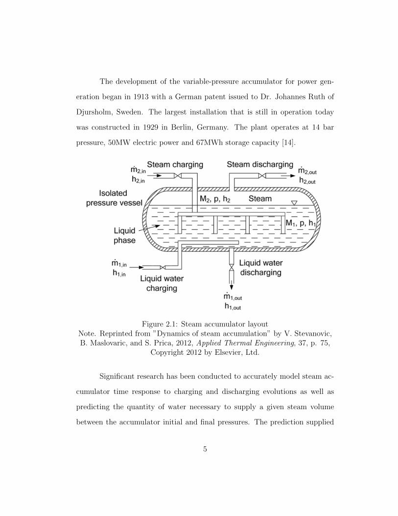
A steam accumulator is a pressurized vessel filled with water and steam
as shown in Figure 2.1. The steam and water phases in the accumulator are
at saturation conditions. As steam is discharged from the accumulator, pres-
sure in the accumulator decreases. The liquid phase in the accumulator is
now at a temperature greater than saturation temperature for the new lower
pressure. A portion of the liquid phase flashes to steam. The latent heat
of vaporization removed by the phase change from liquid to steam reduces
the liquid phase temperature to saturation temperature for the lower pres-
sure. As steam continues to be drawn off, this process continuously occurs
with water level and pressure decreasing. To recharge the accumulator, steam
is introduced, increasing pressure in the accumulator. As pressure increases,
the temperature of the steam phase is below saturation temperature for the
new higher pressure. A portion of the steam phase condenses to liquid. The
latent heat of vaporization due to the phase change is absorbed by the remain-
ing steam phase, increasing its temperature to saturation temperature at the
higher pressure. As steam continues to be charged to the accumulator, this
process continuously occurs with water level and pressure increasing.
4
The development of the variable-pressure accumulator for power gen-
eration began in 1913 with a German patent issued to Dr. Johannes Ruth of
Djursholm, Sweden. The largest installation that is still in operation today
was constructed in 1929 in Berlin, Germany. The plant operates at 14 bar
pressure, 50MW electric power and 67MWh storage capacity [14].
Figure 2.1: Steam accumulator layoutNote. Reprinted from ”Dynamics of steam accumulation” by V. Stevanovic,B. Maslovaric, and S. Prica, 2012, Applied Thermal Engineering, 37, p. 75,
Copyright 2012 by Elsevier, Ltd.
Significant research has been conducted to accurately model steam ac-
cumulator time response to charging and discharging evolutions as well as
predicting the quantity of water necessary to supply a given steam volume
between the accumulator initial and final pressures. The prediction supplied
5
by these models rely on several approximations.
2.2 Approximations in Modeling
Despite the maturity of steam accumulator usage, methods employed
in their thermal design rely heavily on approximations. When predicting the
required steam accumulator volume or the charging and discharging capacity
of steam accumulators, Steinmann and Eck [9] determine the energy of phase
transition removed or added to the liquid phase by using a mean value of the
latent heat, which is itself determined by taking the mean of latent heats at the
initial and final operating pressures of the steam accumulator. Depending on
the initial and final operating pressures, the variation in latent heat of water
is non-linear, resulting in approximate results.
Some models approximate the equations of state for the thermodynamic
properties of the accumulator phases. Steinmann and Eck [9] use the Antoine
correlation, which assumes a temperature independent heat of vaporization,
for the relationship between saturation pressure and temperature and relies
on the Watson correlation for the latent heat of vaporization. Schnaider et al.
[8] use the ideal-gas law for approximating the equations of state for saturated
or near-saturated states. Two main types of models exist, equilibrium and
non-equilibrium.
6
2.3 Equilibrium versus Non-equilibrium Models
Most existing models rely on a thermal equilibrium between the steam
and liquid phases. Both phases are assumed to have the same pressure and
saturation temperature. Another noteworthy feature of equilibrium models is
that they rely on infinite rates of condensation and evaporation to resolve any
changes in thermodynamic state between the liquid and vapor phases.
The equilibrium model developed by Studovic and Stevanovic [12] and
employed by Stevanovic et al. [10] [11] and Sun et al. [13] calculates the
thermodynamic properties of the steam and vapor phases separately and allows
for different temperatures between the two phases that are in contact. In lieu
of infinite rates of condensation and evaporation, the non-equilibrium model
derives correlations from the Herz-Knudsen equation used in surface chemistry
to describe the sticking of gas molecules on a surface by expressing the time
rate of change of the concentration of molecules on the surface as a function
of the pressure of the gas and other parameters. The correlations from the
Herz-Knudsen equation quantify the values for phase transition surfaces and
the local water to steam interface thermodynamic conditions with a single
empirical constant, the relaxation time.
When compared with each other, the non-equilibrium model appears
to provide more accurate predictions of temperature, pressure, and water level
during accumulator charging and discharging transients [10] [11] [13]. A better
understanding of the model types and their strengths and weaknesses can be
obtained by examining the derivations of the different models in the literature.
7
2.4 Existing Models
Several steam accumulator models are present in the literature. Some
provide a complete picture of model response over time, others provide only
a few parameters with no time response prediction. Most of the literature
regards the integration of steam accumulators into concentrated solar plants.
An additional area of focus in the literature was the predictive response of
steam catapults used onboard aircraft carriers for for accelerating aircraft to
high speeds over a very short period of time to assist take off. A few models
are valuable for predicting the response of an accumulator in a steam plant
and are discussed in detail below.
2.4.1 Steinmann and Eck
The model developed by Steinmann and Eck [9] is not a complete
model. This model was developed to predict the amount of steam available
for discharge given an initial and final pressure. The model makes several
assumptions:
1. There is no heat transfer between the environment and the fluid volume
inside the pressure vessel.
2. There is no heat transfer between the walls of the pressure vessel and
the fluid volume.
3. The fluid inside the pressure vessel is always in thermal equilibrium.
8
4. The specific exit enthalpy (hexit) equals the specific enthalpy of saturated
steam (h′′) at the pressure of the vessel (pvessel).
The model relates the change in internal energy of the liquid water vol-
ume with mass mvessel in the pressure vessel with the enthalpy flow transported
by the exiting mass flow dmvessel:
d (mvesseluvessel) = hexitdmvessel (2.1)
Based on the assumption 4 above:
uvesseldmvessel +mvesselduvessel = h′′pvesseldmvessel (2.2)
Integration of Equation 2.2 approximates the mass of saturated steam
that is provided during discharge of the steam accumulator.
This model also provides a method for quickly estimating the storage
capacity for discharge given a starting pressure (pstart), an end pressure (pend),
and an initial liquid mass (mliquid) based on the following assumptions:
1. All of the heat of vaporization is provided by the liquid phase.
2. It is reasonable to use an average specific heat capacity of liquid water
cliquid, avg determined from an average pressure pavg = pstart+pend2
.
3. It is reasonable to use an average specific heat of vaporization ∆hfg, avg
determined from an average pressure pavg = pstart+pend2
.
9
4. The change in liquid mass (mliquid) during discharge is neglected.
Based on these assumptions, the mass of saturated steam (msteam) pro-
vided by accumulator is approximated by:
msteam∆hfg, avg = mliquidcliquid, avg
(Tsatpstart
− Tsatpend
)(2.3)
As discussed in Section 2.2, this model uses the Antoine equation to
approximate the saturation temperature for a given pressure and the Watson
equation to determine the specific heat of vaporization.
Tsat =B
A− ln psat
− C (2.4)
where:
Tsat is the saturation temperature, in ◦C.
psat is the saturation pressure, in bar.
A = 11.934
B = 3985
C = 234.1
∆hfg = ∆hfg, ref
(1 − T+273.15
647
1 − Tref+273.15647
)0.38
(2.5)
where:
10
∆hfg, ref is the specific heat of vaporization at a reference temperature, Tref,
in kJ kg−1.
T is the temperature at which to approximate the specific heat of vaporization,
in ◦C.
Tref is the reference temperature at which the reference specific heat of vapor-
ization, ∆hfg, ref, is known, in ◦C.
Combining Equations 2.3, 2.4, and 2.5 allows for the estimation of the
total mass of saturated steam msteam, provided when discharging from the
initial pressure, pstart, to the final pressure, pend.
msteam =mliquidcliquid, avgB
(1
A−ln pstart− 1
A−ln pend
)∆hfg, ref
(1−
BA−ln pavg
−C+273.15
647
1−Tref+273.15
647
) (2.6)
2.4.2 Schnaider et al.
The steam accumulator modeled in Schnaider et al. [8] was developed
to predict the response of a steam accumulator in an industrial steam sup-
ply system used in steel manufacturing. This model employs the Clapeyron-
Mendeleev equations to approximate the relationship between steam temper-
ature, pressure, and density (p = ρRT ) as mentioned in Section 2.2. Pressure
in the accumulator is calculated as follows:
11
PA =R× TA ×ms
Vs
(2.7)
where:
PA is the ambient pressure in the accumulator, in Pa.
R is the specific gas constant, 0.411526 kJ K−1 kg−1.
TA is the ambient temperature in the accumulator, in K.
ms is the steam mass in the accumulator, in kg.
Vs is the steam volume in the accumulator, in m3.
The Schnaider et al. model is an equilibrium model. Consequently, it
is assumed that the pressure and temperature of the liquid and vapor phases
are the same. The temperature TA and pressure pA are interrelated due to the
saturated conditions in the accumulator. Temperature TA can be evaluated as
a function of pA. This relationship could be determined via direct calculation
of thermodynamic properties or approximated using a relationship like the
Antoine equation (Equation 2.4).
Volume of the steam phase, Vs, is calculated by subtracting the volume
of the water phase from the total accumulator volume.
Vs = VA − mw
ρw
(2.8)
where:
12
VA is the total accumulator volume, in m3.
mw is the mass of water in the accumulator, in kg.
ρw is the density of water in the accumulator for a given temperature, TA, in
kg m−3
mw is evaluated by integrating the three material balance terms shown
above.
mw (t) =
∫ t
0
(G1 (t) −G2 (t) +Gs(t)
)dt (2.9)
where:
G1 is the mass flow rate of incoming charging steam, in kg s−1.
G2 is the mass flow rate of outgoing discharge steam, in kg s−1.
Gs is the feedwater supply, in kg s−1.
The energy balance is determined by integrating the heat transfer terms
associated with the heat flows in and out of the model.
EA (t) =
∫ t
0
(Q1 (t) −Q2 (t) −Qloss (t) +Qs (t)) dt (2.10)
where:
EA is the heat energy stored in the accumulator, in kJ.
13
Q1 is the heat rate of the inlet charging steam, in kJ s−1.
Q2 is the heat rate of the outlet discharge steam, in kJ s−1.
Qloss is the heat rate due to environmental losses, in kJ s−1.
Qs is the heat rate due to feeding, in kJ s−1.
The heat rates Q1, Q2, and Qs are calculated according to the following
expressions:
Q1 (t) = G1 (t) × is1 (2.11)
Q2 (t) = G2 (t) × is2 (2.12)
Qs (t) = Gs (t) × is3 (2.13)
where:
is1 is the specific enthalpy of the inlet charging steam, in kJ kg−1.
is2 is the specific enthalpy of the outlet discharge steam, in kJ kg−1.
is3 is the specific enthalpy of the feedwater, in kJ kg−1.
The rate of environmental heat losses, Qloss, is calculated as follows:
Qloss = Kn × FA × (TA − Tout) (2.14)
where:
14

Kn is the heat transfer coefficient from the tank surface to the environment,
in kJ kg−1 K−1.
FA is the surface area of the accumulator, in m2.
Tout is the ambient air temperature, in K.
Equations 2.7, 2.8, 2.9, 2.10, 2.11, 2.12, 2.13, and 2.14 represent a
dynamic, equilibrium based model for steam accumulator response.
2.4.3 Stevanovic et al.
The model developed by Studovic and Stevanovic [12] and employed by
Stevanovic et al. [10] [11] and Sun et al. [13] is one of the most recent models
in the literature. The Stevanovic et al. model is based on a variable-pressure
steam accumulator and is designed to accurately predict response from indus-
trial and power plant accumulators. This model is a non-equilibrium model
that is presented as a tool for the design of steam accumulator volume and
control systems to govern the accumulator charging and discharging transients.
The more recent model documented in the literature by Stevanovic
et al. [11] provides a detailed analysis of the control system and provides
the derivation of an equilibrium based model to allow for a comparison of
equilibrium and non-equilibrium models. The equilibrium model developed by
Stevanovic et al. [11] was developed at a later time that the non-equilibrium
model [10], but is presented first to allow for a more ready identification of the
15
differences in modeling approaches between this equilibrium model, Schnaider
et al. [8], and the non-equilibrium model [10].
2.4.3.1 Equilibrium Model
Recall from Section 2.3 that equilibrium based models assume that the
pressures and saturation temperatures of the liquid and steam phases are the
same and rely on infinite rates of condensation and evaporation to resolve
any differences in thermodynamic properties between the two phases. Balance
equations address the entire accumulator versus the non-equilibrium approach
of addressing each phase independently.
Mass balance
dM
dt= m1B + m2B (2.15)
m1B = m1, in + m1, out (2.16)
m2B = m2, in + m2, out (2.17)
where:
dMdt
is change in mass of the accumulator, water and steam, with respect to
time, in kg s−1
Energy balance can be described as the following:
dH
dt= (mh)1B + (mh)2B + V
dp
dt(2.18)
16
(mh)1B = m1, inh1, in − m1, outh1, out (2.19)
(mh)2B = m2, inh2, in − m2, outh2, out (2.20)
where:
dHdt
is change in bulk enthalpy of the accumulator with respect to time, in
kJ s−1
Thermodynamic properties of the water and steam phases can be in-
ferred using the saturation properties and steam quality. Quality is determined
by the specific volume of the saturated mixture in the accumulator:
x =v − v′
v′′ − v′(2.21)
where:
x is the steam quality.
v is the specific volume of the saturated mixture in the accumulator, in m3 kg−1.
This value is determined using the total volume of the accumulator and
total mass in the accumulator. v = VM
v′ is the specific volume of saturated liquid at the current pressure in the
accumulator, in m3 kg−1.
v′′ is the specific volume of saturated steam at the current pressure in the
accumulator, in m3 kg−1.
17
Given that H = hM , differentiation of total enthalpy results in:
dH
dt= M
dh
dt+ h
dM
dt(2.22)
The derivative of the specific enthalpy is:
dh
dt=
(dh′
dp+ x
dhfg
dp
)dp
dt+ hfg
dx
dt(2.23)
The derivative of quality is:
dx
dt= − 1
M
v
v′′ − v′dM
dt−(
1
v′′ − v′dv′
dp+
v − v′
(v′′ − v′)2
d (v′′ − v′)
dpo
)dp
dt(2.24)
Based on the assumed thermodynamic equilibrium of the phases, v′, v′′,
h′, and hfg are purely functions of pressure. By incorporating Equations 2.22,
2.23, 2.24 into Equation 2.18, the differential equation for pressure is obtained
as:
dp
dt=
(mh)1B (mh)2B +(hfg
VM
v′′−v′ − h)
(m1B + m2B)
M(
dh′
dp+
VM−v′
v′′−v′ −hfg
v′′−v′dv′
dp− hfg
VM−v′
(v′′−v′)2d(v′′−v)
dp
) (2.25)
Equations 2.15 and 2.25 can be solved numerically for specified initial
values of water and steam masses and initial pressure.
18
2.4.3.2 Non-equilibrium Model
The steam accumulator model is based on the the following mass and
energy balance equations for each phase:
Liquid mass balance can be described as the following:
dM1
dt= m1B + mPT1 (2.26)
m1B = m1, in + m1, out (2.27)
mPT1 = mc − me (2.28)
where:
dM1
dtis the change in liquid mass with respect to time, in kg s−1.
m1B is the net mass balance of liquid water inlet and outlet flows, in kg s−1.
mPT1 is the liquid mass rate change due to evaporation and condensation
rates, in kg s−1.
m1, in is the liquid mass flow into the accumulator, in kg s−1.
m1, out is the liquid mass flow into the accumulator, in kg s−1.
mc is the condensation rate in the accumulator, in kg s−1.
me is the evaporation rate in the accumulator, in kg s−1.
19
Steam mass balance can be described as the following:
dM2
dt= m2B + mPT2 (2.29)
m2B = m2, in + m2, out (2.30)
mPT2 = me − mc (2.31)
where:
dM2
dtis the change in steam mass with respect to time, in kg s−1.
m2B is the net mass balance of steam inlet and outlet flows, in kg s−1.
mPT2 is the steam mass rate change due to evaporation and condensation
rates, in kg s−1.
m2, in is the steam mass flow into the accumulator, in kg s−1.
m2, out is the steam mass flow into the accumulator, in kg s−1.
Liquid energy balance can be described as the following:
dH1
dt= (mh)1B + mPT1h
′′ + Q21 + 1000 V1dp
dt(2.32)
(mh)1B = m1, inh1, in − m1, outh1, out (2.33)
where:
dH1
dtis the change in liquid bulk enthalpy in the accumulator, in kJ s−1.
20
(mh)1B is the net energy balance of inlet and outlet liquid flows, in kJ s−1.
h′′ is the specific enthalpy of saturated steam at the current pressure in the
accumulator, in kJ kg−1.
Q21 is the heat transfer rate from superheated steam to liquid, in kJ s−1.
V1 is the volume of liquid in the accumulator, in m3.
dpdt
is the rate of pressure change in the accumulator, in MPa s−1.
h1, in is the specific enthalpy of liquid flowing into the accumulator, in kJ kg−1.
h1, out is the specific enthalpy of liquid flowing out of the accumulator, in
kJ kg−1.
Steam energy balance can be described as the following:
dH2
dt= (mh)2B + mPT2h
′′ − Q21 + 1000 V2dp
dt(2.34)
(mh)2B = m2, inh2, in − m2, outh2, out (2.35)
where:
dH2
dtis the change in steam bulk enthalpy in the accumulator, in kJ s−1.
(mh)2B is the net energy balance of inlet and outlet steam flows, in kJ s−1.
V2 is the volume of steam in the accumulator, in m3.
h2, in is the specific enthalpy of steam flowing into the accumulator, in kJ kg−1.
21

h2, out is the specific enthalpy of steam flowing out of the accumulator, in
kJ kg−1.
Volume balance can be described as the following:
V1 + V2 = V (2.36)
where:
V1 is the volume of the liquid phase, in m3.
V2 is the volume of the steam phase, in m3.
V is the total volume of the liquid and steam phases, in m3. This should also
be equal to the total controlled volume of the accumulator.
Condensation and Evaporation Rates
A key feature of the non-equilibrium model is the finite rates of con-
densation (mc) and evaporation (me) employed to determine water mass ex-
changed between the liquid and steam phases. The condensation and evap-
oration relaxation times τc and τe are correlations from the Herz-Knudsen
equation that quantify the values for phase transition surfaces and the local
water to steam interface thermodynamic conditions with a single empirical
constant for condensation or evaporation. Derivation of the condensation and
evaporation relaxation times τc and τe will be discussed in more detail later in
22
this chapter. The condensation (mc) and evaporation (me) rates are calculated
as shown below.
mc =
{ρ1V1(h′−h1)
τchfgh1 < h′
0 h1 ≥ h′(2.37)
me =
{ρ1V1(h1−h′)
τehfgh1 > h′
0 h1 ≤ h′(2.38)
where:
ρ1 is the density of the liquid phase, in kg m−3.
h′ is the specific enthalpy of saturated liquid at the current pressure in the
accumulator, in kJ kg−1.
h1 is the specific enthalpy of the liquid phase, in kJ kg−1.
τc is the condensation relaxation time, in s.
τe is the evaporation relaxation time, in s.
hfg is the latent heat of vaporization at the current pressure in the accumula-
tor, in kJ kg−1.
The heat transfer rate from superheated steam to liquid, Q21, represents
the heat transfer at the steam-water interface. It has been shown [11] that
the majority of heat transfer occurs at the steam-water interfaces of steam
bubbles that form in the liquid volume and that the heat transfer coefficient
23
and the interfacial area concentration are conditions of steam bubble flow in
stagnant water and not heat transfer between the steam-water interface at the
surface of the liquid.
Q21 = (ha)21 (T2 − T1)V1 (2.39)
where:
(ha)21 is the product of the heat transfer coefficient, h, and the steam-water
interface area concentration, a, in W m−3 K−1.
T1 is the temperature of the liquid phase, in K.
T2 is the temperature of the steam phase, in K.
V1 is the volume of the liquid phase, in m3.
The accumulator model employed by Stevanovic et al. [10] empirically
identifies that 5 × 10⁴ W m−3 K−1 for (ha)21 provides a good agreement be-
tween calculated and measured pressure data in their validation. This value
for (ha)21 is also used in another model in the literature, Sun et al. [13], that
is based upon the Stevanovic et al. model.
The system of balance equations outlined in Equations 2.26, 2.29, 2.32,
2.34, and 2.36 are then rewritten into a set of first-order differential equations.
This is accomplished by transforming the steam and mass volumes in the
volume balance (Equation 2.36) as products of their mass and specific volume.
24
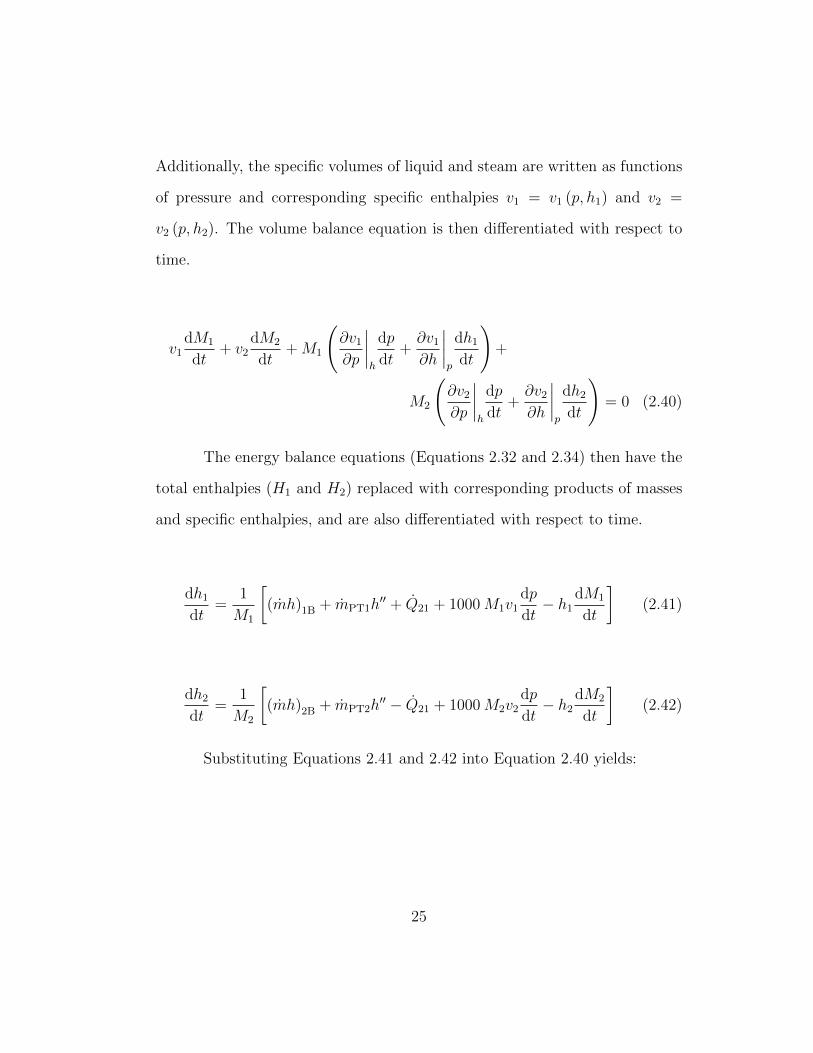
Additionally, the specific volumes of liquid and steam are written as functions
of pressure and corresponding specific enthalpies v1 = v1 (p, h1) and v2 =
v2 (p, h2). The volume balance equation is then differentiated with respect to
time.
v1dM1
dt+ v2
dM2
dt+M1
(∂v1
∂p
∣∣∣∣h
dp
dt+∂v1
∂h
∣∣∣∣p
dh1
dt
)+
M2
(∂v2
∂p
∣∣∣∣h
dp
dt+∂v2
∂h
∣∣∣∣p
dh2
dt
)= 0 (2.40)
The energy balance equations (Equations 2.32 and 2.34) then have the
total enthalpies (H1 and H2) replaced with corresponding products of masses
and specific enthalpies, and are also differentiated with respect to time.
dh1
dt=
1
M1
[(mh)1B + mPT1h
′′ + Q21 + 1000M1v1dp
dt− h1
dM1
dt
](2.41)
dh2
dt=
1
M2
[(mh)2B + mPT2h
′′ − Q21 + 1000M2v2dp
dt− h2
dM2
dt
](2.42)
Substituting Equations 2.41 and 2.42 into Equation 2.40 yields:
25

dp
dt=
(h1
∂v1∂h
∣∣∣∣p
− v1
)dM1
dt+
(h2
∂v2∂h
∣∣∣∣p
− v2
)dM2
dt
− ∂v1∂h
∣∣∣∣h
[(mh)1B + mPT1h
′′ + Q21
]− ∂v2
∂h
∣∣∣∣h
[(mh)2B + mPT2h
′′ − Q21
](∂v1∂p
∣∣∣∣h
+ 1000 v1∂v1∂h
∣∣∣∣p
)M1 +
(∂v2∂p
∣∣∣∣h
+ 1000 v2∂v2∂h
∣∣∣∣p
)M2
(2.43)
Equations 2.26, 2.29, 2.41, 2.42, and 2.43 provide a set of five first-order
ordinary differential equations for the prediction of water and steam masses,
enthalpies, and steam accumulator pressure for specified initial values for water
and steam masses, enthalpies, and initial pressure.
2.4.3.3 Equilibrium versus Non-equilibrium Prediction Differences
As part of the verification and validation conducted by Stevanovic et
al. [10], they modeled charge and discharge evolutions using both the equi-
librium and non-equilibrium model. The equilibrium model was developed
by adjusting the model relaxation time to a value that resulted in heat and
mass transfer rates between phases thousands of times greater than in the
non-equilibrium model. Effectively, thermodynamic equilibrium between the
phases was nearly instantaneous.
During the charging evolution (Figure 2.2) it was noted that, upon se-
curing the charge when the non-equilibrium model at 50.0 bar, pressure quickly
decreased to 46.6 bar. Both the equilibrium and non-equilibrium ended at a
approximately the same value for the mass and energy introduced into the
26
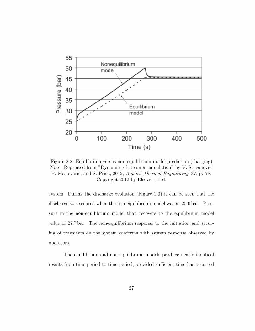
Figure 2.2: Equilibrium versus non-equilibrium model prediction (charging)Note. Reprinted from ”Dynamics of steam accumulation” by V. Stevanovic,B. Maslovaric, and S. Prica, 2012, Applied Thermal Engineering, 37, p. 78,
Copyright 2012 by Elsevier, Ltd.
system. During the discharge evolution (Figure 2.3) it can be seen that the
discharge was secured when the non-equilibrium model was at 25.0 bar . Pres-
sure in the non-equilibrium model than recovers to the equilibrium model
value of 27.7 bar. The non-equilibrium response to the initiation and secur-
ing of transients on the system conforms with system response observed by
operators.
The equilibrium and non-equilibrium models produce nearly identical
results from time period to time period, provided sufficient time has occurred
27
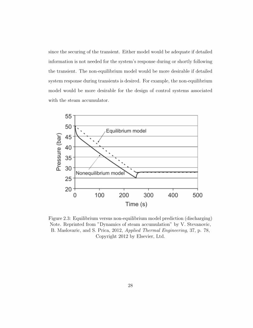
since the securing of the transient. Either model would be adequate if detailed
information is not needed for the system’s response during or shortly following
the transient. The non-equilibrium model would be more desirable if detailed
system response during transients is desired. For example, the non-equilibrium
model would be more desirable for the design of control systems associated
with the steam accumulator.
Figure 2.3: Equilibrium versus non-equilibrium model prediction (discharging)Note. Reprinted from ”Dynamics of steam accumulation” by V. Stevanovic,B. Maslovaric, and S. Prica, 2012, Applied Thermal Engineering, 37, p. 78,
Copyright 2012 by Elsevier, Ltd.
28
2.4.3.4 Derivation of Condensation and Evaporation RelaxationTimes
The derivation of finite rates of condensation and evaporation in non-
equilibrium accumulator models constitutes a significant contribution to steam
accumulator modeling. Stevanovic et al. [10] [11] and Sun et al. [13] use
τc = 85s and assume that τc = τe. Evaluation of the use of this empirical value
of 85 s versus a more detailed calculation of relaxation times was performed
by Stevanovic et al. [11]. Their analysis justified the use of the empirical
value of 85 s and the assumption that τc = τe versus a direct calculation of the
relaxation times.
29
Chapter 3
Methodology
Previous work has examined the integration of steam accumulators in
nuclear steam plant systems, but it was limited to the incorporation of a
separate turbine and generator. This work analyzes the incorporation of steam
accumulators that are integrated into the plant to leverage existing pathways
for the reintroduction of stored thermal energy back into the system. The
specific items studied as part of this analysis were:
1. Steam plant efficiency η
2. Steam accumulator discharge rate
3. Feasibility of specific points of stored thermal energy reintroduction
Section 3.1 provides details of the steam plant configurations used in
this study. Section 3.2 discusses the steam accumulator model evaluated for
the plant conditions identified by the steam plant configurations.
30
High PressureTurbine
Low Pressure Turbine
Condenser
SteamGenerator
CondensatePump
FeedwaterPump
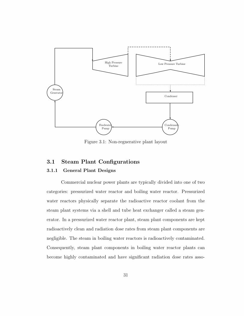
Figure 3.1: Non-regnerative plant layout
3.1 Steam Plant Configurations
3.1.1 General Plant Designs
Commercial nuclear power plants are typically divided into one of two
categories: pressurized water reactor and boiling water reactor. Pressurized
water reactors physically separate the radioactive reactor coolant from the
steam plant systems via a shell and tube heat exchanger called a steam gen-
erator. In a pressurized water reactor plant, steam plant components are kept
radioactively clean and radiation dose rates from steam plant components are
negligible. The steam in boiling water reactors is radioactively contaminated.
Consequently, steam plant components in boiling water reactor plants can
become highly contaminated and have significant radiation dose rates asso-
31
ciated with them. Additionally, steam plant components in a boiling water
reactor plant are required to be housed in a radiologically controlled area and
engineered structure.
Commercial nuclear power plants employ a Rankine cycle to extract
work from the steam [7]. Figure 3.1 summarizes a typical layout for a non-
regenerative Rankine cycle. In a non-regenerative cycle, all the steam produced
in the steam generator is used to produce work in the turbine. In regenerative
plant designs, condensate and feedwater are heated before entering the steam
generator by steam tapped off at various points in the steam plant. Regenera-
tion increases cycle efficiency by reducing the heat input required in the steam
generator necessary to change the phase of the incoming feedwater from liquid
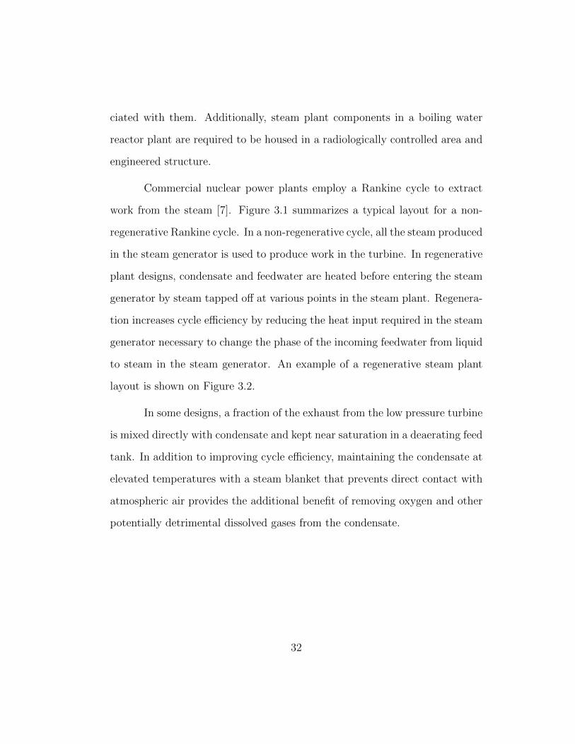
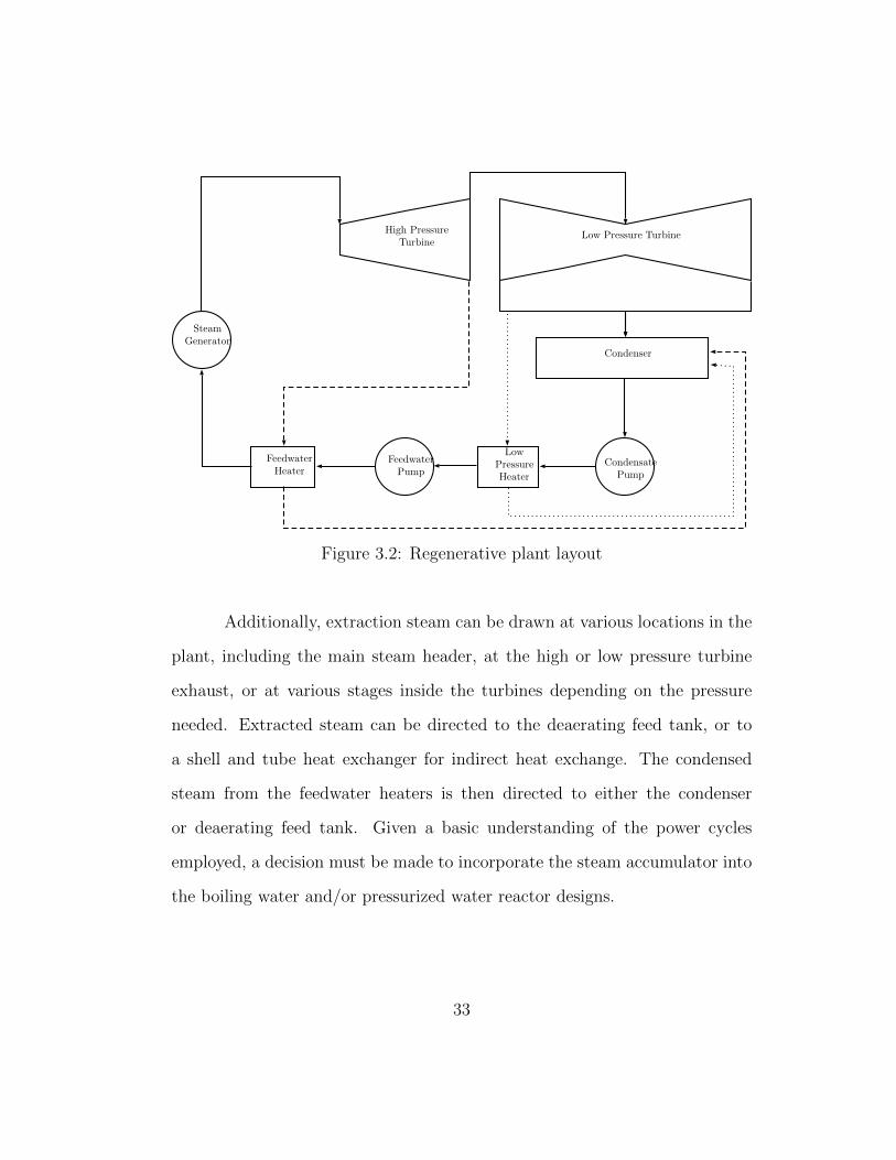
to steam in the steam generator. An example of a regenerative steam plant
layout is shown on Figure 3.2.
In some designs, a fraction of the exhaust from the low pressure turbine
is mixed directly with condensate and kept near saturation in a deaerating feed
tank. In addition to improving cycle efficiency, maintaining the condensate at
elevated temperatures with a steam blanket that prevents direct contact with
atmospheric air provides the additional benefit of removing oxygen and other
potentially detrimental dissolved gases from the condensate.
32
High PressureTurbine
Low Pressure Turbine
Condenser
SteamGenerator
CondensatePump
FeedwaterPump
FeedwaterHeater
LowPressureHeater
Figure 3.2: Regenerative plant layout
Additionally, extraction steam can be drawn at various locations in the
plant, including the main steam header, at the high or low pressure turbine
exhaust, or at various stages inside the turbines depending on the pressure
needed. Extracted steam can be directed to the deaerating feed tank, or to
a shell and tube heat exchanger for indirect heat exchange. The condensed
steam from the feedwater heaters is then directed to either the condenser
or deaerating feed tank. Given a basic understanding of the power cycles
employed, a decision must be made to incorporate the steam accumulator into
the boiling water and/or pressurized water reactor designs.
33
3.1.2 Selection of Plant Design for Analysis
Boiling water and pressurized water reactors have their own strengths
and weaknesses. This analysis will be limited to pressurized water reactor
designs. Steam plant components in pressurized water reactor plants are ra-
dioactively clean and are not subject to the stringent controls associated with
contaminated equipment. Pressurized water reactor plants are more likely to
integrate steam accumulators into their steam plant design due to lower capital
and operating costs and less regulatory burden.
Existing commercial plants leverage a regenerative thermal cycle. Re-
generative thermal cycles present more opportunities to reintroduce stored
thermal energy back into the cycle aside from the direct production of elec-
tricity via a separate turbine and generator. For these reasons, a regenerative
thermal cycle will be the subject of this analysis. It must determined how the
steam accumulator will be incorporated into plant design.
34

High PressureTurbine
Low Pressure Turbine
Condenser
SteamGenerator
CondensatePump
FeedwaterPump
SteamAccumulator Accumulator
Turbine
Figure 3.3: Non-regenerative plant with steam accumulator layout
3.1.3 Integration
Integrating steam accumulators into power plant design is not a new
concept. Older examples in the literature [3] focus mainly on generating elec-
tricity with a separate turbine and generator, drawing steam from the accu-
mulator during times of peak demand. This configuration would be preferred
if the steam plant was non-regenerative. An example of this configuration is
provided on Figure 3.3. Systems designed around a regenerative thermal cycle
present numerous potential points for stored thermal energy to be reintroduced
back into the system, allowing steam flow that would otherwise be diverted to
auxiliary loads to be directed through the turbine and increase power output.
An illustration of potential entry points in a regenerative steam cycle is shown
35
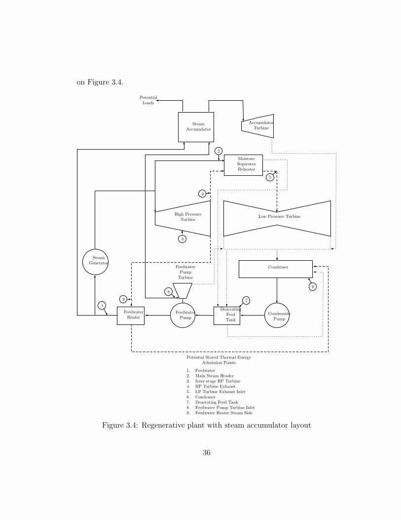
on Figure 3.4.
High PressureTurbine
Low Pressure Turbine
Condenser
SteamGenerator
CondensatePump
FeedwaterPump
FeedwaterHeater
DeaeratingFeedTank
MoistureSeparatorReheater
1
2
3
4
5
6
7
8
9
FeedwaterPumpTurbine
1. Feedwater2. Main Steam Header3. Inter-stage HP Turbine4. HP Turbine Exhaust5. LP Turbine Exhaust Inlet6. Condenser7. Deaerating Feed Tank8. Feedwater Pump Turbine Inlet9. Feedwater Heater Steam Side
Potential Stored Thermal EnergyAdmission Points
SteamAccumulator
AccumulatorTurbine
PotentialLoads
Figure 3.4: Regenerative plant with steam accumulator layout
36
Many of the potential entry points for stored energy reintroduction can
be eliminated based on the desired design characteristics of the accumulator
itself. The pressure in the accumulator will determine the loads to which the
accumulator will be able to supply steam, particularly when augmenting steam
from other sources that are supplied at a well-regulated pressure.
In general, nuclear steam plant cycles produce saturated steam. Ad-
ditionally, the steam available from the accumulator will decrease in pressure
over the course of the discharge. For these reasons, several admission points
can be eliminated.
The inter-stage high pressure turbine admission points (3) occur at very
specific stages and their associated pressures throughout the turbine. With
a variable pressure band, inter-stage high pressure turbine admission points
would only be available as a viable admission point for a relatively short period
when the accumulator pressure is within a small range of the stage pressure.
Otherwise, steam could backflow into the accumulator or upstream into the
turbine, reducing the pressure drop across upstream turbine stages and the
work extracted from the steam in those stages.
Injection of steam accumulator variable-pressure steam at either the
high pressure turbine exhaust (4) or the low pressure turbine inlet (5) pose a
considerable design problem. Significant engineering effort is spent designing
the turbine layout including the pressure drop across each stage, turbine steam,
extraction points, and steam quality throughout the turbine. Injection of
steam at the high pressure turbine exhaust (4) will result in a decrease in
37
the differential pressure across the high pressure turbine and the overall work
extracted from the steam.
Steam exiting the moisture separator reheater has a significant amount
of superheat. The introduction of saturated steam from a variable-pressure
steam accumulator into the low pressure turbine inlet (5) is likely to reduce
the specific enthalpy of the steam entering the low pressure turbine. This
could result in moisture formation in the turbine in locations not normally
designed for wet steam. The difficulty in designing a turbine train to operate
under both sets of conditions could present a serious obstacle, particularly
when other locations are available with fewer design considerations.
Steam admission to the deaerating feed tank (7) would provide some
benefit. However, temperature increases upstream of the feedwater pumps are
limited by the suction pressure of the main feed pump in order to prevent
cavitation. The same benefit can be obtained by supplying steam to the
feedwater heaters with no restrictions, beyond design, on the temperature
increase. Additionally, the steam flow rates required to the deaerating feed
tank are relatively low and minimize the benefit of supplying steam from the
steam accumulator.
Feed pump turbines are designed to operate efficiently at specific steam
pressures and flow rates. Supplying steam to the feed pump turbine inlet (8)
from a variable-pressure source would complicate feed pump turbine design.
However, plant power output could be increased on effectively one for one
basis if steam were supplied to the turbine from the accumulator. Given the
38
relatively small size of these turbines, several MW, this avenue would supply
limited benefits for the effort required.
Due to the saturated conditions in the accumulator, as the pressure de-
creases, so does the temperature of the available steam. Direct injection into
the feedwater header (1) may be undesirable due to the potential for changes
in feedwater injection temperature to result in an undesirable reactivity ex-
cursion. Additionally, two-phase flow may be introduced into portions of the
feed header and steam generator not designed for it. Another concern would
be the high precision feed flow detectors installed downstream of the feedwater
heaters in most designs. Typically, they function by measuring the velocity of
flow eddies in the feedwater. Operation of these high precision flow detectors
decreases instrumentation uncertainty and allows the units to more precisely
determine core thermal power, allowing for a reduction in operating margin
that translates into slightly greater power production. Introduction of steam
into the feedwater header may have unanticipated consequences with regards
to a plant’s ability to leverage these high precision flow meters.
It is normally unnecessary and undesirable to heat condensate in the
condenser (6). Some small amount of subcooling, called condensate depression,
is necessary to prevent cavitation of condensate as it is drawn into the suction
of the condensate pumps. For this reason, the condenser is a poor choice as
an admission point for the reintroduction of stored thermal energy into the
system.
The feedwater heater steam supply (9) would be a desirable admission
39
point. With a sophisticated enough control system and instrumentation, a rel-
atively constant feedwater injection temperature could be maintained during
the accumulator discharge.
Discharging the accumulator to the moisture separator reheater (2)
would also provide some gains. However, the low pressure steam discharged
to the low pressure turbine typically has a large amount of superheat supplied
by the high temperature main steam header. Replacing this steam with the
variable-pressure and variable-temperature steam from the steam accumula-
tor limits the minimum allowable pressure in the accumulator to ensure that
adequate superheat is present.
High PressureTurbine
Low Pressure Turbine
SteamGenerator
FeedwaterPump
P = 72.0 barT = 288 ◦Ch = 2,770 kJ kg−1
x = 1.0m = 1,347 kg s−1
P = 0.07 barT = 39 ◦Ch = 1,799 kJ kg−1
x = 0.67m = 1,347 kg s−1
Condenser
P = 0.07 barT = 39 ◦Ch = 163 kJ kg−1
m = 1,347 kg s−1
P = 72.0 barT = 39 ◦Ch = 170 kJ kg−1
m = 1,347 kg s−1
Thermal Power = 3500 MWElectrical Power = 1307 MW
Figure 3.5: Non-regenerative plant design with parameters
40
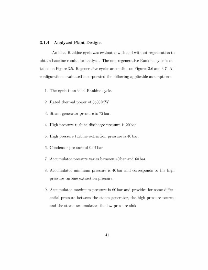
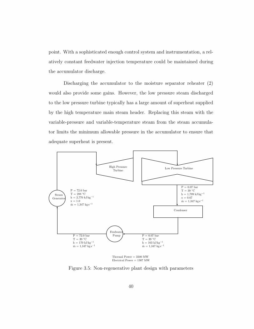
3.1.4 Analyzed Plant Designs
An ideal Rankine cycle was evaluated with and without regeneration to
obtain baseline results for analysis. The non-regenerative Rankine cycle is de-
tailed on Figure 3.5. Regenerative cycles are outline on Figures 3.6 and 3.7. All
configurations evaluated incorporated the following applicable assumptions:
1. The cycle is an ideal Rankine cycle.
2. Rated thermal power of 3500 MW.
3. Steam generator pressure is 72 bar.
4. High pressure turbine discharge pressure is 20 bar.
5. High pressure turbine extraction pressure is 40 bar.
6. Condenser pressure of 0.07 bar
7. Accumulator pressure varies between 40 bar and 60 bar.
8. Accumulator minimum pressure is 40 bar and corresponds to the high
pressure turbine extraction pressure.
9. Accumulator maximum pressure is 60 bar and provides for some differ-
ential pressure between the steam generator, the high pressure source,
and the steam accumulator, the low pressure sink.
41
High PressureTurbine
Low Pressure Turbine
SteamGenerator
FeedwaterPump
P = 72.0 barT = 288 ◦Ch = 2,770 kJ kg−1
x = 1.0m = 1,744 kg s−1
P = 0.07 barT = 39 ◦Ch = 1,799 kJ kg−1
x = 0.679m = 1,333 kg s−1
Condenser
P = 0.07 barT = 39 ◦Ch = 163 kJ kg−1
m = 1,744 kg s−1
P = 72.0 barT = 179 ◦Ch = 763 kJ kg−1
m = 1,744 kg s−1
Thermal Power = 3500 MWElectrical Power = 1318 MW
FeedwaterHeater
P = 40.0 barT = 250 ◦Ch = 2,660 kJ kg−1
x = 0.9177m = 421 kg s−1
P = 20.0 barT = 212 ◦Ch = 2,537 kJ kg−1
x = 0.8615m = 1,333 kg s−1
P = 72.0 barT = 39 ◦Ch = 171 kJ kg−1
m = 1,744 kg s−1
P = 0.07 barT = 39 ◦Ch = 163 kJ kg−1
m = 502 kg s−1
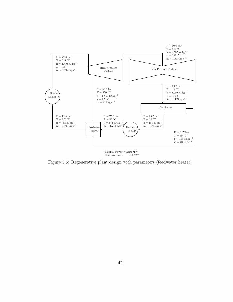
Figure 3.6: Regenerative plant design with parameters (feedwater heater)
42
High PressureTurbine
Low Pressure Turbine
SteamGenerator
FeedwaterPump
P = 72.0 barT = 288 ◦Ch = 2,770 kJ kg−1
x = 1.0m = 1,606 kg s−1
P = 0.07 barT = 39 ◦Ch = 1,970 kJ kg−1
x = 0.75m = 1,161 kg s−1
Condenser
P = 0.07 barT = 39 ◦Ch = 163 kJ kg−1
m = 1,606 kg s−1
P = 72.0 barT = 139 ◦Ch = 590 kJ kg−1
m = 1,606 kg s−1
Thermal Power = 3500 MWElectrical Power = 1255 MW
FeedwaterHeater
P = 40.0 barT = 250 ◦Ch = 2,660 kJ kg−1
x = 0.9177m = 275 kg s−1
P = 20.0 barT = 213 ◦Ch = 2,802 kJ kg−1
x = > 1.0m = 1,161 kg s−1
P = 72.0 barT = 39 ◦Ch = 171 kJ kg−1
m = 1,606 kg s−1
P = 1.0 barT = 49 ◦Ch = 206 kJ kg−1
m = 275 kg s−1
ReheaterP = 20.0 barT = 212 ◦Ch = 2,537 kJ kg−1
x = 0.8615m = 1,161 kg s−1
P = 72.0 barT = 223 ◦Ch = 961 kJ kg−1
m = 170 kg s−1
P = 72.0 barT = 288 ◦Ch = 2,770 kJ kg−1
x = 1.0m = 170 kg s−1
P = 72.0 barT = 288 ◦Ch = 2,770 kJ kg−1
x = 1.0m = 1,436 kg s−1
Figure 3.7: Regenerative plant design with parameters (feedwater heater, re-heater)
3.1.5 Integration Assessment
The benefit of steam accumulator integration will be assessed by the
change in time-averaged electrical power generated during charging and dis-
charging evolutions compared to time-averaged electrical power generation
without the accumulator.
43
benefit =
{discharging
∫ t0Qdisch dt −
∫ t0Qbaseline dt
charging∫ t
0Qbaseline dt −
∫ t0Qch dt
(3.1)
where:
Qdisch is the electrical power output of the plant with the accumulator dis-
charging, in MW.
Qch is the electrical power output of the plant with the accumulator charging,
in MW.
Qbaseline is the electrical power output of the plant with the accumulator idle,
in MW.
3.1.6 Accumulator Efficiency
The accumulator efficiency will be negatively impacted by heat losses to
the environment from the accumulator and its associated piping and enthalpy
loss due to pressure drop in the piping during flow.
3.2 Steam Accumulator Model
3.2.1 Model Selection
Two general types of models, equilibrium and non-equilibrium, have
been explored. Each model type has its own strengths and weaknesses, and
each is well suited to different types of analysis. The non-equilibrium model
provides the following advantages:
44
1. The non-equilibrium model is better suited to dynamic modeling of
steam accumulator response to charging and discharging evolutions.
2. The non-equilibrium model results in a lower final pressure following
accumulator discharge. The non-equilibrium model will provide more
conservative results when analyzing the the time required to discharge
the accumulator to a minimum allowable pressure.
3. Adequate data is available to validate and verify model response.
An example of accumulator response during and after plant transients
for both the equilibrium and non-equilibrium models was previously outlined
in Section 2.4.3.3. For these reasons, the non-equilibrium model will be used in
this analysis. The non-equilibrium model should allow for more accurate pre-
diction of desired accumulator parameters and response times during dynamic
evolutions. As discussed below in Section 3.2.2.1, the model used in this work
does not account for heat loss to the surroundings or head loss. Accumulator
efficiency would be calculated as shown below:
η =
∫ t
0Qdisch − Qbaseline − Qheat loss − Qflow loss dt∫ t
0Qbaseline − Qch + Qheat loss + Qflow loss dt
(3.2)
Qheat loss is the rate of heat loss to the environment, in MW.
Qflow loss is the electrical power output of the plant with the accumulator
charging, in MW.
45
Qbaseline is the electrical power output of the plant with the accumulator idle,
in MW.
The Qheat loss heat loss term is a function of how well insulated the
piping and tank are, the temperature/pressure of the accumulator, and the
temperature of the environment around the accumulator and its associated
piping. It should vary linearly with temperature changes, and greater than
linearly with the change in piping length and change in accumulator volume.
Most of these will be set by the design and will not vary significantly during
operations.
The Qflow loss will be the parameter that operators have the ability to
affect the most. It is a function of piping design and the flow rate through
the system. It will vary with the greater than linearly with the flow rate too
or from the accumulator. Accumulator efficiency could be maximized, for a
given discharge rate, by minimizing the charging flow rate to a value that is
just high enough to ensure the accumulator is available for discharge during
the next period of peak pricing.
3.2.2 Model Design
3.2.2.1 Solution Method
The first-order differential equations that comprise the non-equilibrium
model were solved using variable time step integration of the Runge-Katta
Method [5] for specified initial values water and steam masses and enthalpies
and initial steam accumulator pressure. The MATLAB code associated with
46
the solution is contained in Appendix C. Thermodynamic properties were
resolved using MATLAB libraries XSteam and IAPWS IF97. XSteam was
used for the majority of steam properties. IAPWS IF97 was mainly used to
directly calculate steam property derivatives. The accumulator was modeled
with the following assumptions:
1. The accumulator is charged using saturated steam available at the steam
generator pressure of 72.0 bar. No liquid is required to be charged to the
accumulator. Over the course of multiple charge/discharge cycles, water
level will slowly rise and must be adjusted by operators. Any liquid
drained can be directed back into the plant to avoid any loss of stored
thermal energy.
2. Moisture separators remove 100% of the moisture from steam being with-
drawn from the accumulator and return it to the accumulator to con-
serve thermal energy. Steam supplied to loads from the accumulator has
a quality of 1.0.
3. The accumulator model behaves like a single large tank. In reality, the
accumulator is likely to consist of a bank of tanks, charging and dis-
charging simultaneously.
4. No heat loss occurs between the tank and its surroundings.
5. There is no energy lost due to flow losses in the piping.
47
40 42 44 46 48 50 52 54 56 58 60
Accumulator Pressure [bar]
398
398.5
399
399.5
400
400.5
401A
ccum
ulat
or M
ass
Flo
w R
ate
[kg/
s]
Discharging and Charging
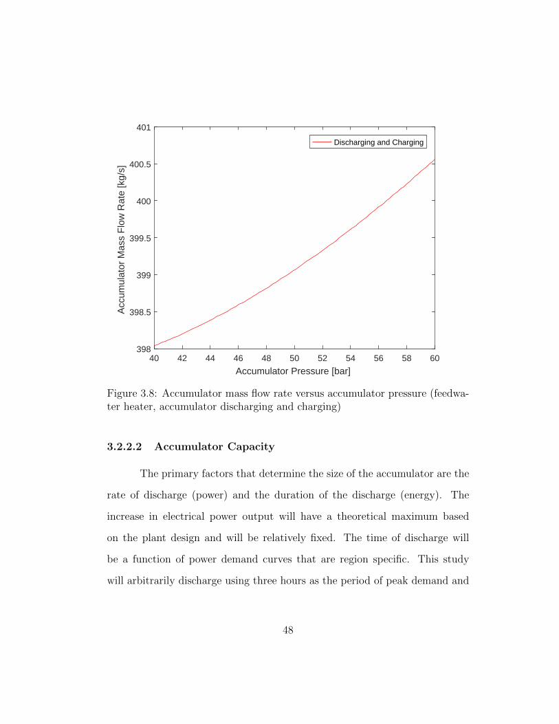
Figure 3.8: Accumulator mass flow rate versus accumulator pressure (feedwa-ter heater, accumulator discharging and charging)
3.2.2.2 Accumulator Capacity
The primary factors that determine the size of the accumulator are the
rate of discharge (power) and the duration of the discharge (energy). The
increase in electrical power output will have a theoretical maximum based
on the plant design and will be relatively fixed. The time of discharge will
be a function of power demand curves that are region specific. This study
will arbitrarily discharge using three hours as the period of peak demand and
48
pricing. The higher the power and the longer the rate of discharge, the larger
the required accumulator volume and water mass required.
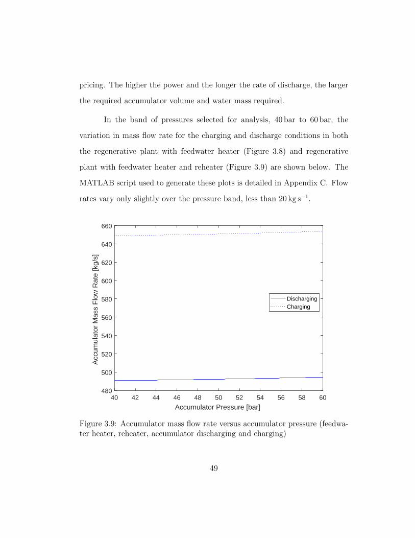
In the band of pressures selected for analysis, 40 bar to 60 bar, the
variation in mass flow rate for the charging and discharge conditions in both
the regenerative plant with feedwater heater (Figure 3.8) and regenerative
plant with feedwater heater and reheater (Figure 3.9) are shown below. The
MATLAB script used to generate these plots is detailed in Appendix C. Flow
rates vary only slightly over the pressure band, less than 20 kg s−1.
40 42 44 46 48 50 52 54 56 58 60
Accumulator Pressure [bar]
480
500
520
540
560
580
600
620
640
660
Acc
umul
ator
Mas
s F
low
Rat
e [k
g/s]
DischargingCharging
Figure 3.9: Accumulator mass flow rate versus accumulator pressure (feedwa-ter heater, reheater, accumulator discharging and charging)
49

Chapter 4
Results
4.1 Steam Accumulator Model
4.1.1 Validation and Verification
A detailed discussion of the validation and verification can be found in
Appendix A. The non-equilibrium model, developed in MATLAB and pro-
vided in Appendix C, compares well with the results in Stevanovic et al. [10].
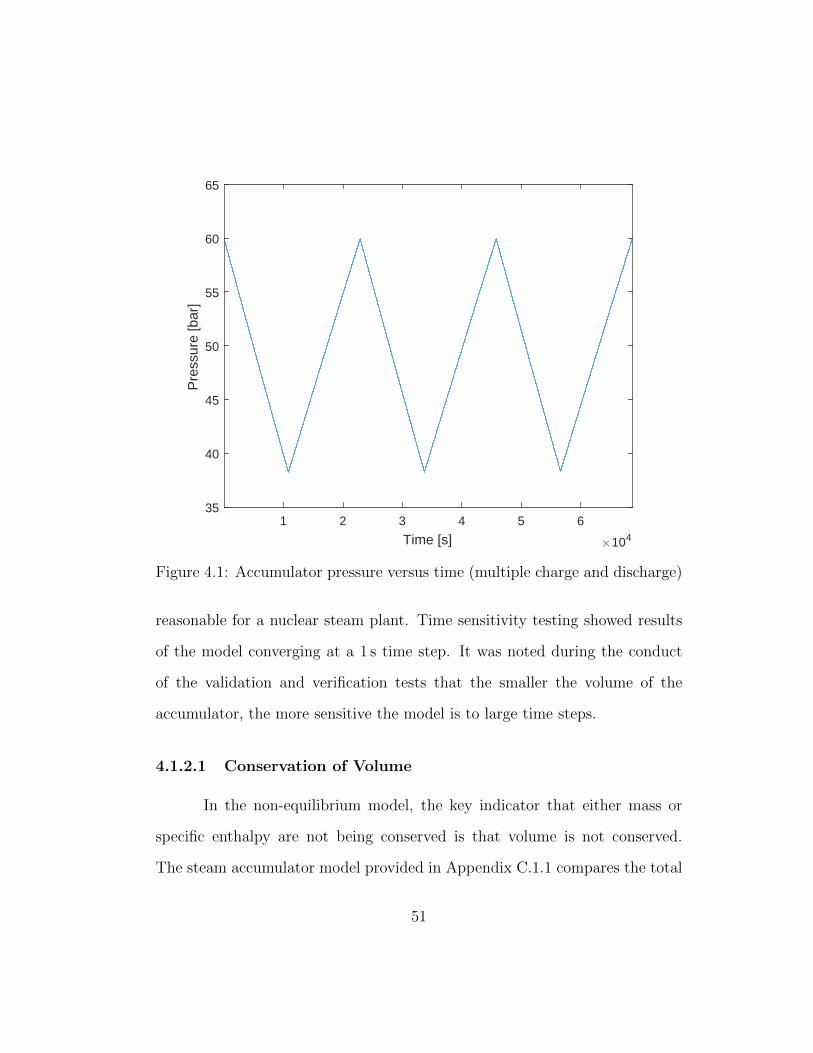
4.1.2 Charge/Discharge Simulation
A simulation was conducted of repeated charge/discharge evolutions on
the accumulator with the following conditions:
1. Accumulator charged pressure is 60 bar
2. Accumulator discharged pressure is 40 bar
3. The accumulator is discharged at 300 MW for 3 h
4. The accumulator is charged at a rate of 600 kg s−1
The MATLAB code for the simulation is provided in Appendix C.1.3.
The above conditions do not necessarily represent optimal conditions, but are
50
1 2 3 4 5 6
Time [s] 104
35
40
45
50
55
60
65P
ress
ure
[bar
]
Figure 4.1: Accumulator pressure versus time (multiple charge and discharge)
reasonable for a nuclear steam plant. Time sensitivity testing showed results
of the model converging at a 1 s time step. It was noted during the conduct
of the validation and verification tests that the smaller the volume of the
accumulator, the more sensitive the model is to large time steps.
4.1.2.1 Conservation of Volume
In the non-equilibrium model, the key indicator that either mass or
specific enthalpy are not being conserved is that volume is not conserved.
The steam accumulator model provided in Appendix C.1.1 compares the total
51
1 2 3 4 5 6
Time [s] 104
35
40
45
50
55
60T
ank
Wat
er L
evel
[%]
Figure 4.2: Accumulator water level versus time (multiple charge and dis-charge)
volume of both the liquid and steam phases each iteration and calculates the
difference between the sum of both phases and the volume of the accumulator.
For this simulation, the highest volume defect detected was 0.04%.
4.1.2.2 Pressure
It can be noted from the pressure response of the model shown in Figure
4.1, that charge and discharge times are roughly equal. The model was set
to discharge at a constant power of 300 MW. The model was charged with
52
1 2 3 4 5 6
Time [s] 104
0
1
2
3
4
5
6
7
8
9
10P
hase
Mas
s [k
g]107
LiquidSteamTotal
Figure 4.3: Accumulator phase mass versus time (multiple charge and dis-charge)
saturated steam at 72 bar at a rate of 600 kg s−1. This value was selected
because it was approximately the accumulator discharge rate calculated by
the heat balance code detailed in Appendix C.
4.1.2.3 Phase Mass
A review of the mass response detailed in Figure 4.3 shows that mass
is roughly conserved through several charge and discharge cycles.
53
1 2 3 4 5 6
Time [s] 104
0
2
4
6
8
10
12
14
Pha
se E
ntha
lpy
[kJ]
1010
LiquidSteamTotal
Figure 4.4: Accumulator phase specific enthalpy versus time (multiple chargeand discharge)
54
1 2 3 4 5 6
Time [s] 104
245
250
255
260
265
270
275
280P
hase
Tem
pera
ture
[C]
LiquidSteam
Figure 4.5: Accumulator phase temperature versus time (multiple charge anddischarge)
4.1.2.4 Phase Specific Enthalpy
A review of the phase specific enthalpy, in conjunction with the phase
mass, shows that the overall bulk enthalpy of the accumulator is conserved
through several charge and discharge cycles.
4.1.2.5 Phase Temperature
Phase temperature behaved as predicted by the non-equilibrium model.
During the charging evolutions, a temperature difference developed between
55
the steam and liquid phase of less than 1 ◦C.
4.2 Steam Plant Integration
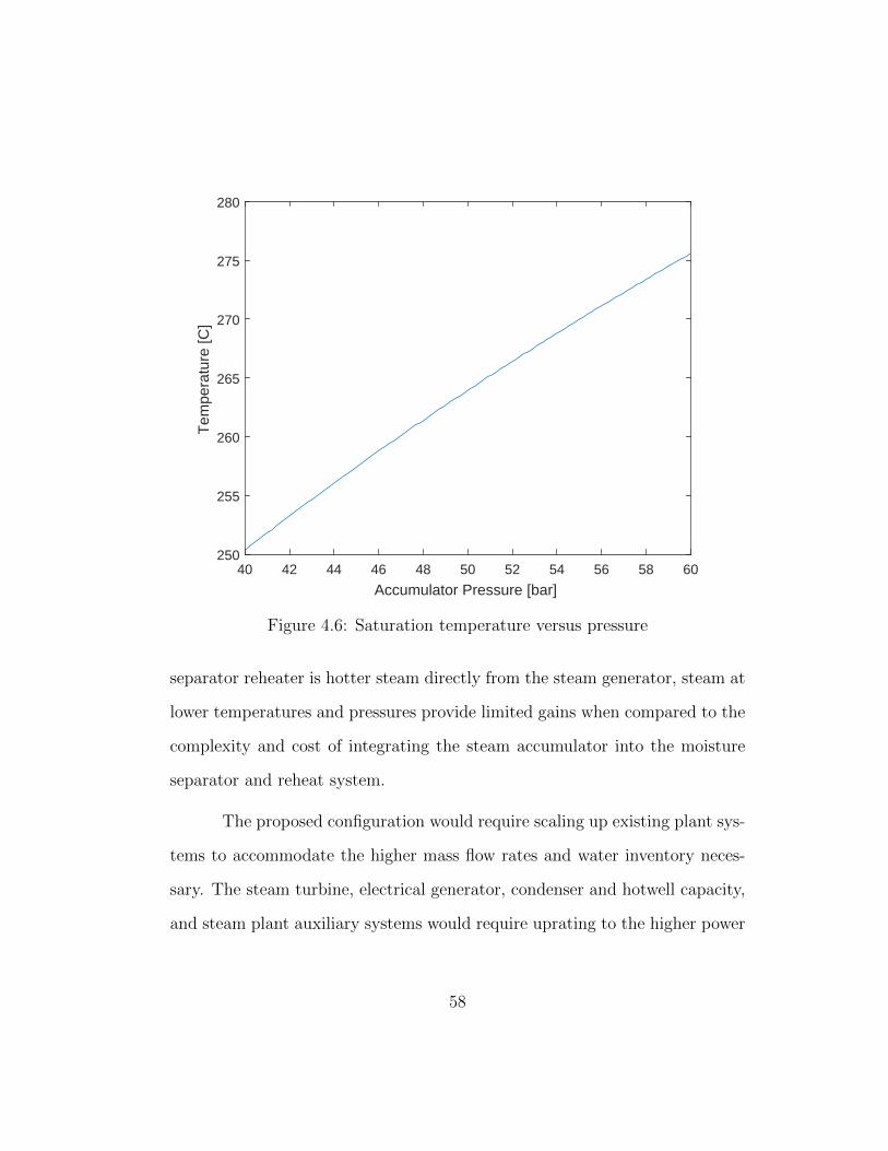
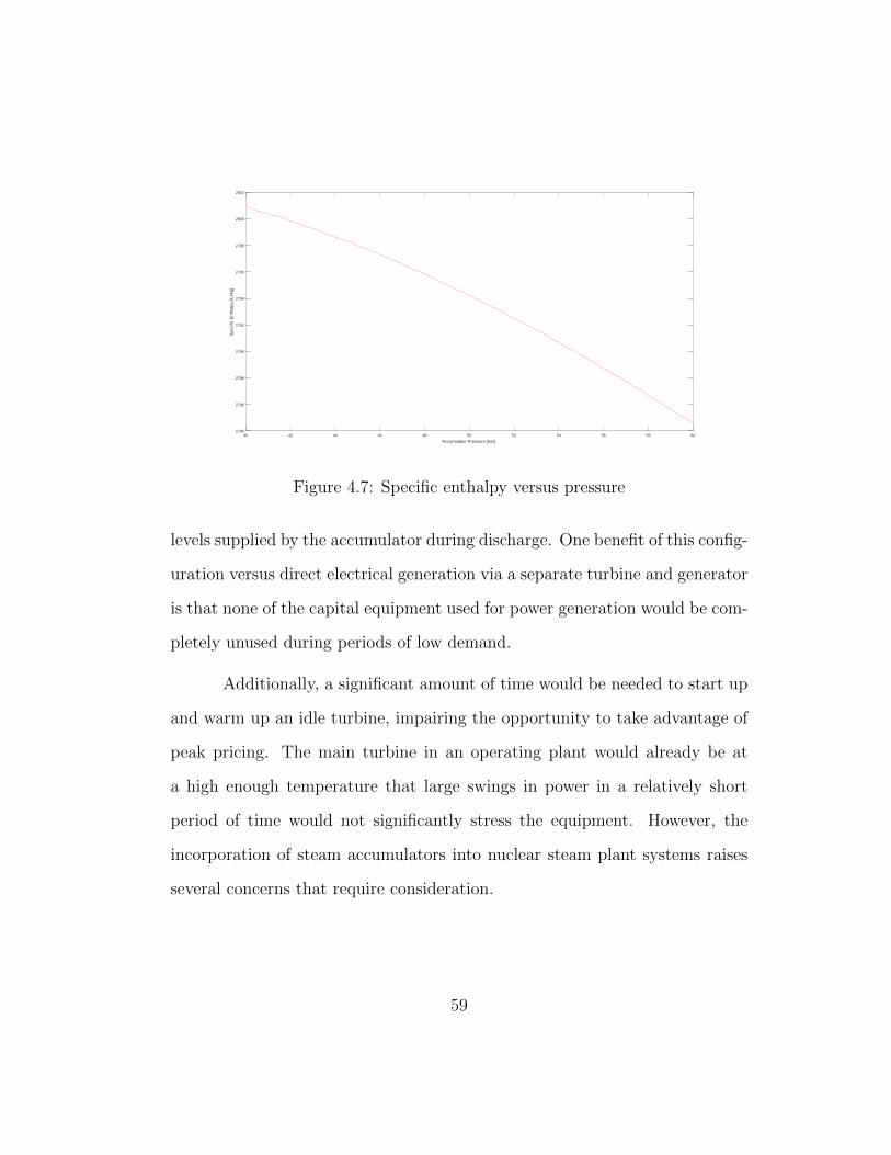
Heat and mass balances were evaluated for the integration of a steam
accumulator for both the feedwater heaters and the moisture separator re-
heater. MATLAB code detailing each model and the script used to evaluate
the steam plant cycles can be found in Appendix C. Provided the pressure
range for the accumulator is small enough, the values for specific enthalpy
and temperature of the steam from the accumulator do not substantially as
shown on Figures 4.6 and 4.7. The result is that flow from the accumula-
tor varies little while maintaining the same rate of heat transfer in the steam
plant loads the accumulator supplies. Consequently, the smaller the amount
that pressure is allowed to decrease from the high pressure, charged condition
for the accumulator, the greater the amount of water mass required in the
accumulator.
During discharging operations, steam from the steam accumulator re-
places steam from the steam generator to the feedwater heater and/or mois-
ture separator reheater. The efficiency gains from the feedwater heater and/or
moisture separator remain and more work can be done by the turbine. Dur-
ing charging operations, the steam mass flow rate to the turbines, feedwater
heater, and moisture separator reheaters decreases. Consequently, turbine ef-
ficiency and electrical power output decreases.
Heat balances and mass flows for the analyzed configurations are de-
56
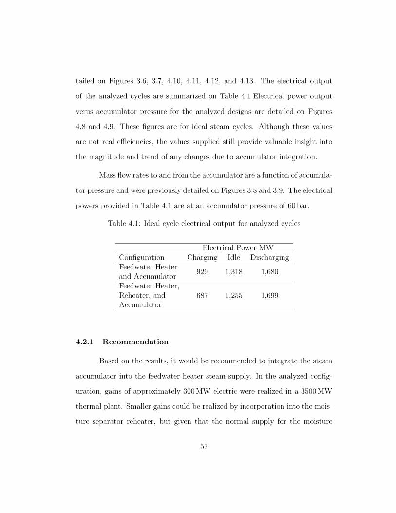
tailed on Figures 3.6, 3.7, 4.10, 4.11, 4.12, and 4.13. The electrical output
of the analyzed cycles are summarized on Table 4.1.Electrical power output
verus accumulator pressure for the analyzed designs are detailed on Figures
4.8 and 4.9. These figures are for ideal steam cycles. Although these values
are not real efficiencies, the values supplied still provide valuable insight into
the magnitude and trend of any changes due to accumulator integration.
Mass flow rates to and from the accumulator are a function of accumula-
tor pressure and were previously detailed on Figures 3.8 and 3.9. The electrical
powers provided in Table 4.1 are at an accumulator pressure of 60 bar.
Table 4.1: Ideal cycle electrical output for analyzed cycles
Electrical Power MWConfiguration Charging Idle DischargingFeedwater Heaterand Accumulator
929 1,318 1,680
Feedwater Heater,Reheater, andAccumulator
687 1,255 1,699
4.2.1 Recommendation
Based on the results, it would be recommended to integrate the steam
accumulator into the feedwater heater steam supply. In the analyzed config-
uration, gains of approximately 300 MW electric were realized in a 3500 MW
thermal plant. Smaller gains could be realized by incorporation into the mois-
ture separator reheater, but given that the normal supply for the moisture
57
40 42 44 46 48 50 52 54 56 58 60
Accumulator Pressure [bar]
250
255
260
265
270
275
280T
empe
ratu
re [C
]
Figure 4.6: Saturation temperature versus pressure
separator reheater is hotter steam directly from the steam generator, steam at
lower temperatures and pressures provide limited gains when compared to the
complexity and cost of integrating the steam accumulator into the moisture
separator and reheat system.
The proposed configuration would require scaling up existing plant sys-
tems to accommodate the higher mass flow rates and water inventory neces-
sary. The steam turbine, electrical generator, condenser and hotwell capacity,
and steam plant auxiliary systems would require uprating to the higher power
58
40 42 44 46 48 50 52 54 56 58 60
Accumulator Pressure [bar]
2784
2786
2788
2790
2792
2794
2796
2798
2800
2802
Spe
cific
Ent
halp
y [k
J/kg
]
Figure 4.7: Specific enthalpy versus pressure
levels supplied by the accumulator during discharge. One benefit of this config-
uration versus direct electrical generation via a separate turbine and generator
is that none of the capital equipment used for power generation would be com-
pletely unused during periods of low demand.
Additionally, a significant amount of time would be needed to start up
and warm up an idle turbine, impairing the opportunity to take advantage of
peak pricing. The main turbine in an operating plant would already be at
a high enough temperature that large swings in power in a relatively short
period of time would not significantly stress the equipment. However, the
incorporation of steam accumulators into nuclear steam plant systems raises
several concerns that require consideration.
59
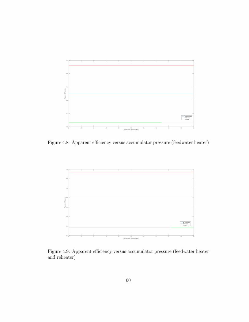
40 42 44 46 48 50 52 54 56 58 60
Accumulator Pressure [bar]
0.25
0.3
0.35
0.4
0.45
0.5
App
aren
t Effi
cien
cy
No AccumulatorDischargingCharging
Figure 4.8: Apparent efficiency versus accumulator pressure (feedwater heater)
40 42 44 46 48 50 52 54 56 58 60
Accumulator Pressure [bar]
0.15
0.2
0.25
0.3
0.35
0.4
0.45
0.5
App
aren
t Effi
cien
cy
No AccumulatorDischargingCharging
Figure 4.9: Apparent efficiency versus accumulator pressure (feedwater heaterand reheater)
60
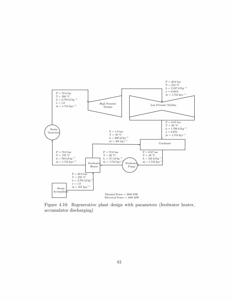
High PressureTurbine
Low Pressure Turbine
SteamGenerator
FeedwaterPump
P = 72.0 barT = 288 ◦Ch = 2,770 kJ kg−1
x = 1.0m = 1,744 kg s−1
P = 0.07 barT = 39 ◦Ch = 1,799 kJ kg−1
x = 0.679m = 1,744 kg s−1
Condenser
P = 0.07 barT = 39 ◦Ch = 163 kJ kg−1
m = 1,744 kg s−1
P = 72.0 barT = 179 ◦Ch = 763 kJ kg−1
m = 1,744 kg s−1
Thermal Power = 3500 MWElectrical Power = 1680 MW
FeedwaterHeater
P = 60.0 barT = 276 ◦Ch = 2,785 kJ kg−1
x = 1.0m = 401 kg s−1
P = 20.0 barT = 212 ◦Ch = 2,537 kJ kg−1
x = 0.8615m = 1,744 kg s−1
P = 72.0 barT = 39 ◦Ch = 171 kJ kg−1
m = 1,744 kg s−1
P = 1.0 barT = 49 ◦Ch = 206 kJ kg−1
m = 401 kg s−1
SteamAccumulator
Figure 4.10: Regenerative plant design with parameters (feedwater heater,accumulator discharging)
61
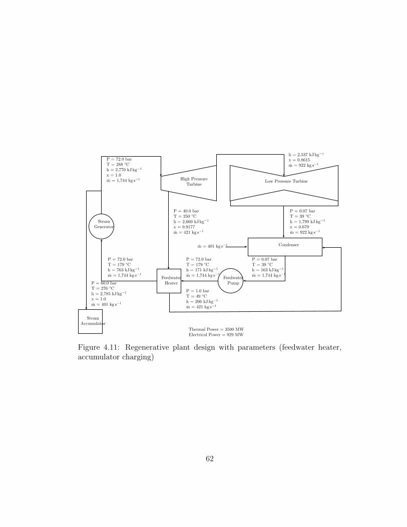
High PressureTurbine
Low Pressure Turbine
SteamGenerator
FeedwaterPump
P = 72.0 barT = 288 ◦Ch = 2,770 kJ kg−1
x = 1.0m = 1,744 kg s−1
P = 0.07 barT = 39 ◦Ch = 1,799 kJ kg−1
x = 0.679m = 922 kg s−1
Condenser
P = 0.07 barT = 39 ◦Ch = 163 kJ kg−1
m = 1,744 kg s−1
P = 72.0 barT = 179 ◦Ch = 763 kJ kg−1
m = 1,744 kg s−1
Thermal Power = 3500 MWElectrical Power = 929 MW
FeedwaterHeaterP = 60.0 bar
T = 276 ◦Ch = 2,785 kJ kg−1
x = 1.0m = 401 kg s−1
h = 2,537 kJ kg−1
x = 0.8615m = 922 kg s−1
P = 1.0 barT = 49 ◦Ch = 206 kJ kg−1
m = 421 kg s−1
SteamAccumulator
P = 40.0 barT = 250 ◦Ch = 2,660 kJ kg−1
x = 0.9177m = 421 kg s−1
P = 72.0 barT = 179 ◦Ch = 171 kJ kg−1
m = 1,744 kg s−1
m = 401 kg s−1
Figure 4.11: Regenerative plant design with parameters (feedwater heater,accumulator charging)
62
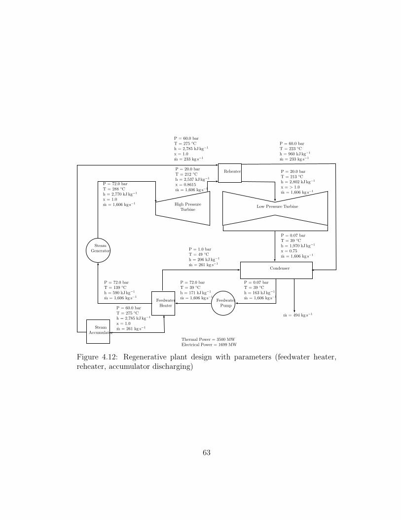
High PressureTurbine
Low Pressure Turbine
SteamGenerator
FeedwaterPump
P = 60.0 barT = 275 ◦Ch = 2,785 kJ kg−1
x = 1.0m = 233 kg s−1
P = 0.07 barT = 39 ◦Ch = 1,970 kJ kg−1
x = 0.75m = 1,606 kg s−1
Condenser
P = 0.07 barT = 39 ◦Ch = 163 kJ kg−1
m = 1,606 kg s−1
P = 72.0 barT = 139 ◦Ch = 590 kJ kg−1
m = 1,606 kg s−1
Thermal Power = 3500 MWElectrical Power = 1699 MW
FeedwaterHeater
P = 60.0 barT = 275 ◦Ch = 2,785 kJ kg−1
x = 1.0m = 261 kg s−1
P = 20.0 barT = 213 ◦Ch = 2,802 kJ kg−1
x = > 1.0m = 1,606 kg s−1
P = 72.0 barT = 39 ◦Ch = 171 kJ kg−1
m = 1,606 kg s−1
P = 1.0 barT = 49 ◦Ch = 206 kJ kg−1
m = 261 kg s−1
ReheaterP = 20.0 barT = 212 ◦Ch = 2,537 kJ kg−1
x = 0.8615m = 1,606 kg s−1
m = 494 kg s−1
P = 60.0 barT = 223 ◦Ch = 960 kJ kg−1
m = 233 kg s−1
P = 72.0 barT = 288 ◦Ch = 2,770 kJ kg−1
x = 1.0m = 1,606 kg s−1
SteamAccumulator
Figure 4.12: Regenerative plant design with parameters (feedwater heater,reheater, accumulator discharging)
63
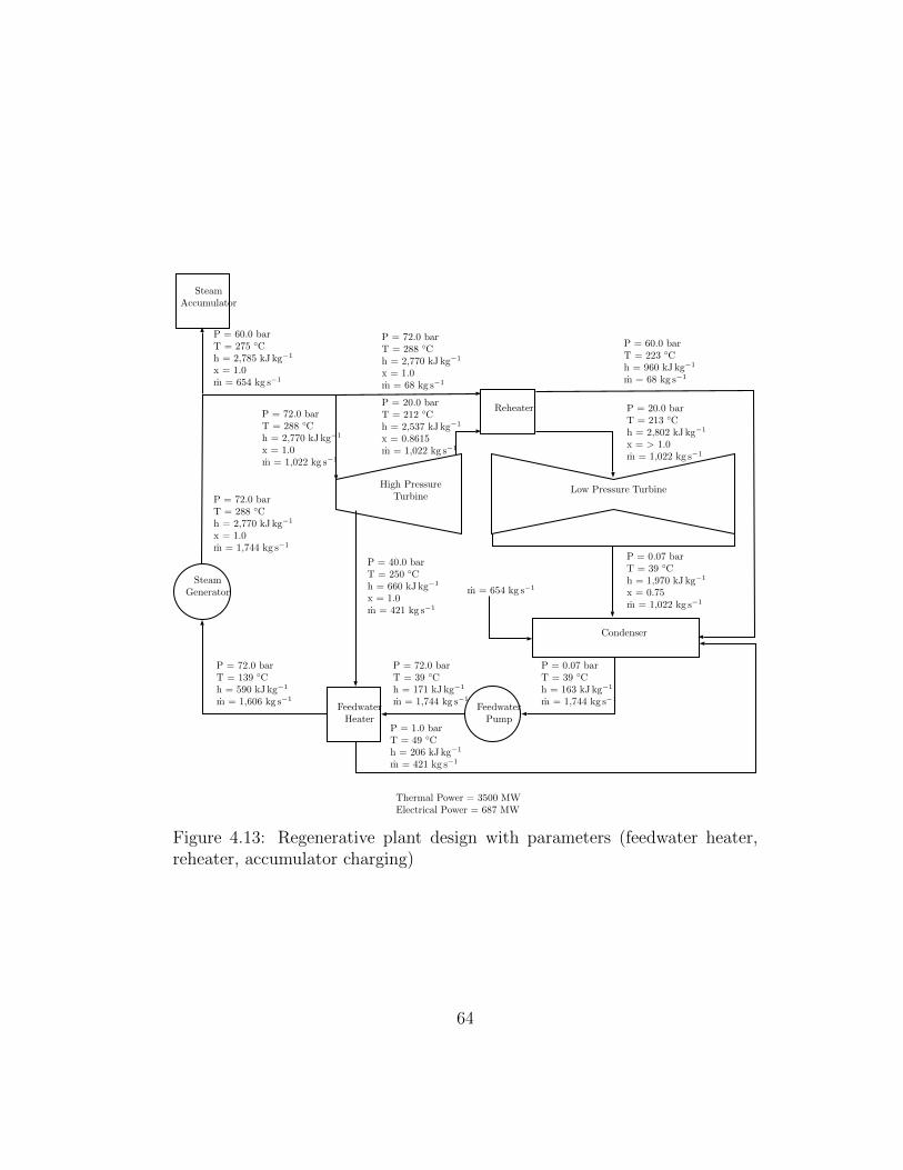
High PressureTurbine
Low Pressure Turbine
SteamGenerator
FeedwaterPump
P = 72.0 barT = 288 ◦Ch = 2,770 kJ kg−1
x = 1.0m = 68 kg s−1
P = 0.07 barT = 39 ◦Ch = 1,970 kJ kg−1
x = 0.75m = 1,022 kg s−1
Condenser
P = 0.07 barT = 39 ◦Ch = 163 kJ kg−1
m = 1,744 kg s−1
P = 72.0 barT = 139 ◦Ch = 590 kJ kg−1
m = 1,606 kg s−1
Thermal Power = 3500 MWElectrical Power = 687 MW
FeedwaterHeater
P = 60.0 barT = 275 ◦Ch = 2,785 kJ kg−1
x = 1.0m = 654 kg s−1
P = 20.0 barT = 213 ◦Ch = 2,802 kJ kg−1
x = > 1.0m = 1,022 kg s−1
P = 72.0 barT = 39 ◦Ch = 171 kJ kg−1
m = 1,744 kg s−1
P = 1.0 barT = 49 ◦Ch = 206 kJ kg−1
m = 421 kg s−1
ReheaterP = 20.0 barT = 212 ◦Ch = 2,537 kJ kg−1
x = 0.8615m = 1,022 kg s−1
m = 654 kg s−1
P = 60.0 barT = 223 ◦Ch = 960 kJ kg−1
m = 68 kg s−1
P = 72.0 barT = 288 ◦Ch = 2,770 kJ kg−1
x = 1.0m = 1,744 kg s−1
SteamAccumulator
P = 72.0 barT = 288 ◦Ch = 2,770 kJ kg−1
x = 1.0m = 1,022 kg s−1
P = 40.0 barT = 250 ◦Ch = 660 kJ kg−1
x = 1.0m = 421 kg s−1
Figure 4.13: Regenerative plant design with parameters (feedwater heater,reheater, accumulator charging)
64
4.2.2 Key Considerations
Several key considerations present themselves in the incorporation of
steam accumulators into the feedwater heater steam supply system.
4.2.2.1 Inadvertent Loss of the Steam Accumulator System DuringCharging or Discharging Operations
Loss of the steam accumulator system during system discharge is un-
likely to result in significant consequences. Operators are already trained to
respond to loss of steam supply to the feedwater heaters. Operators are also
very sensitive to proper feedwater heater operation, due to the probability of
a reactivity excursion due to improper operation of the system.
Loss of the steam accumulator during system charging is a larger con-
cern. If the charging rate were sufficiently high, loss of the steam accumulator
during charging would result in an automatic reactor trip. To the reactor plant,
the loss of the steam accumulator would look exactly like a turbine runback or
load rejection. In some designs, automatic systems such as steam dumps can
automatically compensate for a load rejection up to a certain fraction of rated
thermal power, up to 40% in some cases. It would be recommended to restrict
the steam accumulator charging rate to a value within the capacity of any
available system designed to automatically compensate for a load rejection.
65
4.2.2.2 Additional Heat Sink
Provided the steam accumulator system is functioning normally, an ac-
cumulator that is not fully charged does provide an additional heat sink to the
plant. It may be worth considering when designing and sizing the accumulator
to identify a maximum accumulator pressure that provides sufficient margin
in accumulator capacity such that additional defense in depth against a loss
of heat sink event is present.
Depending on the reactor design and configuration, designing the sys-
tem to safety-related standards may provide additional flexibility that permit
continued operation when technical specifications applying to current designs
would require a shutdown and immediate correction of a deficiency.
4.2.2.3 Increased Hotwell Capacity
Accumulator flowrates during discharging evolutions, 500 kg s−1 to 600 kg s−1
for an approximately 300 MW increase in electrical power output, could over-
whelm typical steam plant water makeup systems. Sufficiently increased hotwell
capacity would alleviate concerns regarding abnormally large swings in hotwell
level.
66
Chapter 5
Conclusions
In deregulated markets, peak demand prices present an opportunity for
nuclear power plants to increase their economic competitiveness. Currently,
the combined cycle fleet dominates this market. The historically low price of
natural gas coupled with their ability to nimbly start up and shut down with
little notice places nuclear power in a precariously uncompetitive position.
Nuclear power plants require an alternative that allows them to maintain their
baseload power level at all times, but not necessarily distribute that power to
the grid during periods of low demand and low prices.
This work expanded on prior studies to incorporate thermal energy stor-
age into existing steam plant components. It has been demonstrated by this
work that a sizable amount of additional power can be produced by augment-
ing existing steam flow paths, as opposed to a separate turbine-generator set.
By leveraging feedwater heaters and moisture separator reheaters as a point
of reintroduction of stored thermal energy, significant increases in electrical
power output can be sustained for hours.
A method for modeling steam plant accumulators was constructed from
prior work to demonstrate the time response of several key parameters during
67
charge and discharge.
Key areas that lend themselves to future work are:
1. Optimization of accumulator design for plant conditions
2. Study of the regulatory environment and licensing basis impacts associ-
ated with steam plant accumulator integration
3. Economic study of accumulator integration
4. Economic optimization of accumulator design to leverage peak demand
pricing
68

Appendices
69
Appendix A
Validation and Verification of the
Non-Equilibrium Steam Accumulator Model
A.1 Discussion
The non-equilibrium MATLAB steam accumulator model was evalu-
ated against two validations and verifications performed by Stevanovic et al.
[10]. Detailed data was not provided by Stevanovic et al. to allow for valida-
tion and verification of their model. Consequently, a graphical comparison of
results was necessary.
The accumulator used by Stevanovic was relatively small, 64 m3, com-
pared to those used in commercial power production. A separate version of the
model was developed for testing to allow the test accumulator to be defined
by the specific parameters listed in the literature [10]. The model is detailed
in Appendix C.1.2.
It was noted while simulating the validation and verification tests that
the smaller volume test accumulator was particularly sensitive to large time
steps. A smaller time step, 0.1 s, provided smooth and consistent results.
Given the time dependent nature of the first order differential equations that
make up the model, this was not unexpected.
70
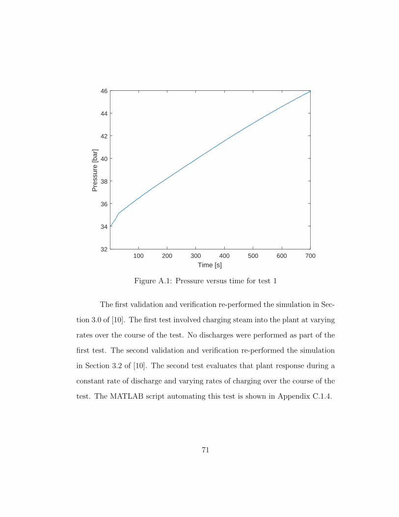
100 200 300 400 500 600 700
Time [s]
32
34
36
38
40
42
44
46P
ress
ure
[bar
]
Figure A.1: Pressure versus time for test 1
The first validation and verification re-performed the simulation in Sec-
tion 3.0 of [10]. The first test involved charging steam into the plant at varying
rates over the course of the test. No discharges were performed as part of the
first test. The second validation and verification re-performed the simulation
in Section 3.2 of [10]. The second test evaluates that plant response during a
constant rate of discharge and varying rates of charging over the course of the
test. The MATLAB script automating this test is shown in Appendix C.1.4.
71
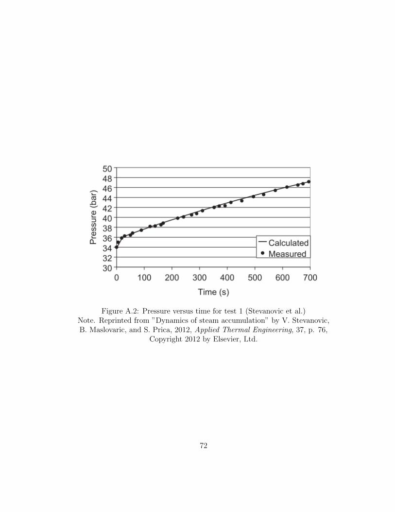
Figure A.2: Pressure versus time for test 1 (Stevanovic et al.)Note. Reprinted from ”Dynamics of steam accumulation” by V. Stevanovic,B. Maslovaric, and S. Prica, 2012, Applied Thermal Engineering, 37, p. 76,
Copyright 2012 by Elsevier, Ltd.
72
A.2 Results
A.2.1 Test Number 1
Graphically, the results compare well. Figure A.1 follows the trend
and finishes very closely to Figure A.2. The final pressure of our model is
approximately 1.0 bar lower than the literature. This is very likely attributed
to the lack of detailed data regarding the exact initial conditions and flow
rates.
A.2.2 Test Number 2
Graphically, the results compare well. Figure A.3 follows the trend and
finishes very closely to Figure A.4. The final pressure of our model is slightly
higher than the literature. This is very likely attributed to the lack of detailed
data regarding the exact initial conditions and flow rates.
A.3 Summary
With the information available for validation and verification, our model
compares well with the literature and is acceptable for use.
73
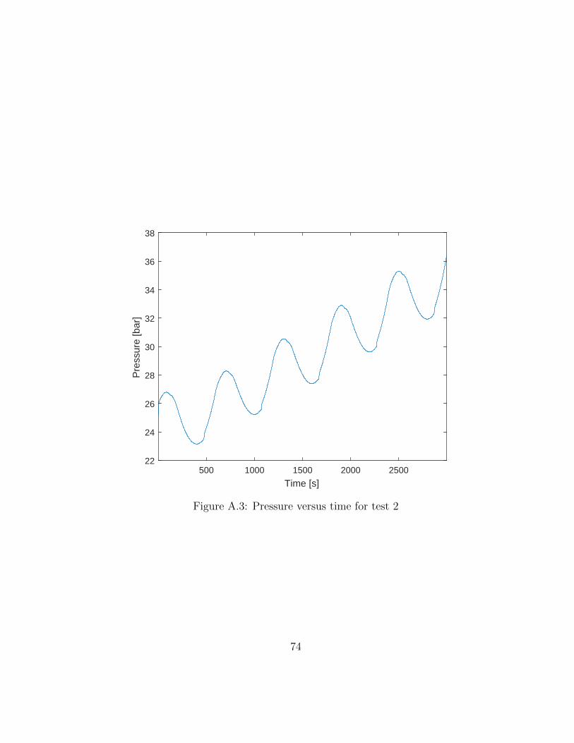
500 1000 1500 2000 2500
Time [s]
22
24
26
28
30
32
34
36
38
Pre
ssur
e [b
ar]
Figure A.3: Pressure versus time for test 2
74
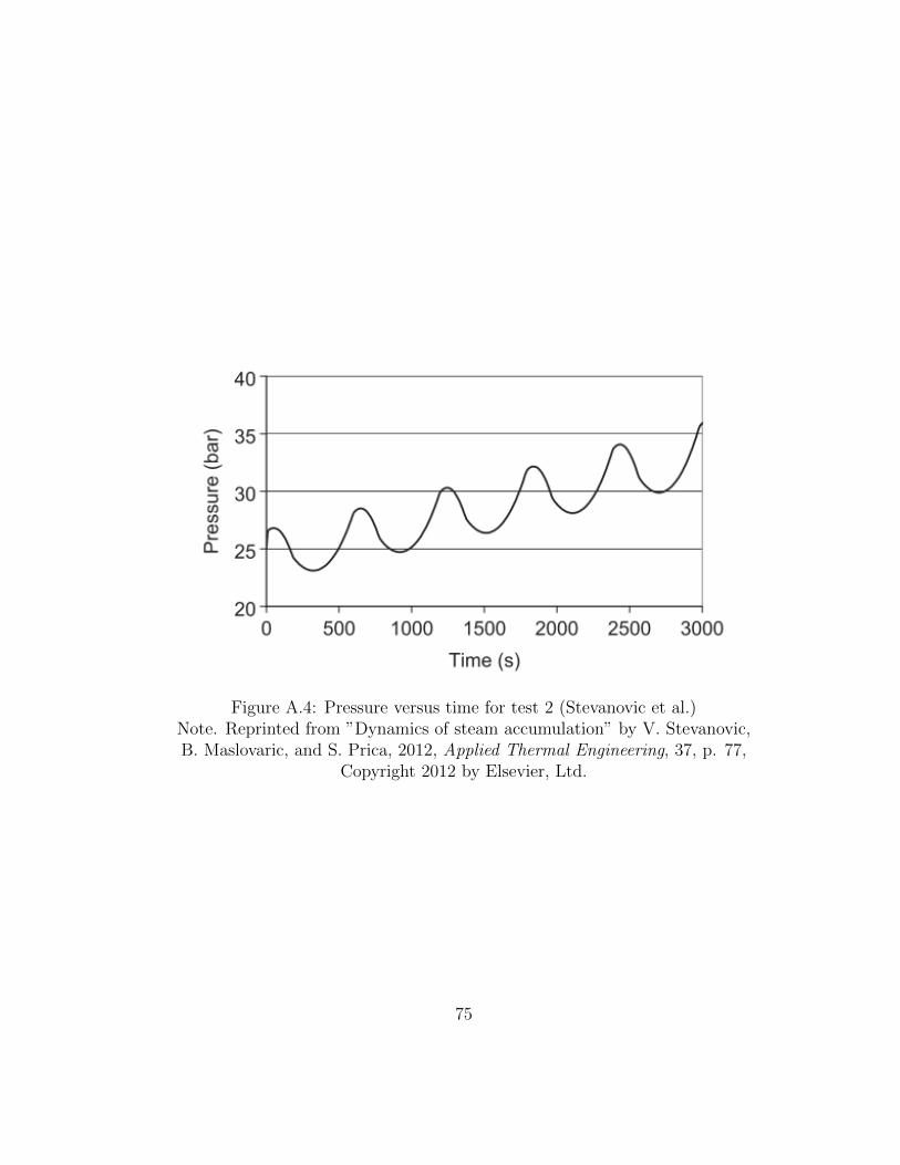
Figure A.4: Pressure versus time for test 2 (Stevanovic et al.)Note. Reprinted from ”Dynamics of steam accumulation” by V. Stevanovic,B. Maslovaric, and S. Prica, 2012, Applied Thermal Engineering, 37, p. 77,
Copyright 2012 by Elsevier, Ltd.
75
Appendix B
Accumulator Model Time Sensitivity
Evaluation
The non-equilibrium steam accumulator model is comprised of first-
order differential equations differentiated with respect to time. Consequently,
the results obtained by employing the Runge-Katta method to iteratively solve
the model are sensitive to the period of time between each iteration. To test
the sensitivity of the model results to the value of the time step.
Two parameters were selected to evaluate the time sensitivity of the
model. Volume defect identifies the fractional difference between the sum of
the liquid and steam phase volumes and the accumulator volume (Equation
B.1). Obviously, the sum of the liquid and steam phase volumes cannot be
larger or smaller than the accumulator volume. The volume of each phase is
the product of the specific volume and mass of each respective phase (Equation
B.2). In the model, the specific volume is a function of pressure and specific
enthalpy. Both of which are solved by the model. Mass is a function of flow
in and out of the accumulator, which is resolved in the model as the product
of the mass flow rate and the time step. All of these factors make the volume
defect an excellent indicator of the consistency of the model. The volume
76
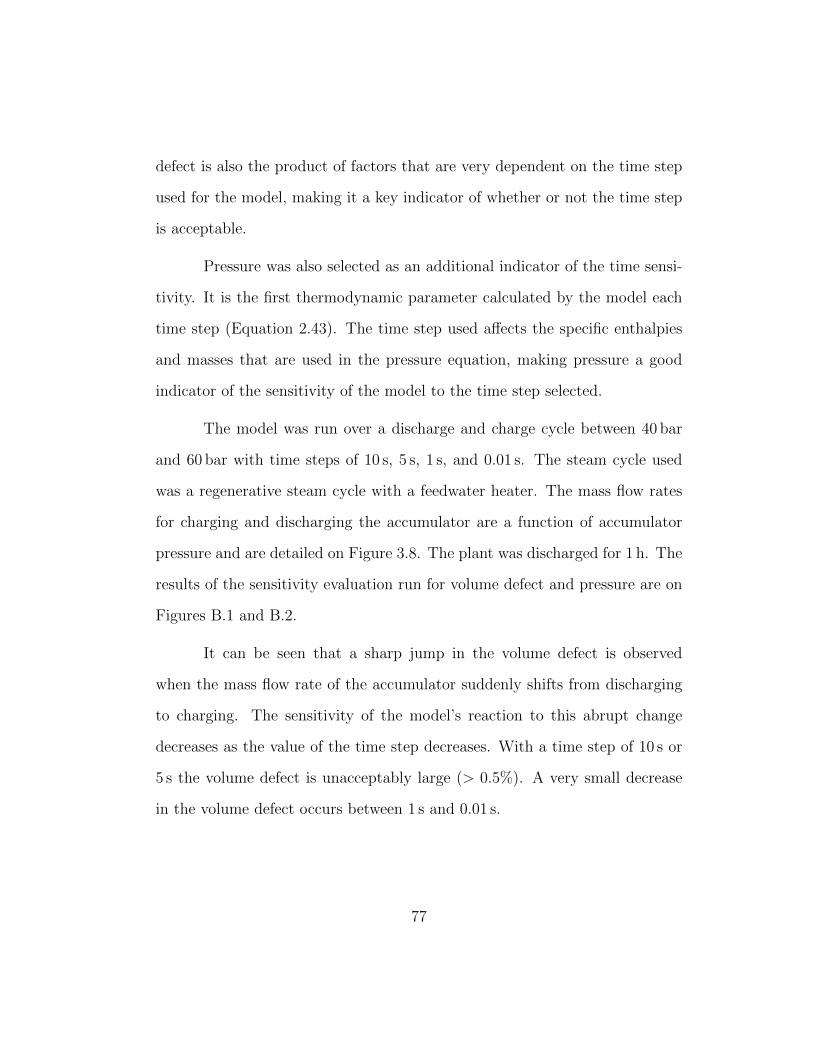
defect is also the product of factors that are very dependent on the time step
used for the model, making it a key indicator of whether or not the time step
is acceptable.
Pressure was also selected as an additional indicator of the time sensi-
tivity. It is the first thermodynamic parameter calculated by the model each
time step (Equation 2.43). The time step used affects the specific enthalpies
and masses that are used in the pressure equation, making pressure a good
indicator of the sensitivity of the model to the time step selected.
The model was run over a discharge and charge cycle between 40 bar
and 60 bar with time steps of 10 s, 5 s, 1 s, and 0.01 s. The steam cycle used
was a regenerative steam cycle with a feedwater heater. The mass flow rates
for charging and discharging the accumulator are a function of accumulator
pressure and are detailed on Figure 3.8. The plant was discharged for 1 h. The
results of the sensitivity evaluation run for volume defect and pressure are on
Figures B.1 and B.2.
It can be seen that a sharp jump in the volume defect is observed
when the mass flow rate of the accumulator suddenly shifts from discharging
to charging. The sensitivity of the model’s reaction to this abrupt change
decreases as the value of the time step decreases. With a time step of 10 s or
5 s the volume defect is unacceptably large (> 0.5%). A very small decrease
in the volume defect occurs between 1 s and 0.01 s.
77

0 1000 2000 3000 4000 5000 6000 7000
Time [s]
0
0.2
0.4
0.6
0.8
1
1.2
1.4
Vol
ume
Def
ect [
%]
10.05.01.00.1
Time Step
Figure B.1: Volume defect versus time for selected values of time step
0 1000 2000 3000 4000 5000 6000 7000
Time [s]
40
42
44
46
48
50
52
54
56
58
60
Pre
ssur
e [b
ar]
10.05.01.00.1
Time Step
Figure B.2: Pressure versus time for selected values of time step
With regards to pressure, the higher the time step, the lower the pre-
dicted pressure at a specific time interval. This can be seen in greater detail
78
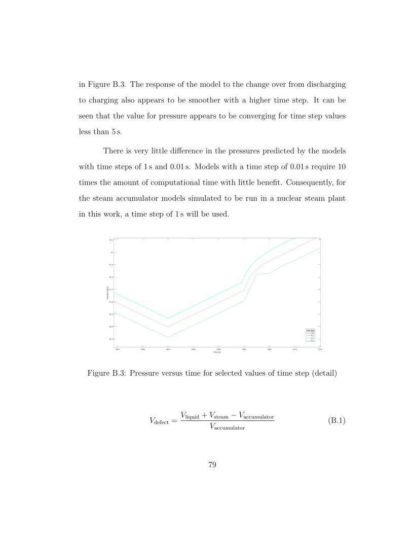
in Figure B.3. The response of the model to the change over from discharging
to charging also appears to be smoother with a higher time step. It can be
seen that the value for pressure appears to be converging for time step values
less than 5 s.
There is very little difference in the pressures predicted by the models
with time steps of 1 s and 0.01 s. Models with a time step of 0.01 s require 10
times the amount of computational time with little benefit. Consequently, for
the steam accumulator models simulated to be run in a nuclear steam plant
in this work, a time step of 1 s will be used.
3560 3580 3600 3620 3640 3660 3680 3700 3720
Time [s]
41.3
41.4
41.5
41.6
41.7
41.8
41.9
42
42.1
Pre
ssur
e [b
ar]
10.05.01.00.1
Time Step
Figure B.3: Pressure versus time for selected values of time step (detail)
Vdefect =Vliquid + Vsteam − Vaccumulator
Vaccumulator
(B.1)
79

V = vm (B.2)
m = mt (B.3)
80
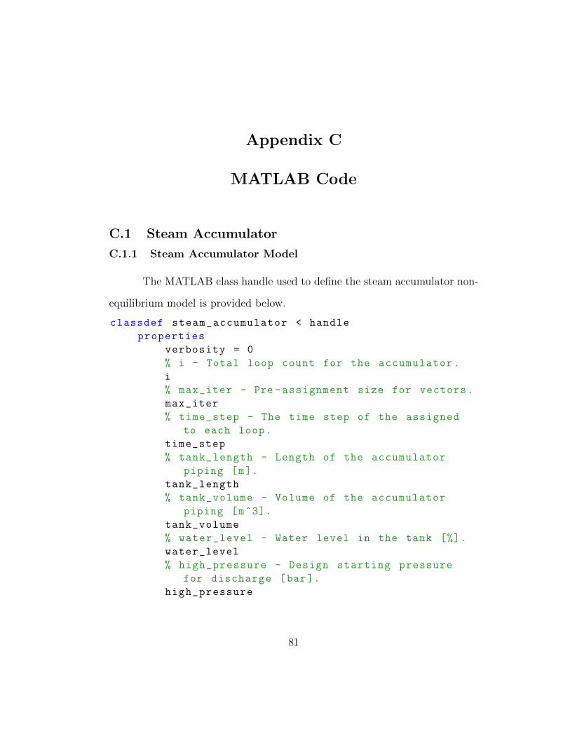
Appendix C
MATLAB Code
C.1 Steam Accumulator
C.1.1 Steam Accumulator Model
The MATLAB class handle used to define the steam accumulator non-
equilibrium model is provided below.
classdef steam_accumulator < handle
properties
verbosity = 0
% i - Total loop count for the accumulator.
i
% max_iter - Pre -assignment size for vectors.
max_iter
% time_step - The time step of the assigned
to each loop.
time_step
% tank_length - Length of the accumulator
piping [m].
tank_length
% tank_volume - Volume of the accumulator
piping [m^3].
tank_volume
% water_level - Water level in the tank [%].
water_level
% high_pressure - Design starting pressure
for discharge [bar].
high_pressure
81

% low_pressure - Design low pressure for
discharge [bar].
low_pressure
% high_quality - Design high steam quality
after charging.
high_quality
% low_quality - Design low steam quality
after discharging.
low_quality
% minimum_efficiency - Design minimum cycle
efficiency.
minimum_efficiency
% minimum_water_mass - Design minimum water
mass required at the
% beginning of a discharge [kg].
minimum_water_mass
% volume_defect_detected - True if a
volume_defect was detected in
% any loop.
volume_defect_detected = false
% initial_total_enthalpy
initial_total_enthalpy
initial_steam_mass
initial_water_mass
initial_water_level
prepared_for_evaluation = false
p = []
x = []
v_1 = []
v_2 = []
rho_1 = []
rho_2 = []
rho_mixture = []
v_mixture = []
t_1 = []
t_2 = []
m_1 = []
82
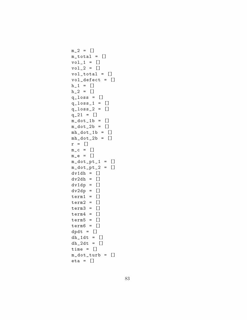
m_2 = []
m_total = []
vol_1 = []
vol_2 = []
vol_total = []
vol_defect = []
h_1 = []
h_2 = []
q_loss = []
q_loss_1 = []
q_loss_2 = []
q_21 = []
m_dot_1b = []
m_dot_2b = []
mh_dot_1b = []
mh_dot_2b = []
r = []
m_c = []
m_e = []
m_dot_pt_1 = []
m_dot_pt_2 = []
dv1dh = []
dv2dh = []
dv1dp = []
dv2dp = []
term1 = []
term2 = []
term3 = []
term4 = []
term5 = []
term6 = []
dpdt = []
dh_1dt = []
dh_2dt = []
time = []
m_dot_turb = []
eta = []
83
m_in = []
m_out = []
loop_time = []
x_1 = []
x_2 = []
end
properties(Constant)
TAU = 85.0 % relaxation time [s]
EPSILON = 0.02 % used to disrupt equilibrium
in temperature between
% liquid and steam phases
when setting up initial
% conditions
MPA_PER_BAR = 0.1 % MPa per bar [MPa/bar]
BAR_PER_MPA = 10 % bar per MPa [bar/MPa]
W_PER_KW = 1000 % watts per kilowatt [W/kW]
KW_PER_W = 0.001 % kilowatts per watt [kW/
W]
MASS_TOLERANCE = 0.01 % tolerance used to
determine if a mass
% imbalance is
present [%]
VOLUME_TOLERANCE = 0.05 % tolerance used to
determine if a volume
% imbalance is
present
PIPE_RADIUS = 0.4064 % radius of the
natural gas pipeline being used
% to construct the
accumulator
PIPE_THICKNESS = 0.15875 % thickness of
the natural gas pipeline
INSULATION_THICKNESS = 0.2032 % insulation
thickness
K_INSULATION = 0.079 % thermal
conductivity of the insulation
84
K_PIPE = 41.0 % thermal conductivity of the
pipe
H_AIR = 15.0 % heat transfer coefficient
of the air
PASCALS_PER_BAR = 1e5 % Pascals per bar [Pa
/bar]
BAR_PER_PASCAL = 1e-5 % bar per Pascal [bar
/Pa]
ATM_PRESSURE_IN_BAR = 1.01325 % atmospheric
pressure [bar]
end
methods
function obj = steam_accumulator(p0, x0 ,
l_tank , dt, max_iter , verbosity)
if nargin > 0
obj.verbosity = verbosity;
obj.i = 1;
obj.max_iter = max_iter;
obj.time_step = dt;
obj.tank_length = l_tank;
obj.initialize_arrays ();
obj.setup_initial_conditions(p0, x0);
end
end
function value = get.tank_volume(obj)
value = pi * (obj.PIPE_RADIUS ^2) * obj.
tank_length;
end
function value = get.initial_total_enthalpy(
obj)
value = obj.h_1(1) * obj.m_1(1) + obj.h_2
(1) * obj.m_2(1);
end
function value = get.initial_water_mass(obj)
value = obj.m_1(1);
end
function value = get.initial_steam_mass(obj)
85
value = obj.m_2(1);
end
function value = get.initial_water_level(obj)
value = obj.vol_1 (1) / obj.vol_total (1);
end
function [mass_charged , charge_time ,
final_quality , volume_defect] = charge(obj
,...
final_pressure , charge_pressure ,...
charge_flowrate , time_step)
mass_charged = 0.0;
obj.time_step = time_step;
if(obj.verbosity > 0)
fprintf('Commencing charge to %.2f
bar.\n', final_pressure);
end
start_time = tic;
i_begin = obj.i;
while obj.p(obj.i) < final_pressure
flow_multiplier = 0.0;
flow_multiplier = 1 - sqrt(obj.p(obj.
i) / charge_pressure);
if(flow_multiplier < 0.0)
flow_multiplier = 0.0;
end
if(flow_multiplier > 1.0)
flow_multiplier = 1.0;
end
charge_steam_flow = 0.0;
charge_liquid_flow = 0.0;
h_1_in = IAPWS_IF97('hL_p',
charge_pressure * obj.MPA_PER_BAR)
;
h_2_in = IAPWS_IF97('hV_p',
charge_pressure * obj.MPA_PER_BAR)
;
if obj.p(obj.i) < final_pressure
86
charge_steam_flow = 600.0 +
charge_flowrate *
flow_multiplier;
end
if(obj.verbosity > 1 && mod(obj.i,
100) == 0)
fprintf('%10s = %.4f.\n', 'Tank
Level ', obj.water_level(obj.i)
);
fprintf('Steam flow: %.2f kg/s.\n
', charge_steam_flow);
fprintf('Liquid flow: %.2f kg/s.\
n', charge_liquid_flow);
end
mass_charged = mass_charged + (
charge_liquid_flow +
charge_steam_flow) * obj.time_step
;
obj.increment_time_step(
charge_liquid_flow , 0.0,
charge_steam_flow , 0.0, h_1_in ,
h_2_in);
end
if(obj.verbosity > 0)
fprintf('Charge function complete in
%.2f seconds .\n', toc(start_time))
;
fprintf('Time to charge %.2f hours.\n
', (obj.i - i_begin) * obj.
time_step / 3600);
end
charge_time = (obj.i - i_begin) * obj.
time_step;
final_quality = obj.x(obj.i);
volume_defect = obj.
volume_defect_detected;
end
87
function [mass_discharged , final_quality ,
volume_defect] = discharge(obj , power ,...
time , time_step)
mass_discharged = 0.0;
if(obj.verbosity > 0)
fprintf('Discharging at %.1f MW for
%.1f hour(s).\n', power , time /
3600);
end
start_time = tic;
obj.time_step = time_step;
i_begin = obj.i;
while (obj.i - i_begin) * obj.time_step <
time
[obj.eta(obj.i), obj.m_dot_turb(obj.i
)] = obj.run_turbine(obj.p(obj.i),
0.9, power , 5);
mass_discharged = mass_discharged +
obj.m_dot_turb(obj.i) * obj.
time_step;
obj.increment_time_step_test (0.0,
0.0, 0.0, obj.m_dot_turb(obj.i),
0.0, 0.0);
end
if(obj.verbosity > 0)
fprintf('Discharge function complete
in %.2f seconds .\n', toc(
start_time));
fprintf('Discharge complete (%.2f MW,
%.2f hours).\n', power , (obj.i -
i_begin) * obj.time_step / 3600);
end
final_quality = obj.x(obj.i);
volume_defect = obj.
volume_defect_detected;
end
88
function [mass_discharged , final_quality ,
volume_defect] = discharge_test(obj , power
,...
time , time_step)
mass_discharged = 0.0;
if(obj.verbosity > 0)
fprintf('Discharging at %.1f MW for
%.1f hour(s).\n', power , time /
3600);
end
start_time = tic;
obj.time_step = time_step;
i_begin = obj.i;
while (obj.i - i_begin) * obj.time_step <
time
[obj.eta(obj.i), obj.m_dot_turb(obj.i
), m_dot_1 , h_1 , m_dot_2 , h_2] =
obj.run_turbine_test(obj.p(obj.i),
obj.h_2(obj.i), 0.9, power , 5);
mass_discharged = mass_discharged +
obj.m_dot_turb(obj.i) * obj.
time_step - m_dot_1 * obj.
time_step;
obj.increment_time_step(m_dot_1 , 0.0,
0.0, obj.m_dot_turb(obj.i), h_1 ,
0.0);
end
if(obj.verbosity > 0)
fprintf('Discharge function complete
in %.2f seconds .\n', toc(
start_time));
fprintf('Discharge complete (%.2f MW,
%.2f hours).\n', power , (obj.i -
i_begin) * obj.time_step / 3600);
end
final_quality = obj.x(obj.i);
89
volume_defect = obj.
volume_defect_detected;
end
function obj = wait(obj , time , time_step)
obj.time_step = time_step;
begin_i = obj.i;
while (obj.i - begin_i) * obj.time_step <
time
obj.increment_time_step (0.0, 0.0,
0.0, 0.0, 0.0, 0.0);
end
end
function obj = get_plots(obj)
time_plot = obj.time (1: obj.i);
p_plot = obj.p(1: obj.i);
figure (1);
plot(time_plot , p_plot);
hold on;
xlabel('Time [s]');
ylabel('Pressure [bar]');
xlim([1, max(time_plot)]);
x_plot = obj.x(1: obj.i);
figure (2);
plot(time_plot , x_plot * 100);
hold on;
xlabel('Time [s]');
ylabel('Quality [%]');
xlim([1, max(time_plot)]);
t_1_plot = obj.t_1(1:obj.i);
t_2_plot = obj.t_2(1:obj.i);
figure (3);
plot(time_plot , t_1_plot - 273.15 , 'r')
hold on;
plot(time_plot , t_2_plot - 273.15)
90
xlabel('Time [s]');
ylabel('Phase Temperature [C]');
legend('Liquid ', 'Steam ');
xlim([1, max(time_plot)]);
vol_1_plot = obj.vol_1 (1:obj.i);
vol_2_plot = obj.vol_2 (1:obj.i);
figure (4);
plot(time_plot , vol_1_plot , 'r');
hold on;
plot(time_plot , vol_2_plot);
plot(time_plot , vol_1_plot + vol_2_plot , '
g');
xlabel('Time [s]');
ylabel('Phase Volume [m^3]');
legend('Liquid ', 'Steam ', 'Total ');
xlim([1, max(time_plot)]);
eta_plot = obj.eta(1:obj.i);
eta_non_zeros = eta_plot(eta_plot ~=0);
average_eta = mean(eta_non_zeros);
average_eta_plot = average_eta * ones(1,
obj.i);
figure (6);
plot(time_plot , eta_plot * 100);
hold on;
plot(time_plot , average_eta_plot * 100, 'r
');
xlabel('Time [s]');
ylabel('Efficiency [%]');
xlim([1, max(time_plot)]);
h_1_plot = obj.h_1(1:obj.i);
m_1_plot = obj.m_1(1:obj.i);
h_2_plot = obj.h_2(1:obj.i);
m_2_plot = obj.m_2(1:obj.i);
figure (7);
91
plot(time_plot , times(h_1_plot , m_1_plot),
'r');
hold on;
plot(time_plot , times(h_2_plot , m_2_plot))
;
plot(time_plot , times(h_1_plot , m_1_plot)
+ times(h_2_plot , m_2_plot), 'g');
xlabel('Time [s]');
ylabel('Phase Enthalpy [kJ]');
legend('Liquid ', 'Steam ', 'Total ');
xlim([1, max(time_plot)]);
figure (8);
plot(time_plot , m_1_plot , 'r');
hold on;
plot(time_plot , m_2_plot);
plot(time_plot , m_1_plot + m_2_plot , 'g');
xlabel('Time [s]');
ylabel('Phase Mass [kg]');
legend('Liquid ', 'Steam ', 'Total ');
xlim([1, max(time_plot)]);
m_dot_pt_1_plot = obj.m_dot_pt_1 (1: obj.i);
m_dot_pt_2_plot = obj.m_dot_pt_2 (1: obj.i);
figure (9);
plot(time_plot , m_dot_pt_1_plot , 'r');
hold on;
plot(time_plot , m_dot_pt_2_plot);
plot(time_plot , m_dot_pt_1_plot +
m_dot_pt_2_plot , 'g');
xlabel('Time [s]');
ylabel('Mass Change from Evaporation/
Condensation [kg/s]');
legend('Liquid ', 'Steam ', 'Total ');
xlim([1, max(time_plot)]);
92
water_level_plot = obj.water_level (1:obj.i
);
figure (10);
plot(time_plot , water_level_plot);
hold on;
xlabel('Time [s]');
ylabel('Tank Water Level [%]');
xlim([1, max(time_plot)]);
v_1_plot = obj.v_1(1:obj.i);
v_2_plot = obj.v_2(1:obj.i);
figure (11);
plot(time_plot , v_1_plot , 'r');
hold on;
plot(time_plot , v_2_plot);
plot(time_plot , v_1_plot + v_2_plot , 'g');
xlabel('Time [s]');
ylabel('Specific Volume [m^3/kg]');
legend('Liquid ', 'Steam ', 'Total ');
xlim([1, max(time_plot)]);
x_1_plot = obj.x_1(1:obj.i);
x_2_plot = obj.x_2(1:obj.i);
figure (12);
plot(time_plot , x_1_plot , 'r');
hold on;
plot(time_plot , x_2_plot);
xlabel('Time [s]');
ylabel('Quality ');
legend('Liquid ', 'Steam ');
xlim([1, max(time_plot)]);
m_c_plot = obj.m_c(1:obj.i);
m_e_plot = obj.m_e(1:obj.i);
figure (13);
plot(time_plot , m_c_plot);
hold on;
93
plot(time_plot , m_e_plot);
xlabel('Time [s]');
ylabel('Mass conversion rate [kg/s]');
legend('Condensation ', 'Evaporation ');
xlim([1, max(time_plot)]);
q_21_plot = obj.q_21 (1: obj.i);
figure (14);
plot(time_plot , q_21_plot);
hold on;
xlabel('Time [s]');
ylabel('Heat Transfer from 2 to 1 [kJ/s]')
;
xlim([1, max(time_plot)]);
end
function obj = reset(obj , pressure , quality)
obj.i = 1;
obj.initialize_arrays ();
obj.setup_initial_conditions(pressure ,
quality);
end
function obj = soft_reset(obj)
if obj.i <= 1
return;
end
obj.p = obj.p(obj.i:end);
obj.x = obj.x(obj.i:end);
obj.v_1 = obj.v_1(obj.i:end);
obj.v_2 = obj.v_2(obj.i:end);
obj.rho_1 = obj.rho_1(obj.i:end);
obj.rho_2 = obj.rho_2(obj.i:end);
obj.rho_mixture = obj.rho_mixture(obj.i:
end);
obj.v_mixture =obj.v_mixture(obj.i:end);
obj.t_1 = obj.t_1(obj.i:end);
obj.t_2 = obj.t_2(obj.i:end);
94
obj.m_1 = obj.m_1(obj.i:end);
obj.m_2 = obj.m_2(obj.i:end);
obj.m_total = obj.m_total(obj.i:end);
obj.vol_1 = obj.vol_1(obj.i:end);
obj.vol_2 = obj.vol_2(obj.i:end);
obj.vol_total = obj.vol_total(obj.i:end);
obj.vol_defect = obj.vol_defect(obj.i:end
);
obj.h_1 = obj.h_1(obj.i:end);
obj.h_2 = obj.h_2(obj.i:end);
obj.q_loss = obj.q_loss(obj.i:end);
obj.q_loss_1 = obj.q_loss_1(obj.i:end);
obj.q_loss_2 = obj.q_loss_2(obj.i:end);
obj.q_21 = obj.q_21(obj.i:end);
obj.m_dot_1b = obj.m_dot_1b(obj.i:end);
obj.m_dot_2b = obj.m_dot_2b(obj.i:end);
obj.mh_dot_1b = obj.mh_dot_1b(obj.i:end);
obj.mh_dot_2b = obj.mh_dot_2b(obj.i:end);
obj.r = obj.r(obj.i:end);
obj.m_c = obj.m_c(obj.i:end);
obj.m_e = obj.m_e(obj.i:end);
obj.m_dot_pt_1 = obj.m_dot_pt_1(obj.i:end
);
obj.m_dot_pt_2 = obj.m_dot_pt_2(obj.i:end
);
obj.dv1dh = obj.dv1dh(obj.i:end);
obj.dv2dh = obj.dv2dh(obj.i:end);
obj.dv1dp = obj.dv1dp(obj.i:end);
obj.dv2dp = obj.dv2dp(obj.i:end);
obj.term1 = obj.term1(obj.i:end);
obj.term2 = obj.term2(obj.i:end);
obj.term3 = obj.term3(obj.i:end);
obj.term4 = obj.term4(obj.i:end);
obj.term5 = obj.term5(obj.i:end);
obj.term6 = obj.term6(obj.i:end);
obj.dpdt = obj.dpdt(obj.i:end);
obj.dh_1dt = obj.dh_1dt(obj.i:end);
95
obj.dh_2dt = obj.dh_2dt(obj.i:end);
obj.time = obj.time(obj.i:end);
obj.m_dot_turb = obj.m_dot_turb(obj.i:end
);
obj.eta = obj.eta(obj.i:end);
obj.m_in = obj.m_in(obj.i:end);
obj.m_out = obj.m_out(obj.i:end);
obj.loop_time = obj.loop_time(obj.i:end);
obj.water_level = obj.water_level(obj.i:
end);
obj.i = 1;
obj.time(obj.i) = 0.0;
obj.time_step = 1.0;
end
function obj = prep_for_eval(obj , power , time
, charge_pressure , charge_flowrate)
for j = 1:3
[mass_discharged , final_qualitym ,
volume_defect] = obj.discharge(
power , time , obj.low_pressure ,
1.0);
[mass_charged , charge_time ,
final_quality , volume_defect] =
obj.charge(obj.high_pressure , obj.
high_quality , charge_pressure ,
charge_flowrate , 1.0);
end
obj.soft_reset ();
obj.prepared_for_evaluation = true;
end
function [avg_mass_charged , avg_charge_time ,
avg_mass_discharged ,...
avg_min_quality , avg_max_quality ,
valid_model] =...
evaluate_accumulator(obj , power , time
, charge_pressure , charge_flowrate
)
96
n = 1;
mass_charged = zeros(1, n);
mass_discharged = zeros(1, n);
charge_time = zeros(1, n);
volume_defect_d = zeros(1, n);
volume_defect_c = zeros(1, n);
max_quality = zeros(1, n);
min_quality = zeros(1, n);
parfor j = 1:n
par_object = obj;
[mass_discharged(j), min_quality(j),
volume_defect_d(j)] = par_object.
discharge_test(power , time , obj.
time_step);
[mass_charged(j), charge_time(j),
max_quality(j), volume_defect_c(j)
] = par_object.charge(obj.
high_pressure , obj.high_quality ,
charge_pressure , charge_flowrate ,
obj.time_step);
end
avg_mass_charged = mean(mass_charged);
avg_charge_time = mean(charge_time);
avg_mass_discharged = mean(
mass_discharged);
avg_min_quality = mean(min_quality);
avg_max_quality = mean(max_quality);
valid_model = all(volume_defect_d ==
false) && all(volume_defect_c == false
);
end
end
methods (Access = private)
function obj = initialize_arrays(obj)
obj.p = zeros(1, obj.max_iter);
obj.x = zeros(1, obj.max_iter);
obj.v_1 = zeros(1, obj.max_iter);
97
obj.v_2 = zeros(1, obj.max_iter);
obj.rho_1 = zeros(1, obj.max_iter);
obj.rho_2 = zeros(1, obj.max_iter);
obj.rho_mixture = zeros(1, obj.max_iter);
obj.v_mixture = zeros(1, obj.max_iter);
obj.t_1 = zeros(1, obj.max_iter);
obj.t_2 = zeros(1, obj.max_iter);
obj.m_1 = zeros(1, obj.max_iter);
obj.m_2 = zeros(1, obj.max_iter);
obj.m_total = zeros(1, obj.max_iter);
obj.vol_1 = zeros(1, obj.max_iter);
obj.vol_2 = zeros(1, obj.max_iter);
obj.vol_total = zeros(1, obj.max_iter);
obj.vol_defect = zeros(1, obj.max_iter);
obj.h_1 = zeros(1, obj.max_iter);
obj.h_2 = zeros(1, obj.max_iter);
obj.q_loss = zeros(1, obj.max_iter);
obj.q_loss_1 = zeros(1, obj.max_iter);
obj.q_loss_2 = zeros(1, obj.max_iter);
obj.q_21 = zeros(1, obj.max_iter);
obj.m_dot_1b = zeros(1, obj.max_iter);
obj.m_dot_2b = zeros(1, obj.max_iter);
obj.mh_dot_1b = zeros(1, obj.max_iter);
obj.mh_dot_2b = zeros(1, obj.max_iter);
obj.r = zeros(1, obj.max_iter);
obj.m_c = zeros(1, obj.max_iter);
obj.m_e = zeros(1, obj.max_iter);
obj.m_dot_pt_1 = zeros(1, obj.max_iter);
obj.m_dot_pt_2 = zeros(1, obj.max_iter);
obj.dv1dh = zeros(1, obj.max_iter);
obj.dv2dh = zeros(1, obj.max_iter);
obj.dv1dp = zeros(1, obj.max_iter);
obj.dv2dp = zeros(1, obj.max_iter);
obj.term1 = zeros(1, obj.max_iter);
obj.term2 = zeros(1, obj.max_iter);
obj.term3 = zeros(1, obj.max_iter);
obj.term4 = zeros(1, obj.max_iter);
98
obj.term5 = zeros(1, obj.max_iter);
obj.term6 = zeros(1, obj.max_iter);
obj.dpdt = zeros(1, obj.max_iter);
obj.dh_1dt = zeros(1, obj.max_iter);
obj.dh_2dt = zeros(1, obj.max_iter);
obj.time = zeros(1, obj.max_iter);
obj.m_dot_turb = zeros(1, obj.max_iter);
obj.eta = zeros(1, obj.max_iter);
obj.m_in = zeros(1, obj.max_iter);
obj.m_out = zeros(1, obj.max_iter);
obj.loop_time = zeros(1, obj.max_iter);
obj.water_level = zeros(1, obj.max_iter);
obj.x_1 = zeros(1, obj.max_iter);
obj.x_2 = zeros(1, obj.max_iter);
end
function obj = setup_initial_conditions(obj ,
p0 , x0)
if(obj.verbosity > 0)
fprintf('Setting up initial
conditions for p = %0.2f bar and x
= %0.2f and length = %0.2f m...\n
', p0, x0, obj.tank_length);
end
obj.time(obj.i) = 0.0;
obj.p(obj.i) = p0;
obj.x(obj.i) = x0;
if(obj.verbosity > 1)
fprintf('%10s = %10f\n', 'p', obj.p(
obj.i));
fprintf('%10s = %10f\n', 'x', obj.x(
obj.i));
end
obj.t_1(obj.i) = IAPWS_IF97('Tsat_p ', obj
.p(obj.i) * obj.MPA_PER_BAR);
obj.t_2(obj.i) = obj.t_1(obj.i);
obj.h_1(obj.i) = IAPWS_IF97('h_pT', obj.p
(obj.i) * obj.MPA_PER_BAR , obj.t_1(obj
99
.i) - obj.EPSILON);
obj.h_2(obj.i) = IAPWS_IF97('h_pT', obj.p
(obj.i) * obj.MPA_PER_BAR , obj.t_2(obj
.i) + obj.EPSILON);
obj.x_1(obj.i) = 0.0;
obj.x_2(obj.i) = 1.0;
obj.v_1(obj.i) = IAPWS_IF97('v_ph', obj.p
(obj.i) * obj.MPA_PER_BAR , obj.h_1(obj
.i));
obj.v_2(obj.i) = IAPWS_IF97('v_ph', obj.p
(obj.i) * obj.MPA_PER_BAR , obj.h_2(obj
.i));
obj.rho_1(obj.i) = 1 / obj.v_1(obj.i);
obj.rho_2(obj.i) = 1 / obj.v_2(obj.i);
obj.rho_mixture(obj.i) = 1 / (obj.x(obj.i
) / obj.rho_2(obj.i) + (1 - obj.x(obj.
i)) / obj.rho_1(obj.i));
obj.v_mixture(obj.i) = 1 / obj.
rho_mixture(obj.i);
obj.m_total(obj.i) = obj.rho_mixture(obj.
i) * obj.tank_volume;
obj.m_1(obj.i) = obj.m_total(obj.i) * (1
- obj.x(obj.i));
obj.m_2(obj.i) = obj.m_total(obj.i) * obj
.x(obj.i);
obj.vol_1(obj.i) = obj.m_1(obj.i) / obj.
rho_1(obj.i);
obj.vol_2(obj.i) = obj.m_2(obj.i) / obj.
rho_2(obj.i);
obj.vol_total(obj.i) = obj.vol_1(obj.i) +
obj.vol_2(obj.i);
obj.vol_defect(obj.i) = abs(obj.vol_total
(obj.i) - obj.tank_volume) / obj.
tank_volume;
if(obj.vol_defect(obj.i) > obj.
VOLUME_TOLERANCE)
obj.volume_defect_detected = true;
100
end
if(obj.verbosity > 0 && obj.vol_defect(
obj.i) > obj.VOLUME_TOLERANCE)
disp('Volume defect detected. Results
unreliable!');
end
obj.water_level(obj.i) = obj.vol_1(obj.i)
/ obj.vol_total(obj.i);
end
function obj = increment_time_step(obj ,
m_dot_1_in , m_dot_1_out , m_dot_2_in ,
m_dot_2_out , h_1_in , h_2_in)
start_time = tic;
obj.m_in(obj.i) = (m_dot_1_in +
m_dot_2_in) * obj.time_step;
obj.m_out(obj.i) = (m_dot_1_out +
m_dot_2_out) * obj.time_step;
h_f = IAPWS_IF97('hL_p', obj.p(obj.i) *
obj.MPA_PER_BAR);
h_g = IAPWS_IF97('hV_p', obj.p(obj.i) *
obj.MPA_PER_BAR);
obj.r(obj.i) = h_g - h_f;
obj.q_loss(obj.i) = obj.heat_loss ();
obj.q_loss_1(obj.i) = (obj.vol_1(obj.i) /
obj.vol_total(obj.i)) * obj.q_loss(
obj.i);
obj.q_loss_2(obj.i) = (obj.vol_2(obj.i) /
obj.vol_total(obj.i)) * obj.q_loss(
obj.i);
obj.q_21(obj.i) = obj.heat_transfer_21 ();
obj.m_dot_1b(obj.i) = m_dot_1_in -
m_dot_1_out;
obj.m_dot_2b(obj.i) = m_dot_2_in -
m_dot_2_out;
obj.mh_dot_1b(obj.i) = m_dot_1_in *
h_1_in - m_dot_1_out * obj.h_1(obj.i);
101
obj.mh_dot_2b(obj.i) = m_dot_2_in *
h_2_in - m_dot_2_out * obj.h_2(obj.i);
obj.m_c(obj.i) = 0.0;
obj.m_e(obj.i) = 0.0;
if(obj.h_1(obj.i) > h_f)
obj.m_e(obj.i) = obj.rho_1(obj.i) *
obj.vol_1(obj.i) * (obj.h_1(obj.i)
- h_f) / (obj.TAU * obj.r(obj.i))
;
else
obj.m_c(obj.i) = obj.rho_1(obj.i) *
obj.vol_1(obj.i) * (h_f - obj.h_1(
obj.i)) / (obj.TAU * obj.r(obj.i))
;
end
obj.m_dot_pt_1(obj.i) = obj.m_c(obj.i) -
obj.m_e(obj.i);
obj.m_dot_pt_2(obj.i) = obj.m_e(obj.i) -
obj.m_c(obj.i);
obj.m_1(obj.i + 1) = obj.m_1(obj.i) + (
obj.m_dot_1b(obj.i) + obj.m_dot_pt_1(
obj.i)) * obj.time_step;
obj.m_2(obj.i + 1) = obj.m_2(obj.i) + (
obj.m_dot_2b(obj.i) + obj.m_dot_pt_2(
obj.i)) * obj.time_step;
obj.m_total(obj.i + 1) = obj.m_1(obj.i +
1) + obj.m_2(obj.i + 1);
obj.dv1dh(obj.i) = IAPWS_IF97('dvdh_ph ',
obj.p(obj.i) * obj.MPA_PER_BAR , obj.
h_1(obj.i));
obj.dv2dh(obj.i) = IAPWS_IF97('dvdh_ph ',
obj.p(obj.i) * obj.MPA_PER_BAR , obj.
h_2(obj.i));
obj.dv1dp(obj.i) = IAPWS_IF97('dvdp_ph ',
obj.p(obj.i) * obj.MPA_PER_BAR , obj.
h_1(obj.i));
102
obj.dv2dp(obj.i) = IAPWS_IF97('dvdp_ph ',
obj.p(obj.i) * obj.MPA_PER_BAR , obj.
h_2(obj.i));
obj.term1(obj.i) = (obj.h_1(obj.i) * obj.
dv1dh(obj.i) - obj.v_1(obj.i)) * (obj.
m_1(obj.i + 1) - obj.m_1(obj.i)) / obj
.time_step;
obj.term2(obj.i) = (obj.h_2(obj.i) * obj.
dv2dh(obj.i) - obj.v_2(obj.i)) * (obj.
m_2(obj.i + 1) - obj.m_2(obj.i)) / obj
.time_step;
obj.term3(obj.i) = obj.dv1dh(obj.i) * (
obj.mh_dot_1b(obj.i) + obj.m_dot_pt_1(
obj.i) * h_g + obj.q_21(obj.i) - obj.
q_loss_1(obj.i));
obj.term4(obj.i) = obj.dv2dh(obj.i) * (
obj.mh_dot_2b(obj.i) + obj.m_dot_pt_2(
obj.i) * h_g - obj.q_21(obj.i) - obj.
q_loss_2(obj.i));
obj.term5(obj.i) = (obj.dv1dp(obj.i) +
obj.v_1(obj.i) * obj.dv1dh(obj.i) *
1000) * obj.m_1(obj.i);
obj.term6(obj.i) = (obj.dv2dp(obj.i) +
obj.v_2(obj.i) * obj.dv2dh(obj.i) *
1000) * obj.m_2(obj.i);
obj.dpdt(obj.i) = ((obj.term1(obj.i) +
obj.term2(obj.i) - obj.term3(obj.i) -
obj.term4(obj.i)) / (obj.term5(obj.i)
+ obj.term6(obj.i))) * obj.BAR_PER_MPA
;
obj.p(obj.i + 1) = obj.p(obj.i) + obj.
dpdt(obj.i) * obj.time_step;
if(obj.verbosity > 1 && mod(obj.i, 100)
== 0)
fprintf('%10s = %10.1f\n', 'Time',
obj.time(obj.i) + obj.time_step);
103
fprintf('%10s = %10f\n', 'p', obj.p(
obj.i + 1));
end
obj.dh_1dt(obj.i) = (obj.mh_dot_1b(obj.i)
+ obj.m_dot_pt_1(obj.i) * h_g + obj.
q_21(obj.i) - obj.q_loss_1(obj.i) +
obj.m_1(obj.i) * obj.v_1(obj.i) * obj.
dpdt(obj.i) * 100 - obj.h_1(obj.i) * (
obj.m_1(obj.i + 1) - obj.m_1(obj.i)) /
obj.time_step) / obj.m_1(obj.i);
obj.h_1(obj.i + 1) = obj.h_1(obj.i) + obj
.dh_1dt(obj.i) * obj.time_step;
obj.x_1(obj.i + 1) = IAPWS_IF97('x_ph',
obj.p(obj.i + 1) * obj.MPA_PER_BAR ,
obj.h_1(obj.i + 1));
obj.dh_2dt(obj.i) = (obj.mh_dot_2b(obj.i)
+ obj.m_dot_pt_2(obj.i) * h_g - obj.
q_21(obj.i) - obj.q_loss_2(obj.i) +
obj.m_2(obj.i) * obj.v_2(obj.i) * obj.
dpdt(obj.i) * 100 - obj.h_2(obj.i) * (
obj.m_2(obj.i + 1) - obj.m_2(obj.i)) /
obj.time_step) / obj.m_2(obj.i);
obj.h_2(obj.i + 1) = obj.h_2(obj.i) + obj
.dh_2dt(obj.i) * obj.time_step;
obj.x_2(obj.i + 1) = IAPWS_IF97('x_ph',
obj.p(obj.i + 1) * obj.MPA_PER_BAR ,
obj.h_2(obj.i + 1));
obj.t_1(obj.i + 1) = IAPWS_IF97('T_ph',
obj.p(obj.i + 1) * obj.MPA_PER_BAR ,
obj.h_1(obj.i + 1));
obj.t_2(obj.i + 1) = IAPWS_IF97('T_ph',
obj.p(obj.i + 1) * obj.MPA_PER_BAR ,
obj.h_2(obj.i + 1));
obj.v_1(obj.i + 1) = IAPWS_IF97('v_ph',
obj.p(obj.i + 1) * obj.MPA_PER_BAR ,
obj.h_1(obj.i + 1));
104
obj.v_2(obj.i + 1) = IAPWS_IF97('v_ph',
obj.p(obj.i + 1) * obj.MPA_PER_BAR ,
obj.h_2(obj.i + 1));
obj.rho_1(obj.i + 1) = 1 / obj.v_1(obj.i
+ 1);
obj.rho_2(obj.i + 1) = 1 / obj.v_2(obj.i
+ 1);
obj.vol_1(obj.i + 1) = obj.m_1(obj.i + 1)
* obj.v_1(obj.i + 1);
obj.vol_2(obj.i + 1) = obj.m_2(obj.i + 1)
* obj.v_2(obj.i + 1);
obj.vol_total(obj.i + 1) = obj.vol_1(obj.
i + 1) + obj.vol_2(obj.i + 1);
obj.vol_defect(obj.i + 1) = abs(obj.
vol_total(obj.i + 1) - obj.tank_volume
) / obj.tank_volume;
if(obj.vol_defect(obj.i) > obj.
VOLUME_TOLERANCE)
obj.volume_defect_detected = true;
end
if(obj.verbosity > 0 && mod(obj.i, 100)
== 0 && obj.vol_defect(obj.i + 1) >
obj.VOLUME_TOLERANCE)
disp('Volume defect detected. Results
unreliable!');
end
obj.water_level(obj.i + 1) = obj.
get_water_level(obj.i + 1);
obj.x(obj.i + 1) = obj.get_quality(obj.i
+ 1);
if(obj.verbosity > 1 && mod(obj.i, 100)
== 0)
fprintf('%10s = %10f\n', 'x', obj.x(
obj.i + 1));
end
105
obj.time(obj.i + 1) = obj.time(obj.i) +
obj.time_step;
obj.loop_time(obj.i) = toc(start_time);
obj.i = obj.i + 1;
end
function value = heat_transfer_21(obj)
value = 5e4 * (obj.t_2(obj.i) - obj.t_1(
obj.i)) * obj.vol_1(obj.i) * obj.
KW_PER_W;
end
function value = heat_loss(obj)
t_acc = IAPWS_IF97('Tsat_p ', obj.p(obj.i)
* obj.MPA_PER_BAR);
t_inf = 313.15;
r_insul_o = obj.PIPE_RADIUS + obj.
PIPE_THICKNESS + obj.
INSULATION_THICKNESS;
r_pipe_i = obj.PIPE_RADIUS - obj.
PIPE_THICKNESS;
sa_tank = 2 * pi * obj.PIPE_RADIUS * obj.
tank_length;
q = (t_acc - t_inf) / (r_insul_o * log(obj
.PIPE_RADIUS / r_pipe_i) / obj.
K_INSULATION + r_insul_o * log(
r_insul_o / obj.PIPE_RADIUS) / obj.
K_PIPE + 1 / obj.H_AIR);
value = q * sa_tank * obj.KW_PER_W;
value = 0.0;
end
function value = get_quality(obj , loop)
value = obj.m_2(loop) / (obj.m_1(loop) +
obj.m_2(loop));
end
function value = get_water_level(obj , loop)
value = obj.vol_1(loop) / obj.vol_total(
loop);
end
106

function value =
adjust_masses_for_new_qualities(obj , loop)
quality_1 = IAPWS_IF97('x_ph', obj.p(loop)
* obj.MPA_PER_BAR , obj.h_1(loop));
quality_2 = IAPWS_IF97('x_ph', obj.p(loop)
* obj.MPA_PER_BAR , obj.h_2(loop));
m_1 = obj.m_1(loop);
m_2 = obj.m_2(loop);
if quality_1 > 0.0
m_1 = obj.m_1(loop) * (1 - quality_1);
m_2 = obj.m_2(loop) + (obj.m_1(loop) *
quality_1);
end
if quality_2 < 1.0
m_1 = m_1 + (obj.m_2(loop) * (1 -
quality_2));
m_2 = m_2 * quality_2;
end
value = m_2 / (m_1 + m_2);
end
end
methods (Static)
function [eff , m_dot_stm] = run_turbine(
p_turb_in , p_turb_exh , turb_power ,
cond_depression)
turb_power = turb_power * 1e6;
MPA_PER_BAR = 0.1;
h_turb_in = IAPWS_IF97('hV_p', p_turb_in
* MPA_PER_BAR);
s_turb_in = XSteam('sV_p', p_turb_in);
t_exh = IAPWS_IF97('Tsat_p ', p_turb_exh *
MPA_PER_BAR);
h_exh = XSteam('h_ps', p_turb_exh ,
s_turb_in);
w_turb = h_turb_in - h_exh;
m_dot_stm = turb_power * 1e-3 / w_turb;
107
h_pump_out = IAPWS_IF97('h_pT', p_turb_in
* MPA_PER_BAR , t_exh -
cond_depression);
h_cond_out = IAPWS_IF97('h_pT',
p_turb_exh * MPA_PER_BAR , t_exh -
cond_depression);
q_cond = h_exh - h_cond_out;
w_pump = h_pump_out - h_cond_out;
q_in = w_turb - w_pump + q_cond;
eff = w_turb / q_in;
end
function [eff , m_dot_total , m_dot_1 , h_1 ,
m_dot_2 , h_2] = run_turbine_test(p_turb_in
, h_turb_in , p_turb_exh , turb_power ,
cond_depression)
turb_power = turb_power * 1e6;
MPA_PER_BAR = 0.1;
x_turb_in = IAPWS_IF97('x_ph', p_turb_in
* MPA_PER_BAR , h_turb_in);
hV_turb_in = IAPWS_IF97('hV_p', p_turb_in
* MPA_PER_BAR);
h_2 = hV_turb_in;
hL_turb_in = IAPWS_IF97('hL_p', p_turb_in
* MPA_PER_BAR);
h_1 = hL_turb_in;
sV_turb_in = XSteam('sV_p', p_turb_in);
t_exh = IAPWS_IF97('Tsat_p ', p_turb_exh *
MPA_PER_BAR);
h_exh = XSteam('h_ps', p_turb_exh ,
sV_turb_in);
w_turb = hV_turb_in - h_exh;
m_dot_stm = turb_power * 1e-3 / w_turb;
m_dot_total = m_dot_stm / x_turb_in;
m_dot_1 = m_dot_total * (1 - x_turb_in);
m_dot_2 = m_dot_stm;
h_pump_out = IAPWS_IF97('h_pT', p_turb_in
* MPA_PER_BAR , t_exh -
108
cond_depression);
h_cond_out = IAPWS_IF97('h_pT',
p_turb_exh * MPA_PER_BAR , t_exh -
cond_depression);
q_cond = h_exh - h_cond_out;
w_pump = h_pump_out - h_cond_out;
q_in = w_turb - w_pump + q_cond;
eff = w_turb / q_in;
end
function value = get_minimum_pressure(
initial_pressure , max_power ,
min_efficiency , verbosity)
min_pressure = 0.0;
efficiency = 0.0;
steam_flow = 0.0;
while efficiency < min_efficiency
if min_pressure < initial_pressure
min_pressure = min_pressure +
1.0;
end
if (min_pressure >= initial_pressure)
assert(true , 'Minimum efficiency
(%.2f) is higher than
efficiency at initial pressure
(%.2f bar).\nTry setting the
initial pressure higher or the
minimum efficiency lower.',
min_efficiency ,
initial_pressure);
end
[efficiency , steam_flow] =
steam_accumulator.run_turbine(
min_pressure , 0.9, max_power , 5);
end
if verbosity > 0
fprintf('Minimum pressure allowable
for desired minimum efficiency
109

(%.2f) is %.2f bar\n',
min_efficiency , min_pressure);
end
value = min_pressure;
end
function value = get_minimum_steam_mass(
initial_pressure , minimum_pressure , power ,
duration , verbosity)
i = 0;
efficiency = 0.0;
steam_mass = 0.0;
steam_flow = 0.0;
current_pressure = initial_pressure;
while i <= duration
current_pressure = initial_pressure +
(minimum_pressure -
initial_pressure) * ( i / duration
);
[efficiency , steam_flow] =
steam_accumulator.run_turbine(
current_pressure , 0.9, power , 5);
steam_mass = steam_mass + steam_flow;
i = i + 1;
end
if verbosity > 0
fprintf('Minimum steam mass is %.6e
kg\n', steam_mass);
end
value = steam_mass;
end
function value = get_minimum_liquid_mass(
steam_mass , initial_pressure ,
final_pressure , verbosity)
MPA_PER_BAR = 0.1;
A = 11.934;
B = 3985;
C = 234.1;
110

average_pressure = (initial_pressure +
final_pressure) / 2;
c_p_avg = XSteam('CpL_p ',
average_pressure);
h_f_ref = IAPWS_IF97('hL_p',
average_pressure * MPA_PER_BAR);
h_g_ref = IAPWS_IF97('hV_p',
average_pressure * MPA_PER_BAR);
t_ref = IAPWS_IF97('Tsat_p ',
average_pressure * MPA_PER_BAR) -
273.15;
r_ref = h_g_ref - h_f_ref;
a = ((B / (A - log(average_pressure))) -
C + 273.15) / 647;
b = (t_ref + 273.15) / 647;
c = ((1 - a) / (1 - b))^(0.38);
numerator = steam_mass * r_ref * c;
d = 1 / (A - log(initial_pressure));
e = 1 / (A - log(final_pressure));
denominator = c_p_avg * B * (d - e);
min_liquid_mass = numerator / denominator
;
if verbosity > 0
fprintf('Minimum liquid mass is %.6e
kg\n', min_liquid_mass);
end
value = min_liquid_mass;
end
function value = get_minimum_tank_length(
liquid_mass , pressure , quality , verbosity)
PIPE_RADIUS = 0.4064;
MPA_PER_BAR = 0.1;
v_1 = IAPWS_IF97('vL_p', pressure *
MPA_PER_BAR);
v_2 = IAPWS_IF97('vV_p', pressure *
MPA_PER_BAR);
rho_1 = 1 / v_1;
111
rho_2 = 1 / v_2;
rho_mixture = 1 / (quality / rho_2 + (1 -
quality) / rho_1);
steam_mass = liquid_mass * quality / (1 -
quality);
m_total = liquid_mass + steam_mass;
length = m_total / (rho_mixture * pi *
PIPE_RADIUS ^2);
if verbosity > 0
fprintf('Minimum tank length is %.2f
m\n', length);
end
value = length;
end
function accumulator = size_accumulator(
initial_pressure , initial_quality ,
minimum_efficiency , max_power ,
max_duration , time_step , max_iter ,
verbosity)
minimum_pressure = steam_accumulator.
get_minimum_pressure(initial_pressure ,
max_power , minimum_efficiency ,
verbosity);
required_steam_mass = steam_accumulator.
get_minimum_steam_mass(
initial_pressure , minimum_pressure ,
max_power , max_duration , verbosity);
required_liquid_mass = steam_accumulator.
get_minimum_liquid_mass(
required_steam_mass , initial_pressure ,
minimum_pressure , verbosity);
tank_length = steam_accumulator.
get_minimum_tank_length(
required_liquid_mass , initial_pressure
, initial_quality , verbosity);
accumulator = steam_accumulator(
initial_pressure , initial_quality ,
112
tank_length , time_step , max_iter ,
verbosity);
accumulator.high_pressure =
initial_pressure;
accumulator.low_pressure =
minimum_pressure;
accumulator.high_quality =
initial_quality;
accumulator.low_quality = 0.01;
accumulator.minimum_efficiency =
minimum_efficiency;
accumulator.minimum_water_mass =
required_liquid_mass;
end
end
end
C.1.2 Validation and Verification Model
The MATLAB class handle used to define the steam accumulator used
in the validation and verification study is provided below.
classdef test_accumulator < handle
properties
verbosity = 0
i
max_iter
time_step
tank_length
tank_height
tank_width
tank_volume
water_level
high_pressure
low_pressure
113
high_quality
low_quality
minimum_efficiency
minimum_water_mass
volume_defect_detected = false
initial_total_enthalpy
initial_steam_mass
initial_water_mass
initial_water_level
prepared_for_evaluation = false
p = []
x = []
v_1 = []
v_2 = []
rho_1 = []
rho_2 = []
rho_mixture = []
v_mixture = []
t_1 = []
t_2 = []
m_1 = []
m_2 = []
m_total = []
vol_1 = []
vol_2 = []
vol_total = []
vol_defect = []
h_1 = []
h_2 = []
q_loss = []
q_loss_1 = []
q_loss_2 = []
q_21 = []
m_dot_1b = []
m_dot_2b = []
mh_dot_1b = []
mh_dot_2b = []
114
r = []
m_c = []
m_e = []
m_dot_pt_1 = []
m_dot_pt_2 = []
dv1dh = []
dv2dh = []
dv1dp = []
dv2dp = []
term1 = []
term2 = []
term3 = []
term4 = []
term5 = []
term6 = []
dpdt = []
dh_1dt = []
dh_2dt = []
time = []
m_dot_turb = []
eta = []
m_in = []
m_out = []
loop_time = []
x_1 = []
x_2 = []
end
properties(Constant)
TAU = 85.0 % relaxation time [s]
EPSILON = 0.02 % used to disrupt equilibrium
in temperature between
% liquid and steam phases
when setting up initial
% conditions
MPA_PER_BAR = 0.1 % MPa per bar [MPa/bar]
BAR_PER_MPA = 10 % bar per MPa [bar/MPa]
W_PER_KW = 1000 % watts per kilowatt [W/kW]
115
KW_PER_W = 0.001 % kilowatts per watt [kW/
W]
MASS_TOLERANCE = 0.01 % tolerance used to
determine if a mass
% imbalance is
present [%]
VOLUME_TOLERANCE = 0.05 % tolerance used to
determine if a volume
% imbalance is
present
PIPE_RADIUS = 0.4064 % radius of the
natural gas pipeline being used
% to construct the
accumulator
PIPE_THICKNESS = 0.15875 % thickness of
the natural gas pipeline
INSULATION_THICKNESS = 0.2032 % insulation
thickness
K_INSULATION = 0.079 % thermal
conductivity of the insulation
K_PIPE = 41.0 % thermal conductivity of the
pipe
H_AIR = 15.0 % heat transfer coefficient
of the air
PASCALS_PER_BAR = 1e5 % Pascals per bar [Pa
/bar]
BAR_PER_PASCAL = 1e-5 % bar per Pascal [bar
/Pa]
ATM_PRESSURE_IN_BAR = 1.01325 % atmospheric
pressure [bar]
end
methods
function obj = test_accumulator(p0 , l_tank ,
h_tank , w_tank , l_water , dt , max_iter ,
verbosity)
if nargin > 0
obj.verbosity = verbosity;
116
obj.i = 1;
obj.max_iter = max_iter;
obj.time_step = dt;
obj.tank_length = l_tank;
obj.tank_height = h_tank;
obj.tank_width = w_tank;
obj.initial_water_level = l_water;
x0 = test_accumulator.
get_quality_from_water_level(p0,
l_water , obj.tank_volume);
obj.initialize_arrays ();
obj.setup_initial_conditions(p0, x0);
end
end
function value = get.tank_volume(obj)
value = obj.tank_width * obj.tank_height
* obj.tank_length;
end
function value = get.initial_total_enthalpy(
obj)
value = obj.h_1(1) * obj.m_1(1) + obj.h_2
(1) * obj.m_2(1);
end
function value = get.initial_water_mass(obj)
value = obj.m_1(1);
end
function value = get.initial_steam_mass(obj)
value = obj.m_2(1);
end
function run_test(obj , charge_enthalpy_data ,
charge_flow_data , discharge_data ,
time_step)
for j = 1:numel(charge_enthalpy_data)
obj.time_step = time_step;
charge_flow = charge_flow_data(j);
charge_enthalpy =
charge_enthalpy_data(j);
117
discharge_flow = discharge_data(j);
obj.increment_time_step (0.0, 0.0,
charge_flow , discharge_flow , 0.0,
charge_enthalpy);
end
end
function [mass_charged , charge_time ,
final_quality , volume_defect] = test_1(obj
,...
duration , time_step)
mass_charged = 0.0;
obj.time_step = time_step;
if(obj.verbosity > 0)
fprintf('Commencing charge for %.2f
seconds .\n', duration);
end
start_time = tic;
i_begin = obj.i;
while (obj.i - i_begin) * obj.time_step
<= duration
charge_steam_flow = 3.0;
charge_liquid_flow = 0.0;
h_1_in = IAPWS_IF97('hL_p', 49.0 *
obj.MPA_PER_BAR);
h_2_in = IAPWS_IF97('hV_p', 49.0 *
obj.MPA_PER_BAR);
if(obj.verbosity > 1 && mod(obj.i,
100) == 0)
fprintf('%10s = %.4f.\n', 'Tank
Level ', obj.get_water_level(
obj.i));
fprintf('Steam flow: %.2f kg/s.\n
', charge_steam_flow);
fprintf('Liquid flow: %.2f kg/s.\
n', charge_liquid_flow);
end
118
mass_charged = mass_charged + (
charge_liquid_flow +
charge_steam_flow) * obj.time_step
;
obj.increment_time_step(
charge_liquid_flow , 0.0,
charge_steam_flow , 0.0, h_1_in ,
h_2_in);
end
if(obj.verbosity > 0)
fprintf('Charge function complete in
%.2f seconds .\n', toc(start_time))
;
fprintf('Time to charge %.2f hours.\n
', (obj.i - i_begin) * obj.
time_step / 3600);
end
charge_time = (obj.i - i_begin) * obj.
time_step;
final_quality = obj.x(obj.i);
volume_defect = obj.
volume_defect_detected;
end
function [mass_discharged , final_quality ,
volume_defect] = discharge(obj , power ,...
time , minimum_pressure , time_step)
mass_discharged = 0.0;
if(obj.verbosity > 0)
fprintf('Discharging at %.1f MW for
%.1f hour(s).\n', power , time /
3600);
end
start_time = tic;
obj.time_step = time_step;
i_begin = obj.i;
while (obj.i - i_begin) * obj.time_step <
time
119
[obj.eta(obj.i), obj.m_dot_turb(obj.i
)] = obj.run_turbine(obj.p(obj.i),
0.9, power , 5);
mass_discharged = mass_discharged +
obj.m_dot_turb(obj.i) * obj.
time_step;
obj.increment_time_step_test (0.0,
0.0, 0.0, obj.m_dot_turb(obj.i),
0.0, 0.0);
end
if(obj.verbosity > 0)
fprintf('Discharge function complete
in %.2f seconds .\n', toc(
start_time));
fprintf('Discharge complete (%.2f MW,
%.2f hours).\n', power , (obj.i -
i_begin) * obj.time_step / 3600);
end
final_quality = obj.x(obj.i);
volume_defect = obj.
volume_defect_detected;
end
function [mass_discharged , final_quality ,
volume_defect] = discharge_test(obj , power
,...
time , time_step)
mass_discharged = 0.0;
if(obj.verbosity > 0)
fprintf('Discharging at %.1f MW for
%.1f hour(s).\n', power , time /
3600);
end
start_time = tic;
obj.time_step = time_step;
i_begin = obj.i;
while (obj.i - i_begin) * obj.time_step <
time
120
[obj.eta(obj.i), obj.m_dot_turb(obj.i
), m_dot_1 , h_1 , m_dot_2 , h_2] =
obj.run_turbine_test(obj.p(obj.i),
obj.h_2(obj.i), 0.9, power , 5);
mass_discharged = mass_discharged +
obj.m_dot_turb(obj.i) * obj.
time_step - m_dot_1 * obj.
time_step;
obj.increment_time_step(m_dot_1 , 0.0,
0.0, obj.m_dot_turb(obj.i), h_1 ,
0.0);
end
if(obj.verbosity > 0)
fprintf('Discharge function complete
in %.2f seconds .\n', toc(
start_time));
fprintf('Discharge complete (%.2f MW,
%.2f hours).\n', power , (obj.i -
i_begin) * obj.time_step / 3600);
end
final_quality = obj.x(obj.i);
volume_defect = obj.
volume_defect_detected;
end
function obj = wait(obj , time , time_step)
obj.time_step = time_step;
begin_i = obj.i;
while (obj.i - begin_i) * obj.time_step <
time
obj.increment_time_step (0.0, 0.0,
0.0, 0.0, 0.0, 0.0);
end
end
function obj = get_plots(obj)
time_plot = obj.time (1: obj.i);
p_plot = obj.p(1: obj.i);
121
figure (1);
plot(time_plot , p_plot);
hold on;
xlabel('Time [s]');
ylabel('Pressure [bar]');
xlim([1, max(time_plot)]);
x_plot = obj.x(1: obj.i);
figure (2);
plot(time_plot , x_plot * 100);
hold on;
xlabel('Time [s]');
ylabel('Quality [%]');
xlim([1, max(time_plot)]);
t_1_plot = obj.t_1(1:obj.i);
t_2_plot = obj.t_2(1:obj.i);
figure (3);
plot(time_plot , t_1_plot - 273.15 , 'r')
hold on;
plot(time_plot , t_2_plot - 273.15)
xlabel('Time [s]');
ylabel('Phase Temperature [C]');
legend('Liquid ', 'Steam ');
xlim([1, max(time_plot)]);
vol_1_plot = obj.vol_1 (1:obj.i);
vol_2_plot = obj.vol_2 (1:obj.i);
figure (4);
plot(time_plot , vol_1_plot , 'r');
hold on;
plot(time_plot , vol_2_plot);
plot(time_plot , vol_1_plot + vol_2_plot , '
g');
xlabel('Time [s]');
ylabel('Phase Volume [m^3]');
legend('Liquid ', 'Steam ', 'Total ');
122
xlim([1, max(time_plot)]);
eta_plot = obj.eta(1:obj.i);
eta_non_zeros = eta_plot(eta_plot ~=0);
average_eta = mean(eta_non_zeros);
average_eta_plot = average_eta * ones(1,
obj.i);
figure (6);
plot(time_plot , eta_plot * 100);
hold on;
plot(time_plot , average_eta_plot * 100, 'r
');
xlabel('Time [s]');
ylabel('Efficiency [%]');
xlim([1, max(time_plot)]);
h_1_plot = obj.h_1(1:obj.i);
m_1_plot = obj.m_1(1:obj.i);
h_2_plot = obj.h_2(1:obj.i);
m_2_plot = obj.m_2(1:obj.i);
figure (7);
plot(time_plot , times(h_1_plot , m_1_plot),
'r');
hold on;
plot(time_plot , times(h_2_plot , m_2_plot))
;
plot(time_plot , times(h_1_plot , m_1_plot)
+ times(h_2_plot , m_2_plot), 'g');
xlabel('Time [s]');
ylabel('Phase Enthalpy [kJ]');
legend('Liquid ', 'Steam ', 'Total ');
xlim([1, max(time_plot)]);
figure (8);
plot(time_plot , m_1_plot , 'r');
hold on;
plot(time_plot , m_2_plot);
123
plot(time_plot , m_1_plot + m_2_plot , 'g');
xlabel('Time [s]');
ylabel('Phase Mass [kg]');
legend('Liquid ', 'Steam ', 'Total ');
xlim([1, max(time_plot)]);
m_dot_pt_1_plot = obj.m_dot_pt_1 (1: obj.i);
m_dot_pt_2_plot = obj.m_dot_pt_2 (1: obj.i);
figure (9);
plot(time_plot , m_dot_pt_1_plot , 'r');
hold on;
plot(time_plot , m_dot_pt_2_plot);
plot(time_plot , m_dot_pt_1_plot +
m_dot_pt_2_plot , 'g');
xlabel('Time [s]');
ylabel('Mass Change from Evaporation/
Condensation [kg/s]');
legend('Liquid ', 'Steam ', 'Total ');
xlim([1, max(time_plot)]);
water_level_plot = obj.water_level (1:obj.i
);
figure (10);
plot(time_plot , water_level_plot);
hold on;
xlabel('Time [s]');
ylabel('Tank Water Level [%]');
xlim([1, max(time_plot)]);
v_1_plot = obj.v_1(1:obj.i);
v_2_plot = obj.v_2(1:obj.i);
figure (11);
plot(time_plot , v_1_plot , 'r');
hold on;
plot(time_plot , v_2_plot);
plot(time_plot , v_1_plot + v_2_plot , 'g');
xlabel('Time [s]');
124
ylabel('Specific Volume [m^3/kg]');
legend('Liquid ', 'Steam ', 'Total ');
xlim([1, max(time_plot)]);
x_1_plot = obj.x_1(1:obj.i);
x_2_plot = obj.x_2(1:obj.i);
figure (12);
plot(time_plot , x_1_plot , 'r');
hold on;
plot(time_plot , x_2_plot);
xlabel('Time [s]');
ylabel('Quality ');
legend('Liquid ', 'Steam ');
xlim([1, max(time_plot)]);
m_c_plot = obj.m_c(1:obj.i);
m_e_plot = obj.m_e(1:obj.i);
figure (13);
plot(time_plot , m_c_plot);
hold on;
plot(time_plot , m_e_plot);
xlabel('Time [s]');
ylabel('Mass conversion rate [kg/s]');
legend('Condensation ', 'Evaporation ');
xlim([1, max(time_plot)]);
q_21_plot = obj.q_21 (1: obj.i);
figure (14);
plot(time_plot , q_21_plot);
hold on;
xlabel('Time [s]');
ylabel('Heat Transfer from 2 to 1 [kJ/s]')
;
xlim([1, max(time_plot)]);
end
function obj = reset(obj , pressure , quality)
125
obj.i = 1;
obj.initialize_arrays ();
obj.setup_initial_conditions(pressure ,
quality);
end
function obj = soft_reset(obj)
if obj.i <= 1
return;
end
obj.p = obj.p(obj.i:end);
obj.x = obj.x(obj.i:end);
obj.v_1 = obj.v_1(obj.i:end);
obj.v_2 = obj.v_2(obj.i:end);
obj.rho_1 = obj.rho_1(obj.i:end);
obj.rho_2 = obj.rho_2(obj.i:end);
obj.rho_mixture = obj.rho_mixture(obj.i:
end);
obj.v_mixture =obj.v_mixture(obj.i:end);
obj.t_1 = obj.t_1(obj.i:end);
obj.t_2 = obj.t_2(obj.i:end);
obj.m_1 = obj.m_1(obj.i:end);
obj.m_2 = obj.m_2(obj.i:end);
obj.m_total = obj.m_total(obj.i:end);
obj.vol_1 = obj.vol_1(obj.i:end);
obj.vol_2 = obj.vol_2(obj.i:end);
obj.vol_total = obj.vol_total(obj.i:end);
obj.vol_defect = obj.vol_defect(obj.i:end
);
obj.h_1 = obj.h_1(obj.i:end);
obj.h_2 = obj.h_2(obj.i:end);
obj.q_loss = obj.q_loss(obj.i:end);
obj.q_loss_1 = obj.q_loss_1(obj.i:end);
obj.q_loss_2 = obj.q_loss_2(obj.i:end);
obj.q_21 = obj.q_21(obj.i:end);
obj.m_dot_1b = obj.m_dot_1b(obj.i:end);
obj.m_dot_2b = obj.m_dot_2b(obj.i:end);
obj.mh_dot_1b = obj.mh_dot_1b(obj.i:end);
126
obj.mh_dot_2b = obj.mh_dot_2b(obj.i:end);
obj.r = obj.r(obj.i:end);
obj.m_c = obj.m_c(obj.i:end);
obj.m_e = obj.m_e(obj.i:end);
obj.m_dot_pt_1 = obj.m_dot_pt_1(obj.i:end
);
obj.m_dot_pt_2 = obj.m_dot_pt_2(obj.i:end
);
obj.dv1dh = obj.dv1dh(obj.i:end);
obj.dv2dh = obj.dv2dh(obj.i:end);
obj.dv1dp = obj.dv1dp(obj.i:end);
obj.dv2dp = obj.dv2dp(obj.i:end);
obj.term1 = obj.term1(obj.i:end);
obj.term2 = obj.term2(obj.i:end);
obj.term3 = obj.term3(obj.i:end);
obj.term4 = obj.term4(obj.i:end);
obj.term5 = obj.term5(obj.i:end);
obj.term6 = obj.term6(obj.i:end);
obj.dpdt = obj.dpdt(obj.i:end);
obj.dh_1dt = obj.dh_1dt(obj.i:end);
obj.dh_2dt = obj.dh_2dt(obj.i:end);
obj.time = obj.time(obj.i:end);
obj.m_dot_turb = obj.m_dot_turb(obj.i:end
);
obj.eta = obj.eta(obj.i:end);
obj.m_in = obj.m_in(obj.i:end);
obj.m_out = obj.m_out(obj.i:end);
obj.loop_time = obj.loop_time(obj.i:end);
obj.water_level = obj.water_level(obj.i:
end);
obj.i = 1;
obj.time(obj.i) = 0.0;
obj.time_step = 1.0;
end
function obj = prep_for_eval(obj , power , time
, charge_pressure , charge_flowrate)
for j = 1:3
127

[mass_discharged , final_qualitym ,
volume_defect] = obj.discharge(
power , time , obj.low_pressure ,
1.0);
[mass_charged , charge_time ,
final_quality , volume_defect] =
obj.charge(obj.high_pressure , obj.
high_quality , charge_pressure ,
charge_flowrate , 1.0);
end
obj.soft_reset ();
obj.prepared_for_evaluation = true;
end
function [avg_mass_charged , avg_charge_time ,
avg_mass_discharged ,...
avg_min_quality , avg_max_quality ,
valid_model] =...
evaluate_accumulator(obj , power , time
, charge_pressure , charge_flowrate
)
n = 1;
mass_charged = zeros(1, n);
mass_discharged = zeros(1, n);
charge_time = zeros(1, n);
volume_defect_d = zeros(1, n);
volume_defect_c = zeros(1, n);
max_quality = zeros(1, n);
min_quality = zeros(1, n);
parfor j = 1:n
par_object = obj;
[mass_discharged(j), min_quality(j),
volume_defect_d(j)] = par_object.
discharge_test(power , time , obj.
time_step);
[mass_charged(j), charge_time(j),
max_quality(j), volume_defect_c(j)
] = par_object.charge(obj.
128
high_pressure , obj.high_quality ,
charge_pressure , charge_flowrate ,
obj.time_step);
end
avg_mass_charged = mean(mass_charged);
avg_charge_time = mean(charge_time);
avg_mass_discharged = mean(
mass_discharged);
avg_min_quality = mean(min_quality);
avg_max_quality = mean(max_quality);
valid_model = all(volume_defect_d ==
false) && all(volume_defect_c == false
);
end
end
methods (Access = private)
function obj = initialize_arrays(obj)
obj.p = zeros(1, obj.max_iter);
obj.x = zeros(1, obj.max_iter);
obj.v_1 = zeros(1, obj.max_iter);
obj.v_2 = zeros(1, obj.max_iter);
obj.rho_1 = zeros(1, obj.max_iter);
obj.rho_2 = zeros(1, obj.max_iter);
obj.rho_mixture = zeros(1, obj.max_iter);
obj.v_mixture = zeros(1, obj.max_iter);
obj.t_1 = zeros(1, obj.max_iter);
obj.t_2 = zeros(1, obj.max_iter);
obj.m_1 = zeros(1, obj.max_iter);
obj.m_2 = zeros(1, obj.max_iter);
obj.m_total = zeros(1, obj.max_iter);
obj.vol_1 = zeros(1, obj.max_iter);
obj.vol_2 = zeros(1, obj.max_iter);
obj.vol_total = zeros(1, obj.max_iter);
obj.vol_defect = zeros(1, obj.max_iter);
obj.h_1 = zeros(1, obj.max_iter);
obj.h_2 = zeros(1, obj.max_iter);
obj.q_loss = zeros(1, obj.max_iter);
129
obj.q_loss_1 = zeros(1, obj.max_iter);
obj.q_loss_2 = zeros(1, obj.max_iter);
obj.q_21 = zeros(1, obj.max_iter);
obj.m_dot_1b = zeros(1, obj.max_iter);
obj.m_dot_2b = zeros(1, obj.max_iter);
obj.mh_dot_1b = zeros(1, obj.max_iter);
obj.mh_dot_2b = zeros(1, obj.max_iter);
obj.r = zeros(1, obj.max_iter);
obj.m_c = zeros(1, obj.max_iter);
obj.m_e = zeros(1, obj.max_iter);
obj.m_dot_pt_1 = zeros(1, obj.max_iter);
obj.m_dot_pt_2 = zeros(1, obj.max_iter);
obj.dv1dh = zeros(1, obj.max_iter);
obj.dv2dh = zeros(1, obj.max_iter);
obj.dv1dp = zeros(1, obj.max_iter);
obj.dv2dp = zeros(1, obj.max_iter);
obj.term1 = zeros(1, obj.max_iter);
obj.term2 = zeros(1, obj.max_iter);
obj.term3 = zeros(1, obj.max_iter);
obj.term4 = zeros(1, obj.max_iter);
obj.term5 = zeros(1, obj.max_iter);
obj.term6 = zeros(1, obj.max_iter);
obj.dpdt = zeros(1, obj.max_iter);
obj.dh_1dt = zeros(1, obj.max_iter);
obj.dh_2dt = zeros(1, obj.max_iter);
obj.time = zeros(1, obj.max_iter);
obj.m_dot_turb = zeros(1, obj.max_iter);
obj.eta = zeros(1, obj.max_iter);
obj.m_in = zeros(1, obj.max_iter);
obj.m_out = zeros(1, obj.max_iter);
obj.loop_time = zeros(1, obj.max_iter);
obj.water_level = zeros(1, obj.max_iter);
obj.x_1 = zeros(1, obj.max_iter);
obj.x_2 = zeros(1, obj.max_iter);
end
function obj = setup_initial_conditions(obj ,
p0 , x0)
130
if(obj.verbosity > 0)
fprintf('Setting up initial
conditions for p = %0.2f bar and x
= %0.2f and volume = %0.2f m
^3...\n', p0, x0, obj.tank_volume)
;
end
obj.time(obj.i) = 0.0;
obj.p(obj.i) = p0;
obj.x(obj.i) = x0;
if(obj.verbosity > 1)
fprintf('%10s = %10f\n', 'p', obj.p(
obj.i));
fprintf('%10s = %10f\n', 'x', obj.x(
obj.i));
end
obj.t_1(obj.i) = IAPWS_IF97('Tsat_p ', obj
.p(obj.i) * obj.MPA_PER_BAR);
obj.t_2(obj.i) = obj.t_1(obj.i);
obj.h_1(obj.i) = IAPWS_IF97('h_pT', obj.p
(obj.i) * obj.MPA_PER_BAR , obj.t_1(obj
.i) - obj.EPSILON);
obj.h_2(obj.i) = IAPWS_IF97('h_pT', obj.p
(obj.i) * obj.MPA_PER_BAR , obj.t_2(obj
.i) + obj.EPSILON);
obj.x_1(obj.i) = 0.0;
obj.x_2(obj.i) = 1.0;
obj.v_1(obj.i) = IAPWS_IF97('v_ph', obj.p
(obj.i) * obj.MPA_PER_BAR , obj.h_1(obj
.i));
obj.v_2(obj.i) = IAPWS_IF97('v_ph', obj.p
(obj.i) * obj.MPA_PER_BAR , obj.h_2(obj
.i));
obj.rho_1(obj.i) = 1 / obj.v_1(obj.i);
obj.rho_2(obj.i) = 1 / obj.v_2(obj.i);
obj.rho_mixture(obj.i) = 1 / (obj.x(obj.i
) / obj.rho_2(obj.i) + (1 - obj.x(obj.
131
i)) / obj.rho_1(obj.i));
obj.v_mixture(obj.i) = 1 / obj.
rho_mixture(obj.i);
obj.m_total(obj.i) = obj.rho_mixture(obj.
i) * obj.tank_volume;
obj.m_1(obj.i) = obj.m_total(obj.i) * (1
- obj.x(obj.i));
obj.m_2(obj.i) = obj.m_total(obj.i) * obj
.x(obj.i);
obj.vol_1(obj.i) = obj.m_1(obj.i) / obj.
rho_1(obj.i);
obj.vol_2(obj.i) = obj.m_2(obj.i) / obj.
rho_2(obj.i);
obj.vol_total(obj.i) = obj.vol_1(obj.i) +
obj.vol_2(obj.i);
obj.vol_defect(obj.i) = abs(obj.vol_total
(obj.i) - obj.tank_volume) / obj.
tank_volume;
if(obj.vol_defect(obj.i) > obj.
VOLUME_TOLERANCE)
obj.volume_defect_detected = true;
end
if(obj.verbosity > 0 && obj.vol_defect(
obj.i) > obj.VOLUME_TOLERANCE)
disp('Volume defect detected. Results
unreliable!');
end
obj.water_level(obj.i) = obj.vol_1(obj.i)
/ obj.vol_total(obj.i);
end
function obj = increment_time_step(obj ,
m_dot_1_in , m_dot_1_out , m_dot_2_in ,
m_dot_2_out , h_1_in , h_2_in)
start_time = tic;
obj.m_in(obj.i) = (m_dot_1_in +
m_dot_2_in) * obj.time_step;
132
obj.m_out(obj.i) = (m_dot_1_out +
m_dot_2_out) * obj.time_step;
h_f = IAPWS_IF97('hL_p', obj.p(obj.i) *
obj.MPA_PER_BAR);
h_g = IAPWS_IF97('hV_p', obj.p(obj.i) *
obj.MPA_PER_BAR);
obj.r(obj.i) = h_g - h_f;
obj.q_loss(obj.i) = obj.heat_loss ();
obj.q_loss_1(obj.i) = (obj.vol_1(obj.i) /
obj.vol_total(obj.i)) * obj.q_loss(
obj.i);
obj.q_loss_2(obj.i) = (obj.vol_2(obj.i) /
obj.vol_total(obj.i)) * obj.q_loss(
obj.i);
obj.q_21(obj.i) = obj.heat_transfer_21 ();
obj.m_dot_1b(obj.i) = m_dot_1_in -
m_dot_1_out;
obj.m_dot_2b(obj.i) = m_dot_2_in -
m_dot_2_out;
obj.mh_dot_1b(obj.i) = m_dot_1_in *
h_1_in - m_dot_1_out * obj.h_1(obj.i);
obj.mh_dot_2b(obj.i) = m_dot_2_in *
h_2_in - m_dot_2_out * obj.h_2(obj.i);
obj.m_c(obj.i) = 0.0;
obj.m_e(obj.i) = 0.0;
if(obj.h_1(obj.i) > h_f)
obj.m_e(obj.i) = obj.rho_1(obj.i) *
obj.vol_1(obj.i) * (obj.h_1(obj.i)
- h_f) / (obj.TAU * obj.r(obj.i))
;
else
obj.m_c(obj.i) = obj.rho_1(obj.i) *
obj.vol_1(obj.i) * (h_f - obj.h_1(
obj.i)) / (obj.TAU * obj.r(obj.i))
;
end
133
obj.m_dot_pt_1(obj.i) = obj.m_c(obj.i) -
obj.m_e(obj.i);
obj.m_dot_pt_2(obj.i) = obj.m_e(obj.i) -
obj.m_c(obj.i);
obj.m_1(obj.i + 1) = obj.m_1(obj.i) + (
obj.m_dot_1b(obj.i) + obj.m_dot_pt_1(
obj.i)) * obj.time_step;
obj.m_2(obj.i + 1) = obj.m_2(obj.i) + (
obj.m_dot_2b(obj.i) + obj.m_dot_pt_2(
obj.i)) * obj.time_step;
obj.m_total(obj.i + 1) = obj.m_1(obj.i +
1) + obj.m_2(obj.i + 1);
obj.dv1dh(obj.i) = IAPWS_IF97('dvdh_ph ',
obj.p(obj.i) * obj.MPA_PER_BAR , obj.
h_1(obj.i));
obj.dv2dh(obj.i) = IAPWS_IF97('dvdh_ph ',
obj.p(obj.i) * obj.MPA_PER_BAR , obj.
h_2(obj.i));
obj.dv1dp(obj.i) = IAPWS_IF97('dvdp_ph ',
obj.p(obj.i) * obj.MPA_PER_BAR , obj.
h_1(obj.i));
obj.dv2dp(obj.i) = IAPWS_IF97('dvdp_ph ',
obj.p(obj.i) * obj.MPA_PER_BAR , obj.
h_2(obj.i));
obj.term1(obj.i) = (obj.h_1(obj.i) * obj.
dv1dh(obj.i) - obj.v_1(obj.i)) * (obj.
m_1(obj.i + 1) - obj.m_1(obj.i)) / obj
.time_step;
obj.term2(obj.i) = (obj.h_2(obj.i) * obj.
dv2dh(obj.i) - obj.v_2(obj.i)) * (obj.
m_2(obj.i + 1) - obj.m_2(obj.i)) / obj
.time_step;
obj.term3(obj.i) = obj.dv1dh(obj.i) * (
obj.mh_dot_1b(obj.i) + obj.m_dot_pt_1(
obj.i) * h_g + obj.q_21(obj.i) - obj.
q_loss_1(obj.i));
134
obj.term4(obj.i) = obj.dv2dh(obj.i) * (
obj.mh_dot_2b(obj.i) + obj.m_dot_pt_2(
obj.i) * h_g - obj.q_21(obj.i) - obj.
q_loss_2(obj.i));
obj.term5(obj.i) = (obj.dv1dp(obj.i) +
obj.v_1(obj.i) * obj.dv1dh(obj.i) *
1000) * obj.m_1(obj.i);
obj.term6(obj.i) = (obj.dv2dp(obj.i) +
obj.v_2(obj.i) * obj.dv2dh(obj.i) *
1000) * obj.m_2(obj.i);
obj.dpdt(obj.i) = ((obj.term1(obj.i) +
obj.term2(obj.i) - obj.term3(obj.i) -
obj.term4(obj.i)) / (obj.term5(obj.i)
+ obj.term6(obj.i))) * obj.BAR_PER_MPA
;
obj.p(obj.i + 1) = obj.p(obj.i) + obj.
dpdt(obj.i) * obj.time_step;
if(obj.verbosity > 1 && mod(obj.i, 100)
== 0)
fprintf('%10s = %10.1f\n', 'Time',
obj.time(obj.i) + obj.time_step);
fprintf('%10s = %10f\n', 'p', obj.p(
obj.i + 1));
end
obj.dh_1dt(obj.i) = (obj.mh_dot_1b(obj.i)
+ obj.m_dot_pt_1(obj.i) * h_g + obj.
q_21(obj.i) - obj.q_loss_1(obj.i) +
obj.m_1(obj.i) * obj.v_1(obj.i) * obj.
dpdt(obj.i) * 100 - obj.h_1(obj.i) * (
obj.m_1(obj.i + 1) - obj.m_1(obj.i)) /
obj.time_step) / obj.m_1(obj.i);
obj.h_1(obj.i + 1) = obj.h_1(obj.i) + obj
.dh_1dt(obj.i) * obj.time_step;
obj.x_1(obj.i + 1) = IAPWS_IF97('x_ph',
obj.p(obj.i + 1) * obj.MPA_PER_BAR ,
obj.h_1(obj.i + 1));
135
obj.dh_2dt(obj.i) = (obj.mh_dot_2b(obj.i)
+ obj.m_dot_pt_2(obj.i) * h_g - obj.
q_21(obj.i) - obj.q_loss_2(obj.i) +
obj.m_2(obj.i) * obj.v_2(obj.i) * obj.
dpdt(obj.i) * 100 - obj.h_2(obj.i) * (
obj.m_2(obj.i + 1) - obj.m_2(obj.i)) /
obj.time_step) / obj.m_2(obj.i);
obj.h_2(obj.i + 1) = obj.h_2(obj.i) + obj
.dh_2dt(obj.i) * obj.time_step;
obj.x_2(obj.i + 1) = IAPWS_IF97('x_ph',
obj.p(obj.i + 1) * obj.MPA_PER_BAR ,
obj.h_2(obj.i + 1));
obj.t_1(obj.i + 1) = IAPWS_IF97('T_ph',
obj.p(obj.i + 1) * obj.MPA_PER_BAR ,
obj.h_1(obj.i + 1));
obj.t_2(obj.i + 1) = IAPWS_IF97('T_ph',
obj.p(obj.i + 1) * obj.MPA_PER_BAR ,
obj.h_2(obj.i + 1));
obj.v_1(obj.i + 1) = IAPWS_IF97('v_ph',
obj.p(obj.i + 1) * obj.MPA_PER_BAR ,
obj.h_1(obj.i + 1));
obj.v_2(obj.i + 1) = IAPWS_IF97('v_ph',
obj.p(obj.i + 1) * obj.MPA_PER_BAR ,
obj.h_2(obj.i + 1));
obj.rho_1(obj.i + 1) = 1 / obj.v_1(obj.i
+ 1);
obj.rho_2(obj.i + 1) = 1 / obj.v_2(obj.i
+ 1);
obj.vol_1(obj.i + 1) = obj.m_1(obj.i + 1)
* obj.v_1(obj.i + 1);
obj.vol_2(obj.i + 1) = obj.m_2(obj.i + 1)
* obj.v_2(obj.i + 1);
obj.vol_total(obj.i + 1) = obj.vol_1(obj.
i + 1) + obj.vol_2(obj.i + 1);
obj.vol_defect(obj.i + 1) = abs(obj.
vol_total(obj.i + 1) - obj.tank_volume
136
) / obj.tank_volume;
if(obj.vol_defect(obj.i) > obj.
VOLUME_TOLERANCE)
obj.volume_defect_detected = true;
end
if(obj.verbosity > 0 && mod(obj.i, 100)
== 0 && obj.vol_defect(obj.i + 1) >
obj.VOLUME_TOLERANCE)
disp('Volume defect detected. Results
unreliable!');
end
obj.water_level(obj.i + 1) = obj.
get_water_level(obj.i + 1);
obj.x(obj.i + 1) = obj.get_quality(obj.i
+ 1);
if(obj.verbosity > 1 && mod(obj.i, 100)
== 0)
fprintf('%10s = %10f\n', 'x', obj.x(
obj.i + 1));
end
obj.time(obj.i + 1) = obj.time(obj.i) +
obj.time_step;
obj.loop_time(obj.i) = toc(start_time);
obj.i = obj.i + 1;
end
function value = heat_transfer_21(obj)
value = 5e4 * (obj.t_2(obj.i) - obj.t_1(
obj.i)) * obj.vol_1(obj.i) * obj.
KW_PER_W;
end
function value = heat_loss(obj)
t_acc = IAPWS_IF97('Tsat_p ', obj.p(obj.i)
* obj.MPA_PER_BAR);
t_inf = 313.15;
r_insul_o = obj.PIPE_RADIUS + obj.
PIPE_THICKNESS + obj.
INSULATION_THICKNESS;
137
r_pipe_i = obj.PIPE_RADIUS - obj.
PIPE_THICKNESS;
sa_tank = 2 * pi * obj.PIPE_RADIUS * obj.
tank_length;
q = (t_acc - t_inf) / (r_insul_o * log(obj
.PIPE_RADIUS / r_pipe_i) / obj.
K_INSULATION + r_insul_o * log(
r_insul_o / obj.PIPE_RADIUS) / obj.
K_PIPE + 1 / obj.H_AIR);
value = q * sa_tank * obj.KW_PER_W;
value = 0.0;
end
function value = get_quality(obj , loop)
quality_1 = IAPWS_IF97('x_ph', obj.p(loop
) * obj.MPA_PER_BAR , obj.h_1(loop));
quality_2 = IAPWS_IF97('x_ph', obj.p(loop
) * obj.MPA_PER_BAR , obj.h_2(loop));
m_1 = obj.m_1(loop);
m_2 = obj.m_2(loop);
if quality_1 > 0.0
m_1 = obj.m_1(loop) * (1 - quality_1)
;
m_2 = obj.m_2(loop) + (obj.m_1(loop)
* quality_1);
end
if quality_2 < 1.0
m_1 = m_1 + (obj.m_2(loop) * (1 -
quality_2));
m_2 = m_2 * quality_2;
end
value = m_2 / (m_1 + m_2);
value = obj.m_2(loop) / (obj.m_1(loop) +
obj.m_2(loop));
end
function value = get_water_level(obj , loop)
quality_1 = IAPWS_IF97('x_ph', obj.p(loop
) * obj.MPA_PER_BAR , obj.h_1(loop));
138
quality_2 = IAPWS_IF97('x_ph', obj.p(loop
) * obj.MPA_PER_BAR , obj.h_2(loop));
m_1 = obj.m_1(loop);
m_2 = obj.m_2(loop);
if quality_1 > 0.0
m_1 = obj.m_1(loop) * (1 - quality_1)
;
m_2 = obj.m_2(loop) + (obj.m_1(loop)
* quality_1);
end
if quality_2 < 1.0
m_1 = m_1 + (obj.m_2(loop) * (1 -
quality_2));
m_2 = m_2 * quality_2;
end
vol_1 = m_1 * obj.v_1(loop);
vol_2 = m_2 * obj.v_2(loop);
value = vol_1 / (vol_1 + vol_2);
value = obj.vol_1(loop) / obj.vol_total(
loop);
end
end
methods (Static)
function [eff , m_dot_stm] = run_turbine(
p_turb_in , p_turb_exh , turb_power ,
cond_depression)
turb_power = turb_power * 1e6;
MPA_PER_BAR = 0.1;
h_turb_in = IAPWS_IF97('hV_p', p_turb_in
* MPA_PER_BAR);
s_turb_in = XSteam('sV_p', p_turb_in);
t_exh = IAPWS_IF97('Tsat_p ', p_turb_exh *
MPA_PER_BAR);
h_exh = XSteam('h_ps', p_turb_exh ,
s_turb_in);
w_turb = h_turb_in - h_exh;
m_dot_stm = turb_power * 1e-3 / w_turb;
139

h_pump_out = IAPWS_IF97('h_pT', p_turb_in
* MPA_PER_BAR , t_exh -
cond_depression);
h_cond_out = IAPWS_IF97('h_pT',
p_turb_exh * MPA_PER_BAR , t_exh -
cond_depression);
q_cond = h_exh - h_cond_out;
w_pump = h_pump_out - h_cond_out;
q_in = w_turb - w_pump + q_cond;
eff = w_turb / q_in;
end
function [eff , m_dot_total , m_dot_1 , h_1 ,
m_dot_2 , h_2] = run_turbine_test(p_turb_in
, h_turb_in , p_turb_exh , turb_power ,
cond_depression)
turb_power = turb_power * 1e6;
MPA_PER_BAR = 0.1;
x_turb_in = IAPWS_IF97('x_ph', p_turb_in
* MPA_PER_BAR , h_turb_in);
hV_turb_in = IAPWS_IF97('hV_p', p_turb_in
* MPA_PER_BAR);
h_2 = hV_turb_in;
hL_turb_in = IAPWS_IF97('hL_p', p_turb_in
* MPA_PER_BAR);
h_1 = hL_turb_in;
sV_turb_in = XSteam('sV_p', p_turb_in);
t_exh = IAPWS_IF97('Tsat_p ', p_turb_exh *
MPA_PER_BAR);
h_exh = XSteam('h_ps', p_turb_exh ,
sV_turb_in);
w_turb = hV_turb_in - h_exh;
m_dot_stm = turb_power * 1e-3 / w_turb;
m_dot_total = m_dot_stm / x_turb_in;
m_dot_1 = m_dot_total * (1 - x_turb_in);
m_dot_2 = m_dot_stm;
h_pump_out = IAPWS_IF97('h_pT', p_turb_in
* MPA_PER_BAR , t_exh -
140

cond_depression);
h_cond_out = IAPWS_IF97('h_pT',
p_turb_exh * MPA_PER_BAR , t_exh -
cond_depression);
q_cond = h_exh - h_cond_out;
w_pump = h_pump_out - h_cond_out;
q_in = w_turb - w_pump + q_cond;
eff = w_turb / q_in;
end
function value = get_minimum_pressure(
initial_pressure , max_power ,
min_efficiency , verbosity)
min_pressure = 0.0;
efficiency = 0.0;
steam_flow = 0.0;
while efficiency < min_efficiency
if min_pressure < initial_pressure
min_pressure = min_pressure +
1.0;
end
if (min_pressure >= initial_pressure)
assert(true , 'Minimum efficiency
(%.2f) is higher than
efficiency at initial pressure
(%.2f bar).\nTry setting the
initial pressure higher or the
minimum efficiency lower.',
min_efficiency ,
initial_pressure);
end
[efficiency , steam_flow] =
steam_accumulator.run_turbine(
min_pressure , 0.9, max_power , 5);
end
if verbosity > 0
fprintf('Minimum pressure allowable
for desired minimum efficiency
141
(%.2f) is %.2f bar\n',
min_efficiency , min_pressure);
end
value = min_pressure;
end
function value = get_minimum_steam_mass(
initial_pressure , minimum_pressure , power ,
duration , verbosity)
i = 0;
efficiency = 0.0;
steam_mass = 0.0;
steam_flow = 0.0;
current_pressure = initial_pressure;
while i <= duration
current_pressure = initial_pressure +
(minimum_pressure -
initial_pressure) * ( i / duration
);
[efficiency , steam_flow] =
steam_accumulator.run_turbine(
current_pressure , 0.9, power , 5);
steam_mass = steam_mass + steam_flow;
i = i + 1;
end
if verbosity > 0
fprintf('Minimum steam mass is %.6e
kg\n', steam_mass);
end
value = steam_mass;
end
function value = get_minimum_liquid_mass(
steam_mass , initial_pressure ,
final_pressure , verbosity)
MPA_PER_BAR = 0.1;
A = 11.934;
B = 3985;
C = 234.1;
142
average_pressure = (initial_pressure +
final_pressure) / 2;
c_p_avg = XSteam('CpL_p ',
average_pressure);
h_f_ref = IAPWS_IF97('hL_p',
average_pressure * MPA_PER_BAR);
h_g_ref = IAPWS_IF97('hV_p',
average_pressure * MPA_PER_BAR);
t_ref = IAPWS_IF97('Tsat_p ',
average_pressure * MPA_PER_BAR) -
273.15;
r_ref = h_g_ref - h_f_ref;
a = ((B / (A - log(average_pressure))) -
C + 273.15) / 647;
b = (t_ref + 273.15) / 647;
c = ((1 - a) / (1 - b))^(0.38);
numerator = steam_mass * r_ref * c;
d = 1 / (A - log(initial_pressure));
e = 1 / (A - log(final_pressure));
denominator = c_p_avg * B * (d - e);
min_liquid_mass = numerator / denominator
;
if verbosity > 0
fprintf('Minimum liquid mass is %.6e
kg\n', min_liquid_mass);
end
value = min_liquid_mass;
end
function value = get_minimum_tank_length(
liquid_mass , pressure , quality , verbosity)
PIPE_RADIUS = 0.4064;
MPA_PER_BAR = 0.1;
v_1 = IAPWS_IF97('vL_p', pressure *
MPA_PER_BAR);
v_2 = IAPWS_IF97('vV_p', pressure *
MPA_PER_BAR);
rho_1 = 1 / v_1;
143

rho_2 = 1 / v_2;
rho_mixture = 1 / (quality / rho_2 + (1 -
quality) / rho_1);
steam_mass = liquid_mass * quality / (1 -
quality);
m_total = liquid_mass + steam_mass;
length = m_total / (rho_mixture * pi *
PIPE_RADIUS ^2);
if verbosity > 0
fprintf('Minimum tank length is %.2f
m\n', length);
end
value = length;
end
function accumulator = size_accumulator(
initial_pressure , initial_quality ,
minimum_efficiency , max_power ,
max_duration , time_step , max_iter ,
verbosity)
minimum_pressure = test_accumulator.
get_minimum_pressure(initial_pressure ,
max_power , minimum_efficiency ,
verbosity);
required_steam_mass = test_accumulator.
get_minimum_steam_mass(
initial_pressure , minimum_pressure ,
max_power , max_duration , verbosity);
required_liquid_mass = test_accumulator.
get_minimum_liquid_mass(
required_steam_mass , initial_pressure ,
minimum_pressure , verbosity);
tank_length = test_accumulator.
get_minimum_tank_length(
required_liquid_mass , initial_pressure
, initial_quality , verbosity);
accumulator = test_accumulator(
initial_pressure , initial_quality ,
144
tank_length , time_step , max_iter ,
verbosity);
accumulator.high_pressure =
initial_pressure;
accumulator.low_pressure =
minimum_pressure;
accumulator.high_quality =
initial_quality;
accumulator.low_quality = 0.01;
accumulator.minimum_efficiency =
minimum_efficiency;
accumulator.minimum_water_mass =
required_liquid_mass;
end
function value = get_quality_from_water_level
(pressure , water_level , tank_volume)
MPA_PER_BAR = 0.1;
v_f = IAPWS_IF97('vL_p', pressure *
MPA_PER_BAR);
v_g = IAPWS_IF97('vV_p', pressure *
MPA_PER_BAR);
m_1 = tank_volume * water_level / v_f;
m_2 = tank_volume * (1 - water_level) /
v_g;
value = m_2 / (m_1 + m_2);
end
function value = get_flowrate_test_1(
current_duration)
value = 0.0;
if(current_duration <= 30.0)
value = 0.1367 * current_duration;
elseif(current_duration <= 210.0)
value = 0.1367 * 30.0 - 0.0047 * (
current_duration - 30.0);
elseif(current_duration <= 410.0)
value = 0.1367 * 30.0 - 0.0047 *
(210.0 - 30.0) - 0.0013 * (
145
current_duration - 210.0);
elseif(current_duration > 410.0)
value = 0.1367 * 30.0 - 0.0047 *
(210.0 - 30.0) - 0.0013 * (410.0 -
210.0) - 0.0021 * (
current_duration - 410.0);
end
if(value < 0.0)
value = 0.0;
end
end
function value = get_charge_pressure_test_1(
current_duration)
value = 49.0;
if(current_duration <= 220.0)
value = 49.0 - 0.0136 *
current_duration;
elseif(current_duration > 220.0)
value = 49.0 - 0.0136 * 220.0 +
0.0078 * (current_duration -
220.0);
end
if (value > 50.0)
value = 50.0;
elseif (value < 46.0)
value = 46.0;
end
end
end
end
C.1.3 Steam Accumulator Charge and Discharge Evolutions
The MATLAB script used to simulate the charge and discharge evolu-
tions is provided below.
146
clear all
close all
clc
POWER = 500.0;
HOURS_TO_DISCHARGE = 3.0;
HOURS_TO_WAIT = 0.0;
CHARGE_PRESSURE = 72.0;
CHARGE_FLOWRATE = 600.0;
START_PRESSURE = 60.0;
INITIAL_PRESSURE = 35.0;
MINIMUM_PRESSURE = 40.0;
INITIAL_QUALITY = 0.05;
MINIMUM_QUALITY = 0.05;
QUALITY = 0.05;
MINIMUM_EFFICIENCY = 0.25;
MAX_ITER = 1000000;
VERBOSITY = 3;
TIME_STEP = 10.0;
SECONDS_PER_HOUR = 3600.0;
start_time = tic;
acc = steam_accumulator.size_accumulator(
START_PRESSURE , QUALITY ,...
MINIMUM_EFFICIENCY , POWER , HOURS_TO_DISCHARGE *
SECONDS_PER_HOUR ,...
TIME_STEP , MAX_ITER , VERBOSITY);
147
for i = 1:3
acc.discharge_test(POWER , HOURS_TO_DISCHARGE *
SECONDS_PER_HOUR , TIME_STEP);
acc.charge(START_PRESSURE , CHARGE_PRESSURE ,
CHARGE_FLOWRATE ,...
TIME_STEP);
acc.wait(HOURS_TO_WAIT * SECONDS_PER_HOUR ,
TIME_STEP);
end
acc.get_plots ();
fprintf('Total time = %.2f seconds .\n', toc(
start_time));
C.1.4 Validation and Verification Scripts
The following MATLAB scripts were used to automate the validation
and verfication of the non-equilibrium model.
C.1.4.1 Validation 1
clear all;
close all;
clc;
TANK_HEIGHT = 4.0;
TANK_WIDTH = 4.0;
TANK_LENGTH = 4.0;
INITIAL_PRESSURE = 34.0;
INITIAL_WATER_LEVEL = 0.86;
148
TIME_STEP = 0.1;
MAX_ITER = 1000000;
VERBOSITY = 3;
enthalpy_data = zeros(1, 700 / TIME_STEP);
charge_flow = zeros(1, 700 / TIME_STEP);
discharge_flow = zeros(1, 700 / TIME_STEP);
for i = 1:(700 / TIME_STEP)
enthalpy_data(i) = XSteam('hV_p',
get_charge_pressure_test_1(i * TIME_STEP));
charge_flow(i) = get_flowrate_test_1(i *
TIME_STEP);
end
acc = test_accumulator(INITIAL_PRESSURE , TANK_LENGTH ,
TANK_HEIGHT , TANK_WIDTH , INITIAL_WATER_LEVEL ,
TIME_STEP , MAX_ITER , VERBOSITY);
acc.run_test(enthalpy_data , charge_flow ,
discharge_flow , TIME_STEP);
acc.get_plots ();
function value = get_flowrate_test_1(current_duration
)
value = 0.0;
if(current_duration <= 30.0)
value = 0.1367 * current_duration;
elseif(current_duration <= 210.0)
value = 0.1367 * 30.0 - 0.0047 * (
current_duration - 30.0);
elseif(current_duration <= 410.0)
149
value = 0.1367 * 30.0 - 0.0047 * (210.0 - 30.0) -
0.0013 * (current_duration - 210.0);
elseif(current_duration > 410.0)
value = 0.1367 * 30.0 - 0.0047 * (210.0 - 30.0) -
0.0013 * (410.0 - 210.0) - 0.0021 * (
current_duration - 410.0);
end
if(value < 0.0)
value = 0.0;
end
end
function value = get_charge_pressure_test_1(
current_duration)
value = 49.0;
if(current_duration <= 220.0)
value = 49.0 - 0.0136 * current_duration;
elseif(current_duration > 220.0)
value = 49.0 - 0.0136 * 220.0 + 0.0078 * (
current_duration - 220.0);
end
if (value > 50.0)
value = 50.0;
elseif (value < 46.0)
value = 46.0;
end
end
C.1.4.2 Validation 2
clear all;
close all;
clc;
TANK_HEIGHT = 4.0;
TANK_WIDTH = 4.0;
TANK_LENGTH = 4.0;
INITIAL_PRESSURE = 25.0;
150
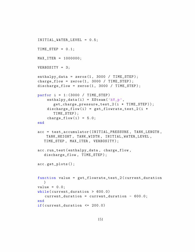
INITIAL_WATER_LEVEL = 0.5;
TIME_STEP = 0.1;
MAX_ITER = 1000000;
VERBOSITY = 3;
enthalpy_data = zeros(1, 3000 / TIME_STEP);
charge_flow = zeros(1, 3000 / TIME_STEP);
discharge_flow = zeros(1, 3000 / TIME_STEP);
parfor i = 1:(3000 / TIME_STEP)
enthalpy_data(i) = XSteam('hV_p',
get_charge_pressure_test_2(i * TIME_STEP));
discharge_flow(i) = get_flowrate_test_2(i *
TIME_STEP);
charge_flow(i) = 5.0;
end
acc = test_accumulator(INITIAL_PRESSURE , TANK_LENGTH ,
TANK_HEIGHT , TANK_WIDTH , INITIAL_WATER_LEVEL ,
TIME_STEP , MAX_ITER , VERBOSITY);
acc.run_test(enthalpy_data , charge_flow ,
discharge_flow , TIME_STEP);
acc.get_plots ();
function value = get_flowrate_test_2(current_duration
)
value = 0.0;
while(current_duration > 600.0)
current_duration = current_duration - 600.0;
end
if(current_duration <= 200.0)
151
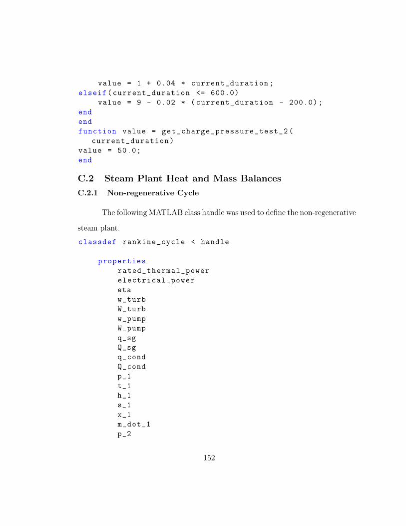
value = 1 + 0.04 * current_duration;
elseif(current_duration <= 600.0)
value = 9 - 0.02 * (current_duration - 200.0);
end
end
function value = get_charge_pressure_test_2(
current_duration)
value = 50.0;
end
C.2 Steam Plant Heat and Mass Balances
C.2.1 Non-regenerative Cycle
The following MATLAB class handle was used to define the non-regenerative
steam plant.
classdef rankine_cycle < handle
properties
rated_thermal_power
electrical_power
eta
w_turb
W_turb
w_pump
W_pump
q_sg
Q_sg
q_cond
Q_cond
p_1
t_1
h_1
s_1
x_1
m_dot_1
p_2
152
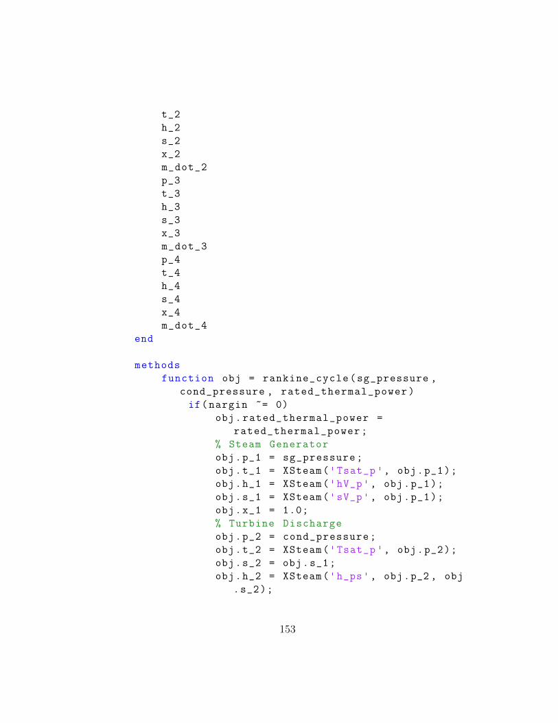
t_2
h_2
s_2
x_2
m_dot_2
p_3
t_3
h_3
s_3
x_3
m_dot_3
p_4
t_4
h_4
s_4
x_4
m_dot_4
end
methods
function obj = rankine_cycle(sg_pressure ,
cond_pressure , rated_thermal_power)
if(nargin ~= 0)
obj.rated_thermal_power =
rated_thermal_power;
% Steam Generator
obj.p_1 = sg_pressure;
obj.t_1 = XSteam('Tsat_p ', obj.p_1);
obj.h_1 = XSteam('hV_p', obj.p_1);
obj.s_1 = XSteam('sV_p', obj.p_1);
obj.x_1 = 1.0;
% Turbine Discharge
obj.p_2 = cond_pressure;
obj.t_2 = XSteam('Tsat_p ', obj.p_2);
obj.s_2 = obj.s_1;
obj.h_2 = XSteam('h_ps', obj.p_2 , obj
.s_2);
153
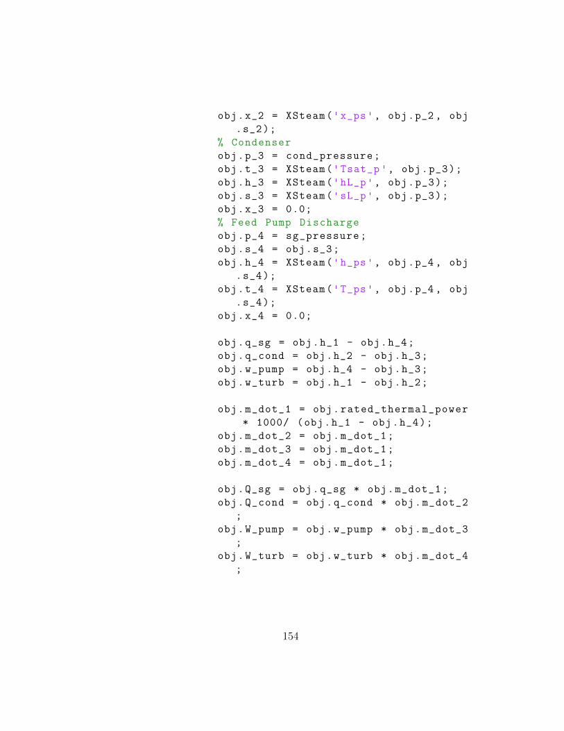
obj.x_2 = XSteam('x_ps', obj.p_2 , obj
.s_2);
% Condenser
obj.p_3 = cond_pressure;
obj.t_3 = XSteam('Tsat_p ', obj.p_3);
obj.h_3 = XSteam('hL_p', obj.p_3);
obj.s_3 = XSteam('sL_p', obj.p_3);
obj.x_3 = 0.0;
% Feed Pump Discharge
obj.p_4 = sg_pressure;
obj.s_4 = obj.s_3;
obj.h_4 = XSteam('h_ps', obj.p_4 , obj
.s_4);
obj.t_4 = XSteam('T_ps', obj.p_4 , obj
.s_4);
obj.x_4 = 0.0;
obj.q_sg = obj.h_1 - obj.h_4;
obj.q_cond = obj.h_2 - obj.h_3;
obj.w_pump = obj.h_4 - obj.h_3;
obj.w_turb = obj.h_1 - obj.h_2;
obj.m_dot_1 = obj.rated_thermal_power
* 1000/ (obj.h_1 - obj.h_4);
obj.m_dot_2 = obj.m_dot_1;
obj.m_dot_3 = obj.m_dot_1;
obj.m_dot_4 = obj.m_dot_1;
obj.Q_sg = obj.q_sg * obj.m_dot_1;
obj.Q_cond = obj.q_cond * obj.m_dot_2
;
obj.W_pump = obj.w_pump * obj.m_dot_3
;
obj.W_turb = obj.w_turb * obj.m_dot_4
;
154
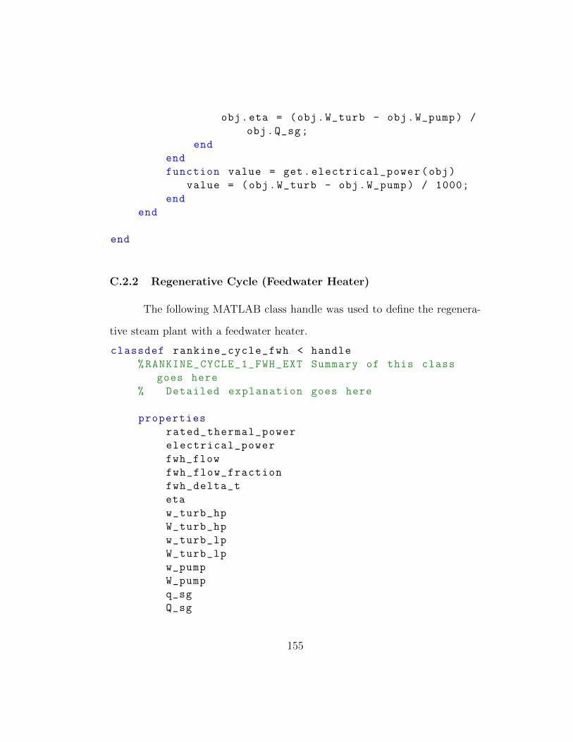
obj.eta = (obj.W_turb - obj.W_pump) /
obj.Q_sg;
end
end
function value = get.electrical_power(obj)
value = (obj.W_turb - obj.W_pump) / 1000;
end
end
end
C.2.2 Regenerative Cycle (Feedwater Heater)
The following MATLAB class handle was used to define the regenera-
tive steam plant with a feedwater heater.
classdef rankine_cycle_fwh < handle
%RANKINE_CYCLE_1_FWH_EXT Summary of this class
goes here
% Detailed explanation goes here
properties
rated_thermal_power
electrical_power
fwh_flow
fwh_flow_fraction
fwh_delta_t
eta
w_turb_hp
W_turb_hp
w_turb_lp
W_turb_lp
w_pump
W_pump
q_sg
Q_sg
155
q_cond
Q_cond
q_fwh
Q_fwh
p_1
t_1
h_1
s_1
x_1
m_dot_1
p_2
t_2
h_2
s_2
x_2
m_dot_2
p_3
t_3
h_3
s_3
x_3
m_dot_3
p_4
t_4
h_4
s_4
x_4
m_dot_4
p_5
t_5
h_5
s_5
x_5
m_dot_5
p_6
t_6
h_6
156
s_6
x_6
m_dot_6
p_7
t_7
h_7
s_7
x_7
m_dot_7
p_8
t_8
h_8
s_8
x_8
m_dot_8
end
methods
function obj = rankine_cycle_fwh(sg_pressure ,
hp_outlet_pressure ,...
hp_extraction_pressure , cond_pressure
, rated_thermal_power ,...
fwh_delta_t)
if(nargin ~= 0)
obj.rated_thermal_power =
rated_thermal_power;
obj.fwh_delta_t = fwh_delta_t;
% Main Steam Header
obj.p_1 = sg_pressure;
obj.t_1 = XSteam('Tsat_p ', obj.p_1);
obj.h_1 = XSteam('hV_p', obj.p_1);
obj.s_1 = XSteam('sV_p', obj.p_1);
obj.x_1 = 1.0;
% Crossover
obj.p_2 = hp_outlet_pressure;
obj.t_2 = XSteam('Tsat_p ', obj.p_2);
157
obj.s_2 = obj.s_1;
obj.h_2 = XSteam('h_ps', obj.p_2 , obj
.s_2);
obj.x_2 = XSteam('x_ps', obj.p_2 , obj
.s_2);
% FW Heater Steam Supply
obj.p_3 = hp_extraction_pressure;
obj.t_3 = XSteam('Tsat_p ', obj.p_3);
obj.s_3 = obj.s_2;
obj.h_3 = XSteam('h_ps', obj.p_3 , obj
.s_3);
obj.x_3 = XSteam('x_ps', obj.p_3 , obj
.s_3);
% LP Discharge
obj.p_4 = cond_pressure;
obj.t_4 = XSteam('Tsat_p ', obj.p_4);
obj.s_4 = obj.s_2;
obj.h_4 = XSteam('h_ps', obj.p_4 , obj
.s_4);
obj.x_4 = XSteam('x_ps', obj.p_4 , obj
.s_4);
% Condenser
obj.p_5 = cond_pressure;
obj.t_5 = XSteam('Tsat_p ', obj.p_5);
obj.h_5 = XSteam('hL_p', obj.p_5);
obj.s_5 = XSteam('sL_p', obj.p_5);
obj.x_5 = 0.0;
% Feed Pump Discharge
obj.p_6 = sg_pressure;
obj.s_6 = obj.s_5;
obj.h_6 = XSteam('h_ps', obj.p_6 , obj
.s_6);
158
obj.t_6 = XSteam('T_ps', obj.p_6 , obj
.s_6);
obj.x_6 = 0.0;
% FW Heater Drain to Condenser
obj.p_8 = 1.0;
obj.t_8 = obj.t_6 + 10.0;
obj.s_8 = XSteam('s_pT', obj.p_8 , obj
.t_8);
obj.h_8 = XSteam('h_pT', obj.p_8 , obj
.t_8);
obj.x_8 = 0.0;
% FW Heater Exit
obj.p_7 = obj.p_6;
obj.t_7 = obj.t_6 + fwh_delta_t;
obj.h_7 = XSteam('h_pT', obj.p_7 , obj
.t_7);
obj.s_7 = XSteam('s_pT', obj.p_7 , obj
.t_7);
obj.x_7 = 0.0;
obj.q_sg = obj.h_1 - obj.h_7;
obj.q_fwh = obj.h_7 - obj.h_6;
obj.w_pump = obj.h_6 - obj.h_5;
obj.m_dot_1 = obj.rated_thermal_power
* 1000/ (obj.h_1 - obj.h_7);
syms m_dot_1 m_dot_2 m_dot_3 m_dot_4
m_dot_5 m_dot_6 m_dot_7 m_dot_8
eqn_1 = m_dot_1 - obj.m_dot_1 == 0.0;
eqn_2 = m_dot_1 - m_dot_7 == 0.0;
eqn_3 = m_dot_7 - m_dot_6 == 0.0;
eqn_4 = m_dot_6 - m_dot_5 == 0.0;
159
eqn_5 = m_dot_1 - m_dot_2 - m_dot_3
== 0.0;
eqn_6 = m_dot_2 - m_dot_4 == 0.0;
eqn_7 = m_dot_5 - m_dot_4 - m_dot_8
== 0.0;
eqn_8 = m_dot_6 * obj.h_6 + m_dot_3 *
obj.h_3 - m_dot_8 * obj.h_8 -
m_dot_7 * obj.h_7 == 0.0;
[A, B] = equationsToMatrix ([eqn_1 ,
eqn_2 , eqn_3 , eqn_4 , eqn_5 , eqn_6 ,
eqn_7 , eqn_8],...
[m_dot_1 , m_dot_2 , m_dot_3 ,
m_dot_4 , m_dot_5 , m_dot_6 ,
m_dot_7 , m_dot_8 ]);
X = linsolve(A, B);
m_dot = double(X);
obj.m_dot_2 = m_dot (2);
obj.m_dot_3 = m_dot (3);
obj.m_dot_4 = m_dot (4);
obj.m_dot_5 = m_dot (5);
obj.m_dot_6 = m_dot (6);
obj.m_dot_7 = m_dot (7);
obj.m_dot_8 = m_dot (8);
obj.fwh_flow = obj.m_dot_3;
obj.fwh_flow_fraction = obj.m_dot_3 /
obj.m_dot_1;
obj.q_cond = (obj.h_4 - obj.h_5) * (
obj.m_dot_4 / obj.m_dot_1)...
+ (obj.h_8 - obj.h_5) * (obj.
m_dot_8 / obj.m_dot_1);
160
obj.w_turb_hp = (obj.h_1 - obj.h_3) +
...
(obj.h_3 - obj.h_2) * (obj.
m_dot_2 / obj.m_dot_1);
obj.w_turb_lp = (obj.h_2 - obj.h_4) *
(obj.m_dot_2 / obj.m_dot_1);
obj.Q_sg = obj.q_sg * obj.m_dot_1;
obj.Q_cond = obj.q_cond * obj.m_dot_1
;
obj.Q_fwh = obj.q_fwh * obj.m_dot_1;
obj.W_pump = obj.w_pump * obj.m_dot_1
;
obj.W_turb_hp = obj.w_turb_hp * obj.
m_dot_1 ;
obj.W_turb_lp = obj.w_turb_lp * obj.
m_dot_1;
obj.eta = (obj.W_turb_hp + obj.
W_turb_lp - obj.W_pump) / obj.Q_sg
;
end
end
function value = get.electrical_power(obj)
value = (obj.W_turb_hp + obj.W_turb_lp -
obj.W_pump) / 1000;
end
end
end
161
C.2.3 Regenerative Cycle (Feedwater Heater and Accumulator Dis-charging)
The following MATLAB class handle was used to define the regenera-
tive steam plant with a feedwater heater with the accumulator discharging.
classdef rankine_cycle_fwh_acc < handle
%RANKINE_CYCLE_1_FWH_EXT Summary of this class
goes here
% Detailed explanation goes here
properties
accumulator_flow
rated_thermal_power
electrical_power
fwh_flow
fwh_flow_fraction
fwh_delta_t
eta
w_turb_hp
W_turb_hp
w_turb_lp
W_turb_lp
w_pump
W_pump
q_sg
Q_sg
q_cond
Q_cond
q_fwh
Q_fwh
p_1
t_1
h_1
s_1
x_1
m_dot_1
162
p_2
t_2
h_2
s_2
x_2
m_dot_2
p_3
t_3
h_3
s_3
x_3
m_dot_3
p_4
t_4
h_4
s_4
x_4
m_dot_4
p_5
t_5
h_5
s_5
x_5
m_dot_5
p_6
t_6
h_6
s_6
x_6
m_dot_6
p_7
t_7
h_7
s_7
x_7
m_dot_7
p_8
163
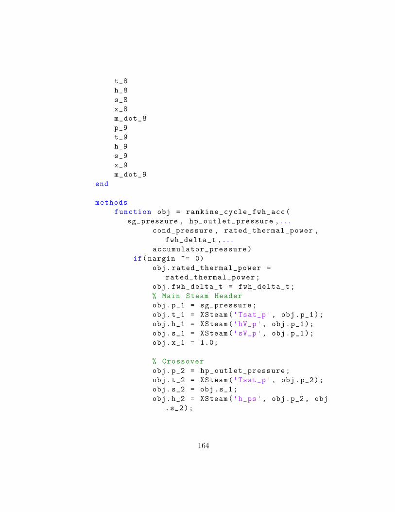
t_8
h_8
s_8
x_8
m_dot_8
p_9
t_9
h_9
s_9
x_9
m_dot_9
end
methods
function obj = rankine_cycle_fwh_acc(
sg_pressure , hp_outlet_pressure ,...
cond_pressure , rated_thermal_power ,
fwh_delta_t ,...
accumulator_pressure)
if(nargin ~= 0)
obj.rated_thermal_power =
rated_thermal_power;
obj.fwh_delta_t = fwh_delta_t;
% Main Steam Header
obj.p_1 = sg_pressure;
obj.t_1 = XSteam('Tsat_p ', obj.p_1);
obj.h_1 = XSteam('hV_p', obj.p_1);
obj.s_1 = XSteam('sV_p', obj.p_1);
obj.x_1 = 1.0;
% Crossover
obj.p_2 = hp_outlet_pressure;
obj.t_2 = XSteam('Tsat_p ', obj.p_2);
obj.s_2 = obj.s_1;
obj.h_2 = XSteam('h_ps', obj.p_2 , obj
.s_2);
164
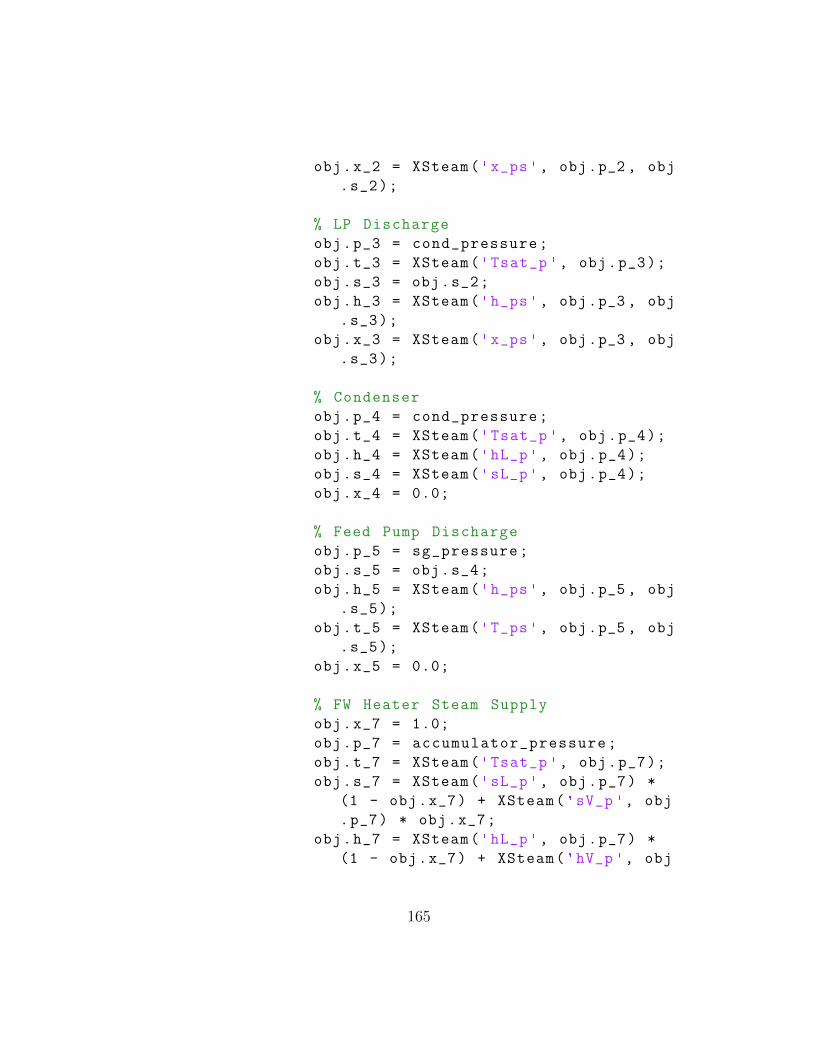
obj.x_2 = XSteam('x_ps', obj.p_2 , obj
.s_2);
% LP Discharge
obj.p_3 = cond_pressure;
obj.t_3 = XSteam('Tsat_p ', obj.p_3);
obj.s_3 = obj.s_2;
obj.h_3 = XSteam('h_ps', obj.p_3 , obj
.s_3);
obj.x_3 = XSteam('x_ps', obj.p_3 , obj
.s_3);
% Condenser
obj.p_4 = cond_pressure;
obj.t_4 = XSteam('Tsat_p ', obj.p_4);
obj.h_4 = XSteam('hL_p', obj.p_4);
obj.s_4 = XSteam('sL_p', obj.p_4);
obj.x_4 = 0.0;
% Feed Pump Discharge
obj.p_5 = sg_pressure;
obj.s_5 = obj.s_4;
obj.h_5 = XSteam('h_ps', obj.p_5 , obj
.s_5);
obj.t_5 = XSteam('T_ps', obj.p_5 , obj
.s_5);
obj.x_5 = 0.0;
% FW Heater Steam Supply
obj.x_7 = 1.0;
obj.p_7 = accumulator_pressure;
obj.t_7 = XSteam('Tsat_p ', obj.p_7);
obj.s_7 = XSteam('sL_p', obj.p_7) *
(1 - obj.x_7) + XSteam('sV_p', obj
.p_7) * obj.x_7;
obj.h_7 = XSteam('hL_p', obj.p_7) *
(1 - obj.x_7) + XSteam('hV_p', obj
165
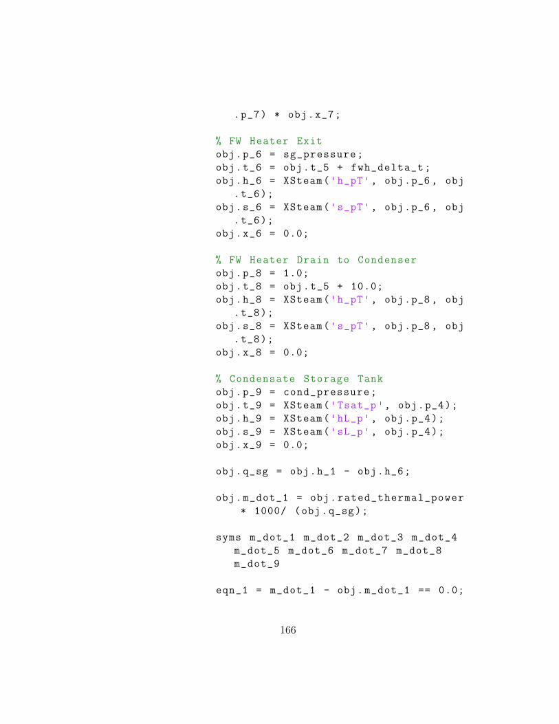
.p_7) * obj.x_7;
% FW Heater Exit
obj.p_6 = sg_pressure;
obj.t_6 = obj.t_5 + fwh_delta_t;
obj.h_6 = XSteam('h_pT', obj.p_6 , obj
.t_6);
obj.s_6 = XSteam('s_pT', obj.p_6 , obj
.t_6);
obj.x_6 = 0.0;
% FW Heater Drain to Condenser
obj.p_8 = 1.0;
obj.t_8 = obj.t_5 + 10.0;
obj.h_8 = XSteam('h_pT', obj.p_8 , obj
.t_8);
obj.s_8 = XSteam('s_pT', obj.p_8 , obj
.t_8);
obj.x_8 = 0.0;
% Condensate Storage Tank
obj.p_9 = cond_pressure;
obj.t_9 = XSteam('Tsat_p ', obj.p_4);
obj.h_9 = XSteam('hL_p', obj.p_4);
obj.s_9 = XSteam('sL_p', obj.p_4);
obj.x_9 = 0.0;
obj.q_sg = obj.h_1 - obj.h_6;
obj.m_dot_1 = obj.rated_thermal_power
* 1000/ (obj.q_sg);
syms m_dot_1 m_dot_2 m_dot_3 m_dot_4
m_dot_5 m_dot_6 m_dot_7 m_dot_8
m_dot_9
eqn_1 = m_dot_1 - obj.m_dot_1 == 0.0;
166
eqn_2 = m_dot_1 - m_dot_6 == 0.0;
eqn_3 = m_dot_1 - m_dot_2 == 0.0;
eqn_4 = m_dot_2 - m_dot_3 == 0.0;
eqn_5 = m_dot_4 - m_dot_3 - m_dot_8 +
m_dot_9 == 0.0;
eqn_6 = m_dot_4 - m_dot_5 == 0.0;
eqn_7 = m_dot_5 - m_dot_6 == 0.0;
eqn_8 = m_dot_5 * obj.h_5 + m_dot_7 *
obj.h_7 - m_dot_6 * obj.h_6 -
m_dot_8 * obj.h_8 == 0.0;
eqn_9 = m_dot_7 - m_dot_8 == 0.0;
[A, B] = equationsToMatrix ([eqn_1 ,
eqn_2 , eqn_3 , eqn_4 , eqn_5 , eqn_6 ,
eqn_7 , eqn_8 , eqn_9],...
[m_dot_1 , m_dot_2 , m_dot_3 ,
m_dot_4 , m_dot_5 , m_dot_6 ,
m_dot_7 , m_dot_8 , m_dot_9 ]);
X = linsolve(A, B);
m_dot = double(X);
obj.m_dot_2 = m_dot (2);
obj.m_dot_3 = m_dot (3);
obj.m_dot_4 = m_dot (4);
obj.m_dot_5 = m_dot (5);
obj.m_dot_6 = m_dot (6);
obj.m_dot_7 = m_dot (7);
obj.m_dot_8 = m_dot (8);
obj.m_dot_9 = m_dot (9);
obj.q_cond = (obj.h_3 - obj.h_4) * (
obj.m_dot_3 / obj.m_dot_1)...
+ (obj.h_8 - obj.h_4) * (obj.
m_dot_8 / obj.m_dot_1);
167
obj.q_fwh = obj.h_6 - obj.h_5;
obj.w_pump = obj.h_5 - obj.h_4;
obj.w_turb_hp = obj.h_1 - obj.h_2;
obj.w_turb_lp = (obj.h_2 - obj.h_3);
obj.Q_sg = obj.q_sg * obj.m_dot_1;
obj.Q_cond = obj.q_cond * obj.m_dot_1
;
obj.Q_fwh = obj.q_fwh * obj.m_dot_1;
obj.W_pump = obj.w_pump * obj.m_dot_1
;
obj.W_turb_hp = obj.w_turb_hp * obj.
m_dot_1 ;
obj.W_turb_lp = obj.w_turb_lp * obj.
m_dot_1;
obj.eta = (obj.W_turb_hp + obj.
W_turb_lp - obj.W_pump) / obj.Q_sg
;
end
end
function value = get.electrical_power(obj)
value = (obj.W_turb_hp + obj.W_turb_lp -
obj.W_pump) / 1000;
end
function value = get.accumulator_flow(obj)
value = obj.m_dot_7;
end
end
end
168
C.2.4 Regenerative Cycle (Feedwater Heater and Accumulator Charg-ing)
The following MATLAB class handle was used to define the regenera-
tive steam plant with a feedwater heater with the accumulator charging.
classdef rankine_cycle_fwh_acc_ch < handle
%RANKINE_CYCLE_1_FWH_EXT Summary of this class
goes here
% Detailed explanation goes here
properties
accumulator_flow
charging_flow
charging_flow_fraction
rated_thermal_power
electrical_power
fwh_flow
fwh_flow_fraction
fwh_delta_t
eta
w_turb_hp
W_turb_hp
w_turb_lp
W_turb_lp
w_pump
W_pump
q_sg
Q_sg
q_cond
Q_cond
q_fwh
Q_fwh
p_1
t_1
h_1
s_1
169
x_1
m_dot_1
p_1a
t_1a
h_1a
s_1a
x_1a
m_dot_1a
p_2
t_2
h_2
s_2
x_2
m_dot_2
p_3
t_3
h_3
s_3
x_3
m_dot_3
p_4
t_4
h_4
s_4
x_4
m_dot_4
p_5
t_5
h_5
s_5
x_5
m_dot_5
p_6
t_6
h_6
s_6
x_6
170
m_dot_6
p_7
t_7
h_7
s_7
x_7
m_dot_7
p_8
t_8
h_8
s_8
x_8
m_dot_8
p_9
t_9
h_9
s_9
x_9
m_dot_9
p_10
t_10
h_10
s_10
x_10
m_dot_10
end
methods
function obj = rankine_cycle_fwh_acc_ch(
sg_pressure , hp_outlet_pressure ,...
hp_extraction_pressure , cond_pressure
, rated_thermal_power , fwh_delta_t
,...
accumulator_pressure)
if(nargin ~= 0)
acc_d = rankine_cycle_fwh_acc(
sg_pressure , hp_outlet_pressure ,...
171
cond_pressure , rated_thermal_power ,
fwh_delta_t ,...
accumulator_pressure);
obj.charging_flow = acc_d.
accumulator_flow;
obj.rated_thermal_power =
rated_thermal_power;
obj.fwh_delta_t = fwh_delta_t;
% Main Steam Header
obj.p_1 = sg_pressure;
obj.t_1 = XSteam('Tsat_p ', obj.p_1);
obj.h_1 = XSteam('hV_p', obj.p_1);
obj.s_1 = XSteam('sV_p', obj.p_1);
obj.x_1 = 1.0;
% Main Steam Header
obj.p_1a = sg_pressure;
obj.t_1a = XSteam('Tsat_p ', obj.p_1);
obj.h_1a = XSteam('hV_p', obj.p_1);
obj.s_1a = XSteam('sV_p', obj.p_1);
obj.x_1a = 1.0;
% Crossover
obj.p_2 = hp_outlet_pressure;
obj.t_2 = XSteam('Tsat_p ', obj.p_2);
obj.s_2 = obj.s_1;
obj.h_2 = XSteam('h_ps', obj.p_2 , obj
.s_2);
obj.x_2 = XSteam('x_ps', obj.p_2 , obj
.s_2);
% LP Discharge
obj.p_3 = cond_pressure;
obj.t_3 = XSteam('Tsat_p ', obj.p_3);
172
obj.s_3 = obj.s_2;
obj.h_3 = XSteam('h_ps', obj.p_3 , obj
.s_3);
obj.x_3 = XSteam('x_ps', obj.p_3 , obj
.s_3);
% Condenser
obj.p_4 = cond_pressure;
obj.t_4 = XSteam('Tsat_p ', obj.p_4);
obj.h_4 = XSteam('hL_p', obj.p_4);
obj.s_4 = XSteam('sL_p', obj.p_4);
obj.x_4 = 0.0;
% Feed Pump Discharge
obj.p_5 = sg_pressure;
obj.s_5 = obj.s_4;
obj.h_5 = XSteam('h_ps', obj.p_5 , obj
.s_5);
obj.t_5 = XSteam('T_ps', obj.p_5 , obj
.s_5);
obj.x_5 = 0.0;
% FW Heater Steam Supply
obj.p_7 = hp_extraction_pressure;
obj.s_7 = obj.s_1;
obj.t_7 = XSteam('Tsat_p ', obj.p_7);
obj.h_7 = XSteam('h_ps', obj.p_7 , obj
.s_7);
obj.x_7 = XSteam('x_ps', obj.p_7 , obj
.s_7);
% FW Heater Exit
obj.p_6 = sg_pressure;
obj.t_6 = obj.t_5 + fwh_delta_t;
obj.h_6 = XSteam('h_pT', obj.p_6 , obj
.t_6);
173
obj.s_6 = XSteam('s_pT', obj.p_6 , obj
.t_6);
obj.x_6 = 0.0;
% FW Heater Drain to Condenser
obj.p_8 = 1.0;
obj.t_8 = obj.t_5 + 10.0;
obj.h_8 = XSteam('h_pt', obj.p_8 , obj
.t_8);
obj.s_8 = XSteam('s_pt', obj.p_8 , obj
.t_8);
obj.x_8 = 0.0;
% Accumulator
obj.p_9 = accumulator_pressure;
obj.t_9 = XSteam('Tsat_p ', obj.p_9);
obj.h_9 = XSteam('hV_p', obj.p_9);
obj.s_9 = XSteam('sV_p', obj.p_9);
obj.x_9 = 1.0;
% Condensate Drain Tank
obj.p_10 = cond_pressure;
obj.t_10 = XSteam('Tsat_p ', obj.p_10)
;
obj.h_10 = XSteam('hL_p', obj.p_10);
obj.s_10 = XSteam('sL_p', obj.p_10);
obj.x_10 = 0.0;
obj.q_sg = obj.h_1 - obj.h_6;
obj.m_dot_1 = obj.rated_thermal_power
* 1000/ (obj.q_sg);
syms m_dot_1 m_dot_1a m_dot_2 m_dot_3
m_dot_4 m_dot_5 m_dot_6 m_dot_7
m_dot_8 m_dot_9 m_dot_10
174
eqn_1 = m_dot_1 - obj.m_dot_1 == 0.0;
eqn_2 = m_dot_1 - m_dot_6 == 0.0;
eqn_3 = m_dot_1 - m_dot_1a - m_dot_9
== 0.0;
eqn_4 = m_dot_1a - m_dot_7 - m_dot_2
== 0.0;
eqn_5 = m_dot_2 - m_dot_3 == 0.0;
eqn_6 = m_dot_4 - m_dot_5 == 0.0;
eqn_7 = m_dot_3 + m_dot_10 + m_dot_8
- m_dot_4 == 0.0;
eqn_8 = m_dot_4 - m_dot_5 == 0.0;
eqn_9 = m_dot_5 - m_dot_6 == 0.0;
eqn_10 = m_dot_7 - m_dot_8 == 0.0;
eqn_11 = m_dot_5 * obj.h_5 + m_dot_7
* obj.h_7 - m_dot_6 * obj.h_6 -
m_dot_8 * obj.h_8 == 0.0;
eqn_12 = m_dot_9 - obj.charging_flow
== 0.0;
[A, B] = equationsToMatrix ([eqn_1 ,
eqn_2 , eqn_3 , eqn_4 , eqn_5 , eqn_6 ,
eqn_7 , eqn_8 , eqn_9 , eqn_10 ,
eqn_11 , eqn_12],...
[m_dot_1 , m_dot_1a , m_dot_2 ,
m_dot_3 , m_dot_4 , m_dot_5 ,
m_dot_6 , m_dot_7 , m_dot_8 ,
m_dot_9 , m_dot_10 ]);
X = linsolve(A, B);
m_dot = double(X);
obj.m_dot_1a = m_dot (2);
obj.m_dot_2 = m_dot (3);
obj.m_dot_3 = m_dot (4);
obj.m_dot_4 = m_dot (5);
obj.m_dot_5 = m_dot (6);
175
obj.m_dot_6 = m_dot (7);
obj.m_dot_7 = m_dot (8);
obj.m_dot_8 = m_dot (9);
obj.m_dot_9 = m_dot (10);
obj.m_dot_10 = m_dot (11);
obj.q_cond = (obj.h_3 - obj.h_4) * (
obj.m_dot_3 / obj.m_dot_1);
obj.q_fwh = (obj.h_6 - obj.h_5) * (
obj.m_dot_5 / obj.m_dot_1);
obj.w_pump = (obj.h_5 - obj.h_4) * (
obj.m_dot_4 / obj.m_dot_1);
obj.fwh_flow = obj.m_dot_7;
obj.fwh_flow_fraction = obj.fwh_flow
/ obj.m_dot_1;
obj.charging_flow_fraction = obj.
charging_flow / obj.m_dot_1;
obj.w_turb_hp = (obj.h_1a - obj.h_7)
* (obj.m_dot_1a / obj.m_dot_1)...
+ (obj.h_7 - obj.h_2) * (obj.
m_dot_2 / obj.m_dot_1);
obj.w_turb_lp = (obj.h_2 - obj.h_3) *
(obj.m_dot_2 / obj.m_dot_1);
obj.Q_sg = obj.q_sg * obj.m_dot_1;
obj.Q_cond = obj.q_cond * obj.m_dot_1
;
obj.Q_fwh = obj.q_fwh * obj.m_dot_1;
obj.W_pump = obj.w_pump * obj.m_dot_1
;
obj.W_turb_hp = obj.w_turb_hp * obj.
m_dot_1 ;
176
obj.W_turb_lp = obj.w_turb_lp * obj.
m_dot_1;
obj.eta = (obj.W_turb_hp + obj.
W_turb_lp - obj.W_pump) / obj.Q_sg
;
end
end
function value = get.electrical_power(obj)
value = (obj.W_turb_hp + obj.W_turb_lp -
obj.W_pump) / 1000;
end
function value = get.accumulator_flow(obj)
value = obj.m_dot_9;
end
end
end
C.2.5 Regenerative Cycle (Feedwater Heater and Reheater)
The following MATLAB class handle was used to define the regenera-
tive steam plant with a feedwater heater and reheater.
classdef rankine_cycle_fwh_msr < handle
%RANKINE_CYCLE_1_FWH_EXT Summary of this class
goes here
% Detailed explanation goes here
properties
rated_thermal_power
electrical_power
fwh_flow
fwh_flow_fraction
fwh_delta_t
msr_superheat
177
msr_flow
msr_flow_fraction
eta
w_turb_hp
W_turb_hp
w_turb_lp
W_turb_lp
w_pump
W_pump
q_sg
Q_sg
q_cond
Q_cond
q_fwh
Q_fwh
q_msr
Q_msr
p_1
t_1
h_1
s_1
x_1
m_dot_1
p_2
t_2
h_2
s_2
x_2
m_dot_2
p_3
t_3
h_3
s_3
x_3
m_dot_3
p_4
t_4
178
h_4
s_4
x_4
m_dot_4
p_5
t_5
h_5
s_5
x_5
m_dot_5
p_6
t_6
h_6
s_6
x_6
m_dot_6
p_7
t_7
h_7
s_7
x_7
m_dot_7
p_8
t_8
h_8
s_8
x_8
m_dot_8
p_9
t_9
h_9
s_9
x_9
m_dot_9
p_10
t_10
h_10
179
s_10
x_10
m_dot_10
p_11
t_11
h_11
s_11
x_11
m_dot_11
p_12
t_12
h_12
s_12
x_12
m_dot_12
end
methods
function obj = rankine_cycle_fwh_msr(
sg_pressure , hp_outlet_pressure ,...
hp_extraction_pressure , cond_pressure
, rated_thermal_power ,...
fwh_delta_t , msr_superheat)
if(nargin ~= 0)
obj.rated_thermal_power =
rated_thermal_power;
obj.fwh_delta_t = fwh_delta_t;
obj.msr_superheat = msr_superheat;
% Main Steam Header
obj.p_1 = sg_pressure;
obj.t_1 = XSteam('Tsat_p ', obj.p_1);
obj.h_1 = XSteam('hV_p', obj.p_1);
obj.s_1 = XSteam('sV_p', obj.p_1);
obj.x_1 = 1.0;
% HP Turbine Inlet
obj.p_2 = obj.p_1;
180
obj.t_2 = obj.t_1;
obj.s_2 = obj.s_1;
obj.h_2 = obj.h_1;
obj.x_2 = obj.x_1;
% MSR Inlet
obj.p_3 = obj.p_1;
obj.t_3 = obj.t_1;
obj.s_3 = obj.s_1;
obj.h_3 = obj.h_1;
obj.x_3 = obj.x_1;
% HP Turbine Extraction
obj.p_4 = hp_extraction_pressure;
obj.t_4 = XSteam('Tsat_p ', obj.p_4);
obj.s_4 = obj.s_2;
obj.h_4 = XSteam('h_ps', obj.p_4 , obj
.s_4);
obj.x_4 = XSteam('x_ps', obj.p_4 , obj
.s_4);
% HP Turbine Discharge
obj.p_5 = hp_outlet_pressure;
obj.t_5 = XSteam('Tsat_p ', obj.p_5);
obj.s_5 = obj.s_2;
obj.h_5 = XSteam('h_ps', obj.p_5 , obj
.s_5);
obj.x_5 = XSteam('x_ps', obj.p_5 , obj
.s_5);
% MSR to LP Turbine
obj.p_7 = obj.p_5;
obj.t_7 = obj.t_5 + msr_superheat;
obj.h_7 = XSteam('h_pT', obj.p_7 , obj
.t_7);
obj.s_7 = XSteam('s_pT', obj.p_7 , obj
.t_7);
181
obj.x_7 = 1.0;
% LP Turbine Discharge
obj.p_8 = cond_pressure;
obj.s_8 = obj.s_7;
obj.t_8 = XSteam('Tsat_p ', obj.p_8);
obj.h_8 = XSteam('h_ps', obj.p_8 , obj
.s_8);
obj.x_8 = XSteam('x_ps', obj.p_8 , obj
.s_8);
% MSR to Condenser
obj.p_6 = sg_pressure;
obj.t_6 = obj.t_7 + 10.0;
obj.s_6 = XSteam('s_pT', obj.p_6 , obj
.t_6);
obj.h_6 = XSteam('h_pT', obj.p_6 , obj
.t_6);
obj.x_6 = XSteam('x_ps', obj.p_6 , obj
.s_6);
% Condenser Discharge
obj.p_9 = obj.p_8;
obj.t_9 = XSteam('Tsat_p ', obj.p_9);
obj.h_9 = XSteam('hL_p', obj.p_9);
obj.s_9 = XSteam('sL_p', obj.p_9);
obj.x_9 = 0.0;
% Feep Pump Discharge
obj.p_10 = sg_pressure;
obj.s_10 = obj.s_9;
obj.t_10 = XSteam('T_ps', obj.p_10 ,
obj.s_10);
obj.h_10 = XSteam('h_ps', obj.p_10 ,
obj.s_10);
obj.x_10 = 0.0;
182
% FWH Discharge
obj.p_11 = sg_pressure;
obj.t_11 = obj.t_10 + fwh_delta_t;
obj.s_11 = XSteam('s_pT', obj.p_11 ,
obj.t_11);
obj.h_11 = XSteam('h_pT', obj.p_11 ,
obj.t_11);
obj.x_11 = 0.0;
% FWH to Condenser
obj.p_12 = 1.0;
obj.t_12 = obj.t_10 + 10.0;
obj.s_12 = XSteam('s_pT', obj.p_12 ,
obj.t_12);
obj.h_12 = XSteam('h_pT', obj.p_12 ,
obj.t_12);
obj.x_12 = 0.0;
obj.q_sg = obj.h_1 - obj.h_11;
obj.m_dot_1 = obj.rated_thermal_power
* 1000/ (obj.q_sg);
syms m_dot_1 m_dot_2 m_dot_3 m_dot_4
m_dot_5 m_dot_6 m_dot_7...
m_dot_8 m_dot_9 m_dot_10 m_dot_11
m_dot_12
eqn_1 = m_dot_1 - obj.m_dot_1 == 0.0;
eqn_2 = m_dot_1 - m_dot_11 == 0.0;
eqn_3 = m_dot_1 - m_dot_2 - m_dot_3
== 0.0;
eqn_4 = m_dot_2 - m_dot_4 - m_dot_5
== 0.0;
eqn_5 = m_dot_3 - m_dot_6 == 0.0;
eqn_6 = m_dot_5 - m_dot_7 == 0.0;
eqn_7 = m_dot_7 - m_dot_8 == 0.0;
183
eqn_8 = m_dot_8 - m_dot_9 + m_dot_6 +
m_dot_12 == 0.0;
eqn_9 = m_dot_9 - m_dot_10 == 0.0;
eqn_10 = m_dot_10 - m_dot_11 == 0.0;
eqn_11 = m_dot_10 * obj.h_10 +
m_dot_4 * obj.h_4 - m_dot_12 * obj
.h_12 - m_dot_11 * obj.h_11 ==
0.0;
eqn_12 = m_dot_3 * obj.h_3 + m_dot_5
* obj.h_5 - m_dot_6 * obj.h_6 -
m_dot_7 * obj.h_7 == 0.0;
[A, B] = equationsToMatrix ([eqn_1 ,
eqn_2 , eqn_3 , eqn_4 , eqn_5 , eqn_6 ,
eqn_7 , eqn_8 , eqn_9 , eqn_10 ,
eqn_11 , eqn_12],...
[m_dot_1 , m_dot_2 , m_dot_3 ,
m_dot_4 , m_dot_5 , m_dot_6 ,
m_dot_7 , m_dot_8 , m_dot_9 ,
m_dot_10 , m_dot_11 , m_dot_12 ])
;
X = linsolve(A, B);
m_dot = double(X);
obj.m_dot_2 = m_dot (2);
obj.m_dot_3 = m_dot (3);
obj.m_dot_4 = m_dot (4);
obj.m_dot_5 = m_dot (5);
obj.m_dot_6 = m_dot (6);
obj.m_dot_7 = m_dot (7);
obj.m_dot_8 = m_dot (8);
obj.m_dot_9 = m_dot (9);
obj.m_dot_10 = m_dot (10);
obj.m_dot_11 = m_dot (11);
obj.m_dot_12 = m_dot (12);
184
obj.fwh_flow = obj.m_dot_4;
obj.fwh_flow_fraction = obj.m_dot_4 /
obj.m_dot_1;
obj.msr_flow = obj.m_dot_3;
obj.msr_flow_fraction = obj.m_dot_3 /
obj.m_dot_1;
obj.q_fwh = (obj.h_11 - obj.h_10);
obj.w_pump = obj.h_10 - obj.h_9;
obj.q_cond = (obj.h_8 - obj.h_9) * (
obj.m_dot_8 / obj.m_dot_1)...
+ (obj.h_6 - obj.h_9) * (obj.
m_dot_6 / obj.m_dot_1) +...
(obj.h_12 - obj.h_9) * (obj.
m_dot_12 / obj.m_dot_1);
obj.q_msr = (obj.h_7 - obj.h_5) * (
obj.m_dot_5 / obj.m_dot_1);
obj.w_turb_hp = (obj.h_2 - obj.h_4) *
(obj.m_dot_2 / obj.m_dot_1)...
+ (obj.h_4 - obj.h_5) * (obj.
m_dot_5 / obj.m_dot_1);
obj.w_turb_lp = (obj.h_7 - obj.h_8) *
(obj.m_dot_7 / obj.m_dot_1);
obj.Q_sg = obj.q_sg * obj.m_dot_1;
obj.Q_cond = obj.q_cond * obj.m_dot_1
;
obj.Q_fwh = obj.q_fwh * obj.m_dot_1;
obj.Q_msr = obj.q_msr * obj.m_dot_1;
obj.W_pump = obj.w_pump * obj.m_dot_1
;
185
obj.W_turb_hp = obj.w_turb_hp * obj.
m_dot_1;
obj.W_turb_lp = obj.w_turb_lp * obj.
m_dot_1;
obj.eta = (obj.W_turb_hp + obj.
W_turb_lp - obj.W_pump) / obj.Q_sg
;
end
end
function value = get.electrical_power(obj)
value = (obj.W_turb_hp + obj.W_turb_lp -
obj.W_pump)/ 1000;
end
end
end
C.2.6 Regenerative Cycle (Feedwater Heater, Reheater, and Ac-cumulator Discharging)
The following MATLAB class handle was used to define the regenera-
tive steam plant with a feedwater heater and reheater with the accumulator
discharging.
classdef rankine_cycle_fwh_msr_acc < handle
%RANKINE_CYCLE_1_FWH_EXT Summary of this class
goes here
% Detailed explanation goes here
properties
accumulator_flow
rated_thermal_power
electrical_power
fwh_flow
fwh_flow_fraction
186
fwh_delta_t
msr_superheat
msr_flow
msr_flow_fraction
eta
w_turb_hp
W_turb_hp
w_turb_lp
W_turb_lp
w_pump
W_pump
q_sg
Q_sg
q_cond
Q_cond
q_fwh
Q_fwh
q_msr
Q_msr
p_1
t_1
h_1
s_1
x_1
m_dot_1
p_2
t_2
h_2
s_2
x_2
m_dot_2
p_3
t_3
h_3
s_3
x_3
m_dot_3
187
p_4
t_4
h_4
s_4
x_4
m_dot_4
p_5
t_5
h_5
s_5
x_5
m_dot_5
p_6
t_6
h_6
s_6
x_6
m_dot_6
p_7
t_7
h_7
s_7
x_7
m_dot_7
p_8
t_8
h_8
s_8
x_8
m_dot_8
p_9
t_9
h_9
s_9
x_9
m_dot_9
p_10
188
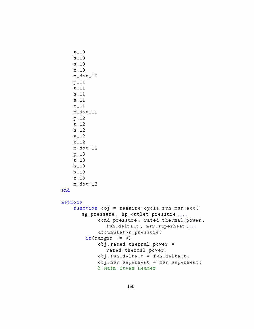
t_10
h_10
s_10
x_10
m_dot_10
p_11
t_11
h_11
s_11
x_11
m_dot_11
p_12
t_12
h_12
s_12
x_12
m_dot_12
p_13
t_13
h_13
s_13
x_13
m_dot_13
end
methods
function obj = rankine_cycle_fwh_msr_acc(
sg_pressure , hp_outlet_pressure ,...
cond_pressure , rated_thermal_power ,
fwh_delta_t , msr_superheat ,...
accumulator_pressure)
if(nargin ~= 0)
obj.rated_thermal_power =
rated_thermal_power;
obj.fwh_delta_t = fwh_delta_t;
obj.msr_superheat = msr_superheat;
% Main Steam Header
189
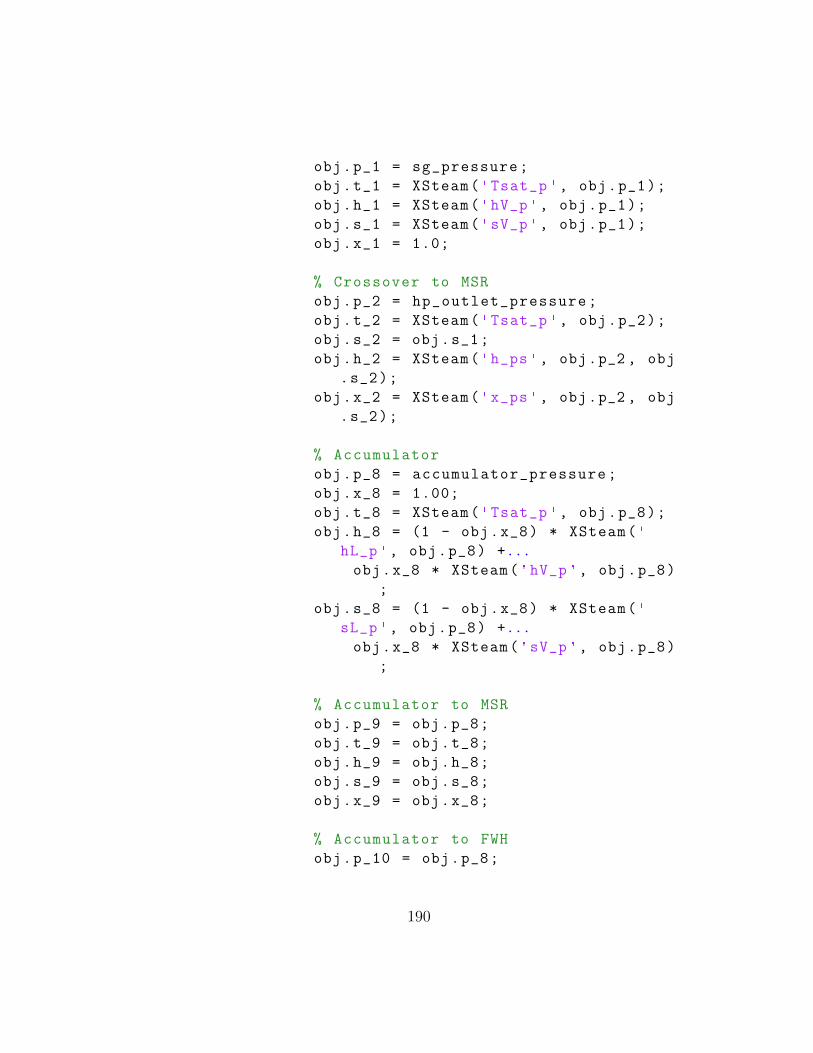
obj.p_1 = sg_pressure;
obj.t_1 = XSteam('Tsat_p ', obj.p_1);
obj.h_1 = XSteam('hV_p', obj.p_1);
obj.s_1 = XSteam('sV_p', obj.p_1);
obj.x_1 = 1.0;
% Crossover to MSR
obj.p_2 = hp_outlet_pressure;
obj.t_2 = XSteam('Tsat_p ', obj.p_2);
obj.s_2 = obj.s_1;
obj.h_2 = XSteam('h_ps', obj.p_2 , obj
.s_2);
obj.x_2 = XSteam('x_ps', obj.p_2 , obj
.s_2);
% Accumulator
obj.p_8 = accumulator_pressure;
obj.x_8 = 1.00;
obj.t_8 = XSteam('Tsat_p ', obj.p_8);
obj.h_8 = (1 - obj.x_8) * XSteam('
hL_p', obj.p_8) +...
obj.x_8 * XSteam('hV_p', obj.p_8)
;
obj.s_8 = (1 - obj.x_8) * XSteam('
sL_p', obj.p_8) +...
obj.x_8 * XSteam('sV_p', obj.p_8)
;
% Accumulator to MSR
obj.p_9 = obj.p_8;
obj.t_9 = obj.t_8;
obj.h_9 = obj.h_8;
obj.s_9 = obj.s_8;
obj.x_9 = obj.x_8;
% Accumulator to FWH
obj.p_10 = obj.p_8;
190
obj.t_10 = obj.t_8;
obj.h_10 = obj.h_8;
obj.s_10= obj.s_8;
obj.x_10 = obj.x_8;
% LP Turbine Inlet
obj.p_3 = obj.p_2;
obj.t_3 = obj.t_2 + msr_superheat;
obj.h_3 = XSteam('h_pT', obj.p_3 , obj
.t_3);
obj.s_3 = XSteam('s_pT', obj.p_3 , obj
.t_3);
obj.x_3 = 1.0;
% LP Turbine Discharge
obj.p_4 = cond_pressure;
obj.s_4 = obj.s_3;
obj.t_4 = XSteam('Tsat_p ', obj.p_4);
obj.h_4 = XSteam('h_ps', obj.p_4 , obj
.s_4);
obj.x_4 = XSteam('x_ps', obj.p_4 , obj
.s_4);
% Condenser Discharge
obj.p_5 = obj.p_4;
obj.t_5 = XSteam('Tsat_p ', obj.p_5);
obj.h_5 = XSteam('hL_p', obj.p_5);
obj.s_5 = XSteam('sL_p', obj.p_5);
obj.x_5 = 0.0;
% Feep Pump Discharge
obj.p_6 = sg_pressure;
obj.s_6 = obj.s_5;
obj.t_6 = XSteam('T_ps', obj.p_6 , obj
.s_6);
obj.h_6 = XSteam('h_ps', obj.p_6 , obj
.s_6);
191
obj.x_6 = 0.0;
% FWH Discharge
obj.p_7 = sg_pressure;
obj.t_7 = obj.t_6 + fwh_delta_t;
obj.s_7 = XSteam('s_pT', obj.p_7 , obj
.t_7);
obj.h_7 = XSteam('h_pT', obj.p_7 , obj
.t_7);
obj.x_7 = 0.0;
% MSR to Condenser
obj.p_11 = sg_pressure;
obj.t_11 = obj.t_3 + 10.0;
obj.h_11 = XSteam('h_pT', obj.p_11 ,
obj.t_11);
obj.s_11 = XSteam('s_pT', obj.p_11 ,
obj.t_11);
obj.x_11 = XSteam('x_ps', obj.p_11 ,
obj.s_11);
% FWH to Condenser
obj.p_12 = 1.0;
obj.t_12 = obj.t_6 + 10.0;
obj.h_12 = XSteam('h_pT', obj.p_12 ,
obj.t_12);
obj.s_12 = XSteam('s_pT', obj.p_12 ,
obj.t_12);
obj.x_12 = 0.0;
% Condensate Storage Tank
obj.p_13 = cond_pressure;
obj.t_13 = XSteam('Tsat_p ', obj.p_13)
;
obj.h_13 = XSteam('hL_p', obj.p_13);
obj.s_13 = XSteam('sL_p', obj.p_13);
obj.x_13 = 0.0;
192
obj.q_sg = obj.h_1 - obj.h_7;
obj.q_fwh = obj.h_7 - obj.h_6;
obj.w_pump = obj.h_6 - obj.h_5;
obj.m_dot_1 = obj.rated_thermal_power
* 1000/ (obj.q_sg);
syms m_dot_1 m_dot_2 m_dot_3 m_dot_4
m_dot_5 m_dot_6 m_dot_7...
m_dot_8 m_dot_9 m_dot_10 m_dot_11
m_dot_12 m_dot_13
eqn_1 = m_dot_1 - obj.m_dot_1 == 0.0;
eqn_2 = m_dot_1 - m_dot_7 == 0.0;
eqn_3 = m_dot_1 - m_dot_2 == 0.0;
eqn_4 = m_dot_2 - m_dot_3 == 0.0;
eqn_5 = m_dot_3 - m_dot_4 == 0.0;
eqn_6 = m_dot_4 + m_dot_11 + m_dot_12
- m_dot_5 - m_dot_13 == 0.0;
eqn_7 = m_dot_5 - m_dot_6 == 0.0;
eqn_8 = m_dot_6 - m_dot_7 == 0.0;
eqn_9 = m_dot_8 - m_dot_9 - m_dot_10
== 0.0;
eqn_10 = m_dot_9 - m_dot_11 == 0.0;
eqn_11 = m_dot_10 - m_dot_12 == 0.0;
eqn_12 = m_dot_2 * obj.h_2 + m_dot_9
* obj.h_9 - m_dot_3 * obj.h_3 -
m_dot_11 * obj.h_11 == 0.0;
eqn_13 = m_dot_6 * obj.h_6 + m_dot_10
* obj.h_10 - m_dot_7 * obj.h_7 -
m_dot_12 * obj.h_12 == 0.0;
[A, B] = equationsToMatrix ([eqn_1 ,
eqn_2 , eqn_3 , eqn_4 , eqn_5 ,...
eqn_6 , eqn_7 , eqn_8 , eqn_9 ,
eqn_10 , eqn_11 , eqn_12 , eqn_13
193
],...
[m_dot_1 , m_dot_2 , m_dot_3 ,
m_dot_4 , m_dot_5 , m_dot_6 ,...
m_dot_7 , m_dot_8 , m_dot_9 ,
m_dot_10 , m_dot_11 , m_dot_12 ,
...
m_dot_13 ]);
X = linsolve(A, B);
m_dot = double(X);
obj.m_dot_2 = m_dot (2);
obj.m_dot_3 = m_dot (3);
obj.m_dot_4 = m_dot (4);
obj.m_dot_5 = m_dot (5);
obj.m_dot_6 = m_dot (6);
obj.m_dot_7 = m_dot (7);
obj.m_dot_8 = abs(m_dot (8));
obj.m_dot_9 = abs(m_dot (9));
obj.m_dot_10 = abs(m_dot (10));
obj.m_dot_11 = abs(m_dot (11));
obj.m_dot_12 = abs(m_dot (12));
obj.m_dot_13 = abs(m_dot (13));
obj.accumulator_flow = obj.m_dot_8;
obj.q_cond = (obj.h_4 - obj.h_5) * (
obj.m_dot_4 / obj.m_dot_5)...
+ (obj.h_12 - obj.h_5) * (obj.
m_dot_12 / obj.m_dot_1) +...
(obj.h_11 - obj.h_5) * (obj.
m_dot_11 / obj.m_dot_1);
obj.q_msr = (obj.h_3 - obj.h_2) * (
obj.m_dot_3 / obj.m_dot_1);
194
obj.w_turb_hp = (obj.h_1 - obj.h_2);
obj.w_turb_lp = (obj.h_3 - obj.h_4);
obj.Q_sg = obj.q_sg * obj.m_dot_1;
obj.Q_cond = obj.q_cond * obj.m_dot_1
;
obj.Q_fwh = obj.q_fwh * obj.m_dot_1;
obj.Q_msr = obj.q_msr * obj.m_dot_1;
obj.W_pump = obj.w_pump * obj.m_dot_1
;
obj.W_turb_hp = obj.w_turb_hp * obj.
m_dot_1;
obj.W_turb_lp = obj.w_turb_lp * obj.
m_dot_1;
obj.eta = (obj.W_turb_hp + obj.
W_turb_lp - obj.W_pump) / obj.Q_sg
;
end
end
function value = get.electrical_power(obj)
value = (obj.W_turb_hp + obj.W_turb_lp -
obj.W_pump)/ 1000;
end
function value = get.accumulator_flow(obj)
value = obj.m_dot_8;
end
end
end
195
C.2.7 Regenerative Cycle (Feedwater Heater, Reheater, and Ac-cumulator Charging)
The following MATLAB class handle was used to define the regenera-
tive steam plant with a feedwater heater and reheater with the accumulator
charging.
classdef rankine_cycle_fwh_msr_acc_ch < handle
%RANKINE_CYCLE_1_FWH_EXT Summary of this class
goes here
% Detailed explanation goes here
properties
accumulator_flow
accumulator_flow_fraction
charging_flow
rated_thermal_power
electrical_power
fwh_flow
fwh_flow_fraction
fwh_delta_t
msr_superheat
msr_flow
msr_flow_fraction
eta
w_turb_hp
W_turb_hp
w_turb_lp
W_turb_lp
w_pump
W_pump
q_sg
Q_sg
q_cond
Q_cond
q_fwh
Q_fwh
196
q_msr
Q_msr
p_1
t_1
h_1
s_1
x_1
m_dot_1
p_2
t_2
h_2
s_2
x_2
m_dot_2
p_3
t_3
h_3
s_3
x_3
m_dot_3
p_4
t_4
h_4
s_4
x_4
m_dot_4
p_5
t_5
h_5
s_5
x_5
m_dot_5
p_6
t_6
h_6
s_6
x_6
197
m_dot_6
p_7
t_7
h_7
s_7
x_7
m_dot_7
p_8
t_8
h_8
s_8
x_8
m_dot_8
p_9
t_9
h_9
s_9
x_9
m_dot_9
p_10
t_10
h_10
s_10
x_10
m_dot_10
p_11
t_11
h_11
s_11
x_11
m_dot_11
p_12
t_12
h_12
s_12
x_12
m_dot_12
198
p_13
t_13
h_13
s_13
x_13
m_dot_13
p_14
t_14
h_14
s_14
x_14
m_dot_14
end
methods
function obj = rankine_cycle_fwh_msr_acc_ch(
sg_pressure , hp_outlet_pressure ,...
hp_extraction_pressure , cond_pressure
, rated_thermal_power ,...
fwh_delta_t , msr_superheat ,
accumulator_pressure)
if(nargin ~= 0)
cycle_regen_fwh_msr_acc =
rankine_cycle_fwh_msr_acc(
sg_pressure ,...
hp_outlet_pressure , cond_pressure
, rated_thermal_power ,
fwh_delta_t ,...
msr_superheat ,
accumulator_pressure);
obj.charging_flow =
cycle_regen_fwh_msr_acc.
accumulator_flow;
199
obj.rated_thermal_power =
rated_thermal_power;
obj.fwh_delta_t = fwh_delta_t;
obj.msr_superheat = msr_superheat;
% Main Steam Header
obj.p_1 = sg_pressure;
obj.t_1 = XSteam('Tsat_p ', obj.p_1);
obj.h_1 = XSteam('hV_p', obj.p_1);
obj.s_1 = XSteam('sV_p', obj.p_1);
obj.x_1 = 1.0;
% Branch to HP Turbine
obj.p_2 = obj.p_1;
obj.t_2 = obj.t_1;
obj.h_2 = obj.h_1;
obj.s_2 = obj.s_1;
obj.x_2 = obj.x_1;
% Branch to MSR
obj.p_3 = obj.p_1;
obj.t_3 = obj.t_1;
obj.h_3 = obj.h_1;
obj.s_3 = obj.s_1;
obj.x_3 = obj.x_1;
% Branch to Accumulator
obj.p_4 = obj.p_1;
obj.t_4 = obj.t_1;
obj.h_4 = obj.h_1;
obj.s_4 = obj.s_1;
obj.x_4 = obj.x_1;
% HP Turbine Extraction
obj.p_5 = hp_extraction_pressure;
obj.t_5 = XSteam('Tsat_p ', obj.p_5);
obj.s_5 = obj.s_2;
200
obj.h_5 = XSteam('h_ps', obj.p_5 , obj
.s_5);
obj.x_5 = XSteam('x_ps', obj.p_5 , obj
.s_5);
% Crossover to MSR
obj.p_6 = hp_outlet_pressure;
obj.t_6 = XSteam('Tsat_p ', obj.p_6);
obj.s_6 = obj.s_2;
obj.h_6 = XSteam('h_ps', obj.p_6 , obj
.s_6);
obj.x_6 = XSteam('x_ps', obj.p_6 , obj
.s_6);
% MSR to Condenser
obj.p_7 = 1.0;
obj.t_7 = XSteam('Tsat_p ', obj.p_7);
obj.h_7 = XSteam('hL_p', obj.p_7);
obj.s_7 = XSteam('sL_p', obj.p_7);
obj.x_7 = 0.0;
% LP Turbine Inlet
obj.p_8 = obj.p_6;
obj.t_8 = obj.t_6 + msr_superheat;
obj.h_8 = XSteam('h_pT', obj.p_8 , obj
.t_8);
obj.s_8 = XSteam('s_pT', obj.p_8 , obj
.t_8);
obj.x_8 = 1.0;
% LP Turbine Discharge
obj.p_9 = cond_pressure;
obj.s_9 = obj.s_8;
obj.t_9 = XSteam('Tsat_p ', obj.p_9);
obj.h_9 = XSteam('h_ps', obj.p_9 , obj
.s_9);
201
obj.x_9 = XSteam('x_ps', obj.p_9 , obj
.s_9);
%Condenser Discharge
obj.p_10 = obj.p_9;
obj.t_10 = XSteam('Tsat_p ', obj.p_10)
;
obj.h_10 = XSteam('hL_p', obj.p_10);
obj.s_10 = XSteam('sL_p', obj.p_10);
obj.x_10 = 0.0;
% Feep Pump Discharge
obj.p_11 = sg_pressure;
obj.s_11 = obj.s_10;
obj.t_11 = XSteam('T_ps', obj.p_11 ,
obj.s_11);
obj.h_11 = XSteam('h_ps', obj.p_11 ,
obj.s_11);
obj.x_11 = 0.0;
% FWH Discharge
obj.p_12 = sg_pressure;
obj.t_12 = obj.t_11 + fwh_delta_t;
obj.s_12 = XSteam('s_pT', obj.p_12 ,
obj.t_12);
obj.h_12 = XSteam('h_pT', obj.p_12 ,
obj.t_12);
obj.x_12 = 0.0;
% FWH to Condenser
obj.p_13 = 1.0;
obj.t_13 = obj.t_11 + 10.0;
obj.h_13 = XSteam('h_pT', obj.p_13 ,
obj.t_13);
obj.s_13 = XSteam('s_pT', obj.p_13 ,
obj.t_13);
obj.x_13 = 0.0;
202
% Condensate Storage Tank
obj.p_14 = cond_pressure;
obj.t_14 = XSteam('Tsat_p ', obj.p_14)
;
obj.h_14 = XSteam('hL_p', obj.p_14);
obj.s_14 = XSteam('sL_p', obj.p_14);
obj.x_14 = 0.0;
obj.q_sg = obj.h_1 - obj.h_12;
obj.q_fwh = obj.h_12 - obj.h_11;
obj.m_dot_1 = obj.rated_thermal_power
* 1000/ (obj.q_sg);
syms m_dot_1 m_dot_2 m_dot_3 m_dot_4
m_dot_5 m_dot_6 m_dot_7...
m_dot_8 m_dot_9 m_dot_10 m_dot_11
m_dot_12 m_dot_13 m_dot_14
eqn_1 = m_dot_1 - obj.m_dot_1 == 0.0;
eqn_2 = m_dot_1 - m_dot_2 - m_dot_3 -
m_dot_4 == 0.0;
eqn_3 = m_dot_1 - m_dot_12 == 0.0;
eqn_4 = m_dot_2 - m_dot_5 - m_dot_6
== 0.0;
eqn_5 = m_dot_3 - m_dot_7 == 0.0;
eqn_6 = m_dot_6 - m_dot_8 == 0.0;
eqn_7 = m_dot_9 + m_dot_14 + m_dot_7
+ m_dot_13 - m_dot_10 == 0.0;
eqn_8 = m_dot_8 - m_dot_9 == 0.0;
eqn_9 = m_dot_10 - m_dot_11 == 0.0;
eqn_10 = m_dot_11 - m_dot_12 == 0.0;
eqn_11 = m_dot_5 - m_dot_13 == 0.0;
eqn_12 = m_dot_5 * obj.h_5 + m_dot_11
* obj.h_11 - m_dot_12 * obj.h_12
- m_dot_13 * obj.h_13 == 0.0;
203
eqn_13 = m_dot_3 * obj.h_3 + m_dot_6
* obj.h_6 - m_dot_7 * obj.h_7 -
m_dot_8 * obj.h_8 == 0.0;
eqn_14 = m_dot_4 - obj.charging_flow
== 0.0;
[A, B] = equationsToMatrix ([eqn_1 ,
eqn_2 , eqn_3 , eqn_4 , eqn_5 ,...
eqn_6 , eqn_7 , eqn_8 , eqn_9 ,
eqn_10 , eqn_11 , eqn_12 , eqn_13
,...
eqn_14],...
[m_dot_1 , m_dot_2 , m_dot_3 ,
m_dot_4 , m_dot_5 , m_dot_6 ,...
m_dot_7 , m_dot_8 , m_dot_9 ,
m_dot_10 , m_dot_11 , m_dot_12 ,
...
m_dot_13 , m_dot_14 ]);
X = linsolve(A, B);
m_dot = double(X);
obj.m_dot_2 = m_dot (2);
obj.m_dot_3 = m_dot (3);
obj.m_dot_4 = m_dot (4);
obj.m_dot_5 = m_dot (5);
obj.m_dot_6 = m_dot (6);
obj.m_dot_7 = m_dot (7);
obj.m_dot_8 = m_dot (8);
obj.m_dot_9 = m_dot (9);
obj.m_dot_10 = m_dot (10);
obj.m_dot_11 = m_dot (11);
obj.m_dot_12 = m_dot (12);
obj.m_dot_13 = m_dot (13);
obj.m_dot_14 = m_dot (14);
204
obj.fwh_flow = obj.m_dot_5;
obj.fwh_flow_fraction = obj.m_dot_5 /
obj.m_dot_1;
obj.msr_flow = obj.m_dot_3;
obj.msr_flow_fraction = obj.msr_flow
/ obj.m_dot_1;
obj.accumulator_flow_fraction = obj.
accumulator_flow / obj.m_dot_1;
obj.q_cond = (obj.h_9 - obj.h_10) * (
obj.m_dot_9 / obj.m_dot_1) +...
(obj.h_7 - obj.h_10) * (obj.
m_dot_7 / obj.m_dot_1) +...
(obj.h_13 - obj.h_10) * (obj.
m_dot_13 / obj.m_dot_1) +...
(obj.h_14 - obj.h_10) * (obj.
m_dot_14 / obj.m_dot_1);
obj.w_pump = (obj.h_11 - obj.h_10) *
(obj.m_dot_10 / obj.m_dot_1);
obj.q_msr = (obj.h_8 - obj.h_6) * (
obj.m_dot_6 / obj.m_dot_1);
obj.w_turb_hp = (obj.h_2 - obj.h_5) *
(obj.m_dot_2 / obj.m_dot_1) +...
(obj.h_5 - obj.h_6) * (obj.
m_dot_6 / obj.m_dot_1);
obj.w_turb_lp = (obj.h_8 - obj.h_9) *
(obj.m_dot_8 / obj.m_dot_1);
obj.Q_sg = obj.q_sg * obj.m_dot_1;
obj.Q_cond = obj.q_cond * obj.m_dot_1
;
obj.Q_fwh = obj.q_fwh * obj.m_dot_1;
205
obj.Q_msr = obj.q_msr * obj.m_dot_1;
obj.W_pump = obj.w_pump * obj.m_dot_1
;
obj.W_turb_hp = obj.w_turb_hp * obj.
m_dot_1;
obj.W_turb_lp = obj.w_turb_lp * obj.
m_dot_1;
obj.eta = (obj.W_turb_hp + obj.
W_turb_lp - obj.W_pump) / obj.Q_sg
;
end
end
function value = get.electrical_power(obj)
value = (obj.W_turb_hp + obj.W_turb_lp )/
1000;
end
function value = get.accumulator_flow(obj)
value = obj.m_dot_4;
end
end
end
C.2.8 Cycle Evaluation Script
The following MATLAB Script was used to evaluate each cycle at dif-
ferent accumulator pressures.
RATED_THERMAL_POWER = 3500;
SG_PRESSURE = 72.0;
HP_DISCHARGE_PRESSURE = 20.0;
HP_DISCHARGE_PRESSURE_MSR = 20.0;
HP_EXTRACTION_PRESSURE = 40.0;
HP_EXTRACTION_PRESSURE_MSR = 40.0;
COND_PRESSURE = 0.07;
206
ACCUMULATOR_PRESSURE = 60.0;
FWH_DELTA_T = 140.0;
FWH_DELTA_T_MSR = 100.0;
MSR_SUPERHEAT = 1.0;
ITER = 300;
p_accum = linspace(HP_EXTRACTION_PRESSURE ,
ACCUMULATOR_PRESSURE , 100);
h_acc = zeros(1, 100);
t_acc = zeros(1, 100);
eta = zeros(1, 100);
eta_fwh = zeros(1, 100);
eta_fwh_msr = zeros(1, 100);
eta_fwh_acc = zeros (1 ,100);
eta_fwh_acc_ch = zeros (1 ,100);
eta_fwh_msr_acc = zeros(1, 100);
eta_fwh_msr_acc_ch = zeros(1, 100);
parfor i = 1:100
cycle_non_regen = rankine_cycle(SG_PRESSURE ,
COND_PRESSURE , RATED_THERMAL_POWER);
cycle_regen_fwh = rankine_cycle_fwh(SG_PRESSURE ,
...
HP_DISCHARGE_PRESSURE , HP_EXTRACTION_PRESSURE
, COND_PRESSURE ,...
RATED_THERMAL_POWER , FWH_DELTA_T);
cycle_regen_fwh_msr = rankine_cycle_fwh_msr(
SG_PRESSURE ,...
HP_DISCHARGE_PRESSURE_MSR ,
HP_EXTRACTION_PRESSURE_MSR , COND_PRESSURE ,
...
RATED_THERMAL_POWER , FWH_DELTA_T_MSR ,
MSR_SUPERHEAT);
207
cycle_regen_fwh_acc = rankine_cycle_fwh_acc(
SG_PRESSURE ,...
HP_DISCHARGE_PRESSURE , COND_PRESSURE ,
RATED_THERMAL_POWER ,...
FWH_DELTA_T , p_accum(i));
cycle_regen_fwh_acc_ch = rankine_cycle_fwh_acc_ch
(SG_PRESSURE ,...
HP_DISCHARGE_PRESSURE , HP_EXTRACTION_PRESSURE
, COND_PRESSURE ,...
RATED_THERMAL_POWER , FWH_DELTA_T , p_accum(i))
;
cycle_regen_fwh_msr_acc =
rankine_cycle_fwh_msr_acc(SG_PRESSURE ,...
HP_DISCHARGE_PRESSURE_MSR , COND_PRESSURE ,
RATED_THERMAL_POWER , FWH_DELTA_T_MSR ,...
MSR_SUPERHEAT , p_accum(i));
cycle_regen_fwh_msr_acc_ch =
rankine_cycle_fwh_msr_acc_ch(SG_PRESSURE ,...
HP_DISCHARGE_PRESSURE , HP_EXTRACTION_PRESSURE
, COND_PRESSURE ,...
RATED_THERMAL_POWER , FWH_DELTA_T ,
MSR_SUPERHEAT , p_accum(i));
eta(i) = cycle_non_regen.eta;
eta_fwh(i) = cycle_regen_fwh.eta;
eta_fwh_msr(i) = cycle_regen_fwh_msr.eta;
eta_fwh_acc(i) = cycle_regen_fwh_acc.eta;
eta_fwh_acc_ch(i) = cycle_regen_fwh_acc_ch.eta;
eta_fwh_msr_acc(i) = cycle_regen_fwh_msr_acc.eta;
eta_fwh_msr_acc_ch(i) =
cycle_regen_fwh_msr_acc_ch.eta;
h_acc(i) = XSteam('hV_p', p_accum(i));
208
t_acc(i) = XSteam('Tsat_p ', p_accum(i));
end
figure (1)
plot(p_accum , eta_fwh);
hold on;
plot(p_accum , eta_fwh_acc , 'r');
plot(p_accum , eta_fwh_acc_ch , 'g');
xlabel('Accumulator Pressure [bar]');
ylabel('Apparent Efficiency ');
legend('No Accumulator ', 'Discharging ', 'Charging ');
figure (2)
plot(p_accum , eta_fwh_msr);
hold on;
plot(p_accum , eta_fwh_msr_acc , 'r');
plot(p_accum , eta_fwh_msr_acc_ch , 'g');
xlabel('Accumulator Pressure [bar]');
ylabel('Apparent Efficiency ');
legend('No Accumulator ', 'Discharging ', 'Charging ');
C.2.9 Accumulator Discharge Rates versus Pressure
The MATLAB script used to generate the plots of accumulator dis-
charge rate versus pressure for different plant configurations is provided below.
RATED_THERMAL_POWER = 3500;
SG_PRESSURE = 72.0;
HP_DISCHARGE_PRESSURE = 20.0;
HP_DISCHARGE_PRESSURE_MSR = 20.0;
HP_EXTRACTION_PRESSURE = 40.0;
HP_EXTRACTION_PRESSURE_MSR = 40.0;
COND_PRESSURE = 0.07;
ACCUMULATOR_PRESSURE = 60.0;
FWH_DELTA_T = 140.0;
FWH_DELTA_T_MSR = 100.0;
209
MSR_SUPERHEAT = 1.0;
ITER = 300;
p_accum = linspace(HP_EXTRACTION_PRESSURE ,
ACCUMULATOR_PRESSURE , 100);
flow_fwh_acc = zeros (1 ,100);
flow_fwh_acc_ch = zeros (1 ,100);
flow_fwh_msr_acc = zeros(1, 100);
flow_fwh_msr_acc_ch = zeros(1, 100);
parfor i = 1:100
cycle_regen_fwh_acc = rankine_cycle_fwh_acc(
SG_PRESSURE ,...
HP_DISCHARGE_PRESSURE , COND_PRESSURE ,
RATED_THERMAL_POWER ,...
FWH_DELTA_T , p_accum(i));
cycle_regen_fwh_acc_ch = rankine_cycle_fwh_acc_ch
(SG_PRESSURE ,...
HP_DISCHARGE_PRESSURE , HP_EXTRACTION_PRESSURE
, COND_PRESSURE ,...
RATED_THERMAL_POWER , FWH_DELTA_T , p_accum(i))
;
cycle_regen_fwh_msr_acc =
rankine_cycle_fwh_msr_acc(SG_PRESSURE ,...
HP_DISCHARGE_PRESSURE_MSR , COND_PRESSURE ,
RATED_THERMAL_POWER , FWH_DELTA_T_MSR ,...
MSR_SUPERHEAT , p_accum(i));
cycle_regen_fwh_msr_acc_ch =
rankine_cycle_fwh_msr_acc_ch(SG_PRESSURE ,...
HP_DISCHARGE_PRESSURE , HP_EXTRACTION_PRESSURE
, COND_PRESSURE ,...
210
RATED_THERMAL_POWER , FWH_DELTA_T ,
MSR_SUPERHEAT , p_accum(i));
flow_fwh_acc(i) = cycle_regen_fwh_acc.
accumulator_flow;
flow_fwh_acc_ch(i) = cycle_regen_fwh_acc_ch.
accumulator_flow;
flow_fwh_msr_acc(i) = cycle_regen_fwh_msr_acc.
accumulator_flow;
flow_fwh_msr_acc_ch(i) =
cycle_regen_fwh_msr_acc_ch.accumulator_flow;
end
figure (1)
plot(p_accum , flow_fwh_acc , 'r');
hold on;
%plot(p_accum , flow_fwh_acc_ch , 'r:');
xlabel('Accumulator Pressure [bar]');
ylabel('Accumulator Mass Flow Rate [kg/s]');
legend('Discharging and Charging ');
figure (2)
plot(p_accum , flow_fwh_msr_acc , 'b');
hold on;
plot(p_accum , flow_fwh_msr_acc_ch , 'b:');
xlabel('Accumulator Pressure [bar]');
ylabel('Accumulator Mass Flow Rate [kg/s]');
legend('Discharging ', 'Charging ');
211
Bibliography
[1] M. Abutayeh, A. Alazzam, and B. El-Khasawneh. Optimizing thermal
energy storage. Solar Energy, 120:318–329, 2015.
[2] G. Beckmann and P. Gilli. Thermal Energy Storage. Springer-Verlag,
1984.
[3] P. Gilli and K. Fritz. Nuclear power plants with integrated steam accu-
mulators for load peaking. Vienna, October 1970. IAEA Symposium on
Economic Integration of Nuclear Power Stations in Electric Power Sys-
tems.
[4] D. Haeseldonckx, L. Peeters, L. Helsen, and W. D’haeseleer. The impact
of thermal storage on the operational behavior of residential chp facili-
ties and the overall CO2. Renewable and Sustainable Energy Reviews,
11:1227–1243, 2007.
[5] J. Kiusalaas. Numerical Methods in Engineering with MATLAB. Cam-
bridge University Press, 2010.
[6] S. Kuravi, J. Trahan, D. Goswami, M. Rahman, and E. Stefanakos.
Thermal energy storage technologies and systems for concentrating so-
lar plants. Progress in Energy and Combustion Science, 39(4):285–319,
2013.
212
[7] A. Raja, A. Srivastava, and M. Dwivedi. Power Plant Engineering. New
Age International, 2006.
[8] D. Schnaider, P. Divnich, and I. Vakhromeev. Modeling the dynamic
mode of steam accumulator. Automation and Remote Control, 71:1994–
1998, 2010.
[9] W. Steinmann and M. Eck. Buffer storage for direct steam generation.
Solar Energy, 80:1277–1282, 2006.
[10] V. Stevanovic, B. Maslovaric, and S. Prica. Dynamics of steam accumu-
lation. Applied Thermal Engineering, 37:73–79, 2012.
[11] V. Stevanovic, M. Petrovic, S. Milivojevic, and B. Maslovaric. Prediction
and control of steam accumulation. Heat Transfer Engineering, 36:498–
510, 2015.
[12] M. Studovic and V. Stevanovic. Non-equilibrium approach to the analysis
of steam accumulator operation. Thermophysics and Aeromechanics,
1:53–60, 1994.
[13] B. Sun, J. Guo, Y. Lei, L. Yang, Y. Li, and G. Zhang. Simulation
and verification of a non-equilibrium thermodynamic model for a steam
catapult’s steam accumulator. International Journal of Heat and Mass
Transfer, 85:88–97, 2015.
[14] A. Ter-Gazarian. Energy Storage for Power Systems. The Institute of
Engineering and Technology, second edition, 2011.
213
[15] Z. Bogdan and D. Kopjar. Improvement of the cogeneration plant econ-
omy by using heat accumulator. Energy, 31(13):1949–1956, 2006.
214