Copyright by Jungmin Lee 2004

Copyright

by

Jungmin Lee

2004

The Dissertation Committee for Jungmin Leecertifies that this is the approved version of the following dissertation:

The Economics of Family and Group Decisions

Committee:

Daniel Hamermesh, Supervisor

Stephen Donald

Stephen Trejo

Gerald Oettinger

Robert Crosnoe


by

Jungmin Lee, B.A., M.A.

DISSERTATION

Presented to the Faculty of the Graduate School of

The University of Texas at Austin

in Partial Fulfillment

of the Requirements

for the Degree of

DOCTOR OF PHILOSOPHY

THE UNIVERSITY OF TEXAS AT AUSTIN

May 2004

To my beloved wife, Soojin Ha

Acknowledgments

This dissertation would not have been possible without my supervisor,

professor Daniel Hamermesh, who led me to the research field of labor eco-

nomics. His brilliant ideas always stimulated my academic imagination and

creativity. I would like to show my sincere gratitude to him for his constant

guidance and all-aspect supports. I am especially grateful of professor Steve

Trejo and Gerald Oettinger who patiently guided me through the dissertation

process. I also wish to say many thanks to professor Stephen Donald, Li Gan,

and Robert Crosnoe for their important comments. At last, I thank my family.

I would deeply thank my parents for their supports and understanding during

the years of my studies. I would like to show my indescribable appreciation

to my wife, Soojin Ha, for giving me the most patient and loving supports

and encouragement to my work. I am especially grateful of her for her many

good suggestions to my dissertation. I wish that the success of finishing this

dissertation could be my present to her.

v


Publication No.

Jungmin Lee, Ph.D.

The University of Texas at Austin, 2004

Supervisor: Daniel Hamermesh

This thesis examines group decision-making processes with emphasis on

households’ decisions and behaviors. It is interesting to study the underlying

decision-making processes within multi-person groups and organizations by

extending and applying our knowledge in microeconomic theory: what is the

raison d’tre for such institutions, when they are created and dissolved, and how

they aggregate and resolve different preferences and values among members.

The first essay estimates the trade-off between child quantity and quality by

exploiting exogenous variations in fertility due to son preference, which prevails

in many Asian countries. I find for the sample of Korean households that

taste covariance is not minimal; adverse effects of fertility on child quality is,

if any, smaller than what would be inferred from a cross-sectional relationship.

The fall in fertility rate over the past decades does not account for increasing

investment in children’s education. Linking population policy to fostering

human capital could be misleading.

vi

The second essay utilizes longitudinal data to analyze the spouse’s indi-

vidual budgets – “pocket money.” This unique data set allows for the specifica-

tion of simultaneous process of household decision-making in a fully stochastic

fashion. By doing this, it is possible to differentiate unobservable spousal bar-

gaining power from heterogeneity at the household level. I find that while

increasing female labor force involvement does lead to resource reallocation

toward women within households, the favorable effect is not significant. On

the other hand, a general improvement of family income has negative impacts

on intra-household inequality, which partially confirms the Kuznets curve at

the micro level. Lastly, spouses are significantly different in their preferences

for education and clothing, but they are not for some other goods.

The last essay examines a different context, beyond households, in

which a group of individuals make aggregate decisions. Using the data on

figure skating judges’ scorings, I find significant evidence for the existence of

outlier aversion. Individual judges manipulate scores to achieve a targeted

level of agreement with the other judges, and the dispersion of scores de-

pends upon the type of judge-assessment system. One major implication of

this paper, which is at variance with the industrial psychology and personnel

management literature, is that agreement may not be a good criterion for the

validity of an evaluation system.

vii

Table of Contents

Acknowledgments v

Abstract vi

List of Tables xi

List of Figures xiv

Chapter 1. Introduction 1

Chapter 2. Children and Household Education Decisions: AnAsian Instrument 5

2.1 Introduction . . . . . . . . . . . . . . . . . . . . . . . . . . . . 5

2.2 Conceptual Framework . . . . . . . . . . . . . . . . . . . . . . 10

2.2.1 Endogenous Fertility . . . . . . . . . . . . . . . . . . . . 10

2.2.2 An Asian Instrument: Son Preference . . . . . . . . . . 13

2.3 Data and Empirical Results . . . . . . . . . . . . . . . . . . . 16

2.3.1 Data and Descriptive Statistics . . . . . . . . . . . . . . 16

2.3.2 Linear Model . . . . . . . . . . . . . . . . . . . . . . . . 20

2.3.3 Inferring Non-linearity from Linear Models . . . . . . . 23

2.3.4 Twin Instrument . . . . . . . . . . . . . . . . . . . . . . 27

2.4 Discussion . . . . . . . . . . . . . . . . . . . . . . . . . . . . . 28

Chapter 3. Household Sharing Rules: Evidence from YoungCouples’ Pocket Money 42

3.1 Introduction . . . . . . . . . . . . . . . . . . . . . . . . . . . . 42

3.2 Conceptual Model and Empirical Strategy . . . . . . . . . . . 47

3.2.1 Recovering Household Sharing Rules with Exogenous Earn-ings . . . . . . . . . . . . . . . . . . . . . . . . . . . . . 47

3.2.2 Allowing for Unobserved Bargaining Power . . . . . . . 51

viii

3.3 Basic Regression Results . . . . . . . . . . . . . . . . . . . . . 57

3.3.1 Data Source and Descriptive Statistics . . . . . . . . . . 57

3.3.2 Are Married Couples Really Different from Singles? . . . 61

3.3.3 The Determinants of Couples’ Pocket Money . . . . . . 63

3.3.4 “Traditional” versus Dual-Earner Marriage . . . . . . . 66

3.3.5 Exogenous Variation in Earnings due to the FinancialCrisis of 1997-1998 . . . . . . . . . . . . . . . . . . . . . 67

3.4 Observable Household Sharing Rules . . . . . . . . . . . . . . 69

3.5 Unobserved Bargaining Power and Non-Assignable Consumption 72

3.6 An Alternative Explanation: The Permanent-Income Hypothesis 77

3.7 Conclusions . . . . . . . . . . . . . . . . . . . . . . . . . . . . 79

Chapter 4. Extreme Sports Evaluation: Evidence from JudgingFigure Skating 93

4.1 Introduction . . . . . . . . . . . . . . . . . . . . . . . . . . . . 93

4.2 Conceptual Framework . . . . . . . . . . . . . . . . . . . . . . 98

4.2.1 Judging Figure Skating and Figure Skating Judges . . . 98

4.2.2 Modelling Outlier Aversion Bias . . . . . . . . . . . . . 100

4.3 Empirical Analysis . . . . . . . . . . . . . . . . . . . . . . . . 106

4.3.1 Data and Descriptive Statistics . . . . . . . . . . . . . . 106

4.3.2 Identification I: Dynamic Panel Data Estimation . . . . 108

4.3.3 Identification II: Interim Judging System . . . . . . . . 118

4.4 Information Loss due to Outlier Aversion . . . . . . . . . . . . 122

4.5 Implications . . . . . . . . . . . . . . . . . . . . . . . . . . . . 124

Chapter 5. Conclusions 134

Appendices 136

Appendix A. Existence of Son Preference 137

Appendix B. Children and Married Women’s Labor Supply 142

Appendix C. Dynamic Outlier Aversion 150

ix

Bibliography 152

Vita 164

x

List of Tables

2.1 Descriptive Statistics . . . . . . . . . . . . . . . . . . . . . 31

2.2 Sex Ratio at Birth by Birth Order . . . . . . . . . . . . . 32

2.3 Investment in Children’s Education (the dependent vari-able is the natural logarithm of total monthly invest-ment in education) . . . . . . . . . . . . . . . . . . . . . . . 33

2.4 Investment in Children’s Education, Multiple Instru-ments (the dependent variable is the natural logarithmof total monthly investment in education) . . . . . . . . 34



2.7 Investment in Children’s Education, Twinning Instru-ment (the dependent variable is the natural logarithmof total monthly investment in education) . . . . . . . . 37

3.1 Descriptive Statistics of Crucial Variables . . . . . . . . 82

3.2 Inequality Measures of Pocket Money . . . . . . . . . . . 83

3.3 Singles versus Married Men and Women, Two-StageLeast Squares Estimation . . . . . . . . . . . . . . . . . . 83

3.4 Earnings and Pocket Money without Controls . . . . . 84

3.5 Earnings and Pocket Money with Controls . . . . . . . 85

3.6 Single-Earner Couples . . . . . . . . . . . . . . . . . . . . . 86

3.7 Random Earnings Shock between 1997 and 1998 . . . . 86

3.8 Exogenous Variation in Earnings and Pocket Moneywithout Controls, 1997-1998 . . . . . . . . . . . . . . . . . 87

3.9 Recovering Household Sharing Rules: Bargaining Ef-fects and Kuznets Effects . . . . . . . . . . . . . . . . . . . 87

3.10 Between-Spouse Log Difference Equations . . . . . . . . 88

xi

3.11 Husbands’ Unobserved Relative Bargaining Power . . . 89

3.12 Non-Assignable Goods, Seemingly Unrelated Regression 90

3.13 Non-Assignable Goods, Seemingly Unrelated Regres-sion (Continued) . . . . . . . . . . . . . . . . . . . . . . . . 91

3.14 Testing Between-Spouse Differences in Marginal Propen-sity to Consume (f ′hj − f ′wj = 0,∀j) and Their EqualityAcross Items (f ′hj − f ′wj = f ′hk − f ′wk,∀j 6= k), p-values . . . 92

3.15 The Predicted Changes in Coefficient Estimates WhenAllowing for Individual-Specific Fixed Effects in Differ-ent Models . . . . . . . . . . . . . . . . . . . . . . . . . . . . 92

4.1 Number of Observations: Skater-Judge Combinations 126

4.2 Panel-Average Scores . . . . . . . . . . . . . . . . . . . . . 127

4.3 Dynamic Panel Data Estimation: Full Sample . . . . . 128

4.4 Dynamic Panel Data Estimation: Full Sample . . . . . 129

4.5 Dynamic Panel Data Estimation: Singles . . . . . . . . . 130

4.6 Dynamic Panel Data Estimation: Pairs . . . . . . . . . . 131

4.7 Interim Judging System: Before-After Analysis . . . . 132

4.8 Interim Judging System: Regression Analysis . . . . . . 133

A.1 Parity Progression Model, Pooled Sample, CompletedFertility . . . . . . . . . . . . . . . . . . . . . . . . . . . . . . 140

A.2 Weibull Hazard Model, Unrestricted Sample . . . . . . 141

B.1 Married Women’s Labor Force Participation (the de-pendent variable is the indicator that her primary jobis not housewife) . . . . . . . . . . . . . . . . . . . . . . . . 145



B.4 Married Women’s Labor Force Participation, TwinningInstrument (the dependent variable is the indicator thather primary job is not housewife) . . . . . . . . . . . . . 148

xii

B.5 Married Women’s Labor Force Participation, MultipleInstruments (the dependent variable is the indicatorthat her primary job is not housewife) . . . . . . . . . . 149

xiii

List of Figures

2.1 Fertility and Per-Child Investment in Education . . . . 38

2.2 Fertility and Number of Private Educational Institutes 39

2.3 Fertility and Household Expenditure on Education . . 40

2.4 Summary: The Trade-Off Between Child Quantity andQuality . . . . . . . . . . . . . . . . . . . . . . . . . . . . . . 41

3.1 Estimated Unobserved Relative Bargaining Power andRelative Earnings . . . . . . . . . . . . . . . . . . . . . . . 81

xiv

Chapter 1

Introduction

The objective of this thesis is to examine group decision-making pro-

cesses with emphasis on households’ decisions and behaviors. While neoclas-

sical microeconomic theory is constructed at the individual level, most human

decisions and behaviors in everyday life cannot be understood with themselves

being detached and isolated from their social contexts and interactions among

different individuals, in particular within households. It is, therefore, inter-

esting to study the underlying decision-making processes within multi-person

groups and organizations by extending and applying our knowledge in microe-

conomic theory: what is the raison d’tre for such institutions, when they are

created and dissolved, and how they aggregate and resolve different preferences

and values among members.

It is important, for government and policy-makers as well as academia,

to scrutinize households from the perspective of group decision-making pro-

cesses. The primary reason is that most of government policies target specific

types of individuals within households, whereas they are in practice designed

and implemented at the household level. Any policy must be filtered by house-

hold decision-making processes to reach individual members within the house-

1

hold. As a result, policy evaluation that fails to take into account the internal

decision-making processes could be misleading.

From an empirical perspective, it is challenging to identify the decision-

making process, because almost all variables of interest are endogenously de-

termined in a broad context of group utility maximization and, furthermore,

because the process itself is endogenously shaped. Identification problems

such as simultaneity and endogeneity should be inherent and potentially bias

conclusions. This thesis attempts to identify unobserved underlying decision-

making processes by exploiting institutional and cultural peculiarities arising

under certain circumstances.

This thesis is organized into three essays. The first essay deals with

the relationship between fertility and household education decisions. In par-

ticular, I examine the well-known hypothesis that large number of children

have adverse effects on child quality - the trade-off between child quantity

and quality. For a sample of Korean households, I estimate the effects of

number of children on parental investment in children’s education by utilizing

exogenous variations in fertility due to son preferences, which are traditionally

deep-rooted in many Asian countries. In regard to fertility and educational

investment for children, Korea is an interesting place for researchers to study,

because the fertility rate has dropped rapidly and, at the same time, private

investment in children’s education has skyrocketed for the past three decades.

The results have interesting implications for popular development strategies

to link population policies to fostering human capital.

2

The second essay attempts to identify households’ decision-making pro-

cess and the significance of individual members’ bargaining power in the pro-

cess. In this essay, a spouse’s bargaining power is determined by two closely-

related factors: his or her relative contribution to the household budget and

social/cultural norms about gender roles. A challenging task in this frame-

work is how we can identify causal effects of one’s relative economic capability

on welfare distribution across individual members within the household, while

spousal division of labor between home and market is traditionally determined

by gender roles especially in developing countries. Using unique longitudinal

data on spouses’ individual expenditure from Korea, I attempt to decompose

the effects of bargaining power on households’ decisions by the above two fac-

tors. It is possible to identify unobserved bargaining power explicitly, given

the assumption that the balance of power within households that cannot be

explained by observed distribution factors is time-constant since it is likely

formed by social norms and cultural values, which are not changing discontin-

uously nor rapidly. I develop a simple model of household bargaining and test

for how household consumption changes in response to changes in bargaining

power, family income, and spousal differences in preferences.

The last essay examines a different context, beyond households, in

which a group of individuals makes aggregate decisions - in particular, reach

agreement. The underlying issue that I attempt to investigate is whether in-

dividual decision-makers in a group change their behaviors in response to the

incentive structure they face, in particular to how they are monitored and

3

evaluated by the supervising organization. The literature in psychology and

economics finds that individual decision-makers are more sensitive to incen-

tive systems when the organization cannot objectively validate the decisions.

It is well known, in the context of performance evaluation, that subjective

evaluation is likely to be distorted and vulnerable to corruption. Figure skat-

ing competitions provide a unique opportunity to study subjective evaluation.

This essay develops a simple model of “outlier aversion bias” in which evalua-

tors avoid submitting outlying judgments, because they are later assessed by

the degree to which their scores match those of the other judges. Empirically,

I attempt to test whether individual judges manipulate scores to achieve a tar-

geted level of agreement with the other judges. The identification of individual

judges’ aversion to outlying scores is achieved by two institutional peculiari-

ties in the sport of figure skating: repeated evaluation by multiple judges in a

game and the judging-system reform after the infamous 2002 Winter Olympic

scandal.

4

Chapter 2

Children and Household Education Decisions:

An Asian Instrument

2.1 Introduction

High fertility has been pointed out as a major obstacle to reducing

poverty and improving labor force quality in developing and underdeveloped

countries such as African and Southwestern Asian countries. The underlying

rationale for the argument is simply that, given limited resources, parents

with fewer children should be able to educate each child better. Examples are

found in East Asian countries such as Korea, Hong Kong, and China that have

successfully cut the fertility rate and, at the same time, increased investment in

education.1 FIGURE 2.1 clearly demonstrates these polar cases; the fertility

rate and per-child investment in education are negatively correlated across

countries during past decades. It seems that slowing population growth is

a high priority in poor countries. However, it is more important for policy-

makers to know beyond recognizing a simple correlation – the extent to which

high fertility adversely affects investment in children’s education, child quality,

1Refer to the World Bank (1994) among others. See also various articles by the WorldBank (www.worldbank.org), linking population policy closely to poverty reduction and hu-man capital development.

5

and ultimately future labor force quality. It is necessary to establish true causal

links.

Rather than directly addressing the cross-country correlation, this pa-

per focuses on the effects of individual household’s fertility on intrafamily re-

source allocation and more specifically investment in children’s education in a

certain country – South Korea, which provides an interesting context in which

to examine this issue in the sense that this country as one of “Asian Tigers”

has been a showcase for many developing countries as a fast track to economic

development. Indeed this country is considered extraordinarily successful in

restricting population growth and increasing the quality of labor force, as seen

in FIGURE 2.1. During the past two decades, the average number of births

per woman between age 15 and 49 decreased by half, from 2.6 in 1981 to

1.3 in 2001. Expenditure on educational institutions accounts for over 7 per-

cent of GDP in 1997, which records highest even among the OECD countries.

The number of private educational institutes literally skyrocketed during the

past two decades (FIGURE 2.2). Educational expenditure’s proportion in a

household’s total expenditure increased from 6.5 percent in 1981 to almost 12

percent in 2001, much higher than 1-2 percent in the U.S. (FIGURE 2.3). It is

found that households’ expenditure on private tutoring alone amounts to 3-5

percent of GDP.

Considerable studies have documented that family size exerts a negative

effect on investments in children and thereby their educational attainments.2

2Blake (1989) among others has done an extensive analysis using various sources of data

6

The primary reason is that family resources available to a child decrease as

number of children increases. This adverse effect has been called as “dilution

effect” in the sociology literature.

It is, however, hard to disentangle fertility effect on child quality from

the spaghetti-like lines of exogenous effects and causal and simultaneous in-

terdependencies. A simple household decision model can show that parental

concern about child quality, or parents’ ability – unobservable in most ex-

isting surveys – would increase investment in children’s education and would

decrease fertility rate. An observed relationship between fertility and invest-

ment in children’s education across households in cross-sectional data is not

a consistent estimate of the trade-off between child quality and quantity as

long as there exists a covariance between fertility and educational investment

resulting from their common link to a third factor (Becker and Lewis 1973,

Becker and Tomes 1976). A limited set of control variables such as family back-

ground and socioeconomic characteristics might not fully capture underlying

differences among families that could be different in unmeasured ways.

What is required to correct for endogeneity bias is a variable which

and finds that sibling size has a substantial and negative effect on performances in schoolsuch as schooling completion and test scores even after controlling for parents’ socioeconomicstatus. Knodel and Wongsith (1991) find the negative effects of large family size on theprobability of attending secondary school in Thailand. Interestingly Gomes (1984) finds forthe sample of Kenya that children from larger family are more likely to complete grades,which can be explained by the fact that parents in Kenya may control their eldest children’searnings and younger children are benefited from this extra source of family resource. Thissuggests that the relationship in a particular country is dependent on its cultural and socialsetting.

7

affects only child quantity and not quality. Rosenzweig and Wolpin (1980)

utilize a random fertility event, twinning at the first birth.3 In this paper, I

use a “random” fertility outcome – the sex of the first child in a household. The

basis of this idea is quite eccentric; Korean parents traditionally have strong

son preferences, and they would decide further childbearing conditional on the

sex composition of existing children. The first child’s sex seems a reasonable

candidate for an instrumental variable for actual number of children in the

household. I call this instrument an Asian instrument since the phenomenon

of son preferences is quite common in Asian countries. The methodology taken

in this paper is potentially applicable to these countries.

My empirical strategy is motivated by the “sex-composition” instru-

mental variable estimation approach, originated by Iacovou (1996) and An-

grist and Evans (1998). To estimate fertility effects on parents’ labor market

outcomes, they exploit the well-known phenomenon in Western countries that

parents prefer a balanced sex composition of children. Parents with same-sex

children are more likely to have an additional child, and the randomness of

children’s sexes provides exogenous variation in family size. Therefore the sex

composition of the first two children can be a reasonable instrumental variable

for actual number of children in the household.4

3Another way to deal with endogeneity bias is fixed-effect estimation, which allows forunobserved time-constant factor. Hanushek (1992) removes time-invariant unobservableeffects by specifying education production function in a valued-added form and finds thatlarger number of children depresses scholastic achievement.

4So they had to restrict their samples to those household with at least two children.Obviously it is impossible to identify marginal effect of fertility transition from one child totwo children in their studies.

8

This paper estimates the effect of fertility on parental investments in

children’s education. As well summarized by Rosenzweig and Wolpin (2000),

the validity of instrumental-variable estimation depends critically on the de-

scription of unobservable or omitted factors in the determination of the out-

come variable of empirical interest.5 That is, instrumental variable estimation

must provide a plausible theory or at least some reasonable story for why the

exploited instrument is not directly correlated with the outcome variable.

For this paper it is particularly important to deal with the potential

defects because I estimate fertility effects on investment in children’s education

that is supposed to depend on the sex composition of children if parents dis-

criminate against daughters in favor of sons in intrafamily resource allocation.

It is critical to recognize this possibility of post-natal discrimination against

daughters in education. However, it must be emphasized in advance that, at

the worst case, the son-preference instrumental variable approach underesti-

mates in absolute value the true effects of fertility on household investment in

education, which turns out to strengthen the conclusion.

Summarizing main findings, I find for the sample of Korean households

that fertility has virtually no impact on per-child investment in education af-

ter accounting for endogenous fertility – unobserved taste heterogeneity across

households. This is at variance with Rosenzweig and Wolpin (1980)’s finding

5For Iacovou (1996) and Angrist and Evans (1998), the assumption is that sex compo-sition does not affect directly parents’ labor market outcomes such as mothers’ labor forceparticipation and working hours.

9

for Indian households for which they find that exogenous increases in fertility

really decrease child quality. This paper implies that, responding to exogenous

addition of a child, Korean parents would increase investment in children’s ed-

ucation so much as not to decrease per-child investment in education, perhaps

by sacrificing consumption for parents themselves in favor of equal child quality

among their children.

2.2 Conceptual Framework

2.2.1 Endogenous Fertility

My purpose is to estimate the effect of fertility on investment in chil-

dren’s education. Suppose that a household maximizes a unitary utility func-

tion with number of children (N), average quality per child (Q), and a compos-

ite commodity (y) as arguments, following the three-commodity model orig-

inated from the seminal paper by Becker and Lewis (1973). The household

maximizes the welfare function,

U = U(N, Q, y; θ), (2.1)

where θ is a vector of preference parameters such as marginal utility of

consumption of S and marginal rate of substitution between N and Q. It is

assumed to have standard neoclassical properties. Parents allocate their full

income (I) between children and consumption, so that the budget constraint

is

10

PNN + PQ(N ·Q) + y ≤ I, (2.2)

where PN is the direct costs of children, and PQ is the unit price of

average child quality. Optimal household decisions depend on exogenous vari-

ables,

Q∗ = Q(PN , PQ, I; θ). (2.3)

N∗ = N(PN , PQ, I; θ). (2.4)

The unobservability of θ and its heterogeneity across households are

of key importance for empirical purposes. The main intuition of this simple

model is the importance of dealing with the simultaneity of child quality and

quantity in household optimization. If households differ in their family plans

and educational investment due to taste heterogeneity in unmeasured ways,

and furthermore if they are different in the productivity in household produc-

tion, then a simple correlation between child quality and quantity does not

suggest any causal link or relationship.6

6In the same vein, many macroeconomic studies point out that fertility is endogenouslydetermined together with human capital accumulation, and economic growth. Using aggre-gated cross-country data, Barro (1991) confirms the endogenous fertility growth model inwhich higher initial stock of human capital would lower fertility by increasing the cost ofrearing children, which, in turn, reduces fertility and transfers resource from raising manychildren to investing in human capital. Interestingly, he shows that the residuals from thegrowth equation and from the fertility equation are negatively correlated, arguing that percapital growth, fertility, and investment are jointly determined as endogenous variables.

11

A parametric example suffices to show the model’s implication for this

paper. Let us assume a quasi-linear utility function, U = NAQB + y where

both A and B are positive and less than one. If N is exogenous, then it is

easy to discover the fertility effect on child quality as

εQN =∂ ln Q∗

∂ ln N= −1− A

1−B< 0. (2.5)

If fertility is endogenously determined by the household, the observed

relationship must deviate from − 1−A1−B

. However, assuming interior solutions,

we can still recover the effect of exogenous fertility on child quality by using

∂ ln Q∗/∂PN

∂ ln N∗/∂PN

= −1− A

1−B= εQN . (2.6)

Note that PN affects Q only indirectly through its effect on N , but PQ

directly affects both N and Q. For empirical purposes the model implies that

at least one instrument for fertility is necessary for identification. This can be

easily inferred from the formula for instrumental-variable estimator. Suppose

that we regress Q on N and use an instrument PN for N . The two-stage least

squares estimator is (P ′NN)−1P ′

NQ, which is exactly the ratio of two ordinary

least squares estimators,(P ′NPN )−1P ′NQ

(P ′NPN )−1P ′NN. On the other hand, PQ is not a valid

instrument since it directly affects both N and Q.

Similarly, using country-level panel data, Ahituv (2001) shows that fertility is endogenousand jointly determined with economic growth while it is hard to find good instrumentalvariables for fertility in cross-country data. So the simple OLS estimate for the coefficientof fertility in a standard growth model is subject to endogeneity bias.

12

2.2.2 An Asian Instrument: Son Preference

Now suppose that, using household-level data, we estimate the following

reduced-form equation,

ln Y = α1N + Xβ + f(θ) + ν, (2.7)

where ν is assumed to be independent with all other explanatory vari-

ables in the specification and f(·) is an unknown function of unobservable

taste parameters.7 Y is total investment in children’s education, which may

proxy total investment for “total” child quality. That is, Y = PQ ·N ·Q, where

PQ is the monetary cost required to increase a unit of “average” child quality.

We assume that it is constant across households conditional on some relevant

characteristics such as parents’ education level. If N is exogenous and all other

explanatory variables in X are orthogonal to f(·) and ν, the OLS estimate of

α1 can consistently pick up the elasticity of average child quality with respect

to child quantity. Using the Slutsky theorem and product rule,

plim(α1) =1

E(N)· (1 + εQN), (2.8)

where εQN is the elasticity of “average” child quality with respect to

7The specification is employed because we only know total investment for all children inthe household rather than investment for each individual child in the data. Although wecan construct per-child investment by dividing Y by N , this would aggravate measurementerror problem in Y and N .

13

child quantity.8 However, the identification problem in practice is that number

of children and investment in education are jointly decided by parents. In this

case, N is correlated with f(θ) and so the OLS estimate is biased.

I use the first child’s sex (Z) as an instrument for fertility where Z = 1

if the first child is a girl, and zero otherwise. The critical rationale for this in-

strument is that under son preferences, the first child’s sex is a good predictor

for actual fertility (“relevance condition”) and, on the other hand, it is exoge-

nous for such household behaviors as investment in children’s education if the

first child’s sex does not directly affect those behaviors (“validity condition”).

While there have been developed various litmus tests (partial R2 and

significance test for instruments in the first stage regression) for relevance

condition in the econometric theory literature on weak instrument problem

(Staiger and Stock 1995, Bound, Jaeger, and Baker. 1995), validity condition

has often been implicitly assumed to be satisfied in previous studies (Rosen-

zweig and Wolpin 2000).

Although it will be formally tested later on, it seems that relevance con-

dition is well satisfied in our context. Korea is considered as a clear example

of a strongly son-preferring country (Park and Cho 1995, Larsen, Chung, and

Das Gupta 1998). The reasons why parents prefer sons rather than daughters

are manifold; sons, especially the eldest sons, mostly carry traditional fam-

8The linearity will be relaxed later on. Allowing for non-linearity, N can take variousforms; it may take on a dummy variable indicating whether there is more than one child(D2, More than One Kid). Or N is the indicator for whether there are more than twochildren (D3, More than Two Kids).

14

ily responsibilities such as serving ancestor worship rites and getting family

together. And they are conventionally considered as being primarily respon-

sible for supporting parents in their old ages.9 Furthermore, parents prefer

sons rather than daughters because sons increase parents’ lifetime income in

the sense that there exists large male earnings premium in labor market and

parents could harvest at least some portion of child earnings in one way or

another.10

As mentioned before, the validity of the instrument is critically de-

pendent on the assumption that having a daughter as the first child does

not directly affect household’s decision on investment in children’s education.

Some readers might as well think that this identification assumption seems

unreasonable. If parents preferred sons to daughters, parents should have in-

vested more in sons than in daughters. If total number of children is equal,

parents with more sons would invest more than others.

If parents invest more in sons, then our instrumental variable estimates

would suffer omitted variable bias. Let G denote the sex composition of chil-

dren, that is, the number of daughters divided by the number of children. If we

omit G and estimate the basic equation (first-stage regression) by two-stage

9According to Korea Social Survey in 1998, almost 30 percent of people think sons,especially the eldest son, are responsible for their old parents, while only 0.5 percent of peoplethink daughters are so. 46 percent responded whoever is able to do, though. Interestingly,this is very opposite to the realities in the U.S. where daughters are more likely to supportold age parents.

10The gender wage gap is highest among the OECD countries during the mid and late1990s; the difference between male and female median full-time earnings is 41 percent ofmale median full-time earnings (for the U.S., about 23 percent).

15

least squares estimation, then the estimate for α1 is

plim(α1,2SLS) = α1 + βCov(Z, G)

Cov(Z,N). (2.9)

Without loss of generality and for simplicity, we ignore other exogenous

explanatory variables, X, and unobserved error term, f(θ). According to the

fertility stopping rule of son preference, the covariance between Z and N would

be positive. And, by definition, the covariance between Z and G is likely to

be positive. Finally β is negative because parents invest less in daughters.

Given that true coefficient is positive, we underestimate, in absolute term,

the coefficient and therefore the elasticity of child quality with respect to child

quantity.11 Since we examine whether there is a trade-off between child quality

and quantity, this lower bound could strengthen our conclusion.

2.3 Data and Empirical Results

2.3.1 Data and Descriptive Statistics

The data used in this study are the Korean Household Panel Study

(KHPS). The KHPS is the first panel study on Korean households, conducted

11There is another possibility that the instrumental-variable estimation using son pref-erence could underestimate the true effect in absolute term. In particular, son preferenceimplies that child spacing between the first and second child tends to decrease if the firstchild is a girl. See APPENDIX A where I estimate hazard models of birth intervals. Anddecreased child spacing acts like an increase in sibling size (Hanushek 1992). Smaller spac-ing means lower probability of being in small family and less attention and resources fromparents. Formally E(α1,2SLS) = α1 + β Cov(Z,S)

Cov(Z,N) where S is child spacing. Since Cov(Z, S)is negative and β is positive, we underestimate α1 in absolute term.

16

by a private institution in Korea, Daewoo Research Institute. It is designed

close to the structure of the PSID in the U.S. The data are available for the

period between 1993 and 1998. Our sample spans the entire period over which

the data are available.

The sample is restricted for the following several reasons. First of all,

I restricted the sample to the households with at least one child. The reason

for this limitation is obvious since the suggested instrumental variable is the

first child’s sex. Sample selectivity seems not to matter since there are few

couples without any child. But we cannot estimate the effects of having the

first child due to this selection. Secondly, the sample is restricted to those

households with young mothers. The motivation for this is twofold; on the

one hand, we must be able to identify complete history of fertility, with the

least amount of measurement error, such as the number of children ever born,

their sexes, and birth orders. It is likely that married children are not reported

in the surveys.12 By focusing on young mothers, the average age of the first-

born children becomes nearly seven in the final sample so that they are not

likely to be married and that the missing data problem should be minimized.

On the other hand, the sample is limited to young mothers because, if any,

the effects of fertility are supposed to be magnified and more relevant when

children are young. Specifically, we deleted observations if mothers are older

12Children in our sample may not match exactly with children ever born because siblingsare likely to neither be in parents’ family register nor live together with them. Note that therespondent is asked to report information of children of household head, who are registeredin official family register or live together at the moment of the survey.

17

than 40 in 1993.13 The cutoff age makes sense in that the age 40 is a critical

point after which fertility rate falls virtually to zero during the sample period.

National statistics show that fertility rate in 1995, measured by number of

births per 1,000 women, is 1.52 for mothers aged 35-39 while it is just about

0.23 for mothers aged 40-44. Finally, any observation was deleted if there was

any missing value for crucial variables in regression. The final sample is an

unbalanced panel, consisting of 7,317 observations on 2,093 individuals over 6

years.14

TABLE 2.1 shows descriptive statistics of our sample.15 One notewor-

thy finding in the descriptive statistics is that fertility rate is lower compared

to the U.S. and even the developed countries in Europe. Surprisingly, fertility

rate is below the replacement rate in 1998.16 This is inconsistent with the

general prediction that the existence of son preferences increases fertility rate

and, in developing countries, is a major obstacle to suppressing population

13To track individuals over time, we include households with mothers aged 41 in 1994,those with mothers aged 42 in 1995, and so on. So the maximum age of mothers is 45 andit appears only in 1998.

14When I estimate the impacts of fertility on investment in children’s education, thesample is further restricted to those households whose first-born child is 18 year old oryounger. So the paper focuses on educational investment for children before college ages.

15The retention rates of the original-wave households are 82 percent in the second year,72 percent in the third year, and only 64 percent in the fourth year, which are overall lowercompared with other panel studies around the world. Even though the survey sufferedattrition, there would be, if any, weak possibility of attrition bias in the estimates. I don’tfind any significant change over years in economic and demographic characteristics likeparents’ age and years of schooling.

16The low fertility rate appears partly because the majority of households in the samplehave not completed childbearing. However, the average number of births per fertile woman(age 15-49) was 1.42 at national level in 1998.

18

growth because parents continue to bear children until they reach their de-

sired number of sons.17 This point is very relevant and critical for the purpose

of this paper since it indicates that parents arbitrarily select their children’s

sexes to achieve son preference and small number of children at the same time,

perhaps by sex-selective abortions.

Various national statistics show that there prevailed sex selective abor-

tions in Korea, unfortunately, especially during the sample period. TABLE

2.2 presents sex ratios (the number of boys divided by the number of girls) by

birth order in the U.S. and Korea between 1981 and 1995. If sex is randomly

or naturally assigned and mortality rates are same over birth orders, then sex

ratios must stay around the normal level, ranging from 103 to 106, regardless

of birth order. Not surprisingly, the U.S. data do not show any particular

relationship between sex ratio and birth order.

In TABLE 2.2, I also find that sex ratio at birth gets more imbalanced

and abnormal as parity progresses. Surprisingly, the rise in sex ratio has

been recorded even between the birth order one and two since the mid 1980s

when prenatal sex-screening technology became presumably more accessible.

Although parents prefer to have sons, they also like to have small number of

children and so female births after a certain number of children are suppressed

by sex-selective abortions. However, note that the sex ratio at the birth order

one has remained around the normal level over the whole period, even during

17In general, sex preference, whether they prefer sons or daughters, is a major barrier tofertility reduction (Park and Cho 1995).

19

the 1990s. Parents select to have sons only if they fail to have son in the first

birth, but they leave the sex of the first child to fate.

Another crucial variable in TABLE 2.1 is monthly educational expendi-

ture, which includes items such as tuition, school books and supplies, reference

books, private tutoring, and other school expenses. It is found that the expen-

diture increased over the sample years except the last year when the economy

suffered in the midst of the financial crisis. But its proportion of family income

increased from 7.7 percent in 1993 to 12.7 percent in 1997 and to 13.1 percent

in 1998. That the proportion increased even while the income dropped shows

an interesting fact that educational expenditure is by large income inelastic

in this country. It is roughly estimated as 0.82. This implies that children’s

education is a high priority in household resource allocation.

2.3.2 Linear Model

The results for the linear specification are shown in TABLE 2.3. Other

control variables in X are monthly family income, indicator of living with

grandparents, residential location, and year dummies. Since educational costs

differ by levels of schooling, we include the share of middle school students and

the share of high-school students among children ever born. In addition, aver-

age age of children and its square term are included as suggested by Browning

(1992).

The OLS estimates suggest that additional child increases total monthly

investment in education by about 28 percentage points. It seems very low

20

considering that it should have been 100 percent if families kept average child

quality constant regardless of the number of children.

On the other hand, the OLS estimate should be biased downward if

there is the taste covariance between child quality and quantity. The two

stage least squares (2SLS) estimate confirms this hypothesis; the OLS esti-

mate is underestimated by 3-4 percentage points. The 2SLS estimate with

time-invariant random effect (RE2SLE) does not make any significant differ-

ence. Calculated using the above formula, the elasticity of child quality with

respect to quantity is -0.39, which is smaller in absolute term than -0.47 de-

rived from the OLS estimate (the sample average number of children is 1.96).

Our findings suggest that there exists a significant trade-off between child

quality and quantity, but unobserved heterogeneity across households due to

taste covariance and joint determination accounts for at least some part of this

trade-off. If parents’ concerns about children’s quality depress their desired

number of children, then any simple OLS estimate should be biased downward.

In summary, the trade-off between quantity and quality of children is smaller

than what we would infer from the cross-sectional relationship.

The instrument, the first child’s sex, predicts well actual number of

children in the first-stage regression. Having a daughter at the first childbirth

increases number of children by about 0.2. Both the partial R2 and F-test for

the instrument indicate that weak instrument problem is unlikely to exist in

this exercise.18

18F statistics for significance of the instrument are, across almost all the specifications,

21

Other coefficients in the first-stage regression are interesting. First,

households that live together with grandparents tend to have more children.

Living together with grandparents might indicate that the household head

is the eldest son because the eldest sons are responsible for supporting their

old parents in Korea. Our finding is consistent with the fact that the eldest

sons are strongly expected to have more children, especially at least sons, to

carry the responsibility for continuing family lineage. Second, fertility rate is

lower in urban areas than in rural areas, which is consistent with demography

literature. Third, family income has virtually no impact on fertility. Small

income effect on fertility might result from interaction between child quality

and quantity, as suggested by Becker and Lewis (1973).

An additional instrument is also available. As mentioned, the eldest

sons are strongly supposed to have at least one son to carry the responsibility

for continuing family lineage. Therefore, they are more likely to have a second

child once they got a girl as the first. Although there is no direct information

about the birth order of household head, the indicator for living together

with grandparents may proxy well whether his is eldest or not. As long as

the existence of grandparents in households is exogenous, that is, the birth

order of household head is exogenous in determining investment in children’s

education, its product with Z should be a good instrument for actual fertility.

well above 10 that Bound, Jaeger, and Baker (1995) suggested as a criteria value. Andpartial R2’s are also sufficiently high compared to Angrist and Evans (1998). The detailedresults are available upon request.

22

The results using multiple instruments are presented in TABLE 2.4.

Overall adding an extra instrument does not make any significant change. As

seen the results from the first-stage regression, once they have a daughter as the

first child, those who are living with children’s grandparents (the eldest sons)

are likely to have additional children beyond the first and, as a consequence,

more children.

The advantage of having multiple instruments is that it is possible to

test for the validity of instruments by testing over-identifying restrictions. The

results indicate that we cannot reject the validity of instruments (the p-value

of Hansen’s test is 0.59).

Although it is larger than the OLS estimate, the 2SLS estimate seems

still too low. In other words, the estimated elasticity is too large in absolute

value. This could result from the linear restriction between log investment and

number of children, which will be examined in the next subsection.19

2.3.3 Inferring Non-linearity from Linear Models

The linear model is attractive due to its simplicity, but cannot address

that adding the second child, for instance, should have a dramatic effect on

the distribution of parental resources than the addition of the third child.

Therefore we estimate the following two regression equations, which allow for

non-linear effects of fertility on log investment.

19Alternatively the 2SLS estimate might be biased downward due to omitted variablessuch as sex composition and birth interval.

23

ln Yit = α2D2,it + Xitβ2 + f(θit) + ν2,it (2.10)

ln Yit = α3D3,it + Xitβ3 + f(θit) + ν3,it (2.11)

where D2 = 1 if there are more than one child and D2 = 0 otherwise.

And, likewise, D3 = 1 if there are more than two children and D3 = 0 oth-

erwise. By some tedious algebra, we can deduce relationship between child

quality and quantity. First we can represent α2 and α3 by conditional proba-

bilities and conditional means.

α2 = E[ln Y |N ≥ 2]− E[ln Y |N = 1]= P (N = 2|N ≥ 2) · E[ln Y |N = 2] + P (N ≥ 3|N ≥ 2) · E[ln Y |N ≥ 3]− E[lnY |N = 1]= P (N = 2|N ≥ 2) ·B + P (N ≥ 3|N ≥ 2) · C −A

= P22 ·B + (1− P22) · C −A.

α3 = E[ln Y |N ≥ 3]− E[ln Y |N ≤ 2]= E[ln Y |N ≥ 3]− P (N = 2|N ≥ 2) · E[ln Y |N = 2]− P (N = 1|N ≤ 2) · E[lnY |N = 1]= C − P (N = 2|N ≤ 2) ·B − P (N = 1|N ≤ 2) ·A= C − (1− P12) ·B − P12 ·A.

We can infer the means of log total investment conditional on number

of children, B = E[ln Y |N = 2] and C = E[ln Y |N ≥ 3], from the estimates.

B = A +α2 − α3 · (1− P22)

1− P12 · (1− P22

(2.12)

C = A +(1− P12) · α2 + P22 · α3

1− P12 · (1− P22). (2.13)

24

Hence, it is straightforward to calculate the following.

YN=2

YN=1

= exp(B − A) = expα2 − α3 · (1− P22)

1− P12 · (1− P22)(2.14)

YN=3

YN=1

= exp(C − A) = exp(1− P12) · α2 + P22 · α3

1− P12 · (1− P22). (2.15)

Replacing α2 and α3 with consistent estimates and population con-

ditional probabilities with their sample analogies, we can obtain consistent

estimate for the trade-off between child quality and quantity.

TABLE 2.5 and 2.6 present the results from the non-linear models. The

most important finding is that the OLS estimates are severely biased downward

compared to the corresponding 2SLS estimates. Furthermore, remember that

the 2SLS estimate is the lower bound in absolute value. This finding suggests

for our sample that unobservable taste covariance between child quality and

quantity is very important. Parents who are more concerned with average

child quality tend to have fewer children so as to invest intensively in these

small number of children.

More interestingly, plugging the 2SLS estimates into the above formu-

las, we can exactly obtain consistent estimates (or a lower bound, at worst) of

the relationship between child quality and quantity. I use the sample analogies

to the share of households with only child among those with two or less chil-

dren for P12 = 0.1783 and the share of households with two children among

those with three or more children for P22 = 0.8708.

25

YN=2

YN=1

= exp1.0218− 0.4960 · (1− 0.8708)

1− 0.1783 · (1− 0.8708)= 2.6651 > 2.

YN=3

YN=1

= exp(1− 0.1783) · 1.0218 + 0.8708 · 0.4960

1− 0.1783 · (1− 0.8708)= 3.6746 > 3.

The corresponding numbers from the OLS estimates are 1.4356 and

1.6319, while those from the RE2SLS estimates are 2.3607 and 3.3884, respec-

tively. FIGURE 2.4 summarizes our findings. Given the assumption that total

investment is evenly distributed among children, there is virtually no trade-off

between child quality and quantity after controlling for endogenous fertility

and allowing for non-linearity. Furthermore, the results seem surprising in

the sense that parents with two children would invest in fact more than twice

than those with only child. In addition, parents with more than two children

would invest in children’s education more than three times than those with

only child, even though both inequalities are not statistically significant. Ko-

rean parents not only try to keep child quality by investing more to offset

unexpected increases in number of children, but they would increase invest-

ment enough to compensate for any loss of non-pecuniary resources such as

attention and caring due to a large number of competing siblings.20

20Downey (1995) finds for the U.S. households that increasing number of siblings decreasesvarious non-pecuniary parental resources such as frequency of talk and knowledge aboutchildren’s friends or their parents. It would be interesting to examine parental optimal timeallocation as well as monetary investment with regard to number of children. I leave furtherconsideration of this to future work.

26

2.3.4 Twin Instrument

In this subsection, for the purpose of comparison, I use a different, but

more popular, instrument for actual fertility, the occurrence of twinning at the

first birth, following the idea of Rosenzweig and Wolpin (1980). There are 41

observations (0.73 percent) for those having twins at the first childbirth out of

5,643 observations. Some of the observations represent same households since

households are repeated over time due to the panel structure.

As with son-preference instrument, while twinning may presumably

predict well actual fertility, the critical identification assumption is that hav-

ing twins at the first childbirth does not directly affect the outcome of interest,

household investment in children’s education.21 However, as mentioned before,

this assumption seems questionable in the sense that the cost of rearing chil-

dren would differ for two singletons and twins due to different birth intervals

even though the number of children are controlled. As mentioned before, de-

creased child spacing, which is virtually zero for twins, acts like an increase

in sibling size (Hanushek 1992). In this case we can predict that the resulting

2SLS estimate should be biased downward. If these effects of unobservable

variables are strong enough, the consequent estimates could be even negative.

TABLE 2.7 shows the estimation results. As expected, it turns out that

twin instrument can predict well actual number of children ever born in the

21Rosenzweig and Wolpin (1980) only considers the possibility that the occurrence oftwinning events could not be random because of the biological relationship between mother’sage and the probability of twin conception.

27

first-stage regression. Having twins at the first childbirth increases number of

children by about 0.41.

The 2SLS estimate for number of children is much less than the cor-

responding OLS estimate as well as the 2SLS estimates using son-preference

instrument, and furthermore it turns out to be even negative, which it is very

difficult to justify by economic theories.

Since it is highly suspected that having twins directly affects (decreases)

total investment in education, I include this variable in the second-stage re-

gression with endogenous fertility instrumented by son-preference instrument.

The results in column 3 and 4 suggest that having twins at the first childbirth

would decrease total investment in education by 25 percentage points. The

magnitude seems almost equivalent to the decrease in average child age by one

year. Therefore we conclude for our sample that twin instrument should not

be valid.

2.4 Discussion

This paper considers the effect of fertility on parental investment in

children’s education. The main contribution is that this paper exploits exoge-

nous variation in fertility due to son preferences to identify the causal effect of

child quantity on quality. Son preferences generate a unique consequence on

household childbearing. Family decisions on fertility should be contingently

made upon a random sequence of children’s sexes. Since households prefer

to have at least one son, those having a daughter as the first child are sub-

28

stantially more likely to have a second child than those who “fortunately” got

a son at their first childbirth. This paper uses son preferences to construct

instrumental variables estimates of the effect of fertility on total investment

in children’s education and average child quality, which has been of particular

interests for policy makers in developing countries. It is important to know

the extent to which population policy aiming at lowering fertility rate is re-

sponsible for and effective in fostering human capital investment in children,

that is, future labor force quality, which is definitely an engine for long-run

economic growth.

With contrast to the findings of Rosenzweig and Wolpin (1980) for In-

dian households, my results for Korean households during 1990s suggest that

taste covariance is not minimal and so the trade-off between child quantity and

quality is smaller than what we would infer from the cross-sectional relation-

ship. In other words, we find that the fall in fertility rate over the past decades

does not account for increasing investment in children’s education. Instead it

is implied that there are other factors outside our model which decrease fertil-

ity rate and, at the same time, increase investment in education, for example,

increasing parental concern about child quality and changes in the returns to

human capital associated with technical changes (Rosenzweig 1990).

Social commentators argue that expenditure on children’s education

has become big financial burden for Korean households and this is responsible

for the recent decrease in fertility rate. What could drive the society in such di-

rection? Some criticize the failure of government’s educational policies. On the

29

other hand, many people think that parents are excessively concerned about

their children’s education. Is the recent increase of educational expenditure

really an outcome of parents’ “rat race” or increasing productive investment in

future labor force? There are still many important questions to be answered.

30

Table 2.1: Descriptive Statistics1

Year 1993 1994 1995 1996 1997 1998FathersAge 35.14 36.00 36.83 37.68 38.40 38.91

(4.96) (4.98) (4.99) (5.08) (5.31) (5.72)Years of Schooling 12.50 12.47 12.59 12.60 12.63 12.65

(2.73) (2.65) (2.63) (2.60) (2.62) (2.60)MothersAge 31.75 32.63 33.42 34.24 34.95 35.53

(4.34) (4.36) (4.37) (4.50) (4.70) (5.13)Years of Schooling 11.61 11.61 11.71 11.74 11.78 11.80

(2.45) (2.35) (2.36) (2.39) (2.40) (2.34)Participation 0.18 0.23 0.31 0.39 0.39 0.40

(0.38) (0.42) (0.46) (0.48) (0.48) (0.49)FamilyNumber of Children 1.77 1.84 1.90 1.93 1.94 1.95

(0.64) (0.63) (0.61) (0.59) (0.60) (0.59)Pre-school child2 0.69 0.66 0.63 0.59 0.53 0.50

(0.45) (0.47) (0.48) (0.49) (0.49) (0.50)Monthly Family Income3 138.3 157.5 181.9 215.8 225.6 188.7

(85.19) (89.25) (98.69) (115.2) (107.0) (111.5)Living in Seoul 0.31 0.33 0.32 0.31 0.31 0.27

(0.46) (0.47) (0.46) (0.46) (0.46) (0.44)Expenditure on 10.65 13.93 20.67 23.53 28.66 24.76Children’s Education (13.24) (15.15) (25.63) (22.99) (25.07) (34.42)N = 1,853 1,399 1,173 1,066 1,013 788

1 Standard deviations are displayed in parentheses.2 Indicator of whether there is a child under age seven.3 10,000 Korean won. Nominal value.

31

Table 2.2: Sex Ratio at Birth by Birth Order1

Year First Second Third Fourth + Total2000 106.2 107.4 141.7 166.9 110.21999 105.6 107.6 141.8 153.8 109.61998 105.9 108.0 144.7 153.2 110.21997 105.1 106.3 133.5 153.5 108.21996 105.3 109.8 164.0 183.4 111.61995 105.8 111.7 177.2 203.7 113.21994 106.0 114.1 202.2 223.5 115.21993 106.4 114.7 202.1 234.8 115.31992 106.2 112.4 191.1 212.1 113.61991 105.7 112.4 179.5 193.5 112.41990 108.5 117.0 188.8 209.2 116.51989 104.1 112.4 181.4 198.7 111.71988 107.2 113.2 164.4 181.7 113.31987 104.7 109.1 134.9 148.8 108.81986 107.3 111.2 138.6 149.9 111.71985 106.0 107.8 129.2 146.8 109.41984 106.1 107.2 116.9 128.1 108.31983 105.8 106.2 111.8 120.0 107.41982 105.4 106.0 109.2 113.6 106.81981 106.3 106.7 107.1 112.9 107.2

1 Data source: Korea National Statistical Office, Vital Statistics, various years.

32

Table 2.3: Investment in Children’s Education (the dependent vari-able is the natural logarithm of total monthly investment in edu-cation)1

OLS 2SLS 2SLS RE2SLS RE2SLSRegression Stage First Second First SecondNumber of Children .2688 .3055 .3011

(.0174) (.0845) (.1124)Average Child Age .2343 .1646 .2280 .1247 .2519

(.0137) (.0086) (.0195) (.0076) (.0188)Average Child Age -.0088 -.0121 -.0083 -.0093 -.0096Squared (.0009) (.0006) (.0013) (.0005) (.0012)Monthly Family Income .3567 .0062 .3566 .0068 .2705

(.0217) (.0132) (.0216) (.0115) (.0184)Grandparents .0090 .0999 .0057 .0889 .0017

(.0323) (.0244) (.0328) (.0242) (.0397)Seoul .0976 -.0871 .1009 -.0802 .0951

(.0207) (.0155) (.0220) (.0168) (.0283)Metropolitan Areas .0453 -.0171 .0457 -.0011 .0359

(.0211) (.0162) (.0211) (.0172) (.0275)Middle School .0109 .4970 -.0082 .3025 .0035

(.0336) (.0232) (.0545) (.0188) (.0464)High School .2169 .7983 .1865 .5169 .1864

(.0482) (.0367) (.0833) (.0303) (.0768)First Girl .2037 .2042

(.0131) (.0144)R2 .3771 .1885 .3766 .1808 .3733N = 5,643

1 Robust standard errors are displayed in parentheses. Sample is restricted to familieswhose first child is 18 year old or younger. Educational investment and family incomeare converted into real values by consumer price index (100 in year 2000). Familyincome is included in natural logarithm.

33

Table 2.4: Investment in Children’s Education, Multiple In-struments (the dependent variable is the natural logarithmof total monthly investment in education)1

2SLS 2SLS RE2SLS RE2SLSRegression Stage First Second First SecondNumber of Children .3133 .3184

(.0839) (.1100)Average Child Age .1648 .2267 .1257 .2492

(.0086) (.0195) (.0076) (.0186)Average Child Age -.0121 -.0082 -.0084 -.0094Squared (.0006) (.0013) (.0005) (.0012)Monthly Family Income .0059 .3565 .0065 .2717

(.0132) (.0216) (.0116) (.0184)Grandparents .0454 .0050 .0346 .0006

(.0322) (.0326) (.0323) (.0395)Seoul -.0879 .1016 -.0804 .0966

(.0155) (.0221) (.0167) (.0281)Metropolitan Areas -.0185 .0458 -.0026 .0360

(.0162) (.0211) (.0172) (.0273)Middle School .4958 -.0122 .3053 -.0021

(.0232) (.0546) (.0189) (.0462)High School .7992 .1807 .5235 .1772

(.0367) (.0831) (.0303) (.0763)First Girl .1940 .1944

(.0137) (.0149)First Girl .1280 .1252× Grandparents (.0492) (.0488)R2 .1893 .3764 .1801 .3730N = 5,631 5,631

1 Robust standard errors are displayed in parentheses.

34

Table 2.5: Investment in Children’s Education (the dependent vari-able is the natural logarithm of total monthly investment in edu-cation)1

OLS 2SLS 2SLS RE2SLS RE2SLSRegression Stage First Second First SecondMore than One Child .3782 1.0218 .9057



(.0214) (.0096) (.0219) (.0083) (.0192)Grandparents .0163 .0473 .0121 .0377 -.0088

(.0320) (.0177) (.0349) (.0178) (.0431)Seoul .0936 -.0527 .1281 -.0490 .1154

(.0206) (.0112) (.0273) (.0125) (.0342)Metropolitan Areas .0458 -.0113 .0520 .0017 .0334

(.0211) (.0117) (.0224) (.0128) (.0296)Middle School .0734 .1967 -.0573 .1070 -.0094

(.0323) (.0168) (.0693) (.0134) (.0511)High School .3331 .2714 .1531 .1629 .1813

(.0464) (.0266) (.0958) (.0215) (.0791)First Girl .0609 .0677

(.0095) (.0108)R2 .3772 .0593 .2983 .0632 .3362N = 5,631

1 Robust standard errors are displayed in parentheses. Sample is restricted to familieswhose first child is 18 year old or younger. Educational investment and family incomeare converted into real values by consumer price index (100 in year 2000). Familyincome is included in natural logarithm. 4 year dummies are included.

35

Table 2.6: Investment in Children’s Education (the dependent vari-able is the natural logarithm of total monthly investment in educa-tion)1

OLS 2SLS 2SLS RE2SLS RE2SLSRegression Stage First Second First SecondMore than Two Children .1926 .4960 .5146



(.0221) (.0076) (.0223) (.0062) (.0188)Grandparents .0263 .0412 .0158 .0387 .0055

(.0328) (.0141) (.0335) (.0133) (.0410)Seoul .0829 -.0478 .0980 -.0409 .0921

(.0210) (.0089) (.0223) (.0094) (.0298)Metropolitan Areas .0435 -.0105 .0457 -.0061 .0381

(.0214) (.0094) (.0216) (.0096) (.0291)Middle School .0993 .2515 .0189 .1428 .0140

(.0338) (.0134) (.0500) (.0100) (.0432)High School .3512 .4382 .2131 .2608 .1946

(.0486) (.0212) (.0792) (.0160) (.0738)First Girl .1255 .1192

(.0076) (.0081)R2 .3546 .1705 .3430 .1688 .3382N = 5,631

1 Robust standard errors are displayed in parentheses. Sample is restricted to familieswhose first child is 18 year old or younger. Educational investment and family incomeare converted into real values by consumer price index (100 in year 2000). Familyincome is included in natural logarithm. 4 year dummies are included.

36

Table 2.7: Investment in Children’s Education, TwinningInstrument (the dependent variable is the natural loga-rithm of total monthly investment in education)1

2SLS 2SLS 2SLS 2SLSRegression Stage First Second First SecondNumber of Children -.2879 .3056

(.3385) (.1000)Average Child Age .1714 .3289 .1710 .2633

(.0088) (.0595) (.0115) (.0251)Average Child Age -.0126 -.0157 -.0115 -.0114Squared (.0006) (.0043) (.0008) (.0017)Monthly Family Income .0043 .3582 .0008 .3583

(.0135) (.0231) (.0137) (.0238)Grandparents .0915 .0587 .1103 .0060

(.0249) (.0459) (.0255) (.0423)Seoul -.0895 .0472 -.0937 .1012

(.0158) (.0383) (.0162) (.0287)Metropolitan Areas -.0094 .0387 -.0165 .0426

(.0165) (.0232) (.0170) (.0269)Middle School .5205 .2995 .5824 .2473

(.0236) (.1787) (.0531) (.0891)High School .8295 .6767 1.1712 .6514

(.0373) (.2829) (.0931) (1752.)Twinning at First Birth .4094 .3130 -.2429

(.0784) (.0807) (.1728)First Girl .2232

(.0137)R2 .1578 .2606 .1095 .3793N = 5,643 5,643 5,643 5,643


37

Figure 2.1: Fertility and Per-Child Investment in Education

Singapore

Congo

Hong Kong

China

Korea

Thailand

Sierra Leone

ZambiaNigeria

Central African Repulic

-2.5

-2

-1.5

-1

-0.5

0

0.5

1

1.5

2

2.5

3

-1.4 -1.2 -1 -0.8 -0.6 -0.4 -0.2 0 0.2 0.4

FERTILITY

ED

UC

AT

ION

38

Figure 2.2: Fertility and Number of Private Educational Institutes

Fertility Rate

Number of

Private

Educational

Institutes

1

1.2

1.4

1.6

1.8

2

2.2

2.4

2.6

2.8

20011999199719951993199119891987198519831981

0

200,000

400,000

600,000

800,000

1,000,000

1,200,000

1,400,000

1,600,000

1,800,000

F

E

R

T

I

L

I

T

Y

P

R

I

V

A

T

E

I

N

S

T

I

T

U

T

E

S

39

Figure 2.3: Fertility and Household Expenditure on Education

Fertility Rate

Educational

Expenditure (%)

1

1.2

1.4

1.6

1.8

2

2.2

2.4

2.6

2.8

20011999199719951993199119891987198519831981

6

7

8

9

10

11

12

F

E

R

T

I

L

I

T

Y

E

X

P

E

N

D

I

T

U

R

E

(

%

)

40

Figure 2.4: Summary: The Trade-Off Between Child Quantity andQuality

��

��

��

0

50

100

150

200

250

300

350

400

1 2 3 and more�� OLS 2SLS RE2SLS

41

Chapter 3

Household Sharing Rules: Evidence from

Young Couples’ Pocket Money

3.1 Introduction

In the past two decades, no single economic theory has been more chal-

lenged than the unitary household model. The leading evidence against it is a

universal rejection of the income-pooling hypothesis. Existing empirical inves-

tigations have found that “where to spend how much” is significantly depen-

dent upon “who earns how much.”1 The underlying assumption is that individ-

ual family members have different and conflicting preferences. Intra-household

resource allocation is therefore determined through a decision-making process

that aggregates individual preferences in a certain way.

A single family member’s income or “relative earnings” would seem to

be a legitimate measure of his or her power to control family resources and

thereby to assert his or her preferences in household expenditures. However,

it is hard to pin down the causal effects of relative income or earnings on

intra-household resource allocation, because the individual’s labor market ac-

1See, among others, Thomas (1990), Phipps and Burton (1992), Browning, Borguignon,Chiappori, and Lechene (1993), Kanbur and Haddad (1994), Lundberg, Pollak, and Wales(1997), Attanasio and Lechene (2002), and Ward-Batts (2003).

42

tivities are also determined by the same household decision-making process

that governs resource allocation.

There are at least three cases that show the endogeneity is not ignor-

able. First, when spouses know that the household decision-making process

is highly influenced by relative earnings, there appears to be an incentive for

each to participate in the labor force, to work longer, and to earn more.2 Rel-

ative earnings are, in this aspect, an outcome of strategic interactions between

household members. Second, earnings and household resource allocation could

be linked to unobservable household characteristics in the social and cultural

contexts. In many developing countries, husbands would depress their wife’s

labor market activity for non-economic and cultural reasons, and as a result

the wife’s choices about work and earnings reflect the underlying balance of

power between the spouses.3 As such, a simple correlation between relative

earnings and household consumption patterns does not allow us to test for uni-

tary models. We can observe, for example, a negative correlation between the

wife’s relative earnings and household consumption of the husband’s favorites,

but this might be a result of unobservable heterogeneity in household prefer-

ences and bargaining power. Third, the sorting of individuals into households

2Browning, Borguignon, Chiappori, and Lechene (1993) regard this issue as a most im-portant area of future research. Lundberg and Pollak (2003) point out that when presentchoices about labor supply are likely to affect future bargaining power, spouses would over-supply labor in the market and would underinvest in marriage-specific goods and activities.

3According to Basu (2001) it is called the “conservative” case in which “a man consid-ers his pride hurt if his wife goes out to work.” On the contrary, Browning, Borguignon,Chiappori, and Lechene (1993) point out the possibility that “an unobservable increase inbargaining power for one partner may lead to a decrease in income since income is not nowso important for maintaining a bargaining position.”

43

is systematically based on preferences rather than simply being random, in

particular preferences for their relationships with their partner.4 As a result,

subsequent decisions about household labor supply and consumption are not

uncorrelated to the initial sorting process in the marriage market. The above

examples clearly demonstrate that while bringing money into the household

yields a sense of entitlement or power to decide the way it is spent, the house-

hold decision-making process determines who earns in the money in the first

place.

As a result, relative earnings should be treated as endogenous in house-

hold consumption. The endogeneity problem of relative earnings has been

dealt with in one way or another in the literature. Unearned income has often

been used as an alternative (McElroy and Horney 1981, Thomas 1990, Schultz

1990). However, it seems to be not entirely exogenous since unearned income

and assets are also possibly an accumulated outcome of the inter-temporal

household allocation process (Lundberg and Pollak 1996, Lee and Pocock

2003). Some studies restricted samples to couples in which both spouses work

full-time (Browning, Bourguignon, Chiappori, and Lechene 1993), but they

had to assume that the selection into this specific group is random for house-

hold consumption decisions, which seems questionable.5 Other observable

4Lundberg (1988) show that individual work choices should be conditioned on thespouse’s permanent characteristics, which were selected at the moment of marriage. Jacob-sen and Rayack (1996) also show that there exists a sorting into “traditional” single-earnermarriage or dual-earner marriage.

5Exogenous variation in spousal relative income is necessary to determine the causal-ity. Lundberg, Pollak, and Wales (1997) and Ward-Batts (2003) exploit exogenous income

44

characteristics have also been used: for example, between-spouse differences

in age, education, and premarital asset holdings. However, they are constant

over the span of marriage and, as a result, cannot capture the dynamic evo-

lution of the balance of power. Furthermore, since marriage is an endogenous

matching between two persons mainly based on those characteristics, a certain

pair of characteristics is endogenously chosen by a couple.

This paper makes two primary contributions to the research. First, I

utilize longitudinal data on household consumption, which allow us to develop

a fully stochastic model of the household decision-making process in which

unobservable family-specific effects and time-invariant bargaining structures

are controlled for. The latter intends to capture systematic initial mating

based on preferences for bargaining power. In doing so I can, at least partially,

resolve the endogeneity problem of relative earnings by allowing for unobserved

heterogeneity of an individual’s long-run earning power, which is omitted in

cross-sectional regressions. This particular structure of the model enables us

to separate out the effects of unobserved bargaining power, or at least its

partial effects, from general heterogeneity among households. Furthermore I

also exploit a randomized redistribution of earnings within households due to

the financial crisis in which spouses’ relative earnings exogenously changed.

Second, my results are free of the so-called “assignability” problem,

pointed out by Chiappori (1992) and Lundberg and Pollak (1996) among oth-

transfer between spouses incurred by the child benefit policy change in the U.K. They rejectthe income-pooling hypothesis.

45

ers, by using a direct measure of the individual’s budget–pocket money. Pocket

money seems more appropriate as an assignable good than any other item, such

as clothing, because it is not likely to be jointly consumed. In Korea, for ex-

ample, pocket money is institutionally considered as the portion of household

budget that each individual member can freely spend for his or her own pur-

poses. Household expenditures on items such as clothing, food, and housing

are usually not included in pocket-money expenditures. Thus problems, like

joint consumption and interdependent preferences, can be minimized when we

try to infer the underlying household decision-making process from observed

pocket-money expenditures.6

I find that, for the sample of Korean couples, unobserved heterogeneity

at both the spouse and household levels plays a significant role in determining

intra-household resource allocation, as well as individual members’ labor mar-

ket activities. While increasing labor force involvement and the earning power

of the wife accompanies resource reallocation toward women, the favorable ef-

fects are not economically significant. This paper suggests that any exogenous

income transfer favorable to the wife, especially when it is a temporary or

one-time measure, would not improve her welfare as much as intended with-

out shaking the underlying intra-household balance of power. Interestingly, a

general improvement of the family’s economic status has negative impacts on

6Another advantage of using pocket money to indicate personal consumption is that ittends to be less lumpy than, for example, expenditures on clothing even though it mightfluctuate slightly day by day. Pocket money is not the expenditure on durables, rather, itis used directly for consumption.

46

intra-household inequality. In addition, I find that spouses preferences differ

significantly over certain goods, such as education and clothing, while they

differ minimally for other goods like housing and utilities. In summary, my

findings suggest that, for the sample of Korean couples, the balance of power

between spouses should be quite stable over time and robust to transitory

changes in earnings.

3.2 Conceptual Model and Empirical Strategy

3.2.1 Recovering Household Sharing Rules with Exogenous Earn-ings

Consider a household with two members, i = h,w, each of whose prefer-

ences are defined over his or her pocket money, Ci, and an L−vector of other

private consumption goods, Ci,l, l = 1, · · · , L.7 In other words, the utility

function is egoistic, Ui = Ui(Ci, Ci,1, · · · , Ci,L). I assume that both members

care for each other (Becker 1991), so that their actual utility is given by Wi,

Wi[Uh, Uw] (3.1)

for i = h,w. These utility functions impose a weak separability between

a member’s own private goods and the spouse’s. Temporarily I assume that

labor supply is fixed and that earnings are exogenous. Under the efficiency

7There is no public consumption in the model. It is only valid under the separabilityassumption that household sharing rules and individual consumption are independent of thechoice of public goods. Therefore each individual’s marginal rate of substitution betweenprivate goods does not depend on the level of public consumption.

47

assumption the household allocates resources to achieve a consumption plan

on the Pareto frontier by maximizing the following “social welfare” function,8

µWh[Uh, Uw] + (1− µ)Ww[Uh, Uw] (3.2)

subject to the household budget constraint,

(Ch + Cw) +L∑

l=1

(Ch,l + Cw,l) ≤ yh + yw. (3.3)

I assume that there is no unearned income.9 A solution to the above

problem corresponds to a specific value of µ, which is interpreted as the

“weight” given to the member h in the aggregated household welfare function.

An interpretation of the parameter µ is a “distribution of power” function

(Browning and Chiappori 1998). Its value and functional form are known to

members, but unknown to the econometrician. Indeed testing for the exis-

tence of µ and recovering its relationships to measurable and unmeasurable

characteristics, such as the spousal earnings gap, are of principal interest in

this paper. Temporarily I assume that µ is solely dependent on θ, spousal

relative earnings,

8Pareto efficiency assumption is reasonable since spouses have a long-term and stablerelationship (Chiappori 1988). This assumption seems valid in the context of Korea wheredivorce rate is, even though recently rising, by far lower than the U.S.

9This paper focuses on young couples for whom unearned income is relatively unimpor-tant in their financial resource, which provides an empirical rationale for the assumption.

48

µ = µ(θ) = µ(yw

yh + yw

).

Relative earnings is specifically defined as the wife’s contribution to

total household earnings. Chiappori (1992) and Bourguignon, Browning, Chi-

appori, and Lechene (1993) show that there exists a specific sharing rule for

the full income that corresponds to each value of µ and gives us the same

solution as that of the original household problem represented by (2) and (3).

It is a well-known two-stage budgeting process; first, the full income is divided

between spouses, and then each spouse separately chooses a consumption bun-

dle subject to the corresponding budget constraint. The idea here is analogous

to the second welfare theorem, which implies the redistribution of resources

to achieve a Pareto-efficient outcome. Representing the solution for pocket

money in terms of the sharing rule, and with interior solutions assumed, we

have:

Ch = fh(Y, µ(θ)) = fh(φ(yh + yw, θ)) (3.4)

Cw = fw(Y, µ(θ)) = fw(Y − φ(yh + yw, θ)), (3.5)

where φ is the husband’s share of the full income. Spouses have different

consumption functions because they have different preferences. For example,

marginal propensity to consume is, in general, different between spouses. Note

that the spouses’ pocket money depends on his/her earnings not only through

49

the full household income, Y = yh + yw, but also through the sharing rule, φ.

The particular structure of consumption functions provides testable restric-

tions and allows us to recover the partials of the sharing rule, ∂φ∂Y

and ∂φ∂θ

. The

partial derivatives of individual consumption with respect to yh and yw are:

αh =∂Ch

∂yh

=∂fh

∂φ· ( ∂φ

∂Y+

∂φ

∂θ· ∂θ

∂yh

),

βh =∂Ch

∂yw

=∂fh

∂φ· ( ∂φ

∂Y+

∂φ

∂θ· ∂θ

∂yw

),

αw =∂Cw

∂yh

= f ′w(·) · (1− (∂φ

∂Y+

∂φ

∂θ· ∂θ

∂yh

)),

βw =∂Cw

∂yw

= f ′w(·) · (1− (∂φ

∂Y+

∂φ

∂θ· ∂θ

∂yw

)).

Clearly, the income-pooling hypothesis does not generally hold in this

model since individual earnings change the sharing rule through the earnings

share, θ. The income-pooling hypothesis indicates that αh = βh and αw = βw,

which is surely testable. Taking ratios of the partial derivatives leads to:

αh

βh

=∂Ch/∂yh

∂Ch/∂yw

=A

B, (3.6)

αw

βw

=∂Cw/∂yh

∂Cw/∂yw

=1− A

1−B, (3.7)

where A = ( ∂φ∂Y

+ ∂φ∂θ

∂θ∂yh

) and B = ( ∂φ∂Y

+ ∂φ∂θ

∂θ∂yw

). Therefore with in-

formation on the partial derivatives, straightforward calculations recover the

sharing rule up to an additive constant.

50

∂φ

∂θ=

1

Y· (B − A) ≤ 0. (3.8)

∂φ

∂Y= A +

∂φ

∂θ· yw

Y 2= B − ∂φ

∂θ· yh

Y 2.

Since an increase in the full income would increase both spouses’ budget

with the earnings ratio held constant, the result implies another inequality,

0 ≤ ∂φ

∂Y≤ 1. (3.9)

Recovering ∂φ/∂θ is important as it measures the marginal effect of

a distribution factor on the individual’s share of resources. Its significance

and magnitude indicate how individual members’ preferences are different and

sometimes even conflicting, and how households aggregate these different pref-

erences. The meaning of ∂φ/∂Y is also interesting; if it is equal to 0.5, then it

is implied that households would equally split any additional amount of fam-

ily income between the spouses. The partial derivative measures the marginal

effect of general family income on intra-household sharing inequality.

3.2.2 Allowing for Unobserved Bargaining Power

There is a major shortcoming in the above model; the model does not

allow for unobserved bargaining power. Social commentators and sociologists

argue that gender role is embedded in social and cultural contexts, and not

easy to observe or to proxy by observable characteristics. In fact virtually

51

all family characteristics that we can observe in surveys are endogenously

determined by so-called “social norms” and “gender roles.” This concern is

particularly important in the context of developing countries where gender

roles are firmly rooted in the culture (Basu 2002, Lundberg and Pollak 1993).

On the other hand, couples have different preferences and how those differences

are resolved hinges on the social context (Rasul 2003, Lundberg and Pollak

1996). In this respect this paper is an attempt to “take power seriously”

(Pollak 1994).10 In the model, this implies that spouse-specific welfare weights

depend on unobserved bargaining power as well, therefore:

µ = µ(θ, θ), (3.10)

where θ represents a measure of unobserved bargaining power. It may

represent the wife’s relative power within the household, which is different

across households in unmeasured ways. As such θ is likely to be positively

correlated with θ, because unobserved bargaining power may determine the

wife’s commitment to housework and her choice whether to work at home or

in the market. Now suppose that we estimate the following equation:

10Addressing popular criticism on neglecting “power” by neoclassical economists, Pollak(1994) distinguishes two different, but closely related strands; misspecification and exogene-ity criticism. The first strand of criticism points out that traditional economic models offamily omit important and relevant explanatory variables related to power. The secondstrand stresses that household behaviors and decisions could be correlated by an underlyingpower structure within households. This paper takes both strands into account by allowingfor a flexible form of unobservable balance of power between spouses.

52

Cift = αiyhft + βiywft + Xftγi + Tit + uift, (3.11)

where i = h,w and Cift is the natural logarithm of average monthly

pocket money of family member i in household f at year t. yift is monthly

earnings and Xft is a vector of time-varying or time-invariant family and spouse

characteristics. A set of dummy variables, Tit, represent spouse-specific time

trends.11

The novelty of the above specifications resides in allowing for unobserv-

able heterogeneity in a comprehensive way. The unobserved term in equation

(11) is decomposed to three parts,

uift = Ff + Θif (θ) + εift, (3.12)

where εift is assumed to be independently and identically distributed

across families and spouses. I allow for heterogeneity at two levels; first,

Ff represents a family-specific fixed effect, which is supposed to capture any

omitted or unobservable time-constant family common characteristic. This is

likely to demonstrate the correlation between spousal independence and his or

her pocket money allocation. As spouses are more “individualistic,” personal

11Working hours are not included because they have, if any, only negligible effects. In-cluding an indicator for women’s labor force participation (an indicator for women withzero earnings) does not make any difference either. Nonlinear specifications of individualearnings do not change the results.

53

expenses generally increase for both spouses.12

Second and more importantly, equation (11) allows for spouse-specific

fixed effects, Θif . Since I define θ as unobserved bargaining power of wives,

then we have that ∂Θhf/∂θ < 0 and ∂Θwf/∂θ > 0. The fixed effects may

pick up any omitted or unobservable determinant specific to the spouse i of

household f – anything that increases his or her pocket money, but is not

necessarily observable to econometricians. If bargaining power is not fully ob-

served, and the unobserved factor of bargaining power is almost invariant over

time, then they may as well be captured by this term. It seems a strong as-

sumption that unobserved bargaining power is invariant over time; but it does

not seem unreasonable, since the time-varying portion of bargaining power is

explained by time-varying observable variables. In this regard, this paper is

an attempt to develop a fully stochastic specification of the “distribution of

power” function (Browning and Chiappori 1998) or a stochastic specification

of “threat points” in the separate spheres bargaining model (Lundberg and

Pollak 1993). Without controlling for unobservable heterogeneity, simple or-

dinary least squares (OLS) estimates of αh, βh, αw, and βw, are biased because

spousal earnings and pocket money may well be commonly linked to the third

factor – unobserved bargaining power.13

12In the sample, spouses’ pocket money is significantly positively correlated for each other,which provides an empirical rationale for including family-specific fixed effects. Spearman’stest for independence between spouses is rejected at any significance level (p-value < .01).

13In technical terms, there exists a prior agreement in which households’ decisions onspousal earnings and expenditure are determined by social norms and gender roles (Lund-berg and Pollak 1996).

54

Having longitudinal data allows us to get rid of unobservable hetero-

geneity and consistently estimate equation (11). This is achieved by the fixed

effects (FE) estimation procedure. Formally, the FE specification is:

Cift = αiyhft + βiywft + Xftγi + εift (3.13)

where double dots over the variables denote a within-transformation.

The FE estimation is necessary and sufficient for researchers who are only

interested in consistently identifying the effects of observable characteristics,

such as earnings on intra-household allocation. Notice that the FE estimation

removes any omitted or unobservable time-constant errors, both family-specific

heterogeneity and unobserved bargaining power.

On the other hand, we cannot differentiate unobservable bargaining

power from family-specific heterogeneity. The distinction is important be-

cause they have completely different meanings in household decision process.

Fortunately, identifying unobservable bargaining power can be achieved by

comparing the differences between the spouses. Let us take the difference on

the basic equation between spouses, following Browning, Bourguignon, Chi-

appori, and Lechene (1993), who called the resulting specification the “log

difference equation.” Specifically, we subtract the equation for wives from that

for husbands, then the “log difference equation” is:

∆Cft = ∆αyhft + ∆βywft + Xft∆γ + ∆Θf (θ) + ∆εft, (3.14)

55

where ∆ represents the difference between spouses. That is, ∆Cft =

Chft−Cwft, ∆α = αh−αw, . . . , and ∆Θf (θ) = Θhf (θ)−Θwf (θ). Furthermore

∂∆Θf/∂θ < 0 by assumption. In equation (14) the family-specific fixed ef-

fect, Ff , is removed and there remains only unobservable bargaining power in

time-constant fixed effects.14 We can consistently estimate equation (15) by

transforming variables into deviations from individual and family means.

∆Cft = ∆αyhft + ∆βywft + Xft∆γ + ∆εft. (3.15)

Due to the existence of ∆Θf (θ), the OLS estimates in equation (14)

would be biased. Therefore any difference in estimates between equation (14)

and (15) should be ascribed to the correlation between explanatory variables

and unobservable bargaining power.

It is important to note that all the explanatory variables, in particu-

lar yift, are potentially endogenous. The distribution of earnings within the

household may be correlated with the unobserved bargaining power structure.

Other spousal and family characteristics may be also endogenous. For ex-

ample, the number of children may be correlated with the bargaining power

relationship between the spouses. We expect that strong female power should

lower fertility if other things are equal. Residential choice in metropolitan ar-

eas may also be correlated with women’s relative power (Lundberg and Pollak

14I only allow for time-constant family-specific effects in the specification, but the between-spouse difference technique actually removes any time-varying family-specific effects.

56

2003, Costa and Kahn 2000). It is interesting to see the effects of unobserved

bargaining power on these variables.15

3.3 Basic Regression Results

3.3.1 Data Source and Descriptive Statistics

The data used in this study are the Korean Household Panel Study

(KHPS). The KHPS is the first panel survey on Korean households, conducted

by Daewoo Research Institute, and designed close to the PSID in the U.S. The

data are available for the period between 1993 and 1998. Our sample spans

the last four-year period over which information on pocket money is available,

from 1995 to 1998. To ensure the homogeneity of sample, I drop observations

if spouses are living separately, household heads are female, or husbands are

not working. I also restrict the sample to young households in which the wife

is younger than 41 in 1995. There are two intuitive reasons for this; first, age-

group cohorts are very different in Korea’s rapidly changing society in both

measurable and unmeasurable ways and; second, earnings are presumably the

most important source of household income for these young couples. This is

helpful for the purpose of this paper to examine whether relative earnings are a

reasonable indicator of bargaining power. On the other hand, intra-household

15Even age and education may be endogenous in the sense that marriage is determinedaccording to the partners’ preferences for power relations in the family. For example, whenhousehold bargaining is highly dependent on spousal age gap, those who prefer to be domi-nant in spousal relationships tend to look for younger partners. However, since the empiricalstrategies employed in this paper exploit transitory changes in variables, the coefficients ontime-constant variables cannot be consistently estimated.

57

allocation for old couples would be affected by many complicating factors

other than their earnings, such as unearned financial incomes and supportive

transfers from adult children. Lastly, observations are deleted if there is any

missing value for crucial variables. The final sample is an unbalanced panel,

consisting of 4,611 observations on 1,393 couples over 4 years.

TABLE 3.1 shows the descriptive statistics of the crucial variables in

each year. Since the data for Korea are likely to be unfamiliar to most readers,

I examine the descriptive statistics for the major variables to check for consis-

tency with other national statistics from various sources. Average monthly

household earnings are roughly 1.83 million Korean won in 1995, 2.24 in

1997, 1.90 in 1998 (approximately $1,400, $1,730, $1,450 respectively), and

they seem to accord well with other national statistics. The National Survey

of Household Income and Expenditures (NSHIE), a cross-sectional household

expenditure annual survey, shows that the average household whose head is

neither self-employed nor unemployed was 1.64 million Korean won in 1995,

1.94 in 1997, and 1.82 in 1998. Family earnings in the sample are slightly

larger than national statistics, in part because residents in metropolitan areas

are a bit over-sampled. In the sample, about 30 percent of households live in

Seoul and about 25 percent in five big cities other than the capital city, Seoul.

According to the 1995 Population Census, 23 percent of the population live

in Seoul and 24.9 percent of the population live in the five other metropolitan

cities. This is because young couples are more likely to live in urban areas.

Women’s wage rates are generally much lower than men’s and the ma-

58

jority of married women in paid work are employed on a part-time basis, so it

is unusual for wives to earn as much as their husbands. The gender earnings

gap in Korea is the highest of all the OECD member countries during the mid

and late 1990s. Surprisingly, men’s weekly working hours are about 60 – well

above statutory weekly working hours. This seems much higher than expected

partly because the sample includes the self-employed who usually work much

longer than wage workers. However, national statistics show that the average

working hours for wage and salary workers are relatively high, 50 hours per

week in 1995.

On the other hand, women’s working hours are very low (on average

15 hours a week), which reflects the low labor force participation of married

women; in Korea, female labor force participation is the lowest of the OECD

countries. It was about 48 percent in 1995. Low female labor market participa-

tion does not seem to arise because of a high fertility rate. The average number

of children in a Korean household is surprisingly low, about 1.8 – below the

replacement rate, which is still consistent with other nationally representative

statistics (about 1.65 children). An interesting point, which is very relevant

here, is that the contrast between men and women in labor market activities

may demonstrate a strong degree of specialization and division of labor within

marriage between spouses (Lundberg 2002).

Our wedge variable is individual spending on pocket money. In TABLE

3.1, we know that pocket money is not a negligible part of household expen-

diture at all. It accounts for about 12 to 15 percent of total earnings, which

59

is slightly smaller than food and beverages (about 16 to 17 percent) and sim-

ilar to education (about 11 percent, much higher than that in the U.S.). It is

important to note that for cultural reasons, Koreans would not consider expen-

ditures for common interests, such as birthday gifts for children as “spending

from their own pocket.” It seems reasonable to assume that pocket money is

the spending for individualistic personal purposes. Furthermore, a crude cal-

culation suggests that the income elasticity of pocket money at the household

level is about 0.45, which is larger than any other item. For example, the

income elasticity is about 0.24 for food and 0.36 for restaurant meals. This

implies that pocket money expenditure is quite responsive to changes in earn-

ings. Thus it makes sense to examine the decision-making process by which

households change pocket money in response to earnings changes.

It is interesting to see how serious the neglect of intra-household in-

equality is for the measurement of general inequality. Following the approach

of Haddad and Kanbur (1990), I calculate various inequality measures at both

the household and individual level and compare one another. At the house-

hold level, we pretend to have only the data on total household spending of

pocket money and take household averages to measure inequality. TABLE

3.2 shows the results. For every measure, inequality is significantly underesti-

mated when we only exploit the household-level data, and the understatement

is quite large, ranging from 26% to 31%. The magnitude is comparable to

that of Haddad and Kanbur (1990) where they use the data on individual

calorie intake. The results here suggest that it is important to understand

60

intra-household resource allocation mechanism in order to measure individual

welfare and true status of inequality and poverty in the economy.

3.3.2 Are Married Couples Really Different from Singles?

Before examining how family resources are allocated between spouses,

I first test whether the predictions of the unitary model hold for singles. This

is necessary because rejecting the unitary model might be a consequence of

general failure of economic theory (Lundberg and Pollak 1996). Otherwise, by

definition, the unitary model must hold for singles. I follow the approach of

Browning and Chiappori (1998). The key idea is that if the unitary model is

correct, total income and intra-household distribution of income should not di-

rectly affect demands once total consumption is conditioned. When we regress

consumption on earnings variables, there should be no independent effect of

individual earnings after controlling for total consumption. An econometric

problem is that total consumption is potentially endogenous; however, given

that income variables such as total family income and individual members’

earnings are strongly correlated with total expenditure and do not directly

affect household consumption, those variables should be valid instruments for

total expenditure. The validity of instrumental variables can be tested if there

are over-identifying restrictions.

Another useful result can be obtained from testing for over-identifying

restrictions for singles and married couples. Suppose that higher-paid jobs

lead to more expenses and therefore require more spending of one’s pocket

61

money.16 This seems reasonable because pocket money – personal spending

outside home – can be considered as socialization costs. Then the earnings

of the husband and wife will enter the demand equations for pocket money

even if we make it conditional on total expenditure and other characteristics

such as age, education, and metropolitan residence. We can check this by

comparing married couples with singles because this story applies to both

groups. Technically, if this effect exists, the exclusion restriction of earnings

variables should be rejected for both singles and couples.

TABLE 3.3 shows the results of Hansen’s J test for singles and married

couples. I regress the natural logarithm of pocket money on total expenditure

and a set of control variables. For singles I include age, education, metropolitan

residence, number of other family members, and three year dummies. Total

expenditure is treated as endogenous and are instrumented by income vari-

ables: monthly earnings and its squared. For couples, I include the spouses’

ages, education, number of children, metropolitan residence, and three year

dummies. The instruments for total expenditure are the husband’s and wife’s

monthly earnings. As a result, there is one over-identifying restriction for both

singles and couples.

The results for both married men and women are not consistent with

the unitary models. The over-identifying restriction is rejected at any rea-

sonable significance level. It implies that individual earnings may directly

16Browning, Bourguignon, Chiappori, and Lechene (1994) test for whether higher-paidjobs require more expensive work clothing.

62

affect couples’ expenditure on pocket money. However, we cannot reject the

over-identifying restriction for singles (p-value is 0.4908 for men and 0.6339

for women). This shows that the data for singles are consistent with the uni-

tary models, which predict that consumption of a specific item is determined

independently of earnings after making it conditional on total expenditure.

3.3.3 The Determinants of Couples’ Pocket Money

TABLE 3.4 presents the basic results from the OLS and FE estimations

of pocket money determination in equation (11) and (13). First, the OLS

estimates in column (1) and (2) imply that pocket money significantly increases

as one’s own earnings as well as the spouse’s earnings increase. Interestingly,

one’s pocket money is more responsive to one’s own earnings than to the

spouse’s earnings. A husband’s pocket money increases by about 26 percent

in response to a unit increase in his own earnings, while it only increases by

15 percent in response to the same increase in the wife’s earnings. Equality

is rejected at any meaningful significance level (p-value < .01), which puts

in question the hypothesis that spouses pool their earnings. According to

the income-pooling hypothesis, the coefficient of one’s own earnings should be

equal to that of the partner’s earnings and total family earnings only matter

in intra-household allocation if earnings are exogenous. Likewise, the wife’s

pocket money is also more sensitive to her own earnings than to her partner’s

earnings. I again reject equality at any significance level (p-value < .01).

The OLS estimates are likely to be biased due to the endogeneity of

63

earnings variables. As seen in the previous section, there are mainly two

sources of bias: unobserved heterogeneity across households and spouse-specific

unobserved decision-making power. As seen in the previous section, fortu-

nately we can get rid of the endogeneity of earnings by exploiting transitory

variation in individual earnings and differences in assignable expenditures be-

tween spouses. The results, when we take the first into account, are presented

in column (3) and (4). A Hausman test rejects the null that the OLS esti-

mates are consistent (p-value < .01). It is notable that the coefficients decrease

in magnitude across the board. Since pocket money represents expenditure

for personal purposes, this unobserved fixed effect may capture the family’s

marginal rate of substitution between private and public consumption (Sub-

ramaniam 1996).17

The last two columns in TABLE 3.4 show the results of the estimation

that includes both family-specific and spouse-specific fixed effects. Compared

to the results in column (3) and (4), it is found that the marginal effects

of one’s own earnings decrease while those of the spouse’s earnings increase.

These changes are consistent with the predictions that the spouse-specific fixed

effect would pick up unobserved decision power, and it is positively correlated

with earnings. The strong correlation between earnings and private consump-

tion comes in part from their common linkages to an unobserved factor: the

spouse’s general decision-making power. In particular, the effect of women’s

17An alternative explanation for the decreases in marginal effects of earnings when wecontrol for family-specific effects is consumption smoothing in the permanent-income hy-pothesis. This is discussed in Section 6.

64

earnings on men’s pocket money significantly increases from almost zero to

about 8 percent. This supports the argument that increases in men’s decision-

making power would depress women’s labor market activities, if other things

are equal.

TABLE 3.5 presents the results of estimation with a set of control vari-

ables. These are: spouses’ age and education, number of children, metropoli-

tan residence, and three yearly dummies. The estimated coefficients on the

earnings variables are almost equivalent to those in TABLE 3.4. The marginal

effects of one’s own earnings decrease as family heterogeneity in taste and in

bargaining relations between spouses are controlled for. The marginal effects

of spousal earnings increase after controlling for spouse-specific fixed effects.

The last row in TABLE 3.4 and 3.5 tests for the income-pooling hy-

pothesis, according to which individual and spouse earnings should have the

same effect on pocket money allocation if earnings are exogenous. Interest-

ingly, we strongly reject the income-pooling hypothesis in the first two columns

where unobserved bargaining power is not included, but the hypothesis cannot

be rejected when unobserved decision power is controlled for. This suggests

that individual earnings might not be distribution factors, but rather are the

outcome of the underlying household decision procedure.

Other results are worth noting here. First, children decrease parents’

personal expenses. This negative effect is expected, since the presence of

children changes the household’s tastes for public and private consumption

and, furthermore, makes resources and budgets tighter. Interestingly, I find

65

this negative effect only for wives. In column (5) and (6), an additional child

significantly decreases the mother’s pocket money by 17 percent while there is

virtually no effect of children on the father’s pocket money. These results are

in harmony with previous findings, that mothers are generally more concerned

about children than fathers are (Thomas 1990, Lundberg and Pollak 1996).

Education has positive effects on pocket money. An additional year

of schooling increases an individual’s pocket money by about 2-5 percent.

Interestingly, education generally increases pocket money, no matter who goes

to school. The results imply that higher-educated couples generally enjoy

more individualistic and independent family life-style and that they spend

more money for personal purposes.

3.3.4 “Traditional” versus Dual-Earner Marriage

Unlike Western countries, single-earner households are the most com-

mon type of household structure in Korea, even though female labor force

participation has been rising and there have recently been increasing numbers

of dual-income couples. In most single-earner households, men are the only

earner, so I focus on male-earner households only.

Investigating male-working single-earner households is interesting and

useful for the purpose of this paper, because men’s labor supply is almost

fixed. So the endogeneity problem of earnings due to endogenous labor supply

is supposedly weak. On the other hand, the disadvantage is that we cannot

recover household sharing rules.

66

TABLE 3.6 shows the results for single-earner households. The results

are surprisingly similar to previous findings. The OLS estimates are overall bi-

ased upward. After controlling for family-specific heterogeneity, the estimates

are reduced in magnitude by half. Also, consistent with previous results, unob-

served bargaining power is correlated with earnings. As expected, men’s earn-

ings are positively correlated with their own power, but negatively correlated

with their wives’ power. Given that men’s labor supply and working hours are

very inelastic and almost fixed, this implies that earning power, represented by

the hourly wage rate, is positively correlated with within-household decision-

making power.18 The endogeneity of earnings in intra-household allocation

cannot be fully explained by an endogenous labor supply.

3.3.5 Exogenous Variation in Earnings due to the Financial Crisisof 1997-1998

Changes in individual earnings and subsequent changes in one’s rela-

tive contribution to family income due to the economy-wide financial crisis are

random as long as they are not correlated with individual characteristics. In

this sense we can say that the financial crisis randomizes the income distri-

bution across households as well as within households. TABLE 3.7 confirms

this assumption. It compares households that suffered earnings loss between

1997 and 1998 with those that did not. They are almost equivalent in age,

18Cooperative bargaining models imply that spouses’ hourly wage rates – earning power– affect intra-household resource allocation because threat points are the maximal level ofutility attainable outside the marriage (McElroy and Horney 1981).

67

education, and other family characteristics.19

TABLE 3.8 presents the results using the quasi-exogenous variation

in earnings due to the financial crisis. The results are again very similar

to the previous ones. The OLS results overestimate the marginal effects of

earnings on pocket money expenditure. Family-specific heterogeneity plays

a significant role for both husbands and wives. The omission of unobserved

bargaining power would severely bias the estimates, in particular the effects

of spouse’s earnings on his or her own pocket money. In column (3) and (4)

where only the family-specific fixed effect is included, women’s earnings have

virtually no impact on men’s pocket money, but the effect is significant in both

magnitude and statistical sense after controlling for the spouse-specific fixed

effect. On the other hand, the effect of men’s earnings on women’s pocket

money does not change much after controlling for spouse-specific fixed effect.

This indicates that men’s earnings are not as important for the household’s

decision about women’s pocket money as women’s earnings are for the decision

on men’s pocket money.

19The significant differences are found in initial earnings before the crisis. Those whosuffered negative earnings shock used to make less money. This is in part because theyhad lower-level jobs. The difference is larger for women because labor force participation isvery low in Korea. For those who worked in 1997, the gap is smaller, but still those whoseearnings decreased made less money in 1997. This indicates that negative earnings shockdue to the financial crisis was more severe in absolute terms for high-income households.

68

3.4 Observable Household Sharing Rules

Having estimated the marginal effects of earnings on spouses’ pocket

money, we can easily recover household sharing rules up to an additive con-

stant. The results are displayed in TABLE 3.9. Unlike in Section 2, I cal-

culate ∂(φ/Y )/∂θ and ∂(φ/Y )/∂Y for expositional simplicity. They indicate

the marginal effects of the earnings ratio and total income on the husband’s

share of total income, respectively.

TABLE 3.9 summarizes them across specifications. Recall that the

partial effects of the earnings ratio, and total earnings on household sharing

rules can be consistently estimated only when both family heterogeneity and

bargaining power are controlled for. First, the effect of the earnings ratio is

estimated as between -.01 and -.06. The negative sign confirms the theory’s

prediction. But the magnitude is quite small, since the estimated marginal

effect, -.06, implies, for example, that an 100 percent increase in the wife’s

contribution to total earnings would induce a small amount of budget transfer

– only 6 percent. It is comparable to the finding of Browning, Bourguignon,

Chiappori, and Lechene (1994). They find for Canadian full-time working

couples that a 50 percent increase, from 25 to 75 percent, in the wife’s supply

of household income raises her share in total expenditure by about 2.3 percent.

Furthermore, our estimates based on random earnings shock during

the financial crisis between 1997 and 1998 suggest that relative earnings have

virtually no impact on the sharing rule. This implies that the sharing rule is

somehow a long-term agreement between spouses and would not change in re-

69

sponse to temporary changes in earnings. Dercon and Krishnan (2000) argue

that Pareto-efficient collective household models should be consistent with ef-

ficient risk sharing among the members.20 Our results confirm this; we cannot

reject equality, αh = αw and βh = βw. Random earnings shock due to the fi-

nancial crisis does not change the between-spouse difference in inter-temporal

path of pocket money expenditure. This finding is very important from the

policy-making perspective. It is suggested that any resource transfer among

household members by temporary short-run policy measures would be inef-

fective in affecting individual welfare. Finally, the income-pooling hypothesis

cannot be rejected for both men and women: αh = βh and αw = βw.

On the other hand, controlling for family-specific effects only would

exaggerate the effects of the earnings ratio on sharing rules. Family fixed-

effect models suggest that a 100 percent increase in the earnings ratio should

lead to an 18 percent budget share transfer from the husband to the wife.

Comparison across specifications shows that the estimates of household

sharing rules based on the simple OLS estimation method are not so biased

(except the lowest panel where random variation in earnings are utilized for

identification). This finding is encouraging because it shows that the previous

estimates on cross-sectional data in the literature are not badly biased. This

is because family heterogeneity and bargaining power generate opposite biases

20They show that the between-spouse difference in (calorie) consumption growth pathover time does not change in response to temporary health shock.

70

so that their effects are offset in the OLS estimates.21 Note that our speci-

fication basically estimates the between-spouse difference in Engel function’s

income-expansion path of pocket money expenditure with respect to changes

in individual earnings over time. We estimate the paths in the pooled-OLS

estimation, family-specific FE estimation, and, finally, individual-specific FE

estimation. The between-spouse difference can be represented by the difference

in slope between estimations.22 It is easy to find geometrically that pooled-

OLS and individual-specific FE estimations could yield very similar results

while family-specific FE estimation tends to exaggerate the difference.

Interestingly, the effects of total earnings on the sharing rules are sig-

nificant. It is notable that the estimates are quite stable across the models.

This indicates that the earnings effects are not so highly correlated with unob-

served family heterogeneity and bargaining power. The magnitudes are quite

larger when compared with the earnings ratio effects. It implies that a one dol-

lar increase in total earnings increases the husband’s budget share by about

70 cents, but it only increases the wife’s share by about 30 cents, regard-

less of which spouse makes the additional dollar. This suggests that women

in low-income households control a higher share of total household resources

than those in high-income households.23 Increases in total household earnings

21However, the OLS estimates are severely biased when we estimate marginal effects ofindividual earnings on the determination of pocket money.

22Unobserved relative bargaining power is estimated by the between-spouse difference inindividual-specific intercepts.

23Browning, Bourguignon, Chiappori, and Lechene (1994) estimate the effect of totalexpenditure on the wife’s share in total expenditure. Given that earnings and expenditure

71

worsen the wife’s position within households. Intra-household inequality is

worse for high-income households. This is in part consistent with the Kuznets

curve at the micro level (Kanbur and Haddad 1994).

3.5 Unobserved Bargaining Power and Non-AssignableConsumption

From equation (14) it is possible to recover θ up to an increasing

transformation–an increasing function of the husband’s relative decision power

over the wife.24 The results for the between-spouse log difference equation are

presented in TABLE 3.10. The OLS estimation is strongly rejected by the FE

specification by Hausman test.

Note that it is an empirical question whether the between-spouse differ-

ences in individual fixed effect really capture unobservable relative bargaining

power. As seen in the previous section, the changes in the coefficient esti-

mates across specifications seem to support our specification of unobservable

bargaining power as individual fixed effect. In this section we look at the

are positively correlated to each other, their results are comparable to mine. Interestingly,contrary to my results, they find a positive effect; for example, a 60 percent increase in totalexpenditure increases the wife’s share by about 12 percent.

24One might argue that variations in the estimated fixed effects across households capturesomething other than differences in unobserved bargaining power structure. Above all, onemight doubt that the fixed effects could pick up systematic residuals related to individualearnings since earnings are linearly specified. However, specifying earnings variables in aquite flexible way such as allowing for polynomials and splines does not change the results.See FIGURE 3.1 for the relationship between the estimated unobserved decision power andbetween-spouse earnings gap. It does not seem that the fixed effects mirror systematicresiduals arising due to the linear specification of earnings variables.

72

relationship between “unobservable” bargaining power and other distribution

factors, which have conventionally been used in the literature. In particular,

we try to test whether the estimated unobservable bargaining power depends

on “extra-household environmental parameters,” such as sex ratio in the mar-

riage market and married women’s economic opportunities in the local labor

market, as suggested in cooperative bargaining models (McElroy and Horney

1981, Dercon and Krishnan 2000, Chiappori, Fortin, and Lacroix 2002). TA-

BLE 3.11 shows the results. The sex ratio is defined as the number of men

per 100 women between age 25-49 in the residential city or region. The results

are consistent with the argument that the wife’s relative position within the

household depends on her economic opportunities outside the household. As

women are more scarce in the marriage market or as they have better chance to

get a job, their husband’s relative bargaining power is weakened. These extra-

household environmental variables are jointly significant, though marginally.

The results support that threat points outside the marriage influence house-

hold bargaining.

Other findings are also interesting. While spousal gap in age and ed-

ucation do not matter, we find that women have more bargaining power for

higher-educated couples. Interestingly, we find that the existence of other

members in the household significantly changes the balance of power between

spouses. As the wife lives together with her parent, her relative bargaining

power increases. However, the presence of young child significantly disadvan-

tages women.

73

It would be interesting to examine whether this estimated unobserved

bargaining power also plays a significant role in deciding household consump-

tion on non-assignable goods. For non-assignable goods, we only observe the

sum of private consumption, Cjft = Chjft + Cwjft. Private consumption is de-

termined by household sharing rules and unobserved decision-making power.

Therefore,

Chj = fhj(φ(yh + yw, θ, ∆Θf (θ))) (3.16)

Cwj = fwj(Y − φ(yh + yw, θ, ∆Θf (θ))) (3.17)

where I omit subscripts for family and time period for simplicity. The

partial derivatives with respect to yh, yw, and θ are:

αj =∂Cj

∂yh

= f ′wj(·) + (f ′hj(·)− f ′wj(·))(∂φ

∂Y+

∂φ

∂θ· ∂θ

∂yh

) (3.18)

βj =∂Cj

∂yw

= f ′wj(·) + (f ′hj(·)− f ′wj(·))(∂φ

∂Y+

∂φ

∂θ· ∂θ

∂yw

) (3.19)

δj =∂Cj

∂∆Θf

= (f ′hj(·)− f ′wj(·))∂φ

∂∆Θf

. (3.20)

The partial derivatives across consumption items are related in a re-

stricted way,

αj − βj

δj

= − 1

Y· ∂φ/∂θ

∂φ/∂∆Θf

=αk − βk

δk

, (3.21)

74

for all j 6= k. The restrictions across different non-assignable goods,

a modified distribution-factor proportionality, are testable (Chiappori, Fortin,

and Lacroix 2002, Bourguignon, Browning, and Chiappori 1995). I estimate

the simultaneous determination of a set of consumption items, which are non-

assignable in the data set, such as dining at home, dining out, clothing and

shoes, education, housing and heating, other non-heating utilities.

Cjft = αjyhft + βjywft + Xftγj + δj∆Θf + ejft, (3.22)

where the correlation structure of the ejft’s across different items is

unrestricted. Cjft is average monthly expenditure on the item j by family

f at year t. If we assume that earnings are exogenous conditional on unob-

served bargaining power and that consumption on these items is separable

from pocket money expenditure, then it is possible to consistently estimate

the system of equations by using seemingly-unrelated regression methods for

the pooled sample.

TABLE 3.12 and 3.13 illustrate the results. To save space, I present

only the estimates of earnings and bargaining power, but other results are

available upon request. Unobserved decision power seems to have impacts on

non-assignable goods that are independent of earnings effects. Controlling for

unobserved bargaining power does not significantly change the other estimates.

The important thing here is that we cannot reject the cross-equation restric-

tions (χ2(7) = 10.31, p-value = .1715). This implies that we cannot reject the

collective household model where households decide on sharing rules.

75

Interestingly, it is possible to identify how spouses are different in terms

of marginal propensity to consume a specific item.25 Note that δj is the product

of between-spouse differences in marginal propensity and the marginal effect of

unobserved relative bargaining power on the sharing rule. Given that the latter

is not zero, testing for the significance of non-zero δj is equivalent to testing

for whether spouses are really different in their preferences for a specific item.

The first column in TABLE 3.14 shows the results. It finds that spouses are

different in preferences for five out of eight items. It seems, for the sample,

that they share same preferences for medical expenses, non-heating utilities,

and housing and heating. For the other items, such as dining at home, clothing

and shoes, and education, women would have stronger propensities to spend

than men.

TABLE 3.14 shows another interesting result: the between-spouse dif-

ferences vary by consumption items. For example, spouses differ in their pref-

erences for clothing and shoes, and that difference is larger than that for dining

at home. Surprisingly, education shows the largest gap in the propensity to

consume between men and women and then clothing and shoes displays the

second largest gap. Korean women are willing to spend more money on these

items than men would, which is consistent with the previous findings for other

developing countries that clothing and shoes are almost female-oriented goods

and that women care more about children than men (Thomas 1990).

25Rasul (2003) finds that spouses have different preferences and there exists householdbargaining over fertility.

76

3.6 An Alternative Explanation: The Permanent-IncomeHypothesis

There is another explanation for the changes in estimates depending on

the unobserved error structure: the permanent-income hypothesis. Suppose

that we estimate the following equation.

Cift = αPi yP

hft + αTi yT

hft + βPi yP

wft + βTi yT

wft + εift, (3.23)

where yPhft and yP

wft are husbands’ and wives’ permanent income and

yThft and yT

wft are their transitory income. εift is the error term which is iden-

tically and independently distributed across individual-household-year pairs.

Note that the equation does not allow for family heterogeneity nor unobserved

decision-making power. Other family characteristics and time dummies are

omitted for simplicity.

If we assume that permanent income is constant over the four-year

sample period, then we can rewrite the above equation as the following:

Cift = αTi yhft + βT

i ywft + (∆αi + ∆βi)yPf −∆βiy

Phf −∆αiy

Pwf + εift, (3.24)

where ∆αi = αPi − αT

i and ∆βi = βPi − βT

i ; and yPf is the household’s

permanent income – that is the sum of the spouses’ permanent income. Actual

income is the sum of permanent and transitory income, yift = yPift + yT

ift. The

77

permanent-income hypothesis implies that ∆αi > 0 and ∆βi > 0. Consump-

tion smoothing means that consumption varies more in response to changes in

permanent income than to changes in transitory income (Deaton 1997).

If we regress consumption on actual income by the OLS estimation

method without knowing permanent and transitory income, then the resulting

estimates are biased upward since omitted permanent income is positively

correlated with actual income.

The FE estimates that control for family-specific effects remove one

source of bias – the omission of household permanent income, yPf . Compared

with the OLS estimates, this may reduce the magnitude of the estimates, as

found across all specifications in this paper. Still individual permanent incomes

are omitted. The FE estimates are biased downward.

TABLE 3.15 summarizes the predictions of the permanent-income hy-

pothesis and compares them with those of the household model in this paper.

When we compare the FE estimates allowing for family-specific effects only

with those allowing for family- and individual-specific effects, the permanent-

income hypothesis implies that the first approach underestimates all the earn-

ings coefficients. On the other hand, unobserved bargaining power implies that

the coefficients for one’s own earnings would be overestimated, but those for the

spouse’s earnings would be underestimated. This comparison suggests that we

cannot explain the findings in the previous sections by the permanent-income

hypothesis. In particular, the permanent-income hypothesis cannot explain

why the coefficients for one’s own earnings would decrease when we allow for

78

individual fixed effects.

3.7 Conclusions

Using unique longitudinal data on assignable, personal expenditures at

the spouse level, this paper specifies household decisions in a fully stochas-

tic fashion, thereby allowing for heterogeneity at the household level as well

as unobserved spouse bargaining power within marriage. The balance of un-

observed bargaining power between the spouses can be inferred from pocket

money expenditures.

I find that unobserved bargaining power plays a significant role in de-

termining intra-household allocations as well as individual members’ labor

market activities. Surprisingly, after controlling for unobservable bargaining

power between spouses, there is, if any, only a small effect of relative earnings

on intra-household resource allocation. In some cases, we cannot reject the

income-pooling hypothesis. The results presented in this paper suggest that

the labor market activities of spouses are jointly decided through the same

decision-making process that also governs household expenditures. Distribu-

tive inequality within households is embedded in the social bargaining power

structure and social norms. Increasing female involvement in labor market ac-

tivities does not generate a significant improvement of the wife’s welfare within

the household. Interestingly, increasing household resources significantly in-

crease intra-household inequality in a way unfavorable to women.

This paper also finds that spouses are different in preferences for dining

79

at home, clothing and shoes, and education, for which women generally have

stronger propensities to spend than men. On the other hand, they share

same preferences for medical expenses, non-heating utilities, and housing and

heating. The results here are consistent with previous findings in the developed

and developing countries.

Family structure in Korea has changed substantially over the past

decades. The fertility rate has rapidly dropped to even below the replace-

ment rate. As a result, small family size has become the norm. Surprisingly,

the divorce rate doubled during the 1990s. This rapid increase seems to be

temporary due to the economic crisis that started in December 1997; how-

ever, we cannot deny that this reflects underlying conflicts between spouses.

The female labor force participation rate has increased, and there are more

dual-career couples. Traditional patriarchal and Confucian values have been

changing. All these phenomena imply that recognizing the heterogeneity of

the population in terms of unobservable and unmeasurable characteristics is

very important for understanding the social and economic dynamics of the

country and, more narrowly, dynamic changes happening within households.

80

Figure 3.1: Estimated Unobserved Relative Bargaining Power andRelative Earnings

-3

-2

-1

0

1

2

3

-6 -4 -2 0 2 4 6 8 10 12

81

Table 3.1: Descriptive Statistics of Crucial Variables1

1995 1996 1997 1998Men: Age 36.33 37.02 37.72 38.40

(4.71) (4.85) (5.09) (5.70)Education 12.66 12.64 12.70 12.61

(2.63) (2.64) (2.66) (2.62)Monthly Earnings 1.68 1.89 1.97 1.65

(.94) (1.06) (.94) (.98)Weekly Hours Worked 60.82 60.03 58.21 58.67

(19.98) (19.11) (18.68) (18.96)Monthly Pocket Money .20 .21 .21 .17

(.18) (.21) (.19) (.12)Women: Age 32.91 33.65 34.35 35.06

(4.01) (4.31) (4.48) (4.96)Education 11.82 11.83 11.87 11.83

(2.28) (2.30) (2.32) (2.27)Monthly Earnings .15 .26 .27 .25

(.39) (.57) (.55) (.52)Weekly Hours Worked 15.21 15.26 16.60 13.88

(28.44) (25.92) (26.89) (27.96)Monthly Pocket Money .07 .08 .08 .06

(.06) (.07) (.07) (.06)Households: Number of Children 1.81 1.86 1.88 1.90

(.70) (.69) (.73) (.77)Metropolitan Cities .56 .56 .56 .55

(.50) (.50) (.50) (.50)N = 1,297 1,212 1,136 966

1 Standard deviations are displayed in parentheses. Monthly earnings and pocketmoney are in million Korean won.

82

Table 3.2: Inequality Measures of Pocket Money1

Households Individuals Underestimate(A) (B) (1− A/B)

Mean (Korean 10,000 won) 13.53 13.53 –Coefficient of Variation (I1) .7658 1.1117 31.12%Gini Coefficient (I2) .3463 .4673 25.90%Log Variance (I3) .6421 .9272 30.75%Relative Mean Deviation (I4) .2466 .3486 29.25%

1 Let Cift denote monthly spending of pocket money of spouse i in household f at yeart. Observation x is Cift at the individual level and 1

2

∑i=h,w Cift at the household

level.

Table 3.3: Singles versus Married Men and Women, Two-StageLeast Squares Estimation1

Single MarriedMen Women Men Women

Monthly Consumption .5974 .4153 .5431 .4539(.1412) (.0827) (.0452) (.0418)

Own Age .0174 .0251 -.0031 -.0074(.0081) (.0079) (.0053) (.0061)

Own Education .0238 .0333 .0177 .0365(.0170) (.0161) (.0078) (.0090)

Number of Children – – -.0571 -.1973(.0210) (.0235)

Number of Family Members -.1695 -.0979 – –(.0374) (.0296)

Hansen’s J Statistic .4750 .2270 9.4120 23.9610p-value [.4908] [.6339] [.0022] [.0000]N = 896 800 4,588 4,588

1 Robust standard errors are in parentheses, corrected for multiple observationsby clustering. Yearly dummies and metropolitan residence are included for bothsingles and married couples. Spouse age and education are included for marriedcouples. Instrumental variables are own earnings and its squared term for singlesand own earnings and spousal earnings for couples. Monthly consumption ismissing for 23 couples.

83

Table 3.4: Earnings and Pocket Money without Controls1

(1) (2) (3) (4) (5) (6)Men Women Men Women Men Women

Men: Earnings .2581 .1765 .1324 .0508 .1243 .0589(.0166) (.0186) (.0134) (.0134) (.0152) (.0152)

Women: Earnings .1512 .3639 -.0006 .2120 .0817 .1297(.0251) (.0302) (.0250) (.0250) (.0282) (.0282)

Women: Constant -1.0090 -1.0090(.0501) (.0324)

R2 .4142 .3922 .1527Family Fixed Effect No No Yes Yes Yes YesSpouse Fixed Effect No No No No Yes YesIncome Pooling .0001 .0000 .0000 .0000 .1545 .0180

1 4,611 couples. A constant and three yearly dummies are included. For column (1) and (2)robust standard errors are in parentheses, corrected for multiple observations by clustering. Fortesting for income pooling hypothesis, p-values are presented.

84

Table 3.5: Earnings and Pocket Money with Controls1


Men: Earnings .2257 .1366 .1309 .0530 .1243 .0595(.0168) (.0178) (.0133) (.0133) (.0152) (.0152)

Age -.0026 .0124 – – – –(.0052) (.0050)

Education .0217 .0229 – – – –(.0076) (.0075)

Women: Earnings .1274 .3225 .0009 .2085 .0817 .1277(.0246) (.0284) (.0249) (.0249) (.0281) (.0281)

Age .0093 .0044 – – – –(.0058) (.0057)

Education .0334 .0497 – – – –(.0089) (.0090)

Number of Children -.0223 -.1565 -.0281 -.1442 -.0066 -.1657(.0198) (.0226) (.0285) (.0285) (.0352) (.0352)

Metropolitan .0975 .0064 .0222 -.0660 -.0071 -.0367(.0283) (.0283) (.0774) (.0774) (.0991) (.0991)


1 4,611 couples. A spouse-specific intercept, a constant, and three yearly dummies are in-cluded. For testing for income-pooling hypothesis, p-values are presented.

85

Table 3.6: Single-Earner Couples1


Men: Earnings .2767 .1978 .1479 .0689 .1314 .0853(.0183) (.0226) (.0162) (.0162) (.0183) (.0183)

Women: Constant -1.0130 -1.0130(.0589) (.0388)

R2 .4444 .4255 .1381Family Fixed Effect No No Yes Yes Yes YesSpouse Fixed Effect No No No No Yes Yes

1 3,013 couples. A constant and three yearly dummies are included.

Table 3.7: Random Earnings Shock between 1997 and 19981

Men Men Women WomenEarnings Shock Non-negative Negative Non-negative NegativeMen: Age 38.91 38.78 38.62 39.49

(5.25) (5.51) (5.11) (5.39)Education 12.77 12.49 12.56 12.67

(2.64) (2.51) (2.51) (3.02)Earnings 1.74 2.21 2.04 1.80

(.79) (.97) (.93) (.91)Women: Age 35.64 35.40 35.34 35.93

(4.44) (4.56) (4.56) (4.39)Education 12.00 11.70 11.82 11.74

(2.21) (2.32) (2.21) (2.54)Earnings .32 .26 .12 .80

(.64) (.49) (.34) (.73)Number of Children 1.96 2.00 2.04 1.80

(.64) (.97) (.93) (.91)Metropolitan Cities .51 .57 .55 .55

(.50) (.50) (.50) (.50)N = 270 520 608 182

1 790 couples. Included are couples that appear in both 1997 and 1998 survey. Standarddeviations are displayed in parentheses. Monthly earnings are pre-crisis earnings in 1997and in million Korean won.

86

Table 3.8: Exogenous Variation in Earnings and Pocket Money withoutControls, 1997-19981


Men: Earnings .2643 .2145 .1437 .0939 .1230 .1146(.0252) (.0252) (.0267) (.0267) (.0336) (.0336)

Women: Earnings .1429 .3982 -.0049 .2503 .1138 .1315(.0398) (.0386) (.0491) (.0491) (.0619) (.0619)


1 2,102 couples. A spouse-specific intercept and a constant are included. For testing forincome-pooling hypothesis, p-values are presented.

Table 3.9: Recovering Household Sharing Rules: BargainingEffects and Kuznets Effects

∂(φ/Y )/∂θ ∂(φ/Y )/∂YOLS w/o controls -.07211 .34988Family FE w/o controls -.18465 .36337Family-Spouse FE w/o controls -.06454 .37921OLS w/ controls -.07985 .36823Family FE w/ controls -.17956 .35754Family-Spouse FE w/ controls -.06385 .37515OLS w/ random earnings -.06876 .30804Family FE w/ random earnings -.14673 .28711Family-Spouse FE w/ random earnings -.01141 .31750

87

Table 3.10: Between-Spouse Log Difference Equations1

OLS FEMen: Earnings .0892 .0648

(.0216) (.0194)Women: Earnings -.1951 -.0461

(.0318) (.0359)R2 .0440 .0274Hausman Test χ2(7) 61.70p-value [.0000]

1 4,611 couples. Number of children, metropolitan residence, threeyearly dummies, and a constant are included. For OLS, time-invariantvariables such as spouses’ age and education are also included. Robuststandard errors are in parentheses, corrected for multiple observationsby clustering.

88

Table 3.11: Husbands’ Unobserved Relative Bargaining Power1

Mean OLS OLS OLS OLSAge Gap 3.38 – -.0159 -.0157 -.0099

[2.71] (.0063) (.0063) (.0065)Average Age 33.90 – -.0123 -.0122 -.0077

[4.51] (.0036) (.0036) (.0049)Education Gap .8232 – .0011 .0011 .0084

[2.09] (.0087) (.0087) (.0086)Average Education 11.84 – -.0161 -.0157 -.0169

[2.29] (.0081) (.0081) (.0084)Living with Husband’s Parents .0883 – – -.0032 .0017

[.2694] (.0622) (.0573)Living with Wife’s Parents .0044 – – -.2130 -.1967

[.0604] (.1293) (.1099)Child under Age 7 .5853 – – – .0799

[.4927] (.0423)Sex Ratio (25-49) 104.79 -.0102 -.0113 -.0111 -.0118

[3.58] (.0051) (.0050) (.0051) (.0052)Female LFP (%) 48.31 -.2919 -.3146 -.3128 -.3233

[2.36] (.1710) (.1682) (.1683) (.1693)Female LFP Squared/100 23.39 .3025 .3260 .3241 .3340

[2.31] (.1767) (.1738) (.1739) (.1749)Constant 8.0961 9.4116 9.3507 10.2104

(4.3427) (4.2724) (4.2740) (4.2988)Joint Significance of EEPs .1568 .0960 .1014 .0834R2 .0032 .0147 .0151 .0174

1 4,588 couples. Sex ratio is defined as the ratio of male to female population between age 25 and49 in the percentage scale. Robust standard errors are in parentheses, corrected for multipleobservations by clustering. p-values are presented for joint significance of Sex Ratio, FemaleLFP, and Female LFP/100. Standard deviations are in brackets.

89

Table 3.12: Non-Assignable Goods, Seemingly Unrelated Re-gression1

Items yh yw ∆Θf pseudo R2

(1) Dining at Home .0416 .0259 – .0017(.0030) (.0052).04197 .0231 -.0148 .1750(.0030) (.0053) (.0047)

(2) Dining Out .0147 .0167 – .2406(.0011) (.0019).0148 .0161 -.0030 .2415

(.0011) (.0020) (.0017)(3) Clothing and Shoes .0171 .0228 – .1619

(.0013) (.0023).0175 .0199 -.0157 .1808

(.0013) (.0023) (.0020)(4) Education .0487 .0572 – .2268

(.0048) (.0083).0495 .0509 -.0343 .2331

(.0048) (.0083) (.0074)

1 2,599 couples. Spouses’ age and education, number of children, metropolitanresidence, three yearly dummies, and a constant are included. Standard errorsare not corrected for multiple observations.

90

Table 3.13: Non-Assignable Goods, Seemingly Unrelated Re-gression (Continued)1

Items yh yw ∆Θf pseudo R2

(5) Entertainment .0147 .0200 – .1526(.0014) (.0024).0149 .0187 -.0069 .1557

(.0014) (.0025) (.0022)(6) Medical Expenses .0069 .0042 – .0246

(.0016) (.0027).0069 .0040 -.0015 .0248

(.0016) (.0028) (.0025)(7) Non-Heating Utilities .0058 .0044 – .3382

(.0007) (.0012).0059 .0043 -.0009 .3383

(.0007) (.0013) (.0011)(8) Housing and Heating .0176 .0328 – .0908

(.0025) (.0043).0175 .0333 .0030 .0910

(.0026) (.0044) (.0039)

1 2,599 couples. Spouses’ age and education, number of children, metropolitanresidence, three yearly dummies, and a constant are included. Standard errorsare not corrected for multiple observations.

91

Table 3.14: Testing Between-Spouse Differences in MarginalPropensity to Consume (f ′hj − f ′wj = 0,∀j) and Their EqualityAcross Items (f ′hj − f ′wj = f ′hk − f ′wk,∀j 6= k), p-values

Items f ′hj = f ′wj (2) (3) (4) (5) (6) (7) (8)

(1) .0016 .0160 .8577 .0230 .1005 .0122 .0034 .0026(2) .0827 – .0000 .0000 .1331 .6104 .2788 .1474(3) .0000 – – .0107 .0001 .0000 .0000 .0000(4) .0000 – – – .0003 .0000 .0000 .0000(5) .0019 – – – – .0981 .0127 .0168(6) .5434 – – – – – .8113 .3198(7) .4345 – – – – – – .3154(8) .4351 – – – – – – –

1 (1) Dining at Home, (2) Dining Out, (3) Clothing and Shoes, (4) Education, (5)Entertainment, (6) Medical Expenses, (7) Non-Heating Utilities, (8) Housing andHeating.

Table 3.15: The Predicted Changes in Coefficient Estimates When Al-lowing for Individual-Specific Fixed Effects in Different Models

Coefficients Permanent Income Bargaining Power Both Togetherαh increase decrease ambiguousβw increase decrease ambiguousαw increase increase increaseβh increase increase increase

92

Chapter 4

Extreme Sports Evaluation: Evidence from

Judging Figure Skating

4.1 Introduction

Many important situations are judged by a subjective evaluation pro-

cess. For example, the evaluation of employees by their supervisors, firms by

their customers and investors, articles by journal referees, and competitive

athletes by a panel of judges.

In these cases, objective measures are usually impractical and/or im-

possible, making subjective measures the only available choice. However, it is

well known that there are problems with subjective performance evaluation.

One significant weakness is that these evaluations cannot be verified by the

principal in the context of principal-supervisor-agent models. Prendergast and

Topel (1996) show that various forms of collusion can be found between the

evaluators and agents (employees) – a phenomenon they call social favoritism.

A second important problem is that subjective measures can be manipulated

or distorted by evaluators who are pursuing their own goals other than un-

biased review. It has even been argued that, under certain circumstances,

accurate evaluation is a relatively minor concern of evaluators.

93

Two types of evaluator bias are often noted in the literature: “cen-

trality bias” and “leniency bias” (Prendergast 1999). Centrality bias occurs

when subjective evaluators do not differentiate accurately between agents, and

leniency bias occurs when evaluators overstate the performance of poor per-

formers.1 The biases of subjective evaluation are closely linked to the incentive

system caused by the organization in which the evaluator is judging. In the

case of employee appraisals, both types of bias can arise because one, the

supervisor wants to maintain a positive relationship with the employee who

is being judged (leading to centrality bias) and, two, also wants to encourage

poorly-performing workers through positive reinforcement (leading to leniency

bias).2

This paper examines another feature of subjective evaluations, to which

economists have paid little attention – “outlier aversion bias.” In this case,

subjective evaluators tend to eschew extreme opinions, thereby biasing the

evaluations toward consensus. The rationale behind this behavior seems quite

straightforward: subjective ratings are usually used because objective mea-

1In the psychology literature other types of bias such as the “halo” effect have also beendocumented.

2There are few empirical studies on this topic simply because of the lack of appropriate“economic” data. Recently several studies have used sports data to show that evaluatorshave many incentives to bias their decisions in the pursuit of objectives other than anaccurate evaluation. Garicano, Palacios, and Prendergast (2001) show that in soccer games,judges feel pressured by home-team spectators, who are usually a majority, and, as a result,manipulate players’ injury time to promote the victory of the home team. In the case ofinternational figure-skating competitions, which this paper will examine in further detail,it has been found that there often exists favoritism toward skaters from the judge’s nativecountry (Campbell and Galbraith 1996, Zitzewitz 2002).

94

surement is impossible and questioned in accuracy. As a result, when multiple

raters independently provide similar ratings for the same individual, it is ac-

cepted as a form of consensual validity or convergent validity (Saal, Downey,

and Lahey 1980).3 It is believed, especially in the psychology and personnel

management literature, that the degree of agreement among evaluators is nec-

essary for evaluating the quality of the evaluations themselves. This literature

argues that consensus demonstrates that the evaluations are not idiosyncratic

or the result of subjective errors. This so-called “inter-rater reliability,” or

“inter-judge reliability,” which measures the extent to which different evalu-

ators agree, provides a quantitative estimate for the amount of measurement

error derived from the scoring inconsistency of evaluators.4 High inter-rater re-

liability is supposedly a necessary condition for the effectiveness and accuracy

of evaluations (Milkovich and Wigdor 1991, Murphy and Cleveland 1991).

In evaluating the accuracy of subjective evaluations, it is important to

note that these evaluations are highly sensitive to the incentive structure that

evaluators face. In this spirit, Prendergast (1993) and Prendergast and Topel

(1995) suppose in their model that a firm management penalizes evaluators

in proportion to the gap between evaluators’ reports and management’s own

observation. However, the management’s evaluation is subjective and based

3On the other hand, disagreement between evaluators might be simply regarded as in-evitable and unimportant, as subjective assessments can be influenced by heterogeneouspreferences and/or measurement errors of the evaluators. It has therefore been argued thatthe amount of disagreement should be suppressed to the minimum and that subjectiveevaluators should develop a common frame of reference.

4Inter-rater reliability is usually calculated by a statistical measure, such as the standarddeviation of ratings by multiple evaluators or the inter-class correlation.

95

on its private observation as well.

One expects that analysis will show that when evaluators are appraised

through comparison with their peer evaluators, there will likely be incentive for

all the evaluators to distort their assessments and to be biased toward a general

consensus, which is often derived from assumptions based on pre-performance

public information. For example, consider a firm that hires consultants from

outside the firm to assess workers. If those consultants know that the firm will

be assessing their work by comparing it with other internal reports, then they

are likely to to hide whatever private information they may have discovered and

will try to imitate the findings of inside analysts. “This aspect of monitoring

leads supervisors to compress their evaluations toward their beliefs on the

firm’s view of the worker” (Prendergast and Topel 1999). Convergence of

evaluations could be exacerbated if none of the evaluators are managers, as

there would be greater incentives for consensus of the evaluations around the

perceived opinions of the management. In sum, subjective evaluators tend to

avoid outlying judgments and are often biased toward a reference point that is

based on assumptions derived from previously accessible public information.5

I call this “outlier aversion bias.”6

5There are a number of factors that make evaluators to agree in their judgments. Thesefactors can be grouped into three categories: (i) shared frames of reference, (ii) sharedrelationship with agents, and (iii) shared perceptions of the organization and appraisalsystem. The last one is of primary interest in this paper.

6One interesting example of outlier aversion bias can be found in macroeconomic fore-casting. Lamont (2002) finds that younger forecasters tend to gravitate toward “consensus”estimates due to their career concerns. This case is different, however, from that analyzedby this paper, because forecasts are at least ex post verifiable, and so they are only partiallysubjective.

96

Using individual judges’ scoring data from World Figure Skating Cham-

pionships between 2001 and 2003, I examine the voting behavior of figure

skating judges and investigate whether they avoid submitting extreme scores.

Figure skating is an excellent sport for testing “outlier aversion bias” because

its judgment process is almost entirely subjective, and a major scandal in 2002

involving the gold medal award for pairs skating caused a discreet change in

the organization and system of evaluation.7 Interestingly, individual judges

are appraised and monitored by the International Skating Union (ISU) based

on their agreement or disagreement with other judges in their scorings.

My empirical analysis is based on the hypothesis that if outlier aversion

exists and the judges’ incentive structure for voting is altered because of it,

the resulting scores and their distribution will likewise change in a systematic

fashion. In this paper, I exploit two kinds of variation in the judges’ incentive:

(i) endogenous variations of an individual judge’s averseness to outlying judg-

ments over the course of performances compared with the degree of extremity

of his or her previous scorings within a game and (ii) exogenous changes in

all the judges’ incentives for outlier aversion due to the judging system reform

in 2002. I expect to find a systematic change in voting, which represents a

similar change in the judges’ incentive structure.

I find evidence that the judges aggressively avoid extreme scores. In

7Since the scandal, reforms of the judging system have been under consideration. Oneproposal is to specify detailed standards to reduce subjectivity. This approach has beencriticized by the commentators who argue that it will change figure skating into “jumpingcontest.”

97

particular, once a judge has already submitted outlying scores for previous

skaters in the competition, there is a strong tendency toward agreement with

the other judges afterwards. I also find that after the launch of the new

judging system that introduced anonymity and a random selection of judges,

the dispersion of scores across judges for the same performance significantly

increased – even after controlling for the possibility that judgments are in

less agreement because anonymity increases nationalistic bias. This paper

confirms that subjective evaluations are sensitive to the appraisal system. The

organizational emphasis on agreement would lead to a significant amount of

information loss, even at the tails of the distribution of opinions. I find that

this loss amounts to about 14 percent in the case of figure skating evaluation.

4.2 Conceptual Framework

4.2.1 Judging Figure Skating and Figure Skating Judges

In figure skating, a panel of judges and a referee are selected by the

ISU for each competition from a pool of international judges who are recom-

mended by national federations.8 Within approximately 30 seconds after each

performance the judges submit two scores – a technical score and an artistic

score – that are combined to form the total score. Each score is then displayed

on a scoreboard for public viewing.9

8Zitzewitz (2002) investigates nationalistic bias in winter sports judging and points outthat, because the promotion of figure skating judges to international competitions is de-termined by national federations, judges have incentives to favor skaters from their nativecountries.

9This subsection explains the judging system before the 2002 reform.

98

In this system, there is significant incentive for outlier aversion. Fol-

lowing each competition, the judges are critiqued by referees, and if the judge

is in substantial disagreement with the others on the panel, he or she must be

able to defend the deviant score given (Yamaguchi et al. 1997). The referee

will submit a report that will be the basis of discussion in a post-competition

meeting called the “Event Review Meeting.” The referee report is supposed to

state any mistakes by the judges and note whether these mistakes have been

admitted. The referee report also includes complaints from other judges or

from skaters and coaches. In this meeting, the judges must respond to every

question raised by the referee, skaters, coaches, or other judges. The so-called

“acceptable range” of score is determined for each performance, and judges

must provide a plausible explanation for any mark outside the range. Those

who do not attend the meeting or cannot answer questions are penalized.10

The following three types of scoring are considered “unsatisfactory” (ISU Com-

munication 1999): (i) systematically deviant scores (e.g. high score for skaters

from specific countries), (ii) extraordinary deviation from other judges’ scores,

10Since they are unpaid volunteers, the penalty is a written warnings or a ban from thenext competitions (ISU Communication no.1025 1995). Besides formal sanctions and penal-ties, the ISU may indirectly punish problematic judges by not assigning them to majorcompetitions such as Olympic games and World Figure Skating Championships. It there-fore seems reasonable to assume that given the monitoring system and consequent careerconcerns, it is privately optimal for judges to eschew deviant scorings, and to tend towardagreement. Another obvious reason why judges are reluctant to submit extreme scores isthat they are trained not to do so. In the U.S., potential judges must spend a certain periodof time as “trial” judges and then “test” judges to become “competition” judges. To bepromoted from trial to test judges, 75 percent of the “trial” judge’s rankings must corre-spond to the regular judges. To be promoted from from “test” to “competition” judges, 90percent of the accordance is required.

99

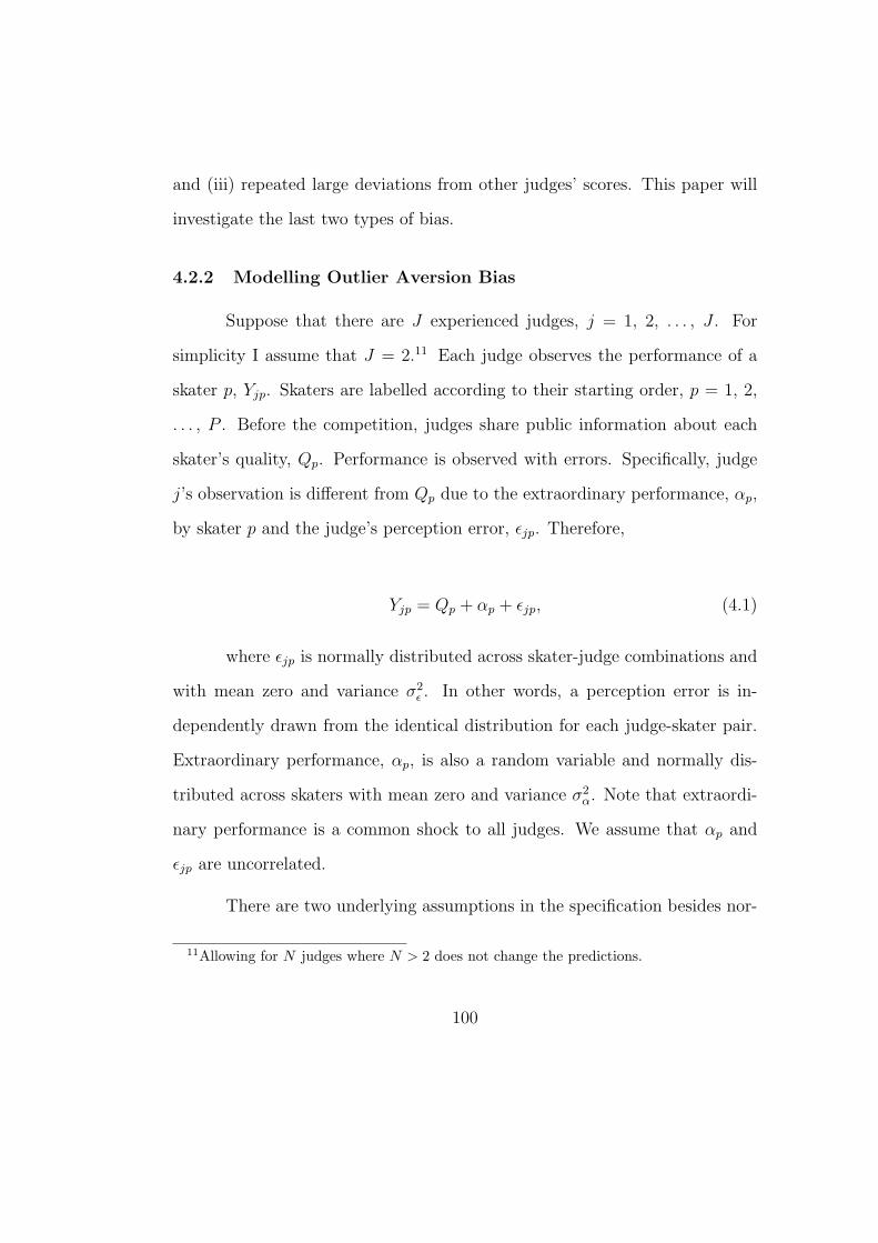
and (iii) repeated large deviations from other judges’ scores. This paper will

investigate the last two types of bias.

4.2.2 Modelling Outlier Aversion Bias

Suppose that there are J experienced judges, j = 1, 2, . . . , J . For

simplicity I assume that J = 2.11 Each judge observes the performance of a

skater p, Yjp. Skaters are labelled according to their starting order, p = 1, 2,

. . . , P . Before the competition, judges share public information about each

skater’s quality, Qp. Performance is observed with errors. Specifically, judge

j’s observation is different from Qp due to the extraordinary performance, αp,

by skater p and the judge’s perception error, εjp. Therefore,

Yjp = Qp + αp + εjp, (4.1)

where εjp is normally distributed across skater-judge combinations and

with mean zero and variance σ2ε . In other words, a perception error is in-

dependently drawn from the identical distribution for each judge-skater pair.

Extraordinary performance, αp, is also a random variable and normally dis-

tributed across skaters with mean zero and variance σ2α. Note that extraordi-

nary performance is a common shock to all judges. We assume that αp and

εjp are uncorrelated.

There are two underlying assumptions in the specification besides nor-

11Allowing for N judges where N > 2 does not change the predictions.

100

mality and independence. First, as already mentioned, judges share common

information on the skaters’ quality based on past performances. Second, judges

are homogenous in the sense that their observations a priori suffer the same

degree of perception errors.

After each skater finishes performance, judges simultaneously submit a

score, Sjp, without knowing the other judges’ scores. Assume that judges get

utility from a reasonable and socially acceptable final ranking of the skater and

also from scores that are similar to those of the other judges on the panel. The

first motivation leads judges to submit scores that are similar to that of an

“average” spectator. Even though individual spectators might observe more

noisy performances, the average of their observations may as well be Qp + αp

by the law of large number. For individual judge j, the maximum likelihood

estimate of the average spectator’s observation is his or her own observation,

Yjp.

Formally, a judge’s objective is to balance the trade-off between two

factors: (i) minimizing the difference between her score and her own obser-

vation and (ii) minimizing the deviation of her score from the other judge’s

score.12 Thus I specify utility as dependent on the squared distance between

Yjp and Sjp to reflect factor (i), and on the squared distance between the

judge’s score, Sjp, and the other judge’s score, S−jp, to reflect factor (ii). The

simplest functional form is

12The model does not allow for favoritism for specific skaters.

101

Vjp = −(Sjp − Yjp)2 − λjp(Sjp − Se

−jp)2, (4.2)

where λjp is the “price” for deviation from the other judge.13 The

parameter λjp is specific to each skater-judge combination. It depends not only

on a given judge’s preferences, but it is also history-dependent. In other words,

the degree of agreement with the judge 2 in previous performances changes the

current price faced by judge 1. For example, if a judge recently submitted an

extreme score, then that judge’s “price” of deviation for a subsequent skater

becomes larger.14 The “price” for the deviation from her own observation is

set to one as a numeraire.

One last point to note is that λ’s are assumed to be known to all judges.

This assumption seems reasonable since international judges are quite homoge-

nous in preferences, and since judges’ scoring of previous skaters is publicly

observable after each performance. However, note that λ’s are unknown to

econometricians. The existence of λ is what this paper attempts to test.

Since the other judge’s score is ex ante unobserved, judge j forms the

conditional expectation of S−jp given available information. Suppose that the

judge guesses S−jp as a weighted sum of Y−jp and Qp. Temporarily assume

13Here I assume that the prices of positive deviation and that of negative deviation areequal. Otherwise we may allow for λ+

jp and λ−jp, separately. The distinction is empiricallytestable.

14It is possible to derive explicitly the dependence of λjp on previous deviations. SeeAppendix A in further detail.

102

that the weight is known to the judge as µ−jp, where µ−jp ∈ [0, 1].15 Then the

guess is as follows:

S−jp = µ−jpY−jp + (1− µ−jp)Qp. (4.3)

Using the law of conditional expectation, we have:

Se−jp = E(S−jp|Yjp, Θp)

= µ−jpE(Y−jp|Yjp, Θp) + (1− µ−jp)Qp

= µ−jp(θYjp + (1− θ)Qp) + (1− µ−jp)Qp

= µ−jpθYjp + (1− µ−jpθ)Qp.

where

θ =σ2

α

σ2α + σ2

ε

. (4.4)

And Θp is a set of common knowledge, Θp = {Qp, αjp ∼ N(0,σ2α), εjp

∼ N(0, σ2ε ), λjp}. Straightforward calculations yield the optimal score:

S∗jp =1 + λjp · µ−jp · θ

1 + λjp

Yjp +λjp · (1− µ−jp · θ)

1 + λjp

Qp, (4.5)

15I find µjp, j = 1, 2, an optimal guess in rational expectation equilibrium. My model isan application of Cournot duopoly.

103

for j = 1, 2. Assuming that the proposed linear scoring strategy is

reciprocally rational in equilibrium, we have explicit solutions for the weight

on a single judge’s observation relative to public information:

µjp =1 + λ−jp + λjp · θ

1 + λ−jp + λjp + (1− θ2) · λjp · λ−jp

, (4.6)

for j = 1, 2. Notice that the optimal weight is known and can be

inferred from common knowledge. Furthermore we have the following useful

results:

∂µjp

∂λjp

< 0,∂µjp

∂λ−jp

< 0,∂µjp

∂θ> 0. (4.7)

If the deviation from the second judge’s score becomes more costly, the

first judge tends to put more weight on Qp. In other words, as a judge’s price

increases, he or she will become more biased toward the public information.

Similarly, if the second judge’s marginal cost of deviating from Sjp increases,

this judge also tends to make her score closer to Qp. Finally, because errors

are relatively more likely to come from judges’ misperception than a skater’s

erratic performance, judges are more biased toward public information.

The above comparative statics provide us with intuitive results. Notice

that the expected squared deviation of judge j is:

104

E[Djp] = E[S∗jp − S∗−jp]2

= E[(µjpYjp + (1− µjp)Qp)− (µ−jpY−jp + (1− µ−jp)Qp)]2.

Plugging (1) into the above, we have:

E[Djp] = E[µjpεjp − µ−jpε−jp]2

= µ2jpE(εjp)

2 + µ2−jpE(ε−jp)

2

= (µ2jp + µ2

−jp)σ2ε < 2 · σ2

ε .

This inequality suggests the surprising result that inter-judge difference

is not a good measure of the validity of judgment. Contrary to conventional

wisdom, this result implies that a high degree of agreement among evaluators

might reflect strategic manipulations due to their aversion to extreme scores.

This seems paradoxical because judges’ concerns about the judge-assessment

system and its implications for their careers force them to put less weight on

their own observation and rely more on public information.16

Furthermore the model suggests some testable hypotheses. We can test

the following:

16The main objective of training judges and measuring the degree of agreement amongthem is to reduce their perception error, σ2

ε . However the effect might be overestimatedwithout taking into account the fact that the type of training and appraisal system wouldaggravate judges’ outlier aversion and thereby increase the degree of agreement.

105

∂E(Djp)

∂λjp

= 2(µjp∂µjp

∂λjp

+ µ−jp∂µ−jp

∂λjp

)σ2ε < 0. (4.8)

∂E(Djp)

∂λ−jp

= 2(µjp∂µjp

∂λ−jp

+ µ−jp∂µ−jp

∂λ−jp

)σ2ε < 0. (4.9)

∂E(Djp)

∂θ= 2(µjp

∂µjp

∂θ+ µ−jp

∂µ−jp

∂θ)σ2

ε > 0. (4.10)

In particular, the first two predictions are related to outlier aversion

bias. For empirical purposes, I can calculate Djp for each judge-skater com-

bination. As a result, if there is any variation in λ, then it is possible to test

predictions for (8) and (9). As is explained in detail in the next section, I ex-

ploit two kinds of variation in carrying out these tests: (i) endogenous changes

in λ over multiple skaters for an individual judge and (ii) exogenous changes

in λ due to the judging system reform in 2002.

4.3 Empirical Analysis

4.3.1 Data and Descriptive Statistics

The data used are scores for figure skating performances given by indi-

vidual judges in the World Figure Skating Championships in the three seasons

between 2001 and 2003. Each Championship consists of four events: men,

ladies, pairs, and ice dancing. Each event is composed of three programs:

preliminary, short, and long. Sometimes there are two sub-programs such as

106

preliminary A and preliminary B.17 The World Figure Skating Championships

requires qualification in the short program, and skaters perform their free skat-

ing in the qualifying program. For each program, there is a panel of judges

composed of one referee and, before 2003, seven to nine judges. The assign-

ment of judges is determined by the ISU, taking into consideration the balance

of national representation.

All the data are available on the International Skating Union (ISU)

official website (www.isu.org) or the United States Figure Skating Association

(USFSA) website. I collected the scoring data on 283 “men” performances,

289 “ladies” performances, and 438 “pairs” and “ice dancing” performances.

These numbers amount to 411 judge-program combinations and 9,573 scorings.

A judge on average scores about 23 performances. TABLE 4.1 illustrates the

sample structure.

As mentioned before, the ISU recently adopted a new judging system

that introduced anonymity and random selection of judges. Two results of

the reform are remarkable. First, the average number of judges in a panel

increased from 8.1 to 12.4. Second, it is no longer possible to identify which

judge submitted each score because of anonymity. It is also now impossible to

combine the technical and artistic score of each judge.

Some information on skater quality is also available, such as years of

skating experience and rankings in past major competitions. In the full sample,

17There is no qualifying program for pairs.

107

those skaters who have been ranked at least once within the top five in the

past four years in World Figure Skating Championships consist of about 18

percent of total observations. “Top ten skaters” make up roughly 32 percent.

TABLE 4.2 presents the means and standard deviations of the average

scores of the panel. Some interesting patterns related to subjective perfor-

mance evaluation are notable. First, artistic score is categorically higher than

technical score. Given that artistic scores are presumably more subjective,

this might imply the presence of leniency bias. Second, it seems that judg-

ments in figure skating reflect on absolute performance evaluation. As skaters

advance from the qualifying round to the long program in the competition,

the average score consistently increases for both technical and artistic scores.

Third, the standard deviation is consistently larger for technical score than for

artistic score. Notice that the standard deviation measures the dispersion of

average scores across performances. In other words, it represents the extent

to which each performance is distinctly scored. Larger standard deviations for

technical scores confirm that there is significant differentiation between per-

formances when judges rate performers on well-defined specific characteristics

(Borman 1982).

4.3.2 Identification I: Dynamic Panel Data Estimation

To reiterate, the purpose of this paper is to examine whether judges

submit scores in a strategic fashion, particularly eschewing outlying scores.

The model from the previous section implies that a direct test would be to

108

calculate whether λ is zero or not. While this calculation does not seem

implementable, there are indirect ways of testing for outlier aversion. For

example, the prediction in equation (8) is true only when there exists non-zero

outlier aversion. Notice that it is possible to test equation (8) if there is any

exogenous variation in λ. In this subsection, I exploit dynamic variations in

λjp over multiple performances within one program, λj1, λj2, . . . , λjP . Recall

that a judge’s “price” for deviation from others may change over time; it will

increase if the judge has already submitted outlying scores for previous skaters.

The basic empirical specification is therefore dynamic as follows:

Dj,p = α1Dj,p−1 + · · ·+ αLDj,p−L + βDp−L−1

j + γQj,p + δp + λj + νj,p, (4.11)

where

Dj,p = (Sj,p − S−j,p)2, (4.12)

and

Dp−L−1

j =1

p− L− 1(

p−L−1∑

k=1

Dj,k). (4.13)

Dp−L−1

j measures the average squared deviation of individual judge j’s

score from the other judges’ average score up to the (p − L − 1)-th previous

skater. And Qj,p is a vector of the skater’s quality and a constant term. It

109

includes dummy variables which are equal to one if the skater was at least once

ranked within top five or top ten in World Figure Skating Championships for

the past four years and zero otherwise. Starting order, p, is included in case

there exists any related systematic effect.18

For identification, I have to assume that the deviations before the L-th

previous performance have only “average” marginal effect, β, while the previ-

ous deviations up to the L-th previous performance have idiosyncratic effects

on the current scoring. This assumption seems reasonable in the sense that

judges have a “fresher memory” about recent performances. I will estimate

the simplest case of equation (11) for L = 1.19

The νj,p’s are assumed to have finite moments and, in particular, E(νj,p)

= E(νj,pνj,q) = 0 for p 6= q. In other words, we assume the lack of serial correla-

tion but not necessarily independence over starting order. The autocorrelation

structure is testable (Arellano and Bond 1991). It is also assumed that the

initial conditions of the dependent variable, Dj,1, are uncorrelated with the

subsequent disturbances νj,p for p = 2, . . ., P . The initial conditions are pre-

determined. However the correlation between Dj,1 and λj is left unrestricted.

The parameter λj is an unobserved judge-specific skater-invariant effect

that allows for heterogeneity in the means of the series of Dj,p across judges.

I treat the judge-specific effects as being stochastic. There are basically two

18Starting order is randomly assigned to each skater except in the case of long programs(or free skating programs), in which the order is determined by rankings from previousprograms.

19In fact increasing L does not make any significant difference in results.

110

interpretations for the judge-specific effect, λj.20 First, it is related to the

“time-constant” part of λjp in the theoretical model that is supposed to be

constant over starting order within a program. Note that λjp is unobservable

to econometricians and is specified as random.

Second, and more importantly, the existence of judge-specific effects

reflects the peculiarity of the judging system. Recall that judges have to

rank skaters relatively, and because of that absolute values of scores do not

matter much. Suppose that a judge mistakenly scores the first skater higher

than do all the other judges. If the judge tries to be consistent – because of

relative ranking – and rank the subsequent skaters accordingly (with the same

inflation), then that judge’s deviations will be larger than those of the other

judges for all skaters in the program. In this case, the following deviations

reflect only the dispersion of initial scores and have nothing to do with outlier

aversion. Therefore, judge-specific effects must be controlled for in order to

test for outlier aversion.21

Because of the presence of λj, lagged dependent variables included in

the right-hand side in equation (11) are necessarily endogenous unless the

distribution of λj is degenerate.22 However, with the assumptions on the error

20I assume that a judge may have different judge-specific effects in different programs.For example a judge, Mr. Fairmind, is treated as two different judges when he judges formen’s short program and for men’s free program.

21In addition the fixed effects enable us to relax the assumption allowing for taste hetero-geneity across judges even though the conceptual model assumes homogenous judges.

22This is the reason why I assume endogenous variation in judges’ preferences over startingorder.

111

terms, it is possible to estimate the coefficients in equation (11) consistently

in two steps: (i) eliminate λj by the first-differencing transformation and (ii)

use the values of the dependent variable lagged by two skaters or more as

instrumental variables (in the case that L = 1). This is called the “Arellano-

Bond GMM estimator” or the “GMM-DIF estimator” (Arellano and Bond

1991, Blundell and Bond 1998).23 Specifically, I will estimate the following

first-differenced equation:

∆Dj,p = α∆Dj,p−1 + β∆Dp−2

j + γ∆Qj,p + δ + ∆νj,p, (4.14)

where ∆ represents the first-differencing transformation. I assume that

Qj,p is strictly exogenous. Notice that Dp−2

j is predetermined, so its lagged

values can be used as additional instrumental variables. The key identifying

assumption is that the lagged level Dj,p−k will be uncorrelated with 4νj,p for

k ≥ 2, together with the assumption of initial conditions.

Before progressing further, I have to deal with one important ques-

tion in my empirical strategy. One might suspect that the squared deviation,

though convenient for analysis, is really what judges are concerned about. For-

tunately, it is possible to conduct a direct test of whether Dj,p is meaningful for

the judge-assessment system and judges’ career concerns. I estimate a simple

Probit equation that regresses Rj,2002 on Dj,p,2001 where Rj,2002 is a dummy

variable that is one if the judge j is re-selected for the 2002 Championships

23I refer to this as the “GMM estimator.”

112

conditional on the fact that the judge is selected in 2001, and zero otherwise.24

Judges’ nationality is controlled for to take into account that each national fed-

eration has its own underlying procedure of recommending judges to the ISU.

After controlling for nation-specific effects, I find that the average squared de-

viation (about 0.13) for one performance significantly reduces the probability

of reselection by about 1 percent (p-value = 0.03).25 Thus if a judge continued

to deviate by the average–for example, for 20 skaters (the average number of

skaters that a typical judge is supposed to score)–then the probability should

have decreased by more than 20 percent. Given that judges are honored to be

selected for major international competitions, like the World Figure Skating

Championships, I conclude that Dj,p is at least one of the important statistics

in the judge-assessment system and that judges are concerned about it.

The coefficients, α and β, are of major interest. I expect that their signs

will be negative, since previous deviations would lead judges to avoid further

deviations. The coefficients for the skater’s quality are presumably negative

in part because top skaters’ performances are stable and less “extraordinary”

(larger θ) and in part because judges’ evaluations are more careful for these

top skaters (larger λ). Greater attention is paid to those performances by

the media, spectators, and therefore the ISU. Furthermore the ISU judge-

monitoring system puts more weight on serious bias or error for highly-ranked

skaters (ISU Communication no.1197).

24The selection of judges in the 2003 Championships is not considered because the totalnumber of judges selected in that year increased due to the judging-system reform.

25The result does not change when nation-specific effects are not controlled for.

113

I estimate equation (11) using ordinary least square (OLS), a within-

group estimator (WG), and the Arellano-Bond dynamic panel data (GMM)

model, of which the estimates are juxtaposed for comparison. Even though

this model can be consistently estimated by GMM, the comparison with these

potentially inconsistent estimates is very useful. The asymptotic results and

Monte-Carlo studies have shown that the OLS estimator is biased upward and

the WG estimator is biased downward if |α| ≤ 1 (Blundell, Bond, and Wind-

meijer 2000).26 Therefore if the empirical model is correctly specified and there

is no finite sample bias, any consistent estimate must lie between the corre-

sponding OLS and WG estimates. Whether this pattern (sometimes called

“Sevestre-Trognon inequality”) is observed or not is a simple and valid test

for specification and finite sample biases (Bond 2002, Sevestre and Trognon

1997).

TABLE 4.3 presents the estimation results for the sample for the 2001

and 2002 seasons.27 I also run the same regressions separately for sub-samples

– singles (men and ladies) and pairs (pairs and ice dancing), the results of

which are presented in TABLE 4.5 and 4.6, respectively.

Before discussing the estimates, let us examine some of the specification

issues mentioned above. First, I find across the board that the OLS estimates

26The WG estimator eliminates λp by transforming the original observations in to devia-tions from individual means. However this transformation induces a non-negligible correla-tion between the transformed lagged dependent variable and the transformed error term.

27Remember that the data on individual scorings are not available for 2003 because ofthe judging system reform.

114

for the lagged dependent variable appear to be larger than the corresponding

GMM estimates, while the WG estimates appear to be smaller. For the full

sample, when skaters’ quality is controlled, the GMM estimate is -0.0375 –

between the OLS estimate (0.0516) and the WG estimate (-0.0807).

The relationship between the estimates confirms the “Sevestre-Trognon

inequality.” The bias in the WG estimates is small relative to that of the

OLS estimates. It is a well known fact that the asymptotic bias of the WG

estimate is inversely related to the length of time period. By the within-group

transformation, the lagged dependent variable becomes Dj,p−1− 1P(Dj,1 + · · ·+

Dj,p + · · · + Dj,P ), and the error term becomes νj,p − 1P(νj,1 + · · · + νj,p−1 +

· · · + νj,P ). These two are obviously correlated, above all because Dj,p−1 and

1Pνj,p−1 are correlated, 1

PDj,p and νj,p are correlated, and so on. For sufficiently

large P the correlations will be negligible. The “time” period in this paper is

quite long – 23 skaters in a typical program. The validity of the instruments

is strongly supported by the Sargan test of over-identifying restrictions (the

p-value is higher than 0.99 for every specification).

Finally, the assumption of no serial correlation of νjp cannot be rejected.

The last two rows in the TABLE present the Arellano-Bond test statistics

for autocorrelation. I find that there is significant negative first-order serial

correlation in the first-differenced residuals, while there is no second-order

correlation. It is consistent with theoretical prediction that if the error term

is serially uncorrelated, there must be first-order serial correlation, but no

second-order serial correlation in the first-differenced residuals. The AR(1)

115

structure is accepted at a p-value lower than 0.01, and the AR(2) structure is

rejected across the board at a p-value higher than 0.50.

The GMM estimates imply that the deviation of a judge’s vote for

the previous skater significantly decreases the deviation from the other judges’

average score for the current skater. This result is consistent with equation (8).

TABLE 4.3 implies that deviation by the average difference between median

and maximum (or minimum) score (about 0.45) pressures judges to be biased

by about 0.0877 point (=√

α× 0.452=√

0.038× 0.452) toward the average for

the current player. Similarly, outlier aversion bias to average deviation is 0.106

(=√

0.056× 0.452) for the singles competition and 0.11 (=√

0.06× 0.452) for

the pairs and ice dancing competitions as seen in TABLE 4.5 and 4.6. The size

of the bias is significant given that the unit of score is 0.1. Based on the idea

put forth by Campbell and Galbraith (1996), the size of the coefficients can be

explained in the following way: imagine a judge who has difficulty in deciding

between two neighboring scores, separated by 0.1. Suppose that there exists a

critical value for that judge’s previous deviation, beyond which he or she will

choose the score closer to the average for the current situation. And if the

previous deviation is less than the critical value, the judge then randomizes

her score between the two neighboring scores. Such a judge show a bias of

0.05 in response to the critical value.28

28It is interesting to compare these estimates with those of nationalistic bias: Zitzewitz(2002) finds that nationalistic bias is on average 0.17, and Campbell and Galbraith (1996)find nationalistic bias of 0.07 by nonparametric estimation.

116

The marginal effect of the average squared deviation up to the (p−L−1)-th previous performance is larger than that of the one-time deviation for

the immediately preceding performance. In other words, |β| > |α|. For the full

sample, when skaters’ quality is controlled, β (-0.1658) is almost five times as

large as α (-0.0375) in absolute terms. This result seems reasonable, because

β picks up a kind of cumulative effect of α.29 For example, the magnitude of

β for the full sample implies that if one judge deviated from the other judges’

average by 0.45, then the current score is likely to be closer to the average by

0.18 (=√

0.1658× 0.452).

The estimates for Qp are also consistent with the model’s predictions.

Judges are more in agreement for top skaters. If a skater was at least once

ranked within top ten in the past four Championships, then the squared de-

viation decreases by about 0.07 to 0.1. As mentioned before, it is in part

because top skaters are less erratic, and also in part because the price of the

deviation for the judge is higher when evaluation top-ranked skaters due to

the judge-assessment system. Both explanations are consistent with the con-

ceptual model.

TABLE 4.4 presents the results when the effects of positive and nega-

tive deviations are separated out. Overall, the results are very similar. Once

a judge has submitted outlying scores, she is more likely to converge toward

the group. Also, judges are more in agreement for top-ranked skaters. In-

29The WG estimates for β are categorically downward biased. This is consistent withNickell (1981).

117

terestingly, the GMM estimates suggest that current scoring should be more

responsive to positive deviations than negative deviations, even though the ef-

fects are not statistically different. This result indicates that judges are more

averse to positive extreme scores. In other words, they may be more afraid of

scoring too high. This makes sense when one considers that positive bias is

usually considered as favoritism, which is a more sensitive issue in this sport.

4.3.3 Identification II: Interim Judging System

In this section, I exploit the quasi-natural experiment of the judging

system reform in 2002 to examine outlier aversion. In 2002 the ISU adopted a

new system–called the Interim Judging System – in which judges’ names are

concealed from outside observers, and judges are randomly drawn from a pool

of possible judges. The new system was implemented in the World Figure

Skating Championships in 2003.

The change in the judging system provides another opportunity to

test the existence of outlier aversion bias since one might expect that judges

would be less pressured to agree under the new system. The ISU itself states

“anonymity reduces the risk of judges coming under external pressure.” The

“external pressure” referred to by the ISU is mainly assumed to be nationalistic

favoritism. In addition, anonymity might also relieve judges of the pressures

exerted by the media and fans, which are not negligible at all. Olympic gold

medalist Carol Jenkins said “people watching at home will be ready in their

mind to do their own judging. It’s the one sport where the spectators judge

118

the judges.” As a result, a meaningful test for the existence of outlier aversion

bias is whether judges’ scores became more dispersed after the changes.

TABLE 4.7 shows the simple mean comparisons of deviations before

and after the system changed. Since it is now impossible to link scores to

individual judges, I compare the distribution of scores for the 2001, 2002 and

2003 Championships.

For robustness, I use three statistical measures of score dispersion for

the same skater:

ξ1p =

1

Jp − 1

Jp∑j=1

(Sj,p − Sp)2,

ξ2p =

2

Jp(Jp − 1)

Jp∑i=1

Jp∑j=1

|Si,p − Sj,p|,

ξ3p = Smax

p − Sminp .

The first measure (ξ1p) is the consistent estimate standard deviation of

the sample. The second measure (ξ2p) is the average absolute deviation. The

last measure (ξ3p) is the range between the maximum and minimum score.

The number of judges in a panel is subscripted by p, because it varies over

programs.

In TABLE 4.7 all the measures increased under the new system. For the

men’s program, the standard deviation of technical scores increased from 0.16

to 0.18, and the range increased from 0.47 to 0.60. For the ladies’ program, the

119

standard deviation of artistic scores increased from 0.18 to 0.20, and the range

increased from 0.52 to 0.65. Most of these changes are statistically significant

at reasonable significance levels. Thus I conclude that the new system seems

to reduce judges’ outlier aversion bias.30

Simple mean comparisons are intuitive, but one can object that they

do not control for other variables. Above all, the increases in dispersion might

reflect aggravated nationalistic bias and an increase in corrupt scorings after

the reform. Indeed, the new system has been harshly criticized in that it could

allow judges to manipulate their scores more easily without accountability.31

To meet this objection, I regress the amount of dispersion on several control

variables, including a measure of nationalistic bias (an indicator of whether

the skater and at least one judge on the panel are from same country (Bp)).

The equation to be estimated is:

ξp = β1Bp + β2Ap + β3BpAp + Qpγ + Xpδ + up, (4.15)

where ξp is one of the three dispersion measures.32 Ap is the indicator

of anonymity (one for the new system and zero for the old system); Xp is a

30One might object to the conclusion above in that the increases in score dispersion simplyreflect the increase in the number of judges on a panel; however, note that the measuresof dispersion are standardized except ξ3

p. Furthermore, it is usually found in the literaturethat the amount of agreement among evaluators increases substantially when the numberof evaluators is increased.

31For related criticisms refer to http://skatefair.visionsnet.com.32Robust standard errors are calculated since the dependent variable is the estimated

parameter (Saxonhouse 1976).

120

vector of indicators for events and programs; Qp is a vector of measures of

skaters’ quality; and one constant.

TABLE 4.8 shows the results. The estimates of β are of primary in-

terest. I find across the board that scores are more dispersed after the in-

troduction of anonymity in the judging system, even after controlling for the

nationalistic bias. Furthermore, the standard deviations significantly increase

by about 0.01, the absolute deviations increase by about 0.1, and the range

increases by about 0.3. The magnitude ranges from 13 to 36 percent of one

standard deviation of each measure.33

For simplicity, the panel with at least one judge from the same country

as the skater is called the “compatriotic panel,” and the panel without any

such judge is called the “neutral panel.” Scores of compatriotic panels are

slightly less dispersed, although the difference is not statistically significant.

However, the votes of compatriotic panels converge less under the Interim

Judging System, which suggests that nationalistic bias is possibly aggravated

under the new system.

Other results are consistent with the predictions of the conceptual

model. First, scores are significantly more converged for top skaters. For all

three measures, the dispersion of scores shrinks by a half standard deviation.

Second, scores in more advanced programs are also less divergent.

33In each case, “one standard deviation” is: 0.08 for the standard deviation, 0.098 for theabsolute deviation, and 0.26 for the range.

121

4.4 Information Loss due to Outlier Aversion

I find that there is an incentive for judges to agree on their scoring

based on the particular judge-assessment system in the sport of figure skating.

Judges’ scoring is biased toward a general consensus based on previously-

acquired publicly-known information. As a result, an interesting question is

to assess how much private information is lost due to outlier aversion. The

best way to evaluate the information loss would be to compare the submitted

scores with actual observations, but this is impossible because we do not have

information on judges’ actual observations.

Fortunately, there seem to be at least two measures that can approx-

imate the information loss. The first is based on the idea that an individ-

ual judge’s deviations could represent the private information.34 Imagine a

judge who does not have outlier aversion at all. Then this judge’s squared

deviation is not strategically manipulated, but randomly assigned. Suppose

that her idiosyncratic squared deviation is on average 0.0256 – the average

for the sample. In this case, there would be no effect of previous deviations

on current scoring, and pure observational error would be on average zero.

Therefore, E(Dj,p) = E(λj) = 0.0256 in terms of equation (11). The ex-

pected average squared deviation for 20 performances must be 0.0256 because

E(D20j ) = 1

20

∑E(Dj,p) = 0.0256.

34This identification strategy ignores the quality of information. Given that the lostinformation is likely to be for extreme outliers, it might be plausible that the lost informationis negligible.

122

What would have happened to the average squared deviation if the

judge did have outlier aversion to the same degree we found in the sample? The

data-generating process, specified by equation (11) with the GMM estimates,

yields 0.0214 as the average for 20 performances.35 It is obvious that on average

the deviation decreases because the judge avoids future outlying scores after

the previous deviations. The ratio of average squared deviations is about 0.84

= 0.02140.0256

. This roughly implies that approximately 16 percent of information

(in terms of squared deviation) is lost due to outlier aversion.

Another crude measure of information loss can be found by comparing

score dispersion before and after the change in the judging system.36 The

underlying idea is similar to that of the first approach; the diversity of scores

among judges reflects their relative inclusion of private observation. A simple

measure to compare dispersion between the two different distributions is the

ratio of variances:

L =V ar(Sj,p,t<2003)

V ar(Sj,p,t=2003). (4.16)

It is straightforward to estimate L from TABLE 4.7 and 4.8. In TABLE

4.8 we know that standard deviation increases by 0.0131 after the reform. Since

35I generate the squared deviations for skater p = 3, 4, · · · , 20, according to the estimatedequation, Djp = α1Dj,p−1 + βD

p−2

j + λj . Therefore E(Djp) = α1Dj,p−1 + βDp−2

j +E(λj). Iassume that the first two deviations, E(Dj1) and E(Dj2), are 0.0256 because the estimationdoes not have any systematic behavioral implication for the initial deviations.

36Note that the measure would underestimate the information loss because there stillexists outlier aversion even after the reform.

123

the average standard deviation before the reform was about 0.165 in TABLE

4.7, an estimate of L is therefore about 0.8583 = ( 0.16500.1650+0.0131

)2. This implies

that the information loss is approximately 14 percent, which is very similar to

the first estimate.

4.5 Implications

The purpose of this paper is to illustrate that subjective evaluators are

sensitive to the incentive structure they work in. In particular, evaluators

make decisions based on how they are monitored and how their evaluations

are perceived. The case of figure skating judging clearly shows that there is

a bias toward agreement, because the degree of agreement among judges is

used, one, as a measure of the reliability of the evaluations and, two, to assess

individual judges themselves.

I derive some interesting implications for decision-making in business

and organizational contexts. First, when deciding to implement subjective

evaluations, it is important to take into account the system used to evaluation

the evaluators. This aspect is especially important in the case of multiple

evaluators.37 When they may manipulate their opinions and judgments if there

exists mutually-beneficial externality (Katz and Shapiro 1986). Second, my

37Relatively little attention has been paid to this scenario while preference-aggregationmechanisms and comparisons for different systems have been intensively studied. There aremany cases where the appraisal is based on multiple sources. Firms gather and integrateinformation about workers from their coworkers and supervisors. Also, school principalscompile their own observations of a student with those from other teachers.

124

results imply that agreement among evaluators is not always desirable. Setting

“agreement” as an objective of the decision-making process will induce the

evaluators to bias their judgments and opinions. Firms often utilize subjective

evaluation in group decision-making process. Unfortunately, as my findings

have demonstrated, these processes are subject to outlier aversion bias because

of the incentives faced by members of the decision-making group (for example,

evaluators may not want to upset their bosses or hold up a time-sensitive

decision). As a result, when firms gather groups for input and decision-making,

they may believe that those processes result in an accurate compilation of

beliefs from those who are involved and informed; however, it is likely that the

outcomes of those meetings are biased toward consensus, do not accurately

reflect the true opinions of the participants, and may harm firms because they

suppress important private information. In those cases, when agreement is

externally induced, this often leads to a loss of valuable private information

that individual evaluators may have had access to but that the others do not.

It should be noted that valuable private information is weighted less when the

diversity of opinion is averaged out.38 Objections to the consensus by credible

informants should be valued, not discouraged.

38Interestingly, Janis (1983) documents historical moments such as the Cuban missilecrisis and Korean war where conforming to group norms within the president’s inner circle,and thereby ignoring minor opinions led to disastrous and irrational consequences. He arguesthat pressure to conform within small cohesive groups of decision-makers is an importantsource of decision-making errors. See also Bernheim (1994) for an economist’s view onconformity pressure.

125

Table 4.1: Number of Observations: Skater-Judge Combinations

Event Program 2001 2002 2003Men Qualifying 301 266 400

Short 270 270 420Long 216 216 216

Ladies Qualifying 329 280 399Short 270 261 420Long 216 207 336

Pairs Qualifying - - -Short 216 180 294Long 171 180 280

Ice Dance Qualifying 490 392 261Short 270 252 406Long 216 216 336

Total 2,965 2,720 3,888

126

Table 4.2: Panel-Average Scores1

2001 2002 2003Technical Artistic Technical Artistic Technical Artistic

Full Sample 4.705 4.889 4.668 4.856 4.695 4.873(.704) (.629) (.715) (.641) (.716) (.656)

Men 4.841 5.003 4.868 4.995 4.773 4.972(.594) (.517) (.639) (.562) (.665) (.598)

Ladies 4.713 4.885 4.561 4.821 4.655 4.845(.655) (.584) (.729) (.608) (.709) (.615)

Pairs 4.621 4.826 4.610 4.792 4.665 4.820(.779) (.704) (.730) (.697) (.760) (.724)

Qualifying 4.593 4.733 4.534 4.662 4.571 4.678(.738) (.683) (.748) (.725) (.765) (.728)

Short 4.657 4.965 4.620 4.938 4.659 4.948(.712) (.580) (.741) (.565) (.743) (.622)

Long 4.963 5.069 4.921 5.047 4.887 5.018(.559) (.521) (.556) (.508) (.576) (.546)

1 Panel-average score is Sp = 1Jp

∑Jp

j=1 Sj,p. Standard deviations are displayed in parenthe-ses.

127

Table 4.3: Dynamic Panel Data Estimation: Full Sample1

OLS WG GMM(1) (2) (3) (4) (5) (6)

Dj,p−1 .0671 .0516 -.0703 -.0807 -.0378 -.0375(.0184) (.0180) (.0147) (.0145) (.0183) (.0180)

Dp−2

j .3024 .3258 -.6787 -.6700 -.1698 -.1658(.0464) (.0466) (.0574) (.0564) (.0821) (.0812)

Top Five -.0087 -.0162 -.0138(.0073) (.0132) (.0812)

Top Ten -.0955 -.0991 -.0997(.0079) (.0110) (.0133)

Starting Order -.0017(.0006)

Constant .0897 .1471 .2465 .2851 .0035 .0012(.0066) (.0107) (.0095) (.0098) (.0009) (.0009)

Observations 4,782 4,782 4,782 4,782 4,540 4,540Number of judges 242 242 242 242 235 235Sargan test 232.89 231.79AR(1) test -38.25 -37.63AR(2) test .44 .68


128

Table 4.4: Dynamic Panel Data Estimation:Full Sample1

OLS WG GMMDj,p−1 .0515 -.0809 -.0497

(.0180) (.0145) (.0179)

Dp−2

j (+) .3615 -.6185 -.2869(.0727) (.0858) (.1769)

Dp−2

j (−) .3060 -.7053 -.1820(.0494) (.0717) (.1125)

Top Five -.0086 -.0162 -.0120(.0073) (.0132) (.0152)

Top Ten -.0955 -.0991 -.1006(.0080) (.0110) (.0132)


Constant .1466 .2844 -.0013(.0107) (.0099) (.0009)

Observations 4,782 4,782 4,540Number of judges 242 242 235Sargan test 818.47AR(1) test -37.48AR(2) test .56


129

Table 4.5: Dynamic Panel Data Estimation: Singles1

OLS WG GMM(1) (2) (3) (4) (5) (6)

Dj,p−1 .0536 .0358 -.0647 -.0721 -.0559 -.0576(.0201) (.0200) (.0208) (.0207) .0258) (.0257)

Dp−2

j .3065 .3519 -.6170 -.6123 -.1406 -.1655(.0508) (.0513) (.0850) (.0844) (.1285) (.1282)

Top Five -.0199 -.0300 -.0197(.0165) (.0161) (.0181)

Top Ten -.0369 -.0429 -.0256(.0141) (.0138) (.0164)


Constant .0894 .1452 .2248 .2471 -.0031 -.0023(.0084) (.0121) (.0127) (.0132) (.0010) (.0010)



130

Table 4.6: Dynamic Panel Data Estimation: Pairs1

OLS WG GMM(1) (2) (3) (4) (5) (6)

Dj,p−1 .0754 .0614 -.0740 -.0858 -.0598 -.0559(.0260) (.0252) (.0210) (.0205) (.0243) (.0238)

Dp−2

j .2982 .3069 -.7163 -.7103 -.3352 -.2941(.0619) (.0604) (.0798) (.0776) (.1035) (.1015)

Top Five -.0281 -.0346 -.0335(.0085) (.0200) (.0224)

Top Ten -.1307 -.1286 -.1485(.0118) (.0158) (.0184)


Constant .0904 .1539 .2655 .3222 -.0040 -.0002(.0098) (.0183) (.0145) (.0150) (.0014) (.0014)



131

Table 4.7: Interim Judging System: Before-After Analysis1

Technical ArtisticMen Before After 4 Before After 4Standard deviation .1589 .1825 .0236 .1629 .1698 .0068

[.0657] [.0753] (.0087) [.0663] [.0698] (.0084)Absolute deviation .1793 .2056 .0263 .1836 .1913 .0077

[.0765] [.0889] (.0102) [.0793] [.0799] (.0100)Range .4651 .5989 .1339 .4672 .5553 .0881

[.2007] [.2674] (.0284) [.2015] [.2308] (.0267)LadiesStandard deviation .1766 .2069 .0303 .1785 .1986 .0201


[.1010] [.0841] (.0120) [.0925] [.0938] (.0116)Range .5192 .6740 .1548 .5192 .6479 .1287

[.2644] [.2556] (.0327) [.2318] [.2660] (.0304)PairsStandard deviation .1748 .1770 .0021 .1638 .1837 .0199


[.1124] [.0961] (.0115) [.1122] [.1063] (.0118)Range .5095 .5805 .0710 .4721 .6008 .1287

[.2771] [.2672] (.0292) [.2817] [.3050] (.0307)

1 Standard deviations are in brackets. Robust standard errors are displayed in parentheses.

132

Table 4.8: Interim Judging System: Regression Analysis1

Standard Absolute RangeDeviation Deviation Max Min

Interim System .0131 .0128 .0932 -.0064 -.0996(.0048) (.0056) (.0155) (.0327) (.0381)

Compatriot -.0038 -.0053 -.0203 .0891 .1094(.0042) (.0048) (.0125) (.0255) (.0312)

Interim System .0095 .0153 .0494 .1062 .0568× Compatriot (.0069) (.0080) (.0227) (.0463) (.0544)Top 5 -.0371 -.0435 -.1260 .2471 .3731

(.0047) (.0055) (.0150) (.0217) (.0309)Top 10 -.0422 -.0491 -.1306 .6362 .7668

(.0041) (.0047) (.0129) (.0210) (.0276)Ladies .0228 .0263 .0733 -.1586 -.2319

(.0041) (.0048) (.0131) (.0283) (.0332)Pairs .0128 .0142 .0358 -.2524 -.2882

(.0040) (.0047) (.0125) (.0252) (.0305)Qualify .0465 .0594 .1007 -.1641 -.2648

(.0039) (.0046) (.0123) (.0250) (.0304)Short .0247 .0292 .0758 -.0948 -.1706

(.0036) (.0041) (.0118) (.0246) (.0292)Artistic -.0035 -.0045 -.0153 .1734 .1887

(.0033) (.0038) (.0103) (.0206) (.0248)Constant .1544 .1721 .4728 4.8904 4.4176

(.0044) (.0051) (.0142) (.0301) (.0359)R2 = .2287 .2377 .2385 .4394 .4650Observations 2,020


133

Chapter 5

Conclusions

This thesis examines group decision-making processes with emphasis on

household decisions. In the first essay, consistent with previous findings, I find

for the sample of Korean households that the covariance of taste between child

quantity and quality is not minimal; adverse effects of fertility on child quality

is, if anything, smaller than what would be inferred from a cross-sectional

relationship. In fact Korean parents not only try to keep child quality constant

by investing more to offset unexpected increases in number of children, but

they would increase investment enough to compensate for any loss of non-

pecuniary resources such as attention and caring due to a large number of

competing siblings. The fall in the fertility rate over the past decades does not

account for increasing investment in children’s education. Linking population

policy to fostering human capital could be misleading.

While the first essay ignores differences in individual preferences within

households, the second essay deals with the household decision-making mech-

anism for resolving different preferences and aggregating them into final de-

cisions. Using unique longitudinal data on personal spending, I specify si-

multaneous process of household decision-making in a fully stochastic fashion.

134

By doing this, it is possible to differentiate unobserved spousal bargaining

power from heterogeneity at the household level. I find that while increasing

female labor force involvement and the economic progress of women in the

labor market lead to resource reallocation toward women within households,

the favorable effect is not economically significant. The results imply that

unobserved bargaining power determines the division of labor between mar-

ket and home and jointly decide about spousal labor supply. On the other

hand, a general improvement of family income has negative impacts on intra-

household inequality, which partially confirms the Kuznets curve at the micro

level. Lastly, spouses are significantly different in their preferences for food,

education, and clothing, but they are not for some other goods, such as medical

expenses, housing, and utilities.

The third essay examines a different context than households in which

individuals make decisions in a group. The underlying issue that I attempt

to address is that a group consists of individuals with different preferences

or opinions. It is, in an economic sense, costly to reach an agreement among

different individuals. I find significant evidence for the existence of outlier aver-

sion in judging figure skating. Individual judges manipulate scores to achieve a

targeted level of agreement with the other judges, and the dispersion of scores

depends upon the type of judge-assessment system. One major implication of

this paper, which is at variance with the industrial psychology and personnel

management literature, is that agreement may not be a good criterion for the

validity of an evaluation system.

135

Appendices

136

Appendix A

Existence of Son Preference

In this appendix, I test for the existence of son preference in Korea by

estimating parity progression model, widely used in demography literature.

Parity progression model is based on the hypothesis of whether having daugh-

ters in earlier phases of fertility increases the final number of children. It is

important to note that parity progression models must be tested for house-

holds that have completed fertility since the household’s decision on further

childbearing should be fully observed and not right-censored. As explained

in section 3.1, we suppose that mothers aged 40 and older should complete

fertility.

TABLE A.1 illustrates the results of parity progression models. The

dependent variable is binary, so we use logit model following the convention in

the literature. Marginal effects are calculated. In the first column, we find that

having a girl as the first child significantly increases the probability of having

a second child by 9.8 percent, which clearly demonstrates that the first child’s

sex is a good candidate for the instrument for actual fertility. While having

two same-sex children at the first two childbirth increases the probability of

having three or more children by about 9.9 percentage points, this effect is

137

explained entirely by large positive effect of having two girls (34.8 percent)

when it is entered separately along with the indicator for having two boys. In

fact, having two boys has a negative effect on further childbearing, implying

that parents with two sons are more likely to stop childbearing compared to the

reference group of parents of one boy and one girl. The last column shows that

having both a boy and a girl as the first two children increases the probability

of having a third child by about 15-19 percent, compared to the reference

group of parents of two boys. This finding implies that Korean parents do not

have preferences for a balanced sex mix of children, which Iacovou (1996) and

Angrist and Evans (1998) are based on.

Hazard model is also widely used for testing for son preference. In this

model, the dependent variable is now the time interval between births. The

underlying hypothesis is that with son preferences, parents tend to advance

the timing of the second birth after the first daughter. Likewise they would

advance the timing of the third child when they got two daughters. In general,

parents with more daughters in previous births have a greater hazard of con-

ceiving additional children. An obvious advantage of hazard model over parity

progression model is that it is not required to restrict sample to families that

have completed fertility. This is particularly favorable since we can test son

preferences for the sample used in this paper. As seen in TABLE 2.1, those

households in the sample are most likely in the middle of their fertility history

and have not completed childbearing yet.

I estimate Weibull hazard models and take account of right-censoring

138

because actual time intervals between births are observed only when two con-

secutive births are observed. Only time-invariant explanatory variables such

as years of schooling and age at first birth are included to avoid any bias that

possibly arises when explanatory variables change during the interval. Rel-

ative hazard ratios are calculated and presented in TABLE A.2. Having a

girl as the first child significantly increases the hazard rate of having a second

child by at least 48 percent. Any positive effect of Same Sex disappears once

we separately include Two Boys and Two Girls, as with the results of par-

ity progression model. In fact, the coefficient of Two Boys is estimated less

than one, which means having two boys decreases the hazard rate of having a

third child. This implies that parents are likely to delay additional childbear-

ing – probably to delay for good – if they got two boys. On the other hand,

Two Girls significantly advances third childbirth or increases the likelihood of

giving another birth. Its magnitude is large enough to suggest that parents

are definitely willing to have a third child once they had two daughters. In

summary there is strong evidence that son preference exists in the sample.

139

Table A.1: Parity Progression Model, Pooled Sample, Completed Fertility1

Dependent Variable More than More than More than More thanOne Child Two Children Two Children Two Children

First Girl .0980 .2857 .0361(.0186) (.0348) (.0463)

Second Girl .2514(.0330)

Same Sex .0994(.0347)

Two Boys -.1507(.0437)

Two Girls .3489 .4988(.0451) (.0382)

First Boy .1553Second Girl (.0476)First Girl .1915Second Boy (.0479)Pseudo R2 .1579 .1506 .1506 .1500N = 4,259 3,373 3,373 3,373

1 Robust standard errors are displayed in parentheses, corrected by clustering. Equations includemother’s age, age squared, age at first birth, living with grandparents, living in Seoul, and livingin metropolitan areas.

140

Table A.2: Weibull Hazard Model, Unrestricted Sample1

Birth Interval Birth Interval Birth Interval Birth IntervalBetween Birth Order One and Two Two and Three Two and ThreeFirst Girl 1.476 2.559 .704

(.111) (.504) (.211)Second Girl 3.452

(.693)Same Sex 2.450

(.479)Two Boys .710

(.227)Two Girls 8.457

(1.972)N = 7,149 5,363 5,363

1 Hazard ratios are presented. Robust standard errors are displayed in parentheses,corrected by clustering. Equations include mother’s age at first birth and mother’seducation.

141

Appendix B

Children and Married Women’s Labor Supply

TABLE 10-14 show the estimation outcomes for married women’s labor

force participation. The sample is restricted to women who are 40 year old or

younger and have at least one child. In this case, son-preference instrument is

valid only if the sex composition of children does not directly affect mothers’

labor supply. This assumption is questionable in the sense of “hand-me down”

effects (Rosenzweig and Wolpin 2000), and furthermore it seems incompatible

with son preferences. Son-preferring parents would prefer to spend more time

with their sons than they do with daughters. Therefore the existence of sons

would increase mothers’ value of time at home relative to that at work and

would reduce labor force participation. As with the case of educational invest-

ment, it provides a lower bound of fertility effects in absolute value, although

the 2SLS estimate may not be consistent. In other words, the son-preference

instrument estimate underestimate the adverse effect of fertility on married

women’s labor supply.

It may be worthwhile to summarize some major findings. First, we find

that the OLS estimates are severely biased. Second, fertility effects are highly

nonlinear in number of children. I can obtain nonlinear effects from TABLE

142

B.1 and B.2. The second child substantially decreases mothers’ labor supply

(about 34 percent), while the marginal effect of having additional children

beyond the first two is much smaller (about 9 percent). Third, as with in-

vestment in children’s education, twin instrument tends to exaggerate adverse

effect of fertility on labor force participation, which indicates that there is a

direct and negative effect of having twins on mothers’ labor market activities.

One interesting finding should be emphasized. I find that fertility and

unobserved component of participation are positively correlated in our sample,

consistent with Chun and Oh (2002) that used a cross-sectional sample in

1992. This finding is surprising in the sense that it is opposite to the previous

findings from developed countries where women with stronger attachment to

labor market are supposed to have fewer children, which is called “endogenous

fertility effect” by Browning (1992).

There is a possible suspect for this unique finding. The positive cor-

relation between fertility and unobservable tastes for labor market could be

explained by a sort of ability bias. If a woman’s general ability were negatively

correlated with both fertility and labor market participation, then there would

be a positive correlation between the unobservable determinant (general abil-

ity) and fertility. This explanation is quite germane to Korea, where women

are supposed to specialize in homework and most of jobs available to married

women are low paying and temporary. Although recently changing a little,

married women are still considered to work in low status jobs, the so-called

‘3D’ jobs in Korea, in which 3D stands for ‘Dirty, Dangerous, and Difficult.’

143

The labor force participation rate for the most educated women is not only

the lowest of the OECD countries, but is actually lower than that for the least

educated women. In this case, there could be a negative selection of women

into workforce in terms of their general ability. We believe that it would be

fruitful to find demand-side story to explain the negative selection. I leave

further consideration of this to future work.

144

Table B.1: Married Women’s Labor Force Participation (the de-pendent variable is the indicator that her primary job is nothousewife)1

OLS 2SLS 2SLS RE2SLS RE2SLSRegression Stage First Second First SecondNumber of Children -.0544 -.1044 -.1058

(.0096) (.0512) (.0826)Mother’s Age .0533 .3207 .0686 .3531 .0715

(.0130) (.0158) (.0201) (.0139) (.0323)Mother’s Age -.0004 -.0040 -.0006 -.0044 -.0007Squared (.0002) (.0002) (.0003) (.0002) (.0004)Age at First Birth -.0178 -.0790 -.0217 -.0836 -.0206

(.0020) (.0021) (.0044) (.0025) (.0073)Grandparents .0791 .1035 .0838 .0498 .0722

(.0201) (.0226) (.0206) (.0220) (.0236)Seoul -.0169 -.0928 -.0219 -.0665 .0097

(.0122) (.0145) (.0132) (.0168) (.0187)Metropolitan Areas -.0230 -.0305 -.0243 -.0098 -.0061

(.0126) (.0152) (.0127) (.0172) (.0183)First Girl .2006 .1916

(.0123) (.0149)R2 .0942 .2962 .0908 .2926 .0898N = 7,292


145

Table B.2: Married Women’s Labor Force Participation (the de-pendent variable is the indicator that her primary job is nothousewife)1

OLS 2SLS 2SLS RE2SLS RE2SLSRegression Stage First Second First SecondMore than One Child -.0663 -.3554 -.3249

(.0132) (.1795) (.2630)Mother’s Age .0552 .2851 .1364 .3170 .1373


(.0020) (.0015) (.0087) (.0020) (.0140)Grandparents .0773 .0510 .0911 .0204 .0730

(.0201) (.0162) (.0221) (.0172) (.0243)Seoul -.0150 -.0505 -.0302 -.0384 .0053

(.0122) (.0104) (.0159) (.0132) (.0211)Metropolitan Areas -.0216 -.0016 -.0217 .0123 -.0002

(.0126) (.0109) (.0130) (.0136) (.0191)First Girl .0589 .0623

(.0088) (.0118)R2 .0931 .2447 .0371 .2531 .0668N = 7,292

1 Robust standard errors are displayed in parentheses. Five year dummies are in-cluded.

146

Table B.3: Married Women’s Labor Force Participation (the depen-dent variable is the indicator that her primary job is not housewife)1

OLS 2SLS 2SLS RE2SLS RE2SLSRegression Stage First Second First SecondMore than Two Children -.0494 -.1806 -.1896

(.0186) (.0888) (.1493)Mother’s Age .0379 .0356 .0415 .0376 .0413


(.0019) (.0012) (.0029) (.0013) (.0046)Grandparents .0756 .0369 .0797 .0178 .0702

(.0201) (.0123) (.0203) (.0112) (.0235)Seoul -.0141 -.0482 -.0209 -.0318 .0105

(.0123) (.0079) (.0131) (.0086) (.0186)Metropolitan Areas -.0225 -.0215 -.0250 -.0167 -.0081

(.0126) (.0083) (.0127) (.0088) (.0185)First Girl .1160 .1069

(.0067) (.0076)R2 .0912 .1449 .0842 .1429 .0828N = 7,292

1 Robust standard errors are displayed in parentheses. Five year dummies are included.

147

Table B.4: Married Women’s Labor Force Participation,Twinning Instrument (the dependent variable is the in-dicator that her primary job is not housewife)1

2SLS 2SLS 2SLS 2SLSRegression Stage First Second First SecondNumber of Children -.2679 -.2201

(.0864) (.1439)Mother’s Age .3119 .1188 .3507 .1113

(.0160) (.0292) (.0140) (.0522)Mother’s Age -.0038 -.0012 -.0044 -.0012Squared (.0002) (.0004) (.0002) (.0007)Age at First Birth -.0783 -.0343 -.0831 -.0300

(.0022) (.0068) (.0026) (.0121)Grandparents .0940 .0990 .0450 .0774

(.0229) (.0221) (.0221) (.0244)Seoul -.0966 -.0381 -.0698 -.0014

(.0147) (.0152) (.0169) (.0206)Metropolitan Areas -.0246 -.0287 -.0087 -.0071

(.0154) (.0133) (.0174) (.0185)Twinning at First Birth .5198 .4400

(.0629) (.0596)R2 .2761 .0327 .2726 .0712N = 7,292 7,292

1 Robust standard errors are displayed in parentheses. Five year dummiesare included.

148

Table B.5: Married Women’s Labor Force Participation, MultipleInstruments (the dependent variable is the indicator that her pri-mary job is not housewife)1

2SLS 2SLS 2SLS 2SLSRegression Stage First Second First SecondNumber of Children -.0989 -.1025

(.0508) (.0742)Mother’s Age .3215 .0669 .3483 .0696

(.0158) (.0200) (.0142) (.0291)Mother’s Age -.0040 -.0006 -.0043 -.0006Squared (.0002) (.0003) (.0002) (.0004)Age at First Birth -.0790 -.0213 -.0831 -.0204

(.0021) (.0044) (.0024) (.0065)Grandparents .0506 .0833 .0074 .0752

(.0301) (.0206) (.0294) (.0228)Seoul -.0931 -.0213 -.0694 .0036

(.0145) (.0132) (.0163) (.0174)Metropolitan Areas -.0315 -.0242 -.0132 -.0097

(.0152) (.0127) (.0168) (.0171)First Girl .1911 .1834

(.0128) (.0147)First Girl .1216 .1139× Grandparents (.0456) (.0444)R2 .2957 .0915 .2834 .0906N = 7,292 7,292

1 Robust standard errors are displayed in parentheses. Five year dummies are included.

149

Appendix C

Dynamic Outlier Aversion

This section provides a rationale as to why λjp increases after previous

deviations. Consider an alternative interpretation of λjp– the probability of

being punished. Then we can interpret the utility function in equation (2)

as judges are only averse to outlying scores when they expect to be punished

afterwards. Suppose that a judge is punished by the organization only if the

average deviation of scores for all skaters, 1 to P , is larger than a certain

number. That is, the judge is punished only if:

1

P

P∑p=1

Djp > c.

In this case, when the judge evaluates skater p, she takes into ac-

count both previous deviations, Dj1, · · · , Djp−1, and expected future devia-

tions, Djp, · · · , DjP . For simplicity, assume that the judge thinks, without

observing performances, that future deviations are independently drawn from

a uniform distribution over the range [0, 2 · c]. For the first skater, the prob-

ability of being punished in the end is simply 1/2. On the other hand, the

probability for the skater p > 1 depends on the previous deviations and the

critical value, c. Given that future deviations are independent each other at

150

the moment of scoring skater p, the expected probability of being punished

can be simplified as the following:

λjp = max[0,min[1, P rob(1

P − (p− 1)

P∑

k=p

Djk >P

P − (p− 1)(c− 1

P

p−1∑

k=1

Djk))]]

= max[0,min[1, P rob(Djp >P

P − (p− 1)(c− 1

P

p−1∑

k=1

Djk))]]

= max[0,min[1, 1− 1

2c

P

P − (p− 1)(c− 1

P

p−1∑

k=1

Djk)]].

It is a straightforward conclusion that the probability of punishment

increases with previous deviations, Dj1, · · · , Djp−1. Thus the judge’s outlier

aversion would increase with previous deviations. ∂λjp/∂Djk ≥ 0 for all k < p.

Another interesting result is that if the mean of past deviations is greater than

the critical value, the judge’s outlier aversion increases as there are smaller

number of performances to be scored. That is, ∂λjp/∂p ≥ 0 if Dpj ≥ c.

It also decreases with the critical value, c, which represents a strictness of

the punishment rule. But the effect of total number of performances, P , is

ambiguous.

151

Bibliography

[1] Ahituv, Avner. “Be Fruitful or Multiply: On the Interplay between Fertil-

ity and Economic Development.” Journal of Population Economics, 2001,

14(1), pp. 51-71.

[2] Anderson, Siwan and Baland, Jean-Marie. “The Economics of Roscas

and Intrahousehold Resource Allocation.” Quarterly Journal of Economics,

August 2002, pp. 963-995.

[3] Angrist, Joshua and Evans, William. “Children and Their Parents’ Labor

Supply: Evidence from Exogenous Variation in Family Size.” American

Economic Review, June 1998, 88(3), pp. 450-477.

[4] Angrist, Joshua and Krueger, Alan. “Instrumental Variables and the

Search for Identification: From Supply and Demand To Natural Experi-

ments.” National Bureau of Economic Research (Cambridge, MA) Working

Paper No. 8465, September 2001.

[5] Arellano, Manuel and Bond, Stephen. “Some Tests of Specification for

Panel Data: Monte Carlo Evidence and an Application to Employment

Equation.” Review of Economic Studies, 1991, 58, pp. 277-297.

[6] Attanasio, Orazio and Lechene, Valerie. “Tests of Income Pooling in

152

Household Decisions.” Review of Economic Dynamics, 2002, 5, pp. 720-

748.

[7] Baker, George and Gibbons, Robert and Murphy, Kevin J. “Subjective

Performance Measures in Optimal Incentive Contracts.” Quarterly Journal

of Economics, November 1994, 109(4), pp. 1125-1156.

[8] Barro, Robert. “Economic Growth in a Cross Section of Countries.” Quar-

terly Journal of Economics, May 1991, 106(2), pp. 407-443.

[9] Bassett, Gilbert W. and Persky, Joseph. “Rating Skating.” Journal of the

American Statistical Association, 1994, 89, pp. 1075-1079.

[10] Basu, Kaushik. “Gender and Say: A Model of Household Behavior

with Endogenously-determined Balance of Power.” mimeo, Department of

Economics, Cornell University, January 2001.

[11] Becker, Gary. A Treatise on the Family. Enlarged Edition, Cambridge,

Mass.: Harvard University Press, 1991.

[12] Becker, Gary and Lewis, Gregg. “Interaction between Quantity and

Quality of Children.” Journal of Political Economy, March-April 1973,

81(2), pp. S279-S288.

[13] Becker, Gary and Tomes, Nigel. “Child Endowments and the Quantity

and Quality of Children.” Journal of Political Economy, 1976, 84(4), pp.

S143-S162.

153

[14] Bernheim, B. Douglas. “A Theory of Conformity.” Journal of Political

Economy, 1994, 102(5), pp. 1075–1079.

[15] Blake, Judith. Family Size and Achievement. Los Angeles, CA: Univer-

sity of California Press, 1989.

[16] Blundell, Richard, Bond, Stephen and Windmeijer, Frank. “Estimation

in Dynamic Panel Data Models: Improving on the Performance of the Stan-

dard GMM Estimators.” Working Paper, 2000.

[17] Bond, Stephen. “Dynamic Panel Data Models: A Guide to Micro Data

Methods and Practice.” Working Paper, April 2002.

[18] Bound, John, Jaeger, David and Baker, Regina. “Problems with Instru-

mental Variables Estimation when the Correlation between the Instruments

and the Endogenous Explanatory Variable is Weak.” Journal of the Amer-

ican Statistical Association, June 1995, 90(430), pp. 443-450.

[19] Bourguignon, Francois, Browning, Martin, Chiappori, Pierre-Andre and

Lechene, Valerie. “Intra Household Allocation of Consumption: A Model

and Some Evidence from French Data.” Annales d’Economie et de Statis-

tique, 1993, 29, pp. 138-156.

[20] Bronars, Stephen and Grogger, Jeff. “The Economic Consequences of

Unwed Motherhood: Using Twins as a Natural Experiment.” American

Economic Review, December 1994, 84(5), pp. 1141-1156.

154

[21] Browning, Martin. “Children and Household Economic Behavior.” Jour-

nal of Economic Literature, September 1992, 30(3), pp. 1434-1475.

[22] Browning, Martin, Bourguignon, Francois, Chiappori, Pierre-Andre and

Lechene, Valerie. “Income and Outcomes: A Structural Model of In-

trahousehold Allocation.” Journal of Political Economy, December 1993,

102(6), pp. 1067-1096.

[23] Browning, Martin and Ciappori, Pierre-Andre. “Efficient Intra-Household

Allocations: A General Characterization and Empirical Tests.” Economet-

rica, November 1998, 66(6), pp. 1241-1278.

[24] Browning, Martin and Meghir, Costas. “The Effects of Male and Female

Labor Supply on Commodity Demands.” Econometrica, July 1991, 59(4),

pp. 925-951.

[25] Butcher, Kristin and Case, Anne. “The Effect of Sibling Sex Composition

on Women’s Education and Earnings.” Quarterly Journal of Economics,

August 1994, 109(3), pp. 531-563.

[26] Campbell, Bryan and Galbraith, John W. “Non-parametric Tests of the

Unbiasedness of Olympic Figure-Skating Judgments.” Statistician, 1996,

45, pp. 521-526.

[27] Chiappori, Pierre-Andre. “Rational Household Labor Supply.” Econo-

metrica, 1988, 56(1), pp. 63-90.

155

[28] Chiappori, Pierre-Andre. “Collective Labor Supply and Welfare.” Jour-

nal of Political Economy, June 1992, 100(3), pp. 437-467.

[29] Chiappori, Pierre-Andre, Fortin, Bernard and Lacroix, Guy. “Marriage

Market, Divorce Legislation, and Household Labor Supply.” Journal of

Political Economy, 2002, 110(1), pp. 37-72.

[30] Chun, Hyunbae and Oh, Jeungil. “An Instrumental Variable Estimate of

the Effect of Fertility on the Labor Force Participation of Married Women.”

Applied Economics Letters, August 2002, 9(10), pp. 631-634.

[31] Costa, Dora and Kahn, Matthew. “Power Couples: Change in the Lo-

cational Choice of the College Educated, 1940-1990.” Quarterly Journal of

Economics, 2000, 115(4), pp. 1287-1315.

[32] Deaton, Angus. The Analysis of Household Surveys: A Microeconometric

Approach to Development Policy Baltimore, Johns Hopkins University Press

for the World Bank, 1997.

[33] Dercon, Stefan and Krishnan, Pramila. “In Sickness and in Health:

Risk Sharing within Households in Rural Ethiopia.” Journal of Political

Economy, August 2000, 108(4), pp. 688-727.

[34] Downey, Douglas. “When Bigger is Not Better: Family Size, Parental

Resources, and Children’s Educational Performance”. American Sociologi-

cal Review, October 1995, 60(5), pp. 746-761.

156

[35] Duggan, Mark and Levitt, Steven D. “Winning isn’t Everything: Cor-

ruption in Sumo Wrestling.” American Economic Review, December 2002,

92(5), pp. 1594-1605.

[36] Garicano, Luis, Palacios, Ignacio and Prendergast, Canice. “Favoritism

under Social Pressure.” Working Paper, 2001.

[37] Ginsburgh, Victor A. and van Ours, Jan C. “Expert Opinion and Com-

pensation: Evidence from a Musical Competition.” American Economic

Review, March 2003, 93(1), pp. 289-296.

[38] Gomes, Melba. “Family Size and Educational Attainment in Kenya.”

Population and Development Review, December 1984, 10(4), pp. 647-660.

[39] Haddad, Lawrence, Hoddinott, John and Alderman, Harold. (ed.) Intra-

household Resource Allocation in Developing Countries: Models, Methods,

and Policy. Baltimore and London: The Johns Hopkins University Press,

1997.

[40] Hanushek, Eric. “The Trade-off between Child Quantity and Quality.”

Journal of Political Economy, February 1992, 100(1), pp. 84-117.

[41] Haveman, Robert and Wolfe, Barbara. “The Determinants of Children’s

Attainments: A Review of Methods and Findings.” Journal of Economic

Literature, December 1995, 33(4), pp. 1829-1878.

157

[42] Hoddinott, John and Haddad, Lawrence. “Does Female Income Share

Influece Household Expenditure?: Evidence from the Cote d’Ivoire.” Oxford

Bulletin of Economics and Statistics, 1995, 57(1), pp. 77-96.

[43] Iacovou, Maria. “Fertility and Female Labor Force Participation.” Work-

ing Paper, University College London, July 1996.

[44] Janis, Irving L. Groupthink: Psychological Studies of Policy Decisions

and Fiascoes, Boston: Houghton Miffin Company, Second Edition, 1983.

[45] Kanbur, R and Haddad, Lawrence. “Are Better Off Households More

Unequal or Less Unequal.” Oxford Economic Papers, 1994, 46(3), pp. 445-

458.

[46] Katz, Michael and Shapiro, Carl. “Technology Adoption in the Presence

of Network Externalities.” Journal of Political Economy, August 1986, 94,

pp. 822-841.

[47] Knodel and Wongsith. “Family Size and Children’s Education in Thai-

land: Evidence from a National Sample.” Demography, February 1991,

28(1), pp. 119-131.

[48] Lamont, Owen A. “Macroeconomic Forecasts and Microeconomic Fore-

casters.” Journal of Economic Behavior and Organization, July 2002, 48(3),

pp. 265-280.

[49] Larsen, Ulla, Chung, Woojin and Das Gupta, Monica. “Fertility and Son

Preference in Korea.” Population Studies, 1998, 52, pp. 317-325.

158

[50] Lee, Jungmin and Pocock, Mark. “Intrahousehold Allocation of Financial

Resources: Evidence from Individual Accounts.” Working Paper, Depart-

ment of Economics, University of Texas at Austin, 2003.

[51] Lundberg, Shelly. “Limits to Specialization: Family Policy and Eco-

nomic Efficiency.” working paper, Department of Economics, University of

Washington, June 2002.

[52] Lundberg, Shelly and Pollak, Robert. “Separate Spheres Bargaining

and the Marriage Market.” Journal of Political Economy, December 1993,

100(6), pp. 988-1010.

[53] Lundberg, Shelly and Pollak, Robert. “Bargaining and Distribution in

Marriage.” Journal of Economic Perspectives, Fall 1996, 10(4), pp. 139-158.

[54] Lundberg, Shelly and Pollak, Robert. “Efficiency in Marriage.” Working

Paper, 2003.

[55] Lundberg, Shelly, Pollak, Robert and Wales, Terry. “Do Husbands and

Wives Pool Resources?: Evidence from the UK Child Benefit.” Journal of

Human Resources, Summer 1997, pp. 463-480.

[56] McElroy, Marjorie and Horney, Mary J. “Nah Bargained Household De-

cisions: Toward a Generalization of the Theory of Demand.” International

Economic Review, June 1981, 22, pp. 333-349.

[57] Meyer, Bruce. “Natural and Quasi-Experiments in Economics.” Journal

of Business and Economic Statistics, April 1995, 13(2), pp. 151-161.

159

[58] Milkovich, George T. and Wigdor, Alexandra K. eds. Pay for Per-

formance: Evaluating Performance Appraisal and Merit Pay, Washington

D.C.: National Academy Press, 1991.

[59] Murphy, Kevin R. and Cleveland, Jeanette N. Performance Appraisal:

An Organizational Perspective. Massachusetts: Allyn and Bacon, 1991.

[60] Nickell, Stephen J. “Biases in Dynamic Models with Fixed Effects.”

Econometrica, 1981, 49(6), pp. 1417-1426.

[61] Park, Chai Bin and Cho, Nam-Hoon. “Consequences of Son Preference

in a Low-Fertility Society: Imbalance of the Sex Ratio at Birth in Korea.”

Population and Development Review, March 1995, 21(1), pp. 59-84.

[62] Phipps, Shelley and Burton, Murray J. “What’s Mine is Yours? The In-

fluence of Male and Female Incomes on Patterns of Household Expenditure.”

working paper 92-12, Department of Economics, Dalhousie University, Hal-

ifax, Canada, 1992.

[63] Prendergast, Canice. “A Theory of “Yes Men.”” American Economic

Review, September 1993, 83(4), pp. 757-770.

[64] Prendergast, Canice. “The Provision of Incentives in Firms.” Journal of

Economic Literature, 1999, 37(1), pp. 7-63.

[65] Pollak, Robert. “For Better or Worse: The Roles of Power in Models

of Distribution within Marriage.” American Economic Review, May 1994,

84(2), pp. 148-152.

160

[66] Rasul, Imran. “Household Bargaining over Fertility: Theory and Ev-

idence from Malaysia.” mimeo, Department of Economics, University of

Chicago, March 2003.

[67] Rosenzweig, Mark. “Population Growth and Human Capital Invest-

ments: Theory and Evidence.” Journal of Political Economy, October 1990,

98(5), pp. S38-S70.

[68] Rosenzweig, Mark and Wolpin, Kenneth. “Testing the Quantity-Quality

Fertility Model: the Use of Twins as a Natural Experiment.” Econometrica,

1980, 48, pp. 227-240.

[69] Rosenzweig, Mark and Wolpin, Kenneth. “Natural “Natural Experi-

ments” in Economics.” Journal of Economic Literature, December 2000,

38(4), pp. 827-874.

[70] Saal, Frank, Downey, Ronald and Lahey, Mary Anne. “Rating the

Ratings: Assessing the Quality of Rating Data.” Psychological Bulletin,

September 1980, 88(2), pp. 413-428.

[71] Saxonhouse, Gary R. “Estimated Parameters as Dependent Variables.”

American Economic Review, March 1976, 66(1), pp. 178-183.

[72] Schultz, T. Paul. “Testing the Neoclassical Model of Family Labor Sup-

ply and Fertility.” Journal of Human Resources, 1990, 25(4), pp. 599-634.

[73] Sevestre, Patrick and Trognon, Alain. “Dynamic Linear Models.” in The

Econometrics of Panel Data, Boston and London: Kluwer Academic, 1996.

161

[74] Staiger, D. and Stock, J.H. “Instrumental Variables Regression with

Weak Instruments.” Econometrica, 1997, 65(3), pp. 557-586.

[75] Subramaniam, Ramesh. “Gender-Bias in India: The Importance of

Household Fixed-Effects.” Oxford Economic Papers, April 1996, 48(2), pp.

280-299.

[76] Thomas, Duncan. “Intra-Household Resource Allocation: An Inferential

Approach.” Journal of Human Resources, Autumn 1990, 25(4), pp. 653-

664.

[77] Thomas, Duncan, Contreras, Dante and Frankenberg, Elizabeth. “Distri-

bution of Power within the Household and Child Health.” mimeo, Depart-

ment of Economics, University of California at Los Angeles, March 2002.

[78] Topel, Robert and Prendergast, Canice. “Favoritism in Organizations.”

Journal of Political Economy, October 1996, 104(5), pp. 958-978.

[79] Udry, Christopher. “Gender, Agricultural Production, and the Theory

of the Household.” Journal of Political Economy, October 1996, 104(5), pp.

1010-1046.

[80] Ward-Batts, Jennifer. “Out of the Wallet and into the Purse: Using

Micro Data to Test Income Pooling.” mimeo, Department of Economics,

Claremont McKenna College, May 2003.

162

[81] Weekley, Jeff A. and Gier, Joseph A. “Ceilings in the Reliability and

Validity of Performance Ratings: The Case of Expert Raters.” Acedemy of

Management Journal, 1989, 32(1), pp. 213-222.

[82] World Bank. Population and Development: Implications for the World

Bank., Washington D.C., 1994.

[83] Yamaguchi, Kristi, Ness, Christy and Meacham, Jody. Figure Skating

for Dummies. IDG Books Worldwide Inc.: Foster City, CA., 1997.

[84] Zitzewitz, Eric. “Nationalism in Winter Sports Judging and Its Lessons

for Organizational Decision Making.” Working Paper, Graduate Business

School, Stanford University, October 2002.

163

Vita

Jungmin Lee was born in Seoul, Korea on 20 October 1971, the son of

Churlhee Lee and Chonghee Park. He received the Bachelor of Arts degree

in International Economics and the Master of Arts degree in Economics from

Seoul National University. He started the doctoral degree program at the

University of Texas at Austin in August 1999. He worked as a trainee in the

Organization for Economic Co-operation and Development (OECD) in Paris,

France, during the summer of 2001. While in Graduate School, he worked as

an Assistant Instructor, Teaching Assistant and Graduate Research Assistant.

Permanent address: 11215 Research Blvd. Apt. 1069Austin, Texas 78759

This dissertation was typeset with LATEX† by the author.

†LATEX is a document preparation system developed by Leslie Lamport as a specialversion of Donald Knuth’s TEX Program.

164

Copyright by Jungmin Lee 2004

Documents

Transcript of Copyright by Jungmin Lee 2004