Coordinating Production and Distribution of

Jobs with Bundling Operations

Chung-Lun Li

Department of Logistics

The Hong Kong Polytechnic University

Hung Hom, Kowloon, Hong Kong

Email: lgtclli@polyu.edu.hk

George Vairaktarakis

Weatherhead School of Management

Department of Operations

Case Western Reserve University

10900 Euclid Avenue

Cleveland, OH 44106-7235, U.S.A.

Email: George.Vairaktarakis@case.edu

August 2005

Revised January 2006

This is the Pre-Published Version.

Abstract

We consider an integrated scheduling and distribution model in which jobs completed by two

different machines must be bundled together for delivery. The objective is to minimize the sum

of delivery cost and customers’ waiting cost. Such a model not only attempts to coordinate the

job schedules on both machines, but it also aims to coordinate the machine schedules with the

delivery plan. Polynomial-time heuristics and approximation schemes are developed for the model

with only direct shipments as well as the general model with milk-run deliveries.

Key words: Scheduling; distribution; bundling operations; coordination; polynomial-time approx-

imation schemes

1 Introduction

Production planning and distribution management are both critical to the success of a manufacturer.

Traditional management approaches consider these two functions separately and sequentially. For

example, when the production department of a manufacturing firm plans its machine schedules, it

normally ignores the delivery arrangements of the finished jobs. Recent advances in supply chain

management research have drawn a lot of attention to the integration and coordination among

different functions across a supply chain. In particular, the integration of production and delivery

schedules has high potential to achieve significant savings in a manufacturer’s operating cost.

In many production and transportation planning environments, the delivery of finished goods is

constrained by the processing of different component parts of the product. It is also quite common

that different components of a product have to be processed by their own dedicated machines or

work centers. For example, in the printing of newspapers and magazines, a printing machine can be

used specifically for printing the main pages, while a different printer is dedicated to the printing

of supplements and inserts. In such a case, a job is not ready for delivery unless the processing of

both printing tasks is complete. In other words, the printed main pages and the printed supple-

ments/inserts must be bundled together for delivery. Take another example in furniture production,

where wooden parts and glass parts are typically produced by different work centers. Both the glass

and wooden parts of the finished product must be bundled together before it can be delivered to the

customers.

In the above examples, if we want to obtain a “systemwide” optimal production and delivery plan,

it is important that the sequencing and scheduling of the tasks at the machines (or work centers)

and the delivery arrangements of the finished jobs are considered at the same time. When such an

integrated plan is developed, the scheduler faces a tradeoff between providing quick deliveries and

minimizing shipping costs. Quick deliveries minimize customers’ waiting time, while low shipping

costs directly benefit the company’s bottom line.

1

In this paper, we develop and analyze a mathematical model in which there are two machines

located at the same production facility. Each job is composed of two tasks; each of them must be

processed by a dedicated machine. The job is ready for delivery once the processing of both of its tasks

has been finished. We will call such a machine processing environment “bundling operations.” The

distribution of finished jobs is carried out by third-party carriers, and therefore, there is an unlimited

number of vehicles available. The objective is to minimize the sum of transportation cost, which

depends mainly on the number of vehicles dispatched and their routing distances, and customers’

waiting cost, which depends on the arrival time of the finished jobs at customers’ locations.

A number of researchers have considered machine scheduling problems with bundling operations

but without delivery considerations. Such machine scheduling problems can also be viewed as open-

shop scheduling problems with jobs overlap. They are similar to the classical open-shop model,

but they allow the operations of any given job to overlap in time. Wagneur and Sriskandarajah

(1993), Ahmadi et al. (2005), Leung et al. (2005c), and Yang (2005) have studied the NP-hardness of

the machine scheduling problem with bundling operations. In particular, Ahmadi et al. (2005) and

Yang (2005) have proven independently that the two-machine bundling operations problem with an

objective of minimizing total job completion time is NP-hard in the strong sense. Sung and Yoon

(1998) and Ahmadi et al. (2005) have considered the same problem with a generalized objective

of minimizing the total weighted job completion time and have developed efficient heuristics for it.

Leung et al. (2005a, 2005b, 2006b) have studied the same problem with multiple machines, job release

dates, due dates, and various objective functions. Cai and Zhou (2004) have studied a stochastic

scheduling model with bundling operations.

The machine scheduling problem with bundling operations is similar to the “customer order

scheduling problem on parallel machines.” The customer order problem differs from the bundling

operations problem in that tasks from a job can be processed by any machine. Different variants of

the customer order problem have been studied by Julien and Magazine (1990), Blocher and Chhajed

(1996), Blocher et al. (1998), Leung et al. (2006a, 2005d), Yang (2003, 2005), and Yang and Posner

2

(2005), among others. None of the abovementioned research work has considered the delivery of the

completed jobs of the bundling machines.

Another scheduling model related to ours is the “three-machine assembly-type flowshop” model

developed by Lee et al. (1993). In their model, two machines are responsible for producing component

parts, while the finished components are fed into an assembly machine for final assembly. The differ-

ence between our model and the assembly-type flowshop model is that instead of having an assembly

machine for final assembly, we consider the delivery arrangements of the finished components. The

delivery arrangements are much more complicated than the operations of a single assembly machine,

since they involve delivery cost, delivery time, vehicle capacity, and routing decisions.

The issues of integrating production and distribution have been addressed by a number of re-

searchers. Some of the work focuses on the strategic or tactic level of decision; see, for example,

Fumero and Vercellis (1999) and Sarmiento and Nagi (1999). The integration of production and

distribution at the operations scheduling level has received increasing attention recently; see, for

example, Hall and Potts (2003) and Chen (2004). In particular, some of the recent work considers

the integration of machine scheduling and finished job delivery. Lee and Chen (2001) have developed

and analyzed scheduling models in which all of the jobs belong to one customer and the number

of delivery vehicles is limited, and therefore, the capacitated vehicles need to travel back and forth

between the machine and the customer. Li and Ou (2005) have considered a similar scheduling

model with pickup and delivery considerations. Chang and Lee (2004) have extended one of Lee and

Chen’s models to the situation in which every job occupies a different amount of vehicle space. Li et

al. (2005) have studied scheduling problems with multiple customer locations and routing decisions

of a single delivery vehicle. Chen and Vairaktarakis (2005) have studied the problem of minimizing a

convex combination of distribution cost and a customer service measure, where multiple capacitated

delivery vehicles are used for delivering the finished jobs to multiple customer locations. Geismar et

al. (2005) have considered a similar problem setting, but their model involves a product with a short

shelf life and allows no inventory in the process. Pundoor and Chen (2005) have studied a scheduling

3

model with direct deliveries of jobs to customers and order due dates. Chen and Pundoor (2006) have

analyzed an integrated order assignment, machine scheduling, and transportation planning model

with multiple machine locations and a single destination. However, all of these papers focus on the

integration of a single/parallel machine schedule and the transportation decisions. In this paper,

we consider the integration of bundling operations and the delivery arrangements of finished jobs to

multiple customer locations, where we take into consideration the transportation cost, customers’

waiting time, and vehicle capacity. We also consider two types of delivery, namely direct delivery

and delivery with milk runs.

Our model is mathematically defined as follows. There are two machines M1,M2 located at a

production plant and a given set of n jobs J = {J1, J2, . . . , Jn}, where each job Jj is made up of

a pair of tasks, namely an a-task and a b-task. The a-task of Jj must be processed by M1 and

requires an uninterrupted processing time of aj ≥ 0, while the b-task of Jj must be processed by M2

and requires an uninterrupted processing time of bj ≥ 0 (j = 1, 2, . . . , n). A job is delivered to its

customer after its a-task and b-task have both been completed. Customers are located in various

geographical locations. There are h > 0 customer locations in total, where h is a fixed number. Thus,

J is partitioned into {J1, J2, . . . , Jh}, where Ji is the subset of jobs whose customers are located at

location i. The travel time from the plant to customer location i is t0i ≥ 0, and the travel time from

customer location i to customer location j is tij ≥ 0 (note: tii = 0). At most Γ > 0 completed jobs

may be delivered together in the same batch, and the delivery cost of a batch of jobs to customer

locations i1, i2, . . . , ik following this sequence is f+g0i1 +gi1i2 + · · ·+gik−1ik +gik0. Here, Γ represents

the capacity of the delivery vehicle, f ≥ 0 is the fixed cost for dispatching the vehicle, and gij ≥ 0

is the travel cost between two locations. In addition to this delivery cost, there is a waiting cost of

µEj if job Jj arrives at its customer at time Ej, where µ ≥ 0 represents a customer’s cost of waiting

per time unit. Suppose the customer of Jj is at location ik and the delivery vehicle that carries job

Jj departs from the plant location at time Dj and travels through customer locations i1, i2, . . . , ik

in this sequence. Then Ej = Dj + t0i1 + ti1i2 + · · · + tik−1ik . All jobs are available for processing

4

at time 0. We assume that there are enough vehicles available so that a batch of jobs can leave

the machine location as soon as all of them have finished processing. For simplicity of analysis, we

assume that for each j = 1, 2, . . . , n, at least one of aj, bj is nonzero. The objective is to schedule the

a-tasks and b-tasks of the jobs on the machines, assign jobs to batches, and sequence the deliveries

of the batches so as to minimize the total cost, which includes the delivery cost of each batch of jobs

and the cost of waiting of each job. We denote this “general problem” as Pgen.

For simplicity, we also assume that Γ ≤ n. Let ni = |Ji| (note:∑h

i=1 ni = n). Let C′j and

C′′j denote the completion time of the a-task and b-task, respectively, of job Jj at the machines.

The completion time of processing of job Jj is given as Cj = max{C′j, C

′′j }. Thus, Dj ≥ Cj for

j = 1, 2, . . . , n.

For example, a feasible solution to a problem instance with n = 5, h = 4, and Γ = 3 is depicted

in Figure 1. In this problem instance, jobs J1, J2, and J5 belong to customers at different locations,

while the customers of jobs J3 and J4 are at the same location. In the solution depicted in the figure,

the first vehicle departs from the machine after jobs J1, J2, and J5 are completed, and it first delivers

J1, followed by J5, and then followed by J2. The second vehicle departs from the machine after jobs J3

and J4 are completed, and it delivers these two jobs to their customers simultaneously. The total cost

of this solution is µ[

3(C1+t01)+2t14+t42

]

+µ[

2(C2+t03)]

+[

f+g01+g14+g42+g20

]

+[

f+g03+g30

]

,

where C1 = b2 + b5 + b1 and C2 = a2 + a1 + a5 + a3 + a4.

In this paper, we consider problem Pgen as well as two of its variants. The first variant, which

we will call the “production scheduling subproblem,” does not consider the batching and delivery

of jobs, and the objective becomes the minimization of the sum of job completion times,∑n

j=1 Cj.

This is the case when the delivery time and cost (i.e., t0i, tij , g0i, gij, and f) are negligible. We

denote this production scheduling subproblem as Ppdt. The second variant, which we will call the

“direct delivery problem,” allows only the delivery of jobs to one customer location at a time (i.e.,

it disallows “milk-run deliveries”). This is the case when gij = +∞ for all i, j 6= 0. In this case, the

delivery cost of a batch becomes f + g0i + gi0 if the batch is delivered to the customers at location

5

i. We denote this direct delivery problem as Pdir.

As mentioned earlier, Ahmadi et al. (2005) and Yang (2005) have shown that problem Ppdt is

strongly NP-hard. Since Ppdt is a special case of both Pdir and Pgen, it is unlikely that polynomial-

time algorithms exist for problems Ppdt, Pdir, and Pgen. Hence, we target at the development of

polynomial-time heuristics and approximation schemes for these problems. Throughout the paper,

we denote an optimal schedule of any problem P as σ∗(P), and we denote the total cost of any

schedule σ as Z(σ).

The rest of the paper is organized as follows. In Section ??, we develop polynomial-time approxi-

mation schemes for the production scheduling subproblem. In Section ??, we extend the polynomial-

time approximation schemes to solve the direct delivery problem. Similarly, in Section ??, we extend

our approximation schemes to solve the general problem. We conduct computational experiments

and report their results in Section ??. We conclude our paper in Section ??. Proofs of all theorems

and lemmas are provided in the Appendix.

2 The Production Scheduling Subproblem

In this section, we consider problem Ppdt. This special case contains only the two-machine scheduling

decision with bundling operations. For simplicity, in this case we assume µ = 1. Thus, the objective

is to minimize the sum of job completion times. The following lemma provides some important

properties of problem Ppdt.

Lemma 1 There exists an optimal solution to problem Ppdt in which (i) there is no idle time on

either machine, (ii) the job sequences on both machines are identical, and (iii) if (aj < ak and

bj ≤ bk) or (aj = ak and bj < bk) then Jj precedes Jk.

6

It suffices to restrict our search to solutions that satisfy the properties stated in Lemma ??. In

the remainder of this section, we will only consider schedules that satisfy these properties.

2.1 Approximation Schemes

In this subsection, we develop approximation schemes for problem Ppdt. First, suppose the job set

J is partitioned into subsets Q(1), Q(2), . . . , Q(`) that satisfy the following condition:

(C1) If Jj, Jk ∈ Q(r) and aj < ak, then bj ≤ bk (r = 1, 2, . . . , `).

We arrange the jobs in each Q(r) in nondecreasing order of aj and bj, and let J(r)j denote the jth job

in the sorted list. Let a(r)j and b

(r)j be the processing time of the a-task and b-task, respectively, of

J(r)j . Denote

J(q1, . . . , q`) =⋃

r=1

{

J(r)1 , J

(r)2 , . . . , J(r)

qr

}

,

A(q1, . . . , q`) =∑

r=1

qr∑

j=1

a(r)j ,

B(q1, . . . , q`) =∑

r=1

qr∑

j=1

b(r)j ,

and

C(q1, . . . , q`) = max{

A(q1, . . . , q`), B(q1, . . . , q`)}

.

Here, A(q1, . . . , q`) and B(q1, . . . , q`) denote the total processing time of the a-tasks and b-tasks,

respectively, of the jobs in J(q1, . . . , q`), while C(q1, . . . , q`) denotes the completion time of processing

of the last job in a schedule that consists of the jobs in J(q1, . . . , q`). The following dynamic program

generates an optimal schedule.

Define F1(q1, q2, . . . , q`) as the minimum total flow time of the partial schedule that consists of

jobs in J(q1, . . . , q`), where qr = 0, 1, . . . , |Q(r)| (r = 1, 2, . . . , `). We have the following recurrence

relation:

F1(q1, q2, . . . , q`) = minr=1,2,...,`s.t. qr>0

{

F1(q1, . . . , qr−1, qr−1, qr+1, . . . , q`) + C(q1, . . . , q`)}

.

7

The boundary condition is F1(0, 0, . . . , 0) = 0, and the objective is F1(|Q(1)|, |Q(2)|, . . . , |Q(`)|).

Sorting the jobs in each subset Q(r) requires O(n logn) time. Suppose ` is fixed. Then predeter-

mining the values of A(q1, . . . , q`), B(q1, . . . , q`), and C(q1, . . . , q`) requires O(n`) time. Evaluating

the values of all F1(q1, q2, . . . , q`) using the recurrence relation also takes O(n`) time. Hence, the

overall computational complexity of this dynamic program is O(n`) for any fixed ` ≥ 2.

Next, we present a heuristic for problem Ppdt. The heuristic uses a positive integer parameter β

to control the efficiency and effectiveness of the heuristic. Let λ = 12

√

(β + 4)/β − 12 > 0. Define:

Sar =

{

Jj

∣

∣ (r − 1)λaj ≤ bj < rλaj

}

(r = 1, 2, . . . , β);

Sbr =

{

Jj

∣

∣ (r − 1)λbj ≤ aj < rλbj}

(r = 1, 2, . . . , β);

Sc ={

Jj

∣

∣ aj ≥ βλbj and bj ≥ βλaj

}

,

(see Figure 2). Let Πβ = {Sa1 , S

a2 , . . . , S

aβ, S

b1, S

b2, . . . , S

bβ, S

c}. Observe that λ < 1/β, and hence Πβ is

a well-defined partition of J. Using this job partition, we construct an auxiliary problem Ppdtβ with

task processing times (aj, bj), j = 1, 2, . . . , n, defined as follows:

aj = aj,

bj = (r − 1)λaj,if Jj ∈ Sa

r (r = 1, 2, . . . , β);

aj = (r− 1)λbj,

bj = bj,if Jj ∈ Sb

r (r = 1, 2, . . . , β);

aj = bj = min{aj , bj}, if Jj ∈ Sc.

Note that if Jj ∈ Sbr then aj differs from aj by at most λbj, and if Jj ∈ Sc then aj differs from aj by

at most ( 1βλ − 1)bj. Also, if Jj ∈ Sa

r then bj differs from bj by at most λaj, and if Jj ∈ Sc then bj

differs from bj by at most ( 1βλ

− 1)aj. For any given value of β, the value of λ has been selected in

such a way that max{λ, 1βλ

− 1} is minimized so that the error of the heuristic solution is as small

as possible.

Clearly, problem Ppdt satisfies condition (C1) with ` = 2β + 1. Hence, we can obtain an optimal

schedule for Ppdtβ by the above dynamic program. We take the job sequence of this schedule and use

8

it as a heuristic solution to the original problem Ppdt. We denote this heuristic as H1 and let its

solution be σH1β . The computational complexity of H1 is O(n2β+1). The following theorem provides

a worst-case error bound for this heuristic.

Theorem 1 [Z(σH1β ) − Z(σ∗(Ppdt))]/Z(σ∗(Ppdt)) ≤ 1

2

√

β+4β − 1

2 for β = 1, 2, . . ..

We now present an alternative heuristic for problem Ppdt. Let λ = 1/β. Define:

Sar =

{

Jj

∣

∣ (r− 1)λaj ≤ bj < rλaj

}

(r = 1, 2, . . . , β);

Sbr =

{

Jj

∣

∣ (r − 1)λbj ≤ aj < rλbj}

(r = 1, 2, . . . , β − 1);

Sbβ =

{

Jj

∣

∣ (β − 1)λbj ≤ aj ≤ bj}

.

Let Πβ = {Sa1 , S

a2 , . . . , S

aβ, S

b1, S

b2, . . . , S

bβ}, which is a partition of J. Using this job partition, we

construct an auxiliary problem Ppdtβ with task processing times (aj, bj), j = 1, 2, . . . , n, defined as

follows:

aj = aj,

bj = (r − 1)λaj,if Jj ∈ Sa

r (r = 1, 2, . . . , β);

aj = (r− 1)λbj,

bj = bj,if Jj ∈ Sb

r (r = 1, 2, . . . , β).

Clearly, this auxiliary problem satisfies condition (C1) with ` = 2β. Hence, we can obtain an optimal

schedule for Ppdtβ by the above dynamic program. We take the job sequence of this schedule and use

it as a heuristic solution to the original problem Ppdt. We denote this heuristic as H2 and let its

solution be σH2β . The computational complexity of H2 is O(n2β). The following theorem provides a

worst-case error bound for heuristic H2.

Theorem 2 [Z(σH2β ) − Z(σ∗(Ppdt))]/Z(σ∗(Ppdt)) ≤ 1

β for β = 1, 2, . . ..

From Theorems ?? and ??, it is easy to see that H1 and H2 are both polynomial-time approx-

imation schemes for Ppdt. Table 1 shows the results of these two theorems for different values of

β.

9

Table 1. Approximation schemes for problem Ppdt.

Heuristic H1 Heuristic H2β

Error Bound Running Time Error Bound Running Time

1 61.8% O(n3)† 100.0% O(n2)‡

2 36.6% O(n5) 50.0% O(n4)

3 26.4% O(n7) 33.3% O(n6)

4 20.7% O(n9) 25.0% O(n8)...

......

......

†This running time is improved to O(n2) in Section ??.‡This running time is improved to O(n log n) in Section ??.

2.2 Efficient Heuristics

When β = 1, heuristic H1 has a running time of O(n3) and an error bound of 61.8%, while heuristic

H2 has a running time of O(n2) and an error bound of 100%. In this subsection, we show that the

auxiliary problems Ppdt1 and P

pdt1 can be solved optimally in O(n2) and O(n logn) time, respectively.

This provides us with more efficient heuristics, namely heuristics H3 and H4, for the production

scheduling subproblem with error bounds of 61.8% and 100%, respectively.

We first consider Ppdt1 , which has the following task processing times:

(aj, bj) =

(aj, 0), if Jj ∈ Sa1 ;

(0, bj), if Jj ∈ Sb1;

(cj, cj), if Jj ∈ Sc;

where cj = min{aj, bj}. Let Na = |Sa1 |, Nb = |Sb

1|, and Nc = |Sc|. Denote Sa1 = {Ja

1 , Ja2 , . . . , J

aNa

},

Sb1 = {Jb

1, Jb2, . . . , J

bNb}, and Sc = {Jc

1, Jc2, . . . , J

cNc

}. Let the processing times of Jaj , Jb

j , and Jcj be

(aj, 0), (0, bj), and (cj, cj), respectively. We assume that the jobs in Sa1 , Sb

1, and Sc are indexed in

such a way that a1 ≤ a2 ≤ · · · ≤ aNa , b1 ≤ b2 ≤ · · · ≤ bNb, and c1 ≤ c2 ≤ · · · ≤ cNc . Clearly, in the

optimal solution of Ppdt1 , the jobs in each of the subsets Sa

1 , Sb1, and Sc are processed in the Shortest

Processing Time first (SPT) order. Hence, we first arrange the jobs in each of Sa1 , Sb

1, and Sc in SPT

order. This requires a computational time of O(n logn). We have the following lemma.

10

Lemma 2 There exists an optimal solution to Ppdt1 in which Ja

j precedes Jbk if and only if

∑jr=1 ar ≤

∑kr=1 br, for j = 1, 2, . . . , Na and k = 1, 2, . . . , Nb.

Using Lemma ??, we can identify the optimal processing sequence for the jobs in Sa1 ∪S

b1 (i.e., first

identify the last job, then the second last job, and so on), and this optimal sequence is independent

of the positions of those jobs in Sc. This requires O(n) time. Finally, we merge this job sequence

with the sequence of jobs in Sc. This is done by a dynamic program similar to the one presented

in subsection ??, which requires a running time of O(n2). Therefore, the overall complexity of this

heuristic (i.e., heuristic H3) is O(n2).

Next, we consider Ppdt1 , which has the following task processing times:

(aj, bj) =

(aj, 0), if Jj ∈ Sa1 ;

(0, bj), if Jj ∈ Sb1.

We first arrange the jobs in each of Sa1 and Sb

1 in SPT order. Note that Ppdt1 is a special case of P

pdt1

with Sc = ∅. Thus, we can apply Lemma ?? to identify the optimal processing sequence for the jobs

in J. The running time of this heuristic (i.e., heuristic H4) is O(n logn).

3 The Direct Delivery Model

In this section, we consider problem Pdir, that is, the case with direct deliveries. The following lemma

provides some important properties of this problem. It is a straightforward extension of Lemma ??,

and therefore, its proof is omitted.

Lemma 3 There exists an optimal solution to problem Pdir in which (i) there is no idle time on

either machine, (ii) the job sequences on both machines are identical, (iii) if Jj and Jk are to be

delivered to the same customer location, and if (aj < ak and bj ≤ bk) or (aj = ak and bj < bk), then

Jj precedes Jk in the processing sequence, and (iv) if Jj precedes Jk in the processing sequence, then

Dj ≤ Dk, where Dj is the time of departure of Jj from the plant location.

11

It suffices to restrict our search to solutions that satisfy the properties stated in Lemma ??. In the

remainder of this section, we only consider schedules that satisfy these properties. The approximation

schemes presented in Section ?? are extended below to problem Pdir.

3.1 Approximation Schemes

Recall that Ji is the subset of jobs to be delivered to customer location i (i = 1, 2, . . . , h). We

now extend the notation defined in Section ??. For i = 1, 2, . . . , h, suppose the job subset Ji is

partitioned into subsets Q(1)i , Q

(2)i , . . . , Q

(`i)i that satisfy condition (C1). We arrange the jobs in each

Q(r)i in nondecreasing order of aj and bj, and let J

(r)ij denote the jth job in the sorted list. Let a

(r)ij

and b(r)ij denote the processing time of the a-task and b-task, respectively, of J

(r)ij . Denote

J(q11, . . . , qh`h) =

h⋃

i=1

`i⋃

r=1

{

J(r)i1 , J

(r)i2 , . . . , J

(r)iqir

}

,

A(q11, . . . , qh`h) =

h∑

i=1

`i∑

r=1

qir∑

j=1

a(r)ij ,

B(q11, . . . , qh`h) =

h∑

i=1

`i∑

r=1

qir∑

j=1

b(r)ij ,

and

C(q11, . . . , qh`h) = max

{

A(q11, . . . , qh`h), B(q11, . . . , qh`h

)}

.

Then the following dynamic program generates an optimal schedule.

Define F2(q11, . . . , q1`1; q21, . . . , q2`2; . . . ; qh1, . . . , qh`h; i, γ) as the minimum total cost of the partial

schedule that consists of jobs in J(q11, . . . , qh`h) given that the last batch, which carries γ of these jobs

to customer location i, is free of charge (i.e., incurs zero travel cost and zero customer waiting cost),

where qkr = 0, 1, . . . , |Q(r)k | (k = 1, 2, . . . , h; r = 1, 2, . . . , `k), i = 1, 2, . . . , h, and γ = 0, 1, . . . ,Γ.

For notational convenience, we use F2(q11, . . . , qh`h; i, γ) to represent F2(q11, . . . , q1`1; q21, . . . , q2`2;

. . . ; qh1, . . . , qh`h; i, γ), and we use F2(q11, . . . , qir−uir , . . . , qh`h

; i, γ) to represent the function with

the same parameters, except that there is one parameter, namely qir, being replaced by qir − uir.

12

We have the following recurrence relation:

F2(q11, . . . , qh`h; i, γ)

=

mink=1,2,...,hφ=1,2,...,Γ

{

F2(q11, . . . , qh`h; k, φ) + (f + g0k + gk0) + µφ

[

C(q11, . . . , qh`h) + t0k

]

}

, if γ = 0;

minr=1,2,...,`i s.t. qir>0

uir=1,2,...,min{qir ,γ}

{

F2(q11, . . . , qir−uir, . . . , qh`h; i, γ−uir)

}

, if γ ≥ 1.

This recurrence relation is interpreted as follows: When γ = 0, a customer location k and a batch size

φ are selected for the last delivery batch of the partial schedule, where a travel cost of f + g0k + gk0

and a total customer waiting cost of µφ[

C(q11, . . . , qh`h) + t0k

]

for the entire batch are incurred.

When γ ≥ 1, uir jobs are selected from Q(r)i (r = 1, 2, . . . , `i) and assigned to the last batch in the

partial schedule.

The boundary condition of this dynamic program is

F2(0, . . . , 0; i, γ) =

0, if γ = 0;

+∞, if γ ≥ 1;

for i = 1, 2, . . . , h. The objective is F2(|Q(1)1 |, . . . , |Q

(`1)1 |; |Q

(1)2 |, . . . , |Q

(`2)2 |; . . . ; |Q

(1)h |, . . . , |Q

(`h)h |; i, 0),

where i can be any customer location. The values of C(q11, . . . , qh`h) can be predetermined effi-

ciently before solving the dynamic program. Thus, the running time of the dynamic program is

O(¯n`1+···+`hΓ2) ≤ O(¯nh¯+2), where ¯= max{`1, `2, . . . , `h}.

The above dynamic program solves the direct delivery problem optimally if each Ji is partitioned

into subsets that satisfy condition (C1). We now present a heuristic for problem Pdir. For each

job subset Ji (i = 1, 2, . . . , h), we apply partition Πβ and adjust the task processing times as in the

auxiliary problem Ppdtβ . Let this modified problem be Pdir

β . We solve Pdirβ by the above dynamic

program. We take the job sequence and the batches induced by this schedule, and use them as

a heuristic solution to problem Pdir. Denote this heuristic as H5 and its solution as σH5β . The

computational complexity of H5 is O(βnh(2β+1)+2), because in this case ` = 2β + 1.

An alternative heuristic can be developed similarly. For each job subset Ji (i = 1, 2, . . . , h),

we apply partition Πβ and adjust the task processing times as in the auxiliary problem Ppdtβ . Let

13

this modified problem be Pdirβ . We solve Pdir

β by the above dynamic program. We take the job

sequence and the batches induced by this schedule, and use them as a heuristic solution to problem

Pdir. Denote this heuristic as H6 and its solution as σH6β . The computational complexity of H6 is

O(βnh(2β)+2), because in this case ` = 2β.

The following theorems provide worst-case error bounds for heuristics H5 and H6.

Theorem 3 [Z(σH5β ) − Z(σ∗(Pdir))]/Z(σ∗(Pdir)) ≤ 1

2

√

β+4β

− 12 for β = 1, 2, . . ..

Theorem 4 [Z(σH6β ) − Z(σ∗(Pdir))]/Z(σ∗(Pdir)) ≤ 1

βfor β = 1, 2, . . ..

From Theorems ?? and ??, it is easy to see that H5 and H6 are both polynomial-time approx-

imation schemes for Pdir. Table 2 shows the results of these two theorems for different values of

β.

Table 2. Approximation schemes for problem Pdir.

Heuristic H5 Heuristic H6β

Error Bound Running Time Error Bound Running Time

1 61.8% O(n3h+2) 100.0% O(n2h+2)†

2 36.6% O(n5h+2) 50.0% O(n4h+2)

3 26.4% O(n7h+2) 33.3% O(n6h+2)

4 20.7% O(n9h+2) 25.0% O(n8h+2)...

......

......

†This running time is improved to O(nh+1) in Section ??.

3.2 A More Efficient Heuristic

We now develop a more efficient heuristic for problem Pdir. This new heuristic has the same error

bound as heuristic H6 when β = 1, but it has a lower computational complexity.

First, suppose we have decided the processing sequence of the jobs in set Ji, for i = 1, 2, . . . , h.

Then the following dynamic program will determine the optimal processing sequence of jobs

14

J1, J2, . . . , Jn. (In other words, this dynamic program will merge different job sequences opti-

mally.) Let a′ij and b′ij denote the processing time of the a-task and b-task, respectively, of the

jth job in set Ji. Denote A′(q1, . . . , qh) =∑h

i=1

∑qr

j=1 a′ij, B

′(q1, . . . , qh) =∑h

i=1

∑qr

j=1 b′ij, and

C′(q1, . . . , qh) = max{

A′(q1, . . . , qh), B′(q1, . . . , qh)}

. Define F3(q1, q2, . . . , qh) as the minimum to-

tal cost of the partial schedule that consists of the first qi jobs from the processing sequence of Ji

(i = 1, 2, . . . , h). Then

F3(q1, q2, . . . , qh) = mini=1,2,... ,h s.t. qi>0

ui=1,2,...,max{qi,Γ}

{

F3(q1, . . . , qi−1, qi − ui, qi+1, . . . , qh)

+ (f + g0i + gi0) + µui

[

C′(q1, . . . , qh) + t0i

]

}

.

In this recurrence relation, ui denotes the number of jobs selected for the last delivery batch in

the partial schedule, and this batch is delivered to customer location i. The boundary condition is

F3(0, 0, . . . , 0) = 0, and the objective is F3(n1, n2, . . . , nh). Next, we present our new heuristic.

Heuristic H7:

Step 1. Let pj = 12 (aj + bj) (j = 1, 2, . . . , n). For i = 1, 2, . . . , h, arrange the elements of Ji in

nondecreasing order of pj.

Step 2. Apply the above dynamic program to determine the overall job processing sequence and to

assign the jobs to batches.

The running time of heuristic H7 is O(nhΓ) ≤ O(nh+1). Let σH7 denote the schedule generated

by heuristic H7. We now analyze its effectiveness. We construct an auxiliary problem P′ with task

processing times (pj, pj), j = 1, 2, . . . , n. By property (iii) of Lemma ??, in an optimal schedule

of problem P′, the elements of each Ji must be arranged in nondecreasing order of pj. Hence, an

optimal schedule of P′ can be obtained by heuristic H7. Therefore, σ∗(P′) and σH7 have the same

job sequence, the same assignment of jobs to batches, and the same delivery cost.

Lemma 4 Z(σ∗(P′)) ≤ Z(σ∗(Pdir)).

15

Lemma ?? provides us with a lower bound on the optimal solution value of problem Pdir. The

next theorem provides a worst-case error bound for heuristic H7.

Theorem 5 [Z(σH7) − Z(σ∗(Pdir))]/Z(σ∗(Pdir)) ≤ 1.

4 The General Problem

In this section, we consider problem Pgen where milk-run deliveries are allowed. The following lemma

provides some important properties of this problem. It is a straightforward extension of Lemmas ??

and ??, and therefore, its proof is omitted.

Lemma 5 There exists an optimal solution to problem Pgen in which (i) there is no idle time on

either machine, (ii) the job sequences on both machines are identical, (iii) if Jj and Jk are to be

delivered to the same customer location, and if (aj < ak and bj ≤ bk) or (aj = ak and bj < bk),

then Jj precedes Jk in the processing sequence, (iv) if Jj precedes Jk in the processing sequence, then

Dj ≤ Dk, and (v) if Jj precedes Jk in the processing sequence, and if Jj and Jk belong to the same

delivery batch, then Jj arrives at its customer location no later than Jk.

In the remainder of this section, we only consider schedules that satisfy properties (i)–(v) in

Lemma ??. Heuristics H5, H6, and H7 can all be modified to solve Pgen. The dynamic program in

Section ?? can be modified as follows. Define F4(q11, . . . , q1`1; q21, . . . , q2`2; . . . ; qh1, . . . , qh`h; i, γ, ψ)

as the minimum total cost of the partial schedule that consists of jobs in J(q11, . . . , qh`h) given that:

(i) The last delivery batch must include exactly γ jobs from J(q11, . . . , qh`h). (ii) The last batch is free

of charge (i.e., incurs zero travel cost and zero customer waiting cost) if it is delivered to customer

location i. (iii) Another ψ − γ jobs from J \ J(q11, . . . , qh`h) are already in that batch; these ψ − γ

jobs can be delivered to their customer locations at no cost (i.e., no travel cost and no customer

waiting cost) provided that their first stop of delivery is location i.

16

Function F4 is defined for qkr = 0, 1, . . . , |Q(r)k | (k = 1, 2, . . . , h; r = 1, 2, . . . , `k); i = 1, 2, . . . , h;

γ = 0, 1, . . . , ψ; and ψ = 1, 2, . . . ,Γ. Note that in the definition of F4, we are allowed to select γ jobs

that belong to different customer locations and assign them to the last delivery batch. However, if

some of these γ jobs belong to customer locations other than i, then a cost adjustment is required.

For example, if all of these γ jobs belong to a customer at location k (k 6= i), then an additional travel

cost of g0k +gki−g0i and an additional customer waiting cost of µ[

γ(t0k−t0i)+(ψ−γ)(t0k+tki−t0i)]

are incurred. The increase in travel cost of g0k+gki−g0i is due to the rerouting of the vehicle from the

plant location through location k to location i (instead of traveling directly from the plant location

to location i). The increase in customer waiting cost is due to the following: (i) The γ jobs now have

a delivery time of t0k instead of t0i. (ii) It now takes t0k + tki units of time (instead of t0i units of

time) for the ψ − γ jobs to arrive at customer location i.

We have the following recurrence relation:

F4(q11, . . . , qh`h; i, γ, ψ)

=

mink=1,2,...,hφ=1,2,... ,Γ

{

F4(q11, . . . , qh`h; k, φ, φ)

+ (f + g0k + gk0) + µφ[

C(q11, . . . , qh`h) + t0k

]

}

, if γ = 0;

min

{

minr=1,2,...,`i s.t. qir>0

uir=1,2,...,min{qir,γ}

{

F4(q11, . . . , qir − uir, . . . , qh`h; i, γ− uir, ψ)

}

,

mink∈{1,2,...,h}\{i}; r=1,2,...,`k s.t. qkr>0

ukr=1,2,...,min{qkr,γ}

{

F4(q11, . . . , qkr − ukr, . . . , qh`h; k, γ − ukr , ψ)

+ (g0k + gki − g0i) + µ[

ψ(t0k + tki − t0i) − γtki

]

}

}

, if γ ≥ 1.

This recurrence relation is interpreted as follows: When γ = 0, a customer location k and a batch size

φ are selected for the last delivery batch of the partial schedule, where no other job has yet occupied

the batch. In such a case, a new vehicle trip is created. As a result, a travel cost of f + g0k + gk0 and

a total customer waiting cost of µφ[

C(q11, . . . , qh`h) + t0k

]

for the entire batch are incurred. This is

the same argument as in the dynamic program for the direct delivery model. When γ ≥ 1, there are

two major choices. The first choice is to select uir > 0 jobs from Q(r)i and assign them to the last

17

delivery batch in the partial schedule, which will be delivered to customer location i by the vehicle

at no cost. The second choice is to select jobs for a different customer location k. This will increase

the travel cost of the vehicle by g0k + gki − g0i, and it will increase the customer waiting cost by

µ[

γ(t0k − t0i) + (ψ − γ)(t0k + tki − t0i)]

= µ[

ψ(t0k + tki − t0i)− γtki

]

.

The boundary condition of this dynamic program is

F4(0, . . . , 0; i, γ, ψ) =

0, if γ = 0;

+∞, if γ ≥ 1;

for i = 1, 2, . . . , h and ψ = 1, 2, . . . ,Γ. The objective is F4(|Q(1)1 |, . . . , |Q

(`1)1 |; |Q

(1)2 |, . . . , |Q

(`2)2 |; . . . ;

|Q(1)h |, . . . , |Q

(`h)h |; i, 0,Γ), where i can be any customer location. The running time of the dynamic

program is O(¯n`1+···+`hΓ3) ≤ O(¯nh¯+3), where ¯= max{`1, `2, . . . , `h}. Hence, the modified heuris-

tic H5 (denoted as H5′) has a running time of O(βnh(2β+1)+3), and the modified heuristic H6

(denoted as H6′) has a running time of O(βnh(2β)+3).

Remark 1 In the above dynamic program, function F4 is defined carefully such that the recursive

calculations can be performed efficiently. The recurrence relation in the dynamic program requires

only the selection of ukr jobs at a time. On the other hand, Chen and Vairaktarakis (2005) have de-

veloped several dynamic programs for various versions of their integrated production and distribution

model. In each iteration of their dynamic programs, an exhaustive enumeration of all possible job

combinations and delivery routes for a delivery batch is performed. This results in very high compu-

tational complexities for their dynamic programs. The technique employed in our dynamic program

can be applied to Chen and Vairaktarakis’s dynamic programs to avoid the enumeration of all possible

routes. For example, in their algorithm DP2, the running time can be reduced from O(cknkkk−1) to

O(c3nkk2) if such a technique is used.

It is easy to see that Theorems ?? and ?? remain valid for these modified heuristics. Therefore,

polynomial-time approximation schemes exist for problem Pgen. To modify heuristic H7 for solving

Pgen, we can use the above dynamic program to perform Step 2 of the heuristic by setting `1 = `2 =

18

· · · = `h = 1. As a result, the modified heuristic (denoted as H7′) has a running time of O(nh+3),

and Theorem ?? remains valid for this modified heuristic.

Table 3 summarizes the results of the analysis of problem Pgen.

Table 3. Approximation schemes for problem Pgen.

Heuristic H5′ Heuristic H6′

βError Bound Running Time Error Bound Running Time

1 61.8% O(n3h+3) 100.0% O(n2h+3)†

2 36.6% O(n5h+3) 50.0% O(n4h+3)

3 26.4% O(n7h+3) 33.3% O(n6h+3)

4 20.7% O(n9h+3) 25.0% O(n8h+3)...

......

......

†This running time is improved to O(nh+3) by heuristic H7′.

5 Computational Experiments

In this section, we report computational experiments conducted using randomly generated problems.

We focus on the testing of the performance of heuristics H1 and H2 for problem Ppdt, heuristics

H5 and H7 with β = 1 for problem Pdir, and heuristics H5′ and H7′ with β = 1 for problem Pgen.

We run experiments with n = 20, 40, and 80 jobs, h = 3, 4, and 5 customer locations, and Γ =

4, 8, and 12 for the vehicle capacity. The task processing times aj and bj are integers uniformly

generated from the range [1, 100]. The unit cost of waiting, µ, takes on the values 0.25, 1, and 4.

The machines are located at the center of a square with width w equal to either 100 or 200 units,

and the h customer locations are uniformly and independently located within the square. In all test

instances, the number of jobs per customer location is balanced, that is, this number does not differ

by more than 1 for the h locations. The speed of the vehicle is set equal to 1.

Our fixed and variable transportation costs are generated similar to Chen and Vairaktarakis

(2005). We use a scaling parameter ρ that captures the relative importance of the customer waiting

cost in comparison to the transportation cost. Parameter ρ is selected in such a way that when

19

µ = 1 and all delivery batches are full, the total waiting cost is approximately equal to the total

transportation cost . When the waiting and transportation costs are equalized in this fashion, the

optimal solution is neither driven primarily by the schedule which is optimal for the production part

alone, nor by the schedule which is optimal for the transportation part alone. Rather, the optimal

solution is a coordination between the two and the resulting problem instances are harder. For a

given value of ρ, the fixed charge f is an integer drawn from the uniform distribution U [50ρ, 250ρ],

while travel costs gij are integers from U [0.8tijρ, 1.2tijρ], where tij is the Euclidean distance between

locations i and j.

Note that the average task processing time is approximately 50, the average workload on each

machine is approximately 50n, and the average task completion time is approximately 25n. Hence,

for direct deliveries, the average customer waiting cost is approximately 25n + 1h

∑hi=1 t0i when

µ = 1. On the other hand, the average transportation cost associated with a batch delivered to

customer i is 150ρ+ t0iρ. Thus, the average transportation cost of a delivery batch is approximately

1h

∑hi=1(150ρ+ t0iρ) = ρ(150 + 1

h

∑hi=1 t0i). When all delivery batches are full, the total number of

deliveries is dn/Γe. Therefore, the total customer waiting cost is approximately n(25n+ 1h

∑hi=1 t0i),

and the total transportation cost is approximately nρΓ (150 + 1

h

∑hi=1 t0i). We select the value of ρ

such that these two quantities are equal. Thus, we use the following value of ρ for the direct delivery

model:

ρdir =n(25n+ 1

h

∑hi=1 t0i)

nΓ(150 + 1

h

∑hi=1 t0i)

=Γ(25nh+

∑hi=1 t0i)

150h+∑h

i=1 t0i

.

The ρ value for milk-run deliveries is motivated similarly. The only difference is in approximating

the average delivery time and cost. Recall that in our experiments the plant is located at the center

of a square with width w. We approximate the length of a delivery tour by the circumference of

a circle located inside the square. The circumference of the circle with diameter w/2 centered at

the plant is wπ/2, which is close to 1.5w. Hence, the total customer waiting cost is approximately

n(25n + 0.75w), and the total transportation cost is approximately nρΓ (150 + 1.5w). Therefore, we

20

use the following value of ρ for the general model:

ρgen =n(25n+ 0.75w)nΓ(150 + 1.5w)

=Γ(25n+ 0.75w)

150 + 1.5w.

For each combination of parameters, we generate 10 random problem instances. For each instance,

we compute ZH1, ZH2, ZH5, ZH7, ZH5′, ZH7′ , LBpdt, LBdir , and LBgen, where ZH denotes the

solution generated by heuristic H , and LBpdt, LBdir, LBgen denote the lower bounds on the optimal

solution values of Ppdt,Pdir,Pgen, respectively. We set LBpdt = max{

Z(σ∗(Ppdt1 )), Z(σ∗(P

pdt1 ))

}

,

where Ppdt1 and P

pdt1 are the auxiliary problems in heuristics H1 and H2, respectively, with β = 1.

The values of LBdir and LBgen are obtained similarly. Denote LBH1 = LBH2 = LBpdt; LBH5 =

LBH7 = LBdir ; and LBH5′ = LBH7′ = LBgen. For each heuristic H , we let e =[

(ZH/LBH) −

1]

× 100%, which is an estimate of the relative error of the heuristic solution. For each combination

of parameters, we calculate the average value of e for each heuristic. For each of the 9 possible

combinations of n and h, we compute the overall average value of e for the 180 problem instances

(there are 18 combinations of Γ, µ, w and 10 random instances per combination of parameters).

We coded the algorithms in C++ and ran the experiments on a 2.8 GHz computer. We allowed

a maximum of 2 minutes per problem instance, within which we were not able to solve many of the

problem instances for n = 80 and k = 5. The CPU time for the remaining problems ranges from a

few seconds to a little over a minute. Table 4 summarizes the results of the computational study.

From the computational results, we observe that the average relative errors (i.e., e) are small

enough to render both algorithms effective. The relative errors for H1, H5, and H5′ are uniformly

smaller than those obtained by H2, H7, and H7′, respectively. This validates empirically the the-

oretical bounds obtained for these heuristics when β = 1. We also observe that the performance

of these heuristics improves as n increases, and for those problems with delivery considerations, the

performance of the heuristics deteriorates as k increases. In addition, for all six heuristics tested, the

relative errors increase in the order of Ppdt,Pdir,Pgen. This is because in problem Ppdt, the heuristic

suboptimality is due to the production part only. For the other two problems, the heuristics intro-

21

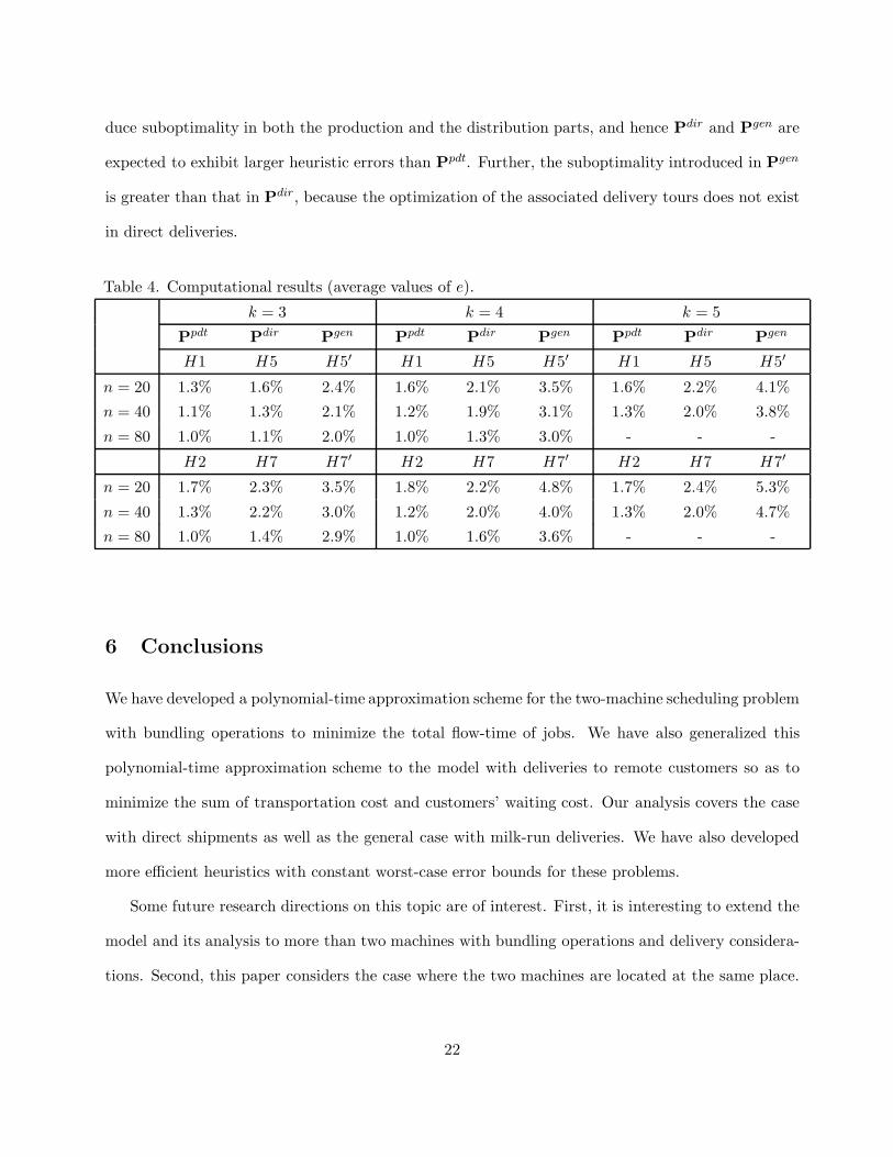
duce suboptimality in both the production and the distribution parts, and hence Pdir and Pgen are

expected to exhibit larger heuristic errors than Ppdt. Further, the suboptimality introduced in Pgen

is greater than that in Pdir, because the optimization of the associated delivery tours does not exist

in direct deliveries.

Table 4. Computational results (average values of e).

k = 3 k = 4 k = 5

Ppdt Pdir Pgen Ppdt Pdir Pgen Ppdt Pdir Pgen

H1 H5 H5′ H1 H5 H5′ H1 H5 H5′

n = 20 1.3% 1.6% 2.4% 1.6% 2.1% 3.5% 1.6% 2.2% 4.1%

n = 40 1.1% 1.3% 2.1% 1.2% 1.9% 3.1% 1.3% 2.0% 3.8%

n = 80 1.0% 1.1% 2.0% 1.0% 1.3% 3.0% - - -

H2 H7 H7′ H2 H7 H7′ H2 H7 H7′

n = 20 1.7% 2.3% 3.5% 1.8% 2.2% 4.8% 1.7% 2.4% 5.3%

n = 40 1.3% 2.2% 3.0% 1.2% 2.0% 4.0% 1.3% 2.0% 4.7%

n = 80 1.0% 1.4% 2.9% 1.0% 1.6% 3.6% - - -

6 Conclusions

We have developed a polynomial-time approximation scheme for the two-machine scheduling problem

with bundling operations to minimize the total flow-time of jobs. We have also generalized this

polynomial-time approximation scheme to the model with deliveries to remote customers so as to

minimize the sum of transportation cost and customers’ waiting cost. Our analysis covers the case

with direct shipments as well as the general case with milk-run deliveries. We have also developed

more efficient heuristics with constant worst-case error bounds for these problems.

Some future research directions on this topic are of interest. First, it is interesting to extend the

model and its analysis to more than two machines with bundling operations and delivery considera-

tions. Second, this paper considers the case where the two machines are located at the same place.

22

If the machines are located at different locations, the delivery plan should include the possibility

of having the same vehicle pick up the two finished tasks of the same job and deliver them to the

customers. Such an extension is also an interesting topic for future research.

Acknowledgments

The authors would like thank the Associate Editor and two referees for their helpful comments and

suggestions. This research was supported in part by the Research Grants Council of Hong Kong under

grant number PolyU6132/02E. Part of George Vairaktarakis’ work was performed at the Department

of Logistics at The Hong Kong Polytechnic University.

References

Ahmadi, R., U. Bagchi and T.A. Roemer (2005). Coordinated scheduling of customer orders for

quick response. Naval Research Logistics, 52, 493–512.

Blocher, J.D. and D. Chhajed (1996). The customer order lead time problem on parallel machines.

Naval Research Logistics, 43, 629–654.

Blocher, J.D., D. Chhajed and M. Leung (1998). Customer order scheduling in a general job shop

environment. Decision Sciences, 29, 951–981.

Cai, X. and X. Zhou (2004). Deterministic and stochastic scheduling with teamwork tasks. Naval

Research Logistics, 51, 818–840.

Chang, Y.-C. and C.-Y. Lee (2004). Machine scheduling with job delivery coordination. European

Journal of Operational Research, 158, 470–487.

Chen, Z.-L. (2004). Integrated production and distribution operations: Taxonomy, models, and

23

review. D. Simchi-Levi, D. Wu and Z.-J. Shen (eds.), Handbook of Quantitative Supply Chain

Analysis: Modeling in the E-Business Era. Kluwer Academic Publishers, Boston, MA.

Chen, Z.-L. and G. Pundoor (2006). Order assignment and scheduling in a supply chain. Operations

Research, forthcoming.

Chen, Z.-L. and G.L. Vairaktarakis (2005). Integrated scheduling of production and distribution

operations. Management Science, 51, 614–628.

Fumero, F. and C. Vercellis (1999). Synchronized development of production, inventory, and dis-

tribution schedules. Transportation Science, 33, 330–340.

Geismar, H.N., G. Laporte, L. Lei and C. Sriskandarajah (2005). The integrated production and

transportation scheduling problem for a product with a short life span and non-instantaneous

transportation time. Working paper.

Hall, N.G. and C.N. Potts (2003). Supply chain scheduling: Batching and delivery. Operations

Research, 51, 566–584.

Julien, F.M. and M.J. Magazine (1990). Scheduling customer orders: An alternative production

scheduling approach. Journal of Manufacturing and Operations Management, 3, 177–199.

Lee, C.-Y. and Z.-L. Chen (2001). Machine scheduling with transportation considerations. Journal

of Scheduling, 4, 3–24.

Lee, C.-Y., T.C.E. Cheng and B.M.T. Lin (1993). Minimizing the makespan in the 3-machine

assembly-type flowshop scheduling problem. Management Science, 39, 616–625.

Leung, J.Y.-T., H. Li and M. Pinedo (2005a). Order scheduling in an environment with dedicated

resources in parallel. Journal of Scheduling, 8, 355–386.

Leung, J.Y.-T., H. Li and M. Pinedo (2005b). Scheduling orders for multiple product types to

minimize total weighted completion time. Working paper.

24

Leung, J.Y.-T., H. Li, M. Pinedo and C. Sriskandarajah (2005c). Open shops with jobs overlap—

revisited. European Journal of Operational Research, 163, 569–571.

Leung, J.Y.-T., H. Li, M. Pinedo and J. Zhang (2005d). Minimizing total weighted completion time

when scheduling orders in a flexible environment with uniform machines. Working paper.

Leung, J.Y.-T., H. Li and M. Pinedo (2006a). Approximation algorithms for minimizing total

weighted completion time of orders on identical machines in parallel. Naval Research Logistics,

forthcoming.

Leung, J.Y.-T., H. Li and M. Pinedo (2006b). Scheduling orders for multiple product types with

due date related objectives. European Journal of Operational Research, 168, 370–389.

Li, C.-L. and J. Ou (2005). Machine scheduling with pickup and delivery. Naval Research Logistics,

52, 617–630.

Li, C.-L., G. Vairaktarakis and C.-Y. Lee (2005). Machine scheduling with deliveries to multiple

customer locations. European Journal of Operational Research, 164, 39–51.

Pundoor, G. and Z.-L. Chen (2005). Scheduling a production-distribution system to optimize the

tradeoff between delivery tardiness and distribution cost. Naval Research Logistics, 52, 571–

589.

Sarmiento, A.M. and R. Nagi (1999). A review of integrated analysis of production-distribution

systems. IIE Transactions, 31, 1061–1074.

Sung, C.S. and S.H. Yoon (1998). Minimizing total weighted completion time at a pre-assembly

stage composed of two feeding machines. International Journal of Production Economics, 54,

247–255.

Wagneur, E. and C. Sriskandarajah (1993). Open shops with jobs overlap. European Journal of

Operational Research, 71, 366–378.

25

Yang, J. (2003). Scheduling parallel machines for the customer order problem with fixed batch

sequence. Journal of the Korean Institute of Industrial Engineers, 29, 304–311.

Yang, J. (2005). The complexity of customer order scheduling problems on parallel machines.

Computers and Operations Research, 32, 1921–1939.

Yang, J. and M.E. Posner (2005). Scheduling parallel machines for the customer order problem.

Journal of Scheduling, 8, 49–74.

Appendix

Proof of Lemma ??: The proof of property (i) is straightforward and is omitted. See Sung and

Yoon (1998) for proofs of properties (ii) and (iii).

Proof of Theorem ??: Consider the difference between schedules σ∗(Ppdtβ ) and σH1

β . Let ∆′ denote

the difference in total flow time of the a-tasks between these two schedules. Note that (i) aj = aj if

Jj ∈ Sa1 ∪ Sa

2 ∪ · · · ∪ Saβ , (ii) aj > aj − λbj if Jj ∈ Sb

1 ∪ Sb2 ∪ · · · ∪ Sb

β , and (iii) aj ≥ aj − ( 1βλ − 1)bj if

Jj ∈ Sc. Thus,

∆′ ≤∑

j=1,...,n s.t.

Jj∈Sb1∪···∪Sb

β

(n− ξj + 1)λbj +∑

j=1,...,ns.t. Jj∈Sc

(n− ξj + 1)( 1

βλ− 1

)

bj,

where ξj is the position of Jj in σ∗(Ppdtβ ). Similarly, let ∆′′ denote the difference in total flow time

of the b-tasks between the two schedules. We have

∆′′ ≤∑

j=1,...,n s.t.

Jj∈Sa1∪···∪Sa

β

(n− ξj + 1)λaj +∑

j=1,...,n

s.t. Jj∈Sc

(n− ξj + 1)( 1

βλ− 1

)

aj.

26

It is easy to check that 1βλ

− 1 = λ. Hence,

Z(σH1β ) − Z(σ∗(Ppdt

β )) ≤ max{∆′,∆′′}

≤ λ · max

{

∑

j=1,...,n s.t.

Jj∈Sb1∪···∪Sb

β

(n− ξj + 1)bj +∑

j=1,...,ns.t. Jj∈Sc

(n− ξj + 1)bj,

∑

j=1,...,n s.t.Jj∈Sa

1∪···∪Sa

β

(n− ξj + 1)aj +∑

j=1,...,ns.t. Jj∈Sc

(n− ξj + 1)aj

}

≤ λ · Z(σ∗(Ppdtβ )).

Note thatZ(σ∗(Ppdtβ )) ≤ Z(σ∗(Ppdt)). Therefore, Z(σH1

β )−Z(σ∗(Ppdt)) ≤ λZ(σ∗(Ppdt)) =(

12

√

β+4β −

12

)

Z(σ∗(Ppdt)).

Proof of Theorem ??: Similar argument as in the proof of Theorem ??.

Proof of Theorem ??: Consider the difference between schedules σ∗(Pdirβ ) and σH5

β . Both schedules

have the same assignment of jobs to batches, and therefore, they have the same delivery cost. Using

the same arguments as in the proof of Theorem ??, we have

Z(σH5β ) − Z(σ∗(Pdir

β )) ≤ λ · Z(σ∗(Pdirβ )).

Note thatZ(σ∗(Pdirβ )) ≤ Z(σ∗(Pdir)). Therefore, Z(σH5

β )−Z(σ∗(Pdir)) ≤ λZ(σ∗(Pdir)) =(

12

√

β+4β −

12

)

Z(σ∗(Pdir)).

Proof of Lemma ??: We consider the case in which∑j

r=1 ar ≤∑k

r=1 br. Suppose that Jbk precedes

Jaj in the optimal schedule. Then moving Jb

k immediately after Jaj will not increase the total flow

time of the schedule. The proof of the case with∑j

r=1 ar >∑k

r=1 br follows a similar argument.

Proof of Theorem ??: Similar argument as in the proof of Theorem ??.

Proof of Lemma ??: Consider an optimal schedule σ∗(Pdir) of problem Pdir. We construct a

27

feasible schedule σ′(P′) for the auxiliary problem P′ by taking the job processing sequence from

σ∗(Pdir) and assigning the jobs to batches the same way as σ∗(Pdir). We now compare schedules

σ′(P′) and σ∗(Pdir). Let Bk denote the kth batch of jobs departing from the plant. Let D′k and D∗

k

be the time of departure of batch Bk from the plant in schedules σ′(P′) and σ∗(Pdir), respectively.

We have

D′k =

∑

Jj∈B1∪···∪Bk

pj =1

2

∑

Jj∈B1∪···∪Bk

(aj + bj) ≤ max

{

∑

Jj∈B1∪···∪Bk

aj,∑

Jj∈B1∪···∪Bk

bj

}

= D∗k.

The travel cost and travel time in schedule σ′(P′) are the same as those in schedule σ∗(Pdir).

Therefore, Z(σ′(P′)) ≤ Z(σ∗(Pdir)). This implies that Z(σ∗(P′)) ≤ Z(σ∗(Pdir)).

Proof of Theorem ??: We compare schedules σH7 and σ∗(P′). As mentioned earlier, σH7 and

σ∗(P′) have the same job sequence, the same assignment of jobs to batches, and the same delivery

cost. Let Bk denote the kth batch of jobs departing from the plant. Let DH7k and Dk be the time of

departure of batch Bk from the plant in schedules σH7 and σ∗(P′), respectively. We have

DH7k = max

{

∑

Jj∈B1∪···∪Bk

aj,∑

Jj∈B1∪···∪Bk

bj

}

≤∑

Jj∈B1∪···∪Bk

(aj + bj) = 2∑

Jj∈B1∪···∪Bk

pj = 2Dk.

Therefore, Z(σH7) ≤ 2Z(σ∗(P′)). By Lemma ??, Z(σH7) ≤ 2Z(σ∗(Pdir)). This implies that

[Z(σH7) − Z(σ∗(Pdir))]/Z(σ∗(Pdir)) ≤ 1.

28

Figure 1. A numerical example

Machine M1:

Machine M2:

Machine location

a-tasks

b-tasks

J2

J2

J1 J5 J3 J4

J1 J3 J5 J4

time

Customer location 1 (for job J1)

C2 C5

D2 = D5 = D1 = C1 (first vehicle

departure time)

C3

D3 = D4 = C4 (second vehicle departure time)

t03

t03 + t30

t01

t01 + t14 t01 + t14 + t42 t01 + t14 + t42 + t20

Customer location 4 (for job J5)

Customer location 2 (for job J2)

Customer location 3 (for jobs J3 and J4)

0

Figure 2. Partition of jobs in heuristic H1

aj

bj

… …

aS1

aS2

aSβ

bS1 bS2 bSβ

cS

slope = λ

slope = 2λ

slope = (β – 1)λ

slope = βλ

slop

e =

1/λ

slop

e =

1/(2

λ)

slop

e =

1/((

β – 1

)λ)

slop

e =1

/(βλ)

0