Journal of Computational and Applied Mathematics 212 (2008) 431–443www.elsevier.com/locate/cam

Convergence rate of a new Bezier variant of Chlodowsky operatorsto bounded variation functions

Harun Karsli, Ertan Ibikli∗

Department of Mathematics, Science Faculty, Ankara University, Tandogan 06100, Ankara, Turkey

Received 21 July 2006; received in revised form 22 November 2006

Abstract

In the present paper, we estimate the rate of pointwise convergence of the Bézier Variant of Chlodowsky operators Cn,� forfunctions, defined on the interval extending infinity, of bounded variation. To prove our main result, we have used some methodsand techniques of probability theory.© 2007 Elsevier B.V. All rights reserved.

MSC: 41A25; 41A35; 41A36

Keywords: Approximation; Bounded variation; Chlodowsky polynomials; Bezier basis; Total variation; Rate of convergence

1. Introduction

Named after the French engineer-mathematician Pierre Bézier, a Bézier curve is a curved line defined by mathematicalformulas. Bézier used these curves for the body design of the Renault car in 1970s. Bézier basis functions [1] play animportant role in computer aided design which have many applications in applied mathematics and computer sciences.

Consider n + 1 control points pk , (k = 0–n). If we choose pk = f (k/n), we get Bernstein–Bézier parametric curvefunction or Bernstein–Bézier operator which is of the form

Bn(f ; x) =n∑

k=0

f

(k

n

)(n

k

)(x)k(1 − x)n−k (0�x�1)

and in general, ��1 Bernstein–Bézier operator is of the form

B(�)n (f ; x) =

n∑k=0

f

(k

n

)Q

(�)n,k(x) (0�x�1)

where Q(�)n,k(x) = J

(�)n,k (x) − J

(�)n,k+1(x) and Jn,k(x) =∑n

j=kPn,j (x) be the Bézier basis functions.

∗ Corresponding author. Tel.: +90 312 2126720/1241; fax: +90 312 2235000.E-mail address: ibikli@science.ankara.edu.tr (E. Ibikli).

0377-0427/$ - see front matter © 2007 Elsevier B.V. All rights reserved.doi:10.1016/j.cam.2006.12.020

432 H. Karsli, E. Ibikli / Journal of Computational and Applied Mathematics 212 (2008) 431–443

Let BV(I ) denotes the class of functions, which are bounded variation on a set I ⊂ R. Some authors studied on somelinear positive operators to obtain the rate of convergence for functions in BV(I ). Some of the important papers on thistopic are due to Bojanic and Vuilleumier [2], Cheng [3] and Zeng and Chen [15]. Very recently, several researchershave studied on some Bézier type operators for functions in BV(I ). For example, Zeng and Gupta [16] estimatedrate of convergence of Baskakov–Bézier type operators for locally bounded functions. Zeng and Piriou [17] estimatedthe rate of convergence of two Bernstein–Bézier type operators for bounded variation functions, Li and Gong [11]investigated order of approximation by the generalized Bernstein–Bézier polynomials. We also mention some of theimportant papers on this subject by Srivastava and Zeng [13] and Gupta [6,7]. Although there have been many studieson Bernstein operators to date, the Chlodowsky type Bernstein operators are not investigated well enough (for example,[5,10]) since they are defined on unbounded interval.

In this paper, by means of the techniques of probability theory, we shall estimate the rate of convergence for theChlodowsky–Bézier operators Cn,� for functions of bounded variation on [0, ∞) at points x where f (x+) and f (x−)

exist.Chlodowsky polynomials are given [4] by

Cn(f ; x) =n∑

k=0

f

(kbn

n

)Pn,k

(x

bn

)(0�x�bn) (1)

where Pn,k(x/bn) = (nk

)(x/bn)

k(1 − x/bn)n−k (0�x�bn) and (bn) is a sequence of increasing positive numbers,

with the properties limn→∞ bn = ∞ and limn→∞ bn/n = 0.For ��1, we now introduce Chlodowsky–Bézier operators Cn,� as follows:

Cn,�(f, x) =n∑

k=0

f

(k bn

n

)Q

(�)n,k

(x

bn

)(0�x�bn), (2)

where Q(�)n,k(x/bn)=(Jn,k(x/bn))

�−(Jn,k+1(x/bn))� and Jn,k(x/bn)=∑n

j=kPn,j (x/bn) be the Bézier basis functions.Obviously, Cn,� is a positive linear operator and Cn,�(1, x) = 1. In particular when � = 1, the operators (2) reduce theoperators (1).

Here we point out that, the rates of convergence in the case � ∈ (0, 1) for functions of bounded variation were alsoobtained by different operators. For example see [8].

The main theorem of this paper is as follows.

Theorem. Let f be a function of bounded variation on every finite subinterval of [0, ∞) and limx→∞ f (x) exists, i.e.f ∈ BV[0, ∞). Then for every x ∈ (0, ∞) and for sufficiently large values of n, we have

∣∣∣∣Cn,�(f ; x) −[

1

2� f (x+) +(

1 − 1

2�

)f (x−)

]∣∣∣∣��

3Bn(x)b2n

x2(bn − x)2

⎧⎨⎩

n∑k=1

x+(bn−x)/√

k∨x−x/

√k

(gx)

⎫⎬⎭

+ �√2enx/bn(1 − x/bn)

[|f (x+) − f (x−)| + |f (x) − f (x−)|en

(x

bn

)], (3)

where

Bn(x) = x(bn − x)

n, en

(x

bn

)=

⎧⎪⎪⎨⎪⎪⎩

1,x

bn

= k′

nfor some k′ ∈ IN

0,x

bn

= k′

nfor all k′ ∈ IN

H. Karsli, E. Ibikli / Journal of Computational and Applied Mathematics 212 (2008) 431–443 433

and∨b

a(gx) is the total variation of gx on [a, b],

gx(t) ={

f (t) − f (x+), x < t �bn,

0, t = x,

f (t) − f (x−), 0� t < x.

2. Auxiliary results

In this section we give certain results, which are necessary to prove our main theorem.

Lemma 1. For every x ∈ [0, bn] and n�1, we have

Cn(1; x) = 1,

Cn(t; x) = x,

Cn(t2; x) = x2 + x(bn − x)

n. (4)

From (4), by direct calculation, we find the following equality:

Cn((t − x)2; x) = x(bn − x)

n. (5)

For proof of this lemma see [5].Using the fact that |a� − b�|��|a − b| with 0�a, b�1 and ��1, we obtain Q

(�)n,k(x/bn)��Pn,k(x/bn). By this

inequality and (5), we have

Cn,�((t − x)2; x)��Cn,1((t − x)2; x) = �

[x(bn − x)

n

]. (6)

Lemma 2. For all x ∈ (0, ∞), we have

�n,�

(x

bn

,t

bn

)=∫ t

0Kn,�

(x

bn

,u

bn

)du, 0� t < x

� �

(x − t)2

x(bn − x)

n, (7)

where

Kn,�

(x

bn

,t

bn

)={ ∑

kbn �nt

Q(�)n,k

(x

bn

), 0 < t �bn,

0, t = 0.

Proof.

�n,�

(x

bn

,t

bn

)=∫ t

0Kn,�

(x

bn

,u

bn

)du

�∫ t

0Kn,�

(x

bn

,u

bn

)(x − u

x − t

)2

du

= 1

(x − t)2

∫ t

0Kn,�

(x

bn

,u

bn

)(x − u)2du

= 1

(x − t)2 Cn,�((u − x)2; x).

434 H. Karsli, E. Ibikli / Journal of Computational and Applied Mathematics 212 (2008) 431–443

From (6), we have

�n,�

(x

bn

,t

bn

)� �

(x − t)2

x(bn − x)

n. �

Lemma 3. If y is a positive valued random variable with a non-degenerate probability distribution then by Schwarzinequality

E(y3)�(E(y2).E(y4))1/2,

provided E(y2), E(y3) and E(y4) < ∞.

Lemma 4. Let �1 be the random variables with two point binomial distributionP(�1 = k) = (x/bn)

k(1 − x/bn)1−k (k = 0, 1, and x ∈ [0, bn] is a parameter).

Then

a1 = E, �1 = x

bn

,

E(�1 − a1)2 = x

bn

(1 − x

bn

)

and

E(�1 − a1)4 =

(x

bn

)− 4

(x

bn

)2

+ 6

(x

bn

)3

− 3

(x

bn

)4

.

Proof. Let {�k}∞k=1 be a sequence of independent random variables identically distributed with �1.For

Mi

(x

bn

)=

1∑k=0

ki

(x

bn

)k(1 − x

bn

)1−k

,

we find that

M0

(x

bn

)=

1∑k=0

k0(

x

bn

)k(1 − x

bn

)1−k

= 1 (here 00 := 1)

M1

(x

bn

)=

1∑k=0

k1(

x

bn

)k(1 − x

bn

)1−k

= x

bn

,

M2

(x

bn

)=

1∑k=0

k2(

x

bn

)k(1 − x

bn

)1−k

= x

bn

,

M3

(x

bn

)=

1∑k=0

k3(

x

bn

)k(1 − x

bn

)1−k

= x

bn

,

M4

(x

bn

)=

1∑k=0

k4(

x

bn

)k(1 − x

bn

)1−k

= x

bn

.

H. Karsli, E. Ibikli / Journal of Computational and Applied Mathematics 212 (2008) 431–443 435

From the definition of expectation, we get E�1 = M1(x/bn) = x/bn. Also

E(�1 − a1)2 =

2∑j=0

(2

j

)(−1)jM2−j

(x

bn

)[M1

(x

bn

)]j

= M2

(x

bn

)− 2

[M1

(x

bn

)]2

+ M0

(x

bn

)[M1

(x

bn

)]2

= x

bn

− 2

[x

bn

]2

+[

x

bn

]2

= x

bn

(1 − x

bn

).

E(�1 − a1)4 =

4∑j=0

(4

j

)(−1)jM4−j

(x

bn

)[M1

(x

bn

)]j

= M4

(x

bn

)− 4M3

(x

bn

)M1

(x

bn

)+ 6M2

(x

bn

)[M1

(x

bn

)]2

− 4M1

(x

bn

)[M1

(x

bn

)]3

+[M1

(x

bn

)]4

=(

x

bn

)− 4

(x

bn

)2

+ 6

(x

bn

)3

− 3

(x

bn

)4

.

Thus in view of Lemma 3, we have

E(�1 − a1)3 �(E(�1 − a1)

2E(�1 − a1)4)1/2

=(

x

bn

(1 − x

bn

)[(x

bn

)− 4

(x

bn

)2

+ 6

(x

bn

)3

− 3

(x

bn

)4])1/2

�√

x

bn

(1 − x

bn

)0.288675.

Such result can be found in [9]. �

Following lemma is the well-known Berry–Esseen bound for the classical central limit theorem of probability theory.

Lemma 5 (Berry–Esseen). Let {�k}∞k=1 be a sequence of independent and identically distributed random variableswith finite variance such that the expectation E(�1) = a1 ∈ R, the variance Var(�1) = E(�1 − a1)

2 = b21 > 0 and

E|�1 − E(�1)|3 < ∞. Then there exists a constant C, 1/√

2��C < 0.82, such that for all n and t

∣∣∣∣∣P(

1

b1√

n

n∑k=1

(�k − a1)� t

)− 1√

2�

∫ t

−∞e−u2/2 du

∣∣∣∣∣< CE|�1 − E(�1)|3

b31√

n.

Its proof can be found in Shiryayev [12, p. 432].

436 H. Karsli, E. Ibikli / Journal of Computational and Applied Mathematics 212 (2008) 431–443

Lemma 6. For all x ∈ [0, bn], we have∣∣∣∣∣∣⎛⎝ ∑

n�k>nx/bn

Pn,k

(x

bn

)⎞⎠−(

1

2

)∣∣∣∣∣∣ �0.82 ∗ 0.288675√nx/bn(1 − x/bn)

� 1√2enx/bn(1 − x/bn)

. (8)

Proof. By direct calculation, one has from Lemmas 4 and 5 the desired result. �

Lemma 7. For all x ∈ (0, bn) and ��1, we have

Cn,�(sgn(t − x); x) = 2�

⎛⎝ ∑

n�k>nx/bn

Pn,k

(x

bn

)⎞⎠�

− 1 + en

(x

bn

)Q

(�)n,k

(x

bn

). (9)

Proof. Since,

Cn,�(sgn(t − x); x) =∑

kbn �nt

sgn

(kbn

n− x

)Q

(�)n,k

(x

bn

)

=∑

n�k>nx/bn

(2� − 1)Q(�)n,k

(x

bn

)−

∑0�k<nx/bn

Q(�)n,k

(x

bn

)

and from (4), we can write

Cn,�(1; x) =∑

n�k>nx/bn

Q(�)n,k

(x

bn

)+

∑0�k<nx/bn

Q(�)n,k

(x

bn

)+ en

(x

bn

)Q

(�)n,k

(x

bn

).

Thus

Cn,�(sgn(t − x); x) =∑

n�k>nx/bn

(2� − 1)Q(�)n,k

(x

bn

)

−⎡⎣1 −

∑n�k>nx/bn

Q(�)n,k

(x

bn

)− en

(x

bn

)Q

(�)n,k

(x

bn

)⎤⎦

= 2�∑

n�k>nx/bn

Q(�)n,k

(x

bn

)− 1 + en

(x

bn

)Q

(�)n,k

(x

bn

)

= 2�

⎛⎝ ∑

n�k>nx/bn

Pn,k

(x

bn

)⎞⎠�

− 1 + en

(x

bn

)Q

(�)n,k

(x

bn

).

This completes the proof of (9). �

Lemma 8. If the conditions of Theorem hold, we have for all x ∈ (0, bn) and ��1∣∣∣∣f (x+) − f (x−)

2� Cn,�(sgn(t − x); x) +[f (x) − 1

2� f (x+) −(

1 − 1

2�

)f (x−)

]Cn,�(�x; x)

∣∣∣∣� �√

2enx/bn(1 − x/bn)

[|f (x+) − f (x−)| + |f (x) − f (x−)|en

(x

bn

)]. (10)

H. Karsli, E. Ibikli / Journal of Computational and Applied Mathematics 212 (2008) 431–443 437

Proof. One has∣∣∣∣f (x+) − f (x−)

2� Cn,�(sgn(t − x); x) +[f (x) − 1

2� f (x+) −(

1 − 1

2�

)f (x−)

]Cn,�(�x; x)

∣∣∣∣�∣∣∣∣f (x+) − f (x−)

2� Cn,�(sgn(t − x); x)

∣∣∣∣+∣∣∣∣[f (x) − 1

2� f (x+) −(

1 − 1

2�

)f (x−)

]Cn,�(�x; x)

∣∣∣∣�

∣∣∣∣∣∣f (x+) − f (x−)

2�

⎡⎣2�

⎛⎝ ∑

n�k>nx/bn

Pn,k

(x

bn

)⎞⎠�

− 1 + en

(x

bn

)Q

(�)n,k

(x

bn

)⎤⎦∣∣∣∣∣∣

+∣∣∣∣[f (x) − 1

2� f (x+) −(

1 − 1

2�

)f (x−)

]en

(x

bn

)Q

(�)n,k

(x

bn

)∣∣∣∣=∣∣∣∣∣∣f (x+) − f (x−)

2�

⎡⎣2�

⎛⎝ ∑

n�k>nx/bn

Pn,k

(x

bn

)⎞⎠�

− 1

⎤⎦∣∣∣∣∣∣

+∣∣∣∣[f (x) − f (x−)]en

(x

bn

)Q

(�)n,k

(x

bn

)∣∣∣∣ .Now we estimate∣∣∣∣∣∣2�

⎛⎝ ∑

n�k>nx/bn

Pn,k

(x

bn

)⎞⎠�

− 1

∣∣∣∣∣∣ .Using the fact that |a� − b�|��|a − b| with 0�a, b�1 and ��1, we obtained

2�

∣∣∣∣∣∣⎛⎝ ∑

n�k>nx/bn

Pn,k

(x

bn

)⎞⎠�

−(

1

2

)�∣∣∣∣∣∣ �2��

∣∣∣∣∣∣⎛⎝ ∑

n�k>nx/bn

Pn,k

(x

bn

)⎞⎠− 1

2

∣∣∣∣∣∣ ,and hence from (8), we have

2�

∣∣∣∣∣∣⎛⎝ ∑

n�k>nx/bn

Pn,k

(x

bn

)⎞⎠�

−(

1

2

)�∣∣∣∣∣∣ �

2��√2enx/bn(1 − x/bn)

,

and replacing the variable x with x/bn in [14, p. 365, Eq. (5)] we get,

Pn,k

(x

bn

)� 1√

2e

1√nx/bn(1 − x/bn)

� 1√2enx/bn(1 − x/bn)

. (11)

Consequently from (11) we get (10). �

3. Proof of main theorem

Proof. For any f ∈ BV[0, ∞), we can decompose f into four parts on [0, bn] for sufficiently large n,

f (t) = 1

2� f (x+) +(

1 − 1

2�

)f (x−) + gx(t) + f (x+) − f (x−)

2� sgn(t − x)

+ �x(t)

[f (x) − 1

2� f (x+) −(

1 − 1

2�

)f (x−)

], (12)

438 H. Karsli, E. Ibikli / Journal of Computational and Applied Mathematics 212 (2008) 431–443

where

�x(t) ={

1, x = t,

0, x = t

and

sgn(t) ={2� − 1, t > 0,

0, t = 0,

−1, t < 0.

If we apply the operator Cn,� on both sides of equality (12), we have

Cn,�(f ; x) =[

1

2� f (x+) +(

1 − 1

2�

)f (x−)

]Cn,�(1; x) + Cn,�(gx; x)

+ f (x+) − f (x−)

2� Cn,�(sgn(t − x); x)

+[f (x) − 1

2� f (x+) −(

1 − 1

2�

)f (x−)

]Cn,�(�x; x).

It follows that:∣∣∣∣Cn,�(f ; x) −[

1

2� f (x+) +(

1 − 1

2�

)f (x−)

]Cn,�(1; x)

∣∣∣∣� |Cn,�(gx; x)| +

∣∣∣∣f (x+) − f (x−)

2� Cn,�(sgn(t − x); x)

+[f (x) − 1

2� f (x+) −(

1 − 1

2�

)f (x−)

]Cn,�(�x; x)

∣∣∣∣ . (13)

Firstly we estimate |Cn,�(gx; x)| as below. Since Chlodowsky Polynomial may be written in the form of a Lebesgue–Stieltjes integral, we can rewrite Cn,�(gx; x) as follows:

|Cn,�(gx; x)| =∣∣∣∣∣

n∑k=0

gx

(kbn

n

)Q

(�)n,k

(x

bn

)∣∣∣∣∣=∣∣∣∣∫ bn

0gx(t)

�

�tKn,�

(x

bn

,t

bn

)∣∣∣∣ . (14)

To estimate (14), we decompose it into three parts, as follows:

=∣∣∣∣∣(∫ x−x/

√n

0+∫ x+(bn−x)/

√n

x−x/√

n

+∫ bn

x+(bn−x)/√

n

)gx(t)

�

�tKn,�

(x

bn

,t

bn

)∣∣∣∣∣�∣∣∣∣∣∫ x−x/

√n

0gx(t)

�

�tKn,�

(x

bn

,t

bn

)dt

∣∣∣∣∣+∣∣∣∣∣∫ x+(bn−x)/

√n

x−x/√

n

gx(t)�

�tKn,�

(x

bn

,t

bn

)∣∣∣∣∣+∣∣∣∣∫ bn

x+(bn−x)/√

n

gx(t)�

�tKn,�

(x

bn

,t

bn

)∣∣∣∣= |I1,�(n, x)| + |I2,�(n, x)| + |I3,�(n, x)|. (15)

H. Karsli, E. Ibikli / Journal of Computational and Applied Mathematics 212 (2008) 431–443 439

We shall evaluate I1,�(n, x), I2,�(n, x) and I3,�(n, x). To do this we first observe that I1,�(n, x), I2,�(n, x) and I3,�(n, x)

can be written as a Lebesque–Stieltjes integral

I1,�(n, x) =∫ x−x/

√n

0gx(t)dt

(�n,�

(x

bn

,t

bn

)),

I2,�(n, x) =∫ x+(bn−x)/

√n

x−x/√

n

gx(t)dt

(�n,�

(x

bn

,t

bn

))

and

I3,�(n, x) =∫ bn

x+(bn−x)/√

n

gx(t)dt

(�n,�

(x

bn

,t

bn

)),

where �n,�(x/bn, t/bn) = ∫ t

0 Kn,�(x/bn, u/bn) du.First we estimate I2,�(n, x). For t ∈ [x − x/

√n, x + (bn − x)/

√n], we have

|I2,�(n, x)| =∣∣∣∣∣∫ x+(bn−x)/

√n

x−x/√

n

(gx(t) − gx(x))dt

(�n,�

(x

bn

,t

bn

))∣∣∣∣∣�∫ x+(bn−x)/

√n

x−x/√

n

|gx(t) − gx(x)|∣∣∣∣dt

(�n,�

(x

bn

,t

bn

))∣∣∣∣�

x+(bn−x)/√

n∨x−x/

√n

(gx)�1

n − 1

n∑k=2

x+(bn−x)/√

n∨x−x/

√n

(gx). (16)

Next, we estimate I1,�(n, x). Using partial Lebesque–Stieltjes integration, we obtain

I1,�(n, x) =∫ x−x/

√n

0gx(t)dt

(�n,�

(x

bn

,t

bn

))

= gx

(x − x√

n

)�n,�

(x

bn

,x − x/

√n

bn

)− gx(0)�n,�

(x

bn

,0

bn

)

−∫ x−x/

√n

0�n,�

(x

bn

,t

bn

)dt (gx(t)).

Since |gx(x − x/√

n)| = |gx(x − x/√

n) − gx(x)|�∨xx−x/

√n(gx), it follows that

|I1,�(n, x)|�x∨

x−x/√

n

(gx)

∣∣∣∣�n,�

(x

bn

,x − x/

√n

bn

)∣∣∣∣+∫ x−x/

√n

0�n,�

(x

bn

,t

bn

)dt

(−

x∨t

(gx)

).

From (7), it is clear that

�n,�

(x

bn

,x − x/

√n

bn

)��

Bn(x)

(x/√

n)2 .

It follows that

|I1,�(n, x)|�x∨

x−x/√

n

(gx)�Bn(x)

(x/√

n)2 +∫ x−x/

√n

0

�

(x − t)2 Bn(x)dt

(−

x∨t

(gx)

)

=x∨

x−x/√

n

(gx)�Bn(x)

(x/√

n)2 + �Bn(x)

∫ x−x/√

n

0

1

(x − t)2 dt

(−

x∨t

(gx)

).

440 H. Karsli, E. Ibikli / Journal of Computational and Applied Mathematics 212 (2008) 431–443

Furthermore, since

∫ x−x/√

n

0

1

(x − t)2 dt

(−

x∨t

(gx)

)= − 1

(x − t)2

x∨t

(gx)

∣∣∣x−x/√

n

0 +∫ x−x/

√n

0

2

(x − t)3

x∨t

(gx) dt

= − 1

(x/√

n)2

x∨x−x/

√n

(gx) + 1

x2

x∨0

(gx)

+∫ x−x/

√n

0

2

(x − t)3

x∨t

(gx) dt .

Putting t = x − x/√

u in the last integral, we get

∫ x−x/√

n

0

2

(x − t)3

x∨t

(gx) dt = 1

x2

∫ n

1

x∨x−x/

√u

(gx) du = 1

x2

n∑k=1

x∨x−x/

√k

(gx).

Consequently,

|I1,�(n, x)|�x∨

x−x/√

n

(gx)�Bn(x)

(x/√

n)2

+ �Bn(x)

⎧⎨⎩− 1

(x/√

n)2

x∨x−x/

√n

(gx) + 1

x2

x∨0

(gx) + 1

x2

n∑k=1

x∨x−x/

√k

(gx)

⎫⎬⎭

= �Bn(x)

⎧⎨⎩ 1

x2

x∨0

(gx) + 1

x2

n∑k=1

x∨x−x/

√k

(gx)

⎫⎬⎭

= �Bn(x)

x2

⎧⎨⎩

x∨0

(gx) +n∑

k=1

x∨x−x/

√k

(gx)

⎫⎬⎭ . (17)

Using the similar method for estimating |I3,�(n, x)|, we get

|I3,�(n, x)|��Bn(x)

(bn − x)2

⎧⎨⎩

bn∨0

(gx) +n∑

k=1

x+(bn−x)/√

k∨x

(gx)

⎫⎬⎭

��Bn(x)

(bn − x)2

⎧⎨⎩

bn∨0

(gx) +n∑

k=1

x+(bn−x)/√

k∨x−x/

√k

(gx)

⎫⎬⎭ . (18)

H. Karsli, E. Ibikli / Journal of Computational and Applied Mathematics 212 (2008) 431–443 441

Putting (16)–(18) in (15), we get

|Cn,�(gx; x)|� |I1,�(n, x)| + |I2,�(n, x)| + |I3,�(n, x)|

��Bn(x)

x2

⎧⎨⎩

x∨0

(gx) +n∑

k=1

x∨x−x/

√k

(gx)

⎫⎬⎭

+ �Bn(x)

(bn − x)2

⎧⎨⎩

bn∨x

(gx) +n∑

k=1

x+(bn−x)/√

k∨x−x/

√k

(gx)

⎫⎬⎭

+ 1

n − 1

n∑k=2

x+(bn−x)/√

k∨x−x/

√k

(gx). (19)

Obviously, 1/x2 + 1/(bn − x)2 = b2n/x

2(bn − x)2, for x/bn ∈ [0, 1] and∨x

x−x/√

k(gx)�

∨x+(bn−x)/√

k

x−x/√

k(gx).

Hence, we obtain from (19)

|Cn,�(gx; x)|��

(Bn(x)

x2 + Bn(x)

(bn − x)2

)⎧⎨⎩

bn∨0

(gx) +n∑

k=1

x+(bn−x)/√

k∨x−x/

√k

(gx)

⎫⎬⎭

+ 1

n − 1

n∑k=2

x+(bn−x)/√

n∨x−x/

√k

(gx)

= �Bn(x)b2

n

x2(bn − x)2

⎧⎨⎩

bn∨0

(gx) +n∑

k=1

x+(bn−x)/√

k∨x−x/

√k

(gx)

⎫⎬⎭+ 1

n − 1

n∑k=2

x+(bn−x)/√

k∨x−x/

√k

(gx).

On the other hand, note that

bn∨0

(gx)�n∑

k=1

x+(bn−x)/√

k∨x−x/

√k

(gx). (20)

By (20), we have

|Cn,�(gx; x)|��2Bn(x)b2

n

x2(bn − x)2

⎧⎨⎩

n∑k=1

x+(bn−x)/√

k∨x−x/

√k

(gx)

⎫⎬⎭+ 1

n − 1

n∑k=2

x+(bn−x)/√

k∨x−x/

√k

(gx).

Note that 1/(n − 1)��(Bn(x)b2n/x

2(bn − x)2), for n > 1, x/bn ∈ [0, 1].Consequently

|Cn,�(gx; x)|��2Bn(x)b2

n

x2(bn − x)2

⎧⎨⎩

n∑k=1

x+(bn−x)/√

k∨x−x/

√k

(gx)

⎫⎬⎭+ 1

n − 1

n∑k=2

x+(bn−x)/√

k∨x−x/

√k

(gx)

��3Bn(x)b2

n

x2(bn − x)2

⎧⎨⎩

n∑k=1

x+(bn−x)/√

k∨x−x/

√k

(gx)

⎫⎬⎭ . (21)

Combining (10) and (21) in (13), we get the required result. Thus, the proof is completed. �

442 H. Karsli, E. Ibikli / Journal of Computational and Applied Mathematics 212 (2008) 431–443

0.4

0.3

0.2

0.1

0

0 1 2 3 4 5 6X

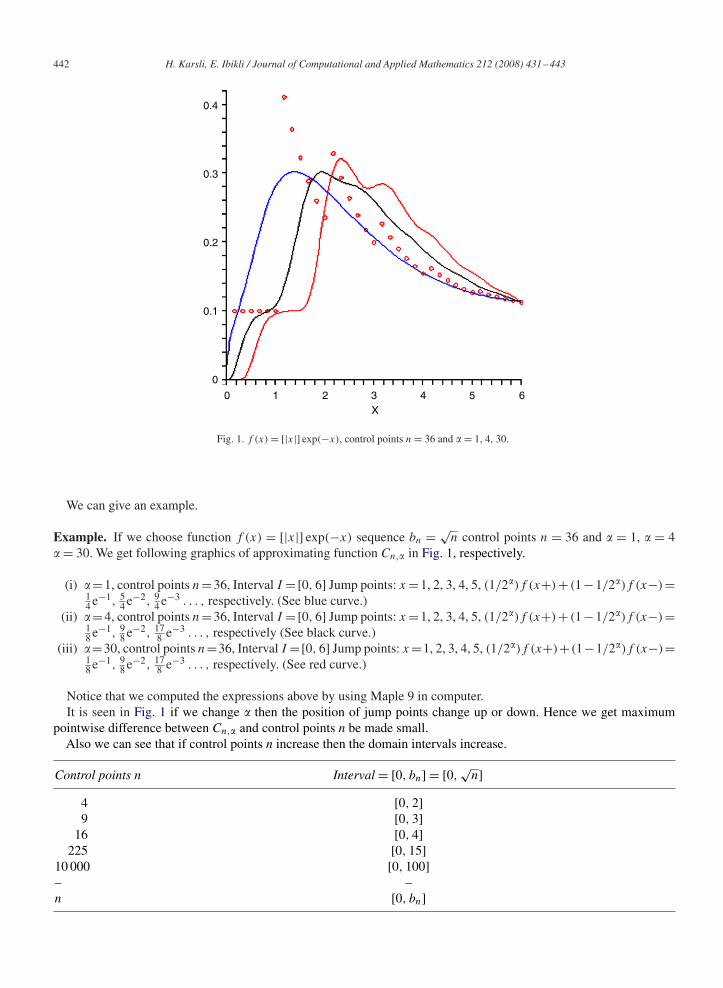
Fig. 1. f (x) = [|x|] exp(−x), control points n = 36 and � = 1, 4, 30.

We can give an example.

Example. If we choose function f (x) = [|x|] exp(−x) sequence bn = √n control points n = 36 and � = 1, � = 4

� = 30. We get following graphics of approximating function Cn,� in Fig. 1, respectively.

(i) �=1, control points n=36, Interval I =[0, 6] Jump points: x =1, 2, 3, 4, 5, (1/2�)f (x+)+ (1−1/2�)f (x−)=14 e−1, 5

4 e−2, 94 e−3 . . . , respectively. (See blue curve.)

(ii) �=4, control points n=36, Interval I =[0, 6] Jump points: x =1, 2, 3, 4, 5, (1/2�)f (x+)+ (1−1/2�)f (x−)=18 e−1, 9

8 e−2, 178 e−3 . . . , respectively (See black curve.)

(iii) �=30, control points n=36, Interval I =[0, 6] Jump points: x =1, 2, 3, 4, 5, (1/2�)f (x+)+(1−1/2�)f (x−)=18 e−1, 9

8 e−2, 178 e−3 . . . , respectively. (See red curve.)

Notice that we computed the expressions above by using Maple 9 in computer.It is seen in Fig. 1 if we change � then the position of jump points change up or down. Hence we get maximum

pointwise difference between Cn,� and control points n be made small.Also we can see that if control points n increase then the domain intervals increase.

Control points n Interval = [0, bn] = [0,√

n]4 [0, 2]9 [0, 3]

16 [0, 4]225 [0, 15]

10 000 [0, 100]– –n [0, bn]

H. Karsli, E. Ibikli / Journal of Computational and Applied Mathematics 212 (2008) 431–443 443

References

[1] P. Bézier, Numerical Control Mathematics and Applications, Wiley, London, 1972.[2] R. Bojanic, M. Vuilleumier, On the rate of convergence of Fourier Legendre series of functions of bounded variation, J. Approx. Theory 31

(1981) 67–79.[3] F. Cheng, On the rate of convergence of Bernstein polynomials of functions of bounded variation, J. Approx. Theory 39 (1983) 259–274.[4] I. Chlodowsky, Sur le developpment des fonctions defines dans un interval infinien series de polynomes de S.N.Bernstein, Compositio Math.

4 (1937) 380–392.[5] E.A. Gadjieva, E. Ibikli, On generalization of Bernstein–Chlodowsky polynomials, Hacettepe Bull. Natural Sci. 24 (B) (1995) 31–40.[6] V. Gupta, Degree of approximation to function of bounded variation by Bezier variant of MKZ operators, J. Math. Anal. Appl. 289 (1) (2004)

292–300.[7] V. Gupta, On the Bezier variant of Kantorovitch operators, Comput. Math. Appl. 47 (2/3) (2004) 227–232.[8] V. Gupta, An estimate on the convergence of Baskakov Bézier operators, J. Math. Anal. Appl. 312 (1) (2005) 380–388.[9] V. Gupta, A. Ahmad, An improved estimate on the degree of approximation to function of bounded variation by certain operators, Revista

Colombiana de Mate. 29 (2) (1995) 119–126.[10] E. Ibikli, On Stancu type generalization of Bernstein–Chlodowsky polynomials, Matematica, Tome 42 (65) (1) (2000) 37–43.[11] P. Li, Y.H. Gong, The order of approximation by the generalized Bernstein–Bézier polynomials, J. China Univ. Sci. Technol. 15 (1) (1985)

15–18.[12] A.N. Shiryayev, Probability, Springer, New York, 1984.[13] H.M. Srivastava, X.M. Zeng, Approximation by means of the Szasz–Bezier integral operators, Internat. J. Pure Appl. Math. 14 (3) (2004)

283–294.[14] X.M. Zeng, Bounds for Bernstein basis functions and Meyer–König–Zeller basis functions, J. Math. Anal. Appl. 219 (1998) 364–376.[15] X.M. Zeng, W. Chen, On the rate of convergence of the generalized Durrmeyer type operators for functions of bounded variation, J. Approx.

Theory 102 (2000) 1–12.[16] X.M. Zeng, V. Gupta, Rate of convergence of Baskakov–Bezier type operators for locally bounded functions, Comput. Math. Appl. 44 (2002)

1445–1453.[17] X.M. Zeng, A. Piriou, On the rate of convergence of two Bernstein–Bezier type operators for bounded variation functions, J. Approx. Theory

95 (1998) 369–387.