No. 1/2011

Convergence Clubs in Latin America:

A Historical Approach

by:

Paola Andrea Barrientos Quiroga

January 2011

The views expressed in the Development Research Working Paper Series are those of

the authors and do not necessarily reflect those of the Institute for Advanced Development

Studies. Copyrights belong to the authors. Papers may be downloaded for personal use

only.

Convergence Clubs in Latin America:

A Historical Approach

Paola Andrea Barrientos Quiroga

pbarrientos@econ.au.dk

January 24, 2011

Abstract

Literature on convergence among Latin American countries is still scarce compared to other

regions. Almost none of the research connects convergence to the economic history of Latin

America and the usual finding is one speed of convergence assuming one globally stable

steady-state. In this paper I analyze 32 countries and 108 years, more observations than any

other study, which allows me to use chronological events to explain, analyze and validate the

historical convergence clubs in Latin America, assuming multiple steady-states. The

chronological time-line is divided into three important known phases, from which I find two

to three convergence clubs. Following Thorp (1998), the first phase, called “the exporting

phase” goes from 1900 to 1930, the second, “the industrialization phase” from 1931 to 1974,

and the last one, “the globalization phase” from 1975 to 2007. During the last two phases, I

find strong evidence of convergence among those clubs that succeeded in industrializing and /

or building good institutions. The reason may be that technology diffusion and capital

accumulation is easier when these two phenomena occur. Furthermore, I find no evidence

that geographical aspects nor integration processes helped countries to converge.

Keywords: Latin America, economic history, convergence, growth.

JEL Classification: N0, N16, O0, O40, O47

Convergence Clubs in Latin America:

A Historical Approach

Paola Andrea Barrientos Quiroga �

School of Economics and Management

University of Århus - Denmark

January 24, 2011

Abstract

Literature on convergence among Latin American countries is still scarce compared to other regions.

Almost none of the research connects convergence to the economic history of Latin America and the usual

�nding is one speed of convergence assuming one globally stable steady-state. In this paper I analyze 32

countries and 108 years, more observations than any other study, which allows me to use chronological events

to explain, analyze and validate the historical convergence clubs in Latin America, assuming multiple steady-

states. The chronological time-line is divided into three important known phases, from which I �nd two to

three convergence clubs. Following Thorp (1998), the �rst phase, called "the exporting phase" goes from1900

to 1930, the second, "the industrilization phase" from 1931 to 1974, and the last one, "the globalization

phase" from 1975 to 2007. During the last two phases, I �nd strong evidence of convergence among those

clubs that succeeded in industrializing and/or building good institutions. The reason may be that technology

di¤usion and capital accumulation is easier when these two phenomena occur. Furthermore, I �nd no evidence

that geographical aspects nor integration processes helped countries to converge.

Introduction

Although economic convergence is not a recent topic, it is crucial in economics and it is still ongoing (Sala-i-

Martin, 2006; Welsh and Bonn, 2008; Hall and Ludwing, 2006, Owen et.al.,2009). It is important for development

economists to �nd out if developing countries are catching-up, if the di¤erences in income across countries tend

to decrease or increase and if there are clubs where countries tend to converge. The detection of income

disparities between economies and clubs of economies can help �nding out how to speed-up the process of

economic development.�E-mail: pbarrientos@econ.au.dk. I would like to thank..

1

.2.4

.6.8

11

.2S

igm

a1950 1955 1960 1965 1970 1975 1980 1985 1990 1995 2000 2005

year

LA 8 OECD

World LA

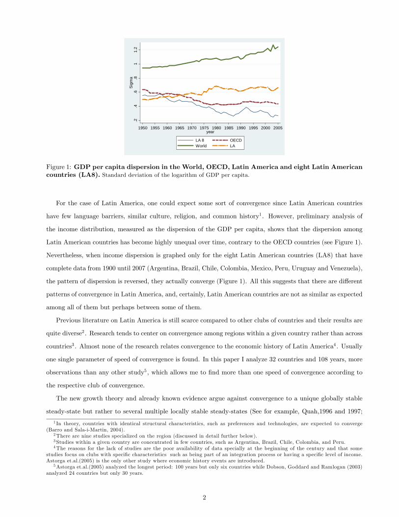
Figure 1: GDP per capita dispersion in the World, OECD, Latin America and eight Latin Americancountries (LA8). Standard deviation of the logarithm of GDP per capita.

For the case of Latin America, one could expect some sort of convergence since Latin American countries

have few language barriers, similar culture, religion, and common history1 . However, preliminary analysis of

the income distribution, measured as the dispersion of the GDP per capita, shows that the dispersion among

Latin American countries has become highly unequal over time, contrary to the OECD countries (see Figure 1).

Nevertheless, when income dispersion is graphed only for the eight Latin American countries (LA8) that have

complete data from 1900 until 2007 (Argentina, Brazil, Chile, Colombia, Mexico, Peru, Uruguay and Venezuela),

the pattern of dispersion is reversed, they actually converge (Figure 1). All this suggests that there are di¤erent

patterns of convergence in Latin America, and, certainly, Latin American countries are not as similar as expected

among all of them but perhaps between some of them.

Previous literature on Latin America is still scarce compared to other clubs of countries and their results are

quite diverse2 . Research tends to center on convergence among regions within a given country rather than across

countries3 . Almost none of the research relates convergence to the economic history of Latin America4 . Usually

one single parameter of speed of convergence is found. In this paper I analyze 32 countries and 108 years, more

observations than any other study5 , which allows me to �nd more than one speed of convergence according to

the respective club of convergence.

The new growth theory and already known evidence argue against convergence to a unique globally stable

steady-state but rather to several multiple locally stable steady-states (See for example, Quah,1996 and 1997;

1 In theory, countries with identical structural characteristics, such as preferences and technologies, are expected to converge(Barro and Sala-i-Martin, 2004).

2There are nine studies specialized on the region (discussed in detail further below).3Studies within a given country are concentrated in few countries, such as Argentina, Brazil, Chile, Colombia, and Peru.4The reasons for the lack of studies are the poor availability of data specially at the beginning of the century and that some

studies focus on clubs with speci�c characteristics such as being part of an integration process or having a speci�c level of income.Astorga et.al.(2005) is the only other study where economic history events are introduced.

5Astorga et.al.(2005) analyzed the longest period: 100 years but only six countries while Dobson, Goddard and Ramlogan (2003)analyzed 24 countries but only 30 years.

2

Azariadis and Stachurski, 2005; Durlauf and Johnson, 1995). In oder words, new �ndings point towards a natural

club clustering where countries tend to converge. However, economic theory does not guide us on the number

of clubs or the way in which the di¤erent variables de�ning initial conditions interact in determining the clubs.

To address this issue, most researchers (e.g. Durlauf and John, 1995; Bai, 1997; Hansen, 2000; Pesaran, 2006;

Paap van Dijk,1998; and Desdoigts, 1998) lean towards the approach of letting the data decide the clubs. They

usually study the shape of the distribution of income per capita and focus on �nding an income threshold to

divide clubs. This paper does not follow this approach. Instead, I use historical facts speci�c to the region to

determine the historical convergence clubs.

The reasons of using historical facts to divide clubs are several. First, I have a long span of data, more

than 100 years, which allows me to look back into history and see the natural clubs of convergence. Second, by

dividing into clubs of similar characteristics I put less demand on the determinants of growth, which are less

available specially at the beginning of the 20th century. Finally, I can analyze the institution hypothesis were

recent literature and evidence has turned to (See for example Easterly (2003); Acemoglu et. al.(2001 and 2002)

, Dollar and Kray (2003), Rodrik et al. 2004)). The argument is that institutions shape economic development,

Easterly (2003) argues that technology is endogenous to the institutions that make adoption of better techniques

of production likely. Therefore, the actions taken by institutions are the ones that shape the way production

functions look like and the way resources are used. Moreover I argue that these actions are shaped by several

factors, such as the resources a country has, the ideological trends, external shocks, and other events which

historians work on capturing. Therefore is important to look at the historical aspects.

Thorp (1998) captures in depth the comparative reality within Latin America and places in a proper historical

context, the development e¤orts, strategies, choices, successes and failures of the di¤erent Latin American

countries. She emphasizes on the "political economy" part of the Latin American history, which term is shorthand

for the interface between political forces, institutional inheritance and economic outcomes.

Based on Thorp (1998), I identify three important phases and two to three clubs within each phase6 . The

�rst phase ranges from 1900 until 1930 - when the Great Depression hit the Latin American economies - and it is

characterized by the Latin American countries intensively exporting primary products. Two clubs are identi�ed:

the mineral and agricultural products exporters. This phase is called exporting phase. During the second

phase, an inward-looking model was the response to the Great Depression. This model is known as Import

Substitution Industrialization (henceforth simply industrialization phase) and goes from 1931 to 1974 when the

oil crisis occurred7 . Two clubs are identi�ed: those that were able to industrialize, despite all the distortions

that the model brought, and the non-industrializers which failed to industrialize for di¤erent reasons. The6 In fact, the division of periods and groups di¤ers slightly from Thorp (1998). These di¤erences are discussed further below.7Thorp (1998) de�ned the period: 1945-1973 and called it �Industrialization and the growing role of the State�, since the state

took a greater role in the industrialization process. However, the industrialization process was triggered before, from when the GreatDepression hit the world economy (1930). I discuss this later.

3

third phase ranges from 1975 to 2007. This phase is characterized by several features. First, Latin America

experienced the debt crises in the early 80s, to which it responded with several "structural reforms". Then, from

these reforms and from an accumulation of several factors during history, the need for a change in development to

one with a more social outlook in a globalization context arose. I call this phase The globalization phase. Three

clubs are identi�ed: the good institutions club, where countries developed institutions that could deal with

growth and/or welfare, the painful club, where countries were traumatized by the debt crises adjustment, and

the vulnerable club, composed by the Caribbean countries who are di¤erent from the rest and are characterized

by being vulnerable to external factors.

After de�ning the convergence clubs, I use the model setup of Barro and Sala-i-Martin (2004), the most

common in the literature to test for convergence. I use single-cross section and panel data regressions with data

from Madisson (2003) combined with the World Bank (2009).

I �nd that during the phase of industrialization, and globalization, there is strong evidence of convergence

among those countries that succeeded in industrializing and/or building good institutions. The reason may

be that technology di¤usion is easier when these phenomena occur, allowing countries that were behind in the

beginning to accumulate capital and catch-up.

I also test for convergence in the most advanced integration processes and geographical regions in Latin

America. Here, convergence fails. The reason is that the integration processes are not yet developed to be able

to reach convergence in real terms and the geographical location is not an issue for convergence.

This paper is laid out as follows. In the �rst section, I present a summary of convergence theory and a

review of previous research on Latin America. In Section 2, I describe the methodology and data used to

test convergence. Section 3 presents the most important events of the economic history of Latin America and

describes each of the convergence clubs. In Section 4, I present the results of the speeds of convergence, and

Section 6 discusses di¤erent issues that may call the validity of the results into question. Finally, I present the

conclusions

1 Theory and Prior Research

Literature on economic growth de�nes four concepts of convergence. Absolute-� or catching-up convergence

when a number of economies converge to one another in the long run, independently of their initial conditions.

Conditional-� when per capita incomes of economies that have identical structural characteristics, i.e. pref-

erences, technologies, rates of population growth etc., converge to one another in the long run independently

of their initial conditions. Club is conditional � convergence conditioned on having similar initial conditions.

Finally, �-convergence across a club of economies exists if the dispersion of their real per capita GDP tends to

decrease over time (For an extensive discussion of concepts see Galor (1996)).

4

The di¤erent concepts of convergence and their arguments behind have emerged from di¤erent theories of

economic growth. The neoclassical growth models, such as Solow (1956) predict conditional convergence to

a unique globally stable steady-state based on diminishing returns of capital (Barro and Sala-i-Martin, 2004).

While the endogenous models, like the AK model, predict zero convergence since they do not assume diminishing

returns to capital. However variations in the AK model predict conditional convergence.(Mulligan and Sala-i-

Martin, 1992).

Furthermore, technology di¤usion models predict convergence based on microfoundations. The main argu-

ment is the existence of lower costs of technology imitation than technology innovation such that followers can

catch-up. Some researchers argue that the technology di¤usion process goes via foreign investments (Barro and

Sala-i-Martin, 2004), trade (Romer,1990; Aghion and Howitt, 1992), �ows of people (Barnebeck and Dalgaard,

2006) or the type of institutions and geography (Acemoglu et al., 2004). Similarly, theory of integration predicts

convergence based on the idea that common markets will allow countries/regions to catch-up. (Navarro and

Sotelsek, 2001).

Finally, new growth theory, such as models of distribution dynamics, also referred to as polarization, persis-

tent poverty (or poverty traps), strati�cation, and/or clustering models (Quah,1996; Quah, 1997; Azariadis and

Stachurski, 2005; Durlauf and Johnson, 1995) recognize the possibility of multiple locally-stable steady- states.

The reasons for the existence of di¤erent converging clubs/clubs may be several, such as the existence of some

threshold level in the endowment of strategic factors of production, nonconvexities or increasing returns, simi-

larities in preferences and technologies, and government policies, which become more similar over time within

certain clubs (Canova, 2004).

In Latin America, there are only nine cross-country studies8 specialized in studying convergence (Blyde,2005

and 2006; Holmes, 2005; Astorga, et.al 2005; Dobson and Ramlogan, 2002a and 2002b; Utrera, 1999; Dabus and

Zinni, 2005; and Madariaga et.al,2003). Although they analyze the same region, they study di¤erent countries,

periods, and apply di¤erent methodologies and theories of growth, making it di¢ cult to compare results.

Some of the authors use methodologies that do not measure a speci�c speed of convergence, such as Blyde

(2006) who studies 21 countries during 1960-2004 and uses a distribution dynamics approach. He �nds that

countries are converging to two clubs; one large for low and low middle income countries and another small for

rich income countries9 . Also, Dobson, Goddard and Ramoglan (2003) study the case of 24 countries during 1965-

1998 by cross-section analysis and unit root with panel data tests, and �nd convergence but not a speci�c speed.

The problem with these methodologies is that they cannot give an idea of the level of speed of convergence.

Other researchers �nd concrete results. For example, Astorga, et.al (2005) study six countries during the

period of 1900-2000. They �nd convergence using panel data and error correction models, at a speed between 1%

8The number of studies within a given country is higher than across countries, usually concentrated in few countries as Chile,Argentina, Brazil and Colombia ( e.g. Marina (2001), Azzoni et al.(2001), Anriquez and Fuentes (2001), Cardenas and Ponton(1995), Magalhaes, Hewings and Azzoni (2005), Serra et al.(2006)).

9The rich-income countries are Uruguay, Argentina, Chile, and Mexico, and the remaining 17 countries are in the other club.

5

and 1.9%, where the oscillation comes from the addition or subtraction of explicative variables that proxy for the

steady-state10 . Dobson and Ramlogan (2002a and b) study 19 countries and 28 and 30 years respectively (1970-

1998 and 1960-1990) using cross-section regression and panel data analysis, and �nd speeds of convergence

of 0.02% to 2%11 . Helliwell (1992) analyzes 18 Latin American countries for the period 1960-1985 and �nds

convergence at a speed of 2.5%12 .

On the contrary, Dabus and Zinni (2005) analyze 23 countries from 1960 to 1998, and �nd absolute and very

high conditional convergence. The authors argue that once controls are introduced and extremely high speeds

of conditional convergence are found, compared to absolute convergence, then it is a signal of divergence. This

is a good point since when controlling by many characteristics, a hypothetical speed of convergence is being

calculated while the real speed of convergence would be absolute convergence. They conclude that convergence

of any type is absent in Latin America. Regarding this, Durlauf and Quah (1999) mention that the choice of

the steady-state proxies depends on the interest of the researcher and that can lead to wrong results.

Almost none of the nine studies relates economic history to convergence. One reason could be the lack of

data in the region, especially at the beginning of the century, most of the papers start their analysis from around

1960, when more detailed data appears. Another reason could be that previous studies did not have the need to

introduce economic history because they grouped few countries as part of a club with a speci�c characteristic,

like being part of an integration process or having a speci�c level of income.

2 Methodology and Data

Based on the new growth theory of multiple steady-states, I analyze the di¤erent patterns of convergence in

Latin America with a historical approach. First, I de�ne the clubs where convergence is expected according to

historical events and then I test for convergence. In the next section I describe the main characteristics of the

convergence clubs. In this section I explain the methodology to test for convergence.

The model setup follows Barro and Sala-i-Martin (2004). The following equation measures the relation for

countries i = 1; :::N during periods t = 1; :::T :

it = a�(1� e��� it)

� it� log [y0it] + ui (1)

where it is the average growth rate of period t, a is a constant for all countries and all periods and includes

the common steady-state (useful to measure absolute convergence). In the case that a varies with each country,

ai; it would include the steady-state for each country and speci�c characteristics (useful to measure conditional

10They include human capital, external, institutional, and economic variables, together with dummy variables related to externalevents as the Great Depression and the Debt Crises. The countries are Argentina, Brazil, Chile, Colombia, Mexico, and Venezuela.11Their studies include, as proxies for the steady-state, sectorial decomposition variables, country dummies, population growth,

savings, and human capital.12He includes variables as investments, population growth, human capital, and scale e¤ects

6

convergence13). Furthermore, y0it is the initial output per capita of period t (measured in logarithms and

instrumented by its lag), � is the speed of convergence if � > 0 (or divergence if � < 0) , � it is the total number

of years within period t, and uit is disturbance term with mean zero, �nite variance, and independent over t and

i.

Equation(1) is estimated, �rst, as a single-cross section regression (t = 1) in order to capture long term

convergence, and then, the analysis is divided into subperiods (t > 1)14 , and panel data regressions are used.

Panel data allows using more information by including time variation, which may lead to more robust

results. It also allows adding more variables, like the steady-state, which tests conditional convergence, and time

dummies, which control for external conditions that a¤ect all countries for speci�c periods. A drawback of panel

data is that convergence is tested in shorter spans of data which may capture short-term adjustments around

the trend rather than long-term convergence.

The analysis covers 32 countries, listed in Table 1, for the period 1900-2007. The potential number of

observations is 3,456 but due to incomplete data for some countries, the number of real observations is reduced

to 2,209. This is the largest data set used in the literature on convergence in Latin America. The second largest

would be from Astorga et.al. (2005) with 606 observations, 6 countries and 100 years.

13As a matter of fact, the di¤erent concepts of convergence used here are mixed. Roughly speaking, absolute or catching-upconvergence should only be measured among all countries and all years before making any sort of grouping or adding any controls.Absolute convergence measured for each period and club can be considered already as conditional convergence since implicit controlsare introduced. Still, inside each group I measure absolute convergence in the sense that no extra explicit controls are included.Furthermore, when dividing the analysis by groups that vary across time, one refers to club convergence as well.14The length of each sub-period was chosen according to the availability of data. In average, the subperiod lenght is 10 years.

7

Country Observations Missingobservations Starting year Ending year

Argentina 108 0 1900 2007The Bahamas 28 80 1975 2002

Belize 33 75 1975 2007Bolivia 63 45 1945 2007Brazil 108 0 1900 2007

 Barbados 25 83 1975 1999Chile 108 0 1900 2007

Colombia 108 0 1900 2007Costa Rica 88 20 1920 2007

Cuba 76 32 1929 2004Dominica 31 77 1977 2007

Dominican Republic 58 50 1950 2007Ecuador 69 39 1939 2007Grenada 28 80 1980 2007

Guatemala 88 20 1920 2007Guyana 33 75 1975 2007

Honduras 88 20 1920 2007Haiti 63 45 1945 2007

Jamaica 64 44 1913 2007St. Kitts and Nevis 31 77 1977 2007

St. Lucia 28 80 1980 2007Mexico 108 0 1900 2007

Nicaragua 88 20 1920 2007Panama 63 45 1945 2007

Peru 108 0 1900 2007Puerto Rico 52 56 1950 2001

Paraguay 69 39 1939 2007El Salvador 88 20 1920 2007

Trinidad and Tobago 58 50 1950 2007Uruguay 108 0 1900 2007

St. Vincent and the Grenadines 33 75 1975 2007Venezuela 108 0 1900 2007

Total 2,209 1,247

Table 1: Description of the data set

The main variable is the GDP per capita measured in constant 1990 International (Geary-Khamis) dollars15 .

This measure allows for comparison of standards of living of the countries; it takes into account the purchasing

power parity of currencies and the international prices of commodities. The sources are the Madison Data Base

(0) and the World Bank Data Base (0)16 .

15 In order to avoid irregular values, I use two year annual averages of the GDP per capita. GDP growth, is calculated as thegeometric annualized average growth of each period.16The �nal data base has information from the Madison database (M) (from 1900 until 1989) and from the World Bank database

(W) (from 1990 to 2007). A converter factor (C) is calculated as: C(1990) = M(1990)=W(1990) for each year and is kept constantfrom 1995. Then C is multiplied by the existent W. In the case of ten small Caribbean countries, M has no data, so C is takenconstant, for the year 1995, from another country that heavily in�uenced these economies and is assumed to have a similar C. Theone from USA is used for The Bahamas; from Great Britain for Barbados and Belize; from Haiti for Dominica St.Kitts and Nevis,St. Lucia, St.Vincent and the Grenadines; from Colombia for Guyana, and �nally from The Dominican Republic for Grenada. Inthe case of Cuba, the available GDP from W was measured in constant 2000 local currency. Here, C was calculated with that kindof data and kept constant for the year 2001. The transformed data go from 2001 to 2007.

8

3 Historical Background and Convergence Clubs

Studying the development of Latin America for 108 years cannot avoid the study of its history. I divide the data

into convergence clubs, with similar characteristics such that convergence is expected. I merge some clubs from

Thorp (1998) in order to have at most three clubs in each phase. The idea is that each club�s main characteristics

matches each phase�s description and that clubs di¤er from each other in a clear way. This section describes the

historical background from where convergence clubs emerge17 .

3.1 The Exporting phase (1900-1930)

The �rst phase ranges from 1900 until 1930 - the year when the Great Depression whipped Latin American

economies - and it is characterized by countries intensively exporting primary products. In this period, countries

were vulnerable to world income and to �uctuations in primary products prices. I identify two clubs: those

that exported agricultural products and those that exported mineral products18 . Agricultural production was

vulnerable to natural disasters and minerals to recessions in the industrialized countries, since minerals were

used in construction, machinery, and chemicals production. While, the mining sector was characterized by using

less land and less labor. It also required more capital and technological investments and had di¤erent transport

needs than the agricultural sector.

The agricultural club is composed by ten countries: Argentina, Brazil, Colombia, Costa Rica, Cuba, El

Salvador, Guatemala, Honduras, Nicaragua, and Uruguay. They were producing mainly co¤ee, bananas, cocoa,

sugar meat and/or wheat19 .

The mineral countries number four: Chile, Mexico, Peru and Venezuela. They exported mainly petroleum

and copper20 .

3.2 The Industrialization Phase (1931-1974)

Thorp (1998) de�nes the period from 1945 to 1973 as: �Industrialization and the growing role of the State�.

However, the industrialization process was triggered before, when the Great depression hit the world economy.

Therefore I expand this phase from 1931, and instead of 1973 as ending year I take 1974, when the oil crises

occurred.17Table 4 shows the membership of each country to the speci�c clubs.18Thorp (1998) organized countries in a more detailed manner, according to their main export product. I merged them in these

2 groups.19Those producing mainly co¤ee were Brazil, Colombia, El Salvador and Nicaragua. For Costa Rica and Guatemala, the main

exports were co¤ee and bananas, while for Honduras it was bananas and precious metals. In general, Central American countriesexperienced higher production of bananas after the American multinational company, United Fruit, came to the region (in the1920s). Cuba produced mainly sugar but also tobacco. Argentina and Uruguay were mainly producing meat and wheat.20Petroleum was produced by all except Chile, and copper was produced by all except Venezuela. Before 1917, Venezuela was

mainly producing co¤ee and cacao, but after that year petroleum became the most important source of revenue. Mexico was themost diversi�ed export country in Latin America. They also exported lead, zinc, silver, gold, co¤ee, rubber, and cotton. Mexicansdiscovered oil in 1910.

9

The Great Depression provoked a fall in economic activity in the industrialized countries, which in turn

reduced their demand for primary products and reversed the capital in�ows to Latin America. This situation

deteriorated the terms of trade of all primary products, leading to an increase of the Latin American real import

prices. The natural mechanism would suggest a decrease in real export prices which should have stimulated

the demand again, but due to the extreme circumstances of the Great Depression, the world demand could not

recover. Instead, Latin American demand shifted from imported manufactured goods to domestic manufactured

products, because the former were expensive. This process stimulated the import substitution phase of Latin

America. Therefore, the Great Depression pushed many Latin American countries into a process of import

substitution strategy by default (Cardoso and Helwege, 1992).

The process of industrialization via import substitution was reinforced by the second World War (1939-

1945). Although WWII brought an increase of Latin American exports, there were constraints on their imports.

Consequently, the scarcity of imports and the deterioration of the terms of trade of primary products encouraged

new e¤orts to substitute imports, but these e¤orts were limited in turn by scarcity of imported inputs and

capital goods. Additionally, the consensus on the importance of industrialization via import substitution found

theoretical and institutional support in the United Nations Economic Commission for Latin America (ECLA).

The inward looking model consisted of substituting imports, and since imports were characterized by being

highly industrialized, Latin America went into a process of industrialization. Therefore, two clubs emerged in

this period: the industrializers and the non-industrializers21 . The industrializers succeeded in creating capital

goods and intermediate input industries, while the non-industrializers remained as primary exporters or created

ine¢ cient industrial sectors that were not able to succeed.

The industrializers are six countries: Argentina, Brazil, Chile, Colombia, Mexico and Uruguay. Only these

few countries succeeded in creating capital goods and intermediate input industries, although they had di¤erent

problems22 .

The non-industrializers are the countries that failed to industrialize. In total there are 17 countries:

Ecuador, El Salvador, Guatemala, Nicaragua, Peru, Venezuela, Paraguay, Bolivia, Costa Rica, Honduras, Do-

minican Republic, Haiti, Panama, Jamaica, Puerto Rico, Trinidad and Tobago, and Cuba. The reasons for these

countries not to industrialize were diverse. Some stayed as primary exporters because of their strong dominating

primary export sector, which in the majority of the cases was overprotected by the government, or because the

21Thorp (1998) had four groups: "strong industrializers", "centrally planned" (Cuba), "primary product export models" and"export promotion and industralizing by invitation". Thorp mentions that the last two groups should be one group because bothtried to industrialize but failed. The di¤erence between them is that the �rst one had the government to promote the proccess ofindustrialization while the second invited foereign capital to do it. Therefore I merge these two groups together with Cuba into thegroup of countries that were not able to industrialize.22Due to their larger domestic markets, Brazil and Mexico managed better than the other countries in the region. Both successfully

created automobile industries. In fact, Brazil experienced the highest growth rates and went through a process of high and persistentgrowth rates, during the 60s and 70s, known as the "Brazilian Miracle". E¢ cient steel production was established in Argentina andBrazil. Chile had political and social structure problems but still promoted the production (and export) of forestry, �shing, mining,and engineering sectors. Colombia industrialized its co¤ee and was the only country without an overvaluation, in�ation, or highlevels of debt, but problems of violence during the 40s and 50s a¤ected the industrialization process. Finally, Uruguay was alreadyindustrialized by 1945 but in mid-1950 they underwent stagnation.

10

government created ine¢ cient industrial sectors that were not able to succeed (Ecuador, El Salvador, Guatemala,

Nicaragua, Peru, Venezuela, Paraguay, and Bolivia). Others were based on di¤erent models, like Cuba and the

Caribbean countries23 .

3.3 The Globalization phase (1975-2007)

The third phase ranges from 1975 to 2007. Due to the oil shock of 1974, Latin American accumulated debt and

did not prevent the coming debt crises, which started in 1979 and 1981, when USA and other OECD countries

kept their money supply tight and increased interest rates radically. Since countries acquired loans at �oating

interest rates, their debt obligations increased vastly. The adjustment left problems that reinforced each other,

like capital out�ows, �scal de�cits, in�ation, overvaluation, and balance of payment crises.

Countries wanted to stabilize and gain access to foreign credit again, so they applied "structural reforms"

to reach stabilization. These reforms were based on �scal orthodoxy, liberalization, and reducing the role of the

state. The IMF suggested to cut budget de�cits by reducing expenses and increasing taxes, privatize, liberalize

imports and exchange controls (devaluate), eliminate price controls, and increase interest rates. Although

countries sooner or later followed the structural reforms, the results were not as good as expected. The export

sectors of several countries failed to react positively to the exchange rate depreciation. Higher prices of imported

goods reinforced in�ation and consequently overvaluation. With higher interest rates it was hard to promote

investments, and due to the tendency of overvaluation and weak export sectors was not possible to promote

exports either. Furthermore, governments had to close factories, resulting in high rates of unemployment and

large informal sectors.

Regarding welfare results, income distributions worsened in all countries outside of the Caribbean, except in

Uruguay and Costa Rica. Poverty, which worsened during the 80s, hardly improved during the 90s. This situation

encouraged rethinking the link between growth and equality. Di¤erent trends of thought arose around the mid

80s; some supported the idea that good institutions create complementaries between productivity growth and

equality, others that policies that are linked to the political constituency will create a combination of economic

23Venezuela, Peru, Bolivia, Ecuador and Paraguay were not well prepared for industrialization. Bolivia and Paraguay were theworst cases in terms of results. Bolivia�s strong and powerful tin sector took advantage of a weak state to concentrate resources (alot of the debt was directed to pay expensive railroads for the sector).. After the revolution in 1952 the tin sector was nationalizedand the government had immense di¢ culties managing it. In the 60s some investments went to the mining and petroleum sectors.Paraguay was dominated by a few families, protected by the military regime of Stroessner, that were producing the traditionalgoods (meat and tobacco), making it hard to change economic structures. Venezuela attempted to industrialize late, and the resultwas the creation of an ine¢ cient industrial sector with strong rent seeking characteristics, which brought a lot of distortions. TheVenezuelan economy was highly dependent on its oil, with characteristics of Dutch Disease. Ecuador�s protectionism carried outin the 60s only bene�ted the traditional elite clubs and failed to industrialize the economy. Peru had good export prospects, soindustrialization through import substitution was low.El Salvador, Guatemala, and Nicaragua concentrated their e¤orts in the cotton sector, which required moving peasants from

their own lands, making them worse o¤ (Williams, 1986). All three countries had very low levels of GDP per capita, especially ElSalvador and Honduras. In fact, El Salvador had the lowest GDP per capita of all Latin American countries. Based on a model ofcentral planning, Cuba tried to diversify their sugar-concentrated economy to corn, rice, cotton, tomatoes, and soybeans, but thelack of skilled labor and shortages of materials pushed them back to the production of sugar.The Caribbean countries were under a program of export promotion and industrializing by invitation. Headed by Puerto Rico,

the Caribbean tried to search for di¤erent markets than sugar. They gave concessions to foreign �rms, so they could invest andindustrialize, but employment did not increase, and by the 60s foreign �rms left.

11

and social development (Thorp,1998).

Following Thorp�s line I divide countries during the third phase in three clubs: those that were able to

provide the link between growth and welfare in a globalization context, the "good institutions" club, the ones

that su¤ered serious consequences of the debt crises, the "painful" club, and the Caribbean countries which are

di¤erent from the other clubs and are vulnerable to external factors, the "vulnerable" club24 .

The club of good institutions is composed by seven countries: Chile, Argentina, Uruguay, Mexico, Colom-

bia, Costa Rica and Brazil. Although some of the countries in this club have had weakened institutions, such as

Argentina, they have managed to reach either acceptable growth rates, good welfare standards, or both25 .

The painful club is composed of nine countries: Peru, Bolivia, Ecuador, Paraguay, Venezuela, Nicaragua, El

Salvador, Guatemala, and Honduras. This clubs is characterized by having weak institutions that lead to bad

results either in terms of growth, welfare, or both26 .

Finally, the vulnerable club includes 16 Caribbean countries: The Bahamas, Barbados, Belize, Cuba,

Dominica, Dominican Republic, Grenada, Guyana, Haiti, Jamaica, Panama, Puerto Rico, St. Kitts and Nevis,

24Thorp (1998) had �ve groups that she called: "using the paradigm shift", "reluctant converters", "other radical stabilizers","pain without gain", "the Caribbean: greatest vulnerability". I merged the �rst two groups into the good institutions group. Thenext two were merged into the painful group and the last was kept as the vulnerable group. More details regarding this union, arein the description of each group.25On the one hand, Chile, Argentina, Uruguay, and Mexico were able to link economics with welfare in a creative and e¤ective

way thanks to the prior conditions they met. Although Chile has a high degree of inequality and poverty, they managed to buildstrong institutions, and good relations among the public and private sector. The state promoted exports and investments. Eventhough they have applied radical orthodox policies and hosted radical violent military regimes, they have built a political consensusafterwards. They truly committed to the rules of the free market game, gaining investor�s con�dence. Moreover Chile has developeda process of consultation to identify poorly designed policies.Argentina and Uruguay had a similar experience to Chile. Both underwent military regimes but Argentina did not learn from this

experience as Chile did, while Uruguay built its political consensus from it. Argentina had a lot of political problems and adoptedboth orthodox and heterodox policies (as Mexico). In the 90s it implemented the "convertibility plan", the purpose of which was toestablish strict discipline on the monetary and �scal policy. The plan was the keystone for entry into the international system. Thisattracted investments, and together with the privatization, the quality of public services improved. Nevertheless, in 2001 Argentinawent into a crisis. The weak �scal policy and high �scal de�cits from the provincial governments were re�ected in an increasingpublic debt burden, and the growing overvaluation led to a debt crisis.Furthermore, Uruguay and Argentina were part of the trade union MERCOSUR , which helped them promote dynamic �rms.

Uruguay was the only country to improve welfare indicators during this period and was known by the democratic process of usingpopular consultation to approve policies. Mexico could provide the link between economics and welfare, particularly because of itsstrong international orientation. Mexico became part of the NAFTA-North American Free Trade Agreement, which involves USAand Canada.On the other hand, Brazil, Colombia, and Costa Rica progressed because they had been coherent with their earlier policies.

Colombia, for example, managed to build very strong and quali�ed institutions that managed the economic issues very well. Theydid not borrow too much and they did not have hyperin�ation. In fact, Thorp (1998) points out that Colombia is the only countrywhere liberalization coincides with a growing state, re�ected in the rapid growth of social spending. Nevertheless, corruption anddrugs were serious social problems. Costa Rica is characterized by their democratic values, good relations with the private sector,and high standards of education. Finally, Brazil, due to its size, was allowed to integrate to the global market in its own way andits own speed, as everybody wants to have access to Brazil´ s big market.26Bolivia and Peru did not meet the prior conditions that link growth with welfare. They applied orthodox policies and their

structural problems exposed them dramatically to the perils of globalization. Peru had institutional weakness, lack of experience,and lack of democracy to sustain the reforms. Bolivia spent a lot of time to recover from its hyperin�ation, which was a hardprocess. Moreover, their levels of poverty are still very high.Ecuador, Paraguay, Venezuela, Nicaragua, El Salvador, Guatemala and Honduras lacked good institutions, had social con�icts

with guerrilla forces (Guatemala and El Salvador), and problems of contraband and corruption (Paraguay). As an oil country,Venezuela mismanaged several oil booms, provoking a banking crisis in 1991. Although they liberalized, there was a lack of politicalsupport and proper communication of the reforms, resulting in social resistance. Venezuela, Ecuador, and Paraguay faced strongopposition in abolishing all protection. After 34 years of a military regime, until 1989, Paraguay could not build an e¢ cient systemof government.The central American economies were severely a¤ected by the debt crises (except Costa Rica), because they had a lot of oppression,

corrupted military, and civilian regimes. They tried to undertake market reforms, but due to political fragility they could not succeed.Moreover, poverty and exclusion are a common denominator for these countries.

12

.2.3

.4.5

.6.7

Sig

ma

1900 1920 1940 1960 1980 2000year

LA 8 LA

Figure 2: GDP per capita dispersion in Latin America. Standard deviation of the logarithm of the smoothenGDP per capita for all available countries and for the eight countries with most data (LA8). The vertical lines show eachof the three phases.

St. Lucia, St. Vincent and the Grenadines, Trinidad and Tobago27 .

4 Results

Figure 1 revealed that the distribution of the World income as for Latin America has become increasingly

unequal. On the contrary, the OECD countries have converged among them. Surprisingly, among the LA8

countries with most data, the dispersion has decreased to even lower levels than the OECD countries in 2007.

Nevertheless, when taking a closer look in the region before 1950 (Figure 2), Latin America�s high dispersion

during the last phase is also observed at the beginning of the 20th century, during the exporting phase. Certainly

there are di¤erent patterns of convergence. In this section I discuss the main results of convergence for all clubs

and phases.

Income dispersion of each club and phase is showed in Figure 3 . The only club that shows a clear pattern

of � - divergence is the non-industrializers, and the only one that shows a clear pattern of �-convergence is

the industrializers. The agricultural and the mineral clubs, from the �rst phase, show a less clear pattern but

still one of convergence. The rest of the clubs, from the third phase, illustrate null convergence being the good

institution club the one with the lowest levels of dispersion and the vulnerable with the highest. The distribution

of income is the most unequal for all Latin American countries during the last phase, showing very high and

27The Caribbean countries were more severely a¤ected by the adverse trends of the 1970s and 1980s than the rest of LatinAmerica. While one or two countries could bene�t by developing �nancial services (the Bahamas, for example), most acquireddebt and vulnerability to capital �ight and international interest rate changes. These economies are characterized by being toovulnerable to external shocks. They are quite open and primary products producers. Their agricultural sector performed so poorlythat they are net food importers. Although Cuba is di¤erent from the other countries, it is still extremely vulnerable to externalfactors. When the Soviet Union collapsed, Cuban exports were reduced dramatically. Additionally, Caribbean countries are exposedto natural disasters. Equality and human development in the Caribbean countries are characterized by very poor indicators, as thecase of Haiti.

13

.2.4

.6.8

Sig

ma

1900 1910 1920 1930year

Period 1 Agricultural

Mineral

.2.4

.6.8

Sig

ma

1930 1940 1950 1960 1970year

Industrialized Not Industrialized

Period 2

.2.4

.6.8

Sig

ma

1975 1980 1985 1990 1995 2000 2005year

Period 3 Good Institutions

Painful Vulnerable

Figure 3: GDP per capita dispersion in Latin America per period and group. Standard deviation of thelogarithm of the smoothen GDP per capita for all periods and groups. The vertical lines show each of the three phases.

persistent levels of dispersion.

The results on �-convergence are validated by the replication of other studies to show that my data and

techniques are good enough to expand the data set. First, I replicate the regressions of Astorga et. al. (2005), the

longest period study, 1900-2000, but only for six countries. Then, I replicate the results of Dobson and Ramlogan

(2002b), the study with most countries, 19, but only for 30 years, 1960-1990. The results are satisfactory (see

last lines in Table 3)28 . Then, the expanded data set and techniques are consistent with the existing literature

using smaller data sets.

Table 2 shows the results of the speeds of convergence. The �rst column display the results of absolute

convergence with single-cross section regression, and the rest show panel data estimations of absolute and

conditional convergence with and without time-e¤ects (I don�t report the coe¢ cients for country nor time-

e¤ects).

28 In Astorga et. al. (2005), their absolute convergence is 1.4%, and mine around 1%. Their conditional convergence is 1.9%and mine here 2%. In Dobson and Ramlogan (2002b), their absolute convergence is 0.5% and mine 0.3%. Their conditionalconvergence is 1.2% and mine 2.8% (my conditional convergence with time e¤ects is the one used to compare to their highest speedsof convergence).

14

Single cross section

t=1 t>1 Time Effects t>1 Time EffectsAll periods β 0.00% 0.21% 0.12% 1.11% 2.31%1900­2007 se 0.0041 0.0024 0.0031 0.0032 0.0035

N 28 267 267 267 267t 12Τ 18,10, 7,7,6,7,7,9,7,7,8,10

8 LA β 0.80% 0.72% 1.05% 0.94% 3.35%se 0.0037 0.0039 0.0036 0.0061 0.0093N 8 56 56 56 56t 7Τ 15,15,16,15,15,15,17

Phase 1 β 0.81% 0.13% 0.43% ­0.47% ­3.22%1900­1930 se 0.0066 0.0057 0.0075 0.1999 0.0629

N 13 21 21 21 21t 2Τ 18,10

Agricultural β ­0.13% ­0.32% ­0.39% ­0.24% 0.76%se 0.0027 0.0040 0.0045 0.0825 0.0145N 9 13 13 13 13t 2Τ 20,10

Mineral β 5.22% 0.36% 6.28% ­0.52% ­5.62%se 0.1114 0.0171 0.0832 0.2136 0.0565N 4 8 8 8 8t 2Τ 20,11

Phase 2 β ­0.02% 0.07% 0.12% 3.72% 4.10%1931­1974 se 0.0057 0.0039 0.0039 0.0099 0.0129

N 23 120 120 120 120t 6Τ 7,7,6,7,7,9

Industrialized β 1.74% 0.97% 1.27% 0.19% ­0.23%se 0.0091 0.0050 0.0034 0.0152 0.0339N 6 24 24 24 24t 4Τ 11,11,11,11

Non­Industriliz β ­0.32% ­0.19% ­0.13% 3.93% 4.26%se 0.0079 0.0047 0.0045 0.0126 0.0143N 17 84 84 84 84t 6Τ 7,6,6,7,7,9

Phase 3 β 0.56% 0.03% 0.07% 3.48% 3.76%1975­2007 se 0.0060 0.0037 0.0038 0.0050 0.0088

N 28 126 126 126 126t 4Τ 7,7,8,10

Good Institutions β 1.99% 2.06% 1.41% 3.09% 7.08%se 0.0137 0.0139 0.0187 0.0092 0.0693N 7 28 28 28 28t 4Τ 7,7,8,11

Painfull β 0.47% 0.95% 0.53% 4.44% 3.88%se 0.0018 0.0032 0.0049 0.0072 0.0092N 9 27 27 27 27t 3Τ 10,10,13

Vulnerable β 0.27% 0.19% 0.13% 3.23% 3.29%se 0.0075 0.0046 0.0047 0.0089 0.0095N 12 62 62 62 62t 4Τ 6,7,8,10

Panel dataAbsoluteGroups of countries Conditional

Table 2: Results. The Table reports the speed of convergence, standard errors, number of observations, number

of periods for the panel data estimations, and the average lenght of each period.

15

Results of absolute convergence are robust since under single-cross section and panel data regressions they

coincide in �nding either convergence or divergence . The di¤erence in levels of speeds of convergence is small.

In general, the speeds of convergence under the single-cross section regression are very similar to the panel data

estimations with time-e¤ects and these ones are higher than the estimations without time-e¤ects. The models

including time-dummies control for time di¤erences so that the speed of convergence rises and approaches the

single-cross section results. Both, the single-cross section regression and panel data with time-e¤ects regression

can be interpreted as long-run convergence concepts because they omit time variation. However, as mentioned

before, the exclusion of time variation is not always desirable. In any case, it seems that the di¤erence is not an

issue for the absolute convergence case. Inside almost all clubs absolute convergence is present under all methods,

except for the agricultural and non industrialized clubs, where both have negative speeds of convergence but

close to zero.

Regarding conditional convergence, the results are also robust between the models with and without

time-e¤ects. In general they don�t contradict each other regarding convergence or divergence but they di¤er

more in their rates compared to the absolute convergence results. Conditional convergence including time-e¤ects

is, in general, higher than without time-e¤ects, since what is left after controlling for country and time-e¤ects

is, of course, a very high speed of convergence which could be interpreted as arti�cial since it gets rid in a

way of time and country variation. For this reason I focus more on the non time-e¤ects models. All clubs show

conditional convergence (without time-e¤ects) except the agricultural and the mineral clubs, with negative speeds

of convergence but close to zero. Conditional convergence tends to be higher than absolute convergence. The

explanation is that countries converge faster after their steady-state and country speci�c e¤ects are controlled

for.

During the �rst phase, countries converge in an absolute way (1%) but diverge in a conditional (-0.5%), and

�-converge in overall. After controlling for each country speci�c characteristic including the steady-state, and

time variation, countries diverge. This could imply that their observed absolute convergence is due to common

factors determined by the international markets and their demand for Latin American products, rather than

the speci�c country characteristics. One can also say that there is long-run convergence rather than short-run

convergence.

In the same way, the mineral countries converge in an absolute way (6%), diverge in a conditional (-0.5%),

and �-convergence in overall. One crucial common factor for the mineral countries to converge in an absolute way

is the WWI (1914-1918). The WWI accelerated the shift in trade and investment structures in Latin America,

specially for the mineral sector. The demand for Latin American minerals increased together with investment

in the mineral sectors. According to Furtado (1981) the war stimulated the industrial growth in Latin America.

On the contrary, the agricultural countries diverge in the long run and short run (without time-e¤ects).

Furthermore, Figure 3 shows that the agricultural club have high levels of dispersion, which stay constant

16

for around the �rst 20 years, and then decrease in levels. This overall divergence may be due to the lack of

accumulation of capital and technology investment that characterizes the agricultural sector, compared, for

example, to the mineral sector. Besides the agricultural countries are more heterogenous than the mineral, they

were producing more di¤erent goods, which can explain the lack of convergence together with the fact that the

WWII bene�ted mostly the mineral sector.

During the second phase of industrialization, countries show an absolute convergence rate close to zero but

a conditional of around 4% (with and without time-e¤ects), and income dispersion increased. The reason for the

lack of absolute convergence and the presence of conditional convergence may be that during this phase, countries

went on their own way of development by industrializing or not, such that each country�s own experience was

more important in determining convergence than the external common factors that had been important during

the frist phase. Therefore, once country speci�c characteristics (and time-e¤ects) are controlled for, countries

converge.

With or without controlling for country speci�c characteristics, the industrializers do not diverge. Their

absolute speed is around 1% , conditional 0.2% (without time-e¤ects), and a very strong pattern of �-convergence.

The reason for their non divergence could be the industrialization process. They were able to succeed, despite

all the distortions that the industrialization via import substitution brought, in innovating some industries and

creating capital such that technology transmission was more �uent, even though countries went on in their own

way and had big di¤erences among them.

On the contrary, the non-industrializers diverge in an absolute way (at speeds below -1%), converge only

after controlling for country and time speci�c e¤ects, at a speed of around 4%, and there is a clear �-divergence

pattern. This implies that they diverge between them but each country converge to their own steady-state.

There was a lack of a common factor that allowed them to converge like in other cases. Each country went in

their own way diverging from each other. Instead of industrializing by producing capital goods and creating

intermediate input industries, some stayed as primary exporters.

Lastly, during the third phase, countries converge in an absolute and conditional sense but at very di¤erent

speeds. Their absolute convergence is less than 1% and conditional around 3.5%, meaning that common external

factors were determining the path, like the debt crises, but also that each country�s own experience was important

for convergence, such as the link between globalization and welfare that each country provided. Regarding income

dispersion, it has been constant but at rather high levels.

The good institution club could develop a connection between globalization and welfare by having ac-

ceptable welfare standards of living, good relations between the public and private sector, democratic values,

and integration to the global markets among others. All of this characteristics are certainly helpful for capital

accumulation and technology di¤usion. Therefore, the results show absolute and conditional convergence. Both

are close to each other, around 2%, which is a sign of strong convergence. As for the total phase, the income

17

dispersion is constant but at very low levels.

The painful club is characterized by having had weak institutions that lead to bad results either in terms

of growth, welfare, or both, which most likely did not motivate technology di¤usion nor capital accumulation.

Nonetheless I �nd convergence by all means but at verydi¤erent rates. Their absolute convergence is around

0.6% and their conditional is around 4%. This implies that they vaguely converge between them but each

converge to their own steady-state. Their income dispersion is constant.

In a similar way, the vulnerable club, composed by the Caribbean countries which were more severely

a¤ected by the adverse trends of the 1970s and 1980s than the rest of Latin America, converge vaguely(around

zero) in an absolute, strongly in a conditional way (around 3%), and a constant rather high income dispersion

compared to the other clubs of this phase. The absolute non-convergence shows no common convergence factors

stronger than their own experience.

From all the clubs, two showed more similar speeds of absolute and conditional convergence than the others:

the industrializers and the good institutions29 . Both clubs are composed by almost the same countries, namely

six: Argentina, Brazil, Chile, Colombia, Mexico and Uruguay, which are all included in the LA8 group. Therefore,

the observed strong �-convergence found among the LA8 is due to the presence of these six countries (LA6).

The speeds of convergence for the six countries for the whole period are shown in Table 3. All types of

convergence are found, and the absolute and conditional convergence are quite similar, around 1%. Notice that

the speeds of convergence are lower than in the 8LA. The reason is that 8LA includes Venezuela that bene�ted

from the oil to catch-up to the others30 .

5 Discussion

In this section I discuss the controversial points of this paper, such as the validity of the grouping and econometric

issues like endogenity problems, and unbalanced panel data issues.

Validity of the grouping

The validity of the division of clubs based on economic history can be questioned. The idea of organizing countries

into clubs is not new and have been addressed by several authors, like for example Durlauf and Johnson (1995),

Hansen (2000) Pesaran, H (2006). Most researchers study the shape of the distribution of income per capita

and �nd an income threshold to divide convergence clubs. This paper let historical facts to decide the natural

groupings instead of letting the data do it. However there may be other ways than the historical approach and

29 In order to compare speeds I take into account only panel data estimators. For absolute convergence I consider the one withtime-e¤ects, since is closer to the single cross sections regression-the long run convergence, and for conditional convergence, I takethe one without time-e¤ects, because as seen before, the concept with time-e¤ect does not take into account the time variationwhich actually interests us.30Note as well that four out of the six countries are included in the list of the rich club found by Blydes (2006). The author found

this club because of their level of income but did not explain the forces, events, or background behind his �ndings.

18

in this section I try di¤erent ways of grouping.

I cluster countries according to their membership to an integration process. In the region, the most advanced

economic integration processes are 4 custom unions: the MCCA (Mercado Común Centroamericano-Central

American Common Market), CAN (Comunidad Andina-Andean Community), CARICOM (Caribbean Commu-

nity) and MERCOSUR. (Mercado Común del Sur - Southern Common Market)31 .

Inside all unions there is a clear pattern of sigma divergence except for CARICOM (See Fig.4). Regarding

absolute convergence (Table 3), there is null convergence for CARICOM, and there is divergence for the rest of

the unions (at least under the single-cross section). Regarding conditional convergence, it is found in all unions

with or without time-e¤ects, except for MERCOSUR which shows conditional divergence without time-e¤ects.

Overall, the results of absolute and sigma divergence validate what was expected, that there is a low degree of

integration in the region in order to reach absolute output convergence32 .

31MCCA was created in 1960, and it is composed by �ve countries: Guatemala, El Salvador, Honduras, Nicaragua, and CostaRica. CAN was installed in1969, and nowadays has four members: Bolivia, Ecuador, Colombia, and Peru. Chile and Venezuelawere members as well, but Chile withdrew in 1976 and Venezuela in 2006. CARICOM was created in 1975, and includes: Antiguaand Barbuda*, The Bahamas, Barbados, Belize, Dominica, Grenada, Guyana, Haiti, Jamaica, Montserrat*, Saint Lucia, St. Kittsand Nevis, St. Vincent and the Grenadines, Suriname*, and Trinidad and Tobago (* indicates the countries are excluded from theanalysis due to lack of data). MERCOSUR was founded in 1986 and currently has �ve members: Argentina, Brazil, Paraguay,Venezuela and Uruguay.32Holmes (2005) and Madariaga et.al.(2003) found convergence for the MCCA and the MERCOSUR unions, which results can

be compared to the conditional convergence results in this paper. Blyde (2005) found increasing dispersion in MERCOSUR, whichcan be compared to the �-divergence here.

19

Single cross section

t=1 t>1 Time Effects t>1 Time Effects

1975­2007 CARICOM β 0.09% 0.23% 0.21% 4.93% 4.56%

se 0.0095 0.0047 0.0047 0.0115 0.0091

N 10 47 47 47 47

t 4

Τ 7,8,8,8

1960­2007 MCCA β ­1.09% ­0.10% ­1.19% 4.36% 0.57%

se 0.0088 0.0082 0.0051 0.0156 0.0099

N 5 30 30 30 30

t 6

Τ 8,8,8,8,8,8

1969­2007 CAN β ­0.17% 0.60% 0.38% 1.76% 6.13%

se 0.0161 0.0076 0.0102 0.0182 0.0291

N 4 20 20 20 20

t 5

Τ 8,8,8,8,7

1986­2007 MERCOSUR β ­1.70% ­2.50% ­1.90% ­4.90% 4.12%

se 0.0011 0.0063 0.0028 0.0046 0.1508

N 4 12 12 12 12

t 3

Τ 7,7,8

Others6 LA β 0.73% 0.20% 0.66% 0.04% 1.46%

se 0.0020 0.0019 0.0018 0.0019 0.0097

N 6 42 42 42 42

t 7

Τ 15,15,16,15,15,15,17

β 1.15% 0.47% 0.85% 0.56% 2.28%

Astorga et.al. (2005) se 0.0047 0.0032 0.0028 0.0049 0.0060

N 6 60 60 60 60

t 10

Τ 10x10

Dobson et.al.(2002) β 0.39% 0.31% 0.00% 4.25% 3.04%

se 0.0043 0.0026 0.0028 0.0081 0.0184

N 19 114 114 114 114

t 6

Τ 5,5,5,5,5,5

Groups of countriesPanel data

Absolute Conditional

Integration Process

Table 3: Results. The Table reports the speed of convergence, standard errors, number of observations, number

of periods for the panel data estimations, and the average lenght of each period.

Another interpretation of these clustering is that the custom unions are also showing grouping by geography.

The MCCA clubs all countries from Central America, CAN countries from the Andean region, CARICOM the

Caribbean countries and MERCOSUR the southern cone countries. Therefore, it seems that geography does

not determine convergence either.

Grouping by economic history is the preferred choice. It makes sense that economic processes that change in

time according to policies, external shocks, and regional trends draw di¤erent patterns of convergence. Regarding

the success of the grouping, only two clubs, the agricultural and the non-industrializers, showed non convergence

20

under at least two concepts.

Econometric Issues

The results presented here could be biased and inconsistent if there were endogeneity problems. There are

three potential sources of endogeneity: Omitted variables, measurement error and/or simultaneity (Wooldridge,

2002). Regarding omitted variables, it may not be convincing not to have other explicit variables in the growth

equations than the initial output33 , country-speci�c characteristics, including the steady-state, and the time-

e¤ects. However, I have introduced implicit controls when dividing the countries into periods and clubs. These

variables are external shocks, sector dummies, export product characteristics, degree of industrialization, and

institutions information. Having in mind both the implicit and explicit variables, the omitted variable problem

can be undermined.

Measurement errors in the GDP per capita at the beginning of each period (the explicit regressor that could

show some sort of measurement error) can be present due to poor calculations and they may be temporary. This

problem is diminished by smoothing the data such that the temporal errors tend to disappear.

Finally, simultaneity in the case of single-cross section regression (contemporaneous) is not possible because

the average growth rate of a period of 30 years, for instance, cannot determine the initial conditions of that

period, unless the growth rate of the period was expected 30 years before, which is not likely. Remember that

the initial conditions are understood as the explicit and implicit explanatory variables. Similary, simultaneity

(sequential) in panel data is absent. The average growth rate of a period of 30 years, for example, cannot

determine the initial conditions of the same period, as explained above, or the initial conditions of past periods

but it can determine the initial condition of the next period. Therefore, panel data estimations are appropriate

as well.

Another topic is unbalanced panel data, some countries do not have information, specially for the �rst years.

This can be a problem if the reason for missing information is related to the error term, but since the reason is

connected to the regressor, our panel data estimators are valid. It is clear that the reason for the lack of data

is due to the development of each country. At the beginning of the century, only strong economies had data.

Therefore, missing information is due to low levels of GDP at the beginning of each period.

Conclusions

This paper, based on Thorp (1998), analyzes the most important and known historical facts of 32 Latin American

countries over more than a century (1900-2007), from where di¤erent phases and several convergence clubs are

identi�ed. I use the model setup from Barro and Sala-i-Martin (2004), which is the most used in the literature

33Actually, the initial output of a period has a strong explanatory power on the average growth in general. Barro and Sala-i-Martin(2004) make a BACE analysis where the intial output is strongly related to growth.

21

and reaches concrete results about convergence. Then, with data from Madisson (2003) and the World Bank

(2009), I use single-cross section and panel data regressions to estimate the speeds of convergence for each phase

and convergence club. In this way, by grouping countries with similar characteristics, I avoid using arbitrary

determinants of growth, I solve the problem of lack of data at the beginning of the century, and I expand the

usual range of data analyzed so far.

During the �rst phase, from 1900 to 1930, since Latin American countries development was focused on

primary product exports, two clubs were identi�ed: the mineral and agricultural products exporters. Throughout

the period and for the mineral countries, there is absolute but not conditional convergence, and a degree of �-

convergence. This suggests that their convergence is determined by common factors as the international markets

and the demand for Latin American products, rather than by speci�c country characteristics. For the mineral

club, the WWI is crucial since it increased their exports and investments on their sector. On the contrary, the

agricultural countries converged only after controlling for speci�c country characteristics, which suggests that

there was not enough capital accumulation nor technology di¤usion to ease the convergence process.

Throughout the second phase, from 1931 to 1974, when countries followed a model of import substitution

by industrialization, two clubs are identi�ed: those that were able to industrialize and the non-industrializers

which failed to industrialize for di¤erent reasons. During the entire period and for the non industrializers there

is strong conditional convergence compared to absolute and �-convergence. Each country speci�c characteristic

is more important for convergence than the common factors. For the industrializers club there is absolute,

conditional, and �-convergence. This suggests that the process of industrialization, despite the distortions,

brought innovation and capital which eased the process of convergence.

During the third phase, from 1975 to 2007, after the arise of a more social concern of development and a

willingness to participate in the globalization process, three clubs are identi�ed: good institutions countries,

which developed institutions that could deal with growth and/or welfare, painful processes countries, which

were traumatized by the debt crises adjustment, and vulnerable countries, the Caribbean, which are di¤erent

from the rest and are characterized by being vulnerable to external factors. Throughout the whole period and

for all clubs there is absolute, conditional, and constant �-convergence. However, the only club with similar

rates of absolute and conditional convergence and with low levels of dispersion is the good institution club.

This robust convergence among the good institution countries show that their ability to develop a connection

between globalization and welfare helped for capital accumulation and technology di¤usion, the main forces

behind convergence.

Overall, two clubs show strong evidence of convergence under all concepts. Their speed of �-convergence is

around 2%. Countries in these clubs were able to succeed in industrializing and/or building good institutions.

Therefore, as long as countries follow appropriate policies on physical and human capital accumulation, the

di¤erence between countries in Latin America will slowly disappear over time, as it did between some countries

22

already.

The idea of having convergence clubs from a historical approach is new and can be controversial. Despite that

it makes sense that economic processes that change in time according to policies, external shocks, and regional

trends draw di¤erent patterns of convergence, there are other ways of �nding convergence clubs. I analyzed two

other alternatives, by integration agreements and geographical vicinity and found no evidence for convergence.

The other possibility is to analyze the income distribution and �nd thresholds that divide clubs. However the

idea from this paper is to have di¤erent clubs based upon prior knowledge of the shared history and not based

on post information of income. In anyway, the correct way of dividing the clubs is unknown, so the validity of

the grouping by history or other way can be easily questioned.

23

References

Astorga, P., Berges, A., and Fitzgerald, V. 2005. "Endogenous growth and exogenous shocks in Latin America

during the twentieth century". University of Oxford. Discussion Paper in Economic and Social History. No.

57, March.

Anriquez, G., and Fuentes, R. 2001. "Convergencia de producto e ingreso de las regiones de Chile: una inter-

pretación". In Navarro, T and Sotelsek, D eds., Convergencia Económica e Integración. Madrid, Ediciones

Pirámide.

Azzoni, C., Menezes, N., Menezes, T., and Silveira, R. 2001. "Geografía y convergencia en renta entre los estados

brasileños". In Navarro, T and Sotelsek, D eds., Convergencia Económica e Integración. Madrid, Ediciones

Pirámide.

Bai, Jushan. 1997. "Estimating Multiple Breaks One at a Time," Econometric Theory, Cambridge University

Press, vol. 13(03), pages 315-352, June.

Barro, R.and Sala-i-Martin, X. 2004. Economic Growth. MIT Press, Cambridge.

Blyde, J. 2005. "Convergence Dynamics in Mercosur". Inter-American Development Bank.

Blyde, J. 2006. "Latin American Clubs: Uncovering Patterns of Convergence". Inter-American Development

Bank.

Cardoso, E., and Helwege, A. 1992. Latin America�s Economy. MIT press.

Cardenas, M and Ponton, A. 1995. "Growth and convergence in Colombia: 1950-1990". Journal of Development

Economics, Vol. 47 (1995) 5-37.

Dabus, C., Zinni, B. 2005. "No convergencia". Politica Economica en Argentina.

Desgoits, A.1998. "Pattern of Economic Development and the formation of Clubs". Université d�Evry-Val D�

Essone EPPE, working paper.

Dobson, S., and Ramlogan, C. 2002a. "Convergence and divergence in Latin America, 1970-1998". Applied

Economics, 34:4, 465 - 470.

Dobson, S. and Ramlogan, C. , 2002b "Economic Growth and Convergence in Latin America�, Journal of

Development Studies, 38:6, 83 - 104

Dobson, S., and Goddard, J. and Ramlogan, C. 2003. "Convergence in developing countries: Evidence from

panel unit root tests". Discussion Paper 0305. Department of Economics, University of Otago.

24

Dollar,D. and Kraay. 2003. "Institutions, Trade and Growth". Journal of Monetary Economics 50(1), 133-162.

Durlauf, S.,and Quah, D. 1999. "The new empirics of economic growth". In Taylor, J., and Woodford, M., eds.,

Handbook of Macroeconomics.

Easterly, W. and R. Levine (2003), "Tropics, Germs, and Crops: How Endowments In�uence Economic Devel-

opment", Journal of Monetary Economics, 50, 1, p. 3-39.

Furtado, C. 1981. Economic Development of Latin America: Historical Background and Contemporary problems.

Cambridge University Press.

Galor, O.1996. "Convergence? Inferences from theoretical models". The Economic Journal, Vol. 106, No. 437.

(Jul., 1996), pp. 1056-1069.

Hall, J., Ludwing, U. "Economic convergence across German regions in light of empirical �ndings". Cambridge

Journal of Economics 2006, 30, 941�953.

Hansen, Bruce E., 2000. "Sample Splitting and Threshold Estimation," Econometrica, Econometric Society, vol.

68(3), pages 575-604, May.

Helliwell, J., Chung, A.1992. "Convergence and growth linkages between north and south". NBER working

papers No 3948.

Holmes, M. 2005. "New evidence on long-run output convergence among Latin American countries". Journal of

Applied Economics. Vol VIII, No. 2 (Nov 2005), 299-319.

Islam, N. 1995. "Growth Empirics: A Panel Data Approach". The Quarterly Journal of Economics, Vol. 110,

No. 4. (Nov., 1995), pp. 1127-1170.

Nelson, P, Phelps, E.1966. "Investment in Humans, Techonological Di¤usion, and Economic Growth".The Amer-

ican Economic Review, Vol. 56, No. 1/2. (Mar. - May, 1966), pp. 69-75.

Madariaga, N., Montout, S., and Ollivaud, P. 2004. "Regional Convergence, Trade Liberalization and Agglom-

eration of Activities: An Analysis of NAFTA and MERCOSUR Cases". Cahiers de la MSE, Maison des

Science Economiques. Université de Paris Panthéon-Sorbonne.

Maddison, A. 2003. "The World Economy: Historical Statistics". Development Centre Studies. OECD.Paris-

France

Magalhaes, A., Hewings, G. and Azzoni, C. 2005. "Spatial Dependence and Regional Convergence in Brazil".

Asociacion Española de Ciencia Regional, pp-5-20.

25

Marina, A. 2001. "Convergencia Económica en la Argentina. ¿Qué nos dice la evidencia empírica?". Asociación

Argentina de Economia Política.

Owen, A., Videras,J., Davis, L. 2009. "Do all countries follow the same growth process?," Journal of Economic

Growth, Springer, vol. 14(4), pages 265-286, December.

Paap, R; Van Dijk, H. 1998. "Distribution and mobility of Wealth Nations". European Economic Review 42

1269-93.

Pesaran, H. 2006. "A pair-wise approach to testing for output and growth convergence". Journal of Econometrics

138 (2007) 312�355.

Rodrik, D. Subramanian A., Trebbi F. 2004. "Institutions Rule: The Primacy of Institutions over Geography

and Integration in Economic Development". Journal of Economic Growth 9 131-165

Sala-i- Martin 2006. "The World Distribution of Income: Falling Poverty and..Convergence, Period. Quarterly

Journal of Economics.

Serra, I., Pazmino, M., Lindow, G., Sutton, B., Ramirez, G. 2006. "Regional Convergence in Latin America".

IMF working paper No.125.

Sotelsek, D. 2001. "La teoria del crecimiento y la convergencia: implicaciones en el analisis economico". In

Navarro, T and Sotelsek, D eds., Convergencia Económica e Integración. Madrid, Ediciones Pirámide.

Thorp, R. 1998. Progress, Poverty and Exclusion. An Economic History of Latin America in the 20th Century.

Baltimore, Md.

Utrera, G. 1999. "El Crecimiento Económico en Latinoamérica".Anales de la Asociación Argentina de Economia

Politica.

Welsh and Bonn, 2006. Economic convergence and life satisfaction in the European Union. The Journal of

Socio-Economics 37 (2008) 1153�1167

Williams, R. 1986. Export Agriculture and the Crisis in Central America. University of North Carolina Press.

World Bank. 2009. �World Development Indicators Data Query�, World Bank. URL:

http://devdata.worldbank.org/data-query/.

Wooldridge, J.2002. "Econometric Analysis of Cross Section and Panel Data". MIT Press, Cambridge

26

Appendix

Arg

entin

a

The 

Bah

amas

Bel

ize

Bol

ivia

Bra

sil

 Bar

bado

s

Chi

le

Col

ombi

a

Cos

ta R

ica

Cub

a

Dom

inic

a

Dom

inic

an R

epub

lic

Ecua

dor

Gre

nada

Gua

tem

ala

Guy

ana

Hon

dura

s

Hai

ti

Jam

aica

St. K

itts a

nd N

evis

St. L

ucia

Mex

ico

Nic

arag

ua

Pana

ma

Peru

Puer

to R

ico

Para

guay

El S

alva

dor

Trin

idad

 and

 Tob

ago

Uru

guay

St. V

ince

nt a

nd th

e G

ren.

Ven

ezue

la

8 LA 1 1 1 1 1 1 1 1

New (6) 1 1 1 1 1 1

Period 1 (15)1900­193031

Agricultural (10) 1 1 1 1 1 1 1 1 1 1

Mineral (4) 1 1 1 1

Period 2 (23)1931­197444

Industrialized (6) 1 1 1 1 1 1

Non­Industriliz 1 1 1 1 1 1 1 1 1 1 1 1 1 1 1 1 1

Period 3 (32)1975­200731

Good Institutions (7)1 1 1 1 1 1 1

Painfull (9) 1 1 1 1 1 1 1 1 1

Vulnerable (16) 1 1 1 1 1 1 1 1 1 1 1 1 1 1 1 1

Regional Blocks

1960­2007 MCCA (5) 1 1 1 1 1

1969­2007 CAN (4) 1 1 1 1

1975­2007 CARICOM (12) 1 1 1 1 1 1 1 1 1 1 1 1

1986­2007 MERCOSUR (5) 1 1 1 1

Other literatureAstorga et.al. (2005) (6)1 1 1 1 1 1

Groups of countries

Table 4: List of countries per group and period. 1 Indicates the participation in the groups and periods

27

.2.3

.4.5

.6S

igm

a

1960 1970 1980 1990 2000 2010year

MCCA

.2.2

5.3

.35

Sig

ma

1970 1980 1990 2000 2010year

CAN

.3.3

5.4

.45

.5.5

5S

igm

a

1985 1990 1995 2000 2005year

MERCOSUR

.7.8

.91

1.1

Sig

ma

1960 1970 1980 1990 2000 2010year

CARICOM

Figure 4: GDP per capita dispersion in Latin America per custom union. Standard deviation of thelogarithm of the smoothen GDP per custom union.

28