Control Systems I - Lecture 14: RHP limits and Implementation ...

Control Systems ILecture 14: RHP limits and Implementation

Readings: notes

Jacopo Tani

Institute for Dynamic Systems and ControlD-MAVT

ETH Zurich

December 21, 2018

J Tani, E. Frazzoli (ETH) Lecture 14: Control Systems I 21/12/2018 1 / 35

Schedule

# Date Topic

1 Sept. 21 Introduction, Signals and Systems2 Sept. 28 Modeling, Linearization

3 Oct. 5 Analysis 1: Time response, Stability4 Oct. 12 Analysis 2: Diagonalization, Modal coordinates5 Oct. 19 Transfer functions 1: Definition and properties6 Oct. 26 Transfer functions 2: Poles and Zeros7 Nov. 2 Analysis of feedback systems: internal stability,

root locus8 Nov. 9 Frequency response9 Nov. 16 Analysis of feedback systems 2: the Nyquist

condition

10 Nov. 23 Frequency response II11 Nov. 30 Specifications for feedback systems12 Dec. 7 PID control13 Dec. 14 Loop Shaping14 Dec. 21 RHP Limits and Implementation


Point of the Situation

Analysis: given a controller, determine properties of the closed loop systemfrom knowledge of open loop transfer function (Root Locus, Bode, Nyquist).

Synthesis: given a plant model (or not?) find a controller that provides:

Stability: closed loop poles have negative real part;

Performance: given time domain and/or frequency domain specifications aremet (e.g.: steady-state error, rise time, overshoot, bandwidth, etc.);

Robustness: margin of gain and margin of phase are satisfactory.

Proportional-Integrative-Derivative control (PID): very popular in practice.

Loop shaping: powerful approach. “Steer” the magnitude of the open loopfrequency response to avoid frequency domain obstacles (e.g., lead/lagcompensators)


Command tracking/disturbance rejection vs. noiserejection

C Pr e u

d

y

n−

Sensitivity function S(s) =e(s)

r(s)=

e(s)

d(s)=

1

1 + L(s)=

1

1 + P(s)C(s)

Tracking and disturbance rejection: S(s) “small’, i.e., L(s) “large”.

Complementary sensitivity T (s) =y(s)

n(s)=

L(s)

1 + L(s).

Noise attenuation: T (s) “small’, i.e., L(s) “small”.

But T (s) + S(s) = 1 so they cannot be “small” at the same time!

Solved by meeting disturbances and tracking specs at “low” frequencies, and noiseattenuation specs at “high” frequency.


Recap: Bode-plot “obstacle course”

attenuation

High frequencymeasurement noise

Load disturbance

Robustnessωgc

logLiω

logωJ Tani, E. Frazzoli (ETH) Lecture 14: Control Systems I 21/12/2018 5 / 35

A general procedure for open-loop stable systems

Proceed from “the left”, i.e., from low frequencies to high frequencies.

1 Figure out how many integrators are needed in C (s). This depends on theorder of the ramp that must be tracked with zero steady-state error.

2 Fix the gain in such a way that the low-frequency asymptote clears thecommand-tracking/disturbance specification (the low-frequency Bodeobstacle).

3 Add terms of the form (1 + τs) at the numerator or denominator in such away that the Bode magnitude plot intersects the 0dB line with a slope ofabout 20 dB/s (this would give you a 90-degree phase margin. Poles steer“down”, zeros steer “up.” Note that normalizing the zero-order term to 1makes it so that these do not affect the Bode plot on the left of thepole/zero.

4 Past the crossover, add poles as needed to clear the high-frequency Bodeobstacle (noise reduction/uncertainty).


A general iterative loop shaping design example

Consider the system with transfer function

P(s) = 0.01(s + 10)2

s(s2 + s + 1);

Design a feedback control system such that

The closed-loop is stable;

The steady-state error to a unit step is zero.

Commands up to 0.05 rad/s are followed with at most 1% error.

The phase margin is no less than 40 degrees;

Noise at frequencies higher than 100 rad/s is attenuated by at least 40 dB.


A general design example

-100

-80

-60

-40

-20

0

20

40

Mag

nitu

de (d

B)

10-2 10-1 100 101 102 103-225

-180

-135

-90

Phas

e (d

eg)

Bode Diagram

Frequency (rad/s)


Loop shaping for non-minimum-phase/unstable systems

Can we extend the techniques learned so far to systems with poles/zeros inthe right half plane? We can — but please always double check with Nyquistand/or the root locus.

That said... factor the plant transfer function as follows:

P(s) = Pmp(s)D(s),

where

Pmp(s) is obtained by replacing all poles/zeros of P(s) in the right half planewith their mirror image w.r.t. the imaginary axis.

D(s) contains all the poles/zeros of P(s) in the right half plane, times theinverse all the mirror images introduced in Pmp(s).

Example: if P(s) = s−zs−p , z , p > 0, then Pmp(s) = s+z

s+p , and D(s) = s−zs+z ·

s+ps−p .


Loop shaping for non-minimum-phase/unstable systems

Pretend that you have to stabilize a “nice” plant Pmp(s), but a little “Bodedemon” placed D(s) inside your control system.

Note that |D(jω)| = 1 for all ω, i.e., D(s) is an all-pass filter. Choose thesign of D(s) so that the phase of D(jω) is negative.

D(s) does not alter the magnitude plot of L(s), but messes up its phaseplot—by introducing a possibly massive phase lag, and hence reducing thephase margin.


Loop shaping for non-minimum-phase system

P(s) =1 − s

s2 + 2s + 2

We have that D(s) = − s−1s+1

. Note that ∠D(0) = 0, ∠D(j) = −90◦, andlimω→∞ ∠D(jω) = −180◦.

-40

-30

-20

-10

0

Mag

nitu

de (d

B)

10-2 10-1 100 101 102-90

0

90

180

270

360

Phas

e (d

eg)

P_mp (s)D(s)P(s)

Bode Diagram

Frequency (rad/s)

NMP zeros limit the crossover frequency and the feedback gain.

In other words, NMP zeros limit how quickly the closed loop system can react.


Loop shaping for open-loop unstable system

P(s) =1

(s + 2)(s − 1)

We have that D(s) = s+1s−1 . Note that ∠D(0) = −180, ∠D(j) = −90◦, and

limω→∞∠D(jω) = 0◦.

-100

-80

-60

-40

-20

0

Mag

nitu

de (d

B)

10-2 10-1 100 101 102-180

-135

-90

-45

0

Phas

e (d

eg)

P_mp (s)D(s)P(s)

Bode Diagram

Frequency (rad/s)

Unstable open-loop poles force the crossover frequency to be large.In other words, unstable poles limit how slowly the control system can react.


Loop shaping summary

Frequency domain specifications on the closed loop system can berepresented on the Bode plot (of the open loop frequency response);

Loop-shaping concept for control design

Use standard elements such as

Gain: increase crossover frequency, reduce steady-state error, etc.

Lead: increase the phase margin at crossover frequency.

Lag: improve tracking and disturbance rejection.

... or use poles/zeros to “steer” the Bode plot through the obstacle course.

Non-minimum-phase zeros limit the crossover frequency (closed-loopbandwidth)

Open loop unstable poles require the crossover frequency to be higher.


Point of the situation

At this point we have enough instruments to anlayse a LTI system and designa controller to meet desired specifications in time or frequency domain.

We have not exhausted what there is to say about control systems!

Implementation: How to implement a controller once we have designed it?

Nuisances: What have we not talked about, that is important to take intoaccount in “real life”?

Next steps: where to go from here?


How to implement a compensator

After a semester of hard work, you have learned how to design a dynamiccompensator for controlling a SISO LTI system.

This compensator usually takes the form of a transfer function, which we canwrite as

C (s) = k +cn−1s

n−1 + cn−2sn−2 + . . .+ c0

sn + an−1sn−1 + an−2sn−2 + . . .+ a0

How can we implement this mathematical object into a physical device?

In the past, and today for some specialized applications, this is implementedusing custom analog electronics;

In typical applications today, this is implemented on a digital microcontroller,running a program implementing the desired compensator.

How?


State space realization

Recall that a realization of a transfer function

C (s) = k +cn−1s

n−1 + cn−2sn−2 + . . .+ c0

sn + an−1sn−1 + an−2sn−2 + . . .+ a0

is the following set of (A,B,C ,D) matrices:

A =

0 1 0 0 . . . 00 0 1 0 . . . 0

. . .

0 0 0 0 . . . 1−a0 −a1 −a2 −a3 . . . −an−1

, B =

00...01

,

C =[c0 c1 . . . cn−1

], D = [k]

Note: the “input” to this system is the error signal e = r − y , the output isthe control input u.


Pseudo-code (Euler approximation)

Once we have a state-space realization, the implementation of a dynamiccompensator is relatively straightforward, in functions that look like thefollowing:

Initialize the state to, e.g., x ← 0.Let dt be some small time interval.loop

Read the reference value r .Read the measured output value y .Compute the error e.Update the state as x ← x + (Ax + Be) ∗ dt.Compute the output as u = Cx + De.Send the command u to the actuators.


Examples

Proportional control: C (s) = K

PI control: C (s) = KP + kIs

Lead-lag: C (s) = k s+zs+p


Non-proper transfer functions?

What if we have a non-proper transfer function, e.g., including a derivativeterm KDs.

We need to change the code to approximate derivatives, e.g.:

Initialize the state to, e.g., x ← 0.Initialize the error to, e.g., eold ← 0;Let dt be some small time interval.loop

Read the reference value r .Read the measured output value y .Compute the error e.Update the state as x ← x + (Ax + Be) ∗ dt.Compute the output as u = Cx + De + KD ∗ (e − eold)/dt.Send the command u to the actuators.Store the error: eold ← e.


Choosing the sampling time dt

In common implementations the commanded value for the input ismaintained over the sampling period dt (“Zero-Order Hold”);

The effect is similar to that of a time delay by dt/2.

On the other hand, if our computer is not fast enough w.r.t. the system, wemay expect large decreases in phase margin, and possibly instability.

In those cases, if buying a faster computer is not an option, one can benefitfrom specialized discrete-time control design techniques, which are outside ofthe scope of this class.


Example

0 20 40 60 80 100 1200

0.2

0.4

0.6

0.8

1

1.2

1.4

1.6

1.8continuous-timedt = 0.1dt=0.5dt=1dt=2

C(s) = 1 + 1/s, P(s) = 1/(10s +1)

Time (seconds)

Ampl

itude


Time delay introduction

Time delays are ubiquitous in control systems:

Delays are incurred when the controller is implemented on a computer, whichneeds some time to compute the appropriate control input, given a certainerror. More in general, the evaluation of sensory information aimed atdeciding the best course of action, will require a finite computation time.

In some systems, delays may also be part of the physical plant.

When taking a shower, the water temperature is felt on the body after it hastraveled through the valve, pipe, and shower head.

On an airplane, the effect of lift variation at the main wing are felt on the tailwhen the vortices shed by the wing reach the tail plane.

A rather extreme example is remote tele-operation: communication with adeep-space spacecraft or planetary rover may require several minutes.

How to take into account the effects of time delays in control system design andanalysis?


The transfer function of a time delay

A time delay is an operator that transforms an input signal t 7→ u(t) into adelayed output signal t 7→ y(t), with y(t) = u(t − T ), where T ≥ 0 is theamount of the delay.

Clearly, this is a linear operator: the delayed version of a linear combinationof signals is equal to the linear combination of the delayed signals.

In order to compute the transfer function of this linear operator, consider aninput of the form u(t) = est . The output will be

y(t) = es(t−T ) = e−sTu(t),

and hence the transfer function of a delay of T seconds is e−sT .

Notice that this is NOT a rational transfer function!


The frequency response of a time delay

In terms of frequency response:

|e jωT | = 1, ∠(e−jωT

)= −ωT .

-1

-0.5

0

0.5

1

0 5 10 15 20

y(t)

t

This is not unexpected, since the time-delayed version of a sinusoid of unitamplitude and zero phase u(t) = sin(ωt) is another sinusoid,y = sin(ω(t − T )), with unit magnitude and a phase delayed by ωT .


Effects of time delays on the loop transfer function

Next, we are going to consider the effects that time delays have onclosed-loop stability, and discuss methods to take such effects into accountwhen designing feedback control systems.

Let us consider a system with loop transfer function L(s) = C (s)P(s), andinclude a time delay of T seconds (this can be either in the controller, or inthe plant). We would get a new loop transfer function

L′(s) = e−sTL(s).

The frequency response of the system with the time delay is obtained fromthe “ideal” frequency response with no time delay, by shifting the phase backby ωT . In other words,

|L′(jω)| = |L(jω)|, ∠L′(jω) = ∠L(jω)− ωT , ∀ω > 0.


Example

Consider a simple plant,

P(s) =1

s + 1,

with a proportional controller C (s) = k .

Hence, the ideal loop transfer function is

L(s) =k

s + 1.

A quick check with the root locus or the Nyquist plot will show that thefeedback system would be stable for all k > 0 (in fact, for all k > −1).

What is the effect of a time delay on the closed-loop stability of such asystem?


Example

The loop transfer function in the presence of a time delay T is

L′(s) = e−sTk

s + 1.

The polar plot of L′ is obtained from the polar plot of L by “smearing” it: inpractice all points L(jω) must be rotated clockwise about the origin by anangle ωT .

-1

-0.5

0

0.5

1

-1 -0.5 0 0.5 1

!

!

!

Re[L(jω)]

Im[L(jω)] |L(jω)|

Arg[L(jω)]


Example

It is easy to recognize that while the polar plot of L never crosses thenegative real axis, the polar plot of L′ crosses it an infinite number of times.

In particular, the “first” crossing occurs when

∠

(k

jω + 1

)− ωT = −180◦,

i.e., whentan−1 ω + ωT = 180◦.

The location of this point determines the gain margin, which will be finite forall T > 0 (it was infinite in the ideal case T = 0).


Example

A similar analysis can be carried out on the Bode plot.

The magnitude plot of L′ is exactly the same as the magnitude plot of L.

The phase plot is obtained by adding the phase plot of L to the phase plot ofthe time delay.

This lets you determine very easily the effect of a time delay on the phasemargin. In fact, the following relationship holds:

φm,T = φm,0 − ωcT , (1)

where φm,T and φm,0 are the phase margins with and without the time delay,respectively, and ωc is the crossover frequency (which does not depend on thetime delay).

The above equation summarizes the main effect of a time delay, that is areduction of the phase margin.

Moreover, the phase margin reduction increases as the crossover frequencyincreases.


A design procedure:

The previous considerations suggest a procedure to design a feedback controlsystem in the presence of time delay, as follows:

1 Design a feedback control system ignoring the time delay.

2 Check the effective phase margin, using (1). If the effective phase margin istoo small (or negative, indicating closed-loop instability), redesign thecontroller according to one or both of these criteria:

Increase the phase at crossover, e.g., using a lead compensator.

Decrease the crossover frequency, e.g., reducing the gain, or possibly a phaselag controller (to maintain command-following performance).

3 Iterate until a satisfactory controller is found.


Alternative approaches to dealing with time delays

We can approximate the time-delay transfer function to ratio of polynomials,so even root locus method can be used.

A first choice would be a Taylor series expansion, which will take the form

e−sT = 1− sT +1

2(sT )2 − 1

6(sT )3 . . .

Let’s truncate this series and maintain only the terms up to the second orderin (sT ), i.e., let us write

e−sT ≈ 1− sT +1

2(sT )2.

Notice that this is a non-proper transfer function with two non-minimumphase zeros. This would be a good approximation for |sT | << 1.

However, the magnitude of the frequency response diverges for ω →∞, whilewe know that the magnitude of e−jωT is always equal to one.


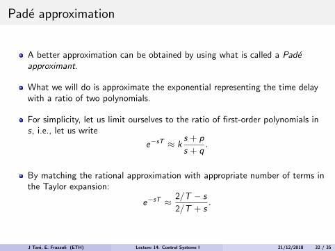
Pade approximation

A better approximation can be obtained by using what is called a Padeapproximant.

What we will do is approximate the exponential representing the time delaywith a ratio of two polynomials.

For simplicity, let us limit ourselves to the ratio of first-order polynomials ins, i.e., let us write

e−sT ≈ ks + p

s + q.

By matching the rational approximation with appropriate number of terms inthe Taylor expansion:

e−sT ≈ 2/T − s

2/T + s.


Using the Pade approximation, we can represent a time delay on the rootlocus as a pole and zero, respectively at ±2/T . Notice the presence of anon-minimum-phase zero.

This approximation method is useful since it allows us to use the root locusmethod for control design, and gain the insight provided by it.

However, the results may not be accurate, and it is recommended that theroot-locus method be used only as a back-of-the-envelope tool providingsome additional insight in the control design process.

Remember: the only tool that would always provide you with correct answersin all cases when a time delay is present (including, e.g., unstable open-looppoles and non-minimum phase zeros) is the Nyquist plot.


Summary of the class

State-space models of physical systems; equilibria and linearization.

Response in the time domain (continuous and discrete time).

Stability of a system (open loop)

Closed-loop stability analysis, root locus and Routh-Criterion

Transfer functions and frequency response

The Nyquist stability condition

Specifications for feedback systems

Loop shaping using the Bode plot; poles/zeros, lead/lag, PID control

Implementation, time delays


Next steps

Laboratory Practice - blackboard 6= hardware!

Control Systems II - nuisances, state feedback, MIMO systems, ”modern”techniques

Optimal Control - focus on ”cost” functions to minimize.

Stochastic Systems - what if the best we can do is describe likelihoods ofsystem dynamics? (very relevant in practice!)

System Modeling - models are important.

Recursive Estimation - a game changer for implementing powerful controlmethods in practive.

Model Predictive Control - how to leverage system behavior predictions tocontrol it better.


Control Systems I - Lecture 14: RHP limits and Implementation ...

Documents

Transcript of Control Systems I - Lecture 14: RHP limits and Implementation ...