Principles of the Minimum Dissipated Power in Stationary Regime

HORIA ANDREI

Faculty of Electrical Engineering University Valahia Targoviste

18-20 Blv. Unirii, Targoviste, Dambovita ROMANIA

http://www.valahia.ro FANICA SPINEI

Faculty of Electrical Engineering University Politehnica Bucharest

313 Splaiul Independentei, sector 6, Bucharest ROMANIA

http://www.elth.pub.ro COSTIN CEPISCA

Faculty of Electrical Engineering University Politehnica Bucharest

313 Splaiul Independentei, sector 6,Bucharest ROMANIA

http://www.elth.pub.ro GIANFRANCO CHICCO

Dipartimento di Ingegneria Elettrica Industriale Politecnica di Torino

Corso Duca degli Abruzzi, 24-10129, Torino ITALY

VASILE DRAGUSIN Faculty of Electrical Engineering

University Valahia Targoviste 18-20 Blv. Unirii, Targoviste, Dambovita

ROMANIA

Abstract: - The use of the power and energy functional in the analysis of the electric circuits makes it possible to appreciate the energetic equilibrium state attained in the circuit at a certain moment. In the present work, a power functional is built and its limit is determined. It is shown that the equilibrium state is one of a minimum energetic state. Key-Words: - electric circuits, Hilbert space, power functionals, minimum of functionals. 1 Introduction Taking into consideration the functional and calculating their limits represents an important breakthrough in formulating and solving some problems related to the optimum. The steady states in the mechanic, thermic, electric conservative systems generally represent limit states from an energetic point of view. For example [1], in the classical mechanics, Hamilton’s principle of the minimum action states that the development in time of a system, from one steady state to another steady state, happens along a curve nR]b,a[: →γ , which extremates the functional

∫ +=b

aM dtUTF )( (1)

called the integral of action, where T is the kinetic energy (the “life power”) of the system and U is the mechanical effect of the power system which works on the system under consideration. In the theory of the electrical circuits, the results obtained by Millar [2] and Stern [3] related to the cocontent function for nonlinear resistive and reciprocal network have a special theoretic importance due to their generality. C. A. Desoer and E. Kuh, [4] (pp. 770-772), had proved the same generally properties of the minimum dissipated power for the linear and resistive networks. As well, the Romanian professors V. Ionescu [5] and C.I. Mocanu [6] (pp. 350-353), had important

2005 WSEAS Int. Conf. on DYNAMICAL SYSTEMS and CONTROL, Venice, Italy, November 2-4, 2005 (pp225-230)

contributions at the theoretical development of the electrical circuits minimax theorems. All these results are basically consequences of Maxwell’s principles of minimum-heat [7] (pp. 407-408). The electromagnetic field analysis admits a differential formulation and a variational equivalent formulation. The mathematical variational model presumes the establishment of a variational principle capable to supply the equations of the differential mathematical model through the stationarity condition of an adequate functional. The energetic functional of the non-stationary electromagnetic field associated to the domain Dc and the volume V, is:

∫ ∫ ρ−+∫ −=cD

Bv

EdxdydzVAJBdHEdDF

00)()( (2)

where: BHED ,,, are the vectors associated to the electric and magnetic field, A is the magnetic vector potential, V is the electric potential, J is the vector of conduction current density, and vρ is the volume density of electric charge. On demonstrate that the condition of minimum of functional (2) involve the fundamental equations,

, , vDdivtDJHrot ρ=

∂∂+= of the electromagnetic field.

Analogue, the energetic functional for electrokinetic field, where the state quantity is the electric potential V, is defined by:

∫ ∫ ∑∫ +=∑c nD

nJ

VdnJdzxdydzEdJVF0

1 )()( (3)

This paper presents three original contributions concerning the energetic functionals of the linear circuits. The first of them proposes an energetic functional for the linear circuits derived of the circuit equations properties. The second represents an other demonstration which proves that the stationary (equilibrium) electrokinetic state for the d.c. networks represents a minimum energetic state as far as the power dissipated by the circuit elements, and the third one proposes an original and general principle of the minimum dissipated active and reactive power for the a.c. linear circuits. 2. The Matrix Equations and the Minimum of Dissipated Power in D.C Circuits Let’s take the case of a reciprocal d.c. electric circuit, with l branches, in an equilibrium state. If G represents the graph of the circuit, then A is a tree and C its complementary tree. The branches voltages and the branches current verify the first and, respectively, the second theorem of Kirchhoff. The l-dimensional current

and voltage matrix can be partitioned as follows

[ ] [ ][ ]

[ ][ ][ ]

Λ−=

=

ccr

c

r

cI

III

I (4)

[ ] [ ][ ]

[ ][ ][ ]

Λ=

=

r

rcr

r

cU

UUU

U (5)

where an adequate notation has been used to point out the sub matrix that refer to the current and voltage links, and the respective branches; [ ] [ ]rBcC−=Λ is the essential incidence matrix. So all the voltage generators become an equivalent current generators, the matrix relation of the branches currents becomes:

[ ] [ ][ ]UGI = (6)where [G] is the square matrix of the branch conductance which can be partitioned under the form of:

[ ] [ ][ ][ ][ ]

=

rrrc

crccGGGG

G (7)

For the reciprocal circuits in stable electrokinetic state, the following power functional can be defined in the Hilbert space nR

RRF n →: (8)

[ ] [ ]IUF T21∆

= (9)

where the superscript T denotes transposition. By using the relations (4), (5), (6), (7) and (9), we can calculate

[ ] [ ] [ ] [ ] [ ][ ][ ][ ][ ][ ]

[ ][ ]

[ ] [ ][ ] [ ] [ ][ ]

[ ] [ ][ ][ ][ ]

[ ] [ ][ ][ ] [ ][ ][ ] [ ] [ ]rrrcrccrc

Tr

rrrT

r

rcrccrcT

r

rrrT

rcccT

c

r

c

rrrc

crcc

Tr

Tc

Tr

UGGU

UGU

UGU

UGUUGU

UU

GGGG

UUIUUF

21

21

21

21

21)(

+ΛΛ=

=+

+ΛΛ=

=+=

=

==

(10)

where [ ] [ ] 0== crcr GG for the reciprocal electric circuits. In relation (10), we have obtained the expression of the functional under consideration, based only on the matrix of the branch voltages. To determine its extreme we apply the function of matrix properties. If

[ ] 0F rU(' = , results

[ ] [ ][ ][ ] [ ] [ ][ ][ ][ ][ ] [ ][ ] 0

0)(=+ΛΛ

=+ΛΛ

rrrrcrccrc

rrrcrccrcT

rUGUG

UGGU (11)

that is

2005 WSEAS Int. Conf. on DYNAMICAL SYSTEMS and CONTROL, Venice, Italy, November 2-4, 2005 (pp225-230)

[ ][ ] [ ] 0=+Λ rcrc II (12) Consequently, the extreme point of the functional verifies the first theorem of Kirchhoff. To demonstrate that extreme point of the functional is minimum, we presumably take a different matrix of the branch voltages,

[ ] [ ] [ ]rrr UUU δ+=∧

(13) which introduced in expression (8) leads to:

[ ] [ ] [ ] [ ][ ][ ][ ] [ ] [ ] [ ][ ] [ ][ ][ ] [ ] [ ]

[ ] [ ][ ][ ] [ ] [ ]rrrcrccrcT

r

rrrcrccrcT

r

Urrrr

crccrcT

rrr

UGGU

UGGU

FUUG

GUUUF

r

21

))(

()(21)(

2

)(

+ΛΛδ+

++ΛΛδ+

+=δ++

+ΛΛδ+=∧

(14)

This demonstrates that the matrixes [ ][ ][ ]crccrc G ΛΛ and [ ]rrG are positively defined, [8], so [ ][ ][ ] [ ] 0⟩+ΛΛ cccrccrc GG and results:

[ ] [ ] )()( rr UFUF ⟩∧

(15)

this means that the functional has a minimum. According to definition (9), the functional [ ])( rUF represents the power dissipated at the terminals of all the branches of a reciprocal circuit in stable electrokinetic state. Therefore, the results obtained (12) shows that the stable electrokinetic state is a minimal power state dissipated by the branches of the circuit. Consequently, we get the following principle (1st Principle of Minimum dissipated Power – PMP): the minimum of the dissipated power by the branches of linear and resistive circuit in stationary regime (d.c.) is satisfied by the solutions in the currents and voltages of the circuit, and these are the currents and voltages which verify the 1st and 2nd theorem of Kirchhoff. 3. Hilbert Space Techniques for Determining the Minimum of the Active and Reactive Dissipated Power Functionals for Linear A.C. circuits We can demonstrate a similar principle for the cvasistationary regime (a.c.) of linear electric circuit.

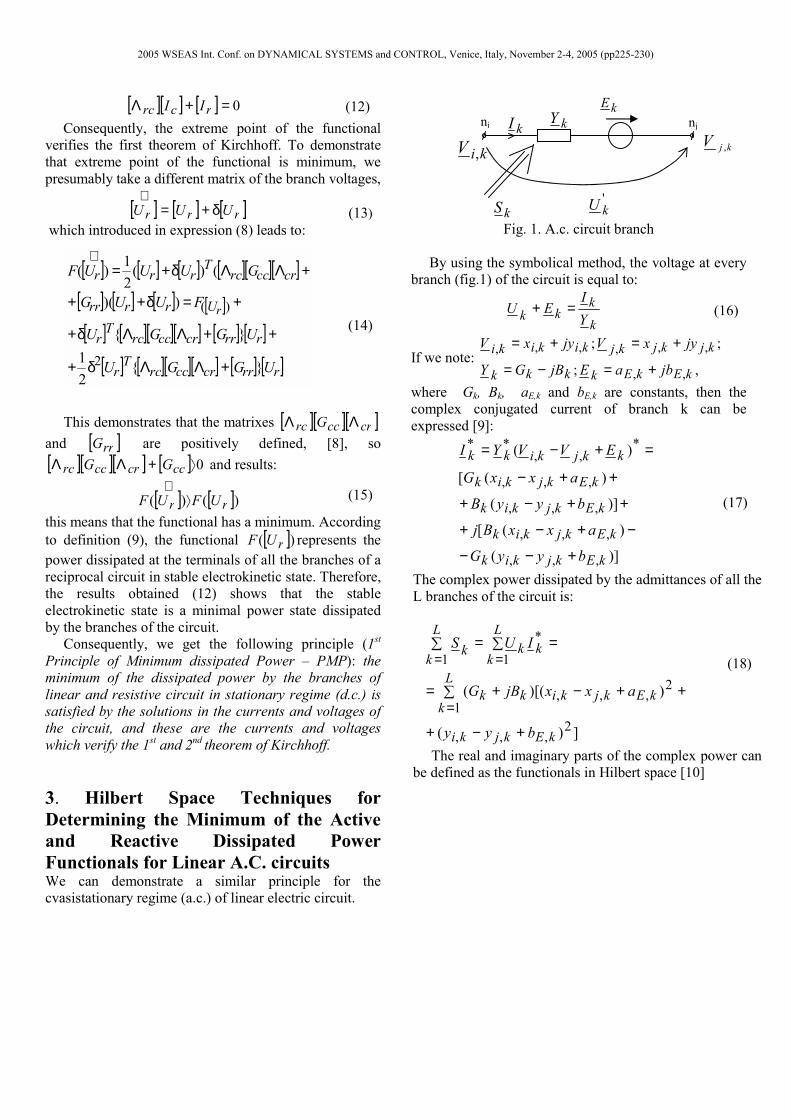
Fig. 1. A.c. circuit branch

By using the symbolical method, the voltage at every branch (fig.1) of the circuit is equal to:

k

kkk Y

IEU =+ (16)

If we note: ,;

;;

,,

,,,,,,

kEkEkkkk

kjkjkjkikikijbaEjBGY

jyxVjyxV

+=−=

+=+=

where Gk, Bk, aE,k and bE,k are constants, then the complex conjugated current of branch k can be expressed [9]:

)](

)([

)](

)([

)(

,,,

,,,

,,,

,,,

*,,

**

kEkjkik

kEkjkik

kEkjkik

kEkjkik

kkjkikk

byyG

axxBj

byyB

axxG

EVVYI

+−−

−+−+

++−+

++−

=+−=

(17)

The complex power dissipated by the admittances of all the L branches of the circuit is:

])(

))[((

2,,,

2,,,

1

*

11

kEkjki

kEkjkikkL

k

kL

kkk

L

k

byy

axxjBG

IUS

+−+

++−+∑=

=∑=∑

=

==

(18)

The real and imaginary parts of the complex power can be defined as the functionals in Hilbert space [10]

kjV ,

ni kI kY kE

nj

'kU kS

kiV ,

2005 WSEAS Int. Conf. on DYNAMICAL SYSTEMS and CONTROL, Venice, Italy, November 2-4, 2005 (pp225-230)

∑ +−++−

==

→≡

∑ +−++−

=≡

→≡

=

=

L

kkEkjkikEkjkik

NNI

NI

L

kkEkjkikEkjkik

NNR

NR

byyaxxB

SyyyxxxF

RRSF

byyaxxG

SyyyxxxF

RRSF

1

2,,,

2,,,

2121

2

1

2,,,

2,,,

2121

2

])()[(21

]Im[21),...,,,,...,,(

:]Im[21

])()[(21

]Re[21),...,,,,...,,(

:]Re[21

(19)

and they are quite obviously a function class 2C in NR2 , and are positively defined, [9], i.e. for all the pair

,,...,1 ),,( Niyx ii = then:0),...,,,,...,,( 2121 ⟩NNR yyyxxxF

and 0),...,,,,...,,( 2121 ⟩NNI yyyxxxF . Consequently, the minimum points of the real and imaginary component of the complex power functionals, [10], are the solutions of the system which contains 4N equations:

00, ,...,0 ,0

,00, ,...,0 ,0

11

11

=∂∂=

∂∂=

∂∂=

∂∂

=∂∂=

∂∂=

∂∂=

∂∂

NI

NIII

NR

NRRR

yF

xF

yF

xF

yF

xF

yF

xF

(20)

If we calculate the algebrical sum of the solutions, with one of them multiplied with (-1) or ±j , we obtain the expressions:

∑ ∑ ==∑ =∈ ∈∈ 21

0 ,...,0 ,0 ***

nl nlkk

nlk

k NkkIII (21)

which are identical with the Kirchhoff’s equations for currents (1st Kirchhoff theorem), expressed in all the N nodes of the circuit. Consequently, the following principle can be issued (2nd Principle of Minimum Active and Reactive dissipated Power –PMARP): the minimum of the active and reactive dissipated power by the branches of a linear circuit in a cvasistationary regime (a.c.) is satisfied by the solutions in currents and voltages of the circuit, and these are the currents and voltages that verify the 1stand 2nd theorem of Kirchhoff.

4. Examples 4.1. Determination of the minimum power functional for a d.c. circuit We consider the d.c. circuit shown in figure 2, where

VERRR 4,3,2,1 1321 =Ω=Ω=Ω= .Because

12 VVU r −= , the power functional dissipated by the

Fig. 2. D.c. circuit with three branches

branches of the circuit, (9), are calculated depending on potentials 21,VV :

)(

)()(21

2213

2212

21121

VVG

VVGEVVGF

−+

+−++−=

The minimum of the power functional are the solutions of the system

which represent the 1st theorem of Kirchhoff expressed in node 1 and 2. We calculate using PSPICE and MATHCAD the variation of the dissipated powers

321 ,, PPP depending by the currents 321 ,, III , shown respectively in figures 3, 4 and 5. Using Thèvenin’s theorem, we obtain the expressions:

,3,2,)( ,0, =−= iIIRUP iiieii where ,, ,0, iei RU are the open voltage and the equivalent resistance of the circuit at the terminals of branch 2, respectively 3. It is remarked that the dissipated power in each branch is a minimum value compared with the maximum value of the power, which is obtained for the

current value of short-circuit divided by 2 (2scI

),

0)(

)()(

1321213

21211211

=∑=++−=−+

+−++−−=∂∂

∈ nlk

kIIIIVVG

VVGEVVGVF

0)(

)()(

2321213

21211212

=∑=−−=−−

−−−+−=∂∂

∈ nlk

kIIIIVVG

VVGEVVGVF

n1

n2

V1

V2

R2

I2 I3

R3 R1

I1

E1

2005 WSEAS Int. Conf. on DYNAMICAL SYSTEMS and CONTROL, Venice, Italy, November 2-4, 2005 (pp225-230)

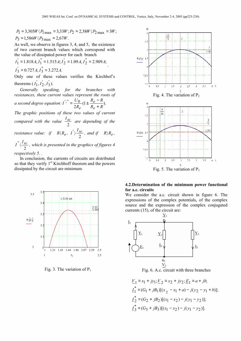
.67,2586,1 ;338,2;33,3305,3

max33

max22max11WPWP

WPWPWPWP≈⟨≈

=⟨≈=⟨≈

As well, we observe in figures 3, 4, and 5, the existence of two current branch values which correspond with the value of dissipated power for each branch

.272.3,727.0

;909.2,09.1;515.1,818.1''

3'3

''2

'2

''1

'1

AIAI

AIAIAIAI

==

====.

Only one of these values verifies the Kirchhof’s theorems ( '

3'2

'1 ,, III ).

Generally speaking, for the branches with resistances, these current values represent the roots of

a second degree equation: ).1(2

0'','RRRR

RU

Iee

e +−

±=

The graphic positions of these two values of current

compared with the value 2scI

are depending of the

resistance value: if eRR⟨ , 2

' scII ⟩ , and if eRR⟩ ,

2'' scI

I ⟨ , which is presented in the graphics of figures 4

respectively 5. . In conclusion, the currents of circuits are distributed so that they verify 1st Kirchhoff theorem and the powers dissipated by the circuit are minimum.

1 1.21 1.43 1.64 1.86 2.07 2.29 2.53

3.1

3.2

3.3

3.4

3.53.5

3

3.3053.33

P1 I1( )

2.51

1.5151.66

I1

Fig. 3. The variation of P1

Fig. 4. The variation of P2

Fig. 5. The variation of P3

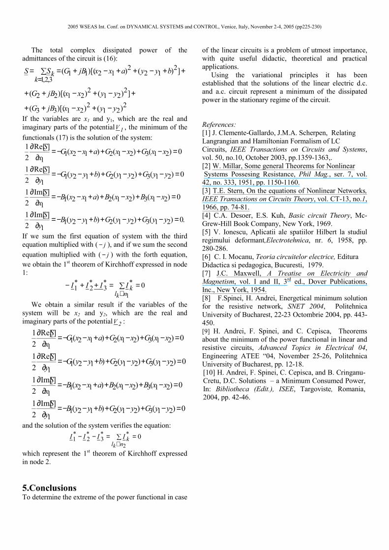
4.2.Determination of the minimum power functional for a.c. circuits We consider the a.c. circuit shown in figure 6. The expressions of the complex potentials, of the complex source and the expression of the complex conjugated currents (15), of the circuit are:

Fig. 6. A.c. circuit with three branches

)].())[((

)];())[((

)];())[((

;;;

212133*3

212122*2

12111*1

1222111

2

yyjxxjBGI

yyjxxjBGI

byyjaxxjBGI

jbaEjyxVjyxV

−−−+=

−−−+=

+−−+−+=

+=+=+=

V1 n1

n2 V2

I1

I3

Y1

E1

Y2

I2

Y3

2005 WSEAS Int. Conf. on DYNAMICAL SYSTEMS and CONTROL, Venice, Italy, November 2-4, 2005 (pp225-230)

The total complex dissipated power of the admittances of the circuit is (16):

221

22133

221

22122

3,2,1

212

21211

)())[((

])())[((

])())[((

yyxxjBG

yyxxjBG

byyaxxjBGSSk

k

−+−++

+−+−++

∑ ++−++−+===

If the variables are x1 and y1, which are the real and imaginary parts of the potential 1V , the minimum of the functionals (17) is the solution of the system:

.0)()()(]Im[21

0)()()(]Im[21

0)()()(]Re[21

0)()()(]Re[21

2132121211

2132121211

2132121211

2132121211

=−+−++−−=∂

∂

=−+−++−−=∂

∂

=−+−++−−=∂

∂

=−+−++−−=∂

∂

yyGyyGbyyBy

S

xxBxxBaxxBx

S

yyGyyGbyyGy

S

xxGxxGaxxGx

S

If we sum the first equation of system with the third equation multiplied with ( j− ), and if we sum the second equation multiplied with ( j− ) with the forth equation, we obtain the 1st theorem of Kirchhoff expressed in node 1:

∑ ==++−∈ 1

0 **3

*2

*1

nlk

kIIII

We obtain a similar result if the variables of the system will be x2 and y2, which are the real and imaginary parts of the potential 2V :

0)()()(]Im[21

0)()()(]Im[21

0)()()(]Re[21

0)()()(]Re[21

2132121211

2132121211

2132121211

2132121211

=−+−++−−=∂

∂

=−+−++−−=∂

∂

=−+−++−−=∂

∂

=−+−++−−=∂

∂

yyGyyGbyyBy

S

xxBxxBaxxBx

S

yyGyyGbyyGy

S

xxGxxGaxxGx

S

and the solution of the system verifies the equation: ∑ ==−−∈ 2

0 **3

*2

*1

nlk

kIIII

which represent the 1st theorem of Kirchhoff expressed in node 2. 5.Conclusions To determine the extreme of the power functional in case

of the linear circuits is a problem of utmost importance, with quite useful didactic, theoretical and practical applications. Using the variational principles it has been established that the solutions of the linear electric d.c. and a.c. circuit represent a minimum of the dissipated power in the stationary regime of the circuit. References: [1] J. Clemente-Gallardo, J.M.A. Scherpen, Relating Langrangian and Hamiltonian Formalism of LC Circuits, IEEE Transactions on Circuits and Systems, vol. 50, no.10, October 2003, pp.1359-1363,. [2] W. Millar, Some general Theorems for Nonlinear Systems Possesing Resistance, Phil Mag., ser. 7, vol. 42, no. 333, 1951, pp. 1150-1160. [3] T.E. Stern, On the equations of Nonlinear Networks, IEEE Transactions on Circuits Theory, vol. CT-13, no.1, 1966, pp. 74-81. [4] C.A. Desoer, E.S. Kuh, Basic circuit Theory, Mc-Grew-Hill Book Company, New York, 1969. [5] V. Ionescu, Aplicatii ale spatiilor Hilbert la studiul regimului deformant,Electrotehnica, nr. 6, 1958, pp. 280-286. [6] C. I. Mocanu, Teoria circuitelor electrice, Editura Didactica si pedagogica, Bucuresti, 1979. [7] J.C. Maxwell, A Treatise on Electricity and Magnetism, vol. I and II, 3rd ed., Dover Publications, Inc., New York, 1954. [8] F.Spinei, H. Andrei, Energetical minimum solution for the resistive network, SNET 2004, Politehnica University of Bucharest, 22-23 Octombrie 2004, pp. 443- 450. [9] H. Andrei, F. Spinei, and C. Cepisca, Theorems about the minimum of the power functional in linear and resistive circuits, Advanced Topics in Electrical 04, Engineering ATEE “04, November 25-26, Politehnica University of Bucharest, pp. 12-18. [10] H. Andrei, F. Spinei, C. Cepisca, and B. Cringanu-Cretu, D.C. Solutions – a Minimum Consumed Power, In: Bibliotheca (Edit.), ISEE, Targoviste, Romania, 2004, pp. 42-46.

2005 WSEAS Int. Conf. on DYNAMICAL SYSTEMS and CONTROL, Venice, Italy, November 2-4, 2005 (pp225-230)