Contents - Universidad de Buenos Aires
294
Contents Foreword ................................................................ IX Preface ................................................................ XI K-theory for group C * -algebras Paul F. Baum, Rub´ en J. S´ anchez-Garc´ ıa ............................... 1 1 Introduction ..................................................... 1 2 C * -algebras ..................................................... 2 2.1 Definitions ................................................ 2 2.2 Examples ................................................. 3 2.3 The reduced C * -algebra of a group ............................ 4 2.4 Two classical theorems ...................................... 5 2.5 The categorical viewpoint .................................... 6 3 K-theory of C * -algebras .......................................... 6 3.1 Definition for unital C * -algebras .............................. 7 3.2 Bott periodicity ............................................ 8 3.3 Definition for non-unital C * -algebras .......................... 8 3.4 Functoriality ............................................... 9 3.5 More on Bott periodicity ..................................... 9 3.6 Topological K-theory ........................................ 10 4 Proper G-spaces .................................................. 11 5 Classifying space for proper actions ................................ 12 6 Equivariant K-homology .......................................... 14 6.1 Definitions ................................................ 14 6.2 Functoriality ............................................... 17 6.3 The index map ............................................. 18 7 The discrete case ................................................ 19 7.1 Equivariant K-homology ..................................... 19 7.2 Some results on discrete groups ............................... 20
-
Upload
khangminh22 -
Category
Documents
-
view
0 -
download
0
Transcript of Contents - Universidad de Buenos Aires
Contents
Foreword. . . . . . . . . . . . . . . . . . . . . . . . . . . . . . . . . . . . . . . . . . . . . . . . . . . . . . . . . . . . . . . . IX
Preface. . . . . . . . . . . . . . . . . . . . . . . . . . . . . . . . . . . . . . . . . . . . . . . . . . . . . . . . . . . . . . . . XI
K-theory for group C∗-algebrasPaul F. Baum, Ruben J. Sanchez-Garcıa . . . . . . . . . . . . . . . . . . . . . . . . . . . . . . . 11 Introduction . . . . . . . . . . . . . . . . . . . . . . . . . . . . . . . . . . . . . . . . . . . . . . . . . . . . . 12 C∗-algebras . . . . . . . . . . . . . . . . . . . . . . . . . . . . . . . . . . . . . . . . . . . . . . . . . . . . . 2
2.1 Definitions . . . . . . . . . . . . . . . . . . . . . . . . . . . . . . . . . . . . . . . . . . . . . . . . 22.2 Examples . . . . . . . . . . . . . . . . . . . . . . . . . . . . . . . . . . . . . . . . . . . . . . . . . 32.3 The reduced C∗-algebra of a group . . . . . . . . . . . . . . . . . . . . . . . . . . . . 42.4 Two classical theorems . . . . . . . . . . . . . . . . . . . . . . . . . . . . . . . . . . . . . . 52.5 The categorical viewpoint . . . . . . . . . . . . . . . . . . . . . . . . . . . . . . . . . . . . 6
3 K-theory of C∗-algebras . . . . . . . . . . . . . . . . . . . . . . . . . . . . . . . . . . . . . . . . . . 63.1 Definition for unital C∗-algebras . . . . . . . . . . . . . . . . . . . . . . . . . . . . . . 73.2 Bott periodicity . . . . . . . . . . . . . . . . . . . . . . . . . . . . . . . . . . . . . . . . . . . . 83.3 Definition for non-unital C∗-algebras . . . . . . . . . . . . . . . . . . . . . . . . . . 83.4 Functoriality . . . . . . . . . . . . . . . . . . . . . . . . . . . . . . . . . . . . . . . . . . . . . . . 93.5 More on Bott periodicity . . . . . . . . . . . . . . . . . . . . . . . . . . . . . . . . . . . . . 93.6 Topological K-theory . . . . . . . . . . . . . . . . . . . . . . . . . . . . . . . . . . . . . . . . 10
4 Proper G-spaces . . . . . . . . . . . . . . . . . . . . . . . . . . . . . . . . . . . . . . . . . . . . . . . . . . 115 Classifying space for proper actions . . . . . . . . . . . . . . . . . . . . . . . . . . . . . . . . 126 Equivariant K-homology . . . . . . . . . . . . . . . . . . . . . . . . . . . . . . . . . . . . . . . . . . 14
6.1 Definitions . . . . . . . . . . . . . . . . . . . . . . . . . . . . . . . . . . . . . . . . . . . . . . . . 146.2 Functoriality . . . . . . . . . . . . . . . . . . . . . . . . . . . . . . . . . . . . . . . . . . . . . . . 176.3 The index map . . . . . . . . . . . . . . . . . . . . . . . . . . . . . . . . . . . . . . . . . . . . . 18
7 The discrete case . . . . . . . . . . . . . . . . . . . . . . . . . . . . . . . . . . . . . . . . . . . . . . . . 197.1 Equivariant K-homology . . . . . . . . . . . . . . . . . . . . . . . . . . . . . . . . . . . . . 197.2 Some results on discrete groups . . . . . . . . . . . . . . . . . . . . . . . . . . . . . . . 20
VI Contents
7.3 Corollaries of the Baum-Connes Conjecture . . . . . . . . . . . . . . . . . . . . . . 218 The compact case . . . . . . . . . . . . . . . . . . . . . . . . . . . . . . . . . . . . . . . . . . . . . . . . . 219 Equivariant K-homology for G-C∗-algebras . . . . . . . . . . . . . . . . . . . . . . . . . . 2210 The conjecture with coefficients . . . . . . . . . . . . . . . . . . . . . . . . . . . . . . . . . . . . 2411 Hilbert modules . . . . . . . . . . . . . . . . . . . . . . . . . . . . . . . . . . . . . . . . . . . . . . . . . 25
11.1 Definitions and examples . . . . . . . . . . . . . . . . . . . . . . . . . . . . . . . . . . . . 2511.2 The reduced crossed-product C∗r (G,A) . . . . . . . . . . . . . . . . . . . . . . . . . 2811.3 Push-forward of Hilbert modules . . . . . . . . . . . . . . . . . . . . . . . . . . . . . . 29
12 Homotopy made precise and KK-theory . . . . . . . . . . . . . . . . . . . . . . . . . . . . . 3013 Equivariant KK-theory . . . . . . . . . . . . . . . . . . . . . . . . . . . . . . . . . . . . . . . . . . . 3214 The index map . . . . . . . . . . . . . . . . . . . . . . . . . . . . . . . . . . . . . . . . . . . . . . . . . . 34
14.1 The Kasparov product . . . . . . . . . . . . . . . . . . . . . . . . . . . . . . . . . . . . . . . 3514.2 The Kasparov descent map . . . . . . . . . . . . . . . . . . . . . . . . . . . . . . . . . . . 3514.3 Definition of the index map . . . . . . . . . . . . . . . . . . . . . . . . . . . . . . . . . . 3514.4 The index map with coefficients . . . . . . . . . . . . . . . . . . . . . . . . . . . . . . . 36
15 A brief history of K-theory . . . . . . . . . . . . . . . . . . . . . . . . . . . . . . . . . . . . . . . . 3715.1 The K-theory genealogy tree . . . . . . . . . . . . . . . . . . . . . . . . . . . . . . . . . 3715.2 The Hirzebruch–Riemann–Roch theorem . . . . . . . . . . . . . . . . . . . . . . . 3815.3 The unity of K-theory . . . . . . . . . . . . . . . . . . . . . . . . . . . . . . . . . . . . . . . 38
References . . . . . . . . . . . . . . . . . . . . . . . . . . . . . . . . . . . . . . . . . . . . . . . . . . . . . . . . . 40
Universal Coefficient Theorems and assembly maps in KK-theoryRalf Meyer . . . . . . . . . . . . . . . . . . . . . . . . . . . . . . . . . . . . . . . . . . . . . . . . . . . . . . . 431 Introduction . . . . . . . . . . . . . . . . . . . . . . . . . . . . . . . . . . . . . . . . . . . . . . . . . . . . 432 Kasparov theory and Baum–Connes conjecture . . . . . . . . . . . . . . . . . . . . . . . 44
2.1 Kasparov theory via its universal property . . . . . . . . . . . . . . . . . . . . . . 442.2 Subcategories in KKG . . . . . . . . . . . . . . . . . . . . . . . . . . . . . . . . . . . . . . . 56
3 Homological algebra . . . . . . . . . . . . . . . . . . . . . . . . . . . . . . . . . . . . . . . . . . . . . . 613.1 Homological ideals in triangulated categories . . . . . . . . . . . . . . . . . . . 623.2 From homological ideals to derived functors . . . . . . . . . . . . . . . . . . . . 673.3 Universal Coefficient Theorems . . . . . . . . . . . . . . . . . . . . . . . . . . . . . . . 85
References . . . . . . . . . . . . . . . . . . . . . . . . . . . . . . . . . . . . . . . . . . . . . . . . . . . . . . . . . . 91
Algebraic v. topological K-theory: a friendly matchGuillermo Cortinas . . . . . . . . . . . . . . . . . . . . . . . . . . . . . . . . . . . . . . . . . . . . . . . . 951 Introduction . . . . . . . . . . . . . . . . . . . . . . . . . . . . . . . . . . . . . . . . . . . . . . . . . . . . 952 The groups Kn for n≤ 1. . . . . . . . . . . . . . . . . . . . . . . . . . . . . . . . . . . . . . . . . . . 96
2.1 Definition and basic properties of K j for j = 0,1. . . . . . . . . . . . . . . . . 962.2 Matrix-stable functors. . . . . . . . . . . . . . . . . . . . . . . . . . . . . . . . . . . . . . . . 1012.3 Sum rings and infinite sum rings. . . . . . . . . . . . . . . . . . . . . . . . . . . . . . . 1022.4 The excision sequence for K0 and K1. . . . . . . . . . . . . . . . . . . . . . . . . . . 1042.5 Negative K-theory. . . . . . . . . . . . . . . . . . . . . . . . . . . . . . . . . . . . . . . . . . . 106
3 Topological K-theory . . . . . . . . . . . . . . . . . . . . . . . . . . . . . . . . . . . . . . . . . . . . 1083.1 Topological K-theory of Banach algebras. . . . . . . . . . . . . . . . . . . . . . . 1083.2 Bott periodicity. . . . . . . . . . . . . . . . . . . . . . . . . . . . . . . . . . . . . . . . . . . . . . 111
Contents VII
4 Polynomial homotopy and Karoubi-Villamayor K-theory . . . . . . . . . . . . . . 1135 Homotopy K-theory . . . . . . . . . . . . . . . . . . . . . . . . . . . . . . . . . . . . . . . . . . . . . 115
5.1 Definition and basic properties of KH. . . . . . . . . . . . . . . . . . . . . . . . . . 1155.2 KH for K0-regular rings. . . . . . . . . . . . . . . . . . . . . . . . . . . . . . . . . . . . . . 1175.3 Toeplitz ring and the fundamental theorem for KH. . . . . . . . . . . . . . . 118
6 Quillen’s Higher K-theory . . . . . . . . . . . . . . . . . . . . . . . . . . . . . . . . . . . . . . . . 1206.1 Classifying spaces. . . . . . . . . . . . . . . . . . . . . . . . . . . . . . . . . . . . . . . . . . . 1206.2 Perfect groups and the plus construction for BG. . . . . . . . . . . . . . . . . . 1206.3 Functoriality issues. . . . . . . . . . . . . . . . . . . . . . . . . . . . . . . . . . . . . . . . . . 1246.4 Relative K-groups and excision. . . . . . . . . . . . . . . . . . . . . . . . . . . . . . . . 1256.5 Locally convex algebras. . . . . . . . . . . . . . . . . . . . . . . . . . . . . . . . . . . . . . 1266.6 Frechet m-algebras with approximate units. . . . . . . . . . . . . . . . . . . . . . 1276.7 Fundamental theorem and the Toeplitz ring. . . . . . . . . . . . . . . . . . . . . . 128
7 Comparison between algebraic and topological K-theory I . . . . . . . . . . . . . 1297.1 Stable C∗-algebras. . . . . . . . . . . . . . . . . . . . . . . . . . . . . . . . . . . . . . . . . . 1297.2 Stable Banach algebras. . . . . . . . . . . . . . . . . . . . . . . . . . . . . . . . . . . . . . . 130
8 Topological K-theory for locally convex algebras . . . . . . . . . . . . . . . . . . . . . . 1318.1 Diffeotopy KV . . . . . . . . . . . . . . . . . . . . . . . . . . . . . . . . . . . . . . . . . . . . . . . 1318.2 Diffeotopy K-theory. . . . . . . . . . . . . . . . . . . . . . . . . . . . . . . . . . . . . . . . . 1338.3 Bott periodicity. . . . . . . . . . . . . . . . . . . . . . . . . . . . . . . . . . . . . . . . . . . . . 134
9 Comparison between algebraic and topological K-theory II . . . . . . . . . . . . . 1359.1 The diffeotopy invariance theorem. . . . . . . . . . . . . . . . . . . . . . . . . . . . . 1359.2 KH of stable locally convex algebras. . . . . . . . . . . . . . . . . . . . . . . . . . . 137
10 K-theory spectra . . . . . . . . . . . . . . . . . . . . . . . . . . . . . . . . . . . . . . . . . . . . . . . . . 13810.1 Quillen’s K-theory spectrum. . . . . . . . . . . . . . . . . . . . . . . . . . . . . . . . . . 13810.2 KV -theory spaces. . . . . . . . . . . . . . . . . . . . . . . . . . . . . . . . . . . . . . . . . . . 13910.3 The homotopy K-theory spectrum. . . . . . . . . . . . . . . . . . . . . . . . . . . . . . 141
11 Primary and secondary Chern characters . . . . . . . . . . . . . . . . . . . . . . . . . . . . 14211.1 Cyclic homology. . . . . . . . . . . . . . . . . . . . . . . . . . . . . . . . . . . . . . . . . . . . 14211.2 Primary Chern character and infinitesimal K-theory. . . . . . . . . . . . . . . 14311.3 Secondary Chern characters. . . . . . . . . . . . . . . . . . . . . . . . . . . . . . . . . . . 14311.4 Application to KD. . . . . . . . . . . . . . . . . . . . . . . . . . . . . . . . . . . . . . . . . . . 145
12 Comparison between algebraic and topological K-theory III . . . . . . . . . . . . 14512.1 Stable Frechet algebras. . . . . . . . . . . . . . . . . . . . . . . . . . . . . . . . . . . . . . . 14512.2 Stable locally convex algebras: the comparison sequence. . . . . . . . . . 146
References . . . . . . . . . . . . . . . . . . . . . . . . . . . . . . . . . . . . . . . . . . . . . . . . . . . . . . . . . 148
Higher algebraic K-theory (after Quillen, Thomason andothers)Marco Schlichting . . . . . . . . . . . . . . . . . . . . . . . . . . . . . . . . . . . . . . . . . . . . . . . . . 1531 Introduction . . . . . . . . . . . . . . . . . . . . . . . . . . . . . . . . . . . . . . . . . . . . . . . . . . . . 1532 The K-theory of exact categories . . . . . . . . . . . . . . . . . . . . . . . . . . . . . . . . . . . 155
2.1 The Grothendieck group of an exact category . . . . . . . . . . . . . . . . . . . 1552.2 Quillen’s Q-construction and higher K-theory . . . . . . . . . . . . . . . . . . . 1582.3 Quillen’s fundamental theorems . . . . . . . . . . . . . . . . . . . . . . . . . . . . . . . 163
VIII Contents
2.4 Negative K-groups . . . . . . . . . . . . . . . . . . . . . . . . . . . . . . . . . . . . . . . . . . 1673 Algebraic K-theory and triangulated categories . . . . . . . . . . . . . . . . . . . . . . . 169
3.1 The Grothendieck-group of a triangulated category . . . . . . . . . . . . . . . 1693.2 The Thomason-Waldhausen Localization Theorem . . . . . . . . . . . . . . . 1743.3 Quillen’s fundamental theorems revisited . . . . . . . . . . . . . . . . . . . . . . . 1843.4 Thomason’s Mayer-Vietoris principle . . . . . . . . . . . . . . . . . . . . . . . . . . 1883.5 Projective Bundle Theorem and regular blow-ups . . . . . . . . . . . . . . . . 193
4 Beyond triangulated categories . . . . . . . . . . . . . . . . . . . . . . . . . . . . . . . . . . . . 1984.1 Statement of results . . . . . . . . . . . . . . . . . . . . . . . . . . . . . . . . . . . . . . . . . 198
A Appendix . . . . . . . . . . . . . . . . . . . . . . . . . . . . . . . . . . . . . . . . . . . . . . . . . . . . . . 202A.1 Background from topology . . . . . . . . . . . . . . . . . . . . . . . . . . . . . . . . . . . 202A.2 Background on triangulated categories . . . . . . . . . . . . . . . . . . . . . . . . . 205A.3 The derived category of quasi-coherent sheaves . . . . . . . . . . . . . . . . . . 212A.4 Proof of compact generation of DZ Qcoh(X) . . . . . . . . . . . . . . . . . . . . 216
References . . . . . . . . . . . . . . . . . . . . . . . . . . . . . . . . . . . . . . . . . . . . . . . . . . . . . . . . . 223
Lectures on DG-categoriesToen Bertrand . . . . . . . . . . . . . . . . . . . . . . . . . . . . . . . . . . . . . . . . . . . . . . . . . . . . 2291 Introduction . . . . . . . . . . . . . . . . . . . . . . . . . . . . . . . . . . . . . . . . . . . . . . . . . . . . 2292 Lecture 1: DG-categories and localization . . . . . . . . . . . . . . . . . . . . . . . . . . . 230
2.1 The Gabriel-Zisman localization . . . . . . . . . . . . . . . . . . . . . . . . . . . . . . 2302.2 Bad behavior of the Gabriel-Zisman localization . . . . . . . . . . . . . . . . . 2332.3 DG-categories and dg-functors . . . . . . . . . . . . . . . . . . . . . . . . . . . . . . . . 2362.4 Localizations as a dg-category . . . . . . . . . . . . . . . . . . . . . . . . . . . . . . . . 248
3 Lecture 2: Model categories and dg-categories . . . . . . . . . . . . . . . . . . . . . . . 2493.1 Reminders on model categories . . . . . . . . . . . . . . . . . . . . . . . . . . . . . . . 2503.2 Model categories and dg-categories . . . . . . . . . . . . . . . . . . . . . . . . . . . . 254
4 Lecture 3: Structure of the homotopy category of dg-categories . . . . . . . . . 2584.1 Maps in the homotopy category of dg-categories . . . . . . . . . . . . . . . . . 2584.2 Existence of internal Homs . . . . . . . . . . . . . . . . . . . . . . . . . . . . . . . . . . . 2624.3 Existence of localizations . . . . . . . . . . . . . . . . . . . . . . . . . . . . . . . . . . . . 2634.4 Triangulated dg-categories . . . . . . . . . . . . . . . . . . . . . . . . . . . . . . . . . . . 266
5 Lecture 4: Some applications . . . . . . . . . . . . . . . . . . . . . . . . . . . . . . . . . . . . . . 2705.1 Functorial cones . . . . . . . . . . . . . . . . . . . . . . . . . . . . . . . . . . . . . . . . . . . . 2705.2 Some invariants . . . . . . . . . . . . . . . . . . . . . . . . . . . . . . . . . . . . . . . . . . . . 2725.3 Descent . . . . . . . . . . . . . . . . . . . . . . . . . . . . . . . . . . . . . . . . . . . . . . . . . . . 2745.4 Saturated dg-categories and secondary K-theory . . . . . . . . . . . . . . . . . 276
References . . . . . . . . . . . . . . . . . . . . . . . . . . . . . . . . . . . . . . . . . . . . . . . . . . . . . . . . . . 281
Foreword
The five articles of this volume evolved from the lecture notes of Swisk1, the SedanoWinter School on K-theory held in Sedano, Spain, during the week January 22–27 of2007. Lectures were delivered by Paul F. Baum, Carlo Mazza, Ralf Meyer, MarcoSchlichting, Betrand Toen and myself, for a public of 45 participants. The schoolwas supported by the Ministerio de Educacion y Ciencia and the Proyecto ConsoliderMathematica of Spain. Funding to cover expenses of US based participants wasprovided by NSF, through a grant to C. A.Weibel, who was responsible, first of all,for preparing a succesful funding application, and then for managing the funds. Thelocal committee, composed of N. Abad and E. Ellis, were in charge of conferencelogistics. Marco Schlichting collaborated in the Scientific Committee. As organizer ofthe school and editor of this volume, I am indebted to all these people and institutionsfor their support, and to my fellow coauthors for their contributions.
Guillermo Cortinas.
1 The webpage of the school can be found athttp://cms.dm.uba.ar/Members/gcorti/workgroup.swisk/index_html.html

Preface
This book evolved from the lecture notes of Swisk, the Sedano Winter School onK-theory held in Sedano, Spain, during the week January 22–27 of 2007. It intends tobe an introduction to K-theory, both algebraic and topological, with emphasis on theirinterconnections. While a wide range of topics is covered, an effort has been made tokeep the exposition as elementary and self-contained as possible.
Since its beginning in the celebrated work of Grothendieck on the Riemmann-Roch theorem, applications of K-theory have been found in a variety of subjects,including algebraic geometry, number theory, algebraic and geometric topology,representation theory and geometric and functional analysis. Because of this, mathe-maticians from each of these areas have become interested in the subject, and theyall look at it from their own perspective. On the one hand, this is the richness andappeal of K-theory. On the other hand, it makes it hard to see a global perspective. Forexample it is not often that an algebraic K-theorist, coming, say, from the algebraicgeometry side of the subject, and a topological K-theorist, coming from the functionalanalysis side, meet together in the same K-theory conference. Thus it is not uncom-mon to find that algebraic and topological K-theory are regarded as distinct subjectsaltogether. These notes modestly attempt to illustrate current developments in bothbranches of the subject, and to emphasize their contacts.
The book is divided into five articles, each of them devoted to different topics.
The first two articles are concerned with Kasparov’s bivariant K-theory of C∗-algebras and its role in the Baum–Connes conjecture. If G is a locally compactgroup and A and B are two separable C∗-algebras equipped with a G-action, theKasparov bivariant K-theory group KKG(A,B) is defined as the homotopy classes ofG-equivariant Hilbert (A,B) bimodules equipped with a suitable Fredholm operator.Kasparov defines an associative product
KG(A,B)⊗KG(B,C)→ KG(A,C)
XII
There is an additive category KKG whose objects are the separable G–C∗-algebras, sothat KKG(A,B) = homKKG(A,B) and composition is given by the Kasparov product.This category is related to usual category G–C∗–Alg of G–C∗-algebras and equivariant∗-homomorphism by means of a functor ι : G–C∗–Alg→ KKG. The functor ι has thefollowing properties:
• (Stability) If A ∈ G–C∗–Alg, and H1,H2 are nonzero G-Hilbert spaces, thenι(A⊗K(H1)→ A⊗K(H1⊕H2)) is an isomorphism.
• (Split Exactness) If Aj→ B
p→C is a short exact sequence of G–C∗-algebras, splitby a G-equivariant homomorphism s : C→ B, then (ι( j), ι(s)) : ι(A)⊕ ι(C)→ι(B) is an isomorphism.
Moreover ι is universal (initial) among stable, split exact functors to additivecategories. Kasparov theory has many other important properties. To mention one,consider the case when G = 1 is the trivial group, and we takeC as the first variable;then
K0(B) = KK(C,B)
is the usual Grothendieck group. Because topological K1 of a C∗-algebra B is just K0of the suspension of B, we also have
Ktop1 (B) = KK(C,SB)
Thus the whole topological K-theory is recovered from KK, since Ktop is 2-periodic.
Another application of equivariant KK is in the definition of equivariant K-homology, which plays a fundamental role in the Baum–Connes conjecture. A Haus-dorff, locally compact, second countable space X equipped with an action of G byhomeomorphisms is called proper if the map
G×X → X×X , (g,x) 7→ (gx,x)
is proper, that is, if the inverse image of any compact subspace is compact. A G-subspace ∆ ⊂ X G is called G-compact if it is proper and the quotient G\∆ is compact.The equivariant K-homology of a proper G-space X is
KG∗ (X) = colim
∆⊂XKKG∗ (C0(∆),C)
Here the colimit is taken over all G-compact subspaces ∆ ⊂ X ; C0 is the C∗-algebraof continous functions vanishing at infinity, and KKG
∗ (A,C) = KKG(S∗A,C).
The Baum–Connes conjecture proposes a description of the topological K-theoryof the reduced C∗-algebra Cr(G) of a locally compact, Hausdorff, second countablegroup G in terms of G-equivariant K-homology of the universal (final) proper G-space.There is a map
KG∗ (EG)→ Ktop
∗ (Cr(G))
Preface XIII
called the assembly map, and the conjecture says it is an isomorphism. The properG-space EG is characterized up to homotopy by the property that any proper G-spaceX maps to EG and that any two such maps are homotopic. The reduced C∗-algebrais defined as follows. If G is a locally compact, second countable group, and µ isa left invariant Haar measure on G, then one can form the separable Hilbert spaceH = L2(G,µ) of square-integrable functions on G. The algebra Cc(G) of compactlysupported continuous functions G→ C with convolution product is faithfully repre-sented inside the algebra B(H) of bounded operators on H, and Cr(G) is the normcompletion of Cc(G).
The conjecture is known to be true for wide classes of groups; no counterexamplesare known. There is also a more general version of the conjecture relating the equiv-arient K-homology of EG with coefficients in a separable G–C∗-algebra A with thetopological K-theory of the reduced C∗-algebra of G with coefficients in A, Cr(G,A).The latter conjecture is also known for large classes of groups, and is expected to betrue in many cases.
The Baum–Connes conjecture is related to a great number of conjectures in func-tional analysis, algebra, geometry and topology. Most of these conjectures follow fromeither the injectivity or the surjectivity of the assembly map. A significant example isthe Novikov conjecture on the homotopy invariance of higher signatures of closed,connected, oriented, smooth manifolds. This conjecture follows from the injectivityof the rationalized assembly map.
The first article of this volume, K-theory for group algebras, written by P. Baumand R. Sanchez-Garcıa, introduces the subject step by step, beginning with the defini-tion of a C∗-algebra, passing through K-theory of C∗-algebras and its connection withAtiyah–Hirzebruch theory, to the general formulation of the Baum–Connes conjecturewith coefficients, and of Kasparov’s equivariant KK-theory. The latter is introducedin terms of homotopy classes of Hilbert bimodules.
Universal Coefficient Theorems and assembly maps in KK-theory, by R. Meyer,looks at KK-theory and the Baum–Connes conjecture from the point of view oftriangulated categories. Equivariant Kasparov theory is introduced using its universalproperty, and it is explained how this category can be triangulated. The Baum–Connesassembly map is constructed by localising the Kasparov category at a suitable subcat-egory. Then a general machinery to construct derived functors and spectral sequencesin triangulated categories is explained. This produces various generalizations of theRosenberg–Schochet Universal Coefficient Theorem.
The next article, Algebraic versus topological K-theory: a friendly match, by G.Cortinas, attempts to be a bridge between the algebraic and topological branches. Itpresents various variants of algebraic K-theory of rings, including Quillen’s, Karoubi–Villamayor’s, and Weibel’s homotopy algebraic K-theory, denoted respectively K, KVand KH. These variants of algebraic K-theory differ in their behavior with respect to
XIV
homotopy and excision. Both KV and KH are invariant under polynomial homotopy;if A is any ring, we have KV∗(A[t]) = KV∗(A) and similarly for KH. On the other handthe identity K∗(A) = K∗(A[t]) holds in particular cases (e.g. when A is noetherianregular) but not in general. As to excision, if
0→ A→ B→C→ 0
is an exact sequence of (nonunital) rings, then there is a long exact sequence (n ∈ Z)
KHn+1(C) // KHn(A) // KHn(B) // KHn(C)
A similar sequence holds for KV under the additional assumption that the sequencebe split by a ring homomorphism C→ B. The sequence
Kn+1(C)→ Kn(A)→ Kn(B)→ Kn(C)
is exact for n≤ 0, but not for n≥ 1, in general. Topological K-theory of topologicalalgebras also has several variants, essentially depending on the type of algebrasconsidered. The topological K-theory of Banach algebras is invariant under continuoushomotopies; that for locally convex algebras is invariant under C∞-homotopies. Bothsatisfy excision and (when suitably stabilized) Bott periodicity: Ktop
n = Ktopn+2.
If A is a topological algebra, there is a comparison map
K∗(A)→ Ktop∗ (A)
which is not an isomorphism in general.Cortinas’ article emphasizes the connections –both formal and concrete– between
the algebraic and topological counterparts. For example, Bott periodicity for topologi-cal K-theory and the fundamental theorem in algebraic K-theory (which computesthe K-groups of the Laurent polynomials) are introduced in a way that makes itclear that each of them is the counterpart of the other. As a concrete connectionbetween algebraic and topological K-theory, the question of whether the comparisonmap K∗(A)→ Ktop
∗ (A) between the algebraic and topological K-theory of a giventopological algebra A is an isomorphism is discussed; Karoubi’s conjecture (Suslin–Wodzicki’s theorem) establishes that the answer is affirmative for stable C∗-algebras.Proofs of this theorem and of some of its variants are given.
The last two articles approach algebraic K-theory from a categorical point of view.
Higher algebraic K-theory (after Quillen, Thomason and others), by M. Schlicht-ing, introduces higher algebraic K-theory of schemes; emphasis is on the modernpoint of view where structure theorems on derived categories of sheaves are used tocompute higher algebraic K-groups. There are many results in the literature aboutthe structure of triangulated categories, and virtually all of them translate into resultsabout higher algebraic K-groups. The link is provided by an abstract localizationtheorem due to Thomason and Waldhausen, which –omitting hypothesis– says that
Preface XV
a short exact sequence of triangulated categories gives rise to a long exact sequenceof algebraic K-groups. This theorem, and its applications, are the heart of the article.Among the main applications presented in the article is Thomason’s Mayer–Vietoristheorem, which says that if X is a quasi-compact, quasi-separated scheme and U andV are open quasi-compact subschemes, then there is a long exact sequence
Kn+1(U ∩V )→ Kn(X)→ Kn(U)⊕Kn(V )→ Kn(U ∩V )→ Kn−1X
Although the particular case of this result for regular noetherian separated schemesfollows from Quillen’s early work in the 1970s, the full generality was obtained onlytwenty years later, by Thomason. The use of derived categories is essential in its proof.Another application is Thomason’s blow-up formula. If Y ⊂ X is a regular embeddingof pure codimension d with X quasi-compact and separated, and X ′ is the blow-up ofX along Y , then
K∗(X ′) = K∗(X)⊕d−1⊕i=1
K∗(Y )
The methods explained in Schlichting’s paper can also be applied to any of theother (co-) homology theories which satisfy an analog of Thomason–Waldhausen’slocalization theorem; these include Hochschild homology, (negative, periodic, ordi-nary) cyclic homology, topological Hochschild (and cyclic) homology, triangular Wittgroups and higher Grothendieck–Witt groups (the last two when 2 is invertible).
Lectures on dg-categories, by B. Toen, provides an introduction to this theory,which is deeply intertwined with K-theory. The connection comes from the fact thatthe categories of complexes of sheaves on a scheme are dg-categories. The approachto the subject emphasizes the localization problem, in the sense of category theory.In the same way that the notion of complexes is introduced for the need of derivedfunctors, dg-categories are introduced here for the need of a “derived version” of thelocalization construction. The existence and properties of this localization are thenstudied. The notion of triangulated dg-categories, which is a refined version of theusual notion of triangulated categories, is presented, and it is shown that many invari-ants (such as K-theory, Hochschild homology, . . . ) are invariants of dg-categories,though it is known that they are not invariants of triangulated categories. Finally thenotion of saturated dg-categories is given and it is explained how they can be used inorder to define a secondary K-theory.
June, 2010.
Paul F. Baum (University Park).Guillermo Cortinas (Buenos Aires).Ruben J. Sanchez-Garcıa (Dusseldorf).Marco Schlichting (Coventry).Betrand Toen (Montpellier).

K-theory for group C∗-algebras
Paul F. Baum1 and Ruben J. Sanchez-Garcıa2
1 Mathematics Department206 McAllister BuildingThe Pennsylvania State UniversityUniversity Park, PA [email protected]
2 Mathematisches InstitutHeinrich-Heine-Universitat DusseldorfUniversitatsstr. 140225 [email protected]
1 Introduction
These notes are based on a lecture course given by the first author in the SedanoWinter School on K-theory held in Sedano, Spain, on January 22-27th of 2007. Theyaim at introducing K-theory of C∗-algebras, equivariant K-homology and KK-theoryin the context of the Baum-Connes conjecture.
We start by giving the main definitions, examples and properties of C∗-algebrasin Section 2. A central construction is the reduced C∗-algebra of a locally compact,Hausdorff, second countable group G. In Section 3 we define K-theory for C∗-algebras,state the Bott periodicity theorem and establish the connection with Atiyah-Hirzebruchtopological K-theory.
Our main motivation will be to study the K-theory of the reduced C∗-algebra of agroup G as above. The Baum-Connes conjecture asserts that these K-theory groupsare isomorphic to the equivariant K-homology groups of a certain G-space, by meansof the index map. The G-space is the universal example for proper actions of G,written EG. Hence we procceed by discussing proper actions in Section 4 and theuniversal space EG in Section 5.
Equivariant K-homology is explained in Section 6. This is an equivariant versionof the dual of Atiyah-Hirzebruch K-theory. Explicitly, we define the groups KG
j (X)for j = 0,1 and X a proper G-space with compact, second countable quotient G\X .These are quotients of certain equivariant K-cycles by homotopy, although the precisedefinition of homotopy is postponed. We then address the problem of extending thedefinition to EG, whose quotient by the G-action may not be compact.
2 Paul F. Baum and Ruben J. Sanchez-Garcıa
In Section 7 we concentrate on the case when G is a discrete group, and in Section8 on the case G compact. In Section 9 we introduce KK-theory for the first time.This theory, due to Kasparov, is a generalization of both K-theory of C∗-algebras andK-homology. Here we define KK j
G(A,C) for a separable C∗-algebra A and j = 0,1,although we again postpone the exact definition of homotopy. The already definedKG
j (X) coincides with this group when A = C0(X).At this point we introduce a generalization of the conjecture called the Baum-
Connes conjecture with coefficients, which consists in adding coefficients in a G-C∗-algebra (Section 10). To fully describe the generalized conjecture we need tointroduce Hilbert modules and the reduced crossed-product (Section 11), and to defineKK-theory for pairs of C∗-algebras. This is done in the non-equivariant situation inSection 12 and in the equivariant setting in Section 13. In addition we give at thispoint the missing definition of homotopy. Finally, using equivariant KK-theory, wecan insert coefficients in equivariant K-homology, and then extend it again to EG.
The only ingredient of the conjecture not yet accounted for is the index map. It isdefined in Section 14 via the Kasparov product and descent maps in KK-theory. Wefinish with a brief exposition of the history of K-theory and a discussion of Karoubi’sconjecture, which symbolizes the unity of K-theory, in Section 15.
We thank the editor G. Cortinas for his colossal patience while we were preparingthis manuscript, and the referee for her or his detailed scrutiny.
2 C∗-algebras
We start with some definitions and basic properties of C∗-algebras. Good referencesfor C∗-algebra theory are [1], [15], [39] or [41].
2.1 Definitions
Definition 1. A Banach algebra is an (associative, not necessarily unital) algebra Aover C with a given norm ‖ ‖
‖ ‖ : A−→ [0,∞)
such that A is a complete normed algebra, that is, for all a,b ∈ A, λ ∈ C,
(a) ‖λa‖= |λ |‖a‖,(b) ‖a+b‖ ≤ ‖a‖+‖b‖,(c) ‖a‖= 0⇔ a = 0,(d) ‖ab‖ ≤ ‖a‖‖b‖,(e) every Cauchy sequence is convergent in A (with respect to the metric d(a,b) =‖a−b‖).
A C∗-algebra is a Banach algebra with an involution satisfying the C∗-algebraidentity.
K-theory for group C∗-algebras 3
Definition 2. A C∗-algebra A = (A,‖ ‖,∗) is a Banach algebra (A,‖ ‖) with a map∗ : A→ A,a 7→ a∗ such that for all a,b ∈ A, λ ∈ C
(a) (a+b)∗ = a∗+b∗,(b) (λa)∗ = λa∗,(c) (ab)∗ = b∗a∗,(d) (a∗)∗ = a,(e) ‖aa∗‖= ‖a‖2 (C∗-algebra identity).
Note that in particular ‖a‖= ‖a∗‖ for all a ∈ A: for a = 0 this is clear; if a 6= 0 then‖a‖ 6= 0 and ‖a‖2 = ‖aa∗‖ ≤ ‖a‖‖a∗‖ implies ‖a‖ ≤ ‖a∗‖, and similarly ‖a∗‖ ≤ ‖a‖.
A C∗-algebra is unital if it has a multiplicative unit 1 ∈ A. A sub-C∗-algebra is anon-empty subset of A which is a C∗-algebra with the operations and norm given onA.
Definition 3. A ∗-homomorphism is an algebra homomorphism ϕ : A→ B such thatϕ(a∗) = (ϕ(a))∗, for all a ∈ A.
Proposition 1. If ϕ : A→ B is a ∗-homomorphism then ‖ϕ(a)‖ ≤ ‖a‖ for all a ∈ A.In particular, ϕ is a (uniformly) continuous map.
For a proof see, for instance, [41, Thm. 1.5.7].
2.2 Examples
We give three examples of C∗-algebras.
Example 1. Let X be a Hausdorff, locally compact topological space. Let X+ =X ∪p∞ be its one-point compactification. (Recall that X+ is Hausdorff if and onlyif X is Hausdorff and locally compact.)
Define the C∗-algebra
C0(X) =
α : X+→ C |α continuous, α(p∞) = 0
,
with operations: for all α,β ∈C0(X), p ∈ X+,λ ∈ C
(α +β )(p) = α(p)+β (p),(λα)(p) = λα(p),(αβ )(p) = α(p)β (p),
α∗(p) = α(p),‖α‖ = sup
p∈X|α(p)| .
Note that if X is compact Hausdorff, then
C0(X) = C(X) = α : X → C |α continuous .
4 Paul F. Baum and Ruben J. Sanchez-Garcıa
Example 2. Let H be a Hilbert space. A Hilbert space is separable if it admits acountable (or finite) orthonormal basis. (We shall deal with separable Hilbert spacesunless explicit mention is made to the contrary.)
Let L (H) be the set of bounded linear operators on H, that is, linear mapsT : H→ H such that
‖T‖= sup‖u‖=1
‖Tu‖< ∞ ,
where ‖u‖= 〈u,u〉1/2. It is a complex algebra with
(T +S)u = Tu+Su,
(λT )u = λ (Tu),(T S)u = T (Su),
for all T,S ∈L (H), u ∈H, λ ∈C. The norm is the operator norm ‖T‖ defined above,and T ∗ is the adjoint operator of T , that is, the unique bounded operator such that
〈Tu,v〉= 〈u,T ∗v〉
for all u,v ∈ H.
Example 3. Let L (H) be as above. A bounded operator is compact if it is a normlimit of operators with finite-dimensional image, that is,
K (H) = T ∈L (H) |T compact operator= T ∈L (H) | dimCT (H) < ∞ ,
where the overline denotes closure with respect to the operator norm. K (H) is asub-C∗-algebra of L (H). Moreover, it is an ideal of L (H) and, in fact, the onlynorm-closed ideal except 0 and L (H).
2.3 The reduced C∗-algebra of a group
Let G be a topological group which is locally compact, Hausdorff and second count-able (i.e. as a topological space it has a countable basis). There is a C∗-algebraassociated to G, called the reduced C∗-algebra of G, defined as follows.
Remark 1. We need G to be locally compact and Hausdorff to guarantee the existenceof a Haar measure. The countability assumption makes the Hilbert space L2(G)separable and also avoids some technical difficulties when later defining Kasparov’sKK-theory.
Fix a left-invariant Haar measure dg on G. By left-invariant we mean that iff : G→ C is continuous with compact support then∫
Gf (γg)dg =
∫G
f (g)dg for all γ ∈ G .
Define the Hilbert space L2G as
K-theory for group C∗-algebras 5
L2G =
u : G→ C∣∣ ∫
G|u(g)|2dg < ∞
,
with scalar product
〈u,v〉=∫
Gu(g)v(g)dg
for all u,v ∈ L2G.Let L (L2G) be the C∗-algebra of all bounded linear operators T : L2G→ L2G.
On the other hand, define
CcG = f : G→ C | f continuous with compact support .
It is an algebra with
( f +h)(g) = f (g)+h(g),(λ f )(g) = λ f (g),
for all f ,h ∈CcG, λ ∈ C, g ∈ G, and multiplication given by convolution
( f ∗h)(g0) =∫
Gf (g)h(g−1g0)dg for all g0 ∈ G.
Remark 2. When G is discrete,∫
G f (g)dg = ∑G f (g) is a Haar measure, CcG is thecomplex group algebra C[G] and f ∗h is the usual product in C[G].
There is an injection of algebras
0 −→ CcG −→ L (L2G)f 7→ Tf
where
Tf (u) = f ∗u u ∈ L2G ,
( f ∗u)(g0) =∫
Gf (g)u(g−1g0)dg g0 ∈ G .
Note that CcG is not necessarily a sub-C∗-algebra of L (L2G) since it may not becomplete. We define C∗r (G), the reduced C∗-algebra of G, as the norm closure of CcGin L (L2G):
C∗r (G) = CcG⊂L (L2G).
Remark 3. There are other possible completions of CcG. This particular one, i.e.C∗r (G), uses only the left regular representation of G (cf. [41, Chapter 7]).
2.4 Two classical theorems
We recall two classical theorems about C∗-algebras. The first one says that any C∗-algebra is (non-canonically) isomorphic to a C∗-algebra of operators, in the sense ofthe following definition.

6 Paul F. Baum and Ruben J. Sanchez-Garcıa
Definition 4. A subalgebra A of L (H) is a C∗-algebra of operators if
(a) A is closed with respect to the operator norm;(b) if T ∈ A then the adjoint operator T ∗ ∈ A.
That is, A is a sub-C∗-algebra of L (H), for some Hilbert space H.
Theorem 1 (I. Gelfand and V. Naimark). Any C∗-algebra is isomorphic, as a C∗-algebra, to a C∗-algebra of operators.
The second result states that any commutative C∗-algebra is (canonically) isomor-phic to C0(X), for some topological space X .
Theorem 2 (I. Gelfand). Let A be a commutative C∗-algebra. Then A is (canonically)isomorphic to C0(X) for X the space of maximal ideals of A.
Remark 4. The topology on X is the Jacobson topology or hull-kernel topology [39,p. 159].
Thus a non-commutative C∗-algebra can be viewed as a ‘non-commutative, locallycompact, Hausdorff topological space’.
2.5 The categorical viewpoint
Example 1 gives a functor between the category of locally compact, Hausdorff,topological spaces and the category of C∗-algebras, given by X 7→C0(X). Theorem 2tells us that its restriction to commutative C∗-algebras is an equivalence of categories,(
commutativeC∗-algebras
)'(
locally compact, Hausdorff,topological spaces
)op
C0(X)←− X
On one side we have C∗-algebras and ∗-homorphisms, and on the other locallycompact, Hausdorff topological spaces with morphisms from Y to X being continuousmaps f : X+ → Y + such that f (p∞) = q∞. (The symbol op means the opposite ordual category, in other words, the functor is contravariant.)
Remark 5. This is not the same as continuous proper maps f : X →Y since we do notrequire that the map f : X+→ Y + maps X to Y .
3 K-theory of C∗-algebras
In this section we define the K-theory groups of an arbitrary C∗-algebra. We first givethe definition for a C∗-algebra with unit and then extend it to the non-unital case. Wealso discuss Bott periodicity and the connection with topological K-theory of spaces.More details on K-theory of C∗-algebras is given in Section 3 of Cortinas’ notes [12],including a proof of Bott periodicity. Other references are [39], [42] and [49].
K-theory for group C∗-algebras 7
Our main motivation is to study the K-theory of C∗r (G), the reduced C∗-algebraof G. From Bott periodicity, it suffices to compute K j (C∗r (G)) for j = 0,1. In 1980,Paul Baum and Alain Connes conjectured that these K-theory groups are isomorphicto the equivariant K-homology (Section 6) of a certain G-space. This G-space is theuniversal example for proper actions of G (Sections 4 and 5), written EG. Moreover,the conjecture states that the isomorphism is given by a particular map called theindex map (Section 14).
Conjecture 1 (P. Baum and A. Connes, 1980). Let G be a locally compact, Hausdorff,second countable, topological group. Then the index map
µ : KGj (EG)−→ K j (C∗r (G)) j = 0,1
is an isomorphism.
3.1 Definition for unital C∗-algebras
Let A be a C∗-algebra with unit 1A. Consider GL(n,A), the group of invertible n by nmatrices with coefficients in A. It is a topological group, with topology inherited fromA. We have a standard inclusion
GL(n,A) → GL(n+1,A)a11 . . . a1n... · · ·
...an1 . . . ann
7→
a11 . . . a1n 0... · · ·
......
an1 . . . ann 00 . . . 0 1A
.
Define GL(A) as the direct limit with respect to these inclusions
GL(A) =∞⋃
n=1
GL(n,A) .
It is a topological group with the direct limit topology: a subset θ is open if and onlyif θ ∩GL(n,A) is open for every n≥ 1. In particular, GL(A) is a topological space,and hence we can consider its homotopy groups.
Definition 5 (K-theory of a unital C∗-algebra).
K j(A) = π j−1 (GL(A)) j = 1,2,3, . . .
Finally, we define K0(A) as the algebraic K-theory group of the ring A, that is, theGrothendieck group of finitely generated (left) projective A-modules (cf. [12, Remark2.1.9]),
K0(A) = Kalg0 (A) .
Remark 6. Note that K0(A) only depends on the ring structure of A and so we can‘forget’ the norm and the involution. The definition of K1(A) does require the normbut not the involution, so in fact we are defining K-theory of Banach algebras withunit. Everything we say in 3.2 below, including Bott periodicity, is true for Banachalgebras.
8 Paul F. Baum and Ruben J. Sanchez-Garcıa
3.2 Bott periodicity
The fundamental result is Bott periodicity. It says that the homotopy groups of GL(A)are periodic modulo 2 or, more precisely, that the double loop space of GL(A) ishomotopy equivalent to itself,
Ω2GL(A)' GL(A) .
As a consequence, the K-theory of the C∗-algebra A is periodic modulo 2
K j(A) = K j+2(A) j ≥ 0.
Hence from now on we will only consider K0(A) and K1(A).
3.3 Definition for non-unital C∗-algebras
If A is a C∗-algebra without a unit, we formally adjoin one. Define A = A⊕C as acomplex algebra with multiplication, involution and norm given by
(a,λ ) · (b,µ) = (ab+ µa+λb,λ µ),(a,λ )∗ = (a∗,λ ),‖(a,λ )‖ = sup
‖b‖=1‖ab+λb‖ .
This makes A a unital C∗-algebra with unit (0,1). We have an exact sequence
0−→ A−→ A−→ C−→ 0.
Definition 6. Let A be a non-unital C∗-algebra. Define K0(A) and K1(A) as
K0(A) = ker(
K0(A)→ K0(C))
K1(A) = K1(A).
This definition agrees with the previous one when A has a unit. It also satisfies Bottperiodicity (see Cortinas’ notes [12, 3.2]).
Remark 7. Note that the C∗-algebra C∗r (G) is unital if and only if G is discrete, withunit the Dirac function on 1G.
Remark 8. There is algebraic K-theory of rings (see [12]). Althought a C∗-algebrais in particular a ring, the two K-theories are different; algebraic K-theory does notsatisfy Bott periodicity and K1 is in general a quotient of Kalg
1 . We shall compare bothdefinitions in Section 15.3 (see also [12, Section 7]).
K-theory for group C∗-algebras 9
3.4 Functoriality
Let A,B be C∗-algebras (with or without units), and ϕ : A→ B a ∗-homomorphism.Then ϕ induces a homomorphism of abelian groups
ϕ∗ : K j(A)−→ K j(B) j = 0,1.
This makes A 7→ K j(A), j = 0,1, covariant functors from C∗-algebras to abeliangroups [42, Sections 4.1 and 8.2].
Remark 9. When A and B are unital and ϕ(1A) = 1B, the map ϕ∗ is the one inducedby GL(A)→ GL(B), (ai j) 7→ (ϕ(ai j)) on homotopy groups.
3.5 More on Bott periodicity
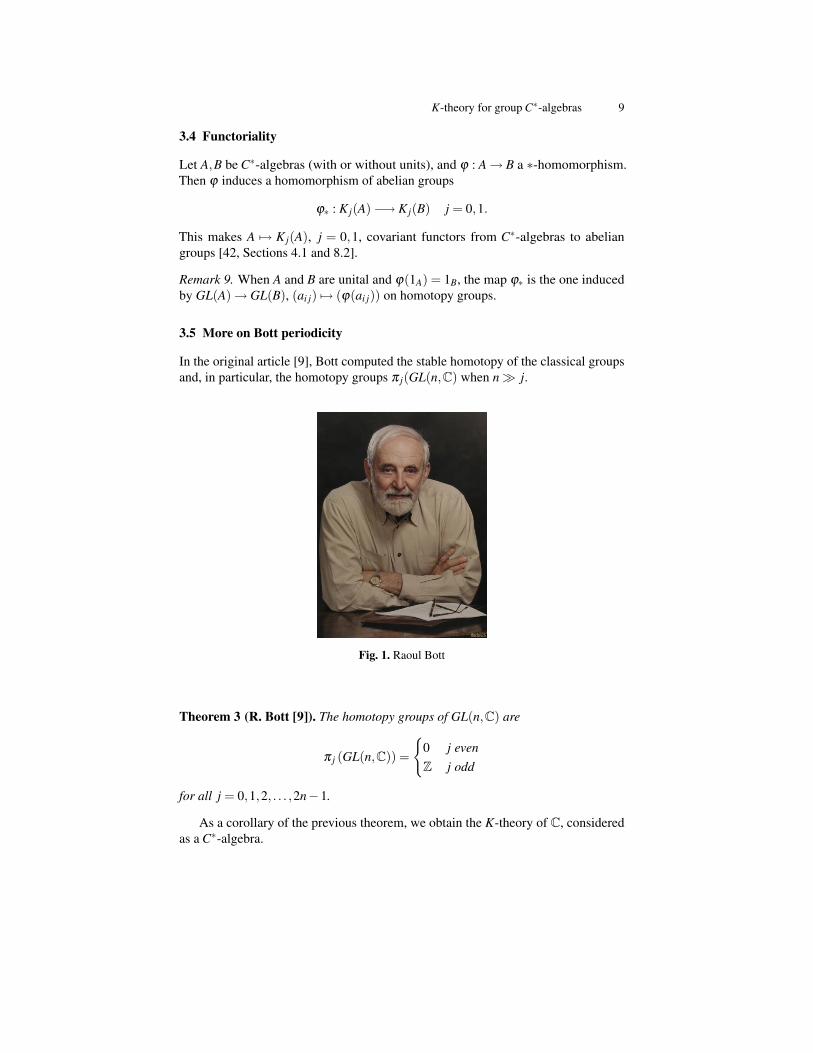
In the original article [9], Bott computed the stable homotopy of the classical groupsand, in particular, the homotopy groups π j(GL(n,C) when n j.
Fig. 1. Raoul Bott
Theorem 3 (R. Bott [9]). The homotopy groups of GL(n,C) are
π j (GL(n,C)) =
0 j evenZ j odd
for all j = 0,1,2, . . . ,2n−1.
As a corollary of the previous theorem, we obtain the K-theory of C, consideredas a C∗-algebra.
10 Paul F. Baum and Ruben J. Sanchez-Garcıa
Theorem 4 (R. Bott).
K j(C) =
Z j even,0 j odd.
Sketch of proof. Since C is a field, K0(C) = Kalg0 (C) =Z. By the polar decomposition,
GL(n,C) is homotopy equivalent to U(n). The homotopy long exact sequence ofthe fibration U(n)→U(n + 1)→ S2n+1 gives π j(U(n)) = π j(U(n + 1)) for all j ≤2n+1. Hence K j(C) = π j−1(GL(C)) = π j−1(GL(2 j−1,C)) and apply the previoustheorem.
Remark 10. Compare this result with Kalg1 (C) = C∗ (since C is a field, see [12, Ex.
3.1.6]). Higher algebraic K-theory groups for C are only partially understood.
3.6 Topological K-theory
There is a close connection between K-theory of C∗-algebras and topological K-theoryof spaces.
Let X be a locally compact, Hausdorff, topological space. Atiyah and Hirzebruch[3] defined abelian groups K0(X) and K1(X) called topological K-theory with com-pact supports. For instance, if X is compact, K0(X) is the Grothendieck group ofcomplex vector bundles on X .
Theorem 5. Let X be a locally compact, Hausdorff, topological space. Then
K j(X) = K j (C0(X)) , j = 0,1.
Remark 11. This is known as Swan’s theorem when j = 0 and X compact.
In turn, topological K-theory can be computed up to torsion via a Chern character.Let X be as above. There is a Chern character from topological K-theory to rationalcohomology with compact supports
ch : K j(X)−→⊕l≥0
H j+2lc (X ;Q) , j = 0,1.
Here the target cohomology theory H∗c (−;Q) can be Cech cohomology with com-pact supports, Alexander-Spanier cohomology with compact supports or representableEilenberg-MacLane cohomology with compact supports.
This map becomes an isomorphism when tensored with the rationals.
Theorem 6. Let X be a locally compact, Hausdorff, topological space. The Cherncharacter is a rational isomorphism, that is,
K j(X)⊗ZQ−→⊕l≥0
H j+2lc (X ;Q) , j = 0,1
is an isomorphism.
Remark 12. This theorem is still true for singular cohomology when X is a locallyfinite CW-complex.

K-theory for group C∗-algebras 11
4 Proper G-spaces
In the following three sections, we will describe the left-hand side of the Baum-Connes conjecture (Conjecture 1). The space EG appearing on the topological side ofthe conjecture is the universal example for proper actions for G. Hence we will startby studying proper G-spaces.
Recall the definition of G-space, G-map and G-homotopy.
Definition 7. A G-space is a topological space X with a given continuous action of G
G×X −→ X .
A G-map is a continuous map f : X → Y between G-spaces such that
f (gp) = g f (p) for all (g, p) ∈ G×X .
Two G-maps f0, f1 : X → Y are G-homotopic if they are homotopic through G-maps,that is, there exists a homotopy ft0≤t≤1 with each ft a G-map.
We will require proper G-spaces to be Hausdorff and paracompact. Recall that aspace X is paracompact if every open cover of X has a locally finite open refinementor, alternatively, a locally finite partition of unity subordinate to any given open cover.
Remark 13. Any metrizable space (i.e. there is a metric with the same underlyingtopology) or any CW-complex (in its usual CW-topology) is Hausdorff and paracom-pact.
Definition 8. A G-space X is proper if
• X is Hausdorff and paracompact;• the quotient space G\X (with the quotient topology) is Hausdorff and paracom-
pact;• for each p ∈ X there exists a triple (U,H,ρ) such that
(a) U is an open neighborhood of p in X with gu ∈U for all (g,u) ∈ G×U;(b) H is a compact subgroup of G;(c) ρ : U → G/H is a G-map.
Note that, in particular, the stabilizer stab(p) is a closed subgroup of a conjugate of Hand hence compact.
Remark 14. The converse is not true in general; the action of Z on S1 by an irrationalrotation is free but it is not a proper Z-space.
Remark 15. If X is a G-CW-complex then it is a proper G-space (even in the weakerdefinition below) if and only if all the cell stabilizers are compact, see Thm. 1.23 in[30].
Our definition is stronger than the usual definition of proper G-space, whichrequires the map G×X → X×X , (g,x) 7→ (gx,x) to be proper, in the sense that thepre-image of a compact set is compact. Nevertheless, both definitions agree for locallycompact, Hausdorff, second countable G-spaces.
12 Paul F. Baum and Ruben J. Sanchez-Garcıa
Proposition 2 (J. Chabert, S. Echterhoff, R. Meyer [11]). If X is a locally compact,Hausdorff, second countable G-space, then X is proper if and only if the map
G×X −→ X×X
(g,x) 7−→ (gx,x)
is proper.
Remark 16. For a more general comparison among these and other definitions ofproper actions see [7].
5 Classifying space for proper actions
Now we are ready for the definition of the space EG appearing in the statement of theBaum-Connes Conjecture. Most of the material in this section is based on Sections 1and 2 of [5].
Definition 9. A universal example for proper actions of G, denoted EG, is a properG-space such that:
• if X is any proper G-space, then there exists a G-map f : X → EG and any twoG-maps from X to EG are G-homotopic.
EG exists for every topological group G [5, Appendix 1] and it is unique up to G-homotopy, as follows. Suppose that EG and (EG)′ are both universal examples forproper actions of G. Then there exist G-maps
f : EG−→ (EG)′
f ′ : (EG)′ −→ EG
and f ′ f and f f ′ must be G-homotopic to the identity maps of EG and (EG)’respectively.
The following are equivalent axioms for a space Y to be EG [5, Appendix 2].
(a) Y is a proper G-space.(b) If H is any compact subgroup of G, then there exists p ∈ Y with hp = p for all
h ∈ H.(c) Consider Y ×Y as a G-space via g(y0,y1) = (gy0,gy1), and the maps
ρ0,ρ1 : Y ×Y −→ Y
ρ0(y0,y1) = y0 , ρ1(y0,y1) = y1 .
Then ρ0 and ρ1 are G-homotopic.
Remark 17. It is possible to define a universal space for any family of (closed) sub-groups of G closed under conjugation and finite intersections [32]. Then EG is theuniversal space for the family of compact subgroups of G.
K-theory for group C∗-algebras 13
Remark 18. The space EG can always be assumed to be a G-CW-complex. Then thereis a homotopy characterization: a proper G-CW-complex X is an EG if and only if foreach compact subgroup H of G the fixed point subcomplex XH is contractible (see[32]).
Examples
(a) If G is compact, EG is just a one-point space.(b) If G is a Lie group with finitely many connected components then EG = G/H,
where H is a maximal compact subgroup (i.e. maximal among compact sub-groups).
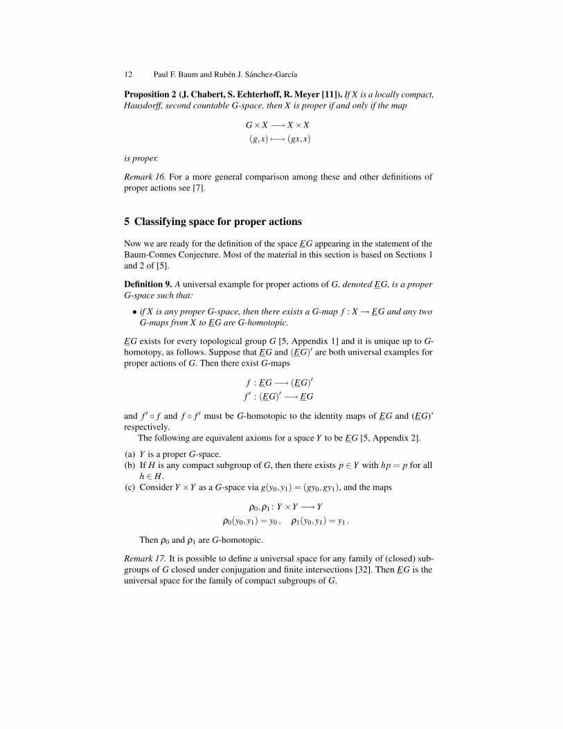
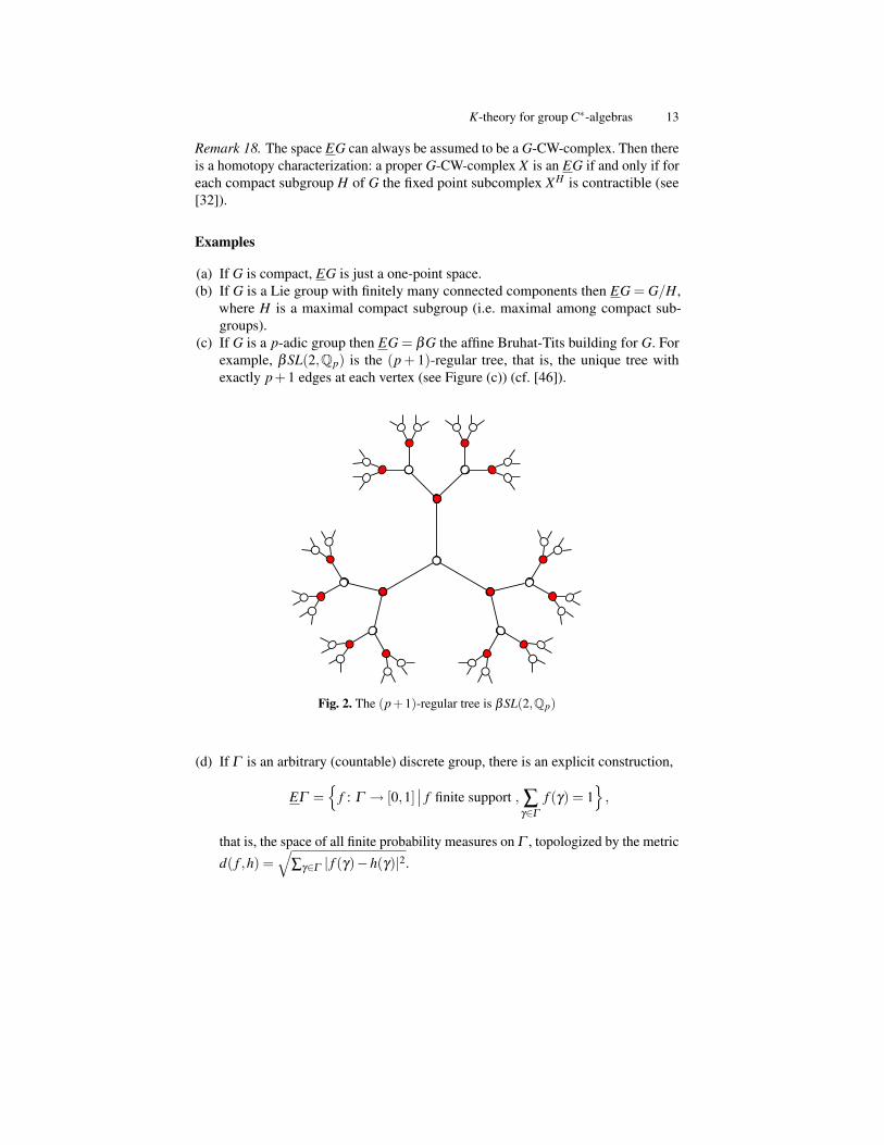
(c) If G is a p-adic group then EG = βG the affine Bruhat-Tits building for G. Forexample, βSL(2,Qp) is the (p + 1)-regular tree, that is, the unique tree withexactly p+1 edges at each vertex (see Figure (c)) (cf. [46]).
Fig. 2. The (p+1)-regular tree is βSL(2,Qp)
(d) If Γ is an arbitrary (countable) discrete group, there is an explicit construction,
EΓ =
f : Γ → [0,1]∣∣ f finite support , ∑
γ∈Γ
f (γ) = 1
,
that is, the space of all finite probability measures on Γ , topologized by the metricd( f ,h) =
√∑γ∈Γ | f (γ)−h(γ)|2.
14 Paul F. Baum and Ruben J. Sanchez-Garcıa
6 Equivariant K-homology
K-homology is the dual theory to Atiyah-Hirzebruch K-theory (Section 3.6). Herewe define an equivariant generalization due to Kasparov [24, 25]. If X is a properG-space with compact, second countable quotient then KG
i (X), i = 0,1, are abeliangroups defined as homotopy classes of K-cycles for X . These K-cycles can be viewedas G-equivariant abstract elliptic operators on X .
Remark 19. For a discrete group G, there is a topological definition of equivariant K-homology and the index map via equivariant spectra [14]. This and other constructionsof the index map are shown to be equivalent in [18].
6.1 Definitions
Let G be a locally compact, Hausdorff, second countable, topological group.Let H be a separable Hilbert space. Write U (H) for the set of unitary operators
U (H) = U ∈L (H) |UU∗ = U∗U = I .
Definition 10. A unitary representation of G on H is a group homomorphism π : G→U (H) such that for each v ∈ H the map πv : G→ H, g 7→ π(g)v is a continuous mapfrom G to H.
Definition 11. A G-C∗-algebra is a C∗-algebra A with a given continuous action of G
G×A−→ A
such that G acts by C∗-algebra automorphisms.
The continuity condition is that, for each a∈A, the map G→A, g 7→ ga is a continuousmap. We also have that, for each g ∈ G, the map A→ A, a 7→ ga is a C∗-algebraautomorphism.
Example 4. Let X be a locally compact, Hausdorff G-space. The action of G on Xgives an action of G on C0(X),
(gα)(x) = α(g−1x),
where g ∈ G, α ∈C0(X) and x ∈ X . This action makes C0(X) into a G-C∗-algebra.
Recall that a C∗-algebra is separable if it has a countable dense subset.
Definition 12. Let A be a separable G-C∗-algebra. A representation of A is a triple(H,ψ,π) with:
• H is a separable Hilbert space,• ψ : A→L (H) is a ∗-homomorphism,• π : G→U (H) is a unitary representation of G on H,• ψ(ga) = π(g)ψ(a)π(g−1) for all (g,a) ∈ G×A.
K-theory for group C∗-algebras 15
Remark 20. We are using a slightly non-standard notation; in the literature this isusually called a covariant representation.
Definition 13. Let X be a proper G-space with compact, second countable quotientspace G\X. An equivariant odd K-cycle for X is a 4-tuple (H,ψ,π,T ) such that:
• (H,ψ,π) is a representation of the G-C∗-algebra C0(X),• T ∈L (H),• T = T ∗,• π(g)T −T π(g) = 0 for all g ∈ G,• ψ(α)T −T ψ(α) ∈K (H) for all α ∈C0(X),• ψ(α)(I−T 2) ∈K (H) for all α ∈C0(X).
Remark 21. If G is a locally compact, Hausdorff, second countable topological groupand X a proper G-space with locally compact quotient then X is also locally compactand hence C0(X) is well-defined.
Write E G1 (X) for the set of equivariant odd K-cycles for X . This concept was intro-
duced by Kasparov as an abstraction an equivariant self-adjoint elliptic operator andgoes back to Atiyah’s theory of elliptic operators [2].
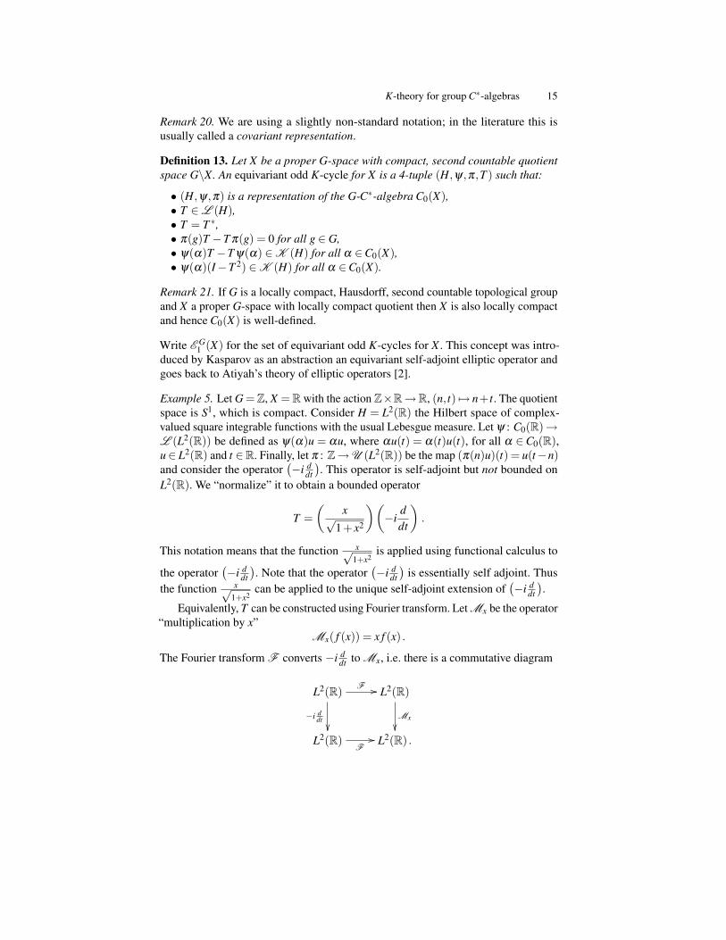
Example 5. Let G =Z, X =R with the action Z×R→R, (n, t) 7→ n+t. The quotientspace is S1, which is compact. Consider H = L2(R) the Hilbert space of complex-valued square integrable functions with the usual Lebesgue measure. Let ψ : C0(R)→L (L2(R)) be defined as ψ(α)u = αu, where αu(t) = α(t)u(t), for all α ∈C0(R),u∈ L2(R) and t ∈R. Finally, let π : Z→U (L2(R)) be the map (π(n)u)(t) = u(t−n)and consider the operator
(−i d
dt
). This operator is self-adjoint but not bounded on
L2(R). We “normalize” it to obtain a bounded operator
T =(
x√1+ x2
)(−i
ddt
).
This notation means that the function x√1+x2
is applied using functional calculus to
the operator(−i d
dt
). Note that the operator
(−i d
dt
)is essentially self adjoint. Thus
the function x√1+x2
can be applied to the unique self-adjoint extension of(−i d
dt
).
Equivalently, T can be constructed using Fourier transform. Let Mx be the operator“multiplication by x”
Mx( f (x)) = x f (x) .
The Fourier transform F converts −i ddt to Mx, i.e. there is a commutative diagram
L2(R) F //
−i ddt
L2(R)
Mx
L2(R)F// L2(R) .
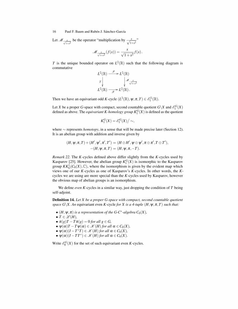
16 Paul F. Baum and Ruben J. Sanchez-Garcıa
Let M x√1+x2
be the operator “multiplication by x√1+x2
”
M x√1+x2
( f (x)) =x√
1+ x2f (x) .
T is the unique bounded operator on L2(R) such that the following diagram iscommutative
L2(R) F //
T
L2(R)
M x√1+x2
L2(R)
F// L2(R) .
Then we have an equivariant odd K-cycle (L2(R),ψ,π,T ) ∈ E Z1 (R).
Let X be a proper G-space with compact, second countable quotient G\X and E G1 (X)
defined as above. The equivariant K-homology group KG1 (X) is defined as the quotient
KG1 (X) = E G
1 (X)/∼,
where ∼ represents homotopy, in a sense that will be made precise later (Section 12).It is an abelian group with addition and inverse given by
(H,ψ,π,T )+(H ′,ψ ′,π ′,T ′) = (H⊕H ′,ψ⊕ψ′,π⊕π
′,T ⊕T ′),−(H,ψ,π,T ) = (H,ψ,π,−T ).
Remark 22. The K-cycles defined above differ slightly from the K-cycles used byKasparov [25]. However, the abelian group KG
1 (X) is isomorphic to the Kasparovgroup KK1
G(C0(X),C), where the isomorphism is given by the evident map whichviews one of our K-cycles as one of Kasparov’s K-cycles. In other words, the K-cycles we are using are more special than the K-cycles used by Kasparov, howeverthe obvious map of abelian groups is an isomorphism.
We define even K-cycles in a similar way, just dropping the condition of T beingself-adjoint.
Definition 14. Let X be a proper G-space with compact, second countable quotientspace G\X. An equivariant even K-cycle for X is a 4-tuple (H,ψ,π,T ) such that:
• (H,ψ,π) is a representation of the G-C∗-algebra C0(X),• T ∈L (H),• π(g)T −T π(g) = 0 for all g ∈ G,• ψ(α)T −T ψ(α) ∈K (H) for all α ∈C0(X),• ψ(α)(I−T ∗T ) ∈K (H) for all α ∈C0(X),• ψ(α)(I−T T ∗) ∈K (H) for all α ∈C0(X).
Write E G0 (X) for the set of such equivariant even K-cycles.
K-theory for group C∗-algebras 17
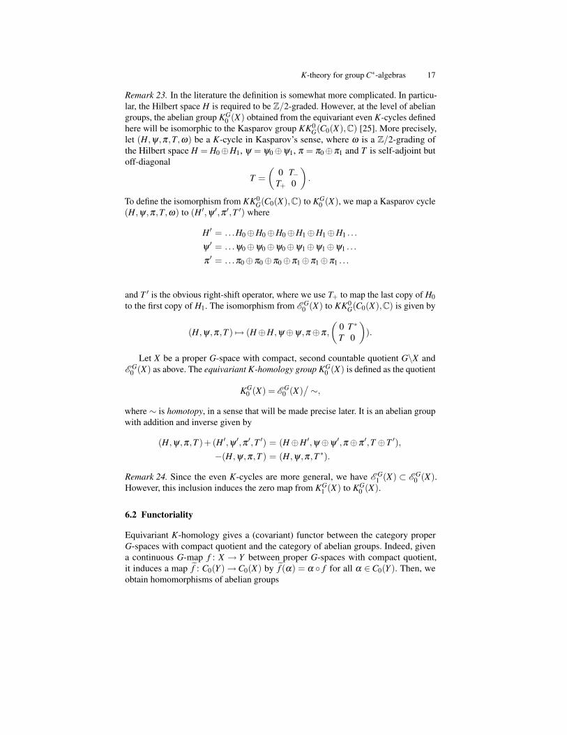
Remark 23. In the literature the definition is somewhat more complicated. In particu-lar, the Hilbert space H is required to be Z/2-graded. However, at the level of abeliangroups, the abelian group KG
0 (X) obtained from the equivariant even K-cycles definedhere will be isomorphic to the Kasparov group KK0
G(C0(X),C) [25]. More precisely,let (H,ψ,π,T,ω) be a K-cycle in Kasparov’s sense, where ω is a Z/2-grading ofthe Hilbert space H = H0⊕H1, ψ = ψ0⊕ψ1, π = π0⊕π1 and T is self-adjoint butoff-diagonal
T =(
0 T−T+ 0
).
To define the isomorphism from KK0G(C0(X),C) to KG
0 (X), we map a Kasparov cycle(H,ψ,π,T,ω) to (H ′,ψ ′,π ′,T ′) where
H ′ = . . .H0⊕H0⊕H0⊕H1⊕H1⊕H1 . . .
ψ′ = . . .ψ0⊕ψ0⊕ψ0⊕ψ1⊕ψ1⊕ψ1 . . .
π′ = . . .π0⊕π0⊕π0⊕π1⊕π1⊕π1 . . .
and T ′ is the obvious right-shift operator, where we use T+ to map the last copy of H0to the first copy of H1. The isomorphism from E G
0 (X) to KK0G(C0(X),C) is given by
(H,ψ,π,T ) 7→ (H⊕H,ψ⊕ψ,π⊕π,
(0 T ∗
T 0
)).
Let X be a proper G-space with compact, second countable quotient G\X andE G
0 (X) as above. The equivariant K-homology group KG0 (X) is defined as the quotient
KG0 (X) = E G
0 (X)/∼,
where ∼ is homotopy, in a sense that will be made precise later. It is an abelian groupwith addition and inverse given by
(H,ψ,π,T )+(H ′,ψ ′,π ′,T ′) = (H⊕H ′,ψ⊕ψ′,π⊕π
′,T ⊕T ′),−(H,ψ,π,T ) = (H,ψ,π,T ∗).
Remark 24. Since the even K-cycles are more general, we have E G1 (X) ⊂ E G
0 (X).However, this inclusion induces the zero map from KG
1 (X) to KG0 (X).
6.2 Functoriality
Equivariant K-homology gives a (covariant) functor between the category properG-spaces with compact quotient and the category of abelian groups. Indeed, givena continuous G-map f : X → Y between proper G-spaces with compact quotient,it induces a map f : C0(Y )→C0(X) by f (α) = α f for all α ∈C0(Y ). Then, weobtain homomorphisms of abelian groups
18 Paul F. Baum and Ruben J. Sanchez-Garcıa
KGj (X)−→ KG
j (Y ) j = 0,1
by defining, for each (H,ψ,π,T ) ∈ E Gj (X),
(H,ψ,π,T ) 7→ (H,ψ f ,π,T ) .
6.3 The index map
Let X be a proper second countable G-space with compact quotient G\X . There is amap of abelian groups
KGj (X) −→ K j (C∗r (G))
(H,ψ,π,T ) 7→ Index(T )
for j = 0,1. It is called the index map and will be defined in Section 14.This map is natural, that is, if X and Y are proper second countable G-spaces
with compact quotient and if f : X → Y is a continuous G-equivariant map, then thefollowing diagram commutes:
KGj (X)
f∗ //
Index
KGj (Y )
Index
KGj (C∗r (G)) = // KG
j (C∗r (G)).
We would like to define equivariant K-homology and the index map for EG. However,the quotient of EG by the G-action might not be compact. The solution will be toconsider all proper second countable G-subspaces with compact quotient.
Definition 15. Let Z be a proper G-space. We call ∆ ⊆ Z G-compact if
(a) gx ∈ ∆ for all g ∈ G, x ∈ ∆ ,(b) ∆ is a proper G-space,(c) the quotient space G\∆ is compact.
That is, ∆ is a G-subspace which is proper as a G-space and has compact quotientG\∆ .
Remark 25. Since we are always assuming that G is locally compact, Hausdorff andsecond countable, we may also assume without loss of generality that any G-compactsubset of EG is second countable. From now on we shall assume that EG has thisproperty.
We define the equivariant K-homology of EG with G-compact supports as the directlimit
KGj (EG) = lim −→
∆⊆EGG-compact
KGj (∆) .
K-theory for group C∗-algebras 19
There is then a well-defined index map on the direct limit
µ : KGj (EG) −→ K j(C∗r G)
(H,ψ,π,T ) 7→ Index(T ), (1)
as follows. Suppose that ∆ ⊂ Ω are G-compact. By the naturality of the functorKG
j (−), there is a commutative diagram
KGj (∆) //
Index
KGj (Ω)
Index
K j(C∗r G) = // K j(C∗r G) ,
and thus the index map is defined on the direct limit.
7 The discrete case
We discuss several aspects of the Baum-Connes conjecture when the group is discrete.
7.1 Equivariant K-homology
For a discrete group Γ , there is a simple description of KΓj (EΓ ) up to torsion, in
purely algebraic terms, given by a Chern character. Here we follow section 7 in [5].Let Γ be a (countable) discrete group. Define FΓ as the set of finite formal sums
FΓ =
∑
finiteλγ [γ] where γ ∈ Γ ,order(γ) < ∞, λγ ∈ C
.
FΓ is a complex vector space and also a Γ -module with Γ -action:
g ·
(∑
λ∈Γ
λγ [γ]
)= ∑
λ∈Γ
λγ [gγg−1] .
Note that the identity element of the group has order 1 and therefore FΓ 6= 0.Consider H j(Γ ;FΓ ), j ≥ 0, the homology groups of Γ with coefficients in the
Γ -module FΓ .
Remark 26. This is standard homological algebra, with no topology involved (Γ isa discrete group and FΓ is a non-topologized module over Γ ). They are classicalhomology groups and have a purely algebraic description (cf. [10]). In general, if Mis a Γ -module then H∗(Γ ;M) is isomorphic to H∗(BΓ ;M), where M means the localsystem on BΓ obtained from the Γ -module M.
20 Paul F. Baum and Ruben J. Sanchez-Garcıa
Let us write Ktopj (Γ ) for KΓ
j (EΓ ), j = 0,1. There is a Chern character ch : Ktop∗ (Γ )→
H∗(Γ ;FΓ ) which maps into odd, respectively even, homology
ch: Ktopj (Γ )→
⊕l≥0
H j+2l(Γ ;FΓ ) j = 0,1.
This map becomes an isomorphism when tensored with C(cf. [4] or [31]).
Proposition 3. The map
ch⊗ZC : Ktopj (Γ )⊗ZC−→
⊕l≥0
H j+2l(Γ ;FΓ ) j = 0,1
is an isomorphism of vector spaces over C.
Remark 27. If G is finite, the rationalized Chern character becomes the charactermap from R(G), the complex representation ring of G, to class functions, given byρ 7→ χ(ρ) in the even case, and the zero map in the odd case.
If the Baum-Connes conjecture is true for Γ , then Proposition 3 computes thetensored topological K-theory of the reduced C∗-algebra of Γ .
Corollary 1. If the Baum-Connes conjecture is true for Γ then
K j(C∗r Γ )⊗ZC∼=⊕l≥0
H j+2l(Γ ;FΓ ) j = 0,1 .
7.2 Some results on discrete groups
We recollect some results on discrete groups which satisfy the Baum-Connes conjec-ture.
Theorem 7 (N. Higson, G. Kasparov [21]). If Γ is a discrete group which isamenable (or, more generally, a-T-menable) then the Baum-Connes conjecture istrue for Γ .
Theorem 8 (I.Mineyev, G. Yu [37]; independently V. Lafforgue [28]). If Γ is a dis-crete group which is hyperbolic (in Gromov’s sense) then the Baum-Connes conjectureis true for Γ .
Theorem 9 (Schick [45]). Let Bn be the braid group on n strands, for any positiveinteger n. Then the Baum-Connes conjecture is true for Bn.
Theorem 10 (Matthey, Oyono-Oyono, Pitsch [35]). Let M be a connected ori-entable 3-dimensional manifold (possibly with boundary). Let Γ be the fundamentalgroup of M. Then the Baum-Connes conjecture is true for Γ .
The Baum-Connes index map has been shown to be injective or rationally injectivefor some classes of groups. For example, it is injective for countable subgroups ofGL(n,K), K any field [17], and injective for
K-theory for group C∗-algebras 21
• closed subgroups of connected Lie groups [26];• closed subgroups of reductive p-adic groups [27].
More results on groups satisfying the Baum-Connes conjecture can be found in [34].The Baum-Connes conjecture remains a widely open problem. For example, it is
not known for SL(n,Z), n≥ 3. These infinite discrete groups have Kazhdan’s property(T) and hence they are not a-T-menable. On the other hand, it is known that the indexmap is injective for SL(n,Z) (see above) and the groups KG
j (EG) for G = SL(3,Z)have been calculated [44].
Remark 28. The conjecture might be too general to be true for all groups. Nevertheless,we expect it to be true for a large family of groups, in particular for all exact groups(a groups G is exact if the functor C∗r (G,−), as defined in 11.2, is exact).
7.3 Corollaries of the Baum-Connes Conjecture
The Baum-Connes conjecture is related to a great number of conjectures in functionalanalysis, algebra, geometry and topology. Most of these conjectures follow fromeither the injectivity or the surjectivity of the index map. A significant example isthe Novikov conjecture on the homotopy invariance of higher signatures of closed,connected, oriented, smooth manifolds. This conjecture follows from the injectivityof the rationalized index map [5]. For more information on conjectures related toBaum-Connes, see the appendix in [38].
Remark 29. By a “corollary” of the Baum-Connes conjecture we mean: if the Baum-Connes conjecture is true for a group G then the corollary is true for that group G.(For instance, in the Novikov conjecture G is the fundamental group of the manifold.)
8 The compact case
If G is compact, we can take EG to be a one-point space. On the other hand,K0(C∗r G) = R(G) the (complex) representation ring of G, and K1(C∗r G) = 0 (seeRemark below). Recall that R(G) is the Grothendieck group of the category of fi-nite dimensional (complex) representations of G. It is a free abelian group with onegenerator for each distinct (i.e. non-equivalent) irreducible representation of G.
Remark 30. When G is compact, the reduced C∗-algebra of G is a direct sum (inthe C∗-algebra sense) over the irreducible representations of G, of matrix algebrasof dimension equal to the dimension of the representation. The K-theory functorcommutes with direct sums and K j(Mn(C)) ∼= K j(C), which is Z for j even and 0otherwise (Theorem 4).
Hence the index map takes the form
µ : K0G(point)−→ R(G) ,
22 Paul F. Baum and Ruben J. Sanchez-Garcıa
for j = 0 and is the zero map for j = 1.Given (H,ψ,T,π) ∈ E 0
G(point), we may assume within the equivalence relationon E 0
G(point) that
ψ(λ ) = λ I for all λ ∈C0(point) = C ,
where I is the identity operator of the Hilbert space H. Hence the non-triviality of(H,ψ,T,π) is coming from
I−T T ∗ ∈K (H) , and I−T ∗T ∈K (H) ,
that is, T is a Fredholm operator. Therefore
dimC (ker(T )) < ∞,
dimC (coker(T )) < ∞,
hence ker(T ) and coker(T ) are finite dimensional representations of G (recall that Gis acting via π : G→L (H)). Then
µ(H,ψ,T,π) = Index(T ) = ker(T )− coker(T ) ∈ R(G) .
Remark 31. The assembly map for G compact just described is an isomorphism(exercise).
Remark 32. In general, for G non-compact, the elements of KG0 (X) can be viewed
as generalized elliptic operators on EG, and the index map µ assigns to such anoperator its ‘index’, ker(T )− coker(T ), in some suitable sense [5]. This should bemade precise later using Kasparov’s descent map and an appropriate Kasparov product(Section 14).
9 Equivariant K-homology for G-C∗-algebras
We have defined equivariant K-homology for G-spaces in Section 6. Now we de-fine equivariant K-homology for a separable G-C∗-algebra A as the KK-theorygroups K j
G(A,C), j = 0,1. This generalises the previous construction since KGj (X) =
KK jG(C0(X),C). Later on we shall define KK-theory groups in full generality (Sec-
tions 12 and 13).
Definition 16. Let A be a separable G-C∗-algebra. Define E 1G(A) to be the set of
4-tuples(H,ψ,π,T )
such that (H,ψ,π) is a representation of the G-C∗-algebra A, T ∈L (H), and thefollowing conditions are satisfied:
• T = T ∗,• π(g)T −T π(g) ∈K (H),
K-theory for group C∗-algebras 23
• ψ(a)T −T ψ(a) ∈K (H),• ψ(a)(I−T 2) ∈K (H),
for all g ∈ G, a ∈ A.
Remark 33. Note that this is not quite E G1 (X) when A = C0(X) and X is a proper
G-space with compact quotient, since the third condition is more general than before.However, the inclusion E G
1 (X)⊂ E 1G(C0(X)) gives an isomorphism of abelian groups
so that KG1 (X) = KK1
G(C0(X),C) (as defined below). The point is that, for a proper G-space with compact quotient, an averaging argument using a cut-off function and theHaar measure of the group G allows us to assume that the operator T is G-equivariant.
Given a separable G-C∗-algebra A, we define the KK-group KK1G(A,C) as E 1
G(A)modulo an equivalence relation called homotopy, which will be made precise later.Addition in KK1
G(A,C) is given by direct sum
(H,ψ,π,T )+(H ′,ψ ′,π ′,T ′) = (H⊕H ′,ψ⊕ψ′,π⊕π
′,T ⊕T ′)
and the negative of an element by
−(H,ψ,π,T ) = (H,ψ,π,−T ) .
Remark 34. We shall later define KK1G(A,B) for a separable G-C∗-algebras A and an
arbitrary G-C∗-algebra B (Section 12).
Let A, B be separable G-C∗-algebras. A G-equivariant ∗-homomorphism φ : A→B gives a map E 1
G(B)→ E 1G(A) by
(H,ψ,π,T ) 7→ (H,ψ φ ,π,T ) ,
and this induces a map KK1G(B,C)→ KK1
G(A,C). That is, KK1G(A,C) is a contravari-
ant functor in A.For the even case, the operator T is not required to be self-adjoint.
Definition 17. Let A be a separable G-C∗-algebra. Define E 0G(A) as the set of 4-tuples
(H,ψ,π,T )
such that (H,ψ,π) is a representation of the G-C∗-algebra A, T ∈L (H) and thefollowing conditions are satisfied:
• π(g)T −T π(g) ∈K (H),• ψ(a)T −T ψ(a) ∈K (H),• ψ(a)(I−T ∗T ) ∈K (H),• ψ(a)(I−T T ∗) ∈K (H),
for all g ∈ G, a ∈ A.
Remark 35. Again, if X is a proper G-space with compact quotient, the inclusionE G
0 (X)⊂ E 0G(C0(X)) gives an isomorphism in K-homology, so we can write KG
0 (X) =KK0(C0(X),C) (as defined below). The issue of the Z/2-grading (which is present inthe Kasparov definition but not in our definition) is dealt with as in Remark 23.
24 Paul F. Baum and Ruben J. Sanchez-Garcıa
We define the KK-groups KK0G(A,C) as E 0
G(A) modulo an equivalence relationcalled homotopy, which will be made precise later. Addition in KK1
G(A,C) is givenby direct sum
(H,ψ,π,T )+(H ′,ψ ′,π ′,T ′) = (H⊕H ′,ψ⊕ψ′,π⊕π
′,T ⊕T ′)
and the negative of an element by
−(H,ψ,π,T ) = (H,ψ,π,T ∗) .
Remark 36. We shall later define in general KK0G(A,B) for a separable G-C∗-algebras
A and an arbitrary G-C∗-algebra B (Section 13).
Let A, B be separable G-C∗-algebras. A G-equivariant ∗-homomorphism φ : A→B gives a map E 0
G(B)→ E 0G(A) by
(H,ψ,π,T ) 7→ (H,ψ φ ,π,T ) ,
and this induces a map KK0G(B,C)→ KK0
G(A,C). That is, KK0G(A,C) is a contravari-
ant functor in A.
10 The conjecture with coefficients
There is a generalized version of the Baum-Connes conjecture, known as the Baum-Connes conjecture with coefficients, which adds coefficients in a G-C∗-algebra. Werecall the definition of G-C∗-algebra.
Definition 18. A G-C∗-algebra is a C∗-algebra A with a given continuous action of G
G×A−→ A
such that G acts by C∗-algebra automorphisms. Continuity means that, for each a ∈ A,the map G→ A, g 7→ ga is a continuous map.
Remark 37. Observe that the only ∗-homomorphism of C as a C∗-algebra is theidentity. Hence the only G-C∗-algebra structure on C is the one with trivial G-action.
Let A be a G-C∗-algebra. Later we shall define the reduced crossed-product C∗-algebra C∗r (G,A), and the equivariant K-homology group with coefficients KG
j (EG,A).These constructions reduce to C∗r (G), respectively KG
j (EG), when A = C. Moreover,the index map extends to this general setting and is also conjectured to be an isomor-phism.
Conjecture 2 (P. Baum, A. Connes, 1980). Let G be a locally compact, Hausdorff,second countable, topological group, and let A be any G-C∗-algebra. Then
µ : KGj (EG,A)−→ K j(C∗r (G,A)) j = 0,1
is an isomorphism.
K-theory for group C∗-algebras 25
Conjecture 1 follows as a particular case when A = C. A fundamental difference isthat the conjecture with coefficients is subgroup closed, that is, if it is true for a groupG for any coefficients then it is true, for any coefficients, for any closed subgroup ofG.
The conjecture with coefficients has been proved for:
• compact groups,• abelian groups,• groups acting simplicially on a tree with all vertex stabilizers satisfying the
conjecture with coefficients [40],• amenable groups and, more generally, a-T-menable groups (groups with the
Haagerup property) [22],• the Lie group Sp(n,1) [23],• 3-manifold groups [35].
For more examples of groups satisfying the conjecture with coefficients see [34].
Expander graphs
Suppose that Γ is a finitely generated, discrete group which contains an expanderfamily [13] in its Cayley graph as a subgraph. Such a Γ is a counter-example to theconjecture with coefficients [19]. M. Gromov outlined a proof that such Γ exists. Anumber of mathematicians are now filling in the details. It seems quite likely that thisgroup exists.
11 Hilbert modules
In this section we introduce the concept of Hilbert module over a C∗-algebra. Itgeneralises the definition of Hilbert space by allowing the inner product to take valuesin a C∗-algebra. Our main application will be the definition of the reduced crossed-product C∗-algebra in Section 11.2. For a concise reference on Hilbert modules see[29].
11.1 Definitions and examples
Let A be a C∗-algebra.
Definition 19. An element a ∈ A is positive (notation: a≥ 0) if there exists b ∈ A withbb∗ = a.
The subset of positive elements, A+, is a convex cone (closed under positive linearcombinations) and A+ ∩ (−A+) = 0 [15, 1.6.1]. Hence we have a well-definedpartial ordering in A given by x≥ y ⇐⇒ x− y≥ 0.
Definition 20. A pre-Hilbert A-module is a right A-module H with a given A-valuedinner product 〈 , 〉 such that:
26 Paul F. Baum and Ruben J. Sanchez-Garcıa
• 〈u,v1 + v2〉= 〈u,v1〉+ 〈u,v2〉,• 〈u,va〉= 〈u,v〉a,• 〈u,v〉= 〈v,u〉∗,• 〈u,u〉 ≥ 0,• 〈u,u〉= 0⇔ u = 0,
for all u,v,v1,v2 ∈H , a ∈ A.
Definition 21. A Hilbert A-module is a pre-Hilbert A-module which is complete withrespect to the norm
‖u‖= ‖〈u,u〉‖1/2 .
Remark 38. If H is a Hilbert A-module and A has a unit 1A then H is a complexvector space with
uλ = u(λ1A) u ∈H ,λ ∈ C .
If A does not have a unit, then by using an approximate identity [41] in A, it is also acomplex vector space.
Example 6. Let A be a C∗-algebra and n ≥ 1. Then An = A⊕ . . .⊕A is a HilbertA-module with operations
(a1, . . . ,an)+(b1, . . . ,bn) = (a1 +b1, . . . ,an +bn),(a1, . . . ,an)a = (a1a, . . . ,ana),
〈(a1, . . . ,an),(b1, . . . ,bn)〉= a∗1b1 + . . .+a∗nbn,
for all a j,b j,a ∈ A.
Example 7. Let A be a C∗-algebra. Define
H =
(a1,a2, . . .)∣∣a j ∈ A,
∞
∑j=1
a∗ja j is norm-convergent in A
,
with operations
(a1,a2, . . .)+(b1,b2 . . .) = (a1 +b1,a2 +b2, . . .),(a1,a2, . . .)a = (a1a,a2a, . . .),
〈(a1,a2, . . .),(b1,b2 . . .)〉=∞
∑j=1
a∗jb j.
The previous examples can be generalized. Note that a C∗-algebra A is a Hilbertmodule over itself with inner product 〈a,b〉= a∗b.
Example 8. If H1, . . . ,Hn are Hilbert A-modules then the direct sum H1⊕ . . .⊕Hnis a Hilbert A-module with
〈(x1, . . . ,xn),(y1, . . . ,yn)〉= ∑i
x∗i yi .
We write H n for the direct sum of n copies of a Hilbert A-module H .
K-theory for group C∗-algebras 27
Example 9. If Hii∈N is a countable family of Hilbert A-modules then
H =
(x1,x2, . . .)∣∣xi ∈Hi,
∞
∑j=1〈x j,x j〉 is norm-convergent in A
is a Hilbert A-module with inner product 〈x,y〉= ∑
∞j=1〈x j,y j〉.
The following is our key example.
Example 10. Let G be a locally compact, Hausdorff, second countable, topologicalgroup. Fix a left-invariant Haar measure dg for G. Let A be a G-C∗-algebra. ThenL2(G,A) is a Hilbert A-module defined as follows. Denote by Cc(G,A) the set of allcontinuous compactly supported functions from G to A. On Cc(G,A) consider thenorm
‖ f‖=∥∥∥∥∫G
g−1 ( f (g)∗ f (g))dg∥∥∥∥ .
L2(G,A) is the completion of Cc(G,A) in this norm. It is a Hilbert A-module withoperations
( f +h)g = f (g)+h(g),( f a)g = f (g)(ga),
〈 f ,h〉=∫
Gg−1 ( f (g)∗h(g))dg .
Note that when A = C the group action is trivial and we get L2(G) (cf. Remark 37).
Definition 22. Let H be a Hilbert A-module. An A-module map T : H →H isadjointable if there exists an A-module map T ∗ : H →H with
〈Tu,v〉= 〈u,T ∗v〉 for all u,v ∈H .
If T ∗ exists, it is unique, and sup‖u‖=1 ‖Tu‖< ∞. Set
L (H ) = T : H →H |T is adjointable .
Then L (H ) is a C∗-algebra with operations
(T +S)u = Tu+Su,
(ST )u = S(Tu),(T λ )u = (Tu)λ
T ∗ as above,‖T‖= sup
‖u‖=1‖Tu‖.
28 Paul F. Baum and Ruben J. Sanchez-Garcıa
11.2 The reduced crossed-product C∗r (G,A)
Let A be a G-C∗-algebra. Define
Cc(G,A) = f : G→ A | f continuous with compact support .
Then Cc(G,A) is a complex algebra with
( f +h)g = f (g)+h(g),( f λ )g = f (g)λ ,
( f ∗h)(g0) =∫
Gf (g)
(gh(g−1g0)
)dg,
for all g,g0 ∈ G, λ ∈ C, f ,h ∈Cc(G,A). The product ∗ is called twisted convolution.Consider the Hilbert A-module L2(G,A). There is an injection of algebras
Cc(G,A) →L (L2(G,A))f 7→ Tf
where Tf (u) = f ∗u is twisted convolution as above. We define C∗r (G,A) as the C∗-algebra obtained by completing Cc(G,A) with respect to the norm ‖ f‖= ‖Tf ‖. WhenA = C, the G-action must be trivial and C∗r (G,A) = C∗r (G).
Example 11. Let G be a finite group, and A a G-C∗-algebra. Let dg be the Haarmeasure such that each g ∈ G has mass 1. Then
C∗r (G,A) =
∑γ∈G
aγ [γ]∣∣∣ aγ ∈ A
with operations (
∑γ∈G
aγ [γ]
)+
(∑γ∈G
bγ [γ]
)= ∑
γ∈G(aγ +bγ)[γ],(
∑γ∈G
aγ [γ]
)λ = ∑
γ∈G(aγ λ )[γ],
(aα [α])(bβ [β ]) = aα(αbβ )[αβ ] (twisted convolution),(∑γ∈G
aγ [γ]
)∗= ∑
γ∈G(γ−1a∗γ)[γ
−1].
Here aγ [γ] denotes the function from G to A which has the value aγ at γ and 0 atg 6= γ .
Let X be a Hausdorff, locally compact G-space. We know that C0(X) becomes aG-C∗-algebra with G-action
(g f )(x) = f (g−1x),
K-theory for group C∗-algebras 29
for g ∈ G, f ∈C0(X) and x ∈ X . The reduced crossed-product C∗r (G,C0(X)) will bedenoted C∗r (G,X).
A natural question is to calculate the K-theory of this C∗-algebra. If G is com-pact, this is the Atiyah-Segal group K j
G(X), j = 0,1. Hence for G non-compact,K j(C∗r (G,X)) is the natural extension of the Atiyah-Segal theory to the case when Gis non-compact.
Definition 23. We call a G-space G-compact if the quotient space G\X (with thequotient topology) is compact.
Let X be a proper, G-compact G-space. Then a G-equivariant C-vector bundle E onX determines an element
[E] ∈ K0(C∗r (G,X)) .
Remark 39. From E, a Hilbert module over C∗r (G,X) is constructed. This HilbertC∗r (G,X)-module determines an element in KK0(C,C∗r (G,X))∼= K0(C∗r (G,X)). Notethat, quite generally, a Hilbert A-module determines an element in KK0(A) if and onlyif it is finitely generated.
Recall that a G-equivariant vector bundle E over X is a (complex) vector bundleπ : E→ X together with a G-action on E such that π is G-equivariant and, for eachp ∈ X , the map on the fibers Ep→ Egp induced by multiplication by g is linear.
Theorem 11 (W. Luck and B. Oliver [33]). If Γ is a (countable) discrete group andX is a proper Γ -compact Γ -space, then
K0(C∗r (Γ ,X)) = Grothendieck group of Γ -equivariant C-vector bundles on X .
Remark 40. In [33] this theorem is not explicitly stated. However, it follows fromtheir results. For clarification see [6] or [?].
Remark 41. Let X be a proper G-compact G-space. Let I be the trivial G-equivariantcomplex vector bundle on X ,
I= X×C , g(x,λ ) = (gx,λ ),
for all g ∈ G, x ∈ X and λ ∈ C. Then [I ] ∈ K0(C∗r (G,X)).
11.3 Push-forward of Hilbert modules
Let A, B be C∗-algebras, ϕ : A→ B a ∗-homomorphism and H a Hilbert A-module.We shall define a Hilbert B-module H ⊗A B, called the push-forward of H withrespect to ϕ or interior tensor product ([29, Chapter 4]). First, form the algebraictensor product H A B = H ⊗alg
A B (B is an A-module via ϕ). This is an abeliangroup and also a (right) B-module
(h⊗b)b′ = h⊗bb′ for all h ∈H ,b,b′ ∈ B .
30 Paul F. Baum and Ruben J. Sanchez-Garcıa
Define a B-valued inner product on H A B by
〈h⊗b,h′⊗b′〉= b∗ϕ(〈h,h′〉)b′.
SetN = ξ ∈H A B | 〈ξ ,ξ 〉= 0 .
N is a B-sub-module of H A B and (H A B)/N is a pre-Hilbert B-module.
Definition 24. Define H ⊗A B to be the Hilbert B-module obtained by completing(H A B)/N .
Example 12. Let X be a locally compact, Hausdorff space. Let A = C0(X), B = Cand evp : C0(X)→ C the evaluation map at a point p ∈ X . Then we can considerthe push-forward of a Hilbert C0(X)-module H . This gives a Hilbert space Hp.These Hilbert spaces do not form a vector bundle but something more general (notnecessarily locally trivial), sometimes called continuous field of Hilbert spaces [15,chapter 10].
12 Homotopy made precise and KK-theory
We first define homotopy and Kasparov’s KK-theory in the non-equivariant setting,for pairs of separable C∗-algebras. A first introduction to KK-theory and furtherreferences can be found in [20].
Let A be a C∗-algebra and let H be a Hilbert A-module. Consider L (H ) thebounded operators on H . For each u,v∈H we have a bounded operator θu,v definedas
θu,v(ξ ) = u〈v,ξ 〉 .
It is clear that θ ∗u,v = θv,u. The θu,v are called rank one operators on H . A finite rankoperator on H is any T ∈L (H ) such that T is a finite sum of rank one operators,
T = θu1,v1 + . . .+θun,vn .
Let K (H ) be the closure (in L (H )) of the set of finite rank operators. K (H ) isan ideal in L (H ). When A = C, H is a Hilbert space and K (H ) coincides withthe usual compact operators on H .
Definition 25. H is countably generated if in H there is a countable (or finite) setsuch that the A-module generated by this set is dense in H .
Definition 26. Let H0, H1 be two Hilbert A-modules. We say that H0 and H1 areisomorphic if there exists an A-module isomorphism Φ : H0→H1 with
〈u,v〉0 = 〈Φu,Φv〉1 for all u,v ∈H0 .
K-theory for group C∗-algebras 31
We want to define non-equivariant KK-theory for pairs of C∗-algebras. Let A andB be C∗-algebras where A is also separable. Define the set
E 1(A,B) = (H ,ψ,T )
such that H is a countably generated Hilbert B-module, ψ : A→ L (H ) is a ∗-homomorphism, T ∈L (H ), and the following conditions are satisfied:
• T = T ∗,• ψ(a)T −T ψ(a) ∈K (H ),• ψ(a)(I−T 2) ∈K (H ),
for all a ∈ A. We call such triples odd bivariant K-cycles.
Remark 42. In the Kasparov definition of KK1(A,B) [24], the conditions of the K-cycles are the same as our conditions except that the requirement T = T ∗ is replacedby ψ(a)(T −T ∗) ∈K (H) for all a ∈ A. The isomorphism of abelian groups from thegroup defined using these bivariant K-cycles to the group defined using our bivariantK-cycles is obtained by sending a Kasparov cycle (H,ψ,T ) to (H,ψ, T+T ∗
2 ).
We say that two such triples (H0,ψ0,T0) and (H1,ψ1,T1) in E 1(A,B) are iso-morphic if there is an isomorphism of Hilbert B-modules Φ : H0→H1 with
Φψ0(a) = ψ1(a)Φ ,
ΦT0 = T1Φ ,
for all a ∈ A. That is, the following diagrams commute
H0ψ0(a) //
Φ
H0
Φ
H1
ψ1(a)// H1
H0T0 //
Φ
H0
Φ
H1 T1
// H1
Let A, B, D be C∗-algebras where A is also separable. A ∗-homomorphism ϕ : B→D induces a map ϕ∗ : E 1(A,B)→ E 1(A,D) by
ϕ∗(H ,ψ,T ) = (H ⊗B D,ψ⊗B I,T ⊗B I)
where I is the identity operator on D, that is, I(α) = α for all α ∈ D.We can now make the definition of homotopy precise. Consider the C∗-algebra of
continuous functions C([0,1],B), and set ρ0, ρ1 to be the ∗-homomorphisms
C([0,1],B)ρ0 //
ρ1// B
defined by ρ0( f ) = f (0) and ρ1( f ) = f (1). In particular, we have induced maps
(ρ j)∗ : E 1(A,C([0,1],B))−→ E 1(A,B) j = 0,1
for any separable C∗-algebra A.
32 Paul F. Baum and Ruben J. Sanchez-Garcıa
Definition 27. Two triples (H0,ψ0,T0) and (H1,ψ1,T1) in E 1(A,B) are homotopicif there exists (H ,ψ,T ) in E 1(A,C([0,1],B)) with
(ρ j)∗(H ,ψ,T )∼= (H j,ψ j,Tj) j = 0,1 .
The even case is analogous, removing the self-adjoint condition T = T ∗.
Remark 43. As above, we do not require the Hilbert B-module H to be Z/2-graded.The isomorphism between the abelian group we are defining and the group KK0(A,B)as defined by Kasparov [24] is dealt with as before (see Remark 23).
Hence we have the set of even bivariant K-cycles
E 0(A,B) = (H ,ψ,T )
where H is a countably generated Hilbert B-module, ψ : A→L (H ) a ∗-homomorphism,T ∈L (H ), and the following conditions are satisfied:
• ψ(a)T −T ψ(a) ∈K (H ),• ψ(a)(I−T ∗T ) ∈K (H ),• ψ(a)(I−T T ∗) ∈K (H ),
for all a ∈ A. The remaining definitions carry over, in particular the definition ofhomotopy in E 0(A,B).
We define the (non-equivariant) Kasparov KK-theory groups of the pair (A,B) as
KK1(A,B) = E 1(A,B)/(homotopy),KK0(A,B) = E 0(A,B)/(homotopy).
A key property is that KK-theory incorporates K-theory of C∗-algebras: for anyC∗-algebra B, KK j(C,B) is isomorphic to K j(B) (see Theorem 25 in [36]).
13 Equivariant KK-theory
We generalize KK-theory to the equivariant setting. An alternative definition to ours,by means of a universal property, is described in Section 2 of Meyer’s notes [36].
All through this section, let A be a G-C∗-algebra.
Definition 28. A G-Hilbert A-module is a Hilbert A-module H with a given continu-ous action
G×H → H
(g,v) 7→ gv
such that
(a) g(u+ v) = gu+gv,(b) g(ua) = (gu)(ga),

K-theory for group C∗-algebras 33
(c) 〈gu,gv〉= g〈u,v〉,
for all g ∈ G, u,v ∈H , a ∈ A.
Here ‘continuous’ means that for each u∈H , the map G→H , g 7→ gu is continuous.
Example 13. If A =C, a G-Hilbert C-module is just a unitary representation of G (theaction of G on C must be trivial).
Remark 44. Let H be a G-Hilbert A-module. For each g ∈ G, denote by Lg the map
Lg : H →H , Lg(v) = gv .
Note that Lg might not be in L (H ). But if T ∈L (H ), then LgT L−1g ∈L (H ).
Hence G acts on the C∗-algebra L (H ) by
gT = LgT L−1g .
Example 14. Let A be a G-C∗-algebra. Set n≥ 1. Then An is a G-Hilbert A-module(cf. Example 6) with
g(a1, . . . ,an) = (ga1, . . . ,gan).
Let A and B be G-C∗-algebras, where A is also separable. Define the set
E 0G(A,B) = (H ,ψ,T )
such that H is a countably generated G-Hilbert B-module, ψ : A→ L (H ) is a∗-homomorphism with
ψ(ga) = gψ(a) for all g ∈ G,a ∈ A ,
and T ∈L (H ), and so that the following conditions are satisfied:
• gT −T ∈K (H ),• ψ(a)T −T ψ(a) ∈K (H ),• ψ(a)(I−T ∗T ) ∈K (H ),• ψ(a)(I−T T ∗) ∈K (H ),
for all g ∈ G, a ∈ A. We define
KK0G(A,B) = E 0
G(A,B)/(homotopy) .
The definition of homotopy in Section 12 can be defined in a straightforward way inthis setting.
KK0G(A,B) is an abelian group with addition and negative
(H ,ψ,T )+(H ′,ψ ′,T ′) = (H ⊕H ′,ψ⊕ψ′,T ⊕T ′),
−(H ,ψ,T ) = (H ,ψ,T ∗) .
The odd case is similar, just restricting to self-adjoint operators. Define the set
34 Paul F. Baum and Ruben J. Sanchez-Garcıa
E 1G(A,B) = (H ,ψ,T )
such that H is a countably generated G-Hilbert B-module, ψ : A→ L (H ) is a∗-homomorphism with
ψ(ga) = gψ(a) for all g ∈ G,a ∈ A ,
and T ∈L (H ), and so that the following conditions are satisfied:
• T = T ∗,• gT −T ∈K (H ),• ψ(a)T −T ψ(a) ∈K (H ),• ψ(a)(I−T 2) ∈K (H ),
for all g ∈ G, a ∈ A.We define
KK1G(A,B) = E 1
G(A,B)/(homotopy) .
KK1G(A,B) is an abelian group with addition and inverse given by
(H ,ψ,T )+(H ′,ψ ′,T ′) = (H ⊕H ′,ψ⊕ψ′,T ⊕T ′),
−(H ,ψ,T ) = (H ,ψ,−T ).
Remark 45. In the even case we are not requiring a Z/2-grading. The isomorphism tothe abelian group defined by Kasparov [25] is given as in Remark 23. Our generalprinciple is that the even and odd cases are identical except that in the odd case theoperator T is required to be self-adjoint but not in the even case.
Using equivariant KK-theory, we can introduce coefficients for equivariant K-homology. Let X be a proper G-space with compact quotient. Recall that
KGj (X) = KK j
G(C0(X),C) and
KGj (EG) = lim −→
∆⊆EGG-compact
KGj (∆) .
We define the equivariant K-homology of X , respectively of EG, with coefficients ina G-C∗-algebra A as
KGj (X ,A) = KK j
G(C0(X),A),
KGj (EG,A) = lim −→
∆⊆EGG-compact
KGj (∆ ,A) .
14 The index map
Our definition of the index map uses the Kasparov product and the descent map.
K-theory for group C∗-algebras 35
14.1 The Kasparov product
Let A, B, D be (separable) G-C∗-algebras. There is a product
KKiG(A,B)⊗ZKK j
G(B,D)−→ KKi+ jG (A,D) .
The definition is highly non-trivial. Some motivation and examples, in the non-equivariant case, can be found in [20, Section 5].
Remark 46. Equivariant KK-theory can be regarded as a category with objects separa-ble G-C∗-algebras and morphisms mor(A,B) = KKi
G(A,B) (as a Z/2-graded abeliangroup), and composition given by the Kasparov product (cf. [36, Thm. 33]).
14.2 The Kasparov descent map
Let A and B be (separable) G-C∗-algebras. There is a map between the equivariantKK-theory of (A,B) and the non-equivariant KK-theory of the corresponding reducedcrossed-product C∗-algebras,
KK jG(A,B)−→ KK j (C∗r (G,A),C∗r (G,B)) j = 0,1 .
The definition is also highly non-trivial and can be found in [25, Section 3]. Alterna-tively, see Proposition 26 in Meyer’s notes [36].
14.3 Definition of the index map
We would like to define the index map
µ : KGj (EG)−→ K j(C∗r G) .
Let X be a proper G-compact G-space. First, we define a map
µ : KGj (X) = KK j
G(C0(X),C)−→ K j(C∗r G)
to be the composition of the Kasparov descent map
KK jG(C0(X),C)−→ KK j (C∗r (G,X),C∗r (G))
(the trivial action of G on C gives the crossed-product C∗r (G,C) = C∗r G) and theKasparov product with the trivial bundle
I ∈ K0(C∗r (G,X)) = KK0(C,C∗r (G,X)),
that is, the Kasparov product with the trivial vector bundle I, when A = C, B =C∗r (G,X), D = C∗r G and i = 0.
Recall thatKG
j (EG) = lim −→∆⊂EG
G-compact
KK jG (C0(∆),C) .
36 Paul F. Baum and Ruben J. Sanchez-Garcıa
For each G-compact ∆ ⊂ EG, we have a map as before
µ : KK jG(C0(∆),C)−→ K j(C∗r G) .
If ∆ and Ω are two G-compact subsets of EG with ∆ ⊂ Ω , then by naturality thefollowing diagram commutes:
KK jG(C0(∆),C) //
KK jG(C0(Ω),C)
K jC∗r G = // K jC∗r G.
Thus we obtain a well-defined map on the direct limit µ : KGj (EG)→ K jC∗r G.
14.4 The index map with coefficients
The coefficients can be introduced in KK-theory at once. Let A be a G-C∗-algebra.We would like to define the index map
µ : KGj (EG;A)−→ K jC∗r (G,A) .
Let X be a proper G-compact G-space and A a G-C∗-algebra. First, we define a map
µ : KK jG(C0(X),A)−→ K jC∗r (G,A)
to be the composition of the Kasparov descent map
KK jG(C0(X),A)−→ KK j (C∗r (G,X),C∗r (G,A))
and the Kasparov product with the trivial bundle
I ∈ K0C∗r (G,X) = KK0(C,C∗r (G,X)).
For each G-compact ∆ ⊂ EG, we have a map as above
µ : KK jG(C0(∆),A)−→ K jC∗r (G,A) .
If ∆ and Ω are two G-compact subsets of EG with ∆ ⊂ Ω , then by naturality thefollowing diagram commutes:
KK jG(C0(∆),A) //
KK jG(C0(Ω),A)
K jC∗r (G,A) = // K jC∗r (G,A).
Thus we obtain a well-defined map on the direct limit µ : KGj (EG;A)→ K jC∗r (G,A).
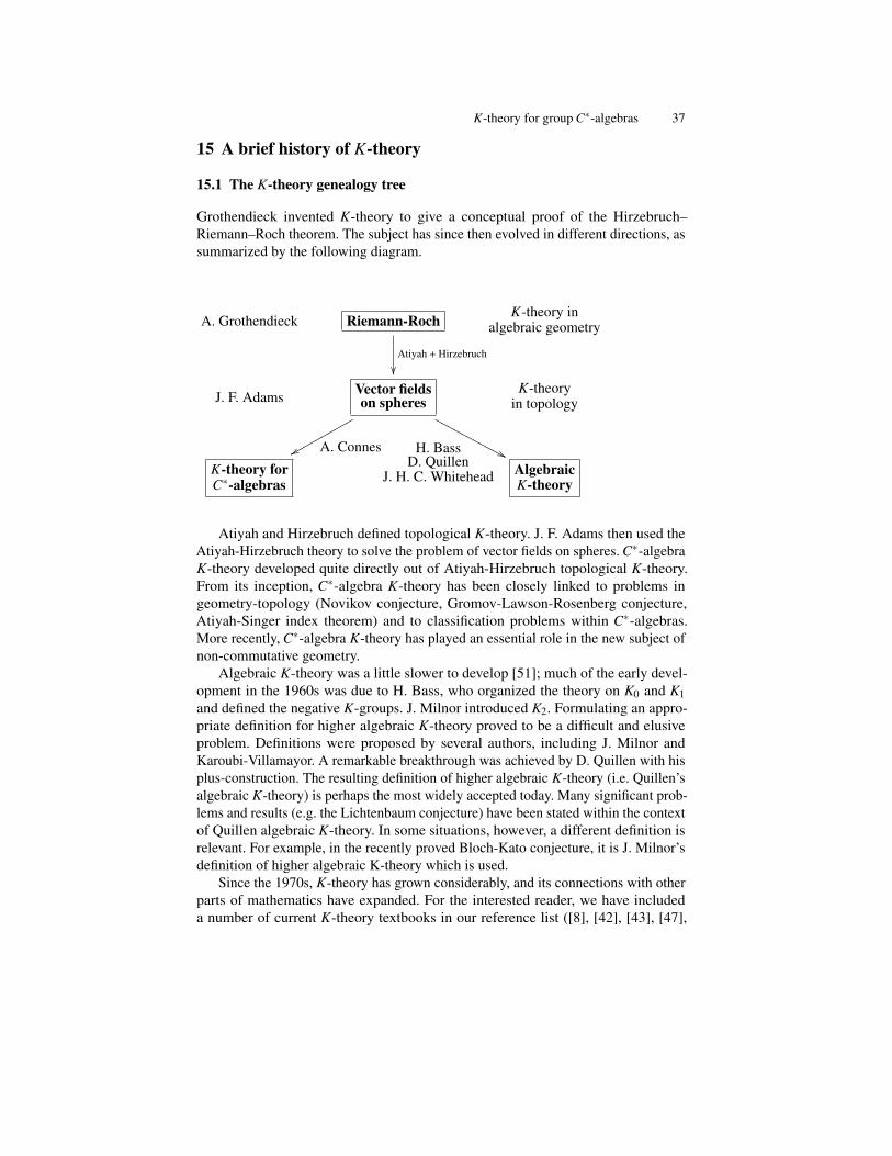
K-theory for group C∗-algebras 37
15 A brief history of K-theory
15.1 The K-theory genealogy tree
Grothendieck invented K-theory to give a conceptual proof of the Hirzebruch–Riemann–Roch theorem. The subject has since then evolved in different directions, assummarized by the following diagram.
A. Grothendieck Riemann-Roch
Atiyah + Hirzebruch
K-theory inalgebraic geometry
J. F. Adams Vector fieldson spheres
A. Connesxxqqqqqqqqqq
H. BassD. Quillen
J. H. C. Whitehead
&&NNNNNNNNNNN
K-theoryin topology
K-theory forC∗-algebras
AlgebraicK-theory
Atiyah and Hirzebruch defined topological K-theory. J. F. Adams then used theAtiyah-Hirzebruch theory to solve the problem of vector fields on spheres. C∗-algebraK-theory developed quite directly out of Atiyah-Hirzebruch topological K-theory.From its inception, C∗-algebra K-theory has been closely linked to problems ingeometry-topology (Novikov conjecture, Gromov-Lawson-Rosenberg conjecture,Atiyah-Singer index theorem) and to classification problems within C∗-algebras.More recently, C∗-algebra K-theory has played an essential role in the new subject ofnon-commutative geometry.
Algebraic K-theory was a little slower to develop [51]; much of the early devel-opment in the 1960s was due to H. Bass, who organized the theory on K0 and K1and defined the negative K-groups. J. Milnor introduced K2. Formulating an appro-priate definition for higher algebraic K-theory proved to be a difficult and elusiveproblem. Definitions were proposed by several authors, including J. Milnor andKaroubi-Villamayor. A remarkable breakthrough was achieved by D. Quillen with hisplus-construction. The resulting definition of higher algebraic K-theory (i.e. Quillen’salgebraic K-theory) is perhaps the most widely accepted today. Many significant prob-lems and results (e.g. the Lichtenbaum conjecture) have been stated within the contextof Quillen algebraic K-theory. In some situations, however, a different definition isrelevant. For example, in the recently proved Bloch-Kato conjecture, it is J. Milnor’sdefinition of higher algebraic K-theory which is used.
Since the 1970s, K-theory has grown considerably, and its connections with otherparts of mathematics have expanded. For the interested reader, we have includeda number of current K-theory textbooks in our reference list ([8], [42], [43], [47],
38 Paul F. Baum and Ruben J. Sanchez-Garcıa
[49], [50]). For a taste of the current developments, it is useful to take a look at theHandbook of K-theory [16] or at the lectures in this volume. The Journal of K-theory(as well as its predecessor, K-theory) is dedicated to the subject, as is the websitemaintained by D. Grayson at http://www.math.uiuc.edu/K-theory. Thissite, started in 1993, includes a preprint archive which at the moment when this is beingwritten contains 922 preprints. Additionally, see the Journal of Non-CommutativeGeometry for current results involving C∗-algebra K-theory.
Finally, we have not in these notes emphasized cyclic homology. However, cyclic(co-)homology is an allied theory to K-theory and any state-of-the-art survey ofK-theory would have to recognize this central fact.
15.2 The Hirzebruch–Riemann–Roch theorem
Let M be a non-singular projective algebraic variety over C. Let E be an algebraicvector bundle on M. Write E for the sheaf (of germs) of algebraic sections of E. Foreach j ≥ 0, consider H j(M,E) the j-th cohomology group of M using E.
Lemma 1. For all j ≥ 0, dimCH j(M,E) < ∞ and for j > dimC(M), H j(M,E) = 0.
Define the Euler characteristic of M with respect to E as
χ(M,E) =n
∑j=0
(−1) j dimCH j(M,E) , where n = dimC(M) .
Theorem 12 (Hirzebruch–Riemann–Roch). Let M be a non-singular projectivealgebraic variety over C and let E be an algebraic vector bundle on M. Then
χ(M,E) = (ch(E)∪Td(M))[M]
where ch(E) is the Chern character of E, Td(M) is the Todd class of M and ∪ standsfor the cup product.
15.3 The unity of K-theory
We explain how K-theory for C∗-algebras is a particular case of algebraic K-theory ofrings.
Let A be a C∗-algebra. Consider the inclusion
Mn(A) → Mn+1(A) a11 . . . a1n...
...an1 . . . ann
7→
a11 . . . a1n 0...
......
an1 . . . ann 00 . . . 0 0
. (2)
This is a one-to-one ∗-homomorphism, and it is norm preserving. Define M∞(A) asthe limit of Mn(A) with respect to these inclusions. That is, M∞(A) is the set of infinite
K-theory for group C∗-algebras 39
matrices where almost all ai j are zero. Finally, define the stabilization of A (cf. [42,6.4] or [49, 1.10]) as the closure
A = M∞(A) .
Here we mean the completion with respect to the norm on M∞(A) and the main pointis that the inclusions above are all norm-preserving. The result is a C∗-algebra withoutunit.
Remark 47. There is an equivalent definition of A as the tensor product A⊗K , whereK is the C∗-algebra of all compact operators on a separable infinite-dimensionalHilbert space, and the tensor product is in the sense of C∗-algebras.
Example 15. Let H be a separable, infinite-dimensional, Hilbert space. That is, H hasa countable, but not finite, orthonormal basis. It can be shown that
C= K ⊂L (H),
where K is the subset of compact operators on H. We have then
K j(C) = K j(C) ,
where K j(−) is C∗-algebra K-theory. This is true in general for any C∗-algebra(Proposition 4 below).On the other hand, the algebraic K-theory of C is
Kalgj (C) =
Z j even,0 j odd,
which therefore coincides with the C∗-algebra K-theory of C. This is also true ingeneral (Theorem 13 below). This answer is simple compared with the algebraicK-theory of C, where only some partial results are known.
The stabilization of a C∗-algebra does not change its (C∗-algebra) K-theory.
Proposition 4. Let A be a C∗-algebra and write K j(−) for K-theory of C∗-algebras.Then
K j(A) = K j(A) j ≥ 0 .
The proof is a consequence of the definition of C∗-algebra K-theory: the inclusions(2) induce isomorphisms in K-theory, and the direct limit (in the sense of C∗-algebras)commute with the K-theory functor (cf. [49, 6.2.11 and 7.1.9]).
Remark 48. In the terminology of Cortinas’ notes[12], Proposition 4 says that thefunctors K0 and K1 are K -stable.
M. Karoubi conjectured that the algebraic K-theory of A is isomorphic to itsC∗-algebra K-theory. The conjecture was proved by A. Suslin and M. Wodzicki.
40 Paul F. Baum and Ruben J. Sanchez-Garcıa
Theorem 13 (A. Suslin and M. Wodzicki [48]). Let A be a C∗-algebra. Then
K j(A) = Kalgj (A) j ≥ 0 ,
where the left-hand side is C∗-algebra K-theory and the right-hand side is (Quillen’s)algebraic K-theory of rings.
A proof can be found in Cortinas’ notes [12, Thm. 7.1.3]. In these notes Cortinaselaborates the isomorphism above into a long exact sequence which involves cyclichomology.
Theorem 13 is the unity of K-theory: It says that C∗-algebra K-theory is a pleasantsubdiscipline of algebraic K-theory in which Bott periodicity is valid and certain basicexamples are easy to calculate.
References
1. William Arveson, An invitation to C∗-algebras, Springer-Verlag, New York, 1976, GraduateTexts in Mathematics, No. 39. MR MR0512360 (58 #23621)
2. M. F. Atiyah, Global theory of elliptic operators, Proc. Internat. Conf. on FunctionalAnalysis and Related Topics (Tokyo, 1969), Univ. of Tokyo Press, Tokyo, 1970, pp. 21–30.MR MR0266247 (42 #1154)
3. M. F. Atiyah and F. Hirzebruch, Riemann-Roch theorems for differentiable manifolds, Bull.Amer. Math. Soc. 65 (1959), 276–281. MR MR0110106 (22 #989)
4. Paul Baum and Alain Connes, Chern character for discrete groups, A fete of topology,Academic Press, Boston, MA, 1988, pp. 163–232. MR MR928402 (90e:58149)
5. Paul Baum, Alain Connes, and Nigel Higson, Classifying space for proper actions and K-theory of group C∗-algebras, C∗-algebras: 1943–1993 (San Antonio, TX, 1993), Contemp.Math., vol. 167, Amer. Math. Soc., Providence, RI, 1994, pp. 240–291. MR MR1292018(96c:46070)
6. Paul Baum, Nigel Higson, and Thomas Schick, A geometric description of equivariantK-homology, to appear in the Conference Proceedings of the Non Commutative GeometryConference in honor of Alain Connes, Paris, 2007.
7. Harald Biller, Characterizations of proper actions, Math. Proc. Cambridge Philos. Soc.136 (2004), no. 2, 429–439. MR MR2040583 (2004k:57043)
8. Bruce Blackadar, K-theory for operator algebras, second ed., Mathematical SciencesResearch Institute Publications, vol. 5, Cambridge University Press, Cambridge, 1998. MRMR1656031 (99g:46104)
9. Raoul Bott, The stable homotopy of the classical groups, Ann. of Math. (2) 70 (1959),313–337. MR MR0110104 (22 #987)
10. Kenneth S. Brown, Cohomology of groups, Graduate Texts in Mathematics, vol. 87,Springer-Verlag, New York, 1982. MR MR672956 (83k:20002)
11. Jerome Chabert, Siegfried Echterhoff, and Ralf Meyer, Deux remarques sur l’applicationde Baum-Connes, C. R. Acad. Sci. Paris Ser. I Math. 332 (2001), no. 7, 607–610. MRMR1841893 (2002k:19004)
12. Guillermo Cortinas, Algebraic v. topological K-theory: a friendly match (this volume).13. Giuliana Davidoff, Peter Sarnak, and Alain Valette, Elementary number theory, group
theory, and Ramanujan graphs, London Mathematical Society Student Texts, vol. 55,Cambridge University Press, Cambridge, 2003. MR MR1989434 (2004f:11001)
K-theory for group C∗-algebras 41
14. James F. Davis and Wolfgang Luck, Spaces over a category and assembly maps in iso-morphism conjectures in K- and L-theory, K-Theory 15 (1998), no. 3, 201–252. MRMR1659969 (99m:55004)
15. Jacques Dixmier, C∗-algebras, North-Holland Publishing Co., Amsterdam, 1977, Trans-lated from the French by Francis Jellett, North-Holland Mathematical Library, Vol. 15.MR MR0458185 (56 #16388)
16. Eric M. Friedlander and Daniel R. Grayson (eds.), Handbook of K-theory. Vol. 1, 2,Springer-Verlag, Berlin, 2005. MR MR2182598 (2006e:19001)
17. Erik Guentner, Nigel Higson, and Shmuel Weinberger, The Novikov conjecture for lineargroups, Publ. Math. Inst. Hautes Etudes Sci. (2005), no. 101, 243–268. MR MR2217050(2007c:19007)
18. Ian Hambleton and Erik K. Pedersen, Identifying assembly maps in K- and L-theory, Math.Ann. 328 (2004), no. 1-2, 27–57. MR MR2030369 (2004j:19001)
19. N. Higson, V. Lafforgue, and G. Skandalis, Counterexamples to the Baum-Connes conjec-ture, Geom. Funct. Anal. 12 (2002), no. 2, 330–354. MR MR1911663 (2003g:19007)
20. Nigel Higson, A primer on KK-theory, Operator theory: operator algebras and applica-tions, Part 1 (Durham, NH, 1988), Proc. Sympos. Pure Math., vol. 51, Amer. Math. Soc.,Providence, RI, 1990, pp. 239–283. MR MR1077390 (92g:19005)
21. Nigel Higson and Gennadi Kasparov, Operator K-theory for groups which act properlyand isometrically on Hilbert space, Electron. Res. Announc. Amer. Math. Soc. 3 (1997),131–142 (electronic). MR MR1487204 (99e:46090)
22. , E-theory and KK-theory for groups which act properly and isometrically onHilbert space, Invent. Math. 144 (2001), no. 1, 23–74. MR MR1821144 (2002k:19005)
23. Pierre Julg, La conjecture de Baum-Connes a coefficients pour le groupe Sp(n,1), C. R.Math. Acad. Sci. Paris 334 (2002), no. 7, 533–538. MR MR1903759 (2003d:19007)
24. G. G. Kasparov, The operator K-functor and extensions of C∗-algebras, Izv. Akad. NaukSSSR Ser. Mat. 44 (1980), no. 3, 571–636, 719. MR MR582160 (81m:58075)
25. , Equivariant KK-theory and the Novikov conjecture, Invent. Math. 91 (1988),no. 1, 147–201. MR MR918241 (88j:58123)
26. , K-theory, group C∗-algebras, and higher signatures (conspectus), Novikov con-jectures, index theorems and rigidity, Vol. 1 (Oberwolfach, 1993), London Math. Soc.Lecture Note Ser., vol. 226, Cambridge Univ. Press, Cambridge, 1995, pp. 101–146. MRMR1388299 (97j:58153)
27. G. G. Kasparov and G. Skandalis, Groups acting on buildings, operator K-theory, andNovikov’s conjecture, K-Theory 4 (1991), no. 4, 303–337. MR MR1115824 (92h:19009)
28. Vincent Lafforgue, K-theorie bivariante pour les algebres de Banach et conjecture deBaum-Connes, Invent. Math. 149 (2002), no. 1, 1–95. MR MR1914617 (2003d:19008)
29. E. C. Lance, Hilbert C∗-modules, London Mathematical Society Lecture Note Series, vol.210, Cambridge University Press, Cambridge, 1995, A toolkit for operator algebraists. MRMR1325694 (96k:46100)
30. Wolfgang Luck, Transformation groups and algebraic K-theory, Lecture Notes inMathematics, vol. 1408, Springer-Verlag, Berlin, 1989, Mathematica Gottingensis. MRMR1027600 (91g:57036)
31. , Chern characters for proper equivariant homology theories and applications toK- and L-theory, J. Reine Angew. Math. 543 (2002), 193–234.
32. , Survey on classifying spaces for families of subgroups, Infinite groups: geometric,combinatorial and dynamical aspects, Progr. Math., vol. 248, Birkhauser, Basel, 2005,pp. 269–322. MR MR2195456 (2006m:55036)
33. Wolfgang Luck and Bob Oliver, The completion theorem in K-theory for proper actions ofa discrete group, Topology 40 (2001), no. 3, 585–616. MR MR1838997 (2002f:19010)
42 Paul F. Baum and Ruben J. Sanchez-Garcıa
34. Wolfgang Luck and Holger Reich, The Baum-Connes and the Farrell-Jones conjectures inK- and L-theory, Handbook of K-theory. Vol. 1, 2, Springer, Berlin, 2005, pp. 703–842.MR MR2181833 (2006k:19012)
35. Michel Matthey, Herve Oyono-Oyono, and Wolfgang Pitsch, Homotopy invariance ofhigher signatures and 3-manifold groups, Bull. Soc. Math. France 136 (2008), no. 1, 1–25.MR MR2415334
36. Ralph Meyer, Universal Coefficient Theorems and assembly maps in KK-theory (thisvolume).
37. Igor Mineyev and Guoliang Yu, The Baum-Connes conjecture for hyperbolic groups,Invent. Math. 149 (2002), no. 1, 97–122. MR MR1914618 (2003f:20072)
38. Guido Mislin, Equivariant K-homology of the classifying space for proper actions, Propergroup actions and the Baum-Connes conjecture, Adv. Courses Math. CRM Barcelona,Birkhauser, Basel, 2003, pp. 1–78. MR MR2027169 (2005e:19008)
39. Gerard J. Murphy, C∗-algebras and operator theory, Academic Press Inc., Boston, MA,1990. MR MR1074574 (91m:46084)
40. Herve Oyono-Oyono, Baum-Connes conjecture and group actions on trees, K-Theory 24(2001), no. 2, 115–134. MR MR1869625 (2002m:19004)
41. Gert K. Pedersen, C∗-algebras and their automorphism groups, London MathematicalSociety Monographs, vol. 14, Academic Press Inc. [Harcourt Brace Jovanovich Publishers],London, 1979. MR MR548006 (81e:46037)
42. M. Rørdam, F. Larsen, and N. Laustsen, An introduction to K-theory for C∗-algebras, Lon-don Mathematical Society Student Texts, vol. 49, Cambridge University Press, Cambridge,2000. MR MR1783408 (2001g:46001)
43. Jonathan Rosenberg, Algebraic K-theory and its applications, Graduate Texts in Mathe-matics, vol. 147, Springer-Verlag, New York, 1994. MR MR1282290 (95e:19001)
44. Ruben Sanchez-Garcıa, Bredon homology and equivariant K-homology of SL(3,Z), J.Pure Appl. Algebra 212 (2008), no. 5, 1046–1059. MR MR2387584
45. Thomas Schick, Finite group extensions and the Baum-Connes conjecture, Geom. Topol.11 (2007), 1767–1775. MR MR2350467
46. Jean-Pierre Serre, Trees, Springer Monographs in Mathematics, Springer-Verlag, Berlin,2003, Translated from the French original by John Stillwell, Corrected 2nd printing of the1980 English translation. MR MR1954121 (2003m:20032)
47. V. Srinivas, Algebraic K-theory, second ed., Progress in Mathematics, vol. 90, BirkhauserBoston Inc., Boston, MA, 1996. MR MR1382659 (97c:19001)
48. Andrei A. Suslin and Mariusz Wodzicki, Excision in algebraic K-theory, Ann. of Math.(2) 136 (1992), no. 1, 51–122. MR MR1173926 (93i:19006)
49. N. E. Wegge-Olsen, K-theory and C∗-algebras, Oxford Science Publications, The Claren-don Press Oxford University Press, New York, 1993, A friendly approach. MR MR1222415(95c:46116)
50. Charles A. Weibel, The K-book: An introduction to algebraic K-theory (book in progress),Available at , OPTkey = , OPTmonth = , OPTyear = , OPTannote = .
51. , The development of algebraic K-theory before 1980, Algebra, K-theory, groups,and education (New York, 1997), Contemp. Math., vol. 243, Amer. Math. Soc., Providence,RI, 1999, pp. 211–238. MR MR1732049 (2000m:19001)
Universal Coefficient Theorems andassembly maps in KK-theory
Ralf Meyer
Mathematisches Institut and Courant Centre “Higher Order Structures”Georg-August-Universitat GottingenBunsenstraße 3–537073 [email protected]
Summary. We introduce equivariant Kasparov theory using its universal property and con-struct the Baum–Connes assembly map by localising the Kasparov category at a suitablesubcategory. Then we explain a general machinery to construct derived functors and spectralsequences in triangulated categories. This produces various generalisations of the Rosenberg–Schochet Universal Coefficient Theorem.
Key words: K-theory, KK-theory, Baum–Connes assembly map, triangulated category, Uni-versal Coefficient Theorem
1 Introduction
We may view Kasparov theory and its equivariant generalisations as categories. These categoriesare non-commutative analogues of (equivariant generalisations of) the stable homotopy categoryof spectra. These equivariant Kasparov categories can be described in two ways:
Abstractly, as the universal split-exact C∗-stable functor on the appropriate category ofC∗-algebras – this approach is due to Cuntz and Higson [10], [11], [15], [16].It is useful for general constructions like the descent functor or the adjointness betweeninduction and restriction functors (see §2.1.6 or [26]).
Concretely, using Fredholm operators on equivariant Hilbert bimodules – this is the originaldefinition of Kasparov [17], [18].It is useful for specific constructions that use, say, geometric properties of a group toconstruct elements in Kasparov groups.
We mainly treat Kasparov theory as a black box. We define G-equivariant Kasparov theoryvia its universal property and equip it with a triangulated category structure. This formalisessome basic properties of the stable homotopy category that are needed for algebraic topology.We later apply this structure to construct spectral sequences in Kasparov theory.
We use the universal property to construct the descent functor and induction and restrictionfunctors for closed subgroups, and to verify that the latter are adjoint for open subgroups.
44 Ralf Meyer
Then we turn to the Baum–Connes assembly map for a locally compact group G, which wetreat as in [26]. Green’s Imprimitivity Theorem suggests that we understand crossed productsfor compactly induced actions much better than general crossed products. We want to constructmore general actions out of compactly induced actions by an analogue of the construction ofCW-complexes. The notion of localising subcategory makes this idea precise.
The orthogonal complement of the compactly induced actions consists of actions thatare KKH -equivalent to 0 for all compact subgroups H of G. We call such actions weaklycontractible.
The compactly induced and weakly contractible objects together generate the wholeKasparov category. This allows us to compute the localisation of a functor at the weaklycontractible objects. The general machinery of localisation yields the Baum–Connes assemblymap
µ∗ : Ktop∗ (G,A)→ K∗(Gnr A)
when we apply it to the functor A 7→ K∗(Gnr A). Roughly speaking, this means thatA 7→ Ktop
∗ (G,A) is the best possible approximation to K∗(Gnr A) that vanishes for weaklycontractible objects. The above statements involve functors and the Baum–Connes assemblymap with coefficients. The above approach only works if we study this generalisation rightaway.
The groups Ktop∗ (G,A) are supposed to be computable by topological methods. We present
one approach to make this precise that works completely within equivariant Kasparov theoryand is a special case of a very general machinery for constructing spectral sequences. We carryover notions from homological algebra like exact chain complexes and projective objects to ourcategory and use them to define derived functors (see [27]). The derived functors of K∗(Gnr A)and Ktop
∗ (G,A) agree and form the E2-term of a spectral sequence that converges towardsKtop∗ (G,A). Many other spectral sequences like the Adams spectral sequence in topology can be
constructed with the same machinery. In simple special cases, the spectral sequence degeneratesto an exact sequence. The Universal Coefficient Theorem by Rosenberg–Schochet in [35] andthe Pimsner–Voiculescu exact sequence are special cases of this machinery.
2 Kasparov theory and Baum–Connes conjecture
2.1 Kasparov theory via its universal property
This subsection is mostly taken from [25], where more details can be found.Let G be a locally compact group.
Definition 1. A G-C∗-algebra is a C∗-algebra with a strongly continuous representation of Gby ∗-automorphisms.
Let G-C∗alg be the category of G-C∗-algebras; its objects are G-C∗-algebras and itsmorphisms A→ B are the G-equivariant ∗-homomorphisms A→ B; we sometimes denote thismorphism set by HomG(A,B).
A C∗-algebra is separable if it has a countable dense subset. We often restrict attention tothe full subcategory G-C∗sep⊆ G-C∗alg of separable G-C∗-algebras.
Homology theories for C∗-algebras are usually required to be homotopy invariant, stable,and exact in a suitable sense. We can characterise G-equivariant Kasparov theory as theuniversal functor on G-C∗sep with these properties, in the following sense.

Universal Coefficient Theorems and assembly maps in KK-theory 45
Definition 2. Let P be a property for functors defined on G-C∗sep. A universal functor with Pis a functor u : G-C∗sep→ UP(G-C∗sep) such that
• F u has P for each functor F : UP(G-C∗sep)→ C;• any functor F : G-C∗sep→ C with P factors uniquely as F = F u for some functor
F : UP(G-C∗sep)→ C;• let F,G : G-C∗sep⇒C be two functors with P, let F , G : UP(G-C∗sep)⇒C be their unique
extensions; then any natural transformation Φ : F ⇒ G remains a natural transformationF ⇒ G.
Of course, such a functor need not exist. If it does, then it restricts to a bijection betweenobjects of G-C∗sep and UP(G-C∗sep). Hence we can completely describe it by the sets ofmorphisms UP(A,B) from A to B in UP(G-C∗sep) and the maps G-C∗sep(A,B)→ UP(A,B) forA,B ∈∈ G-C∗sep. The universal property means that for any functor F : G-C∗sep→ C with Pthere is a unique functorial way to extend the maps HomG(A,B)→ C
(F(A),F(B)
)to UP(A,B).
The condition about natural transformations makes precise what it means for this extension tobe natural.
2.1.1 Some basic homotopy theory
We define cylinders, cones, and suspensions of objects, and mapping cones and mappingcylinders of morphisms in G-C∗alg. Then we define homotopy invariance for functors. Mappingcones will be used later to introduce the triangulated category structure on Kasparov theory.
Definition 3. Let A be a G-C∗-algebra. We define the cylinder, cone, and suspension over A by
Cyl(A) := C([0,1],A),
Cone(A) := C0([0,1]\0,A),
Sus(A) := C0([0,1]\0,1,A)∼= C0(S1,A).
If A = C0(X) for a pointed compact space X , then the cylinder, cone, and suspension of Aare C0(Y ) with Y equal to the usual cylinder [0,1]+∧X , cone [0,1]∧X , or suspension S1∧X ,respectively; here [0,1] has the base point 0.
Definition 4. Let f : A→ B be a morphism in G-C∗alg. The mapping cylinder Cyl( f ) and themapping cone Cone( f ) of f are the limits of the diagrams
Af−→ B ev1←−− Cyl(B), A
f−→ B ev1←−− Cone(B)
in G-C∗alg. More concretely,
Cone( f ) :=(a,b) ∈ A×C0
((0,1],B
) ∣∣ f (a) = b(1),
Cyl( f ) :=(a,b) ∈ A×C
([0,1],B
) ∣∣ f (a) = b(1).
If f : X→Y is a morphism of pointed compact spaces, then the mapping cone and mappingcylinder of the induced ∗-homomorphism C0( f ) : C0(Y )→ C0(X) agree with C0
(Cyl( f )
)and
C0(Cone( f )
), respectively.
The familiar maps relating mapping cones and cylinders to cones and suspensions continueto exist in our case. For any morphism f : A→ B in G-C∗alg, we get a morphism of extensions
46 Ralf Meyer
Sus(B) // //
Cone( f ) // //
A
Cone(B) // // Cyl( f ) // // A
The bottom extension splits and the maps A↔ Cyl( f ) are inverse to each other up to homotopy.The composite map Cone( f )→ A→ B factors through Cone(idB) ∼= Cone(B) and hence ishomotopic to the zero map.
Definition 5. Let f0, f1 : A⇒ B be two parallel morphisms in G-C∗alg. We write f0 ∼ f1 andcall f0 and f1 homotopic if there is a morphism f : A→ Cyl(B) with evt f = ft for t = 0,1.
A functor F : G-C∗alg→ C is called homotopy invariant if f0 ∼ f1 implies F( f0) = F( f1).
It is easy to check that homotopy is an equivalence relation on HomG(A,B). We let [A,B]be the set of equivalence classes. The composition of morphisms in G-C∗alg descends to maps
[B,C]× [A,B]→ [A,C],([ f ], [g]
)7→ [ f g],
that is, f1 ∼ f2 and g1 ∼ g2 implies f1 g1 ∼ f2 g2. Thus the sets [A,B] form the morphism setsof a category, called the homotopy category of G-C∗-algebras. A functor is homotopy invariantif and only if it descends to the homotopy category. Other characterisations of homotopyinvariance are listed in [25, §3.1].
Of course, our notion of homotopy restricts to the usual one for pointed compact spaces.
2.1.2 Morita–Rieffel equivalence and stable isomorphism
One of the basic ideas of non-commutative geometry is that GnC0(X) (or Gnr C0(X)) shouldbe a substitute for the quotient space G\X , which may have bad singularities. In the specialcase of a free and proper G-space X , we expect that GnC0(X) and C0(G\X) are “equivalent”in a suitable sense. Already the simplest possible case X = G shows that we cannot expect anisomorphism here because
GnC0(G)∼= Gnr C0(G)∼=K(L2G).
The right notion of equivalence is a C∗-version of Morita equivalence introduced by Marc A.Rieffel ([32], [33], [34]); therefore, we call it Morita–Rieffel equivalence.
The definition of Morita–Rieffel equivalence involves Hilbert modules over C∗-algebrasand the C∗-algebras of compact operators on them; these notions are crucial for Kasparovtheory as well. We refer to [20] for the definition and a discussion of their basic properties.
Definition 6. Two G-C∗-algebras A and B are called Morita–Rieffel equivalent if there are afull G-equivariant Hilbert B-module E and a G-equivariant ∗-isomorphism K(E )∼= A.
It is possible (and desirable) to express this definition more symmetrically: E is an A,B-bimodule with two inner products taking values in A and B, satisfying various conditions(see also [32]). Two Morita–Rieffel equivalent G-C∗-algebras have equivalent categories ofG-equivariant Hilbert modules via the functor H 7→H ⊗A E . The converse is not so clear.
Universal Coefficient Theorems and assembly maps in KK-theory 47
Example 1. The following is a more intricate example of a Morita–Rieffel equivalence. Let Γ
and P be two subgroups of a locally compact group G. Then Γ acts on G/P by left translationand P acts on Γ \G by right translation. The corresponding orbit space is the double coset spaceΓ \G/P. Both Γ nC0(G/P) and PnC0(Γ \G) are non-commutative models for this doublecoset space. They are indeed Morita–Rieffel equivalent; the bimodule that implements theequivalence is a suitable completion of Cc(G).
These examples suggest that Morita–Rieffel equivalent C∗-algebras are different ways todescribe the same non-commutative space. Therefore, we expect that reasonable functors onC∗alg should not distinguish between Morita–Rieffel equivalent C∗-algebras.
Definition 7. Two G-C∗-algebras A and B are called stably isomorphic if there is a G-equivariant∗-isomorphism A⊗K(HG)∼= B⊗K(HG), where HG := L2(G×N) is the direct sum of count-ably many copies of the regular representation of G; we let G act on K(HG) by conjugation,of course.
The following technical condition is often needed in connection with Morita–Rieffelequivalence.
Definition 8. A C∗-algebra is called σ -unital if it has a countable approximate identity or,equivalently, contains a strictly positive element.
All separable C∗-algebras and all unital C∗-algebras are σ -unital; the algebra K(H ) isσ -unital if and only if H is separable.
Theorem 1 ([7]). σ -unital G-C∗-algebras are G-equivariantly Morita–Rieffel equivalent ifand only if they are stably isomorphic.
In the non-equivariant case, this theorem is due to Brown–Green–Rieffel ([7]). A simplerproof that carries over to the equivariant case appeared in [28].
2.1.3 C∗-stable functors
The definition of C∗-stability is more intuitive in the non-equivariant case:
Definition 9. Fix a rank-one projection p∈K(`2N). The resulting embedding A→A⊗K(`2N),a 7→ a⊗ p, is called a corner embedding of A.
A functor F : C∗alg→ C is called C∗-stable if any corner embedding induces an isomor-phism F(A)∼= F
(A⊗K(`2N)
).
The correct equivariant generalisation is the following:
Definition 10. A functor F : G-C∗alg→ C is called C∗-stable if the canonical embeddingsH1→H1⊕H2←H2 induce isomorphisms
F(A⊗K(H1)
) ∼=−→ F(A⊗K(H1⊕H2)
) ∼=←− F(A⊗K(H2)
)for all non-zero G-Hilbert spaces H1 and H2.
Of course, it suffices to require F(A⊗K(H1)
) ∼=−→ F(A⊗K(H1⊕H2)
). It is not hard to
check that Definitions 9 and 10 are equivalent for trivial G.Our next goal is to describe the universal C∗-stable functor. We abbreviate AK :=K(L2G)⊗
A.
48 Ralf Meyer
Definition 11. A correspondence from A to B (or A 99K B) is a G-equivariant HilbertBK-module E together with a G-equivariant essential (or non-degenerate) ∗-homomorphismf : AK→K(E ).
Given correspondences E from A to B and F from B to C, their composition is thecorrespondence from A to C with underlying Hilbert module E ⊗BK F and map AK→K(E )→K(E ⊗BK F ), where the last map sends T 7→ T ⊗1; this yields compact operators because BKmaps to K(F ). See [20] for the definition of the relevant completed tensor product of Hilbertmodules.
The composition of correspondences is only defined up to isomorphism. It is associativeand the identity maps A→ A = K(A) act as unit elements, so that we get a category CorrGwhose morphisms are the isomorphism classes of correspondences. Any ∗-homomorphismϕ : A→ B yields a correspondence: let E be the right ideal ϕ(AK) ·BK in BK, viewed as aHilbert B-module, and let ϕ(a) ·b = ϕ(a) ·b; this restricts to a compact operator on E . Thisdefines a canonical functor \ : G-C∗alg→ CorrG.
Proposition 1. The functor \ : G-C∗alg→CorrG is the universal C∗-stable functor on G-C∗alg;that is, it is C∗-stable, and any other such functor factors uniquely through \.
Proof. First we sketch the proof in the non-equivariant case. First we must verify that \is C∗-stable. The Morita–Rieffel equivalence between K(`2N)⊗A ∼= K
(`2(N,A)
)and A is
implemented by the Hilbert module `2(N,A), which yields a correspondence(id, `2(N,A)
)from K(`2N)⊗A to A; this is inverse to the correspondence induced by a corner embeddingA→K(`2N)⊗A.
A Hilbert B-module E with an essential ∗-homomorphism A→ K(E ) is countably gen-erated because A is assumed σ -unital. Kasparov’s Stabilisation Theorem yields an isometricembedding E → `2(N,B). Hence we get ∗-homomorphisms
A→K(`2N)⊗B← B.
This diagram induces a map F(A)→ F(K(`2N)⊗B)∼= F(B) for any stable functor F . Nowwe should check that this well-defines a functor F : CorrG→ C with F \ = F , and that thisyields the only such functor. We omit these computations.
The generalisation to the equivariant case uses the crucial property of the left regularrepresentation that L2(G)⊗H ∼= L2(G×N) for any countably infinite-dimensional G-Hilbertspace H . Since we replace A and B by AK and BK in the definition of correspondence rightaway, we can use this to repair a possible lack of G-equivariance; similar ideas appear in [23].
ut
Example 2. Let u be a G-invariant multiplier of B. Then the identity map and the inner au-tomorphism B→ B, b 7→ ubu∗, associated to u define isomorphic correspondences B 99K B(via u). Hence inner automorphisms act trivially on C∗-stable functors. Actually, this is one ofthe computations that we have omitted in the proof above; the argument can be found in [12].
2.1.4 Exactness properties
Definition 12. A diagram I → E → Q in G-C∗alg is an extension if it is isomorphic to thecanonical diagram I→ A→ A/I for some G-invariant ideal I in a G-C∗-algebra A. We writeI E Q to denote extensions. A section for an extension
Universal Coefficient Theorems and assembly maps in KK-theory 49
Ii E
p Q (1)
in G-C∗alg is a map (of sets) Q→ E with p s = idQ. We call (1) split if there is a sectionthat is a G-equivariant ∗-homomorphism. We call (1) G-equivariantly cp-split if there is aG-equivariant, completely positive, contractive, linear section.
Sections are also often called lifts, liftings, or splittings.
Definition 13. A functor F on G-C∗alg is split-exact if, for any split extension Ki E
p Q
with section s : Q→ E, the map(F(i),F(s)
): F(K)⊕F(Q)→ F(E) is invertible.
Split-exactness is useful because of the following construction of Joachim Cuntz ([10]).Let B/E be a G-invariant ideal and let f+, f− : A⇒ E be G-equivariant ∗-homomorphisms
with f+(a)− f−(a) ∈ B for all a ∈ A. Equivalently, f+ and f− both lift the same morphismf : A→ E/B. The data (A, f+, f−,E,B) is called a quasi-homomorphism from A to B.
Pulling back the extension B E E/B along f , we get an extension B E ′ A withtwo sections f ′+, f ′− : A⇒ E ′. The split-exactness of F shows that F(B) F(E ′) F(A)is a split extension in C. Since both F( f ′−) and F( f ′+) are sections for it, we get a mapF( f ′+)−F( f ′−) : F(A)→ F(B). Thus a quasi-homomorphism induces a map F(A)→ F(B)if F is split-exact. The formal properties of this construction are summarised in [12].
Given a C∗-algebra A, there is a universal quasi-homomorphism out of A. Let Q(A) := A∗Abe the free product of two copies of A and let πA : Q(A)→ A be the folding homomorphism thatrestricts to idA on both factors. Let q(A) be its kernel. The two canonical embeddings A→ A∗Aare sections for the folding homomorphism. Hence we get a quasi-homomorphism A ⇒Q(A).q(A). The universal property of the free product shows that any quasi-homomorphismyields a G-equivariant ∗-homomorphism q(A)→ B.
Theorem 2. Functors that are C∗-stable and split-exact are automatically homotopy invariant.
This is a deep result of Nigel Higson ([16]); a simple proof can be found in [12]. Besidesbasic properties of quasi-homomorphisms, it only uses that inner endomorphisms act identicallyon C∗-stable functors.
Definition 14. We call F exact if F(K)→ F(E)→ F(Q) is exact (at F(E)) for any extensionK E Q in G-C∗alg. More generally, given a class E of extensions in G-C∗alg like, say,the class of equivariantly cp-split extensions, we define exactness for extensions in E .
Most functors we are interested in satisfy homotopy invariance and Bott periodicity, andthese two properties prevent a functor from being exact in the stronger sense of being left orright exact. This explains why our notion of exactness is much weaker than usual in homologicalalgebra.
It is reasonable to require that a functor be part of a homology theory, that is, a sequenceof functors (Fn)n∈Z together with natural long exact sequences for all extensions. We do notrequire this because this additional information tends to be hard to get a priori but often comesfor free a posteriori:
Proposition 2. Suppose that F is homotopy invariant and exact (or exact for equivariantlycp-split extensions). Then F has long exact sequences of the form
· · · → F(Sus(K)
)→ F
(Sus(E)
)→ F
(Sus(Q)
)→ F(K)→ F(E)→ F(Q)
for any (equivariantly cp-split) extension K E Q. In particular, F is split-exact.
50 Ralf Meyer
See §21.4 in [4] for the proof.Together with Bott periodicity, this yields long exact sequences that extend towards ±∞ in
both directions, showing that an exact homotopy invariant functor that satisfies Bott periodicityis part of a homology theory in a canonical way.
2.1.5 Definition of Kasparov theory
Kasparov theory maps two Z/2-graded C∗-algebras to an Abelian group KKG0 (A,B); this is a
vast generalisation of K-theory and K-homology. The most remarkable feature of this theoryis an associative product on KK called Kasparov product, which generalises various knownproduct constructions in K-theory and K-homology. We do not discuss KKG for Z/2-gradedG-C∗-algebras here because it does not fit so well with the universal property approach.
Fix a locally compact group G. The Kasparov groups KKG0 (A,B) for A,B ∈ G-C∗sep form
morphisms sets A→ B of a category, which we denote by KKG; the composition in KKG isthe Kasparov product. The categories G-C∗sep and KKG have the same objects. We have acanonical functor
KK: G-C∗sep→ KKG
that acts identically on objects.
Theorem 3. The functor KKG : G-C∗sep→ KKG is the universal split-exact C∗-stable functor;in particular, KKG is an additive category. In addition, KKG also has the following propertiesand is, therefore, universal among functors with some of these extra properties: KKG is
• homotopy invariant;• exact for G-equivariantly cp-split extensions;• satisfies Bott periodicity, that is, in KKG there are natural isomorphisms Sus2(A)∼= A for
all A ∈∈ KKG.
Definition 15. A G-equivariant ∗-homomorphism f : A→ B is called a KKG-equivalence ifKK( f ) is invertible in KKG.
Corollary 1. Let F : G-C∗sep→ C be split-exact and C∗-stable. Then F factors uniquelythrough KKG, is homotopy invariant, and satisfies Bott periodicity. A KKG-equivalence A→ Binduces an isomorphism F(A)→ F(B).
We will take the universal property of Theorem 3 as a definition of KKG and thus of thegroups KKG
0 (A,B). We also let
KKGn (A,B) := KKG(A,Susn(B)
);
since the Bott periodicity isomorphism identifies KKG2∼= KKG
0 , this yields a Z/2-graded theory.By the universal property, K-theory descends to a functor on KK, that is, we get canonical
mapsKK0(A,B)→ Hom
(K∗(A),K∗(B)
)for all separable C∗-algebras A,B, where the right hand side denotes grading-preserving grouphomomorphisms. For A =C, this yields a map KK0(C,B)→Hom
(Z,K0(B)
)∼= K0(B). Usingsuspensions, we also get a corresponding map KK1(C,B)→ K1(B).
Theorem 4. The maps KK∗(C,B)→ K∗(B) constructed above are isomorphisms for all B ∈∈C∗sep.
Universal Coefficient Theorems and assembly maps in KK-theory 51
Thus Kasparov theory is a bivariant generalisation of K-theory.Roughly speaking, KK∗(A,B) is the place where maps between K-theory groups live. Most
constructions of such maps, say, in index theory can in fact be improved to yield elements ofKK∗(A,B). One reason for this is the Universal Coefficient Theorem (UCT) by Rosenberg andSchochet [35], which computes KK∗(A,B) from K∗(A) and K∗(B) for many C∗-algebras A,B.If A satisfies the UCT, then any group homomorphism K∗(A)→ K∗(B) lifts to an element ofKK∗(A,B) of the same parity.
With our definition, it is not obvious how to construct elements in KKG0 (A,B). The only
source we know so far are G-equivariant ∗-homomorphisms. Another important source areextensions, more precisely, equivariantly cp-split extensions. Any such extension I E Qyields a class in KKG
1 (Q, I) ∼= KKG0 (Sus(Q), I) ∼= KKG
0(Q,Sus(I)
). Conversely, any element
in KKG1 (Q, I) comes from an extension in this fashion in a rather transparent way.
Thus it may seem that we can understand all of Kasparov theory from an abstract, categorytheoretic point of view. But this is not the case. To get a category, we must compose extensions;this leads to extensions of higher length. If we allow such higher-length extensions, we caneasily construct a category that is isomorphic to Kasparov theory; this generalisation still worksfor more general algebras than C∗-algebras (see [12]) because it does not involve any difficultanalysis any more. But such a setup offers no help to compute products. Here computingproducts means identifying them with other simple things like, say, the identity morphism. Thisis why the more concrete approach to Kasparov theory is still necessary for the interestingapplications of the theory.
In connection with the Baum–Connes conjecture, our abstract approach allows us toformulate it and analyse its consequences. But to verify it, say, for amenable groups, we mustshow that a certain morphism in KKG is invertible. This involves constructing its inverse andchecking that the two Kasparov products in both order are 1. These computations require theconcrete description of Kasparov theory that we omit here. We merely refer to [4] for a detailedtreatment.
2.1.6 Extending functors and identities to KKG
We use the universal property to extend functors from G-C∗alg to KKG and check identities inKKG without computing Kasparov products. As our first example, consider the full and reducedcrossed product functors
Gnr ,Gn : G-C∗alg→ C∗alg.
Proposition 3. These two functors extend to functors
Gnr ,Gn : KKG→ KK
called descent functors.
Kasparov constructs these functors directly using the concrete description of Kasparovcycles. This requires a certain amount of work; in particular, checking functoriality involvesknowing how to compute Kasparov products.
Proof. We only write down the argument for reduced crossed products, the other case is similar.It is well-known that Gnr
(A⊗K(H )
) ∼= (Gnr A)⊗K(H ) for any G-Hilbert space H .Therefore, the composite functor
G-C∗sep Gnr−−−→ C∗sepKK−−→ KK
52 Ralf Meyer
is C∗-stable. This functor is split-exact as well (we omit the proof). Now the universal propertyprovides an extension to a functor KKG→ KK. ut
Similarly, we get functors
A⊗min ,A⊗max : KKG→ KKG
for any G-C∗-algebra A. Since these extensions are natural, we even get bifunctors
⊗min,⊗max : KKG×KKG→ KKG.
For the Baum–Connes assembly map, we need the induction functors
IndGH : KKH → KKG
for closed subgroups H ⊆ G. For a finite group H, IndGH(A) is the H-fixed point algebra of
C0(G,A), where H acts by h · f (g) = αh(
f (gh)). For infinite H, we have
IndGH(A) = f ∈ Cb(G,A) |
αh f (gh) = f (g) for all g ∈ G, h ∈ H, and gH 7→ ‖ f (g)‖ is C0;
the group G acts by translations on the left. This construction is clearly functorial for equivariant∗-homomorphisms. Furthermore, it commutes with C∗-stabilisations and maps split extensionsagain to split extensions. Therefore, the same argument as above allows us to extend it to afunctor
IndGH : KKH → KKG
The following examples are more trivial. Let τ : C∗alg→G-C∗alg equip a C∗-algebra withthe trivial G-action; it extends to a functor τ : KK→ KKG. The restriction functors
ResHG : KKG→ KKH
for closed subgroups H ⊆ G are defined by forgetting part of the equivariance.The universal property also allows us to prove identities between functors. For instance,
Green’s Imprimitivity Theorem provides Morita equivalences
Gn IndGH(A)∼M HnA, Gnr IndG
H(A)∼M Hnr A (2)
for any H-C∗-algebra A. This is proved by completing C0(G,A) to an imprimitivity bimodulefor both C∗-algebras. This equivalence is clearly natural for H-equivariant ∗-homomorphisms.Since all functors involved are C∗-stable and split exact, the uniqueness part of the universalproperty of KKH shows that the KK-equivalences Gn IndG
H(A)∼= HnA and Gnr IndGH(A)∼=
Hnr A are natural for morphisms in KKH . That is, the diagram
Gnr IndGH(A1)
∼= //
GnrIndGH ( f )
Hnr A1
Hnr f
Gnr IndG
H(A2)∼= // Hnr A2
in KK commutes for any f ∈ KKH0 (A1,A2). More examples of this kind are discussed in §4.1
of [25].We can also prove adjointness relations in Kasparov theory in an abstract way by construct-
ing the unit and counit of the adjunction. An important example is the adjointness betweeninduction and restriction functors (see also §3.2 of [26]).
Universal Coefficient Theorems and assembly maps in KK-theory 53
Proposition 4. Let H ⊆ G be a closed subgroup. If H is open, then we have natural isomor-phisms
KKG(IndGH A,B)∼= KKH(A,ResH
G B) (3)
for all A ∈∈ H-C∗alg, B ∈∈ G-C∗alg. If H ⊆ G is cocompact, then we have natural isomor-phisms
KKG(A, IndGH B)∼= KKH(ResH
G A,B) (4)
for all A ∈∈ G-C∗alg, B ∈∈ H-C∗alg.
Proof. We will not use (4) later and therefore only prove (3). We must construct naturalelements
αA ∈ KKG0 (IndG
H ResHG A,A), βB ∈ KKH
0 (B,ResHG IndG
H B)
that satisfy the conditions for unit and counit of adjunction ([22]).We have a natural G-equivariant ∗-isomorphism IndG
H ResGH(A) ∼= C0(G/H)⊗A for any
G-C∗-algebra A. Since H is open in G, the homogeneous space G/H is discrete. We rep-resent C0(G/H) on the Hilbert space `2(G/H) by pointwise multiplication operators. Thisis G-equivariant for the representation of G on `2(G/H) by left translations. Thus we get acorrespondence from IndG
H ResHG(A) to A, which yields αA ∈ KKG
0 (IndGH ResH
G(A),A) becauseKKG is C∗-stable.
For any H-C∗-algebra B, we may embed B in ResHG IndG
H(B) as the subalgebra offunctions supported on the single coset H. This embedding is H-equivariant and providesβB ∈ KKH
0 (B,ResHG IndG
H B).Now we have to check that the following two composite maps are identity morphisms in
KKG and KKH , respectively:
IndGH(B)
IndGH (βB)−−−−−→ IndG
H ResHG IndG
H(B)αIndG
H (B)−−−−→ IndG
H(B)
ResHG A
βResHG A
−−−−→ ResHG IndG
H ResHG(A)
ResHG αA−−−−−→ ResH
G A
This yields the desired adjointness by a general argument from category theory (see [22]). Infact, both composites are already equal to the identity as correspondences. Hence we need noknowledge of Kasparov theory except for its C∗-stability to prove (3). ut
The following example is discussed in detail in §4.1 of [25]. If G is compact, then thetrivial action functor τ : KK→ KKG is left adjoint to Gn = Gnr , that is, we have naturalisomorphisms
KKG∗ (τ(A),B)∼= KK∗(A,GnB). (5)
This is also known as the Green–Julg Theorem. For A = C, it specialises to a natural isomor-phism KG
∗ (B)∼= K∗(GnB).
2.1.7 Triangulated category structure
We can turn KKG into a triangulated category by extending standard constructions for topologi-cal spaces (see [26]). A triangulated category is a category T with a suspension automorphismΣ : T→ T and a class of exact triangles, subject to various axioms (see [29], [26], [37]). Anexact triangle is a diagram in T of the form
A→ B→C→ ΣA or A // B
C,
[1][[88
54 Ralf Meyer
where the [1] in the arrow C→ A warns us that this map has degree 1. A morphism of trianglesis a triple of maps α,β ,γ making the obvious diagram commute.
A typical example is the homotopy category Ho(C) of chain complexes over an additivecategory C. Here the suspension functor is the (signed) translation functor
Σ((Cn,dn)
):= (Cn−1,−dn−1) on objects,
Σ(( fn)
):= ( fn−1) on morphisms;
a triangle is exact if it is isomorphic to a mapping cone triangle
Af−→ B→ Cone( f )→ ΣA
for some chain map f ; the maps B→ Cone( f )→ ΣA are the canonical ones. It is well-knownthat this defines a triangulated category.
Another classical example is the stable homotopy category, say, of compactly generatedpointed topological spaces (it is not particularly relevant which category of spaces or spectrawe use). The suspension is Σ(A) := S1∧A; a triangle is exact if it is isomorphic to a mappingcone triangle
Af−→ B→ Cone( f )→ ΣA
for some map f ; the maps B→ Cone( f )→ ΣA are the canonical ones.We are mainly interested in the categories KK and KKG introduced above. Their triangulated
category structure is discussed in detail in [26]. We are facing a notational problem becausethe functor X 7→ C0(X) from pointed compact spaces to C∗-algebras is contravariant, so thatmapping cone triangles now have the form
Af←− B← Cone( f )← C0(R,A)
for a ∗-homomorphism f : B→ A as in Definition 4.It is reasonable to view a ∗-homomorphism from A to B as a morphism from B to A.
Nevertheless, we prefer the convention that an algebra homorphism A→ B is a morphismA→ B. But then the most natural triangulated category structure lives on the opposite categoryKKop. This creates only notational difficulties because the opposite category of a triangulatedcategory inherits a canonical triangulated category structure, which has “the same” exacttriangles. However, the passage to opposite categories exchanges suspensions and desuspensionsand modifies some sign conventions. Thus the functor A 7→ C0(R,A), which is the suspensionfunctor in KKop, becomes the desuspension functor in KK. Fortunately, Bott periodicity impliesthat Σ 2 ∼= id, so that Σ and Σ−1 agree.
Depending on your definition of a triangulated category, you may want the suspension tobe an equivalence or isomorphism of categories. In the latter case, you must replace KK(G) byan equivalent category (see [26]); since this is not important here, we do not bother about thisissue.
Definition 16. A triangle A→ B→ C→ ΣA in KKG is called exact if it is isomorphic as atriangle to the mapping cone triangle
Sus(B)→ Cone( f )→ Af−→ B
for some G-equivariant ∗-homomorphism f .

Universal Coefficient Theorems and assembly maps in KK-theory 55
Alternatively, we can use G-equivariantly cp-split extensions in G-C∗sep. Any such exten-sion I E Q determines a class in KKG
1 (Q, I)∼= KKG0 (Sus(Q), I), so that we get a triangle
Sus(Q)→ I→ E→Q in KKG. Such triangles are called extension triangles. A triangle in KKG
is exact if and only if it is isomorphic to the extension triangle of a G-equivariantly cp-splitextension.
Theorem 5. With the suspension automorphism and exact triangles defined above, KKG is atriangulated category.
Proof. This is proved in detail in [26]. ut
Triangulated categories clarify the basic bookkeeping with long exact sequences. Mayer–Vietoris exact sequences and inductive limits are discussed from this point of view in [26]. Moreimportantly, this framework sheds light on more advanced constructions like the Baum–Connesassembly map.
The triangulated category axioms are discussed in greater detail in [29], [26], [37]. Theyencode some standard machinery for manipulating long exact sequences. Most of them amountto formal properties of mapping cones and mapping cylinders, which we can prove as inclassical topology. The only axiom that requires more care is that any morphism f : A→ Bshould be part of an exact triangle.
Unlike in [26], we prefer to construct this triangle as an extension triangle because thisworks in greater generality; we have learned this idea from Alexander Bonkat ([5]). Any elementin KKG
0 (A,B)∼= KKG1(A,C0(R,B)
)can be represented by an extension K(H ) E A with
an equivariant completely positive contractive section, where H is a full G-equivariant HilbertC0(R,B)-module, so thatK(H ) is KKG-equivalent to C0(R,B). Hence the resulting extensiontriangle in KKG is isomorphic to one of the form
C0(R,A)→ C0(R,B)→ E→ A;
by construction, it contains the suspension of the given class in KKG0 (A,B); it is easy to remove
the suspension.
Definition 17. Let T be a triangulated and C an Abelian category. A covariant functor F : T→C is called homological if F(A)→ F(B)→ F(C) is exact at F(B) for all exact trianglesA→ B→C→ ΣA. A contravariant functor with the analogous exactness property is calledcohomological.
Let A→ B→C→ ΣA be an exact triangle. Then a homological functor F : T→ C yieldsa natural long exact sequence
· · · → Fn+1(C)→ Fn(A)→ Fn(B)→ Fn(C)→ Fn−1(A)→ Fn−1(B)→ ···
with Fn(A) := F(Σ−nA) for n ∈ Z, and a cohomological functor F : Top→ C yields a naturallong exact sequence
· · · ← Fn+1(C)← Fn(A)← Fn(B)← Fn(C)← Fn−1(A)← Fn−1(B)← ·· ·
with Fn(A) := F(Σ−nA).
Proposition 5. Let T be a triangulated category. The functors
T(A, ) : T→ Ab, B 7→ T(A,B)
56 Ralf Meyer
are homological for all A ∈∈ T. Dually, the functors
T( ,B) : Top→ Ab, A 7→ T(A,B)
are cohomological for all B ∈∈ T.
Observe that
Tn(A,B) = T(Σ−nA,B)∼= T(A,Σ nB)∼= T−n(A,B).
Definition 18. A functor F : T→ T′ between two triangulated categories is called exact if itintertwines the suspension automorphisms (up to specified natural isomorphisms) and mapsexact triangles in T again to exact triangles in T′.
Example 3. The restriction functor ResHG : KKG→ KKH for a closed subgroup H of a locally
compact group G and the crossed product functors Gn ,Gnr : KKG→KK are exact becausethey preserve mapping cone triangles.
Let F : T1→T2 be an exact functor. If G : T2→? is exact, homological, or cohomological,then so is GF .
2.2 Subcategories in KKG
Now we turn to the construction of the Baum–Connes assembly map by studying varioussubcategories of KKG that are related to it.
2.2.1 Compactly induced actions
Definition 19. Let G be a locally compact group. A G-C∗-algebra is compactly induced if itis of the form IndG
H(A) for some compact subgroup H of G and some H-C∗-algebra A. We letC I be the class of all G-C∗-algebras that are KKG-equivalent to a direct summand of
⊕i∈NAi
with compactly induced G-C∗-algebras Ai for i ∈ N.
Equivalently, C I is the smallest class of objects in KKG that is closed under direct sums,direct summands and isomorphism and contains all compactly induced G-C∗-algebras.
Green’s Imprimitivity Theorem (2) tells us that the (reduced) crossed product for a com-pactly induced action IndG
H(A) is equivalent to the crossed product Hnr A for the compactgroup H. Hence we have
K∗(Gn IndGH A)∼= K∗(Gnr IndG
H A)∼= K∗(HnA)∼= KH∗ (A)
by the Green–Julg Theorem, compare (5).Since the computation of equivariant K-theory for compact groups is a problem of classical
topology, operator algebraists can pretend that it is Somebody Else’s Problem. We are morefascinated by the analytic difficulties created by crosssed products by infinite groups. Forinstance, it is quite hard to see which Laurent series ∑n∈Z anzn correspond to an element ofC∗redZ= C∗Z or, equivalently, which of them are the Fourier series of a continuous function onthe unit circle. The Baum–Connes conjecture, when true, implies that such analytic difficultiesdo not influence the K-theory.
Universal Coefficient Theorems and assembly maps in KK-theory 57
2.2.2 Two simple examples
It is best to explain our goals with two examples, namely, the groups R and Z. The Baum–Connes conjectures for these groups hold and are equivalent to the Connes–Thom isomor-phism [9] and a Pimsner–Voiculescu exact sequence [30]. Although the Baum–Connes conjec-ture only concerns the K-theory of C∗redG and, more generally, of crossed products Gnr A, weget much stronger statements in this case.
Both R and Z are torsion-free, that is, they have no non-trivial compact subgroups. Hencethe compactly induced actions are of the form C0(G,A) with G ∈ R,Z acting by translation.If A carries another action of G, then it makes no difference whether we let G act on C0(G,A) byt · f (x) := f (t−1x) or t · f (x) := αt
(f (t−1x)
): both definitions yield isomorphic G-C∗-algebras.
Theorem 6. Any R-C∗-algebra is KKR-equivalent to a compactly induced one. More briefly,C I = KKR.
Proof. Let A be an R-C∗-algebra. Let R act on R by translation and extend this to an action onX = (−∞,∞] by t ·∞ := ∞ for all t ∈ R. Then we get an extension of R-C∗-algebras
C0(R,A) C0(X ,A) A,
where we let R act diagonally. It does not yet have an R-equivariant completely positivesection, but it becomes equivariantly cp-split if we tensor with K(L2G). Therefore, it yields anextension triangle in KKR.
The Dirac operator for the standard Riemannian metric onR defines a class in KKR1 (C0(R),C)which we may then map to KKR1 (C0(R,A),A) by exterior product. This yields another cp-splitextension
K(L2R)⊗AT ⊗A C0(R,A).
The main work in the proof is to check that the resulting classes in KKR1(A,C0(R,A)
)and
KKR1 (C0(R,A),A) are inverse to each other, so that A is KKR-equivalent to the inducedR-C∗-algebra C0(R,A).
This involves computing their Kasparov products in both orders and writing down ho-motopies to the identity transformation. The coefficient algebra A is irrelevant for these computa-tions, that is, we may reduce everything to computations in KKR0 (C,C) and KKR0
(C0(R),C0(R)
).
Since we did not describe the definition of the Kasparov product, we cannot say much aboutwhat is involved in this computation. We may, however, remark that we are dealing with anequivariant form of Bott periodicity, and that we merely have to follow a particular proof ofBott periodicity involving Kasparov theory and check that all the homotopies involved aresufficiently R-equivariant to lift from KK to KKR. ut
Since the crossed product is functorial on Kasparov categories, this implies
RnA = Rnr A∼ Rnr Sus(C0(R,A)
)∼= Sus(K(L2R)⊗A)∼ Sus(A),
where ∼ denotes KK-equivalence. Taking K-theory, we get the Connes–Thom IsomorphismK∗(RnA)∼= K∗+1(A).
For most groups, we have C I 6= KKG. We now study the simplest case where this happens,namely, G = Z.
We have seen above that C0(R) with the translation action of R is KKR-equivalent toC0(R) with trivial action. This equivalence persists if we restrict the action from R to thesubgroup Z⊆ R. Hence we get a KKZ-equivalence
58 Ralf Meyer
A∼ Sus(C0(R,A)
),
where n ∈ Z acts on C0(R,A) ∼= C0(R)⊗ A by (αn f )(x) := αn(
f (x− n)). Although the
Z-action on R is free and proper, the action of Z on C0(R,A) need not be induced fromthe trivial subgroup.
Theorem 7. For any Z-C∗-algebra A, there is an exact triangle
P1→ P0→ A→ ΣP1
in KKZ with compactly induced P0 and P1; more explicitly, P0 = P1 = C0(Z,A).
Proof. Restriction to Z⊆ R provides a surjection C0(R,A) C0(Z,A), whose kernel may beidentified with C0
((0,1)
)⊗C0(Z,A). The resulting extension
C0((0,1)
)⊗C0(Z,A) C0(R,A) C0(Z,A)
is Z-equivariantly cp-split and hence provides an extension triangle in KKZ. Since C0(R,A) isKKZ-equivalent to the suspension of A, we get an exact triangle of the desired form. ut
When we apply a homological functor KKG→ C such as K∗(Zn ) to the exact triangle inTheorem 7, then we get the Pimsner–Voiculescu exact sequence
K1(A) // K0(ZnA) // K0(A)
α∗−1
K1(A)
α∗−1
OO
K1(ZnA)oo K0(A).oo
Here α∗ : K∗(A)→ K∗(A) is the map induced by the automorphism α(1) of A. It is not hard toidentify the boundary map for the above extension with this map. Our approach yields suchexact sequences for any homological functor.
Now we formulate some structural results for R and Z that have a chance to generalise toother groups.
Theorem 8. Let G be R or Z. Let A1 and A2 be G-C∗-algebras and let f ∈ KKG(A1,A2). IfResG( f ) ∈ KK(A1,A2) is invertible, then so is f itself. In particular, if ResG(A1)∼= 0 in KK,then already A∼= 0 in KKG.
Proof. We only write down the proof for G = Z; the case G = R is similar but simpler. If fwere an equivariant ∗-homomorphisms, then it would induce a morphism of extensions
C0((0,1)×Z,A1
) //
f∗
C0(R,A1
) //
f∗
C0(Z,A1
)f∗
C0((0,1)×Z,A2
) // C0(R,A2
) // C0(Z,A2
)and hence a morphism of triangles between the resulting extension triangles. The latter mor-phism still exists even if f is merely a morphism in KKZ. This can be checked directly ordeduced in a routine fashion from the uniqueness part of the universal property of KKZ. IfResG( f ) is invertible, then so are the induced maps C0
((0,1)×Z,A1
)→ C0
((0,1)×Z,A2
)and C0(Z,A1)→ C0(Z,A2) because C0(Z,A)∼= IndZResZ(A). Hence the Five Lemma in tri-angulated categories shows that f itself is invertible. To get the second statement, apply thefirst one to the zero maps 0→ A1→ 0. ut
Universal Coefficient Theorems and assembly maps in KK-theory 59
Definition 20. A path of G-actions (αt)t∈[0,1] is continuous if its pointwise application definesa strongly continuous action of G on Cyl(A) := C([0,1],A).
Corollary 2. Let G = R or Z. If (αt)t∈[0,1] is a continuous path of G-actions on A, then thereis a canonical KKG-equivalence (A,α0)∼ (A,α1). As a consequence, the crossed products forboth actions are KK-equivalent.
Proof. Equip Cyl(A) with the automorphism α . Evaluation at 0 and 1 provides elements inKKZ
(Cyl(A),(A,αt)
)that are non-equivariantly invertible because KK is homotopy invariant.
Hence they are invertible in KKG by Theorem 8. Their composition yields the desired KKG-equivalence (A,α0)∼ (A,α1). ut
It is not hard to extend Theorem 8 and hence Corollary 2 to the groups Rn and Zn for anyn ∈ Z. With a bit more work, we could also treat solvable Lie groups. But Theorem 8 as statedabove fails for finite groups: there exists a space X and two homotopic actions α0,α1 of Z/2on X for which K∗Z/2(X ,αt) are different for t = 0,1. Reversing the argument in the proof ofCorollary 2, this provides the desired counterexample. Less complicated counterexamples canbe constructed where A is a UHF C∗-algebra.
Such counterexamples force us to amend our question:
Suppose ResHG(A)∼= 0 for all compact subgroups H ⊆G. Does it follow that A∼= 0 in
KKG? Or at least that K∗(Gnr A)∼= 0?
It is shown in [26] that the second question has a positive answer if and only if the Baum–Connes conjecture holds for G with arbitrary coefficients. For many groups for which weknow the Baum–Connes conjecture with coefficients, we also know that the first questionhas a positive answer. But the first question can only have a positive answer if the group isK-amenable, that is, if reduced and full crossed products have the same K-theory. The Liegroup Sp(n,1) and its cocompact subgroups are examples where we know the Baum–Connesconjecture with coefficients although the group is not K-amenable.
Definition 21. A G-C∗-algebra A is called weakly contractible if ResHG(A)∼= 0 for all compact
subgroups H ⊆ G. Let C C be the class of weakly contractible objects.A morphism f ∈ KKG(A1,A2) is called a weak equivalence if ResH
G( f ) is invertible for allcompact subgroups H ⊆ G.
Recall that any f ∈KKG(A1,A2) is part of an exact triangle A1→ A2→C→ ΣA1 in KKG.We have C ∈ C C if and only if f is a weak equivalence. Hence our two questions above areequivalent to:
Are all weak equivalences invertible in KKG? Do they at least act invertibly onK∗(Gnr )?
The second question is equivalent to the Baum–Connes conjecture.Suppose now that G is discrete. Then any subgroup is open, so that the adjointness
isomorphism (3) always applies. It asserts that the subcategories C I and C C are orthogonal,that is, KKG(A,B) = 0 if A∈∈C I , B∈∈C C . Even more, if KKG(A,B) = 0 for all A∈∈C I ,then it follows that B ∈∈ C C . A more involved argument in [26] extends these observations toall locally compact groups G.
Definition 22. Let 〈C I 〉 be the smallest full subcategory of KKG that contains C I and isclosed under suspensions, (countable) direct sums, and exact triangles.
60 Ralf Meyer
We may think of objects of 〈C I 〉 as generalised CW-complexes that are built out of thecells in C I .
Theorem 9. The pair of subcategories (〈C I 〉,C C ) is complementary in the following sense(see [26]):• KKG(P,N) = 0 if P ∈∈ 〈C I 〉, N ∈∈ C C ;• for any A ∈∈ KKG, there is an exact triangle P → A → N → ΣP with P ∈∈ 〈C I 〉,
N ∈∈ C C .Moreover, the exact triangle P→ A→ N→ ΣP above is unique up to a canonical isomorphismand depends functorially on A, and the ensuing functors A 7→ P(A), A 7→ N(A) are exactfunctors on KKG.
Proof. The orthogonality of 〈C I 〉 and C C follows easily from the orthogonality of C Iand C C . The existence of an exact triangle decomposition is more difficult. The proof in [26]reduces this to the special case A = C. A more elementary construction of this exact triangle isexplained in [12]. ut
Theorem 9 asserts that C I and C C together generate all of KKG. This is why thevanishing of K∗(Gnr A) for A ∈∈ C C is so useful: it allows us to replace an arbitrary objectby one in 〈C I 〉. The latter is built out of objects in C I . We have already agreed that thecomputation of K∗(Gnr A) for A ∈∈ C I is Somebody Else’s Problems. Once we understanda mechanism for decomposing objects of 〈C I 〉 into objects of C I , the computation ofK∗(Gnr A) for A ∈∈ 〈C I 〉 becomes a purely topological affair and hence Somebody Else’sProblem as well.
For the groups Zn and Rn, the subcategory C C is trivial, so that Theorem 9 simply assertsthat KKG = 〈C I 〉 is generated by the compactly induced actions. More generally, this isthe case for all amenable groups; the proof of the Baum–Connes conjecture by Higson andKasparov for such groups also yields this stronger assertion (see [26]).
Definition 23. Let F : KKG→ C be a functor. Its localisation at C C (or at the weak equiva-lences) is the functor
LF := F P : KKG→ 〈C I 〉 ⊆ KKG→ C,
where we use the functors P : KKG → 〈C I 〉 and N : KKG → C C that are part of a naturalexact triangle P(A)→ A→ N(A)→ ΣP(A).
The natural transformation P(A)→ A furnishes a natural transformation LF(A)→ F(A).If F is homological or exact, then F N(A) is the obstruction to invertibility of this map.
The localisation LF can be characterised by a universal property. First of all, it vanisheson C C because P(A)∼= 0 whenever A ∈∈ C C . If F is another functor with this property, thenany natural transformation F → F factors uniquely through LF → F . This universal propertycharacterises LF uniquely up to natural isomorphism of functors.
Theorem 10. The natural transformationLF(A)→F(A) for F(A) := K∗(Gnr A) is equivalentto the Baum–Connes assembly map. That is, there is a natural isomorphismLF(A)∼= Ktop
∗ (G,A)compatible with the maps to F(A).
Proof. It is known (but not obvious) that Ktop∗ (G,A) vanishes for C C and that the Baum–
Connes assembly map is an isomorphism for coefficients in C I . These two facts togetherimply the result. ut
The Baum–Connes conjecture asserts that the assembly map LF(A)→ F(A) is invertiblefor all A if F(A) := K∗(Gnr A). This follows if C I = KKG, of course. In particular, theBaum–Connes conjecture is trivial if G itself is compact.
Universal Coefficient Theorems and assembly maps in KK-theory 61
3 Homological algebra
It is well-known that many basic constructions from homotopy theory extend to categoriesof C∗-algebras. As we argued in [26], the framework of triangulated categories is ideal forthis purpose. The notion of triangulated category was introduced by Jean-Louis Verdier toformalise the properties of the derived category of an Abelian category. Stable homotopytheory provides further classical examples of triangulated categories. The triangulated categorystructure encodes basic information about manipulations with long exact sequences and (total)derived functors. The main point of [26] is that the domain of the Baum–Connes assembly mapis the total left derived functor of the functor that maps a G-C∗-algebra A to K∗(Gnr A).
Projective resolutions are among the most fundamental concepts in homological algebra;several others like derived functors are based on it. Projective resolutions seem to live in theunderlying Abelian category and not in its derived category. This is why total derived functorsmake more sense in triangulated categories than the derived functors themselves. Nevertheless,we can define derived functors in triangulated categories and far more general categories. Thisgoes back to Samuel Eilenberg and John C. Moore ([13]). We learned about this theory inarticles by Apostolos Beligiannis ([3]) and J. Daniel Christensen ([8]).
Homological algebra in non-Abelian categories is always relative, that is, we need addi-tional structure to get started. This is useful because we may fit the additional data to our needs.In a triangulated category T, there are several kinds of additional data that yield equivalenttheories; following [8], we use an ideal in T. We only consider ideals I⊆ T of the form
I(A,B) := x ∈ T(A,B) | F(x) = 0
for a stable homological functor F : T→ C into a stable Abelian category C. Here stable meansthat C carries a suspension automorphism and that F intertwines the suspension automorphismson T and C, and homological means that exact triangles yield exact sequences. Ideals of thisform are called homological ideals.
A basic example is the ideal in the Kasparov category KK defined by
IK(A,B) := f ∈ KK(A,B) | 0 = K∗( f ) : K∗(A)→ K∗(B). (6)
For a locally compact group G and a (suitable) family of subgroups F , we define thehomological ideal
V C F (A,B) := f ∈ KKG(A,B) | ResHG( f ) = 0 in KKH(A,B) for all H ∈F. (7)
If F is the family of compact subgroups, then V C F is related to the Baum–Connes assemblymap ([26]). Of course, there are analogous ideals in more classical categories of (spectra of)G-CW-complexes.
All these examples can be analysed using the machinery we explain; but we only carry thisout in some cases.
We use an ideal I to carry over various notions from homological algebra to our triangulatedcategory T. In order to see what they mean in examples, we characterise them using a stablehomological functor F : T→ C with kerF = I. This is often easy. For instance, a chaincomplex with entries in T is I-exact if and only if F maps it to an exact chain complex in theAbelian category C, and a morphism in T is an I-epimorphism if and only if F maps it to anepimorphism. Here we may take any functor F with kerF = I.
But the most crucial notions like projective objects and resolutions require a more carefulchoice of the functor F . Here we need the universal I-exact functor, which is a stable homolog-ical functor F with kerF = I such that any other such functor factors uniquely through F (up
62 Ralf Meyer
to natural equivalence). The universal I-exact functor and its applications are due to ApostolosBeligiannis ([3]).
If F : T→ C is universal, then F detects I-projective objects, and it identifies I-derivedfunctors with derived functors in the Abelian category C. Thus all our homological notionsreduce to their counterparts in the Abelian category C.
In order to apply this, we need to know when a functor F with kerF = I is the universalone. We are going to develop a useful criterion for this purpose that uses partially definedadjoint functors.
Our criterion shows that the universal IK-exact functor for the ideal IK ⊆ KK in (6) isthe K-theory functor K∗, considered as a functor from KK to the category Ab
Z/2c of countable
Z/2-graded Abelian groups. Hence the derived functors for IK only involve Ext and Tor forAbelian groups.
The derived functors that we have discussed above appear in a spectral sequence which –in favourable cases – computes morphism spaces in T (like KKG(A,B)) and other homologicalfunctors. This spectral sequence is a generalisation of the Adams spectral sequence in stablehomotopy theory and is the main motivation for [8]. Much earlier, such spectral sequenceswere studied by Hans-Berndt Brinkmann in [6]. Here we concentrate on the much easier casewhere this spectral sequence degenerates to an exact sequence. This generalises the familiarUniversal Coefficient Theorem for KK∗(A,B).
3.1 Homological ideals in triangulated categories
After fixing some basic notation, we introduce several interesting ideals in bivariant Kasparovcategories; we are going to discuss these ideals throughout this article. Then we briefly recallwhat a triangulated category is and introduce homological ideals. Before we begin, we shouldpoint out that the choice of ideal is important because all our homological notions depend on it.It seems to be a matter of experimentation and experience to find the right ideal for a givenpurpose.
3.1.1 Generalities about ideals in additive categories
All categories we consider will be additive, that is, they have a zero object and finite directproducts and coproducts which agree, and the morphism spaces carry Abelian group structuressuch that the composition is additive in each variable ([22]).
Definition 24. Let C be an additive category. We write C(A,B) for the group of morphismsA→ B in C, and A ∈∈ C to denote that A is an object of the category C.
Definition 25. An ideal I in C is a family of subgroups I(A,B) ⊆ C(A,B) for all A,B ∈∈ C
such thatC(C,D)I(B,C)C(A,B)⊆ I(A,D) for all A,B,C,D ∈∈ C.
We write I1 ⊆ I2 if I1(A,B) ⊆ I2(A,B) for all A,B ∈∈ C. Clearly, the ideals in C forma complete lattice. The largest ideal C consists of all morphisms in C; the smallest ideal 0contains only zero morphisms.
Definition 26. Let C and C′ be additive categories and let F : C→ C′ be an additive functor. Itskernel kerF is the ideal in C defined by
kerF(A,B) := f ∈ C(A,B) | F( f ) = 0.
Universal Coefficient Theorems and assembly maps in KK-theory 63
This should be distinguished from the kernel on objects, consisting of all objects withF(A)∼= 0, which is used much more frequently. This agrees with the class of kerF-contractibleobjects that we introduce below.
Definition 27. Let I⊆ C be an ideal. Its quotient category C/I has the same objects as C andmorphism groups C(A,B)
/I(A,B).
The quotient category is again additive, and the obvious functor F : C→ C/I is additiveand satisfies kerF = I. Thus any ideal I ⊆ C is of the form kerF for a canonical additivefunctor F .
The additivity of C/I and F depends on the fact that any ideal I is compatible with finiteproducts in the following sense: the natural isomorphisms
C(A,B1×B2)∼=−→ C(A,B1)×C(A,B2), C(A1×A2,B)
∼=−→ C(A1,B)×C(A2,B)
restrict to isomorphisms
I(A,B1×B2)∼=−→ I(A,B1)×I(A,B2), I(A1×A2,B)
∼=−→ I(A1,B)×I(A2,B).
3.1.2 Examples of ideals
Example 4. Let KK be the Kasparov category, whose objects are the separable C∗-algebrasand whose morphism spaces are the Kasparov groups KK0(A,B), with the Kasparov productas composition. Let AbZ/2 be the category of Z/2-graded Abelian groups. Both categories areevidently additive.
K-theory is an additive functor K∗ : KK→ AbZ/2. We let IK := kerK∗ (as in (6)). ThusIK(A,B)⊆ KK(A,B) is the kernel of the natural map
γ : KK(A,B)→ Hom(K∗(A),K∗(B)
):= ∏
n∈Z/2Hom
(Kn(A),Kn(B)
).
There is another interesting ideal in KK, namely, the kernel of a natural map
κ : IK(A,B)→ Ext(K∗(A),K∗+1(B)
):= ∏
n∈Z/2Ext(Kn(A),Kn+1(B)
)due to Lawrence Brown (see [35]), whose definition we now recall. We represent f ∈KK(A,B)∼= Ext
(A,C0(R,B)
)by a C∗-algebra extension C0(R,B)⊗K E A. This yields
an exact sequenceK1(B) // K0(E) // K0(A)
f∗
K1(A)
f∗
OO
K1(E)oo K0(B).oo
(8)
The vertical maps in (8) are the two components of γ( f ). If f ∈ IK(A,B), then (8) splits intotwo extensions of Abelian groups, which yield an element κ( f ) in Ext
(K∗(A),K∗+1(B)
).
Example 5. Let G be a second countable, locally compact group. Let KKG be the associatedequivariant Kasparov category; its objects are the separable G-C∗-algebras and its morphismspaces are the groups KKG(A,B), with the Kasparov product as composition. If H ⊆ G is a
64 Ralf Meyer
closed subgroup, then there is a restriction functor ResHG : KKG→ KKH , which simply forgets
part of the equivariance.If F is a set of closed subgroups of G, we define an ideal V C F ⊆ KKG by
V C F (A,B) := f ∈ KKG(A,B) | ResHG( f ) = 0 for all H ∈F
as in (7). Of course, the condition ResHG( f ) = 0 is supposed to hold in KKH(A,B). We are
mainly interested in the case where F is the family of all compact subgroups of G and simplydenote the ideal by V C in this case.
This ideal arises if we try to compute G-equivariant homology theories in terms ofH-equivariant homology theories for H ∈F . The ideal V C is closely related to the approachto the Baum–Connes assembly map in [26].
Many readers will prefer to work in categories of spectra of, say, G-CW-complexes. Wedo not introduce these categories here because the author happens to be more familiar withKasparov theory than with spectra; but it shoud be clear enough that spectra of G-CW-complexessupport similar restriction functors, which provide analogues of the ideals V C F .
Finally, we consider a classical example from homological algebra.
Example 6. Let C be an Abelian category. Let Ho(A) be the homotopy category of unboundedchain complexes
· · · →Cnδn−→Cn−1
δn−1−−→Cn−2δn−2−−→Cn−3→ ···
over C. The space of morphisms A→ B in Ho(C) is the space [A,B] of homotopy classes ofchain maps A→ B.
Taking homology defines functors Hn : Ho(C)→ C for n ∈ Z, which we combine to asingle functor H∗ : Ho(C)→ CZ. We let IH ⊆ Ho(C) be its kernel:
IH(A,B) := f ∈ [A,B] | H∗( f ) = 0. (9)
We also consider the category Ho(C;Z/p) of p-periodic chain complexes over C forp ∈ N≥1; its objects satisfy Cn = Cn+p and δn = δn+p for all n ∈ Z, and chain maps andhomotopies are required p-periodic as well. The category Ho(C;Z/2) plays a role in connectionwith cyclic cohomology, especially with local cyclic cohomology ([31], [24]). The categoryHo(C;Z/1) is isomorphic to the category of chain complexes without grading. By convention,we let Z/0 = Z, so that Ho(C;Z/0) = Ho(C).
The homology of a periodic chain complex is, of course, periodic, so that we get ahomological functor H∗ : Ho(C;Z/p)→ CZ/p; here CZ/p denotes the category of Z/p-gradedobjects of C. We let IH ⊆ Ho(C;Z/p) be the kernel of H∗ as in (9).
Definition 28. A stable additive category is an additive category equipped with an (additive)automorphism Σ : C→ C, called suspension.
A stable homological functor is a homological functor F : T→ C into a stable Abeliancategory C together with natural isomorphisms F
(ΣT(A)
)∼= ΣC
(F(A)
)for all A ∈∈ T.
Example 7. The category CZ/p of Z/p-graded objects of an Abelian category C is stable for anyp∈N; the suspension automorphism merely shifts the grading. The functors K∗ : KK→AbZ/2
and H∗ : Ho(C;Z/p)→ CZ/p introduced in Examples 4 and 6 are stable homological functors.
If F : T→ C is any homological functor, then
F∗ : T→ CZ, A 7→(Fn(A)
)n∈Z
Universal Coefficient Theorems and assembly maps in KK-theory 65
is a stable homological functor. Many of our examples satisfy Bott periodicity, that is, there is anatural isomorphism F2(A)∼= F(A). Then we get a stable homological functor F∗ : T→ CZ/2.A typical example for this is the functor K∗.
Examples 7 and 3 show that the functors that define the ideals kerγ in Example 4, V C F
in Example 5, and IH in Example 6 are all stable and either homological or exact.
3.1.3 The universal homological functor
The following general construction of Peter Freyd ([14]) plays an important role in [3]. Foran additive category C, let Fun(Cop,Ab) be the category of contravariant additive functorsCop→ Ab, with natural transformations as morphisms. Unless C is essentially small, this isnot quite a category because the morphisms may form classes instead of sets. We may ignorethis set-theoretic problem because the bivariant Kasparov categories that we are interested inare essentially small, and the subcategory Coh(C) of Fun(Cop,Ab) defined below is an honestcategory for any C.
The category Fun(Cop,Ab) is Abelian: if f : F1→ F2 is a natural transformation, then itskernel, cokernel, image, and co-image are computed pointwise on the objects of C, so that theyboil down to the corresponding constructions with Abelian groups.
The Yoneda embedding is an additive functor
Y : C→ Fun(Cop,Ab), B 7→ C( ,B).
This functor is fully faithful, and there are natural isomorphisms
Hom(Y(B),F)∼= F(B) for all F ∈∈ Fun(Cop,Ab), B ∈∈ C
by the Yoneda Lemma. A functor F ∈∈ Fun(Cop,Ab) is called representable if it is isomorphicto Y(B) for some B ∈∈ C. Hence Y yields an equivalence of categories between C and thesubcategory of representable functors in Fun(Cop,Ab).
A functor F ∈∈ Fun(Cop,Ab) is called finitely presented if there is an exact sequenceY(B1)→ Y(B2)→ F → 0 with B1,B2 ∈∈ C. Since Y is fully faithful, this means that F is thecokernel of Y( f ) for a morphism f in C.
Definition 29. We let Coh(C) be the full subcategory of finitely presented functors inFun(Cop,Ab).
Since representable functors belong to Coh(C), we still have a Yoneda embedding Y : C→Coh(C). Although the category Coh(C) tends to be very big and therefore unwieldy, it plays animportant theoretical role.
Theorem 11 (Freyd’s Theorem). Let T be a triangulated category.Then Coh(T) is a stable Abelian category that has enough projective and enough injective
objects, and the projective and injective objects coincide.The functor Y : T→ Coh(T) is fully faithful, stable, and homological. Its essential range
Y(T) consists of projective-injective objects. Conversely, an object of Coh(T) is projective-injective if and only if it is a retract of an object of Y(T).
The functor Y is the universal (stable) homological functor in the following sense: any(stable) homological functor F : T→ C′ to a (stable) Abelian category C′ factors uniquely asF = F Y for a (stable) exact functor F : Coh(T)→ C′.
If idempotents in T split – as in all our examples – then Y(T) is closed under retracts, sothat Y(T) is equal to the class of projective-injective objects in Coh(T).
66 Ralf Meyer
3.1.4 Homological ideals in triangulated categories
Let T be a triangulated category, let C be a stable additive category, and let F : T→ C be astable homological functor. Then kerF is a stable ideal in the following sense:
Definition 30. An ideal I⊆ T is called stable if the suspension isomorphisms Σ : T(A,B)∼=−→
T(ΣA,ΣB) for A,B ∈∈ T restrict to isomorphisms
Σ : I(A,B)∼=−→ I(ΣA,ΣB).
If I is stable, then there is a unique suspension automorphism on T/I for which thecanonical functor T→ T/I is stable. Thus the stable ideals are exactly the kernels of stableadditive functors.
Definition 31. An ideal I⊆ T in a triangulated category is called homological if it is the kernelof a stable homological functor.
Remark 1. Freyd’s Theorem shows that Y induces a bijection between (stable) exact functorsCoh(T)→ C′ and (stable) homological functors T→ C′ because F Y is homological ifF : Coh(T)→ C′ is exact. Hence the notion of homological functor is independent of thetriangulated category structure on T because the Yoneda embedding Y : T→ Coh(T) doesnot involve any additional structure. Hence the notion of homological ideal only uses thesuspension automorphism, not the class of exact triangles.
All the ideals considered in §3.1.2 except for kerκ in Example 4 are kernels of stablehomological functors or exact functors. Those of the first kind are homological by definition. IfF : T→ T′ is an exact functor between two triangulated categories, then YF : T→ Coh(T′)is a stable homological functor with kerYF = kerF by Freyd’s Theorem 11. Hence kernelsof exact functors are homological as well.
Is any homological ideal the kernel of an exact functor? This is not the case:
Proposition 6. Let Der(Ab) be the derived category of the category Ab of Abelian groups.Define the ideal IH ⊆Der(Ab) as in Example 6. This ideal is not the kernel of an exact functor.
We postpone the proof to the end of §3.2.1 because it uses the machinery of §3.2.1.It takes some effort to characterise homological ideals because T/I is almost never Abelian.
The results in [3, §2–3] show that an ideal is homological if and only if it is saturated in thenotation of [3]. We do not discuss this notion here because most ideals that we consider are ob-viously homological. The only example where we could profit from an abstract characterisationis the ideal kerκ in Example 4.
There is no obvious homological functor whose kernel is kerκ because κ is not a functoron KK. Nevertheless, kerκ is the kernel of an exact functor; the relevant functor is the functorKK→ UCT, where UCT is the variant of KK that satisfies the Universal Coefficient Theoremin complete generality. This functor can be constructed as a localisation of KK (see [26]). TheUniversal Coefficient Theorem implies that its kernel is exactly kerκ .
Universal Coefficient Theorems and assembly maps in KK-theory 67
3.2 From homological ideals to derived functors
Various notions from homological algebra still make sense in the context of homological idealsin triangulated categories. Our discussion mostly follows [1], [3], [8], [13]. Once we have astable homological functor F : T→ C, it is not surprising that we can do a certain amount ofhomological algebra in T. For instance, we may call a chain complex of objects of T F-exactif F maps it to an exact chain complex in C; and we may call an object F-projective if F mapsit to a projective object in C. But are these definitions reasonable?
We propose that a reasonable homological notion should depend only on the ideal kerF .We will see that the notion of F-exact chain complex is reasonable and only depends on kerF .In contrast, the notion of projectivity above depends on F and is only reasonable in specialcases. There is another, more useful, notion of projective object that depends only on the idealkerF .
All our definitions involve only the ideal, not a stable homological functor that defines it.We reformulate them in terms of an exact or a stable homological functor defining the ideal inorder to understand what they mean in concrete cases. Following [13], we construct projectiveobjects using adjoint functors.
The most sophisticated concept in this subsection is the universal I-exact functor, whichgives us complete control over projective resolutions and derived functors. We can usuallydescribe such functors very concretely.
3.2.1 Basic notions
We introduce some useful terminology related to an ideal:
Definition 32. Let I be a homological ideal in a triangulated category T.
• Let f : A→ B be a morphism in T; embed it in an exact triangle Af−→ B
g−→C h−→ ΣA. Wecall f
– I-monic if h ∈ I;– I-epic if g ∈ I;– an I-equivalence if it is both I-monic and I-epic, that is, g,h ∈ I;– an I-phantom map if f ∈ I.
• An object A ∈∈ T is called I-contractible if idA ∈ I(A,A).
• An exact triangle Af−→ B
g−→C h−→ ΣA in T is called I-exact if h ∈ I.
The notions of monomorphism (or monic morphism) and epimorphism (or epic morphism)– which can be found in any book on category theory such as [22] – are categorical ways toexpress injectivity or surjectivity of maps of sets. A morphism in an Abelian category that isboth monic and epic is invertible.
The classes of I-phantom maps, I-monomorphisms, I-epimorphisms, and of I-exacttriangles determine each other uniquely because we can embed any morphism in an exacttriangle in any position. It is a matter of taste which of these is considered most fundamental.Following Daniel Christensen ([8]), we favour the phantom maps. Other authors prefer exacttriangles instead ([1], [3], [13]). Of course, the notion of an I-phantom map is redundant; itbecomes more relevant if we consider, say, the class of I-exact triangles as our basic notion.
Notice that f is I-epic or I-monic if and only if − f is. If f is I-epic or I-monic, then soare Σ n( f ) for all n ∈ Z because I is stable. Similarly, (signed) suspensions of I-exact trianglesremain I-exact triangles.
68 Ralf Meyer
Lemma 1. Let F : T→ C be a stable homological functor into a stable Abelian category C.
• A morphism f in T is– a kerF-phantom map if and only if F( f ) = 0;– kerF-monic if and only if F( f ) is monic;– kerF-epic if and only if F( f ) is epic;– a kerF-equivalence if and only if F( f ) is invertible.
• An object A ∈∈ T is kerF-contractible if and only if F(A) = 0.• An exact triangle A→ B→C→ ΣA is kerF-exact if and only if
0→ F(A)→ F(B)→ F(C)→ 0
is a short exact sequence in C.
Proof. Sequences in C of the form X 0−→Yf−→ Z or X
f−→Y 0−→ Z are exact at Y if and only if f is
monic or epic, respectively. Moreover, a sequence of the form X 0−→ Y → Z→U 0−→W is exactif and only if 0→ Y → Z→U → 0 is exact.
Combined with the long exact homology sequences for F and suitable exact triangles, theseobservations yield the assertions about monomorphisms, epimorphisms, and exact triangles.The description of equivalences and contractible objects follows. ut
Now we specialise these notions to the ideal IK ⊆ KK of Example 4, replacing IK by K inour notation to avoid clutter.
• Let f ∈ KK(A,B) and let K∗( f ) : K∗(A)→ K∗(B) be the induced map. Then f is– a K-phantom map if and only if K∗( f ) = 0;– K-epic if and only if K∗( f ) is surjective;– K-monic if and only if K∗( f ) is injective;– a K-equivalence if and only if K∗( f ) is invertible.
• A C∗-algebra A ∈∈ KK is K-contractible if and only if K∗(A) = 0.• An exact triangle A→ B→C→ ΣA in KK is K-exact if and only if
0→ K∗(A)→ K∗(B)→ K∗(C)→ 0
is a short exact sequence (of Z/2-graded Abelian groups).
Similar things happen for the other ideals in §3.1.2 that are naturally defined as kernels ofstable homological functors.
Remark 2. It is crucial for the above theory that we consider functors that are both stable andhomological. Everything fails if we drop either assumption and consider functors such as K0(A)or Hom
(Z/4,K∗(A)
).
Lemma 2. An object A ∈∈ T is I-contractible if and only if 0: 0→ A is an I-equivalence. Amorphism f in T is an I-equivalence if and only if its cone is I-contractible.
Thus the classes of I-equivalences and of I-contractible objects determine each other.But they do not allow us to recover the ideal itself. For instance, the ideals IK and kerκ inExample 4 have the same contractible objects and equivalences.
Universal Coefficient Theorems and assembly maps in KK-theory 69
Proof. Recall that the cone of f is the object C that fits in an exact triangle Af−→ B→C→ ΣA.
The long exact sequence for this triangle yields that F( f ) is invertible if and only if F(C) = 0,where F is some stable homological functor F with kerF = I. Now the second assertionfollows from Lemma 1. Since the cone of 0→ A is A, the first assertion is a special case of thesecond one. ut
Many ideals are defined as kerF for an exact functor F : T→ T′ between triangulatedcategories. We can also use such a functor to describe the above notions:
Lemma 3. Let T and T′ be triangulated categories and let F : T→ T′ be an exact functor.
• A morphism f ∈ T(A,B) is– a kerF-phantom map if and only if F( f ) = 0;– kerF-monic if and only if F( f ) is (split) monic.– kerF-epic if and only if F( f ) is (split) epic;– a kerF-equivalence if and only if F( f ) is invertible.
• An object A ∈∈ T is kerF-contractible if and only if F(A) = 0.• An exact triangle A → B → C → ΣA is kerF-exact if and only if the exact triangle
F(A)→ F(B)→ F(C)→ F(ΣA) in T′ splits.
We will explain the notation during the proof.
Proof. A morphism f : X → Y in T′ is called split epic (split monic) if there is g : Y → X
with f g = idY (g f = idX ). An exact triangle Xf−→ Y
g−→ Z h−→ ΣX is said to split if h = 0.This immediately yields the characterisation of kerF-exact triangles. Any split triangle isisomorphic to a direct sum triangle, so that f is split monic and g is split epic ([29, Corollary1.2.7]). Conversely, either of these conditions implies that the triangle splits.
Since the kerF-exact triangles determine the kerF-epimorphisms and kerF-monomor-phisms, the latter are detected by F( f ) being split epic or split monic, respectively. It is clearthat split epimorphisms and split monomorphisms are epimorphisms and monomorphisms,respectively. The converse holds in a triangulated category because if we embed a monomor-phism or epimorphism in an exact triangle, then one of the maps is forced to vanish, so that theexact triangle splits.
Finally, a morphism is invertible if and only if it is both split monic and split epic, and thezero map F(A)→ F(A) is invertible if and only if F(A) = 0. ut
We may also prove Lemma 1 using the Yoneda embedding Y : T′→ Coh(T′). The asser-tions about phantom maps, equivalences, and contractibility boil down to the observation that Yis fully faithful. The assertions about monomorphisms and epimorphisms follow because a mapf : A→ B in T′ becomes epic (monic) in Coh(T′) if and only if it is split epic (monic) in T′.
There is a similar description for⋂
kerFi for a set Fi of exact functors. This appliesto the ideal V C F for a family of subgroups F in a locally compact group G (Example 5).Replacing V C F by F in our notation to avoid clutter, we get:
• A morphism f ∈ KKG(A,B) is– an F -phantom map if and only if ResH
G( f ) = 0 in KKH for all H ∈F ;– F -epic if and only if ResH
G( f ) is (split) epic in KKH for all H ∈F ;– F -monic if and only if ResH
G( f ) is (split) monic in KKH for all H ∈F ;– an F -equivalence if and only if ResH
G( f ) is a KKH -equivalence for all H ∈F .• A G-C∗-algebra A ∈∈ KKG is F -contractible if and only if ResH
G(A)∼= 0 in KKH for allH ∈F .
70 Ralf Meyer
• An exact triangle A→ B→C→ ΣA in KKG is F -exact if and only if
ResHG(A)→ ResH
G(B)→ ResHG(C)→ Σ ResH
G(A)
is a split exact triangle in KKH for all H ∈F .
Lemma 3 allows us to prove that the ideal IH in Der(Ab) cannot be the kernel of an exactfunctor:
Proof (of Proposition 6). We embed Ab→ Der(Ab) as chain complexes concentrated indegree 0. The generator τ ∈ Ext(Z/2,Z/2) corresponds to the extension of Abelian groupsZ/2 Z/4 Z/2, where the first map is multiplication by 2 and the second map is thenatural projection. We get an exact triangle
Z/2→ Z/4→ Z/2 τ−→ Z/2[1]
in Der(Ab). This triangle is IH-exact because the map Z/2→ Z/4 is injective as a grouphomomorphism and hence IH-monic in Der(Ab).
Assume there were an exact functor F : Der(Ab)→ T′ with kerF = IH. Then F(τ) = 0,so that F maps our triangle to a split triangle and F(Z/4)∼= F(Z/2)⊕F(Z/2) by Lemma 3.It follows that F(2 · idZ/4) = 2 · idF(Z/4) = 0 because 2 · idF(Z/2) = F(2 · idZ/2) = 0. Hence2 · idZ/4 ∈ kerF = IH, which is false. This contradiction shows that there is no exact functor Fwith kerF = IH. ut
One of the most interesting questions about an ideal is whether all I-contractible objectsvanish or, equivalently, whether all I-equivalences are invertible. These two questions areequivalent by Lemma 2. The answer is negative for the ideal IK ⊆ KK because the UniversalCoefficient Theorem does not hold for arbitrary separable C∗-algebras. If G is an amenablegroup, then V C -equivalences in KKG are invertible; this follows from the proof of the Baum–Connes conjecture for these groups by Nigel Higson and Gennadi Kasparov (see [26]). Theseexamples show that this question is subtle and may involve difficult analysis.
3.2.2 Exact chain complexes
We are going to extend to chain complexes the notion of I-exactness, which we have onlydefined for exact triangles so far. Our definition differs from Beligiannis’ one ([1], [3]), whichwe recall first.
Let T be a triangulated category and let I be a homological ideal in T.
Definition 33. A chain complex
C• := (· · · →Cn+1dn+1−−→Cn
dn−→Cn−1dn−1−−→Cn−2→ ···)
in T is called I-decomposable if there is a sequence of I-exact triangles
Kn+1gn−→Cn
fn−→ Knhn−→ ΣKn+1
with dn = gn−1 fn : Cn→Cn−1.
Such complexes are called I-exact in [1], [3]. This definition is inspired by the followingwell-known fact: a chain complex over an Abelian category is exact if and only if it splits intoshort exact sequences of the form KnCn Kn−1 as in Definition 33.
We prefer another definition of exactness because we have not found a general explicitcriterion for a chain complex to be I-decomposable.
Universal Coefficient Theorems and assembly maps in KK-theory 71
Definition 34. Let C• = (Cn,dn) be a chain complex over T. For each n ∈ N, embed dn in anexact triangle
Cndn−→Cn−1
fn−→ Xngn−→ ΣCn. (10)
We call C• I-exact in degree n if the map Xngn−→ ΣCn
Σ fn+1−−−→ ΣXn+1 belongs to I(Xn,ΣXn+1).This does not depend on auxiliary choices because the exact triangles in (10) are unique up to(non-canonical) isomorphism.
We call C• I-exact if it is I-exact in degree n for all n ∈ Z.
This definition is designed to make the following lemma true:
Lemma 4. Let F : T→ C be a stable homological functor into a stable Abelian category C
with kerF = I. A chain complex C• over T is I-exact in degree n if and only if
F(Cn+1)F(dn+1)−−−−→ F(Cn)
F(dn)−−−→ F(Cn−1)
is exact at F(Cn).
Proof. The complex C• is I-exact in degree n if and only if the map
Σ−1F(Xn)
Σ−1F(gn)−−−−−−→ F(Cn)F( fn+1)−−−−→ F(Xn+1)
vanishes. Equivalently, the range of Σ−1F(gn) is contained in the kernel of F( fn+1). The longexact sequences
· · · → Σ−1F(Xn)
Σ−1F(gn)−−−−−−→ F(Cn)F(dn)−−−→ F(Cn−1)→ ··· ,
· · · → F(Cn+1)F(dn+1)−−−−→ F(Cn)
F( fn+1)−−−−→ F(Xn+1)→ ···
show that the range of Σ−1F(gn) and the kernel of F( fn+1) are equal to the kernel of F(dn) andthe range of F(dn+1), respectively. Hence C• is I-exact in degree n if and only if kerF(dn)⊆rangeF(dn+1). Since dn dn+1 = 0, this is equivalent to kerF(dn) = rangeF(dn+1). ut
Corollary 3. I-decomposable chain complexes are I-exact.
Proof. Let F : T→ C be a stable homological functor with kerF = I. If C• is I-decomposable,then F(C•) is obtained by splicing short exact sequences in C. This implies that F(C•) is exact,so that C• is I-exact by Lemma 4. ut
Example 8. For the ideal IK ⊆ KK, Lemma 4 yields that a chain complex C• over KK isK-exact (in degree n) if and only if the chain complex
· · · → K∗(Cn+1)→ K∗(Cn)→ K∗(Cn−1)→ ·· ·
of Z/2-graded Abelian groups is exact (in degree n). Similar remarks apply to the other idealsin §3.1.2 that are defined as kernels of stable homological functors.
As a trivial example, we consider the largest possible ideal I = T. This ideal is definedby the zero functor. Lemma 4 or the definition yield that all chain complexes are T-exact. Incontrast, it seems hard to characterise the I-decomposable chain complexes, already for I = T.
72 Ralf Meyer
Lemma 5. A chain complex of length 3
· · · → 0→ Af−→ B
g−→C→ 0→ ···
is I-exact if and only if there are an I-exact, exact triangle A′f ′−→ B′
g′−→ C′ → ΣA′ and acommuting diagram
A′f ′ //
α∼
B′g′ //
β∼
C′
γ∼
Af // B
g // C
(11)
where the vertical maps α,β ,γ are I-equivalences. Furthermore, we can achieve that α and β
are identity maps.
Proof. Let F be a stable homological functor with I = kerF .Suppose first that we are in the situation of (11). Lemma 1 yields that F(α), F(β ), and
F(γ) are invertible and that 0→ F(A′)→ F(B′)→ F(C′)→ 0 is a short exact sequence. Henceso is 0→ F(A)→ F(B)→ F(C)→ 0. Now Lemma 4 yields that our given chain complex isI-exact.
Conversely, suppose that we have an I-exact chain complex. By Lemma 4, this meansthat 0→ F(A)→ F(B)→ F(C)→ 0 is a short exact sequence. Hence f : A→ B is I-monic.Embed f in an exact triangle A→ B→C′→ ΣA. Since f is I-monic, this triangle is I-exact.Let α = idA and β = idB. Since the functor T( ,C) is cohomological and g f = 0, we canfind a map γ : C′→C making (11) commute. The functor F maps the rows of (11) to shortexact sequences by Lemmas 4 and 1. Now the Five Lemma yields that F(γ) is invertible, sothat γ is an I-equivalence. ut
Remark 3. Lemma 5 implies that I-exact chain complexes of length 3 are I-decomposable.We do not expect this for chain complexes of length 4. But we have not searched for acounterexample.
Which chain complexes over T are I-exact for I = 0 and hence for any homological ideal?The next definition provides the answer.
Definition 35. A chain complex C• over a triangulated category is called homologically exactif F(C•) is exact for any homological functor F : T→ C.
Example 9. If A→ B→C→ ΣA is an exact triangle, then the chain complex
· · · → Σ−1A→ Σ
−1B→ Σ−1C→ A→ B→C→ ΣA→ ΣB→ ΣC→ ···
is homologically exact by the definition of a homological functor.
Lemma 6. Let F : T→ T′ be an exact functor between two triangulated categories. Let C• bea chain complex over T. The following are equivalent:
(1) C• is kerF-exact in degree n;(2) F(C•) is I-exact in degree n with respect to the zero ideal I = 0;(3) the chain complex YF(C•) in Coh(T′) is exact in degree n;(4) F(C•) is homologically exact in degree n;(5) the chain complexes of Abelian groups T′
(A,F(C•)
)are exact in degree n for all A ∈∈ T′.
Universal Coefficient Theorems and assembly maps in KK-theory 73
Proof. By Freyd’s Theorem 11, Y F : T→ Coh(T′) is a stable homological functor withkerF = ker(YF). Hence Lemma 4 yields (1)⇐⇒ (3). Similarly, we have (2)⇐⇒ (3) becauseY : T′ → Coh(T′) is a stable homological functor with kerY = 0. Freyd’s Theorem 11 alsoasserts that any homological functor F : T′→ C′ factors as F Y for an exact functor F . Hence(3)=⇒(4). Proposition 5 yields (4)=⇒(5). Finally, (5)⇐⇒ (3) because kernels and cokernelsin Coh(T′) are computed pointwise on objects of T′. ut
Remark 4. More generally, consider a set of exact functors Fi : T→ T′i. As in the proof ofthe equivalence (1)⇐⇒ (2) in Lemma 6, we see that a chain complex C• is
⋂kerFi-exact (in
degree n) if and only if the chain complexes Fi(C•) are exact (in degree n) for all i.
As a consequence, a chain complex C• over KKG for a locally compact group G is F -exactif and only if ResH
G(C•) is homologically exact for all H ∈F .
Example 10. We exhibit an I-exact chain complex that is not I-decomposable for the idealI = 0. By Lemma 3, any 0-exact triangle is split. Therefore, a chain complex is 0-decomposable
if and only if it is a direct sum of chain complexes of the form 0→ Knid−→ Kn→ 0. Hence any
decomposable chain complex is contractible and therefore mapped by any homological functorto a contractible chain complex. By the way, if idempotents in T split then a chain complex is0-decomposable if and only if it is contractible.
As we have remarked in Example 9, the chain complex
· · · → Σ−1C→ A→ B→C→ ΣA→ ΣB→ ΣC→ Σ
2A→ ·· ·
is homologically exact for any exact triangle A→ B→C→ ΣA. But such chain complexesneed not be contractible. A counterexample is the exact triangle Z/2→ Z/4→ Z/2→ ΣZ/2in Der(Ab), which we have already used in the proof of Proposition 6. The resulting chaincomplex over Der(Ab) cannot be contractible because H∗ maps it to a non-contractible chaincomplex.
3.2.3 More homological algebra with chain complexes
Using our notion of exactness for chain complexes, we can do homological algebra in thehomotopy category Ho(T). We briefly sketch some results in this direction, assuming somefamiliarity with more advanced notions from homological algebra. We will not use this later.
The I-exact chain complexes form a thick subcategory of Ho(T) because of Lemma 4. Welet Der := Der(T,I) be the localisation of Ho(T) at this subcategory and call it the derivedcategory of T with respect to I.
We let Der≥n and Der≤n be the full subcategories of Der consisting of chain complexesthat are I-exact in degrees < n and > n, respectively.
Theorem 12. The pair of subcategories Der≥0, Der≤0 forms a truncation structure (t-structure)on Der in the sense of [2].
Proof. The main issue here is the truncation of chain complexes. Let C• be a chain complexover T. We embed the map d0 in an exact triangle C0→C−1→ X → ΣC0 and let C≥0
• be thechain complex
· · · →C2→C1→C0→C−1→ X → ΣC0→ ΣC−1→ ΣX → Σ2C0→ ·· · .
74 Ralf Meyer
This chain complex is I-exact – even homologically exact – in negative degrees, that is,C≥0• ∈Der≥0. The triangulated category structure allows us to construct a chain map C≥0
• →C•that is an isomorphism on Cn for n ≥ −1. Hence its mapping cone C≤−1
• is I-exact – evencontractible – in degrees ≥ 0, that is, C≤−1
• ∈∈Der≤−1. By construction, we have an exacttriangle
C≥0• →C•→C≤−1
• → ΣC≥0•
in Der.We also have to check that there is no non-zero morphism C•→D• in Der if C• ∈∈Der≥0
and D• ∈∈Der≤−1. Recall that morphisms in Der are represented by diagrams C•∼←− C•→D•
in Ho(T), where the first map is an I-equivalence. Hence C• ∈∈Der≥0 as well. We claim thatany chain map f : C≥0
• →D≤−1• is homotopic to 0. Since the maps C≥0
• →C• and D•→D≤−1•
are I-equivalences, any morphism C•→ D• vanishes in Der.It remains to prove the claim. In a first step, we use that D≤−1
• is contractible in degrees≥ 0 to replace f by a homotopic chain map supported in degrees < 0. In a second step, weuse that C≥0
• is homologically exact in the relevant degrees to recursively construct a chainhomotopy between f and 0. ut
Any truncation structure gives rise to an Abelian category, its core. In our case, we get thefull subcategory C⊆Der of all chain complexes that are I-exact except in degree 0. This is astable Abelian category, and the standard embedding T→ Ho(T) yields a stable homologicalfunctor F : T→ C with kerF = I.
This functor is characterised uniquely by the following universal property: any (stable)homological functor H : T→ C′ with I ⊆ kerH factors uniquely as H = H F for an exactfunctor H : C→ C′. We construct H in three steps.
First, we lift H to an exact functor Ho(H) : Ho(T,I)→Ho(C′). Secondly, Ho(H) descendsto a functor Der(H) : Der(T,I)→Der(C′). Finally, Der(H) restricts to a functor H : C→ C′
between the cores. Since I⊆ kerH, an I-exact chain complex is also kerH-exact. Hence Ho(H)preserves exactness of chain complexes by Lemma 4. This allows us to construct Der(H) andshows that Der(H) is compatible with truncation structures. This allows us to restrict it toan exact functor between the cores. Finally, we use that the core of the standard truncationstructure on Der(C) is C. It is easy to see that we have H F = H.
Especially, we get an exact functor Der(F) : Der(T,I)→Der(C), which restricts to theidentity functor idC between the cores. Hence Der(F) is fully faithful on the thick subcategorygenerated by C ⊆ Der(T,I). It seems plausible that Der(F) should be an equivalence ofcategories under some mild conditions on I and T.
We will continue our study of the functor T→ C in §3.2.8. The universal property deter-mines it uniquely. Beligiannis ([3]) has another, simpler construction.
3.2.4 Projective objects
Let I be a homological ideal in a triangulated category T.
Definition 36. A homological functor F : T→C is called I-exact if F( f ) = 0 for all I-phantommaps f or, equivalently, I ⊆ kerF . An object A ∈∈ T is called I-projective if the functorT(A, ) : T→ Ab is I-exact. Dually, an object B ∈∈ T is called I-injective if the functorT( ,B) : T→ Abop is I-exact.
We write PI for the class of I-projective objects in T.
Universal Coefficient Theorems and assembly maps in KK-theory 75
The notions of projective and injective object are dual to each other: if we pass to theopposite category Top with the canonical triangulated category structure and use the sameideal Iop, then this exchanges the roles of projective and injective objects. Therefore, it sufficesto discuss one of these two notions in the following. We will only treat projective objectsbecause all the ideals in §3.1.2 have enough projective objects, but most of them do not haveenough injective objects.
Notice that the functor F is I-exact if and only if the associated stable functor F∗ : T→ CZ
is I-exact because I is stable.Since we require F to be homological, the long exact homology sequence and Lemma 4
yield that the following conditions are all equivalent to F being I-exact:
• F maps I-epimorphisms to epimorphisms in C;• F maps I-monomorphisms to monomorphisms in C;• 0→ F(A)→ F(B)→ F(C)→ 0 is a short exact sequence in C for any I-exact triangle
A→ B→C→ ΣA;• F maps I-exact chain complexes to exact chain complexes in C.
This specialises to equivalent definitions of I-projective objects.
Lemma 7. An object A ∈∈ T is I-projective if and only if I(A,B) = 0 for all B ∈∈ T.
Proof. If f ∈ I(A,B), then f = f∗(idA). This has to vanish if A is I-projective. Suppose,conversely, that I(A,B) = 0 for all B ∈∈ T. If f ∈ I(B,B′), then T(A, f ) maps T(A,B) toI(A,B′) = 0, so that T(A, f ) = 0. Hence A is I-projective. ut
An I-exact functor also has the following properties (which are strictly weaker than beingI-exact):
• F maps I-equivalences to isomorphisms in C;• F maps I-contractible objects to 0 in C.
Again we may specialise this to I-projective objects.
Lemma 8. The class of I-exact homological functors T→ Ab or T→ Abop is closed undercomposition with Σ±1 : T→ T, retracts, direct sums, and direct products. The class PI ofI-projective objects is closed under (de)suspensions, retracts, and possibly infinite direct sums(as far as they exist in T).
Proof. The first assertion follows because direct sums and products of Abelian groups areexact; the second one is a special case. ut
Definition 37. Let P⊆ T be a set of objects. We let (P)⊕ be the smallest class of objects of T
that contains P and is closed under retracts and direct sums (as far as they exist in T).
By Lemma 8, (P)⊕ consists of I-projective objects if P does. We say that P generatesall I-projective objects if (P)⊕ = PI. In examples, it is usually easier to describe a class ofgenerators in this sense.
Example 11. Suppose that G is discrete. Then the adjointness between induction and restrictionfunctors implies that all compactly induced objects are projective for the ideal V C . Even more,the techniques that we develop below show that PV C = C I .
76 Ralf Meyer
3.2.5 Projective resolutions
Definition 38. Let I⊆ T be a homological ideal in a triangulated category and let A ∈∈ T. Aone-step I-projective resolution is an I-epimorphism π : P→ A with P∈∈PI. An I-projectiveresolution of A is an I-exact chain complex
· · · δn+1−−→ Pnδn−→ Pn−1
δn−1−−→ ·· · δ1−→ P0δ0−→ A
with Pn ∈∈PI for all n ∈ N.We say that I has enough projective objects if each A ∈∈ T has a one-step I-projective
resolution.
The following proposition contains the basic properties of projective resolutions, which arefamiliar from the similar situation for Abelian categories.
Proposition 7. If I has enough projective objects, then any object of T has an I-projectiveresolution (and vice versa).
Let P•→ A and P′•→ A′ be I-projective resolutions. Then any map A→ A′ may be liftedto a chain map P• → P′•, and this lifting is unique up to chain homotopy. Two I-projectiveresolutions of the same object are chain homotopy equivalent. As a result, the construction ofprojective resolutions provides a functor
P : T→ Ho(T).
Let Af−→ B
g−→ C h−→ ΣA be an I-exact triangle. Then there exists a canonical mapη : P(C)→ P(A)[1] in Ho(T) such that the triangle
P(A)P( f )−−−→ P(B)
P(g)−−→ P(C)η−→ P(A)[1]
in Ho(T) is exact; here [1] denotes the translation functor in Ho(T), which has nothing to dowith the suspension in T.
Proof. Let A ∈∈ T. By assumption, there is a one-step I-projective resolution δ0 : P0 → A,which we embed in an exact triangle A1→ P0→ A→ ΣA1. Since δ0 is I-epic, this triangle isI-exact. By induction, we construct a sequence of such I-exact triangles An+1→ Pn→ An→ΣAn+1 for n ∈ N with Pn ∈∈P and A0 = A. By composition, we obtain maps δn : Pn→ Pn−1for n≥ 1, which satisfy δn δn+1 = 0 for all n≥ 0. The resulting chain complex
· · · → Pnδn−→ Pn−1
δn−1−−→ Pn−2→ ·· · → P1δ1−→ P0
δ0−→ A→ 0
is I-decomposable by construction and therefore I-exact by Corollary 3.The remaining assertions are proved exactly as their classical counterparts in homological
algebra. We briefly sketch the arguments. Let P•→ A and P′•→ A′ be I-projective resolutionsand let f ∈ T(A,A′). We construct fn ∈ T(Pn,P′n) by induction on n such that the diagrams
P0δ0 //
f0
@@@@@@@ A
f
P′0δ ′0
// A′,
Pnδn //
fn
BBBBBBBB Pn−1
fn−1
P′n
δ ′n
// P′n−1
Universal Coefficient Theorems and assembly maps in KK-theory 77
for n≥ 1 commute. We must check that this is possible. Since the chain complex P′•→ A isI-exact and Pn is I-projective for all n≥ 0, the chain complexes
· · · → T(Pn,P′m)(δ ′m)∗−−−→ T(Pn,P′m−1)→ ··· → T(Pn,P′0)
(δ ′0)∗−−−→ T(Pn,A)→ 0
are exact for all n ∈ N. This allows us to find the needed maps fn. By construction, these mapsform a chain map lifting f : A→ A′. Its uniqueness up to chain homotopy is proved similarly.If we apply this unique lifting result to two I-projective resolutions of the same object, we getthe uniqueness of I-projective resolutions up to chain homotopy equivalence. Hence we get awell-defined functor P : T→ Ho(T).
Now consider an I-exact triangle A→ B→ C → ΣA as in the third paragraph of thelemma. Let X• be the mapping cone of some chain map P(A)→ P(B) in the homotopy classP( f ). This chain complex is supported in degrees ≥ 0 and has I-projective entries becauseXn = P(A)n−1⊕P(B)n. The map X0 = 0⊕P(B)0→ B→C yields a chain map X•→C, thatis, the composite map X1→ X0→C vanishes. By construction, this chain map lifts the givenmap B→C and we have an exact triangle P(A)→ P(B)→ X•→ P(A)[1] in Ho(T). It remainsto observe that X• → C is I-exact. Then X• is an I-projective resolution of C. Since suchresolutions are unique up to chain homotopy equivalence, we get a canonical isomorphismX• ∼= P(C) in Ho(T) and hence the assertion in the third paragraph.
Let F be a stable homological functor with I = kerF . We have to check that F(X•)→ F(C)is a resolution. This reduces to a well-known diagram chase in Abelian categories, using thatF(P(A)
)→ F(A) and F
(P(B)
)→ F(B) are resolutions and that F(A) F(B) F(C) is
exact. ut
3.2.6 Derived functors
We only define derived functors if there are enough projective objects because this case is rathereasy and suffices for our applications. The general case can be reduced to the familiar case ofAbelian categories using the results of §3.2.3.
Definition 39. Let I be a homological ideal in a triangulated category T with enough projectiveobjects. Let F : T→ C be an additive functor with values in an Abelian category C. It induces afunctor Ho(F) : Ho(T)→Ho(C), applying F pointwise to chain complexes. Let P : T→Ho(T)be the projective resolution functor constructed in Proposition 7. Let Hn : Ho(C)→ C be thenth homology functor for some n ∈ N. The composite functor
LnF : TP−→ Ho(T)
Ho(F)−−−−→ Ho(C) Hn−→ C
is called the nth left derived functor of F . If F : Top→ C is a contravariant additive functor,then the corresponding functor Hn Ho(F)P : Top→ C is denoted by RnF and called the nthright derived functor of F .
More concretely, let A ∈∈ T and let (P•,δ•) be an I-projective resolution of A. If F iscovariant, then LnF(A) is the homology at F(Pn) of the chain complex
· · · → F(Pn+1)F(δn+1)−−−−→ F(Pn)
F(δn)−−−→ F(Pn−1)→ ··· → F(P0)→ 0.
If F is contravariant, then RnF(A) is the cohomology at F(Pn) of the cochain complex
· · · ← F(Pn+1)F(δn+1)←−−−− F(Pn)
F(δn)←−−− F(Pn−1)← ··· ← F(P0)← 0.
78 Ralf Meyer
Lemma 9. Let A→ B→C→ ΣA be an I-exact triangle. If F : T→ C is a covariant additivefunctor, then there is a long exact sequence
· · · → LnF(A)→ LnF(B)→ LnF(C)→ Ln−1F(A)
→ ··· → L1F(C)→ L0F(A)→ L0F(B)→ L0F(C)→ 0.
If F : Top→ C is contravariant instead, then there is a long exact sequence
· · · ← RnF(A)← RnF(B)← RnF(C)← Rn−1F(A)
← ·· · ← R1F(C)← R0F(A)← R0F(B)← R0F(C)← 0.
Proof. This follows from the third assertion of Proposition 7 together with the well-knownlong exact homology sequence for exact triangles in Ho(C). ut
Lemma 10. Let F : T→ C be a homological functor. The following assertions are equivalent:
(1) F is I-exact;(2) L0F(A)∼= F(A) and LpF(A) = 0 for all p > 0, A ∈∈ T;(3) L0F(A)∼= F(A) for all A ∈∈ T.
The analogous assertions for contravariant functors are equivalent as well.
Proof. If F is I-exact, then F maps I-exact chain complexes in T to exact chain complexesin C. This applies to I-projective resolutions, so that (1)=⇒(2)=⇒(3). It follows from (3)and Lemma 9 that F maps I-epimorphisms to epimorphisms. Since this characterises I-exactfunctors, we get (3)=⇒(1). ut
It can happen that LpF = 0 for all p > 0 although F is not I-exact.We have a natural transformation L0F(A)→ F(A) (or F(A)→R0F(A)), which is induced
by the augmentation map P•→ A for an I-projective resolution. Lemma 10 shows that thesemaps are usually not bijective, although this happens frequently for derived functors on Abeliancategories.
Definition 40. We let ExtnT,I(A,B) be the nth right derived functor with respect to I of thecontravariant functor A 7→ T(A,B).
We have natural maps T(A,B)→ Ext0T,I(A,B), which usually are not invertible. Lemma 9yields long exact sequences
· · · ← ExtnT,I(A,D)← ExtnT,I(B,D)← ExtnT,I(C,D)← Extn−1T,I(A,D)←
·· · ← Ext1T,I(C,D)← Ext0T,I(A,D)← Ext0T,I(B,D)← Ext0T,I(C,D)← 0
for any I-exact, exact triangle A→ B→C→ ΣA and any D ∈∈ T.We claim that there are similar long exact sequences
0→ Ext0T,I(D,A)→ Ext0T,I(D,B)→ Ext0T,I(D,C)→ Ext1T,I(D,A)→ ·· ·
→ Extn−1T,I(D,C)→ ExtnT,I(D,A)→ ExtnT,I(D,B)→ ExtnT,I(D,C)→ ·· ·
in the second variable. Since P(D)n is I-projective, the sequences
0→ T(P(D)n,A)→ T(P(D)n,B)→ T(P(D)n,C)→ 0
Universal Coefficient Theorems and assembly maps in KK-theory 79
are exact for all n ∈ N. This extension of chain complexes yields the desired long exactsequence.
We list a few more elementary properties of derived functors. We only spell things out forthe left derived functors LnF : T→ C of a covariant functor F : T→ C. Similar assertions holdfor right derived functors of contravariant functors.
The derived functors LnF satisfy I⊆ kerLnF and hence descend to functors LnF : T/I→C because the zero map P(A)→ P(B) is a chain map lifting of f if f ∈ I(A,B). As a conse-quence, LnF(A)∼= 0 if A is I-contractible. The long exact homology sequences of Lemma 9show that LnF( f ) : LnF(A)→ LnF(B) is invertible if f ∈ T(A,B) is an I-equivalence.
Remark 5. The derived functors LnF are not homological and therefore do not deserve to becalled I-exact even though they vanish on I-phantom maps. Lemma 9 shows that these functorsare only half-exact on I-exact triangles. Thus LnF( f ) need not be monic (or epic) if f isI-monic (or I-epic). The problem is that the I-projective resolution functor P : T→ Ho(T) isnot exact; it even fails to be stable.
The following remarks require a more advanced background in homological algebra andare not going to be used in the sequel.
Remark 6. The derived functors introduced above, especially the Ext functors, can be inter-preted in terms of derived categories.
We have already observed in §3.2.3 that the I-exact chain complexes form a thick subcate-gory of Ho(T). The augmentation map P(A)→ A of an I-projective resolution of A ∈∈ T is aquasi-isomorphism with respect to this thick subcategory. The chain complex P(A) is projective(see [19]), that is, for any chain complex C•, the space of morphisms A→C• in the derivedcategory Der(T,I) agrees with [P(A),C•]. Especially, ExtnT,I(A,B) is the space of morphismsA→ B[n] in Der(T,I).
Now let F : T → C be an additive covariant functor. Extend it to an exact functorF : Ho(T)→ Ho(C). It has a total left derived functor
LF : Der(T,I)→Der(C), A 7→ F(P(A)
).
By definition, we have LnF(A) := Hn(LF(A)
).
Remark 7. In classical Abelian categories, the Ext groups form a graded ring, and the derivedfunctors form graded modules over this graded ring. The same happens in our context. The mostconceptual construction of these products uses the description of derived functors sketched inRemark 6.
Recall that we may view elements of ExtnT,I(A,B) as morphisms A→ B[n] in the derivedcategory Der(T,I). Taking translations, we can also view them as morphisms A[m]→ B[n+m]for any m ∈ Z. The usual composition in the category Der(T,I) therefore yields an associativeproduct
ExtnT,I(B,C)⊗ExtmT,I(A,B)→ Extn+mT,I (A,C).
Thus we get a graded additive category with morphism spaces(ExtnT,I(A,B)
)n∈N.
Similarly, if F : T → C is an additive functor and LF : Der(T,I) → Der(C) is as inRemark 7, then a morphism A→ B[n] in Der(T,I) induces a morphism LF(A)→ LF(B)[n]in Der(C). Passing to homology, we get canonical maps
ExtnT,I(A,B)→ HomC
(LFm(A),LFm−n(B)
)∀m≥ n,
80 Ralf Meyer
which satisfy an appropriate associativity condition. For a contravariant functor, we get canoni-cal maps
ExtnT,I(A,B)→ HomC
(RFm(B),RFm+n(A)
)∀m≥ 0.
3.2.7 Projective objects via adjointness
We develop a method for constructing enough projective objects. Let T and C be stable additivecategories, let F : T→ C be a stable additive functor, and let I := kerF . In our applications, T
is triangulated and the functor F is either exact or stable and homological.Recall that a covariant functor R : T→ Ab is (co)representable if it is naturally isomorphic
to T(A, ) for some A ∈∈ T, which is then unique. If the functor B 7→ C(A,F(B)
)on T is
representable, we write F†(A) for the representing object. By construction, we have naturalisomorphisms
T(F†(A),B)∼= C(A,F(B)
)for all B ∈ T. Let C′ ⊆ C be the full subcategory of all objects A ∈∈ C for which F†(A) isdefined. Then F† is a functor C′→ T, which we call the (partially defined) left adjoint of F .Although one usually assumes C = C′, we shall also need F† in cases where it is not definedeverywhere.
The functor B 7→ C(A,F(B)
)for A ∈∈ C′ vanishes on I = kerF for trivial reasons. Hence
F†(A) ∈∈ T is I-projective. This simple observation is surprisingly powerful: as we shall see,it often yields all I-projective objects.
Remark 8. We have F†(ΣA) ∼= ΣF†(A) for all A ∈∈ C′, so that Σ(C′) = C′. Moreover, F†
commutes with infinite direct sums (as far as they exist in T) because
T(⊕
F†(Ai),B)∼= ∏T(F†(Ai),B)∼= ∏C
(Ai,F(B)
)∼= C(⊕
Ai,F(B))
.
Example 12. Consider the functor K∗ : KK→ AbZ/2. Let Z ∈∈ AbZ/2 denote the triviallygraded Abelian group Z. Notice that
Hom(Z,K∗(A)
)∼= K0(A)∼= KK(C,A),
Hom(Z[1],K∗(A)
)∼= K1(A)∼= KK(C0(R),A),
where Z[1] means Z in odd degree. Hence K†∗(Z) = C and K†
∗(Z[1]) = C0(R). More generally,Remark 8 shows that K†
∗(A) is defined if both the even and odd parts of A ∈∈ AbZ/2 arecountable free Abelian groups: it is a direct sum of at most countably many copies of C andC0(R). Hence all such countable direct sums are IK-projective (we briefly say K-projective).As we shall see, K†
∗ is not defined on all of AbZ/2; this is typical of homological functors.
Example 13. Consider the functor H∗ : Ho(C;Z/p)→ CZ/p of Example 6. Let j : CZ/p →Ho(C;Z/p) be the functor that views an object of CZ/p as a p-periodic chain complex whoseboundary map vanishes.
A chain map j(A) → B• for A ∈∈ CZ/p and B• ∈∈ Ho(C;Z/p) is a family of mapsϕn : An→ ker(dn : Bn→ Bn−1). Such a family is chain homotopic to 0 if and only if each ϕnlifts to a map An→ Bn+1. Suppose that An is projective for all n ∈ Z/p. Then such a liftingexists if and only if ϕn(An)⊆ dn+1(Bn+1). Hence
[ j(A),B•]∼= ∏n∈Z/p
C(An,Hn(B•)
)∼= CZ/p(A,H∗(B•)).
Universal Coefficient Theorems and assembly maps in KK-theory 81
As a result, the left adjoint of H∗ is defined on the subcategory of projective objectsP(C)Z/p ⊆ CZ/p and agrees there with the restriction of j. We will show in §3.2.9 thatP(C)Z/p is equal to the domain of definition of H†
∗ and that all IH-projective objects are of theform H†
∗(A) (provided C has enough projective objects).
These examples show that F† yields many kerF-projective objects. We want to get enoughkerF-projective objects in this fashion, assuming that F† is defined on enough of C. In order totreat ideals of the form
⋂Fi, we now consider a more complicated setup. Let Ci | i ∈ I be a
set of stable homological or triangulated categories together with full subcategories PCi ⊆ Ciand stable homological or exact functors Fi : T→ Ci for all i ∈ I. Assume that
• the left adjoint F†i is defined on PCi for all i ∈ I;
• there is an epimorphism P→ Fi(A) in Ci with P ∈∈PCi for any i ∈ I, A ∈∈ T;• the set of functors F†
i : PCi→T is cointegrable, that is,⊕
i∈I F†i (Bi) exists for all families
of objects Bi ∈PCi, i ∈ I.
The reason for the notation PCi is that for a homological functor Fi we usually take PCi to bethe class of projective objects of Ci; if Fi is exact, then we often take PCi = Ci. But it may beuseful to choose a smaller category, as long as it satisfies the second condition above.
Proposition 8. In this situation, there are enough I-projective objects, and PI is generatedby⋃
i∈IF†i (B) | B ∈PCi. More precisely, an object of T is I-projective if and only if it is a
retract of⊕
i∈I F†i (Bi) for a family of objects Bi ∈PCi.
Proof. Let P0 :=⋃
i∈IF†i (B) | B ∈PCi and P0 := (P0)⊕. To begin with, we observe that
any object of the form F†i (B) with B∈∈PCi is kerFi-projective and hence I-projective because
I⊆ kerFi. Hence P0 consists of I-projective objects.Let A ∈∈ T. For each i ∈ I, there is an epimorphism pi : Bi→ Fi(A) with Bi ∈PCi. The
direct sum B :=⊕
i∈I F†i (Bi) exists. We have B ∈∈ P0 by construction. We are going to
construct an I-epimorphism p : B→ A. This shows that there are enough I-projective objects.The maps pi : Bi→ Fi(A) provide maps pi : F†
i (Bi)→ A via the adjointness isomorphismsT(F†
i (Bi),A)∼= Ci(Bi,Fi(A)
). We let p := ∑ pi :
⊕F†
i (Bi)→ A. We must check that p is anI-epimorphism. Equivalently, p is kerFi-epic for all i ∈ I; this is, in turn equivalent to Fi(p)being an epimorphism in Ci for all i ∈ I, because of Lemma 1 or 3. This is what we are goingto prove.
The identity map on F†i (Bi) yields a map αi : Bi→ FiF
†i (Bi) via the adjointness isomor-
phism T(F†
i (Bi),F†i (Bi)
)∼= Ci(Bi,FiF
†i (Bi)
). Composing with the map
FiF†i (Bi)→ Fi
(⊕F†
i (Bi))
= Fi(B)
induced by the coordinate embedding F†i (Bi)→B, we get a map α ′i : Bi→Fi(B). The naturality
of the adjointness isomorphisms yields Fi(pi)αi = pi and hence Fi(p)α ′i = pi. The map piis an epimorphism by assumption. Now we use a cancellation result for epimorphisms: if f gis an epimorphism, then so is f . Thus Fi(p) is an epimorphism as desired.
If A is I-projective, then the I-epimorphism p : B→ A splits; to see this, embed p in anexact triangle N→ B→ A→ ΣN and observe that the map A→ ΣN belongs to I(A,ΣN) = 0.Therefore, A is a retract of B. Since P0 is closed under retracts and B ∈∈P0, we get A ∈∈P0.Hence P0 generates all I-projective objects. ut
82 Ralf Meyer
3.2.8 The universal exact homological functor
For the following results, it is essential to define an ideal by a single functor F instead of afamily of functors as in Proposition 8.
Definition 41. Let I ⊆ T be a homological ideal. An I-exact stable homological functorF : T→ C is called universal if any other I-exact stable homological functor G : T→ C′ factorsas G = GF for a stable exact functor G : C→ C′ that is unique up to natural isomorphism.
This universal property characterises F uniquely up to natural isomorphism. We haveconstructed such a functor in §3.2.3. Beligiannis constructs it in [3, §3] using a localisation of theAbelian category Coh(T) at a suitable Serre subcategory; he calls this functor projectivisationfunctor and its target category Steenrod category. This notation is motivated by the special caseof the Adams spectral sequence. The following theorem allows us to check whether a givenfunctor is universal:
Theorem 13. Let T be a triangulated category, let I ⊆ T be a homological ideal, and letF : T→ C be an I-exact stable homological functor into a stable Abelian category C; let PC
be the class of projective objects in C. Suppose that idempotent morphisms in T split.The functor F is the universal I-exact stable homological functor and there are enough
I-projective objects in T if and only if
• C has enough projective objects;• the adjoint functor F† is defined on PC;• F F†(A)∼= A for all A ∈∈PC.
Proof. Suppose first that F is universal and that there are enough I-projective objects. Then Fis equivalent to the projectivisation functor of [3]. The various properties of this functor listedin [3, Proposition 4.19] include the following:
• there are enough projective objects in C;• F induces an equivalence of categories PI
∼= PC (PI is the class of projective objectsin T);
• C(F(A),F(B)
)∼= T(A,B) for all A ∈∈PI, B ∈∈ T.
Here we use the assumption that idempotents in T split. The last property is equivalent toF† F(A)∼= A for all A ∈∈PI. Since PI
∼= PC via F , this implies that F† is defined on PC
and that F F†(A)∼= A for all A ∈∈PC. Thus F has the properties listed in the statement ofthe theorem.
Now suppose conversely that F has these properties. Let P′I ⊆ T be the essential range ofF† : PC→ T. We claim that P′I is the class of all I-projective objects in T. Since F F† isequivalent to the identity functor on PC by assumption, F |P′I and F† provide an equivalenceof categories P′I
∼= PC. Since C is assumed to have enough projectives, the hypotheses ofProposition 8 are satisfied. Hence there are enough I-projective objects in T, and any objectof PI is a retract of an object of P′I. Idempotent morphisms in the category P′I
∼= PC
split because C is Abelian and retracts of projective objects are again projective. Hence P′Iis closed under retracts in T, so that P′I = PI. It also follows that F and F† provide anequivalence of categories PI
∼= PC. Hence F† F(A) ∼= A for all A ∈∈ PI, so that we getC(F(A),F(B)
)∼= T(F† F(A),B)∼= T(A,B) for all A ∈∈PI, B ∈∈ T.Now let G : T→ C′ be a stable homological functor. We will later assume G to be I-exact,
but the first part of the following argument works in general. Since F provides an equivalence
Universal Coefficient Theorems and assembly maps in KK-theory 83
of categories PI∼= PC, the rule G
(F(P)
):= G(P) defines a functor G on PC. This yields a
functor Ho(G) : Ho(PC)→Ho(C′). Since C has enough projective objects, the construction ofprojective resolutions provides a functor P : C→ Ho(PC). We let G be the composite functor
G : CP−→ Ho(PC)
Ho(G)−−−−→ Ho(C′) H0−→ C′.
This functor is right-exact and satisfies GF = G on I-projective objects of T.Now suppose that G is I-exact. Then we get GF = G for all objects of T because this
holds for I-projective objects. We claim that G is exact. Let A ∈∈ C. Since C has enoughprojective objects, we can find a projective resolution of A. We may assume this resolution tohave the form F(P•) with P• ∈∈ Ho(PI) because F(PI) ∼= PC. Lemma 4 yields that P• isI-exact except in degree 0. Since I ⊆ kerG, the chain complex P• is kerG-exact in positivedegrees as well, so that G(P•) is exact except in degree 0 by Lemma 4. As a consequence,LpG(A) = 0 for all p > 0. We also have L0G(A) = G(A) by construction. Thus G is exact.
As a result, G factors as G = G F for an exact functor G : C→ C′. It is clear that G isstable. Finally, since C has enough projective objects, a functor on C is determined up to naturalequivalence by its restriction to projective objects. Therefore, our factorisation of G is uniqueup to natural equivalence. Thus F is the universal I-exact functor. ut
Remark 9. Let P′C ⊆ PC be some subcategory such that any object of C is a quotient of adirect sum of objects of P′C. Equivalently, (P′C)⊕ = PC. Theorem 13 remains valid if weonly assume that F† is defined on P′C and that F F†(A) ∼= A holds for A ∈∈P′C becauseboth conditions are evidently hereditary for direct sums and retracts.
Theorem 14. In the situation of Theorem 13, the functors F and F† restrict to equivalences ofcategories PI
∼= PC inverse to each other.An object A ∈∈ T is I-projective if and only if F(A) is projective and
C(F(A),F(B)
)∼= T(A,B)
for all B ∈∈ T; following Ross Street [36], we call such objects F-projective. F(A) is projectiveif and only if there is an I-equivalence P→ A with P ∈∈PI.
The functors F and F† induce bijections between isomorphism classes of projective resolu-tions of F(A) in C and isomorphism classes of I-projective resolutions of A ∈∈ T in T.
If G : T→ C′ is any (stable) homological functor, then there is a unique right-exact (stable)functor G : C→ C′ such that GF(P) = G(P) for all P ∈∈PI.
The left derived functors of G with respect to I and of G are related by natural isomorphismsLnGF(A) = LnG(A) for all A ∈∈ T, n ∈ N. There is a similar statement for cohomologicalfunctors, which specialises to natural isomorphisms
ExtnT,I(A,B)∼= ExtnC(F(A),F(B)
).
Proof. We have already seen during the proof of Theorem 13 that F restricts to an equivalenceof categories PI
∼=−→ PC, whose inverse is the restriction of F†, and that C(F(A),F(B)
) ∼=T(A,B) for all A ∈∈PI, B ∈∈PC.
Conversely, if A is F-projective in the sense of Street, then A is I-projective because alreadyT(A,B)∼= C
(F(A),F(B)
)for all B ∈∈ T yields A∼= F† F(A), so that A is I-projective; notice
that the projectivity of F(A) is automatic.Since F maps I-equivalences to isomorphisms, F(A) is projective whenever there is an
I-equivalence P→ A with I-projective P. Conversely, suppose that F(A) is I-projective. Let
84 Ralf Meyer
P0 → A be a one-step I-projective resolution. Since F(A) is projective, the epimorphismF(P0)→ F(A) splits by some map F(A)→ F(P0). The resulting map F(P0)→ F(A)→ F(P0)is idempotent and comes from an idempotent endomorphism of P0 because F is fully faithfulon PI. Its range object P exists because we require idempotent morphisms in C to split. Itbelongs again to PI, and the induced map F(P)→ F(A) is invertible by construction. Hencewe get an I-equivalence P→ A.
If C• is a chain complex over T, then we know already from Lemma 4 that C• is I-exactif and only if F(C•) is exact. Hence F maps an I-projective resolution of A to a projectiveresolution of F(A). Conversely, if P•→ F(A) is any projective resolution in C, then it is of theform F(P•)→ F(A) where P• := F†(P•) and where we get the map P0 → A by adjointnessfrom the given map P0→ F(A). This shows that F induces a bijection between isomorphismclasses of I-projective resolutions of A and projective resolutions of F(A).
We have seen during the proof of Theorem 13 how a stable homological functor G : T→ C′
gives rise to a unique right-exact functor G : C→ C′ that satisfies G F(P) = G(P) for allP ∈∈ PI. The derived functors LnG
(F(A)
)for A ∈∈ T are computed by applying G to a
projective resolution of F(A). Since such a projective resolution is of the form F(P•) foran I-projective resolution P•→ A and since G F = G on I-projective objects, the derivedfunctors LnG(A) and LnG
(F(A)
)are computed by the same chain complex and agree. The
same reasoning applies to cohomological functors and yields the assertion about Ext. ut
Remark 10. The assumption that idempotents split is only needed to check that the universalI-exact functor has the properties listed in Theorem 13. The converse directions of Theorem 13and Theorem 14 do not need this assumption.
If T has countable direct sums or countable direct products, then idempotents in T auto-matically split by [29, §1.3]. This covers categories such as KKG because they have countabledirect sums.
3.2.9 Derived functors in homological algebra
Now we study the kernel IH of the homology functor H∗ : Ho(C;Z/p)→ CZ/p introducedExample 6. We get exactly the same statements if we replace the homotopy category by itsderived category and study the kernel of H∗ : Der(C;Z/p)→ CZ/p. We often abbreviate IHto H and speak of H-epimorphisms, H-exact chain complexes, H-projective resolutions, and soon. We denote the full subcategory of H-projective objects in Ho(C;Z/p) by PH.
We assume that the underlying Abelian category C has enough projective objects. Then thesame holds for CZ/p, and we have P(CZ/p)∼= (PC)Z/p. That is, an object of CZ/p is projectiveif and only if its homogeneous pieces are.
Theorem 15. The category Ho(C;Z/p) has enough H-projective objects, and the functorH∗ : Ho(C;Z/p)→ CZ/p is the universal H-exact stable homological functor. Its restrictionto PH provides an equivalence of categories PH ∼= PCZ/p. More concretely, a chain complexin Ho(C;Z/p) is H-projective if and only if it is homotopy equivalent to one with vanishingboundary map and projective entries.
The functor H∗ maps isomorphism classes of H-projective resolutions of A in Ho(C;Z/p)bijectively to isomorphism classes of projective resolutions of H∗(A) in CZ/p. We have
ExtnHo(C;Z/p),IH(A,B)∼= ExtnC
(H∗(A),H∗(B)
).
Let F : C→ C′ be some covariant additive functor and define
Universal Coefficient Theorems and assembly maps in KK-theory 85
F : Ho(C;Z/p)→ Ho(C′;Z/p)
by applying F entrywise. Then LnF(A) ∼= LnF(H∗(A)
)for all n ∈ N. Similarly, we have
RnF(A)∼= RnF(H∗(A)
)if F is a contravariant functor.
Proof. The category CZ/p has enough projective objects by assumption. We have already seenin Example 13 that H†
∗ is defined on PCZ/p; this functor is denoted by j in Example 13. It isclear that H∗ j(A)∼= A for all A ∈∈ CZ/p. Now Theorem 13 shows that H∗ is universal. Wedo not need idempotent morphisms in Ho(C;Z/p) to split by Remark 10. ut
Remark 11. Since the universal I-exact functor is essentially unique, the universality ofH∗ : Der(C;Z/p) → CZ/p means that we can recover this functor and hence the stableAbelian category CZ/p from the ideal IH ⊆Der(C;Z/p). That is, the ideal IH and the functorH∗ : Der(C;Z/p)→ CZ/p contain exactly the same amount of information.
For instance, if we forget the precise category C by composing H∗ with some faithfulfunctor C→ C′, then the resulting homology functor Ho(C;Z/p)→ C′ still has kernel IH. Wecan recover CZ/p by passing to the universal I-exact functor.
We compare this with the situation for truncation structures ([2]). These cannot exist forperiodic categories such as Der(C;Z/p) for p≥ 1. Given the standard truncation structure onDer(C), we can recover the Abelian category C as its core; we also get back the homologyfunctors Hn : Der(C)→ C for all n ∈ Z. Conversely, the functor H∗ : Der(C)→ CZ togetherwith the grading on CZ tells us what it means for a chain complex to be exact in degrees ≥ 0 or≤ 0 and thus determines the truncation structure. Hence the standard truncation structure onDer(C) contains the same amount of information as the functor H∗ : Der(C)→ CZ togetherwith the grading on CZ.
3.3 Universal Coefficient Theorems
First we study the ideal IK := kerK∗ ⊆ KK of Example 4. We complete our analysis of thisexample and explain the Universal Coefficient Theorem for KK in our framework. We callIK-projective objects and IK-exact functors briefly K-projective and K-exact and let PK ⊆KKbe the class of K-projective objects.
Let AbZ/2c ⊆AbZ/2 be the full subcategory of countable Z/2-graded Abelian groups. Since
the K-theory of a separable C∗-algebra is countable, we may view K∗ as a stable homologicalfunctor K∗ : KK→ Ab
Z/2c .
Theorem 16. There are enough K-projective objects in KK, and the universal K-exact func-tor is K∗ : KK→ Ab
Z/2c . It restricts to an equivalence of categories between PK and the
full subcategory AbZ/2fc ⊆ Ab
Z/2c of Z/2-graded countable free Abelian groups. A separable
C∗-algebra belongs to PK if and only if it is KK-equivalent to⊕
i∈I0C⊕
⊕i∈I1
C0(R) wherethe sets I0, I1 are at most countable.
If A ∈∈ KK, then K∗ maps isomorphism classes of K-projective resolutions of A in KKbijectively to isomorphism classes of free resolutions of K∗(A). We have
ExtnKK,IK(A,B)∼=
Hom
AbZ/2
(K∗(A),K∗(B)
)for n = 0;
Ext1AbZ/2
(K∗(A),K∗(B)
)for n = 1;
0 for n≥ 2.
86 Ralf Meyer
Let F : KK→ C be some covariant additive functor; then there is a unique right-exactfunctor F : Ab
Z/2c →C with F K∗ = F. We have LnF = (LnF)K∗ for all n∈N; this vanishes
for n≥ 2. Similar assertions hold for contravariant functors.
Proof. Notice that AbZ/2c ⊆ AbZ/2 is an Abelian category. We shall denote objects of AbZ/2
by pairs (A0,A1) of Abelian groups. By definition, (A0,A1) ∈∈ AbZ/2fc if and only if A0 and A1
are countable free Abelian groups, that is, they are of the form A0 = Z[I0] and A1 = Z[I1] for atmost countable sets I0, I1. It is well-known that any Abelian group is a quotient of a free Abeliangroup and that subgroups of free Abelian groups are again free. Moreover, free Abelian groupsare projective. Hence Ab
Z/2fc is the subcategory of projective objects in Ab
Z/2c and any object
G ∈∈ AbZ/2c has a projective resolution of the form 0→ F1→ F0 G with F0,F1 ∈∈ Ab
Z/2fc .
This implies that derived functors on AbZ/2c only occur in dimensions 1 and 0.
As in Example 12, we see that K†∗ is defined on Ab
Z/2fc and satisfies
K†∗(Z[I0],Z[I1]
)∼=⊕i∈I0
C⊕⊕i∈I1
C0(R)
if I0, I1 are countable. We also have K∗ K†∗(Z[I0],Z[I1]
)∼= (Z[I0],Z[I1]), so that the hypothe-
ses of Theorem 13 are satisfied. Hence there are enough K-projective objects and K∗ is universal.The remaining assertions follow from Theorem 14 and our detailed knowledge of the homolog-ical algebra in Ab
Z/2c . ut
Example 14. Consider the stable homological functor
F : KK→ AbZ/2c , A 7→ K∗(A⊗B)
for some B ∈∈ KK, where ⊗ denotes, say, the spatial C∗-tensor product. We claim that theassociated right-exact functor Ab
Z/2c → Ab
Z/2c is
F : AbZ/2c → Ab
Z/2c , G 7→ G⊗K∗(B).
It is easy to check F K†∗(G) ∼= G⊗K∗(B) ∼= F(G) for G ∈∈ Ab
Z/2fc . Since the functor G 7→
G⊗K∗(B) is right-exact and agrees with F on projective objects, we get F(G) = G⊗K∗(B)for all G ∈∈ Ab
Z/2c . Hence the derived functors of F are
LnF(A)∼=
K∗(A)⊗K∗(B) for n = 0;Tor1(K∗(A),K∗(B)
)for n = 1;
0 for n≥ 2.
Here we use the same graded version of Tor as in the Kunneth Theorem ([4]).
Example 15. Consider the stable homological functor
F : KK→ AbZ/2, B 7→ KK∗(A,B)
for some A ∈∈ KK. We suppose that A is a compact object of KK, that is, the functor Fcommutes with direct sums. Then KK∗
(A,K†
∗(G)) ∼= KK∗(A,C)⊗G for all G ∈∈ Ab
Z/2fc
because this holds for G = (Z,0) and is inherited by suspensions and direct sums. Now we getF(G)∼= KK∗(A,C)⊗G for all G ∈∈ Ab
Z/2c as in Example 14. Therefore,
Universal Coefficient Theorems and assembly maps in KK-theory 87
LnF(B)∼=
KK∗(A,C)⊗K∗(B) for n = 0;Tor1(KK∗(A,C),K∗(B)
)for n = 1;
0 for n≥ 2.
Generalising Examples 14 and 15, we have F(G)∼= F(C)⊗G and hence
LnF(B)∼=
F(C)⊗K∗(B) for n = 0,Tor1(F(C),K∗(B)
)for n = 1,
for any covariant functor F : KK→ C that commutes with direct sums.Similarly, if F : KKop→ C is contravariant and maps direct sums to direct products, then
F(G)∼= Hom(G,F(C)) and
RnF(B)∼=
Hom
(K∗(B),F(C)
)for n = 0,
Ext1(K∗(B),F(C)
)for n = 1.
The description of ExtnKK,IKin Theorem 16 is a special case of this.
3.3.1 Universal Coefficient Theorem in the hereditary case
In general, we need spectral sequences in order to relate the derived functors LnF back to F .Here we concentrate on the simple case where we have projective resolutions of length 1,so that the spectral sequence degenerates to a short exact sequence. The following universalcoefficient theorem is very similar to but slightly more general than [3, Theorem 4.27] becausewe do not require all I-equivalences to be invertible.
Theorem 17. Let T be a triangulated category and let I ⊆ T be a homological ideal. LetA ∈∈ T have an I-projective resolution of length 1. Suppose also that T(A,B) = 0 for allI-contractible B. Let F : T→ C be a homological functor, F : Top → C a cohomologicalfunctor, and B ∈∈ T. Then there are natural short exact sequences
0→ L0F∗(A)→ F∗(A)→ L1F∗−1(A)→ 0,
0→ R1F∗−1(A)→ F∗(A)→ R0F∗(A)→ 0,
0→ Ext1T,I(ΣA,B)→ T(A,B)→ Ext0T,I(A,B)→ 0.
Example 16. For the ideal IK ⊆ KK, any object has a K-projective resolution of length 1 byTheorem 16. The other hypothesis of Theorem 17 holds if and only if A satisfies the UniversalCoefficient Theorem (UCT). The UCT for KK(A,B) predicts KK(A,B) = 0 if K∗(B) = 0.Conversely, if this is the case, then Theorem 17 applies, and our description of ExtKK,IK inTheorem 16 yields the UCT for KK(A,B) for all B. This yields our claim.
Thus the UCT for KK(A,B) is a special of Theorem 17. In the situations of Examples 14and 15, we get the familiar Kunneth Theorems for K∗(A⊗B) and KK∗(A,B). These argumentsare very similar to the original proofs (see [4]). Our machinery allows us to treat other situationsin a similar fashion.
Proof (of Theorem 17). We only write down the proof for homological functors. The cohomo-logical case is dual and contains T( ,B) as a special case.
Let 0→ P1δ1−→ P0
δ0−→ A be an I-projective resolution of length 1 and view it as an I-exactchain complex of length 3. Lemma 5 yields a commuting diagram
88 Ralf Meyer
P1δ1 // P0
δ0 // A
α
P1
δ1 // P0δ0 // A,
such that the top row is part of an I-exact, exact triangle P1 → P0 → A→ ΣP1 and α is anI-equivalence. We claim that α is an isomorphism in T.
We embed α in an exact triangle Σ−1B → A α−→ Aβ−→ B. Lemma 2 shows that B is
I-contractible because α is an I-equivalence. Hence T(A,B) = 0 by our assumption on A. Thisforces β = 0, so that our exact triangle splits: A∼= A⊕B. Then T(B,B)⊆ T(A,B) vanishes aswell, so that B∼= 0. Thus α is invertible.
We get an exact triangle in T of the form P1δ1−→ P0
δ0−→ A→ ΣP1 because any triangleisomorphic to an exact one is itself exact.
Now we apply F . Since F is homological, we get a long exact sequence
· · · → F∗(P1)F∗(δ1)−−−→ F∗(P0)→ F∗(A)→ F∗−1(P1)
F∗−1(δ1)−−−−−→ F∗−1(P0)→ ·· · .
We cut this into short exact sequences of the form
coker(F∗(δ1)
) F∗(A) ker
(F∗−1(δ1)
).
Since cokerF∗(δ1) = L0F∗(A) and kerF∗(δ1) = L1F∗(A), we get the desired exact sequence.The map L0F∗(A)→ F∗(A) is the canonical map induced by δ0. The other map F∗(A)→L1F∗−1(A) is natural for all morphisms between objects with an I-projective resolution oflength 1 by Proposition 7. ut
The proof shows that – in the situation of Theorem 17 – we have
Ext0T,I(A,B)∼= T/I(A,B), Ext1T,I(A,B)∼= I(A,ΣB).
More generally, we can construct a natural map I(A,ΣB)→ Ext1T,I(A,B) for any homologicalideal, using the I-universal homological functor F : T→ C. We embed f ∈ I(A,ΣB) in anexact triangle B→C→ A→ ΣB. We get an extension[
F(B) F(C) F(A)]∈∈ Ext1C
(F(A),F(B)
)because this triangle is I-exact. This class κ( f ) in Ext1C
(F(A),F(B)
)does not depend on
auxiliary choices because the exact triangle B→C→ A→ ΣB is unique up to isomorphism.Theorem 14 yields Ext1T,I(A,B)∼= Ext1C
(F(A),F(B)
)because F is universal. Hence we get a
natural mapκ : I(A,ΣB)→ Ext1T,I(A,B).
We may view κ as a secondary invariant generated by the canonical map
T(A,B)→ Ext0T,I(A,B).
For the ideal IK, we get the same map κ as in Example 4.An Abelian category with enough projective objects is called hereditary if any subobject
of a projective object is again projective. Equivalently, any object has a projective resolution oflength 1. This motivates the following definition:
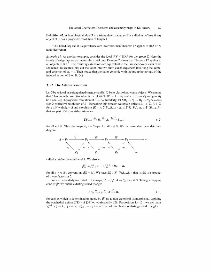
Universal Coefficient Theorems and assembly maps in KK-theory 89
Definition 42. A homological ideal I in a triangulated category T is called hereditary if anyobject of T has a projective resolution of length 1.
If I is hereditary and if I-equivalences are invertible, then Theorem 17 applies to all A∈∈T
(and vice versa).
Example 17. As another example, consider the ideal V C ⊆ KKZ for the group Z. Here thefamily of subgroups only contains the trivial one. Theorem 7 shows that Theorem 17 applies toall objects of KKZ. The resulting extensions are equivalent to the Pimsner–Voiculescu exactsequence. To see this, first cut the latter into two short exact sequences involving the kerneland cokernel of α∗−1. Then notice that the latter coincide with the group homology of theinduced action of Z on K∗(A).
3.3.2 The Adams resolution
Let I be an ideal in a triangulated category and let P be its class of projective objects. We assumethat I has enough projective objects. Let A ∈∈ T. Write A = B0 and let ΣB1→ P0→ B0→ B1be a one-step I-projective resolution of A = B0. Similarly, let ΣB2→ P1→ B1→ B2 be a one-step I-projective resolution of B1. Repeating this process we obtain objects Bn ∈∈ T, Pn ∈P
for n ∈N with B0 = A and morphisms β n+1n ∈ I(Bn,Bn+1), πn ∈ T(Pn,Bn), αn ∈ T1(Bn+1,Pn)
that are part of distinguished triangles
ΣBn+1αn−→ Pn
πn−→ Bnβ n+1
n−−−→ Bn+1 (12)
for all n ∈ N. Thus the maps πn are I-epic for all n ∈ N. We can assemble these data in adiagram
A = B0β 1
0 // B1β 2
1 //
α0
B2β 3
2 //
α1
B3 //
α2
· · ·
P0
π0
__???????P1
π1
[[8888888P2
π2
[[8888888· · ·
\\8888888
called an Adams resolution of A. We also let
βnm := β
nn−1 · · · β
m+1m : Bm→ Bn
for all n≥ m (by convention, β mm = id). We have β n
m ∈ In−m(Bm,Bn), that is, β nm is a product
of n−m factors in I.We are particularly interested in the maps β n := β n
0 : A→ Bn for n ∈ N. Taking a mappingcone of β n we obtain a distinguished triangle
ΣBnσn−→Cn
ρn−→ Aβ n
−→ Bn (13)
for each n, which is determined uniquely by β n up to non-canonical isomorphism. Applyingthe octahedral axiom (TR4) of [37] or, equivalently, [29, Proposition 1.4.12], we get mapsγn+1
n : Cn→Cn+1 and νn : Cn+1→ Pn that are part of morphisms of distinguished triangles
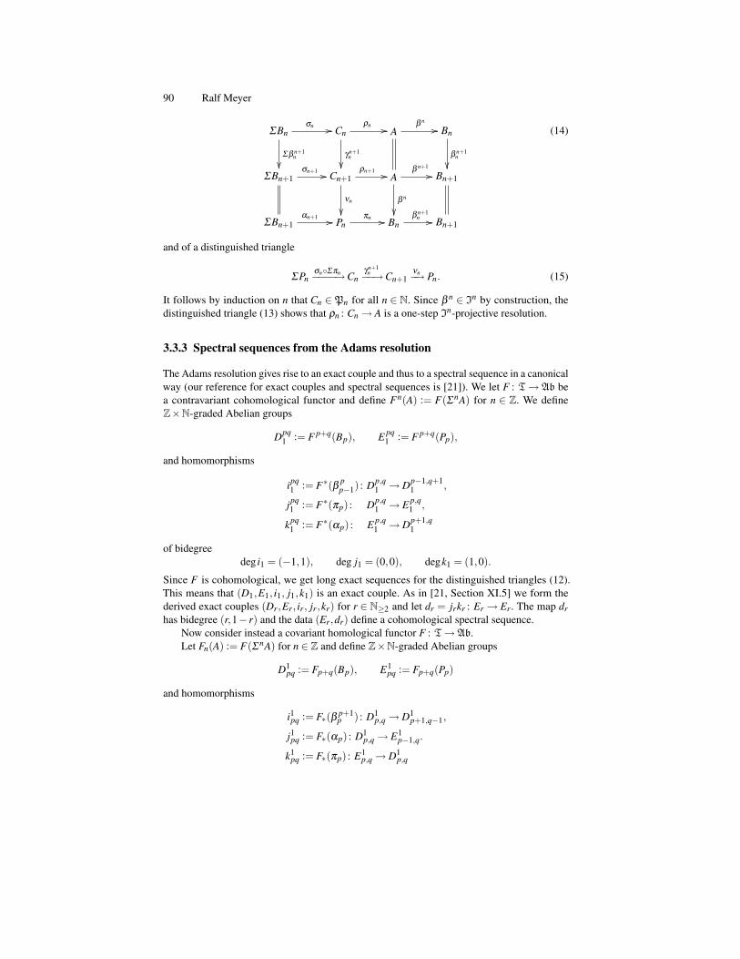
90 Ralf Meyer
ΣBnσn //
Σβ n+1n
Cnρn //
γn+1n
Aβ n// Bn
β n+1n
ΣBn+1
σn+1 // Cn+1ρn+1 //
νn
Aβ n+1//
β n
Bn+1
ΣBn+1αn+1 // Pn
πn // Bnβ n+1
n // Bn+1
(14)
and of a distinguished triangle
ΣPnσnΣπn−−−−→Cn
γn+1n−−→Cn+1
νn−→ Pn. (15)
It follows by induction on n that Cn ∈Pn for all n ∈ N. Since β n ∈ In by construction, thedistinguished triangle (13) shows that ρn : Cn→ A is a one-step In-projective resolution.
3.3.3 Spectral sequences from the Adams resolution
The Adams resolution gives rise to an exact couple and thus to a spectral sequence in a canonicalway (our reference for exact couples and spectral sequences is [21]). We let F : T→ Ab bea contravariant cohomological functor and define Fn(A) := F(Σ nA) for n ∈ Z. We defineZ×N-graded Abelian groups
Dpq1 := F p+q(Bp), E pq
1 := F p+q(Pp),
and homomorphisms
ipq1 := F∗(β p
p−1) : Dp,q1 → Dp−1,q+1
1 ,
jpq1 := F∗(πp) : Dp,q
1 → E p,q1 ,
kpq1 := F∗(αp) : E p,q
1 → Dp+1,q1
of bidegreedeg i1 = (−1,1), deg j1 = (0,0), degk1 = (1,0).
Since F is cohomological, we get long exact sequences for the distinguished triangles (12).This means that (D1,E1, i1, j1,k1) is an exact couple. As in [21, Section XI.5] we form thederived exact couples (Dr,Er, ir, jr,kr) for r ∈ N≥2 and let dr = jrkr : Er → Er. The map drhas bidegree (r,1− r) and the data (Er,dr) define a cohomological spectral sequence.
Now consider instead a covariant homological functor F : T→ Ab.Let Fn(A) := F(Σ nA) for n ∈ Z and define Z×N-graded Abelian groups
D1pq := Fp+q(Bp), E1
pq := Fp+q(Pp)
and homomorphisms
i1pq := F∗(β p+1p ) : D1
p,q→ D1p+1,q−1,
j1pq := F∗(αp) : D1p,q→ E1
p−1,q.
k1pq := F∗(πp) : E1
p,q→ D1p,q
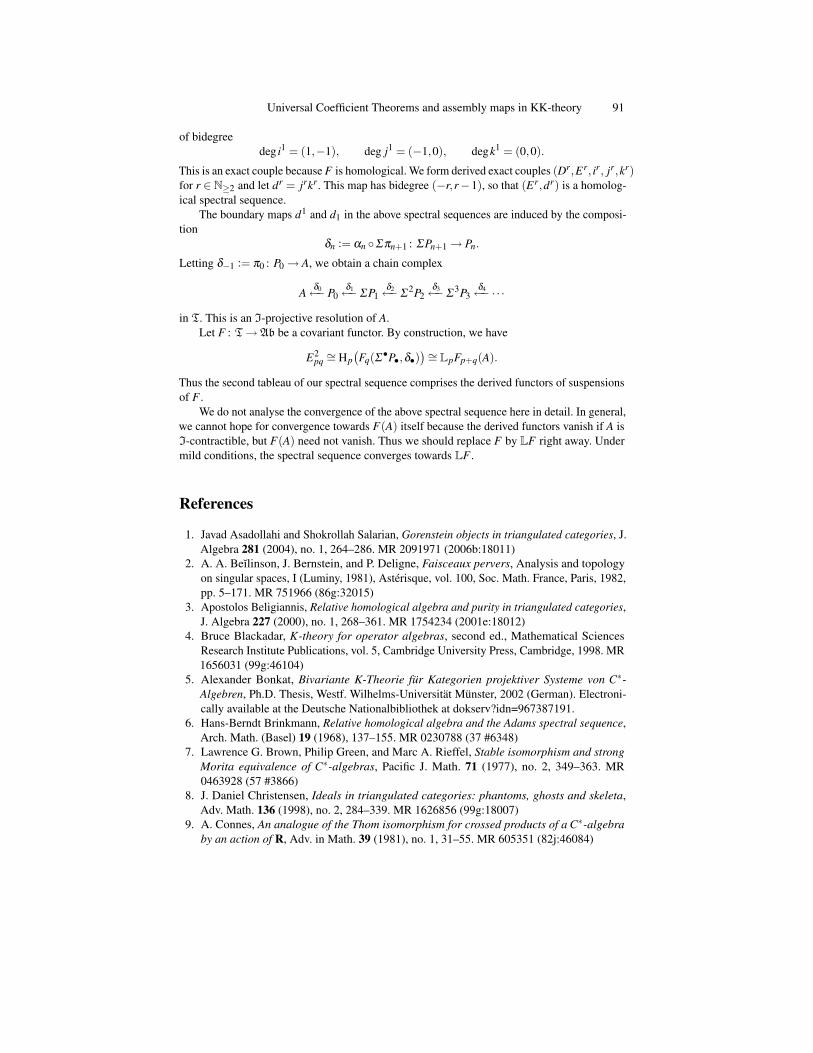
Universal Coefficient Theorems and assembly maps in KK-theory 91
of bidegreedeg i1 = (1,−1), deg j1 = (−1,0), degk1 = (0,0).
This is an exact couple because F is homological. We form derived exact couples (Dr,Er, ir, jr,kr)for r ∈ N≥2 and let dr = jrkr . This map has bidegree (−r,r−1), so that (Er,dr) is a homolog-ical spectral sequence.
The boundary maps d1 and d1 in the above spectral sequences are induced by the composi-tion
δn := αn Σπn+1 : ΣPn+1→ Pn.
Letting δ−1 := π0 : P0→ A, we obtain a chain complex
Aδ0←− P0
δ1←− ΣP1δ2←− Σ
2P2δ3←− Σ
3P3δ4←− ·· ·
in T. This is an I-projective resolution of A.Let F : T→ Ab be a covariant functor. By construction, we have
E2pq∼= Hp
(Fq(Σ•P•,δ•)
)∼= LpFp+q(A).
Thus the second tableau of our spectral sequence comprises the derived functors of suspensionsof F .
We do not analyse the convergence of the above spectral sequence here in detail. In general,we cannot hope for convergence towards F(A) itself because the derived functors vanish if A isI-contractible, but F(A) need not vanish. Thus we should replace F by LF right away. Undermild conditions, the spectral sequence converges towards LF .
References
1. Javad Asadollahi and Shokrollah Salarian, Gorenstein objects in triangulated categories, J.Algebra 281 (2004), no. 1, 264–286. MR 2091971 (2006b:18011)
2. A. A. Beılinson, J. Bernstein, and P. Deligne, Faisceaux pervers, Analysis and topologyon singular spaces, I (Luminy, 1981), Asterisque, vol. 100, Soc. Math. France, Paris, 1982,pp. 5–171. MR 751966 (86g:32015)
3. Apostolos Beligiannis, Relative homological algebra and purity in triangulated categories,J. Algebra 227 (2000), no. 1, 268–361. MR 1754234 (2001e:18012)
4. Bruce Blackadar, K-theory for operator algebras, second ed., Mathematical SciencesResearch Institute Publications, vol. 5, Cambridge University Press, Cambridge, 1998. MR1656031 (99g:46104)
5. Alexander Bonkat, Bivariante K-Theorie fur Kategorien projektiver Systeme von C∗-Algebren, Ph.D. Thesis, Westf. Wilhelms-Universitat Munster, 2002 (German). Electroni-cally available at the Deutsche Nationalbibliothek at dokserv?idn=967387191.
6. Hans-Berndt Brinkmann, Relative homological algebra and the Adams spectral sequence,Arch. Math. (Basel) 19 (1968), 137–155. MR 0230788 (37 #6348)
7. Lawrence G. Brown, Philip Green, and Marc A. Rieffel, Stable isomorphism and strongMorita equivalence of C∗-algebras, Pacific J. Math. 71 (1977), no. 2, 349–363. MR0463928 (57 #3866)
8. J. Daniel Christensen, Ideals in triangulated categories: phantoms, ghosts and skeleta,Adv. Math. 136 (1998), no. 2, 284–339. MR 1626856 (99g:18007)
9. A. Connes, An analogue of the Thom isomorphism for crossed products of a C∗-algebraby an action of R, Adv. in Math. 39 (1981), no. 1, 31–55. MR 605351 (82j:46084)
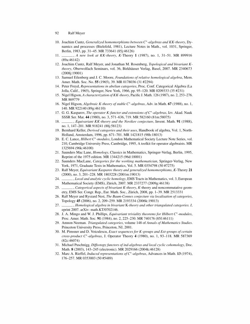
92 Ralf Meyer
10. Joachim Cuntz, Generalized homomorphisms between C∗-algebras and KK-theory, Dy-namics and processes (Bielefeld, 1981), Lecture Notes in Math., vol. 1031, Springer,Berlin, 1983, pp. 31–45. MR 733641 (85j:46126)
11. , A new look at KK-theory, K-Theory 1 (1987), no. 1, 31–51. MR 899916(89a:46142)
12. Joachim Cuntz, Ralf Meyer, and Jonathan M. Rosenberg, Topological and bivariant K-theory, Oberwolfach Seminars, vol. 36, Birkhauser Verlag, Basel, 2007. MR 2340673(2008j:19001)
13. Samuel Eilenberg and J. C. Moore, Foundations of relative homological algebra, Mem.Amer. Math. Soc. No. 55 (1965), 39. MR 0178036 (31 #2294)
14. Peter Freyd, Representations in abelian categories, Proc. Conf. Categorical Algebra (LaJolla, Calif., 1965), Springer, New York, 1966, pp. 95–120. MR 0209333 (35 #231)
15. Nigel Higson, A characterization of KK-theory, Pacific J. Math. 126 (1987), no. 2, 253–276.MR 869779
16. Nigel Higson, Algebraic K-theory of stable C∗-algebras, Adv. in Math. 67 (1988), no. 1,140. MR 922140 (89g:46110)
17. G. G. Kasparov, The operator K-functor and extensions of C∗-algebras, Izv. Akad. NaukSSSR Ser. Mat. 44 (1980), no. 3, 571–636, 719. MR 582160 (81m:58075)
18. , Equivariant KK-theory and the Novikov conjecture, Invent. Math. 91 (1988),no. 1, 147–201. MR 918241 (88j:58123)
19. Bernhard Keller, Derived categories and their uses, Handbook of algebra, Vol. 1, North-Holland, Amsterdam, 1996, pp. 671–701. MR 1421815 (98h:18013)
20. E. C. Lance, Hilbert C∗-modules, London Mathematical Society Lecture Note Series, vol.210, Cambridge University Press, Cambridge, 1995, A toolkit for operator algebraists. MR1325694 (96k:46100)
21. Saunders Mac Lane, Homology, Classics in Mathematics, Springer-Verlag, Berlin, 1995,Reprint of the 1975 edition. MR 1344215 (96d:18001)
22. Saunders MacLane, Categories for the working mathematician, Springer-Verlag, NewYork, 1971, Graduate Texts in Mathematics, Vol. 5. MR 0354798 (50 #7275)
23. Ralf Meyer, Equivariant Kasparov theory and generalized homomorphisms, K-Theory 21(2000), no. 3, 201–228. MR 1803228 (2001m:19013)
24. , Local and analytic cyclic homology, EMS Tracts in Mathematics, vol. 3, EuropeanMathematical Society (EMS), Zurich, 2007. MR 2337277 (2009g:46138)
25. , Categorical aspects of bivariant K-theory, K-theory and noncommutative geom-etry, EMS Ser. Congr. Rep., Eur. Math. Soc., Zurich, 2008, pp. 1–39. MR 2513331
26. Ralf Meyer and Ryszard Nest, The Baum-Connes conjecture via localisation of categories,Topology 45 (2006), no. 2, 209–259. MR 2193334 (2006k:19013)
27. , Homological algebra in bivariant K-theory and other triangulated categories. I,eprint 2007. arXiv: math.KT/0702146.
28. J. A. Mingo and W. J. Phillips, Equivariant triviality theorems for Hilbert C∗-modules,Proc. Amer. Math. Soc. 91 (1984), no. 2, 225–230. MR 740176 (85f:46111)
29. Amnon Neeman. Triangulated categories, volume 148 of Annals of Mathematics Studies.Princeton University Press, Princeton, NJ, 2001.
30. M. Pimsner and D. Voiculescu, Exact sequences for K-groups and Ext-groups of certaincross-product C∗-algebras, J. Operator Theory 4 (1980), no. 1, 93–118. MR 587369(82c:46074)
31. Michael Puschnigg, Diffeotopy functors of ind-algebras and local cyclic cohomology, Doc.Math. 8 (2003), 143–245 (electronic). MR 2029166 (2004k:46128)
32. Marc A. Rieffel, Induced representations of C∗-algebras, Advances in Math. 13 (1974),176–257. MR 0353003 (50 #5489)
Universal Coefficient Theorems and assembly maps in KK-theory 93
33. , Morita equivalence for C∗-algebras and W ∗-algebras, J. Pure Appl. Algebra 5(1974), 51–96. MR 0367670 (51 #3912)
34. , Strong Morita equivalence of certain transformation group C∗-algebras, Math.Ann. 222 (1976), no. 1, 7–22. MR 0419677 (54 #7695)
35. Jonathan Rosenberg and Claude Schochet, The Kunneth theorem and the universal co-efficient theorem for Kasparov’s generalized K-functor, Duke Math. J. 55 (1987), no. 2,431–474. MR 894590 (88i:46091)
36. Ross Street, Homotopy classification of filtered complexes, J. Austral. Math. Soc. 15 (1973),298–318. MR 0340380 (49 #5135)
37. Jean-Louis Verdier, Des categories derivees des categories abeliennes, Asterisque (1996),no. 239, xii+253 pp. (1997), With a preface by Luc Illusie, Edited and with a note byGeorges Maltsiniotis. MR 1453167 (98c:18007)

94 Ralf Meyer
1
Algebraic v. topological K-theory: a friendly match
Guillermo Cortinas
Dep. MatematicaFacultad de Ciencias Exactas y NaturalesUniversidad de Buenos AiresCiudad Universitaria Pab 1(1428) Buenos Aires, [email protected]
1 Introduction
These notes evolved from the lecture notes of a minicourse given in Swisk, the Sedano WinterSchool on K-theory held in Sedano, Spain, during the week January 22–27 of 2007, and fromthose of a longer course given in the University of Buenos Aires, during the second half of2006. They intend to be an introduction to K-theory, with emphasis in the comparison betweenits algebraic and topological variants. We have tried to keep as elementary as possible. Section2 introduces Kn for n ≤ 1. Elementary properties such as matrix stability and excision arediscussed. Section 3 is concerned with topological K-theory of Banach algebras; its excisionproperty is derived from the excision sequence for algebraic K0 and K1. Cuntz’ proof of Bottperiodicity for C∗-algebras, via the C∗-Toeplitz extension, is sketched. In the next section wereview Karoubi-Villamayor K-theory, which is an algebraic version of Ktop, and has someformally similar properties, such as (algebraic) homotopy invariance, but does not satisfyexcision in general. Section 5 discusses KH, Weibel’s homotopy K-theory, which is introducedin a purely algebraic, spectrum-free manner. Several of its properties, including excision,homotopy invariance and the fundamental theorem, are proved. The parallelism between Bottperiodicity and the fundamental theorem for KH is emphasized by the use of the algebraicToeplitz extension in the proof of the latter. Quillen’s higher K-theory is introduced in Section6, via the plus construction of the classifying space of the general linear group. This is the firstplace where some algebraic topology is needed. The “decalage” formula KnΣR = Kn−1R viaKaroubi’s suspension is proved, and some some of the deep results of Suslin and Wodzickion excision are discussed. Then the fundamental theorem for K-theory is reviewed, and itsformal connection to Bott periodicity via the algebraic Toeplitz extension is established. Thenext section is the first of three devoted to the comparison between algebraic and topologicalK-theory of topological algebras. Using Higson’s homotopy invariance theorem, and theexcision results of Suslin and Wodzicki, we give proofs of the C∗- and Banach variantsof Karoubi’s conjecture, that algebraic and topological K-theory become isomorphic afterstabilizing with respect to the ideal of compact operators (theorems of Suslin-Wodzicki andWodzicki, respectively). Section 8 defines two variants of topological K-theory for locally
∗ Work for this notes was partly supported by FSE and by grants PICT03-12330, UBACyT-X294, VA091A05, and MTM00958.
96 Guillermo Cortinas
convex algebras: KV dif and KD which are formally analogue to KV and KH. Some of theirbasic properties are similar and derived with essentially the same arguments as their algebraiccounterparts. We also give a proof of Bott periodicity for KD of locally convex algebrasstabilized by the algebra of smooth compact operators. The proof uses the locally convexToeplitz extension, and is modelled on Cuntz’ proof of Bott periodicity for his bivariant K-theory of locally convex algebras. In Section 9 we review some of the results of [13]. Usingthe homotopy invariance theorem of Cuntz and Thom, we show that KH and KD agree onlocally convex algebras stabilized by Frechet operator ideals. The spectra for Quillen’s andWeibel’s K-theory, and the space for Karoubi-Villamayor K-theory are introduced in Section10, where also the primary and secondary characters going from K-theory to cyclic homologyare reviewed. The technical results of this section are used in the next, where we again deal withthe comparison between algebraic and topological K-theory of locally convex algebras. Wegive proofs of the Frechet variant of Karoubi’s conjecture (due to Wodzicki), and of the 6-termexact sequence of [13], which relates algebraic K-theory and cyclic homology to topologicalK-theory of a stable locally convex algebra.
2 The groups Kn for n≤ 1.
Notation. Throughout these notes, A,B,C will be rings and R,S,T will be rings with unit.
2.1 Definition and basic properties of K j for j = 0,1.
Let R be a ring with unit. Write MnR for the matrix ring. Regard MnR⊂Mn+1R via
a 7→[
a 00 0
](1)
Put
M∞R =∞⋃
n=1MnR
Note M∞R is a ring (without unit). We write IdemnR and Idem∞R for the set of idempotentelements of MnR and M∞R. Thus
M∞R⊃ Idem∞R =∞⋃
n=1IdemnR.
We write GLnR = (MnR)∗ for the group of invertible matrices. Regard GLnR⊂ GLn+1R via
g 7→[
g 00 1
]Put
GLR :=∞⋃
n=1GLnR.
Note GLR acts by conjugation on M∞R, Idem∞R and, of course, GLR.For a,b ∈M∞R there is defined a direct sum operation
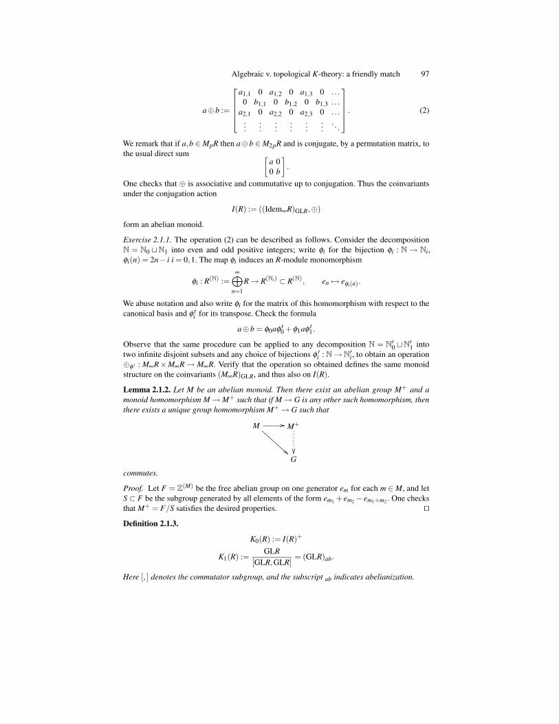
Algebraic v. topological K-theory: a friendly match 97
a⊕b :=
a1,1 0 a1,2 0 a1,3 0 . . .
0 b1,1 0 b1,2 0 b1,3 . . .a2,1 0 a2,2 0 a2,3 0 . . .
......
......
......
. . .
. (2)
We remark that if a,b ∈MpR then a⊕b ∈M2pR and is conjugate, by a permutation matrix, tothe usual direct sum [
a 00 b
].
One checks that ⊕ is associative and commutative up to conjugation. Thus the coinvariantsunder the conjugation action
I(R) := ((Idem∞R)GLR,⊕)
form an abelian monoid.
Exercise 2.1.1. The operation (2) can be described as follows. Consider the decompositionN = N0 tN1 into even and odd positive integers; write φi for the bijection φi : N → Ni,φi(n) = 2n− i i = 0,1. The map φi induces an R-module monomorphism
φi : R(N) :=∞⊕
n=1R→ R(Ni) ⊂ R(N), en 7→ eφi(n).
We abuse notation and also write φi for the matrix of this homomorphism with respect to thecanonical basis and φ t
i for its transpose. Check the formula
a⊕b = φ0aφt0 +φ1aφ
t1.
Observe that the same procedure can be applied to any decomposition N = N′0 tN′1 intotwo infinite disjoint subsets and any choice of bijections φ ′i : N→ N′i, to obtain an operation⊕φ ′ : M∞R×M∞R→ M∞R. Verify that the operation so obtained defines the same monoidstructure on the coinvariants (M∞R)GLR, and thus also on I(R).
Lemma 2.1.2. Let M be an abelian monoid. Then there exist an abelian group M+ and amonoid homomorphism M→M+ such that if M→ G is any other such homomorphism, thenthere exists a unique group homomorphism M+→ G such that
M //
!!BBBBBBBB M+
G
commutes.
Proof. Let F = Z(M) be the free abelian group on one generator em for each m ∈M, and letS⊂ F be the subgroup generated by all elements of the form em1 + em2 − em1+m2 . One checksthat M+ = F/S satisfies the desired properties. ut
Definition 2.1.3.
K0(R) := I(R)+
K1(R) :=GLR
[GLR,GLR]= (GLR)ab.
Here [, ] denotes the commutator subgroup, and the subscript ab indicates abelianization.
98 Guillermo Cortinas
Propostion 2.1.4. (see [44, Section 2.1])• [GLR,GLR] = ER :=< 1 + aei, j : a ∈ R, i 6= j >, the subgroup of GLR generated by
elementary matrices.• If α ∈ GLnR then [
α 00 α−1
]∈ E2nR (Whitehead’s Lemma).
(Here E2nR = ER∩GL2nR). utAs a consequence of Whitehead’s lemma above, if β ∈ GLnR, then
αβ =[
αβ 00 1n×n
]=[
α 00 β
][β 00 β−1
](3)
≡α⊕β -modER.
Exercise 2.1.5. Let R be a unital ring, and let φ ′ and ⊕φ ′ be as in Exercise 2.1.1. Prove that⊕φ ′ and ⊕ define the same operation in K1(R), which coincides with the product of matrices.
Let r ≥ 1. Thenpr = 1r×r ∈ Idem∞R.
Because pr⊕ ps = pr+s, the assignment r 7→ pr defines a monoid homomorphism N→ I(R).Applying the group completion functor we obtain a group homomorphism
Z= N+→ I(R)+ = K0R. (4)
Similarly, the inclusion R∗ = GL1R⊂ GLR induces a homomorphism
R∗ab→ K1R. (5)
Example 2.1.6. If F is a field, and e ∈ Idem∞F is of rank r, then e is conjugate to pr; moreoverpr and ps are conjugate ⇐⇒ r = s. Thus (4) is an isomorphism in this case. Assume moregenerally that R is commutative. Then (4) is a split monomorphism. Indeed, there exists asurjective unital homomorphism R F onto a field F ; the induced map K0(R)→ K0(F) = Zis a left inverse of (4). Similarly, for commutative R, the homomorphism (5) is injective, sinceit is split by the map det : K1R→ R∗ induced by the determinant.
Example 2.1.7. The following are examples of rings for which the maps (4) and (5) areisomorphisms (see [44, Ch.1§3, Ch.2§2,§3]): fields, division rings, principal ideal domains andlocal rings. Recall that a ring R is a local ring if the subset R\R∗ of noninvertible elements isan ideal of R. For instance if k is a field, then the k-algebra k[ε] := k⊕ kε with ε2 = 0 is a localring. Indeed k[ε]∗ = k∗+ kε and k[ε]\k[ε]∗ = kε / k[ε].
Example 2.1.8. Here is an example of a local ring involving operator theory. Let H be aseparable Hilbert space over C; put B = B(H) for the algebra of bounded operators. WriteK ⊂ B for the ideal of compact operators, and F for that of finite rank operators. TheRiesz-Schauder theorem from elementary operator theory implies that if λ ∈ C∗ and T ∈Kthen there exists an f ∈F such that λ + T + f is invertible in B. In fact one checks that ifF ⊂ I ⊂K is an ideal of B such that T ∈ I then the inverse of λ +T + f is again in C⊕ I.Hence the ring
RI := C⊕ I/F
is local, and thus K0(RI) = Z.
Algebraic v. topological K-theory: a friendly match 99
Remark 2.1.9. (K0 from projective modules) In the literature, K0 of a unital ring is often definedin terms of finitely generated projective modules. This approach is equivalent to ours, as weshall see presently. If R is a unital ring and e ∈ IdemnR, then left multiplication by e defines aright module homomorphism Rn = Rn×1→ Rn with image eRn. Similarly (1− e)Rn ⊂ Rn is asubmodule, and we have a direct sum decomposition
Rn = eRn⊕ (1− e)Rn.
Hence eRn is a finitely generated projective module, as it is a direct summand of a finitelygenerated free R-module. Note every finitely generated projective right R-module arises inthis way for some n and some e ∈ IdemnR. Moreover, one checks that if e ∈ IdemnR andf ∈ IdemmR, then the modules eRn and f Rm are isomorphic if and only if the images of e andf in Idem∞R define the same class in I(R) (see [44, Lemma 1.2.1]). Thus we have a naturalbijection from the monoid I(R) to the set P(R) of isomorphism classes of finitely generatedprojective modules; further, one checks that the direct sum of idempotents corresponds to thedirect sum of modules. Hence the monoids I(R) and P(R) are isomorphic, and therefore theyhave the same group completion:
K0(R) = I(R)+ = P(R)+.
Additivity.
If R1 and R2 are unital rings, then M∞(R1×R2)→M∞R1×M∞R2 is an isomorphism. It followsfrom this that the natural map induced by the projections R1×R2→ Ri is an isomorphism:
K j(R1×R2)→ K jR1⊕K jR2 ( j = 0,1).
Application: extension to nonunital rings.
If A is any (not necessarily unital) ring, then the abelian group A = A⊕Z equipped with themultiplication
(a+n)(b+m) := ab+nm (a,b ∈ A, n,m ∈ Z) (6)
is a unital ring, with unit element 1 ∈ Z, and A→ Z, a+n 7→ n, is a unital homomorphism. Put
K j(A) := ker(K jA→ K jZ) ( j = 0,1).
If A happens to have a unit, we have two definitions for K jA. To check that they are the same,one observes that the map
A→ A×Z, a+n 7→ (a+n ·1,n) (7)
is a unital isomorphism. One verifies that, under this isomorphism, A→ Z identifies with theprojection A×Z→ Z, and ker(K j(A)→ K jZ) with ker(K jA⊕K jZ→ K jZ) = K jA. Note thatthe same procedure works to extend any additive functor of unital rings unambiguously to allrings.
Notation. We write Ass for the category of rings and ring homomorphisms, and Ass1 for thesubcategory of unital rings and unit preserving ring homomorphisms.
100 Guillermo Cortinas
Remark 2.1.10. The functor GL : Ass1→Grp preserves products. Hence it extends to all ringsby
GL(A) := ker(GL(A)→ GLZ)It is a straightforward exercise to show that, with this definition, GL becomes a left exactfunctor in Ass; thus if A/B is an ideal embedding, then GL(A) = ker(GL(B)→ GL(B/A)). Itis straightforward from this that the group K1A defined above can be described as
K1A = GL(A)/E(A)∩GL(A) (8)
A little more work shows that E(A)∩GL(A) is the smallest normal subgroup of E(A) whichcontains the elementary matrices 1+aei, j with a ∈ A (see [44, 2.5]).
Matrix stability.
Let R be a unital ring and n≥ 2. A choice of bijection φ :N×N≤n∼=N gives a ring isomorphismφ : M∞(MnR)∼= M∞(R) which induces, for j = 0,1, a group isomorphism φ j : K j(MnR)∼= K jR.Next, consider the decomposition N=N′0tN′1, N′0 = φ(N×1), N′1 = φ(N×N<n\N×1).Setting ψ0 : N→ N′0, ψ0(m) = φ(m,1) and choosing any bijection ψ1 : N→ N′1, we obtain, asin Exercise 2.1.1, a direct sum operation⊕ψ : M∞R×M∞R→M∞R. Set ι : R 7→MnR, r 7→ re11.The composite of M∞ι followed by the isomorphism induced by φ is the map sending
ei, j(r) 7→ eφ(i,1),φ( j,1)(r) = ei, j(r)⊕ψ 0. (9)
By Exercise 2.1.1 the latter map induces the identity in K0. Moreover, one checks that (9)induces the map GL(MnR)→ GL(MnR), g 7→ g⊕ψ 1, whence it also gives the identity in K1,by Exercise 2.1.5. It follows that, for j = 0,1, the map
K j(ι) : K j(R)→ K j(MnR)
is an isomorphism, inverse to φ j. Starting with a bijection φ : N×N→ N and using the sameargument as above, one shows that also
K j(ι) : K j(R)→ K j(M∞R)
is an isomorphism.
Nilinvariance for K0.
If I / R is a nilpotent ideal, then K0(R)→ K0(R/I) is an isomorphism. This property is aconsequence of the well-known fact that nilpotent extensions admit idempotent liftings, andthat any two liftings of the same idempotent are conjugate (see for example [3, 1.7.3]). Notethat K1 does not have the same property, as the following example shows.
Example 2.1.11. Let k be a field. Then by 2.1.7, K1(k[ε]) = k∗+ kε and K1(k) = k∗. Thusk[ε]→ k[ε]/εk[ε] = k does not become an isomorphism under K1.
Example 2.1.12. Let A be an abelian group; make it into a ring with the trivial product:ab = 0 ∀a,b ∈ A. The map A→ GL1A, a 7→ 1 + a is an isomorphism of groups, and thusinduces a group homomorphism A→ K1A. We are going to show that the latter map is anisomorphism. First of all, it is injective, since GL1(A)→ K1(A) is (by 2.1.6) and since bydefinition, K1A⊂ K1(A). Second, note that if ε = 1+aei j is an elementary matrix with a ∈ Aand g∈GLA, then (εg)i j = gi j +a, and (εg)p,q = gp,q for (p,q) 6= (i, j). Thus g is congruent toits diagonal in K1A. But by Whitehead’s lemma, any diagonal matrix in GL(A) is K1-equivalentto its determinant (see (3)). This shows that A→ K1A is surjective, whence an isomorphism.
Algebraic v. topological K-theory: a friendly match 101
Remark 2.1.13. The example above shows that K1 is no longer matrix stable when extended togeneral nonunital rings. In addition, it gives another example of the failure of nilinvariance forK1 of unital rings. It follows from 2.1.11 and 2.1.12 that if k and ε are as in Example 2.1.11,then K1(kε) = ker(K1(k[ε])→ K1(k)). In 2.4.4 below, we give an example of a unital ring Tsuch that kε is an ideal in T , and such that ker(T → T/kε) = 0.
Exercise 2.1.14. Prove that K0 and K1 commute with filtering colimits; that is, show thatif I is a small filtering category and A : I → Ass is a functor, then for j = 0,1, the mapcolimI K jAi→ K j(colimI Ai) is an isomorphism.
2.2 Matrix-stable functors.
Definition 2.2.1. Let C⊂ Ass be a subcategory of the category of rings, S : C→ C a functor,and γ : 1C→ S a natural transformation. If D is any category, F : C→D a functor and A ∈ C,then we say that F is stable on A with respect to (S,γ) (or S-stable on A, for short) if the mapF(γA) : F(A)→ F(S(A)) is an isomorphism. We say that F is S-stable if it is stable on everyA ∈ C.
Example 2.2.2. We showed in Section 2.1 that K j is Mn and even M∞-stable on unital rings; inboth cases, the natural transformation of the definition above is r 7→ re11.
Exercise 2.2.3. Let F : Ass→ Ab be a functor and A a ring. Prove:i) The following are equivalent:
• For all n, p ∈ N, F is Mp-stable on MnA.• For all n ∈ N, F is M2-stable on MnA
In particular, an M2-stable functor is Mn-stable, for all n.ii) If F is M∞-stable on both A and MnA, then F is Mn-stable on A. In particular, if F isM∞-stable, then it is Mn-stable for all n.
Lemma 2.2.4. Let F : Ass→D be a functor, and A ∈ Ass. Assume F is M2-stable on both Aand M2A. Then the inclusions ι0, ι1 : A→M2A
ι0(a) = ae11, ι1(a) = ae22
induce the same isomorphism FA→ FM2A.
Proof. Consider the composites j0 = ι0M2 ι0 and j1 = ι0M2 ι1, and the matrices
J2 =
0 1 0 01 0 0 00 0 1 00 0 0 1
, J3 =
0 0 1 01 0 0 00 1 0 00 0 0 1
∈ GL4Z.
Conjugation by Ji induces an automorphism σi of M4A = M2M2A of order i such that
σi j0 = j1 (i = 2,3).
Since F( j0) is an isomorphism, and the orders of σ2 and σ3 are relatively prime, it follows thatF(σ2) = F(σ3) = 1F(M4A) and hence that F( j0) = F( j1) and F(ι0) = F(ι1). ut
102 Guillermo Cortinas
Exercise 2.2.5. Let F and A be as in Lemma 2.2.4. Assume in addition that D and F areadditive. Consider the map
diag : A×A→M2A, diag(a,b) =[
a 00 b
].
Prove that the composite
F(A)⊕F(A) = F(A×A)F(diag)−→ F(M2A)
F(i0)−1
−→ F(A)
is the codiagonal map (i.e. it restricts to the identity on each copy of F(A)).
Propostion 2.2.6. Let F and A be as in Lemma 2.2.4, A⊂B an overring, and V,W ∈B elementssuch that
WA,AV ⊂ A, aVWa′ = aa′ (a,a′ ∈ A).
Thenφ
V,W : A→ A, a 7→WaV
is a ring homomorphism, andF(φV,W ) = 1F(A).
Proof. We may assume that B is unital. Consider the elements V ⊕1 and W ⊕1 ∈M2B. Thehypothesis guarantee that both φ := φV,W and φ ′ := φV⊕1,W⊕1 : M2A→M2A are well-definedring homomorphisms. Moreover, φ ′ι1 = ι1 and φ ′ι0 = ι0φ . It follows that F(φ ′) and F(φ) arethe identity maps, by Lemma 2.2.4. ut
Exercise 2.2.7.i) Let R be a unital ring and L a free, finitely generated R-module of rank n. A choice ofbasis B of L gives an isomorphism φ = φB : MnR→ EndRL. Use 2.2.6 to show that K j(φ) isindependent of the choice of B ( j = 0,1).
ii) Assume R is a field. If e ∈ EndRL is idempotent, then ιe : R→ EndRL, x 7→ xe is a ringmonomorphism. Show that if e ∈ EndRL is of rank 1, then K j(ιe) = K j(φι). In particular,K j(ιe) is independent of the choice of the rank-one idempotent e.iii) Let H and F be as in Example 2.1.8. If V ⊂W ⊂ H are finite dimensional subspaces andU = V⊥∩W then the decomposition W = V ⊕U induces an inclusion EndC(V )⊂ EndC(W ).Show that
F =⋃
dimV<∞
EndC(V )
iv) Prove that if e ∈F is any self-adjoint, rank-one idempotent, then the inclusion C→F ,x 7→ xe, induces an isomorphism K j(C)
∼=→ K j(F ). Show moreover that this isomorphism isindependent of the choice of e.
2.3 Sum rings and infinite sum rings.
Recall from [53] that a sum ring is a unital ring R together with elements αi,βi, i = 0,1 suchthat the following identities hold
α0β0 = α1β1 = 1
β0α0 +β1α1 = 1 (10)
Algebraic v. topological K-theory: a friendly match 103
If R is a sum ring, then
: R×R→ R, (11)
(a,b) 7→ ab = β0aα0 +β1bα1
is a unital ring homomorphism. An infinite sum ring is a sum ring R together with a unitpreserving ring homomorphism ∞ : R→ R, a 7→ a∞ such that
aa∞ = a∞ (a ∈ R). (12)
Propostion 2.3.1. Let D be an additive category, F : Ass→D a functor, and R a sum ring. As-sume that the sum of projection maps γ = Fπ0 +Fπ1 : F(R×R)→ FR⊕FR is an isomorphism,and that F is M2-stable on both R and M2R. Then the composite
F(R)⊕F(R)γ−1// F(R×R)
F() // F(R)
is the codiagonal map; that is, it restricts to the identity on each copy of F(R). If moreover R isan infinite sum ring, then F(R) = 0.
Proof. Let j0, j1 : R→ R×R, j0(x) = (x,0), j1(x) = (0,x). Note that γ−1 = F j0 + F j1. Be-cause F is M2-stable on both R and M2R, F()F( ji) = 1F(R), by Proposition 2.2.6. ThusF() γ−1 is the codiagonal map, as claimed. It follows that if α,β : R→ R are homomor-phisms, then Fα +Fβ = F((α,β )). In particular, if R is an infinite sum ring, then
F(∞)+1F(R) = F(∞)+F(1R) = F((∞,1R)) = F(∞).
Thus 1F(R) = 0, whence F(R) = 0. ut
Example 2.3.2. Let A be a ring. Write Γ A for the ring of all N×N matrices a = (ai, j)i, j≥1which satisfy the following two conditions:
i) The set ai j, i, j ∈ N is finite.ii) There exists a natural number N ∈ N such that each row and each column has at most N
nonzero entries.
It is an exercise to show that Γ A is indeed a ring and that M∞A⊂ Γ A is an ideal. The ring Γ Ais called (Karoubi’s) cone ring; the quotient ΣA := Γ A/M∞A is the suspension of A. A usefulfact about Γ and Σ is that the well-known isomorphism M∞Z⊗A∼= M∞A extends to Γ , so thatthere are isomorphisms (see [12, 4.7.1])
ΓZ⊗A∼=→ Γ A and ΣZ⊗A
∼=→ ΣA. (13)
Let R be a unital ring. One checks that the following elements of Γ R satisfy the identities (10):
α0 =∞
∑i=1
ei,2i, β0 =∞
∑i=1
e2i,i, α1 =∞
∑i=1
ei,2i−1, and β1 =∞
∑i=1
e2i−1,i.
Let a ∈ Γ R. Because the map N×N→ N, (k, i) 7→ 2k+1i+2k−1, is injective, the followingassignment gives a well-defined, N×N-matrix
φ∞(a) =
∞
∑k=0
βk1 β0aα0α
k1 = ∑
k,i, je2k+1i+2k−1,2k+1 j+2k−1⊗ai, j. (14)
One checks that α1β0 = α0β1 = 0 and α0α i1β
j1 β0 = δi j. It follows from this that φ ∞ is a ring
endomorphism of Γ R; it is straightforward that (12) is satisfied too. In particular KnΓ R = 0 forn = 0,1.
104 Guillermo Cortinas
Exercise 2.3.3. Let A be a ring. If m = (mi, j) is an N×N-matrix with coefficients in A, andx ∈M∞A, then both m · x and x ·m are well-defined N×N-matrices. Put
Γ`A := m ∈MN×NA : m ·M∞A⊂M∞A⊃M∞A ·m. (15)
Provei) Γ `A consists of those matrices in MN×NA having finitely many nonzero elements in eachrow and column. In particular, Γ `A⊃ Γ A.ii) The usual matrix sum and product operations make Γ `A into a ring.iii) If R is a unital ring then Γ `R is an infinite sum ring.
Remark 2.3.4. The ring Γ `A is the cone ring considered by Wagoner in [53], where it wasdenoted `A. The notion of infinite sum ring was introduced in loc. cit., where it was also shownthat if R is unital, then Γ `R is an example of such a ring.
Exercise 2.3.5. Let F : Ass→ Ab be a functor. Assume F is both additive and M2-stable forunital rings and for rings of the form M∞R, with R unital. Show that if R is a unital ring, thenthe direct sum operation (2), induces the group operation in F(M∞R), and that the same is trueof any of the other direct sum operations of 2.1.1.
Exercise 2.3.6. Let B and H be as in Example 2.1.8. Choose a Hilbert basis eii≥1 of H, andregard B as a ring of N×N matrices. With these identifications, show that B ⊃ ΓC. Deducefrom this that B is a sum ring. Further show that (14) extends to B, so that the latter is in factan infinite sum ring.
2.4 The excision sequence for K0 and K1.
A reason for considering K0 and K1 as part of the same theory is that they are connected by along exact sequence, as shown in Theorem 2.4.1 below. We need some notation. Let
0→ A→ B→C→ 0 (16)
be an exact sequence of rings. If g ∈MnB maps to an invertible matrix g ∈ GLnC and g∗ mapsto g−1, then
h = h(g, g∗) :=[
2g− gg∗g gg∗−11− g∗g g∗
](17)
=[
1 g0 1
]·[
1 0−g∗ 1
]·[
1 g0 1
]·[
0 −11 0
]∈ E2n(B)⊂ GL2n(B)
Note that h maps to diag(g,g−1) ∈GL2n(C). Thus hpnh−1 maps to pn, whence hpnh−1− pn ∈M2nA and hpnh−1 ∈M2nA. Put
∂ (g, g∗) := [hpnh−1]− [pn] ∈ ker(K0(A)→ K0Z) = K0A (18)
Theorem 2.4.1. If (16) is an exact sequence of rings, then there is a long exact sequence
K1A // K1B // K1C
∂
K0C K0Boo K0Aoo
The map ∂ sends the class of an element g∈GLnC to the class of the element (18); in particularthe latter depends only on the K1-class of g.
Algebraic v. topological K-theory: a friendly match 105
Proof. (Sketch) The exactness of the top row of the sequence of the theorem is straightforward.Putting together [44, Thms. 1.5.5, 1.5.9 and 2.5.4] we obtain the theorem for those sequences(16) in which B→ C is a unital homomorphism. It follows that we have a map of exactsequences
K1B //
K1C
// K0A
// K0B
// K0C
K1Z K1Z // 0 // K0Z K0Z
Taking kernels of the vertical maps, we obtain an exact sequence
K1B // K1C // K0A // K0B // K0C
It remains to show that the map K1C→ K0A of this sequence is given by the formula of thetheorem. This is done by tracking down the maps and identifications of the proofs of [44, Thms.1.5.5, 1.5.9 and 2.5.4] (see also [40, §3,§4]), and computing the idempotent matrices to whichthe projective modules appearing there correspond, taking into account that B→C sends thematrix h ∈ GL2nB of (17) to the diagonal matrix diag(g,g−1) ∈ GL2nC. ut
Remark 2.4.2. In [44, 2.5.4], a sequence similar to that of the theorem above is obtained, inwhich K1A is replaced by a relative K1-group K1(B : A), depending on both A and B. Forexample if B→ B/A is a split surjection, then ([44, Exer. 2.5.19])
K1(B : A) = ker(K1B→ K1(B/A))
The groups K1(B : A) and K1A are not isomorphic in general (see Example 2.4.4 below);however their images in K1B coincide. We point out also that the theorem above can be deduceddirectly from Milnor’s Mayer-Vietoris sequence for a Milnor square ([40, §4]).
The following corollary is immediate from the theorem.
Corollary 2.4.3. Assume (16) is split by a ring homomorphism C→ B. Then K0A→ K0B isinjective, and induces an isomorphism
K0A = ker(K0B→ K0C)
Because of this we say that K0 is split exact.
Example 2.4.4. (Swan’s example [50]) We shall give an example which shows that K1 is notsplit exact. Let k be a field with at least 3 elements (i.e. k 6= F2). Consider the ring of uppertriangular matrices
T :=[
k k0 k
]with coefficients in k. The set I of strictly upper triangular matrices forms an ideal of T ,isomorphic as a ring, to the ideal kε / k[ε], via the identification ε = e12. By Examples 2.1.11and 2.1.12, ker(K1(k[ε])→ K1(k)) = K1(kε)∼= kε , the additive group underlying k. If K1 weresplit exact, then also
K1(T : I) = ker(K1T → K1(k× k)) (19)
should be isomorphic to kε . However we shall see presently that K1(T : I) = 0. Note thatT → k× k is split by the natural inclusion diag : k× k→ T . Thus any element of K1(T : I) isthe class of an element in GL(kε), and by 2.1.11 it is congruent to the class of an element in
106 Guillermo Cortinas
GL1(kε) = 1+ kε . We shall show that if λ ∈ k, then 1+λε ∈ [GL1T,GL1T ]. Because we areassuming that k 6= F2, there exists µ ∈ k−0,1; one checks that
1+λε =[
1 λ
0 1
]=
[[µ 00 1
],
[1 λ
µ−10 1
]]∈ [GL1T,GL1T ].
Example 2.4.5. Let R be a unital ring. Applying the theorem above to the cone sequence
0→M∞R→ Γ R→ ΣR→ 0 (20)
we obtain an isomorphismK1ΣR = K0R. (21)
Exercise 2.4.6. Use Corollary 2.4.3 to prove that all the properties of K0 stated in 2.1 for unitalrings, remain valid for all rings. Further, show that K0(Γ A) = 0 for all rings A, and thus thatfor any ring A, the boundary map gives a surjection
K1ΣA K0A.
2.5 Negative K-theory.
Definition 2.5.1. Let A be a ring and n≥ 0. Put
K−nA := K0ΣnA.
Propostion 2.5.2.i) For n≤ 0, the functors Kn : Ass→ Ab are additive, nilinvariant and M∞-stable.ii) The exact sequence of 2.4.1 extends to negative K-theory. Thus if
0→ A→ B→C→ 0
is a short exact sequence of rings, then for n≤ 0 we have a long exact sequence
KnA // KnB // KnC
∂
Kn−1C Kn−1Boo Kn−1Aoo
Proof.i) By (13), we have ΣA = ΣZ⊗A. Thus Σ commutes with finite products and with M∞, andsends nilpotent rings to nilpotent rings. Moreover, Σ is exact, because both M∞ and Γ are.Hence the general case of i) follows from the case n = 0, which is proved in Section 2.1.
ii) Consider the sequence0→ A→ B→ C→ 0
Applying Σ , we obtain0→ ΣA→ Σ B→ ΣC→ 0
By (21), if D is any ring, then K0D = K1Σ D. Thus by 2.4.1 and 2.4.3, we get an exact sequence
Algebraic v. topological K-theory: a friendly match 107
K0A // K0B⊕K0Z // K0C⊕K0Z
∂
K−1C⊕K−1Z K−1B⊕K−1Zoo K−1Aoo
Splitting off the K jZ summands, we obtain
K0A // K0B // K0C
∂
K−1C K−1Boo K−1Aoo
This proves the case n = 0 of the proposition. The general case follows from this. ut
Example 2.5.3. Let B be as in Example 2.1.8 and I /B a proper ideal. It is classical thatF ⊂ I ⊂K for any such ideal. We shall show that the map
K0F → K0I (22)
is an isomorphism; thus K0I = K0F = Z, by Exercise 2.2.7. As in 2.1.8 we consider the localring RI = C⊕ I/F . We have a commutative diagram with exact rows and split exact columns
0 // F // I
// I/F //
0
0 // F // C⊕ I
// RI //
0
C C
By 2.1.8 and split exactness, K0(I/F ) = 0. Thus the map (22) is onto. From the diagramabove, K1(I/F )→ K0F factors through K1(RI)→ K0F . But it follows from the discussionof Example 2.1.8 that the map K1(C⊕ I)→ K1(RI) is onto, whence K1(RI)→ K0F and thusalso K1(I/F )→ K0F , are zero. Thus (22) is an isomorphism.
Exercise 2.5.4. A theorem of Karoubi asserts that K−1(K ) = 0 [34]. Use this and excision toshow that K−1(I) = 0 for any operator ideal I.
Exercise 2.5.5. Prove that if n < 0, then the functor Kn commutes with filtering colimits.
Remark 2.5.6. The definition of negative K-theory used here is taken from Karoubi-Villamayor’spaper [37], where cohomological notation is used. Thus what we call KnA here is denotedK−nA in loc. cit. (n≤ 0). There is also another definition, due to Bass [2]. A proof that the twodefinitions agree is given in [37, 7.9].
108 Guillermo Cortinas
3 Topological K-theory
We saw in the previous section (Example 2.4.4) that K1 is not split exact. It follows from thisthat there is no way of defining higher K-groups such that the long exact sequence of Theorem2.4.1 can be extended to higher K-theory. This motivates the question of whether this problemcould be fixed if we replaced K1 by some other functor. This is succesfully done in topologicalK-theory of Banach algebras.
3.1 Topological K-theory of Banach algebras.
A Banach (C-) algebra is a C-algebra together with a norm || || which makes it into a Banachspace and is such that ||xy|| ≤ ||x|| · ||y|| for all x,y ∈ A. If A is a Banach algebra then itsC-unitalization is the unital Banach algebra
AC = A⊕C
equipped with the product (6) and the norm ||a+λ || := ||a||+ |λ |. An algebra homomorphismis a morphism of Banach algebras if it is continuous. If X is a compact Hausdorff space and V isany topological vectorspace, we write C (X ,V ) for the topological vectorspace of all continuousmaps X → V . If A is a Banach algebra, then C (X ,A) is again a Banach algebra with norm|| f ||∞ := supx || f (x)||. If X is locally compact, X+ its one point compactification, and V atopological vectorspace, we write
V (X) = C0(X ,V ) = f ∈ C (X+,V ) : f (∞) = 0.
Note that if X is compact, V (X) = C (X ,V ). If A is a Banach algebra then A(X) is againa Banach algebra, as it is the kernel of the homomorphism C (X+,A)→ A, f 7→ f (∞). Forexample, A[0,1] is the algebra of continous functions [0,1]→ A, and A(0,1] and A(0,1) areidentified with the ideals of A[0,1] consisting of those functions which vanish respectively at0 and at both endpoints. Two homomorphisms f0, f1 : A→ B of Banach algebras are calledhomotopic if there exists a homomorphism H : A→ B[0,1] such that the following diagramcommutes.
B[0,1]
(ev0,ev1)
A
H==zzzzzzzz
( f0, f1)// B×B
A functor G from Banach algebras to a category D is called homotopy invariant if it mapshomotopic maps to equal maps.
Exercise 3.1.1. Prove that G is homotopy invariant if and only if for every Banach algebra Athe map G(A)→ G(A[0,1]) induced by the natural inclusion A⊂ A[0,1] is an isomorphism.
Theorem 3.1.2. ([44, 1.6.11]) The functor K0 : ((Banach Algebras))→ Ab is homotopy in-variant.
Example 3.1.3. K1 is not homotopy invariant. The algebra A := C[ε] is a Banach algebra withnorm ||a + bε|| = |a|+ |b|. Both the inclusion ι : C→ A and the projection π : A→ C arehomomorphisms of Banach algebras; they satisfy πι = 1. Moreover the map H : A→ A[0,1],H(a + bε)(t) = a + tbε is also a Banach algebra homomorphism, and satisfies ev0H = ιπ ,ev1H = 1. Thus any homotopy invariant functor G sends ι and π to inverse homomorphisms;since K1 does not do so by 2.1.11, it is not homotopy invariant.
Algebraic v. topological K-theory: a friendly match 109
Next we consider a variant of K1 which is homotopy invariant.
Definition 3.1.4. Let R be a unital Banach algebra. Put
GLR0 := g ∈ GLR : ∃h ∈ GL(R[0,1]) : h(0) = 1,h(1) = g.
Note GL(R)0 /GLR. The topological K1 of R is
Ktop1 R = GLR/GL(R)0.
Exercise 3.1.5. Show that if we regard GLR = colimn GLnR with the weak topology inheritedfrom the topology of R, then Ktop
1 R = π0(GLR) = colimn π0(GLnR). Then show that Ktop1 is
homotopy invariant.
Note that if R is a unital Banach algebra, a ∈ R and i 6= j, then 1+ taei, j ∈ E(R[0,1]) is apath connecting 1 to the elementary matrix 1+aei, j. Thus ER = [GL(R),GL(R)]⊂ GL(R)0,whence GL(R)0 is normal, and we have a surjection
K1R Ktop1 R. (23)
In particular, Ktop1 R is an abelian group.
Example 3.1.6. Because C is a field, K1C=C∗. Since on the other hand C∗ is path connected,we have Ktop
1 C= 0.
Note that Ktop1 is additive. Thus we can extend Ktop
1 to nonunital Banach algebras in theusual way, i.e.
Ktop1 A := ker(Ktop
1 (AC)→ Ktop1 C) = Ktop
1 (AC)
Exercise 3.1.7. Show that if A is a (not necessarily unital) Banach algebra, then
Ktop1 A = GLA/GL(A)0.
Propostion 3.1.8. ([5, 3.4.4]) If R S is a surjective unital homomorphism of unital Banachalgebras, then GL(R)0→ GL(S)0 is surjective. ut
Let0→ A→ B→C→ 0 (24)
be an exact sequence of Banach algebras. Then
0→ A→ BC→ CC→ 0
is again exact. By (23) and 3.1.8, the connecting map ∂ : K1(CC)→ K0A of Theorem 2.4.1sends ker(K1(CC)→ Ktop
1 C) to zero, and thus induces a homomorphism
∂ : Ktop1 C→ K0A.
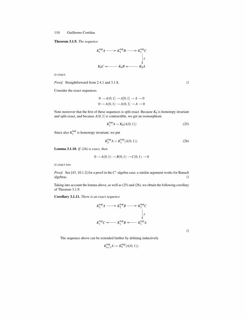
110 Guillermo Cortinas
Theorem 3.1.9. The sequence
Ktop1 A // Ktop
1 B // Ktop1 C
∂
K0C K0Boo K0Aoo
is exact.
Proof. Straightforward from 2.4.1 and 3.1.8. ut
Consider the exact sequences
0→ A(0,1]→ A[0,1]→ A→ 0
0→ A(0,1)→ A(0,1]→ A→ 0
Note moreover that the first of these sequences is split exact. Because K0 is homotopy invariantand split exact, and because A(0,1] is contractible, we get an isomorphism
Ktop1 A = K0(A(0,1)) (25)
Since also Ktop1 is homotopy invariant, we put
Ktop2 A = Ktop
1 (A(0,1)). (26)
Lemma 3.1.10. If (24) is exact, then
0→ A(0,1)→ B(0,1)→C(0,1)→ 0
is exact too.
Proof. See [43, 10.1.2] for a proof in the C∗-algebra case; a similar argument works for Banachalgebras. ut
Taking into account the lemma above, as well as (25) and (26), we obtain the following corollaryof Theorem 3.1.9.
Corollary 3.1.11. There is an exact sequence
Ktop2 A // Ktop
2 B // Ktop2 C
∂
Ktop
1 C Ktop1 Boo Ktop
1 Aoo
ut
The sequence above can be extended further by defining inductively
Ktopn+1A := Ktop
n (A(0,1)).
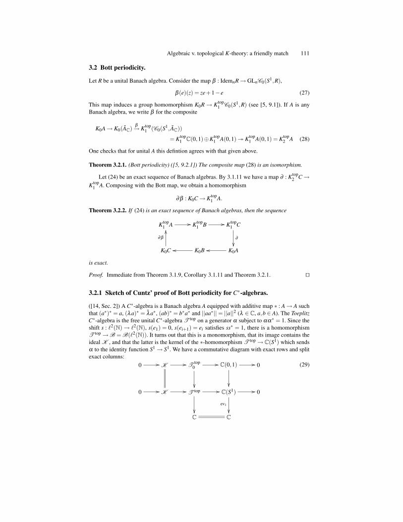
Algebraic v. topological K-theory: a friendly match 111
3.2 Bott periodicity.
Let R be a unital Banach algebra. Consider the map β : IdemnR→ GLnC0(S1,R),
β (e)(z) = ze+1− e (27)
This map induces a group homomorphism K0R→ Ktop1 C0(S1,R) (see [5, 9.1]). If A is any
Banach algebra, we write β for the composite
K0A→ K0(AC)β→ Ktop
1 (C0(S1, AC))
= Ktop1 C(0,1)⊕Ktop
1 A(0,1) Ktop1 A(0,1) = Ktop
2 A (28)
One checks that for unital A this defintion agrees with that given above.
Theorem 3.2.1. (Bott periodicity) ([5, 9.2.1]) The composite map (28) is an isomorphism.
Let (24) be an exact sequence of Banach algebras. By 3.1.11 we have a map ∂ : Ktop2 C→
Ktop1 A. Composing with the Bott map, we obtain a homomorphism
∂β : K0C→ Ktop1 A.
Theorem 3.2.2. If (24) is an exact sequence of Banach algebras, then the sequence
Ktop1 A // Ktop
1 B // Ktop1 C
∂
K0C
∂β
OO
K0Boo K0Aoo
is exact.
Proof. Immediate from Theorem 3.1.9, Corollary 3.1.11 and Theorem 3.2.1. ut
3.2.1 Sketch of Cuntz’ proof of Bott periodicity for C∗-algebras.
([14, Sec. 2]) A C∗-algebra is a Banach algebra A equipped with additive map ∗ : A→ A suchthat (a∗)∗ = a, (λa)∗ = λa∗, (ab)∗ = b∗a∗ and ||aa∗||= ||a||2 (λ ∈ C, a,b ∈ A). The ToeplitzC∗-algebra is the free unital C∗-algebra T top on a generator α subject to αα∗ = 1. Since theshift s : `2(N)→ `2(N), s(e1) = 0, s(ei+1) = ei satisfies ss∗ = 1, there is a homomorphismT top→B = B(`2(N)). It turns out that this is a monomorphism, that its image contains theideal K , and that the latter is the kernel of the ∗-homomorphism T top→ C(S1) which sendsα to the identity function S1→ S1. We have a commutative diagram with exact rows and splitexact columns:
0 // K // T top0
//
C(0,1) //
0
0 // K // T top //
C(S1) //
ev1
0
C C
(29)
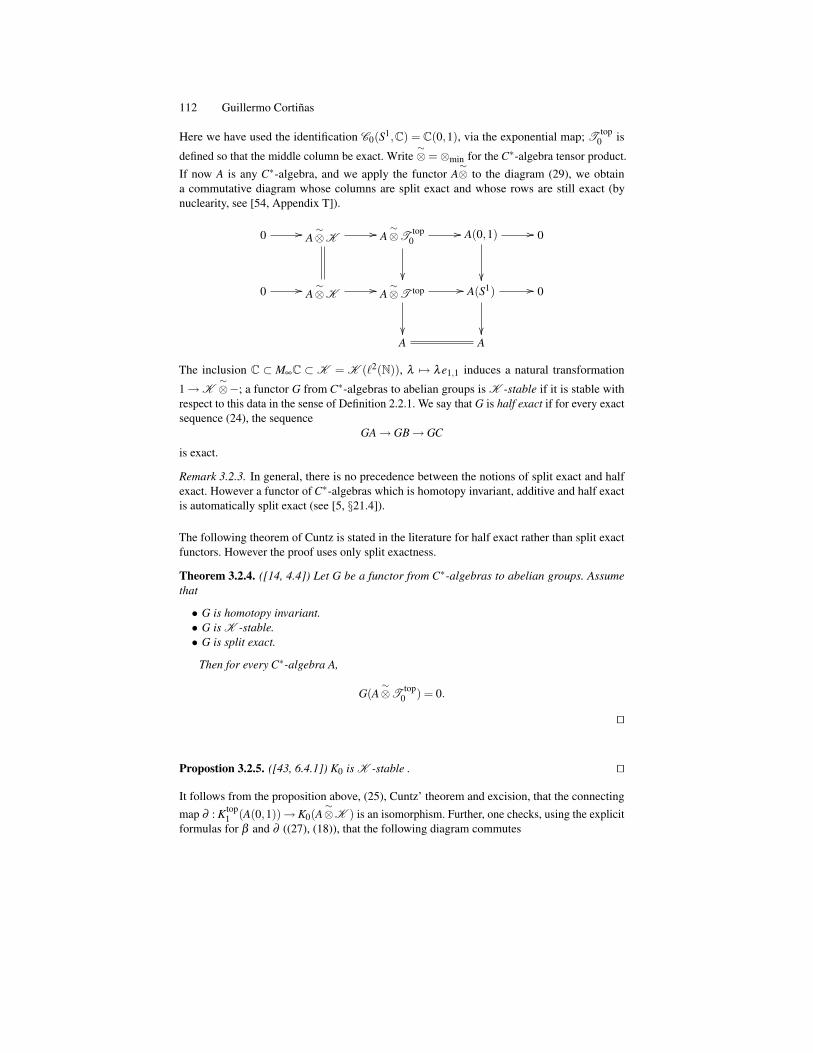
112 Guillermo Cortinas
Here we have used the identification C0(S1,C) = C(0,1), via the exponential map; T top0 is
defined so that the middle column be exact. Write∼⊗=⊗min for the C∗-algebra tensor product.
If now A is any C∗-algebra, and we apply the functor A∼⊗ to the diagram (29), we obtain
a commutative diagram whose columns are split exact and whose rows are still exact (bynuclearity, see [54, Appendix T]).
0 // A∼⊗K
// A∼⊗T top
0//
A(0,1) //
0
0 // A∼⊗K
// A∼⊗T top //
A(S1) //
0
A A
The inclusion C ⊂ M∞C ⊂ K = K (`2(N)), λ 7→ λe1,1 induces a natural transformation
1→K∼⊗−; a functor G from C∗-algebras to abelian groups is K -stable if it is stable with
respect to this data in the sense of Definition 2.2.1. We say that G is half exact if for every exactsequence (24), the sequence
GA→ GB→ GC
is exact.
Remark 3.2.3. In general, there is no precedence between the notions of split exact and halfexact. However a functor of C∗-algebras which is homotopy invariant, additive and half exactis automatically split exact (see [5, §21.4]).
The following theorem of Cuntz is stated in the literature for half exact rather than split exactfunctors. However the proof uses only split exactness.
Theorem 3.2.4. ([14, 4.4]) Let G be a functor from C∗-algebras to abelian groups. Assumethat
• G is homotopy invariant.• G is K -stable.• G is split exact.
Then for every C∗-algebra A,
G(A∼⊗T top
0 ) = 0.
ut
Propostion 3.2.5. ([43, 6.4.1]) K0 is K -stable . ut
It follows from the proposition above, (25), Cuntz’ theorem and excision, that the connectingmap ∂ : Ktop
1 (A(0,1))→ K0(A∼⊗K ) is an isomorphism. Further, one checks, using the explicit
formulas for β and ∂ ((27), (18)), that the following diagram commutes
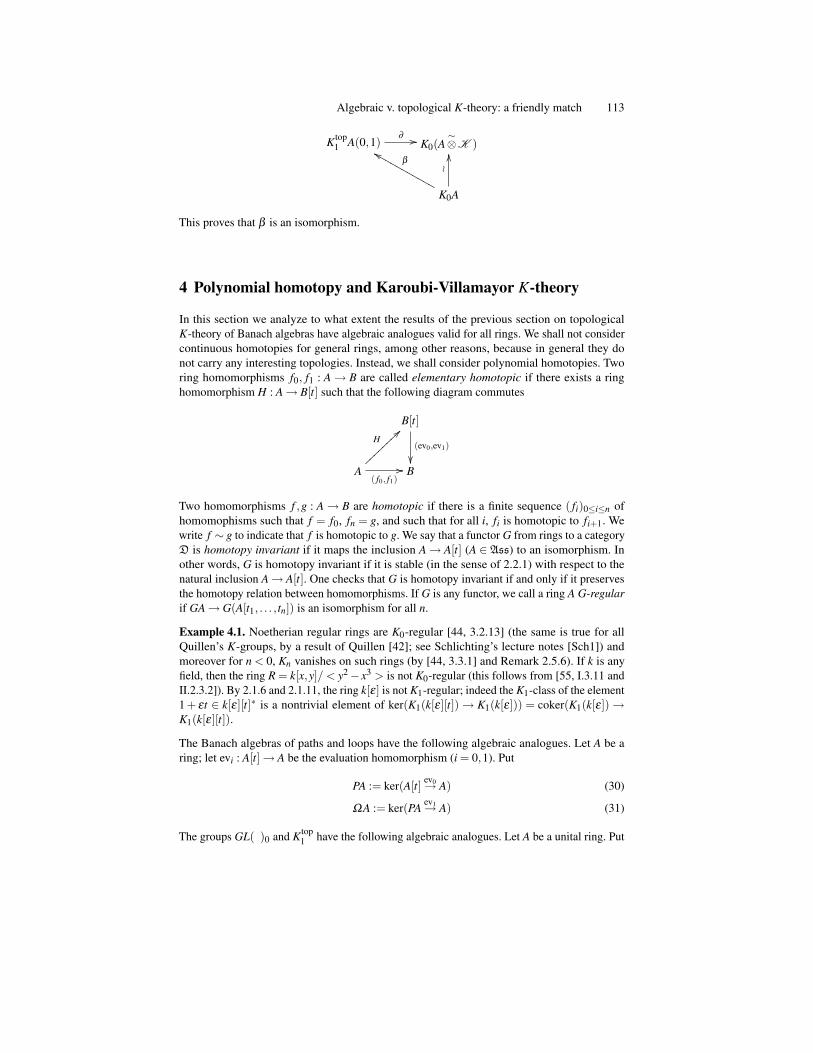
Algebraic v. topological K-theory: a friendly match 113
Ktop1 A(0,1)
∂ // K0(A∼⊗K )
K0A
β
ffMMMMMMMMMMMo
OO
This proves that β is an isomorphism.
4 Polynomial homotopy and Karoubi-Villamayor K-theory
In this section we analyze to what extent the results of the previous section on topologicalK-theory of Banach algebras have algebraic analogues valid for all rings. We shall not considercontinuous homotopies for general rings, among other reasons, because in general they donot carry any interesting topologies. Instead, we shall consider polynomial homotopies. Tworing homomorphisms f0, f1 : A→ B are called elementary homotopic if there exists a ringhomomorphism H : A→ B[t] such that the following diagram commutes
B[t]
(ev0,ev1)
A
H>>
( f0, f1)// B
Two homomorphisms f ,g : A→ B are homotopic if there is a finite sequence ( fi)0≤i≤n ofhomomophisms such that f = f0, fn = g, and such that for all i, fi is homotopic to fi+1. Wewrite f ∼ g to indicate that f is homotopic to g. We say that a functor G from rings to a categoryD is homotopy invariant if it maps the inclusion A→ A[t] (A ∈ Ass) to an isomorphism. Inother words, G is homotopy invariant if it is stable (in the sense of 2.2.1) with respect to thenatural inclusion A→ A[t]. One checks that G is homotopy invariant if and only if it preservesthe homotopy relation between homomorphisms. If G is any functor, we call a ring A G-regularif GA→ G(A[t1, . . . , tn]) is an isomorphism for all n.
Example 4.1. Noetherian regular rings are K0-regular [44, 3.2.13] (the same is true for allQuillen’s K-groups, by a result of Quillen [42]; see Schlichting’s lecture notes [Sch1]) andmoreover for n < 0, Kn vanishes on such rings (by [44, 3.3.1] and Remark 2.5.6). If k is anyfield, then the ring R = k[x,y]/ < y2− x3 > is not K0-regular (this follows from [55, I.3.11 andII.2.3.2]). By 2.1.6 and 2.1.11, the ring k[ε] is not K1-regular; indeed the K1-class of the element1 + εt ∈ k[ε][t]∗ is a nontrivial element of ker(K1(k[ε][t])→ K1(k[ε])) = coker(K1(k[ε])→K1(k[ε][t]).
The Banach algebras of paths and loops have the following algebraic analogues. Let A be aring; let evi : A[t]→ A be the evaluation homomorphism (i = 0,1). Put
PA := ker(A[t] ev0→ A) (30)
ΩA := ker(PA ev1→ A) (31)
The groups GL( )0 and Ktop1 have the following algebraic analogues. Let A be a unital ring. Put
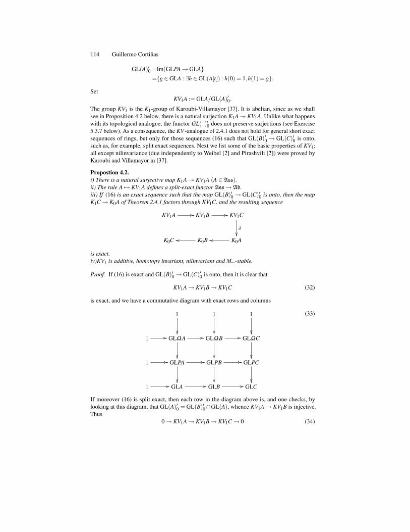
114 Guillermo Cortinas
GL(A)′0 =Im(GLPA→ GLA=g ∈ GLA : ∃h ∈ GL(A[t]) : h(0) = 1,h(1) = g.
SetKV1A := GLA/GL(A)′0.
The group KV1 is the K1-group of Karoubi-Villamayor [37]. It is abelian, since as we shallsee in Proposition 4.2 below, there is a natural surjection K1A KV1A. Unlike what happenswith its topological analogue, the functor GL( )′0 does not preserve surjections (see Exercise5.3.7 below). As a consequence, the KV -analogue of 2.4.1 does not hold for general short exactsequences of rings, but only for those sequences (16) such that GL(B)′0 → GL(C)′0 is onto,such as, for example, split exact sequences. Next we list some of the basic properties of KV1;all except nilinvariance (due independently to Weibel [?] and Pirashvili [?]) were proved byKaroubi and Villamayor in [37].
Propostion 4.2.i) There is a natural surjective map K1A KV1A (A ∈ Ass).ii) The rule A 7→ KV1A defines a split-exact functor Ass→ Ab.iii) If (16) is an exact sequence such that the map GL(B)′0→ GL(C)′0 is onto, then the mapK1C→ K0A of Theorem 2.4.1 factors through KV1C, and the resulting sequence
KV1A // KV1B // KV1C
∂
K0C K0Boo K0Aoo
is exact.iv)KV1 is additive, homotopy invariant, nilinvariant and M∞-stable.
Proof. If (16) is exact and GL(B)′0→ GL(C)′0 is onto, then it is clear that
KV1A→ KV1B→ KV1C (32)
is exact, and we have a commutative diagram with exact rows and columns
1
1
1
1 // GLΩA
// GLΩB
// GLΩC
1 // GLPA
// GLPB
// GLPC
1 // GLA // GLB // GLC
(33)
If moreover (16) is split exact, then each row in the diagram above is, and one checks, bylooking at this diagram, that GL(A)′0 = GL(B)′0∩GL(A), whence KV1A→ KV1B is injective.Thus
0→ KV1A→ KV1B→ KV1C→ 0 (34)
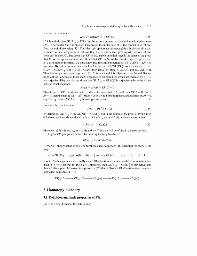
Algebraic v. topological K-theory: a friendly match 115
is exact. In particularKV1A = ker(KV1A→ KV1Z). (35)
If R is unital, then GL(R)′0 ⊃ E(R), by the same argument as in the Banach algebra case(23). In particular KV1R is abelian. This proves the unital case of i); the general case followsfrom the unital one using (35). Thus the right split exact sequence (34) is in fact a split exactsequence of abelian groups. It follows that KV1 is split exact, proving ii). Part iii) followsfrom part i) and (32). The proof that KV1 is M∞-stable on unital rings is the same as the proofthat K1 is. By split exactness, it follows that KV1 is M∞-stable on all rings. To prove thatKV1 is homotopy invariant, we must show that the split surjection ev0 : KV1(A[t])→ KV1A isinjective. By split exactness, its kernel is KV1PA = GLPA/GL(PA)′0, so we must prove thatGLPA ⊂ GL(PA)′0. But if α(s) ∈ GLPA, then β (s, t) := α(st) ∈ GLPPA and evt=1(β ) = α .Thus homotopy invariance is proved. If (16) is exact and A is nilpotent, then PA and ΩA arenilpotent too, whence all those maps displayed in diagram (33) which are induced by B→Care surjective. Diagram chasing shows that GL(B)′0→ GL(C)′0 is surjective, whence by iii) wehave an exact sequence
KV1A→ KV1B→ KV1C→ 0
Thus to prove KV1 is nilinvariant, it suffices to show that if A2 = 0 then KV1A = 0. But ifA2 = 0, then the map H : A→ A[t], H(a) = at is a ring homomorphism, and satisfies ev0H = 0,ev1H = 1A. Hence KV1A = 0, by homotopy invariance. ut
Consider the exact sequence0→ΩA→ PA ev1→ A→ 0 (36)
By definition, GL(A)′0 = Im(GL(PA)→ GL(A)). But in the course of the proof of Proposition4.2 above, we have shown that GL(PA) = GL(PA)′0, so by 4.2 iii), we have a natural map
KV1(A) ∂→ K0(ΩA). (37)
Moreover, (37) is injective, by 4.2 iii) and iv). This map will be of use in the next section.Higher KV -groups are defined by iterating the loop functor Ω :
KVn+1(A) = KV1(Ω nA).
Higher KV -theory satisfies excision for those exact sequences (16) such that for every n, themap
α ∈ GL(B[t1, . . . , tn]) : α(0, . . . ,0) = 1→ α ∈ GL(C[t1, . . . , tn]) : α(0, . . . ,0) = 1
is onto. Such sequences are usually called GL-fibration sequences (a different notation wasused in [37]). Note that if (16) is a GL-fibration, then GL(B)′0 → GL(C)′0 is surjective, andthus 4.2 iii) applies. Moreover it is proved in [37] that if (16) is a GL-fibration, then there is along exact sequence (n≥ 1)
KVn+1B // KVn+1C // KVn(A) // KVn(B) // KVn(C).
5 Homotopy K-theory
5.1 Definition and basic properties of KH.
Let A be a ring. Consider the natural map
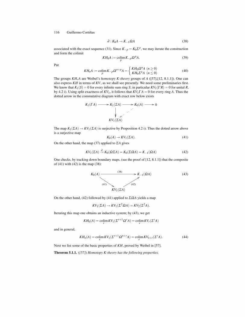
116 Guillermo Cortinas
∂ : K0A→ K−1ΩA (38)
associated with the exact sequence (31). Since K−p = K0Σ p, we may iterate the constructionand form the colimit
KH0A := colimp
K−pΩpA. (39)
Put
KHnA := colimp
K−pΩn+pA =
KH0Ω nA (n≥ 0)KH0Σ nA (n≤ 0) (40)
The groups KH∗A are Weibel’s homotopy K-theory groups of A ([57],[12, 8.1.1]). One canalso express KH in terms of KV , as we shall see presently. We need some preliminaries first.We know that K1(S) = 0 for every infinite sum ring S; in particular KV1(Γ R) = 0 for unital R,by 4.2 i). Using split exactness of KV1, it follows that KV1Γ A = 0 for every ring A. Thus thedotted arrow in the commutative diagram with exact row below exists
K1(Γ A) // K1(ΣA)
// K0(A)
zz
// 0
KV1(ΣA)
The map K1(ΣA)→ KV1(ΣA) is surjective by Proposition 4.2 i). Thus the dotted arrow aboveis a surjective map
K0(A) KV1(ΣA). (41)
On the other hand, the map (37) applied to ΣA gives
KV1(ΣA) ∂→ K0(ΩΣA) = K0(ΣΩA) = K−1(ΩA) (42)
One checks, by tracking down boundary maps, (see the proof of [12, 8.1.1]) that the compositeof (41) with (42) is the map (38):
K0(A)(38) //
(41) $$JJJJJJJJJK−1(ΩA)
KV1(ΣA)
(42)
99rrrrrrrrrr
(43)
On the other hand, (42) followed by (41) applied to ΣΩA yields a map
KV1(ΣA)→ KV1(Σ 2ΩA) = KV2(Σ 2A).
Iterating this map one obtains an inductive system; by (43), we get
KH0(A) = colimr
KV1(Σ r+1Ω
rA) = colimr
KVr(Σ rA)
and in general,
KHn(A) = colimr
KV1(Σ r+1Ω
n+rA) = colimr
KVn+r(Σ rA). (44)
Next we list some of the basic properties of KH, proved by Weibel in [57].
Theorem 5.1.1. ([57]) Homotopy K-theory has the following properties.

Algebraic v. topological K-theory: a friendly match 117
i) It is homotopy invariant, nilinvariant and M∞-stable.ii) It satisfies excision: to the sequence (16) there corresponds a long exact sequence (n ∈ Z)
KHn+1C→ KHnA→ KHnB→ KHnC→ KHn−1A.
Proof. From (44) and the fact that, by 4.2, KV is homotopy invariant, it follows that KH ishomotopy invariant. Nilinvariance, M∞-stability and excision for KH follow from the fact that(by 2.5.2) these hold for nonpositive K-theory, using the formulas (39), (40). ut
Exercise 5.1.2. Note that in the proof of 5.1.1, the formula (44) is used only for homotopyinvariance. Prove that KH is homotopy invariant without using (44), but using excision instead.Hint: show that the excision map KH∗(A)→ KH∗−1(ΩA) coming from the sequence (36) isan isomorphism.
Exercise 5.1.3. Show that KH commutes with filtering colimits.
5.2 KH for K0-regular rings.
Lemma 5.2.1. Let A be a ring. Assume that A is Kn-regular for all n ≤ 0. Then KV1(A)→K0(ΩA) is an isomorphism, and for n ≤ 0, Kn(PA) = 0, PA and ΩA are Kn-regular, andKnA→ Kn−1ΩA an isomorphism.
Proof. Consider the split exact sequence
0 // PA[t1, . . . , tr] // A[s, t1, . . . , tr] // A[t1, . . . , tr] // 0
Applying Kn (n≤ 0) and using that Kn is split exact and that, by hypothesis, A is Kn-regular,we get that Kn(PA[t1, . . . , tr]) = 0. As this happens for all r ≥ 0, PA is Kn-regular. Hence themap of exact sequences
0 // ΩA
// PA
// A
// 0
0 // ΩA[t1, . . . , tr] // PA[t1, . . . , tr] // A[t1, . . . , tr] // 0
induces commutative squares with exact rows
0 // KV1(A)
// K0(ΩA)
// 0
0 // KV1(A[t1, . . . , tr]) // K0(ΩA[t1, . . . , tr]) // 0
and
0 // Kn(A)
// Kn−1(ΩA)
// 0
0 // Kn(A[t1, . . . , tr]) // Kn−1(ΩA[t1, . . . , tr]) // 0
(n≤ 0)
By Proposition 4.2 and our hypothesis, the first vertical map in each diagram is an isomorphism;it follows that the second is also an isomorphism. ut
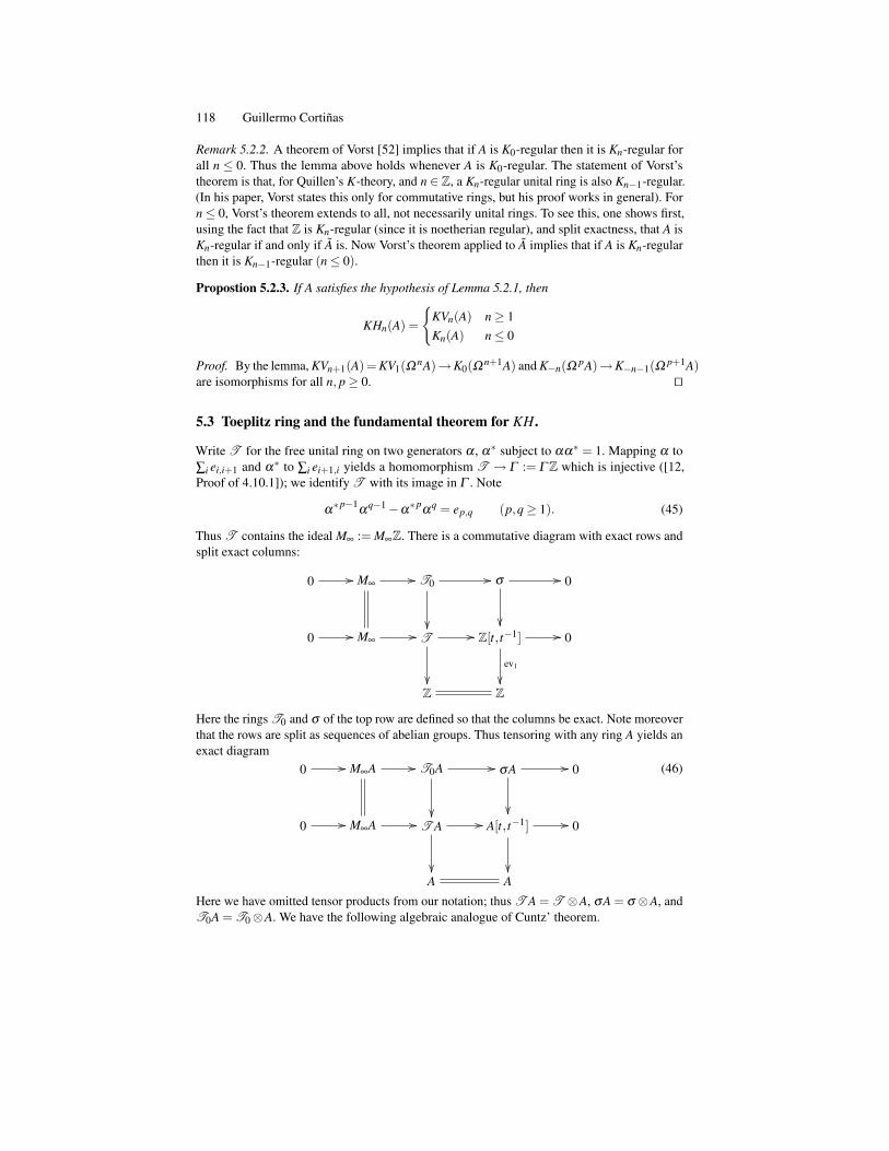
118 Guillermo Cortinas
Remark 5.2.2. A theorem of Vorst [52] implies that if A is K0-regular then it is Kn-regular forall n ≤ 0. Thus the lemma above holds whenever A is K0-regular. The statement of Vorst’stheorem is that, for Quillen’s K-theory, and n ∈ Z, a Kn-regular unital ring is also Kn−1-regular.(In his paper, Vorst states this only for commutative rings, but his proof works in general). Forn≤ 0, Vorst’s theorem extends to all, not necessarily unital rings. To see this, one shows first,using the fact that Z is Kn-regular (since it is noetherian regular), and split exactness, that A isKn-regular if and only if A is. Now Vorst’s theorem applied to A implies that if A is Kn-regularthen it is Kn−1-regular (n≤ 0).
Propostion 5.2.3. If A satisfies the hypothesis of Lemma 5.2.1, then
KHn(A) =
KVn(A) n≥ 1Kn(A) n≤ 0
Proof. By the lemma, KVn+1(A)= KV1(Ω nA)→K0(Ω n+1A) and K−n(Ω pA)→K−n−1(Ω p+1A)are isomorphisms for all n, p≥ 0. ut
5.3 Toeplitz ring and the fundamental theorem for KH.
Write T for the free unital ring on two generators α , α∗ subject to αα∗ = 1. Mapping α to∑i ei,i+1 and α∗ to ∑i ei+1,i yields a homomorphism T → Γ := ΓZ which is injective ([12,Proof of 4.10.1]); we identify T with its image in Γ . Note
α∗p−1
αq−1−α
∗pα
q = ep,q (p,q≥ 1). (45)
Thus T contains the ideal M∞ := M∞Z. There is a commutative diagram with exact rows andsplit exact columns:
0 // M∞// T0
// σ
// 0
0 // M∞// T
// Z[t, t−1]
ev1
// 0
Z Z
Here the rings T0 and σ of the top row are defined so that the columns be exact. Note moreoverthat the rows are split as sequences of abelian groups. Thus tensoring with any ring A yields anexact diagram
0 // M∞A // T0A
// σA
// 0
0 // M∞A // T A
// A[t, t−1]
// 0
A A
(46)
Here we have omitted tensor products from our notation; thus T A = T ⊗A, σA = σ ⊗A, andT0A = T0⊗A. We have the following algebraic analogue of Cuntz’ theorem.
Algebraic v. topological K-theory: a friendly match 119
Theorem 5.3.1. ([12, 7.3.2]) Let G be a functor from rings to abelian groups. Assume that:
• G is homotopy invariant.• G is split exact.• G is M∞-stable.
Then for any ring A, G(T0A) = 0. ut
Theorem 5.3.2. Let A be a ring and n ∈ Z. Then
KHn(σA) = KHn−1(A).
Proof. By Theorem 5.1.1, KH satisfies excision. Apply this to the top row of diagram (46) anduse Theorem 5.3.1. ut
The following result of Weibel [57, 1.2 iii)] is immediate from the theorem above.
Corollary 5.3.3. (Fundamental theorem for KH, [57, 1.2 iii)]). KHn(A[t, t−1]) = KHn(A)⊕KHn−1(A). ut
Remark 5.3.4. We regard Theorem 5.3.2 as an algebraic analogue of Bott periodicity for KH.What is missing in the algebraic case is an analogue of the exponential map; there is noisomorphism ΩA→ σA.
Remark 5.3.5. We have shown in Proposition 4.2 that KV1 satisfies the hypothesis of Theo-rem 5.3.1. Thus KV1(T0A) = 0 for every ring A. However, there is no natural isomorphismKV1(σA) = K0(A). Indeed, since KV1(σPA) = KV1(PσA) = 0 the existence of such an iso-morphism would imply that K0(PA) = 0, which in turn, given the fact that K0 is split exact,would imply that K0(A[t]) = K0(A), a formula which does not hold for general A (see Example4.1).
We finish the section with a technical result which will be used in Subsection 6.7.
Propostion 5.3.6. Let D be an additive category, F : Ass→D an additive functor, and A a ring.Assume F is M∞-stable on A and M2-stable on both T A and M2(T A). Then F(M∞A→T A)is the zero map.
Proof. Because F is M∞-stable on A, it suffices to show that F sends the inclusion : A→T A,a 7→ ae11, to the zero map. Note that e11 = 1−α∗α , by (45). Consider the inclusion ∞ : A→T A, ∞(a) = a ·1 = diag(a,a,a, . . .). One checks that the following matrix
Q =[
1−α∗α α∗
α 0
]∈ GL2T (A)
satisfies Q2 = 1 and
Q[
(a) 00 ∞(a)
]Q =
[∞(a) 0
0 0
].
Since we are assuming that F is additive and M2-stable on both T A and M2T A, we may nowapply Exercise 2.2.5 and Proposition 2.2.6 to deduce the following identity between elementsof the group homD(F(A),F(T A)):
+ ∞ = ∞.
It follows that = 0, as we had to prove. ut
Exercise 5.3.7. Deduce from Remark 5.3.5 and propositions 5.3.6 and 4.2 iii) that the canonicalmaps GL(T0A)′0→ GL(σA)′0 and GL(T A)′0→ GL(A[t, t−1])′0 are not surjective in general.
120 Guillermo Cortinas
6 Quillen’s Higher K-theory
Quillen’s higher K-groups of a unital ring R are defined as the homotopy groups of a certainCW -complex; the plus construction of the classifying space of the group GL(R) [?]. The latterconstruction is defined more generally for CW -complexes, but we shall not go into this generalversion; for this and other matters connected with the plus construction approach to K-theory,the interested reader should consult standard references such as Jon Berrick’s book [4], orthe papers of Loday [39], and Wagoner [44]. We shall need a number of basic facts fromalgebraic topology, which we shall presently review. First of all we recall that if X and Y areCW -complexes, then the cartesian product X×Y , equipped with the product topology, is nota CW -complex in general. That is, the category of CW -complexes is not closed under finiteproducts in Top. On the other hand, any CW -complex is a compactly generated –or Kelley–space, and the categorical product of two CW -complexes in the category Ke of compactlygenerated spaces is again CW , and also has the cartesian product X ×Y as underlying set.Moreover, in case the product topology in X ×Y happens to be compactly generated, thenit agrees with that of the product in Ke. In these notes, we write X ×Y for the cartesianproduct equipped with its compactly generated topology. (For a more detailed treatment of thecategorical properties of Ke see [25]).
6.1 Classifying spaces.
The classifying space of a (discrete) group G is a pointed connected CW -complex BG such that
πnBG =
G n = 10 n 6= 1
This property characterizes BG and makes it functorial up to homotopy. Further there arevarious strictly functorial models for BG ([44, Ch. 5§1], [27, 1.5]). We choose the modelcoming from the realization of the simplicial nerve of G ([27]), and write BG for that model.Here are some basic properties of BG which we shall use.
Properties 6.1.1.i) If
1→ G1→ G2→ G3→ 1
is an exact sequence of groups, then BG2→ BG3 is a fibration with fiber BG1.ii) If G1 and G2 are groups, then the map B(G1×G2)→ BG1×BG2 is a homeomorphism.iii) The homology of BG is the same as the group homology of G; if M is π1BG = G-module,then
Hn(BG,M) = Hn(G,M) := TorZGn (Z,M)
ut
6.2 Perfect groups and the plus construction for BG.
A group P is called perfect if its abelianization is trivial, or equivalently, if P = [P,P]. Notethat a group P is perfect if and only if the functor homGrp(P,−) : Ab→ Ab is zero. Thusthe full subcategory ⊂ Grp of all perfect groups is closed both under colimits and underhomomorphic images. In particular, if G is group, then the directed set of all perfect subgroupsof G is filtering, and its union is again a perfect subgroup N, the maximal perfect subgroup of
Algebraic v. topological K-theory: a friendly match 121
G. Since the conjugate of a perfect subgroup is again perfect, it follows that N is normal inG. Note that N ⊂ [G,G]; if moreover the equality holds, then we say that G is quasi-perfect.For example, if R is a unital ring, then GLR is quasi-perfect, and ER is its maximal perfectsubgroup ([44, 2.1.4]). Quillen’s plus construction applied to the group G yields a cellular mapof CW -complexes ι : BG→ (BG)+ with the following properties (see [39, 1.1.1, 1.1.2]).
i) At the level of π1, ι induces the projection G G/N.ii) At the level of homology, ι induces an isomorphism H∗(G,M)→ H∗((BG)+,M) for each
G/N-module M.iii) If BG→ X is any continuous function which at the level of π1 maps N → 1, then the
dotted arrow in the following diagram exists and is unique up to homotopy
BGι //
(BG)+
X
iv) Properties i) and iii) above characterize ι : BG→ BG+ up to homotopy.
From the universal property, it follows that if f : BG1→ BG2 is a continuous map, then there isa (continuous) map BG+
1 → BG+2 , unique up to homotopy, which makes the following diagram
commute
BG1
f // BG2
BG+
1f +// BG+
2
Properties 6.2.1. ([39, 1.1.4])
i) If G1 and G2 are groups, and πi : B(G1 ×G2)→ BGi is the projection, then the map(π+
1 ,π+2 ) : B(G1×G2)+→ BG+
1 ×BG+2 is a homotopy equivalence.
ii) The map BN+→ BG+ is the universal classifying space of BG+. ut
If1→ G1→ G2
π→ G3→ 1 (47)
is an exact sequence of groups, then we can always choose π+ to be a fibration; write F forits fiber. If the induced map G1 → π1F kills the maximal perfect subgroup N1 of G1, thenBG1→ F factors through a map
BG+1 → F (48)
Propostion 6.2.2. Let (47) be an exact sequence of groups. Assume that
i) G1 is quasi-perfect and G2 is perfect.ii)G3 acts trivially on H∗(G1,Z).iii)π1F acts trivially on H∗(F,Z).
122 Guillermo Cortinas
Then the map (48) is a homotopy equivalence.
Proof. Consider the map of fibration sequences
BG1
// BG2
// BG3
F // BG+
2// BG+
3
By the second property of the plus construction listed above, the maps BGi→ BG+i are ho-
mology equivalences. For i ≥ 2, we have, in addition, that Gi is perfect, so BG+i is simply
connected and F is connected with abelian π1, isomorphic to coker(π2BG+2 → π2BG+
3 ). Henceπ1F → H1F is an isomorphism, by Poincare’s theorem. All this together with the ComparisonTheorem ([64]), imply that BG1→ F and thus also (48), are homology equivalences. Moreover,because G1 is quasi-perfect by hypothesis, the Hurewicz map π1BG+
1 → H1BG+1 is an iso-
morphism, again by Poincare’s theorem. Summing up, BG+1 → F is a homology isomorphism
which induces an isomorphism of fundamental groups; since π1F acts trivially on H∗F byhypothesis, this implies that (48) is a weak equivalence ([8, 4.6.2]). ut
Lemma 6.2.3. Let (47) be an exact sequence of groups. Assume that for every g∈G2 and everyfinite set h1, . . . ,hk of elements of G1, there exists an h∈G1 such that for all i, ghig−1 = hhih−1.Then G3 acts trivially on H∗(G1,Z).
Proof. If g ∈G2 maps to g ∈G3, then the action of g on H∗(G1,Z) is that induced by conjuga-tion by g. The hypothesis implies that the action of g on any fixed cycle of the standard barcomplex which computes H∗(BG1,Z) ([56, 6.5.4]) coincides with the conjugation action by anelement of G1, whence it is trivial ([56, 6.7.8]). ut
Quillen’s higher K-groups of a unital ring R are defined as the homotopy groups of(BGLR)+; we put
K(R) : = (BGLR)+
KnR : = πnK(R) (n≥ 1).
In general, for a not necessarily unital ring A, we put
K(A) := fiber(K(A)→ K(Z)), Kn(A) = πnK(A) (n≥ 1)
One checks, using 6.2.1 i), that when A is unital, these definitions agree with the previous ones.
Remark 6.2.4. As defined, K is a functor from Ass to the homotopy category of topologicalspaces HoTop. Further note that for n = 1 we recover the definition of K1 given in 2.1.3.
We shall see below that the main basic properties of Section 2.1 which hold for K1 holdalso for higher Kn ([39]). First we need some preliminaries. If W : N→ N is an injection, weshall identify W with the endomorphism Z(N)→ Z(N), W (ei) = ew(i) and also with the matrixof the latter in the canonical basis, given by Wi j = δi,w( j). Let V = W t be the transpose matrix;then VW = 1. If now R is a unital ring, then the endomorphism ψV,W : M∞R→M∞R of 2.2.6induces a group endomorphism GL(R)→ GL(R), which in turn yields homotopy classes ofmaps
ψ : K(R)→ K(R), ψ′ : BE(R)+→ BE(R)+. (49)
Algebraic v. topological K-theory: a friendly match 123
Lemma 6.2.5. ([39, 1.2.9]) The maps (49) are homotopic to the identity. ut
A proof of the previous lemma for the case of ψ can be found in loc. cit.; a similar argumentworks for ψ ′.
Propostion 6.2.6. Let n≥ 1 and let R be a unital ring.
i) The functor Kn : Ass1→ Ab is additive.ii) The direct sum ⊕ : GLR×GLR→ GLR of (2) induces a map K(R)×K(R)→ K(R) whichmakes K(R) into an H-group, that is, into a group up to homotopy. Similarly, BE(R)+ also hasan H-group structure induced by ⊕.iii) The functors K : Ass1→ HoTop and Kn : Ass1→ Ab are M∞-stable.
Proof. Part i) is immediate from 6.2.1 i). The map of ii) is the composite of the homotopyinverse of the map of 6.2.1 i) and the map BGL(⊕)+. One checks that, up to endomorphismsof the form ψV,W induced by injections N→N, the map ⊕ : GL(R)×GL(R) is associative andcommutative and the identity matrix is a neutral element for ⊕. Hence by 6.2.5 it follows thatBGL(R)+ is a commutative and associative H-space. Since it is connected, this implies thatit is an H-group, by [60, X.4.17]. The same argument shows that BE(R)+ is also an H-group.Thus ii) is proved. Let ι : R→M∞R be the canonical inclusion. To prove iii), one observesthat a choice of bijection N×N→ N gives an isomorphism φ : M∞M∞R
∼=→ M∞R such thatthe composite with M∞ι is a homomorphism the form ψV,W for some injection W : N→ N,whence the induced map K(R)→ K(R) is homotopic to the identity, by Lemma 6.2.5. Thisproves that K(ι) is a homotopy equivalence. ut
Corollary 6.2.7. If S is an infinite sum ring, then K(S) is contractible.
Proof. It follows from the theorem above, using Exercise 2.2.3 ii) and Proposition 2.3.1. ut
Propostion 6.2.8. Let R be a unital ring, ΣR the suspension, ΩK(ΣR) the loopspace, andΩ0K(ΣR) ⊂ ΩK(ΣR) the connected component of the trivial loop. There is a homotopyequivalence
K(R) ∼→Ω0K(ΣR).
Proof. Consider the exact sequence of rings
0→M∞R→ Γ R→ ΣR→ 0
Since K1(Γ R) = 0, we haveGL(Γ R) = E(Γ R),
which applies onto EΣR. Thus we have an exact sequence of groups
1→ GLM∞R→ GLΓ R→ EΣR→ 1
One checks that the inclusion GL(M∞R)→ GL(Γ R) satisfies the hypothesis of 6.2.3 (see [53,bottom of page 357] for details). Thus the perfect group E(ΣR) acts trivially on H∗(GLM∞R,Z).On the other hand, by 6.2.6 ii), both K(Γ R) and BE(ΣR)+ are H-groups, and moreover sinceπ : GL(Γ R)→ GL(ΣR) is compatible with ⊕, the map π+ : K(Γ R)→ BE(ΣR)+ can bechosen to be compatible with the induced operation. This implies that the fiber of π+ is aconnected H-space (whence an H-group) and so its fundamental group acts trivially on itshomology. Hence by Propositions 6.2.6 iii) and 6.2.2, we have a homotopy fibration
124 Guillermo Cortinas
K(R)→ K(Γ R)→ BE(ΣR)+
By 6.2.7, the mapΩBE(ΣR)+→ K(R) (50)
is a homotopy equivalence. Finally, by 6.2.1 ii),
ΩBE(ΣR)+ ∼→Ω0K(ΣR). (51)
Now compose (51) with a homotopy inverse of (50) to obtain the theorem. ut
Corollary 6.2.9. For all n ∈ Z, Kn(ΣR) = Kn−1(R)
Proof. For n≤ 0, the statement of the proposition is immediate from the definition of Kn. Forn = 1, it is (21). If n≥ 2, then
Kn(ΣR) = πn(K(ΣR)) = πn−1(ΩK(ΣR)) = πn−1(Ω0K(ΣR)) = πn−1K(R) = Kn−1R. ut
Remark 6.2.10. The homotopy equivalence of Proposition 6.2.8 is the basis for the constructionof the nonconnective K-theory spectrum; we will come back to this in Section 10.
6.3 Functoriality issues.
As defined, the rule K : R 7→ BGL(R)+ is only functorial up to homotopy. Actually its possibleto choose a functorial model for KR; this can be done in different ways (see for example [38,11.2.4,11.2.11]). However, in the constructions and arguments we have made (notably in theproof of 6.2.8) we have often used Whitehead’s theorem that a map of CW -complexes whichinduces an isomorphism at the level of homotopy groups (a weak equivalence) always hasa homotopy inverse. Now, there is in principle no reason why a natural weak equivalencebetween functorial CW -complexes will admit a homotopy inverse which is also natural; thusfor example, the weak equivalence of Proposition 6.2.8 need not be natural for an arbitrarilychosen functorial version of KR. What we need is to be able to choose functorial models sothat any natural weak equivalence between them automatically has a natural homotopy inverse.In fact we can actually do this, as we shall now see. First of all, as a technical restrictionwe have to choose a small full subcategory I of the category Ass, and look at K-theory as afunctor on I. This is no real restriction, as in practice we always start with a set of rings (ofterwith only one element) and then all the arguments and constructions we perform take placein a set (possibly larger than the one we started with, but still a set). Next we invoke the factthat the category TopI
∗ of functors from I to pointed spaces is a closed model category wherefibrations and weak equivalences are defined objectwise (by [32, 11.6.1] this is true of thecategory of functors to any cofibrantly generated model category; by [32, 11.1.9], Top∗ is sucha category). This implies, among other things, that there is a full subcategory (TopI
∗)c→ TopI∗,
the subcategory of cofibrant objects (among which any natural weak equivalence has a naturalhomotopy inverse), a functor TopI
∗→ (TopI∗)c, X 7→ X and a natural transformation X → X
such that X(R)→ X(R) is a fibration and weak equivalence for all R. Thus we can replace ourgiven functorial model for BGL+(R) by BGL(R)+, and redefine K(R) = BGL(R)+.
Algebraic v. topological K-theory: a friendly match 125
6.4 Relative K-groups and excision.
Let R be a unital ring, I /R an ideal, and S = R/I. Put
GLS := Im(GLR→ GLS)
The inclusion GLS⊂ GLS induces a map
(BGLS)+→ K(S) (52)
By 6.2.1 ii), (52) induces an isomorphism
πn(BGLS)+ = KnS (n≥ 2).
On the other hand,π1(BGLS+) = GLS/ES = Im(K1R→ K1S).
Consider the homotopy fiber
K(R : I) := fiber((BGLR)+→ (BGLS)+).
The relative K-groups of I with respect to the ideal embedding I /R are defined by
Kn(R : I) :=
πnK(R : I) n≥ 1Kn(I) n≤ 0
The long exact squence of homotopy groups of the fibration which defines K(R : I), splicedtogether with the exact sequences of Theorem 2.4.1 and Proposition 2.5.2, yields a long exactsequence
Kn+1R→ Kn+1S→ Kn(R : I)→ KnR→ Kn(S) (n ∈ Z) (53)
The canonical map I→ R induces a map
Kn(I)→ Kn(R : I) (54)
This map is an isomorphism for n≤ 0, but not in general (see Remark 2.4.4). The rings I sothat this map is an isomorphism for all n and R are called K-excisive. Suslin and Wodzicki havecompletely characterized K-excisive rings ([61],[49],[48]). We have
Theorem 6.4.1. ([48]) The map (54) is an isomorphism for all n and R ⇐⇒ TorIn(Z, I) = 0
∀n. ut
Note that
TorI0(Z, I) = I/I2
TorIn(Z, I) = TorI
n+1(Z,Z).
Example 6.4.2. Let G be a group, IG /ZG the augmentation ideal. Then ZG = ˜IG is theunitalization of IG. Hence
Tor ˜IGn (Z, IG) = Hn+1(G,Z).
In particularTor ˜IG
0 (Z, I) = Gab
126 Guillermo Cortinas
So if IG is K-excisive, then G must be a perfect group. Thus, for example, IG is not K-excisiveif G is a nontrivial abelian group. In particular, the ring σ is not K-excisive, as it coincides withthe augmentation ideal of Z[Z] = Z[t, t−1]. As another example, if S is an infinite sum ring,then
Hn(GL(S),Z) = Hn(K(S),Z) = Hn(pt,Z) = 0 (n≥ 1).Thus the ring IGL(S) is K-excisive.
Remark 6.4.3. We shall introduce a functorial complex L(A) which computes TorA∗ (Z,A) and
use it to show that the functor Tor(−)∗ (Z,−) commutes with filtering colimits. Consider the
functor ⊥: A−mod→ A−mod,⊥M =
⊕m∈M
A.
The functor ⊥ is the free A-module cotriple [56, 8.6.6]. Let L(A)→ A be the canonical freeresolution associated to ⊥ [56, 8.7.2]; by definition, its n-th term is Ln(A) =⊥n A. Put L(A) =Z⊗A L(A). Then L(A) is a functorial chain complex which satisfies H∗(L(A)) = TorA
∗ (Z,A).Because ⊥ commutes with filtering colimits, it follows that the same is true of L and L, and
therefore also of Tor(−)∗ (Z,−) = H∗L(−).
Exercise 6.4.4.i) Prove that any unital ring is K-excisive.ii) Prove that if R is a unital ring, then M∞R is K-excisive. (Hint: M∞R = colimn MnR).
Remark 6.4.5. If A is flat over k (e.g. if k is a field) then the canonical resolution Lk(A) ∼→ Aassociated with the induced module cotriple Ak⊗k (−), is flat. Thus Lk(A) := Lk(A)/ALk(A)computes TorAk∗ (k,A). Modding out by degenerates, we obtain a homotopy equivalent complex([56]) Cbar(A/k), with Cbar
n (A/k) = A⊗kn+1. The complex Cbar is the bar complex consideredby Wodzicki in [61]; its homology is the bar homology of A relative to k, Hbar
∗ (A/k). If A isa Q-algebra, then A is flat as a Z-module, and thus Hbar
∗ (A/Z) = TorA∗ (Z,A). Moreover, as
A⊗Zn = A⊗Qn, we have Cbar(A/Z) = Cbar(A/Q), whence
TorA∗ (Z,A) = TorAQ
∗ (Q,A) = Hbar∗ (A/Q)
6.5 Locally convex algebras.
A locally convex algebra is a complete topological C-algebra L with a locally convex topology.Such a topology is defined by a family of seminorms ρα; continuity of the product meansthat for every α there exists a β such that
ρα (xy)≤ ρβ (x)ρβ (y) (x,y ∈ L). (55)
If in addition the topology is determined by a countable family of seminorms, we say that L isa Frechet algebra.
Let L be a locally convex algebra. Consider the following two factorization properties:(a) Cohen-Hewitt factorization.
∀n≥ 1,a = (a1, . . . ,an) ∈ L⊕n =n⊕
i=1L ∃z ∈ L, x ∈ Ln such that (56)
z · x = a and x ∈ L ·a
Here the bar denotes topological closure in L⊕n.
Algebraic v. topological K-theory: a friendly match 127
(b) Triple factorization.
∀a ∈ L⊕n,∃b ∈ L⊕n, c,d ∈ L, (57)
such that a = cdb and (0 : d)l := v ∈ L : dv = 0= (0 : cd)l (58)
The right ideal (0 : d)l is called the left annihilator of d. Note that property (b) makes sense foran arbitrary ring L.
Lemma 6.5.1. Cohen-Hewitt factorization implies triple factorization. That is, if L is a locallyconvex algebra which satisfies property (a) above, then it also satisfies property (b).
Proof. Let a ∈ L⊕n. By (a), there exist b ∈ L⊕n and z ∈ L such that a = zb. Applying (a) again,we get that z = cd with d ∈ L · z; this implies that (0 : d)l = (0 : z)l .
Theorem 6.5.2. ([49, 3.12, 3.13(a)]) Let L be a ring. Assume that either L or Lop satisfy (57).Then A is K-excisive. ut
6.6 Frechet m-algebras with approximate units.
A uniformly bounded left approximate unit (ublau) in a locally convex algebra L is a net eλ of elements of L such that eλ a 7→ a for all a and supα ρα (a) < ∞. Right ubau’s are definedanalogously. If L is a locally convex algebra such that a defining family of seminorms can bechosen so that condition (55) is satisfied with α = β (i.e. the seminorms are submultiplicative)we say that L is an m-algebra. An m-algebra which is also Frechet will be called a Frechetm-algebra.
Example 6.6.1. Every C∗-algebra has a two-sided ubau ([21, I.4.8]). If G is a locally compactgroup, then the group algebra L1(G) is a Banach algebra with two sided ubau [61, 8.4]. If L1and L2 are locally convex algebras with ublaus eλ and fµ, then eλ ⊗ fµ is a ublau forthe projective tensor product L1⊗L2, which is a (Frechet) m-algebra if both L1 and L2 are.
Remark 6.6.2. In a Banach algebra, any bounded approximate unit is uniformly bounded. Thusfor example, the unit of a unital Banach algebra is an ublau. However, the unit of a generalunital locally convex algebra (or even of a Frechet m-algebra) need not be uniformly bounded.
Let L be an m-Frechet algebra. A left Frechet L-module is a Frechet space V equipped witha left L-module structure such that the multiplication map L×V → V is continuous. If L isequipped with an ublau eλ such that eλ · v→ v for all v ∈V , then we say that V is essential.
Example 6.6.3. If L is an m-Frechet algebra with ublau eλ and x ∈ L⊕n (n≥ 1) then eλ x→ x.Thus L⊕n is an essential Frechet L-module. The next exercise generalizes this example.
Exercise 6.6.4. Let L be an m-Frechet algebra with ublau eλ , M a unital m-Frechet algebra,and n≥ 1. Prove that for every x ∈ (L⊗M)⊕n, (eλ ⊗1)x→ x. Conclude that (L⊗M)⊕n is anessential L⊗M-module.
The following Frechet version of Cohen-Hewitt’s factorization theorem (originally provedin the Banach setting) is due to M. Summers.
Theorem 6.6.5. ([47, 2.1]) Let L be an m-Frechet algebra with ublau, and V an essentialFrechet left L-module. Then for each v ∈V and for each neighbourhood U of the origin in Vthere is an a ∈ L and a w ∈V such that v = aw, w ∈ Lv, and w− v ∈U. ut

128 Guillermo Cortinas
Theorem 6.6.6. ([61, 8.1]) Let L be a Frechet m-algebra. Assume L has a right or left ubau.Then L is K-excisive.
Proof. In view of Lemma (6.5.1), it suffices to show that L satisfies property (56). This followsby applying Theorem 6.6.5 to the essential L-module L⊕n. ut
Exercise 6.6.7. Prove that if L and M are as in Exercise (6.6.4), then L⊗M is K-excisive.
Remark 6.6.8. In [13, 8.1.1] it asserted that if k ⊃ Q is a field, and A is a k-algebra, then
TorAQ∗ (Q,A) = TorAk∗ (k,A), but the proof uses the identity Ak⊗A ? = k⊗ ? , which is wrong.
In loc. cit., the lemma is used in combination with Wodzicki’s theorem ([61, 8.1]) that a Frechetalgebra L with ublau is H-unital as a C-algebra, to conclude that such L is K-excisive. InTheorem 6.6.6 we gave a different proof of the latter fact.
6.7 Fundamental theorem and the Toeplitz ring.
Notation. If G : Ass→ Ab is a functor, and A is a ring, we put
NG(A) := coker(GA→ G(A[t])).
Let R be a unital ring. We have a commutative diagram
R
// R[t]
R[t−1] // R[t, t−1]
Thus applying the functor Kn we obtain a map
KnR⊕NKnR⊕NKnR→ KnR[t, t−1] (59)
which sends NKnR⊕NKnR inside kerev1. Thus KnR→ KnR[t, t−1] is a split mono, and theintersection of its image with that of NKnR⊕NKnR is 0. On the other hand, the inclusionT R→ Γ R induces a map of exact sequences
0 // M∞R // T R
// R[t, t−1]
// 0
0 // M∞R // Γ R // ΣR // 0
In particular, we have a homomorphism R[t, t−1]→ ΣR, and thus a homomorphism
η : KnR[t, t−1]→ Kn−1R.
Note that the maps R[t]→ T R, t 7→ α and t 7→ α∗, lift the homomorphisms R[t]→ R[t, t−1],t 7→ t and t 7→ t−1. It follows that kerη contains the image of (59). In [39], Loday introduced aproduct operation in K-theory of unital rings
Kp(R)⊗Kq(S)→ Kp+q(R⊗S).
Algebraic v. topological K-theory: a friendly match 129
In particular, multiplying by the class of t ∈ K1(Z[t, t−1]) induces a map
∪t : Kn−1R→ KnR[t, t−1]. (60)
Loday proves in [39, 2.3.5] that η (−∪ t) is the identity map. Thus the images of (59) and(60) have zero intersection. Moreover, we have the following result, due to Quillen [?], whichis known as the fundamental theorem of K-theory.
Theorem 6.7.1. ([?], see also [Sch1]) Let R be a unital ring. The maps (59) and (60) inducean isomorphism
KnR⊕NKnR⊕NKnR⊕Kn−1R∼=→ KnR[t, t−1] (n ∈ Z).
Corollary 6.7.2. (cf. Theorem 5.3.2)
Kn(R[t, t−1] : σR) = Kn−1R⊕NKnR⊕NKnR (n ∈ Z).
Propostion 6.7.3. (cf. Theorem 5.3.1) Let R be a unital ring, and n ∈ Z. Then
KnT R = KnR⊕NKnR⊕NKnR,
Kn(T R : T0R) = NKnR⊕NKnR.
Proof. Consider the exact sequence
0→M∞R→T R→ R[t, t−1]→ 0
By Proposition 10.1.2, Exercise 6.4.4 and matrix stability we have a long exact sequence
KnR→ KnT R→ KnR[t, t−1]→ Kn−1R→ Kn−1T R (n ∈ Z).
By 5.3.6, the first and the last map are zero. The proposition is immediate from this, fromCorollary 6.7.2, and from the discussion above. ut
7 Comparison between algebraic and topological K-theory I
7.1 Stable C∗-algebras.
The following is Higson’s homotopy invariance theorem.
Theorem 7.1.1. [31, 3.2.2] Let G be a functor from C∗-algebras to abelian groups. Assumethat G is split exact and K -stable. Then G is homotopy invariant. ut
Lemma 7.1.2. Let G be a functor from C∗-algebras to abelian groups. Assume that G isM2-stable. Then the functor F(A) := G(A
∼⊗K ) is K -stable.
Proof. Let H be an infinite dimensional separable Hilbert space. The canonical isomorphismC2⊗2 H ∼= H ⊕H induces an isomorphism K
∼⊗K → M2K which makes the following
diagram commute
K∼⊗K
∼= // M2K
K
e11⊗1
ccGGGGGGGG
ι1
<<zzzzzzzzz
Since G is M2-stable by hypothesis, it follows that F(1A∼⊗ e1,1
∼⊗1K ) is an isomorphism for
all A. ut
130 Guillermo Cortinas
The following result, due to Suslin and Wodzicki, is (one of the variants of) what is known asKaroubi’s conjecture [34].
Theorem 7.1.3. [49, 10.9] Let A be a C∗-algebra. Then there is a natural isomorphism Kn(A∼⊗
K ) = Ktopn (A
∼⊗K ).
Proof. By definition K0 = Ktop0 on all C∗-algebras. By Example 6.6.1 and Theorem 6.6.6,
C∗-algebras are K-excisive. In particular K∗ is split exact when regarded as a functor of C∗-algebras. By 6.2.6 iii), 2.5.2 i), and split exactness, K∗ is M∞-stable on C∗-algebras; thisimplies it is also M2-stable (Exercise 2.2.3). Thus K∗(−
∼⊗K ) is K -stable, by 7.1.2. Hence
Kn(A(0,1]∼⊗K ) = 0, by split exactness and homotopy invariance (Theorem 7.1.1). It follows
thatKn+1(A
∼⊗K ) = Kn(A(0,1)
∼⊗K ) (61)
by excision. In particular, for n≥ 0,
Kn(A∼⊗K ) = K0(A
∼⊗∼⊗
ni=1C(0,1)
∼⊗K ) = Ktop
n (A∼⊗K ). (62)
On the other hand, by Cuntz’ theorem 3.2.4, excision applied to the C∗-Toeplitz extension and7.1.2, Kn+1(A(0,1)
∼⊗K ) = Kn(A
∼⊗K
∼⊗K ) = Kn(A
∼⊗K ). Putting this together with (61),
we get that K∗(K∼⊗A) is Bott periodic. It follows that the identity (62) holds for all n ∈ Z. ut
7.2 Stable Banach algebras.
The following result is a particular case of a theorem of Wodzicki.
Theorem 7.2.1. ([62, Thm. 2], [13, 8.3.3, 8.3.4]) Let L be Banach algebra with right or leftubau. Then there is an isomorphism K∗(L⊗K ) = Ktop
∗ (L⊗K ).
Proof. Consider the functor GL : C∗→ Ab, A 7→ K∗(L⊗(A∼⊗K )). By the same argument as
in the proof of 7.1.3, GL is homotopy invariant. Hence C→ C[0,1] induces an isomorphism
GL(C) =K∗(L⊗K )∼=→ GL(C[0,1]) = K∗(L⊗(C[0,1]
∼⊗K ))
=K∗(L⊗K [0,1]) = K∗((L⊗K )[0,1]).
Hence Kn+1(L⊗K ) = Kn(L⊗K (0,1)), by 6.6.6 and 6.6.1. Thus Kn(L⊗K ) = Ktopn (L⊗K )
for n≥ 0. Consider the punctured Toeplitz sequence
0→K →T top0 → C(0,1)→ 0
By [21, V.1.5], this sequence admits a continuous linear splitting. Hence it remains exact afterapplying the functor L⊗−. By 3.2.4, we have
K−n(L⊗(K∼⊗T0)) = 0 (n≥ 0).
Thus
K−n(L⊗K ) = K−n(L⊗(K∼⊗K )) = K0((L⊗K )⊗⊗n
i=1C(0,1)) = Ktop−n (L⊗K ). ut
Algebraic v. topological K-theory: a friendly match 131
Remark 7.2.2. The theorem above holds more generally for m-Frechet algebras ([62, Thm. 2],[13, 8.3.4]), with the appropriate definition of topological K-theory (see Section 12 below).
Exercise 7.2.3. Let A be a Banach algebra. Consider the map K0(A)→ K−1(A(0,1)) comingfrom the exact sequence
0→ A(0,1)→ A(0,1]→ A→ 0
PutA(0,1)m = A⊗
(⊗m
i=1C(0,1))
and defineKCn(A) = colim
pK−p(A(0,1)n+p) (n ∈ Z)
i) Prove that KC∗ satisfies excision, M∞-stability, continuous homotopy invariance, and nilin-variance.ii) Prove that KC∗(A⊗K ) = Ktop
∗ (A).iii) Prove that the composite
Ktopn A = K0(A(0,1)n)→ KCn(A)→ KCn(A⊗K ) = Ktop
n (A) (n≥ 0)
is the identity map. In particular KCn(A)→ Ktopn (A) is surjective for n≥ 0.
Remark 7.2.4. J. Rosenberg has conjectured (see [45, 3.7]) that, for n ≤ −1, the restrictionof Kn to commutative C∗-algebras is homotopy invariant. Note that if A is a Banach algebra(commutative or not) such that, K−q(A(0,1)p)→ K−q(A(0,1)p[0,1]) is an isomorphism forall p,q ≥ 0, then KCn(A)→ Ktop
n A is an isomorphism for all n. In particular, if Rosenberg’sconjecture holds, this will happen for all commutative C∗-algebras A.
8 Topological K-theory for locally convex algebras
8.1 Diffeotopy KV .
We begin by recalling the notion of C∞-homotopies or diffeotopies (from [15], [16]). Let Lbe a locally convex algebra. Write C ∞([0,1],L) for the algebra of those functions [0,1]→ Lwhich are restrictions of C ∞-functions R→ L. The algebra C ∞([0,1],L) is equipped with alocally convex topology which makes it into a locally convex algebra, and there is a canonicalisomorphism
C ∞([0,1],L) = C ∞([0,1],C)⊗L
Two homomorphisms f0, f1 : L→M of locally convex algebras are called diffeotopic if there isa homomorphism H : L→ C ∞([0,1],M) such that the following diagram commutes
C ∞([0,1],M)
(ev0,ev1)
L
H::tttttttttt
( f0, f1)// M×M
Consider the exact sequences
132 Guillermo Cortinas
0→ PdifL→ C ∞([0,1],L) ev0→ L→ 0 (63)
0→ΩdifL→ PdifL ev1→ L→ 0 (64)
Here PdifL and Ω difL are the kernels of the evaluation maps. The first of these is split by thenatural inclusion L→ C ∞([0,1],L), and the second is split the continous linear map sendingl 7→ (t 7→ tl). We have
ΩdifL = Ω
difC⊗L, PdifL = PdifC⊗L.
Put
GL(L)′′0 = Im(GLPdifL→ GL(L))
KV dif1 (L) = GL(L)/GL(L)′′0 .
The following is the analogue of Proposition 4.2 for KV dif1 (except for nilinvariance, treated
separately in Exercise 8.1.2).
Propostion 8.1.1.i) The functor KV dif
1 is split exact.ii)For each locally convex algebra L, there is a natural surjective map K1L→ KV dif
1 L.iii) If
0→ L→M→ N→ 0 (65)
is an exact sequence such that the map GL(M)′′0 → GL(N)′′0 is onto, then the map K1N→ K0Lof Theorem 2.4.1 factors through KV dif
1 N, and the resulting sequence
KV dif1 L // KV dif
1 M // KV dif1 N
∂
K0N K0Moo K0Loo
is exact.iv)KV dif
1 is additive, diffeotopy invariant and M∞-stable.
Proof. One checks that, mutatis-mutandis, the same argument of the proof of 4.2 shows this.ut
By the same argument as in the algebraic case, we obtain a natural injection
KV dif1 L → K0(Ω difL)
Higher KV dif-groups are defined by
KV difn (L) = KV dif
1 ((Ω dif)n−1L) (n≥ 2)
Exercise 8.1.2.i) Show that if L is a locally convex algebra such that Ln = 0 and such that L→ L/Li admits acontinuous linear splitting for all i≤ n−1, then KV dif
1 L = 0.ii) Show that if L is as in i) then the map KV dif
1 M→KV dif1 N induced by (65) is an isomorphism.
Algebraic v. topological K-theory: a friendly match 133
8.2 Diffeotopy K-theory.
Consider the excision map
KnL→ Kn−1(Ω difL) (n≤ 0)
associated to the sequence (64). The diffeotopy K-theory of the algebra L is defined by theformula
KDnL = colimp
K−p((Ω dif)n+pL) (n ∈ Z)
It is also possible to express KD in terms of KV dif. First we observe that, since ΣC is acountably dimensional algebra, equipping it with the fine topology makes it into a locallyconvex algebra [16, 2.1], and if L is any locally convex algebra then we have
ΣL = ΣC⊗C L = ΣC⊗L.
ThusΩ
difΣL = ΣΩ
difL.
Taking this into account, and using the same argument as used to prove (44), one obtains
KDnL = colimr
KV dif1 (Σ r+1(Ω dif)n+rL) = colim
rKV dif
n+r+1(Σr+1L).
Propostion 8.2.1. Diffeotopy K-theory has the following properties.i) It is diffeotopy invariant, nilinvariant and M∞-stable.ii) It satisfies excision for those exact sequences which admit a continuous linear splitting. Thatis, if
0→ L→M π→ N→ 0 (66)
is an exact sequence of locally convex algebras and there exists a continuous linear maps : N→M such that πs = 1N , then there is a long exact sequence
KDn+1M→ KDn+1N→ KDnL→ KDnM→ KDnN (n ∈ Z).
Proof. The proof is essentially the same as that of Theorem (5.1.1). The splitting hypothesis inii) guarantees that the functor L 7→Ω difL = Ω difC⊗L and its iterations, send (66) to an exactsequence. ut
Comparing KV dif and KD.
The analogue of Proposition 5.2.3 is 8.2.3 below. It is immediate from Lemma 8.2.2, which isthe analogue of Lemma 5.2.1; the proof of 8.2.2 is essentially the same as that of 5.2.1.
Lemma 8.2.2. Let L be a locally convex algebra. Assume that for all n ≤ 0 and all p ≥ 1,the natural inclusion ιp : L→ L⊗
(⊗p
i=1C∞([0,1])
)= C ∞([0,1]p,L) induces an isomorphism
Kn(L)∼=→ KnC ∞([0,1]p,L). Then KV dif
1 L→ K0Ω difL is an isomorphism, and for every n≤ 0and every p ≥ 0, Kn(C ∞([0,1]p,PdifA)) = 0 and Kn(Ω difA)→ Kn(C∞([0,1]p,Ω difA)) is anisomorphism.
Propostion 8.2.3. Let L be a locally convex algebra. Assume L satisfies the hypothesis ofLemma 8.2.2. Then
KDnL =
KV dif
n L n≥ 1KnL n≤ 0

134 Guillermo Cortinas
8.3 Bott periodicity.
Next we are going to prove a version of Bott periodicity for KD. The proof is analogous toCuntz’ proof of Bott periodicity for Ktop of C∗-algebras, with the algebra of smooth compactoperators and the smooth Toeplitz algebra substituted for the C∗-algebra of compact operatorsand the Toeplitz C∗-algebra.
Smooth compact operators.
The algebra K of smooth compact operators ([41, §2],[15, 1.4]) consists of all those N×N-matrices (zi, j) with complex coefficients such that for all n,
ρn(z) := ∑p,q
pnqn|zp,q|< ∞
The seminorms ρn are submultiplicative, and define a locally convex topology on K. Since thetopology is defined by submultiplicative seminorms, it is an m-algebra. Further because theseminorms above are countably many, it is Frechet; summing up K is an m-Fechet algebra. Wehave a map
e11 : C→ K,z 7→ e11z
Whenever we refer to K-stability below, we shall mean stability with respect to the functorK⊗− and the map e11.
Smooth Toeplitz algebra.
The smooth Toeplitz algebra ([15, 1.5]), is the free m-algebra T sm on two generators α , α∗
subject to αα∗ = 1. As in the C∗-algebra case, there is a commutative diagram with exact rowsand split exact columns
0 // K // T sm0
//
Ω difC //
0
0 // K // T sm //
C ∞(S1,C) //
ev1
0
C C
Here T sm0 is defined so that the middle column be exact, and we use the exponential map to
identify Ω difC with the kernel of the evaluation map. Moreover the construction of T sm givenin [15] makes it clear that the rows are exact with a continuous linear splitting, and thus theyremain exact after applying L⊗, where L is any locally convex algebra.
Bott periodicity.
The following theorem, due to J. Cuntz, appears in [15, Satz 6.4], where it is stated for functorson m-locally convex algebras. The same proof works for functors of all locally convex algebras.
Theorem 8.3.1. (Cuntz, [15, Satz 6.4]) Let G be a functor from locally convex algebras toabelian groups. Assume that
Algebraic v. topological K-theory: a friendly match 135
• G is diffeotopy invariant.• G is K-stable.• G is split exact.
Then for every locally convex algebra L, we have:
G(L⊗T sm0 ) = 0
Theorem 8.3.2. For every locally convex algebra L, there is a natural isomorphism KD∗(L⊗K)∼=KD∗+2(L⊗K).
Proof. Consider the exact sequence
0 // L⊗K // L⊗T sm0
//Ω difL // 0
This sequence is linearly split by construction (see [15, 1.5]). This splitting property is clearlypreserved if we apply the functor K⊗. Hence by Proposition 8.2.1 ii), we have a natural map
KD∗+1(L⊗K) = KD∗(Ω difL⊗K)→ KD∗−1(L⊗K⊗K) (67)
By [15, Lemma 1.4.1], the map 1⊗e11 : K→ K⊗K is diffeotopic to an isomorphism. SinceKD is diffeotopy invariant, this shows that KD∗(K⊗−) is K-stable. Hence KD∗−1(L⊗K⊗K) =KD∗−1(L⊗K), and by Cuntz’ theorem 8.3.1, (67) is an isomorphism. ut
Remark 8.3.3. Cuntz has defined a bivariant topological K-theory for locally convex algebras([16]). This theory associates groups kklc
∗ (L,M) to any pair (L,M) of locally convex alge-bras, and is contravariant in the first variable and covariant in the second. Roughly speaking,kklc
n (L,M) is defined as a certain colimit of diffeotopy classes of m-fold extensions of L by M(m≥ n). There is also an algebraic version of Cuntz’ theory, kk∗(A,B), which is defined for allpairs of rings (A,B) ([12]). We point out that
kklc∗ (C,M) = KD∗(M⊗K). (68)
Indeed the proof given in [12, 8.1.2] that for algebraic kk, KH∗(A) = kk∗(Z,A) for all ringsA, can be adapted to prove (68); one just needs to observe that, for the algebraic suspen-sion, kklc
∗ (L,ΣM) = kklc∗−1(L,M). Note that, in view of the definition of KD, (68) implies the
following “algebraic” formula for kklc:
kklcn (C,L) = colim
pK−p((Ω dif)p+q(L⊗K)).
9 Comparison between algebraic and topological K-theory II
9.1 The diffeotopy invariance theorem.
Let H be an infinite dimensional separable Hilbert space; write H ⊗2 H for the completedtensor product of Hilbert spaces. Note any two infinite dimensional separable Hilbert spacesare isomorphic; hence we may regard any operator ideal J /B(H) as a functor from Hilbertspaces to C-algebras (see [33, 3.3]). Let J /B be an ideal.
• J is multiplicative if B⊗B→B(H⊗2 H) maps J ⊗J to J .
136 Guillermo Cortinas
• J is Frechet if it is a Frechet algebra and the inclusion J →B is continuous. A Frechetideal is a Banach ideal if it is a Banach algebra.
Write ω = (1/n)n for the harmonic sequence.
• J is harmonic if it is a multiplicative Banach ideal such that J (`2(N)) contains diag(ω).
Example 9.1.1. Let p ∈ R>0. Write Lp for the ideal of those compact operators whose se-quence of singular values is p-summable; Lp is called the p-Schatten ideal. It is Banach ⇐⇒p≥ 1, and is harmonic ⇐⇒ p > 1. There is no interesting locally convex topology on Lp forp < 1.
The following theorem, due to J. Cuntz and A. Thom, is the analogue of Higson’s homotopyinvariance theorem 7.1.1 in the locally convex algebra context. The formulation we use here isa consequence of [20, 5.1.2] and [20, 4.2.1].
Theorem 9.1.2. ([20]) Let J be a harmonic operator ideal, and G a functor from locallyconvex algebras to abelian groups. Assume that
i) G is M2-stable.ii) G is split exact.
Then L 7→ G(L⊗J ) is diffeotopy invariant.
We shall need a variant of 9.1.2 which is valid for all Frechet ideals J . In order to state it,we introduce some notation. Let α : L→M be a homomorphism of locally convex algebras.We say that α is an isomorphism up to square zero if there exists a continous linear mapβ : M⊗M→ L such that the compositions β (α⊗α) and α β are the multiplication maps ofL and M. Note that if α is an isomorphism up to square zero, then its image is a ideal of M,and both its kernel and its cokernel are square-zero algebras.
Definition 9.1.3. Let G be a functor from locally convex algebras to abelian groups. We call Gcontinously nilinvariant if it sends isomorphisms up to square zero into isomorphisms.
Example 9.1.4. For any n ∈ Z, KHn is a continously nilinvariant functor of locally convexalgebras. If n ≤ 0, the same is true of Kn. In general, if H∗ is the restriction to locally con-vex algebras of any excisive, nilinvariant homology theory of rings, then H∗ is continouslynilinvariant.
Theorem 9.1.5. [13, 6.1.6] Let J be a Frechet operator ideal, and G a functor from locallyconvex algebras to abelian groups. Assume that
i) G is M2-stable.ii) G is split exact.
iii) G is continuously nilinvariant.
Then L 7→ G(L⊗J ) is diffeotopy invariant.
Exercise 9.1.6. Prove:i) If L is a locally convex algebra, then L[t] is a locally convex algebra, and there is anisomorphism L[t]∼= L⊗C[t] where C[t] is equipped with the fine topology.ii) Let G be a diffeotopy invariant functor from locally convex algebras to abelian groups. Provethat G is polynomial homotopy invariant.
Algebraic v. topological K-theory: a friendly match 137
The following fact shall be needed below.
Lemma 9.1.7. Let G be a functor from locally convex algebras to abelian groups, and J aFrechet ideal. Assume that G is M2-stable and that F(−) := G(−⊗J ) is diffeotopy invariant.Then F is K-stable.
Proof. Let ι : C→ K be the inclusion; put α = 1J ⊗ι . We have to show that if L is a locallyconvex algebra, then G maps 1L⊗α to an isomorphism. To do this one constructs a mapβ : K⊗J → K, and shows that G(1L⊗β ) is inverse to G(1L⊗α). To define β , proceedas follows. By [13, 5.1.3], J ⊃ L 1, and the tensor product of operators defines a mapθ : L 1⊗J →J . Write φ : K→L 1 for the inclusion. Put β = θ (φ⊗1J ). The argumentof the proof of [20, 6.1.2] now shows that G sends both 1L⊗αβ and 1L⊗βα to identity maps.
ut
9.2 KH of stable locally convex algebras.
Let L be a locally convex algebra. Restriction of functions defines a homomorphism of locallyconvex algebras L[t]→ C ∞([0,1],L), which sends ΩL→Ω difL. Thus we have a natural map
KHn(L) = colimp
K−p(Ω p+nL)→ colimp
K−p((Ω dif)p+nL) = KDn(L) (69)
Theorem 9.2.1. [13, 6.2.1] Let L be a locally convex algebra, J a Frechet ideal, and A aC-algebra. Theni) The functors KHn(A⊗C (−⊗J )) (n ∈ Z) and Km(A⊗C (−⊗J )) (m≤ 0) are diffeotopyinvariant.ii) A⊗C (L⊗J ) is Kn-regular (n≤ 0).iii)The map KHn(L⊗J )→ KDn(L⊗J ) of (69) is an isomorphism for all n. Moreover wehave
KHn(L⊗J ) = KVn(L⊗J ) = KV difn (L⊗J) (n≥ 1)
Proof. Part i) is immediate from 5.1.1, 9.1.4 and 9.1.5. It follows from part i) and Exercise9.1.6 that A⊗C (L⊗J ) is Kn-regular for all n≤ 0, proving ii). From part i) and excision, weget that the two vertical maps in the commutative diagram below are isomorphisms (n≤ 0):
Kn(L⊗J )
1 // Kn(L⊗J )
Kn−1(ΩL⊗J ) // Kn−1(Ω difL⊗J )
It follows that the map at the bottom is an isomorphism. This proves the first assertion of iii).The identity KHn(L⊗J ) = KVn(L⊗J ) (n≥ 1) follows from part i), using Proposition 5.2.3and Remark 5.2.2. Similarly, part i) together with Proposition 8.2.3 imply that KDn(L⊗J ) =KV dif
n (L⊗J ) (n≥ 1). ut
Corollary 9.2.2.
KHn(A⊗C (L⊗J )) =
K0(A⊗C (L⊗J )) n even.K−1(A⊗C (L⊗J )) n odd.
138 Guillermo Cortinas
Proof. Put B = A⊗C (L⊗J ). By part ii) of Theorem 9.2.1 above and Remark 5.2.2, ordirectly by the proof of the theorem, we have that B is Kn-regular for all n≤ 0. Thus KHn(B) =Kn(B) for n≤ 0, by Propostion 5.2.3. To finish, we must show that KHn(B) is 2-periodic. By9.1.7, KH∗(A⊗C (−⊗J )) is K-stable. Thus KH∗(A⊗C (T sm
0 ⊗J )) = 0, by Theorem 8.3.1.Whence KH∗+1(B) = KH∗−1(B), by excision and diffeotopy invariance. ut
Example 9.2.3. If J is a Frechet operator ideal, then by 2.5.3, 2.5.4 and Corollary 9.2.2, weget:
KHn(J ) =Z n even.0 n odd.
This formula is valid more generally for “subharmonic” ideals (see [13, 6.5.1] for the definitionof this term, and [13, 7.2.1] for the statement). For example, the Schatten ideals Lp aresubharmonic for all p > 0, but are Frechet only for p≥ 1.
10 K-theory spectra
In this section we introduce spectra for Quillen’s and other K-theories. For a quick introductionto spectra, see [56, 10.9].
10.1 Quillen’s K-theory spectrum.
Let R be a unital ring. Since the loopspace depends only on the connected component of thebase point, applying the equivalence of Proposition 6.2.8 to ΣR induces an equivalence
ΩK(ΣR) ∼→Ω2K(Σ 2R) (70)
Moreover, by 6.3, this map is natural. Put
nKR := ΩK(Σ n+1R).
The equivalence (70) applied to Σ nR yields an equivalence
nKR ∼→Ω(n+1KR).
The sequence KR = nKR together with the homotopy equivalences above constitute aspectrum (in the notation of [56, 10.9], Ω -spectrum in that of [51, Ch. 8]), the K-theoryspectrum; the equivalences are the bonding maps of the spectrum. The n-th (stable) homotopygroup of KR is
πnKR = colimp
πn+p(nKR) = KnR (n ∈ Z).
Because its negative homotopy groups are in general nonzero, we say that the spectrum KRis nonconnective. Recall that the homotopy category of spectra HoSpt is triangulated, and, inparticular, additive. In the first part of the proposition below, we show that Ass1 → HoSpt,R 7→KR is an additive functor. Thus we can extend the functor K to all (not necessarily unital)rings, by
KA := hofiber(K(A)→K(Z)) (71)
Propostion 10.1.1.i) The functor K : Ass1→ HoSpt is additive.
Algebraic v. topological K-theory: a friendly match 139
ii) The functor K : Ass→ HoSpt defined in (71) above, is M∞-stable on unital rings.
Proof. It follows from 6.2.6 i) and iii). ut
If A/B is an ideal, we define the relative K-theory spectrum by
K(B : A) = hofiber(K(B)→K(B/A)).
Propostion 10.1.2. Every short exact sequence of rings (16) with A K-excisive, gives rise to adistinguished triangle
KA→KB→KC→Ω−1KA
Proof. Immediate from Theorem 6.4.1. ut
10.2 KV -theory spaces.
Let A be a ring. Consider the simplicial ring
∆A : [n] 7→ A⊗Z[t0, . . . , tn]/〈1− (t0 + · · ·+ tn)〉.
It is useful to think of elements of ∆nA as formal polynomial functions on the algebraic n-simplex (x0, . . . ,xn) ∈ Zn+1 : ∑xi = 1 with values in A. Face and degeneracy maps are givenby
di( f )(t0, . . . , tn−1) = f (t0, . . . , ti−1,0, ti, . . . , tn) (72)
s j( f )(t0, . . . , tn+1) = f (t0, . . . , ti−1, ti + ti+1, . . . , tn+1).
Here f ∈ ∆nA, 0≤ i≤ n, and 0≤ j ≤ n−1.In the next proposition and below, we shall use the geometric realization of a simplicial
space; see [26, I.3.2 (b)] for its definition. We shall also be concerned with simplicial groups;see [56, Ch.8] for a brief introduction to the latter. The following proposition and the next aretaken from D.W. Anderson’s paper [1].
Propostion 10.2.1. ([1, 1.7]) Let A be a ring and n ≥ 1. Then KVnA = πn−1GL∆A =πn|BGL∆A|.
Proof. The second identity follows from the fact that if G is a group, then ΩBG ∼→ G [7] andthe fact that, for a simplicial connected space X , one has Ω |X | ∼→ |ΩX |. To prove the firstidentity, proceed by induction on n. Write ∼ for the polynomial homotopy relation in GLA andcoeq for the coequalizer of two maps. The case n = 1 is
π0GL(∆A) =coeq(GL∆1Aev0⇒ev1
GLA)
=GLA/∼=GLA/GL(A)′0 = KV1A.
For the inductive step, proceed as follows. Consider the exact sequence of rings
0→ΩA→ PA→ A→ 0
Using that GL(−)′0 = Im(GLP(−)→ GL(−)) and that P∆ = ∆P and Ω∆ = ∆Ω , we obtainexact sequences of simplicial groups
140 Guillermo Cortinas
1 // GL∆ΩA // GL∆PA // GL(∆A)′0 // 1 (73)
1 // GL(∆A)′0 // GL∆A // KV1(∆A) // 1 (74)
Since KV1 is homotopy invariant (by 4.2), we have π0KV1∆A = KV1A and πnKV1∆A = 0 forn > 0. It follows from (74) that
πnGL(∆A)′0 =
0 n = 0πnGL(∆A) n≥ 1
(75)
Next, observe that there is a split exact sequence
1→ GL∆PA→ GL∆A[x]→ GL∆A→ 1
Here, the surjective map and its splitting are respectively GLd0 and GLs0. One checks that themaps
hi : ∆n∆1A→ ∆n+1A,
hi( f )(t0, . . . , tn,x) = f (t0, . . . , ti + ti+1, . . . , tn,(ti+1 + · · ·+ tn)x)
0≤ i≤ n form a simplicial homotopy between the identity and the map ∆n(s0d0). Thus GLd0is a homotopy equivalence, whence π∗GL∆PA = 0. Putting this together with (75) and usingthe homotopy exact sequence of (73), we get
πnGL∆ΩA = πn+1GL∆A (n≥ 0).
The inductive step is immediate from this. ut
Exercise 10.2.2. Let L be a locally convex algebra. Consider the geometric n-simplex
An := (x0, . . . ,xn) ∈ Rn+1 : ∑xi = 1 ⊃ ∆n := x ∈ An : xi ≥ 0 (0≤ i≤ n).
If L is a locally convex algebra, we write
∆difn L := C ∞(∆ n,L).
Here, C ∞(∆ n,−) denotes the locally convex vectorspace of all those functions on ∆ n which arerestrictions of C ∞-functions on An. The cosimplicial structure on [n] 7→ ∆ n induces a simplicialone on ∆ difL. In particular, ∆ difL is a simplicial locally convex algebra, and GL(∆ difL) is asimplicial group.i) Prove that KV dif
n L = πn−1GL(∆ difL) (n≥ 1).ii) Let A be a Banach algebra. Consider the simplicial Banach algebra ∆
top∗ A = C (∆∗,A) and
the simplcial group GL(∆ topA). Prove that Ktopn A = πn−1GL(∆ topA) (n≥ 1).
Propostion 10.2.3. ([1, 2.3]) Let R be a unital ring. Then the map |BGL∆R| → |K∆R| is anequivalence. ut
Corollary 10.2.4. If A is a ring and n≥ 1, then
KVnA = πn|K(∆ A : ∆A)|ut
Algebraic v. topological K-theory: a friendly match 141
Remark 10.2.5. The argument of the proof of Proposition 10.2.3 in [1] applies verbatim to theC ∞ case, showing that if T is a unital locally convex algebra, then
|BGL∆difT | ∼→ |K∆
difT |.
It follows that if L is any, not necessarily unital locally convex algebra and LC = L⊕C is itsunitalization, then
KV difn L = πn|K(∆ difLC : ∆
difL)|The analogous formulas for the topological K-theory of Banach algebras are also true and canbe derived in the same manner.
10.3 The homotopy K-theory spectrum.
Let R be a unital ring. Consider the simplicial spectrum K∆R. Put
KH(R) = |K∆R|
One checks that KH : Ass1→ HoSpt is additive. Thus KH extends to arbitrary rings by
KH(A) = hofiber(KHA→KHZ) = |K(∆ A : ∆A)|
Remark 10.3.1. If A is any, not necessarily unital ring, one can also consider the spectrum|K∆A|; the map
K∆A =K(∆A : ∆A)→K(∆ A : ∆A) (76)
induces|K∆A| → |KHA|. (77)
If A happens to be unital, then (76) is an equivalence, whence the same is true of (77). Further,we shall show below that (77) is in fact an equivalence for all Q-algebras A.
Propostion 10.3.2. Let A be a ring, and n ∈ Z. Then KHn(A) = πnKH(A).
Proof. It is immediate from the definition of the spectrum KHA given above that
π∗KH(A) = ker(π∗KHA→ π∗KHZ)
Since a similar formula holds for KH∗, it suffices to prove the proposition for unital rings. Let Rbe a unital ring. By definition, the spectrum |KH(R)| is the spectrification of the pre-spectrumwhose p-th space is |ΩK∆Σ p+1R|. Thus
πnKH(R) =colimp
πn+p|ΩK∆Σp+1R|= colim
pπn+pΩ |K∆Σ
p+1R|
=colimp
πn+p+1|K∆Σp+1R|= colim
pKVn+pΣ
pR = KHnR. ut
Exercise 10.3.3. Let L be a locally convex algebra. Put
KDL = |K(∆ difLC : ∆difL)|.
i) Show that πnKDL = KDnL (n ∈ Z).ii) Construct a natural map
K∆difL→KDL
and show it is an equivalence for unital L.
142 Guillermo Cortinas
11 Primary and secondary Chern characters
In this section, and for the rest of the paper, all rings considered will be Q-algebras.
11.1 Cyclic homology.
The different variants of cyclic homology of an algebra A are related by an exact sequence,Connes’ SBI sequence
HPn+1A S // HCn−1A B // HNnA I // HPnAS // HCn−2A (78)
Here HC, HN and HP are respectively cyclic, negative cyclic and periodic cyclic homology. Thesequence (78) comes from an exact sequence of complexes ofQ-vectorspaces. The complex forcyclic homology is Connes’ complex Cλ A, whose definition we shall recall presently; see [38,5.1] for the negative cyclic and periodic cyclic complexes. The complex Cλ A is a nonnegativelygraded chain complex, given in dimension n by the coinvariants
Cλn A := (A⊗n+1)Z/(n+1)Z (79)
of the tensor power –taken over Z, or, what is the same, overQ– under the action of Z/(n+1)Zdefined by the signed cyclic permutation
λ (a0⊗·· ·⊗an) = (−1)nan⊗a0⊗·· ·⊗an−1.
The boundary map b : Cλn A→Cλ
n−1A is induced by
b : A⊗n+1→ A⊗n, b(a0⊗·· ·⊗an) =n−1
∑i=0
(−1)ia0⊗·· ·⊗aiai+1⊗·· ·⊗an
+(−1)nana0⊗·· ·⊗an−1
Example 11.1.1. The map Cλ1 (A)→Cλ
0 (A) sends the class of a⊗b to [a,b] := ab−ba. Hence
HC0A = A/[A,A].
By definition, HCnA = 0 if n < 0. Also by definition, HP is periodic of period 2.The following theorem subsumes the main properties of HP.
Theorem 11.1.2.i) (Goodwillie, [28]; see also [18]) The functor HP∗ :Q−Ass→ Ab is homotopy invariantand nilinvariant.ii)(Cuntz-Quillen, [19]) HP satisfies excision for Q-algebras; to each exact sequence (16) ofQ-algebras, there corresponds a 6-term exact sequence
HP0A // HP0B // HP0C
HP1C
OO
HP1Boo HP1Aoo
(80)
ut
Algebraic v. topological K-theory: a friendly match 143
Remark 11.1.3. The sequence (78) comes from an exact sequence of complexes, and thus, viathe Dold-Kan correspondence, it corresponds to a homotopy fibration of spectra
Ω−1HCA→HNA→HPA (81)
Similarly, the excision sequence (80) comes from a cofibration sequence in the category ofpro-supercomplexes [?]; applying the Dold-Kan functor and taking homotopy limits yields ahomotopy fibration of Bott-periodic spectra
HPA→HPB→HPC (82)
The sequence (80) is recovered from (82) after taking homotopy groups.
11.2 Primary Chern character and infinitesimal K-theory.
The main or primary character is a map going from K-theory to negative cyclic homology
cn : KnA→ HNnA (n ∈ Z).
(See [38, Ch. 8, Ch. 11] for its definition). This group homomorphism is induced by a map ofspectra
KA→HNA
Put KinfA := hofiber(KA→HNA) for its fiber; we call Kinf∗ A the infinitesimal K-theory of A.
Thus, by definition,KinfA→KA→HNA (83)
is a homotopy fibration. The main properties of Kinf are subsumed in the following theorem.
Theorem 11.2.1.i) (Goodwillie, [29]) The functor Kinf
n :Q−Ass→ Ab is nilinvariant (n ∈ Z).ii)([11]) Kinf satisfies excision for Q-algebras. Thus to every exact sequence of Q-algebras(16) there corresponds a triangle
KinfA→KinfB→KinfC→Ω−1KinfA
in Ho(Spt) and therefore an exact sequence
Kinfn+1C→ Kinf
n A→ Kinfn B→ Kinf
n C→ Kinfn−1A ut
11.3 Secondary Chern characters.
Starting with the fibration sequence (83), one builds up a commutative diagram with homotopyfibration rows and columns
Kinf,nilA
// KinfA //
|Kinf∆A|
KnilA //
KA
c
// |K∆A|
c∆
HNnilA // HNA // |HN∆A|.
(84)
144 Guillermo Cortinas
The middle column is (83); that on the right is (83) applied to ∆A; the horizontal map ofhomotopy fibrations from middle to right is induced by the inclusion A→ ∆A, and its fiber isthe column on the left.
Lemma 11.3.1. ([13, 2.1.1]) Let A be a simplicial algebra; write π∗A for its homotopy groups.Assume πnA = 0 for all n. Then HCA ∼→ 0 and HNA ∼→HPA. ut
Propostion 11.3.2. Let A be a Q-algebra. Then there is a weak equivalence of fibration se-quences
HNnilA //
o
HNA //
o
HN∆A
o
Ω−1HCA // HNA // HPA
Proof. By Lemma 11.3.1 and Theorem 11.1.2, we have equivalences
HN∆A∼ // HP∆A HPA
∼oo
The proposition is immediate from this. ut
Propostion 11.3.3. If A is a Q-algebra, then the natural map |K∆A| →KHA of (77) above isan equivalence.
Proof. We already know that the map is an equivalence for unital algebras. Thus since KH isexcisive, it suffices to show that K∆(−) is excisive. Using Proposition 11.3.2 and diagram (84),we obtain a homotopy fibration
Kinf∆A→K∆A→HPA
NoteHP is excisive by Cuntz-Quillen’s theorem 11.1.2 ii). Moreover,Kinf∆(−) is also excisive,because Kinf is excisive (11.2.1 ii)), and because ∆(−) preserves exact sequences and |− |preserves fibration sequences. It follows that K∆(−) is excisive; this completes the proof. ut
In view of Propositions 11.3.2 and 11.3.3, we may replace diagram (84) by a homotopyequivalent diagram
Kinf,nilA
// KinfA //
|Kinf∆A|
KnilA //
ν
KA
c
// KHA
ch
Ω−1HCA // HNA // HPA.
(85)
The induced maps ν∗ : KnilA→ HC∗−1A and ch∗ : KH∗A→ HP∗A are the secondary and thehomotopy Chern characters. By definition, they fit together with the primary character c∗ into acommutative diagram with exact rows
KHn+1A //
chn+1
Kniln A //
νn
KnA //
cn
KHnA
chn
// τKniln−1A
νn−1
HPn+1A
S// HCn−1A
B// HNnA
I// HPnA
S// HCn−2A.
(86)
Algebraic v. topological K-theory: a friendly match 145
Remark 11.3.4. The construction of secondary characters given above goes back to Weibel’spaper [58], where a a diagram similar to (86), involving Karoubi-Villamayor K-theory KVinstead of KH (which had not yet been invented by Weibel), appeared (see also [36]). ForK0-regular algebras and n≥ 1, the latter diagram is equivalent to (86).
Recall that, according to the notation of Section 4, an algebra is Kinfn -regular if Kinf
n A→Kinfn ∆pA
is an isomorphism for all p≥ 0. We say that A is Kinf-regular if it is Kinfn -regular for all n.
Propostion 11.3.5. Let A be a Q-algebra. If A is Kinf-regular, then the secondary characterν∗ : Knil
∗ A→ HC∗−1A is an isomorphism.
Proof. The hypothesis implies that the map KinfA→Kinf∆nA is a weak equivalence (n≥ 0).Thus, viewing KinfA as a constant simplicial spectrum and taking realizations, we obtain anequivalence KinfA ∼→ |Kinf∆A|. Hence Kinf,nilA ∼→ 0 and therefore ν is an equivalence. ut
Example 11.3.6. The notion of Kinf-regularity ofQ-algebras was introduced in [13, §3], wheresome examples are given and some basic properties are proved; we recall some of them. First ofall, for n≤−1, Kinf
n -regularity is the same as Kn-regularity. A Kinf0 -regular algebra is K0-regular,
but not conversely. If R is unital and Kinf1 -regular, then the two sided ideal < [R,R] > generated
by the additive commutators [r,s] = rs− sr is the whole ring R. In particular, no nonzero unitalcommutative ring is Kinf
1 -regular. Both infinite sum and nilpotent algebras are Kinf-regular. If(16) is an exact sequence of Q-algebras such that any two of A, B, C are Kinf-regular, then so isthe third.
We shall see in 12.2.1 that any stable locally convex algebra is Kinf-regular.
11.4 Application to KD.
Propostion 11.4.1. Let L be a locally convex algebra. Then the natural map K∆ difL→KDLof 10.3.3 ii) is an equivalence.
Proof. By Exercise 10.3.3 ii), the proposition is true for unital L. Thus it suffices to showthat K∆ dif(−) satisfies excision for those exact sequences (65) which admit a continuouslinear splitting. Applying the sequence (83) to ∆ difL and taking realizations yields a fibrationsequence
|Kinf∆
difL| → |K∆difL| → |HN∆
difL|One checks that π∗∆ difL = 0 (see [13, 4.1.1]). Hence the map I :HN∆ difL→HP∆ difL is anequivalence, by Lemma 11.3.1. Now proceed as in the proof of Proposition 11.3.3, taking intoaccount that ∆ dif(−) preserves exact sequences with continuous linear splitting. ut
Corollary 11.4.2. Assume that the map KnL→ Kn∆ difp L is an isomorphism for all n ∈ Z and
all p≥ 0. Then KL→KDL is an equivalence.
Proof. Analogous to the first part of the proof of Proposition 11.3.5. ut
12 Comparison between algebraic and topological K-theory III
12.1 Stable Frechet algebras.
The following is the general version of theorem 7.2.1, also due to Wodzicki.
146 Guillermo Cortinas
Theorem 12.1.1. ([62, Thm. 2],[13, 8.3.3, 8.3.4]) Let L be an m-Frechet algebra with uniformlybounded left or right approximate unit. Then there is a natural isomorphism:
Kn(L⊗K ) ∼→ KDn(L⊗K ), ∀n ∈ Z.
Proof. Write C for the full subcategory of those locally convex algebras which are m-Frechetalgebras with left ubau. In view of Corollary 11.4.2, it suffices to show that for all n ∈ Z andp≥ 0, the map
Kn(L⊗K )→ Kn(∆ difp L⊗K ) (87)
is an isomorphism for each L ∈ C. Note that, since ∆ difp C is a unital m-Frechet algebra and its
unit is uniformly bounded, the functor ∆ difp (−) =−⊗∆ dif
p Cmaps C into itself. Since L→ ∆ difp L
is a diffeotopy equivalence, this means that to prove (87) is to prove that Kn(−⊗K ) : C→ Ab
is diffeotopy invariant. Applying the same argument as in the proof of Theorem 7.2.1, we getthat the natural map
K∗(L⊗K )→ K∗((L⊗K )[0,1])
is an isomorphism. It follows that K∗(−⊗K ) is invariant under continous homotopies, andthus also under diffeotopies.
Exercise 12.1.2. Prove that if L is as in Theorem 12.1.1 and M = L⊗K , then KD∗(M(0,1)) =KD∗+1M.
Exercise 12.1.3. Prove that the map Kn(L⊗K )→KDn(L⊗K ) is an isomorphism for everyunital Frechet algebra L, even if the unit of L is not uniformly bounded. (Hint: use Exercise6.6.7).
Remark 12.1.4. N.C. Phillips has defined a Ktop for m-Frechet algebras ([41]) which extendsthat of Banach algebras discussed in Section 3 above. We shall see presently that, for L as inTheorem 12.1.1,
Ktop∗ (L⊗K ) = KD∗(L⊗K ) = K∗(L⊗K ).
Phillips’ theory is Bott periodic and satisfies Ktop0 (M)= K0(M⊗K) and Ktop
1 (M)= K0((M⊗K)(0,1))for every Frechet algebra M. On the other hand, for L as in the theorem, we have KD0(L⊗K ) =K0(L⊗K ) and KD1(L⊗K )= K0((L⊗K )(0,1)). But by 9.1.7, K0(M⊗K )= K0(M⊗K ⊗K)for every locally convex algebra M. This proves that KDn(L⊗K ) = Ktop
n (L⊗K ) for n = 0,1;by Bott periodicity, we get the equality for all n.
12.2 Stable locally convex algebras: the comparison sequence.
Theorem 12.2.1. (see [13, 6.3.1]) Let A be a C-algebra, L be a locally convex algebra, andJ a Frechet operator ideal. Theni) A⊗C (L⊗J ) is Kinf-regular.ii) For each n ∈ Z, there is a 6-term exact sequence
K−1(A⊗C (L⊗J )) // HC2n−1(A⊗C (L⊗J ) // K2n(A⊗C (L⊗J ))
K2n−1(A⊗C (L⊗J ))
OO
HC2n−2(A⊗C (L⊗J ))oo K0(A⊗C (L⊗J )).oo
(88)
Algebraic v. topological K-theory: a friendly match 147
Proof. According to Theorem 11.2.1, Kinf is nilinvariant and satisfies excision. Hence, byTheorem 9.1.5, L 7→ Kinf
∗ (A⊗C (L⊗J )) is diffeotopy invariant, whence it is invariant underpolynomial homotopies. This proves (i). Put B = A⊗C (L⊗J ). By (i) and 11.3.5, ν∗ : Knil
∗ B→HC∗−1B is an isomorphism. Hence from (86) we get a long exact sequence
KHm+1B // HCm−1B // KmB // KHmBSchm // HCm−2B (89)
By Corollary 9.2.2, KH2nB = K0B and KH2n−1B = K−1B; the sequence of the theorem followsfrom this, using the sequence (89). ut
Corollary 12.2.2. For each n ∈ Z, there is a 6-term exact sequence
KD1(L⊗J ) // HC2n−1(L⊗J ) // K2n(L⊗J )
K2n−1(L⊗J )
OO
HC2n−2(L⊗J )oo KD0(L⊗J ).oo
(90)
Proof. By Theorem 9.2.1 iii), KD∗(L⊗J ) = KH∗(L⊗J ). Now use Corollary 9.2.2. ut
Example 12.2.3. We saw in Theorem 12.1.1 that the comparison map K∗(L⊗K )→KD∗(L⊗K )is an isomorphism whenever L is an m-Frechet algebra with left ubau. Thus
HC∗(L⊗K ) = 0 (91)
by Corollary 12.2.2. It is also possible to prove (91) directly and deduce Theorem 12.1.1 fromthe corollary above; see [13, 8.3.3].
Example 12.2.4. If we set L = C in Theorem 12.2.1 above, we obtain an exact sequence
K−1(A⊗CJ ) // HC2n−1(A⊗CJ ) // K2n(A⊗CJ )
K2n−1(A⊗CJ )
OO
HC2n−2(A⊗CJ )oo K0(A⊗CJ ).oo
(92)
Further specializing to A = C and using 2.5.3 and 2.5.4 yields
0→ HC2n−1I → K2nI → Zαn→ HC2n−2I → K2n−1I → 0.
Here we have written αn for the composite of S ch2n with the isomorphism Z ∼= K0J . Iffor example J ⊂Lp (p ≥ 1) then αn is injective for n ≥ (p + 1)/2, by a result of Connesand Karoubi [10, 4.13] (see also [13, 7.2.1]). Setting p = 1 we obtain, for each n ≥ 1, anisomorphism
K2nL1 = HC2n−1L1
and an exact sequence
0→ Z αn→ HC2n−2L1→ K2n−1L1→ 0.
Note that since HC2n−2L1 is a Q-vectorspace by definition, the sequence above implies thatK2n−1L1 is isomorphic to the sum of a copy of Q/Z plus a Q-vectorspace.
Remark 12.2.5. The exact sequence (92) is valid more generally for subharmonic ideals (see[13, 6.5.1] for the definition of this term, and [13, 7.1.1] for the statement). In particular, (92) isvalid for all the Schatten ideals Lp, p > 0. In [13, 7.1.1] there is also a variant of (92) involvingrelative K-theory and relative cyclic homology; the particular case of the latter when A isK-excisive is due to Wodzicki ([62, Theorem 5]).
148 Guillermo Cortinas
References
1. D. Anderson. Relationship among K-theories. In Higher K-theories, H. Bass (Ed.).Springer Lecture Notes in Math. 341, (1972) 57–72.
2. H. Bass. Algebraic K-theory. W.A. Benjamin, New York, 1968.3. D. J. Benson. Representations and cohomology. Second edition. Cambridge Studies in
Advanced Mathematics, 30. Cambridge University Press, Cambridge, 1998.4. A. J. Berrick. An approach to algebraic K-theory. Research Notes in Mathematics 56.
Pitman Books, London, 1982.5. B. Blackadar. K-theory for operator algebras. Second Edition, Cambridge Univ. Press,
Cambridge, 1998.6. A. Bousfield, D. Kan. Homotopy limits, completions and localizations. Lecture Notes in
Math. 304. Springer-Verlag, Berlin, 1972.7. A. Bousfield, E. Friedlander. Homotopy theory of Γ -spaces, spectra, and bisimplicial
sets. In Geometric applications of homotopy theory (Proc. Conf., Evanston, Ill., 1977), II,volume 658 of Lecture Notes in Math., pages 80–130. Springer, Berlin, 1978.
8. W. Browder. Higher torsion in H-spaces. Trans. Amer. Math. Soc. 108 (1963), 353–375.9. A. Connes, Noncommutative geometry. Academic Press, Inc., San Diego, CA, 1994.
10. A. Connes, M. Karoubi. Caractere mulitplicatif d’un module de Fredholm. K-theory 2(1988) 431–463.
11. G. Cortinas. The obstruction to excision in K-theory and in cyclic homology, Invent. Math.454 (2006) 143–173.
12. G. Cortinas, A. Thom. Bivariant algebraic K-theory, to appear in J. reine angew. Math.13. G. Cortinas, A. Thom. Comparison between algebraic and topological K-theory of locally
convex algebras. math.KT/06722214. J. Cuntz, K-theory and C∗-algebras in Algebraic K-theory, number theory and analysis.
Springer Lecture Notes in Math 1046 55–79.15. J. Cuntz. Bivariante K-theorie fur lokalkonnvexe Algebren und der Chern-Connes-
Charakter. Documenta Mathematica 2 (1997) 139–182.16. J. Cuntz. Bivariant K-theory and the Weyl algebra. K-Theory 35(2005), 93–137.17. J. Cuntz. Cyclic theory and the bivariant Chern-Connes character. In Noncommutative
geometry. Lectures given at the C.I.M.E. Summer School held in Martina Franca, Septem-ber 3–9, 2000. Edited by S. Doplicher and R. Longo. Lecture Notes in Mathematics,1831. Springer-Verlag, Berlin. 2004, 73–135.
18. J. Cuntz, D. Quillen, Cyclic homology and nonsingularity, J. Amer. Math. Soc. 8 (1995),373–441.
19. J. Cuntz, D. Quillen. Excision in periodic bivariant cyclic cohomology, Invent. Math. 127(1997), 67–98.
20. J. Cuntz, A. Thom. Algebraic K-theory and locally convex algebras. Math. Ann. 334(2006) 339–371.
21. K. R. Davidson. C∗-algebras by example. Fields Institute Monographs 6. Amer. Math.Soc., Providence, 1996.
22. B. Dayton, C. Weibel. K-theory of hyperplanes. Trans. AMS 257 (1980) 119–141.23. K. Dykema, T. Figiel, G. Weiss, M. Wodzicki. The commutator structure of operator
ideals. Adv. Math. 185 (2004), 1–78.24. S. Geller, C. Weibel. Hochschild and cyclic homology are far from being homotopy
functors. Proc. Amer. Math. Soc. 106 (1989), no. 1, 49–57.25. P. Gabriel, G. Zisman. Calculus of fractions and homotopy theory. Ergebnisse der Math-
ematik und ihrer Grenzgebiete, Band 35. Springer-Verlag New York, Inc., New York1967.
Algebraic v. topological K-theory: a friendly match 149
26. I. Gelfand, Y. Manin. Methods of homological algebra (second edition). Springer Mono-graphs in Mathematics. Springer, New York, 2002.
27. P. Goerss, J. Jardine. Simplicial homotopy theory. Progress in Mathematics, 174. BirkhuserVerlag, Basel, 1999.
28. T. Goodwillie. Cyclic homology, derivations, and the free loopspace. Topology 24 (1985)187-215.
29. T. Goodwillie. Relative algebraic K-theory and cyclic homology, Ann. Math. 124 (1986),347-402.
30. A. Hatcher. Spectral sequences in algebraic topology.31. N. Higson. Algebraic K-theory of C∗-algebras. Adv. in Math. 67, (1988) 1–40.32. P. Hirschorn. Model categories and their localizations. Mathematical Surveys and Mono-
graphs 99. Amer. Math. Soc., Providence, 2003.33. D. Husemoller. Algebraic K-theory of operator ideals (after Mariusz Wodzicki). In K-
theory, Strasbourg 1992. Asterisque 226 (1994) 193–209.34. M. Karoubi. K-theorie algebrique de certaines algebres d’operateurs. Algebres
d’operateurs (Sem., Les Plans-sur-Bex, 1978), pp. 254–290, Lecture Notes in Math., 725,Springer, Berlin, 1979.
35. M. Karoubi. Homologie cyclique et K-theorie. Asterisque 149.36. M. Karoubi. Sur la K-theorie Multiplicative. In Cyclic homology and noncommutative
geometry. Fields Institute Communications 17 (1997) 59–77.37. M. Karoubi, O. Villamayor. K-theorie algebrique et K-theorie topologique. Math. Scand
28, (1971) 265–307.38. J. L. Loday, Cyclic homology, 1st ed. Grund. math. Wiss. 301. Springer-Verlag Berlin,
Heidelberg 1998.39. J. L. Loday, K-theorie algebrique et representations de groupes. Annales Scientifiques
de l’ENS. 4 Serie, tome 9, (3) (1976) 309–377.40. J. Milnor, Introduction to algebraic K-theory. Annals of Mathematics Studies, 72. Prince-
ton University Press, Princeton, 1971.41. N. C. Phillips. K-theory for Frechet algebras. International Journal of Mathematics, 2
(1991) 77–129.42. D. Quillen. Higher algebraic K-theory. I. Algebraic K-theory, I: Higher K-theories (Proc.
Conf., Battelle Memorial Inst., Seattle, Wash., 1972), pp. 85–147. Lecture Notes in Math.,Vol. 341, Springer, Berlin 1973.
43. M. Rordam, F. Larsen, N.J. Laustsen. An introduction to K-theory for C∗-algebras.London Math. Society Student Texts 49. Cambridge University Press, Cambridge UK,2000.
44. J. Rosenberg. Algebraic K-theory and its applications. Graduate Texts in Mathematics,147. Springer-Verlag, New York, 1994.
45. J. Rosenberg Comparison between algebraic and topological K-theory for Banach alge-bras and C∗-algebras. In Handbook of K-Theory, Friedlander, Eric M.; Grayson, DanielR. (Eds.). Springer-Verlag, New York, 2005.
46. M. Schlichting. Algebraic K-theory of schemes.-47. M. Summers. Factorization in Frchet modules. J. London Math. Soc. 5 (1972), 243–248.48. A. Suslin. Excision in the integral algebraic K-theory. Proc. Steklov Inst. Math. 208
(1995) 255–279.49. A. Suslin, M. Wodzicki. Excision in algebraic K-theory, Ann. of Math. 136 (1992)
51-122.50. R. Swan, Excision in algebraic K-theory, J. Pure Appl. Algebra 1 (1971) 221–252.51. R. Switzer. Algebraic topology-homotopy and homology. Grundlehren der math. Wiss.
212. Springer-Verlag, Berlin 1975.

150 Guillermo Cortinas
52. T. Vorst. Localization of the K-theory of polynomial extensions. Math. Annalen 244(1979) 33–54.
53. J. B. Wagoner. Delooping classifying spaces in algebraic K-theory. Topology 11 (1972)349-370.
54. N. E. Wegge-Olsen. K-theory and C∗-algebras. Oxford University Press, Oxford, 1993.55. C. Weibel. The K-book: An introduction to algebraic K-theory. Book-in-progress, avail-
able at its author’s webpage: http://www.math.rutgers.edu/ weibel/Kbook.html56. C. Weibel, An introduction to homological algebra, Cambridge Univ. Press, 1994.57. C. Weibel. Homotopy Algebraic K-theory. Contemporary Math. 83 (1989) 461–488.58. C. Weibel. Nil K-theory maps to cyclic homology. Trans. Amer. Math. Soc. 303 (1987)
541–558.59. C. Weibel. Mayer-Vietoris sequences and mod p K-theory, Springer Lect. Notes Math.
966 (1982) 390-406.60. G. W. Whitehead, Elements of Homotopy Theory, Springer, 1978.61. M. Wodzicki. Excision in cyclic homology and in rational algebraic K-theory. Ann. of
Math. (2) 129 (1989), 591–639.62. M. Wodzicki. Algebraic K-theory and functional analysis. First European Congress of
Mathematics, Vol. II (Paris, 1992), 485–496, Progr. Math., 120, Birkhauser, Basel, 1994.63. M. Wodzicki. Homological properties of rings of functional analytic type. Proc. Natl.
Acad. Sci. USA, 87 (1990) 4910–4911.64. E.C. Zeeman. A proof of the comparison theorem for spectral sequences. Proc. Camb.
Philos. Soc. 53, (1957) 57–62.
Algebraic v. topological K-theory: a friendly match 151
1

Higher algebraic K-theory(after Quillen, Thomason and others)
Marco Schlichting
Mathematics InstituteZeeman BuildingUniversity of WarwickCoventry CV4 7AL [email protected]
Summary. We present an introduction (with a few proofs) to higher algebraic K-theory ofschemes based on the work of Quillen, Waldhausen, Thomason and others. Our emphasis is onthe application of triangulated category methods in algebraic K-theory.
1 Introduction
These are the expanded notes for a course taught by the author at the Sedano Winter Schoolon K-theory, January 23 – 26, 2007, in Sedano, Spain. The aim of the lectures was to give anintroduction to higher algebraic K-theory of schemes. I decided to give only a quick overviewof Quillen’s fundamental results [Qui73], [Gra76], and then to focus on the more modern pointof view where structure theorems about derived categories of sheaves are used to computehigher algebraic K-groups.
Besides reflecting my own taste, there are at least two other good reasons for this emphasis.First, there is an ever growing number of results in the literature about the structure of triangu-lated categories. To name only a few of their authors, we refer the reader to the work of Bondal,Kapranov, Orlov, Kuznetsov, Samarkhin, Keller, Thomason, Rouquier, Neeman, Drinfeld, Toen,van den Bergh, Bridgeland, etc. ... The relevance for K-theory is that virtually all results aboutderived categories translate into results about higher algebraic K-groups. The link is providedby an abstract Localization Theorem due to Thomason and Waldhausen which – omittinghypothesis – says that a “short exact sequence of triangulated categories gives rise to a longexact sequence of algebraic K-groups”. The second reason for this emphasis is that an analogof the Thomason-Waldhausen Localization Theorem also holds for many other (co-) homologytheories besides K-theory, among which Hochschild homology, (negative, periodic, ordinary)cyclic homology [Kel99], topological Hochschild (and cyclic) homology [AJB08], triangularWitt groups [Bal00] and higher Grothendieck-Witt groups [Scha]. All K-theory results thatare proved using triangulated category methods therefore have analogs in all these other (co-)homology theories.
∗ The author acknowledges support from NSF and MPIM-Bonn
154 Marco Schlichting
Here is an overview of the contents of these notes. Section 2 is an introduction to Quillen’sfundamental article [Qui73]. Here the algebraic K-theory of exact categories is introduced viaQuillen’s Q-construction. We state some fundamental theorems, and we state/derive resultsabout the G-theory of noetherian schemes and the K-theory of smooth schemes. The proofs in[Qui73] are all elegant and very well-written, so there is no reason to repeat them here. Theonly additions I have made are a hands-on proof of the fact that Quillen’s Q-construction givesthe correct K0-group, and a description of negative K-groups which is absent in Quillen’s work.
Section 3 is an introduction to algebraic K-theory from the point of view of triangulatedcategories. In §3.1 we introduce the Grothendieck-group K0 of a triangulated category, giveexamples and derive some properties which motivate the introduction of higher algebraicK-groups. In §3.2 we introduce the K-theory space (and the non-connected IK-theory spectrum)of a complicial exact category with weak equivalences via Quillen’s Q-construction. Thisavoids the use of the technically heavier S•-construction of Waldhausen [Wal85]. We state in3.2.27 the abstract Localization Theorem mentioned above that makes the link between exactsequences of triangulated categories and long exact sequences of algebraic K-groups. In §3.3we show that most of Quillen’s results in [Qui73] – with the notable exception of Devissage –can be viewed as statements about derived categories, in view of the Localization Theorem.In §3.4 we give a proof – based on Neeman’s theory of compactly generated triangulatedcategories – of Thomason’s Mayer-Vietoris principle for quasi-compact and separated schemes.In §3.5 we illustrate the use of triangulated categories in the calculation of the K-theory ofprojective bundles and of blow-ups of schemes along regularly embedded centers. We also referthe reader to results on derived categories of rings and schemes which yield further calculationsin K-theory.
Section 4 is a mere collection of statements of mostly recent results in algebraic K-theorythe proofs of which go beyond the methods explained in §2 and §3.
In Appendix A.1 and A.2 we assemble results from topology and the theory of triangulatedcategories that are used throughout the text. In Appendix A.3 we explain the constructions andelementary properties of the derived functors we will need. Finally, we give in Appendix A.4 aproof of the fact that the derived category of complexes of quasi-coherent sheaves (supportedon a closed subset with quasi-compact open complement) on a quasi-compact and separatedscheme is compactly generated – a fact used in the proof of Thomason’s Mayer-Vietorisprinciple in §3.4.
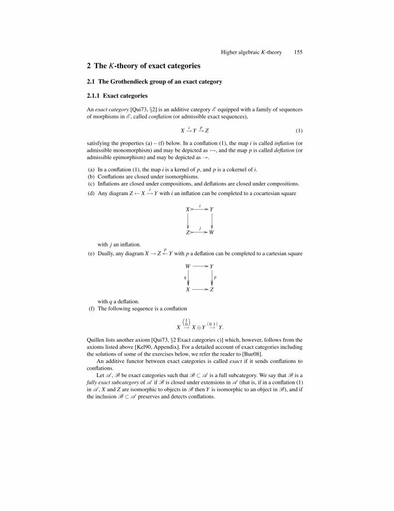
Higher algebraic K-theory 155
2 The K-theory of exact categories
2.1 The Grothendieck group of an exact category
2.1.1 Exact categories
An exact category [Qui73, §2] is an additive category E equipped with a family of sequencesof morphisms in E , called conflation (or admissible exact sequences),
X i→ Yp→ Z (1)
satisfying the properties (a) – (f) below. In a conflation (1), the map i is called inflation (oradmissible monomorphism) and may be depicted as, and the map p is called deflation (oradmissible epimorphism) and may be depicted as.
(a) In a conflation (1), the map i is a kernel of p, and p is a cokernel of i.(b) Conflations are closed under isomorphisms.(c) Inflations are closed under compositions, and deflations are closed under compositions.
(d) Any diagram Z← Xi Y with i an inflation can be completed to a cocartesian square
X //i //
Y
Z //
j // W
with j an inflation.
(e) Dually, any diagram X → ZpY with p a deflation can be completed to a cartesian square
W //
q
Y
p
X // Z
with q a deflation.(f) The following sequence is a conflation
X
(10
)→ X⊕Y
(0 1)→ Y.
Quillen lists another axiom [Qui73, §2 Exact categories c)] which, however, follows from theaxioms listed above [Kel90, Appendix]. For a detailed account of exact categories includingthe solutions of some of the exercises below, we refer the reader to [Bue08].
An additive functor between exact categories is called exact if it sends conflations toconflations.
Let A , B be exact categories such that B ⊂A is a full subcategory. We say that B is afully exact subcategory of A if B is closed under extensions in A (that is, if in a conflation (1)in A , X and Z are isomorphic to objects in B then Y is isomorphic to an object in B), and ifthe inclusion B ⊂A preserves and detects conflations.
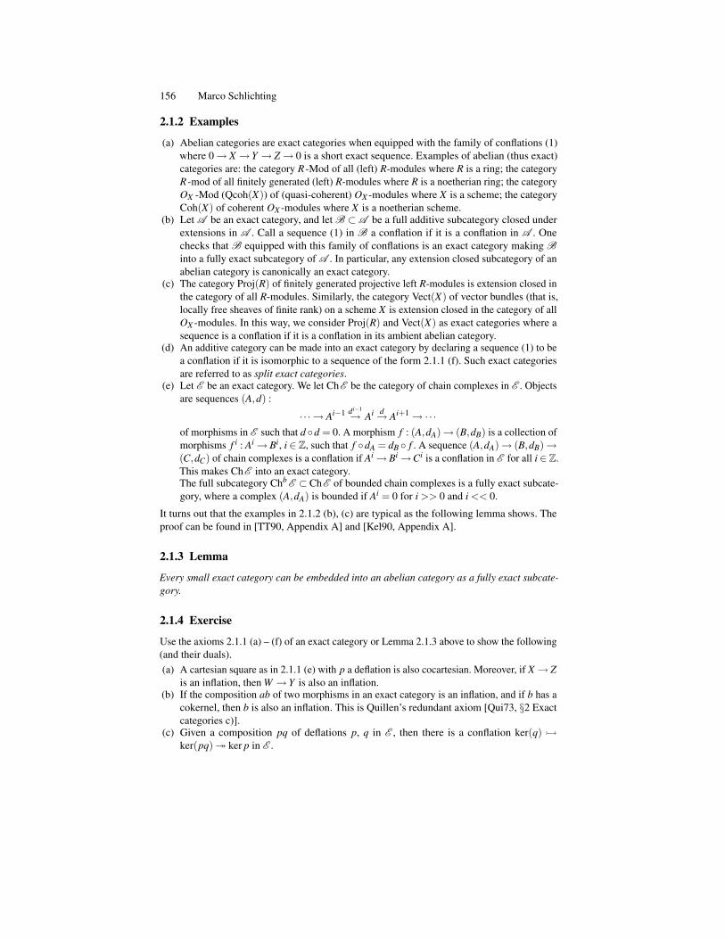
156 Marco Schlichting
2.1.2 Examples
(a) Abelian categories are exact categories when equipped with the family of conflations (1)where 0→ X → Y → Z→ 0 is a short exact sequence. Examples of abelian (thus exact)categories are: the category R -Mod of all (left) R-modules where R is a ring; the categoryR -mod of all finitely generated (left) R-modules where R is a noetherian ring; the categoryOX -Mod (Qcoh(X)) of (quasi-coherent) OX -modules where X is a scheme; the categoryCoh(X) of coherent OX -modules where X is a noetherian scheme.
(b) Let A be an exact category, and let B ⊂A be a full additive subcategory closed underextensions in A . Call a sequence (1) in B a conflation if it is a conflation in A . Onechecks that B equipped with this family of conflations is an exact category making Binto a fully exact subcategory of A . In particular, any extension closed subcategory of anabelian category is canonically an exact category.
(c) The category Proj(R) of finitely generated projective left R-modules is extension closed inthe category of all R-modules. Similarly, the category Vect(X) of vector bundles (that is,locally free sheaves of finite rank) on a scheme X is extension closed in the category of allOX -modules. In this way, we consider Proj(R) and Vect(X) as exact categories where asequence is a conflation if it is a conflation in its ambient abelian category.
(d) An additive category can be made into an exact category by declaring a sequence (1) to bea conflation if it is isomorphic to a sequence of the form 2.1.1 (f). Such exact categoriesare referred to as split exact categories.
(e) Let E be an exact category. We let ChE be the category of chain complexes in E . Objectsare sequences (A,d) :
· · · → Ai−1 di−1
→ Ai d→ Ai+1→ ···of morphisms in E such that d d = 0. A morphism f : (A,dA)→ (B,dB) is a collection ofmorphisms f i : Ai→ Bi, i ∈ Z, such that f dA = dB f . A sequence (A,dA)→ (B,dB)→(C,dC) of chain complexes is a conflation if Ai→ Bi→Ci is a conflation in E for all i ∈ Z.This makes ChE into an exact category.The full subcategory Chb E ⊂ ChE of bounded chain complexes is a fully exact subcate-gory, where a complex (A,dA) is bounded if Ai = 0 for i >> 0 and i << 0.
It turns out that the examples in 2.1.2 (b), (c) are typical as the following lemma shows. Theproof can be found in [TT90, Appendix A] and [Kel90, Appendix A].
2.1.3 Lemma
Every small exact category can be embedded into an abelian category as a fully exact subcate-gory.
2.1.4 Exercise
Use the axioms 2.1.1 (a) – (f) of an exact category or Lemma 2.1.3 above to show the following(and their duals).(a) A cartesian square as in 2.1.1 (e) with p a deflation is also cocartesian. Moreover, if X→ Z
is an inflation, then W → Y is also an inflation.(b) If the composition ab of two morphisms in an exact category is an inflation, and if b has a
cokernel, then b is also an inflation. This is Quillen’s redundant axiom [Qui73, §2 Exactcategories c)].
(c) Given a composition pq of deflations p, q in E , then there is a conflation ker(q)ker(pq) ker p in E .
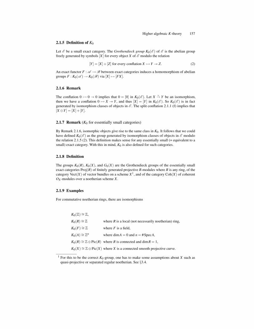
Higher algebraic K-theory 157
2.1.5 Definition of K0
Let E be a small exact category. The Grothendieck group K0(E ) of E is the abelian groupfreely generated by symbols [X ] for every object X of E modulo the relation
[Y ] = [X ]+ [Z] for every conflation X Y Z. (2)
An exact functor F : A →B between exact categories induces a homomorphism of abeliangroups F : K0(A )→ K0(B) via [X ] 7→ [FX ].
2.1.6 Remark
The conflation 0 0 0 implies that 0 = [0] in K0(E ). Let X∼=→ Y be an isomorphism,
then we have a conflation 0 X Y , and thus [X ] = [Y ] in K0(E ). So K0(E ) is in factgenerated by isomorphism classes of objects in E . The split conflation 2.1.1 (f) implies that[X⊕Y ] = [X ]+ [Y ].
2.1.7 Remark (K0 for essentially small categories)
By Remark 2.1.6, isomorphic objects give rise to the same class in K0. It follows that we couldhave defined K0(E ) as the group generated by isomorphism classes of objects in E modulothe relation 2.1.5 (2). This definition makes sense for any essentially small (= equivalent to asmall) exact category. With this in mind, K0 is also defined for such categories.
2.1.8 Definition
The groups K0(R), K0(X), and G0(X) are the Grothendieck groups of the essentially smallexact categories Proj(R) of finitely generated projective R-modules where R is any ring, of thecategory Vect(X) of vector bundles on a scheme X1, and of the category Coh(X) of coherentOX -modules over a noetherian scheme X .
2.1.9 Examples
For commutative noetherian rings, there are isomorphisms
K0(Z)∼= Z,
K0(R)∼= Z where R is a local (not necessarily noetherian) ring,
K0(F)∼= Z where F is a field,
K0(A)∼= Zn where dimA = 0 and n = #SpecA,
K0(R)∼= Z⊕Pic(R) where R is connected and dimR = 1,
K0(X)∼= Z⊕Pic(X) where X is a connected smooth projective curve.
1 For this to be the correct K0-group, one has to make some assumptions about X such asquasi-projective or separated regular noetherian. See §3.4.
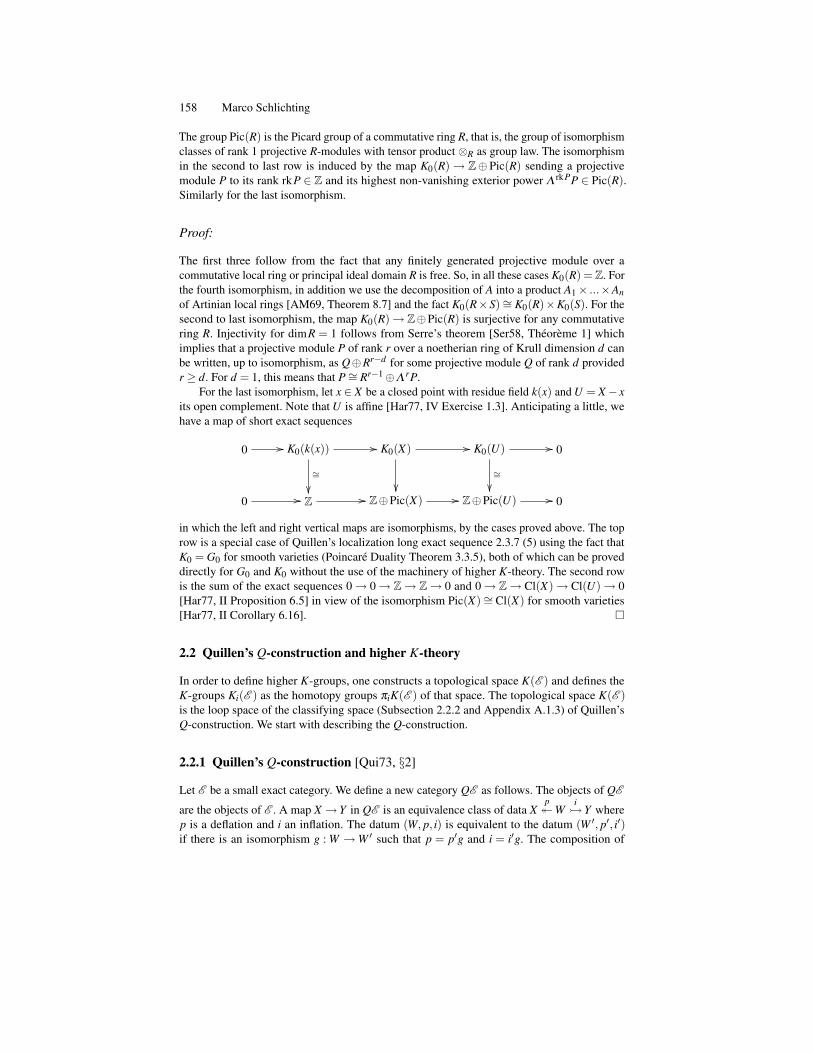
158 Marco Schlichting
The group Pic(R) is the Picard group of a commutative ring R, that is, the group of isomorphismclasses of rank 1 projective R-modules with tensor product ⊗R as group law. The isomorphismin the second to last row is induced by the map K0(R)→ Z⊕ Pic(R) sending a projectivemodule P to its rank rkP ∈ Z and its highest non-vanishing exterior power Λ rkPP ∈ Pic(R).Similarly for the last isomorphism.
Proof:
The first three follow from the fact that any finitely generated projective module over acommutative local ring or principal ideal domain R is free. So, in all these cases K0(R) =Z. Forthe fourth isomorphism, in addition we use the decomposition of A into a product A1× ...×Anof Artinian local rings [AM69, Theorem 8.7] and the fact K0(R×S)∼= K0(R)×K0(S). For thesecond to last isomorphism, the map K0(R)→ Z⊕Pic(R) is surjective for any commutativering R. Injectivity for dimR = 1 follows from Serre’s theorem [Ser58, Theoreme 1] whichimplies that a projective module P of rank r over a noetherian ring of Krull dimension d canbe written, up to isomorphism, as Q⊕Rr−d for some projective module Q of rank d providedr ≥ d. For d = 1, this means that P∼= Rr−1⊕Λ rP.
For the last isomorphism, let x ∈ X be a closed point with residue field k(x) and U = X− xits open complement. Note that U is affine [Har77, IV Exercise 1.3]. Anticipating a little, wehave a map of short exact sequences
0 // K0(k(x))
∼=
// K0(X)
// K0(U)
∼=
// 0
0 // Z // Z⊕Pic(X) // Z⊕Pic(U) // 0
in which the left and right vertical maps are isomorphisms, by the cases proved above. The toprow is a special case of Quillen’s localization long exact sequence 2.3.7 (5) using the fact thatK0 = G0 for smooth varieties (Poincare Duality Theorem 3.3.5), both of which can be proveddirectly for G0 and K0 without the use of the machinery of higher K-theory. The second rowis the sum of the exact sequences 0→ 0→ Z→ Z→ 0 and 0→ Z→ Cl(X)→ Cl(U)→ 0[Har77, II Proposition 6.5] in view of the isomorphism Pic(X)∼= Cl(X) for smooth varieties[Har77, II Corollary 6.16].
2.2 Quillen’s Q-construction and higher K-theory
In order to define higher K-groups, one constructs a topological space K(E ) and defines theK-groups Ki(E ) as the homotopy groups πiK(E ) of that space. The topological space K(E )is the loop space of the classifying space (Subsection 2.2.2 and Appendix A.1.3) of Quillen’sQ-construction. We start with describing the Q-construction.
2.2.1 Quillen’s Q-construction [Qui73, §2]
Let E be a small exact category. We define a new category QE as follows. The objects of QE
are the objects of E . A map X → Y in QE is an equivalence class of data XpW
i Y where
p is a deflation and i an inflation. The datum (W, p, i) is equivalent to the datum (W ′, p′, i′)if there is an isomorphism g : W →W ′ such that p = p′g and i = i′g. The composition of
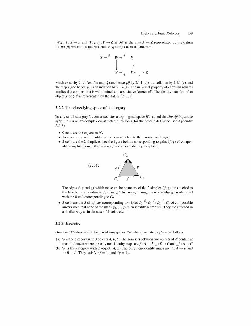
Higher algebraic K-theory 159
(W, p, i) : X → Y and (V,q, j) : Y → Z in QE is the map X → Z represented by the datum(U, pq, ji) where U is the pull-back of q along i as in the diagram
X Wpoooo
i
Uqoooo
i
Y Vqoooo //
j// Z
which exists by 2.1.1 (e). The map q (and hence pq by 2.1.1 (c)) is a deflation by 2.1.1 (e), andthe map i (and hence ji) is an inflation by 2.1.4 (a). The universal property of cartesian squaresimplies that composition is well-defined and associative (exercise!). The identity map idX of anobject X of QE is represented by the datum (X ,1,1).
2.2.2 The classifying space of a category
To any small category C , one associates a topological space BC called the classifying spaceof C . This is a CW -complex constructed as follows (for the precise definition, see AppendixA.1.3).
• 0-cells are the objects of C .• 1-cells are the non-identity morphisms attached to their source and target.• 2-cells are the 2-simplices (see the figure below) corresponding to pairs ( f ,g) of compos-
able morphisms such that neither f nor g is an identity morphism.
C1
C2
C0
( f ,g) : g f g
f
The edges f , g and g f which make up the boundary of the 2-simplex ( f ,g) are attached tothe 1-cells corresponding to f , g, and g f . In case g f = idC0 , the whole edge g f is identifiedwith the 0-cell corresponding to C0.
• 3-cells are the 3-simplices corresponding to triples C0f0→C1
f1→C2f2→C3 of composable
arrows such that none of the maps f0, f1, f2 is an identity morphism. They are attached ina similar way as in the case of 2-cells, etc.
2.2.3 Exercise
Give the CW -structure of the classifying spaces BC where the category C is as follows.
(a) C is the category with 3 objects A, B, C. The hom sets between two objects of C contain atmost 1 element where the only non-identity maps are f : A→ B, g : B→C and g f : A→C.
(b) C is the category with 2 objects A, B. The only non-identity maps are f : A→ B andg : B→ A. They satisfy g f = 1A and f g = 1B.
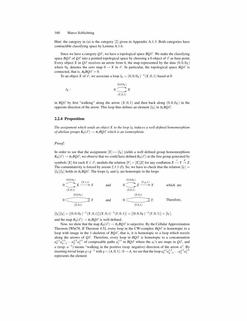
160 Marco Schlichting
Hint: the category in (a) is the category [2] given in Appendix A.1.3. Both categories havecontractible classifying space by Lemma A.1.6.
Since we have a category QE , we have a topological space BQE . We make the classifyingspace BQE of QE into a pointed topological space by choosing a 0-object of E as base-point.Every object X in QE receives an arrow from 0, the map represented by the data (0,0,0X )where 0X denotes the zero map 0→ X in E . In particular, the topological space BQE isconnected, that is, π0BQE = 0.
To an object X of E , we associate a loop lX = (0,0,0X )−1(X ,0,1) based at 0
lX : 0(X ,0,1)
66
(0,0,0X )((X
in BQE by first “walking” along the arrow (X ,0,1) and then back along (0,0,0X ) in theopposite direction of the arrow. This loop thus defines an element [lX ] in π1BQE .
2.2.4 Proposition
The assignment which sends an object X to the loop lX induces a well-defined homomorphismof abelian groups K0(E )→ π1BQE which is an isomorphism.
Proof:
In order to see that the assignment [X ] 7→ [lX ] yields a well defined group homomorphismK0(E )→ π1BQE , we observe that we could have defined K0(E ) as the free group generated by
symbols [X ] for each X ∈ E , modulo the relation [Y ] = [X ][Z] for any conflation Xi Y
p Z.
The commutativity is forced by axiom 2.1.1 (f). So, we have to check that the relation [lY ] =[lX ][lZ ] holds in π1BQE . The loops lX and lZ are homotopic to the loops
0(X ,0,1)
66
(0,0,0X )((X
(X ,1,i) // Y and 0(Z,0,1)
66
(0,0,0Z)((Z
(Y,p,1) // Y which are
0(X ,0,i)
33(0,0,0Y )
++ Y and 0(Y,0,1)
33(X ,0,i)
++ Y. Therefore,
[lX ][lZ ] = [(0,0,0Y )−1(X ,0, i)][(X ,0, i)−1(Y,0,1)] = [(0,0,0Y )−1(Y,0,1)] = [lY ],
and the map K0(E )→ π1BQE is well-defined.Now, we show that the map K0(E )→ π1BQE is surjective. By the Cellular Approximation
Theorem [Whi78, II Theorem 4.5], every loop in the CW-complex BQE is homotopic to aloop with image in the 1-skeleton of BQE , that is, it is homotopic to a loop which travelsalong the arrows of QE . Therefore, every loop in BQE is homotopic to a concatenationa±1
n a±1n−1 · · ·a
±12 a±1
1 of composable paths a±1i in BQE where the ai’s are maps in QE , and
a (resp. a−1) means “walking in the positive (resp. negative) direction of the arrow a”. Byinserting trivial loops gg−1 with g = (A,0,1) : 0→A, we see that the loop a±1
n a±1n−1 · · ·a
±12 a±1
1represents the element
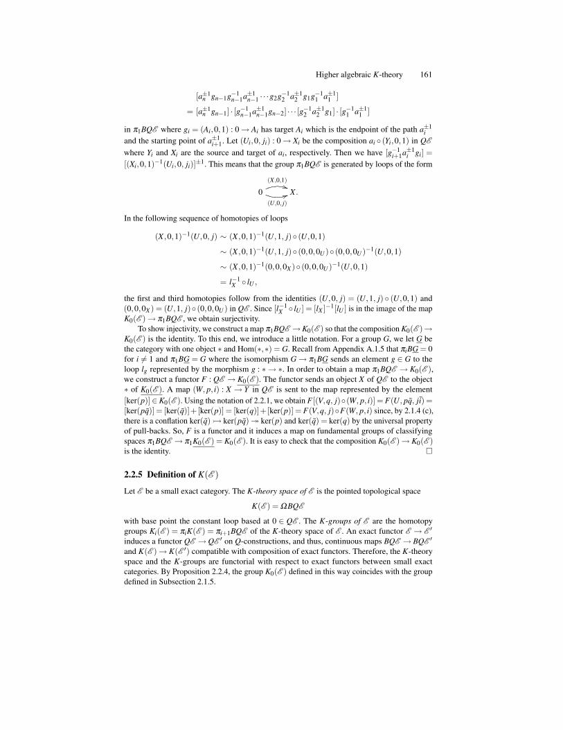
Higher algebraic K-theory 161
[a±1n gn−1g−1
n−1a±1n−1 · · ·g2g−1
2 a±12 g1g−1
1 a±11 ]
= [a±1n gn−1] · [g−1
n−1a±1n−1gn−2] · · · [g−1
2 a±12 g1] · [g−1
1 a±11 ]
in π1BQE where gi = (Ai,0,1) : 0→ Ai has target Ai which is the endpoint of the path a±1i
and the starting point of a±1i+1. Let (Ui,0, ji) : 0→ Xi be the composition ai (Yi,0,1) in QE
where Yi and Xi are the source and target of ai, respectively. Then we have [g−1i+1a±1
i gi] =[(Xi,0,1)−1(Ui,0, ji)]±1. This means that the group π1BQE is generated by loops of the form
0(U,0, j)
55
(X ,0,1)))X .
In the following sequence of homotopies of loops
(X ,0,1)−1(U,0, j) ∼ (X ,0,1)−1(U,1, j) (U,0,1)
∼ (X ,0,1)−1(U,1, j) (0,0,0U ) (0,0,0U )−1(U,0,1)
∼ (X ,0,1)−1(0,0,0X ) (0,0,0U )−1(U,0,1)
= l−1X lU ,
the first and third homotopies follow from the identities (U,0, j) = (U,1, j) (U,0,1) and(0,0,0X ) = (U,1, j) (0,0,0U ) in QE . Since [l−1
X lU ] = [lX ]−1[lU ] is in the image of the mapK0(E )→ π1BQE , we obtain surjectivity.
To show injectivity, we construct a map π1BQE →K0(E ) so that the composition K0(E )→K0(E ) is the identity. To this end, we introduce a little notation. For a group G, we let G bethe category with one object ∗ and Hom(∗,∗) = G. Recall from Appendix A.1.5 that πiBG = 0for i 6= 1 and π1BG = G where the isomorphism G→ π1BG sends an element g ∈ G to theloop lg represented by the morphism g : ∗ → ∗. In order to obtain a map π1BQE → K0(E ),we construct a functor F : QE → K0(E ). The functor sends an object X of QE to the object∗ of K0(E ). A map (W, p, i) : X → Y in QE is sent to the map represented by the element[ker(p)]∈K0(E ). Using the notation of 2.2.1, we obtain F [(V,q, j)(W, p, i)] = F(U, pq, ji) =[ker(pq)] = [ker(q)]+[ker(p)] = [ker(q)]+[ker(p)] = F(V,q, j)F(W, p, i) since, by 2.1.4 (c),there is a conflation ker(q) ker(pq) ker(p) and ker(q) = ker(q) by the universal propertyof pull-backs. So, F is a functor and it induces a map on fundamental groups of classifyingspaces π1BQE → π1K0(E ) = K0(E ). It is easy to check that the composition K0(E )→ K0(E )is the identity.
2.2.5 Definition of K(E )
Let E be a small exact category. The K-theory space of E is the pointed topological space
K(E ) = ΩBQE
with base point the constant loop based at 0 ∈ QE . The K-groups of E are the homotopygroups Ki(E ) = πiK(E ) = πi+1BQE of the K-theory space of E . An exact functor E → E ′
induces a functor QE → QE ′ on Q-constructions, and thus, continuous maps BQE → BQE ′
and K(E )→ K(E ′) compatible with composition of exact functors. Therefore, the K-theoryspace and the K-groups are functorial with respect to exact functors between small exactcategories. By Proposition 2.2.4, the group K0(E ) defined in this way coincides with the groupdefined in Subsection 2.1.5.
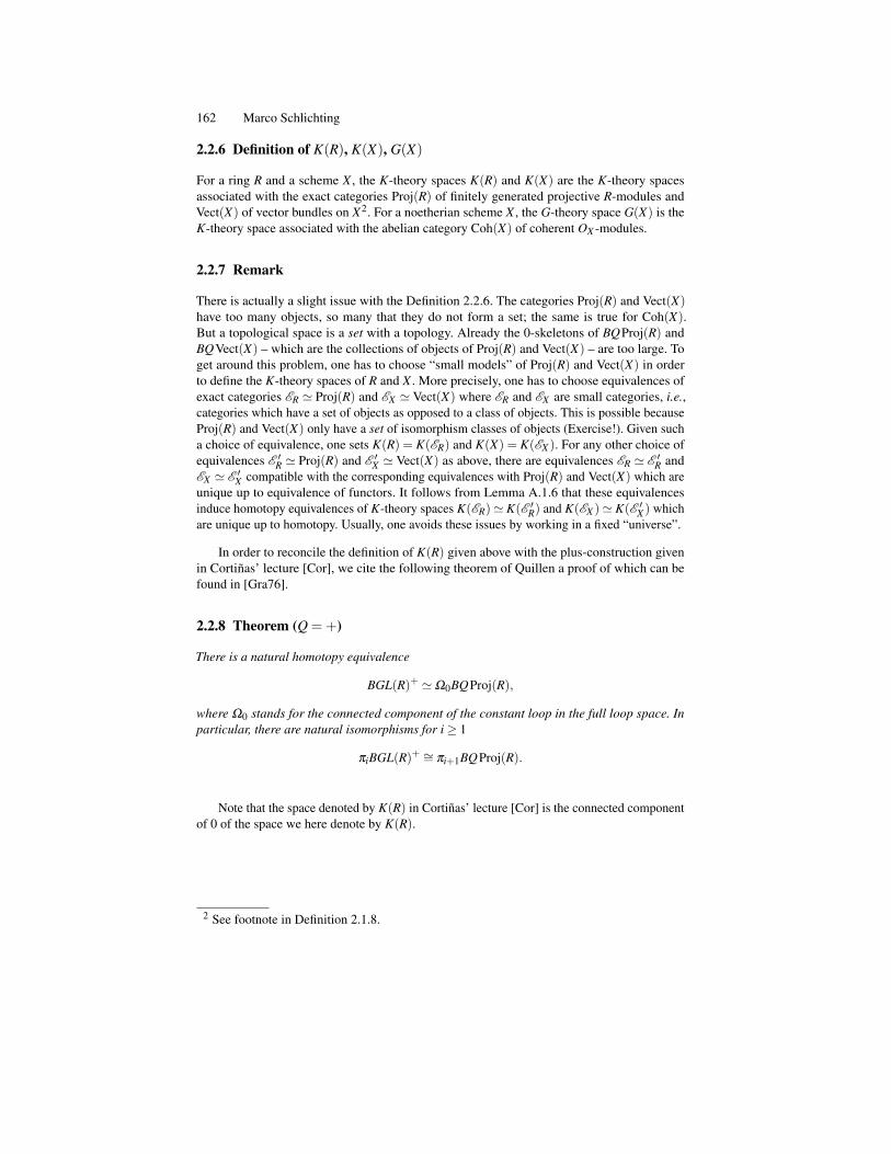
162 Marco Schlichting
2.2.6 Definition of K(R), K(X), G(X)
For a ring R and a scheme X , the K-theory spaces K(R) and K(X) are the K-theory spacesassociated with the exact categories Proj(R) of finitely generated projective R-modules andVect(X) of vector bundles on X2. For a noetherian scheme X , the G-theory space G(X) is theK-theory space associated with the abelian category Coh(X) of coherent OX -modules.
2.2.7 Remark
There is actually a slight issue with the Definition 2.2.6. The categories Proj(R) and Vect(X)have too many objects, so many that they do not form a set; the same is true for Coh(X).But a topological space is a set with a topology. Already the 0-skeletons of BQProj(R) andBQVect(X) – which are the collections of objects of Proj(R) and Vect(X) – are too large. Toget around this problem, one has to choose “small models” of Proj(R) and Vect(X) in orderto define the K-theory spaces of R and X . More precisely, one has to choose equivalences ofexact categories ER ' Proj(R) and EX ' Vect(X) where ER and EX are small categories, i.e.,categories which have a set of objects as opposed to a class of objects. This is possible becauseProj(R) and Vect(X) only have a set of isomorphism classes of objects (Exercise!). Given sucha choice of equivalence, one sets K(R) = K(ER) and K(X) = K(EX ). For any other choice ofequivalences E ′R ' Proj(R) and E ′X ' Vect(X) as above, there are equivalences ER ' E ′R andEX ' E ′X compatible with the corresponding equivalences with Proj(R) and Vect(X) which areunique up to equivalence of functors. It follows from Lemma A.1.6 that these equivalencesinduce homotopy equivalences of K-theory spaces K(ER)' K(E ′R) and K(EX )' K(E ′X ) whichare unique up to homotopy. Usually, one avoids these issues by working in a fixed “universe”.
In order to reconcile the definition of K(R) given above with the plus-construction givenin Cortinas’ lecture [Cor], we cite the following theorem of Quillen a proof of which can befound in [Gra76].
2.2.8 Theorem (Q = +)
There is a natural homotopy equivalence
BGL(R)+ 'Ω0BQProj(R),
where Ω0 stands for the connected component of the constant loop in the full loop space. Inparticular, there are natural isomorphisms for i≥ 1
πiBGL(R)+ ∼= πi+1BQProj(R).
Note that the space denoted by K(R) in Cortinas’ lecture [Cor] is the connected componentof 0 of the space we here denote by K(R).
2 See footnote in Definition 2.1.8.
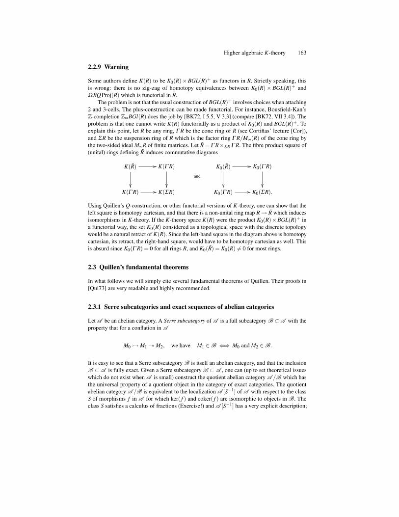
Higher algebraic K-theory 163
2.2.9 Warning
Some authors define K(R) to be K0(R)×BGL(R)+ as functors in R. Strictly speaking, thisis wrong: there is no zig-zag of homotopy equivalences between K0(R)× BGL(R)+ andΩBQProj(R) which is functorial in R.
The problem is not that the usual construction of BGL(R)+ involves choices when attaching2 and 3-cells. The plus-construction can be made functorial. For instance, Bousfield-Kan’sZ-completion Z∞BGl(R) does the job by [BK72, I 5.5, V 3.3] (compare [BK72, VII 3.4]). Theproblem is that one cannot write K(R) functorially as a product of K0(R) and BGL(R)+. Toexplain this point, let R be any ring, Γ R be the cone ring of R (see Cortinas’ lecture [Cor]),and ΣR be the suspension ring of R which is the factor ring Γ R/M∞(R) of the cone ring bythe two-sided ideal M∞R of finite matrices. Let R = Γ R×ΣR Γ R. The fibre product square of(unital) rings defining R induces commutative diagrams
K(R) //
K(Γ R)
and
K0(R) //
K0(Γ R)
K(Γ R) // K(ΣR) K0(Γ R) // K0(ΣR).
Using Quillen’s Q-construction, or other functorial versions of K-theory, one can show that theleft square is homotopy cartesian, and that there is a non-unital ring map R→ R which inducesisomorphisms in K-theory. If the K-theory space K(R) were the product K0(R)×BGL(R)+ ina functorial way, the set K0(R) considered as a topological space with the discrete topologywould be a natural retract of K(R). Since the left-hand square in the diagram above is homotopycartesian, its retract, the right-hand square, would have to be homotopy cartesian as well. Thisis absurd since K0(Γ R) = 0 for all rings R, and K0(R) = K0(R) 6= 0 for most rings.
2.3 Quillen’s fundamental theorems
In what follows we will simply cite several fundamental theorems of Quillen. Their proofs in[Qui73] are very readable and highly recommended.
2.3.1 Serre subcategories and exact sequences of abelian categories
Let A be an abelian category. A Serre subcategory of A is a full subcategory B ⊂A with theproperty that for a conflation in A
M0M1M2, we have M1 ∈B ⇐⇒ M0 and M2 ∈B.
It is easy to see that a Serre subscategory B is itself an abelian category, and that the inclusionB ⊂A is fully exact. Given a Serre subcategory B ⊂A , one can (up to set theoretical issueswhich do not exist when A is small) construct the quotient abelian category A /B which hasthe universal property of a quotient object in the category of exact categories. The quotientabelian category A /B is equivalent to the localization A [S−1] of A with respect to the classS of morphisms f in A for which ker( f ) and coker( f ) are isomorphic to objects in B. Theclass S satisfies a calculus of fractions (Exercise!) and A [S−1] has a very explicit description;
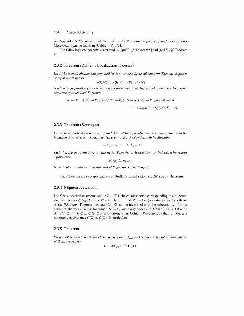
164 Marco Schlichting
see Appendix A.2.6. We will call B→A →A /B an exact sequence of abelian categories.More details can be found in [Gab62], [Pop73].
The following two theorems are proved in [Qui73, §5 Theorem 5] and [Qui73, §5 Theorem4].
2.3.2 Theorem (Quillen’s Localization Theorem)
Let A be a small abelian category, and let B ⊂A be a Serre subcategory. Then the sequenceof topological spaces
BQ(B)→ BQ(A )→ BQ(A /B)
is a homotopy fibration (see Appendix A.1.7 for a definition). In particular, there is a long exactsequence of associated K-groups
· · · → Kn+1(A )→ Kn+1(A /B)→ Kn(B)→ Kn(A )→ Kn(A /B)→ ·· ·
· · · → K0(A )→ K0(A /B)→ 0.
2.3.3 Theorem (Devissage)
Let A be a small abelian category, and B ⊂A be a full abelian subcategory such that theinclusion B ⊂A is exact. Assume that every object A of A has a finite filtration
0 = A0 ⊂ A1 ⊂ ...⊂ An = A
such that the quotients Ai/Ai−1 are in B. Then the inclusion B ⊂ A induces a homotopyequivalence
K(B) ∼→ K(A ).
In particular, it induces isomorphisms of K-groups Ki(B)∼= Ki(A ).
The following are two applications of Quillen’s Localization and Devissage Theorems.
2.3.4 Nilpotent extensions
Let X be a noetherian scheme and i : Z → X a closed subscheme corresponding to a nilpotentsheaf of ideals I ⊂ OX . Assume In = 0. Then i∗ : Coh(Z)→ Coh(X) satisfies the hypothesisof the Devissage Theorem because Coh(Z) can be identified with the subcategory of thosecoherent sheaves F on X for which IF = 0, and every sheaf F ∈ Coh(X) has a filtration0 = InF ⊂ In−1F ⊂ ... ⊂ IF ⊂ F with quotients in Coh(Z). We conclude that i∗ induces ahomotopy equivalence G(Z)' G(X). In particular:
2.3.5 Theorem
For a noetherian scheme X, the closed immersion i : Xred → X induces a homotopy equivalenceof G-theory spaces
i∗ : G(Xred) ∼−→ G(X).
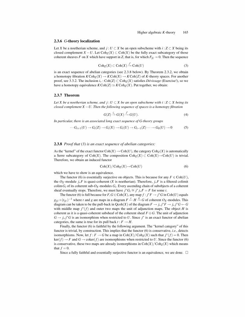
Higher algebraic K-theory 165
2.3.6 G-theory localization
Let X be a noetherian scheme, and j : U ⊂ X be an open subscheme with i : Z ⊂ X being itsclosed complement X −U . Let CohZ(X) ⊂ Coh(X) be the fully exact subcategory of thosecoherent sheaves F on X which have support in Z, that is, for which F|U = 0. Then the sequence
CohZ(X)⊂ Coh(X)j∗→ Coh(U) (3)
is an exact sequence of abelian categories (see 2.3.8 below). By Theorem 2.3.2, we obtaina homotopy fibration K CohZ(X)→ K Coh(X)→ K Coh(Z) of K-theory spaces. For anotherproof, see 3.3.2. The inclusion i∗ : Coh(Z)⊂ CohZ(X) satisfies Devissage (Exercise!), so wehave a homotopy equivalence K Coh(Z)' K CohZ(X). Put together, we obtain:
2.3.7 Theorem
Let X be a noetherian scheme, and j : U ⊂ X be an open subscheme with i : Z ⊂ X being itsclosed complement X−U. Then the following sequence of spaces is a homotopy fibration
G(Z) i∗→ G(X)j∗→ G(U). (4)
In particular, there is an associated long exact sequence of G-theory groups
· · ·Gi+1(U)→ Gi(Z)→ Gi(X)→ Gi(U)→ Gi−1(Z) · · · → G0(U)→ 0 (5)
2.3.8 Proof that (3) is an exact sequence of abelian categories:
As the “kernel” of the exact functor Coh(X)→Coh(U), the category CohZ(X) is automaticallya Serre subcategory of Coh(X). The composition CohZ(X) ⊂ Coh(X)→Coh(U) is trivial.Therefore, we obtain an induced functor
Coh(X)/CohZ(X)→Coh(U) (6)
which we have to show is an equivalence.The functor (6) is essentially surjective on objects. This is because for any F ∈ Coh(U),
the OX -module j∗F is quasi-coherent (X is noetherian). Therefore, j∗F is a filtered colimitcolimGi of its coherent sub-OX -modules Gi. Every ascending chain of subobjects of a coherentsheaf eventually stops. Therefore, we must have j∗Gi ∼= j∗ j∗F = F for some i.
The functor (6) is full because for F,G∈Coh(X), any map f : j∗F→ j∗G in Coh(U) equalsg|U (t|U )−1 where t and g are maps in a diagram F t← H
g→ G of coherent OX -modules. Thisdiagram can be taken to be the pull-back in Qcoh(X) of the diagram F→ j∗ j∗F→ j∗ j∗G←Gwith middle map j∗( f ) and outer two maps the unit of adjunction maps. The object H iscoherent as it is a quasi-coherent subsheaf of the coherent sheaf F⊕G. The unit of adjunctionG→ j∗ j∗G is an isomorphism when restricted to U . Since j∗ is an exact functor of abeliancategories, the same is true for its pull back t : F → H.
Finally, the functor (6) is faithful by the following argument. The “kernel category” of thisfunctor is trivial, by construction. This implies that the functor (6) is conservative, i.e., detectsisomorphisms. Now, let f : F → G be a map in Coh(X)/CohZ(X) such that j∗( f ) = 0. Thenker( f )→ F and G→ coker( f ) are isomorphisms when restricted to U . Since the functor (6)is conservative, these two maps are already isomorphisms in Coh(X)/CohZ(X) which meansthat f = 0.
Since a fully faithful and essentially surjective functor is an equivalence, we are done.
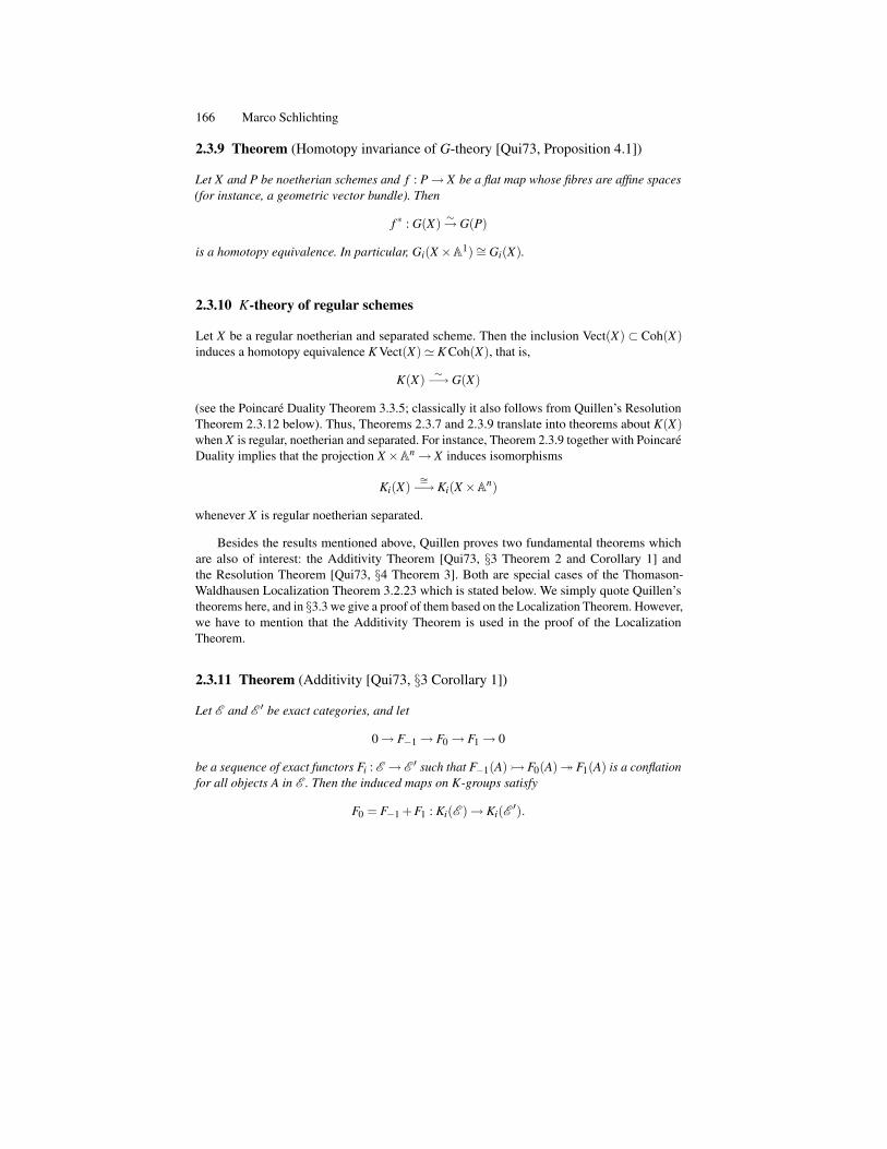
166 Marco Schlichting
2.3.9 Theorem (Homotopy invariance of G-theory [Qui73, Proposition 4.1])
Let X and P be noetherian schemes and f : P→ X be a flat map whose fibres are affine spaces(for instance, a geometric vector bundle). Then
f ∗ : G(X) ∼→ G(P)
is a homotopy equivalence. In particular, Gi(X×A1)∼= Gi(X).
2.3.10 K-theory of regular schemes
Let X be a regular noetherian and separated scheme. Then the inclusion Vect(X) ⊂ Coh(X)induces a homotopy equivalence K Vect(X)' K Coh(X), that is,
K(X) ∼−→ G(X)
(see the Poincare Duality Theorem 3.3.5; classically it also follows from Quillen’s ResolutionTheorem 2.3.12 below). Thus, Theorems 2.3.7 and 2.3.9 translate into theorems about K(X)when X is regular, noetherian and separated. For instance, Theorem 2.3.9 together with PoincareDuality implies that the projection X×An→ X induces isomorphisms
Ki(X)∼=−→ Ki(X×An)
whenever X is regular noetherian separated.
Besides the results mentioned above, Quillen proves two fundamental theorems whichare also of interest: the Additivity Theorem [Qui73, §3 Theorem 2 and Corollary 1] andthe Resolution Theorem [Qui73, §4 Theorem 3]. Both are special cases of the Thomason-Waldhausen Localization Theorem 3.2.23 which is stated below. We simply quote Quillen’stheorems here, and in §3.3 we give a proof of them based on the Localization Theorem. However,we have to mention that the Additivity Theorem is used in the proof of the LocalizationTheorem.
2.3.11 Theorem (Additivity [Qui73, §3 Corollary 1])
Let E and E ′ be exact categories, and let
0→ F−1→ F0→ F1→ 0
be a sequence of exact functors Fi : E → E ′ such that F−1(A) F0(A) F1(A) is a conflationfor all objects A in E . Then the induced maps on K-groups satisfy
F0 = F−1 +F1 : Ki(E )→ Ki(E ′).
Higher algebraic K-theory 167
2.3.12 Theorem (Resolution [Qui73, §4])
Let A ⊂B be a fully exact subcategory of an exact category B. Assume that
(a) if M−1M0M1 is a conflation in B with M0, M1 ∈A , then M−1 ∈A , and(b) for every B ∈B there is an exact sequence
0→ An→ An−1→ ·· ·A0→ B→ 0
with Ai ∈A .
Then the inclusion A ⊂B induces a homotopy equivalence of K-theory spaces
K(A ) ∼−→ K(B).
2.4 Negative K-groups
Besides the positive K-groups, one can also define the negative K-groups Ki with i < 0. Theyextend certain K0 exact sequences to the right (see Cortinas’ lecture [Cor]). For rings andadditive (or split exact) categories they were introduced by Bass [Bas68] and Karoubi [Kar68].The treatment for exact categories below follows [Sch04].
2.4.1 Idempotent completion
Let A be an additive category, and B ⊂A be a full additive subcategory. We call the inclusionB ⊂A cofinal, or equivalence up to factors if every object of A is a direct factor of an objectof B. If A and B are exact categories, we require moreover that the inclusion B ⊂A is fullyexact, that is, the inclusion is extension closed, and it preserves and detects conflations. Asan example, the category of (finitely generated) free R-modules is cofinal in the category of(finitely generated) projective R-modules.
Given an additive category A , there is a “largest” category ˜A of A such that the inclusionA ⊂ ˜A is cofinal. This is the idempotent completion ˜A of A . An additive category is calledidempotent complete if for every idempotent map p = p2 : A→ A, there is an isomorphismA∼= X ⊕Y under which the map p corresponds to
(1 00 0)
: X ⊕Y → X⊕Y . The objects of theidempotent completion ˜A of A are pairs (A, p) with A an object of A and p = p2 : A→ Aan idempotent endomorphism. Maps (A, p)→ (B,q) in ˜A are maps f : A→ B in A suchthat f p = f = q f . Composition is composition in A , and id(A,p) = p. Every idempotentq = q2 : (A, p)→ (A, p) corresponds to
(1 00 0)
under the isomorphism (q, p− q) : (A,q)⊕(A, p−q)∼= (A, p). Therefore, the category ˜A is indeed idempotent complete. Furthermore,we have a fully faithful embedding A ⊂ ˜A : A 7→ (A,1) which is cofinal since the object (A, p)of ˜A is a direct factor the object (A,1) of A .
If E is an exact category, its idempotent completion E becomes an exact category whenwe declare a sequence in E to be a conflation if it is a retract (in the category of conflations) ofa conflation of E . For more details, see [TT90, Appendix A]. Note that the inclusion E ⊂ E isindeed fully exact.
168 Marco Schlichting
2.4.2 Proposition (Cofinality [Gra79, Theorem 1.1])
Let A be an exact category and B ⊂A be a cofinal fully exact subcategory. Then the mapsKi(B)→ Ki(A ) are isomorphisms for i > 0 and a monomorphism for i = 0. This holds inparticular for Ki(E )→ Ki(E ).
2.4.3 Negative K-theory and the spectrum IK(E )
To any exact category E , one can associate a new exact category SE (see Subsection 2.4.6),called the suspension of E , such that there is a natural homotopy equivalence [Sch04]
K(E ) ∼→ΩK(SE ). (7)
If E = Proj(R) one can take SE = Proj(ΣR) where ΣR is the suspension ring of R; see Cortinas’lecture [Cor]) for the definition of ΣR.
One uses the suspension construction to slightly modify the definition of algebraic K-theory in order to incorporate negative K-groups as follows. One sets IKi(E ) = Ki(E ) for
i≥ 1, IK0(E ) = K0(E ) and IKi(E ) = K0(S−iE ) for i < 0. Since Vect(X), Coh(X) and Proj(R)are all idempotent complete, we have the equalities IK0 Vect(X) = K0 Vect(X) = K0(X),IK0 Coh(X) = K0 Coh(X) = G0(X) and IK0 Proj(R) = K0 Proj(R) = K0(R). In these cases, wehave not changed the definition of K-theory; we have merely introduced “negative K-groups”IKi for i < 0. For this reason, we may write Ki(X) and Ki(R) instead of IKi(X) and IKi(R) forall i ∈ Z.
In a fancy language, one constructs a spectrum IK(E ) whose homotopy groups are thegroups IKi(E ) for i ∈ Z. The n-th space of this spectrum is K(SnE ), and the structure maps aregiven by (7). For terminology and basic properties of spectra, we refer the reader to AppendixA.1.8.
By Bass’ Fundamental Theorem stated in 3.5.3 below there is a split exact sequence fori ∈ Z
0→ Ki(R)→ Ki(R[T ])⊕Ki(R[T−1])→ Ki(R[T,T−1])→ Ki−1(R)→ 0.
One can use this sequence to give a recursive definition of the negative K-groups Ki(R) fori < 0, starting with the functor K0. This was Bass’ original definition.
2.4.4 Remark
Although Quillen did not define negative K-groups of exact categories, all K-theory statementsin [Qui73] and [Gra76] extend to negative K-theory. The only exceptions are Quillen’s Local-ization Theorem 2.3.2 and the Devissage Theorem 2.3.3. To insure that these two theoremsalso extend to negative K-theory, we need the abelian categories in question to be noetherian,though it is conjectured that the noetherian hypothesis is unnecessary.
2.4.5 Remark
Not much is known about IKi(E ) when i < 0, even though we believe their calculations to beeasier than those of Ki(E ) when i≥ 0. However, we do know the following. We have Ki(R) = 0for i < 0 when R is a regular noetherian ring [Bas68]. We have IK−1(A ) = 0 for any abeliancategory A [Sch06, Theorem 6], and IKi(A ) = 0 for i < 0 when A is a noetherian abeliancategory [Sch06, Theorem 7]. In particular, K−1(R) = 0 for a regular coherent ring R, and
Higher algebraic K-theory 169
Ki(X) = 0 for i < 0 when X is any regular noetherian and separated scheme. In [CHSW08]it is shown that Ki(X) = 0 for i <−d when X is a d-dimensional scheme essentially of finitetype over a field of characteristic 0, but K−d(X) = Hd
cdh(X ,Z) can be non-zero [Rei87]. Forfinite-type schemes over fields of positive characteristic, the same is true provided strongresolution of singularities holds over the base field [GH08]. It is conjectured that Ki(ZG) = 0for i <−1 when G is a finitely presented group [Hsi84]. For results in this direction see [LR05].
2.4.6 Construction of the suspension SE
Let E be an exact category. The countable envelope FE of E is an exact category whoseobjects are sequences
A0 A1 A2 ...
of inflations in E . The morphism set from a sequence A∗ to another sequence B∗ is
HomFE (A∗,B∗) = limi colimj
HomE (Ai,B j).
A sequence in FE is a conflation iff it is isomorphic in FE to the sequence of maps ofsequences A∗ → B∗ → C∗ where Ai → Bi → Ci is a conflation in E for i ∈ N. Colimits ofsequences of inflations exist in FE , and are exact. In particular, FE has exact countable directsums. There is a fully faithful exact functor E →FE which sends an object X ∈ E to the
constant sequence X 1→ X 1→ X 1→ ··· . For details of the construction see [Kel90, Appendix B]where FE was denoted by E ∼.
The suspension SE of E is the quotient FE /E of the countable envelope FE by thesubcategory E . The quotient is taken in the category of small exact categories. The proof ofthe existence of FE /E and an explicit description is given in [Sch04]. By [Sch04, Theorem2.1 and Lemma 3.2] the sequence E →FE → SE induces a homotopy fibration K(E )→K(FE )→ K(SE ) of K-theory spaces. Since FE has exact countable direct sums, the totalspace K(FE ) of the fibration is contractible. This yields the homotopy equivalence 2.4.3 (7).
3 Algebraic K-theory and triangulated categories
3.1 The Grothendieck-group of a triangulated category
Most calculations in the early days of K-theory were based on Quillen’s Localization Theorem2.3.2 for abelian categories together with Devissage 2.3.3. Unfortunately, not all K-groups are(not even equivalent to) the K-groups of some abelian category, notably K(X) where X is somesingular variety. Also, there is no satisfactory generalization of Quillen’s Localization Theoremto exact categories which would apply to all situations K-theorists had in mind. This is wheretriangulated categories come in. They provide a flexible framework that allows us to provemany results which cannot be proved with Quillen’s methods alone.
For the rest of this subsection, we will assume that the reader is familiar with AppendixA.2.1 – A.2.7.
3.1.1 Definition of K0(T )
Let T be a small triangulated category. The Grothen-dieck-group K0(T ) of T is the abeliangroup freely generated by symbols [X ] for every object X of T , modulo the relation [X ]+[Z] =[Y ] for every distinguished triangle X → Y → Z→ T X in T .
170 Marco Schlichting
3.1.2 Remark
As in Remark 2.1.6, we have [X ] = [Y ] if there is an isomorphism f : X ∼= Y in view of the
distinguished triangle Xf→ Y → 0→ T X . We also have [X ⊕Y ] = [X ]+ [Y ] because there is
a distinguished triangle X → X ⊕Y → Y → T X which is the direct sum of the distinguishedtriangles X→X→ 0→ T X and 0→Y→Y→ 0. Moreover, the distinguished triangle X→ 0→T X → T X shows that [T X ] =−[X ]. In particular, every element in K0(T ) can be representedas [X ] for some object X in T .
One would like to relate the Grothendieck-group K0(E ) of an exact category E to theGrothendieck-group of a triangulated category associated with E . This role is played by thebounded derived category D b(E ) of E .
3.1.3 The bounded derived category of an exact category
Let Chb E be the exact category of bounded chain complexes in E ; see Example 2.1.2 (e). Calla bounded chain complex (A,d) in E strictly acyclic if every differential di : Ai→ Ai+1 can befactored as Ai Zi+1 Ai+1 such that the sequence Zi Ai Zi+1 is a conflation in E forall i ∈ Z. A bounded chain complex is called acyclic if it is homotopy equivalent to a strictlyacyclic chain complex. A map f : (A,d)→ (B,d) is called quasi-isomorphism if its cone C( f )(see Appendix A.2.5 for a definition) is acyclic.
As a category, the bounded derived category D b(E ) is the category
D b(E ) = [quis−1]Chb E
obtained from the category of bounded chain complexes Chb E by formally inverting the quasi-isomorphisms. A more explicit description of D b(E ) is obtained as follows. Let K b(E ) be thehomotopy category of bounded chain complexes in E . Its objects are bounded chain complexesin E , and maps are chain maps up to chain homotopy. With the same definitions as in AppendixA.2.5, the homotopy category K b(E ) is a triangulated category. Let K b
ac(E )⊂K b(E ) be thefull subcategory of acyclic chain complexes. The category K b
ac(E ) is closed under taking conesand shifts T and T−1 in K b(E ). Therefore, it is a full triangulated subcategory of K b(E ).The bounded derived category of the exact category E is the Verdier quotient K b(E )/K b
ac(E ).It turns out that distinguished triangles in D b(E ) are precisely those triangles which are
isomorphic to the standard triangles constructed as follows. A conflation Xi Y
p Z of chain
complexes in Chb E yields the standard distinguished triangle
X i−→ Yp−→ Z
qs−1
−→ T X
in D b(E ) where s is the quasi-isomorphism C(i)→C(i)/C(idX )∼= Z, and q is the canonicalmap C( f )→ T X as in A.2.5. For more details, see [Kel96].
3.1.4 Exercise
Let E be an exact category. Consider the objects of E as chain complexes concentrated indegree zero. Show that the map K0(E )→ K0(D bE ) given by [X ] 7→ [X ] is an isomorphism.Hint: The inverse K0(D bE )→ K0(E ) is given by [A,d] 7→ Σi(−1)i[Ai]. The point is to showthat this map is well-defined.
Higher algebraic K-theory 171
3.1.5 Definition
A sequence of triangulated categories A →B→ C is called exact if the composition sendsA to 0, if A →B is fully faithful and coincides (up to equivalence) with the subcategoryof those objects in B which are zero in C , and if the induced functor B/A → C from theVerdier quotient B/A to C is an equivalence.
3.1.6 Exercise
Let A →B→C be an exact sequence of triangulated categories. Then the following sequenceof abelian groups is exact
K0(A )→ K0(B)→ K0(C )→ 0. (8)
Hint: Show that the map K0(C )→ coker(K0(A )→K0(B)) given by [C] 7→ [B] is well-definedwhere B ∈B is any object whose image in the category C is isomorphic to the object C.
How can we decide whether a sequence of exact categories induces an exact sequence ofbounded derived categories so that we could apply Exercise 3.1.6 and Theorems 3.2.23 and3.2.27 below? For this, the following facts are often quite useful.
3.1.7 Some criteria and facts
Let A →B be an exact functor between exact categories.
(a) If B is the localization Σ−1A of A with respect to a set of maps Σ which satisfies acalculus of left (or right) fractions, then Chb B is the localization of Chb A with respect toto the set of maps which degree-wise belong to Σ . This set of maps also satisfies a calculusof left (right) fractions, and therefore, D b(A )→ D b(B) is a localization. In particular,D b(B) is the Verdier quotient of D b(A ) modulo the full triangulated subcategory ofobjects which are zero in D b(B).
(b) Suppose that A is a fully exact subcategory of B. If for any inflation A B in B withA∈A there is a map B→ A′ with A′ ∈A such that the composition A→ A′ is an inflationin A , then the functor D b(A )→ D b(B) is fully faithful [Kel96, 12.1].
(c) If A →B is a cofinal fully exact inclusion, then D bA → D bB is fully faithful andcofinal. If E is an idempotent complete exact category, then its bounded derived categoryD bE is also idempotent complete [BS01, Theorem 2.8].
(d) The bounded derived category D bE of an exact category E is generated (as a triangulatedcategory) by the objects of E (considered as complexes concentrated in degree zero)in the sense that D bE is the smallest triangulated subcategory of D bE closed underisomorphisms which contains the objects of E (Exercise!).
We illustrate these facts by giving an example of a sequence of exact categories whichinduces an exact sequence of bounded derived categories.
172 Marco Schlichting
3.1.8 Example
Let R be a ring with unit, and let S ⊂ R be a multiplicative set of central non-zero-divisorsin R. Let HS(R) ⊂ R -Mod be the full subcategory of those left R-modules which are directfactors of finitely presented S-torsion R-modules of projective dimension at most 1. Thiscategory is extension closed in the category of all left R-modules. We consider it as an exactcategory where a sequence in HS(R) is a conflation if it is a conflation of R-modules. LetP1(R) ⊂ R -Mod be the full subcategory of those left R-modules M which fit into an exactsequence 0→ P→M→ H → 0 of R-modules where P is finitely generated projective andH ∈HS(R). The inclusion P1(R)⊂R -Mod is closed under extensions and we consider P1(R)as a fully exact subcategory of R -Mod. Finally, let P ′(S−1R)⊂ Proj(S−1R) be the full additivesubcategory of those finitely generated projective S−1R-modules which are localizations offinitely generated projective R-modules.
3.1.9 Lemma
The sequence HS(R) → P1(R) → P ′(S−1R) induces an exact sequence of associatedbounded derived categories. Moreover, the inclusion Proj(R) ⊂P1(R) induces an equiv-alence D b Proj(R) '→ D bP1(R) of categories. In particular, there is an exact sequence oftriangulated categories
D bHS(R)→ D b Proj(R)→ D bP ′(S−1R). (9)
For instance, let R be a Dedekind domain and S ⊂ R be the set of non-zero elements inR. Then S−1R = K is the field of fractions of R, the category P ′(S−1R) is the category offinite dimensional K-vector spaces, and HS(R) is the category of finitely generated torsionR-modules.
Proof of Lemma 3.1.9:
Let P10 (R) ⊂P1(R) be the full subcategory of those R-modules M which fit into an exact
sequence 0→ P→ M → H → 0 with P finitely generated projective, and H an S-torsionR-module of projective dimension at most 1. The inclusion P1
0 (R) ⊂P1(R) is fully exactand cofinal. By 3.1.7 (c), the induced triangle functor D bP1
0 (R)→ D bP1(R) is fully faithfuland cofinal. By the dual of 3.1.7 (b), the functor D b Proj(R)→ D bP1
0 (R) is fully faithful.By 3.1.7 (d), this functor is also essentially surjective (hence an equivalence) since everyobject of P1
0 (R) has projective dimension at most 1. The category Proj(R) is idempotentcomplete. By 3.1.7 (c), the same is true for D b Proj(R). It follows that the cofinal inclusionsD b Proj(R)⊂ D bP1
0 (R)⊂ D bP1(R) are all equivalences.For any finitely generated projective R-modules P and Q, the natural map S−1 HomR(P,Q)→
HomS−1R(S−1P,S−1Q) is an isomorphism. Therefore, the category P ′(S−1R) is obtained fromProj(R) by a calculus of right fractions with respect to the multiplication maps P→ P : x 7→ sxfor s ∈ S and P ∈ Proj(R). By 3.1.7 (a), the functor Db Proj(R)∼= DbP1(R)→ D bP ′(S−1R)is a localization, that is, D bP ′(S−1R) is the Verdier quotient DbP1(R)/K where K ⊂DbP1(R) is the full triangulated subcategory of those objects which are zero in D bP ′(S−1R).The functor D bHS(R) → D bP1(R) is fully faithful by 3.1.7 (b), and it factors throughK . We have to show that the full inclusion D bHS(R) ⊂ K is an equivalence, that is,
Higher algebraic K-theory 173
we have to show that every object E in K is isomorphic to an object of D bHS(R). SinceD b Proj(R) ∼= D bP1(R), we can assume that E is a complex of projective R-modules. Theacyclic complex S−1E is a bounded complex of projective S−1R-modules, and thus it is con-tractible. The degree-wise split inclusion i : E CE of E into its cone CE induces a mapof contractible complexes S−1E S−1CE which a fortiori is degree-wise split injective. Adegree-wise split inclusion of contractible complexes always has a retraction; see Example 3.2.6.Applied to the last map we obtain a retraction r : S−1CE→ S−1E in Chb P ′(S−1R). We canwrite r as a right fraction ps−1
0 with p : CE→ E a chain map and s0 : CE→CE : x 7→ s0x themultiplication by s0 for some s0 ∈ S. After localization at S, we have 1 = ri = ps−1
0 i = s−10 pi,
and thus, s0 = pi since the elements of S are central. By the calculus of fractions, there is ans1 ∈ S such that p i s1 = s0s1. Since the set S ⊂ R consists of non-zero-divisors and sinceE consists of projective modules in each degree, the morphism s : E → E given by x 7→ sxwith s ∈ S is injective. Therefore, we obtain a conflation of chain complexes of R-modulesCE E⊕CE/is1(E) E/s0s1E where the maps CE → E and CE/is1(E)→ E/s0s1E areinduced by p and the other two maps are (up to sign) the natural quotient maps. This showsthat in D bP1(R) we have an isomorphism E⊕CE/is1(E)∼= E/s0s1E. In particular, the chaincomplex E is a direct factor of an object of D bHS(R), namely of E/s0s1E. By 3.1.7 (c), thecategory D bHS(R) is idempotent complete. Hence, the complex E must be in D bHS(R).
Lemma 3.1.9 illustrates a slight inconvenience. The definition of the K-theory of S−1Ruses all finitely generated projective S−1R-modules and not only those lying in P ′(S−1R).Therefore, one would like to replace D bP ′(S−1R) with D b Proj(S−1R) in Lemma 3.1.9, butthese two categories are not equivalent, in general. However, the inclusion D bP ′(S−1R) ⊂D b Proj(S−1R) is an equivalence up to factors by 3.1.7 (c). This observation together withNeeman’s Theorem 3.4.5 below motivates the following.
3.1.10 Definition
A sequence of triangulated categories A →B→ C is exact up to factors if the composition iszero, the functor A →B is fully faithful, and the induced functor B/A →C is an equivalenceup to factors. (See Subsection 2.4.1 for the definition of “exact up to factors”.)
In this situation, the inclusion A ⊂A ′ of A into the full subcategory A ′ of B whoseobjects are zero in C is also an equivalence up to factors [Nee01, 2.1.33]. Thus, a sequenceA →B → C of triangulated categories is exact up to factors if, up to equivalences up tofactors, A is the kernel category of B→ C and C is the cokernel category of A →B.
3.1.11 Example
Keep the hypothesis and notation of Example 3.1.8. The sequence of triangulated categories
D bHS(R)→ D b Proj(R)→ D b Proj(S−1R)
is exact up to factors but not exact, in general.
3.1.12 Idempotent completion of triangulated categories
A triangulated category A is, in particular, an additive category. So we can speak of itsidempotent completion ˜A ; see Subsection 2.4.1. It turns out that ˜A can be equipped with
174 Marco Schlichting
the structure of a triangulated category such that the inclusion A ⊂ ˜A is a triangle functor[BS01]. A sequence in ˜A is a distinguished triangle if it is a direct factor of a distinguishedtriangle in A . Note that the triangulated categories D b Vect(X), D b Coh(X) and D b Proj(R)are all idempotent complete by 3.1.7 (c).
3.1.13 Exercise
(a) Let A ⊂B be a cofinal inclusion of triangulated categories. Show that the map K0(A )→K0(B) is injective [Tho97, Corollary 2.3].
(b) Let A →B→ C be a sequence of triangulated categories which is exact up to factors.Then the following sequence of abelian groups is exact
K0( ˜A )→ K0(B)→ K0(C ). (10)
3.1.14 Remark
The statement in Exercise 3.1.13 (a) is part of Thomason’s classification of dense subcategories.Call a triangulated subcategory A ⊂B dense if A is closed under isomorphisms in B and ifthe inclusion is cofinal. Thomason’s Theorem [Tho97, Theorem 2.1] says that the map whichsends a dense subcategory A ⊂B to the subgroup K0(A ) ⊂ K0(B) is a bijection betweenthe set of dense subcategories of B and the set of subgroups of K0(B).
We note that an object of B of the form A⊕A[1] is in every dense triangulated subcategoryof B since [A⊕A[1]] = [A]− [A] = 0 ∈ K0(B).
3.2 The Thomason-Waldhausen Localization Theorem
We would like to extend the exact sequence 3.1.6 (8) to the left, and the exact sequence 3.1.13(10) in both directions. However, there is no functor from triangulated categories to spaces (orspectra) which does that and yields Quillen’s K-theory of an exact category E when applied toD bE [Sch02, Proposition 2.2]. This is the reason why we need to introduce more structure.
3.2.1 Notation
To abbreviate, we write Chb(Z) for the exact category of bounded chain complexes of finitelygenerated free Z-modules; see Example 2.1.2 (e). A sequence here is a conflation if it splitsin each degree (that is, it is isomorphic in each degree to the sequence 2.1.1 (f)). There is asymmetric monoidal tensor product
⊗ : Chb(Z)×Chb(Z)→ Chb(Z)
which extends the usual tensor product of free Z-modules. It is given by the formulas
(E⊗F)n =⊕
i+ j=nE i⊗F j, d(x⊗ y) = (dx)⊗ y+(−1)|x|x⊗dy. (11)
where |x| denotes the degree of x. The unit of the tensor product is the chain complex 11 =Z ·1Z which is Z in degree 0 and 0 elsewhere. There are natural isomorphisms isomorphismsα : A⊗ (B⊗C)∼= (A⊗B)⊗C, λ : 11⊗A∼= A and ρ : A⊗11∼= A such that certain pentagonal
Higher algebraic K-theory 175
and triangular diagrams commute and such that λ11 = ρ11; see [ML98, VII.1] and Definition3.2.2 below. Formally, the sextuplet (Chb(Z),⊗,11,α,ρ,λ ) is a symmetric monoidal category.
Besides the chain complex 11, we have two other distinguished objects in Chb(Z). Thecomplex C = Z ·1C⊕Z ·η is concentrated in degrees 0 and −1 where it is the free Z-moduleof rank 1 generated by 1C and η , respectively. The only non-trivial differential is dη = 1C. Infact, C is a commutative differential graded Z-module with unique multiplication such that1C is the unit in C. Furthermore, there is the complex T = Z ·ηT which is the free Z-modulegenerated by ηT in degree −1 and it is 0 elsewhere. Note that there is a short exact sequencesof chain complexes
0→ 11C T → 0 : 1Z 7→ 1C, (1C,η) 7→ (0,ηT ).
3.2.2 Definition
An exact category E is called complicial if it is equipped with a bi-exact tensor product
⊗ : Chb(Z)×E → E (12)
which is associative and unital in the sense that there are natural isomorphisms α : A⊗(B⊗X)∼=(A⊗B)⊗X and λ : 11⊗X ∼= X such that the pentagonal diagrams
A⊗ (B⊗ (C⊗X)) α //
1⊗α
(A⊗B)⊗ (C⊗X) α // ((A⊗B)⊗C)⊗X
α⊗1
A⊗ ((B⊗C)⊗X) α // (A⊗ (B⊗C))⊗X
and triangular diagrams
A⊗ (11⊗X) α //
1⊗λ ''OOOOOOOOOOO(A⊗11)⊗X
ρ⊗1
A⊗X
commute for all A,B,C ∈ Chb(Z) and X ∈ E . In other words, a complicial exact category is anexact category E equipped with a bi-exact action of the symmetric monoidal category Chb(Z)on E ; see [Gra76, p. 218] for actions of monoidal categories.
For an object X of E , we write CX and T X instead of C⊗X and T ⊗X . Note that there isa functorial conflation XCX T X which is the tensor product of 11C T with X . Fora morphism f : X → Y in E , we write C( f ) for the push-out of f along the inflation X CX ,and we call it the cone of f . As a push-out of an inflation, the morphism Y →C( f ) is also aninflation with the same cokernel T X . This yields the conflation in E
Y C( f ) T X . (13)
3.2.3 Example
Let X be a scheme. The usual tensor product of vector bundles ⊗OX : Vect(X)×Vect(X)→Vect(X) extends to a tensor product
⊗ : Chb Vect(X)×Chb Vect(X)−→ Chb Vect(X)
176 Marco Schlichting
of bounded chain complexes of vector bundles defined by the same formula as in 3.2.1 (11).The structure map p : X → SpecZ associated with the unique ring map Z→ Γ (X ,OX ) inducesa symmetric monoidal functor p∗ : Proj(Z)→ Vect(X) and thus an action
⊗ : Chb(Z)×Chb Vect(X) : (M,V ) 7→ p∗M⊗V
which makes Chb Vect(X) into a complicial exact category.
3.2.4 Example
For any exact category E , the category Chb E of bounded chain complexes in E can bemade into a complicial exact category as follows. Write F(Z) for the category of finitelygenerated free Z-modules where each module is equipped with a choice of a basis. So, wehave an equivalence Chb(Z)∼= Chb F(Z). We define an associative and unital tensor productF(Z)×E → E by Zn⊗X = Xe1⊕ ...⊕Xen where Xei stands for a copy of X correspondingthe the basis element ei of the based free module Zn = Ze1⊕ ...⊕Zen. On maps, the tensorproduct is defined by (ai j)⊗ f = (ai j f ). With the usual formulas for the tensor product of chaincomplexes as in 3.2.1 (11), this tensor product extends to an associative, unital and bi-exactpairing
⊗ : Chb(Z)×Chb E → Chb E
making the category of bounded chain complexes Chb E into a complicial exact category.
3.2.5 The stable category of a complicial exact category
Let E be a complicial exact category. Call a conflation XY Z in E a Frobenius conflationif for every object U ∈ E the following holds: Every map X →CU extends to a map Y →CU ,and every map CU → Z lifts to a map CU → Y . It is shown in Lemma A.2.16 that E togetherwith the Frobenius conflations is a Frobenius exact category. That is, it is an exact categorywhich has enough injectives and enough projectives, and where injectives and projectivescoincide; see Appendix A.2.14. The injective-projective objects are precisely the direct factorsof objects of the form CU for U ∈ E . The stable category E of the complicial exact category Eis, by definition, the stable category of the Frobenius exact category E ; see Appendix A.2.14.It has objects the objects of E , and maps are the homotopy classes of maps in E where twomaps f ,g : X → Y are homotopic if their difference factors through an object of the form CU .As the stable category of a Frobenius exact category, the category E is a triangulated category(Appendix A.2.14). Distinguished triangles are those triangles which are isomorphic in E tosequences of the form
Xf→ Y →C( f )→ T X (14)
attached to any map f : X → Y in E and extended by the sequence (13).
3.2.6 Example
Continuing the Example 3.2.4, the complicial exact category Chb E of bounded chain complexesof E has as associated stable category the homotopy category K bE of Subsection 3.1.3. Thisis because contractible chain complexes are precisely the injective-projective objects for theFrobenius exact structure of Chb E (Exercise!). See also Lemma A.2.16.
Higher algebraic K-theory 177
3.2.7 Definition
An exact category with weak equivalences is an exact category E together with a set w⊂MorEof morphisms in E . Morphisms in w are called weak equivalences. The set of weak equivalencesis required to contain all identity morphisms; to be closed under isomorphisms, retracts, push-outs along inflations, pull-backs along deflations, composition; and to satisfy the “two out ofthree” property for composition: if two of the three maps among a, b, ab are weak equivalences,then so is the third.
3.2.8 Example
Let E be an exact category. The exact category Chb E of bounded chain complexes in E ofExample 2.1.2 (e) together with the set quis of quasi-isomorphisms as defined in Subsection3.1.3 is an exact category with weak equivalences.
3.2.9 Definition
An exact category with weak equivalences (E ,w) is complicial if E is complicial and if thetensor product 3.2.2 (12) preserves weak equivalences in both variables, that is, if f is ahomotopy equivalence in Chb(Z) and g is a weak equivalence in E , then f ⊗ g is a weakequivalence in E .
3.2.10 Example
The exact category with weak equivalences (Chb E ,quis) of Example 3.2.8 is complicial withaction by Chb(Z) as defined in Subsection 3.2.4.
Before we come to the definition of the K-theory space of a complicial exact category, weintroduce some notation. Let E = (E ,w) be a complicial exact category with weak equivalences.We write E w ⊂ E for the fully exact subcategory of those objects X in E for which the map0→ X is a weak equivalence.
3.2.11 Exercise
Show that E w is closed under retracts in E . More precisely, let X be an object of E . Show thatif there are maps i : X → A and p : A→ X with pi = 1X and A ∈ E w then X ∈ E w. In particular,objects of E which are isomorphic to objects of E w are in E w.
3.2.12 Definition of K(E ,w), K(E)
The algebraic K-theory space K(E) = K(E ,w) of a complicial exact category with weakequivalences E = (E ,w) is the homotopy fibre of the map of pointed topological spacesBQ(E w)→ BQ(E ) induced by the inclusion E w ⊂ E of exact categories. That is,
K(E) = K(E ,w) = F(g) where g : BQ(E w)→ BQ(E )
and where F(g) is the homotopy fibre of g as in Appendix A.1.7. The higher algebraic K-groupsKi(E) of E are the homotopy groups πiK(E) of the K-theory space of E for i≥ 0.
Exact functors preserving weak equivalences induce maps between algebraic K-theoryspaces of complicial exact categories with weak equivalences.
178 Marco Schlichting
3.2.13 Remark
The K-theory space of an exact category with weak equivalences is usually defined usingWaldhausen’s S•-construction [Wal85, p. 330, Definition]. A complicial exact category E =(E ,w) has a “cylinder functor” in the sense of [Wal85, §1.6] obtained as the tensor product withthe usual cylinder in Chb(Z) via the action of Chb(Z) on E . Theorem [Wal85, 1.6.4] togetherwith [Wal85, §1.9] then show that the K-theory space of any complicial exact category withweak equivalences as defined in 3.2.12 is equivalent to the one in [Wal85].
3.2.14 Theorem [TT90, Theorem 1.11.7]
Let E be an exact category. The embedding of E into Chb E as degree-zero complexes inducesa homotopy equivalence
K(E )' K(Chb E ,quis).
3.2.15 The triangulated category T (E)
Let E = (E ,w) be a complicial exact category with weak equivalences. For objects X of E w
and A of Chb(Z), the object A⊗X is in E w because the map 0→ A⊗X is a weak equivalencesince it is the tensor product idA⊗ (0→ X) of two weak equivalences. It follows that we canconsider E w as a complicial exact category where the action by Chb(Z) is induced from theaction on E . For every object U ∈ E , the object CU is in E w because the map 0→CU is aweak equivalence as it is the a tensor product (0→C)⊗1U of two weak equivalences. Moregenerally, every retract of an object of the form CU is in E w by Exercise 3.2.11. Therefore, thetwo Frobenius categories E and E w have the same injective-projective objects. It follows thatthe inclusion E w ⊂ E induces a fully faithful triangle functor of associated stable categoriesE w ⊂ E .
3.2.16 Exercise
Show that E w is closed under retracts in E . More precisely, let X be an object of E . Show thatif there are maps i : X → A and p : A→ X in E with pi = 1X and A ∈ E w then X ∈ E w. Inparticular, objects of E which are isomorphic in E to objects of E w are already in E w.
3.2.17 Definition
The triangulated category T (E) associated with a complicial exact category with weak equiva-lences E = (E ,w) is the Verdier quotient
T (E) = E /E w
of the inclusion of triangulated stable categories E w ⊂ E . By construction, distinguishedtriangles in T (E) are those triangles which are isomorphic in T (E) to triangles of the form3.2.5 (14).
One easily checks that the canonical functor E → T (E) : X 7→ X induces an isomorphismof categories
w−1E∼=→T (E).
Therefore, as a category, the triangulated category T (E ,w) of (E ,w) is obtained from E byformally inverting the weak equivalences.
Higher algebraic K-theory 179
3.2.18 Exercise
Let (E ,w) be a complicial exact category with weak equivalences. Show that a morphism inE which is an isomorphism in T (E ,w) is a weak equivalence. Hint: Show that (a) if in aconflation X Y A the object A is in E w then X Y is a weak equivalence, and (b) amap f : X → Y is an isomorphism in T (E ,w) iff its cone C( f ) is in E w by Exercise 3.2.16.Conclude using the conflation X CX⊕Y C( f ).
3.2.19 Remark
A conflation Xi Y
p Z in a complicial exact category with weak equivalences (E,w) gives
rise to a distinguished triangle
X i−→ Yp−→ Z −→ T X
in T (E ,w). By definition, this triangle is isomorphic to the standard distinguished triangle3.2.5 (14) via the quotient map C(i)C(i)/CX ∼= Z which is weak equivalence in E and anisomorphism in T (E ,w).
3.2.20 Example
For an exact category E , the triangulated category T (Chb E ,quis) associated with the com-plicial exact category with weak equivalences (Chb E ,quis) of Example 3.2.10 is the usualbounded derived category D bE of E as defined in Subsection 3.1.3.
3.2.21 Example (DG categories)
Let C be a dg-category ([Kel06], or see Toen’s lecture [Toe]). There is a canonical embeddingC ⊂ C pretr of dg-categories of C into a “pretriangulated dg-category” C pretr associatedwith C [BLL04, §4.4]. It is obtained from C by formally adding iterated shifts and cones ofobjects of C . The homotopy category Ho(C pretr) of C pretr is equivalent to the full triangulatedsubcategory of the derived category D (C ) of dg C -modules which is generated by C . Theidempotent completion of Ho(C pretr) is equivalent to the triangulated category of compactobjects in D (C ) which is sometimes called the derived category of perfect C -modules, and itis also equivalent to the homotopy category of the triangulated hull of C mentioned Toen’slecture [Toe].
Exercise: Show that C pretr and the triangulated hull of C can be made into complicialexact categories with weak equivalences such that the associated triangulated categories are thehomotopy categories of C pretr and of the triangulated hull of C .
3.2.22 Proposition (Presentation of K0(E))
Let E = (E ,w) be a complicial exact category with weak equivalences. Then the map K0(E)→K0(T (E)) : [X ] 7→ [X ] is well-defined and an isomorphism of abelian groups.
180 Marco Schlichting
Proof:
By Definition 3.2.12 and Proposition 2.2.4, the group K0(E) is the cokernel of the mapK0(E w)→ K0(E ). By Remark 3.2.19, conflations in E yield distinguished triangles in T (E).Therefore, the map K0(E )→ K0(T (E)) given by [X ] 7→ [X ] is well-defined. This map clearlysends K0(E w) to zero. It follows that the map in the Proposition is also well-defined.
Now, we show that the inverse map K0(T (E))→ K0(E) defined by [X ] 7→ [X ] is alsowell-defined. We first observe that the existence of a weak equivalence f : X → Y impliesthat [X ] = [Y ] in K0(E). This is because there is a conflation X CX ⊕Y C( f ) in E bythe definition of the mapping cone C( f ). The objects CX and C( f ) are in E w which implies[X ] = [Y ] ∈ K0(E). More generally, any two objects which are isomorphic in T (E) give riseto the same element in K0(E) because they are linked by a zigzag of weak equivalences byExercise 3.2.18 and the definition of T (E). Next, we observe that for every object X of E ,the existence of the conflation X CX T X in E with CX ∈ E w shows that [X ] =−[T X ] inK0(E). Finally, every distinguished triangle A→ B→C→ TA in T (E) is isomorphic in T (E)to a triangle of the form 3.2.5 (14) where Y C( f ) T X is a conflation in E . Therefore, wehave [A]− [B]+ [C] = [X ]− [Y ]+ [C( f )] = [X ]− [Y ]+ [Y ]+ [T X ] = [X ]− [Y ]+ [Y ]− [X ] = 0in K0(E), and the inverse map is well-defined.
Now, we come to the theorem which extends the sequence 3.1.6 (8) to the left. It is due toThomason [TT90, 1.9.8., 1.8.2] based on the work of Waldhausen [Wal85].
3.2.23 Theorem (Thomason-Waldhausen Localization, connective version)
Given a sequence A→ B→ C be of complicial exact categories with weak equivalences.Assume that the associated sequence T A→T B→T C of triangulated categories is exact.Then the induced sequence of K-theory spaces
K(A)→ K(B)→ K(C)
is a homotopy fibration. In particular, there is a long exact sequence of K-groups
· · · → Ki+1(C)→ Ki(A)→ Ki(B)→ Ki(C)→ Ki−1(A)→ ···
ending in K0(B)→ K0(C)→ 0.
The following special case of Theorem 3.2.23 which is important in itself is due toThomason [TT90, Theorem 1.9.8].
3.2.24 Theorem (Invariance under derived equivalences)
Let A→ B be a functor of complicial exact categories with weak equivalences. Assume that theassociated functor of triangulated categories T A→T B is an equivalence. Then the inducedmap K(A)→ K(B) of K-theory spaces is a homotopy equivalence. In particular, it inducesisomorphisms Ki(A)∼= Ki(B) of K-groups for i≥ 0.
Higher algebraic K-theory 181
3.2.25 Example
Theorem 3.2.23 applied to Example 3.1.8 yields a homotopy fibration
K(HS(R))→ K(R)→ K(P ′(S−1R))
of K-theory spaces. As mentioned earlier, one would like to replace P ′(S−1R) with Proj(S−1R)in the homotopy fibration and its associated long exact sequence of homotopy groups. We cando so by the Cofinality Theorem 2.4.2, and we obtain a long exact sequence of K-groups
· · · → Ki+1(S−1R)→ Ki(HS(R))→ Ki(R)→ Ki(S−1R)→ Ki(HS(R))→ ···
ending in · · · → K0(R)→ K0(S−1R). The last map K0(R)→ K0(S−1R), however, is not sur-jective, in general. We have already introduced the negative K-groups of an exact category in§2.4. They do indeed extend this exact sequence to the right. But this is best understood in theframework of complicial exact categories with weak equivalences.
3.2.26 Negative K-theory of complicial exact categories
To any complicial exact category with weak equivalences E, one can associate a new complicialexact category with weak equivalences SE, called the suspension of E, such that there is anatural map
K(E)→ΩK(SE) (15)which is an isomorphism on πi for i≥ 1 and a monomorphism on π0 [Sch06]; see the construc-tion in Subsection 3.2.33 below. In fact, K1(SE) = K0((T E)∼) where (T E)∼ denotes theidempotent completion of T E. Moreover, the suspension functor sends sequences of complicialexact categories with weak equivalences whose associated sequence of triangulated categoriesis exact up to factors to sequences with that same property.
One uses the suspension construction to slightly modify the definition of algebraic K-theory in order to incorporate negative K-groups as follows. One sets IKi(E) = Ki(E) fori ≥ 1, IK0(E) = K0((T E)∼) and IKi(E) = K0((T S−iE)∼) for i < 0. As in the case of exactcategories in Subsection 2.4.3, one constructs a spectrum IK(E) whose homotopy groups arethe groups IKi(E) for i ∈ Z. The n-th space of this spectrum is K(SnE), and the structure mapsare given by (15).
If the category T E is idempotent complete, then we may write Ki(E) instead of IKi(E) fori ∈ Z. In this case, IKi(E) = Ki(E) for all i≥ 0. Therefore, we have merely introduced negativeK-groups without changing the definition of IK0.
The following theorem extends the exact sequence 3.1.13 (10) in both directions. For thedefinition of a homotopy fibration of spectra, see Appendix A.1.8.
3.2.27 Theorem (Thomason-Waldhausen Localization, non-connective version)
Let A→ B→C be a sequence of complicial exact categories with weak equivalences such thatthe associated sequence of triangulated categories T A→T B→T C is exact up to factors.Then the sequence of K-theory spectra
IK(A)→ IK(B)→ IK(C)
is a homotopy fibration. In particular, there is a long exact sequence of K-groups for i ∈ Z
· · · → IKi+1(C)→ IKi(A)→ IKi(B)→ IKi(C)→ IKi−1(A)→ ···
182 Marco Schlichting
3.2.28 Remark
Theorem 3.2.27 is proved in [Sch06, Theorem 9] in view of the fact that for a complicial exactcategory with weak equivalences (E ,w), the pair (E ,E w) is a “Frobenius pair” in the sense of[Sch06, Definition 5] when we equip E with the Frobenius exact structure.
3.2.29 Theorem (Invariance of IK-theory under derived equivalences)
If a functor A→ B of complicial exact categories with weak equivalences induces an equiv-alence up to factors T A→ T B of associated triangulated categories, then it induces ahomotopy equivalence of IK-theory spectra IK(A) ∼→ IK(B) and isomorphisms IKi(A)∼= IKi(B)of IK-groups for i ∈ Z.
3.2.30 Agreement
Let E be an exact category and (Chb E ,quis) be the associated complicial exact category ofbounded chain complexes with quasi-isomorphisms as weak equivalences. There are naturalisomorphisms
IKi(Chb E ,quis)∼= IKi(E ) for i ∈ Zbetween the IK-groups defined in Subsection 3.2.26 and those defined in Subsection 2.4.3.For i > 0, this is Theorem 3.2.14. For i = 0, we have IK0(E ) = K0(E ) = K0(D b(E )) =K0(D b(E )∼) = IK0(Chb E ,quis) by Exercise 3.1.4, Subsection 3.1.7 (c) and Proposition 3.2.22.For i < 0, this follows from Theorem 3.2.27, from the case i = 0 above, from the fact that thesequence E →FE → SE of Subsection 2.4.6 induces a sequence of associated triangulatedcategories which is exact up to factors [Sch04, Proposition 2.6, Lemma 3.2] and from the factthat FE has exact countable sums which implies IKi(FE ) = 0 for all i ∈ Z.
3.2.31 Example
From Example 3.1.11, we obtain a homotopy fibration of K-theory spectra
IK(HS(R))→ IK(R)→ IK(S−1R)
and an associated long exact sequence of K-groups
· · · → Ki+1(S−1R)→ Ki(HS(R))→ Ki(R)→ Ki(S−1R)→ Ki(HS(R))→ ·· ·
for i ∈ Z. Here we wrote Ki instead of IKi since all exact categories in this example as well astheir bounded derived categories are idempotent complete.
3.2.32 IK-theory of dg-categories
The IK-theory IK(C ) of a dg-category C is the IK-theory associated with the complicial exactcategory C pretr with weak equivalences the homotopy equivalences, that is, those maps whichare isomorphisms in DC . By construction, IK0(C ) is K0 of the triangulated category of compactobjects in DC . Instead of C pretr, we could have also used the triangulated hull of C in thedefinition of IK(C ) because both dg-categories are derived equivalent up to factors.
Higher algebraic K-theory 183
By the Thomason-Waldhausen Localization Theorem 3.2.27, a sequence of dg categoriesA →B→ C whose sequence DA → DB→ DC of derived categories of dg-modules isexact induces a homotopy fibration of IK-theory spectra
IK(A )→ IK(B)→ IK(C ).
This is because the sequence T (A pretr)→T (Bpretr)→T (C pretr) of triangulated categorieswhose idempotent completion is the sequence of compact objects associated with DA →DB→ DC is exact up to factors by Neeman’s Theorem 3.4.5 (b) below.
3.2.33 Construction of the suspension SE
Let E = (E ,w) be a complicial exact category with weak equivalences. Among others, thismeans that E is an exact category, and we can construct its countable envelope FE as inSubsection 2.4.6. The complicial structure on E extends to a complicial structure on FE bysetting
A⊗ (E0 → E1 → E2 → ···) = (A⊗E0 → A⊗E1 → A⊗E2 → ···)
for A ∈ Chb(Z) and E∗ ∈FE . Call a map in FE a weak equivalence if its cone is a directfactor of an object of F (E w). As usual, we write w for the set of weak equivalences inFE . The pair FE = (FE ,w) defines a complicial exact category with weak equivalences.The fully exact inclusion E →FE of exact categories of Subsection 2.4.6 defines a functorE→FE of complicial exact categories with weak equivalences such that the induced functorT (E)→T (FE) of associated triangulated categories is fully faithful.
Now, the suspension SE of E is the complicial exact category with weak equivalenceswhich has as underlying complicial exact category the countable envelope FE and as setof weak equivalences those maps in FE which are isomorphisms in the Verdier quotientT (FE)/T (E).
3.2.34 Remark (Suspensions of dg-categories)
If C is a dg-category, one can also define its suspension as ΣC = Σ ⊗ZC where Σ = ΣZ is thesuspension ring of Z as in Cortinas’ lecture [Cor]. The resulting spectrum whose n-th space isK((Σ nC )pretr) is equivalent to the spectrum IK(C ) as defined in Subsection 3.2.32. The reasonis that the sequence C → Γ ⊗C → Σ ⊗C induces a sequence of pretriangulated dg-categorieswhose associated sequence of homotopy categories is exact up to factors. This follows from[Dri04] in view of the fact that the sequence of flat dg categories Zpretr → Γ pretr → Σ pretr
induces a sequence of homotopy categories which is exact up to factors. Moreover, IK(Γ ⊗C )'0.
Sketch of the proof of Theorem 3.2.27:
We first construct the map (15). For that, denote by E ′ ⊂FE the full subcategory of thoseobjects which are zero in T SE = T (FE)/T (E). The category E ′ inherits the structureof a complicial exact category with weak equivalences from FE which we denote by E′.By construction, the sequence E′ → FE→ SE induces an exact sequence of associatedtriangulated categories, and hence, a homotopy fibration K(E′)→ K(FE)→ K(SE) of K-theory spaces by the Thomason-Waldhausen Localization Theorem 3.2.23. Since FE has

184 Marco Schlichting
infinite exact sums which preserve weak equivalences, we have K(FE)' 0. Therefore, weobtain a homotopy equivalence K(E′) '→ΩK(SE). By construction of E ′, the inclusion E ⊂ E ′
induces a cofinal triangle functor T E⊂T E′; see Appendix A.2.7. By Thomason’s CofinalityTheorem 3.2.35 below, the map K(E)→ K(E′) induces isomorphisms on πi for i > 0 and amonomorphism on π0.
The main step in proving Theorem 3.2.27 consists in showing that for a sequence ofcomplicial exact categories with weak equivalences A→ B→ C where T A→T B→T Cis exact up to factors, the suspended sequence SA→ SB→ SC induces a sequence T SA→T SB→T SC of associated triangulated categories which is also exact up to factors. This isproved in [Sch06, Theorem 3] for complicial exact categories with weak equivalences whoseexact structure is the Frobenius exact structure. The proof for general exact structures is mutatismutandis the same.
3.2.35 Theorem (Cofinality [TT90, 1.10.1, 1.9.8])
Let A→ B be a functor of complicial exact categories with weak equivalences such thatT A→T B is cofinal. Then Ki(A)→ Ki(B) is an isomorphism for i≥ 1 and a monomorphismfor i = 0.
3.3 Quillen’s fundamental theorems revisited
The results of this subsection are due to Quillen [Qui73]. However, we give proofs basedon the Thomason-Waldhausen Localization Theorem. This has the advantage that the sameresults hold for other cohomology theories such as Hochschild homology, (negative, periodic,ordinary) cyclic homology, triangular Witt-groups, hermitian K-theory etc. where the analog ofthe Thomason-Waldhausen Localization Theorem also holds.
3.3.1 G-theory localization (revisited)
It is not true that every exact sequence of abelian categories induces an exact sequence ofassociated bounded derived categories. For a counter example, see [Kel99, 1.15 Example (c)]where the abelian categories are even noetherian and artinian. However, the exact sequence ofabelian categories 2.3.6 (3) which (together with Devissage) gives rise to the G-theory fibration2.3.7 (4) does induce an exact sequence of triangulated categories. So, at least in this case, wecan apply the Thomason-Waldhausen Localization Theorem.
3.3.2 Theorem
Let X be a noetherian scheme, j : U ⊂ X be an open subscheme and Z = X−U be the closedcomplement. Then the exact sequence of abelian categories 2.3.6 (3) induces an exact sequenceof triangulated categories
D b CohZ(X)→ D b Coh(X)j∗→ D b Coh(U).
In particular, it induces a homotopy fibration in K-theory
K CohZ(X)→ K Coh(X)j∗→ K Coh(U).
Higher algebraic K-theory 185
Proof [Kel99, 1.15 Lemma and Example b)]:
Since the sequence 2.3.6 (3) is an exact sequence of abelian categories, the functor Coh(X)→Coh(U) is a localization by a calculus of fractions. By Subsection 3.1.7 (a), the functorD b Coh(X)→D b Coh(U) is a localization of triangulated categories. Therefore, j∗ induces anequivalence D b Coh(X)/D b
Z Coh(X)∼= D b Coh(U) where D bZ Coh(X)⊂ D b Coh(X) denotes
the full triangulated subcategory of those complexes whose cohomology is supported in Z, orequivalently, which are acyclic over U .
The functor D b CohZ(X)→ D b Coh(X) is fully faithful by an application of Subsection3.1.7 (b). To check the hypothesis of 3.1.7 (b), let NM be an inclusion of coherent OX -modules with N ∈ CohZ(X). If I ⊂ OX denotes the ideal sheaf of the reduced subschemeZred ⊂ X associated with Z, then a coherent OX -module E has support in Z iff InE = 0 for somen ∈ N. By the Artin-Rees Lemma [AM69, Corollary 10.10] which also works for noetherianschemes with the same proof, there is an integer c > 0 such that N ∩ InM = In−c(N ∩ IcM)for n ≥ c. Since N has support in Z, the same is true for N ∩ IcM, and we find N ∩ InM =In−c(N ∩ IcM) = 0 for n large enough. For such an n, the composition N ⊂M→M/InM isinjective, and we have M/InM ∈ CohZ(X). Hence, the functor D b CohZ(X)→ D b
Z Coh(X) isfully faithful. It is essentially surjective – hence an equivalence – since both categories aregenerated as triangulated categories by CohZ(X) considered as complexes concentrated indegree zero.
The homotopy fibration of K-theory spaces follows from the Thomason-Wald-hausenLocalization Theorem 3.2.23.
3.3.3 Remark
The exact sequence of triangulated categories in Theorem 3.3.2 also induces a homotopy fibra-tion of non-connective K-theory spectra IK CohZ(X)→ IK Coh(X)→ IK Coh(U) by Theorem3.2.27. But this does not give us more information since the negative K-groups of noetherianabelian categories such as CohZ(X), Coh(X) and Coh(U) are all trivial; see Remark 2.4.5.
3.3.4 Devissage
The Devissage Theorem 2.3.3 does not follow from the Thomason-Waldhausen LocalizationTheorem 3.2.27 since Devissage does not hold for Hochschild homology [Kel99, 1.11]. YetTheorem 3.2.27 holds when K-theory is replaced with Hochschild homology.
Recall that a noetherian scheme X is called regular if all its local rings OX ,x are regularlocal rings for x ∈ X . For the definition and basic properties of regular local rings, see [AM69],[Mat89], [Wei94].
3.3.5 Theorem (Poincare Duality, [Qui73, §7.1])
Let X be a regular noetherian separated scheme. Then the fully exact inclusion Vect(X) ⊂Coh(X) of vector bundles into coherent OX -modules induces an equivalence of triangulatedcategories
D b Vect(X)∼= D b Coh(X).
In particular, it induces a homotopy equivalence K(X) ∼−→ G(X).
186 Marco Schlichting
Proof:
We show below that every coherent sheaf F on X admits a surjective map V F of OX -modules where V is a vector bundle. This implies that the dual of criterion 3.1.7 (b) is satisfied,and we see that D b Vect(X)→D b Coh(X) is fully faithful. The existence of the surjection alsoimplies that every coherent sheaf F admits a resolution
· · · →Vi→Vi−1→ ·· · →V0→ F → 0
by vector bundles Vi. By Serre’s Theorem [Wei94, Theorem 4.4.16], [Mat89, Theorem 19.2],for every point x ∈ X , the stalk at x of the image Ei of the map Vi→Vi−1 is a free OX ,x-modulewhen i = dimOX ,x. Since Ei is coherent, there is an open neighborhood Ux of x over which thesheaf Ei is free and i = dimOX ,x. Then Ei is locally free on Ux for all i≥ dimOX ,x. Since X isquasi-compact, finitely many of the Ux’s suffice to cover X , and we see that Ei is locally free onX for i 0. The argument shows that we can truncate the resolution of F at some degree i 0,and we obtain a finite resolution of F by vector bundles. Since D b Coh(X) is generated bycomplexes concentrated in degree 0, the last statement implies that D b Vect(X)→ D b Coh(X)is also essentially surjective, hence an equivalence. By Agreement and Invariance under derivedequivalences (Theorems 3.2.24 and 3.2.14), we have K(X)' G(X).
To see the existence of a surjection V F , we can assume that X is connected, henceintegral. The local rings OX ,x are regular noetherian, hence UFD’s. This implies that for anyclosed Z ⊂ X of pure codimension 1, there is a line bundle L and a section s : OX →L suchthat Z = X −Xs where Xs is the non-vanishing locus x ∈ X | sx : OX ,x ∼= Lx ⊂ X of s; see[Har77, Propositions II 6.11, 6.13]. Since any proper closed subset of X is in such a Z, the opensubsets Xs indexed by pairs (L ,s) form a basis for the topology of X where L runs throughthe line bundles of X and s ∈ Γ (X ,L ).
For a ∈ F(Xs), there is an integer n ≥ 0 such that a⊗ sn ∈ Γ (Xs,F ⊗L n) extends toa global section of F ⊗L n; see [Har77, Lemma 5.14]. This global section defines a mapL −n→ F of OX -modules such that a∈ F(Xs) is in the image of L −n(Xs)→ F(Xs). It followsthat there is a surjection
⊕Li F from a sum of line bundles Li to F . Since F is coherent
and X is quasi-compact, finitely many of the Li’s are sufficient to yield a surjection.
3.3.6 Additivity (revisited)
Let E be an exact category, and let E(E ) denote the exact category of conflations in E . Objectsare conflations A B C in E , and maps are commutative diagrams of conflations. Asequence of conflations is called exact if it is exact at the A, B and C-spots. We define exactfunctors
λ : E → E(E ) : A 7→ (A1 A 0)
ρ : E(E )→ E : (A BC) 7→ A
L : E(E )→ E : (A BC) 7→C
R : E → E(E ) : C 7→ (0C1C).
Note that λ and L are left adjoint to ρ and R. The unit and counit of adjunctions induce naturalisomorphisms id
∼=→ ρλ and LR∼=→ id and a functorial conflation λρ id RL.
Higher algebraic K-theory 187
3.3.7 Theorem (Additivity)
The sequence (λ ,L) of exact functors induces an exact sequence of triangulated categories
D bE → D bE(E )→ D bE .
The associated homotopy fibrations of K-theory spaces and spectra split via (ρ,R), and weobtain homotopy equivalences
(ρ,L) : K(E(E )) ∼−→ K(E )×K(E ) and (ρ,L) : IK(E(E )) ∼−→ IK(E )× IK(E )
with inverses λ ⊕R.
Proof:
The functors ρ , λ , L and R are exact. Therefore, they induce triangle functors D bρ , D bλ ,D bL and D bR on bounded derived categories. Moreover, D bλ and D bL are left adjoint toD bρ and D bR. The unit and counit of adjunctions id
∼=→ D bρ D bλ and D bLD bR∼=→ id are
isomorphisms. The natural conflation λρ idRL induces a functorial distinguished triangleD bλ D bρ → id→ D bRD bL→ D bλ D bρ[1]. By Appendix A.2.8 (c), this implies thatthe sequence of triangulated categories in the theorem is exact. The statements about K-theoryfollow from the Thomason-Waldhausen Localization Theorems 3.2.23 and 3.2.27.
Proof of Additivity 2.3.11:
The exact sequence of functors E → E ′ in Theorem 2.3.11 induces an exact functor F• : E →E(E ′). Let M : E(E ′)→ E ′ denote the functor sending a conflation (A BC) to B. By theAdditivity Theorem 3.3.7, the composition of the functors
E(E ′)(ρ,L)−→ E ′×E ′
λ⊕R−→ E(E ′)
induces a map on K-theory spaces and spectra which is homotopic to the identity functor.Therefore, the two functors
AF•−→ E(E ′) M−→ E ′ and A
F•−→ E(E ′)(ρ,L)−→ E ′×E ′
λ⊕R−→ E(E ′) M−→ E ′
induce homotopic maps on K-theory spaces and spectra. But these two functors are F0 andF−1⊕F1.
3.3.8 Proposition (Resolution revisited)
Under the hypothesis of the Resolution Theorem 2.3.12, the inclusion A ⊂B of exact categoriesinduces an equivalence of triangulated categories
D b(A ) '−→ D b(B).
In particular, it induces homotopy equivalences of K-theory spaces and spectra
K(A ) ∼−→ K(B) and IK(A ) ∼−→ IK(B).
188 Marco Schlichting
Proof:
The hypothesis 2.3.12 (a) and (b) imply that the dual of criterion 3.1.7 (b) is satisfied, and thefunctor D b(A )→ D b(B) is fully faithful. Finally, the hypothesis 2.3.12 (b) implies that thetriangle functor is also essentially surjective; see Subsection 3.1.7 (d).
3.4 Thomason’s Mayer-Vietoris principle
Any reasonable cohomology theory for schemes should come with a Mayer-Vietoris long exactsequence for open covers. For K-theory this means that for a scheme X = U ∪V covered bytwo open subschemes U and V , we should have a long exact sequence of K-groups
· · · → Ki+1(U ∩V )→ Ki(X)→ Ki(U)⊕Ki(V )→ Ki(U ∩V )→ Ki−1(X)→ ···
for i ∈ Z. Surprisingly, the existence of such an exact sequence was only proved by Thomason[TT90] about 20 years after the introduction of higher algebraic K-theory by Quillen. Here,the use of derived categories is essential. For a regular noetherian separated scheme X , theexact sequence also follows from Quillen’s Localization Theorem 2.3.7 together with PoincareDuality 3.3.5. The purpose of this subsection is to explain the ideas that go into provingThomason’s Mayer-Vietoris exact sequence. Details of some proofs are given in Appendix A.3and A.4.
If we defined IK(X) naively as the K-theory IK Vect(X) of vector bundles, we would nothave such a long exact sequence, in general. For that reason, one has to use perfect complexesinstead of vector bundles in the definition of K-theory. For a quasi-projective scheme or aregular noetherian separated scheme, this is the same as vector bundle K-theory; see Proposition3.4.8. Thomason proves the Mayer-Vietoris exact sequence for general quasi-compact andquasi-separated schemes; see Remark 3.4.13. Here, we will only give definitions and proofs forquasi-compact and separated schemes. This allows us to work with complexes of quasi-coherentsheaves as opposed to complexes of OX -modules which have quasi-coherent cohomology. Thisis easier and it is sufficient for most applications.
For the following, the reader is advised to be acquainted with the definitions and statementsin Appendix A.3. For a quasi-compact and separated scheme X , we denote by Qcoh(X) thecategory of quasi-coherent sheaves on X , by D Qcoh(X) its unbounded derived category (seeAppendix A.3.1), and for a closed subset Z ⊂ X we denote by D Z Qcoh(X) the full subcategoryof D Qcoh(X) of those complexes which are acyclic when restricted to X−Z.
3.4.1 Perfect complexes
Let X be a quasi-compact and separated scheme. A complex (A,d) of quasi-coherent OX -modules is called perfect if there is a covering X =
⋃i∈I Ui of X by affine open subschemes
Ui ⊂ X such that the restriction of the complex (A,d)|Uito Ui is quasi-isomorphic to a bounded
complex of vector bundles for i ∈ I. The fact that this is independent of the chosen affinecover follows from Appendix A.4. Let Z ⊂ X be a closed subset of X with quasi-compactopen complement X −Z. We write PerfZ(X)⊂ ChQcoh(X) for the full subcategory of perfectcomplexes on X which are acyclic over X −Z. The inclusion of categories of complexes isextension closed, and we can consider PerfZ X as a fully exact subcategory of the abeliancategory ChQcoh(X). As in Subsection 3.2.3, the ordinary tensor product of chain complexesmakes (PerfZ(X),quis) into a complicial exact category with weak equivalences. It is customaryto write D PerfZ(X) for T (PerfZ(X),quis) and Perf(X) for PerfX (X).
Higher algebraic K-theory 189
3.4.2 Definition
Let X be a quasi-compact and separated scheme, and let Z ⊂ X be a closed subset of X withquasi-compact open complement X−Z. The K-theory spectrum of X with support in Z is theIK-theory spectrum
IK(X on Z) = IK(PerfZ(X),quis)
of the complicial exact category (PerfZ(X),quis) as defined in Subsection 3.4.1. In case Z = X ,we simply write IK(X) instead of IK(X on Z). It follows from Proposition 3.4.6 below thatthe triangulated categories D PerfZ(X) are idempotent complete. Therefore, we may writeKi(X on Z) instead of IKi(X on Z) for the K-groups of X with support in Z and i ∈ Z.
In order to be able to say anything about the K-theory of perfect complexes, we need tounderstand, to a certain extend, the structure of the triangulated categories D PerfZ(X). Lemma3.4.3 and Proposition 3.4.6 summarize what we will need to know.
3.4.3 Lemma
Let X be a quasi-compact and separated scheme and Z ⊂ X be a closed subset with quasi-compact open complement j : U = X−Z ⊂ X.
(a) The following sequence of triangulated categories is exact
D Z Qcoh(X)→ D Qcoh(X)→ D Qcoh(U).
(b) Let g : V ⊂ X be a quasi-compact open subscheme such that Z ⊂V . Then the restrictionfunctor is an equivalence of triangulated categories
g∗ : D Z Qcoh(X) '−→ D Z Qcoh(V ).
Proof:
For (a), the restriction j∗ : D Qcoh(X)→ D Qcoh(U) has a right adjoint R j∗ : D Qcoh(U)→D Qcoh(X) which for E ∈D Qcoh(U) is R j∗E = j∗I where E ∼→ I is a K -injective resolutionof E. The counit of adjunction j∗R j∗ → 1 is an isomorphism in D Qcoh(U) since for E ∈D Qcoh(U) it is j∗R j∗E = j∗ j∗I
∼=→ I ∼← E. The claim now follows from general facts abouttriangulated categories; see Exercise A.2.8 (a).
For (b), note that the functor Rg∗ : D Qcoh(V )→ D Qcoh(X) sends D Z Qcoh(V ) intoD Z Qcoh(X). This follows from the Base-Change Lemma A.3.7 since for a complex E ∈D Z Qcoh(V ), the lemma says (Rg∗E)|X−Z = Rg∗(E|V−Z) = 0 where g : V −Z ⊂ X −Z. Theunit and counit of adjunction 1→ Rg∗ g∗ and g∗Rg∗→ 1 are isomorphisms in the triangulatedcategory of complexes supported in Z because for such complexes this statement only needs tocheck when restricted to V where it trivially holds since Z ⊂V .
The reason why Lemma 3.4.3 is so useful lies in the theory of compactly generatedtriangulated categories and the fact that the categories D Z Qcoh(X) are indeed compactlygenerated when X and X−Z are quasi-compact and separated. See 3.4.6 below.
190 Marco Schlichting
3.4.4 Compactly generated triangulated categories
References are [Nee96] and [Nee92]. Let A be a triangulated category in which all set indexeddirect sums exist. An object A of A is called compact if the canonical map⊕
i∈IHom(A,Ei)→ Hom(A,
⊕i∈I
Ei)
is an isomorphism for any set of objects Ei in A and i ∈ I. Let A c ⊂A be the full subcategoryof compact objects. It is easy to see that A c is an idempotent complete triangulated subcategoryof A .
A set S of compact objects is said to generate A , or A is compactly generated (by S), iffor every object E ∈A we have
Hom(A,E) = 0 ∀A ∈ S =⇒ E = 0.
3.4.5 Theorem (Neeman [Nee92])
(a) Let A be a compactly generated triangulated category with generating set S of compactobjects. Then A c is the smallest idempotent complete triangulated subcategory of Acontaining S.
(b) Let R be a compactly generated triangulated category, S0⊂Rc be a set of compact objectsclosed under taking shifts. Let S ⊂R be the smallest full triangulated subcategory closedunder formation of coproducts in R which contains the set S0. Then S and R/S arecompactly generated triangulated categories with generating sets S0 and the image of Rc
in R/S . Moreover, the functor Rc/S c→R/S induces an equivalence between theidempotent completion of Rc/S c and the category of compact objects in R/S .
The following proposition will be proved in Appendix A.4.
3.4.6 Proposition
Let X be a quasi-compact and separated scheme, and let Z ⊂ X be a closed subset withquasi-compact open complement U = X −Z. Then the triangulated category DZ Qcoh(X) iscompactly generated with category of compact objects the derived category of perfect complexesD PerfZ(X).
In many interesting cases, the K-theory of perfect complexes is equivalent to the K-theoryof vector bundles. This is the case for quasi-projective schemes and for regular noetherianseparated schemes both of which are examples of schemes with an ample family of line bundles.
3.4.7 Schemes with an ample family of line bundles
A quasi-compact scheme X has an ample family of line bundles if there is a finite set L1, ...,Lnof line bundles with global sections si ∈ Γ (X ,Li) such that the non-vanishing loci Xsi = x ∈X | si(x) 6= 0 form an open affine cover of X . See [TT90, Definition 2.1], [SGA71, II 2.2.4].
Any quasi-compact open (or closed) subscheme of a scheme with an ample family of linebundles has itself an ample family of line bundles, namely the restriction of the ample family to
Higher algebraic K-theory 191
the open (or closed) subscheme. Any scheme which is quasi-projective over an affine schemehas an ample line-bundle. A fortiori it has an ample family of line-bundles. Every separatedregular noetherian scheme has an ample family of line bundles. This was shown in the proofof Poincare Duality 3.3.5. For more on schemes with an ample family of line-bundles, see[Bor63], [SGA71], [TT90, 2.1.2] and Appendix A.4.2
3.4.8 Proposition [TT90, Corollary 3.9]
Let X be a quasi-compact and separated scheme which has an ample family of line bundles. Thenthe inclusion of bounded complexes of vector bundles into perfect complexes Chb Vect(X)⊂Perf(X) induces an equivalence of triangulated categories D b Vect(X)∼= D Perf(X). In partic-ular,
IK Vect(X)' IK(X).
Proof (see also Appendix A.4.7 (a)):
Since X has an ample family of line bundles, every quasi-coherent sheaf F on X admits asurjective map
⊕Li→ F from a direct sum of line bundles to F . The argument is the same as
in the last paragraph in the proof of Theorem 3.3.5. This implies that the dual of criterion 3.1.7(b) is satisfied, and we have fully faithful functors D b Vect(X)⊂ D b Qcoh(X)⊂ D Qcoh(X).This also implies that the compact objects Vect(X) generate D Qcoh(X) as a triangulatedcategory with infinite sums. Since D b Vect(X) is idempotent complete [BS01], the functorD b Vect(X)→ D Perf(X) is an equivalence by Theorem 3.4.5 (a) and Proposition 3.4.6.
3.4.9 Theorem (Localization)
Let X be a quasi-compact and separated scheme. Let U ⊂ X be a quasi-compact open sub-scheme with closed complement Z = X−U. Then there is a homotopy fibration of IK-theoryspectra
IK(X on Z)−→ IK(X)−→ IK(U).
In particular, there is a long exact sequence of K-groups for i ∈ Z
· · · → Ki+1(U)→ Ki(X on Z)→ Ki(X)→ Ki(U)→ Ki−1(X on Z)→ ·· ·
Proof:
In view of the Thomason-Waldhausen Localization Theorem 3.2.27, we have to show that thesequence of complicial exact categories with weak equivalences
(PerfZ(X),quis)→ (Perf(X),quis)→ (Perf(U),quis)
induces a sequence of associated triangulated categories
D PerfZ(X)→ D Perf(X)→ D Perf(U) (16)
which is exact up to factors. By Proposition 3.4.6, the sequence (16) is the sequence of categoriesof compact objects associated with the exact sequence of triangulated categories in Lemma3.4.3 (a). The claim now follows from Neeman’s Theorem 3.4.5 (b).
192 Marco Schlichting
3.4.10 Theorem (Zariski excision)
Let j : V ⊂ X be a quasi-compact open subscheme of a quasi-compact and separated schemeX. Let Z ⊂ X be a closed subset with quasi-compact open complement such that Z ⊂V . Thenrestriction of quasi-coherent sheaves induces a homotopy equivalence of IK-theory spectra
IK(X on Z) ∼−→ IK(V on Z).
In particular, there are isomorphisms of K-groups for all i ∈ Z
Ki(X on Z)∼=−→ Ki(V on Z).
Proof:
By the Invariance Of K-theory Under Derived Equivalences Theorem 3.2.29, it suffices to showthat the functor of complicial exact categories with weak equivalences
(PerfZ(X),quis)→ (PerfZ(V ),quis)
induces an equivalence of associated triangulated categories. This follows from Lemma 3.4.3(b) in view of Proposition 3.4.6.
3.4.11 Remark
There is a more general excision result where open immersions are replaced with flat maps[TT90, Theorem 7.1]. It is also a consequence of an equivalence of triangulated categories.
3.4.12 Theorem (Mayer-Vietoris for open covers)
Let X = U ∪V be a quasi-compact and separated scheme which is covered by two open quasi-compact subschemes U and V . Then restriction of quasi-coherent sheaves induces a homotopycartesian square of IK-theory spectra
IK(X) //
IK(U)
IK(V ) // IK(U ∩V ).
In particular, we obtain a long exact sequence of K-groups for i ∈ Z
· · · → Ki+1(U ∩V )→ Ki(X)→ Ki(U)⊕Ki(V )→ Ki(U ∩V )→ Ki−1(X)→ ···
Proof:
By the Localization Theorem 3.4.9, the horizontal homotopy fibres of the square are IK(X on Z)and IK(V on Z) with Z = X −U = U −U ∩V ⊂V . The claim follows from Zariski-excision3.4.10.
Higher algebraic K-theory 193
3.4.13 Remark (separated versus quasi-separated)
Thomason proves Theorems 3.4.9, 3.4.10 and 3.4.12 for quasi-compact and quasi-separatedschemes. A scheme X is quasi-separated if the intersection of any two quasi-compact opensubsets of X is quasi-compact. For instance, any scheme whose underlying topological space isnoetherian is quasi-separated. Of course, every separated scheme is quasi-separated.
In the generality of quasi-compact and quasi-separated schemes X one has to work withperfect complexes of OX -modules rather than with perfect complexes of quasi-coherent sheaves.The reason is that the Base-Change Lemma A.3.7 – which is used at several places in theproofs of Lemma 3.4.3 (b) and Proposition 3.4.6 – does not hold for D Qcoh(X) when X isquasi-compact and quasi-separated, in general.
Verdier gives a counter example in [SGA71, II Appendice I]. He constructs a quasi-compactand quasi-separated scheme Z (whose underlying topological space is even noetherian), acovering Z = U ∪V of Z by open affine subschemes j : U = SpecA → Z and V , and aninjective A-module I such that for its associated sheaf I on U , the natural map
j∗ I = R jQcoh∗ I−→ R jMod∗ I (17)
is not a quasi- isomorphism where jQcoh∗ and jMod∗ are j∗ on the category of quasi-coherentmodules and OZ-modules, respectively. If R jQcoh∗ did satisfy the Base-Change Lemma, thenthe map (17) would be a quasi- isomorphism on U and V hence a quasi- isomorphism on Z,contradicting (17). Verdier also shows that for this scheme, the forgetful functor
D Qcoh(Z)→ D qc(OZ -Mod)
from the derived category of quasi-coherent modules to the derived category of complexes ofOZ-modules with quasi-coherent cohomology is not fully faithful. In particular, it is not anequivalence contrary to the situation when Z is quasi-compact and separated [BN93, Corollary5.5], [ATJLL97, Proposition 1.3].
3.5 Projective Bundle Theorem and regular blow-ups
We will illustrate the use of triangulated categories in the calculation of higher algebraic K-groups with two more examples: in the proof of the Projective Bundle Formula 3.5.1 and inthe (sketch of the) proof of the Blow-up Formula 3.5.4. There is, of course, much more to sayabout triangulated categories in K-theory. For instance, Example 3.1.11 has been generalizedin [NR04] to stably flat non-commutative Cohn localizations R→ S−1R from which onecan derive Waldhausen’s calculations in [Wal78]; see [Ran06]. As another example, Swan’scalculation of the K-theory of a smooth quadric hypersurface Q⊂ Pn
k [Swa85] can be derivedfrom Kapranov’s description of D Perf(Q) given in [Kap88]. For certain homogeneous spaces,see [Kap88] [Kuz08], [Sam07]. After all, any statement about the structure of triangulatedcategories translates into a statement about higher algebraic K-groups via the Thomason-Waldhausen Localization Theorem 3.2.27.
3.5.1 Theorem (Projective Bundle Theorem [Qui73, §8 Theorem 2.1])
Let X be a quasi-compact and separated scheme, and let E → X be a geometric vector bundleover X of rank n+1. Let p : PE → X be the associated projective bundle with twisting sheafOE (1). Then we have an equivalence
194 Marco Schlichting
n
∏l=0
OE (−l)⊗Lp∗ :n
∏l=0
IK(X) ∼−→ IK(PE ).
For the proof we will need the following useful lemma which is a special case of PropositionA.4.7 (a).
3.5.2 Lemma
Let X be a scheme with an ample line-bundle L. Then the category D b Vect(X) is generated –as an idempotent complete triangulated category – by the set L⊗k of line-bundles for k < 0.
Proof of the Projective Bundle Theorem 3.5.1:
By the Mayer-Vietoris Theorem 3.4.12, the question is local in X . Therefore, we may assumethat X = SpecA is affine and that p : PE → X is the canonical projection Proj(A[T0, ...,Tn]) =PnA
p→ SpecA. In this case, X and PE have an ample line-bundle A and O(1), and their derivedcategories of perfect complexes agree with the bounded derived categories of vector bundlesby Proposition 3.4.8. Since the twisting sheaf O(1) is ample, we can apply Lemma 3.5.2, andwe see that the triangulated category D Vect(Pn) is generated – as an idempotent completetriangulated category – by the family of line bundles OPn(−l)| l≥ 0. Consider the polynomialring S = A[T0, ...,Tn] as a graded ring with degTi = 1. The sequence T0, ...,Tn is a regular
sequence in S. Therefore, the Koszul complex⊗n
i=0( S(−1) Ti→ S ) induces an exact sequenceof graded S-modules
0→ S(−n−1)→n+1⊕
1S(−n)→
(n+12 )⊕1
S(−n+1)→ ··· →n+1⊕
1S(−1)→ S→ A→ 0.
Taking associated sheaves, we obtain an exact sequence of vector bundles on PnA
0→ O(−n−1)→n+1⊕
1O(−n)→
(n+12 )⊕1
O(−n+1)→ ··· →n+1⊕
1O(−1)→ OPn → 0.
This shows that D b Vect(PnA ) is generated as an idempotent complete triangulated category
by O(−n), ...,O(−1),OPn . For i≤ j, let D b[i, j] ⊂ D b Vect(Pn) be the full idempotent complete
triangulated subcategory generated by O(l) where i≤ l ≤ j. We have a filtration
0⊂ D b[0,0] ⊂ D b
[−1,0] ⊂ ...⊂ D b[−n,0] = D b Vect(Pn).
The unit of adjunction F → Rp∗Lp∗F is a quasi-isomorphism for F = A because A→H0(Rp∗Lp∗A) = H0(Rp∗OPn) = H0(Pn,OPn) is an isomorphism and H i(Pn,OPn) = 0 fori 6= 0 [Gro61, Proposition III 2.1.12]. Since D b Proj(A) is generated as an idempotent completetriangulated category by A, we see that the unit of adjunction F → Rp∗Lp∗F is a quasi-isomorphism for all F ∈ D b Proj(A). This implies that Lp∗ = p∗ : D b Proj(A)→ D b Vect(Pn)is fully faithful and, hence, an equivalence onto its image D b
[0,0]. Since O(l) is an invertible
sheaf, we obtain equivalences O(−l)⊗Lp∗ : D b Proj(A)→ D b[−l,−l].
Higher algebraic K-theory 195
By the calculation of the cohomology of the projective space PnA (loc.cit.), we have
H∗(PnA ,O(−k)) = 0 for k = 1, ...,n. Therefore, the homomorphism sets in D b Vect(Pn
A ) satisfy
Hom(O(− j)[r],O(−l)[s]) = Hs−r(PnA ,O(−l + j)) = 0
for 0≤ j < l ≤ n. This implies that the composition
D b[−l,−l] ⊂ D b
[−l,0]→ D b[−l,0]/D b
[−l+1,0]
is an equivalence; see Exercise A.2.8 (b).To finish the proof, we simply translate the statements about triangulated categories above
into statements about K-theory. For i ≤ j, let Chb[i, j] ⊂ Chb Vect(Pn) be the full subcategory
of those chain complexes which lie in D b[i, j]. Write w for the set of maps in Chb
[−l,0] which
are isomorphisms in the quotient triangulated category D b[−l,0]/D b
[−l+1,0]. By construction, thesequence
(Chb[−l+1,0],quis)→ (Chb
[−l,0],quis)→ (Chb[−l,0],w) (18)
induces an exact sequence of associated triangulated categories, and by Theorem 3.2.27, itinduces a homotopy fibration in IK-theory for l = 1, ...,n. We have seen that the composition
O(−l)⊗ p∗ : (Chb Proj(A),quis)→ (Chb[−l,0],quis)→ (Chb
[−l,0],w)
induces an equivalence of associated triangulated categories. By Theorem 3.2.29, the composi-tion induces an equivalence in IK-theory. It follows that the IK-theory fibration associated with(18) splits, and we obtain a homotopy equivalence
(O(−l)⊗ p∗,1) : IK(A)× IK(Chb[−l+1,0],quis) ∼−→ IK(Chb
[−l,0],quis)
for l = 1, ...,n. Since Chb[−n,0] = Chb Vect(Pn
A ), this implies the theorem.
3.5.3 Theorem (Bass’ Fundamental Theorem)
Let X be a quasi-compact and separated scheme. Then there is a split exact sequence for alln ∈ Z
0→ IKn(X)→ IKn(X [T ])⊕ IKn(X [T−1])→ IKn(X [T,T−1])→ IKn−1(X)→ 0.
Proof:
The projective line P1X over X has a standard open covering given by X [T ] and X [T−1] with
intersection X [T,T−1]. Thomason’s Mayer-Vietoris Theorem 3.4.12 applied to this coveringyields a long exact sequence
→ IKn(P1X )
β→ IKn(X [T ])⊕ IKn(X [T−1])→ IKn(X [T,T−1])→ IKn−1(P1X )→
By the Projective Bundle Theorem 3.5.1, the group IKn(P1X ) is IKn(X)⊕ IKn(X) with basis
[OP1 ] and [OP1(−1)]. Making a base-change, we can write IKn(P1X ) as IKn(X)⊕ IKn(X) with
basis [OP1 ] and [OP1 ]− [OP1(−1)]. Since on X [T ] and on X [T−1] the two line-bundles OP1
and OP1(−1) are isomorphic, the map β in the long Mayer-Vietoris exact sequence above is
196 Marco Schlichting
trivial on the direct summand K(X) corresponding to the base element [OP1 ]− [OP1(−1)]. Themap β is split injective on the other summand K(X) corresponding to the base element [OP1 ].Therefore, the long Mayer-Vietoris exact sequence breaks up into shorter exact sequences. Theseare the exact sequences in the theorem. The splitting of the map IKn(X [T,T−1])→ IKn−1(X) isgiven by the cup product with the element [T ] ∈ K1(Z[T,T−1]).
The following theorem is due to Thomason [Tho93]. For the (sketch of the) proof givenbelow, we follow [CHSW08, §1].
3.5.4 Theorem (Blow-up Formula)
Let i : Y ⊂ X be a regular embedding of pure codimension d with X quasi-compact andseparated. Let p : X ′→ X be the blow-up of X along Y and j : Y ′ ⊂ X ′ the exceptional divisor.Write q : Y ′→ Y for the induced map. Then the square of IK-theory spectra
IK(X) Li∗ //
Lp∗
IK(Y )
Lq∗
IK(X ′)
L j∗// IK(Y ′)
is homotopy cartesian. Moreover, there is a homotopy equivalence
IK(X ′)' IK(X)×d−1
∏1
IK(Y ).
Proof (sketch):
To simplify the argument, we note that the question as to whether the square of IK-theoryspectra is homotopy cartesian is local in X by Thomason’s Mayer-Vietoris Theorem 3.4.12.Therefore, we can assume that X = SpecA and Y = SpecA/I are affine and that I ⊂ A is anideal generated by a regular sequence x1, ...,xd of length d. In this case, all schemes X , X ′,Y , Y ′ have an ample line-bundle. By Proposition 3.4.8, the K-theory of perfect complexes onX , X ′, Y , Y ′ agrees with the vector bundle K-theory on those schemes. Furthermore, the mapY ′→ Y is the canonical projection Pd−1
Y → Y .Let S =
⊕i≥0 In. Then we have X ′ = ProjS and Y ′ = ProjS/IS. The exact sequence
0→ IS = S(1)→ S→ S/IS→ 0 of graded S-modules induces an exact sequence of sheaves 0→OX ′(1)→ OX ′ → j∗OY ′ → 0 on X ′ and an associated distinguished triangle OX ′(1)→ OX ′ →R j∗OY ′ → OX ′(1)[1] in D b Vect(X ′). Restricted to Y ′, this triangle becomes the followingdistinguished triangle: OY ′(1)→ OY ′ → j∗R j∗OY ′ → OY ′(1)[1]. Since OY ′(1)→ OY ′ is thezero map (as Y ′ = Pd−1
Y ), we have an isomorphism j∗R j∗OY ′ ∼= OY ′⊕OY ′(1)[1] in D b Vect(Y ′).This shows that L j∗ respects the filtration of triangulated subcategories
D 0X ′ ⊂
L j∗
D 1X ′ ⊂
L j∗
· · · ⊂ D d−1X ′
=
L j∗
D b Vect(X ′)
D 0Y ′ ⊂ D 1
Y ′ ⊂ · · · ⊂ D d−1Y ′
= D b Vect(Y ′)
Higher algebraic K-theory 197
defined by setting D lX ′ and D l
Y ′ to be the full idempotent complete triangulated subcategoriesof D b Vect(X ′) and D b Vect(Y ′) generated by OX ′ and the complexes OX ′(−k)⊗R j∗OY ′ fork = 1, ..., l in the first case, and by OY ′(−k) for k = 0, ..., l in the second case. The fact thatD d−1
Y ′ = D b Vect(Y ′) was shown in the proof of Theorem 3.5.1. A similar argument – using theampleness of OX ′(1) and the Koszul complex associated with the regular sequence x1, ...,xd ∈ S– shows that we have D d−1
X ′ = D b Vect(X ′). One checks that, on associated graded pieces, L j∗
induces equivalences of triangulated categories for l = 1, ...,d−1
L j∗ : DlX ′/Dl−1
X ′'−→ Dl
Y ′/Dl−1Y ′ . (19)
A cohomology calculation shows that the units of adjunction E→ Rp∗Lp∗E and F→ Rq∗Lq∗Fare isomorphisms for E = OX and F = OY . Since X and Y are affine, the triangulated categoriesD b Vect(X) and D b Vect(Y ) are generated (up to idempotent completion) by OX and OY .Therefore, the units of adjunction E→ Rp∗Lp∗E and F → Rq∗Lq∗F are isomorphisms for allE ∈ D b Vect(X) and F ∈ D b Vect(Y ). It follows that Lp∗ and Lq∗ are fully faithful and induceequivalences onto their images
Lp∗ : D b Vect(X) '−→ D 0X ′ and Lq∗ : D b Vect(Y ) '−→ D 0
Y ′ . (20)
This finishes the triangulated category background.In order to prove the IK-theory statement, define categories Chl
X ′ ⊂ Chb Vect(X ′) andChl
Y ′ ⊂ Chb Vect(Y ′) as the fully exact complicial subcategories of those complexes whichlie in D l
X ′ and D lY ′ , respectively. Then T (Chl
X ′ ,quis) = D lX ′ and T (Chl
Y ′ ,quis) = D lY ′ . The
functor j∗ respects the filtration of exact categories with weak equivalences
(Ch0X ′ ,quis) ⊂
j∗
(Ch1X ′ ,quis) ⊂
j∗
... ⊂ (Chd−1X ′ ,quis)
j∗
(Ch0
Y ′ ,quis) ⊂ (Ch1Y ′ ,quis) ⊂ ... ⊂ (Chd−1
Y ′ ,quis).
(21)
If we denote by quisl the set of maps in Chl which are isomorphisms in D l/D l−1, thenT (Chl ,quisl) = D l/D l−1. By the Theorem on Invariance Of IK-theory Under DerivedEquivalences 3.2.29, the equivalence (19) yields an equivalence of IK-theory spectra j∗ :IK(Chl
X ′ ,quisl) '−→ IK(ChlY ′ ,quisl) for l = 1, ...,d−1. The sequence (Chl−1,quis)→ (Chl ,quis)→
(Chl ,quisl) induces a homotopy fibration of IK-theory spectra by the Thomason-WaldhausenLocalization Theorem 3.2.27. Therefore, all individual squares in (21) induce homotopy carte-sian squares of IK-theory spectra. As a composition of homotopy cartesian squares, the outersquare also induces a homotopy cartesian squares of IK-theory spectra. By (20), the outer squareof (21) yields the IK-theory square in the theorem.
The formula for IK(X ′) in terms of IK(X) and IK(Y ) follows from the fact that Lp∗ :IK(X)→ IK(X ′) is split injective with retraction given by Rp∗ and the fact that the cofibre ofLp∗ is the cofibre of Lq∗ : IK(Y )→ IK(Y ′) which is given by the Projective Bundle Theorem3.5.1.
198 Marco Schlichting
4 Beyond triangulated categories
4.1 Statement of results
Of course, not all results in algebraic K-theory can be obtained using triangulated categorymethods. In this subsection we simply state some of these results. For more overviews on avariety of topics in K-theory, we refer the reader to the K-theory handbook [FG05].
4.1.1 Brown-Gersten-Quillen spectral sequence [Qui73]
Let X be a noetherian scheme, and write X p ⊂ X for the set of points of codimension p in X .There is a filtration 0 ⊂ ... ⊂ Coh2(X) ⊂ Coh1(X) ⊂ Coh0(X) = Coh(X) of Coh(X) by theSerre abelian subcategories Cohi(X)⊂ Coh(X) of those coherent sheaves whose support hascodimension ≥ i. This filtration together with Quillen’s Localization and Devissage Theoremsleads to the Brown-Gersten-Quillen (BGQ) spectral sequence
E p,q1 =
⊕x∈X p
K−p−q(k(x))⇒ G−p−q(X).
If X is regular and of finite type over a field, inspection of the differential d1 yields anisomorphism
E p,−p2
∼= CHp(X)
where CHp(X) is the Chow-group of codimension p cycles modulo rational equivalence asdefined in [Ful98].
4.1.2 Gersten’s conjecture and Bloch’s formula
The Brown-Gersten-Quillen spectral sequence yields a complex
0→ Gn(X)→⊕x∈X0
Kn(k(x))d1→⊕x∈X1
Kn−1(k(x))d1→ ·· ·
The Gersten conjecture says that this complex is exact for X = SpecR where R is a regular localnoetherian ring. The conjecture is proved in case R (is regular local noetherian and) contains afield [Pan03] building on the geometric case proved in [Qui73]. For other examples of ringssatisfying the Gersten conjecture, see [She82]. For K-theory with finite coefficients, Gersten’sconjecture holds for the local rings of a smooth variety over a discrete valuation ring [GL00].
As a corollary, Quillen [Qui73] obtains for a regular scheme X of finite type over a field acalculation of the E2-term of the BGQ-spectral sequence as E p,q
2∼= H p
Zar(X ,K−q,X ), and heobtains Bloch’s formula
CHp(X)∼= H pZar(X ,Kp,X )
where Kp,X denotes the Zariski sheaf associated with the presheaf U 7→ Kp(U).
4.1.3 Computation of K(Fq)
Quillen computed the K-groups of finite fields in [Qui72]. They are given by the formulasK0(Fq)∼= Z, K2n(Fq) = 0 for n > 0 and K2n−1(Fq)∼= Z/(qn−1)Z for n > 0.
Higher algebraic K-theory 199
4.1.4 The motivic spectral sequence
Let X be a smooth scheme over a perfect field. Then there is a spectral sequence [FS02],[Lev08]
E p,q2 = H p−q
mot (X ,Z(−q))⇒ K−p−q(X)
where H pmot(X ,Z(q)) denotes the motivic cohomology of X as defined in [VSF00], [MVW06].
It is proved in loc.cit. that this group is isomorphic to Bloch’s higher Chow group CHq(X ,2q−p) as defined in [Blo86]. Rationally, the spectral sequence collapses and yields an isomorphism[Blo86], [Lev94]
Kn(X)Q ∼=⊕
iCHi(X ,n)Q.
4.1.5 Milnor K-theory and the Bloch-Kato conjecture
Let F be a commutative field. The Milnor K-theory KM∗ (F) of F is the graded ring generated
in degree 1 by symbols a for a ∈ F× a unit in F , modulo the relations ab = a+band c · 1− c = 0 for c 6= 1. One easily computes KM
0 (F) = Z and KM1 (F) = F×. Since
K1(F) = F×, since Quillen’s K-groups define a graded ring K∗(F) which is commutative inthe graded sense, and since the Steinberg relation c ·1−c= 0 holds in K2(F), we obtain amorphism KM
∗ (F)→ K∗(F) of graded rings extending the isomorphisms in degrees 0 and 1above. Matsumoto’s Theorem says that this map is also an isomorphism in degree 2, that is, themap KM
2 (F)→ K2(F) is an isomorphism; see [Mil71].In a similarly way, the ring structure on motivic cohomology yields a map
KMn (F)→ Hn
mot(F,Z(n))
from Milnor K-theory to motivic cohomology. This map is an isomorphism for all n ∈ N andany field F by results of Nesterenko-Suslin [NS89] and Totaro [Tot92].
Let m = pν be a prime power with p different from the characteristic of F , and let Fs be aseparable closure of F . Then we have an exact sequence of Galois modules 1→ µm→ F×s
m→F×s → 1 where µm denotes the group of m-th roots of unity. The first boundary map in theassociated long exact sequence of etale cohomology groups induces a map F×→ H1
et(F,µm).Using the multiplicative structure of etale cohomology, this map extends to a map of gradedrings KM
∗ (F)→ H∗et(F,µ⊗∗m ) which induces the “norm residue homomorphism”
KMn (F)/m→ Hn
et(F,µ⊗nm ).
The Bloch-Kato conjecture [BK86] for the prime p says that this map is an isomorphism for alln. The conjecture for m = 2ν was proved by Voevodsky [Voe03], and proofs for m = pν oddhave been announced by Rost and Voevodsky.
As a consequence of the Bloch-Kato conjecture, Suslin and Voevodsky show in [SV00](see also [GL01]) that the natural map from motivic cohomology with finite coefficients toetale cohomology is an isomorphism in a certain range:
H imot(X ,Z/m( j))
∼=−→ H iet(X ,µ
⊗ jm ) for i≤ j and m = pν (22)
where X is a smooth scheme over a field F of characteristic 6= p. For i = j +1, this map is stillinjective. If charF = p, Geisser and Levine show in [GL00] that
H imot(F,Z/pν ( j)) = 0 for i 6= j and KM
n (F)/pν ∼= Kn(F,Z/pν ).
200 Marco Schlichting
4.1.6 Quillen-Lichtenbaum
The Bloch-Kato conjecture implies the Quillen-Lich-tenbaum conjecture. Let X be a smoothquasi-projective scheme over the complex numbers C. A comparison of the motivic spectralsequence 4.1.4 with the Atiyah-Hirzebruch spectral sequence converging to complex topolog-ical K-theory using the isomorphisms (22) and Grothendieck’s isomorphism between etalecohomology with finite coefficients and singular cohomology implies an isomorphism
Kalgn (X ,Z/m)
∼=−→ Ktopn (XC,Z/m) for n≥ dimX−1
between the algebraic K-theory with finite coefficients of X and the topological complexK-theory of the analytic topological space XC of complex points associated with X ; see forinstance [PW00, Theorem 4.1]. For schemes over fields F other than the complex numbers,there is an analogous isomorphism where topological K-theory is replaced with etale K-theoryand dimX with cdmX provided charF - m; see for instance [Lev99, Corollary 13.3].
4.1.7 Computation of K(Z)
Modulo the Bloch-Kato conjecture for odd primes (which is announced as proven by Rostand Voevodsky) and the Vandiver conjecture, the K-groups of Z for n≥ 2 are given as follows[Wei05], [Kur92], [Mit97]
n mod 8 1 2 3 4 5 6 7 0
Kn(Z) Z⊕Z/2 Z/2ck Z/2w2k 0 Z Z/ck Z/w2k 0
where k is the integer part of 1 + n4 , and the numbers ck and w2k are the numerator and
denominator of Bk4k with Bk the k-th Bernoulli number. The Bk’s are the coefficients of the power
seriest
et −1= 1− t
2+
∞
∑k=1
(−1)k+1Bkt2k
(2k)!
The Vandiver is still wide open, though it seems to be hard to come by a counter example;see [Was82, Remark on p. 159] for a discussion of the probability for finding such a counterexample. The Vandiver conjecture is only used in the calculation of K2m(Z). It is in factequivalent to K4m(Z) = 0 for all m > 0. In contrast, the calculation of K2m+1(Z) is independentof the Vandiver conjecture but it does use the Bloch-Kato conjecture.
4.1.8 Cdh descent [CHSW08]
The following is due to Hasemeyer [Hae04]. Let k be a field of characteristic 0, and write Schkfor the category of separated schemes of finite type over k. Let F be a contravariant functorfrom Schk to the category of spectra (or chain complexes of abelian groups). Let Y → X ← X ′
be maps of schemes in Schk and Y ′ = Y ×X X ′ be the fibre product. Consider the followingsquare of spectra (or chain complexes)
F(X)
// F(Y )
F(X ′) // F(Y ′)
(23)
Higher algebraic K-theory 201
obtained by functoriality of F . Suppose that F satisfies the following.
(a) Nisnevich Descent. Let f : X ′ → X be an etale map and Y → X be an open immersion.Assume that f induces an isomorphism f : (X ′−Y ′)red ∼= (X −Y )red . Then the square(23) is homotopy cartesian.
(b) Invariance under nilpotent extensions. The map Xred → X induces an equivalence F(X)'F(Xred).
(c) Excision for ideals. Let f : R→ S be a map of commutative rings, I ⊂ R be an idealsuch that f : I→ f (I) is an isomorphism and f (I) is an ideal in S. Consider X = SpecR,Y = SpecR/I, X ′ = SpecS, Y ′ = SpecS/ f (I) and the induced maps between them. Then(23) is homotopy cartesian.
(d) Excision for blow-ups along regularly embedded centers. Let Y ⊂ X be a regular embed-ding of pure codimension. A closed immersion is regular of pure codimension d if, locally,its ideal sheaf is generated by a regular sequence of length d. Let X ′ be the blow-up of Xalong Y and Y ′ ⊂ X ′ be the exceptional divisor. Then (23) is homotopy cartesian.
If a functor F satisfies (a) – (d), then the square (23) is homotopy cartesian for any abstractblow-up square in Schk. A fibre square of schemes as above is called abstract blow-up if Y ⊂ Xis a closed immersion, X ′→ X is proper and X ′−Y ′→ X−Y is an isomorphism.
A functor F is said to satisfy cdh-descent if it satisfies Nisnevich descent (see (a) above)and if it sends abstract blow-up squares to homotopy cartesian squares. Thus, a functor forwhich (a) – (d) hold satisfies cdh-descent for separated schemes of finite type over a field ofcharacteristic 0.
Example (Infinitesimal K-theory [CHSW08])
By Remark 3.4.11, Theorems 3.2.27 and 3.5.4, IK-theory satisfies (a) and (d). But neither (b)nor (c) hold for IK-theory. The same is true for cyclic homology and its variants since (a) and(d) are formal consequences of the Localization Theorem 3.2.27. Therefore, the homotopy fibreKin f of the Chern character IK→ HN from IK-theory to negative cyclic homology satisfies (a)and (d). By a theorem of Goodwillie [Goo86], Kin f satisfies (b), and by a theorem of Cortinas[Cor06], Kin f satisfies (c). Therefore, infinitesimal K-theory Kin f satisfies cdh-descent incharacteristic 0.
This was used in [CHSW08] to prove that Ki(X) = 0 for i <−d when X is a d-dimensionalscheme essentially of finite type over a field of characteristic 0. Moreover, we have K−d(X) =Hd
cdh(X ,Z).
Examples
Cdh-descent in characteristic 0 also holds for homotopy K-theory KH [Hae04], periodic cyclichomology HP [CHSW08] and stabilized Witt groups [Schb].
4.1.9 Homotopy invariance and Vorst’s conjecture
Recall from Subsection 2.3.10 that algebraic K-theory is homotopy invariant for regular rings.More precisely, if R is a commutative regular noetherian ring, then the inclusion of constantpolynomials R→ R[T1, ...,Tn] induces for all i ∈ Z an isomorphism on K-groups
Ki(R)∼=−→ Ki(R[T1, ...,Tn). (24)
202 Marco Schlichting
In fact, the converse – a (special case of a) conjecture of Vorst [Vor79]– is true in the followingsense [CHW08]. Let R be (a localization of) a ring of finite finite type over a field of character-istic zero. If the map (24) is an isomorphism for all n ∈ N and all i ∈ Z (in fact i = 1+dimRsuffices), then R is a regular ring.
A Appendix
A.1 Background from topology
In this appendix we recall the definition of a simplicial set and of a classifying space of acategory. Details can be found for instance in [FP90], [GJ99], [May67], [Wei94]. We also recallin Appendix A.1.7 the definition of a homotopy fibration and in Appendix A.1.8 the definitionof a spectrum.
A.1.1 Simplicial sets
Let ∆ be the category whose objects are the ordered sets [n] = 0,1,2, ...,n for n ≥ 0. Amorphism in this category is an order preserving map of sets. Composition in ∆ is compositionof maps of sets. For i = 0, ...,n the unique order preserving injective maps di : [n−1]→ [n]which leave out i are called face maps. For j = 0, ...,n−1 the unique order preserving surjectivemaps s j : [n]→ [n−1] for which the pre-image of j ∈ [n−1] contains two elements are calleddegeneracy maps. Every map in ∆ is a composition of face and degeneracy maps. Thus, ∆ isgenerated by face and degeneracy maps modulo some relations which the reader can find in thereferences cited above.
A simplicial set is a functor X : ∆ op→ Sets where Sets stands for the category of sets. Thus,for every integer n≥ 0 we are given a set Xn, and for every order preserving map θ : [n]→ [m]we are given a map of sets θ∗ : Xm→ Xn such that (θ σ)∗ = (σ)∗ (θ)∗. Since ∆ is generatedby face and degeneracy maps, it suffices to specify θ∗ for face and degeneracy maps and tocheck the relations alluded to above. A map of simplicial sets X→Y is a natural transformationof functors.
A cosimplicial space is a functor ∆ → Top where Top stands for the category of compactlygenerated Hausdorff topological spaces. A Hausdorff topological space is compactly generatedif a subset is closed iff its intersection with every compact subset is closed in that compact subset.Every compact Hausdorff space and every CW-complex is compactly generated. For details,see [ML98, VIII.8], [Whi78, I.4]. The standard cosimplicial space is the functor ∆∗ : ∆ → Topwhere
∆n = (t0, ..., tn) ∈ Rn | ti ≥ 0, t0 + · · · tn = 1 ⊂ Rn
is equipped with the subspace topology coming from Rn.An order preserving map θ : [n]→ [m] defines a continuous map
θ∗ : ∆n→ ∆m : (s0, ...,sn) 7→ (t0, ..., tm) with ti = ∑θ( j)=i
s j
such that (θ σ)∗ = θ∗ σ∗. The space ∆n is homeomorphic to the usual n-dimensional ballwith boundary ∂∆n =
⋃0≤i≤n(di)∗∆n−1 ⊂ ∆n homeomorphic to the n−1-dimensional sphere.
The topological realization of a simplicial set X is the quotient topological space
|X |=⊔j≥0
X j×∆ j/∼
Higher algebraic K-theory 203
where the equivalence relation ∼ is generated by (θ∗x, t) = (x,θ∗t) for x ∈ X j, t ∈ ∆i andθ : [i]→ [ j]. A simplex x ∈ Xn is called non-degenerate if x /∈ s∗j Xn−1 for all j = 0, ...n− 1.Write Xnd
n ⊂ Xn for the set of non-degenerate n-simplices. Let |X |n ⊂ |X | be the image of⊔n≥ j≥0 X j×∆ j in |X |. Note that |X |0 = X0. One checks that the square
Xndn ×∂∆n
//
Xndn ×∆n
|X |n−1
// |X |n
is cocartesian. Therefore, the space |X |n is obtained from |X |n−1 by attaching exactly onen-cell ∆n along its boundary ∂∆n for each non-degenerate n-simplex in X . In particular,|X |=
⋃n≥0 |X |n has the structure of a CW-complex.
If X and Y are simplicial sets, the product simplicial set X ×Y has n-simplices Xn×Ynwith structure maps given by θ∗(x,y) = (θ∗x,θ∗y). A proof of the following proposition canbe found in [FP90, Proposition 4.3.15].
A.1.2 Proposition
For simplicial sets X and Y the projection maps X ×Y → X and X ×Y → Y induce a mapof topological spaces |X×Y | → |X |× |Y | which is a homeomorphism provided the cartesianproduct |X |×|Y | is taken in the category of compactly generated Hausdorff topological spaces.
A.1.3 The classifying space of a category
Consider the ordered set [n] as a category whose objects are the integers 0, 1, ..., n. There is aunique map i→ j if i≤ j. Then a functor [n]→ [m] is nothing else than an order preservingmap. Thus, we can consider ∆ as the category whose objects are the categories [n] for n≥ 0,and where the morphisms in ∆ are the functors [n]→ [m].
Let C be a small category. Its nerve is the simplicial set N∗C whose n-simplices NnC arethe functors [n]→ C . A functor θ : [n]→ [m] defines a map NmC → NnC given by F 7→ F θ .We have (θ σ)∗ = (σ)∗ (θ)∗ and N∗C is indeed a simplicial set. An n-simplex in N∗C , thatis, a functor [n]→ C , is nothing else than a string of composable arrows
C0f0→C1
f1→ ··· fn−1→ Cn (25)
in C . The face map d∗i deletes the object Ci and, if i 6= 0,n, it composes the maps fi−1 andfi. The degeneracy map si doubles Ci and it inserts the identity map 1Ci . In particular, then-simplex (25) is non-degenerate iff none of the maps fi is the identity map for i = 0, ...,n−1.
The classifying space BC of a small category C is the topological realization
BC = |N∗C |
of the nerve simplicial set N∗C of C . Any functor C → C ′ induces maps N∗C → N∗C ′ andBC → BC ′ on associated nerves and classifying spaces.
The classifying space construction commutes with products. This is because a functor[n]→ C ×C ′ is the same as a pair of functors [n]→ C , [n]→ C ′. Therefore, we have N∗(C ×C ′) = N∗C ×N∗C ′ and B(C ×C ′) = BC ×BC ′ by Proposition A.1.2.
204 Marco Schlichting
A.1.4 Example B[1]
The nerve of the category [1] has two non-degenerate 0-simplices, namely the objects 0 and 1.It has exactly one non-degenerate 1-simplex, namely the map 0→ 1. All other simplices aredegenerate. Thus, the classifying space B[1] of [1] is obtained from the two point set 0,1 byattaching a 1-cell ∆1 along its boundary ∂∆1. The attachment is such that the two points of∂∆1 are identified with the two points 0,1. We see that B[1] is homeomorphic to the usualinterval ∆1 ∼= [0,1].
A.1.5 Example BG
For a group G, we let G be the category with one object ∗ and where Hom(∗,∗) = G. ThenπiBG = 0 for i 6= 1 and π1BG = G where the isomorphism G→ π1BG sends an element g ∈ Gto the loop lg represented by the morphism g : ∗ → ∗. For details, see for instance [Wei94,Exercise 8.2.4, Example 8.3.3].
A.1.6 Lemma
A natural transformation η : F0→ F1 between functors F0,F1 : C → C ′ induces a homotopyBF0 ' BF1 between the associated maps on classifying spaces BF0,BF1 : BC → BC ′. Inparticular, an equivalence of categories C → C ′ induces a homotopy equivalence BC →BC ′.
Proof:
A natural transformation η : F0 → F1 defines a functor H : [1]×C → C ′ which sends theobject (i,X) to Fi(X) where i = 0,1 and X ∈ C . There are two types of morphisms in [1]×C ,namely (idi, f ) and (0→ 1, f ) where i = 0,1 and f : X → Y is a map in C . They are sent toFi( f ) for i = 0,1 and to ηY F0( f ) = F1( f )ηX , respectively. It is easy to check that H is indeeda functor. Now, H induces a map [0,1]×BC = B[1]×BC = B([1]×C )→ BC ′ on classifyingspaces whose restrictions to 0×BC and 1×BC are BF0 and BF1. Thus, BF0 and BF1 arehomotopic maps.
If F : C → C ′ is an equivalence of categories, then there are a functor G : C ′→ C andnatural isomorphisms FG ∼= 1 and 1 ∼= GF . Thus, the map BG : BC ′ → BC is a homotopyinverse of BF .
A.1.7 Homotopy fibres and homotopy fibrations
Let g : Y → Z be a map of pointed topological spaces. The homotopy fibre F(g) of g is thepointed topological space
F(g) = (γ,y)| γ : [0,1]→ Z s.t. γ(0) = ∗,γ(1) = g(y) ⊂ Z[0,1]×Y
with base-point the pair (∗,∗) where the first ∗ is the constant path t 7→ ∗ for t ∈ [0,1]. Thereis a continuous map of pointed spaces F(g)→ Y given by (γ,y) 7→ y which fits into a naturallong exact sequence of homotopy groups [Whi78, Corollary IV.8.9]
· · · → πi+1Z→ πiF(g)→ πiY → πiZ→ πi−1F(g)→ ··· (26)
Higher algebraic K-theory 205
ending in π0Y → π0Z. For more details, see [Whi78, chapter I.7].
A sequence of pointed spaces Xf→ Y
g→ Z such that the composition is the constantmap to the base-point of Z is called homotopy fibration if the natural map X → F(g) givenby x 7→ (∗, f (x)) is a homotopy equivalence. In this case, there is a long exact sequence ofhomotopy groups as in (26) with X in place of F(g).
A.1.8 Spectra and homotopy cartesian squares of spectra
A spectrum is a sequence E0,E1,E2, ... of pointed topological spaces together with pointedmaps σi : Ei→ΩEi+1 called bonding maps or structure maps. The spectrum (E,σ) is calledΩ -spectrum if the bonding maps σi are homotopy equivalences for all i ∈ N. For i ∈ Z, thehomotopy group πiE of the spectrum (E,σ) is the colimit
πiE = colim(πi+lΩk−lEk
σ→ πi+lΩk−l+1Ek+1
σ→ πi+lΩk−l+2Ek+2→ ·· ·).
This colimit is independent of k and l as long as i+ l ≥ 0 and k ≥ l. Thus, it also makes sensefor i < 0. If (E ,σ) is an Ω -spectrum, then πiE = πiE0 for i≥ 0 and πiE = π0E−i for i < 0.
A map of spectra f : (E,σ)→ (E ′,σ ′) is a sequence of pointed maps fi : Ei→ E ′i suchthat σ ′i fi = (Ω fi+1)σi. The map of spectra is called equivalence of spectra if it induces anisomorphism on all homotopy groups πi for i∈Z. The homotopy fibre F( f ) of a map of spectraf : (E,σ)→ (E ′,σ ′) is the sequence of pointed topological spaces F( f0),F( f1),F( f2), ...together with bonding maps F( fi)→ΩF( fi+1) = F(Ω fi+1) between the homotopy fibres offi and Ω fi+1 given by the maps σi and σ ′i . Taking a colimit over the exact sequences (26)yields the exact sequence of abelian groups for i ∈ Z
· · · → πi+1E ′→ πiF( f )→ πiE→ πiE ′→ πi−1F( f )→ ··· (27)
A sequence of spectra E ′′→ Ef→ E ′ is a homotopy fibration if the composition E ′′→ E ′
is (homotopic to) the zero spectrum (the spectrum with all spaces a point), and the induced mapE ′′→ F( f ) is an equivalence of spectra. In this case, we can replace F( f ) by E ′′ in the longexact sequence (27). A commutative square of spectra
E00f0 //
g0
E01
g1
E10
f1 // E11
is called homotopy cartesian if the induced map F( f0)→ F( f1) on horizontal homotopy fibres(or equivalently, the map F(g0)→ F(g1) on vertical homotopy fibres) is an equivalence ofspectra. From the exact sequence (27) and the equivalence F( f0)
∼→ F( f1), we obtain a longexact sequence of homotopy groups of spectra for i ∈ Z
· · · → πi+1(E11)→ πi(E00)→ πi(E01)⊕πi(E10)→ πi(E11)→ πi−1(E00)→ ·· ·
For more on spectra, see [Ada74, III], [BF78], [HSS00], [Schc].
A.2 Background on triangulated categories
Our main references here are [Ver96], [Kel96] and [Nee01].
206 Marco Schlichting
A.2.1 Definition
A triangulated category is an additive category A together with an auto-equivalence3 T : A →A and a class of sequences
X u→ Y v→ Z w→ T X (28)
of maps in A called distinguished triangles. They are to satisfy the axioms TR1 – TR4 below.
TR1. Every sequence of the form (28) which is isomorphic to a distinguished triangle is a
distinguished triangle. For every object A of A , the sequence A 1→ A→ 0→ TA is adistinguished triangle. Every map u : X → Y in A is part of a distinguished triangle (28).
TR2. A sequence (28) is distinguished if and only if Y v→ Z w→ T X −Tu→ TY is a distinguishedtriangle.
TR3. For any two distinguished triangles X u→ Y v→ Z w→ T X and X ′ u′→ Y ′ v′→ Z′ w′→ T X ′ and forany pair of maps f : X → X ′ and g : Y → Y ′ such that gu = u′ f there is a map h : Z→ Z′
such that hv = v′g and (T f )w = w′h.TR4. Octahedron axiom, see [Ver96], [Kel96] and A.2.2 below.
In a distinguished triangle (28) the object Z is determined by the map u up to (non-canonical)isomorphism. We call Z “the” cone of u.
A.2.2 Good maps of triangles and the octahedron axiom
A useful reformulation of the octahedron axiom TR4 (which we haven’t stated...) is as follows[Nee01, Definition 1.3.13 and Remark 1.4.7]. Call a map of distinguished triangles
A0a0 //
f0
A1a1 //
f1
A2a2 //
f2
TA0
Ta0
B0
b0 // B1b1 // B2
b2 // T B0
(29)
good if the mapping cone (in the sense of complexes)
B0⊕A1
(b0 f10 −a1
)// B1⊕A2
(b1 f20 −a2
)// B2⊕TA0
(b2 T f00 −Ta0
)// T B0⊕TA1 (30)
is a distinguished triangle. The reformulation of the octahedron axiom [Nee91, Theorem 1.8]says that in a triangulated category every commutative diagram
A0a0 //
f0
A1a1 //
f1
A2a2 // TA0
Ta0
B0
b0 // B1b1 // B2
b2 // T B0
in which the rows are distinguished triangles can be completed into a good morphism ofdistinguished triangles.
We will need the following special case below. If in a good map of distinguished trianglesas in (29) the map f2 is an isomorphism then the triangle
3 We may sometimes write A[1] instead of TA especially when A is a complex.
Higher algebraic K-theory 207
A0
(− f0a0
)// B0⊕A1
(b0 f1 ) // B1a2 f−1
2 b1 // TA0
is distinguished. This is because, in case f2 is an isomorphism, this triangle is a direct factorof the distinguished triangle obtained by rotating via TR2 the distinguished triangle (30).Therefore, it is a distinguished triangle itself [BS01, Lemma 1.6].
A.2.3 Definition
Let R and S be triangulated categories. A triangle functor [Kel96, §8] from R to S is a pair(F,ϕ) where F : R→S is an additive functor and ϕ : FT
∼=→ T F is a natural isomorphismsuch that for any distinguished triangle (28) in R, the triangle FX → FY → FZ→ T FX givenby the maps (Fu,Fv,ϕX Fw) is distinguished in S . Triangle functors can be composed in theobvious way.
If a triangle functor has an adjoint, then the adjoint can be made into a triangle functor in acanonical way [Nee01, Lemma 5.3.6], [Kel91, 6.7]. In particular, if a triangulated category hasinfinite sums, then an arbitrary direct sum of distinguished triangles is a distinguished triangle.
A.2.4 Exercise
Let F : S →T be a triangle functor. If the functor is conservative (that is, a map f in S is anisomorphism iff F( f ) is) and full, then F is fully faithful.
A.2.5 Example (The homotopy category of an additive category)
Let A be an additive category. We denote by K (A ) the homotopy category of chain complexesin A . Its objects are the chain complexes in A . Maps in K (A ) are chain maps up to chainhomotopy. The category K (A ) is a triangulated category where a sequence is a distinguishedtriangle if it is isomorphic in K (A ) to a cofibre sequence
Xf→ Y
j→C( f )q→ T X .
Here, C( f ) is the mapping cone of the chain map f : X → Y which is C( f )i = Y i⊕X i+1 in
degree i and has differential di =(
dY f0 −dX
). The object T X is the shift of X which is (T X)i =
X i+1 in degree i and has differential di =−di+1X . The maps j : Y →C( f ) and q : C( f )→ T X
are the canonical inclusions and projections in each degree.
A.2.6 Calculus of fractions
Let C be a category and w ⊂MorC be a class of morphisms in C . The localization of Cwith respect to w is the category obtained from C by formally inverting the morphisms in w.This is a category C [w−1] together with a functor C → C [w−1] which satisfies the followinguniversal property. For any functor C →D which sends maps in w to isomorphisms, there is aunique functor C [w−1]→D such that the composition C → C [w−1]→D is the given functorC →D . In general, the category C [w−1] may or may not exist. It always exists if C is a smallcategory.
If the class w satisfies a “calculus of right (or left) fractions”, there is an explicit descriptionof C [w−1] as we shall explain now. A class w of morphisms in a category C is said to satisfy acalculus of right fractions if (a) – (c) below hold.
208 Marco Schlichting
(a) The class w is closed under composition. The identity morphism 1X is in w for everyobject X of C .
(b) For all pairs of maps u : X → Y and s : Z→ Y such that s ∈ w, there are maps v : W → Zand t : W → X such that t ∈ w and sv = ut.
(c) For any three maps f ,g : X → Y and s : Y → Z such that s ∈ w and s f = sg, there is a mapt : W → X such that t ∈ w and f t = gt.
If the class w satisfies the dual of (a) – (c) then it is said to satisfy a calculus of left fractions.If w satisfies both, a calculus of left and right fractions, then w is said to satisfy a calculus offractions.
If a class w of maps in a category C satisfies a calculus of right fractions, then the localizedcategory C [w−1] has the following description. Objects are the same as in C . A map X → Y in
C [w−1] is an equivalence class of data X s←Mf→ Y written as a right fraction f s−1 where f
and s are maps in C such that s ∈ w. The datum f s−1 is equivalent to the datum X t← Ng→ Y
iff there are map s : P→ N and t : P→M such that s (or t) is in w and such that st = st andf t = gs. The composition ( f s−1)(gt−1) is defined as follows. By (b) above, there are maps hand r in C such that r ∈ w and sh = gr. Then ( f s−1)(gt−1) = ( f h)(tr)−1. In this descriptionit is not clear whether HomC [w−1](X ,Y ) is actually a set. However, it is a set if C is a smallcategory. But in general, this issue has to be dealt with separately.
A.2.7 Verdier quotient
Let A be a triangulated category and B ⊂ A be a full triangulated subcategory. The classw of maps whose cones are isomorphic to objects in B satisfies a calculus of fractions. TheVerdier quotient A /B is, by definition, the localized category A [w−1]. It is a triangulatedcategory where a sequence is a distinguished triangle if it is isomorphic to the image of adistinguished triangle of A under the localization functor A →A [w−1]; see [Ver96], [Nee01,§2]. If B′ ⊂ A denotes the full subcategory of those objects which are zero in the Verdierquotient A /B, then we have B ⊂B′, the category B′ is a triangulated category and everyobject of B′ is a direct factor of an object of B [Nee01, 2.1.33].
A.2.8 Exercise
The following exercises are variations on a theme called “Bousfield localization”; see [Nee01,§9].
(a) Let L : S → T be a triangle functor which has a right adjoint R such that the counit ofadjunction LR→ id is an isomorphism. Let λ : R ⊂S be the full subcategory of S ofthose objects which are zero in T . Then the sequence R→S →T is an exact sequenceof triangulated categories (in the sense of Definition 3.1.5). Furthermore, the inclusionλ : R ⊂S has a right adjoint ρ : S →R, and the counit and unit of adjunction fit into afunctorial distinguished triangle in S
λρ → 1→ RL→ λρ[1].
(b) Let T be a triangulated category, and let T0,T1 ⊂T be full triangulated subcategories.Assume that Hom(A0,A1) = 0 for all objects A0 ∈T0 and A1 ∈T1. If T is generated as atriangulated category by the union of T0 and T1, then the composition T1 ⊂T →T /T0is an equivalence. Moreover, an inverse induces a left adjoint T → T /T0 ∼= T1 to theinclusion T1 ⊂T .
Higher algebraic K-theory 209
(c) Let Aλ→B
L→ C be a sequence of triangle functors. Assume that λ and L have rightadjoints ρ and R such that the unit 1→ ρλ and counit LR→ 1 are isomorphisms. Assumefurthermore that for every object B of B the unit and counit of adjunction extend to adistinguished triangle in B
λρ(B)→ B→ RL(B)→ λρ(B)[1].
Then the sequence of triangulated categories (λ ,L) is exact.
A.2.9 Example (The derived category of an abelian category)
Let A be an abelian category. Its unbounded derived category D (A ) is obtained from the cate-gory ChA of chain complexes in A by formally inverting the quasi-isomorphisms. Recall thata chain map f : A→ B is a quasi-isomorphism if it induces isomorphisms H i( f ) : H iA→ H iBin cohomology for all i ∈ Z where for a chain complex (C,d) we have H iC = kerdi/imdi−1.Since homotopy equivalences are quasi-isomorphisms, the category D (A ) is also obtainedfrom the homotopy category K (A ) by formally inverting the quasi-isomorphisms. LetKac(A )⊂K (A ) be the full subcategory of acyclic chain complexes. This is the category ofthose chain complexes C for which H iC = 0 for all i ∈ Z. The inclusion Kac(A ) ⊂K (A )is closed under taking cones. Furthermore, a chain complex A is acyclic iff TA is. Therefore,Kac(A ) is a full triangulated subcategory of K (A ). Since a map is a quasi-isomorphism iffits cone is acyclic, we see that the category D (A ) is the Verdier quotient K (A )/Kac(A ). Inparticular, the category D(A ) is a triangulated category (provided it exists, that is, provided ithas small homomorphism sets).
There are versions D bA , D +A , D−A of DA which are obtained from the categoryof bounded, bounded below, bounded above chain complexes in A by formally invertingthe quasi-isomorphisms. Again, they are the Verdier quotients K b+−(A )/K b+−
ac (A ) of thecorresponding homotopy categories by the homotopy category of acyclic chain complexes.
A.2.10 Exercise
Let A be an abelian category. Show that the obvious triangle functors D bA ,D +A ,D−A →DA are fully faithful. Hint: Use the existence of the truncation functors τ≥n : DA → D +Aand τ≤n : DA → D−A which for a complex E are the quotient complex τ≥nE = · · ·0→cokerdn−1→ En+1→ ··· and the subcomplex τ≤nE = · · · → En−1→ ker(dn)→ 0→ ·· · ofE; see [BBD82, Exemple 1.3.2].
A.2.11 The derived category of a Grothendieck abelian category
Recall that a Grothendieck abelian category is an abelian category A in which all set-indexedcolimits exist, where filtered colimits are exact and which has a generator. An object U is agenerator of A if for every object X of A there is a surjection
⊕I U → X with I some index
set. A set of objects is called set of generators if their direct sum is a generator. The unboundedderived category DA of a Grothendieck abelian category has small hom sets [Wei94, Remark10.4.5], [Fra01], [ATJLSS00].
For a Grothendieck abelian category A , the derived category DA has the followingexplicit description. Following [Spa88], a complex I ∈ ChA is called K -injective if forevery map f : X → I and every quasi-isomorphism s : X → Y there is a unique map (up to
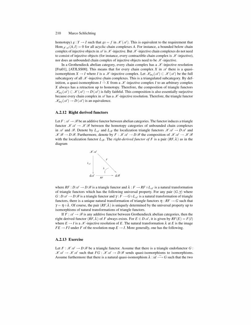
210 Marco Schlichting
homotopy) g : Y → I such that gs = f in K (A ). This is equivalent to the requirement thatHomK A (A, I) = 0 for all acyclic chain complexes A. For instance, a bounded below chaincomplex of injective objects in A is K -injective. But K -injective chain complexes do not needto consist of injective objects (for instance, every contractible chain complex is K -injective),nor does an unbounded chain complex of injective objects need to be K -injective.
In a Grothendieck abelian category, every chain complex has a K -injective resolution[Fra01], [ATJLSS00]. This means that for every chain complex X in A there is a quasi-isomorphism X → I where I is a K -injective complex. Let Kin j(A ) ⊂K (A ) be the fullsubcategory of all K -injective chain complexes. This is a triangulated subcategory. By def-inition, a quasi-isomorphism I ∼→ X from a K -injective complex I to an arbitrary complexX always has a retraction up to homotopy. Therefore, the composition of triangle functorsKin j(A )⊂K (A )→ D (A ) is fully faithful. This composition is also essentially surjectivebecause every chain complex in A has a K -injective resolution. Therefore, the triangle functorKin j(A )→ D (A ) is an equivalence.
A.2.12 Right derived functors
Let F : A →B be an additive functor between abelian categories. The functor induces a trianglefunctor K A → K B between the homotopy categories of unbounded chain complexesin A and B. Denote by LA and LB the localization triangle functors K A → DA andK B→ DB. Furthermore, denote by F : K A → DB the composition of K A →K Bwith the localization functor LB . The right-derived functor of F is a pair (RF,λ ) as in thediagram
K A
dA dB
λ
LA
RF
F
where RF : DA → DB is a triangle functor and λ : F → RF LA is a natural transformationof triangle functors which has the following universal property. For any pair (G,γ) whereG : DA →DB is a triangle functor and γ : F→GLA is a natural transformation of trianglefunctors, there is a unique natural transformation of triangle functors η : RF → G such thatγ = η λ . Of course, the pair (RF,λ ) is uniquely determined by the universal property up toisomorphisms of natural transformations of triangle functors.
If F : A →B is any additive functor between Grothendieck abelian categories, then theright derived functor (RF,λ ) of F always exists. For E ∈ DA , it is given by RF(E) = F(I)where E→ I is a K -injective resolution of E. The natural transformation λ at E is the imageFE→ FI under F of the resolution map E→ I. More generally, one has the following.
A.2.13 Exercise
Let F : K A → DB be a triangle functor. Assume that there is a triangle endofunctor G :K A → K A such that FG : K A → DB sends quasi-isomorphisms to isomorphisms.Assume furthermore that there is a natural quasi-isomorphism λ : id ∼−→ G such that the two
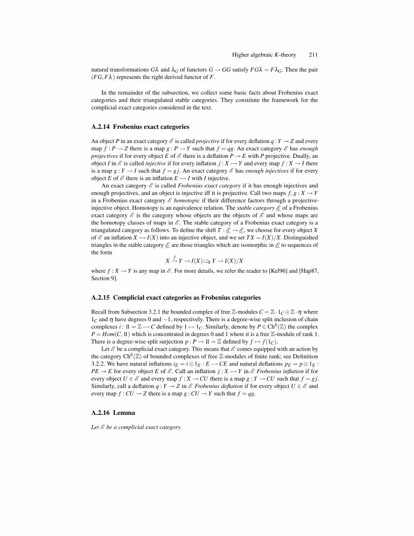
Higher algebraic K-theory 211
natural transformations Gλ and λG of functors G→ GG satisfy FGλ = FλG. Then the pair(FG,Fλ ) represents the right derived functor of F .
In the remainder of the subsection, we collect some basic facts about Frobenius exactcategories and their triangulated stable categories. They constitute the framework for thecomplicial exact categories considered in the text.
A.2.14 Frobenius exact categories
An object P in an exact category E is called projective if for every deflation q : Y Z and everymap f : P→ Z there is a map g : P→ Y such that f = qg. An exact category E has enoughprojectives if for every object E of E there is a deflation P E with P projective. Dually, anobject I in E is called injective if for every inflation j : X Y and every map f : X → I thereis a map g : Y → I such that f = g j. An exact category E has enough injectives if for everyobject E of E there is an inflation E I with I injective.
An exact category E is called Frobenius exact category if it has enough injectives andenough projectives, and an object is injective iff it is projective. Call two maps f ,g : X → Yin a Frobenius exact category E homotopic if their difference factors through a projective-injective object. Homotopy is an equivalence relation. The stable category E of a Frobeniusexact category E is the category whose objects are the objects of E and whose maps arethe homotopy classes of maps in E . The stable category of a Frobenius exact category is atriangulated category as follows. To define the shift T : E → E , we choose for every object Xof E an inflation X I(X) into an injective object, and we set T X = I(X)/X . Distinguishedtriangles in the stable category E are those triangles which are isomorphic in E to sequences ofthe form
Xf→ Y → I(X)tX Y → I(X)/X
where f : X → Y is any map in E . For more details, we refer the reader to [Kel96] and [Hap87,Section 9].
A.2.15 Complicial exact categories as Frobenius categories
Recall from Subsection 3.2.1 the bounded complex of free Z-modules C = Z ·1C⊕Z ·η where1C and η have degrees 0 and −1, respectively. There is a degree-wise split inclusion of chaincomplexes i : 11 = ZC defined by 1 7→ 1C. Similarly, denote by P ∈ Chb(Z) the complexP = Hom(C,11) which is concentrated in degrees 0 and 1 where it is a free Z-module of rank 1.There is a degree-wise split surjection p : P→ 11 = Z defined by f 7→ f (1C).
Let E be a complicial exact category. This means that E comes equipped with an action bythe category Chb(Z) of bounded complexes of free Z-modules of finite rank; see Definition3.2.2. We have natural inflations iE = i⊗1E : ECE and natural deflations pE = p⊗1E :PE E for every object E of E . Call an inflation j : X Y in E Frobenius inflation if forevery object U ∈ E and every map f : X →CU there is a map g : Y →CU such that f = g j.Similarly, call a deflation q : Y Z in E Frobenius deflation if for every object U ∈ E andevery map f : CU → Z there is a map g : CU → Y such that f = qg.
A.2.16 Lemma
Let E be a complicial exact category.
212 Marco Schlichting
(a) For every object E of E , the natural inflation iX : X CX is a Frobenius inflation, andthe natural deflation pX : PX X is a Frobenius deflation.
(b) Frobenius inflations (deflations) are closed under composition.(c) Frobenius inflations (deflations) are preserved under push-outs (pull-backs)(d) Split injections (surjections) are Frobenius inflations (deflations).(e) For a conflation X Y Z in E , the map X Y is a Frobenius inflation iff the map
Y Z is a Frobenius deflation.(f) The category E equipped with the Frobenius conflations as defined in Subsection 3.2.5 is
a Frobenius exact category. In this exact structure, an object is injective (projective) iff itis a direct factor of an object of the form CU with U ∈ E .
Proof:
For (a), we note that C is a commutative dg Z-algebra with unique multiplication µ : C⊗C→Cand unit map i : 11→C : 1 7→ 1C. Let f : X→CU be a map in E . We define the map f ′ : CX→CU as the composition CX
1⊗ f→ CCUµ⊗1→ CU . Then we have f ′iX = (µ⊗1U ) (1C⊗ f ) (i⊗
1X ) = (µ⊗1U ) (i⊗1C⊗1U ) f = f since the composition C i⊗1→ C⊗Cµ→C is the identity.
This shows that iX is a Frobenius inflation. The proof that PX → X is a Frobenius deflation issimilar using the fact that P = Hom(C,11) is a co-algebra. Sections (b), (c) and (d) are clear.For (e), we note that the map CX → T X is a Frobenius deflation. This is because this mapis isomorphic to PT X → T X via the isomorphism C→ Hom(C,T ) = PT which is adjoint toC⊗C
µ→C→ T . Let X Y be a Frobenius inflation. By definition, there is a map Y →CXsuch that the composition X → Y → CX is the canonical Frobenius inflation iX : X CX .Passing to quotients, we see that Y Z is a pull-back of CX T X . Since the latter is aFrobenius deflation, we can apply (c), and we see that Y Z is a Frobenius deflation as well.The other implication in (e) is dual. For (f), we note that (a) – (e) imply that E together with theFrobenius conflations is an exact category. By definition, objects of the form CU are injectiveand projective for the Frobenius exact structure, hence any of its direct factors is injectiveand projective. For an object I of E which is injective in the Frobenius exact structure, theFrobenius inflation ICI has a retraction since, by the definition of injective objects, the map1 : I→ I to the injective I extends to CI. Therefore, the injective object I is a direct factor of CI.Similarly for projective objects.
A.3 The derived category of quasi-coherent sheaves
A.3.1 Separated schemes and their quasi-coherent sheaves
Let X be a quasi-compact and separated scheme. In the category Qcoh(X) of quasi-coherentOX -modules, all small colimits exist and filtered colimits are exact (as they can be calculatedlocally on quasi-compact open subsets). Every quasi-coherent OX -module is a filtered colimit ofits quasi-coherent submodules of finite type [Gro60, 9.4.9]. Therefore, the set of quasi-coherentOX -modules of finite type forms a set of generators for Qcoh(X). Hence, the category Qcoh(X)is a Grothendieck abelian category. In particular, its derived category D Qcoh(X) exists, and ithas an explicit description as in Appendix A.2.11.
Higher algebraic K-theory 213
A.3.2 Examples of Hom-sets in D Qcoh(X)
For a complex E of quasi-coherent OX -modules, the set of homomorphisms Hom(OX ,E) inthe triangulated category D Qcoh(X) is given by the formula
Hom(OX ,E) = H0(Rg∗E)
where g : X → SpecZ is the structure map of X . We can see this by replacing E with aK -injective resolution E ∼→ I. Then both sides are H0(I(X)).
More generally, for a vector bundle A on X , the homomorphism set Hom(A,E) inD Qcoh(X) can be calculated as above using the equality
Hom(A,E) = Hom(OX ,E⊗A∨)
where A∨ is the dual sheaf Hom(A,OX ) of A. Again, we can see this by choosing a K-injectiveresolution E ∼→ I of E and noting that E⊗A∨ ∼→ I⊗A∨ is a K -injective resolution of E⊗A∨
when A (and thus A∨) is a vector bundle.
A.3.3 The Cech resolution
Let X be a quasi-compact scheme, and let U = U0, ...,Un be a finite cover of X by quasi-compact open subsets Ui ⊂ X . For a k +1 tuple i = (i0, ..., ik) such that 0≤ i0, ..., ik ≤ n, writeji : Ui = Ui0 ∩ ...∩Uik ⊂ X for the open immersion of the intersection of the correspondingUi’s. Let F be a quasi-coherent OX module. We consider the sheafified Cech complex C(U ,F)associated with the cover U of X . In degree k it is the quasi-coherent OX -module
C(U ,F)k =⊕
iji∗ j∗i F
where the indexing set is taken over all k+1-tuples i = (i0, ..., ik) such that 0≤ i0 < · · ·< ik ≤ n.The differential dk : C(U ,F)k→ C(U ,F)k+1 for the component i = (i0, ..., ik+1) is given bythe formula
(dk(x))i =k+1
∑l=0
(−1)l ji∗ j∗i x(i0,...,il ,...,ik+1).
Note that the complex C(U ,F) is concentrated in degrees 0, ...,n.The units of adjunction F → ji∗ j∗i F define a map F → C(U ,F)0 =
⊕ni=0 ji∗ j∗i F into the
degree zero part of the Cech complex such that d0(F) = 0. Therefore, we obtain a map ofcomplexes of quasi-coherent OX -modules F → C(U ,F). This map is a quasi-isomorphism forany quasi-coherent OX -module F as can be checked by restricting the map to the open subsetsUi of the cover U of X .
More generally, if F is a complex, then C(U ,F) is a bicomplex, and we can considerits total complex TotC(U ,F) which, by a slight abuse of notation, we will still denote byC(U ,F). The map F → C(U ,F) is a map of bicomplexes. Taking total complexes, we obtaina natural quasi-isomorphism of complexes of quasi-coherent OX -modules
λF : F ∼→ C(U ,F). (31)
which is called the Cech resolution of F associated with the open cover U .
214 Marco Schlichting
A.3.4 Exercise
Let X be a scheme and U be a finite open cover of X . Write C for the functor F 7→ C(U ,F)from complexes of quasi-coherent sheaves to itself defined in Subsection A.3.3 above. Show thatfor any complex F of quasi-coherent sheaves on X , the following two maps C(F)→ C(C(F))are chain homotopic:
C(λF )∼ λC(F).
A.3.5 Explicit description of Rg∗
Let g : X → Y be a map of quasi-compact schemes such that there is a finite cover U =U0, ...,Un of X with the property that the restrictions gi : Ui→ Y of g to to all finite intersec-tions Ui =Ui0 ∩ ...∩Uik of the Ui’s are affine maps where i = (i0, ..., ik) and i0, ..., ik ∈ 0, ...,n.If X and Y are quasi-compact and separated such a cover always exists. In this case, any coverU = U0, ...,Un of X by affine open subschemes Ui ⊂ X such that each Ui maps into an openaffine subscheme of Y has this property.
Using the cover U instead of K -injective resolutions, one can construct the right-derivedfunctor Rg∗ : D Qcoh(X)→ D Qcoh(Y ) of g∗ : Qcoh(X)→ Qcoh(Y ) as follows. By assump-tion, for every k + 1-tuple i = (i0, ..., ik), the restriction gi = g ji : Ui → Y of g to Ui is anaffine map. Therefore, the functor
g∗C(U ) : Qcoh(X)→ ChQcoh(Y ) : F 7→ g∗C(U ,F)
is exact. Taking total complexes, this functor extends to a functor on all complexes
g∗C(U ) : ChQcoh(X)→ ChQcoh(Y ) : F 7→ g∗C(U ,F)
which preserves quasi-isomorphisms as it is exact and sends acyclics to acyclics. This functoris equipped with a natural quasi-isomorphism given by the Cech resolution
λF : F ∼−→ C(U ,F).
By Exercises A.2.13 and A.3.4, the right derived functor Rg∗ of g∗ is represented by the pair(g∗C(U ),g∗λ ).
A.3.6 Lemma
Let g : X → Y be a map of quasi-compact and separated schemes. Then for any set Ei, i ∈ I,of complexes of quasi-coherent OX -modules, the following natural map of complexes of OY -modules is a quasi-isomorphism
⊕I Rg∗ (Ei)
∼−→ Rg∗ (⊕
I Ei) .
Proof:
This follows from the explicit construction of Rg∗ given in Appendix A.3.5 for which the mapin the lemma is already an isomorphism in ChQcoh(Y ).
Higher algebraic K-theory 215
A.3.7 Lemma (Base-Change for open immersions)
Let X = U ∪V be a quasi-compact separated scheme which is covered by two quasi-compactopen subschemes U and V . Denote by j : U → X, jV : U ∩V →V , i : V → X, iU : U ∩V →Uthe corresponding open immersions. Then for every complex E of quasi-coherent OU -modules,the natural map
i∗ R j∗E∼=−→ R jV∗ i∗U E
of complexes of quasi-coherent OV -modules is an isomorphism in D Qcoh(V ).
Proof:
We first make the following remark. For a quasi-coherent OU -module M, we have the canonicalmap i∗ j∗M→ jV∗i∗U M which is adjoint to the map j∗V i∗ j∗M = i∗U j∗ j∗M→ i∗U M obtained byapplying i∗U to the counit map j∗ j∗M→M. Calculating sections over open subsets, we see thatthe map i∗ j∗M→ jV∗i∗U M is an isomorphism for every quasi-coherent OU -module M.
For the proof of the lemma, recall that U is quasi-compact. Therefore we can find a finiteopen affine cover U = U0, ...,Un of U . For this cover, all inclusions Ui0 ∩ ...∩Uik ⊂ X areaffine maps because X is separated. By Appendix A.3.5 and the remark above, for a complex Eof quasi-coherent OU -modules, we have an isomorphism
i∗R j∗E = i∗ j∗C(U ,E)∼=→ jV∗i∗UC(U ,E) = jV∗C(U ∩V, i∗U E)
where U ∩V is the cover U0∩V, ...,Un∩V of V . Pull-backs of affine maps are affine maps.Hence, all inclusions (Ui0 ∩V )∩ ...∩ (Uik ∩V )⊂V are affine maps. By Appendix A.3.5, thefunctor jV∗C(U ∩V ) represents R jV∗. So, the isomorphism above represents an isomorphismof functors i∗ R j∗
∼=−→ R jV∗ i∗U .
A.3.8 Lemma
Let X = V1 ∪V2 be a quasi-compact and separated scheme which is covered by two quasi-compact open subschemes V1,V2 ⊂ X. Denote by ji : Vi → X and j12 : V1 ∩V2 → X thecorresponding open immersions. Then for E ∈ D Qcoh(X), there is a distinguished triangle inD Qcoh(X)
E −→ R j1∗( j∗1 E)⊕R j2∗( j∗2 E)−→ R j12∗( j∗12 E)−→ E[1].
Proof:
Consider the commutative square in D Qcoh(X)
E //
R j1∗( j∗1 E)
R j2∗( j∗2 E) // R j12∗( j∗12 E)
in which the maps are induced by the unit of adjunction maps 1→ R j∗ j∗ and the base-change isomorphism in Lemma A.3.7. By Appendix A.2.2, we can complete this square
216 Marco Schlichting
to the right into a good map of distinguished triangles. The map on horizontal cones is anisomorphism when restricted to U1 (since both cones are zero, by Base-Change A.3.7) and whenrestricted to U2 (by the Five Lemma and Base-Change A.3.7). Therefore, the map on horizontalcones is an isomorphism in D Qcoh(X). Finally, the sequence E→ R j1∗( j∗1 E)⊕R j2∗( j∗2 E)→R j12∗( j∗12 E) can be completed to a distinguished triangle by the last paragraph in AppendixA.2.2.
A.4 Proof of compact generation of DZ Qcoh(X)
In this appendix, we prove Proposition 3.4.6, first for schemes with an ample family of linebundles and then, by a formal induction argument, for general quasi-compact and separatedschemes. To summarize, in Lemma A.4.10 we show that DZ Qcoh(X) is compactly generatedand in Lemmas A.4.8 and A.4.9 we show that the compact objects in DZ Qcoh(X) are preciselythose complexes which are isomorphic (in the derived category) to bounded complexes ofvector bundles when restricted to the open subsets of an affine open cover of X . Part of theexposition is taken from [Sch08]. When Z = X , the reader may also find proofs in [Nee96,Corollary 2.3 and Proposition 2.5] and [BvdB03, Theorems 3.1.1 and 3.1.3].
We first recall the usual technique of extending a section of a quasi-coherent sheaf from anopen subset cut out by a divisor to the scheme itself. For a proof, see [Gro60, Theoreme 9.3.1],[Har77, Lemma II.5.14].
A.4.1 Lemma
Let X be a quasi-compact and separated scheme, s ∈ Γ (X ,L) be a global section of a linebundle L on X, and Xs = x ∈ X | s(x) 6= 0 ∈ Lx/mxLx be the non-vanishing locus of s. Let Fbe a quasi-coherent sheaf on X. Then the following hold.
(a) For every f ∈ Γ (Xs,F), there is an n ∈ N such that f ⊗ sn extends to a global section ofF⊗L⊗n.
(b) For every f ∈ Γ (X ,F) such that f|Xs= 0, there is an n ∈ N such that f ⊗ sn = 0.
A.4.2 Schemes with an ample family of line bundles
A scheme X has an ample family of line bundles if there is a finite set L1, ...,Ln of linebundles on X and if there are global sections si ∈ Γ (X ,Li) such that the non-vanishing lociXsi = x ∈ X | si(x) 6= 0 ∈ Lx/mxLx form an open affine cover of X ; see [TT90, Definition2.1], [SGA71, II 2.2.4]. Note that such an X is necessarily quasi-compact.
Recall that if f ∈ Γ (X ,L) is a global section of a line bundle L on a scheme X , then theopen inclusion X f ⊂ X is an affine map (as can be seen by choosing an open affine cover of Xtrivializing the line bundle L). As a special case, the open subscheme X f is affine whenever Xis affine. Thus, for the affine cover X =
⋃Xsi associated with an ample family of line-bundles
as above, all finite intersections of the Xsi ’s are affine.Let X be a scheme which has an ample family of line bundles. Then there is a set Li| i∈ I
of line bundles on X together with global sections si ∈ Γ (X ,Li) such that the set Xsi | i ∈ Iof non-vanishing loci forms an open affine basis for the topology of X [TT90, 2.1.1 (b)]. If X isaffine, this follows from the definition of the Zariski topology. For a general X (with an amplefamily of line bundles), the sections which give rise to a basis of topology on an open affineXs can be extended (up to a power of s) to global sections, by Lemma A.4.1. Therefore, every

Higher algebraic K-theory 217
open subset of a basis for Xs is also the non-vanishing locus of a global section of some linebundle on X .
Let X be a scheme which has an ample family of line bundles L1, ...,Ln. Then for everyquasi-coherent sheaf F on X , there is a surjective map M F of quasi-coherent sheaves whereM is a (possibly infinite) direct sum of line bundles of the form Lk
i for i = 1, ...,n and k < 0.This follows from the definition of an ample family of line bundles and Lemma A.4.1.
A.4.3 Truncated Koszul complexes
Let X be a quasi-compact and separated scheme, and let Li, i = 1, ..., l be a finite set of linebundles together with global sections si ∈ Γ (X ,Li). Let U =
⋃li=1 Xsi be the union of the
non-vanishing loci Xsi of the si’s, and j : U ⊂ X be the corresponding open immersion. Theglobal sections si define maps si : OX → Li of line-bundles whose OX -duals are denoted bys−1i : L−1
i →OX . We consider the maps s−1i as (cohomologically graded) chain-complexes with
OX placed in degree 0. For an l-tuple n = (n1, ...,nl) of negative integers, the Koszul complex
l⊗i=1
(Lnii
sni→ OX ) (32)
is acyclic over U . This is because the map sni = (s−1i )⊗|ni| : Lni
i →OX is an isomorphism whenrestricted to Xsi , hence the Koszul complex (32) is acyclic (even contractible) over each Xsi . LetK(sn) denote the bounded complex which is obtained from the Koszul complex (32) by deletingthe degree zero part OX and placing the remaining non-zero part in degrees −l +1, ...,0. Thelast differential d−1 of the Koszul complex defines a map
K(sn) =
[l⊗
i=1(Lni
isni→ OX )
]≤−1
[−1] ε−→ OX
of complexes of vector bundles. This map of complexes is a quasi-isomorphism over U , since itscone, the Koszul complex, is acyclic over U . For a complex M of quasi-coherent OX -modules,we write εM for the tensor product map εM = 1M⊗ ε : M⊗K(sn)→M⊗OX ∼= M.
The following proposition is a generalization of Lemma A.4.1. It is implicit in the proofof [TT90, Proposition 5.4.2]. We omit the proof (which is not very difficult, but not veryenlightening either). Details can be found in loc.cit. and in [Sch08, Lemma 9.6].
A.4.4 Proposition
Let X be a quasi-compact and quasi-separated scheme, and L1, ...Ln be a finite set of linebundles together with global sections si ∈ Γ (X ,Li) for i = 1, ...,n. Let U =
⋃ni=1 Xsi be the
union of the non-vanishing loci Xsi of the si’s, and j : U ⊂ X be the corresponding openimmersion. Let M be a complex of quasi-coherent OX -modules and let A be a bounded complexof vector bundles on X. Then the following hold.(a) For every map f : j∗A→ j∗M of complexes of OU -modules between the restrictions
of A and M to U, there is an l-tuple of negative integers n = (n1, ...,nl) and a mapf : A⊗K(sn)→M of complexes of OX -modules such that f j∗(εA) = j∗( f ).
(b) For every map f : A→M of complexes of OX -modules such that j∗( f ) = 0, there is anl-tuple of negative integers n = (n1, ...,nl) such that f εA = 0.
218 Marco Schlichting
A.4.5 Lemma
Let X be a quasi-compact scheme, and s ∈ Γ (X ,L) be a global section of a line-bundle L suchthat Xs is affine. Let N→ E be a map of complexes of quasi-coherent OX -modules such thatits restriction to Xs is a quasi-isomorphism. If E is a bounded complex of vector bundles on X,then there is an integer k > 0 and a map of complexes E⊗L−k→ N whose restriction to Xs isa quasi-isomorphism.
Proof:
Write j : Xs ⊂ X for the open inclusion. Since Xs is affine, say Xs = SpecA, we have anequivalence of categories between quasi-coherent OXs -modules and A-modules under whichthe map j∗N → j∗E becomes a quasi-isomorphism of complexes of A-modules with j∗E abounded complex of projectives. Any quasi-isomorphism of complexes of A-modules withtarget a bounded complex of projectives has a retraction up to homotopy. Therefore, the choiceof a homotopy right inverse f : j∗E → j∗N yields a quasi-isomorphisms. By Lemma A.4.1,there is a map of complexes f : E⊗Lk→ N such that j∗ f = f · sk for some k < 0. In particular,f is a quasi-isomorphism when restricted to Xs.
Lemma A.4.5 has the following generalization.
A.4.6 Lemma
Let X be a quasi-compact and separated scheme. Let U =⋃n
i=1 Xsi be the union of affine non-vanishing loci Xsi associated with global sections si ∈ Γ (X ,Li) of line bundles Li on X wherei = 1, ...,n. Denote by j : U ⊂ X the open immersion. Let b : M→ B be a map of complexes ofquasi-coherent OX -modules such that its restriction j∗b to U is a quasi-isomorphism. If B is abounded complex of vector bundles on X, then there is a map of complexes a : A→M such thatits restriction to U is a quasi-isomorphism and A is a bounded complex of vector bundles on X.
Proof:
We prove the lemma by induction on n. For n = 1, this is Lemma A.4.5. Let U0 =⋃n−1
i=1 Xsi ⊂ X .By the induction hypothesis, there is map a0 : A0 → M from a bounded complex of vectorbundles A0 such that a0 is a quasi-isomorphism when restricted to U0. The induced mapb0 : C(a0)→C(ba0) on mapping cones is a quasi-isomorphism when restricted to U (hencewhen restricted to Xsn ) since b is. Moreover, both cones are acyclic on U0. Note that we havea distinguished triangle A0 → M → C(a0)→ A0[1] in K Qcoh(X). Since Xsn is affine andC(ba0) a bounded complex of vector bundles, Lemma A.4.5 implies the existence of a mapa1 : A1→C(a0) of complexes with A1 = C(ba0)⊗Lk
n a bounded complex of vector bundleson X which is acyclic when restricted to U0, and a1 is a quasi-isomorphism when restricted toXsn . It follows that a1 is a quasi-isomorphism when restricted to U . Let A be a complex suchthat A→ A1→ A0[1] extends to a distinguished triangle in K Qcoh(X) where the last map isA1→C(a0)→ A0[1]. We can choose A to be a bounded complex of vector bundles becauseA0 and A1 are also of this form. Let a : A→M be a map such that (a,a1,1A0[1]) is a map oftriangles. By the Five-lemma, the map a : A→M is a quasi-isomorphism when restricted to U .
Higher algebraic K-theory 219
The following proposition is a more precise version of Proposition 3.4.6 in case X has anample line bundle. For a closed subscheme Z ⊂ X of a scheme X , denote by D b
Z Vect(X) ⊂D b Vect(X) the full triangulated subcategory of those complexes of vector bundles which areacyclic over X −Z. Recall from subsection 3.4.4 the definition of a “compact object” and of a“compactly generated triangulated category”.
A.4.7 Proposition
Let X be a quasi-compact and separated scheme which has an ample family of line bundlesL1, ...,Ln. Let Z⊂X be a closed subset with quasi-compact open complement j :U = X−Z⊂X.Then the following hold.
(a) D Qcoh(X) is a compactly generated triangulated category with generating set of compactobjects the set
L = Lkii [l] | i = 1, ...,n, ki < 0, ki, l ∈ Z .
The inclusion Vect(X) ⊂ Qcoh(X) yields a triangle functor D b Vect(X) ⊂ D Qcoh(X)which is fully faithful and induces an equivalence of D b Vect(X) with the triangulatedsubcategory of compact objects in D Qcoh(X). In particular, D b Vect(X) is generated –as an idempotent complete triangulated category – by the set of line bundles Lki
i wherei = 1, ...,n, where ki < 0 and ki ∈ Z.
(b) The following sequence of triangulated categories is exact up to factors
D bZ Vect(X)→ D b Vect(X)→ D b Vect(U).
(c) The triangulated category D Z Qcoh(X) is compactly generated, and the inclusionVect(X)⊂ Qcoh(X) of vector bundles into quasi-coherent sheaves yields a fully faithfultriangle functor D b
Z Vect(X)⊂ D Z Qcoh(X) which induces an equivalence of D bZ Vect(X)
with the triangulated subcategory of compact objects in D Z Qcoh(X).
Proof:
For (a), we first note that a vector bundle A on X is compact in D Qcoh(X). This is because thefunctor E 7→ Hom(A,E) is, in the notation of Subsection A.3.2, the same as the functor E 7→H0(Rg∗(E⊗A∨)). The latter functor commutes with infinite direct sums since its componentfunctors E 7→ E⊗A∨, Rg∗ and H0 : D (Z -Mod)→ Z -Mod have this property. Secondly, recallthat the compact objects form a triangulated subcategory. Therefore, every complex of vectorbundles is compact in D Qcoh(X). Next, we will check that the set L which consists ofcompact objects generates D Qcoh(X). For that, let E be a complex such that every mapL→ E is zero in D Qcoh(X) when L ∈L . We have to show that E = 0 in D Qcoh(X), that is,that H∗E = 0. Since L is closed under shifts, it suffices to show that the cohomology sheafH0E = ker(d0)/im(d−1) is zero where di is the i-th differential of E. By ampleness of thefamily L1, ...,Ln, we can choose a surjection M ker(d0) of quasi-coherent OX -modules withM a (possibly infinite) direct sum of line bundles of the form Lki
i where i = 1, ...,n and ki < 0.Composing the inclusion of complexes ker(d0)→ E with this surjection defines a map ofcomplexes M ker(d0)→ E which induces a surjective map M = H0M ker(d0) H0Eof cohomology sheaves. Since every map Lki
i → E is zero in D Qcoh(X), the induced surjectivemap M H0E is the zero map, hence H0E = 0. Altogether, the arguments above show thatD Qcoh(X) is compactly generated by the set L . Finally, the triangle functors D b Vect(X)⊂

220 Marco Schlichting
D b Qcoh(X) ⊂ D Qcoh(X) are fully faithful. The first by the dual of Subsection 3.1.7 (b)and the second by Subsection A.2.10. The remaining statements in (a) follow directly fromNeeman’s Theorem 3.4.5 (a) and from Subsection 3.1.7 (c).
For part (b), denote by U -quis the set of maps of complexes of vector bundles on X whichare quasi-isomorphisms when restricted to U = X−Z. By construction, the following sequenceof triangulated categories is exact
D bZ Vect(X)→ D b Vect(X)→T (Chb Vect(X),U -quis),
and the triangle functor T (Chb Vect(X),U -quis)→ D b Vect(U) is conservative. Using Propo-sition A.4.4 and Lemma A.4.6 we see that the last triangle functor is full. Any conservative andfull triangle functor is fully faithful, by Subsection A.2.4. Hence, the last triangle functor isfully faithful. The restriction to U of an ample family of line bundles on X is an ample family ofline bundles on U . Therefore, part (a) shows that the triangle functor is also cofinal. It followsthat the sequence in part (b) of the Proposition is exact up to factors.
For part (c), we already know that the functor D bZ Vect(X)→ D Z Qcoh(X) is fully faith-
ful since both categories are full subcategories of D Qcoh(X). By part (a), every object inD b
Z Vect(X) is compact in D Qcoh(X). Since the inclusion D Z Qcoh(X) ⊂ D Qcoh(X) com-mutes with infinite sums, the objects of D b
Z Vect(X) are also compact in D Z Qcoh(X). LetS ⊂ D Z Qcoh(X) be the smallest full triangulated subcategory closed under arbitrary co-products in D Z Qcoh(X) which contains D b
Z Vect(X). Then S is compactly generated withcategory of compact objects D b
Z Vect(X). By Neeman’s Theorem 3.4.5 (b), the triangulatedcategory D Qcoh(X)/S is compactly generated. It has as category of compact objects theidempotent completion of D b Vect(X)/D b
Z Vect(X). By part (b), this category is D b Vect(U).The functor D Qcoh(X)/S → D Qcoh(U) preserves coproducts and compact objects, andit induces an equivalence of categories of compact objects. Any triangle functor betweencompactly generated triangulated categories which commutes with coproducts and whichinduces an equivalence on compact objects is an equivalence. Therefore, the triangle functorD Qcoh(X)/S → D Qcoh(U) is an equivalence. It follows that S = D Z Qcoh(X).
For the remainder of the subsection, write D X (A,F) for maps in D Qcoh(X) from A to F ,and similarly for U , V and U ∩V in place of X .
A.4.8 Lemma
Let X = U ∪V be a quasi-compact and separated scheme covered by two quasi-compactopen subschemes U, V . Then a complex A ∈ D Qcoh(X) is compact iff A|U ∈ D Qcoh(U) andA|V ∈ D Qcoh(V ) are compact.
Proof:
Write j : U → X for the open immersion. Let A ∈ D Qcoh(X) be a compact object, and letFi ∈ D Qcoh(U) be a set of complexes on U where i ∈ I. In the sequence of equations
DU ( j∗A,⊕
I Fi) = D X (A,R j∗⊕
I Fi)
= D X (A,⊕
I R j∗Fi)
=⊕
I D X (A,R j∗Fi)
=⊕
I DU ( j∗A,Fi),
Higher algebraic K-theory 221
the first and last are justified by adjointness of j∗ and R j∗, the second by Subsection A.3.6, andthe third by compactness of A. This shows that A|U is compact. The same argument also showsthat A|V is compact.
For the other direction, assume that A|U and A|V are compact. Then A|U∩V is also compact,by the argument above. Let Fi ∈ D Qcoh(X) be a set of complexes of quasi-coherent sheaveson X where i ∈ I. We have
D X (A,R j∗ j∗⊕
I Fi) = DU ( j∗A, j∗⊕
I Fi) = DU ( j∗A,⊕
I j∗Fi), (*)
by adjointness of j∗ and R j∗ and the fact that j∗ commutes with infinite sums (as it is a leftadjoint). Similarly, for V and U ∩V in place of U . For every i ∈ I, Lemma A.3.8 provides uswith a distinguished triangle
Fi −→ R j1∗( j∗1 Fi)⊕R j2∗( j∗2 Fi)−→ R j12∗( j∗12 Fi)−→ Fi[1] (**)
where j1 : U ⊂ X , j2 : V ⊂ X and j12 : U ∩V ⊂ X are the corresponding open immersions.Taking direct sum, we obtain a distinguished triangle⊕
I Fi→⊕
I R j1∗( j∗1 Fi)⊕⊕
I R j2∗( j∗2 Fi)→⊕
I R j12∗( j∗12 Fi)→⊕
I Fi[1]
which receives a canonical map from (**). Using Lemma A.3.6, we have a canonical isomor-phism
⊕I Rg∗(g∗Fi)
∼=→ Rg∗(g∗⊕
I Fi) for g = j1, j2, j12, and the last distinguished trianglebecomes⊕
I Fi→ R j1∗( j∗1⊕
I Fi)⊕R j2∗( j∗2⊕
I Fi)→ R j12∗( j∗12⊕
I Fi)→⊕
I Fi[1].
Applying the functor D X (A, ) to the last triangle, the triangles (**) and the natural map from(**) to the last triangle, we obtain a map of long exact sequences of abelian groups. In view ofthe identification (*) above, this is the commutative diagram
· · · →⊕
ID X (A,Fi) →
⊕IDU (A,Fi)⊕
⊕IDV (A,Fi) →
∼=
⊕IDU∩V (A,Fi)→ ···
∼=
· · · → D X (A,⊕
IFi) → DU (A,⊕
IFi)⊕DV (A,⊕
IFi) →DU∩V (A,⊕
IFi)→ ···
where we wrote DU (A,Fi) in place of DU (A|U ,Fi|U ), similarily for V and U ∩V . All but everythird vertical map in the diagram is an isomorphism, by compactness of A|U , A|V and A|U∩V .By the Five Lemma, the remaining vertical maps are also isomorphisms. Hence, A is compact.
Let j : U ⊂ X be an open immersion of quasi-compact and separated schemes with closedcomplement Z = X−U . Recall that j∗ : D Qcoh(X)→D Qcoh(U) has a right adjoint R j∗ suchthat the counit of adjunction j∗R j∗→ 1 is an isomorphism. By Exercise A.2.8 (a), the inclusionJ : D Z Qcoh(X) ⊂ D Qcoh(X) has a right adjoint which we denote by R : D Qcoh(X)→D Z Qcoh(X). It is part of a functorial distinguished triangle
JR(E)→ E→ R j∗ j∗E→ JR(E)[1]. (33)
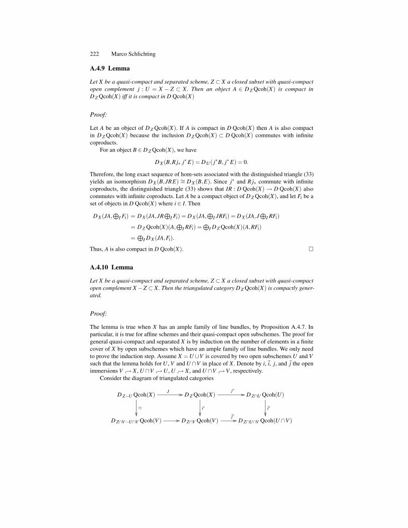
222 Marco Schlichting
A.4.9 Lemma
Let X be a quasi-compact and separated scheme, Z ⊂ X a closed subset with quasi-compactopen complement j : U = X − Z ⊂ X. Then an object A ∈ D Z Qcoh(X) is compact inD Z Qcoh(X) iff it is compact in D Qcoh(X)
Proof:
Let A be an object of D Z Qcoh(X). If A is compact in D Qcoh(X) then A is also compactin D Z Qcoh(X) because the inclusion D Z Qcoh(X) ⊂ D Qcoh(X) commutes with infinitecoproducts.
For an object B ∈ D Z Qcoh(X), we have
D X (B,R j∗ j∗E) = DU ( j∗B, j∗E) = 0.
Therefore, the long exact sequence of hom-sets associated with the distinguished triangle (33)yields an isomorphism D X (B,JRE) ∼= D X (B,E). Since j∗ and R j∗ commute with infinitecoproducts, the distinguished triangle (33) shows that IR : D Qcoh(X)→ D Qcoh(X) alsocommutes with infinite coproducts. Let A be a compact object of D Z Qcoh(X), and let Fi be aset of objects in D Qcoh(X) where i ∈ I. Then
D X (JA,⊕
I Fi) = D X (JA,JR⊕
I Fi) = D X (JA,⊕
I JRFi) = D X (JA,J⊕
I RFi)
= D Z Qcoh(X)(A,⊕
I RFi) =⊕
I D Z Qcoh(X)(A,RFi)
=⊕
I D X (JA,Fi).
Thus, A is also compact in D Qcoh(X).
A.4.10 Lemma
Let X be a quasi-compact and separated scheme, Z ⊂ X a closed subset with quasi-compactopen complement X−Z ⊂ X. Then the triangulated category D Z Qcoh(X) is compactly gener-ated.
Proof:
The lemma is true when X has an ample family of line bundles, by Proposition A.4.7. Inparticular, it is true for affine schemes and their quasi-compact open subschemes. The proof forgeneral quasi-compact and separated X is by induction on the number of elements in a finitecover of X by open subschemes which have an ample family of line bundles. We only needto prove the induction step. Assume X = U ∪V is covered by two open subschemes U and Vsuch that the lemma holds for U , V and U ∩V in place of X . Denote by i, i, j, and j the openimmersions V → X , U ∩V →U , U → X , and U ∩V →V , respectively.
Consider the diagram of triangulated categories
D Z−U Qcoh(X) J //
'
D Z Qcoh(X)j∗ //
i∗
D Z∩U Qcoh(U)
i∗
D Z∩V−U∩V Qcoh(V ) // D Z∩V Qcoh(V )
j∗ // D Z∩U∩V Qcoh(U ∩V )
Higher algebraic K-theory 223
in which the rows are exact, by (the argument in the proof of) Lemma 3.4.3 (a), and the leftvertical map is an equivalence, by Lemma 3.4.3 (b).
Let A be a compact object of D Z∩U Qcoh(U). We will show that E = A⊕A[1] is (up toisomorphism) the image j∗C of a compact object C of D Z Qcoh(X). By induction hypothesis,the lower row in the diagram is an exact sequence of compactly generated triangulated in whichthe functors preserve infinite coproducts and compact objects (Lemmas A.4.8 and A.4.9). ByLemmas A.4.8 and A.4.9, i∗A is compact. By Neeman’s Theorem 3.4.5 (b) and Remark 3.1.14,there is a compact object B of D Z∩V Qcoh(V ) and an isomorphism g : j∗B
∼=→ i∗E. Define theobject C of D Z Qcoh(X) to be the third object in the distinguished triangle in D Z Qcoh(X)
C −→ Ri∗B⊕R j∗E−→Ri j∗(i∗E)−→C[1]
in which the middle map on the summands Ri∗B and R j∗E are given by the maps g : (i j)∗Ri∗B =j∗B→ j∗E and id : (i j)∗R j∗E = ( ji)∗R j∗E = i∗E→ i∗E, in view of the adjunction betweenR(i j)∗ and (i j)∗. By the Base-Change Lemma A.3.7, we have j∗C ∼= E and i∗C ∼= B. ByLemmas A.4.8 and A.4.9, C is compact. Summarizing, every compact object of D Z∩U Qcoh(U)is a direct factor of the image of a compact object of D Z Qcoh(X).
To finish the proof that D Z Qcoh(X) is compactly generated, let E be an object ofD Z Qcoh(X) such that every map from a compact object of D Z Qcoh(X) to E is trivial. Wehave to show that E = 0. Since compact objects of D Z−U Qcoh(X) are also compact objectsof D Z Qcoh(X) (Lemma A.4.9), all maps from compact objects of D Z−U Qcoh(X) to E van-ish. The category D Z−U Qcoh(X) is compactly generated. This is because it is equivalentto D Z∩V∪(V−U) Qcoh(V ) which is compactly generated, by induction hypothesis. Therefore,all maps from all objects of D Z−U Qcoh(X) to E are trivial. For the right adjoint R of J,we therefore have R(E) = 0. The distinguished triangle (33) then shows that the unit of ad-junction E → R j∗ j∗E is an isomorphism. I claim that j∗E = 0. For that, it suffices to showthat DU (A, j∗E) = 0 for all compact A ∈ D Z∩U Qcoh(U), since D Z∩U Qcoh(U) is compactlygenerated, by induction hypothesis. All such compact A’s are direct factors of objects of theform j∗C with C ∈D Z Qcoh(X) compact. Therefore, it suffices to show that DU ( j∗C, j∗E) = 0for all compact C ∈ D Z Qcoh(X). But DU ( j∗C, j∗E) = DX (C,R j∗ j∗E) = DX (C,E) = 0. Soj∗E = 0. In view of the isomorphism E ∼= R j∗ j∗E, we have E = 0.
References
[Ada74] J. F. Adams. Stable homotopy and generalised homology. University of ChicagoPress, Chicago, Ill., 1974. Chicago Lectures in Mathematics.
[AJB08] Michael A. Mandell Andrew J. Blumberg. Localization theoremsin topological Hochschild homology and topological cyclic homology.arXiv:0802.3938v2, 2008.
[AM69] M. F. Atiyah and I. G. Macdonald. Introduction to commutative algebra. Addison-Wesley Publishing Co., Reading, Mass.-London-Don Mills, Ont., 1969.
[ATJLL97] Leovigildo Alonso Tarrıo, Ana Jeremıas Lopez, and Joseph Lipman. Localhomology and cohomology on schemes. Ann. Sci. Ecole Norm. Sup. (4), 30(1):1–39, 1997.
[ATJLSS00] Leovigildo Alonso Tarrıo, Ana Jeremıas Lopez, and Marıa Jose Souto Salorio.Localization in categories of complexes and unbounded resolutions. Canad. J.Math., 52(2):225–247, 2000.
[Bal00] Paul Balmer. Triangular Witt groups. I. The 12-term localization exact sequence.K-Theory, 19(4):311–363, 2000.
224 Marco Schlichting
[Bas68] Hyman Bass. Algebraic K-theory. W. A. Benjamin, Inc., New York-Amsterdam,1968.
[BBD82] A. A. Beılinson, J. Bernstein, and P. Deligne. Faisceaux pervers. In Analysis andtopology on singular spaces, I (Luminy, 1981), volume 100 of Asterisque, pages5–171. Soc. Math. France, Paris, 1982.
[BF78] A. K. Bousfield and E. M. Friedlander. Homotopy theory of Γ -spaces, spectra,and bisimplicial sets. In Geometric applications of homotopy theory (Proc. Conf.,Evanston, Ill., 1977), II, volume 658 of Lecture Notes in Math., pages 80–130.Springer, Berlin, 1978.
[BK72] A. K. Bousfield and D. M. Kan. Homotopy limits, completions and localizations.Lecture Notes in Mathematics, Vol. 304. Springer-Verlag, Berlin, 1972.
[BK86] Spencer Bloch and Kazuya Kato. p-adic etale cohomology. Inst. Hautes EtudesSci. Publ. Math., (63):107–152, 1986.
[BLL04] Alexey I. Bondal, Michael Larsen, and Valery A. Lunts. Grothendieck ring ofpretriangulated categories. Int. Math. Res. Not., (29):1461–1495, 2004.
[Blo86] Spencer Bloch. Algebraic cycles and higher K-theory. Adv. in Math., 61(3):267–304, 1986.
[BN93] Marcel Bokstedt and Amnon Neeman. Homotopy limits in triangulated categories.Compositio Math., 86(2):209–234, 1993.
[Bor63] Mario Borelli. Divisorial varieties. Pacific J. Math., 13:375–388, 1963.[BS01] Paul Balmer and Marco Schlichting. Idempotent completion of triangulated
categories. J. Algebra, 236(2):819–834, 2001.[Bue08] Theo Buehler. Exact categories. To appear in Expositiones Mathematicae, preprint
2008. arXiv:0811.1480.[BvdB03] A. Bondal and M. van den Bergh. Generators and representability of functors
in commutative and noncommutative geometry. Mosc. Math. J., 3(1):1–36, 258,2003.
[CHSW08] G. Cortinas, C. Haesemeyer, M. Schlichting, and C. Weibel. Cyclic homology,cdh-cohomology and negative K-theory. Ann. of Math. (2), 167(2):549–573, 2008.
[CHW08] G. Cortinas, C. Haesemeyer, and C. Weibel. K-regularity, cdh-fibrant Hochschildhomology, and a conjecture of Vorst. J. Amer. Math. Soc., 21(2):547–561, 2008.
[Cor] Guillermo Cortinas. Algebraic v. topological K-theory: a friendly match. In thisvolume.
[Cor06] Guillermo Cortinas. The obstruction to excision in K-theory and in cyclic homol-ogy. Invent. Math., 164(1):143–173, 2006.
[Dri04] Vladimir Drinfeld. DG quotients of DG categories. J. Algebra, 272(2):643–691,2004.
[FG05] Eric M. Friedlander and Daniel R. Grayson, editors. Handbook of K-theory. Vol.1, 2. Springer-Verlag, Berlin, 2005.
[FP90] Rudolf Fritsch and Renzo A. Piccinini. Cellular structures in topology, volume 19of Cambridge Studies in Advanced Mathematics. Cambridge University Press,Cambridge, 1990.
[Fra01] Jens Franke. On the Brown representability theorem for triangulated categories.Topology, 40(4):667–680, 2001.
[FS02] Eric M. Friedlander and Andrei Suslin. The spectral sequence relating algebraicK-theory to motivic cohomology. Ann. Sci. Ecole Norm. Sup. (4), 35(6):773–875,2002.
[Ful98] William Fulton. Intersection theory, volume 2 of Ergebnisse der Mathematik undihrer Grenzgebiete. 3. Folge. A Series of Modern Surveys in Mathematics [Results
Higher algebraic K-theory 225
in Mathematics and Related Areas. 3rd Series. A Series of Modern Surveys inMathematics]. Springer-Verlag, Berlin, second edition, 1998.
[Gab62] Pierre Gabriel. Des categories abeliennes. Bull. Soc. Math. France, 90:323–448,1962.
[GH08] Thomas Geisser and Lars Hesselholt. On the vanishing of negative k-groups.arXiv:0811.0652, 2008.
[GJ99] Paul G. Goerss and John F. Jardine. Simplicial homotopy theory, volume 174 ofProgress in Mathematics. Birkhauser Verlag, Basel, 1999.
[GL00] Thomas Geisser and Marc Levine. The K-theory of fields in characteristic p.Invent. Math., 139(3):459–493, 2000.
[GL01] Thomas Geisser and Marc Levine. The Bloch-Kato conjecture and a theorem ofSuslin-Voevodsky. J. Reine Angew. Math., 530:55–103, 2001.
[Goo86] Thomas G. Goodwillie. Relative algebraic K-theory and cyclic homology. Ann.of Math. (2), 124(2):347–402, 1986.
[Gra76] Daniel Grayson. Higher algebraic K-theory. II (after Daniel Quillen). In AlgebraicK-theory (Proc. Conf., Northwestern Univ., Evanston, Ill., 1976), pages 217–240.Lecture Notes in Math., Vol. 551. Springer, Berlin, 1976.
[Gra79] Daniel R. Grayson. Localization for flat modules in algebraic K-theory. J. Algebra,61(2):463–496, 1979.
[Gro60] A. Grothendieck. Elements de geometrie algebrique. I. Le langage des schemas.Inst. Hautes Etudes Sci. Publ. Math., (4):228, 1960.
[Gro61] A. Grothendieck. Elements de geometrie algebrique. III. Etude cohomologiquedes faisceaux coherents. I. Inst. Hautes Etudes Sci. Publ. Math., (11):167, 1961.
[Hae04] Christian Haesemeyer. Descent properties of homotopy K-theory. Duke Math. J.,125(3):589–620, 2004.
[Hap87] Dieter Happel. On the derived category of a finite-dimensional algebra. Comment.Math. Helv., 62(3):339–389, 1987.
[Har77] Robin Hartshorne. Algebraic geometry. Springer-Verlag, New York, 1977. Grad-uate Texts in Mathematics, No. 52.
[Hsi84] Wu Chung Hsiang. Geometric applications of algebraic K-theory. In Proceedingsof the International Congress of Mathematicians, Vol. 1, 2 (Warsaw, 1983), pages99–118, Warsaw, 1984. PWN.
[HSS00] Mark Hovey, Brooke Shipley, and Jeff Smith. Symmetric spectra. J. Amer. Math.Soc., 13(1):149–208, 2000.
[Kap88] M. M. Kapranov. On the derived categories of coherent sheaves on some homoge-neous spaces. Invent. Math., 92(3):479–508, 1988.
[Kar68] Max Karoubi. Foncteurs derives et K-theorie. Categories filtrees. C. R. Acad. Sci.Paris Ser. A-B, 267:A328–A331, 1968.
[Kel90] Bernhard Keller. Chain complexes and stable categories. Manuscripta Math.,67(4):379–417, 1990.
[Kel91] Bernhard Keller. Derived categories and universal problems. Comm. Algebra,19(3):699–747, 1991.
[Kel96] Bernhard Keller. Derived categories and their uses. In Handbook of algebra, Vol.1, pages 671–701. North-Holland, Amsterdam, 1996.
[Kel99] Bernhard Keller. On the cyclic homology of exact categories. J. Pure Appl.Algebra, 136(1):1–56, 1999.
[Kel06] Bernhard Keller. On differential graded categories. In International Congress ofMathematicians. Vol. II, pages 151–190. Eur. Math. Soc., Zurich, 2006.
[Kur92] Masato Kurihara. Some remarks on conjectures about cyclotomic fields andK-groups of Z. Compositio Math., 81(2):223–236, 1992.
226 Marco Schlichting
[Kuz08] Alexander Kuznetsov. Derived categories of quadric fibrations and intersectionsof quadrics. Adv. Math., 218(5):1340–1369, 2008.
[Lev94] Marc Levine. Bloch’s higher Chow groups revisited. Asterisque, (226):10, 235–320, 1994. K-theory (Strasbourg, 1992).
[Lev99] Marc Levine. K-theory and motivic cohomology of schemes. K-theory archivepreprint 336, 1999.
[Lev08] Marc Levine. The homotopy coniveau tower. J. Topol., 1(1):217–267, 2008.[LR05] Wolfgang Luck and Holger Reich. The Baum-Connes and the Farrell-Jones
conjectures in K- and L-theory. In Handbook of K-theory. Vol. 1, 2, pages 703–842. Springer, Berlin, 2005.
[Mat89] Hideyuki Matsumura. Commutative ring theory, volume 8 of Cambridge Studiesin Advanced Mathematics. Cambridge University Press, Cambridge, secondedition, 1989. Translated from the Japanese by M. Reid.
[May67] J. Peter May. Simplicial objects in algebraic topology. Van Nostrand MathematicalStudies, No. 11. D. Van Nostrand Co., Inc., Princeton, N.J.-Toronto, Ont.-London,1967.
[Mil71] John Milnor. Introduction to algebraic K-theory. Princeton University Press,Princeton, N.J., 1971. Annals of Mathematics Studies, No. 72.
[Mit97] Stephen A. Mitchell. Hypercohomology spectra and Thomason’s descent theorem.In Algebraic K-theory (Toronto, ON, 1996), volume 16 of Fields Inst. Commun.,pages 221–277. Amer. Math. Soc., Providence, RI, 1997.
[ML98] Saunders Mac Lane. Categories for the working mathematician, volume 5 ofGraduate Texts in Mathematics. Springer-Verlag, New York, second edition, 1998.
[MVW06] Carlo Mazza, Vladimir Voevodsky, and Charles Weibel. Lecture notes on motiviccohomology, volume 2 of Clay Mathematics Monographs. American Mathemati-cal Society, Providence, RI, 2006.
[Nee91] Amnon Neeman. Some new axioms for triangulated categories. J. Algebra,139(1):221–255, 1991.
[Nee92] Amnon Neeman. The connection between the K-theory localization theorem ofThomason, Trobaugh and Yao and the smashing subcategories of Bousfield andRavenel. Ann. Sci. Ecole Norm. Sup. (4), 25(5):547–566, 1992.
[Nee96] Amnon Neeman. The Grothendieck duality theorem via Bousfield’s techniquesand Brown representability. J. Amer. Math. Soc., 9(1):205–236, 1996.
[Nee01] Amnon Neeman. Triangulated categories, volume 148 of Annals of MathematicsStudies. Princeton University Press, Princeton, NJ, 2001.
[NR04] Amnon Neeman and Andrew Ranicki. Noncommutative localisation in algebraicK-theory. I. Geom. Topol., 8:1385–1425 (electronic), 2004.
[NS89] Yu. P. Nesterenko and A. A. Suslin. Homology of the general linear group over alocal ring, and Milnor’s K-theory. Izv. Akad. Nauk SSSR Ser. Mat., 53(1):121–146,1989.
[Pan03] I. A. Panin. The equicharacteristic case of the Gersten conjecture. Tr. Mat. Inst.Steklova, 241(Teor. Chisel, Algebra i Algebr. Geom.):169–178, 2003.
[Pop73] N. Popescu. Abelian categories with applications to rings and modules. AcademicPress, London, 1973. London Mathematical Society Monographs, No. 3.
[PW00] Claudio Pedrini and Charles Weibel. The higher K-theory of complex varieties.K-Theory, 21(4):367–385, 2000. Special issues dedicated to Daniel Quillen onthe occasion of his sixtieth birthday, Part V.
[Qui72] Daniel Quillen. On the cohomology and K-theory of the general linear groupsover a finite field. Ann. of Math. (2), 96:552–586, 1972.
Higher algebraic K-theory 227
[Qui73] Daniel Quillen. Higher algebraic K-theory. I. In Algebraic K-theory, I: HigherK-theories (Proc. Conf., Battelle Memorial Inst., Seattle, Wash., 1972), pages85–147. Lecture Notes in Math., Vol. 341. Springer, Berlin, 1973.
[Ran06] Andrew Ranicki. Noncommutative localization in topology. In Non-commutativelocalization in algebra and topology, volume 330 of London Math. Soc. LectureNote Ser., pages 81–102. Cambridge Univ. Press, Cambridge, 2006.
[Rei87] Les Reid. N-dimensional rings with an isolated singular point having nonzeroK−N . K-Theory, 1(2):197–205, 1987.
[Sam07] Alexander Samokhin. Some remarks on the derived categories of coherent sheaveson homogeneous spaces. J. Lond. Math. Soc. (2), 76(1):122–134, 2007.
[Scha] Marco Schlichting. Hermitian K-theory, derived equivalences and Karoubi’sfundamental theorem, in preparation.
[Schb] Marco Schlichting. Witt groups of singular varieties, in preparation.[Schc] Stefan Schwede. Book project about symmetric spectra.
www.math.uni-bonn.de/people/schwede.[Sch02] Marco Schlichting. A note on K-theory and triangulated categories. Invent. Math.,
150(1):111–116, 2002.[Sch04] Marco Schlichting. Delooping the K-theory of exact categories. Topology,
43(5):1089–1103, 2004.[Sch06] Marco Schlichting. Negative K-theory of derived categories. Math. Z., 253(1):97–
134, 2006.[Sch08] Marco Schlichting. The Mayer-Vietoris principle for Grothendieck-Witt groups
of schemes. Invent. Math., 179(2):349–433, 2010.[Ser58] J.-P. Serre. Modules projectifs et espaces fibres a fibre vectorielle. In Seminaire P.
Dubreil, M.-L. Dubreil-Jacotin et C. Pisot, 1957/58, Fasc. 2, Expose 23, page 18.Secretariat mathematique, Paris, 1958.
[SGA71] Theorie des intersections et theoreme de Riemann-Roch. Lecture Notes inMathematics, Vol. 225. Springer-Verlag, Berlin, 1971. Seminaire de GeometrieAlgebrique du Bois-Marie 1966–1967 (SGA 6), Dirige par P. Berthelot, A.Grothendieck et L. Illusie. Avec la collaboration de D. Ferrand, J. P. Jouanolou, O.Jussila, S. Kleiman, M. Raynaud et J. P. Serre.
[She82] Clayton Sherman. Group representations and algebraic K-theory. In AlgebraicK-theory, Part I (Oberwolfach, 1980), volume 966 of Lecture Notes in Math.,pages 208–243. Springer, Berlin, 1982.
[Spa88] N. Spaltenstein. Resolutions of unbounded complexes. Compositio Math.,65(2):121–154, 1988.
[SV00] Andrei Suslin and Vladimir Voevodsky. Bloch-Kato conjecture and motiviccohomology with finite coefficients. In The arithmetic and geometry of algebraiccycles (Banff, AB, 1998), volume 548 of NATO Sci. Ser. C Math. Phys. Sci., pages117–189. Kluwer Acad. Publ., Dordrecht, 2000.
[Swa85] Richard G. Swan. K-theory of quadric hypersurfaces. Ann. of Math. (2),122(1):113–153, 1985.
[Tho93] R. W. Thomason. Les K-groupes d’un schema eclate et une formule d’intersectionexcedentaire. Invent. Math., 112(1):195–215, 1993.
[Tho97] R. W. Thomason. The classification of triangulated subcategories. CompositioMath., 105(1):1–27, 1997.
[Toe] Bertrand Toen. Lectures on DG-categories. In this volume.[Tot92] Burt Totaro. Milnor K-theory is the simplest part of algebraic K-theory. K-Theory,
6(2):177–189, 1992.
228 Marco Schlichting
[TT90] R. W. Thomason and Thomas Trobaugh. Higher algebraic K-theory of schemesand of derived categories. In The Grothendieck Festschrift, Vol. III, volume 88 ofProgr. Math., pages 247–435. Birkhauser Boston, Boston, MA, 1990.
[Ver96] Jean-Louis Verdier. Des categories derivees des categories abeliennes. Asterisque,(239):xii+253 pp. (1997), 1996. With a preface by Luc Illusie, Edited and with anote by Georges Maltsiniotis.
[Voe03] Vladimir Voevodsky. Motivic cohomology with Z/2-coefficients. Publ. Math.Inst. Hautes Etudes Sci., (98):59–104, 2003.
[Vor79] Ton Vorst. Localization of the K-theory of polynomial extensions. Math. Ann.,244(1):33–53, 1979. With an appendix by Wilberd van der Kallen.
[VSF00] Vladimir Voevodsky, Andrei Suslin, and Eric M. Friedlander. Cycles, transfers,and motivic homology theories, volume 143 of Annals of Mathematics Studies.Princeton University Press, Princeton, NJ, 2000.
[Wal78] Friedhelm Waldhausen. Algebraic K-theory of generalized free products. I, II.Ann. of Math. (2), 108(1):135–204, 1978.
[Wal85] Friedhelm Waldhausen. Algebraic K-theory of spaces. In Algebraic and geometrictopology (New Brunswick, N.J., 1983), volume 1126 of Lecture Notes in Math.,pages 318–419. Springer, Berlin, 1985.
[Was82] Lawrence C. Washington. Introduction to cyclotomic fields, volume 83 of Gradu-ate Texts in Mathematics. Springer-Verlag, New York, 1982.
[Wei94] Charles A. Weibel. An introduction to homological algebra, volume 38 of Cam-bridge Studies in Advanced Mathematics. Cambridge University Press, Cambridge,1994.
[Wei05] Charles Weibel. Algebraic K-theory of rings of integers in local and global fields.In Handbook of K-theory. Vol. 1, 2, pages 139–190. Springer, Berlin, 2005.
[Whi78] George W. Whitehead. Elements of homotopy theory, volume 61 of GraduateTexts in Mathematics. Springer-Verlag, New York, 1978.
Lectures on DG-categories
Toen Bertrand
Universite Montpellier 2, Case Courrier 051,Place Eugene Bataillon, 34095 MONTPELLIER Cedex [email protected]
1 Introduction
The purpose of these four lectures is to provide an introduction to the theory of dg-categories.There are several possible points of view to present the subject, and my choice has been
to emphasised its relations with the localization problem (in the sense of category theory). Inthe same way that the notion of complexes can be introduced for the need of derived functors,dg-categories will be introduced here for the need of a derived version of the localizationconstruction. The purpose of the first lecture is precisely to recall the notion of the localizationof a category and to try to explain its bad behaviour throught several examples. In the secondpart of the first lecture I will introduce the notion of dg-categories and quasi-equivalences, andexplain how they can be used in order to state a refined version of the notion of localization.The existence and properties of this new localization will be studied in the next lectures.
The second lecture is concerned with reminders about model category theory, and itsapplications to the study of dg-categories. The first part is a very brief overview of the basicnotions and results of the theory, and the second part presents the specific model categoriesappearing in the context of dg-categories.
Lecture three goes into the heart of the subject and is concerned with the study of thehomotopy category of dg-categories. The key result is a description of the set of morphismsin this homotopy category as the set of isomorphism classes of certain objects in a derivedcategory of bi-modules. This result possesses several important consequences, such as theexistence of localizations and of derived internal Homs for dg-categories. The very last partof this third lecture presents the notion of triangulated dg-categories, which is a refined (andbetter) version of the usual notion of triangulated categories.
The last lecture contains a few applications of the general theory explaining how the prob-lems with localization mentioned in the first lecture are solved when working with dg-categories.We start to show that triangulated dg-categories have functorial cones, unlike the case of trian-gulated categories. We also show that many invariants (such as K-theory, Hochschild homology,. . . ) are invariant of dg-categories, though it is know that they are not invariant of triangulatedcategories. We also give a gluing statement, providing a way to glue objects in dg-categories ina situation where it is not possible to glue objects in derived categories. To finish I will presentthe notion of saturated dg-categories and explain how they can be used in order to define asecondary K-theory.
230 Toen Bertrand
Aknowledgements: It is my pleasure to thank the referee for his detailed lecture, and forall its comments, which, I hope, have been very useful in order to make these notes morereadable.
2 Lecture 1: DG-categories and localization
The purpose of this first lecture is to explain one motivation for working with dg-categoriesconcerned with the localization construction in category theory (in the sense of Gabriel-Zisman,see below). I will start by presenting some very concrete problems often encountered whenusing the localization construction. In a second part I will introduce the homotopy categoryof dg-categories, and propose it as a setting in order to define a better behaved localizationconstruction. This homotopy category of dg-categories will be further studied in the nextlectures.
2.1 The Gabriel-Zisman localization
Let C be a category and S be a subset of the set of morphisms in C 1. A localization of C withrespect to S is the data of a category S−1C and a functor
l : C −→ S−1C
satisfying the following property: for any category D the functor induced by composition with l
l∗ : Hom(S−1C,D)−→ Hom(C,D)
is fully faithful and its essential image consists of all functors f : C −→ D such that f (s) isan isomorphism in D for any s ∈ S (here Hom(A,B) denotes the category of functors from acategory A to another category B).
Using the definition it is not difficult to show that if a localization exists then it is unique, upto an equivalence of categories, which is itself unique up to a unique isomorphism. It can alsobe proved that a localization always exists. One possible proof of the existence of localizationsis as follows. Let I be the category with two objects 0 and 1 and a unique morphism u : 0→ 1.In the same way, let I be the category with two objects 0 and 1 and with a unique isomorphismu : 0→ 1. There exists a natural functor I −→ I sending 0 to 0, 1 to 1 and u to u. Let now C bea category and S be a set of morphisms in C. For any s ∈ S, with source x ∈C and target y ∈C,we define a functor is : I −→C sending 0 to x, 1 to y and u to s. We get this way a diagram ofcategories and functors
C
⊔s∈S I
⊔is
OO
// ⊔s I.
We consider this as a diagram in the category of categories (objects are categories and mor-phisms are functors), and we form the push-out
1 In these lectures I will not take into account set theory problems, and will do as if allcategories were small. I warn the ready that, at some point, we will have to consider non-small categories, and thus that these set theory problems should be solved somehow. Onpossible solution is for instance by fixing various Grothendieck universes (see [?, Exp. 1]).
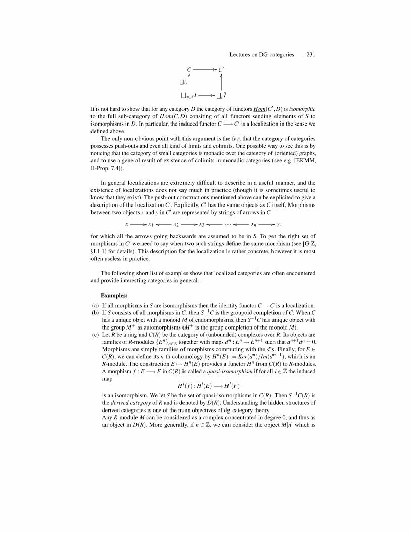
Lectures on DG-categories 231
C // C′
⊔s∈S I
⊔is
OO
// ⊔s I
OO
It is not hard to show that for any category D the category of functors Hom(C′,D) is isomorphicto the full sub-category of Hom(C,D) consiting of all functors sending elements of S toisomorphisms in D. In particular, the induced functor C −→C′ is a localization in the sense wedefined above.
The only non-obvious point with this argument is the fact that the category of categoriespossesses push-outs and even all kind of limits and colimits. One possible way to see this is bynoticing that the category of small categories is monadic over the category of (oriented) graphs,and to use a general result of existence of colimits in monadic categories (see e.g. [EKMM,II-Prop. 7.4]).
In general localizations are extremely difficult to describe in a useful manner, and theexistence of localizations does not say much in practice (though it is sometimes useful toknow that they exist). The push-out constructions mentioned above can be explicited to give adescription of the localization C′. Explicitly, C′ has the same objects as C itself. Morphismsbetween two objects x and y in C′ are represented by strings of arrows in C
x // x1 x2oo // x3 . . .oo xnoo // y,
for which all the arrows going backwards are assumed to be in S. To get the right set ofmorphisms in C′ we need to say when two such strings define the same morphism (see [G-Z,§I.1.1] for details). This description for the localization is rather concrete, however it is mostoften useless in practice.
The following short list of examples show that localized categories are often encounteredand provide interesting categories in general.
Examples:
(a) If all morphisms in S are isomorphisms then the identity functor C→C is a localization.(b) If S consists of all morphisms in C, then S−1C is the groupoid completion of C. When C
has a unique objet with a monoid M of endomorphisms, then S−1C has unique object withthe group M+ as automorphisms (M+ is the group completion of the monoid M).
(c) Let R be a ring and C(R) be the category of (unbounded) complexes over R. Its objects arefamilies of R-modules Enn∈Z together with maps dn : En→ En+1 such that dn+1dn = 0.Morphisms are simply families of morphisms commuting with the d’s. Finally, for E ∈C(R), we can define its n-th cohomology by Hn(E) := Ker(dn)/Im(dn−1), which is anR-module. The construction E 7→ Hn(E) provides a functor Hn from C(R) to R-modules.A morphism f : E −→ F in C(R) is called a quasi-isomorphism if for all i ∈ Z the inducedmap
H i( f ) : H i(E)−→ H i(F)
is an isomorphism. We let S be the set of quasi-isomorphisms in C(R). Then S−1C(R) isthe derived category of R and is denoted by D(R). Understanding the hidden structures ofderived categories is one of the main objectives of dg-category theory.Any R-module M can be considered as a complex concentrated in degree 0, and thus asan object in D(R). More generally, if n ∈ Z, we can consider the object M[n] which is
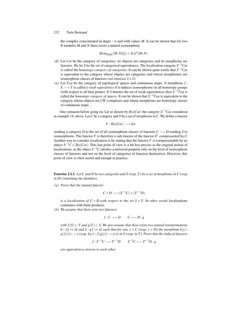
232 Toen Bertrand
the complex concentrated in degre −n and with values M. It can be shown that for twoR-modules M and N there exists a natural isomorphism
HomD(R)(M,N[n])' Extn(M,N).
(d) Let Cat be the category of categories: its objects are categories and its morphisms arefunctors. We let S be the set of categorical equivalences. The localization category S−1Catis called the homotopy category of categories. It can be shown quite easily that S−1Catis equivalent to the category whose objetcs are categories and whose morphismes areisomorphism classes of functors (see exercice 2.1.2).
(e) Let Top be the category of topological spaces and continuous maps. A morphism f :X −→ Y is called a weak equivalence if it induces isomorphisms on all homotopy groups(with respect to all base points). If S denotes the set of weak equivalences then S−1Top iscalled the homotopy category of spaces. It can be shown that S−1Top is equivalent to thecategory whose objects are CW -complexes and whose morphisms are homotopy classesof continuous maps.
One comment before going on. Let us denote by Ho(Cat) the category S−1Cat consideredin example (4) above. Let C be a category and S be a set of morphisms in C. We define a functor
F : Ho(Cat)−→ Set
sending a category D to the set of all isomorphism classes of functors C −→ D sending S toisomorphisms. The functor F is therefore a sub-functor of the functor hC corepresented by C.Another way to consider localization is by stating that the functor F is corepresentable by anobject S−1C ∈ Ho(Cat). This last point of view is a bit less precise as the original notion oflocalizations, as the object S−1C satisfies a universal property only on the level of isomorphismclasses of functors and not on the level of categories of functors themselves. However, thispoint of view is often useful and enough in practice.
Exercise 2.1.1 Let C and D be two categories and S (resp. T ) be a set of morphisms in C (resp.in D) containing the identities.
(a) Prove that the natural functor
C×D−→ (S−1C)× (T−1D)
is a localization of C×D with respect to the set S× T . In other words localizationscommutes with finite products.
(b) We assume that there exist two functors
f : C −→ D C←− D : g
with f (S)⊂ T and g(T )⊂ S. We also assume that there exists two natural transformationsh : f g⇒ id and k : g f ⇒ id such that for any x ∈ C (resp. y ∈ D) the morphism k(y) :g( f (x))→ x (resp. h(y) : f (g(y))→ y) is in S (resp. in T ). Prove that the induced functors
f : S−1C −→ T−1D S−1C←− T−1D : g
are equivalences inverse to each other.
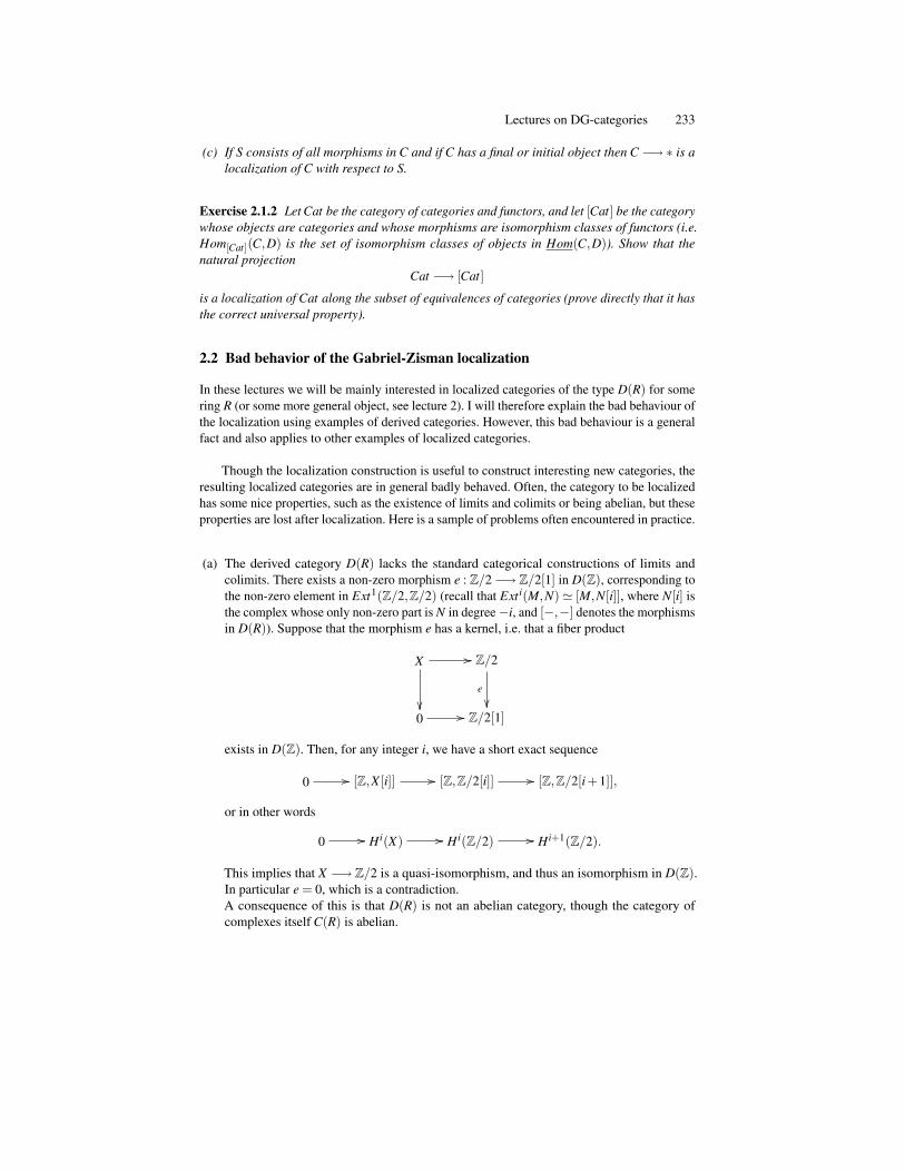
Lectures on DG-categories 233
(c) If S consists of all morphisms in C and if C has a final or initial object then C −→ ∗ is alocalization of C with respect to S.
Exercise 2.1.2 Let Cat be the category of categories and functors, and let [Cat] be the categorywhose objects are categories and whose morphisms are isomorphism classes of functors (i.e.Hom[Cat](C,D) is the set of isomorphism classes of objects in Hom(C,D)). Show that thenatural projection
Cat −→ [Cat]
is a localization of Cat along the subset of equivalences of categories (prove directly that it hasthe correct universal property).
2.2 Bad behavior of the Gabriel-Zisman localization
In these lectures we will be mainly interested in localized categories of the type D(R) for somering R (or some more general object, see lecture 2). I will therefore explain the bad behaviour ofthe localization using examples of derived categories. However, this bad behaviour is a generalfact and also applies to other examples of localized categories.
Though the localization construction is useful to construct interesting new categories, theresulting localized categories are in general badly behaved. Often, the category to be localizedhas some nice properties, such as the existence of limits and colimits or being abelian, but theseproperties are lost after localization. Here is a sample of problems often encountered in practice.
(a) The derived category D(R) lacks the standard categorical constructions of limits andcolimits. There exists a non-zero morphism e : Z/2−→ Z/2[1] in D(Z), corresponding tothe non-zero element in Ext1(Z/2,Z/2) (recall that Ext i(M,N)' [M,N[i]], where N[i] isthe complex whose only non-zero part is N in degree−i, and [−,−] denotes the morphismsin D(R)). Suppose that the morphism e has a kernel, i.e. that a fiber product
X //
Z/2
e
0 // Z/2[1]
exists in D(Z). Then, for any integer i, we have a short exact sequence
0 // [Z,X [i]] // [Z,Z/2[i]] // [Z,Z/2[i+1]],
or in other words
0 // H i(X) // H i(Z/2) // H i+1(Z/2).
This implies that X −→ Z/2 is a quasi-isomorphism, and thus an isomorphism in D(Z).In particular e = 0, which is a contradiction.A consequence of this is that D(R) is not an abelian category, though the category ofcomplexes itself C(R) is abelian.
234 Toen Bertrand
(b) The fact that D(R) has no limits and colimits might not be a problem by itself, as it ispossible to think of interesting categories which do not have limits and colimits (e.g. anynon-trivial groupoid has no final object). However, the case of D(R) is very frustating as itseems that D(R) is very close to having limits and colimits. For instance it is possbile toshow that D(R) admits homotopy limits and homotopy colimits in the following sense. Fora category I, let C(R)I be the category of functors from I to C(R). A morphism f : F −→G(i.e. a natural transformation between two functors F,G : I −→C(R)) is called a levelwisequasi-isomorphism if for any i ∈ I the induced morphism f (i) : F(i)−→ G(i) is a quasi-isomorphism in C(R). We denote by D(R, I) the category C(R)I localized along levelwisequasi-isomorphisms. The constant diagram functor C(R) −→ C(R)I is compatibe withlocalizations on both sides and provides a functor
c : D(R)−→ D(R, I).
It can then been shown that the functor c has a left and a right adjoint denoted by
HocolimI : D(R, I)−→ D(R) D(R)←− D(R, I) : HolimI ,
called the homotopy colimit and the homotopy limit functor. Homotopy limits and colimitsare very good replacement of the notions of limits and colimits, as they are the best possibleapproximation of the colimit and limit functors that are compatible with the notion ofquasi-isomorphisms. However, this is quite unsatisfactory as the category D(R, I) dependson more than the category D(R) alone (note that D(R, I) is not equivalent to D(R)I), andin general it is impossible to recontruct D(R, I) from D(R).
(c) To the ring R are associated several invariants such as its K-theory spectrum, its Hochschild(resp. cyclic) homology . . . . It is tempting to think that these invariants can be directlydefined on the level of derived categories, but this is not the case (see [?]). However,it has been noticed that these invariants only depend on R up to some notion of equiv-alence that is much weaker than the notion of isomorphism. For instance, any functorD(R) −→ D(R′) which is induced by a complex of (R,R′)-bi-modules induces a mapon K-theory, Hochschild homology and cyclic homology. However, it is not clear thatevery functor D(R) −→ D(R′) comes from a complex of (R,R′)-bi-modules (there arecounter examples when R and R′ are dg-algebras, see [Du-Sh, 2.5,6.8]). Definitely, thederived category of complexes of (R,R′)-bi-modules is not equivalent to the category offunctors D(R) −→ D(R′). This is again an unsatisfactory situation and it is then quitedifficult (if not impossible) to understand the true nature of these invariants (i.e. of whichmathematical structures are they truly invariants ?).
(d) Another important problem with the categories D(R) is their non local nature. To explainthis let P1 be the projective line (e.g. over Z). As a scheme P1 is the push-out
SpecZ[X ,X−1] //
SpecZ[T ]
SpecZ[U ] // P1,
where T is sent to X and U is sent to X−1. According to the push-out square, the categoryof quasi-coherent sheaves on P1 can be described as the (2-categorical) pull-back
Lectures on DG-categories 235
QCoh(P1) //
Mod(Z[T ])
Mod(Z[U ]) // Mod(Z[X ,X−1]).
In other words, a quasi-coherent module on P1 is the same thing as a triple (M,N,u),where M (resp. N) is a Z[T ]-module (resp. Z[U ]-module), and u is an isomorphism
u : M⊗Z[T ]Z[X ,X−1]' N⊗Z[U ]Z[X ,X−1]
of Z[X ,X−1]-modules. This property is extremely useful in order to reduce problems ofquasi-coherent sheaves on schemes to problems of modules over rings. Unfortunately, thisproperty is lost when passing to the derived categories. The square
Dqcoh(P1) //
D(Z[T ])
D(Z[U ]) // D(Z[X ,X−1]),
is not cartesian (in the 2-categorical sense) anymore (e.g. there exist non zero morphismsOX −→OX (−2)[1] that go to zero as a morphism in D(Z[U ])×D(Z[X ,X−1]) D(Z[T ])). Thederived categories of the affine pieces of P1 do not determine the derived category ofquasi-coherent sheaves on P1.
The list of problems above suggests the existence of a some sort of categorical structurelying in between the category of complexes C(R) and its derived category D(R), which israther close to D(R) (i.e. in which the quasi-isomorphisms are inverted in some sense), but forwhich (1)− (4) above are no longer a problem. There exist several possible approaches, andmy purpose is to present one of them using dg-categories.
Exercise 2.2.1 Let I = BN be the category with a unique object ∗ and with the monoid Nof natural numbers as endomorphism of this object. There is a bijection between the set offunctors from I to a category C and the set of pairs (x,h), where x in an object in C and h is anendomorphism of x.
Let R be a commutative ring.
(a) Show that there is a natural equivalence of categories
D(R, I)' D(R[X ]),
where D(R, I) is the derived category of I-diagram of complexes of R-modules as describedin example (2) above. Deduce from this that D(R, I) is never an abelian category (unlessR = 0).
(b) Prove that D(R) is abelian when R is a field (show that D(R) is equivalent to the categoryof Z-graded R-vector spaces).
(c) Deduce that D(R, I) and D(R)I can not be equivalent in general.(d) Let now I be the category with two objects 0 and 1 and a unique morphism from 1 to 0.
Using a similar approach as above show that D(R, I) and D(R)I are not equivalent ingeneral.
236 Toen Bertrand
2.3 DG-categories and dg-functors
We now fix a base commutative ring k. Unless specified, all the modules and tensor productswill be over k.
2.3.1 DG-categories
We start by recalling that a dg-category T (over k) consists of the following data.
• A set of objects Ob(T ), also sometimes denoted by T itself.• For any pair of objects (x,y) ∈ Ob(T )2 a complex T (x,y) ∈C(k).• For any triple (x,y,z) ∈ Ob(T )3 a composition morphism µx,y,z : T (x,y)⊗ T (y,z) −→
T (x,z).• For any object x ∈ Ob(T ), a morphism ex : k −→ T (x,x).
These data are required to satisfy the following associativity and unit conditions.
(a) (Associativity) For any four objects (x,y,z, t) in T , the following diagram
T (x,y)⊗T (y,z)⊗T (z, t)id⊗µy,z,t //
µx,y,z⊗id
T (x,y)⊗T (y, t)
µx,y,t
T (x,z)⊗T (z, t)
µx,z,t
// T (x, t)
commutes.(b) (Unit) For any (x,y) ∈ Ob(T )2 the two morphisms
T (x,y)' k⊗T (x,y)ex⊗id // T (x,x)⊗T (x,y)
µx,x,y // T (x,y)
T (x,y)' T (x,y)⊗ kid⊗ey // T (x,y)⊗T (y,y)
µx,y,y // T (x,y)
are equal to the identities.
In a more explicit way, a dg-category T can also be described as follows. It has a set ofobjects Ob(T ). For any two objects x and y, and any n ∈ Z it has a k-module T (x,y)n, thoughas morphisms of degre n from x to y. For three objects x, y and z, and any integers n and mthere is a composition map
T (x,y)n×T (y,z)m −→ T (x,z)n+m
which is bilinear and associative. For any object x, there is an element ex ∈ T (x,x)0, which isa unit for the composition. For any two objects x and y there is a differential d : T (x,y)n −→T (x,y)n+1, such that d2 = 0. And finally, we have the graded Leibnitz rule
d( f g) = d( f )g+(−1)m f d(g),
for f and g two composable morphisms, with f of degree m. Note that this implies thatd(ex) = 0, and thus that ex is always a zero cycle in the complex T (x,x).
Lectures on DG-categories 237
On a more conceptual side, a dg-category is a C(k)-enriched category in the sense of [Kel],where C(k) is the symmetric monoidal category of complexes of k-modules. All the basicnotions of dg-categories presented in these notes can be expressed in terms of enriched categorytheory, but we will not use this point of view. We, however, encourage the reader to consult [?]and to (re)consider the definitions of dg-categories, dg-functors, tensor product of dg-categories. . . in the light of enriched category theory.
Examples:
(a) A very simple example is the opposite dg-category T op of a dg-category T . The set ofobjects of T op is the same as the one of T , and we set
T op(x,y) := T (y,x)
together with the obvious composition maps
T (y,x)⊗T (z,y)' T (z,y)⊗T (y,x)−→ T (z,x),
where the first isomorphism is the symmetry isomorphism of the monoidal structure onthe category of complexes (see [Bour, §X.4.1] for the signs rule).
(b) A fundamental example of dg-category over k is the one given by considering the categoryof complexes over k itself. Indeed, we define a dg-category C(k) by setting its set ofobjects to be the set of complexes of k-modules. For two complexes E and F , we defineC(k)(E,F) to be the complex Hom∗(E,F) of morphisms from E to F . Recall, that for anyn ∈ Z the k-module of elements of degre n in Hom∗(E,F) is given by
Homn(E,F) := ∏i∈Z
Hom(E i,F i+n).
The differentiald : Homn(E,F)−→ Homn+1(E,F)
sends a family f ii∈Z to the family d f i−(−1)n f i+1 di∈Z. Note that the zero cyclesin Hom∗(E,F) are precisely the morphisms of complexes from E to F . The compositionof morphisms induces composition morphisms
Homn(E,F)×Homm(E,F)−→ Homn+m(E,F).
It is easy to check that these data defines a dg-category C(k).(c) There is slight generalization of the previous example for the category C(R) of complexes
of (left) R-modules, where R is any associative and unital k-algebra. Indeed, for twocomplexes of R-modules E and F , there is a complex Hom∗(E,F) defined as in theprevious example. The only difference is that now Hom∗(E,F) is only a complex ofk-modules and not of R-modules in general (except when R is commutative). Thesecomplexes define a dg-category C(R) whose objects are complexes of R-modules.
(d) A far reaching generalization of the two previous examples is the case of complexes ofobjects in any k-linear Grothendieck category (i.e. an abelian cocomplete category with asmall generator and for which filtered colimits are exact, or equivalently a localization of amodules category, see [G-P]). Indeed, for such a category A and two complexes E and Fof objects in A , we define a complex of k-modules Hom∗(E,F) as above
Homn(E,F) := ∏i∈Z
Hom(E i,F i+n),
238 Toen Bertrand
with the differential given by the same formula as in example (2). The composition ofmorphisms induce morphisms
Homn(E,F)×Homm(F,G)−→ Homn+m(E,G).
It is easy to check that these data define a dg-category whose objects are complexes in A .It will be denoted by C(A ).
(e) From a dg-category T , we can construct a category Z0(T ) of 0-cycles as follows. It hasthe same objects as T , and for two such objects x and y the set of morphisms between xand y in Z0(T ) is defined to be the set of 0-cycles in T (x,y) (i.e. degre zero morphismsf ∈ T (x,y)0 such that d( f ) = 0. The Leibniz rule implies that the composition of two0-cycles is again a 0-cycle, and thus we have induced composition maps
Z0(T (x,y))×Z0(T (y,z))−→ Z0(T (x,z)).
These composition maps define the category Z0(T ). The category Z0(T ) is often namedthe underlying category of T . We observe that Z0(T ) is more precisely a k-linear category(i.e. that Homs sets are endowed with k-module structures such that the composition mapsare bilinear).For instance, let A be a Grothendieck category and C(A ) its associated dg-category ofcomplexes as defined in example (4) above. The underlying category of C(A ) is thenisomorphic to the usual category C(A ) of complexes and morphisms of complexes in A .
(f) Conversely, if C is a k-linear category we view C as a dg-category in a rather obvious way.The set of objects is the same of the one of C, and the complex of morphisms from x to y issimply the complex C(x,y)[0], which is C(x,y) in degre 0 and 0 elsewhere. In the sequel,every k-linear category will be considered as a dg-category in this obvious way. Note that,this way the category of k-linear categories and k-linear functors form a full sub-categoryof dg-categories and dg-functors (see §1.3.2 below).
(g) A dg-category T with a unique object is essentially the same thing as a dg-algebra. Indeed,if x is the unique object the composition law on T (x,x) induces a unital and associative dg-algebra structure on T (x,x). Conversely, if B is a unital and associative dg-algebra we canconstruct a dg-category T with a unique object x and with T (x,x) := B. The multiplicationin B is then used to define the composition on T (x,x).
(h) Here is now a non-trivial example of a dg-category arising from geometry. In this examplek = R. Let X be a differential manifold (say C ∞). Recall that a flat vector bundle on Xconsists the data of a smooth (real) vector bundle V on X together with a connexion
∇ : A0(X ,V )−→ A1(X ,V ),
(where An(X ,V ) is the space of smooth n-forms on X with coefficients in V ) such that∇2 = 0. For two such flat bundles (V,∇V ) and (W,∇W ) we define a complex A∗DR(V,W )by
A∗DR(V,W )n := An(X ,Hom(V,W )),
where Hom(V,W ) is the vector bundle of morphisms from V to W . The differential
d : AnDR(V,W )−→ An+1
DR (V,W )
is defined by sending ω⊗ f to d(ω)⊗ f +(−1)nω ∧∇( f ). Here, ∇( f ) is the 1-form withcoefficients in Hom(V,W ) defined by
∇( f ) := ∇W f − ( f ⊗ id)∇V .
Lectures on DG-categories 239
The fact that ∇2V = ∇2
W = 0 implies that A∗DR(V,W ) is a complex. Moreover, we define acomposition
AnDR(U,V )×Am
DR(V,W )−→ An+m(U,W )
for three flat bundles U , V and W by
(ω⊗ f ).(ω ′⊗g) := (ω ∧ω′)⊗ ( f g).
It is easy to check that these data defines a dg-category TDR(X) (over R) whose objectsare flat bundles on X , and whose complex of morphisms from (V,∇V ) to (W,∇W ) are thecomplexes A∗DR(V,W ).By construction the underlying category of TDR(X) is the category of flat bundles and flatmaps. By the famous Riemann-Hilbert correspondence (see [De] for the analog statementin the complex analytic case) this category is thus equivalent to the category of finitedimensional linear representations of the fundamental group of X , or equivalently offinite dimensional local systems (i.e. of locally constant sheaves of finite dimensionalC-vector spaces). Moreover, for two flat bundles (V,∇V ) and (W,∇W ), corresponding totwo local systems L1 and L2, the cohomology group H i(TDR(X)(V,W )) = H i(A∗DR(V,W ))is isomorphic to the Ext group Ext i(L1,L2), computed in the category of abelian sheavesover X . Therefore, we see that even when X is simply connected the dg-category TDR(X)contains interesting informations about the cohomology of X (even though the underlyingcategory of TDR(X) is simply the category of finite dimensional vector spaces).
(i) The previous example has the following complex analog. Now we let k = C, and X be acomplex manifold. We define a dg-category TDol(X) in the following way. The objects ofTDol(X) are the holomorphic complex vector bundles on X . For two such holomorphicbundles V and W we let
TDol(X)(V,W ) := A∗Dol(V,W ),
where A∗Dol(V,W ) is the Dolbeault complex with coefficients in the vector bundle ofmorphisms from V to W . Explicitely,
AqDol(V,W ) := A0,q(X ,Hom(V,W ))
is the space of (0,q)-forms on X with coefficients in the holomorphic bundle Hom(V,W )of morphisms from V to W . The differential
AqDol(V,W )−→ Aq+1
Dol (V,W )
is the operator ∂ , sending ω⊗ f to
∂ (ω⊗ f ) := ∂ (ω)⊗ f +(−1)qω ∧∂ ( f ),
where ∂ ( f ) is defined by
∂ ( f ) = ∂W f − ( f ⊗ id)∂V ,
with∂V : A0(X ,V )−→ A0,1(X ,V ) ∂W : A0(X ,W )−→ A0,1(X ,W )
being the operators induced by the holomorphic structures on V and W (see [Gr-Ha, Chap0 §5]). As in the previous example we can define a composition
A∗Dol(U,V )×A∗Dol(V,W )−→ A∗Dol(U,W )
240 Toen Bertrand
for three holomorphic bundles U , V and W on X . These data defines a dg-category TDol(X)(over C).By construction, the underlying category of TDol(X) has objects the holomorphic vectorbundles, and the morphisms in this category are the C ∞-morphisms of complex vectorbundles f : V −→W satisfying ∂ ( f ) = 0, or equivalently the holomorphic morphisms. Mo-roever, for two holomorphic vector bundles V and W the cohomology group H i(TDol(X))is isomorphic to Ext i
OX(V ,W ), the i-th ext-group between the associated sheaves of holo-
morphic sections (or equivalently the ext-group in the category of holomorphic coherentsheaves). For instance, if 1 is the trivial vector bundle of rank 1 and V is any holomorphicvector bundle, we have
H i(TDol(1,V ))' H iDol(X ,V ),
the i-th Dolbeault cohomology group of V .The dg-category TDol(X) is important as it provides a rather explicit model for the derivedcategory of coherent sheaves on X . Indeed, the homotopy category H0(TDol(X)) (seedefinition 2.3.1) is equivalent to the full sub-category of Db
coh(X), the bounded coherentderived category of X , whose objects are holomorphic vector bundles. Also, for two suchholomorphic vector bundles V and W and all i we have
HomDbcoh(X)(V,W [i])' H i(TDol(X)(V,W ))' Ext i
OX(V ,W ).
(j) Here is one last example of a dg-category in the topological context. We construct adg-category dgTop, whose set of objects is the set of all topological spaces. For twotopological spaces X and Y , we define a complex of morphisms dgTop(X ,Y ) in thefollowing way. We first consider Hom∆ (X ,Y ), the simplicial set (see [Ho1] for the notionof simplicial sets) of continuous maps between X and Y : by definition the set of n-simplicies in Hom∆ (X ,Y ) is the set of continuous maps X ×∆ n −→ Y , where ∆ n :=x ∈ [0,1]n+1/∑xi = 1 is the standard simplex of dimension n in Rn+1. The face anddegeneracy operators of Hom∆ (X ,Y ) are defined using the face embeddings (0≤ i≤ n)
di : ∆ n −→ ∆ n+1
x 7→ (x0, . . . ,xi−1,0,xi, . . .xn),
and the natural projections (0≤ i≤ n)
si : ∆ n+1 −→ ∆ n
x 7→ (x0, . . . ,xi + xi+1,xi+2, . . . ,xn+1).
Now, for any two topological spaces X and Y we set
dgTop(X ,Y ) := C∗(Hom∆ (X ,Y )),
the homology chain complex of Hom∆ (X ,Y ) with coefficients in k. Explicitly, Cn(Hom∆ (X ,Y ))is the free k-module generated by continuous maps f : X×∆ n −→ Y . The differential ofsuch a map is given by the formula
d( f ) := ∑0≤i≤n
(−1)idi( f ),
where di( f ) is the map X×∆ n−1 −→ Y obtained by composition
X×∆ n−1id×di // X×∆ n f // Y.
Lectures on DG-categories 241
For three topological spaces X , Y and Z, there exists a composition morphism at the levelof simplicial sets of continuous maps
Hom∆ (X ,Y )×Hom∆ (Y,Z)−→ Hom∆ (X ,Z).
This induces a morphism on the level of chain complexes
C∗(Hom∆ (X ,Y )×Hom∆ (Y,Z))−→C∗(Hom∆ (X ,Z)).
Composing this morphism with the famous Eilenberg-MacLane map (see [May, §29])
C∗(Hom∆ (X ,Y ))⊗C∗(Hom∆ (Y,Z))−→C∗(Hom∆ (X ,Y )×Hom∆ (Y,Z))
defines a composition
dgTop(X ,Y )⊗dgTop(Y,Z)−→ dgTop(X ,Z).
The fact that the Eilenberg-MacLane morphisms are associative and unital (they aremoreover commutative, see [May, §29]) implies that this defines a dg-category dgTop.
2.3.2 DG-functors
For two dg-categories T and T ′, a morphism of dg-categories (or simply a dg-functor) f :T −→ T ′ consists of the following data.
• A map of sets f : Ob(T )−→ Ob(T ′).• For any pair of objects (x,y) ∈ Ob(T )2, a morphism in C(k)
fx,y : T (x,y)−→ T ′( f (x), f (y)).
These data are required to satisfy the following associativity and unit conditions.
(a) For any (x,y,z) ∈ Ob(T )3 the following diagram
T (x,y)⊗T (y,z)µx,y,z //
fx,y⊗ fy,z
T (x,z)
fx,z
T ′( f (x), f (y))⊗T ′( f (y), f (z))
µ ′f (x), f (y), f (z)
// T ′( f (x), f (z))
commutes.(b) For any x ∈ Ob(T ), the following diagram
kex //
e′f (x) $$IIIIIIIIIII T (x,x)
fx,x
T ′( f (x), f (x))
commutes.
Examples:
242 Toen Bertrand
(a) Let T be any dg-category and x ∈ T be an object. We define a dg-functor
f = hx : T −→C(k)
in the following way (recall that C(k) is the dg-category of complexes over k). The mapon the set of objects sends an object y ∈ T to the complex T (x,y). For two objects y and zin T we define a morphism
fy,z : T (y,z)−→C(k)( f (y), f (x)) = Hom∗(T (x,y),T (x,z)),
which by definition is the adjoint to the composition morphism
mx,y,z : T (x,y)⊗T (y,z)−→ T (x,z).
The associativity and unit condition on composition of morphisms in T imply that thisdefines a morphism of dg-categories
hx : T −→C(k).
Dually, we can also define a morphism of dg-categories
hx : T op −→C(k)
by sending y to T (y,x).(b) For any dg-category T there exists a dg-functor
T ⊗T op −→C(k),
sending a pair of objects (x,y) to the complex T (y,x). Here, T ⊗ T op denotes the dg-category whose set of objects is Ob(T )×Ob(T ′), and whose complex of morphisms aregiven by
(T ⊗T op)((x,y),(x′,y′)) := T (x,x′)⊗T (y′,y).
We refer to exercise 2.3.4 and §3.2 for more details about the tensor product of dg-categories.
(c) Let R and S be two associative and unital k-algebras, and f : R −→ S be a k-morphism.The morphism f induces two functors
f ∗ : C(R)−→C(S) C(R)←−C(S) : f∗,
adjoint to each others. The functor f∗ sends a complex of S-modules to the correspondingcomplex of R-modules obtained by restricting the scalars from S to R by the morphism f .Its left adjoint f ∗ sends a complex of R-modules E to the complex S⊗R E. It is not difficultto show that the functors f∗ and f ∗ are compatible with the complex of morphisms Hom∗
and thus define morphisms of dg-categories
f ∗ : C(R)−→C(S) C(R)←−C(S) : f∗.
More generally, if f : A −→B is any k-linear functor between Grothendieck categories,there is an induced morphism of dg-categories
f : C(A )−→C(B).

Lectures on DG-categories 243
(d) Let f : X −→Y be a C ∞-morphism between two differential manifolds. Then, the pull-backfor flat bundles and differential forms defines a morphism of dg-categories constructed inour example 8
f ∗ : TDR(Y )−→ TDR(X).
In the same way, if now f is a holomorphic morphism between two complex varieties,then there is a dg-functor
f ∗ : TDol(Y )−→ TDol(X)
ontained by pulling-back the holomorphic vector bundles and differential forms.
DG-functors can be composed in an obvious manner, and dg-categories together withdg-functors form a category denoted by dg− catk (or dg− cat if the base ring k is clear).
For a dg-category T , we define a category H0(T ) in the following way. The set of objectsof H0(T ) is the same as the set of objects of T . For two objects x and y the set of morphisms inH0(T ) is defined by
H0(T )(x,y) := H0(T (x,y)).
Finally, the composition of morphisms in H0(T ) is defined using the natural morphisms
H0(T (x,y))⊗H0(T (y,z))−→ H0(T (x,y)⊗T (y,z))
composed with the morphism
H0(µx,y,z) : H0(T (x,y)⊗T (y,z))−→ H0(T (x,z)).
Definition 2.3.1 The category H0(T ) is called the homotopy category of T .
Examples:
(a) If C is a k-linear category considered as a dg-category as explained in our example 6 above,then H0(C) is naturally isomorphic to C itself.
(b) We have H0(T op) = H0(T )op for any dg-category T .(c) For a k-algebra R, the homotopy category H0(C(R)) is usually denoted by K(R), and
is called the homotopy category of complexes of R-modules. More generally, if A isa Grothendieck category, H0(C(A )) is denoted by K(A ), and is called the homotopycategory of complexes in A .
(d) If X is a differentiable manifold, then H0(TDR(X)) coincides with Z0(TDR(X)) and isisomorphic to the category of flat bundles and flat maps between them. As we alreadymentioned, this last category is equivalent by the Riemann-Hilbert correspondence to thecategory of local systems on X .When X is a complex manifold, we also have that H0(TDol(X)) coincides with Z0(TDol(X))and is isomorphic to the category of holomorphic vector bundles and holomorphic mapsbetween them.
(e) The category H0(dgTop) is the category whose objects are topological spaces and whoseset of morphisms between X and Y is the free k-module over the set of homotopy classesof maps from X to Y .
One of the most important notions in dg-category theory is the notion of quasi-equivalences,a mixture in between quasi-isomorphisms and categorical equivalences.
244 Toen Bertrand
Definition 2.3.2 Let f : T −→ T ′ be a dg-functor between dg-categories
(a) The morphism f is quasi-fully faithful if for any two objects x and y in T the morphismfx,y : T (x,y)−→ T ′( f (x), f (y)) is a quasi-isomorphism of complexes.
(b) The morphism f is quasi-essentially surjective if the induced functor H0( f ) : H0(T )−→H0(T ′) is essentially surjective.
(c) The morphism f is a quasi-equivalence if it is quasi-fully faithful and quasi-essentiallysurjective.
We will be mainly interested in dg-categories up to quasi-equivalences. We thereforeintroduce the following category.
Definition 2.3.3 The homotopy category of dg-categories is the category dg− cat localizedalong quasi-equivalences. It is denoted by Ho(dg− cat). Morphisms in Ho(dg− cat) betweentwo dg-categories T and T ′ will often be denoted by
[T,T ′] := HomHo(dg−cat)(T,T ′).
Note that the construction T 7→H0(T ) provides a functor H0(−) : dg−cat −→Cat, whichdescends as a functor on homotoy categories
H0(−) : Ho(dg− cat)−→ Ho(Cat).
Remark 1. In the last section we have seen that the localization construction is not wellbehaved, but in the definition above we consider Ho(dg−cat) which is obtained by localization.Therefore, the category Ho(dg− cat) will not be well behaved itself. In order to get the mostpowerful approach the category dg− cat should have been itself localized in a more refinedmaner (e.g. as a higher category, see [To2, §2]). We will not need such an evolved approach,and the category Ho(dg− cat) will be enough for most of our purpose.
Examples:
(a) Let f : T −→ T ′ be a quasi-fully faithful dg-functor. We let T ′0 be the full (i.e. with thesame complexes of morphisms as T ′) sub-dg-category of T ′ consisting of all objectsx ∈ T ′ such that x is isomorphic in H0(T ′) to an object in the image of the induced functorH0( f ) : H0(T )−→H0(T ′). Then the induced dg-functor T −→ T ′0 is a quasi-equivalence.
(b) Let f : R−→ S be a morphism of k-algebras. If the morphism of dg-categories
f ∗ : C(R)−→C(S)
is quasi-fully faithful then the morphism f is an isomorphism. Indeed, if f ∗ is quasi-fullyfaithful we have that
Hom∗(R,R)−→ Hom∗(S,S)
is a quasi-isomorphism. Evaluating this morphism of complexes at H0 we find that theinduced morphism
R' H0(Hom∗(R,R))−→ H0(Hom∗(S,S))' S
is an isomorphism. This last morphism being f itself, we see that f is an isomorphism.
Lectures on DG-categories 245
(c) Suppose that T is a dg-category such that for all objects x and y we have H i(T (x,y)) = 0for all i 6= 0. We are then going to show that T and H0(T ) are isomorphic in Ho(dg−cat).We first define a dg-category T≤0 in the following way. The dg-category T≤0 possesses thesame set of objects as T itself. For two objects x and y we let
T≤0(x,y)n := T (x,y) i f n < 0 T≤0(x,y)n := 0 i f n > 0
andT≤0(x,y)0 := Z0(T (x,y)) = Ker(d : T (x,y)0→ T (x,y)1).
The differential on T≤0(x,y) is simply induced by the one on T (x,y). It is not hard to seethat the composition morphisms of T induces composition morphisms
T≤0(x,y)n×T≤0(y,z)m −→ T≤0(x,z)n+m
which makes these data into a dg-category T≤0 (this is because the composition of two0-cocycles is itself a 0-cocycle). Moreover, there is a natural dg-functor
T≤0 −→ T
which is the identity on the set of objects and the natural inclusions of complexes
T≤0(x,y)⊂ T (x,y)
on the level of morphisms. Now, we consider the natural dg-functor (here, as always, thek-linear category H0(T ) is considered as a dg-category in the obvious way)
T≤0 −→ H0(T )
which is the identity on the set of objects and the natural projection
T≤0(x,y)−→ H0(T (x,y)) = H0(T≤0(x,y)) = T≤0(x,y)0/Im(T (x,y)−1→ T≤0(x,y)0)
on the level of morphisms. We thus have a diagram of dg-categories and dg-functors
H0(T ) T≤0 //oo T,
which by assumptions on T are all quasi-equivalences. This implies that T and H0(T )becomes isomorphic as objects in Ho(dg− cat).
(d) Suppose that f : X −→ Y is a C ∞ morphism between differentiable manifolds, such thatthere exists another C ∞ morphism g : Y −→ X and two C ∞ morphisms
h : X×R−→ X k : Y ×R−→ Y
withhX×0 = g f , hX×1 = id kY×0 = f g, kY×1 = id.
Then the dg-functorf ∗ : TDR(Y )−→ TDR(X)
is a quasi-equivalence. Indeed, we know that H0(TDR(X)) is equivalent to the categoryof linear representations of the fundamental group of X . Therefore, as the morphism fis in particular a homotopy equivalence it induces an isomorphisms on the level of thefundamental groups, and thus the induced functor
246 Toen Bertrand
f ∗ : H0(TDR(Y ))−→ H0(TDR(X))
is an equivalence of categories. The fact that the dg-functor f ∗ is also quasi-fully faithfulfollows from the homotopy invariance of de Rham cohomology, and more precisely fromthe fact that the projection p : X×R−→ X induces a quasi-equivalence of dg-categories
p∗ : TDR(X)−→ TDR(X×R).
We will not give more details in these notes.As particular case of the above statement we see that the projection Rn −→ ∗ induces aquasi-equivalence
TDR(∗)−→ TDR(Rn).
As TDR(∗) is itself isomorphic to the category of finite dimensional real vector spaces, wesee that TDR(Rn) is quasi-equivalent to the category of finite dimensional vector spaces.
(e) Let now X be a connected complex manifold and p : X −→ ∗ be the natural projection.Then the induced dg-functor
p∗ : TDol(∗)−→ TDol(X)
is quasi-fully faithful if and only if H i(X ,OX ) = 0 for all i 6= 0 (here OX is the sheaf ofholomorphic functions on X). Indeed, all the vector bundles are trivial on ∗. Moreover, for1r and 1s two trivial vector bundles of rank r and s on ∗ we have
TDol(X)(p∗(1r), p∗(1s))' TDol(X)(1,1)rs,
where 1 also denotes the trivial holomorphic bundle on X . Therefore, p∗ is quasi-fullyfaithful if and only if H i(TDol(X))(1,1) = 0 for all i 6= 0. As we have
H i(TDol(X)(1,1)) = H iDol(X ,1) = H i(X ,OX )
this implies the statement. As an example, we see that
TDol(∗)−→ TDol(Pn)
is quasi-fully faithful (here Pn denotes the complex projective space), but
TDol(∗)−→ TDol(E)
is not for any complex elliptic curve E.More generally, if f : X −→ Y is any proper holomorphic morphism between complexmanifolds, then the dg-functor
f ∗ : TDol(Y )−→ TDol(X)
is quasi-fully faithful if and only if we have
Ri f∗(OX ) = 0 ∀ i > 0,
whereRi f∗(OX ) denotes the higher direct images of the coherent sheaf OX of holomorphicfunctions on X (see e.g. [Gr-Ha]). We will not prove this statement in these notes. Asa consequence we see that f ∗ is quasi-fully faithful if it is a blow-up along a smoothcomplex sub-manifold of Y , or if it is a bundle in complex projective spaces.

Lectures on DG-categories 247
(f) For more quasi-equivalences between dg-categories in the context of non-abelian Hodgetheory see [Si].
Exercise 2.3.4 (a) Let T and T ′ be two dg-categories. Show how to define a dg-categoryT ⊗T ′ whose set of objects is the product of the sets of objects of T and T ’, and for anytwo pairs (x,y) and (x′,y′)
(T ⊗T ′)((x,y),(x′,y′)) := T (x,y)⊗T ′(x′,y′).
(b) Show that the construction (T,T ′) 7→ T ⊗T ′ defines a symmetric monoidal structure onthe category dg− cat.
(c) Show that the symmetric monoidal structure ⊗ on dg− cat is closed (i.e. that for any twodg-categories T and T ′ there exists a dg-category Hom(T,T ′) together with functorialisomorphisms
Hom(T ′′,Hom(T,T ′))' Hom(T ′′⊗T,T ′).
Exercise 2.3.5 Let k→ k′ be a morphism of commutative rings, and dg−catk (resp. dg−catk′ )the categories of dg-categories over k (resp. over k′).
(a) Show that there exists a forgetful functor
dg− catk′ −→ dg− catk
which consists of seing complexes over k′ as complexes over k using the morphism k→ k′.(b) Show that this forgetful functor admits a left adjoint
−⊗k k′ : dg− catk −→ dg− catk′ .
(c) Let 1k′ be the dg-category over k with a single object and with k′ as k-algebra of endo-morphisms of this object. Show that for any dg-category T over k, there exists a naturalisomorphism of dg-categories over k
T ⊗k k′ ' T ⊗1k′ ,
where the tensor product on the right is the one of dg-categories over k as defined inexercice 2.3.4, and the left hand side is considered as an object in dg− catk throught theforgetful functor.
(d) Show that the forgetful functor
dg− catk′ −→ dg− catk
also possesses a right adjoint
(−)k′/k : dg− catk −→ dg− catk′
(show that for any T ∈ dg− catk the dg-category Hom(1k′ ,T ) can be naturally endowedwith a structure of dg-category over k′).
Exercise 2.3.6 Let T be a dg-category and u ∈ Z0(T (x,y)) a morphism in its underlyingcategory. Show that the following four conditions are equivalent.
(a) The image of u in H0(T (x,y)) is an isomorphism in H0(T ).
248 Toen Bertrand
(b) There exists v ∈ Z0(T (y,x)) and two elements h ∈ T (x,x)−1, k ∈ T (y,y)−1 such that
d(h) = vu− ex d(k) = uv− ey.
(c) For any object z ∈ T , the composition with u
u− : T (z,x)−→ T (z,y)
is a quasi-isomorphism of complexes.(d) For any object z ∈ T , the composition with u
−u : T (y,z)−→ T (x,z)
is a quasi-isomorphism of complexes.
Exercise 2.3.7 We denote by B the commutative k-dg-algebra whose underlying graded k-algebra is a (graded commutative) polynomial algebra in two variables k[X ,Y ], with X indegree 0, Y in degree −1 and d(Y ) = X2. We consider B as a dg-category with a unique object.
(a) Show that there exists a natural quasi-equivalence
p : B−→ k[X ]/(X2) =: k[ε],
where k[ε] is the commutative algebra of dual numbers, considered as a dg-category witha unique object.
(b) Show that p does not admit a section in dg− cat. Deduce from this that unlike the caseof categories, there are quasi-equivalences T −→ T ′ in dg− cat such that the inverseof f in Ho(dg− cat) can not be represented by a dg-functor T ′ −→ T in dg− cat (i.e.quasi-inverses do not exist in general).
Exercise 2.3.8 Show that two k-linear categories are equivalent (as k-linear categories) if andonly if they are isomorphic in Ho(dg− cat).
2.4 Localizations as a dg-category
For a k-algebra R, the derived category D(R) is defined as a localization of the category C(R),and thus has a universal property in Ho(Cat). The purpose of this series of lectures is to showthat C(R) can also be localized as a dg-category C(R) in order to get an object L(R) satisfyinga universal property in Ho(dg− cat). The two objects L(R) and D(R) will be related by theformula
H0(L(R))' D(R),
and we will see that the extra information encoded in L(R) is enough in order to solve all theproblems mentioned in §1.2.
Let T be any dg-category, S be a subset of morphisms in the category H0(T ), and let usdefine a subfunctor FT,S of the functor [T,−], corepresented by T ∈ Ho(dg− cat). We define
FT,S : Ho(dg− cat)−→ Ho(Cat)
by sending a dg-category T ′ to the subset of morphisms [T,T ′] consisting of all morphism fwhose induced functor H0( f ) : H0(T ) −→ H0(T ′) sends morphisms of S to isomorphisms
Lectures on DG-categories 249
in H0(T ′). Note that the functor H0( f ) is only determined as a morphism in Ho(Cat), or inother words up to isomorphism. However, the property that H0( f ) sends elements of S toisomorphisms is preserved under isomorphisms of functors, and thus only depends on the classof H0( f ) as a morphism in Ho(Cat).
Definition 2.4.1 For T and S as above, a localization of T along S is a dg-category LSTcorepresenting the functor FT,S.
To state the previous definition in more concrete terms, a localization is the data of adg-category LST and a dg-functor l : T −→ LST , such that for any dg-category T ′ the inducedmap
l∗ : [LST,T ′]−→ [T,T ′]
is injective and identifies the left hand side with the subset FT,S(T ′)⊂ [T,T ′].
An important first question is the existence of localization as above. We will see that likelocalizations of categories they always exist. This, of course, requires to know how to computethe set [T,T ′] of morphisms in Ho(dg− cat). As the category Ho(dg− cat) is itself definedby localization this is not an easy problem. We will give a solution to this question in the nextlectures, based on an approach using model category theory.
3 Lecture 2: Model categories and dg-categories
The purpose of this second lecture is to study in more details the category Ho(dg− cat).Localizations of categories are very difficult to describe in general. The purpose of modelcategory theory is precisely to provide a general tool to describe localized categories. Bydefinition, a model category is a category together with three classes of morphisms, fibrations,cofibrations and (weak) equivalences satisfying some axioms mimicking the topological notionsof Serre fibrations, cofibrations and weak homotopy equivalences. When M is a model category,with W as equivalences, then the localized category W−1M possesses a very nice descriptionin terms of homotopy classes of morphisms between objects belonging to a certain class ofnicer objects called fibrant and cofibrant. A typical example is when M = Top is the categoryof topological spaces and W is the class of weak equivalences (see example 5 of §2.1). Thenall objects are fibrant, but the cofibrant objects are the retracts of CW-complexes. It is wellknown that the category W−1Top is equivalent to the category of CW-complexes and homotopyclasses of continuous maps between them.
In this lecture, I will start by some brief reminders on model categories. I will then explainhow model category structures appear in the context of dg-categories by describing the modelcategory of dg-categories (due to G. Tabuada, [Tab]) and the model category of dg-modules. Wewill also see how model categories can be used in order to construct interesting dg-categories. Inthe next lecture these model categories will be used in order to understand maps in Ho(dg−cat),and to prove the existence of several important constructions such as localization and internalHoms.
250 Toen Bertrand
3.1 Reminders on model categories
In this section we use the conventions of [Ho1] for the notion of model category. We also referthe reader to this book for the proofs of the statements we will mention.
We let M be a category with arbitrary limits and colimits. Recall that a (closed) modelcategory structure on M is the data of three classes of morphisms in M, the fibrations Fib, thecofibrations Co f and the equivalences W , satisfying the following axioms (see [Ho1]).
(a) If Xf // Y
g // Z are morphisms in M, then f , g and g f are all in W if and only iftwo of them are in W .
(b) The fibrations, cofibrations and equivalences are all stable by retracts.(c) Let
Af //
i
X
p
B g
// Y
be a commutative square in M with i ∈Co f and p ∈ Fib. If either i or p is also in W thenthere is a morphism h : B−→ X such that ph = g and hi = f .
(d) Any morphism f : X −→ Y can be factorized in two ways as f = pi and f = q j, with p ∈Fib, i∈Co f ∩W , q∈ Fib∩W and j ∈Co f . Moreover, the existence of these factorizationsare required to be functorial in f .
The morphisms in Co f ∩W are usually called trivial cofibrations and the morphisms inFib∩W trivial fibrations. Objects x such that /0 −→ x is a cofibration are called cofibrant.Dually, objects y such that y−→ ∗ is a fibration are called fibrant. The factorization axiom (4)implies that for any object x there is a diagram
Qx i // xp // Rx,
where i is a trivial fibration, p is a trivial cofibration, Qx is a cofibrant object and Rx is a fibrantobject. Moreover, the functorial caracter of the factorization states that the above diagram canbe, and will always be, chosen to be functorial in x.
Exercise 3.1.1 Let M be a model category and i : A −→ B a morphism. We assume that forevery commutative square
Af //
i
X
p
B g
// Y,
with p a fibration (resp. a trivial fibration) there is a morphism h : B−→ X such that ph = gand hi = f . Then i is a trivial cofibration (resp. a cofibration). (Hint: factor i using axiom (4)and use the stability of Co f and W by retracts). As a consequence, the class Fib is determinedby W and Co f , and similarly the class Co f is determined by W and Fib.
Lectures on DG-categories 251
By definition, the homotopy category of a model category M is the localized category
Ho(M) := W−1M.
A model category structure is a rather simple notion, but in practice it is never easy to checkthat three given classes Fib, Co f and W satisfy the four axioms above. This can be explained bythe fact that the existence of a model category structure on M has a very important consequenceon the localized category W−1M. For this, we introduce the notion of homotopy betweenmorphisms in M in the following way. Two morphisms f ,g : X −→ Y are called homotopic ifthere is a commutative diagram in M
X
i
f
!!CCCCCCCCC
C(X) h // Y
X
j
OO
g
==
satisfying the following two properties:
(a) There exists a morphism p : C(X)−→ X , which belongs to Fib∩W , such that pi = p j = id.(b) The induced morphism
i⊔
j : X⊔
X −→C(X)
is a cofibration.
When X is cofibrant and Y is fibrant in M (i.e. /0 −→ X is a cofibration and Y −→ ∗ is afibration), it can be shown that being homotopic as defined above is an equivalence relation onthe set of morphisms from X to Y . This equivalence relation is shown to be compatible withcomposition, which implies the existence of a category Mc f /∼, whose objects are cofibrantand fibrant objects and morphisms are homotopy classes of morphisms.
It is easy to see that if two morphisms f and g are homotopic in M then they are equal inW−1M. Indeed, in the diagram above defining the notion of being homotopic, the image of pin Ho(M) is an isomorphism. Therefore, so are the images of i and j. Moreover, the inverses ofthe images of i and j in Ho(M) are equal (because equal to the image of p), which implies thati and j have the same image in Ho(M). This implies that the image of f and of g are also equal.From this, we deduce that the localization functor
M −→ Ho(M)
restricted to the sub-category of cofibrant and fibrant objects Mc f induces a well defined functor
Mc f /∼−→ Ho(M).
The main statement of model category theory is that this last functor is an equivalence ofcategories.
Our first main example of a model category will be C(k), the category of complexes oversome base commutative ring k. The fibrations are taken to be the degree-wise surjective mor-phisms, and the equivalences are taken to be the quasi-isomorphisms. This determines the classof cofibrations as the morphisms having the correct lifting property. It is an important theorem
252 Toen Bertrand
that this defines a model category structure on C(k) (see [Ho1]). The homotopy category ofthis model category is by definition D(k) the derived category of k. Therefore, maps in D(k)can be described as homotopy classes of morphisms between fibrant and cofibrant complexes.As the cofibrant objects in C(k) are essentially the complexes of projective modules (see [Ho1]or exercise 3.1.2 below) and that every object is fibrant, this gives back essentially the usualway of describing maps in derived categories.
Exercise 3.1.2 (a) Prove that if E is a cofibrant object in C(k) then for any n∈Z the k-moduleEn is projective.
(b) Prove that if E is a complex which is bounded above (i.e. there is an n0 such that En = 0for all n≥ n0), and such that En is projective for all n, then E is cofibrant.
(c) Contemplate the example in [Ho1, Rem. 2.3.7] of a complex of projective modules whichis not a cofibrant object in C(k).
Here are few more examples of model categories.
Examples:
(a) The category Top of topological spaces is a model category whose equivalences arethe weak equivalences (i.e. continuous maps inducing isomorphisms on all homotopygroups) and whose fibrations are the Serre fibrations (see [Ho1, Def. 2.3.4]). All objectsare fibrant for this model category, and the typical cofibrant objects are the CW-complexes.Its homotopy category Ho(Top) is also equivalent to the category of CW-complexes andhomotopy classes of continuous maps between them.
(b) For any model category M and any (small) category I we consider MI the category ofI-diagrams in M (i.e. of functors from I to M). We define a morphism f : F −→G in MI tobe a fibration (resp. an equivalence) if for all i ∈ I the induced morphism fi : F(i)−→G(i)is a fibration (resp. an equivalence) in M. When M satisfies a technical extra condition,precisely when M is cofibrantly generated (see [Ho1, §2.1]), then these notions define amodel category structure on MI . The construction M 7→MI is very useful as it allows toconstruct new model categories from old ones.
(c) Let Cat be the category of categories. We define a morphism in Cat to be an equivalenceif it is a categorical equivalence, and a cofibration if it is injective on the set of objects.This defines a model category structure on Cat (see [Jo-Ti]).
(d) Let A be any Grothendieck category and M = C(A ) be its category of complexes. Thenit can be shown that there exists a model category structure on M whose equivalences arethe quasi-isomorphisms and the cofibrations are the monomorphisms (see [Ho2]).
Exercise 3.1.3 Let M be a model category and Mor(M) be the category of morphisms in M(objects are morphisms and morphisms are commutative squares in M). We define a morphism( f ,g) : u−→ v
Af //
u
A′
v
B g
// B′,
Lectures on DG-categories 253
to be an equivalence (resp. a fibration) if both f and g are equivalences (resp. fibrations) in M.Show that this defines a model category structure on Mor(M). Show moreover that a morphism( f ,g) a cofibration if and only if f is cofibration and the induced morphism
B⊔A
A′ −→ B′
are cofibrations in M.
Before going back to dg-catgeories we will need a more structured notion of a modelcategory structure, the notion of a C(k)-model category structure. Suppose that M is a modelcategory. A C(k)-model category structure on M is the data of a functor
−⊗− : C(k)×M −→M
satisfying the following two conditions.
(a) The functor ⊗ above defines a closed C(k)-module structure on M (see [Ho1, §4]). Inother words, we are given functorial isomorphisms in M
E⊗ (E ′⊗X)' (E⊗E ′)⊗X k⊗X ' X
for any E,E ′ ∈C(k) and X ∈M (satisfying the usual associativity and unit conditions, see[Ho1, §4]). We are also given for two objects X and Y in M a complex Hom(X ,Y ) ∈C(k),together with functorial isomorphisms of complexes
Hom(E,Hom(X ,Y ))' Hom(E⊗X ,Y )
for E ∈C(k), and X ,Y ∈M.(b) For any cofibration i : E −→ E ′ in C(k), and any cofibration j : A−→ B in M, the induced
morphismE⊗B
⊔E⊗A
E ′⊗A−→ E ′⊗B
is a cofibration in M, which is moreover an equivalence if i or j is so.
Condition (1) above is a purely categorical stucture, and simply asserts the existence of anenrichement of M into C(k) in a rather strong sense. The second condition is a compatibilitycondition between this enrichement and the model structures on C(k) and M (which is the nontrivial part to check in practice).
Examples:(a) The category C(k) can be considered as enriched over itself by using the tensor product of
complexes −⊗− : C(k)×C(k)−→C(k). For this tensoring it is a C(k)-model category(this is another way to state that C(k) is a monoidal model category in the sense of [Ho1,Def. 4.2.6]).
(b) Let X be a topological space. We let Sh(X ,k) be the category of sheaves of k-modulesand C(Sh(X ,k)) be the category of complexes in Sh(X ,k). As Sh(X ,k) is a Grothendieckcategory, the category C(Sh(X ,k)) can be endowed with a model category structure forwhich the equivalences are the quasi-isomorphisms and the cofibrations are the mono-morphisms of complexes. The category Sh(X ,k) has a natural tensoring over the categoryof k-modules, and this structure extends to a tensoring of C(Sh(X ,k)) over the categoryC(k). Explicitely, if F is any sheaf of complexes of k-modules over X and E ∈C(k), welet E⊗F to be the sheaf associated with the presheaf U 7→ E⊗F (U) ∈C(k). It can beshown that this tensoring makes C(Sh(X ,k)) into a C(k)-model category.
254 Toen Bertrand
One main consequence for a model category M to be a C(k)-model category is that itshomotopy category Ho(M) comes equipped with a natural enrichment over D(k) = Ho(C(k)).Explicitely, for two objects x and y in M we set
RHom(x,y) := Hom(Qx,Ry),
where Qx is a cofibrant replacement of x and Ry is a fibrant replacement of y. The objectRHom(x,y) ∈ D(k) can be seen to define an enrichment of Ho(M) into D(k) (see [Ho1, Thm.4.3.4] for details). A direct consequence of this is the important formula
H0(RHom(x,y))' HomHo(M)(x,y).
Therefore, we see that if x and y are cofibrant and fibrant, then set of morphisms between x andy in Ho(M) can be identified with H0(RHom(x,y)).
Exercise 3.1.4 Let f : M −→ N be a functor between two model categories.
(a) Show that if f preserves cofibrations and trivial cofibrations then it also preserves equiva-lences between cofibrant objects.
(b) Assume that f preserves cofibrations and trivial cofibrations and that it does admit a rightadjoint g : N −→M. Show that g preserves fibrations and trivial fibrations.
(c) Under the same conditions as in (2), define
L f : Ho(M)−→ Ho(N)
by sending an object x to f (Qx) where Qx is a cofibrant replacement of x. In the same way,define
Rg : Ho(M)−→ Ho(N)
by sending an object y to g(Ry) where Ry is a fibrant replacement of y. Show that L f andRg are adjoint functors.
3.2 Model categories and dg-categories
We start by the model category of dg-categories itself. The equivalences for this model structureare the quasi-equivalences. The fibrations are defined to be the morphisms f : T −→ T ′
satisfying the following two properties. The cofibrations are then defined to be the morphismswith the correct lifting property.
(a) For any two objects x and y in T , the induced morphism
fx,y : T (x,y)−→ T ′(( f (x), f (y))
is a fibration in C(k) (i.e. is surjective).(b) For any isomorphism u′ : x′→ y′ in H0(T ′), and any y ∈ H0(T ) such that f (y) = y′, there
is an isomorphism u : x→ y in H0(T ) such that H0( f )(u) = u′.
Theorem 3.2.1 (see [Tab]) The above definitions define a model category structure on dg−cat.
Lectures on DG-categories 255
This is a key statement in the homotopy theory of dg-categories, and many results in thesequel will depend in an essential way from the existence of this model structure. We will nottry to describe its proof in these notes, this would lead us too far.
The theorem 3.2.1 is of course very useful, even though it is not very easy to find cofibrantdg-categories and also to describe the homotopy equivalence relation in general. However, wewill see in the next lecture that this theorem implies another statement which provide a veryuseful way to described maps in Ho(dg− cat). It is this last description that will be used inorder to check that localizations in the sense of dg-categories (see definition 2.4.1) always exist.
Exercise 3.2.2 (a) Let 1 be the dg-category with a unique object and k as endomorphism ofthis object (this is also the unit for the monoidal structure on dg− cat). Show that 1 is acofibrant object.
(b) Let ∆ 1k be the k-linear category with two objects 0 and 1 and with (all k’s are here placed
in degree 0)
∆1k (0,0) = k ∆
1k (0,1) = k ∆
1k (1,1) = k ∆
1k (1,0) = 0
and obvious compositions (∆ 1k is the k-linearization of the category with two objects and a
unique non trivial morphism between them). Show that ∆ 1k is a cofibrant object.
(c) Use exercice 2.3.7 in order to show that k[ε] is not a cofibrant dg-category (when consid-ered as a dg-category with a unique object).
(d) Let T be the dg-category with four objects x, x′, y and y′ and with the following non trivialcomplex of morphisms (here we denote by k < x > the rank 1 free k-module with basis x)
T (x,x′)0 = k < f > T (x,y)0 = k < u > T (x′,y′)0 = k < u′> T (y,y′)0 = k < g >
T (x,y′)0 = k < u′ f >⊕k < gu > T (x,y′)−1 = k < h > T (x,y′)i = 0 f or i 6= 0,−1such that d(h) = u′ f −gu. In other words, T is freely generated by four morphisms of degre0, u, u′, f and g, one morphism of degre −1, h, and has a unique relation d(h) = u′ f −gu.Show that there exists a trivial fibration
T −→ ∆1k ⊗∆
1k .
Show moreover that this trivial fibration possesses no section, and conclude that ∆ 1k ⊗∆ 1
kis not a cofibrant dg-category.
Let now T be a dg-category. A T -dg-module is the data of a dg-functor F : T −→C(k). Inother words a T -dg-module F consists of the data of complexes Fx ∈C(k) for each object x ofT , together with morphisms
Fx⊗T (x,y)−→ Fy
for each objects x and y, satisfying the usual associativity and unit conditions. A morphismof T -dg-module consists of a natural transformation between dg-functors (i.e. families ofmorphisms Fx −→ F ′x commuting with the maps Fx⊗T (x,y)−→ Fy and F ′x ⊗T (x,y)−→ F ′y ).
We let T −Mod be the category of T -dg-modules. We define a model category structureon T −Mod by defining equivalences (resp. fibrations) to be the morphisms f : F −→ F ′ suchthat for all x ∈ T the induced morphism fx : Fx −→ F ′x is an equivalence (resp. a fibration) inC(k). It is known that this defines a model category structure (see [To1]). This model categoryis in a natural way a C(k)-model category, for which the C(k)-enrichment is defined by theformula (E⊗F)x := E⊗Fx.
256 Toen Bertrand
Definition 3.2.3 The derived category of a dg-category T is
D(T ) := Ho(T −Mod).
The previous definition generalizes the derived categories of rings. Indeed, if R is a k-algebra it can also be considered as a dg-category, sometimes denoted by BR, with a uniqueobject and R as endomorphism of this object (considered as a complex of k-modules concen-trated in degree 0). Then D(BR) ' D(R). Indeed, a BR-dg-module is simply a complex ofR-modules.
Exercise 3.2.4 Let T be a dg-category.
(a) Let x ∈ T be an object in T and hx : T op −→C(k) the T -dg-module represented by x (theone sending y to T (y,x)). Prove that hx is cofibrant and fibrant as an object in T op−Mod.
(b) Prove that x 7→ hx defines a functor
H0(T )−→ D(T op).
(c) Show that for any F ∈ D(T op) there is a functorial bijection
HomD(T op)(hx,F)' H0(Fx).
(d) Show that the above functor H0(T )−→ D(T op) is fully faithful.
Any morphism of dg-categories f : T −→ T ′ induces an adjunction on the correspondingmodel categories of dg-modules
f! : T −Mod −→ T ′−Mod T −Mod←− T ′−Mod : f ∗,
for which the functor f ∗ is defined by composition with f , and f! is its left adjoint. Thisadjunction is a Quillen adjunction, i.e. f ∗ preserves fibrations and trivial fibrations, andtherefore can be derived into an adjunction on the level of homotopy categories (see exercice3.1.4 and [Ho1, Lem. 1.3.10])
L f! : D(T )−→ D(T ′) D(T )←− D(T ′) : f ∗ = R f ∗.
It can be proved that when f is a quasi-equivalence then f ∗ and L f! are equivalences ofcategories inverse to each others (see [To1, Prop. 3.2]).
Exercise 3.2.5 Let f : T −→ T ′ be a dg-functor. Prove that for any x ∈ T we have
L f!(hx)' h f (x)
in D(T ′) (recall that hx is the T -dg-module corepresented by x, sending y to T (x,y)).
Lectures on DG-categories 257
For a C(k)-model category M we can also define a notion of T -dg-modules with coefficientsin M as being dg-functors T −→M (where M is considered as a dg-category using its C(k)-enrichment). This category is denoted by MT (so that T −Mod = C(k)T ). When M satisfiessome mild assumptions (e.g. being cofibrantly generated, see [Ho1, §2.1]) we can endow MT
with a model category structure similar to T −Mod, for which equivalences and fibrations aredefined levelwise in M. The existence of model categories as MT will be used in the sequel todescribe morphisms in Ho− (dg− cat).
Exercise 3.2.6 Let T and T ′ be two dg-categories. Prove that there is an equivalence ofcategories
M(T⊗T ′) ' (MT )T ′ .
Show moreover that this equivalence of categories is compatible with the two model categorystructures on both sides.
We finish this second lecture by describing a way to construct many examples of dg-categories using model categories. For this, let M be a C(k)-enriched model category. Using theC(k)-enrichment M can also be considered as a dg-category whose set of objects is the same asthe set of objects of M and whose complexes of morphisms are Hom(x,y). This dg-categorywill sometimes be denoted by M, but it turns out not to be the right dg-category associated tothe C(k)-model category M (at least it is not the one we will be interested in in the sequel).Instead, we let Int(M) be the full sub-dg-category of M consisting of fibrant and cofibrantobjects in M. From the general theory of model categories it can be easily seen that the categoryH0(Int(M)) is naturally isomorphic to the category of fibrant and cofibrant objects in M andhomotopy classes of morphisms between them. In particular there exists a natural equivalenceof categories
H0(Int(M))' Ho(M).
The dg-category Int(M) is therefore a dg-enhancement of the homotopy category Ho(M). Ofcourse, not every dg-category is of form Int(M). However, we will see that any dg-catgeorycan be, up to a quasi-equivalence, fully embedded into some dg-category of the form Int(M).This explains the importance of C(k)-model categories in the study of dg-categories.
Remark 2. The construction M 7→ Int(M) is an ad-hoc construction, and does not seem veryintrinsic (e.g. as it is defined it depends on the choice of fibrations and cofibrations in M, andnot only on equivalences). However, we will see in the next lecture that Int(M) can also becharacterized by as the localization of the dg-category M along the equivalences in M, showingthat it only depends on the dg-category M and the subset W (and not of the classes Fib andCo f ).
Let T be a dg-category. We can consider the C(k)-enriched Yoneda embedding
h− : T −→ T op−Mod,
which is a dg-functor when T op−Mod is considered as a dg-category using its natural C(k)-enrichment. It turns out that for any x ∈ T , the T op-dg-module hx is cofibrant (see exercice3.2.4) and fibrant (avery T op-dg-module if fibrant by definition). We therefore get a naturaldg-functor
h : T −→ Int(T op−Mod).
It is easy to check that h is quasi-fully faithful (it even induces isomorphisms on complexes ofmorphisms).
258 Toen Bertrand
Definition 3.2.7 For a dg-category T the morphism
h : T −→ Int(T op−Mod)
is called the Yoneda embedding of the dg-category T .
4 Lecture 3: Structure of the homotopy category of dg-categories
In this lecture we will truly start to go into the heart of the subject and describe the categoryHo(dg− cat). I will start by a theorem describing the set of maps between two objects inHo(dg− cat). This fundamental result has two important consequences: the existence oflocalizations of dg-categories, and the existence of dg-categories of morphisms between twodg-categories, both characterized by universal properties in Ho(dg− cat). At the end of thislecture, I will introduce the notion of Morita equivalences and triangulated dg-categories, andpresent a refine version of the category Ho(dg− cat), better suited for many pruposes.
4.1 Maps in the homotopy category of dg-categories
We start by computing the set of maps in Ho(dg− cat) from a dg-category T to a dg-categoryof the form Int(M). As any dg-category can be fully embedded into some Int(M) this will beenough to compute maps in Ho(dg− cat) between any two objects.
Let M be a C(k)-model category. We assume that M satisfies the following three technicalconditions (they will always be satisfied for the applications we have in mind).
(a) M is cofibrantly generated, and the domain and codomain of the generating cofibrationsare cofibrant objects in M.
(b) For any cofibrant object X in M, and any quasi-isomorphism E −→ E ′ in C(k), the inducedmorphism E⊗X −→ E ′⊗X is an equivalence.
(c) Infinite sums preserve weak equivalences in M.
Exercise 4.1.1 Let R be a k-algebra considered as a dg-category. Show that the C(k)-modelcategory R−Mod = C(R) does not satisfy condition (2) above if R is not flat over k.
Condition (1) this is a very mild condition, as almost all model categories encounteredin real life are cofibrantly generated. Condition (2) is more serious, as it states that cofibrantobjects of M are flat in some sense, which is not always the case. For example, to be surethat the model category T −Mod satisfies (2) we need to impose the condition that all thecomplexes T (x,y) are flat (e.g. cofibrant in C(k)). Conditions (3) is also rather mild and isoften satisfied for model categories of algebraic nature. The following proposition is the mainresult concerning the description of the set of maps in Ho(dg− cat), and almost all the furtherresults are consequences of it. Note that it is wrong if condition (2) above is not satisfied.
Proposition 4.1.2 Let T be any dg-category and M be a C(k)-model category satisfyingconditions (1), (2) and (3) above. Then, there exists a natural bijection
[T, Int(M)]' Iso(Ho(MT ))
Lectures on DG-categories 259
between the set of morphisms from T to Int(M) in Ho(dg− cat) and the set of isomorphismclasses of objects in Ho(MT ).
Ideas of proof (see [To1] for details): Let Q(T ) −→ T be a cofibrant model for T . Thepull-back functor on dg-modules with coefficients in M induces a functor
Ho(MT )−→ Ho(MQ(T )).
Condition (2) on M insures that this is an equivalence of categories, as shown by the followinglemma.
Lemma 4.1.3 Let f : T ′ −→ T be a quasi-equivalence between dg-categories and M be a C(k)-model category satisfying conditions (1), (2) and (3) as above. Then the Quillen adjunction
f! : Ho(MT ′)−→ Ho(MT ) Ho(MT ′)←− Ho(MT ) : f ∗
is a Quillen equivalence.
Idea of a proof of the lemma: We need to show that the two natural transformations
L f! f ∗⇒ id id⇒ f ∗L f!
are isomorphism. For this, we first check that this is the case when evaluated at a certain kind ofobjects. Let x ∈ T and X ∈M be a cofibrant object. We consider the object hx⊗X ∈ Ho(MT ),sending y ∈ T to T (x,y)⊗X ∈M. Let x′ ∈ T ′ be an object such that f (x′) and x are isomorphicin H0(T ′). Because of our condition (2) on M it is not hard to show that hx⊗X and h f (x′)⊗Xare isomorphic in Ho(MT ). Therefore, we have
f ∗(hx⊗X)' f ∗(h f (x′)⊗X).
Moreover, f ∗(h f (x′)⊗X) ∈ Ho(MT ′) sends an object y′ ∈ T ′ to T ( f (x′), f (y′))⊗X . Becausef is quasi-fully faithful (and because of our assumption (2) on M) we see that f ∗(h f (x′)⊗X) isisomorphic in Ho(MT ′) to hx′ ⊗X which sends y′ to T ′(x′,y′)⊗X . Finally, it is not hard to seethat hx′ ⊗X is a cofibrant object and that
L f!(hx′ ⊗X)' f!(hx′ ⊗X)' h f (x′)⊗X .
Thus, we haveL f! f ∗(hx⊗X)' L f!(hx′ ⊗X)' h f (x′)⊗X ' hx⊗X ,
or in other words the adjunction morphism
L f! f ∗(hx⊗X)−→ hx⊗X
is an isomorphism. In the same way, we can see that for any x′ ∈ T ′ the adjunction morphism
hx′ ⊗X −→ f ∗L f!(hx′ ⊗X)
is an isomorphism.To conclude the proof of the lemma we use that the objects hx⊗X generate the category
Ho(MT ) be homotopy colimits and that f ∗ and L f! both commute with homotopy colimits.
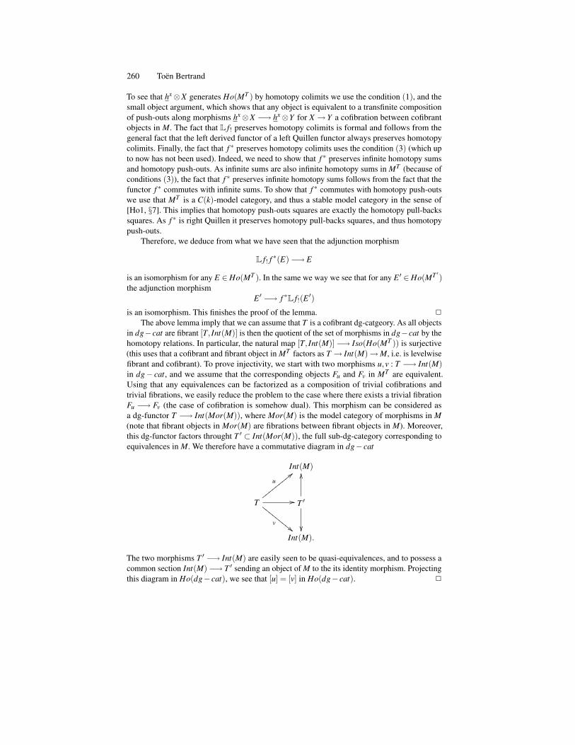
260 Toen Bertrand
To see that hx⊗X generates Ho(MT ) by homotopy colimits we use the condition (1), and thesmall object argument, which shows that any object is equivalent to a transfinite compositionof push-outs along morphisms hx⊗X −→ hx⊗Y for X → Y a cofibration between cofibrantobjects in M. The fact that L f! preserves homotopy colimits is formal and follows from thegeneral fact that the left derived functor of a left Quillen functor always preserves homotopycolimits. Finally, the fact that f ∗ preserves homotopy colimits uses the condition (3) (which upto now has not been used). Indeed, we need to show that f ∗ preserves infinite homotopy sumsand homotopy push-outs. As infinite sums are also infinite homotopy sums in MT (because ofconditions (3)), the fact that f ∗ preserves infinite homotopy sums follows from the fact that thefunctor f ∗ commutes with infinite sums. To show that f ∗ commutes with homotopy push-outswe use that MT is a C(k)-model category, and thus a stable model category in the sense of[Ho1, §7]. This implies that homotopy push-outs squares are exactly the homotopy pull-backssquares. As f ∗ is right Quillen it preserves homotopy pull-backs squares, and thus homotopypush-outs.
Therefore, we deduce from what we have seen that the adjunction morphism
L f! f ∗(E)−→ E
is an isomorphism for any E ∈Ho(MT ). In the same we way we see that for any E ′ ∈Ho(MT ′)the adjunction morphism
E ′ −→ f ∗L f!(E ′)
is an isomorphism. This finishes the proof of the lemma. 2
The above lemma imply that we can assume that T is a cofibrant dg-catgeory. As all objectsin dg−cat are fibrant [T, Int(M)] is then the quotient of the set of morphisms in dg−cat by thehomotopy relations. In particular, the natural map [T, Int(M)]−→ Iso(Ho(MT )) is surjective(this uses that a cofibrant and fibrant object in MT factors as T → Int(M)→M, i.e. is levelwisefibrant and cofibrant). To prove injectivity, we start with two morphisms u,v : T −→ Int(M)in dg− cat, and we assume that the corresponding objects Fu and Fv in MT are equivalent.Using that any equivalences can be factorized as a composition of trivial cofibrations andtrivial fibrations, we easily reduce the problem to the case where there exists a trivial fibrationFu −→ Fv (the case of cofibration is somehow dual). This morphism can be considered asa dg-functor T −→ Int(Mor(M)), where Mor(M) is the model category of morphisms in M(note that fibrant objects in Mor(M) are fibrations between fibrant objects in M). Moreover,this dg-functor factors throught T ′ ⊂ Int(Mor(M)), the full sub-dg-category corresponding toequivalences in M. We therefore have a commutative diagram in dg− cat
Int(M)
T
u<<yyyyyyyyy //
v""EEEEEEEEE T ′
OO
Int(M).
The two morphisms T ′ −→ Int(M) are easily seen to be quasi-equivalences, and to possess acommon section Int(M)−→ T ′ sending an object of M to the its identity morphism. Projectingthis diagram in Ho(dg− cat), we see that [u] = [v] in Ho(dg− cat). 2
Lectures on DG-categories 261
We will now deduce from proposition 4.1.2 a description of the set of maps [T,T ′] betweentwo objects in Ho(dg− cat). For this we use the C(k)-enriched Yoneda embedding
h : T ′ −→ Int((T ′)op−Mod),
sending an object x ∈ T ′ to the (T ′)op-dg-module defined by
hx : (T ′)op −→ C(k)y 7→ T ′(y,x).
The dg-module h is easily seen to be cofibrant and fibrant in (T ′)op−Mod, and thus we havehx ∈ Int((T ′)op−Mod) as required. The enriched version of the Yoneda lemma implies that his a quasi-fully faithful dg-functor. More precisely, we can show that the induced morphism ofcomplexes
T ′(x,y)−→ Hom(hx,hy) = Int((T ′)op−Mod)((hx,hy)
is an isomorphims of complexes.Using the description of maps in Ho(dg− cat) as being homotopy classes of morphisms
between cofibrant objects, we see that the morphism h induces a injective map
[T,T ′] → [T, Int((T ′)op−Mod)]
whose image consists of morphisms T −→ Int((T ′)op−Mod) factorizing in Ho(dg− cat)throught the quasi-essential image of h. We easily get this way the following corollary (see§3.2 and exercice 2.3.4 for the definition of the tensor product of two dg-categories).
Corollary 1. Let T and T ′ be two dg-categories, one of them having cofibrant complexes ofmorphisms. Then, there exists a natural bijection between [T,T ′] and the subset of Iso(Ho(T ⊗(T ′)op−Mod)) consisting of T ⊗ (T ′)op-dg-modules F such that for any x ∈ T , there is y ∈ T ′
such that Fx,− and hy are isomorphic in Ho((T ′)op−Mod).
Exercise 4.1.4 Let T be a dg-category.
(a) Show that [1,T ] is in bijection with the set of isomorphism classes of objects in the categoryH0(T ) (recall that 1 is the unit dg-category, with a unique object and k as algebra ofendormorphisms).
(b) Show that [∆ 1k ,T ] is in bijection with the set of isomorphism classes of morphisms in the
category H0(T ) (recall that ∆ 1k is the dg-category with two object and freely generated by
a unique non trivial morphism).
Exercise 4.1.5 Let C and D be two k-linear categories, also considered as dg-categories overk. Show that there exists a natural bijection between [C,D] and the set of isomorphism classesof k-linear functors from C to D. Deduce from this that there exists a fully faithful functor
Ho(k− cat)−→ Ho(dg− catk),
from the homotopy category of k-linear categories (k-linear categories and isomorphism classesof k-linear functors) and the homotopy category of dg-categories.
Exercise 4.1.6 Let R be an associative and unital k-algebra, which is also considered asdg-category with a unique object and R as endomorphisms of this object. Show that there isa natural bijection between [R, Int(C(k))] and the set of isomorphism classes of the derivedcategory D(R).
262 Toen Bertrand
4.2 Existence of internal Homs
For two dg-catgeories T and T ′ we can construct their tensor product T ⊗T ′ in the followingway. The set of objects of T ⊗T ′ is the product Ob(T )×Ob(T ′). For (x,y) ∈ Ob(T )2 and(x′,y′) ∈ Ob(T ′)2 we set
(T ⊗T ′)((x,x′),(y,y′)) := T (x,y)⊗T (x′,y′),
with the obvious compositions and units. When k is not a field the functor ⊗ does not preservesquasi-equivalences. However, it can be derived by the following formula
T ⊗L T ′ := Q(T )⊗Q(T ′),
where Q is a cofibrant replacement functor on dg− cat. This defines a symmetric monoidalstructure
−⊗L− : Ho(dg− cat)×Ho(dg− cat)−→ Ho(dg− cat).
Proposition 4.2.1 The monoidal structure −⊗L − is closed. In other words, for two dg-categories T and T ′ there is third dg-category RHom(T,T ′) ∈Ho(dg−cat), such that for anythird dg-category U there exists a bijection
[U,RHom(T,T ′)]' [U⊗L T,T ′],
functorial in U ∈ Ho(dg− cat).
Idea of proof: As for the corollary 1 we can reduce the problem of showing thatRHom(T, Int(M)) exists for a C(k)-model category M satisfying the same conditions as inproposition 4.1.2. Under the same hypothesis than corollary 1 it can be checked (using proposi-tion 4.1.2) that RHom(T, Int(M)) exists and is given by Int(MT ). 2
For two dg-categories T and T ′, one of them having cofibrant complexes of mor-phisms it is possible to show that RHom(T,T ′) is given by the full sub-dg-category ofInt(T ⊗ (T ′)op−Mod) consisting of dg-modules satifying the condition of corollary 1.
Finally, note that when M = C(k) we have
RHom(T, Int(C(k)))' Int(T −Mod).
In particular, we find a natural equivalence of categories
D(T )' H0(RHom(T, Int(C(k)))),
which is an important formula.
In the sequel we will use the following notations for a dg-category T
L(T ) := Int(T −Mod)' RHom(T, Int(C(k)))
T := Int(T op−Mod)' RHom(T op, Int(C(k))).
Note that we have natural equivalences
Lectures on DG-categories 263
H0(L(T ))' D(T ) H0(T )' D(T op).
Therefore, L(T ) and T are dg-enhancement of the derived categories D(T ) and D(T op). Notealso that the Yoneda embedding of definition 3.2.7 is now a dg-functor
h : T −→ T .
Exercise 4.2.2 (a) Let R be an associative and unital k-algebra which is considered as adg-category with a unique object. Show that there is an isomorphism in Ho(dg− cat)
RHom(R, Int(C(k)))' L(R).
(b) Show that for any two k-algebras R and R′, one of them being flat over k we have
RHom(R,L(R′))' L(R⊗R′).
Exercise 4.2.3 Let T be a dg-category. We define the Hochschild cohomology of T by
HH∗(T ) := H∗(RHom(T,T )(id, id)).
Let R be an associative k-algebra, flat over k, and considered as a dg-category with a uniqueobject. Show that we have
HH∗(R) := Ext∗R⊗Rop(R,R),
where the right hand side are the ext-groups computed in the derived category of R⊗Rop-modules.
4.3 Existence of localizations
Let T be a dg-category and let S be subset of morphisms in H0(T ) we would like to invertin Ho(dg− cat). For this, we will say that a morphism l : T −→ LST in Ho(dg− cat) is alocalization of T along S if for any T ′ ∈ Ho(dg− cat) the induced morphism
l∗ : [LST,T ′]−→ [T,T ′]
is injective and its image consists of all morphisms T −→ T ′ in Ho(dg− cat) whose inducedfunctor H0(T )−→ H0(T ′) sends all morphisms in S to isomorphisms in H0(T ). Note that thefunctor H0(T )−→ H0(T ′) is only well defined in Ho(Cat) (i.e. up to isomorphism), but thisis enough for the definition to makes sense as the condition of sending S to isomorphisms isstable by isomorphism between functors.
Proposition 4.3.1 For any dg-category T and any set of maps S in H0(T ), a localizationT −→ LST exists in Ho(dg− cat).
Idea of proof (see [To1] for details): We start by the most simple example of a localization.We first suppose that T := ∆ 1
k is the dg-category freely generated by two objects, 0 and 1, and aunique morphism u : 0→ 1. More concretely, T (0,1) = T (0,0) = T (1,1) = k and T (1,0) = 0,together with the obvious compositions and units. We let 1 be the dg-category with a uniqueobject ∗ and 1(∗,∗) = k (with the obvious composition). We consider the dg-foncteur T −→ 1
264 Toen Bertrand
sending the non trivial morphism of T to the identity of ∗ (i.e. k = T (0,1)→ 1(∗,∗) = k isthe identity). We claim that this morphism T −→ 1 is a localization of T along S consistingof the morphism u : 0→ 1 of T = H0(T ). This in fact follows easily from our proposition4.1.2. Indeed, for a C(k)-model category M the model category MT is the model category ofmorphisms in M. It is then easy to check that the functor Ho(M) −→ Ho(MT ) sending anobject of M to the identity morphism in M is fully faithful and that its essential image consistsof all equivalences in M.
In the general case, let S be a subset of morphisms in H0(T ) for some dg-category T . Wecan represent the morphisms S by a dg-functor⊔
S∆
1k −→ T,
sending the non trivial morphism of the component s to a representative of s in T . We defineLST as being the homotopy push-out (see [Ho1] for this notion)
LST := (⊔S
1)L⊔
⊔S ∆ 1
k
T.
The fact that each morphism ∆ 1k −→ 1 is a localization and the universal properties of homotopy
push-outs imply that the induced morphism T −→ LST defined as above is a localization of Talong S. 2
Exercise 4.3.2 Let ∆ 1k be the dg-category with two objects and freely generated by a non
trivial morphism u between these two objects. We let S := u be the image of u in H0(∆ 1k ).
Show that LS∆ 1k ' 1.
Exercise 4.3.3 Let T and T ′ be two dg-categories and S and S′ be two sets of morphisms inH0(T ) and H0(T ′) that contain all the identities. Prove that there is a natural isomorphism inHo(dg− cat)
LST ⊗L LS′T′ ' LS⊗LS′T ⊗L T ′.
The following proposition describes Int(M) as a dg-localization of M.
Proposition 4.3.4 Let M be a cofibrantly generated C(k)-model category, considered also asdg-category M. There exists a natural isomorphism in Ho(dg− cat)
Int(M)' LW M.
Idea of proof: We consider the natural inclusion dg-functor i : Int(M)−→M. This inclusionfactors as
Int(M)j // M f k // M,
where M f is the full sub-dg-category of M consisting of fibrant objects. Using that M iscofibrantly generated we can construct dg-functors
Lectures on DG-categories 265
r : M −→M f q : M f −→ Int(M)
together with morphisms
jq→ id q j→ id id→ ri id→ ir.
Moreover, these morphisms between dg-functors are levelwise in W . This can be seen to implythat the induced morphisms on localizations
LW Int(M)−→ LW M f −→ LW M
are isomorphisms in Ho(dg− cat). Finally, as morphisms in W are already invertible inH0(Int(M))' Ho(M), we have LW Int(M)' Int(M). 2
Finally, one possible way to understand localizations of dg-categories is by the followingproposition.
Proposition 4.3.5 Let T be a dg-category and S be a subset of morphisms in H0(T ). Then, thelocalization morphism l : T −→ LST induces a fully faithful functor
l∗ : D(LST )−→ D(T )
whose image consists of all T -dg-modules F : T −→ C(k) sending all morphisms of S toquasi-isomorphisms in C(k).
Idea of proof: This follows from the existence of internal Homs and localizations, as wellas the formula
D(T )' H0(RHom(T, Int(C(k)))) D(LST )' H0(RHom(LST, Int(C(k)))).
Indeed, the universal properties of localizations and internal Homs implies thatRHom(LST, Int(C(k)))can be identified full the full sub-dg-category of RHom(T, Int(C(k))) consisting of dg-functorssending S to quasi-isomorphisms in C(k). 2
Exercise 4.3.6 Let l : T −→ LST be a localization of a dg-category with respect to set ofmorphisms S in H0(T ), and let
Ll! : D(T op)−→ D(LST op)
be the induced functor in the corresponding derived categories of modules. Let WS be the thesubset of morphisms u in D(T op) such that Ll!(u) is an isomorphism in D(LST op).
(a) Show that a morphism u : E −→ F of D(T op) is in WS if and only if for any G ∈ D(T op)such that Gx −→ Gy is a quasi-isomorphism for all x→ y in S, the induced map
u∗ : HomD(T op)(F,G)−→ HomD(T op)(E,G)
is bijective.(b) Show that the induced functor
W−1S D(T op)−→ D(LST op)
is an equivalence of categories.
266 Toen Bertrand
4.4 Triangulated dg-categories
In this section we will introduce a class of dg-categories called triangulated. The notion ofbeing triangulated is the dg-analog of the notion of being Karoubian for linear categories. Wewill see that any dg-category has a triangulated hull, and this will allow us to introduce a notionof Morita equivalences which is a dg-analog of the usual notion of Morita equivalences betweenlinear categories. The homotopy category of dg-categories up to Morita equivalences will thenbe introduced and shown to have better properties than the category Ho(dg− cat). We will seein the next lecture that many invariants of dg-categories (K-theory, Hochschild homology . . . )factor throught Morita equivalences.
Let T be a dg-category. We recall the existence of the Yoneda embedding (see definition3.2.7)
T −→ T = Int(T op−Mod),
which is quasi-fully faithful. Passing to homotopy categories we get a fully faithful morphism
h : H0(T )−→ D(T op).
An object in the essential image of this functor will be called quasi-representable.Recall that an object x ∈ D(T op) is compact if the functor
[x,−] : D(T op)−→ k−Mod
commutes with arbitrary direct sums. It is easy to see that any quasi-representable object iscompact (see exercice 3.2.4). The converse is not true and we set the following definition.
Definition 4.4.1 A dg-category T is triangulated if and only if every compact object in D(T op)is quasi-representable.
Remark 3. When T is triangulated we have an equivalence of categories H0(T )' D(T op)c,where D(T op)c is the full sub-category of D(T ) of compact objects. The category D(T ) has anatural triangulated structure which restricts to a triangulated structure on compact objects(see [Ne] for more details on the notion of triangulated categories). Therefore, when T istriangulated dg-category its homotopy category H0(T ) comes equiped with a natural trian-gulated structure. This explains the terminology of triangulated dg-category. For more aboutthe relations between the notions of triangulated dg-categories and the notions of triangulatedcategories we refer to [Bo-Ka]. However, it is not necessary to know the theory of triangulatedcategories in order to understand triangulated dg-categories, and thus we will not study indetails the precise relations between triangulated dg-categories and triangulated categories.
We let Ho(dg− cattr) ⊂ Ho(dg− cat) be the full sub-category of triangulated dg-categories. Note that the notation Ho(dg− cattr) suggests that this category is the homotopycategory of some model category.We will see that it is, equivalent to, the localization of thecategory dg− cat along the class of Morita equivalences, that will be introduced later on inthis section.
Proposition 4.4.2 The natural inclusion
Ho(dg− cattr)−→ Ho(dg− cat)
has a left adjoint. In other words, any dg-category has a triangulated hull.
Lectures on DG-categories 267
Idea of proof: Let T be a dg-category. We consider the Yoneda embedding (see definition3.2.7)
h : T −→ T .
This is a quasi-fully faithful dg-functor. We consider Tpe ⊂ T , the full sub-dg-category consist-ing of all objects which are compact in D(T op) (these objects will simply be called compact).The dg-category Tpe will be called the dg-category of perfect T op-dg-modules, or equiva-lently of compact T op-dg-modules. As any quasi-representable object is compact, the Yonedaembedding factors as a full embedding
h : T −→ Tpe.
Let now T ′ be a triangulated dg-category. By definition, the natural morphism
T ′ −→ T ′pe
is an isomorphism in Ho(dg− cat). We can then consider the induced morphism
[Tpe, T ′pe]−→ [T, T ′pe],
induced by the resytiction along the morphism T −→ Tpe. The hard point is to show that thismap in bijective and that Tpe is a triangulated dg-category. These two facts can be deducedfrom the followin lemma and the proposition 4.1.2.
Lemma 4.4.3 Let T be a dg-category, and h : T −→ Tpe be the natural inclusion. Let M be aC(k)-model category which satisfies the conditions (1), (2) and (3) of §3.1. Then the Quillenadjunction
h! : MT −→MTpe MT ←−MTpe : h∗
is a Quillen equivalence.
The proof of the above lemma can be found in [To1, Lem. 7.5]. It is based on the fundamen-tal fact that the quasi-representable objects in D(T op) generate the sub-category of compactobjects by taking a finite number of finite homotopy colimits, shifts and retracts, together withthe fact that Lh! and h∗ both preserve these finite homotopy colimits, shifts and retracts. 2
The proof of the proposition shows that the left ajoint to the inclusion is given by
(−)pe : Ho(dg− cat)−→ Ho(dg− cattr),
sending a dg-category T to the full sub-dg-category Tpe of T consisting of all compact objects.For example, if R is a k-algebra, considered as a dg-category with a unique object BR, BRpe
is the dg-category of cofibrant and perfect complexes of R-modules. In particular
H0(BRpe)' Dpar f (R)
is the perfect derived category of R. This follows from the fact that compact objects in D(R) areprecisely the perfect complexes (this is a well known fact which can also be deduced from thegeneral result [To-Va, Prop. 2.2]). Therefore, we see that the dg-category of perfect complexesover some ring R is the triangulated hull of R.
268 Toen Bertrand
Definition 4.4.4 A morphism T −→ T ′ in Ho(dg− cat) is called a Morita equivalence if theinduced morphism in the triangulated hull
Tpe −→ T ′pe
is an isomorphism in Ho(dg− cat).
It follows formally from the existence of the left adjoint T 7→ Tpe that Ho(dg− cattr)is equivalent to the localized category W−1
mordg− cat, where Wmor is the subset of Moritaequivalences in dg− cat as defined above.
Exercise 4.4.5 Prove the above assertion: the functor
(−)pe : Ho(dg− cat)−→ Ho(dg− cattr)
induces an equivalence of categories
W−1morHo(dg− cat)' Ho(dg− cattr).
We can characterize the Morita equivalences in the following equivalent ways.
Proposition 4.4.6 Let f : T −→ T ′ be a morphism of dg-categories. The following are equiva-lent.
(a) The morphism f is a Morita equivalence.(b) For any triangulated dg-category T0, the induced map
[T ′,T0]−→ [T,T0]
is bijective.(c) The induced functor
f ∗ : D(T ′)−→ D(T )
is an equivalence of categories.(d) The functor
L f! : D(T )−→ D(T ′)
induces an equivalence between the full sub-category of compact objects.
Exercise 4.4.7 Prove the proposition 4.4.6.
We finish this section by a description of morphisms in Ho(dg−cattr) in termes of derivedcategories of bi-dg-modules.
Proposition 4.4.8 Let T and T ′ be two dg-categories. Then, there exists a natural bijection be-tween [Tpe, T ′pe] and the subset of Iso(D(T ⊗L (T ′)op)) consisting of T ⊗L (T ′)op-dg-modulesF such that for any x ∈ T , the (T ′)op-dg-module Fx,− is compact.
Lectures on DG-categories 269
Exercise 4.4.9 Give a proof of proposition 4.4.8.
Exercise 4.4.10 (a) Show that the full sub-category Ho(dg− cattr) ⊂ Ho(dg− cat) is notstable by finite coproducts (taken inside Ho(dg− cat)).
(b) Show that the category Ho(dg− cattr) has finite sums and finite products.(c) Show that in the category Ho(dg− cattr), the natural morphism
T⊔
T ′ −→ T ×T ′,
for any T and T ′ objects in Ho(dg− cattr). Note that the symbols⊔
and × refer here tothe categorical sum and product in the category Ho(dg− cattr).
(d) Deduce from this that the set of morphisms Ho(dg− cattr) are endowed with naturalstructure of commutative monoids such that the composition is bilinear. Identify thismonoid structure with the direct sum on the level of bi-dg-modules throught the bijectionof corollary 1.
Exercise 4.4.11 Let T −→ T ′ be a Morita equivalence and T0 be a dg-category. Show that theinduced morphism
T ⊗L T0 −→ T ′⊗L T0
is again a Morita equivalence (use the lemma 4.4.3).
Exercise 4.4.12 Let T and T ′ be two triangulated dg-catgeory, and define
T ⊗LT ′ := T ⊗L T ′pe.
(a) Show that (T,T ′) 7→ T ⊗LT ′ defines a symmetric monoidal structure on Ho(dg−cattr) insuch a way that the functor
(−)pe : Ho(dg− cat)−→ Ho(dg− cattr)
is a symmetric monoidal functor.(b) Show that the monoidal structure ⊗L is closed on Ho(dg− cattr).
Exercise 4.4.13 (a) Let T and T ′ be two dg-categories. Prove that the Yoneda embeddingh : T → Tpe induces an isomorphism in Ho(dg− cat)
RHom(Tpe, T ′pe)−→ RHom(T, T ′pe).
(b) Deduce from this that for any dg-category T there is a morphism in Ho(dg− cat)
RHom(T,T )−→ RHom(Tpe, Tpe)
which is quasi-fully faithful.(c) Deduce from this that for any dg-category T there exist isomorphisms
HH∗(T )' HH∗(Tpe).
270 Toen Bertrand
5 Lecture 4: Some applications
In this last lecture I will present some applications of the homotopy theory of dg-categories. Wewill see in particular how the problems mentioned in §1.2 can be solved using dg-categories.The very last section will be some discussions on the notion of saturated dg-categories andtheir use in the definition of a secondary K-theory functor.
5.1 Functorial cones
One of the problem encountered with derived categories is the non existence of functorial cones.In the context of dg-categories this problem can be solved as follows.
Let T be a triangulated dg-category. We let ∆ 1k be the dg-category freely generated by two
objects 0 and 1 and freely generated by one non trivial morphism 0→ y, and 1 be the unitdg-category (with a unique object and k for its endomorphism). There is a morphism
∆1k −→ 1pe
sending 0 to 0 and 1 to k. We get an induced morphism in Ho(dg− cat)
RHom(1pe,T )−→ RHom(∆ 1k ,T ).
As T is triangulated we have
RHom(1pe,T )' RHom(1,T )' T.
Therefore, we have defined a morphism in Ho(dg− cat)
f : T −→ RHom(∆ 1k ,T ) =: Mor(T ).
The dg-category Mor(T ) is also the full sub-dg-category of Int(Mor(T op−Mod)) correspond-ing to quasi-representable dg-modules, and is called the dg-category of morphisms in T . Themorphism f defined above intuitively sends an object x ∈ T to 0→ x in Mor(T ) (note that 0 isan object in T because T is triangulated).
Proposition 5.1.1 There exists a unique morphism in Ho(dg− cat)
c : Mor(T )−→ T
such that the following two (T ⊗LMor(T )op)-dg-modules
(z,u) 7→Mor(T )(u, f (z)) (z,u) 7→ T (c(u),z)
are isomorphic in D(T ⊗LMor(T )op) (In other words, the morphism f admits a left adjoint).
Idea of proof: We consider the following explicit models for T , Mor(T ) and f . We let T ′
be the full sub-dg-category of T consisting of quasi-representable objects (or equivalentelyof compact objects as T is triangulated). We let Mor(T )′ be the full sub-dg-category ofInt(Mor(T op−Mod)) consisting of morphisms between quasi-representable objects (theseare also the compact objects in Ho(Mor(T op−Mod)) because T is triangulated). We note
Lectures on DG-categories 271
that Mor(T )′ is the dg-category whose objects are cofibrations between cofibrant and quasi-representable T op-dg-modules. To each compact and cofibrant T op-dg-module z we consider0→ z as an object in T ′. This defines a dg-functor T ′ −→Mor(T )′ which is a model for f . Wedefine c as being a C(k)-enriched left adjoint to c (in the most naive sense), sending an objectc : x−→ y of Mor(T )′ to c(u) defined by the push-out in T op−Mod
x //
y
0 // c(u).
We note that the T op-module c(u) is compact and thus belongs to T ′. It is easy to check that c,as a morphism in Ho(dg− cat) satisfies the property of the proposition.
The unicity of c is proved formally, in the same way that one proves the unicity of adjointsin usual category theory. 2
The morphism c : Mor(T ) −→ T is a functorial cone construction for the triangulateddg-category T . The important fact here is that there is a natural functor
H0(Mor(T ))−→Mor(H0(T )),
which is essentially surjective, full but not faithful in general. The functor
H0(c) : H0(Mor(T ))−→ H0(T )
does not factor in general throught Mor(H0(T )).
To finish, proposition 5.1.1 becomes really powerful when combined with the followingfact.
Proposition 5.1.2 Let T be a triangulated dg-category and T ′ be any dg-category. ThenRHom(T ′,T ) is triangulated.
Exercise 5.1.3 Deduce proposition 5.1.2 from exercice 4.4.11.
One important feature of triangulated dg-categories is that any dg-functor f : T −→ T ′
between triangulated dg-categories commutes with cones. In other words, the diagram
Mor(T ) c //
c( f )
T
f
Mor(T ′) c
// T ′
commutes in Ho(dg− cat). This has to be understood as a generalization of the fact that anylinear functor between additive categories commutes with finite direct sums. This propertyof triangulated dg-categories is very useful in practice, as then any dg-functor T −→ T ′
automatically induces a triangulated functor H0(T )−→ H0(T ′).
272 Toen Bertrand
Exercise 5.1.4 Prove the above assertion, that
Mor(T ) c //
c( f )
T
f
Mor(T ′) c
// T ′
commutes in Ho(dg− cat) (here T and T ′ are triangulated dg-categories).
5.2 Some invariants
Another problem mentioned in §1.2 is the fact that the usual invariants, (K-theory, Hochschildhomology and cohomology . . . ), are not invariants of derived categories. We will see here thatthese invariants can be defined on the level of Ho(dg− cattr). We will treat the examples ofK-theory and Hochschild cohomology.
(a) Let T be a dg-category. We consider T op−Modcc the full sub-category of compact andcofibrant T op-dg-modules. We can endow T op−Modcc with a structure of an exact com-plicial category (see [Sch2]) whose equivalences are quasi-isomorphisms and cofibrationsare the cofibrations of the model category structure on T op−Mod. This Waldhausencategory defines a K-theory space K(T ) (see [Sch2]). We note that if T is triangulated wehave
K0(T ) := π0(K(T ))' K0(H0(T )),
where the last K-group is the Grothendieck group of the triangulated category H0(T ).Now, let f : T −→ T ′ be a morphism between dg-categories. It induces a functor
f! : T op−Mod −→ (T ′)op−Mod.
This functor preserves cofibrations, compact cofibrant objects and push-outs. Therefore, itinduces a functor between Waldhausen categories
f! : T op−Modcc −→ (T ′)op−Modcc
and a morphism on the corresponding spaces
f! : K(T )−→ K(T ′).
This defines a functorK : dg− cat −→ Sp
from dg-categories to spectra. It is possible to show that this functor sends Morita equiva-lences to stable equivalences, and thus defines a functor
K : Ho(dg− cattr)−→ Ho(Sp).
We see it particular that two dg-categories which are Morita equivalent have the sameK-theory.
Lectures on DG-categories 273
(b) (See also exercice 4.4.13) Let T be a dg-category. We consider RHom(T,T ), the dg-category of (derived) endomorphisms of T . The identity gives an object id ∈RHom(T,T ),and we can set
HH ·(T ) := RHom(T,T )(id, id),
the Hochschild complex of T . This is a well defined object in D(k), the derived categoryof complexes of k-modules, and the construction T 7→ HH ·(T ) provides a functor ofgroupoids
Ho(dg− cat)iso −→ D(k)iso.
Using the results of §3.2 we can see that
HH∗(T )' Ext∗(T,T ),
where the Ext-group is computed in the derived category of T ⊗L T op-dg-modules. Inparticular, when T is given by an associative flat k-algebra R we find
HH∗(T )' Ext∗R⊗R(R,R),
which is usual Hochschild cohomology. The Yoneda embedding T −→ Tpe, provides anisomorphism in Ho(dg− cat)
RHom(Tpe, Tpe)' RHom(T, Tpe),
and a quasi-fully faithful morphism
RHom(T,T )−→ RHom(T, Tpe).
Therefore, we get a quasi-fully faithful morphism in Ho(dg− cat)
RHom(T,T )−→ RHom(Tpe, Tpe)
sending the identity to the indentity. Therefore, we obtain a natural isomorphism
HH ·(T )' HH ·(Tpe).
We get that way that Hochschild cohomology is a Morita invariant.(c) There also exists an interpretation of Hochschild homology purely in termes of dg-
categories in the following way. We consider two dg-categories T and T ′, and the Yonedaembedding h : T → T . We obtain an induced functor
h! : RHom(T, T ′)−→ RHom(T , T ′).
It is possible to show that this morphism is quasi-fully faithful and that its quasi-essentialimage consists of all morphisms T −→ T ′ which are continuous (i.e. commute with directsums). We refer to [To1, Thm. 7.2] for more details about this statement. This implies thatthere is an isomorphism in Ho(dg− cat)
RHom(T, T ′)' RHomc(T , T ′),
where RHomc denotes the full sub-dg-category of continuous dg-functors.Let now T be a dg-category and consider the T ⊗LT op-dg-module sending (x,y) to T (y,x).This dg-module can be represented by an object in the dg-category
274 Toen Bertrand
L(T ⊗L T op)' RHom(T ⊗L T op, 1)' RHomc(T ⊗L T op, 1),
and thus by a continuous in Ho(dg− cat)
L(T ⊗L T op)−→ 1.
The image of T , considered as a bi-module sending (x,y) to T (y,x), by this morphism isdenoted by HH·(T ) ∈ D(k)' H0(1), and is called the Hochschild homology complex ofT . When T is a flat k-algebra R then we have
HH·(T )' R⊗LR⊗Rop R ∈ D(k).
From its definition, it is not hard to show that T 7→ HH·(T ) is invariant by Morita equiva-lences.
5.3 Descent
In this section we will see how to solve the non-local nature of derived categories explained in§1.2. For this, let X be a scheme. We have the Grothendieck category C(OX ) of (unbounded)complexes of sheaves of OX -modules. This category can be endowed with a model categorystructure for which the equivalences are the quasi-isomorphisms (of complexes of sheaves) andthe cofibrations are the monomorphisms (see e.g. [Ho2]). Moreover, when X is a k-schemethen the natural C(k)-enrichment of C(OX ) makes it into a C(k)-model category. We let
L(OX ) := Int(C(OX )),
and we let Lpe(X) be the full sub-dg-category consisting of perfect complexes on X . TheK-theory of X can be defined as
K(X) := K(Lpe(X)),
using the definition of K-theory of dg-categories we saw in the last section.When f : X −→ Y is a morphism of schemes, it is possible to define two morphisms in
Ho(dg− cat)L f ∗ : L(OY )−→ L(OX ) L(OY )←− L(OX ) : R f∗,
which are adjoints (according to the model we chose L f ∗ is a bit tricky to define explicitly).The morphism
L f ∗ : L(OY )−→ L(OX )
always preserves perfect complexes are induces a morphism
L f ∗ : Lpe(Y )−→ Lpe(X).
This construction provides a functor
Lpe : k−Schop −→ Ho(dg− cattr),
from the (opposite of) category of k-schemes to the category of triangulated dg-categories.The existence of this functor is the starting point of an extremelly rich source of questionsabout its behaviour. Following the philosophy of non-commutative geometry according to M.Kontsevich, Ho(dg− cattr) can be considered as the category of non-commutative schemes,and the functor Lpe above is simply passing from the commutative to the non-commutativesetting. Contrary to what this might suggest, at leas as first naive thoughts, the functor Lpe isfar from being an embedding and its general study leads to very interesting questions.
Lectures on DG-categories 275
(a) A first observation is that two schemes X and Y can be such that Lpe(X)' Lpe(Y ) withoutbeing isomorphic, as shown by many well known examples of derived equivalences (see[Ro] for more about this). The fibers of the functor Lpe, that is the set of schemes, upto isomorphisms, having the same dg-categories of perfect complexes, is expected to befinite, at least when we restrict to smooth and projective schemes. It is shown in [An-To]that these fibers are discrete and countable.
(b) The functor Lpe sends direct product of k-schemes into tensor product in Ho(dg− cattr),at least under reasonable conditions (see [To1], [Fr-Be-Na]). In other words, Lpe is asymmetric monoidal functor, when k−Sch is considered as a symmetric monoidal categoryfor the direct monoidal structure.
(c) The image of the smooth and proper k-schemes inside Ho(dg− cattr) has an explicitdescrition: its objects are smooth and projective k-schemes, and morphisms between twosuch schemes X and Y are given by quasi-isomorphism classes of perfect complexes onX ×k Y (see 5.3.2 below). This category is very close to the category of Chow motives, forwhich morphisms are rather correspondences up to rationnal equivalences. By analogy,Ho(dg− cattr) can be used in order to define a notion of non-commutative motives (see[Ko]). Constructing realisations for these non-commutative motives has lead to the notionof non-commutative Hodge structures (see [Ka-Ko-Pa]), and to the construction of thenon-commutative Gauss-Manin connexion (see [To-Ve]).
We now come back to the descent property. The following proposition will not be provedin these notes. We refer to [Hir-Si] for more details about the descent for perfect complexes.
Proposition 5.3.1 Let X = U ∪V , where U and V are two Zariski open subschemes. Then thefollowing square
Lpe(X) //
Lpe(U)
Lpe(V ) // Lpe(U ∩V )
is homotopy cartesian in the model category dg− cat.
Let us also mention the following related statement.
Proposition 5.3.2 Let X and Y be two smooth and proper schemes over Speck. Then, thereexists a natural isomorphism in Ho(dg− cat)
RHom(Lpe(X),Lpe(Y ))' Lpe(X×k Y ).
For a proof we refer the reader to [To1]. It should be emphasised here that the correspondingstatement is false on the level of derived categories. More precisely, let E ∈Dpar f (X×k Y ) andlet
φE : Dpar f (X) −→ Dpar f (Y )F 7→ R(pY )∗(E⊗L p∗X (F))
be the corresponding functor. The construction E 7→ φE defines a functor
φ− : Dpar f (X×k Y )−→ Funtr(Dpar f (X),Dpar f (Y )),
276 Toen Bertrand
where the right hand side is the category of triangulated functors from Dpar f (X) to Dpar f (Y ).When X and Y are projective over Speck (and that k is field) then it is known that this functoris essentially surjective (see [Ro]). In general it is not known if φ− is essentially surjective ornot. In any case, even for very simple X and Y the functor φ− is not faithful, and thus is not anequivalence of categories in general. Suppose for instance that X = Y = E and elliptic curveover k =C, and let ∆ ∈Dpar f (X×k X) be the structure sheaf of the diagonal. The image by φ−of the objects ∆ and ∆ [2] are respectively the identity functor and the shift by 2 functor. BecauseX is of cohomological dimension 1 we have Hom(id, id[2]) = 0, where this hom is computedin Funtr(Dpar f (X),Dpar f (X)). However, Hom(∆ ,∆ [2])' HH2(X)' H1(E,OE)' k.
5.4 Saturated dg-categories and secondary K-theory
We arrive at the last section of these lectures. We have seen that dg-categories can be usedin order to replace derived categories, and that they can be used in order to define K-theory.In this section we will see that dg-categories can also be considered as coefficients that canthemselves be used in order to define a secondary version of K-theory. For this I will present ananalogy between the categories Ho(dg− cattr) and k−Mod. Throught this analogy projectivek-modules of finite rank correspond to the notion of saturated dg-categories. I will then showhow to define secondary K-theory spectrum K(2)(k) using saturated dg-categories, and givesome ideas of how to define analogs of the rank and chern character maps in order to see thatthis secondary K-theory K(2)(k) is non-trivial. I will also mention a relation between K(2)(k)and the Brauer group, analog to the well known relation between K-theory and the Picard group.
We start by the analogies between the categories k−Mod of k-modules and Ho(dg−cattr).The true analogy is really betwen k−Mod and the homotopy theory of triangulated dg-categories, e.g. the simplicial category Ldg− cattr obtained by simplicial localization (see[To2]). The homotopy category Ho(dg− cattr) is sometimes too coarse to see the analogy. Wewill however restrict ourselves with Ho(dg−cattr), even though some of the facts below aboutHo(dg− cattr) are not completely intrinsic and requires to lift things to the model category ofdg-categories.
(a) The category k−Mod is a closed symmetric monoidal category for the usual tensor product.In the same way, Ho(dg− cattr) has a closed symmetric monoidal structure induced fromthe one of Ho(dg−cat) (see §3.2). Explicitly, if T and T ′ are two triangulated dg-categorywe form T ⊗L T ′ ∈ Ho(dg− cat). This is not a triangulated dg-category anymore and weset
T ⊗LT ′ := (T ⊗L T ′)pe ∈ Ho(dg− cattr).
The unit of this monoidal structure is the triangulated hull of 1, i.e. the dg-category ofcofibrant and perfect complexes of k-modules. The corresponding internal Homs is theone of Ho(dg− cat), as we already saw that RHom(T,T ′) is triangulated if T and T ′ are.
(b) The category k−Mod has a zero object and finite sums are also finite products. This isagain true in Ho(dg−cattr). The zero dg-category (with one object and 0 as endomorphismring of this object) is a zero object in Ho(dg− cattr). Also, for two triangulated dg-categories T and T ′ their sum T
⊔T ′ as dg-categories is not triangulated anymore. Their
direct sum in Ho(dg− cattr) is the triangulated hull of T⊔
T ′ , that is
T⊔
T ′pe' Tpe× T ′pe ' T ×T ′.
Lectures on DG-categories 277
We note that this second remarkable property of Ho(dg−cattr) is not satisfied by Ho(dg−cat) itself. We can say that Ho(dg− cattr) is semi-additive, which is justififed by the factthat the Homs in Ho(dg− cattr) are abelian monoids (or abelian semi-groups).
(c) The category k−Mod has arbitrary limits and colimits. The corresponding statement isnot true for Ho(dg− cattr). However, we have homotopy limits and homotopy colimits inHo(dg− cattr), whose existence are insured by the model category structure on dg− cat.
(d) There is a natural notion of short exact sequences in k−Mod. In the same way, there is anatural notion of short exact sequences in Ho(dg− cattr). These are the sequences of theform
T0j // T
p // (T/T0)pe,
where i is a quasi-fully faithful functor between triangulated dg-categories, and (T/T0)peis the quotient defined as the triangulated hull of the homotopy push-out of dg-categories
T0 //
T
0 // T/T0.
These sequences are natural in terms of the homotopy theory of triangulated dg-categoriesas it can be shown that quasi-fully faithful dg-functors are precisely the homotopy mono-morphisms in dg− cat, i.e. the morphsms T −→ T ′ such that the diagonal map
T −→ T ×hT ′ T
is a quasi-equivalence (the right hand side is a homotopy pull-back). This defines a dualnotion of homotopy epimorphisms of triangulated dg-categories as being the morphismT −→ T ′ such that for any triangulated dg-categories T ′′ the induced morphism
RHom(T ′,T ′′)−→ RHom(T,T ′′)
is a homotopy monomorphisms (i.e. is quasi-fully faithful). In the exact sequences above jis a homotopy monomorphism, p is a homotopy epimorphism, p is the cokernel of j and jis the kernel of p. The situation is therefore really close to the situation in k−Mod.
If k−Mod and Ho(dg−cattr) are so analoguous then we should be able to say what is theanalog property of being projective of finite rank, and to define a K-group or even a K-theoryspectrum of such objects. It turns that this can be done and that the theory can actually bepushed rather far. Also, we will see that this new K-theory migt have some geometric andarithmetic significance.
It is well know that the projective modules of finite rank over k are precisely the dualizable(also called rigid) objects in the closed monoidal category k−Mod. Recall that any k-moduleM has a dual M∨ := Hom(M,k), and that there always exists an evaluation map
M∨⊗M −→ Hom(M,M).
The k-module M is dualizable if this evaluation map is an isomorphism, and this is known tobe equivalent to the fact that M is projective of finite rank.
We will take this as a definition of projective triangulated dg-categories of finite rank. Thestriking fact is that these dg-categories have already been studied for other reasons under thename of saturated dg-categories, or smooth and proper dg-categories.
278 Toen Bertrand
Definition 5.4.1 A triangulated dg-category T is saturated if it is dualizale in Ho(dg− cattr),i.e. if the evaluation morphism
RHom(T, 1pe)⊗LT −→ RHom(T,T )
is an isomorphism in Ho(dg− cattr).
The saturated triangulated dg-categories can be characterized nicely using the notion ofsmooth and proper dg-algebras (see [To3, To-Va, Ko-So]). Recall that a dg-algebra B is smoothif B is a compact object in D(B⊗L Bop). Recall also that such a dg-algebra is proper if itsunderlying complex if perfect (i.e. if B is compact in D(k)). The following proposition can bededuced from the results of [To-Va]. We omit the proof in these notes (see however [To-Va] forsome statements about saturated dg-categories).
Proposition 5.4.2 A triangulated dg-category is saturated if and only if it is Morita equivalentto a smooth and proper dg-algebra.
This proposition is interesting as it allows us to show that there are many examples ofsaturated dg-categories. The two main examples are the following.
(a) Let X be a smooth and proper k-scheme. Then Lpe(X) is a saturated dg-category (see[To-Va]).
(b) For any k-algebra, which is projective of finite rank as a k-module and which is of finiteglobal cohomlogical dimension, the dg-category Ape of perfect complexes of A-modulesis saturated.
The symmetric monoidal category Ho(dg−catsat) of saturated dg-categories is rigid. Notethat any object T has a dual T∨ := RHom(T, 1pe). Moroever, it can be shown that T∨ ' T op
is simply the opposite dg-category (this is only true when T is saturated). In particular, for Tand T ′ two saturated dg-categories we have the following important formula
T op⊗LT ′ ' RHom(T,T ′).
We can now define the secondary K-group. We start by Z[sat], the free abelian group onisomorphism classes (in Ho(dg−cattr)) of satuared dg-categories. We define K(2)
0 (k) to be thequotient of Z[sat] by the relation
[T ] = [T0]+ [(T/T0)pe]
for any full saturated sub-dg-category T0 ⊂ T with quotient (T/T0)pe.More generally, we can consider a certain Waldhausen category Sat, whose objects are
cofibrant dg-categories T such that Tpe is saturated, whose morphisms are morphisms of dg-categories, whose equivalences are Morita equivalences, and whose cofibrations are cofibrationsof dg-categories which are also fully faithful. From this we can construct a spectrum, denotedby K(2)(k) by applying Waldhausen’s construction, called the secondary K-theory spectrum ofk. We have
π0(K(2)(k))' K(2)0 (k).
We no finish with some arguments that K(2)(k) to show that is non trivial and interesting.First of all, we have the following two basic properties.

Lectures on DG-categories 279
(a) k 7→ K(2)(k) defines a functor from the category of commutative rings to the homotopycategory of spectra. To a map of rings k→ k′ we associate the base change −⊗Lk k′ fromsaturated dg-categories over k to saturated dg-categories over k′, which induces a functorof Waldhausen categories and thus a morphism on the corresponding K-theory spectra.
(b) If k = colimiki is a filtered colimit of commutative rings then we have
K(2)(k)' colimiK(2)(ki).
This follows from the non trivial statement that the homotopy theory of saturated dg-categories over k is the filtered colimit of the homotopy theories of saturated dg-categoriesover the ki (see [To4]).
(c) The monoidal structure on Ho(dg−cattr) induces a commutative ring structure on K(2)0 (k).
I guess that this monoidal structure also induces a E∞-multiplication on K(2)(k).
Our next task is to prove that K(2)(k) is non zero. For this we construct a rank map
rk(2)0 : K(2)
0 (k)−→ K0(k)
which an analog of the usual rank map (also called the trace map)
rk0 : K0(k)−→ HH0(k) = k.
Let T be a saturated dg-category. As T is dualizable in Ho(dg− cattr) there exists a trace map
RHom(T,T )' T op⊗LT −→ 1pe,
which is the dual of the identity map
id : 1pe −→ T op⊗LT.
The image of the identity provides a perfect complex of k-modules, and thus an element
rk(2)0 (T ) ∈ K0(k).
This defines the maprk(2)
0 : K(2)0 (k)−→ K0(k).
It can be shown that rk(2)0 (T ) is in fact HH·(T ), the Hochschild homology complex of T .
Lemma 5.4.3 For any saturated dg-category T we have
rk(2)0 (T ) = [HH·(T )] ∈ K0(k),
where HH·(T ) is the (perfect) complex of Hochschild homology of T .
In particular we see that for X a smooth and proper k-scheme we have
rk(2)0 (Lpe(X)) = [HH·(X)] ∈ K0(k).
When k = C then HH∗(X) can be identified with Hodge cohomology H∗(X ,Ω∗X ), and thus
rk(2)0 (Lpe(X)) is then the euler characteristic of X . In other words, we can say that the rank of
280 Toen Bertrand
Lpe(X) is χ(X). The map rk(2)0 shows that K(2)
0 (k) is non zero.
The usual rank rk0 : K0(k)−→ HH0(k) = k is only the zero part of a rank map
rk∗ : K∗(k)−→ HH∗(k).
In the same way, it is possible to define a secondary rank map
rk(2)∗ : K(2)
∗ (k)−→ K∗(S1⊗L k),
where S1⊗L k is a simplicial ring that can be defined as
S1⊗L k = k⊗Lk⊗LZk k.
Note that by definition of Hochschild homology we have
HH·(k)' S1⊗L k,
so we can also writerk(2)∗ : K(2)
∗ (k)−→ K∗(HH·(k)).
Using this map I guess it could be possible to check that the higher K-groups K(2)i (k) are also
non zero in general. Actually, I think it is possible to construct an analog of the Chern character
Ch : K∗(k)−→ HC∗(k)
as a mapCh(2) : K(2)
∗ (k)−→ HC(2)∗ (k) := KS1
∗ (S1⊗L k),where the right hand side is the S1-equivariant K-theory of S1⊗L k (note that S1 acts on S1⊗L k),which we take as a definition of secondary cyclic homology (see [To-Ve1, To-Ve] for moredetails about this construction).
To finish we show that K(2)0 (k) has a relation with the Brauer group, analog to the relation
between K0(k) and the Picard group. For this, we define Brdg(k) to be the group of isomorphismclasses of invertible objects (for the monoidal structure) in Ho(dg− cattr). As being invertibleis stronger than being dualizable we have a natural map
Brdg(k)−→ K(2)0 (k)
analog to the natural mapPic(k)−→ K0(k).
Now, by definition Brdg(k) can also be described as the Morita equivalence classes of Azumaya’sdg-algebras, that is of dg-algebras B satisfying the following two properties(a)
Bop⊗L B−→ REndC(k)(B)is a quasi-isomorphism.
(b) The underlying complex of B is a compact generator of D(k).In particular, a non-dg Azumaya’s algebra over k defines an element in Brdg(k), and we
thus get a map Br(k)−→ Brdg(k), from the usual Brauer group of k (see [Mi]) to the dg-Brauer
group of k. Composing with the map Brdg(k)−→ K(2)0 (k) we get a map
Br(k)−→ K(2)0 (k),
from the usual Brauer group to the secondary K-group of k. I do not know if this map is injectivein general, but I guess it should be possible to prove that it is non zero in some examples byusing the Chern character mentioned above.
Lectures on DG-categories 281
References
[An-To] M. Anel, B. Toen, Denombrabilite des classes d’equivalences derivees de varietesalgebriques, J. Algebraic Geom. 18 (2009), no. 2, 257–277.
[SGA4-I] M. Artin, A. Grothendieck, J. L. Verdier, Theorie des topos et cohomologie etaledes schemas- Tome 1, Lecture Notes in Math 269, Springer Verlag, Berlin, 1972.
[Fr-Be-Na] J. Francis, D. Ben-Zvi, D. Nadler, Integral Transforms and Drinfeld Centers inDerived Algebraic Geometry, preprint arXiv arXiv:0805.0157.
[Bo-Ka] A. Bondal, M. Kapranov, Enhanced triangulated categories, Math. URSS Sbornik70 (1991), 93–107.
[Bour] N. Bourbaki, Elements de mathematique. Algbre. Chapitre 10. Algebre homologique,Springer-Verlag, Berlin, 2007.
[De] P. Deligne, Equations differentielles a points singuliers reguliers, Lecture Notes inMathematics 163, Springer-Verlag, Berlin-New York, 1970.
[Du-Sh] D. Dugger, B. Shipley, K-theory and derived equivalences, Duke J. Math 124 (2004),no. 3, 587–617.
[EKMM] A.D. Elmendorf, I. Kriz, M.A. Mandell, J.P. May, Rings, modules, and algebrasin stable homotopy theory, Mathematical Surveys and Monographs, vol. 47, AmericanMathematical Society, Providence, RI, 1997.
[G-Z] P. Gabriel, M. Zisman, Calculus of fractions and homotopy theory, Ergebnisse derMathematik und ihrer Grenzgebiete, Band 35 Springer-Verlag New York, Inc., New York1967.
[G-P] P. Gabriel, N. Popesco, Caracterisation des categories abeliennes avec generateurs etlimites inductives exactes, C. R. Acad. Sci. Paris 258 (1964) 4188–4190.
[Gr-Ha] P. Griffiths, J. Harris, Principles of algebraic geometry, Wiley Classics Library, JohnWiley and Sons, Inc., New York, 1994.
[Hir-Si] A. Hirschowitz, C. Simpson, Descente pour les n-champs, Preprint math.AG/9807049.[Ho1] M. Hovey, Model categories, Mathematical surveys and monographs, Vol. 63, Amer.
Math. Soc. Providence 1998.[Ho2] M. Hovey, Model category structures on chain complexes of sheaves, Trans. Amer.
Math. Soc. 353 (2001), no. 6, 2441–2457[Jo-Ti] A. Joyal, M. Tierney, Strong stacks and classifying spaces, Category theory (Como,
1990), 213–236, Lecture Notes in Math. 1488, Springer, Berlin, 1991.[Ka-Ko-Pa] L. Katzarkov, M. Kontsevich, T. Pantev, Hodge theoretic aspects of mirror sym-
metry, prepublication arXiv:0806.0107.[Kel] G. Kelly, Basic concepts of enriched category theory, London Mathematical Society
Lecture Note Series, 64, Cambridge Universtity Press, Cambridge-New York, 1982.[Ko] M. Kontsevich, Note of motives in finite characteristic, preprint arXiv math/0702206.[Ko-So] M. Kontsevich, Y. Soibelman, Notes on A-infinity algebras, A-infinity categories and
non-commutative geometry, preprint math.RA/060624.[May] J.P. May, Simplicial objects in algebraic topology, Van Nostrand Mathematical Studies
11, D. Van Nostrand Co., Inc., Princeton, N.J.-Toronto, Ont.-London 1967.[Mi] J. Milne, Etale cohomology, Princeton mathematical series 33, Princeton University Press
1980.[Ne] A. Neeman, Triangulated categories, Annals of Mathematics Studies 148, Princeton
University Press, Princeton, NJ, 2001.[Ro] R. Rouquier, Categories derivees et geometrie birationnelle (d’apres Bondal, Orlov,
Bridgeland, Kawamata et al.), Seminaire Bourbaki. Vol. 2004/2005. Astrisque No. 307(2006), Exp. No. 946, viii, 283–307.
282 Toen Bertrand
[Sch1] M. Schlichting, A note on K-theory and triangulated categories, Inv. Math. 150 (2002),111–116.
[Sch2] M. Schlichting, Higher Algebraic K-theory, this volume.[Si] C. Simpson, Higgs bundles and local systems, Inst. Hautes tudes Sci. Publ. Math. No. 75
(1992), 5–95.[Tab] G. Tabuada, Une structure de categorie de modeles de Quillen sur la categorie des
dg-categories, Comptes Rendus de l’Acadademie de Sciences de Paris 340 (2005), 15–19.[To1] B. Toen, The homotopy of dg-categories and derived Morita theory, Invent. Math. 167
(2007), no. 3, 615–667.[To2] B. Toen, Higher and derived stacks: A global overview Algebraic geometry—Seattle
2005. Part 1, 435–487, Proc. Sympos. Pure Math., 80, Part 1, Amer. Math. Soc., Provi-dence, RI, 2009.
[To3] B. Toen, Finitude homotopique des dg-algebres propres et lisses, Proc. Lond. Math. Soc.(3) 98 (2009), no. 1, 217–240.
[To4] B. Toen, Anneaux de definitions des dg-algebres propres et lisses, Bull. Lond. Math.Soc. 40 (2008), no. 4, 642–650.
[To-Va] B. Toen, M. Vaquie, Moduli of objects in dg-categories, Ann. Sci. de l’ENS Volume40, Issue 3, Pages 387–444.
[To-Ve1] B. Toen, G. Vezzosi, Chern character, loop spaces and derived algebraic geometry,In Algebraic Topology. (Proc. The Abel Symposium 2007), volume 4 of Abel symposia,pages 331–354. Springer, Berlin, 2009.
[To-Ve] B. Toen, M. Vezzosi, ∞-Categories monoidales rigides, traces et caracteres de Chernpreprint arXiv 0903.3292.