Constructing Optimal Educational TestsUsing GMDH-Based Item Ranking and Selection

Radwan E. Abdel-Aal1 and El-Sayed M. El-Alfy2

1Computer Engineering Department and 2Information and Computer Science Department College of Computer Sciences and Engineering King Fahd University of Petroleum and Minerals

Dhahran 31261, Saudi Arabia {radwan, alfy}@kfupm.edu.sa

Address for corresponding author:

Dr. Radwan E. Abdel-Aal P. O. Box 1759 KFUPMDhahran 31261 Saudi Arabia

Email: radwan@kfupm.edu.saPhone: +(966) 3 860 4320 Fax: +(966) 3 860 3059

Abstract

Item ranking and selection plays a key role in constructing concise and informative educational

tests. Traditional techniques based on the item response theory (IRT) have been used to

automate this task, but they require model parameters to be determined a priori of each item

and their application becomes more tedious with larger item banks. Machine learning

techniques can be used to build data-based models that relate the test result as output to the

examinees’ responses to various test items as inputs. With this approach, test item selection

can benefit from the vast amount of literature on feature selection in many areas of machine

learning and artificial intelligence that are characterized by high data dimensionality. This paper

describes a novel technique for item ranking and selection using abductive network pass/fail

classifiers based on the group method of data handling (GMDH). Experiments were carried out

on a dataset consisting of the response of 2000 examinees to 45 test items together with the

examinee’s true ability level. The approach utilizes the ability of GMDH-based learning

algorithms to automatically select optimum input features from a set of available inputs.

Rankings obtained by iteratively applying this procedure are similar to those based on the

average item information function at the pass-fail ability threshold, IIF ( =0), and the average

information gain (IG). An optimum item subset derived from the GMDH-based ranking contains

only one third of the test items and performs pass/fail classification with 91.2% accuracy on a

500-case evaluation subset, compared to 86.8% for a randomly selected item subset of the

same size and 92% for a subset of the 15 items having the largest values for IIF( =0). Item

rankings obtained with the proposed approach compare favorably with those obtained using

neural network modeling and popular filter type feature selection methods, and the proposed

approach is much faster than wrapper methods employing genetic search.

Keywords: GMDH algorithm, Abductive networks, Neural networks, Machine learning, Optimal

test design, Feature selection, Feature ranking, Educational measurements, Item response

theory, Mutual information, Filter methods, Wrapper methods, Genetic algorithms.

3

1. Introduction

Computers are increasingly used for automating the construction and analysis of educational

tests [15, 23, 29, 31-33, 44]. The prime objective of an educational test is to locate examinees

on the ability scale and classify them into mastery levels with adequate accuracy. This is

usually achieved by observing examinees response to a set of items selected from a larger

bank or pool. There has been a growing interest in optimizing the size of the test to include

only the minimum number of items that satisfy the test objective, with useful time savings for

both examiners and examinees and economizing on physical resources such as paper.

Moreover, the resulting data reduction provides greater insight into the educational processes

involved, offers more meaningful and parsimonious summary of the data, and simplifies

subsequent data analysis. Several methods have been proposed for automating test

construction. Based on the item response theory (IRT) [20, 23, 29-33, 44, 45], the examinee’s

ability is described by a single latent variable, and each test item is described by the Fisher’s

information function. The item information function (IIF) indicates the measurement precision

for a test item at various ability levels, and therefore a test can be formed by selecting items

based on their information functions. Lord [30] described an item selection procedure which

ensures that the information function of the constructed test (sum of the information functions

for constituent items) approximates a specified target information function. Although

conceptually simple, the process becomes intractable as the item bank grows in size.

Mathematical programming provides more systematic approaches for optimal test design,

where the process is modeled as an optimization problem to maximize (or minimize) some

objective function subject to constraints imposed by given test specifications [20,30,45].

However, implementations are often hindered by the requirement to estimate item

characteristics a priori. Moreover, the search for optimal solutions becomes computationally

intensive with larger item banks. Heuristic approaches have been proposed to facilitate finding

4

adequate solutions in a reasonable computation time, e.g. using Tabu search [23] and

simulated annealing [24].

Machine learning techniques can be used to build data-based models that relate the test

result, as an output, to the examinees response to the various test items, as inputs. Sun and

Chen [43] used neural networks for constructing educational tests, where the test information

function is transformed into an energy function which is minimized through training the

network. In this way, test item selection could benefit from the vast amount of work carried out

on feature selection and ranking in areas of machine learning which are characterized by high

data dimensionality, as manifested by the low ratio between the number of training examples

and the number of available input features. Examples of such areas include remote sensing

[48], seismic data processing [22], speech recognition [6], drug design [37], and

characterization of EEG data [49]. The resulting reduction in the number of input features

should alleviate the problem of poor model performance with high data dimensionality. Other

practical advantages include reducing the number of measurements required, shortening

training and execution times, and improving model compactness, transparency and

interpretability. Discarding redundant features also reduces noise and spurious correlations

with the output, and avoids problems caused by colinearity between inputs.

Feature subset selection techniques can be classified into three main categories: embedded,

filter (open-loop), and wrapper (closed-loop) techniques [13]. With embedded techniques,

feature selection is performed as part of the induction learning itself, e.g. with decision tree

algorithms [18]. Both filter and wrapper techniques perform feature selection as a

preprocessing step prior to the modeling application. Filter techniques do not use the learning

mechanism for feature selection. They filter out undesirable and redundant features through

checking data consistency and eliminating features whose information content is represented

by others. Examples of filter techniques include Relief [37] and correlation-based feature

5

selection (CFS) [19]. Information theoretic measures, such as the mutual information criterion,

were used for feature selection [12]. The Bhattacharyya probabilistic distance and other

statistical measures were used to select feature subsets that maximize class separability [26].

Since filter methods do not use the learning algorithm, they are fast and therefore suitable for

use with large databases. Also, resulting feature selections are applicable to various learning

techniques. Wrapper techniques [27] search for an optimal feature subset by testing the

performance of candidate subsets using the learning algorithm, and are therefore slower than

filter methods. Wrapper feature selections are unique to the learning algorithm used; and the

process should be repeated for a different learning algorithm. Strategies used for searching the

feature space include sequential feature selection (SFS) methods [8]. Genetic algorithm (GA)

search methods have been used with both filters and wrappers [14, 35].

Another approach to feature selection relies on ranking all features based on a given quality

criterion and then selecting a given number of the top features. An optimum feature subset can

also be derived from the ranking list. While investigating key scientific misconceptions found

with students of introductory astronomy courses, Sadler [41] developed shortened tests by

ranking items based on P-values representing their difficulty and D-values representing their

discriminatory power. He also used a stepwise regression approach to determine a small

subset of questions that accounts for the largest amount of variance in student grades. It was

found that only 6 out of the 47 test items used explained 70% of the variance in the final grade.

In a study by Johnstone et al., item rankings based on difficulty were compared for tests

performed on different groups of students to identify test items that function differentially for

students with disabilities in comparison to those without disability, and therefore present

potential problems to the former group [25].

This paper describes a novel technique for test item ranking and selection using abductive

network classifiers based on the group method of data handling (GMDH) self-organizing

6

machine learning paradigm [17,34]. Abductive machine learning builds a model in the form of a

network of polynomial functional elements (nodes) which is self-organized in layers to

represent complex relationships between dependent (output) and independent (input)

variables. Unlike most other approaches based on regression and neural networks, the

technique automatically synthesizes optimal networks without requiring the user to specify the

form for the model relationship or the network architecture in advance. Compared to neural

networks, abductive network models are easier to use, can be faster, require fewer training

parameters [7] and yet can be more accurate [34]. The method selects only relevant model

inputs and synthesizes more transparent models that provide greater insight and give better

explanation of the modeled phenomena. The latter advantage is particularly important in

disciplines such as education, medicine, and the environment. Abductive networks have been

used for modeling the educational score in school health surveys [5] and for weather prediction

[4], financial modeling [7], electric load forecasting [2], and processing nuclear spectra [1].

The proposed method for item ranking iteratively utilizes the property that abductive learning

algorithms automatically select subsets of optimum predictors [38] at given levels of model

complexity specified by the user. Information gathered in this way is used to rank the available

items according to their predictive quality. Such ranking highlights test items that are most

effective in explaining the test score, which should be of interest to educational practitioners.

An optimum feature subset can also be derived by starting with the best feature at the top of

the list and progressively adding more features while evaluating the resulting classifier on an

out-of-sample dataset at each step. This procedure is repeated until the error rate on the

external evaluation set starts to rise due to overfitting. This paper applies this technique to

educational testing using a dataset consisting of the responses and scores of 2000 examinees

for a 45-item test [40].

7

The rest of the paper is organized as follows: Section 2 gives a brief introduction to the GMDH

algorithm and the abductive network modeling technique adopted for item ranking. It also

reviews other existing approaches for item ranking based on IRT and mutual information which

are used later in the paper for comparison purposes. Section 3 describes the dataset used.

Section 4 presents results of abductive network modeling of the pass/fail test outcome and the

item ranking experiments performed. Section 5 compares the performance of the proposed

approach with that of popular feature ranking and selection methods commonly used in

machine learning and data mining. Section 6 describes how optimum item subsets were

derived to construct more concise tests, and compares their classification performance with

that of other subsets selected using IRT and mutual information concepts. Conclusions and

suggestions for future work are given in Section 7.

2. Methods

2.1 GMDH and AIM Abductive Networks

AIM (abductory inductive mechanism) [9] is a GMDH-based supervised machine-learning tool

for automatically synthesizing abductive network models from a database of solved examples.

Automation of model synthesis lessens the burden on the analyst and safeguards the model

generated against influence by human biases and misjudgments. The GMDH approach is a

formalized paradigm for iterated (multi-phase) polynomial regression capable of producing a

high-degree polynomial model in effective predictors. The process is 'evolutionary' in nature,

using initially simple (myopic) regression relationships to derive more accurate representations

in the next iteration. To prevent exponential growth and limit model complexity, the algorithm

selects only relationships having good predicting powers within each phase. Iteration is

stopped when the new generation regression equations start to have poorer prediction

performance than those of the previous generation, at which point the model starts to become

overspecialized and therefore unlikely to perform well with new data. The algorithm has three

main elements (representation, selection, and stopping) and applies abduction heuristics for

making decisions concerning some or all of these three aspects. A good review of the classical

GMDH approach can be found in [17]. A number of GMDH methods operate on the whole

training dataset thus eliminating the need for a dedicated selection set. As an example of the

adaptive learning network (ALN) approach, AIM uses the predicted squared error (PSE)

criterion [11] for selection and stopping to avoid model overfitting. The criterion minimizes the

expected squared error that would be obtained when the network is used for predicting new

data. AIM expresses the PSE as [11]:

2)2( pNKCPMFSEPSE (1)

where FSE is the fitting squared error on the training data, CPM is a complexity penalty

multiplier selected by the user, K is the number of model coefficients, N is the number of

samples in the training set, and is a prior estimate for the variance of the error obtained

with the unknown model, usually taken as half the variance of the dependent variable. PSE

goes through a minimum at the optimum model size that strikes a balance between accuracy

and simplicity (exactness and generality). The user may optionally control this trade-off using

the CPM parameter. Larger values than the default value of 1 lead to simpler models that are

less accurate but may generalize well with new data, while lower values produce more

complex networks that may overfit the training data, thus degrading actual prediction

performance.

2

p

AIM builds networks consisting of various types of polynomial functional elements. The

network size, element types, connectivity, and coefficients for the optimum model are

automatically determined using well-proven optimization criteria, thus reducing the need for

user intervention compared to neural networks. This simplifies model development and

considerably reduces the learning/development time and effort. The models take the form of

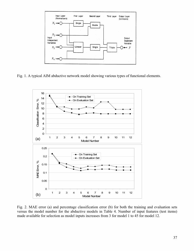
layered feed-forward abductive networks of functional elements (nodes) [9], see Fig. 1.

8

9

Elements in the first layer operate on various combinations of the independent input variables

(x's) and the element in the final layer produces the predicted output for the dependent variable

y. An input layer of normalizes convert the input variables into an internal representation as Z

scores with zero mean and unity variance, and an output unitizer unit restores the results to the

original problem space. AIM supports the following main functional elements:

(i) A linear element which consists of a constant plus the linear weighted sum of all outputs of

the previous layer, i.e.

"Linear" Output = w0 + w1x1 + w2x2 + w3x3 + .... + wnx n (2)

where x1, x

2,..., x

nare the element inputs and w

0, w

1, ..., w

n are the element weights.

(ii) Single, doublet, and triplet elements which implement a third-degree polynomial expression

for one, two, and three inputs respectively; for example,

"Double" Output = w0 + w1x1 + w2x2 + w3x12 + w4x2

2 + w5x1x2 + w6x13 + w7x2

3 (3)

2.2 GMDH-Based Feature Ranking and Selection

This paper describes a novel approach for ranking the input features of a training set according

to their predictive quality by repeatedly forcing the GMDH-based AIM learning algorithm to

automatically select a few optimum predictors at reduced model complexity settings. Selected

features are successively removed from the dataset and the process is repeated for the

selection of a new group. In this way, features are ranked in groups having different values of

predictive quality, with those selected earlier being of higher quality. Depending on the problem

being modeled, it may be possible to further rank the features within each group by

constructing models using only such variables and repeating the selection process at greater

simplicity settings. With the used version of AIM, the CPM parameter that controls model

complexity has a maximum value of 10, which may preclude the synthesis of models that are

simple enough to allow such ranking within each group for some problems.

10

With all input features available for use by the model, we start by using a large CPM value to

synthesize a simple model consisting of a single functional element using a group of up to

three input features that are automatically selected by the learning algorithm. When modeling

complex input-output relationships, this may also require specifying lower limits on the number

of layers in the model and the number of variables in the first layer prior to training. Features

selected in the first step would be those having the best predictive quality among the feature

set. Inputs in the dataset corresponding to the selected features are then disabled to prevent

their selection in subsequent modeling steps. The process is then repeated for the selection of

the next group of input features that will have a lower predictive power compared to the earlier

group, until all features have been selected. If required and deemed feasible, this process can

be followed by further ranking within each of the groups selected to achieve a complete

ranking of all individual features.

Two approaches can be adopted for selecting a feature subset from the ranking list obtained

above. In the first approach, a compact m-feature subset can be obtained by taking the first m

features starting at the top of the ranking list. In the second approach, the optimum subset of

features is determined by repeatedly forming subsets of k features, k = 1, 2, 3, …, n, where n

is the total number of available features, starting at the top of the ranking list. A classifier is

trained on each of the formed subsets. As k increases, classification error rate for the resulting

models on the training set is expected to monotonically decrease as the models fit the training

data more accurately. However, performance on an out-of-sample evaluation dataset would

first improve and then starts to deteriorate due to the model overfitting the training data. The

optimum model corresponding to the optimum feature subset would correspond to the smallest

value for k where the minimum classification error rate on the evaluation set is reached.

2.3 IRT-Based Item Ranking

Since the inception of the theory in the late 1960s, the item response theory (IRT) has been

the prevalent test modeling methodology for representing examinee’s behavior on a test in

terms of the characteristics of test items and examinee’s ability [20,23,30,45]. Within the

framework of traditional IRT, the examinee’s proficiency level is typically modeled by a single

latent trait, , and each item is characterized by up to three parameters, namely discrimination

parameter a, difficulty parameter b, and pseudo-guessing parameter c. The theoretical values

of item parameters are a (0, ), b (- , ) and c (0, 1) but practically a (0, 0.28), b (-

3, 3) and c (0, 0.35). Following the three-parameter logistic model (3PL), the probability that

a test taker with ability correctly answers item i having parameters (ai, bi, ci) is given by [30]:

))(7.1exp(1

1)|1Pr()(

ii

iiii

ba

cczP , (4)

where zi is the examinee’s response for item i. The above function is also known as the item

response function (IRF). To select the most informative subset of items for a particular test,

items in the item pool can be ranked based on their individual parameters, such as difficulty

levels, discrimination power or guessing levels. However, this approach considers only one

aspect of the item characteristics and does not take into account the proficiency levels of the

test takers when selecting items. Alternatively, items can be ranked based on a measure

known as Fisher’s item information function that describes the information revealed by an item

as a function of the examinee’s ability. For dichotomously scored items, the item information

function (IIF) for item i at the ability estimate is defined asˆ

ˆ)()(

))(()ˆ(

ii

ii

QP

PI (5)

where Qi( ) = 1 - Pi( ). The IIF provides test developers with a method for ranking items

according to the examinee’s ability level. The effectiveness of a group of m items can be

11

expressed as the sum of the information functions of all the items (also known as the test

information function, TIF), i.e.

m

i

iII1

)ˆ()ˆ( (6)

Groups having different numbers of items can be compared using the average TIF per item.

m

i

iavg Im

I1

)ˆ(1

)ˆ( (7)

Using this ranking measure, item selection can be tailored to match the purpose of the test.

Lord [30] outlined a test assembly procedure for selecting items such that the information

function of the constructed test approximates a target information function to a satisfactory

degree. The closer the matching between the target information function and the constructed

test information function, the more precise the test is in measuring ability.

2.4 Mutual Information-Based Item Ranking

Test items can also be ranked based on information theory criteria [16]. Mutual information is a

commonly used measure that quantifies the degree of dependence (or information sharing)

between two variables. Mutual information has been used widely in many machine learning

applications, including pattern recognition and data mining. Recently, it has been used to

evaluate the effectiveness of using a test item in assessing examinee’s competence level [29,

39]. Three equivalent methods have been reported in the literature for computing the mutual

information [16]. In the context of educational testing, let Y and X be the domains of tested

ability and item response respectively. Also let Y and X be discrete random variables denoting

the learner’s ability and an item response with realizations y Y and x X respectively. Thus,

the expected information gained about Y by observing X can be measured by the mutual

information between X and Y as defined by:

y x yPxP

yxPyxPYXIG

)()(

),(log),();( 2 , (8)

12

where P(x, y) is the joint probability mass function of X and Y and P(x) and P(y) are their

marginal probability mass functions respectively.

Another equivalent method for computing the mutual information can be expressed in terms of

Shannon’s entropy, a central concept in information theory, defined as [42]:

)|()();( XYHYHYXIG , (9)

where H(Y) is the Shannon entropy of Y and H(Y|X) is the conditional entropy of Y given X. As

indicated by Shannon, entropy can be viewed as a measure of the degree of uncertainty.

Hence, mutual information can be interpreted as the amount of uncertainty reduction about Y

by observing the item response X (or the degree of relevance of using X in measuring Y).

The third method computes mutual information in terms of the Kullback-Leibler (KL) distance,

also known as relative entropy, as [28]:

))()(),,(();( xPyPxyPDXYIG KL . (10)

This distance quantifies the divergence between two probability distributions P(z) and Q(z) as

defined by:

z

KLzQ

zPzPzQzPD

)(

)(log)())(),(( 2 . (11)

Similarly if X = (X1, X2, …, Xm) denotes a random vector representing an item response pattern

to a set of m items, known as a testlet, with a realization vector x = (x1, x2, …, xm), the

information gained about Y can be defined using any of the previously mentioned methods.

For example, using equation (8) the information gain (IG) is defined as:

y yPP

yPyPYIG

x x

xxX

)()(

),(log),();( 2 . (12)

Knowing the prior probability distribution {P(y)} and the conditional probability for each item

{P(x| y)} and assuming that item responses are conditionally independent given the learner’s

ability, the joint probability mass function P(x) can be expressed as:

13

.)|()(

)|()()(

1y

m

i

i

y

yxPyP

yPyPP xx

(13)

3. The Dataset

To evaluate the performance of the proposed approach, we used a dataset from [40] which

consists of a sample of 2000 cases for a 45-item test. It is assumed that examinees are

classified based on a single-ability parameter, , and therefore each case in the dataset gives

the response vector and the true ability level for an individual test taker. The test items are

numbered as 1, 2, 3, …, 45 according to the column they occupy in the dataset. The column

number is used as the item identification number (IID) throughout this paper. Test items are

dichotomously scored, i.e. when the test is taken, the examinee’s response to each item is

encoded as +1 (i.e. correct) or -1 (i.e. incorrect). It is also assumed that the examinees can

skip test items, in which case they are assigned 0. For the 2000 cases, ability values, varied

over the range -4.1456 to +4.0583. For the purpose of experiments reported in this paper, the

total sample population is symmetrically divided about the = 0 axis into two categories (fail

and pass). Estimation of item parameters and individual abilities was performed using Newton-

Raphson maximum likelihood estimation as outlined in Lord [30]. Table 1 shows the estimated

item parameters for each of the 45 test items. The table also lists the ascendant sorting of the

test items based on their individual item parameters and on the item’s IIF at the ability level =

0, which is the cut-off level between the fail and pass categories. All experiments reported in

this paper were performed on a Pentium 4 PC running Microsoft Windows XP Professional

with Service Pack 2.

4. Abductive Item Ranking and Selection for Pass/Fail Classification

This paper is concerned with the binary classification of examinees’ ability as a function of

relevant inputs among the 45 test items of the dataset described in Section 3. Ability values

14

15

over the range {-4.1456 to +0.0055} were assigned an output level 0 (fail category) while

values over the range {+0.0075 to +4.0583} were assigned an output level 1 (pass category),

with each category comprising 1000 case. Each of the two pass and fail categories was

randomly split into 750 cases for training and 250 cases for evaluation, thus providing a

training set of 1500 case and an evaluation set of 500 cases for the overall population. Ability

values predicted by the abductive network models constructed through training on the training

set were converted to a binary ability level through simple rounding at a threshold of 0.5.

Approximate ranking of the 45 test items comprising the dataset was carried out through model

training in 12 steps using the procedure described in section 2.2. All steps were performed at

the same model complexity settings of CPM = 10 (maximum value permitted with the AIM

version used), maximum number of model layers = 1, size of first layer = 3. Initially, all input

features were enabled for selection as inputs for the synthesized model by the abductive

learning algorithm. Following modeling step i; i = 1, 2, …, 12, inputs selected for the model

synthesized during that step were disabled to prevent their use as model inputs in all

succeeding steps: i+1, i+2, …, 11, 12. This forces selection from lower quality inputs and

allows partial ranking of the overall feature space in the form of the small groups of items which

are sequentially selected. Inputs selected at lower values of i are expected to have superior

predictive quality. Results of the 12 modeling steps are shown in Table 2. In addition to the

inputs excluded from being selected at each step, the table shows the structure of the

abductive model synthesized and a summary of its performance on the evaluation set.

Performance is measured in terms of the mean absolute error (MAE) between the actual and

predicted values for the binary ability output as well as the percentage classification error. The

variable number indicated at a model input, e.g. Var_i, corresponds to the IID of the test item

selected as model input, while Var_46 is the model output. In all steps except 11 and 12, a 3-

input triplet model was synthesized. Towards later steps, input features available for selection

become progressively poorer in predictive quality, thus driving the training algorithm to select a

16

larger subset of inputs to ensure adequate prediction performance by the synthesized model.

With the AIM software used, this requirement could override the limit of 3 specified for the size

of the first layer in the model. The model generated at step 11 is a linear functional element

with 11 inputs and that at step 12 uses all remaining 4 inputs. In spite of the larger number of

inputs, the complexity of model 11 is comparable to that of other models, for example the

number of coefficients for its linear element is 11 as compared to 14 for the triplet element of

model 10. Due to the gradual degradation in the predictive quality of selected model inputs,

there is a general trend of increasing MAE and classification errors at later steps, with the latter

more than doubling from 15.2% at step 1 to 35.6% at step 12. Training time is fast, with none

of the 12 models in Table 2 taking longer than 4 seconds to train.

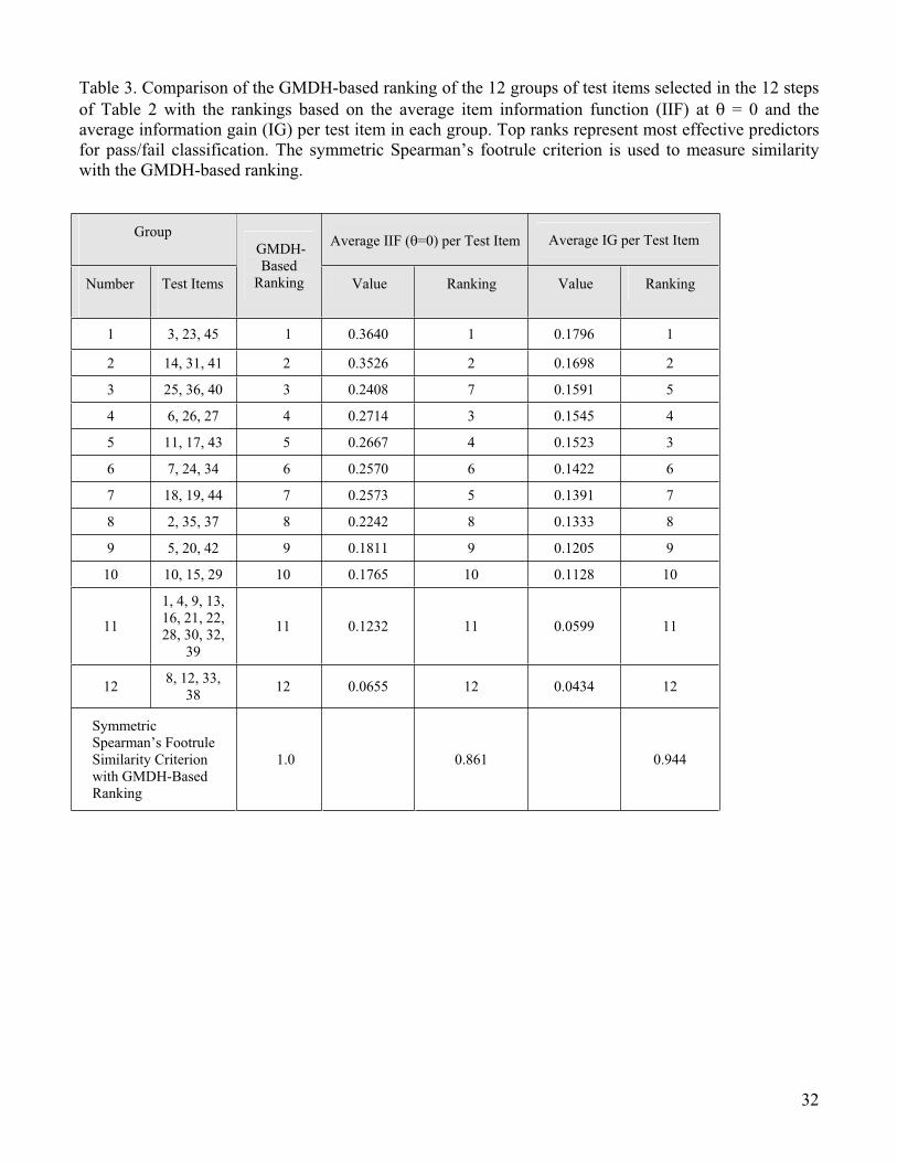
Table 3 lists the composition of the 12 groups of test items selected as model inputs in the

sequence of 12 modeling steps of Table 2, with group number i consisting of the subset of

inputs for the model synthesized at step i. Based on the assumption that higher quality

predictors are selected at earlier steps, the GMDH-based ranking of the groups is identical to

the group number, with group 1 {Items 3, 23, 45} having the highest predictive quality and

group 12 {Items 8,12, 33, 38} having the lowest quality. This suggests the following partial

ranking list for the 45 test items: {3, 23, 45, 14, 31, 41, 25, 36, 40, 6, 26, 27, 11, 17, 43, 7, 24,

34, 18, 19, 44, 2, 35, 37, 5, 20, 42, 10, 15, 29, 1, 4, 9, 13, 16, 21, 22, 28, 30, 32, 39, 8, 12, 33,

38}, where items within a group are listed in the order they appeared in the model structures

shown in Table 2. Table 3 lists also the ranking of the 12 groups of items based on the average

IIF at = 0 per item in the group as discussed in Section 2.3. The third ranking shown in the

table is that based on the average information gain (IG) described in Section 2.4. In order to

compare the GMDH-based ranking with each of the other two rankings we used the symmetric

Spearman’s footrule ranking similarity criterion [36]. Let {Q1, Q2, …, Qn} and {R1, R2, …, Rn} be

the vectors representing the two n-element rankings to be compared. The symmetric version of

the Spearman’s footrule is given by:

])1([1

1

n

i iiii

n

n RQnRQM

C (14)

where Mn = n2/2 if n is even or (n2-1)/2 if n is odd. The value obtained for ranges from -1, for

two exactly reversed rankings, to +1, for two identical rankings. Results in Table 3 shows that

the GMDH-based ranking is reasonably close to the rankings based on the IIF and the IG

criteria, with values being 0.861 and 0.944, respectively.

nC

nC

To determine the optimum subset of test items from the GMDH-based ranking results

described above, we developed 12 new abductive models trained on subsets of inputs of a

gradually increasing number of the groups selected in the 12 modeling steps described above.

The inputs enabled during the synthesis of model j; j = 1, 2, …, 12 include group j and all

preceding groups 1, 2, …, j-1. This arrangement produces 12 models trained on increasingly

larger subsets of test items starting always at the top of the partial ranking list and stopping at

group boundaries. For example, model 1 was trained on an input subset consisting of group 1,

i.e. {3, 23, 45}, model 2 on a subset consisting of groups 1 and 2, i.e. {3, 23, 45, 14, 31, 41},

etc. Model 12 was trained on the full set of 45 inputs. The default training settings of CPM = 1,

maximum number of model layers = 4, size of first layer = 15 were used for all these models,

and each model was evaluated on both the training set and the evaluation set. For each of the

12 models, Table 4 shows the model structures synthesized, lists the input features available

but not selected during model synthesis, and gives the classification error on both the training

and evaluation sets. Fig. 2 plots the MAE errors and the classification errors on both datasets.

As more input features are initially brought in, prediction errors on both the training and

evaluation set decrease as indicated in Fig. 2 and Table 4. Further increase in the number of

input features is expected to continue a monotonic reduction in the errors on the training set as

17

18

the model fits the training data more accurately. However, error rates on the out-of-sample

evaluation set are expected to reach a minimum before they start to rise again as further

increase in the number of input features causes the model to overfit the training data, thus

reducing its ability to generalizes well with the new data of the evaluation set. The subset of

input features corresponding to this minimum is considered the optimum feature subset.

Referring to Fig. 2(a), the MAE error on the evaluation set bottoms at model 5, suggesting an

optimum feature subset that consists of groups 1, 2, 3, 4, and 5 in Table 3, for a total of 15 test

items {3, 23, 45, 14, 31, 41, 25, 36, 40, 6, 26, 27, 11, 17, 43}. Table 4 indicates that all input

features provided for training models 1, 2, 3, 4, and 5 are selected as model inputs during

training, with none of the features discarded, which indicates the good predictive quality of the

five groups comprising the optimum subset. Beyond model 5, additional input features down

the ranking list which have poorer predictive quality become available for selection, and

therefore an increasing number of such features is discarded. For example, model 6 uses only

13 out of the 18 inputs available. Models 8 and 9 are identical, which indicates that the three

inputs comprising group 9 are completely discarded. Similarly, groups 11 and 12 (a total of 15

inputs) are totally discarded, leading to models 10, 11, and 12 being identical. Ignoring such

poorer quality inputs leads to synthesizing simpler models that may not overfit the training

data. This explains why the MAE and classification errors do not monotonically decrease on

the training set and do not monotonically increase on the evaluation set beyond model 5, see

Fig. 2.

5. Comparison with Other Feature Ranking Methods and Neural Network Classifiers

We have compared the GMDH-based item ranking described above with results obtained

using a number of popular feature ranking/selection methods used in data mining and machine

learning and with results from neural network modeling. The feature ranking/selection methods

included three filter techniques, namely information gain, information gain ratio, and chi-

19

squared, as well as a wrapper method that uses a neural network classifier with a genetic

search approach [47]. The neural network modeling method used probabilistic neural networks

(PNN) trained with a genetic learning algorithm using the NeuroShell Classifier software [46].

Compared to conventional neural networks, such networks take longer time to train but have

the advantage of generalizing well on external data [46]. The NeuroShell Classifier software

provides an estimate of the relative importance of each input feature used to train the model,

which can be compared with the GMDH-based ranking. Prior to training, the maximum number

of generations allowed without performance improvement by the genetic algorithm was set to

20, and the goal of the genetic optimization during training was set to minimize the total

number of incorrect classifications in the two classification categories. Training was stopped

automatically after 34 generations and took 85 minutes. Overall classification accuracy

achieved was 90.5% and 89.2% on the training set and evaluation set, respectively. The bar

chart in Fig. 3 depicts the importance of input attributes at the end of training and forms the

basis for item ranking with this method. The wrapper method with a neural network classifier

and genetic search [47] proved very slow, with training lasting for 67 hours, and achieved a

classification accuracy of 91.2%.

Table 5 lists ranking results for the 45 test items according to: (i) the GMDH-based partial

ranking, (ii) the information gain method, (iii) the information gain ratio method, (iv) the chi-

squared method, (v) the wrapper method, and (vi) the NeuroShell neural network classifier with

genetic training. Method (vi) selects an optimum subset of 28 input features without ranking

them. As a rough comparison between the GMDH-based ranking and the other methods,

Table 5 gives the percentage overlap between the optimum 15-item subset forming the top

third of the GMDH-based ranking list and the top 15 items of each of the other ranking lists.

The percentage overlap ranges from 46.7% with the NeuroShell classifier to 93.3% with the

chi-squared method. 14 out of the 15 items forming the optimum GMDH-based subset are

included in the 28 items selected by the wrapper method. Poor overlap with the NeuroShell

20

classifier can be attributed to the fact that the NeuroShell ranking is reliable only for a small

number of input features [46]. The GMDH-based ranking approach proposed does not suffer

from this limitation.

6. Optimum Item Subsets and Comparisons

We obtained the optimum abductive model synthesized using the optimum subset of test items

selected by the GMDH-based ranking described in Section 4. This was achieved by developing

models over a range of values for the CPM parameter with all remaining training parameters

kept at their default values. Synthesized model structures, shown in Table 6, indicate that a

decade of variations in CPM (from 0.5 to 5) introduces no changes in the input features

selected as model inputs, with no input features being discarded by simpler models (larger

CPM values). The difficulty in dispensing with any of the input features at such model simplicity

levels is an indication of the good predictive quality of the selected optimum subset. Further

model simplification with CPM = 10 causes only one input item, item 11, to be discarded.

Referring to Table 3, it is interesting to note that item 11 belongs to group 5 which has the

poorest predictive quality among the five groups of test items comprising the optimum subset.

Table 6 lists the percentage classification errors on both the training and evaluation sets.

Results show that the optimum model at CPM = 5 gives the minimum error of 8.8% on the

evaluation set. The 3-layer model uses the full optimum subset and consists of only 3 simple

functional elements comprising a linear, a singlet, and a doublet. Classification of the

evaluation set using this optimum model gives an overall classification accuracy of 91.2%, a

sensitivity of 93.7%, a specificity of 88.6%, a positive predictive value of 89.5%, and a negative

predictive value of 93.2%.

We examined the adequacy of the optimum input subset selection described above in

comparison with several other subsets selected using other criteria based on abductive, IRT,

and random approaches. Comparisons were based on the classification performance of

21

optimum abductive network models developed using the respective subsets. The optimum

model for each of the other subsets was taken as that giving the best performance on the

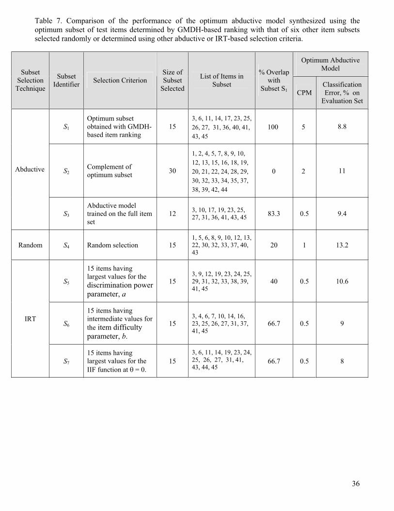
evaluation set among three models trained at CPM = 0.5, 1, and 2. Table 7 shows the results

for comparing the optimum GMDH-based subset, identified as subset S1, with two other

subsets (S2 and S3) based on abductive selection, a randomly selected subset S4 and three

subsets (S5, S6, and S7) based on three different IRT-based selection criteria. Each of the

subsets S4, S5, S6, and S7 has the same size of 15 items as the optimum GMDH-based subset.

Subset S2 is the complement of subset S1, i.e. it consists of the remaining 30 test items not

included in subset S1. Subset S3 is that selected by the optimum abductive model trained on

the full set of 45 test items. Referring to Table 1, the three IRT-based selection criteria used

are: largest item discriminatory power (i.e. items in the bottom third of the ascendant sorting

column for the parameter a), intermediate values for item difficulty (items in the middle third of

the ranking column for the parameter b), and largest values for the IIF item information function

at the pass/fail ability cut-off (items in the bottom third of the ascendant ranking column for IIF

at = 0). Referring to Table 7, the 12 items comprising subset S3 are those selected by the

abductive model from the full set of test inputs. For the optimum GMDH-based subset S1, the

list of subset items given in the Table are those items available for training and also actually

selected by the model. For all other subsets in the table, the list of items given represents the

inputs used for training and may not be all selected by the synthesized optimum abductive

model used for the comparison. Table 7 shows the percentage overlap between each subset

and the optimum subset as well as the CPM parameter used and the classification

performance on the evaluation set for the corresponding abductive model. Results indicate that

the optimum subset outperforms all other subsets considered except subset S7 selected

according to the IRT IIF function. However, the abductive selection method has the

advantages that it does not require knowledge of the three-parameter model for the test items

or the calculation of the information function for each item. All subsets except S2 have

22

approximately the same size, and results for those subsets suggest significant negative

correlation between the percentage overlap with the optimum set and the percentage

classification error.

The performance comparison described above was carried out at a single cut-off point (0.5)

marking the pass/fail transition in the test outcome as represented by the binary value of the

estimated ability. A more useful comparison would involve several such cut-off points over the

range 0 to 1 using the receiver operating characteristics (ROC) analysis [21]. The ROC curve

is a plot of the sensitivity (true positive rate) versus the false positive rate (= 1 – specificity) for

various values of the threshold used to sort a continuous classifier output into normal or

abnormal classes. The area under the curve (AUC) is a useful measure for determining the

quality of classification schemes and diagnostic tests, and statistically comparing their

performance. This parameter is ideally 1.0 for an ideal classifier which has an ROC curve that

passes through the point (0,1), thus giving 100% sensitivity at 100% specificity. Practically

useful classifiers would have AUC values in the range (0.5 < AUC 1.0). ROC analysis was

used to compare the performance of three models having the same size of 15 test items.

These models correspond to the optimum subset S1 based on GMDH ranking, subset S4

based on random selection, and subset S7 based on IRT-IIF ranking. We used the Analyse-it

statistical software package [10] which employs the Hanley and McNeil method [21] for

performing the ROC analysis. Fig. 4 plots the three ROC curves and gives values of the AUC

parameter and its standard error (SE) for each model. Results indicate that both the GMDH-

based and IRT-IIF based subsets are of practically identical classification quality, with AUC

0.975. Both subsets are superior to the randomly selected subset which has an AUC of 0.949.

Analysis results indicate that the difference between the AUC values is statically significant at

the 95% confidence level in both cases.

23

7. Conclusions

We have demonstrated the use abductive machine learning for the partial ranking of test items

according to their ability to predict pass-fail test outcomes. The procedure relies on the ability

of GMDH-based learning algorithms to automatically select optimum input features, and

involves iteratively forcing the synthesis of a simple model and excluding the inputs selected at

each stage. Ranking of 12 subsets of items obtained in this way compares favorably with

rankings for the same subsets based on the average item information function at the pass-fail

ability threshold, IIF ( =0), and the average information gain (IG). The partial ranking obtained

was used to determine an optimum subset that contained only of one third of the available test

items, yet achieved a pass/fail classification accuracy of 91.2%. This accuracy is exceeded

only by a model that uses a subset of the same size but consists of test items having the

largest values for the IIF at = 0 (92%). Both subsets achieved approximately the same area

of 0.975 under the ROC curve. In both cases, the AUC is significantly greater than that of a

subset of the same size that consists of randomly selected test items. Compared to IIF based

ranking, the proposed GMDH-based approach should be easier to derive, as it does not make

any assumptions on the form of the item-competence model (e.g. 3PL) nor does it require the

calculation of any parameters for the test items or their IIF functions. Therefore, the proposed

approach should prove attractive for practitioners who are less interested in (and less

experienced with) the tools, as compared to the actual educational application. The proposed

method is self-contained, whereas IRT based methods may require mastering several tools

and utilities. Item selections and rankings are comparable with those obtained using popular

filter-type feature ranking methods. However, the proposed approach has the added

advantage that feature selection is automatically associated with the synthesis of classification

models that provide evidence of the quality of the resulting feature selection and ranking. The

proposed approach has a clear advantage over wrapper feature selection methods that use

genetic search, as it achieves comparable classification performance much faster. Overall,

24

results indicate that abductive machine learning can provide a useful non-parametric approach

for constructing optimal shortened tests that are more economical to administer and allow

better insight into the test results. Future work would consider methods for finer ranking within

item groups to achieve complete ranking of the item set, and the use of such ranking to

develop ensembles of tests which can be combined to explain the test outcome more

accurately.

Acknowledgment

The authors are grateful to King Fahd University of Petroleum and Minerals (KFUPM),

Dhahran, Saudi Arabia for continuous support during this work.

References

[1] R.E. Abdel-Aal, Automatic fitting of Gaussian peaks using abductive machine learning,

IEEE Transactions on Nuclear Science 45 (1998) 1-16.

[2] R.E. Abdel-Aal, Short term hourly load forecasting using abductive networks, IEEE

Transactions on Power Systems 19 (2004) 164-173.

[3] R.E. Abdel-Aal, GMDH-based feature ranking and selection for improved classification of

medical data, Journal of Biomedical Informatics 38 (2005) 456-468.

[4] R.E. Abdel-Aal and M.A. Elhadidy, Modeling and forecasting the maximum temperature

using abductive machine learning, Weather and Forecasting 10 (1995) 310-325.

[5] R.E. Abdel-Aal and A.M. Mangoud, Abductive machine learning for modeling and predicting

the educational score in school health surveys, Methods of Information in Medicine 35 (1996)

265-271.

[6] W.H. Abdulla and N. Kasabov, Reduced feature-set based parallel CHMM speech

recognition systems, Information Sciences Journal 156 (2003) 21-38.

25

[7] A. Agarwal, Abductive networks for two-group classification: A comparison with neural

networks, The Journal of Applied Business Research 15 (1999) 1-12.

[8] D.W. Aha and R.L. Bankert, A comparative evaluation of sequential feature selection

algorithms, Learning from Data: AI and Statistics V, Springler-Verlag, New York, 1996.

[9] AIM User's Manual, AbTech Corporation, Charlottesville, VA, 1990.

[10] Analyse-it Software Ltd, PO Box 77, Leeds, LS12 5XA, UK.

[11] A.R. Barron, Predicted squared error: A criterion for automatic model selection, in: S.J.

Farlow (Ed.), Self-Organizing Methods in Modeling: GMDH Type Algorithms, Marcel-Dekker,

New York, 1984, pp. 87-103.

[12] R. Battiti, Using mutual information for selecting features in supervised neural net learning,

IEEE Transactions on Neural Networks 5 (1994) 537-550.

[13] A. Blum, P. Langley, Selection of relevant features and examples in machine learning,

Artificial Intelligence 97 (1997) 245-271.

[14] F.Z. Brill, D.E. Brown, and W.N. Martin, Fast genetic selection of features for neural

network classifiers, IEEE Transactions on Neural Networks 3 (1992) 324-328.

[15] S. Buyske, Optimal design in educational testing, in: M.P.F. Berger and W.K. Wong (eds.),

Applied Optimal Designs, John Wiley & Sons, New York, 2005.R.K.

[16] T. Cover and J. Thomas, Elements of Information Theory. John Wiley, New York, 1991.

[17] S.J. Farlow, The GMDH algorithm, in: S.J. Farlow (Ed.), Self-Organizing Methods in

Modeling: GMDH Type Algorithms, Marcel-Dekker, New York, 1984, pp. 1-24.

[18] K. Grabczewski, N. Jankowski, Feature selection with decision tree criterion, Fifth

International Conference on Hybrid Intelligent Systems, 2005.

26

[19] M.A. Hall, Correlation-based feature selection for discrete and numeric class machine

learning, Proceedings of the 17th International Conference on Machine Learning, Stanford

University, CA. Morgan Kaufmann Publishers, 2000.

[20] R.K. Hambleton, H. Swaminathan, Item Response Theory: Principles and Applications.

Kluwer Academic Publishers Group, Netherlands, 1985.

[21] J.A. Hanley and B.J.A. McNeil, Method of comparing the areas under receiver operating

characteristic curves derived from the same cases, Radiology 148 (1983) 839-843.

[22] A.J. Hoffman, C. Hoogenboezem, N. T. van der Merwe, C. J. A. Tollig, Seismic buffer

recognition using mutual information for selecting wavelet based features, IEEE International

Symposium on Industrial Electronics, 1998, pp. 663-667.

[23] G.-J. Hwang, P.-Y. Yin, S. H. Yeh, A Tabu search approach to generating test sheets for

multiple assessment criteria, IEEE Transactions on Education 49 (2006) 88-97.

[24] H.L. Jeng, S.G. Shih, A comparison of pair-wise and group selections of items using

simulated annealing in automated construction of parallel tests, Psychological Testing 44

(1997) 195-210.

[25] C.J. Johnstone, S.J. Thompson, R.E. Moen, S. Bolt, and K. Kato, Analyzing results of

large-scale assessments to ensure universal design, NCEO Technical Report 41, July 2005,

Published by the National Center on Educational Outcomes, USA.

[26] J. Kittler, Feature selection and extraction, in: T.Y. Young and K.S. Fu (Eds.),

EdsHandbook of Pattern Recognition and Image Processing, Academic, San Diego, CA, 1986,

pp. 59–83.

[27] R. Kohavi, G.H. John, Wrappers for feature subset election, Artificial Intelligence 7 (1997)

273-323.

27

[28] S. Kullback and R.A. Leibler, On information and sufficiency, Annals of Mathematical

Statistics 22 (1951) 79–86.

[29] C.-L. Liu, Using mutual information for adaptive item comparison and student assessment,

Journal of Educational Technology and Society 8 (2005) 100-119.

[30] F.M. Lord, Applications of Item Response Theory to Practical Testing Problems, Lawrence

Erlbaum, New Jersey, 1980.

[31] R.M. Luecht, Computer-assisted test assembly using optimization heuristics. Applied

Psychological Measurement, 22 (1998) 224-236

[32] R.M. Luecht, Implementing the computer-adaptive sequential testing (CAST) framework to

mass produce high quality computer-adaptive and mastery tests. Symposium paper presented

at the Annual Meeting of the National Council on Measurement in Education, New Orleans,

LA., 2000.

[33] R.M. Luecht, T. Brumfield, and K. Breithaupt, A testlet assembly design for the uniform

CPA examination. Paper presented at the Annual Meeting of the National Council on

Measurement in Education. New Orleans, 2002.

[34] G.J. Montgomery and K.C. Drake, Abductive reasoning networks, Neurocomputing 2

(1991) 97-104.

[35] D.P. Muni, N.R. Pal, and J. Das, Genetic programming for simultaneous feature selection

and classifier design, IEEE Transactions on Systems, Man and Cybernetics, Part B 36 (2006)

106 – 117.

[36] R.B. Nelsen and M. Ubeda-Flores, The symmetric footrule is Gini’s rank association

coefficient,” Communications in Statistics: Theory and Methods 33 (2004) 195–196.

28

[37] M. Ozdemir, M.J. Embrechts, F. Arciniegas, C.M. Breneman, L. Lockwood, and K.P.

Bennett, Feature selection for in-silico drug design using genetic algorithms and neural

networks, IEEE Mountain Workshop on Soft Computing in Industrial Applications, 2001, pp.

53-57.

[38] Y.A. Pachepsky and W.J. Rawls, Accuracy and reliability of pedotransfer functions as

affected by grouping soils, Soil Science Society of America Journal 63 (1999) 1748–1757.

[39] L.M. Rudner, The classification accuracy of measurement decision theory, Paper

Presented at the Annual Meeting of the National Council on Measurement in Education,

Chicago, 2003.

[40] L.M. Rudner, PARAM-3PL calibration software for the 3-parameter logistic IRT model,

2005. Available: http://edres.org/irt/param

[41] P.M. Sadler, The initial knowledge state of high school astronomy students, PhD

Dissertation, Harvard University, 1992.

[42] C.E. Shannon, A mathematical theory of communication, The Bell System Technical

Journal 27 (1948) 379-423, 623-656.

[43] K.T. Sun, S.F. Chen, A study of applying the artificial intelligent technique to select test

items, Psychological Testing 46 (1999) 75-88.

[44] W.J. van der Linden, Optimal assembly of psychological and educational tests. Applied

Psychological Measurement, 22 (1998) 195-211.

[45] W.J. van der Linden, R.K. Hambleton (eds.), Handbook of Modern Item Response Theory,

Springer-Verlag, 1997.

[46] Ward Systems Group. NeuroShell Classifier Software. Ward Systems Group, Inc.,

Executive Park West, 5 Hillcrest Drive, Frederick, MD 21703, USA.

29

[47] I.H. Witten, and E. Frank, Data Mining: Practical Machine Learning Tools and Techniques,

Second Edition, Morgan Kaufmann, 2005

[48] S. Yu, S. De Backer, P. Scheunders, Genetic feature selection combined with composite

fuzzy nearest neighbor classifiers for high-dimensional remote sensing data, IEEE International

Conference on Systems, Man, and Cybernetics, 2000, pp. 1912-1916.

[49] P. Zarjam, M. Mesbah, B. Boashash, An optimal feature set for seizure detection systems

for newborn EEG signals, International Symposium on Circuits and Systems, 2003, V-33-36.

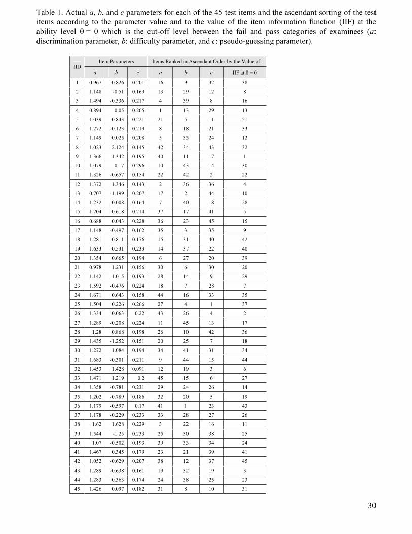
Table 1. Actual a, b, and c parameters for each of the 45 test items and the ascendant sorting of the test

items according to the parameter value and to the value of the item information function (IIF) at the

ability level = 0 which is the cut-off level between the fail and pass categories of examinees (a:

discrimination parameter, b: difficulty parameter, and c: pseudo-guessing parameter).

Item Parameters Items Ranked in Ascendant Order by the Value of: IID

a b c a b c IIF at = 0

1 0.967 0.826 0.201 16 9 32 38

2 1.148 -0.51 0.169 13 29 12 8

3 1.494 -0.336 0.217 4 39 8 16

4 0.894 0.05 0.205 1 13 29 13

5 1.039 -0.843 0.221 21 5 11 21

6 1.272 -0.123 0.219 8 18 21 33

7 1.149 0.025 0.208 5 35 24 12

8 1.023 2.124 0.145 42 34 43 32

9 1.366 -1.342 0.195 40 11 17 1

10 1.079 0.17 0.296 10 43 14 30

11 1.326 -0.657 0.154 22 42 2 22

12 1.372 1.346 0.143 2 36 36 4

13 0.707 -1.199 0.207 17 2 44 10

14 1.232 -0.008 0.164 7 40 18 28

15 1.204 0.618 0.214 37 17 41 5

16 0.688 0.043 0.228 36 23 45 15

17 1.148 -0.497 0.162 35 3 35 9

18 1.281 -0.811 0.176 15 31 40 42

19 1.633 0.531 0.233 14 37 22 40

20 1.354 0.665 0.194 6 27 20 39

21 0.978 1.231 0.156 30 6 30 20

22 1.142 1.015 0.193 28 14 9 29

23 1.592 -0.476 0.224 18 7 28 7

24 1.671 0.643 0.158 44 16 33 35

25 1.504 0.226 0.266 27 4 1 37

26 1.334 0.063 0.22 43 26 4 2

27 1.289 -0.208 0.224 11 45 13 17

28 1.28 0.868 0.198 26 10 42 36

29 1.435 -1.252 0.151 20 25 7 18

30 1.272 1.084 0.194 34 41 31 34

31 1.683 -0.301 0.211 9 44 15 44

32 1.453 1.428 0.091 12 19 3 6

33 1.471 1.219 0.2 45 15 6 27

34 1.358 -0.781 0.231 29 24 26 14

35 1.202 -0.789 0.186 32 20 5 19

36 1.179 -0.597 0.17 41 1 23 43

37 1.178 -0.229 0.233 33 28 27 26

38 1.62 1.628 0.229 3 22 16 11

39 1.544 -1.25 0.233 25 30 38 25

40 1.07 -0.502 0.193 39 33 34 24

41 1.467 0.345 0.179 23 21 39 41

42 1.052 -0.629 0.207 38 12 37 45

43 1.289 -0.638 0.161 19 32 19 3

44 1.283 0.363 0.174 24 38 25 23

45 1.426 0.097 0.182 31 8 10 31

30

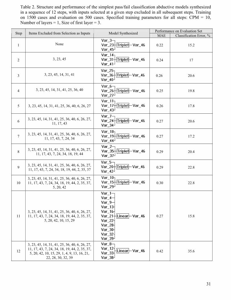
Table 2. Structure and performance of the simplest pass/fail classification abductive models synthesized

in a sequence of 12 steps, with inputs selected at a given step excluded in all subsequent steps. Training

on 1500 cases and evaluation on 500 cases. Specified training parameters for all steps: CPM = 10,

Number of layers = 1, Size of first layer = 3.

Performance on Evaluation Set Step Items Excluded from Selection as Inputs Model Synthesized

MAE Classification Error, %

1 None 0.22 15.2

2 3, 23, 45 0.24 17

3 3, 23, 45, 14, 31, 41 0.26 20.6

4 3, 23, 45, 14, 31, 41, 25, 36, 40 0.25 19.8

5 3, 23, 45, 14, 31, 41, 25, 36, 40, 6, 26, 27 0.26 17.8

63, 23, 45, 14, 31, 41, 25, 36, 40, 6, 26, 27,

11, 17, 43 0.27 20.6

73, 23, 45, 14, 31, 41, 25, 36, 40, 6, 26, 27,

11, 17, 43, 7, 24, 340.27 17.2

83, 23, 45, 14, 31, 41, 25, 36, 40, 6, 26, 27,

11, 17, 43, 7, 24, 34, 18, 19, 44 0.29 20.4

93, 23, 45, 14, 31, 41, 25, 36, 40, 6, 26, 27,

11, 17, 43, 7, 24, 34, 18, 19, 44, 2, 35, 370.29 22.8

10

3, 23, 45, 14, 31, 41, 25, 36, 40, 6, 26, 27,

11, 17, 43, 7, 24, 34, 18, 19, 44, 2, 35, 37,

5, 20, 42

0.30 22.8

11

3, 23, 45, 14, 31, 41, 25, 36, 40, 6, 26, 27,

11, 17, 43, 7, 24, 34, 18, 19, 44, 2, 35, 37,

5, 20, 42, 10, 15, 29

0.27 15.8

12

3, 23, 45, 14, 31, 41, 25, 36, 40, 6, 26, 27,

11, 17, 43, 7, 24, 34, 18, 19, 44, 2, 35, 37,

5, 20, 42, 10, 15, 29, 1, 4, 9, 13, 16, 21,

22, 28, 30, 32, 39

0.42 35.6

31

32

Table 3. Comparison of the GMDH-based ranking of the 12 groups of test items selected in the 12 steps

of Table 2 with the rankings based on the average item information function (IIF) at = 0 and the

average information gain (IG) per test item in each group. Top ranks represent most effective predictors

for pass/fail classification. The symmetric Spearman’s footrule criterion is used to measure similarity

with the GMDH-based ranking.

Group Average IIF ( =0) per Test Item Average IG per Test Item

Number Test Items

GMDH-

Based

Ranking Value Ranking Value Ranking

1 3, 23, 45 1 0.3640 1 0.1796 1

2 14, 31, 41 2 0.3526 2 0.1698 2

3 25, 36, 40 3 0.2408 7 0.1591 5

4 6, 26, 27 4 0.2714 3 0.1545 4

5 11, 17, 43 5 0.2667 4 0.1523 3

6 7, 24, 34 6 0.2570 6 0.1422 6

7 18, 19, 44 7 0.2573 5 0.1391 7

8 2, 35, 37 8 0.2242 8 0.1333 8

9 5, 20, 42 9 0.1811 9 0.1205 9

10 10, 15, 29 10 0.1765 10 0.1128 10

11

1, 4, 9, 13,

16, 21, 22,

28, 30, 32,

39

11 0.1232 11 0.0599 11

128, 12, 33,

38 12 0.0655 12 0.0434 12

Symmetric

Spearman’s Footrule

Similarity Criterion

with GMDH-Based

Ranking

1.0 0.861 0.944

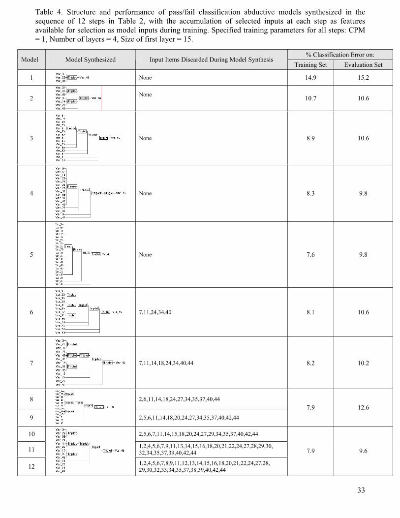
Table 4. Structure and performance of pass/fail classification abductive models synthesized in the

sequence of 12 steps in Table 2, with the accumulation of selected inputs at each step as features

available for selection as model inputs during training. Specified training parameters for all steps: CPM

= 1, Number of layers = 4, Size of first layer = 15.

% Classification Error on:Model Model Synthesized Input Items Discarded During Model Synthesis

Training Set Evaluation Set

1 None 14.9 15.2

2None

10.7 10.6

3 None 8.9 10.6

4 None 8.3 9.8

5 None 7.6 9.8

6 7,11,24,34,40 8.1 10.6

7 7,11,14,18,24,34,40,44 8.2 10.2

8 2,6,11,14,18,24,27,34,35,37,40,44

9 2,5,6,11,14,18,20,24,27,34,35,37,40,42,44

7.9 12.6

10 2,5,6,7,11,14,15,18,20,24,27,29,34,35,37,40,42,44

111,2,4,5,6,7,9,11,13,14,15,16,18,20,21,22,24,27,28,29,30,

32,34,35,37,39,40,42,44

121,2,4,5,6,7,8,9,11,12,13,14,15,16,18,20,21,22,24,27,28,

29,30,32,33,34,35,37,38,39,40,42,44

7.9 9.6

33

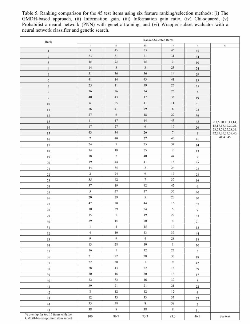
Table 5. Ranking comparison for the 45 test items using six feature ranking/selection methods: (i) The

GMDH-based approach, (ii) Information gain, (iii) Information gain ratio, (iv) Chi-squared, (v)

Probabilistic neural network (PNN) with genetic training, and (vi) Wrapper subset evaluator with a

neural network classifier and genetic search.

34

Ranked/Selected ItemsRank

i ii iii iv v vi

1 3 45 23 45 45

2 23 31 31 31 34

3 45 23 45 3 10

4 14 3 3 23 24

5 31 36 36 14 29

6 41 14 43 41 15

7 25 11 39 26 35

8 36 26 34 25 3

9 40 43 17 36 19

10 6 25 11 11 31

11 26 41 29 6 23

12 27 6 18 27 36

13 11 17 14 43 43

14 17 27 6 17 26

15 43 34 26 7 1

16 7 40 27 40 41

17 24 7 35 34 14

18 34 18 25 2 13

19 18 2 40 44 7

20 19 44 41 18 32

21 44 35 2 24 25

22 2 24 9 19 28

23 35 42 7 37 16

24 37 19 42 42 6

25 5 37 37 35 40

26 20 29 5 20 20

27 42 20 44 15 37

28 10 39 24 5 9

2,3,5,10,11,13,14,

15,17,18,19,20,21,

23,25,26,27,28,31,

32,35,36,37,39,40,

41,43,45

29 15 5 19 29 33

30 29 15 20 4 21

31 1 4 15 10 12

32 4 10 13 39 44

33 9 9 4 28 38

34 13 28 10 1 30

35 16 1 32 22 5

36 21 22 28 30 18

37 22 30 1 9 42

38 28 13 22 16 39

39 30 16 30 13 17

40 32 32 16 32 8

41 39 21 21 21 22

42 8 12 12 12 4

43 12 33 33 33 27

44 33 38 8 38 2

45 38 8 38 8 11

% overlap for top 15 items with the

GMDH-based optimum item subset100 86.7 73.3 93.3 46.7 See text

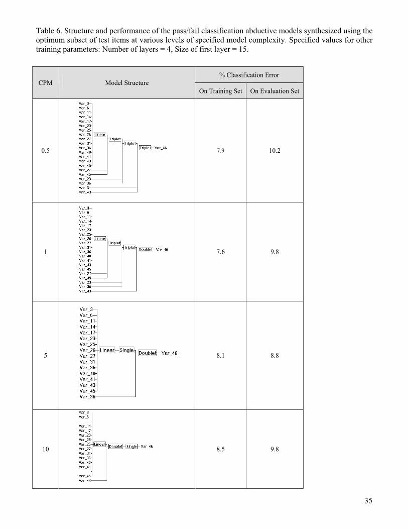
Table 6. Structure and performance of the pass/fail classification abductive models synthesized using the

optimum subset of test items at various levels of specified model complexity. Specified values for other

training parameters: Number of layers = 4, Size of first layer = 15.

% Classification Error

CPM Model Structure

On Training Set On Evaluation Set

0.5 7.9 10.2

1 7.6 9.8

5 8.1 8.8

10 8.5 9.8

35

36

Table 7. Comparison of the performance of the optimum abductive model synthesized using the

optimum subset of test items determined by GMDH-based ranking with that of six other item subsets

selected randomly or determined using other abductive or IRT-based selection criteria.

Optimum Abductive

ModelSubset

Selection

Technique

Subset

IdentifierSelection Criterion

Size of

Subset

Selected

List of Items in

Subset

% Overlap

with

Subset S1 CPM

Classification

Error, % on

Evaluation Set

S1

Optimum subset

obtained with GMDH-

based item ranking

15

3, 6, 11, 14, 17, 23, 25,

26, 27, 31, 36, 40, 41,

43, 45

100 5 8.8

S2Complement of

optimum subset 30

1, 2, 4, 5, 7, 8, 9, 10,

12, 13, 15, 16, 18, 19,

20, 21, 22, 24, 28, 29,

30, 32, 33, 34, 35, 37,

38, 39, 42, 44

0 2 11Abductive

S3

Abductive model

trained on the full item

set

123, 10, 17, 19, 23, 25,

27, 31, 36, 41, 43, 45 83.3 0.5 9.4

Random S4 Random selection 151, 5, 6, 8, 9, 10, 12, 13,

22, 30, 32, 33, 37, 40,

4320 1 13.2

S5

15 items having

largest values for the

discrimination power

parameter, a

153, 9, 12, 19, 23, 24, 25,

29, 31, 32, 33, 38, 39,

41, 45 40 0.5 10.6

S6

15 items having

intermediate values for

the item difficulty

parameter, b.

153, 4, 6, 7, 10, 14, 16,

23, 25, 26, 27, 31, 37,

41, 45 66.7 0.5 9

IRT

S7

15 items having

largest values for the

IIF function at = 0.

15

3, 6, 11, 14, 19, 23, 24,

25, 26, 27, 31, 41,

43, 44, 4566.7 0.5 8

37

Linear

Fig. 1. A typical AIM abductive network model showing various types of functional elements.

0

2

4

6

8

10

12

14

16

1 2 3 4 5 6 7 8 9 10 11 12

Model Number

On Training Set

On Evaluation Set

Cla

ssific

ation Err

or,

%

(b)

0

0.05

0.1

0.15

0.2

0.25

1 2 3 4 5 6 7 8 9 10 11 12

Model Number

On Training Set

On Evaluation Set

MAE E

rror,

%

(b)

(a)

Fig. 2. MAE error (a) and percentage classification error (b) for both the training and evaluation sets

versus the model number for the abductive models in Table 4. Number of input features (test items)

made available for selection as model inputs increases from 3 for model 1 to 45 for model 12.

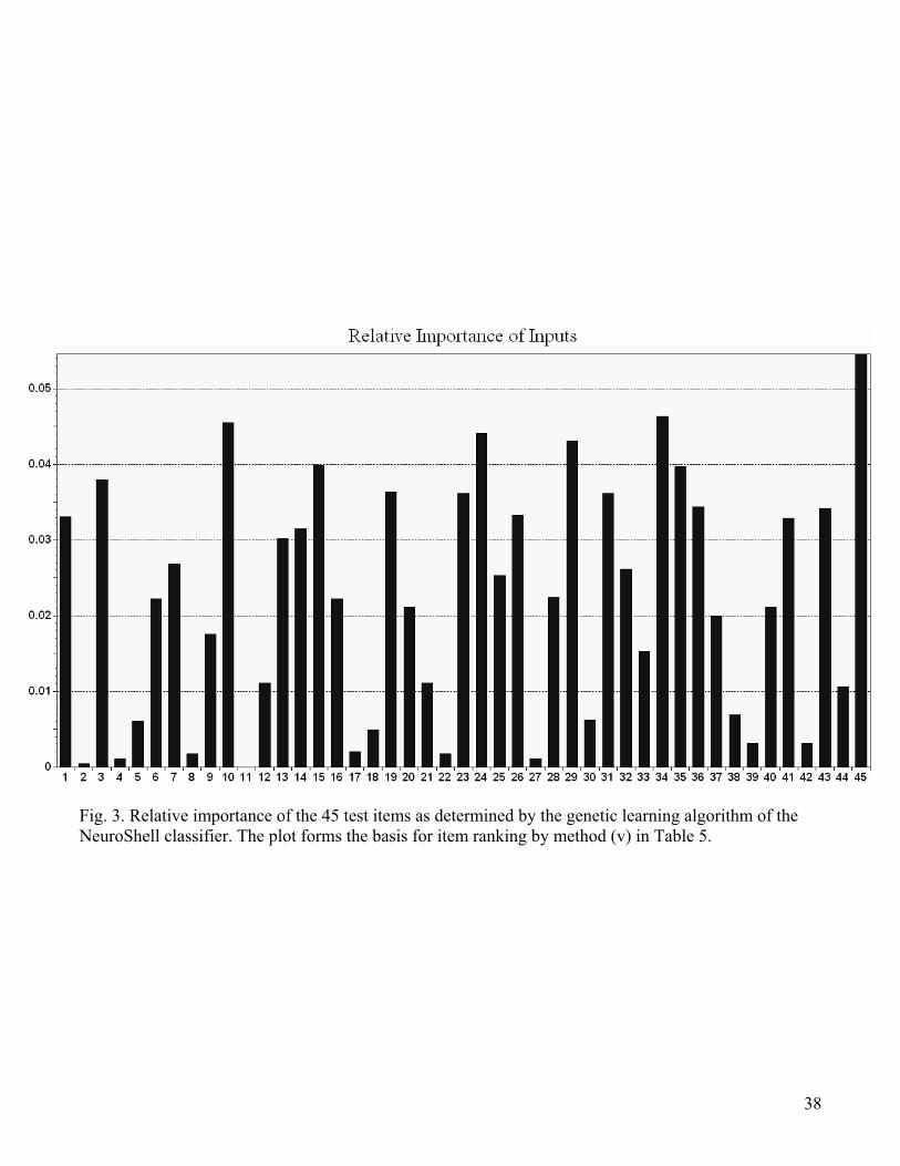
Fig. 3. Relative importance of the 45 test items as determined by the genetic learning algorithm of the

NeuroShell classifier. The plot forms the basis for item ranking by method (v) in Table 5.

38

0

0.1

0.2

0.3

0.4

0.5

0.6

0.7

0.8

0.9

1

0 0.1 0.2 0.3 0.4 0.5 0.6 0.7 0.8 0.9 1

Sensitiv

ity (

true p

ositiv

es)

GMDH: AUC = 0.975, SE = 0.0058

Random: AUC = 0.949, SE = 0.0093

IRT-IIF: AUC = 0.974, SE = 0.0066

1 - Specificity (false positives)1 – Specificity (false positives)

Fig. 4. Comparison of the ROC characteristics for the optimum abductive models developed

using subsets S1, S4, and S7 in Table 7. The subsets correspond to GMDH-based ranking and

selection, random selection, and IRT-based selection, respectively. Indicated on the figure are the

values for the area under the curve (AUC) and the associated standard error (SE) in each case.

39