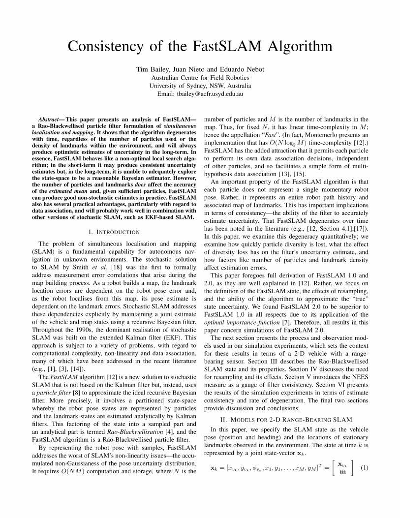
Consistency of the FastSLAM AlgorithmTim Bailey, Juan Nieto and Eduardo Nebot

Australian Centre for Field RoboticsUniversity of Sydney, NSW, Australia

Email: tbailey@acfr.usyd.edu.au

Abstract— This paper presents an analysis of FastSLAM—a Rao-Blackwellised particle filter formulation of simultaneouslocalisation and mapping. It shows that the algorithm degenerateswith time, regardless of the number of particles used or thedensity of landmarks within the environment, and will alwaysproduce optimistic estimates of uncertainty in the long-term. Inessence, FastSLAM behaves like a non-optimal local search algo-rithm; in the short-term it may produce consistent uncertaintyestimates but, in the long-term, it is unable to adequately explorethe state-space to be a reasonable Bayesian estimator. However,the number of particles and landmarks does affect the accuracyof the estimated mean and, given sufficient particles, FastSLAMcan produce good non-stochastic estimates in practice. FastSLAMalso has several practical advantages, particularly with regard todata association, and will probably work well in combination withother versions of stochastic SLAM, such as EKF-based SLAM.

I. INTRODUCTION

The problem of simultaneous localisation and mapping(SLAM) is a fundamental capability for autonomous nav-igation in unknown environments. The stochastic solutionto SLAM by Smith et al. [18] was the first to formallyaddress measurement error correlations that arise during themap building process. As a robot builds a map, the landmarklocation errors are dependent on the robot pose error and,as the robot localises from this map, its pose estimate isdependent on the landmark errors. Stochastic SLAM addressesthese dependencies explicitly by maintaining a joint estimateof the vehicle and map states using a recursive Bayesian filter.Throughout the 1990s, the dominant realisation of stochasticSLAM was built on the extended Kalman filter (EKF). Thisapproach is subject to a variety of problems, with regard tocomputational complexity, non-linearity and data association,many of which have been addressed in the recent literature(e.g., [1], [3], [14]).

The FastSLAM algorithm [12] is a new solution to stochasticSLAM that is not based on the Kalman filter but, instead, usesa particle filter [8] to approximate the ideal recursive Bayesianfilter. More precisely, it involves a partitioned state-spacewhereby the robot pose states are represented by particlesand the landmark states are estimated analytically by Kalmanfilters. This factoring of the state into a sampled part andan analytical part is termed Rao-Blackwellisation [4], and theFastSLAM algorithm is a Rao-Blackwellised particle filter.

By representing the robot pose with samples, FastSLAMaddresses the worst of SLAM’s non-linearity issues—the accu-mulated non-Gaussianess of the pose uncertainty distribution.It requires O(NM) computation and storage, where N is the

number of particles and M is the number of landmarks in themap. Thus, for fixed N , it has linear time-complexity in M ;hence the appellation “Fast”. (In fact, Montemerlo presents animplementation that has O(N log2 M) time-complexity [12].)FastSLAM has the added attraction that it permits each particleto perform its own data association decisions, independentof other particles, and so facilitates a simple form of multi-hypothesis data association [13], [15].

An important property of the FastSLAM algorithm is thateach particle does not represent a single momentary robotpose. Rather, it represents an entire robot path history andassociated map of landmarks. This has important implicationsin terms of consistency—the ability of the filter to accuratelyestimate uncertainty. That FastSLAM degenerates over timehas been noted in the literature (e.g., [12, Section 4.1],[17]).In this paper, we examine this degeneracy quantitatively; weexamine how quickly particle diversity is lost, what the effectof diversity loss has on the filter’s uncertainty estimate, andhow factors like number of particles and landmark densityaffect estimation errors.

This paper foregoes full derivation of FastSLAM 1.0 and2.0, as they are well explained in [12]. Rather, we focus onthe definition of the FastSLAM state, the effects of resampling,and the ability of the algorithm to approximate the “true”state uncertainty. We found FastSLAM 2.0 to be superior toFastSLAM 1.0 in all respects due to its application of theoptimal importance function [7]. Therefore, all results in thispaper concern simulations of FastSLAM 2.0.

The next section presents the process and observation mod-els used in our simulation experiments, which sets the contextfor these results in terms of a 2-D vehicle with a range-bearing sensor. Section III describes the Rao-BlackwellisedSLAM state and its properties. Section IV discusses the needfor resampling and its effects. Section V introduces the NEESmeasure as a gauge of filter consistency. Section VI presentsthe results of the simulation experiments in terms of estimateconsistency and rate of degeneration. The final two sectionsprovide discussion and conclusions.

II. MODELS FOR 2-D RANGE-BEARING SLAMIn this paper, we specify the SLAM state as the vehicle

pose (position and heading) and the locations of stationarylandmarks observed in the environment. The state at time k isrepresented by a joint state-vector xk.

xk = [xvk, yvk

, φvk, x1, y1, . . . , xM , yM ]T =

[xvk

m

](1)

Notice that the map parameters m = [x1, y1, . . . , xM , yM ]T

do not have a time subscript as they are modelled as stationary.To describe the vehicle motion, we use the kinematic model

for the trajectory of the front wheel of a bicycle subject torolling motion constraints (i.e., assuming zero wheel slip).

xvk= fv

(xvk−1 ,uk

)=

xvk−1 + Vk∆T cos(φvk−1 + γk)yvk−1 + Vk∆T sin(φvk−1 + γk)

φvk−1 + Vk∆TB sin(γk)

(2)Here the time from k − 1 to k is denoted ∆T , and duringthis period the velocity Vk and steering angle γk of the frontwheel are assumed constant. Collectively, the velocity andsteering values uk = [Vk, γk]T are termed the “controls”. Thewheelbase between the front and rear axles is B. The processmodel for the joint SLAM state is simply a concatenation ofthe vehicle motion model and the stationary landmark model.

xk = f (xk−1,uk) =[

fv(xvk−1 ,uk

)m

](3)

For a range-bearing measurement from the vehicle to land-mark mi = [xi, yi]T , the observation model is given by

zik= hi (xk) =

[ √(xi − xvk

)2 + (yi − yvk)2

arctan yi−yvk

xi−xvk− φvk

](4)

Adding new landmarks to the map uses an inverse form of theobservation model as described in [1, Section 2.2.4] and [10,Section 2].

The vehicle motion model, the observation model, and themeasured values of the control parameters uk, are not exact,but are subject to noise, which lead to uncertainty in the stateestimate. For this reason, we require a probabilistic filter torecursively estimate a distribution over the state given noisyinformation.

We make the usual basic assumptions regarding the depen-dencies of measurement errors. That is, the process model isfirst-order Markov and independent of the map states,1

p(xvk

|Xv0:k−1 ,m,Z0:k−1,U0:k

)= p

(xvk

|xvk−1 ,uk

)(5)

and the observations are independent conditioned on the jointSLAM state.

p (Z0:k|Xv0:k ,m,U0:k) =k∏

i=0

p (zi|xvi ,m) (6)

Multiple observations made at time k are also assumed condi-tionally independent. We further assume that the distributionsin Eqns. 5 and 6 are Gaussian as this allows certain parts ofthe FastSLAM algorithm to be reasonably approximated byEKF equations.

1A brief note on notation. The probability density function (PDF) of arandom variable x is denoted p (x) and a sample drawn from this distributionis x(i). A history of values {x0, . . . ,xk} from time 0 to time t is denotedX0:k .

III. RAO-BLACKWELLISATED SLAM

Rao-Blackwellisation is a variance reduction technique forMonte Carlo integration, whereby a joint probability densityfunction (PDF) is factored according to the product rule so asto reduce the dimensionality of the simulation-space.

x =[

x1

x2

](7)

p (x) = p (x2|x1) p (x1) (8)

It is applicable when p (x2|x1) can be evaluated analyticallyso that simulation is restricted to the space of p (x1),

x(i)1 ∼ p (x1) (9)

and exact inference can be used to compute p(x2|x(i)

1

).

Marginal estimates may be found as sums.

p (x2) ≈ 1N

N∑

i=1

p(x2|x(i)

1

)(10)

For a fixed number of samples, the random variation inestimates based on Rao-Blackwellised sampling is always lessthan (or equal to) that obtained by sampling from the entirespace of p (x).

A discussion of Rao-Blackwellisation applied to variousforms of Monte Carlo sampling is provided in [4], and ispresented as a way to reduce weight variance for particle filtersin [7]. A good discussion in the context of particle filters isgiven in [16, Section 3.3], which shows the derivation of ageneral state-space problem partitioned into particle filter andKalman filter components.

FastSLAM employs a particle filter primarily to address theproblem of representing a system that is non-linear and non-Gaussian. It applies Rao-Blackwellisation to reduce the filter’ssample-space from the joint state [xvk

,m]T to just the vehiclepose states xvk

. The state partitioning in FastSLAM is definedas follows.

p (Xv0:k ,m|Z0:k,U0:k)= p (Xv0:k |Z0:k,U0:k) p (m|Xv0:k ,Z0:k,U0:k)= p (Xv0:k |Z0:k,U0:k) p (m|Xv0:k ,Z0:k)

(11)

Here the joint posterior is factored into a vehicle pose partand a map part conditioned on the pose. Notice that the jointPDF is defined in terms of the vehicle pose history Xv0:k . Thisis a critical aspect of the FastSLAM formulation as it permitsefficient estimation of the map states. That is, given Xv0:k , andas a consequence of Eqn. 6, the individual landmark PDFs areindependent.

p (m|Xv0:k ,Z0:k) =M∏

i=1

p (mi|Xv0:k ,Zi0:k) (12)

The FastSLAM posterior at time k is represented as aset of N weighted particles {w0,X

(0)v0:k , . . . , wN ,X(N)

v0:k} overthe vehicle pose states. Each sample X(i)

v0:k has an associatedmap PDF p

(m|X(i)

v0:k ,Z0:k

), which is assumed approximately

Gaussian and is manipulated by an EKF. From Eqn. 12, themap PDF is a set of M independent 2-D Gaussians rather thana single joint 2M -D Gaussian. Thus, each particle actuallyrepresents: a pose history X(i)

v0:k , its weight wi, and its map{m1,P1, . . . , mM ,PM}.

Conditioning the map by the vehicle pose history is essentialfor the efficiency of the algorithm; keeping the landmarkestimates independent avoids the quadratic cost of computinga joint map covariance matrix. Dependence on pose history isalso the key weakness of the FastSLAM algorithm as it meansthe implicit dimension of the state-space increases with time.

IV. EFFECTS OF RESAMPLING

When implementing the FastSLAM algorithm, it is easyto forget that each particle represents a history X(i)

v0:k sincethe recursive equations at each time-step only require themomentary pose estimate x(i)

vk . However, the dependence onpose history is recorded in the sample weight and, mostsignificantly, in its map estimate. It is important to recognisethat a particle’s estimate of the map at time k is based onthe assumption that the vehicle pose was exactly known forall preceeding time-steps. As time progresses, the likelihoodof adequately exploring the sample-space becomes vanishinglysmall. This is seen most clearly in the particle resampling step.

A property of particle filters is that the variance of sampleweights increases with time [7].The filter degenerates untileventually all samples but one possess negligible weight. Tooffset this problem, resampling is performed, whereby samplesare chosen with replacement from the original sample set, togenerate an equal-weight sample set. This has been shown topermit consistent recursive estimation with a fixed number ofparticles provided a system exhibits “exponential forgetting”of its past estimate errors [6].

The problem with FastSLAM is that past pose estimateerrors are not forgotten; they are recorded in the map estimates.Whenever resampling is performed, for each particle notselected, an entire pose history and map hypothesis is lostforever. This depletes the number of samples representing pastposes and consequently erodes the statistics of the landmarkestimates conditioned on these past poses. After resampling,some particles share a common ancestry, and loss of trackindependence and loss of landmark estimate diversity increasesmonotonically.

V. MEASURING CONSISTENCY

Ideally, to measure if a filter is consistent, one wouldcompare its estimate with the probability density functionobtained from an ideal Bayesian filter. This is not practicalfor the FastSLAM algorithm. When the “true” PDF is notavailable, but the true state xk is known, we can use thenormalised estimation error squared (NEES) [2, page 234]to characterise the filter performance,

εk = (xk − xk)T P−1k (xk − xk) (13)

where {xk,Pk} are the estimated mean and covariance.

A measure of filter consistency is found by examination ofthe average NEES over N Monte Carlo runs of the filter.2

Under the hypothesis that the filter is consistent and approxi-mately linear-Gaussian, εk is χ2 (chi-square) distributed withdim(xk) degrees of freedom. Then the average value of εk

tends towards the dimension of the state as N approachesinfinity.

E[εk] = dim(xk) (14)

The validity of this hypothesis can be subjected to a χ2

acceptance test.Consistency of FastSLAM is evaluated by performing multi-

ple Monte Carlo runs and computing the average NEES. GivenN runs, the average NEES is computed as

εk =1N

N∑

i=1

εik(15)

Given the hypothesis of a consistent linear-Gaussian filter,Nεk has a χ2 density with N dim(xk) degrees of freedom.Thus, for the 3-dimensional vehicle pose, with N = 50, the95% probability concentration region for εk is bounded bythe interval [2.36, 3.72]. If εk rises significantly higher thanthe upper bound, the filter is optimistic, if it tends below thelower bound, the filter is conservative.

VI. EXPERIMENTAL RESULTS

In the following experiments, the vehicle model wheelbaseis 4 metres, the control noise is (σV = 0.3m/s, σγ = 3◦), andthe observation noise is (σr = 0.1m,σθ = 1◦). Controls areupdated at 40 Hz and observation scans are obtained every 5Hz. Each scan consists of range-bearing measurements to alllandmarks within a 30 metre radius in front of the vehicle.Data association is assumed known throughout.

Experiments were performed in the two simulated environ-ments in Fig. 1, one sparsely populated and one dense. Ineach environment, simulations were run with 100 particlesand 1000 particles. Resampling was performed, not after eachobservation, but once the “effective sample size” [7] fallsbelow 75% of the total number of particles. Each run involvedtwo loops of the trajectory partially shown in Fig. 1 and theywere each repeated for 50 Monte Carlo trials.

It is immediately apparent from Fig. 1 that the dense mappermits more accurate results than the sparse map in terms ofreal errors; the particles have smaller spread and are nearerthe true state. However, FastSLAM’s ability to estimate theseerrors is less intuitive.

An estimate of the rate of loss of particle diversity isobtained by recording the number of distinct particles rep-resenting a chosen landmark. Once the landmark goes out ofsight, resampling causes some estimates to be lost and othersto be multiplied, and diversity is depleted. Fig. 2 shows that

2A commonly used test of filter consistency is to examine the sequence ofnormalised errors {ε0, . . . , εk} over a single run. This test is not adequateas the error sequence is correlated and does not follow a χ2 distribution.Thus, even for a linear system, a single run of a consistent filter may appearinconsistent and a single run of an inconsistent filter may appear consistent.

−120 −100 −80 −60 −40 −20 0 20 40 60 80

−80

−60

−40

−20

0

20

40

60

80

metres

met

res

(a) Sparse map (b) Dense map

Fig. 1. Feature maps used in simulation experiments. The stars denote the true landmark locations. The dots are the particle estimates forvehicle and landmark locations during a typical run with 1000 particles, and the line is the mean estimate of the vehicle trajectory.

0 10 20 30 40 50 60 70 80 90 1000

20

40

60

80

100

Time (s)

Num

ber

of d

istin

ct s

ampl

es

(a) Sparse map, 100 particles

0 10 20 30 40 50 60 70 80 90 1000

200

400

600

800

1000

Time (s)

Num

ber

of d

istin

ct s

ampl

es

(b) Sparse map, 1000 particles

0 10 20 30 40 50 60 70 80 90 1000

20

40

60

80

100

Time (s)

Num

ber

of d

istin

ct s

ampl

es

(c) Dense map, 100 particles

0 10 20 30 40 50 60 70 80 90 1000

200

400

600

800

1000

Time (s)

Num

ber

of d

istin

ct s

ampl

es

(d) Dense map, 1000 particles

Fig. 2. Particle diversity for a landmark that is no longer visible. Each figure shows the number of distinct samples representing a singlelandmark from the moment it disappears from the vehicle’s field-of-view. The three lines are the minimum, maximum and median diversityobtained over 50 Monte Carlo runs.

diversity is lost exponentially. That Figs. 2(a) and 2(b) have thesame shape indicates that the ratio of distinct samples to totalnumber of samples remains approximately constant for a fixedlandmark density; sample size does not affect depletion rate.However, Figs. 2(c) and 2(d) show that the rate of diversityloss increases with landmark density. Thus, counter-intuitively,more observation information implies faster depletion.

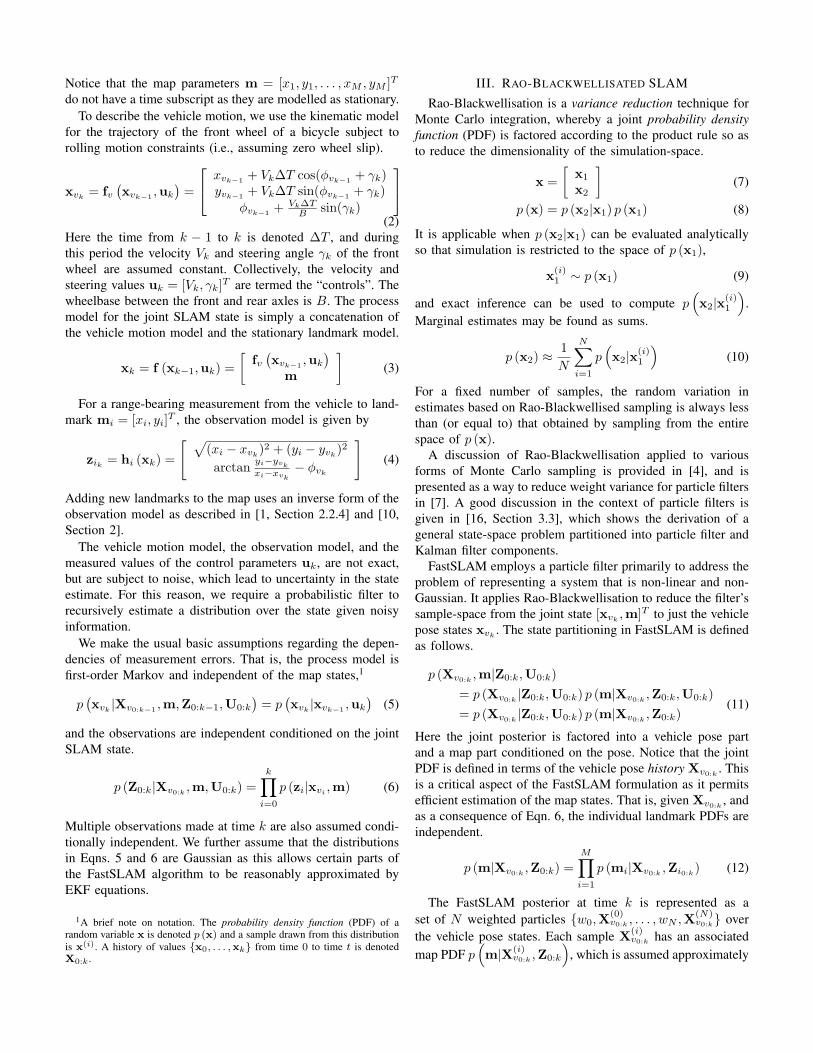
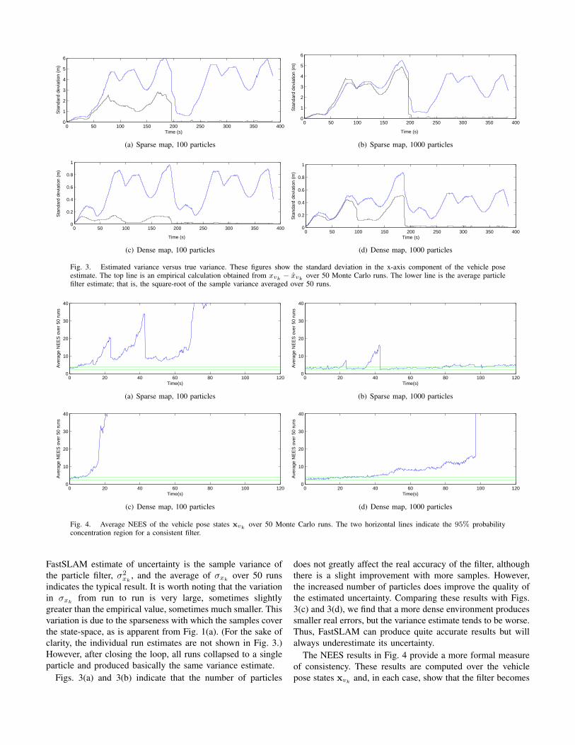
A comparison of the real errors and FastSLAM’s errorestimates is shown in Fig. 3. These figures plot the standard

deviations of the x-axis component of the vehicle pose.3 Anempirical estimate is calculated as the standard deviation ofxvk

− xvkover 50 Monte Carlo runs, where xvk

is the truestate and xvk

is the sample mean of the particle filter. The

3These results tend to make FastSLAM look better than it really isas process noise injects diversity into the pose estimate and maintainsits variance. If a landmark state had been chosen instead, the differencebetween empirical and estimated variance would occur sooner and be morepronounced.

0 50 100 150 200 250 300 350 4000

1

2

3

4

5

6

Time (s)

Sta

ndar

d de

viat

ion

(m)

(a) Sparse map, 100 particles

0 50 100 150 200 250 300 350 4000

1

2

3

4

5

6

Time (s)

Sta

ndar

d de

viat

ion

(m)

(b) Sparse map, 1000 particles

0 50 100 150 200 250 300 350 4000

0.2

0.4

0.6

0.8

1

Time (s)

Sta

ndar

d de

viat

ion

(m)

(c) Dense map, 100 particles

0 50 100 150 200 250 300 350 4000

0.2

0.4

0.6

0.8

1

Time (s)

Sta

ndar

d de

viat

ion

(m)

(d) Dense map, 1000 particles

Fig. 3. Estimated variance versus true variance. These figures show the standard deviation in the x-axis component of the vehicle poseestimate. The top line is an empirical calculation obtained from xvk − xvk over 50 Monte Carlo runs. The lower line is the average particlefilter estimate; that is, the square-root of the sample variance averaged over 50 runs.

0 20 40 60 80 100 1200

10

20

30

40

Time(s)

Ave

rage

NE

ES

ove

r 50

run

s

(a) Sparse map, 100 particles

0 20 40 60 80 100 1200

10

20

30

40

Time(s)

Ave

rage

NE

ES

ove

r 50

run

s

(b) Sparse map, 1000 particles

0 20 40 60 80 100 1200

10

20

30

40

Time(s)

Ave

rage

NE

ES

ove

r 50

run

s

(c) Dense map, 100 particles

0 20 40 60 80 100 1200

10

20

30

40

Time(s)

Ave

rage

NE

ES

ove

r 50

run

s

(d) Dense map, 1000 particles

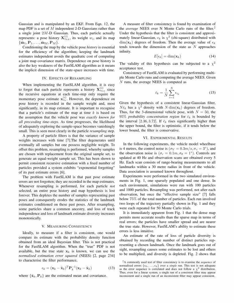
Fig. 4. Average NEES of the vehicle pose states xvk over 50 Monte Carlo runs. The two horizontal lines indicate the 95% probabilityconcentration region for a consistent filter.

FastSLAM estimate of uncertainty is the sample variance ofthe particle filter, σ2

xk, and the average of σxk

over 50 runsindicates the typical result. It is worth noting that the variationin σxk

from run to run is very large, sometimes slightlygreater than the empirical value, sometimes much smaller. Thisvariation is due to the sparseness with which the samples coverthe state-space, as is apparent from Fig. 1(a). (For the sake ofclarity, the individual run estimates are not shown in Fig. 3.)However, after closing the loop, all runs collapsed to a singleparticle and produced basically the same variance estimate.

Figs. 3(a) and 3(b) indicate that the number of particles

does not greatly affect the real accuracy of the filter, althoughthere is a slight improvement with more samples. However,the increased number of particles does improve the quality ofthe estimated uncertainty. Comparing these results with Figs.3(c) and 3(d), we find that a more dense environment producessmaller real errors, but the variance estimate tends to be worse.Thus, FastSLAM can produce quite accurate results but willalways underestimate its uncertainty.

The NEES results in Fig. 4 provide a more formal measureof consistency. These results are computed over the vehiclepose states xvk

and, in each case, show that the filter becomes

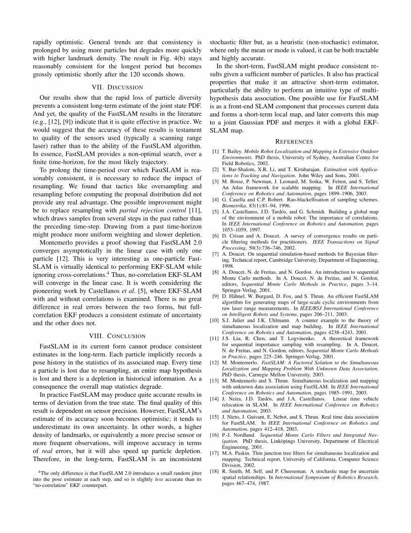
rapidly optimistic. General trends are that consistency isprolonged by using more particles but degrades more quicklywith higher landmark density. The result in Fig. 4(b) staysreasonably consistent for the longest period but becomesgrossly optimistic shortly after the 120 seconds shown.

VII. DISCUSSION

Our results show that the rapid loss of particle diversityprevents a consistent long-term estimate of the joint state PDF.And yet, the quality of the FastSLAM results in the literature(e.g., [12], [9]) indicate that it is quite effective in practice. Wewould suggest that the accuracy of these results is testamentto quality of the sensors used (typically a scanning rangelaser) rather than to the ability of the FastSLAM algorithm.In essence, FastSLAM provides a non-optimal search, over afinite time-horizon, for the most likely trajectory.

To prolong the time-period over which FastSLAM is rea-sonably consistent, it is necessary to reduce the impact ofresampling. We found that tactics like oversampling andresampling before computing the proposal distribution did notprovide any real advantage. One possible improvement mightbe to replace resampling with partial rejection control [11],which draws samples from several steps in the past rather thanthe preceding time-step. Drawing from a past time-horizonmight produce more uniform weighting and slower depletion.

Montemerlo provides a proof showing that FastSLAM 2.0converges asymptotically in the linear case with only oneparticle [12]. This is very interesting as one-particle Fast-SLAM is virtually identical to performing EKF-SLAM whileignoring cross-correlations.4 Thus, no-correlation EKF-SLAMwill converge in the linear case. It is worth considering thepioneering work by Castellanos et al. [5], where EKF-SLAMwith and without correlations is examined. There is no greatdifference in real errors between the two forms, but full-correlation EKF produces a consistent estimate of uncertaintyand the other does not.

VIII. CONCLUSION

FastSLAM in its current form cannot produce consistentestimates in the long-term. Each particle implicitly records apose history in the statistics of its associated map. Every timea particle is lost due to resampling, an entire map hypothesisis lost and there is a depletion in historical information. As aconsequence the overall map statistics degrade.

In practice FastSLAM may produce quite accurate results interms of deviation from the true state. The final quality of thisresult is dependent on sensor precision. However, FastSLAM’sestimate of its accuracy soon becomes optimistic; it tends tounderestimate its own uncertainty. In other words, a higherdensity of landmarks, or equivalently a more precise sensor ormore frequent observations, will improve accuracy in termsof real errors, but it will also speed up particle depletion.Therefore, in the long-term, FastSLAM is an inconsistent

4The only difference is that FastSLAM 2.0 introduces a small random jitterinto the pose estimate at each step, and so is slightly less accurate than its“no-correlation” EKF counterpart.

stochastic filter but, as a heuristic (non-stochastic) estimator,where only the mean or mode is valued, it can be both tractableand highly accurate.

In the short-term, FastSLAM might produce consistent re-sults given a sufficient number of particles. It also has practicalproperties that make it an attractive short-term estimator,particularly the ability to perform an intuitive type of multi-hypothesis data association. One possible use for FastSLAMis as a front-end SLAM component that processes current dataand forms a short-term local map, and later converts this mapto a joint Gaussian PDF and merges it with a global EKF-SLAM map.

REFERENCES

[1] T. Bailey. Mobile Robot Localisation and Mapping in Extensive OutdoorEnvironments. PhD thesis, University of Sydney, Australian Centre forField Robotics, 2002.

[2] Y. Bar-Shalom, X.R. Li, and T. Kirubarajan. Estimation with Applica-tions to Tracking and Navigation. John Wiley and Sons, 2001.

[3] M. Bosse, P. Newman, J. Leonard, M. Soika, W. Feiten, and S. Teller.An Atlas framework for scalable mapping. In IEEE InternationalConference on Robotics and Automation, pages 1899–1906, 2003.

[4] G. Casella and C.P. Robert. Rao-blackellisation of sampling schemes.Biometrika, 83(1):81–94, 1996.

[5] J.A. Castellanos, J.D. Tardos, and G. Schmidt. Building a global mapof the environment of a mobile robot: The importance of correlations.In IEEE International Conference on Robotics and Automation, pages1053–1059, 1997.

[6] D. Crisan and A. Doucet. A survey of convergence results on parti-cle filtering methods for practitioners. IEEE Transactions on SignalProcessing, 50(3):736–746, 2002.

[7] A. Doucet. On sequential simulation-based methods for Bayesian filter-ing. Technical report, Cambridge University, Department of Engineering,1998.

[8] A. Doucet, N. de Freitas, and N. Gordon. An introduction to sequentialMonte Carlo methods. In A. Doucet, N. de Freitas, and N. Gordon,editors, Sequential Monte Carlo Methods in Practice, pages 3–14.Springer-Verlag, 2001.

[9] D. Hahnel, W. Burgard, D. Fox, and S. Thrun. An efficient FastSLAMalgorithm for generating maps of large-scale cyclic environments fromraw laser range measurements. In IEEE/RSJ International Conferenceon Intelligent Robots and Systems, pages 206–211, 2003.

[10] S.J. Julier and J.K. Uhlmann. A counter example to the theory ofsimultaneous localization and map building. In IEEE InternationalConference on Robotics and Automation, pages 4238–4243, 2001.

[11] J.S. Liu, R. Chen, and T. Logvinenko. A theoretical frameworkfor sequential importance sampling with resampling. In A. Doucet,N. de Freitas, and N. Gordon, editors, Sequential Monte Carlo Methodsin Practice, pages 225–246. Springer-Verlag, 2001.

[12] M. Montemerlo. FastSLAM: A Factored Solution to the SimultaneousLocalization and Mapping Problem With Unknown Data Association.PhD thesis, Carnegie Mellon University, 2003.

[13] M. Montemerlo and S. Thrun. Simultaneous localization and mappingwith unknown data association using FastSLAM. In IEEE InternationalConference on Robotics and Automation, pages 1985–1991, 2003.

[14] J. Neira, J.D. Tardos, and J.A. Castellanos. Linear time vehiclerelocation in SLAM. In IEEE International Conference on Roboticsand Automation, 2003.

[15] J. Nieto, J. Guivant, E. Nebot, and S. Thrun. Real time data associationfor FastSLAM. In IEEE International Conference on Robotics andAutomation, pages 412–418, 2003.

[16] P.-J. Nordlund. Sequential Monte Carlo Filters and Integrated Nav-igation. PhD thesis, Linkopings University, Department of ElectricalEngineering, 2001.

[17] M.A. Paskin. Thin junction tree filters for simultaneous localization andmapping. Technical report, University of California, Computer ScienceDivision, 2002.

[18] R. Smith, M. Self, and P. Cheeseman. A stochastic map for uncertainspatial relationships. In International Symposium of Robotics Research,pages 467–474, 1987.