
Conformance Relations and Hyperproperties for Doping ...
39
Logical Methods in Computer Science Volume 18, Issue 1, 2022, pp. 14:1–14:39 https://lmcs.episciences.org/ Submitted Dec. 08, 2020 Published Jan. 19, 2022 CONFORMANCE RELATIONS AND HYPERPROPERTIES FOR DOPING DETECTION IN TIME AND SPACE SEBASTIAN BIEWER a , RAYNA DIMITROVA b , MICHAEL FRIES c , MACIEJ GAZDA d , THOMAS HEINZE c , HOLGER HERMANNS a,e , AND MOHAMMAD REZA MOUSAVI f a Saarland University — Computer Science, Saarland Informatics Campus, Saarbr¨ ucken, Germany b CISPA Helmholtz Center for Information Security, Saarbr¨ ucken, Germany c Automotive Powertrain Institute, htw saar — University of Applied Sciences, Saarbr¨ ucken, Germany d Department of Computer Science, University of Sheffield, Sheffield, UK e Institute of Intelligent Software, Guangzhou, China f Department of Informatics, King’s College London, London, UK Abstract. We present a novel and generalised notion of doping cleanness for cyber- physical systems that allows for perturbing the inputs and observing the perturbed outputs both in the time—and value—domains. We instantiate our definition using existing notions of conformance for cyber-physical systems. As a formal basis for monitoring conformance- based cleanness, we develop the temporal logic HyperSTL*, an extension of Signal Temporal Logics with trace quantifiers and a freeze operator. We show that our generalised definitions are essential in a data-driven method for doping detection and apply our definitions to a case study concerning diesel emission tests. 1. Introduction System doping, in our terminology, is an intentional intervention causing a change in the system’s normal behaviour against the interests of the user or other stakeholders (such as the society at large). Examples of system doping are widespread and range from vendors’ enforcing a monopoly on chargers and spare parts (by checking for and refusing third-party chargers and spare parts, respectively) to tampering with exhaust emission in order to detect and pass emission tests. Doping can be the result of embedding a piece of code or smuggling a piece of electronic circuit into the system and it can be caused by the original developers or by hackers. Software and system doping has been studied in the past couple of years and rigorous theories for it have been developed [BDFH16, DBB + 17, BDH18]. These theories were subsequently adopted in order to detect doping, or formally, to check system cleanness [HBDK18, BDH19] (corresponding to the absence of doping). Key words and phrases: Software Doping, Conformance Testing, Hybrid Systems. LOGICAL METHODS IN COMPUTER SCIENCE DOI:10.46298/LMCS-18(1:14)2022 © S. Biewer, R. Dimitrova, M. Fries, M. Gazda, T. Heinze, H. Hermanns, and M. R. Mousavi CC Creative Commons
-
Upload
khangminh22 -
Category
Documents
-
view
1 -
download
0
Transcript of Conformance Relations and Hyperproperties for Doping ...

Logical Methods in Computer ScienceVolume 18, Issue 1, 2022, pp. 14:1–14:39https://lmcs.episciences.org/
Submitted Dec. 08, 2020Published Jan. 19, 2022
CONFORMANCE RELATIONS AND HYPERPROPERTIES FOR
DOPING DETECTION IN TIME AND SPACE
SEBASTIAN BIEWER a, RAYNA DIMITROVA b, MICHAEL FRIES c, MACIEJ GAZDA d,THOMAS HEINZE c, HOLGER HERMANNS a,e, AND MOHAMMAD REZA MOUSAVI f
a Saarland University — Computer Science, Saarland Informatics Campus, Saarbrucken, Germany
b CISPA Helmholtz Center for Information Security, Saarbrucken, Germany
c Automotive Powertrain Institute, htw saar — University of Applied Sciences, Saarbrucken, Germany
d Department of Computer Science, University of Sheffield, Sheffield, UK
e Institute of Intelligent Software, Guangzhou, China
f Department of Informatics, King’s College London, London, UK
Abstract. We present a novel and generalised notion of doping cleanness for cyber-physical systems that allows for perturbing the inputs and observing the perturbed outputsboth in the time—and value—domains. We instantiate our definition using existing notionsof conformance for cyber-physical systems. As a formal basis for monitoring conformance-based cleanness, we develop the temporal logic HyperSTL*, an extension of Signal TemporalLogics with trace quantifiers and a freeze operator. We show that our generalised definitionsare essential in a data-driven method for doping detection and apply our definitions to acase study concerning diesel emission tests.
1. Introduction
System doping, in our terminology, is an intentional intervention causing a change in thesystem’s normal behaviour against the interests of the user or other stakeholders (such asthe society at large). Examples of system doping are widespread and range from vendors’enforcing a monopoly on chargers and spare parts (by checking for and refusing third-partychargers and spare parts, respectively) to tampering with exhaust emission in order todetect and pass emission tests. Doping can be the result of embedding a piece of code orsmuggling a piece of electronic circuit into the system and it can be caused by the originaldevelopers or by hackers. Software and system doping has been studied in the past couple ofyears and rigorous theories for it have been developed [BDFH16, DBB+17, BDH18]. Thesetheories were subsequently adopted in order to detect doping, or formally, to check systemcleanness [HBDK18, BDH19] (corresponding to the absence of doping).
Key words and phrases: Software Doping, Conformance Testing, Hybrid Systems.
LOGICAL METHODSl IN COMPUTER SCIENCE DOI:10.46298/LMCS-18(1:14)2022© S. Biewer, R. Dimitrova, M. Fries, M. Gazda, T. Heinze, H. Hermanns, and M. R. MousaviCC© Creative Commons

14:2 S. Biewer, R. Dimitrova, M. Fries, M. Gazda, T. Heinze, H. Hermanns, and M. R. Mousavi Vol. 18:1
istidev
istiddev
o(ist)o(iddev)
o'(ist)o'(iddev)
(a) (b) (c) (d) t
em(mg)v(km/h)
t
v(km/h)
t t
em(mg)
𝜖 𝜖
𝜏
𝜖 𝜖
𝜏t0 t0
Figure 1: Running Example: Specified (a) and Actual (b) Test Cycles and Emission Foot-prints obtained from Different (Fictitious) Vehicles (c) and (d).
In the present paper, we extend the theory of doping to the setting of cyber-physicalsystems (CPS) by exploiting the notions of conformance testing for CPS [AMF14, DMP17,KM15]. The existing theories of software doping define doping in terms of drastic deviationsin output as a result of minor deviations in input, where the term “deviation” refers todifferences in validity of propositions or values of variables. However, the current notionscome short of properly dealing with the issues of retiming and delays, which are commonlypresent in the signals of CPS. We observe that this is an essential aspect of detecting dopingfor cyber-physical systems: often the traces to be tested for doping have subtly differenttiming behaviour, e.g., due to measurement and calibration errors or due to the slightdeviations of human actors in acting upon the planned scenarios. The insufficient treatmentof retiming and delays can both lead to false negatives, i.e., missing cases of doping, as wellas false positives, i.e., reporting spurious doping cases.
To address these issues, we exploit the notion of conformance to devise a generaltheory of being clean from doping and instantiate that theory with some existing notionsof conformance for hybrid systems. We show how these notions can account for retimingand lead to more precise notions of cleanness. Furthermore, we show how the retiming canbe synchronized between input and output, leading to a refined notion of cleanness with arigorous account of the relation between the retiming of input and output.
We illustrate the usefulness of our theory by empirical analysis of diesel engine exhaustemissions in the context of one of the official test cycles, the New European Driving Cycle(NEDC) [Uni13]. In particular, we show that catering for retiming is essential in effectivelyexploiting the actual driving cycles for performing doping analysis. We thus demonstratethat our new theory remedies a major shortcoming in the existing notions from the literature.To facilitate the presentation, we use throughout the remainder of this paper the followingsimple running example, which is inspired by our case study.
Example 1.1. Fig. 1.(a) shows two test cycles (evolution of speed over time), designed todetect whether the exhaust emission control of a particular vehicle is doped. The test cycleist , depicted with a black solid line, is the standard one prescribed by the (fictitious) officialregulation, while test cycle idev , depicted by a red dotted line, is a slight deviation thereof. Ifthe exhaust emissions measured during the test cycle idev turn out to be significantly higherthan the ones measured in test cycle ist , then we can conclude that the exhaust emissionsystem is potentially doped, since it appears tailored to the standard test cycle.
Fig. 1.(b) addresses a notorious problem of testing cars: a human tester is supposed todrive the car as just described, however, she can do this only up to a certain imprecision.Assume her driving of idev exhibits a slight time shift τ relative to the test cycle, as in iddev ,while ist is being driven as intended.

Vol. 18:1CONFORMANCE AND HYPERPROPERTIES FOR DOPING DETECTION IN TIME AND SPACE14:3
The result of a test is the emission footprint measured at the exhaust pipe of the car.Fig. 1.(c) and Fig. 1.(d) show two different possible test results (obtained from differentcars) for the scenario in Fig. 1.(b). Intuitively, the footprints in Fig. 1.(c) provide significantevidence for doping — a slightly different test cycle has resulted in significantly largerfootprint. However, due to the time shift on the input side in Fig. 1.(b) the point-wisedifference of the two driven test-cycles has grown very large. As we show in the remainderof this paper, the existing theory of doping fails to detect such a clear evidence, due to theminor delay during the execution of the driving cycle. The emission footprint in Fig. 1.(d) isanother (synthetic) example of a significant deviation which cannot be detected for the inputin Fig. 1.(b) using existing theories; this latter footprint sheds some light on the intricatedesign decisions in the theory we develop in this paper.
The contributions for this paper can be summarized as follows:
• We define a general notion of conformance that can express different ways of comparingexecution traces by allowing deviations both in value and in time;• We define a general notion of cleanness for hybrid systems, and show that it subsumes
the existing notion of robust cleanness [DBB+17];• We define the notion of synchronized retiming, which provides a rigorous tool for relating
the retiming of input and output and use it to produce a refined notion of cleanness;• We provide a logical account of cleanness (based on the notion of hybrid conformance) by
developing a temporal logic, called HyperSTL*, that extends Signal Temporal Logic (STL)with a freeze operator and quantifiers over traces; and• We demonstrate the usefulness of the proposed generic framework by applying it to software
doping tests in the automotive domain, where we show that the new cleanness definition isable to flag a case of software doping that goes unnoticed when robust cleanness is used.
This paper substantially extends the theoretical material and the experimental resultspublished in the earlier conference publication [DGM+20]. In particular, the followingcontributions of the present paper are new with respect to the earlier conference publication:
• the notion of cleanness with synchronised retiming in Section 5 and its application inSection 7 for doping detection in our case study,• the logical approach to cleanness in Section 6, the introduction of our logical formalism
HyperSTL*, its monitoring, and its application to specify hybrid conformance, and• the redesign of our experimental setup to comply with the NEDC test cycle (with
preconditioning and control of ambient temperature), as well as several new experimentsto make full use of our theories of retiming. These new experiments led to much moresubstantial and decisive evidence for our case study.
2. Related Work
The term “software doping” was coined around 2015 [HHB15] in media uncovering the dieselexhaust emissions scandal. An informal problem formulation [BDFH16] pointed out thegeneral phenomenon of intentionally added hidden software behaviour, which is not in theinterest of the consumer. Shortly after, this observation has been complemented by a setof formal cleanness definitions [DBB+17] laying the theoretical foundations upon whichformal methods to detect such software behaviour can be used. It is possible to detectmissing functionality and undesired existing functionality. The definitions support bothsequential programs and nondeterministic reactive programs. To check satisfaction of the
14:4 S. Biewer, R. Dimitrova, M. Fries, M. Gazda, T. Heinze, H. Hermanns, and M. R. Mousavi Vol. 18:1
definitions, it is necessary to compare two (or more) execution traces of the same system.Such properties are called hyperproperties [CS08] (whereas classical properties are traceproperties). Tool support for analysing hyperproperties typically requires high computationaleffort [CFK+14, FRS15]. There exist several temporal logics for analysing satisfaction oftrace properties of various kinds of systems, one of them being Linear Temporal Logic(LTL) [Pnu77] for systems producing outputs in discrete time steps and properties thatdo not consider the time passing between outputs. LTL has been extended to the logicHyperLTL, which can express hyperproperties by allowing explicit quantification of executiontraces in front of an LTL formula [CFK+14]. Tools for model-checking boolean circuits,satisfiability and monitoring of HyperLTL specifications have been developed [AB16, BSB17,FRS15, FH16, FHS17, FHST17, FHST18, HST19].
Signal Temporal Logic (STL) [MN04] is an extension of LTL that adds support fortime constraints and real-valued signals. Tools exist that automatically try to falsify STLformulas [Don10, ALFS11]. There has been an extension of STL to HyperSTL in a similarfashion as it was done for HyperLTL [NKJ+17]. The syntax of HyperSTL, however, is notable to express the cleanness definitions (for deterministic systems) in a way that allows(efficient) falsification. Freeze Temporal Logic [AH94] introduces a freeze quantifier to“record” the moment of time while evaluating a formula and later use the recorded time tomeasure time lapse. The concept of freeze quantifier has been used to specify properties ofdata-dependent systems (using models such as register automata) [DL09] and dynamicalsystems [BDSV14, DMP17]. In the present paper, we introduce the concept of freezequantifier [BDSV14] into a logic that is inspired by HyperSTL [NKJ+17]. The combinationturns out to be expressive enough to specify cleanness with respect to hybrid conformance.Moreover, we use a monitoring procedure inspired by an earlier extension of STL withfreeze operator [STB+19] to check for cleanness with respect to hybrid conformance. Robustcleanness is defined for distance functions on inputs and outputs [DBB+17]. When usedwith temporal logics the distance functions are restricted to those compatible with the logics.To be fully independent, robust cleanness analysis has been embedded into the theory ofmodel-based testing [BDH19] with input-output conformance [Tre92, Tre96].
Notions of conformance for discrete event systems have been discussed for almost acentury. The earliest work on this topic dates back to 1960’s when researchers studiedmodel-based testing of digital circuits using Finite State Machine models [Hen64, LY96].Concurrency theory contributed ideas to this field, such as decoupling (i.e., removing thesynchronised assumption between) inputs and outputs and observing failures to engage in acommunication (and more specifically quiescence) [DH84, Tre92]. A theory of conformancetesting for systems with continuous dynamics was developed by Michiel van Osch [vO06]; thistheory did not gain much popularity in practice, partly because of its insufficient treatment ofapproximation (e.g., differences in values and retiming). Pappas and Girard [GJP08, GP11]proposed the use of Metric Bisimulation for conformance checking in dynamical systemsand Pappas and Fainekos [FP09] developed a falsification framework for the same purpose.This research led to two notions of conformance used in the present paper, namely hybridconformance by Abbas and Fainekos [AMF14] and Skorokhod conformance by Deshmukh,Majumdar, and Prabhu [DMP17].

Vol. 18:1CONFORMANCE AND HYPERPROPERTIES FOR DOPING DETECTION IN TIME AND SPACE14:5
3. Preliminaries
3.1. Semantic domain. In this section, we provide definitions regarding semantic domain,conformance, and robust cleanness. We begin with the definition of our semantic domain,called generalised timed traces [GM20]. This definition subsumes both discrete-time statesequences and continuous-time trajectories. A generalised timed trace is a function with adiscrete or continuous domain (called time domain) and a co-domain which is a metric space.Intuitively, a generalized timed trace maps each element of its time domain to a state. Werequire that the set of possible states is a metric space since we study conformance notionsthat compare traces based on the distance between the states of the traces.
Definition 3.1. Let (Y, dY) be a metric space. A Y-valued generalised timed trace (GTT)is a function µ : T → Y such that T ⊆ R≥0. We call T the time domain of µ, denoteddom(µ). GTT (Y) is the set of all Y-valued generalised timed traces.
For a GTT µ : T → Y and time t0 ∈ T , by µ[. . . t0] we denote the prefix of µ upto t0, i.e., the restriction µ|t∈T :t≤t0 ; likewise, by µ[ts . . . te], we shall denote the restrictionµ|t∈T :ts≤t≤te
A hybrid system is a mapping from generalised (input) timed traces to sets of generalised(output) timed traces.
Definition 3.2. A Y-valued hybrid system is a function H : GTT (Y)→ P(GTT (Y)) suchthat for all µ ∈ GTT (Y) and all µ′ ∈ H (µ) it holds that dom(µ′) = dom(µ). We defineH(Y) to be the set of all Y-valued hybrid systems.
In addition, we distinguish deterministic hybrid systems whose output values range oversingleton sets only. In what follows, we identify deterministic hybrid systems with functionsof the type GTT (Y)→ GTT (Y).
For simplicity, we assume that the input and output domain are defined on the samemetric spaces. The generalisation to different spaces is straightforward.
3.2. Conformance relations. Recently, a number of notions of conformance for cyber-physical systems have been proposed [ARM17, KM15]. It turns out that these notions, twoof which are quoted below, can provide a rigorous basis for doping detection.
Note that throughout the paper, the variables τ and ε (with possible subscripts) alwaysrange over non-negative real numbers.
Definition 3.3. We say that Y-valued GTTs µ1 : T1 → Y and µ2 : T2 → Y are:
• trace conformant with tolerance threshold for signal value ε, notation TraceConfε(µ1, µ2),if T1 = T2 and for all t ∈ T1, dY(µ1(t), µ2(t)) ≤ ε• hybrid conformant with thresholds τ and ε, denoted HybridConfτ,ε(µ1, µ2), if:
– ∀t1 ∈ T1 ∃t2 ∈ T2 : |t2 − t1| ≤ τ ∧ dY(µ2(t2), µ1(t1)) ≤ ε– ∀t2 ∈ T2 ∃t1 ∈ T1 : |t1 − t2| ≤ τ ∧ dY(µ1(t1), µ2(t2)) ≤ ε• Skorokhod conformant with tolerance thresholds τ and ε, notation SkorConfτ,ε(µ1, µ2), ifT1 and T2 are intervals and there is a strictly increasing continuous bijection r : T1 → T2called retiming, such that:– for all t ∈ T1, |r(t)− t| ≤ τ , and– for all t ∈ T1, dY(µ1(t), µ2(r(t))) ≤ ε.

14:6 S. Biewer, R. Dimitrova, M. Fries, M. Gazda, T. Heinze, H. Hermanns, and M. R. Mousavi Vol. 18:1
We show in the proposition below and also in our generalisation results in Section 4.2, thatthese notions are closely related. However, they also have some fundamental differences,that can be illustrated using the example in Fig. 1.
Example 3.4. Consider again the example shown in Fig. 1.We can see that in Fig. 1.(a) ist and idev are trace conformant with value threshold ε,
as they only exhibit point-wise deviations by values less than ε. In contrast, ist and iddev inFig. 1.(b) are not trace conformant, yet they are hybrid conformant with time and valuemargins τ and ε, respectively. The key difference is that the inputs depicted in Fig. 1.(b) arevery different if compared point-wise, but if one allows for retiming, they are close enoughin value after retiming.
The outputs o′(ist) and o′(iddev ) in Fig. 1.(d) illustrate the fundamental differencebetween hybrid and Skorokhod conformance: although the order of rising and fallingsignals are reversed in the two trajectories, they are still hybrid conformant, because hybridconformance disregards the order. However, Skorokhod conformance requires an order-preserving retiming, and hence distinguishes these two trajectories. On the other hand, suchretiming exists, e.g., for ist and iddev in Fig. 1.(b), witnessing their Skorokhod conformance.
We shall use the following notation. We write Conf1 v Conf2 whenever for all µ1 : T1 → Yand µ2 : T2 → Y, we have Conf1(µ1, µ2) =⇒ Conf2(µ1, µ2). We write Conf1 < Conf2whenever Conf1 v Conf2 and ¬Conf2 v Conf1.
Proposition 3.5. For any τ, ε ∈ R≥0, the following relations hold:
TraceConfε < SkorConfτ,ε < HybridConfτ,ε
3.3. Robust cleanness. We shall now state the original definition of robust cleannessfrom [DBB+17], adapted to our framework of hybrid systems. It is based on Definition 7 andProposition 19 from [DBB+17]; the phrasing below abstracts from the so-called parametersof interest and standard inputs. Moreover it is cast in the setting of generalised timedtraces rather than discrete-step programs, and stated using trace conformance with differentthresholds for inputs and outputs, κI and κO.
Intuitively, a hybrid system is robustly clean if for every pair of input prefixes on whichno difference in the inputs exceeding κI has occurred so far (i.e., all sub-prefixes are traceconformant), the corresponding sets of output prefixes are also conformant with respect toκO. As we consider nondeterministic systems, Hausdorff distance is used to compare sets ofoutputs (see [DBB+17] for details).
Definition 3.6. A hybrid system H is robustly clean, denotedRobustClean(κI , κO), whenever:∀i1, i2 ∈ GTT (Y) : ∀t ∈ dom(i1) ∪ dom(i2) :(∀t′ ≤ t : TraceConfκI (i1[. . . t
′], i2[. . . t′]) =⇒(
(∀o1 ∈ H (i1) ∃o2 ∈ H (i2) : TraceConfκO(o1[. . . t], o2[. . . t])) ∧(∀o2 ∈ H (i2)∃o1 ∈ H (i1) : TraceConfκO(o1[. . . t], o2[. . . t]))
)Note that in the above definition we do not require that dom(i1) = dom(i2). In practice,
robust cleanness is typically applied to pairs of traces that are both defined over N. Here,however, for the sake of generality we impose no such restriction. In particular, when the

Vol. 18:1CONFORMANCE AND HYPERPROPERTIES FOR DOPING DETECTION IN TIME AND SPACE14:7
time domains of two traces are different, for example disjoint, the predicate RobustClean willtrivially evaluate to true.
Example 3.7. Consider the traces depicted in Fig. 1. The input prefixes ist and iddev aregiven in Fig. 1.(b), and the corresponding pair of outputs is shown in Fig. 1.(c). For t ≤ t0,we have iddev (t) = 0 and o(iddev )(t) = 0. The trace ist results in output o(ist) and iddev
results in o(iddev ). Suppose that ε < |ist(t0)− iddev (t0)|, and for every t < t0 it holds that|o(ist)(t) − o(iddev )(t)| ≤ |ist(t) − iddev (t)|. Furthermore, ε < |o(ist)(t1) − o(iddev )(t1)| atsome time t1 ≥ t0. Consider Def. 3.6 instantiated with κI = κO = ε. Clearly, for every t < t0the implication in Def. 3.6 is satisfied, since |o(ist)(t
′) − o(iddev )(t′)| ≤ |ist(t′) − iddev (t′)|
for all t′ ≤ t < t0, and κI = κO. For t ≥ t0 the implication is true as well: for t′ < t0the reasoning is as above, and for all t′ ≥ t0 the left-hand side of the implication is false.Hence, regardless of the difference in the output values at t1, this pair of inputs satisfies thecondition of RobustClean(ε, ε), and, if these are the only traces in a hybrid system H thenwe can conclude that H is RobustClean(ε, ε).
4. Conformance-Based Cleanness
We now define a general notion of conformance-based cleanness and provide two instantiationsbased on the conformance notions defined in the previous section.
4.1. Motivation. The need for considering disturbance in time as well as in value ismotivated by our running example from Fig. 1. One of the challenges in performing dopingtests for cyber-physical systems is that in such systems timing is rarely perfectly precise, dueto imprecision in measurements, or caused by the interaction with the physical world. Asillustrated in Example 1.1, for instance, when checking for software doping in a car [BDH19],the input to the system is the value of the car’s speed over time, which is under the controlof a driver, and can thus vary from one execution to the other, even if the driver is tryingto execute the same input sequence. Clearly, those variations can be in value, as well as intime.
Example 4.1. Consider the test setup sketched in Fig. 1. There, ist and iddev , depicted inFig. 1.(b) define the speed of a car as a function of time. These two input sequences followa trajectory of values differing by a small margin ε (the difference in value allowed by thestandard defining the doping tests), but also shifted by a small unit of time τ . Observefurther that |ist(t0) − iddev (t0)| � ε. Thus, without allowing for deviations in time whencomparing these input sequences, they will be considered sufficiently different, and as a resulttheir respective exhaust emission outputs will fall out of the comparison when checkingfor doping according to Def. 3.6, even if the outputs H (ist(t)) and H (iddev (t)) are vastlydifferent, as depicted in Fig. 1.(c). This results in a false negative, i.e., failing to detect aclearly doped system.
In the above example, we demonstrated that not accounting for timing disturbanceswhen relating input trajectories can result in false negatives in doping detection. Dually,using the traditional comparison for output traces can result in false positives by requiringoverly strict matching of outputs.

14:8 S. Biewer, R. Dimitrova, M. Fries, M. Gazda, T. Heinze, H. Hermanns, and M. R. Mousavi Vol. 18:1
The above example motivates the need to account for timing deviations in trajectories.Intuitively, for input trajectories this relaxation results in considering more traces as con-forming, and thus enforcing more comparisons when checking if a system is clean. For outputtrajectories this means relaxing the conformance requirement by considering two outputsequences as conforming even if their values are not perfectly aligned in time. Furthermore,different types of timing deviations need to be considered in different scenarios, for example,depending on whether the order in which values occur is important or not.
Example 4.2. Consider the testing workflow from Example 1.1 and Fig. 1, where inputs ist
and iddev are passed to a car. In the second experiment, depicted in Fig. 1.(d), the outputsof the car are o′(ist) and o′(iddev ), which are hybrid conformant for ε and τ . Hence, thisobservation of the system is classified as clean under hybrid output conformance. However,the output o′(iddev ) is clearly suspicious, as the values in o′(iddev ) and o′(ist) are reversed.This motivates considering conformance notions that require retimings to be order-preserving.Indeed, using Skorokhod conformance we can detect that the system is doped.
The above examples show that in order to be useful in a diverse set of applications,a software cleanness theory should allow for using a variety of conformance notions. Tothis end, we next take a more general view on conformance notions, in order to be able todevelop a generic conformance-based cleanness framework.
4.2. Retimings and a more generic view on conformance notions. So far, we havedefined three specific notions of conformance which either coincide, or are closely inspiredby ones that have appeared in the literature. In order to define a general framework forcleanness, we also wish to treat notions of conformance in a more generic manner. To thisend, we propose an abstract definition of conformance predicates. As conformance predicatesadmit variations in time, as well as in value, our definition is based on retimings, a devicethat will play a key role in the context of this work. In its general form a retiming is apair of functions between two time domains. Intuitively, given two GTTs, a retiming willdefine a mapping from points in each of the traces to points in the other trace. Note thatin general the mappings are not required to be injective; this way we can cater for notionsof conformance allowing for the so-called local disorder phenomenon (in particular hybridconformance — see Proposition 4.5).
Definition 4.3. A retiming is a pair of functions between two time domains, i.e., a pairof the form (r1, r2), where r1 : T1 → T2 and r2 : T2 → T1, with time domains T1, T2 ⊆ R≥0.Given two time domains T1 and T2, we denote the set of all retimings between T1 and T2with RET (T1, T2).
Retiming is explicitly present in the definition of Skorokhod conformance; there, eachSkorokhod retiming is required to be a strictly increasing continuous bijection. We canexpress a Skorokhod retiming r as an instance of our definition as the pair (r, r−1). In fact,one can also define hybrid conformance, as well as a whole class of conformance notions,using a suitable family of retimings.
A family of retimings Ret can be further constrained by τ to a subset Retτ of Retcontaining only functions that shift time by at most τ time units. In order to use a familyof retimings for concrete sequences µ1 and µ2, it is necessary to consider only functionsthat match the domains of the sequences. This leads to a generic notion of conformance

Vol. 18:1CONFORMANCE AND HYPERPROPERTIES FOR DOPING DETECTION IN TIME AND SPACE14:9
associated with a given family of retimings Ret, a given time threshold τ and a given valuethreshold ε.
Definition 4.4. Let Ret be a family of retimings, and let
Retτ4= {(r1, r2) ∈ Ret | ∀t ∈ dom(ri) : |ri(t)− t| ≤ τ (i = 1, 2)},
Retτ (T1, T2)4= Retτ ∩RET (T1, T2).
A conformance notion with time threshold τ and value threshold ε induced by Ret is apredicate Conf Retτ,ε on pairs of GTTs such that, for µ1 : T1 → Y, µ2 : T2 → Y:
Conf Retτ,ε (µ1, µ2) ⇐⇒ ∃(r1, r2) ∈ Retτ (T1, T2) : ∀t ∈ T1 : dY(µ1(t), µ2 ◦ r1(t)) ≤ ε∧ ∀t ∈ T2 : dY(µ2(t), µ1 ◦ r2(t)) ≤ ε.
A conformance notion with unbounded time deviation and value threshold ε induced byRet is a predicate Conf Ret∞,ε on pairs of GTTs such that, for µ1 : T1 → Y, µ2 : T2 → Y:
Conf Ret∞,ε(µ1, µ2) ⇐⇒ ∃(r1, r2) ∈ Ret(T1, T2) : ∀t ∈ T1 : dY(µ1(t), µ2 ◦ r1(t)) ≤ ε∧ ∀t ∈ T2 : dY(µ2(t), µ1 ◦ r2(t)) ≤ ε.
Unless we state explicitly otherwise, we consider conformance notions with finite timethreshold τ ∈ R≥0. Using the above definition, we can easily express the specific notions ofconformance defined in the previous section by selecting a suitable family of retimings.
Proposition 4.5. The conformance predicates below coincide with the notions of confor-mance induced by the corresponding families of retimings:
• TraceConfε is induced by the family of retimings containing only identity functions: Retid ={(id, id) | id : T → T is the identity on some T ⊆ R≥0}.• SkorConfτ,ε is induced by the family of retimings
Ret = {(r, r−1) | r is a strictly increasing continuous bijection}.• HybridConfτ,ε is induced by pairs of arbitrary functions.
Definition 4.4 also enables us to define other notions of conformance, such as, for instance a“shift conformance”, which, intuitively, shifts all time points by a given constant c ∈ R, i.e.,Retc = {(r, r−1) | r(t) = t+ c}.
Next, we define a generic notion of cleanness, parametrised by conformance predicatesfor the input and for the output traces. Instantiating these predicates with existing ornew conformance notions, yields different conformance-based notions of cleanness that cancapture a variety of cleanness specifications.
4.3. Definition of Conformance-based Cleanness. We now extend the notion of robustcleanness [DBB+17] to allow for “small” variations in time, in addition to the variationsin value. To this end, the new notion makes use of two conformance predicates, one thatpostulates when two input traces should be considered close enough, and another one thatspecifies when two output traces are close enough.
Our starting point, the notion of robust cleanness in Definition 3.6, is based on comparisonof matching prefixes of a pair of input traces and the corresponding prefixes of the associatedoutput traces. As we now want to accommodate for distance in time, we (1) compare prefixesusing a conformance relation, and (2) allow for variation in the length of the comparedprefixes that is within the corresponding time-distance threshold. More precisely, whencomparing two prefixes, we allow for discarding start and end segments of length at most τ .

14:10 S. Biewer, R. Dimitrova, M. Fries, M. Gazda, T. Heinze, H. Hermanns, and M. R. Mousavi Vol. 18:1
This intuition is formalized by the predicate PrefConf for relaxed comparison of GTTprefixes using a notion of conformance Conf with tolerance threshold τ for time disturbance.We use cascaded notation to define PrefConf as a higher-order function taking Conf as itsfirst argument. The predicate PrefConf compares two prefixes µ1 and µ2 by requiring thatthere exist traces µ1[ts1 . . . t
e1] and µ2[ts2 . . . t
e2] obtained from them, that are conformant with
respect to Conf. These traces are obtained by possibly removing a sub-prefix of length atmost τ , and/or removing extending with a suffix of length at most τ .
Definition 4.6. Let Conf be a notion of conformance on GTTs with tolerance thresholdτ ∈ R≥0 for time disturbance. For any pair of GTTs µ1 : T1 → Y, µ2 : T2 → Y, andt ∈ T = T1 ∪ T2, the predicate PrefConf is defined as:
PrefConf(µ1, µ2, t) ⇐⇒ ∃ts1 ∈ [0, τ ] ∩ T1, ∃te1 ∈ [t− τ, t+ τ ] ∩ T1,∃ts2 ∈ [0, τ ] ∩ T2, ∃te2 ∈ [t− τ, t+ τ ] ∩ T2:Conf(µ1[t
s1 . . . t
e1], µ2[t
s2 . . . t
e2]).
For conformance notions with unbounded timing deviation PrefConf coincides with Conf.The predicate PrefConf provides a generic notion of prefix-conformance. By instantiating
it with conformance relations ConfI and ConfO for input and output traces respectively, wedefine the notion of (ConfI ,ConfO)-cleanness.
For deterministic systems (ConfI ,ConfO)-cleanness requires that for all pairs of inputprefixes for which all sub-prefixes are prefix-conformant w.r.t. ConfI , the corresponding pairof output prefixes are prefix-conformant w.r.t. ConfO .
Definition 4.7. A deterministic system H is (ConfI ,ConfO)-clean if
∀i1, i2 ∈ GTT (Y) : ∀t ∈ dom(i1) ∪ dom(i2) :(∀t′ ≤ t : PrefConfI (i1, i2, t
′))
=⇒ PrefConfO(H (i1),H (i2), t).
The above definition naturally generalises to nondeterministic hybrid systems, by comparingsets of possible output prefixes using Hausdorff distance as in [DBB+17].
Definition 4.8. A system H is (ConfI ,ConfO)-clean if
∀i1, i2 ∈ GTT (Y) : ∀t ∈ dom(i1) ∪ dom(i2) :(∀t′ ≤ t : PrefConfI (i1, i2, t
′))
=⇒((∀o1 ∈ H (i1) ∃o2 ∈ H (i2) : PrefConfO(o1, o2, t)) ∧(∀o2 ∈ H (i2) ∃o1 ∈ H (i1) : PrefConfO(o1, o2, t))
).
Robust cleanness [DBB+17] can be now formulated as conformance-based cleanness,which establishes that (ConfI ,ConfO)-cleanness is a generalisation. Using hybrid confor-mance, we define hybrid-conformance cleanness, and similarly, plugging in Skorokhodconformance, we define Skorokhod-conformance cleanness. Formally:
• A hybrid system H is robustly clean, denoted RobustClean(κI , κO), if and only if H is(TraceConfκI ,TraceConfκO)-clean.• A hybrid system H is hybrid-conformance clean with conformance thresholds (τI , εI ,τO, εO), which we denote by HybridClean(τI , εI , τO, εO), if and only if H is (HybridConfτI ,εI ,HybridConfτO,εO)-clean.• A hybrid systemH is Skorokhod-conformance clean with conformance thresholds (τI , εI , τO, εO),
denoted SkorClean(τI , εI , τO, εO), if and only if H is (SkorConfτI ,εI , SkorConfτO,εO)-clean.

Vol. 18:1CONFORMANCE AND HYPERPROPERTIES FOR DOPING DETECTION IN TIME AND SPACE14:11
4.4. Properties. We will now establish some key relations between the cleanness notionsdefined previously. We begin by lifting the implication between conformance relations toimplication between cleanness notions defined using those relations.
Proposition 4.9. Suppose that Conf 1I w Conf 2I and Conf 1O v Conf 2O. Then for any systemH: H is (Conf 1I ,Conf 1O)-clean =⇒ H is (Conf 2I ,Conf 2O)-clean.
The proposition above has two important corollaries. The first one explains the relation-ships between the original robust cleanness, and notions of cleanness based on Skorokhodconformance and hybrid conformance, in particular stating the conservative generalisationproperty for the latter notions. The second corollary compares cleanness notions withdifferent conformance thresholds.
Corollary 4.10. For all τI , τO, εI , εO ∈ R≥0, the following implications hold:
(1) RobustClean(εI , εO) =⇒ SkorClean(0, εI , τO, εO) =⇒ HybridClean(0, εI , τO, εO),(2) HybridClean(τI , εI , 0, εO) =⇒ SkorClean(τI , εI , 0, εO) =⇒ RobustClean(εI , εO).
Also, RobustClean(εI , εO) = SkorClean(0, εI , 0, εO) = HybridClean(0, εI , 0, εO) and henceSkorClean and HybridClean are conservative extensions of robust cleanness.
Corollary 4.11. For all εI , ε′I , εO , ε
′O , τI , τ
′I , τO , τ
′O that satisfy the inequalities
ε′I ≤ εI , τ ′I ≤ τI , ε′O ≥ εO , τ ′O ≥ τO the following implications hold:
(1) RobustClean(εI , εO) =⇒ RobustClean(ε′I , ε′O);
(2) HybridClean(εI , τI , εO , τO) =⇒ HybridClean(ε′I , τ′I , ε′O , τ
′O);
(3) SkorClean(εI , τI , εO , τO) =⇒ SkorClean(ε′I , τ′I , ε′O , τ
′O).
Example 4.12. Consider the testing workflow in Fig. 1. The inputs passed to a car are ist
and iddev , depicted in Fig. 1.(b). One of the test results is presented in Fig. 1.(c), where ist
reveals output o(ist) and iddev reveals o(iddev ). We assume that ε < |ist(t0)− iddev (t0)| andε < |o(ist)(t1)− o(iddev )(t1)| at some time t1 ≥ t0.• As we saw in Example 3.7, for inputs ist and iddev , the car that emits the outputs depicted
in Fig. 1.(c) is deemed RobustClean(ε, ε). Note, that in the presence of other inputs thecar used for testing might not be RobustClean(ε, ε).• As explained in Example 3.4, ist and iddev are hybrid conformant for ε and τ , i.e., the
predicate PrefConfI on the left-hand side of the implication in Def. 4.7 holds. PrefConfO,however, fails at time t1 for signals o(ist) and o(iddev ). Hence, the system tested inFig. 1.(c) is not HybridClean(ε, τ, ε, τ).
We now discuss testing and falsification of conformance-based cleanness. For systems withdiscrete time domains the existing methods for verifying [DBB+17] or testing [BDH19]robust cleanness can be readily applied.
In the case of hybrid cleanness, existing methods for testing hybrid conformance, suchas [AHF+14] and [ACM+18] can be extended to testing and falsification of hybrid cleannessof hybrid systems consisting of traces with finite time domains. Methods for checkingSkorokhod conformance were presented in [DMP17]. Due to the quantification over alltime-points t′ in our Definition 4.7 and Definition 4.8, it is not clear how to directly extendthem to testing Skorokhod cleanness.

14:12 S. Biewer, R. Dimitrova, M. Fries, M. Gazda, T. Heinze, H. Hermanns, and M. R. Mousavi Vol. 18:1
5. Cleanness with Synchronized Retimings
5.1. Practical motivation. An intuitive and useful notion of doping cleanness shouldcapture precisely what we expect from a clean system subject to disturbances in time andvalue. In this regard, one can observe that even the more discriminating SkorClean predicatehas certain drawbacks. The following example motivates why one may want to resort to thefiner definition to be proposed in this section.
Example 5.1. Consider the scenario of particle emission cleanness presented in Example 3.4and the input (velocity)- and output trajectories depicted in Fig. 2. Assume that for someinput trajectory i1, the vehicle shows the output (emission) profile o1; for a second inputi2(t) = i1(t− τ), consider two possible output trajectories: one output is o1(t− τ), i.e., itis shifted in the same manner as input; this is assumed to be the best response to i2. Theother output is of the form o1(t− τ − δ), where δ > 0 can be arbitrarily small, i.e., it is theoptimal output with an arbitrary small shift to the right. Skorokhod-conformance cleannesswith τI = τO would accept the first output, but it would reject the second one. A potentialsolution could be to increase the value of τO so that it is significantly larger than τI , butthis increases the imprecision by accepting too many trajectories shifted far to the left fromo1(t− τ).
Intuitively, when the input shifts by some τ , we would like to compare the correspondingoutput trajectory with the one that is shifted accordingly. In the above-mentioned case, onewould therefore ideally like to perform conformance check of output against o1(t− τ), ratherthan o1(t).
t
v(km/h)
i1
i2
τ
t
em(mg)
o1o1(t− τ) !o1(t− τ − δ) $
τ δ
Figure 2: Imprecision problem in Skorokhod-conformance cleanness without synchronisationof retimings. While o1(t− τ) is the best expected response to i2, no trajectory tothe right of o1(t− τ) is accepted when τI = τO = τ .
5.2. Formal theory of synchronized retiming. In order to alleviate this imprecision,we propose a definition of conformance-based cleanness with synchronised retimings, inwhich we do not check the conformance of the resulting outputs directly, but rather checkconformance of each of the outputs against the transformation of the other output withthe retiming that is expected, based on the retiming of the corresponding input. Note thatthe expected retiming of the output is not always precisely the same as that of the input.Instead, we assume that the set of expected output retimings to a given input retiming isavailable through a synchronisation function.

Vol. 18:1CONFORMANCE AND HYPERPROPERTIES FOR DOPING DETECTION IN TIME AND SPACE14:13
As mentioned earlier, we can include in the set of conforming output trajectories thebest expected response o1(t− τ) by allowing a sufficiently large τO , but this comes at theprice of introducing imprecision in the conformance relation. By shifting the referencepoint of conformance comparison, our cleanness with synchronised retimings avoids thisimprecision. What is more important, by performing the synchronisation independently ofτO , we introduce the opportunity to constrain the set of conforming output traces to thosetraces that are as close as desired to the ideal expected output behaviour.
We proceed to formalise the enhanced notion of cleanness with synchronisation outlinedabove. We start with two auxiliary definitions.
Definition 4.4 entails that whenever the conformance predicate Conf holds for certainpair of timed traces, it is witnessed by at least one relevant retiming (r1, r2). The followingoperator “extracts” all such witness retimings:
Wit Conf Retτ,ε (µ1, µ2)4= {(r1, r2) ∈ Retτ (T1, T2) |∀t ∈ T1 : dY(µ1(t)− µ2 ◦ r1(t)) ≤ ε∧∀t ∈ T2 : dY(µ1 ◦ r2(t)− µ2(t)) ≤ ε}.
Similarly, we define the collection of all retimings that witness prefix conformance(PrefConf predicate, Definition 4.6):
PrefixWit Conf(µ1, µ2, t)4= {(r1, r2) ∈Wit Conf(µ1[t
s1 . . . t
e1], µ2[t
s2 . . . t
e2]) |
ts1 ∈ [0, τ ] ∩ T1, te1 ∈ [t− τ, t+ τ ] ∩ T1,ts2 ∈ [0, τ ] ∩ T2, te2 ∈ [t− τ, t+ τ ] ∩ T2}.
Note that the domains of the retimings in PrefixWit Conf(µ1, µ2, t) can be smaller thanthe domains of µ1 and µ2.
Synchronisation is realised through a function Sync specifying all allowed pairs ofoutput retimings for a given pair of input retimings. With this, we can extend the defi-nition of (ConfI ,ConfO) cleanness as follows. Given two inputs that are conformant, i.e.,PrefConfI (i1, i2), we may pick any pair (r1, r2) from the set PrefixWit ConfI (i1, i2) of pairsof retiming functions for which the input conformance holds. This pair induces another pair(r′1, r
′2) ∈ Sync(r1, r2) of retiming functions for the output timeline. For those, the prefix
conformance predicates ConfO(o1 ◦ r′2, o2) and ConfO(o1, o2 ◦ r′1) must hold. This is formallyexpressed in the following definition.
Definition 5.2. A deterministic system H is (ConfI ,ConfO)–clean with synchronised re-timing through Sync : RET (T1, T2)→ P(RET (T1, T2)) if the following holds:
∀i1, i2 ∈ GTT (Y) : ∀t ∈ dom(i1) ∪ dom(i2)(∀t′ ≤ t : PrefConfI (i1, i2, t
′))
=⇒∃(r1, r2) ∈ PrefixWit ConfI (i1, i2, t) :∃(r′1, r′2) ∈ Sync(r1, r2) :PrefConfO(H (i1) ◦ r′2,H (i2), t)∧PrefConfO(H (i1),H (i2) ◦ r′1, t)
Through the function Sync, which is a parameter to the above definition, we can specifythe allowed retimings for the output, such as, for example a scaling of the input retiming whenthe timelines of the input and the output have different scales. It is the responsibility of thecleanness tester or verifier to accurately specify the expected behaviour, as an inappropriatelychosen Sync function can result in declaring doped systems to be clean.

14:14 S. Biewer, R. Dimitrova, M. Fries, M. Gazda, T. Heinze, H. Hermanns, and M. R. Mousavi Vol. 18:1
One important aspect of this definition is that by selecting a suitable synchronisationfunction Sync we can incorporate in the cleanness check any available knowledge regardingthe expected output behaviours for conforming input trajectories. The following proposi-tion states how the conformance-based notions of cleanness can be recovered by choosingappropriate retimings.
Proposition 5.3. For a given class of retimings Ret, an arbitrary induced conformancerelation on inputs ConfI = Conf Retτ,ε , and a conformance relation on outputs ConfO , thereexists a synchronised retiming Sync such that (ConfI ,ConfO)-cleanness (as per Definition 4.7)is a special instance of (ConfI ,ConfO)-cleanness through Sync.
By setting Sync(r1, r2) = {(id, id)} we obtain the corresponding notion of (ConfI ,ConfO)–cleanness, which, in particular, means that cleanness with synchronised retimings is also aconservative generalization of robust cleanness.
Example 5.4. Consider the behaviour introduced in Example 5.1. As for the retimingwitnessing conformance between i1 and i2, let us take the most obvious one i.e. (r1, r2) =(t − τ, t + τ). If (r1, r2) covers the whole domain of the output trace, then we can useSync(r1, r2) = {(r1, r2)}, according to which the output should be retimed in the same wayas the input is. By reusing the same retiming of input for output, o1(t− τ − δ) conforms tothe retimed output o1 with respect to the margin δ.
We use this theory in our experimental setup in Section 7 and show how it can lead toa more accurate analysis of emission data in practice.
6. Expressing Cleanness in Timed Hyper Logics
In this section we introduce a logic that is capable of characterizing the notions of robust andhybrid cleanness. Since robust cleanness can be characterized in the logic HyperLTL [CFK+14],the logic we propose is a temporal logic for hyperproperties. Our semantic domain consistsof generalized timed traces, and thus, our logic extends Signal Temporal Logic (STL) [MN04]with quantifiers over traces. In order to be able to express deviations in time, our logic usesfreeze quantifiers as the mechanism for comparing values at different time points. Moreprecisely, the proposed logic is obtained by extending STL* [BDSV14] with trace quantifiers.In the remainder of the section we provide the formal definition of the logic and discuss itsapplicability in the context of specifying and monitoring cleanness of hybrid systems.
6.1. Preliminaries. For the presentation in this section it will be convenient to considerhybrid systems as sets of GTTs, where each GTT represents a pair of input and outputGTTs. The reason for this is that we will define a logic whose formulas refer to both theinputs and the outputs of a hybrid system over time, and are therefore interpreted over setsof such combined traces that contain both the input to the system and the system’s output.
Formally, we will represent a Y ′-valued hybrid system H : GTT (Y ′) → P(GTT (Y ′))as a subset of GTT (Y) where Y = Y ′ × Y ′, defined as {µ ∈ GTT (Y ′ × Y ′) | ∃µI , µO ∈GTT (Y ′), µO ∈ H (µI), µ(t) = (µI(t), µO(t)) for all t ∈ dom(µI)}. The definition of theGTTs µ in this set is possible since according to Definition 3.2 we have that for all µI ∈GTT (Y ′) and all µO ∈ H (µI) it holds that dom(µI) = dom(µO).
For the rest of this subsection, whenever we refer to a GTT µ ∈ H of a Y ′-valued hybridsystem H , we mean a function µ : T → Y defined as above, with Y = Y ′ ×Y ′. Given µ ∈ H

Vol. 18:1CONFORMANCE AND HYPERPROPERTIES FOR DOPING DETECTION IN TIME AND SPACE14:15
such that µ(t) = (µI(t), µO(t)) for t ∈ dom(µ), we denote with µI : T → Y ′ the projection ofµ on the input component and with µO : T → Y ′ its projection on the output component.
Let µ : T → Y be a GTT. If T is an interval of the form [0, b] ⊆ R≥0 with b ∈ Q>0, orof the form [0,∞), and Y = Rn for some n ∈ N, we say that µ is a real-valued signal, anddefine length(µ) = b, respectively length(µ) =∞, to be the time length of µ. If T is insteada strictly increasing sequence t0, t1, t2, . . . of rational numbers such that t0 = 0 we say thatµ is a timed word and similarly define its time length as length(µ) = max T if T is finiteand length(µ) =∞ otherwise.
Let X be a finite set of real-valued variables. We denote with RX the set of possiblevaluations of X. In the rest of this section we assume that the range of all GTTs thatwe consider is RX for a given finite set of real-valued variables. We will assume that thevariables in X are indexed, i.e., X = {x1, x2, . . . xn} for some n ∈ N, and use Rn instead ofRX with the expected interpretation. An atomic predicate over X is a function α : RX → B.Recall from Definition 3.1 that a GTT µ : T → Y is defined for a metric space (Y, dY).When Y = RX for some set of variables X, we assume that the metric d can be expressedas an arithmetic expression dY(X,X ′) over the variables X ∪X ′, where X ′ = {x′ | x ∈ X}.More precisely, we have that the expression dY(X,X ′) evaluates to u ∈ R for valuations
v ∈ RX and v′ ∈ RX′ of X and X ′, respectively, if and only if dY(v, v′) = u. For a Y ′-valuedhybrid system H we denote with dI and dO the arithmetic expressions that define the metricsassociated with the underlying metric spaces for the input and output values of H.
6.2. The logic HyperSTL*. We now define the logic HyperSTL*, which extends the logicSTL* [BDSV14] with quantifiers over traces, that are used to relate multiple GTTs in ahybrid system. To this end, let Vtrace be a countably infinite set of trace variables. For a setX of real-valued variables and a given trace variable π ∈ Vtrace , let Xπ = {xπ | x ∈ X} bethe set of variables indexed with π.
Let I = {1, . . . ,m} for some m ∈ N be a finite index set. As in the logic STL*, the indexset I consists of the indices of the positions in the frozen time vector. Intuitively, at eachposition of the frozen time vector a time point can be stored. For a trace variable π ∈ Vtrace
and an index i ∈ I, let X∗iπ = {x∗iπ | x ∈ X} be the set of variables indexed with π and ∗i.
6.2.1. Syntax. Let X be a finite set of real-valued variables, and AP be a set of atomicpredicates over the set of indexed variables
⋃π∈Vtrace Xπ ∪
⋃π∈Vtrace ,i∈I X
∗iπ .
HyperSTL* formulas are defined according to the following grammar.
Φ ::= ∃π.Φ | ∀π.Φ | ϕ,ϕ ::= α | > | ¬ϕ | ϕ ∨ ϕ | ϕUJ ϕ | ϕSJ ϕ | ∗i ϕ,
where π ∈ Vtrace is a trace variable, α is an atomic predicate from AP , J ⊆ R≥0 is an intervalwith endpoints in Q≥0 ∪ {∞}, and i ∈ I is an index.
The operators U and S are the temporal operators Until and Since. The ∗i operator, fori ∈ I is the signal-value freeze operator. Their semantics is formally defined below. Whenthe interval J is of the form [0,∞) we often omit it for convenience.
The Boolean constant ⊥ (false), additional Boolean operators, as well as additional
temporal operators are defined in the usual way. More concretely, we define J ϕ4= >UJ ϕ,
J ϕ4= ¬ J ¬ϕ, J ϕ
4= >SJ ϕ, and J ϕ
4= ¬ J ¬ϕ.

14:16 S. Biewer, R. Dimitrova, M. Fries, M. Gazda, T. Heinze, H. Hermanns, and M. R. Mousavi Vol. 18:1
A HyperSTL* formula is well-formed if each occurrence of a trace quantifier introduces aunique variable name, and it is closed if every occurrence of a variable in Xπ is in the scopeof a quantifier for π. We will consider only well-formed HyperSTL* formulas.
Note that in HyperSTL*, unlike [BDSV14], we also allow the past operator S, as well asarbitrary intervals J in the operators U and S. We define HyperSTL*fin to be the fragmentof HyperSTL* such that every interval J is of the form [a, b], where a, b ∈ Q≥0 and a < b.
6.2.2. Semantics. HyperSTL* formulas are interpreted over trace assignments and registervaluations. A trace assignment is a partial function with finite domain from Vtrace to the setof GTTs in a given hybrid system. Formally, given a hybrid system H represented as a setof input-output GTTs, a trace assignment Π is a partial function Π : Vtrace → H . Registervaluations are |I|-dimensional vectors over R≥0.
Let Π be a trace assignment with domain Utrace ⊆ Vtrace , and let α be an atomicpredicate defined over the variables in
⋃π∈Utrace
Xπ ∪⋃π∈Utrace ,i∈I X
∗iπ . Consider a time
point t ∈ R≥0 such that for each π ∈ Vtrace for which a variable from Xπ occurs in α it holdsthat t ∈ dom(Π(π)), and a register valuation T such that for each pair π ∈ Vtrace and i ∈ Isuch that a variable from X∗iπ occurs in α it holds that T (i) ∈ dom(Π(π)). Then, the valueof the atomic predicate α at the tuple (Π, T, t) is defined as:
α(Π, T, t)4= α((Π(π)(t))π∈Utrace , (Π(π)(T (i)))π∈Utrace ,i∈I).
Intuitively, the atomic predicate is evaluated using the signal values at time point t and atthe time points stored in the frozen time vector T . If for some of the indexed variables thatoccur in α the corresponding time point is not in the time domain of the correspondingtrace, then the value of the atomic predicate is undefined.
To define the semantics of HyperSTL*, we define the function Value that maps a formulaΨ, a trace assignment Π, a register assignment T and a time point t to a value in the set{T,F,U}, which indicates whether Ψ is true (T), false (F) or undefined (U) at (Π, T, t).Formally, for a hybrid system H, a trace assignment Π, a register valuation T , and t ∈ R≥0,the value Value(Ψ, H,Π, T, t) is defined by induction on the structure of HyperSTL* formulas.
• If Ψ = α, then
Value(Ψ, H,Π, T, t) =
{α(Π, T, t) if the value of α is defined at (Π, T, t),
U otherwise.
• If Ψ = >, then Value(Ψ, H,Π, T, t) = T.• If Ψ = ¬ϕ, then
Value(Ψ, H,Π, T, t) =
T if Value(ϕ,H,Π, T, t) = F,
F if Value(ϕ,H,Π, T, t) = T,
U if Value(ϕ,H,Π, T, t) = U.
• If Ψ = ϕ1 ∨ ϕ2, then
Value(Ψ, H,Π, T, t) =
T if Value(ϕ1, H,Π, T, t) = T or Value(ϕ2, H,Π, T, t) = T,
F if Value(ϕ1, H,Π, T, t) = F and Value(ϕ2, H,Π, T, t) = F,
U otherwise.

Vol. 18:1CONFORMANCE AND HYPERPROPERTIES FOR DOPING DETECTION IN TIME AND SPACE14:17
• If Ψ = ϕ1 UJ ϕ2, then
Value(Ψ, H,Π, T, t) =
T if for some t′ ≥ t such that t′ − t ∈ J : Value(ϕ2, H,Π, T, t
′) = T and
for all t′′ ∈ [t, t′) : Value(ϕ1, H,Π, T, t′′) ∈ {T,U} or
t′′ − t ∈ J and Value(ϕ2, H,Π, T, t′′) = T,
F otherwise.
• If Ψ = ϕ1 SJ ϕ2, then
Value(Ψ, H,Π, T, t) =
T if for some t′ ∈ [0, t] such that t− t′ ∈ J : Value(ϕ2, H,Π, T, t
′) = T and
for all t′′ ∈ (t′, t] : Value(ϕ1, H,Π, T, t′′) ∈ {T,U} or
t′′ − t ∈ J and Value(ϕ2, H,Π, T, t′′) = T,
F otherwise.
• If Ψ = ∗iϕ, then
Value(Ψ, H,Π, T, t) =
{Value(ϕ,H,Π, T [i 7→ t], t) if t ∈ dom(Π(π)) for all x∗iπ that appear in ϕ,
U otherwise.
where T [i 7→ t](j)4= t if j = i and T [i 7→ t](j)
4= T (j) if j 6= i.
• If Ψ = ∃π.Φ, then
Value(Ψ, H,Π, T, t) =
{T if for some µ ∈ H : Value(Φ, H,Π[π 7→ µ], T, t) = T,
F otherwise.
• If Ψ = ∀π.Φ, then
Value(Ψ, H,Π, T, t) =
{T if for all µ ∈ H : Value(Φ, H,Π[π 7→ µ], T, t) ∈ {T,U},F otherwise.
Note that if a formula is closed, then its value is always either T or F.For a hybrid system H, a trace assignment Π, a register valuation T , t ∈ R≥0, and a
HyperSTL* formula Φ we can define the satisfaction relation |= where
(H,Π, T, t) |= Φ if and only if Value(Φ, H,Π, T, t) = T.
We say that a hybrid system H satisfies a closed formula Φ, denoted H |= Φ, if andonly if it holds that (H,Π∅, T0, 0) |= Φ, where Π∅ is the empty trace assignment and T0 isthe register valuation in which 0 is stored at every index.
Example 6.1. Let H = {µ1, µ2} be a hybrid system that consists of two generalized timedtraces, µ1 with dom(µ1) = {0, 2, 4} and µ2 with dom(µ2) = {0, 1, 3}, where µ1(t) = 0 for allt ∈ {0, 2, 4}, and µ2(0) = µ2(1) = 1 and µ2(3) = 0.
Consider the HyperSTL* formula Φ1 = ∀π1.∀π2. [0,4](xπ1 = xπ2) that states that forevery pair of timed traces and every time point in the interval [0, 4] the value of the twotraces must be equal (i.e., they agree on the value of variable x). We have that H 6|= Φ1
since the two traces differ at time point t = 0. If, on the other hand we consider the formulaΦ2 = ∀π1.∀π2. [1,4](xπ1 = xπ2) obtained from Φ1 by replacing the interval [0, 4] by [1, 4],we have that H |= Φ2. The justification behind this is that there is no time point in theinterval [1, 4] where we witness a violation of the atomic predicate xπ1 = xπ2 . In particular,in the time interval [1, 4] there is no point at which both traces are defined.

14:18 S. Biewer, R. Dimitrova, M. Fries, M. Gazda, T. Heinze, H. Hermanns, and M. R. Mousavi Vol. 18:1
Now, consider the HyperSTL* formula Φ3 = ∀π1.∀π2. [0,4](xπ1 = xπ2) that states thatfor every pair of traces, in the interval [0, 4] there exists a time point where the values ofthe two traces are the same. We have that H 6|= Φ3, as expected, since there is no point inthis interval where both traces are defined and have the same value. Note that we also haveH 6|= ∀π1.∀π2. [1,4](xπ1 = xπ2) for the interval where the value of xπ1 = xπ2 is undefined.
Finally, let Φ4 = ∀π1.∀π2. [0,3] ∗1 [0,1] x∗1π1 = xπ2 . The formula Φ4 states that for
every pair of traces there exists a time point t1 in [0, 3] such that there is a time point t2 atmost 1 time unit later, such that the value of the first trace at t1 is equal to the value ofthe second trace at time t2. Here t1 is the frozen time point per the semantics of the freezeoperator ∗. We have that H |= Φ4. To see this, when π1 is µ1 and π2 is µ2 let t1 = 2 andt2 = 3, and when π1 is µ2 and π2 is µ1 let t1 = 3 and t2 = 4.
Remark 6.2. Due to the generality of our semantic domain, which generalizes bothcontinuous signals and timed words, we have to address the issue of having to definethe interpretation of HyperSTL* formulas over all time points in R≥0 while the consideredtraces might not be defined at all points. Furthermore, the semantics of the logic has toaccount for the fact that formulas, even atomic propositions, refer to different traces whichare possibly defined over different time domains. To this end, we defined the functionValue that assigns values in the set {T,F,U}. For instance, if Value(α,H,Π, T, t) = U, thenValue(α ∨ ¬α,H,Π, T, t) = U. For the temporal operators, our semantics is reminiscent ofthat in [GM20], in the sense that for evaluating ϕ1 U ϕ2 the subformula ϕ1 is evaluated onlyin time points where its value is defined, and the time point where the obligation ϕ2 musthold is one where its value is defined. The treatment in S is analogous. Our semanticsinterprets trace quantifiers over the traces for which the formula has a defined value.
Other temporal logics for timed hyperproperties face similar issues, which we discussin Remark 6.4. The logic HyperSTL [NKJ+17], on the other hand is not affected by suchdifficulties, since its semantics is defined over continuous signals defined over a whole interval.
Remark 6.3. In our definition of the semantics of ϕ1 UJ ϕ2, similarly to [DMP17] and [GM20],we account for the fact that in a dense time domain there might not exist a first time pointwhere ϕ2 is satisfied. Therefore we allow for ϕ1 to be violated at intermediate time pointsas long as at those points the value of ϕ2 is T and the constraint imposed by J is satisfied.More precisely, ϕ1 UJ ϕ2 is T at time point t if there exists a time point t′ ≥ t such thatt′ − t ∈ J , ϕ2 is T at t′, and for all intermediate points t′′ ∈ [t, t′) it holds that if ϕ1 is F att′′, then t′′ must be such that t′′ − t ∈ J and ϕ2 is T at t′′. The analogous holds for S.
Remark 6.4. Existing temporal logics for timed hyperproperties have also faced thechallenge of dealing with timed traces that are defined over different sets of time points.
In [HZJ19] this leads to the consideration of two different semantics of their logicHyperMTL: an asynchronous semantics that does not require the time stamps in two timedtraces to match, and a synchronous semantics in which the range of quantifiers is restrictedto the traces that synchronize with the current trace assignment. The logic HyperMTLincludes for each trace variable a Boolean constant > (true) indexed with that variable,which allows for expressing syntactically in formulas the requirement that the current timepoint is in the domain of the corresponding trace. In contrast, in our logic HyperSTL* weaccount for undefined values on the semantic level in the definition of the value function, andvalues at different points in time on different traces can be related via the freeze operator.
The authors of [BPS20] provide an alternative logic HyperMTL by extending the logicMTL with quantifiers over traces in the point-wise semantics. The semantics of their logic

Vol. 18:1CONFORMANCE AND HYPERPROPERTIES FOR DOPING DETECTION IN TIME AND SPACE14:19
has both a synchronous and an asynchronous layer. At the synchronous layer, traces arecompared at the same points in time, and if a trace is undefined at a given point, the valueat the closest previous event is used. At the asynchronous layer, an asynchronous version ofthe U operator allows for a bounded difference in the time points when the obligation ofthe Until formula is fulfilled in different traces. Our logic, on the other hand, allows for ageneral and flexible way of relating time points on different traces via the freeze operator.
6.3. Expressing robust and hybrid cleanness. Using the logic HyperSTL* we canexpress trace and hybrid conformance and robust and hybrid cleanness. We begin by firstformalizing the conformance notions, and then provide the characterization of cleanness.
Let π1 and π2 be two trace variables, and let τ and ε be non-negative rational constants.We can express hybrid conformance with thresholds τ and ε, i.e., HybridConfτ,ε, as follows:
ϕHybridConfτ,ε =
(∗1(
[0,τ ] dY(Xπ2 , X∗1π1) ≤ ε ∨ [0,τ ] dY(Xπ2 , X
∗1π1) ≤ ε
))∧(
∗2(
[0,τ ] dY(Xπ1 , X∗2π2) ≤ ε ∨ [0,τ ] dY(Xπ1 , X
∗2π2) ≤ ε
))where dY(X,X ′) is an arithmetic expression characterizing the metric dY . Note that in theabove formula the trace variables π1 and π2 are not quantified, and hence it is not closed.
Intuitively, the formula states that for every time point on the trace described by π1 itholds that within τ time units in the past or in the future, there exists a point on the tracedescribed by π2 where the value is ε-close to the value of π1 at the current time point, andsymmetrically for the other direction with traces π1 and π2 swapped.
Proposition 6.5. Let H be a deterministic hybrid system defined over a set of real-valuedvariables X such that 0 ∈ dom(µ) for each µ ∈ H. Let τ, ε ≥ 0 be rational constants, andµ1, µ2 ∈ H. Let π1 and π2 be trace variables and Π = {π1 7→ µ1, π2 7→ µ2}. Then
HybridConfτ,ε(µ1, µ2) if and only if (H,Π, T0, 0) |= ϕHybridConfτ,ε .
Proof. (=⇒) First, suppose that HybridConfτ,ε(µ1, µ2).By Definition 3.3, we have that for all t1 ∈ dom(µ1) there exists t2 ∈ dom(µ2) such
that |t1 − t2| ≤ τ and dY(µ2(t2), µ1(t1)) ≤ ε. Hence, when t1 ∈ dom(µ1), we have thatValue
(∗1(
[0,τ ] dY(Xπ2 , X∗1π1) ≤ ε ∨ [0,τ ] dY(Xπ2 , X
∗1π1) ≤ ε
), H,Π, T0, t1
)= T.
If t1 6∈ dom(µ1), then, from the definition of the semantics of the operator ∗1 we havethat Value
(∗1(
[0,τ ] dY(Xπ2 , X∗1π1) ≤ ε ∨ [0,τ ] dY(Xπ2 , X
∗1π1) ≤ ε
), H,Π, T0, t1
)= U.
Thus, Value(∗1(
[0,τ ] dY(Xπ2 , X∗1π1) ≤ ε ∨ [0,τ ] dY(Xπ2 , X
∗1π1) ≤ ε
), H,Π, T0, 0
)= T.
Value(∗2(
[0,τ ] dY(Xπ1 , X∗2π2) ≤ ε ∨ [0,τ ] dY(Xπ1 , X
∗2π2) ≤ ε
), H,Π, T0, 0
)= T can be
shown by applying the same reasoning as above, this time for µ2.
From the two facts we showed, we can conclude that (H,Π, T0, 0) |= ϕHybridConfτ,ε .
(⇐=) For the other direction, assume that (H,Π, T0, 0) |= ϕHybridConfτ,ε .
Let t1 ∈ dom(µ1). Since (H,Π, T0, 0) |= ϕHybridConfτ,ε , by the semantics of we have that
Value(∗1(
[0,τ ] dY(Xπ2 , X∗1π1) ≤ ε∨ [0,τ ] dY(Xπ2 , X
∗1π1) ≤ ε
), H,Π, T0, t1
)∈ {T,U}. Taking
into account that we are considering the case when t1 ∈ dom(µ1), and that by definition
• Value(
[0,τ ] dY(Xπ2 , X∗1π1) ≤ ε,H,Π, T0, t1
)6= U and
• Value(
[0,τ ] dY(Xπ2 , X∗1π1) ≤ ε,H,Π, T0, t1
)6= U ,

14:20 S. Biewer, R. Dimitrova, M. Fries, M. Gazda, T. Heinze, H. Hermanns, and M. R. Mousavi Vol. 18:1
we conclude that Value(∗1(
[0,τ ] dY(Xπ2 , X∗1π1) ≤ ε∨ [0,τ ] dY(Xπ2 , X
∗1π1) ≤ ε
), H,Π, T0, t1
)=
T. Therefore, there exists t2 ∈ dom(µ2) such that |t1 − t2| ≤ τ and dY(µ2(t2), µ1(t1)) ≤ ε.The reasoning for the other conjunct when t2 ∈ dom(µ2) is symmetric. We hence obtain
HybridConfτ,ε(µ1, µ2), which concludes the proof.
As a special case, we can express TraceConfε as
ϕTraceConfε =
(∗1(
[0,0] dY(Xπ2 , X∗1π1) ≤ ε
))∧(∗2(
[0,0] dY(Xπ1 , X∗2π2) ≤ ε
)).
Note that the formula ϕε = dY(Xπ1 , Xπ2) ≤ ε does not characterize trace conformanceas it does not assert the requirement that the time domains of the two traces must be thesame. The formula ϕTraceConf
ε , on the other hand, requires that each time point where one ofthe traces is defined, must be matched by a value of the other trace at the same time point.
Proposition 6.6. Let H be a deterministic hybrid system defined over a set of real-valuedvariables X such that 0 ∈ dom(µ) for each µ ∈ H. Let ε ≥ 0 be a rational constant, andµ1, µ2 ∈ H. Let π1 and π2 be trace variables and Π = {π1 7→ µ1, π2 7→ µ2}. Then
TraceConfε(µ1, µ2) if and only if (H,Π, T0, 0) |= ϕTraceConfε .
Proof. (=⇒) First, suppose that TraceConfε(µ1, µ2).By Definition 3.3, we have that dom(µ1) = dom(µ2) and for all t1 ∈ dom(µ1) it holds
that dY(µ2(t1), µ1(t1)) ≤ ε. This is equivalent to the conjunction of the following statements:
• for all t1 ∈ dom(µ1), it holds that t1 ∈ dom(µ2) and dY(µ2(t1), µ1(t1)) ≤ ε, and• for all t2 ∈ dom(µ2), it holds that t2 ∈ dom(µ1) and dY(µ1(t2), µ2(t2)) ≤ ε.Therefore, if t ∈ dom(µ1) = dom(µ2) it holds that
Value(∗1(
[0,0] dY(Xπ2 , X∗1π1) ≤ ε
), H,Π, T0, t
)= T and
Value(∗2(
[0,0] dY(Xπ1 , X∗2π2) ≤ ε
), H,Π, T0, t
)= T.
When t 6∈ dom(µ1) = dom(µ2) we have that that
Value(∗1(
[0,0] dY(Xπ2 , X∗1π1) ≤ ε
), H,Π, T0, t
)= U and
Value(∗2(
[0,0] dY(Xπ1 , X∗2π2) ≤ ε
), H,Π, T0, t
)= U.
Thus, Value(ϕTraceConfε , H,Π, T0, 0
)= T, which is what we had to prove.
(⇐=) For the other direction, assume that (H,Π, T0, 0) |= ϕTraceConfε .
Let t1 ∈ dom(µ1). We have that Value(∗1(
[0,0] dY(Xπ2 , X∗1π1) ≤ ε
), H,Π, T0, t1
)= T.
This implies that t1 ∈ dom(µ2) and Value(dY(Xπ2 , X
∗1π1) ≤ ε,H,Π, {1 7→ t1}, t1
)= T.
Thus, we can conclude that for all t1 ∈ dom(µ1), it holds that t1 ∈ dom(µ2) anddY(µ2(t1), µ1(t1)) ≤ ε. Analogously, we can show that for all t2 ∈ dom(µ2), it holds thatt2 ∈ dom(µ1) and dY(µ1(t2), µ2(t2)) ≤ ε. Hence, by Definition 3.3, TraceConfε(µ1, µ2).
We use the idea of the above encoding to define a closed HyperSTL* formula thatcharacterizes hybrid cleanness, HybridClean(τI , εI , τO, εO), for deterministic hybrid systems.
For the rest of the section we consider hybrid systems H such that for every µ ∈ H itholds that 0 ∈ dom(µ), that is, we assume that all traces are defined at time point 0.
Furthermore, we assume that the set of variables X defining the states of the hybridsystem H contains an explicit clock variable c representing the current time, that is neverreset. That is, c simply captures the time-stamps of the values of the GTTs in H. Formally,for every GTT µ ∈ H, and every t ∈ R≥0, it holds that µ(t)(c) = t. With that, the atomicpropositions in AP can refer to the current time point, and the freeze operator captures the

Vol. 18:1CONFORMANCE AND HYPERPROPERTIES FOR DOPING DETECTION IN TIME AND SPACE14:21
current time-stamp together with the current values of the other variables. Let α ∈ AP bean atomic proposition and r, ri ∈ R≥0 for i ∈ I be non-negative real constants. We denoteby α[r, r1, . . . , r|I|] the atomic predicate obtained from α by replacing each variable cπ byr, and each variable c∗iπ by ri, for all π ∈ Vtrace and i ∈ I. By the definition of the clockvariable c, for every trace assignment Π, register valuation T , and t ∈ R≥0 we have that
Value(α,H,Π, T, t) = Value(α[t, T (1), . . . , T (|I|)], H, π, T, t),
when for every π ∈ Vtrace for which cπ occurs in α it holds that t ∈ dom(Π(π)) and for everyπ ∈ Vtrace and i ∈ I for which c∗iπ occurs in α it holds that T (i) ∈ dom(Π(π)).
Let τI and εI be non-negative rational constants defining the threshold values for theinput conformance relation, and τO and εO be the ones for the output conformance.
Let π and π′ be trace variables and i, s, e ∈ I. First, we define the formulas
ϕmatchIτI ,εI
(π, i, π′, s, e) = ∗i(
[0,τI ](dI(Xπ′ , X∗iπ ) ≤ εI ∧ cπ′ ≥ c∗sπ′ ∧ cπ′ ≤ c
∗eπ′ )∨
[0,τI ](dI(Xπ′ , X∗iπ ) ≤ εI ∧ cπ′ ≥ c∗sπ′ ∧ cπ′ ≤ c
∗eπ′ )),
ϕmatchOτO,εO
(π, i, π′, s, e) = ∗i(
[0,τO](dO(Xπ′ , X∗iπ ) ≤ εO ∧ cπ′ ≥ c∗sπ′ ∧ cπ′ ≤ c
∗eπ′ )∨
[0,τO](dO(Xπ′ , X∗iπ ) ≤ εO ∧ cπ′ ≥ c∗sπ′ ∧ cπ′ ≤ c
∗eπ′ )),
where dI(X,X′) and dO(X,X ′) are the arithmetic expressions characterizing the metrics on
the sets of input and output values of the considered hybrid system.Intuitively, the formula ϕmatchI
τI ,εI(π, i, π′, s, e) evaluated at time point t and register valua-
tion T is true if and only if there exists a time point t′ ∈ [t− τI , t+ τI ] ∩ [T (s), T (e)] suchthat the input value at time t on the trace represented by π and the input value at time t′
on the trace represented by π′ are εI -close. The formula ϕmatchOτO,εO
(π, i, π′, s, e) states the samefor the output values. The need to constrain the time t′ where the match of the values at tmust be found comes from the fact that in the definition of cleanness in Section 4, prefixesare compared using the predicate PrefConf. Recall that PrefConf compares two prefixes µ1and µ2 by requiring that there exist segments µ1[t
s1 . . . t
e1] and µ2[t
s2 . . . t
e2] obtained from
them, that are conformant. In the above formulas, the frozen values of the clock variable crepresent the end points of the interval for the trace assigned to π′.
Using the formula ϕmatchIτI ,εI
(π, i, π′, s, e) we define the formula ϕPrefConfIτI ,εI
(π1, π2) which istrue if and only if the current time point defines a pair of prefixes of the traces representedby π1 and π2 for which there exist hybrid conforming segments obtained from the prefixes bypossibly removing a prefix/suffix of length at most τI or adding a suffix of length at most τI .
The formula is defined as a disjunction over the possible ways in which the end-pointsof the two segments are ordered on the time line. Let P be a set of 4-tuples of the indices{3, 4, 5, 6} ⊆ I such that (s1, e1, s2, e2) ∈ P if and only if s1, e1, s2, e2 are pairwise different,and s1, s2 ∈ {3, 4} and e1, e2 ∈ {5, 6}. For p = (s1, e1, s2, e2) ∈ P , abusing notation we definep(s1) = p(e1) = π1 and p(s2) = p(e2) = π2. That is, the function p maps each endpoint
14:22 S. Biewer, R. Dimitrova, M. Fries, M. Gazda, T. Heinze, H. Hermanns, and M. R. Mousavi Vol. 18:1
index to the trace variable with which it is associated. We now define
ϕPrefConfIτI ,εI
(π1, π2) =∨
p=(s1,e1,s2,e2)∈P
(∗7 ϕπ1 ∧ ∗7ϕπ2
)ϕπ1 =
(cp(3) ≤ τI ∧ ∗3
(cp(4) ≤ τI∧
∗4(cp(5) ≥ (c∗7π1 − τI) ∧ cp(5) ≤ (c∗7π1 + τI)∧
∗5(cp(6) ≥ (c∗7π1 − τI) ∧ cp(6) ≤ (c∗7π1 + τI) ∧ ∗6 ϕConfI
))))ϕπ2 =
(cp(3) ≤ τI ∧ ∗3
(cp(4) ≤ τI∧
∗4(cp(5) ≥ (c∗7π2 − τI) ∧ cp(5) ≤ (c∗7π2 + τI)∧
∗5(cp(6) ≥ (c∗7π2 − τI) ∧ cp(6) ≤ (c∗7π2 + τI) ∧ ∗6 ϕConfI
))))ϕConfI =
((cπ1 ≥ c
∗s1π1 ∧ cπ1 ≤ c
∗e1π1 )→ ϕmatchI
τI ,εI(π1, 1, π2, s2, e2)
)∧((
cπ2 ≥ c∗s2π2 ∧ cπ2 ≤ c
∗e2π2 )→ ϕmatchI
τI ,εI(π2, 2, π1, s1, e1)
).
The conjunct ∗7ϕπ1 handles the case when the current time point t (i.e., the last time pointfor the considered prefixes) is in the domain of π1. The second conjunct handles the casewhen t is in the domain of π2. If neither is the case, then the value of the conjunction isU. Since the formulas ∗7ϕπ1 and ∗7ϕπ2 differ only in the trace on which the time-point t isfrozen, if both of them have a defined value, than these values are necessarily the same.
Each of ϕπ1 and ϕπ2 asserts the existence of a sequence of time points defining thecompared segments of the two traces and their input conformance (formula ϕConfI). Theformula ϕConfI captures the requirement that the two input prefixes ending at the currenttime point have segments (defined by the pairs of time points c
∗s1π1 and c
∗e1π1 , and c
∗s2π2 and
c∗e2π2 , respectively) that are hybrid conformant, as in Definition 4.6.
The formula ϕPrefConfOτO,εO
(π1, π2) is defined analogously using ϕmatchOτO,εO
(π, i, π′, s, e).
Proposition 6.7. Let H be a deterministic hybrid system defined over a set of real-valuedvariables X that includes an explicit clock variable c, and such that 0 ∈ dom(µ) for eachµ ∈ H. Let τI , τO, εI , εO ≥ 0 be rational constants, and the predicates PrefConfI andPrefConfO be instantiated using HybridConfτI ,εI and HybridConfτO,εO respectively. That is,let ConfI = HybridConfτI ,εI and ConfO = HybridConfτO,εO . Let µ1, µ2 ∈ H, let π1 and π2 betrace variables and Π = {π1 7→ µ1, π2 7→ µ2} a trace assignment.
(1) If t ∈ dom(µ1) ∪ dom(µ2), then
PrefConfI(µI1, µ
I2, t) is true if and only if Value
(ϕPrefConfIτI ,εI
(π1, π2), H,Π, T0, t)∈ {T,U}.
(2) If t ∈ dom(µ1) ∪ dom(µ2), thenPrefConfO(µO1 , µ
O2 , t) is true if and only if Value
(ϕPrefConfOτO,εO
(π1, π2), H,Π, T0, t)∈ {T,U}.
(3) If t 6∈ dom(µ1) ∪ dom(µ2) then Value(ϕPrefConfIτI ,εI
(π1, π2), H,Π, T0, t)
= U.
(4) If t 6∈ dom(µ1) ∪ dom(µ2) then Value(ϕPrefConfOτO,εO
(π1, π2), H,Π, T0, t)
= U.
Proof. We show (1), the proof for (2) is analogous.(=⇒) Suppose that PrefConfI(µ
I1, µ2,
I t) is true. By Definition 4.6, there exist ts1, ts2 ∈
[0, τI ] and te1, te2 ∈ [t− τI , t+ τI ] such that ConfI(µ
I1[ts1 . . . t
e1], µ
I2[ts2 . . . t
e2]) is true.
Let t3, t4, t5, t6 be a permutation of ts1, ts2, t
e1, t
e2 such that t3 ≤ t4 ≤ t5 ≤ t6. Then,
t3, t4 ∈ [0, τI ] and t5, t6 ∈ [t− τI , t+ τI ]. Let p = (s1, e1, s2, e2) ∈ P be defined according tothe permutation t3, t4, t5, t6, that is, s1 = i where ts1 is ti, and so on. Let t7 = t. We definethe register valuation T = {i 7→ ti | i ∈ {3, 4, 5, 6, 7}}.
Since ConfI(µI1[ts1 . . . t
e1], µ
I2[ts2 . . . t
e2]), we have that Value
(ϕConfI, H,Π, T, t6
)= T.

Vol. 18:1CONFORMANCE AND HYPERPROPERTIES FOR DOPING DETECTION IN TIME AND SPACE14:23
Since t ∈ dom(µ1)∪dom(µ2), assume, without loss of generality that t ∈ dom(µ1). By thechoice of t3, t4, t5, t6 we have that t3 ≤ t4 ≤ t5 ≤ t6, and t3, t4 ∈ [0, τ ] and t5, t6 ∈ [t−τI , t+τI ]which, together with the definition of ϕπ1 implies that Value
(ϕπ1 , H,Π, {7 7→ t7}, t7
)= T.
If t ∈ dom(µ2) we can show as above that the value of ∗7ϕπ2 is T. Otherwise, the valueof ∗7ϕπ2 is U. Hence, we conclude that Value
(ϕPrefConfIτI ,εI
(π1, π2), H,Π, T0, t)∈ {T,U}.
(⇐=) Now, suppose that Value(ϕPrefConfIτI ,εI
(π1, π2), H,Π, T0, t)∈ {T,U}. Hence, there
exists p = (s1, e1, s2, e2) ∈ P for which we have Value((∗7 ϕπ1 ∧∗7ϕπ2
), H,Π, T0, t) ∈ {T,U}.
Since t ∈ dom(µ1) ∪ dom(µ2), assume, without loss of generality, that t ∈ dom(µ1). Thenwe must have that Value
(∗7 ϕπ1 , H,Π, T0, t
)= T. Let t7 = t. Then, Value
(ϕπ1 , H,Π, {7 7→
t7}, t)
= T. Therefore, according to the definition of ϕπ1 we have that there existt3 ≤ t4 ≤ t5 ≤ t6 such that t3, t4 ∈ [0, τ ] and t5, t6 ∈ [t − τI , t + τI ], and, furthermore,Value
(ϕConfI, H,Π, T, t6
)= T for the valuation T = {i 7→ ti | i ∈ {3, 4, 5, 6, 7}}.
We define ts1, ts2, t
e1, t
e2 to be the permutation of t3, t4, t5, t6 determined by p, that is ts1 =
ts1 , and so on. Then, since Value(ϕπ1 , H,Π, {7 7→ t7}, t
)= T, we have that ts1 ≤ te1, ts2 ≤ te2,
and ts1, ts2 ∈ [0, τI ] and te1, t
e2 ∈ [t − τI , t + τI ]. Hence, Value
(ϕConfI, H,Π, T, t6
)= T implies
that ConfI(µI1[ts1 . . . t
e1], µ
I2[ts2 . . . t
e2]), which allows us to conclude that PrefConfI(µ
I1, µ
I2, t).
(3) and (4) follow directly from the semantics of the operators ∧ and ∗.
We now define the formula characterizing hybrid cleanness as
ΦHybridCleanτI ,εI ,τO,εO
= ∀π1.∀π2.((
ϕPrefConfIτI ,εI
(π1, π2))→ ϕPrefConfO
τO,εO(π1, π2)
).
Proposition 6.8. Let H be a deterministic hybrid system defined over a set of real-valuedvariables X that includes an explicit clock variable c, and such that 0 ∈ dom(µ) for eachµ ∈ H. Let τI , τO, εI , εO ≥ 0 be rational constants. It holds that
H is HybridClean(τI , εI , τO, εO) if and only if H |= ΦHybridCleanτI ,εI ,τO,εO .
Proof. (=⇒) First, suppose that H is HybridClean(τI , εI , τO, εO). Let µ1, µ2 ∈ H be twoarbitrarily chosen traces. Let π1 and π2 be trace variables, and let Π = {π1 7→ µ1, π2 7→ µ2}.
Let t ≥ 0 be an arbitrary time point. If Value(ϕPrefConfOτO,εO
(π1, π2), H,Π, T0, t) ∈ {T,U},then it holds that Value
((ϕPrefConfIτI ,εI
(π1, π2))→ ϕPrefConfO
τO,εO(π1, π2), H,Π, T0, t
)∈ {T,U}. If,
on the other hand we have that Value(ϕPrefConfOτO,εO
(π1, π2), H,Π, T0, t) = F, then it holds
that t ∈ dom(µ1) ∪ dom(µ2) and by Proposition 6.7 we have that PrefConfO(µO1 , µO2 , t)
is false. According to Definition 4.7, this means that there exists t′ ≤ t such thatPrefConfI(µ
I1, µ
I2, t′) is false. Applying Proposition 6.7 we obtain for the time point t′ that
Value(ϕPrefConfIτI ,εI
(π1, π2), H,Π, T0, t′) = F, and hence Value
(ϕPrefConfIτI ,εI
(π1, π2), H,Π, T0, t) =
F. This implies that Value((
ϕPrefConfIτI ,εI
(π1, π2))→ ϕPrefConfO
τO,εO(π1, π2), H,Π, T0, t
)= T.
Therefore, since t ≥ 0 was chosen arbitrarily, (H,Π, T0, 0) |=((
ϕPrefConfIτI ,εI
(π1, π2))→
ϕPrefConfOτO,εO
(π1, π2)). Since µ1 and µ2 were arbitrary, we conclude (H,Π∅, T0, 0) |= ΦHybridClean
τI ,εI ,τO,εO .
(⇐=) Now, suppose that (H,Π∅, T0, 0) |= ΦHybridCleanτI ,εI ,τO,εO . Let µ1, µ2 ∈ H be two arbitrarily
chosen traces. Let π1 and π2 be trace variables, and define Π = {π1 7→ µ1, π2 7→ µ2}.Let t ∈ dom(µ1) ∪ dom(µ2) be such that for every t′ ≤ t with t′ ∈ dom(µ1) ∪
dom(µ2) it holds that PrefConfI(µI1, µ
I2, t′) is true. By Proposition 6.7, for every such
t′ we have Value(ϕPrefConfIτI ,εI
(π1, π2), H,Π, T0, t′) ∈ {T,U}. If t′ 6∈ dom(µ1)∪dom(µ2), we have
Value(ϕPrefConfIτI ,εI
(π1, π2), H,Π, T0, t′) = U. Thus, Value( ϕPrefConfI
τI ,εI(π1, π2),Π, T0, t) = T.

14:24 S. Biewer, R. Dimitrova, M. Fries, M. Gazda, T. Heinze, H. Hermanns, and M. R. Mousavi Vol. 18:1
By assumption, Value((
ϕPrefConfIτI ,εI
(π1, π2))→ ϕPrefConfO
τO,εO(π1, π2), H,Π, T0, t
)∈ {T,U}.
Therefore, Value(ϕPrefConfOτO,εO
(π1, π2), H,Π, T0, t)∈ {T,U}. Since t ∈ dom(µ1) ∪ dom(µ2), by
Proposition 6.7, this implies that PrefConfO(µO1 , µO2 , t) is true. Since t ∈ dom(µ1)∪ dom(µ2)
was chosen arbitrarily, we conclude that HybridClean(τI , εI , τO, εO).
In the special case when τI = τO = 0, i.e., when we consider robust cleanness, thecharacterization of cleanness is simpler, since in the definition of PrefConf we only needto consider the actual compared prefixes (and not their truncated or extended versions)because the timing deviation is 0. As per the definition of robust cleanness, we considerPrefConf instantiated with TraceConf.
Thus, we can characterize robust cleanness as
ΦRobustCleanεI ,εO
= ∀π1.∀π2.((
ϕIεI)→ ϕOεO
), where
ϕIεI =(∗1 [0,0] dI(Xπ2 , X
∗1π1) ≤ εI
)∧(∗2 [0,0] dI(Xπ1 , X
∗2π2) ≤ εI
)and
ϕOεO =(∗3 [0,0] dO(Xπ2 , X
∗3π1) ≤ εO
)∧(∗4 [0,0] dO(Xπ1 , X
∗4π2) ≤ εO
).
Proposition 6.9. Let H be a deterministic hybrid system defined over a set of real-valuedvariables X such that 0 ∈ dom(µ) for each µ ∈ H. Let εI , εO ≥ 0 be rational constants. Itholds that
H is RobustClean(εI , εO) if and only if H |= ΦRobustCleanεI ,εO
.
Proof. (=⇒) First, suppose that H is RobustClean(εI , εO). Let µ1, µ2 ∈ H be two arbitrarilychosen traces. Let π1 and π2 be trace variables, and let Π = {π1 7→ µ1, π2 7→ µ2}.
Let t ≥ 0 be an arbitrary time point. If Value(ϕOεO , H,Π, T0, t) ∈ {T,U}, then it holds
that Value( ((
ϕIεI)→ ϕOεO
), H,Π, T0, t
)∈ {T,U}. If, on the other hand we have that
Value(ϕOεO , H,Π, T0, t) = F, then it holds that at least one of the conjuncts of ϕOεO is false.
Suppose that, without loss of generality, Value(∗3 [0,0] dO(Xπ2 , X
∗3π1) ≤ εO, H,Π, T0, t) = F.
Hence, t ∈ dom(µ1) ∪ dom(µ2) and according to Definition 4.7, this means that there existst′ ≤ t such that Value
(ϕIεI , H,Π, T0, t
′) = F. Therefore, Value(
ϕIεI , H,Π, T0, t) = F. Thus,
in this case we obtain that Value((
ϕIεI)→ ϕOεO , H,Π, T0, t
)= T.
Therefore, since t ≥ 0 was chosen arbitrarily, we have (H,Π, T0, 0) |=((
ϕIεI)→ ϕOεO
).
Since µ1 and µ2 were arbitrary, we can conclude (H,Π∅, T0, 0) |= ΦRobustCleanτI ,εI ,τO,εO
.
(⇐=) Now, suppose that (H,Π∅, T0, 0) |= ΦRobustCleanτI ,εI ,τO,εO
. Let µ1, µ2 ∈ H be two arbitrarilychosen traces. Let π1 and π2 be trace variables, and define Π = {π1 7→ µ1, π2 7→ µ2}.
Let t ∈ dom(µ1) ∪ dom(µ2) be such that for every t′ ≤ t with t′ ∈ dom(µ1) ∪dom(µ2) it holds that Value
(ϕIεI , H,Π, T0, t
′) = T. If t′ 6∈ dom(µ1) ∪ dom(µ2), we have
Value(ϕIεI , H,Π, T0, t
′) = U. Therefore, we have that Value( ϕIεI ,Π, T0, t) = T.
By assumption, Value((
ϕIεI)→ ϕOεO , H,Π, T0, t
)∈ {T,U}. Therefore, we obtain that
Value(ϕOεO , H,Π, T0, t
)= T, since t ∈ dom(µ1) ∪ dom(µ2). Since t was chosen arbitrarily, we
can conclude that RobustClean(εI , εO).
6.4. Monitoring HyperSTL*fin over finite-length real-valued signals. We now con-sider the fragment HyperSTL*fin and describe a method for offline monitoring of HyperSTL*fin
properties on finite sets of finite-length signals.

Vol. 18:1CONFORMANCE AND HYPERPROPERTIES FOR DOPING DETECTION IN TIME AND SPACE14:25
If the given traces are finite timed words, we can obtain from them piecewise linearsignals by linear interpolation, or piecewise constant signals by fixing the value for eachhalf-closed interval between time points to be the value at the starting point of this interval.
If the signals in the set are of different time length, we take the minimum length acrossthe set, and consider the traces up to that length. Thus, we ensure that for some B, all tracesare defined over the interval [0, B]. Furthermore, we only consider formulas in HyperSTL*fin
for which the bounds of the temporal operators are such that every subformula has a definedvalue when the formula is evaluated over traces with time domain [0, B].
Our method handles the trace quantifiers similarly to the algorithm for offline monitoringof HyperLTL formulas on finite traces given in [FHST17, FHST19]. The method iteratesover tuples of generalized timed traces. The arity of the tuples is determined by thequantifier prefix of the formula. For instance, for monitoring a formula of the form Φ =∀π1 . . . ∀πn∃π′1 . . . ∃π′m.ϕ we will evaluate ϕ on tuples of GTTs of arity n + m, to eitherdetermine that Φ is satisfied over the given set of traces, or return an n-tuple witnessinga violation. In order to evaluate the trace-quantifier-free formula ϕ on an (n+m)- tupleof traces we compute a satisfaction evidence by using the method proposed in [BDSV14].Note that unlike [FHST17, FHST19] we consider finite traces and formulas with boundedtemporal operators. Since we assume that the length of the traces is sufficient for allsubformulas of a given HyperSTL*fin formula of interest to have a defined value, the truthvalue of the quantifier-free part of the formula is defined. As we consider a fixed set ofrecorded traces, we can check offline the satisfaction of HyperSTL*fin formulas with arbitraryquantifier alternations similarly to [FHST17, FHST19], as outlined above.
Let ϕ be a trace-quantifier-free formula. Let H be a finite set of Rl-valued finite-lengthsignals, and let K ∈ Hk be a tuple of traces of arity k. Then, we can interpret K as areal-valued signal κ of order k × l. The satisfaction set of the formula ϕ over the signalκ is defined analogously to [BDSV14]. Similarly to [BDSV14], we assume that the tracesin H are piecewise linear and that the atomic predicates are linear, in order to make thecomputation of the satisfaction set tractable. Note that the atomic predicates used in thecharacterization of hybrid cleanness in Section 6.3 are linear when the expressions dI(X,X
′)and dO(X,X ′) are linear. The explicit clock variable defines a linear signal. Clearly, if thetraces in H are piecewise linear, then so is the signal κ. Thus, the satisfaction set for ϕ canbe calculated effectively, represented as convex polytopes.
The satisfaction set for the formula ϕ given the signal κ is a subset of R≥0×RI≥0, definedinductively with respect to structure of ϕ. Here, a signal κ of order k × l is interpreted as atrace assignment for k trace variables, in which each trace variable is assigned a GTT in theform of a real-valued signal of order l.
Sat(α, κ) = {(t, T ) ∈ R≥0 × RI≥0 | Value(α,H, κ, T, t) = T};Sat(>, κ) = R≥0 × RI≥0;Sat(¬ϕ′, κ) = (R≥0 × RI≥0) \ Sat(ϕ′, κ);Sat(ϕ1 ∨ ϕ2, κ) = Sat(ϕ1, κ) ∪ Sat(ϕ2, κ);Sat(ϕ1 U [a,b] ϕ2, κ) = {(t, T ) ∈ R≥0 × RI≥0 | ∃t′ ∈ [t+ a, t+ b] : (t′, T ) ∈ Sat(ϕ2, κ)∧
∀t′′ ∈ [t, t′) : (t′′, T ) ∈ Sat(ϕ1, κ) ∪ Sat(ϕ2, κ) ∩ [t+ a, t+ b]};Sat(ϕ1 S [a,b] ϕ2, κ) = {(t, T ) ∈ R≥0 × RI≥0 | ∃t′ ∈ [t− b, t− a] : (t′, T ) ∈ Sat(ϕ2, κ)∧
∀t′′ ∈ (t′, t] : (t′′, T ) ∈ Sat(ϕ1, κ) ∪ Sat(ϕ2, κ) ∩ [t− b, t− a]};Sat(∗iϕ′, κ) = {(t, T ) ∈ R≥0 × RI≥0 | (t, T [i 7→ t]) ∈ Sat(ϕ′, κ)}.

14:26 S. Biewer, R. Dimitrova, M. Fries, M. Gazda, T. Heinze, H. Hermanns, and M. R. Mousavi Vol. 18:1
Once the satisfaction sets for the atomic predicates appearing in the given formula have beencomputed, the satisfaction sets for the composite formulas can be constructed by followingthe inductive definition above. Under the assumptions we made above about the signalsand the atomic predicates, the satisfaction sets for the atomic predicates can be computeddirectly using the method described in [BDSV14]. For further details, we refer to [BDSV14].
In order to perform monitoring for the formula ΦHybridCleanτI ,εI ,τO,εO defined in Section 6.3, we
bound the temporal operators based on the signal length B, and consider the case whenτI > 0 and τO > 0 which ensures that the intervals in the operators are non-singular.
7. Case Study
In this section we evaluate the proposed notion of conformance-based cleanness in a realapplication context, known as the Diesel Emissions Scandal [BDH19, HBDK18, KHB18,BDH18, DBB+17, CLP+17, BDFH16]: Starting in fall 2015, millions of diesel cars werefound being equipped with defeat devices reducing the effectiveness of emission cleaningsystems during real-world usage — in contrast to the regulator-defined driving scenarioson a chassis dynamometer, where the amount of emitted pollutants stay well below theapplicable limits.
It was soon suspected, that the singularities of the testing procedure were straightforwardto identify and hence made cheating easy; in particular, there was only a single test cyclefor testing emission cleaning systems, to be executed under very particular conditions. Inthe European Union, this was the New European Driving Cycle (NEDC) [Uni13], the speedprofile of which is shown in Fig. 3. The NEDC consists of four repetitions of an elementaryurban driving cycle (UDC) followed by one extra urban driving cycle (EUDC). Each testrun is preceded by a preconditioning phase (PreCon), in which three EUDCs are drivenconsecutively. Between PreCon and the test, the vehicle has to cool down for 6 to 36 hoursat an ambient temperature between 20 and 30 degrees Celsius.
Robust cleanness gives us a way of deriving additional test cycles that are reasonablew.r.t. the official NEDC. For a concrete context, “reasonable” is defined by an accompanyingformally defined contract. The contributions of this paper enable us to go beyond previouswork [BDH19] where a contract allowed inputs and outputs to deviate only in the valuedomains, but not in the time domain.
7.1. Experimental Setup. Our empirical studies apply the theory developed in the pre-vious sections in a very specific setting. The system under test is a Nissan NV200 Evaliaequipped with a Renault 1.5 dci (110hp) diesel engine and approved w.r.t. regulation Euro6b. All tests were conducted in November 2020. As shown in Fig. 3, the car is fixed on achassis dynamometer and attached to a portable emissions measurement system (PEMS)in preparation for the test. The PEMS is connected to the onboard diagnostics (OBD)interface of the vehicle. During a test, the PEMS measures the amount of several gases atthe end of the car’s exhaust pipe and logs the data received from OBD. The PEMS is able tointernally synchronise the times of gas measurements and OBD data. We will not considerthe internal PEMS retiming and instead analyse the final data set. As input, we considerthe OBD speed data, as output, the sum of emitted NO and NO2 (abbreviated as NOx).The input and output is sampled by 1 Hz. The amount of NOx emitted along different runsis comparable only to a limited extend. This is because the emission cleaning system usedcan have internal regeneration phases, which — from an external observer perspective — are

Vol. 18:1CONFORMANCE AND HYPERPROPERTIES FOR DOPING DETECTION IN TIME AND SPACE14:27
0 200 400 600 800 1,000 1,1800
32
70
100120
Time [s]
Sp
eed
[km h]
Figure 3: Left: New European Driving Cycle (NEDC); Right: Test Setup with NissanNV200 Evalia on a chassis dynamometer attached to a PEMS.
0 200 400 600 800 1,000 1,1800
32
70
100
120
Time [s]
Sp
eed
[km h]
Figure 4: PermNEDC (solid, black line) compared to NEDC (dashed, blue line)
triggered nondeterministically. Hence, for the formal analysis we consider the accumulatedoutput over 1180 seconds (the length of a complete NEDC). This is also the value decisivefor type approval according to the official regulations.
Formally, a contract specifying clean behaviour for a system is given as a tuple. Previouswork [BDH19] proposes the concrete contract Ct = 〈dI , dO, εI , εO〉 for diesel doping tests,
where dI(i1, i2)4= |i1 − i2| and dO(o1, o2)
4= |o1 − o2|, and εI = 15 km/h and εO = 180
mg/km. Ct is based on robust cleanness, i.e., TraceConfεI and TraceConfεO conformancefor inputs and outputs. In the following, we will add the designated conformance notionsto the tuple, i.e., instead of Ct we write C = 〈dI , dO,TraceConfεI ,TraceConfεO〉 (implicitlyencoding εI and εO). In C the degree of deviation is constrained by a threshold on thepointwise difference of the new and the reference test input. Comparisons of data at differenttime points are not possible. The theory of conformance-based doping tests developed inthis paper improves upon the previous testing methodology by enabling variation in thetime domain. This gives us the possibility of reordering NEDC segments, lengthening atest beyond the time limits of the original NEDC, and of increased tolerance regardinghuman-caused input distortions during test execution. With the parameters dI , dO, εI , εOand TraceConfεO in C fixed, we show how adaptations of C with different input conformancerelations are of benefit for software doping analysis.
NEDC Permutations: Based on the conformance notions in this work, we propose a newtest cycle PermNEDC in which NEDC segments are permuted on the time axis.Fig. 4 shows the test cycle. In each of the four UDC segments the three non-zerospeed-phases are permuted. The transformation from NEDC to PermNEDC can be

14:28 S. Biewer, R. Dimitrova, M. Fries, M. Gazda, T. Heinze, H. Hermanns, and M. R. Mousavi Vol. 18:1
0 200 400 600 800 1,000 1,180 2,3600
3270
100120
Time [s]
Sp
eed
[km h]
Figure 5: DoubleNEDC (solid, black line) compared to NEDC (dashed, blue line)
described by a retiming function rp. An explicit definition of rp is space consuming,hence we omit it. Along with the new cycle, we propose two suitable variants ofcontract C with different input conformances. Neither input conformance is constrainedby a time threshold; in other words, τ =∞, so we omit τ in the index.• Contract Ca is as C, but entails input conformance Conf RetaεI
, where Reta = {(r, r−1) |r ∈ T → T and r is total and bijective} is the family of retimings that allows anyreordering of the NEDC inputs. Notably, no inputs can be added or removed.
• Contract Cp adjusts C by enforcing input conformance ConfRetpεI , where Retp =
{(rp, r−1p )} is the family of retimings that only allows the particular retiming rpused to design the test cycle as discussed above. This input conformance is stricterthan Conf RetaεI
above; it enforces that PermNEDC is not permuted any further bythe driver.
NEDC Lengthening: Conformance-based doping tests can run longer than the NEDC;this is not possible with robust cleanness. We propose the test cycle DoubleNEDC,which consists of two consecutive NEDCs. In contrast to all other test cycles in thispaper, DoubleNEDC produces two outputs: the first after 1180 seconds, and thesecond after 2360 seconds. The first half of this cycle is a classical “cold” NEDC (i.e.,the engine cooled down before the test execution). The second half is a “hot” NEDC,since the cool-down phase was implicitly skipped. Also, the PreCon phase is skippedimplicitly; there is only a single EUDC (instead of three) prior to the second NEDC.The inputs of both NEDCs can be compared by using the retiming functions id andrd = λ t. t mod 1180. rd maps time points of the global “test case clock” to the localtime point in the NEDC time domain. DoubleNEDC requires to adapt contract Cto Cd by replacing robust cleanness by cleanness with synchronised retiming: it entailsinput conformance Conf RetdεI
, which allows only id and rd as retiming functions, i.e.,Retd = {(id, rd)}. Similarly, Cd must include the synchronisation retiming functionSyncd(r1, r2) = (id, rd), which enforces that both DoubleNEDC outputs are comparedto the single NEDC output (independent of the input retimings r1 and r2).
Human Time Imprecision Tolerance: Diesel doping tests are executed by humans driv-ing a car. Humans tend to make mistakes when driving. Mistakes can be the over- orundershooting of the targeted speed (the error is on the value axis), or accelerations ordecelerations happening too early or too late (the error is a shift on the time axis), orsuperpositions thereof. To compensate for both value and time errors, we use hybridconformance. As a formal contract, this would be expressed by a variant of C, in whichthe input conformance is replaced by HybridConfτI ,εI for some τI > 0. For the purposeof demonstration, we will later analyse several such variants of C, each variant with a

Vol. 18:1CONFORMANCE AND HYPERPROPERTIES FOR DOPING DETECTION IN TIME AND SPACE14:29
0 200 400 600 800 1,000 1,1800
32
70
100
120
Time [s]
Sp
eed
[km h]
Figure 6: SineNEDC (solid, black line) compared to NEDC (dashed, blue line)
unique value for τI and εI , i.e., we consider the contract C(τI , εI) parametrised in τIand εI . Concrete values for τI and εI must be specified when using the contract.
A test cycle that reflects drivings rich of acceleration and deceleration phases—and is hence particularly prone to human driving errors—is SineNEDC [BDH19].SineNEDC is defined as the NEDC superimposed by a sine curve, formally
SineNEDC(t) = max{0,NEDC(t) + 5 sin(0.5t)},
with a maximum input deviation from NEDC of 5km/h, compare Fig. 6. We willevaluate SineNEDC under several variants of C(τI , εI).
Human time imprecision is as yet not considered in test cycles PermNEDC and Dou-bleNEDC, both cycles require a cycle-specific conformance predicate. However, toler-ance for human imprecision can be added to these predicates by means of conformanceand retiming composition. Let Ret(1) and Ret(2) be two families of retimings. Then
Ret(2) ◦Ret(1)4= {(r(2)1 ◦r
(1)1 , r
(2)2 ◦r
(1)2 | (r
(2)1 , r
(2)2 ) ∈ Ret(2) and (r
(1)1 , r
(1)2 ) ∈ Ret(1)} is
the component-wise function composition. The definition for conformance composition
is Conf Ret(2)
τ2,ε ◦ Conf Ret(1)
τ1,ε4= Conf Ret
(3)
∞,ε , where Ret(3) = Ret(2)τ2 ◦ Ret
(1)τ1 composes the
individual retimings. The τ1- and τ2-constraints on Ret(1) and Ret(2) are appliedbefore the composition. It is not necessary to apply further timing constraints to theresulting retiming, hence we allow infinite τ . To overcome the human imprecisions forPermNEDC and DoubleNEDC, we use the parametrised contracts Cp(τI , εI) andCd(τI , εI), adaptations of Cp and Cd, with input conformances HybridPermConfτI ,εI =
HybridConfτI ,εI ◦ ConfRetpεI and HybridDoubleConfτI ,εI = HybridConfτI ,εI ◦ Conf RetdεI
, re-spectively. As for hybrid conformance in C(τI , εI), we will specify concrete τI and εIupon usage of the contracts. Notably, for DoubleNEDC, this does not have effectson the output conformance, because Syncd does not consider the input retiming. Thisis important, because outputs are available only at time points 1180 and 2360 andmust not be moved to time points different than that. We do not compose Conf RetaεIand hybrid conformance, because Reta allows any possible NEDC permutation, whichnaturally reduces the effect of timing imprecisions.
Table 1 summarises the contracts presented above.

14:30 S. Biewer, R. Dimitrova, M. Fries, M. Gazda, T. Heinze, H. Hermanns, and M. R. Mousavi Vol. 18:1
C = 〈dI , dO, TraceConfεI , TraceConfεO 〉
Ca = 〈dI , dO, Conf RetaεI, TraceConfεO 〉
Cp = 〈dI , dO, ConfRetpεI , TraceConfεO 〉
Cd = 〈dI , dO, Conf RetdεI, TraceConfεO , Syncd〉
C(τI , εI) = 〈dI , dO, HybridConfτI ,εI , TraceConfεO 〉
Cp(τI , εI) = 〈dI , dO, HybridConfτI ,εI ◦ ConfRetpεI , TraceConfεO 〉
Cd(τI , εI) = 〈dI , dO, HybridConfτI ,εI ◦ Conf RetdεI, TraceConfεO , Syncd〉
Table 1: Overview of the evaluated contracts. For C, Ca, Cp and Cd, εI = 15 km/h. For allcontracts, εO = 180 mg/km, dI(i1, i2) = |i1 − i2| and dO(o1, o2) = |o1 − o2|. Reta,Retp and Retd are defined as explained in the text above.
7.2. Computing Parameters of Hybrid Conformance. In some experiments we com-pute, for a fixed time threshold τ and two test cycles, the minimal value error ε such thathybrid conformance holds for the input. The implementation of this computation is inspired
by the the HyperSTL* formula ϕHybridConfτ,ε , i.e., it computes minε ϕ
HybridConfτ,ε for two test
executions π1 and π2. The algorithm is sketched below.
localMin(t1, µ1, µ2, τ) = min {dY(µ2[t2], µ1[t1]) | t2 ∈ [t1 − τ ; t1 + τ ] ∩ dom(µ2)}globalMin(µ1, µ2, τ) = max {localMin(t1, µ1, µ2, τ) | t1 ∈ dom(µ1)}
εmin(µ1, µ2, τ) = max {globalMin(µ1, µ2, τ), globalMin(µ2, µ1, τ)}
Here, localMin(t1, x1, x2, τ) computes the minimal ε for subformula [0,τ ] dY(Xπ2 , X∗1π1) ≤
ε ∨ [0,τ ] dY(Xπ2 , X∗1π1) ≤ ε, where the value of X∗1π1 is frozen at time t1. globalMin(x1, x2, τ)
reflects the Globally and Freeze operator: it finds the maximum by quantifying over allt1 ∈ dom(x1) and by calling localMin with the frozen time value t1. To reflect the completeformula, εmin(x1, x2, τ) returns the maximum of the conjuncts, which are the results ofglobalMin for both combinations of x1 and x2.
The computations for HybridPermConf and HybridDoubleConf proceed in two steps.Both Retp and Retd are singleton sets; it is known which retiming must be applied first.For two traces µ1 and µ2 and retiming (r1, r2), there are shifted traces µ′1 = µ1 ◦ r2and µ′2 = µ2 ◦ r1. The minimal ε for hybrid conformance is given by ε
(r1,r2)min (µ1, µ2, τ) =
max {globalMin(µ1, µ′2, τ), globalMin(µ2, µ
′1, τ)}.
7.3. Test Results & Verdicts. We executed each of NEDC, PermNEDC, DoubleNEDCand SineNEDC two times. We identify a concrete test execution by a suffix -1 or -2 to testcycle identifier (e.g., NEDC-1 is the first and NEDC-2 the second execution of NEDC). Rawdata and the implementation of the analysis is available online [BFH20]. For NEDC, wecombined the result of both executions to an average value of 182 mg/km of NOx. Notably,the Euro 6b regulation (to which our car is supposed to conform to) allows at most 80mg/km, and the car under test is certified with 60.8 mg/km according to its documentation.The car is 3 years old.

Vol. 18:1CONFORMANCE AND HYPERPROPERTIES FOR DOPING DETECTION IN TIME AND SPACE14:31
0 200 400 600 800 1,000 1,1800
32
70
100
120
Time [s]
Sp
eed
0
80
182
392
NOx
Figure 7: PermNEDC-1 speed (black) and NEDC speed (blue) in km/h, and accumulatedNOx for PermNEDC-1 (red) and NEDC (orange) in mg/km.
For doping detection, a test verdict is only meaningful if its input trace is conformantto that of the average NEDC execution; otherwise, the test is trivially passed. We will firstevaluate PermNEDC w.r.t. Ca and Cp, DoubleNEDC w.r.t. Cd, and SineNEDC w.r.t. C.To demonstrate the effects of hybrid conformance, we then analyse the experiments w.r.t.the parametrised variants of the contracts C, Cp and Cd, respectively. By definition of thetest cycles, the nominal value difference for PermNEDC and DoubleNEDC after retimingis zero, and for SineNEDC it is 5 km/h. Though, due to human imprecisions, the actualdifferences are significantly higher.
• The executions of PermNEDC are shown in Fig. 7 and 8. The amount of emitted NOx
were 392 mg/km for PermNEDC-1 and 316 mg/km for PermNEDC-2. Conf RetaεIdoes
hold for εI ≥ 3 km/h for both executions; with contract Ca, which defines εI = 15 km/h,drastic deviations of NOx can be detected as doping. It is detected for PermNEDC-1,i.e., the cleanness test fails, as the difference of NOx (compared to NEDC) is 210 mg/kmand hence greater than εO = 180 mg/km defined by Ca. Test PermNEDC-2 passes withan NOx difference of 134 mg/km which is within the contract.
With contract Cp and input conformance ConfRetpεI , the test verdict for PermNEDC-1 is
different. ConfRetpεI would only hold for εI ≥ 16 km/h, which is above the contract defined
threshold of 15 km/h. Hence, PermNEDC-1 is not adduced and the test trivially passed.• DoubleNEDC-1 and 2, shown in Fig. 9 and 10, lead to an average emission of 305
mg/km, respectively 308 mg/km of NOx. Executions of DoubleNEDC are twice as longas regular NEDC tests and produce two outputs. The measurements for DoubleNEDC-1report (229, 382) mg/km, for DoubleNEDC-2 (207, 408) mg/km. To determine the
verdicts for contract Cd, we first check if Conf RetdεIholds. This turns out not to hold for
DoubleNEDC-2, because we observed value deviations of up to 25 km/h. This test istherefore trivially passed. For DoubleNEDC-1 all value deviations remain below the15 km/h threshold; this test run is thus to be considered relevant for output comparison.According to the retiming synchronisation in Cd, each of the outputs 229 and 382 must be
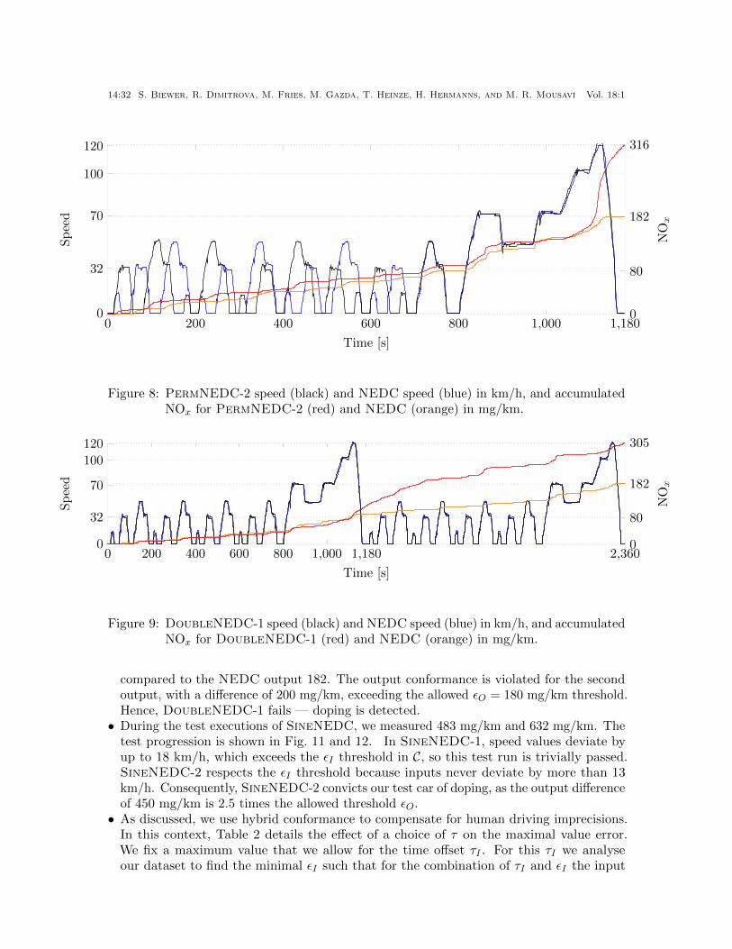
14:32 S. Biewer, R. Dimitrova, M. Fries, M. Gazda, T. Heinze, H. Hermanns, and M. R. Mousavi Vol. 18:1
0 200 400 600 800 1,000 1,1800
32
70
100
120
Time [s]
Sp
eed
0
80
182
316
NOx
Figure 8: PermNEDC-2 speed (black) and NEDC speed (blue) in km/h, and accumulatedNOx for PermNEDC-2 (red) and NEDC (orange) in mg/km.
0 200 400 600 800 1,000 1,180 2,3600
32
70
100
120
Time [s]
Sp
eed
0
80
182
305
NOx
Figure 9: DoubleNEDC-1 speed (black) and NEDC speed (blue) in km/h, and accumulatedNOx for DoubleNEDC-1 (red) and NEDC (orange) in mg/km.
compared to the NEDC output 182. The output conformance is violated for the secondoutput, with a difference of 200 mg/km, exceeding the allowed εO = 180 mg/km threshold.Hence, DoubleNEDC-1 fails — doping is detected.• During the test executions of SineNEDC, we measured 483 mg/km and 632 mg/km. The
test progression is shown in Fig. 11 and 12. In SineNEDC-1, speed values deviate byup to 18 km/h, which exceeds the εI threshold in C, so this test run is trivially passed.SineNEDC-2 respects the εI threshold because inputs never deviate by more than 13km/h. Consequently, SineNEDC-2 convicts our test car of doping, as the output differenceof 450 mg/km is 2.5 times the allowed threshold εO.• As discussed, we use hybrid conformance to compensate for human driving imprecisions.
In this context, Table 2 details the effect of a choice of τ on the maximal value error.We fix a maximum value that we allow for the time offset τI . For this τI we analyseour dataset to find the minimal εI such that for the combination of τI and εI the input

Vol. 18:1CONFORMANCE AND HYPERPROPERTIES FOR DOPING DETECTION IN TIME AND SPACE14:33
0 200 400 600 800 1,000 1,180 2,3600
32
70
100
120
Time [s]
Sp
eed
0
80
182
308
NOx
Figure 10: DoubleNEDC-2 speed (black) and NEDC speed (blue) in km/h, and accumu-lated NOx for DoubleNEDC-2 (red) and NEDC (orange) in mg/km.
0 200 400 600 800 1,000 1,1800
32
70
100
120
Time [s]
Sp
eed
0
80
182
483
NOx
Figure 11: SineNEDC-1 speed (black) and NEDC speed (blue) in km/h, and accumulatedNOx for SineNEDC-1 (red) and NEDC (orange) in mg/km.
Test Name Contract Input Conformance τI = 0 τI = 1 τI = 2 τI = 3 τI = 5 τI = 10 τI = 15 τI = 20
PermNEDC-1 Cp(τI , εI) HybridPermConf εI = 16 εI = 16 εI = 16 εI = 11 εI = 8 εI = 8 εI = 8 εI = 8
PermNEDC-2 Cp(τI , εI) HybridPermConf εI = 11 εI = 10 εI = 7 εI = 7 εI = 7 εI = 7 εI = 7 εI = 7
DoubleNEDC-1 Cd(τI , εI) HybridDoubleConf εI = 15 εI = 12 εI = 11 εI = 9 εI = 6 εI = 6 εI = 6 εI = 6
DoubleNEDC-2 Cd(τI , εI) HybridDoubleConf εI = 25 εI = 18 εI = 10 εI = 8 εI = 8 εI = 8 εI = 8 εI = 8
SineNEDC-1 C(τI , εI) HybridConf εI = 18 εI = 16 εI = 15 εI = 12 εI = 9 εI = 7 εI = 6 εI = 6
SineNEDC-2 C(τI , εI) HybridConf εI = 13 εI = 11 εI = 9 εI = 9 εI = 7 εI = 7 εI = 7 εI = 7
Table 2: Comparison of minimal value thresholds εI for fixed τI . Values are given as km/hand time in seconds.
traces under consideration satisfy the cycle-specific hybrid conformance. For τI = 0 we
get exactly the εI for which the two traces satisfy ConfRetpεI (for PermNEDC), Conf RetdεI
(for DoubleNEDC), and TraceConfεO (for SineNEDC). Table 2 shows the computed εI

14:34 S. Biewer, R. Dimitrova, M. Fries, M. Gazda, T. Heinze, H. Hermanns, and M. R. Mousavi Vol. 18:1
0 200 400 600 800 1,000 1,1800
32
70
100
120
Time [s]
Sp
eed
0
80
182
632
NOx
Figure 12: SineNEDC-2 speed (black) and NEDC speed (blue) in km/h, and accumulatedNOx for SineNEDC-2 (red) and NEDC (orange) in mg/km.
values for τI = 0, 1, 2, 5, 10, 15 and 20 seconds. As expected, an increasing τI induces theminimal εI to decrease. At τI = 5 the decrease in the value error reduces notably. Thishappens because the error is only partially caused by the incorrect timing of the driver.From the values reported in Table 2 we see that if we allow deviation for the input τI = 2,and keep εI = 15, then we have that HybridDoubleConfτI ,εI (NEDC,DoubleNEDC-2)and HybridConfτI ,εI (NEDC,SineNEDC-1) hold. For time threshold τI = 3 secondsHybridPermConfτI ,εI (NEDC,PermNEDC-1) also holds. Thus, under hybrid conformancethese pairs of traces will be considered in the cleanness test for contracts Cd(2, 15), C(2, 15)and Cp(3, 15), respectively, while under their original contract and input conformance theyare to be dismissed.
7.4. Evaluation and Discussion. The amounts of emitted NOx observed during ourexperiments provide clear indications of software doping regarding the car’s emission cleaningsystem. The conformance-based contracts provide the formal basis for this verdict, asdiscussed above. We here complement this fact with a more intuitive explanation of thebehaviour observed.
• PermNEDC slightly reorders NEDC segments in the UDC part of the test cycle.During this part, the measured NOx does not significantly differ from the NEDC reference.However, during the (unmodified) EUDC part, the amount of emissions grows significantly.It is very unlikely to find a physical explanation for the NOx increase; and very likely,that the cleaning system is optimised specifically for the NEDC.• The DoubleNEDC executions appear to reveal that the emission cleaning system
optimisation can also rely on engine temperature or execution time instead of speed data.Physically, many of the common emission cleaning techniques require a hot engine to workproperly (and none of them requires a cold engine). Therefore, a lower NOx value canbe expected if the NEDC is run with a hot engine. In our experiments, however, theNOx emissions in the hot half are almost two times higher than in the initial cold part. In

Vol. 18:1CONFORMANCE AND HYPERPROPERTIES FOR DOPING DETECTION IN TIME AND SPACE14:35
other words, the emission cleaning performance is reduced after the first NEDC execution.There is no physical explanation for this behaviour. Inside the software, detecting the endof an NEDC trip can be implemented very easily, for instance with a timer counting from1180 — the length of NEDC — to zero.• With SineNEDC, we test the cleaning system during driving behaviour which is rich in
accelerations and decelerations. An increased amount of NOx can possibly be explainedby physical phenomena. However, we measured an increase of factors 2.7 and 3.5; thesenumbers can be safely considered as too high for a trustworthy emission cleaning system.
Software doping theory provides the basis for detecting software behaviour violating a formalcontract. In this, physical aspects of the emission cleaning system should be consideredduring the construction of test cases, and test cycles for which drastically higher emissionscan be explained physically, should not be considered. The test cycles we used for ourexperiments were picked with automotive expertise to avoid physically stressful cycles. Iftest cases are generated automatically from a contract, the physical constraints could becaptured by the contract.
The contracts we use for our experiments can be interpreted as very generous in favourof the manufacturers. Input thresholds such as 15 km/h and 2 seconds appear as reasonablevalues, keeping all tests close enough to the original NEDC. For the output threshold,we use a very large deviation value of 180 mg/km, which allows NOx emissions to almostdouble compared to the original NEDC value. Despite the generosity of the contracts, ourexperiments have been able to reveal doping for all experiments except PermNEDC-2.
The analysis of the data shows that it is indeed necessary to not only consider adeviation of value, but to also allow for timing deviations. Considering value and timingdeviations offers a rich set of potential test cycles for doping tests and allows to realisticallyverify conformance of a test cycle and a reference cycle; especially when the quality ofthe studied driving tests suffers from the human-caused input distortions. In this regard,cleanness notions entailing hybrid conformance are more adequate than conformance notionsdemanding punctual test executions, such as robust cleanness. Without hybrid conformance,more of the doping cases we have detected would slip through.
Finally, while hybrid conformance is central to the case study considered here, ourgeneric theory of conformance-based cleanness allows for using other conformance notionsas appropriate for the CPS under test.
Acknowledgments
The work of Sebastian Biewer and Holger Hermanns is supported by the ERC Grant695614 (POWVER) and by the Deutsche Forschungsgemeinschaft (DFG, German ResearchFoundation) grant 389792660 as part of TRR 248, see https://perspicuous-computing.
science. The work of Sebastian Biewer is supported by the Saarbrucken Graduate Schoolof Computer Science. The work of Holger Hermanns is supported by the Key-Area Researchand Development Program Grant 2018B010107004 of Guangdong Province. The workof Mohammad Reza Mousavi has been partially supported by the UKRI TrustworthyAutonomous Systems Node in Verifiability, with Grant Award Reference EP/V026801/1.

14:36 S. Biewer, R. Dimitrova, M. Fries, M. Gazda, T. Heinze, H. Hermanns, and M. R. Mousavi Vol. 18:1
References
[AB16] Shreya Agrawal and Borzoo Bonakdarpour. Runtime verification of k-safety hyperproperties inhyperltl. In IEEE 29th Computer Security Foundations Symposium, CSF 2016, Lisbon, Portugal,June 27 - July 1, 2016, pages 239–252. IEEE Computer Society, 2016. doi:10.1109/CSF.2016.24.
[ACM+18] Hugo L. S. Araujo, Gustavo Carvalho, Morteza Mohaqeqi, Mohammad Reza Mousavi, and AugustoSampaio. Sound conformance testing for cyber-physical systems: Theory and implementation.Sci. Comput. Program., 162:35–54, 2018. doi:10.1016/j.scico.2017.07.002.
[AH94] Rajeev Alur and Thomas A. Henzinger. A really temporal logic. J. ACM, 41(1):181–204, 1994.doi:10.1145/174644.174651.
[AHF+14] Houssam Abbas, Bardh Hoxha, Georgios E. Fainekos, Jyotirmoy V. Deshmukh, James Kapinski,and Koichi Ueda. Wip abstract: Conformance testing as falsification for cyber-physical systems.In ACM/IEEE International Conference on Cyber-Physical Systems, ICCPS, Berlin, Germany,April 14-17, 2014, page 211. IEEE Computer Society, 2014. doi:10.1109/ICCPS.2014.6843724.
[ALFS11] Yashwanth Annpureddy, Che Liu, Georgios E. Fainekos, and Sriram Sankaranarayanan. S-taliro: A tool for temporal logic falsification for hybrid systems. In Parosh Aziz Abdulla andK. Rustan M. Leino, editors, Tools and Algorithms for the Construction and Analysis of Systems- 17th International Conference, TACAS 2011, Held as Part of the Joint European Conferenceson Theory and Practice of Software, ETAPS 2011, Saarbrucken, Germany, March 26-April 3,2011. Proceedings, volume 6605 of Lecture Notes in Computer Science, pages 254–257. Springer,2011. doi:10.1007/978-3-642-19835-9_21.
[AMF14] Houssam Abbas, Hans D. Mittelmann, and Georgios E. Fainekos. Formal property verification ina conformance testing framework. In Twelfth ACM/IEEE International Conference on FormalMethods and Models for Codesign, MEMOCODE 2014, Lausanne, Switzerland, October 19-21,2014, pages 155–164. IEEE, 2014. doi:10.1109/MEMCOD.2014.6961854.
[ARM17] A. Aerts, M. Reniers, and M.R. Mousavi. Chapter 19 - model-based testing of cyber-physical systems. In Houbing Song, Danda B. Rawat, Sabina Jeschke, and Christian Brecher,editors, Cyber-Physical Systems, Intelligent Data-Centric Systems, pages 287 – 304. Aca-demic Press, Boston, 2017. URL: http://www.sciencedirect.com/science/article/pii/
B9780128038017000195, doi:https://doi.org/10.1016/B978-0-12-803801-7.00019-5.[BDFH16] Gilles Barthe, Pedro R. D’Argenio, Bernd Finkbeiner, and Holger Hermanns. Facets of software
doping. In Tiziana Margaria and Bernhard Steffen, editors, Leveraging Applications of FormalMethods, Verification and Validation: Discussion, Dissemination, Applications - 7th InternationalSymposium, ISoLA 2016, Part II, volume 9953 of LNCS, pages 601–608, 2016. URL: http:
//dx.doi.org/10.1007/978-3-319-47169-3_46, doi:10.1007/978-3-319-47169-3_46.[BDH18] Sebastian Biewer, Pedro R. D’Argenio, and Holger Hermanns. Cyber-physical doping tests. In 3rd
Workshop on Monitoring and Testing of Cyber-Physical Systems, MT@CPSWeek 2018, Porto,Portugal, April 10, 2018, pages 18–19. IEEE, 2018. doi:10.1109/MT-CPS.2018.00016.
[BDH19] Sebastian Biewer, Pedro R. D’Argenio, and Holger Hermanns. Doping tests for cyber-physicalsystems. In David Parker and Verena Wolf, editors, Quantitative Evaluation of Systems, 16thInternational Conference, QEST 2019, Glasgow, UK, September 10-12, 2019, Proceedings, volume11785 of Lecture Notes in Computer Science, pages 313–331. Springer, 2019. doi:10.1007/
978-3-030-30281-8\_18.[BDSV14] Lubos Brim, Petr Dluhos, David Safranek, and Tomas Vejpustek. STL*: Extending signal
temporal logic with signal-value freezing operator. Inf. Comput., 236:52–67, 2014. doi:10.1016/j.ic.2014.01.012.
[BFH20] Sebastian Biewer, Michael Fries, and Thomas Heinze. Conformance relations and hyperpropertiesfor doping detection in time and space (supplementary material). https://www.powver.org/publications/conformance-based-doping-detection, 2020.
[BPS20] Borzoo Bonakdarpour, Pavithra Prabhakar, and Cesar Sanchez. Model checking timed hyper-properties in discrete-time systems. In Ritchie Lee, Susmit Jha, and Anastasia Mavridou, editors,NASA Formal Methods - 12th International Symposium, NFM 2020, Moffett Field, CA, USA,May 11-15, 2020, Proceedings, volume 12229 of Lecture Notes in Computer Science, pages 311–328.Springer, 2020. doi:10.1007/978-3-030-55754-6\_18.
[BSB17] Noel Brett, Umair Siddique, and Borzoo Bonakdarpour. Rewriting-based runtime verificationfor alternation-free hyperltl. In Axel Legay and Tiziana Margaria, editors, Tools and Algorithms

Vol. 18:1CONFORMANCE AND HYPERPROPERTIES FOR DOPING DETECTION IN TIME AND SPACE14:37
for the Construction and Analysis of Systems - 23rd International Conference, TACAS 2017,Held as Part of the European Joint Conferences on Theory and Practice of Software, ETAPS2017, Uppsala, Sweden, April 22-29, 2017, Proceedings, Part II, volume 10206 of Lecture Notesin Computer Science, pages 77–93, 2017. doi:10.1007/978-3-662-54580-5\_5.
[CFK+14] Michael R. Clarkson, Bernd Finkbeiner, Masoud Koleini, Kristopher K. Micinski, Markus N.Rabe, and Cesar Sanchez. Temporal logics for hyperproperties. In Martın Abadi and SteveKremer, editors, POST 2014, volume 8414 of LNCS, pages 265–284. Springer, 2014. URL:http://dx.doi.org/10.1007/978-3-642-54792-8_15, doi:10.1007/978-3-642-54792-8_15.
[CLP+17] Moritz Contag, Guo Li, Andre Pawlowski, Felix Domke, Kirill Levchenko, Thorsten Holz, andStefan Savage. How they did it: An analysis of emission defeat devices in modern automobiles.In 2017 IEEE Symposium on Security and Privacy, SP 2017, San Jose, CA, USA, May 22-26,2017, pages 231–250. IEEE Computer Society, 2017. doi:10.1109/SP.2017.66.
[CS08] Michael R. Clarkson and Fred B. Schneider. Hyperproperties. In CSF’08, pages 51–65, 2008.URL: http://dx.doi.org/10.1109/CSF.2008.7, doi:10.1109/CSF.2008.7.
[DBB+17] Pedro R. D’Argenio, Gilles Barthe, Sebastian Biewer, Bernd Finkbeiner, and Holger Hermanns.Is your software on dope? - formal analysis of surreptitiously ”enhanced” programs. In HongseokYang, editor, Programming Languages and Systems - 26th European Symposium on Programming,ESOP 2017, Held as Part of the European Joint Conferences on Theory and Practice of Software,ETAPS 2017, Uppsala, Sweden, April 22-29, 2017, Proceedings, volume 10201 of Lecture Notesin Computer Science, pages 83–110. Springer, 2017. doi:10.1007/978-3-662-54434-1_4.
[DGM+20] Rayna Dimitrova, Maciej Gazda, Mohammad Reza Mousavi, Sebastian Biewer, and HolgerHermanns. Conformance-based doping detection for cyber-physical systems. In Alexey Gotsmanand Ana Sokolova, editors, Formal Techniques for Distributed Objects, Components, and Systems -40th IFIP WG 6.1 International Conference, FORTE 2020, Held as Part of the 15th InternationalFederated Conference on Distributed Computing Techniques, DisCoTec 2020, Valletta, Malta,June 15-19, 2020, Proceedings, volume 12136 of Lecture Notes in Computer Science, pages 59–77.Springer, 2020. doi:10.1007/978-3-030-50086-3\_4.
[DH84] Rocco De Nicola and Matthew Hennessy. Testing equivalences for processes. Theor. Comput.Sci., 34:83–133, 1984. doi:10.1016/0304-3975(84)90113-0.
[DL09] Stephane Demri and Ranko Lazic. LTL with the freeze quantifier and register automata. ACMTrans. Comput. Log., 10(3):16:1–16:30, 2009. doi:10.1145/1507244.1507246.
[DMP17] Jyotirmoy V. Deshmukh, Rupak Majumdar, and Vinayak S. Prabhu. Quantifying conformanceusing the skorokhod metric. Formal Methods in System Design, 50(2-3):168–206, 2017.
[Don10] Alexandre Donze. Breach, A toolbox for verification and parameter synthesis of hybrid systems.In Tayssir Touili, Byron Cook, and Paul B. Jackson, editors, Computer Aided Verification,22nd International Conference, CAV 2010, Edinburgh, UK, July 15-19, 2010. Proceedings,volume 6174 of Lecture Notes in Computer Science, pages 167–170. Springer, 2010. doi:10.1007/978-3-642-14295-6_17.
[FH16] Bernd Finkbeiner and Christopher Hahn. Deciding hyperproperties. In Josee Desharnais andRadha Jagadeesan, editors, 27th International Conference on Concurrency Theory, CONCUR2016, August 23-26, 2016, Quebec City, Canada, volume 59 of LIPIcs, pages 13:1–13:14. SchlossDagstuhl - Leibniz-Zentrum fuer Informatik, 2016. doi:10.4230/LIPIcs.CONCUR.2016.13.
[FHS17] Bernd Finkbeiner, Christopher Hahn, and Marvin Stenger. EAHyper: Satisfiability, implication,and equivalence checking of hyperproperties. In Rupak Majumdar and Viktor Kuncak, editors,Computer Aided Verification - 29th International Conference, CAV 2017, Heidelberg, Germany,July 24-28, 2017, Proceedings, Part II, volume 10427 of Lecture Notes in Computer Science, pages564–570. Springer, 2017. doi:10.1007/978-3-319-63390-9_29.
[FHST17] Bernd Finkbeiner, Christopher Hahn, Marvin Stenger, and Leander Tentrup. Monitoring hy-perproperties. In Shuvendu K. Lahiri and Giles Reger, editors, Runtime Verification - 17thInternational Conference, RV 2017, Seattle, WA, USA, September 13-16, 2017, Proceed-ings, volume 10548 of Lecture Notes in Computer Science, pages 190–207. Springer, 2017.doi:10.1007/978-3-319-67531-2_12.
[FHST18] Bernd Finkbeiner, Christopher Hahn, Marvin Stenger, and Leander Tentrup. RVHyper: Aruntime verification tool for temporal hyperproperties. In Dirk Beyer and Marieke Huisman,editors, Tools and Algorithms for the Construction and Analysis of Systems - 24th International

14:38 S. Biewer, R. Dimitrova, M. Fries, M. Gazda, T. Heinze, H. Hermanns, and M. R. Mousavi Vol. 18:1
Conference, TACAS 2018, Held as Part of the European Joint Conferences on Theory andPractice of Software, ETAPS 2018, Thessaloniki, Greece, April 14-20, 2018, Proceedings, PartII, volume 10806 of Lecture Notes in Computer Science, pages 194–200. Springer, 2018. doi:10.1007/978-3-319-89963-3_11.
[FHST19] Bernd Finkbeiner, Christopher Hahn, Marvin Stenger, and Leander Tentrup. Monitoring hyper-properties. Formal Methods Syst. Des., 54(3):336–363, 2019. doi:10.1007/s10703-019-00334-z.
[FP09] Georgios E. Fainekos and George J. Pappas. Robustness of temporal logic specifications forcontinuous-time signals. Theor. Comput. Sci., 410(42):4262–4291, 2009. doi:10.1016/j.tcs.2009.06.021.
[FRS15] Bernd Finkbeiner, Markus N. Rabe, and Cesar Sanchez. Algorithms for model checking HyperLTLand HyperCTL∗. In Daniel Kroening and Corina S. Pasareanu, editors, CAV 2015, volume 9206 ofLNCS, pages 30–48. Springer, 2015. URL: http://dx.doi.org/10.1007/978-3-319-21690-4_3,doi:10.1007/978-3-319-21690-4_3.
[GJP08] Antoine Girard, A. Agung Julius, and George J. Pappas. Approximate simulation relationsfor hybrid systems. Discrete Event Dynamic Systems, 18(2):163–179, 2008. doi:10.1007/
s10626-007-0029-9.[GM20] Maciej Gazda and Mohammad Reza Mousavi. Logical characterisation of hybrid conformance. In
Artur Czumaj, Anuj Dawar, and Emanuela Merelli, editors, 47th International Colloquium onAutomata, Languages, and Programming, ICALP 2020, July 8-11, 2020, Saarbrucken, Germany(Virtual Conference), volume 168 of LIPIcs, pages 130:1–130:18. Schloss Dagstuhl - Leibniz-Zentrum fur Informatik, 2020. doi:10.4230/LIPIcs.ICALP.2020.130.
[GP11] Antoine Girard and George J. Pappas. Approximate bisimulation: A bridge between computerscience and control theory. Eur. J. Control, 17(5-6):568–578, 2011. doi:10.3166/ejc.17.568-578.
[HBDK18] Holger Hermanns, Sebastian Biewer, Pedro R. D’Argenio, and Maximilian A. Kohl. Verification,testing, and runtime monitoring of automotive exhaust emissions. In Gilles Barthe, Geoff Sutcliffe,and Margus Veanes, editors, LPAR-22. 22nd International Conference on Logic for Programming,Artificial Intelligence and Reasoning, Awassa, Ethiopia, 16-21 November 2018, volume 57 ofEPiC Series in Computing, pages 1–17. EasyChair, 2018. URL: http://www.easychair.org/publications/paper/xgqz.
[Hen64] F. C. Hennie. Fault detecting experiments for sequential circuits. In 5th Annual Symposium onSwitching Circuit Theory and Logical Design, Princeton, New Jersey, USA, November 11-13,1964, pages 95–110. IEEE Computer Society, 1964. doi:10.1109/SWCT.1964.8.
[HHB15] Thorsten Hapke, Peter Hornung, and Joachim Becker. Schummeln auch in Europa. ARD / Nord-deutscher Rundfunk, https://www.tagesschau.de/wirtschaft/vw-schummelsoftware-101.
html, 2015. Online; accessed: 2019-04-19.[HST19] Christopher Hahn, Marvin Stenger, and Leander Tentrup. Constraint-based monitoring of
hyperproperties. In Tomas Vojnar and Lijun Zhang, editors, Tools and Algorithms for theConstruction and Analysis of Systems - 25th International Conference, TACAS 2019, Held asPart of the European Joint Conferences on Theory and Practice of Software, ETAPS 2019,Prague, Czech Republic, April 6-11, 2019, Proceedings, Part II, volume 11428 of Lecture Notes inComputer Science, pages 115–131. Springer, 2019. doi:10.1007/978-3-030-17465-1_7.
[HZJ19] Hsi-Ming Ho, Ruoyu Zhou, and Timothy M. Jones. On verifying timed hyperproperties. InJohann Gamper, Sophie Pinchinat, and Guido Sciavicco, editors, 26th International Symposiumon Temporal Representation and Reasoning, TIME 2019, October 16-19, 2019, Malaga, Spain,volume 147 of LIPIcs, pages 20:1–20:18. Schloss Dagstuhl - Leibniz-Zentrum fur Informatik, 2019.doi:10.4230/LIPIcs.TIME.2019.20.
[KHB18] Maximilian A. Kohl, Holger Hermanns, and Sebastian Biewer. Efficient monitoring of realdriving emissions. In Christian Colombo and Martin Leucker, editors, Runtime Verification -18th International Conference, RV 2018, Limassol, Cyprus, November 10-13, 2018, Proceedings,volume 11237 of Lecture Notes in Computer Science, pages 299–315. Springer, 2018. doi:10.1007/978-3-030-03769-7_17.
[KM15] Narges Khakpour and Mohammad Reza Mousavi. Notions of conformance testing for cyber-physical systems: Overview and roadmap (invited paper). In Luca Aceto and David de Frutos-Escrig, editors, 26th International Conference on Concurrency Theory, CONCUR 2015, Madrid,

Vol. 18:1CONFORMANCE AND HYPERPROPERTIES FOR DOPING DETECTION IN TIME AND SPACE14:39
Spain, September 1.4, 2015, volume 42 of LIPIcs, pages 18–40. Schloss Dagstuhl - Leibniz-Zentrumfuer Informatik, 2015. doi:10.4230/LIPIcs.CONCUR.2015.18.
[LY96] D. Lee and M. Yannakakis. Principles and methods of testing finite-state machines - a survey.Proceedings of the IEEE, 84(8):1089–1123, 1996. doi:10.1109/5.533956.
[MN04] Oded Maler and Dejan Nickovic. Monitoring temporal properties of continuous signals. In YassineLakhnech and Sergio Yovine, editors, Formal Techniques, Modelling and Analysis of Timed andFault-Tolerant Systems, Joint International Conferences on Formal Modelling and Analysis ofTimed Systems, FORMATS 2004 and Formal Techniques in Real-Time and Fault-Tolerant Systems,FTRTFT 2004, Grenoble, France, September 22-24, 2004, Proceedings, volume 3253 of LectureNotes in Computer Science, pages 152–166. Springer, 2004. doi:10.1007/978-3-540-30206-3_12.
[NKJ+17] Luan Viet Nguyen, James Kapinski, Xiaoqing Jin, Jyotirmoy V. Deshmukh, and Taylor T.Johnson. Hyperproperties of real-valued signals. In Jean-Pierre Talpin, Patricia Derler, andKlaus Schneider, editors, Proceedings of the 15th ACM-IEEE International Conference on FormalMethods and Models for System Design, MEMOCODE 2017, Vienna, Austria, September 29 -October 02, 2017, pages 104–113. ACM, 2017. doi:10.1145/3127041.3127058.
[Pnu77] Amir Pnueli. The temporal logic of programs. In 18th Annual Symposium on Foundations ofComputer Science, Providence, Rhode Island, USA, 31 October - 1 November 1977, pages 46–57.IEEE Computer Society, 1977. doi:10.1109/SFCS.1977.32.
[STB+19] David Safranek, Matej Trojak, Vojtech Bruza, Tomas Vejpustek, Jan Papousek, Martin Demko,Samuel Pastva, Ales Pejznoch, and Lubos Brim. Barbaric robustness monitoring revisited forstl* in parasim. In Luca Bortolussi and Guido Sanguinetti, editors, Computational Methods inSystems Biology - 17th International Conference, CMSB 2019, Trieste, Italy, September 18-20,2019, Proceedings, volume 11773 of Lecture Notes in Computer Science, pages 356–359. Springer,2019. doi:10.1007/978-3-030-31304-3\_26.
[Tre92] Jan Tretmans. A formal Approach to conformance testing. PhD thesis, University of Twente, TheNetherlands, 1992.
[Tre96] Jan Tretmans. Conformance testing with labelled transition systems: Implementation relationsand test generation. Computer Networks and ISDN Systems, 29(1):49–79, 1996. doi:10.1016/S0169-7552(96)00017-7.
[Uni13] United Nations. UN Vehicle Regulations - 1958 Agreement, Revision 2, Addendum 100, RegulationNo. 101, Revision 3 — E/ECE/324/Rev.2/Add.100/Rev.3, 2013. URL: http://www.unece.org/trans/main/wp29/wp29regs101-120.html.
[vO06] Michiel van Osch. Hybrid input-output conformance and test generation. In Klaus Havelund,Manuel Nunez, Grigore Rosu, and Burkhart Wolff, editors, Formal Approaches to SoftwareTesting and Runtime Verification, First Combined International Workshops, FATES 2006 andRV 2006, Seattle, WA, USA, August 15-16, 2006, Revised Selected Papers, volume 4262 of LectureNotes in Computer Science, pages 70–84. Springer, 2006. doi:10.1007/11940197_5.
This work is licensed under the Creative Commons Attribution License. To view a copy of thislicense, visit https://creativecommons.org/licenses/by/4.0/ or send a letter to CreativeCommons, 171 Second St, Suite 300, San Francisco, CA 94105, USA, or Eisenacher Strasse 2,10777 Berlin, Germany