Concise Hydraulics

2

Dawei Han

Concise Hydraulics

Download free eBooks at bookboon.com

3

Concise Hydraulics1st edition© 2014 Dawei Han & bookboon.comISBN 978-87-7681-396-3


http://bookboon.com

Concise Hydraulics

4

Contents

Contents

Preface 9

1 Fundamentals 101.1 Properties of Fluids 101.2 Flow Description 111.3 Fundamental Laws of Physics 12

2 Hydrostatics 152.1 Pressure 152.2 Manometer 162.3 Pressure Force on Plane Surface 172.4 Pressure Force on Curved Surface 182.5 Flotation 19

3 Energy Equation 273.1 Basic Formula 273.2 Applications 28


Click on the ad to read more

Free eBook on Learning & DevelopmentBy the Chief Learning Officer of McKinsey

Download Now

http://s.bookboon.com/Download_Free

Concise Hydraulics

5

Contents

4 Momentum Equation 344.1 The Principle 344.2 Applications 35

5 Pipe Flow 435.1 Introduction 435.2 Energy losses in pipe flow 445.3 Local losses (or Minor losses) 475.4 Grade Line 475.5 Combination of pipes 475.6 Energy Loss in Non-circular Pipes 48

6 Physical Modelling 536.1 Background 536.2 Dimensional Analysis 536.3 Analysis of Experimental Data 566.4 Model and Similarity 57


Click on the ad to read moreClick on the ad to read more

www.sylvania.com

We do not reinvent the wheel we reinvent light.Fascinating lighting offers an infinite spectrum of possibilities: Innovative technologies and new markets provide both opportunities and challenges. An environment in which your expertise is in high demand. Enjoy the supportive working atmosphere within our global group and benefit from international career paths. Implement sustainable ideas in close cooperation with other specialists and contribute to influencing our future. Come and join us in reinventing light every day.

Light is OSRAM

http://s.bookboon.com/osram

Concise Hydraulics

6

Contents

7 Open Channel Flow 637.1 What is “Open Channel Flow” 637.2 Channel Geometric Properties 647.3 Calculation of Hydraulic Radius and Hydraulic Mean Depth 66

8 Uniform Flow 738.1 Introduction 738.2 Laminar or Turbulent Flow 738.3 Energy Loss Equations 748.4 Computation of Uniform Flow 76

9 Channel Design 839.1 Channel Design 839.2 Compound Channel 839.3 The Best Hydraulic Section 86

10 Critical Flow 9410.1 Small Wave in Open Channel 9410.2 Critical Flow 9410. 3 Critical Flow Computation 96


Click on the ad to read moreClick on the ad to read moreClick on the ad to read more

© Deloitte & Touche LLP and affiliated entities.

360°thinking.

Discover the truth at www.deloitte.ca/careers


360°thinking.



360°thinking.

Discover the truth at www.deloitte.ca/careers © Deloitte & Touche LLP and affiliated entities.

360°thinking.


http://www.deloitte.ca/careers

Concise Hydraulics

7

Contents

11 Rapidly Varied Flow 10311.1 Sudden Transitions 10311.2 Depth of Flow 10411.3 Height of Hump 10611.4 Specific Energy 107

12 Hydraulic Jump 11412.1 Jump Equation 11412.2 Hydraulic Jump in Rectangular Channel 11712.3 Hydraulic Jump in Trapezoidal Channel 11712.4 Hydraulic jump in Sloping Channel 119

13 Hydraulic Structures 12413.1 Flumes (Venturi) 12413.2 Weirs (Broad-crested weir) 12613.3 Energy dissipators 12713.4 Sluice Gates 129


Click on the ad to read moreClick on the ad to read moreClick on the ad to read moreClick on the ad to read more

We will turn your CV into an opportunity of a lifetime

Do you like cars? Would you like to be a part of a successful brand?We will appreciate and reward both your enthusiasm and talent.Send us your CV. You will be surprised where it can take you.

Send us your CV onwww.employerforlife.com

http://www.employerforlife.com

Concise Hydraulics

8

Contents

14 Gradually Varied Flow 13314.1 Equation of Gradually Varied Flow 13314.2 Classification of Surface Profiles 13514.3 Flow Profile Sketch 13614.4 Flow transitions 138

15 Computation of Flow Profile 14215.1 Introduction 14215.2 Numerical integration methods 14215.3 Computation Procedure through an Example 14415.4 Further Computational Information 146

16 Unsteady Flow 15216.1 Basic Types 15216.2 Rapidly Varied Unsteady Flow 15316.3 Gradually Varied Unsteady Flows (Saint-Venant equations) 15516.4 Software packages 159

17 Hydraulic Machinery 16417.1 Hydropower and Pumping Station 16417.2 Turbines 16617.3 Pump and Pipeline 169

18 Appendix: Further Reading Resources 182


Concise Hydraulics

9

Preface

PrefaceHydraulics is a branch of scientific and engineering discipline that deals with the mechanical properties of fluids, mainly water. It is widely applied in many civil and environmental engineering systems (water resources management, flood defence, harbour and port, bridge, building, environment protection, hydropower, irrigation, ecosystem, etc.). This is an introductory book on hydraulics and written for undergraduate students in civil and environmental engineering, environmental science and geography. The aim of this book is to provide a concise and comprehensive coverage of hydraulics that is easy to access through the Internet.

The book content covers the fundamental theories (continuity, energy and momentum equations), hydrostatics, pipe flow, physical modelling (dimensional analysis and similarity), open channel flow, uniform flow, channel design, critical flow, rapidly varied flow, hydraulic jump, hydraulic structures, gradually varied flow, computation of flow profile, unsteady flow and hydraulic machinery (pump and turbine). The text has been written in a concise format that is integrated with the relevant graphics. There are many examples to further explain the theories introduced. The questions at the end of each chapter are accompanied by the corresponding answers and full solutions. A list of recommended reading resources is provided in the appendix for readers to further explore the interested hydraulics topics.

Due to its online format, it is expected that the book will be updated regularly. If you find any errors and inaccuracies in the book, you are encouraged to email me with feedback and suggestions for further improvements.

Dawei HanReader in Civil and Environmental Engineering,

Water and Environmental Management Research CentreDepartment of Civil Engineering

University of Bristol, BS8 1TR, UKE-mail: [email protected]

http://www.bris.ac.uk/civilengineering/person/d.han.html

August 2014


mailto:E-mail:%20d.han%40bristol.ac.uk%0D?subject=

http://www.bris.ac.uk/civilengineering/person/d.han.html

Concise Hydraulics

10

Fundamentals

1 FundamentalsHydraulics is a branch of scientific and engineering discipline that deals with the mechanical properties of fluids, mainly water. It is widely applied in water resources, harbour and port, bridge, building, environment, hydropower, pumps, turbines, etc.

1.1 Properties of Fluids

1. Density: Mass per unit volume r (kg/m3)For water, r = 1000kg/m3 at 4°C, r = 998 kg/m3 at 20°CFor air, r = 1.2kg/m3 at 20°C at standard pressure

2. Specific gravity: Ratio of the substance’s density and water’s density at 4oC3. Pressure: Normal fluid force divided by area over which it acts (N/m2). (Note: pressure is

scalar while force is a vector. A force is generated by the action of pressure on a surface and its direction is given by the surface orientation)

4. Viscosity and shear stressTake an element from the fluid

u+du

u

dy

Stationary

Moving with U

d

du

dy

and the total force

F AUA

d

where m absolute viscosity (N s/m2) , t shear stress (N/m2). Fluids that follow the aforementioned formulas are called Newtonian fluids.

ExamplesAir m =1.79 × 10-5 Ns/m2

Water m = 1.137 × 10-3 Ns/m2

Engine oil SAE30W m =0.44 Ns/m2


Concise Hydraulics

11

Fundamentals

High viscosity: sticky fluid; low viscosity: slippy fluid

m is not a constant and changes with temperature.

Another form of viscosity is kinematic viscosity (m2/s)

Assumptions for the equation:

1. Fluids are Newtonian fluids (Non-Newtonian fluids are studied by Rheology, the science of deformation and flow);

2. The continuum approximation: the properties of the fluid can be represented by continuous fields representing averages over many molecules (The exception is when we are dealing with gases at low pressures).

1.2 Flow Description

There are two approaches

1. Lagrangian approach: follow individual fluid element as it moves about;2. Eulerian approach: focus on a fixed location and consider how the fluid properties change at

that location as time goes on.

Definitions relating to Fluids in Motion

Ideal flow: frictionless and incompressible (i.e. nonviscous).

Steady flow: The flow is steady if the properties at each point in the fluid do not change with time.

One, Two and 3D flows:One dimensional flow requires only one coordinate to describe the change in flow properties.Two dimensional flow requires two coordinates to describe the change in flow properties.Three dimensional flow requires all three coordinates to describe the change in flow properties.In general, most flow fields are three dimensional. However, many practical problems can be simplified into one or two dimensions for computational convenience.

Control Volume

A suitable mass of fluid can be identified by using control volume. A control volume is a purely imaginary region within a body of flowing fluid. The region is usually at a fixed location and of fixed size. Inside the region, all the dynamic forces cancel each other. Attention may therefore be focused on the forces acting externally on the control volume.


Concise Hydraulics

12

Fundamentals

1.3 Fundamental Laws of Physics

The fundamental equations that govern the motions of fluids such as water are derived from the basic laws of physics, i.e., the conservation laws of mass, momentum and energy. The conservation of momentum comes from Newton’s second law of motion stated in 1687 in Principia Mathematica. The law of conservation of mass was formulated in the late eighteen century and the law of conservation of energy in the mid-nineteenth century. In modern physics, mass and energy can be converted from one to the other as suggested by Albert Einstein in 1905. This combines two individual conservation laws into a single law of conservation of mass/energy. However, since conversion between mass and energy are not of relevance to fluids studied by hydraulics, the two individual laws of conservation are used in hydraulics. The conservation of mass is also called the equation of continuity.

Conservation of mass: mass can be neither created nor destroyed.Conservation of energy: energy can be neither created nor destroyed.Conservation of momentum: a body in motion cannot gain or lose momentum unless some external force is applied.

The application of the three fundamental laws will be further explained in the following chapters.

Questions 1Fundamentals

1. A plate separated by 0.5 mm from a fixed plate moves at 0.5 m/s under a shear stress of 4.0 N/m2. Determine the viscosity of the fluid between the plates.

(Answer: 0.004 Ns/m2)

2. A Newtonian fluid fills the gap between a shaft and a concentric sleeve. When a force of 788N is applied to the sleeve parallel to the shaft, the sleeve attains a speed of 2m/s. If a 1400 N force is applied, what speed will the sleeve attain? The temperature of the sleeve remains constant.

(Answer: 3.55 m/s)


Concise Hydraulics

13

Fundamentals

3. Water is moving through a pipe. The velocity profile at some section is shown below and is

given mathematically as

−= 2

2

44rdu

µβ , where u = velocity of water at any position r, b = a

constant, m = viscosity of water, d = pipe diameter, and r = radial distance from centreline.

What is the shear stress at the wall of the pipe due to water? What is the shear stress at

a position r = d/4? If the given profile persists a distance L along the pipe, what drag is

induced on the pipe by the water in the direction of flow over this distance?

r

u d

(Answer: bd/4, bd/8, bd2pL/4)

Solutions 1Fundamentals

1. From U

d

4.00.5

0.5 0.001,

so m = 0.004 Ns/m2

2. F

A

U

d

Rearrange as FU

Ad

= =µ constant

Therefore, F1

U1

F2

U2

788

2

1400

U2

So U2 3.55m / s

3. From u4

d2

4r 2

so du

dr 42r

r

2

Then du

dr

r

2


Concise Hydraulics

14

Fundamentals

At the wall, r = d/2,

hence wall

d

4

r d / 4

d

8 ( The negative signs can be ignored)

Drag wall(area)d

4( dL) d2 L / 4


Click on the ad to read moreClick on the ad to read moreClick on the ad to read moreClick on the ad to read moreClick on the ad to read more

http://s.bookboon.com/elearningforkids

Concise Hydraulics

15

Hydrostatics

2 HydrostaticsHydrostatics deals with the pressures and forces resulting from the weight of fluids at rest.

2.1 Pressure

Pressure is the force per unit area acting on a surface and it acts equally in all directions. A common pressure unit is N/m2, also called Pascal (Pa). Depending on the benchmark used (with/without atmospheric pressure), pressure can be described as absolute pressure or relative pressure.

1. Atmospheric pressure ( ap ): is the pressure at any given point in the Earth’s atmosphere caused by the weight of air above the measurement point. The standard atmosphere (symbol: atm) is a unit of pressure equal to 101.325 kPa (or 760 mmHg, 1013.25 millibars).

2. Absolute pressure ( absp ): is the pressure with its zero point set at the vacuum pressure.3. Relative pressure ( rp ): is the pressure with its zero set at the atmospheric pressure. It is

more widely used in engineering than absolute pressure.

The relationship between them is

r abs ap p p= −

The change of pressure within the fluid can be expressed as

dp gdzρ= −


Concise Hydraulics

16

Hydrostatics

For a fluid with constant density, the differential formula can be integrated as

pz Cgρ

+ =

where C is a constant that can be set from the boundary condition. If the top boundary pressure is p0 and depth of the fluid is h, the bottom pressure can be derived as

0p gh pρ= +

For any two points in the same fluid, it can be derived

1 21 2

p pz zg gρ ρ

+ = +

2.2 Manometer

Simple manometers

A simple manometer is a tube with its one end attached to the fluid and the other one open to the atmosphere (also called Piezometer). The pressure at Point A can be derived from the height hA in the tube.

A Ap ghρ=

A more complicated manometer uses U-tube with a different fluid to the measured one. The pressure at Point A will be

A m B Ap gh ghρ ρ= −


Concise Hydraulics

17

Hydrostatics

A differential manometer is used to measure the pressure difference between two points. A U-tube with mercury (or other fluids) is attached to two points whose pressures are to be measured. The pressure difference can be derived by measuring the elevation differences between Point A and Point B (i.e., Dz), and between the mercury levels (Dh).

Therefore[ ) ]A B mp p g h zρ ρ ρ− = − ∆ + ∆

2.3 Pressure Force on Plane Surface

For a plane surface with area A, the total pressure force can be derived by the following integration formula:

A A

F pdA ghdAρ= =∫ ∫where h is the depth of fluid from its surface.


Click on the ad to read moreClick on the ad to read moreClick on the ad to read moreClick on the ad to read moreClick on the ad to read moreClick on the ad to read more

AXA Global Graduate Program

Find out more and apply

http://s.bookboon.com/AXA

Concise Hydraulics

18

Hydrostatics

If the centroid of the area is known, the pressure force can be derived as

F ghAρ=

where h is the depth of A’s centroid.

The centre of pressure is the point through which the resultant pressure acts.

2

A AP

A A

ypdA y dAy

pdA ydA= =∫ ∫

∫ ∫

The numerator is the moment of inertia of the surface about the axis through O, and it equals to2

x CI I y A= + . Therefore

CP

Iy yyA

= +

Shape Area A Centroid y Moment of Inertia Ic

Circle (r radius) πr2 r πr4 / 4

Rectangle (b width, h height ) bh h / 2 bh3 / 12

Triangle (b bottom width, h height) bh / 2 2h / 3 bh3 / 36

2.4 Pressure Force on Curved Surface

For curved surfaces, the pressure force is divided into horizontal and vertical components. The vertical force Fy is the total weight of the fluid above the curved surface and its centre of pressure acts through its centre of gravity. The horizontal force Fx equals to the pressure force on a vertical plane surface projected by the curved surface. The resultant force is a triangular combination of the horizontal and vertical parts.


Concise Hydraulics

19

Hydrostatics

yF gVρ= where V is the volume of the fluid above the curved surface.

2 2

x yF F F= +

2.5 Flotation

1. BuoyancyBuoyancy is the upward force on an object from the surrounding fluid (liquid or gas). This force is due to the pressure difference of the fluid at different parts of the object. The buoyancy force is derived by

BF gVρ=

where V is the displaced fluid volume by the object, ρ is the fluid density.

An object submerged in a fluid is subject to two forces: gravity and buoyancy. When gravity force is greater than buoyancy force, the object sinks to the bottom. If the situation is reversed, the object will float. If two forces equal to each other, the object could be anywhere in the fluid.

2. Stable flotation and metacentreA floating object is stable if it tends to return to its original position after an angular displacement. This can be illustrated by the following example. When a vessel is tipped, the centre of buoyancy moves from C to C’. This is because the volume of displaced water at the left of G has been decreased while the volume of displaced water to the right is increased. The centre of buoyancy, being at the centre of gravity of the displaced water, moves to point C’, and a vertical line through this point passes G and intersects the original vertical at M. The distance GM is known as the metacentric height. This illustrates the fundamental law of stability. When M is above G, the metacentric height is positive and the floating body is stable, otherwise it is unstable.


Concise Hydraulics

20

Hydrostatics

There are two ways to find the metacentre: experiment and analytical method.

a) Metacentre by experiment (if a ship is already built, the experiment method is easy to apply)Shift a known weight w from the centre of the ship by a distance l to create a turning moment P=wl and the ship (with a total weight of W) is tilted by an angle a. The metacentre can be derived by the balance of moments at the point G.

sin sinP l lGM

W W Wω ω

α α α= = ≈


Click on the ad to read moreClick on the ad to read moreClick on the ad to read moreClick on the ad to read moreClick on the ad to read moreClick on the ad to read moreClick on the ad to read more

Maersk.com/Mitas

�e Graduate Programme for Engineers and Geoscientists

Month 16I was a construction

supervisor in the North Sea

advising and helping foremen

solve problems

I was a

hes

Real work International opportunities

�ree work placementsal Internationaor�ree wo

I wanted real responsibili� I joined MITAS because

Maersk.com/Mitas





solve problems

I was a

hes




Maersk.com/Mitas





solve problems

I was a

hes




Maersk.com/Mitas





solve problems

I was a

hes




www.discovermitas.com

http://s.bookboon.com/mitas

Concise Hydraulics

21

Hydrostatics

b) Metacentre by analytical methodImage the displacement centre (centroid of the buried body) is moved by x due to a turning moment. This centroid displacement is contributed from only the top two triangles (worked out one triangle and the other one is doing the same thing, with either added buoyancy and reduced buoyancy). If the ship’s displacement volume is V, length is L and width is D, we can derive around C point the following,

/ 2

0

2 ( tan ) (tan )D

oVx L x xdx Iα α= =∫ , ( oI is the 2nd moment of the area)

So (tan ) oIx

Vα

=

Therefore

tanoIxCM

Vα= =

From the centre of gravity and buoyancy,

GM CM CG= −


Concise Hydraulics

22

Hydrostatics

Questions 2Hydrostatics

1. A rectangular plate gate is placed in a water channel (density of water: 1000kg/m3). Its width is 0.8m and the water depth is 2m. Estimate the pressure force and its centre of pressure

(Answer: 15.7 kN, 1.33 m)

2. Estimate the resultant force of water on a quadrant gate. Its radius is 1m and width 2m. The centre of gravity for the quarter circular sector is 4 / 3R π (from the circle centre to the right).

(Answer: 18.3 kN, 57.3o)

3. A cube of timber 1m on each side floats in water. The density of the timber is 600 kg/m3. Estimate the submerged depth of the cube.

(Answer: 0.6 m)

4. A crane barge which is rectangular in plan, has a large water plane area compared with its depth for stability. The barge weighs 500 kN and the crane 50 kN. The resulting centre of gravity of the combination is at the level of the deck, while the centre of gravity of the crane itself is 3m above the deck.

Tests are being undertaken to ensure the stability of the crane barge. The crane is moved horizontally sideways by 0.8 m and the barge rolls through an angle of 50. What is the metacentric height of the system? When the crane is back in its central position, we need to know how high the jib can be raised before the barge becomes unstable.

(Answer: 0.834 m, 9.2m)


Concise Hydraulics

23

Hydrostatics

Solutions 2Hydrostatics

1. The centroid of the gate is

2 1 2 2hh m= = =

The area is

20.8 2 1.6 A bh m= = × =

Therefore

1000 9.81 1 1.6 15.7 F ghA kNρ= = × × × =

The centre of pressure

3 340.8 2 0.533

12 12CbhI m×

= = =

The gate is vertical, so y and h are the same.

0.5331 1.33 1 1.6

CP

Ih h mhA

= + = + =×


Click on the ad to read moreClick on the ad to read moreClick on the ad to read moreClick on the ad to read moreClick on the ad to read moreClick on the ad to read moreClick on the ad to read moreClick on the ad to read more

MASTER IN MANAGEMENT

[email protected] Follow us on IE MIM Experiencewww.ie.edu/master-management

#10 WORLDWIDEMASTER IN MANAGEMENT

FINANCIAL TIMES

55 Nationalitiesin class

5 SpecializationsPersonalize your program

Length: 1O MONTHSAv. Experience: 1 YEARLanguage: ENGLISH / SPANISHFormat: FULL-TIMEIntakes: SEPT / FEB

• STUDY IN THE CENTER OF MADRID AND TAKE ADVANTAGE OF THE UNIQUE OPPORTUNITIES THAT THE CAPITAL OF SPAIN OFFERS• PROPEL YOUR EDUCATION BY EARNING A DOUBLE DEGREE THAT BEST SUITS YOUR PROFESSIONAL GOALS• STUDY A SEMESTER ABROAD AND BECOME A GLOBAL CITIZEN WITH THE BEYOND BORDERS EXPERIENCE

93%OF MIM STUDENTS ARE

WORKING IN THEIR SECTOR 3 MONTHSFOLLOWING GRADUATION

http://s.bookboon.com/MIMEnglish

Concise Hydraulics

24

Hydrostatics

2. a) Vertical force

211000 9.81 2 15.4 4yF gV kNπρ ×

= = × × × =

Its centre of pressure is at

4 / 3 0.424 R mπ = to the right of the circle centre.

b) Horizontal force

The centroid for a vertical plane surface of 1m tall and 2 m wide is 0.5m

1000 9.81 0.5 2 9.81 xF ghA kNρ= = × × × =

Its centre of pressure is at 1/3 of the height

0.333m to the bottom.

c) Resultant force

2 2 2 215.4 9.81 18.3 x yF F F kN= + = + =

Direction

1 1tan ( / ) tan (15.4 / 9.81) 1.00( ) 57.3o

y xF F radianθ − −= = = =

It is 57.3o below the horizontal line and passes through the joint point between the vertical force line and horizontal force line..


Concise Hydraulics

25

Hydrostatics

3. Weight of the cube

600 9.81 5886wood woodW gV Nρ= = × =

The volume of water to be displaced is

35886 0.61000water

water

WV mg gρ

= = =

So the submerged depth will be

0.6 0.61 1

waterVh mArea

= = =×

4. This is to find the metacentre by experiment, so

( )0

50000 0.8 0.834sin 550000sin 5

lGM mWω

α×

= = =

The metacentre is 0.834m above the deck.

The centre of gravity of the barge is

500 3 50h = ×


Concise Hydraulics

26

Hydrostatics

0.3h m= (below the deck surface)

If the centre of jib gravity is up by H from the deck and the system centre of gravity moves by 0.834m above the deck

50 ( 0.834) 500 (0.3 0.834)H× − = × + H=12.2m

So it can move by 12.2 - 3 =9.2m


Click on the ad to read moreClick on the ad to read moreClick on the ad to read moreClick on the ad to read moreClick on the ad to read moreClick on the ad to read moreClick on the ad to read moreClick on the ad to read moreClick on the ad to read more

http://s.bookboon.com/EOT

Concise Hydraulics

27

Energy Equation

3 Energy EquationThe energy equation is based on the conservation of energy, i.e., energy can be neither created nor destroyed.

3.1 Basic Formula

1. From solidsTotal energy = kinetic energy + potential energy (unit: joule)

2

2

muTotal energy mgz= +

2. For fluidsIn comparison with the solid mechanics, there is an extra energy term in fluids (pressure).

Total energy = kinetic + potential + pressure (unit: metre)

i.e. u2

2gz

p

g (per unit weight)

Pressure energy is similar to potential energy and they are closely linked ( /z p g Cρ+ = ). One thing to be noticed is that in physics, energy unit is joule, but in hydraulics, engineers use meter and call it energy head. Unlike solid objects, fluid can move around and change its shape, so we use metre per unit fluid weight to describe the energy in fluid. One meter of energy head is equivalent of one joule energy of 1 Newton weight of fluid.

3. Energy equation and continuity equationWith the conservation of energy, the energy equation for one dimensional flow can be derived as

A2A1

1

2

V2V1

z1

p1

g

u12

2gz2

p2

g

u22

2g


Concise Hydraulics

28

Energy Equation

This is called the Bernoulli equation and it has been widely used in practical problems.

In addition to the energy equation, the conservation of mass is usually used jointly to solve fluid problems.

Rate of mass flow across 1 = Rate of mass flow across 2

1A1u1 2 A2u2

If r is constant

A1u1 A2u2

It is usually called the continuity equation.

3.2 Applications

1) ExampleA large tank with a well-rounded, small opening as an outlet. What is the velocity of a jet issuing from the tank (neglect the kinetic energy at section 1)?

Solution:

The energy equation for section 1 and 2

2 21 1 2 2

1 22 2p u p uz zg g g gρ ρ

+ + = + +

Use Section 2 as the datum, so

220 0 0 0

2uhg

+ + = + +

Therefore

2 2u gh=


Concise Hydraulics

29

Energy Equation

2) Energy Loss and GainIn practice, some energy is ‘lost’ through friction (hf ), and external energy may be added by means of a pump or extracted by a turbine (E). The energy equation will be

z1

p1

g

u12

2gE z2

p2

g

u22

2ghf

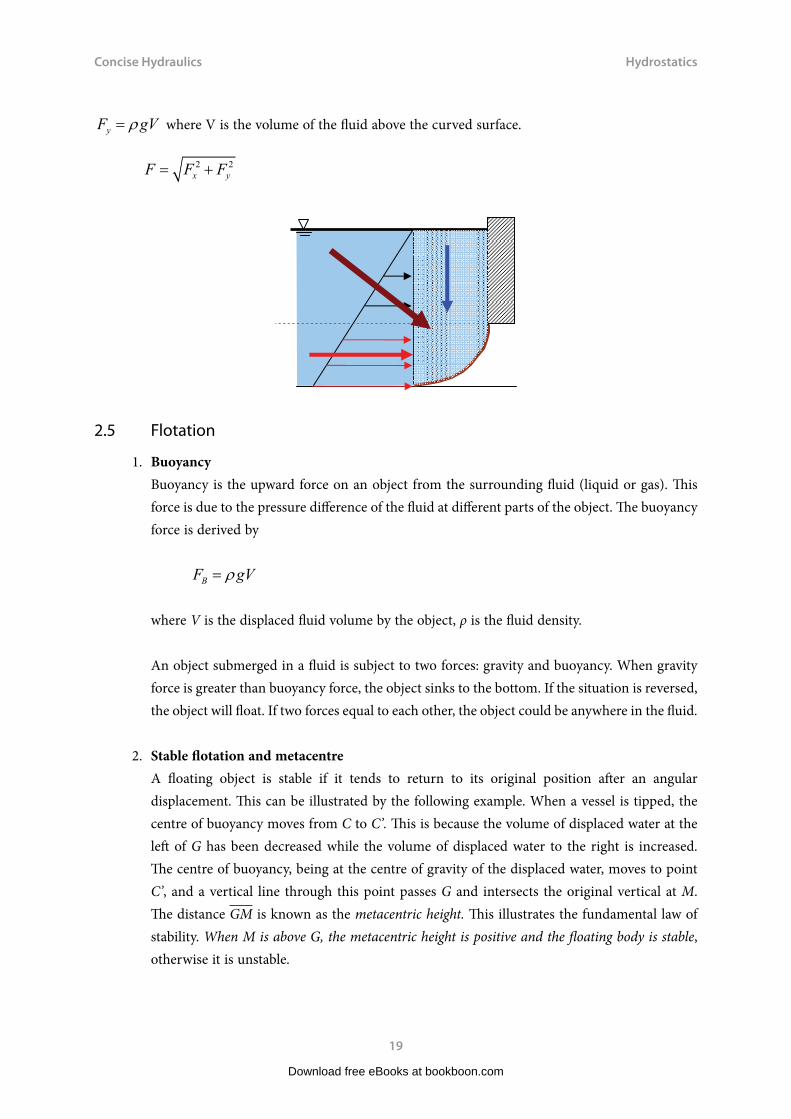
3) Venturi Meteris an instrument which may be used to measure discharge in pipelines. By measuring the difference in pressure, discharge may be made as (assume no energy loss)

2 21 1 2 2

1 22 2p u p uz zg g g gρ ρ

+ + = + +


Click on the ad to read moreClick on the ad to read moreClick on the ad to read moreClick on the ad to read moreClick on the ad to read moreClick on the ad to read moreClick on the ad to read moreClick on the ad to read moreClick on the ad to read moreClick on the ad to read more

“The perfect start of a successful, international career.”

CLICK HERE to discover why both socially

and academically the University

of Groningen is one of the best

places for a student to be www.rug.nl/feb/education

Excellent Economics and Business programmes at:

http://www.rug.nl/feb/bookboon?utm_source=AdBookboon&utm_medium=Bookboon&utm_campaign=130215Bookboon

Concise Hydraulics

30

Energy Equation

i.e.

2 2

1 1 2 2

2 2p u p ug g g gρ ρ+ = +

From the continuity equation

1 1 2 2Q Au A u= =

1 1 22

1 2

2( )( / ) 1

A p pQA A ρ

−=

−

The actual discharge will be slightly less than this due to the energy losses between Sections 1 and 2. A coefficient of discharge is introduced to take account of these energy loses.

actual dQ C Q= (Cd values can be found in British Standard 1042 or other hydraulic handbooks)

Orifice plate

is similar to Venturi meter with compact size (hence more economical) but less accurate and more energy loss.

Questions 3

Energy Equation

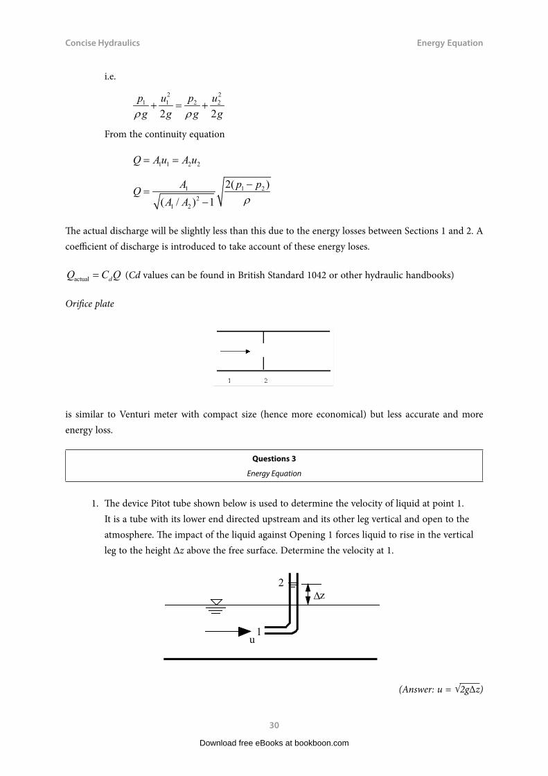
1. The device Pitot tube shown below is used to determine the velocity of liquid at point 1. It is a tube with its lower end directed upstream and its other leg vertical and open to the atmosphere. The impact of the liquid against Opening 1 forces liquid to rise in the vertical leg to the height Dz above the free surface. Determine the velocity at 1.

∆

z

u

1

2

(Answer: u = √2gΔz)


Concise Hydraulics

31

Energy Equation

2. What should the water level h be for the free jet just to clear the wall?

(Answer: 0.156 m)

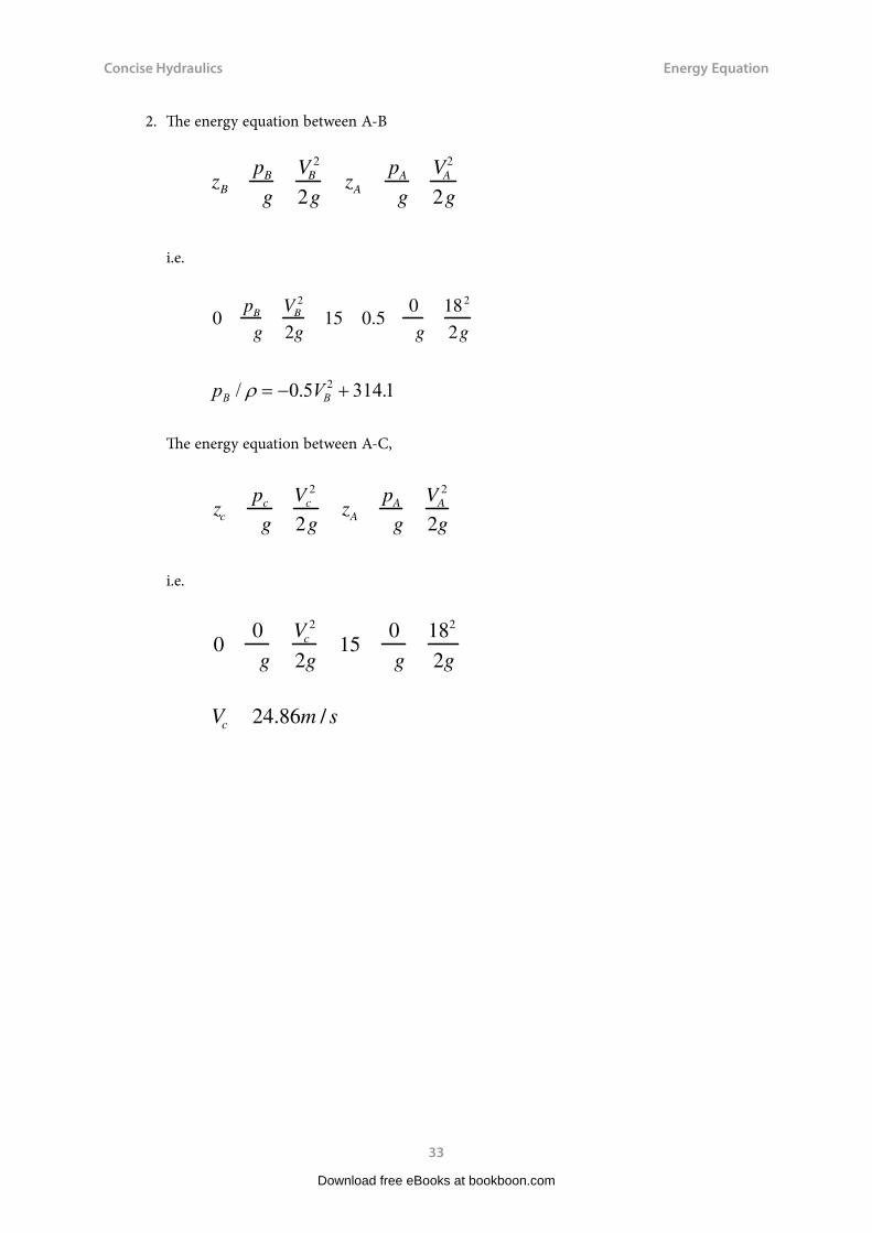
3. If the velocity at Point A is 18m/s, what is the pressure at Point B if we neglect friction?

A

B

D=200mm

D=75mm

C 0.5m

15 m

Water

(Answer: 308KN/m2)

Solutions 3Energy Equation

1. Kinetic energy at 1 is converted into Dz increase of the fluid at 2

ug

z12

2= ∆


Concise Hydraulics

32

Energy Equation

hence

u1 2g z

uo 2gh

Fall distance gt 2 / 2 0.40

So 0.8944 /t g=

Horizontal distance = uot ( 2gh)(0.8944 / g) 0.50

h 0.156m


Click on the ad to read moreClick on the ad to read moreClick on the ad to read moreClick on the ad to read moreClick on the ad to read moreClick on the ad to read moreClick on the ad to read moreClick on the ad to read moreClick on the ad to read moreClick on the ad to read moreClick on the ad to read more

American online LIGS University

▶ enroll by September 30th, 2014 and

▶ save up to 16% on the tuition!

▶ pay in 10 installments / 2 years

▶ Interactive Online education ▶ visit www.ligsuniversity.com to

find out more!

is currently enrolling in theInteractive Online BBA, MBA, MSc,

DBA and PhD programs:

Note: LIGS University is not accredited by any nationally recognized accrediting agency listed by the US Secretary of Education. More info here.

http://s.bookboon.com/LIGS

Concise Hydraulics

33

Energy Equation

2. The energy equation between A-B

zB

pB

g

VB2

2gzA

pA

g

VA2

2g

i.e.

0

pB

g

VB2

2g15 0.5

0

g

182

2g

p VB B/ . .ρ = − +0 5 314 12

The energy equation between A-C,

zc

pc

g

Vc2

2gzA

pA

g

VA2

2g

i.e.

00

g

Vc2

2g15

0

g

182

2g

Vc 24.86m / s


Concise Hydraulics

34

Energy Equation

4 Momentum Equation4.1 The Principle

From Newton’s 2nd law

F = ma

where 2 1

t−

=∆

V Va

So 2 12 1 2 1

( ) ( ) ( )m m Qt t

ρ−= = − = −

∆ ∆V VF V V V V

where ρQV is the momentum, i.e. Momentum = Mass × Velocity

It is important to note that momentum and velocity are both vectors.

Therefore, momentum force is a vector: F Q u u= −ρ ( )2 1


Click on the ad to read moreClick on the ad to read moreClick on the ad to read moreClick on the ad to read moreClick on the ad to read moreClick on the ad to read moreClick on the ad to read moreClick on the ad to read moreClick on the ad to read moreClick on the ad to read moreClick on the ad to read moreClick on the ad to read more

http://s.bookboon.com/GTca

Concise Hydraulics

35

Momentum Equation

It is more convenient to use scalar forms by separating the momentum force into three basic components:

F Q u ux x x= −ρ ( )2 1

F Q u uy y y= −ρ ( )2 1

F Q u uz z z= −ρ ( )2 1

4.2 Applications

Two steps:

a) Calculating the total momentum force; b) find out where this force is sourced.1) A jet normal to a fixed plate

Estimate FR ( the force exerted on the fluid by the plate)

Solution:

a) In the horizontal direction, the total momentum force is

− = −F Q u ux xρ ( )2 1

Here

u2x

=0, u1x

= u, Q=Au

F Au= ρ 2

b) Since there is only one force FR acting on the water jet, the total momentum force equals to FR

F F AuR = = ρ 2

u F FR

1 2


Concise Hydraulics

36

Momentum Equation

2) Force exerted by a nozzle

Calculate the force FR required to hold a nozzle to the firehose for a discharge of 5 litre/second if the nozzle has an inlet diameter of 75 mm and an outlet diameter of 25 mm.

Solution:

a) The total momentum force can be derived from

u 2 u 1

Control volume (Grey area)

p 1 F

FR

1 2

2 1( )F Q u uρ= −

23 2

1(0.075 ) 4.42 10

4A mπ −= = ×

24 2

2(0.025 ) 4.91 10

4A mπ −= = ×

1 1/ 1.131 /u Q A m s= =

2 2/ 10.18 /u Q A m s= =

So the total momentum force on the fluid is

2 1( ) 1000 0.005 (10.18 1.131) 45.25F Q u u Nρ= − = × × − =

b) Force balance

1 1 RF p A F= −

From the energy equation

2 21 1 2 2

2 2u p u pg g g gρ ρ+ = +


Concise Hydraulics

37

Momentum Equation

Therefore

2 222 1

1( ) 51.2 /

2u up kN mρ −

= =

Substitute into

1 1 RF p A F= −

1 1 51.2 4.42 45.25 181RF p A F N= − = × − =

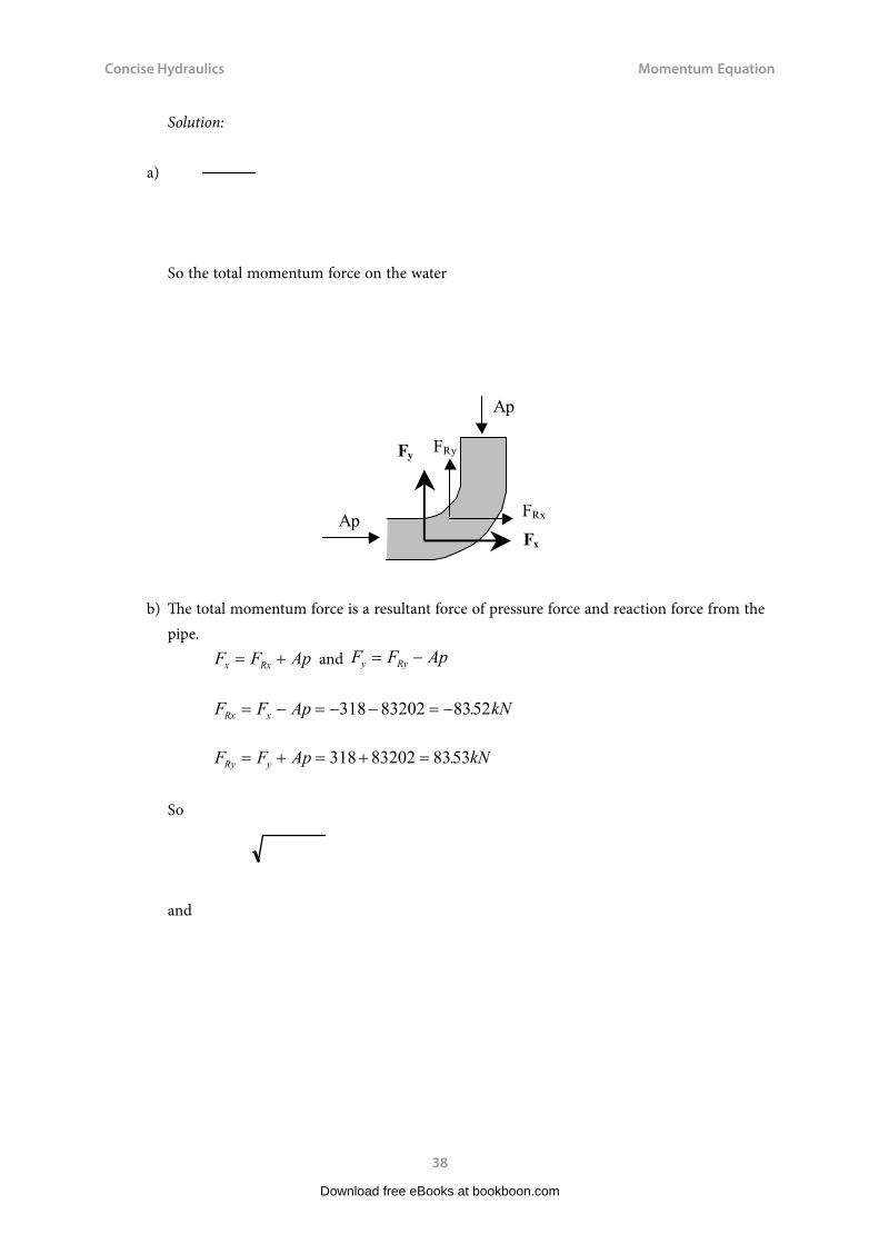
3. Two dimensional flowCalculate the magnitude and direction of the force exerted by the pipe bend if the diameter is 600 mm, the discharge is 0.3m3/s and the pressure head at both end is 30m.

u

u FRx

FRy

1

2


Click on the ad to read moreClick on the ad to read moreClick on the ad to read moreClick on the ad to read moreClick on the ad to read moreClick on the ad to read moreClick on the ad to read moreClick on the ad to read moreClick on the ad to read moreClick on the ad to read moreClick on the ad to read moreClick on the ad to read moreClick on the ad to read more

.

http://s.bookboon.com/AlcatelLucent

Concise Hydraulics

38

Momentum Equation

Solution:

a)

So the total momentum force on the water

Ap

Ap

FRx

FRy

Fx

Fy

b) The total momentum force is a resultant force of pressure force and reaction force from the pipe.

F F Apx Rx= + and F F Apy Ry= −

F F Ap kNRx x= − = − − = −318 83202 8352.

F F Ap kNRy y= + = + =318 83202 8353.

So

and


Concise Hydraulics

39

Momentum Equation

Questions 4Momentum Equation

1. A small ingot and platform rest on a steady water jet. If the total weight supported is 825N, what is the jet velocity? Neglect energy losses.

(Answer: 17.1m/s)

2. Calculate the magnitude and direction of the force exerted by the T-junction if the water discharges are Q1=0.3m3/s, Q2=0.15m3/s and Q3=0.15m3/s, the diameters are D1=450mm, D2=300mm and D3=200mm, and the upstream pressure p

1=500kN/m2. Neglect energy

losses.

1

2

3

(Answer:82.43kN, 166.3o)


Concise Hydraulics

40

Momentum Equation

3. A vertical jet of water leaves a nozzle at a speed of 10m/s and a diameter of 20mm. It suspends a plate having a mass of 1.5kg. What is the vertical distance h?

h

(Answer:3.98m)

Solutions 4Momentum Equation

1.

From the momentum equation


Click on the ad to read moreClick on the ad to read moreClick on the ad to read moreClick on the ad to read moreClick on the ad to read moreClick on the ad to read moreClick on the ad to read moreClick on the ad to read moreClick on the ad to read moreClick on the ad to read moreClick on the ad to read moreClick on the ad to read moreClick on the ad to read moreClick on the ad to read more

www.mastersopenday.nl

Visit us and find out why we are the best!Master’s Open Day: 22 February 2014

Join the best atthe Maastricht UniversitySchool of Business andEconomics!

Top master’s programmes• 33rdplaceFinancialTimesworldwideranking:MScInternationalBusiness

• 1stplace:MScInternationalBusiness• 1stplace:MScFinancialEconomics• 2ndplace:MScManagementofLearning• 2ndplace:MScEconomics• 2ndplace:MScEconometricsandOperationsResearch• 2ndplace:MScGlobalSupplyChainManagementandChange

Sources: Keuzegids Master ranking 2013; Elsevier ‘Beste Studies’ ranking 2012; Financial Times Global Masters in Management ranking 2012

MaastrichtUniversity is

the best specialistuniversity in the

Netherlands(Elsevier)

http://www.mastersopenday.nl

Concise Hydraulics

41

Momentum Equation

So

2.

2.

Pressure

The total external force

Reaction force

1 1x RxF p A F= + , 3 3 2 2y RyF p A p A F= − +

Hence

2 2 82.43R Rx RyF F F kN= + =


Concise Hydraulics

42

Momentum Equation

3. The required speed to suspend the plate

Q VA m s= = × =10 0 02 4 0 003142 3. / . /π

F Q u u V gx x x= − = − × =ρ ( ) . .2 1 1000 0 00314 15

So

V g m s=

×=

151000 0 00314

4 69..

. /

The energy equation

pg

z Vg

pg

z Vg

11

12

22

22

2 2ρ ρ+ + = + +

h z z V

gV

g gm= − = − =

−=2 1

12

22 2 2

2 210 4 69

2398. .


Click on the ad to read moreClick on the ad to read moreClick on the ad to read moreClick on the ad to read moreClick on the ad to read moreClick on the ad to read moreClick on the ad to read moreClick on the ad to read moreClick on the ad to read moreClick on the ad to read moreClick on the ad to read moreClick on the ad to read moreClick on the ad to read moreClick on the ad to read moreClick on the ad to read more

http://s.bookboon.com/BI

Concise Hydraulics

43

Momentum Equation

5 Pipe Flow5.1 Introduction

Pipes are widely used in engineering to deliver fluid from one place to another. There are two flow types.

Laminar: flow in discrete layers with no mixing

Turbulent: flow with eddying or mixing action.

Reynolds Number is used to predict the laminar/turbulent flows

ReDV

The Reynolds number represents a ratio of forces

Re < 2000, laminar,Re > 4000, turbulent,2000 < Re < 4000, transition region

Velocity distribution in laminar flow

ru R

u umax 1r2

R2 umax 2u

Velocity distribution in turbulent flow

u umax 1r

R

1/ 7

umax 1.23u


Concise Hydraulics

44

Pipe Flow

Mean velocity

V u Q

A

udA

A

The energy and momentum equations may then be rewritten in terms of the mean velocity

V 2

2gF Q V2 V1

In most pipe flow, 1.06 and 1.02 both may safely be ignored in practice.

5.2 Energy losses in pipe flow

Darcy-Weisbach equation

where hf is the energy head loss, L is the pipe length, D is the diameter and V is the mean velocity.

The friction factor l is dimensionless and can be derived by experiments or from the following chart or formulas.

For laminar flow

64

Re


Concise Hydraulics

45

Pipe Flow

For turbulent flow (Colebrook-White formula)

12 log

ks

3.7D

2.51

Re

Ks is the roughness factor

Typical Ks values (in mm)brass, copper, glass 0.003plastic 0.03galvanised iron 0.15

Example

Oil flows through a 25 mm diameter pipe with a mean velocity of 0.3 m/s. Given that m=4.8×10-2 kg/ms and r=800kg/m3, calculate (a) the pressure drop in a 45 m length and the maximum velocity, and (b) the velocity 5mm from the pipe wall.

Solution:

1) Check if the flow is laminar or turbulent

2Re / 800 0.025 0.3 /(4.8 10 ) 125 2000DVρ µ −= = × × × = <

So it is laminar flow

2) Pressure drop

64 64 /125 0.512Re

λ = = =

2 20.512 45 0.3 4.23 (of oil)2 0.025 2fVh L m

D g gλ × ×

= = =×

or convert it into kN/m2

233.2 /fgh kN mρ =


Concise Hydraulics

46

Pipe Flow

3) Velocity

max 2 0.6 /u V m s= =

From 2

max

1u ru R

= −

so 212.5 51

0.6 125u − = −

0.384 /u m s=


Click on the ad to read moreClick on the ad to read moreClick on the ad to read moreClick on the ad to read moreClick on the ad to read moreClick on the ad to read moreClick on the ad to read moreClick on the ad to read moreClick on the ad to read moreClick on the ad to read moreClick on the ad to read moreClick on the ad to read moreClick on the ad to read moreClick on the ad to read moreClick on the ad to read moreClick on the ad to read more

Get Help Now

Go to www.helpmyassignment.co.uk for more info

Need help with yourdissertation?Get in-depth feedback & advice from experts in your topic area. Find out what you can do to improvethe quality of your dissertation!

http://www.helpmyassignment.co.uk

Concise Hydraulics

47

Pipe Flow

5.3 Local losses (or Minor losses)

Local losses occur at pipe bends, junctions and valves, etc.

h K VgL L=2

2

where is the local head loss and KL is a loss factor for a particular fitting (usually derived from experiments). V is the mean flow velocity before or after the pipe fitting (use the higher value if they are different).

The energy equation for a complete pipe with fittings will be

z1

p1

g

V12

2gz2

p2

g

V22

2ghf hL

5.4 Grade Line

Hydraulic grade lines: A line that represents the potential energy and pressure energy in the fluid.

zp

g

When a hydraulic grade line is below the pipeline, the pressure in the pipe is less than the atmospheric pressure (negative pressure).

Energy grade lines: A line that represents the total energy in the fluid.

zp

g

V 2

2g

It is always vertically above the hydraulic grade line by a distance of .

5.5 Combination of pipes

1) Pipes in seriesTwo or more pipes of different sizes or roughnesses are so connected that fluid flows through one pipe and then through the others in turn.

H local loss hf 1 hf 2

Q1 Q2

H

1 2


Concise Hydraulics

48

Pipe Flow

2) Pipes in parallelThe flow is divided among the pipes and then is joined again.

Q Q1 Q2 Q3

Energy loss in pipe 1 = Energy loss in pipe 2 = …

A B

3) Networks of PipesProblems on networks of pipes in general are complicated and require trial solutions in which the elementary circuits are balanced in turn until all conditions for the flow are satisfied.

5.6 Energy Loss in Non-circular Pipes

The Darcy-Weisbach equation for circular pipes can also be used by replacing diameter D with hydraulic radius R.

gV

RLhf 24

2

λ=

where

PerimeterAreaR =

It can be applied to square, oval, triangular, and similar types of sections.


Concise Hydraulics

49

Pipe Flow

Questions 5Pipe Flow

1. In the laminar flow of a fluid in a circular pipe, the velocity profile is exactly a true parabola. The discharge is then represented by the volume of a paraboloid. Prove that for this case the ratio of the mean velocity to the maximum velocity is 0.5. (Note: u = umax 1 − r / R( )2[ ])

2. An oil (r=868.5 kg/m3 and m=0.0814 kg/ms) is to flow through a 300m level concrete pipe. What size pipe will carry 0.0142m3/s with a pressure drop due to friction of 23.94kPa?

(Answer: 155 mm)

3. Water flows at a rate of 0.04m3/s in a 0.12-m-diameter horizontal pipe that contains a sudden contraction to a 0.06-m-diameter pipe (KL=0.40). Determine the pressure drop across the contraction section. How much of this pressure difference is due to energy losses and how much is due to kinetic energy change?

(Answer: 133.9 kPa , 40.0 kPa, 93.9kPa)


Click on the ad to read moreClick on the ad to read moreClick on the ad to read moreClick on the ad to read moreClick on the ad to read moreClick on the ad to read moreClick on the ad to read moreClick on the ad to read moreClick on the ad to read moreClick on the ad to read moreClick on the ad to read moreClick on the ad to read moreClick on the ad to read moreClick on the ad to read moreClick on the ad to read moreClick on the ad to read moreClick on the ad to read more

By 2020, wind could provide one-tenth of our planet’s electricity needs. Already today, SKF’s innovative know-how is crucial to running a large proportion of the world’s wind turbines.

Up to 25 % of the generating costs relate to mainte-nance. These can be reduced dramatically thanks to our systems for on-line condition monitoring and automatic lubrication. We help make it more economical to create cleaner, cheaper energy out of thin air.

By sharing our experience, expertise, and creativity, industries can boost performance beyond expectations.

Therefore we need the best employees who can meet this challenge!

The Power of Knowledge Engineering

Brain power

Plug into The Power of Knowledge Engineering.

Visit us at www.skf.com/knowledge

http://www.skf.com/knowledge

Concise Hydraulics

50

Pipe Flow

4. If H = 11m, find the discharge through pipes 1, 2, and 3 (Neglect local losses).

(Answer: 0.0009, 0.00856, 0.00946 m3/s)

Solutions 5Pipe Flow

1.

Q udA umax0

R

1r2

R2 2 rdr umax

R2

2

VQ

A

umax R2 / 2

R2 0.5umax

Thus V / umax 0.5

2.

hf

p

g

23940

868.5 9.812.81m

Trial 1: V=1 m/s, from, Q AVD2

4V 0.0142 D 0.0181/ V 0.135m

Re DV 868.5 1 0.135

0.08141440 (laminar)

64

Re0.0444 and hf

L

D

V2

2g5.03m too high,

Sub hf with 2.81 m to estimate V. hf

L

D

V2

2g2.81m

i.e. 0.044300

0.135

V 2

2g2.81m

V 0.751m / s


Concise Hydraulics

51

Pipe Flow

Trial 2 V=0.751 m/s so D 0.0181/ V 0.155m

ReDV 868.5 0.751 0.155

0.08141242 (laminar)

64

Re0.0515 so hf

L

D

V2

2g2.87m close to 2.81 m

Hence a pipe diameter of 0.155m would be required.

3. From energy equation

pg

z Vg

pg

z Vg

K VgL

11

12

22

22

22

2 2 2ρ ρ+ + = + + +

So

p pg

V Vg

K VgL

1 2 22

12

22

2 2−

=−

+ρ

V m s1 2

0 04012 4

354= =.

. /. /

π

V m s2 2

0 040 06 4

1415= =.

. /. /

π

p pg

V Vg

K Vg g g

m

L1 2 2

212

22 2 2 2

2 21415 354

20 4 1415

29 57 4 08 1365

−=

−+ =

−+

= + =ρ

. . . .

. . .

p p kPa1 2 939 40 0 1339− = + =. . .

This represents a 40.0 kPa drop from energy losses and a 93.9kPa drop due to an increase in kinetic energy.

4. V1

Q1

A1

Q1

0.0252 509.6Q1 V2

Q2

A2

Q1

0.062 88.5Q2 V3

Q3

A3

Q1

0.052 127.4Q3

hf 1 hf 2

i.e.

1

L1

D1

V12

2g 2

L2

D2

V22

2g


Concise Hydraulics

52

Pipe Flow

So

0.11470

0.05

(509.6Q1)2

2g0.088

80

0.12

(88.5Q2 )2

2g

Q1 0.105Q2

Q3 Q1 Q2 1.105Q2

11 2

L2

D2

V22

2g 3

L3

D3

V32

2g

11 0.08880

0.12

(88.5Q2 )2

2g0.114

110

0.1

(127.4Q3)2

2g

or 11 0.08880

0.12

(88.5Q2 )2

2g0.114

110

0.1

(127.4 1.105Q2 )2

2g

Q2 0.00856m3 / s Q1 0.105Q2 0.0009m 3 / s Q3 1.105Q2 0.00946m3 / s


Click on the ad to read moreClick on the ad to read moreClick on the ad to read moreClick on the ad to read moreClick on the ad to read moreClick on the ad to read moreClick on the ad to read moreClick on the ad to read moreClick on the ad to read moreClick on the ad to read moreClick on the ad to read moreClick on the ad to read moreClick on the ad to read moreClick on the ad to read moreClick on the ad to read moreClick on the ad to read moreClick on the ad to read moreClick on the ad to read more

http://s.bookboon.com/Subscrybe

Concise Hydraulics

53

Physical Modelling

6 Physical Modelling6.1 Background

Hydraulic modelling includes physical and mathematical models. Initially, due to a lack of computing power, physical models dominated the hydraulic modelling field. Froude (1870) established the famous Froude similarity when he was testing a ship model. In 1885, Reynolds built a river model for Mersey based on the Froude similarity. The Buckingham’s Pi theorem (by J. Buckingham in 1914) extended the similarity principle to a broader sense. Since then, physical models have been widely used in hydraulics, including complex 3D river models with sediments.

With the advent of computers, mathematical modelling has been gaining popularity. It is possible to solve complicated differential equations using numerical techniques due to modern computer’s large memory and CPU speed. Nowadays, mathematical models are highly accurate and efficient to tackle 1D river problems. They are cheaper to build and fast to run in comparison with physical models. In 2D modelling, mathematical models are gaining ground from physical models. However, for 3D modelling, physical models still have superior performance in many complicated problems and it would be a long time before mathematical models are able to totally replace them.

6.2 Dimensional Analysis

Dimensional Analysis is a branch of applied mathematics for investigating the form of a physical relationship. Dimensional Analysis not only helps us to design experiments but also allows us to gain an insight into how all the factors depend on each other even before we start experimenting.

Example:

A thin rectangular plate having a width w and a height h is located so that it is normal to a moving stream of fluid. Assume the drag D, that the fluid exerts on the plate is a function of w, h, the fluid viscosity m and density r, and the velocity V of the fluid approaching the plate. Perform a dimensional analysis of this problem.


Concise Hydraulics

54

Physical Modelling

Basic steps:

1. Decide variables to be used

2. Express each of the variables in terms of basic dimensionsmass M, length L and time T (or force F, L, T)

w L= , h L= , µ = − −ML T1 1 (= dimensionally equal to)

3MLρ −= , 1V LT −= , 2D MLT −=

3. Determine the required number of Π terms (free variables)Buckingham Πtheorem: the number of Π terms (free variable) is equal to k-r, where k is the total number of variables in the problem and r is the number of reference dimensions (up to 3).

k-r = 6-3=3 so we have three free variables

4. Select dependent variables,Select w,V and r as dependent variables ( Avoid choosing both w and h since they have the same dimension). The rest are free variables (D,m,h).

5. Form a Π term by grouping one of the free variables with all dependent variables,Starting with the free variable, D, the first Π term can be formed by combining D with the dependent variables such that

Estimate a,b,c so that the combination is dimensionless

2 1 3 0 0 0( )( ) ( ) ( ) a b cMLT L LT ML M L T− − − =


Concise Hydraulics

55

Physical Modelling

So 1+c =0 (for M) 1+a+b-3c = 0 (for L) -2-b = 0 (for T)

Therefore a = -2, b = -2, c = -1, the Π term then becomes

6. Repeat step 5 for each of the remaining free variables,

So 2 /h wΠ =

And

3a b cw Vµ ρΠ = , and a=-1, b=-1, c=-1

So 3 wVµρ

Π =


Click on the ad to read moreClick on the ad to read moreClick on the ad to read moreClick on the ad to read moreClick on the ad to read moreClick on the ad to read moreClick on the ad to read moreClick on the ad to read moreClick on the ad to read moreClick on the ad to read moreClick on the ad to read moreClick on the ad to read moreClick on the ad to read moreClick on the ad to read moreClick on the ad to read moreClick on the ad to read moreClick on the ad to read moreClick on the ad to read moreClick on the ad to read more

http://s.bookboon.com/volvo

Concise Hydraulics

56

Physical Modelling

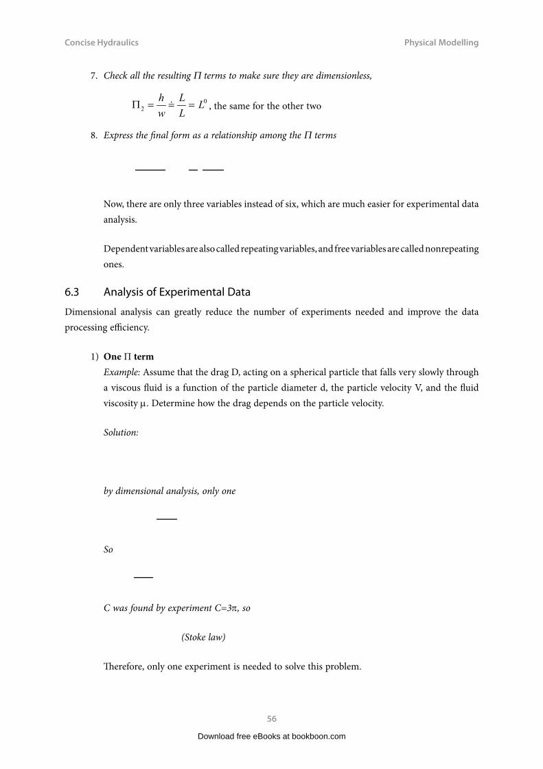
7. Check all the resulting Π terms to make sure they are dimensionless,

Π2

0= = =hw

LL

L , the same for the other two

8. Express the final form as a relationship among the Π terms

Now, there are only three variables instead of six, which are much easier for experimental data analysis.

Dependent variables are also called repeating variables, and free variables are called nonrepeating ones.

6.3 Analysis of Experimental Data

Dimensional analysis can greatly reduce the number of experiments needed and improve the data processing efficiency.

1) One Π termExample: Assume that the drag D, acting on a spherical particle that falls very slowly through a viscous fluid is a function of the particle diameter d, the particle velocity V, and the fluid viscosity m. Determine how the drag depends on the particle velocity.

Solution:

by dimensional analysis, only one

So

C was found by experiment C=3p, so

(Stoke law)

Therefore, only one experiment is needed to solve this problem.


Concise Hydraulics

57

Physical Modelling

2) Two Π terms

For problems involving two Π terms, results of an experiment can be conveniently presented in a simple graph. The relationship between the two terms can be solved with curve fitting techniques (e.g., linear or nonlinear regression).

3) Three Π terms or more

It is still possible represent three variable problems in 3D graphics. Mathematically, surface fitting is needed to solve the relationship among them. If more than three terms are involved, more complicated data mining techniques are needed (such as Artificial Neural Networks, Support Vector Machines, etc).

6.4 Model and Similarity

A model is a representation of a physical system that may be used to predict the behaviour of the system of interest.

As we know, any given problem can be described in terms of a set of Π terms as

For a model to represent such a system

Therefore

If

This is the prediction equation and indicates that the measured value of obtained with the model will be equal to the corresponding for the prototype as long as other pi terms are equal.

In many hydraulic engineering problems, models are with free surfaces (rivers, estuaries etc). Force F is linked with length, velocity, viscosity, and gravity acceleration, hence ( , , , , , ) 0f F l V gρ µ = .


Concise Hydraulics

58

Physical Modelling

From which, dimensional analysis gives:

2

2 2 ,F Vl VfV l gl

ρρ µ

=

or ( )2 2 Re,F f Fr

V lρ= ,

where Reynolds number Re Vlρµ

= , Froude numberVFrgl

= (to be introduced in later chapters).

In practice, it is usually impossible to satisfy all the Π terms, so it is important to identify the dominant terms. The Froude number is very common in river modelling, which represents gravitational forces in dominance. Hence, the Froude numbers for the model and the real-world structure (prototype) should be the same.

Froude Number / /p m p p m mFr Fr V gl V gl= = = , hence / /m p m p LV V L L λ= =

Similarities

Geometric Kinematic (velocity) Dynamic (force)

mL

p

LL

λ= //

m m m LV

p p p T

V L TV L T

λ λλ

= = = 2 2 22

m m m m m L LL L V

p p p p p T T

F M a LF M a L ρ ρ

ρ λ λλ λ λ λ λρ λ λ

= = × = =


Click on the ad to read moreClick on the ad to read moreClick on the ad to read moreClick on the ad to read moreClick on the ad to read moreClick on the ad to read moreClick on the ad to read moreClick on the ad to read moreClick on the ad to read moreClick on the ad to read moreClick on the ad to read moreClick on the ad to read moreClick on the ad to read moreClick on the ad to read moreClick on the ad to read moreClick on the ad to read moreClick on the ad to read moreClick on the ad to read moreClick on the ad to read moreClick on the ad to read more

EXPERIENCE THE POWER OF FULL ENGAGEMENT…

RUN FASTER. RUN LONGER.. RUN EASIER…

READ MORE & PRE-ORDER TODAY WWW.GAITEYE.COM

Challenge the way we run

1349906_A6_4+0.indd 1 22-08-2014 12:56:57

http://s.bookboon.com/Gaiteye

Concise Hydraulics

59

Physical Modelling

Questions 6Physical Modelling

1. Water flows over a dam as illustrated below. Assume the flow rate q (per unit length along the dam, hence with unit of m2/s) depends on the head H, width b, acceleration of gravity g, fluid density r, and fluid viscosity m. Develop a suitable set of dimensionless parameters for this problem using b, g, and r as repeating variables.

(Answer: q

b gHb b g3 2 1 2 3 2 1 2/ / / /( , )= φ µ

ρ)

2. A 1:50 model of a boat has a wave resistance of 0.02N when operating in water at 1.0m/s. Find the corresponding prototype wave resistance. Find also the horsepower requirement for the prototype. What velocity does this test represent in the prototype? (use Froude criterion, 1Kilowatt = 1.34 Horsepower)

(Answer: 2500N, 23.7 hp, 7.07m/s)

Solutions 6Physical Modelling

1. q f H b g= ( , , , , )ρ µ

q L

T=

2

, HL

=1

, b L= , g LT

= 2 , ρ =ML3 , µ = − −ML T1 1

Six variables, only three reference dimensions,

so k-r = 6-3 =3, three Π terms

Repeating variables: b,g and r


Concise Hydraulics

60

Physical Modelling

Π12 1 2 3 0 0 0

2 3 01 2 0

0

= = =+ + − =

− − ==

− − −qb g L T L LT ML L T Ma b c

bc

a b c a b cρ ( ) ( ) ( )

Therefore c=0; b=-1/2; a = -3/2

So, Π1 3 2 1 2=q

b g/ /

Π22 3 0 0 0

1 3 02 0

0

= = =+ + − =− ==

− −Hb g L L LT ML L T Ma b cb

c

a b c a b cρ ( ) ( ) ( )

Therefore,

c=0; b=0; a=-1

Π2 =

Hb

Π31 1 2 3 0 0 0

1 3 01 2 0

1 0

= = =− + + − =− − =+ =

− − − −µ ρb g ML T L LT ML L T Ma b cb

c

a b c a b c ( ) ( ) ( )

Hence c=-1; b=-1/2; a=-3/2

Π3 3 2 1 2=

µρb g/ /

Therefore q

b gHb b g3 2 1 2 3 2 1 2/ / / /( , )= φ µ

ρ

2. The geometric ratio is

1 0.0250

mL

p

LL

λ = = =


Concise Hydraulics

61

Physical Modelling

From the Froude number

Froude number / /p m p p m mFr Fr V gl V gl= = = ,

hence / / 0.02 0.1414V m p m p LV V L Lλ λ= = = = =

The velocity of 1.0m/s in the model represents the prototype velocity

/ 0.1414 1/ 0.1414 7.07 /p mV V m s= = =

Dynamic (force) similarity can be derived as

F mass acceleration= ×

3 2 4 4

3 2 2 2

0.02m m m m m m m L

p p p p p p p T T

F M a L L TF M a L L T

ρ λρ λ λ

−

−= = × = = (The fluid density is the same in both cases)

The time ratio can be derived from Kinematic (velocity) similarity

//

m m m LV

p p p T

V L TV L T

λ λλ

= = =


Click on the ad to read moreClick on the ad to read moreClick on the ad to read moreClick on the ad to read moreClick on the ad to read moreClick on the ad to read moreClick on the ad to read moreClick on the ad to read moreClick on the ad to read moreClick on the ad to read moreClick on the ad to read moreClick on the ad to read moreClick on the ad to read moreClick on the ad to read moreClick on the ad to read moreClick on the ad to read moreClick on the ad to read moreClick on the ad to read moreClick on the ad to read moreClick on the ad to read moreClick on the ad to read more

PDF components for PHP developers

www.setasign.com

SETASIGNThis e-book is made with SetaPDF

http://s.bookboon.com/Setasign

Concise Hydraulics

62

Physical Modelling

Hence

0.02 0.14140.1414

LT

V

λλλ

= = =

So

2 2

4 4

0.1414 0.02 125000 0.02 25000.02 0.02

Tp mF F Nλ= = = × =

The force ratio is

61 8 10125000

mF

p

FF

λ −= = = ×

From Power V F= ×

2500 7.07( ) 17.68( ) 23.67p p pP F V watt kilowatt hp= = × = =


Click on the ad to read moreClick on the ad to read moreClick on the ad to read moreClick on the ad to read moreClick on the ad to read moreClick on the ad to read moreClick on the ad to read moreClick on the ad to read moreClick on the ad to read moreClick on the ad to read moreClick on the ad to read moreClick on the ad to read moreClick on the ad to read moreClick on the ad to read moreClick on the ad to read moreClick on the ad to read moreClick on the ad to read moreClick on the ad to read moreClick on the ad to read moreClick on the ad to read moreClick on the ad to read moreClick on the ad to read more


Download Now


Concise Hydraulics

63

Open Channel Flow

7 Open Channel Flow7.1 What is “Open Channel Flow”

Open channel flow is flow of liquid in a conduit in which the upper surface of the liquid is in contact with the atmosphere. The flows in the following cases are all open channel flow (include the one in the circular pipe).

There are many types of open channel flow and a common classification system is as follows.

Classifications

Steady Flow

Unsteady Flow

By time

By space

Uniform Flow

Varied Flow

Gradually Varied Flow

Rapidly Varied Flow

Steady Flow

Unsteady Flow

By time

Uniform Flow

Varied Flow


Rapidly Varied Flow

The uniform flow refers to flow whose water depth, width, flow area and velocity do not change with distance. If any of these factors change, the flow will be called varied flow (or nonuniform flow).


Concise Hydraulics

64

Open Channel Flow

The steady flow refers to flow factors and variables that do not change with time, otherwise the flow will be called unsteady flow.

7.2 Channel Geometric Properties

The measurable geometric properties of channels are:Depth (y), Area (A), Wetted perimeter (P), Surface width (B)

They are aggregated into two useful factors:Hydraulic radius (R=A/P), Hydraulic mean depth (Dm=A/B)

Irregular channels


Concise Hydraulics

65

Open Channel Flow

By

x

x

h

x x12

By

x

xx x12

By

x

x

h

x x12

By

x

xx x12

2

1

( )

x

xA h y dx= −∫

2 2

1 1

2 2 2

1

x x

x xP dx dy y dx′= + = +∫ ∫

In practice, the cross section is divided into a finite number of sections. A and P are the sum of those segments.


Click on the ad to read moreClick on the ad to read moreClick on the ad to read moreClick on the ad to read moreClick on the ad to read moreClick on the ad to read moreClick on the ad to read moreClick on the ad to read moreClick on the ad to read moreClick on the ad to read moreClick on the ad to read moreClick on the ad to read moreClick on the ad to read moreClick on the ad to read moreClick on the ad to read moreClick on the ad to read moreClick on the ad to read moreClick on the ad to read moreClick on the ad to read moreClick on the ad to read moreClick on the ad to read moreClick on the ad to read moreClick on the ad to read more

www.sylvania.com


Light is OSRAM


Concise Hydraulics

66

Open Channel Flow

7.3 Calculation of Hydraulic Radius and Hydraulic Mean Depth

Example 1: Rectangular channel

3m

1m

From 23 , 3 , 1 1 3 5A m B m P m= = = + + + =

So 3/ 5 0.6R m= = , 3/ 3 1mD m= =

Example 2: Trapezoidal Channel

3m

1m45o

3m

1m45o

From 24 , 5 , 5.83A m B m P= = =

So 4 / 5.83 0.686R m= = , 4 / 5 0.8mD m= =

Example 3: Circular Channel

902m o902m o

From 22 1.414 , 3.14 / 2 1.57 , 3.14 / 4 1/ 2 0.285B m P m A m= = = = = − =

So 0.285 /1.57 0.182R m= = , 0.285 /1.414 0.202mD m= =


Concise Hydraulics

67

Open Channel Flow

Questions 7Open Channel Flow

1. Compute the hydraulic radius and hydraulic mean depth for a trapezoidal channel.

5 m

3 m

1.5 m

(Answer: 0.91m, 1.2m)

2. Compute the hydraulic radius and hydraulic mean depth for a smooth concrete-lined channel.

1.0

6m

0.5 3m

(Answer 0.735m, 1.0 m)

3. Derive equations for hydraulic radius and hydraulic mean depth for a parabolic channel. If B=6 m and h = 3m for the channel, calculate its hydraulic radius and hydraulic mean depth.

Function for a parabolic curve y=kx20 X

YP (B/2, h)

B

h

B

h

Note:

ax2 cdxx2ax 2 c

c2 a

ln(x a ax 2 c )

(Answer 1.35m, 2.0 m)


Concise Hydraulics

68

Open Channel Flow

Solutions 7Open Channel Flow

1. A(5 3) 1.5

26m2

P 3 2 1 1.52 6.61m

Hydraulic radius R= A/P=6/6.61= 0.91 mB=5 mHydraulic mean depth Dm=A/B = 6/5= 1.2 m

2. A m= × +×

=3 15 1 32

6 2.

P m= + + + + =3 15 05 1 3 8162. . .B m= 6Hydraulic radius R m= =6 816 0 735/ . .Hydraulic mean depth D mm = =6 6 10/ .


Click on the ad to read moreClick on the ad to read moreClick on the ad to read moreClick on the ad to read moreClick on the ad to read moreClick on the ad to read moreClick on the ad to read moreClick on the ad to read moreClick on the ad to read moreClick on the ad to read moreClick on the ad to read moreClick on the ad to read moreClick on the ad to read moreClick on the ad to read moreClick on the ad to read moreClick on the ad to read moreClick on the ad to read moreClick on the ad to read moreClick on the ad to read moreClick on the ad to read moreClick on the ad to read moreClick on the ad to read moreClick on the ad to read moreClick on the ad to read more


360°thinking.



360°thinking.



360°thinking.


360°thinking.



Concise Hydraulics

69

Open Channel Flow

3. Assume the parabolic curve function is y=kx2

h

B

0 X

Y

(B/2, h)

h

B

0 X

Y

(B/2, h)

Replace (x,y) with (B/2,h)

So k= 4h/B2

The following steps can be done either manually, or by Matlab (or Maple)

Method 1 (manual)

Area A (h y)dxB2

B2

23Bh

P 1 y' 2dxB2

B2 2 1 y'2dx0

B2

2 1 (2kx)2dx0

B2

Since ax2 cdxx2ax 2 c

c2 a

ln(x a ax 2 c )

and let s=(2k)2

P 2 1 sx2 dx0

B2 2( x

2sx2 1 1

2 sln(x s sx2 1)

0

B2 )

B2s B

2

2

1 1s

ln(B s2

s B2

2

1)


Concise Hydraulics

70

Open Channel Flow

substitute s with (2k)2

P B2

(2k)2 B2

2

112k

ln(2Bk

2(2k)2 B

2

2

1)

B2

kB 2 11

2kln(kB (kB)2 1)

B2

kB 2 11kB

ln(kB (kB)2 1)

let t=kB = 4h/B, then

P (B / 2)[ 1 t2 1/ t ln(t 1 t2 )]

Since

R=A/P

so equations for hydraulic radius and hydraulic mean depth are:

R4h

3[ 1 t 2 1/ t ln(t 1 t2 )] where

and

DmAB

2h3

When B = 6 and h = 3 then

t4hB

4 36

2

R 4h3[ 1 t 2 1/ t ln(t 1 t2 )]

4 3

3[ 1 22 12

ln(2 1 22 )]

4

[ 5 12

ln(2 5)]

4

[2.236 12

(1.444)]1.35m

Dm2h3

2 33

2m


Concise Hydraulics

71

Open Channel Flow

Method 2 : Matlab (it actually uses Maple as its symbolic engine hence you can also use Maple directly)

Write the following lines into openchannel.m, then run it:

%-- Matlab code for Open Channel Q3syms x k h B%-- curve equationk=4*h/B^2;y=k*x^2;

%- area AA=int(h-y, -B/2, B/2);

% wetted perimeterP=int((1+(diff(y))^2)^0.5,-B/2,B/2);

%-- hydraulic factorR=A/P;R=simple(R)Dm=A/B


Click on the ad to read moreClick on the ad to read moreClick on the ad to read moreClick on the ad to read moreClick on the ad to read moreClick on the ad to read moreClick on the ad to read moreClick on the ad to read moreClick on the ad to read moreClick on the ad to read moreClick on the ad to read moreClick on the ad to read moreClick on the ad to read moreClick on the ad to read moreClick on the ad to read moreClick on the ad to read moreClick on the ad to read moreClick on the ad to read moreClick on the ad to read moreClick on the ad to read moreClick on the ad to read moreClick on the ad to read moreClick on the ad to read moreClick on the ad to read moreClick on the ad to read more





Concise Hydraulics

72

Open Channel Flow

%--- substitute values B=6, h=3B=6;h=3;eval(R)eval(Dm)

Results:

R =32*h^2*B/(24*(B^2+16*h^2)^(1/2)*h+3*log((h^2*64^(1/2)+2*((B^2+16*h^2)/B^2)^(1/2)*B^3*(h^2/B^4)^(1/2))/B^3/(h^2/B^4)^(1/2))*B^2-3*log((-h^2*64^(1/2)+2*((B^2+16*h^2)/B^2)^(1/2)*B^3*(h^2/B^4)^(1/2))/B^3/(h^2/B^4)^(1/2))*B^2)Dm = 2/3*hR = 1.3523Dm = 2


Concise Hydraulics

73

Open Channel Flow

8 Uniform Flow8.1 Introduction

Definition: Water depth, width, flow area and velocity do not change with distance.

An important term in hydraulics is flow rate or discharge. It is defined as the volume of water that passes a particular reference point in a unit of time. Its common units are m3/s or cumecs (other units: cfs , mgd, etc).

To understand how large 1m3/s is, here is an example.

Example:If the daily water consumption in Bristol is 300 liters/person, how many people would be provided with water by 1 m3/s flow?

Solution:

1000 24 3600( / ) / 300 288,000l day× × =

So it could supply water to 288,000 people in Bristol.

8.2 Laminar or Turbulent Flow

As in a pipe flow, the Reynolds Number (Re) can be used to identify laminar and turbulent flow state for open channels.

ReRV

where :

R hydraulic radius (m) r density (kg/m3), 1000 kg/m3

V mean velocity (m/s) m viscosity ( kg/m s), about 1.14 x 10-3 Ns/m2

Laminar Flow Re < 500Turbulent Flow Re > 1000

For practical open channel flows in civil engineering, usually Re >> 1000, i.e., turbulent flow (try Re for R=1m and V=1m/s).


Concise Hydraulics

74

Uniform Flow

8.3 Energy Loss Equations

hf

L

V

Similar to the pipe flow energy equation (replace pipe diameter D with hydraulic radius R), hence

h LR

Vgf = λ 2

2

Rearrange it into

V g RhL

f=2λ


Click on the ad to read moreClick on the ad to read moreClick on the ad to read moreClick on the ad to read moreClick on the ad to read moreClick on the ad to read moreClick on the ad to read moreClick on the ad to read moreClick on the ad to read moreClick on the ad to read moreClick on the ad to read moreClick on the ad to read moreClick on the ad to read moreClick on the ad to read moreClick on the ad to read moreClick on the ad to read moreClick on the ad to read moreClick on the ad to read moreClick on the ad to read moreClick on the ad to read moreClick on the ad to read moreClick on the ad to read moreClick on the ad to read moreClick on the ad to read moreClick on the ad to read moreClick on the ad to read more


Concise Hydraulics

75

Uniform Flow

So

V C RSo= where 0 /fS h L= , and 2 /C g λ=

This is the famous Chézy Equation and C = the Chézy coefficient. C is not constant and depends on the Reynolds Number and boundary roughness.

Another derivation with the coefficient by setting 1/ 6 /C R n= results in the Manning Equation. Manning’s Equation is the most widely used formula in engineering and all the examples and questions in this book are based on this formula.

Manning’s Equation

2/30R S

Vn

=

where n = Manning’s coefficient

Since Q=AV, another form of the Manning Equation is

QA5/ 3 S0

nP2 / 3

Manning’s n can be estimated by measuring Q, A, P, and So for a chosen channel reach & cross section. In practice, many researchers have carried out a large number of experiments to estimate Manning’s n and they can be found in most hydraulics handbooks.

Typical values of Manning’s n

Channel type Surface nRiver earth 0.02 - 0.025 gravel 0.03 - 0.04Unlined canals earth 0.018 - 0.025 rock 0.025 - 0.045Lined canals concrete 0.012 - 0.017

Note: More values can be found in Chow’s Open Channel Hydraulics (1959).


Concise Hydraulics

76

Uniform Flow

8.4 Computation of Uniform Flow

There are two common problems to solve:

1) Determine the discharge given the depth

Example:The normal depth of flow in a trapezoidal concrete lined channel is 2 m. The channel has a base width of 5 m and side slope of 1 (vertical):2 (Horizontal). Manning’s n is 0.015 and the bed slope So is 0.001. Determine the discharge Q and the mean velocity V.

Solution:Known: b = 5 m, y = 2 m, x = 2, n = 0.015, So=0.001Unknown: Q, V

2( ) (5 2 2) 2 18A b xy y m= + = + × × =

22 1 5 2 2 5 13.94P b y x m= + + = + × =

/ 1.29R A P m= =

Compute V first, then Q

2/3 2 /30 1.29 0.01 2.5 /

0.015R S

V m sn

= = =

318 2.5 45 /Q AV m s= = × =

2) Determine the depth given the discharge

Example:If the discharge in the channel given in the last example is 30 m3/s, find the normal depth of the flow.

Solution:Known: b = 5 m, Q=30 m3/s, x = 2, n = 0.015 and So=0.001Unknown: y

A = (b+xy)y = (5 + 2 y) y

P b 2y 1 x2 5 2 5y

So QA5/ 3 S0

nP2 / 3

[(5 2y)y]5/3

0.001

0.015 [5 2 5y]2/ 3


Concise Hydraulics

77

Uniform Flow

or 14.23[(5 2y)y]5 / 3

(5 2 5y)2 / 3

Trial-and-error method (try to find a y value which makes the Right-Hand-Side close to 14.23)

y RHS

1 5.72

1.5 12.20

1.6 13.80

1.7 15.52

1.65 14.65

Hence the answer is y =1.65 m

Note:

Slope description options (different descriptions for the same slope):

1

1000


Click on the ad to read moreClick on the ad to read moreClick on the ad to read moreClick on the ad to read moreClick on the ad to read moreClick on the ad to read moreClick on the ad to read moreClick on the ad to read moreClick on the ad to read moreClick on the ad to read moreClick on the ad to read moreClick on the ad to read moreClick on the ad to read moreClick on the ad to read moreClick on the ad to read moreClick on the ad to read moreClick on the ad to read moreClick on the ad to read moreClick on the ad to read moreClick on the ad to read moreClick on the ad to read moreClick on the ad to read moreClick on the ad to read moreClick on the ad to read moreClick on the ad to read moreClick on the ad to read moreClick on the ad to read more




Concise Hydraulics

78

Uniform Flow

Channel bed slope So= tan q

a) 0.001; b) 0.1 percent; c) 1:1000; d) 1 (V):1000 (H); e) 1m drop over 1km length

Channel side slopea) 1:2 (as the channel bed slope); b) 1 (V): 2(H) ; c) x=2 (X is the inverse of slope)

Questions 8Uniform Flow

1. Water is in steady uniform flow through a finished-concrete channel (Manning’s n=0.012) as shown below. If the bed slope is So= 0.0016, what is the discharge?

(Answer: 102 m3/s)

0.9m

3.1m

2. A trapezoidal channel has Manning’s n=0.020 and bed slope So=0.0004, which is made in the shape of a half-hexagon for maximum efficiency. For what length of L will the channel carry 7.1m3/s of water at its full capacity?

LL

L60o

(Answer: 2.33 m)

3. A trapezoidal channel with a bottom width of 6m, a side slope of 1 (vertical):2 (horizontal), n=0.02, and a bed slope So=0.0014, conveys a flow of 30m3/s. Estimate the normal depth of flow in this situation.

(Answer: 1.60 m)

4. Given a circular culvert of 0.95 m in diameter with So=0.0016 and Manning’s n=0.015, find the normal depth of flow for a discharge of 0.41 m3/s.

(Answer: 0.511 m)


Concise Hydraulics

79

Uniform Flow

Solutions 8Uniform Flow

1. Area

A m=

⋅+ × × =

π 312

0 9 2 31 20 72

2. . . .

Hydraulic radius

R A

Pm= =

+ ×=

20 731 2 0 9

18.. .

.π

From the Manning Equation

Q AV A

R Sn

m so= = = =2 3 2 3

320 7 18 0 00160 012

102/ /

. . ..

/

2.

LL

L60o

A L L L L Lo= + = =sin ( cos ) .60 60 32

32

12990 2 2

P L= 3

R A P L L= = =/ . / .1299 3 0 433

Q AV AR S

nL Lo= = = =

2 32

0 667

1299 0 433 0 00040 02

71/ .

. ( . ) ..

.

L2 667 9 55. .=

L m= 2 33.

3. From the Manning Equation

A (b xy)y (6 2y)y

P b 2y 1 x2 6 2y 1 22 6 4.47y

R

(6 2y)y

6 4.47y

Q

A5/ 3 So

nP2 / 3

(6 2y)y5/ 3

0.0014

0.02 6 4.47y2 / 3 30m 3 / s


Concise Hydraulics

80

Uniform Flow

Simplifying

(6 2y)y5/ 3

6 4.47y2 / 3 16.03

Try Lefty=1 6.69y=1.5 14.05y=1.6 15.87

So the normal depth is about 1.60 m


Click on the ad to read moreClick on the ad to read moreClick on the ad to read moreClick on the ad to read moreClick on the ad to read moreClick on the ad to read moreClick on the ad to read moreClick on the ad to read moreClick on the ad to read moreClick on the ad to read moreClick on the ad to read moreClick on the ad to read moreClick on the ad to read moreClick on the ad to read moreClick on the ad to read moreClick on the ad to read moreClick on the ad to read moreClick on the ad to read moreClick on the ad to read moreClick on the ad to read moreClick on the ad to read moreClick on the ad to read moreClick on the ad to read moreClick on the ad to read moreClick on the ad to read moreClick on the ad to read moreClick on the ad to read moreClick on the ad to read more

Maersk.com/Mitas





solve problems

I was a

hes




Maersk.com/Mitas





solve problems

I was a

hes




Maersk.com/Mitas





solve problems

I was a

hes




Maersk.com/Mitas





solve problems

I was a

hes






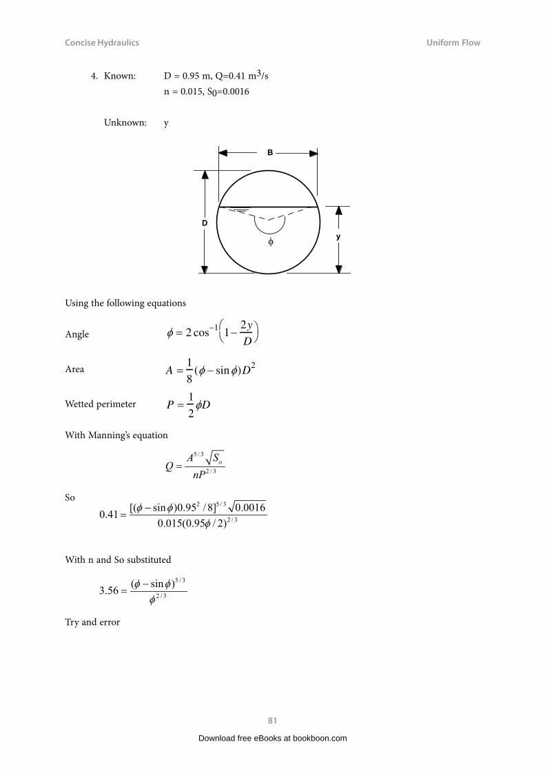
Concise Hydraulics

81

Uniform Flow

4. Known: D = 0.95 m, Q=0.41 m3/s n = 0.015, S0=0.0016

Unknown: y

φ

Dy

B

Using the following equations

Angle 2 cos 1 12y

D

Area A1

8( sin )D2

P1

2DWetted perimeter

A1

8( sin )D2

P1

2D

With Manning’s equation

5 / 3

2 / 3oA S

QnP

=

So

2 5 / 3

2 / 3

[( sin )0.95 / 8] 0.00160.410.015(0.95 / 2)

φ φφ

−=

With n and So substituted

5 / 3

2 / 3

( sin )3.56 φ φφ

−=

Try and error


Concise Hydraulics

82

Uniform Flow

Method 1: Try different angles ( note: from range 0- 2p)

f 1 2 3 3.5 3.3

RHS 0.046 0.73 2.77 4.1 3.57

So f =3.3,

From 5 / 3

2 / 3oA S

QnP

[1 cos( / 2)] / 2 0.95[1 cos(3.3 / 2)] / 2 0.51y D mφ= − = − =

Method 2: Try different depths (slightly more calculations)

Guess a y and then use to get the angle

Y 0.1 0.5 0.55 0.51

f 1.32 3.25 3.46 3.28

RHS 0.15 3.42 3.99 3.54

So y = 0.51

Method 3: Matlab

With 5 / 3

2 / 3

( sin )3.56 φ φφ

−=

Write a function in f.m:

function y = f(x)

y = (x-sin(x))^(5/3)/x^(2/3)-3.65;

then

>>z = fzero(@f,2)

3.3308φ =

So

[1 cos( / 2)] / 2 0.95[1 cos(3.3308 / 2)] / 2 0.5199 0.52y D m mφ= − = − = ≈


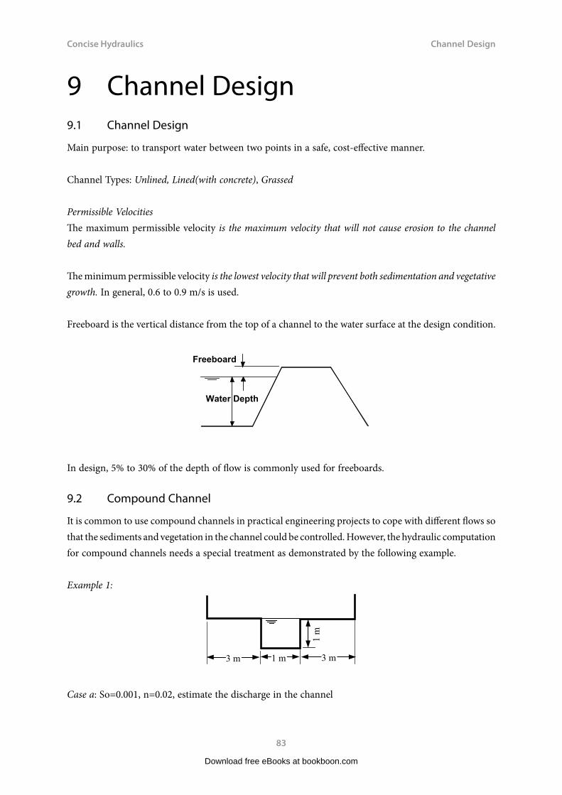
Concise Hydraulics

83

Channel Design

9 Channel Design9.1 Channel Design

Main purpose: to transport water between two points in a safe, cost-effective manner.

Channel Types: Unlined, Lined(with concrete), Grassed

Permissible VelocitiesThe maximum permissible velocity is the maximum velocity that will not cause erosion to the channel bed and walls.

The minimum permissible velocity is the lowest velocity that will prevent both sedimentation and vegetative growth. In general, 0.6 to 0.9 m/s is used.

Freeboard is the vertical distance from the top of a channel to the water surface at the design condition.

Freeboard

Water Depth

In design, 5% to 30% of the depth of flow is commonly used for freeboards.

9.2 Compound Channel

It is common to use compound channels in practical engineering projects to cope with different flows so that the sediments and vegetation in the channel could be controlled. However, the hydraulic computation for compound channels needs a special treatment as demonstrated by the following example.

Example 1:

3 m 3 m 1 m

1 m

Case a: So=0.001, n=0.02, estimate the discharge in the channel


Concise Hydraulics

84

Channel Design

Solution:The flow is contained in the main channel.

A = by = 1 m2, P = b+2y = 3 m, R = A/P = 1/3 = 0.333 m

2/3 2 /30 0.333 0.001 0.76 /

0.02R S

V m sn

= = =

31 0.76 0.76 /Q AV m s= = × =

Case b: The same channel with a slightly more discharge (0.01m extra water)

Solution:

0.01m

3 m 3 m 1 m 1

m


Click on the ad to read moreClick on the ad to read moreClick on the ad to read moreClick on the ad to read moreClick on the ad to read moreClick on the ad to read moreClick on the ad to read moreClick on the ad to read moreClick on the ad to read moreClick on the ad to read moreClick on the ad to read moreClick on the ad to read moreClick on the ad to read moreClick on the ad to read moreClick on the ad to read moreClick on the ad to read moreClick on the ad to read moreClick on the ad to read moreClick on the ad to read moreClick on the ad to read moreClick on the ad to read moreClick on the ad to read moreClick on the ad to read moreClick on the ad to read moreClick on the ad to read moreClick on the ad to read moreClick on the ad to read moreClick on the ad to read moreClick on the ad to read more




FINANCIAL TIMES








Concise Hydraulics

85

Channel Design

The whole compound channel is treated as a whole cross section.

21 1 7 0.01 1.07A m= × + × =

3 3 3 0.01 0.01 9.02P m= + + + + =

/ 1.07 / 9.02 0.1186R A P m= = =

2/3 2 /30 0.1186 0.001 0.38 /

0.02R S

V m sn

= = =

31.07 0.38 0.41 /Q AV m s= = × =

The illogical result is due to the very different flow patterns between the main channel and the over bank flow. To solve this problem, it is necessary to treat different parts of the channel separately.

Divided the channel into three parts:

a

b c

d e

f g

h i j

The main channel and two over-bank sections

Areas: A1, A2, A3Wetted perimeter: P1(abc), P2(cdef), P3(fgh)Calculate V and Q separately and combine them together.

Example 2

During a large flood, the water level in the channel is given in the following figure. Manning’s n is 0.015 for the main channel and 0.035 for the flood banks. The bed slope So is 0.001. Estimate the discharge for a maximum flood depth of 4 m.

y=4m1.5m1.5m

1:2

1:3

14.5m15.0m14.5m

10m5m10m


Concise Hydraulics

86

Channel Design

Solution:

Split the section into subsections (1) in the middle, (2) and (3) as overbank parts and apply Manning’s equation to each one in turn and then sum the discharges.

For Subsection 1 in the middle

2

1 15 1.5 (5 15) 2.5 / 2 47.5A m= × + + × =

1 5 (2 5 2.5) 16.18P m= + × =

5/3 5/30 3

2/3 2 /3

47.5 0.001 205.3 /0.015 16.18

A SQ m s

nP= = =

×

Subsection 2 and Subsection 3 have the same dimensions, hence

2

2 310 14.5 1.5 18.38

2( )A A m+

= = × =

( )2 3 10 10 1.5 14.74P P m= = + × =

5/3 5/30 3

2 3 2/3 2 /3

18.38 0.001 19.2 /0.035 14.74

A SQ Q m s

nP= = = =

×

Hence

Q=Q1+Q2+Q3=243.7 m3/s

9.3 The Best Hydraulic Section

A channel can have many shapes and dimensions. However, certain types of channels are better at conveying flows than others.

Example: The following channels have the same amount of excavation (cross section area), as well as the same Manning’s n and bed slope. Which channel is the best hydraulically?

2 0.5m

41

(a) (b) (c)2 m

2 m


Concise Hydraulics

87

Channel Design

Solution:

Since 4,4.24,8.5P =

From 5/3

2 /3 2 /3

A S KQnP P

= = (let 5/3A SK

n= )

Then

0.397aQ K= , 0.382bQ K= , 0.240cQ K=

Hence a is the best and c is the worst.

A general pattern can be concluded from this example.

From Manning’s Equation 3/20

3/5

nPSA

Q

The channel having the least wetted perimeter for a given area has the maximum conveyance; such a section is known as the best hydraulic section.

The derivation of the best hydraulic sections for some common shapes is illustrated here.


Click on the ad to read moreClick on the ad to read moreClick on the ad to read moreClick on the ad to read moreClick on the ad to read moreClick on the ad to read moreClick on the ad to read moreClick on the ad to read moreClick on the ad to read moreClick on the ad to read moreClick on the ad to read moreClick on the ad to read moreClick on the ad to read moreClick on the ad to read moreClick on the ad to read moreClick on the ad to read moreClick on the ad to read moreClick on the ad to read moreClick on the ad to read moreClick on the ad to read moreClick on the ad to read moreClick on the ad to read moreClick on the ad to read moreClick on the ad to read moreClick on the ad to read moreClick on the ad to read moreClick on the ad to read moreClick on the ad to read moreClick on the ad to read moreClick on the ad to read more


Concise Hydraulics

88

Channel Design

Rectangular

b

y

Let A = by = constant b= A/y

So P=2y+b =2y+A/y

Minimising P

22 0dP Ady y

= − =

Then 2 2Ay

= or 2 2byy

= so 2b y=

The best rectangular channel is the one with its depth being half of its width.

Trapezoidal

b

y x

1

A = (b+xy)y

22 1P b y x= + +

Now Ab xyy

= −

Hence 2 1AP xy y xy

= − + +

22 2 1 0P A x x

y y∂

= − − + + =∂

2

2 01

P xy yx x

∂= − + =

∂ +


Concise Hydraulics

89

Channel Design

y

30O

b

Solve both equations

3 tan 303

ox = =

and

( )2 32 1 2

3yb y x x

= + − =

Its is one-half of a hexagon

Questions 9Channel Design

1. Compute the discharge in a compound channel. The estimated Manning’s ns are 0.015 for the main channel and 0.035 for the over-bank sections. The bed slope of the channel So is 0.001.

(Answer: 97.09 m3/s)

y=3m 1m1 m 12 3

1:2

1:3 1:31:2

7m 3m 4m


Concise Hydraulics

90

Channel Design

2. A rectangular, concrete lined channel (Manning’s n = 0.015) is to be constructed to carry flood water. The slope of the channel bed slope is 1 in 500. The design discharge is 10m3/s. (a) Calculate the proportions of the rectangular channel that will minimize excavation and result in the optimum hydraulic section. (b) If the cross sectional area of flow is kept the same as in part (a) but for safety reasons the depth of flow in the channel is limited to 1.00m, what will be the discharge now?

(Answer: a) B=2y=2.89 m b) 9.55m3/s)

3. Compare semicircular section with rectangular and trapezoidal sections to show that it is the most hydraulically efficient.

4. Show that the best hydraulic isosceles triangular section is one-half of a square.

Solutions 9Channel Design

1. Split the section into subsections (1), (2) and (3) and apply Manning’s equation to each one in turn and then sum the discharges.For Subsection 1: B=3+2xy=3+2×2×2=11m, A1=11×1+(3+11)×2/2 = 25 m2

( )2

1 3 2 1 3 2 2 1 4 11.94P y x m= + + = + × + =

5/3 5/30 3

1 2/3 2 /3

25 0.001 6.74 86.1 /0.015 11.94 0.0782

A SQ m s

nP= = = =

×

Subsection 2

22

10 7 1.0 8.52

A m+ = × =

, 2 7 10 10.16P m= + =

5/3 5/30 3

2 2/3 2 /3

8.5 0.001 1.12 6.82 /0.035 10.16 0.164

A SQ m s

nP= = = =

×Subsection 3

23

4 7 1.0 5.52

A m+ = × =

, 3 4 10 7.16P m= + =

5/3 5/30 3

3 2/3 2 /3

5.5 0.001 0.542 4.17 /0.035 7.16 0.130

A SQ m s

nP= = = =

×

Hence Q=Q1+Q2+Q3=86.1+6.82+4.17= 97.09 m3/s


Concise Hydraulics

91

Channel Design

2. a) For the best rectangular section, b=2y, so bybP 22 =+= ,

10)2(015.0

002.0)2/(3/2

3/52

3/20

3/5

bb

nPSA

Q

So

Channel width is 2.89m and depth is 1.45m

b) 216.444.189.2 mbyA If y=1.0, then

myAb 16.41/16.4/ , mybP 16.6216.42

smnP

SAQ /55.9

16.6015.0002.016.4 3

3/2

3/5

3/20

3/5


Click on the ad to read moreClick on the ad to read moreClick on the ad to read moreClick on the ad to read moreClick on the ad to read moreClick on the ad to read moreClick on the ad to read moreClick on the ad to read moreClick on the ad to read moreClick on the ad to read moreClick on the ad to read moreClick on the ad to read moreClick on the ad to read moreClick on the ad to read moreClick on the ad to read moreClick on the ad to read moreClick on the ad to read moreClick on the ad to read moreClick on the ad to read moreClick on the ad to read moreClick on the ad to read moreClick on the ad to read moreClick on the ad to read moreClick on the ad to read moreClick on the ad to read moreClick on the ad to read moreClick on the ad to read moreClick on the ad to read moreClick on the ad to read moreClick on the ad to read moreClick on the ad to read more








Concise Hydraulics

92

Channel Design

3. For the same A, the best hydraulic sections for rectangle, trapezoid and semicircle are

1) Rectangle 2

2bA =

so 2b A= , 2 2 2 2.83p b A A= = =

2) Trapezoid 22 1( ) ( ) 33 3

A b xy y y y yy

= + = + =

So 0.763

Ay A= =

2 4 2 42 1 2 3 2.63 3 3y yP b y x b y y A= + + = + = + = =

3) Semicircle 23.14

2rA = , so 2 0.798

3.14r A A= =

3.14 3.14 0.798 2.51P r A A= = × =

So semicircle has the least perimeter among all sections with the same area; hence it is the most hydraulically efficient of all sections.

4. Method 1

y 1

x

The area and wetted perimeter of a triangle are

2xyA , so /y A x22 1 2 1/P y x A x x

21 1/ 01/

dP xAdx x x

i.e., 21 1/ 0xox 45tan1

This means that the section is a half square.


Concise Hydraulics

93

Channel Design

Method 2

( )2 tan / 2A y α= , / tan( / 2)y A α=

2 / cos( / 2) 2 / tan( / 2) / cos( / 2)P y Aα α α= =

To minimize P is equivalent to minimize P2, i.e.,Min 2 1 11/[tan( / 2)cos ( / 2)] sin ( / 2)cos ( / 2)z α α α α− −= =

2 1 1 2/ [ sin ( / 2)cos( / 2)cos ( / 2)] / 2 sin ( / 2)cos ( / 2)sin( / 2)] / 2 0dz dα α α α α α α− − − −= − + =2 2sin ( / 2) cos ( / 2) 0α α− −− + =

tan( / 2) 1α = so / 2 45oα = hence 90oα =

This means that the section is a half square.Method 3 Using Matlab to do the minimisationWith 2 / cos( / 2) 2 / tan( / 2) / cos( / 2)P y Aα α α= =>>fminunc(inline(‘ 2*(1/tan(x/2)^0.5/cos(x/2))’),1)1.5709 (radian) i.e., 1.5709*180/3.14159=90o

Or with

22 1 2 1/P y x A x x= + = +

>>fminunc(inline(‘ 2*(x+1/x)^0.5’),1)

Answer =1, hence it is a half rectangular.


Concise Hydraulics

94

Critical Flow

10 Critical FlowSimilar to airplanes with supersonic and subsonic speed classifications, water flow in open channels can also be classified into supercritical and subcritical flows. As a counterpart to the sound speed, the wave speed (also called celerity) is used in hydraulics.

10.1 Small Wave in Open Channel

cPush

A small wave can be generated in an open channel by pushing a plate. The celerity of a small wave in open channel is

c gDm

The derivation of this formula is explained in the unsteady flow chapter.

If a pebble is dropped into a channel with flowing water, the pattern generated could be one of the following cases that represent the four types of flow.

Still water Critical flow Subcritical flow Supecritical flow

cc Flow 2c Flow V+cc-V Flow c+V

10.2 Critical Flow

Critical velocity

Vc gDm

Froude Number

Fr VgDm

=


Concise Hydraulics

95

Critical Flow

where

V the mean velocityDm hydraulic mean depth, A/B

Flow state

Critical Fr = 1 or Fr = 1 or V gDmFr>1 or V gDmFr<1 orV gDm

Supercritical Fr>1 or

Subcritical Fr<1 or

In relation to critical flow

yc the critical depth y>yc, subcritical y<yc, supercritical

Sc the critical slope So<Sc, mild slope So>Sc, steep slope

Vc the critical velocity V<Vc, tranquil flow V>Vc, rapid flow


Click on the ad to read moreClick on the ad to read moreClick on the ad to read moreClick on the ad to read moreClick on the ad to read moreClick on the ad to read moreClick on the ad to read moreClick on the ad to read moreClick on the ad to read moreClick on the ad to read moreClick on the ad to read moreClick on the ad to read moreClick on the ad to read moreClick on the ad to read moreClick on the ad to read moreClick on the ad to read moreClick on the ad to read moreClick on the ad to read moreClick on the ad to read moreClick on the ad to read moreClick on the ad to read moreClick on the ad to read moreClick on the ad to read moreClick on the ad to read moreClick on the ad to read moreClick on the ad to read moreClick on the ad to read moreClick on the ad to read moreClick on the ad to read moreClick on the ad to read moreClick on the ad to read moreClick on the ad to read more






find out more!





Concise Hydraulics

96

Critical Flow

10. 3 Critical Flow Computation

a) If the critical depth is known, Vc is solved by

mc gDV and Q=AVc

b) If the discharge is known, yc is solved by (trial and error)

mgDAQ

c) To get the critical slope Sc , use the Manning Equation

V

R Snc

c c=2 3/

Rearrange it into

2

3/2c

cc R

nVS

Example

For a trapezoidal channel with a base width b=6.0 m, side slope x=2 (i.e., 1 vertical: 2 horizontal) and Manning’s n=0.02, calculate the critical depth, critical velocity and critical slope if its discharge Q=17m3/s.

Solution

A b xy y y yc c c c= + = +( ) ( )6 2

B b xy yc c= + = +2 6 4

D A

B(6 + 2y )y

6 + 4y(3+ y )y

3+ 2ymc c

c

c c

c

= = =

The discharge is

Q A V A gDc c c m= =

So 17 6 2= +++

( )y y gc c(3 y )y

3 2yc c

c

Simplifying,

7.363 yc yc

3

(3 2yc )


Concise Hydraulics

97

Critical Flow

By trial and error, the critical depth is approximately

0.84cy m=

and the corresponding critical velocity is

26.45A m=

17 2.6 /6.45cV m s= =

The critical slope

22 1 9.76cP b y x m= + + =

0.66AR mP

= =

2 2

2 / 30.052 0.0050.758c

cSV nR

= = =

Questions 10Critical Flow

1. A rectangular channel is 3.0 m wide, has a 0.01 slope, flow rate of 5.3 m3/s, and n=0.011. Find its normal depth yn and critical depth yc.

(Answer: 0.4m, 0.683m)

2. Water flows in a rectangular channel at a depth of 1.22m and discharge of Q=5.66m3/s. Determine the minimum channel width if the channel is to be subcritical.

(Answer: 1.34m)

3. A rectangular channel has a bottom width of 8 m and Manning’s n=0.025a) Determine the normal slope at a normal depth of 2m when the discharge is 12 m3/s;b) Determine the critical slope and the critical depth when the discharge is 12m3/s;c) Determine the critical slope at the critical depth of 1.5m and compute the corresponding

discharge. (Answer: a) 0.0002, b) 0.009, 0.61 m, c) 0.008, 46.1m3/s)


Concise Hydraulics

98

Critical Flow

4. For a trapezoidal channel with a base width b=3.0 m, Manning’s n=0.025 and side slope x=2 (i.e. 1 vertical: 2 horizontal), calculate the critical depth, critical velocity and critical slope if its discharge Q=10m3/s.

(Answer: 0.86 m, 2.46 m/s, 0.0076)

Solutions 10Critical Flow

1. From the Manning equation A = by = 3y , P = b + 2y = 3 = 2y

Since QA S

nPo=

5 3

2 3

/

/ so 53 3 0 01

0 011 3 2

5 3

2 3. ( ) .. ( )

/

/=+

yy

Simplifying

Trial and error

y=1.0 0.342 y=0.5 0.125 y=0.3 0.057 y=0.4 0.089 y=0.45 0.107 close to 0.4


Click on the ad to read moreClick on the ad to read moreClick on the ad to read moreClick on the ad to read moreClick on the ad to read moreClick on the ad to read moreClick on the ad to read moreClick on the ad to read moreClick on the ad to read moreClick on the ad to read moreClick on the ad to read moreClick on the ad to read moreClick on the ad to read moreClick on the ad to read moreClick on the ad to read moreClick on the ad to read moreClick on the ad to read moreClick on the ad to read moreClick on the ad to read moreClick on the ad to read moreClick on the ad to read moreClick on the ad to read moreClick on the ad to read moreClick on the ad to read moreClick on the ad to read moreClick on the ad to read moreClick on the ad to read moreClick on the ad to read moreClick on the ad to read moreClick on the ad to read moreClick on the ad to read moreClick on the ad to read moreClick on the ad to read more


Concise Hydraulics

99

Critical Flow

So yn=0.4 m

From the Froude number=1

Q A gDm Byc gyc

y QB gc

3 2/

So

yc

5.32

32g

13

0.683m

2. For a critical flow

1VFrgy

= =

566 122122

1. / ( . ).

bg×

=

b=1.34m

Hence, the minimum channel width if the flow is to be subcritical is 1.34m.

3. a) For the given data

A by m= = × =8 2 16 2

P b 2y 8 2 2 12m

RAP

1612

1.33m

From the Manning equation

SonQ

AR23

20.025 12

16 1.3323

2

0.0002

Thus, So=0.0002 will maintain a uniform flow of 12m3/s in this channel at a depth of 2m.


Concise Hydraulics

100

Critical Flow

b) The critical depth

A byc 8yc

DmAB

bycb

yc

Flow velocity is

Vc

QA

128yc

1.5yc

and at the critical depth

So

Vc gDm1.5yc

gyc

yc1.52

g3 0.61m

Then A byc 8 0.61 4.88m2

P b 2yc 8 2 0.61 9.22m

RAP

4.889.22

0.53m

Sc

Qn

AR23

2

12 0.025

4.88 0.5323

2

0.009

c) A byc 8 1.5 12m2

P b 2yc 8 2 1.5 11m

RAP

1211

1.09m

and at critical flow

Vc gDm gyc 1.5g 3.84m / s

The critical slope will be

ScVcn

R23

2

3.84 0.025

1.0923

2

0.008

The flow rate is given by

Q VcA 3.84 12 46.1m3 / s


Concise Hydraulics

101

Critical Flow

4. A (b xyc)yc (3 2yc )yc B b 2xyc 3 4yc

DmAB

(3 2yc )yc3 4yc

The flow velocity is

VcQA

10(3 2yc )yc

and at the critical depth

Vc gDm

so

10(3 2yc )yc

g(3 2yc )yc

3 4yc

Simplifying, 10.193 2yc yc

3

(3 4yc )


Click on the ad to read moreClick on the ad to read moreClick on the ad to read moreClick on the ad to read moreClick on the ad to read moreClick on the ad to read moreClick on the ad to read moreClick on the ad to read moreClick on the ad to read moreClick on the ad to read moreClick on the ad to read moreClick on the ad to read moreClick on the ad to read moreClick on the ad to read moreClick on the ad to read moreClick on the ad to read moreClick on the ad to read moreClick on the ad to read moreClick on the ad to read moreClick on the ad to read moreClick on the ad to read moreClick on the ad to read moreClick on the ad to read moreClick on the ad to read moreClick on the ad to read moreClick on the ad to read moreClick on the ad to read moreClick on the ad to read moreClick on the ad to read moreClick on the ad to read moreClick on the ad to read moreClick on the ad to read moreClick on the ad to read moreClick on the ad to read more

.


Concise Hydraulics

102

Critical Flow

By trial and error, the critical depth is approximately

yc=1.0 17.86 yc=0.5 1.6 yc=0.75 6.41 yc=0.85 9.96 yc=0.86 10.38 close to 10.19

So

yc=0.75 6.41 yc=0.85 9.96 yc=0.86 10.38 yc 0.86m

and the corresponding critical velocity is

A (3 2 0.86) 0.86 4.06m2

Vc10

4.062.46m / s

The critical slope

P b 2yc 1 x2 3 2 0.86 1 22 6.85m

RAP

4.066.85

0.59m

2 2


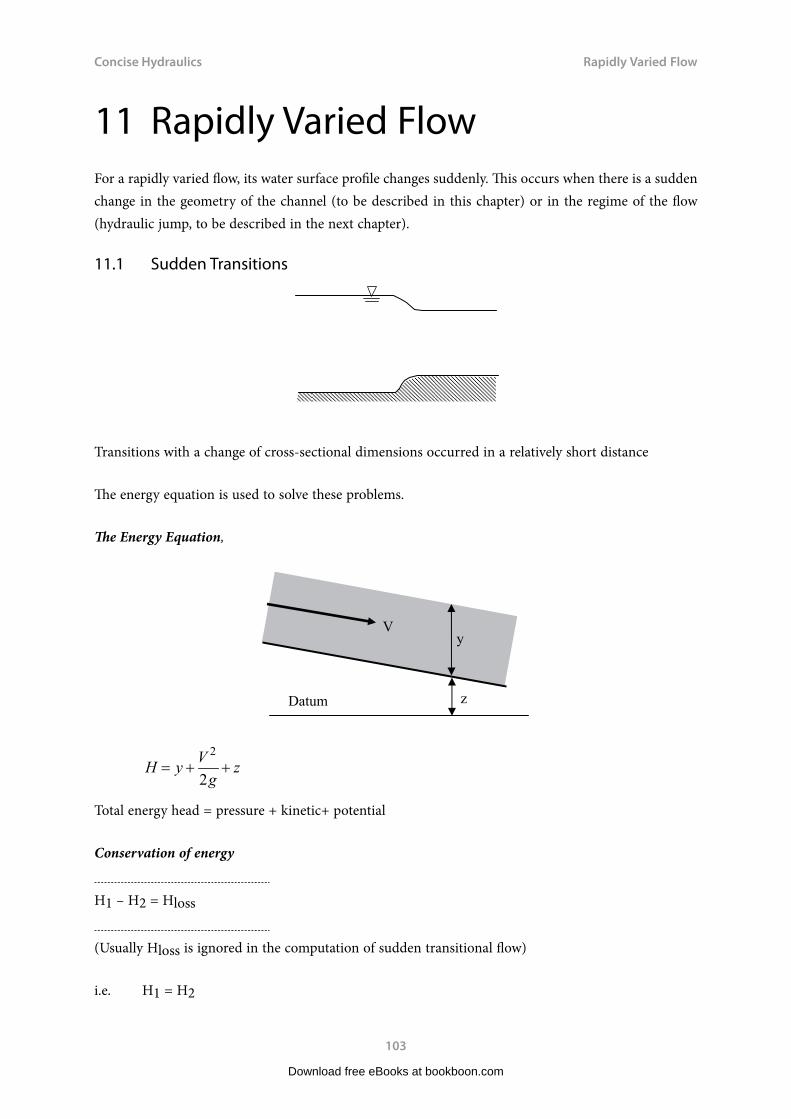
Concise Hydraulics

103

Rapidly Varied Flow

11 Rapidly Varied FlowFor a rapidly varied flow, its water surface profile changes suddenly. This occurs when there is a sudden change in the geometry of the channel (to be described in this chapter) or in the regime of the flow (hydraulic jump, to be described in the next chapter).

11.1 Sudden Transitions

Transitions with a change of cross-sectional dimensions occurred in a relatively short distance

The energy equation is used to solve these problems.

The Energy Equation,

Datum

y

z

V

H y V

gz= + +

2

2

Total energy head = pressure + kinetic+ potential

Conservation of energy H1 – H2 = Hloss (Usually Hloss is ignored in the computation of sudden transitional flow)

i.e. H1 = H2


Concise Hydraulics

104

Rapidly Varied Flow

11.2 Depth of Flow

A steady uniform flow in a rectangular channel of width 5m is interrupted by the presence of a hump of 0.2m in the channel. The upstream depth is 1.25 m and the discharge is 10 m3/s, find the depth of flow at position 2 (taking a=1 and assume no energy loss).

1 2

z=0.2m

y2=? y1=1.25m

Solution:

Applying the energy equation,

y1V1

2

2gy2

V22

2gz

Known: y1 V1 z

Unknown: y2 V2


Click on the ad to read moreClick on the ad to read moreClick on the ad to read moreClick on the ad to read moreClick on the ad to read moreClick on the ad to read moreClick on the ad to read moreClick on the ad to read moreClick on the ad to read moreClick on the ad to read moreClick on the ad to read moreClick on the ad to read moreClick on the ad to read moreClick on the ad to read moreClick on the ad to read moreClick on the ad to read moreClick on the ad to read moreClick on the ad to read moreClick on the ad to read moreClick on the ad to read moreClick on the ad to read moreClick on the ad to read moreClick on the ad to read moreClick on the ad to read moreClick on the ad to read moreClick on the ad to read moreClick on the ad to read moreClick on the ad to read moreClick on the ad to read moreClick on the ad to read moreClick on the ad to read moreClick on the ad to read moreClick on the ad to read moreClick on the ad to read moreClick on the ad to read more











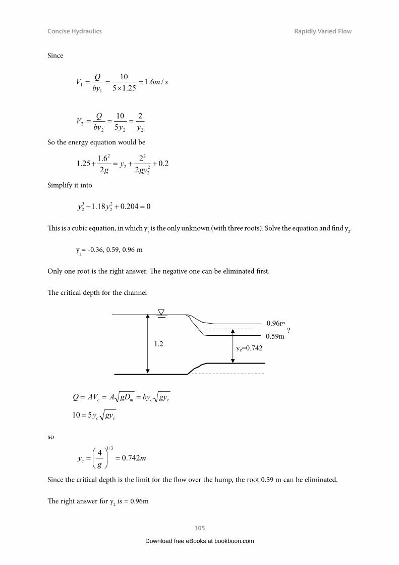
Concise Hydraulics

105

Rapidly Varied Flow

Since

smbyQV /6.1

25.1510

11

2222

2510

yybyQV

So the energy equation would be

2 2

2 22

1.6 21.25 0.22 2

yg gy

+ = + +

Simplify it into

3 22 21.18 0.204 0y y− + =

This is a cubic equation, in which y2 is the only unknown (with three roots). Solve the equation and find y2.

y2= -0.36, 0.59, 0.96 m

Only one root is the right answer. The negative one can be eliminated first.

The critical depth for the channel

1.2

0.96m

0.59m?

yc=0.742

Q AV A gD by gyc m c c= = =

10 5 c cy gy=

so1/3

4 0.742cy mg

= =

Since the critical depth is the limit for the flow over the hump, the root 0.59 m can be eliminated.

The right answer for y2 is = 0.96m


Concise Hydraulics

106

Rapidly Varied Flow

11.3 Height of Hump

1 2

z

ycy1=2.5m

If the depth of flow in a 2m wide rectangular channel is 2.5 m when the discharge is 4 m3/s, estimate the height of the hump which would produce critical conditions.

Solution:

The energy equation

22c1

1VV

2g 2gcy y z+ = + + ∆

sm

AQV /8.0

5.224

11 =

×==

Q AV A gy by gyc c c c= = =

So

1/34 0.742cy mg

= =

4 2.70 /2 0.742c

c

QV m sby

= = =×

Substitute it into the energy equation

2 20.8 2.702.5 0.7422g 2g

z+ = + + ∆

2.53 1.11 z= + ∆

Then

1.42z m∆ =


Concise Hydraulics

107

Rapidly Varied Flow

11.4 Specific Energy

(Pressure + Kinetic energy)

gVyEs 2

2

+=

E s

y

yc

Q = constant

At critical depth, the specific energy is at the minimum point.

Mathematical derivation:

dA

dy B


Click on the ad to read moreClick on the ad to read moreClick on the ad to read moreClick on the ad to read moreClick on the ad to read moreClick on the ad to read moreClick on the ad to read moreClick on the ad to read moreClick on the ad to read moreClick on the ad to read moreClick on the ad to read moreClick on the ad to read moreClick on the ad to read moreClick on the ad to read moreClick on the ad to read moreClick on the ad to read moreClick on the ad to read moreClick on the ad to read moreClick on the ad to read moreClick on the ad to read moreClick on the ad to read moreClick on the ad to read moreClick on the ad to read moreClick on the ad to read moreClick on the ad to read moreClick on the ad to read moreClick on the ad to read moreClick on the ad to read moreClick on the ad to read moreClick on the ad to read moreClick on the ad to read moreClick on the ad to read moreClick on the ad to read moreClick on the ad to read moreClick on the ad to read moreClick on the ad to read more


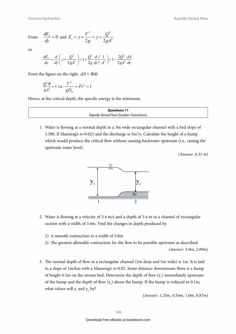
Concise Hydraulics

108

Rapidly Varied Flow

From 0sdEdy

= and 2 2

22 2sV QE y y

g gA= + = +

so

2 2 2

2 2 3

1 21 12 2 2

sdE d Q Q d Q dAydy dy gA g dy A gA dy

= + = + = −

From the figure on the right, dA Bdy=

2

3 1Q BgA

= i.e. 2

2 1m

V FrgD

= =

Hence, at the critical depth, the specific energy is the minimum.

Questions 11Rapidly Varied Flow (Sudden Transitions)

1. Water is flowing at a normal depth in a 3m wide rectangular channel with a bed slope of 1:500. If Manning’s n=0.025 and the discharge is 5m3/s. Calculate the height of a hump which would produce the critical flow without causing backwater upstream (i.e., raising the upstream water level).

(Answer: 0.31 m)

y1

1 2

z

yc

2. Water is flowing at a velocity of 3.4 m/s and a depth of 3.4 m in a channel of rectangular section with a width of 3.4m. Find the changes in depth produced by

1) A smooth contraction to a width of 3.0m2) The greatest allowable contraction for the flow to be possible upstream as described.

(Answer: 3.0m, 2.89m)

3. The normal depth of flow in a rectangular channel (2m deep and 5m wide) is 1m. It is laid to a slope of 1m/km with a Manning’s n=0.02. Some distance downstream there is a hump of height 0.5m on the stream bed. Determine the depth of flow (y1) immediately upstream of the hump and the depth of flow (y2) above the hump. If the hump is reduced to 0.1m, what values will y1 and y2 be?

(Answer: 1.25m, 0.54m, 1.0m, 0.87m)


Concise Hydraulics

109

Rapidly Varied Flow

Solutions 11Rapidly Varied Flow (Sudden Transitions)

1. From Manning equation A = by = 3y , P = b + 2y = 3 + 2y

Since QA

5

3 S0

nP2

3

so 53y

53 0.002

0.025 3 2y2

3

Simplifying

2.7953y

53

3 2y2

3

Trial and error

y=1.0 2.13 y=1.2 2.74 close to 2.795

So y=1.20 m

V QA

m s11

53 12

139= =×

=.

. /

From Froude number=1

Q A gDm Byc gyc

y Q B gc3 2/ / ( )

so

y g mc [5 / ( )] ./2 2 1 33 0 66

VcQ

ycB2.53m / s

From the energy equation

y1V1

2

2gz yc

Vc2

2g

12 1392 9 8

0 66 2 532 9 8

2 2

. ..

. ..

z

z 0.31m


Concise Hydraulics

110

Rapidly Varied Flow

2. 1) By the energy equation

y1

V12

2gy2

V22

2g

3.43.42

2gy2

V22

2g

Since Q V1y1b 3.4 3.4 3.4 39.3m3 / s

V2

Q

b2 y2

39.3

3y2

13.1

y2

So

3.4

3.42

2gy2

13.12

2gy22

Simply

3.99 y2

8.75

y22


Click on the ad to read moreClick on the ad to read moreClick on the ad to read moreClick on the ad to read moreClick on the ad to read moreClick on the ad to read moreClick on the ad to read moreClick on the ad to read moreClick on the ad to read moreClick on the ad to read moreClick on the ad to read moreClick on the ad to read moreClick on the ad to read moreClick on the ad to read moreClick on the ad to read moreClick on the ad to read moreClick on the ad to read moreClick on the ad to read moreClick on the ad to read moreClick on the ad to read moreClick on the ad to read moreClick on the ad to read moreClick on the ad to read moreClick on the ad to read moreClick on the ad to read moreClick on the ad to read moreClick on the ad to read moreClick on the ad to read moreClick on the ad to read moreClick on the ad to read moreClick on the ad to read moreClick on the ad to read moreClick on the ad to read moreClick on the ad to read moreClick on the ad to read moreClick on the ad to read moreClick on the ad to read more

Get Help Now




Concise Hydraulics

111

Rapidly Varied Flow

Before trial and error, find the critical depth

From Vc gyc

Q

ycb y Q gb g mc = = =[ / ( )] [( . / )] ./ /2 2 1 3 2 2 1 339 3 3 2 60

by trial and error between (2.6 m to 3.4 m)

y2=3.0 m, 3.97 y2=3.1 m, 4.01

So y2=3.0 m

2) Critical depth at section 2

Energy equation y1

V12

2gy2

V22

2g

3.43.42

2gy2

V22

2g

Since ,

3.99

3

2yc , yc 2.66m

b Q

V y gy ym

c c c c2

39 3 2 89= = =. .

Maximum contraction to 2.89 m

3. a) Area

A m= 5 2

Hydraulic radius

R A

Pm= =

+=

55 2

0 71.

Q AV A

R Sn

m so= = = =2 3 2 3

35 0 71 0 0010 02

6 29/ /. .

.. /


Concise Hydraulics

112

Rapidly Varied Flow

Q A V by gy b g yc c c c c= = = =( ) ./3 2 6 29

y b g mc = =( . / ) / .6 29 05423 ,

V gy g m sc c= = =054 2 3. . /

b) Check the height of hump that can produce critical flow without causing backwaterThe total energy at the hump

y V

gz

gz zc

c+ + = + + = +2 2

2054 2 3

2081. . .

Before the hump

y V

g gm1

12 2

21 6 29 5

2108+ = + =

( . / ) .

So

081 108. .+ =z z m= − =108 081 0 27. . .

c) Therefore, 0.5m hump will produce critical flow over the hump and cause backwater The total energy at the hump

y V

gz

gmc

c+ + = + + =2 2

2054 2 3

205 131. . . .

Before the hump

y V

gy Q by

gm1

12

11

2

2 2131+ = + =

( / ) .

y y m1 120 081 131+ =−. .

Trial and error (y1>1.0m due to the hump):

y1=1.1, LHS=1.17 y1=1.2, LHS=1.26 y1=1.3, LHS=1.35 y1=1.25, LHS=1.30 So y1=1.25 m


Concise Hydraulics

113

Rapidly Varied Flow

d) If the hump is 0.1m, no backwater will be produced, therefore,

y m1 1=

The total energy at the hump

222

2 2 20.081 0.12Vy z y y

g−+ + = + +

Before the hump

y V

g gm1

12 2

21 6 29 5

2108+ = + =

( . / ) .

so

2

2 20.081 0.1 1.08y y−+ + =

i.e.

3 22 20.98 0.081 0y y− + =

Estimate y2 (trial above 0.54m)

2 0.87y m=


Click on the ad to read moreClick on the ad to read moreClick on the ad to read moreClick on the ad to read moreClick on the ad to read moreClick on the ad to read moreClick on the ad to read moreClick on the ad to read moreClick on the ad to read moreClick on the ad to read moreClick on the ad to read moreClick on the ad to read moreClick on the ad to read moreClick on the ad to read moreClick on the ad to read moreClick on the ad to read moreClick on the ad to read moreClick on the ad to read moreClick on the ad to read moreClick on the ad to read moreClick on the ad to read moreClick on the ad to read moreClick on the ad to read moreClick on the ad to read moreClick on the ad to read moreClick on the ad to read moreClick on the ad to read moreClick on the ad to read moreClick on the ad to read moreClick on the ad to read moreClick on the ad to read moreClick on the ad to read moreClick on the ad to read moreClick on the ad to read moreClick on the ad to read moreClick on the ad to read moreClick on the ad to read moreClick on the ad to read more






Brain power




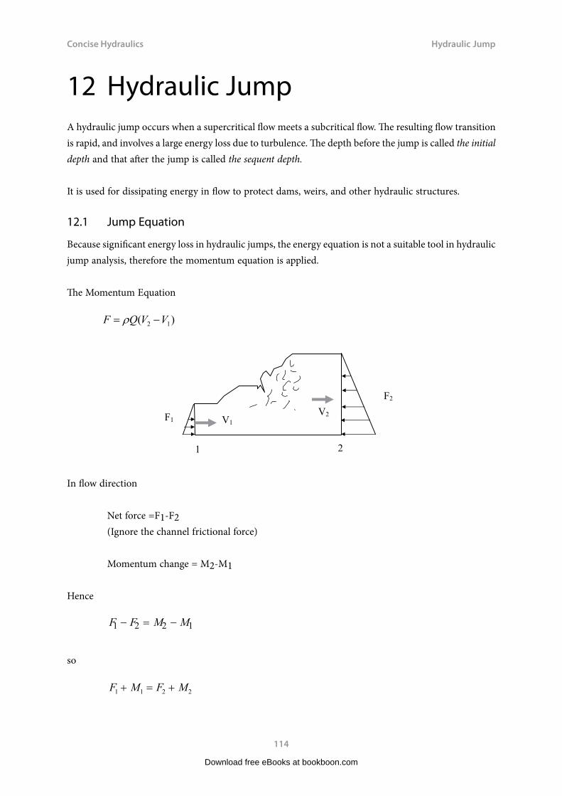
Concise Hydraulics

114

Hydraulic Jump

12 Hydraulic JumpA hydraulic jump occurs when a supercritical flow meets a subcritical flow. The resulting flow transition is rapid, and involves a large energy loss due to turbulence. The depth before the jump is called the initial depth and that after the jump is called the sequent depth.

It is used for dissipating energy in flow to protect dams, weirs, and other hydraulic structures.

12.1 Jump Equation

Because significant energy loss in hydraulic jumps, the energy equation is not a suitable tool in hydraulic jump analysis, therefore the momentum equation is applied.

The Momentum Equation

F Q V V= −ρ ( )2 1

1 2

V2V1F1

F2

In flow direction

Net force =F1-F2(Ignore the channel frictional force)

Momentum change = M2-M1

Hence

F1 F2 M2 M1

so

F M F M1 1 2 2+ = +


Concise Hydraulics

115

Hydraulic Jump

i.e.

F M+ = constant

Hydrostatic pressure force

F gAy and M QV= ρwhere A = area F gAy = the depth of centroidso

g(A1y1 A2y2 ) Q(V2 V1)

The jump height can thus be evaluated knowing either upstream or downstream conditions

Energy dissipation

∆H H H y Vg

y Vg

= − = + − +1 2 112

222

2 2( ) ( )

Hydraulic jump lengths can only be roughly estimated. One of the popular equations is L=6.1 y2


Click on the ad to read moreClick on the ad to read moreClick on the ad to read moreClick on the ad to read moreClick on the ad to read moreClick on the ad to read moreClick on the ad to read moreClick on the ad to read moreClick on the ad to read moreClick on the ad to read moreClick on the ad to read moreClick on the ad to read moreClick on the ad to read moreClick on the ad to read moreClick on the ad to read moreClick on the ad to read moreClick on the ad to read moreClick on the ad to read moreClick on the ad to read moreClick on the ad to read moreClick on the ad to read moreClick on the ad to read moreClick on the ad to read moreClick on the ad to read moreClick on the ad to read moreClick on the ad to read moreClick on the ad to read moreClick on the ad to read moreClick on the ad to read moreClick on the ad to read moreClick on the ad to read moreClick on the ad to read moreClick on the ad to read moreClick on the ad to read moreClick on the ad to read moreClick on the ad to read moreClick on the ad to read moreClick on the ad to read moreClick on the ad to read more


Concise Hydraulics

116

Hydraulic Jump

Examle

1.25m y1=?

A hydraulic jump forms in a rectangular open channel with a width of 2 m in which water is flowing at 4. If the depth just downstream of the jump is 1.25 m. Calculate the theoretical depth upstream of the jump. Estimate the energy loss as a percentage of the initial energy.

Solution

From F1 F2 M2 M1

21

1 1 1 1 1(2 ) 9.812yF gA y g y yρ ρ ρ= = =

2 2 2

1.25(2 1.25) 15.332

F gA y gρ ρ ρ= = × =

1 11 1 1

4 4 8(4)2

QM QVA y y

ρ ρ ρ ρ×= = = =

2 22

4 4(4) 6.42 1.25

QM QVA

ρ ρ ρ ρ×= = = =

×

Substitute them into the momentum equation

21

1

89.81 15.33 6.4yy

ρ ρ ρ ρ− = −

Simplify it

y y13

12 22 082 0− + =. .

Find y1 (trial and error) y1 LHS 1 -0.4 0.5 -0.165 0.4 0.004


Concise Hydraulics

117

Hydraulic Jump

So y1= 0.4m

2

1

11 1.6942

Vy m

gH + ==

2

2

22 1.3802

Vy m

gH + ==

Energy loss=1.694 – 1.380 = 0.314 m

%loss= 18.5%0.3141.694

=

12.2 Hydraulic Jump in Rectangular Channel

If a jump occurs in a rectangular channel, there is no need to use trail and error approach and the unknown depth can be solved by the following equations.

y y qgy

y2

12 2

1

1

42

2= + − y y q

gyy

122 2

2

2

42

2= + −

where qQb

or in another form :

y y Fr2

112

21 8 1= + −( )

y y Fr1

222

21 8 1= + −( )

For the last example: Input y2 = 1.25 and q=2

1 0.396y m=

12.3 Hydraulic Jump in Trapezoidal Channel

A trapezoidal channel with a 6m bed width and side slope of 1:1.5 discharges water at a rate of 8.5 m3/s. If the normal depth downstream of a hydraulic jump is 1.2 m, what is the flow depth upstream of the jump?


Concise Hydraulics

118

Hydraulic Jump

Solution:Since F F M M1 2 2 1− = −

so ρ ρg A y A y Q V V( ) ( )1 1 2 2 2 1− = −

From

F F M M1 2 2 1

g A y A y Q V V( ) ( )1 1 2 2 2 1

A y(6 1.5y)

A y y1 1 16 15( . )

A m2212 6 15 12 9 36. ( . . ) .

so A y y1 1 16 15= +( . )

A m2212 6 15 12 9 36= + × =. ( . . ) .

2 2 3 2 3

00

[6 3( )] 3 1.5 3 0.5y

yAy y z zdz z yz z y y = + − = + − = + ∫

6m

11.5 dz

z

So

A y y y1 12 33 05= + .

A y m2 22 3 33 12 05 12 5184= × + × =. . . .


Click on the ad to read moreClick on the ad to read moreClick on the ad to read moreClick on the ad to read moreClick on the ad to read moreClick on the ad to read moreClick on the ad to read moreClick on the ad to read moreClick on the ad to read moreClick on the ad to read moreClick on the ad to read moreClick on the ad to read moreClick on the ad to read moreClick on the ad to read moreClick on the ad to read moreClick on the ad to read moreClick on the ad to read moreClick on the ad to read moreClick on the ad to read moreClick on the ad to read moreClick on the ad to read moreClick on the ad to read moreClick on the ad to read moreClick on the ad to read moreClick on the ad to read moreClick on the ad to read moreClick on the ad to read moreClick on the ad to read moreClick on the ad to read moreClick on the ad to read moreClick on the ad to read moreClick on the ad to read moreClick on the ad to read moreClick on the ad to read moreClick on the ad to read moreClick on the ad to read moreClick on the ad to read moreClick on the ad to read moreClick on the ad to read moreClick on the ad to read more


Concise Hydraulics

119

Hydraulic Jump

Let V=Q/A

Thus, ,

9.81(3y12 0.5y1

3 5.184) 8.52 19.36

1y1(6 1.5y1)

Simplifying

5 97 3 05 7 366 151

213

1 1

. . .( . )

− − =+

y yy y

By trial and error

y1=0.2 m

12.4 Hydraulic jump in Sloping Channel

In flow direction: Net force =Fg sinq+F1-F2

Gravity force

1 21 ( )2gF gL h hρ≈ + , 2

1 11 cos2

F ghρ θ= , 22 2

1 cos2

F ghρ θ=

where h1 and h2 are the perpendicular depths to the channel bed

1

2

V2V1F1

F2

Fg

So 212 1( 1 8 1)

2hh W= + −

where

11

2 1

sincos

FrWLh h

θθ=

−−

then vertical depth y1=h1/cosq and y2=h2/cosq


Concise Hydraulics

120

Hydraulic Jump

Questions 12Hydraulic Jump

1. Water is flowing at a rate of 10m3/s through a rectangular channel 4 m wide, at a depth of 0.5 m. A weir downstream causes the water to backup the channel and a hydraulic jump occurs. Find the sequent depth and the loss of energy at the jump.

(Answer: 1.37m, 0.234 m)

2. Water flows in a rectangular channel at a depth of 30cm and with a velocity of 16m/s. If a downstream sill forces a hydraulic jump, what will be the depth and velocity downstream of the jump? What head loss is produced by the jump?

(Answer: 3.81m, 1.26m/s, 9.46m)

3. Starting from the first principles, show that the following equation holds true for a hydraulic jump in a trapezoidal channel:

ρ ρg by xy Q

b xy y( )

( )

2 3 2

2 3+ +

+= constant

where y is the depth of flow, b is the bottom width, Q is the discharge and x is the side slope (1 vertical to x horizontal). Draw the force momentum diagram for the following conditions and determine the initial depth if the sequent depth is 0.2m: Q=50 l/s, b=0.46m, x=1.

1z

x

bdz

y

(Answer: the initial depth is 0.04m)


Concise Hydraulics

121

Hydraulic Jump

Solutions 12Hydraulic Jump

1. From the rectangular channel equation

y y qgy

y2

12 2

1

1

42

2= + −

Input y m1 05= . and q=2.5

y y qgy

yg

m212 2

1

12 2

42

205

42 2 5

05052

137= + − = +×

− =. .

.. .

H y Vg

y qgy

m1 112

1

2

12

2

22 22 5

2 9 81 050 5 1 774= + = +

× ×= + =. .

.. .

H y Vg

y qgy

m2 222

2

2

22

2

22 22 5

2 9 81 1371 37 1540= + = +

× ×= + =. .

.. .

Energy loss DH=H1-H2=1.774 – 1.540 = 0.234 m


Click on the ad to read moreClick on the ad to read moreClick on the ad to read moreClick on the ad to read moreClick on the ad to read moreClick on the ad to read moreClick on the ad to read moreClick on the ad to read moreClick on the ad to read moreClick on the ad to read moreClick on the ad to read moreClick on the ad to read moreClick on the ad to read moreClick on the ad to read moreClick on the ad to read moreClick on the ad to read moreClick on the ad to read moreClick on the ad to read moreClick on the ad to read moreClick on the ad to read moreClick on the ad to read moreClick on the ad to read moreClick on the ad to read moreClick on the ad to read moreClick on the ad to read moreClick on the ad to read moreClick on the ad to read moreClick on the ad to read moreClick on the ad to read moreClick on the ad to read moreClick on the ad to read moreClick on the ad to read moreClick on the ad to read moreClick on the ad to read moreClick on the ad to read moreClick on the ad to read moreClick on the ad to read moreClick on the ad to read moreClick on the ad to read moreClick on the ad to read moreClick on the ad to read more

EXPERIENCE THE POWER OF FULL ENGAGEMENT…

RUN FASTER. RUN LONGER.. RUN EASIER…

READ MORE & PRE-ORDER TODAY WWW.GAITEYE.COM

Challenge the way we run

1349906_A6_4+0.indd 1 22-08-2014 12:56:57

http://s.bookboon.com/Gaiteye

Concise Hydraulics

122

Hydraulic Jump

2. Since F Vgy g1

1

1

160 3

9 33= = =.

.

Use the rectangular hydraulic jump equation

mFryy 81.3133.981

23.0181

222

11

2

Since V y b V y b1 1 2 2=

So V V yy

m s21 1

2

16 0 3381

126= =×

=.

.. /

E y V

gy V

g g gmloss = + − + = + − + =1

12

222 2 2

2 20 3 16

2381 126

29 46( ) . ( . . ) .

3. F M+ = constant

ρ ρg Ay QV( ) + = constant

A y b yx= +( )

1z

x

bdz

y

So

2 2 3

002 3

[ 2 ( )] / 2 2 / 3

/ 2 / 3

y yAy b x y z zdz bz xyz xz

by xy

= + − = + − =

+

∫

∴ + = + +

+= constantρ ρ ρ ρg Ay QV g by xy Q

b xy y( ) ( / / )

( )2 3

2

2 3


Concise Hydraulics

123

Hydraulic Jump

0

0.05

0.1

0.15

0.2

0.25

0 100 200 300 400 500 600

y

F+M

Force + momentum curve

F + M = 1000 0 46 2 3 0 050 46

1000 0 23 0 333 0 050 46

2 32

2 32

[ ( . / / ) .( . )

]

[ ( . . ) .( . )

]

g y yy y

g y yy y

+ ++

= + ++

y = 0.2 F + M = 135 ; y = 0.15 F + M = 89 ;

y = 0.1 F + M = 70.5 ; y = 0.05 F + M = 104 ;

y = 0.01 F + M = 532 ; y = 0.03 F + M = 172

So the initial depth is about 0.04m.


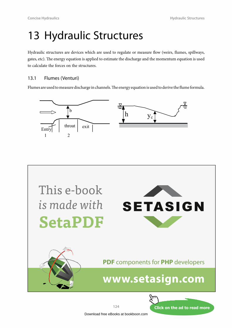
Concise Hydraulics

124

Hydraulic Structures

13 Hydraulic StructuresHydraulic structures are devices which are used to regulate or measure flow (weirs, flumes, spillways, gates, etc). The energy equation is applied to estimate the discharge and the momentum equation is used to calculate the forces on the structures.

13.1 Flumes (Venturi)

Flumes are used to measure discharge in channels. The energy equation is used to derive the flume formula.

ych

Entrythroat exit

b

1 2


Click on the ad to read moreClick on the ad to read moreClick on the ad to read moreClick on the ad to read moreClick on the ad to read moreClick on the ad to read moreClick on the ad to read moreClick on the ad to read moreClick on the ad to read moreClick on the ad to read moreClick on the ad to read moreClick on the ad to read moreClick on the ad to read moreClick on the ad to read moreClick on the ad to read moreClick on the ad to read moreClick on the ad to read moreClick on the ad to read moreClick on the ad to read moreClick on the ad to read moreClick on the ad to read moreClick on the ad to read moreClick on the ad to read moreClick on the ad to read moreClick on the ad to read moreClick on the ad to read moreClick on the ad to read moreClick on the ad to read moreClick on the ad to read moreClick on the ad to read moreClick on the ad to read moreClick on the ad to read moreClick on the ad to read moreClick on the ad to read moreClick on the ad to read moreClick on the ad to read moreClick on the ad to read moreClick on the ad to read moreClick on the ad to read moreClick on the ad to read moreClick on the ad to read moreClick on the ad to read more

PDF components for PHP developers

www.setasign.com

SETASIGNThis e-book is made with SetaPDF

http://s.bookboon.com/Setasign

Concise Hydraulics

125


If the width b is small enough, there will be a critical flow in the throat (also it will cause backwater upstream to get extra energy and a hydraulic jump after the flume to get rid of the energy gained from the backwater).

The energy equation between section 1 and 2 (ignore energy losses):

1 2H H= .

The total energy head at 2 is ( )2

2

2 1.52 2

ccc c c

gyVH y y yg g

= + = + =

So 1

1.5cHy =

The discharge through the flume will be1.5

3/ 2 1.5111.705

1.5ideal c c c cHQ AV by gy b g y b g bH = = = = =

In reality (to consider the energy losses)

1.511.705d ideal dQ C Q bC H= =

where Cd is the coefficient of discharge for the energy losses (see BS3680 4C)

If the depth h is used Q bC C hd v= 1705 1 5. .

where Cv is the coefficient of velocity for the upstream velocity head (also see BS3680 4C).

Such a structure is an example of critical depth meter.

Example Venturi FlumeAn open channel is 2 m wide and of rectangular cross section. A venturi flume having a throat width of 1.0m is installed at one point. Estimate the discharge:

a) if the upstream depth is 1.2 m and a critical flow occurs in the flumeb) if the upstream depth is 1.2 m and the depth in the throat is 1.05 m

(Take Cv=1 and Cd=0.95)


Concise Hydraulics

126


Solution:

a) If the flow in the throat is critical

1.5 1.5 321.705 1.705 0.95 1.0 1.2 2.13 /d vQ C C b h m s= = × × × =

b) If h=1.2 and y2=1.05, use the energy equation (ignore the energy loss)

2 21 2

1 22 2V Vy y

g g+ = +

2 2

2 21.2 1.052 (2 1.2) 2 (1 1.05)

Q Qg g

+ = +× ×

( )2

0.907 0.174 0.152Q

g− =

So 32.0 /idealQ m s=

Considering the coefficient of discharge with energy losses

30.95 2.0 1.90 /Q m s= × =

13.2 Weirs (Broad-crested weir)

y1

h yc

z

In a similar way to Venturi flume

1.51.705 d vQ C C bh=

where:

Cd – the coefficient of dischargeCv – the coefficient of velocity


Concise Hydraulics

127


Broad crested weirs are robust structures and usually used in larger rivers in comparison with flumes. However, flumes usually create relatively smaller backwater (or afflux) than weirs and hence less energy loss. The floating debris can usually pass through them smoothly (a useful feature in sewerage treatment works).

13.3 Energy dissipators

Kinetic energy in flow can erode the foundation of dams and other hydraulic structures. It is important that excessive energy should be dissipated to protect the foundation.

1) Spillways

h

SpillwayHydraulic jump


Click on the ad to read moreClick on the ad to read moreClick on the ad to read moreClick on the ad to read moreClick on the ad to read moreClick on the ad to read moreClick on the ad to read moreClick on the ad to read moreClick on the ad to read moreClick on the ad to read moreClick on the ad to read moreClick on the ad to read moreClick on the ad to read moreClick on the ad to read moreClick on the ad to read moreClick on the ad to read moreClick on the ad to read moreClick on the ad to read moreClick on the ad to read moreClick on the ad to read moreClick on the ad to read moreClick on the ad to read moreClick on the ad to read moreClick on the ad to read moreClick on the ad to read moreClick on the ad to read moreClick on the ad to read moreClick on the ad to read moreClick on the ad to read moreClick on the ad to read moreClick on the ad to read moreClick on the ad to read moreClick on the ad to read moreClick on the ad to read moreClick on the ad to read moreClick on the ad to read moreClick on the ad to read moreClick on the ad to read moreClick on the ad to read moreClick on the ad to read moreClick on the ad to read moreClick on the ad to read moreClick on the ad to read more


Download Now


Concise Hydraulics

128


are safety structures for dams. They must have the capacity to discharge major floods without damage to the dams.

1.5Q Cbh= (C usually lies within 1.6–2.3)

2) Others a) Stilling basin; b) Submerged bucket; c) Ski jump

h1 y1y2

lb

z

Stilling basin calculation

The velocity at Section 1

1 12V ghφ=

φ is usually taken as 0.90–0.95

The depth before the jump (rectangular channel)

11

QybV

=

The sequent depth

y y Fr2

112

21 8 1= + −( )

The wall at the end can be treated as a weir, so from Q = 1.705bh1.5 (ignore the energy loss) to derive h.

The height of the wall will be 2z y h∆ = −

The length of the basin is shorter than free jumps (6.1y2) due to the baffling effect from the end wall, so

lb = (4.0 ~ 5.0)y2


Concise Hydraulics

129


13.4 Sluice Gates

Energy Equation (Section 1 – 2)

y1

yg y2

y3

yc

y1V1

2

2gy2

V22

2g

If y1 and y

2 are known, discharge through the gate can be derived

Q by1y22gy1 y2

In practice, it is easier to link the discharge with the gate opening, so

Q CdbyG 2gy1

where

y2 CcyG and CdCc

1 (CcyG / y1)

Cc can be found from hydraulics manuals for various types of gates (usually between 0.61–0.66)

The force acting on the gate can be derived from the momentum equation between section 1 and 2 (ignore frictional forces). If the downstream depth is greater than the critical depth yc, a hydraulic jump will occur in the channel. The sequent depth y3 can be derived from the depth at y2. If the downstream depth is greater than y3, a submerged gate flow will occur and the flow equation derived here is not applicable anymore.


Concise Hydraulics

130


Questions 13Hydraulic Structures

1. The depth-measurement scale of a Venturi flume with a 1.2m throat give an h reading that is 0.02m too large. Compute the percentage errors in discharge when the observed h readings are 0.2m and 0.6m (assume the critical flow condition for both cases).

(Answer: Around 17%, 5%)

2. Determine the width b2 of the throat for a Venturi flume so that it will just produce critical flow, given Q=40m3/s, b1=10m and h1=2m. Also calculate the possible downstream supercritical flow depth h3 (Neglect energy losses).

yc

throat

b2= h3 =? b1=10

h1=2

(Answer: 7.17m, 0.75m)


Click on the ad to read moreClick on the ad to read moreClick on the ad to read moreClick on the ad to read moreClick on the ad to read moreClick on the ad to read moreClick on the ad to read moreClick on the ad to read moreClick on the ad to read moreClick on the ad to read moreClick on the ad to read moreClick on the ad to read moreClick on the ad to read moreClick on the ad to read moreClick on the ad to read moreClick on the ad to read moreClick on the ad to read moreClick on the ad to read moreClick on the ad to read moreClick on the ad to read moreClick on the ad to read moreClick on the ad to read moreClick on the ad to read moreClick on the ad to read moreClick on the ad to read moreClick on the ad to read moreClick on the ad to read moreClick on the ad to read moreClick on the ad to read moreClick on the ad to read moreClick on the ad to read moreClick on the ad to read moreClick on the ad to read moreClick on the ad to read moreClick on the ad to read moreClick on the ad to read moreClick on the ad to read moreClick on the ad to read moreClick on the ad to read moreClick on the ad to read moreClick on the ad to read moreClick on the ad to read moreClick on the ad to read moreClick on the ad to read more

www.sylvania.com


Light is OSRAM


Concise Hydraulics

131


Solutions 13Hydraulic Structures

1. Method a)

From

Q 1.705CdCvb2h3 / 2

dQdh

1.705CdCvb232h 1/ 2 2.558CdCvb2h

1 / 2

Q 1.705CdCvb232h 1/ 2 h 2.558CdCvb2h

1 / 2 h

andQ 1.705CdCvb2h

3 / 2

dQdh

1.705CdCvb232h 1/ 2 2.558CdCvb2h

1 / 2

Q 1.705CdCvb232h 1/ 2 h 2.558CdCvb2h

1 / 2 hthen

Q 1.705CdCvb2h3 / 2

dQdh

1.705CdCvb232h 1/ 2 2.558CdCvb2h

1 / 2

Q 1.705CdCvb232h 1/ 2 h 2.558CdCvb2h

1 / 2 h

The percentage error will be

1/ 22

3/ 22

2.558 2.558 0.02 0.031.705 1.705

d v

true d v

C C b h hQQ C C b h h h

∆∆ ×≈ = =

At h=0.2 m

0.03 16.6%0.18true

QQ∆

= =

At h=0.6 m

0.03 5.2%0.6 0.02true

QQ∆

= =−

Method b)

From

If h is 0.02 too large, the percentage error will be

1.5 1.5 1.5 1.52 2

1.5 1.52

1.705 ( ) 1.705 ( 0.02) ( ) ( 0.02)1.705 ( 0.02) ( 0.02)

d v d v

true d v

C C b h C C b hQ h hQ C C b h h

− −∆ − −= =

− −


Concise Hydraulics

132


At h=0.2 m

1.5 1.5

1.5

0.2 0.18 17.1%0.18

QQ∆ −

= =

At h=0.6 m

1.5 1.5

1.5

0.6 0.58 5.2%0.58true

QQ∆ −

= =

2. From the Venturi flume equation

Q 1.705CdCvb2h3 / 2

Since Q=40 m3/s and H h Vg

Qg b h g

m1 112 2

12

2

2 222

22 40

2 10 22 204= + = + = +

× ×=

( ).

So b QH

m213 2 1 51705

401705 2 205

7 170= =×

=. . .

./ .

(You can also derive b2 from the energy equation)

For the downstream depth h3,

H3 h3V3

2

2gh3

Q2

2g(b1h3 )2 h30.8157h3

2

Since H1 H3 So 2.204 h30.8157h3

2

Trial and error (below 2m),

h3 = 0.75m


Concise Hydraulics

133


14 Gradually Varied FlowGradually varied flow refers to the flow whose depth and velocity smoothly change over a long distance.

14.1 Equation of Gradually Varied Flow

dz

1 2

y

z

dH

dx

Energy line


Click on the ad to read moreClick on the ad to read moreClick on the ad to read moreClick on the ad to read moreClick on the ad to read moreClick on the ad to read moreClick on the ad to read moreClick on the ad to read moreClick on the ad to read moreClick on the ad to read moreClick on the ad to read moreClick on the ad to read moreClick on the ad to read moreClick on the ad to read moreClick on the ad to read moreClick on the ad to read moreClick on the ad to read moreClick on the ad to read moreClick on the ad to read moreClick on the ad to read moreClick on the ad to read moreClick on the ad to read moreClick on the ad to read moreClick on the ad to read moreClick on the ad to read moreClick on the ad to read moreClick on the ad to read moreClick on the ad to read moreClick on the ad to read moreClick on the ad to read moreClick on the ad to read moreClick on the ad to read moreClick on the ad to read moreClick on the ad to read moreClick on the ad to read moreClick on the ad to read moreClick on the ad to read moreClick on the ad to read moreClick on the ad to read moreClick on the ad to read moreClick on the ad to read moreClick on the ad to read moreClick on the ad to read moreClick on the ad to read moreClick on the ad to read more


360°thinking.



360°thinking.



360°thinking.


360°thinking.



Concise Hydraulics

134


The energy line slope Sf

S dHdxf = −

(The ‘-’ sign is to compensate for the negative dH so Sf is positive)

The channel bed slope is So

S dzdxo = −

The energy equation dHdx

ddx

y Vg

z= + +( )2

2

Only the kinetic energy change needs special treatment (other terms are straightforward).

− = + −S dydx

ddx

Vg

Sf o( )2

2

For the kinetic energy change

ddx

Vg

ddx

Q Ag

Qg

dAdx

QgA

dAdx

QgA

Bdydx

( ) [ ( / ) ]2 2 2 2

2

3

2

3

2 2 2= =

= − = −

−

(Since dA=dy B)

so − = − −S dydx

Q BgA

dydx

Sf o

2

3

Since 2 2

23

m

V Q BFrgD gA

= =

hence, the final general flow profile equation is

21o fS Sdy

dx Fr−

=−

From the Manning Equation (Replace So with Sf and Sf ≠ So for gradually varied flow)

VR S

nf=

2 3/

so S n VRf =

2 2

4 3/


Concise Hydraulics

135


The qualitative relationship between the relevant variables is as below.

21o fS Sdy

dx Fr

VR Sn

f2 3/

m

VFrgD

When y> yn Sf < So When y> yc Fr < 1

When y< yn Sf > So When y< yc Fr > 1

14.2 Classification of Surface Profiles

Flow surface profiles are classified based on the actual depth and the channel bed slope.

1) Depth

The depth space is divided into three regions by normal and critical depths.

region 1

region 2

region 3

yn

yc

2) Slopes

The channel bed slops are classified into five groups: M mild, S steep, C critical, H horizontal and A adverse.

Region 1

Region 2

Region 3

Mild slope

yn

yc

Region 1

Region 2

Region 3

Steep slope

yn

yc

Region 1

Region 3

Critical slope

yn

yc

Horizontal Slope(No normal depth)

Region 2

Region 3

yc

Adverse slope

(No normal depth)

Region 2

Region 3

yc


Concise Hydraulics

136


3) Profile name

A letter+ a digit e.g. M1, S2where: Letter – the type of slope (M, S, C, H or A Digit – the region (1, 2 or 3)

14.3 Flow Profile Sketch

It is possible to sketch flow profiles based on the analysis of the general flow profile equation. Here is an example for a mild slop case.

Example: In a mild slope, if y is in Region 1, which profile is correct?

M1 ?M1 ?

yc

yn

dydx

or ?> < 0


Click on the ad to read moreClick on the ad to read moreClick on the ad to read moreClick on the ad to read moreClick on the ad to read moreClick on the ad to read moreClick on the ad to read moreClick on the ad to read moreClick on the ad to read moreClick on the ad to read moreClick on the ad to read moreClick on the ad to read moreClick on the ad to read moreClick on the ad to read moreClick on the ad to read moreClick on the ad to read moreClick on the ad to read moreClick on the ad to read moreClick on the ad to read moreClick on the ad to read moreClick on the ad to read moreClick on the ad to read moreClick on the ad to read moreClick on the ad to read moreClick on the ad to read moreClick on the ad to read moreClick on the ad to read moreClick on the ad to read moreClick on the ad to read moreClick on the ad to read moreClick on the ad to read moreClick on the ad to read moreClick on the ad to read moreClick on the ad to read moreClick on the ad to read moreClick on the ad to read moreClick on the ad to read moreClick on the ad to read moreClick on the ad to read moreClick on the ad to read moreClick on the ad to read moreClick on the ad to read moreClick on the ad to read moreClick on the ad to read moreClick on the ad to read moreClick on the ad to read more





Concise Hydraulics

137


It is subcritical flow, so Fr < 1

M1yn

yc

and y>yn, so Sf < So

2 0

1o fS Sdy positive

dx Fr positive−

= = >−

The profile with increasing depth is the correct answer.

Self Practice

For the same channel bed slope, if y is in Region 2, which profile curve is correct?

M2=?M2=?

yn

yc

i.e.dydx

or ?0

M2yc

yn

i.e. dydx

or ?> < 0

(Answer: the one with decreasing depth)


Concise Hydraulics

138


Steep slope cases (derived in the similar way as mild slope cases)

S1

S2

yc

yn

S3

14.4 Flow transitions

1) A smooth surface link

2) Linked by hydraulic jump

Questions 14Gradually Varied Flow

1. Water flows in a rectangular channel with a bottom slope of 0.8m/km and a head loss of 0.4m/km. At a section where the flow depth is 1.7m and the average velocity 1.8m/s, does the water depth increase or decrease in the direction of flow?


Concise Hydraulics

139


2. Roughly sketch the possible flow profiles in the channels shown belowa)

yn

yn

yn

Mild Mild

Steep


Click on the ad to read moreClick on the ad to read moreClick on the ad to read moreClick on the ad to read moreClick on the ad to read moreClick on the ad to read moreClick on the ad to read moreClick on the ad to read moreClick on the ad to read moreClick on the ad to read moreClick on the ad to read moreClick on the ad to read moreClick on the ad to read moreClick on the ad to read moreClick on the ad to read moreClick on the ad to read moreClick on the ad to read moreClick on the ad to read moreClick on the ad to read moreClick on the ad to read moreClick on the ad to read moreClick on the ad to read moreClick on the ad to read moreClick on the ad to read moreClick on the ad to read moreClick on the ad to read moreClick on the ad to read moreClick on the ad to read moreClick on the ad to read moreClick on the ad to read moreClick on the ad to read moreClick on the ad to read moreClick on the ad to read moreClick on the ad to read moreClick on the ad to read moreClick on the ad to read moreClick on the ad to read moreClick on the ad to read moreClick on the ad to read moreClick on the ad to read moreClick on the ad to read moreClick on the ad to read moreClick on the ad to read moreClick on the ad to read moreClick on the ad to read moreClick on the ad to read moreClick on the ad to read more


Concise Hydraulics

140


b)

Mild

Mild

Steep

yn

yn yn

3) Show that the gradually varied flow equation is reduced to a uniform flow formula if dy/dx=0

Solutions 14Gradually varied flow

1. The Froude number

1.8 0.441.7

VFrgy g

= = = , So=0.0008, Sf=0.0004

From the general flow profile equation

2 2

0.0008 0.0004 0.0005 01 1 0.44

o fS Sdydx Fr

− −= = = > − −

so the flow depth is increasing.

2. a)

yn

yn

yn

Mild Mild

Steep


Concise Hydraulics

141


b)

Mild

Mild

Steep

yn

yn yn

3. From 21

o fS Sdydx Fr

−=

−

If, then 2 0

1o fS S

Fr−

=−

, i.e.

Since Sf

nQP2 / 3

A5 / 3

2

So

nQP2 / 3

A5 / 3

2

QA5/ 3 So

2 / 3

So

Sf

nQP2 / 3

A5 / 3

2

So

nQP2 / 3

A5 / 3

2

QA5/ 3 So

2 / 3Hence It is the Manning Equation for uniform flows.


Concise Hydraulics

142


15 Computation of Flow Profile15.1 Introduction

The general flow profile equation is 21o fS Sdy

dx Fr−

=−

It is possible to derive y=f(x) from a simple differential equation. For example, if dy / dx = 0.5, the solution for it would be y = x/2 + c, where c is a constant. There are an infinite number of curves by changing the c value. To uniquely identify the profile, a control point is required (i.e., a boundary condition).

X

y=x/2+ c c1c2

c3

X

(0,3)

Control Point

y=x/2+ 3

For example, if y=3 when x=0, the curve function would be fixed as y = x/2 + 3.

For practical flow profile computation, there are three types of solutions: 1. direct integration; 2. graphical integration; 3. numerical integration. The first two methods are superseded by numerical integration methods due to the widespread use of computers.

15.2 Numerical integration methods

1. The direct step method: to solve section length from depth.2. The standard step method: to solve depth from section length.

1) The direct step method

y1

y2

x=?

y


Concise Hydraulics

143

Computation of Flow Profile

Known: y1 and y

2 Unknown: DX=?

By using a finite difference form

21

o f mean

Frx yS S

−∆ = ∆ −

where ‘mean’ refers to the mean value for the interval (Dx).

2) The standard step method

Known: y1 and Dx Unknown: y

2=?

By using a finite difference form

21

o f

mean

S Sy x

Fr−

∆ = ∆ − (Iterations are required since y2 is unknown and the means of Sf and Fr need y2.)

For approximation, use

2

11o f

Section

S Sy x

Fr−

∆ = ∆ − to avoid iterations.


Click on the ad to read moreClick on the ad to read moreClick on the ad to read moreClick on the ad to read moreClick on the ad to read moreClick on the ad to read moreClick on the ad to read moreClick on the ad to read moreClick on the ad to read moreClick on the ad to read moreClick on the ad to read moreClick on the ad to read moreClick on the ad to read moreClick on the ad to read moreClick on the ad to read moreClick on the ad to read moreClick on the ad to read moreClick on the ad to read moreClick on the ad to read moreClick on the ad to read moreClick on the ad to read moreClick on the ad to read moreClick on the ad to read moreClick on the ad to read moreClick on the ad to read moreClick on the ad to read moreClick on the ad to read moreClick on the ad to read moreClick on the ad to read moreClick on the ad to read moreClick on the ad to read moreClick on the ad to read moreClick on the ad to read moreClick on the ad to read moreClick on the ad to read moreClick on the ad to read moreClick on the ad to read moreClick on the ad to read moreClick on the ad to read moreClick on the ad to read moreClick on the ad to read moreClick on the ad to read moreClick on the ad to read moreClick on the ad to read moreClick on the ad to read moreClick on the ad to read moreClick on the ad to read moreClick on the ad to read more




Concise Hydraulics

144


15.3 Computation Procedure through an Example

2.5m

yn

h

2.5m

y w=h

+2.5

yc

Determine the flow profile for the following conditions if 10 depth steps are used in the calculation:

Channel: Q=600m3/s,rectangular, width 50 m,So=2m/km, n=0.04Weir: CdCv=0.88Sill height: 2.5 m

Solution:

a) The normal depth yn from Manning’s equation

QA5/ 3 S0

nP2 / 3 so 60050yn

5/ 3 0.0020.04 50 2yn

2 / 3

By trial and error y mn = 4 44.

b) The critical depth yc

c c cQ AV by gy= = , so

1/32 21/3( / ) (600 / 50)[ ] 2.448c

Q by mg g

= = =

c) The depth over the weir (h)From the weir equation 3/ 21.705 d vQ C C Bh= then 3/ 2600 1.705 0.88 50h= × × so h=4 m

d) The total depth over the weir (hw)

yw = h+2.5 = 4+2.5 = 6.5 m yw > yn > yc. This is a M1 type profile.


Concise Hydraulics

145


e) Profile computation

Take yw = 6.5 m as the initial depth and y = 4.5 m (slightly greater than yn) as the final depth, and proceed upstream at a small interval of depth

Dy = (4.5-6.5)/10 = – 0.2 m

Simplify the formulas to be used as

6.5m4.5 m

X

600 3.831

50

V QFr

gy by gy y gy y y= = = =

SnQP

A

P

A

P

Af

FHGIKJFHG

IKJ

2 3

5 3

2 0 667

1.667

2 1.333

3 333

0 04 600 576/

/

.

.

.

21

o f mean

Frx y

S S

y A P Fr1-Fr2

meanSf

So-Sf mean

Dx x

6.5 325 63.0 0.2312 0.0006 00.9439 0.0014 -135

6.3 315 62.6 0.2423 0.0007 -1350.9383 0.0013 -144

6.1 305 62.2 0.2543 0.0007 -279…4.9 245 59.8 0.3532 0.0015 -1491

0.8669 0.00044.7 235 59.4 0.3760 0.0017 -1920

0.8488 0.00024.5 225 59.0 0.4014 0.0019 -2769


Concise Hydraulics

146


Note: the negative values of x indicate that they are in the opposite direction of X.

X

y=4.5 y=6.5

0-2000 -1000

15.4 Further Computational Information

1) Computation steps for flow profiles

a) find the critical and normal depths;b) find the slope type;c) find a control point with a known relationship between depth and discharge (weirs, flumes

and gates):i) Subcritical flow: its profile is controlled from downstream;ii) Supercritical flow: its profile is controlled from upstream.

2) Computation direction

Computation direction

yc

Mild slope

Upstream if the flow is subcritical

Computation directionyc

Steep slope

Control point

Downstream if the flow is supercritical


Concise Hydraulics

147


3) Locations of the control points

Subcritical flow

yw is calculated from the weir equation (plus weir sill

Mild slope

Control point Control point

yc

y


Click on the ad to read moreClick on the ad to read moreClick on the ad to read moreClick on the ad to read moreClick on the ad to read moreClick on the ad to read moreClick on the ad to read moreClick on the ad to read moreClick on the ad to read moreClick on the ad to read moreClick on the ad to read moreClick on the ad to read moreClick on the ad to read moreClick on the ad to read moreClick on the ad to read moreClick on the ad to read moreClick on the ad to read moreClick on the ad to read moreClick on the ad to read moreClick on the ad to read moreClick on the ad to read moreClick on the ad to read moreClick on the ad to read moreClick on the ad to read moreClick on the ad to read moreClick on the ad to read moreClick on the ad to read moreClick on the ad to read moreClick on the ad to read moreClick on the ad to read moreClick on the ad to read moreClick on the ad to read moreClick on the ad to read moreClick on the ad to read moreClick on the ad to read moreClick on the ad to read moreClick on the ad to read moreClick on the ad to read moreClick on the ad to read moreClick on the ad to read moreClick on the ad to read moreClick on the ad to read moreClick on the ad to read moreClick on the ad to read moreClick on the ad to read moreClick on the ad to read moreClick on the ad to read moreClick on the ad to read moreClick on the ad to read more

Maersk.com/Mitas





solve problems

I was a

hes




Maersk.com/Mitas





solve problems

I was a

hes




Maersk.com/Mitas





solve problems

I was a

hes




Maersk.com/Mitas





solve problems

I was a

hes






Concise Hydraulics

148


Supercritical flow

Steep slope

Control point

Control point

yc

yc

Steep slope

Questions 15Computation of Flow Profile

1. A rectangular channel is 3.0 m wide, has a 0.01 slope, discharge of 5.3 m3/s, and n=0.011. Find yn and yc. If the actual depth of flow is 1.7 m, what type of profile exists?

(Answer: 0.4 m, 0.683 m, S1 curve)

2. A rectangular channel has a gradient of 2 in 1000 and ends in a free outfall. At a discharge of 4.53m3/s with Manning’s n=0.012 and b=1.83m, how far from the outfall is the depth equal to 99% of normal depth if five depth steps are used in the calculation?

(Answer: 196.4 m)

Solutions 15Computation of Flow Profile

1. From the Manning equation

A by 3y , P b 2y 3 2y

Since QA

5

3 S0

nP2

3

so 5.33y

5

3 0.01

0.011 3 2y2

3Simplifying

0.093

y5/ 3

(3 2y)2 / 3


Concise Hydraulics

149


Trial and error y=1.0 0.342 y=0.5 0.125 y=0.3 0.057 y=0.4 0.089 y=0.45 0.107 close to 0.4

So yn=0.4 m

From Froude number=1

Q A gDm Byc gyc

yc

32 Q

B g

yc5.32

32g

13

0.683m

y=1.7 m, so yn yc y

so

Q A gDm Byc gyc

yc

32 Q

B g

yc5.32

32g

13

0.683m

y=1.7 m, so yn yc y Since

Q A gDm Byc gyc

yc

32 Q

B g

yc5.32

32g

13

0.683m

y=1.7 m, so yn yc y

This is a steep slope and the profile is S1.

2. From the Manning equation

QA

53 S0

nP23

A=by=1.83y, P=b+2y=1.83+2y Since A=by=1.83y, P=b+2y=1.83+2y

The normal depth

4.531

0.0121.83yn

1.83yn1.83 2yn

2 /30.0021/ 2

Simplifying

0.444yn

5/ 3

1.83 2yn2 / 3


Concise Hydraulics

150


The right hand side

y=1.0 0.408 y=1.1 0.463 y=1.05 0.435 y=1.07 0.446 close to 0.444

so yn=1.07 m

The critical depth

yc4.532

1.832g

1/ 3

0.855m

Since yn>yc, the flow is subcritical and the water surface profile is M2.


Click on the ad to read moreClick on the ad to read moreClick on the ad to read moreClick on the ad to read moreClick on the ad to read moreClick on the ad to read moreClick on the ad to read moreClick on the ad to read moreClick on the ad to read moreClick on the ad to read moreClick on the ad to read moreClick on the ad to read moreClick on the ad to read moreClick on the ad to read moreClick on the ad to read moreClick on the ad to read moreClick on the ad to read moreClick on the ad to read moreClick on the ad to read moreClick on the ad to read moreClick on the ad to read moreClick on the ad to read moreClick on the ad to read moreClick on the ad to read moreClick on the ad to read moreClick on the ad to read moreClick on the ad to read moreClick on the ad to read moreClick on the ad to read moreClick on the ad to read moreClick on the ad to read moreClick on the ad to read moreClick on the ad to read moreClick on the ad to read moreClick on the ad to read moreClick on the ad to read moreClick on the ad to read moreClick on the ad to read moreClick on the ad to read moreClick on the ad to read moreClick on the ad to read moreClick on the ad to read moreClick on the ad to read moreClick on the ad to read moreClick on the ad to read moreClick on the ad to read moreClick on the ad to read moreClick on the ad to read moreClick on the ad to read moreClick on the ad to read more




FINANCIAL TIMES








Concise Hydraulics

151


The final depth 0.99 0.99 1.07 1.06ny y m= = × =

Dy=(1.06-0.855)/5=0.041m

1.5

4.53 0.791.83

V QFrygy by gy y gy

= = = =

y=(1.06-0.855)/5=0.041m

1.5

4.53 0.791.83

V QFrygy by gy y gy

S fnQP2 /3

A5/ 3

20.012 4.53P0.667

A1.667

20.00296P1.333

A3.333

From x y 1 F2

S0 Sf mean

The computations are shown in the following table:

Y A P Fr1-Fr2

meanSf

So-Sfmean x

0.855 1.565 3.54 0.999 0.003588 00.0676 -0.001375

0.896 1.640 3.62 0.931 0.003162 -2.020.1873 -0.000984

0.937 1.715 3.70 0.871 0.002805 -9.820.2869 -0.000658

0.978 1.790 3.79 0.817 0.002511 -27.700.3713 -0.000382

1.019 1.865 3.87 0.768 0.002252 -67.60.4430 -0.000141

1.06 1.940 3.95 0.724 0.002029 -196.4

x= -196.4 m


Concise Hydraulics

152

Unsteady Flow

16 Unsteady Flow16.1 Basic Types

If the flow velocity at a point varies with time, the flow is called unsteady flow. They can be further divided into (in a similar way as to steady flow types):

a) Rapidly varied unsteady flows: Surges and bores by dam break, quick operation of control structures, tidal effects

b) Gradually varied unsteady flows: Translatory waves by flood waves, slow operation of control structures (gates, etc.)


Click on the ad to read moreClick on the ad to read moreClick on the ad to read moreClick on the ad to read moreClick on the ad to read moreClick on the ad to read moreClick on the ad to read moreClick on the ad to read moreClick on the ad to read moreClick on the ad to read moreClick on the ad to read moreClick on the ad to read moreClick on the ad to read moreClick on the ad to read moreClick on the ad to read moreClick on the ad to read moreClick on the ad to read moreClick on the ad to read moreClick on the ad to read moreClick on the ad to read moreClick on the ad to read moreClick on the ad to read moreClick on the ad to read moreClick on the ad to read moreClick on the ad to read moreClick on the ad to read moreClick on the ad to read moreClick on the ad to read moreClick on the ad to read moreClick on the ad to read moreClick on the ad to read moreClick on the ad to read moreClick on the ad to read moreClick on the ad to read moreClick on the ad to read moreClick on the ad to read moreClick on the ad to read moreClick on the ad to read moreClick on the ad to read moreClick on the ad to read moreClick on the ad to read moreClick on the ad to read moreClick on the ad to read moreClick on the ad to read moreClick on the ad to read moreClick on the ad to read moreClick on the ad to read moreClick on the ad to read moreClick on the ad to read moreClick on the ad to read moreClick on the ad to read more


Concise Hydraulics

153

Unsteady Flow

16.2 Rapidly Varied Unsteady Flow

1) Dynamic Wave Propagation

cplate

y

h

c

1 2

Generation of a solitary wave in a rectangular channel

cplate

y

h

c

1 2

An observer following the wave

The energy equation

y Vg

y Vg1

12

222

2 2+ = +

Since y1=y, y2=y+h, V1=c, V2 can be derived from the continuity equation V1y =V2(y+h)

Therefore yc2

2gy h

c2

2gyy h

2

c2g(y h)2

2y hc gy

Solving for c,

yc2

2gy h

c2

2gyy h

2

c2g(y h)2

2y hc gy

for waves of small height

yc2

2gy h

c2

2gyy h

2

c2g(y h)2

2y hc gy

Similarly, for non-rectangular channels c gDm

where Dm – the hydraulic mean depth (A/B)

2) Surges & Bores

y1y2

V1

V2

Vsrg


Concise Hydraulics

154

Unsteady Flow

A surge wave results from a sudden change in flow (e.g., a partial or complete closure of a gate that increases the depth), called positive surge (similar to water hammers). It is termed as a bore if caused by tides. The momentum equation is used in a similar way to hydraulic jumps. A surge can be considered as a steady flow case if an observer is travelling at the surge speed.

For a rectangular channel, the continuity equation is

1 1 2 2( ) ( )srg srgV V y V V y+ = +

or simplified as 1 1 2 2

2 1( )srgV y V yV

y y−

=−

The momentum equation

1 1 2 2F M F M+ = + (where M QVρ= and F gAyρ= )

There are two equations so the two unknowns can be solved (with the three knowns). Iterations are usually required in the nonlinear calculations (assume Vsrg=0, calculate the other unknown from the continuity equation, then get Vsrg from the momentum equation, enter it into the continuity equation again to get the other unknown, repeat the process until the required accuracy is achieved). Note, the surge velocity is much faster than small solitary waves.


Concise Hydraulics

155

Unsteady Flow

16.3 Gradually Varied Unsteady Flows (Saint-Venant equations)

1) The Continuity Equation

At any time t, the outgoing velocity is

2 1QQ Q dxx

∂= +

∂

dx

y

1 2

Q1

Q2

The net flow into the control volume (dx long) during dt period is

1 2( ) QQ Q dt dx dtx

∂ − = − ∂


Click on the ad to read moreClick on the ad to read moreClick on the ad to read moreClick on the ad to read moreClick on the ad to read moreClick on the ad to read moreClick on the ad to read moreClick on the ad to read moreClick on the ad to read moreClick on the ad to read moreClick on the ad to read moreClick on the ad to read moreClick on the ad to read moreClick on the ad to read moreClick on the ad to read moreClick on the ad to read moreClick on the ad to read moreClick on the ad to read moreClick on the ad to read moreClick on the ad to read moreClick on the ad to read moreClick on the ad to read moreClick on the ad to read moreClick on the ad to read moreClick on the ad to read moreClick on the ad to read moreClick on the ad to read moreClick on the ad to read moreClick on the ad to read moreClick on the ad to read moreClick on the ad to read moreClick on the ad to read moreClick on the ad to read moreClick on the ad to read moreClick on the ad to read moreClick on the ad to read moreClick on the ad to read moreClick on the ad to read moreClick on the ad to read moreClick on the ad to read moreClick on the ad to read moreClick on the ad to read moreClick on the ad to read moreClick on the ad to read moreClick on the ad to read moreClick on the ad to read moreClick on the ad to read moreClick on the ad to read moreClick on the ad to read moreClick on the ad to read moreClick on the ad to read moreClick on the ad to read more








Concise Hydraulics

156

Unsteady Flow

The storage change rate (the top part)

yB dxdtt

∂∂

Applying the conservation of mass

0Q yBx t

∂ ∂∂ ∂

+ = or 0Q Ax t

∂ ∂∂ ∂

+ =

The equation indicates that when the river level is going up with time ( / 0y t∂ ∂ > ), the incoming discharge is greater than the outgoing discharge ( / 0Q x∂ ∂ < ). This represents the flood wave’s arrival.

2) The Momentum Equation (Dynamic equation)

From the momentum principle,

External Forces = Momentum Change Rate

The forces includes the gravity Fg, friction Ff along the channel bed and wall, and the pressure force Fp

Gravity

The total weight of water in the control volume is

W gAdxρ=

dx

y

1 2

Datumz

V

So

sin sing oF W gAdx gAdxSθ ρ θ ρ= = ≈

(when the slope is mild, tan sinoS θ θ= ≈ )


Concise Hydraulics

157

Unsteady Flow

Friction

The work done by friction force along distance dx is

rF dx

This will result in the energy loss of water in the control volume (hf)

f fWh gAhρ=

So

r fF dx Wh= i.e. /r f f fF Wh dx WS gAdxSρ= = =

Sf is the friction slope (use the Manning, Chezy, etc. to estimate).

Pressure

The hydrostatic pressure force difference between Sections 1 and 2 is mainly caused by the extra depth increase at Section 2 to exert extra uniform pressure over cross section area A

( )pyF gdy A g dx Ax

ρ ρ ∂ = = ∂

The momentum change rate

Output – input ( )QV dx

xρ∂∂

in the control volume with time

[( ) ] ( )Adx V AV dxt t

ρ ρ∂ ∂=

∂ ∂

So ( ) ( )

o fy QV AVgAS gAS gAx x t

ρ ρ ρ ρ ρ∂ ∂ ∂− − = +

∂ ∂ ∂

Simplify and ignore wind effect

( ) ( )( )o fy QV AVgA S Sx x t∂ ∂ ∂

− − = +∂ ∂ ∂

The right hand side can be expanded as

( ) ( )QV AV V Q V A V VQ V A V Q Ax t x x t t x t

∂ ∂ ∂ ∂ ∂ ∂ ∂ ∂+ = + + + = +

∂ ∂ ∂ ∂ ∂ ∂ ∂ ∂

(from continuity equation 0Q Ax t

∂ ∂∂ ∂

+ = )


Concise Hydraulics

158

Unsteady Flow

So

( )o fy V Vg S S Vx x t

Rearranging

or

Sf Soyx

VgVx

1gVt

Steady, uniform

Steady, nonuniform

Unsteady, nonuniform

1o f

y V V VS Sx g x g t

Gravity Friction

Momentum change rate Pressure

Forces

With position With time

The continuity and dynamic equations are also called the Saint-Venant equations

Solutions

Unknowns: V, y. Known: Initial and boundary conditions


Click on the ad to read moreClick on the ad to read moreClick on the ad to read moreClick on the ad to read moreClick on the ad to read moreClick on the ad to read moreClick on the ad to read moreClick on the ad to read moreClick on the ad to read moreClick on the ad to read moreClick on the ad to read moreClick on the ad to read moreClick on the ad to read moreClick on the ad to read moreClick on the ad to read moreClick on the ad to read moreClick on the ad to read moreClick on the ad to read moreClick on the ad to read moreClick on the ad to read moreClick on the ad to read moreClick on the ad to read moreClick on the ad to read moreClick on the ad to read moreClick on the ad to read moreClick on the ad to read moreClick on the ad to read moreClick on the ad to read moreClick on the ad to read moreClick on the ad to read moreClick on the ad to read moreClick on the ad to read moreClick on the ad to read moreClick on the ad to read moreClick on the ad to read moreClick on the ad to read moreClick on the ad to read moreClick on the ad to read moreClick on the ad to read moreClick on the ad to read moreClick on the ad to read moreClick on the ad to read moreClick on the ad to read moreClick on the ad to read moreClick on the ad to read moreClick on the ad to read moreClick on the ad to read moreClick on the ad to read moreClick on the ad to read moreClick on the ad to read moreClick on the ad to read moreClick on the ad to read moreClick on the ad to read more






find out more!





Concise Hydraulics

159

Unsteady Flow

Three methods:

a) Finite differences: currently the most common method.b) Characteristics: suitable for the simple regular channelc) Finite elements: suitable for irregular boundaries

16.4 Software packages

1) Software packages for 1D river flows

Free Software

FLDWAV is a generalized flood routing model that can be used by hydrologists/ engineers for real-time flood forecasting of dam-break floods and/or natural floods, dam-breach flood analysis for sunny-day piping or overtopping associated with the PMF flood, floodplain inundation mapping for contingency dam-break flood planning, and design of waterway improvements. Its predecessors are DAMBRK, BREACH, DWOPER/NETWORK models that are also available from the same web site. Availability: FLDWAV version 2, June 2000.

http://www.nws.noaa.gov/oh/hrl/rvrmech/fldwav_instructions2.htm

HEC-RAS is (formerly HEC-2) is a comprehensive computer program designed to compute water surface profiles under a variety of conditions. The HEC-RAS software was developed at the Hydrologic Engineering Center (HEC). The system is capable of performing Steady Flow water surface profile calculations, and unsteady Flow, Sediment Transport, and several hydraulic design computations. HEC-RAS is the most widely used program by practitioners for the calculation of open channel flows. Its success is due to the detail that the program is able to handle. Availability: HEC-RAS version 4.0, November 2006, http://www.hec.usace.army.mil/software/hec-ras/.

Commercial SoftwareMIKE 11 is a professional engineering software package for the simulation of flows, water quality and sediment transport in estuaries, rivers, irrigation systems, channels and other water bodies. It is a dynamic, one-dimensional modelling tool for the detailed design, management and operation of both simple and complex river and channel systems. Availability: Purchase from DHI (Danish Hydraulic Institute), http://www.dhisoftware.com/mike11/.

ISIS models open channel systems containing loops, branches, floodplain conveyance and storage incorporates standard equations and modelling techniques for structures including weirs, sluices, bridges, culverts, pumps, siphons, orifices and outfalls, logical control of moving structures. Availability: Purchase from Wallingford Software Ltd, http://www.wallingfordsoftware.com/products/isis.asp.


http://www.nws.noaa.gov/oh/hrl/rvrmech/fldwav_instructions2.htm

http://www.hec.usace.army.mil/software/hec-ras/

http://www.dhisoftware.com/mike11/

http://www.wallingfordsoftware.com/products/isis.asp

Concise Hydraulics

160

Unsteady Flow


Free packages

SSIIM: SSIIM is an abbreviation for Sediment Simulation In Intakes with Multiblock option. The program is designed to be used in teaching and research for hydraulic/river/sedimentation engineering. It solves the Navier-Stokes equations using the control volume method with the SIMPLE algorithm and the k-epsilon turbulence model. http://www.bygg.ntnu.no/~nilsol/ssiimwin/.

Commercial packages

MIKE21: MIKE 21 is the preferred 2D engineering modelling tool for rivers, estuaries and coastal waters. MIKE 21 consists of more than twenty modules covering the following areas: Coastal hydrodynamics; Environmental hydraulics; Sediment Processes; Wave processes, http://www.dhisoftware.com/mike21/.


Free packages

SSIIM: as above

Commercial packages

MIKE 3: MIKE 3 is applicable for simulations of hydrodynamics, water quality and sediment transport in all water bodies where 3D effects are important. MIKE 3 is compatible with MIKE 21 and other DHI Software products, allowing for easy model setup, transfer of boundary data, etc. http://www.dhisoftware.com/mike3/.

DELFT-3D: DELFT3D is a fully-integrated two or three-dimensional compound modelling system. It simulates the flows, waves, sediments, morphological developments and water quality aspects. The sediment transport module models bottom and suspended transport of sediment separately using a variety of formulae. The effects of wave motion on transport magnitude and direction are included. The morphological

module computes bottom changes due to transport gradients and various types of boundary conditions. It can be run in a time-dependent way (coupling of hydrodynamics with computed bottom changes) or in a time-independent mode.

In the time dependent mode, animation’s can be made of the bottom development over several years. http://www.alkyon.nl/Tools/Delft3D.htm


http://www.bygg.ntnu.no/~nilsol/ssiimwin/




http://www.alkyon.nl/Tools/Delft3D.htm

Concise Hydraulics

161

Unsteady Flow

Questions 16Unsteady Flow

1. The average depth of oceans is 3720m. Estimate the tsunami wave speed in km/hour based on the dynamic wave propagation equation and the average ocean depth.

(Answer: 687 km/hour)

2. There is a uniform flow of 4 m3/s of 0.6m deep in a rectangular channel of 4m wide. If the upstream gate is suddenly lifted up and the flow in the channel is increased to 6.7m3/s. Estimate the surge wave speed and wave height.

(Answer: 4.5m/s, 0.15m)

Solutions 16Unsteady Flow

1. From the dynamic wave propagation equation

9.81 3720 191 / 687 /c gy m s km hour= = × = =


Click on the ad to read moreClick on the ad to read moreClick on the ad to read moreClick on the ad to read moreClick on the ad to read moreClick on the ad to read moreClick on the ad to read moreClick on the ad to read moreClick on the ad to read moreClick on the ad to read moreClick on the ad to read moreClick on the ad to read moreClick on the ad to read moreClick on the ad to read moreClick on the ad to read moreClick on the ad to read moreClick on the ad to read moreClick on the ad to read moreClick on the ad to read moreClick on the ad to read moreClick on the ad to read moreClick on the ad to read moreClick on the ad to read moreClick on the ad to read moreClick on the ad to read moreClick on the ad to read moreClick on the ad to read moreClick on the ad to read moreClick on the ad to read moreClick on the ad to read moreClick on the ad to read moreClick on the ad to read moreClick on the ad to read moreClick on the ad to read moreClick on the ad to read moreClick on the ad to read moreClick on the ad to read moreClick on the ad to read moreClick on the ad to read moreClick on the ad to read moreClick on the ad to read moreClick on the ad to read moreClick on the ad to read moreClick on the ad to read moreClick on the ad to read moreClick on the ad to read moreClick on the ad to read moreClick on the ad to read moreClick on the ad to read moreClick on the ad to read moreClick on the ad to read moreClick on the ad to read moreClick on the ad to read moreClick on the ad to read more


Concise Hydraulics

162

Unsteady Flow

2. The surge wave moves from the upstream to downstream,

y1 y2

V1

V2

Vsrg

1 2 1 1 1/( ) 6.7 /(4 ) 1.68 /V Q by y y= = =

2 2 2/( ) 4 /(4 0.6) 1.67 /V Q by m s= = × =

The surge can be considered as a steady flow case if an observer is travelling at the surge speed.

y1y2

V1-Vsrg V2-Vsrg

The continuity equation is

1 1 2 2( ) ( )srg srgV V y V V y− = −

or simplified as 1 1 2 2

1 2 1 1

1.68 1.67 0.6 0.68( ) 0.6 0.6srg

V y V yVy y y y− − ×

= = =− − −

The momentum equation

1 1 2 2F M F M+ = + (where M QVρ= and F gAyρ= )

i.e., 2 21 1 1 2 2 2

1 1( ) ( )2 2srg srggby Q V V gby Q V Vρ ρ ρ ρ+ − = + −

so 2 21 12 6.7(1.68 / ) 2 (0.6) 4(1.67 )srg srggy y V g V+ − = + −

Simplify 21 119.6 11.3 / 2.7 13.7srgy y V+ − =

Substitute srgV 21 1

1

1.8419.6 11.3 / 13.70.6

y yy

+ − =−


Concise Hydraulics

163

Unsteady Flow

With trial and error

1y = 1, LHS= 26,

0.7, LHS=7.3

0.75, LHS=13.8 close to 13.7

so 1 0.75y m= , the wave height is 0.75-0.6= 0.15m

1

0.68 0.68 4.5 /0.6 0.75 0.6srgV m s

y= = =

− −


Click on the ad to read moreClick on the ad to read moreClick on the ad to read moreClick on the ad to read moreClick on the ad to read moreClick on the ad to read moreClick on the ad to read moreClick on the ad to read moreClick on the ad to read moreClick on the ad to read moreClick on the ad to read moreClick on the ad to read moreClick on the ad to read moreClick on the ad to read moreClick on the ad to read moreClick on the ad to read moreClick on the ad to read moreClick on the ad to read moreClick on the ad to read moreClick on the ad to read moreClick on the ad to read moreClick on the ad to read moreClick on the ad to read moreClick on the ad to read moreClick on the ad to read moreClick on the ad to read moreClick on the ad to read moreClick on the ad to read moreClick on the ad to read moreClick on the ad to read moreClick on the ad to read moreClick on the ad to read moreClick on the ad to read moreClick on the ad to read moreClick on the ad to read moreClick on the ad to read moreClick on the ad to read moreClick on the ad to read moreClick on the ad to read moreClick on the ad to read moreClick on the ad to read moreClick on the ad to read moreClick on the ad to read moreClick on the ad to read moreClick on the ad to read moreClick on the ad to read moreClick on the ad to read moreClick on the ad to read moreClick on the ad to read moreClick on the ad to read moreClick on the ad to read moreClick on the ad to read moreClick on the ad to read moreClick on the ad to read moreClick on the ad to read more

.


Concise Hydraulics

164

Hydraulic Machinery

17 Hydraulic MachineryHydraulic machinery refers to a device either for converting the energy held by a fluid into mechanical energy (turbines) or vice versa (pumps).

17.1 Hydropower and Pumping Station

1) Energy of water in motionThe gross energy head = potential energy head + pressure energy+ kinetic energy

2

2p VH zg gρ

= + + (unit: metre)

Total water power from the gross energy head if expressed in WattP = rgHQ (Watt)whereP= total water power by gross energy head (Watt)H= gross energy head (m)Q= discharge (m3/s)r=density of water (1000 kg/m3)

2) EfficiencyEfficiency of a hydraulic machinery device is measured as the ratio of energy output to input. The overall efficiency of a hydro power plant/pumping station is a product of the efficiencies of its several elements.

hs=h1h

2…hn

Hydropower plant/pumping station output power

Po = hsPiwherePi = Input power (Watt or K Watt)Po= Output power (Watt or K Watt)hs= Overall Efficiency

3) Hydroelectric power

Water is dammed and then diverted through a mechanical device to convert water’s kinetic energy into rotational energy which can then be converted into electrical energy in a generator.


Concise Hydraulics

165

Hydraulic Machinery

Advantages of Hydro Power

a) Continuous low-cost production;b) No consumption of fossil fuel;c) Low maintenance cost;d) No air pollution;e) Reservoir can be used for recreation and other purposes

(irrigation, water supply, etc.);f ) Low insurance and low tax.

Limitations

a) High initial cost;b) Loss of land suitable for agriculture;c) Relocation of highways, railroads, even small towns;d) Change of local environment;e) Long transmission line.

System Components

a) Hydraulic Works; b) Power House; c) Turbines; d) Generators; d) Power lines.

Classification of Hydropower Plant

a) Storage Plant has a reservoir of sufficient size to develop a firm flow substantially more than the minimum natural flow.

b) Run-of-River Plant can use water only as it comes. It is cheaper than the storage plant of equal capacity, but suffers seasonal variation of output.

c) Pumped Storage Plant generates energy at peak load and at off peak, water is pumped from the lower pool to upper pool.


Concise Hydraulics

166

Hydraulic Machinery

4) Pumping Station

Pumps play important role in various civil engineering projects. In water supply, pumps are necessary if gravitational flow could be not achieved. They are also used in urban sewers, drainage of low land, abstraction of water from bore hole, etc.

PumpSuction pipe

Sump

Upstream storage reservoir

Screen

Valve

Intake

Delivery pipe

Gate

Classification of pumping stations

a) Abstraction from surface sources: water is fed from an open-surface source such as canal, river, or a reservoir, often through a sump and intake. The water level may change over a large range and sediment trapping structure may be necessary.

b) Water supply from treatment plants: treated water from treatment plants is usually supplied to a distribution network or a storage tower-reservoir through a pumping station. The water is clear and free from sediments, hence no screen and sediment settling structure is needed.

c) Storm water pumping: storm water is full of suspended sediments and a coarse screen should be installed before the pump’s intake. The pumping station is used intermittently.

d) Sewage (untreated) pumping: a sewage pump should be able to pass all solid matter through its system. Stagnant areas or corners must be avoided.

e) Abstraction from borehole: the pumps used are normally less bulky (around 100-400 mm diameter), which could be fitted into well diameters of 150-600mm.

17.2 Turbines

A turbine is a device that converts the energy in water into rotating mechanical energy.

1) Classification of Turbinesa) Impulse Turbines: use water velocity to move the runner, rather than pressure (e.g., Pelton

Wheel).b) Reaction Turbines: mainly use pressure rather than velocity (e.g., Francis turbine and

Propeller turbine).


Concise Hydraulics

167

Hydraulic Machinery

A Pelton Wheel is a disc with buckets attached to the outside edge. The jet strikes the buckets one at a time, causing the wheel to spin. For a Francis turbine, water is introduced just above the runner and all around it and then falls through, causing it to spin. A Propeller Turbine resembles a boat propeller running in a tube and operates on a similar principle. Type ‘Pelton Wheel’, ‘Francis turbine’ and ‘ Kaplan turbine’ in Wikipedia for further information.

Selection of turbines is based on the following factors: performance (i.e. efficiency at various discharges), energy production, machine cost, availability, powerhouse construction cost, etc.

2) Hydraulics of TurbinesThe geometry of turbines is specifically shaped so that the fluid exerts a torque on the rotor in the direction of its rotation. The shaft power generated is available to drive electric generators. The hydraulics of a Pelton Wheel is used here to illustrate the application of the momentum principle in turbine analysis. The wheel has a series of split buckets located around its periphery. When the jet strikes the dividing ridge of the bucket, it is split into two parts that discharge at both sides of the bucket. The speed of the wheel is kept constant under varying load through use of a governor that actuates a mechanism that changes the setting of the nozzle.


Click on the ad to read moreClick on the ad to read moreClick on the ad to read moreClick on the ad to read moreClick on the ad to read moreClick on the ad to read moreClick on the ad to read moreClick on the ad to read moreClick on the ad to read moreClick on the ad to read moreClick on the ad to read moreClick on the ad to read moreClick on the ad to read moreClick on the ad to read moreClick on the ad to read moreClick on the ad to read moreClick on the ad to read moreClick on the ad to read moreClick on the ad to read moreClick on the ad to read moreClick on the ad to read moreClick on the ad to read moreClick on the ad to read moreClick on the ad to read moreClick on the ad to read moreClick on the ad to read moreClick on the ad to read moreClick on the ad to read moreClick on the ad to read moreClick on the ad to read moreClick on the ad to read moreClick on the ad to read moreClick on the ad to read moreClick on the ad to read moreClick on the ad to read moreClick on the ad to read moreClick on the ad to read moreClick on the ad to read moreClick on the ad to read moreClick on the ad to read moreClick on the ad to read moreClick on the ad to read moreClick on the ad to read moreClick on the ad to read moreClick on the ad to read moreClick on the ad to read moreClick on the ad to read moreClick on the ad to read moreClick on the ad to read moreClick on the ad to read moreClick on the ad to read moreClick on the ad to read moreClick on the ad to read moreClick on the ad to read moreClick on the ad to read moreClick on the ad to read more











Concise Hydraulics

168

Hydraulic Machinery

β

V-u

V-u

V-u

β

V-u

V-u

V-u

The momentum force is

F Q V u V u= − − −ρ β( ) cos ( )

The force from water to the blades is

F AV V uw = − −ρ β( )( cos )1

P F u AV V u uw= = − −ρ β( )( cos )1

There is no power developed when u=0 or when u=V. For a given turbine and jet, the maximum power occurs at an intermediate u that can be found by differentiating the equation above and equating to zero.

dPdu

AV V u= − − =ρ β( )( cos )2 1 0

from which u=V/2. Thus the greatest hydraulic efficiency (neglecting fluid friction) occurs when the peripheral speed of the wheel is half of the jet velocity.

Blade speed u

Pow

er

1.0V0.5V0.0

Blade speed u

Pow

er

1.0V0.5V0.0

The maximum power

P AVmax . ( cos )= −0 25 13ρ β

Torque

T FR R AV V ushaft = = − −ρ β( )( cos )1


Concise Hydraulics

169

Hydraulic Machinery

Pelton wheels are best suited (i.e., most efficient) for low flow rate and high head operations.

The efficiency of turbines is defined by

power delivered to the shaftpower taken from the water

TQhωη

γ= =

where T is the torque delivered to the shaft by the turbine, w is the rotative speed in radians per second, Q is the discharge, and h is the net head on the turbine. The efficiencies of various types of turbines change with load. The impulse turbine maintains high efficiency over a wide range of loads, with significant decrease in efficiency occurring when the load drops below about 30% of normal load. The efficiency of propeller turbines is very sensitive to load, and a significant drop in efficiency is experienced as the load falls below the normal load. In contrast, the Kaplan turbine, with its adjustable blades, maintains high efficiency over a wide range

Impulse

Francis

Propeller

Effic

ienc

y (i

llust

ratio

n)

Percent of Power output

17.3 Pump and Pipeline

1) Performance curves

The following curves can be found using a pump test (or obtainable from the manufacturers)

Discharge ~ Head (Q~hp)

0

100

0 20 40 60 80 100 120 140Discharge (%)

Hea

d (%

) Centrifugal

Mixed

Axial


Concise Hydraulics

170

Hydraulic Machinery

Discharge and head hp ~ Q,Discharge and power Ps ~ QDischarge and efficiency h ~ Q

The discharge and efficiency curve is not independent and is derived from the other two curves.

Discharge and Head

Discharge ~ Power (Q ~ P)

0

100

0 20 40 60 80 100 120 140Discharge (%)

Pow

er (%

)

Cetrifugal

Mixed

Axial


Click on the ad to read moreClick on the ad to read moreClick on the ad to read moreClick on the ad to read moreClick on the ad to read moreClick on the ad to read moreClick on the ad to read moreClick on the ad to read moreClick on the ad to read moreClick on the ad to read moreClick on the ad to read moreClick on the ad to read moreClick on the ad to read moreClick on the ad to read moreClick on the ad to read moreClick on the ad to read moreClick on the ad to read moreClick on the ad to read moreClick on the ad to read moreClick on the ad to read moreClick on the ad to read moreClick on the ad to read moreClick on the ad to read moreClick on the ad to read moreClick on the ad to read moreClick on the ad to read moreClick on the ad to read moreClick on the ad to read moreClick on the ad to read moreClick on the ad to read moreClick on the ad to read moreClick on the ad to read moreClick on the ad to read moreClick on the ad to read moreClick on the ad to read moreClick on the ad to read moreClick on the ad to read moreClick on the ad to read moreClick on the ad to read moreClick on the ad to read moreClick on the ad to read moreClick on the ad to read moreClick on the ad to read moreClick on the ad to read moreClick on the ad to read moreClick on the ad to read moreClick on the ad to read moreClick on the ad to read moreClick on the ad to read moreClick on the ad to read moreClick on the ad to read moreClick on the ad to read moreClick on the ad to read moreClick on the ad to read moreClick on the ad to read moreClick on the ad to read moreClick on the ad to read more


Concise Hydraulics

171

Hydraulic Machinery

The discharge and head curve is the most important curve among the pump characteristics. It demonstrates that a pump can deliver a wide range of discharges but there will be the changes in pressure as the discharge changes. The speed of at which the pump runs can also change the discharge and head. Each curve is produced under a specified speed and several curves should be obtained from the manufacturers under different speeds so that a whole picture can be obtained. In the curve, the normal operating condition is represented as 100% and all other values are relative to this point. It can be seen that all pumps have higher heads at low discharge and lower heads when discharges go up.

Discharge and Power

Discharge ~ Efficiency

0

100

0 20 40 60 80 100 120 140

Discharge (%)

Centrifugal

Mixed Axial

Effic

ienc

y (%

)

All pumps need power to rotate their impellers. The amount of power needed depends on the speed of a pump and the head and discharge required. For centrifugal pumps the power requirement is low when starting up but it rises steadily as the discharge increase. For axial pumps, the trend is different. There is a very large power demand when starting up and it will decrease as discharge increases. Mixed flow pumps lie in between other two types and their power consumption is more uniformly distributed.

Discharge and Efficiency

It is quite important to consider the pump efficiency under its operational conditions, because of losses occurring in transferring fuel energy to water energy via the power unit and pump. The losses are caused by friction and water turbulence. The maximum range of efficiency is usually between 30 and 80% so there is only limited range of discharges and heads over which pumps operate at maximum efficiency.

2) Initial pump selectionMany features of a pump are summarised into one factor, i.e., specific speed, which provides a common base for comparing pumps. It is the speed at which a pump will deliver 1m3/s at 1.0m head when operating at peak efficiency and is calculated as

3 / 4sp

Qn n

h=

where n is rotational speed of the pump (rpm), Q is the pump discharge (m3/s), H is the pump head (m).


Concise Hydraulics

172

Hydraulic Machinery

Specific speed is independent of the pump size so it describes the shape of the pump rather than how large it is.

Specific speed for different pumps (Kay 1998)

Pump type Specific speed ns Comments

Centrifugal 10~70 High head, low discharge

Mixed flow 70~170Medium head, medium discharge

Axial flow >170 Low head, large discharge

A user can calculate the specific speed required and check the table to find the suitable pump types.

3) Similarity and pump model

From dimensional analysis, the scaling law can be derived, so it is possible to experimentally determine the performance characteristics of one pump in the laboratory and then use these data to predict the corresponding characteristics for other pumps with the geometrically similar shape under different operating condition. The two geometrically similar pumps will have the same specific speed.

For two pumps with the geometric ratio l = L/LM,

3l

M M

Q nQ n

λ= , ( n is the angular speed of the pump rotor)

22pl

pM M

h nh n

λ

=

, 3

5sl

sM M

P nP n

λ

=

For the same pump,

1 1

2 2

Q nQ n

= , 2

1

2

p

p M

h nh n

=

, 3

1 1

2 2

s

s

P nP n

=

Example: A centrifugal pump having an impeller diameter of 1m is to be constructed so that it will supply a head rise of 200m at a discharge of 4.1m3/s of water when operating at a speed of 1200rpm. To study the characteristics of this pump, a 1/5 scale geometrically similar model operated at the same speed is to be tested in the laboratory. Determine the required model discharge and head rise based on the pump similarity law.


Concise Hydraulics

173

Hydraulic Machinery

Solution:

The scale ll = 5

From

3l

M M

Q nQ n

λ= , 33 3

4.1 0.0328 /5

MM

l

n QQ m snλ

= = =

From2

2pl

pM M

h nh n

λ

=

, 2

2 2

200 85

p MpM

l

h nh mnλ

= = =

4) Pump selection and pipeline

Duty Point

A duty point refers to the point in terms of head and discharge at which a pump normally operates. There are many pumps on the market and there may be several that can meet the duty point or near it. The next is to examine the efficiency of each pump at the duty point and select the one that will operate near the maximum efficiency.


Click on the ad to read moreClick on the ad to read moreClick on the ad to read moreClick on the ad to read moreClick on the ad to read moreClick on the ad to read moreClick on the ad to read moreClick on the ad to read moreClick on the ad to read moreClick on the ad to read moreClick on the ad to read moreClick on the ad to read moreClick on the ad to read moreClick on the ad to read moreClick on the ad to read moreClick on the ad to read moreClick on the ad to read moreClick on the ad to read moreClick on the ad to read moreClick on the ad to read moreClick on the ad to read moreClick on the ad to read moreClick on the ad to read moreClick on the ad to read moreClick on the ad to read moreClick on the ad to read moreClick on the ad to read moreClick on the ad to read moreClick on the ad to read moreClick on the ad to read moreClick on the ad to read moreClick on the ad to read moreClick on the ad to read moreClick on the ad to read moreClick on the ad to read moreClick on the ad to read moreClick on the ad to read moreClick on the ad to read moreClick on the ad to read moreClick on the ad to read moreClick on the ad to read moreClick on the ad to read moreClick on the ad to read moreClick on the ad to read moreClick on the ad to read moreClick on the ad to read moreClick on the ad to read moreClick on the ad to read moreClick on the ad to read moreClick on the ad to read moreClick on the ad to read moreClick on the ad to read moreClick on the ad to read moreClick on the ad to read moreClick on the ad to read moreClick on the ad to read moreClick on the ad to read moreClick on the ad to read more

Get Help Now




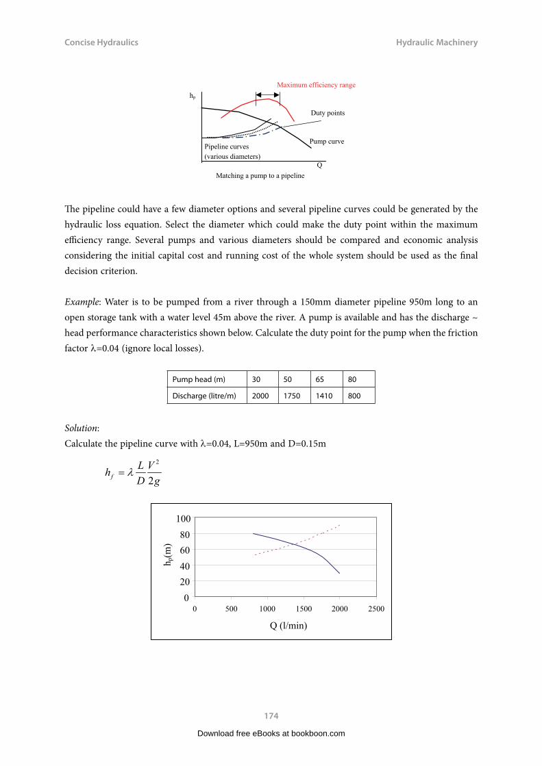
Concise Hydraulics

174

Hydraulic Machinery

Q

hp

Pump curve

Maximum efficiency range

Pipeline curves (various diameters)

Duty points

Matching a pump to a pipeline

The pipeline could have a few diameter options and several pipeline curves could be generated by the hydraulic loss equation. Select the diameter which could make the duty point within the maximum efficiency range. Several pumps and various diameters should be compared and economic analysis considering the initial capital cost and running cost of the whole system should be used as the final decision criterion.

Example: Water is to be pumped from a river through a 150mm diameter pipeline 950m long to an open storage tank with a water level 45m above the river. A pump is available and has the discharge ~ head performance characteristics shown below. Calculate the duty point for the pump when the friction factor l=0.04 (ignore local losses).

Pump head (m) 30 50 65 80

Discharge (litre/m) 2000 1750 1410 800

Solution:Calculate the pipeline curve with l=0.04, L=950m and D=0.15m

2

2fL VhD g

λ=

020406080

100

0 500 1000 1500 2000 2500

Q (l/min)

h p(m

)


Concise Hydraulics

175

Hydraulic Machinery

For different discharge, we can derive

Q hf hf+45m2000 46.0 91.0

1750 35.2 80.2

1410 22.9 67.9800 7.14 52.4

The duty point can be found at Q= 1400 l/s, H= 65 m

Series and parallel arrangement

When the required flow or head is greater than a single centrifugal pump, two or more pumps could be combined to meet the demand. Also if the demand varies greatly with time, it is desirable to have a few smaller pumps that can be run in parallel instead of a single one.

To increase the head, two or more identical pumps are operated in series. The same flow passes through Pump 1 and Pump 2 so that the discharge is the same as individual pumps but the head is doubled (in case of two pumps). The discharge~head curve for two pumps can be obtained by taking the curve for one pump and doubling the head for each value of discharge. Like in series electricity circus, the whole system breaks down when one pump stops.

Pump 1

Suctionpipe

Q

Pump 2

Deliverypipe

H

One pump

Head double for two pumps

Two pumps in series

To increase the discharge, two or pumps could be operated in parallel. Again the pumps must be identical, have individual suction pipes but share a common delivery pipe. The head is the same as for a single pump but the discharge is doubled. The dischare~head curve is obtained by taking the curve for one pump and doubling the discharge for each value of head. Usually one pump is used to provide low flow demand and other pumps are used to provide extra flow when the demand is increased.


Concise Hydraulics

176

Hydraulic Machinery

Cavitation and safe installation height

ZWhen a pump is operating, it draws water from the sump and the water is pushed by the atmospheric pressure. At the sea level, the atmospheric pressure is about 10m of water head and would be considerably less in high mountains. Considering the hydraulic loss along the pipeline, the practical limit is below 7 meters. In addition, low pressure will increase the possibility of cavitation within the pump, which occurs when the liquid pressure at a given location is reduced to vapour pressure of the liquid. When this occurs, vapour bubbles form (the liquid starts to ‘boil’). Cavitation can cause a loss in efficiency as well as structural damage to the pump. To decide the maximum elevation for a pump installation, an important parameter is introduced: NPSHR (Net Positive Suction Head), which is a value provided by pump manufacturers as a reference for limiting suction lift under each discharge to ensure that a pump operates satisfactorily.


Click on the ad to read moreClick on the ad to read moreClick on the ad to read moreClick on the ad to read moreClick on the ad to read moreClick on the ad to read moreClick on the ad to read moreClick on the ad to read moreClick on the ad to read moreClick on the ad to read moreClick on the ad to read moreClick on the ad to read moreClick on the ad to read moreClick on the ad to read moreClick on the ad to read moreClick on the ad to read moreClick on the ad to read moreClick on the ad to read moreClick on the ad to read moreClick on the ad to read moreClick on the ad to read moreClick on the ad to read moreClick on the ad to read moreClick on the ad to read moreClick on the ad to read moreClick on the ad to read moreClick on the ad to read moreClick on the ad to read moreClick on the ad to read moreClick on the ad to read moreClick on the ad to read moreClick on the ad to read moreClick on the ad to read moreClick on the ad to read moreClick on the ad to read moreClick on the ad to read moreClick on the ad to read moreClick on the ad to read moreClick on the ad to read moreClick on the ad to read moreClick on the ad to read moreClick on the ad to read moreClick on the ad to read moreClick on the ad to read moreClick on the ad to read moreClick on the ad to read moreClick on the ad to read moreClick on the ad to read moreClick on the ad to read moreClick on the ad to read moreClick on the ad to read moreClick on the ad to read moreClick on the ad to read moreClick on the ad to read moreClick on the ad to read moreClick on the ad to read moreClick on the ad to read moreClick on the ad to read moreClick on the ad to read more






Brain power




Concise Hydraulics

177

Hydraulic Machinery

The actual NPSH for an installation can be calculated as NPSHa=Pa – Z- Vp – hL

where Pa is the atmospheric pressure (m), Z is the elevation difference between the pump and intake water level (m), Vp is the vapour pressure of water (approximately 0.5m, depending temperature) and hL is the head loss in the suction pipe (approximately 0.75m, local loss is more dominant). To prevent cavitation, it is necessary that

A RNPSH NPSH≥

Example:

A centrifugal pump is to be placed above a large open water tank with discharge 14 litres/s. The required net positive suction head (NPSHR) is 4.6 m, as specified by the pump manufacturer. If the water temperature is 27oC and atmospheric pressure is 101.353 KPa, determine the maximum height Z, that the pump can be located above the water surface without cavitation. Ignore the friction loss, and the local loss is mainly caused by a special inlet filter with KL=20. The diameter of the inlet pipe is 10cm.

The water properties are

Temperature (oC) 0 4 10 20 30 40

Density (kg/m3) 999.9 1000.0 999.7 998.2 995.7 992.2

Vapour pressure (N/m2) 610.5 872.2 1228 2338 4243 7376

Solution

The energy loss 2 2 2[0.014 /(0.05 )]20 3.24

2 2L LVh K m

g gπ

= = =

From the table, water at 27oC, density = 996 kg/m3, vapour pressure = 3671 N/m2,

From NPSHa=Pa – Z- Vp – hL≥ NPSHR

So

101353/(996g)- Z- 3671/(996g)- 3.24 ≥ 4.6,

Z ≤ 2.16m


Concise Hydraulics

178

Hydraulic Machinery

Surges in pumping stations

1. Pump stops suddenly and water continues to flow to create water column separation

2. Flow reverses and a sudden impact on the pump

Water hammer can cause damages to the pipelines and this could also be a problem for pump mains, which is the slower mass movement of water often resulting from the faster-moving water hammer shock waves. When a pump stops, the flow in the pipe does not stop immediately but continues to move along the pipe. Since the driving force is gone and the water will gradually slow down due to friction. As the flow moves away from the pump and no water enters the pipe, the empty space forms near the pump. This is called water column separation and pressure in the empty space drops rapidly to the vapour pressure. Then the water begins to flow back towards the pump gathering speed as it goes, and comes to a sudden stop as it hits the pump (similar to a sudden closure of a valve on a pipeline). This could burst the pipe and the pump.

Possible solutions are:

1) Stop pumps slowly: This will avoid the water column separation and minimise the surge. Diesel pumps are more suitable for this solution since they stop gradually after the fuel is cut off, while electric pumps usually have sudden stop when the electricity is switched off.

2) Use a non-return valve: it will allow water to pass in one direction only and protect the pump (not the pipeline) when water flows back.

Water flows in and out of vessel to cushion water hammer


Concise Hydraulics

179

Hydraulic Machinery

3) Use an air vessel: This is similar to a surge tank. When a pump stops and pressure starts to drop, water flows from a pressured tank into the pipeline to fill the void and stop the water column from separating, and water is allowed to flow back into the tank when the flow is reversed. The water will oscillate back and forth until it eventually stops through friction (much like a car shock absorbers). This device is expensive and should be used only for large scale pump stations where serious water hammers are expected.

Questions 17Hydraulic Machinery

1. Each day 600m3 of water is pumped by 10m to a tank above the ground. Calculate the amount of power required to do this (assume the system is 100% efficient and there is no energy loss in the pipeline).

(Answer: about 0.7 kW)

2. A Hydraulic power plant takes in 30m3/s of water through its turbine and discharges it at V=2m/s at atmospheric pressure. The head loss in the turbine and conduit system is 20 meters. Estimate the power extracted by the turbine.

(Answer: 23.5 MW)


Click on the ad to read moreClick on the ad to read moreClick on the ad to read moreClick on the ad to read moreClick on the ad to read moreClick on the ad to read moreClick on the ad to read moreClick on the ad to read moreClick on the ad to read moreClick on the ad to read moreClick on the ad to read moreClick on the ad to read moreClick on the ad to read moreClick on the ad to read moreClick on the ad to read moreClick on the ad to read moreClick on the ad to read moreClick on the ad to read moreClick on the ad to read moreClick on the ad to read moreClick on the ad to read moreClick on the ad to read moreClick on the ad to read moreClick on the ad to read moreClick on the ad to read moreClick on the ad to read moreClick on the ad to read moreClick on the ad to read moreClick on the ad to read moreClick on the ad to read moreClick on the ad to read moreClick on the ad to read moreClick on the ad to read moreClick on the ad to read moreClick on the ad to read moreClick on the ad to read moreClick on the ad to read moreClick on the ad to read moreClick on the ad to read moreClick on the ad to read moreClick on the ad to read moreClick on the ad to read moreClick on the ad to read moreClick on the ad to read moreClick on the ad to read moreClick on the ad to read moreClick on the ad to read moreClick on the ad to read moreClick on the ad to read moreClick on the ad to read moreClick on the ad to read moreClick on the ad to read moreClick on the ad to read moreClick on the ad to read moreClick on the ad to read moreClick on the ad to read moreClick on the ad to read moreClick on the ad to read moreClick on the ad to read moreClick on the ad to read more


Concise Hydraulics

180

Hydraulic Machinery

Water Turbine

Elevation 150 m

2m/s Elev. 50m

3. A power plant is to be built on a stream capable of utilising a flow up to 1 m3/s with a gross head of 40m at 78 percent overall efficiency. Assume the stream has enough flow to maintain the plant working at full capacity continuously and the power is valued at £0.05 per kilowatt-hour. What annual revenue could be expected from this plant?

(Answer: £134,000)

4. A Pelton Wheel is to be selected to drive a generator at 600rpm. The water jet is 75mm in diameter and has a velocity of 100m/s. With the blade angle at 170o, the ratio of vane speed to initial jet speed at 0.47, and neglecting losses, determine 1) diameter of wheel to centerline of buckets (vanes); 2) power developed. (Note P AV V u u= − −ρ β( )( cos )1 )

(Answer: 1.497m, 2.18 MW)

Solutions 17Hydraulic Machinery

1. Convert discharge to m3/s

3600 / 24 / 3600 0.007 /Q m s= =

1000 9.81 10 0.007 686 0.7P gHQ W kWρ= = × × × = ≈

2. Set up the energy equation between the reservoir surface and the turbine outlet

z1

V12

2gz2

V22

2ghL H

so 10022

2ghL H

With hf=20m, so H =100- 20 -0.2 = 79.8 m

Power extracted by turbine will be

P = ρgQH = 1000 × 9.81× 30 × 79.8 = 23.5MW


Concise Hydraulics

181

Hydraulic Machinery

3) Power output P = gQH/1000 kW = 0.78

kW

Annual revenue = revenue=P £134.1 3

So the annual revenue from this plant will be 134 thousand pounds.

4) 1) The peripheral speed of the wheel is u m s m s= × =0 47 100 47. / /

uD

rpmπ

× =60 600 so D mu= × = =600

4710

60 1497π π

.

2) The power is P AV V u u= − −ρ β( )( cos )1

so P

W MW

o=×

− −

= =

1000 0 0754

100 100 47 1 170 47

2183154 218

2π . ( )( cos )

.


Click on the ad to read moreClick on the ad to read moreClick on the ad to read moreClick on the ad to read moreClick on the ad to read moreClick on the ad to read moreClick on the ad to read moreClick on the ad to read moreClick on the ad to read moreClick on the ad to read moreClick on the ad to read moreClick on the ad to read moreClick on the ad to read moreClick on the ad to read moreClick on the ad to read moreClick on the ad to read moreClick on the ad to read moreClick on the ad to read moreClick on the ad to read moreClick on the ad to read moreClick on the ad to read moreClick on the ad to read moreClick on the ad to read moreClick on the ad to read moreClick on the ad to read moreClick on the ad to read moreClick on the ad to read moreClick on the ad to read moreClick on the ad to read moreClick on the ad to read moreClick on the ad to read moreClick on the ad to read moreClick on the ad to read moreClick on the ad to read moreClick on the ad to read moreClick on the ad to read moreClick on the ad to read moreClick on the ad to read moreClick on the ad to read moreClick on the ad to read moreClick on the ad to read moreClick on the ad to read moreClick on the ad to read moreClick on the ad to read moreClick on the ad to read moreClick on the ad to read moreClick on the ad to read moreClick on the ad to read moreClick on the ad to read moreClick on the ad to read moreClick on the ad to read moreClick on the ad to read moreClick on the ad to read moreClick on the ad to read moreClick on the ad to read moreClick on the ad to read moreClick on the ad to read moreClick on the ad to read moreClick on the ad to read moreClick on the ad to read moreClick on the ad to read more


Concise Hydraulics

182

Appendix: Further Reading Resources

18 Appendix: Further Reading Resources

The following resources are highly recommended if you want to further explore the interested topics in hydraulics. This is not an exhaustive list and will be updated regularly in the future. You are welcome to recommend useful books/web sites that are not on the list.

Biswas, A.K., 1970, History of Hydrology, North-Holland Publishing Company

Chadwick, A., Morfett, J. and Borthwick, 2004, Hydraulics in Civil and Environmental Engineering, 4th Edition, Spon Press

Chanson, H., 1999, The Hydraulics of Open Channel Flow, Butterworth-Heinemann, Oxford

Chow, V.T.,1959, Open Channel Hydraulics, McGraw-Hill College

Evett, J.B. and Liu, C., 1989, 2500 solved problems in Fluid Mechanics & Hydraulics, McGraw Hill

French, R.H., 1985, Open-Channel Hydraulics, McGraw-Hill

IAHR, 2008, Media Library, http://www.iahrmedialibrary.net/

Kay, M., 1998, Practical Hydraulics, E&FN Spon

Liggett, J.A. and Caughey, D.A., 1999, Fluid Mechanics, ASCE Press

Munson, B.R., Yong, D.F. and Okiishi, T.H., 2002, Fundamentals of Fluid Mechanics, John Wiley and Sons.

Novak, P., Moffat, A, Nalluri, C. and Narayanan, 1996, Hydraulic Structures, Second Edition, E & FN Spon

Wikipedia, 2008, ‘Hydraulics’, ‘Hydrostatics’, … http://en.wikipedia.org/wiki/Hydraulics


http://www.iahrmedialibrary.net/

http://en.wikipedia.org/wiki/Hydraulics

Concise Hydraulics

Documents

Transcript of Concise Hydraulics