MAGNETIC STUDIES OF COBALT BASED GRANULAR THIN

FILMS

Colin John Oates

A Thesis Submitted for the Degree of PhD

at the University of St Andrews

2002

Full metadata for this item is available in St Andrews Research Repository

at: http://research-repository.st-andrews.ac.uk/

Please use this identifier to cite or link to this item: http://hdl.handle.net/10023/12928

This item is protected by original copyright

MAGNETIC STUDIES OF COBALT BASED GRANULAR

THIN FILMS

Colin John OatesUniversity o f St. Andrews

Thesis submitted for the degree of Doctor of Philosophy,August 2002

ProQuest Number: 10167033

All rights reserved

INFORMATION TO ALL USERS The quality of this reproduction is dependent upon the quality of the copy submitted.

In the unlikely event that the author did not send a com p le te manuscript and there are missing pages, these will be noted. Also, if material had to be removed,

a note will indicate the deletion.

uestProQuest 10167033

Published by ProQuest LLO (2017). Copyright of the Dissertation is held by the Author.

All rights reserved.This work is protected against unauthorized copying under Title 17, United States C ode

Microform Edition © ProQuest LLO.

ProQuest LLO.789 East Eisenhower Parkway

P.Q. Box 1346 Ann Arbor, Ml 48106- 1346

Abstract

The m agnetic record ing m edia used for hard disks in laptops and P C ’s

is constan tly being im proved, leading to rapid increases in data rate

and storage density. How ever, by the year 2010, it is p red ic ted that the

superparam agnetic lim it w ill be reached, which is po tentia lly

insu ffic ien t for data storage. At the beginning o f th is century, CoCr -

based alloys are used in long itud inal m edia since cobalt has a high

m agnetocrysta lline anisotropy.

In this thesis, the s tatic and dynamic properties o f longitudinal

recording th in films were investigated in order to explain and correlate

the ir magnetic charac te ris tics to the ir recording properties . The

samples in question were te s t sam ples and some were in com m ercial

use. M agnetic techniques such as h igh field ferrom agnetic resonance

and torque m agnetom etry were used to determ ine accurate ly the

c rystalline anisotropy field. High field ferrom agnetic resonance is an

ideal tool to determ ine the crystalline anisotropy, m agnetisa tion . Lande

g-factor and the gyrom agnetic dam ping factor. In con trast to previous

work, there are no FMR sim ulations and so all the re levant param eters

were determ ined d irectly from m easurem ent. Ideally, there should be

no exchange in teractions betw een the neighbouring cobalt grains;

however, in teractions be tw een the grains w ith in the CoCr-alloy

recording layer exist. Previous work on the m easurem ents o f

in teractions in record ing m edia involves m easuring the sam ple ’s

m agnetisa tion . In this thesis , an a lternative novel m ethod involves

torque magnetom etry.

A nother technique that was used in this thesis is small angle neutron

scattering, which aims to determ ine the size o f the m agnetic grains and

compare tha t w ith the physical size determ ined from TEM, by Seagate.

There is an extended sec tion on CoxAgj.x granular th in films^ which

involves determ ining the sam ple ’s g-factor, effective anisotropy, grain

size, exchange constant and com paring the FMR lineshapes at 9.5 and

92GHz.

Declarations

1, Colin John Oates, hereby certify that this thesis, which is approximately 30000

words in length, has been written by me, that it is the record of work carried out by

me and that it has not been submitted in any previous application for a higher degree.

Colin John Oates

August 2002

I was admitted as a research student in October 1998 and as a candidate for the degree

of Doctor of Philosophy in October 1999; the higher study for which this is a record

was carried out in the University of St. Andrews between 1998 and 2002.

Colin John Oates

August 2002

I hereby certify that the candidate has fulfilled the conditions of the Resolution and

Regulations appropriate for the degree of Doctor of Philosophy in the University of

St. Andrews and that the candidate is qualified to submit this thesis in application for

that degree.

P.C.Riédi

August 2002

In submitting this thesis to the University of St. Andrews I understand that I am

giving permission for it to be made available for use in accordance with the

regulations of the University Library for the time being in force, subject to any

copyright vested in the work not being affected thereby. I also understand that the title

and abstract will be published, and that a copy of the work may be made and supplied

to any bona fide library or research worker.

^ Colin John Oates

August 2002

Acknowledgements

I would like to thank both Prof. Peter R iedi and Dr. Graham Smith for

their support and un lim ited patience throughout my PhD. Both Peter

and Graham have provided sound advice on problem s arisen throughout

the four years o f my PhD.

I am also grateful to Dr. Feodor Ogrin, now in Exeter University ,

Feodor was very helpful and his d iscussions and guidance on FMR and

torque m agnetom etry were invaluable.

I would also like to thank Prof. Steve Lee for a llowing me to take part

in the SANS experim ent as well as partic ipating in the ‘torque te am ’,

which I feel I have benefited .

Dr. Tom Thom son, who is now working for IBM has been a great help

th roughout my Ph.D. His providence o f recording th in films and

background d iscussions on the m ateria ls were o f course invaluable and

Tom also played an im portan t part in allow ing some o f my work in this

thesis to be published w ith Seaga te ’s perm ission.

Dr. N igel Poolton, who is now working in Daresbury, was a very

helpful postdoc who had a lot o f patience in explain ing how the

spectrom eter worked as well as the software designs. Dr. A droja (now

in Rutherford Appleton Laboratory in Didcot) has shown how to run

the NM R spectrom eter and explain o ther parts o f m agnetism that I did

not fully understand.

Thanks to Prof. John W alton for a llow ing me to carry out FMR work on

the Bruker; Dr. N ata lia Lesnik for p rovid ing nanocluster samples as

well as d iscussions based on FMR and P ro f Bob Cywinski for his

d iscussions on neutron d iffrac tion and fine partic le m agnetism .

Thanks also to Shannon Brown (soon to be Dr. S .G .Brown), Paul

C ruickshank, Prof. C zeslaw K apusta and Dr. Charles D ew hurst from

the ILL.

There are m embers o f the workshop who have worked hard in

constructing a 90GHz in-p lane sample ro ta tor and prepared samples for

FMR m easurem ents, as d iscussed in chapter four. Thanks to George

Radley, Paul ‘n eeb o r’ A itken, Steven Balfour, Andy Barman, Bob

M itchell, Reg Gavine and Fritz Akerboom .

Finally, there are two more people to whom I am in debt to for their

unlim ited moral support during my undergraduate and postgraduate

studies: John and Sheila Oates. This thesis is dedicated to these two

special people.

Contents

L

1 .

1.3

C h a p te r 1 B asic T h e o ry : F e r ro m a g n e t i s m a n d R e c o rd in g T h in

Film M ed ia ..................................................................................... 1

Fundam entals .................................................................................. 1

.1.1. In ternal fie ld ............................................................................... 1

.1.2. M agnetic m om ents .................................... ............................... 2

.1.3. Basic quantum m echanics o f m agnetism ........................... 4

.1.4. P a ram agnetism .............................................................................. 7

.1.5. F e rrom agne tism ............................................................................ 9

.1.6. Exchange in te ra c t io n ................................................................. 11

.1.7. M agnetic an iso tro p y ................................................................. 13

.1.8. Superparam agnetic b eh av io u r ................................................. 14

.1.9. R eversing m ech an ism s .............................................................. 15

M agnetic recording m e d ia .......................................................... 17

.2.1 Com pound annual growth r a te ............................................... 17

.2.2. Longitudinal recording m ed ia ............................................... 20

R efe ren ces ........................................................................................ 23

C h a p te r 2 F e r r o m a g n e t ic r e s o n a n c e ............................................................ 25

2.1. Theory o f F M R ................................................................................. 25

2.1.1. In tro d u c tio n ................................................................................... 25

2.1.2. High frequency m agnetic su scep tib il i ty ............................ 28

2.1.3. High frequency suscep tib ili ty with d am p in g .................. 31

2.1.4 C ircular po la risa t ion o f h -f ra d ia t io n ................................ 33

2.1.5. Internal fie lds in fe rrom agne tics ......................................... 35

2.1.6. M ethods o f analysis o f FMR in anisotropic

fe rrom agne ts ..................................................................................... 37

2.1.7. Features o f FMR o f m e ta ls ...................................................... 40

2.1.8. Spin wave re so n an ce ................................................................. 43

2.2. FMR sp ec tro m ete r ........................................................................... 44

2.2.1. 12 Tesla quasi-op tical spec trom ete r .................................... 44

2.2.2. In-plane sam ple h o ld e r .......................................................... 47

2.2.3. Prelim inary ex p e r im en ts ...................................................... 49

2.2.3.1. Cobalt (3 0 n m )..................................................... 49

2.2.3.2. FeTiN thin f i lm s ................................................................... 52

2.3. R efe ren ces ........................................................................................ 56

Chapter 3 FMR and torque m agnetom etry o f high and low 59

noise CoCr alloy longitud inal recording m ed ia ............

3.1. In tro d u c tio n ....................................................................................... 59

3.2. Ferrom agnetic re so n an ce ........................................... 59

3.2.1 Summary o f previous works on the FMR o f CoCr- 59

alloy record ing m ed ia ................................................................

3.2.2. High and low noise recording m ed ia ................................. 62

3.2.3. M o d e ll in g ......................................................................... 65

3.2.4. Experim enta l set and re su l ts .................................................. 70

3 .2 .4 .1. Static p ro p e r t ie s ............................................................... 71

3.2.4.2 . Dynamic p ro p e r t ie s .............................................................. 75

3.2.5. C o n c lu s io n s .................................................................................. 77

3.3. Torque m agnetom etry ................................................................... 78

3.3.1. In tro d u c tio n .................................................................................. 78

3.3.2. Experim ent eq u ip m en t.............................................................. 79

3.3.3. C losing po in t m easu rem en ts .............................................. 80

3.3.3.1 . M ean fie ld ................... m o d e l ............................................... 81

3.3 .3 .2 . E x p e r im en t............................................................................... 83

3.3.4. D eterm ination o f in te rac t io n s ............................................... 86

3.3.4.1. The AM and AT technique: Theory o f the AM 87

m eth o d ................................................................................................

3 .3.4.2. AT m ethod and re s u l ts ...................................................... 90

3.4. C o n c lu s io n s ......................................................................................... 94

3.5. R efe ren ces .......................................................................................... 95

Chapter 4

4.1.

4.2.

4.3.

4.4.

4.4.1

4.4.1.1.

4.4.1.2.

4.4.2.

4.4.2.1,

4.4.2.2.

4.5.

4.6.

Chapter 5

5.1

5.2

5.2.1.

5.2.2.

5.2.3.

5.2.4.

5.3.

5.4.

5.5.

5.5.1.

5.5.2.

5.5.2.1

5.5.3.

High field FMR of CoCrPtB longitud inal media w ith 97

varying com positions o f platinum and b o ro n .................

In tro d u c tio n ..................... ............................................................... 97

Sample c h a rac te r is t ic s ................................................................. 97

Sample p rep a ra t io n ........................................................................ 101

FMR o f CoCrPtB m ed ia .............................................................. 104

P la tinum se r ie s ........................................................................... 104

Static p ro p e r t ie s ................................................................... 104

Dynamic p ro p e r t ie s ............................................................. 109

Boron se r ie s ................................................................................. I l l

Static p ro p e r t ie s ................................................................... I l l

Dynamic p ro p e r t ie s ............................................................. 114

Sum m ary............................................................................................. 115

R eferences ........................................................................................ 117

Small Angle N eutron Scattering of L ongitudinal 118

R ecording M ed ia ...........................................................................

In tro d u c tio n ..................................................................................... 118

Basic theory o f neutron d if f rac t io n ....................................... 118

Why neu tron d iffrac tion? ..................................................... 118

N uclear d if f ra c t io n ................................................................... 120

E lastic m agnetic sca t te r in g ................................................... 123

Small angle neutron sca tte r in g ............................................ 124

SANS e x p er im en t .......................................................................... 128

Recording m edia sam p les ........................................................... 130

SANS m easu rem en ts .................................................................... 132

Sample p repara tion for m easu rem en ts .............................. 132

SANS o f 2D -iso trop ic longitudinal record ing media. 133

SANS model and results for the iso tropic 138

m ed ia ...................................................................................................

SANS o f an iso trop ic m e d ia .................................................... 146

5.6. C o n c lu s io n s ....................................................................................... 147

5.7 R efe ren ces ..................... 148

C hapter 6 Cobalt n a n o c lu sters ..................................................................... 149

6.1. In tro d u c tio n ...................................................................................... 149

6.2. P rep a ra t io n ......................................................................................... 149

6.3. V ibrating sample m agnetom etry .............................................. 151

6.4. Ferrom agnetic re so n an ce ............................................................. 155

6.4.1. 9 .5GHz m easu rem en ts ...................... 155

6.4.2. 92GHz m easu rem en ts ................................................................ 162

6.5. Sum m ary .............................................................................................. 170

6 .6 . R efe rences ......................................................................................... 171

C hapter 7 Summary and Future w o r k s .................................................... 172

Appendices 176

A G aussian beam s and the in-plane sample h o ld e r 176

B Lineshape an a ly s is ......................................................................... 180

C The FMR condition for longitudinal recording m edia 184

D SQUID m easurem ents on CoCrPtB (Pt s e r ie s ) ................. 186

Publications .......... 188

Chapter 1

Basic Theory: Ferromagnetism and Recording Thin Film Media

This thesis presents m ethods o f determ ining the magnetic properties o f

ferrom agnetic granular th in films. Exam ples o f films studied are those

o f the CoCr alloy record ing media, w hich were either test samples or in

com m ercial use.

To start off, it is necessary to cover in this chapter the fundam entals

and features o f ferrom agnetism and recording media.

1.1 Fundamentals1.1.1 Internal field

The fundam ental equation for the m agnetic induction 5 inside a

m agnetic m aterial is g iven by:

5 = //q(^ + m ) in s i units ( 1. 1)

or B = H + 47tM in e.g.s. units ( 1.2 )

From the SI units version, the term juo is the perm eability o f free space

{47t X 1 0 ' ^ H is the m agnetic field in tensity and M is the

m agnetisation , generally defined as the to ta l m agnetic m om ent per unit

volume. (In th is thesis, all m easurem ents are in cgs units).

I f a m agnetic body o f fin ite size is m agnetised, free poles are induced

on both ends as shown in figure 1. 1.

M

F igure 1.1. F r ee p o l e s on m a g n e t i c m a te r ia l s

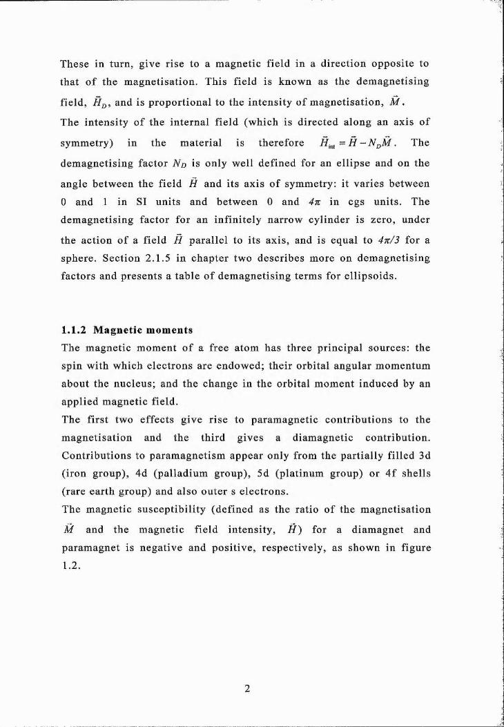
These in turn , give rise to a m agnetic field in a d irection opposite to

that o f the m agnetisation . This field is known as the dem agnetis ing

field, and is p roportional to the in tensity o f m agnetisa tion , M ,

The in tensity o f the in ternal fie ld (which is d irected along an axis o f

symmetry) in the m ateria l is therefore = H ~ N ,^M . The

dem agnetis ing factor No is only well defined for an e llipse and on the

angle between the field H and its axis o f symmetry: it varies between

0 and 1 in SI units and betw een 0 and 4tl in cgs units. The

dem agnetis ing factor for an in fin ite ly narrow cylinder is zero, under

the action o f a field H para lle l to its axis, and is equal to 4it/3 for a

sphere. Section 2.1.5 in chapter two describes more on dem agnetis ing

factors and presents a tab le o f dem agnetis ing terms for e llipso ids.

1.1.2 M agnetic moments

The m agnetic moment o f a free atom has three principal sources: the

spin with which electrons are endowed; the ir orbital angular m omentum

about the nucleus; and the change in the orbital mom ent induced by an

applied m agnetic field.

The first two effects give rise to param agnetic contribu tions to the

m agnetisa tion and the th ird gives a diam agnetic contribution.

C ontributions to param agnetism appear only from the partia lly fil led 3d

(iron group), 4d (pallad ium group), 5d (platinum group) or 4 f shells

(rare earth group) and also outer s e lectrons.

The m agnetic suscep tib ility (defined as the ratio o f the m agnetisa tion

M and the m agnetic fie ld in tensity , H ) for a diam agnet and

param agnet is negative and positive , respectively , as shown in figure

1.2 .

à iLangevin (free spin) paramagnetism

Itinerant Pauli paramagnetism (metals)

Temperature

Diamagnetism

F ig ure 1 .2: C h a r a c t e r i s t i c m a g n e t i c s u s c e p t i b i l i t y o f d i a m a g n e t i c a n d

p a r a m a g n e t i c s u b s ta n c e s [ 1 ]

Ordered arrays o f m agnetic m om ents may be ferrom agnetic ,

ferrim agnetic , an tiferrom agnetic or may be more com plex in form, as

shown in figure 1.3.

0.0 0.0

F igure 1.3. G ra p h s o f the t e m p e r a t u r e d e p e n d e n c e o f (a) the m a g ne t is a t io n ,

M, o f a f e r r o m a g n e t i c m a t e r i a l a n d the d e p e n d e n c e o f the inv er se

s u s c e p t i b i l i t y a n d (b) o f the s u s c e p t i b i l i t y o f an a n t i f e r r o m a g n e t i c mater ia l .

[ 2]

N uclear m agnetic m om ents gives rise to nuclear param agnetism .

M agnetic moments o f nuclei are o f the order o f 10’ tim es sm aller than

the m agnetic moment o f e lectrons, since nuclear mass is 1836 times

larger than electron mass.

1.1.3 Basic quantum m echanics o f magnetism

Before proceeding w ith the defin ition o f cooperative phenom ena, such

as ferrom agnetism and param agnetism , it is necessary to go over the

concepts o f elem entary m agnetic m oments.

As m entioned previously , the m agnetic moments are spin and orbital

m agnetic m om ents o f e lectrons. The net moments o f all inner (filled)

e lectron shells o f atoms are equal to zero. In ionic crystals , the total

spin plus orbital m agnetic m om ents o f ions can be regarded as

elem entary m agnetic m om ents.

In quantum m echanics, the state o f the e lectron is charac terised by four

quantum numbers.

1. P rincipal quantum num ber «, w hich determ ines the energy o f the

shell or orbit;

2. Orbital quantum num ber (in teger) /, which determ ines the orbital

angular m om entum o f the e lectron, whose magnitude is g iven by

■Jl(l + \)h. The value o f I s tarts from 0, 1.

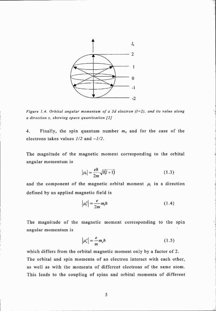
3. The m agnetic quantum num ber mi, which gives the com ponent o f

the orbital m om entum along a g iven d irec tion and may be equal to 1,1-

1 tha t is, it takes 21+1 values. In the spatial

represen ta tion o f the a tom ic quan tities the orbital m om entum can only

po in t along certain d irec tions and its p ro jec tions are given by mi, as

il lus tra ted in figure 1.4 for a 3d e lectron.

k

2

1

0

-1

-2

Figure 1.4. Orbi tal angular momentum o f a 3d electron (1=2), and its value along

a direction z, showing space quant izat ion [2 ]

4. F inally , the spin quantum num ber nis and for the case o f the

e lec trons takes values 1/2 and -1 /2 .

The m agnitude o f the m agnetic m om ent corresponding to the orbital

angular m om entum is

(1.3)

and the com ponent o f the m agnetic orb ital mom ent //, in a d irection

defined by an applied m agnetic field is

I e\Li:\ = m ,ti

2 m '(1.4)

The m agnitude o f the m agnetic m om ent corresponding to the spin

angular m om entum is

I .1 e ■mMm

(1.5)

which differs from the orb ital m agnetic m om ent only by a factor o f 2 .

The orbital and spin m om enta o f an e lec tron in teract w ith each other,

as well as with the m om enta o f d ifferen t electrons o f the same atom.

This leads to the coupling o f spins and orbital m om enta o f d ifferent

electrons, forming the to ta l spin angular mom entum S and orbital

mom entum L. This is called the R usse ll-Saunders coupling:

In heavy atoms, there is a strong coupling between // and 5, o f each

electron, which leads to the to ta l angular mom enta per e lec tron _//. This

is called j j coupling.

Since the total spin and orbital m om enta in teract through the atomic

sp in-orb it in teraction L and S combine to form the to ta l angular

mom entum J. The corresponding quantum number J may take values

J = ^L + S, L + S - 1 |Z - S'! (1.7)

and the levels defined by these values o f J are called m ultip le ts and the

p ro jec tion o f J along an arb itrary d irec tion is quantised w ith the

corresponding quantum num ber M j, which take values

M j = J, J - 1, J. (1.8)

As a resu lt o f jUj = jUgL and ju = Iju^S , the vector addition o f the

orbital and spin com ponents to the m agnetic moment gives a value

juj = gjjUgJ for the overall m agnetic mom ent, where the Lande g-factor

has the form

_ s( + l)+/p + l)-z(z + l)

which is usually derived in tex ts on m odern physics [2-4]. Typical

values o f the spectroscopic sp litt ing factor o f cobalt, iron and nickel

are 2 .20, 2.09 and 2.23 [5], respectively . O f course for pure spin or

orbital m otion these expressions reduce to = //gZ and jUg=2jUgS,

respectively .

The next two sections will now look at the theory o f param agnetism

and ferrom agnetism .

1.1.4, Param agnetism

The states with d ifferen t values are degenerate in the absence o f an

external m agnetic field. W hen the m agnetic field H is applied, there

appears the potentia l energy o f a m agnetic moment in th is field (the

Zeeman energy)

Ej = - ji ijH = -gPjiJH (1.10)

and the degeneracy is rem oved. There are (2J+1) equ id is tan t energy

levels separated by in tervals

AE = )^H ( 1. 11)

Transitions between these levels, w ith the absorp tion o f a

e lec trom agnetic energy quanta hco, are called electron param agnetic

resonance, or e lectron spin resonance. Only transitions between the

ne ighbouring levels are allow ed by the selection rules, Airij = ±1 and

the resonance condition is given as

a, = yH = ^ H (1.12)

The difference in popula tions o f the levels with d ifferent results in

the appearance o f the net m om ent in the direction o f the field H. The

calcu lation , with the use o f the general form ulae o f quantum statistics

leads to the expression for the m agnetisa tion

( W 3 )

where B j (x) is the B rillou in function [4-6] defined as

5,(x) = fl + — Icoth f l + — Ix — î-cothf— 1 (1.14)I 2 J ) IL 2 J ) J 2 J \ 2 J )

where M ^ -y f iN J is the satu ration m agnetisa tion , N is the num ber o f

m agnetic m om ents in a unit volum e, and k is the B oltzm ann constant.

From the B rillou in function , as x approaches infinity; tha t is, in the

very high m agnetic f ie ld and/or low tem perature lim it, Bj(x) tends

towards unity, and all the m agnetic m oments are orien ted in the

d irec tion o f the field. For small x, expanding Bj(x) as a pow er series,

one w ould obtain from (1.13) the re la tion M = X p ^ • The param agnetic

suscep tib ility Xp^ which does not depend on H in this lim iting case,

can be w ritten as

X p = — (1*15)

where C = + Mb (1 .16)3k

is the Curie constant and (1.15) is the Curie law. The constant C

contains g V ( j + l), w hich is the square o f the effective param agnetic

moment:

P ,f f= g (J (J+ I))‘'^ (1 .17)

The values o f the mom ents Pe// o f the rare earths (set o f elem ents o f

atomic num ber betw een 57 (La) and 71 (Lu) plus elem ents Sc and Y

[2]) determ ined experim entally are in good agreem ent w ith the Pe//

com puted with the above expression.

I f we compare the effective param agnetic m oments o f the transition

salts o f the d series one finds a large d isagreem ent betw een the

com puted effective mom ents Pe// and the m easured m om ents [1]. With

g equal to 2, agreem ent is recovered i f we write S ra ther than J in the

expression o f Pe//. This is evidence for the im portance o f the

in teraction o f these ions w ith the e lec trosta tic crystalline field. This

in teraction is larger than the sp in-orb it in teraction.

The d ifference in behaviour o f the rare earth and the iron group is that

the 4 f shell responsib le for param agnetism in rare earth ions lies deep

inside the ions, w ith in the 5s and 5p shells, whereas in the iron group

ions the 3d shell responsib le for the m agnetism is the outerm ost shell.

The 3d shell experiences the in tense inhom ogeneous electric field

produced by neighbouring ions. This inhom ogeneous e lectric field is

called the crystal field . The in te rac tion o f the 3d param agnetic ions

w ith the crystal f ie ld has two m ajor effects: L-S coupling is largely

broken up, so that the states are no longer specified by their J values

and the 2L + 1 states for a g iven value o f L may now be split by the

crystal field. This sp lit t ing d im inishes the contribution o f the orbital

m otion to the magnetic mom ent.

L angevin param agnetism

In the deriva tion o f the express ion o f the m agnetic m om ent o f an

assem bly o f atoms, the quan tiza tion o f the angular m om entum was

taken into account. I f the angular m om entum were not quantized , as in

the c lassica l case, any value o f would be allowed, and the m agnetic

mom ents could point along any d irec tion in re la tion to the d irec tion o f

the ex ternal field, B .

The m agnetic m om ent’s z pro jec tion is defined as

{ti^) = gM,NJL(x) (1.18)

where L(x) is the Langevin function. This function describes well the

m agnetisa tion o f small partic les form ed o f large c lusters o f atoms, in

systems known as superparam agnetic . The effective m om ents in these

systems are very large; for exam ple, 10^ Bohr magnetons.

1.1.5. Ferrom agnetism

In ferrom agnetic m ateria ls there is a non-zero m agnetic m om ent (inside

a dom ain), even in the absence o f an external field. This order

disappears above a cer ta in tem peratu re called the Curie tem perature,

Tc. The formal exp lana tion o f th is fact was p resented by W eiss in

1907 [7]. He postu la ted tha t an indiv idual atomic m om ent is oriented

under the influence o f o ther m agnetic moments, which act through an

effective m agnetic field , known as the m olecular field

=AM (1.19)

and is p roportional to the m agnetisa tion . Here A is a large constant,

the physical nature o f w hich W eiss was not able to explain.

(Substitu ting H +H m for H in M - M^Bj —-— , equation (1.13), we

V kT

obtain

Mo(Æ + AM)NkT

( 1.20 )

Solving the above equation for M in the most in teresting case o f H=0,

we see that there is a non-tr iv ia l solution. M is non-zero , i f T<Tc where

Tc= A C and C is the Curie constant. The tem perature Tc is the Curie

point, and M is the spontaneous m agnetisa tion o f a ferrom agnet. Table

1.1 is the m agnetic data for 3d ferrom agnetic metals be low the Curie

point.

Material Magnetisation at 290K Magnetisation at OK

(kOe) (kOe)

iron 1.707 1.752nickel 0.485 0.510cobalt 1.408 1.446

Table 1.1 M a g n e t i s a t i o n d a t a f o r 3 d i ro n-g ro up m e t a l s [ 5 ]

At T>Tc the spontaneous m agnetisa tion is equal to zero; however,

under the influence o f an ex ternal fie ld , a non-zero m agnetisa tion

appears, as in the case o f a param agnet and the B rillou in function

becom es small. The suscep tib ility per unit volume is g iven as

CX f = T - 9 r

and3k

( 1.21)

( 1.22)

This re la tion is the C urie-W eiss law and Op is the param agnetic Curie

tem perature.

The results o f the experim ental investigation o f the suscep tib ility o f

iron, n ickel and cobalt [8] above the ferrom agnetic Curie point shows

that for tem peratures a few degrees above Tc, the inverse o f the

suscep tib ility versus tem peratu re curves are linear over a considerable

tem perature range. In the neighbourhood o f the ferrom agnetic Curie

point, however, all three metals show a curvature, concave upward. The

in tercept on the linear part o f the curve with the tem perature axis is

ju s t Op. Since Op does not coincide w ith Tc, as predic ted by the Weiss

theory, it is often called the param agnetic Curie tem perature.

IQ

1.1.6. Exchange interaction

In ferrom agnetic m ateria ls the individual atomic dipoles are coupled

with each other and form ferrom agnetically ordered states. Such a

coupling is quantum m echanical and e lec trosta tic in nature and is

known as the exchange in teraction . The lowest value o f energy in a

m ateria l occurs when the m agnetic m om ent and the m agnetic field are

aligned. The process o f alignm ent due to their own in ternal fields

(m olecular fields) is again called the exchange interaction.

The accepted in te rpre ta tion o f the nature o f the m olecu lar field was

first presented by Heisenberg. A ccording to his theory, the force which

makes the spins line up is an exchange force o f quantum m echanical

nature. The potentia l energy betw een two atoms having spin Sj and Sj is

given by

H y = - 2 J S r S j (1.23)

where J is the exchange in tegral and is re la ted to the overlap o f the

charge d is tribu tions o f the atoms i and j \

The Pauli p rinc ip le perm its an orbit to be occupied by spin up and spin

down electrons, while two e lectrons with the same kind o f spin cannot

approach one another closely. Thus the mean d istance between two

electrons should be d ifferen t for para lle l spins from that for an ti­

parallel spins, and thus the Coulom bic energy (e lectrosta tic) o f a

system will depend on the re la tive orien tation o f the spins: the

d ifference in energy defines the exchange energy. For exchange

in teractions between nearest neighbours, the exchange in tegral J is

p roportional to the m olecu lar field constant. A, through the expression

[2]

j = (1.24)2 ( g - l f z

where z is the num ber o f nearest ne ighbours and n is the num ber o f

atoms per unit volum e. As exam ples, J(Fe) ~ 0.015meV and J(Ni) -

0.02 meV [2].

11

There are two ways o f in terpre ting spin configurations in ferrom agnetic

m ateria ls . One is based on a localised model in which the electrons

responsib le for ferrom agnetism are regarded as localised at their

respective atoms. Rare earth m etals , such as gadolin ium are good

exam ples, because the e lec tron spins responsib le for the m agnetism o f

these metals are confined to the deep inner 4 f shell o f ind iv idual atoms

and the atomic m om ents in te ract w ith one another by an exchange

in teraction through conduction e lec trons is an RKKY (Ruderman-

K itte l-K asuya-Y oshida) in teraction .

Secondly, the it inerant model, in which electrons responsib le for

ferrom agnetism are thought o f as w andering th roughout the crystal

la ttice. Since the 3d shells o f the 3d transition metals such as cobalt,

iron and nickel are m ost exposed except for the conducting 4s

e lectrons, the 3d shells o f ind iv idual atoms are thought to be nearly

touching or overlapping w ith those o f neighbouring atoms (direct

exchange). Hence the energy levels o f the 3d electrons are perturbed

and spread to form a narrow energy band [2].

A sim ple model for the descrip tion o f transition metal ferrom agnetism

is the Stoner model (1938) [9], w hich treats the e lec tron-elec tron

in teractions w ithin the m ean field approxim ation. S im ilar to the

trea tm ent o f the m agnetism o f localised electrons, one can obtain the

m agnetisa tion o f the i t ine ran t e lectron (Pauli param agnetism ), as

d iscussed in [2, 3, 5] and add an extra m agnetic field , the m olecular

field, to the external field. The Stoner Criterion at T=OK is given as

[1-C/Y(F^;t)]< 0 where { /(= //^a) is the e lec tron-elec tron in teractions and

N (E f) is the density o f states at the Fermi level. From the condition,

ferrom agnetism is favoured for strong e lec tron-elec tron in teraction

(large U) and high density o f e lectronic states at the Fermi level.

Com puted values o f [ l g i v e -0 .5 to -0 .7 for Fe and -1 .1 for Ni

[10]. For the T case, the Stoner model has a critica l value o f the

param eter 0 \ which is the m olecu lar field param eter defined as

12

<9’ = ———. I f —, then there is no ferrom agnetic order [2]. Thisk Ep 3

condition is equivalen t to the Stoner Criterion. Further d iscussion on

the band theory o f ferrom agnetism are found in [2-5, 11].

1.1.7. M agnetic anisotropy

Many m agnetic m ateria ls show preferen tia l directions for the alignm ent

o f m agnetisa tion . These direc tions are energetically favourable and

called “easy axes” . The energetica lly unfavourable d irections are

known as “hard axes” and are ro ta ted through 90 degrees from the easy

axes for a hexagonal close packed lattice. The s trength o f the

anisotropy determ ines the d iff icu lty in rota ting the m agnetisa tion

d irec tion from its stable alignm ent along the preferred axis. The

anisotropy energy arises m ainly from the in teraction o f the e lectronic

orbital angular m om enta w ith the crystalline field; tha t is, w ith the

electric field at the site o f the m agnetic ions. The exchange energy is

isotropic , and therefore , cannot be responsib le for th is anisotropy; the

m icroscopic orig in o f the aniso tropy lies in the in teraction o f the

atom ic orbital mom ent w ith charges o f the lattice. The spin m omentum

of the atoms, is involved in th is in te rac tion through L-S coupling. The

energy o f the crystal m agnetic anisotropy Eanis can be represented in

the form o f a power series w ith respect to the directional cosines o f the

m agnetisa tion vector re la tive to the c ry s ta l’s principal axes. In this

case, for crystals w ith cubic symmetry we have [2 , 12]

E,,,,=K^ + K ^[a la la l)+ K ^(pc la l+ a la l+ a la l) (1.25)

where «j, « 2,^3 are the d irec tional cosines o f M re la tive to the edges

o f the cube and K i and K 2 are firs t and second anisotropy constants.

When a m ateria l, such as cobalt, has only one easy axis, the m aterial is

said to have uniaxial an iso tropy w hich is defined as [2, 4]

E ^ ,= K „ + K ,s ia ^0 + K ,s ia*e + K ,sm ‘’e (1.26)

where 0 is the angle betw een M and the c ry s ta l’s m ain axis. Examples

o f an iso tropy constants for 3d iron-group metals at room tem perature

are given in table 1.2 .

13

Metal Ki (ergs/cc) K 2 (ergs/cc)

Fe 4.6 X 10' 1.5 X 10'

Ni - 5 x 1 0 “ "

Co 4.1 X 10^ 1 X 10*

Table 1.2. R e p r e s e n t a t i v e v a lu e s o f the a n i s o t r o p y c o n s ta n t f o r

f e r r o m a g n e t i c m e ta l s a t r o o m t e m p e r a t u r e [ 4 , 5 ] .

Ignoring Ko, and because the aniso tropy is uniaxial, that is, Eanis does

not depend on the angle w ith the direc tions o f the basal plane, the

aniso tropy energy is w ritten as [2]

E ^ , = K,sin^O (1.27)

There are other con tribu tions to the anisotropy, re la ted to the shape o f

the samples, the ir state o f m echanical stress and so on. These are the

ex trinsic contributions. A niso tropy can also be induced by applying a

strong m agnetic field during sample preparation.

In the case o f th in films and especially m ultilayer s tructures, the so-

called in terface aniso tropy (rela ted to the surface and stra in) is also o f

great influence. The m agnetic an iso tropy field can be determ ined by

torque m agnetom etry and ferrom agnetic resonance [13].

1.1.8. Superparam agnetic behaviour

Thermal fluc tuations agita te the m agnetic moment o f a nanogra in and

cause a ‘Brownian m o tio n ’ o f the m agnetisation. Neel [14] proposed

that the m agnetisa tion reversa l tim e r from one energy m inim a to

another can be estim ated by A rrhenius exponent [15]

/osxpkT

/oexpr - vkT

(1.28)

where Eb is the aniso tropy energy barrier, T is the tem perature and fo is

the a ttem pt frequency. The reduction o f the volume, F, o f the particle

leads to a small an isotropy barrie r Eb=Ke/fV, which can be less than the

therm al energy. The m agnetic m om ent o f the nanopartic le can then

14

jum p over the aniso tropy barrie r betw een the d ifferen t equilibrium

positions. This effect called superparam agnetism determ ines the

critica l partic le size. Below this size, the partic le loses its m agnetic

memory. I f we use param eters: Kef / = 1 0 ^ J/m^, T = 3 0 0 K , tq = 10'^s,

the re laxation time o f r = 0 . 1 s is determ ined for a crit ica l diam eter o f

3 . 4 n m . I f the critical d iam eter is 4 . 4 n m , then the reversal time is lO^s

[16]. This example shows a very narrow area in w hich the partic le

changes from a stable to an unstable state. I f the partic le o f a certain

m ateria l becom es sm aller then the therm al s tability {KeffV/kT) becomes

smaller. In m agnetically hard m etals with Kef/ = the m agnetic

lifetim es becom es longer than 10 years for a partic le d iam eter o f Inm

[17].

1.1.9. Reversing m echansism s

The reversal o f the m agnetisa tion is a basic p rinc ip le o f magnetic

recording. M agnetisation in a m ateria l can be reversed by applying a

field and finally the whole m ateria l will be saturated in a d irection

parallel to the field. The two d ifferen t states o f + and - m agnetisa tion

are the basic idea for d igital in form ation storage. The mode o f

m agnetisa tion reversal depends on the m aterial and its size and shape.

The two principal m ethods for reversing the m agnetisa tion are ro ta tion

and dom ain-w all m otion. D epending on the crystal size and the

chem ical hom ogeneity , the th in film structures can operate as a

continuous layer (reverse by dom ain wall m otion) or more like a

particu la te medium (less exchange betw een the c rysta ll ites), which

reverses its m agnetisa tion by one o f the ro ta tion m echanism s. From the

schem atic next page, figure 1.5, in the coherent ro ta tion mode the

atomic spins rem ain para lle l during reversal process and th is may apply

only for small partic les. I f the partic le size increases, incoherent

sw itching m echanism s like curling, buckling and fanning are used [16].

15

continuous

multidomainmultidomain Singledomain

Domian wall

particulate

Domainwall

Coherentrotation

Reversalmechanism

Incoherentrotation

Magneticmorphology

Magnetic reversal hierarchy

F igure 1.5. S ch em a t ic o v e r v i e w o f the p o s s i b l e r e v e r s a l m echan ism s

d e p e n d i n g in the d i m en s io n s o f the s a m p l e [ 1 6 ] .

The ideal m agnetic s tructure for a m agnetic record ing medium

consisting o f po lycrysta lline m icrostructure is a c rysta ll ite that

reverses its m agnetisa tion by ro ta tion and not by dom ain-w all motion.

In o ther words, for h igh density recording the c rystallites should act as

independent single-dom ain partic les w ithout exchange in teraction .

O f course for this type o f medium , m agnetosta tic in te rac tion will play

an im portant role and depends on the type o f m ateria l and the

in tercrysta lline distances.

In p rac tice , th in films possessed a wide d is tr ibu tion o f grain size and

not all c rystallites are com ple tely separated from each other. This

m ixture o f exchange and m agnetosta tic coupling w ill influence the

reversal behaviour. M easurem ents on the in teractions in particu late

recording m edia are d iscussed in chapter three, section 3.3.

Table 1.3 is a lis t o f the critical single domain diam eters o f spherical

partic les.

m aterial Dcrit (nm)

Cobalt 70

Iron 14

N ickel 55

Table 1.3. C r i t i c a l d i a m e t e r s o f s in g l e d o m a in p a r t i c l e s f o r a m a g n e t i s a t io n

r e v e r s a l o f 10 y e a r s a t 3 0 0 K [ 1 6 ] .

16

Advanced m agnetic recording systems are designed for extrem ely high

areal densities and data rate. These two aspects require both

m agnetisa tion reversal at very short tim es (< ln s ) and long term (5 to

10 years) s tab ility against therm al fluctuations. These are two basic

physics problem s associated w ith these requirem ents. The firs t is an

understanding o f the physics o f the re laxation m echanism s for

m agnetisa tion motions. The second is a charac terisation o f therm ally

agita ted m agnetisa tion reversa l over wide time range. Chapter two,

section 2.1.7 explains the m agnetisa tion dynamics w ith a d iscussion in

the dam ping m echanism s. The Landau-L iftsch itz and G ilbert equation

is applicable to coherent ro ta tion.

Further d iscussions on the therm al fluctuations and on mechanism s

associated with small and large m agnetisa tion m otions are found in re f

[17].

1.2. Magnetic recording media1.2.1 Compound annual growth rate

M agnetic storage has p layed a key role in audio, video and com puter

developm ent since it was first pa tented in 1898 by the Danish

te lephone and te legraph engineer, Valdem ar Poulsen [16]. IBM built

the orig inal hard disk drive, known as RAMAC in 1956. It had an areal

density o f 2kbits/in^, a data rate o f 70 kbits/s and stored 5M bytes o f

inform ation on fifty 24-inch disks. From 1956 to 1991, the areal

density has been increasing at an average rate o f 23% per year (10 fold

in 10 years). The areal density o f m agnetic recording has accelerated to

100%/year at present, figure 1.6. This rapid increase is made through

the in troduction o f advanced com ponents such as the GMR (giant

m agnetoresis tance) head and fine-grain recording media.

17

1JQ

10

10

10

10

s 10

so

10

io"

10*

IBM Areal Density Perspective ^44 Years of Technology Progress

kFirst GMR Head

100%to r 72ZXCGR

First MR H eack^ ^ 60% CGR

First Thin Film Hea<t^^8.5 Million X 1

25% CGRrtcrease

/iBIfRAMilC (Fir^t Hart Disk Çhve) , , , , __ ;

60 70 80 90

Production Year

F igure 1.6 The s t o r a g e d e n s i t y r o a d map [ 1 8 ]

2000 2010

Currently , it takes about 2 years from a laboratory dem onstration to

market in troduction . With the rapid advancem ent o f areal density and

data rate in magnetic disk drives, lOOGb/in^ and 1 OOMbytes/sec will be

reached early in this decade [18]. Current P C ’s and laptops operate at

around 2GHz with data rates around 500 M bytes/sec [18].

To support high density recording, the magnetic media must be very

thin with small grain size and high coercivity (the point on the

hysteresis curve where the m agnetisa tion is zero). The coercivity

ascerta ins how easily data can be recorded and erased or changed. On

the other hand it also controls the ease with which data can be

destroyed, for example, by stray fields. The lower the coercivity , the

more sensitive the medium is to all k inds o f fields.

The areal density o f the recording m edia in disk drive products is now

increasing at a 100% com pound annual growth rate, which involves a

corresponding small bit cell size. As this areal density increases, the

individual storage bit cell size and cell volume decrease

correspondingly , and since the signal to noise is p roportional to the

number o f magnetic partic les or grains in each bit cell, a smaller

grained m edia is required [18]. However, grains cannot be made

arb itrarily small since the m agnetic thermal s tability is determ ined by

18

the grain volume. The therm al energy o f a grain can exceed an energy

barrier and reverse from one stable d irec tion to another.

One exam ple in overcom ing th is p roblem is to in troduce hard magnetic

m ateria ls. Here, continued grain size scaling to d iam eters considerably

below 10-12nm would be possib le and allow densities well beyond the

current perceived 40 - 100 Gbits/in^ m ark [19]. This prospect has been

the main driv ing force behind industria l and academic research in the

area o f th in film hard m agnetic m ateria ls , which prom ise minimal

therm ally stable grain sizes down to 2-3nm and a more than tenfold

potentia l density gain [19]. Table 1.4 is a lis t o f alloy systems and

their c rystalline anisotropy. All these m ateria ls are capable o f

susta in ing partic le d iam eters less than lOnm over storage tim es o f 10

years [17, 19].

Alloy

system

M aterial Ms (emu/cc) Hk (kOe)

Crystal

anisotropy

field

Particle

diam eter

(nm)

CoCrPtB 320 20 8

Co-alloys Co 1400 6.4 8.4

hex CogPt 1100 36 4.8

FePd 1100 33 5.0

Llo FePt 1140 116 2.8 - 3.3

Phases CoPt 800 123 3.8

MnAl 560 69 5.1

Rare-earth FeuN dzB 1270 73 3.7

Transition

metals

SmCos 910 240-400 2.8-2.3

Tab le 1.4. P r o p e r t i e s o f m a g n e t i c m a t e r i a l s ca p a b l e o f s u s ta i n i n g g ra in

s i z e s le s s than or e q u a l to lOnm o v e r s t o r a g e t imes o f ten y e a r s [ 1 7 , 1 9 ] .

At the time o f w riting this thesis , the m aximum areal density for

research samples has now reached up to 206Gbits/in^. This has been

19

achieved by using patterned media, CoCrigPti2 o f 60nm is lands with a

spacing o f lOOnm [20].

The development o f new media alloys which will support high areal

densit ies requires advanced studies in alloy composi t ions and new

sputter deposit ion equipment, a materia ls science unders tanding o f the

interactions o f these alloys, and finally the development o f new

measurement and test ing procedures to identify the microstructure [20].

There are two types o f recording media: longitudinal and perpendicula r

media but only the longitudinal media have been studied for this thesis.

1.2.2. L ongitudinal recording media

Today’s s ta te-of-the-art longitudinal magnetic recording media are

granular, f igure 1.7. They are composed of several hundred weakly

coupled and randomly oriented ferromagnetic grains per unit cell.

These grains may be viewed as small permanent-magnet-par t ic les ,

supporting two magnetic states along an internal easy axis, which is

de termined by the magnetocrysta ll ine anisotropy.

GMR Read Sensor

Inductive Write Element

w

Recording MediumF igure 1 .7 B as ic r e c o r d i n g p r o c e s s a n d d im en s io n s in l o n g i tu d in a l

r e c o r d in g [ 1 9 ] . F un dam en ta l l y , a b i t o f informat ion is s t o r e d by a p p l y i n g a

p u l s e d f i e l d in a n e g a t i v e d i r e c t i o n to a p r e v i o u s l y s a t u r a t e d m a t e r i a l w he re

the s a tu r a t io n f i e l d was a p p l i e d in the o p p o s i t e d i r ec t ion . In this way, an

output s i g n a l is p r o d u c e d due to the vo l ta g e p u l s e s g e n e r a t e d at e i th e r en d

o f the bit.

20

From the above diagram, the inductive write element is used to record

hor izontally aligned N-S and S-N magnetic trans it ions (S=South,

N=North). The flux emanating from these transit ions is detected with a

giant magneto-resis t ive sensor element. The medium is a granular

CoCr-based magnetic alloy, composed o f 100-500 weakly coupled

ferromagnet ic grains per bit cell. Typical grain diameters , D, are 10 to

15nm. The achievable areal density is inversely proportional to the

product o f the trans it ion spacing (bit length), B\ the write track width

f^write', S: medium thickness in nm and a: t ransi t ion width parameter in

nm. Further discussion on the various requirements and dynamic

strategies for extremely high-density magnetic recording media are

found in [17-19].

A typical structure o f a thin film used for magnetic recording is shown

in figure 1.8. The magnetic layer is in contact with an intermedia te

layer, which in turn is in contact with an underlayer. The seedlayer and

the underlayer set up the grain size as well as the crystallographic

orienta tions in the layers. The in termediate layer enhances the epitaxy

growth o f the magnet ic layer. Furthermore, atoms from the

in termediate layer may diffuse up the grain boundaries, giving rise to

magnetic isolation o f the grains within the magnetic layer. All these

processes affect the magnetic propert ies o f the film [16, 17].

^ overcoat/lubricant

magnetic layer . intermediate layer underlayer

seedlayer

substrate

F igure 1.8. S ch em a t ic o f the l a y e r s t r u c tu r e o f thin f i l m s u sed f o r

l o n g i tu d in a l m a g n e t i c r e c o r d i n g [ 1 7 ]

21

For particula te media, the major source o f media noise is the stationary

background noise often re fe rred to as dc-erased noise because it is

measured in the absence o f writ ten transit ions [17, 19]. This noise

arises from particle size d is tr ibut ions , part icle misorienta tion, part icle

agglomeration , or from nonmagnet ic inclus ions such as a luminium

oxide particles or coat ing voids. It has been unders tood for years that

this type o f noise decreases as the average particle size is reduced.

Chapter three determines the static propert ies o f low and high noise

media and correla tes dif ferences found in these 3Gbits/ in^ CoCrPtTa

samples to di fferences in their record ing performance.

The major technique for the control o f noise in thin fi lm media has

been the use o f composi t ional segregation. Such mater ia ls are generally

o f the form CoegCrigPtioTas. High magnetocrysta ll ine anisotropy is

generally desired in the Co-alloys to provide high coercivity and

thermal stabil ity. In these alloys, it is found that the pla tinum serves to

expand the c-axis o f the HCP cobalt lat tice giving rise to a high

coercivi ty [19]. The inc lus ion o f tan ta lum has been long known to

produce a low noise medium and recent ly it was observed that this

feature arises not due to the tanta lum i tse l f but due to the fact that the

presence o f tanta lum within the cobalt lat t ice promotes the movement

o f chromium to the grain boundaries. Chromium has been used

extensively due to its l imited solubil i ty in cobalt and its tendency to

migrate to grain boundaries to decouple the grains in the alloy [19].

Apart from tanta lum, boron is also used in production disks. In the

CoCrPtB media, the addit ion o f boron has been shown to increase the

coercivity and the role o f boron in reducing noise is through reduced

grain size and grain boundary segregation [19]. Chapter four examines

any trends in the static and dynamic properties o f the CoCrPtB media

with varying pla tinum and boron content from high field FMR.

Throughout the 1990’s, CoCrTa, CoCrPt and CoCrPtTa were the most

popular alloys used by the hard disk industry. CoCrTa has very low

noise properties, CoCrPt has a high magnetocrysta ll ine anisot ropy and

coercivity, while CoCrPtTa is a compromise between the former two

alloys.

22

The study o f CoCrPtB alloys began in 1991 [19, 21]. The coercivity of

the CoCrPtB fi lm was found to be very large and the noise level was

low compared to other alloys o f the same period o f t ime. Recently,

CoCrPtB was also found to have a narrow grain size dis tr ibution and

better intergranular de-coupling than the CoCrPtTa alloys thin film

[19, 22]. Therefore, CoCrPtB is now being widely used at the

beginning o f the 21®* Century.

The saturation magnet isa tion and coercivity o f CoCrPtB th in films with

boron addit ions up to 15%, pla t inum up to 20% and chromium up to

20% have been studied [19, 23]. The saturation magnet isation

decreases l inearly with boron addi t ions . A recent study [19, 24]

showed that the saturation magnet isa tion decrease rate caused by

adding boron is similar to that caused by adding platinum. It has also

been shown that the anisot ropy increase rate due to boron addit ion is

s imilar to that due to p la tinum addition.

1.3. References[1] C. Kittel , In troduction to S o l id State Physics 7* ed., Wiley, New

York, 1996

[2] A.P. Guimaraes, M agnetism and M agnetic Resonance in Solids,

Wiley, New York, 1998

[3] S. Chikazumi, Physics o f M agnetism , Wiley, New York, 1964

[4] D. Craik, Magnetism . P r inc ip les and A ppl ica t ions, Wiley,

Chichester, 1995

[5] A.H. Morrish, The P hys ica l P r inc ip les o f M agnetism , Wiley, 1964

[6] L. Bril loun, J. Phys. Radium, 8 (1927) 74

[7] P. Weiss, J. Phys., 6 (1907) 667

[8] W. Sucksmith and R. R. Pierce, Proc. Roy. Soc. (London), A-167

(1938) 189

[9] B.C. Stoner, Proc. Roy. Soc. (London) A-165 (1938) 372, Phil .

Mag. 25 (1938) 899

23

[10] E.P. Wohlfarth , in E.P. Wohlfarth , Ed., Ferrom agnetic M aterials

Vol 1, North-Hol land, Amsterdam, 1980

[11] T. Moriya, Sp in F luctua t ions in It inerant E lectron Magnetism,

Springer-Verlag , 1985

[12] S.V. Vonsovski i , Yerrom agnetic Resonance, Pergamon Press, New

York, 1966

[13] J.J.K. Chang, Q. Peng, H.N. Bertram, R. Sinclair, IEEE Trans.

Magn. 32 (1996) 4902, U. Netzelmann, J .Appl. Phys. , 68 (1990) 1800

[14] L. Neel , Compt. Rend. (Paris) , 228 (1949) 604

[15] J.L. Dormann and D. Fiorani , Ed., M agnetic P roperties o f Fine

Part ic les , North-Hol land, Amsterdam, 1992

[16] J.C. Lodder 1998, in H andbook o f M agnetic M aterials , ed

Buschow K.H.J. (North-Holland), vol 11, ch2

[17] D. Weller and M.F. Doerner , Anna. Rev. Mater. Sci. 30 (2000)

611

[18] www.ibm.com

[19] M.L.Plummer , J .van Ek and D. Weller, The Physics o f U ltra-H igh

D ens i ty M agnetic Recording, Spr inger-Ver lag, New York, 2001

[20]T.Thomson, p r iva te com m un ica t ions , 2002

[21] N. Tani, T. Takahashi, M. Hashimoto, M. Ishikawa, Y. Ota, K.

Nakamura, IEEE Trans. Magn. 27 (1991) 4736

[22] G.R. Jones, K. O ’Grady, X. Bian, M. Mirzamaani, M.F. Doerner,

#BP06, Intermag 2000

[23] C.R. Paik, I. Suzuki, N. Tani, M. Ishikawa, Y. Ota, K. Nakamura,

IEEE Trans. Magn. 28 (1992) 3084

[24] R. Ran]an, H.J. Richter , J. Chen, S.D. Harkness, S.Z. Wu, R.

Ristau, Er. Girt, C. Chang, R.M. Brochie, G.C. Rauch, S.

Gangopadhyay, K. Subramanian, #HA-01, the 8**' Joint MMM-Inte rmag

Conference, 2001

24

Chapter 2

Ferromagnetic resonance

This chapter explains the main principles of ferromagnetic resonance.

2.1 Theory of FMR2.1.1. Introduction

V.K.Arkad’yev (1912)[1] discovered the selective absorption o f cm radio

waves in iron and nickel wires and the change in magnetisation

accompanying it. He also explained the appearance of absorption bands in

the magnetic spectrum by the resonance response of elementary carriers of

a magnetic moment in the ferromagnet to the applied r f field. The first

quantum theory explanation of this phenomenon was given by

Ya.G.Dorfman (1923) [2] and N.S.Akulov (1926) [3] was the first to pose

the question o f the effect of parallel and perpendicular magnetising fields

on the magnetic spectra o f ferromagnetism.

In 1944, E.K.Zavoiskii [4] discovered experimentally the phenomenon of

EPR absorption. He and Griffiths [5] (working independently) in 1946,

discovered FMR absorption in metals in their purest form. The Landau-

Lifschitz theory (1935) [6] as applied to the new experimental facts was

developed by Kittel (1947[7], 1948 [8]) and Polder (1949) [9].

This subchapter looks at the basic theory of ferromagnetic resonance

using a semi-classical approach. Magnetism books [10-13] adopt this

method in explaining the theory o f this technique. The theoretical basis

for this is that the quantum numbers o f the corresponding energy levels99 iare o f the order of 10 and above [14]. On the basis of the j

correspondence principle, one expects the results of the classical and the j

quantum mechanical treatment o f the problem to be identical [10]. j

- 25-

The electron may be considered as a spinning mass, which is charged

electrically and is similar in many respects to the classical mechanical

gyroscope. The dc magnetic forces acting on the magnetic dipole are

analogous to the gravitational force acting on a spinning mechanical top.

When the high frequency (hf) magnetic field is applied perpendicular to

the dc field it will exert a periodic sidewise thrust or torque.

Figure 2.1 illustrates the precessional motion of a magnetic moment in a

field H with torque vectors.

(Oq

F igure 2.1: The p r e c e s s i o n a l mot ion o f a magnet ic mom en t wi th angular

momentum a n d torque vectors .

The rate o f change of angular momentum, p , defines the torque f . In the

t ime interval dt, the change in angular momentum is Tdt and the change in

(p is dip. The angle dip is equal to the arc Tdt divided by the radius of the

precession circle psm O , thus

dG T— — co —--------dt ps in^

(2 . 1)

dpFrom (2.1), we obtain — = (u^psin^ and thus in vector notation:dt

dpdt

= 0)qX P ( 2 . 2 )

-26-

which is the equation of motion of the angular momentum vector.

The angular momentum and magnetic moment are aligned vectors with a

constant value of p and \ for the electron, they are oppositely directed.

The gyromagnetic ratio is defined as y = - ^ and the equation of motionP

is ^ = r . It is convenient to evaluate the torque from the potential energy

f/ o f a magnetic dipole in a constant field H.

Since U ~ T - - p^HsmO (2.3)do

then ^ = p ^ x f l = y {h x ^ = d>Q><.p (2.4)

From equations (2.2) and (2.4), a relation =yH is established, which is

the natural precession frequency o f a magnetic dipole in a constant field.

Equation (2.4) is therefore refined in terms of the magnetisation of a

system of magnetically aligned spins. The macroscopic equation of the

magnetisation vector form is

dM = - y { M x n ) (2.5)dt

The minus sign in this equation is due to the negative charge o f the

electron. In practice [13], the absolute value of the electronic charge is

used and the macroscopic equation of motion is stated as

dMdt

\[m ^ h ) (2.6)

where = = {2 .8M H zO e '\ for g=2), e is the absolute value o f the2mc h

electronic charge, m is the rest mass of the electron, c is the velocity of

light, and g is the spectroscopic spli tt ing factor, or the Lande g-factor and

is approximately equal to 2 (as discussed in section 1.1.3.).

Throughout the theory, we shall resort to equation (2.5).

- 27-

Note that this equation does not allow for ‘losses’; that is, the dissipation

of magnetic energy. Equation (2.5) is valid strictly for uniform

magnetisation and approximately as M varies sufficiently slowly in space

[13].

An important feature o f the equation o f motion is that it ensures the

conservation o f the vector M length. A dot product on both sides by M ,

provides us

dM^dt

= 0 (2.7)

If we regard M as a vector with one end fastened, the other end,

according to equation (2.7), will move on the surface o f a sphere. Such

movement is called the precession of magnetization [13].

2.1.2. High frequency magnetic susceptibilty

We shall first consider the oscil lations o f magnetisation in a ferromagnet,

under the influence o f a given internal ac magnetic field as shown in

figure 2.2. Having solved this problem we shall find the high-frequency

magnetic susceptibili ty o f a ferromagnet.

Figure 2.2. P reces s io n o f the magn e t iza t ion vector M in a s ta t i c magne t ic f i e l d

H q and h f magne t ic f i e l d h [10 ] .

-28-

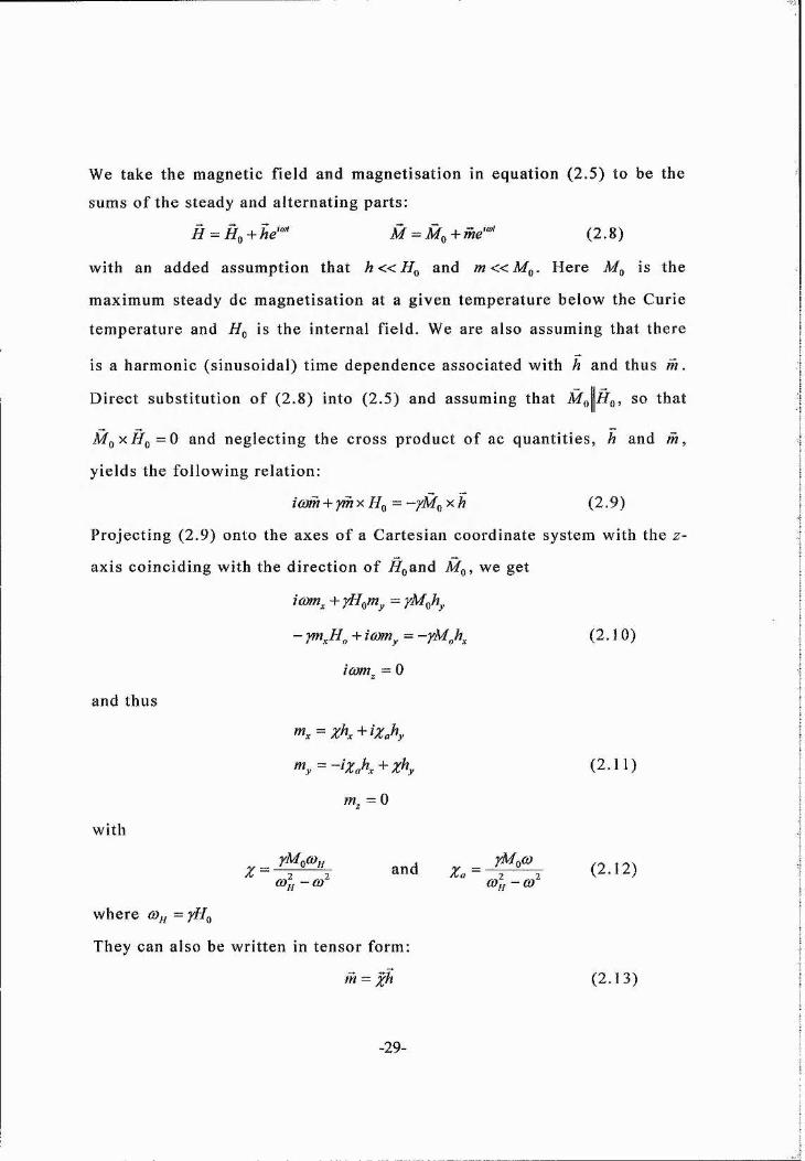
We take the magnetic field and magnetisation in equation (2.5) to be the

sums o f the steady and alternating parts:

H = H^ + he'^ M = M,,+me'^‘ (2.8)

with an added assumption that h « H q and . Here is the

maximum steady dc magnetisation at a given temperature below the Curie

temperature and H q is the internal field. We are also assuming that there

is a harmonic (sinusoidal) time dependence associated with h and thus m .

Direct substi tution of (2.8) into (2.5) and assuming that so that

M qXH q =0 and neglecting the cross product of ac quantit ies, h and rh

yields the following relation:

icoih + phx H q = -yMQxh (2.9)

Projecting (2.9) onto the axes of a Cartesian coordinate system with the z-

axis coinciding with the direction o f J^^and M q, we get

icDtn^ + yH orriy = yMQhy

- ym ^H ^ + icotriy = -y M ^ h ^ (2.10)

i(om„ = 0

and thus

with

% = and (2.12)CDfj - CD ( D f j - C D

where co = yHQ

They can also be written in tensor form:

fh = z h ( 2 . 13)

-29-

where the high-frequency magnetic susceptibility % is a non-symmetric

second rank tensor [9].

X iXa 0%= X 0 (2.14)

0 0 0

The solution (2.11) can also be written in vector form:

w = + (2.15)

where - h - (2.16)

and is the magnetic gyration vector.

In the considered case o f an isotropic and lossless ferromagnet,

magnetised to saturation, the longitudinal component of the ac field,

does not produce any ac magnetisation. However, the transverse ac field,

excites not only the magnetisation component parallel to the field, but

also a component perpendicular to it. Such property of a medium, caused

by the non-symmetry o f the susceptibil ity tensor, is called gyro tropy . It

is observed from figure 2.3, that the components grow without limit when

CO or H approaches the asymptote co = cOq = .

—— X

Xa

( 0 - const

Figure 2.3. D e pendence o f the su s cep t ib i l i t y tensor compo nen ts on s t ea d y

magnet ic f i e l d H q ( f requency is kep t cons tant) [13] .

-30-

This resonant dependence of the tensor results in the phenomenon of

ferromagnetic resonance.

2.1.3. High frequency susceptibilty with damping

Oscillations of magnetisation are accompanied by dissipation o f energy,

which is transferred into other kinds o f energy, mainly thermal energy.

Theoretically, the energy transfer (relaxation) from coherent

magnetization rotation to the thermal bath can occur by interactions with

itinerant electrons, spin waves (magnons), lattice vibrations (phonons)

and crystal imperfections (impurities and defects) [15]. Discussions on the

mechanisms of gyromagnetic damping are found in references [13, 15,

16]. The equation o f motion o f magnetisation (2.5) is modified; such that,

an extra term leading to dissipation should be added onto the right hand

side of this equation [13].

(2.17)dt ' M'

This is the Landau—Lifschitz equation, where A is the dissipation

parameter. This is i llustrated in figure 2.4.

W 7 ,

F igure 2 .4. D a m p ed p r e c e s s io n o f m ag ne t iza t ion vector when there is no h f

f i e l d [1 0 ] .

- 31-

- - - 1 dMIf the term M x H is replaced b y (using the equation of motion

y dt

Zwithout dissipation) and we introduce a dimensionless parameter

then the Gilbert equation is obtained [17,18]:

(2.18)dM w fr (Z= -yM X +dt y

where a is the Gilbert damping factor. The dissipative term in this

equation can be written supposing that an effective field of friction,

proportional to the rate o f change o f M , is acting on M . If one were to

change from (2.17) to (2.18), then one needs to substitute

y . g ocM/ 5T and A - > -------^l+a" 1 + a"

into (2.17). It is clear that when the damping term is far less than unity,

then equations (2.17) and (2.18) are equivalent [13]. One should note that

the LLG equation is only rigorously applicable for the case o f coherent

rotation o f a given unit volume [15].

From section 2.1.2, equation (2.9) is the derived linearisation o f the

equation o f motion. If one were to include loss, then (2.9) is modified and

yields:

_ ictco _ — _icùfh 4- ymxT/qH wx M q = x h (2.1 9)M q

We will use this equation, again, in section 2.1.5. in determining the

resonant condition.

To find the susceptibili ty tensor components in the presence of loss it is

found that the result is the same as replacing by coj^-\-iao).

From (2.12), we directly substitute the term. Thus

= = (2 .20) ( ( D f ^ + i a o ) - C D

- 32-

Similarly X a ^ x 'a - ^ x l

we have

and

X a =

X a =

\o)]f -<î?^(l+a^)f +Aa <D G)]

________laco^&fjMQY________

(2 .21 )

(2 .22)

The dependence of the real and the imaginary parts o f the tensor %

components on H q is shown in figure 2.5. Here, resonance takes place

G>uwhen Û)0.5

0.5

4 620

F igure 2.5. Rea l and im ag inary p a r t s o f the su scep t ib i l i t y te n sor compon en ts

versus H q [13] .

2.1.4. C i r c u l a r po la r i sa t ion of h -f r ad ia t ion

It should also be pointed out that the resonant behavior o f the oscillat ion

amplitudes occurs only under the influence o f an ac magnetic field

circular component with right-hand rotation (relative to the direction o f

M q ) . The circular components o f the susceptibility tensor in the presence

of loss are [13]

YMq

{cDff -\-6))+iaû)( 2 . 23 )

-33-

where %+ and X- are right and left-hand rotation, respectively. If the field

is right hand polarised, then this corresponds to the circular polarised

wave that rotates in the same sense as the precessional motion [13,19].

Thus, %+ + which can be expanded to %+ The

dispersion and absorption components are (x ' + Xa) and

respectively.

Conversely, for left-hand polarisation, which describes the response of the

medium to a circularly polarised magnetic field rotating in the opposite

sense; then the quantit ies x'_ and X- are close to zero, as shown in figure

2.6. The posit ive susceptibil ity has a singularity at û) - g)q whilst X- has

no singularity. 1.0

0.5

0

-0.50.05

0 2 4 6Ho(kOe)

F igure 2.6. Plot s o f the rea l and im aginar y p a r t s o f the s u s c e p t ib i l i t y tensor

versus a p p l i e d f i e l d [ I S ] .

This shows that for FMR measurements, it is the right hand polarisation

that is resonantly absorbed by the medium.

- 34-

2.1.5. Internal fields in ferromagnetics

So far, there has been no discussion o f demagnetising effects, preferred

directions of magnetisation and crystalline imperfections. The resonance

frequency is influenced by all o f these in any real speciman. In practice,

we deal with finite samples and in this thesis, the medium is lossy, with

its thickness small compared with the hf wavelength. The h f magnetic

field inside the sample has uniform intensity, but it is not equal to the

field outside the sample because the normal component o f the

susceptibil ity is discontinuous at the sample’s interface [13]. It is also

difficult, or impossible, to solve the electromagnetic problem for an

arbitrary sample shape.

If we consider a small ferromagnetic ellipsoidal sample in a uniform

magnetic field, the relation between the internal and external magnetic

field is given by

# = = (2.24)

where is the external magnetic field, H is the internal magnetic field,

and M is the magnetisation. Both H and M are uniform i f is uniform

in and near the ellipsoid. N is the demagnetising tensor. The tensor is

symmetric and becomes diagonal when the axes coincide with the axes o f

the ellipsoid. The components o f N in these axes, Ny and are

called demagnetising factors and depend only on the shape o f the ellipsoid

and the sum in cgs units is N^+Ny-yN^ = Atc (in SI units the sum of the

demagnetizing factors is unity) [20]. The quantity is the

demagnetising field. If one were to substitute the ac and dc components of

H and M into the above equation, then

( 2 . 2 5 )

h = h„ ~ Nm

- 35-

Substi tution of equation (2.25) in the linearised equation o f motion (2.19),

from section 2.1.3, gives the following relation:

icom + ymifl^Q - j W g )+ ^-yM ^ xh^Q (2.26)M q

We set the external h f field, and the damping t e r m ,a , to zero. Equation

(2.26) is projected onto the axes o f a Cartesian coordinate system in

which the z-axis coincides with the direction o f M q. The demagnetisation

tensor have, in these axes, the form [13]

Nn ^\2w = ^22 ^23 (2.27)

^32 ^33

When substituted into (2.26), the linearized equation is rewritten as

{io)-\'yN^2MQ)m^ +y (H^q -N ^^M q +iV22-^oVy = 0 (2.28)

- r(^eOz - ^ 33^0 + + # ,2 ^ 0 Wy = 0

which results in an expression for the eigenfrequency:

®o = - N,,M^)jryN^M^)-y'^N^^Ml\^ (2.29)

The maximum absorption o f electromagnetic energy by a small

ferromagnetic ellipsoid takes place at a frequency very near to the

eigenfrequency. This frequency, which depends on the shape of the

sample, is the frequency o f ferromagnetic resonance.

If the external field H^q is directed along one of the axes o f the ellipsoid,

then M q and the z-axis are also oriented along this ell ipsoidal axis. The

tensor N becomes diagonal, and thus in cgs units,

®o = r K o + K + ( i V , (2. 30)

which is Kit te l’s equation [8].

Examples o f the use o f equation (2.30) for three types o f ellipsoid are

tabulated below:

- 36-

Sample Magnetisation

direction

Demagnetising

factor

Eigenfrequency

Infinitely

thin film

Tangential

Normal

0 47t 0

0 0 4 n

Infinite

thin

cylinder

Longitudinal

Transverse

2ii

2 n

2 n

2 n

r )

r )

Sphere 47u/ 3 4 n /3 4 tj:/3= H..

Table 2.1. Set o f FMR cond i t io ns wi th app l i ca t io n o f K i t t e l ’s equat ion. The

re son an t equat ion and d em a g n e t i z in g f a c t o r s are ex p re s se d in cg s units.

2.1.6. Methods of analysis of FMR in anisotropic ferromagnets

The equations o f motion may be expressed in terms o f the total free

energy E instead of effective fields. There are several advantages to the

energy formulation of the equations of motion: first, they are rather

general in form. Second, when the free energy terms are complicated

functions o f angular coordinates, they can be introduced routinely into the

equations. Thirdly, when the easy direction of the various anisotropies

have different orientations, the computations are more straightforward

with the energy equations. One other method that is used to determine the

FMR in anisotropic media is the method o f spherical coordinates proposed

by Smit and Beljers [21] and Suhl [22]. Suppose the magnetisation of

a ferromagnetic speciman has the static equilibrium direction described by

the azimuth % and polar angle 6q as shown in figure 2.7:

-37-

X

Figure 2.7. Sta t i c equ i l ib r ium p o s i t i o n o f magne t i sa t ion.

This method is based on the transit ion from the variables Af^,M^and M^to

the variable 6, (p and where 6 and (p are the angles of M in spherical

co-ordinate system, and is the vector M length. It is assumed that the

magnetization vector has the same length.

From the Landau-Lifschitz and Gilbert relation:

dM iTr TT ^ M x dMdt

(2.31)

where is the effective field and is defined as

dUaM

(2.32)

and U is the total energy o f the system.

Substi tution o f the %,yand z -components of the Heff itvxn into the LLG

will give us

dO _ y dU ay dUdt

d(p

M^ sin^ d(p M^ dO

y dU ay dU

( 2 . 33 )

dt M ^ s i n ^ a ^ M ^sm ^O dç

-38-

For small deviations o f M from the angles ^ and q) o f M, can be

found from the equilibrium conditions

dU ^ a<9

= 0 andy 0=0o,çi=Po d(p= 0 . (2.34)

One has to make sure that the obtained 6q and % values correspond to an

energy minimum. The derivatives

written as

a ^ jlor Ug and dU or U c m be

+ and + (2.35)

and the deviations from equilibrium are defined as

SO(t) = 0 { t ) - d a = ^ ^ '“‘ and Sç(t) = ç(t)-ç>„ = Sç>e"“ (2.36)

Substi tuting (2.35, 2.36) into (2.33), we obtain the linear equations

icD +V M^sin^o M, y

se+ r^M,sin6lo ^ M

ÏÛ)M, sin^o

T/_ + a y

sin Oq-U,. ÔÇ 7

sin^o■U.

5 q ) = 0

a y M, sin^ Or,

(2.37)\

U.0(p <(9 = 0y

where Ugg = uqnp d(pand =

y

^ d^U ^ dOd(p

at equilibrium (where

0 = 0q and ( p - ç f ) .

We can express (2.37) in matrix form, set the determinant of the matrix to

zero and finally gather the real and imaginary components separately, so

that one can obtain expressions [12, 13, 21]:

\ i y M. sin 0,(2.38)

and

39-

Act) = d û ) ^ . a / f

dHAH =

j M , sin cfg )Uoa-^-

sin <9,(2.39)

Equation (2.38) is often called in FMR papers, the Smit-Beljers or Smit-

Suhl equation. This is the resonant condition of an anisotropic elliptical

medium. The equation is strictly valid only for One has to look at

the equilibrium condition and make sure that the applied field is not along

the z-axis, otherwise at saturation, the magnetisation will align with the

field (assuming that the angle between the magnetization and field is

small).

The l inewidth o f resonance is defined by the full width ha l f maximum,

A/T, on the field scale. If a « l , then there is an insignificant shift in the

resonance frequency.

2.1.7. F e a tu re s o f FM R of metals

Previous work on the FMR of linewidth measurements [23, 24, 25] has

related the l inewidth to the intrinsic mechanism (viscous damping) and

the extrinsic mechanism caused by structural imperfections.

There are two main methods which allows one to extract each of the

contributions to the entire linewidth. The first approach entails multi-

frequency linewidth measurements, in which the damping term is

determined from the frequency dependent curve. The frequency

independent term is related to the presence o f magnetic inhomogeneities.

The second approach [26, 27] deals with the dependence o f the field-

swept linewidth A H (at a constant frequency). The dependence of AH on

the angle 6 between the applied field and film normal may be transformed

to the frequency-swept l inewidth (a is the Gilbert damping and y/ y

is the gyromagnetic ratio), which is nearly angle-independent in most

perfect films [28]. Any anomalous increase in is due to two-magnony

- 40-

scattering on defects, which is operative when the magnetisation lies in­

plane. The contributions o f two-magnon process caused by non-uniform

elastic stresses are large in poorly annealed samples [13]. If the

magnetisation is however out-of-plane, then this mechanism is inoperative

and AH {6=0) should be minimal. A mathematical description of two-

magnon contribution in l inewidth measurements in ferromagnetic metals

is discussed in Cochran [23]. In some studies on the FMR linewidth, in

the high frequency limit (assuming that the magnetisation precession is

circular rather than ell iptical), the l inewidth is represented by

Aff(o) = Aff(0)+ — . (2.40)r

For a homogeneous metal, the frequency independent linewidth is

expected to be quite small (of the order o f a few oersteds), it is a

consequence of exchange-conductivity broadening [23, 24]. Two magnon

scattering can also be included in the frequency independent term [29].

Chappert ’s work [30] on polycrystall ine ultrathin cobalt films involved

determining two sources o f the l inewidth, which arises from the spatial

variation o f the c-axis: AiT = A ^ ^ j ( A^^ is the angular spread o f

the c-axis) and the distribution o f internal field: AH = j (Afif,.

is the internal field inhomogeneity).

The resonance lineshape changes i f the sample thickness is greater than

the skin depth. Estimates o f the skin depth for pure metals at 90GHz at

room temperature are shown in table 2.2. However, the granular thin films

for this study have a skin depth greater than the effective sample

thickness [31].

-41

Conductivity at room Skin depthsample temperature {pm)

Iron 1.03 0.52Cobalt 1.60 0.42Nickel 1.46 0.44

Table 2.2: Values o f the skin depth at 90GHz for Pr^l-

It is clear that from many books on the theory of ferromagnetic resonance,

the relative permeablilty o f the sample is not unity when the sample is at

resonance. As a result, from equation (2.41),

^mcjpL(2.41)

the skin depth, which is inversely proportional to the permeabili ty will be

close to zero, since at resonance the permeability reaches a significantly

high value. The samples of interest in this thesis have thicknesses below

the skin depth.

- 42-

2.1.8. Spin Wave Resonance

Kittel [32] suggested that a uniform microwave field should be able to

excite standing spin waves in thin films. In order that microwave energy

may be absorbed, the spins must be pinned at least at one boundary o f the

film. Three cases, figure 2.8, represent (a) complete pinning at both

surfaces, (b) complete pinning at one surface but not at the other surface,

and (c) no pinning at either surface o f the film.

p = 1

pss(l-p P —(1-1)

p«*2

P *(2-p p == (2-1)

p = 3

p«(3-i) p = (3-l)

Figure 2.8. C o m p le te p inn in g at both ends (a), p inning at one end and no t a t

the o ther (b), and no p in n in g at e i ther boundar y o f the thin f i l m (c) [13 ] .

For (a), there will be a net absorption of energy only for modes with an

odd number of half-wavelengths, p = l , 3, 5... For (b), all modes will

absorb energy and for (c), only the uniform mode (k=0) couples with the

microwaves [13].

The resonance condition for standing spin waves for the field normal to

the film surface is

Û) - 4nM + (2.42)r K

If the static field is applied parallel to the film surface, then the resonance

condition is

— = //|[ H--------------iff, 4- AttM 4-------Vr) I MS /V M

( 2 . 43 )

- 43-

where A is the exchange constant (ergs/cm) and where p is the

number of half-wavelengths in the film in the film thickness, Z, and

p=n-S, where n is an integer and ô lies between zero and unity, depending

on the pinning conditions at the boundaries. Examples o f the exchange

constant for nickel and cobalt at room temperature are 0.75x10'^ ergs/cm

[33] and 1.30xl0~^ ergs/cm [34], respectively.

An example o f SWR at 87GHz is shown in figure 2.9. The sample is

lOOnm thick iron thin film.

frequency 87.41GHz

1stiU.M.2nd4th 3rd3(d

I Uniform m ode; S.06T 1st m ode 2nd m ode 3rd m ode 4th m ode

I : 4.98T : 4.83T : 4.62T : 4.31T

01

3 .5 4 .0 4.5applied field (Tesla)

5.0

Figure 2.9. SWR o f i ron thin f i lm a t 8 7 G H z wi th the f i e ld , H, a p p l i e d normal tothe f i lm surface .

2 .2 . FMR spectrometer

2.2.1. 12 Tesla quasi-optical spectrometer

FMR measurements of thin films were measured using an in-house quasi-

optical continuous wave high field 90 to 270 GHz spectrometer [35]

(Some measurements were also performed on a conventional X band

Bruker spectrometer).

- 4 4 -

The cryostat is a vapour shielded Oxford instruments design, capable of

holding 40 litres of liquid helium. It has a 12T superconducting magnet

and its magnetic field homogeneity is one part in 10^ over Icm^. The

cryostat is fitted to an 1TC4 (Intell igent Temperature Controller) , which

allows the temperature to be varied from 2.5K to room temperature. The

cryostat has inbuilt modulation coils which ensure that problems

associated with coil vibrations are minimised.

The spectrometer is controlled and all instruments are interfaced using

LAB VIEW. Conventionally, an FMR spectrum is obtained by slowly

sweeping the dc magnetic field while keeping the mm-wave frequency

fixed. The reflected signal is encoded by simultaneously modulating the

magnetic field and using a lock-in amplifier after detection. The lock-in

amplifier is used to display the spectrum in the derivative mode.

Fig 2.10. Q u a s i - o p t i c a l s p ec t ro m e te r

- 45-

The system is constructed using a reconfigurable “half-cube” system on an

optical bread board and sits on top of a large metal frame that allows it to

be posit ioned over the cryostat. The breadboard may be axially tilted by

four gimbals to give fine adjustment of the alignment of the bread board

over the cryostat.

The sample is inserted into a non-resonant system; that is, there is no

cavity as shown in figure 2.1 1.

ABSORPTION

Fig 2.11. A l inear ly p o l a r i s e d mm -w ave beam t ravel s down a H E n co r r u g a ted

w a vegu ide (a). This l inear p o l a r i s e d beam (b), can also be r e p r e s e n t e d as a left

and r ight hand p o l a r i z e d (LHP, RHP) beam (c). On resonance, only one

c i rcu lar p o l a r i z e d beam is absorbed, t rans ferr ing p o w e r in the or thogon al

l ine ar ly p o l a r i z e d s ta te which is d e t e c t e d in the sp ec t r o m e te r (d) [35 ] .

The W-band Gunn oscil lator has a maximum power output of around

20mW at 94 GHz. FMR signals have not been observed after frequency

doubling or trebling because o f the low power available.

The key advantage of this type of technique is that sample handling is

easier at high frequencies than placing the thin film in a cavity, but even

- 46-

more important, multi-frequency FMR is possible. Multi-frequency high

field FMR offers many practical advantages over low frequency

measurements. In most cases, the sample will be saturated by the dc field,

it is easier to measure extremely broad lines and multi-frequency analysis

and orientational studies can help to evaluate the static and dynamic

properties o f thin films with small ferromagnetic content.

The reason why samples were not placed in a cavity is due to the fact that

at 90 GHz, the sample holder which fits into the cavity has an inner bore

of 0.6mm. This means that the sample needs to be cut in order to fit into

the sample holder, which may give rise to a subtle change to the intrinsic

properties o f the sample. Also, it would be difficult to determine whether

the sample is in parallel or perpendicular configuration. The samples are

also lossy (highly absorbing) and so the signal to noise of the FMR

spectra would not improve greatly in a resonant system.

2.2.2 In-plane sample holder

FMR on thin films were carried out in perpendicular configuration;

however, it is also necessary to measure in-plane to fully characterize the

material. There was no available holder to carry out the latter

configuration so an in-plane sample holder was therefore designed and

constructed in the physics workshop in St. Andrews.

A basic theory of Gaussian Beam Optics [36, 37] was required to

determine the relevant parameters, such as the mirror radius, the distance

between the reflecting mirror and sample mirror and the focusing lens.

Appendix A is a Mathcad sheet which shows the derivation o f the relevant

parameters as mentioned above.

The holder, shown below, was designed to operate at 94GHz and to fit

into a cryostat with a sample bore o f 49mm.

-47-

27mm

C

20mm

27mm35mm

d

15mm

49mm

Figure 2.12. A 94GHz sam ple holder f o r in-plane FMR. The o u te rc a s ing is

made o f tufnol. The HDPE (high den s i t y p o l ye th y l en e ) lens (b) s i t s on top o f the

tufnol cas ing, which fo c u s e s the Gauss ian beam f ro m the wavegu ide (a) onto

the 45 deg re e mir ror (e), which is r e f l e c t e d to the copp er sam ple mirro r (c) and

FM sam ple (d). The FM sam ple is s tuck onto the sample ho lder wi th vacuum

grease .

The sample change over requires lifting the waveguide and the attached

sample holder out of the cryostat. The sample mirror, labeled c in figure

2.12, can be removed and a thin film sample is inserted into the holder.

The sample holder was only ready towards the end of the period when the

work was completed. However, a preliminary example of use is shown in

the next section on FeTiN samples.

-48-

2.2.3. Preliminary experimentsTwo examples are given o f preliminary multi-frequency (75 to 95GHz)

FMR experiments. The results on one sample, a cobalt thin film, are

compared to the known properties of cobalt. The FMR of in and out-of­

plane configurations has been studied on samples o f FeTiN with varying

composit ions o f nitrogen.

2.2.3.1 Cobalt (30nm)

A 30nm cobalt thin film was prepared by MBE at Leeds on a silicon

substrate with a gold capping layer. NMR work on this sample shows the

presence of strains with an admixture o f different cobalt phases: fee and

hep phases [38, 39]. Figure 2.13 i llustrates an NMR spectra o f the sample

at 4.2K.

NMRsignal(nV)

250

hep signal at the domain’s - wall edge at 220 MHz200

fee at 217 MHz

150

hep signal at the - domain’s wall I

\ centre at 227 \ MHz. :

100

200 210 220 230 240Frequency (MHz)

Figure 2.13. Zero f i e l d NMR sp ec t r a o f the coba l t (30nm) thin f i lm at 4 .2 K

s h o w in g the p r e s e n c e o f F C C an d H C P p h a s e s [39 ] .

- 49-

M ulti-frequency FMR on cobalt film at frequencies between 75 to 95 GHz

was carried out with the field normal to the film surface. A typical FMR

signal o f the cobalt sample at 91.25GHz is shown in figure 2.14a and

2.14b.

0.00

-0.04

0.04

0.02

ID 0.00

-0.02

-0.04

4.2 4.4 4.8 5.04.6 5.2Applied field Applied field (te s la s)

Figure 2 .14. F i rs t d e r iva t ive ab sorp t io n (a) and d ispers ion (b) l ineshapes .

The reader should note that obtaining decent FMR signals from the quasi-

optical set-up is time consuming, particularly if one were to carry out

multi-frequency FMR on films with small ferromagnetic content.

A fitting to the lineshape is required in order to determine the resonant

field and the linewidth because it was not always possible to phase the

signal correctly. A fitting package in Easyplot software provides a

Levenberg-Marquardt fit to the data. The equation used is an admixture of

a Lorentzian absorption and dispersion lineshape [40] o f the following

form:

-50-

y{H) =

r \ f \H ^ - H

+ 9b — 3b-AH,

V 2 ) I 2 Jf \ 2"

H ^ - H3 +AH,

< 2 V

+ background (2.44)

where y(H) is the FMR signal, H and H,. are the scanning and resonant

fields, respectively. The coefficients a and b are the amplitudes o f

absorption and dispersion signals, respectively. AiT, is h a lf the peak to2

peak linewidth. In order to test the validity of the above equation, figure

2.14a and 2.14b illustrate the derivative o f an absorption and dispersion

lineshape, respectively. Four repeat measurements on the absorption and

dispersion measurements on the cobalt sample were carried out and a

fitting to the lineshape using equation (2.44) was used and compared.

Lineshape A Lineshape B Difference

(kOe) (kOe) (Oe)

absorption dispersion

Hr 47.37 47.35 13.5

AH,2

0.54 0.54 7.8

Table 2.3. E x t ra c t ed res on an t f i e l d and l inewid th f r o m a f i t to the d ispe rs ion

and a b so rp t io n l ineshape.

The results in table 2.3 shows that the equation used to determine the

resonant field and linewidth is valid.

Appendix B shows a Mathcad simulation of an FMR signal with an

admixture o f absorption and dispersion lineshapes for the field normal to

the plane o f a thin film.

-51

From the fit to the resonant field, it is possible to determine the

spectroscopic splitting factor and the perpendicular anisotropy. Here, the

perpendicular anisotropy is attributed to shape and perpendicular uniaxial

anisotropy (due to crystalline, stress and interface effects on the thin

film) [39, 41]. The resonance condition is given as — = wherer

is the sum of the demagnetising and uniaxial perpendicular anisotropy

[39]. Applying this analysis to the cobalt film, the g-factor is 2.16 ± 0.01

and the effective anisotropy is 17.15 ± 0.20 kOe. I f it is assumed that the

saturation magnetisation for this film is the same as for bulk cobalt

( l7 .6kO e [18]), the crystalline anisotropy field extracted in this way is

0.5kOe. Consequently, the magnetocrystalline anisotropy constant Ku is

deduced to be (3.15 ± 1.45)xl0^ ergs/cc. This value is much less than that

o f bulk hep cobalt, which is typically (3-4)xl0^ ergs/cc at room

temperature [12, 39] and most likely, is a result o f the mixture in the

crystalline phases and the polycrystalline nature o f the sample [41].

Previous measurements showed that torque magnetometry o f the same

cobalt film has a perpendicular anisotropy o f 16.20 ± 0.70 kOe which is

slightly lower than that determined from FMR [41].

2.2.3.2 FeTiN thin films

FeTiN alloys are promising candidates for next generation inductive read

heads due to their high moments and soft magnetic properties (4tvMs = 18

to 21 kOe) [42]. The nitrogen atoms occupy interstitial sites in the iron

lattice and the stability o f the anisotropy upon transverse field annealing

depends on the nitrogen content [43]. Samples with atomic percent

nitrogen less than about 6.5% exhibit stable anisotropy, whilst those

above it are unstable. All samples except for 10 at.% nitrogen have a film

thickness o f 75nm with 3at.% titanium and tantalum capping layer. The

sample with lOat.% nitrogen has a film thickness o f 60nm with

-52-

approximately 3 at.% titanium and no capping layer [43]. This section

does not concentrate on the physics o f these samples, but aims to show

that the magnetic properties o f these films deduced from measurements in

the range 75 to 95 GHz, in perpendicular configuration are consistent with

in-plane and out-of-plane measurements at 94 GHz. These experiments

were designed to test the new sample holder described in section 2,2.2 and

appendix A.

Figure 2.15 is an FMR spectra o f FeTiN with 0 at.% nitrogen. It is

observed that the spectra have lines below the main resonance due to spin

waves. This will be discussed shortly.

S am p le 1 (no nitrogen) a t 76.43 GHz1.0

0.51 St m ode

2nd m ode3rd m ode

m -0.5

- 1.0

-1.54.0 4.2 4.4 4.6

applied field

(xlO kOe)

Figure 2.15. SWR o f FeTi f i l m at 76GHz.

From table 2.4, the spectroscopic splitting factor from both methods is

around that o f bulk iron, 2.09 [18]. In addition, the perpendicular

anisotropy for both types o f measurements almost agree with each other.

The FMR equations for in-plane

Kr )( 2 . 45 )

and out-of-plane

-53-

CO

eff (2.46)

were deduced from (2.38). He// is the perpendicular uniaxial anisotropy,

which includes the shape and crystalline anisotropy.

N itro g e n

con ten t (%)

with sam ple

number in

brackets

Lande g-factor

from in and

o u t-o f-p la n e at

94 GHz

Lande g-factor

from m ulti-

frequency

m easu rem ents

76 - 97 GHz

Perpendicular

anisotropy (kO e)

from in and out-

of-p lan e at 94

GHz

Perpendicular

anisotrop y (kOe)

from m ult i- freq uency

m easurem ents 76

97 GHz

0 (1 ) 2 .0 8 2.11 ± 0.01 18.41 18 .66 ± 0 .3 4

4 .3 5 (2 ) 2 .0 7 2 .08 ± 0 .02 17.97 18 .17 ± 0 .48

5 (3 ) 2 .0 8 2 .1 2 ± 0 .03 17.60 17 .52 ± 0 .3 0

6.5 (4) 2 .0 7 2 .0 9 ± 0 .03 17.22 17 .27 ± 0 .3 7

7 .8 (5 ) 2 .07 2 .0 9 ± 0 .03 15.66 15 .40 ± 0 .47

10 (6) 2 .08 2 .0 7 ± 0 .03 14.51 14 .74 ± 0 .64

Table 2.4. The g -f a c to r and Hg// d e t e r m in e d fr o m the two met hods d i s cu s s ed

above . D e t e r m in in g the er ror f o r va lues in columns two an d f o u r was not

s t r a ig h t f o r w a r d , therefore , a com par i son o f the two p a r a m e t e r s f r o m one

m eth o d to ano ther is required. Note , f o r the two or ien ta t ions at 94GHz, values

o f the p e r p e n d i c u l a r a n i s o t r o p y co in c id e wi th those d e t e r m i n e d f r o m m ul t i ­

f r e q u e n c y measurements .

Samples with 0, 4.35, 5 and 10 at.% nitrogen exhibit spin wave resonance.

It was not possible to determine the exchange constant A (in ergs/cm),

equation 2.42, as this requires knowledge of the sam ple’s saturation

magnetization. However, from another expression,.2a)

rH, D ( (2.47)

the spin wave stiffness constant D, is determined [44]. The spin wave

stiffness constant D for iron is 4.48 x 10'^^ ergs cm^ [44]. From equation

- 54-

(2.47) and figure 2.16 (as an example), the stiffness constant D is close to

bulk iron for mode numbers n = U 2 and 3 for samples listed in table 2.5.

44 -

§43 -

842 -

0 2 4 6 8 10

mode number, n

Figure 2.16. Plot o f the resonant f ie ld (measured from the 0% nitrogen sample) o f lines below the main resonance with the square o f the mode number, n^.

N itrogen Spin w a v e s t i f fn e s s

con ten t (%) con stant (x 10'^^

ergs cm^)

0 3 .50

4 .35 3 .35

5 2 .53

10 3 .90

Table 2.5. Spin wave stiffness constant, D, determined from FMR.

-55-

2.3. References

[1] V.K. A rkad’yev., J.Russ. Phys.-Chem. Soc. Phys. 44 (1912) 165

[2] Ya.G. Dorfman, Zs. f. Phys., 17 (1923) 98

[3] M.S. Akulov, J. Russ. Phys.-Chem. Soc. Phys., 58 (1926) 577

[4] E.K. Zavoiskii, J.Phys. USSR 10 (1944) 197

[5] J.H.E. Griffiths, Nature, 158 (1946) 670

[6] L.D. Landau and E.M .Liftschitz, Phys. Zs. Soviet Union 8 (1935) 153

[7] C. Kittel, Phys. Rev., 71 (1947) 270

[8] C. Kittel, Phys. Rev., 73 (1948) 155

[9] D. Polder, Phil. Mag. 40 (1949) 99

[10] S.V. Vonsovskii, Ferromagnetic Resonance, Pergamon, Press, New

York, 1966

[11] A.H. M orrish., The Physical Pr inc ip les o f Magnetism, Wiley, 1964

[12] D. Craik., Magnetism . Pr incples and Applications, Wiley, Chichester,

1995

[13] A.G. Melkov and G.A. Gurevich, M agnetisation Osc illations and

fVaves, CRC Press, 1996

[14] J.M. Luttinger and C. Kittel., Helv. Phys. Acta., 21 (1948) 480

[15] M.L. Plummer, J.van Ek and D. Weller, The Physics o f Ultra-H igh

Dens ity Magnetic Recording, Springer-Verlag, New York, 2001

[16] R. Urban, G. W oltersdorf, B .Heinrich, Phys. Rev. Lett., 87 (2001)

217204

[17] T.L. Gilbert, Phys. Rev. 100 (1955) 243

[18] S. Chikazumi, Phys ics o f Magnetism, John Wily and Sons, Inc (1964)

[19] B. Lax and K.J. Button, Microwave Ferrites and Ferrimagnetics,

McGraw-Hill, New York, 1962, Chap 4.

[20] J.A. Osborn, Phys. Rev., 67 (1945) 351

[21] J. Smit and H.C. Beljers, Philips Res. Rep. 2 (1955) 113

[22] H. Suhl., Phys. Rev. B. 97 (1955) 555

-56-

[23] J.F. Cochran, R.W. Qiao and B. Heinrich, Phys. Rev. B. 39 (1989)

4399

[24] B. Heinrich, in Ultrathin Magnetic Structures II, edited by Heinrich

amd J.A.C.Bland.,Springer, Berlin, 1994, Chap 3.

[25] F. Schreiber, Z.Frait, Solid State Commun., 93 (1995) 965

[26] M. Farle, Rep. Prog, Phys. 61 (1998) 4344

[27] H. Hurdequint, J. Magn. Magn. Mat., 242-245 (2002) 521

[28] R.D. McMichels, M.D. Stilles, P.J. Chen, W.F. Egelhoff, J. Appl.

Phys. 83 (1998) 7037

[29] J.F. Cochran, R.W. Qiao, B. Heinrich, Phys. Rev. B., 39 (1989) 4399

[30] C. Chappert, K.Le Dang, P. Beauvillain, H. Hurdequint, D. Renard,

Phys. Rev. B., 34 (1986) 3192

[31] P.C.Riedi, p r/va /e commun ications, 2002

[32] C. Kittel, Phys. Rev., 110 (1958) 1295

[33] S.M. Bhagat and L.L. Hirst and J.R. Anderson, J. Appl. Phys., 37

(1966) 194

[34] P.E. Tannenwald and R. Weber, Phys. Rev. 121 (1961) 715

[35] G.M. Smith, J.C.G.Lesurf, R.H.Mitchell and P.C.Riedi, Rev. Sci.

Instrum. 69 (1998) 3924

[36] P.F. Goldsmith, Quas i-optical Systems: Gaussian Beam Qausioptical

Propagation., IEEE Press/Chapman and Hall Publishers, 1998

[37] J. Lesurf, M illimetre-Wave Optics, Devices and Systems, Adam

Hilger, Bristol, 1990

[38] P.C. Riedi, T. Thomson and G.J. Tomka, NMR o f Thin Magnetic

Films and Superlattices, Handbook o f Magnetic Materials 12 (1999),

edited by K.H.J.Buskow, Elsevier Science, B.V., 1999, Chap 2.

[39] C.J. Oates, F.Y. Ogrin, P.C. Riedi, S.L. Lee, G.M. Smith, T.

Thomson, J. Magn. Mag. Matt. 242-245 (2002) 402

[40] C.P. Poole, Electron Spin Resonance — A Comprehensive Treatise on

Experimental Techniques, Wiley, New York, 1967.

- 5 7 -

[41] F.Y. Ogrin, S.L. Lee, Y.F. Ogrin, J. Magn. Magn. Mat., 219 (2000)

331

[42] C. Alexander Jr., IEEE Trans. Magn. (2001) In press

[43] C. Alexander ix., pr ivate com mun ications,2001

[44] A. Butera, J.N. Zhou, J.A. Barnard, Phys. Rev. B, 60 (1999) 12270

- 58-

Chapter 3

FMR and torque magnetometry of high and low

noise CoCr alloy longitudinal recording media

3.1 Introduction

This chapter, which is in two parts , centres on CoCr alloys longitudinal

recording th in films. The first h a lf looks at how it is possib le to

determ ine the magnetic charac te ris tics o f recording m edia with high

field FMR, w ithout in troducing m icrom agnetic and/or m ean field

sim ulations, fo llowed by corre la ting these charac te ris tics to their

recording properties and com paring the anisotropy field derived from

torque m agnetom etry m easured in Seagate with that o f FMR, in St.

Andrews. The second part o f th is chapter examines low fie ld torque

m agnetom etry as a technique to m easure exchange and/or dipole

in teractions and the anisotropy. Both the technique and sim ulation o f

results will be presented.

The sam ples are o f two types: h igh and low noise m edia, the difference

being attribu ted to the ir d ifferen t grain size and grain size

d is tribu tions . This is d iscussed again in section 3.2.2.

3.2 Ferromagnetic resonance

3 .2 .1 S u m m a r y o f p r e v io u s w o r k s on the F M R o f C o C r - a l lo y

r e c o r d in g m e d ia

The firs t group to m easure the in-plane uniaxial aniso tropy o f planar

random polycrysta lline grains CoCrPt longitudinal recording m edia was

that o f Igarashi et al [1]. The com position o f the m edia concerned was

5 9

30nm CoCrPt/lO nm CrTiB/10 nm Ta/32nm Zr and was dc m agnetron

sputtered onto a glass substrate . In their experim ent a h igh-in tensity

m agnetic field was applied normal to the film surface at frequencies 71

and 117 GHz, figure 3.1. As w ill be seen in figure 3.1, the signal to

noise was very poor in th is experim ent.

OOP 31.0 kOa

23 28H(kOe)

33

48.0 k

41.7 kOt

H (kOe)Figure 3.1. FMR absorption spectra o f the polycrystalline CoCrPt thin film

at 70.51 (a) and 116.8 GHz (b) [1].

The group carried out m icrom agnetic sim ulations (based on the

Landau-L ifschitz-G ilbert equation) and confirm ed tha t m agnetic

(exchange and/or m agnetosta tic ) interactions and the uniaxial

anisotropic field d is tribu tions had very little e ffect on the resonant

field in the configura tion used. The im portan t physical param eters that

affect the recording perform ance were estim ated using the linew idth o f

the FMR spectra for d ifferen t frequencies with the aid o f

m icrom agnetic sim ulations. From the s im ulation, they deduced the

uniaxial anisotropy and its d ispersion to be 7.0 ± 0.2kOe and 1.2 ±

O.SkOe, respectively; the G ilbert dam ping constant a as 0.03 ± 0.01

and the Lande g-value o f 2.19 ± 0.02 which is in the reg ion o f bulk

cobalt, 2.18 to 2.25 [2,3]. The s im ula tion agreed very well with the

results ob tained from the resonant field m easurem ents. The FMR

equation, which they used for obtaining the g-factor and uniaxial

anisotropy is used in this chapter and a section on the deriva tion o f the

resonant condition is d iscussed in 3.2.3.

- 60 “

The group also deduced (from the ir s im ulations) that the linewidth o f

the FMR spectra becomes large o f the order o f exchange in teraction ,

d ispersion in the uniaxial aniso tropy and the Gilbert dam ping constant.

Another group, w hich m easured FMR o f m aterials o f in terest for m edia

thin films was Inaba et al [4]. Here, they looked at the G ilbert damping

constants o f single crystal CoCrTa and CoCrPt thin films by Q-band

FMR with the high fie ld applied w ith in the film surface. The samples

were ep itax ially grown on MgO (110) substrate with the HCP c-axis in ­

plane and parallel to MgO [001]. From the FMR m easurem ents, they

showed that the dam ping factor, a , o f Co7?Cri9Ta4 increased from

0.016 to 0.028 w ith respec t to its film thickness, as il lu s tra ted in figure

3.2.

0.04

0.02

0 100 200 300Mangetic Layer Thickness, tmag, (nm)

Figure 3.2 Variations o f resonance magnetic field, anisotropy field, linewidth and damping constant with magnetic layer thickness ranging from 25 to 240nm [4].

-61

The group believes that an increase in a is likely to be caused by eddy

current losses induced in the film when a high frequency m agnetic field

is applied.

When the Cr concentra tion in the 60nm thick Co96-xCrxTa4 magnetic

layer is increased from 8 to 19 at.%, the damping factor increased from

0.009 to 0.019. They also found that the damping factor in 25nm thick

Co8iC r i5P t4 film is 2.5 tim es larger (0 .038) than the C o8iC risT a4 film

(a = 0.014) w ith the same th ickness . The group concluded that the

d ifference in a between the CoCrTa and CoCrPt films may be related to

the po larisa tion o f p la tinum in the CoCrPt layer.

3 .2 .2 H ig h and low n o is e r e c o r d in g m ed ia

The two samples were dc m agnetron sputtered on a super-sm ooth glass

ceram ic substrate by Seagate Technologies in California. The m agnetic

layers o f both media were sputtered from the same CoCrPtTa alloy

target. The underlayer o f the 2D in-p lane isotropic m edia consisted o f

50nm th ick CrM n for m edia A and 40nm /10nm th ick N iA l/C rM n for

m edia B, as shown in figure 3.3. Both types o f m edia were processed

under identical deposit ion conditions , including substrate heating,

sputtering gas pressure and deposit ion rate. The th ickness o f the

recording th in film for both m edia is 27.5 ± 0.5 nm. These films had

very d ifferen t record ing perform ance, grain size and grain size

d is tr ibu tions , but s im ilar m agnetic p roperties [5,6].

- 6 2

.J

M edia A M edia B carbon overcoat

recording layer 27.5nm

CrMn underlayer 1 Onm

NiAl underlayer 40nm

Glass substrate

High noise Low noise

Figure 3.3. L a yo u t o f two thin f i l m media.

The mean physical grain size was obtained from TEM by Seagate

Technologies as shown in figure 3.4. M edia A (sample 15A) has a wide

d ispersion o f grain sizes ranging from 20 to 200nm. The large regions

appear to be com posed o f sm aller sub-grains. To a first approxim ation ,

the mean size o f these regions is o f the order o f 50nm. Media B

(sam ple 15B) has a grain size o f 17 ± 1.5nm [5].

r .Jm»/

1 GOnm

Figure 3.4. TEM im age o f low (a) an d high n o is e (h)

( c o u r t e s y o f Yen et a l ) [ 5 , 6 ] .

63 -

Yen [5] and Laidler [7] found that the magnetic thin films sputtered

onto the glass ceram ic substrate when CrMn is used as a single

underlayer possessed high medium noise. This is absent from otherwise

identically sputtered m edia with a N iAl/CrM n double underlayer

structure.

M agnetisation m easurem ents, figure 3.5, were measured using a non­

destructive Seagate ro ta ting disk m agnetom eter at room tem perature.

The saturation m agnetisa tion was m easured with the field in the plane

o f the sample. Hysteresis plots o f the high and low noise media are

shown in figure 3.5. The saturation m agnetisa tion was found to be 4.87

± 0.10 kOe and 4.47 ± 0.09 kOe for the high and low noise media,

respectively [6]. The uncerta in ty in the saturation m agnetisa tion arises

as a com bination o f errors: the m easured total m agnetic moment,

m agnetic layer th ickness and sample area; for example, the high noise

m edia has a moment, (209 ± 1) pemu, with a film area o f 19.6 ± 0.2

mm^; sim ilarly for low noise media, the moment size is (192 ± 1)

pemu, with the same film area.

0.0003

0.0002

0.0001

-20 XX) -10 XX) 1(XKX)ÿ -0.0001

ra -0.0002

-0.0003

Applied field (Oe)

0.0003

00002

- 10)00

~ *0.0003- Applied field (Oe)

A BFigure 3 .5 . H y s t e r e s i s o f low (A) a n d high (B) no ise m ed ia [6 ] .

The anisotropy field o f the low and high noise media was measured

using a DMS model 800 com bined VSM /torque m agnetom eter at room

tem perature in Seagate. The angular dependence o f the torque was

- 64 -

m easured in an applied fie ld o f 13 kOe at room tem perature and the

resu lting data fit ted to a uniaxia l anisotropy model contain ing a

constan t term Ko, a term in Kjs in^ and a term in K 2Sin'^, K 2 was found

to be neglig ib le a llow ing the an iso tropy to be determ ined solely from

K i . The anisotropy field was subsequently calculated using H k^2K j/M s.

Torque m agnetom etry m easurem ents o f both the high and low noise

m edia gave a value o f 9.65 kOe for the m agnetocrysta lline anisotropy

[6 ,8].

3 .2 .3 M o d e l l in g

The h igh field FMR data o f the recording m edia is m odelled as non­

in teracting HCP cobalt grains w ith the c-axis d is tr ibu ted randomly

w ith in the film plane. We will look at the general case where the c-axis

o f the HCP grain is at an angle p re la tive to the x-axis as il lus tra ted in

figure 3.6.

recording film surface HCP

c-axis

X

Figure 3.6 Longitudinal recording thin fi lm with the c-axis o f one o f the HCP grains, which lies within the film surface at an angle p relative to the x~axis.

6 5 -

A ctually , the deriva tion o f the FMR condition below, w hich is in

spherical po lar coord inates , shows tha t for any value o f p the resonant

frequency is exactly the same. This is true for the case for an applied

field , w hich is directed perpendicu lar to the film surface.

We consider the total energy o f the system; that is, the sum o f the

Zeeman in teractions, m agnetocrysta lline and shape anisotropy. The

exchange energy is not included as it is assumed that for high field

FMR (around 40 kOe w ith the mm -wave frequency set to 90 GHz) the

neighbouring grains are decoupled from exchange in teractions. The

total energy o f each grain is:

^T ota l ^Zeeman ^anisotropic ^shape (3 1)with the Zeeman energy given as

^Zeeman = 6 cos(^^ - ^)sin 0 1 + cos<9 c o s ) (3.2)

the dem agnetis ing con tribu tions due to d ipole-d ipole effects is

^ shape = sin^ <9sin^ Ç9 (3.3)

and the in-plane uniaxial anisotropy is expressed in the form

(3.4) j

where a is the angle betw een the c-axis of the hep grain and the

m agnetisa tion , M. Hence the an iso tropy is re-w ritten in term s o f the

polar and azim uthal angles as

^ a ,,M o p y = (1 - S in ^ 6» COS V COS V - i

o . 7 1 . (3.5)cos ^sin p ~ —s in 2 ^ s in 2 p c o s^ )

IThe c-axis was random ly oriented w ith in the film plane and the |

un iax ia l aniso tropy o f each grain is considered to be j

m agnetocrysta lline [6].

M inim izing the energy w ith respect to the polar and azim uthal angles

defines the m agnetisa tion ’s equilibrium position (provided that the

- 66 -

double derivative o f the energy w ith respect to the polar and azim uthal

angles is greater than zero).

= - M H (cos 6 cos {(Ph ~ Ç^)sin 9 - sin $ cos 93 9

I ttM ^sin 29 ~ (3.6)

(sin 29 cos cp cos - sin 2^ sin /? + cos 29 cos ^ sin 2 p )

and

3E.,'Total

3(p

K

~MH{ûn9ûn(<p^ -ç?)sin6^^)+2;zM^ sin^ ^ sin 2 ^ +

r 1 \sin^ 9 sin 2cpcos^ pA— sin 2 9 sin ç?sin 2 p

(3.7) ^s in 2(pcos^

V y

and that

^ ^Total I ^ Q ^ ^Total

l =0.<!'=P0> 0 and

P=Po

^ ^ Total ^ ^ ^Total ^ ^Total / o n

Since the dc field is applied normal to the film plane, a tr iv ia l solution

to the static equilibrium position o f the m agnetisation is given by

7C9 ,j = — i f p = 0 and thus <p is given by

(3.8)

Otherwise one would employ an ite ra tive procedure such as the N ewton

Rhapson m ethod in order to determ ine individual values o f $eq and (peq

for corresponding values o f p.

Figure 3.7 shows the equilib rium angle (peq with respect to H, the

applied field, for d ifferen t values o f the uniaxial an iso tropy field. The

saturation m agnetisa tion is f ixed to 4 .90 kOe and the angle between

the c-axis o f the HCP grain and the x-axis , is set to zero.

■67 -

0

ta1

100 T

A p p lie d f ie ld (x lO kO e)

Figure 3.7. A plot o f the moment's equilibrium position, q>eq in degrees, fo r

different values o f the uniaxial anisotropy.

If the in-plane uniaxial an iso tropy is varied from 10.0 kOe (red line) to

20.0 kOe (blue) to 40.0 kOe (m agenta) then a m uch larger fie ld is

required to orient the m om ent from in-plane (easy axes) to out-of-p lane

(normal to the film plane). The poin t at which the angle o f orien ta tion

o f the m om ent is norm al to the film surface (labelled X, Y and Z on

figure 3.7) occurs when the applied field is equal to the sum o f the

dem agnetis ing field and the in-p lane uniaxial anisotropy field.

It was assum ed in th is calcu la tion that there are no exchange

in teractions between the grains, w hich may not be va lid at lower fields.

There is an added assum ption that the sample is a perfect longitudinal

record ing media: one w ith no out-of-p lane deviation o f the g ra in ’s c-

axis.

From the Sm it-B elje r’s equation (2.38) [9]:

- 6 8

d ^E f d ^E '12 >

j M sin 0 , d<p^ ^dffdip ^ J( 3 . 9 )

it is c lear that double and partia l derivatives are required in order to

fully determ ine the resonant condition. Note that for perpend icu lar

FMR, the sine term in the denom inator must be non-zero. We are also

assum ing that the con tribu tion from the damping factor in the above

equation is negligible.

Total

09'= MH (sin 6 c o s - ^ )s in + cos 9 cos 9 j )+

cos 29 sin^ ^ - 2K^ ^cos 29 cos^ (p cos^ p - cos 29 sin^ p - sin 29 cos ^ sin 2 p

and

Total

dtp"= MH{sin 9 ~ 9))sin 9 j )+

AttM^ sin^9 cos2cp + K \ 2 sin^ 9 cos2(pcos^ p + —sm 2 9 cos^s in2/7

and

Total M //(cos 9 sin 0 sin(ç7 - cpj )) + 2;rM^ sin 29 sin 2(pd6d(p

x(sin 26 sin 2<p cos^ p + cos 29 sin (p sin 2 p )

+

(3.10)

(3.11)

(3.12)

Equations (3.10) to (3.12) are substitu ted into the S m it-B elje r’s

equation, which results in the general resonant condition.

Y{MHifixxÔQ cos(%; - %)sin6^ + cos o cos^^) + ^

^^0082^0 cos^ % cos^ p - z q s IO q sin^ p

sin 2^ cos^o sin2/7

1M sin &

^7M^ cos2^o sin % - 2E„JJ

Affl(sin(9o cos(^^ - %)sin6^) +

1 .sin^ (9o cos2ç?o + E , 2 sin^ 6 cos2% co ^ /? + - sin2^o cosg% sm 2p

V 2

( M H ^ osOq s i n ^ sin(% - % ) ) + Ird t/f sm2^o

(^E„(sin2<9o sin 2% cos^ p + c o s 2 ^ sin% sin2/?)

( 3 . 13 )

- 69 -

Thus, for high field FMR and from figures 3.5 and 3.6 where both the

7tequilibrium angles 0^ and is equal to — (for perpendicu lar

configura tion), the resonant condition is given by

- 1 = - A tM - H A (3 .14)\ 7 )

where Hr is the resonant field. This is the same equation derived by

Igarashi and N etze lm ann [1,10]. Regardless o f what value p takes (the

angle w hich the g ra in ’s c-axis subtends relative to the x -axis), the

resonant condition is still the same, as shown in appendix C. From

geometry, this is obvious as the axis o f symmetry is norm al to the film

plane.

3 .2 .4 E x p e r i m e n t a l set up and resu l t s

The thin film is sandw iched betw een the waveguide and the sample

holder so that the m m -wave is t id ily focussed onto the sam ple w ithout

scattering o f the m m-wave from the sample edge.

At the time o f m easurem ent, the sensitiv ity o f the spectrom eter at 180

and 270 GHz was insu ffic ien t for FMR; hence, m easurem ents were

confined w ithin the 75 to 95 GHz range at room tem perature, figure

3.8. M ulti-frequency FM R w ith in the range o f in terest was necessary in

order to determ ine the three in tr insic properties o f the record ing media.

Because we were res tr ic ted to a small range o f frequencies, it was

necessary to carry out m ultip le m easurem ents at each frequency.

-70 -

-0.003

■9 -0.004

-0.0053.3 3.6 3.9 4.2

Applied field (tesla)

Figure 3.8. Typical FMR spectra with a f i t t ing to the lineshape using equation 2.44 from section 2.2.3.1.

Sim ilarly to the cobalt th in film m easurem ents, there were problem s in

the phasing o f the FM R signal. A gain, absorption and d ispersion

lineshape fitting was inc luded to determ ine the re levant features o f the

spectra.

3.2.4.1 Static properties

Since the s ignificant error in our m easurem ents comes from the values

o f the field for resonance, equation (3.14) is re-w ritten as

H,. + (3.15)2 V ^ y

From the resonant cond ition over the range 75 - 95 GHz, it is not

possib le to determ ine the indiv idual values o f the Lande g-factor,

saturation m agnetisa tion and m agnetocrysta lline an iso tropy uniquely;

this is a lim ita tion inheren t to high fie ld FMR. The app lication o f non-

- 71 -

linear regression m ethod to equation (3.15) showed that w hile the sum

for 15A and 15B is 9.75 ± 0.75 kOe, a range o f values o f

4tvMs and H k will lead to an equally good fit to the data. A b inom ial

expansion o f equation 3.15 will give a linear and non-linear term. At

higher fields, the non-linear term is very small but necessary in order

to accurate ly determ ine the m agnetic parameters.

From (3.15), one obtains

rSince we are dealing w ith high frequency m easurem ents, the term —0)

will tend towards zero, thus the whole expression for the resonant field

becomes linear,

+ ^ + - (3.16)2 r

(Note tha t in X and Q band FMR the non-linear term becomes

im portant and values o f the g-factor, saturation m agnetisa tion and the

mean uniaxial an iso tropy may be obtained. Ftowever, the whole point

o f our exercise is to work at high field so that the in teractions betw een

the grains are decoupled.)

Figure 3.9 shows the V -shaped valley o f the possible sets o f solutions

found by X-Y non-linear regression fits to the data for sample 15A

(high noise media), for a given g-value o f 2.16. The z-axis is the mean

square error o f the d ifference betw een the calculated and experim ental

values o f the resonant field (for sample 15A), in oersteds. It is c lear

that the sm allest residual is about 40 Oe for a wide range o f values o f

the dem agnetising fie ld and the uniaxia l anisotropy field separately.

72 -

400013000

m m

Hk (Oe)

1 2 0 0 0I 1000 5000

10000 4500

6000

5500

9000 4000 4tiMs (Oe)

Figure 3.9. V -s haped p r o f i l e o f the p o s s i b l e s e t o f s o lu t io n s wi th the g-

va lue s e t to 2 .16. N ote the d i f f e r en ce d o e s not take into c o n s i d e r a t i o n the

e r r o r o f ea ch f i e l d po in t .

To overcom e this problem it is clear that another technique is required

in order to determ ine one o f the param eters: this is the saturation

m agnetisa tion , which is described in section 3.2.2.

Figure 3.10 is a plot o f the resonant field to the m m -wave frequency

for the high and low noise media, which is fitted to equation 3.15 in

order to solve the g-fac tor and m agnetocrysta lline an isotropy (for a

given value o f the sam ple ’s saturation m agnetisation).

- 73 -

»— low no ise m edia '>— high noise m edia

90

85

7035 36 37 38 39 40 41 42

resonant field (kOe)

Figure 3.10. Plots o f the resonant field, fo r samples 15A and 15B, against the frequency o f the mm-wave.

A summary o f the results is shown in table 3.1.

Types o f (VSM) Lande g-factor Mean H k (kOe)

noise m edia FMR Torque

m agnetom etry

High noise 4.86 ± 0.10 2.16 ± 0.01 10.85 ± 0.20 9.65

(15AJ

Low noise 4.47 ± 0.10 2.17 ± 0.01 10.73 + 0.20 9.65

(15B)

Table 3.1 Magnetic properties obtained from TM, VSM and high f ie ld FMR.

From the resu lts , there is not m uch difference in the anisotropy

between the two m edia samples. At lower fields, the exchange

in te rac tion can play a s ign ifican t role in the collective behav iour o f the

m agnetic grains. In the m agnetisa tion or torque m easurem ents this may

- 74 -

be seen as an effect o f the reduced anisotropy field as observed in

section 3.2.2 [1,7]. At high field , however, the effects o f coupling are

not s ignificant as the sample is com pletely saturated and the resonance

is only due to the uniform precession . As a result, the h igh fie ld FM R

m easurem ents dem onstrate the h igher value o f H k> Consequently , the

presence o f the d ifference between the anisotropy field values from the

two techniques is a good ind ica tor o f the presence o f exchange

coupling.

3 .2.4.2 D ynam ic p ro p e r t ie s

The G ilbert damping factor o f both m edia was derived from equation

(2.39) [11]. Here, we directly substitu te (3.13) into (2.39). The

71equilibrium angle 0^ is taken to be — for magnetic fields above 20kOe

and applied norm al to the film surface. The p recession o f

m agnetisa tion is assum ed to be circular. As a result, the Gilbert

damping term is determ ined from

(3.17)

The factor o f V3 arises due to the fact that the signal is recorded as

the first order derivative o f the lineshape and the ratio o f the

Lorentzian linew idth FWHM and derivative peak-peak linew idth is V3 .

From figure 3.11, a fit to the linew idth using 3.17 enables one to

determ ine two features: G ilbert dam ping factor and the inhom ogeneous

broadening where the la tter is determ ined from the linew id th in tercept,

as d iscussed in section 2.1.7. Table 3.2 presents resu lts for both

sam ple’s dynamic properties .

•75 -

o

1.1—©— high noise media —o— low noise media1.05

1

0.95

0.9

0.85

0.8

0.7570 75 80 85

mm-wave fiequency(GHz)

90 95

Fig 3.11. A f i t to the measured line width fo r (a) low noise and (b) high

media noise.

Types o f m edia G ilbert damping Inhom ogeneous

factor broadening (kOe)

High noise (1 5A) 0.025 ± 0.003 0.15 ± 0.08

(0.027 ± 0.003) (0.13 ± 0.08)

Low noise (1 5B) 0.016 ± 0.002 0.36 ± 0.07

(0.017 ± 0.003) (0.32 ± 0.11)

Table 3.2 Dynamic properties o f high and low noise media. The values in brackets were deduced from the average linewidth at each frequency.

It is clear that from table 3.2, the values o f the G ilbert damping term , a

lie w ith in those quoted from previous work, typically betw een 0.01 and

0.04 [1,4,12].

- 7 6 .

3.2.5 Conclusions

From tables 3.1 and 3.2, it appears that there is little d ifference in the

static and magnetic properties o f the high and low noise m edia

samples. The crystalline aniso tropy o f the low and high noise m edia is

10.73 ± 0.20 and 10.85 ± 0.20 kOe, respectively. H owever, it is clear

tha t the G ilbert dam ping and inhom ogeneous broadening term s, which

characterises the dynamic response are s ignificantly d ifferen t. The

inhom ogeneous term for the low noise m edia (0.36 ± 0 .0 7 k 0 e ) is more

than tw ice as much as the high noise m edia (0.15 ± 0 .0 8 k 0 e ) . The

G ilbert dam ping term for the h igh noise media (0.025 ± 0.003) is

h igher than the low noise m edia (0 .016 ± 0.002).

The low noise m edia is com prised o f sm aller grains w ith be tter grain

segregation than that o f the h igh noise media. This segregation leads to

better iso la tion o f the m agnetic m oments and hence reduces the

exchange coupling betw een the grains. C onsequently , the

inhom ogeneity o f the m edium is grea ter as a result o f a larger num ber

o f spins in d ifferen t local m agnetic environm ents which is reflected in

the value o f AHpp(0){6,\l>^. Lower exchange coupling contributes to

reduced noise in the case o f the m edium with sm aller grains [6]. This

in terpre ta tion is supported by the values o f the G ilbert dam ping factor.

For the sample with larger grains (high noise medium) the damping

factor is greater. The fas tes t re laxation time would occur for critical

damping where the G ilbert dam ping fac tor is unity [3], thus the sample

with larger grains has a fas ter re laxation time. This faster re laxation

time may again be as a resu lt o f stronger in tergrain coupling in the

high noise medium. It is clear that more work is required in order to

back-up our suggestions.

■77 -

3.3 Torque magnetometry

3.3.1 IntroductionThe torque section is sp lit into two parts: the first part provides a

m ethod o f de term ining the un iax ia l aniso tropy o f the h igh and low

noise media. It is based on the c losing point m easurem ents, w hich is a

process o f re la ting the com pleted magnetic moment reversa l at a

certain field and angle to the m agnetic g ra in ’s aniso tropy and

m agnetisation .

The final part concerns an a lternative , but sim ilar method, to A M

m easurem ents. Using th is technique, the progress o f m agnetisa tion

reversal is compared for the sample having the m agnetisa tion in the

m axim um rem anent state (m agnetised) and in the zero rem anent state

(dem agnetised). Using the fact tha t for non-in terac tive m edia [14],

both processes are equivalent, a deviation from zero is then taken as a

resu lt o f in teraction betw een the mom ents. This m ethod has been

shown to be useful for s tudying dipole-d ipole and exchange

in teractions in particu la te and polycrysta lline media. In section 3.3.4,

this m ethod is applied to torque m agnetom etry so that in tergranular

coupling in longitudinal record ing m edia is measured. M icrom agnetic

s im ula tions and experim ental data carried out on the low noise media

will be shown in section 3.3.4.

The author feels tha t Dr. Feodor Ogrin and Professor Stephen Lee

should be acknow ledged at the start o f this sub-chapter since they

developed the theory behind the c losing po in t and A T m ethod. Dr.

O grin also carried out m icrom agnetic s im ulations, as d iscussed in

section 3.3 .4 , and fits to the data. Throughout this chapter, Dr. Ogrin

and Prof. Lee are often re ferenced as [15], as part o f private

com m unications. The au th o r’s con tribu tion in this p ro jec t was to carry

out the torque m easurem ents for the c losing point and A T m ethod.

- 78-

3.3.2. Torque magnetometry

Torque m agnetom etry is ideal for anisotropy m easurem ents. In

ferrom agnetic thin film s, this an isotropy results from intrinsic

(crysta lline) and shape anisotropy. The torque m agnetom eter, in St.

Andrews, that was used for recording media m easurem ents is

illustra ted below.

Figure 3.12. In-house to r q u e m a g n e t o m e te r which has a c a p a c i t a n c e

d e t e c t i o n sy s tem .

The ferrom agnetic thin film is attached to a cantilever using a mixture

o f Bostik glue and acetone. The m agnetom eter has a detection system

that is based on can tilever techniques, which is operated in capacitance

mode. (Both the capacitance plates and the cantilever were made from

phosphor bronze.) The can tilever is caused to deflect through tiny

dis tances in response to the torque exerted on it, which results in a

varia tion in capacitance between the cantilever and the fixed

capacitance plates. A typical noise level detected is one m icrovolt.

Prior to torque m easurem ents, the voltage across the capacitance bridge

was balanced to zero for zero deflection .

-79-

The canti lever is inserted into an orange cryostat , supplied by A.S.

Scientif ic products Ltd, which was mounted on a ro tation rig, which

allowed the cryostat and therefore the cant i lever to be rotated 360

degrees in the horizonta l plane re lative to a fixed field direction. The

field could also be swept through a field range o f 9.6 kOe and

temperatures as low as 1.4K could be attained.

3.3.3 Closing point measurements

The closing point can be def ined as the last point in the magnetisa tion

reversal , as i l lustrated in figure 3.13. The ‘markers ’ (orange arrows) of

the closing point are from the moments whose easy axis is

perpendicular to the di rection o f the applied field [15].

H C H

Fig 3.13. C o n s i d e r a ra n d o m d i s t r i b u t io n o f momen ts w here each moment

has an e a s y axis. For c a s e (A), a s m a l l f i e l d is a p p l i e d a n d the m omen ts

f r o m the g r a in s w hose e a s y axi s a re e i th e r p a r a l l e l or a n t i - p a r a l l e l to the

f i e l d s t a r t to r o t a t e t o w a r d s tha t f i e l d . The momen ts w ho se e a s y ax es were

i n i t i a l l y a n t i - p a r a l l e l (or a t an an g le g r e a t e r than n in e ty d e g r e e s ) to the

f i e l d d i r e c t i o n then i r r e v e r s i b l y f l i p o v e r the i r e n e r g y b a rr ie r , as shown by

the r e d a r r o w (here the re is a f l i p f r o m the lef t to the r ig h t h a n d s ide) . In

(B), a h ig h er f i e l d is a p p l i e d a n d o ther m om en ts f o l l o w this i r r e v e r s i b l e f l i p

(from the lef t to the r ight ) a n d in (C), the la s t momen ts (o ra n g e a r r o w s ) to

c o m p l e t e the r e v e r s a l (f l ip) a re f r o m g r a in s w ho se e a s y axis is

p e r p e n d i c u l a r to the a p p l i e d f i e l d . Even tua l l y , a l l the m om ents w i l l

c o h e r e n t l y r o t a t e t o w a r d s tha t f i e l d as f i e l d the increases .

-80-

3.3.3.1 Mean field model

The th in fi lm is considered to be composed o f a large number of

crystall i tes, which are closely packed with in the fi lm surface. For

simplicity, we look at the single domain model with the c-axis o f the

HCP grain direc ted along the y-axis and perpendicula r to the field

direction, H , as shown in figure 3.14.

axis of rotation

Electrode of the cantilever

c-axis

thin film

Figure 3.14. Schematic diagram o f the thin f i lm that was used to model the closing point method.

The total energy o f the system is given as (N.B. units are cgs):

E - - M ' H + K siv^a-\-2nM lcos^0 (3.18)

where the uniaxia l anisot ropy term is expressed as

Ef. - K - (p (3 . 19)

-81

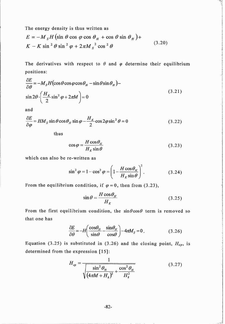
The energy density is thus writ ten as

E = ~ M { s i n 6 cos cp co s 9 + cos 0 sin 0^ ) +

AT - iT sin <9 sin ^ + I j z M ^ co s 6(3 .20 )

The derivatives with respect to Q and ç determine their equil ibr ium

posit ions:

^ = -M j , / / ( co s 6 cos(pcosOfj - s in O s in9 f j)~

f H ^sin 2^- — —sin^ ^ + 2;zM = 0

and

— = / f M . s in^cos^„ sin cos 2® sin 0 = 0dcp " 2 ^

(3.21)

thus

cos^ =H cos 0H

Hj^sinO

(3.22)

(3.23)

which can also be re -wri t ten as

sin^ (p = l - cos^ (p^ cosOfj^

V / / f S i n # /(3.24)

From the equi l ibrium condition , i f (p = 0^ then from (3.23),

H cos 0^sin <9 ' H

/ / ,(3.25)

From the first equil ib rium condition, the sin^cos^ term is removed so

that one has

a<9= - H ( cosOu sin^.

^ ' 4M^^=0. (3.26) sin^ cosO )

Equation (3.25) is subst i tuted in (3.26) and the closing point. Hep, is

determined from the express ion [15]:

1

sin" 6(3.27)

+

-82-

F igure 3.15 i l lustrates the re lation, 3.27, be tween the closing point and

the angle o f applied field, 6h, relat ive to the fi lm surface. Here, the

anisotropy is set to lOkOe and the sa tura tion magnet isa tion to 4.4kOe

(for the low noise media).

1.5

1.4

1.3

1.2

1.1

0.9 0 20 40 60 80 100

angle o f rotation

Figure 3.15. Plot o f the closing po int (xlOkOe) with respect to Qh (degrees)

the angle o f applied f ie ld relative to the film surface. The field, H, is

perpendicular to the in-plane c-axis, as shown in figure 3.14.

From equat ion 3.27, i f the field is applied with in the fi lm surface, then

the closing point provides a measure o f the sam ple ’s

magnetocrysta ll ine anisotropy. I f the field is applied normal to the fi lm

surface, the closing poin t is therefore the sum of the crystall ine and

shape anisotropy.

3.3.3.2 Experiment

In order to carry out closing point measurements , the sample was

cooled down to 2K: this al lows one to determine the maximum

anisotropy in the media. After cooling, the field, H , ini t ial ly lies

with in the film surface, 6h = 0 degrees. A field sweep from -9 .6 k O e to

-83-

+9.6kOe and back to -9 .6 k O e produces a torque signal as shown in

figure 3.16.

0.10

0.08

'®h=30 -«2 0.06

ÏX 0 04S

- 0.02

-0.04

-5Applied field (kOe)

5

F ig ure 3 .16. Torque s i g n a l s f o r the l o w n o is e media , as a f u n c t i o n o f

a p p l i e d f i e l d a t 15 a n d 30 d e g r e e s to the f i l m p l a n e [ 1 5 ] . The r a w d a t a o f

the tw o to r q u e cu rve s w e r e n o t s i g n a l a v e r a g e d a n d the s i g n a l to no ise is

high even b efore s m o o t h i n g the cu r ve s (u s ing IGOR) in o r d e r to d e t e r m in e

the c l o s i n g p o i n t (shown in inset) .

The sample is rotated at another angle and again a f ield sweep is

carried out. There is however a l imit in the angle to which you can

rotate the sample: where the observed closing point exceeds the field

l imit , which is ±9.6kOe.

Here, the closing point with respect to the angle o f f i lm ro ta tion to the

field H is f i t ted using equation 3.27, provid ing values o f the low noise

m ed iu m ’s anisot ropy and saturat ion magnet isa tion o f 8.4 and 4kOe,

respectively. 12

10

8

6X

Z

00 4020 60 80Angle (degrees)

Figure 3 .17. P lo t s o f c l o s i n g p o i n t w i th a n g le o f r o ta t io n o f f i e l d f o r the low

no ise m e d ia [ 1 5 ] .

-84-

An al terna t ive me thod in de term in ing the anisotropy is through

s imula t ing the torque signal. A mean field model of the torque signal

was used; however, the s imula t ion fai led to trace the experimen tal

torque curve [15]. Here, a micromagnetic model was used with a

Gaussian d is tr ibu t ion o f the anisotropy (wi th a FWHM of 2kOe) for the

low no ise media, as shown in f igure 3.18.

-10

-10 -5 0Applied field (kO e)

5 10

F igure 3 .1 8 Torque as a f u n c t i o n o f the a p p l i e d f i e l d f o r lo w no ise m ed ia

s a m p l e w i th a g a u s s ia n d i s t r i b u t io n o f the a n is o t ro p y . The r e d cu rve is the

e x p e r im e n t a l d a t a a n d the blue l ine is a s im ula t ion f r o m m ic r o m a g n e t i c

m o d e l l in g [ 15].

From the m ic romagne t ic model, the anisotropy o f the low noise med ia

was found to be lOkOe, which is sl igh t ly lower than tha t de term ined

from FMR, 10.8(2)kOe, and the in tergranular exchange cons tant

(d iscussed in sec t ion 3.3.2.1), C, was 0.2 [15].

The high noise med ia has a lognormal d is tr ibu t ion o f the anisotropy

field, as shown in f igure 3.19. The anisotropy is lO.bkOe wi th an

in tergranular cons tant o f 0.4 [15].

-85-

0.10

3 0.05

-0.05

-10 5 0 5 10Applied field (kOe)

Figure 3 .19 Torque as a f u n c t i o n o f the a p p l i e d f i e l d f o r high n o i se sample .

The l o g n o r m a l d i s t r i b u t io n o f Hk wi th a^O.3 [ 1 5 ]

3.3.4 Determination of interactions

Realis t ically there are in terac t ions wi thin the thin film due to exchange

or d ipole coupling. In order to observe these in terac t ions, the A M

me thod is used [16-18].

In this sec t ion, another novel technique is in troduced which is

analogous to the A M me thod. We will look at how accura te this

technique is wi th previous measuremen ts carried out by the magne t ic

record ing group in Seagate.

First we shall look at the de f in i t ion o f the AM me thod. Although there

were no magne tome try measuremen ts carried out using this me thod, a

m ic romagne t ic model is used to i l lus trate the resul ts o f this technique.

-86-

3.3.4.1 The AM and AT technique

Theory of the AM method

In the A M me thod there are two types of measuremen ts: IRM

(isothermal) remanence curve and the DCD (dc-magne t is ing remanen t)

curve.

The IRM me thod s tarts of f w ith the sample in the demagne t i sed state.

After demagne t is ing, the f ield is raised to / / ; , as shown in figure 3.20,

then set to zero, so tha t there exis ts a remanence of M j. The field is

then raised to H 2 and set to zero g iving rise to a remanence of M 2 and

so on until there is a max imum remanence, termed M r ( o o ) . Each of the

remanence po in ts A//, M 2 to M o o are represen ted by M r ( H ) .

M4

Q Hi H 2 H 3 H 4 H 5

Figure 3 .20. I l lu s t ra t io n o f the I R M curve .

A DCD curve s tarts off w ith the sample in the negat ive remanen t state

(magne t ised s tate) and a posi t ive field is applied the same way as the

IRM curve, as shown in f igure 3.21. The value of each successive

remenen t po in t is denoted as M d ( H ) .

-87-

Figure 3 .21. I l lu s t ra t io n o f the D C D curve .

The d if ference be tween the IRM and the DCD curve is described by the

Wohl farth rela t ion [14]:

m A h ) = m X «^)-2 m Xh ) (3.28)

This express ion is correc t i f there are no in terac t ions in the thin film.

If in terac t ions were presen t , then the d ifference be tween the left and

r ight hand side of the Wohlfarth rela t ion would be non-zero. This

d ifference be tween the two sides o f the equa t ion is denoted as A M [14]

AM = m X h )-M X«>)+2M X h ) (3.29)

An example of this A M resul t is shown in f igure 3.22. This was

simula ted using m ic romagne t ic simula t ions and each momen t

represen ts a magne t ic grain with its own uniaxial anisotropy. The

model used for this simula t ion and for other s imula t ions has a

d i s tr ibu t ion o f axes in random or ien ta t ion. The total free energy for

each grain is descr ibed as [19]:

inE, = - f h , - H + Y , + ATsin V + C Z ' ”.

rrij<Kioc/My (3.30)

7 ij

The first term is the Zeeman energy, the second is magne tos ta t ic , the

third is the anisotropy and the last term is the exchange energy. The

magne tos ta t ic in terac t ion is accoun ted as a d ipole-d ipole in terac t ion

be tween the grains in the m ic romagne t ic model. is the unit

magne t isa t ion vector, K =2M .

is the magne tocrys ta l l ine anisotropy

cons tant , n is the unit vec tor normal to surface, C is the in tergranular

exchange cons tant and Rioc de f ines the rad ius of the exchange

interac t ion.

With re ference to f igure 3.22, there are two types of s imula t ions: one

with only d ipolar contr ibu t ions (blue squares); that is, where C is set to

zero and the A M curve resul ts in having a negat ive dip at H/Hk =0.4.

The other has exchange and d ipolar coupling (red c ircles); tha t is, C is

set to unity, and the resul t ing A M curve is posi tive.0.8

0.0

-0.2

c=o

0.2 0.4 0.6 0.8 1.0

F ield (H /H ^)

F igure 3 .22. M i c r o m a g n e t i c s im u la t io n o f A M curve f o r d i p o l a r in t e r a c t io n s

only (C = 0, m a r k e d in blue s q u a r e s ) a n d ex change a n d d i p o l a r c o n t r ib u t io n s

( C = I , m a r k e d in r e d c i r c l e s ) [ 1 9 ] .

AT m ethod and results

The A T me thod is s im i la r to the A M me thod: it is the torque tha t is

measured ins tead o f the remanen t magne t isa t ion. The sample was

measured at 2K, the reason for this is to reduce the thermal reversal ,

— = Ejr ! kT) and obta in an accura te value of the anisotropy,r

There are three par ts o f the measuremen t tha t is required in order to

de term ine the type o f in terac t ion in the thin film. The f irs t is tha t o f

the Tr(H) measuremen t which is s im i la r to the IRM curve. The sample

is in a demagne t i sed s tate, which was achieved by se t t ing the f ield to

9.6kOe and cycl ing the f ield down to zero in s teps o f 0.2kOe. After

demagne t is ing, a f ield o f value H i is applied w i thin the f i lm surface

and the sample is rotated 90 degrees ou t-of-p lane where a torque signal

is measured. The max imum torque for a g iven f ield Hi is def ined as

Tr(Hi). The sample is rota ted back to zero degrees and a higher field

H 2 is applied. Aga in, the sample is rota ted 90 degrees wi th a higher

torque signal Tr(H2). This exper imen t cont inues un t i l we reach the f ield

l imi t , which is 9.6kOe.

The second and third part o f the measuremen ts is the Troo(H) and Td(H)

curve. Here the sample is in the magne t ised s tate whose ‘single

dom a in ’ is at an arb i t rary d irec t ion w i thin the f ilm plane. The sample

is rota ted to 90 degrees ou t -of-p lane , where Troo(Hi) is measured. The

sample is rotated another nine ty degrees where the torque is zero; tha t

is, the f ield is applied in the opposi te d irec t ion to the momen t . The

sample is then rotated back to n ine ty degrees until Td(Hi) is measured,

as shown in f igure 3.23 [19].

-90-

-2 7

20 40 00 00 100 120 140 too 100Angia (dagrMs)

Figure 3.23. Simulation o f the angular dependence o f torque fo r initially demagnetised (squares) and magnetised (filled circles) sample. Vectors Tr, Troo and Td are determined by measuring the torque amplitude at 90 degrees. The intergranular coupling (both dipolar and exchange) is not present in this case; the inset demonstrates that the Wohlfarth relation (3.28) is satisfied.

After measur ing Trœ(Hi) and Td(Hj), the sample is rota ted back to zero

degrees; tha t is, the field is f inally applied w i thin the f ilm surface. A

higher f ield, Hj, is applied so tha t T,co(H2) and Td(H2) are de term ined.

Aga in, higher f ields are applied un t i l we reach the f ield max imum. All

values of Tr(H), Td(H) and Trco(H) for H rang ing from zero to the f ield

max imum are plotted as shown in f igure 3.24.

20

-20

-40

0 2 4

Applied field (kG)6 8

Figure 3.24. Tr(H), Td(H) and Tyco(H) curves measured fo r low noise media, 15B.

-91-

Wi th no in terac t ion, the rela t ion is sim i lar to that o f Wohlfa rth [19]:

TAh )= T ,S h ) -2 T X h ) (3.31)

Where in terac t ions are presen t , J T is a measure of devia t ion from the

left and r ight side o f the equa t ion. The rela tion for the case of

in terac t ions can be de f ined in the follow ing way:

Ar = 2r,(//)-r,_(//)+7;(//) (3.32)

A pos i t ive value of A T is assoc ia ted wi th in tergranular exchange

in terac t ion; a nega t ive value is assoc ia ted with mos t ly d ipolar

coupling. A simula t ion o f A T , f igure 3.25, using the m ic romagne t ic

model (3.30) shows tha t for no exchange, a negat ive peak is observed;

the sample with s trong exchange coupling (C = l ) , a posi t ive peak

occurs.0.6

0.4C=1

0.2

I °»Q

- 0.2

c=o-0.4

- 0.60.0 0.2 0.4 0.6 0.8 1.0

Field (H/H

Figure 3.25. Simula t ion o f the A T cu rve [ 1 9 ] .

-92-

A simula t ion o f the A T curve of the low noise med ia, f igure 3.26,

required the follow ing parame ters o f the exchange coupling and the

anisotropy field; C=0.5 and = 9.0(4) kOe [19].0.4

experimentS im u la t io n

c 0.0

-0.2

0 2 4 6Applied field (kOe)

8 10

Figure 3.26. AT plo t o f low noise media with simulation and data points.

The uniaxia l anisotropy f ield value is sl igh t ly lower than tha t measured

from a vec tor VSM, which was 9.6 kOe and from FMR it was 10.7(2)

kOe. The problem here is tha t the f ield is res t r ic ted to 9.6 kOe, which

is insu ff ic ien t for comple tely sa tura t ing or demagne t is ing the sample.

The presence o f in tergranular exchange coupling in the low no ise

med ia agrees wi th the conclusions in the FMR sec t ion; tha t is, the low

f ield measuremen ts exhib i t lower values o f an isotropy due to the

presence o f exchange coupling.

Previous A M measuremen ts as shown in f igure 3.27 [5] shows tha t the

presence of exchange in the low and high no ise med ia is very small for

all va lues o f the applied f ield, which sugges ts tha t there are m inimal

in terac t ions [14,19]. There may be an ef fec t o f balance when exchange

compensa tes the d ipolar in terac t ions resul t ing in A M curves close to

zero [17]. A nega t ive A M s ignal does not necessari ly imply no

exchange.

-93-

Media A - Nose

Meda B - Low Nose

1 2 3 4 5 6

A|i|]lie(l FieW (kOe)

Figure 3.27. AM curves o f high and low noise media [5]

3.4 Conclusions

The f irs t part o f this chap ter has shown tha t high f ield FMR w i th

grea t ly improved resolu t ion and signal to no ise allows one to de term ine

the s tat ic and dynam ic proper t ies o f the record ing med ia wi thou t

in troducing m ic romagne t ic model l ing. Al though the FMR cond i t ion

res tr ic ts the user from obta in ing the magne t isa t ion and an isotropy

uniquely, one can de term ine from equa t ion 3.15 (using Ma thcad) the

sum o f the two s tat ic proper t ies. However , one needs to know the

magne t isa t ion in order to solve for the anisotropy.

In sec t ion 3.2.4.1, the anisotropy de term ined from FMR is higher than

tha t obta ined from torque magne tome t ry . In torque magne tome t ry

measuremen ts , the f ield is below sa tura t ion and thus the f ield is not

s trong enough to decouple exchange in terac t ions be tween the grains.

Torque magne tome try measured in St. Andrews has shown tha t i f one

were to employ the closing po in t me thod and apply m ic romagne t ic

modell ing to simula te the torque signal, then there exis ts an exchange

in terac t ion and the anisotropy agrees wi th tha t de term ined from FMR.

Another me thod, w i th the aid o f torque magne tome try is the A T

me thod, which is s im i la r to the conven t ional technique A M for

observ ing in terac t ions in polycrys ta l l ine media. For the case of the low

-94-

no ise med ia , there exis ts exchange coupling and the anisotropy

however was lower than tha t de term ined from the closing po in t me thod,

FMR and also torque measured in Seaga te. The problem w i th the torque

magne tome ter in St. Andrews is tha t the magne t ic f ield is not high

enough to satura te the med ia in order to accura tely de term ine the

anisotropy.

A table o f the anisotropy values through FMR, torque in Seaga te and

St. Andrews is shown below.

Torque magnetometrySample FMR Seagate St.Andrews

Closing point ATHigh noise 10.7(2) kOe 9.6 kOe 10.6 kOe -

media (15A)Low noise 10.8(2) kOe 9.6 kOe 10.0 kOe 9.6 kOe

media (15B)

3.5 References[1] M. Igarashi, T. Kambe, K. Yoshida, Y. Hosoe, Y. Sugi ta, J.

Appl. Phys. 85 (1999) 4720

[2] C. Ki t tel, In troduction to So l id State Physics 7ed. John Wiley &

Sons, Inc (1996)

[3] S. Chikazum i , Physics o f M agnetism John Wiley & Sons, Inc

(1964)

[4] N. Inabi , Y. Uesaka, A. Nakamura, M. Fu tomoto, Y. Sugita,

IEEE Trans. Magn. 33 (1997) 2989

[5] E.T. Yen, S.Z.Wu, T.Thomson, R.R is tau, R. Ranjan, G.C. Rauch,

IEEE Trans. Magn. 35 (1999) 2730

[6] T. Thomson, com m un ications 2001

[7] H. La idler et al. Subm i t ted to MMM/Intermag 2001

-95-

[8] C.J. Oates, F.Y.Ogrin , P .C.Ried i , S.L.Lee, G.M.Sm i th,

T.Thomson, JMMM, 242-245 (2002) 402

9] J. Smi t , H.C. Bel jers, Phil ips Res. Rep. 10 (2) 1955 113

10] U. Ne tzelmann, J. Appl. Phys. 68 (1990) 1800

11] S.V.Vonsovskii , F errom agnetic Resonance, Pergamon, Press,

New York, 1966.

12] M. Fu tomoto, N. Inaba, A.Nakamura , Y.Honda, Acta Me tal l. 46

1998) 3777

13] C.J.Oates, F.Y. Ogrin, S.L. Lee, P.O. Riedi , G.M. Smi th, T.

Thomson, J. Appl. Phys, 91 (2002) 1417

14] E.P .Wohl far th , J. Appl. Phys. 595 (1958)

15] F.Y. Ogrin, p r iva te com m un ications, 2001.

16] P.E. Kelly, K. O ’Grady, P.I. Mayo, R. W. Chan trell , IEEE Trans.

Magn. 25 (1989) 3881

17] C.Dean, R.W.Chan trell , H. Suzuki, N. Kodama, P.R. B issell , J.

Appl. Phys. 79 (1996) 6467

18] N.S. Walmsley, R.W. Chan trel l , J. Appl. Phys. 85 (1999) 6154

19] F.Y. Ogrin, C.J. Oa tes, S.L. Lee, J. Magn. Mag. Mat . , 242-245

2002) 321

.96-

Chapter 4

High field FMR of CoCrPtB longitudinal media with varying compositions of platinum and boron.

4.1 IntroductionThe record ing layer o f in teres t in this chap ter is d if feren t from tha t

d i scussed in chap ter three, as it conta ins boron ins tead o f tantalum in

the CoCrPt layer. The samples s tud ied in this chap ter are classed as

one wi th varying p la t inum and cobalt content , the other wi th varying

boron and cobalt conten t . These are in fact tes t samples , unlike the

high and low no ise med ia, which were in commercial use.

This chap ter is split in to two parts. The first part presen ts a d iscussion

on previous me thods used to charac ter ise the pla t inum and boron

series, carried out by Seaga te and IBM, and also the sample prepara t ion

o f the two series for FMR measuremen ts. The nex t part involves m u l t i ­

frequency FMR of the two batches and prov ides explana t ions ex tracted

from the analysis.

There are two ma in aims in this chap ter: first to compare the average

uniaxial anisotropy data measured by FMR with previous measuremen ts

carried out by Seagate. Secondly, to exam ine any trends in the dynam ic

and s tat ic proper t ies o f the record ing med ia with respec t to changes in

the pla t inum and boron concen trat ion.

4.2. Sample characteristics

The schemat ic d iagram o f the record ing media, d iscussed in this

chap ter, is shown in f igure 4.1. The pla t inum and boron samples were

DC spu t tered on a N iA l/P subs trate, which is a soft ferromagne t w i th a

coercivi ty o f 85 Oe.

97

CoCrPtB ~x nm

NiP ~ 1 micron

A1 O.Smm

Lubricant 2nm

Carbon protection layer 5nm

Figure 4.1 La yo u t o f the r e c o r d i n g m e d ia s t u d i e d in this c h a p t e r [1 ] .

The hard discs have a small var ia t ion in magne t isa t ion from inner

d iame ter (12.5mm) to ou ter d iame ter (42mm). The samples were

prepared by cu t ting 8mm d iame ter m in i-d i sks 30 mm from the disc

cen tre as explained in detai l in sec t ion 4.3. Any region o f the disc tha t

lies be tween 20 to 38mm (which is the flat, m iddle sec t ion o f the disk)

from the disc cen tre has a fairly uniform magne t isa t ion and remanence

[1].The magne t ic proper t ies o f both sides of the disk are not the same.

Each side o f the disk was spu t tered from a d ifferen t physical target , so

that both sides of the d isk were fabr ica ted s imul taneously. Because

these d isks are test samples, it was not the chie f goal o f the process

engineer, in Seagate, to match the proper t ies of both sides.

Independen t magne t isa t ion and an i sotropy measuremen ts on the 2-D

isotrop ic in-plane med ia were carried ou t on a vec tor VSM by IBM [1]

and Seaga te [2]. Table 4.1 presen ts the follow ing magne t isa t ion and

uniaxial anisotropy values for both the pla t inum and boron series. The

thickness o f the magne t ic layer was de term ined from TEM by Seagate

[2].

9 8

(D0

1+

k>So

-73<uOa0>

T3

u CO0 >

1 1—. <u<a >

1 I5

o>o.JZ4{o

H

ofxSo

O

CQ

"O4>

«<oa

tq"Occti

m

0)

<20ceCD

CO

CDOJsc! CQ

VOGO VO

0vn "d"

mVOd- C"

c3\CM

03d)R

-=t ro rn as sn R""C CM CM r- r-l >

CD

bOaCD

CO

vri GOCO GO mCM CM

CDO

co

CDAWO(d

cdCO

CQt r-H CM VOGO C" d- 0

GO CO CO cn in

d" c3\ VOCD Q <=) cd d

d)s D -n -H -H< O' CM CO VOCO d- GO 004-)CO d- CO CO

CD%WOcdCD

CO

a OcPh

N CMu !>-' CM

X cd "TC4-I0

m

<C"

cS CDX ) Ut-i a CTi

CDCO 0a

in0d -Pk

(NOo c3\

roQ\

0 \GO

GO t—'"4" m m co

c3\'O

cn (Nt"C3\C3\

(SC3S o \ri

(SC3\

O

>oGO

o\ Os

<N-d-

Mso

soso<N

C" d- C" CM r~ VO 0in cn CM r- CO Os d"CO CO CO in m CO CO

00 0 0 in 0 r—< d"Ov in

CMGOCM

CO C" CMCM

0CO

p? P-( mffl mCM CM CMd GOd" VO GO

dC30d

GOm m

< < PQ < <d" C-. d1—H CM

ÔCM

u 0 U 00\ Ov d din m CM CM0 0 VO VOd d X CM CM

Ph X X

m

<c--6■d-csVOCMX

03§ •

a

IS O)03 Cq

sC4i

K<y

So

I

C3

diCo

"Q<!Uk.%03QC&)

k.CU03ROO

-Ci"(3SQ

Cii-R

<3Q

'd>

d)-R

CÜ>

Rcu

C3)k.

03/UCdJ03

KOIkO

-R

RR

%•S

-5%CU

03C3JoR

"R

"R

§S '

I6C3

. 2

I

Ii

'RRRR•2R

■scy

I

0<0

"r

Ci)

sQ

Rd)

1

GyCi)

-R

IR

"Rd)R

"R

'R

R

-R

R03

fnd)

•:S

"S'03

Ci)

"RR

X

R

RO

•Rd)

Rd)03R

-RO-R

"Rd)k.R

cRO

(3vc3v

Each sample has its own product code where F4059C and X2624C are

the p la tinum and boron varying media , respectively. It is clear tha t

from the boron series, in table 4.1, there is a maximum in the uniaxia l

anisotropy at 12 at .% boron measured by Seagate; however,

measurements car ried out by IBM show that the anisotropy increases

with boron content. Anothe r independent measurement , again carried

out by Seagate was based on the dynamic coercivity, figure 4.2. From

the plot , the anisotropy is much smaller than that from the vecto r VSM,

although there is a maximum in again, at 12 at.% boron.

Dynamic He - Hk plot9500 1

9000 -'STS' 8500 -X

8000 -

760014-8-4 14-8-12 14-8-16

A lloy ty p e

Figure 4.2. Dynamic coercivity measurements o f the boron series with a maximum in anisotropy at 12 at.% boron [2].

From table 4.1, in the p la tinum series, the magnet isa tion measured

from SQUID in St. Andrews (as shown in appendix D) differs from that

in Seagate and IBM. Because o f this, one has to question how accurate

or re liable is the magnet isa tion and therefore the uniaxia l anisot ropy

measurement for each sample? The reader should note that it was not

possible to obtain hysteres is plots from IBM and Seagate in order to

verify their values to the s am ple ’s saturation magnet isa tion and

anisotropy field. Instead the sample parameters , as shown in table 4.1,

were given.

The final column in table 4.1 is the sum o f the saturation

magnet isation, 4 tuM s (measured from IBM and Seagate, as tabula ted in

100

the forth column) and ha l f the anisotropy field, Hk/2 (again measured

from IBM and Seagate, as tabula ted in the fifth column). This term is

compared with the high field FMR result , as shown in table 4.2 (for the

plat inum series) and table 4.5 (for the boron series).

4.3. Sample preparation

The samples were prepared by Seagate and were presented as a series

o f hard disks. Figure 4.3 i l lus tra tes a hard disk in which four samples

were cut out for FMR measurements.

Figure 4.3. C o C r P t B h a r d d i sk w i th inner a n d ou ter r a d ius o f 12 .5mm a n d

42mm, r e s p e c t iv e l y .

The workshop in the School o f Physics in St. Andrews const ructed a

two-f lute mill which is made o f high speed steel, and attached it to a

Bridgeport mill ing machine, figure 4.4. With reference to figure 4.4, a

mandrel ( labelled B on the figure) was constructed for posi t ioning and

clamping the disks (labelled D), which was then centred on the cutter

101

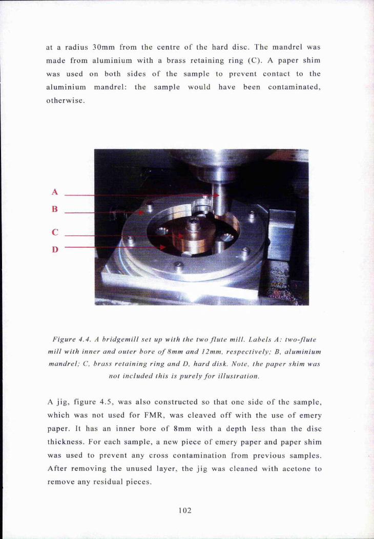
at a radius 30mm from the centre o f the hard disc. The mandrel was

made from aluminium with a brass retaining ring (C). A paper shim

was used on both sides o f the sample to prevent contact to the

aluminium mandrel: the sample would have been contaminated,

otherwise.

A

B

C

D

Figure 4.4. A h r id g e m i l l s e t up w i th the two f l u t e mill . L a b e l s A: tw o - f lu te

mil l w i th inner a n d o u te r b o r e o f 8mm a n d 12mm, r e s p e c t i v e l y ; B, a lumin ium

m andre l ; C, b ra ss r e t a i n in g r ing a n d D, h a r d disk. Note, the p a p e r shim was

not i n c l u d e d this is p u r e l y f o r i l lu s t ra t ion .

A jig, f igure 4.5, was also const ructed so that one side o f the sample,

which was not used for FMR, was cleaved off with the use o f emery

paper. It has an inner bore o f 8mm with a depth less than the disc

thickness. For each sample, a new piece o f emery paper and paper shim

was used to prevent any cross contaminat ion from previous samples.

After removing the unused layer, the j ig was cleaned with acetone to

remove any residual pieces.

102

■mm

Figure 4.5. The j i g , wh ich w a s u s ed f o r c l e a v i n g one s id e o f the l a y e r to

f o r m a s u b s tr a te .

103

4.4.1 FMR:

Platinum series4.4.1.1 S ta t ic p r o p e r t i e s

High frequency FMR on the recording media was measured in the range

77 to 95 GHz. Typical l ineshapes o f the three samples at 94 GHz are

shown in figure 4.6.

0.06

E x tra m o dUniform

^ mode 14 at.% Pt

0.04

12 at.% Pt

0.02

Uniformmode

Extra mod

16 at.% Pt

4.0 4.5 5.0

applied field ( x l O k O e )

Figure 4.6. FMR s ig n a l s o f the p l a t in u m s e r i e s a t 94 GHz.

The method of de termin ing the static and dynamic properties o f the

recording media was the same way as in chapter three. A fit to the

resonant field at d ifferent f requencies is shown in figure 4.7. The

results presented in table 4.2 are based on the saturation magnet isa tion

provided by Seagate, IBM and from the SQUID in St. Andrews.

104

4.6

4,4

16 at.% Pt 1 2a t%Pt 14 at.% Pt

R e s o n a n tf i e l d( x 1 O k O e )

4

3.8

3.675 80 85 90 95

mm-wave frequency

Figure 4.7. Main l ine r e s o n a n t f i e l d as a funct ion o f f r e q u e n c y f o r s a m p le s

with d i f f e ren t p l a t in u m conten t .

From tables 4.1 and 4.2, it is observed that the higher the platinum

content, the smaller the satura tion magnet isa tion, this may be due to

the reduction o f cobalt in the magnet ic layer. Although the measured

saturat ion magnet isation o f the three samples differ from laboratory to

laboratory, from FMR analysis, the mean uniaxial anisotropy inereases

and the Lande g-factor decreases s l igh t ly as the concent ra tion o f

pla tinum increases. The g-factor o f each sample is the same, regardless

o f what value the magnet isa tion takes. However, the der ived mean

uniaxial anisot ropy coincides within error. The uniaxial anisotropy, in

table 4.1, measured in Seagate differs significantly with that from

FMR, in table 4.2. Independent measurements from IBM have also

deduced the anisot ropy o f 14 and 16 at .% Pt to be 23kOe, which is 6 to

7kOe higher than that de te rmined from FMR. From the results , one can

only state that FMR provides reasonable values for the anisot ropy as

well as the Lande g-facto r for each sample, even though their largest

difference in the saturation magnet isa tion is around 21%.

05

Bo

"O(U

(doB

!üO«

o

bJ3<DT3Üa*

J

OO

g

co

es en ese=0 o C=)

s O <d <D

CQ 44 44 44m nf- Oes >—e >—ee s e s e s

e s m eso <=> CDeu CD o O

noG 44 44 44

< Hd- nt- oc s e—e e—1

W e s es es

e s en eseu O e=) CDcd e=5 CD <D(30G -H 44 44eu m nf- o

00 eses es es

m

a>

&taa>(/)

eu PhG,Bcd

00 G

en co esO a \en es es

G coO en eneu»-. e—'CA no

G 44 44 44O < es va r->G va CD o(50G

en en en

nf o ooo r-' soes es es

es <o

nod>OO noV

no no<ü M O

k>Bo

nO<uoO

"O(Uno

Ork

no(UoO

nod>no

§+

ïni-03

(/)

6otM

(UoK-.CkoVh k

«DûG

X A<cQ »«T4ü<

o(*3

O

no(ü

cd<üBüq

rsi no

^ «+

ï>

enHd- va

vaen

m

o44

o44

CD44

en00

\oCD

nj-Os

va sô sô

oova

eO\O

oova

eu CD <d CDnoG<

44 44 44V3O

v>oo

vaen

va va S3

ennt

'Ova

vaeneu

f30Cdeu00

m

nj" ni­ CDes es CD

va va

a>

bOCd(D

CO

(50<u <üo

Ph

O-Hoonf-

o-H

vo so

es eO\en SOva es var-H T-H T-H

CD va vava t"' esCD CD CD44 44 44CD va vaCD r-es T—1 T—4

r-H h-H

es so

na«Q

Iïnt-

tn%)3

>

Cj

(30"QKQ

%)S

<3RQ

I

3_%Q

%%]

S'

<S>

<3k

§+

ï'n-Q)

o%<3eueuk.eus

%naKQ

"%%

Co

a

%)Co

euI«

%

C5

na<u

"Q

-Z ^ea eu

Ik.

<3-%"-%

eueu

OǤ

Sea

eaeuk.

KaQ3O

eu

eu!k

0 < naeueu"Q"Q

1+

kn*-

S3eceu•JCea

<0

îa

euCOna«ea

naeuk.3§

\oO

From figure 4.6, the sample with 12 at.% pla tinum shows only the

uniform FMR mode. However, as the composi tion o f p la tinum increases

there exists a lower field mode as well as the usual Kittel mode. This

feature is also observed on another part o f the disk, 27mm from the

disk centre. At all measureable frequencies in the range 75 to 95 GHz,

the lower field line is more obvious from samples with 16 at .% than 14

at .% platinum. This lower field signal may be a ttr ibuted to the

exis tence o f an addi t ional layer, called the trans it ion layer. This result

is s imilar to that o f Artman [3,4] on the Q-band FMR of CoCr

perpendicula r recording media. From his measurements, he found that

there were two signals present and suggested that one signal is due to

the bulk magnet ic layer and the other signal from a t rans it ion layer.

This transit ion layer is si tuated between the substrate and the bulk

layer and it is a highly disordered, small grained region. In his FMR

analysis, he assumed that the magnet isa tion o f the layers was the same

and determined the fractional th ickness o f the transit ion and bulk layer.

He also deduced the total effective anisot ropy (taken to be the sum of

the intrinsic and shape anisotropy) o f the recording media , which

agreed with his previous torque magnetometry measurements.

If we fo llow the same method, then a fit to the lower s igna l ’s resonant

f ield at di fferent frequencies, figure 4.8, will provide values o f the

mean uniaxia l anisot ropy and g-factor , table 4.3. Similar to A r tm an’s

work, the saturation magnet isa tion o f the two layers were assumed to

be the same and there is an assumption that there is no exchange

coupling between the two magnetic layers.

107

B

95

90

85

80

753.6 3.7 3.8 3.9 4 4.1 4.2 4.3 4.4

resonant field (x I 0 k O e )

95

90

85

80

753.6 3.7 3.8 3.9 4 4.1 4.2 4.3

resonant field ( x l O k O e )

Figure 4.8. R eson an t f r e q u e n c y ve r sus f i e l d p l o t s o f the l o w e r f i e l d mode

show n in f i g u r e 4.6. P lo t s A a n d B r e p r e s e n t the l o w e r f i e l d m ode o f 14 an d

16 a t .% Pt, r e s p e c t iv e l y . The f i t to the d a t a in this f i g u r e r e q u i r e d

m a g n e t i s a t i o n va lues f r o m Seaga te .

108

Sample (at% Pt)

Lande

Seagate

f-factor

St. Andrews

Average uniax

(kC

Seagate

ial anisotropy

)e)

St. Andrews14 1.95 ± 0.03 1.85 ± 0.01 9.09 ± 0.09 5.23 ± 0.32

14 2* 2* 10.27 ± 0.06 9.63 ± 0.32

16 2.02 ± 0.03 2.02 ± 0.01 10.90 ± 0.08 9.85 ± 0.25

16 2* 2* 10.35 ± 0.06 9.33 ± 0.30

Table 4.3. The g-factor and the average uniaxial anisotropy o f the low fie ld mode derived from FMR is based on magnetisation measurements carried out in Seagate and St. Andrews. The star (*) beside the two in the g-factor column is a set value. It is assumed that the saturation magnetisation in the transition layer is the same as the bulk layer.

In table 4.1, the highest measured magnet isa tion was in St. Andrews

and the lowest by Seagate. The static properties o f the lower field

signal in 14 and 16 at.% Pt were determined from FMR, using two

extreme values o f the ir magnet isa tion as tabulated in table 4.3. Here,

the calculated g-value o f the 14 at .% Pt sample is less than two: for

cobalt , the g-factor is expected to be sl ightly higher than two. I f one

were to set the g-value to two, then the anisotropy o f 14 and 16 at.%

coincide within error.

It was suggested [1] that the t rans it ion layer is sandwiched between the

bulk magnetic layer and the underlayer; that is, it is the region where

the magnet ic layer o f interes t was first deposited. There may be a

mixed region from the underlayers and so the first few monolayers o f

the deposi ted film has not formed a full anisotropy.

4.4.1.2 D ynam ic p r o p e r t i e s

Linewid th analysis on the pla tinum series is not straight forward. If

one used the equation

(4 .1)

109

and fit ted it to the data points as shown in figure 4.9, then one would

obtain the Gilbert damping term and the inhomogeneous broadening.

0.17

M e a s u r e d l i n e w i d t h ( X 1 O k O e )

0.16

0.15

0.14

0.13

0.12

0.11

12 at.% Pt 16 at.% Pt 14 at.% Pt

0.17 5 80 85 90 95

mm-wave frequency (GHz)

Figure 4.9. P lo t o f the m e a s u r e d l in e w id th wi th f r e q u e n c y . N o te that the p l o t

sh o w s a l l the l in e w id th p o i n t s a t ea ch f r e q u e n c y a n d w er e f i t t e d to eq ua t ion

4.1.

Because the signal to noise on the lower field signal is poor, it is

dif ficult to determine its l inewidth. Table 4.4 provides values to the

damping factor and inhomogeneous broadening from linewidth

measurements to the uniform mode.

Samples Gilbert damping Inhomogenous(at.% Pt) factor broadening (kOe)

12 0.017 ± 0.003 0.592 ± 0.104

(0.017 ± 0.006) (0.605 ± 0.222)14 0.035 ± 0.005 0.275 ± 0.170

(0.030 ± 0.014) (0.367 ± 0.090)16 0.025 ± 0.004 0.696 ± 0.142

(0.027 ± 0.007) (0.605 ± 0.239)Table 4 .4 Values o f the G i l b e r t d a m p i n g term a n d inhom ogenous

bro a d en ing . The va lues in b r a c k e t s w er e d e r i v e d f r o m the f i t to the a v e r a g e

l in e w id th at each f r e q u e n c y .

110

From figure 4.9, it is clear that as the cobalt and p la tinum content

decrease and increase, respectively , the measured l inewid th also

increases. Inaba’s [5] work on the damping term, as discussed in

chapter three, states that the large increase in the Gilbert damping term

in the CoCrPt series compared to CoCrTa is due to the pola risat ion o f

pla tinum in the magnet ic layer. The polarisat ion o f p la tinum means a

spin and/or orbital po la r isa t ion o f pla tinum electrons (mainly 5s and

6sp) induced by magnet ic neighbours [6]. This feature may account for

the rise in l inewidth as there is more pla tinum in the layer o f interest .

Table 4.4 shows that there is no obvious trend between the Gilbert

damping factor and the pla tinum concentrat ion. The main problem in

applying equat ion 4.1 to the l inewid th measurements is that o f the

l imited range o f frequencies; in addition, the measured value o f the

l inewidth, at a f ixed frequency, for one signal shows a large spread

from run to run. The inhomogeneous terms are between 0.2 to 0.7kOe,

which is in the same region as the high and low noise media in chapter

three. At this stage, it is di ff icult to correlate both terms to the

sam ple ’s recording proper ties.

4,4.2 Boron series4.4.2.1 Static properties

Multi -f requency wo rk on the boron series shows that there is only a

single resonance peak, as shown in figure 4.10 and 4.11.

I l l

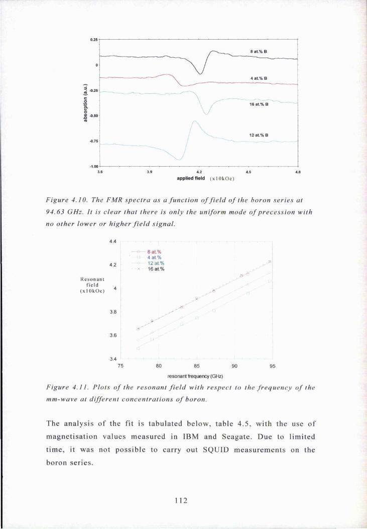
0.25

8 at.% B

4 at.% B

i -0.25

16 at.% B

2 4 .5 0

1 2 a t % B-0.75

- 1.003.6 3.9 4.84.2 4.5

applied field ( x I O k O e )

Figure 4.10. The FMR s p e c t r a as a f u n c t i o n o f f i e l d o f the b oron s e r i e s at

94 .63 GHz. It is c l e a r that the re is on ly the uniform m od e o f p r e c e s s i o n wi th

no o th e r l o w e r or h ig her f i e l d s ignal .

4 . 4

4 . 2

8 at.%4 at.% 12 at.% 16 at.%

R e s o n a n t f i e l d

( x 1 O k O e )

3.8

3.6

3 . 4

75 80 85 90 95

resonant frequency (GHz)

Figure 4.11. P lo t s o f the r e s o n a n t f i e l d w i th r e s p e c t to the f r e q u e n c y o f the

m m -w a ve a t d i f f e ren t c o n c e n t r a t i o n s o f boron.

The analysis o f the fit is tabulated below, table 4.5, with the use o f

magnet isa tion values measured in IBM and Seagate. Due to l imited

time, it was not possible to carry out SQUID measurements on the

boron series.

112

<4JO

+

I+

l i<0

OQ

o>ÜS3T3OT3

T30>Ü3

"O

"3

<0O

cuo

P£5

T3d)o3

X»d>T3

o

003

o

00(U

X»33

J

X(U

k

XJ33

lU30030300

3O3

eo

0003

X03

k

003

3 «tî Ca

B

03 PQCLB3

C/3

m

OOd

ON ON NONO m d

o O o o

-H -H -H 41

ONNO

dd o

00ON

OO 1—1 C*N

3300303OO

PQ

03300303

00

PQ

03300303

OO

ONoo

OO■3'

COON ON

fN

ir><NO-HONC4

m t-" VN d■3*

mo

CNON

ONC -O-HVN

OO ON

ONmo4)ON

OO ON ONO00 NO CN d

o O o o

41 41 41 -H

ooNO

do ON

ON■X

o O d

oCNo

do o

o o o o41 41 41 41ON C<N

zd d d d

odo

do o

o o o o-H 41 41 41od

ON TT

d d d d

d ON OO do d oo'4* d d d

'Oc -d

d NO

3k.3

IO

-SKQ

ou"S

RQik0O

1RQ

• < 13

S=0

QRQ

I

-C3E?

Q)-R

rnR

_o

Q%Cm%

.1

'RSRa

(u

&%

ROSvO-Xi3

-R

to(u

III

RO&.o

<5

Q

IN.X

o

<

%)

C

-R

«0CD(U

S’

S+

k

Again, we have a sl ight change in the g-factor with respect to the

concent ra tion o f boron in the media layer; in addit ion, the average

derived FMR uniaxial anisotropy surprisingly increases. Unlike

previous measurements carried out by Seagate (Dr. J-P. Chen and Dr.

Thomson) , there is no turning point in the uniaxial anisotropy term.

However, another set o f measurements carried out by Dr. Thomson

(now at IBM) has shown that the magnetoc rysta ll ine anisotropy, table

4.5, inc reases with respect to boron content which agrees with the FMR

measurements .

4.4.2.2 D ynam ic m e a s u r e m e n t s

Multi -f requency l inewidth measurements on the boron series, figure

4.12 were fit ted to equat ion 4.1. Table 4.6 shows the derived values of

the Gilbert factor and inhomogenous term for l inewidths at each

frequency and the averaged l inewidth at each frequency, respectively.

0.12

0.11

M e a s u r e d 0.1 l i n e w i d t h ( x 1 O k O e )

0. 09

0.08

0.07

0.06

75 8 0 85 90 95

resonant frequency (GHz)

Figure 4.12. P lo t o f the m e a s u r e d l in e w id th wi th f r e q u e n c y . The l ines

throu gh the d a t a p o i n t s a re s t r a i g h t l ine f i t s to equa t ion 4 . 1 .

16 at.% B4 at.% B8 at.% B12 at.% B

114

Sample Gilbert damping Inhomogeneous term(at.% B) factor (kOe)

4 0.007 + 0.005 0.82 ± 0.21

(0.017 ± 0.015) (0.45 ± 0.53)8 0.018 ± 0.002 0.19 ± 0.08

(0.017 ± 0.004) (0.14 ± 0.14)12 0.023 ± 0.021 0.11 ± 0.10

(0.021 ± 0.017) (0.10 ± 0.58)16 0.022 ± 0.002 0.24 ± 0.08

(0.013 ± 0.008) (0.29 ± 0.19)

Table 4.6. Damping and inhomogenous terms deduced from all the linewidth data points at each frequency. The values in brackets were derived from the f i t to the average linewidth at each frequency.

Unlike the pla tinum series, there is no trend to the change in l inewidth

with boron composi tion. However, the damping factor var ies between

0.01 and 0.04, ju s t like the p la tinum series in section 4,4.1.2. It is very

difficult to explain why the inhomogeneous term deduced from the

average l inewidth at each frequency for 4, 8 and 12 at .% boron has an

associated error that is comparable or larger than its es timated value.

This was not observed for the p la tinum series or the high and low noise

media.

4.5 Summary

Previous measurements on the uniaxia l anisotropy field for both types

o f reco rding media (plat inum and boron series) do not seem to agree

very well with that o f FMR. Init ial measurements by Seagate showed

that the anisotropy in the boron series has a turning point at 12 at.%

boron but from FMR, the anisotropy still increases with boron content.

From table 4.5, i f one were to apply values o f the sam ple ’s saturation

magnet isa tion (measured in Seagate and IBM) to the resonant

115

condition, equat ion (3.14), then the g-value for each sample in the

boron series coincides within error. The same applies to the anisotropy

for samples 4 and 12 at .% boron. It is encouraging to learn that another

independent measurement by Dr. Thomson in IBM, using the VSM,

follows this trend on the inc rease o f the average uniaxia l

magnetoc rysta ll ine anisotropy with boron content. Howeve r , it is

uncertain, as to why measurements in Seagate have a peak value in the

anisotropy.

SQUID measurements , in St. Andrews, on the pla tinum series shows

that the coercivity is around 3.5kOe and that the product o f the

remanence and fi lm thickness , Mrt agrees very well with that deduced

from the vecto r VSM in Seagate [1]. Although the saturation

magnet isation o f each sample from the SQUID measurements is no t

s ignif icantly different from that measured in Seagate, this paramete r is

required for FMR analysis and so a sl ight change in one paramete r will

create a shift to the sam ple ’s g-facto r and anisotropy. As mentioned

earlier , in the pla tinum series section, the g-value has not changed

although the largest dif ference in the anisot ropy is approximate ly 2kOe

for each sample. The smal ler peak in the 14 and 16 at .% Pt series may

be a tt r ibuted to the deposited layer which has not reached its full

anisotropy. It is clear that more p la tinum samples with dif ferent

composi tions are required to enhance our unders tanding o f the lower

field signal and to asce rta in i f there is a genuine trend o f the sam ple ’s

g-factor and uniaxial anisotropy with p la tinum content.

Since the magnetocrysta ll ine anisotropy and the g-factor o f a trans it ion

element is a t t r ibuted to spin-orbit coupling, one assumes that i f the

anisot ropy increases then the g-factor will also increase. Yet it is the

reverse for both the platinum and boron series.

Non-l inear regress ion (NLR) to equation (3.15) shows that in table 4.2

(the p la tinum series), the sum 4tüM s+Hk/2 for each sample varies

between 11.0 to 12.5 kOe. However , only sample 7A (12 at.% Pt,

measured in IBM) in table 4.1, has the sum lying within tha t range. For

the boron series and with reference to table 4.1, the sum for sample 7B

(4 at.% boron) measured in IBM also lies within the range determined

116

from NLR. I f one were to add 4tzM s (measured from IBM, Seagate and

St. Andrews) to H k/2 (deduced from FMR), then for each sample in

both series, the sum deduced from exper iment lies in the same region

generated from NLR. This suggests tha t high field FMR is a re liable

method for f inding 4tcM s+Hk/2.

For both the pla tinum and boron series, the damping factor agrees with

previous damping values [5,7]. Although a wider frequency range is

required for accurate values o f the damping and inhomogeneous term.

4.6 References:[1] T. Thomson, private communications 2002

[2] S.D. Harkness and J-P. Chen, private communicat ions 2002

[3] J.O. Artman, J. Appl. Phys. 61 (1987) 3137

[4] P.V. Mitchell , A. Layadi, N.S. VanderVen, and J.O. Artman, J.

Appl. Phys. 57 (1985) 3976

[5] N. Inaba, Y. Uesaka, A. Nakamura, M. Futamoto, and Y. Sugita,

IEEE Trans. Mag. 33 (1997) 2989

[6] Cz. Kapusta, private communications 2002

[7] M.L.Plummer, J .van Ek and D. Weller, The Physics o f U ltra-H igh

D ens i ty M agnetic Recording., Springer-Ver lag, New York 2001

117

Chapter 5

Small Angle Neutron Studies tSANS^ of

Longitudinal Recording Media.

5.1 IntroductionThis chapter examines neutron di ff ract ion o f longi tudinal recording

media measured at different fields. Three types o f samples were

examined in this chapter; 2D-isot ropic, 2D-anisotropic media (the

moments are preferent ia lly aligned along the disk radius) and a NiAlP

substrate. The au thor ’s contr ibution was to carry out SANS

measurements and assemble the data, which was then analysed by Prof.

Stephen Lee. (Par t icipants in the group include Dr. Feodor Ogrin and

Dr. Tom Thomson.) The analysis on the reco rding media was not

straight forward and there are d iscussions on methods tha t were used to

analyse the spectra. The main feature, here, is to compare the physical

mean grain size, de termined from TEM to the magnet ic grain size,

deduced from SANS. Before desc rib ing the results , a background

introduction to neutron di ff raction and SANS is required.

5.2 Basic theory of neutron diffraction5.2.1. W hy n e u t r o n d i f f r a c t io n ?

The basic properties o f the neutron are tabulated below:

basic properties o f the neutron

mass m 1.675x10"^" kg

charge e 0

Spin

magnetic dipole moment

* is t he nuc l e on m agn eton , w h ich is equal to 5 . 0 5 1 x 1 0 ’ ’ JT ‘

Table 5.1. Basic properties o f the neutron [1]

118

The kinetic energy o f a neutron is re lated to its wavevector k by the

equation.

1 81.81

In these equat ions, X is in A , k is in lO^^m'% F in kms"% E in meV,

and T in Kelvin.

With reference to equat ion 5.1, a neutron at 293K has an average

wavelength o f 1.8^1, its energy is 25.3meV and it travels at a speed o f

2.20 km s" \ For example, i f we diff ract neutrons from the planes o f

metall ic iron at room temperature (having the atomic spacing, 2.88 ^4),

then planes (111) and (200) have very different scatte ring angles and

are therefore easily resolved.

Other advantages o f neutron scattering are as follows:

(a) neutrons have energies comparable to thermal energies o f

the sample;

(b) neutrons are deeply penetrating;

(c) neutrons are scattered with a strength that var ies randomly

from element to element;

(d) neutrons have a magnetic moment;

(e) the t ime a neutron passes an atom is o f the order o f 10’^ s,

which is comparable to the re laxation t imes o f the sample and

(f) neutrons in teract with nuclei at a range between 10‘ '^m

and 10'*^m, which is smaller than the thermal neutron wavelength,

implying that the neutron is scatte red isotropically by a nucleus (S-

wave scattering) and is therefore an ideal probe o f the solid state.

119

5.2.2. Nuclear diffract ion

Figure 5.1 shows a typical scattering system in which neutrons o f

wavevector k and energy E are scattered by a target sample. If a

neutron counter was used to measure the number o f neutrons scattered

in a given direction as a function o f their energy E \ and the distance o f

the counter from the target is assumed to be large compared to the

dimens ions o f the counter and the target, then the small angle d O

subtended by the counter at the target is well defined. Let the direction

o f the scattered neutrons be 0,^. hi and kf is the neu tron’s incident and

scattered wavevector , respectively.

X axis

d n

Direction

Incidentneutrons

Z axisTarget

Y axis

Figure 5.1. G e o m e t r y f o r s c a t t e r i n g ex p e r im e n t [ 1 ]

The partial dif ferent ial cross-section is defined by the equation [1]

_ (number of neutrons scattered per second into a small angle dOdE solid angle dQ in the direction 0,<j) with final energy

between E ’ and E ’+dE ’) / 0dOdE ’

(5.2)

where 0 is the incident neutron flux; that is, the number o f neutrons

through unit area per second, the area being perpendicula r to the

direction o f the neutron beam.

120

If we do not analyse the energy o f the scattered neutrons , but count all

the neutrons scattered into the solid angle d O in the di rection 0,(j), then

the c ross-sect ion co rresponding to these measurements is known as the

dif ferent ial cross-section, which is defined by [1]

_ (number of neutrons scattered per second into dO in the (5 3)do. direction 0,(t>)/ 0dD

The total scattering cross-section is defined by the equation [1]

cJtotai = (total number o f neutrons scatte red per second)/ 0 (5.4)

The total number means the number o f neutrons scattered in all

directions.

With reference to figure 5.1, the intensity o f the scattered neutrons is

measured as a function o f momentum transfer:

n Q = n i ^ ^ - k j ) (5.5)

where Q is the scatte ring vector . The corresponding energy transfer is

given by

%co — {kf ~k^i\ (5.6)

There are two types o f scattering: elas tic and inelastic. Figure 5.2 is an

i l lust ra tion o f scatte ring tr iangles for the types o f scattering.

121

scatteringdirection

(a)

incident direction

kf< ki

Q

(bl)incident direction

kf> ki

incident direction

Figure 5 .2 (a) E l a s t i c s c a t t e r i n g w h e r e kj = kf an d (b) ki ^ k / f o r ine la s t i c

s ca t t e r in g , ( h i ) is w h e r e the neu tr on l o s s e s e n er g y a n d (h2 ) is the neu tron

a b s o r b i n g energy.

The in te ract ion o f a neutron with a nucleus can be thought o f as a

neutron in the presence o f a potentia l well , with a potent ia l o f Vo> The

neutron can be considered as a plane wave, e*'' . Outside the well, the

neu tron’s wavevecto r is & = 2mEand inside the well , the wavevector

becomes q = _ The total wave function outs ide the well is

f= + — wher e / is the scatte ring amplitude. In the l imit o f

r

Â:->0(low energy scattering), b = ~ \ \ m f is defined, where b is the

neutron scattering length. This scatte ring length is dependent on the

type o f nucleus scattering the neutron. The physical in te rpre ta tion o f a

negative / value is tha t the scat te red wave in the A:-» 0 l imit is shifted

by 180 degrees in phase with respect to the incoming wave. Scattering

o f neutrons from fixed nuclei is well approximated by the Fourier

transform o f the in teract ion potentia l , which is given by the Fermi

mpseudo-potential [2,3]: V(r) = ^ - i ?J (5.7).

122

References [1,4] cover a mathemat ical background on the partial

di fferential c ross-sect ions resul t ing from the Fermi pseudo-potential .

5.2.3. Elastic Magnetic scattering

The neutron has a magnetic moment, which interacts with the atomic

moments on the atoms. The interact ion is actually - J i - B , the neutron

moment interacts with the flux density associated with the unpaired

electrons in the sample. An appropria te scale for the in te ract ion is the

Bohr radius [2,3];

=2 mc^ J

( 5 . 8 )

where vq is the Bohr radius, 0.54x10"^^ m and y is the gyromagnetic

ratio o f the neutron. An effective magnet ic scattering length is given2

by P = - ^ ~ g J f ( Q ) , where g is the Lande g-factor o f the ion, J is the 2 mc

total angular momentum and f(Q) is the magnetic form factor,

<7 - This form factor is the Fourier transform o f the

magnetic density o f the magnet ic ion. Because the magnet ic scattering

process involves an in te ract ion with electrons over long distances

comparable to neutron wavelengths , the magnet ic sca tte ring intensity is

reduced as Q increases. The form factor represents the non- isotropic

scattering from magnetic ions caused by the spatial ex tent o f the

elect ron dis tr ibut ion [1].

If we assume that the neutrons are unpolarised and that we are dealing

with elastic scattering, then the elast ic cross-sect ion is defined for a

Bravais lat tice with local ised electrons [1,2]:

exp(-2PT)2(<5„^ - • {l, - i M s f ' p ' ’)^ a , P i j

Equation (5.9), above, involves the sum over all latt ice sites i and j and

over all Cartes ian directions , a , (3 = jc, y , z. The exp(-2W) term is the

Debye-Waller factor as discussed in [1].

123

dcr ^ ( y r ^ Nmagnetic

and ( s f ^ are the t ime averaged spin components on sites i and J.

For a ferromagnet , the c ross-section for a sample with many domains is

[1]

dc7d a e x p ( - 2 » r ) ^ - ( r - C M e - ? ) ( 5 1 0 )

magnetic ^ 0

where is the mean value o f the component o f the spin in the

direct ion o f fj for each domain, Vq is the volume o f the reciprocal

latt ice, ^ is a unit vecto r in the mean direction o f the spins, f is a unit

vecto r in the d irection o f f (in the reciprocal lat tice), f is an arb itrary

di rection in k-space and we take the scattering vecto r Q = k f - k ^ - f .

The average (f - , is taken over all the domains, and so equals to 2/3

i f all d irections in space are equal.

If an external magnet ic field is applied in the direction o f t , then the

spin directions o f all the domains will tend to align so that fj is along

-X [1]. Therefore f = -1 and the magnetic scattering vanishes . The

difference in the c ross-section with and without a high external f ield

gives the magnet ic sca tte ring alone [1].

5.2.4. Small angle neutron scattering

Small angle neutron scat te ring provides structural in format ion on a

scale ranging from a few angstroms up to regions with dimensions o f

the order o f 5000 angstroms in bulk specimens [4].

In an ideal SANS exper iment, f igure 5.3, the momentum o f the incident

and scattered neutrons must be defined in order to invest igate the

propert ies o f the sample. In the SANS experiments, no energy

discr imination is carr ied out on the scattered beam and thus the

124

ine lastic contr ibution is measured along with the elastic scat te ring to

give the to ta l scattering. For elastic scattering, the magnitude o f the

I I 47Tscatte ring vector [4,5,6], | g ] , is — sin^. The term small angle neutron

scatte ring is used in mate ria ls science to cover the Q range ^ < Q < ~d

where d is the in te ra tomic dis tance in the materia l under invest igation.

multi­detector

sample

Figure 5.3. Schematic representation o f a SANS experiment [7].

If one were to invest igate magnet ic samples , then there exists two

contr ibutions to the scattering: nuclea r and magnet ic scattering.

Considering nuclea r scatte ring first , the coherent scatte ring cross-

section (a rising due to in terference effects be tween the scattered

neutrons from each nuc leus) pe r atom is [6]

d(7 _ 1~dQ.~~N

(5 .11)

where N is the number o f sca tte ring nuclei exposed in the beam, ba is

the coherent scattering length o f the e lements occupying the site with

the pos it ion vector R . Q is def ined as the scattering vector , which is

the difference between the inc ident and scattered wavevecto r .

The scatte ring cross section for the whole sample is

125

ê i P>’ (5 12)

where hR is replaced by p j f ) , which is the locally averaged scattering

length density and is averaged over all volumes and the integral is

over a sample volume, V.

I f one were to consider a binary system; that is a sample tha t contains

Np pa rt icles with a homogenous scatte ring length density P bp~ ~ ^ap

(where is the sca tte ring length, which is averaged over the particle

volume, and Vap is the atomic volume in the particle), which is

embedded in a matr ix o f homogeneous scattering length density

Pbm , then one obtains the express ion [6]

(5.13)do. N

where the integral extends over the volume V occupied by all part icles.

This can be re-writ ten as

<5.14)

where F ( g ) = - i - i s the single particle form factor [6].

The form factor above is used for dif ferent particle shapes; for

example, for a sphere [6]

(5.15)\Qn

Other form factors for cylinders and ellipses can be found in Kostorz

[6].For a concentra ted system o f interact ing spheres, the interference

between these pa rt icles become important and so the scat te ring cross-

section becomes [6]:

126

(5 .16)

where is the st ructure factor.

Another example o f the st ructure factor is that for hard spheres, where

the volumetric packing fract ion is be tween 30 to 50%. Therefore, one

employs the Pe rkus-Yevik model [8,9]

The defin it ion o f the structure factor is that it provides the

in tereference effects from a collect ion o f different grains; the form

factor is the Fourier transform o f the shape and size o f the grains.

Examples o f the st ructure factor and form factor are shown in figure

5.4.

(a)

Intensity Intensity

0.1 -

Figure 5.4. Form f a c t o r (a) o f a sphere , the r e d a n d blue l ine r e p r e s e n t s a

s p h e r e w i th d i f f e ren t radi i , wh ich is the f i r s t min ima o f the I v.v q curve ; (b)

is the s t r u c tu r e f a c t o r w h e r e the r e d a n d blue l ines r e p r e s e n t a g r o u p o f

s p h e r e s w i th d i f f e ren t p a c k i n g den s i t i e s . These are s i m u la t io n s p r o v i d e d by

Prof. S .L .L ee [ 1 0 ] .

127

For magnet ic scattering, i f M(r) is the local magnet isa tion at posit ion

f , then m ( ^ ) is its Fourier transform [6]:

m {q )= (5.17)

and the magnet ic contr ibution to the scatte ring c ross-sect ion is [4]

^ = (5.1S)

where M^{q ) is the component o f m (q ) perpendicula r to the scatte ring

vecto r Q and y is the neutron magnet ic moment in nuclea r magnetons.

For a system composed o f different magnetic states [4]

g = |(iw;.) - {M„)f [ l -{q -m ) ] [F (e ) f (5.19)

where g is a unit vector in the direction o f Q , M, is the moment o f the

impurity, is the moment o f the matrix and M is a unit vecto r

parallel to the direction defined by the vector

As previously ment ioned, a system composed o f random magnet isa tion

vectors, in the absence o f a magnet ic field, the term is equal

to 2/5, thus iso tropic scatte ring is observed. If the field is above the

saturating field, then the magnetic contr ibut ion to the scat tering is zero

(as M \ \ Q ) in the field direction and maximum perpendicula r to it.

Nuclear sca tte ring is unaffected and remains isotropic [4,6].

5.3. SANS experimentAll neutron measurements were carr ied out at the I.L.L (Inst i tut-Laue-

Langevin) on ins truments D l l and D22. The ILL is the w or ld ’s most

powerful reactor source, with a peak flux o f 57MW, producing neutrons

for a wide range o f inst ruments. Figure 5.5 shows a schematic

representation o f the exper imental a rrangement for a SANS experiment.

128

CdlimaiûT ApertureNeutron veloaly

Neuînxi beati

ApertureVacuun tube

Neutron L--20m, <3>=25m guide

Detector 129x128 pixels

Figure 5.5. S c h em a t ic r e p r e s e n t a t i o n o f the SANS ex p e r im e n t in D22, in the

I.L.L. [ 7 ]

The specifications o f both D l l and 0 2 2 are tabulated below.

D i f f r a c t o m e t e r s p e c i f i c a t i o n s

I n s t r u m e n t

in IL L

S a m p l e

d e t e c t o r

d i s t a n c e

( m )

C o l l i m a t i o n

d i s t a n c e ( m )

W a v e l e n g t h

( a n g s t r o m s )

D e t e c t o r

a r r a y

P i x e l

s i z e

( m m ^ )

D1 1 2 . 5 - 41 2 . 5 - 41 4 . 5 - 4 0 1 2 8 X 1 2 8 10 X 10

D 2 2 1 . 4 - 1 8 1 . 4 - 18 4 . 5 - 4 0 6 4 X 6 4 7 . 5 X 7 . 5

Table 5.2. S p e c i f i c a t i o n s o f D l l a n d 0 2 2 [ 7 ] , which w er e u s ed d u r in g

in v e s t i g a t i o n s c a r r i e d out in this chap ter .

The neutron beam passes through a veloci ty /wavelength selector for the

incoming neutrons . It then passes through a monitor, which records the

number o f neutrons incident on the sample. After passing through a

source slit, the beam travels along an evacuated tube and is incident on

the sample. The coll imation length is variable to a llow the optimum

trade-off be tween resolut ion and intensity to be obtained.

The de tecto r can be moved back and forth relative to the sample so that

one can obtain a full q-range o f the neutron scattering intensity.

The software, called GRASP, designed by Dr. Charles Dewhurst from

the ILL is a user friendly package that is used for graphical inspection,

analysis and reduction o f mul ti -detecto r data produced by D l l and

D22. The software has the added advantage o f quickly processing and

129

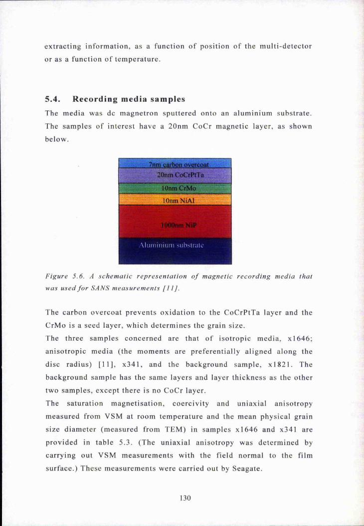
extract ing information, as a function o f posit ion o f the mul ti -detecto r

or as a function o f temperature.

5 .4 . R e c o r d i n g m e d i a s a m p l e s

The media was dc magnetron sputtered onto an alumin ium substrate.

The samples of interest have a 20nm CoCr magnetic layer, as shown

below.

20nm CcCrPtTa

1 Onm CrMo

lOnmNiAl

AliiniiniuiTi siibslralc

Figure 5.6. A s c h e m a t i c r e p r e s e n t a t i o n o f m agne t ic r e c o r d i n g m ed ia that

was u s ed f o r SANS m e a s u r em en t s [ 1 1 ] .

The carbon overcoat prevents oxidation to the CoCrPtTa layer and the

CrMo is a seed layer, which determines the grain size.

The three samples conce rned are that o f isotropic media, x l6 4 6 ;

anisotropic media (the moments are preferential ly aligned along the

disc radius) [11], x341, and the background sample, x l8 2 1 . The

background sample has the same layers and layer thickness as the other

two samples, except there is no CoCr layer.

The saturation magnet isa tion, coercivity and uniaxial anisotropy

measured from VSM at room temperature and the mean physical grain

size d iameter (measured from TEM) in samples x l6 4 6 and x341 are

provided in table 5.3. (The uniaxia l anisotropy was determined by

carrying out VSM measurements with the field normal to the film

surface.) These measurements were carr ied out by Seagate.

130

samples 4 71 Ms Coercivi ty Uniaxial Mean grain size Size

(kOe) (kOe) anisotropy diameter , d (nm) dist.

(kOe)

X1646 5.73 2.87 10.11 10 0.2

X341 8.50 2.31 5.98 30 0.4

Figure 5.3. M a g n e t i c p r o p e r t i e s o f the i s o t r o p i c an d a n i s o t r o p i c media.

Hysteresis loops o f both types o f media were carried out by Seagate

[11], as shown below, figure 5.7.

0

-500-20 -15 -10 -5 0 5

applied field (kO e)

10 15 20

600

400

200

0

-200

-400

-600

-800-10 -5 0 5

applied field (kO e)

10 15 20

(A)

Figure 5. 7. In -p lane m a g n e t i s a t i o n l o o p s o f the i so t ro p ic ,

a n is o t r o p i c , x341, (B) media.

(B)

XÏ646 , (A) an d

131

5.5. SANS measurements5.5.1. Sample preparation for measurements

Since there is a very small amount o f active layer for SANS

measurements , it is necessary to use a composite system o f some thirty

disks. Background scatte ring from the aluminium substra te on which

the magnetic layers were grown must be reduced without damaging the

active layer. However, this still leaves the substrate o f the order of one

hundred microns thick, which gives rise to a large background signal.

The disks were wrapped in an a lumin ium foil and placed into a sample

holder, as shown below, which had a cadmium cover around the edge of

the holder [10].

Figure 5.8. A lumin ium h o ld e r w i th s a m p l e f o r neu tron m ea su rem en ts . The la bel s , (A) r e p r e s e n t s the p o l e p i e c e s o f the e l e c t r o m a g n e t ; (B), the

alum in ium s a m p l e h o ld er ; (C), ca d m iu m cover , which was u s e d to sa n d w h ich the s a m p l e s b e tw ee n the a lum in iu m p l a t e s ; (D), the thin f i l m s a m p l e s an d

(E) r e p r e s e n t s the neu tron f l u x into p a p e r [ 1 0 ] .

As ment ioned previously, the de tecto r can be moved back and forth

relative to the sample so that one can obtain a full ^-range o f the

scattering intensity. However, there was a higher incident neutron flux

at higher q (where the sample de tecto r distance is as small as 1 to 2m),

than that at lower q (sample detector distance is o f the order o f 18m for

D l l and D22). In order to obta in a good signal to noise ratio, there

must be more statist ics; that is, longer runs at lower q than at higher q.

132

An example of this is shown later in f igure 5.12, for the in-plane

isotropic media, where the error bars are bigger at lower q.

5.5.2. SANS of 2D - isotropic longitudinal recording media

The fields o f interest in this section are 14.5 and 4.5kOe. This is

because these were the two fields in which we obtained a full ^-range

(which was available at the t ime o f measurement) . The 2D m ul t i ­

detector plot o f scatter ing at 14.5kOe is shown.

B

Figure 5.9. A p p a r e n t i s o t r o p i c s c a t t e r i n g d e t e c t e d at 14 .5kOe. The f i e l d l ine

r e p r e s e n t s the d i r e c t i o n o f the a p p l i e d f i e l d , B, a n d the y e l l o w s q u a r e in the

m id d le o f the d e t e c t o r is a beam s to p p e r , which p r e v e n t s the d e t e c t o r f r o m

s a tura t in g . The two b la ck c i r c l e s r e p r e s e n t an annulus , which was u s ed in

G RASP f o r o b s e r v i n g m a g n e t i c s c a t t e r i n g ; that is, we w ere l o o k in g f o r a

1 — {m • ^ j = (l — cos^ 9^ c u r ve as shown in equ a t ion (5 .19) .

With reference to figure 5.9, the magnetic field was applied

horizonta lly . From theory, there should be no magnetic scattering

along the field direct ion i f the sample is magnet ically saturated, but

there should be magnet ic scatte ring along the y-direct ion; the refore, i f

the e lectromagnet were strong, then one would expect from equation

(5.19), to observe a f igure e ight- l ike dis tribut ion o f the magnetic

scatte ring [10]. However, as shown in figure 5.9, there was no obvious

133

figure eight-l ike dis tr ibution o f the magnetic scattering. In fact, the 2D

detector plot for 14.5kOe looks very simi lar to zero field measurement

(where the sample is in a randomised isotropic state). If we used

GRASP to take an annulus o f the 2D detector for 14.5kOe, then there is

no clear sine square dependence, figure 5.10. This is because there is

more nuclea r scatte ring (i sotropic) than magnetic scattering, plus a

random fluctuation in the background arising from the stack o f

substrates. Therefore, in order to observe magnetic scatte ring, the

moments in the reco rding media must be magnet ically saturated and

there should be no nuclea r scat te ring present [10].

Intensity

800

700

600

500

-200 -50-150 -100 0 50 100 150 200

angle (degrees)

Figure 5 .10. The s c a t t e r i n g in t e n s i t y ve r sus the angle o f s w e e p a r o u n d the

d e tec to r , w here z e r o d e g r e e s is r e p r e s e n t e d by a b la ck s t r a ig h t l ine as

shown in f i g u r e 5.9.

The highest field avai lable was 14.5 kOe, which was around the

sam ple ’s saturation field (see figure 5.7a). Magnetic scatte ring can

then be observed by s u b t r a c t i n g the randomised (isotropic) state from

the magnet ised state at B =I4 .5kO e . (Ideally, the demagneti sed state

should be subtracted from the magnetic state, but it was not possible to

demagnetise each disk. Instead the disks were re-shuffled and stacked

together to produce a randomised isotropic state.) Figure 5.1 la , is a 2D

134

multi -detecto r plot o f anisotropic magnetic scattering with a figure

eight-l ike d is tribution at 14.5kOe in D l l . Another example o f magnetic

scatte ring in the isotropic media was measured at D22 with the field set

to 11.8kOe.

If we plot the scattering intensi ty against the angle o f sweep around the

detector , then a sin^ ^ trace (which is based on \ - ( m , from

equat ion 5.19) shows that there is magnetic scattering present, as

i l lus tra ted underneath the 2D detecto r plots in figure 5.11.

200 :

-200 -150 -100 -50 0 50 100 150 200

angle (deg rees)

D ll

% vP

D22

-150 -100 -50 0 50 100 150 200

angle (degrees)

Figure 5 .11. 2D d e t e c t o r p l o t s o f the i s o t r o p i c media. D l l p l o t a t high Q (at

14.5k Oe) wi th e v id e n c e o f m a g n e t i c s c a t t e r in g , underneath . D 2 2 p l o t at

m id d le Q (at 1 l .S k O e ) w i th a sin^O t race , underneath .

135

The total nuclear scatte ring for all ^- ranges at 14.5 kOe is shown in

figure 5.12. The magnet ic signal is a level o f 0.1% to 1% o f the total

scattering.

Intensity

Total scattering10®

Magnetic signal1000

100

0.01 0.1

Figure 5.12. A comparison o f the magnetic and total scattering at 14.5kOe.

A note to the reader. In the GRASP package [7], there are options in

which you can present and/or analyse the data:

1. The s in e - sq u a re d a m p l i tu d e . This measures the difference in Q

scattering parallel and perpendicula r to the field direction. This

is defined as FT(x,my(x)}-FT(y,mx(y)}, which is the difference

between the Four ier transform (FT) o f the m om en t’s x-

component , my(x) and the m o m en t ’s y-component, mx(y) [10].

The expression FT{x,my(x)}-FT{y,mx(y)} is derived from equation

(5.10) where mx(y)=mcos6 , my(x)^msinO and 6 is the orientat ion

of the magnet isation rela tive to the x-direction. The sine-squared

amplitude plot will have the same angular dependence as the

magnetic scatte ring c ross-sect ion; however , to extract the

absolute cross-sect ion, one needs to introduce factors such as the

sample transmission, detector efficiency, the neu t ron’s

wavelength and the incident neutron flux.

136

2. The scattering intensity with respect to the angle around the

detector ( / vs 0). This is based on which shows that

there is magnetic sca tte ring taking place in the expe riment .

3. The phase of the sine-squared relative to the x-direct ion. The

phase o f the scat te ring depends on the sign of

FT{x,my(x)}-FT{y,mx(y)} [10]. If the value FT{x,rriy(x)} is greater

than FT{y,rrix(y)} in one q-range, and vice versa in another q-

range, then the phase o f the scattering is changed by ninety

degrees. An example o f this is shown in figure 5.13, one with the

phase taken into considera tion; the other without. Here, we have

to accept that the difference in Q scattering, FT{x,m y(x)}-

FT{y,m x(y)}, can change sign [10].

3000

2000

1000

-1000

-2000

3000

2000

1000

-1000

-20000.01 0.1 0.01

(A) (B)Figure 5 .13. P lo t s o f the s i n e - s q u a r e d a m p l i tu d e whe re (A) the p h a s e is

c o n s i d e r e d a n d (B) w here the p h a s e is ignored. In o r d e r to ob ta in

r e a s o n a b l e s i g n a l to noise , it is n e c e s s a r y to c a r r y out l o n g e r runs a t l o w e r

q than h ig h er q.

Figure 5.14 i l lustrates 2D-detecto r plots at 14.5kOe and 4.5kOe, each

at a different ^-range. A sin^ ^ dependence shows that there is a ninety

degree phase shift between the two. This may suggest that the moments

137

at 4.5 kOe are not saturated and so transverse components (moments

whose component are along the field di rect ion) exist [10].

200 m

H

-200 -150 -100 -50 0 50 100 150

angle (de g ree s)-200 -150 -1 0 0 -50 0 5 0 100 150 2 00

ang le (d e g re e s )

Figure 5.14. 2 D d e t e c t o r p l o t a n d s ine s q u a r e d d e p e n d e n c e on the m a g n e t ic

s c a t t e r i n g at (A) 14 .5kO e a n d (B) 4 .5kOe.

5.5.2.1. SANS model and results for the isotropic media

The reader should note that the au tho r ’s cont ribution to this project

involved measur ing the SANS data and assembling it in a meaningful

form so that P rofessor Stephen Lee could analyse it. Throughout this

section. Professor Lee is often re ferenced as [10], which means that

Prof. Lee provided the modell ing, the physics and the fit to the data.

Since the cobalt grain structure is approximate ly close packed

(locally, but with no long range order) it was not possible to fit the

138

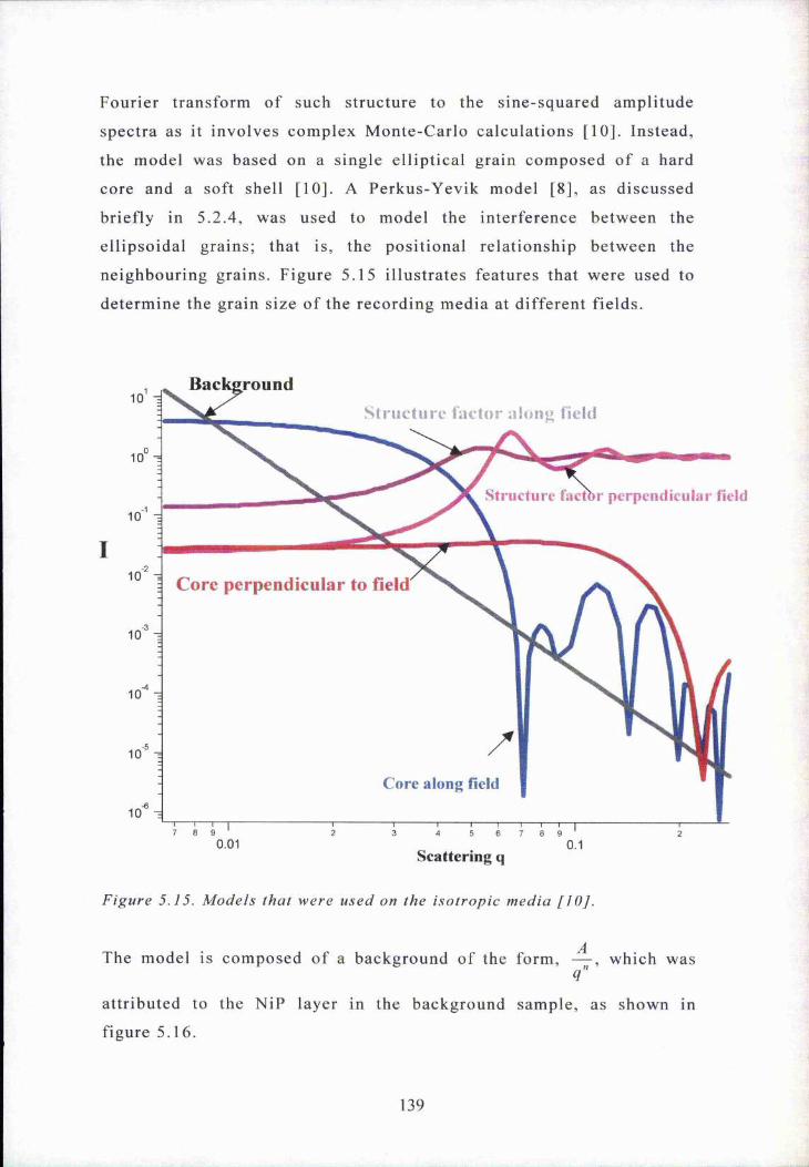
Fourier transform of such st ructure to the sine-squared amplitude

spectra as it involves complex Monte-Carlo calculations [10]. Instead,

the model was based on a single el l iptical grain composed o f a hard

core and a soft shell [10]. A Pe rkus-Yevik model [8], as discussed

briefly in 5.2.4, was used to model the in terference between the

ell ipsoidal grains; that is, the posit ional re la tionship between the

neighbouring grains. Figure 5.15 i l lust ra tes features that were used to

determine the grain size o f the reco rding media at dif ferent f ields.

I

round110

Structure factor alon« tleld

010

Structure factbr perpendicular field■1

10

-210 Core perpendicular to field

-310

.-410

-510

Core along field-6

10

0.01 0.1Scattering q

Figure 5 .15. M o d e l s that w e r e u sed on the i s o t r o p i c m ed ia [ 1 0 ] .

The model is composed o f a background o f the form, which was

attributed to the NiP layer in the background sample, as shown in

figure 5.16.

139

Intensity1000

100

0.04 0 06 0 08 0 10.02 03

Figure 5 .16. A f i t to the s c a t t e r i n g in t e n s i t y d a t a on the NiP su b s t r a t e . This

a r i s e s f r o m a la rg e s c a l e d i s o r d e r o f so f t f e r r o m a g n e t i s m in z e r o f i e l d [ 1 0 ] .

The power law exponent n represents the spatial symmetry o f the

mic rostructu re in a sample: n = 3 for the case o f part icles which have a

rod like shape elongated in one di rect ion and n = 4 for spherical

part icles [12]. For the background sample, n = 4 [10]. With reference

to figure 5.15, the structure factor S(Q) is included along and

perpendicula r to the field di rect ion and the form factor F(Q), again

along and normal to the field direct ion [10].

As a result , the sine squared ampli tude is proport ional to

F^{Q,^p^,^p^)s[Q)+-^, where A p i = p i - p 3 , A p 2 =p2- p 3 and pi , p 2 , ps is

the scat te ring density (which is equivalent toV

with n the number

of atoms, b is the scat te ring length and V is the volume) [10].

hard core son shell

matrix

Figure 5.17. The la yo u t o f an e l l i p t i c a l g r a n u le wi th v a r y in g s c a t t e r i n g

dens i t ie s .

140

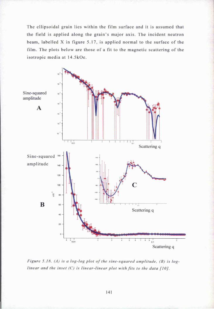
The ell ipsoidal grain lies within the film surface and it is assumed that

the field is applied along the g ra in ’s major axis. The incident neutron

beam, labelled X in figure 5.17, is applied normal to the surface o f the

film. The plots below are those o f a fit to the magnetic scatte ring of the

isotropic media at 14.5kOe.

Sine-squaredamplitude

Scattering q

Sine-squared

ampli tude

120

Scattering q

Scattering q

Figure 5.18. (A) is a l o g - l o g p l o t o f the s i n e - s q u a r e d a m pl i tu de , (B) is log-

l i n e a r a n d the inset (C) is l i n e a r - l i n e a r p l o t wi th f i t s to the d a t a [ 1 0 ] .

141

The sine-squared ampl itude o f the isotropic media, at 4.5kOe is

sl ightly different from the 14.5kOe spectra, as shown in figure 5.19.

The blue line is a fit to the data using the same model for the 14.5kOe

spectra.

Sine-squaredamplitude

V

S c a t t e r i n g q

Figure 5 .19. L o g - l o g p l o t o f the s i n e - s q u a r e d a m p l i tu d e at d i f f e ren t q ranges

f o r B ^ 4 . 5 k O e [ 1 0 ] .

Table 5.4 presents results o f the fit to the data for 14.5kOe and 4.5kOe.

The terms 2ry‘” and 2rx‘" in the e ll ipsoidal parameters column represent

the cobalt co re ’s dimensions. The 2ry^“ and 2rf^'^^ terms represent the

d imensions o f the shell , as shown in figure 5.20. dx and dy represent the

dis tance between the centres o f the cores along the x and y-d irect ion,

respectively.

Although the single grain model was used in the fit to the sine-squared

ampli tude at 4.5kOe and 14.5 kOe, the angles o f the chromium and

cobalt moment relative to the field direction, as shown in table 5.4, is

assumed to be the same for each grain in the reco rding media sample.

Thus, these angles are averages for an ensemble o f grains. The single

domain model is reasonable at f ields close to saturation.

142

El l ip s iod ’s parameters 14.5 kOe 4.5 kOe

2r/" 38 Â 42 A

2 ^ ^ 68 Â 64 A2ry°"' 88 A 86 A

150 A 128 Ady 104 A 105 A

dx 115 A 119 AThe angle between the cobaltmoment and the field, H (degrees) 52 69The angle between the moment inthe chromium shell and the field 93 27(degrees)

Table 5.4. Parameters determined from the f i t to the sine-squared amplitude [10].

143

88Â

14.5kOe

150Â

4.5kOe

àV

86Â 42Â fJ ^ 6 9 ^ 2 É

Bo = J

64Â

128Â

H

Figure 5 .20. A s c h e m a t i c r e p r e s e n t a t i o n o f an e l l i p s o i d a l g r a i n at 14 .5kO e

a n d 4 .5 k O e ,w i t h d i m e n s io n s o f the c o r e a n d shel l . The d i r e c t i o n s o f the

m a g n e t ic momen t in the c o b a l t c o r e (y e l l o w ) a n d the w e a k l y m a g n e t i c s h e l l

(green) a re a l so shown. The blue a r r o w r e p r e s e n t s the d i r e c t i o n o f the

a p p l i e d f i e l d .

144

The size o f the core and ch romium shell does not seem to change much

from 4.5 kOe to 14.5kOe; similarly, the distance between the centres o f

the neighbouring grains are a lmost the same at both fields.

With reference to figure 5.20a, the direction o f the moment in the

ch romium shell and the cobalt core is 93 degrees and 52 degrees to the

field direction, respectively . From the 4.5kOe analysis, the direction o f

the moment in the chromium shell and cobalt core is 27 and 69 degrees

to the field direction, respect ively. From mic romagnetic simulations

[10], even at 14.5kOe the di rections o f the moments in the cobalt cores

are not al igned along the field. In fact, they are less than 45 degrees to

the field direction, as shown in figure 5.21. From the SANS analysis,

the chromium moments are not al igned along the field. The reason for

this may be due to the core moments being responsible for the

orienta tion o f the moments in the chromium shell. As the field is

increased from 4.5kOe to 14.5kOe, there is a large inf luence from the

cobalt core on the ch romium moments , therefore the moments follow

the field line generated by the core and are surprisingly normal to the

direction o f the applied field rather than along it [10].

. — •

• -»

— T» -

—-A"

- - - - 7

— * — » —o*. n -? ■—

V--1 ' “* ♦ A - . # ' V»#

B

F igure 5 .21. M i c r o m a g n e t i c s i m u la t io n o f co re momen ts ( r e p r e s e n t e d by

a r r o w s ) a t a f i e l d o f 1 4 .5 k O e [ 1 0 ] .

145

5.5.3. SANS of anisotropic media

Figure 5.22 i l lustrates magnetic scat te ring on D l l (at 10.8 kOe) and

D22 (11.8 kOe). With reference to figure 5.7b, both fields were above

m,■ ■ ■

/T

I-51

-575

-1100

-1625

-2150

-2675

Figure 5.22. High Q m a g n e t i c s c a t t e r i n g at lO .SkOe (A) an d m id d le Q at 11 .8 kOe (B).

the saturat ion field, which is app roximate ly 9kOe.

The magnet ic scattering is around 2.5 to 15% of the total scattering, as

shown in figure 5.23.

Total scatteringIntensity

Magnetic signal1000

100

0.01 0.1

Figure 5.23. Total a n d m a g n e t ic s c a t t e r i n g o f x341.

146

Work is still being carried out on the anisot ropic media. Since the

grain size o f this type o f media is larger than that of x l6 4 6 (isotropic

media), then it is necessary to push measurements to a g-range lower

than that already measured. There is an indication o f a very short

length scale, which is most l ikely to be due to the non-magnetic shell

in the saturated state, as shown in figure 5.24 [10].

Sine-squaredamplitude

scattering q

Figure 5 .24. A f i t to the s i n e - s q u a r e d a m p l i t u d e d a ta fo r x341 . The a r r o w

i n d i c a te s the p r e s e n c e o f a n o n - m a g n e t i c s h e l l in the s a t u r a t e d s ta te .

5.6. ConclusionsSection 5.5.1. has shown that magnet ic scattering is possible by

removing a large fraction o f the a luminium substrates; repeating runs

at very high flux inst ruments on D l l and 0 2 2 at the ILL; subtraction

o f the isotropic nuclear scatte ring by magnet ically saturating the film

and then subtract the randomised state from the magnet ised state, and

the use o f a large number o f multi layers.

There are l imitations to the model: there is the assumption of

concentr ic ell ipses as an app roximation, which will introduce

abe rrat ions in fits. The results conce rn ing the cores seem nonetheless

robust over a range o f f ields, as shown in table 5.4. For future work, it

is necessary to saturate the isotropic media, x l6 4 6 completely,

preferably above 30kOe, in order to uniquely determine one element of

147

the function FT{x,my(x)}-FT(y,mx(y)} and also determine the direction

o f the moments in the hard core and soft shell. Further work is required

in analysing the remanent state o f the isotropic and anisot ropic media.

5.7. References[1] G.L. Squires, In troduction to the Theory o f Thermal Neutron

Scattering, Dover Publ ications , Inc, New York, 1996

[2] J.A. Dann, Ph.D thesis, St. Andrews, 2000

[3] J.R. Stewart , Ph.D thesis, St. Andrews, 1999

[4] R.J. Newport , B.D. Rainford, R. Cywinski, Neutron Scattering at a

Pu lsed Source , Adam Hilger, 1988

[5] D.J. Cebula, S.W. Charles , J. Popplewel l , Colloid & Polymer Sci.,

259 (1981) 395

[6] G. Kostorz, Treat ise on Materia ls Science and Technology, vol 15,

Academic Press, New York, 1979

[7] www.il l .f r

[8] N.W. Ashc rof t , J. Lekner. , Phys. Rev., 145 (1966) 83

[9] R. Heenan, private commun icat ions, 2001

[10] lu .hQQ, pr ivate commun icat ions , 2002

[11] T .T hom son , pr ivate commun icat ions, 2001

[12] J. Suzuki, K. Takei, Y. Maeda, Y. Morii , J. Magn. Magn. Mater. ,

184 (1998) 116

148

Chapter 6

Cobalt nanoclusters

6.1 IntroductionMagnetic nanopar t icles are a subject o f intensive research due to their

unique magnetic properties , which make them of great interest both

from theoretical and technica l point o f view, as d iscussed in chapter

one [1,2].

This chapte r presents FMR and VSM measurements o f the magnet ic

properties o f CoxAg/.^ granular th in films with a concentra tion range

9 < X < 71 at.%. The aim here is to compare and contrast previous

measurements car ried out by Pogorelov et al [3] on the granular

systems which involved fi lms with a concent ra tion range 18 < x < 81

at.%. There are three more samples in this chapte r that were not

previously measured on low field FMR and VSM whose concentra tion

was below 18 at.%. There are also discussions on high field FMR,

which aims to provide explanations to any changes in the sam ple ’s

signal with that at lower frequencies.

6.2 PreparationThe fi lms were prepared at the Ins ti tute o f Magnetism, in Kiev, in the

Ukraine. The CO;cAg/.x fi lms were deposi ted by electron beam co­

evapo ra tion o f cobal t and silver atoms onto a glass substrate , from two

independent sources, p rovid ing an init ial fi lm with gradually varying

composi tions along a total length o f 450mm, figure 6.1 [3]. A whole

set o f separate f i lm samples with cobal t volumetric factor / , ranging

from 0.06 to 0.62 (equivalent to x ranging from 9 to 71 at .%), was

subsequently obtained. The deposit ion rates o f each component were

contro lled using cal ib ra ted quartz monitors .

149

Silver sourceCobalt source

0,09 20mm

450mm

Figure 6.1. D e p o s i t i o n o f c o b a l t a n d s i l v e r on to a g l a s s s u b s t r a t e wi th x

d e n o t i n g the f e r r o m a g n e t i c c o n c e n t r a t i o n in a t.%.

The volumetric packing fraction, f is determined from the relation [3]

f =xKcohall , where Vcobait = 6.67 moles/cc, Ki/ver = 10.27

^Koha/l + 0 “ ^)Ki/ver

moles/cc [4] and x is the concentra tion in at.%, as shown in table 6.1.

As the volumetric fi l l ing factor grows, more granules aggregate into

worm-l ike clusters. If the distance between such clusters gets smaller

than the ir size (even without direct contact between them), they behave

as a ferromagnetic continuum with respect to the dipolar forces; this is

the magnetic percolation point. This is denoted as fp and Xp for the

volume fraction and in atomic pe rcent, respectively. The samples in

this chapte r have a percola tion point around 28 at.% cobalt ; that is, fp

= 0.20 and Xp = 0.28 [5]. Films with x > x^ have an in-plane uniaxial

anisotropy, which is induced due to obl ique deposit ion. The easy axis

was formed perpendicula r to an imaginary line connecting the two

evaporat ion sources [5].

150

Sample Cobaltconcent ra tion

(a t .%)

Volumetric

packingfraction

I ’ilmthickness

(nm)▲

1.7 71 0.62 270

2.7 64 0.54 3503.9 54 0.43 3704.7 45 0.35 3905.8 34 0.25 420

6.7 25 0.18 4607.7 17 0.12 500

8.7 11 0.07 5109.3 9 0.06 520

V

f > LP>

/ < / ,P>

X < X n

Table 6.1. Cobalt clusters with increasing f i lm thickness with respect to cobalt concentration [5J. Samples with cobalt concentrations above 28 at.% have an induced uniaxial anisotropy. The dotted line separates the volume fract ions o f the samples which are either greater or less than the percolation point, fp.

6.3 Viljratintg sample magnetometryMagnetometry measurements were carr ied out at lOK, lOOK and room

temperature on a 12 Tesla Oxford Instruments vibra ting sample

magnetomete r in St. Andrews, as shown below.

superconducting magnet ^

PSD

sample

detector coils'

Figure 6.2 Schematic layout o f the 12T vibrating sample magnetometer.

151

The sample is v ibra ted at a frequency o f 66Hz along the vertical axis

o f the uniform field with amplitude o f 1.5mm. This frequency avoids

interference from the mains supply noise and larger f requencies could

result in unwanted eddy cu rrents. The motion o f the sample induces an

em f in two detector coils which is p ropor tional to the rate o f change of

magnetic flux through them.

Typical M-H loops at dif feren t tempera tures o f the nanoclus te r samples

are shown in figures 6.3a to 6.3c. Three examples are shown, one with

the cobalt volume fract ion, above, be low and around the percolat ion

point.

0.008

0.006 -

0.004 -

' S 0.002 -

A0.000 -

2 - 0.002 -

-0.004 - — RT 100K

- 10K-0.006 -

-0.008-1.0e+5 0.0 5.0e+4 1.0e+5 1,5e+5

applied field (Oe)

152

B

0.008

0.006 -

0.004 -

? 0.002 -

0.000 -

E -0 .0 0 2 -

RT 100K 10K

-0.004 -

-0.006 -

-0.008-5.0e+4 1.0e+5-1.0e+5 0.0 5.0e+4 1.5e+5

applied field (Oe)

0.006

0.004 -

^ 0.002 -

C 0.000 -

-0.002 -

RT 100K 10K

-0.004 -

-0.006-1.5e+5 -1 .Oe+5 -5.0e+4 0.0 5.0e+4 1 .Oe+5 1.5e+5

applied field (Oe)

F igure 6.3. M - H lo o p s o f c o b a l t n a n o c lu s t e r s a t th re e d i f f e ren t

t em p er a tu r e s . The f i l m s sh o w n a b o y e are (A) C o 7 iA g 2 9 , (B) Coj^Ag^ô a n d (C)

CoÿAgfji.

These exper imenta l magnet isa tion curves cannot be fi t ted using the

classical Langevin law [2,6]:

m (h ) = m , coth M , v H \ kTkT M^vH

(6.1)

153

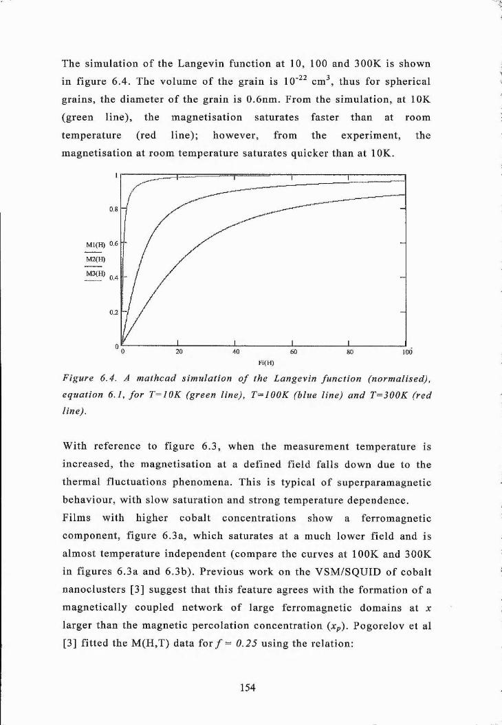
The simula tion o f the Langevin function at 10, 100 and 300K is shown

in figure 6.4. The volume o f the grain is 10'^^ cm^, thus for spherical

grains, the diameter o f the grain is 0.6nm. From the s imulation, at lOK

(green line), the magnet isa t ion saturates faster than at room

temperature (red l ine); however , from the exper iment , the

magnet isa t ion at room tempera ture saturates quicker than at lOK.

M1(H) 0.6

M2(H)

^ 0 . 4

0.2

100Fi(H)

Figure 6.4. A mathcad simulation o f the Langevin function (normalised), equation 6.1, fo r T=IOK (green line), T=100K (blue line) and T=300K (red line).

With reference to figure 6.3, when the measurement tempera ture is

increased, the magnet isa t ion at a defined field falls down due to the

thermal f luctuations phenomena. This is typical o f superparamagnet ic

behaviour , wi th slow saturat ion and strong temperature dependence.

Films with higher cobal t concentra tions show a ferromagnetic

component , f igure 6.3a, which saturates at a much lowe r f ield and is

almost tempera ture independent (compare the curves at lOOK and 300K

in figures 6.3a and 6.3b). P revious work on the VSM/SQUID o f cobalt

nanocluste rs [3] suggest that this feature agrees with the fo rmation o f a

magnet ically coupled network o f large ferromagnetic domains at x

larger than the magnet ic pe rcola tion concentra tion (Xp). Pogorelov et al

[3] f i t ted the M(H,T) data for / == 0.25 us ing the relation:

154

M = M , (6 .2 )

where P(v) is the volume dis tr ibut ion, expressed in the form

P(v) = ^^(v-v , )+( l -g)<5(v-v2) (6.3)

with V/ and V2 representing the volume o f the two grains. II, is the

internal field: for a spherical granule with the field applied with in the

film plane, I!, takes the form H, = H - ^ ( 1 - / ) M .

From their analysis on / = 0.J8, they deduced that the sample is

dominated by clusters with d iameters o f 3.6nm.

6.4 Ferromagnetic resonanceThis sect ion looks at two frequencies: 9.5GHz and 92GHz FMR.

6.4.1. 9.5GHz measurements

9.5 GHz FMR on cobal t nanoclus te rs was carried out on a I 6 k 0 e

Bruker Instruments ESR spectrometer, at room temperature , in the

School o f Chemistry, in St. Andrews. Angle rota tion measurements

from 0 to 360 degrees were possible ; however, the precis ion was as low

as 3 to 5 degrees. A quartz sample holder was used for this type o f

measurement . R ef [7] provides fur ther information on the 9.5GHz

spectrometer.

Films with composit ions above the percolat ion point:

It was observed that f i lms that have less than 17 at.% cobal t ( f = 0.J2)

have the same resonant f ield at d ifferent angles o f orientat ion. As the

concentra tion o f cobalt increases from 17 at.% cobalt , there is a change

in the resonant f ield between the in-plane and out-of-plane

configuration, as shown in figure 6.5.

155

10 -

(U2

TO

I

200 40 60 80 100angle of orientation (degrees)

Figure 6.5. A ng le r o t a t io n FMR a t 9 .5 G H z o f som e g r a n u l a r thin f i lm s . The

p l o t s a re thos e o f the uniform m ode only. Zero d e g r e e s r e p r e s e n t s the f i e l d

n o r m a l to the f i l m su r fa ce a n d n in e ty d e g r e e s is in -p lane FMR. F o r in -p lane

m ea su rem en ts , the e x t e r n a l f i e l d was a p p l i e d a lo n g the ea sy -a x i s .

Figure 6.6 is an FMR spectrum of 9 at .% cobalt .

back­groundFMR

^ignalg -1600 -

8 -1800

0 2 4 6 8 10 12a p p lie d field (kO e)

F igure 6 . 6 . 9 a t .% c o b a l t m e a s u r e d at 9 .5 G H z in the p e r p e n d i c u l a r

co n f i gu ra t ion . The e x t ra h ig h er f i e l d s i g n a l is b a c k g r o u n d f r o m the c a v i t y

a n d q u a r t z tube.

156

The angular dependence resonant f ield, HriOn), for a magnet ically

undersaturated thin fi lm [3] for volume fractions less than the

pe rcola tion point is given by:

' 2;zMW3cos"61-iy ^ ^

m (6.4)

where Oh is the field angle re lative to the film normal, v is the mean

grain volume, 6 is the m agnet i sa t ion ’s equi l ibrium angle and / is the

volumetr ic fi l l ing factor. The granules are assumed to be spherical and1/

so the equation d =6v is used to determine the granule diameter.

From Mathcad analysis, table 6.2 presents values to the sam ple ’s g-

factor and mean grain diameter:

Cobalt content g-factor Grain diameter

(at .%) (Angstroms)

9 2.28 4.6

11 2.23 5.6

17 2.28 11.0

Table 6.2. Values o f the sample's g-factor and grain diameter from angle rotation measurements at 9.5GHz with the use o f equation (6.4)

The g-factor is in good agreement to that o f bulk cobalt : 2.20 [8]. It is

also observed that the grain diameter deduced from FMR increases with

composi tion. The analysis was not s traightforward for 25 at.%. This

may be due to the inaccuracy o f the sam ple ’s posit ion re la tive to the

field direction: as mentioned previously, there may a three or five

degree error, consequent ly , the resonant field may be out by a few tens

o f oersteds; therefore, it was dif f icult to compare the FMR result with

that previously measured by SQUID.

157

Filins with composit ions above the percolat ion point:

At angles closer to and at the film normal, granular thin fi lms with

cobalt composi tion greater than 34 at .% ( / = 0.25) have resonant fields

that split into two or more peaks.

Figure 6.7, shows a typical X-band FMR spectrum of 71 at .% cobalt ( f

= 0.62).

6e+5

4e+5 -

2e+5 -10°

a.

40°-2e+5 -

90°

-4e+5 -

-6e+50 2000 4000 6000 8000 10000 12000 14000 16000

applied field (Oe)

Figure 6.7. FMR s p e c t r a a t 9 .5 G H z on 71 a t .% coba l t . The a n g le s a t the s ide

o f the s p e c t r a r e p r e s e n t the d i r e c t i o n o f the f i e l d r e l a t i v e to the f i l m normal .

FMR s p e c t r a m e a s u r e d at ten d e g r e e s has a h igher f i e l d s i g n a l at 8 kOe,

which is no t a t t r i b u t e d to ba ckground .

With reference to figure 6.7, for 71 at .% cobalt , there exists only one

FMR signal when the field is applied at angles between thirty and

ninety degrees to the film normal. However, at ten and twenty degrees,

there exist only two signals: this may be attr ibuted to coupling between

the precessing magnet ic moments o f isolated granules and o f infinite

158

fe rromagnetic cluster in the mixed phase [3]. Previous angle rotation

measurements at 9.4GHz, shows similar results , for 81 at .% cobalt [3].

Howeve r , it was not possib le for the group in the Ukraine to carry out

9.5GHz FMR with the field normal to the film plane (for f i lms whose

concent ra tions are above 54at.%) as this requires f ields higher than

lOkOe.

The FMR signal measured in the perpendicula r con figura tion has five

peaks, as shown in figure 6.8. Sueh a structure was previously

observed in Fe-SiOz granular f i lms [9] where it was a tt r ibuted to spin-

wave resonance and surface modes near the uniform FMR line. (Here,

they showed that the exchange constant, 8.3x10'^^ ergscm^ was smaller

than that o f bulk iron (at room temperature) , 5x10'^^ ergscm^. The

d ifference in the exchange constant was attributed to the abundance o f

magnetic surfaces or a cut o f f o f the spin waves with wavelengths

larger than the physical dimens ions o f the partieles.)

Applied field (Oe)

Figure 6.8. 9.5 GHz FMR signal o f 71 at. configuration.

6e+5

Abs.4e+5 - (a.u.)

36+5 -

26+5 -

le+5 -

12000 14000

cobalt in perpendicular

From figure 6.8, the dis tance between peaks three and four and peaks

four and five is 340 ± 40 Oe. This may suggest that these modes are

159

att r ibuted to standing spin waves. The second peak may be a uniform

mode while peak one is possibly a surface mode.

For bulk cobalt , the exchange constant is 1.3x10'^ e rgs/cm [10]. From

equation 2.42, the separa tion between consecutive l ines is

M

8 (« + i ) ^ r 7T where n is odd (6.5)

The exchange constant for this part icula r sample is (2 .2±0 .3)x l0 '^

ergs/cm, which is higher than the bulk value and L is taken as the fi lm

thickness , 270nm. The value o f n for peaks 3, 4 and 5 is 1, 3 and 5,

respectively. For the above calcula tion, the saturation magnet isa tion

was assumed to be the same as the bulk value, 1.43kOe. I f the

magnet isa tion term were to be replaeed by fMs, where / is the volume

fraction, then the exchange constant is (1.4±0.2)xl0~^ ergs/cm. If the

value L was the same as the grain size and not the fi lm th ickness , then

the exchange constant will be reduced to 10'^^ ergs/cm. More work is

required in order to unders tand standing spin waves in the CoAg

granular f ilms.

The perpendicula r FMR spectra o f samples whose concentra tions are

above the percola tion point ( f = 0.20) are shown below. These

lineshapes will be eompared with higher frequency measurements in

the next section.

160

6e+5

4e+5 -

'T' 2e+5 -

P -

CO -2e+5 -

2000 4000 6000 8000 10000 12000 14000 160000applied field (Oe)

Figure 6.9. 9.5GHz spectra o f granular f i lms with concentrations above the percolation point. The external f i e ld was applied normal to the f i lm surface.

The l inewid th o f the uniform mode for all samples measured in parallel

and perpendicula r con figura tion, are plo tted in figure 6,10.

o

0

O ' 9.5GHz perp. config.••■o •O ' 9.5GHz parallel config.

CD......O ' .. O , 0 . ..

©. '■■O'..

o . . . • " O

" o .................. O .............o

0.0 0.1 0.2 0.3 0.4 0.5 0.6

volumetric packing fraction, f

Figure 6.10. The measured linewidth in parallel and perpendicular configuration.

161

Further discussions on the low and high frequency measurements on

the l inewidth will be d iscussed in the next section.

6.4.2. 92G H z m e a s u r e m e n t s

High field ferromagnet ic resonance was carried out at 92 GHz. Figures

6.11 shows the l ineshapes, which have a poor signal to noise ratio as

the cobalt composi tion decrease. It was not possible to carry out in ­

plane measurements with the use o f an in-plane sample holder, as

discussed in section 2.2.4, due to the poor signal to noise.

0.10

0.05 -

3(Ôco

9-

-0.15 -

- 0.2010 15 20 25 30 35 40 5045

applied field (kOe)

Figure 6.11. FMR l i n e s h a p e s o f g r a n u l a r thin f i lms at 92GHz. The

c o m p o s i t i o n s o f c o b a l t va r i e s b e tw ee n 11 a n d 71 at .%.

It was observed that samples with composi tion greater than 34 at.%

have at least two FMR signals: the usual Kittel mode and the lower

field mode. The resolut ion at 92GHz for the case o f 45 to 71 at.% is

not as good as that at 9.5GHz. Consequently , it is diff icult to observe

162

lower field modes. It is unce r ta in what mechanism is responsib le for

the lower field mode in the 45, 54 and 64 at.% sample.

0.06

0.04 -

0.02 -=3

1 0.00 -

I(0 - 0.02 -

-0.04 -

-0.064

applied field (x 10 kOe)

Figure 6.12. FMR spectra o f 71 at.% cobalt with fa in t lower f i e ld lines.

Figure 6.12 is an FMR signal o f 71 at .% cobalt . The arrows point to

lower field modes. There are five signals in the spectra: the main

resonance line and four equal ly spaced l ines, which were 320Oe apart.

The spacing between the lower field modes is the same as in 9.5GHz.

As previous ly mentioned in the low frequency section, this may be due

to standing spin waves. Peak one in figure 6.8 may be a surface mode.

However , there is no higher f ield signal above the uniform mode in

figure 6.12.

Examples o f smal ler f ield modes that were observed in 54 and 64at.%

are shown in figure 6.13. Here, there is the high intens ity uniform

mode and two lower field modes.

163

a )

b)

0.04

0.02 '

0.00-

d - 0 . 0 2 -

-0.04 -

-0.06-

-0.08-

-0 .10 J

3.5 4.0

Applied field (xlOkOe)

0.02

0.01 -

0.0 0 -

8 - 0.01 -

-0.02 -

-0.03-

-0.043.5 4.0

Applied field (xlOkOe)

Figure 6.13. FMR spectra o f 54at.% (a) and 64at.% (b).

Table 6.3 is a set o f f ield values o f the uniform and lower field mode.

The data in the top and bottom table was collected from the FMR

spect ra at 92 and 9.5GHz, respectively .

164

Sample Uniform mode mode 2" mode 3" mode 4 mode

71 at.% 40.37 kOe 39.83 kOe 39.54 kOe 39.25 kOe 38.91 kOe

64 at.% 39.10 kOe 38.36 kOe - - -

54 at.% 37.38 kOe 36.74kOe 36.25 kOe - -

45 at.% 35.42 kOe 34.70 kOe - -T ab le 6 . 3 A

Sample Uniform mode 2" mode 3" mode Surface

mode mode

71at% 12.63 kOe 12.49 kOe 12.17 kOe 11.89kOe 12.82 kOe

64at% 9.74 kOe 9.13 kOe 4.19 kOe - -

54at% 9.58 kOe 9.18 kOe 8.92 kOe 4.50 kOe -

45at% 6.75 kOe 3.10 kOe - - 7.05 kOeT ab le 6 . 3B

Table 6.3. Values o f the r e s o n a n t f i e l d s f o r s a m p le s wi th c o m p o s i t i o n s a b o v e

34 at.%0 . The va lu es in t a b le s A a n d B w e r e taken at 9 2 G H z a n d 9 .5GH z,

r e s p e c t iv e l y .

From both tables, it is clear tha t the spectra measured at 9.5GHz has

one more signal than that at 92GHz. Referring back to figure 6.12,

which is the 71at.% cobal t signal, the spectra looks as though there is

only the uniform mode o f precession. Smoothing the data still shows

faint lower field signals.

Figure 6.14 is a plot o f the uniform resonant field (in perpendicula r

configura tion) with respect to the volumetric fil l ing factor at 9.5GHz

and 92GHz.

165

9.5GHz perp. config. 92GHz perp. config.40 -

10 -

0.70.0 0.1 0.2 0.3 0.4 0.5 0.6

volumetric packing fraction, f

Figure 6.14. P lo ts o f the uniform r e s o n a n t f i e l d at 9 .5 G H z a n d 92GHz, in

p e r p e n d i c u l a r co nf i gura t ion .

References [3] and [9] provide a detai led theoretical background on the

FMR in granular thin fi lms. For a thin film, for which the prineipal

values o f N are (0, 0, 47t) composed o f spherieal granules, the resonant

condi tions at T # 0Æ are:

where the volume fraction is below the percolation point, f < f p i

The perpendicula r and parallel resonant field are and

+ , respectively [3,11]. ( 6 .6 )

Here, =A7rfM^ with = M ^ L ( y M J k T ) and a = X ,

2. where the volume fraction is above the percolat ion point, f > f n \

Here the magnetic material is d is tr ibuted between the granular fraction,

/g, and ferromagnet ic fraction, f fM, so that / = /g + f p u [11] and

Hef f ^ 47T(fgMg+fFM^FM) [11]. Thc rcsonant field is given by

166

H t =\ r

where 6 is the m agnet i sa t ion ’s equil ibr ium angle, deduced from

Hsin{0ff ~ 0 )= 77^sin6)cos^ [3].

M fm is app roximate ly the same as Ms, which is about 1.43 kOe and

M g « M p M [3]. Equations 6.6 and 6.7 apply to the uniform mode.

In the analysis, the g-factor was assumed to be 2.20 and Mg = 1.43kOe

[3]. A plot o f Heff/4itMs, deduced from equations (6.6) and (6.7), with

respect to the packing fraction, / , for the field perpendicula r to the fi lm

plane {9=0) is shown in figure 6.15. I f one were to draw a dotted-line

as shown in the Hgff/4'n:Ms plot , then there exists a ‘b u m p ’, which is

lower than the percola tion poin t ( / = 0.20).

P revious work on 9.4GHz [11] have shown that this ‘b u m p ’ exists at

/ = 0.30 near the percola tion point, which is higher than that measured

at 92GHz. This was the main point o f this experiment: to locate the

pe rcolat ion point via FMR. One should note that the pe rcola tion point

in [11] is different from that d iscussed in [3]. After pr ivate discussions

[5], the pe rcola tion poin t is 0.20, as ment ioned in the beginning o f this

chapter.

167

• 92 GHz— solid line solution

0.7 -

0.6 -

I 0.5 -4

0.4 -

0.2 -

0.00.10.0 0.2 0.3 0.4 0.5 0.6 0.7 0.8 0.9 1.0

volume packing fraction, f

Figure 6.15, A plot o f the ratio o f the effective field, Heff, and saturation magnetisation (at OK) versus the cobalt packing fraction, f deduced from perpendicular FMR. There exists a bump at f — 0.12 rather than 0.20, where

the percolation point lies. The solid line is the ratio (with

4kMs = 17,6kG) and 4nfMs represents the demagnetising term o f the effective f i e ld fo r spherical particles [9,11].

Linewidth measurements at 92GHz (figure 6.16), shows that the

l inewidth increases s igni ficant ly as the volumetric fi l l ing factor

decreases. It is uncer ta in what mechanisms take part in these granular

f ilms. However in-plane l inewid th measurements on CoFe granular

f i lms in AI2O3 matrix was studied [12]. Here, they suggest that the

standard treatment o f the l inewid th th rough the damping term in the

Landau-Lif tschitz equat ion is insu ff ic ient to describe its high values in

granular systems and should be supplemented by the process o f non-

uniform broadening o f the resonance line. Mechanisms such as the

168

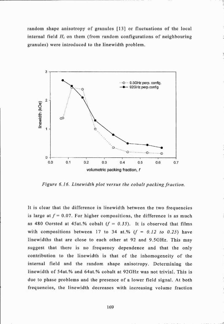
random shape anisotropy o f granules [13] or f luctuations o f the local

internal f ield Hi on them (from random conf igura tions o f ne ighbouring

granules) were in troduced to the l inewid th problem.

3

■ O ' 9.5GHz perp. config. — 92GHz perp. config

2

1

00.0 0.1 0.2 0.3 0.4 0.5 0.6 0.7

volumetric packing fraction, f

Figure 6.16. L inewid th p lo t versus the cobalt pack in g fract ion.

It is clear that the d ifference in l inewidth between the two frequeneies

is large at / = 0.07. For h igher composi tions, the difference is as much

as 480 Oersted at 45at.% cobalt { f = 0 .35). It is observed that films

with composi tions between 17 to 34 at .% { f = 0.12 to 0.25) have

l inewidths that are close to each other at 92 and 9.5GHz. This may

suggest that there is no frequency dependence and that the only

contr ibut ion to the l inewid th is tha t o f the inhomogeneity o f the

internal f ield and the random shape anisotropy. Determin ing the

l inewidth o f 54at.% and 64at .% cobal t at 92GHz was not trivial . This is

due to phase problems and the presence o f a lower field signal. At both

frequencies, the l inewidth decreases with increasing volume fraction

169

(for sam ples whose com positions are above 17at.%). I f an error was

known, then the two cu rves may coincide and so one may suggest that

their linew idths does not change dram atically with frequency, and so

the m echanism s associated w ith these samples does not include

damping . The change in linew id th at 11 at.% ( / = 0.07) is considerable

and so damping contribu tions may take place.

It is clear tha t more w ork is required in order to unders tand the

m echanism s in the CoAg granular films.

6.5. SummaryM ost o f the work in th is chapte r is based on low and h igh frequency

FMR. In contrast to previous works on low frequency FMR, this

chapter has deduced the m ean grain size for sam ples w ith

concentra tions below 25at.% . The m ean grain size o f 25at.% cobalt

determ ined from SQUID [3] was 36 Angstroms; the m ean grain size

determ ined from FMR for 17at.% was 11 Angstroms, w hich seems to be

in the right order o f m agnitude.

Samples such as 71 at.% cobalt have field lines that are equally

separated, w hich may suggest tha t they may be s tanding spin waves.

The exchange constant is h igher than that o f bulk cobalt. It is uncertain

as to why that is. The effective field , Heff, versus the packing fraction

shows a bump, which should locate the pe rcolation point. In contrast to

Pogorelov et al, h igh frequency m easurem ents located a ‘b um p’ at

/ = 0 .12 ra ther than / = 0.20. Pe rpendicular FM R linew idth

m easurem ents on sam ples w ith com positions greater than the

perco lation point have shown tha t the b iggest d ifference in linew idth

between the two frequencies is 5 0 0 0 e a t / = 0.35. It is clear that more

work is required in o rder to fully understand the m echanism s o f the

linew idth and the lower field signals.

170

6.6. R eferences[1] M X .P lum m er, J. van Ek and D .W eller, The Physics o f U ltra-H igh

D ens ity M agnetic Recording, Springer-V erlag, New York 2001

[2] M. Respaud, J. Appl. Phys., (1999)

[3] Yu. G. Pogorelov, G.N. K akazei, J.B. Sousa, A.F. K ravets, N.A.

Lesnik, M.M. Pe re ira de A zevedo, M. M alinowska, P. Panissod, Phys.

Rev. B., 60 (1999) 12200

[4] w w w .w ebelem ents.com

[5] N.A. Lesnik, pr iva te com m un ica t ions , 2002

[6] A.H. M orrish, The Physical Pr inc ip les o f M agnetism , Wiley, New

York, 1965

[7] Bruker H andbook on EPR Spectrom eter, J .C .W alton , priva te

com m unications, 2001

[8] S. Chikazum i, Physics o f M agnetism Wiley, Inc (1964)

[9] A .Butera, J .N .Zhou, J .A .B arnard , Phys.Rev.B, 60 (1999) 12270

[10] M .P ru tton, Thin Ferrom agnetic Films, B utterw orths, London,

1964

[11] G.N. Kakazei, A.F. K ravets, N.A. Lesnik, M.M. Pere ira de

Azevedo, Yu. G. Pogorelov, J.B. Sousa, J. Appl. Phys., 85 (1999) 5654

[12] V.O. Golub, G.N. K akazei, A.F. K ravets, N.A. Lesnik, Yu.G.

Pogorelov, J.B. Sousa, A .Y a.V ork, IEEE Trans. Magn., 2002 (In press)

[13] M. R ubinstein , B.N. Das, N .C. Koon, B.D. Chrisey, J. H orw itz,

Phys. Rev. B. 50 (1994) 184

171

Chapter 7

Summary and Future Work

This chapte r presents a synopsis on m agnetic studies o f cobalt-based

granular th in films w ith d iscussions on some projects tha t are worth

continuing. The layout o f the summary and future work is based on

experim ental chapters , two to six.

Chapter two is split into two parts: the theory o f FM R and the

experim ental layout o f the 12 Tesla spectrom eter. The la tte r includes

d iscussions on an in-plane sample ho lder that was used on th in films as

well as methods o f analysing an asym m etric signal from a cobalt th in

film, in order to determ ine the s ig n a l’s resonant field and linewidth.

Since the in-plane sample holder was not used for cobalt based

granular sam ples, it was not possib le to carry out in-p lane and ou t-o f­

plane FMR at the same frequency. Instead, m ulti-frequency FM R was

used. 75 to 95GHz FMR on the cobalt film , allows one to determ ine its

g-facto r and perpend icu la r an iso tropy field, which was found to be

s lightly h igher than that deduced from torque m agnetom etry.

If there was more tim e, it w ould be w orth finding another method o f

de term ining the resonant field and linew idth from an asym m etric non-

Lo ren tzian lineshape. I f the signal to noise ratio at 180 and 270GHz

had im proved, then it would be in teresting to compare FMR results

obtained from a narrow range, 20GHz, w ith that o f a broader range, 90

to 270GHz.

Chapter three involves the FM R and torque m agnetom etry o f two types

o f reco rd ing media. Each sample has its own grain size and size

d is tribu tion , which affects the sam ple’s recording properties . High

field FMR was used to solve the g-facto r, crystalline aniso tropy field

and the dam ping facto r. It was observed that from non-linear

172

f Hregression , the sum 4;rM^ +—— is well defined for these samples. ForV 2 /

both types o f media, the value o f the g-facto r and an iso tropy were

a lm ost the same, but the dam ping facto r was slightly d ifferent. Further

work is required in order to back-up conclusions p rov ided in section

3.2.5. A m ic rom agnetic sim ulation on the FMR spectra as d iscussed in

section 3.2.2. would be useful to com pare the properties deduced from

sim ula tion w ith experim ent. P rev ious work on the high and low noise

m edia were carried out on torque m agnetom etry in Seagate and they

showed tha t there is a d ifference in the c rystalline an iso tropy field. It

was observed that high fie ld FM R provided a higher value o f Hk than

low field torque m agnetom etry . A nother section in chapte r three

involves determ ining the value o f Hk and the in tergranular in teractions,

which are likely to be p resen t in the reco rd ing media, at fie lds lower

than lOkOe. A broader frequency range would also have been useful in

determ ining accu ra te ly the dam ping facto r and inhom ogeneous term.

The torque m agnetom etry section was split into two parts: the closing

point and A T method. Both techniques are novel and involved a

m ic rom agnetic s im ulation o f the torque signal, in order to solve for the

reco rd ing m ed ium ’s m agnetoc rysta lline anisotropy and in tergranular

in teractions. The A T m ethod was carried out on the low noise m edia

only, since there were problem s w ith the m easurem ent on the high

noise sample. I f there were more time, a A T m easurem ent on the high

noise sample would be usefu l. It w ould be in teresting to compare the

in te rgranu lar constant o f both types o f m edia and re la te them to their

reco rd ing properties.

Chapter four deals w ith the investigation o f the trend in the crystalline

anisotropy, g-facto r and possib ly the dam ping facto r for CoCrPtB

reco rd ing m edia w ith varying Pt and B content. The satu ration

m agnetisa tion on both the p la tinum and boron varying m edia m easured

in Seagate and IBM were not the same. It was observed tha t for both

sets o f samples, there was in fact a trend: the anisotropy and g-facto r

173

inc reases w ith Pt and B content, even though the sam ple ’s saturation

m agnetisa tion deduced from independent techniques were d ifferent.

It would be in teresting to carry out an out-of-p lane SQUID

m easurem ent (in St. Andrew s) on the two series so that the c rystalline

anisotropy was determ ined and com pared with 75-95 GHz FMR.

The G ilbert dam ping term for reco rd ing m edia m easured in chapters

three and four were in the range 0.01 to 0.04, which is in the region o f

tha t p reviously m easured by I nab a and Igarashi et al, as d iscussed in

section 3.2.1. It w ould be in te resting to carry out damping

m easurem ents using the optical pump probe FMR system in Exeter and

compare these results w ith the 75 - 95 GHz system.

Chapter five is conce rned w ith small angle neutron scatte ring o f 2D-

iso tropic and aniso tropic longitud ina l reco rd ing media. SANS analysis

o f the 2D iso tropic m edia shows that the fitting to the sine-squared

am plitude versus the scatte ring q is m odelled by an e llipso idal hard

core and soft shell. It was observed that the dim ensions o f the core and

shell at 14.5kOe is s im ila r to that at 4 .5kOe, as d iscussed in section

5.5,3. The o rien ta tion o f the m om ents in the cobalt core and soft shell

re la tive to the field d irection was also determ ined.

2D iso tropic and aniso trop ic m edia were also m easured in the rem anent

state, but they were not d iscussed in this thesis, and it would be

in teresting , as future work, to com pare the m agnetic grain size at

rem anence with non-ze ro fields.

Chapter six presents 9 .5G H z and 92GHz FMR o f cobalt nanocluste rs .

A lthough M-H loops on the CoxAgi_% th in films were m easured at

d ifferent tem peratures and were shown to exhibit superparam agnetism ,

an analysis w ith the equations derived by Pogorelov should be carried

out in order to rela te the m ean grain size w ith respect to the f i lm ’s

cobalt content. A com parison o f the m ean grain size from M-H loops to

9.5GHz m easurem ents for samples whose concentra tion are below

17at.% w ould be useful.

174

Angle ro ta tion work at 92GHz was not possib le , a lthough it would have

been useful to compare the grain sizes, for sample com positions less

than 17at.%, with the 9 .5GHz m easurem ents. This sort o f work requires

designing an angle ro ta tion sample holder, in addition, an FMR model

for h igh frequency m easurem ents. A model to solve the frequency

dependent and independent linew idth , is also required to back my

conclusions.

175

Appendix A

G aussian beams and the in-plane sam ple holder

Gaussian Beams

At m m -wave, te rahertz and h igher frequencies , free space beams are a

more convenient m ethod to desc ribe the way fields to travel from place

to place. The G aussian beam mode (GBM) approach is used for

m anipula ting m illim etre s ignals w ith free space beams. In the GBM

theory:

1. the rad ia tion is assum ed to be a paraxial beam (travelling along

the z-d irection), whose w idth is not very large com pared with the

rad ia tion w avelength;

2, the EM field satisfies a linked set o f scalar wave equations o f the

form = 0 (A .l )

where k = 2 ;^c is the speed o f light, / is the signal frequency

and (p is the field (p = u{x,y,z)ç.x^{~jkz)Qx^{j27ft) (A .2)

The so lu tion to (A .l ) defines a series o f free space G aussian beam

modes

1CO

(A.3)

where

J

=x^ + y ^ , R - zf 2

1 + 71(0[ ^ J _

={m + n + l)arctan<[ COq

(A.4, A.5, A.6 & A.7)

and H,n is the H erm ite polynom ial o f order m. E,„n is a com plex num ber

whose value is a m easure o f the f ie ld ’s overall am plitude and phase, r

176

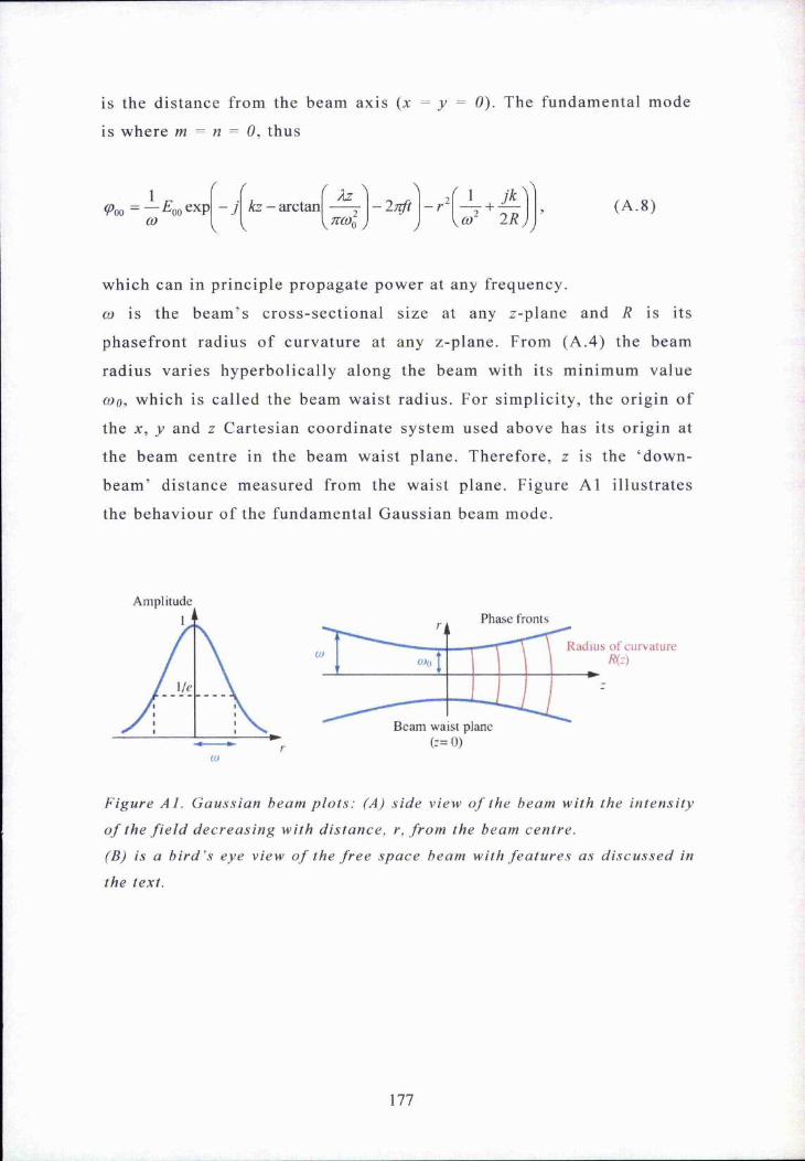
is the distance from the beam axis {x ^ y = 0). The fundam ental mode

is where m = n = 0, thus

1 ^ ( f^ 0 0 ~ ^ 0 0 - j kz - arctan 2 -2 7 ft

COV V y

- r0) 2R

(A .8)

which can in p rinciple p ropagate power at any frequency.

CO is the beam ’s c ross-sectional size at any z-plane and R is its

phasefront radius o f cu rvature at any z-plane. From (A.4) the beam

radius varies hyperbolically along the beam with its m inim um value

(Oo, which is called the beam w aist radius. For s im plicity , the origin o f

the X, y and z Cartesian coo rd inate system used above has its origin at

the beam centre in the beam waist plane. Therefore, z is the ‘down-

b eam ’ distance m easured from the waist plane. Figure A1 illustra tes

the behaviour o f the fundam ental Gaussian beam mode.

Amplitude

rCO

Phase fronts

Radius of curvature /?(--)

Beam waist plane (:= 0)

Figure A l . Gau ss ian beam p l o t s : (A) s id e v i ew o f the beam wi th the in tens i t y

o f the f i e l d d e c r e a s i n g wi th d i s ta nce , r, f r o m the beam centre .

(B) is a b i r d ’s eye v iew o f the f r e e s p a c e beam wi th f e a t u r e s as d i s c u s s e d in

the text.

177

Mathcad sheet; In-plane sample holder.

The mirrors were made of copper and the focussing lens, HOPE, was attachedto the bottom of the waveguide as illustrated in figure 2.12 in chapter two.1. We need to know the dimensions of the sample mirror and2. the distance between the mirror and sample holder which can be used for FMR/EPR/ESR measurements in the 12T magnet (with an inner bore of 49mm).

The frequency here is 94GHz

d := 0.634-13.4

d = 8.496 Beam waist at the waveguideand 13.4mm is the radius of the

90GHz waveguide.

X := 3 1 010"

94-10"wavelength of the beam

X = 3.191

z i := 20 distance between H O P E lens and 45 deg. mirror

wO := — -t- 2

equation A4

waist := - /v ^

waist = 8 .119 beam waist at 45 degree mirror

z2 := 15 distance between 45 degree mirror and left side mirror

w2 := (waist)- 1 +(z2)'

Ti -(waist)'^

equation A4 re-written in terms of the waist size at a certain distance along the beam

w2 = 8.333 beam waist at sample mirror

D1 := 27D1

w2= 3.24 ratio o f side mirror

Appendix B

Lineshape analysis

Lineshape analysis: this appendix looks at lineshapes that were observed from FMR measurements. In some cases, one would observe a perfect absorption lineshape; however, there were traces of dispersion in the signal. In order to determine the resonant field and linewidth, a fit to the lineshape using an admixture of absorption and dispersion is required.This sheet looks at1. pure absorption and dispersion signals2. the addition of background noise to the signal

If we assume the area under the lineshape defines the number of moments participating in the resonance experiment, then it is clear that the integral of the absorption and dispersion shapes are not the same, as shown below.

For a Lorentzian absorption lineshape, the integral is

1

1 +( x - r)

L

~l2dx

w here L is the half peak to peak linewidth, r is the resonant field and x is the scanning field.

which g ives us:

1 (2-x — 2 r) 2* L

L-atan

For a Lorentzian dispersion lineshape, the Integral is

( x - r )

- — dxwhich g ives us:

1 +( x - r )

—-L-ln(L^ + x - 2 X r + r )

Therefore, w e introduce a factor A to the dispersion curve which will match the number of m oments from the absorption line shape, where A>0.

From FMR m easurem ents, w e are measuring in first order derivative, therefore, the double derivative of the m om ents in absorption m ode is:

-L-atandxT

1 (2 -x -2 -r )

2 " Lwhich is equal to

-1 (2 X — 2-r)

, 1 (2-x - 2-r)'1 H ------------

180

Similarly for a dispersion mode;

dx

this g ives us AI (2 .x -2 .r X

— A 'L * .

(l^ + ^ - 2-x-r + r ) ( j2 ^ 2 _ 2.x-r +

AN EXAMPLE; 90GHz FMR on cobalt thin film where we have the resonant field 'r' at 40 kOe and the linewidth 'L* is 8kOe

r:=4.0 L := 0 .4 x := 0 ,0 .01 .. 8

Absorption and dispersion lineshapes (from above) are:

absn(x):=-1 (2-x - 2-r)

1 + 1 (2-x - 2-r)'

W e introduce a value to the term A, say 0.5

A := 0.5

L 1dispn(x) := A- A-L-

(2-x - 2-r)'

2-x-r + r 2\:L + X - 2-x-r + r )

The plots of dispersion and absorption curves using the above equations are shown below:

Observation o f line shapes

absn(x)I•S dispn(x) 0 .0-----

- 2

Xfield (Tesla)

181

If we introduce background noise to the signal, then we have following lineshape:

absorption plus random noise

ab(x) := absn(x) + (rnd(0.5) + m d(-0.5))

introduce noise

dispersion plus random noise

dp(x) := dispn(x) + (md(0.5) + md(-0.5))

introduce noise

sum(x) := ab(x) + dp(x) + 0.3x

Plot of line sh ape with random noise;

= sum(x)

field (tesla)

If say, seven grains contributed to the uniform mode, denoted absn#(x), then the resultant lineshape is:

First lineshape: resonant field YT and linewidth 'La' La := 0.1 rl := 3.9

-1 ( 2 . x - 2.rl)absnl(x) :=

, I (2 x - 2 . r l ) '1 H------------------4 La'

' La'

Second lineshape: resonant field 'r2' and linewidth 'Lb' Lb := 0.1 r2 := 3.93

-1 ( 2 -x - 2 .r 2 )absn2(x) :=

1 (2 x - 2 r2)'_|----------------------------------

4 Lb'

' Lb'

182

Le ;= 0.1 r3 := 3.96

- 1absn3(x) ;= ------------------

( 2 .x - 2 . r 3 )

, 1 (2.x - 2.r3)'1 H-----------

4 Le"

2 Le" absn4(x):=

Ld := 0.1 r4 := 3.99

—1 (2.x — 2.r4)

, 1 (2 .x - 2.r4X1 H *—

4 Ld^

Ld

absn5(x):=

r5 := 4.02 Lh = 0.1 r6:=4.05

-1 ( 2 .x - 2-r5)absn6(x):=

-1

1 ( 2 x -2 .r 5 ) "

4 Lf"

" Lf", . 1 (2 x - 2 r6)"

4 Lh"

(2.x — 2.r6) Lh

Li :=0.1 r7:=4.08

absn7(x):=(2 .x - 2.r7)

, 1 (2.x - 2.1-7)'1 + —4 Li"

" Li"

The sum of all seven lineshapes (from each grain) is;

ab(x) ;= absnl(x) + absn2(x) + absn3(x) + absn4(x) + absn5(x) + absn6(x) + absn7(x)

Plots of all individual reson ances from each grain and the main signal

30

20

ab(x)

absnl(x)10

absn2(x)

absn3(x)0

absn4(x)

absn5(x)

absn6(x) 1*

absii7(x)

-2 0

-3 0

field (tesla)

183

Appendix C

The FMR condition for longitudinal recording media

Verify that for any value of rho, the angle between the c-axis and the x-axis will generatethe same resonant condition. We will look at the rhs of equation (3.13).

Hk := 1.08 in plane uniaxial anisotropy

M ;=0.4872 magnetisation

4*71

H := 4.17 resonant field

tiiH := — phH := — field angles wrt 2 2 film surface

HkKu := M anisotropy constant

2Ku = 0.021 Kperp := 0

th := — ph := — assum ing that the m om ents are along the field 2 2 direction, then both the polar and azimuth

angle of the m oment is the sam e a s the field

angle rotation of the c-axis, rho, relative to the x-axis a s shown in chapter three, in radians.

rho := 0,0.01..271

The equations below are parts of the resonant condition (3.13)

rhl(rho) := M-H-(sin(th)-cos(phH - ph)-sin(thH) + cos(th)-cos(thH)) + [(4-7t*M" - 2 Kperp) cos(2 th)

rh2(rho) := -2*Ku-[cos(2'th)'(cos(ph))"-(cos(rho))" - cos(2 - th) (sin(rho))" - sin(2 th) - cos(ph) sin(2 rhc

rh3(rho) := M-H-(sin(th)-cos(phH - ph)-sin(thH)) + [(4-7i -m " - 2-Kperp)-(sin(th))"-cos(2-ph)J

rh4(rho) := Ku 2 .(s m (th ))" .c o s (2 .p h ) .(c o s ( rh o ))" + : .( s m (2 ;th )c o s (p h ) .s m (2 .rh o ) )

rh5(rho) := M-H-(cos(th)-sin(thH)-sin(th - thH)) + [(2*71>m " - Kperp)•sin(2-th)-sin(2-ph)J

rh6(rho) := Ku [sin(2 th) sin(2 ph) (cos(rho))" + cos(2-th)-sin(ph)*sin(2-rho)J

rh7(rho) — t-(*4il(rho) + rh2(rho))-(rh3(rho) + rh4(rho)) - (rh5(rho) + rh6(rho))"J

M"-(sin(th))"

rh8(rho) ;= -\J rh7(rho)

184

The frequency of the mm-wave is ^ ^ 9W := 9 3 .3 6 - lU

Here w e look at the g-factor, derived and observe how the g-factor varies with the angle rho.

. - 3 4g(rlio) := w-6.63-

10"(9.27-10""'^.rh8(rho))

The g-value is around 2 .157 and it d oes not change with respect to the orientation of the moment relative to the x-axis

2.16

2,158

g{rho)

2.156

2.154

185

Appendix D

SQUID m easurem ents on CoCrPtB (Pt series) thin film s

M agnetisation m easurem ents on the p la tinum varying m edia were

carried out by a 5T SQUID (superconducting quantum interference

device) in St. Andrews. The SQUID has a sensitiv ity o f 10'* emu and

the physics o f the SQUID m agnetom eter is found in the Institu te o f

Physics postgraduate w orkshop handbook on Bulk C harac te risa tion o f

M agnetic M ate ria ls (1999).

Here, the external field is applied w ith in the film surface at room

tem perature.

0.0006

0.0004 -

^ 0.0002 -

0.0000 -

- 0.0002 -

-0.0004 -

-0.0006

16 at.% platinum

-60000 -40000 -20000 0 20000

fie ld (O e )

40000

186

0.0006

0.0004

0.0002 -

0.0000

- 0.0002

-0.0004

-0.0006-60000 -40000 -20000 0 20000

applied field (Oe)

14 at.% platinum

40000 60000

0.0006

0.0004 -

0.0002

- 0.0002

-0.0004

-0.0006-60000 -40000 -20000 0 20000

applied field (Oe)

12 at.% platinum

40000 60000

187

Publications

188

JOURNAL OF APPLIED PHYSICS VOLUME 91, NUMBER 3 1 FEBRUARY 2002

High field ferroniagiietic resonance measurements of the anisotropy field of longitudinal recording thin-fllm media

C. J. Oates, F. Y. Ogrin,* S . L. Lee, P. C. RIedi, and G. M. SmifliSchool o f Physics and Astronomy, University o f St. Andrews, KY16 9SS, United Kingdom

T. Thomson^)Seagate Technology, 470W Kato Road, Fremont, California 94538

(Received 25 June 2001; accepted for publication 27 October 2001)

The average value of the magnetocrystalline anisotropy field, Jf*, is an important parameter for the characterization of magnetic recording media but is difficult to measure accurately due in part to the effect o f interactions between the grains. In order to evaluate we have studied two model CoCrPtTa magnetic films using a number o f complementary techniques: high field ferromagnetic resonance (FMR) (35.0-45.0 kOe), low field (<20 kOe) vector vibrating-sample magnetometry and torque magnetometry. The FMR measurements were performed at a number o f discrete frequencies in the range 75-93 GHz using a new quasi-optical spectrometer developed at the University o f St.Andrews. The values o f derived by FMR (10.8 kOe) are approximately 10% greater than those obtained from conventional magnetometry (9.6 kOe). This difference is believed to be due to the presence o f intergranular exchange coupling which reduces the measured value o f anisotropy when the applied field is not sufficiently large to completely align the magnetic moments. © 2002 American Institute o f Physics. [DOI: 10.1063/1.1428804]

I. INTRODUCTION

Anisotropy and saturation magnetization are the two fundamental properties that determine the static characteris­tics o f ferromagnetic materials.' Magnetic anisotropy deter­mines the difficulty o f changing the state o f the atomic mag­netic moments for a given set o f experimental conditions while the saturation magnetization measures the effect o f alignment o f the atomic magnetic moments. In addition the dynamic properties o f ferromagnetic materials during rever­sal are characterized by the Gilbert damping constant, a? Interest in a has recently increased particularly in materials used for data storage such as CoCr-based thin films as data rates, and hence the time available to switch the magnetiza­tion, decrease to below 1 ns. ’'' Despite the fimdamental na­ture of these quantities it remains an on-going experimental challenge to determine their values accurately, particularly when materials are in the form of thin films. In this study we report comprehensive work aimed at deterrnining the anisot­ropy and the Gilbert damping constant by high field ferro­magnetic resonance (FMR).

We have chosen two model CoCrPtTa thin films of in­terest as media for data storage with different magnetic re­cording properties. The two samples were sputtered on super-smooth glass-ceramic substrates using a standard com­mercial dc magnetron sputtering system. The magnetic layers of both media were sputtered from the same CoCrPtTa alloy target with the underlayers consisting o f SO nm thick CrMn for media A and 40 nm/10 nm thick NLAI/CrMn for media B.

“ Currently at thc University o f Exeter, School o f Physics, University o f Exeter, Stocker Road, Exeter BX4 4QL, UK.

’’’Currently at IBM, IBM—Almaden Research Center, 650 Harry Road, San Jose, CA 95120.

Previous work on these samples shows that they have sub­stantially different recording properties; with media A having higher noise than media B which was attributed primarily to the differences in grain size and grain size distribution. *'

This paper examines the relative merits o f the techniques used to determine these fundamental magnetic properties o f thin-film media and correlates the differences found in these model samples to differences in their recording performance.

II. EXPERIMENTThe FMR measurements were performed at a number of

discrete frequencies in the range 75-93 GHz (35.0-45.0 kOe) using a new quasi-optical spectrometer developed at the University o f St. Andrews.^ As a preliminary experiment FMR and low field (<20 kOe) torque magnetometry meth­ods were applied to a polycrystaUine Co film. Good agree­ment was found between the two values derived for the ef­fective anisotropy which is discussed later in section four. In the FMR experiments the field is applied normal to the film plane and is sufficiently large to decouple the interactions between the grains. In principle all the parameters required to characterize the material, Landé g-factor, saturation magne­tization A/j, anisotropy field and the Gilbert damping factor or, may be obtained firom the field for resonance and the linewidth o f the FMR signal as a function o f frequency. In practice, it was found that a more accurate data set can be obtained when Af, was measured using a vibrating-sample magnetometer (VSM).

Magnetization measurements were taken using a ADE/ Digital Measurement Systems model 10 vector VSM, with a maximum applied field o f 20 kOe. The temperature was held constant at 20 °C during all measurements. The saturation magnetization was determined from hysteresis loops using

0021-8979/2002/91 (3)/1417/6/$ 19.00 1417 © 2002 American Institute of Physics

Downloaded 25 Ja n 2002 to 138.251.31.115. R edistribution su b je c t to AlP license o r copy right, se e h ttp ://o jps.a jp .o rg /japo /japc r.jsp

1418 J. Appl. Phys., Vol. 91, No. 3. 1 February 2002 Oates et al.

s u b ^ ra tethin film

easy

FIG. !. Orientation of the magnetization M, applied field H and easy axes of the magnetic grains with respect to the film plane.

the instrument in conventional mode with the sample plane aligned parallel to the applied field. A Ni foil standard o f the same diameter as tfie sample was used to calibrate the instru­ment. Corrections for the substrate and sample rod were at­tempted using two techniques. The first involved fitting a linear function to the high field region o f the hysteresis loops and using the slope as a correction factor. The second tech­nique consisted of removing the magnetic film from the sub­strate and remeasuring to give a point-by-point subtraction. The two techniques yielded extremely similar results and the linear function method was adopted as this minimized the error on individual data points.

Anisotropy was measured using our in-house torque magnetometer. In this technique, the film is rotated from 0 to 90 deg relative to the field direction. Details o f this technique are further described in Ref. 8. [Table II (Sec. IV) provides values to the saturation magnetization and anisotropy that were derived fix>m the above techniques.]

+N^oé is the effective demagnetizing factor with directional cosines a, which define the orientation of the magnetization vector with respect to the coordinate axes. In the thin film limit the demagnetizing factor N is simplified assuming that

^2=0 and iV^=4ir. Minimizing Eq. (1) will determine the magnetization’s static orientation which is used to simu­late FMR and torque data.

B. Equation of magnetic motionTo calculate the FMR response the equation of motion of

the magnetization vector is used:’

(2)A/, sin 0Q

where w is the resonance frequency, y is the gyromagnetic ratio and Eg^, E^^ and Eg^ represent the second partial derivatives of the free energy taken at the magnetization vec­tor’s equilibrium position (#o,<Po)

cP-E

E aa —

âdd<p ’

d EdOde

d Ed(pd<p

(3)e=-$Q.(p=<pQ

From Eqs. (1), (2) and (3) the resonance frequency is easily related to the parameters g, //* , 4irM^. In our configuration (Fig. 1) this relation is expressed as

o> = [((47rA/^ sin <Pq + M ^ H c o s 2 0q

+ HMs sin do cos(<Pff-<Po))

X sin $0 cos 2 (po + H M , sin Oq c o s ( <pff

~<Po))“ (2 irA/j sin2 (?o sin2 (po

III. FMR MODEL OF LONGITUDINAL RECORDING MEDIAA. Free energy density equation

In order to simulate the resonant conditions we applied a model in which the thin-film media consists o f a large num­ber of crystallites (grains), each containing an easy uniaxial anisotropy axis. The orientation of the uniaxial axes is iso­tropic and confined to the film plane (see Fig. 1). It is as­sumed that the interaction between the grains is negligible and that the properties o f each crystallite in a high magnetic field is described by a single domain model. With these con­ditions the free energy per unit voliune for each grain is written in the following form:

-H M , cos ^0 sin(<p;^- (po))^]' (4)

I/=-M,.H+}NA/J + A:sin2 ( 1 )

where M, is the saturation magnetization vector, K = M jH t/2 is the magnetocrystalline anisotropy constant, H * is the anisotropy field and <f> is the angle between the grain’s magnetization and crystallographic axis. N= N ^al + N ^a l

sin do '

If the applied field H is sufficiently high and directed normal to the film surface (i.e., (p^=90°), the equilibrium position of the magnetization vector will therefore align with the ap­plied field: <po = 90°. Thus for the perpendicularconfiguration in the high field limit, the resonant condition, [Eq. (4)] is simplified to

—j = (^ r ~ 4 7 r A f,- //* )( //,.-4 ir A /J , (5)

where is the resonant field.

C. Solution to the FMR conditionIn principle it is possible to determine the three param­

eters g, //* and 4 irM using a minimum of three frequencies. However, in practice, due to the error in determining the resonant field it is difficult to determine 4 ttM , and H sepa­rately but only the sum of the two variables, (4ttA/^ + //^).

Downloaded 25 Ja n 2002 to 138.251.31.115. R edistribution su b je c t to AlP license o r copy right, se e h ttp ://o jps.a ip .o rg /japo /japc r.jsp

J . Appl. Phys., Vol. 91, No. 3, 1 February 2002 O ates et al. 1419

18

75 GHz 93 GHz16

14

12

10

a

2 3 4 s 6 7

4icMs (kG)

FIG. 2. Graphical representation of solution to Eq. (5) for two frequencies: 75 GHz and 93 GHz. The resonance fields were determined from the ex­perimental measurement on sample ISA and equal to 35.85 kOe and 41.75 kOe, respectively. Thé resonance field error SH^ was estimated from fitting the resonance line shape into Eq. (7). With g fixed to 2.15, it was found that for both samples 100 Oe (which corresponds to the thickness o f the lines at 75 and 93 GIfe).

At high frequencies, the function form o f the equation is such that a small variation in lead to a significant change in the individual values of 7/* and as shown by thesize of the intersection area in Fig. 2. Even for a fixed value of g and a small error in (=0.5%) an error as high as 50% in 77* is observed. This error can be reduced by applying frequencies with the maximum possible separation. The angle between the solution Unes that correspond to the two frequencies increases resulting in a reduction to the area of intersection (see Fig. 3). Consequently, the spread in possible solutions of 77* and 4irMj. decreases. As an example. Table I provides results o f the numerical simulation for two different frequencies with g and SH^ fixed to 2.15 and 100 Oe, re­spectively.

Applying frequencies over a broader range will reduce the error in the sample’s saturation magnetization and anisot­ropy significantly. However, even at a maximum possible separation (for our spectrometer A /=200G H z) the best er­ror in 77* still remains not less than ±1.1 kOe (<577,. = 100 Oe) which is similar to the uncertainty commonly re­ported for other techniques used to measure anisotropy. In order to reduce errors further one should either try to im­prove the precision o f the resonance field Hr and/or employ other techniques that will measure one o f the Ë)ove param­eters separately. In this work we follow both directions. We carefully analyze the resonance line shape by fitting it to an analytically derived distribution from which the resonance field can be extracted as a parameter. We also use vibrating sample magnetometry to measure precisely the value of the media’s saturation magnetization which is used as a fixed parameter in Eq. (5).

18 5H ~ lOOOc75 GHz

270 GHz15

o

^12

11

10

2.52.0 3.0 3.5 4.0 4.5 5.0 5.54jlMs (kG)

FIG. 3. Intersection of two solutions for 75 GHz and 270 GHz as simulated using Eq. (5). For both samples g is fixed to 2.15 and SHr is taken as 100 Oe.

IV. RESULTS AND DISCUSSION

It has been shown previously that FMR can provide use­ful information on anisotropy in thin films.'® In many cases the analysis of anisotropy is built upon the angular depen­dence o f the resonance field." For high field spectrometers based on superconducting coils it is not always easy to ar­range experiments with an angular variation of the applied field. This is due to space restrictions or mechanical com­plexities o f the rotational mechanisms. An alternative is to set up an experiment where the applied field angle is fixed and the excitation frequency is varied. This is the approach we adopt in high field, multi-frequency FMR measurements where the field was always normal to the plane o f the film. As a preliminary example, multi-frequency measurements on a 30 nm polycrystalline Co film were performed to find the effective anisotropy The cobalt film was grown using molecular beam epitaxy on a silicon substrate. The deposited cobalt layer consisted mainly of a polycrystalline hep phase, with some fee phase and stacking faults as determined by nuclear magnetic resonance.'^ Given that the direction o f the easy axes is mainly out-of-plane for the Co film, the reso­nance equation in this case is different to that for the media samples and given by the following relation;

-=77,-77eff. (6)

TABLE I. Intersection of possible solutions for two different frequency ranges (sec Figs. 2, 3) as simulated using Eq. (5). Parameters o f g and arc fixed to 2.15 and 100 Oe, respectively.

fx h g SHr \4 n M r

75 GHz 93 GHz 2.15 100 Oe 8.4 kOe 5.0 kG75 GHz 270 GHz 2.15 100 Oe 2.2 kOe 1.3 kG

D ow nloaded 25 Ja n 2002 to 138.251.31.115. R edistribution su b je c t to AlP license o r copy right, se e h ttp ://o jps.aip .o rg /japo /japc r.jsp

1420 J. Appl. Phys., Vol. 91, No. 3 ,1 February 2002 O ates 0 t aL

100 PF

95 -

® as

80

75

70

6542 4844 4640 50

Resonance field (kOe)

FIG. 4. Resonance frequency as a function of the resonance field for an hep Co fihn. Solid line— fit using Eq. (6).

where Equation (6) was derived from Eqs.(1), (2) and (3) assuming that the orientation of the easy c axes and the applied field are perpendicular to the fihn plane. Figure 4 illustrates the resonance field dependence o f the frequency measured for the Co film. The experimental points were fitted with Eq. (6). The extracted values of g and Hf.fi were 2.156(5) and 17.15(20) kOe, respectively. This was in reasonable agreement with previous measurement of on the same film by torque magnetometry which was 16.2(7) kOe.'^ If it is assumed that the saturation magnetization for this fihn is the same as for bulk Co, the crystalline anisotropy field Hk extracted in this way is o f the order of 0.5 kOe. Consequently, the magnetocrystalline anisotropy constant is deduced to be (3.15 ± 1.45) X 10 ergs/cc. This value is much less than that o f bulk cobalt, which is typically (3- —4) X 10 ergs/cc. and, most likely, is a result o f the mix­ture in the crystalline phases and the polycrysalline nature o f the s a m p l e . H o w e v e r , the emphasis here is on the analysis of the perpendicular effective field which is measured independently o f the saturation magnetization and, therefore, is very usefiil for comparison with the equivalent measurements with other magnetization techniques, includ­ing torque magnetometry.

It should be noted that in the configuration of the Co film the magnetocrystalline anisotropy has the same symmetry as the demagnetizing field. This makes it impossible to measure

separately without contribution from the demagnetrzing fields. Nevertheless, the eflfective field is measured with good precision firom a relatively narrow range o f fioquencies with­out involving magnetometry. A simulation o f Eq. (6) with the cobalt’s effective field measured as a fimction of the g-factor for two different frequencies: 75 and 93 GHz is shown in Fig. 5. For thin film longitudinal media with easy axes in­plane of the film, unlike the cobalt film, it is theoretically possible to separate the magnetocrystalline anisotropy from the demagnetizing field [compare Eqs. (5) and (6)]. How­ever, in practice, due to the high sensitivity to the resonance

75 GHz

93 GHzZ.13 2.14 2.15 2.18 2.17 2.18

1.8 1.8 2.0 2.2 2.4 2.6g factor

FIG. 5. Graphical solution to Eq. (6) for a polycrystalline Co film. HfS = 17.15(20) kOe, g=2.156(5). The resonance frequencies, 75 GHz and 93 GHz correspond to the resonance fields o f 42.04 IcOe and 47.95 kOe, re­spectively. The error in the estimate of the resonance field; <5//,=80 Oe.

field error SH^ the spread in possible solutions to and AttM s is very high and hence additional magnetization mea­surements are required.

The FMR measurements on the media samples were car­ried out in the range of frequencies between 75 GHz and 93 GHz. In contrast to previously published results by Igarashi et al. we were able to obtain very well resolved resonance lines which allowed us to determine the resonance fields with a precision of better than ±0.25%. Figure 6 illustrates an example of a first order derivative absorption line shape of

n.9 -2

34 36 38Applied field (kOe)

40 44

FIG. 6. FMR spectrum measured on high noise media at 84 GHz. Circles— experimental data. Solid line—fit using Eq. (7) 77, = 38 750 Oe± 50 Oe.

D ow nloaded 25 Ja n 2002 to 138.251.31.115. R edistribution su b je c t to AlP license or copy right, s e e h ttp ://o lps.a ip .o rg /japo ljapc r.jsp

J. Appl. Phys., Vol. 91, No. 3, 1 February 2002 O ates at al. 1421

92

90

88

® 86 cr

84

82

78

3837 39 40 41Resonance field (kOe)

FIG. 7. Resonance frequency as a function o f resonance field for high noise media (sample 15A).

high noise (sample 15A) media at 84 GHz. The resonance field is extracted firom a fit to a first derivative Lorentzian line shape’* which is in the form

+ 9b~-3b\ \ ÛlM. I I(7)

H r - H^Hr

3 +H r - HàHr

H r - H

I-------

where y is the FMR response, H and Hr are the applied and resonance fields, LHr is the resonance half peak-to-peak linewidth and a and b are the amplitudes o f absorption and dispersion signals, respectively. The last two parameters are, in fact, very important for the determination o ^ H r . It is a common feature of FMR spectrometers that the output signal often contains a mixture of the absorption and dispersion phases. This is in contrast to the ideal situation when ordy the absorption signal should be detected. Thus, by adding the presence of a dispersion signal we can always fit the output signal correctly and determine the resonance field with high precision.

Figure 7 shows the variation o f the excitation frequency {(üH tt) as a function o f resonance field Hr measured for the high noise (15 A) sample. The solid line is the result o f a fit using Eq. (5) with the value of the saturation magnetization given by the VSM measurement. The value of the anisotropy field Hj produced by the fit is given in Table II. It should be

TABLE n. Parameters of the anisotropy field and g-factor as a result of the fit using equation 5. is measured separately by vector VSM. The value by torque magnetometer is taken from Ref. 8.

Sample flk (kOe) ffk (kOe) 4irA/, (kG)name Torque FMR VSM gI5A (high noise media) 9.6(4) 10.8(2) 4.9(1) 2.150(5)15B (low noise media) 9.6(4) 10.7(2) 4.5(1) 2.160(5)

noted that the precision of the calculated value o f is di­rectly dependent on the precision o f . In the present case the uncertainty in arises as a combination o f errors: the measured total magnetic moment //,, magnetic layer thickness d and the sample area 5 (e.g., for sample 15A: /x = 209± 1 X 10“ emu, 27.5± 0.5 nm, 5=19 . 6 ±0.2mm^.)

It is interesting to note that similarly to the Co film, the values of the anisotropy field H/ measured by torque mag­netometry were close, but slightly lower than those measured by FMR. This discrepancy in H^ is believed to be not just a lack of experimental precision but a consequence o f the in­trinsic characteristics o f polycrystalline materials. In FMR the external field is o f the order o f 40 kOe which is several times larger than that required to saturate the media. As a result only uniform precession o f the magnetic moments is produced. Any possible effects o f coupling between the grains of the material will not affect the resonant conditions. In contrast to FMR, torque measurements are typically car­ried out at lower fields (up to 20 kOe). Within this field range both the magnetostatic and exchange interaction can play a significant role in the collective behavior o f the magnetic grains which form the sample. This behavior is more com­plicated than that described by the simple model given here(1) and requires a more detailed micromagnetic approach. Although the interaction in these samples is quite weak it is sufficient to give a lower value of the anisotropy field mea­sured by low field (<20 kOe) torque magnetometry.*

V. DYNAMIC PROPERTIESFMR linewidth measurements provide details on the

sample’s inhomogeneous broadening and relaxation con­stant. The relaxation constant is related to tlie switching mechanism of the magnetization vector . In the present measurements the linewidth of the FMR signal was deter­mined in the same way as the resonant field: a fit to the line shape using Eq. (7). The linewidth ùkHr in Eq. (7) is defined as half of the field difference between the maximum and minimum of the first derivative absorption line shape. The firequency dependence of the peak-to-peak linewidth was de­rived from the following equation:’

a y 1(8)

where a is the Gilbert damping factor. An additional fre­quency independent term is included which contributes to the inhomogeneous broadening.^® Thus the linewidth is ex­pressed as:

A if( <u ) = A //( 0 ) +la o i

(9)

where àH(<o) and A /f(0) is the frequency dependent and independent peak-to-peak linewidth. Figure 8 shows a fit to the linewidth using Eq. (9) and Table III shows the results for both media samples.

The inhomogeneous broadening term in the low noise medium is twice that of the high noise medium. This may result from the following: The low noise media is comprised

D ow nloaded 25 Ja n 2002 to 138.251.31.115. R edistribution su b je c t to AlP license o r copyright, see h ttp ://o jp s .a ip .o rg /jap o /jap c r.jsp

1422 J. Appl. Phys., Vol. 91, No. 3, 1 February 2002 O ates et al.

1050

1000

15A

950

ai

900

15B860

80085

Frequency (Hz)90X108075

FIG. 8. Resonance linewidth for samples 15A (circles) and 15B (squares) as a function of frequency. Solid lines—result of fits using Eq. 9.

of smaller grains (11 nm) with better grain segregation than that o f the high noise media where the mean grain size (42 nm) is approximately four times greater. The segregation leads to better isolation of the magnetic moments and, there­fore, reduces exchange coupling between the grains. Conse­quently, the inhomogeneity of the medium is greater as a result o f a larger number of spins in different local magnetic environments, nonetheless, the noise, associated with the ex­change coupling, is lower. This interpretation is also sup­ported by the values of the Gilbert damping factors. For the sample with larger grains (high noise medium) the damping factor is greater. This indicates a faster relaxation time which may again be a result of stronger intergrain coupling in this sample.

VI. CONCLUSIONSIn this paper we have for the first time shown convinc­

ingly that high field, multi-frequency (75-93 GHz) FMR may be used to determine the static (7/^) and dynamic prop­erties (damping constant a) of realistic («=3 Gbits/in^) longi­tudinal thin film recording media. While, in principle,Mg and the Lande g-factor may all be extracted from the FMR data, in practice we find that fixing the value of M g , which is easily obtained from magnetometry measurements, reduces the uncertainty in the values obtained for the other

TABLE in. Parameters of the Inhomogeneous broadening and theGilbert damping factor a as a result of fitting to Eq. (9),

Sample (Oe)

ISA (high noise) I50±84 0.0249+0.002515B (low noise) 358±69 0.0159+0.0021

parameters. The advantage o f high applied fields is that neighboring grains are more decoupled, minimizing the ef­fect o f interactions. Interactions often lead to a lower value of magnetocrystalline anisotropy being reported when mea­suring materials such as CoCr based thin films (Hf. «=6-9 kOe) using moderate applied fields from iron-cored electromagnets <20 kOe.

Two thin-film recording media chosen for this investiga­tion have already been extensively studied.^’® The media con­sisted of the same composition of CoCrPtTa alloy sputtered onto different underlayer structures leading to very different recording properties. The anisotropy field measured by FMR was 10.8 kOe for both media investigated which is 1.2 kOe greater than values of 9.6 kOe obtained from torque magne­tometry. The Lande g-factor derived was 2.15. Differences in the damping constant a were measured for the two media, with the high noise medium having a =0.025 and the me­dium with a superior recording performance having a = 0.016. Given the very different microstructures o f these media it is possible to speculate that the anisotropy is more strongly dependent on the alloy composition whereas the damping factor and therefore the high frequency reversal properties are more strongly governed by the microstructure. However, significant extra work will need to be completed in order to validate such a speculation.

ACKNOWLEDGMENTCJO gratefully acknowledges the EPSRC for providing

frmding to do this experiment.

's . Cliikazumi, Physics o f Magnetism (Wiley, New York, 1964).^T. L. Gilbert, Phys. Rev. 100, 1243 (1955). A. F. Torabi, H. Zhou, and H. N. Bertram, J. Appl. Phys. 87, 5669 (2000),

■’M. E. Schabès, H. Zhou, and H. N. Bertram, J. Appl. Phys. 87, 5666 (2000).

’ E. T. Yen, S. Z. Wu, T. Thomson, R. Ristau, R. Ranjan, G. C. Rauch, C, Habermeier, and R. Sinclair, IEEE Trans. Magn. 35, 2730 (1999).

*L. Halloway and H. Laidler, IEEE Trans. Magn. 37, 1459 (2001).^G. Smith, J. C. G. Lesurf, R. H. Mitchell, and P. C. Riedi, Rev. Sci.

Instrum. 69, 3924 (1998).*F. Y. Ogrin, J. Magn. Magn. Mater, (to be published).’ J. Smit and H. G. Beljers, Philips Res. Rep. 10, 113 (1955).

'°J. F. Cochran, J. M. Rudd, M. From, B. Heinrich, W. Bennett, W.Schwatzacher, and W. F. EgelhofF, Phys. Rev. B 45, 4676 (1992).

" F. Y. Ogrin, “Ferromagnetic resonance studies of cobalt films and cobalt based multilayers produced by MOCVD,” Ph.D. thesis. University of Keeie, U.K. (1996).

' P. C. Riedi, T. Thomson, and G. J. Tomka, NMR o f Thin Magnetic Films and Superlattices, Handbook of Magnetic Materials 12 (1999), edited by K. H. J. Buskow, (Elsevier Science, B.V., 1999), Chap. 2.

‘ F. Y. Ogrin, S. L. Lee, and Y. F. Ogrin, J. Magn. Magn. Mater. 219, 331 (2000).

‘'‘M. Prutton, ndn Ferromagnetic Films (Butterworth, London, 1964).'*L. Atbini, G. Carlotti, G. Gubbiotti, L. Pareti, G. Socino, and G. Turilli, J.

Magn. Magn. Mater. 199, 363 (1999).'®T. Hill, S. Stempel, T. Risse, M. Baumer, and H. J. Freund, J. Magn.

Magn. Mater. 199, 354 (1999).’’ M. Igarashi, T. Kambe, K. Yoshida, Y. Hosoe, and Y. Sugita, J. Appl. Phys.

85, 4720 (1999).'®C. P. Poole, Electron Spin Resonance—A Comprehensive Treatise on Ex­

perimental Techniques (Wiley, New York, 1967).'’ s. V. Vonsovskii, Ferromagnetic Resonance (Pergamon, New York, 1966). ®C. Chappert, K. Le Dang, P. Beauvillain, H. Hardequint, and D. Renard. Phys. Rev. B 34, 3192 (1986).

D ow nloaded 25 Ja n 2002 to 138.251.31.115. Redistribution su b je c t to AlP license or copy right, se e h ttp ://o jps.aip .o rg /japo /japc r.jsp

ELSEVIER Journal of Magnetism and Magnetic Materials 242-245 (2002) 402-404y y i n n tn i t

www.elsevierxom/locale/jmmm

High field ferromagnetic resonance and torque magnetometry of longitudinal recording media

C.J. Oates' *, F.Y. Ogrin', P.O. Riedi', S.L. Lee', G.M. Smith', T. Thomson’’'’'^School o f Physics and Astronomy, University o f St. Andrews, St. Andrews, Fife, Scotland KY16 9SS, UK

^Seagate Technology, 47010 Kato Road, Fremont, CA 94538, USA

Abstract

High field (>20kO e) multi-frequency, 75-95 GHz, ferromagnetic resonance was used to determine the magnetocrystalline anisotropy and Gilbert damping parameter of two types of CoCrPtTa. longitudinal recording media. The magnetocrystalline anisotropy as measured by FMR of both samples was 10.8 kOe which is larger than that measured from torque magnetometry which was 9.6 kOe. We suggest that this difference is due to the presence of exchange coupling between the grains. © 2002 Elsevier Science B.V. All rights reserved.

Keywords: Ferromagnetic resonance; Anisotropy-magnetocrystalline; Information storage— longitudinal

1. Introduction

FMR is a useful tool for determining the magneto­crystalline anisotropy and Gilbert damping factor of recording media [1,2]. The two samples concerned here have different grain size and grain size distributions wliich lead to their different recording properties; that is, one media sample has a higher noise than the other. The low noise media is comprised of smaller grains (11 nm) than that of the liigh noise media where the mean grain size (42 nm) is approximately four times greater [3]. The samples also have a different crystallographic texture as detailed in Ref. [3].

As a preliminary experiment, we examined a cobalt (30 nm) thin film. The NMR spectra. Fig. 1 shows the presence of different cobalt phases: HCP and FCC cobalt.

Analysis of 75-95 GHz FMR (with the external field, 40-50 kOe, applied normal to the plane of the thin film) showed that the Landé g-factor was 2.16+0.01. This is in excellent agreement with previously measured

^Corresponding author, Tel.: +44-1334-463079; fax: +44- 1334-463104.

E-mail address: cjo@st-andrews.ac.uk (C.J. Oates).' Present address. IBM, Almaden Research Center, San Jose,

CA 95120, USA.

g-factor of cobalt which is 2.15+0.02 [4]. The effective anisotropy (which is the sum of the demagnetising field and crystalline anisotropy) was found to be 17.15+0.20kOe. From torque magnetometry the effec­tive anisotropy is 16.20 + 0.70 kOe [5] which is lower than that measured from FMR.

The high field FMR data-from the recording media is modeled as non-interacting HCP CoCrPtTa grains with the c-axis distributed randomly within the film plane [2] and is derived from the Smit-Beljers equation [6]. The FMR resonant condition for the field normal to the plane is

7.' 4nMs) (1)

where Hr is the resonant field, y is the spectroscopic splitting factor, (o is the angular resonant frequency of the mm-wave, 4jiMa is the saturation magnetisation and jKu is the uniaxial anisotropy coiwtant. The anisotropy field Jfffc is defined as

A typical FMR signal o f longitudinal recording media is shown in Fig. 2. (Note that the signal-to-noise is far better than that shown for earlier measurements [2].)

Since the significant error in our measurements comes from the value of the field for resonance, Eq. (1) is

0304-8853/02/$-see front m atter © 2002 Elsevier Science B.V. All rights reserved. PII: 8 0 3 0 4 - 8 8 5 3 ( 0 1 ) 0 1 2 2 6 - 4

C.J. Oates et al. I Journal o f Magnetism and Magnetic Materials 242-245 (2002) 402-404 403

rr s 150

100

1—I—'—'— r—1—hcp signal at the

■ domain wail A edge at 220 MHz :, fee at 217 MHzIr Afa

V hep signal at :the domain '

J wall centre at:

'—•—*—'—1—'—1—I—•-

•^27 MHz.

-1_1_1___1_i.JHl,tilü.!.illU210 220 230 240

Frequency (MHz)

Fig. 1. Zero field NM R spectra of the cobalt (30 nm) thin film at 4.2 K showing the presence o f FCC and HCP phases.

0.006

line width Mipp

Î0 0.002

Î1

30.0

Applied field (tesla)

Fig. 2. FM R signal of low noise media at 84.96 GHz with the field normal to the film plane.

re-written as

Ht = 47tiWs + + 2y (2)

From the resonant condition over the range 75- 95 GHz, it is not possible to determine the individual values of the Landé g-factor, saturation magnetisation and magnetocrystalline anisotropy uniquely. The appli­cation of a non-linear regression method to Eq. (2) showed that, while the sum (Mg + H\t/2) is well de&aed, a range of values of Mg and H\t lead to an equally good fit to the data.

One way to overcome this problem is to introduce another technique, for example, vibrating sample magnetometry, which gives an independent determina­tion of one of the parameters. VSM measurements gave the saturation magnetisation for the high and low noise media of 4.9 and 4.4 kOe, respectively.

The static properties (magnetocrystalline anisotropy and g-factor), determined by FMR, of both types of media were found to be similar: The higher noise sample has a g-factor of 2.15+0.01 and magnetocrystalline

anisotropy of 10.80 ±0.20 kOe, while the low noise sample has a g-factor of 2.16±0.01 and magnetocrystal­line anisotropy of 10.70 ± 0.20 kOe.

The anisotropy was also measured using a DMS model 800 combined VSM/torque magnetometer. The angular dependence of the torque was measured in an applied field of 13 kOe and the resulting data fitted to a uniaxial anisotropy model containing a constant term Kq, a term in Ki sin and, a term in üTasin**. Kz was found to be negligible allowing the anisotropy to be determined solely from K\, The anisotropy field was subsequently calculated using ÆTfc Torque magnetometrymeasurements of both the high and low noise media gave a value of 9.6 kOe for the magnetocrystalline anisotropy. As in the case of the pure cobalt film, this value is lower than that derived from FMR. This may be attributed to a presence of exchange coupling between the grains of the medium. At lower fields, the exchange and magnetostatic interaction can play a significant role in the collective behaviour of the magnetic grains. In the magnetisation or torque measurements this may be seen as an effect of the reduced anisotropy. At high-field FMR, however, the effects o f coupling are not significant as the sample is completely saturated and the resonance is only due to the uniform precession. As a result, the high-field FMR measurements demonstrate higher value of iïjc. Consequently, the presence of a difference between the anisotropy field values for the two techniques is a good indicator of the presence of exchange coupling.

Frequency dependent line width measurements pro­vide information on the Gilbert damping factor, which is related to the switching time of the magnetisation vector and is important in characterising the dynamic response of the media. The frequency-dependent peak to peak line width [8], Fig. 2, is expressed as

Aiïpp(<u) = AATpp(O) +2aoj

(3)

High noise media& . _ jc. 10

a Low noise media

0.7’5 80 85 »

mm-wave frequency (GHz)

Fig. 3. Frequency-dependent line width plot of low and high noise media.

404 C ./. Oates et a l / Journal o f Magnetism and Magnetic Materials 242-245 (2002) 402-404

where a is the Gilbert damping factor and AHpp(0) is related to the sample’s inhomogeneous broadening.

In previous FMR work on cobalt-based recording media, the Gilbert damping factor varied between 0.013 and 0.040 [2,7]. The present line width measurements. Fig. 3, as a function of frequency showed that the Gilbert damping factor was 0.025 ±0.003 and 0.016 ± 0.002 for high and low noise media, respectively.

The inhomogenous broadening term was found to be 0.36 ± 0.07 kOe in the low noise material and 0.15 ±0.08 kOe in the high noise medium.

2. Conclusions

From our results it appears that there is little difference in the static and magnetic properties o f the high and low noise media samples. However, it is clear that the Gilbert damping and inhomogenous broadening terms which characterises the dynamic response are significantly different.

The low noise media is comprised of smaller grains with better segregation than that of the high noise media [3]. This segregation leads to better isolation of the magnetic moments and hence reduces the exchange coupling between the grains. Consequently, the inho­mogeneity of the medium is greater as a result of a larger number of spins in different local magnetic environ­ments which is reflected in the value of Afifpp(0). Lower exchange coupling contributes to reduced noise in the case of the medium with smaller grains. This interpreta­

tion is supported by the values of the Gilbert damping factors. For the sample with larger grains (high noise medium) the damping factor is greater. The fastest relaxation time would occur for critical damping where the Gilbert damping factor is unity, thus the sample with larger grains has a faster relaxation time. This faster relaxation time may again be a result of stronger intergrain coupling in the high noise medium.

Acknowledgements

CJO gratefully acknowledges the EPSRC for provid­ing funding to carry out these measurements.

References

[1] U. Netzeimann, J. Appl. Phys. vol. 68 (1990) 1800.[2] M. Igarashi, T. Kambe, K. Yoshida, Y. Hosoe, Y. Sugita,

J. Appl. Phys. 85 (1999) 4720.[3] E.T. Yen, S.Z. Wu, T. Thomson, R. Ristau, R. Ranjan,

G.C. Rauch, IEEE Trans. Magn. 35 (1999) 2730.[4] F. Schreiber, J. Pflaum, Z. Frait, Tb. Muhge, J. Pelzl, Sol.

State Commun. 93 (1995) 965.[5] F.Y. Ogrin, S.L. Lee, Y.F. Ogrin, J. Magn. Magn. Mater.

219(2000)331.[6] J. Smit, H.C. Beljers, Philips Res. Rep. 10 (2) (1995) 113.[7] N. Inaba, Y. Uesaka, A. Nakamura, M. Futamoto,

Y. Sugita, IEEE Trans. Magn. 33 (1997) 2989.[8] S.V. Vonsovskii, Ferromagnetic Resonance, Pergamon

Press, New York, 1966.

ELSEVIER Journal o f Magnetism and Magnetic Materials 242-245 (2002) 321-324

■«— ii«w A A mM maMflalt

www.eIsevier.com/locate/jnunm

Torque magnetometry; investigation of the intergranular exchange interaction in longitudinal magnetic recording media

F.Y. Ogrin"'*, C.J. Oates*’, S.L. Lee”^School o f Physics, University o f Exeter, Stocker Road, Exeter EX4 4QL, UK '^School o f Physics and Astronomy, University o f St. Artdrews, K Y I 6 9SS, UK

Abstract

We demonstrate a new method for investigation of intergranular exchange coupling in longitudinal magnetic recording media by means o f torque magnetometry. The technique we use is based on an analogy with the A M method where the analysis involves comparison of reversal processes in the sample with different initial magnetic states. We show that the AM curve has an equivalent torque representation A t which can be similarly exploited for studies on the longitudinal media. To validate the method we involve micromagnetic modeling, results of which are compared with the experimental measurements on a model CoCrPtTa media sample. © 2002 Elsevier Science B.V. All rights reserved.

Keywords: Longitudinal magnetic recording media; Intergranular coupling; Magnetocrystalline anisotropy

Magnetocrystalline anisotropy and intergranular ex­change coupling are the fundamental properties which determine recording characteristics o f the storage media. Despite considerable efforts it still remains an experi­mental challenge to quantify correctly parameters of the anisotropy field Hk and the exchange stiffness constant for the longitudinal media. The main difficulty is that in a collective motion of the magnetic moments the exchange interaction acts in a similar manner to the anisotropy. As a result it is difficult to distinguish between the two effects. A number of methods have been utilised in order to deal with the effects separately. For instance, for the case of the magnetocrystalline anisotropy effect an application of high external field can help to reduce the influence of the intergranular exchange energy [1]. For the case of the exchange coupling not many techniques are available, because of the inhomogeneous nature of the media samples. One method which has been utilised so far is the “AM” technique [2]. Using this technique the progress of the magnetisation reversal is compared for the system having the initial magnetisation in the maximum remanent state (magnetised) and in the zero remanent

‘Corresponding author: Tel.: +44-1392-264116; fax: +44- 1392-264111.

E-m ail address: f.y.ogrin@exeter.ac.uk (F.Y. Ogrin).

state (demagnetised). Using the fact that for the noninteractive media both processes are equivalent, a deviation from zero is then taken as a result of interaction between the moments. This explicit method has been shown to be useful for studying both dipole- dipole and exchange interactions in particulate and

“polycrystalline media. Here we extend this approach to torque magnetometry and describe a method which uses an analogy of the AM technique to measure the intergranular coupling in longitudinal media by means of torque magnetometry. Using this analogy we show that torque measurements can be equally useful as magnetisation measurements. As an example we demon­strate micromagnetic simulations and experimental data performed on a CoCrPtTa media sample.

The sample was prepared by sputtering on super­smooth glass-ceramic substrates using a standard commercial DC magnetron sputtering system [3]. The micromagnetic model is based on a simple two-dimen­sional thin film interpretation where the magnetic layer is represented by a square array of magnetic moments. Each moment corresponds to a crystalline magnetic grain with a uniaxial anisotropy. Easy directions of grains are random, but confined to the film plane. The interactions between the grains are governed by the dipolar and exchange forces. While the exchange field is calculated only for the local neighbouring moments the

0304-8853/02/$ - see front m atter © 2002 Elsevier Science B.V. All rights reserved. PU: 8 0 3 0 4 - 8 8 5 3 ( 0 1 ) 0 1 2 2 5 - 2

322 F. K Ogrin et oL I Journal o f Magnetism and Magnetic Materials 242-245 (2002) 321-324

dipolar (or demagnetising) field is calculated as a contribution from all moments comprising the film. The latter is achieved by using a two-dimensional fast- Fourier transform (FFT). The total free energy for each grain is described by

(a)

hf+ C ^ rhi-fhj,

J-ri/< Rhc(1)

where nii — M/A/» is the unit magnetisation vector, K = Hk/2Ms is the magnetocrystalline anisotropy constant, Hj normal to surface unit vector, C is the intergranular exchange constant and iîioo defines radius of the exchange interaction. The four terms in Eq. (1) represent consequently Zeeman, magnetostatic, anisotropy and exchange energies.

The main idea behind the AM technique k to measure only that part o f the magnetisation which undergoes an irreversible transition. The experiment is performed by a successive increase of the applied field at each point followed by a return of the field to zero where the magnetisation is measured. To perform analogous measurements with the torque one can use the fact that when the applied field is perpendicular to the film plane, the resultant torque from the system is changed from the previous field value by only those moments which irreversibly “flipped” to a lower-energy minimum. To make an account of this and build a A t curve one can use the following procedure.

IR M curve: The sample is primarily demagne­tised. The external field is applied gradually starting with zero. At each point the field is first directed in the plane of the fihn and increased up to the next successive value. Then the field is rotated into the perpendicular orienta­tion to the sample where the torque signal is measured. Any detected torque at this point is a contribution from the reversed moments and those which have the same easy axis orientation. Other moments do not produce torque as they cancel each other due to random distribution of the easy axes and randomisation during the demagnetisation process. If no reversal occurred the total torque is zero (see Fig. 1(a)).

DCD and M r(oo)(J^ curves: Td(H) and Z^%)(^. The sample is fully magnetised in an arbitrary direction within the film plane. At each point the external field is applied in the direction of the initial magnetising and then moved in to the perpendicular orientation where the value of Tt^oo)(H) is measured (see Fig. 1(b)). The torque here contains contributions from the all mo­ments: due to the field-dependent nature of torque Tt(oa)(,H) cannot be simply normalised to unity, as it is the case for Mt(oo) in the AM method, and therefore must be measured for all the field values. Next, the external field is moved back to the film plane, but in the

revenod momenlt H*M=0

initially demaiptetised

■ initially magnetised

initially magnetised

Fig. I . Diagram of magnetic moment orientations in the torque measurements of (a) TV, (b) 7 (00) and (c) Ta .

opposite direction to the initial magnetising. By this point the moments which could overcome the energy barriers will have completed the reversal, whereas the others will still be residing at the local energy minima. Then, the field is moved back to the perpendicular direction where the value of Ta{H) is measured. The resultant torque at this point contains contribution both from the moments which have reversed and from those which have not, however the difference between the values of Tr(co)iH) and Ta(H) give information only on the moments which performed the reversal (see Fig. 1(c)).

It is easy to verify that for a noninteractive media the Wohlfarth relation [4] is also valid for the torque:

TiiH) = rr(oo)( - 2TriH) (2)Fig. 2 shows an example of simulation on noninteractive media produced for an arbitrary field value. One can see from the inset diagram that relation (2) is perfectly satisfied in this case. For an interactive media (i.e. intergranular coupling is present) the situation can be considered explicitly, as in the case of AM curves, by introducing a parameter A t which can be defined in the following way:

Ax(H) = 2TriH) - (r,(oo)(^ - ïd (iï)) (3)

The meaning of Az(H) is to measure the deviation from the Wohlfarth relation (2). In a simplified interpretation a positive value of At(^0 is associated

F. Y. Ogrin et a l I Journal o f Magnetism and Magnetic Materials 242-245 (2002) 321-324 323

80 100 120 140 160 18020 40 60

Angle (degrees)

Fig. 2. Simulation of the angular dependence o f torque for initially demagnetised (squares) and magnetised (filled circles) sample. Vectors 7^, T^oo) and Tk are determined by measuring the torque amplitude at 90®. The intergranular coupling (both dipolar and exchange) is not present in this case; the inset demonstrates that the Wohlfarth Relation (2) is satisfied.

Field H/K)

Fig. 3. At curves produced by micromagnetic simulation for a media sample with no exchange coupling (C = 0) and strong exchange coupling (C = I). The insets show domain patterns corresponding to these cases (77/% % 0.2).

with an increase of the intergranular exchange interac­tion; a negative value is associated with mostly dipolar coupling; and At(H) = 0 implies no interaction between the grains.

To check the validity of this interpretation we simulated Ax(H) using our micromagnetic model. Fig. 3 demonstrates two examples of the Ax(H) curves

0.4

• Expertmant — SIm uM km

-0.2

8 1062 4OApplied field (kOe)

Fig. 4. Experimental and simulated At curves produced for a sample of CoCrPtTa.

simulated for a sample with only dipole-dipole coupling and a sample with both dipolar and exchange coupling. For the sample with no exchange a negative peak is observed, whereas for the sample with a strong exchange coupling (C = 1) a positive peak takes place. For the intermediate values of C the Ax{H) curve takes intermediate positions in a similar way as described by Walmsley and Chantrell [5] for A M curves. It should be noted that given the regular structure of the model (i.e. moments are arranged in a perfect lattice), and a simplified description of the exchange energy, the values of the exchange constant should only be treated as indicators of a different extent of interaction. In an irregular (or more realistic) system the exchange coupling is most likely to produce a different type of curve, however the general trend with the increase of C is expected to be the same.

Fig. 4 shows Ax(H) curves measured and simulated for sample 15A, which has been previously investigated by other techniques, including A M measurements [3,6]. In the simulation we used the following parameters of the exchange coupling and the anisotropy; C = 0.5, Hk = 9,0(4) kG. The anisotropy field value is consistent with that measured on vector/torque VSM (9.6 kG) [6] and Hk values previously deter­mined on similar compounds [7]. However, it is found to be lower than the value measured on the same sample by FMR (Hk = 10.7(2) kG) [6]. This might be explained by the restricted range of the applied field (up to 9.6 kG), which was not enough to completely magnetise/demagnetise the sample. The presence of intergranular exchange coupling in the sample comes in agreement with the suggested idea [6] that the low field measurements exhibit lower values of anisotropy (% «9.6k G ) due to the influence of the exchange forces.

324 F. Y. Ogrin et aL I Journal o f Magnetism and Magnetic Materials 242-245 (2002) 321-324

In conc lusion , we h ave described a new m eth o d w hich [2] P.E. Kelly, K. O’Grady, P.I. Mayo, R.W. Chantrell, IEEEc an be app lied fo r stud ies o f co u p lin g effects in Trans. Magn. 25 (1989) 3881.long itud inal m agnetic reco rd in g m ed ia using to rq u e [ 1 S.Z. Wu, T. Thomson, R. Ristau, R. Ranjan,m aen eto m etrv G.C. Rauch, IEEE Trans. Magn. 35 (1999) 2730.

^ [41 E.P. Wohlfarth, J. Appl. Phys. 29 (1958) 595.[5] N.S. Walmsley, R.W. Chantrell, J. Appl. Phys. 85 (1999)

6154.R eferences [6] C.J. Oates, F.Y. Ogrin, S.L. Lee, P C. Riedi, G. Smith,

T. Thomson, J. Appl. Phys. 91 (2002), in press.[1] J.J.K. Chang, Q. Peng, H.N. Bertram, R. Sinclair, IEEE [7] N. Inaba, Y. Uesaka, A, Nakamura, M. Futamoto,

Trans. Magn. 32 (1996) 4902. Y. Sugita, IEEE Trans. Magn. 33 (1997) 2989.