Computing Three-Dimensional Thin Film Flows Including Contact Lines

Journal of Computational Physics 183, 274–306 (2002)doi:10.1006/jcph.2002.7197

Computing Three-Dimensional Thin Film FlowsIncluding Contact Lines

Javier A. Diez∗ and L. Kondic†∗Instituto de Fisica Arroyo Seco, Universidad Nacional del Centro, Pinto 399, 7000, Tandil, Argentina; and†Department of Mathematical Sciences, New Jersey Institute of Technology, Newark, New Jersey 07102

E-mail: [email protected], [email protected]

Received April 15, 2002; revised August 13, 2002

We present a computational method for quasi 3D unsteady flows of thin liquidfilms on a solid substrate. This method includes surface tension as well as gravityforces in order to model realistically the spreading on an arbitrarily inclined substrate.The method uses a positivity preserving scheme to avoid possible negative valuesof the fluid thickness near the fronts. The “contact line paradox,” i.e., the infinitestress at the contact line, is avoided by using the precursor film model which alsoallows for approaching problems that involve topological changes. After validatingthe numerical code on problems for which the analytical solutions are known, wepresent results of fully nonlinear time-dependent simulations of merging liquid dropsusing both uniform and nonuniform computational grids. c© 2002 Elsevier Science (USA)

Key Words: thin film flows; nonlinear fourth-order diffusion; finite differences;drops coalescence; nonuniform grid.

1. INTRODUCTION

The scenario where a solid surface is being coated by a thin liquid film is ubiquitous innature, and it also appears in a variety of technological problems (microchip production ormicroscopic fluidic devices). Basically, the coating process develops as a balance betweenviscous and surface tension forces; in some configurations, other body forces (such ascentrifugal [1, 2] or thermocapillary forces [3–5]) may also be relevant to drive the flow.Coating flows exhibit two main features: one is the existence of a free surface, whoseposition must be calculated as a consequence of the balance among the driving forces, andthe other is the presence of a contact line, which defines the boundary between the filmand the uncoated surface. The combination of these two characteristics may give a place tocomplex topologies of stable or unstable flows, with nontrivial shapes of the free surfaceand corrugations of the contact line.

274

0021-9991/02 $35.00c© 2002 Elsevier Science (USA)

All rights reserved.

3D THIN FILM FLOWS 275

Coating flows are usually approached within the lubrication approximation which reducesNavier–Stokes equations to a single nonlinear, fourth-order PDE describing time evolutionof the free surface h(x, y, t) (see, e.g., review article [6]). The boundary condition for thenormal stress at the free surface is of the Laplace–Young type; we also require that theshear stress vanishes there. The boundary conditions at the contact line are more involved,since, at present, knowledge of the relevant physics is still incomplete [7, 8]. In particular, amoving contact line coupled with no-slip boundary conditions at the solid surface leads toa divergence of viscous energy dissipation; this is the so-called “contact line paradox.” Inthis work, we use the precursor film model, which basically assumes that the solid surfaceis prewetted, to overcome this problem. Previous studies [9] have shown computationaladvantages of this approach over the alternative approach that relaxes no-slip at the solid–liquid interface. The main conclusion of these studies was that the precursor film modelproduced equivalent results to slip models, while significantly reducing the computationaleffort.

We concentrate on the case of completely wetting fluids (for which the precursor filmmodel is applicable) and employ a “global” model that considers the contact line as anintegral part of the system. Our method captures the topological transitions of the flow,such as merging or film rupture, as illustrated in Section 7. Another important feature ofthe presented method is that it is straightforward to include additional driving mechanisms,such as centrifugal, thermocapillary, or van der Waals forces. These forces simply lead tonew terms that can be easily added to the basic formulation. We note that there has recentlybeen considerable activity in computing thin film flows including contact line motion in theflow of both completely and partially wetting fluids. These recent works use van der Waalsforces [10, 11], slip model [12], or precursor film [13–16]. While most of these works arebased on finite differences, some researchers have also developed volume of fluid methodswith numerically introduced slip [17] and finite element methods [18].

In this work we present a detailed description of the implementation of our computa-tional method to simulate lubrication flows over planar substrates. In particular, we presentvalidation tests, as well as computations of the coalescence of a linear array of sessile drops.This is quite an interesting problem because it combines two major phenomena, namely,the contact line motion and the coalescence process itself. Both issues have been studiedseparately as drop spreading [19–21], or as a coalescence of two cylindrical or sphericaldrops set in contact [22–26]. Here, we use this challenging combined problem as a bench-mark for the performance of our computational method. Finally, we discuss the advantagesof performing simulations on nonuniform Cartesian grids.

2. BASIC EQUATIONS

The starting point for modeling coating thin film flows are Navier–Stokes equations foran incompressible fluid (∇ · u = 0)

∂u∂t

+ (u · ∇)u = − 1

ρ∇ p + µ

ρ∇2u + g sin βi − g cos βk, (1)

where u = (v, w) is the fluid velocity, p is the pressure,ρ is the density, andµ is the viscosity.The vector v stands for the x and y velocity components in the plane of the substrate, andw stands for the perpendicular component (i, j are in-plane, and k is the perpendicular

276 DIEZ AND KONDIC

unit vector). In this work we concentrate on the flows on a horizontal substrate, where theinclination angle β = 0; however, we keep β in the presentation for generality.

Major simplification of the above equations follows by using the long-wave (lubrication)approximation, which is outlined here (see, e.g., [19] for details). The main assumptionsare that (i) the flow has a negligible Reynolds number, Re = U Lρ/µ, where U is a typicalvelocity, L is a typical length scale, and (ii) that w |v|, which follows from the incom-pressibility condition and the requirement that the film is thin; later we will also assumethat the gradients of the solution are small. In the limit of vanishing Re, the inertial terms(right-hand side of Eq. (1)) can be safely ignored, leading to

∇2 p = µ∂2v∂z2

+ ρg sin βi,(2)

∂p

∂z= −ρg cos β,

where ∇2 = (∂x , ∂y). Integration of these equations leads to the well-known quadratic ve-locity profile:

v =[

1

µ∇2 P − ρg

µsin βi

][z2

2− hz

], (3)

where P = ρgh cos β − γ κ , and we use the following boundary conditions: (1) No-slipboundary condition at the solid surface; i.e., v|z=0 = 0; (2) Laplace–Young boundary con-dition at the air/fluid interface, z = h(x, y), p(h) = −γ κ + p0, where γ is the surface ten-sion, κ ≈ ∇2h is the curvature, and p0 is the atmospheric pressure; and (3) vanishing shearstresses at z = h(x, y), leading to ∂v/∂z|z=h(x,y) = 0. Integration over the short, z, dimensionallows us to define the averaged flow velocity 〈v〉 as

〈v〉 = − h2

3µ[∇ P − ρg sin βi]. (4)

The continuity equation for a fluid element of volume h(x, y) dx dy is

∂h

∂t+ ∇ · (h〈v〉) = 0. (5)

Substitution of the expression for 〈v〉 from Eq. (4) leads to

∂h

∂t= − 1

3µ∇ · [γ h3∇∇2h − ρgh3∇h cos β + ρgh3 sin βi]. (6)

Thus, the lubrication approximation reduces Navier–Stokes equations to a nonlinear fourth-order PDE that governs the time evolution of the film thickness h(x, y, t). Choosing thescales hc, xc, and tc for h, x , y, and t , we cast Eq. (6) into the following nondimensionalform,

∂h

∂t= −C∇ · [h3∇∇2h] + G∇ · [h3∇h] − F ∂h3

∂x, (7)

where h, x , y, and t are now dimensionless variables. The constants C,G, and F depend onthe scales and will be specified as appropriate for the problem at hand.


As mentioned in the Introduction, all theoretical and computational methods requiresome regularizing mechanism—either assumption of a thin precursor film in front of theapparent contact line [27–29] or relaxing the no-slip boundary condition at the fluid–solidinterface [19, 30, 31]. We have recently performed an extensive analysis of the computationalperformance of these regularizing mechanisms applied to the spreading drop problem [9].In that paper it is shown that the precursor film performs much better computationally thanthe various slip models. Hence, we also use a precursor film of nondimensional thicknessb as a regularizing method in this work.

3. SPATIAL DISCRETIZATION

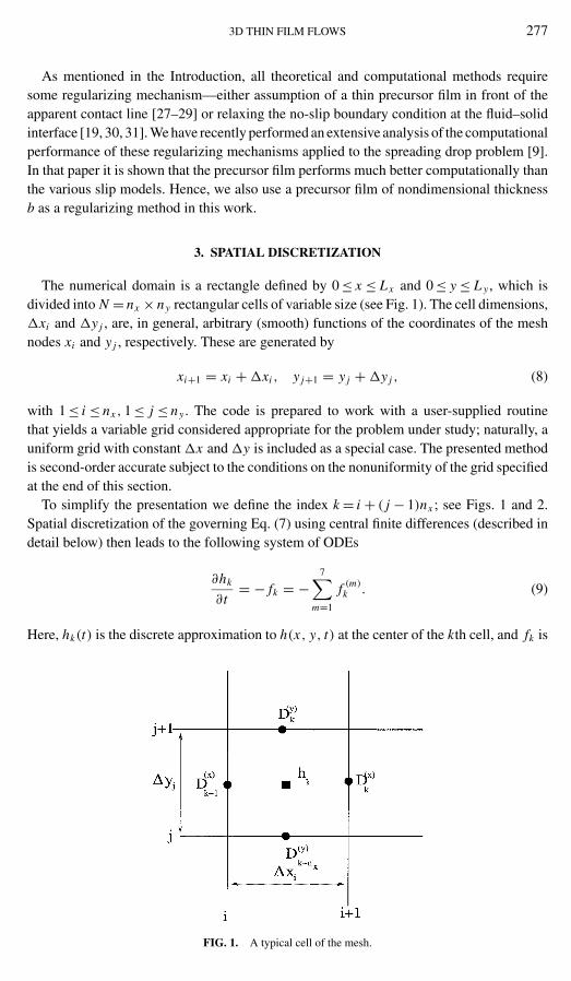
The numerical domain is a rectangle defined by 0 ≤ x ≤ Lx and 0 ≤ y ≤ L y , which isdivided into N = nx × ny rectangular cells of variable size (see Fig. 1). The cell dimensions,�xi and �y j , are, in general, arbitrary (smooth) functions of the coordinates of the meshnodes xi and y j , respectively. These are generated by

xi+1 = xi + �xi , y j+1 = y j + �y j , (8)

with 1 ≤ i ≤ nx , 1 ≤ j ≤ ny . The code is prepared to work with a user-supplied routinethat yields a variable grid considered appropriate for the problem under study; naturally, auniform grid with constant �x and �y is included as a special case. The presented methodis second-order accurate subject to the conditions on the nonuniformity of the grid specifiedat the end of this section.

To simplify the presentation we define the index k = i + ( j − 1)nx ; see Figs. 1 and 2.Spatial discretization of the governing Eq. (7) using central finite differences (described indetail below) then leads to the following system of ODEs

∂hk

∂t= − fk = −

7∑m=1

f (m)k . (9)

Here, hk(t) is the discrete approximation to h(x, y, t) at the center of the kth cell, and fk is

FIG. 1. A typical cell of the mesh.

278 DIEZ AND KONDIC

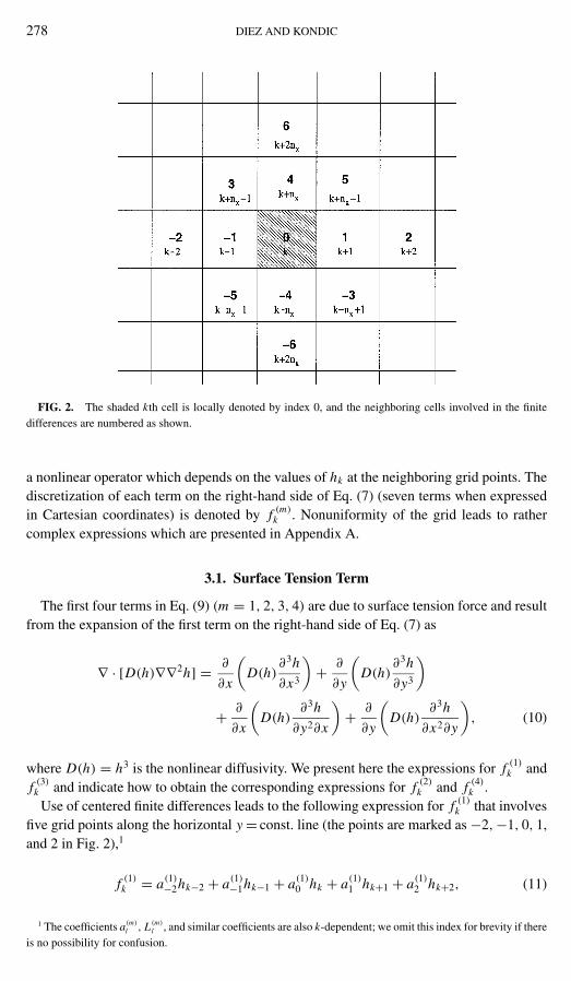
FIG. 2. The shaded kth cell is locally denoted by index 0, and the neighboring cells involved in the finitedifferences are numbered as shown.

a nonlinear operator which depends on the values of hk at the neighboring grid points. Thediscretization of each term on the right-hand side of Eq. (7) (seven terms when expressedin Cartesian coordinates) is denoted by f (m)

k . Nonuniformity of the grid leads to rathercomplex expressions which are presented in Appendix A.

3.1. Surface Tension Term

The first four terms in Eq. (9) (m = 1, 2, 3, 4) are due to surface tension force and resultfrom the expansion of the first term on the right-hand side of Eq. (7) as

∇ · [D(h)∇∇2h] = ∂

∂x

(D(h)

∂3h

∂x3

)+ ∂

∂y

(D(h)

∂3h

∂y3

)

+ ∂

∂x

(D(h)

∂3h

∂y2∂x

)+ ∂

∂y

(D(h)

∂3h

∂x2∂y

), (10)

where D(h) = h3 is the nonlinear diffusivity. We present here the expressions for f (1)k and

f (3)k and indicate how to obtain the corresponding expressions for f (2)

k and f (4)k .

Use of centered finite differences leads to the following expression for f (1)k that involves

five grid points along the horizontal y = const. line (the points are marked as −2, −1, 0, 1,and 2 in Fig. 2),1

f (1)k = a(1)

−2hk−2 + a(1)−1hk−1 + a(1)

0 hk + a(1)1 hk+1 + a(1)

2 hk+2, (11)

1 The coefficients a(m)

l , L (m)

l , and similar coefficients are also k-dependent; we omit this index for brevity if thereis no possibility for confusion.


where

a(1)l = L(1)

l D(x)k−1 + R(1)

l D(x)k , −2 ≤ l ≤ 2, (12)

and

D(x)k = D(hk, hk+1). (13)

Here, D stands for an appropriate interpolation of the diffusivity D(h) (see Section 3.2) at theborder (grid line) of two consecutive cells in the x direction (�k = ±1). Thus, D(x)

k−1(D(x)k )

is evaluated at the left (right) side of the kth cell (see Fig. 1). The coefficients L(1)l (left) and

R(1)l (right) are, in general, grid-dependent functions, given in Appendix A.The second term in Eq. (10) is analogous to the first term, with appropriate substitutions

(see Fig. 2), yielding

f (2)k = a(2)

−6hk−2nx + a(2)−4hk−nx + a(2)

0 hk + a(2)4 hk+nx + a(2)

6 hk+2nx , (14)

where

a(2)l = B(2)

l D(y)k−nx

+ T (2)l D(y)

k , l = −6, −4, 0, 4, 6, (15)

and

D(y)k = D

(hk, hk+nx

). (16)

The coefficients B(2)l (bottom) and T (2)

l (top) are obtained by exchanging �xi → �y j in theexpressions for L(1)

l and R(1)l (Appendix A). Also, D(y)

k−nx(D(y)

k ) are evaluated at the middleof the bottom (top) side of the kth cell.

The cross derivatives in the third term of Eq. (10) include nine neighboring cells (markedas ±5, ±4, ±3, ±1, and 0 in Fig. 2), giving

f (3)k = a(3)

−5hk−nx −1 + a(3)−4hk−nx + a(3)

−3hk−nx +1 + a(3)−1hk−1 + a(3)

0 hk + a(3)1 hk+1

+ a(3)3 hk+nx −1 + a(3)

4 hk+nx + a(3)5 hk+nx +1, (17)

where

a(3)l = L(3)

l D(x)k−1 + R(3)

l D(x)k , l = ±5, ±4, ±3, ±1, 0. (18)

Finally, the fourth term in Eq. (10) yields

f (4)k = a(4)

−5hk−nx −1 + a(4)−4hk−nx + a(4)

−3hk−nx +1 + a(4)−1hk−1 + a(4)

0 hk + a(4)1 hk+1

+ a(4)3 hk+nx −1 + a(4)

4 hk+nx + a(4)5 hk+nx +1, (19)

where

a(4)l = B(4)

l D(y)k−nx

+ T (4)l D(y)

k , l = ±5, ±4, ±3, ±1, 0. (20)

Similarly, as above, the coefficients B(4)l and T (4)

l are obtained by exchanging �xi ↔ �y j

in the expressions for L(3)l and R(3)

l (Appendix A).

280 DIEZ AND KONDIC

3.2. Discretization of the Diffusivity

In one-dimensional simulations, we have analyzed the performance of the positivitypreserving scheme (PPS) [32, 33] to discretize the diffusivity D(h) = hs(s ≥ 1) in Eq. (10)[9]. In those simulations, we have found that this scheme allows for computations on coarsergrids. This property is of capital importance for the computationally expensive 2D (or quasi3D) simulations presented here.

In a 1D setting, PPS prescribes the following interpolation of the diffusivity at the nodei (hi is defined at the center of the line element (xi , xi+1))

Di ={ hi+1 − hi

gi+1 − gi, hi+1 �= hi

hsi , hi+1 = hi

, (21)

where

g(h) =∫

dh

D(h)={

h1−s/(1 − s), s �= 1

ln h, s = 1. (22)

For our 2D problem with s = 3, this interpolation leads to the following expression forD in Eqs. (13) and (16), for hk �= hk+1

D(x)k = 2

h2kh2

k+1

hk + hk+1, D(y)

k = 2h2

kh2k+nx

hk + hk+nx

. (23)

For 0 < s < 2, the above-mentioned technique does not guarantee positive values ofhk . However, a positive smooth solution can be guaranteed for the regularized problem[34]. The regularization involves altering the definition of D(h) and also lifting the initialcondition h(x, 0) by an amount b (artificial precursor film). The regularized new diffusivityis of the form [35]

Dreg(h) = D(h)h4

εD(h) + h4, (24)

where ε = ε(b) is a small parameter. Note that Dreg(h) → D(h) as ε → 0, and also thatDreg(h) → h4/ε for h → 0 and s < 4, which is a more tractable singularity. In particular,in the case of planar symmetry it is required [34] that b < ε1/2 for 2 < s < 3 and b ≤ ε2/5

for 3/8 < s < 2. Here, we shall take b = ε0.3 whenever regularization is needed. Thus, ε

is defined by

ε ={

b10/3; if s < 2

0; if s ≥ 2.(25)

We use this scheme to simulate cases with s = 1, whose analytical solutions are known (seeSection 6).

3.3. Gravity Terms

In this section we present the discretization developed for the (second-order) gravityterms. Usually, the performance of a scheme is determined by the discretization of the


highest order term, as long as the order of approximation of the lower order terms is at leastthe same as that of the high-order term. For the particular problems considered in this paper,it is, however, important that this discretization preserves the conservative properties of thecontinuous equation.

3.3.1. Normal Component of Gravity

The normal gravity term (third term on the right-hand side of Eq. (7)) in Cartesiancoordinates reads as

∇ · [G(h)∇h] = ∂

∂x

(G(h)

∂h

∂x

)+ ∂

∂y

(G(h)

∂h

∂y

), (26)

where G(h) = h3. It is discretized using centered finite difference as

G(x)k = h3

k + h3k+1

2, G(y)

k = h3k + h3

k+nx

2. (27)

Thus, the discretization of the first term in Eq. (26) takes the form (see Fig. 2),

f (5)k = a(5)

−1hk−1 + a(5)0 hk + a(5)

1 hk+1, (28)

where

a(5)l = L(5)

l G(x)k−1 + R(5)

l G(x)k , l = −1, 0, 1, (29)

and G(x)k is located at the boundaries of the cell similarly to the definition of D(x)

k in Fig. 1.Analogously, for the second term in Eq. (26), we have

f (6)k = a(6)

−4hk−nx + a(6)0 hk + a(6)

4 hk+nx , (30)

where

a(6)l = B(6)

l G(y)k−nx

+ T (6)l G(y)

k , l = −4, 0, 4. (31)

The general expressions for L(5)l , R(5)

l , B(6)l , and T (6)

l for a nonuniform grid are given inAppendix A.

3.3.2. Parallel Component of Gravity

The fourth term on the right-hand side of Eq. (7) is discretized as

(∂h3

∂x

)k

≈ 1

4�xi

[(h2

k+1 + h2k

)(hk+1 + hk) − (h2

k + h2k−1

)(hk + hk−1)

], (32)

so that we have

f (7)k = a(7)

−1hk−1 + a(7)0 hk + a(7)

1 hk+1, (33)

282 DIEZ AND KONDIC

where

a(7)l = L(7)

l Hk−1 + R(7)l Hk, l = −1, 0, 1, (34)

and

Hk = h2k + h2

k+1

2. (35)

3.4. Final Expressions

By summing up the equations for f (m)k with m = 1, . . . , 7, we obtain (see Eq. (9))

fk = ak,−6hk−2nx + ak,−5hk−nx −1 + ak,−4hk−nx + ak,−3hk−nx +1 + ak,−2hk−2

+ ak,−1hk−1 + ak,0hk + ak,1hk+1 + ak,2hk+2 + ak,3hk+nx −1

+ ak,4hk+nx + ak,5hk+nx +1 + ak,6hk+2nx ,

where

ak,l = Lk,l D(x)k−1 + Rk,l D(x)

k + Bk,l D(y)k−nx

+ Tk,l D(y)k + Lk,l G

(x)k−1 + Rk,l G

(x)k

+ Bk,l G(y)k−nx

+ Tk,l G(y)k + Lk,l Hk−1 + Rk,l Hk, (36)

and

Lk,l = C4∑

m=1

L(m)l , Rk,l = C

4∑m=1

R(m)l ,

Bk,l = C4∑

m=1

B(m)l , Tk,l = C

4∑m=1

T (m)l ,

Lk,l = G6∑

m=5

L(m)l , Rk,l = G

6∑m=5

R(m)l , (37)

Bk,l = G6∑

m=5

B(m)l , Tk,l = G

6∑m=5

T (m)l ,

Lk,l = FL(7)l , Rk,l = FR(7)

l .

In summary, the nonlinear operator fk is a combination of the 13 values hk in the neighboringcells, with coefficients ak,l . These coefficients contain the nonlinear contributions (D’s,G’s, or H ’s) of each (discretized) term of Eq. (7) at the four boundaries of the kth cell (seeEq. (36)). The weight of each contribution depends on the finite differences expression ofthe corresponding term on the (uniform or nonuniform) grid (see Eq. (37)).

We note that the implementation of the resulting scheme is robust and versatile. First,the addition of other physical effects is achieved very easily by simply adding extra termsto the definition of ak,l ; see Eq. (36). Second, various boundary conditions can be simplyimplemented by modifying directly the coefficients of Eq. (37). Since these conditionsusually involve only h and its derivatives, and are not time-dependent, the coefficientsin Eq. (37) are determined only at the beginning of the calculation. This approach saves


computing time, as well as effectively reduces the effort of computing on a nonuniform gridto that on a uniform grid with the same number of cells.

The discretization outlined in this section is clearly second-order accurate when appliedon a uniform grid. Grid nonuniformity can in principle lead to a decrease in the order ofaccuracy. To analyze this effect, consider for a moment a simple example of the centraldifference formula applied to calculate the first derivative in the x direction at the pointk. To simplify the notation, let j = 1, so that i = k (see also Fig. 2). Simple error analysis(performed in a standard manner using Taylor series expansion) shows that the truncationerror on a nonuniform grid (using the notation as in Fig. 1) is of the order (�xi+1 − �xi−1) +O(�x2

i ). Therefore, if our grid is weakly nonuniform, in the sense that 1 − �xi−1/�xi+1 =O(�xi ), then the second-order accuracy is preserved. The grids used in this work satisfythis property; more details regarding second-order accuracy are given in the following, inparticular in Section 7.

4. BOUNDARY CONDITIONS

In this work we concentrate on the problems characterized by no-flow boundary condi-tions of Neumann type. As mentioned above, our computational method allows for easymodification of the boundary conditions.

No-flow boundary conditions are implemented by setting to zero the normal componentof Φ on all sides of the domain, where Φ = hv is the fluid flux, and v is the dimensionlessversion of the velocity in Eq. (4). For instance, along the line y = 0 (0 ≤ x ≤ Lx ), we setΦy = 0 by requiring that

∂h

∂y= ∂3h

∂y3= 0, at y = 0, 0 ≤ x ≤ Lx . (38)

To enforce this condition, we need two fictitious rows of cells outside the domain, that aremirror images of two interior adjacent cells. Thus, for the first and second rows below the xaxis ( j = 0) we have the mirror conditions hk−nx = hk , hk−2nx = hk+nx , 1 ≤ k ≤ nx . Proceed-ing analogously with the other three sides, we define a rectangular frame (two-cell width)surrounding the real domain. Care is required if the parallel gravity term enters the problem,since the normal component of the velocity along x = 0, Lx boundaries contains an addi-tional term proportional to h2. To have a vanishing flow there, we enforce h = 0 wheneverthis term has to be calculated in the fictitious cells, thus ensuring volume conservation.

The boundary conditions affect the evaluation of Eq. (36) at k’s for which some of the13 neighbors fall outside the physical domain (note that some cells near the corners includemirror “reflections” on two sides). The values of the (grid-dependent) coefficients Ll,k, . . . ,

Ll,k, . . . , Ll,k (Eq. (37)) for such cells are redefined using the appropriate fictitious cells.Also, the solution-dependent coefficients (D(x)

k , G(x)k , Hk , etc.) in the fictitious cells are

defined using the mirror values of h. We note that this assignment has to be made only atthe beginning of the calculation.

The no-flow boundary conditions considered here assure us that the fluid volume V withinthe physical domain remains constant in time; i.e.,

V =∫ Lx

0

∫ L y

0h(x, y, t) dx dy ∼=

nx∑i=1

ny∑j=1

hnk �xi�y j = const., (39)

284 DIEZ AND KONDIC

where n indicates the nth time level. The constancy of V during the evolution constitutes anexcellent check of the accuracy of the solution. All presented simulations preserve V with arelative error less than 10−11. It should be pointed out that since only the normal componentof the velocity is set to zero and the tangential component is set free, the boundaries of thedomain may represent “slipping walls” as well as symmetry planes. We will see that thisfeature is very useful to study flows characterized by some degree of symmetry.

5. TIME DISCRETIZATION

The time discretization of Eqs. (9), 1 ≤ k ≤ N is performed by �-scheme

hn+1k − hn

k

�tn+ θ f n+1

k + (1 − θ) f nk = 0, (40)

where 0 ≤ θ ≤ 1 and n stands for the time level tn . Here, θ = 0 gives the forward Eulerscheme (explicit, O(�tn)), θ = 1 gives the backward Euler scheme (implicit, O(�tn)), andθ = 1/2 yields the Crank–Nicholson scheme (implicit, O((�tn)2)).

Equation (40) forms a system of N nonlinear algebraic equations, which are solved usingiterative Newton–Kantorovich’s method. Briefly, the solution at time tn+1 is written as

hn+1k = h∗

k + qk, (41)

where h∗k is a guess and qk is the correction. To linearize the equations, we expand in Taylor

series around h∗k

f n+1k = f ∗

k + ∂ fk

∂ql

∣∣∣∣∗ql , (42)

so that Eq. (40) becomes

(δk,l + θ�tn F∗k,l)ql = Rk, (43)

where δk,l is the Kronecker delta, and

F∗k,l = ∂ fk

∂ql

∣∣∣∣∗

(44)

is the Jacobian matrix (the asterisk indicates evaluation using the guess h∗k ). Each row of

this matrix has at most 13 nonzero elements, which are given in Appendix B. The naturalordering of the grid points that we use in this work results in this matrix being in a usualblock diagonal form.

The right-hand side in Eq. (43) is given by

Rk = hnk − h∗

k − θ�tn f ∗k − (1 − θ)�tn f n

k . (45)

The linear system specified by Eq. (43) is then solved for the correction qk using thebiconjugate gradient method. Concerning the guess for the solution, we usually use h∗

k = hnk ,

i.e., the solution at the previous time level. If Q = maxk(qk), 1 ≤ k ≤ N , is greater than agiven tolerance (typically, we choose 10−10), then h∗

k + qk is taken as a new guess. This


procedure is iteratively performed until Q is less than the tolerance. In Section 7.1, weprovide more details regarding the number of iterations needed for convergence of bothbiconjugate gradient and Newton iterations in the case of the coalescence of two sessiledrops.

5.1. Time Step Control

In this work, we use θ = 1/2, which leads to an unconditionally stable scheme. However,one still needs to consider a number of issues when deciding on the size of the timestep. The most obvious requirement is to produce an accurate result; this is explainedin more detail below. Another requirement is that the solution has to be strictly positive;too large of a time step may let the solution erroneously approach zero. The final aspectthat influences the size of the time step is the fact that the guess for the solution may notbe close enough to the correct solution. This may prevent the Newton method outlinedabove from converging in a reasonable number of iterations and augment computationaltime unnecessarily. Obviously, there is an optimum value of the time step which is, in oursimulations, determined dynamically using these three criteria.

The accuracy requirement for the Crank-Nicholson scheme is formulated as follows.Since the scheme is O(�t2), the relative error of the numerical solution at the point k isgiven by

Ek = (�tn)2

hnk

∣∣∣∣d2hnk

dt2

∣∣∣∣. (46)

By multiplying the expansions around hnk and hn−1

k by �tn−1 and �tn (time steps per-formed before and after tn), respectively, and summing up we obtain the following expres-sion for the maximum relative error:

E = max1≤k≤N

[2�tn

�tn−1

�tn−1hn+1k + �tnhn−1

k − (�tn−1 + �tn)hnk

(�tn−1 + �tn)hnk

]. (47)

If E is less than a given tolerance Tol (typically, Tol = 10−2 − 10−3), the solution hn+1k

obtained using time step �tn is accepted; otherwise, the time step is reduced and a newiteration is performed.

6. CODE VALIDATION

The optimal way of validating a numerical code is to compare its results to a knownanalytical solution. It is clear that the nonlinear fourth-order term in Eq. (7) is the mostcritical feature of the computation; therefore we must look for a problem involving thishigh-order term. Since there are no analytical solutions for problems involving surfacetension with contact lines (s = 3), we test the code using s = 1. The analytic solutions forthis value of s are of source-type, emulating the “spreading” of a drop. First we test thecorrectness and convergence properties of our code assuming radial symmetry [36], andthen using elliptical symmetry [37].

286 DIEZ AND KONDIC

6.1. Radial Spreading with s = 1

We consider the special case C = 1 and G =F = 0 and assume radial symmetry.2 Thesolution emulates the “spreading” of a “drop” of constant volume, V , governed by theequation,

∂h

∂t+ ∇ · (h∇∇2h) = 0. (48)

By performing a scaling analysis, one obtains the self-similar solution [36]

h(r, t) = Hs(t)

[1 −

(r

r f,s(t)

)2]2

, (49)

where

r f,s(t) =[

192

(3V

π

)t

]1/6

, Hs(t) = 3V

π(r f,s(t))2, (50)

are the radius of the front (h(r f,s(t), t) = 0) and the thickness at the center of the drop (r = 0),respectively. The self-similar solution given by Eqs. (49) and (50) is reached asymptoticallyfor an arbitrary initial condition. It is also the exact solution of the degenerate problem inwhich the initial condition is given by a delta function δ(r) (see, e.g., [38]). While we cannotstart the simulations using δ(r), we can use the profile to which δ(r) would evolve aftersome specified time, t0. Therefore, we specify the initial condition

h(r, 0) = (1 − x2 − y2)2 (51)

and require that h(r, 0) agrees with Eq. (49) for r f,s(t0) = Hs(t0) = 1. It can be easily checkedthat this initial condition would be reached by δ(r) at t0 = (π/3V )/192. For any time t > t0,the evolution proceeds according to Eq. (49), with the front position and the thickness atr = 0 given by

r f (t) = [1 + t/t0]1/6,(52)

H(t) = [192t0(1 + t/t0)]−1/3.

Since in our case V = π/3, it follows that t0 = 1/192, fully specifying the solution. It shouldbe noted that the computations still require use of a precursor film to avoid a singular Jacobianmatrix of the discrete system, Eq. (43).

Figure 3 shows the comparison of numerical and analytical results for the front posi-tion, r f (t). We use b = 10−3 on a uniform grid (�xi = �y j = const.), and keep constant�t = 10−5 small enough, to reduce errors resulting from time discretization. The sym-metry of the problem allows for the simulations to be performed in the first quadrantonly; therefore we choose the domain 0 ≤ x ≤ 3, 0 ≤ y ≤ 3. The front position r f (t) is de-fined as the position of the depression that develops just in front of the main body of thefluid (see [9] and Fig. 8), along the line y = 0. Figure 3 shows clearly that the solution

2 We note that s = 1 is not a physical case and we choose C = 1 for illustration only.


FIG. 3. Time evolution of the front position x f (t) of the radial drop spreading with s = 1 and b = 10−3. Thethick solid line corresponds to the self-similar solution, Eq. (52).

r f (t) converges as the cell size decreases. The difference of the computed and the ana-lytical solution given by Eq. (52) (thick solid line) is due to the presence of our artificialprecursor film. We have verified that this difference decreases for smaller b’s. Naturally,smaller b’s also require smaller grid sizes, even when using the regularization schemespecified by Eq. (24). The drop thickness at the center, H(t), converges quadratically tothe analytical solution. For instance, H(t = 0.6) takes values 0.2518, 0.2129, 0.2025 for�x = 0.2, 0.1, 0.05, respectively. The analytical value is 0.2049, and this value is approachedas b → 0.

6.2. Elliptical Spreading

To validate our code using a problem that explicitly involves more than one space dimen-sion, we consider the spreading of an initially (t = 0) elliptical drop

h(x, y, 0) = H0

(1 − x2

a0− y2

b0

)2

, (53)

where√

a0 and√

b0 are lengths of the semi-axes. For the case s = 1, we assume thatfor t > 0

h(x, y, t) = H(t)

(1 − x2

a(t)− y2

b(t)

)2

, (54)

where a(t), b(t), and H(t) are obtained by substituting this ansatz into Eq. (48). The solutionis given implicitly in terms of the difference α(t) = a(t) − b(t) as [37]

29√

�(t + t1) = −β tanh−1√

1 − α6/β2 +√

β2 − α6

3α6(β2 + 2α6), (55)

288 DIEZ AND KONDIC

FIG. 4. Time evolution of the shape of the contact line for spreading of an elliptical drop with s = 1, b = 10−3,a0 = 4, and b0 = 1. The time interval between consecutive curves is δt = 1. These results are obtained using�x = �y = 0.05.

where

� = H(t)2a(t)b(t) =(

45

52V

)2

= const., (56)

and β = (a0 + b0) (a0 − b0)2. Note that 0 ≤ α ≤ α0 (the subscript 0 stands for the initial

condition). The integration constant t1 is obtained from Eq. (55) for t = 0. The semi-axesof the ellipse x f and y f are calculated from α(t) as

x2f (t) = a(t) = 1

2

(α(t) + β

α(t)2

),

(57)

y2f (t) = b(t) = 1

2

(β

α(t)2− α(t)

),

and the thickness at the center, H(t), is obtained from Eq. (56). Asymptotically (as t → ∞),the front moves according to the radial solution given in the previous section, but with adifferent time shift, t1. Thus, for t → ∞ and α β, Eqs. (55) and (57) yield

x f ≈ y f ≈ 2[3�(t + t1)]1/6. (58)

Figure 4 shows the numerical results for the evolution of the contact line, where theinitial condition is specified by Eq. (53). Clearly the elliptical curves quickly become morecircular as times increases, in agreement with the asymptotic solutions.

Figure 5 depicts more precisely the comparison between numerical and analytical results.This figure shows x f (t) and y f (t) resulting from three runs that use different uniform grids.The corresponding analytical solution as given by Eq. (57) is also plotted (solid lines),together with the asymptotic radial solution, Eq. (58). Clearly the numerical result closelyfollows the exact result. To analyze the convergence rate of the solution, we consider againthe drop thickness at the origin. At t = 10 we have H = 0.12769, 0.12755, and 0.12752 for


FIG. 5. Time evolution of the semi-axes x f (t) and y f (t) for the spreading of the elliptical drop in Fig. 4.The solid lines correspond to the analytical solution, Eq. (57), and the dashed line shows the asymptotic (radial)behavior, Eq. (58).

�x = 0.2, 0.1, 0.05, respectively. The convergence is quadratic, and the theoretical value is0.127170. The difference between the converged value and the theoretical value is due tothe artificial precursor film. Once again, it decreases as b → 0.

7. COALESCENCE OF SESSILE DROPS

To further illustrate the capabilities of the above-described numerical scheme, we nowchoose a simple but interesting problem: the coalescence of sessile drops that are simultane-ously and isotropically spreading on a horizontal substrate. We concentrate on the physicalcase where s = 3.

As outlined in the Introduction, the interest in this configuration is twofold, since itinvolves both the contact line motion and the coalescence process. A similar problem wasstudied for the case of two mercury drops on a glass surface [39]. More recently, the kineticsof coalescence of two water drops on a plane solid surface was analyzed experimentally[40]. However, in those works the fluid is strongly nonwetting, while here we consider onlycompletely wetting fluids. Furthermore, in [39] the dynamics of the drops is driven by anapplied electric field, and in [40] the volume growing by condensation from the surroundingatmosphere is a major effect. Therefore, we can compare only qualitative features of theresults. To our knowledge, no other experimental or theoretical results have been reportedregarding this problem.

Let us consider two identical sessile drops of radius R, with centers at (0, 0) and (0, d)(d > 2R) on a horizontal plane. After spreading, the drops begin to coalesce. The interac-tion between the drops breaks the radial symmetry of each drop. However, mirror sym-metry with respect to the line y = 0 is preserved. To preserve also the mirror symmetrieswith respect to the perpendicular lines x = 0 and x = d, let us consider instead an infi-nite linear array of equidistant identical droplets, placed along the x axis and centered atx = . . . ,−2d, −d, 0, d, 2d, . . . . Each drop is involved now in two simultaneous coales-cence processes so that simulations can be performed only in the first quadrant; see Fig. 6.Naturally, the code can also handle the case of two isolated drops, but symmetry could notbe exploited to reduce the computational domain.

290 DIEZ AND KONDIC

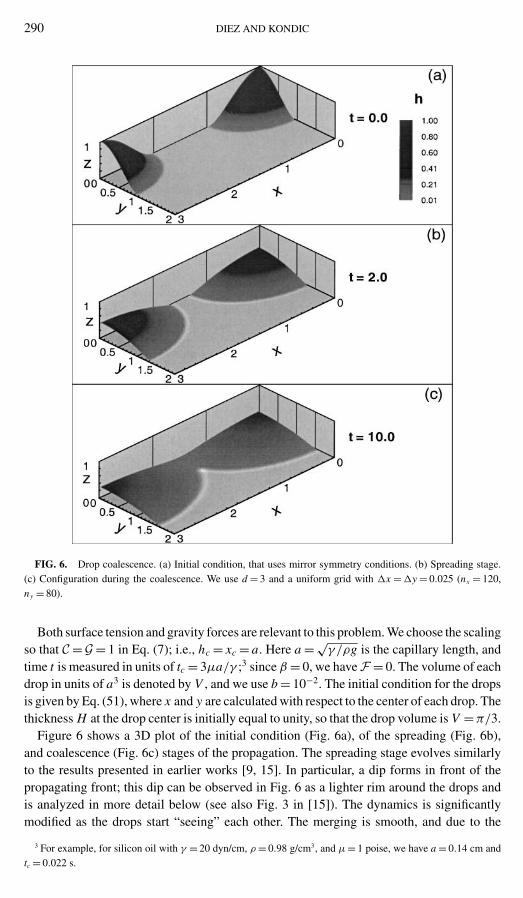
FIG. 6. Drop coalescence. (a) Initial condition, that uses mirror symmetry conditions. (b) Spreading stage.(c) Configuration during the coalescence. We use d = 3 and a uniform grid with �x = �y = 0.025 (nx = 120,ny = 80).

Both surface tension and gravity forces are relevant to this problem. We choose the scalingso that C =G = 1 in Eq. (7); i.e., hc = xc = a. Here a = √

γ /ρg is the capillary length, andtime t is measured in units of tc = 3µa/γ ;3 since β = 0, we have F = 0. The volume of eachdrop in units of a3 is denoted by V , and we use b = 10−2. The initial condition for the dropsis given by Eq. (51), where x and y are calculated with respect to the center of each drop. Thethickness H at the drop center is initially equal to unity, so that the drop volume is V = π/3.

Figure 6 shows a 3D plot of the initial condition (Fig. 6a), of the spreading (Fig. 6b),and coalescence (Fig. 6c) stages of the propagation. The spreading stage evolves similarlyto the results presented in earlier works [9, 15]. In particular, a dip forms in front of thepropagating front; this dip can be observed in Fig. 6 as a lighter rim around the drops andis analyzed in more detail below (see also Fig. 3 in [15]). The dynamics is significantlymodified as the drops start “seeing” each other. The merging is smooth, and due to the

3 For example, for silicon oil with γ = 20 dyn/cm, ρ = 0.98 g/cm3, and µ = 1 poise, we have a = 0.14 cm andtc = 0.022 s.


FIG. 7. (a) Thickness profile h(x, y = 0, t) along the symmetry line; dashed line corresponds to the initialcondition, not completely visible on the scale of the figure. (b) Cross section h(x = 1.5, y, t) of the connectingneck at the coalescence line. The profiles are shown in δt = 1 intervals; all the parameters are as in Fig. 6. Anexplanation of the cylindrical cap and the definition of y f , the front position, are given in the text. For a close-upof the coalescence region see Fig. 8.

presence of the precursor film it proceeds in a regular fashion. The coalescence processinvolves a transition from two contact lines to a single line enclosing both original drops.

Figure 7a shows the evolution of the fluid thickness h(x, t) along the symmetry liney = 0. The coalescence proceeds by forming a connecting neck at t ≈ 5 (see also Fig. 8a).Figure 7b shows how this neck widens in the y direction along x = 1.5. These profiles havethe shape of cylindrical caps, as exemplified in Fig. 7b for t = 20. This behavior is typicalfor very small droplets [21].

Figure 8 shows a close-up of both the longitudinal and transversal profiles of the neck.To have well-resolved profiles at this short scale, we report results obtained using a nonuni-form grid in the x with the smallest cell sizes located at the coalescence region (see alsoSection 7.1.2). As mentioned above, before the coalescence the precursor film developsa damped oscillating profile [41]. The main features of this profile are a dip of thickness≈0.85b (visible also in Fig. 6) and a bump ahead of the dip, of height ≈1.01b; see Fig. 8. Theposition of the dip is used below to define the location (x f , y f ) of the contact line (front).

In Fig. 8a we see that the bumps at the fronts of the individual drops start interacting att ≈ 3, much earlier than the neck forms. At this time, the little bumps ahead of the dips atthe fronts of each drop come into contact (see also Fig. 9a). For 3 < t < 5, the thickness(height) of the region around x = 1.5 diminishes due to the arrival of the dips; see Fig. 8a.

292 DIEZ AND KONDIC

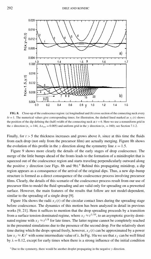
FIG. 8. Close-up of the coalescence region: (a) longitudinal and (b) cross section of the connecting neck everyδt = 1. The numerical values give corresponding times; for illustration, the dashed lined marked as y f (t) showsthe position of the dip defining the (half) width of the connecting neck at t = 6. Here we use a nonuniform grid inthe x direction (nx = 144, �xmin = 0.005) and uniform grid in the y direction (ny = 160); see Section 7.1.2.

Finally, for t > 5 the thickness increases and grows above b, since at this time the fluidsfrom each drop (not only from the precursor film) are actually merging. Figure 8b showsthe evolution of this profile in the y direction along the symmetry line x = 1.5.

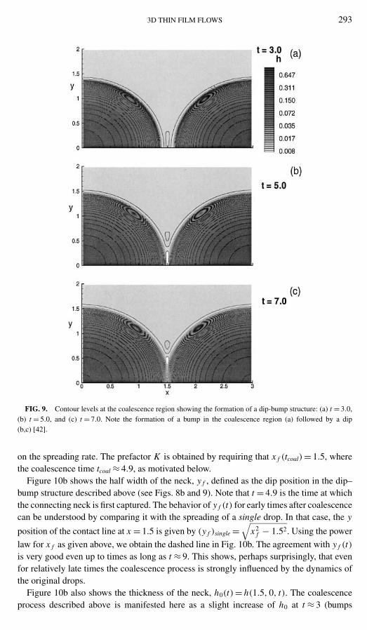
Figure 9 shows more clearly the details of the early stages of drop coalescence. Themerge of the little bumps ahead of the fronts leads to the formation of a minidroplet that issqueezed out of the coalescence region and starts traveling perpendicularly outward alongthe positive y direction (see Figs. 8b and 9b).4 Behind this propagating minidrop, a dipregion appears as a consequence of the arrival of the original dips. Thus, a new dip–bumpstructure is formed as a direct consequence of the coalescence process involving precursorfilms. Clearly, the details of this scenario of the coalescence process result from our use ofprecursor film to model the fluid spreading and are valid only for spreading on a prewettedsurface. However, the main features of the results that follow are not model-dependent,similar to the spreading of a single drop [9].

Figure 10a shows the radii x f (t) of the circular contact lines during the spreading stagebefore coalescence. The dynamics of this motion has been analyzed in detail in previousworks [9, 21]. Here it suffices to mention that the drop spreading proceeds by a transitionfrom a surface tension dominated regime, where x f ≈ t1/10, to an asymptotic gravity domi-nated regime with x f ≈ t1/8 for late times. The latter regime cannot be completely reachedin the presented simulations due to the presence of the second drop. For the relatively shorttime during which the drops spread freely, however, x f (t) can be approximated by a powerlaw x f ≈ K tλ with some intermediate value of λ. In Fig. 10a we see that x f can be well fittedby λ = 0.12, except for early times when there is a strong influence of the initial condition

4 Due to the symmetry, there would be another droplet propagating in the negative y direction.


FIG. 9. Contour levels at the coalescence region showing the formation of a dip-bump structure: (a) t = 3.0,(b) t = 5.0, and (c) t = 7.0. Note the formation of a bump in the coalescence region (a) followed by a dip(b,c) [42].

on the spreading rate. The prefactor K is obtained by requiring that x f (tcoal) = 1.5, wherethe coalescence time tcoal ≈ 4.9, as motivated below.

Figure 10b shows the half width of the neck, y f , defined as the dip position in the dip–bump structure described above (see Figs. 8b and 9). Note that t = 4.9 is the time at whichthe connecting neck is first captured. The behavior of y f (t) for early times after coalescencecan be understood by comparing it with the spreading of a single drop. In that case, the y

position of the contact line at x = 1.5 is given by (y f )single =√

x2f − 1.52. Using the power

law for x f as given above, we obtain the dashed line in Fig. 10b. The agreement with y f (t)is very good even up to times as long as t ≈ 9. This shows, perhaps surprisingly, that evenfor relatively late times the coalescence process is strongly influenced by the dynamics ofthe original drops.

Figure 10b also shows the thickness of the neck, h0(t) = h(1.5, 0, t). The coalescenceprocess described above is manifested here as a slight increase of h0 at t ≈ 3 (bumps

294 DIEZ AND KONDIC

FIG. 10. (a) Front position x f (t) for the radial spreading of the drops; the power-law fits are explained in thetext. (b) Half width, y f (t), and thickness, h0(t), of the connecting neck for the case shown in Fig. 6. The brokenline shows the propagation of the contact line of a single drop in the y direction at x = 1.5 (see text).

interaction), a local minimum at t ≈ 5 (dips arrival), and a monotonous increase for latertimes (drops coalescence itself). This curve is qualitatively similar to those reported inFig. 9 of [39] for the coalescence of two mercury drops. To our knowledge, no otherdocumented experimental nor numerical results exist for the evolution of this quantity.

Figure 11 shows how h0(t) depends on the thickness of the precursor film, b. As expected,the curves are qualitatively similar; the main difference is that they are shifted in time, besidesbeing displaced vertically due to different b values. This shift is due to a decreased viscousdissipation rate for larger b’s, resulting in larger front velocities and earlier coalescence.

FIG. 11. Thickness h0 of the connecting neck as a function of time for different values of the precursor film b.


7.1. Convergence Properties

The main goal of the presentation that follows is to explore the convergence propertiesof various uniform and nonuniform discretizations. Since our numerical method allows usto implement any of these two possibilities in either direction, we will be able to discussthe resolution needed for converged results, as well as the appropriateness of computing onnonuniform grids. We take the time evolution of the fluid thickness at the coalescence point,h0(t), as a testing parameter, since it is a very sensitive measure of the quality of the solution.

7.1.1. Uniform Grid

Figure 12 shows h0(t) computed by using uniform grids; in Fig. 12a �x is changed,and in Fig. 12b we modify �y (see also Table I). In these calculations the time step isvaried following the requirements of Section 5.1 with Tol = 10−2. The solid line in bothparts corresponds to the most resolved case for each set. It is interesting to observe thatconvergence in the x direction proceeds from smaller values of h0, while the y convergenceis achieved starting from larger values.

Table I shows more precisely how the results converge as the number of grid points isincreased, separately in the x and y directions. To estimate the rate of convergence, wecalculate the ratio of the differences of h∗

0 values computed using a different number ofgrid points; see Section 7.2 for more details. These ratios should be approximately equalto 4 for a second-order method. The results shown in Table I give the values 4.04 and 4.86for the x and y directions, respectively. We note also that for not too large numbers of gridpoints, CPU time grows according to tcpu ∼ N log N , where N is the total number of points.There are several factors that influence tcpu, including accuracy requirements, the numberof Newton iterations needed for convergence, as well as the number of iterations of ourbiconjugate gradient method. For very large N , these factors lead to faster growth of tcpu.

FIG. 12. Thickness of the connecting neck h0(t) as obtained using different uniform grids: (a) �x is varied(�y = const.); (b)�y is varied (�x = const.). The arrows show the direction of decreasing�x and�y, respectively.

296 DIEZ AND KONDIC

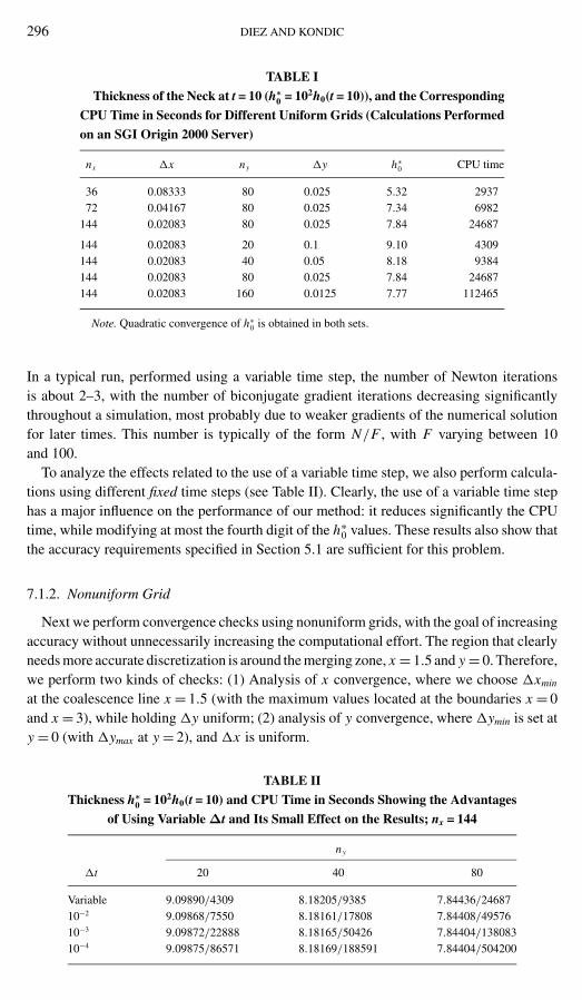
TABLE I

Thickness of the Neck at t = 10 (h∗0 = 102h0(t = 10)), and the Corresponding

CPU Time in Seconds for Different Uniform Grids (Calculations Performed

on an SGI Origin 2000 Server)

nx �x ny �y h∗0 CPU time

36 0.08333 80 0.025 5.32 293772 0.04167 80 0.025 7.34 6982

144 0.02083 80 0.025 7.84 24687

144 0.02083 20 0.1 9.10 4309144 0.02083 40 0.05 8.18 9384144 0.02083 80 0.025 7.84 24687144 0.02083 160 0.0125 7.77 112465

Note. Quadratic convergence of h∗0 is obtained in both sets.

In a typical run, performed using a variable time step, the number of Newton iterationsis about 2–3, with the number of biconjugate gradient iterations decreasing significantlythroughout a simulation, most probably due to weaker gradients of the numerical solutionfor later times. This number is typically of the form N/F , with F varying between 10and 100.

To analyze the effects related to the use of a variable time step, we also perform calcula-tions using different fixed time steps (see Table II). Clearly, the use of a variable time stephas a major influence on the performance of our method: it reduces significantly the CPUtime, while modifying at most the fourth digit of the h∗

0 values. These results also show thatthe accuracy requirements specified in Section 5.1 are sufficient for this problem.

7.1.2. Nonuniform Grid

Next we perform convergence checks using nonuniform grids, with the goal of increasingaccuracy without unnecessarily increasing the computational effort. The region that clearlyneeds more accurate discretization is around the merging zone, x = 1.5 and y = 0. Therefore,we perform two kinds of checks: (1) Analysis of x convergence, where we choose �xmin

at the coalescence line x = 1.5 (with the maximum values located at the boundaries x = 0and x = 3), while holding �y uniform; (2) analysis of y convergence, where �ymin is set aty = 0 (with �ymax at y = 2), and �x is uniform.

TABLE II

Thickness h∗0 = 102h0(t = 10) and CPU Time in Seconds Showing the Advantages

of Using Variable ∆t and Its Small Effect on the Results; nx = 144

ny

�t 20 40 80

Variable 9.09890/4309 8.18205/9385 7.84436/2468710−2 9.09868/7550 8.18161/17808 7.84408/4957610−3 9.09872/22888 8.18165/50426 7.84404/13808310−4 9.09875/86571 8.18169/188591 7.84404/504200


FIG. 13. Sketch of a nonuniform grid, and the (quadratic) curves for the cell size as a function of x and y(coordinates of the (i , j) corner of the cell; see Fig. 1). Here, nx = 74 and ny = 40 with �xmin = 0.02083 at x = 1.5and �ymin = 0.025 at y = 0.

In all cases, our mesh generator produces nonuniform grids with quadratic dependenceof the cell size on the spatial variable. Figure 13 shows an example of a mesh nonuniformin both directions, together with the corresponding quadratic curves �x(x) and �y(y). If�xmin is reduced, and the number of cells is kept fixed, we obtain steeper curves �x(x),and both the cell concentration around �xmin and the value of �xmax increase. On the otherhand, if nx is increased while �xmin is fixed, the contrary effect is obtained. In the limitof very large nx , the curve tends to �x(x) = �xmin = const., so that the mesh becomesuniform; the same holds in the y direction.

Figure 14 shows the results for h0(t), where the number of grid points (nx and ny ,respectively) is varied, while the corresponding minimum values (�xmin and �ymin) are

FIG. 14. Thickness of the connecting neck h0(t) as obtained for different nonuniform grids: (a) nonuniformin x , uniform in y; (b) uniform in y, nonuniform in x . The arrows point in the direction of increasing nx and ny ,respectively.

298 DIEZ AND KONDIC

TABLE III

Thickness h∗0 = 102h0(t = 10) and CPU Time

in Seconds, as nx for a Nonuniform x Grid Is

Varied; ∆y = 0.0125 (ny = 160)

nx �xmin h∗0 CPU time

36 0.02083 6.02 2186672 0.02083 7.45 46362

144 0.02083 7.77 112465

kept fixed. The most resolved case is shown by the solid line in Fig. 14, and by the last rowin Tables III and IV. To verify quadratic convergence, we double the number of grid pointsand calculate the ratio of the differences of h∗

0, similar to the uniform grid case. These ratiosare 4.61 and 5.70 for the sets in Tables III and IV, respectively.

We have also performed runs using fixed nx (ny) and decreasing �xmin (�ymin) withuniform grid in the y (x) direction. For brevity we do not show plots for this case becausethe differences among the results are very small. In these cases, we also obtain a quadraticconvergence rate for h∗

0.

7.2. Numerical Performances

In this section we investigate the relative performances of the computations performedon uniform and nonuniform grids. In general, there is no clear rule on whether a uniform ornonuniform grid is more efficient. This certainly depends on the problem at hand and hasto be investigated separately in each case.

Usually, nonuniform grids can be of advantage if the solution varies slowly almost ev-erywhere, while the interesting aspects of the problem are limited to a small portion of thedomain. This is not clear a priori in our problem, since it involves two different phenomena:contact line motion and coalescence itself. Both of these processes are sensitive to the meshsize; for instance, if for a given number of points one chooses a finer grid at the coalescencepoint, then the results can lose accuracy because of the coarse grid used to compute thecontact line motion elsewhere.

TABLE IV

Thickness h∗0 = 102h0(t = 10) and CPU

Time in Seconds, as ny for a Nonuniform y

Grid Is Varied with ∆x = 0.02083 (nx = 144)

ny �ymin h∗0 CPU time

20 0.0125 9.46 1691940 0.0125 8.44 1307880 0.0125 7.87 33120

160 0.0125 7.77 112465

Note. The case ny = 160 is coincident with the uni-form case in the last row of Table I, because for thislarge ny, �ymax = �ymin.


To decide in favor of one kind of grid, one can compare the computational effort neededto perform calculations that lead to the same quality (accuracy) of the results. Conversely,one can also make a comparison of the accuracy under the same number of cells; this iswhat we do here. To compare accuracies we take as the most accurate solution that givenby the well-resolved case with uniform grid; namely, nx = 144 and ny = 160. This grid willbe denoted by (144u, 160u), where u means that the grid is uniform in the correspondingdirection; n will be used to denote a nonuniform grid. For uniform grids, and at t = 10, weobtain

|h∗0(144u, 160u) − h∗

0(72u, 160u)| = 0.50

|h∗0(144u, 160u) − h∗

0(36u, 160u)| = 2.5.

Equivalent differences for nonuniform grids and the same nx are

|h∗0(144u, 160u) − h∗

0(72n, 160u)| = 0.32

|h∗0(144u, 160u) − h∗

0(36n, 160u)| = 1.7.

We see that, in general, a nonuniform grid in the x direction yields results which are moreaccurate than the uniform grid that uses the same number of cells. Furthermore, this greateraccuracy is obtained using less CPU time, as seen in Tables I and III. Therefore, fromthese results we conclude that it is more efficient to use a nonuniform x grid for thisproblem.

Next, we perform a similar comparison for the y direction. In this case, we obtain

|h∗0(144u, 160u) − h∗

0(144u, 80u)| = 0.07

|h∗0(144u, 160u) − h∗

0(144u, 40u)| = 0.41.

The equivalent differences for a nonuniform grid in the y direction are

|h∗0(144u, 160u) − h∗

0(144u, 80n)| = 0.10

|h∗0(144u, 160u) − h∗

0(144u, 40n)| = 0.67.

In this case, the differences are in favor of the uniform grid. Also, CPU times are muchsmaller for uniform than for nonuniform y grids (see Tables I and IV).

In summary, based on the numerical effort required for a given accuracy, we concludethat the use of a nonuniform x grid and a uniform y grid is advisable for the present problem.This result can be understood by observing the geometry of the problem. A nonuniform gridin the x direction resolves well the most critical area (x = 1.5) along which the coalescenceof the drops occurs. A nonuniform grid in y, on the other hand, resolves well only the zoneabout y = 0, where just the initial part of the coalescence takes place.

8. SUMMARY AND CONCLUSIONS

We have developed a computational method for quasi 3D unsteady coating flows. Inthis work, we applied this method to the spreading and coalescence of an incompressible

300 DIEZ AND KONDIC

fluid on a horizontal substrate; the simulations of flows on inclined planes were presentedelsewhere (see [14–16]).

The first part of this paper explained in some detail the computational issues involvedin modeling thin film flows in higher dimensions. In particular, we presented an efficientapproach to perform computations on nonuniform Cartesian grids. As a result, we were ableto address the evolution of features characterized by very short length scales, as exemplifiedin Section 7. The numerical method was validated by using the problems for which analyticalsolutions exist. These problems were obtained by setting the exponent, s, of the coefficientof fourth-order capillary terms to s = 1. Careful analysis has shown quadratic convergenceto the exact solution for both radial and elliptic drops.

The second part of this work combined the two main issues that are relevant in under-standing of thin film flows: (1) contact line paradox and (2) topology changes, such ascoalescence or rupture. We approached both of these issues by using a precursor film modeland illustrated how it allows us to proceed smoothly through the process of coalescenceof two sessile drops spreading on a horizontal substrate. In particular, we focused on thedescription of the connecting neck that develops in the contact region. We observed thatthe merging process comprises two stages, one being the early interaction of the dip–bumpstructure of the front region of each drop and the other the coalescence itself, involvingthe fluid from the bulks. Interestingly enough, as a result of this interaction a new dip–bump-isolated structure is formed at the coalescence line. This structure spans in bothdirections and travels outward ahead of the connecting neck. This is a novel feature of theproblem, and it has been observed in our simulations solely due to a very fine resolutionof the critical region of the flow, resolved using nonuniform meshes. While this dip–bumpstructure is a direct consequence of the presence of the precursor film, the results for otherproperties of the flow are more general. In particular, the evolution of the height and ofthe width of the connecting neck as well as the transversal and longitudinal thickness pro-files depend (weakly) only on the length scales introduced at the contact lines, but noton the model itself. Therefore, it is expected that the results regarding the dynamics ofthese quantities can be confirmed by experiment. The work in this direction is currently inprogress.

Going back to the computational issues, our analysis shows that, while nonuniform gridsare very useful to analyze the dynamics of localized structures in the flow, one has to becareful of their use. In particular, for the problem of drop merging, the use of a nonuniformgrid in the direction connecting the drop centers, and of a uniform grid in the normaldirection is most advisable from the viewpoint of numerical efficiency.

Additional usefulness of the presented numerical scheme is due to fact that it allows foreasy inclusion of other physical effects. These can be accounted for by forces as different asthermocapillary (Marangoni effect), electrical, inertial (e.g., centrifugal), or intermolecular(van der Waals interaction). The computational studies of problems in these areas arecurrently being performed.

APPENDIX A: COEFFICIENTS FOR NONUNIFORM GRIDS

We present here the general expressions for the coefficients L(m)l , R(m)

l , B(m)l , and T (m)

l

(1 ≤ m ≤ 7, −6 ≤ l ≤ 6) for a nonuniform, Cartesian grid, which result from a centered finitedifference scheme applied to each term of Eq. (7).


Surface Tension Term

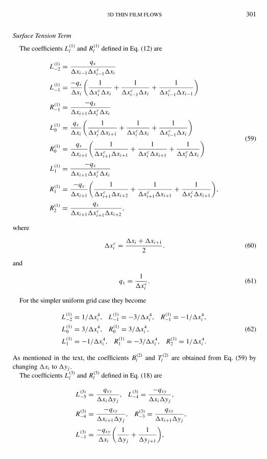
The coefficients L(1)l and R(1)

l defined in Eq. (12) are

L(1)−2 = qx

�xi−1�xci−1�xi

L(1)−1 = −qx

�xi

(1

�xci �xi

+ 1

�xci−1�xi

+ 1

�xci−1�xi−1

)

R(1)−1 = −qx

�xi+1�xci �xi

L(1)0 = qx

�xi

(1

�xci �xi+1

+ 1

�xci �xi

+ 1

�xci−1�xi

)(59)

R(1)0 = qx

�xi+1

(1

�xci+1�xi+1

+ 1

�xci �xi+1

+ 1

�xci �xi

)

L(1)1 = −qx

�xi+1�xci �xi

R(1)1 = −qx

�xi+1

(1

�xci+1�xi+2

+ 1

�xci+1�xi+1

+ 1

�xci �xi+1

),

R(1)2 = qx

�xi+1�xci+1�xi+2

,

where

�xci = �xi + �xi+1

2. (60)

and

qx = 1

�xci

. (61)

For the simpler uniform grid case they become

L(1)−2 = 1/�x4

i , L(1)−1 = −3/�x4

i , R(1)−1 = −1/�x4

i ,

L(1)0 = 3/�x4

i , R(1)0 = 3/�x4

i , (62)

L(1)1 = −1/�x4

i , R(1)1 = −3/�x4

i , R(1)2 = 1/�x4

i .

As mentioned in the text, the coefficients B(2)l and T (2)

l are obtained from Eq. (59) bychanging �xi to �y j .



L(3)−5 = qxy

�xi�y j, L(3)

−4 = −qxy

�xi�y j,

R(3)−4 = −qxy

�xi+1�y j, R(3)

−3 = qxy

�xi+1�y j,

L(3)−1 = −qxy

�xi

(1

�y j+ 1

�y j+1

),

302 DIEZ AND KONDIC

L(3)0 = qxy

�xi

(1

�y j+ 1

�y j+1

),

R(3)0 = qxy

�xi+1

(1

�y j+ 1

�y j+1

),

R(3)1 = −qxy

�xi+1

(1

�y j+ 1

�y j+1

),

L(3)3 = qxy

�xi�y j+1, R(3)

5 = qxy

�xi+1�y j+1,

L(3)4 = −qxy

�xi�y j, R(3)

4 = −qxy

�xi+1�y j+1,

where

qxy = 1

�xci �yc

j

, �ycj = �y j + �y j+1

2.

The coefficients B(4)l and T (4)

l are obtained by changing �xi ↔ �y j .

Normal Gravity Terms



L(5)−1 = qx

�xi, R(5)

1 = qx

�xi+1

L(5)0 = − qx

�xi, R(5)

0 = − qx

�xi+1.

Analogously, the coefficients B(6)l and T (6)


B(6)−2 = qy

�y j, T (6)

2 = qy

�y j+1,

B(6)0 = −qy

�y j, T (6)

0 = −qy

�y j+1,

where

qy = 1

�ycj

.

Parallel Gravity Term



L(7)−1 = −qx

2, R(7)

1 = qx

2,

L(7)0 = −qx

2, R(7)

0 = qx

2,


APPENDIX B: JACOBIAN

The elements of the Jacobian needed for the Newton–Kantorovich’s method (see Eq. (44))are given by

Fk,−6 = ∂ fk

∂hk−2nx

= ak,−6, Fk,−5 = ∂ fk

∂hk−nx −1= ak,−5,

Fk,−3 = ∂ fk

∂hk−nx +1= ak,−3, Fk,−2 = ∂ fk

∂hk−2= ak,−2,

Fk,2 = ∂ fk

∂hk+2= ak,2, Fk,3 = ∂ fk

∂hk+nx −1= ak,3, (63)

Fk,5 = ∂ fk

∂hk+nx +1= ak,5, Fk,6 = ∂ fk

∂hk+2nx

= ak,6,

and

Fk,−4 = ∂ fk

∂hk−nx

= ak,−4 + ∂ D(y)k−nx

∂hk−nx

A−4 + ∂G(y)k−nx

∂hk−nx

A−4

Fk,−1 = ∂ fk

∂hk−1= ak,−1 + ∂ D(x)

k−1

∂hk−1A−1 + ∂G(x)

k−1

∂hk−1A−1 + ∂ Hk−1

∂hk−1A−1

Fk,0 = ∂ fk

∂hk= ak,0 + ∂ D(y)

k−nx

∂hkA−4 + ∂ D(x)

k−1

∂hkA−1 + ∂ D(x)

k

∂hkA1

(64)

+ ∂ D(y)k

∂hkA4 + ∂G(x)

k−1

∂hkA−1 + ∂G(y)

k−nx

∂hkA−4

Fk,1 = ∂ fk

∂hk+1= ak,1 + ∂ D(x)

k

∂hk+1A1 + ∂G(x)

k

∂hk+1A1 + ∂ Hk

∂hk+1A1,

Fk,4 = ∂ fk

∂hk+nx

= ak,4 + ∂ D(y)k

∂hk+nx

A4 + ∂G(x)k

∂hk+1A4.

Here, the A’s are related to the surface tension terms, while the A’s and A’s correspond tothe normal and parallel gravity terms, respectively. They are given by

A−4 = Bk,−6hk−2nx + Bk,−5hk−nx −1 + Bk,−4hk−nx + Bk,−3hk−nx +1

+ Bk,0hk + Bk,1hk+1 + Bk,4hk+nx

A−1 = Lk,−5hk−nx −1 + Lk,−4hk−nx + Lk,−2hk−2 + Lk,−1hk−1

+ Lk,1hk+1 + Lk,3hk+nx −1 + Lk,4hk+nx

(65)A1 = Rk,−4hk−nx + Rk,−3hk−nx +1 + Rk,−1hk−1 + Rk,0hk + Rk,1hk+1

+ Rk,2hk+2 + Rk,4hk+nx + Rk,5hk+nx +1

A4 = Tk,−4hk−nx + Tk,−1hk−1 + Tk,0hk + Tk,1hk+1 + Tk,3hk+nx −1

+ Tk,4hk+nx + Tk,5hk+nx +1 + Tk,6hk+2nx ,

304 DIEZ AND KONDIC

and

A−4 = Bk,0hk + Bk,−2hk+nx , A−1 = Lk,−1hk−1 + Lk,0hk,

A1 = Rk,0hk + Rk,1hk+1, A4 = Tk,0hk + Tk,2hk+nx , (66)

A1 = Rk,0hk + Rk,1hk+1, A−1 = Lk,−1hk−1 + Lk,0hk .

The derivatives of the nonlinear coefficients due to the surface tension term required toevaluate Eq. (64) are given by

∂ D(x)k

∂hk= −D(x)

k

hk+1 − hk

(1 − D(x)

k

h3k

),

∂ D(x)k

∂hk+1= D(x)

k

hk+1 − hk

(1 − D(x)

k

h3k+1

),

(67)∂ D(y)

k

∂hk= −D(y)

k

hk+nx − hk

(1 − D(y)

k

h3k

),

∂ D(y)k

∂hk+nx

= D(y)k

hk+nx − hk

(1 − D(y)

k

h3k+nx

)

while for both gravity terms the calculation of the corresponding derivatives is straightfor-ward from Eqs. (27) and (35).

ACKNOWLEDGMENTS

The authors thank Andrew Bernoff and Thomas Witelski for useful comments. J. D. acknowledges the FulbrightFoundation, NJIT, and Consejo Nacional de Investigaciones Cientıficas y Tecnicas (CONICET-Argentina) forsupporting his visit to NJIT. The authors acknowledge the support from NSF Grant INT-0122911, and L. K. thesupport from NJIT Grant 421210.

REFERENCES

1. N. Fraysse and G. M. Homsy, An experimental study of rivulet instabilities in centrifugal spin coating ofviscous Newtonian and non-Newtonian fluids, Phys. Fluids 6, 1491 (1994).

2. F. Melo, J. F. Joanny, and S. Fauve, Fingering instability of spinning drops, Phys. Rev. Lett. 63, 1958(1989).

3. A. M. Cazabat, F. Heslot, S. M. Troian, and P. Carles, Finger instability of this spreading films driven bytemperature gradients, Nature 346, 824 (1990).

4. M. J. Tan, S. G. Bankoff, and S. H. Davis, Steady thermocapillary flows of thin liquid layers. I. Theory, Phys.Fluids A 2, 313 (1990).

5. X. Fanton, A. M. Cazabat, and D. Quere, Thickness and shape of films driven by a Marangoni flow, Langmuir12, 5875 (1996).

6. A. Oron, S. H. Davis, and S. G. Bankoff, Long-scale evolution of thin liquid films, Rev. Mod. Phys. 69, 931(1997).

7. E. B. Dussan V., On the spreading of liquids on solid surfaces: Static and dynamic contact lines, Annu. Rev.Fluid Mech. 11, 317 (1979).

8. P. G. de Gennes, Wetting: Statics and dynamics, Rev. Mod. Phys. 57, 827 (1985).


9. J. Diez, L. Kondic, and A. L. Bertozzi, Global models for moving contact lines, Phys. Rev. E 63, 011208(2001).

10. M. H. Eres, L. W. Schwartz, and R. V. Roy, Fingering phenomena for driven coating films, Phys. Fluids 12,1278 (2000).

11. T. P. Witelski and M. Bowen, ADI schemes for higher-order nonlinear diffusion equations, J. Applied Num.Math., to appear.

12. D. T. Moyle, M. S. Chen, and G. M. Homsy, Nonlinear rivulet dynamics during unstable dynamic wettingflows, Int. J. Mult. Flow 25, 1243 (1999).

13. Y. Ye and H. Chang, A spectral theory for fingering on a prewetted plane, Phys. Fluids 11, 2494 (1999).

14. J. Diez and L. Kondic, Contact line instabilites of thin liquid films, Phys. Rev. Lett. 86, 632 (2001).

15. L. Kondic and J. Diez, Contact line instabilities of thin film flows: Constant flux configuration, Phys. Fluids13, 3168 (2001).

16. L. Kondic and J. Diez, Flow of thin films on patterned surfaces: Controlling the instability, Phys. Rev. E 65,045301 (2002).

17. M. Renardy, Y. Renardy, and J. Li, Numerical simulation of moving contact line problems using a volume-of-fluid method, J. Comput. Phys. 171, 243 (2001).

18. G. Grun and M. Rumpf, Simulation of singularities and instabilities arising in thin film flow, Eur. J. Appl.Math. 12, 293 (2001).

19. H. P. Greenspan, On the motion of a small viscous droplet that wets a surface, J. Fluid Mech. 84, 125(1978).

20. A. M. Cazabat and C. Stuart, Dynamics of wetting: Effects of surface roughness, J. Phys. Chem. 90, 5845(1986).

21. R. Gratton, J. Diez, L. P. Thomas, B. Marino, and S. Betelu, Quasi-self-similarity for wetting drops, Phys.Rev. E 53, 3563 (1996).

22. J. Eggers, J. R. Lister, and H. A. Stone, Coalescence of liquid drops, J. Fluid Mech. 401, 293 (1999).

23. R. W. Hopper, Coalescence of two viscous cylinders by capillarity: Part I. Theory, J. Amer. Ceram. Soc. 76,2947 (1993).

24. R. W. Hopper, Coalescence of two viscous cylinders by capillarity: Part II. Shape evolution, J. Amer. Ceram.Soc. 76, 2953 (1993).

25. Y. D. Shikhmurzaev, Coalescence and capillary breakup of liquid volume, Phys. Fluids 12, 2386 (2000).

26. V. Cristini, J. Blawsdziewics, and M. Loewenberg, An adaptive mesh algorithm for evolving surfaces: Simu-lations of drop breakup and coalescence, J. Comput. Phys. 168, 445 (2001).

27. S. M. Troian, E. Herbolzheimer, S. A. Safran, and J. F. Joanny, Fingering instabilities of driven spreadingfilms, Europhys. Lett. 10, 25 (1989).

28. A. L. Bertozzi and M. P. Brenner, Linear stability and transient growth in driven contact lines, Phys. Fluids9, 530 (1997).

29. M. A. Spaid and G. M. Homsy, Stability of Newtonian and viscoelastic dynamic contact lines, Phys. Fluids8, 460 (1996).

30. Dussan V., E. B., The moving contact line: The slip boundary condition, J. Fluid Mech. 77, 665 (1976).

31. L. M. Hocking and A. D. Rivers, The spreading of a drop by capillary action, J. Fluid Mech. 121, 425 (1982).

32. L. Zhornitskaya and A. L. Bertozzi, Positivity preserving numerical schemes for lubrication-type equations,SIAM J. Numer. Anal. 37, 523 (2000).

33. L. Zhornitskaya, Positivity Preserving Numerical Schemes for Lubrication-Type Equations, Ph.D. thesis (DukeUniversity, 1999).

34. A. L. Bertozzi, Symmetric singularity formation in lubrication-type equations for interface motion, SIAM J.Appl. Math. 56, 681 (1996).

35. F. Bernis and A. Friedman, Source-type solutions to thin-film equations in higher dimensions, J. DifferentialEquations 83, 179 (1990).

36. R. Ferreira and F. Bernis, Source-type solutions to thin-film equations in higher dimensions, Eur. J. Appl.Math. 8, 507 (1997).

306 DIEZ AND KONDIC

37. S. Betelu and J. King, Explicit solutions of a two-dimensional fourth order non-linear diffusion equation,Math. Comp. Modeling, to appear.

38. G. I. Barenblatt, Scaling, Self-Similarity, and Intermediate Asymptotics (Cambridge Univ. Press, Cambridge,UK, 1996).

39. A. Menchaca-Rocha, A. Martınez-Davalos, R. Nunez, S. Popinet, and S. Zaleski, Coalescence of liquid dropsby surface tension, Phys. Rev. E 63, 046309 (2001).

40. C. Andrieu, D. A. Beysens, V. S. Nikolaev, and Y. Pomeau, J. Fluid. Mech. 453, 427 (2002).

41. L. Tanner, The spreading of silicone oil drops on horizontal surfaces, J. Phys. D. 12, 1473 (1979).

42. Animations can be found at http://math.njit.edu/˜kondic/thin films/drops.html.

Computing Three-Dimensional Thin Film Flows Including Contact Lines

Documents

Transcript of Computing Three-Dimensional Thin Film Flows Including Contact Lines