
Computer Music
283
Introduction to Computer Music Roger B. Dannenberg
-
Upload
khangminh22 -
Category
Documents
-
view
4 -
download
0
Transcript of Computer Music

Introductionto
ComputerMusic
Roger B. Dannenberg

2
Copyright © 2021 Roger B. Dannenberg
This book may not be reproduced, in whole or in part, including illustrations,in any form (beyond that copying permitted by Sections 107 and 108 of theU.S. Copyright Law and except by reviewers for the public press), withoutwritten permission from the publisher.
Published in the United States of America byDannenberg MusicManufactured in the United States of AmericaDistributed by Lulu.com
The author has used his best efforts in preparing this book. These effortsinclude the development of software. The author makes no warranty of anykind, expressed or implied, with regard to the software included or referencedin this book.
Cover design by Roger B. Dannenberg

Contents
1 Introduction 111.1 Theory and Practice . . . . . . . . . . . . . . . . . . . . . . . 121.2 Fundamentals of Computer Sound . . . . . . . . . . . . . . . 131.3 Nyquist, SAL, Lisp . . . . . . . . . . . . . . . . . . . . . . . 201.4 Using SAL In the IDE . . . . . . . . . . . . . . . . . . . . . 211.5 Examples . . . . . . . . . . . . . . . . . . . . . . . . . . . . 221.6 Constants, Variables and Functions . . . . . . . . . . . . . . . 231.7 Defining Functions . . . . . . . . . . . . . . . . . . . . . . . 241.8 Simple Commands . . . . . . . . . . . . . . . . . . . . . . . 261.9 Control Constructs . . . . . . . . . . . . . . . . . . . . . . . 28
2 Basics of Synthesis 352.1 Unit Generators . . . . . . . . . . . . . . . . . . . . . . . . . 352.2 Storing Sounds or Not Storing Sounds . . . . . . . . . . . . . 382.3 Waveforms . . . . . . . . . . . . . . . . . . . . . . . . . . . 402.4 Piece-wise Linear Functions: pwl . . . . . . . . . . . . . . . 432.5 Basic Wavetable Synthesis . . . . . . . . . . . . . . . . . . . 462.6 Introduction to Scores . . . . . . . . . . . . . . . . . . . . . . 462.7 Scores . . . . . . . . . . . . . . . . . . . . . . . . . . . . . . 502.8 Summary . . . . . . . . . . . . . . . . . . . . . . . . . . . . 52
3 Sampling Theory Introduction 553.1 Sampling Theory . . . . . . . . . . . . . . . . . . . . . . . . 603.2 The Frequency Domain . . . . . . . . . . . . . . . . . . . . . 633.3 Sampling and the Frequency Domain . . . . . . . . . . . . . . 723.4 Sampling without Aliasing . . . . . . . . . . . . . . . . . . . 753.5 Imperfect Sampling . . . . . . . . . . . . . . . . . . . . . . . 753.6 Sampling Summary . . . . . . . . . . . . . . . . . . . . . . . 773.7 Special Topics in Sampling . . . . . . . . . . . . . . . . . . . 783.8 Amplitude Modulation . . . . . . . . . . . . . . . . . . . . . 79
3

4 CONTENTS
3.9 Summary . . . . . . . . . . . . . . . . . . . . . . . . . . . . 82
4 Frequency Modulation 834.1 Introduction to Frequency Modulation . . . . . . . . . . . . . 834.2 Theory of FM . . . . . . . . . . . . . . . . . . . . . . . . . . 844.3 Frequency Modulation with Nyquist . . . . . . . . . . . . . . 884.4 Behavioral Abstraction . . . . . . . . . . . . . . . . . . . . . 904.5 Sequential Behavior (seq) . . . . . . . . . . . . . . . . . . . . 934.6 Simultaneous Behavior (sim) . . . . . . . . . . . . . . . . . . 934.7 Logical Stop Time . . . . . . . . . . . . . . . . . . . . . . . 944.8 Scores in Nyquist . . . . . . . . . . . . . . . . . . . . . . . . 954.9 Summary . . . . . . . . . . . . . . . . . . . . . . . . . . . . 95
5 Spectral Analysis and Nyquist Patterns 975.1 The Short Time Fourier Transform and FFT . . . . . . . . . . 975.2 Spectral Centroid . . . . . . . . . . . . . . . . . . . . . . . . 1025.3 Patterns . . . . . . . . . . . . . . . . . . . . . . . . . . . . . 1025.4 Score Generation and Manipulation . . . . . . . . . . . . . . 1085.5 Introduction to Algorithmic Composition . . . . . . . . . . . 1125.6 Tendency Masks . . . . . . . . . . . . . . . . . . . . . . . . 1175.7 Summary . . . . . . . . . . . . . . . . . . . . . . . . . . . . 118
6 Nyquist Techniques and Granular Synthesis 1196.1 Programming Techniques in Nyquist . . . . . . . . . . . . . . 1196.2 Granular Synthesis . . . . . . . . . . . . . . . . . . . . . . . 125
7 Sampling and Filters 1317.1 Sampling Synthesis . . . . . . . . . . . . . . . . . . . . . . . 1317.2 Filters . . . . . . . . . . . . . . . . . . . . . . . . . . . . . . 138
8 Spectral Processing 1458.1 FFT Analysis and Reconstruction . . . . . . . . . . . . . . . 1458.2 Spectral Processing . . . . . . . . . . . . . . . . . . . . . . . 150
9 Vocal and Spectral Models 1559.1 Introduction: Source-Filter Models . . . . . . . . . . . . . . . 1559.2 Linear Prediction Coding (LPC) . . . . . . . . . . . . . . . . 1589.3 Vocoder . . . . . . . . . . . . . . . . . . . . . . . . . . . . . 1629.4 VOSIM . . . . . . . . . . . . . . . . . . . . . . . . . . . . . 1639.5 FOF Synthesis . . . . . . . . . . . . . . . . . . . . . . . . . . 1649.6 Phase Vocoder . . . . . . . . . . . . . . . . . . . . . . . . . . 1669.7 McAulay-Quatieri (MQ) Synthesis . . . . . . . . . . . . . . . 167

CONTENTS 5
9.8 Spectral Modeling Synthesis (SMS) . . . . . . . . . . . . . . 1689.9 Summary . . . . . . . . . . . . . . . . . . . . . . . . . . . . 169
10 Acoustics, Perception, Effects 17110.1 Introduction . . . . . . . . . . . . . . . . . . . . . . . . . . . 17110.2 Perception: Pitch, Loudness, Localization . . . . . . . . . . . 17510.3 Effects and Reverberation in Nyquist . . . . . . . . . . . . . . 186
11 Physical Modeling 20111.1 Introduction . . . . . . . . . . . . . . . . . . . . . . . . . . . 20111.2 Mass-Spring Model . . . . . . . . . . . . . . . . . . . . . . . 20211.3 Karplus-Strong Plucked String Algorithm . . . . . . . . . . . 20311.4 Waveguide Model . . . . . . . . . . . . . . . . . . . . . . . . 20611.5 Mechanical Oscillator . . . . . . . . . . . . . . . . . . . . . . 20611.6 Flute Physical Model . . . . . . . . . . . . . . . . . . . . . . 21011.7 Physical Models in Nyquist . . . . . . . . . . . . . . . . . . . 21111.8 Commuted Synthesis . . . . . . . . . . . . . . . . . . . . . . 21211.9 Electric Guitar Model . . . . . . . . . . . . . . . . . . . . . . 21211.10Analysis Example . . . . . . . . . . . . . . . . . . . . . . . . 21711.112D Waveguide Mesh . . . . . . . . . . . . . . . . . . . . . . 21911.12Summary . . . . . . . . . . . . . . . . . . . . . . . . . . . . 219
12 Spectral Modeling,Algorithmic Control,3-D Sound 22112.1 Additive Synthesis and Table-Lookup Synthesis . . . . . . . . 22212.2 Spectral Interpolation Synthesis . . . . . . . . . . . . . . . . 22312.3 Algorithmic Control of Signal Processing . . . . . . . . . . . 23512.4 3-D Sound . . . . . . . . . . . . . . . . . . . . . . . . . . . . 239
13 Audio Compression 24513.1 Introduction to General Compression Techniques . . . . . . . 24513.2 Coding Redundancy . . . . . . . . . . . . . . . . . . . . . . . 24613.3 Intersample Redundancy . . . . . . . . . . . . . . . . . . . . 24813.4 Psycho-Perceptual Redundancy and MP3 . . . . . . . . . . . 25113.5 LPC: Linear Predictive Coding . . . . . . . . . . . . . . . . . 25513.6 Physical Models – Speech Analysis/Synthesis . . . . . . . . . 25613.7 Music Notation . . . . . . . . . . . . . . . . . . . . . . . . . 25613.8 Summary . . . . . . . . . . . . . . . . . . . . . . . . . . . . 257

6 CONTENTS
14 Computer Music Futures 25914.1 Introduction . . . . . . . . . . . . . . . . . . . . . . . . . . . 25914.2 Computer Accompaniment . . . . . . . . . . . . . . . . . . . 26014.3 Style Classification . . . . . . . . . . . . . . . . . . . . . . . 26314.4 Audio-to-Score Alignment . . . . . . . . . . . . . . . . . . . 26514.5 Human-Computer Music Performance . . . . . . . . . . . . . 26914.6 Summary . . . . . . . . . . . . . . . . . . . . . . . . . . . . 271
15 Where Next? 27315.1 NIME and Physical Computing . . . . . . . . . . . . . . . . . 27315.2 Music Information Retrieval . . . . . . . . . . . . . . . . . . 27415.3 Signal Processing . . . . . . . . . . . . . . . . . . . . . . . . 27415.4 Real-Time Systems . . . . . . . . . . . . . . . . . . . . . . . 27515.5 General Computer Music . . . . . . . . . . . . . . . . . . . . 275

Preface
Computer Music has evolved from a world of generalists: composers whohad the science and engineering skills to figure out how to use computersand digital signal processing theory to accomplish musical objectives, and sci-entist/engineers who had the musical knowledge to use their technical back-grounds to create new musical possibilities. After decades of development,and greatly assisted by falling costs of computing, we are in a new worldwhere enthusiasts can open software synthesizers in their Web browsers, andfree programs such as Audacity offer audio processing tools that are vastlybeyond the capabilities of any system created by Computer Music pioneers inthe early days.
One might ask, with so many off-the-shelf tools for music creation exist-ing today, why bother learning a programming language and why study musicsignal processing? I can offer two answers. First, while there are plenty ofcreative ways to use off-the-shelf technologies, musicians always push bound-aries to explore new sounds and new ways to make music. At least one pathto novelty and original work is to create new tools, new sounds and new pro-cesses using an infinitely flexible programming language rather than workingwithin the constraints of existing hardware and software. In short, why limitone’s creative practice to the concepts offered by others?
Secondly, understanding the theory that underlies all Computer Music sys-tems can be enormously helpful in imagining new directions for art and sci-ence. Knowing important properties of musical sounds and how those prop-erties can be digitally generated or manipulated can guide musicians alongproductive paths. Without a theoretical foundation, exploring the possibilitiesof Computer Music becomes a random walk in a huge landscape. There aremany treasures to be found if you first learn how to search for them.
This book grew from a course taught for many years at Carnegie MellonUniversity. Originally, I used Curtis Roads’ wonderful Computer Music Tuto-rial, but I wanted to take a more project-oriented approach using the Nyquistprogramming language, and my students were largely Computer Science and
7

8 CONTENTS
Electrical Engineering students for whom this approach made great sense.Eventually, I created a mostly online version of the course. After committinglectures to video, it made sense to create some lecture notes to complementthe video format. These lecture notes are now compiled into this book, whichforms a companion to the online course.
Chapters are each intended to cover roughly a week of work and mostlycontain a mix of theory and practice, including many code examples in Nyquist.Remember there is a Nyquist Reference Manual full of details and additionaltutorials.
Roger B. Dannenberg December, 2020
Acknowledgments
Thanks to Sai Samarth and Shuqi Dai for editing assistance throughout. Sub-stantial portions of Chapters 4 and 10 were adapted from course notes, on FMsynthesis and panning, by Anders Öland.
Portions of this book are taken almost verbatim from Music and Comput-ers, A Theoretical and Historical Approach (sites.music.columbia.edu/cmc/MusicAndComputers/) by Phil Burk, Larry Polansky, Douglas Repetto,Mary Robert, and Dan Rockmore.
Other portions are taken almost verbatim from Introduction to ComputerMusic: Volume One (www.indiana.edu/~emusic/etext/toc.shtml) byJeffrey Hass. I would like to thank these authors for generously sharing theirwork and knowledge.
9

10 CONTENTS

Chapter 1
IntroductionTopics Discussed: Sound, Nyquist, SAL, Lisp and Control Constructs
Computers in all forms – desktops, laptops, mobile phones – are usedto store and play music. Perhaps less obvious is the fact that music is nowrecorded and edited almost exclusively with computers, and computers arealso used to generate sounds either by manipulating short audio clips calledsamples or by direct computation. In the late 1950s, engineers began to turnthe theory of sampling into practice, turning sound into bits and bytes andthen back into sound. These analog-to-digital converters, capable of turningone second’s worth of sound into thousands of numbers made it possible totransform the acoustic waves that we hear as sound into long sequences ofnumbers, which were then stored in computer memories. The numbers couldthen be turned back into the original sound. The ability to simply record asound had been known for quite some time. The major advance of digital rep-resentations of sound was that now sound could be manipulated very easily,just as a chunk of data. Advantages of employing computer music and digitalaudio are:
1. There are no limits to the range of sounds that a computer can help ex-plore. In principle, any sound can be represented digitally, and thereforeany sound can be created.
2. Computers bring precision. The process to compute or change a soundcan be repeated exactly, and small incremental changes can be specifiedin detail. Computers facilitate microscopic changes in sounds enablingus to produce desirable sounds.
3. Computation implies automation. Computers can take over repetitivetasks. Decisions about music making can be made at different levels,
11

12 CHAPTER 1. INTRODUCTION
from the highest level of composition, form and structure, to the min-utest detail of an individual sound. Unlike with conventional music, wecan use automation to hear the results of these decisions quickly and wecan refine computer programs accordingly.
4. Computers can blur the lines between the traditional roles of the com-poser and the performer and even the audience. We can build interactivesystems where, thanks to automation, composition is taking place in realtime.
The creative potential for musical composition and sound generation empow-ered a revolution in the world of music. That revolution in the world of elec-troacoustic music engendered a wonderful synthesis of music, mathematicsand computing.
1.1 Theory and PracticeThis book is intended for a course that has two main components: the technol-ogy of computer music and making music with computers. The technologyof computer music includes theory, which covers topics such as digital audioand digital signal processing, software design and languages, data structuresand representation. All of these form a conceptual framework that you need tounderstand the field. The second aspect of the technology of computer musicis putting these concepts into practice to make them more concrete and prac-tical. We also make music. Making music also has a theoretical side, mainlylistening to music and discussing what we find in the music. Of course, there isalso a practical side of making music, consisting in this book mostly of writingprograms in Nyquist, a powerful composition and sound synthesis language.
A composer is expected to have understanding of acoustics and psychoa-coustics. The physics of sound (acoustics) is often confused with the wayin which we perceive it (psychoacoustics). We will get to these topics later.In the next section, we discuss sound’s physical characteristics and commonmeasurements. Following that, we change topics and give a brief introductionto the Nyquist language.
1.1.1 Warning! Programming!This is not an introduction to programming! If you do not already knowhow to program in some language such as Python or Java, you will not un-derstand much of the content in this book. If you already have some pro-gramming experience, you should be able to pick up Nyquist quickly withthe introduction in this and the next chapter. If you find the pace is too

1.2. FUNDAMENTALS OF COMPUTER SOUND 13
quick, I recommend Algorithmic Composition: A Guide to Composing Mu-sic with Nyquist [Simoni and Dannenberg, 2013], which was written for ınon-programmers and introduces Nyquist at a slower pace. As the title implies,that book also covers more algorithmic composition techniques than this one.
You should also install Nyquist, the programming language, from Source-Forge (sourceforge.net/projects/nyquist/). Once installed, find the Nyquist Ref-erence Manual. Whenever you have questions about Nyquist, look in the ref-erence manual for details and more examples.
1.2 Fundamentals of Computer SoundAll musicians work with sound in some way, but many have little understand-ing of its properties. Computer musicians can benefit in myriad ways froman understanding of the mechanisms of sound, its objective measurements andthe more subjective area of its perception. This understanding is crucial to theproper use of common studio equipment and music software, and novel com-positional strategies can be derived from exploiting much of the informationcontained in this section.
1.2.1 What is Sound?Sound is a complex phenomenon involving physics and perception. Perhapsthe simplest way to explain it is to say that sound involves at least three things:
1. something moves,
2. something transmits the results of that movement,
3. something (or someone) hears the results of that movement (though thisis philosophically debatable).
All things that make sound move, and in some very metaphysical sense, allthings that move (if they don’t move too slowly or too quickly) make sound.As things move, they push and pull at the surrounding air (or water or whatevermedium they occupy), causing pressure variations (compressions and rarefac-tions). Those pressure variations, or sound waves, are what we hear as sound.
Sound is produced by a rapid variation in the average density or pressure ofair molecules above and below the current atmospheric pressure. We perceivesound as these pressure fluctuations cause our eardrums to vibrate. When dis-cussing sound, these usually minute changes in atmospheric pressure are re-ferred to as sound pressure and the fluctuations in pressure as sound waves.

14 CHAPTER 1. INTRODUCTION
Figure 1.1: Illustration of a wave and the corresponding pressure variations inthe air.
Sound waves are produced by a vibrating body, be it an oboe reed, loud-speaker cone or jet engine. The vibrating sound source disturbs surroundingair molecules, causing them to bounce off each other with a force proportionalto the disturbance.
The speed at which sound propagates (or travels from its source) is directlyinfluenced by both the medium through which it travels and the factors affect-ing the medium, such as altitude, humidity and temperature for gases like air.There is no sound in the vacuum of space because there are too few moleculesto propagate a wave. The approximate speed of sound at 20° Celsius (68°Fahrenheit) is 1128 feet per second (f/s).
It is important to note that the speed of sound in air is determined by theconditions of the air itself (e.g. humidity, temperature, altitude). It is notdependent upon the sound’s amplitude, frequency or wavelength.
Pressure variations travel through air as waves. Sound waves are oftencharacterized by four basic qualities, though many more are related: fre-quency, amplitude, wave shape and phase.1 Some sound waves are periodic,in that the change from equilibrium (average atmospheric pressure) to maxi-mum compression to maximum rarefaction back to equilibrium is repetitive.The “round trip” back to the starting point just described is called a cycle orperiod.
The number of cycles per unit of time is called the frequency. For conve-nience, frequency is measured in cycles per second (cps) or the interchange-
1It could be argued that phase is not a characteristic of a single wave, but only as a comparisonbetween two or more waves.

1.2. FUNDAMENTALS OF COMPUTER SOUND 15
Figure 1.2: Illustration of how waveform changes with the change in fre-quency.
able Hertz (Hz) (60 cps = 60 Hz), named after the 19th C. physicist. 1000 Hzis often referred to as 1 kHz (kilohertz) or simply “1k” in studio parlance.
The range of human hearing in the young is approximately 20 Hz to 20kHz—the higher number tends to decrease with age (as do many other things).It may be quite normal for a 60-year-old to hear a maximum of 16,000 Hz.Frequencies above and below the range of human hearing are also commonlyused in computer music studios.
Amplitude is the objective measurement of the degree of change (posi-tive or negative) in atmospheric pressure (the compression and rarefaction ofair molecules) caused by sound waves. Sounds with greater amplitude willproduce greater changes in atmospheric pressure from high pressure to lowpressure to the ambient pressure present before sound was produced (equilib-rium). Humans can hear atmospheric pressure fluctuations of as little as a fewbillionths of an atmosphere (the ambient pressure), and this amplitude is calledthe threshold of hearing. On the other end of the human perception spectrum,a super-loud sound near the threshold of pain may be 100,000 times the pres-sure amplitude of the threshold of hearing, yet only a 0.03% change at your eardrum in the actual atmospheric pressure. We hear amplitude variations overabout 5 orders of magnitude from threshold to pain.
1.2.2 Analog Sound
Sound itself is a continuous wave; it is an analog signal. When we recordaudio, we start with continuous vibrations that are analogous to the originalsound waves. Capturing this continuous wave in its entirety requires an analogrecording system; what the microphone receives is transformed continuously

16 CHAPTER 1. INTRODUCTION
into a groove of a vinyl disk or magnetism of a tape recorder. Analog can besaid to be the true representation of the sound at the moment it was recorded.The analog waveform is nice and smooth, while the digital version is kind ofchunky. This “chunkiness” is called quantization. Does this really matter?Keep reading...
Figure 1.3: Before audio recording became digital, sounds were “carved” intovinyl records or written to tape as magnetic waveforms. Left image showswiggles in vinyl record grooves and the right image shows a typical tape usedto store audio data.
1.2.3 Digital Audio Representation
Sounds from the real world can be recorded and digitized using an analog-to-digital converter (ADC). As in the Figure 1.4, the circuit takes a sample ofthe instantaneous amplitude (not frequency) of the analog waveform. Alter-natively, digital synthesis software can also create samples by modeling andsampling mathematical functions or other forms of calculation. A sample ineither case is defined as a measurement of the instantaneous amplitude of areal or artificial signal. Frequencies will be recreated later by playing back thesequential sample amplitudes at a specified rate. It is important to rememberthat frequency, phase, waveshape, etc. are not recorded in each discrete sam-ple measurement, but will be reconstructed during the playback of the storedsequential amplitudes.
Samples are taken at a regular time interval. The rate of sample measure-ment is called the sampling rate (or sampling frequency). The sampling rate isresponsible for the frequency response of the digitized sound.

1.2. FUNDAMENTALS OF COMPUTER SOUND 17
Figure 1.4: An analog waveform and its digital cousin: the analog wave-form has smooth and continuous changes, and the digital version of the samewaveform consists only of a set of points shown as small black squares. Thegrey lines suggest that the rest of the signal is not represented-—all that thecomputer knows about are the discrete points marked by the black squares.There is nothing in between those points. (It is important to note, however,that it might be possible to recover the original continuous signal from just thesamples.)

18 CHAPTER 1. INTRODUCTION
To convert the digital audio into the analog format, we use Digital to Ana-log Converters. A Digital to Analog Converter, or DAC, is an electronic devicethat converts a digital code to an analog signal such as a voltage, current, orelectric charge. Signals can easily be stored and transmitted in digital form;a DAC is used for the signal to be recognized by human senses or non-digitalsystems.
1.2.4 The Table-Lookup Oscillator
Although we still have a lot to learn about digital audio, it is useful to look ata very concrete example of how we can use computers to synthesize audio inaddition to simply recording and playing it back. One of the simplest synthe-sis algorithms is the table-lookup oscillator. The goal is to create a periodic,repeating signal. Ideally, we should have control over the amplitude and fre-quency, because scaling the amplitude makes the sound quieter or louder, andmaking the frequency higher makes the pitch higher.
To get started, consider Algorithm 1.1, which simply outputs samples se-quentially and repeatedly from a table that stores one period of the repeatingsignal.
This will produce 120,000 samples, or about 3 seconds of audio if thesample rate is 44,100 samples per second. The frequency (rate of repetitionin the signal) will be 12/44,100 = 3675, which is near the top note of thepiano. We want very fine control over frequency, so this simple algorithmwith integer-length repeating periods is not adequate. Instead, we need to usesome kind of interpolation to allow for fractional periods. This approach isshown in Algorithm 1.2.
This code example is considerably longer than the first one. It uses the vari-able phase to keep track of how much of the waveform period we have outputso far. After each sample is output, phase is incremented by phase_incr,which is initialized so that phase will reach the table length and wrap aroundto zero (using the mod operator) 440 times per second. Since phase is nowfractional, we cannot simply write table[phase] to look up the value of thewaveform at location phase. Instead, we read two adjacent values from thetable and form a weighted sum based on the fractional part (frac) of phase.Even though the samples may not exactly repeat due to interpolation, we cancontrol the overall frequency (or repetition rate) at which we sweep throughthe table very precisely.
In addition, this version of the code multiplies the computed sample (y)by amplitude. This scale factor gives us control over the overall amplitude,which is related to the loudness of the resulting sound.
In practice, we would normally use a much larger table, e.g. 2048 ele-

1.2. FUNDAMENTALS OF COMPUTER SOUND 19
// create a table with one period of the signal:table = [0, 0.3, 0.6, 0.9, 0.6, 0.3,
0, -0.3, -0.4, -0.9, -0.6, -0.3]// output audio samples:repeat 10000 times:
for each element of table:write(element)
Algorithm 1.1: Simple table-lookup oscillator
// create a table with one period of the signal:table = [0, 0.3, 0.6, 0.9, 0.6, 0.3,
0, -0.3, -0.4, -0.9, -0.6, -0.3]// make a variable to keep track of phase:phase = 0.0// increment phase by this to get 440 Hz:phase_incr = 440 * len(table) / 44100.0// output audio samples:repeat 44100 * 10 times: // 10 seconds of audio
i1 = floor(phase) // integer part of phase, first sample indexfrac = phase - i1 // fractional part of phasei2 = (i1 + 1) mod len(table) // index of next sample in table// linearly interpolate between two samples in the table:y = (1 - frac) * table[i1] + frac * table[i2]write(y * amplitude)// increment phase and wrap around when we reach the end of the tablephase = (phase + phase_incr) mod len(table)
Algorithm 1.2: Interpolating table-lookup oscillator

20 CHAPTER 1. INTRODUCTION
ments, and we would use a smoother waveform. (We will talk about whydigital audio waveforms have to be smooth later.) It is common to use thistechnique to generate sinusoids. Of course, you could just call sin(phase) forevery sample, but in most cases, pre-computing values of the sin function andsaving them in a table, then reading the samples from memory, is much fasterthan computing the sin function once per sample.
Instead of synthesizing sinusoids, we can also synthesize complex wave-forms such as triangle, sawtooth, and square waves of analog synthesizers, orwaveforms obtained from acoustic instruments or human voices.
We will learn about many other synthesis algorithms and techniques, butthe table-lookup oscillator is a computationally efficient method to producesinusoids and more complex periodic signals. Besides being efficient, thismethod offers direct control of amplitude and frequency, which are very im-portant control parameters for making music. The main drawback of table-lookup oscillators is that the waveform or wave shape is fixed, whereas mostmusical tones vary over time and with amplitude and frequency. Later, wewill see alternative approaches to sound synthesis and also learn about filters,which can be used to alter wave shapes.
1.3 Nyquist, SAL, Lisp
Nyquist2 is a language for sound synthesis and music composition. Unlikescore languages that tend to deal only with events, or signal processing lan-guages that tend to deal only with signals and synthesis, Nyquist handles bothin a single integrated system. Nyquist is also flexible and easy to use3 becauseit is based on an interactive Lisp interpreter (XLisp).
The NyquistIDE program combines many helpful functions and interfacesto help you get the most out of Nyquist. NyquistIDE is implemented in Java,and you will need the Java runtime system or development system installed onyour computer to use NyquistIDE. The best way to learn about NyquistIDEis to just use it. NyquistIDE helps you by providing a Lisp and SAL editor,hints for command completion and function parameters, some graphical inter-faces for editing envelopes and graphical equalizers, and a panel of buttons forcommon operations.
2The Nyquist Reference Manual is included as PDF and HTML in the Nyquist download; alsoavailable online: www.cs.cmu.edu/~rbd/doc/nyquist
3All language designers tell you this. Don’t believe any of them.

1.4. USING SAL IN THE IDE 21
Figure 1.5: NyquistIDE System Architecture
1.3.1 SALNyquist is based on the Lisp language. Many users found Lisp’s syntax un-familiar, and eventually Nyquist was extended with support for SAL, whichis similar in semantics to Lisp, but similar in syntax to languages such asPython and Javascript. The NyquistIDE supports two modes, Lisp and SAL.SAL mode means that Nyquist reads and evaluates SAL commands rather thanLisp. The SAL mode prompt is “SAL> ” while the Lisp mode prompt is “> ”.When Nyquist starts, it normally enters SAL mode automatically, but certainerrors may exit SAL mode. You can reenter SAL mode by typing the Lispexpression (sal) or finding the button labeled SAL in the IDE.
In SAL mode, you type commands in the SAL programming language.Nyquist reads the commands, compiles them into Lisp, and evaluates the com-mands. Some examples of SAL commands are the following:
• print expression – evaluate and expression and print the result.
• exec expression – evaluate expression but do not print the result.
• play expression – evaluate an expression and play the result, whichmust be a sound.
• set var = expression – set a variable.
1.4 Using SAL In the IDEIt is important to learn to use the NyquistIDE program, which provides aninterface for editing and running Nyquist programs. The NyquistIDE is dis-

22 CHAPTER 1. INTRODUCTION
cussed in the Nyquist Reference Manual. You should take time to learn:
• How to switch to SAL mode. In particular, you can “pop” out to the toplevel of Nyquist by clicking the “Top” button; then, you can enter SALmode by clicking the “SAL” button.
• How to run a SAL command, e.g. type print "hello world" in theinput window at the upper left.
• How to create a new file. In particular, you should normally save a newempty file to a file named something.sal in order to tell the editor thisis a SAL file and thereby invoke the SAL syntax coloring, indentationsupport, etc.
• How to execute a file by using the Load menu item or keyboard shortcut.
1.5 ExamplesThis would be a good time to install and run the NyquistIDE. You can findNyquist downloads on sourceforge.net/projects/nyquist, and “readme” filescontain installation guidelines.
The program named NyquistIDE is an “integrated development environ-ment” for Nyquist. When you run NyquistIDE, it starts the Nyquist programand displays all Nyquist output in a window. NyquistIDE helps you by provid-ing a Lisp and SAL editor, hints for command completion and function param-eters, some graphical interfaces for editing envelopes and graphical equalizers,and a panel of buttons for common operations. A more complete descriptionof NyquistIDE is in Chapter “The NyquistIDE Program” in the Nyquist Refer-ence Manual.
For now, all you really need to know is that you can enter Nyquist com-mands by typing into the upper left window. When you type return, the ex-pression you typed is sent to Nyquist, and the results appear in the windowbelow. You can edit files by clicking on the New File or Open File buttons.After editing some text, you can load the text into Nyquist by clicking the Loadbutton. NyquistIDE always saves the file first; then it tells Nyquist to load thefile. You will be prompted for a file name the first time you load a new file.
Try some of these examples. These are SAL commands, so be sure to enterSAL mode. Then, just type these one-by-one into the upper left window.
play pluck(c4)
play pluck(c4) ~ 3
play piano-note(5, fs1, 100)

1.6. CONSTANTS, VARIABLES AND FUNCTIONS 23
play osc(c4)
play osc(c4) * osc(d4)
play pluck(c4) ~ 3
play noise() * env(0.05, 0.1, 0.5, 1, 0.5, 0.4)
1.6 Constants, Variables and FunctionsAs in XLISP, simple constant value expressions include:
• integers (FIXNUM’s), such as 1215,
• floats (FLONUM’s) such as 12.15,
• strings (STRING’s) such as "Magna Carta",
• symbols (SYMBOL’s) can be denoted by quote(name), e.g. symbolFOO is denoted by quote(foo). Think of symbols as unique strings.Every time you write quote(foo), you get exactly the same identicalvalue. Symbols in this form are not too common, but “raw” symbols,e.g. foo, are used to denote values of variables and to denote functions.
Additional constant expressions in SAL are:
• lists such as {c 60 e 64}. Note that there are no commas to sepa-rate list elements, and symbols in lists are not evaluated as variables butstand for themselves. Lists may contain numbers, booleans (which rep-resent XLisp’s T or nil, SAL identifiers (representing XLisp symbols),strings, SAL operators (representing XLisp symbols), and nested lists.
• Booleans: SAL interprets #t as true and #f as false. (But there is alsothe variable t to indicate “true,” and nil to indicate “false.” Usually weuse these cleaner and prettier forms instead of #t and #f.
A curious property of Lisp and Sal is that false and the empty list are thesame value. Since SAL is based on Lisp, #f and {} (the empty list) are equal.
Variables are denoted by symbols such as count or duration. Variablenames may include digits and the characters - + * $ ~ ! @ # % ^ & \ : < > ./ ? _; however, it is strongly recommended to avoid special characters whennaming variables and functions. One exception is that the dash (-) is used tocreate compound names.
Recommended form: magna-carta, phrase-len; to be avoided:magnaCarta, magna_carta, magnacarta, phraseLen, phrase_len,phraselen.

24 CHAPTER 1. INTRODUCTION
SAL and Lisp convert all variable letters to upper case, so foo and FOOand Foo all denote the same variable. The preferred way to write variablesand functions is in all lower case. (There are ways to create symbols andvariables with lower case letters, but this should be avoided.)
A symbol with a leading colon (:) evaluates to itself. E.g. :foo has thevalue :FOO. Otherwise, a symbol denotes either a local variable, a formal pa-rameter, or a global variable. As in Lisp, variables do not have data types ortype declarations. The type of a variable is determined at runtime by its value.
Functions in SAL include both operators, e.g. 1 + 2 and standard func-tion notation, e.g. sqrt(2). The most important thing to know about opera-tors is that you must separate operators from operands with white space. Forexample, a + b is an expression that denotes “a plus b”, but a+b (no spaces)denotes the value of a variable with the unusual name of “A+B”.
Functions are invoked using what should be familiar notation, e.g. sin(pi)or max(x, 100). Some functions (including max) take a variable number ofarguments. Some functions take keyword arguments, for example
string-downcase("ABCD", start: 2)
returns ABcd because the keyword parameter start: 2 says to convert tolower case starting at position 2.
1.7 Defining FunctionsBefore a function be called from an expression (as described above), it mustbe defined. A function definition gives the function name, a list of parameters,and a statement. When a function is called, the actual parameter expressionsare evaluated from left to right and the formal parameters of the function def-inition are set to these values. Then, the function body, a statement, is evalu-ated. The syntax to define functions in SAL is:
[define] function name ([ parameter {, parameter }*] )statement
This syntax meta-notation uses brackets [...] to denote optional elementsand braces with a star {...}* to denote zero or more repetitions, but you donot literally write brackets or braces. Italics denote place-holders, e.g. namemeans you write the name of the function you are defining, e.g. my-function(remember names in SAL can have hyphens). Beginning a function definitionwith the keyword define is optional, so a minimal function definition is:
function three() return 3

1.7. DEFINING FUNCTIONS 25
Note that space and newlines are ignored, so that could be equivalentlywritten:
function three()return 3
A function with two parameters is:
function simple-adder(a, b) return a + b
The formal parameters may be positional parameters that are matched withactual parameters by position from left to right. Syntactically, these are sym-bols and these symbols are essentially local variables that exist only until state-ment completes or a return statement causes the function evaluation to end. Asin Lisp, parameters are passed by value, so assigning a new value to a formalparameter has no effect on the caller. However, lists and arrays are not copied,so internal changes to a list or array produce observable side effects.
Alternatively, formal parameters may be keyword parameters. Here theparameter is actually a pair: a keyword parameter, which is a symbol followedby a colon, and a default value, given by any expression. Within the bodyof the function, the keyword parameter is named by a symbol whose namematches the keyword parameter except there is no final colon.
define function foo(x: 1, y: bar(2, 3))display "foo", x, y
exec foo(x: 6, y: 7)
In this example, x is bound to the value 6 and y is bound to the value 7,so the example prints “foo : X = 6, Y = 7”. Note that while the keywordparameters are x: and y:, the corresponding variable names in the functionbody are x and y, respectively.
The parameters are meaningful only within the lexical (static) scope ofstatement. They are not accessible from within other functions even if they arecalled by this function.
Use a begin-end compound statement if the body of the function shouldcontain more than one statement or you need to define local variables. Use areturn statement to return a value from the function. If statement completeswithout a return, the value false (nil) is returned.
See the Nyquist Reference Manual for complete information and details ofbegin-end, return, and other statements.

26 CHAPTER 1. INTRODUCTION
1.8 Simple Commands
1.8.1 execexec expressionUnlike most other programming languages, you cannot simply type an expres-sion as a statement. If you want to evaluate an expression, e.g. call a function,you must use an exec statement. The statement simply evaluates the expres-sion. For example,
exec set-sound-srate(22050.0) ; change default sample rate
1.8.2 loadload expressionThe load command loads a file named by expression, which must evauate toa string path name for the file. To load a file, SAL interprets each statementin the file, stopping when the end of the file or an error is encountered. If thefile ends in .lsp, the file is assumed to contain Lisp expressions, which areevaluated by the XLISP interpreter. In general, SAL files should end with theextension .sal.
1.8.3 playplay exprThe play statement plays the sound computed by expr, an expression.
1.8.4 plotplot expr, dur, nThe plot statement plots the sound denoted by expr, an expression. If youplot a long sound, the plot statement will by default truncate the sound to 2.0seconds and resample the signal to 1000 points. The optional dur is an ex-pression that specifies the (maximum) duration to be plotted, and the optionaln specifies the number of points to be plotted. Executing a plot statement isequivalent to calling the s-plot function.
1.8.5 printprint expr , expr ...The print statement prints the values separated by spaces and followed by anewline. There may be 0, 1, or more expressions separated by commas (,).

1.8. SIMPLE COMMANDS 27
1.8.6 displaydisplay string, expression, expressionThe display statement is handy for debugging. When executed, displayprints the string followed by a colon (:) and then, for each expression, theexpression and its value are printed; after the last expression, a newline isprinted. For example,
display "In function foo", bar, baz
prints
In function foo : bar = 23, baz = 5.3
SAL may print the expressions using Lisp syntax, e.g. if the expression is“bar + baz,” do not be surprised if the output is:
(sum bar baz) = 28.3
1.8.7 setset var op expressionThe set statement changes the value of a variable var according to the opera-tor op and the value of expression. The operators are:
= The value of expression is assigned to var.
+= The value of expression is added to var.
*= The value of var is multiplied by the value of the expression.
&= The value of expression is inserted as the last element of the list referencedby var. If var is the empty list (denoted by nil or \#f), then var is as-signed a newly constructed list of one element, the value of expression.
ˆ= The value of expression, a list, is appended to the list referenced by var. Ifvar is the empty list (denoted by nil or \#f), then var is assigned the(list) value of expression.
@= Pushes the value of expression onto the front of the list referenced by var.If var is empty (denoted by nil or \#f), then var is assigned a newlyconstructed list of one element, the value of expression.
<= Sets the new value of var to the minimum of the old value of var and thevalue of expression.
>= Sets the new value of var to the maximum of the old value of var and thevalue of expression.

28 CHAPTER 1. INTRODUCTION
The set command can also perform multiple assignments separated bycommas (,):
; example from Rick Taube’s SAL descriptionloop
with a, b = 0, c = 1, d = {}, e = {}, f = -1, g = 0for i below 5set a = i, b += 1, c *= 2, d &= i, e @= i, f <= i, g >= ifinally display "results", a, b, c, d, e, f, g
end
1.9 Control Constructs
1.9.1 begin end
A begin-end statement consists of a sequence of statements surrounded bythe begin and end keywords. This form is often used for function definitionsand after then or else where the syntax demands a single statement but youwant to perform more than one action. Variables may be declared using anoptional with statement immediately after begin. For example:
beginwith db = 12.0,
linear = db-to-linear(db)print db, "dB represents a factor of", linearset scale-factor = linear
end
1.9.2 if then else
ifexpression then statement [else statement]An if statement evaluates a test expression. If it is true, it evaluates the state-ment following then. If false, the statement after else is evaluated. Use abegin-end statement to evaluate more than one statement in then or elseparts.
Here are some examples...
if x < 0 then x = -x ; x gets its absoute value

1.9. CONTROL CONSTRUCTS 29
if x > upper-bound thenbeginprint "x too big, setting to", upper-boundx = upper-bound
endelseif x < lower-bound thenbeginprint "x too small, setting to", lower-boundx = lower-bound
end
Notice in this example that the else part is another if statement. An ifmay also be the then part of another if, so there could be two possible if’swith which to associate an else. An else clause always associates with theclosest previous if that does not already have an else clause.
1.9.3 loop
The loop statement is by far the most complex statement in SAL, but it offersgreat flexibility for just about any kind of iteration. However, when computingsounds, loops are generally the wrong approach, and there are special func-tions such as seqrep and simrep to use iteration to create sequential andsimultaneous combinations of sounds as well as special functions to iterateover scores, apply synthesis functions, and combine the results.
Therefore, loops are mainly for imperative programming where you wantto iterate over lists, arrays, or other discrete structures. You will probably needloops at some point, so at least scan this section to see what is available, butthere is no need to dwell on this section for now.
The basic function of a loop is to repeatedly evaluate a sequence of actionswhich are statements. The syntax for a loop statement is:
loop [ with-stmt ] { stepping }* { stopping }* { action }+[ final ] end
Before the loop begins, local variables may be declared in a with state-ment.
The stepping clauses do several things. They introduce and initialize ad-ditional local variables similar to the with statement. However, these localvariables are updated to new values after the actions. In addition, some step-ping clauses have associated stopping conditions, which are tested on eachiteration before evaluating the actions.

30 CHAPTER 1. INTRODUCTION
There are also stopping clauses that provide additional tests to stop the it-eration. These are also evaluated and tested on each iteration before evaluatingthe actions.
When some stepping or stopping condition causes the iteration to stop,the final clause is evaluated (if present). Local variables and their values canstill be accessed in the final clause. After the final clause, the loop statementcompletes.
The stepping clauses are the following:
repeat expression
Sets the number of iterations to the value of expression, which should bean integer (FIXNUM).
for var = expression [ then expr2 ]
Introduces a new local variable named var and initializes it to expression.Before each subsequent iteration, var is set to the value of expr2. If the thenpart is omitted, expression is re-evaluated and assigned to var on each subse-quent iteration. Note that this differs from a with statement where expressionsare evaluated and variables are only assigned their values once.
for var in expression
Evaluates expression to obtain a list and creates a new local variable ini-tialized to the first element of the list. After each iteration, var is assigned thenext element of the list. Iteration stops when var has assumed all values fromthe list. If the list is initially empty, the loop actions are not evaluated (thereare zero iterations).
for var [from from-expr] [ [ to | below | downto | above ]to-expr ] [ by step-expr ]
Note that here we have introduced a new meta-syntax notation: [ term1| term2 | term3 ] means a valid expression contains one of term1, term2, orterm3.
This for clause introduces a new local variable named var and intializedto the value of the expression from-expr (with a default value of 0). Aftereach iteration of the loop, var is incremented by the value of step-expr (witha default value of 1). The iteration ends when var is greater than the valueof to-expr if there is a to clause, greater than or equal to the value of to-exprif there is a below clause, less than the value of to-expr if there is a downtoclause, or less than or equal to the value of to-expr if there is an above clause.(In the cases of downto and above, the default increment value is -1. If there

1.9. CONTROL CONSTRUCTS 31
is no to, below, downto, or above clause, no iteration stop test is created forthis stepping clause.)
The stopping clauses are the following:
while expression
The iterations are stopped when expression evaluates to false. Anythingnot false is considered to be true.
until expression
The iterations are stopped when expression evaluates to anything that isnot false (nil).
The loop action consists of one or more SAL statements (indicated by the“+” in the meta-syntax).
The final clause is defined as follows:
finally statement
The statement is evaluated when one of the stepping or stopping clausesends the loop. As always, statement may be a begin-end statement. If anaction in the loop body evaluates a return statement, the finally statementis not executed. Loops often fall into common patterns, such as iterating afixed number of times, performing an operation on some range of integers,collecting results in a list, and linearly searching for a solution. These formsare illustrated in the examples below.
; iterate 10 timeslooprepeat 10print random(100)
end
; print even numbers from 10 to 20; note that 20 is printed. On the next iteration,; i = 22, so i >= 22, so the loop exits.loopfor i from 10 to 22 by 2print i
end

32 CHAPTER 1. INTRODUCTION
; collect even numbers in a listloopwith lisfor i from 0 to 10 by 2set lis @= i ; push integers on front of list,
; which is much faster than append,; but list is built in reverse
finally set result = reverse(lis)end
; now, the variable result has a list of evens; find the first even number in a listresult = #f ; #f means "false"loopfor elem in lisuntil evenp(elem)finally result = elem
end; result has first even value in lis (or it is #f)
1.9.4 simrep ExampleWe can define function pluck-chord as follows:
function pluck-chord(pitch, interval, n)beginwith s = pluck(pitch)loopfor i from 1 below nset s += pluck(pitch + interval * i)
endreturn s
end
play pluck-chord(c3, 5, 2)play pluck-chord(d3, 7, 4) ~ 3play pluck-chord(c2, 10, 7) ~ 8
But we mentioned earlier that loops should not normally be used to com-pute sounds. Just to preview what is coming up ahead, here is how pluck-chordshould be written:
function pluck-chord(pitch, interval, n)return simrep(i, n, pluck(pitch + i * interval))

1.9. CONTROL CONSTRUCTS 33
play pluck-chord(c3, 5, 2)play pluck-chord(d3, 7, 4) ~ 3play pluck-chord(c2, 10, 7) ~ 8
Note that this version of the function is substantially smaller (loop is pow-erful, but sometimes a bit verbose). In addition, one could argue this simrepversion is more correct – in the case where n is 0, this version returns silence,whereas the loop version always initializes s to a pluck sound, even if n iszero, so it never returns silence.

34 CHAPTER 1. INTRODUCTION

Chapter 2
Basics of SynthesisTopics Discussed: Unit Generators, Implementation, Functional Pro-gramming, Wavetable Synthesis, Scores in Nyquist, Score Manipulation
2.1 Unit Generators
In the 1950’s Max Mathews conceived of sound synthesis by software usingnetworks of modules he called unit generators. Unit generators (sometimescalled ugens) are basic building blocks for signal processing in many computermusic programming languages.
Unit generators are used to construct synthesis and signal processing al-gorithms in software. For example, the simple unit generator osc generatesa sinusoidal waveform at a fixed frequency. env generates an “envelope” tocontrol amplitude. Multiplication of two signals can be achieved with a multunit generator (created with the * operator), so
osc(c4) * env(0.01, 0.02, 0.1, 1, 0.9, 0.8)
creates a sinusoid with amplitude that varies according to an envelope.Figure 2.1 illustrates some unit generators. Lines represent audio signals,
control signals and numbers.In many languages, unit generators can be thought of as interconnected ob-
jects that pass samples from object to object, performing calculations on them.In Nyquist, we think of unit generators as functions with sounds as inputs andoutputs. Semantically, this is an accurate view, but since sounds can be verylarge (typically about 10MB/minute), Nyquist uses a clever implementationbased on incremental lazy evaluation so that sounds rarely exist as completearrays of samples. Instead, sounds are typically computed in small chunks
35

36 CHAPTER 2. BASICS OF SYNTHESIS
Figure 2.1: Some examples of Unit Generators.
Figure 2.2: Combining unit generators.
that are “consumed” by other unit generators and quickly deleted to conservememory.
Figure 2.2 shows how unit generators can be combined. Outputs froman oscillator and an envelope generator serve as inputs to the multiply unitgenerator in this figure.
Figure 2.3 shows how the “circuit diagram” or “signal flow diagram” nota-tion used in Figure 2.2 relates to the functional notation of Nyquist. As you cansee, whereever there is output from one unit generator to the input of anotheras shown on the left, we can express that as nested function calls as shown inthe expression on the right.
2.1.1 Some Basic Unit GeneratorsThe osc function generates a sound using a table-lookup oscillator. Thereare a number of optional parameters, but the default is to compute a sinusoidwith an amplitude of 1.0. The parameter 60 designates a pitch of middle C.(Pitch specification will be described in greater detail later.) The result of theosc function is a sound. To hear a sound, you must use the play command,which plays the file through the machine’s D/A converters. E.g. you can write

2.1. UNIT GENERATORS 37
Figure 2.3: Unit Generators in Nyquist.
play osc(c4) to play a sine tone.It is often convenient to construct signals in Nyquist using a list of (time,
value) breakpoints which are linearly interpolated to form a smooth signal.The function pwl is a versatile unit generator to create Piece-Wise Linear(PWL) signals and will be described in more detail below.
An envelope constructed by pwl is applied to another sound by multipli-cation using the multiply (*) operator. For example, you can make the simplesine tone sound smoother by giving it an envelope:
play osc(c4) * pwl(0.03, 1, 0.8, 1, 1)
While this example shows a smooth envelope multiplied by an audio sig-nal, you can also multiply audio signals to achieve what is often called ringmodulation. For example:
play osc(c4) * osc(g4)
2.1.2 EvaluationNormally, Nyquist expressions (whether written in SAL or Lisp syntax) eval-uate their parameters, then apply the function. If we write f(a, b), Nyquistwill evaluate a and b, then pass the resulting values to function f.
Sounds are different. If Nyquist evaluated sounds immediately, they couldbe huge. Even something as simple as multiply could require memory for twohuge input sounds and one equally huge output sound. Multiplying two 10-minute sounds would require 30 minutes’ worth of memory, or about 300MB.This might not be a problem, but what happens if you are working with multi-channel audio, longer sounds, or more parameters?
To avoid storing huge values in memory, Nyquist uses lazy evaluation.Sounds are more like promises to deliver samples when asked, or you canthink of a sound as an object with the potential to compute samples. Samplesare computed only when they are needed. Nyquist Sounds can contain eithersamples or the potential to deliver samples, or some combination.

38 CHAPTER 2. BASICS OF SYNTHESIS
2.1.3 Unit Generator ImplementationWhat is inside a Unit Generator and how do we access it? If sounds have thepotential to deliver audio samples on demand, sounds must encapsulate someinformation, so sounds in Nyquist are basically represented by the unit gener-ators that produce them. If a unit generator has inputs, the sound (representedby a unit generator) will also have references to those inputs. Unit generatorsare implemented as objects that contain internal state such as the phase andfrequency of an oscillator. This state is used to produce samples when the unitgenerator is called upon.
Although objects are used in the implementation, programs in Nyquist donot have access to the internal state of these objects. You can pass sounds asarguments to other unit generator functions and you can play sounds or writesounds to files, but you cannot access or modify these sound objects. Thus,it is more correct to think of sounds as values rather than objects. “Object”implies state and the possibility that the state can change. In contrast, a soundin Nyquist represents a long stream of samples that might eventually be com-puted and whose values are predetermined and immutable.
Other languages often expose unit generators as mutable objects and ex-pose connections between unit generators as “patches” that can be modified.In this model, sound is computed by making a pass over the graph of inter-connected unit generators, computing either one sample or a small block ofsamples. By making repeated passes over the graph, sound is incrementallycomputed.
While this incremental block-by-block computation sounds efficient (andit is), this is exactly what happens with Nyquist, at least in typical applica-tions. In Nyquist, the play command demands a block of samples, and allthe Nyquist sounds do some computation to produce the samples, but they are“lazy” so they only compute incrementally. In most cases, intermediate resultsare all computed incrementally, used, and then freed quickly so that the totalmemory requirements are modest.
2.2 Storing Sounds or Not Storing SoundsIf you write
play sound-expression
then sound-expression can be evaluated incrementally and after playing thesamples, there is no way to access them, so Nyquist is able to free the samplememory immediately. The entire sound is never actually present in memory atonce.

2.2. STORING SOUNDS OR NOT STORING SOUNDS 39
On the other hand, if you write:
set var = sound-expression
then initially var will just be a reference to an object with the potential to com-pute samples. However, if you play var, the samples must be computed.And since var retains a reference to the samples, they cannot be deleted.Therefore, as the sound plays, the samples will build up in memory.
In general, you should never assign sounds to global variables becausethis will prevent Nyquist from efficiently freeing the samples.
2.2.1 Functional Programming in NyquistPrograms are expressions! As much as possible, Nyquist programs should beconstructed in terms of functions and values rather than variables and assign-ment statements.
Avoid sequences of statements and use nested expressions instead. Com-pose functions to get complex behaviors rather than performing sequentialsteps. An example of composing a nested expression is:
f(g(x), h(x))
An exception is this: Assigning expressions to local variables can makeprograms easier to read by keeping expressions shorter and simpler. However,you should only assign values to local variables once. For example, the previ-ous nested expression could be expanded using local variables as follows (inSAL):
;; rewrite exec f(g(x), h(x))begin with gg, hh ;; local variablesset gg = g(x)set hh = h(x)exec f(gg, hh)
end
2.2.2 Eliminating Global VariablesWhat if you want to use the same sound twice? Wouldn’t you save it in avariable?
Generally, this is a bad idea, because, as mentioned before, storing a soundin a variable can cause Nyquist to compute the sound and keep it in memory.There are other technical reasons not to store sounds in variables – mainly,sounds have an internal start time, and sounds are immutable, so if you com-pute a sound at time zero and store it in a variable, then try to use it later, you

40 CHAPTER 2. BASICS OF SYNTHESIS
will have to write some extra code to derive a new sound at the desired startingtime.
Instead of using global variables, you should generally use (global) func-tions. Here is an example of something to avoid:
;; this is NOT GOOD STYLEset mysound = pluck(c4);; attempt to play mysound twice;; this expression has problems but it might workplay seq(mysound, mysound)
Instead, you should write something like this:
;; this is GOOD STYLEfunction mysound() return pluck(c4)play seq(mysound(), mysound())
Now, mysound is a function that computes samples rather than storingthem. You could complain that now mysound will be computed twice andin fact some randomness is involved so the second sound will not be identicalto the first, but this version is preferred because it is more memory efficientand more “functional.”
2.3 WaveformsOur next example will be presented in several steps. The goal is to createa sound using a wavetable consisting of several harmonics as opposed to asimple sinusoid. We begin with an explanation of harmonics. Then, in order tobuild a table, we will use a function that adds harmonics to form a wavetable.
2.3.1 Terminology – Harmonics, etcThe shape of a wave is directly related to its spectral content, or the particularfrequencies, amplitudes and phases of its components. Spectral content is theprimary factor in our perception of timbre or tone color. We are familiar withthe fact that white light, when properly refracted, can be broken down intocomponent colors, as in the rainbow. So too with a complex sound wave,which is the composite shape of multiple frequencies.
So far, we have made several references to sine waves, so called becausethey follow the plotted shape of the mathematical sine function. A perfectsine wave or its cosine cousin will produce a single frequency known as thefundamental. Once any deviation is introduced into the sinus shape (but notits basic period), other frequencies, known as harmonic partials are produced.

2.3. WAVEFORMS 41
Partials are any additional frequencies but are not necessarily harmonic.Harmonics or harmonic partials are integer (whole number) multiples of thefundamental frequency (f) (1f, 2f, 3f, 4f . . . ). Overtones refers to any partialsabove the fundamental. For convention’s sake, we usually refer to the fun-damental as partial #1. The first few harmonic partials are the fundamentalfrequency, octave above, octave plus perfect fifth above, 2 octaves above, twooctaves and a major 3rd, two octaves and a major fifth, as pictured in Figure2.4 for the pitch “A.” After the eighth partial, the pitches begin to grow evercloser and do not necessarily correspond closely to equal-tempered pitches, asshown in the chart. In fact, even the fifths and thirds are slightly off their equal-tempered frequencies. You may note that the first few pitches correspond tothe harmonic nodes of a violin (or any vibrating) string.
Figure 2.4: Relating harmonics to musical pitches.
2.3.2 Creating a Waveform by Summing Harmonics
In the example below, the function mkwave calls upon build-harmonic togenerate a total of four harmonics with amplitudes 0.5, 0.25, 0.125, and 0.0625.These are scaled and added (using +) to create a waveform which is boundtemporarily to *table*.
A complete Nyquist waveform is a list consisting of a sound, a pitch, andT, indicating a periodic waveform. The pitch gives the nominal pitch of thesound. (This is implicit in a single cycle wave table, but a sampled sound mayhave many periods of the fundamental.) Pitch is expressed in half-steps, wheremiddle C is 60 steps, as in MIDI pitch numbers. The list of sound, pitch, andT is formed in the last line of mkwave: since build-harmonic computes signalswith a duration of one second, the fundamental is 1 Hz, and the hz-to-step
42 CHAPTER 2. BASICS OF SYNTHESIS
function converts to pitch (in units of steps) as required.
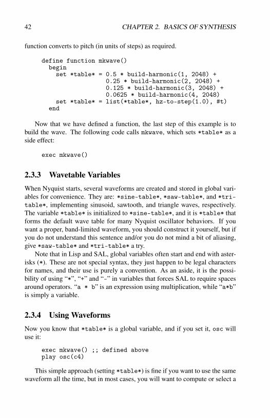
define function mkwave()beginset *table* = 0.5 * build-harmonic(1, 2048) +
0.25 * build-harmonic(2, 2048) +0.125 * build-harmonic(3, 2048) +0.0625 * build-harmonic(4, 2048)
set *table* = list(*table*, hz-to-step(1.0), #t)end
Now that we have defined a function, the last step of this example is tobuild the wave. The following code calls mkwave, which sets *table* as aside effect:
exec mkwave()
2.3.3 Wavetable VariablesWhen Nyquist starts, several waveforms are created and stored in global vari-ables for convenience. They are: *sine-table*, *saw-table*, and *tri-table*, implementing sinusoid, sawtooth, and triangle waves, respectively.The variable *table* is initialized to *sine-table*, and it is *table* thatforms the default wave table for many Nyquist oscillator behaviors. If youwant a proper, band-limited waveform, you should construct it yourself, but ifyou do not understand this sentence and/or you do not mind a bit of aliasing,give *saw-table* and *tri-table* a try.
Note that in Lisp and SAL, global variables often start and end with aster-isks (*). These are not special syntax, they just happen to be legal charactersfor names, and their use is purely a convention. As an aside, it is the possi-bility of using “*”, “+” and “-” in variables that forces SAL to require spacesaround operators. “a * b” is an expression using multiplication, while “a*b”is simply a variable.
2.3.4 Using WaveformsNow you know that *table* is a global variable, and if you set it, osc willuse it:
exec mkwave() ;; defined aboveplay osc(c4)
This simple approach (setting *table*) is fine if you want to use the samewaveform all the time, but in most cases, you will want to compute or select a

2.4. PIECE-WISE LINEAR FUNCTIONS: PWL 43
waveform, use it for one sound, and then compute or select another waveformfor the next sound. Using the global default waveform *table* is awkward.
A better way is to pass the waveform directly to osc. Here is an exampleto illustrate:
;; redefine mkwave to set *mytable* instead of *table*define function mkwave()
beginset *mytable* = 0.5 * build-harmonic(1, 2048) +
0.25 * build-harmonic(2, 2048) +0.125 * build-harmonic(3, 2048) +0.0625 * build-harmonic(4, 2048)
set *mytable* = list(*mytable*, hz-to-step(1.0), #t)end
exec mkwave() ;; run the code to build *mytable*
play osc(c4, 1.0, *mytable*) ;; use *mytable*
;; note that osc(c4, 1.0) will still generate a sine tone;; because the default *table* is still *sine-table*
Now, you should be thinking “wait a minute, you said to avoid settingglobal variables to sounds, and now you are doing just that with these wave-form examples. What a hypocrite!” Waveforms are a bit special because theyare
• typically short so they do not claim much memory,
• typically used many times, so there can be significant savings by com-puting them once and saving them,
• not used directly as sounds but only as parameters to oscillators.
You do not have to save waveforms in variables, but it is common practice, inspite of the general advice to keep sounds out of global variables.
2.4 Piece-wise Linear Functions: pwlIt is often convenient to construct signals in Nyquist using a list of (time, value)breakpoints which are linearly interpolated to form a smooth signal. The pwlfunction takes a list of parameters which denote (time, value) pairs. There isan implicit initial (time, value) pair of (0, 0), and an implicit final value of 0.There should always be an odd number of parameters, since the final value(but not the final time) is implicit. Thus, the general form of pwl looks like:
pwl(t1, v1, t2, v2, . . . , tn)

44 CHAPTER 2. BASICS OF SYNTHESIS
Figure 2.5: Piece-wise Linear Functions.
and this results in a signal as shown in Figure 2.5.Here are some examples of pwl:
; symmetric rise to 10 (at time 1) and fall back to 0 (at time 2):;pwl(1, 10, 2)
; a square pulse of height 10 and duration 5.; Note that the first pair (0, 10) overrides the default initial; point of (0, 0). Also, there are two points specified at time 5:; (5, 10) and (5, 0). (The last 0 is implicit). The conflict is; automatically resolved by pushing the (5, 10) breakpoint back to; the previous sample, so the actual time will be 5 - 1/sr, where; sr is the sample rate.;pwl(0, 10, 5, 10, 5)
; a constant function with the value zero over the time interval; 0 to 3.5. This is a very degenerate form of pwl. Recall that there; is an implicit initial point at (0, 0) and a final implicit value of; 0, so this is really specifying two breakpoints: (0, 0) and (3.5, 0):;pwl(3.5)
; a linear ramp from 0 to 10 and duration 1.; Note the ramp returns to zero at time 1. As with the square pulse; above, the breakpoint (1, 10) is pushed back to the previous; sample.;pwl(1, 10, 1)
; If you really want a linear ramp to reach its final value at the; specified time, you need to make a signal that is one sample longer.; The RAMP function does this:;ramp(10) ; ramp from 0 to 10 with duration 1 + one sample; period. RAMP is based on PWL; it is defined in nyquist.lsp.

2.4. PIECE-WISE LINEAR FUNCTIONS: PWL 45
2.4.1 Variants of pwl
Sometimes, you want a signal that does not start at zero or end at zero. There isalso the option of interpolating between points with exponential curves insteadof linear interpolation. There is also the option of specifying time intervalsrather than absolute times. These options lead to many variants, for example:
pwlv(v0, t1,v1, t2,v2, . . . , tn,vn) – “v” for “value first” is used forsignals with non-zero starting and ending points
pwev(v1, t2, l2, . . . , tn,vn) – exponential interpolation, vi > 0pwlr(i1,v1, i2,v2, . . . , in) – relative intervals rather than absolute
times
See the Nyquist Reference Manual for more variants and combinations.
2.4.2 The Envelope Function: env
Envelopes created by env are a special case of the more general piece-wiselinear functions created by pwl. The form of env is
env(t1, t2, t4, l1, l2, l3,dur)
(duration given by dur is optional). One advantage of env over pwl is that
Figure 2.6: Envelope function env.
env allows you to give fixed attack and decay times that do not stretch withduration. In contrast, the default behavior for pwl is to stretch each segment inproportion when the duration changes. (We have not really discussed durationin Nyquist, but we will get there later.)

46 CHAPTER 2. BASICS OF SYNTHESIS
2.5 Basic Wavetable SynthesisNow, you have seen examples of using the oscillator function (or unit gener-ator) osc to make tones and various functions (unit generators) to make en-velopes or smooth control signals. All we need to do is multiply them togetherto get tones with smooth onsets and decays. Here is an example function toplay a note:
; env-note produces an enveloped note. The duration; defaults to 1.0, but stretch can be used to change the duration.; Uses mkwave, second version defined above, to create *mytable*.
exec mkwave() ;; run the code to build *mytable*
function env-note(p)return osc(p, 1.0, *mytable*) *
env(0.05, 0.1, 0.5, 1.0, 0.5, 0.4)
; try it out:;play env-note(c4)
This is a basic synthesis algorithm called wavetable synthesis. The advan-tages are:
• simplicity – one oscillator, one envelope,
• efficiency – oscillator samples are generated by fast table lookup and(usually) linear interpolation,
• direct control – you can specify the desired envelope and pitch
Disadvantages are:
• the spectrum (strength of harmonics) does not change with pitch or timeas in most acoustic instruments.
Often filters are added to change the spectrum over time, and we will see manyother synthesis algorithms and variations of wavetable synthesis to overcomethis problem.
2.6 Introduction to ScoresSo far, we have seen how simple functions can be used in Nyquist to createindividual sound events. We prefer this term to notes. While a sound eventmight be described as a note, the term note usually implies a single musicaltone with a well-defined pitch. A note is conventionally described by:

2.6. INTRODUCTION TO SCORES 47
• pitch – from low (bass) to high,
• starting time (notes begin and end),
• duration – how long is the note,
• loudness – sometimes called dynamics,
• timbre – everything else such as the instrument or sound quality, soft-ness, harshness, noise, vowel sound, etc.)
while sound event captures a much broader range of possible sound). A soundevent can have:
• pitch, but may be unpitched noise or combinations,
• time – sound events begin and end,
• duration – how long is the event,
• loudness – also known as dynamics,
• potentially many evolving qualities.
Now, we consider how to organize sound events in time using scores in Nyquist.What is a score? Authors write books. Composers write scores. Figure 2.7illustrates a conventional score. A score is basically a graphical display of mu-sic intended for conductors and performers. Usually, scores display a set ofnotes including their pitches, timing, instruments, and dynamics. In computermusic, we define score to include computer readable representations of sets ofnotes or sound events.
2.6.1 Terminology – PitchMusical scales are built from two-sizes of pitch intervals: whole steps and halfsteps, where a whole step represents about a 12 percent change in frequency,and a half step is about a 6 percent change. A whole step is exactly two halfsteps. Therefore the basic unit in Western music is the half step, but this is abit wordy, so in Nyquist, we call these steps.1
Since Western music more-or-less uses integer numbers of half-steps forpitches, we represent pitches with integers. Middle C (ISO C4) is arbitrarily
1Physicists have the unit Hertz to denote cycles per second. Wouldn’t it be great if we had aspecial name to denote half-steps? How about the Bach since J. S. Bach’s Well-Tempered Clavieris a landmark in the development of the fixed-size half step, or the Schoenberg, honoring Arnold’sdevelopment of 12-tone music. Wouldn’t it be cool to say 440 Hertz is 69 Bachs? Or to arguewhether it’s “Bach” or “Bachs?” But I digress ....

48 CHAPTER 2. BASICS OF SYNTHESIS
Figure 2.7: A score written by Mozart.
represented by 60. Nyquist pre-defines a number of convenient variables torepresent pitches symbolically. We have c4 = 60, cs4 (C# or C-sharp) = 61,cf4 (Cb or C-flat) = 59, b3 (B natural, third octave) = 59, bs3 (B# or B-sharp,3rd octave) = 60, etc. Note: In Nyquist, we can use non-integers to denotedetuned or microtonal pitches: 60.5 is a quarter step above 60 (C4).
Some other useful facts: Steps are logarithms of frequency, and frequencydoubles every 12 steps. Doubling frequency (or halving) is called an intervalof an octave.
2.6.2 Lists
Scores are built on lists, so let’s learn about lists.
Lists in Nyquist
Lists in Nyquist are represented as standard singly-linked lists. Every elementcell in the list contains a link to the value and a link to the next element. Thelast element links to nil, which can be viewed as pointing to an empty list.Nyquist uses dynamic typing so that lists can contain any types of elements orany mixture of types; types are not explicitly declared before they are used.

2.6. INTRODUCTION TO SCORES 49
Also, a list can have nested lists within it, which means you can make anybinary tree structure through arbitrary nesting of lists.
Figure 2.8: A list in Nyquist.
Notation
Although we can manipulate pointers directly to construct lists, this is frownedupon. Instead, we simply write expressions for lists. In SAL, we use curlybrace notations for literal lists, e.g. {a b c}. Note that the three elements hereare literal symbols, not variables (no evaluation takes place, so these symbolsdenote themselves, not the values of variables named by the symbols). To con-struct a list from variables, we call the list function with an arbitrary numberof parameters, which are the list elements, e.g. list(a, b, c). These pa-rameters are evaluated as expressions in the normal way and the values of theseexpressions become list elements.
Literals, Variables, Quoting, Cons
Consider the following:
set a = 1, b = 2, c = 3print {a b c}
This prints: {a b c}. Why? Remember that the brace notation {} doesnot evaluate anything, so in this case, a list of the symbols a, b and c is formed.To make a list of the values of a, b and c, use list, which evaluates itsarguments:
print list(a, b, c)
This prints: {1 2 3}.What about numbers? Consider
print list(1, 2, 3)

50 CHAPTER 2. BASICS OF SYNTHESIS
This prints: {1 2 3}. Why? Because numbers are evaluated immediately bythe Nyquist (SAL or Lisp) interpreter as the numbers are read. They becomeeither integers (known as type FIXNUM) or floating point numbers (known astype FLONUM). When a number is used as an expression (as in this example)or a subexpression, the number evaluates to itself.
What if you want to use list to construct a list of symbols?
print list(quote(a), quote(b), quote(c))
This prints: {a b c}. The quote() form can enclose any expression,but typically just a symbol. The quote() form returns the symbol withoutevaluation.
If you want to add an element to a list, there is a special function, cons:
print cons(a, {b})
This prints: {1 b}. Study this carefully; the first argument becomes thefirst element of a new list. The elements of the second argument (a list) formthe remaining elements of the new list.
In contrast, here is what happens with list:
print list(a, {b c d})
This prints: {1 {b c d}}. Study this carefully too; the first argumentbecomes the first element of a new list. The second argument becomes thesecond element of the new list, so the new list has two elements.
2.7 ScoresIn Nyquist, scores are represented by lists of data. The form of a Nyquist scoreis the following:
{ sound-event-1sound-event-2...sound-event-n }
where a sound event is also a list consisting of the event time, duration,and an expression that can be evaluated to compute the event. The expression,when evaluated, must return a sound:
{ {time-1 dur-1 expression-1}{time-2 dur-2 expression-2}...{time-n dur-n expression-n} }

2.7. SCORES 51
Each expression consists of a function name (sometimes called the instru-ment and a list of keyword-value style parameters:
{ {time-1 dur-1 {instrument-1 pitch: 60}}{time-2 dur-2 {instrument-2 pitch: 62}}...{time-n dur-n {instrument-3 pitch: 62 vel: 100}} }
Here is an example score:
{ {0 1 {note pitch: 60 vel: 100}}{1 1 {note pitch: 62 vel: 110}}{2 1 {note pitch: 64 vel: 120}} }
Important things to note (pardon the pun) are:
• Scores are data. You can compute scores using by writing code andusing the list construction functions from the previous section (and seethe Nyquist Reference Manual for many more).
• Expressions in scores are lists, not SAL expressions. The first elementof the list is the function to call. The remaining elements form the pa-rameter list.
• Expressions use keyword-style parameters, never positional parameters.The rationale is that keywords label the values, allowing us to pass thesame score data to different instruments, which may implement somekeywords, ignore others, and provide default values for missing key-words.
• keyword parameters also allow us to treat scores as data. For exam-ple, Nyquist has a built-in function to find all the pitch: parametersand transpose them. If positional parameters were used, the transposefunction would have to have information about each instrument func-tion to find the pitch values (if any). Keyword parameters are moreself-defining.
2.7.1 The score-begin-end “instrument” EventSometimes it is convenient to give the entire score a begin time and an endtime because the logical time span of a score may include some silence. Thisinformation can be useful when splicing scores together. To indicate start andend times of the score, insert a sound event of the form
{0 0 {score-begin-end 1.2 6}}

52 CHAPTER 2. BASICS OF SYNTHESIS
In this case, the score occupies the time period from 1.2 to 6 seconds.For example, if we want the previous score, which nominally ends at time
3 to contain an extra second of silence at the end, we can specify the time spanof the score is from 0 to 4 as follows:
{ {0 0 {score-begin-end 0 4}}{0 1 {note pitch: 60 vel: 100}}{1 1 {note pitch: 62 vel: 110}}{2 1 {note pitch: 64 vel: 120}} }
2.7.2 Playing a ScoreTo interpret a score and produce a sound, we use the timed-seq() function.The following plays the previous score:
set myscore = {{0 0 {score-begin-end 0 4}}{0 1 {note pitch: 60 vel: 100}}{1 1 {note pitch: 62 vel: 110}}{2 1 {note pitch: 64 vel: 120}} }
play timed-seq(myscore)
2.7.3 Making an InstrumentNow you know all you need to know to make scores. The previous examplewill work because note is a built-in function in Nyquist that uses a built-in pi-ano synthesizer. But it might be helpful to see a custom instrument definition,making the connection between scores and the wavetable synthesis exampleswe saw earlier. In the next example, we define a new instrument functionthat calls on our existing env-note instrument. The reason for making a newfunction to be our instrument is we want to use keyword parameters. Then, wemodify myscore to use myinstr. (See Algorithm 2.1.)
Note that in myinstr we scale the amplitude of the output byvel-to-linear(vel) to get some loudness control. “vel” is short for “ve-locity” which refers to the velocity of piano keys – higher numbers mean fasterwhich means louder. The “vel” scale is nominally 1 to 127 (as in the MIDIstandard) and vel-to-linear() converts this to a scale factor. We will learnmore about amplitude later.
2.8 SummaryNow you should know how to build a simple wavetable instrument with thewaveform consisting of any set of harmonics and with an arbitrary envelope

2.8. SUMMARY 53
variable *mytable* ;; declaration avoids parser warnings
function mkwave()beginset *mytable* = 0.5 * build-harmonic(1, 2048) +
0.25 * build-harmonic(2, 2048) +0.125 * build-harmonic(3, 2048) +0.0625 * build-harmonic(4, 2048)
set *mytable* = list(*mytable*, hz-to-step(1.0), #t)end
exec mkwave()
function env-note(p)return osc(p, 1.0, *mytable*) *
env(0.05, 0.1, 0.5, 1.0, 0.5, 0.4)
;; define the "instrument" myinstr that uses keyword parameters;; this is just a stub, env-note() does most of the work...function myinstr(pitch: 60, vel: 100)
return env-note(pitch) * vel-to-linear(vel)
set myscore = {{0 0 {score-begin-end 0 4}}{0 1 {myinstr pitch: 60 vel: 50}}{1 1 {myinstr pitch: 62 vel: 70}}{2 1 {myinstr pitch: 64 vel: 120}} }
play timed-seq(myscore)
Algorithm 2.1: Defining an instrument, using it in a Nyquist score, and playingthe score.

54 CHAPTER 2. BASICS OF SYNTHESIS
controlled by pwl or env. You can also write or compute scores containingmany instances of your instrument function organized in time, and you cansynthesize the score using timed-seq. You might experiment by creatingdifferent waveforms, different envelopes, using non-integer pitches for micro-tuning, or notes overlapping in time to create chords or clusters.

Chapter 3
Sampling TheoryIntroduction
Topics Discussed: Sampling Theory, Analog to/from Digital Conversion,Fourier Synthesis, Aliasing, Quantization Noise, Amplitude Modulation
The principles which underlie almost all digital audio applications and de-vices, be they digital synthesis, sampling, digital recording, or CD or iPodplayback, are based on the basic concepts presented in this chapter. New formsof playback, file formats, compression, synthesis, processing and storage ofdata are all changing on a seemingly daily basis, but the underlying mecha-nisms for converting real-world sound into digital values and converting themback into real-world sound has not varied much since Max Mathews developedMUSIC I in 1957 at Bell Labs.
The theoretical framework that enabled musical pioneers such as MaxMathews to develop digital audio programs stretches back over a century. Thegroundbreaking theoretical work done at Bell Labs in the mid-20th century isworth noting. Bell Labs was concerned with transmitting larger amounts ofvoice data over existing telephone lines than could normally be sent with ana-log transmissions, due to bandwidth restrictions. Many of the developmentspertaining to computer music were directly related to work on this topic.
Harry Nyquist, a Swedish-born physicist laid out the principles for sam-pling analog signals at even intervals of time and at twice the rate of the highestfrequency so they could be transmitted over telephone lines as digital signals[Nyquist, 1928], even though the technology to do so did not exist at the time.Part of this work is now known as the Nyquist Theorem. Nyquist workedfor AT&T, then Bell Labs. Twenty years later, Claude Shannon, mathemati-cian and early computer scientist, also working at Bell Labs and then M.I.T.,
55

56 CHAPTER 3. SAMPLING THEORY INTRODUCTION
developed a proof for the Nyquist theory.1 The importance of their work toinformation theory, computing, networks, digital audio, digital photographyand computer graphics (images are just signals in 2D!) cannot be understated.Pulse Code Modulation (PCM), a widely used method for encoding and de-coding binary data, such as that used in digital audio, was also developed earlyon at Bell Labs, attributed to John R. Pierce, a brilliant engineer in many fields,including computer music.
In this chapter, we will learn the basic theory of sampling, or representingcontinuous functions with discrete data.
3.0.1 Intuitive Approach
The world is continuous. Time marches on and on, and there are plenty ofthings that we can measure at any instant. For example, weather forecastersmight keep an ongoing record of the temperature or barometric pressure. Ifyou are in the hospital, the nurses might be keeping a record of your temper-ature, your heart rate, or your brain waves. Any of these records gives you afunction f (t) where, at a given time t, f (t) is the value of the particular thingthat interests you.
Figure 3.1: Carbon dioxide concentration data from climate.nasa.gov.
1The Shannon Theorem [Shannon, 1948], a pioneering work in information theory, shouldnot be confused with the Shannon Juggling Theory of the same author, in which he worked outthe mathematics of juggling numerous objects ((F+D)H=(V+D)N, where F is the time an objectspends in the air, D is the time a object spends in a hand, V is the time a hand is vacant, N is thenumber of objects juggled, and H is the number of hands)–he was an avid juggler as well.

57
Figure 3.1 represents a continuous function of time. What we mean by“continuous” is that at any instant of time the function takes on a well-definedvalue, so that it makes a squiggly line graph that could be traced without thepencil ever leaving the paper. This might also be called an analog function.Of course, the time series that interest us are those that represent sound. Inparticular, we want to take these time series, stick them on the computer, andplay with them!
Now, if you’ve been paying attention, you may realize that at this momentwe’re in a bit of a bind: sound is a continuous function. That is, at every instantin time, we could write down a number that is the value of the function atthat instant—–how much your eardrum has been displaced, the instantaneousair pressure, voltage from a microphone, and so on. But such a continuousfunction would provide an infinite list of numbers (any one of which may havean infinite expansion, like = 3.1417...), and no matter how big your computeris, you’re going to have a pretty tough time fitting an infinite collection ofnumbers on your hard drive.
So how do we do it? How can we represent sound as a finite collectionof numbers that can be stored efficiently, in a finite amount of space, on acomputer, and played back and manipulated at will? In short, how do werepresent sound digitally? That’s the problem that we’ll investigate in thischapter.
Somehow we have to come up with a finite list of numbers that does agood job of representing our continuous function. We do it by sampling theoriginal function at some predetermined rate, called the sampling rate, record-ing the value of the function at that moment. For example, maybe we onlyrecord the temperature every 5 minutes. The graph in Figure 3.1 really comesfrom discrete samples obtained from ice cores, so this is also an example ofsampling to represent a continuous function using discrete values. For soundwe need to go a lot faster, and we often use a special device that grabs instan-taneous amplitudes at rapid, audio rates (called an analog to digital converter,or ADC).
A continuous function is also called an analog function, and, to restatethe problem, we have to convert analog functions to lists of samples, in binary,which is the fundamental way that computers store information. In computers,think of a digital sound as a function of location in computer memory. Thatis, sounds are stored as lists of numbers, and as we read through them we arebasically creating a discrete function of time of individual amplitude values.
In analog to digital conversions, continuous functions (for example, airpressures, sound waves, or voltages) are sampled and stored as numerical val-ues. (See Figure 3.2.) In digital to analog conversions, numerical values areinterpolated by the converter to force some continuous system (such as am-

58 CHAPTER 3. SAMPLING THEORY INTRODUCTION
Figure 3.2: A pictorial description of the recording and playback of soundsthrough an ADC/DAC.
plifiers, speakers, and subsequently the air and our ears) into a continuous vi-bration. Interpolation just means smoothly transitioning between the discretenumerical values.
3.0.2 Analog Versus DigitalThe distinction between analog and digital information is fundamental to therealm of computer music (and in fact computer anything!). In this section,we’ll offer some analogies, explanations, and other ways to understand thedifference more intuitively.
Imagine watching someone walking along, bouncing a ball. Now imaginethat the ball leaves a trail of smoke in its path. What does the trail look like?(See Figure 3.3.) Probably some sort of continuous zigzag pattern, right?
Figure 3.3: The path of a bouncing ball.
OK, keep watching, but now blink repeatedly. What does the trail looklike now? Because we are blinking our eyes, we’re only able to see the ball atdiscrete moments in time. It’s on the way up, we blink, now it’s moved up abit more, we blink again, now it may be on the way down, and so on. We’llcall these snapshots samples because we’ve been taking visual samples of thecomplete trajectory that the ball is following. (See Figure 3.4.) The rate atwhich we obtain these samples (blink our eyes) is called the sampling rate.
It’s pretty clear, though, that the faster we sample, the better chance wehave of getting an accurate picture of the entire continuous path along whichthe ball has been traveling.

59
Figure 3.4: The same path, but sampled by blinking.
What’s the difference between the two views of the bouncing ball: theblinking and the nonblinking? Each view pretty much gives the same pictureof the ball’s path. We can tell how fast the ball is moving and how high it’sbouncing. The only real difference seems to be that in the first case the trailis continuous, and in the second it is broken, or discrete. That’s the maindistinction between analog and digital representations of information: analoginformation is continuous, while digital information is not.
3.0.3 Analog and Digital Waveform RepresentationsNow let’s take a look at two time domain representations of a sound wave, oneanalog and one digital, in Figure 3.5.
Figure 3.5: An analog waveform and its digital cousin: the analog waveformhas smooth and continuous changes, and the digital version of the same wave-form has a stairstep look. The black squares are the actual samples taken bythe computer. Note that the grey lines are only for show – all that the com-puter knows about are the discrete points marked by the black squares. Thereis nothing in between those points stored in the computer.
The gray “staircase” waveform in Figure 3.5 emphasizes the point thatdigitally recorded waveforms are apparently missing some original informa-tion from analog sources. However, by increasing the number of samples takeneach second (the sample rate), as well as increasing the accuracy of those sam-
60 CHAPTER 3. SAMPLING THEORY INTRODUCTION
ples (the resolution), an extremely accurate recording can be made. In fact, wecan prove mathematically that discrete samples can represent certain contin-uous functions without any loss of information! And in practice, we can usethis theory to record audio with imperceptible loss or distortion.
3.1 Sampling Theory
So now we know that we need to sample a continuous waveform to representit digitally. We also know that the faster we sample it, the better. But this isstill a little vague. How often do we need to sample a waveform in order toachieve a good representation of it?
The answer to this question is given by the Nyquist sampling theorem,which states that to represent a signal well, the sampling rate (or samplingfrequency – not to be confused with the frequency content of the sound) needsto be at least twice the highest frequency contained in the sound.
3.1.1 Frequency Content
We’ll be giving a much more precise description of the frequency domainlater, but for now we can simply think of sounds as combinations of morebasic sounds that are distinguished according to their rate of vibration, calledfrequency. Perceptually, higher frequencies are associated with higher pitchheight and higher brightness.
As we learned earlier, the basic sound is called a sinusoid, the general termfor sine-like waveforms. The term pitch height refers to our perception ofthese components if we could hear them separately, but ordinarily, we cannot.To summarize, sounds can be decomposed into the sum of basic sinusoidalcomponents, each of which has a frequency.
All sound can ve viewed as a combination of these sinusoids with varyingamplitudes. It’s sort of like making soup and putting in a bunch of basic spices:the flavor will depend on how much of each spice you include, and you canchange things dramatically when you alter the proportions. The sinusoids areour basic sound spices! The complete description of how much of each of thefrequencies is used is called the spectrum of the sound.
Since sounds change over time, the proportions of each of the sinusoidschanges too. Just like when you spice up that soup, as you let it boil the spiceproportion may be changing as things evaporate.

3.1. SAMPLING THEORY 61
Figure 3.6: Two graphical representations of sound.

62 CHAPTER 3. SAMPLING THEORY INTRODUCTION
3.1.2 Highest Frequency in a Sound
Consider Figure 3.6. The graph at the top is our usual time domain graph, oraudiogram, of the waveform created by a five-note whistled melody. Time ison the x-axis, and amplitude is on the y-axis.
The bottom graph is the same melody, but this time we are looking at atime-frequency representation. The idea here is that if we think of the whistleas made up of contiguous small chunks of sound, then over each small timeperiod the sound is composed of differing amounts of various pieces of fre-quency. The amount of frequency y at time t is encoded by the brightness ofthe pixel at the coordinate (t, y). The darker the pixel, the more of that fre-quency at that time. For example, if you look at time 0.4 you see a band ofwhite, except near 2,500, showing that around that time we mainly hear a puretone of about 2,500 Hz, while at 0.8 seconds, there are contributions all aroundfrom about 0 Hz to 5,500 Hz, but stronger ones at about 2,500 Hz and 200 Hz.
It looks like the signal only contains frequencies up to 8,000 Hz. If thiswere the case, we would need to sample the sound at a rate of 16,000 Hz (16kHz) in order to accurately reproduce the sound. That is, we would need totake sound bites (bytes?!) 16,000 times a second.
In the next section, when we talk about representing sounds in the fre-quency domain (as a combination of various amplitude levels of frequencycomponents, which change over time) rather than in the time domain (as a nu-merical list of sample values of amplitudes), we’ll learn a lot more about theramifications of the Nyquist theorem for digital sound. For example, since thehuman ear only responds to sounds up to about 20,000 Hz, we need to samplesounds at least 40,000 times a second, or at a rate of 40,000 Hz, to representthese sounds for human consumption. You may be wondering why we evenneed to represent sonic frequencies that high (when the piano, for instance,only goes up to the high 4,000 Hz range in terms of pitches or repetition rate.).The answer is timbral, particularly spectral. Those higher frequencies do existand fill out the descriptive sonic information.
Just to review: we measure frequency in cycles per second (cps) or Hertz(Hz). The frequency range of human hearing is usually given as 20 Hz to20,000 Hz, meaning that we can hear sounds in that range. Knowing that,if we decide that the highest frequency we’re interested in is 20 kHz, thenaccording to the Nyquist theorem, we need a sampling rate of at least twicethat frequency, or 40 kHz.

3.2. THE FREQUENCY DOMAIN 63
3.2 The Frequency Domain
Earlier, we talked about the basic atoms of sound—–the sine wave, and aboutthe function that describes the sound generated by a vibrating tuning fork. Inthis section we’re talking a lot about the frequency domain. If you remem-ber, our basic units, sine waves, only had two parameters: amplitude and fre-quency. It turns out that these dull little sine waves are going to give us thefundamental tool for the analysis and description of sound, and especially forthe digital manipulation of sound. That’s the frequency domain: a place wherelots of little sine waves are our best friends.
But before we go too far, it’s important to fully understand what a sinewave is, and it’s also wonderful to know that we can make these simple littlecurves ridiculously complicated, too. And it’s useful to have another modelfor generating these functions. That model is called a phasor.
3.2.1 Description of a Phasor
Think of a bicycle wheel suspended at its hub. We’re going to paint one ofthe spokes bright red, and at the end of the spoke we’ll put a red arrow. Wenow put some axes around the wheel—the x-axis going horizontally throughthe hub, and the y-axis going vertically. We’re interested in the height ofthe arrowhead relative to the x-axis as the wheel—our phasor—spins aroundcounterclockwise. (See Figure 3.7.)
Figure 3.7: Sine waves and phasors. As the sine wave moves forward in time,the arrow goes around the circle at the same rate. The height of the arrow(that is, how far it is above or below the x-axis) as it spins around in a circle isdescribed by the sine wave.

64 CHAPTER 3. SAMPLING THEORY INTRODUCTION
In other words, if we trace the arrow’s location on the circle and measurethe height of the arrow on the y-axis as our phasor goes around the circle, theresulting curve is a sine wave!
As time goes on, the phasor goes round and round. At each instant, wemeasure the height of the dot over the x-axis. Let’s consider a small exam-ple first. Suppose the wheel is spinning at a rate of one revolution per sec-ond. This is its frequency (and remember, this means that the period is 1second/revolution). This is the same as saying that the phasor spins at a rateof 360 degrees per second, or better yet, 2π radians per second (if we’re goingto be mathematicians, then we have to measure angles in terms of radians). So2π radians per second is the angular velocity of the phasor.
This means that after 0.25 second the phasor has gone π/2 radians (90degrees), and after 0.5 second it’s gone π radians or 180 degrees, and so on.So, we can describe the amount of angle that the phasor has gone around attime t as a function, which we call θ(t).
Now, let’s look at the function given by the height of the arrow as timegoes on. The first thing that we need to remember is a little trigonometry.
Figure 3.8: Triangle.
The sine and cosine of an angle are measured using a right triangle. For ourright triangle, the sine of θ , written sin(θ) is given by the equation: sin(θ) =a/c (See Figure 3.8.)
This means that: a = c× sin(θ)We’ll make use of this in a minute, because in this example a is the height
of our triangle.Similarly, the cosine, written cos(θ), is: cos(θ) = b/cThis means that: b = c× cos(θ)This will come in handy later, too.Now back to our phasor. We’re interested in measuring the height at time
t, which we’ll denote as h(t). At time t, the phasor’s arrow is making anangle of θ(t) with the x-axis. Our basic phasor has a radius of 1, so we getthe following relationship: h(t) = sin(θ(t)) = sin(2πt). We also get this nicegraph of a function, which is our favorite old sine curve.

3.2. THE FREQUENCY DOMAIN 65
Figure 3.9: Basic sinusoid.
Now, how could we change this curve? Well, we could change the am-plitude—this is the same as changing the length of our arrow on the phasor.We’ll keep the frequency the same and make the radius of our phasor equal to3. Then we get: h(t) = 3×sin(2πt) Then we get the nice curve in Figure 3.10,which is another kind of sinusoid (bigger!).
Figure 3.10: Bigger sine curve.
Now let’s start messing with the frequency, which is the rate of revolutionof the phasor. Let’s ramp it up a notch and instead start spinning at a rate of

66 CHAPTER 3. SAMPLING THEORY INTRODUCTION
five revolutions per second. Now: θ(t) = 5× (2πt) = 10πt. This is easy tosee since after 1 second we will have gone five revolutions, which is a totalof 10 radians. Let’s suppose that the radius of the phasor is 3. Again, at eachmoment we measure the height of our arrow (which we call h(t)), and we get:h(t) = 3× sin(θ(t)) = 3× sin(10πt). Now we get the sinusoid in Figure 3.11.
Figure 3.11: Bigger, faster sine curve.
In general, if our phasor is moving at a frequency of v revolutions persecond and has radius A, then plotting the height of the phasor is the same asgraphing this sinusoid: h(t) = A× sin(v× 2πt). Now we’re almost done, butthere is one last thing we could vary: we could change the place where westart our phasor spinning. For example, we could start the phasor moving at arate of five revolutions per second with a radius of 3, but start the phasor at anangle of π/4 radians, instead.
Now, what kind of function would this be? Well, at time t = 0 we want tobe taking the measurement when the phasor is at an angle of π/4, but otherthan that, all is as before. So the function we are graphing is the same asthe one above, but with a phase shift of π/4. The corresponding sinusoid is:h(t) = 3× sin(10πt +π/4), which is shown in Figure 3.12.
Our most general sinusoid of amplitude A, frequency v, and phase shift φ
has the form: h(t) = A×sin(v×2πt+φ), which is more commonly expressedwith frequency ω in radians per second instead of frequency v in cycles persecond: h(t) = A× sin(ωt +φ).
A particularly interesting example is what happens when we take the phaseshift equal to 90 degrees, or π/2 radians. Let’s make it nice and simple, withfrequency equal to one revolution per second and amplitude equal to 1 as well.

3.2. THE FREQUENCY DOMAIN 67
Figure 3.12: Changing the phase.
Then we get our basic sinusoid, but shifted ahead π/2. Does this look familiar?This is the graph of the cosine function!
Figure 3.13: 90-degree phase shift (cosine).
You can do some checking on your own and see that this is also the graphthat you would get if you plotted the displacement of the arrow from the y-axis.So now we know that a cosine is a phase-shifted sine!

68 CHAPTER 3. SAMPLING THEORY INTRODUCTION
3.2.2 Fourier AnalysisNow we know that signals can be decomposed into a (possibly infinite) sumof phasors or partials or sinusoids—however you want to look at it. But howdo we determine this sum?
The Fourier Transform, named for French scientist and mathematicianJean Baptiste Fourier (1768–1830), is a surprisingly simple and direct for-mula to write this infinite sum. Since we have to deal with phase somehow,we will begin with an expression of the Fourier Transform that keeps the sineand cosine parts separate. The signal we want to analyze is f (t). The resultof the analysis will be two functions. R(ω) is a function of frequency (in radi-ans per second) that gives us the amplitude of a cosine at that frequency, andX(ω) is a function of frequency that gives us the amplitude of a sinusoid atthat frequency.
R(ω) =∫
∞
−∞
f (t)cos(ωt)dt
X(ω) =−∫
∞
−∞
f (t)sin(ωt)dt
Why the minus sign when computing X? It relates to whether the positivedirection of rotation is considered clockwise or counterclockwise. You wouldthink the convention would be based on the simplest form (so drop the mi-nus sign), but the Fourier Transform is closely related the the Inverse FourierTransform (how to we construct a time domain signal from it’s frequency do-main representation?), and one or the other transform has to have a minus sign,so this is the convention.
Note that this is all continuous math. We will get back to sampling soon,but if we want to understand what sampling does to a continuous signal, wehave to deal with continuous functions.
Note also, and this is very important, that we are “integrating out” all time.The functions R and X are functions of frequency. It does not make sense (atthis point) to say “What is the Fourier Transform of the signal at time t?”—instead, we transform infinite functions of time ( f (t)) into infinite functions offrequency, so all notions of time are absorbed into frequencies.
What About Phase?
We saw in the previous section how cosine is simply a sine function that is“phase shifted,” and we can achieve any phase by some combination of sineand cosine at the same frequency. Thus, we get to choose: Do we want totalk about sinusoids with frequency, amplitude and phase? Or do we want totalk about cosines and sines, each with just frequency and amplitude? The two

3.2. THE FREQUENCY DOMAIN 69
are equivalent, so we started with cosines and sines. Once we have the cosineR(ω) and sine X(ω) parts, we can derive a representation in terms of phase.For any given ω of interest, we have:
R(ω)× cos(ωt)+X(ω)× sin(ωt) =√R(ω)2 +X(ω)2× sin(ωt +arctan(X(ω)/R(ω)))
In other words, we can write the partial with frequency ω as A(ω)× sin(ωt +θ(ω)) where
A(ω) =√
R(ω)2 +X(ω)2
andθ(ω) = arctan(X(ω)/R(ω)))
Complex Representation
Rather than separating the sine and cosine parts, we can use complex numbersbecause, among other properties, each complex number has a real part and animaginary part. We can think of a phasor as rotating in the complex plane, soa single complex number can represent both amplitude and phase:
F(ω) = R(ω)+ j ·X(ω)
Here, we use j to represent√−1. You probably learned to use i for imaginary
numbers, but i is also the electrical engineering symbol for current (usuallyin units of Amperes), and since digital signal processing falls largely into thedomain of electrical engineering, we go along with the EE’s and replace i byj.
Now things get interesting... Recall Euler’s formula:2
e jx = cos(x)+ j · sin(x)
If we rewrite the pair R,X as R+ j ·X , and use Euler’s formula, we canderive:
F(ω) =∫
∞
−∞
f (t)e− jωtdt
2Which one is Euler’s formula? There are no less than seven formulas named for Euler, not tomention conjectures, equations, functions, identities, numbers, theorems and laws. This is the onein complex analysis. Euler invented so much mathematics that many things are named for the firstperson that proved Euler’s original idea, just to spread the fame a little. There’s a whole article inWikipedia named “List of things named after Leonhard Euler,” but I digress ....

70 CHAPTER 3. SAMPLING THEORY INTRODUCTION
Example Spectrum
The result of a Fourier Transform is a continuous function of frequency some-times called the frequency spectrum or just spectrum. Figure 3.14 shows thespectrum measured from a gamelan tone. You can see there is energy in awide range of frequencies, but also some peaks that indicate strong sinusoidalpartials here and there.
Figure 3.14: FFT plot of a gamelan instrument.
3.2.3 Fourier and the Sum of SinesIn this section, we’ll try to give some intuition into the spectrum, building onthe previous section.
A long time ago, Fourier proved the mathematical fact that any periodicwaveform can be expressed as the sum of an infinite set of sine waves. Thefrequencies of these sine waves must be integer multiples of some fundamentalfrequency.
In other words, if we have a trumpet sound at middle A (440 Hz), weknow by Fourier’s theorem that we can express this sound as a summation ofsine waves: 440 Hz, 880Hz, 1,320Hz, 1,760 Hz..., or 1, 2, 3, 4... times the

3.2. THE FREQUENCY DOMAIN 71
fundamental, each at various amplitudes. This is rather amazing, since it saysthat for every periodic waveform, if we know the repetition rate, we basicallyknow the frequencies of all of its partials. (Keep in mind however, that notrumpet player will ever play an infinitely long, steady tone, and no real-lifetone is truly periodic if the periodicity comes to an end. We will not worryabout this for now.)3
Figure 3.15: The spectrum of the sine wave has energy only at one frequency.The triangle wave has energy at odd-numbered harmonics (meaning odd mul-tiples of the fundamental), with the energy of each harmonic decreasing as 1over the square of the harmonic number (1/N2). In other words, at the fre-quency that is N times the fundamental, we have 1/N2 as much energy as inthe fundamental.
Figure 3.15 shows some periodic waveforms and their associated spectra.The partials in the sawtooth wave decrease in energy in proportion to the in-
3By the way, periodic waveforms generally have clear pitches. In evolutionary terms, peri-odicity implies an energy source to sustain the vibration, and pitch is a good first-order featurethat tells us whether the energy source is big enough to be a threat or small enough to be food.Think lion roar vs. goat bleat. It should not be too suprising that animals—remember we are thelife forms capable of running away from danger and chasing after food—developed a sense ofhearing, including pitch perception, which at the most basic level serves to detect energy sourcesand estimate size.

72 CHAPTER 3. SAMPLING THEORY INTRODUCTION
verse of the harmonic number (1/N). Pulse (or rectangle or square) waveformshave energy over a broad area of the spectrum.
Real, Imaginary, Amplitude, Phase
In these drawing, we are carelessly forgetting about phase. Generally, wecannot hear phase differences, but we are very adept at hearing amplitudesat different frequencies. Therefore, we usually plot just the amplitude of thesignal when we plot the spectrum, and we ignore the phase. Recall that interms of real and imaginary parts, the amplitude is just the square root of thesum of squares:
A(ω) =√
R(ω)2 +X(ω)2
3.3 Sampling and the Frequency Domain
Now that we understand something about the Fourier Transform, we return toour problem of understanding sampling. What does sampling do to a signal?In the continuous math world, we can model sampling as a simple multiplica-tion of two time domain signals, as shown in Figure 3.16.
Figure 3.16: Sampling is effectively multiplication in the time domain: Wemultiply by 1 (or more properly an instantaneous but infinite impulse whoseintegral is 1) whereever we capture samples, and we remove the rest of thesignal by multiplying by zero.
This gets quite interesting in the frequency domain. Multiplying by a seriesof impulses in the time domain (Figure 3.16) is equivalent to copying andshifting the spectrum in the frequency domain (Figure 3.17). The copies areshifted by the sampling rate, which of course is a frequency.

3.3. SAMPLING AND THE FREQUENCY DOMAIN 73
Figure 3.17: Sampling in the time domain gives rise to shifted spectral copiesin the frequency domain.
3.3.1 Negative FrequenciesLooking at Figure 3.17, you should be wondering why the spectrum is shownwith negative as well as positive frequencies. You can consider negative fre-quencies to be just the result of the formulas for the Fourier Transform. While“negative 440 Hertz” may sound like nonsense, in mathematical terms, it isjust a question of writing sin(ωt) or sin(−ωt), but sin(−ωt) = sin(ωt +π),so we are really talking about certain phase shifts. Since we mostly ignorephase anyway, we often plot only the positive frequencies. In the case of sam-pling theory, we show both negative and positive frequencies of the spectrum.
3.3.2 AliasingNotice in Figure 3.17 that after sampling, the copies of the spectrum comeclose to overlapping. What would happen if the spectrum contained higherfrequencies. Figure 3.18 illustrates a broader spectrum.
Figure 3.18: A broader spectrum (contains higher frequencies) before sam-pling.
Figure 3.19 illustrates the signal after sampling. What a mess! The copiesof the spectrum now overlap. The Nyquist frequency (one-half the samplingrate, and one half the amount by which copies are shifted) is shown by a ver-

74 CHAPTER 3. SAMPLING THEORY INTRODUCTION
tical dotted line. Notice that there is a sort of mirror symmetry around thatline: the original spectrum extending above the Nyquist frequency is “folded”to become new frequencies below the Nyquist frequency.
Figure 3.19: A broader spectrum (contains higher frequencies) after sam-pling. While shown as separate overlapping copies here, the copies are infact summed into a single spectrum.
This is really bad because new frequencies are introduced and added to theoriginal spectrum. The frequencies are in fact aliases of the frequencies abovethe Nyquist frequency. To avoid aliasing, it is necessary to sample at higherthan twice the frequency of the original signal.
In the time domain, aliasing is a little more intuitive, at least if we considerthe special case of a sinusoid. Figure 3.20 shows a fast sinusoid at a frequencymore than half the sample rate. This frequency is “folded” to become a lowerfrequency below half the sample rate. Note that both sinusoids pass perfectlythrough the available samples, which is why they are called aliases. They havethe same “signature” in terms of samples.
To summarize, the frequency range (bandwidth) of a sampled signal isdetermined by the sample rate. We can only capture and represent frequenciesbelow half the sample rate, which is also called the Nyquist rate or Nyquistfrequency.
Figure 3.20: Aliasing, or foldover, happens when we sample a frequency thatis more than half the sampling rate. When the frequency we want to sample istoo high, we undersample and get an unwanted lower-frequency that is createdby the sampling process itself).

3.4. SAMPLING WITHOUT ALIASING 75
3.4 Sampling without Aliasing
In practice, we seldom have the luxury of controlling the bandwidth of our ana-log signals. How do you tell the triangle player to make those tinkly sounds,but don’t go above 22 kHz? The real world is full of high frequencies wecannot hear, but which can become audible as aliases if we are not careful.The solution and standard practice is to filter out the high frequencies beforesampling, as shown in Figure 3.21.
Figure 3.21: Aliasing is avoided by removing frequencies above the Nyquistfrequency (half the sample rate) using a prefilter (sometimes called an anti-aliasing filter.
3.4.1 Converting Back to Analog
A similar process is used to convert digital signals back to analog. If we wereto simply output a train of impulses based on the digital samples, the spec-trum would look like that in the lower half of Figure 3.17, with lots of veryhigh frequencies (in fact, these are aliases of all the sinusoids in the originalspectrum). We remove these unwanted parts of the signal with another filteras shown in Figure 3.22.
3.5 Imperfect Sampling
So far, we have described sampling as if samples were real numbers obtainedwithout error. What happens in the imperfect real world, and what happens torounding errors, since real samples are actually integers with finite precision?
3.5.1 How to Describe Noise
To describe error in audio, we need a way to measure it. Since our hearingbasically responds to audio in a logarithmic manner, the important thing is not

76 CHAPTER 3. SAMPLING THEORY INTRODUCTION
Figure 3.22: To convert a digital signal to analog, we need to remove theartifacts of sampling. This is accomplished by sending the output of thedigital-to-analog converter first into a sample-and-hold circuit that holds thesignal steady while the converter is transitioning to the next sample value,then through a reconstruction filter, which removes high frequencies abovethe Nyquist frequency.
the absolute error but the ratio between the signal and the error. We call errorsin audio “noise,” and we measure the signal-to-noise ratio.
Ratio is so important in audio, and the range of signals and noise is solarge, that we use a special unit, the dB or decibel to represent ratios, or moreprecisely logarithms of ratios. A bel represents a factor of 10 in power, whichis 10 decibels. Since this is a logarithmic scale, 20 decibels is two factors of 10or a factor of 100 in power. But power increases with the square of amplitude,so 20 dB results in only a factor of 10 in amplitude. A handy constant toremember is a factor of 2 in amplitude is about 6 dB, a factor of 4 is about 12dB. What can you hear? A change of 1 dB is barely noticeable. A change of10 dB is easily noticeable, but your range of hearing is about 10 of these steps(around 100 dB).
3.5.2 Quantization NoiseWhat is the effect of rounding? Imagine that there is significant signal changebetween each pair of samples and the true value of the signal we are capturinghas no preference for any value over any other. In that case, we can expectthe signal to fall randomly between two integer sample values. If we round tothe nearest value, the rounding error will be a uniformly distributed randomnumber between -0.5 and 0.5 (considering samples to be integers).
Figure 3.23 illustrates a signal being captured and the resulting roundingerror. Note that the samples must fall on the grid of discrete time points anddiscrete integer sample values, but the actual signal is continuous and real-valued.
Rather than thinking of the signal as being recorded with error, considerthis: If we could subtract the quantization error from the original signal, then

3.6. SAMPLING SUMMARY 77
the original signal would pass through integer sample values and we couldcapture the signal perfectly! Thus, the effect of quantization error is to addrandom values in the range -0.5 to +0.5 to the original signal before sampling.
It turns out that uniform random samples are white noise, so calling error“noise” is quite appropriate. How loud is the noise? The resulting signal-to-noise ratio, given M-bit samples, is 6.02M + 1.76 dB. This is very closeto saying “the signal-to-noise ratio is 6dB per bit.” You only get this signal-to-noise ratio if the signal uses the full range of the integer samples. In reallife, you always record with some “headroom,” so you probably lose 6 to 12dB of the best possible signal. There is also a limit to how many bits youcan use—remember that the bits are coming from analog hardware, so howquiet can you make circuits, and how accurately can you measure voltages?In practice, 16-bit converters offering a theoretical 98 dB signal-to-noise ratioare readily available and widely used. 20- and 24-bit converters are used inhigh-end equipment, but these are not accurate to the least-significant bit, sodo not assume the signal-to-noise ratio can be estimated merely by countingbits.
Figure 3.23: When a signal is sampled, the real-valued signal must be roundedat each sample to the nearest integer sample value. The resulting error is calledquantization error.
3.6 Sampling SummaryOne amazing result of sampling theory is that if the signal being sampled hasa finite bandwidth, then we can sample the signal at discrete time points andcompletely recover the original continuous signal. It seems too good to be truethat all those infinitely many values between samples are not really necessary!
Aside from this startling theoretical finding, we learned that the samplerate should be at least double that of the highest frequency of the signal. Also,error is introduced by rounding samples to integers, an unavoidable step in the

78 CHAPTER 3. SAMPLING THEORY INTRODUCTION
real world, but the signal-to-noise ratio is about 6 dB per bit, so with 16 bitsor more, we can make noise virtually imperceptible.
3.7 Special Topics in Sampling
3.7.1 DitherWhen we described quantization noise, we assumed that rounding error wasrandom. Now consider the case where the signal is a pure sine tone withamplitude from -1.4 to +1.4. It should be clear that after rounding, this signalwill progress through sample values of -1, 0, 1, 0, -1, 0, 1, 0, ... (possiblyrepeating each of these values, depending on frequency). This is anythingbut random, and this non-random rounding will inject higher, possibly audiblefrequencies into the recorded signal rather than noise. To avoid this unpleasantphenomenon, it is common to actually add noise on purpose before sampling.The added noise “randomizes” the rounding so that more audible artifacts areavoided.
This process of adding noise is called dithering. Dithering is also usedin computer graphics, photography and printing to avoid “posterized” effectswhen rendering smooth color gradients. Another, more sophisticated way touse dithering, also called noise shaping, is to design the spectrum of the addeddither noise to optimize the perceived signal-to-noise ratio. Since we are moresensitive to some frequencies than others, when we add noise to a signal it is agood idea to include more hard-to-hear frequencies in the noise than easy-to-hear noise. With this trick, we can make the apparent quality of 16-bit audiobetter than 16-bits in some frequency regions where we are most sensitive, bysacrificing the signal-to-noise ratio at frequencies (especially high ones) wherewe do not hear so well.
3.7.2 OversamplingAnother great idea in sampling is oversampling. A problem with high-qualitydigital audio conversion is that we need anti-aliasing filters and reconstruc-tion filters that are (1) analog and (2) have very difficult to achieve require-ments, namely that the filter passes everything without alteration right up tothe Nyquist frequency, then suddenly cuts out everything above that frequency.Filters, typically have a smooth transition from passing signal to cutting sig-nals, so anti-aliasing filters and reconstruction filters used to be marvels oflow-noise audio engineering and fabrication.
With oversampling, the idea is to sample at a very high sample rate to avoidstringent requirements on the analog anti-aliasing filter. For example, suppose

3.8. AMPLITUDE MODULATION 79
your goal is to capture frequencies up to 20 kHz. Using a sample rate of 44.1kHz means your anti-aliasing filter must pass 20 kHz and reject everythingabove 22.05 kHz (half of 44.1 kHz). This requires an elaborate and expensivefilter. Instead, suppose you (over)sample at 176.4 kHz so you can capture upto 88.2 kHz. Now, your analog filter can pass everything up to 20 kHz anddoes not need to reject everything until 88.2 kHz, so there are about 2 octavesto make that transition, a much easier filter to build in practice.
But, now you have a 176.4 kHz sample rate, and some frequencies be-tween 20 and 88.2 kHz leaked through your cheap filter. No problem! We canimplement another filter in the digital domain to get rid of everything above 20kHz and then simply drop 3 out of 4 samples to get down to the desired 44.1kHz sample rate.
Similarly, we can digitally up-sample from 44.1 kHz to 176.4 kHz justbefore digital-to-analog conversion so that the high output frequencies startabove 88.2 kHz, making it easy to build a high-quality, low-noise reconstruc-tion (smoothing) filter.
Oversampling was invented by Paul Lansky, a computer music composerat Princeton, and first published as a letter to Computer Music Journal. Pauldid not patent his invention or anticipate that it would be used in billions ofdigital audio devices.
3.8 Amplitude Modulation
Time-domain representations show us a lot about the amplitude of a signalat different points in time. Amplitude is a word that means, more or less,“how much of something,” and in this case it might represent pressure, voltage,some number that measures those things, or even the in-out deformation of theeardrum.
For example, the time-domain picture of the waveform in Figure 3.24 startswith the attack of the note, continues on to the steady-state portion (sustain)of the note, and ends with the cutoff and decay (release). We sometimes callthe attack and decay transients because they only happen once and they don’tstay around! We also use the word transient, perhaps more typically, to de-scribe timbral fluctuations during the sound that are irregular or singular andto distinguish those kinds of sounds from the steady state.
From the typical sound event shown in Figure 3.24, we can tell somethingabout how the sound’s amplitude develops over time (what we call its ampli-tude envelope).

80 CHAPTER 3. SAMPLING THEORY INTRODUCTION
Figure 3.24: A time-domain waveform. It’s easy to see the attack, steady-state, and decay portions of the “note” or sound event, because these are allpretty much variations of amplitude, which time-domain representations showus quite well. The amplitude envelope is a kind of average of this picture.
3.8.1 Envelopes in Sound Synthesis
In sound synthesis, we often start with a steady tone such as a periodic wave-form and multiply by an envelope function to create an artificial amplitudeenvelope. In Nyquist (the programming language), we write this using themultiply (*) operator in expressions that typically look like:
steady-signal-expression * envelope-expression
In Nyquist, you can use the pwl or env functions, for example, to makeenvelopes, as we have seen before.
Another type of amplitude modulation is amplitude vibrato, where wewant a wavering amplitude. One way to create this effect is to vary the ampli-tude using a low-frequency oscillator (LFO). However, be careful not to simplymultiply by the LfO. Figure 3.25) shows what happens to a signal multipliedby lfo(6).
Figure 3.25: The output from osc(c4) * lfo(6). The signal has extremepulses at twice the LFO rate because osc(6) crosses through zero twice foreach cycle. Only 1/4 second is plotted.
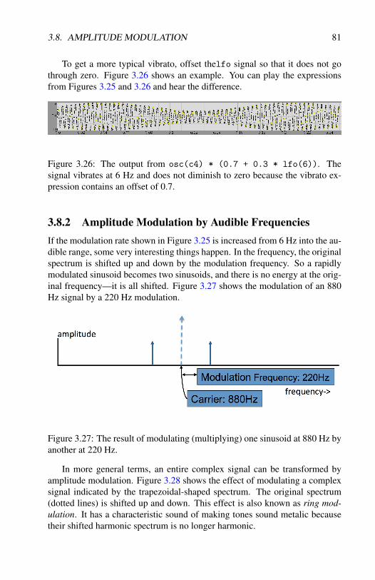
3.8. AMPLITUDE MODULATION 81
To get a more typical vibrato, offset thelfo signal so that it does not gothrough zero. Figure 3.26 shows an example. You can play the expressionsfrom Figures 3.25 and 3.26 and hear the difference.
Figure 3.26: The output from osc(c4) * (0.7 + 0.3 * lfo(6)). Thesignal vibrates at 6 Hz and does not diminish to zero because the vibrato ex-pression contains an offset of 0.7.
3.8.2 Amplitude Modulation by Audible FrequenciesIf the modulation rate shown in Figure 3.25 is increased from 6 Hz into the au-dible range, some very interesting things happen. In the frequency, the originalspectrum is shifted up and down by the modulation frequency. So a rapidlymodulated sinusoid becomes two sinusoids, and there is no energy at the orig-inal frequency—it is all shifted. Figure 3.27 shows the modulation of an 880Hz signal by a 220 Hz modulation.
Figure 3.27: The result of modulating (multiplying) one sinusoid at 880 Hz byanother at 220 Hz.
In more general terms, an entire complex signal can be transformed byamplitude modulation. Figure 3.28 shows the effect of modulating a complexsignal indicated by the trapezoidal-shaped spectrum. The original spectrum(dotted lines) is shifted up and down. This effect is also known as ring mod-ulation. It has a characteristic sound of making tones sound metalic becausetheir shifted harmonic spectrum is no longer harmonic.

82 CHAPTER 3. SAMPLING THEORY INTRODUCTION
Figure 3.28: The result of modulating (multiplying) a complex signal (illus-trated by the trapezoidal spectrum in dotted lines) by a sinusoidal modulator.The original spectrum is shifted up and down by the frequency of the modula-tor.
3.9 SummarySampling obtains a discrete digital representation of a continuous signal. Al-though intuition suggests that the information in a continuous signal is infinite,this is not the case in practice. Limited bandwith (or the fact that we only careabout a certain bandwidth) means that we can capture all frequencies of inter-est with a finite sampling rate. The presence of noise in all physical systemsmeans that a small amount of quantization noise is not significant, so we canrepresent each sample with a finite number of bits.
Dither and noise shaping can be applied to signals before quantization oc-curs to reduce any artifacts that might occur due to non-random rounding —typically this occurs in low amplitude sinusoids where rounding errors canbecome periodic and audible. Another interesting technique is oversampling,where digital low-pass filtering performs some of the work typically done bya hardware low-pass filter to prevent aliasing.
Amplitude modulation at low frequencies is a fundamental operation usedto control loudness in mixing and to shape notes and other sound events insynthesis. We typically scale the signal by a factor from 0 to 1 that varies overtime. On the other hand, periodic amplitude modulation at audible frequenciesacts to shift frequencies up and down by the modulating frequency. This canbe used as a form of distortion, for synthesis, and other effects.

Chapter 4
Frequency ModulationTopics Discussed: Frequency Modulation, Behaviors and Transforma-tions in Nyquist
Frequency modulation (FM) is a versatile and efficient synthesis techniquethat is widely implemented in software and hardware. By understanding howFM works, you will be able to design parameter settings and control strategiesfor your own FM instrument designs.
4.1 Introduction to Frequency ModulationFrequency modulation occurs naturally. It is rare to hear a completely stablesteady pitch. Some percussion instruments are counter-examples, e.g. a pianotone or a tuning fork or a bell, but most instruments and the human voice tendto have at least some natural frequency change.
4.1.1 ExamplesCommon forms of frequency variation in music include:
• Voice inflection, natural jitter, and vibrato in singing.
• Vibrato in instruments. Vibrato is a small and quasi-periodic variationof pitch, often around 6 Hz and spanning a fraction of a semitone.
• Instrumental effects, e.g. electric guitars sometimes have “whammybars” that stretch or relax all the strings to change their pitch. Guitaristscan “bend” strings by pushing the string sideways across the fretboard.
• Many tones begin low and come up to pitch.
83

84 CHAPTER 4. FREQUENCY MODULATION
• Loose vibrating strings go sharp (higher pitch) as they get louder. Looseplucked strings get flatter (lower pitch) especially during the initial de-cay.
• The slide trombone, Theremin, voice, violin, etc. create melodies bychanging pitch, so melodies on these instruments can be thought of asexamples of frequency modulation (as opposed to, say, pianos, wheremelodies are created by selecting from fixed pitches).
4.1.2 FM SynthesisNormally, vibrato is a slow variation created by musicians’ muscles. Withelectronics, we can increase the vibrato rate into the audio range, where inter-esting things happen to the spectrum. The effect is so dramatic, we no longerrefer to it as vibrato but instead call it FM Synthesis.
Frequency modulation (FM) is a synthesis technique based on the simpleidea of periodic modulation of the signal frequency. That is, the frequency ofa carrier sinusoid is modulated by a modulator sinusoid. The peak frequencydeviation, also known as depth of modulation, expresses the strength of themodulator’s effect on the carrier oscillator’s frequency.
FM synthesis was invented by John Chowning [Chowning, 1973] and be-came very popular due to its ease of implementation and computationally lowcost, as well as its (somewhat surprisingly) powerful ability to create realisticand interesting sounds.
4.2 Theory of FMLet’s look at the equation for a simple frequency controlled sine oscillator.Often, this is written
y(t) = Asin(2πφ t) (4.1)
where φ (phi) is the frequency in Hz. Note that if φ is in in Hz (cycles persecond), the frequency in radians per second is 2πφ . At time t, the phase willhave advanced from 0 to 2πφ t, which is the integral of 2πφ over a time spanof t. We can express what we are doing in detail as:
y(t) = Asin(2π
∫ t
0φdx) (4.2)
To deal with a time-varying frequency modulation, we will substitute fre-quency function f (·) for φ :
y(t) = Asin(2π
∫ t
0f (x)dx) (4.3)

4.2. THEORY OF FM 85
Frequency modulation uses a rapidly changing function
f (t) =C+Dsin(2πMt) (4.4)
where C is the carrier, a frequency offset that is in many cases is the funda-mental or “pitch”. D is the depth of modulation that controls the amount offrequency deviation (called modulation), and M is the frequency of modula-tion in Hz. Plugging this into Equation 4.3 and simplifying gives the equationfor FM:
y(t) = Asin(2π
∫ t
0C+Dsin(2πMx)dx) (4.5)
Note that the integral of sin is cos, but the only difference between the two isphase. By convention, we ignore this detail and simplify Equation 4.5 to getthis equation for an FM oscillator:
f (t) = Asin(2πCt +Dsin(2πMt)) (4.6)
I = D/M is known as the index of modulation. When D 6= 0, sidebandsappear in the spectra of the signal above and below the carrier frequency C,at multiples of ±M. In other words, we can write the set of frequency com-ponents as C± kM, where k=0,1,2,.... The number of significant componentsincreases with I, the index of modulation.
4.2.1 Negative FrequenciesAccording to these formulas, some frequencies will be negative. This can beinterpreted as merely a phase change: sin(−x) =−sin(x) or perhaps not evena phase change: cos(−x) = cos(x). Since we tend to ignore phase, we canjust ignore the sign of the frequency and consider negative frequencies to bepositive. We sometimes say the negative frequencies “wrap around” (zero) tobecome positive. The main caveat here is that when frequencies wrap aroundand add to positive frequencies of the same magnitude, the components maynot add in phase. The effect is to give FM signals a complex evolution asthe index of modulation increases and adds more and more components, bothpositive and negative.
4.2.2 Harmonic RatioThe human ear is very sensitive to harmonic vs. inharmonic spectra. Percep-tually, harmonic spectra are very distinctive because they give a strong senseof pitch. The harmonic ratio [Truax, 1978] is the ratio of the modulating fre-quency to the carrier frequency, such that H = M/C. If H is a rational number,the spectrum is harmonic; if it is irrational, the spectrum is inharmonic.

86 CHAPTER 4. FREQUENCY MODULATION
4.2.3 Rational HarmonicityIf H = 1 the spectrum is harmonic and the carrier frequency is also the fun-damental, i.e. F0 = C. To show this, remember that the frequencies will beC± kM, where k=0,1,2,..., but if H = 1, then M = C, so the frequencies areC± kC, or simply kC. This is the definition of a harmonic series: multiples ofsome fundamental frequency C.
When H = 1/m, and m is a positive integer, C instead becomes the mth
component (harmonic) because the spacing between harmonics is M = C/m,which is also the fundamental: F0 = M =C/m.
With H = 2, we will get sidebands at C± 2kC (where k=0,1,2,...), thusomitting all even harmonics — which is a characteristic of cylindrical wood-winds such as the clarinet.
4.2.4 Irrational HarmonicityIf H is irrational, the negative frequencies that wrap around at 0 Hz tend toland between the positive frequency components, thus making the spectrumdenser. If we make H much less than 1 (M much less than C), and if H isirrational (or at least not a simple fraction such as 1/n), the FM-generatedfrequencies will cluster around C (the spacing between components will berelatively small); yielding sounds that have no distinct pitch and that can mimicdrums and gongs.
4.2.5 FM Spectra and Bessel FunctionsThe sidebands infused by FM are governed by Bessel functions of the first kindand nth order; denoted Jn(I), where I is the index of modulation. The Besselfunctions determine the magnitudes and signs of the frequency components inthe FM spectrum. These functions look a lot like damped sine waves, as canbe seen in Figure 4.1.
Here are a few insights that help explain why FM synthesis sounds the wayit does:
• J0(I) gives the amplitude of the carrier.
• J1(I) gives the amplitude of the first upper and lower sidebands.
• Generally, Jn(I) governs the amplitudes of the nth upper and lower side-bands.
• Higher-order Bessel functions start from zero and increase more andmore gradually, so higher-order sidebands only have significant energywhen I is large.

4.2. THEORY OF FM 87
Figure 4.1: Bessel functions of the first kind, orders 0 to 3. The x axis repre-sents the index of modulation in FM.
• The spectral bandwidth increases with I. The upper and lower sidebandsrepresent the higher and lower frequencies, respectively. The larger thevalue of I, the more significant sidebands you get.
• As I increases, the energy of the sidebands vary much like a dampedsinusoid.
4.2.6 Index of ModulationThe index of modulation, I = D/M, allows us to relate the depth of modula-tion, D, the modulation frequency, M, and the index of the Bessel functions.In practice, this means that if we want a spectrum that has the energy of theBessel functions at some index I, with frequency components separated byM, then we must choose the depth of modulation according to the relationI = D/M [Moore, 1990]. As a rule-of-thumb , the number of sidebands isroughly equivalent to I + 1. That is, if I = 10 we get 10+ 1 = 11 sidebandsabove, and 11 sidebands below the carrier frequency. In theory, there are in-finitely many sidebands at C±kM, where k=0,1,2,... if the modulation is non-zero, but the intensity of sidebands falls rapidly toward zero as k increases, butthis rule of thumb considers only significant sidebands. (Note that this formulafails at I = 0: it predicts the carrier plus 1 side band above and one below, butthere are no side bands in this case.)
4.2.7 Time-Varying ParametersFor music applications, constant values of A, C, D, and M would result ina rock-steady tone of little interest. In practice, we usually vary all of theseparameter, replacing them with A(t), C(t), D(t), and M(t). Usually, theseparameters change slowly compared to carrier and modulator frequencies, so

88 CHAPTER 4. FREQUENCY MODULATION
we assume that all the analysis here still applies and allows us to make pre-dictions about the short-time spectrum. FM is particularly interesting becausewe can make very interesting changes to the spectrum with just a few controlparameters, primarily D(t), and M(t).
4.2.8 Examples of FM SignalsFigures 4.2 and 4.3 show examples of FM signals. The X-axes on the plotsrepresent time — here denoted in multiples of π .
Figure 4.2: A = 1, C = 242 Hz, D = 2, M = 40 Hz.
Figure 4.3: A = 2, C = 210 Hz, D = 10, M = 35 Hz.
4.3 Frequency Modulation with NyquistNow that you have a grasp of the theory, let’s use it to make some sound.
4.3.1 Basic FMThe basic FM oscillator in Nyquist is the function fmosc. The signature forfmosc is

4.3. FREQUENCY MODULATION WITH NYQUIST 89
fmosc(basic-pitch, modulation [, table [, phase ] ] )
Let’s break that down:
• basic-pitch is the carrier frequency, expressed in steps. If there is nomodulation, this controls the output frequency. Remember this is insteps, so if you put in a number like 440 expecting Hz, you will actuallyget step-to-hz(440), which is about 0.9 terahertz!1 Use A4 instead,or write something like hz-to-step(441.0) if you want to specifyfrequency in Hertz.
• modulation is the modulator. The amplitude of the modulator controlsthe depth of modulation—how much does the frequency deviate fromthe nominal carrier frequency based on basic-pitch? An amplitude of1 (the nominal output of (osc) for example), gives a frequency devia-tion of ±1. If you have been paying attension, you will realize that 1gives a very low index of modulation (1/m)—you probably will not hearanything but a sine tone, so typically,
– you will use a large number for modulation, and– you will also scale modulation by some kind of envelope. By vary-
ing the depth of modulation, you will vary the spectrum, which istypical in FM synthesis.
The frequency of modulation is just the modulation frequency. It can bethe same as the carrier frequency if you want the C:M ratio to be is 1:1.This parameter is where you control the C:M ratio.
• table is optional and allows you to replace the default sine waveformwith any waveform table. The table data structure is exactly the sameone you learned about earlier for use with the osc function.
• phase is also optional and gives the initial phase. Generally, changingthe initial phase will not cause any perceptible changes.
4.3.2 Index of Modulation ExampleProduce a harmonic sound with about 10 harmonics and a fundamental of 100Hz. We can choose C = M = 100, which gives C : M = 1 and is at least oneway to get a harmonic spectrum. Since the number of harmonics is 10 we needthe carrier plus 9 sidebands, and so I +1 = 9 or I = 8. I = D/M so D = IM,D = 8∗100 = 800. Finally, we can write
fmosc(hz-to-step(100), 800 * hzosc(100)).1Need we point out this is somewhat higher than the Nyquist rate?

90 CHAPTER 4. FREQUENCY MODULATION
4.3.3 FM Example in Nyquist
The following plays a characteristic FM sound in Nyquist:
play fmosc(c4, pwl(1, 4000, 1) * osc(c4)) ~ 10
Since the modulation comes from osc(c4), the modulation frequency matchesthe carrier frequency (given by fmosc(c4, ...), so the C:M ratio is 1:1. Theamplitude of modulation ramps from 0 to 4000, giving a final index of mod-ulation of I = 4000/steptohz(C4) = 15.289. Thus, the spectrum will evolvefrom a sinusoid to a rich spectrum with the carrier and around I+1 sidebands,or about 17 harmonics. Try it!
For a musical tone, you should multiply the fmosc signal by an envelope.Otherwise, the output amplitude will be constant. Also, you should replacethe pwl function with an envelope that increases and then decreases, at least ifyou want the sound to get brighter in the middle.
4.4 Behavioral Abstraction
In Nyquist, all functions are subject to transformations. You can think of trans-formations as additional parameters to every function, and functions are freeto use these additional parameters in any way. The set of transformation pa-rameters is captured in what is referred to as the transformation environment.(Note that the term environment is heavily overloaded in computer science.This is yet another usage of the term.)
Behavioral abstraction is the ability of functions to adapt their behaviorto the transformation environment. This environment may contain certain ab-stract notions, such as loudness, stretching a sound in time, etc. These notionswill mean different things to different functions. For example, an oscillatorshould produce more periods of oscillation in order to stretch its output. Anenvelope, on the other hand, might only change the duration of the sustain por-tion of the envelope in order to stretch. Stretching recorded audio could meanresampling it to change its duration by the appropriate amount.
Thus, transformations in Nyquist are not simply operations on signals. Forexample, if I want to stretch a note, it does not make sense to compute thenote first and then stretch the signal. Doing so would cause a drop in thepitch. Instead, a transformation modifies the transformation environment inwhich the note is computed. Think of transformations as making requests tofunctions. It is up to the function to carry out the request. Since the functionis always in complete control, it is possible to perform transformations with“intelligence;” that is, the function can perform an appropriate transformation,

4.4. BEHAVIORAL ABSTRACTION 91
such as maintaining the desired pitch and stretching only the “sustain” portionof an envelope to obtain a longer note.
4.4.1 BehaviorsNyquist sound expressions denote a whole class of behaviors. The specificsound computed by the expression depends upon the environment. There area number of transformations, such as stretch and transpose that alter theenvironment and hence the behavior.
The most common transformations are shift and stretch, but remem-ber that these do not necessarily denote simple time shifts or linear stretching:When you play a longer note, you don’t simply stretch the signal! The behav-ior concept is critical for music.
4.4.2 Evaluation EnvironmentTo implement the behavior concept, all Nyquist expressions evaluate withinan environment.
The transformation environment is implemented in a simple manner. Theenvironment is simply a set of special global variables. These variables shouldnot be read directly and should never be set directly by the programmer. In-stead, there are functions to read them, and they are automatically set andrestored by transformation operators, which will be described below. TheNyquist environment includes: starting time, stretch factor, transposition, legatofactor, loudness, sample rates, and more.
4.4.3 Manipulating the Environment ExampleA very simple example of a transformation affecting a behavior is the stretchoperator (~):
pluck(c4) ~ 5
This example can be read as “evaluate pluck in an environment that has beenstretched by 5 relative to the current environment.”
4.4.4 TransformationsMany transformations are relative and can be nested. Stretch does not just setthe stretch factor; instead, it multiplies the stretch factor by a factor, so thefinal stretch factor in the new environment is relative to the current one.
Nyquist also has “absolute” transformations that override any existing valuein the environment. For example,

92 CHAPTER 4. FREQUENCY MODULATION
function tone2() return osc(c4) ~~ 2
returns a 2 second tone, even if you write:
play tone2() ~ 100 ; 2 second tone
because the “absolute stretch” (~~) overrides the stretch operator ~. Eventhough tone2 is called with a stretch factor of 100, its absolute stretch trans-formation overrides the environment and sets it to 2.
Also, note that once a sound is computed, it is immutable. The followinguse of a global variable to store a sound is not recommended, but serves toillustrate the immutability aspect of sounds:
mysnd = osc(c4) ; compute sound, duration = 1play mysnd ~ 2 ; plays duration of 1
The stretch factor of 2 in the second line has no effect because mysnd evaluatesto an immutable sound. Transformations only apply to functions2 (which weoften call behaviors to emphasize they behave differently in different contexts)and expressions that call on functions to compute sounds. Transformations donot affect sounds once they are computed.
An Operational View
You can think about this operationally: When Nyquist evaluates expr ~ 3, the~ operator is not a function in the sense that expressions on the left and rightare evaluated and passed to a function where “stretching” takes place. Instead,it is better to think of ~ as a control construct that:
• changes the environment by tripling the stretch factor
• evaluates expr in this new environment
• restores the environment
• returns the sound computed by expr
Thus, if expr is a behavior that computes a sound, the computation will beaffected by the environment. If expr is a sound (or a variable that stores asound), the sound is already computed and evaluation merely returns the soundwith no transformation.
Transformations are described in detail in the Nyquist Reference Manual(find “Transformations” in the index). In practice, the most critical transfor-mations are at (@) and stretch (~), which control when sounds are computedand how long they are.
2This is a bit of a simplification. If a function merely returns a pre-computed value of typeSOUND, transformations will have no effect.

4.5. SEQUENTIAL BEHAVIOR (SEQ) 93
4.5 Sequential Behavior (seq)Consider the simple expression:
play seq(my-note(c4, q), my-note(d4, i))
The idea is to create the first note at time 0, and to start the next note when thefirst one finishes. This is all accomplished by manipulating the environment.In particular, *warp* is modified so that what is locally time 0 for the secondnote is transformed, or warped, to the logical stop time of the first note.
One way to understand this in detail is to imagine how it might be exe-cuted: first, *warp* is set to an initial value that has no effect on time, andmy-note(c4, q) is evaluated. A sound is returned and saved. The sound hasan ending time, which in this case will be 1.0 because the duration q is 1.0.This ending time, 1.0, is used to construct a new *warp* that has the effect ofshifting time by 1.0. The second note is evaluated, and will start at time 1.0.The sound that is returned is now added to the first sound to form a compositesound, whose duration will be 2.0. Finally, *warp* is restored to its initialvalue.
Notice that the semantics of seq can be expressed in terms of transforma-tions. To generalize, the operational rule for seq is: evaluate the first behav-ior according to the current *warp*. Evaluate each successive behavior with*warp* modified to shift the new note’s starting time to the ending time ofthe previous behavior. Restore *warp* to its original value and return a soundwhich is the sum of the results.
In the Nyquist implementation, audio samples are only computed whenthey are needed, and the second part of the seq is not evaluated until the endingtime (called the logical stop time) of the first part. It is still the case that whenthe second part is evaluated, it will see *warp* bound to the ending time ofthe first part.
A language detail: Even though Nyquist defers evaluation of the secondpart of the seq, the expression can reference variables according to ordinaryLisp/SAL scope rules. This is because the seq captures the expression in aclosure, which retains all of the variable bindings.
4.6 Simultaneous Behavior (sim)Another operator is sim, which invokes multiple behaviors at the same time.For example,
play 0.5 * sim(my-note(c4, q), my-note(d4, i))

94 CHAPTER 4. FREQUENCY MODULATION
will play both notes starting at the same time.The operational rule for sim is: evaluate each behavior at the current
*warp* and return the sum of the results. (In SAL, the sim function appliedto sounds is equivalent to adding them with the infix + operator.
4.7 Logical Stop TimeWe have seen that the default behavior of seq is to cause sounds to begin at theend of the previous sound in the sequence. What if we want to play a sequenceof short sounds separated by silence? One possibility is to insert silence (sees-rest), but what if we want to play equally spaced short sounds? We haveto know how long each short sound lasts in order to know how much silence toinsert. Or what if sounds have long decays and we want to space them equally,requiring some overlap?
All of these cases point to an important music concept: We pay specialattention to the beginnings of sounds, and the time interval between these onsettimes (often called IOI for “Inter-Onset Interval”) is usually more importantthan the specific duration of the sound (or note). Thus, spacing notes accordingto their duration is not really a very musical idea.
Instead, we can try to separate the concepts of duration and IOI. In musicnotation, we can write a quarter note, meaning “play this sound for one beat,”but put a dot over it, meaning “play this sound short, but it still takes a totalof one beat.” (See Figure 5.5.) It is not too surprising that music notation andtheory would have rather sophisticated concepts regarding the organization ofsound in time.
Figure 4.4: Standard quarter notes nominally fill an entire beat. Staccato quar-ter notes, indicated by the dots, are played shorter, but they still occupy a timeinterval of one beat. The “on” and “off” time of these short passages is indi-cated graphically below each staff of notation.
Nyquist incorporates this musical thinking into its representation of sounds.

4.8. SCORES IN NYQUIST 95
A sound in Nyquist has one start time, but there are effectively two “stop”times. The signal stop is when the sound samples end. After that point, thesound is considered to continue forever with value of zero. The logical stopmarks the “musical” or “rhythmic” end of the sound. If there is a sound afterit (e.g. in a sequence computed by seq), the next sound begins at this logicalstop time of the sound.
The logical stop is usually the signal stop by default, but you can change itwith the set-logical-stop function. For example, the following will playa sequence of 3 plucked-string sounds with durations of 2 seconds each, butthe IOI, that is, the time between notes, will be only 1 second.
play seq(set-logical-stop(pluck(c4) ~ 2, 1)set-logical-stop(pluck(c4) ~ 2, 1),set-logical-stop(pluck(c4) ~ 2, 1))
4.8 Scores in NyquistScores in Nyquist indicate “sound events,” which consist of functions to calland parameters to pass to them. For each sound event there is also a start timeand a “duration,” which is really a Nyquist stretch factor. When you rendera score into a sound (usually by calling timed-seq or executing the functionsound-play), each sound event is evaluated by adjusting the environmentaccording to the time and duration as if you wrote
sound-event(parameters) ~ duration @ timeThe resulting sounds are then summed to form a single sound.
4.9 SummaryIn this unit, we covered frequency modulation and FM synthesis. Frequencymodulation refers to anything that changes pitch within a sound. Frequencymodulation at audio rates can give rise to many partials, making FM Synthe-sis a practical, efficient, and versatile method of generating complex evolvingsounds with a few simple control parameters.
All Nyquist sounds are computed by behaviors in an environment that canbe modified with transformations. Functions describe behaviors. Each be-havior can have explicit parameters as well as implicit environment values, sobehaviors represent classes of sounds (e.g. piano tones), and each instance ofa behavior can be different. Being “different” includes having different starttimes and durations, and some special constructs in Nyquist, such as sim, seq,at (@) and shift (~) use the environment to organize sounds in time. Theseconcepts are also used to implement scores in Nyquist.

96 CHAPTER 4. FREQUENCY MODULATION
Chapter 5
Spectral Analysis andNyquist Patterns
Topics Discussed: Short Time Fourier Transform, Spectral Centroid,Patterns, Algorithmic Composition
In this chapter, we dive into the Fast Fourier Transform for spectral anal-ysis and use it to compute the Spectral Centroid. Then, we learn about someNyquist functions that make interesting sequences of numbers and how to in-corporate those sequences as note parameters in scores. Finally, we consider avariety of algorithmic composition techniques.
5.1 The Short Time Fourier Transform and FFTIn practice, the Fourier Transform cannot be used computationally becausethe input is infinite and the signals are continuous. Therefore, we use the Dis-crete Short Time Fourier Transform, where the continuous integral becomesa summation of discrete time points (samples), and where the summation isperformed over a finite time interval, typically around 50 to 100 ms. Theso-called Short-Time Discrete Fourier Transform (STDFT, or just DFT) equa-tions are shown in Figure 5.1. Note the similarity to the Fourier Transformintegrals we saw earlier. Here, Rk represents the real coefficients and Xk arethe imaginary coefficients.
The Fast Fourier Transform (FFT) is simply a fast algorithm for com-puting the DFT. FFT implies DFT, but rather than directly implementing theequations in Figure 5.1, which has a run time proportional to N2, the FFT usesa very clever NlogN algorithm to transform N samples.
An FFT of a time domain signal takes the samples and gives us a new setof numbers representing the frequencies, amplitudes, and phases of the sine
97

98 CHAPTER 5. SPECTRAL ANALYSIS AND PATTERNS
Figure 5.1: Equations for the Short Time Discrete Fourier Transform. EachRk, Xk pair represents a different frequency in the spectrum.
waves that make up the sound we have analyzed. It is these data that aredisplayed in the sonograms we looked at earlier.
Figure 5.2 illustrates some FFT data. It shows the first 16 bins of a typicalFFT analysis after the conversion is made from real and imaginary numbers toamplitude/phase pairs. We left out the phases, because, well, it was too muchtrouble to just make up a bunch of arbitrary phases between 0 and 2. In a lotof cases, you might not need them (and in a lot of cases, you would!). In thiscase, the sample rate is 44.1 kHz and the FFT size is 1,024, so the bin width (infrequency) is the Nyquist frequency (44,100/2 = 22,050) divided by the FFTsize, or about 22 Hz.
We confess that we just sort of made up the numbers; but notice that wemade them up to represent a sound that has a simple, more or less harmonicstructure with a fundamental somewhere in the 66 Hz to 88 Hz range (youcan see its harmonics at around 2, 3, 4, 5, and 6 times its frequency, and notethat the harmonics decrease in amplitude more or less like they would in asawtooth wave).
One important consequence of the FFT (or equivalently, DFT) is that weonly “see” the signal during a short period. We pretend that the spectrum isstable, at least for the duration of the analysis window, but this is rarely true.Thus, the FFT tells us something about the signal over the analysis window,but we should always keep in mind that the FFT changes with window sizeand the concept of a spectrum at a point in time is not well defined. Forexample, harmonics of periodic signals usually show up in the FFT as peaksin the spectrum with some spread rather than single-frequency spikes, eventhough a harmonic intuitively has a single specific frequency.
5.1.1 How to Interpret a Discrete SpectrumJust as we divide signals over time into discrete points (called samples), theDFT divides the spectrum into discrete points we call frequency bins. TheDFT captures all of the information in the analysis window, so if you analyzeN samples, it you should have N degrees of freedom in the DFT. Since each

5.1. THE SHORT TIME FOURIER TRANSFORM AND FFT 99
Figure 5.2: Graph and table of spectral components.

100 CHAPTER 5. SPECTRAL ANALYSIS AND PATTERNS
DFT bin has an amplitude and phase, we end up with about N/2 bins. Thecomplete story is that there are actually N/2+1 bins, but one represents zerofrequency where only the real term is non-zero (because sin(0) is 0), and onebin represents the Nyquist frequency where again, only the real term is non-zero (because sin(2πki/N) is zero).1
These N/2+ 1 bins are spaced across the frequency range from 0 to theNyquist frequency (half the sample rate), so the spacing between bins is thesample rate divided by the number of bins:
bin frequency spacing = sample rate / number of samples
We can also relate the frequency spacing of bins to the duration of the analysiswindow:
number of samples = analysis duration × sample rate, sobin frequency spacing =
sample rate / (analysis duration × sample rate), sobin frequency spacing = 1 / analysis duration
5.1.2 Frame or Analysis Window SizeSo let’s say that we decide on a frame size of 1,024 samples. This is a commonchoice because most FFT algorithms in use for sound processing require anumber of samples that is a power of two, and it’s important not to get toomuch or too little of the sound.
A frame size of 1,024 samples gives us 512 frequency bands. If we assumethat we’re using a sample rate of 44.1 kHz, we know that we have a frequencyrange (remember the Nyquist theorem) of 0 kHz to 22.05 kHz. To find outhow wide each of our frequency bins is, we use one of the formulas above, e.g.sample rate / number of samples, or 44100 / 1024, or about 43 Hz. Rememberthat frequency perception is logarithmic, so 43 Hz gives us worse resolutionat the low frequencies and better resolution (at least perceptually) at higherfrequencies.
By selecting a certain frame size and its corresponding bandwidth, weavoid the problem of having to compute an infinite number of frequency com-ponents in a sound. Instead, we just compute one component for each fre-quency band.
1With each bin having 2 dimensions (real and imaginary), N/2+ 1 bins implies the result ofthe transform has N + 2 dimensions. That should set off some alarms: How can you transformN input dimensions (real-valued samples) into N +2 output dimensions? This apparent problemis resolved when you realize that the first and last imaginary terms are zero, so there are reallyonly N output dimensions that carry any information. Without this property, the DFT would notbe invertible.

5.1. THE SHORT TIME FOURIER TRANSFORM AND FFT 101
5.1.3 Time/Frequency Trade-off and the Uncertainty Prin-ciple
A drawback of the FFT is the trade-off that must be made between frequencyand time resolution. The more accurately we want to measure the frequencycontent of a signal, the more samples we have to analyze in each frame of theFFT. Yet there is a cost to expanding the frame size—the larger the frame, theless we know about the temporal events that take place within that frame. Thistrade-off is captured in the expression:
bin frequency spacing = 1 / analysis duration.
Small frequency spacing is good, but so is a short duration, and they are in-versely proportional! We simply can’t have it both ways. See Figure 5.3 foran illustration.
Figure 5.3: Selecting an FFT size involves making trade-offs in terms of timeand frequency accuracy. Basically it boils down to this: The more accuratethe analysis is in one domain, the less accurate it will be in the other. Thisfigure illustrates what happens when we choose different frame sizes. In thefirst illustration, we used an FFT size of 512 samples, giving us pretty goodtime resolution. In the second, we used 2,048 samples, giving us pretty goodfrequency resolution. As a result, frequencies are smeared vertically in thefirst analysis, while time is smeared horizontally in the second. What’s thesolution to the time/frequency uncertainty dilemma? Compromise.
This time/frequency trade-off in audio analysis is mathematically identi-cal to the Heisenberg Uncertainty Principle, which states that you can never

102 CHAPTER 5. SPECTRAL ANALYSIS AND PATTERNS
simultaneously know the exact position and the exact speed of an object.
5.1.4 Magnitude or Amplitude Spectrum
Figure 5.1 shows that we get real (cosine) and imaginary (sine) numbers fromthe DFT or FFT. Typically, we prefer to work with amplitude and phase (infact, we often ignore the phase part and just work with amplitude). You canthink of real and imaginary as Cartesian coordinates, and amplitude and phaseas radius and angle in polar coordinates. The amplitude components Ai areeasily computed from the real Ri and imaginary Xi components using the for-mula
Ai =√
R2i +X2
i (5.1)
For an N-point FFT (input contains N samples), the output will have N/2+1 bins and therefore N/2 + 1 amplitudes. The first amplitude correspondsto 0 Hz, the second to (sample rate / N), etc., up to the last amplitude thatcorresponds to the frequency (sample rate / 2).
5.2 Spectral CentroidMusic cognition researchers and computer musicians commonly use a mea-sure of sounds called the spectral centroid. The spectral centroid is a measureof the “brightness” of a sound, and it turns out to be extremely important inthe way we compare different sounds. If two sounds have a radically differentcentroid, they are generally perceived to be timbrally distant (sometimes thisis called a spectral metric).
Basically, the spectral centroid can be considered the average frequencycomponent (taking into consideration the amplitude of all the frequency com-ponents), as illustrated in Figure 5.4. The formula for the spectral centroid ofone FFT frame of a sound is:
c =∑ fiai
∑ai,where fi is the frequency of the ith bin and ai is the amplitude.
(5.2)
5.3 PatternsNyquist offers pattern objects that generate data streams. For example, thecycle-class of objects generate cyclical patterns such as “1 2 3 1 2 3 1 2 3

5.3. PATTERNS 103
Figure 5.4: A magnitude spectrum and its spectral centroid (dashed line). Ifyou were to cut out the spectrum shape from cardboard, it would balance onthe centroid. The spectral centroid is a good measure of the overall placementof energy in a signal from low frequencies to high.
Figure 5.5: The centroid curve of a sound over time. This curve is of a rapidlychanging voice (Australian sound poet Chris Mann). Each point in the hori-zontal dimension represents a new spectral frame. Note that centroids tend tobe rather high and never the fundamental (this would only occur if our soundis a pure sine wave).

104 CHAPTER 5. SPECTRAL ANALYSIS AND PATTERNS
...”, or “1 2 3 4 3 2 1 2 3 4 ...”. Patterns can be used to specify pitch sequences,rhythm, loudness, and other parameters.
In this section, we describe a variety of pattern objects. These patternsare pretty abstract, but you might think about how various types of sequencesmight be applied to music composition. In the following section, we will seehow to incorporate patterns into the generation of scores for Nyquist, using avery powerful macro called score-gen.
Pattern functions are automatically loaded when you start Nyquist. To usea pattern object, you first create the pattern, e.g.
set pitch-source = make-cycle(list(c4, d4, e4, f4))
In this example, pitch-source is an object of class cycle-class whichinherits from pattern-class.2
After creating the pattern, you can access it repeatedly with next to gen-erate data, e.g.
play seqrep(i, 13, pluck(next(pitch-source), 0.2))
This will create a sequence of notes with the following pitches: c, d, e, f, c, d,e, f, c, d, e, f, c. If you evaluate this again, the pitch sequence will continue,starting on d.
It is very important not to confuse the creation of a sequence with its ac-cess. Consider this example:
play seqrep(i, 13, pluck(next(make-cycle(list(c4, d4, e4, f4))), 0.2))
This looks very much like the previous example, but it only repeats notes onmiddle-C. The reason is that every time pluck is evaluated, make-cycle iscalled and creates a new pattern object. After the first item of the patternis extracted with next, the cycle is not used again, and no other items aregenerated.
To summarize this important point, there are two steps to using a pattern.First, the pattern is created and stored in a variable. Second, the pattern isaccessed (multiple times) using next.
next(pattern-object [,#t ])
next returns the next element from a pattern generator object. If the optionalsecond argument is true (default value is false), then an entire period is re-turned as a list.
2Because SAL is not an object-oriented language, these classes and their methods are notdirectly accessible from SAL. Instead, Nyquist defines a functional interface, e.g. make-cyclecreates an instance of cycle-class, and the next function, introduced below, retrieves the nextvalue from any instance of pattern-class. Using LISP syntax, you can have full access to themethods of all objects.

5.3. PATTERNS 105
5.3.1 Pattern ExamplesThe following descriptions cover the basic ideas of the Nyquist pattern library.In most cases, details and optional parameters are not described here to keepthe descriptions short and to emphasize the main purpose of each type of pat-tern. For complete descriptions, see the Nyquist Reference Manual, or betteryet, just read the manual instead of these summaries.
Heap
The heap-class selects items in random order from a list without replace-ment, which means that all items are generated once before any item is re-peated. For example, two periods of make-heap({a b c}) might be (C AB) (B A C). Normally, repetitions can occur even if all list elements are dis-tinct. This happens when the last element of a period is chosen first in the nextperiod. To avoid repetitions, the max: keyword argument can be set to 1. If themain argument is a pattern instead of a list, a period from that pattern becomesthe list from which random selections are made, and a new list is generatedevery period. (See Section 5.3.2 on nested patterns.)
Palindrome
The palindrome-class repeatedly traverses a list forwards and then back-wards. For example, two periods of make-palindrome({a b c}) would be(A B C C B A) (A B C C B A). The elide: keyword parameter controlswhether the first and/or last elements are repeated:
make-palindrome(a b c, elide: nil);; generates A B C C B A A B C C B A ...
make-palindrome(a b c, elide: t);; generates A B C B A B C B ...
make-palindrome(a b c, elide: :first);; generates A B C C B A B C C B ...
make-palindrome(a b c, elide: :last);; generates A B C B A A B C B A ...
Random
The random-class generates items at random from a list. The default selec-tion is uniform random with replacement, but items may be further specifiedwith a weight, a minimum repetition count, and a maximum repetition count.

106 CHAPTER 5. SPECTRAL ANALYSIS AND PATTERNS
Weights give the relative probability of the selection of the item (with a defaultweight of one). The minimum count specifies how many times an item, onceselected at random, will be repeated. The maximum count specifies the max-imum number of times an item can be selected in a row. If an item has beengenerated n times in succession, and the maximum is equal to n, then the itemis disqualified in the next random selection. Weights (but not currently minimaand maxima) can be patterns. The patterns (thus the weights) are recomputedevery period.
Line
The line-class is similar to the cycle class, but when it reaches the end ofthe list of items, it simply repeats the last item in the list. For example, twoperiods of make-line({a b c}) would be (A B C) (C C C).
Accumulation
The accumulation-class takes a list of values and returns the first, followedby the first two, followed by the first three, etc. In other words, for each listitem, return all items form the first through the item. For example, if the list is(A B C), each generated period is (A A B A B C).
Copier
The copier-class makes copies of periods from a sub-pattern. For exam-ple, three periods of make-copier( make-cycle({a b c}, for: 1),repeat: 2, merge: t) would be (A A) (B B) (C C). Note that en-tire periods (not individual items) are repeated, so in this example the for:keyword was used to force periods to be of length one so that each item isrepeated by the repeat: count.
Length
The length-class generates periods of a specified length from another pat-tern. This is similar to using the for: keyword, but for many patterns, thefor: parameter alters the points at which other patterns are generated. Forexample, if the palindrome pattern has an elide: pattern parameter, the valuewill be computed every period. If there is also a for: parameter with a valueof 2, then elide: will be recomputed every 2 items. In contrast, if the palin-drome (without a for: parameter) is embedded in a length pattern with alength of 2, then the periods will all be of length 2, but the items will come

5.3. PATTERNS 107
from default periods of the palindrome, and therefore the elide: values willbe recomputed at the beginnings of default palindrome periods.
Window
The window-class groups items from another pattern by using a sliding win-dow. If the skip value is 1, each output period is formed by dropping the firstitem of the previous period and appending the next item from the pattern. Theskip value and the output period length can change every period. For a simpleexample, if the period length is 3 and the skip value is 1, and the input patterngenerates the sequence A, B, C, ..., then the output periods will be (A B C), (BC D), (C D E), (D E F), ....
5.3.2 Nested PatternsPatterns can be nested, that is, you can write patterns of patterns. In general,the next function does not return patterns. Instead, if the next item in a patternis a (nested) pattern, next recursively gets the next item of the nested pattern.
While you might expect that each call to next would advance the top-levelpattern to the next item, and descend recursively if necessary to the inner-mostnesting level, this is not how next works. Instead, next remembers the lasttop-level item, and if it was a pattern, next continues to generate items fromthat same inner pattern until the end of the inner pattern’s period is reached.The next paragraph explains the concept of the period.
Periods
The data returned by a pattern object is structured into logical groups calledperiods. You can get an entire period (as a list) by calling next(pattern,t). For example:
set pitch-source = make-cycle(list(c4, d4, e4, f4))print next(pitch-source, t)
This prints the list (60 62 64 65), which is one period of the cycle.You can also get explicit markers that delineate periods by calling
send(pattern, :next). In this case, the value returned is either the nextitem of the pattern, or the symbol +eop+ if the end of a period has beenreached. What determines a period? This is up to the specific pattern class, sosee the documentation for specifics. You can override the “natural” period byusing the keyword for:, e.g.
set pitch-source =make-cycle(list(c4, d4, e4, f4), for: 3)

108 CHAPTER 5. SPECTRAL ANALYSIS AND PATTERNS
print next(pitch-source, t)print next(pitch-source, t)
This prints the lists (60 62 64) (65 60 62). Notice that these periods justrestructure the stream of items into groups of 3.
Nested patterns are probably easier to understand by example than by spec-ification. Here is a simple nested pattern of cycles:
set cycle-1 = make-cycle(a b c)set cycle-2 = make-cycle(x y z)set cycle-3 = make-cycle(list(cycle-1, cycle-2))exec dotimes(i, 9, format(t, "~A ", next(cycle-3)))
This will print “A B C X Y Z A B C.” Notice that the inner-most cyclescycle-1 and cycle-2 generate a period of items before the top-level cycle-3advances to the next pattern.
5.3.3 Summary of Patterns
Pattern generators are a bit like unit generators in that they represent sequencesor streams of values, they can be combined to create complex computations,they encapsulate state on which the next output depends, and they can be eval-uated incrementally. Patterns produce streams of numbers intended to becomeparameters for algorithmic compositions, while unit generators produce sam-ples.
Patterns can serve as parameters to other pattern objects, enabling complexbehaviors to run on multiple time scales. Since patterns are often constructedfrom lists (e.g. cycle, random, heap, copier, line, palindrome patterns), theoutput of each pattern is structured into groupings called periods, and pat-tern generators have parameters (especially for:) to control or override periodlengths. Even period lengths can be controlled by patterns!
5.4 Score Generation and Manipulation
A common application of pattern generators is to specify parameters for notes.(It should be understood that “notes” in this context means any Nyquist behav-ior, whether it represents a conventional note, an abstract sound object, or evensome micro-sound event that is just a low-level component of a hierarchicalsound organization. Similarly, “score” should be taken to mean a specifica-tion for a sequence of these “notes.”) The score-gen macro establishes aconvention for representing scores and for generating them using patterns.

5.4. SCORE GENERATION AND MANIPULATION 109
The timed-seq macro already provides a way to represent a score as a listof expressions. We can go a bit further by specifying that all notes are spec-ified by an alternation of keywords and values, where some keywords havespecific meanings and interpretations. By insisting on this keyword/value rep-resentation, we can treat scores as self-describing data, as we will see below.
To facilitate using patterns to create scores, we introduce the score-genconstruct, which looks like a function but is actually a macro. The main dif-ference is that a macro does not evaluate every parameter immediately, but in-stead can operate on parameters as expressions. The basic idea of score-genis you provide a template for notes in a score as a set of keywords and values.For example,
set pitch-pattern = make-cycle(list(c4, d4, e4, f4))score-gen(dur: 0.4, name: quote(my-sound),
pitch: next(pitch-pattern), score-len: 9)
Generates a score of 9 notes as follows:
((0 0 (SCORE-BEGIN-END 0 3.6))(0 0.4 (MY-SOUND :PITCH 60))(0.4 0.4 (MY-SOUND :PITCH 62))(0.8 0.4 (MY-SOUND :PITCH 64))(1.2 0.4 (MY-SOUND :PITCH 65))(1.6 0.4 (MY-SOUND :PITCH 60))(2 0.4 (MY-SOUND :PITCH 62))(2.4 0.4 (MY-SOUND :PITCH 64))(2.8 0.4 (MY-SOUND :PITCH 65))(3.2 0.4 (MY-SOUND :PITCH 60)))
The use of keywords like :PITCH helps to make scores readable and easyto process without specific knowledge about the functions called in the score.For example, one could write a transpose operation to transform all the :pitchparameters in a score without having to know that pitch is the first parameterof pluck and the second parameter of piano-note. Keyword parameters arealso used to give flexibility to note specification with score-gen. Since thisapproach requires the use of keywords, the next section is a brief explanationof how to define functions that use keyword parameters.
5.4.1 Keyword ParametersKeyword parameters are parameters whose presence is indicated by a specialsymbol, called a keyword, followed by the actual parameter. Keyword pa-rameters in SAL have default values that are used if no actual parameter isprovided by the caller of the function.

110 CHAPTER 5. SPECTRAL ANALYSIS AND PATTERNS
To specify that a parameter is a keyword parameter, use a keyword symbol(one that ends in a colon) followed by a default value. For example, here is afunction that accepts keyword parameters and invokes the pluck function:
define function k-pluck(pitch: 60, dur: 1)return pluck(pitch, dur)
Notice that within the body of the function, the actual parameter value forkeywords pitch: and dur: are referenced by writing the keywords withoutthe colons (pitch and dur) as can be seen in the call to pluck. Also, keywordparameters have default values. Here, they are 60 and 1, respectively.
Now, we can call k-pluck with keyword parameters. A function call wouldlook like:
k-pluck(pitch: c3, dur: 3)
Usually, it is best to give keyword parameters useful default values. That way,if a parameter such as dur: is missing, a reasonable default value (1) canbe used automatically. It is never an error to omit a keyword parameter, butthe called function can check to see if a keyword parameter was supplied ornot. Because of default values, we can call k-pluck(pitch: c3) with noduration, k-pluck(dur: 3) with only a duration, or even k-pluck() withno parameters.
5.4.2 Using score-genThe score-gen macro computes a score based on keyword parameters. Somekeywords have a special meaning, while others are not interpreted but merelyplaced in the score. The resulting score can be synthesized using timed-seq.The form of a call to score-gen is simply:
score-gen(k1: e1, k2: e2, ...)
where the k’s are keywords and the e’s are expressions. A score is generatedby evaluating the expressions once for each note and constructing a list ofkeyword-value pairs. A number of keywords have special interpretations. Therules for interpreting these parameters will be explained through a set of “Howdo I ...” questions below.
How many notes will be generated? The keyword parameter score-len:specifies an upper bound on the number of notes. The keyword score-dur:specifies an upper bound on the starting time of the last note in the score. (Tobe more precise, the score-dur: bound is reached when the default startingtime of the next note is greater than or equal to the score-dur: value. This
5.4. SCORE GENERATION AND MANIPULATION 111
definition is necessary because note times are not strictly increasing.) Wheneither bound is reached, score generation ends. At least one of these twoparameters must be specified or an error is raised. These keyword parametersare evaluated just once and are not copied into the parameter lists of generatednotes.
What is the duration of generated notes? The keyword dur: defaults to 1and specifies the nominal duration in seconds. Since the generated note list iscompatible with timed-seq, the starting time and duration (to be precise, thestretch factor) are not passed as parameters to the notes. Instead, they controlthe Nyquist environment in which the note will be evaluated.
What is the start time of a note? The default start time of the first noteis zero. Given a note, the default start time of the next note is the start timeplus the inter-onset time, which is given by the ioi: parameter. If no ioi:parameter is specified, the inter-onset time defaults to the duration, given bydur:. In all cases, the default start time of a note can be overridden by thekeyword parameter time:. So in other words, to get the time of each note,compute the expression given as (time:). If there is no time: parameter,compute the time of the previous note plus the value of ioi:, and if there isno ioi:, then use dur:, and if there is no dur:, use 1.
When does the score begin and end? The behavior SCORE-BEGIN-ENDcontains the beginning and ending of the score (these are used for score manip-ulations, e.g. when scores are merged, their begin times can be aligned.) Whentimed-seq is used to synthesize a score, the SCORE-BEGIN-END marker is notevaluated. The score-gen macro inserts an event of the form
(0 0 (SCORE-BEGIN-END begin-time end-time ))
with begin-time and end-time determined by the begin: and end: keywordparameters, respectively. (Recall that these score-begin-end events do notmake sound, but they are used by score manipulation functions for splicing,stretching, and other operations on scores.) If the begin: keyword is notprovided, the score begins at zero. If the end: keyword is not provided, thescore ends at the default start time of what would be the next note after the lastnote in the score (as described in the previous paragraph). Note: if time: isused to compute note starting times, and these times are not increasing, it isstrongly advised to use end: to specify an end time for the score, because thedefault end time may not make sense.
What function is called to synthesize the note? The name: parameternames the function. Like other parameters, the value can be any expression,including something like next(fn-name-pattern), allowing function namesto be recomputed for each note. The default value is note.
Can I make parameters depend upon the starting time or the duration of

112 CHAPTER 5. SPECTRAL ANALYSIS AND PATTERNS
the note? score-gen sets some handy variables that can be used in expres-sions that compute parameter values for notes:
• the variable sg:start accesses the start time of the note,
• sg:ioi accesses the inter-onset time,
• sg:dur accesses the duration (stretch factor) of the note,
• sg:count counts how many notes have been computed so far, startingat 0.
The order of computation is: sg:count, then sg:start, then sg:ioi and fi-nally sg:dur, so for example, an expression for dur: can depend on sg:ioi.
Can parameters depend on each other? The keyword pre: introducesan expression that is evaluated before each note, and post: provides an ex-pression to be evaluated after each note. The pre: expression can assign oneor more global variables which are then used in one or more expressions forparameters.
How do I debug score-gen expressions? You can set the trace: parameterto true (t) to enable a print statement for each generated note.
How can I save scores generated by score-gen that I like? If the keywordparameter save: is set to a symbol, the global variable named by the symbolis set to the value of the generated sequence. Of course, the value returned byscore-gen is just an ordinary list that can be saved like any other value.
In summary, the following keywords have special interpretations inscore-gen: begin:, end:, time:, dur:, name:, ioi:, trace:, save:,score-len:, score-dur:, pre:, post:. All other keyword parameters areexpressions that are evaluated once for each note and become the parametersof the notes.
5.5 Introduction to Algorithmic Composition
There are many types and approaches to machine-aided composition, whichis also called algorithmic composition, computer-assisted composition, auto-matic composition, and machine generated music (all of which have varyingshades of meaning depending on the author that uses them and the context).
Some examples of approaches include:
• Use of music notation software, which is arguably computer-assisted,but rarely what we mean by “machine-aided composition.”

5.5. INTRODUCTION TO ALGORITHMIC COMPOSITION 113
• Cutting and pasting of music materials (notation or audio) in editorscan be effective, but leaves all the decision making to the composer, soagain, this is not usually considered to be machine-aided composition.
• Editing macros and other high-level operations enable composers to(sometimes) delegate some musical decision-making to machines andperform high-level operations on music compositions.
• Algorithmic composition usually refers to simple numerical or symbolicalgorithms to generate musical material, e.g. mapping the digits of π topitches.
• Procedures + random numbers allow composers to create structures withrandomized details.
• Artificial intelligence seeks to model music composition as search, prob-lem solving, knowledge-directed decisions or optimization.
• Music models attempt to formalize music theory or perhaps particularmusical styles to enable examples to be generated computationally.
• Machine learning typically seeks to learn music models automaticallyfrom examples, often using sequence-learning techniques from otherdomains such as natural language processing.
• Constraint solving and search techniques allow composers to describemusic in terms of properties or restrictions and then use computers tosearch for solutions that satisfy the composers’ specifications.
The following sections describe a number of approaches that I have founduseful. The list is by no means exhaustive. One thing you will discover isthat there are few if any music generation systems that one can simply pickup and use. Almost every approach and software package offers a frameworkwithin which composers can adjust parameters or provide additional details toproduce material which is often just the starting point in producing a completepiece of music. There is no free lunch!
For much more on algorithmic composition, see Algorithmic Composition:A Guide to Composing Music with Nyquist [Simoni and Dannenberg, 2013].This book contains many examples created with Nyquist.
5.5.1 Negative Exponential DistributionRandom numbers can be interesting, but what does it mean to be “random”in time? You might think that it would be useful to make the inter-onset in-terval (IOI) be a uniform random distribution, but this turns out to be not sointeresting because the resulting sequence or rhythm is a little too predictable.

114 CHAPTER 5. SPECTRAL ANALYSIS AND PATTERNS
In the real world, we have random events in time such as atomic decay orsomething as mundane as the time points when a yellow car drives by. Theinter-arrival time of these random events has a negative exponential distribu-tion, as shown in Figure 5.6. The figure shows that the pobability of longerand longer intervals is less and less likely.
Figure 5.6: The negative exponential distribution.
See “Distributions” in the Nyquist Reference Manual for implementations.(The exponential-dist function can be used directly to compute ioi: val-ues in score-gen. You might want to code upper and lower bounds to avoidthe extremes of this infinite distribution.) Another way to generate somethinglike a (negative) exponential distribution is, at every time point (e.g. everysixteenth note or every 10 ms), play a note with some low probability p. Inthis approach, IOI is not explicitly computed, but the distribution of IOI’s willapproximate the negative exponential shown in Figure 5.6.
Yet another way to achieve a negative exponential distribution is to choosetime points uniformly within a time span (e.g. in Nyquist, the expressionrrandom() * dur will return a random number in [0, dur).) Then, sort thetime points into increasing order, and you will obtain points where the IOI hasa negative exponential distribution.
Nyquist supports many other interesting probability distributions. See“Distributions” in the Nyquist Reference Manual for details.
5.5.2 Random WalkWhat kinds of pitch sequences create interesting melodies? Melodies aremostly made up of small intervals, but a uniform random distribution cre-

5.5. INTRODUCTION TO ALGORITHMIC COMPOSITION 115
ates many large intervals. Melodies often have fractal properties, with a mixof mainly small intervals, but occasional larger ones. An interesting idea isto randomly choose a direction (up or down) and interval size in a way thatemphasizes smaller intervals over larger ones. Sometimes, this is called a“random walk,” as illustrated in Figure 5.7.
Figure 5.7: A random walk in two dimensions (fromhttp://www2.ess.ucla.edu/ jewitt/images/random.gif).
5.5.3 Markov ChainsA Markov Chain is a formal model of random sequential processes that iswidely used in many fields. A Markov Chain consists of a set of states (inmusic, these could be chords, for example). The output of a Markov Chain isa sequence of states. The probability of making a transition to a state dependsonly on the previous state. Figure 5.8 illustrates a Markov Chain.
Figure 5.8: A Markov Chain for simple chord progressions (fromhttps://luckytoilet.files.wordpress.com/2017/04/3.png).

116 CHAPTER 5. SPECTRAL ANALYSIS AND PATTERNS
5.5.4 Rhythmic Pattern GenerationThere are many techniques for rhythmic patterns. An interesting perceptualfact about rhythms is that almost any rhythm will make a certain amount ofmusical sense if it has at least two or three sound events, not so many soundevents that we cannot remember the sequence, and the rhythm is repeated.Therefore, a simple but effective “random rhythm generator” is the following:Decide on a length. Generate this many random Boolean values in sequence.Make each element of the sequence represent an onset or a rest and play atleast several repetitions of the resulting rhythm. For example, if each 0 or 1represents a sixteenth note, and we play a sound on each “1”, a clear structuredrhythm will be heard:
01101110100 01101110100 01101110100 01101110100 ...
5.5.5 SerialismAt the risk of over-simplifying, serialism arose as an attempt to move beyondthe tonal concepts that dominated Western musical thought through the begin-ning of the 20th Century. Arnold Schoenberg created his twelve-tone tech-nique that organized music around “tone rows” which are permutations of the12 pitch classes of the chromatic scale (namely, C, C#, D, D#, E, F, F#, G,G#, A, A#, B). Starting with a single permutation, the composer could gener-ate new rows through transposition, inversion, and playing the row backwards(called retrograde). Music created from these sequences tends to be atonalwith no favored pitch center or scale. Because of the formal constraints onpitch selection and operations on tone rows, serialism has been an inspirationfor many algorithmic music compositions.
5.5.6 Fractals and NatureMelodic contours are often fractal-like, and composers often use fractal curvesto generate music data. Examples include Larry Austin’s Canadian Coastline,based on the fractal nature of a natural coastline, and John Cage s Atlas Eclip-ticalis, based on positions of stars.
5.5.7 GrammarsFormal grammars, most commonly used in formal descriptions of program-ming languages, have been applied to music. Consider the formal grammar:
melody ::= intro middle endingmiddle ::= phrase | middle phrasephrase ::= A B C B | A C D A

5.6. TENDENCY MASKS 117
which can be read as: “A melody is an intro followed by a middle followedby and ending. A middle is recursively defined as either a phrase or a middlefollowed by a phrase (thus, a middle is one or more phrases), and a phrase isthe sequence A B C B or the sequence A C D A. We haven’t specified yet whatis an intro or ending.
Grammars are interesting because they give a compact description of manyalternatives, e.g. the the formal grammar for Java allows for all Java programs,and the music grammar above describes many possibilities as well. However,grammars give clear constraints—a Nyquist program is rejected by the gram-mar for Java, and music in the key of C# cannot be generated by the musicgrammar example above.
5.5.8 Pitch and Rhythm Grids
Traditional Western music is based on discrete pitch and time values. Webuild scales out of half steps that we often represent with integers, and wedivide time into beats and sub-beats. One interesting and useful technique inalgorithmic music is to compute parameters from continuous distributions, butthen quantize values to fit pitches into conventional scales or round times anddurations to the nearest sixteenth beat or some other rhythmic grid.
5.6 Tendency Masks
A problem with algorithmic composition is that the output can become staticif the same parameters or probability distributions are used over and over. Atsome point, we recognize that even random music has an underlying probabil-ity distribution, so what is random becomes just a confirmation of our expec-tations.
One way to combat this perception of stasis is to create multi-level struc-tures, e.g. patterns of patterns of patterns. A more direct way is to simplygive the high-level control back to the composer. As early as 1970, GottfriedMichael Koenig used tendency masks to control the evolution of parameters intime in order to give global structure and control to algorithmic music compo-sition. Figure 5.9 illustrates tendency masks for two parameters. The masksgive a range of possible values for parameters. Note that the parameter valuescan be chosen between upper and lower bounds, and that the bounds changeover time.
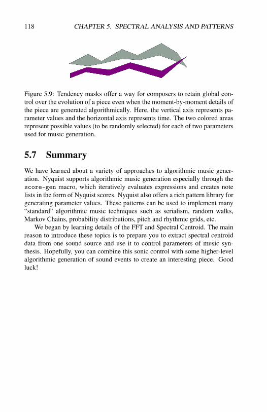
118 CHAPTER 5. SPECTRAL ANALYSIS AND PATTERNS
Figure 5.9: Tendency masks offer a way for composers to retain global con-trol over the evolution of a piece even when the moment-by-moment details ofthe piece are generated algorithmically. Here, the vertical axis represents pa-rameter values and the horizontal axis represents time. The two colored areasrepresent possible values (to be randomly selected) for each of two parametersused for music generation.
5.7 SummaryWe have learned about a variety of approaches to algorithmic music gener-ation. Nyquist supports algorithmic music generation especially through thescore-gen macro, which iteratively evaluates expressions and creates notelists in the form of Nyquist scores. Nyquist also offers a rich pattern library forgenerating parameter values. These patterns can be used to implement many“standard” algorithmic music techniques such as serialism, random walks,Markov Chains, probability distributions, pitch and rhythmic grids, etc.
We began by learning details of the FFT and Spectral Centroid. The mainreason to introduce these topics is to prepare you to extract spectral centroiddata from one sound source and use it to control parameters of music syn-thesis. Hopefully, you can combine this sonic control with some higher-levelalgorithmic generation of sound events to create an interesting piece. Goodluck!

Chapter 6
Nyquist Techniques andGranular Synthesis
Topics Discussed: Recursion, Duration Matching, Control Functions,and Granular Synthesis
6.1 Programming Techniques in NyquistOne of the unusual things about Nyquist is the support for timing (temporalsemantics), which is lacking in most programming languages. Nyquist alsohas signals as a fundamental data type. Here we introduce a number of dif-ferent programming techniques related to timing and signals that are useful inNyquist.
6.1.1 Recursive Sound SequencesWe first look at the idea of recursive sound sequences. The seq function delaysevaluation of each behavior until the previous behavior is finished. There areother functions, including timed-seq that work in a similar way. This delayedevaluation, a form of lazy evaluation, is important in practice because if soundcomputation can be postponed until needed, Nyquist can avoid storing largesignals in memory. Lazy evaluation has another benefit, in that it allows youto express infinite sounds recursively. Consider a drum roll as an example.We define a drum roll recursively as follows: Start with one drum stroke andfollow it with a drum roll!
The drum-roll() function below is a direct implementation of this idea.drum-roll() builds up a drum roll one stroke at a time, recursively, and re-turns an infinite drum roll sound sequence. Even Google doesn’t have that
119
120 CHAPTER 6. TECHNIQUES AND GRANULAR SYNTHESIS
much disk space, so to avoid the obvious problem of storing an infinite sound,we can multiply drum-roll() by an envelope. In limited-drum-roll(),we make a finite drum roll by multiplying drum-roll() by const(1, 2).const(1, 2) is a unit generator that returns a constant value of 1 until theduration of 2, then it drops to 0. Here, multiplying a limited sound by an infi-nite sound gives us a finite computation and result. Note that the multiplicationoperator in Nyquist is quite smart. It knows that when multiplying by 0, theresult is always 0; and when a sound reaches its stop time, it remains 0 forever,thus Nyquist can terminate the recursion at the sound stop time.
define function drum-stroke()return noise() * pwev(1, 0.05, 0.1)
define function drum-roll()return seq(drum-stroke(), drum-roll()) ; recursion!
define function limited-drum-roll()return const(1, 2) * drum-roll() ; duration=2
play limited-drum-roll()
Note that in this example, there is a risk that the “envelope” const(1, 2)might cut off a drum-stroke suddenly.1 Here, drum-strokes happen to be 0.1seconds long, which means a 2-second drum-roll has exactly 20 full drum-strokes, so a drum-stroke and and the envelope will end exactly together. Ingeneral, either seqrep or an envelope that gives a smooth fadeout would be abetter design.
6.1.2 Matching DurationsIn Nyquist, sounds are considered to be functions of time, with no upper boundon time. Sounds do have a “stop time” after which the signal is considered toremain at zero forever. This means that you can easily combine sounds ofdifferent durations by mistake. For example, you can multiply a 1-secondoscillator signal by a 2-second envelope, resulting in a 1-second signal thatprobably ends abruptly before the envelope goes to zero.
It is a “feature” of Nyquist that you can compose longer sounds fromshorter sounds or multiply by short envelopes to isolate sections of longersounds, but this leads to one of the most common errors in Nyquist: Combin-ing sounds and controls with different durations by mistake.
Here is an example of this common error:
1Recall that const(1, 2) is a control signal with the constant value 1 for 2 seconds. It cutsoff instantly at 2 seconds.

6.1. PROGRAMMING TECHNIQUES IN NYQUIST 121
play pwl(0.5, 1, 10, 1, 13) * ; 13-seconds durationosc(c4) ; nominally 1-second duration
; final result: sound stops at 1 second(!)
Remember that Nyquist sounds are immutable. Nyquist will not and cannotgo back and recompute behaviors to get the “right” durations–how would itknow? There are two basic approaches to make durations match. The first isto make everything have a nominal length of 1 and use the stretch operator tochange durations:
(pwl(0.1, 1, 0.8, 1, 1) * osc(c4)) ~ 13
Here we have changed pwl to have a duration of 1 rather than 13. This is thedefault duration of osc, so they match. Note also the use of parentheses toensure that the stretch factor applies to both pwl and osc.
The second method is to provide duration parameters everywhere:
pwl(0.5, 1, 10, 1, 13) * osc(c4, 13)
Here, we kept the original 13-second long pwl function, but we explicitly setthe duration of osc to 13. If you provide duration parameters everywhere, youwill often end up passing duration as a parameter, but that’s not always a badthing as it makes duration management more explicit.
6.1.3 Control Functions
Another useful technique in Nyquist is to carefully construct control functions.Synthesizing control is like synthesizing sound, and often control is even moreimportant that waveforms and spectra in producing a musical result.
Smooth Transitions
Apply envelopes to almost everything. Even control functions can have controlfunctions! A good example is vibrato. A “standard” vibrato function mightlook like lfo(6) * 5, but this would generate constant vibrato throughouta tone. Instead, consider lfo(6) * 5 * pwl(0.3, 0, 0.5, 1, 0.9, 1,1) where the vibrato depth is controlled by an envelope. Initially, there is novibrato, the vibrato starts to emerge at 0.3 and reaches the full depth at 0.5, andfinally tapers rapidly from 0.9 to 1. Of course this might be stretched, so thesenumbers are relative to the whole duration. Thus, we not only use envelopes toget smooth transitions in amplitude at the beginnings and endings of notes, wecan use envelopes to get smooth transitions in vibrato depth and other controls.

122 CHAPTER 6. TECHNIQUES AND GRANULAR SYNTHESIS
Composing Control Functions
The are a few main “workhorse” functions for control signals.
1. for periodic variation such as vibrato, the lfo function generates low-frequency sinusoidal oscillations. The default sample rate of lfo is 1/20of the audio sample rate, so do not use this function for audio frequen-cies. If the frequency is not constant, the simplest alternative is hzosc,which allows its first argument to be a SOUND as well as a number.
2. for non-periodic but deterministic controls such as envelopes, pwl andthe related family (including pwlv and pwlev) or the envelope functionenv are good choices.
3. for randomness, a good choice is noise. By itself, noise generates au-dio rate noise, which is not suitable for adding small random fluctuationsto control signals. What we often use in this case is a random signal thatramps smoothly from one amplitude to the next, with a new amplitudeevery 100 ms or so. You can obtain this effect by making a very lowsample rate noise signal. When this signal is added to or multiplied bya higher sample rate signal, the noise signal is linearly interpolatedto match the rate of the other signal, thus achieving a smooth rampbetween samples. The expression for this is sound-srate-abs(10,noise()), which uses the sound-srate-abs transform to change theenvironment for noise to a sample rate of 10 Hz. See Figure 6.1.
Figure 6.1: Plots of: noise, sound-srate-abs(10, noise()), ramp()and sound-srate-abs(10, noise()) * 0.1 + ramp(). The bottom plotshows how the noise function can be used to add jitter or randomness to anotherwise mathematically smooth control function. Such jitter or randomnessoccurs naturally, often due to minute natural human muscle tremors.

6.1. PROGRAMMING TECHNIQUES IN NYQUIST 123
Global vs. Local Control Functions
Nyquist allows you to use control functions including envelopes at differentlevels of hierarchy. For example, you could synthesize a sequence of noteswith individual amplitude envelopes, then multiply the whole sequence by anoverarching envelope to give a sense of phrase. Figure 6.2 illustrates howglobal and “local” envelopes might be combined.
Figure 6.2: Hierarchical organization of envelopes.
In the simple case of envelopes, you can just apply the global envelopethrough multiplication after notes are synthesized. In some other cases, youmight need to actually pass the global function as a parameter to be used forsynthesis. Suppose that in Figure 6.2, the uppermost (global) envelope is sup-posed to control the index of modulation in FM synthesis. This effect cannotbe applied after synthesis, so you must pass the global envelope as a parameterto each note. Within each note, you might expect the whole global envelope tosomehow be shifted and stretched according to the note’s start time and dura-tion, but that does not happen. Instead, since the control function has alreadybeen computed as a SOUND, it is immutable and fixed in time. Thus, the noteonly “sees” the portion of the control function over the duration of the note, asindicated by the dotted lines in Figure 6.2.
In some cases, e.g. FM synthesis, the control function determines the notestart time and duration, so fmosc might try to create a tone over the entireduration of the global envelope, depending on how you use it. One way to“slice” out a piece of a global envelope or control function according to thecurrent environment is to use const(1) which forms a rectangular pulse thatis 1 from the start time to the nominal duration according to the environment.If you multiply a global envelope parameter by const(1), you are sure to getsomething that is confined within the nominal starting and ending times in theenvironment.
6.1.4 Stretchable BehaviorsAn important feature of Nyquist is the fact that functions represent classes ofbehaviors that can produce signals at different start times, with different dura-tions, and be affected by many other parameters, both explicit and implicit.
Nyquist has default stretch behaviors for all of its primitives, and we haveseen this many times. Often, the default behavior does the “right thing,” (see

124 CHAPTER 6. TECHNIQUES AND GRANULAR SYNTHESIS
the discussion above about matching durations). But sometimes you need tocustomize what it means to “stretch” a sound. For example, if you stretcha melody, you make notes longer, but if you stretch a drum roll, you do notmake drum strokes slower. Instead, you add more drum strokes to fill the time.With Nyquist, you can create your own abstract behaviors to model things likedrum rolls, constant-rate trills, and envelopes with constant attack times, noneof which follow simple default rules of stretching.
Here is an example where you want the number of things to increase withduration:
define function n-things()beginwith dur = get-duration(1),
n = round(dur / *thing-duration*)return seqrep(i, n, thing() ~~ 1)
end
The basic idea here is to first “capture” the nominal duration using
get-duration(1)
Then, we compute n in terms of duration. Now, if we simply made n things inthe current stretch environment (stretch by dur), we would create a sound withduration roughly n × *thing-duration* × dur, but we want to computething() without stretching. The ~~ operator, also called absolute stretch,resets the environment stretch factor to 1 when we call thing(), so now thetotal duration will be approximately n × *thing-duration*, which is aboutequal to get-duration(1) as desired.
Here is an example where you want an envelope to have a fixed rise time.
define function my-envelope()beginwith dur = get-duration(1)return pwl(*rise-time*, 1, dur - *fall-time*,
1, dur) ~~ 1end
As in the previous example, we “capture” duration to the variable dur andthen compute within an absolute stretch (~~) of 1 so that all duration control isexplicit and in terms of dur. We set the rise time to a constant, *rise-time*and compute the beginning and ending of the “release” relative to dur whichwill be the absolute duration of the envelope.

6.2. GRANULAR SYNTHESIS 125
6.1.5 Summary
We have seen a number of useful Nyquist programming techniques. To makesure durations match, either normalize durations to 1 and stretch everythingas a group using the stretch operator (~), or avoid stretching altogether anduse explicit duration parameters everywhere. In general, use envelopes every-where to achieve smooth transitions, and never let an oscillator output startor stop without a smooth envelope. Control is all important, so in spite ofmany simplified examples you will encounter, every parameter should be acandidate for control over time: amplitude, modulation, vibrato, filter cutoff,and even control functions themselves can be modulated or varied at multipletime scales. And speaking of multiple time scales, do not forget that musicalgestures consisting of multiple notes or sound events can be sculpted usingover-arching envelopes or smooth control changes that span whole phrases.
6.2 Granular Synthesis
We know from our discussion of the Fourier transform that that complexsounds can be created by adding together a number of sine waves. Granu-lar synthesis uses a similar idea, except that instead of a set of sine waveswhose frequencies and amplitudes change over time, we use many thousandsof very short (usually less than 100 milliseconds) overlapping sound burstsor grains. The waveforms of these grains are often sinusoidal, although anywaveform can be used. (One alternative to sinusoidal waveforms is to usegrains of sampled sounds, either pre-recorded or captured live.) By manipu-lating the temporal placement of large numbers of grains and their frequencies,amplitude envelopes, and waveshapes, very complex and time-variant soundscan be created.
6.2.1 Grains
To make a grain, we simply take any sound (e.g. a sinusoid or sound from asound file) and apply a short smoothing envelope to avoid clicks. (See Figure6.3.) The duration is typically from around 20ms to 200ms: long enoughto convey a little content and some spectral information, but short enough toavoid containing an entire note or word (from speech sounds) or anything toorecognizable.

126 CHAPTER 6. TECHNIQUES AND GRANULAR SYNTHESIS
Figure 6.3: Applying a short envelope to a sound to make a grain for granularsynthesis. How would a different amplitude envelope, say a square one, affectthe shape of the grain? What would it do to the sound of the grain? Whatwould happen if the sound was a recording of a natural sound instead of asinusoid? What would be the effect of a longer or shorter envelope?
6.2.2 Clouds of Sound
Granular synthesis is often used to create what can be thought of as “soundclouds”—shifting regions of sound energy that seem to move around a sonicspace. A number of composers, like Iannis Xenakis and Barry Truax, thoughtof granular synthesis as a way of shaping large masses of sound by usinggranulation techniques. These two composers are both considered pioneersof this technique (Truax wrote some of the first special-purpose software forgranular synthesis). Sometimes, cloud terminology is even used to talk aboutways of arranging grains into different sorts of configurations.
6.2.3 Grain Selection, Control and Organization
In granular synthesis, we make and combine thousands of grains (sometimesthousands of grains per second), which is too much to do by hand, so weuse computation to do the work, and we use high-level parameters to controlthings. Beyond this, granular synthesis is not a specific procedure and thereis no right or wrong way to do it. It is good to be aware of the range ofmechanisms by which grains are selected, processed, and organized.
One important control parameter is density. Typically granular synthesis isquite dense, with 10 or more grains overlapping at any given time. But grainscan also be sparse, creating regular rhythms or isolated random sound events.

6.2. GRANULAR SYNTHESIS 127
Figure 6.4: Visualization of a granular synthesis “score.” Each dot represents agrain at a particular frequency and moment in time. An image such as this onecan give us a good idea of how this score might sound, even though there issome important information left out (such as the grain amplitudes, waveforms,amplitude envelopes, and so on). What sorts of sounds does this image imply?If you had three vocal performers, one for each cloud, how would you go aboutperforming this piece? Try it!
Stochastic or statistical control is common in granular synthesis. For ex-ample, we could pick grains from random locations in a file and play them atrandom times. An interesting technique is to scan through a source file, butrather than taking grains sequentially, we add a random offset to the source lo-cation, taking grains in the neighborhood of a location that progresses throughthe file. This produces changes over time that mirror what is in the file, but atany given time, the cloud of sound can be quite chaotic, disguising any specificaudio content or sound events in the file.
It is also possible to resample the grain to produce pitch shifts. If pitchshifting is random, a single tone in the source can become a multi-pitch clusteror cloud in the output. If you resample grains, you can shift the pitch byoctaves or harmonics, which might tend to harmonize the output sound whenthere is a single pitch on the input, or you can resample by random ratios,creating an atonal or microtonal effect. When you synthesize grains, you canuse regular spacing, e.g. play a grain every 10 ms, which will tend to createa continuous sounding texture, or you can play grains with randomized inter-onset intervals, creating a more chaotic or bubbly sound.
Some interesting things to do with granular synthesis include vocal mum-blings using grains to chop up speech and make speech-sounding nonsense,especially using grains with approximately the duration of phonemes so that

128 CHAPTER 6. TECHNIQUES AND GRANULAR SYNTHESIS
whole words are obliterated. Granular synthesis can also be used for timestretching: By moving through a file very slowly, fetching overlapping grainsand outputting them with less overlap, the file is apparently stretched, a shownin Figure 6.5. There will be artifacts because grains will not add up perfectlysmoothly to form a continuous sound, but this can be a feature as well as alimitation, depending on your musical goals.
Figure 6.5: Stretching with granular synthesis.
6.2.4 Granular Synthesis in NyquistNyquist does not have a “granular synthesis” function because there are somany ways to implement and control granular synthesis. However, Nyquist isalmost unique in its ability to express granular synthesis using a combinationof signal processing and control constructs.
Generating a Grain
Figure 6.6 illustrates Nyquist code to create an smooth envelope and read agrain’s worth of audio from a file to construct a smooth grain. Note the useof duration d both to stretch the envelope and control how many samples areread from the file. Below, we consider two approaches to granular synthesisimplementation. The first uses scores and the second uses seqrep.
6.2.5 Grains in ScoresA score for granular synthesis treats each grain as a sound event:
{{0 0.05 {grain offset: 2.1}}{0.02 0.06 {grain offset: 3.0}}...}
The score calls upon grain, which we define below. Notice that grain dura-tions are specified in the score and implemented through the environment,so the cos-pulse signal will be stretched by the duration, but s-read isunaffected by stretching. Therefore, we must obtain the stretch factor using

6.2. GRANULAR SYNTHESIS 129
Figure 6.6: Contructing a grain in Nyquist.
get-duration(1) and pass that value to s-read as the optional dur: key-word parameter:
function grain(offset: 0)begin with dur = get-duration(1)return s-read("filename.wav",
time-offset: offset, dur: dur) *cos-pulse()
end
Now, we can make make a score with score-gen. In the following expres-sion, we construct 2000 grains with randomized inter-onset intervals and usingpattern objects to compute the grain durations and file offsets:
score-gen(score-len: 2000,ioi: 0.05 + rrandom() * 0.01,dur: next(dur-pat),offset: next(offset-pat))
You could also use more randomness to compute parameters, e.g. the du-ration could come from a Gaussian distribution (see the Nyquist functiongaussian-dist), and offset: could be computed by slowly moving throughthe file and adding a random jitter, e.g.
max(0, sg-count * 0.01 + rrandom() * 0.2)
6.2.6 Grains with SeqrepRather than computing large scores, we can use Nyquist control constructsto creates grains “on the fly.” In the following example, seqrep is used to

130 CHAPTER 6. TECHNIQUES AND GRANULAR SYNTHESIS
create and sum 2000 sounds. Each sound is produced by a call to grain,which is stretched by values from dur-pat. To obtain grain overlap, weuse set-logical-stop with an IOI (logical stop time) parameter of 0.05+ rrandom() * 0.01, so the grain IOI will be 50 ms ± 10 ms:
seqrep(i, 2000,set-logical-stop(
grain(offset: next(offset-pat)) ~next(dur-pat),
0.05 + rrandom() * 0.01))
For another example, you can install the gran extension using Nyquist’sExtension Manager. The package includes a function sf-granulate that im-plements granular synthesis using a sound file as input.
6.2.7 Other IdeasYou might want to implement something like the tendency masks we describedearlier or use a pwl function to describe how some granular synthesis parame-ters evolve over time. Since pwl produces a signal and you often need numbersto control each grain, you can use sref to evaluate the signal at a specific time,e.g. s-ref(sound, time) will evaluate sound at time.
Another interesting idea is to base granular synthesis parameters on thesource sound itself. A particularly effective technique is to select grains byslowly advancing through a file, causing a time-expansion of the file content.The most interesting portions of the file are usually note onsets and placeswhere things are changing rapidly, which you might be able to detect by mea-suring either amplitude or spectral centroid. Thus, if the rate at which youadvanced through the file can be inversely proportional to amplitude or spec-tral centroid, then the “interesting” material will be time-expanded, and youwill pass over the “boring” steady-state portions of the signal quickly.
6.2.8 SummaryGranular synthesis creates sound by summing thousands of sound particles orgrains with short durations to form clouds of sounds. Granular synthesis canconstruct a wide range of textures, and rich timbres can be created by tak-ing grains from recordings of natural sounds. Granular synthesis offers manychoices of details including grain duration, density, random or deterministictiming, pitch shifts and source.

Chapter 7
Sampling and FiltersTopics Discussed: Samples, Filters, High-pass, Low-pass, Band-pass
7.1 Sampling SynthesisAlthough direct synthesis of sound is an important area of computer music, itcan be equally interesting (or even more so!) to take existing sounds (recordedor synthesized) and transform, mutate, deconstruct—in general, mess aroundwith them. There are as many basic sound transformation techniques as thereare synthesis techniques, and in this chapter we’ll describe a few importantones. For the sake of convenience, we will separate them into time-domainand frequency-domain techniques.
7.1.1 Tape Music / Cut and PasteThe most obvious way to transform a sound is to chop it up, edit it, turn itaround, and collage it. These kinds of procedures, which have been used inelectronic music since the early days of tape recorders, are done in the timedomain. There are a number of sophisticated software tools for manipulat-ing sounds in this way, called digital sound editors. These editors allow forthe most minute, sample-by-sample changes of a sound. These techniquesare used in almost all fields of audio, from avant-garde music to Hollywoodsoundtracks, from radio station advertising spots to rap.
7.1.2 Time-Domain RestructuringComposers have experimented a lot with unusual time-domain restructuringof sound. By chopping up waveforms into very small segments and radically
131

132 CHAPTER 7. SAMPLING AND FILTERS
reordering them, some noisy and unusual effects can be created. As in collagevisual art, the ironic and interesting juxtaposition of very familiar materialscan be used to create new works that are perhaps greater than the sum of theirconstituent parts.
Unique, experimental, and rather strange programs for deconstructing andreconstructing sounds in the time domain are Herbert Brün’s SAWDUST seeFigure 7.1 and Argeïphontes Lyre (see Figure 7.2, written by the enigmaticAkira Rabelais. Argeïphontes Lyre provides a number of techniques for rad-ical decomposition/recomposition of sounds—techniques that often precludethe user from making specific decisions in favor of larger, more probabilisticdecisions.
Figure 7.1: Herbert Brün said of his program SAWDUST: “The computerprogram which I called SAWDUST allows me to work with the smallest partsof waveforms, to link them and to mingle or merge them with one another.Once composed, the links and mixtures are treated, by repetition, as periods,or by various degrees of continuous change, as passing moments of orientationin a process of transformations.”
7.1.3 Sampling
Sampling refers to taking small bits of sound, often recognizable ones, andrecontextualizing them via digital techniques. By digitally sampling, we caneasily manipulate the pitch and time characteristics of ordinary sounds and usethem in any number of ways.
We’ve talked a lot about samples and sampling in the preceding chapters.In popular music (especially electronic dance and beat-oriented music), theterm sampling has acquired a specialized meaning. In this context, a samplerefers to a (usually) short excerpt from some previously recorded source, such

7.1. SAMPLING SYNTHESIS 133
Figure 7.2: Sample GUI from Argeïphontes Lyre, for sound deconstruction.This is time-domain mutation.
as a drum loop from a song or some dialog from a film soundtrack, that is usedas an element in a new work. A sampler is the hardware used to record, store,manipulate, and play back samples. Originally, most samplers were stand-alone pieces of gear. Today sampling tends to be integrated into a studio’scomputer-based digital audio system.
Sampling was pioneered by rap artists in the mid-1980s, and by the early1990s it had become a standard studio technique used in virtually all types ofmusic. Issues of copyright violation have plagued many artists working withsample-based music, notably John Oswald of “Plunderphonics” fame and theband Negativland, although the motives of the “offended” parties (generallylarge record companies) have tended to be more financial than artistic. Oneresult of this is that the phrase “Contains a sample from xxx, used by permis-sion” has become ubiquitous on CD cases and in liner notes.
Although the idea of using excerpts from various sources in a new workis not new (many composers, from Béla Bartók, who used Balkan folk songs,to Charles Ives, who used American popular music folk songs, have done so),digital technology has radically changed the possibilities.

134 CHAPTER 7. SAMPLING AND FILTERS
7.1.4 Drum Machines
Drum machines and samplers are close cousins. Many drum machines are justspecialized samplers—their samples just happen to be all percussion/drum-oriented. Other drum machines feature electronic or digitally synthesizeddrum sounds. As with sampling, drum machines started out as stand-alonepieces of hardware but now have largely been integrated into computer-basedsystems.
7.1.5 DAW Systems
Digital-audio workstations (DAWs) in the 1990s and 2000s have had the sameeffect on digital sound creation as desktop publishing software had on the pub-lishing industry in the 1980s: they’ve brought digital sound creation out ofthe highly specialized and expensive environments in which it grew up andinto people’s homes. A DAW usually consists of a computer with some sortof sound card or other hardware for analog and digital input/output; soundrecording/editing/playback/multi-track software; and a mixer, amplifier, andother sound equipment traditionally found in a home studio. Even the mostmodest of DAW systems can provide sixteen or more tracks of CD-qualitysound, making it possible for many artists to self-produce and release theirwork for much less than it would traditionally cost. This ability, in conjunctionwith similar marketing and publicizing possibilities opened up by the spreadof the Internet, has contributed to the explosion of tiny record labels and inde-pendently released CDs we’ve seen recently.
In 1989, Digidesign came out with Sound Tools, the first professionaltape–less recording system. With the popularization of personal computers,numerous software and hardware manufacturers have cornered the marketfor computer-based digital audio. Starting in the mid-1980s, personal com-puter–based production systems have allowed individuals and institutions tomake the highest-quality recordings and DAW systems, and have also revo-lutionized the professional music, broadcast, multimedia, and film industrieswith audio systems that are more flexible, more accessible, and more creativelyoriented than ever before.
Today DAWs come in all shapes and sizes and interface with most com-puter operating systems, from Mac to Windows to LINUX. In addition, manyDAW systems involve a breakout box—a piece of hardware that usually pro-vides four to twenty or more channels of digital audio I/O (inputs and outputs).Nowadays many DAW systems also have control surfaces—pieces of hard-ware that look like a standard mixer but are really controllers for parametersin the digital audio system.

7.1. SAMPLING SYNTHESIS 135
7.1.6 Sampling as a Synthesis TechniqueSampling is often used to produce musical tones or notes, and some thinkof sampling as the opposite of synthesis. In this view, sampling is based onrecordings while synthesis produces sound by mathematical calculation. How-ever, sample-based tone production involves considerable calculation and al-lows for parametric control, so we will describe it as yet another synthesistechnique or algorithm.
The main attraction of sampling is that recordings of actual acoustic in-struments generally sound realistic. (You might think samples by definitionmust always sound realistic, but this is an overstatement we will discuss later.)There are three basic problems with samples:
1. Samples of musical tones have definite pitches. You could collect sam-ples for every pitch, but this requires a lot of storage, so most samplersneed the capability of changing the pitch of samples through calculation.
2. Samples of musical tones have definite durations. In practice, we needto control the duration of tones, and capturing every possible durationis impractical, so we need the capability of changing the duration ofsamples.
3. Samples have a definite loudness. In practice we need to produce soundsfrom soft to loud.
Pitch Control
The standard approach to pitch control over samples (here, sample means ashort recording of a musical tone) is to change the sample rate using interpo-lation. If we upsample, or increase the sample rate, but play at the normalsample rate, the effect will be to slow down and drop the pitch of the originalrecording. Similarly, if we downsample, or lower the sample rate, but play atthe normal rate, the effect will be to speed up and raise the pitch of the originalrecording.
To change sample rates, we interpolate existing samples at new time points.Often, “interpolation” means linear interpolation, but with signals, linear in-terpolation does not result in the desired smooth band-limited signal, which isanother way of saying that linear interpolation will distort the signal; it maybe a rough approximation to proper reconstruction, but it is not good enoughfor high-quality audio. Instead, good audio sample interpolation requires aweighted sum taken over a number of samples. The weights follow an inter-esting curve as shown in Figure 7.3. The more the samples considered, thebetter the quality, but the more the computation. Commercial systems do not

136 CHAPTER 7. SAMPLING AND FILTERS
advertise the quality of their interpolation, but a good guess is that interpola-tion typically involves less than 10 samples. In theoretical terms, maintaining16-bit quality requires interpolation over about 50 samples in the worst case.
Figure 7.3: To resample a signal, we need to interpolate between existingsamples in order to reconstruct the signal at a new time. A sequence of thesenew samples at a narrower or wider spacing creates a representation of thesignal at a new sample rate. For each of these new samples (in this figure, thenew sample will be at the dotted line), we form a weighted sum of existingsamples. The weights are given by the so-called sinc function shown here (thethin wavy line). This weighted sum is essentially a low-pass filter that doesin the digital domain what the reconstruction filter does in the analog domainwhen converting a digital signal to analog.
Another problem with resampling is that when pitch is shifted by a lot, thequality of sound is significantly changed. For example, voices shifted to higherpitches begin so sound like cartoon voices or people breathing helium. This isunacceptable, so usually, there are many samples for a given instrument. Forexample, one might use four different pitches for each octave. Then, pitchshifts are limited to the range of 1/4 octave, eliminating the need for extremepitch shifts.
Duration Control
A simple way to control duration is simply to multiply samples by an envelopeto end them as early as needed. However, this could require a considerableamount of memory to store long raw samples in case long notes are required.To save memory, samplers can loop or repeat portions of samples to sustain thesound. Usually, there is an initial attack portion of the sample at the beginning,and when the sample settles down to a periodic waveform, the sampler canrepeat that portion of the sample. To loop samples, one must be very careful tofind points where the end of the loop flows smoothly into the beginning of theloop to avoid discontinuities that impart a buzzy sound to the loop. Loopingis a painstaking manual process, which is another reason to simply use longersamples as long as the added memory requirements are acceptable.

7.1. SAMPLING SYNTHESIS 137
Loudness Control
A simple way to produce soft and loud versions of samples is to just multiplythe sample by a scale factor. There is a difference, however, between amplitudeand loudness in that many instruments change their sound when they playlouder. Imagine a whisper in your ear vs. a person shouting from 100 yardsaway. Which is louder? Which has higher amplitude?
To produce variations in perceptual loudness, we can use filters to alterthe spectrum of the sound. E.g. for a softer sound, we might filter out higherfrequencies as well as reduce the amplitude by scaling. Another option isto record samples for different amplitudes and select samples according gothe desired loudness level. Amplitude changes can be used to introduce fineradjustments.
Sampling in Nyquist
In Nyquist, the sampler function can be used to implement sampling synthe-sis. The signature of the function is:
sampler(pitch, modulation, sample)
The pitch parameter gives the desired output pitch, and modulation is a fre-quency deviation function you can use to implement vibrato or other modu-lation. The output duration is controlled by modulation, so if you want zeromodulation and a duration of dur, use const(0, dur) for modulation. Thesample parameter is a list of the form: (sound pitch loop-start), where sound isthe sample (audio), pitch is the natural pitch of the sound, and loop-start is thetime at which the loop starts. Resampling is performed to convert the naturalpitch of the sample to the desired pitch computed from the pitch parameterand modulation. The sampler function returns a sound constructed by read-ing the audio sample from beginning to end and then splicing on copies of thesame sound from the loop point (given by loop-start) to the end. Currently,only 2-point (linear) interpolation is implemented, so the quality is not high.However, you can use resample to upsample your sound to a higher samplerate, e.g. 4x and this will improve the resulting sound quality. Note also thatthe loop point may be fractional, which may help to make clean loops.
Summary
Sampling synthesis combines pre-recorded sounds with signal processing toadjust pitch, duration, and loudness. For creating music that sounds likeacoustic instruments, sampling is the currently dominant approach. One ofthe limitations of sampling is the synthesis of lyrical musical phrases. While

138 CHAPTER 7. SAMPLING AND FILTERS
samples are great for reproducing single notes, acoustic instruments performconnected phrases, and the transitions between notes in phrases are very dif-ficult to implement with sampling. Lyrical playing by wind instruments andbowed strings is very difficult to synthesize simply by combining 1-note sam-ples. Some sample libraries even contain transitions to address this problem,but the idea of sampling all combinations of articulations, pitches, durations,and loudness levels and their transitions does not seem feasible.
7.2 FiltersThe most common way to think about filters is as functions that take in a signaland give back some sort of transformed signal. Usually, what comes out isless than what goes in. That’s why the use of filters is sometimes referred toas subtractive synthesis.
It probably won’t surprise you to learn that subtractive synthesis is in manyways the opposite of additive synthesis. In additive synthesis, we start withsimple sounds and add them together to form more complex ones. In subtrac-tive synthesis, we start with a complex sound (such as noise or a rich harmonicspectrum) and subtract, or filter out, parts of it. Subtractive synthesis can bethought of as sound sculpting—you start out with a thick chunk of sound con-taining many possibilities (frequencies), and then you carve out (filter) partsof it. Filters are one of the sound sculptor’s most versatile and valued tools.
The action of filters is best explained in the frequency domain. Figure7.4 explains the action of a filter on the spectrum of a signal. In terms ofthe magnitude spectrum, filtering is a multiplication operation. Essentially,the filter scales the amplitude of each sinusoidal component by a frequency-dependent factor. The overall frequency-dependent scaling function is calledthe frequency response of the filter.
A common misconception among students is that since filtering is multi-plication in the frequency domain, and since the FFT converts signals to thefrequency domain (and the inverse FFT converts back), then filtering must beperformed by an FFT-multiply-IFFT sequence. This is false! At least sim-ple filters operate in the time domain (details below). Filtering with FFTs ispossible but problematic because it is not practical to perform FFTs on longsignals.
7.2.1 Four Basic Types of FiltersFigure 3 illustrates four basic types of filters: low-pass, high-pass, band-pass,and band-reject. Low-pass and high-pass filters should already be familiarto you—they are exactly like the tone knobs on a car stereo or boombox. A

7.2. FILTERS 139
Figure 7.4: Filtering in the frequency domain. The input signal with spectrumX is multiplied by the frequency response of the filter H to obtain the outputspectrum Y. The result of filtering is to reduce the amplitude of some frequen-cies and boost the amplitudes of others. In addition to amplitude changes,filters usually cause phase shifts that are also frequency dependent. Since weare so insensitive to phase, we usually ignore the phase response of filters.
Figure 7.5: Four common filter types (clockwise from upper left): low-pass,high-pass, band-reject, band-pass.

140 CHAPTER 7. SAMPLING AND FILTERS
low-pass (also known as high-stop) filter stops, or attenuates, high frequencieswhile letting through low ones, while a high-pass (low-stop) filter does just theopposite.
Band-Pass and Band-Reject Filters
Band-pass and band-reject filters are basically combinations of low-pass andhigh-pass filters. A band-pass filter lets through only frequencies above acertain point and below another, so there is a band of frequencies that getthrough. A band-reject filter is the opposite: it stops a band of frequencies.Band-reject filters are sometimes called notch filters, because of the shape oftheir frequency response.
Low-Pass and High-Pass Filters
Low-pass and high-pass filters have a value associated with them called thecutoff frequency, which is the frequency where they begin “doing their thing.”So far we have been talking about ideal, or perfect, filters, which cut off in-stantly at their cutoff frequency. However, real filters are not perfect, and theycan’t just stop all frequencies at a certain point. Instead, frequencies die outaccording to a sort of curve around the corner of their cutoff frequency. Thus,the filters in Figure 3 don’t have right angles at the cutoff frequencies—insteadthey show general, more or less realistic response curves for low-pass andhigh-pass filters.
7.2.2 Cutoff Frequency
The cutoff frequency of a filter is defined as the point at which the signal isattenuated to 0.707 of its maximum value (which is 1.0). No, the number0.707 was not just picked out of a hat! It turns out that the power of a signal isdetermined by squaring the amplitude: 0.7072 = 0.5. So when the amplitudeof a signal is at 0.707 of its maximum value, it is at half-power. The cutofffrequency of a filter is sometimes called its half-power point.
7.2.3 Transition Band
The area between where a filter “turns the corner” and where it “hits the bot-tom” is called the transition band. The steepness of the slope in the transitionband is important in defining the sound of a particular filter. If the slope is verysteep, the filter is said to be “sharp;” conversely, if the slope is more gradual,the filter is “soft” or “gentle.”

7.2. FILTERS 141
Things really get interesting when you start combining low-pass and high-pass filters to form band-pass and band-reject filters. Band-pass and band-reject filters also have transition bands and slopes, but they have two of them:one on each side. The area in the middle, where frequencies are either passedor stopped, is called the passband or the stopband. The frequency in the mid-dle of the band is called the center frequency, and the width of the band iscalled the filter’s bandwidth.
You can plainly see that filters can get pretty complicated, even these sim-ple ones. By varying all these parameters (cutoff frequencies, slopes, band-widths, etc.), we can create an enormous variety of subtractive synthetic tim-bres.
7.2.4 A Little More Technical: IIR and FIR Filters
Filters are often talked about as being one of two types: finite impulse response(FIR) and infinite impulse response (IIR). This sounds complicated (and canbe!), so we’ll just try to give a simple explanation as to the general idea ofthese kinds of filters.
Finite impulse response filters are those in which delays are used alongwith some sort of averaging. Delays mean that the sound that comes out at agiven time uses some of the previous samples. They’ve been delayed beforethey get used.
We’ve talked about these filters earlier. What goes into an FIR is alwaysless than what comes out (in terms of amplitude). Sounds reasonable, right?FIRs tend to be simpler, easier to use, and easier to design than IIRs, and theyare very handy for a lot of simple situations. An averaging low-pass filter, inwhich some number of samples are averaged and output, is a good example ofan FIR.
Infinite impulse response filters are a little more complicated, because theyhave an added feature: feedback. You’ve all probably seen how a micro-phone and speaker can have feedback: by placing the microphone in front ofa speaker, you amplify what comes out and then stick it back into the system,which is amplifying what comes in, creating a sort of infinite amplificationloop. Ouch! (If you’re Jimi Hendrix, you can control this and make greatmusic out of it.)
Well, IIRs are similar. Because the feedback path of these filters consists ofsome number of delays and averages, they are not always what are called unitygain transforms. They can actually output a higher signal than that which isfed to them. But at the same time, they can be many times more complex andsubtler than FIRs. Again, think of electric guitar feedback—IIRs are harder tocontrol but are also very interesting.

142 CHAPTER 7. SAMPLING AND FILTERS
Figure 7.6: FIR and IIR filters. Filters are usually designed in the time domain,by delaying a signal and then averaging (in a wide variety of ways) the delayedsignal and the nondelayed one. These are called finite impulse response (FIR)filters, because what comes out uses a finite number of samples, and a sampleonly has a finite effect.
If we delay, average, and then feed the output of that process back into thesignal, we create what are called infinite impulse response (IIR) filters. Thefeedback process actually allows the output to be much greater than the input.These filters can, as we like to say, “blow up.”
These diagrams are technical lingo for typical filter diagrams for FIR andIIR filters. Note how in the IIR diagram the output of the filter’s delay issummed back into the input, causing the infinite response characteristic. That’sthe main difference between the two filters.

7.2. FILTERS 143
Designing filters is a difficult but key activity in the field of digital signalprocessing, a rich area of study that is well beyond the range of this book. Itis interesting to point out that, surprisingly, even though filters change the fre-quency content of a signal, a lot of the mathematical work done in filter designis done in the time domain, not in the frequency domain. By using things likesample averaging, delays, and feedback, one can create an extraordinarily richvariety of digital filters.
For example, the following is a simple equation for a low-pass filter. Thisequation just averages the last two samples of a signal (where x(n) is thecurrent sample) to produce a new sample. This equation is said to have aone-sample delay. You can see easily that quickly changing (that is, high-frequency) time domain values will be “smoothed” (removed) by this equa-tion.
x(n) = (x(n)+ x(n−1))/2 (7.1)
In fact, although it may look simple, this kind of filter design can be quitedifficult (although extremely important). How do you know which frequen-cies you’re removing? It’s not intuitive, unless you’re well schooled in digitalsignal processing and filter theory and have some background in mathematics.The theory introduces another transform, the Laplace transform and its dis-crete cousin, the Z-transform, which, along with some remarkable geometry,yields a systematic approach to filter design.
7.2.5 Filters in Nyquist
Fortunately, you do not need to know filter design theory to use filters inNyquist. Nyquist has an assortment of filters that will work for most pur-poses. The following expression applies a low-pass filter to signal with acutoff frequency of cutoff:
lp(signal, cutoff)
Note that cutoff can also be a signal, allowing you to adjust the cutoff fre-quency over the course of the signal. Normally, cutoff would be a control-rate signal computed as an envelope or pwl function. Changing the filter cutofffrequency involves some trig functions, and Nyquist filters perform these up-dates at the sample rate of the control signal, so if the control signal samplerate is low (typically 1/20 of the audio sample rate), you save a lot of expensivecomputation.
Some other filters in Nyquist include:
• hp - a high-pass filter.

144 CHAPTER 7. SAMPLING AND FILTERS
• reson - a low-pass filter with a resonance (emphasis) at the cutoff fre-quency and a bandwidth parameter to control how narrow is the resonantpeak.
• areson - the opposite of reson; adding the two together recreates theoriginal signal, so areson is a sort of high-pass filter with a notch at thecutoff frequency.
• comb - a comb filter has a set of harmonically spaced resonances andcan be very interesting when applied to noisy signals.
• eq-lowshelf, eq-highshelf and eq-band filters are useful for gen-erally shaping spectra the way you would with a parametric equalizer.
• lowpass2, lowpass4, lowpass6, lowpass8, highpass2, highpass4,highpass6 and highpass8 are optimized lowpass and highpass filterswith different transition slopes. The digits refer to the order of the fil-ter: second order filters have a 12 dB-per-octave slope, fourth have 24dB-per-octave slopes, etc.
All of these are described in greater detail in the Nyquist Reference Manual.
7.2.6 Filter SummaryFilters are essential building blocks for sound synthesis and manipulation. Theeffect of a filter in the frequency domain is to multiply the spectrum by afilter response. Most filters are actually implemented in the time domain usinga discrete sample-by-sample process applied to a stream of samples, whicheliminates the problems of dealing with finite-sized FFT frames, and is alsousually faster than performing FFTs.

Chapter 8
Spectral ProcessingTopics Discussed: FFT, Inverse FFT, Overlap Add, Reconstruction fromSpectral Frames
8.1 FFT Analysis and ReconstructionPreviously, we have learned about the spectral domain in the context of sam-pling theory, filters, and the Fourier transform, in particular the fast Fouriertransform, which we used to compute the spectral centroid. In this chapter,we focus on the details of converting from a time domain representation to afrequency domain representation, operating on the frequency domain repre-sentation, and then reconstructing the time domain signal.
We emphasized earlier that filters are not typically implemented in thefrequency domain, in spite of our theoretical understanding that filtering iseffectively multiplication in the frequency domain. This is because we can-not compute a Fourier transform on a infinite signal or even a very long one.Therefore, our only option is to use short time transforms as we did with com-puting the spectral centroid. That could be used for filtering, but there areproblems associated with using overlapping short-time transforms. Generally,we do not use the FFT for filtering.
Nevertheless, operations on spectral representations are interesting for anal-ysis and synthesis. In the following sections, we will review the Fourier trans-form, consider the problems of long-time analysis/synthesis using short-timetransforms, and look at spectral processing in Nyquist.
8.1.1 Review of FFT AnalysisHere again are the equations for the Fourier Transform in the continuous anddiscrete forms:
145

146 CHAPTER 8. SPECTRAL PROCESSING
Continuous Fourier TransformReal part:
R(ω) =∫
∞
−∞
f (t)cos(ωt)dt (8.1)
Imaginary part:
X(ω) =−∫
∞
−∞
f (t)sin(ωt)dt (8.2)
Discrete Fourier TransformReal part:
Rk =N−1
∑x=0
xi cos(2πki/N) (8.3)
Imaginary part:
Xk =−N−1
∑x=0
xi sin(2πki/N) (8.4)
Recall from the discussion of the spectral centroid that when we take FFTsin Nyquist, the spectra appear as floating point arrays. As shown in Figure8.1, the first element of the array (index 0) is the DC (0 Hz) component,1
and then we have alternating cosine and sine terms all the way up to the topelement of the array, which is the cosine term of the Nyquist frequency. Tovisualize this in a different way, in Figure 8.2, we represent the basis functions(cosine and sine functions that are multiplied by the signal), and the numbershere are the indices in the array. The second element of the array (the bluecurve labeled 1), is a single period of cosine across the duration of the analysisframe. The next element in the array is a single sine function over the length ofthe array. Proceeding from there, we have two cycles of cosine, two cycles ofsine. Finally, the Nyquist frequency term has n/2 cycles of a cosine, formingalternating samples of +1, -1, +1, -1, +1, .... (The sine terms at 0 and theNyquist frequency N/2 are omitted because sin(2πki/N) = 0 if k = 0 or k =N/2.)
Following the definition of the Fourier transform, these basis functionsare multiplied by the input signal, the products are summed, and the sumsare the output of the transform, the so-called Fourier coefficients. Each oneof the basis functions can be viewed as a frequency analyzer—it picks out a
1This component comes from the particular case where ω = 0, so cosωt = 1, and the integralis effectively computing the average value of the signal. In the electrical world where we candescribe electrical power as AC (alternating current, voltage oscillates up an down, e.g. at 60 Hz)or DC (direct current, voltage is constant, e.g. from a 12-volt car battery), the average value of thesignal is the DC component or DC offset, and the rest is “AC.”

8.1. FFT ANALYSIS AND RECONSTRUCTION 147
Figure 8.1: The spectrum as a floating point array in Nyquist. Note that thereal and imaginary parts are interleaved, with a real/imaginary pair for eachfrequency bin. The first and last bin have only one number (the real part)because the imaginary part for these bins is zero.
Figure 8.2: The so-called basis functions for the Fourier transform labeledwith bin numbers. To compute each Fourier coefficient, form the dot productof the basis function and the signal. You can think of this as the weightedaverage of the signal where the basis function provides the weights. Note thatall basis functions, and thus the frequencies they select from the input signal,are harmonics: multiples of a fundamental frequency that has a period equal tothe size of the FFT. Thus, if the N input points represent 1/10 second of sound,the bins will represent 10 Hz, 20 Hz, 30 HZ, ..., etc. Note that we show sinfunctions, but the final imaginary (sin) coefficient of the FFT is negated (seeEquation 8.4.)

148 CHAPTER 8. SPECTRAL PROCESSING
particular frequency from the input signal. The frequencies selected by thebasis functions are K/duration, where index K ∈ {0,1, ...,n/2}.
Knowing the frequencies of basis functions is very important for interpret-ing or operating on spectra. For example, if the analysis window size is 512samples, the sample rate is 44100 Hz, and value at index 5 of the spectrum islarge, what strong frequency does that indicate? The duration is 512/44100 =0.01161 s, and from Figure 8.2, we can see there are 3 periods within the anal-ysis window, so K = 3, and the frequency is 3/0.01161 = 258.398 Hz. A largevalue at array index 5 indicates a strong component near 258.398 Hz.
Now, you may ask, what about some near-by frequency, say, 300 Hz? Thenext analysis frequency would be 344.531 Hz at K = 4, so what happens tofrequencies between 258.398 and 344.531 Hz? It turns out that each basisfunction is not a perfect “frequency selector” because of the finite number ofsamples considered. Thus, intermediate frequencies (such as 300 Hz) willhave some correlation with more than one basis function, and the discretespectrum will have more than one non-zero term. The highest magnitude co-efficients will be the ones whose basis function frequencies are nearest that ofthe sinusoid(s) being analyzed.
8.1.2 Perfect Reconstruction
Is it possible to go from the time domain to the spectral domain and back tothe time domain again without any loss or distortion? One property that worksin our favor is that the FFT is information-preserving. There is a Fast In-verse Short-Time Discrete Fourier Transform, or IFFT for short, that convertsFourier coefficients back into the original signal. Thus, one way to convert tothe spectral domain and back, without loss, is shown in Figure 8.3.
In general, each short-time spectrum is called a spectral frame or an anal-ysis frame.
The problem with Figure 8.3 is that if we change any coefficients in thespectrum, it is likely that the reconstructed signal will have discontinuitiesat the boundaries between one analysis frame and the next. You may recallfrom our early discussion on splicing that cross-fades are important to avoidclicks due to discontinuities. In fact, if there are periodic discontinuities (everyanalysis frame), a distinct buzz will likely be heard.
Just as we used envelopes and cross-fades to eliminate clicks in other situ-ations, we can use envelopes to smooth each analysis frame before taking theFFT, and we can apply the smoothing envelope again after the IFFT to ensurethere are no discontinuities in the signal. These analysis frames are usuallycalled windows and the envelope is called a windowing function.
Figure 8.4 illustrates how overlapping windows are used to obtain groups

8.1. FFT ANALYSIS AND RECONSTRUCTION 149
Figure 8.3: One (flawed) approach to lossless conversion to the frequencydomain and back to the time domain. This works fine unless you do any ma-nipulation in the frequency domain, in which case discontinuities will createhorrible artifacts.
of samples for analysis. From the figure, you would (correctly) expect thatideal window functions would be smooth and sum to 1. One period of thecosine function raised by 1 (so the range is from 0 to 2) is a good exampleof such a function. Raised cosine windows (also called Hann or Hanningwindows, see Figure 8.5) sum to one if they overlap by 50%.
The technique of adding smoothed overlapped intervals of sound is relatedto granular synthesis. When the goal is to produce a continuous sound (asopposed to a turbulent granular texture), this approach is called overlap-add.
Figure 8.4: Multiple overlapping Windows. The distance between windows isthe step size.
But windows are applied twice: Once before FFT analysis because smooth-ing the signal eliminates some undesirable artifacts from the computed spec-trum, and once after the IFFT to eliminate discontinuities. If we windowtwice, do the envelopes still sum to one? Well, no, but if we change the overlap

150 CHAPTER 8. SPECTRAL PROCESSING
Figure 8.5: The raised cosine, Hann, or Hanning window, is named after theMathematician Von Hann. This figure, from katja (www.katjaas.nl), showsmultiple Hann windows with 50% overlap, which sum to 1. But that’s notenough! In practice, we multiply by a smoothing window twice: once beforethe FFT and once after the IFFT. See the text on how to resolve this problem.
to 75% (i.e. each window steps by 1/4 window length), then the sum of thewindows is one!2
With windowing, we can now alter spectra more-or-less arbitrarily, thenreconstruct the time domain signal, and the result will be smooth and prettywell behaved.
For example, a simple noise reduction technique begins by converting asignal to the frequency domain. Since noise has a broad spectrum, we expectthe contribution of noise to the FFT to be a small magnitude at every frequency.Any magnitude that is below some threshold is likely to be “pure noise,” sowe set it to zero. Any magnitude above threshold is likely to be, at least inpart, a signal we want to keep, and we can hope the signal is strong enough tomask any noise near the same frequency. We then simply convert these alteredspectra back into the time domain. Most of the noise will be removed andmost of the desired signal will be retained.
8.2 Spectral ProcessingIn this section, we describe how to use Nyquist to process spectra.
8.2.1 From Sound to SpectraNyquist has a built-in type for sound together with complex and rich inter-faces, however, there is nothing like that in Nyquist for spectra, which are
2The proof is straightforward using trigonometric identities, in particular sin2(t)+cos2(t) = 1.If you struggled to learn trig identities for high-school math class but never had any use for them,this proof will give you a great feeling of fulfillment.

8.2. SPECTRAL PROCESSING 151
represented simply as arrays of floats representing spectral frames. Thus, wehave to design an architecture for processing spectra in Nyquist (Figure 8.6).In this figure, data flows right-to-left. We first take input sounds, extract over-lapping windows, and apply the FFT to these windows to get spectral frames.We then turn those spectral frames back into time domain frames and samples,and overlap add them to produce an output sound. The data chain goes fromtime domain to spectral domain and back to time domain.
In terms of control flow, everything is done in a lazy or demand-drivenmanner, which means we start with the output on the left. When we needsome sound samples, we generate a request to the object providing samples.It generates a request for a spectral frame, which it needs to do an IFFT. Therequest goes to the FFT interator, which pulls samples from the source sound,performs the FFT, and retuns the spectrum to SND-IFFT.
Figure 8.6: Spectral processing in Nyquist. Dependencies of sounds, unit gen-erators, and objects are indicated by arrows. Computation is demand driven,and demand flows left-to-right following pointers to signal sources. Signaldata flows right-to-left from signal sources to output signals after processing.
Given this simple architecture, we can insert a spectral processing objectbetween SND-IFFT and FFT interator to alter the spectra before convertingthem back to the time domain. We could even chain multiple spectral pro-cessors in sequence. Nyquist represents the FFT iterator in Figure 8.6 as anobject, but SAL does not support object-oriented programming, so Nyquistprovides a procedural interface for SAL programmers.
The following is a simple template for spectral processing in SAL. You canfind more extensive commented code in the “fftsal” extension of Nyquist (usethe menu in the NyquistIDE to open the extension manager to find and installit). In particular, see comments in the files lib/fftsal/spectral-process

152 CHAPTER 8. SPECTRAL PROCESSING
.lsp and in runtime/spectral-analysis.lsp.To get started, we use the sa-init function to return an object that will
generate a sequence of FFT frames by analyzing an input audio file:
set sa = sa-init(input: "./rpd-cello.wav",fft-dur: 4096 / 44100.0,skip-period: 512 / 44100.0,window: :hann)
Next, we create a spectral processing object that pulls frames as needed fromsa, applies the function processing-fn to each spectrum, and returns theresulting spectrum. The two zeros passed to sp-init are additional state wehave added here just for example. The processing-fn must take at least twoparameters: the spectral analysis object sa, and the spectram (array of floats)to be modified. You can have additional parameters for state that is preservedfrom one frame to the next. In this case, processing-fn will have p1 andp2, corresponding in number to the two zeros passed to sp-init.
set sp = sp-init(sa, quote(processing-fn), 0, 0)
Since SAL does not have objects, but one might want object-like behaviors,the spectral processing system is carefully implemented with “stateful” object-oriented processing in mind. The idea is that we pass state variables into theprocessing function and the function returns the final values of the state vari-ables so that they can be passed back to the function on its next invocation.The definition of processing-fn looks like this:
function processing-fn(sa, frame, p1, p2)begin
... Process frame here ...set frame[0] = 0.0 ; simple example: remove DCreturn list(frame, p1 + 1, p2 + length(frame))
end
In this case, note that processing-fn works with state represented by p1 andp2. This state is passed into the function each time it is called. The functionreturns a list consisting of the altered spectral frame and the state values, whichare saved and passed back on the next call. Here, we update p1 to maintaina count of frames, and p2 to maintain a count of samples processed so far.These values are not used here. A more realistic example using state variablesis you might want to compute the spectral difference between each frame andthe next. In that case, you could initialize p1 to an array of zeros and inprocessing-fn, copy the elements of frame to p1. Then, processing-fnwill be called with the current frame in frame as well as the previous frame inp1.

8.2. SPECTRAL PROCESSING 153
Getting back to our example, to run the spectral processing, you write thefollowing:
play sp-to-sound(sp)
The sp-to-sound function takes a spectral processing object created bysp-init, calls it to produce a sequence of frames, converts the frames back tothe time domain, applies a windowing function, and performs an overlap add,resulting in a sound.

154 CHAPTER 8. SPECTRAL PROCESSING

Chapter 9
Vocal and Spectral ModelsTopics Discussed: Source Filter Models, Linear Prediction Coding, Vocoder,VOSIM, FOF Synthesis, Phase Vocoder, MacAulay-Quatieri (MQ) Synthe-sis, Spectral Modeling Synthesis (SMS)
9.1 Introduction: Source-Filter ModelsThis chapter is about creating sounds of the human voice. You have undoubt-edly heard speech synthesizers, sometimes called text-to-speech systems. Mu-sicians have adopted speech synthesis algorithms to music and created somenew algorithms used exclusively for music.
Why speech and singing? Vocal sounds are very important in daily life,and we are very sensitive to the sound of the human voice. Singing synthesisand vocal sounds are often used in computer music because that they grab ourattention. The tension formed when a sound is recognizably both human andnot human at the same time makes for interesting listening. We are going tolearn about how voice sounds are made, what are their characteristics and alsoa number of different algorithms for achieving those kinds of results.
We will begin this story of human voice and singing synthesis with theintroduction to source-filter models.
9.1.1 How The Voice WorksFigure 9.1 is a diagram of a human head, taken at a cross-section so that we cansee the air passageways and how the voice works. At the bottom of the diagramare the vocal folds (commonly called vocal cords), which is the structure thatvibrates when you push air through the larynx. The waveform at the vocal foldis a series of pulses formed as the air passage opens and closes. The right side
155

156 CHAPTER 9. VOCAL AND SPECTRAL MODELS
of Figure 9.1 shows roughly what the waveform looks like. Pulses from thevocal folds are rounded, and we have some control over both the shape andfrequency of the pulses by using our muscles.
These pulses go into a resonant chamber that is formed by the oral cavity(the mouth) and the nasal cavity. The shape of the oral cavity can be manip-ulated extensively by the tongue and lips. Although you are usually unawareof your tongue and lips while speaking, you can easily attend to them as youproduce different vocal sounds to get some idea of their function in speechproduction and singing.
Figure 9.1: Diagram of a human head to illustrate how the voice works. Thewaveform at right is roughly what the “input” sound looks like coming fromthe vocal folds.
One of the most fundamental concepts of speech production is the vowel.Vowels are sounds we can sustain, and include “a, e, i, o, u.” When speakingthese vowels with same pitch and volume, what changes is the spectrum. Infact, the main characteristic of the spectral changes between different vowelsare changes in resonances, which are narrow ranges of frequencies that areboosted. The main characteristic of a resonance is the center frequency, andthe resonances with the two lowest frequencies are the most important ones indetermining the vowel we hear. These two resonances are also called formants.
If we plot the first formant frequency verses the second formant frequencyfor different vowel sounds (see Figure 9.2, we can get the picture shown inFigure 9.2. For example, if the first formant is a little below 500 Hz, and the

9.1. INTRODUCTION: SOURCE-FILTER MODELS 157
second formant is around 1500 Hz, we will get vowel sound IR as in “sir.” Onthe other hand, if we increase those frequencies to around 800 Hz for the firstformant and close to 2000 Hz for the second one, we will get an A as in “sat,”which is perceived quite differently. After plotting all of the vowels, we seethat vowels form regions in the space of formant frequencies. We control thosefrequencies by changing the shape of our vocal tract to make vowel sounds.
Figure 9.2: Frequency plots for vowels. (from www.phy.davidson.edu/fachome/dmb/digitalspeech/formantmap.gif)
9.1.2 Source-Filter ModelsThe above mechanism leads to a very common and simple model which wecan build for voice synthesis. It is called the source-filter model, which de-scribes sound production as a source (e.g. the vocal folds and their productionof pulses, as shown in Figure 9.1) and a filter, which is mainly the effect ofresonances (formants) created by the vocal tract (see Figure 9.3).
The source in most voice synthesis systems is actually a choice of either a

158 CHAPTER 9. VOCAL AND SPECTRAL MODELS
noise signal (whispered / unvoiced sound, where the vocal folds are not vibrat-ing, used for sounds like “sss”), or a pulse train of periodic impulses creatingvoiced speech as is normal for vowels. The selected source input goes into thevocal tract filter, which is characterized by the resonances or formants that wesaw in the previous paragraphs.
Notice that the frequency of the source (i.e. the rate of pulses) determinesthe pitch of the voiced sound, and this is independent of the resonant fre-quencies (formant frequencies). The source spectrum for voiced sounds is aharmonic series with many strong harmonics arising from the periodic pulses.The effect of filtering is to multiply the spectrum by the filter response, whichboosts harmonics at or near the formant frequencies.
Figure 9.3: Framework of source-filter models.(Credit: Tony Robinson, Speech Analysis,http://svr-www.eng.cam.ac.uk/~ajr/SA95/SpeechAnalysis.html)
9.2 Linear Prediction Coding (LPC)
In the previous section, we have learned how the source-filter model is usedto model voice and produce voice sounds. Now we are going to talk abouta specific speech analysis/synthesis method that can be used to construct thefilter part of the source-filter model. This method is called Linear PredictionCoding (LPC).
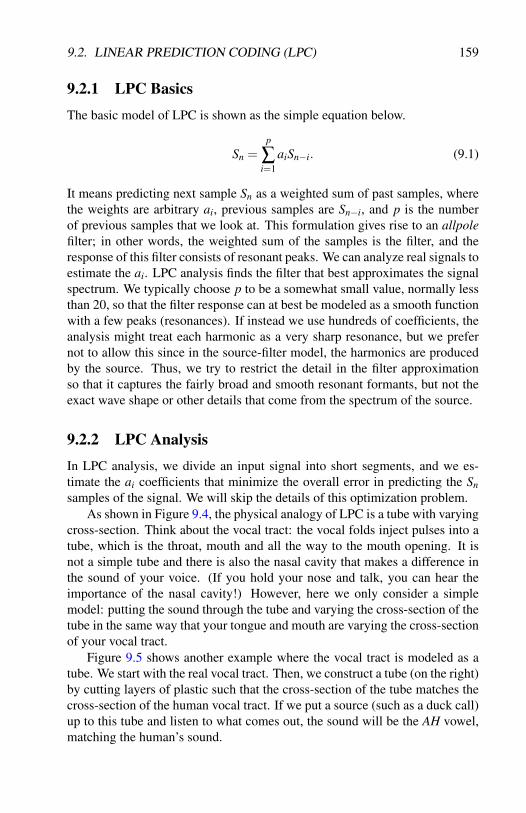
9.2. LINEAR PREDICTION CODING (LPC) 159
9.2.1 LPC BasicsThe basic model of LPC is shown as the simple equation below.
Sn =p
∑i=1
aiSn−i. (9.1)
It means predicting next sample Sn as a weighted sum of past samples, wherethe weights are arbitrary ai, previous samples are Sn−i, and p is the numberof previous samples that we look at. This formulation gives rise to an allpolefilter; in other words, the weighted sum of the samples is the filter, and theresponse of this filter consists of resonant peaks. We can analyze real signals toestimate the ai. LPC analysis finds the filter that best approximates the signalspectrum. We typically choose p to be a somewhat small value, normally lessthan 20, so that the filter response can at best be modeled as a smooth functionwith a few peaks (resonances). If instead we use hundreds of coefficients, theanalysis might treat each harmonic as a very sharp resonance, but we prefernot to allow this since in the source-filter model, the harmonics are producedby the source. Thus, we try to restrict the detail in the filter approximationso that it captures the fairly broad and smooth resonant formants, but not theexact wave shape or other details that come from the spectrum of the source.
9.2.2 LPC AnalysisIn LPC analysis, we divide an input signal into short segments, and we es-timate the ai coefficients that minimize the overall error in predicting the Snsamples of the signal. We will skip the details of this optimization problem.
As shown in Figure 9.4, the physical analogy of LPC is a tube with varyingcross-section. Think about the vocal tract: the vocal folds inject pulses into atube, which is the throat, mouth and all the way to the mouth opening. It isnot a simple tube and there is also the nasal cavity that makes a difference inthe sound of your voice. (If you hold your nose and talk, you can hear theimportance of the nasal cavity!) However, here we only consider a simplemodel: putting the sound through the tube and varying the cross-section of thetube in the same way that your tongue and mouth are varying the cross-sectionof your vocal tract.
Figure 9.5 shows another example where the vocal tract is modeled as atube. We start with the real vocal tract. Then, we construct a tube (on the right)by cutting layers of plastic such that the cross-section of the tube matches thecross-section of the human vocal tract. If we put a source (such as a duck call)up to this tube and listen to what comes out, the sound will be the AH vowel,matching the human’s sound.

160 CHAPTER 9. VOCAL AND SPECTRAL MODELS
Figure 9.4: The physical analogy of LPC: a tube with varying cross-section.
Figure 9.5: Acoustic Tube Producing “AH”. 1

9.2. LINEAR PREDICTION CODING (LPC) 161
Another important point here is that we are not talking about a fixed shapebut a shape that is rapidly changing, which makes speech possible. We aremaking sequences of vowel sounds and consonants by rapidly moving thetongue and mouth as well as changing the source sound. To apply LPC tospeech, we analyze speech sounds in short segments (and as usual, we callshort analysis segments frames). This is analogous to short-time windows inthe SFFT. At each LPC analysis frame, we re-estimate the geometry of thetube, which means we re-estimate the coefficient values that determine the fil-ter. Frames give rise to changing coefficients, which model changes in tubegeometry (or vocal tract shape).
LPC actually creates an inverse filter. Applying the inverse filter to a vocalsound yields a residual that sounds like the source signal. The residual may ei-ther be an estimate of glottal pulses, making the residual useful for estimatingthe pitch of the source, or noise-like.
Taking all this into account, an overall LPC analysis system is shown inFigure 9.6. We have an input signal and do formant analysis, which is theestimation of coefficients that can reconstruct the filter part of the source-filtermodel. After applying the result filter of the formant analysis to the inputsignal, we can get the residual and then do further analysis to detect the pitch.We can also do analysis to see if the input is periodic or not so that it gives us adecision of whether the input is voiced or unvoiced. Finally, we can computethe RMS amplitude of the signal. So, for each frame of LPS analysis, we getnot only the filter part of the source-filter model, but also estimated pitch, theamplitude, and whether the source is voiced or unvoiced.
9.2.3 Musical Applications
There are many musical applications of voice sounds and source-filter models.One common application pursued by many composers is to replace the sourcewith some other sound. For example, rather than having a pitched source ornoise source based on the human voice, you can apply human sounding for-mants to a recording of an orchestra to make it sound like speech. This idea oftaking elements from two different sounds and putting them together is some-times called “cross-synthesis.” You can also “warp” the filter frequencies toget human-like but not really human filters. Also, you can modify the sourceand LPC coefficients (glottal pulses or noise) to perform time stretching, slow-ing speech down or speeding up.

162 CHAPTER 9. VOCAL AND SPECTRAL MODELS
Figure 9.6: Diagram of LPC.
9.3 Vocoder
The Vocoder is related to LPC in that it makes a low-dimensional (i.e. smooth,very approximate) estimation of the spectral shape. Thus, formants can becaptured and modeled. The main idea of the vocoder is that the input signalis divided into frequency “channels” and bandpass filters are used to isolateeach channel and measure the amplitude in that channel. An FFT can be usedsince it acts as a bank of bandpass filters, but vocoders are also implementedin analog hardware with electronic filters, or you could use a bank of digitalbandpass filters instead of the FFT.
Vocoders are often used for cross-synthesis where the formants are esti-mated using one sound source (the “modulator”) and then applied to a secondsound source (the “carrier”). For example, one could analyze a voice to ex-tract formants and apply them to chords played on a keyboard. Figure 9.7illustrates a vocoder in this cross-synthesis application. The “ENV Follow”box takes a filtered signal and extracts an amplitude “envelope” that is used tomodulate the amplitude of the carrier using a “VCA”-voltage-controlled am-plifier. Only two frequency bands are shown, but a typical vocoder (even inhardware) would have 8 or more channels.
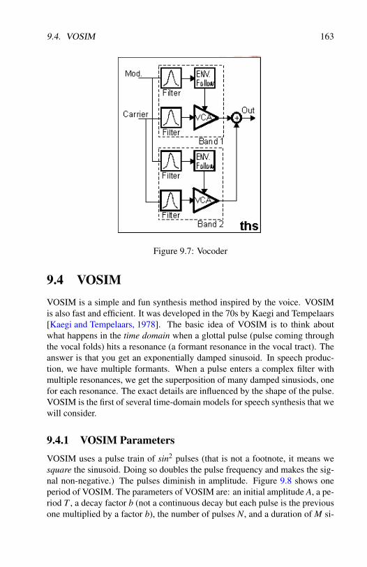
9.4. VOSIM 163
Figure 9.7: Vocoder
9.4 VOSIMVOSIM is a simple and fun synthesis method inspired by the voice. VOSIMis also fast and efficient. It was developed in the 70s by Kaegi and Tempelaars[Kaegi and Tempelaars, 1978]. The basic idea of VOSIM is to think aboutwhat happens in the time domain when a glottal pulse (pulse coming throughthe vocal folds) hits a resonance (a formant resonance in the vocal tract). Theanswer is that you get an exponentially damped sinusoid. In speech produc-tion, we have multiple formants. When a pulse enters a complex filter withmultiple resonances, we get the superposition of many damped sinusiods, onefor each resonance. The exact details are influenced by the shape of the pulse.VOSIM is the first of several time-domain models for speech synthesis that wewill consider.
9.4.1 VOSIM ParametersVOSIM uses a pulse train of sin2 pulses (that is not a footnote, it means wesquare the sinusoid. Doing so doubles the pulse frequency and makes the sig-nal non-negative.) The pulses diminish in amplitude. Figure 9.8 shows oneperiod of VOSIM. The parameters of VOSIM are: an initial amplitude A, a pe-riod T , a decay factor b (not a continuous decay but each pulse is the previousone multiplied by a factor b), the number of pulses N, and a duration of M si-

164 CHAPTER 9. VOCAL AND SPECTRAL MODELS
lence that follows the pulses. As you can see in Figure 9.8, the result is at leastsomewhat like a decaying sinusoid, and this gives an approximation of a pulsefiltered by a single resonance. The fundamental frequency (establishing thepitch) is determined by the entire period, which is NT +M and the resonantfrequency is 1/T , so we expect the harmonics near 1/T to be stronger.
Figure 9.8: Diagram of VOSIM.
9.4.2 VOSIM Application
In the original VOSIM paper, Tempelaars used various “delta” or “increment”parameters so that the continuous parameters T , M, and b could change overtime. This was probably just a simplification over using more general en-velopes to control change over time. The vosim extension in Nyquist (openthe Extension Manager in the NyquistIDE) contains some code and examples.
9.5 FOF Synthesis
FOF is a French acronym for “Formant Wave Function” (Synthesis). LikeVOSIM, FOF is a time-domain approach to creating formants and speech-likesounds. Compared to VOSIM, FOF can be seen as a more sophisticated andmore accurate model of a pulse train filtered by a resonant filter. Instead ofthe sine-squared pulses of VOSIM, FOF uses a sinusoid with an exponentialdecay (see Figure 9.9), and instead of just N pulses of the decaying resonantfrequency, FOF allows the sinusoid to decay to a very small amplitude. Thismight result in overlapping decaying sinusoids (recall that in VOSIM, N de-caying pulses are followed by M seconds of silence before the next pulse, so

9.5. FOF SYNTHESIS 165
pulses do not overlap.) This makes the implementation of FOF more difficult,and we will describe the implemenation below.
One final detail about FOF is that the decaying sinusoid has an initialsmooth rise time. The rise time gives some additional control over the re-sulting spectrum, as shown in Figure 9.10.
Figure 9.9: FOF
Figure 9.10: FOF in the frequency domain.
9.5.1 FOF AnalysisOne of the advantages of FOF synthesis is that FOF parameters can be ob-tained automatically. The basic approach is to analyze the spectrum of a soundwith an FFT. Then, analyse the shape of the FFT to detect formants. Use a FOFgenerator for each formant. If the spectrum indicates many harmonics, the firstharmonic or the spacing between harmonics can be used as the fundamentalperiod.

166 CHAPTER 9. VOCAL AND SPECTRAL MODELS
Since analysis can be performed using any spectrum, FOF is not limited tovoice synthesis, and FOF has been used for a wide range of sounds.
9.5.2 FOF SynthesisConsider the FOF signal shown in Figure 9.9. This represents the responseof a single formant to a single impulse – essentially a grain. Let’s assume wehave a FOF generator that can create this grain, probably using an envelopegenerator for the onset, a sine oscillator for the main signal, an exponentialdecay generator, and multipliers to combine them.
To model a periodic pulse, we need a pool of these FOF generators. Weallocate one for each formant at every pulse period and release the generatorsback to the pool when their output decays to a negligible value. The size of thepool depends on the amount of overlap (longer decays and higher fundamentalfrequencies mean more overlap), so the implementation may need to makethe pool size dynamically expandable or simply allocate every FOF generatorfrom the general memory heap.
Figure 9.11 illustrates a collection of FOF “grains:” at each pulse period(the fundamental frequency), there is one grain for each formant. The overlap-ping grains from FOF generators are summed to form a single output signal.
Figure 9.11: FOF synthesis.
9.6 Phase VocoderThe Phase Vocoder is not really a speech synthesis method but it is often usedto manipulate speech signals. The main assumption of the Phase Vocoder is

9.7. MCAULAY-QUATIERI (MQ) SYNTHESIS 167
that input sounds consist of fairly steady sinusoidal partials, there are relativelyfew partials and they are well-separated in frequency. If that is the case, thenwe can use the FFT to separate the partials into different bins (different coeffi-cients) of the discrete spectrum. Each frequency bin is assigned an amplitudeand phase. A signal is reconstructed using the inverse FFT (IFFT).
The main attraction of the phase vocoder is that by changing the spacing ofanalysis frames, the reconstructed signal can be made to play faster or slower,but without pitch changes because the partial frequencies stay the same. Timestretching without pitch change also permits pitch change without time stretch-ing! This may seem contradictory, but the technique is simple: play the soundfaster or slower (by resampling to a new sample rate) to make the pitch go upor down. This changes the speed as well, so use a phase vocoder to changethe altered speed back to the original speed. Now you have pitch change with-out speed change, and of course you can have any combination or even time-variable pitch and speed.
When successive FFT frames are used to reconstruct signals, there is thepotential that partials in one frame will be out of phase with partials in thenext frame and some cancellation will occur where the frames overlap. Thisshould not be a problem if the signal is simply analyzed and reconstructedwith no manipulation, but if we want to achieve a speed-up or slow-down ofthe reconstructed signal, then the partials can become out of phase.
In the Phase Vocoder, we use phase measurements to shift the phase of par-tials in each frame to match the phase in the previous frame so that cancellationdoes not occur. This tends to be more pleasing because it avoids the somewhatbuzzy sound of partials being amplitude-modulated at the FFT frame rate. Inreturn for eliminating the frame-rate discontinuities, the Phase Vocoder oftensmears out transients (by shifting phases more-or-less randomly), resulting ina sort of fuzzy or smeared quality, especially if frames are long. As we oftensee (and hear), there is a time-frequency uncertainty principle at play: shorterframes give better transient (time) behavior, and longer frames give better re-production of sustained timbres due to better frequency resolution.
9.7 McAulay-Quatieri (MQ) SynthesisMcAulay and Quatieri developed a speech compression technique where thesignal is decomposed into time-varying as well as amplitude-varying sinusoids[McAulay and Quatieri, 1986]. This differs from the phase vocoder mainly inthat with the phase vocoder, we assume all sinusoids are fixed in frequency andmatch the FFT bin frequencies.2 In contrast, MQ analysis tracks peaks from
2This is a bit of over-simplification. In fact, the phase change from frame to frame in the phasevocoder indicates small deviations from the center frequency of each bin, so the phase vocoder,

168 CHAPTER 9. VOCAL AND SPECTRAL MODELS
analysis frame to analysis frame and creates a description in which sinusoidscan change frequency dramatically. The analysis for MQ is quite differentfrom phase vocoder analysis. Reconstruction is also different and relies upona bank of sinusoid oscillators with frequency and amplitude controls. This isjust additive synthesis using sinusoids.
With MQ’s additive-synthesis representation, time stretching and frequencyshifting are easily accomplished just by scaling the amplitude and frequencycontrol functions. The reconstruction does not involve the IFFT or overlap-ping windows, so there are no problems with frames or phase discontinuities,i.e. no “buzz” at the frame rate.
Some limitations of MQ are that it takes large numbers of sinusoids tomodel noise sounds. Also, resonances are not modeled (similar to phasevocoder), so one cannot easily treat resonance details as control parameters.Because it uses additive synthesis, MQ is not particularly efficient or flexi-ble. With source-filter models, we saw how one could replace the source tocreate a “cross-synthesis” model, but there is no obvious way to achieve cross-synthesis with MQ.
9.8 Spectral Modeling Synthesis (SMS)
Spectral Modeling Synthesis (SMS) was developed by Xavier Serra in hisPh.D. thesis work and continued in the Music Technology Group, Audiovi-sual Institute, Pompeu Fabra University, Barcelona. SMS extends MQ analy-sis/synthesis with an explicit model for noise. The model is shown in Figure9.12.
You can see the box labeled “additive synthesis” and this essentially out-puts a resynthesis of the input signal using MQ analysis/synthesis. Rather thanstopping there, SMS subtracts this resynthesis from the input signal to obtaina residual signal. Assuming that most of the spectral peaks representing si-nusoidal partials have been modeled, the subtraction removes them and theresidual should contain mostly noise. The “spectral fitting” stage constructsa low-dimensional (i.e. few coefficients) description of the spectrum of thisresidual. SMS considers the sinusoidal tracks to be the “deterministic” partof the signal, and the residual noise spectrum to be the “stocastic” part of thesignal.
Resynthesis is accomplished by additive synthesis of the sinusoidal tracks(as in MQ synthesis) and adding filtered noise, using the “stocastic” coeffi-cients to control the noise filter. As with many synthesis techniques, one can
when properly implemented, is modeling frequencies accurately, but the model is still one wherepartial frequencies are modeled as fixed frequencies.

9.9. SUMMARY 169
time stretch and manipulate all the control parameters. The noise modeling inSMS allows for more accurate reconstruction as well as control over how muchof the noise in the signal should be retained (or for that matter emphasized) insynthesis.
Figure 9.12: Spectral Modeling Synthesis (SMS)
9.9 Summary
We have considered many approaches to voice modeling and synthesis. Thenumber of methods is some indication of the broad attraction of the humanvoice in computer music, or perhaps in all music, considering the prevalence ofvocals in popular music. The source-filter model is a good way to think aboutsound production in the voice: a source signal establishes the pitch, amplitudeand harmonicity or noisiness of the voice, and more-or-less independently,formant filters modify the source spectrum to impose resonances that we canperceive as vowel sounds.
LPC and the Vocoder are examples of models that actually use resonantfilters to modify a source sound. These methods are open to interesting cross-synthesis applications where the source sound of some original vocal sound isreplaced by another, perhaps non-human, sound.
Resonances can also be modeled in the time domain as decaying sinusoids.VOSIM and FOF synthesis are the main examples. Both can be seen as related

170 CHAPTER 9. VOCAL AND SPECTRAL MODELS
to granular synthesis, where each source pulse creates new grains in the formof decaying sinusoids, one to model each resonance.
In the spectral domain, the Phase Vocoder is a powerful method that isespecially useful for high-quality time-stretching without pitch change. Time-stretching also allows us to “undo” time stretch due to resampling, so we canuse the Phase Vocoder to achieve pitch shifting without stretching. MQ analy-sis and synthesis models sounds as sinusoidal tracks that can vary in amplitudeand frequency, and it uses addition of sinusoidal partials for synthesis. Spec-tral Modeling Synthesis (SMS) extends MQ analysis/synthesis by modelingnoise separately from partials, leading to a more compact representation andoffering more possibilities for sound manipulation.
Although we have focused on basic sound production, the voice is com-plex, and singing involves vibrato, phrasing, actual speech production beyondvowel sounds, and many other details. Undoubtedly, there is room for moreresearch and for applying recent developments in speech modeling to musicalapplications. At the same time, one might hope that the speech communitycould become aware of sophisticated control and modeling techniques as wellas the need for very high quality signals arising in the computer music com-munity.

Chapter 10
Acoustics, Perception,Effects
Topics Discussed: Pitch vs. Frequency, Loudness vs. Amplitude, Lo-calization, Linearity, Reverberation, Echo, Equalization, Chorus, Panning,Dynamics Compression, Sample-Rate Conversion, Convolution Reverber-ation
10.1 IntroductionAcoustics and perception are very different subjects: acoustics being aboutthe physics of sound and perception being about our sense and cognitive pro-cessing of sound. Though these are very different, both are very importantfor computer sound and music generation. In sound generation, we generallystrive to create sounds that are similar to those in the real world, sometimes us-ing models of how sound is produced by acoustic instruments. Alternatively,we may try to create sound that will cause a certain aural impression. Some-times, an understanding of physics and perception can inspire sounds that haveno basis in reality.
Sound is vibration or air pressure fluctuations (see Figure 10.1). We canhear small pressure variations, e.g. 0.001 psi (lbs/in2) for loud sound. (We arepurposefully using English units of pounds and inches because if you inflate abicycle tire or check tires on an automobile – at least in the U.S. – you mighthave some idea of what that means.) One psi ∼= 6895 Pascal (Pa), so 0.001psi is about 7 Pascal. At sea level, air pressure is 14.7 pounds per square inch,while the cabin pressure in an airplane is about 11.5 psi, so 0.001 (and remem-ber that is a loud sound) is a tiny tiny fraction of the nominal constant pressurearound us. Changes in air pressure deflect our ear drum. The amplitude of de-
171

172 CHAPTER 10. ACOUSTICS, PERCEPTION, EFFECTS
Figure 10.1: Sound is vibration or air pressure fluctuations.(credit: mediacollege.com)
flection of ear drum is about diameter of hydrogen atom for the softest sounds.So we indeed have a extremely sensitive ears!
What can we hear? The frequencies that we hear range over three orders ofmagnitude from about 20 to 20 kHz. As we grow older and we are exposed toloud sounds, our high frequency hearing is impaired, and so the actual rangeis typically less.
Our range of hearing, in terms of loudness, is about 120 dB, which ismeasured from threshold of hearing to threshold of pain (discomfort from loudsounds). In practical terms, our dynamic range is actually limited and oftendetermined by background noise. Listen to your surroundings right now andlisten to what you can hear. Anything you hear is likely to mask even softersounds, limiting your ability to hear them and reducing the effective dynamicrange of sounds you can hear.
We are very sensitive to the amplitude spectrum. Figure 10.2 shows a spec-tral view that covers our range of frequency, range of amplitude, and suggeststhat the shape of the spectrum is something to which we are sensitive.
Real-world sounds are complex. We have seen many synthesis algorithmsthat produce very clean, simple, specific spectra and waveforms. These canbe musically interesting, but they are not characteristic of sounds in the “realworld.” This is important; if you want to synthesize musical sounds that arepleasing to the ear, it is important to know that, for example, real-world soundsare not simple sinusoids, they do not have constant amplitude, and so on.
Let’s consider some “real-world” sounds. First, noisy sounds, such as thesound of “shhhh,” tend to be broadband, meaning they contain energy at al-most all frequencies, and the amount of energy in any particular frequency, orthe amplitude at any particular time, is random. The overall spectrum of noisysounds looks like the top spectrum in Figure 10.3.

10.1. INTRODUCTION 173
Figure 10.2: The actual spectrum shown here is not important, but the graphcovers the range of audible frequencies (about 20KHz) and our range of am-plitudes (about 120 dB). We are very sensitive to the shape of the spectrum.
Percussion sounds on the other hand, such as a thump, bell clang, ping, orknock, tend to have resonances, so the energy is more concentrated around cer-tain frequencies. The middle picture of Figure 10.3 gives the general spectralappearance of such sounds. Here, you see resonances at different frequen-cies. Each resonance produces an exponentially decaying sinusoid. The decaycauses the spectral peak to be wider than that of a steady sinusoid. In general,the faster the decay, the wider the peak. It should also be noted that, dependingon the material, there can be non-linear coupling between modes. In that case,the simple model of independent sinusoids with exponential decay is not exactor complete (but even then, this can be a good approximation.)
Figure 10.4 shows some modes of vibration in a guitar body. This is the topof an acoustic guitar, and each picture illustrates how the guitar top plate flexesin each mode. At the higher frequencies (e.g. “j” in Figure 10.4), you can seepatches of the guitar plate move up while neighboring patches are move down.If you tap a guitar body, you will “excite” these different modes and get acollection of decaying sinusoids. The spectrum might look something like themiddle of Figure 10.3. (When you play a guitar, of course, you are strummingstrings that have a different set of modes of vibration that give sharper peaksand a clearer sense of pitch.)
Pitched sounds are often called tones and tend to have harmonically related

174 CHAPTER 10. ACOUSTICS, PERCEPTION, EFFECTS
Figure 10.3: Some characteristic spectra. Can you identify them? Horizontalaxis is frequency. Vertical axis is magnitude (amplitude). The top representsnoise, with energy at all frequencies. The middle spectrum represents a per-cussion sound with resonant or “characteristic” frequencies. This might be abell sound. The bottom spectrum represents a musical tone, which has manyharmonics that are multiples of the first harmonic, or fundamental.
Figure 10.4: Modes of vibration in an acoustic guitar body.(credit: http://michaelmesser.proboards.com/thread/7581/resonator-cone-physics)

10.2. PERCEPTION: PITCH, LOUDNESS, LOCALIZATION 175
sinusoids. For example, an “ideal” string has characteristic frequencies thatform a harmonic series, as illustrated in Figure 10.5. This can be seen as aspecial case of vibrating objects in general, such as the guitar body (Figure10.4.) The vibrating string just happens to have harmonically related modefrequencies.
Figure 10.5: Modes of vibration in a stretched string. In an “ideal” string, thecharacteristic frequencies are multiples of the frequency of the first mode. Themodes of vibration are independent, so the “sound” of the string is formed bythe superposition of all the vibrating modes, resulting in a harmonic spectrum.(credit: phycomp.technion.ac.il)
We know from previous discussions that if the signal is purely periodic,then it has harmonically related sinusoids. In other words, any periodic signalcan be decomposed into a sum of sinusoids that are all multiples of somefundamental frequency. In physical systems, periodicity is characteristic ofsome kind of mechanical oscillator that is driven by an outside energy source.If you bow a string, sing a tone, or blow into a clarinet, you drive an oscillatorwith a constant source of energy, and almost invariably you end up with astable periodic oscillation.
In summary, there are two ways to obtain harmonic or near-harmonic par-tials that are found in musical tones: One is to strike or pluck an object thathas modes of vibration that just happen to resonate at harmonic frequencies.An example is a piano string or chime. The other is to drive oscillation with asteady input of energy, as in a bowed string or wind instrument, giving rise to aperiodic signal. In addition to these sounds called “tones,” we have inharmonicspectra and noisy spectra.
10.2 Perception: Pitch, Loudness, LocalizationHaving focused mainly on physical properties of sound and sound sources, wenow our attention to our perception of sound. It is important to keep in mind

176 CHAPTER 10. ACOUSTICS, PERCEPTION, EFFECTS
that our perception does not directly correspond to the underlying physicalproperties of sound. For example, two sounds with the same perceived loud-ness might have very different amplitudes, and two pitch intervals perceivedto be the same musically could be not at all the same in terms of frequencydifferences.
10.2.1 Pitch PerceptionPitch is fundamental to most music. Where does it come from? How sensitiveare ears to pitch? Our sense of pitch is strongly related to frequency. Higherfrequencies mean higher pitch. Our sense of pitch is enhanced by harmonicspartials. In fact, the connection is so strong that we are unable to hear indi-vidual partials. In most cases, we collect all of these partials into a single tonethat we percieve as a single pitch, that of the lowest partial.
Pitch perception is approximately logarithmic, meaning that when pitchdoubles, you hear the pitch interval of one octave. When it doubles again, youhear the same interval even though now the frequency is four times as high.If we divide the octave (factor of 2 in frequency) into 12 log-spaced intervals,we get what are called musical semitones or half-steps. This arrangement of12 equal ratios per octave (each one 12√2) is the basis for most Western music,as shown in the keyboard (Figure 10.6).
Figure 10.6: A piano keyboard. The ratio between frequencies of adjacentkeys is 12√2. (credit: http://alijamieson.co.uk/2017/12/03/describing-relationship-two-notes/)
We can divide a semitone ( 12√2) into 100 log-spaced frequency intervalscalled cents. Often cents are used in studies of tuning and intonation. We aresensitive to about 5 cents, which is a ratio of about 0.3%. No wonder it is sohard for musicians to play in tune!
10.2.2 AmplitudeThe term pitch refers to perception while frequency refers to objective or phys-ical repetition rates. In a similar way, loudness is the perception of intensity

10.2. PERCEPTION: PITCH, LOUDNESS, LOCALIZATION 177
or amplitude of sound. Here, we introduce some terminology and units ofmeasurement for amplitude. Below, we will return to the topic of loudness.
There are multiple ways of defining amplitude. One definition is: “a mea-sure of a periodic function’s change over a single period.” Figure 10.7 illus-trates the three different ways amplitude may be measured:
1. The peak amplitude
2. The peak-to-peak amplitude
3. The root mean square (RMS) amplitude
Figure 10.7: Three different ways of measuring amplitude. Note: the 4 on theFigure indicates the length of one period. credit: Wikipedia
In specifying amplitude in code, we are mostly using the peak amplitude ofa signal. Thus, the amplitude of a sine wave, y = sin(t), is 1, and the amplitudeof y = 2cos(t) is 2. When we multiply an oscillator in Nyquist by an envelope,we’re varying the amplitude of that oscillator over time.
Volume
There is no one formal definition for what the volume of sound means. Gener-ally, volume is used as a synonym for loudness. In music production, adjustingthe volume of a sound usually means to move a volume fader on e.g. a mixer.Faders can be either linear or logarithmic, so again, it is not exactly clear whatvolume means (i.e. is it the fader position, or the perceived loudness?).
Power
Power is the amount of work done per unit of time; e.g. how much energyis transferred by an audio signal. Hence, the average power P̄ is the ratio ofenergy E to time t: P̄ = E/t. Power is usually measured in watts (W); which
178 CHAPTER 10. ACOUSTICS, PERCEPTION, EFFECTS
are joules (J) per second: J/s=W . The power of a sound signal is proportionalto the squared amplitude of that signal. Note that in terms of relative poweror amplitude, it does not really matter whether we think of amplitude as theinstantaneous amplitude (i.e. the amplitude at a specific point in time), or thepeak, the peak-to-peak, or the root mean square amplitude over a single period.It makes no significant difference to ratios.
Pressure
In general, the pressure p is the amount of force F applied perpendicularly(normal) to a surface area divided by the size a of that area: p = F/a. Pressureis normally measured in pascal (Pa), which is newtons (N) per square meter.Thus, Pa = N/m2.
Intensity
Intensity I is the energy E flowing across a unit surface area per unit of time t:I = E
a1t . For instance, the energy from a sound wave flowing to an ear. As the
average power P̄ = E/t, we can express the intensity as I = P̄/a, meaning thepower flowing across a surface of area a. The standard unit area is one squaremeter, and therefore we measure intensity in W/m2; i.e. watts per squaremeter.
Range of Human Hearing
Just as the frequency range of the human ear is limited, so is the range ofintensity. For a very sensitive listener, and a 1 kHz frequency:
• The threshold of hearing th = 10−12W/m2
• The limit of hearing lh = 1W/m2 (the threshold of pain).
The perceptual range of intensity for a 1 kHz frequency is an impressivelh/th = 1/10−12 = 1012, or a trillion to one.
The Bel Scale
Bel (B) is a sound intensity scale named in honor of the renowned AlexanderGraham Bell (1847-1922). Given the enormous range of human hearing, onebel is defined as a factor of 10 in intensity or power, and thus we get:
lhth
= log101
10−12W/m2 = 12Bel
In other words, bel is the log ratio of intensity or power.

10.2. PERCEPTION: PITCH, LOUDNESS, LOCALIZATION 179
The Decibel Scale (dB)
Using just a range of 12 to express the entire range of hearing is inconvenient,so it is customary to use decibels, abbreviated dB, instead:
10log10lhth
= 10log101
10−12W/m2 = 120dB
Hence, the intensity range of human hearing is 120 dB.
Decibels for Comparing Sound Intensity Levels
Decibels can be used to compare the intensity levels of two sounds. We cantake the intensity I of some sound and compare it to a reference intensity Ire f :
10 log10I
Ire f
So for example, instead of using th as the reference intensity, we could usethe limit of hearing lh, and thus measure down from pain instead of measuringup from silence.
Decibels for Comparing Amplitude Levels
A common confusion arises when working with intensity and amplitudes. Wejust saw that given an intensity ratio r, we can express the ratio in decibelsusing 10log10 r. This also works for a ratio of power because power and in-tensity are proportional. However, when we are working with amplitudes, thisformula does not apply. Why? Because decibels is a measure of power or in-tensity ratio. Since power is proportional to the square of amplitude, a differentformula must be used for amplitudes. For two amplitudesA and B, we can usethe power formula if we square them. Then we can simplify the expression:
dB = 10log10A2
B2 = 10log10(AB)2 = 20log10
AB
Main idea: for power or intensity we use 10log10 ratio, but for amplitudes,we must use 20log10 ratio.
Other dB Variants
You see the abbreviaton dB in many contexts.
• dBa uses the so-called A-weighting to account for the relative loudnessperceived by the human ear; based on equal-loudness contours.
180 CHAPTER 10. ACOUSTICS, PERCEPTION, EFFECTS
• dBb and dBc are similar to dBa, but apply different weightingschemes.
• dBm (or dBmW ) is the power ratio in dB of a measured power refer-enced to one milliwatt (mW); used e.g. in radio, microwave and fiberoptic networks as a measure of absolute power.
• dB SPL – see below.
Amplitude and Gain in Recording Equipment
In a music studio, we usually want to measure down from the limit of theloudest sound that can be recorded without introducing distortion from therecording equipment. This is why it is standard for e.g. mixing consoles andmusic software to use volume faders and meters that show negative dB. In thiscontext, 0 dB is the upper limit for recording without distortion; let’s call it thelimit of recording = lr. Hence, the loudest sound we may record without anydistortion has intensity I = lr, and the corresponding dB is 10log10
lrlr= 0 dB.
Note that it is customary for producers of recording gear to leave some amountof head room at the top of this scale to safeguard against distortion, which iswhy you’ll see some positive dB values above 0 dB on meters and faders.
Sound Pressure
Measuring the intensity of a sound signal is usually not practical (or possible);i.e. measuring the energy flow over an area is tricky. Fortunately, we canmeasure the average variation in pressure. Pressure is the force applied normalto a surface area, so if we sample a sufficiently large area we’ll get a decentapproximation; this is exactly what a microphone does!
It is worth noting that we can relate sound pressure to intensity by thefollowing ratio,
∆p2
V δ
where ∆p is the variation in pressure, V is the velocity of sound in air, and δ
is the density of air. What this tells us is that intensity is proportional to thesquare of the variation in pressure.
dB SPL (Sound Pressure Level)
Sound pressure level is defined as the average pressure variation per unit area.The dB SPL is defined as 20log10
PP0
, where the reference pressure, P0, is0.00005 Pa, which is approximately the threshold of hearing at 1 kHz.

10.2. PERCEPTION: PITCH, LOUDNESS, LOCALIZATION 181
The Microphone: Measuring Sound Pressure
Most microphones use electromagnetic induction to transform the sound pres-sure applied to a diaphragm into an electrical signal; as shown in Figure 10.8.
Figure 10.8: Microphone. Credit: infoplease.com
For more information on loudness, dB, intensity, pressure etc., see Musi-mathics Vol. 1 [Loy, 2011].
10.2.3 Loudness
Loudness is a perceptual concept. Equal loudness does necessarily result fromequal amplitude because the human ear’s sensitivity to sound varies with fre-quency. This sensitivity, the loudness, is depicted in equal-loudness contoursfor the human ear; often referred to as the Fletcher-Munson curves. Fletcherand Munson’s data were revised to create an ISO standard. Both are illus-trated in Figure 10.9 below. Each curve traces changes in amplitude requiredto maintain equal loudness as the frequency of a sine tone varies. In otherwords, each curve depicts amplitude as a function of frequency at a constantloudness level.
Loudness is commonly measured in phons.

182 CHAPTER 10. ACOUSTICS, PERCEPTION, EFFECTS
Figure 10.9: Equal-loudness contours (left-most / red) from ISO 226:2003revision. So-called Fletcher-Munson curves, as measured by Robinson andDadson, shown (right-most / black) for comparison. credit: http://hyperphysics.phy-astr.gsu.edu/hbase/Sound/eqloud.html
Phon
Phon expresses the loudness of a sound in terms of a reference loudness. Thatis, the phon level of a sound, A, is the dB SPL (defined earlier) of a referencesound—of frequency 1 kHz—that has the same (perceived) loudness as A.Zero phon is the limit of audibility of the human ear; inaudible sounds havenegative phon levels.
Rules of Thumb
Loudness is mainly dependent on amplitude, and this relationship is approx-imately logarithmic, which means equal ratios of amplitude are more-or-lessperceived as equal increments of loudness. We are very sensitive to small ra-tios of frequency, but we are not very sensitive to small ratios of amplitude. Todouble loudness you need about a 10-fold increase in intensity or about 20 dB.We are sensitive to about 1 dB of amplitude ratio. 1 dB is a change of about12%.
The fact that we are not so sensitive to amplitude changes is important tokeep in mind when adjusting amplitude. If you synthesize a sound and it istoo soft, try scaling it by a factor of 2. People are often tempted to make smallchanges, e.g. multiply by 1.1 to make something louder, but in most cases, a

10.2. PERCEPTION: PITCH, LOUDNESS, LOCALIZATION 183
10% change is not even audible.Loudness also depends on frequency because we are not so sensitive to
very high and very low frequencies. The Fletcher-Munson Curve contoursshown above are lowest around 4 kHz where we are most sensitive. The curveis low here because a low amplitude at 4 kHz sounds as loud as higher ampli-tudes at other frequencies. As we move to even higher frequencies over on theright, we become less sensitive once again. The curves trace the combinationsof frequency and amplitude that sound equally loud. If you sweep a sinusoidfrom low frequency to high frequency at equal amplitude, you will hear thatthe sound appears to get louder until you hit around 4 kHz, and then the soundbegins to get quieter. Depending on how loud it is, you might stop hearing itat some point before you hit 20 kHz, even if you can hear loud sounds at 20kHz.
The red (or gray) lines in Figure 10.9 show an update to the Fletcher-Munson Curve based on new measurements of typical human hearing. Itshould be noted that these curves are based on sinusoids. In most music, lowpitches actually consist of a mixture of harmonics, some of which can haverather high frequencies. So even if you cannot hear the fundamental becauseit is too low or too quiet, you might hear the pitch, which is implied by theupper partials (to which you are more sensitive). This is also why, on yourlaptop, you can hear a piano tone at the pitch C2 (below the bass clef, with afundamental frequency of about 65 Hz), even though your laptop speaker isbarely able to produce any output at 65 Hz. You might try this SAL command,which plays a piano tone followed by a sine tone:
play seq(note(pitch: c2), osc(c2))
It is instructive to listen to this using a quiet volume setting with good head-phones. You should hear the two tones at the same pitch. Then, listen to thesame sounds on your built-in laptop speaker. You will probably not hear thesecond tone, indicating that your computer cannot produce frequencies thatlow. And yet, the pitch of the first tone, even with no fundamental frequencypresent retains the same pitch!
10.2.4 LocalizationLocalization is the ability to perceive direction of the source of a sound andperhaps the distance of that sound. We have multiple cues for localization,including relative amplitude, phase or timing, and spectral effects of the pinnae(outer ears). Starting with amplitude, if we hear something louder in our rightear than our left ear, then we will perceive that the sound must be coming fromthe right, all other things be equal.

184 CHAPTER 10. ACOUSTICS, PERCEPTION, EFFECTS
We also use relative phase or timing for localization: if we hear somethingarrive earlier in our right ear than our left ear, then we will perceive that soundas coming from the right.
The third cue is produced by our pinnae or outer ears. Sound reflects offthe pinnae, which are very irregularly shaped. These reflections cause somecancellation or reinforcement at particular wavelengths, depending on the di-rection of the sound source and the orientation of our head. Even though wedo not know the exact spectrum of the source sound, our amazing brain is ableto disentangle all this information and compute something about localization.This is especially important for the perception of elevation, i.e. is the soundcoming from ahead or above? In either case, the distance to our ears is thesame, so whether the source is ahead or above, there should be no differencein amplitude or timing. The only difference is in spectral changes due to ourouter ears and reflections from our shoulders.
All of these effects or cues can be described in terms of filters. Taken to-gether, these effects are sometimes called the HRTF, or Head-Related TransferFunction. (A “transfer function” describes the change in the spectrum fromsource to destination.) You might have seen some artificial localization sys-tems, including video games and virtual reality application systems based onHRTF. The idea is, for each source to be placed in a virtual 3D space, computean appropriate HRTF and apply that to the source sound. There is a differentHRTF for the left ear and right ear, and typically the resulting stereo signal ispresented through headphones. Ideally, the headphones are tracked so that theHRTFs can be recomputed as the head turns and the angles to virtual sourceschange.
Environmental cues are also important for localization. If sounds reflect offwalls, then you get a sense of being in a closed space, how far away the wallsare, and what the walls are made of. Reverberation and ratio of reverberationto direct sound are important for distance estimation, especially for computermusic if you want to create the effect of a sound source fading off into thedistance. Instead of just turning down the amplitude of the sound, the director dry sound should diminish faster than the reverberation sound to give theimpression of greater distance.
Finally, knowledge of the sound source, including vision, recognition etc.is very important to localization. For example, merely placing a silent loud-speaker in front of a listener wearing headphones can cause experimental sub-jects to localize sound at the loudspeaker, ignoring whatever cues are presentin the actual sound!

10.2. PERCEPTION: PITCH, LOUDNESS, LOCALIZATION 185
10.2.5 More AcousticsThe speed of sound is about 1 ft/ms. Sound travels at different speeds at differ-ent altitudes, different temperatures and different humidities, so it is probablymore useful to have a rough idea of the speed of sound than to memorize aprecise number. (But for the record, the speed of sound is 343 m/s in dry air at20° C.) Compared to the speed of light, sound is painfully slow. For example,if you stand in front of a wall and clap, you can hear that the sound reflectsfrom the wall surfaces, and you can perceive the time for the clap to travelto the wall and reflect back. Our auditory system merges multiple reflectionswhen they are close in time (usually up to about 40 ms), so you do not perceiveechoes until you stand back 20 feet or so from the reflecting wall.
In most listening environments, we do not get just one reflection, calledan echo. Instead, we get a diffuse superposition of millions of echos as soundscatters and bounces between many surfaces in a room. We call this reverber-ation. In addition to reflection, sound refracts (bends around objects). Wave-lengths vary from 50 feet to a fraction of an inch, and diffraction is morepronounced at lower frequencies, allowing sound to bend around objects.
Linearity is a very important concept for understanding acoustics. Let’sthink about the transmission of sounds from the source of sound to the listener.We can think of the whole process as a function F shown in the equationsbelow, where y = F(x) means that source x is transformed by the room into yat the ear of the listener. Linearity means that if we increase the sound at thesource, we will get a proportional increase at the listening side of channel F .Thus, F(ax) = aF(x). The other property, sometimes called the superposition,is that if we have two sources: pressure signals x1 and x2, and play them at thesame time, then the effect on the listener will be the sum of individual effectfrom x1 and x2:
F(ax) = aF(x), F(x1 + x2) = F(x1)+F(x2)
Why does linearity matter? First, air, rooms, performance spaces are verylinear. Also, many of processes we used on sounds such as filters are designedto be linear. Linearity means that if there are two sound sources playing at thesame time, then the signal at the listening end is equivalent to what you getfrom one sound plus what you get from the other sound. Another interestingthing about linearity is that we can decompose a sound into sinusoids or com-ponents (i.e. compute the Fourier transform). If we know what a linear systemdoes to each one of those component frequencies, then by the superpositionprinciple, we know what the system does to any sound, because we can: breakit up into component frequencies, compute the transfer function at each of thefrequencies and sum the results together. That is one way of looking at whata filter does. A filter associates different scale factors with each frequency,

186 CHAPTER 10. ACOUSTICS, PERCEPTION, EFFECTS
and because filters are linear, they weight or delay frequencies differently butindependently. If we add two sounds and put them through the filter, the resultis equivalent to putting the two sounds through the filter independently andsumming the results.
10.2.6 Summary: Acoustics and PerceptionNow we summarize this discussion of acoustics and perception. Acousticsrefers to the physics of sound, while perception concerns our sense of sound.As summarized in Figure 10.10, pitch is the perception of (mainly) frequency,and loudness is the perception (mainly) of amplitude or intensity. Our percep-tion of pitch and loudness is roughly logarithmic with frequency and ampli-tude. This relationship is not exact, and we saw in the Fletcher-Munson Curvethat we are more sensitive to some frequencies than others. Generally, every-thing else we perceive is referred to as timbre, and you can think of timbre as(mainly) the perception of spectral shape. In addition to these properties, wecan localize sound in space using various cues that give us a sense of directionand distance.
Figure 10.10: A comparison of concepts and terms from perception (left col-umn) to acoustics (right column).
Struck objects typically exhibit characteristic frequencies with exponentialdecay rates (each mode of vibration has its own frequency and decay). Incontrast, driven oscillators typically exhibit almost exactly periodic signalsand hence harmonic spectra.
Our discussion also covered the speed of sound (roughly 1 ft/ms), trans-mission of sound as equivalent to filtering and the superposition principle.
10.3 Effects and Reverberation in NyquistThere are a lot of effects and processes that you can apply to sound withNyquist. Some are described here, and you can find more in the Nyquist Refer-ence Manual. There are also many sound processing functions you can installwith the Nyquist Extension Manager (in the NyquistIDE).

10.3. EFFECTS AND REVERBERATION IN NYQUIST 187
10.3.1 Delay or EchoIn Nyquist, we do not need any special unit generator to implement delay. Wecan directly create delay simply by adding sounds using an offset. Recall thatNyquist sounds have a built-in starting time and duration which are both im-mutable, so applying a shift operator to a sound does not do anything. How-ever, the cue behavior takes a sound as parameter and returns a new soundthat has been shifted according to the environment. So we usually combinecue with the shift operator @, and a delay expression has the form:
cue(sound) @ delay
10.3.2 Feedback DelayAn interesting effect is to not only produce an echo, but to add an attenuatedcopy of the output back into the input of the effect, producing a series of echoesthat die away exponentially. There is a special unit generator in Nyquist calledfeedback-delay with three parameters: feedback-delay(sound, delay,feedback). Figure 10.11 shows the echo algorithm: The input comes in andis stored in memory in a first-in-first-out (FIFO) queue; samples at the endof the buffer are recycled by adding them to the incoming sound. This is anefficient way to produce many copies of the sound that fade away. The delayparameter must be a number (in seconds). It is rounded to the nearest sampleto determine the length of the delay buffer. The amount of feedback should beless than one to avoid an exponential increase in amplitude.
Figure 10.11: Echo algorithm in Nyquist.
Note that the duration of the output of this unit generator is equal to theduration of the input, so if the input is supposed to come to an end and thenbe followed by multiple echos, we need to append silence to the input sourceto avoid a sudden ending. The example below uses s-rest() to construct 10seconds of silence, which follows the sound.
feedback-delay(seq(sound, s-rest(10)), delay, feedback)
In principle, the exponential decay of the feedback-delay effect never ends,so it might be prudent to use an envelope to smoothly bring the end of thesignal to zero:

188 CHAPTER 10. ACOUSTICS, PERCEPTION, EFFECTS
feedback-delay(seq(sound, s-rest(10)), delay, feedback) *pwlv(1, d + 9, 1, d + 10, 0)
, where d is the duration of sound. The sound is extended with 10 seconds ofsilence, so the envelope remains at 1 for the sound duration plus 9 seconds,then linearly falls to zero at sound duration + 10.
10.3.3 Comb FilterConsider a feedback delay with a 10 ms delay. If the input is a sinusoid with10 ms period (100 Hz), the echoes superimpose on one another and boost theamplitude of the input. The same happens with 200 Hz, 300 Hz, 400 Hz, etc.sinusoids because they all repeat after 10 ms. Other frequencies will produceechoes that do not add constructively and are not boosted much. Thus, thisfeedback delay will act like a filter with resonances at multiples of a funda-mental frequency, which is the reciprocal of the delay time. The frequencyresponse of a comb filter looks like Figure 10.12. Longer decay times givesthe comb filter sharper peaks, which means the output has a more definite pitchand longer “ring.”
Figure 10.12: Filter response of a comb filter. The horizontal axis is frequencyand the vertical axis is amplitude. The comb filter has resonances at multiplesof some fundamental frequency.
The code below shows how to apply a comb filter to sound in Nyquist. Acomb filter emphasizes (resonates at) frequencies that are multiples of a hz.The decay time of the resonance is given by decay. The decay may be a soundor a number. In either case, it must also be positive. The resulting sound willhave the start time, sample rate, etc. of sound. One limitation of comb is thatthe actual delay will be the closest integer number of sample periods to 1/hz, sothe resonance frequency spacing will one that divides the sample rate evenly.
comb(sound, decay, hz)
10.3.4 EqualizationEqualization is generally used to adjust spectral balance. For example, wemight want to boost the bass, or boost the high frequencies, or cut some objec-

10.3. EFFECTS AND REVERBERATION IN NYQUIST 189
tionable frequencies in the middle range. The function nband(input, gains)takes an array of gains, one for each band, where the bands are evenly dividedacross the 20–20kHz range. An interesting possibility is using computed con-trol functions to make the equalization change over time.
The Equalizer Editor in Nyquist provides a graphical equalizer interfacefor creating and adjusting equalizers. It has a number of sliders for differentfrequency bands, and you can slide them up and down and see graphicallywhat the frequency response looks like. You can use this interface to createfunctions to be used in your code. Equalizers are named eq-0, eq-1, etc.,and you select the equalizer to edit using a pull-down menu. The “Set” buttonshould be use to record changes.
The following expression in Nyquist is a fixed- or variable-parameter,second-order midrange equalization (EQ) filter:
eq-band(signal, hz, gain, width)
The hz parameter is the center frequency, gain is the boost (or cut) in dB, andwidth is the half-gain width in octaves. Alternatively, hz, gain, and width maybe sounds, but they must all have the same sample rate, e.g. they should allrun at the control rate or at the sample rate.
You can look up filters in the Nyquist manual for many more filters andoptions.
10.3.5 ChorusThe chorus effect is a very useful way to enrich a simple and dry sound. Es-sentially, the “chorus” effect is a very short, time-varying delay that is addedto the original sound. Its implementation is shown in Figure 10.13. The orig-inal sound passes through the top line, while a copy of the sound with someattenuation is added to the sound after a varying delay, which is indicated bythe diagonal arrow.
Figure 10.13: Chorus effect algorithm. A signal is mixed with a delayed copyof itself. The delay varies, typically by a small amount and rather slowly.
To implement chorus in Nyquist, you need to first load librarytime-delay-fns1 and then call the chorus function as shown below.
1In the future, time-delay-fns will be an extension installed with the Extension Manager.

190 CHAPTER 10. ACOUSTICS, PERCEPTION, EFFECTS
chorus(sound, delay: delay, depth: depth, rate: rate,saturation: saturation, phase: phase)
Here, a chorus effect is applied to sound. All parameters may be arrays asusual. The chorus is implemented as a variable delay modulated by a sinusoidshifted by phase degrees oscillating at rate Hz. The sinusoid is scaled bydepth. The delayed signal is mixed with the original, and saturation gives thefraction of the delayed signal (from 0 to 1) in the mix. Default values are delay= 0.03, depth = 0.003, rate = 0.3, saturation = 1.0, and phase = 0.0 (degrees).
See also the Nyquist Reference Manual for the functionsstereo-chorus and stkchorus.
10.3.6 PanningPanning refers to the simulation of location by splitting a signal between leftand right (and sometimes more) speakers. When panning a mono source fromleft to right in a stereo output, you are basically adjusting the volume of thatsource in the left and right channels. Simple enough. However, there aremultiple reasonable ways of making those adjustments. In the following, weshall cover the three most common ones.
A typical two-speaker stereo setup is depicted in Figure 10.14; the speakersare placed symmetrically at±45-degree angles, and equidistant to the listener,who is located at the so-called “sweet-spot,” while facing the speakers.
Figure 10.14: Speaker positioning and sweet spot.
Note that the range of panning (for stereo) is thus 90 degrees. However, itis practical to use radians instead of degrees. By convention, the left speaker isat 0 radians and the right speaker is at π/2 radians, giving us a panning rangeof θ ∈ [0;π/2], with the center position at θ = π/4.
Linear Panning
The simplest panning strategy is to adjust the channel gains (volumes) linearlywith inverse correlation.

10.3. EFFECTS AND REVERBERATION IN NYQUIST 191
Main idea: for a stereo signal with gain 1, the gains of the leftand right channels should sum to 1; i.e. L(θ)+R(θ) = 1.
With the panning angle θ ∈ [0;π/2] we thus get the gain functions
L(θ) = (π
2−θ)
1π
2= (1−θ
2π)
, and
R(θ) = θ1π
2= θ
2π
as plotted in Figure 10.15.
Figure 10.15: Linear panning.
A drawback of implementing panning in this way is that, even though thegains L(θ) and R(θ) always sum to 1, the loudness of the signal is still af-fected. Linear panning creates a “hole-in-the-middle” effect, such that thesignal is softer at the middle than at the side-positions. At the center position,where θ = π/4, we have L(π/4)+R(π/4) = 1. However, when a signal ispanned to the center, the amplitudes coming from two speakers will typicallynot sum (unless they are perfectly in phase). In general, due to reflections andphase differences, the power is additive.2 If we add power (proportional to thesquared amplitude) we get L2(π/4)+R2(π/4) = 0.52+0.52 = 0.5. Expressedin dB, measuring down from the maximum gain (amplitude) of 1 (0 dB), weget 10log10(0.5)dB = −3dB. Thus, when a signal is panned to the middle, itsounds 3 dB quieter than when panned fully left or right!
2This also relates to the law of conservation of energy.

192 CHAPTER 10. ACOUSTICS, PERCEPTION, EFFECTS
Constant Power Panning
One way of dealing with the “hole-in-the-middle” effect is to use constantpower panning. Basically, we change the linear functions for L(θ) and R(θ)to the sine and cosine functions, letting L(θ) = cos(θ) and R(θ) = sin(θ).
Main idea: power is proportional to the squared amplitude, andcos2+sin2 = 1.
Thus, L(θ) = cos(θ) and R(θ) = sin(θ) yields constant power panning.As seen in the Figure 10.16, this boosts the center, giving us a gain of
cos(π/4) = sin(π/4) = 0.71 as opposed to the 0.5 center gain we saw withlinear panning. Now, the power of the signal at the center is L2(π/4) +R2(π/4) = cos2(π/4)+ sin2(π/4) = 1, which is 10log10(
11 )dB = 0dB. The
per-channel attenuation is 20log10(0.71) = −3 dB. Thus, the center pan po-sition is boosted by 3 dB3 compared to linear panning, and the total power atevery pan position is 0 dB.
Figure 10.16: Constant power panning.
-4.5 dB Pan Law (the compromise)
What if our statement that power is additive is wrong? If amplitudes add, thenthe center pan position will get a 3 dB boost. This can happen if you convert
3In fact, the exact number is not 0.71 but√
2, which in dB is approximately 3.0103. This is soclose to 3 that even formal texts refer to this number as “3 dB,” and a linear factor of 2 is oftencalled “6 dB” instead of 6.0206. This is similar to calling 1024 bytes “one kilobyte.” If you everwonder how a factor of 2 got to be exactly 6 dB, well, it didn’t!
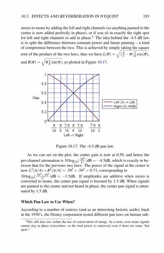
10.3. EFFECTS AND REVERBERATION IN NYQUIST 193
stereo to mono by adding the left and right channels (so anything panned to thecenter is now added perfectly in phase), or if you sit in exactly the right spotfor left and right channels to add in phase.4 The idea behind the -4.5 dB lawis to split the difference between constant power and linear panning – a kindof compromise between the two. This is achieved by simply taking the square
root of the product of the two laws, thus we have L(θ) =√(π
2 −θ) 2π
cos(θ),
and R(θ) =√
θ2π
sin(θ); as plotted in Figure 10.17.
Figure 10.17: The -4.5 dB pan law.
As we can see on the plot, the center gain is now at 0.59, and hence theper-channel attenuation is 10log10(
.592
12 )dB =−4.5dB, which is exactly in be-tween that for the previous two laws. The power of the signal at the center isnow L2(π/4)+R2(π/4) = .592 + .592 = 0.71, corresponding to10log10(
.592+.592
12 )dB = −1.5dB. If amplitudes are additive when stereo isconverted to mono, the center pan signal is boosted by 1.5 dB. When signalsare panned to the center and not heard in phase, the center pan signal is atten-uated by 1.5 dB.
Which Pan Law to Use When?
According to a number of sources (and as an interesting historic aside), backin the 1930’s, the Disney corporation tested different pan laws on human sub-
4This still does not violate the law of conservation of energy. In a room, even mono signalscannot stay in phase everywhere, so the total power is conserved even if there are some “hotspots’.”

194 CHAPTER 10. ACOUSTICS, PERCEPTION, EFFECTS
jects, and found that constant power panning was preferred by the listeners.Then, in the 1950’s, the BBC conducted a similar experiment and concludedthat the -4.5 dB compromise was the better pan law. Now, we know next tonothing about the details of those experiments, but their results might makesense if we assume that Disney’s focus was on movie theaters and the BBC’swas on TV audiences. Let’s elaborate on that. It all depends on the listeningsituation. That is, how are the speakers placed, what is the size of the room,where is the listener placed, and can we expect the listener to stay in the sameplace? If the speakers are placed close to each other in a small room (withvery little reverb) or if the listener is in the sweet spot, then one can reason-ably expect that the phases of the signals from the two speakers will add upconstructively (at least at lower frequencies, acting pretty much as one singlespeaker (at least at lower frequencies); as depicted in Figure 10.18.
Figure 10.18: Two speakers in phase acting as one.
In such a case where signals are in phase so that the left and right ampli-tudes sum, the sounds that are panned to the center will experience up to 3 dBof boost with constant power panning but a maximum of only 1.5 dB boostusing the -4.5 dB compromise. Thus, the -4.5 dB rule might give more equalloudness panning. It could also be that the BBC considered mono TV setswhere the left and right channels are added perfectly in phase. In this case,the -4.5 dB compromise gives a 1.5 dB boost to center-panned signals vs. a3 dB boost with constant power panning. (Recall that linear panning is idealfor mono reproduction because the center-panned signals are not boosted atall. However, linear panning results in the “hole-in-the-middle” problem forstereo.)
On the other hand, if the speakers are placed far from each other in a bigroom, then the phases will not add up constructively; as seen in Figure 10.19.
Furthermore, in this case, the listeners are probably not always placed atthe sweet spot – there are probably multiple listeners placed at different dis-tances and angles to the speakers (as e.g. in a movie theater). One wouldexpect constant power panning to produce more uniform loudness at all pan-ning positions in this situation.
Given the variables of listener position, speaker placement, and possible

10.3. EFFECTS AND REVERBERATION IN NYQUIST 195
Figure 10.19: Two speakers out of phase; phases do not add constructively.
stereo-to-mono conversion, there is no universal solution that optimizes pan-ning. Both constant power panning and the -4.5 dB compromise are widelyused, and both are preferred over linear panning.
Panning and Room Simulation
A more sophisticated approach to panning is to consider that in stereo record-ing, a left-facing microphone signal is very different from that of a right-facingmicrophone. Signal differences have to do with room reflections and thesource location. A sound source at stage left will undergo different modifi-cations getting to each microphone, and similarly for the source at stage right.Thus there are four different paths from sources to microphones, and that isconsidering only two source locations! Some panning systems take these pathsinto consideration or even integrate panning with reverberation simulation.
Panning in Nyquist
In Nyquist, panning splits a monophonic signal (single channel) into stereooutputs (two channels; recall that multiple channel signals are represented us-ing arrays of sounds), and the degree of left or right of that signal can becontrolled by either a fixed parameter or a variable control envelope:
pan(sound, where)
The pan function pans sound (a behavior) according to where (another behav-ior or a number). Sound must be monophonic. The where parameter shouldrange from 0 to 1, where 0 means pan completely left, and 1 means pan com-pletely right. For intermediate values, the sound is scaled linearly between leftand right.

196 CHAPTER 10. ACOUSTICS, PERCEPTION, EFFECTS
10.3.7 Compression/LimitingA Compression/Limiting effect refers to automatic gain control, which reducesthe dynamic range of a signal. Do not confuse dynamics compression withdata compression such as producing an MP3 file. When you have a signalthat ranges from very soft to very loud, you might like to boost the soft part.Alternatively, when you have a narrow dynamic range, you can expand it tomake soft sounds much quieter and louder sounds even louder.
Figure 10.20: Compression/Limiting effect. The input signal is analyzed toobtain the RMS (average) amplitude. The amplitude is mapped to obtain again, and the signal is multiplied by the gain. The solid line shown in themapping (at right) is typical, indicating that soft sounds are boosted, but as theinput becomes increasingly loud, the gain is less, reducing the overall dynamicrange (i.e. the variation in amplitude is compressed.)
The basic algorithm for compression is shown in Figure 10.20. The com-pressor detects the signal level with a Root Mean Square (RMS) detector5 anduses table-lookup to determine how much gain to place on the original signalat that point. The implementation in Nyquist is provided by the Nyquist Ex-tension named compress, and there are two useful functions in the extension.The first one is compress, which compresses input using map, a compressioncurve probably generated by compress-map.6 Adjustments in gain have thegiven rise-time and fall-time. lookahead tells how far ahead to look at the sig-nal, and is rise-time by default. Another function is agc, an automatic gain
5The RMS analysis consists of squaring the signal, which converts each sample from positiveor negative amplitude to a positive measure of power, then taking the mean of a set of consecutivepower samples perhaps 10 to 50 ms in duration, and finally taking the square root of this“meanpower” to get an amplitude.
6compress-map(compress-ratio, compress-threshold, expand-ratio, expand-threshold,limit, transition, verbose) constructs a map for the compress function. The map consistsof two parts: a compression part and an expansion part. The intended use is to compresseverything above compress-threshold by compress-ratio, and to downward expand everythingbelow expand-threshold by expand-ratio. Thresholds are in dB and ratios are dB-per-dB. 0 dBcorresponds to a peak amplitude of 1.0 or RMS amplitude of 0.7. If the input goes above 0dB, the output can optionally be limited by setting limit: (a keyword parameter) to T. Thiseffectively changes the compression ratio to infinity at 0 dB. If limit: is nil (the default), thenthe compression-ratio continues to apply above 0 dB.

10.3. EFFECTS AND REVERBERATION IN NYQUIST 197
control applied to input. The maximum gain in dB is range. Peaks are attenu-ated to 1.0, and gain is controlled with the given rise-time and fall-time. Thelook-ahead time default is rise-time.
compress(input, map, rise-time, fall-time, lookahead)
agc(input, range, rise-time, fall-time, lookahead)
10.3.8 ReverseReverse is simply playing a sound backwards. In Nyquist, the reverse func-tions can either reverse a sound or a file, and both are part of the Nyquist ex-tension named reverse. If you reverse a file, Nyquist reads blocks of samplesfrom the file and reverses them, one-at-a-time. Using this method, Nyquist canreverse very long sounds without using much memory. See s-read-reversein the Nyquist Reference Manual for details.
To reverse a sound, Nyquist must evaluate the whole sound in memory,which requires 4 bytes per sample plus some overhead. The functions-reverse(sound) reverses sound, which must be shorter than*max-reverse-samples* (currently initialized to 25 million samples). Thisfunction does sample-by-sample processing without an efficiently compiledunit generator, so do not be surprised if it calls the garbage collector a lotand runs slowly. The result starts at the starting time given by the currentenvironment (not necessarily the starting time of sound). If sound has multiplechannels, a multiple channel, reversed sound is returned.
10.3.9 Sample-Rate ConversionNyquist has high-quality interpolation to alter sample rates. There are a lotof sample rate conversions going on in Nyquist behind the scenes: Nyquistimplicitly changes the sample rate of control functions such as produced byenv and lfo from their default sample rate which is 1/20 of the audio samplerate. When you multiply an envelope by an audio rate signal, Nyquist linearlyinterpolates the control function. This is reasonable with most control func-tions because, if they are changing slowly, linear interpolation will be a goodapproximation of higher-quality signal reconstruction, and linear interpolationis fast. However, if you want to change the sample rate of audio, for exam-ple if you read a file with a 48 kHz sample rate and you want the rate to be44.1 kHz, then you should use high-quality sample-rate conversion to avoiddistortion and aliasing that can arise from linear interpolation.
The algorithm for high-quality sample-rate conversion in Nyquist is a dig-ital low pass filter followed by digital reconstruction using sinc interpolation.There are two useful conversion functions:

198 CHAPTER 10. ACOUSTICS, PERCEPTION, EFFECTS
force-srate(srate, sound)
returns a sound which is up- or down-sampled to srate. Interpolation is linear,and no pre-filtering is applied in the down-sample case, so aliasing may occur.
resample(snd, rate)
Performs high-quality interpolation to reconstruct the signal at the new sam-ple rate. The result is scaled by 0.95 to reduce problems with clipping. (Why?Interestingly, an interpolated signal can reconstruct peaks that exceed the am-plitude of the the original samples.)
Nyquist also has a variable sample-rate function:
sound-warp(warp-fn, signal, wrate)
applies a warp function warp-fn to signal using function composition. If theoptional parameter wrate is omitted or NIL, linear interpolation is used. Oth-erwise, high-quality sample interpolation is used, and the result is scaled by0.95 to reduce problems with clipping. Here, warp-fn is a mapping from score(logical) time to real time, and signal is a function from score time to real val-ues. The result is a function from real time to real values at a sample rate of*sound-srate*. See the Nyquist Reference Manual for details about wrate.
To perform high-quality stretching by a fixed ratio, as opposed to a vari-able ratio allowed in sound-warp, use scale-srate to stretch or shrink thesound, and then resample to restore the original sample rate.
10.3.10 Sample Size Conversion (Quantization)
Nyquist allows you to simulate different sample sizes using the unit generatorquantize:
quantize(sound, steps)
This unit generator quantizes sound as follows: sound is multiplied by stepsand rounded to the nearest integer. The result is then divided by steps. For ex-ample, if steps is 127, then a signal that ranges from -1 to +1 will be quantizedto 255 levels (127 less than zero, 127 greater than zero, and zero itself). Thiswould match the quantization Nyquist performs when writing a signal to an8-bit audio file. The sound may be multi-channel.
10.3. EFFECTS AND REVERBERATION IN NYQUIST 199
10.3.11 ReverberationA reverberation effect simulates playing a sound in a room or concert hall.Typical enclosed spaces produce many reflections from walls, floor, ceiling,chairs, balconies, etc. The number of reflections increases exponentially withtime due to secondary, tertiary, and additional reflections, and also becausesound is following paths in all directions.
Typically, reverberation is modeled in two parts:
• Early reflections, e.g. sounds bouncing off one wall before reaching thelistener, are modeled by discrete delays.
• Late reflections become very dense and diffuse and are modeled using anetwork of all-pass and feedback-delay filters.
Reverberation often uses a low-pass filter in the late reflection model becausehigh frequencies are absorbed by air and room surfaces.
The rate of decay of reverberation is described by RT60, the time to decayto -60 dB relative to the peak amplitude. (-60 dB is about 1/1000 in amplitude.)Typical values of RT60 are around 1.5 to 3 s, but much longer times are easyto create digitally and can be very interesting.
In Nyquist, the reverb function provides a simple reverberator. You willprobably want to mix the reverberated signal with some “dry” original signal,so you might like this function:
function reverb-mix(s, rt, wet)return s * (1 – wet) + reverb(s, rt) * wet
Nyquist also has some reverberators from the Synthesis Tool Kit: nrev (simi-lar to Nyquist’s reverb), jcrev (ported from an implementation by John Chown-ing), and prcrev (created by Perry Cook). See the Nyquist Reference Manualfor details.
Convolution-based Reverberators
Reverberators can be seen as very big filters with long irregular impulse re-sponses. Many modern reverberators measure the impulse response of a realroom or concert hall and apply the impulse response to an input signal usingconvolution (recall that filtering is equivalent to multiplication in the frequencydomain, and that is what convolution does).
With stereo signals, a traditional approach is to mix stereo to mono, com-pute reverberation, then add the mono reverberation signal to both left andright channels. In more modern reverberation implementations, convolution-based reverberators use 4 impulse responses because the input and output are

200 CHAPTER 10. ACOUSTICS, PERCEPTION, EFFECTS
stereo. There is an impulse response representing how the stage-left (left in-put) signal reaches the left channel or left ear (left output), the stage-left signalto the right channel or right ear, stage-right to the left channel, and stage-rightto the right channel.
Nyquist has a convolve function to convolve two sounds. There is noNyquist library of impulse responses for reverberation, but seewww.openairlib.net/, www.voxengo.com/impulses/ and other sources.Convolution with different sounds (even if they are not room responses) is aninteresting effect for creating new sounds.
10.3.12 SummaryMany audio effects are available in Nyquist. Audio effects are crucial in mod-ern music production and offer a range of creative possibilities. Synthesizedsounds can be greatly enhanced through audio effects including filters, chorus,and delay. Effects can be modulated to add additional interest.
Panning algorithms are surprisingly non-obvious, largely due to the “hole-in-the-middle” effect and the desire to minimize the problem. The -4.5 dBpanning law seems to be a reasonable choice unless you know more about thelistening conditions.
Reverberation is the effect of millions of “echoes” caused by reflectionsoff of walls and other surfaces when sound is created in a room or reflectivespace. Reverberation echos generally become denser with greater delay, andthe sound of reverberation generally has an approximately exponential decay.

Chapter 11
Physical ModelingTopics Discussed: Mass-Spring Models, Karplus-Strong, WaveguideModels, Guitar Models
11.1 Introduction
One promising way to create sounds is to simulate or model an acoustic in-strument. If the model is accurate, then the details of control and vibration canin principle lead to realistic sounds with all the control possibilities of phys-ical instruments. This approach might be called physics-based modeling, butthe common terminology is simply physical models. Physical models can becontrasted with abstract synthesis or the use of mathematical functions (suchas FM synthesis and Additive synthesis), sampling, and source/filter models.None of these alternative approaches really capture the complexities of phys-ical systems. When aspects of physical systems defy analysis, we can resortto simulation to compute and predict the behavior of those systems. However,even simulation is selective and incomplete. The key is to model the interest-ing aspects while keeping the overall simulation and its computation tractable.
Like all of the synthesis methods we have covered, physical modeling isnot one specific technique, but rather a variety of related techniques. Behindthem all, however, is the basic idea that by understanding how sound / vi-bration / air / string behaves in some physical system (an instrument), we canmodel that system in a computer and thereby generate realistic sounds throughcomputation.
201

202 CHAPTER 11. PHYSICAL MODELING
11.2 Mass-Spring Model
A simple example of a physical model is the Mass-Spring model consisting ofa string and a set of masses attached to the string (shown in Figure 11.1). Thisis a discrete approximation of a continuous string where mass is distributeduniformly throughout the length of the string. By “lumping” the mass at afinite set of points, we can use digital simulation to model the string. In themodel, we consider the string between masses to be mass-less springs that pullon the masses with a force that is proportional to the stretch of the spring.
To analyze all the forces here: the springs are pulling on the objects inopposite directions, the masses at the ends are assumed fixed. Because thesprings are pulling in both directions, there is little/no longitudinal force onthe objects, but there is a vertical restoring force. So when the string is bentup with the concave side facing down, some of the forces on the masses aredownward, as shown by “Restoring Force” in Figure 11.1. Conversely, whenthe string is down with the concave side facing up, the net force is pullingup. These forces will accelerate the objects. If we put the string in this con-figuration and release it, then the left half will accelerate downward and righthalf would go upward. As the masses are pulled to zero displacement, or to astraight line between the end points, there is no more net force on the objectsbut the masses will keep moving and stretch the string in the opposite directionuntil the restoring force can slow them down and reverse the direction. Thismotion will repeat, causing the string to oscillate.
Figure 11.1: Mass-Spring Model of a String
This is a computationally expensive model because you have to computethe force on each one of the masses and store the velocity and position ofthe masses for each time step of the simulation. But computers are fast, anddiscrete time simulation is mostly multiplies and adds, so you can easily runinteresting models (including this one) in real-time. The number of modes(partials) that you can support corresponds to the number of masses. Also,you can add stiffness and other interesting properties into the string, e.g. thestring can be non-linear, it can have a driving force, there can be friction, etc.

11.3. KARPLUS-STRONG PLUCKED STRING ALGORITHM 203
11.3 Karplus-Strong Plucked String Algorithm
Let’s take a look at a variation of the Mass-Spring model. This is a really sim-ple but very effective physical model of a plucked string, called the Karplus-Strong algorithm (so named for its principal inventors, Kevin Karplus and AlexStrong). One of the first musically useful physical models (dating from theearly 1980s1), the Karplus-Strong algorithm has proven quite effective at gen-erating a variety of plucked-string sounds (acoustic and electric guitars, ban-jos, and kotos) and even drumlike timbres [Karplus and Strong, 1983]. Nyquisthas an implementation in the function pluck.
Here’s a simplified view of what happens when we pluck a string: Atfirst the string is highly energized and it vibrates, creating a fairly complex(meaning rich in harmonics) sound wave whose fundamental frequency is de-termined by the mass and tension of the string. Gradually, thanks to frictionbetween the air and the string, as well as the dissipation of energy in the formof sound waves, the string’s energy is depleted. The higher frequencies tendto lose energy the fastest, so the wave becomes less complex as it decays, re-sulting in a purer tone with fewer harmonics. After some amount of time allof the energy from the pluck is gone, and the string stops vibrating.
If you have access to a stringed instrument, particularly one with somevery low notes, give one of the strings a good pluck and see if you can see andhear what’s happening based on the description above.
11.3.1 How a Computer Models a Plucked String with theKarplus-Strong Algorithm
Now that we have a physical idea of what happens in a plucked string, howcan we model it with a computer? The Karplus-Strong algorithm does it likethis: first we start with a buffer full of random values—noise. (A buffer isjust some computer memory (RAM) where we can store a bunch of numbers.)The numbers in this buffer represent the initial energy that is transferred to thestring by the pluck. The Karplus-Strong algorithm looks like this:
Yt =12(Yt−p +Yt−p−1) (11.1)
1When I was an undergraduate at Rice University, a graduate student was working with a PDP-11 mini-computer with a vector graphics display. There were digital-to-analog converters to drivethe display, and the student had connected them to a stereo system to make a primitive digitalaudio system. I remember his description of the synthesis system he used, and it was exactly theKarplus-Strong algorithm, including initializing the buffer with random numbers. This was in thelate 1970s, so it seems Karplus and Strong reinvented the algorithm, but certainly deserve creditfor publishing their work.

204 CHAPTER 11. PHYSICAL MODELING
Here, p is the period or length of the buffer, t is the current sample count,and Y is the output of the system.
To generate a waveform, we start reading through the buffer and using thevalues in it as sample values. If we were to just keep reading through the bufferover and over again, we would get a complex, periodic, pitched waveform. Itwould be complex because we started out with noise, but pitched because wewould be repeating the same set of random numbers. (Remember that any timewe repeat a set of values, we end up with a pitched sound.) The pitch we getis directly related to the size of the buffer (the number of numbers it contains)we’re using, since each time through the buffer represents one complete cycle(or period) of the signal.
Now, here’s the trick to the Karplus-Strong algorithm: each time we reada value from the buffer, we average it with the last value we read. It is thisaveraged value that we use as our output sample. (See Figure 11.2.) We thentake that averaged sample and feed it back into the buffer. That way, overtime, the buffer gets more and more averaged (this is a simple filter, like theaveraging filter, Equation 7.1). Let’s look at the effect of these two actionsseparately.
Figure 11.2: Schematic view of a computer software implementation of thebasic Karplus-Strong algorithm. For each note, the switch is flipped and thecomputer memory buffer is filled with random values (noise). To generate asample, values are read from the buffer and averaged. The newly calculatedsample is both sent to the output stream and fed back into the buffer. When theend of the buffer is reached, we simply wrap around and continue reading atthe beginning. This sort of setup is often called a circular buffer. After manyiterations of this process, the buffer’s contents will have been transformed fromnoise into a simple waveform. If you think of the random noise as a lot ofenergy and the averaging of the buffer as a way of lessening that energy, thisdigital explanation is not all that dissimilar from what happens in the real,physical case. Thanks to Matti Karjalainen for this graphic.

11.3. KARPLUS-STRONG PLUCKED STRING ALGORITHM 205
11.3.2 Averaging and Feedback
First, what happens when we average two values? Averaging acts as a low-pass filter on the signal. Since high frequencies have a high rate of change,averaging has a bigger effect on high frequencies than low ones. So, averaginga signal effectively reduces high frequencies.
The “over time” part is where feeding the averaged samples back into thebuffer comes in. If we were to just keep averaging the values from the bufferbut never actually putting the average back into the buffer, then we wouldbe stuck with a static waveform. We would keep averaging the same set ofrandom numbers, so we would keep getting the same results.
Instead, each time we generate a new sample, we store it back into thebuffer. That way our waveform evolves as we move through it. The effect ofthis low-pass filtering accumulates over time, so that as the string “rings,” moreand more of the high frequencies are filtered out of it. Figure 11.3 illustrateshow the contents of the Karplus-Strong buffer changes and decays over time.After enough times through the process, the signal has been averaged so manytimes that it reaches equilibrium—the waveform is a flat line and the vibrationhas died out.
Figure 11.3: Applying the Karplus-Strong algorithm to a random waveform.After 60 passes through the filter/feedback cycle, all that’s left of the wild ran-dom noise is a gently curving wave. The result is much like what we describedin a plucked string: an initially complex, periodic waveform that gradually be-comes less complex over time and ultimately fades away.

206 CHAPTER 11. PHYSICAL MODELING
Physical models generally offer clear, “real world” controls that can beused to play an instrument in different ways, and the Karplus-Strong algo-rithm is no exception: we can relate the buffer size to pitch, the initial randomnumbers in the buffer to the energy given to the string by plucking it, and thelow-pass buffer feedback technique to the effect of air friction on the vibratingstring.
11.4 Waveguide ModelNow, we consider another model of the string, called the waveguide model,introduced by Julius Smith. In a real string, waves travel down the string untilthey reach the end where the wave is reflected and travels back in the oppositedirection. A vibrating string is actually a wave travelling up and down thestring, reflecting at both ends, and the left-going and right-going waves sumthrough superposition to determine the displacement of the string at any givenlocation and time.
It is easy to model wave travel in one direction: we simply delay the sam-ples by storing incoming samples in an array (wrapping around when we reachthe end), and reading out older samples. This allows a delay up to the length ofthe array. If we ignore friction and other losses, a string carrying a waveformcan be modeled as a delay.
To model left-going and right-going waves, we simply use two one-waymodels, i.e. two delays. The output of one delay connects to the input ofthe other. (See Figure 11.4.) If we want the amplitude of the string at someparticular point, we access both delays (the left-going and right-going wavemodels) and sum the amplitudes.
11.4.1 “Lumped” FiltersNow, what about losses? In a continuous string, there should be loss at everystep of the way through the string. Since this would be computationally ex-pensive, we use a shortcut and compute the total losses for the entire trip fromone end of the string to the other. This can be expressed as a filter that we canapply to the output of the delay. This so-called “lumped” filter is efficient andcan give the same effect as accumulating tiny losses at each sample of delay.
11.5 Mechanical OscillatorTo make a sustained sound, we must overcome the losses in the waveguide.The case of the bowed string is probably the easiest to understand, so we will

11.5. MECHANICAL OSCILLATOR 207
Figure 11.4: A waveguide model. The right-going and left-going wave, whichare superimposed on a single string, are modeled separately as simple de-lays. The signal connections at the ends of the delays represent reflections.A waveguide can also model a column of air as in a flute.
start there. Figure 11.5 illustrates the oscillation in a bowed string. The bowalternately sticks to and slips across the string. Rather than reaching a steadyequilibrium where the bow pulls the string to some steady stretched configura-tion, the “slip” phase reduces friction on the the string and allows the string tomove almost as if were plucked. Interestingly, string players put rosin on thebow, which is normally sticky, but when the string begins to slide, the rosinheats up and a molecular level of rosin liquifies and lubricates the bow/stringcontact area until the string stops sliding. It’s amazing to think that rosin onthe string and bow can melt and re-solidify at audio rates!
11.5.1 McIntyre, Woodhouse (1979) + Schumacher (1983)
An important advance in physical models came from McIntyre and Wood-house who resorted to models to help understand the nature of oscillation inacoustical instruments. Later, Schumacher, a physics professor at CarnegieMellon University, visited McIntyre and Woodhouse to learn more about theirwork and the three physicists wrote a paper that formed the basis for a lot ofwork in the field of Computer Music.
Their model follows the basic ideas we have outlined so far. Rather than abi-directional waveguide, they combined the two delays into one as shown inFigure 11.6, with a single low-pass filter to model losses over the entire loop.Since the model is for a woodwind rather than a bowed string, the delay isconsidered to represent a traveling pressure wave rather than string displace-ment. McIntyre, Woodhouse and Schumacher added a non-linear element togenerate oscillation.

208 CHAPTER 11. PHYSICAL MODELING
Figure 11.5: A bowed string is pulled by the bow when the bowsticks to the string. At some point the bow does not have enoughfriction to pull the string further, and the string begins to slip. Thesliding reduces the friction on the string, which allows it to stretchin opposition to the bowing direction. Finally, the stretching slowsthe string and the bow sticks again, repeating the cycle. (Fromhttp://physerver.hamilton.edu/courses/Fall12/Phy175/ClassNotes/Violin.html)
Figure 11.6: McIntyre Woodhouse model consisting of a delay representingsound traveling through the bore of a clarinet and a filter representing thelosses over the round trip. The figure shows that the single delay is equiva-lent to a bi-directional waveguide with perfect reflection at one end.

11.5. MECHANICAL OSCILLATOR 209
11.5.2 Smith: Efficient Reed-Bore and Bow-String Mecha-nisms (ICMC 86)
Julius Smith was influenced by McIntyre, Woodhouse and Schumacher anddeveloped computer music instruments that model the clarinet and violin.
Figure 11.7 shows Smith’s clarinet model. It includes a waveguide withlow-pass filter (-LP in the figure). At the left side of the figure is a model ofthe reed, which has non-linear behavior that enables oscillation. A clarinetreed is a thin, flat, flexible plate that vibrates over an opening to the clarinet’sbody or bore. The reed acts as a valve to let air in when the reed is up or open,and to block the air when the reed is down or closed.
Figure 11.7: Clarinet model
To understand oscillation in the clarinet model, we can follow the “story”of one period. To being with, the reed is open and pressure from the mouthenters the clarinet. The pressure also closes the reed valve, at least to someextent. The high pressure front travels to the bell, the flare at the end of theclarinet, where the pressure is reflected. The reflection is inverted, so nowthe pressure front is negative. The negated pressure wave returns to the reed,where it is reflected again. This time, the reflection does not invert the wavebecause this end is effectively closed. The negative pressure acts to close thereed even further. The negative pressure returns to the bell, is inverted againand reflects back to the reed as a positive pressure wave. This positive pressuretends to open the reed, allowing air through the reed valve, which reinforcesthe positive pressure wave, and another cycle begins. If the addition of energyor pressure compensates for losses, a sustained oscillation will result.
Figure 11.8 illustrates a bowed string model. In this model, the bow is notat the end of the string, so there is one waveguide from the bow to the bridge(where strings are anchored over the body) and one waveguide from the bowto the nut (where strings are anchored at the end of the fingerboard). The bowhas a non-linear element (ρ in the figure) that models the change in friction
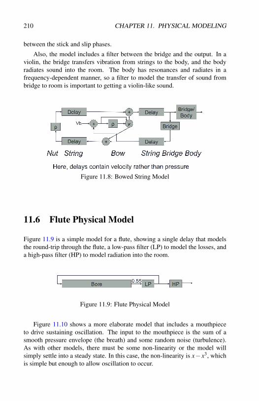
210 CHAPTER 11. PHYSICAL MODELING
between the stick and slip phases.
Also, the model includes a filter between the bridge and the output. In aviolin, the bridge transfers vibration from strings to the body, and the bodyradiates sound into the room. The body has resonances and radiates in afrequency-dependent manner, so a filter to model the transfer of sound frombridge to room is important to getting a violin-like sound.
Figure 11.8: Bowed String Model
11.6 Flute Physical Model
Figure 11.9 is a simple model for a flute, showing a single delay that modelsthe round-trip through the flute, a low-pass filter (LP) to model the losses, anda high-pass filter (HP) to model radiation into the room.
Figure 11.9: Flute Physical Model
Figure 11.10 shows a more elaborate model that includes a mouthpieceto drive sustaining oscillation. The input to the mouthpiece is the sum of asmooth pressure envelope (the breath) and some random noise (turbulence).As with other models, there must be some non-linearity or the model willsimply settle into a steady state. In this case, the non-linearity is x− x3, whichis simple but enough to allow oscillation to occur.

11.7. PHYSICAL MODELS IN NYQUIST 211
Figure 11.10: Flute Physical Model
11.7 Physical Models in Nyquist
Nyquist has a number of built-in physical models. Many of them come fromthe Synthesis Tool Kit (STK).
pluck(pitch, dur, final-amp) is an extended Karplus-Strong pluckedstring model. The extension inserts a filter into the loop (besides the sim-ple averaging filter we learned about) to allow sub-sample delays needed foraccurate tuning. In addition, the rate of decay can be modified by the optionalparameters dur and final-amp. Increasing either or both parameters lowers thedecay rate. You might want to multiply by an envelope to avoid a click at theend if the final-amp is high.
clarinet(step, breath-env) is a basic STK clarinet model. There areseveral variations on this model in Nyquist that allow continuous control overfrequency, breath envelope, vibrato, reed-stiffness, and noise through addi-tonal parameters. See the Nyquist Reference Manual for details.
sax(step, breath-env) is a basic STK saxophone model (called “sax-ophony”). As with clarinet, there are variations with additional parameters.
A number of other models can be found in the Nyquist Reference Manual.

212 CHAPTER 11. PHYSICAL MODELING
11.8 Commuted SynthesisOne of the problems with physical models of guitars, violins, and pianos is thatvibrating strings excite a complex 3-dimensional body that is computationallyhard to simulate. We can assume that the body is a kind of complex filter. Wecan characterize the body by tapping it at the bridge or point where the stringis attached and measuring the impulse response.
Now, one way to model the body is to simply convolve the string forcewith the body’s impulse response. In other words we just filter the string withthe body filter and we are done. But convolution is expensive, so researchersthought of another approach.
Consider a piano model with a hammer model that transmits force to astring model, the string model transmits force to a bridge, and the body modelfilters the bridge force to obtain an output. Now, the string and body are bothjust filters! Multiplication and convolution and linear filters are all commuta-tive (it’s all more-or-less the same thing), so we can switch the order of thestring and body filters. This makes no sense physically, but in our simulation,instead of driving the string with an impulse (as if hit by a hammer), we candrive the string with the impulse response of the body! Thus, for every note,we just have to “play” the impulse response into the string model, saving theneed for a complex body filter on the output.
For strings, the commuted synthesis model is a little more complex be-cause the bow is repeatedly pumping energy into the string. We need to runa bowed string model to detect when the bow slip occurs. Then, we treat thatas the driving impulse, and every time the bow slips, we drive a second stringmodel with the violin body impulse response. We take the output from thissecond string model.
11.9 Electric Guitar ModelCharles R. Sullivan developed an interesting guitar model [Sullivan, 1990].His work was motivated more by obtaining usable control than by being afaithful model.
The basic model is shown in Figure 11.11, and you can see that this isclosely related to the Karplus-Strong model. The low-pass filter determinesthe decay rate of the string and can also change the effective length (and fre-quency) of the string by inserting additional delay. In this model, an FIR filteris used:
yn = a0xn +a1xn−1 +a2xn−2 (11.2)
but this potentially has gain at zero Hz (DC).

11.9. ELECTRIC GUITAR MODEL 213
Figure 11.11: Electric Guitar Model by Charles R. Sullivan. The model isbased on Karplus-Strong, but the low-pass filter is customized and the modelallows continuous input through the summation node to allow for pluckingwhile the string is still vibrating and feedback.
11.9.1 Loop Filter Design
To eliminate DC, we can add a high-pass filter:
yn = a0xn +a1xn−1 +b1yn−1 (11.3)
We also want to provide continuous tuning, for which we need a sub-sampledelay. Simple linear interpolation:
yn = c0xn + c1xn−1 (11.4)
can be used, but this also produces attenuation (low-pass filter), so we canadjust the loop filter (FIR) to provide only the additional attenuation required.
After all this, the model is still not perfect and might require a compensat-ing boost at higher frequencies, but Sullivan decided to ignore this problem:Sometimes higher frequencies will suffer, but the model is workable.
11.9.2 Tuning and Glissandi
For tuning, we can just round the desired delay length to an integer numberof samples and use interpolation to add the remaining fractional length. Toachieve glissando, where the pitch changes continuously, we slowly changec0, c1 in the interpolator. When one coefficient reaches 1, we can change thedelay length by 1, flip c0, c1, and there is no glitch, but we are ready to continuethe glissando.
However, changing the loop length will require a change in the loop FIRfilter. It is expensive to recalculate all the filters every sample, so Sullivanupdates the filters once per period. There may be small artifacts, but these willgenerate harmonics that are masked by the string harmonics.

214 CHAPTER 11. PHYSICAL MODELING
11.9.3 Distortion
In electric guitars, distortion of a single note just adds harmonics, but distortionof a sum of notes is not the sum of distorted notes: distortion is not linear, soall those nice properties of linearity do not apply here.
Sullivan creates distortion using a soft clipping function so that as ampli-tude increases, there is a gradual introduction of non-linear distortion. Thesignal is x and the distorted signal is F(x) in the following equation, which isplotted in Figure 11.12:
F(x) =
23 x≥ 1x− x3
3 −1 < x < 1− 2
3 x≤−1(11.5)
Figure 11.12: Distortion functions. At left is “hard clipping” where the signalis unaffected until it reaches limits of 1 and -1, at which points the signal islimited to those values. At right is a “soft clipping” distortion that is more likeanalog amplifiers with limited output range. The amplification is very linearfor small amplitudes, but diminishes as the signal approaches the limits of 1and -1.
11.9.4 Feedback
A wonderful technique available to electric guitarists is feedback, where theamplified signal is coupled back to the strings which then resonate in a sus-tained manner. Figure 11.13 illustrates Sullivan’s configuration for feedback.There are many parameters to control gain and delay. Sullivan notes that oneof the interesting things about synthesizing guitar sounds with feedback is thateven though it is hard to predict exactly what will happen, once you find pa-rameter settings that work, the sounds are very reproducible. One guiding

11.9. ELECTRIC GUITAR MODEL 215
principle is that the instrument will tend to feedback at periods that are mul-tiples of the feedback delay. This is quite different from real feedback withreal guitars, where the player must interact with the amplifier and guitar, andparticular sounds are hard to reproduce.
Figure 11.13: Feedback is achieved by feeding some of the output through adelay and back into each string model.
11.9.5 Initializing the StringWhen plucking a guitar string in this model, how should we initialize thestring? In the Karplus-Strong model, strings are just initialized with randomnumbers, but this is not necessary, and it can be more interesting to simulateplucking as displacing the string at a particular point and releasing it. Pluckingcloser to the end of the string gives a brighter sound (try it if you have a guitar)!Figure 11.14 (a) shows the desired geometry of the initial string configuration.In the light of what we know about waveguides, this initial position must besplit as right- and left-going waves as shown in Figure 11.14 (b). If there isa single delay (as in Karplus-Strong), we need to concatenate the right- andleft-going wave configurations, resulting in an initial value as shown in Figure11.14 (c).
11.9.6 Additional FeaturesSullivan’s electric guitar model is interesting because it shows how models canbe extended incrementally to incorporate various features, either for study orfor additional sound generation and control. There are still more things onecould do with this model, including:
• Adding guitar body resonances,

216 CHAPTER 11. PHYSICAL MODELING
Figure 11.14: Initializing the string. The physical string shape (a) containsboth left- and right-going waves (b), so we need to combine them to get a fullround-trip initial waveform (c).

11.10. ANALYSIS EXAMPLE 217
• Coloration and distortion of guitar amplifiers,
• Effects processors, including:
– Distortion,
– Wah-wah pedals,
– Chorus, etc.
11.10 Analysis ExampleOne of the challenges of physical models is that we need many parameters tomake the model behave like real acoustic instruments. In some cases, param-eters are obtained by trial-and-error, or else calculated, e.g. given a desiredpitch, we can calculate the length of a waveguide.
However, it is interesting to estimate parameters from real sounds, anddoing this enables us to check on whether the model is really capturing thebehavior of the acoustic instrument. We present an example of the analysis ofacoustic guitar sounds to estimate physical model parameters. This exampleshould give some idea of how parameter estimation can be approached. Theword estimation should be emphasized—we rarely get the chance to measureanything exactly or directly.
In Figure 11.15, we see a plot of the amplitudes of harmonics of a pluckedguitar string as they decay over time. Since decay is mainly due to losses asthe wave travels up and down the string, we can fit lines to the curves andestimate the loss as a function of frequency. (Note that the decay should beexponential, so by plotting on a dB (log) scale, the decays appear as straightlines.)
After measuring the decay at different frequencies, we can fit a filter to thedata, as shown in the lower half of the figure. If the filter is simple as shown,the fit will not be perfect, but measurement errors will tend to average out andthe overall trend of the filter is likely to be well-estimated. Alternatively, onecould fit a complex filter exactly to all the data points, but this would run therisk of “overfitting,” or incorportaing measurement errors into the model.
11.10.1 Driving ForceAnother part of the model we might like to measure is the driving force on thestring. After fitting a filter to the string recording, we can create an inverse fil-ter, apply that to the recording, and end up with a “residual” that represents theinput. Then, we can drive the string model with the residual to get a realisticsound.

218 CHAPTER 11. PHYSICAL MODELING
Figure 11.15: Analysis Example, from Karjalainen, Valimaki, and Janosy[Karjalainen et al., 1993].

11.11. 2D WAVEGUIDE MESH 219
11.11 2D Waveguide MeshThe 1-dimensional waveguide can be extended to 2 or 3 dimensions. This addsa lot of computation, but allows us to model plates and drums in the 2-D case,and resonant chambers and wind instruments in the 3-D case.
Figure 11.16 shows a 2-D waveguide mesh and the modeled propagationof a wave over a surface in work by Van Duyne and Smith.
Figure 11.16: 2D Waveguide Mesh and some some simulation results.
11.12 SummaryPhysical models simulate physical systems to create sound digitally. A com-mon approach is to model strings and bores (in wind instruments) with re-circulating delays, and to “lump” the losses in a filter at some point in theloop. Non-linear elements are added to model how a driving force (a bow orbreath) interacts with the wave in the recirculating delay to sustain an oscil-lation. Digital waveguides offer a simple model that separates the left- andright-going waves of the medium.
11.12.1 Advantages of Physical ModelingOne advantage of physical models is that non-linear vibrating systems havecomplex behaviors. Simulations can create complex and interesting behav-

220 CHAPTER 11. PHYSICAL MODELING
iors that tend to arise naturally from models. In spite of potentially complexbehavior, physical models tend to have a relatively small set of controls thatare meaningful and intuitively connected to real-world phenomena and expe-rience. Models also tend to be modular. It is easy to add coupling betweenstrings, refine a loop filter, etc. to obtain better sound quality or test theoriesabout how instruments work.
11.12.2 Disadvantages of Physical ModelsOn the other hand, the real 3-D world resists simplifications. For example, vio-lin bodies are very complex and perceptually important. When simplificationsbreak down, physical model computation becomes very high. For example,there are experiments using 3-D waveguides models of brass instruments thatrun on supercomputers much slower than real time.
Control is also difficult. Just as real instruments require great skill andpractice, we should not expect simple inputs will immediately result in greatsounds. It is difficult to invert recorded sounds to determine the control re-quired to produce them. Consider all the muscles and motions involved inplaying the violin or trumpet, or the fact that it takes years to become an ac-complished performer on these instruments. One answer to this problem isthat physical models should form the basis of new instruments that can becontrolled in real-time by humans. These instruments might be as difficult toplay as acoustic instruments, but they might have interesting new sounds andcapabilities worth the learning effort.

Chapter 12
Spectral Modeling,Algorithmic Control,3-D Sound
Topics Discussed: Additive Synthesis, Table-Lookup Synthesis, Spec-tral Interpolation Synthesis, Algorithmic Control of Signal Processing, 3-DSound, Head-Related Transfer Functions, Multi-Speaker Playback
Previously, we considered physical models which simulate physical sys-tems from which we get vibration and sound. We saw that these are mod-els and not necessarily even realistic simulations. Therefore, the approach issometimes called physics-inspired or physics-based modeling. In contrast, wecan think about sound in more perceptual terms: What do we hear? And howcan we create sounds that contain acoustic stimuli to create desired impres-sions on the listener? Your first reaction might be that our hearing is so good,the only way to create the impression of a particular sound is to actually makethat exact sound. But we know, for example, that we are not very sensitive tophase. We can scramble the phase in a signal and barely notice the difference.This leads to the idea that we can recreate the magnitude spectrum of a desiredsound, perhaps without even knowing how the sound was created or knowingmuch about the details of the sound in the time domain.
This approach is sometimes called spectral modeling and it is a power-ful alternative to physical modeling. While physical modeling requires us tounderstand something about the sound source, spectral modeling requires usto understand the sound content. We can often just measure and manipulatethe spectra of desired sounds, giving us an approach that is simple to imple-ment and relatively easy to control. In this section, we consider variations onspectral modeling, from additive synthesis to spectral interpolation.
221

222 CHAPTER 12. SPECTRAL MODELING
12.1 Additive Synthesis and Table-Lookup Syn-thesis
One of the earliest synthesis methods drew upon the intuition that if all soundscould be represented as sums of sine waves, why not simply add sine wavesto create the desired sound? This additive synthesis approach is not the mostefficient one, and another intuition, that musical tones are mostly periodic, ledto the idea of constructing just one period and repeating it to create tones.
12.1.1 Additive SynthesisAdditive synthesis usually means the summation of sinusoids to create com-plex sounds. In this approach, every partial has independent frequency and am-plitude, giving unlimited freedom (according to what we know about Fourieranalysis and synthesis) to create any sound. Earlier, we studied analysis/synthesissystems such as McAuley-Quatieri (MQ) and Spectral Modeling Synthesis(SMS) showing that analysis and synthesis are possible. We also learned thatparametric control is somewhat limited. For example, time-stretching is pos-sible, but more musical control parameters such as articulation, formant fre-quencies and vibrato do not map directly to any additive synthesis parameters.
12.1.2 Table-Lookup SynthesisIf we are willing to limit sinusoidal (partial) frequencies to harmonics andwork with a fixed waveform shape, then we can save a lot of computationby creating a table containing one period of the periodic waveform. Usually,the table is oversampled (the sample rate is much higher than twice that ofthe highest harmonic) so that inexpensive linear interpolation can be used to“read” the table at different rates. By stepping through the table by a variableincrement and performing linear interpolation between neighboring samples,we can get frequency control. A simple multiplication provides amplitudecontrol.
Here is a software implementation of a table-lookup oscillator, building onthe algorithm introduced in Section 1.2.4. This code computes BLOCK_SIZEsamples every time osc is called. In a real implementation, we would keep thetable and current phase variables in a structure or object so that we couldavoid these as global variables and have more than one oscillator instance.This code does not implement amplitude control, so the output should be mul-tiplied by an amplitude envelope separately.

12.2. SPECTRAL INTERPOLATION SYNTHESIS 223
float table[513] = ... some waveform ... ;double phase = 0.0;
void osc(double hz, float table[], float out[]) {double incr = hz * 512 / sample_rate;for (int i = 0; i < BLOCK_SIZE; i++) {
int iphase = floor(phase);double x1 = table[iphase];out[i] = x1 + (phase – iphase) *
(table[iphase+1] – x1);phase += incr;if (phase >= 512) phase = phase - 512;
}}
One trick in this code is that table should be initialized to a 512-pointwaveform, with the first value duplicated as the 513th entry. By duplicatingthe first sample at the end, we insure that th expression table[iphase + 1](used to interpolate between two samples in the table) never accesses a valueoutside the bounds of the array, particularly when the phase is exceeds 511but has not “wrapped around” to zero.
Table-lookup oscillators have two basic parameters: frequency and ampli-tude, and otherwise they are limited to a fixed wave shape, but often table-lookup oscillators can be combined with filters or other effects for additionalcontrol and spectral variation.
12.2 Spectral Interpolation Synthesis
One simple idea to introduce spectral variation into table-lookup oscillators isto use two tables and interpolate between them, as shown in Figure 12.1. Withno constraints, this could lead to phase cancellation and unpredictable results,but if the phases of harmonics are identical in both tables, and if the tablesare accessed at the same offset (i.e. index or phase), then when we interpolatebetween tables, we are also interpolating between the magnitude spectra ofthe two tables. This is interesting! With interpolation between tables, we cancreate any smoothly varying harmonic spectrum.
There are some commercial synthesizers that use a 2-D joystick to controlreal-time interpolation between 4 spectra. This can be an interesting controlstrategy and is related to using filters to modify spectra—in both cases, you geta low dimensional (1-D cutoff frequency or 2-D interpolation) control spacewith which to vary the spectrum.

224 CHAPTER 12. SPECTRAL MODELING
Figure 12.1: Basic Spectral Interpolation. Phase is incremented after eachsample to scan through tables as in a simple table-lookup oscillator, but here,the phase is used for two table lookups, and the output is an interpolationbetween Table1 and Table2.
12.2.1 Time-Varying Spectrum
Perhaps more interesting (or is it just because I invented this?) is the idea thatthe spectrum can evolve arbitrarily over time. For example, consider a trum-pet tone, which typically follows an envelope of getting louder, then softer.As the tone gets softer, it gets less bright because higher harmonics are re-duced disproportionately when the amplitude decreases. If we could record asequence of spectra, say one spectrum every 100 ms or so, then we could cap-ture the spectral variation of the trumpet sound. The storage is low (perhaps20 harmonic amplitudes per table, and 10 tables per second, so that is only 200samples per second). The computation is also low: Consider that full additivesynthesis would require 20 sine oscillators at the sample rate for 20 harmon-ics. With spectral interpolation, the cost is only 2 table lookups per sample.We also need to compute tables from stored harmonic amplitudes, but tablesare small, so the cost is not high. Overall, we can expect spectral interpolationto run 5 to 10 times faster than additive synthesis, or only a few times slowerthan a basic table-lookup oscillator.
Of course, if we just want to reproduce recorded instrument tones, maybesampling is a better approach because it captures inharmonic attack transientsvery well. While the storage cost is higher, the computational cost of sampling(mostly due to sample-rate conversion to control frequency) is in the samerange as spectral interpolation synthesis. But with sampling, we are stuckwith a particular recording of every tone and we have little control over it.With spectral interpolation, we have the opportunity to compute the evolvingspectrum.

12.2. SPECTRAL INTERPOLATION SYNTHESIS 225
12.2.2 Use Pitch and Amplitude to Compute Spectra
One successful approach that is especially good for wind instrument simula-tion is to model the spectrum as a function of amplitude and frequency. Wecarefully record instruments playing crescendos (increasing loudness) at dif-ferent pitches. Then we analyze these tones to get a matrix of spectra at dif-ferent pitch and loudness levels. As shown in Figure 12.2, we input desiredfrequency and amplitude, do a lookup in our 2-D matrix to find the appro-priate next spectrum, then use spectral interpolation to smoothly change tothat spectrum. As long as amplitude and frequency are slowly changing, asin vibrato and amplitude envelopes, the output will realistically change spec-trum just like the real instrument. In fact, when amplitude is changing rapidly,we cannot hear the spectral changes very well. In our model (Figure 12.2), wenormalize all the spectra in the 2D matrix so everything comes out of the spec-tral interpolation oscillator at about the same level, and we multiply that bythe amplitude envelope. This captures the rapidly varying amplitude envelopefaithfully, and at least approximately does the right thing with the spectrum,even though spectral changes may lag behind or be smoothed out a little.
This basic approach is used in the Dannenberg Brass software for NativeInstruments Reaktor synthesizer. (www.native-instruments.com/en/reaktor-community/reaktor-user-library/entry/show/13607/). This implementationcredits this author but was developed without any direct collaboration.
12.2.3 Dealing with Rapid and Inharmonic Attacks
The “pure” spectral interpolation synthesis model works well for some instru-ments, but others, particularly brass and saxophones,1 have distinctive attacksounds that are too inharmonic and noisy to recreate from harmonic wave-forms. The solution is to combine sampling with spectral interpolation, usingshort sampled attacks of about 30 ms duration. It is tricky to join the sampledattacks smoothly to table-lookup signals because a rapid cross-fade causesphase cancellation if the sample and table are not matched in phase. The so-lution is to make the sample long enough (and 30 ms is usually enough) thatit settles into a harmonic spectrum. Then, we perform analysis on the end ofthe attack to obtain the amplitude and phase of each partial. This becomesthe first waveform, and every waveform after than has to keep the same phaserelationship. With these tricks, we can achieve realistic, inharmonic or noisyattacks and then control the evolution of the harmonic spectrum using almostarbitrary amplitude and frequency controls.
1Saxophones are also made of brass, but are considered woodwinds.

226 CHAPTER 12. SPECTRAL MODELING
Figure 12.2: Computation for Spectral Interpolation Synthesis. Frequency andamplitude are input controls. The spectrum is varied by mapping the currentfrequency and amplitude to a spectrum stored in a matrix. This may be aninterpolated lookup using the 4 nearest data points (spectra) to yield smoothspectral variations as a function of the continuous frequency and amplitudesignals. There is also interpolation through time from one spectrum to thenext, using a two-table-lookup oscillator. Since amplitude variations may needto be quite rapid, the amplitude scaling takes place at audio rates just beforethe output.
12.2.4 Where Do We Get Control Information?
This raises the question of where to get amplitude and frequency controls. Intraditional synthesis research, illustrated at the left of Figure 12.3, control isconsidered an input to the instrument, which is characterized by some synthe-sis algorithm (perhaps a physical model or a vocal model, etc.) To evaluate thesynthesis technique, we make sounds with the synthesizer and (often) compareto acoustic sounds. The assumption is that if the comparison is not good, weshould go back and fix the synthesis algorithm.
The SIS Research Approach
In contrast, the approach of Spectral Interpolation Synthesis is that control isan integral part of the synthesizer. If you do not control a synthesis algorithmproperly, it will never sound natural. This idea is illustrated on the right ofFigure 12.3. Research has shown that crude ADSR envelopes, and even en-velopes derived from the analysis of individual acoustic instrument tones, donot give musical results even if the synthesis algorithm is perfect, so it followsthat decades of synthesis research are based on faulty assumptions!

12.2. SPECTRAL INTERPOLATION SYNTHESIS 227
Figure 12.3: Left: Traditional approach to synthesis algorithm research anddevelopment. It is assumed that control functions are not critical and not partof the synthesis algorithm. Right: The SIS approach. Control and synthesisare considered to be related and must be developed and optimized together.Both control and synthesis are critical to good, realistic and musical output.
Divide-and-Conquer: Performance Model vs. Synthesis Model
To develop control for spectral interpolation, we take the divide-and-conquerapproach shown in Figure 12.4 of separating the control problem from thesynthesis problem (but keep in mind that we need both together to get goodsounds in the end). In this model, the input is a score—the notes we wantto play, along with phrase marks, loudness indications, and perhaps other an-notations. The performance model models how the performer interprets thescore and produces controls for the instrument—in the spectral interpolationapproach, this is mainly amplitude and frequency. Then, we use the synthesismodel (Figure 12.2) to convert control signals into sound.
Research Model: Synthesis Refinement
Given this framework, we can develop and refine the synthesis model by ex-tracting control signals from real audio produced by human performers andacoustic instruments. As shown in Figure 12.5, the human-produced controlsignals are used to drive the synthesis, or instrument, model, and we can listento the results and compare them directly to the actual recording of the human.If the synthesis sounds different, we can try to refine the synthesis model. Forexample, dissatisfaction with the sound led us to introduce sampled attacks forbrass instruments.
Note that the ability to drive the instrument model with amplitude andfrequency, in other words parameters directly related to the sound itself, is abig advantage over physical models, where we cannot easily measure physical

228 CHAPTER 12. SPECTRAL MODELING
Figure 12.4: The divide-and-conquer approach. Even though control and syn-thesis must both be considered as part of the problem of musical sound syn-thesis, we can treat them as two sub-problems.
Figure 12.5: Synthesis refinement. To optimize and test the synthesis part ofthe SIS model, control signals can be derived from actual performances ofmusical phrases. This ensures that the control is “correct,” so any problemswith the sound must be due to the synthesis stage. The synthesis stage isrefined until the output is satisfactory.

12.2. SPECTRAL INTERPOLATION SYNTHESIS 229
parameters, like bow-string friction or reed stiffness, that are critical to thebehavior of the model.
Research Model: Control Refinement
Assuming we have produced a good-sounding synthesizer, we can then turn tothe control problem. The idea here is to get humans to perform scores, extractcontrol information, drive the synthesis with controls, and produce a sound.This output from measured control signals represents the best we could hopeto achieve since a human produced the control with a real instrument. Now,we can also translate the score to controls with a performance model. If we donot like the results, we can improve the model and keep iterating until we havesomething we like. This is shown in Figure 12.6.
Figure 12.6: Control refinement. Having developed an adequate synthesismodel (see Figure 12.5), we compare controls from a performance model tocontrols extracted from human performance. Both controls are synthesized bythe known-to-be-good synthesis model, so any problems can be attributed tothe performance model that computes controls. The model is refined until theoutput sounds good compared to the output based on human performance.
12.2.5 A Study Of Trumpet EnvelopesWe will now discuss a particular study that followed the paradigm just de-scribed. My students and I constructed a good spectral-interpolation-basedtrumpet synthesizer and set out to obtain good control envelopes from scores.

230 CHAPTER 12. SPECTRAL MODELING
This discussion is not just relevant to spectral interpolation synthesis. Thefindings are relevant to any synthesis method and help explain some of thesubtleties we find in acoustic instrument synthesis.
The main conclusion of this work is that
• envelopes are largely determined by context;
• envelope generation techniques can improve synthesis.
In early experiments, we studied the question of how the context of notes inthe score affect the center of mass of amplitude envelopes. The center of masstells us, if we were to cut out the envelope shape from a piece of cardboard,where would the shape balance? If the beginning of the note is loud, the centerof mass will be earlier. If the sound grows steadily, the center of mass will belater. This is one of the simplest measures of shape and a good place to start.
Figure 12.7 shows some results of this study. The multiple curves showgreat consistency from one performance to the next when the same music isplayed, but there is a striking difference between the envelopes on the left,from articulated tones, to the ones on the right, from slurred tones. Someresults from measuring center of mass include:
• When the previous pitch is lower and the next pitch is higher (we callthis an “up-up” condition), notes showed a later center of mass thanother combinations;
• large pitch intervals before and after the tone resulted in an earlier centerof mass than small intervals;
• legato articulation gave a later center of mass than others (this is clearlyseen in Figure 12.7.
Envelope Model
The center of mass does not offer enough detail to describe a complete trumpetenvelope. A more refined model is illustrated in Figure 12.8. In this model,the envelope is basically smooth as shown by the dashed line, but this overallshape is modified at the beginning and ending, as shown inside the circles. Itis believed that the smooth shape is mainly due to large muscles controllingpressure in the lungs, and the beginning and ending are modified by the tongue,which can rapidly block or release the flow of air through the lips and into thetrumpet.
The next figure (Figure 12.9) shows a typical envelope from a slurred notewhere the tongue is not used. Here, there is less of a drop at the beginning

12.2. SPECTRAL INTERPOLATION SYNTHESIS 231
Figure 12.7: Context influences amplitude envelopes. The envelopes on theleft are from the second of three articulated (tongued) notes. At right, theenvelopes are from the second of three slurred notes. It is clear that articulationand context are significant factors in determining envelope shape. There is nota single “characteristic” trumpet envelope, and measuring the envelope of onetone out of context will not produce many of the features seen above.
Figure 12.8: The “tongue and breath” envelope model is based on the ideathat there is a smooth shape (dashed line) controlled by the diaphram, upperbody and lungs, and this shape is modified at note transitions by the tongueand other factors. (Deviations from the smooth shape are circled.)
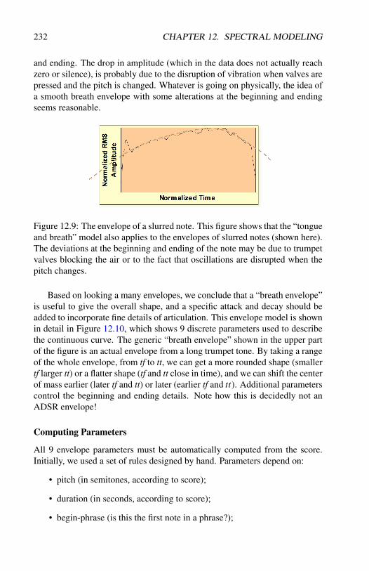
232 CHAPTER 12. SPECTRAL MODELING
and ending. The drop in amplitude (which in the data does not actually reachzero or silence), is probably due to the disruption of vibration when valves arepressed and the pitch is changed. Whatever is going on physically, the idea ofa smooth breath envelope with some alterations at the beginning and endingseems reasonable.
Figure 12.9: The envelope of a slurred note. This figure shows that the “tongueand breath” model also applies to the envelopes of slurred notes (shown here).The deviations at the beginning and ending of the note may be due to trumpetvalves blocking the air or to the fact that oscillations are disrupted when thepitch changes.
Based on looking a many envelopes, we conclude that a “breath envelope”is useful to give the overall shape, and a specific attack and decay should beadded to incorporate fine details of articulation. This envelope model is shownin detail in Figure 12.10, which shows 9 discrete parameters used to describethe continuous curve. The generic “breath envelope” shown in the upper partof the figure is an actual envelope from a long trumpet tone. By taking a rangeof the whole envelope, from tf to tt, we can get a more rounded shape (smallertf larger tt) or a flatter shape (tf and tt close in time), and we can shift the centerof mass earlier (later tf and tt) or later (earlier tf and tt). Additional parameterscontrol the beginning and ending details. Note how this is decidedly not anADSR envelope!
Computing Parameters
All 9 envelope parameters must be automatically computed from the score.Initially, we used a set of rules designed by hand. Parameters depend on:
• pitch (in semitones, according to score);
• duration (in seconds, according to score);
• begin-phrase (is this the first note in a phrase?);

12.2. SPECTRAL INTERPOLATION SYNTHESIS 233
Figure 12.10: An amplitude envelope specification. In order to produce awide variety of shapes based on the “tongue and breath” envelope model, wedescribe continuous envelopes with 9 parameters, as shown here.
• end-phrase (is this the last note in a phrase?)
• from-slur (is there a slur from preceding note?);
• to-slur (is there a slur to the next note?);
• direction-up (is this note higher than preceding note?).
The rules were developed by fitting generated envelopes to actual mea-sured envelopes and generalizing from observed trends. Here is one exam-ple, illustrating the computation of the parameter tf. As shown in Figure12.11, there are three cases. If coming from a slur and the direction is up,tf = 0.1. If the direction is not up, tf = 0.4. If not coming from a slur, tf =0.03−0.01× log2(dur).
Similar rules are used to compute all 9 parameters of every envelope. Thescore-to-envelope mapping is hand-crafted and far from complete and perfect,but the results, at least for simple scores, is quite good and sounds very natural.Constructing mappings between multi-dimensional spaces (in this case, frommultiple features of scores to multiple envelope parameters) is a natural prob-lem for machine learning. In fact, my student Ning Hu created an automatedsystem to analyze audio recordings of acoustic instruments and create both aspectral interpolation synthesis model and a performance model that includesamplitude envelopes and vibrato. No manual rule construction or design wasrequired [Hu, 2013].

234 CHAPTER 12. SPECTRAL MODELING
Figure 12.11: Computing envelope parameters. This example shows how theparameter tf is derived from score features from-slur, direction-up and dur.
12.2.6 Summary and Discussion of Spectral Interpolation
Spectral Interpolation Synthesis is based on modeling “real” performances,using measurements of spectra and other audio features to model what the lis-tener hears without any modeling of the physical instrument. The performancemodel results in phrase-long control functions rather than individual notes.Since control functions are based on note-to-note transitions and context, themethod requires some look-ahead. (The shape of the envelope depends on thepitch and articulation of the following note.)
12.2.7 Conclusions
What have we learned? First, envelopes and control are critical to music syn-thesis. It is amazing that so much research was done on synthesis algorithmswithout much regard for control! Research on the spectral centroid showedstatistically valid relationships between score parameters and envelope shape,which should immediately raise concerns about sampling synthesis: If sampleshave envelopes “baked in,” how can sampling ever create natural-soundingmusical phrases? Certainly not without a variety of alternative samples withdifferent envelopes and possibly some careful additional control through am-plitude envelopes, but for brass, that also implies spectral control. Large sam-ple libraries have moved in this direction.

12.3. ALGORITHMIC CONTROL OF SIGNAL PROCESSING 235
The idea that envelopes have an overall “breath” shape and some fine de-tails in the beginning and ending of every note seems to fit real data betterthan ADSR and other commonly used models. Even though spectral interpo-lation or even phrase-based analysis/synthesis have not become commonplaceor standard in the world of synthesis, it seems that the study of musical phrasesand notes in context is critical to future synthesis research and systems.
12.3 Algorithmic Control of Signal ProcessingIn the previous section, we looked carefully at some ideas on the synthesis ofacoustic instrument sounds. In this section, we consider something that hasno basis in the acoustical world: the direct generation and control of audiothrough algorithms.
There are relatively few works that push decision making, selection, waveshape, and parametric control down below the note level and into the audiosignal itself. Ianis Xenakis developed a system called GENDYN that createswaveforms from line segments using algorithmic processes [Xenakis, 1992].Herbert Brun’s SAWDUST is another example, described as a program forcomposing waveforms (see Section 7.1.2). Curtis Roads wrote the book Mi-crosound [Roads, 2004], which concerns granular synthesis and more gener-ally the realm between samples and notes. We have explored granular syn-thesis with Nyquist in some detail. In this section, we will look at signalscontrolled by (Nyquist) patterns and patterns controlled by signals.
12.3.1 Sounds controlled by PatternsIn Figure 12.12, we see a some code and a generated control function (aNyquist signal). The signal is created by the SAL function pat-ctrl, whichtakes two patterns as parameters. The first pattern (durpat) returns durationsand the second (valpat) returns amplitude values. As seen in the generatedsignal, durpat alternates between 0.1 and 0.2, while valpat cycles throughthe stair-step values of 0, 1, 2.
Pat-ctrl
The implementation of pat-ctrl is shown below. This is a recursive se-quence that produces one segment of output followed by a recursive call toproduce the rest. The duration is infinite:
define function pat-ctrl(durpat, valpat)return seq(const(next(valpat), next(durpat)),
pat-ctrl(durpat, valpat))

236 CHAPTER 12. SPECTRAL MODELING
Figure 12.12: The pat-ctrl function creates a piecewise-constant functionwhere each step has a duration and amplitude determined by the two patterngenerator object parameters. Each pair of numbers retrieved from the twopatterns produces one step in the stair-step-like function.
We can use pat-ctrl to construct a frequency control function and synthesizethat frequency contour. The function pat-fm, shown below, adds the result ofpat-ctrl to a pitch parameter, converts the pitch from steps to Hz, andthen synthesizes a sinusoid. If durpat returns very small values, the resultingsound will not have discernible pitch sequences, at least not at the level ofsegment durations returned by durpat. However, higher-level structures indurpat and valpat will create structured timbral variations that catch ourattention. In other words, the intent here is to modulate the sine tone at audiorates using complex patterns and resulting in novel sounds.
define function pat-fm(durpat, valpat, pitch, dur)beginwith hz =step-to-hz(pitch + pat-ctrl(durpat, valpat))
return pwl(0.01, 1, dur - 0.1, 1, dur) *hzosc(hz + 4.0 * hz * hzosc(hz))
end
Using Scores
One long sine tone may not be so interesting, even if it is modulated rapidlyby patterns. The following example shows how we can write a score that“launches” a number of pat-fm sounds (here, the durations are 30, 20, 18,and 13 seconds) with different parameters. The point here is that scores arenot limited to conventional note-based music. Here we have a score organiz-ing long, overlapping, and very abstract sounds.

12.3. ALGORITHMIC CONTROL OF SIGNAL PROCESSING 237
exec score-play({{ 0 30 {pat-fm-note :grain-dur 8 :spread 1
:pitch c3 :fixed-dur t :vel 50}}{10 20 {pat-fm-note :grain-dur 3 :spread 10
:pitch c4 :vel 75}}{15 18 {pat-fm-note :grain-dur 1 :spread 20
:pitch c5}}{20 13 {pat-fm-note :grain-dur 1 :spread 10
:pitch c1}}})
12.3.2 Pattern Controlled by SoundsIf we consider sounds controlled by patterns, we should think about the oppo-site. Here, we will look at control envelopes (which are also of type SOUND inNyquist) and how they can be used in patterns. (Maybe you can also think ofinteresting ways for audio sounds to control patterns.)
When constructing sequences of events, scores and score-gen may be allyou need. But if you want to influence the evolution of fine-grain decisions,such as pattern output over time, then perhaps envelopes and other controlscan be useful. This relates to a concept we saw before: tendency masks, whichspecify long-term trends. A standard example is: randomly choose the nextpitch between an upper and lower bound, where the bounds are given by func-tions that change over time.
To implement something like tendency masks in patterns, we will useNyquist SOUNDs to specify the global continuous evolution of parameter val-ues. To access the sound at a particular time, we use sref(sound, time).Note that sound can be any SOUND, but it might be most convenient to use apiece-wise linear envelope.
In sref, time is relative to the environment, so time = 0 means “now.” Andremember that while behaviors start at “now,” existing sounds have a definitestart time. So when we write sref(sound, 0), it means access sound at thecurrent time, not access the beginning (time 0) of sound.
A Template for Global Control using Sounds
Here is an example you can build on for controlling patterns with sounds.There are three definitions:
• pitch-contour defines a time-varying contour that we want to usewith some pattern computation;
• get-pitch is a function that simply accesses the pitch contour at thecurrent time (indicated by time 0);

238 CHAPTER 12. SPECTRAL MODELING
• pwl-pat-fm is a function that will create and use a pattern. Within thepattern, we see make-eval({get-pitch}). The make-eval patternconstructor takes an expression, which is expressed in Lisp syntax. Eachtime the pattern is called to return a value, the expression is evaluated.Recall that in Lisp, the function call syntax is (function-name arg1arg2 ...), so with no arguments, we get (function-name), and in SAL,we can write a quoted list as {function-name}. Thus, make-eval({get-pitch}) is the pattern that calls get-pitch to produce eachvalue.
variable pitch-contour =pwl(10, 25, 15, 10, 20, 10, 22, 25, 22)
function get-pitch()return sref(pitch-contour, 0)
function pwl-pat-fm()begin...make-eval(get-pitch),...
end
play pwl-pat-fm()
We can do something similar with score-gen, using a SOUND to provide atime-varying value that guides the progress of some parameter. In the follow-ing example, the variable pitch-contour is accessed as part of the pitch:calculation.
beginwith pitch-contour =
pwl(10, 25, 15, 10, 20, 10, 22, 25, 22),ioi-pattern = make-heap(0.2 0.3 0.4)
exec score-gen(save: quote(pwl-score),score-dur: 22,pitch: truncate(
c4 + sref(pitch-contour, sg:start) +#if(oddp(sg:count), 0, -5)),
ioi: next(ioi-pattern),dur: sg:ioi - 0.1,vel: 100)
end
You can even use the envelope editor in the NyquistIDE to graphicallyedit pitch-contour. To evaluate pitch-contour at a specific time, sref

12.4. 3-D SOUND 239
is used as before, but the time parameter to sref is sg:start, not 0. Weneed to use sg:start here because the entire score-gen computation is per-formed at time 0. We are not in a behavior, and there is no environment thatchanges the current time with each new note. Since everything is (normally)relative to time 0, we use score-gen’s special sg:start variable to refer tothe “current” time, that is, the start time of each note.
12.4 3-D SoundWe now turn to the topic of sound as originating in 3-D space. We know fromprevious discussions of perception that there are various cues that give the im-pression of the origin of sounds we hear. In computer music work, composersare interested in simulating these cues to simulate a 3-D sonic environment.Earlier, we introduced the idea of head-related transfer functions and the sim-ulation of spatial cues over headphones. In this section, we expand on thisdiscussion and also consider the use of multiple speakers in rooms and partic-ularly in concert halls.
12.4.1 IntroductionTo review from our discussion of sound localization, we use a number of cuesto sense direction and distance. Inter-aural time delay and amplitude differ-ences give us information about direction in the horizontal plane, but suffersfrom symmetry between sounds in front and sounds behind us. Spectral cueshelp to disambiguate front-to-back directions and also give us a sense of heightor elevation. Reverberation, and especially the direct-sound-to-reverberant-sound ratio gives us the impression of distance, as do spectral cues.
12.4.2 Duplex TheoryIn the duplex theory of Lord Rayleigh, sound localization is achieved through acombination of interaural time difference (ITD) and interaural level difference(ILD). ITD is caused by the difference in distance between our ears and thesound source when the source is to the left or right. The time difference isrelated to the speed of sound, and remembering that sound travels about 1 footper millisecond, we can estimate that ITD is a fraction of a millisecond. (Nowonder our ears can perceive time so precisely—without very precise timing,or at least relative time between left and right ears, we would not be able tolocalize sounds.)
The ILD is caused by the masking effect of our heads when sound comesfrom one side or the other. Since different frequencies refract around our heads

240 CHAPTER 12. SPECTRAL MODELING
differently, the ILD is frequency dependent and more pronounced at higherfrequencies where the wavelengths are short and our head does a better job ofshielding one ear from the sound.
In duplex theory, there is ambiguity caused by symmetry. Any directionfrom the head falls on a cone-shaped surface, where the apex of the cone isat the head and center line of the cone runs through the two ears. This set ofambiguous directions is called the cone of confusion (Figure 12.13) becauseevery point on the cone produces the same ITD and ILD.
Figure 12.13: The “cone of confusion,” where different sound directions givethe same ITD and ILD. (Credit: Bill Kapralos, Michael Jenkin and Evangelos Milios, “Vir-tual Audio Systems,” Presence Teleoperators & Virtual Environments, 17, 2008, pp. 527-549).
In fact, the duplex theory ignores the pinnae, our outer ears, which are notsymmetric from front-to-back or top-to-bottom. Reflections in the pinnae cre-ate interference that is frequency-dependent and can be used by our auditorysystem to disambiguate sound directions. The cues from our pinnae are not asstrong as ITD and ILD, so it is not unusual to be confused about sound sourcelocations, especially along the cone of confusion.
12.4.3 HRTF: Head-Related Transfer FunctionsWhen sound reaches our ears from a particular direction, there is a combina-tion of ITD, ILD, and spectral changes due to the pinnae. Taken together, thesecues can be expressed as a filter called the head-related transfer function, orHRTF. We can measure the HRTF, for example by placing tiny microphonesin the ears of a subject in an anechoic chamber, holding their head steady, andrecording sound from a speaker placed at a carefully controlled angle and el-evation. There are some clever ways to estimate the HRTF, but we will skip

12.4. 3-D SOUND 241
the signal processing details. To fully characterize the HRTF, the loudspeakerand/or listener must be moved to many different angles and elevations. Thenumber of different angles and elevations measured can range from one hun-dred to thousands.
To simulate a sound source at some angle and elevation, we retrieve thenearest HRTF measurement to that direction and apply the left and right HRTFsas filters to the sound before playing the sound to the left and right ears throughheadphones. (See Figure 12.14.)
Figure 12.14: Sound is localized with HRTFs by filtering a sound to simulatethe effect of delays, head, and ears on the sound. A different filter is usedfor left and right channels, and the filters are different for different directions.(From http://www.ais.riec.tohoku.ac.jp/Lab3/sp-array/index.html).
One way to implement the HRTF filters is to compute the HRIR, or head-related impulse response, which is the response of the HRTF to an impulseinput. To filter a sound by the HRTF, we can convolve the sound with theHRIR. If the sound is moving, it is common to interpolate between the nearestHRTFs or HRIRs so that there is no sudden switch from one filter to another,which might cause pops or clicks in the filtered sound.
12.4.4 HRTF, Headphones, and Head TrackingWhen HRTFs are used, the listener normally wears headphones, which isolatesounds to the left and right ears and eliminate most of the effects of actualroom acoustics in the listening space. Headphones have the problem that ifthe listener moves their head, the simulated space will rotate with the head and

242 CHAPTER 12. SPECTRAL MODELING
the headphones. To solve this problem, headphones are often tracked. Then,if the head turns 20◦ to the left, the virtual sound source is rotated to the rightto compensate. Headphones with head tracking are sometimes combined withvirtual reality (VR) goggles that do a similar thing with computer graphics:when the listener turns 20◦ to the left, the virtual world is rotated to the right,giving the impression that the world is real and we are moving the head withinthat world to see different views.
12.4.5 Room Models
An alternative to HRTFs and headphones is to use speakers in a room to cre-ate the effect of localized sounds. One approach is to use ray-tracing ideasfrom computer graphics to estimate a sound field in an imaginary space. Onedifficulty is that sound is slow and has long wavelengths relative to objectsand rooms, which means that refraction is significant—sound does not alwaystravel in straight lines! The refraction is frequency dependent. Nevertheless,ray tracing can be used to develop early reflection models for artificial re-verberation that convey the geometry of rooms, even if the simulation is notperfect.
12.4.6 Doppler Shift
Another interesting process that works well with loudspeakers is the simula-tion of motion using Doppler shift. Sound at a distance is delayed. Whensound sources move, the distance changes, and so does the delay. The changein delay creates Doppler shift, or a change in frequency. Doppler shift can bemodeled with actual delay consisting of buffers of samples, perhaps with someinterpolation to “tap” into the delay at fractional positions. Alternatively, wecan sometimes use frequency modulation to give the effect of Doppler shiftwithout any real simulation of delay. If there are multiple reflections, each re-flection can have a different Doppler shift. This could add additional realism,but I have never seen a system that models reflections with individual Dopplershifts.
12.4.7 Reverberation
Doppler shift is enhanced through the use of reverberation. If a sound is re-ceding rapidly, we should hear several effects: the pitch drops, the sound de-creases in amplitude and the ratio of reverberation to direct sound increases.Especially with synthesized sounds, we do not have any pre-conceptions aboutthe absolute loudness of the (virtual) sound source. Simply making the source

12.4. 3-D SOUND 243
quieter does not necessarily give the impression of distance, but through thecareful use of reverberation, we can give the listener clues about distance andloudness.
12.4.8 PanningStereo loudspeaker systems are common. A standard technique to simulatethe location of a sound source between two speakers is to “pan” the source,sending some of the source to each speaker. Panning techniques and the “hole-in-the-middle” problem were presented in detail in Section 10.3.6. Panningbetween two speakers can create ILD, but not ITD or spectral effects consistentwith the desired sound placement, so our ears are rarely fooled by stereo intobelieving there is a real 3-D or even 1-D space of sound source locations.2
Finally, room reflections defeat some of the stereo effect or at least lead tounpredictable listening conditions.
12.4.9 Multi-Speaker PlaybackIf two speakers are better than one, why not many speakers? This is not sopractical in the home or apartment, but common in movie theaters and concerthalls, especially for concerts of computer music. “Surround Sound” systemsare available as consumer audio systems as well. In general, the simulation ofdirection is achieved by choosing the nearest speaker in the desired direction.Often, sound is panned between the nearest 2 speakers when speakers are in aplane around the audience, or between the nearest 3 speakers when speakersare arranged in a dome.
At the risk of over-generalization, there are two general schools of thoughton sound reproduction with loudspeakers. One school views loudspeakers asan approximation to some ideal. In this view, loudspeakers should have highfidelity to recreate any desired source sound with minimal alteration. Whenmany speakers are used, they are almost invariably identical and uniformlydistributed to allow panning to any angle. The focus is on sound content, andany speaker limitations are just a necessary evil.
The other school views electro-acoustic music more holistically. Loud-speakers are a part of the process. Rather than bemoan speaker imperfections,
2Thus, the whole idea of stereo is highly suspect. Could it be that stereo was promoted bymanufacturers who wanted to sell more gear? There were multi-speaker systems in use beforeconsumer stereo, and experiments have shown that three-channel systems (adding a center chan-nel) are significantly better than stereo. My guess is that stereo is ubiquitous today because it wasboth interesting enough to sell to consumers yet simple enough to implement in consumer mediaincluding the phonograph record and FM radio. Even though we have only two ears, stereo withtwo channels falls far short of delivering a full two-dimensional sound experience, much less threedimensions.
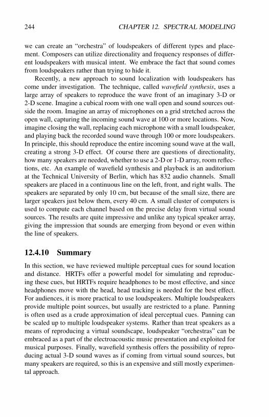
244 CHAPTER 12. SPECTRAL MODELING
we can create an “orchestra” of loudspeakers of different types and place-ment. Composers can utilize directionality and frequency responses of differ-ent loudspeakers with musical intent. We embrace the fact that sound comesfrom loudspeakers rather than trying to hide it.
Recently, a new approach to sound localization with loudspeakers hascome under investigation. The technique, called wavefield synthesis, uses alarge array of speakers to reproduce the wave front of an imaginary 3-D or2-D scene. Imagine a cubical room with one wall open and sound sources out-side the room. Imagine an array of microphones on a grid stretched across theopen wall, capturing the incoming sound wave at 100 or more locations. Now,imagine closing the wall, replacing each microphone with a small loudspeaker,and playing back the recorded sound wave through 100 or more loudspeakers.In principle, this should reproduce the entire incoming sound wave at the wall,creating a strong 3-D effect. Of course there are questions of directionality,how many speakers are needed, whether to use a 2-D or 1-D array, room reflec-tions, etc. An example of wavefield synthesis and playback is an auditoriumat the Technical University of Berlin, which has 832 audio channels. Smallspeakers are placed in a continuous line on the left, front, and right walls. Thespeakers are separated by only 10 cm, but because of the small size, there arelarger speakers just below them, every 40 cm. A small cluster of computers isused to compute each channel based on the precise delay from virtual soundsources. The results are quite impressive and unlike any typical speaker array,giving the impression that sounds are emerging from beyond or even withinthe line of speakers.
12.4.10 SummaryIn this section, we have reviewed multiple perceptual cues for sound locationand distance. HRTFs offer a powerful model for simulating and reproduc-ing these cues, but HRTFs require headphones to be most effective, and sinceheadphones move with the head, head tracking is needed for the best effect.For audiences, it is more practical to use loudspeakers. Multiple loudspeakersprovide multiple point sources, but usually are restricted to a plane. Panningis often used as a crude approximation of ideal perceptual cues. Panning canbe scaled up to multiple loudspeaker systems. Rather than treat speakers as ameans of reproducing a virtual soundscape, loudspeaker “orchestras” can beembraced as a part of the electroacoustic music presentation and exploited formusical purposes. Finally, wavefield synthesis offers the possibility of repro-ducing actual 3-D sound waves as if coming from virtual sound sources, butmany speakers are required, so this is an expensive and still mostly experimen-tal approach.

Chapter 13
Audio CompressionTopics Discussed: Coding Redundancy, Intersample Redundancy, Psycho-Perceptual Redundancy, Huffman Coding
13.1 Introduction to General Compression Tech-niques
High-quality audio takes a lot of space—about 10M bytes/minute for CD-quality stereo. Now that disk capacity is measured in terabytes, storing un-compressed audio is feasible even for personal libraries, but compression isstill useful for smaller devices, downloading audio over the Internet, or some-times just for convenience. What can we do to reduce the data explosion?
Data compression is simply storing the same information in a shorter stringof symbols (bits). The goal is to store the most information in the small-est amount of space, without compromising the quality of the signal (or atleast, compromising it as little as possible). Compression techniques and re-search are not limited to digital sound—–data compression plays an essentialpart in the storage and transmission of all types of digital information, fromword-processing documents to digital photographs to full-screen, full-motionvideos. As the amount of information in a medium increases, so does theimportance of data compression.
What is compression exactly, and how does it work? There is no one thingthat is “data compression.” Instead, there are many different approaches, eachaddressing a different aspect of the problem. We’ll take a look at a few waysto compress digital audio information. What’s important about these differentways of compressing data is that they tend to illustrate some basic ideas in therepresentation of information, particularly sound, in the digital world.
245

246 CHAPTER 13. AUDIO COMPRESSION
There are three main principles or approaches to data compression youshould know:
• Coding Redundancy eliminates extra bits used to represent symbols.For example, computer code generally uses 8-bit characters, but thereare less than 100 different characters, at least for written English. Wecould use 7 bits per character for an immediate savings of 12.5%, and avariable-length encoding would be even more efficient.
• Intersample Redudancy looks at how sequences of symbols can be rep-resented more compactly. For example, a fax machine could send ablack-and-white image as a sequence of bits for black and white, e.g.1111111000011111100110100000..., but since there are typically largeblack and white regions, we can encode this as the number of 1’s fol-lowed by the number of 0’s followed by the number of 1’s, etc. Thesame bits could be represented as 7 4 6 2 2 1 1 5 ..., which is typicallymuch more compact.
• Psycho-Perceptual Redundancy considers the waste of transmitting in-formation that will never be perceived. A 16-bit audio recording con-tains a lot of information and detail we cannot hear. Yes, in the worstcase, you really need 16 bits, and yes, in the worst case you really needa frequency response up to 20 kHz, but a lot of the audio informationrepresented in the samples is inaudible, and that fact can be used to sendless data.
13.2 Coding Redundancy
Let’s look at how these principles are used in audio data compression. Startingwith coding redundancy, we can think of each sample as a “symbol” that mustbe represented in bits. In “uncompressed” audio, each sample is encoded as anumber on a linear scale. This is the so-called PCM, or pulse-code modulationrepresentation.1
Another representation of samples uses a more-or-less logarithmic encod-ing called µ-law. This representation is not truly logarithmic and instead usesa floating-point representation with 1 sign bit, 3 exponent bits, and 4 mantissabits. The encoding spans a 13-bit dynamic range where the quantization levels
1I’ve always thought PCM was odd terminology. It literally refers to the transmission ofbinary codes through pulses—see Patent US2801281A—which misses the point that this is aboutrepresentation, not transmission, but since this work came out of a phone company, maybe it isnot so surprising that PCM was viewed as a form of transmission.

13.2. CODING REDUNDANCY 247
are smaller at low amplitudes. A less common but similar encoding is A-law,which has a 12-bit dynamic range.
Figure 13.1 shows a schematic comparison of (linear) PCM to µ-law en-coding. The tick-marks on the left (PCM) and right (µ-law) scales show actualvalues to which the signal will be quantized. You can see that at small signalamplitudes, µ-law has smaller quantization error because the tick marks arecloser together. At higher amplitudes, µ-law has larger quantization error. Atleast in perceptual terms, what matters most is the signal-to-noise ratio. In µ-law, quantization error is approximately proportional to the signal amplitude,so the signal-to-noise ratio is roughly the same for soft and loud signals. Atlow amplitudes, where absolute quantization errors are smaller than PCM, thesignal-to-noise ratio of µ-law is better than PCM. This comes at the cost oflower signal-to-noise ratios at higher amplitudes. All around, µ-law is gener-ally better than PCM, at least when you do not have lots of bits to spare, butwe will discuss this further in Section 13.2.2.
Figure 13.1: µ-law vs. PCM. Quantization levels are shown at the left andright vertical scales. µ-law has a better signal-to-quantization-error ratio atlower amplitudes but a higher ratio than PCM at higher amplitudes.
13.2.1 µ-law ImplementationTo convert from 8-bit µ-law to PCM, we can treat the µ-law code as an un-signed integer, from 0 to 255, and store the corresponding PCM value in atable. Then, translation from µ-law to PCM is a simple table lookup:ulaw_to_pcm[ulaw_code].
To convert from PCM to µ-law, we could also use a table to map from eachof 216 16-bit PCM values to the corresponding µ-law value. It turns out thelow-order 2 bits of the 16-bit code do not matter, so we can reduce the tablesize to 214, and we can use symmetry around zero to reduce the table size to213 or 8 kB.2
2Of course, you could also do binary search to find the nearest µ-law code using the muchsmaller ulaw_to_pcm table, but it is much faster to use direct lookup.
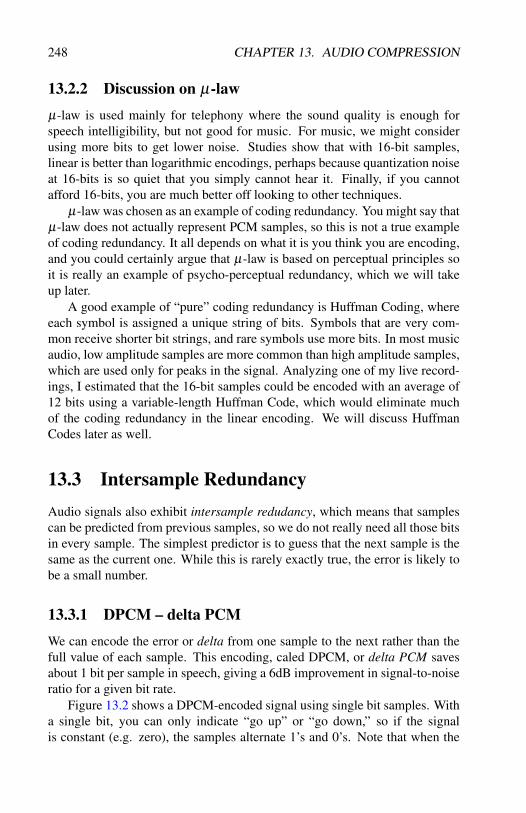
248 CHAPTER 13. AUDIO COMPRESSION
13.2.2 Discussion on µ-lawµ-law is used mainly for telephony where the sound quality is enough forspeech intelligibility, but not good for music. For music, we might considerusing more bits to get lower noise. Studies show that with 16-bit samples,linear is better than logarithmic encodings, perhaps because quantization noiseat 16-bits is so quiet that you simply cannot hear it. Finally, if you cannotafford 16-bits, you are much better off looking to other techniques.
µ-law was chosen as an example of coding redundancy. You might say thatµ-law does not actually represent PCM samples, so this is not a true exampleof coding redundancy. It all depends on what it is you think you are encoding,and you could certainly argue that µ-law is based on perceptual principles soit is really an example of psycho-perceptual redundancy, which we will takeup later.
A good example of “pure” coding redundancy is Huffman Coding, whereeach symbol is assigned a unique string of bits. Symbols that are very com-mon receive shorter bit strings, and rare symbols use more bits. In most musicaudio, low amplitude samples are more common than high amplitude samples,which are used only for peaks in the signal. Analyzing one of my live record-ings, I estimated that the 16-bit samples could be encoded with an average of12 bits using a variable-length Huffman Code, which would eliminate muchof the coding redundancy in the linear encoding. We will discuss HuffmanCodes later as well.
13.3 Intersample RedundancyAudio signals also exhibit intersample redudancy, which means that samplescan be predicted from previous samples, so we do not really need all those bitsin every sample. The simplest predictor is to guess that the next sample is thesame as the current one. While this is rarely exactly true, the error is likely tobe a small number.
13.3.1 DPCM – delta PCMWe can encode the error or delta from one sample to the next rather than thefull value of each sample. This encoding, caled DPCM, or delta PCM savesabout 1 bit per sample in speech, giving a 6dB improvement in signal-to-noiseratio for a given bit rate.
Figure 13.2 shows a DPCM-encoded signal using single bit samples. Witha single bit, you can only indicate “go up” or “go down,” so if the signalis constant (e.g. zero), the samples alternate 1’s and 0’s. Note that when the

13.3. INTERSAMPLE REDUNDANCY 249
signal to be encoded (the solid line) changes rapidly, the 1-bit DPCM encodingis not able to keep up with it.
Figure 13.2: DPCM. The solid line is encoded into 1’s and 0’s shown below.The reconstructed signal is shown as small boxes. Each box is at the value ofthe previous one plus or minus the step size.
A DPCM encoder is shown in 13.3. This is a common configuration wherethe output (on the right) is fed into a decoder (labeled “Integrate” in the fig-ure). The decoded signal is subtracted from the incoming signal, providing adifference that is encoded as bits by the box labeled “Quantize.” In this way,the overall encoding process drives the error toward zero.
Figure 13.3: DCPM Coder. A reconstructed signal is subtracted from thesignal to be encoded (at left) to decide whether the next output should be up(1) or down (0).
13.3.2 ADPCM – Adaptive Delta PCMYou can see that the DPCM coder suffers when the input changes rapidly (thelimited step size means that the encoded signal cannot change fast enough)and when the input does not change at all (the minimum step size introduceserror and noise). In Adaptive Delta PCM (ADPCM), the step size is variable.In the one-bit case, repeating bits mean the encoded signal is moving too fastin one direction, so the step size is increased to keep up. Alternating bits mean

250 CHAPTER 13. AUDIO COMPRESSION
the encoded signal is overshooting the target, so the step size is decreased.ADPCM achieves an improvement of 10-11 dB, or about 2 bits per sample,over PCM for speech.
Figure 13.4 illustrates the action of ADPCM. Notice how the steps in theencoded signal (shown in small squares) changes. In this example, the stepsize changes by a factor of two, and there is a minimum step size so thatreasonably large step sizes can be reached without too many doublings.
Figure 13.4: ADPCM. The step size is increased when bits repeat, and the stepsize is decreased (down to a minimum allowed step size) when bits alternate.
Figure 13.5 shows a schematic of an ADPCM coder. It is similar to theDPCM coder except repetitions or alternations in the output bits are used tomodify the step size. The step size is also incorporated into the decoder labeled“Integrate,” which decodes the signal.
Figure 13.5: ADPCM Coder. This is similar do DPCM, but the step size isvariable and controlled by additional logic that looks for same bits or alternat-ing bits in the encoded output.

13.4. PSYCHO-PERCEPTUAL REDUNDANCY AND MP3 251
13.3.3 Adaptive Prediction
If the previous sample is a good predictor and helps us to encode signals,why not use more samples to get even better prediction? A simple Nth-orderpredictor forms a weighted sum of previous samples to predict the next sample.If the weights are adapted, this is called adaptive prediction. The gain is about3 or 4 dB, or a fraction of a bit per sample, and there is little to be gainedbeyond 4th- or 5th-order prediction.
13.3.4 DPCM for High-Quality Audio
It might seem that we could replace 16-bit PCM with DPCM. Maybe 12 bitswould be enough to store deltas, or maybe we could get better-than 16-bitquality with only 16 bits. Unfortunately, to encode any PCM signal with N-bitsamples, you need (N + 1)-bit deltas because the delta must span the entirerange of an N-bit number, plus it needs a sign bit for the direction of change.Thus, DPCM at the same bit rate cannot be a lossless encoding. In carefullistening experiments, PCM is slightly better than DPCM.
13.3.5 Review
The term PCM refers to uncompressed audio where amplituded is convertedto binary numbers using a linear scale. By coding differently with µ-law andA-law, we can achieve better quality, at least for low-fidelity speech audio.Using intersample redundancy schemes such as DPCM and ADPCM, we canachieve further gains, but when we consider very high quality audio (16-bitPCM), these coding schemes lose their advantage.
As we will see in the next section, psycho-perceptual redundancy offers abetter path to high-quality audio compression.
13.4 Psycho-Perceptual Redundancy and MP3
We have seen how coding redundancy and intersample redundancy are usedin compression, especially for speech signals. For high-quality music audio,the FLAC lossless encoder can compress audio by about 50%, which gives anidea of how redundant is PCM. To get well beyond a 2:1 compression ratio,we must turn to lossy schemes, where the original audio is not preserved,but where the differences are not perceptible and therefore acceptable in mostapplications.

252 CHAPTER 13. AUDIO COMPRESSION
13.4.1 Masking and Perceptual CodingOur auditory system is complex and has some surprising behaviors. First, ourears act as filter banks, separating frequencies into different channels. There issome interaction between frequencies so that a loud sound in a channel masksor covers up soft sounds in adjacent channels. Masking also applies withina channel so that if you mix soft noise with a loud sound, the noise will beinaudible. This means that it is not always necessary to encode audio withvery low noise. We can get away with a lot of quantization as long as there issound to mask the quantization noise.
Another form of masking occurs over time. A loud sound masks softsounds that follow for a brief period of time. Most of the masking dissipateswithin 100 ms. Amazingly, masking also works backwards in time: a loudsound can mask sounds that happened a few milliseconds earlier!
Another important idea for compression is that when we are digitizinga narrow frequency channel, we do not have to sample at the Nyquist rate.This matters because if we model human hearing and split a sound into, say,32 channels, we might expect that we need 32 times as many samples. Butsuppose we have a channel with frequencies from 1000 to 1100 Hz. Ratherthan sample at 2200 Hz or higher, we can frequency shift the signal down tothe range of 0 to 100 Hz. Now, we can sample at only 200 Hz and capture allof the signal. To recover the original sound, we have to frequency shift backto the 1000 to 1100 Hz range. In theory, you can encode a signal as N bands,each at 1/N of the sample rate, so the total information is the same.
13.4.2 Some Insight on Frequency Domain and CodingAll perceptual coding is done in the frequency domain even though PCMworks in the time domain. Redundancy is hard to find in the time domainbecause sound is vibration, implying constant change. Spectral data tends tobe more static. The spectrum at time t is a good predictor for spectrum at timet +1. In tonal music, the spectrum also tends to be relatively sparse. It is non-zero only where there are sinusoidal partials. Sparse data is easier to encodeefficiently.
13.4.3 MP3 - MPEG Audio Layer 3MPEG is a video compression standard. Within MPEG is the “MPEG Au-dio Layer 3” standard for audio compression, commonly known as “MP3.”This standard specifies how to decode audio so that MP3 files are treated con-sistently. Interestingly, the standard does not specify how to encode audio,so there are slight variations among encoders, resulting in different levels of

13.4. PSYCHO-PERCEPTUAL REDUNDANCY AND MP3 253
quality and efficiency. In tests, a 6-to-1 compression of 48 kHz audio gives noperceptual difference from the original. The Fraunhofer Institute, who createdthe MP3 standard, claims 12-to-1 compression with no perceptual differences.
Let’s take a high-level view of how MP3 works. The first step is to apply afilter bank that separates the signal into 32 bands of equal width. As describedearlier, each band is sub-sampled by factor of 32 to avoid increasing the over-all sample rate. In practice, bands have some overlap and this sub-samplingcauses some aliasing. Also, the filters and their inverses are slightly lossy interms of recovering the original signal.
Next, a psychoacoustic model is applied to estimate the amount of maskingthat is present in each channel. This determines how much each band can bequantized. The model uses a 1024-point FFT and identifies sinusoids becausethe masking effect of sinusoids differs from that of noise. The model producesa signal-to-mask ratio for each of the 32 subbands.
Each subband is then transformed with modified discrete cosine transform(MDCT) of length 18 or 6 subband samples. Essentially, this is a short-termfrequency representation of the subbands, which allows for more efficient cod-ing. For example, if there is only one sinusoid in the subband, only one MDCTcoefficient should be high and others should be low. Next, the MDCT coeffi-cients are quantized according to the signal-to-masking ratio. This results in576 coefficients per frame (18 MDCT coefficients × 32 subbands).
The coefficients are ordered by increasing frequency because the highestfrequencies tend to be zeros—these can be encoded without expending anybits. Next, there will be a run of coefficients that are -1, 0, or 1. These areencoded 4 at a time into alphabet of 81 symbols. The remaining values arecoded in pairs.
13.4.4 Details of Huffman Coding
To encode the MDCT coefficients, Huffman Coding is used. Huffman Codingis the most popular technique for removing coding redundancy. A HuffmanCode is a variable length encoding of symbols into bit strings, and assumingthat each symbol is encoded separately into a string of bits, Huffman Cod-ing is optimal in producing the smallest expected bit length of any string ofsymbols.3
Figure 13.6 illustrates the Huffman coding process. To begin with, eachsymbol is given a probability. E.g. in English, we know that the letter E occursabout 12% of the time, while Z occurs only 0.07%. Thus, we should use fewer
3Another technique, arithmetic coding, and some variations, offer even shorter encodings,essentially by representing symbols by fractional rather than whole bits.

254 CHAPTER 13. AUDIO COMPRESSION
bits for E than Z. For this example, we encode only symbols A, B, C, D, E andF, which we assume occur with the probabilities shown in Figure 13.6.
The algorithm produces a binary tree (13.6) using a simple process: Start-ing with the symbols as leaves of the tree, create a node whose branches havethe 2 smallest probabilities. (This would combine D and E in Figure 13.6.)Then, give this node the probability of the sum of the two branches and re-peat the process. For example, we now have C with probability 0.1 and theDF node with probability 0.1. Combining them, we get a new internal nodeof probability 0.2. Continue until there is just one top-level node. Now, eachsymbol is represented by the path from the root to the leaf, encoding a leftbranch as 0 and a right branch as 1. The final codes are shown at the right ofFigure 13.6.
Figure 13.6: Huffman Coding Tree example.
13.4.5 MP3 Coefficient CodingReturning to MP3, the terminology of “codes” and “symbols” may be con-fusing. In Figure 13.6, the symbols were A, B, C, etc., but in general, thesesymbols can stand for numbers or even vectors. Any finite set of values can beconsidered a set of symbols that we can encode. In MP3, one of the things wewant to encode are runs of coefficients -1, 0, or 1. These are grouped into 4,so the “symbols” are 4-tuples such as [-1, 0, 1, -1]. To make a Huffman Code,we can let:
A = [-1, -1, -1, -1]B = [-1, -1, -1, 0]C = [-1, -1, -1, 1]D = [-1, -1, 0, -1]

13.5. LPC: LINEAR PREDICTIVE CODING 255
E = [-1, -1, 0, 0]F = [-1, -1, 0, 1]etc.
Encoding in groups of 4 allows Huffman Coding to find a more compact over-all representation.
13.4.6 Bit Reservoir and Bit AllocationEven if audio encoding uses a fixed bit rate, some frames are going to be easierto encode than others. A trick used in MP3 is to take advantage of easy-to-compress frames. When bandwidth is left over, bits can be “donated” to a “bitreservoir” and used later to temporarily exceed the maximum data rate andimprove the quality of more difficult frames.
Deciding how to use bits for encoding is a difficult problem. Encodersallocate bits to bands where the masking threshold is exceeded by quantizationnoise. The band is re-encoded and quantization noise is recalculated. Thismakes encoding slow.
13.4.7 SummaryMasking reduces our ability to hear “everything” in a signal, and in particularquantization noise. MP3 uses a highly quantized frequency domain represen-tation. Because of different quantization levels and coefficient sizes, Huffmancoding is used to encode the coefficients.
13.5 LPC: Linear Predictive CodingAnother way to achieve compression is to use better, more predictive mod-els of the source sound. This is especially important for voice, where a lot isknown about the voice and where there is a big demand for voice data com-pression. For voice, source/filter models are used because the voice pitch andfilter coefficients change slowly. Data rates for speech can be as low as 1 to 2kbps (kilobits per second) and in cell phone communication are generally inthe 5-10 kbps range.
LPC, discussed earlier, is an example of using intersample redundancy.Analysis estimates a vocal tract filter model that allows for good predictionsof the output. By inverse filtering the desired signal, we get a source signalthat is relatively easy to encode. Figure 13.7 illustrates the LPC model. Thisis also an example of an “object model” for data compression. The idea is toextract simple control parameters for an “object” that generates sound. The

256 CHAPTER 13. AUDIO COMPRESSION
control parameters and object parameters can be quite small compared to theaudio signal that is generated.
Figure 13.7: Linear Predictive Coding in Practice
13.6 Physical Models – Speech Analysis/Synthesis
It seems feasible that object models and physical models can offer interestingcompression techniques in the future. Our speech is controlled by muscles,and we know that muscles have low bandwidth compared to audio signals.Also, speech sounds are highly constrained. If we could transmit a model forspeech production and muscle control parameters, perhaps the data rate forspeech could be much lower and the quality could be higher.
13.7 Music Notation
The physical and object models approach to compression leads us to considermusic notation. In some sense, music notation is high-level, low-bandwith“control” information for performers who actually produce audio. Of course,in normal situations, no two music performances are alike, so we cannot reallysay that music notation is a compressed form of audio, but it is still interestingto consider notation, what it encodes, and what it does not.
Music notation is compact and symbolic as opposed to digital audio. Mu-sic notation is missing a lot of detail of how music is performed, for exampledetails of instruments or muscle movement of performers. Furthermore, get-ting any musical rendition of music notation, complete with expressive inter-

13.8. SUMMARY 257
pretation and natural sounding voices and instruments is a big challenge thathas not been automated.
Another representation that is similar to music notation is the performanceinformation found in MIDI, or Musical Instrument Digital Interface. Theidea of MIDI is to encode performance “gestures” including keyboard perfor-mances (when do keys go down?, how fast?, when are they released?) as wellas continuous controls such as volume pedals and other knobs and sensors.
The bandwidth of MIDI is small, with a maximum over MIDI hardware of3 KB/s. Typically, the bandwidth is closer to 3 KB/minute. For example, thecomplete works of ragtime composer Scott Joplin, in MIDI form, takes about1 MB. The complete output of 50 composers (400 days of continuous music)fits into 500 MB of MIDI—less data than a single compact disc.
MIDI has many uses, but one big limitation is the inability in most casesto synthesize MIDI to create, say, the sound of an orchestra or even a rockband. An exception is that we can send MIDI to a player piano to at leastproduce a real acoustic piano performance that sounds just like the original.Another limitation, in terms of data compression, is that there is no “encoder”that converts music audio into a MIDI representation.
13.8 SummaryWe have discussed three kinds of redundancy: coding redundancy, intersam-ple redundancy, and psycho-perceptual redundancy. µ-law, ADPCM, etc. of-fer simple, fast, but not high-quality or high-compression representations ofaudio. MP3 and related schemes are more general, of higher quality, and of-fer higher compression ratios, but the computation is fairly high. We alsoconsidered model-based analysis and synthesis, which offer even greater com-pression when the source can be accurately modeled and control parameterscan be estimated. Music notation and MIDI are examples of very abstractand compact digital encodings of music, but currently, we do not have goodautomatic methods for encoding and decoding.

258 CHAPTER 13. AUDIO COMPRESSION
Chapter 14
Computer Music FuturesTopics Discussed: Computer Accompaniment, Style Classification, Mu-sic Alignment, Human-Computer Music Performance
14.1 IntroductionLet’s take a step back from details and technical issues to think about wherecomputer music is heading, and maybe where music is heading. This chapteris a personal view, and I should state at the beginning that the ideas here arehighly biased by my research, which is in turn guided by my own knowledge,interests, abilities, and talents.
I believe that if we divide computer music into a “past” and “future” thatthe “past” is largely characterized by the pursuit of sound and the concept ofthe instrument. Much of the early work on synthesis tried to create interestingsounds, model acoustic instruments or reproduce their sounds, and build inter-faces and real-time systems that could be used in live performance in the sameway that traditional musicians master and perform with acoustic instruments.The “future,” I believe, will be characterized by the model of the musicianrather than the instrument. The focus will be on models of music performance,musical interaction among players, music described in terms of style, genre,“feel,” and emotion rather than notes, pitch, amplitude, and spectrum. A keytechnology will be the use of AI and machine learning to “understand” musicat these high levels of abstraction and to incorporate music understanding intothe composition, performance, and production of music.
Much of my research has been in the area of music understanding, andin some sense, the “future” is already here. Everything I envision as part ofthe future has some active beginnings well underway. It’s hard to foresee thefuture as anything but an extension of what we already know in the present!
259

260 CHAPTER 14. COMPUTER MUSIC FUTURES
However, I have witnessed the visions of others as they developed into reality:high-level languages enabling sophisticated music creation, real-time controlof sound with gestural control, and all-digital music production. These visionstook a long time to develop, and even if they were merely the logical pro-gression of what was understood about computer music in the 70s or 80s, theresults are truly marvelous and revolutionary. I think in another 20 or 30 years,we will have models of musicians and levels of automatic music understandingthat make current systems pale by comparison.
The following sections describe a selection of topics in music understand-ing. Each section will describe a music understanding problem and outline asolution or at least some research systems that address the problem and showsome possibilities for the future.
14.2 Computer Accompaniment
A basic skill for the musically literate is to read music notation while listeningto a performance. Humans can follow quite complex scores in real-time with-out having previously heard the music or seen the score. The task of ComputerAccompaniment is to follow a live performance in a score and to synchronizea computer performance. Note that the computer performs a pre-composedpart, so there is no real-time composition involved but rather a responsive syn-chronization. There are now many accompaniment systems, at least in theliterature, as well as a few commercial systems.
Accompaniment systems have two basic parts. First, a score-followermatches an incoming live performance signal (usually either audio or datataken directly from a piano-like keyboard using the MIDI protocol) to a ma-chine-readable note-list or score. Second, an accompaniment algorithm usesscore location to estimate tempo, position, and decide how to schedule upcom-ing notes or sound events in the accompaniment score.
The score-following component of Computer Accompaniment can be dis-sected further into two sub-tasks as shown in Figure 14.1.
14.2.1 Input Processing
The first task, the Input Processor, translates the human performance (whichmay be detected by a microphone or by sensors attached to keys) into a se-quence of symbols, which typically correspond to pitches. With microphoneinput, the pitch must be estimated and quantized to the nearest semitone, andadditional processing is useful to reduce the number of false outputs that typi-cally arise.

14.2. COMPUTER ACCOMPANIMENT 261
Figure 14.1: Score following block diagram.
14.2.2 Matching
The Matcher receives input from the Input Processor and attempts to find a cor-respondence between the real-time performance and the score. The Matcherhas access to the entire score before the performance begins. As each note isreported by the Input Processor, the matcher looks for a corresponding note inthe score. Whenever a match is found, it is output. The information neededfor Computer Accompaniment is just the real-time occurrence of the note per-formed by the human and the designated time of the note according to thescore.
Since the Matcher must be tolerant of timing variations, matching is per-formed on sequences of pitches only. This decision throws away potentiallyuseful information, but it makes the matcher completely time-independent.One problem raised by this pitch-only approach is that each pitch is likely tooccur many times in a composition. In a typical melody, a few pitches occurin many places, so there may be many candidates to match a given performednote.
The matcher described here overcomes this problem and works well inpractice. Many different matching algorithms have been explored, often in-troducing more sophisticated probabilistic approaches, but my goal here is toillustrate one simple approach. The matcher is derived from the dynamic pro-gramming algorithm for finding the longest common subsequence (LCS) oftwo strings. Imagine starting with two strings and eliminating arbitrary charac-ters from each string until the the remaining characters (subsequences) matchexactly. If these strings represent the performance and score, respectively,then a common subsequence represents a potential correspondence betweenperformed notes and the score (see Figure 14.2). If we assume that most ofthe score will be performed correctly, then the longest possible common sub-sequence should be close to the “true” correspondence between performanceand score.
In practice, it is necessary to match the performance against the score as
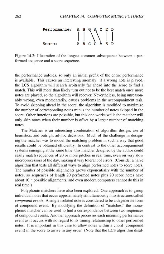
262 CHAPTER 14. COMPUTER MUSIC FUTURES
Figure 14.2: Illustration of the longest common subsequence between a per-formed sequence and a score sequence.
the performance unfolds, so only an initial prefix of the entire performanceis available. This causes an interesting anomaly: if a wrong note is played,the LCS algorithm will search arbitrarily far ahead into the score to find amatch. This will more than likely turn out not to be the best match once morenotes are played, so the algorithm will recover. Nevertheless, being unreason-ably wrong, even momentarily, causes problems in the accompaniment task.To avoid skipping ahead in the score, the algorithm is modified to maximizethe number of corresponding notes minus the number of notes skipped in thescore. Other functions are possible, but this one works well: the matcher willonly skip notes when their number is offset by a larger number of matchingnotes.
The Matcher is an interesting combination of algorithm design, use ofheuristics, and outright ad-hoc decisions. Much of the challenge in design-ing the matcher was to model the matching problem in such a way that goodresults could be obtained efficiently. In contrast to the other accompanimentsystems emerging at the same time, this matcher designed by the author couldeasily match sequences of 20 or more pitches in real time, even on very slowmicroprocessors of the day, making it very tolerant of errors. (Consider a naivealgorithm that tests all different ways to align performed notes to score notes.The number of possible alignments grows exponentially with the number ofnotes, so sequences of length 20 performed notes plus 20 score notes haveabout 1012 possible alignments, and even modern computers cannot do this inreal time.)
Polyphonic matchers have also been explored. One approach is to groupindividual notes that occur approximately simultaneously into structures calledcompound events. A single isolated note is considered to be a degenerate formof compound event. By modifying the definition of “matches,” the mono-phonic matcher can be used to find a correspondence between two sequencesof compound events. Another approach processes each incoming performanceevent as it occurs with no regard to its timing relationship to other performednotes. It is important in this case to allow notes within a chord (compoundevent) in the score to arrive in any order. (Note that the LCS algorithm disal-

14.3. STYLE CLASSIFICATION 263
lows reordering.) The resulting algorithm is time-independent.The Matcher performs a fairly low-level recognition task where efficiency
is important and relatively little knowledge is required. When matches arefound, they are output for use by an Accompaniment Performance subtask,which uses knowledge about musical performance to control a synthesizer.Several systems have been implemented based on these techniques, and the re-sults are quite good. (You can find a video demonstration at www.cs.cmu.edu/~rbd/videos.html.)
The Matcher has also been extended to handle trills, glissandi, and gracenotes as special cases that would otherwise cause problems, and this versionhas been used successfully for several concerts. A commercial Computer Ac-companiment system, SmartMusic, is derived directly from the author’s workand has been used mainly for music education since the 1990’s. Other accom-paniment systems include Tonara, Antescofo, and Music Plus One.
14.3 Style ClassificationMany computer music applications can benefit from higher-level music un-derstanding. For example, interactive performance systems are sometimes de-signed to react to higher-level intentions of the performer. Unfortunately, thereis often a discrepancy between the ideal realization of an interactive system,in which the musician and machine carry on a high-level musical discourse,and the realization, in which the musician does little more than trigger storedsound events. This discrepancy is caused in part by the difficulty of recogniz-ing high-level characteristics or style of a performance with any reliability.
Our experience has suggested that even relatively simple stylistic features,such as playing energetically, playing lyrically, or playing with syncopation,are difficult to detect reliably. Although it may appear obvious how one mightdetect these styles, good musical performance is always filled with contrast.For example, energetic performances contain silence, slow lyrical passagesmay have rapid runs of grace notes, and syncopated passages may have a va-riety of confusing patterns. In general, higher-level musical intent appearschaotic and unstructured when presented in low-level terms such as MIDI per-formance data.
Machine learning has been shown to improve the performance of manyperception and classification systems (including speech recognizers and vi-sion systems). This section describes a machine-learning-based style classi-fier for music. Our initial problem was to classify an improvisation as one offour styles: lyrical, frantic, syncopated, or pointillistic (the latter consistingof short, well-separated sound events). We later added the additional styles:blues, quote (play a familiar tune), high, and low. The exact meaning of these

264 CHAPTER 14. COMPUTER MUSIC FUTURES
terms is not important. What really matters is the ability of the performer toconsistently produce intentional and different styles of playing at will.
The ultimate test is the following: Suppose, as an improviser, you want tocommunicate with a machine through improvisation. You can communicatefour different tokens of information: lyrical, frantic, syncopated, and pointil-listic. The question is, if you play a style that you identify as frantic, what isthe probability that the machine will perceive the same token? By describingmusic as a kind of communication channel and music understanding as a kindof decoder, we can evaluate style recognition systems in an objective scientificway.
It is crucial that this classification be responsive in real time. We arbitrarilyconstrained the classifier to operate within five seconds.
Figure 14.3: Training data for a style recognition system is obtained by askinga human performer to play in different styles. Each style is played for about 15seconds, and 6 overlapping 5-second segments or windows of the performanceare extracted for training. A randomly selected style is requested every 15seconds for many minutes to produce hundreds of labeled style examples fortraining.
Figure 14.3 illustrates the process of collecting data for training and evalu-ating a classifier. Since notions of style are personal, all of data is provided byone performer, but it takes less than one hour to produce enough training datato create a customized classifier for a new performer or a new set of style la-bels. The data collection provided a number of 5-second “windows” of musicperformance data, each with a label reflecting the intended style.
The data was analyzed by sending music audio from an instrument (a trum-pet) through an IVL Pitchrider, a hardware device that detects pitch, note-onsets, amplitude, and other features and encodes them into MIDI. This ap-proach was used because, at the time (1997), audio signal processing in soft-ware was very limited on personal computers, and using the MIDI data streamwas a simple way to pre-process the audio into a useful form. We extracted a

14.4. AUDIO-TO-SCORE ALIGNMENT 265
number of features from each 5-second segment of the MIDI data. Featuresincluded average pitch, standard deviation of pitch, number of note onsets,mean and standard deviation of note durations, and the fraction of time filledwith notes (vs. silence).
Various style classifiers were constructed using rather simple and standardtechniques such as linear classifiers and neural networks.
While attempts to build classifiers by hand were not very successful, thisdata-driven machine-learning approach worked very well, and it seems thatour particular formulation of the style-classification problem was not evenvery difficult. All of the machine-learning algorithms performed well, achiev-ing nearly perfect classification in the 4-class case, and around 90% accuracyin the 8-class case. This was quite surprising since there seems to be no simpleconnection between the low-level features such as pitch and duration and thehigh-level concepts of style. For example the “syncopation” style is recogniz-able from lots of notes on the upbeat, but the low-level features do not includeany beat or tempo information, so evidently, “syncopation” as performed hap-pens to be strongly correlated with some other features that the machine learn-ing systems were able to discover and take advantage of. Similarly, “quote,”which means “play something familiar” is recognizable to humans becausewe might recognize the familiar tune being quoted by the performer, but themachine has no database of familiar tunes. Again, it must be that playingmelodies from memory differs from free improvisation in terms of low-levelpitch and timing features, and the machine learning systems were able to dis-cover this.
You can see a demonstration of this system by finding “Automatic stylerecognition demonstration” on www.cs.cmu.edu/~rbd/videos.html. Since thiswork was published, machine learning and classifiers have been applied tomany music understanding problems including genre recognition from musicaudio, detection of commercials, speech, and music in broadcasts, and thedetection of emotion in music.
14.4 Audio-to-Score AlignmentThe off-line version of score following is called audio-to-score alignment. Off-line means that we do not need to output alignment or location data in real-time. Instead, we get to observe the entire audio stream and the entire scorebefore computation begins. This means that we can look ahead into the datafor both audio and score. As a result, ambiguous information can be resolvedby finding clearer matches happening both earlier and later.
This turns out to be a very big advantage. Earlier we said that computeraccompaniment system work in real-time and perform quite well, which is
266 CHAPTER 14. COMPUTER MUSIC FUTURES
true, but that is partly because accompaniment systems tend to be built formonophonic instruments (those that produce one note at a time). Dealing withpolyphony (multiple notes) or something as complex as an orchestra or evena popular music recording poses a very challenging problem to detect notesaccurately. Our ability to do real-time score following is greatly diminishedwhen the input consists of polyphonic music audio.
These problems are compensated for by the additional power of usinglook-ahead in a non-real-time audio-to-score alignment system. This sectionoutlines the basic principles that are used and then presents some applicationsand opportunities for this technology.
14.4.1 Chroma Vectors and Similarity
In a monophonic score follower or polyphonic MIDI score follower, we nor-mally use note pitch as the “feature” that we match between performance andscore. With polyphonic audio, extracting pitches is difficult and unreliable, butanother feature, called the chroma vector, has been shown to be quite usefuland robust. The chroma vector is related to the spectrum. You might thinkthe spectrum would be a good feature itself since it requires very little inter-pretation and certainly contains all the necessary information about the perfor-mance. The problem with the spectrum is that just by playing a little louder(brighter) or changing the microphone location, we can get fairly large shiftsin the spectrum. Also, to align audio recordings to symbolic representations,we would need a way to determine the spectrum from symbolic representa-tions, i.e. we need to synthesize a band or orchestra in a way that accuratelyreproduces the spectrum of the recorded version. Our symbolic descriptionsdo not contain enough information and our synthesis methods are not goodenough to reproduce spectra.
The chroma vector divides the spectrum into semitones, i.e. we look atfrequency bands for C1, C#1, D1, ... B1, C2, C#2, D2, ... B2, and all theway to the top octave. Then, we take all the magnitudes in the spectrum forpitch class C, namely the frequency bands for all the octaves of C: C1, C2, C3,etc., and add the magnitudes together to get one number we will call C. Thenwe do the same for C-sharp: C#1, C#2, C#3, etc., and then D1, D2, D3, etc.,and all the other pitch classes. The result is a vector of 12 elements: C, C#,D, D#, E, F, F#, G, G#, A, A#, B. To finish processing, the chroma vector isoften normalized to have a sum-of-squares magnitude of one so that scalingthe amplitude of the source signal has no effect on the chroma vector.
You can think of chroma vectors as a summary or projection of the detailedspectrum into a simpler representation. A sequence of chroma vectors overtime is analogous to a spectrogram and we call it a chromagram.
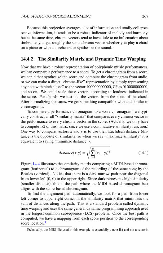
14.4. AUDIO-TO-SCORE ALIGNMENT 267
Because this projection averages a lot of information and totally collapsesoctave information, it tends to be a robust indicator of melody and harmony,but at the same time, chroma vectors tend to have little to no information abouttimbre, so you get roughly the same chroma vector whether you play a chordon a piano or with an orchestra or synthesize the sound.
14.4.2 The Similarity Matrix and Dynamic Time WarpingNow that we have a robust representation of polyphonic music performances,we can compare a performance to a score. To get a chromagram from a score,we can either synthesize the score and compute the chromagram from audio,or we can make a direct “chroma-like” representation by simply representingany note with pitch class C as the vector 100000000000, C# as 010000000000,and so on. We could scale these vectors according to loudness indicated inthe score. For chords, we just add the vectors from the notes of the chord.After normalizing the sums, we get something compatible with and similar tochromagrams.
To compare a performance chromagram to a score chromagram, we typi-cally construct a full “similarity matrix” that compares every chroma vector inthe performance to every chroma vector in the score. (Actually, we only haveto compute 1/2 of this matrix since we use a commutative similarity function.)One way to compare vectors x and y is to use their Euclidean distance (dis-tance is the opposite of similarity, so when we say “maximize similarity” it isequivalent to saying “minimize distance”).
distance(x,y) =
√n
∑i=1
(xi− yi)2 (14.1)
Figure 14.4 illustrates the similarity matrix comparing a MIDI-based chroma-gram (horizontal) to a chromagram of the recording of the same song by theBeatles (vertical). Notice that there is a dark narrow path near the diagonalfrom lower left (0, 0) to the upper right. Since dark represents high similarity(smaller distance), this is the path where the MIDI-based chromagram bestaligns with the score-based chromagram.
To find the alignment path automatically, we look for a path from lowerleft corner to upper right corner in the similarity matrix that minimizes thesum of distances along the path. This is a standard problem called dynamictime warping and uses the same general dynamic programming approach usedin the longest common subsequence (LCS) problem. Once the best path iscomputed, we have a mapping from each score position to the correspondingscore location.1
1Technically, the MIDI file used in this example is essentially a note list and not a score in

268 CHAPTER 14. COMPUTER MUSIC FUTURES
Figure 14.4: A similarity matrix illustrating data used for audio-to-score align-ment. Darker means more similar.
14.4.3 Applications of Audio-to-Score AlignmentOne application of audio-to-score alignment is to make navigation of audioeasier. Figure 14.5 shows an experimental version of Audacity that was ex-tended by the author to “warp” the tempo of a MIDI file to align to an audiorecording. This is not simply a synthesized version of the MIDI file. TheMIDI file came from a MIDI library, and the audio is a commercial recordingof a Haydn symphony. By aligning these two different representations, we canimmediately see much more of the music structure. For example, if one werelooking for the places where the whole orchestra plays a long note together, itis much easier to find those spots with the MIDI file as a reference.
In studio recordings of new music, scores are often prepared using mu-sic notation software, so it is often the case that machine-readable commonpractice notation is available. In principle, that information could be used todisplay music notation to aid navigation in a future audio editor.
Alignment has also been used in systems to identify “cover songs,” whichare versions of popular songs performed by someone other than the originalrecording artists. Another interesting possibility is to use alignment to provide
the sense of common practice music notation. It might be better to say this is signal-to-symbolalignment, but symbol is a vague term, so it is common to use score to refer to any representationof notes or sound events with some indication of timing and properties such as pitch.

14.5. HUMAN-COMPUTER MUSIC PERFORMANCE 269
Figure 14.5: Alignment of MIDI in a piano-roll display to audio in an experi-mental version of the Audacity audio editor.
meta-data or labels for audio. This data can then be used to train machinelearning systems to identify chords, pitches, tempo, downbeats and other mu-sic information.
14.5 Human-Computer Music PerformanceAnother interesting application for computers in music is live performance ofpopular music such as rock, jazz, and folk music. By and large, “popular” mu-sic has a definite form and steady tempo, but players often have the possibilityto interpret the score rather freely. A consequence is that players synchronizemore by beat than by note-by-note score following. In fact, many times thereis no note-level score for guitars or drums, and even vocalists sing expressivelywithout strictly following notated rhythms.
Computers are often used in such music, but computers play sequences ata strict tempo, and human musicians are forced to play along and synchronizeto the computer (or even a digital audio recording, sometimes referred to as abacking track). This type of performance is restrictive to musicians, who oftenend up focused more on keeping with the computer than playing musically,and it is usually not enjoyable to have a completely inflexible tempo.
As an alternative, imagine a system where computers could follow hu-

270 CHAPTER 14. COMPUTER MUSIC FUTURES
mans, much like in computer accompaniment systems, only now with popularbeat-based music. One could imagine a computer using beat-tracking algo-rithms to find the beat and then synchronize to that. Some experimental sys-tems have been built with this model, but even state-of-the-art beat tracking(another interesting research problem) is not very reliable. An alternative issimple foot tapping using a sensor that reports the beat to the computer.
In addition to beats, the computer needs to know when to start, so wecan add sensors for giving cues to start a performance sequence. Just as hu-man conductors give directions to humans—play something now, stop play-ing, play louder or softer, go back and repeat the chorus, etc.—we can usemultiple sensors or different gestures to give similar commands to computerperformers.
We call this scenario Human-Computer Music Performance (HCMP), withterminology that is deliberately derived from Human-Computer Interaction(HCI) since many of the problems of HCMP are HCI problems: How can com-puters and humans communicate and work cooperatively in a music perfor-mance? The vision of HCMP is a variety of compatible systems for creating,conducting, cueing, performing, and displaying music. Just as rock musicianscan now set up instruments, effects pedals, mixers, amplifiers and speakers,musicians in the future should be able to interconnect modular HCMP sys-tems, combining sensors, virtual performers, conducting systems, and digitalmusic displays as needed to create configurations for live performance.
Some of the interesting challenges for HCMP are:
• Preparing music for virtual players: Perhaps you need a bass player tojoin your band, but you only have chord progressions for your tunes.Can software write bass parts in a style that complements your musicaltastes?
• Sharing music: Can composers, arrangers, and performers share HCMPsoftware and content? How can a band assemble the software compo-nents necessary to perform music based on HCMP?
• Music display systems: Can digital music displays replace printed mu-sic? If so, can we make the displays interactive and useful for cueing andconducting? Can a band leader lead both human and virtual performersthrough a natural music-notation-based interface?
Clearly, music understanding is important for HCMP systems to interactwith musicians in high-level musical terms. What if a band leader tells a virtualmusician to make the music sound more sad? Or make the bass part morelively? HCMP is an example of how future music systems can move from afocus on instruments and sounds to a focus on music performance and musicalinteraction.

14.6. SUMMARY 271
14.6 SummaryMusic understanding encompasses a wide range of research and practice withthe goal of working with music at higher levels of abstraction that include emo-tion, expressive performance, musical form and structure, and music recogni-tion. We have examined just a limited selection of music understanding capa-bilities based on work by the author. These include:
• computer accompaniment—the computer as virtual interactive and re-sponsive musical accompanist,
• automatic style recognition—the detection of different performance stylesusing machine classifiers,
• audio-to-score alignment—the ability to match sounds to symbolic rep-resentations of music event sequences, and
• Human-Computer Music Performance—an evolving practice of bring-ing virtual performers into collaboration with humans in live perfor-mance.
All of these tasks rely on new techniques for processing musical informationthat we call music understanding.

272 CHAPTER 14. COMPUTER MUSIC FUTURES

Chapter 15
Where Next?
This book has introduced fundamental technologies of digital audio, soundsynthesis, and music creation by computer. We have touched on some relatedfields including musical acoustics, music perception, music theory, music in-formation retrieval, and music understanding.
This is still just an introduction to a rapidly growing field. To explorefurther, it is good to have some idea of what is out there and where to look forit. This final chapter is far from complete, but offers some directions for studyand some references to consider.
15.1 NIME and Physical ComputingIn 2001, a workshop called “New Interfaces for Musical Expression” or NIMEwas organized to discuss physical controls and interfaces that sit between per-formers and computer music systems. Since then, the annual NIME confer-ence continues to draw researchers who study sensors, control strategies, hap-tics, robots, and many other topics. NIME proceedings are all online and free(www.nime.org).
In the early days, it was an accomplishment simply to combine a sensor, amicrocontroller, and perhaps a MIDI interface to send controls to a synthesizer,and many projects explored variations of this configuration. Today, parts areavailable “off-the-shelf” to quickly put together the electronics needed for acomputer music instrument controller. See offerings from www.adafruit.comand www.sparkfun.com for example. Still, if you have no electronics skills, itcould be quite liberating to master some basic skills. Many universities offercourses in “physical computing” or “Internet of Things” where you can learnto assemble small self-contained computing devices with sensors and outputs
273

274 CHAPTER 15. WHERE NEXT?
of various kinds. If not, look for Electrical Engineering courses in digitalelectronics or microcomputers/microcontrollers with lab sections where youactually build things.
15.2 Music Information Retrieval
Almost coincident with the beginnings of NIME, a new field emerged com-bining library science, data retrieval, computer music, and machine learningcalled Music Information Retrieval. Like NIME, the International Societyfor Music Information Retrieval (ISMIR) conference draws hundreds of re-searchers every year who present work which has steadily drifted from re-trieval problems to more general research on music understanding and mu-sic composition by computer. This field is strongly weighted toward popularmusic and commercial music. Proceedings tend to be very technical and areavaiable online at ismir.net. Also, ISMIR has become a favorite venue forapplications of machine learning to music.
Some textbooks, mainly for graduate students, have appeared, includingFundamentals of Music Processing [Müller, 2015]. George Tzanetakis has abook online as well as course materials for his “Music Retrieval Systems”class at the University of Victoria (marsyas.cs.uvic.ca/mirBook/course).
15.3 Signal Processing
Our introduction to music signal processing is an attempt to convey “whatevery computer scientist should know” about signal processing. A more rig-orous approach is certainly possible and to design new algorithms or reallymaster the application of signal processing to music, there is much more tolearn. Julius Smith has a wonderful resource consisting of multiple onlinebooks (ccrma.stanford.edu/ jos). A formal Electrical Engineering course inSignals and Systems or Advanced Digital Signal Processing is a good way tolearn more. The book Audio Content Analysis introduces many signal pro-cessing techniques for music analysis [Lerch, 2012]. Another conference se-ries, DAFX, has many papers on various synthesis and analysis techniquesfor music (www.dafx.de) and there is a book: DAFX - Digital Audio Effects[Zölzer, 2011].

15.4. REAL-TIME SYSTEMS 275
15.4 Real-Time SystemsIt is surprising given the importance of time in music that there is not moreliterature on building real-time systems for music. There are some importanttechniques, but few good sources to learn from. One recommendation is RossBencina’s blog (www.rossbencina.com/code/real-time-audio-programming-101-time-waits-for-nothing). Ross and I gave a workshop and wrote a shortdocument with some good references. This might be a good starting pointfor further reading (www.cs.cmu.edu/ rbd/doc/icmc2005workshop/real-time-systems-concepts-design-patterns.pdf).
15.5 General Computer MusicBeyond these more specialized areas, there are many musicians, scientists andengineers who simply create and explore music with computers. There are toomany ideas to classify or label them. Literally thousands of papers on com-puter music are reported in Proceedings of the International Computer Mu-sic Conference (ICMC), available free online from the International ComputerMusic Association (computermusic.org). Two main publications on ComputerMusic are the Computer Music Journal (www.computermusicjournal.org) andJournal of New Music Research. Unfortunately, neither of these journals isopen, but your library may have access to online content. Computer MusicJournal has a wide readership and tends to be less technical and less aca-demic, while Journal of New Music Research has more in-depth articles andwork related to contemporary art music. There is a good deal of overlap intopics, and both are important resources.
There are many more conferences we have not mentioned. Most of theseconferences publish proceedings online. Searching the Internet for scholarlyarticles in journals and conferences is a good way to learn, and you will getto know which journal and conferences are most relevant to your personalinterests.

276 CHAPTER 15. WHERE NEXT?

Bibliography
[Chowning, 1973] Chowning, J. (1973). The synthesis of complex audiospectra by means of frequency modulation. Journal of the Audio Engi-neering Society, 21(7).
[Hu, 2013] Hu, N. (2013). Automatic Construction of Synthetic Musical In-struments and Performers. PhD thesis, Carnegie Mellon University Com-puter Science Department.
[Kaegi and Tempelaars, 1978] Kaegi, W. and Tempelaars, S. (1978). Vosim—a new sound synthesis system. Journal of the Audio Engineering Society,26(6):418–425.
[Karjalainen et al., 1993] Karjalainen, M., Valimaki, V., and Janosy, Z.(1993). Towards high quality sound synthesis of the guitar and string in-struments. In Proceedings of the 1993 International Computer Music Con-ference, pages 56–63. University of Michigan Publishing.
[Karplus and Strong, 1983] Karplus, K. and Strong, A. (1983). Digital syn-thesis of plucked-string and drum timbres. Computer Music Journal,7(2):43–55.
[Lerch, 2012] Lerch, A. (2012). An Introduction to Audio Content Analysis:Applications in Signal Processing and Music Informatics. Wiley.
[Loy, 2011] Loy, G. (2011). Musicmathics, Volume 1: The MathematicalFoundations of Music. MIT Press, Cambridge MA, USA.
[McAulay and Quatieri, 1986] McAulay, R. J. and Quatieri, T. (1986).Speech analysis/synthesis based on a sinusoidal representation. IEEETransactions on Acoustics, Speech, and Signal Processing, 34:744–754.
[Moore, 1990] Moore, F. R. (1990). Elements of Computer Music. PrenticeHall, NJ, USA.
277

278 BIBLIOGRAPHY
[Müller, 2015] Müller, M. (2015). Fundamentals of Music Processing.Springer.
[Nyquist, 1928] Nyquist, H. (1928). Certain topics in telegraph transmissiontheory. Trans. AIEE, 47:617–644.
[Roads, 2004] Roads, C. (2004). Microsound. MIT Press.
[Shannon, 1948] Shannon, C. (1948). A mathematical theory of communica-tion. Bell System Technical Journal, 27:379–423.
[Simoni and Dannenberg, 2013] Simoni, M. and Dannenberg, R. B. (2013).Algorithmic Composition: A Guide to Composing Music with Nyquist. TheUniversity of Michigan Press, Ann Arbor.
[Sullivan, 1990] Sullivan, C. (1990). Extending the karplusstrong algorithmto synthesize electric guitar timbres with distortion and feedback. ComputerMusic Journal, 14(3).
[Truax, 1978] Truax, B. (1978). Organizational techniques for c:m ratios infrequency modulation. Computer Music Journal, 1(4):39–45. reprinted inFoundations of Computer Music, C. Roads and J. Strawn (eds.). MIT Press,1985.
[Xenakis, 1992] Xenakis, I. (1992). Formalized Music: Thought and Mathe-matics in Music. Pendragon Press, Stuyvesant NY.
[Zölzer, 2011] Zölzer, U. (2011). DAFX - Digital Audio Effects (Second Edi-tion). Wiley.

Index
3D sound, 239
A-law, 251absolute stretch, 92accumulation pattern, 106Acoustics, 171Adaptive Delta PCM, 249Additive Synthesis, 222ADPCM, 249air pressure, 171Aliasing, 73alignment, score, 265Amplitude and perception, 176Amplitude Modulation, 79amplitude modulation, 81analog vs digital, 58analysis frame, 148analysis of guitar, 217anti-aliasing filter, 75areson filter, 144atonal, 116audio compression, 245
Band-Pass Filter, 140Band-Reject Filter, 140bandwidth, 141Bartók, Béla, 133basis functions, 146begin-end score event, 51Behavioral Abstraction, 90Bel Scale, 178Bessel Functions, 86bin frequency, 100
Booleans, 23bowed string model, 209Brün, Herbert, 132brightness, 102
Chorus effect, 189chroma vector, 266chromagram, 266clarinet model, 209Coding Redundancy, 246Comb Filter, 188comb filter, 144Commuted Synthesis, 212Complex Representation, 69Compression, dynamic, 196Computer Accompaniment, 260Computer Music Journal, 275cone of confusion, 240Constant Power Panning, 192control functions, 121Convolution-based Reverberators, 199copier pattern, 106Cutoff Frequency, 140cycle pattern, 102
DAFX, 274Dannenberg Brass, 225data compression, 245DAW, 134decibel, 179Delay effect, 187delta PCM, 248DFT, 97
279

280 INDEX
Digital Audio Workstation, 134digital vs analog, 58digital-to-analog, 75Discrete Fourier Transform, 97Distortion, guitar, 214distributions, probabilistic, 114Dither, 78Doppler Shift, 242DPCM, 248Drum Machines, 134drum roll, 119Duplex Theory, 239duration matching, 120dynamic range, hearing, 172Dynamic Time Warping, 267
Echo, 187Electric Guitar Model, 212env, 45envelope, 37envelopes, 80eq-band filter, 144eq-highshelf filter, 144eq-lowshelf filter, 144Equalization, 188Euler’s formula, 69exponential decay, 173
Feedback Delay, 187Feedback, guitar, 214FFT, 97Filters, 138finite impulse response, 141FIR Filters, 141flute model, 210FM examples, 88FM synthesis, 83FOF Synthesis, 164Formant Wave Function Synthesis, 164formant, vocal, 156Fourier, 70Fourier Analysis, 68
fractals, 116frequency domain, 63frequency modulation, 83frequency response, 138functional programming, 39
Glissandi, 213global control functions, 123global variables, 39
eliminating, 39grains, 125grammars in composition, 116gran, Nyquist extension, 130granular synthesis, 125grids, pitch and rhythm, 117guitar, 173guitar analysis, 217
Hann window, 149harmonics, 40HCMP, 269Head Tracking, 241Head-Related Transfer Functions, 240heap pattern, 105High-Pass Filter, 140highpass2 filter, 144highpass4 filter, 144highpass6 filter, 144highpass8 filter, 144hp filter, 143HRTF, 240Huffman Coding, 253Human-Computer Music Performance,
269
ICMC, 275IIR Filters, 141Index of Modulation, 87infinite impulse response, 141instrument, 52Intensity, 178interaural level difference, 239

INDEX 281
interaural time difference, 239International Computer Music Confer-
ence, 275Internet of Things, 273Intersample Redundancy, 246inversion, 116ISMIR, 274iteration, 29Ives, Charles, 133
Journal of New Music Research, 275
Karplus-Strong Algorithm, 203keyword parameters, 25
Lansky, Paul, 79larynx, 155lazy evaluation, 37length pattern, 106Limiter effect, 196line pattern, 106Linear Panning, 190Linear Prediction Coding, 158Linear Predictive Coding, 255Linearity, 185Lists, 48Localization of sound source, 183Logical Stop Time, 94loop statement, 29Lord Rayleigh, 239Loudness, 181Low-Pass Filter, 140lowpass2 filter, 144lowpass4 filter, 144lowpass6 filter, 144lowpass8 filter, 144LPC, 158, 255lumped filters, 206
Magnitude Spectrum, 102markov chains, 115Mass-Spring model, 202
matching durations, 120Mathews, Max, 35McAulay-Quatieri Synthesis, 167McAuley-Quatieri, 222McIntyre, 207MIDI, 257modes of vibration, 173modulation
amplitude, 81frequency, 83
MP3 compression, 251MPEG Audio Layer 3, 252MQ Synthesis, 167mu-law, 247Multi-Speaker Playback, 243Music Information Retrieval, 274Musical Instrument Digital Interface,
257
Negative Exponential Distribution, 113Negative Frequencies, 73Negativland, 133nested patterns, 107New Interfaces for Musical Expres-
sion, 273NIME, 273Nyquist
assignment, 27examples, 22IDE, 20loop, 29set command, 27statements, 26
order of filter, 144osc function, 36Oswald, John, 133overlap-add, 149Oversampling, 78
palindrome pattern, 105Panning, 190

282 INDEX
pat-ctrl function, 235pattern period, 107Patterns, 102perception, 171Perception of pitch, 176perceptual coding, 252Percussion, spectrum, 173period of pattern, 107periodic signals, 175Phase Vocoder, 166phasor, 63Phon, 182physical computing, 273Physical Modeling, advantages, 219Physical Modeling, disadvantages, 220physical models, 201pitch grid, 117pitch perception, 176plucked string, 203Plunderphonics, 133prefilter, anti-aliasing, 75Psycho-Perceptual Redundancy, 246pwl, 43pwl function, 37
Quantization effect in Nyquist, 198Quantization Noise, 76quoting, 49
raised cosine window, 150random pattern, 105random walk, 114Rayleigh, Lord, 239Reaktor, 225Real-Time Systems, 275reconstruction from spectra, 148reconstruction, analog, 75recursion, 119Redundancy and data compression, 246reson filter, 144retrograde, 116Reverberation, 199, 242
Reverse effect, 197rhythm generation, 116rhythm grid, 117ring modulatio , 37Room Models, 242Room Simulation, 195Ross Bencina , 275
SAL, 21Sample-Rate Conversion in Nyquist,
197sampling, 132Sampling Synthesis, 131, 135sampling theory, 56SAWDUST, 132Schoenberg, Arnold, 116Schumacher, Bob, 207score
playing, 52score alignment, 265score-gen macro, 108scores, 50seq, 93serialism, 116set-logical-stop function, 95shift, 91Short Time Fourier Transform, 97signal-to-noise ratio, 76sim, 93Similarity Matrix, 267simrep, 32sine tone, 37Smith, Julius, 209, 274SMS (synthesis technique), 168sound, speed, 185Source-Filter Models, 155Spectral Centroid, 102spectral frame, 148Spectral Interpolation Synthesis, 223spectral modeling, 221Spectral Modeling Synthesis, 168, 222spectral processing, 145, 150

INDEX 283
speed of sound, 185STDFT, 97Stereo, limitations of, 243Stretch, 91Stretchable Behaviors, 123string model, 202, 209Style Classification, 263subtractive synthesis, 138Sullivan, Charles R., 212
Table-Lookup Synthesis, 222Tendency Masks, 117Three-Dimensional Sound, 239threshold of hearing, 172threshold of pain, 172timed-seq function, 52tone row, 116Transformations, 91Transition Band, 140transposition, 116Trumpet Envelopes, 229twelve-tone system, 116Two-Dimensional Waveguide, 219Tzanetakis, George, 274
Uncertainty Principle, 101Unit Generators, 35
Van Duyne, 219vel-to-linear, 52vocal folds, 155Vocoder, 162voice, human, 155Volume, 177VOSIM, 163vowel sound, 156
wavefield synthesis, 244waveform creation, 41Waveguide, 206Wavetable Synthesis, 46window pattern, 107Woodhouse, 207