arX

iv:1

302.

2224

v1 [

cs.S

C]

9 F

eb 2

013

Computer-Aided Derivation of Multi-scale Models: A Rewriting

Framework ∗

Bin Yang

Department of Applied MathematicsNorthwestern Polytechnical University

710129 Xi’an Shaanxi, China

University of Franche-Comte,26 chemin de l’Epitaphe, 25030 Besancon Cedex, France

bin.yang@femto-st.fr

Walid Belkhir

INRIA Nancy - Grand Est,CASSIS project,

54600 Villers-les-Nancy, France

walid.belkhir@inria.fr

Michel Lenczner

FEMTO-ST, Departement Temps-Frequence,University of Franche-Comte,

26 chemin de l’Epitaphe, 25030 Besancon Cedex, Francemichel.lenczner@utbm.fr

February 12, 2013

Abstract

We introduce a framework for computer-aided derivation of multi-scale models. It relies on a com-bination of an asymptotic method used in the field of partial differential equations with term rewritingtechniques coming from computer science. In our approach, a multi-scale model derivation is characterizedby the features taken into account in the asymptotic analysis. Its formulation consists in a derivation ofa reference model associated to an elementary nominal model, and in a set of transformations to apply tothis proof until it takes into account the wanted features. In addition to the reference model proof, theframework includes first order rewriting principles designed for asymptotic model derivations, and secondorder rewriting principles dedicated to transformations of model derivations. We apply the method togenerate a family of homogenized models for second order elliptic equations with periodic coefficients thatcould be posed in multi-dimensional domains, with possibly multi-domains and/or thin domains.

1 Introduction

There is a vast literature on multi-scale methods for partial differential equations both in applied mathe-matics and in many modeling areas. Among all developed methods, asymptotic methods occupy a specialplace because they have rigorous mathematical foundations and can lead to error estimates based on thesmall parameters involved in the approach. This is a valuable aspect from the model reliability point ofview. They have been applied when a physical problem depends on one or more small parameters whichcan be some coefficients or can be related to the geometry. Their principle is to identify the asymptotic

∗This work is partially supported by the European Territorial Cooperation Programme INTERREG IV A France-Switzerland2007-2013.

1

model obtained when the parameters tend to zero. For instance, this method applies in periodic homoge-nization, i.e. to systems consisting of a large number of periodic cells, the small parameter being the ratioof the cell size over the size of the complete system, see for instance [BLP78, CD99, JZKO94]. Anotherwell-developed case is when parts of a system are thin, e.g. thin plates as in [Cia], that is to say that someof their dimensions are small compared to others. A third kind of use is that of strongly heterogeneoussystems e.g. [BB02], i.e. when equation coefficients are much smaller in some parts of a system than inothers. These three cases can be combined in many ways leading to a broad variety of configurations andmodels. In addition, it is possible to take into account several nested scales and the asymptotic charac-teristics can be different at each scale: thin structures to a scale, periodic structures to another, etc.... Itis also possible to cover cases where the asymptotic phenomena happen only in certain regions or evenare localized to the boundary. Moreover, different physical phenomena can be taken into account: heattransfer, solid deformations, fluid flow, fluid-structure interaction or electromagnetics. In each model, thecoefficients can be random or deterministic. Finally, different operating regimes can be considered as thestatic or the dynamic regimes, or the associated spectral problems. Today, there exists a vast literaturecovering an impressive variety of configurations.

Asymptotic methods, considered as model reduction techniques, are very useful for complex systemsimulation and are of great interest in the software design community. They enjoy a number of advantages.The resulting models are generally much faster (often by several order of magnitude – depending on the kindof model simplification –) to simulate than the original one and are fully parameterized. In addition, theydo not require any long numerical calculation for building them, so they can be inserted into identificationand optimization loops of a design process. Finally, they are of general use and they can be rigorouslyapplied whenever a model depends on one or several small parameters and the error between their solutionand nominal model solution can be estimated.

Despite these advantages, we observe that the asymptotic modeling techniques have almost not beentransferred in general industrial simulation software while numerical techniques, as for instance the FiniteElement Method, have been perfectly integrated in many design tools. The main limitation factor for theirdissemination is that each new problem requires new long hand-made calculations that may be based ona relatively large variety of techniques. In the literature, each published paper focus on a special caseregarding geometry or physics, and no work is oriented in an effort to deal with a more general picture.Moreover, even if a large number of models combining various features have already been derived, the set ofalready addressed problems represents only a tiny fraction of those that could be derived from all possiblefeature combinations using existing techniques.

Coming to this conclusion, we believe that what prevents the use of asymptotic methods by non-specialists can be formulated as a scientific problem that deserves to be posed. It is precisely the issue thatwe discuss in this paper. We would like to establish a mathematical framework for combining asymptoticmethods of different nature and thus for producing a wide variety of models. This would allow the derivationof complex asymptotic models are made by computers. In this paper, we present first elements of a solutionby combining some principles of asymptotic model derivations and rewriting methods issued from computerscience.

In computer science equational reasoning is usually described by rewrite rules, see [BN98] for a classicalreference. A rewrite rule t → u states that every occurrence of an instance of t in a term can be replacedwith the corresponding instance of u. Doing so, a proof based on a sequence of equality transformations isreduced to a series of rewrite rule applications. Rules can have further conditions and can be combined byspecifying strategies which specify where and when to apply them, see for instance [Ter03, CK01, CFK05,BKKR01, CKLW03]

The method developed in this paper is led by the idea of derivating models by generalization. For thispurpose, it introduces a reference model with its derivation and a way to generate generalizations to cover

2

more cases. The level of detail in the representation of mathematical objects should be carefully chosen.On the one hand it should have enough precision to cover fairly wide range of models and on the otherhand calculations should be reasonably sized. The way the generalizations are made is important so thatthey could be formulated in a single framework.

In this paper, we select as reference problem that of the periodic homogenization of a scalar second orderelliptic equation posed in a one-dimension domain and with Dirichlet boundary conditions. Its derivationis based on the use of the two-scale transform operator introduced in [ADH90], and reused in [BLM96].We quote that homogenization of various problems using this transformation was performed accordingto different techniques in [Len97, Len06, LS07, CD00, CDG02, CDG08]. Here, we follow that of [LS07],so a number of basic properties coming from this paper are stated and considered as the building blocksof the proofs. The complete derivation of the model is organized into seven lemmas and whose proofis performed by a sequence of applications of these properties. Their generalization to another problemrequires generalization of certain properties, which is assumed to be made independently. It may alsorequire changes in the path of the proof, and even adding new lemmas. The mathematical concepts arecommon in the field of partial differential equations: geometric domains, variables defined on these domains,functions of several variables, operators (e.g. derivatives, integrals, two-scale transform, etc..). Finally, theproofs of Lemmas are designed to be realizable by rewriting.

Then, we presents a computational framework based on the theory of rewriting to express the abovemethod. Each property is expressed as a rewrite rule that can be conditional, so that it can be applied ornot according to a given logical formula. A step in a lemma proof is realized by a strategy that expresseshow the rule applies. The complete proof of a lemma is then a sequence of such strategies. Ones we

use have been developed in previous work [BGL] that is implemented in MapleR©, here we provide its

formalization. To allow the successful application of rewriting strategies to an expression that containsassociative and/or commutative operations, such as +, ∗,∪,∩, etc, we use the concept of rewriting moduloan equational theory [BN98, §11]. Without such concept one needs to duplicate the rewriting rules.

In this work, rewriting operates on expressions whose level of abstraction accurately reflects the math-ematical framework. Concrete descriptions of geometric domains, functions or operators are not provided.Their description follows a grammar that has been defined in order that they carry enough information al-lowing for the design of the rewriting rules and the strategies. In some conditions of rewriting rules, the setof variables on which an expression depends is required. This is for example the case for the linearity prop-erty of the integral. Rather than introducing a typing system, which would be cumbersome and restrictive,we introduced a specific functionality in the form of a λ-term (i.e. a program). The language of strategyallows this use. Put together all these concepts can express a lemma proof as a strategy, i.e. a first orderstrategy, and therefore provide a framework of symbolic computation. The concept of generalization of aproof is introduced as second order rewrite strategies, made with second order rewriting rules, operating onfirst order strategies. They can transform first order rewrite rules and strategies and, where appropriate,

remove or add new ones. This framework has been implemented in the software MapleR©. We present

its application to the complete proof of the reference problem and also to the generalizations of the firstlemma, by applying second order strategies, to multi-dimensional geometrical domains, multi-dimensionalthin domains and multi-domains.

The paper is organized as follows. Section 2 is devoted to all mathematical aspects. This includes alldefinitions and properties, the lemmas and their proof. The principles of rewrite rules and strategies areformulated in Section 3. Section 4 is devoted to the theoretical framework that allows to derive a modeland its generalizations. Implementation results are described in section 6.

3

2 Skeleton of two-scale modeling

We recall the framework of the two-scale convergence as presented in [LS07], and the proof of the referencemodel whose implementation and extension under the form of algorithms of symbolic computation arediscussed in Section 6. The presentation is divided into three subsections. The first one is devoted to basicdefinitions and properties, stated as Propositions. The latter are admitted without proof because theyare assumed to be prerequisites, or building blocks, in the proofs. They are used as elementary steps inthe two other sections detailing the proof of the convergence of the two-scale transform of a derivative,and the homogenized model derivation. The main statements of these two subsections are also stated asPropositions and their proofs are split into numbered blocks called lemmas. Each lemma is decomposedinto steps refering to the definitions and propositions. All components of the reference model derivation,namely the definitions, the propositions, the lemmas and the proof steps are designed so that to be easilyimplemented and also to be generalized for more complex models. We quote that a number of elementaryproperties are used in the proof but are not explicitely stated nor cited.

2.1 Notations, Definitions and Propositions

Note that the functional framework used in this section is not as precise as it should be for a usualmathematical work. The reason is that the functional analysis is not covered by our symbolic computation.So, precise mathematical statements and justifications are not in the focus of this work.

In the sequel, A ⊂ Rn is a bounded open set, with measure |A|, having a ”sufficiently” regular boundary

∂A and with unit outward normal denoted by n∂A. We shall use the set L1(A) of integrable functionsand the set Lp(A), for any p > 0, of functions f such that fp ∈ L1(A), with norm ||v||Lp(A) = (

∫A |v|p

dx)1/p. The Sobolev space H1(A) is the set of functions f ∈ L2(A) whose gradient ∇f ∈ L2(A)n. Theset of p times differentiable functions on A is denoted by Cp(A), where p can be any integer or ∞. Itssubset Cp

0(A) is composed of functions whose partial derivatives are vanishing on the boundary ∂A of Auntil the order p. For any integers p and q, Cq(A) ⊂ Lp(A). When A = (0, a1) × ... × (0, an) is a cuboid(or rectangular parallelepiped) we say that a function v defined in R

n is A-periodic if for any ℓ ∈ Zn,

v(y +∑n

i=1 ℓiaiei) = v(y) where ei is the ith vector of the canonical basis of Rn. The set of A-periodicfunctions which are C∞ is denoted by C∞

♯ (A) and those which are in H1(A) is denoted by H1♯ (A). The

operator tr (we say trace) can be defined as the restriction operator from functions defined on the closureof A to functions defined on its boundary ∂A. Finally, we say that a sequence (uε)ε>0 ∈ L2(A) convergesstrongly in L2(A) towards u0 ∈ L2(A) when ε tends to zero if limε→0 ||u

ε − u0||L2(A) = 0. The convergenceis said to be weak if limε→0

∫A(u

ε − u0)v dx = 0 for all v ∈ L2(A). We write uε = u0 +Os(ε) (respectivelyOw(ε)), where Os(ε) (respectively Ow(ε)) represents a sequence tending to zero strongly (respectivelyweakly) in L2(A). Moreover, the simple notation O(ε) refers to a sequence of numbers which simply tendsto zero. We do not detail the related usual computation rules.

Proposition 1 [Interpretation of a weak equality] For u ∈ L2(A) and for any v ∈ C∞0 (A),

if

∫

Au(x) v(x) dx = 0 then u = 0

in the sense of L2(A) functions.

Proposition 2 [Interpretation of a periodic boundary condition] For u ∈ H1(A) and for anyv ∈ C∞

# (A),

if

∫

∂Au(x) v(x) n∂A(x) dx = 0 then u ∈ H1

♯ (A) .

4

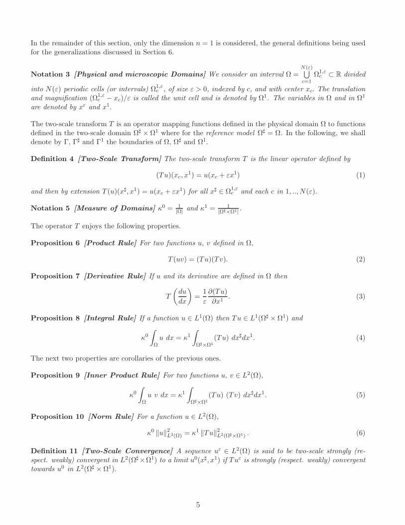
In the remainder of this section, only the dimension n = 1 is considered, the general definitions being usedfor the generalizations discussed in Section 6.

Notation 3 [Physical and microscopic Domains] We consider an interval Ω =N(ε)⋃c=1

Ω1,εc ⊂ R divided

into N(ε) periodic cells (or intervals) Ω1,εc , of size ε > 0, indexed by c, and with center xc. The translation

and magnification (Ω1,εc − xc)/ε is called the unit cell and is denoted by Ω1. The variables in Ω and in Ω1

are denoted by xε and x1.

The two-scale transform T is an operator mapping functions defined in the physical domain Ω to functionsdefined in the two-scale domain Ω♯ × Ω1 where for the reference model Ω♯ = Ω. In the following, we shalldenote by Γ, Γ♯ and Γ1 the boundaries of Ω, Ω♯ and Ω1.

Definition 4 [Two-Scale Transform] The two-scale transform T is the linear operator defined by

(Tu)(xc, x1) = u(xc + εx1) (1)

and then by extension T (u)(x♯, x1) = u(xc + εx1) for all x♯ ∈ Ω1,εc and each c in 1, .., N(ε).

Notation 5 [Measure of Domains] κ0 = 1|Ω| and κ

1 = 1|Ω♯×Ω1|

.

The operator T enjoys the following properties.

Proposition 6 [Product Rule] For two functions u, v defined in Ω,

T (uv) = (Tu)(Tv). (2)

Proposition 7 [Derivative Rule] If u and its derivative are defined in Ω then

T

(du

dx

)=

1

ε

∂(Tu)

∂x1. (3)

Proposition 8 [Integral Rule] If a function u ∈ L1(Ω) then Tu ∈ L1(Ω♯ × Ω1) and

κ0∫

Ωu dx = κ1

∫

Ω♯×Ω1

(Tu) dx♯dx1. (4)

The next two properties are corollaries of the previous ones.

Proposition 9 [Inner Product Rule] For two functions u, v ∈ L2(Ω),

κ0∫

Ωu v dx = κ1

∫

Ω♯×Ω1

(Tu) (Tv) dx♯dx1. (5)

Proposition 10 [Norm Rule] For a function u ∈ L2(Ω),

κ0 ‖u‖2L2(Ω) = κ1 ‖Tu‖2L2(Ω♯×Ω1) . (6)

Definition 11 [Two-Scale Convergence] A sequence uε ∈ L2(Ω) is said to be two-scale strongly (re-spect. weakly) convergent in L2(Ω♯×Ω1) to a limit u0(x♯, x1) if Tuε is strongly (respect. weakly) convergenttowards u0 in L2(Ω♯ × Ω1).

5

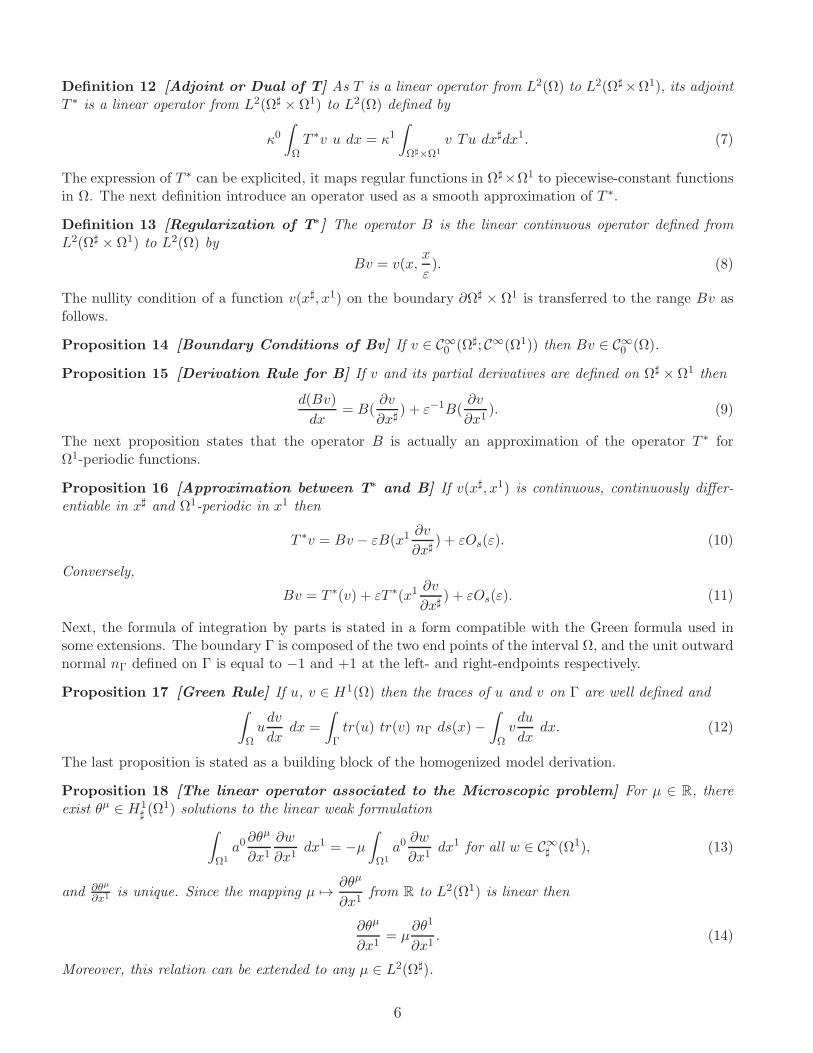
Definition 12 [Adjoint or Dual of T] As T is a linear operator from L2(Ω) to L2(Ω♯×Ω1), its adjointT ∗ is a linear operator from L2(Ω♯ × Ω1) to L2(Ω) defined by

κ0∫

ΩT ∗v u dx = κ1

∫

Ω♯×Ω1

v Tu dx♯dx1. (7)

The expression of T ∗ can be explicited, it maps regular functions in Ω♯×Ω1 to piecewise-constant functionsin Ω. The next definition introduce an operator used as a smooth approximation of T ∗.

Definition 13 [Regularization of T∗] The operator B is the linear continuous operator defined fromL2(Ω♯ × Ω1) to L2(Ω) by

Bv = v(x,x

ε). (8)

The nullity condition of a function v(x♯, x1) on the boundary ∂Ω♯ × Ω1 is transferred to the range Bv asfollows.

Proposition 14 [Boundary Conditions of Bv] If v ∈ C∞0 (Ω♯; C∞(Ω1)) then Bv ∈ C∞

0 (Ω).

Proposition 15 [Derivation Rule for B] If v and its partial derivatives are defined on Ω♯ × Ω1 then

d(Bv)

dx= B(

∂v

∂x♯) + ε−1B(

∂v

∂x1). (9)

The next proposition states that the operator B is actually an approximation of the operator T ∗ forΩ1-periodic functions.

Proposition 16 [Approximation between T∗ and B] If v(x♯, x1) is continuous, continuously differ-entiable in x♯ and Ω1-periodic in x1 then

T ∗v = Bv − εB(x1∂v

∂x♯) + εOs(ε). (10)

Conversely,

Bv = T ∗(v) + εT ∗(x1∂v

∂x♯) + εOs(ε). (11)

Next, the formula of integration by parts is stated in a form compatible with the Green formula used insome extensions. The boundary Γ is composed of the two end points of the interval Ω, and the unit outwardnormal nΓ defined on Γ is equal to −1 and +1 at the left- and right-endpoints respectively.

Proposition 17 [Green Rule] If u, v ∈ H1(Ω) then the traces of u and v on Γ are well defined and∫

Ωudv

dxdx =

∫

Γtr(u) tr(v) nΓ ds(x)−

∫

Ωvdu

dxdx. (12)

The last proposition is stated as a building block of the homogenized model derivation.

Proposition 18 [The linear operator associated to the Microscopic problem] For µ ∈ R, thereexist θµ ∈ H1

♯ (Ω1) solutions to the linear weak formulation

∫

Ω1

a0∂θµ

∂x1∂w

∂x1dx1 = −µ

∫

Ω1

a0∂w

∂x1dx1 for all w ∈ C∞

♯ (Ω1), (13)

and ∂θµ

∂x1 is unique. Since the mapping µ 7→∂θµ

∂x1from R to L2(Ω1) is linear then

∂θµ

∂x1= µ

∂θ1

∂x1. (14)

Moreover, this relation can be extended to any µ ∈ L2(Ω♯).

6

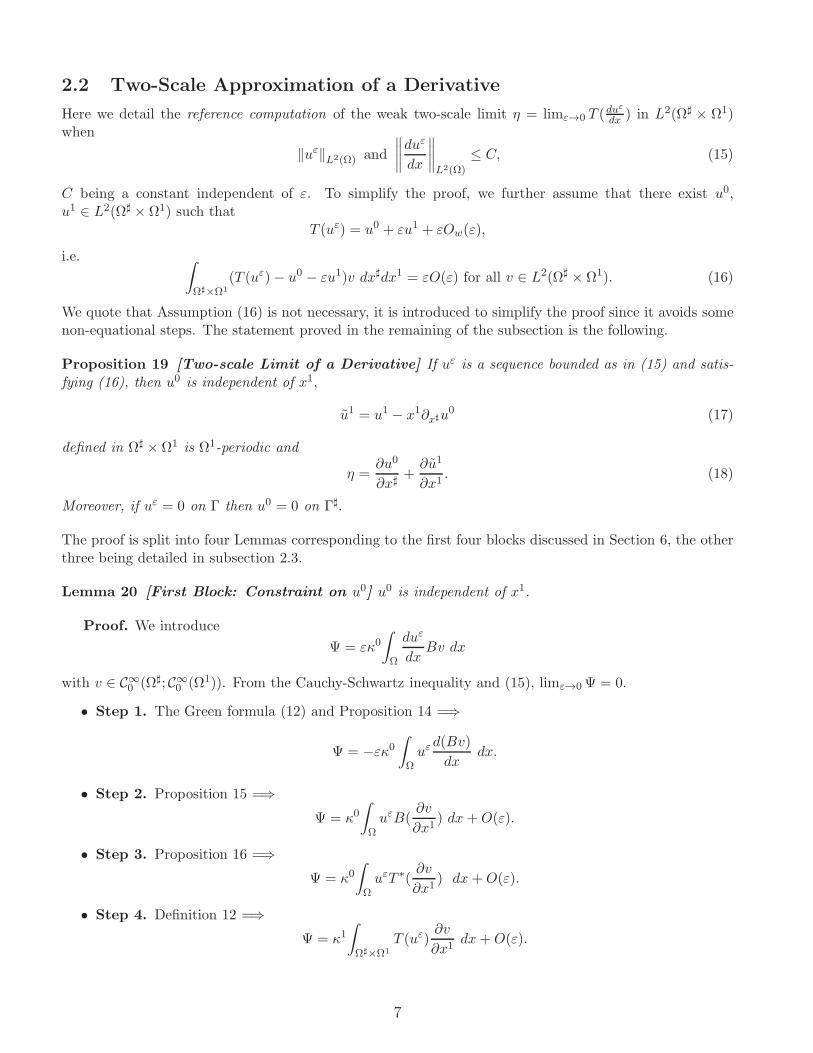
2.2 Two-Scale Approximation of a Derivative

Here we detail the reference computation of the weak two-scale limit η = limε→0 T (duε

dx ) in L2(Ω♯ × Ω1)when

‖uε‖L2(Ω) and

∥∥∥∥duε

dx

∥∥∥∥L2(Ω)

≤ C, (15)

C being a constant independent of ε. To simplify the proof, we further assume that there exist u0,u1 ∈ L2(Ω♯ × Ω1) such that

T (uε) = u0 + εu1 + εOw(ε),

i.e. ∫

Ω♯×Ω1

(T (uε)− u0 − εu1)v dx♯dx1 = εO(ε) for all v ∈ L2(Ω♯ × Ω1). (16)

We quote that Assumption (16) is not necessary, it is introduced to simplify the proof since it avoids somenon-equational steps. The statement proved in the remaining of the subsection is the following.

Proposition 19 [Two-scale Limit of a Derivative] If uε is a sequence bounded as in (15) and satis-fying (16), then u0 is independent of x1,

u1 = u1 − x1∂x♯u0 (17)

defined in Ω♯ × Ω1 is Ω1-periodic and

η =∂u0

∂x♯+∂u1

∂x1. (18)

Moreover, if uε = 0 on Γ then u0 = 0 on Γ♯.

The proof is split into four Lemmas corresponding to the first four blocks discussed in Section 6, the otherthree being detailed in subsection 2.3.

Lemma 20 [First Block: Constraint on u0] u0 is independent of x1.

Proof. We introduce

Ψ = εκ0∫

Ω

duε

dxBv dx

with v ∈ C∞0 (Ω♯; C∞

0 (Ω1)). From the Cauchy-Schwartz inequality and (15), limε→0Ψ = 0.

• Step 1. The Green formula (12) and Proposition 14 =⇒

Ψ = −εκ0∫

Ωuεd(Bv)

dxdx.

• Step 2. Proposition 15 =⇒

Ψ = κ0∫

ΩuεB(

∂v

∂x1) dx+O(ε).

• Step 3. Proposition 16 =⇒

Ψ = κ0∫

ΩuεT ∗(

∂v

∂x1) dx+O(ε).

• Step 4. Definition 12 =⇒

Ψ = κ1∫

Ω♯×Ω1

T (uε)∂v

∂x1dx+O(ε).

7

• Step 5. Assumption (16) and passing to the limit when ε→ 0 =⇒

κ1∫

Ω♯×Ω1

u0∂v

∂x1dx = 0.

• Step 6. The Green formula (12) and v = 0 on Ω♯ × Γ1 =⇒

κ1∫

Ω♯×Ω1

∂u0

∂x1v dx = 0.

• Step 7. Proposition 1 =⇒∂u0

∂x1= 0.

Lemma 21 [Second Block: Two-Scale Limit of the Derivative] η = ∂u1

∂x1 .

Proof. We choose v ∈ C∞0 (Ω♯; C∞

0 (Ω1)) in

Ψ = κ1∫

Ω♯×Ω1

T (duε

dx)v dx♯dx1. (19)

• Step 1. Definition 12 =⇒

Ψ = κ0∫

Ω

duε

dxT ∗v dx.

• Step 2. Proposition 16 (to approximate T ∗ by B), the Green formula (12), the linearity of integrals,and again Proposition 16 (to approximate B by T ∗) =⇒

Ψ = −κ0∫

ΩuεT ∗(

∂v

∂x♯) dx−

κ0

ε

∫

ΩuεT ∗(

∂v

∂x1) dx− κ0

∫

ΩuεT ∗(

∂2v

∂x1∂x♯x1) dx+O(ε).

• Step 3. Definition 12 =⇒

Ψ = −κ1∫

Ω♯×Ω1

T (uε)∂v

∂x♯dx♯dx1 −

κ1

ε

∫

Ω♯×Ω1

T (uε)∂v

∂x1dx♯dx1

−κ1∫

Ω♯×Ω1

T (uε)x1∂2v

∂x1∂x♯dx♯dx1 +O(ε).

• Step 4. Assumption (16) =⇒

Ψ = −κ1∫

Ω♯×Ω1

u0∂v

∂x♯dx♯dx1 −

κ1

ε

∫

Ω♯×Ω1

u0∂v

∂x1dx♯dx1 − κ1

∫

Ω♯×Ω1

u1∂v

∂x1dx♯dx1

−κ1∫

Ω♯×Ω1

u0∂2v

∂x1∂x♯x1 +O(ε).

• Step 5. The Green formula (12), Lemma 20, and passing to the limit when ε→ 0 =⇒

κ1∫

Ω♯×Ω1

η v dx♯dx1 = κ1∫

Ω♯×Ω1

∂u1

∂x1v dx♯dx1.

• Step 6. Proposition 1 =⇒

η =∂u1

∂x1.

8

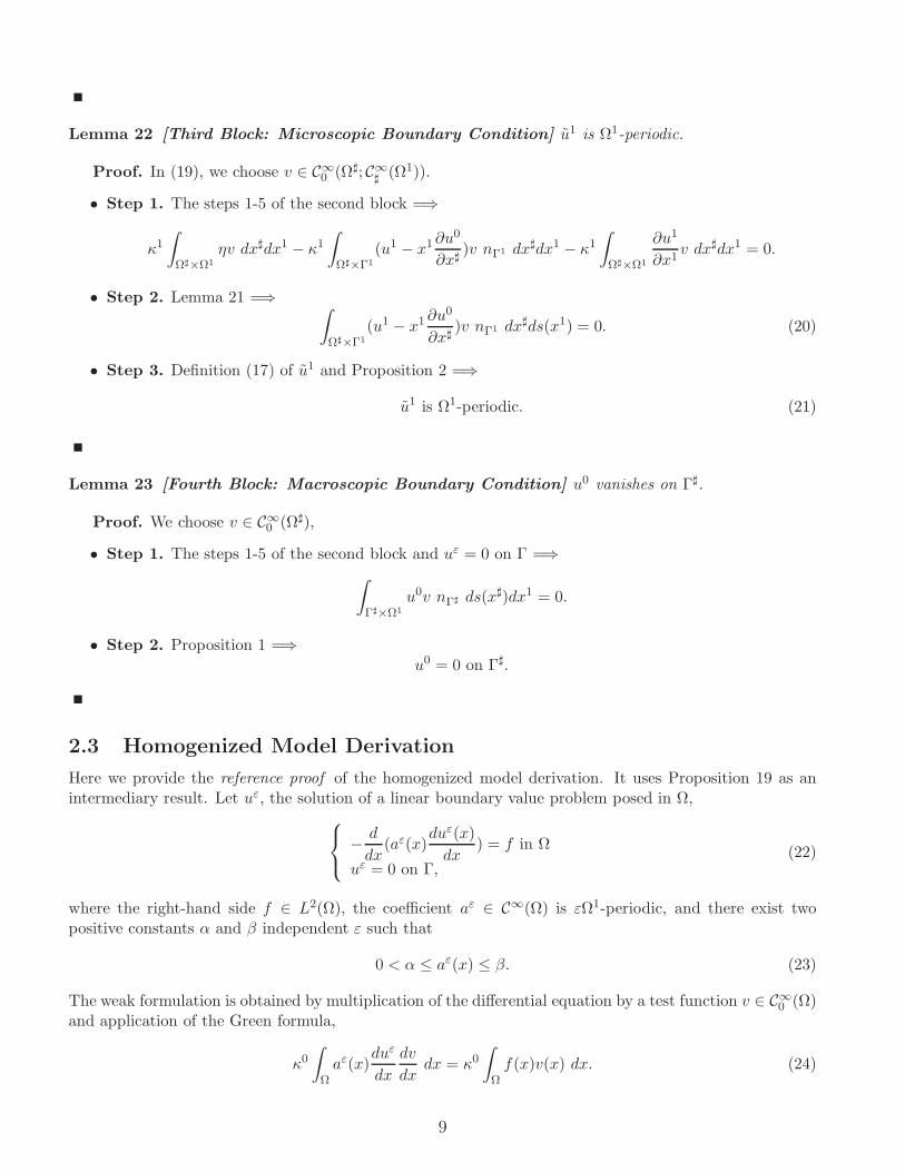
Lemma 22 [Third Block: Microscopic Boundary Condition] u1 is Ω1-periodic.

Proof. In (19), we choose v ∈ C∞0 (Ω♯; C∞

♯ (Ω1)).

• Step 1. The steps 1-5 of the second block =⇒

κ1∫

Ω♯×Ω1

ηv dx♯dx1 − κ1∫

Ω♯×Γ1

(u1 − x1∂u0

∂x♯)v nΓ1 dx♯dx1 − κ1

∫

Ω♯×Ω1

∂u1

∂x1v dx♯dx1 = 0.

• Step 2. Lemma 21 =⇒ ∫

Ω♯×Γ1

(u1 − x1∂u0

∂x♯)v nΓ1 dx♯ds(x1) = 0. (20)

• Step 3. Definition (17) of u1 and Proposition 2 =⇒

u1 is Ω1-periodic. (21)

Lemma 23 [Fourth Block: Macroscopic Boundary Condition] u0 vanishes on Γ♯.

Proof. We choose v ∈ C∞0 (Ω♯),

• Step 1. The steps 1-5 of the second block and uε = 0 on Γ =⇒

∫

Γ♯×Ω1

u0v nΓ♯ ds(x♯)dx1 = 0.

• Step 2. Proposition 1 =⇒u0 = 0 on Γ♯.

2.3 Homogenized Model Derivation

Here we provide the reference proof of the homogenized model derivation. It uses Proposition 19 as anintermediary result. Let uε, the solution of a linear boundary value problem posed in Ω,

−d

dx(aε(x)

duε(x)

dx) = f in Ω

uε = 0 on Γ,(22)

where the right-hand side f ∈ L2(Ω), the coefficient aε ∈ C∞(Ω) is εΩ1-periodic, and there exist twopositive constants α and β independent ε such that

0 < α ≤ aε(x) ≤ β. (23)

The weak formulation is obtained by multiplication of the differential equation by a test function v ∈ C∞0 (Ω)

and application of the Green formula,

κ0∫

Ωaε(x)

duε

dx

dv

dxdx = κ0

∫

Ωf(x)v(x) dx. (24)

9

It is known that its unique solution uε is bounded as in (15). Moreover, we assume that for some functionsa0(x1) and f0(x♯),

T (aε) = a0 and T (f) = f0(x♯) +Ow(ε). (25)

The next proposition states the homogenized model and is the main result of the reference proof. For θ1 asolution to the microscopic problem (13) with µ = 1, the homogenized coefficient and right-hand side aredefined by

aH =

∫

Ω1

a0(1 +

∂θ1

∂x1

)2

dx1 and fH =

∫

Ω1

f0 dx1. (26)

Proposition 24 [Homogenized Model] The limit u0 is solution to the weak formulation

∫

Ω♯

aHdu0

dx♯dv0

dx♯dx♯ =

∫

Ω♯

fHv0 dx♯ (27)

for all v0 ∈ C∞0 (Ω♯).

The proof is split into three lemmas.

Lemma 25 [Fifth Block: Two-Scale Model] The couple (u0, u1) is solution to the two-scale weakformulation ∫

Ω♯×Ω1

a0(∂u0

∂x♯+∂u1

∂x1

)(∂v0

∂x♯+∂v1

∂x1

)dx♯dx1 =

∫

Ω♯×Ω1

f0v0 dx♯dx1 (28)

for any v0 ∈ C∞0 (Ω♯) and v1 ∈ C∞

0 (Ω♯, C∞♯ (Ω1)).

Proof. We choose the test functions v0 ∈ C∞0 (Ω♯), v1 ∈ C∞

0 (Ω♯, C∞♯ (Ω1)).

• Step 1 Posing v = B(v0 + εv1) in (24) and Proposition 14 =⇒

Bv ∈ C∞0 (Ω) and κ0

∫

Ωaεduε

dx

dB(v0 + εv1)

dxdx = κ0

∫

Ωf B(v0 + εv1) dx.

• Step 2 Propositions 15 and 16 =⇒

κ0∫

Ωaεduε

dxT ∗

(∂v0

∂x♯+∂v1

∂x1

)dx = κ0

∫

Ωf T ∗(v0)dx+O(ε).

• Step 3 Definition 12 and Proposition 6 =⇒

κ1∫

Ω♯×Ω1

T (aε)T (duε

dx)

(∂v0

∂x♯+∂v1

∂x1

)dx♯dx1 = κ1

∫

Ω♯×Ω1

T (f) v0 dx♯dx1 +O(ε). (29)

• Step 4 Definitions (25), Lemma 19, and passing to the limit when ε→ 0 =⇒

∫

Ω♯×Ω1

a0(∂u0

∂x♯+∂u1

∂x1

)(∂v0

∂x♯+∂v1

∂x1

)dx♯dx1 =

∫

Ω♯×Ω1

f0v0 dx♯dx1

which is the expected result.

Lemma 26 [Sixth Block: Microscopic Problem] u1 is solution to (13) with µ =∂u0

∂x♯and

∂u1

∂x1=∂u0

∂x♯∂θ1

∂x1.

10

Proof. We choose v0 = 0 and v1(x♯, x1) = w(x1)ϕ(x♯) in (28) with ϕ ∈ C∞(Ω♯) and w1 ∈ C∞♯ (Ω1).

• Step 1 Proposition 1, Lemma 20, and the linearity of the integral =⇒

∫

Ω1

a0∂u1

∂x1∂w1

∂x1dx1 = −

∂u0

∂x♯

∫

Ω1

a0∂w1

∂x1dx1. (30)

• Step 2 Proposition 18 with µ =∂u0

∂x♯=⇒

∂u1

∂x1=∂u0

∂x♯∂θ1

∂x1

as announced.

Lemma 27 [Seventh Block: Macroscopic Problem] u0 is solution to (27).

Proof. We choose v0 ∈ C∞0 (Ω♯) and v1 =

∂v0

∂x♯∂θ1

∂x1∈ C∞

0 (Ω♯, C∞♯ (Ω1)) in (28).

• Step 1 Lemma 26 =⇒

∫

Ω♯×Ω1

a0(∂u0

∂x♯+∂θ1

∂x1∂u0

∂x♯

)(∂v0

∂x♯+∂θ1

∂x1∂v0

∂x♯

)dx♯dx1 =

∫

Ω♯×Ω1

f0v0 dx♯dx1. (31)

• Step 2 Factorizing and definitions (26) =⇒

∫

Ω♯

aH∂u0

∂x♯∂v0

∂x♯dx♯ =

∫

Ω♯

fHv0 dx♯.

3 Rewriting strategies

In this section we recall the rudiments of rewriting, namely, the definitions of terms over a signature, ofsubstitution and of rewriting rules. We introduce a strategy language: its syntax and semantics in termsof partial functions. This language will allow us to express most of the useful rewriting strategies.

3.1 Term, substitution and rewriting rule.

We start with an example of rewriting rule. We define a set of rewriting variables X = x, y and a setof function symbols Σ = f, g, a, b, c. A term is a combination of elements of X ∪ Σ, for instance f(x)or f(a). The rewriting rule f(x) g(x) applied to a term f(a) is a two-step operation. First, it consistsin matching the left term f(x) with the input term f(a) by matching the two occurences of the functionsymbol f, and by matching the rewriting variable x with the function symbol a. Then, the result g(a) ofthe rewriting operation is obtained by replacing the rewriting variable x occuring in the right hand sideg(x) by the subterm a that have been associated to x. In case where a substitution is possible, as in theapplication of f(b) → g(x) to f(a), we say that the rewriting rule fails.

Definition 28 Let Σ be a countable set of function symbols, each symbol f ∈ Σ is associated with a non-negative integer n, its arity ar(f) i.e. the number of arguments of f . Let X be a countable set of variablessuch that Σ ∩ X = ∅. The set of terms, denoted by T (Σ,X ), is inductively defined by

11

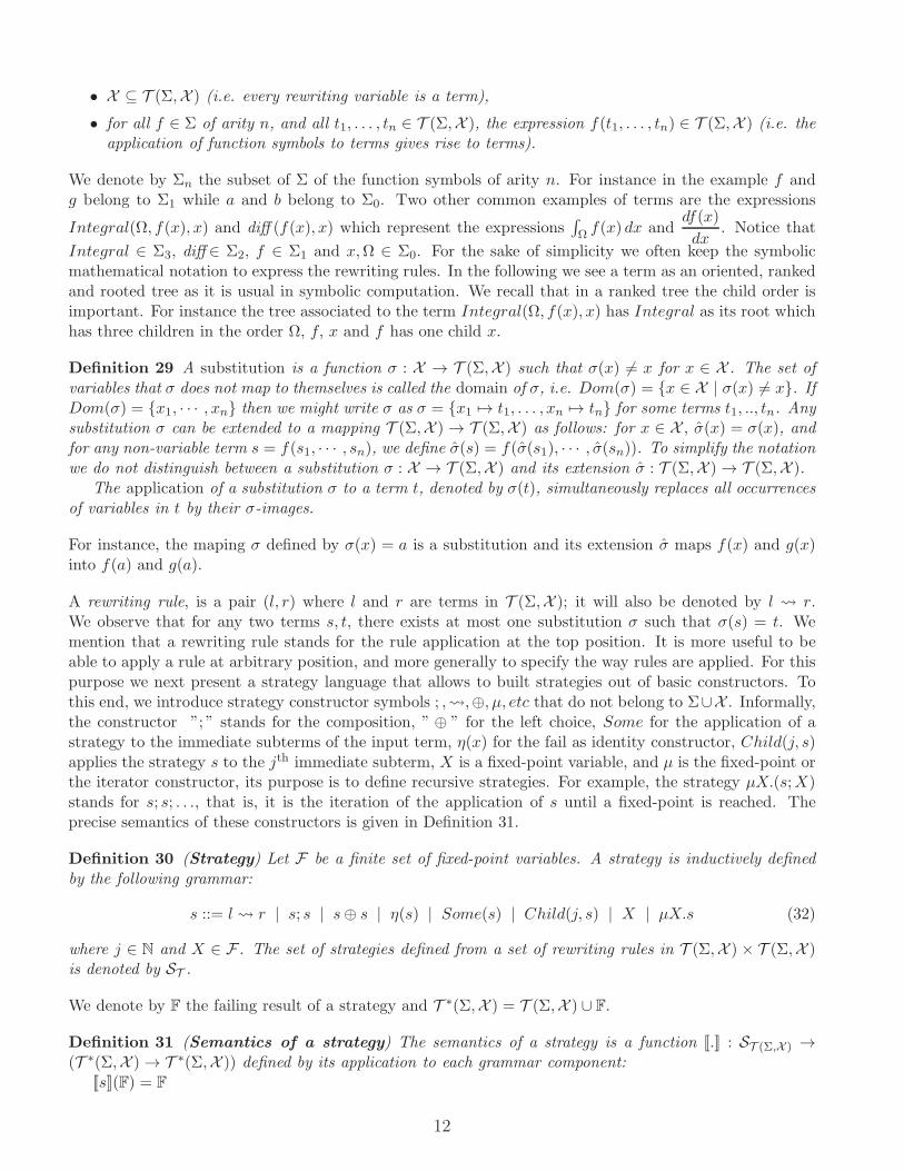
• X ⊆ T (Σ,X ) (i.e. every rewriting variable is a term),

• for all f ∈ Σ of arity n, and all t1, . . . , tn ∈ T (Σ,X ), the expression f(t1, . . . , tn) ∈ T (Σ,X ) (i.e. theapplication of function symbols to terms gives rise to terms).

We denote by Σn the subset of Σ of the function symbols of arity n. For instance in the example f andg belong to Σ1 while a and b belong to Σ0. Two other common examples of terms are the expressions

Integral(Ω, f(x), x) and diff (f(x), x) which represent the expressions∫Ω f(x) dx and

df(x)

dx. Notice that

Integral ∈ Σ3, diff ∈ Σ2, f ∈ Σ1 and x,Ω ∈ Σ0. For the sake of simplicity we often keep the symbolicmathematical notation to express the rewriting rules. In the following we see a term as an oriented, rankedand rooted tree as it is usual in symbolic computation. We recall that in a ranked tree the child order isimportant. For instance the tree associated to the term Integral(Ω, f(x), x) has Integral as its root whichhas three children in the order Ω, f, x and f has one child x.

Definition 29 A substitution is a function σ : X → T (Σ,X ) such that σ(x) 6= x for x ∈ X . The set ofvariables that σ does not map to themselves is called the domain of σ, i.e. Dom(σ) = x ∈ X | σ(x) 6= x. IfDom(σ) = x1, · · · , xn then we might write σ as σ = x1 7→ t1, . . . , xn 7→ tn for some terms t1, .., tn. Anysubstitution σ can be extended to a mapping T (Σ,X ) → T (Σ,X ) as follows: for x ∈ X , σ(x) = σ(x), andfor any non-variable term s = f(s1, · · · , sn), we define σ(s) = f(σ(s1), · · · , σ(sn)). To simplify the notationwe do not distinguish between a substitution σ : X → T (Σ,X ) and its extension σ : T (Σ,X ) → T (Σ,X ).

The application of a substitution σ to a term t, denoted by σ(t), simultaneously replaces all occurrencesof variables in t by their σ-images.

For instance, the maping σ defined by σ(x) = a is a substitution and its extension σ maps f(x) and g(x)into f(a) and g(a).

A rewriting rule, is a pair (l, r) where l and r are terms in T (Σ,X ); it will also be denoted by l r.We observe that for any two terms s, t, there exists at most one substitution σ such that σ(s) = t. Wemention that a rewriting rule stands for the rule application at the top position. It is more useful to beable to apply a rule at arbitrary position, and more generally to specify the way rules are applied. For thispurpose we next present a strategy language that allows to built strategies out of basic constructors. Tothis end, we introduce strategy constructor symbols ; , ,⊕, µ, etc that do not belong to Σ∪X . Informally,the constructor ”; ” stands for the composition, ” ⊕ ” for the left choice, Some for the application of astrategy to the immediate subterms of the input term, η(x) for the fail as identity constructor, Child(j, s)applies the strategy s to the jth immediate subterm, X is a fixed-point variable, and µ is the fixed-point orthe iterator constructor, its purpose is to define recursive strategies. For example, the strategy µX.(s;X)stands for s; s; . . ., that is, it is the iteration of the application of s until a fixed-point is reached. Theprecise semantics of these constructors is given in Definition 31.

Definition 30 (Strategy) Let F be a finite set of fixed-point variables. A strategy is inductively definedby the following grammar:

s ::= l r | s; s | s⊕ s | η(s) | Some(s) | Child(j, s) | X | µX.s (32)

where j ∈ N and X ∈ F . The set of strategies defined from a set of rewriting rules in T (Σ,X ) × T (Σ,X )is denoted by ST .

We denote by F the failing result of a strategy and T ∗(Σ,X ) = T (Σ,X ) ∪ F.

Definition 31 (Semantics of a strategy) The semantics of a strategy is a function [[.]] : ST (Σ,X ) →(T ∗(Σ,X ) → T ∗(Σ,X )) defined by its application to each grammar component:

[[s]](F) = F

12

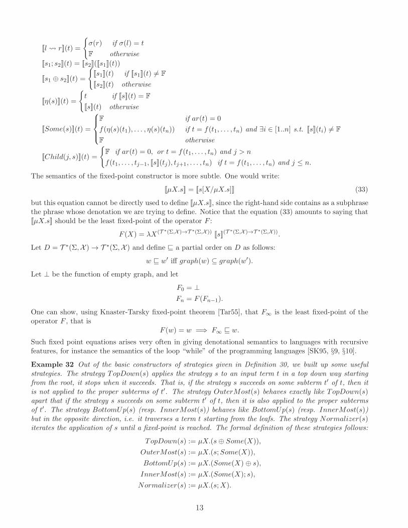
[[l r]](t) =

σ(r) if σ(l) = t

F otherwise

[[s1; s2]](t) = [[s2]]([[s1]](t))

[[s1 ⊕ s2]](t) =

[[s1]](t) if [[s1]](t) 6= F

[[s2]](t) otherwise

[[η(s)]](t) =

t if [[s]](t) = F

[[s]](t) otherwise

[[Some(s)]](t) =

F if ar(t) = 0

f(η(s)(t1), . . . , η(s)(tn)) if t = f(t1, . . . , tn) and ∃i ∈ [1..n] s.t. [[s]](ti) 6= F

F otherwise

[[Child(j, s)]](t) =

F if ar(t) = 0, or t = f(t1, . . . , tn) and j > n

f(t1, . . . , tj−1, [[s]](tj), tj+1, . . . , tn) if t = f(t1, . . . , tn) and j ≤ n.

The semantics of the fixed-point constructor is more subtle. One would write:

[[µX.s]] = [[s[X/µX.s]]] (33)

but this equation cannot be directly used to define [[µX.s]], since the right-hand side contains as a subphrasethe phrase whose denotation we are trying to define. Notice that the equation (33) amounts to saying that[[µX.s]] should be the least fixed-point of the operator F :

F (X) = λX(T ∗(Σ,X )→T ∗(Σ,X )) [[s]](T∗(Σ,X )→T ∗(Σ,X )).

Let D = T ∗(Σ,X ) → T ∗(Σ,X ) and define ⊑ a partial order on D as follows:

w ⊑ w′ iff graph(w) ⊆ graph(w′).

Let ⊥ be the function of empty graph, and let

F0 = ⊥

Fn = F (Fn−1).

One can show, using Knaster-Tarsky fixed-point theorem [Tar55], that F∞ is the least fixed-point of theoperator F , that is

F (w) = w =⇒ F∞ ⊑ w.

Such fixed point equations arises very often in giving denotational semantics to languages with recursivefeatures, for instance the semantics of the loop “while” of the programming languages [SK95, §9, §10].

Example 32 Out of the basic constructors of strategies given in Definition 30, we built up some usefulstrategies. The strategy TopDown(s) applies the strategy s to an input term t in a top down way startingfrom the root, it stops when it succeeds. That is, if the strategy s succeeds on some subterm t′ of t, then itis not applied to the proper subterms of t′. The strategy OuterMost(s) behaves exactly like TopDown(s)apart that if the strategy s succeeds on some subterm t′ of t, then it is also applied to the proper subtermsof t′. The strategy BottomUp(s) (resp. InnerMost(s)) behaves like BottomUp(s) (resp. InnerMost(s))but in the opposite direction, i.e. it traverses a term t starting from the leafs. The strategy Normalizer(s)iterates the application of s until a fixed-point is reached. The formal definition of these strategies follows:

TopDown(s) := µX.(s ⊕ Some(X)),

OuterMost(s) := µX.(s;Some(X)),

BottomUp(s) := µX.(Some(X) ⊕ s),

InnerMost(s) := µX.(Some(X); s),

Normalizer(s) := µX.(s;X).

13

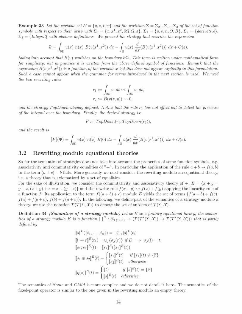
Example 33 Let the variable set X = y, z, t, w and the partition Σ = Σ0∪Σ1∪Σ2 of the set of functionsymbols with respect to their arity with Σ0 = x, x1, x2, ∂Ω,Ω, ε, Σ1 = u, v, n,O,B, Σ2 = derivative,Σ3 = Integral with obvious definitions. We present the strategy that rewrites the expression

Ψ =

∫

∂Ωu(x) n(x) B(v(x1, x2)) dx−

∫

Ωu(x)

d

dx(B(v(x1, x2))) dx+O(ε),

taking into account that B(v) vanishes on the boundary ∂Ω. This term is written under mathematical formfor simplicity, but in practice it is written from the above defined symbol of functions. Remark that theexpression B(v(x1, x2)) is a function of the variable x but this does not appear explicitly in this formulation.Such a case cannot appear when the grammar for terms introduced in the next section is used. We needthe two rewriting rules

r1 :=

∫

∂Ωw dt

∫

∂Ωw dt,

r2 := B(v(z, y)) 0,

and the strategy TopDown already defined. Notice that the rule r1 has not effect but to detect the presenceof the integral over the boundary. Finally, the desired strategy is:

F := TopDown(r1;TopDown(r2)),

and the result is

[[F ]](Ψ) =

∫

∂Ωu(x) n(x) B(0) dx−

∫

Ωu(x)

d

dx(B(v(x1, x2))) dx+O(ε).

3.2 Rewriting modulo equational theories

So far the semantics of strategies does not take into account the properties of some function symbols, e.g.associativity and commutativity equalities of ”+”. In particular the application of the rule a+ b f(a, b)to the term (a + c) + b fails. More generally we next consider the rewriting modulo an equational theory,i.e. a theory that is axiomatized by a set of equalities.For the sake of illustration, we consider the commutativity and associativity theory of +, E = x + y =y+ x, (x+ y) + z = x+ (y + z) and the rewrite rule f(x+ y) f(x) + f(y) applying the linearity rule ofa function f . Its application to the term f((a+ b) + c) modulo E yields the set of terms f(a+ b) + f(c),f(a) + f(b+ c), f(b) + f(a+ c). In the following, we define part of the semantics of a strategy modulo atheory, we use the notation P(T (Σ,X )) to denote the set of subsets of T (Σ,X ).

Definition 34 (Semantics of a strategy modulo) Let be E be a finitary equational theory, the seman-tics of a strategy modulo E is a function [[.]]E : ST (Σ,X ) → (P(T ∗(Σ,X )) → P(T ∗(Σ,X ))) that is partlydefined by

[[s]]E(t1, . . . , tn) = ∪ni=1[[s]]

E(ti)

[[l r]]E(t1) = ∪jσj(r) if E =⇒ σj(l) = t,

[[s1; s2]]E(t) = [[s2]]

E([[s1]]E(t))

[[s1 ⊕ s2]]E(t) =

[[s1]]

E(t) if [[s1]](t) 6= F

[[s2]]E(t) otherwise

[[η(s)]]E(t) =

t if [[s]]E(t) = F

[[s]]E(t) otherwise.

The semantics of Some and Child is more complex and we do not detail it here. The semantics of thefixed-point operator is similar to the one given in the rewriting modulo an empty theory.

14

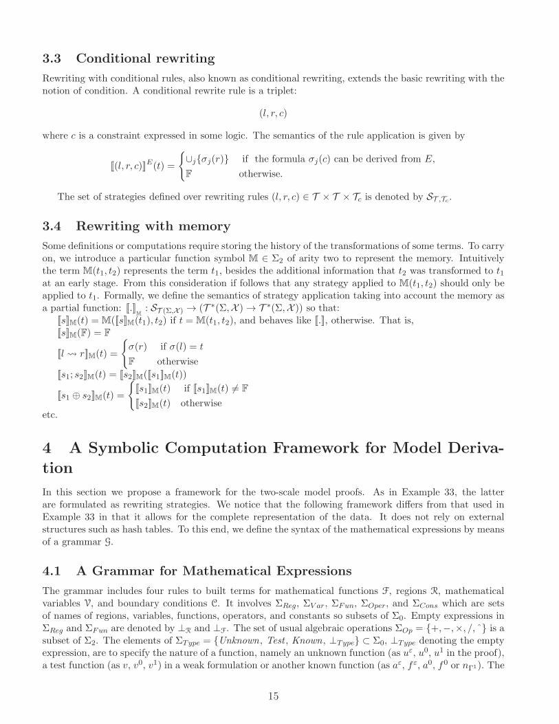
3.3 Conditional rewriting

Rewriting with conditional rules, also known as conditional rewriting, extends the basic rewriting with thenotion of condition. A conditional rewrite rule is a triplet:

(l, r, c)

where c is a constraint expressed in some logic. The semantics of the rule application is given by

[[(l, r, c)]]E(t) =

∪jσj(r) if the formula σj(c) can be derived from E,

F otherwise.

The set of strategies defined over rewriting rules (l, r, c) ∈ T × T × Tc is denoted by ST ,Tc .

3.4 Rewriting with memory

Some definitions or computations require storing the history of the transformations of some terms. To carryon, we introduce a particular function symbol M ∈ Σ2 of arity two to represent the memory. Intuitivelythe term M(t1, t2) represents the term t1, besides the additional information that t2 was transformed to t1at an early stage. From this consideration if follows that any strategy applied to M(t1, t2) should only beapplied to t1. Formally, we define the semantics of strategy application taking into account the memory asa partial function: [[.]]

M: ST (Σ,X ) → (T ∗(Σ,X ) → T ∗(Σ,X )) so that:

[[s]]M(t) = M([[s]]M(t1), t2) if t = M(t1, t2), and behaves like [[.]], otherwise. That is,[[s]]M(F) = F

[[l r]]M(t) =

σ(r) if σ(l) = t

F otherwise

[[s1; s2]]M(t) = [[s2]]M([[s1]]M(t))

[[s1 ⊕ s2]]M(t) =

[[s1]]M(t) if [[s1]]M(t) 6= F

[[s2]]M(t) otherwiseetc.

4 A Symbolic Computation Framework for Model Deriva-

tion

In this section we propose a framework for the two-scale model proofs. As in Example 33, the latterare formulated as rewriting strategies. We notice that the following framework differs from that used inExample 33 in that it allows for the complete representation of the data. It does not rely on externalstructures such as hash tables. To this end, we define the syntax of the mathematical expressions by meansof a grammar G.

4.1 A Grammar for Mathematical Expressions

The grammar includes four rules to built terms for mathematical functions F, regions R, mathematicalvariables V, and boundary conditions C. It involves ΣReg, ΣV ar, ΣFun, ΣOper, and ΣCons which are setsof names of regions, variables, functions, operators, and constants so subsets of Σ0. Empty expressions inΣReg and ΣFun are denoted by ⊥R and ⊥F. The set of usual algebraic operations ΣOp = +,−,×, /, ˆ is asubset of Σ2. The elements of ΣType = Unknown, Test , Known, ⊥Type ⊂ Σ0, ⊥Type denoting the emptyexpression, are to specify the nature of a function, namely an unknown function (as uε, u0, u1 in the proof),a test function (as v, v0, v1) in a weak formulation or another known function (as aε, f ε, a0, f0 or nΓ1). The

15

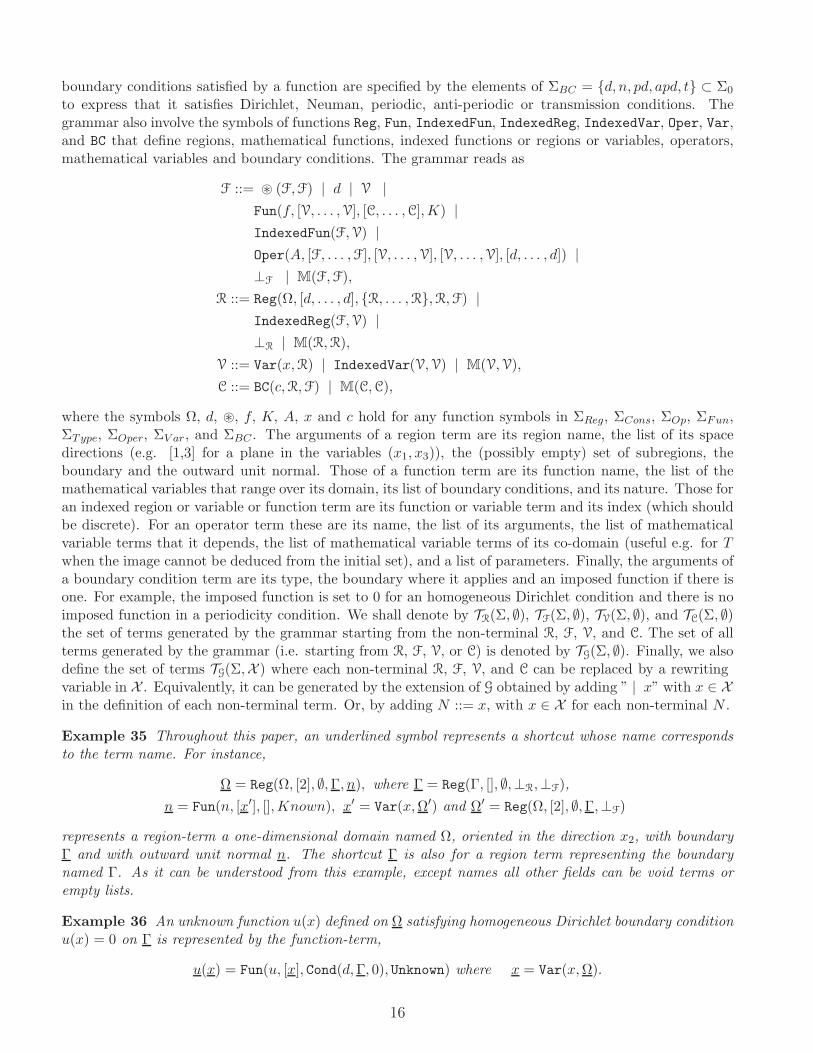
boundary conditions satisfied by a function are specified by the elements of ΣBC = d, n, pd, apd, t ⊂ Σ0

to express that it satisfies Dirichlet, Neuman, periodic, anti-periodic or transmission conditions. Thegrammar also involve the symbols of functions Reg, Fun, IndexedFun, IndexedReg, IndexedVar, Oper, Var,and BC that define regions, mathematical functions, indexed functions or regions or variables, operators,mathematical variables and boundary conditions. The grammar reads as

F ::= ⊛ (F,F) | d | V |

Fun(f, [V, . . . ,V], [C, . . . ,C],K) |

IndexedFun(F,V) |

Oper(A, [F, . . . ,F], [V, . . . ,V], [V, . . . ,V], [d, . . . , d]) |

⊥F | M(F,F),

R ::= Reg(Ω, [d, . . . , d], R, . . . ,R,R,F) |

IndexedReg(F,V) |

⊥R | M(R,R),

V ::= Var(x,R) | IndexedVar(V,V) | M(V,V),

C ::= BC(c,R,F) | M(C,C),

where the symbols Ω, d, ⊛, f, K, A, x and c hold for any function symbols in ΣReg, ΣCons, ΣOp, ΣFun,ΣType, ΣOper, ΣV ar, and ΣBC . The arguments of a region term are its region name, the list of its spacedirections (e.g. [1,3] for a plane in the variables (x1, x3)), the (possibly empty) set of subregions, theboundary and the outward unit normal. Those of a function term are its function name, the list of themathematical variables that range over its domain, its list of boundary conditions, and its nature. Those foran indexed region or variable or function term are its function or variable term and its index (which shouldbe discrete). For an operator term these are its name, the list of its arguments, the list of mathematicalvariable terms that it depends, the list of mathematical variable terms of its co-domain (useful e.g. for Twhen the image cannot be deduced from the initial set), and a list of parameters. Finally, the arguments ofa boundary condition term are its type, the boundary where it applies and an imposed function if there isone. For example, the imposed function is set to 0 for an homogeneous Dirichlet condition and there is noimposed function in a periodicity condition. We shall denote by TR(Σ, ∅), TF(Σ, ∅), TV(Σ, ∅), and TC(Σ, ∅)the set of terms generated by the grammar starting from the non-terminal R, F, V, and C. The set of allterms generated by the grammar (i.e. starting from R, F, V, or C) is denoted by TG(Σ, ∅). Finally, we alsodefine the set of terms TG(Σ,X ) where each non-terminal R, F, V, and C can be replaced by a rewritingvariable in X . Equivalently, it can be generated by the extension of G obtained by adding ” | x” with x ∈ Xin the definition of each non-terminal term. Or, by adding N ::= x, with x ∈ X for each non-terminal N .

Example 35 Throughout this paper, an underlined symbol represents a shortcut whose name correspondsto the term name. For instance,

Ω = Reg(Ω, [2], ∅,Γ, n), where Γ = Reg(Γ, [], ∅,⊥R,⊥F),

n = Fun(n, [x′], [],Known), x′ = Var(x,Ω′) and Ω′ = Reg(Ω, [2], ∅,Γ,⊥F)

represents a region-term a one-dimensional domain named Ω, oriented in the direction x2, with boundaryΓ and with outward unit normal n. The shortcut Γ is also for a region term representing the boundarynamed Γ. As it can be understood from this example, except names all other fields can be void terms orempty lists.

Example 36 An unknown function u(x) defined on Ω satisfying homogeneous Dirichlet boundary conditionu(x) = 0 on Γ is represented by the function-term,

u(x) = Fun(u, [x], Cond(d,Γ, 0), Unknown) where x = Var(x,Ω).

16

4.2 Short-cut Terms

For the sake of conciseness, we introduce shortcut terms that are constantly used in the end of the paper:Ω ∈ TR(Σ,X ), x ∈ TV(Σ,X ) defined in Ω, I ∈ TR(Σ,X ) used for (discrete) indices, i ∈ TV(Σ,X ) used as anindex defined in I, u ∈ TF(Σ,X ) or u(x) ∈ TF(Σ,X ) to express that it depends on the variable x and ui theindexed-term of the function u indexed by i. Similar definitions can be given for the other notations usedin the proof as Ω♯, x♯, Ω1, x1, Ω′, x′, v(x♯, x1) etc. The operators necessary for the proof are the integral,the derivative, the two-scale transform T , its adjoint T ∗, and B. In addition, for some extensions of thereference proof we shall use the discrete sum.Instead of writing operator-terms as defined in the grammar, we prefer to use the usual mathematicalexpressions. The table below establishes the correspondance between the two formulations.

∫u dx ≡ Oper(Integral, u, [x], [], []),

∂u

∂x≡ Oper(Partial, u, [x], [x], []),

tr(u, x)(x′) ≡ Oper(Restriction, u, [x], [x′], []),

T (u, x)(x♯, x1) ≡ Oper(T, u, [x], [x♯, x1], [ε]),

T ∗(v, [x♯, x1])(x) ≡ Oper(T ∗, v, [x♯, x1], [x], [ε]),

B(v, [x♯, x1])(x) ≡ Oper(B, v, [x♯, x1], [x], [ε]),∑

i

ui ≡ Oper(Sum, ui, [i], [], []).

The multiplication and exponentiation involving two terms f and g are written fg and f g as usual inmathematics. All these conventions have been introduced for terms in T (Σ, ∅). For terms in T (Σ,X) asthose encoutered in rewriting rules, the rewriting variables can replace any of the above short cut terms.

Example 37 The rewriting rule associated to the Green rule (12) reads

∫∂u

∂xv dx −

∫u∂v

∂xdx+

∫tr(u) tr(v) n dx′.

with the short-cuts Γ = Reg(Γ, d1, ∅,⊥R,⊥F), Ω = Reg(Ω, d2, ∅,Γ, n), x = Var(x,Ω) and x′ = Var(x,Γ).The other symbols u, v, x, Ω, Γ, d1, d2, n are rewriting variables, and for instance

∂u

∂x≡ Oper(Partial, u, x, [], []).

Applying this rule according to an appropriate strategy, say the top down strategy, to a term in T (Σ, ∅) like

Ψ =

∫∂f(z)

∂zg(z) dz,

for a given variable term z and function terms f, g. As expected, the result is

−

∫f∂g

∂zdz +

∫f g n dz′

with evident notations for n and z′.

17

4.3 A Variable Dependency Analyzer

The variable dependency analyzer Θ is related to effect systems in computer science [MM09]. It is afunction from TF(Σ, ∅) to the set P(TV(Σ, ∅)) of the parts of TV(Σ, ∅). When applied to a term t ∈ TF(Σ, ∅),it returns the set of mathematical variables on which t depends. The analyzer Θ is used in the conditionpart of some rewriting rules and is inductively defined by

Θ(d) = ∅ for d ∈ ΣCons,

Θ(x) = x for x ∈ TV(Σ, ∅),

Θ(⊛(u, v)) = Θ(u) ∪Θ(v) for u, v ∈ TF(Σ, ∅) and ⊛ ∈ ΣOp,

Θ(⊥F) = ∅,

Θ(u(x1, .., xn)) = x1, .., xn for u ∈ TF(Σ, ∅) and x1, .., xn ∈ TV(Σ, ∅),

Θ(ui) = Θ(u) for u ∈ TV(Σ, ∅) and i ∈ TV(Σ, ∅),

Θ([u1, . . . , un]) = Θ(u1) ∪ · · · ∪Θ(un) for u1, . . . , un ∈ TF(Σ, ∅).

The definition of Θ on the operator-terms is done case by case,

Θ(

∫u dx) = Θ(u) \Θ(x),

Θ(∂u

∂x) =

Θ(u) if Θ(x) ⊆ Θ(u),∅ otherwise,

Θ(tr(u, x)(x′)) = Θ(x′),

Θ(T (u, x)(x♯, x1)) = (Θ(u) \Θ(x)) ∪Θ([x♯, x1]) if Θ(x) ∩Θ(u) 6= ∅,

Θ(T ∗(v, [x♯, x1])(x)) = (Θ(v) \Θ([x♯, x1])) ∪Θ(x) if Θ([x♯, x1]) ∩Θ(v) 6= ∅,

Θ(B(v, [x♯, x1])(x))) = (Θ(v) \Θ([x♯, x1])) ∪Θ(x) if Θ([x♯, x1]) ∩Θ(v) 6= ∅,

Θ(∑

i

ui) =⋃

i

Θ(ui).

We observe that these definitions are not very general, but they are sufficient for the applications of thispaper. To complete the definition of Θ, it remains to define it on memory terms,

Θ(M(u, v)) = Θ(u).

Example 38 For

Ψ =

∫

Ω♯[

∫

Ω1

T (u(x), x)(x♯, x1)∂v(x♯, x1)

∂x1dx1]dx♯ ∈ TF(Σ, ∅),

the set Θ(Ψ) of mathematical variables on which Ψ depends is hence inductively computed as follows:

Θ(u(x)) = x, Θ(T (u(x), x)(x♯, x1)) = x♯, x1, Θ(v(x♯, x1)) = x♯, x1, Θ(∂v(x♯,x1)

∂x1 ) = x♯, x1, Θ(T (u(x), x)

(x♯, x1) ∂v(x♯,x1)∂x1 ) = x♯, x1, Θ(

∫Ω1 T (u(x), x)(x♯, x1)

∂v(x♯,x1)∂x1 dx1) = x♯, and Θ(Ψ) = ∅, that is, Ψ is a

constant function.

4.4 Formulation of the Symbolic Framework for Model Derivation

Now we are ready to define the framework for two-scale model derivation by rewriting. To do so, therewriting rules are restricted to left and right terms (l, r) ∈ TG(Σ,X ) × TG(Σ,X ). Their conditions c areformulas generated by a grammar, not explicited here, combining terms in TG(Σ,X ) with the usual logicaloperators in Λ = ∨,∧, ⌉,∈. It also involves operations with the dependency analyzer Θ. The set of termsgenerated by this grammar is denoted by TL(Σ,X ,G,Θ,Λ).

18

It remains to argue that, given a strategy s in STG(Σ,X ),TL(Σ,X ,G,Θ,Λ), the set of terms TG(Σ, ∅) is closedunder the application of s. It is sufficient to show that for each rewriting r rule in s, the application of rto any term t ∈ TG(Σ, ∅) at any position yields a term in TG(Σ, ∅). As an example, TG(Σ, ∅) is not closedunder the application of the rule x Ω, where x is a variable. But it is closed under the application ofthe linearity rule

∫z f + g dx

∫z f dx +

∫z g dx at any position, where f, g, x, z are rewriting variables.

The argument is, since∫z f + g dx ∈ TF(Σ, ∅), then f + g ∈ TF(Σ, ∅), and hence f, g ∈ TF(Σ, ∅). Thus,∫

z f dx+∫z g dx ∈ TF(Σ, ∅). That is, a term in TF(Σ, ∅) is replaced by a another term in TF(Σ, ∅). A more

general setting that deals with the closure of regular languages under specific rewriting strategies can befound in [GGJ09].A model derivation is divided into several intermediary lemmas. Each of them is intended to produce a newproperty that can be expressed as one or few rewriting rules to be applied in another part of the derivation.Since dynamical creation of rules is not allowed, a strategy is covering one lemma only and is operatingwith a fixed set of rewriting rules. The conversion of a result of a strategy to a new set of rewriting rulesis done by an elementary external operation that is not a limitation for generalizations of proofs. Thefollowing definition summarizes the framework of symbolic computation developed in this paper.

Definition 39 The components of the quintuplet Ξ = 〈Σ,X , E,G,Θ〉 provide a framework for symboliccomputation to derive multi-scale models. A two-scale model derivation is expressed as a strategy π ∈STG(Σ,X ),TL(Σ,X ,G,Θ,Λ) for which the semantics [[π]]E is applicable to an initial expression Ψ ∈ T (Σ, ∅).

In the end of this section we argue that this framework is in the same time relatively simple, it covers thereference model derivation and it allows for the extensions presented in the next section.

The grammar of terms is designed to cover all mathematical expressions occuring in the proof of thereference model as well as of their generalizations. A term produced by the grammar includes locallyall useful information. This avoids the use of external tables and facilitates design of rewriting rules,in particular to take into account the context of subterms to be transformed. It allows also for localdefinitions, for instance a same name of variable x can be used in different parts of a same term withdifferent meaning, which is useful for instance in integrals. A limitation regarding generalizations presentedin the next section, is that the grammar must cover by anticipation all needed features. This drawbackshould be fixed in another work by supporting generalization of grammars in the same time as generalizationof proofs.

Each step in the proof consists in replacing parts of an expression according to a known mathematicalproperty. This is well done, possibly recursively, using rewriting rules together with strategies allowingfor precise localization. Some steps need simplifications and often use the second linearity rule of a linearoperator, A(λu) = λAu when λ is a scalar (or is independent of the variables in the initial set of A).So variable dependency of each subterm should be determined, this is precisely what Θ, the variabledependency analyzer, is producing. The other simplifications do not require the use of Θ. In addition tothe grammar G, the analyzer Θ must be upgraded in view of each new extension.

In all symbolic computation based on the grammar G, it is implicitely assumed that the derivatives, theintegrals and the traces (i.e. restriction of a function to the boundary) are well defined since the regularityof functions is not encoded.

Due to the algebraic nature of the mathematical proofs, this framework has been formulated by consideringthese proofs as a calculus rather than formal proofs that can be formalized and checked with a proof assistant[BC04, Won96]. Indeed, this is far simpler and allows, from a very small set of tools, for building significantmathematical derivation. To cover broader proofs, the framework must be changed by extending thegrammar and the variable dependency analyzer only. Yet, the language Tom [BBK+07] does not provide acomplete environment for the implementation of our framework since it does not support the transformationof rewriting rules, despite it provides a rich strategy language and a module for the specification of thegrammar.

19

5 Transformation of Strategies as Second Order Strategies

For a given rewriting strategy representing a model proof, one would like to transform it to obtain aderivation of more complex models. Transforming a strategy π ∈ ST (Σ,X ) is achieved by applying strategiesto the strategy π itself. For this purpose, we consider two levels of strategies: the first order ones ST (Σ,X )

as defined in Definition 30, and the strategies of second order in such a way that second order strategies canbe applied to first order ones. That is, the second order strategies are considered as terms in a set T (Σ,X )of terms where Σ and X remain to be defined. Given a set of strategies ST (Σ,X ) that comes with a set of

fixed-point variables F , we pose Σ ⊃ Σ ∪ , ; ,⊕, Some,Child, η, µ ∪ F . Let X be a set of second orderrewriting variables such that X ∩ (X ∪ Σ) = ∅. Notice that first order rewriting variables and fixed-pointvariables are considered as constants in T (Σ,X ), i.e. function symbols in Σ0. Notice also that the arity ofthe function symbols , ; ,⊕, Child, µ is two, and the arity of Some and η is one. In particular, the rulel r can be viewed as the term (l, r) with the symbol at the root, and the strategy µX.s viewed asthe term µ(X, s). This allows us to define second order strategies ST (Σ,X ) by the grammar

s ::= l r | s;s | s⊕s | η(s) | Some(s) | Child(j, s) | X | µX.s (34)

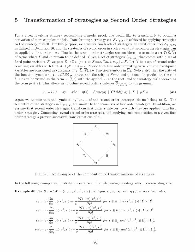
Again we assume that the symbols , ;,⊕, . . . of the second order strategies do no belong to Σ. Thesemantics of the strategies in ST (Σ,X ) are similar to the semantics of first order strategies. In addition, weassume that second order strategies transform first order strategies, to which they are applied, into firstorder strategies. Composing several second order strategies and applying such composition to a given firstorder strategy s provide successive transformations of s.

s1

s2 s3

s23

Π2

⑧⑧⑧⑧⑧⑧⑧⑧⑧⑧⑧⑧⑧

Π3

Π3

Π2

⑧⑧⑧⑧⑧⑧⑧⑧⑧⑧⑧⑧⑧

Figure 1: An example of the composition of transformations of strategies.

In the following example we illustrate the extension of an elementary strategy which is a rewriting rule.

Example 40 For the set X = i, j, x, x♯, x1, u, ε we define s1, s2, s3, and s23 four rewriting rules,

s1 := T (∂u

∂x, x)(x♯, x1)

1

ε

∂T (u, x)(x♯, x1)

∂x1for x ∈ Ω and (x♯, x1) ∈ Ω♯ × Ω1,

s2 := T (∂u

∂xi, x)(x♯, x1)

1

ε

∂T (u, x)(x♯, x1)

∂x1ifor x ∈ Ω and (x♯, x1) ∈ Ω♯ × Ω1,

s3 := T (∂u

∂x, x)(x♯, x1)

1

ε

∂T (u, x)(x♯, x1)

∂x1for x ∈ Ωj and (x♯, x1) ∈ Ω♯

j ×Ω1j ,

s23 := T (∂u

∂xi, x)(x♯, x1)

1

ε

∂T (u, x)(x♯, x1)

∂x1ifor x ∈ Ωj and (x♯, x1) ∈ Ω♯

j × Ω1j .

20

The rule s1 is encountered in the reference proof, s2 is a (trivial) generalization of s1 in the sense that itapplies to multi-dimensional regions Ω1 referenced by a set of variables (x1i )i, and s3 is a second (trivial)

generalization of s1 on the number of sub-regions (Ωj)j , (Ω♯j)j and (Ω1

j )j in Ω, Ω♯ and Ω1. The rule s23 isa generalization combining the two previous generalizations. First, we aim at transforming the strategy s1into the strategy s2 or the strategy s3. To this end, we introduce two second order strategies with X = v, zand Σ ⊃ i, j, Ω, Ω♯, Ω1, Partial, IndexedFun, IndexedV ar, IndexedReg,

Π1 := OuterMost(∂v

∂z ∂v

∂zi)

Π2 := OuterMost(Ω Ωj);OuterMost(Ω♯ Ω♯

j);OuterMost(Ω1 Ω1

j )

Notice that Π1 (resp. Π2) applies the rule∂v

∂z ∂v

∂zi(resp. Ω Ωj, Ω

♯ Ω♯

j, and Ω1 Ω1

j) at all of the

positions 1 of the input first order strategy so that

Π1(s1) = s2 and Π2(s1) = s3.

Once Π1 and Π2 have been defined, they can be composed to produce s23 :

Π2Π1(s1) = s23 or Π1Π2(s1) = s23.

The diagram of Figure 1 illustrates the application of Π1, Π2 and of their compositions.

The next example shows how an extension can not only change rewriting rules but also to add newones.

Example 41 To operate simplifications in the reference model, we use the strategy

s1 := TopDown(∂x

∂x 1).

In the generalization to multi-dimensional regions, it is replaced by two strategies involving the Kroneckersymbol δ, usually defined as δ(i, j) = 1 if i = j and δ(i, j) = 0 otherwise,

s2 : = TopDown

(∂xi∂yj δ(i, j), x = y

),

s3 : = TopDown (δ(i, j) 1, i = j) ,

s4 : = TopDown (δ(i, j) 0, i 6= j) .

The second order strategy that transforms s1 into the strategy Normalizer(s2 ⊕ s3 ⊕ s4) is

Π := TopDown(s1 s2 ⊕ s3 ⊕ s4).

1Notice the difference with TopDown which could not apply these rules at any position.

21

6 Implementation and Experiments

The framework presented in Section 4.4 has been implemented in MapleR©. The implementation includes,

the language Symbtrans of strategies already presented in [BGL]. The derivation of the reference modelpresented in Section 2 has been fully implemented. It starts from an input term which is the weakformulation (24) of the physical problem,

∫a∂u

∂x

∂v

∂xdx =

∫f v dx, (35)

where a = Fun(a, [Ω], [ ],Known), u = Fun(u, [Ω], [Dirichlet], Unknown), v = Fun(u, [Ω], [Dirichlet], T est),Ω = Reg(Ω, [1], ∅,Γ, nΩ), Γ = Reg(Γ, [ ], ∅, ⊥R, ⊥F), Dirichlet = BC(Dirichlet,Γ, 0) and where the short-cuts of the operators are those of Section 4.2. The information regarding the two-scale transformation isprovided through the test functions. For instance, in the first block the proof starts with the expression

Ψ =

∫∂u

∂xB(v(x♯, x1)(x) dx,

where the test function B(v(x♯, x1)(x) is also an input, with v = Fun(a, [x♯, x1], [Dirichlet♯], T est), x♯ =

Var(x♯,Ω♯), x1 = Var(x1,Ω1), Ω♯ = Reg(Ω♯, [1], ∅,Γ♯, nΩ♯), Γ♯ = Reg(Γ♯, [ ], ∅,⊥R,⊥F), Ω1 = Reg(Ω1, [1], ∅,

Γ1, nΩ1), Γ1 = Reg(Γ1, [ ], ∅,⊥R,⊥F), and Dirichlet♯ = BC(Dirichlet♯,Γ♯, 0).

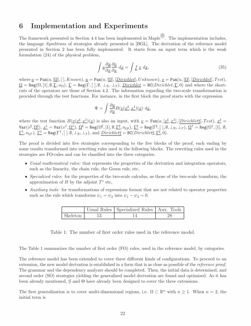
The proof is divided into five strategies corresponding to the five blocks of the proof, each ending bysome results transformed into rewriting rules used in the following blocks. The rewriting rules used in thestrategies are FO-rules and can be classified into the three categories.

• Usual mathematical rules: that represents the properties of the derivation and integration operators,such as the linearity, the chain rule, the Green rule, etc,

• Specialized rules: for the properties of the two-scale calculus, as those of the two-scale transform, theapproximation of B by the adjoint T ∗ etc,

• Auxiliary tools: for transformations of expressions format that are not related to operator propertiessuch as the rule which transforms ψ1 = ψ2 into ψ1 − ψ2 = 0.

Usual Rules Specialized Rules Aux. Tools

Skeleton 53 14 28

Table 1: The number of first order rules used in the reference model.

The Table 1 summarizes the number of first order (FO) rules, used in the reference model, by categories.

The reference model has been extended to cover three different kinds of configurations. To proceed to anextension, the new model derivation is established in a form that is as close as possible of the reference proof.The grammar and the dependency analyzer should be completed. Then, the initial data is determined, andsecond order (SO) strategies yielding the generalized model derivation are found and optimized. As it hasbeen already mentioned, G and Θ have already been designed to cover the three extensions.

The first generalization is to cover multi-dimensional regions, i.e. Ω ⊂ Rn with n ≥ 1. When n = 2, the

initial term is

22

n∑

i=1

n∑

j=1

∫aij

∂u

∂xi

∂v

∂xjdx =

∫f v dx,

where Ω = Reg(Ω, [1, 2], ∅,Γ, nΩ), aij = Indexed(Indexed(a, j), i), i = Var(i, I), I = Reg(I, [1, 2], ∅,⊥R ,⊥F)

and the choice of the test function is trivially deduced. Then, the model derivation is very similar to thisof the reference model, see [LS07], so much so it is obtained simply by applying the SO strategy Π1definedin Example 40. This extension has been tested on the four first blocks.

The second generalization transforms the reference model into a model with several adjacent one-dimensionalregions (or intervals) (Ωk)k=1,..,m so that Ω is still an interval i.e. Ω ⊂ R. For m = 2, the initial term is thesame as (35) but with Ω = Reg(Ω, [1], Ω1,Ω2, Γ, nΩ), Ω1 = Reg(Ω1, [1], ∅, Γ1, nΩ1

), and Ω2 = Reg(Ω2, [1],∅, Γ2, nΩ2

). The two-scale geometries, all variables, all kind of functions and also the operators B and Tare defined subregion by subregion. All definitions and properties apply for each subregion, and the proofsteps are the same after spliting the integrals over the complete region Ω into integrals over the subregions.The only major change is in the fourth step where the equality u01 = u02 at the interface between Ω1 andΩ2 which is encoded as transmission conditions in the boundary conditions of u01 and u02.

The third extension transforms the multi-dimensional model obtained from the first generalization to amodel related to thin cylindrical regions, in the sense that the dimension of Ω is in the order of ε in somedirections i ∈ I and of the order 1 in the others i ∈ I♯ e.g. Ω = (0, 1)× (0, ε) where I = 2 and I♯ = 1.The boundary Γ is split in two parts, the lateral part Γlat and the other parts Γother where the Dirichletboundary conditions are replaced by homogeneous Neuman boundary conditions i.e. duε

dx = 0. In thisspecial case the integrals of the initial term are over a region which size is of the order of ε so it is requiredto multiply each side of the equality by the factor 1/ε to work with expressions of the order of 1. Moreover,the macroscopic region differs from Ω, it is equal to Ω♯ = (0, 1) when the microscopic region remains

unchanged. In general, the definition of the adjoint T ∗ is unchanged but (Bv)(x) = v((xi)i∈I♯ , (x− x♯c)/ε)

where x♯c is the center of the cth cell in Ω♯. It follows that the approximations (10, 11) are between T ∗ andεB with

∑i∈I♯ x

1i∂v

∂x♯i

instead of∑n

i=1 x1i∂v

∂x♯i

. With these main changes in the definitions and the preliminary

properties, the proof steps may be kept unchanged.

Usual Rules Specialized Rules Aux. Tools

Multi-Dimension 6 0 4

Thin-Region 2 0 0

Multi-Region 3 0 0

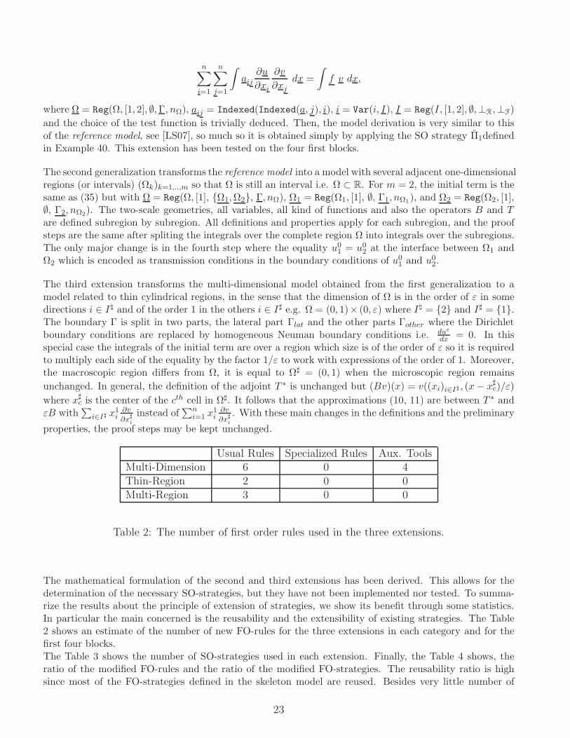
Table 2: The number of first order rules used in the three extensions.

The mathematical formulation of the second and third extensions has been derived. This allows for thedetermination of the necessary SO-strategies, but they have not been implemented nor tested. To summa-rize the results about the principle of extension of strategies, we show its benefit through some statistics.In particular the main concerned is the reusability and the extensibility of existing strategies. The Table2 shows an estimate of the number of new FO-rules for the three extensions in each category and for thefirst four blocks.The Table 3 shows the number of SO-strategies used in each extension. Finally, the Table 4 shows, theratio of the modified FO-rules and the ratio of the modified FO-strategies. The reusability ratio is highsince most of the FO-strategies defined in the skeleton model are reused. Besides very little number of

23

Usual Rules Specialized Rules Aux. Tools

Multi-Dimension 9 2 3

Thin-Region 0 0 0

Multi-Region 1 0 0

Table 3: The number of second order strategies used in the extension of proofs.

Input model Resulting model % Modi. FO-rules % Modi. FO-strategies

Reference Multi-Dim. 16.6% 5%

Multi-Dim. Thin 0 0

Thin Multi-Reg. 0 2.5%

Table 4: The ratio of modified FO-rules and FO-strategies.

SO-strategies is used in the extensions. This systematic way of the generation of proofs is a promising paththat will be further validated within more complex configurations for which the proofs can not obtainedby hand. In the future, we plan to introduce dedicated tools to aid in the design of composition of severalextensions.

24

References

[ADH90] Todd Arbogast, Jim Douglas, Jr., and Ulrich Hornung. Derivation of the double porosity modelof single phase flow via homogenization theory. SIAM J. Math. Anal., 21:823–836, May 1990.

[BB02] G. Bouchitte and M. Bellieud. Homogenization of a soft elastic material reinforced by fibers.Asymptotic Analysis, 32(2):153, 2002.

[BBK+07] Emilie Balland, Paul Brauner, Radu Kopetz, Pierre-Etienne Moreau, and Antoine Reilles.Tom: Piggybacking rewriting on Java. In the proceedings of the 18th International Conferenceon Rewriting Techniques and Applications RTA 07, pages 36–47, 2007.

[BC04] Yves Bertot and Pierre Casteran. Interactive Theorem Proving and Program Development.Coq’Art: The Calculus of Inductive Constructions. Texts in Theoretical Computer Science.Springer Verlag, 2004.

[BGL] W. Belkhir, A. Giorgetti, and M. Lenczner. A symbolic transformation language and its appli-cation to a multiscale method. Submitted. December 2010, http://arxiv.org/abs/1101.3218v1.

[BKKR01] Peter Borovansky, Claude Kirchner, Helene Kirchner, and Christophe Ringeissen. Rewritingwith strategies in ELAN: a functional semantics. International Journal of Foundations ofComputer Science, 12(1):69–95, 2001.

[BLM96] Alain Bourgeat, Stephan Luckhaus, and Andro Mikelic. Convergence of the homogenizationprocess for a double-porosity model of immiscible two-phase flow. SIAM J. Math. Anal.,27:1520–1543, November 1996.

[BLP78] A. Bensoussan, J.L. Lions, and G. Papanicolaou. Asymptotic Methods for Periodic Structures.North-Holland, 1978.

[BN98] F. Baader and T. Nipkow. Term rewriting and all that. Cambridge University Press, 1998.

[CD99] D. Cioranescu and P. Donato. An introduction to homogenization. Oxford University Press,1999.

[CD00] J. Casado-Dıaz. Two-scale convergence for nonlinear Dirichlet problems in perforated domains.Proc. Roy. Soc. Edinburgh Sect. A, 130(2):249–276, 2000.

[CDG02] D. Cioranescu, A. Damlamian, and G. Griso. Periodic unfolding and homogenization. C. R.Math. Acad. Sci. Paris, 335(1):99–104, 2002.

[CDG08] D. Cioranescu, A. Damlamian, and G. Griso. The periodic unfolding method in homogenization.SIAM Journal on Mathematical Analysis, 40(4):1585–1620, 2008.

[CFK05] H. Cirstea, G. Faure, and C. Kirchner. A ρ-calculus of explicit constraint application. ElectronicNotes in Theoretical Computer Science, 117:51 – 67, 2005. Proceedings of the Fifth InternationalWorkshop on Rewriting Logic and Its Applications (WRLA 2004).

[CK01] Horatiu Cirstea and Claude Kirchner. The rewriting calculus — Part I and II. Logic Journalof the Interest Group in Pure and Applied Logics, 9(3):427–498, May 2001.

[CKLW03] Horatiu Cirstea, Claude Kirchner, Luigi Liquori, and Benjamin Wack. Rewrite strategies inthe rewriting calculus. In Bernhard Gramlich and Salvador Lucas, editors, 3rd InternationalWorkshop on Reduction Strategies in Rewriting and Programming , volume 86(4) of ElectronicNotes in Theoretical Computer Science, pages 18–34, Valencia, Spain, 2003. Elsevier.

[GGJ09] Adria Gascon, Guillem Godoy, and Florent Jacquemard. Closure of tree automata languagesunder innermost rewriting. Electron. Notes Theor. Comput. Sci., 237:23–38, April 2009.

[JZKO94] V.V. Jikov, V. Zhikov, M. Kozlov, and O.A. Oleinik. Homogenization of differential operatorsand integral functionals. Springer-Verlag, 1994.

25

[Len97] M. Lenczner. Homogeneisation d’un circuit electrique. C. R. Acad. Sci. Paris Ser. II b,324(9):537–542, 1997.

[Len06] Michel Lenczner. Homogenization of linear spatially periodic electronic circuits. NHM,1(3):467–494, 2006.

[LS07] M. Lenczner and R. C. Smith. A two-scale model for an array of AFM’s cantilever in the staticcase. Mathematical and Computer Modelling, 46(5-6):776–805, 2007.

[MM09] Daniel Marino and Todd Millstein. A generic type-and-effect system. In Proceedings of the4th international workshop on Types in language design and implementation, TLDI ’09, pages39–50, New York, NY, USA, 2009. ACM.

[SK95] Kenneth Slonneger and Barry L. Kurtz. Formal syntax and semantics of programming languages- a laboratory based approach. Addison-Wesley, 1995.

[Tar55] Alfred Tarski. A lattice-theoretical fixpoint theorem and its applications. The Journal ofSymbolic Logic, 5(4):370, 1955.

[Ter03] Terese. Term Rewriting Systems, volume 55 of Cambridge Tracts in Theor. Comp. Sci. Cam-bridge Univ. Press, 2003.

[Won96] Wai Wong. A proof checker for hol, 1996.

26