Computationally Efficient Quantitative Testing ofImage Segmentation with a Genetic Algorithm

H. Al-Muhairi, M. Fleury and A. F. ClarkUniversity of Essex, Computing and Electronic Systems Department,

Wivenhoe Park, Colchester, United Kingdom CO4 3SQEmail: hoalmu,fleum,alien@essex.ac.uk

Abstract— Quantitative testing of segmentation algorithms im-plies rigorous testing against ground truth segmentations. Thoughunder-reported in the literature, the performance of a segmen-tation algorithm depends on the choice of input parameters.The paper reports wide variety both in evaluation time andsegmentation results for an example mean-shift algorithm. Whentesting extends over an algorithm’s parameter space, then thesearch for satisfactory settings has a considerable cost in time.This paper considers the use of a genetic algorithm (GA) to avoidan exhaustive search. As application of the GA drastically reducessearch times, the paper investigates how best to apply the GAin terms of initial candidate population, convergence speed, andapplication of a final polishing round. The GA parameter searchforms part of a three-component computation environment aimedat automating the search and reducing the evaluation time.The first component relies on scripted testing and collation ofresults. The second component transfers to a commodity clustercomputer. And the third component applies a genetic algorithmto avoid an exhaustive search.

I. INTRODUCTION

The contribution of this paper is to propose a compu-tationally efficient environment for conducting quantitativealgorithm testing, with image segmentation as an example.A harness in a scripting language provides a structured routeto testing, in such a way that various evaluation metrics canbe applied. To improve the speed of evaluation a clustercomputer can act as a throughput engine. However, thisassumes a full or exhaustive search is made, whereas thesearch can be optimized by using a genetic algorithm (GA)as a convenient tool. This paper provides guidance on how toapply a GA to the problem of finding input parameters to asegmentation algorithm. The given parameters should improvethe segmentation according to an objective or cost function.

One of the problems with evaluation is that there arefrequently multiple parameter settings, whereas the settingsused are not always reported in the literature. Therefore, arange of parameters have to be cycled through to establishthe best values. This considerably adds to the complexity ofthe task. To the best of the authors’ knowledge, this paperis amongst the first to consider the importance of parametersetting and the impact it has on the testing regime. An effectivegraphical method of displaying the parameter space of aparticular algorithm is introduced and examples based on themean-shift algorithm [1] illustrate the techniques. It should becarefully noted that the work in [1] does include parameter

settings and analysis of their effect, though with no hardrecommendation for any particular setting.

Section II of this paper outlines our three component en-vironment (scripting, cluster computer, genetic algorithm) foralgorithm evaluation. Section IV considers other work on thequantitative approach to algorithm testing. Section V reportsinvestigations into the parameter space of algorithms, whileSection VI concludes the paper.

II. TESTING USING AN EVALUATION HARNESS

The first component of the evaluation environment is ascripting language harness or structure for running tests. Theharness is written entirely in Tcl, a high-level scriptinglanguage [2][3], which means it runs essentially unchangedon all flavors of Unix (including Linux and MacOS X) andon Windows operating systems. This Section outlines how theharness is typically used, and then explains how the programworks. The harness has the potential for entirely decentralizedtesting: tests and datasets are downloaded over the Internet asrequired and executed locally and securely.

A. Operating modes

There are two major ‘modes’ of operation, the first ofwhich runs the tests against the program under test, whilethe second analyzes the results. This separation is deliberateas it allows different analyzes to be performed withoutnecessitating time-consuming re-execution of the tests; andcomparison is greatly facilitated, as there is a test-by-testrecord of the results.

Running tests In ‘run mode,’ one invokes the harness byspecifying a test script on the command line, capturing itsoutput into a file, as in:

harn -run hdig.harn >hdig.out

This may be a local file or the URL of a remote test script (onlyHTTP is supported). If the test script is not specified precisely,the harness will try to find it in a series of pre-definedlocations; this includes a directory on the local machine andthe script repository on the harness web-site. Files downloadedover the network are cached locally; by default, scripts areretained for a week and data files for a year.

The harness outputs a “transcript” which conciselysummarizes each test and the output of the program under

test. The transcript also includes the name and version ofthe test script, the cost function (discussed below), and theelapsed time for performing the tests; the latter is not used bythe harness but is often of interest to algorithm developers.The subsequent analysis stage works solely with transcriptfiles.

Evaluating segmentation algorithms Given a transcript file,one assesses performance simply by running the harness inits default ‘evaluate’ mode:

harn hdig.out

When used this way, the harness reports evaluation statistics,which are dependent on the cost function. An alternative is toinvoke the harness with more than one transcript:

harn hdig.out otheralg.out http://loc/hdig.best

In this case, the harness compares each algorithm with eachother and reports the probability that the algorithms achievestatistically significant differing performances. Receiver oper-ating characteristic (ROC) compare True Positive and FalsePositive counts [4] (Precision-Recall curves [5] are an ROCvariant). As ROC curves give no assessment as to the statisticalsignificance of any reported differences, another method suchas McNemar’s test, which is a modified χ2 test, may bepreferred. Again there is a logistical implication, as typicallymore than thirty tests are needed before the results approacha normal distribution.

B. Working with the harness

Interfacing to the algorithm under testThe algorithm developer writes a short piece of Tcl code,

called the interface script, which interfaces the segmentationalgorithm under test to the harness. Generally speaking, thiscode will invoke an external program that implements thealgorithm with specific input files and/or parameters andperform any ‘massaging’ of the program’s outputs to get theminto the required form. The interface script is loaded by theharness when it is executed, and it is invoked once for eachtest performed.Specifying the tests.

The test script is also written in Tcl as it may be desirableto perform computation in generating either the actual testsor in specifying the locations of any data files it may use.Downloading and executing code is, of course, a dangerousthing to do with the current Internet, so the test script is notexecuted by the harness itself but rather passed to a slave Tclinterpreter in which all operations that might affect the localsystem have been removed; this is similar to the ‘sandbox’environment of Java interpreters in web browsers. The codeexecuting in the slave interpreter is able to perform tests by acallback to a single routine in the main interpreter.

The test script should define two Tcl procedures, named asfollows:harn TestInfo: This is invoked with one of a set ofkeywords and is expected to return the corresponding value.The harness uses this to obtain ancillary information about the

tests, such as the number of tests and the cost function to beused.harn RunTests: This performs the actual tests and shouldinvoke the procedure harn_Test for each test.

The user must also specify a cost function (or equivalentlyevaluation method) that forms the basis of the comparison.Though some cost functions are built in, there is also amechanism for providing alternative cost functions.

III. REDUCING EVALUATION TIME

A cluster computer, the second component of the evaluationenvironment represents an accessible resource upon whichalgorithmic testing takes place in batch mode. Testing isotherwise a laborious operation if only a desktop computer isavailable. A distributed version of the harness is able to reducethe turnaround time when testing an algorithm. The distributedversion runs on a cluster, using static load-balancing andprocess spawning through the rsh utility. The harness actsas a ‘throughput engine’ delivering jobs on demand, on a perjob basis. A job is defined as a set of one or more tests orapplications of an algorithm to one image.

The cluster computer employed by us consists of thirty-seven processing nodes connected with two Ethernet switches.Each node is a small form factor Shuttle box (Model XPCSN41G2) with an AMD Athlon XP 2800+ Barton core (CPUfrequency 2.1 GHz), with 512 KB level 2 cache and dualchannel 1 GB DDR333 RAM. The nodes are connectedvia two 24 port unmanaged Gigabit (Gb) Ethernet switchesmanufactured by D-Link (model DGS-1024T). Each switch isnon-blocking and allows full-duplex Gb bandwidth betweenany pair of ports simultaneously.

The cluster computer software environment is as importantas the physical hardware. To make maintenance and cluster-wide propagation of configuration changes easier, at boottime all nodes transfer their root file system from a fileserver to the local disk, while other file systems are accessedvia the Network Filing System. The development branch ofDebian sid (unstable but more current) serves to manageupgrades to the Linux operating system. To (re)build nodestftp and udpcast (both Linux utilities) are employed in amanner akin to a simplified SystemImager (software thatautomates Linux installs, software distribution, and productiondeployment). A customized script is available to synchro-nize packages and configuration with the clusters mastertemplate, whenever it is inconvenient to reboot and rebuild.This operation is simply accomplished through an AdvancedPackaging Tool cache that is shared between nodes and ashared debconf db (a configuration database), and runs inparallel across the cluster by means of dsh (an implementationof a wrapper for executing multiple remote shells, such as thersh or remsh or ssh commands). Nodes rarely need to beadded or removed, though there is a script to do that too.The cluster is monitored with the scalable, distributed systemGanglia (refer to http://ganglia.info).

As a third component of the environment, a Genetic Algo-rithm (GA) [6] search module lowers the processing time for

the search as a whole. The GA has been integrated within theharness, with a particularly use in optimizing the selection ofparameters. As is well-known, a GA emulates to some extentthe supposed process of genetic evolutionary adaptation. Forexample, the algorithm employed allows mutation of variablevalues as a means of preventing chromosomes becoming tooclose to each other and remaining in local minima. Whilein genetics a chromosome is a molecular package containinggenes, in a GA a chromosome becomes a vector containing aset of variable elements.

The first stage of the GA is to create a population ofchromosomes for a predetermined population size. Given therange of parameter values, random values of each parametermake up the genes of each chromosome. The GA employedin this paper is a real-valued GA following from Polheim’sGEATbx, a GA toolbox for Matlab [7] (though the output maybe integer-valued parameter settings). In the second stage ofthe GA, pairs of parent chromosomes are selected accordingto a fitness or cost function value. Then the number of siblingsa parent acquires is statistically proportional to the weightingof that value. For segmentation, the cost function’s value isdetermined by evaluation of the segmentation. In the thirdstage, each pair of parents is combined to reproduce itself withtwo child chromosomes. The genes of the chromosome pairsare firstly recombined and then mutated. GEATbx employsextended intermediate recombination [8], wherein an offspringgene gO is conceived from its two parent genes g1 and g2 bygO = αg1+(1−α)g2, where α is a scaling factor in the range[−d, 1+d]. Assuming that the N genes in a chromosome forman N -dimensional hypercube then, when d = 0, gO lies alongthe straight line between g1 and g2; if d > 0, extrapolationis permitted. In this work, d = 0. Real-valued mutation thentakes place by which randomly chosen low values are addedto genes with a low probability or mutation rate. Once the newgeneration’s members are found, the GA returns to stage two.

As there can be only one solution to choice of segmentationparameters, the best chromosome is chosen at the end ofa run according to its cost function value. It is possibleto select a stopping point by checking when the differencein the cost function’s value between successive generationspassed below a minimum value. However, because of therelatively lengthy time taken to evaluate each application ofa segmentation algorithm to an image, stopping after a givennumber of generations is a practical alternative. The rate ofconvergence to a global minimum value of the cost functionfor the mean-shift algorithm in the tests in Section V wasfound to be determined by the size of the population at eachgeneration. However, the convergence over many generationsis also examined.

IV. RELATED WORK

The image-processing and computer vision communitieshave developed both de jure (e.g. , IPI-PIKS) and de facto(e.g. , IUE, Target Jr, VXL, RAVL, Tina, ITK, and theIntel Open Computer Vision Library) facilities, containingcollections of algorithms. In particular, ITK hosts the code

for numerous image segmentation algorithms intended formedical applications. (For surveys of segmentation algorithmsrefer for example to [9][10].) The value of these would beenhanced if there existed a direct route to selecting one or morealgorithms for a particular application, as it is difficult to assessthe suitability of a segmentation algorithm without detailedcomparison through testing. Contrasting image segmentationto recognition tasks such as the use of handwriting, andface databases, the authors of [11] remark ”Typically [insegmentation] researchers will show their results on a fewimages and point out why the results ‘look good’”. Part ofthe problem is the difficulty of establishing metrics, whetherpixel-based figures of merit [12] or rankings against a set ofcriteria [13] or through precision-recall curves [5]. However,part of the problem may also be the logistics of performing alarge number of tests. Additionally, a user needs guidance inthe form of a testing structure or evaluation framework.A. Quantitative evaluation

There has been a emphasis in the past on algorithmicnovelty, whereas increasingly the importance of systematicvalidation on sufficient datasets is stressed. For a given input,the corresponding correct output is also known, either becausethe input is simulated or by virtue of either expert opinion orthe presence of a ground truth such as hand-segmented images.The developer aspires to make the algorithm agree with thecorrect output for every corresponding input. Implicit in thisprocedure is that the finite set of test data is representative ofvariation in the real world and that the number of samples islarge enough [14].

At the University of Berkeley, CA Martin [11] supervisedthe creation of a database of 12,000 hand-labelled (from a poolof 30 human subjects) segmentations of images taken from theCorel dataset of 1,000 images. The smaller Sowerby database[15] is an earlier collection of hand-segmented images whichhas been used to evaluate edge-detection algorithms [16]. Thework in [17] also used ground truth from a set of fifty imagesand applied analysis of variance to five evaluation metricsfor object recognition algorithms. The Berkeley database [11]encourages users to download benchmarking code as well as200 training images and a further 100 test images of size240×160 pixels. The originators of the database ran a multiplecue segmentation algorithm of their own using this database.A number of pattern classifiers were applied to combining thecues prior to benchmarking with times reported on a 1 GHzPentium IV ranging from several minutes to several hours (fora Support Vector Machine) per image.B. Evaluation structures

The PCCV project on benchmarking vision systems ex-tended a software harness for evaluation and testing (HATE)[18], for running quantitative and statistical tests on theresults of different image-processing algorithms. HATE canalso automate the application of an algorithm across a largeenough set of images to be statistically significant. However, ifthese tests are performed on a PC alone, even a high-end PC,then the time consumed is likely to be large. A set of 1,441

cloud images, size 768× 576 pixels, on a dual-processor 1.8GHz Athlon MP 2200+ (256 KB L2 cache) took 22 hoursto process. Processing consisted of applying an algorithm todetect the amount of cloud cover and the approximate heightof the clouds in images taking from a camera looking in thedirection of a satellite uplink.

Algoval [19] provides a testing framework. Researchersupload their software to a website, where it is run against aseries of tests and the results are reported on the website. Thisapproach has the advantage that memory usage and speed canbe compared in addition to algorithmic performance; however,this must be balanced by: the need to write the software in Java(and to interface to the Algoval testing classes); the centralizednature of the testing; the need to upload the software fortesting — and the possible embarrassment resulting from poorperformance. The need to upload code, even in compiled form,makes this type of system unattractive to industrial users, whoneed to preserve commercial confidentiality.C. Evaluation methods

Evaluation methods for segmentation can be divided intothose that are independent of ground truth and those that arenot. An early survey of independent segmentation evaluationmethods was completed in [20]. Apart from a categorizationinto five types of evaluation, [20] also investigated the methodsfor their ability to discriminate between different segmentationthresholds. An interesting feature of this comparison was that,while no reference was made to ground truth, the methodsdid agree on which of the alternative segmentations waspreferable. An entropy-based method [21] was introduced ata later date to Zhang’s survey. Its authors advocate its use inpreference to those from the quantitative school, because thelatter tend to be empirically based.

The global and local consistency measures introduced in[11] produce high scores for segmentations by humans and,hence, will rate a computer-generated segmentation highly if itcorresponds to a human segmentation. Because these measuresare tolerant to refinements, over and under segmentation isaccepted, in the sense that the scores do not vary greatlywhen the same algorithm has been applied with the differentparameters. Over segmentation may not be a problem ifsubsequent processing is able to aggregate regions but ifsegmentation is regarded as the end product it is an issue.Another measure based on Hamming distance [22] may beused as a corrective. Both [11] and [22] are intended for thequantitative approach considered in this paper. However, themain purpose herein is not to compare evaluations, thoughin the next Section, the evaluation methods appear as costfunctions which are inserted into an evaluation harness.

V. RESULTS

The mean-shift algorithm makes a convenient example,especially as the authors have made EDISON code availableat http://www.caip.rutgers.edu/riul/research/robust.html, for which we are grateful. Previous modeinformation avoided re-applying the mean-shift procedure tosome data points.

The approximate cost of an exhaustive search across pa-rameter space for a single image on a single cluster nodeis as follows. The processing time on a single cluster nodetakes between a minimum of 907 ms (less than 1 s) anda maximum of 26799 ms (about 27 s), depending on theparameters selected for a particular image. The average timetaken was 5937 ms. Assuming 6 s per test with each of threeparameters varied between 1 and 20, i.e. 8000 tests, then acomplete run would take 13.3 hours. Evaluation of each result,the cost function after normalization, consists of pixel-by-pixel comparison with a ground truth image from the Berkeleydatabase. However, this calculation took less than 1% of theprocessing time. The cluster was employed as a throughputengine, in the sense that no exploitation of internal parallelismtook place. In the unlikely event that all nodes were availableand disregarding input/output overhead the per image run timefor a single image is still 22 min. For the same image, a runwith a GA took 130635 ms, i.e. 2.2 min, which on a clustertakes about 35 s. This is, of course a considerable reductionon an exhaustive search.

Table I is an illustrative rather than representative runshowing the generation-by-generation most fit selection of‘chromosomes’. Three parameters formed the chromosomes:radiusR (the range radius of the mean-shift sphere incolor space), radiusS (the spatial radius in grid space),and colorDistance (defining the region merge threshold).There was a population of just five for each generation,which explains why the cost function’s value does not reacha minimal value (as shown next). Two GA parameters, therecombination rate, i.e. α in the line recombination, and themutation rate were set to 0.6 and 0.8 respectively . Thelatter governs the ability to escape from a local minimum. Aswith such evolutionary algorithms, it is not otherwise possibleto directly govern their behavior, which is probably theirprincipal disadvantage. However, the reduction in durationat reaching a selection adequately compensates for that. Forthe image in this test, the average time for each call to thesegmentation algorithm was 6 s, with the maximum time at21 s and the minimum time at 0.9 s. The total time takenin running the calls was 298 s, while the total time for allprocessing was 299 s, i.e. about 5 min.

A disadvantage of truncating the search after a fixed numberof generations is that there is no guarantee that the GA couldbe (say) performing hill climbing to leave a suspected localminimum. In Table I, the seventh generation value is less thanthe eighth and, therefore, had the search been concluded atthe eighth unhelpful parameter values would be selected. Apossible solution to this problem is to include a refinementor polishing stage in which the path taken by the GA overeach generation is inspected to more closely approach a globalminimum. This issue is returned to at the end of this Sectionin relation to graph-based segmentation. Experimenting withthe GA as in Table II with a population of ten chromosomesin each generation gives rise to interesting observations. Thefirst point to notice is that the cost function’s value remainsthe same throughout the tests. The rapid descent to a global

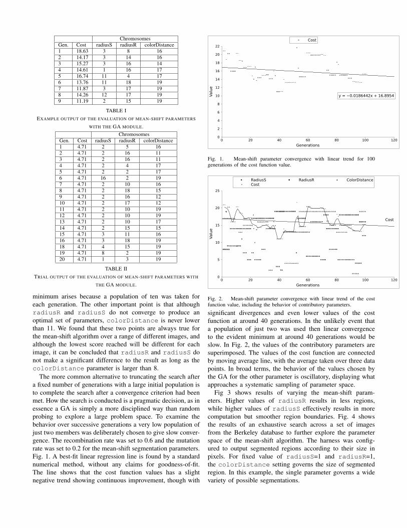
ChromosomesGen. Cost radiusS radiusR colorDistance1 18.63 3 8 162 14.17 3 14 163 15.27 3 16 144 14.61 1 16 175 16.74 11 4 176 13.76 11 18 197 11.87 3 17 198 14.26 12 17 199 11.19 2 15 19

TABLE IEXAMPLE OUTPUT OF THE EVALUATION OF MEAN-SHIFT PARAMETERS

WITH THE GA MODULE.Chromosomes

Gen. Cost radiusS radiusR colorDistance1 4.71 2 5 162 4.71 2 16 113 4.71 2 16 114 4.71 2 4 175 4.71 2 2 176 4.71 16 2 197 4.71 2 10 168 4.71 2 18 159 4.71 2 16 1210 4.71 2 17 1211 4.71 2 10 1912 4.71 2 10 1913 4.71 2 10 1714 4.71 2 15 1515 4.71 3 11 1616 4.71 3 18 1918 4.71 4 15 1919 4.71 8 2 1920 4.71 1 3 19

TABLE IITRIAL OUTPUT OF THE EVALUATION OF MEAN-SHIFT PARAMETERS WITH

THE GA MODULE.

minimum arises because a population of ten was taken foreach generation. The other important point is that althoughradiusR and radiusS do not converge to produce anoptimal set of parameters, colorDistance is never lowerthan 11. We found that these two points are always true forthe mean-shift algorithm over a range of different images, andalthough the lowest score reached will be different for eachimage, it can be concluded that radiusR and radiusS donot make a significant difference to the result as long as thecolorDistance parameter is larger than 8.

The more common alternative to truncating the search aftera fixed number of generations with a large initial population isto complete the search after a convergence criterion had beenmet. How the search is conducted is a pragmatic decision, as inessence a GA is simply a more disciplined way than randomprobing to explore a large problem space. To examine thebehavior over successive generations a very low population ofjust two members was deliberately chosen to give slow conver-gence. The recombination rate was set to 0.6 and the mutationrate was set to 0.2 for the mean-shift segmentation parameters.Fig. 1. A best-fit linear regression line is found by a standardnumerical method, without any claims for goodness-of-fit.The line shows that the cost function values has a slightnegative trend showing continuous improvement, though with

0 20 40 60 80 100 120

Generations

0

2

4

6

8

10

12

14

16

18

20

22

Valu

e

y = −0.0186442x + 16.8954

Cost

Fig. 1. Mean-shift parameter convergence with linear trend for 100generations of the cost function value.

0 20 40 60 80 100 120

Generations

0

5

10

15

20

25

Value

RadiusS RadiusR ColorDistanceCost

Cost

Fig. 2. Mean-shift parameter convergence with linear trend of the costfunction value, including the behavior of contributory parameters.

significant divergences and even lower values of the costfunction at around 40 generations. In the unlikely event thata population of just two was used then linear convergenceto the evident minimum at around 40 generations would beslow. In Fig. 2, the values of the contributory parameters aresuperimposed. The values of the cost function are connectedby moving average line, with the average taken over three datapoints. In broad terms, the behavior of the values chosen bythe GA for the other parameter is oscillatory, displaying whatapproaches a systematic sampling of parameter space.

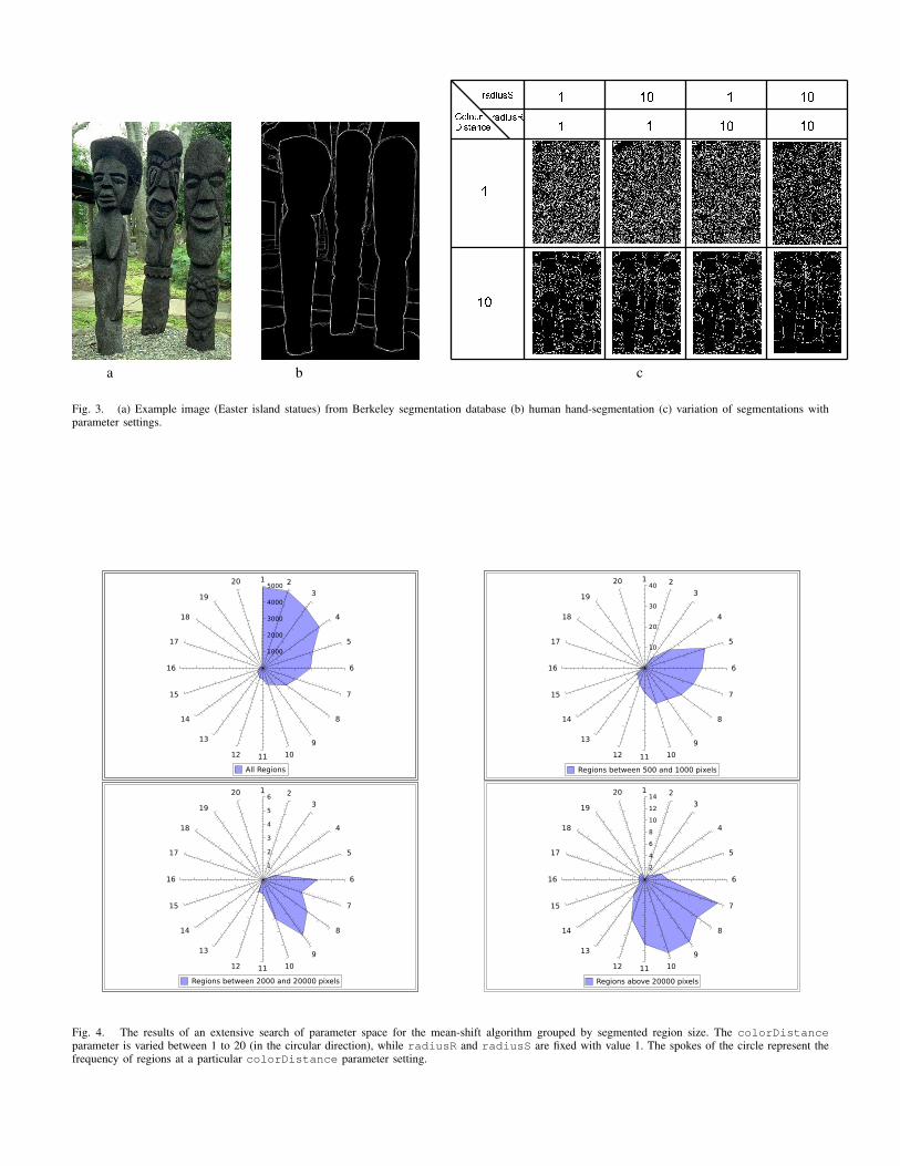
Fig 3 shows results of varying the mean-shift param-eters. Higher values of radiusR results in less regions,while higher values of radiusS effectively results in morecomputation but smoother region boundaries. Fig. 4 showsthe results of an exhaustive search across a set of imagesfrom the Berkeley database to further explore the parameterspace of the mean-shift algorithm. The harness was config-ured to output segmented regions according to their size inpixels. For fixed value of radiusS=1 and radiusR=1,the colorDistance setting governs the size of segmentedregion. In this example, the single parameter governs a widevariety of possible segmentations.

a b c

Fig. 3. (a) Example image (Easter island statues) from Berkeley segmentation database (b) human hand-segmentation (c) variation of segmentations withparameter settings.

Fig. 4. The results of an extensive search of parameter space for the mean-shift algorithm grouped by segmented region size. The colorDistanceparameter is varied between 1 to 20 (in the circular direction), while radiusR and radiusS are fixed with value 1. The spokes of the circle represent thefrequency of regions at a particular colorDistance parameter setting.

D

Th

No.of C

256

6

1

1 10

100

1

1 11

I 1 1 1 100

Fig. 5. Variation of segmentations of Fig. 3 with parameter settings forWatershed segmentation [23].

0 20 40 60 80 100 120

Generations

0

5

10

15

20

25

30

35

40

45

50

55

60

Valu

e

y = −0.0522127x + 39.9061

Cost

Fig. 6. Watershed segmentation parameter convergence with linear trend ofthe cost function value.

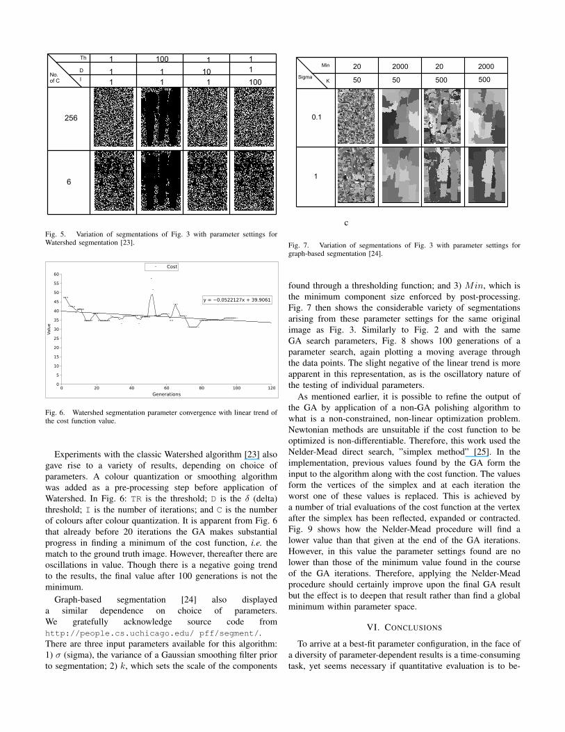
Experiments with the classic Watershed algorithm [23] alsogave rise to a variety of results, depending on choice ofparameters. A colour quantization or smoothing algorithmwas added as a pre-processing step before application ofWatershed. In Fig. 6: TR is the threshold; D is the δ (delta)threshold; I is the number of iterations; and C is the numberof colours after colour quantization. It is apparent from Fig. 6that already before 20 iterations the GA makes substantialprogress in finding a minimum of the cost function, i.e. thematch to the ground truth image. However, thereafter there areoscillations in value. Though there is a negative going trendto the results, the final value after 100 generations is not theminimum.

Graph-based segmentation [24] also displayeda similar dependence on choice of parameters.We gratefully acknowledge source code fromhttp://people.cs.uchicago.edu/ pff/segment/.There are three input parameters available for this algorithm:1) σ (sigma), the variance of a Gaussian smoothing filter priorto segmentation; 2) k, which sets the scale of the components

K

Min

Sigma

0.1

1

20 2000 200020

50 50050 500

c

Fig. 7. Variation of segmentations of Fig. 3 with parameter settings forgraph-based segmentation [24].

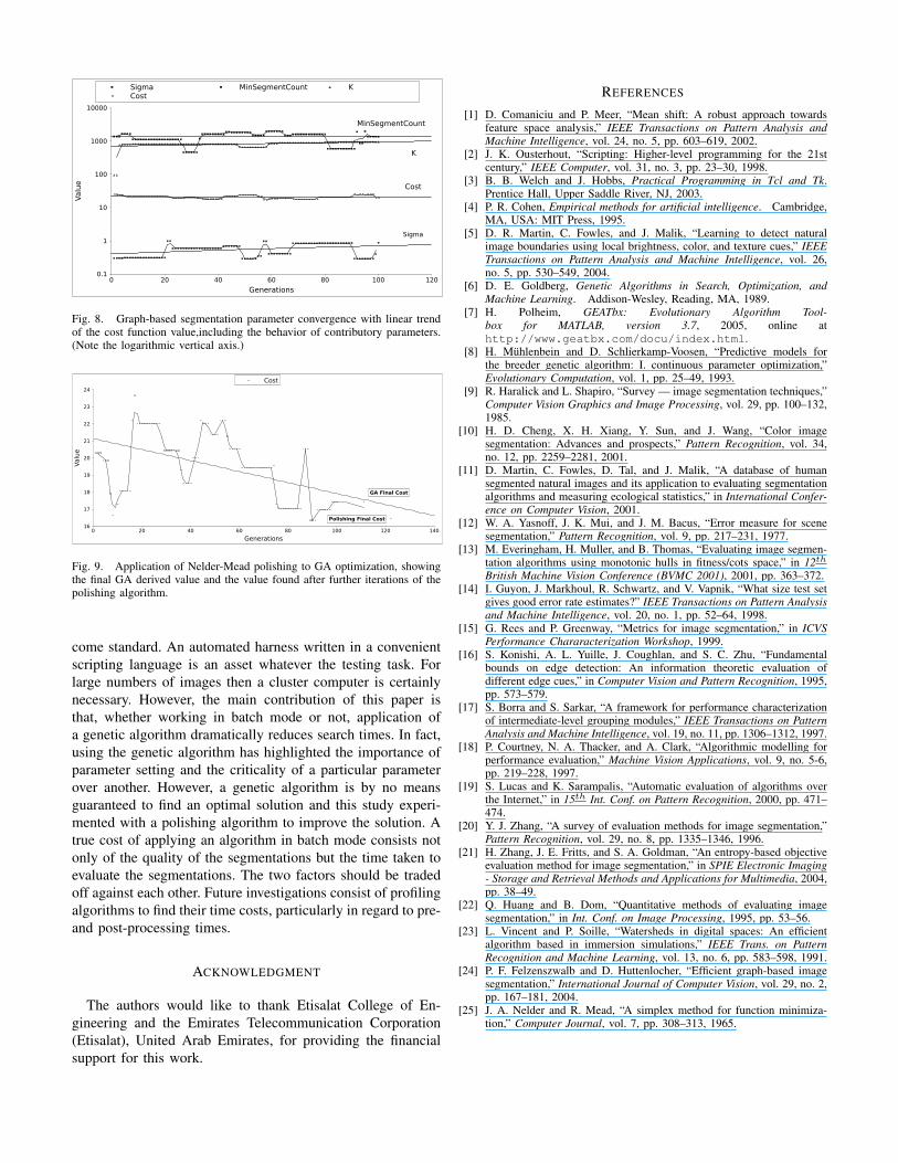
found through a thresholding function; and 3) Min, which isthe minimum component size enforced by post-processing.Fig. 7 then shows the considerable variety of segmentationsarising from these parameter settings for the same originalimage as Fig. 3. Similarly to Fig. 2 and with the sameGA search parameters, Fig. 8 shows 100 generations of aparameter search, again plotting a moving average throughthe data points. The slight negative of the linear trend is moreapparent in this representation, as is the oscillatory nature ofthe testing of individual parameters.

As mentioned earlier, it is possible to refine the output ofthe GA by application of a non-GA polishing algorithm towhat is a non-constrained, non-linear optimization problem.Newtonian methods are unsuitable if the cost function to beoptimized is non-differentiable. Therefore, this work used theNelder-Mead direct search, ”simplex method” [25]. In theimplementation, previous values found by the GA form theinput to the algorithm along with the cost function. The valuesform the vertices of the simplex and at each iteration theworst one of these values is replaced. This is achieved bya number of trial evaluations of the cost function at the vertexafter the simplex has been reflected, expanded or contracted.Fig. 9 shows how the Nelder-Mead procedure will find alower value than that given at the end of the GA iterations.However, in this value the parameter settings found are nolower than those of the minimum value found in the courseof the GA iterations. Therefore, applying the Nelder-Meadprocedure should certainly improve upon the final GA resultbut the effect is to deepen that result rather than find a globalminimum within parameter space.

VI. CONCLUSIONS

To arrive at a best-fit parameter configuration, in the face ofa diversity of parameter-dependent results is a time-consumingtask, yet seems necessary if quantitative evaluation is to be-

0 20 40 60 80 100 120

Generations

0.1

1

10

100

1000

10000

Value

Sigma MinSegmentCount KCost

Sigma

Cost

MinSegmentCount

K

Fig. 8. Graph-based segmentation parameter convergence with linear trendof the cost function value,including the behavior of contributory parameters.(Note the logarithmic vertical axis.)

0 20 40 60 80 100 120 140

Generations

16

17

18

19

20

21

22

23

24

Value

GA Final Cost

Polishing Final Cost

Cost

Fig. 9. Application of Nelder-Mead polishing to GA optimization, showingthe final GA derived value and the value found after further iterations of thepolishing algorithm.

come standard. An automated harness written in a convenientscripting language is an asset whatever the testing task. Forlarge numbers of images then a cluster computer is certainlynecessary. However, the main contribution of this paper isthat, whether working in batch mode or not, application ofa genetic algorithm dramatically reduces search times. In fact,using the genetic algorithm has highlighted the importance ofparameter setting and the criticality of a particular parameterover another. However, a genetic algorithm is by no meansguaranteed to find an optimal solution and this study experi-mented with a polishing algorithm to improve the solution. Atrue cost of applying an algorithm in batch mode consists notonly of the quality of the segmentations but the time taken toevaluate the segmentations. The two factors should be tradedoff against each other. Future investigations consist of profilingalgorithms to find their time costs, particularly in regard to pre-and post-processing times.

ACKNOWLEDGMENT

The authors would like to thank Etisalat College of En-gineering and the Emirates Telecommunication Corporation(Etisalat), United Arab Emirates, for providing the financialsupport for this work.

REFERENCES

[1] D. Comaniciu and P. Meer, “Mean shift: A robust approach towardsfeature space analysis,” IEEE Transactions on Pattern Analysis andMachine Intelligence, vol. 24, no. 5, pp. 603–619, 2002.

[2] J. K. Ousterhout, “Scripting: Higher-level programming for the 21stcentury,” IEEE Computer, vol. 31, no. 3, pp. 23–30, 1998.

[3] B. B. Welch and J. Hobbs, Practical Programming in Tcl and Tk.Prentice Hall, Upper Saddle River, NJ, 2003.

[4] P. R. Cohen, Empirical methods for artificial intelligence. Cambridge,MA, USA: MIT Press, 1995.

[5] D. R. Martin, C. Fowles, and J. Malik, “Learning to detect naturalimage boundaries using local brightness, color, and texture cues,” IEEETransactions on Pattern Analysis and Machine Intelligence, vol. 26,no. 5, pp. 530–549, 2004.

[6] D. E. Goldberg, Genetic Algorithms in Search, Optimization, andMachine Learning. Addison-Wesley, Reading, MA, 1989.

[7] H. Polheim, GEATbx: Evolutionary Algorithm Tool-box for MATLAB, version 3.7, 2005, online athttp://www.geatbx.com/docu/index.html.

[8] H. Muhlenbein and D. Schlierkamp-Voosen, “Predictive models forthe breeder genetic algorithm: I. continuous parameter optimization,”Evolutionary Computation, vol. 1, pp. 25–49, 1993.

[9] R. Haralick and L. Shapiro, “Survey — image segmentation techniques,”Computer Vision Graphics and Image Processing, vol. 29, pp. 100–132,1985.

[10] H. D. Cheng, X. H. Xiang, Y. Sun, and J. Wang, “Color imagesegmentation: Advances and prospects,” Pattern Recognition, vol. 34,no. 12, pp. 2259–2281, 2001.

[11] D. Martin, C. Fowles, D. Tal, and J. Malik, “A database of humansegmented natural images and its application to evaluating segmentationalgorithms and measuring ecological statistics,” in International Confer-ence on Computer Vision, 2001.

[12] W. A. Yasnoff, J. K. Mui, and J. M. Bacus, “Error measure for scenesegmentation,” Pattern Recognition, vol. 9, pp. 217–231, 1977.

[13] M. Everingham, H. Muller, and B. Thomas, “Evaluating image segmen-tation algorithms using monotonic hulls in fitness/cots space,” in 12th

British Machine Vision Conference (BVMC 2001), 2001, pp. 363–372.[14] I. Guyon, J. Markhoul, R. Schwartz, and V. Vapnik, “What size test set

gives good error rate estimates?” IEEE Transactions on Pattern Analysisand Machine Intelligence, vol. 20, no. 1, pp. 52–64, 1998.

[15] G. Rees and P. Greenway, “Metrics for image segmentation,” in ICVSPerformance Chararacterization Workshop, 1999.

[16] S. Konishi, A. L. Yuille, J. Coughlan, and S. C. Zhu, “Fundamentalbounds on edge detection: An information theoretic evaluation ofdifferent edge cues,” in Computer Vision and Pattern Recognition, 1995,pp. 573–579.

[17] S. Borra and S. Sarkar, “A framework for performance characterizationof intermediate-level grouping modules,” IEEE Transactions on PatternAnalysis and Machine Intelligence, vol. 19, no. 11, pp. 1306–1312, 1997.

[18] P. Courtney, N. A. Thacker, and A. Clark, “Algorithmic modelling forperformance evaluation,” Machine Vision Applications, vol. 9, no. 5-6,pp. 219–228, 1997.

[19] S. Lucas and K. Sarampalis, “Automatic evaluation of algorithms overthe Internet,” in 15th Int. Conf. on Pattern Recognition, 2000, pp. 471–474.

[20] Y. J. Zhang, “A survey of evaluation methods for image segmentation,”Pattern Recognition, vol. 29, no. 8, pp. 1335–1346, 1996.

[21] H. Zhang, J. E. Fritts, and S. A. Goldman, “An entropy-based objectiveevaluation method for image segmentation,” in SPIE Electronic Imaging- Storage and Retrieval Methods and Applications for Multimedia, 2004,pp. 38–49.

[22] Q. Huang and B. Dom, “Quantitative methods of evaluating imagesegmentation,” in Int. Conf. on Image Processing, 1995, pp. 53–56.

[23] L. Vincent and P. Soille, “Watersheds in digital spaces: An efficientalgorithm based in immersion simulations,” IEEE Trans. on PatternRecognition and Machine Learning, vol. 13, no. 6, pp. 583–598, 1991.

[24] P. F. Felzenszwalb and D. Huttenlocher, “Efficient graph-based imagesegmentation,” International Journal of Computer Vision, vol. 29, no. 2,pp. 167–181, 2004.

[25] J. A. Nelder and R. Mead, “A simplex method for function minimiza-tion,” Computer Journal, vol. 7, pp. 308–313, 1965.