Computation of changes in the run-off regimen of the Lake Santa Ana watershed (Zacatecas, Mexico):...

Lakes & Reservoirs: Research and Management 2008 13: 155–167

© 2008 The AuthorsDoi: 10.1111/j.1440-1770.2008.00364.x Journal compilation © 2008 Blackwell Publishing Asia Pty Ltd

Blackwell Publishing Asia Case ReportsLake Santa Ana watershedComputation of changes in the run-off regimen of the

Lake Santa Ana watershed (Zacatecas, Mexico)Roberto Gaytán,1 José de Anda2* and Jim Nelson3

1Departamento de Recursos Hidráulicos, Universidad Autónoma de Zacatecas, Ramón López Velarde, Zacatecas, Mexico, 2Centro de Investigación y Asistencia en Tecnología y Diseño del Estado de Jalisco, Guadalajara, Jalisco, Mexico,

3Department of Civil and Environmental Engineering, Brigham Young University, Provo, Utah, USA

AbstractThis study describes the application of a water run-off model for Lake Santa Ana, Mexico, developed through the combinedapplication of two simulation models: the Watershed Modelling System (WMS) and the Hydrologic Modelling System(HEC-HMS). The WMS was used to estimate the geometric parameters of the hydrographic basin from a digital elevationmodel and geographical information describing the location of the hydraulic infrastructure developed in the basin in recentyears. The HEC-HMS was used to estimate the run-off hydrographs, by using historical rainfall data and calibrating themodel with the observed hydrometric data. The lake bathymetry was taken into account in order to estimate the lake’swater balance. Recent observations indicate that anthropogenic activities have modified the natural run-off features of thelake basin. The magnitude of these modifications was estimated by linking the WMS and HEC-HMS models. Application ofthese linked tools allowed the successful estimation of the modified basin limits and hydraulic behaviour of Lake Santa Ana.

Key wordsclosed basin, hydrological balance, Lake Santa Ana, run-off models, playa lake, watershed modification.

INTRODUCTIONThe hydrological cycle and its individual processes(precipitation, run-off, evaporation, evapotranspiration,infiltration) are central subjects of hydrology (USGS2006). Each process exhibits a high spatial and temporalvariability, and plays a critical role in physical, chemicaland biological processes that control the terrestrial system.Furthermore, human activities are inseparable from thesenatural events (Dunne & Leopold 1978; Elkaduwa &Sakthivadivel 1998). Local modifications produced byhuman activities can result in large-scale consequencesin the hydrological cycle (UNESCO 2003, 2006). Changesin vegetation coverage, as a result of the expansion ofagriculture and urban land uses, with their associatedcontamination impacts, have a strong effect on hydro-logical processes. Thus, it is necessary to study both smallbasins and larger, regional level basins (Shahagian 2000;Sharma et al. 2000).

Hydrological modelling of large and small basins hasbeen widely applied in assessing environmental impacts

caused by changes in the hydrological cycle, or fromland-use changes resulting from human activities(Henderson-Sellers et al. 1993; Kite 1993; Harbor 1994;Bhaduri et al. 1997; Sharma et al. 2000). At the same time,mismanagement of water resources, and its potentiallong-term repercussions for regional and global climatechanges, also has attracted the attention of other researchers(Gleick 1987; Vorosmarty & Moore 1991; Rind et al. 1992;Nikolaidis et al. 1993; McGuffie et al. 1998; Xu 2000).

In this context, the hydrological management ofwatersheds supplies the conceptual and spatial frameworkto allow the development and implementation of normsand conservation practices, based on the understandingof ecological and social processes, and interactionsnecessary to assure the integrity of the basin while, at thesame time, to assess the impacts of human activities on thehydrological processes (EPA 1995; Ersten 1999; Jain et al.2000). It is necessary, however, to appreciate that it is notpossible to achieve reliable assessment or appropriatemanagement practices, if the hydrological data are notsufficiently good for a regional analysis (Bergström &Graham 1998; Mendoza et al. 2002). Hydrologists haveaddressed this problem by quantifying the behaviour of

*Corresponding author. Email: [email protected]

Accepted for publication 20 January 2008.

156 R. Gaytán et al.

© 2008 The AuthorsJournal compilation © 2008 Blackwell Publishing Asia Pty Ltd

the different processes of the hydrological cycle over along time period, thereby making it possible to simulatethese processes at the watershed level (de Anda et al.1998; Winter & Springer 2003; Ortiz-Jiménez et al. 2005;Awulachew 2006a,b). With hydrology, as with othersciences, the development of new measurement methodshas facilitated significant advances in our knowledge ofthese functional relationships.

Study areaZacatecas State is located in the north central part of theMexican Republic. It is characterized by a dry climate,with an average annual temperature of 16°C, and a meanrainfall of 510 mm. The mean extreme annual variationsin temperature and rainfall are 35°C (maximum) and6°C (minimum); and 910 mm (maximum) and 324 mm(minimum), respectively (INEGI 2006). The Calerawatershed is located in the middle of Zacatecas State.It is a closed basin covering � 2056.57 km2 (CONAGUA2007a). Its natural limits are bordered on the east by theZacatecas Mountains, on the west by the FresnilloMountains, on the north by El Algodon hill, and on thesouth by the La Mesa hills. The Calera watershed is part ofthe El Salado hydrological region number 37 (RH37),being located in the Fresnillo-Yesca basin above the CaleraAquifer. The aquifer is the only water supply in the basin,because of its predominantly dry climate (Conagua 2007a).Agricultural and industrial activities have caused animbalance between water abstractions and recharge inthe Calera Aquifer, creating a situation of water over-exploitation (CONAGUA 2002; Betsco Consulting group2004). Lake Santa Ana is located at the north end of theCalera watershed (Fig. 1), being the most importantwater body in the region. It is located at 23°22′15′′Ν and102°42′20′′W. The lake’s surface area fluctuates between816 ha in the rainy season (with a mean depth of 0.82 m)and 450 ha in the dry season (with a mean depth of0.35 m). Accordingly, it is considered an intermittentshallow lake, located in a semiarid zone.

Lake Santa Ana receives � 86.5% of the surface run-offin the Calera watershed. It represents a diverse habitatof migratory species (e.g. ringed teals, white geese,Canadian geese, grey crane, etc.) (Pinedo-Robles &López-Gámez 2002). The lake, located at the north to thecentral portion of Mexico, is a priority site for wildfowlconservation in Mexico (Pérez-Arteaga et al. 2005). Thetypical rainfall in the basin during the dry season is36.9 mm (February to May), compared to 321 mm in therainy season (June to September). The shallow featuresof the lake, and its high evaporation rate, also are factorscontributing to the intermittent nature of the waterbody.

However, the build-up of irrigation channels during 1973–1979 in the Calera watershed modified the run-off patternsof the basin, increasing water run-off to Lake Santa Ana.According to Bates and Jackson (1984) and Briere (2000),Lake Santa Ana can be considered a ‘playa lake’ or sabkha(an Arabic word meaning a salty waterbody). Playalakes are characterized by shallowness and intermittency,normally being located in arid or semiarid closed basins.This type of lake inundates the beach during the rainyseason, with the beaches gradually reappearing duringthe evaporation period of the dry season. As a result of theintermittent processes in the lake, the concentration ofdissolved solids and salts in the lake increases, resultingin higher conductivity.

There are efforts worldwide to inventory and classifylakes, dams and reservoirs (Lehner & Döll 2004). In thecase of ‘playa lakes’, some studies are directed at theirclassification and characterization (Last & Schweyen 1983;Lichvar et al. 2004; Quillin et al. 2005). Hydrological andlimnological studies of this type of lakes are relative recent(Cooper & Koch 1984; Querlat et al. 1997; Seddon &Briggs 1998; Briggs et al. 2000; Gaberscik et al. 2003;Bren & Sandell 2004) and, particularly in Mexico, thecontributions are scarce (Alcocer & Escobar 1996).

There is very little published research on Lake SantaAna, with the few existing official technical reports notconsidering the lake to be a potential water resource. Mostof the related information focuses on the Calera Aquifer

Fig. 1. Location of Lake Santa Ana and its basin.

Lake Santa Ana watershed 157


(Conagua 2002). Between the 1960s and 1990s, severalstudies of the quality and quantity of groundwater in theCalera Aquifer were carried out by different governmentaland academic institutions (Conagua 2002), mainly becauseit was the main water supply in the region.

The goals of this study are to: (i) describe the primarybathymetric features of Lake Santa Ana; (ii) quantify thechanges induced in the limits and area of the basin due tothe build-up of hydraulic infrastructure; and (iii) generatea first approach to a calibrated water balance model thatquantifies the components of the hydrological cyclerelevant to the lake. This study is intended to contribute tothe body of knowledge about playa lakes, and particularlyto establish the importance of Lake Santa Ana as apotential area for waterfowl conservation and recreation.

METHODS

Water balance of the lakeThe input and output components of the water balance of alake or reservoir depend on its bathymetric features, theclimate, and hydrological, geological and anthropogenicfactors (de Anda et al. 1998). A lake’s water balanceequation can be developed from a simple continuityequation that considers the hydrological cycle processes(Eqn 1). Furthermore, this continuity equation is governedby the conservation of mass, which is described byequilibrium between the input and the output of waterfluxes, as follows (Awulachew 2006a,b):

Vin − Vout + P − E − ΔS = 0 (1)

where: Vin = surface and subsurface water inflow (m3);Vout = surface and subsurface water outflow (m3); P =

precipitation volume (m3); E = evaporation volume (m3);and ΔS = change in water storage (m3).

Alternatively, the hydrological parameters can bedefined in terms of the water depth. The variables of thewater balance equation in an ideal situation are computedseparately, providing a closed solution. In practice, however,the computation leads to a discrepancy, or residual error.Considering the error term (δ ) therefore Equation 1 canbe rewritten as follows (Awulachew 2006a,b):

Vin − Vout + P − E − ΔS ± δ = 0 (2)

Solution procedureThe water balance model equations, as written in theabove form, can be used to compute and simulate watervolume, area and depth, or to estimate unknown waterbalance components. The purpose of the water balancehere is to simulate the water level, and compute the watervolume, area and temporal variability on monthly or yearlytime intervals. With the water levels thus determined,volume-based or depth-based equations or storage capacity(rating curves of depth versus volume) curves can beemployed to estimate the area and volume of the lake.The depth-based simulation procedure has been employedin this study, and is described in the following steps(Awulachew 2006a,b):

1 Compute initial parameters (area, volume, etc.) fromthe initial depth, as the boundary conditions

2 Assume an average water surface area over the timeperiod i, Ami = A1,i, where A1,i = initial lake area

3 Compute the change in depth (ΔZi) from the followingequation:

(3)

where: Al,i = surface area of lake for evaporation and rainfallcomputation; p = rainfall depth; e = evaporation depth; PF =rainfall correction factor; and EF = evaporation correctionfactors, which are used to adjust rainfall and evaporationfor the lakes.

The water depth at the end of the simulation interval isgiven as:

Z2,i = Z1,i + ΔZi (4)

It is calculated from the following steps:1 Compute A2,i (surface area at end of time interval i),

from the area elevation curve:

(5)Fig. 2. Location of the meteorological stations and calculated

limits of the Santa Ana basin.

ΔZ

PF p EF e A V VAi

l i in i out i

m i

( ) , , ,

,

=⋅ − ⋅ + −

A

A Am i

i i,

, ,

=+1 2

2



2 Repeat steps 3 and 4 until a reasonable agreement inZ is obtained.

3 Compute volume V2,i at end of time interval i, usingthe storage capacity curve.

4 For the next time interval, Z1,i+1, A1,i+1, and V1,i+1 aredescribed by Z2,i, A2,i, and V2,i.

Boundary conditionsAs a water balance for Lake Santa Ana requires the basinrun-off, as indicated in the Vin component of Equation 2,a strategy must be developed to estimate it. This strategyrequires first that the natural and modified hydrographicbasin conditions be determined.

Modern GIS software allows digital–spatial data to beprocessed and used in developing hydrological modellingstudies. For this study, the Watershed Modelling System®

(WMS 2006) was chosen, as it is capable of processingdigital elevation, land use and soils files available for thestudy. It also is connected to multiple numerical run-offmodels adequate for the intended study (Mustafa et al.2005). The natural limits of the Lake Santa Ana basin weredetermined using the WMS grid-based delineation methods,and the digital topographical information or digital elevationmodels (DEM). The DEM for this work was obtainedfrom the Mexican Institute of Statistics, Geography, andInformatics, at a spatial scale of 1 : 50 000 (INEGI 2003).

The physical limits of the lake itself were obtained fromthe lake bathymetry. Because of the shallowness of thelake, the bathymetric survey was carried out by directmeasurements, using a level rod and a Global PositioningSystem (GPS). The resulting survey data were laterregistered and drawn, using the AutoCAD® (http://www.autodesk.es/adsk/servlet/index?siteID=455755&id=6693291)program. The resulting data were subsequently suppliedto WMS as part of the digital information necessary todelineate the hydrographic and bathymetric features ofboth the basin and the lake.

Changes in boundary conditionsThe hydrographic limits of the Lake Santa Ana basin haveundergone significant changes over the past several years,due largely to construction of 169 km of channels outsidethe natural basin in 1973–1979. The reason for developingthese channels was to protect important agricultural landfrom flooding during the rainy season. These channelswere designed to discharge excess water into Lake SantaAna, extending the basin limits and creating new sourcesto the lake. Furthermore, the lake has received municipalwastewater effluents from the towns of Calera and RamónLópez-Velarde since 1979, and industrial wastewatereffluents from a large brewery since 2005.

To estimate the additional run-off contribution fromthe flood protection channel system, the channels werefirst measured, and located with the use of a GPS. Thisinformation subsequently was supplied to WMS for use indetermining the modified basin areas.

Rainfall and evaporationThe daily rainfall information over the period of 1963–2006 from the meteorological stations located in Fresnillo(23°10′40′′N, 102°53′20′′W), Calera (22°54′00′′N 102°39′00′′W)and Zacatecas (22°45′39′′N, 102°34′30′′W (Conagua 2002)was used to estimate the average rainfall over the basin,using the Thiessen polygon technique (Pizarro et al. 2003)(Figure 2). The dynamics of the monthly mean rainfall,and the rainfall frequency in the studied period wasanalysed using the WinSTAT® (2002) program.

In addition to evaporation data from the meteorologicalstations, direct daily measurements of evaporation weremade at the lake throughout March 2006, using anevaporation pan (diameter of 1.2 m; depth of 0.26 m)installed near the lake. Daily water losses in the lake weremeasured with a permanent scale, assuming that theobserved water losses were because of evaporation. Thescale, divided into centimeters, has a height of 2.40 m,and is located at the geographical coordinates 23°13′53′′Nand 102°43′59′′S.

The observed measurements were used to determinethe evaporation coefficient of the lake, calculated as thelake evaporation divided by the pan evaporation. Thedepths in the lake, and the heights in the pan, weremeasured on a daily basis, and compared to the dailyinformation measured at the Fresnillo, Calera, andZacatecas meteorological stations, which were monitoredby the Water National Commission (CONAGUA) duringthe same period.

Run-off modelRun-off from the Lake Santa Ana basin was estimatedwith the HEC-HMS hydrological simulation programme.In addition to the delineated watershed boundary,HEC × HMS requires information on rainfall, soil type andland use to formulate a run-off response. HEC-HMS isdesigned to simulate the run-off process from dendriticnetworks for a wide range of geographical areas andproblems, including large river basin water supply andflood hydrology, as well as small urban or naturalwatershed run-off (HEC 2006). Rainfall data for the HEC-HMS model were obtained from the Water NationalCommission (CONAGUA 2007b) for the period 2000–2006. Soil type and land-use information was obtained fromareal maps at scales of 1 : 50 000 and 1 : 250 000 (INEGI

http://www.autodesk.es/adsk/servlet/index?siteID=455755&id=6693291



1975a,b,c). These digital datasets were overlaid on thepreviously delineated watershed boundary in WMS toextract the necessary boundary fluxes (i.e. rainfall) andestimate the infiltration and run-off parameters by indexingthem to physical properties (i.e. land use and soils).

The spatially derived parameters in WMS were thenexported to the HEC-HMS program in order to completethe numerical simulation water balance. Daily rainfall dataand monthly potential evaporation measured for the basinalso were supplied. The potential evaporation was adjusted,using the estimated average evaporation coefficient.Utilizing this information, the run-off simulation wascarried out for the rainy and dry seasons on a continuousbasis, considering both the natural and modified basinsduring the period from January to December 2006 (Linseyet al. 1992; Daniil et al. 2005; Chin 2006).

Another advantage of using HEC-HMS is that it includestwo models that permit continuous simulation with dailyrainfall data; namely, the Soil Moisture Accounting (SMA)Method and the Deficit Constant Method (DCM). TheSMA Method was selected for this study, as it is moreadequate for simulating complex systems than the DCM.The SMA requires a rainfall excess transformationmodel in the run-off process. In the case of the HEC-HMSprogram, it includes the Clark and Snyder Unit-Hydrographmethod, and the Soil Conservation Service (SCS) Method.The unit hydrograph ordinates proposed by the user alsocan be applied.

The Clark Unit-Hydrograph method was used in thisstudy, as it permits the use of mean daily rainfall values.Finally, it was necessary to select a routing method tocomplete the run-off model. For the Lake Santa Anamodel, a linear reservoir method was chosen because itcan best simulate the base flow, water storage andsubsurface water flow in the soil.

The method selected in the HEC-HMS program toestimate evapotranspiration in the basin was the monthlymean value, which permitted the use of a monthly

measured pan evaporation coefficient. A time step of 24 hwas used in the calculations. The run-off hydrographsobtained by using HEC-HMS for each simulated monthwere compared to the estimated volumes through ahydrological balance for the lake. The hydrologicalparameters of the HEC-HMS model were adjusted untilthe run-off estimations were in accord with the calculatedresults from the hydraulic balance in Lake Santa Ana.

Water extractions and water usesInformation on the surface water sources, and the extractedyearly water volumes (Tables 1 and 2, respectively), wascollected to estimate the annual surface water volumeextractions used for agricultural and municipal services.As seen in these tables, surface water extractions of13.2 million m3 year–1 in the basin are mainly used foragriculture and cattle. A water volume 7.5 times lessthan that of the groundwater extractions of 99.25 millionm3 year–1 in 2002 was used for agriculture and cattle in thesame area, representing 79.4% of the total groundwaterextractions in the basin (Conagua 2002).

Groundwater contributionTo determine the water balance for Lake Santa Ana, it wasnecessary to know the sources and sinks in the system.It is possible that groundwater can be both a water sourceand/or a sink. In this study, however, net groundwatercontributions were assumed to be negligible, comparedto run-off, precipitation, and stream flow sources, orevaporation sinks. This hypothesis will be verified with acomparison of the main surface water processes of thewater balance to the changes in the lake water storage.

RESULTS

Lake bathymetryThe measured bathymetric data for Lake Santa Ana arepresented in Table 3, with its respective depth–area anddepth–volume rating curves represented graphically in

Table 1. Main surface water sources in the Lake Santa Ana basin (Conagua 2002)

Name Municipality

Water extractions

(mm3 year–1)

Creek used

for extraction

Irrigated

land (ha)

En Medio creek Gral. Enrique Estrada 2.9 Barrancos 230

Toribio Reservoir Calera 2.8 En medio 620

Calera Dam Calera 2.0 Calera 207

La Bomba Dam Fresnillo 2.0 El Aguila 457

Los Chilitos creek Fresnillo 1.9 Prieto –

El Peñasco Dam Gral. Enrique Estrada 1.6 Las Iglesias 135

Total 13.2 1649



Figure 3. The shape and bathymetric features of the lakeare illustrated in Figure 4, with its general morphologicalfeatures during the rainy and dry seasons presented inTable 4.

Precipitation and evaporationThe interpolated rainfall, temperature and evaporationdata for the Calera, Fresnillo and Zacatecas meteorologicalstations are presented in Table 5 (also see Fig. 4). Theinterpolated annual rainfall precipitation, evaporation andrainfall depths were estimated with the Thiessen polygonstechnique, based on the period from 1963 to 2006, whereregular time-series data are available (Conagua 2007b).A mean annual precipitation and evaporation height of

427 mm and 2247 mm, respectively, and a meantemperature of 15.5°C in the Calera watershed area wereobtained (Table 5). The monthly patterns of precipitation,evaporation and temperature in the basin area for the

Table 2. Groundwater volume abstractions, based on consumptive uses (Conagua 2002)

Water

extraction

source

Water uses

Non-used

water

sources

Agriculture Cattle Municipal services Industry Total

No.

Extracted

volume

(mm3 year–1) No.

Extracted

volume

(mm3 year–1) No.

Extracted

volume

(mm3 year–1) No.

Extracted

volume

(mm3 year–1) No.

Extracted

volume

(mm3 year–1)

Wells 804 95.710 14 0.020 36 18.220 14 6.000 868 119.95 144

Wheels 207 3.500 22 0.020 23 1.530 0 0.000 322 5.05 54

Total 1081 99.210 36 0.040 59 19.750 14 6.000 1190 125.00 198

Table 3. Bathymetric features of Lake Santa Ana

Elevation (m a.s.l.) Area (m2) Volume (m3)

2046.30 21 353.97 2135.40

2046.40 366 262.15 38 761.61

2046.50 800 830.50 118 844.66

2046.60 1 591 696.13 278 014.28

2046.70 2 339 384.54 511 952.73

2046.80 3 104 685.04 822 421.23

2046.90 4 005 257.43 1 222 946.98

2047.00 5 104 523.52 1 733 399.33

2047.10 5 737 411.33 2 307 140.46

2047.19 7 780 525.09 3 085 192.97

2047.30 7 835 905.86 3 868 783.56

2047.40 7 887 184.35 4 657 501.99

2047.50 7 898 978.40 5 447 399.83

2047.60 7 989 741.33 6 246 373.96

2047.70 8 041 019.16 7 050 475.88

2047.80 8 092 298.31 7 859 705.71

2047.90 8 143 576.79 8 674 063.39

2047.94 8 165 113.76 9 490 574.77

Table 4. Morphometric features of Lake Santa Ana (average

values for rainy and dry season from January to December 2006)

Parameter Units Rainy season Dry season

Altitude m a.s.l. 2047.94 2046.90

Basin area + lake area km2 1778.10 1773.94

Lake area + islands km2 8.17 4.01

Average width km 2.175 1.013

Maximum depth m 1.64 0.82

Average depth m 0.82 0.41

Shoreline length km 16.86 11.01

Lake volume Mm3 8.17 1.22

Table 5. Interpolated rainfall, temperature, and evaporation data for

Calera, Fresnillo, and Zacatecas meteorological stations for 1963–2006

Month

Precipitation

(mm)

Evaporation

(mm)

Temperature

(°C)

Jan 16.11 133.68 10.31

Feb 8.10 160.49 11.64

Mar 4.50 240.92 13.80

Apr 6.57 268.08 16.73

May 17.69 269.47 19.32

Jun 67.88 235.97 20.25

Jul 89.87 199.03 18.96

Aug 90.10 181.17 18.61

Sep 73.13 153.04 17.25

Oct 31.71 150.20 15.38

Nov 9.69 133.71 12.64

Dec 11.66 121.08 11.30

Yearly 427.00 2246.84 15.52



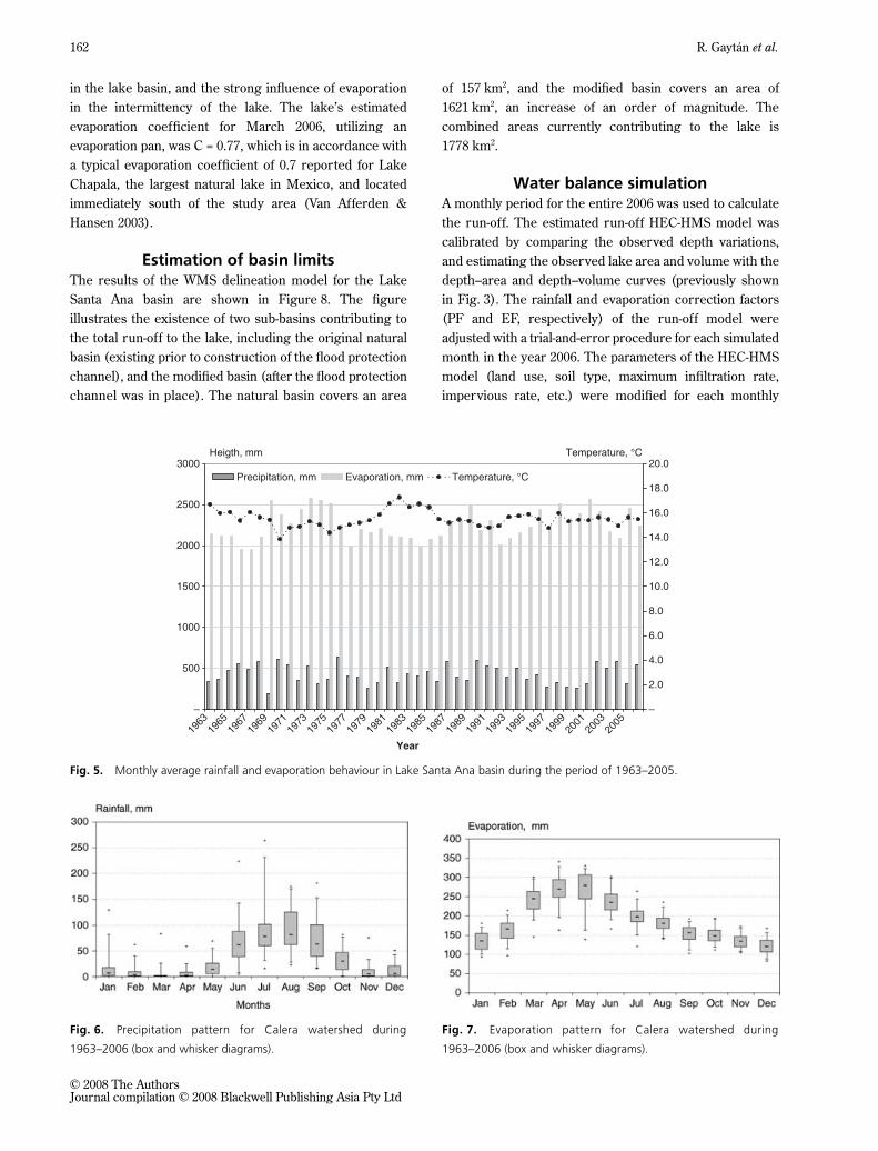
period from 1963 to 2006 are presented in Figure 5, whichalso illustrates a cyclical behaviour of precipitation andevaporation that could be associated with the El Niñophenomenon. The monthly rainfall and evaporationpatterns for the period from 1963 to 2006 are shown inFigures 6 and 7, respectively. The main precipitationperiod occurs annually from June to October, and the dry

season from November to May, with July and Augustgenerally exhibiting the greatest intensity. However, thehighest evaporation rates occur in the warmest part of thedry season, from March to June, being highest in May.During the rainy season, the evaporation rates graduallydiminish, with the lowest average value in December.These values highlight the low quantity of precipitation

Fig. 3. Altitude-area and altitude-volume curves for Lake Santa Ana basin.

Fig. 4. Bathymetric map of Lake Santa Ana.



in the lake basin, and the strong influence of evaporationin the intermittency of the lake. The lake’s estimatedevaporation coefficient for March 2006, utilizing anevaporation pan, was C = 0.77, which is in accordance witha typical evaporation coefficient of 0.7 reported for LakeChapala, the largest natural lake in Mexico, and locatedimmediately south of the study area (Van Afferden &Hansen 2003).

Estimation of basin limitsThe results of the WMS delineation model for the LakeSanta Ana basin are shown in Figure 8. The figureillustrates the existence of two sub-basins contributing tothe total run-off to the lake, including the original naturalbasin (existing prior to construction of the flood protectionchannel), and the modified basin (after the flood protectionchannel was in place). The natural basin covers an area

of 157 km2, and the modified basin covers an area of1621 km2, an increase of an order of magnitude. Thecombined areas currently contributing to the lake is1778 km2.

Water balance simulationA monthly period for the entire 2006 was used to calculatethe run-off. The estimated run-off HEC-HMS model wascalibrated by comparing the observed depth variations,and estimating the observed lake area and volume with thedepth–area and depth–volume curves (previously shownin Fig. 3). The rainfall and evaporation correction factors(PF and EF, respectively) of the run-off model wereadjusted with a trial-and-error procedure for each simulatedmonth in the year 2006. The parameters of the HEC-HMSmodel (land use, soil type, maximum infiltration rate,impervious rate, etc.) were modified for each monthly

Fig. 6. Precipitation pattern for Calera watershed during

1963–2006 (box and whisker diagrams).

Fig. 7. Evaporation pattern for Calera watershed during

1963–2006 (box and whisker diagrams).

Fig. 5. Monthly average rainfall and evaporation behaviour in Lake Santa Ana basin during the period of 1963–2005.



simulation, until the resulting run-off agreed with themeasured data for the lake water balance for the samemonth. The results of the run-off simulation, and itsimpacts in the water balance, are shown in Table 6 andFigure 9(a,b). These figures highlight a relatively goodagreement between the observed and the calculatedvalues for the lake area and volume during the period fromJanuary to December 2006.

DISCUSSIONTable 6 illustrates a significant difference in the LakeSanta Ana basin area and, as a consequence, increasedrun-off volume that contributes to its increases average

Fig. 8. Natural and modified basins contributing to run-off to

Lake Santa Ana.

Table 6. Model run-off simulation results for January to December 2006

2006

month

Elevation

(observed)

m a.s.l.

Lake area

(observed)

ha

Lake volume

(observed)

m3 × 1000

Lake area

(calculated)

ha

Lake volume

(calculated)

m3 × 1000

Area

difference

%

Volume

difference

%

Jan 2046.75 262.55 667.19 272.20 695.72 –3.68% –4.28%

Feb 2046.68 221.98 512.16 196.34 460.40 11.55% 10.11%

Mar 2046.58 155.35 315.18 119.63 294.84 23.00% 6.46%

Apr 2046.32 14.03 105.95 19.38 123.40 –38.10% –16.46%

May 2046.52 95.90 150.68 119.63 180.69 –24.74% –19.92%

Jun 2046.69 226.46 560.56 196.55 459.89 13.21% 17.96%

Jul 2046.89 391.01 1152.89 355.50 1166.48 9.08% –1.18%

Aug 2047.04 535.77 1962.82 542.10 1967.27 –1.18% –0.23%

Sep 2047.45 789.31 5005.25 789.31 5031.92 0.00% –0.53%

Oct 2047.41 780.84 4870.74 789.31 4712.19 –1.08% 3.26%

Nov 2047.34 778.64 4134.27 786.15 4205.29 –0.96% –1.72%

Dec 2047.32 775.62 4056.53 776.15 4026.35 –0.07% 0.74%

Fig. 9. (a) Correlation between observed and calculated lake area.

(b) Correlation between observed and calculated lake volume.



water storage volume. The construction of the drainagechannels, as a means of addressing flooding in theagriculture areas, increased the lake basin area from167.3 ha to 780.6 ha. This represents an increase, in termsof run-off, from 571 × 103 to 5724 × 103 m3 year–1. Thestudy area is located in a dry climate environment, witha rainfall < 74 mm in depth from November to May,causing the well-known natural intermittency of thelake prior to 1973. The new water contributions result-ing from the channeling system, as well as municipalwastewater discharges into the lake beginning in 1979,and the recent discharges from a brewery into the lakesince 2005, have virtually eliminated the intermittencyof the waterbody.

The proposed water balance model was able to simulatethe recent water regime of the lake. Major deviations inthe model predictions, however, are present from Marchto July, which change some of the estimated values frompositive to negative numbers. These deviations could beattributable to a unique evaporation coefficient for thelake, which was estimated in March 2006 throughout thesimulated period. As illustrated in Figure 7, the lake basinhas the highest evaporation rates over the annual cyclebetween March to July. Thus, the model requires a specificevaporation coefficient estimated by month to refine thepredicted values.

Another source of deviation could be caused bygroundwater contributions to the lake. This componentof the water balance is very complex, as informationabout the soil structure at the bottom of the lake, and itshydraulic conductivity features are not well known.

CONCLUSIONThe limits of the Lake Santa Ana basin have been modifiedfrom 156.83 km2, up to 1778.10 km2, mainly because of theconstruction of a canal system from agriculture areasin the basin, as well as wastewater discharges from thelocal municipality and industry. These changes modifiedthe water balance of the lake, increasing the run-offcontributions by a factor of 10, and reducing theintermittency of the lake caused by natural hydrologicalconditions. The WMS and HEC-HMS models permittedsimulation of the natural and modified condition of thelake, quantifying the main processes of its hydrologicalcycle. The model was calibrated with measured monthlyhydrological and hydrometric data for 2006. Nevertheless,although Figure 9(a,b) illustrates a relatively high correlationin the lake area and volume between observed andcalculated values with the applied model, there are stilldifferences between both values. The difference betweenthe measured and estimated lake volume, for example,

is > 10% during the period of high evaporation, reachinga maximum difference of 20% in May. In contrast, themaximum difference between the measured and theestimated lake volume during July to January is < 5%. Aspreviously noted, it will be necessary to include atemporary relationship in the model that considers themonthly variation of the lake’s evaporation coefficient.Further research also must consider the groundwatercontributions to, and from, the lake.

The model used in this study ultimately was able tosimulate the influence of anthropogenic activities on theLake Santa Ana basin, which has increased the waterrun-off contributions to the lake by a factor of 10, whilealso significantly reducing the intermittency cycle of thewaterbody. The new hydrological condition in the lakeincreases potential water uses, including providingpermanent habitats for terrestrial and aquatic endemicspecies; increasing waterfowl populations; developingareas for bird watchers, canoeing and camping; andforestation of nearby areas to produce an environmentconducive to recreation and amusement for the inhabitantsof Fresnillo City (currently close to 110 892 inhabitants),and without a natural recreation place located in closeproximity (INEGI 2006).

As Lake Santa Ana is a saline lake located in a semiaridzone, its biodiversity is relatively low. Nevertheless, it isstill possible to improve and restore the wildlife habitat forseveral endemic and migratory species resistant to salinewater quality conditions, mainly by controlling the saltsources and increasing the contribution of clean water tothe lake (Herbst & Blinn 1998; Williams 1999; Kindscheret al. 2004). In developing and implementing a restorationplan for Lake Santa Ana, it will be necessary to carryout water quality studies in order to determine thelake’s salt concentrations, and to identify and quantifythe anthropogenic sources of the salt, as well as possibleresponses of the lake to management practices and climatechanges (Valero-Garcés et al. 2000). Such actions wouldmake it possible to add Lake Santa Ana to the list ofpriority sites for waterfowl conservation in Mexico(Pérez-Arteaga et al. 2005).

ACKNOWLEDGEMENTSThe authors graciously acknowledge the meteorologicalinformation supplied by Ing. Humberto Abelardo DíazValdéz, Hydrometeorology Department, National WaterCommission (CONAGUA), at its Zacatecas headquarters.

REFERENCESAlcocer J. & Escobar E. (1996) Limnological regionalization

of Mexico. Lakes Reserv.: Res. Manage. 2, 55–69.



de Anda J., Quiñones S. E., French R. & Guzmán M. (1998)Hydrologic balance of Lake Chapala, (Mexico). J. Am.Water Resour. Assoc. 34, 1319–31.

Awulachew S. B. (2006a) Modelling natural conditions andimpacts of consumptive water use and sedimentation ofLake Abaya and Lake Chamo, Ethiopia. Lakes Reserv.:Res. Manage. 11, 73–82.

Awulachew S. B. (2006b) Investigation of physical andbathymetric characteristics of Lakes Abaya and Chamo,Ethiopia, and their management implications. LakesReservoirs Res. Manage. 11, 133–40.

Bates R. L. & Jackson J. A. (1984) Dictionary of GeologicalTerms, 3rd edn. Anchor Press/Doubleday, New York.

Bergström S. & Graham L. P. (1998) On the scale problemin hydrological modeling. J. Hydrol. 211, 235–65.

Betsco Consultoria (2004) Actualización Piezométrica delAcuífero Calera, Zacatecas. Subgerencia de Ingeniería,Gerencia Estatal Zacatecas, Comisión Nacional delAgua, Mexico.

Bhaduri B., Grove M., Lowry C. & Harbor J. (1997)Assessment of long-term, hydrologic effects of land usechange. The curve number technique for calculatingrun-off is modified to estimate lost groundwaterrecharge. J. Am. Water Works Assoc. 89, 94–106.

Briere P. R. (2000) Playa, playa lake, sabkha: Proposeddefinitions for old terms. J. Arid Environ. 45, 1–7.

Briggs S. V., Seddon J. A. & Thornton S. A. (2000) Wildlifein dry lake and associated habitats in western NewSouth Wales. Rangeland J. 22, 256–71.

Chin S. Ch (2006) Development of post dry periodhydrographs. Report, Bachelor of Civil Engineering,Faculty of Civil Engineering, University TeknologiMalaysia, Kuala Lumpur, Malaysia.

Comisión Nacional del Agua (CONAGUA) (2002)Determinación de la disponibilidad de agua en elacuífero calera, Estado de Zacatecas. Comisión Nacionaldel Agua. Subdirección General Técnica. Gerencia deAguas Subterráneas, Subgerencia de Evaluación yModelación Hidrológica, D.F., México.

Comisión Nacional del Agua (CONAGUA) (2007a) Mapade las Cuencas Hidrográficas de México. Sistema deInformación Geográfica del Agua. Comisión Nacionaldel Agua, México. Available from URL: http://siga.cna.gob.mx/. Accessed 23 July 2007.

Comisión Nacional del Agua (CONAGUA) (2007b)Información meteorológica proporcionada por laComisión Nacional del Agua. Gerencia Zacatecas,March 2007. Zacatecas, México.

Cooper J. J. & Koch D. L. (1984) Limnology of a deserticterminal lake, Walker Lake, Nevada, USA. Hydrobiologia118, 275–92.

Daniil E. I., Michas S. N. & Lazaridis L. S. (2005) Hydrologicmodeling for the determination of design discharges inungauged basins. GLOBAL NEST: Int. J. 7, 296–305.

Dunne T. & Leopold L. B. (1978) Water in EnvironmentalPlanning. W.H. Freeman, San Francisco, California.

Elkaduwa W. K. B. & Sakthivadivel R. (1998) Use ofhistorical data as a decision support tool in watershedmanagement: A case of study of the Upper NilwalaBasin in Sri Lanka. Report 26, International WaterManagement Institute, Colombo, Sri Lanka.

EMRL-BYU (2006) Watershed Modeling System SoftwareV.7.1. Brigham Young University, Provo, Utah. Avail-able from URL: http://www.emrl.byu.edu/wms.htm.Accessed 23 July 2007.

Environmental Protection Agency (EPA) (1995) WatershedProtection: A Project Focus. Assessment and WatershedDivision, Office of Wetlands, Oceans and Watersheds,US EPA, Washington, D.C. Available from URL: http://www.epa.gov/owow/watershed/focus/. Accessed 23 July2007.

Ersten A. C. D. (1999) Ecohydrological impact-assessmentmodeling: An example for terrestrial ecosystems inNord-Holland, The Netherlands. Environ. Model. Assess.4, 13–22.

Gaberscik A., Urbanc-Bercic O., Krzic N., Kosi G. &Branceli A. (2003) The intermittent Lake Cerknica:various faces of the same ecosystem. Lakes Reservoirs.Res. Manage. 8, 159–68.

Gleick P. H. (1987) The development and testing of waterbalance model for climate impact assessment modellingthe Sacramento basin. Water Resour. Res. 23, 1049–61.

Harbor J. (1994) A practical method for estimating theimpact of land-use change on surface run-off groundwaterrecharge and wetland hydrology. J. Am. Plann. Assoc.60, 95–108.

HEC-HMS (2006) Hydrologic Modeling System HEC-HMSV3.0.0. US Army Corps of Engineers®. Available fromURL: http://www.hec.usace.army.mil/software/hec-hms/download.html. Accessed 23 July 2007.

Henderson-Sellers A., Dickinson R. E., Durbidge T. B.,Kennedy P. J., McGuffie K. & Pitman A. J. (1993)Tropical deforestation: Modeling local- to regional-scaleclimate change. J. Geophisycal Res. 98, 7289–351.

Herbst D. B. & Blinn D. W. (1998) Experimental meso-cosm studies of salinity effects on the benthic algalcommunity of a saline lake. J. Phycol. 34, 772–8.

Instituto Nacional de Estadística Geografía E Informática(INEGI) (1975a) Carta Uso del Suelo F13B47. Escala 1:50 000. Dirección de Estudios Económicos Comisión deEstudios del Territorio Nacional. INEGI, Aguascalientes,México.

http://siga.cna.gob.mx/

http://www.emrl.byu.edu/wms.htm

http://www.epa.gov/owow/watershed/focus/

http://www.hec.usace.army.mil/software/hec-hms/download.html



Instituto Nacional de Estadística Geografía E Informática(INEGI) (1975b) Carta Edafológica F13B47. Escala 1:50 000. Dirección de Estudios Económicos Comisión deEstudios del Territorio Nacional. INEGI, Aguascalientes,México.

Instituto Nacional de Estadística Geografía E Informática(INEGI) (1975c) Carta Hidrología Superficial F13B47.Escala 1: 50 000. Dirección de Estudios EconómicosComisión de Estudios del Territorio Nacional. INEGI,Aguascalientes, México.

Instituto Nacional de Estadística Geografía E Informática(INEGI) (2003) Sistema de Descargas Del Continuo deElevaciones Digitales (CEM), Modelos Digitales deElevación (MDE) Escala 1 : 50 000: F13B36, F13B46,F13B56, F13B37, F13B47, F13B57, F13B38, F13B48,F13B58, F13B67, and F13B68. INEGI, Aguascalientes,México. Available from URL: http://mapserver.inegi.gob.mx/DescargaMDEWeb/. Accessed 23 July 2007.

Instituto Nacional de Estadística Geografía E Informática(INEGI) (2006) Mapa de Climas. Estado de Zacatecas.INEGI, Aguascalientes, Aguascalientes, México.Available from URL: http://mapserver.inegi.gob.mx/geografia/espanol/estados/zac/clim.cfm?c=444&e=18.Accessed 23 July 2007.

Jain A., Ray S. C. & Sharma E. (2000) Hydroecologicalanalysis of a sacred lake watershed system in relation toland-use cover range from Sikkim Himalaya. Catena 4,263–78.

Kindscher K., Aschenbach T. & Ashworth S. M. (2004)Wetland vegetation response to the restoration sheet flowat Cheyenne Bottoms, Kansas. Restor Ecol. 3, 368–75.

Kite G. W. (1993) Application of a land class hydrologicalmodel to climate change. Water Resour. Res. 29, 2377–84.

Last W. M. & Schweyen T. H. (1983) Sedimentology andgeochemistry of saline lakes of the Great Plains.Hydrobiologia 105, 245–63.

Lehner B. & Döll P. (2004) Development and validationof a global database of lakes, reservoirs and wetlands.J. Hydrol. 296, 1–22.

Lichvar R., Gustina G. & Bolus R. (2004) Ponding duration,ponding frequency, and field indicators: A case study onthree California, USA, playas. Wetlands 24, 406–13.

Linsey R. K., Franzini J. B., Freyberg D. L. &Tchobanoglous G. (1992) Water Resource Engineering,4th edn. McGraw-Hill Inc., New York.

McGuffie K., Henderson-Sellers A. & Zhang H. (1998)Modelling climate impacts of future rainforest destruction.In: Human Activities and the Tropical Rainforest (ed.B. K. Maloney) pp. 169–93. Kluwer Academic Publisher,Dordrecht, the Netherlands.

Mendoza M. E., Bocco G. & Bravo M. (2002) Spatialprediction in hydrology: Status and implications in theestimation of hydrological processes for appliedresearch. Prog. Phys. Geogr. 26, 319–38.

Mustafa Y. M., Amin M. S. M. & Lee T. S. (2005)Evaluation of land development impact on a tropicalwatershed hydrology using remote sensing and GIS.J. Spatial Hydrol. 5, 16–30. Available from URL:www.spatialhydrology.com/journal/paper/watershed/watershed.pdf. Accessed 23 July 2007.

Nikolaidis N. P., Hu H. L., Ecsedy C. & Lin J. D. (1993)Hydrologic response of fresh water to climatic variability.Model Dev. Water Resour. Res. 29, 3317–28.

Ortiz-Jiménez M. A., de Anda J. & Shear H. (2005)Hydrologic balance of Lake Zapotlan (Mexico). J.Environ. Hydrol. 13 (Paper 5), 1–12.

Pérez-Arteaga A., Jackson S. F., Carrera E. & Gaston K. J.(2005) Priority sites for wildfowl conservation inMexico. Anim. Conserv. 8, 41–50.

Pinedo-Robles R. & López-Gámez C. (2002) Fresnillo.Enciclopedia de los Municipios de México. Estado deZacatecas, Instituto Nacional para el Federalismo y elDesarrollo Municipal, Gobierno del Estado de Zacatecas,Centro de Investigaciones Históricas de Fresnillo, A. C.(CIHFAC). Available from URL: http://www.e-local.gob.mx/work/templates/enciclo/zacatecas/municipios/32010a.htm. Accessed 23 July 2007.

Pizarro T. R., Ramírez B. & Flores J. (2003) Análisiscomparativo de cinco métodos para la estimación deprecipitaciones areales anuales en períodos extremosNota Técnica. Bosque 24, 31–8.

Querlat I., Juliá R., Plana F. & Bischoff J. L. (1997) A hydrousCa-bearing magnesium carbonate from playa lake sediments,Salines Lake Spain. Am. Mineralog. 82, 812–9.

Quillin J. P., Zartman R. E. & Fish E. B. (2005) Spatialdistribution of playas basins in Texas high plains. TexasJ. Agric. Nat. Resources 18, 1–14.

Rind D., Rosenzweig C. & Goldberg R. (1992) Modellingthe hydrological cycle in assessment of climate change.Nature 359, 119–21.

Seddon J. A. & Briggs S. V. (1998) Lakes and lakebedcropping in the western division of New South Wales.Rangeland J. 20, 237–54.

Shahagian D. (2000) Global physical effects ofanthropogenic hydrological alterations: Sea level andwater redistribution. Global Planet. Change 25, 39–48.

Sharma K. V. P., Vorósmarty C. J. & Moore III B. (2000)Sensitivity of the Himalayan hydrology to land use andclimatic changes. J. Clim. Change, 47, 117–39.

UNESCO (2003) Water for People. Water for Life. TheUnited Nations, World Water Development Report.

http://mapserver.inegi.gob.mx/DescargaMDEWeb/

http://mapserver.inegi.gob.mx/geogra�a/espanol/estados/zac/clim.cfm?c=444&e=18

http://www.e-local.gob.mx/work/templates/enciclo/zacatecas/municipios/32010a.htm

www.spatialhydrology.com/journal/paper/watershed/watershed.pdf



United Nations Educational, Scientific, and CulturalOrganization (UNESCO, Paris), and Bergham Books.(Washington, D.C.).

UNESCO (2006) Water: A Shared Responsibility. TheUnited Nations World Water Development Report 2. UN-WATER/WWAP/2006/3. United Nations Educational,Scientific, and Cultural Organization (UNESCO),Paris.

US Geological Survey (USGS) (2006) The water cycle.Available from URL: http://ga.water.usgs.gov/edu/watercyclehi.html. Accessed 23 July 2007.

Valero-Garcés B. L., Navas A., Machin J., Stevenson T. &Davis B. (2000) Responses of a saline lake ecosystem ina semiarid region to irrigation and climate variability.The History of Salada Chiprana, Central Ebro Basin,Spain. AMBIO 29, 344–50.

Van Afferden M. & Hansen A. M. (2003) Forecast of lake

volume and salt concentration in Lake Chapala, Mexico.Aquat Sci. Res. Across Boundaries 66, 257–65.

Vorosmarty C. J. & Moore B. III (1991) Modeling basin-scale hydrology and support of physical climate andglobal biogeochemical studies: An example using theZambezi River. Surveys Geophys. 12, 271–311.

Williams W. D. (1999) Salinisation: A major threat to waterresources in the arid and semi-arid regions of the world.Lakes Reservoirs: Res. Manage. 4, 85–91.

WinSTAT® (2002) Users Manual and Software. The WinSTAT®

for Excel is a registered trademark of R. Fitch, p. 118.Winter L. & Springer E. P. (2003) Virtual watershed:

Simulating the water balance of the Rio Grande Basin.Los Alamos Sci. 28, 232–7.

Xu C. Y. (2000) Climate change and hydrologic models:A review of existing gaps and recent researchdevelopments. Water Resources Manage. 13, 269–382.

http://ga.water.usgs.gov/edu/watercyclehi.html

Computation of changes in the run-off regimen of the Lake Santa Ana watershed (Zacatecas, Mexico):...

Documents

Transcript of Computation of changes in the run-off regimen of the Lake Santa Ana watershed (Zacatecas, Mexico):...