Computation of a general integral of Fermi-Dirac distribution by McDougall-Stoner method

This article appeared in a journal published by Elsevier. The attachedcopy is furnished to the author for internal non-commercial researchand education use, including for instruction at the authors institution

and sharing with colleagues.

Other uses, including reproduction and distribution, or selling orlicensing copies, or posting to personal, institutional or third party

websites are prohibited.

In most cases authors are permitted to post their version of thearticle (e.g. in Word or Tex form) to their personal website orinstitutional repository. Authors requiring further information

regarding Elsevier’s archiving and manuscript policies areencouraged to visit:

http://www.elsevier.com/authorsrights

http://www.elsevier.com/authorsrights

Author's personal copy

Computation of a general integral of Fermi–Dirac distributionby McDougall–Stoner method

Toshio FukushimaNational Astronomical Observatory of Japan, 2-21-1, Ohsawa, Mitaka, Tokyo 181-8588, Japan

a r t i c l e i n f o

Keywords:Double exponential quadrature rulesFermi–Dirac distributionFermi–Dirac integralGeneralized Fermi–Dirac integralMcDougall–Stoner method

a b s t r a c t

We extended the method of McDougall and Stoner (1938) [15] to the computation of a gen-eral integral of the Fermi–Dirac distribution, FðgÞ. When g > 0, the new method splits FðgÞinto a sum of three parts, AðgÞ;BðgÞ, and CðgÞ, and integrates them exactly and/or numer-ically by means of the double-exponential quadrature rules. As g increases, BðgÞ=FðgÞdamps algebraically while CðgÞ=FðgÞ decays exponentially. Thus, they can be ignored wheng exceeds certain threshold values depending on the input error tolerance. When AðgÞ isexactly computable and g is sufficiently large such that BðgÞ and CðgÞ are negligible, thenew method was 60–1000 times faster than the numerical integration of FðgÞ. Even ifBðgÞ and/or CðgÞ are not negligible, their smallness and rapid decay significantly acceleratetheir numerical quadrature so that the speed-up factor becomes 3–20 unless g is less than2.0–4.5. On the other hand, when AðgÞ is numerically integrated, the speed-up factordiminishes to 2–5. Still, the superiority of the new method to the numerical integrationof FðgÞ is unchanged.

� 2014 Elsevier Inc. All rights reserved.

1. Introduction

In quantum statistics, two kinds of distribution are essential; the Fermi–Dirac distribution and the Bose–Einstein distri-bution [1]. Their distribution functions are expressed as a one-parameter function as

p�ðx;gÞ ¼ 1expðx� gÞ � 1

; ð1Þ

where the plus ‘+’ and the minus ‘�’ sign denotes the Fermi–Dirac and the Bose–Einstein distribution, respectively.From the physical viewpoint, g is a normalization of the chemical potential l defined as

g � lkBT

; ð2Þ

where kB is the Boltzmann constant and T is the absolute temperature. Meanwhile, the integration variable x means the spe-cific energy scaled by the same unit, kBT . In this article, we concentrate ourselves with the Fermi–Dirac distribution only.

A general integral of the Fermi–Dirac distribution may be expressed as

Fðg; aÞ �Z 1

af ðxÞpþðx; gÞ dx; ð3Þ

http://dx.doi.org/10.1016/j.amc.2014.04.0280096-3003/� 2014 Elsevier Inc. All rights reserved.

E-mail address: [email protected]

Applied Mathematics and Computation 238 (2014) 485–510

Contents lists available at ScienceDirect

Applied Mathematics and Computation

journal homepage: www.elsevier .com/ locate/amc


where we assume that (i) f ðxÞ is integrable in ½a;1Þ, and (ii) it grows not faster than the exponential function when x!1.We call Fðg; aÞ a general incomplete integral of the Fermi–Dirac distribution.

The special case a ¼ 0 is referred to as a general complete integral of the Fermi–Dirac distribution. Any incomplete inte-gral reduces to a complete one as

Fðg; aÞ ¼Z 1

0f ðt þ aÞpþðt; g� aÞdt: ð4Þ

Therefore, without losing generality, we consider only the complete integrals hereafter.Among various forms of the function f ðxÞ, the following two are frequently used in physics: (i) the Fermi–Dirac integral

(or function) of order k [1] where

f ðxÞ ¼ fkðxÞ � xk ðk > �1Þ ð5Þ

and (ii) the generalized Fermi–Dirac integral of order k and parameter b [2, Section 24.7] where

f ðxÞ ¼ fkðx; bÞ � xk

ffiffiffiffiffiffiffiffiffiffiffiffiffiffiffiffiffiffi1þ 1

2bx

rðk > �1; b P 0Þ: ð6Þ

Here b is a parameter representing the degree of special relativity defined as

b � kBTm0c2 ; ð7Þ

where m0 is the rest mass of fermion and c is the speed of light in vacuum.Two types of the normalization exist in the literature [3, Section 6.10]: those with and without a scaling factor, 1=Cðkþ 1Þ,

respectively. Here CðsÞ is the gamma function of argument s [4, Section 5.2(i)]. Usually, the first type integral is written bythe script face such as

F1=2ðgÞ ¼1

Cð3=2Þ

Z 1

0

ffiffiffixp

dxexpðx� gÞ þ 1

¼ffiffiffiffipp

2

Z 1

0

ffiffiffixp

dxexpðx� gÞ þ 1

; ð8Þ

while the second type is expressed in the Roman face as

F3=2ðg;bÞ ¼Z 1

0

xffiffiffiffiffiffiffiffiffiffiffiffiffiffiffiffiffiffiffiffiffiffiffiffiffixþ ðb=2Þx2

pexpðx� gÞ þ 1

dx: ð9Þ

As stressed in [5], the definition with the scaling factor is more preferable from the mathematical viewpoint.The Fermi–Dirac integrals are used in the non-relativistic situation such as the condensed matter physics in laboratory

environments [1]. The number density of n-dimensional ideal fermion gas is described by the Fermi–Dirac integral of orderk ¼ ðn� 2Þ=2. Also, the integrals of higher order are needed in discussing the electronic transport phenomena. For example,those of the order k ¼ mþ ðn� 2Þ=2 are required if the transport relaxation time varies as the mth power of the energy [1].Then, needed are the integrals of some integer and half-integer order such as k ¼ �1=2;0;1=2; . . . ;7 [5, Table 1].

Meanwhile, the generalized Fermi–Dirac integral is deployed in treating high velocity fermions such as in astrophysics[6]. In these cases, demanded are the integrals of the positive half-integer order, k ¼ 1=2;3=2, and 5/2 [2, Section 24.7].As for the argument and the parameter, we frequently encounter with their values in the intervals �15 < g < 104 and0 6 b < 10�2, respectively [7]. However, it is not uncommon to deal with the cases of other values of g and b [8]. Refer to[9, Section 1] for the summary of applications of the generalized integrals.

The Fermi–Dirac integral of order k or its generalization given in Eq. (6) are merely idealized approximations of the realphysical situation. In actual applications, we encounter with a more complicated functional form.

For example, [10] provide an example in the plasma physics where f ðxÞ is the logarithm of a linear function offfiffiffixp

as

f ðxÞ ¼ f ðx; yÞ � ln jffiffiffixpþ yj: ð10Þ

Also, [11] extended the Fermi–Dirac integrals into a form like the defining integral of the Laplace transformation by assum-ing the functional form

f ðxÞ ¼ fkðx;g; mÞ � xk exp½�mðx� gÞ�: ð11Þ

Even in the regime of the Fermi–Dirac integrals and their generalization, there arises a necessity to deal with a complicatedfunction in computing their partial derivatives with respect to g and/or b [12, Appendix] such as

f ðxÞ ¼ @3fkðx;g; bÞ@g@b2 ¼ �xkþ2

4½1þ ðb=2Þx�3=2 1þ expðg� xÞ½ �; ð12Þ

used in computing @3Fkðg; bÞ= @g@b2� �.

The direct numerical integration is the only approach in treating complicated integrals such as reviewed in the above.Especially, this is true when the computing precision becomes the issue.

486 T. Fukushima / Applied Mathematics and Computation 238 (2014) 485–510


In order to conduct an efficient numerical quadrature of an integral of the Fermi–Dirac distribution, we must split theintegration interval at x ¼ g since it is the closest point on the real line to the complex conjugate poles of the integrand,

z ¼ g� ð2nþ 1Þpi: ðn ¼ 0;1; . . .Þ ð13Þ

Thus, [3, Section 6.10] recommends the introduction of splitting when g > 15. However, an appropriate threshold value ofthe splitting introduction seems to be smaller.

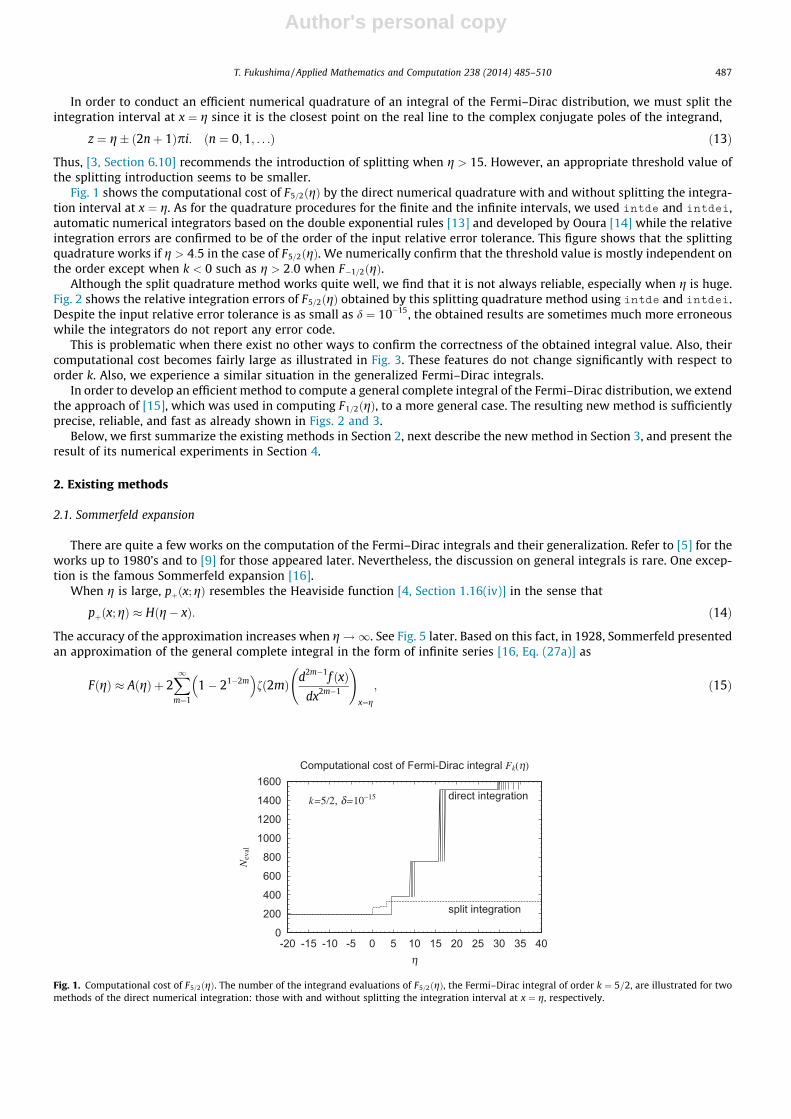
Fig. 1 shows the computational cost of F5=2ðgÞ by the direct numerical quadrature with and without splitting the integra-tion interval at x ¼ g. As for the quadrature procedures for the finite and the infinite intervals, we used intde and intdei,automatic numerical integrators based on the double exponential rules [13] and developed by Ooura [14] while the relativeintegration errors are confirmed to be of the order of the input relative error tolerance. This figure shows that the splittingquadrature works if g > 4:5 in the case of F5=2ðgÞ. We numerically confirm that the threshold value is mostly independent onthe order except when k < 0 such as g > 2:0 when F�1=2ðgÞ.

Although the split quadrature method works quite well, we find that it is not always reliable, especially when g is huge.Fig. 2 shows the relative integration errors of F5=2ðgÞ obtained by this splitting quadrature method using intde and intdei.Despite the input relative error tolerance is as small as d ¼ 10�15, the obtained results are sometimes much more erroneouswhile the integrators do not report any error code.

This is problematic when there exist no other ways to confirm the correctness of the obtained integral value. Also, theircomputational cost becomes fairly large as illustrated in Fig. 3. These features do not change significantly with respect toorder k. Also, we experience a similar situation in the generalized Fermi–Dirac integrals.

In order to develop an efficient method to compute a general complete integral of the Fermi–Dirac distribution, we extendthe approach of [15], which was used in computing F1=2ðgÞ, to a more general case. The resulting new method is sufficientlyprecise, reliable, and fast as already shown in Figs. 2 and 3.

Below, we first summarize the existing methods in Section 2, next describe the new method in Section 3, and present theresult of its numerical experiments in Section 4.

2. Existing methods

2.1. Sommerfeld expansion

There are quite a few works on the computation of the Fermi–Dirac integrals and their generalization. Refer to [5] for theworks up to 1980’s and to [9] for those appeared later. Nevertheless, the discussion on general integrals is rare. One excep-tion is the famous Sommerfeld expansion [16].

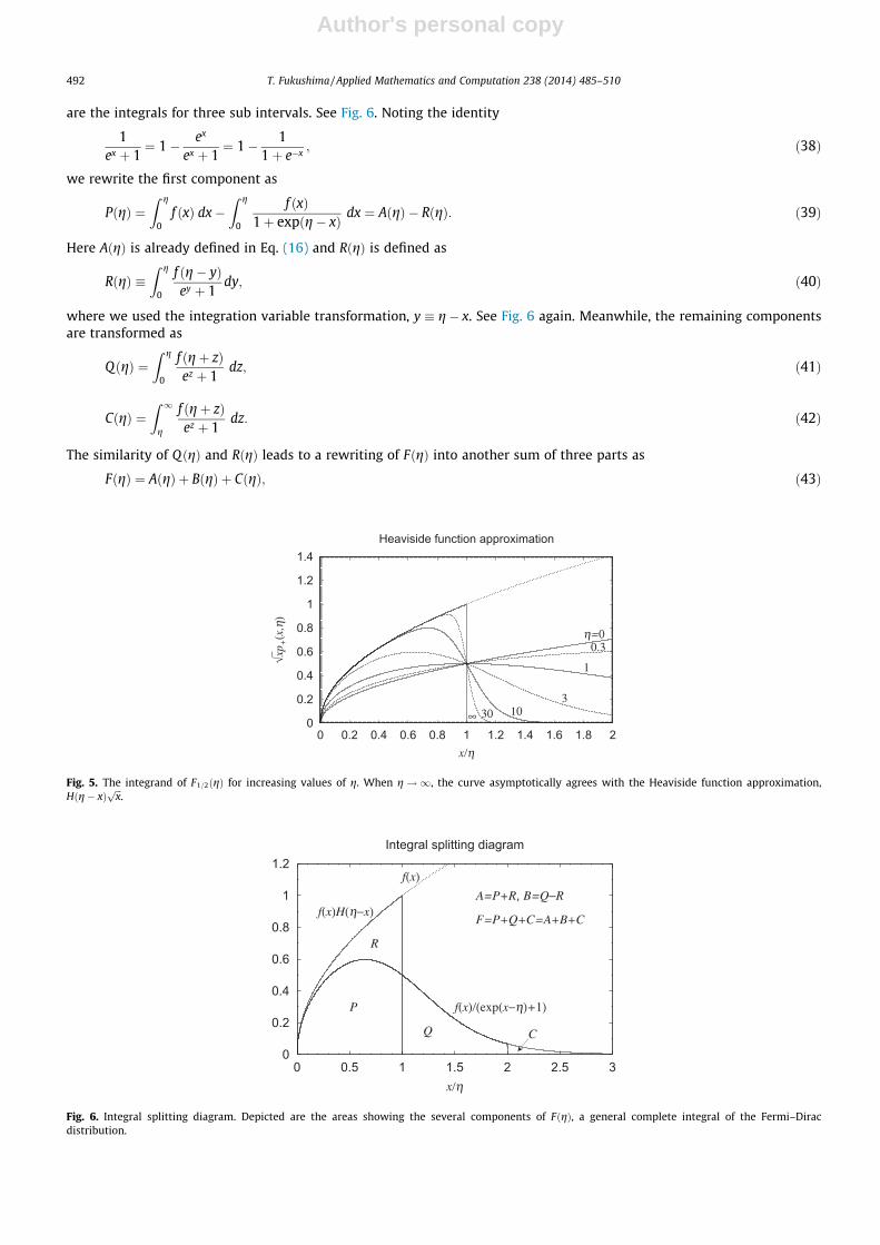
When g is large, pþðx;gÞ resembles the Heaviside function [4, Section 1.16(iv)] in the sense that

pþðx;gÞ � Hðg� xÞ: ð14Þ

The accuracy of the approximation increases when g!1. See Fig. 5 later. Based on this fact, in 1928, Sommerfeld presentedan approximation of the general complete integral in the form of infinite series [16, Eq. (27a)] as

FðgÞ � AðgÞ þ 2X1m¼1

1� 21�2m� �

fð2mÞ d2m�1f ðxÞdx2m�1

!x¼g

; ð15Þ

0

200

400

600

800

1000

1200

1400

1600

-20 -15 -10 -5 0 5 10 15 20 25 30 35 40

Neval

η

Computational cost of Fermi-Dirac integral Fk(η)

direct integration

split integration

k=5/2, δ=10−15

Fig. 1. Computational cost of F5=2ðgÞ. The number of the integrand evaluations of F5=2ðgÞ, the Fermi–Dirac integral of order k ¼ 5=2, are illustrated for twomethods of the direct numerical integration: those with and without splitting the integration interval at x ¼ g, respectively.

T. Fukushima / Applied Mathematics and Computation 238 (2014) 485–510 487


where

AðgÞ �Z g

0f ðxÞ dx ð16Þ

is the Heaviside function approximation of FðgÞ, and fðsÞ is the Riemann zeta function [4, Section 25.2(i)].As shown in [17], the convergence of the infinite series in Eq. (15) is not always guaranteed unless f ðxÞ is a polynomial of

finite degree when the series becomes finite. Indeed, the zeta function of even integer argument is explicitly expressed [4,Formula 25.6.2] as

fð2mÞ ¼ ð2pÞ2m

2ð2mÞ! jB2mj; ð17Þ

where Bn is the Bernoulli number of index n [4, Section 24.2(i)], which has an asymptotic value for the even integer index [4,Formula 24.11.1] as

B2m � ð�1Þmþ1 2ð2mÞ!ð2pÞ2m ðm!1Þ: ð18Þ

Therefore, the series expansion coefficient of Eq. (15) asymptotically tends to unity as

limm!1

1� 21�2m� �

fð2mÞ ¼ 1: ð19Þ

Meanwhile, the magnitude of the odd-order derivatives of arbitrary function, jðd2m�1f ðxÞ=dx2m�1Þx¼gj, does not alwaysdecrease with respect to m for arbitrary argument g. For example, when f ðxÞ ¼

ffiffiffixp

and g ¼ 1, the magnitude of the derivativecombinatorially explodes according as the order of differentiation as

-16-15-14-13-12-11-10-9-8

Computational error of Fermi-Dirac integral Fk(η)

split integration

k=5/2, δ=10−15

-16-15-14

-2 -1 0 1 2 3 4 5 6 7 8 9 10

log 1

0|ΔF

/F|

log10η

new method

Fig. 2. Relative errors of F5=2ðgÞ computed by two methods: (i) the direct numerical integration with splitting the integration interval at x ¼ g and (ii) thenew method described in Section 3. The errors are measured as the difference from the reference solution obtained by the first method in the quadrupleprecision environment with a tiny error tolerance, 10�33.

0

100

200

300

400

500

-2 -1 0 1 2 3 4 5 6 7 8 9 10

Neval

log10η

Computational cost of Fermi-Dirac integral Fk(η)

directintegration

split integration

new method

k=5/2δ=10−15

Fig. 3. Cost of computing F5=2ðgÞ with the methods presented in Fig. 1 and the new method. When g > 108, the number of the new method reduces to 2.This means only the exactly integrable part is evaluated.



d2m�1 ffiffiffixp

dx2m�1

!x¼1

¼ ð4m� 5Þ!!22m�1 !1 ðm!1Þ: ð20Þ

Also, the remainder of this expansion is not small for general values of g, especially when g is small. Refer to the completeseries expression of the Fermi–Dirac integral of non-integer order [18, Eq.(17)], which illustrates the behavior of the remain-der term clearly. In other words, the Sommerfeld expansion is of asymptotic nature. Thus, it is usually truncated so as to keeponly its first few terms [2, Eq. (24.176)] such as

FðgÞ � AðgÞ þ p2

6f 0ðgÞ þ 7p4

360f 000ðgÞ: ð21Þ

This is enough for a low precision approximation. Recently, we realized its 15-digit computation by using the higher ordertruncations for the generalized Fermi–Dirac integrals of physically important orders, k ¼ �1=2;1=2;3=2, and 5=2 [17].

2.2. Other non-numerical approaches

If we limit the functional form of f ðxÞ to a simple power, for example, there exist plenty of exact or asymptotic treatments[19,7,20–24]. In fact, the complete Fermi–Dirac integrals are exactly expressed in terms of a special function named the poly-logarithm [4, Formula 25.12.6].

However, this is a rare case. The availability of exact expressions is hopeless for a general case. This is true even when f ðxÞitself is exactly integrable as assumed in the Sommerfeld expansion. For example, despite a fact that f ðxÞ of Fkðg; bÞ given inEq. (6) is exactly integrable when k is an integer or a half integer satisfying the condition k > �1 [17], no exact method hasbeen reported to compute the integral covering the full range of k;g, and b. Only when g! �1, the convergent series expan-sions are known for general values of b [7].

Also, even if the exact expression exists, it does not automatically mean that its evaluation is practical. Actually, the com-putation of the polylogarithm for general values of index and argument is itself a difficult task [25].

2.3. Numerical approaches

If the integrals are one-parameter functions such as in the case of FkðgÞ, Chebyshev or other one-dimensional interpola-tion methods can be applicable. For example, [26] provides a precise and fast procedure of FkðgÞ for k ¼ �1=2;1=2;3=2, and5=2 using the Chebyshev polynomial expansions when g < 2:56� 108 (see Fig. 14). Nevertheless, if the number of freeparameters are two or more such as in the case of Fkðg; bÞ, the approach of multi-variable interpolation tends to be cumber-some and slow.

Let us show an example. Consider the two-dimensional approximation of not Fkðg; bÞ but fkðg; bÞ by a truncation of itsTaylor series as

fkðg;bÞ �XN

n¼0

XM

m¼0

1n!m!

@nþmfkðg;bÞ@gn@bm

� �ðg;bÞ¼ g0 ;b0ð Þ

g� g0ð Þn b� b0ð Þn: ð22Þ

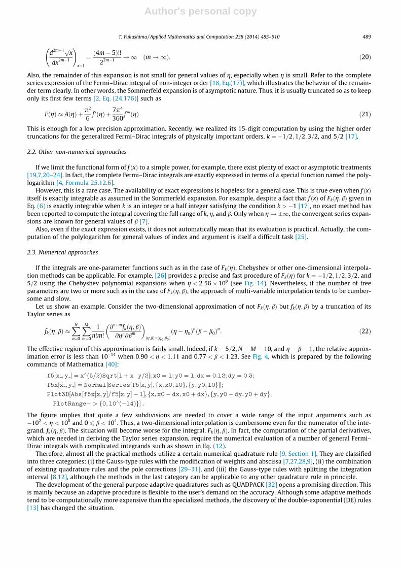
The effective region of this approximation is fairly small. Indeed, if k ¼ 5=2;N ¼ M ¼ 10, and g ¼ b ¼ 1, the relative approx-imation error is less than 10�14 when 0:90 < g < 1:11 and 0:77 < b < 1:23. See Fig. 4, which is prepared by the followingcommands of Mathematica [40]:

f5½x ;y � ¼ x^ð5=2ÞSqrt½1þ x y=2�;x0 ¼ 1;y0 ¼ 1;dx ¼ 0:12;dy ¼ 0:3;

f5x½x ;y � ¼ Normal½Series½f5½x;y�; fx;x0;10g; fy;y0;10g��;Plot3D½Abs½f5x½x;y�=f5½x;y� � 1�; fx;x0� dx;x0þ dxg; fy;y0� dy;y0þ dyg;PlotRange� > f0;10^ð�14Þg� :

The figure implies that quite a few subdivisions are needed to cover a wide range of the input arguments such as�102 < g < 108 and 0 6 b < 104. Thus, a two-dimensional interpolation is cumbersome even for the numerator of the inte-grand, fkðg; bÞ. The situation will become worse for the integral, Fkðg; bÞ. In fact, the computation of the partial derivatives,which are needed in deriving the Taylor series expansion, require the numerical evaluation of a number of general Fermi–Dirac integrals with complicated integrands such as shown in Eq. (12).

Therefore, almost all the practical methods utilize a certain numerical quadrature rule [9, Section 1]. They are classifiedinto three categories: (i) the Gauss-type rules with the modification of weights and abscissa [7,27,28,9], (ii) the combinationof existing quadrature rules and the pole corrections [29–31], and (iii) the Gauss-type rules with splitting the integrationinterval [8,12], although the methods in the last category can be applicable to any other quadrature rule in principle.

The development of the general purpose adaptive quadratures such as QUADPACK [32] opens a promising direction. Thisis mainly because an adaptive procedure is flexible to the user’s demand on the accuracy. Although some adaptive methodstend to be computationally more expensive than the specialized methods, the discovery of the double-exponential (DE) rules[13] has changed the situation.



Consequently, [3, Section 6.10] recommends an adaptive method based on the DE rules in computing Fkðg; bÞ. Still, it istrue that the computational labor is fairly large as already shown in Fig. 3. Also, there is a worry about its reliability in thecomputing precision as illustrated in Fig. 2. In order to attempt a breakthrough, we shall track back the history of numericalcomputation.

2.4. McDougall–Stoner method

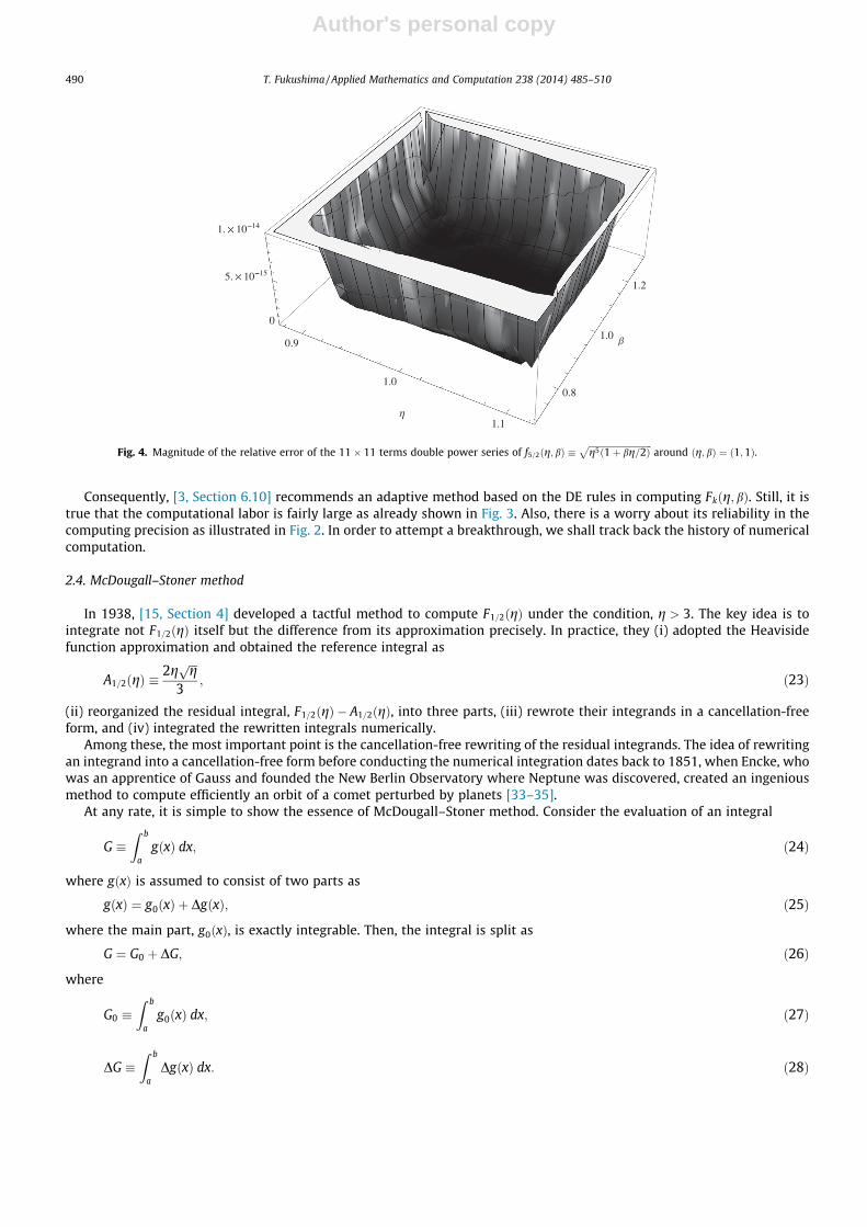
In 1938, [15, Section 4] developed a tactful method to compute F1=2ðgÞ under the condition, g > 3. The key idea is tointegrate not F1=2ðgÞ itself but the difference from its approximation precisely. In practice, they (i) adopted the Heavisidefunction approximation and obtained the reference integral as

A1=2ðgÞ �2g ffiffiffigp

3; ð23Þ

(ii) reorganized the residual integral, F1=2ðgÞ � A1=2ðgÞ, into three parts, (iii) rewrote their integrands in a cancellation-freeform, and (iv) integrated the rewritten integrals numerically.

Among these, the most important point is the cancellation-free rewriting of the residual integrands. The idea of rewritingan integrand into a cancellation-free form before conducting the numerical integration dates back to 1851, when Encke, whowas an apprentice of Gauss and founded the New Berlin Observatory where Neptune was discovered, created an ingeniousmethod to compute efficiently an orbit of a comet perturbed by planets [33–35].

At any rate, it is simple to show the essence of McDougall–Stoner method. Consider the evaluation of an integral

G �Z b

agðxÞ dx; ð24Þ

where gðxÞ is assumed to consist of two parts as

gðxÞ ¼ g0ðxÞ þ DgðxÞ; ð25Þ

where the main part, g0ðxÞ, is exactly integrable. Then, the integral is split as

G ¼ G0 þ DG; ð26Þ

where

G0 �Z b

ag0ðxÞ dx; ð27Þ

DG �Z b

aDgðxÞ dx: ð28Þ

0.9

1.0

1.1

0.8

1.0

1.2

0

5. 10 15

1. 10 14

Fig. 4. Magnitude of the relative error of the 11� 11 terms double power series of f5=2ðg;bÞ �ffiffiffiffiffiffiffiffiffiffiffiffiffiffiffiffiffiffiffiffiffiffiffiffiffiffiffiffiffig5ð1þ bg=2Þ

paround ðg; bÞ ¼ ð1;1Þ.



Since G0 is exactly computable as assumed, the problem is reduced to the numerical integration of DG, which is expected tobe easier than that of G.

Therefore, the McDougall–Stoner method is effective if, for a given error tolerance to compute G, the sum of (i) the com-putational labor to integrate DG numerically and (ii) that to evaluate G0 exactly is significantly less than that to integrate Gnumerically.

2.5. Example of McDougall–Stoner method

Let us show an example of the McDougall–Stoner method. Consider a following hyper-elliptic integral,

I �Z g

0

ffiffiffiffiffiffiffiffiffiffiffiffiffiffiffiffiffiffiffiffiffiffiffiffiffiffiffix 1þ x

a

� �5 s

dx; ð29Þ

under the assumption that the perturbation parameter, g=a, is sufficiently small, say less than 0.1 for example. By ignoringthe contribution of x=a in the integrand, we obtain a reference integral defined as

I0 �Z g

0

ffiffiffixp

dx ¼ 2g ffiffiffigp3

: ð30Þ

Then, the residual integral is expressed as

DI � I � I0 ¼Z g

0

x6=a5� �

dxffiffiffiffiffiffiffiffiffiffiffiffiffiffiffiffiffiffiffiffiffiffiffiffiffiffiffiffiffix 1þ ðx=aÞ5h ir

þffiffiffixp : ð31Þ

The rewriting of the integrand into a cancellation-free form is the essence of the McDougall–Stoner method. Ignoring ðx=aÞ5

in the square root in the rewritten integrand, we obtain a rough estimate of DI as

DI � DI �Z g

0

x5ffiffiffixp

2a5 dx ¼ g6 ffiffiffigp13a5 : ð32Þ

The availability of such a crude but reliable estimate of the residual integral is another key point of the McDougall–Stonermethod. At any rate, if we want to obtain I with the relative error tolerance d, we may integrate DI with a larger relative errortolerance, dI , as

dI �I0

DI

� �d ¼ 26

3ag

� �5

d: ð33Þ

If g=a ¼ 0:025, for example, dI is roughly 9� 108 times larger than d. Thus, the single precision integration of DI is enough toprovide I with the full double precision accuracy. This will result a significant improvement in the actual integration process.

In the next section, we shall apply this approach to a general complete integral of the Fermi–Dirac distribution.

3. New method

3.1. Integral splitting

When g 6 0, we compute FðgÞ by its direct numerical integration using Ooura’s intdei [14], an automatic integrator forthe semi-open interval based on the theory of the double exponential quadrature [13], without splitting the integrationinterval. As reported in [3, Section 6.10], this approach is sufficiently efficient since the denominator of the integrand,expðx� gÞ þ 1, has no complex singularity the real part of which lies in the integration interval, 0 < x <1.

When g > 0, on the other hand, following [15, Section 3], we split the integration interval of FðgÞ into three sub intervals,½0;gÞ; ½g;2gÞ, and ½2g;1Þ, as

FðgÞ ¼ PðgÞ þ QðgÞ þ CðgÞ; ð34Þ

where

PðgÞ �Z g

0

f ðxÞexpðx� gÞ þ 1

dx; ð35Þ

QðgÞ �Z 2g

g


dx; ð36Þ

CðgÞ �Z 1

2g


dx; ð37Þ



are the integrals for three sub intervals. See Fig. 6. Noting the identity

1ex þ 1

¼ 1� ex

ex þ 1¼ 1� 1

1þ e�x; ð38Þ

we rewrite the first component as

PðgÞ ¼Z g

0f ðxÞ dx�

Z g

0

f ðxÞ1þ expðg� xÞ dx ¼ AðgÞ � RðgÞ: ð39Þ

Here AðgÞ is already defined in Eq. (16) and RðgÞ is defined as

RðgÞ �Z g

0

f ðg� yÞey þ 1

dy; ð40Þ

where we used the integration variable transformation, y � g� x. See Fig. 6 again. Meanwhile, the remaining componentsare transformed as

QðgÞ ¼Z g

0

f ðgþ zÞez þ 1

dz; ð41Þ

CðgÞ ¼Z 1

g

f ðgþ zÞez þ 1

dz: ð42Þ

The similarity of QðgÞ and RðgÞ leads to a rewriting of FðgÞ into another sum of three parts as

FðgÞ ¼ AðgÞ þ BðgÞ þ CðgÞ; ð43Þ

0

0.2

0.4

0.6

0.8

1

1.2

1.4

0 0.2 0.4 0.6 0.8 1 1.2 1.4 1.6 1.8 2

√xp +

(x, η

)

x/η

Heaviside function approximation

η=00.3

1

31030∞

Fig. 5. The integrand of F1=2ðgÞ for increasing values of g. When g!1, the curve asymptotically agrees with the Heaviside function approximation,Hðg� xÞ

ffiffiffixp

.

0

0.2

0.4

0.6

0.8

1

1.2

0 0.5 1 1.5 2 2.5 3x/η

Integral splitting diagram

F=P+Q+C=A+B+C

A=P+R, B=Q−Rf(x)

f(x)H(η−x)

f(x)/(exp(x−η)+1)P

R

Q C

Fig. 6. Integral splitting diagram. Depicted are the areas showing the several components of FðgÞ, a general complete integral of the Fermi–Diracdistribution.



where BðgÞ is defined as

BðgÞ � QðgÞ � RðgÞ ¼Z g

0

Df ðx;gÞex þ 1

dx; ð44Þ

while Df ðx;gÞ is a finite difference of f ðxÞ defined as

Df ðx;gÞ � f ðgþ xÞ � f ðg� xÞ: ð45Þ

Eq. (43) is a generalization of Eq. (4.2) of [15] for arbitrary function f ðxÞ. In case of [15], f ðxÞ was set as f ðxÞ ¼ffiffiffixp

in order tocompute F1=2ðgÞ.

3.2. Integration of BðgÞ and CðgÞ

If f ðxÞ is exactly integrable, namely if AðgÞ is expressed as an explicit function of g in a closed form, then the problem isreduced to the evaluation of the rest two auxiliary integrals, BðgÞ and CðgÞ.

We evaluate BðgÞ and CðgÞ by their direct numerical integration using the DE rules. In case of BðgÞ, we must resolve thecancellation problem in computing Df ðx;gÞ by a suitable rewriting such as

Df1=2ðx;gÞ ¼ffiffiffiffiffiffiffiffiffiffiffiffigþ x

p� ffiffiffiffiffiffiffiffiffiffiffiffi

g� xp ¼ 2xffiffiffiffiffiffiffiffiffiffiffiffi

gþ xp þ ffiffiffiffiffiffiffiffiffiffiffiffig� x

p ; ð46Þ

in the case of F1=2ðgÞ. This is because the problem becomes serious when x g and hinders a proper convergence of somequadrature rules assuming the analyticity of the integrand such as the DE rules.

Also, the integrand of BðgÞmay have a singularity at the upper endpoint as in the case of the Fermi–Dirac integrals of half-integer order. Indeed, this is the reason why [15] adopted the splitting into not three components as in their Eq. (4.2) but fouras in their Eq. (4.3) in the actual computation of F1=2ðgÞ. We solve this issue by using integration methods which can handlethe end point singularities such as the DE rules [13].

At any rate, if AðgÞ is a good approximation of FðgÞ, the input relative error tolerance in evaluating BðgÞ and/or CðgÞ can beincreased, and therefore, we may expect a decrease in the total computational labor and/or an increase in the computingprecision.

3.3. Truncation of integration interval

The upper endpoint of the defining integrals of BðgÞ and/or CðgÞ, given in Eqs. (44) and (42), respectively, may be trun-cated since the integrand contains a rapidly decaying factor, 1=ðex þ 1Þ. The factor is practically negligible when x exceeds acertain threshold value. For example, [3, Section 6.10] recommends the choice of its value as 60 in computing the generalizedFermi–Dirac integrals in the double precision environment.

Let us return to the general cases. If the numerator of the integrand is monotonically decreasing in the integration inter-val, we may set the truncation value as

gT ¼ � ln �; ð47Þ

where � is the machine epsilon in the adopted computing environment. An approximate value of � ln � is 16.6 and 36.7 in thesingle and double precision environments, respectively.

This setting of gT is not appropriate otherwise, especially when the numerator of the integrand is monotonically increas-ing instead. If not the numerator but the integrand itself is known to have the maximum at x ¼ n, then the suitable choicewould be

gT ¼ n� ln �: ð48Þ

When the numerator is a simple power of the argument such as in the case of Fermi–Dirac integral, the location of the max-imum is analytically evaluated by means of Lambert W-function [37,38]. See Section B for the details.

At any rate, we truncate the integrals as

BðgÞ �Z min g;gBð Þ

0

Df ðx; gÞex þ 1

dx; ð49Þ

CðgÞ �Z gC

g

f ðgþ xÞex þ 1

dx; ð50Þ

where gB and gC are the truncation values corresponding to Df ðx;gÞ and f ðgþ xÞ, respectively, and we understand that

CðgÞ � 0; if g > gC ; ð51Þ

since the magnitude of the integrand jf ðgþ xÞ=ðex þ 1Þj is always less than the machine epsilon for x P gC .



3.4. Amplification of relative error tolerance

Frequently, the rough estimate of an integral is helpful for its efficient numerical quadrature. This is also true in evalu-ating the auxiliary integrals, BðgÞ and/or CðgÞ, especially when their contribution is expected to be small. Namely, if therough estimates of the auxiliary integrals are known a priori, the input relative error tolerance for their numerical quadraturecan be amplified so as to save their computational amount significantly as will be shown later in Section 4.

When AðgÞ is exactly computable, the specific description of the procedure is as follows. First AðgÞ is rigorously evaluated.Next, the rough estimates of BðgÞ and CðgÞ are calculated such as discussed in Section A and B, respectively. Third, a roughestimate of FðgÞ is obtained as

FðgÞ � FðgÞ � AðgÞ þ BðgÞ þ CðgÞ; ð52Þ

where ⁄ means the estimate value. Fourth, we omit the computation of CðgÞ if

jCðgÞj < jFðgÞjd: ð53Þ

where d is the input relative error tolerance of F. Also, we skip the evaluation of BðgÞ if

jBðgÞj < jFðgÞjd: ð54Þ

Finally, the input relative error tolerances to integrate BðgÞ and CðgÞ numerically are set as

dB � min 0:01;FðgÞBðgÞ

��d

� �; ð55Þ

dC � min 0:01;FðgÞCðgÞ

��d

� �; ð56Þ

where 0.01 is a safety value to assure the convergence of automatic integrators such as Ooura’s intde or dqag inQUADPACK.

3.5. Numerical evaluation of AðgÞ

In general, it is difficult to find a closed form expression of the integral AðgÞ for an arbitrary function, f ðxÞ. Also, even if itsexpression is rigorously known, its evaluation may be cumbersome. For example, in case of the integration of a cometaryorbit, the reference parabolic orbit is exactly expressed in terms of the solution of a kind of cubic equation named Barker’sequation [34]. Of course, the solution can be written in a closed form [4, Section 1.11(iii)]. However, its actual implementa-tion is rather time-consuming [39].

In such occasion, there always exists a powerful approach: the numerical evaluation of AðgÞ itself. Indeed, Encke himselfused the Newton method in solving Barker’s equation numerically. This approach may sound silly since it means the directnumerical quadrature of three different integrals, AðgÞ;BðgÞ, and CðgÞ, instead of that of a single integral, FðgÞ. Of course, thisassertion is correct if the computational difficulty to evaluate all these integrals is the same. Nevertheless, there exist someinstances where the quadrature of the three components is rather easier than that of FðgÞ itself. We shall see such an exam-ple later.

4. Numerical experiments

4.1. Implementation for Fermi–Dirac integrals

Let us begin with the Fermi–Dirac integrals, FkðgÞ, of integer and half-integer orders. For the case k ¼ �1=2, fkðxÞ is writtenas

f�1=2ðxÞ ¼1ffiffiffixp : ð57Þ

The formulas required in the new method are obtained as

A�1=2ðgÞ �Z g

0

1ffiffiffixp dx ¼ 2

ffiffiffigp

; ð58Þ

Df�1=2ðx;gÞ � 1ffiffiffiffiffiffiffiffiffiffiffiffigþ xp � 1ffiffiffiffiffiffiffiffiffiffiffiffig� x

p ¼ �2xrþr� rþ þ r�ð Þ ; ð59Þ

where

r� �ffiffiffiffiffiffiffiffiffiffiffiffig� x

p: ð60Þ



Notice the cancellation-free rewriting of f�1=2ðx;gÞ. Also, the first-order derivative of fkðxÞ is computed as

f 0�1=2ðxÞ �df�1=2ðxÞ

dx¼ �1

2xffiffiffixp ; ð61Þ

which is needed in evaluating an approximation of the B-component, BkðgÞ, as defined in Appendix A.Similarly, those for the case k ¼ 0 are expressed as

A0ðgÞ ¼ g; Df0ðx;gÞ ¼ 0; f 00ðxÞ ¼ 0; ð62Þ

while those for the case k ¼ 1=2 are given as

A1=2ðgÞ ¼2g ffiffiffigp

3; Df1=2ðx;gÞ ¼ 2x

rþ þ r�; f 01=2ðxÞ ¼

12ffiffiffixp ; ð63Þ

and those for the case k ¼ 1 are derived as

A1ðgÞ ¼g2

2; Df1ðx;gÞ ¼ 2x; f 01ðxÞ ¼ 1: ð64Þ

For general values of k, the necessary expressions are given as

AkðgÞ ¼gkþ1

kþ 1; ð65Þ

Dfkðx; gÞ ¼ 2xrþ þ r�

X2k�1

m¼0

rmþr2k�1�m� ðk ¼ 3=2;5=2; . . .Þ; ð66Þ

Dfkðx;gÞ ¼ 2xXbk=2c

m¼0

k2mþ 1

� �x2mgk�2m�1 ðk ¼ 2;3; . . .Þ; ð67Þ

f 0kðxÞ ¼ kxk�1: ð68Þ

Important is the rewriting of Dfkðx;gÞ into a cancellation-free form as shown in the above.In the case k ¼ �1=2, the loss of information in evaluating the small divisor, r�, can be harmful in using the DE rules, espe-

cially when the input relative error tolerance is small. In order to avoid a possible precision loss, it is better to change thearguments of the function Df�1=2 from the pair of x and g to the pair of x and y � g� x.

4.2. Characteristics of three components

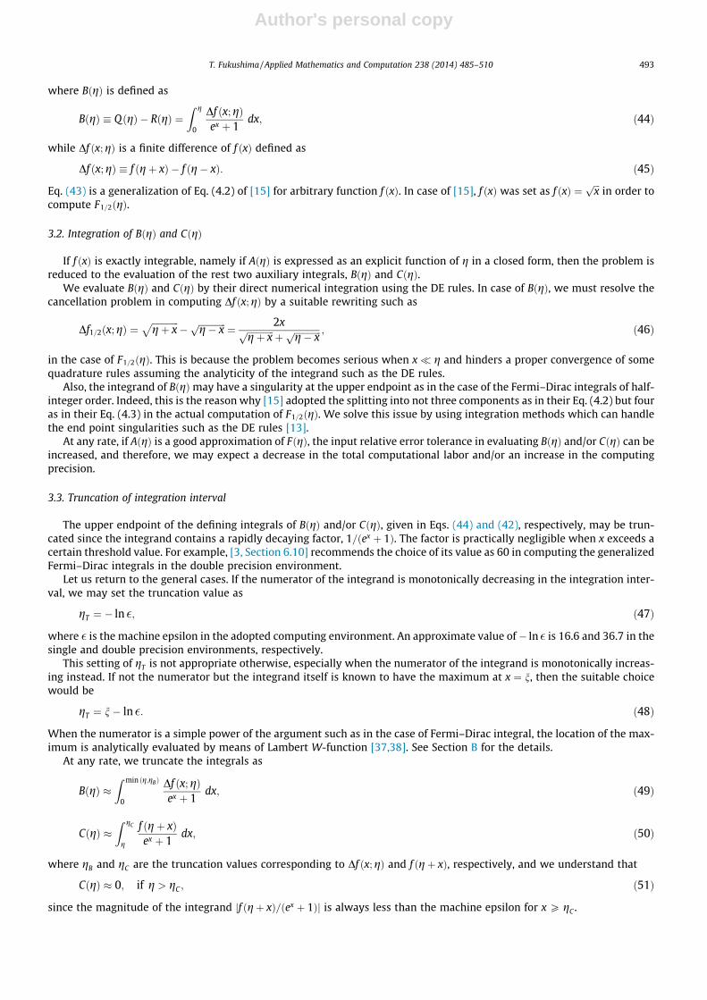
Before going further, let us observe the characteristics of the three components of the Fermi–Dirac integrals, AkðgÞ;BkðgÞ,and CkðgÞ. Fig. 7 shows their contribution, namely their ratios to FkðgÞ, as functions of g for various orders, i.e.,k ¼ �1=2; 0;1=2; . . . ;7=2, and 4. They are obtained by the direct numerical quadrature by using the DE rules with an errortolerance of 10�15.

-0.2

0

0.2

0.4

0.6

0.8

1

1.2

0 2 4 6 8 10 12 14 16 18 20

Frac

tion

η

Fraction of three components of Fk(η)

k=−1/2, 0, 1/2, 1, 3/2, 2, 5/2, 3, 7/2, 4−1/2

−1/2

4

4

4A/F

B/F

C/F

Fig. 7. Relative fractions A=F;B=F, and C=F for the Fermi–Dirac integral of some integer and half-integer orders. The integral values are obtained by thedirect numerical quadrature based on the double exponential rules in the double precision environment with an input relative error tolerance, d ¼ 10�16.The solid lines are the curves of half-integer order while the broken lines are those of integer order.



First, the C-component is governing when g is small, say less than k=2. Next, the B-component becomes dominant in themedium range when g � kþ 1. Finally, the A-component overwhelms the others when g is large, say greater than 2k.

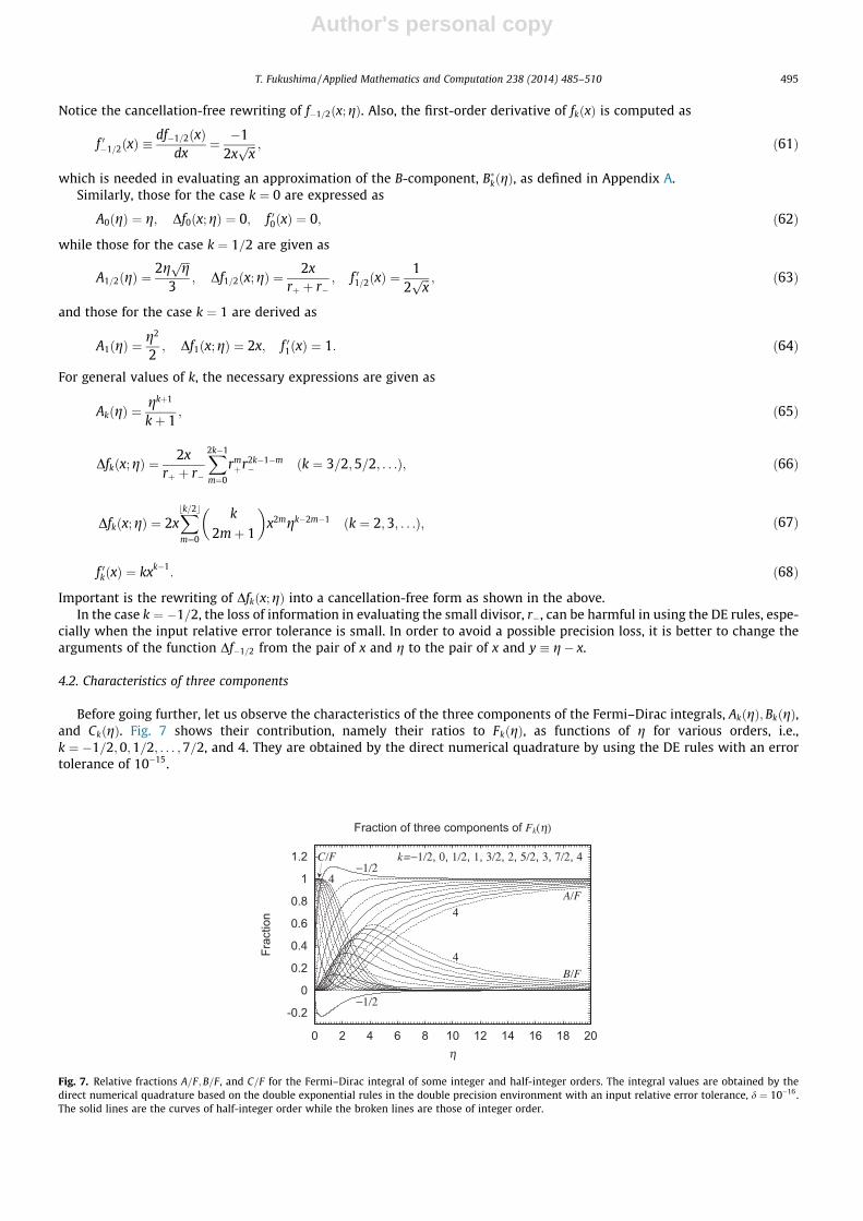
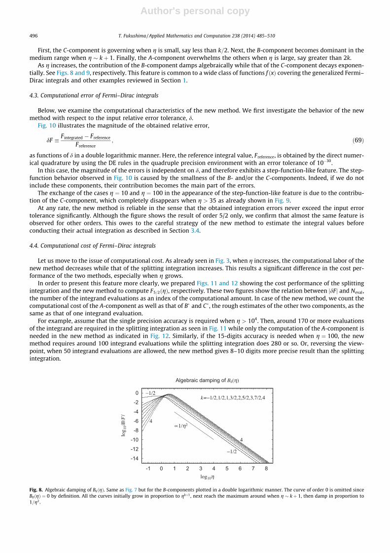
As g increases, the contribution of the B-component damps algebraically while that of the C-component decays exponen-tially. See Figs. 8 and 9, respectively. This feature is common to a wide class of functions f ðxÞ covering the generalized Fermi–Dirac integrals and other examples reviewed in Section 1.

4.3. Computational error of Fermi–Dirac integrals

Below, we examine the computational characteristics of the new method. We first investigate the behavior of the newmethod with respect to the input relative error tolerance, d.

Fig. 10 illustrates the magnitude of the obtained relative error,

dF � F integrated � Freference

Freference; ð69Þ

as functions of d in a double logarithmic manner. Here, the reference integral value, Freference, is obtained by the direct numer-ical quadrature by using the DE rules in the quadruple precision environment with an error tolerance of 10�30.

In this case, the magnitude of the errors is independent on d, and therefore exhibits a step-function-like feature. The step-function behavior observed in Fig. 10 is caused by the smallness of the B- and/or the C-components. Indeed, if we do notinclude these components, their contribution becomes the main part of the errors.

The exchange of the cases g ¼ 10 and g ¼ 100 in the appearance of the step-function-like feature is due to the contribu-tion of the C-component, which completely disappears when g > 35 as already shown in Fig. 9.

At any rate, the new method is reliable in the sense that the obtained integration errors never exceed the input errortolerance significantly. Although the figure shows the result of order 5/2 only, we confirm that almost the same feature isobserved for other orders. This owes to the careful strategy of the new method to estimate the integral values beforeconducting their actual integration as described in Section 3.4.

4.4. Computational cost of Fermi–Dirac integrals

Let us move to the issue of computational cost. As already seen in Fig. 3, when g increases, the computational labor of thenew method decreases while that of the splitting integration increases. This results a significant difference in the cost per-formance of the two methods, especially when g grows.

In order to present this feature more clearly, we prepared Figs. 11 and 12 showing the cost performance of the splittingintegration and the new method to compute F5=2ðgÞ, respectively. These two figures show the relation between jdFj and Neval,the number of the integrand evaluations as an index of the computational amount. In case of the new method, we count thecomputational cost of the A-component as well as that of B and C, the rough estimates of the other two components, as thesame as that of one integrand evaluation.

For example, assume that the single precision accuracy is required when g > 104. Then, around 170 or more evaluationsof the integrand are required in the splitting integration as seen in Fig. 11 while only the computation of the A-component isneeded in the new method as indicated in Fig. 12. Similarly, if the 15-digits accuracy is needed when g ¼ 100, the newmethod requires around 100 integrand evaluations while the splitting integration does 280 or so. Or, reversing the view-point, when 50 integrand evaluations are allowed, the new method gives 8–10 digits more precise result than the splittingintegration.

-14

-12

-10

-8

-6

-4

-2

0

-1 0 1 2 3 4 5 6 7 8

log 1

0|B/F|

log10η

Algebraic damping of Bk(η)

k=−1/2,1/2,1,3/2,2,5/2,3,7/2,4

−1/2

−1/2

4

4∝1/η2

Fig. 8. Algebraic damping of BkðgÞ. Same as Fig. 7 but for the B-components plotted in a double logarithmic manner. The curve of order 0 is omitted sinceB0ðgÞ ¼ 0 by definition. All the curves initially grow in proportion to gkþ1, next reach the maximum around when g � kþ 1, then damp in proportion to1=g2.



This superiority of the new method is more directly illustrated by Fig. 13 plotting the acceleration factor, i.e., the ratio ofthe number of integrand evaluations of the new method and the splitting integration for the same input relative errortolerance, as functions of g. The factor increases according as g since (i) the B-component algebraically damps, (ii) theC-component exponentially decays, and therefore (iii) their computational cost also significantly reduces when g increases.

The curves for positive orders are almost the same at this scale. Meanwhile, the acceleration factor of the case k ¼ 0 isextraordinary large since the B-component completely vanishes. At any rate, except the case of k ¼ 0 where the

-14

-12

-10

-8

-6

-4

-2

0

0 5 10 15 20 25 30 35

log 1

0|C/F|

η

Exponential decay of Ck(η)

k=−1/2,0,1/2,1,3/2,2,5/2,3,7/2,4

−1/24

∝exp(−η)

Fig. 9. Exponential decay of CkðgÞ. Same as Fig. 7 but for the C-components plotted in a single logarithmic manner. All the curves decay exponentially.

-20-18-16-14-12-10-8-6-4-202

-16 -14 -12 -10 -8 -6 -4 -2

log 1

0|ΔF

/F|

log10δ

Reliability of Fk(η) computation

k=5/2

η=108107

106105

104 103

102

10

Fig. 10. Reliability of FkðgÞ computation. Shown are the relative errors of F5=2ðgÞ obtained by the new method as a function of the input relative errortolerance, d. The results for various values of g from 10 to 108 are plotted in a double logarithmic manner. The broken line shows the condition, jDF=Fj ¼ d.

-16

-14

-12

-10

-8

-6

-4

-2

0 50 100 150 200 250 300 350 400

log 1

0|ΔF

/F|

Neval

Cost performance of Fk(η) computation by split integration

k=5/2η=10

102103

104

105

Fig. 11. Cost performance of FkðgÞ computation by the split integration method. Same as Fig. 10 but plotted as a function of the number of integrandevaluations in a single logarithmic manner.



B-component vanishes by definition, the increasing manner of the acceleration factor with respect to g is almost indepen-dent on the order.

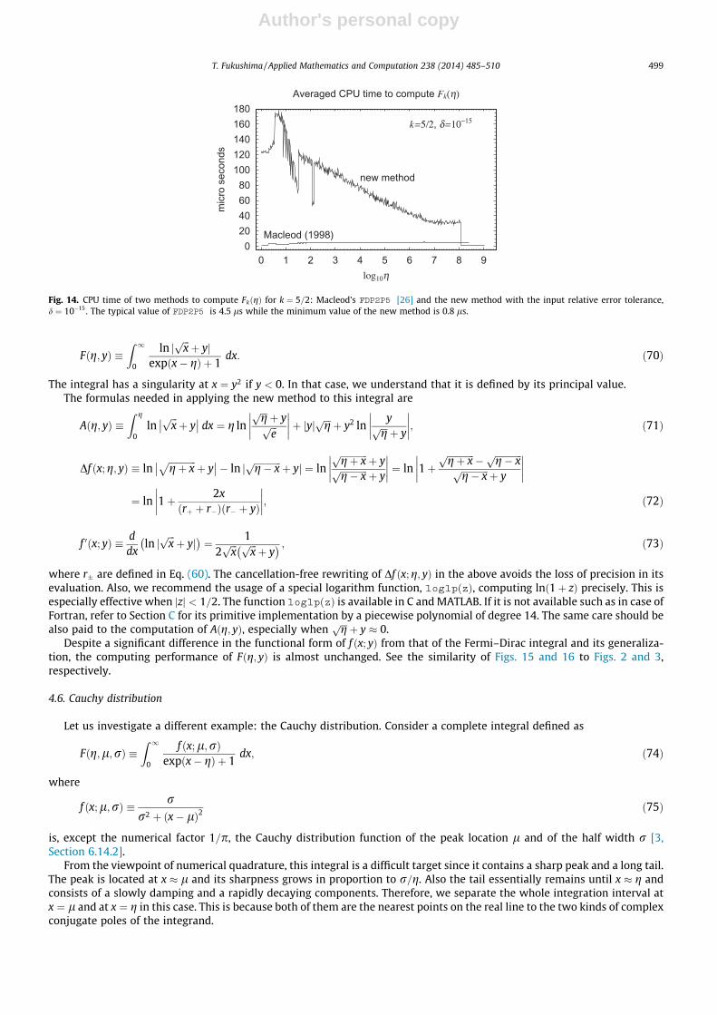
Finally, let us examine the actual CPU time of the new method. Fig. 14 compares the averaged CPU times to compute FkðgÞfor the case k ¼ 5=2 by the Chebyshev polynomial approximation [26] and the new method with an input relative error tol-erance, d ¼ 10�15. For each g, the CPU times to compute Fkðgþ DgÞ are averaged with respect to 222ð¼ 4194304Þ values of Dgevenly distributed in the range 0 6 Dg < 10�3g. Notice that Macleod’s FDP2P5 provides the result for the argument in therange, g < 2:55� 108.

All the computation codes were (i) written in Fortran 90, (ii) compiled by the Intel Visual Fortran Composer XE 2011update 8 with the level 3 optimization, and (iii) executed at a PC with an Intel Core i7-2675QM CPU and 16 GB main memoryrun at the clock 2.20 GHz under the 32 bit Windows 7 OS. In order to avoid the inefficiency of the computer with a mobileprocessor, the electric power was continuously supplied and all other time-consuming jobs were turned-off.

The CPU time of the Chebyshev polynomial expansion is quite small and almost independent on g. Its actual value is4.5 ls at this specific PC. Meanwhile, that of the new method ranges from the maximum value, 178 ls reached wheng � 5, down to the minimum value, 0.8 ls when g > 1:2� 108.

Comparing Fig. 14 with Fig. 13, we learn that the CPU time of a single evaluation of the integrand in this case is roughlyestimated as 178=320 � 0:556 ls. Thus, the minimum CPU time of the new method, which is that of the sum of the compu-tation of AkðgÞ;BkðgÞ, and CkðgÞ, is 1.5 times that of the integrand evaluation. This roughly supports our assumption to countit as 2. We experimentally confirmed that the feature observed in Fig. 14 does not change significantly for other values of k.

4.5. Case of Fðg; yÞ

Move to an example other than the Fermi–Dirac integral and its generalization. Consider a following integral associatedwith the function f ðx; yÞ given in Eq. (10) as

-16

-14

-12

-10

-8

-6

-4

-2

0 50 100 150 200

log 1

0|Δ F

/F|

Neval

Cost performance of Fk(η) computation by new method

k=5/2η=10102

103

104

105

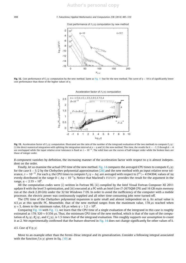
Fig. 12. Cost performance of FkðgÞ computation by the new method. Same as Fig. 11 but for the new method. The curve of g ¼ 10 is of significantly lowercost performance than those of the higher values of g.

0

0.5

1

1.5

2

2.5

-2 -1 0 1 2 3 4 5 6 7 8 9 10

log 1

0|Neval

(split)/Neval

(new

)|

log10η

Acceleration factor of Fk(η) computation

k=−1/2,0,1/2,1,3/2,2,5/2,3,7/2,4δ=10−15

0

−1/2

−1/2 4F≈A+B+C F≈A+B

F≈A

Fig. 13. Acceleration factor of FkðgÞ computation. Illustrated are the ratio of the number of the integrand evaluation of the two methods to compute FkðgÞ:(i) the direct numerical integration with splitting the integration interval at x ¼ g and (ii) the new method. This time, the results for k ¼ �1=2 through k ¼ 4are overlapped while the input relative error tolerance is fixed as d ¼ 10�15. The solid lines are the curves of half-integer order while the broken lines arethose of integer order.



Fðg; yÞ �Z 1

0

ln jffiffiffixpþ yj

expðx� gÞ þ 1dx: ð70Þ

The integral has a singularity at x ¼ y2 if y < 0. In that case, we understand that it is defined by its principal value.The formulas needed in applying the new method to this integral are

Aðg; yÞ �Z g

0ln

ffiffiffixpþ y

�� dx ¼ g lnffiffiffigp þ yffiffiffi

ep

��þ jyj ffiffiffigp þ y2 ln

yffiffiffigp þ y

��; ð71Þ

Df ðx;g; yÞ � lnffiffiffiffiffiffiffiffiffiffiffiffigþ x

pþ y

�� lnffiffiffiffiffiffiffiffiffiffiffiffig� xp þ yj j ¼ ln

ffiffiffiffiffiffiffiffiffiffiffiffigþ xp þ yffiffiffiffiffiffiffiffiffiffiffiffig� xp þ y

�� ¼ ln 1þ

ffiffiffiffiffiffiffiffiffiffiffiffigþ xp � ffiffiffiffiffiffiffiffiffiffiffiffig� x

pffiffiffiffiffiffiffiffiffiffiffiffig� xp þ y

��

¼ ln 1þ 2xrþ þ r�ð Þ r� þ yð Þ

��; ð72Þ

f 0ðx; yÞ � ddx

ln jffiffiffixpþ yj

� �¼ 1

2ffiffiffixp ffiffiffi

xpþ y

� � ; ð73Þ

where r� are defined in Eq. (60). The cancellation-free rewriting of Df ðx;g; yÞ in the above avoids the loss of precision in itsevaluation. Also, we recommend the usage of a special logarithm function, log1pðzÞ, computing lnð1þ zÞ precisely. This isespecially effective when jzj < 1=2. The function log1pðzÞ is available in C and MATLAB. If it is not available such as in case ofFortran, refer to Section C for its primitive implementation by a piecewise polynomial of degree 14. The same care should bealso paid to the computation of Aðg; yÞ, especially when

ffiffiffigp þ y � 0.Despite a significant difference in the functional form of f ðx; yÞ from that of the Fermi–Dirac integral and its generaliza-

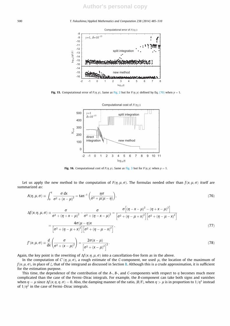
tion, the computing performance of Fðg; yÞ is almost unchanged. See the similarity of Figs. 15 and 16 to Figs. 2 and 3,respectively.

4.6. Cauchy distribution

Let us investigate a different example: the Cauchy distribution. Consider a complete integral defined as

Fðg;l;rÞ �Z 1

0

f ðx;l;rÞexpðx� gÞ þ 1

dx; ð74Þ

where

f ðx;l;rÞ � rr2 þ x� lð Þ2

ð75Þ

is, except the numerical factor 1=p, the Cauchy distribution function of the peak location l and of the half width r [3,Section 6.14.2].

From the viewpoint of numerical quadrature, this integral is a difficult target since it contains a sharp peak and a long tail.The peak is located at x � l and its sharpness grows in proportion to r=g. Also the tail essentially remains until x � g andconsists of a slowly damping and a rapidly decaying components. Therefore, we separate the whole integration interval atx ¼ l and at x ¼ g in this case. This is because both of them are the nearest points on the real line to the two kinds of complexconjugate poles of the integrand.

020406080

100120140160180

0 1 2 3 4 5 6 7 8 9

mic

ro s

econ

ds

log10η

Averaged CPU time to compute Fk(η)

new method

Macleod (1998)

k=5/2, δ=10−15

Fig. 14. CPU time of two methods to compute FkðgÞ for k ¼ 5=2: Macleod’s FDP2P5 [26] and the new method with the input relative error tolerance,d ¼ 10�15. The typical value of FDP2P5 is 4.5 ls while the minimum value of the new method is 0.8 ls.



Let us apply the new method to the computation of Fðg;l;rÞ. The formulas needed other than f ðx;l;rÞ itself aresummarized as:

Aðg;l;rÞ �Z g

0

r dx

r2 þ x� lð Þ2¼ tan�1 gr

r2 þ lðl� gÞ

� �; ð76Þ

Df ðx;g;l;rÞ � rr2 þ gþ x� lð Þ2

� rr2 þ g� x� lð Þ2

¼r g� x� lð Þ2 � gþ x� lð Þ2h i

r2 þ ðg� lþ xÞ2h i

r2 þ ðg� l� xÞ2h i

¼ 4rðl� gÞxr2 þ ðg� lþ xÞ2h i

r2 þ ðg� l� xÞ2h i ; ð77Þ

f 0ðx;l;rÞ � ddx

rr2 þ x� lð Þ2

!¼ 2rðx� lÞ

r2 þ ðx� lÞ2h i2 : ð78Þ

Again, the key point is the rewriting of Df ðx;g;l;rÞ into a cancellation-free form as in the above.In the computation of Cðg;l;rÞ, a rough estimate of the C-component, we used l, the location of the maximum of

f ðx;l;rÞ, in place of n, that of the integrand as discussed in Section B. Although this is a crude approximation, it is sufficientfor the estimation purpose.

This time, the dependence of the contribution of the A-, B-, and C-components with respect to g becomes much morecomplicated than the case of the Fermi–Dirac integrals. For example, the B-component can take both signs and vanisheswhen g ¼ l since Df ðx;g;g;rÞ ¼ 0. Also, the damping manner of the ratio, jB=Fj, when g > l is in proportion to 1=g3 insteadof 1=g2 in the case of Fermi–Dirac integrals.

-16-15-14-13-12-11-10-9-8

Computational error of F(η,y)

split integration

y=1, δ=10−15

-16-15-14

-2 -1 0 1 2 3 4 5 6 7 8

log 1

0|ΔF

/F|

log10η

new method

Fig. 15. Computational error of Fðg; yÞ. Same as Fig. 2 but for Fðg; yÞ defined by Eq. (70) when y ¼ 1.

0

100

200

300

400

500

-2 -1 0 1 2 3 4 5 6 7 8 9 10 11

Neval

log10η

Computational cost of F(η,y)

directintegration

split integration

new method

y=1δ=10−15

Fig. 16. Computational cost of Fðg; yÞ. Same as Fig. 3 but for Fðg; yÞ when y ¼ 1.



4.7. Cost performance of Fðg;l;rÞ computation

Let us examine the cost performance of the new method applied to Fðg;l;rÞ. For simplicity, we fix l and r as l ¼ 10 andr ¼ 1 while changing g.

First, we confirm that the relative errors obtained by the new method never exceed d, the input relative error tolerance.Rather, they are much smaller, say less than 10�2d or so. This situation is the same as observed for the Fermi–Dirac integrals.Similarly, we also confirm that those of the direct numerical quadrature are satisfactorily small in the sense to be of the sameorder of magnitude as d.

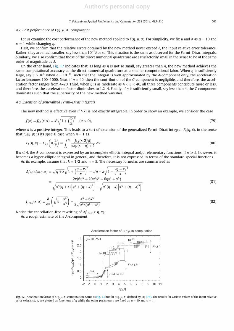
On the other hand, Fig. 17 indicates that, as long as g is not so small, say greater than 4, the new method achieves thesame computational accuracy as the direct numerical quadrature at a smaller computational labor. When g is sufficientlylarge, say g > 105 when d ¼ 10�15, such that the integral is well approximated by the A-component only, the accelerationfactor becomes 100–1000. Next, if g > 40, then the contribution of the C-component is negligible, and therefore, the accel-eration factor ranges from 4–20. Third, when g is as moderate as 4 < g < 40, all three components contribute more or less,and therefore, the acceleration factor diminishes to 1.2–4. Finally, if g is sufficiently small, say less than 4, the C-componentdominates such that the superiority of the new method vanishes.

4.8. Extension of generalized Fermi–Dirac integrals

The new method is effective even if f ðxÞ is not exactly integrable. In order to show an example, we consider the case

f ðxÞ ¼ fk;nðx;aÞ ¼ xk

ffiffiffiffiffiffiffiffiffiffiffiffiffiffiffiffiffiffiffiffi1þ x

a

� �nr

ða > 0Þ; ð79Þ

where n is a positive integer. This leads to a sort of extension of the generalized Fermi–Dirac integral, Fkðg; bÞ, in the sensethat Fkðg; bÞ is its special case when n ¼ 1 as

Fkðg; bÞ ¼ Fk;1 g;2b

� ��Z 1

0

fk;1ðx; 2=bÞexpðx� gÞ þ 1

dx: ð80Þ

If n 6 4, the A-component is expressed by an incomplete elliptic integral and/or elementary functions. If n P 5, however, itbecomes a hyper-elliptic integral in general, and therefore, it is not expressed in terms of the standard special functions.

As its example, assume that k ¼ 1=2 and n ¼ 5. The necessary formulas are summarized as

Df1=2;5ðx; g;aÞ �ffiffiffiffiffiffiffiffiffiffiffiffigþ x

p ffiffiffiffiffiffiffiffiffiffiffiffiffiffiffiffiffiffiffiffiffiffiffiffiffiffiffiffi1þ gþ x

a

� �5r

� ffiffiffiffiffiffiffiffiffiffiffiffig� xp

ffiffiffiffiffiffiffiffiffiffiffiffiffiffiffiffiffiffiffiffiffiffiffiffiffiffiffiffi1þ g� x

a

� �5r

¼2x 6g5 þ 20g3x2 þ 6gx4 þ a5� �

ffiffiffiffiffiffiffiffiffiffiffiffiffiffiffiffiffiffiffiffiffiffiffiffiffiffiffiffiffiffiffiffiffiffiffiffiffiffiffiffiffiffiffiffiffiffiffiffiffiffiffiffia5ðgþ xÞ a5 þ ðgþ xÞ5

h irþ

ffiffiffiffiffiffiffiffiffiffiffiffiffiffiffiffiffiffiffiffiffiffiffiffiffiffiffiffiffiffiffiffiffiffiffiffiffiffiffiffiffiffiffiffiffiffiffiffiffiffiffiffia5ðg� xÞ a5 þ ðg� xÞ5

h ir ; ð81Þ

f 01=2;5ðx; aÞ � ddx

ffiffiffiffiffiffiffiffiffiffiffiffiffiffixþ x6

a5

r !¼ a5 þ 6x5

2ffiffiffiffiffiffiffiffiffiffiffiffiffiffiffiffiffiffiffiffiffiffiffiffiffiffiffia5x a5 þ x5ð Þ

p : ð82Þ

Notice the cancellation-free rewriting of Df1=2;5ðx;g;aÞ.As a rough estimate of the A-component

0

0.5

1

1.5

2

2.5

3

-2 -1 0 1 2 3 4 5 6 7 8 9 10 11

log 1

0|Neval

(split)/Neval

(new

)|

log10η

Acceleration factor of F(η,μ,σ) computation

μ=10, σ=1

δ=10−3

10−710−11

10−15

F≈A+B+C

F≈A+B

F≈A

F≈C

Fig. 17. Acceleration factor of Fðg;l;rÞ computation. Same as Fig. 13 but for Fðg;l;rÞ defined by Eq. (74). The results for various values of the input relativeerror tolerance, d, are plotted as functions of g while the other parameters are fixed as l ¼ 10 and r ¼ 1.



Ak;nðg;aÞ �Z g

0xk

ffiffiffiffiffiffiffiffiffiffiffiffiffiffiffiffiffiffiffiffi1þ x

a

� �nr

dx; ð83Þ

we adopt its upper bound as

Ak;nðg;aÞ 6 Ak;nðg;aÞ � AkðgÞ þAkþn=2ðgÞffiffiffiffiffi

anp ¼ gkþ1

kþ 11þ kþ 1

kþ n=2þ 1

ffiffiffiga

r� �n" #; ð84Þ

derived from the inequality of the integrand

fk;nðx;aÞ 6 f k;nðx;aÞ � xk þ xkþn=2ffiffiffiffiffianp ; ð85Þ

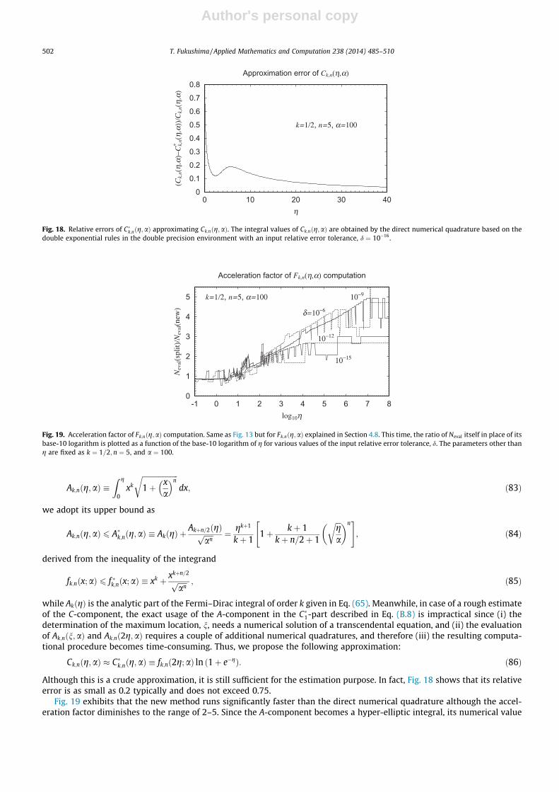
while AkðgÞ is the analytic part of the Fermi–Dirac integral of order k given in Eq. (65). Meanwhile, in case of a rough estimateof the C-component, the exact usage of the A-component in the C1-part described in Eq. (B.8) is impractical since (i) thedetermination of the maximum location, n, needs a numerical solution of a transcendental equation, and (ii) the evaluationof Ak;nðn;aÞ and Ak;nð2g;aÞ requires a couple of additional numerical quadratures, and therefore (iii) the resulting computa-tional procedure becomes time-consuming. Thus, we propose the following approximation:

Ck;nðg;aÞ � Ck;nðg;aÞ � fk;nð2g;aÞ ln 1þ e�gð Þ: ð86Þ

Although this is a crude approximation, it is still sufficient for the estimation purpose. In fact, Fig. 18 shows that its relativeerror is as small as 0.2 typically and does not exceed 0.75.

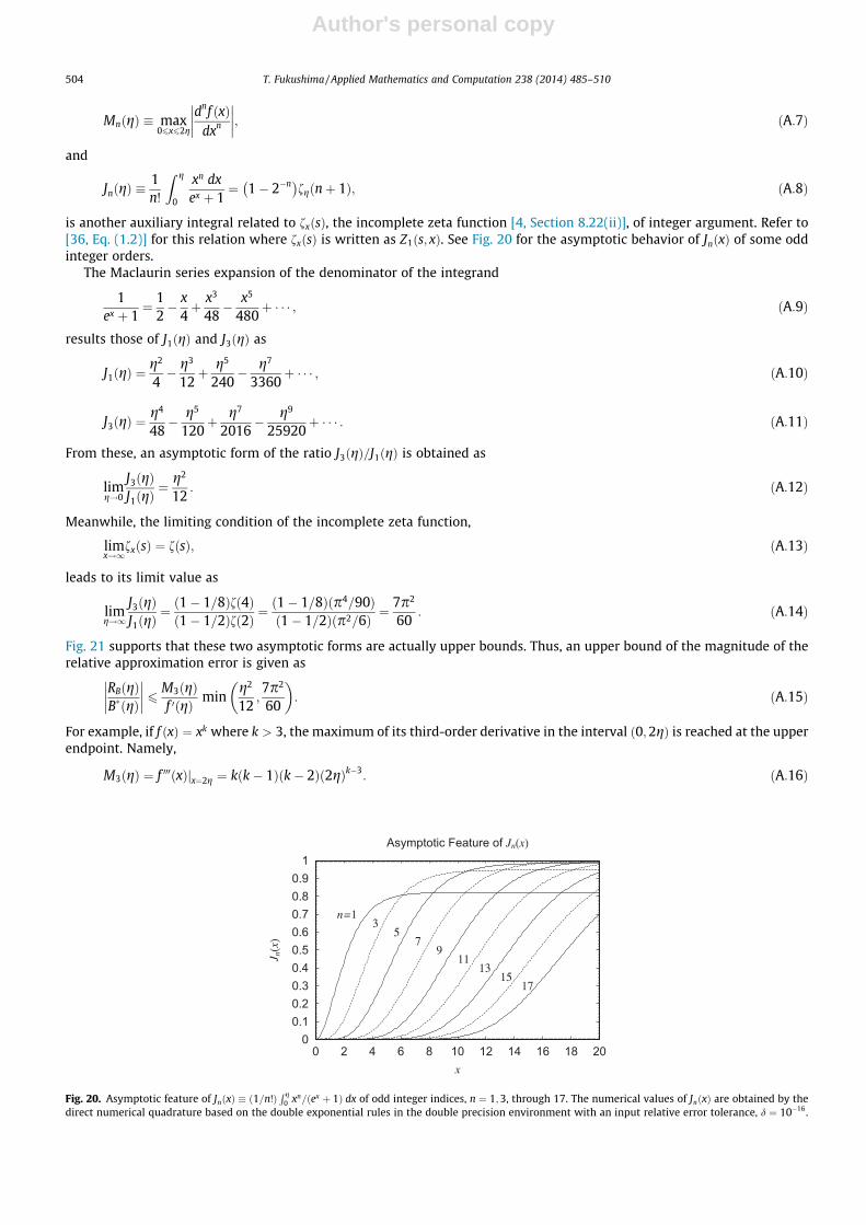
Fig. 19 exhibits that the new method runs significantly faster than the direct numerical quadrature although the accel-eration factor diminishes to the range of 2–5. Since the A-component becomes a hyper-elliptic integral, its numerical value

0

0.1

0.2

0.3

0.4

0.5

0.6

0.7

0.8

0 10 20 30 40

(Ck,n(

η,α )

−C* k,n(

η,α)

)/Ck,n(

η ,α)

η

Approximation error of Ck,n(η,α)

k=1/2, n=5, α=100

Fig. 18. Relative errors of Ck;nðg;aÞ approximating Ck;nðg;aÞ. The integral values of Ck;nðg;aÞ are obtained by the direct numerical quadrature based on thedouble exponential rules in the double precision environment with an input relative error tolerance, d ¼ 10�16.

0

1

2

3

4

5

-1 0 1 2 3 4 5 6 7 8

Neval

(split)/Neval

(new

)

log10η

Acceleration factor of Fk,n(η,α) computation

k=1/2, n=5, α=100

δ=10−6

10−9

10−12

10−15

Fig. 19. Acceleration factor of Fk;nðg;aÞ computation. Same as Fig. 13 but for Fk;nðg;aÞ explained in Section 4.8. This time, the ratio of Neval itself in place of itsbase-10 logarithm is plotted as a function of the base-10 logarithm of g for various values of the input relative error tolerance, d. The parameters other thang are fixed as k ¼ 1=2;n ¼ 5, and a ¼ 100.



is computed by the direct numerical quadrature based on the double exponential rules in the double precision environmentwith an input relative error tolerance, d ¼ 10�16. This is the reason why the acceleration factor diminishes. This factor will beincreased if we utilize the technique illustrated in Section 2.5 to the numerical quadrature of the A-component itself. Weshall omit such further extension here.

5. Conclusion

In order to evaluate a general integral of the Fermi–Dirac distribution FðgÞ for positive g (Eq. (3)), we extended theapproach of [15]. The key points of the new method are (i) the splitting FðgÞ ¼ AðgÞ þ BðgÞ þ CðgÞ into components such thatthe decreasing manner of which with respect to g are different from each other, (ii) the rewriting of the integrand of BðgÞ intoa cancellation-free form so as to reduce the loss of information in its numerical evaluation and to assure the proper conver-gence of the DE quadrature rules, (iii) the avoidance of possible end point singularities of BðgÞ by selecting the DE rules for itsnumerical integration, and (iv) the amplification of error tolerance in the numerical integration of BðgÞ and/or CðgÞ by pro-viding crude but reliable estimates of their magnitude beforehand.

As a result, the new method achieves a significant improvement in the computation of FðgÞ. First, the new method is soreliable that the relative error of the obtained integral value never exceeds the input relative error tolerance. Second, if AðgÞis exactly computable and g is not so small, say greater than 4, the computational speed of the new method becomes 2–1000times faster than the direct numerical integration of FðgÞ. The acceleration factor varies with respect to the value of g and therequired error tolerance. Typically, it amounts to 2–20 when g is greater than 30 or so. On the other hand, if AðgÞ is integratednumerically, the range of the acceleration factor diminishes to 2–5. Still, the generality of the new method will be helpful inthe precise, reliable, and fast computation of a general integral of the Fermi–Dirac distribution.

As an implementation of the new method, a Fortran function to compute FkðgÞ for k ¼ �1=2;0;1=2; . . ., and 4 is availableat the author’s personal WEB page at ResearchGate:

https://www.researchgate.net/profile/Toshio_Fukushima/

or from the author upon request.

Acknowledgments

The author thanks the anonymous referees for numerous, detailed, and valuable advices to improve the quality and read-ability of the article.

Appendix A. Rough estimate of BðgÞ

Consider a rough estimate of BðgÞ defined as

BðgÞ �Z g

0

Df ðx; gÞex þ 1

dx: ðA:1Þ

We find that this is an effective approach that is similar to the derivation of the Sommerfeld expansion formula, Eq. (15). Infact, under the assumption that f ðxÞ is at least three times differentiable in the interval, ð0;2gÞ, the numerator of the inte-grand of BðgÞ is rewritten as

Df ðx;gÞ � f ðgþ xÞ � f ðg� xÞ ¼ 2f 0ðgÞxþ 13

f 000ðgþ hðg; xÞxÞx3; ðA:2Þ

where the first term is the central difference formula, the second term is the remainder, and hðg; xÞ is in the interval�1 6 hðg; xÞ 6 1. This leads to the approximation of the integral as

BðgÞ ¼ BðgÞ þ RBðgÞ; ðA:3Þ

where

BðgÞ � 2f 0ðgÞZ g

0

xex þ 1

dx ¼ 2f 0ðgÞJ1ðgÞ ðA:4Þ

is the approximate integral and

RBðgÞ �13

Z g

0

f 000ðgþ hðg; xÞxÞx3

ex þ 1dx; ðA:5Þ

is the residual integral. If f 000ðxÞ is regular in the interval ð0;2gÞ, the magnitude of RBðgÞ is bound as

jRBðgÞj 6 2M3ðgÞJ3ðgÞ; ðA:6Þ

where



MnðgÞ � max06x62g

dnf ðxÞdxn

��; ðA:7Þ

and

JnðgÞ �1n!

Z g

0

xn dxex þ 1

¼ 1� 2�n� �fgðnþ 1Þ; ðA:8Þ

is another auxiliary integral related to fxðsÞ, the incomplete zeta function [4, Section 8.22(ii)], of integer argument. Refer to[36, Eq. (1.2)] for this relation where fxðsÞ is written as Z1ðs; xÞ. See Fig. 20 for the asymptotic behavior of JnðxÞ of some oddinteger orders.

The Maclaurin series expansion of the denominator of the integrand

1ex þ 1

¼ 12� x

4þ x3

48� x5

480þ � � � ; ðA:9Þ

results those of J1ðgÞ and J3ðgÞ as

J1ðgÞ ¼g2

4� g3

12þ g5

240� g7

3360þ � � � ; ðA:10Þ

J3ðgÞ ¼g4

48� g5

120þ g7

2016� g9

25920þ � � � : ðA:11Þ

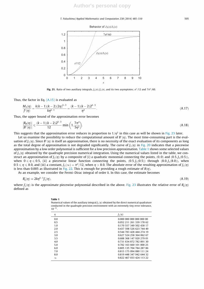
From these, an asymptotic form of the ratio J3ðgÞ=J1ðgÞ is obtained as

limg!0

J3ðgÞJ1ðgÞ

¼ g2

12: ðA:12Þ

Meanwhile, the limiting condition of the incomplete zeta function,

limx!1

fxðsÞ ¼ fðsÞ; ðA:13Þ

leads to its limit value as

limg!1

J3ðgÞJ1ðgÞ

¼ ð1� 1=8Þfð4Þð1� 1=2Þfð2Þ ¼

ð1� 1=8Þðp4=90Þð1� 1=2Þðp2=6Þ ¼

7p2

60: ðA:14Þ

Fig. 21 supports that these two asymptotic forms are actually upper bounds. Thus, an upper bound of the magnitude of therelative approximation error is given as

RBðgÞBðgÞ

�� 6 M3ðgÞ

f 0ðgÞ ming2

12;7p2

60

� �: ðA:15Þ

For example, if f ðxÞ ¼ xk where k > 3, the maximum of its third-order derivative in the interval ð0;2gÞ is reached at the upperendpoint. Namely,

M3ðgÞ ¼ f 000ðxÞjx¼2g ¼ kðk� 1Þðk� 2Þð2gÞk�3: ðA:16Þ

00.10.20.30.40.50.60.70.80.9

1

0 2 4 6 8 10 12 14 16 18 20

J n(x

)

x

Asymptotic Feature of Jn(x)

n=13

57

911

1315

17

Fig. 20. Asymptotic feature of JnðxÞ � ð1=n!ÞR g

0 xn=ðex þ 1Þ dx of odd integer indices, n ¼ 1;3, through 17. The numerical values of JnðxÞ are obtained by thedirect numerical quadrature based on the double exponential rules in the double precision environment with an input relative error tolerance, d ¼ 10�16.



Thus, the factor in Eq. (A.15) is evaluated as

M3ðgÞf 0ðgÞ ¼

kðk� 1Þðk� 2Þð2gÞk�3

kgk�1 ¼ ðk� 1Þðk� 2Þ2k�3

g2 : ðA:17Þ

Thus, the upper bound of the approximation error becomes

RBðgÞBðgÞ

�� 6 ðk� 1Þðk� 2Þ2k�3

12min 1;

7p2

5g2

� �: ðA:18Þ

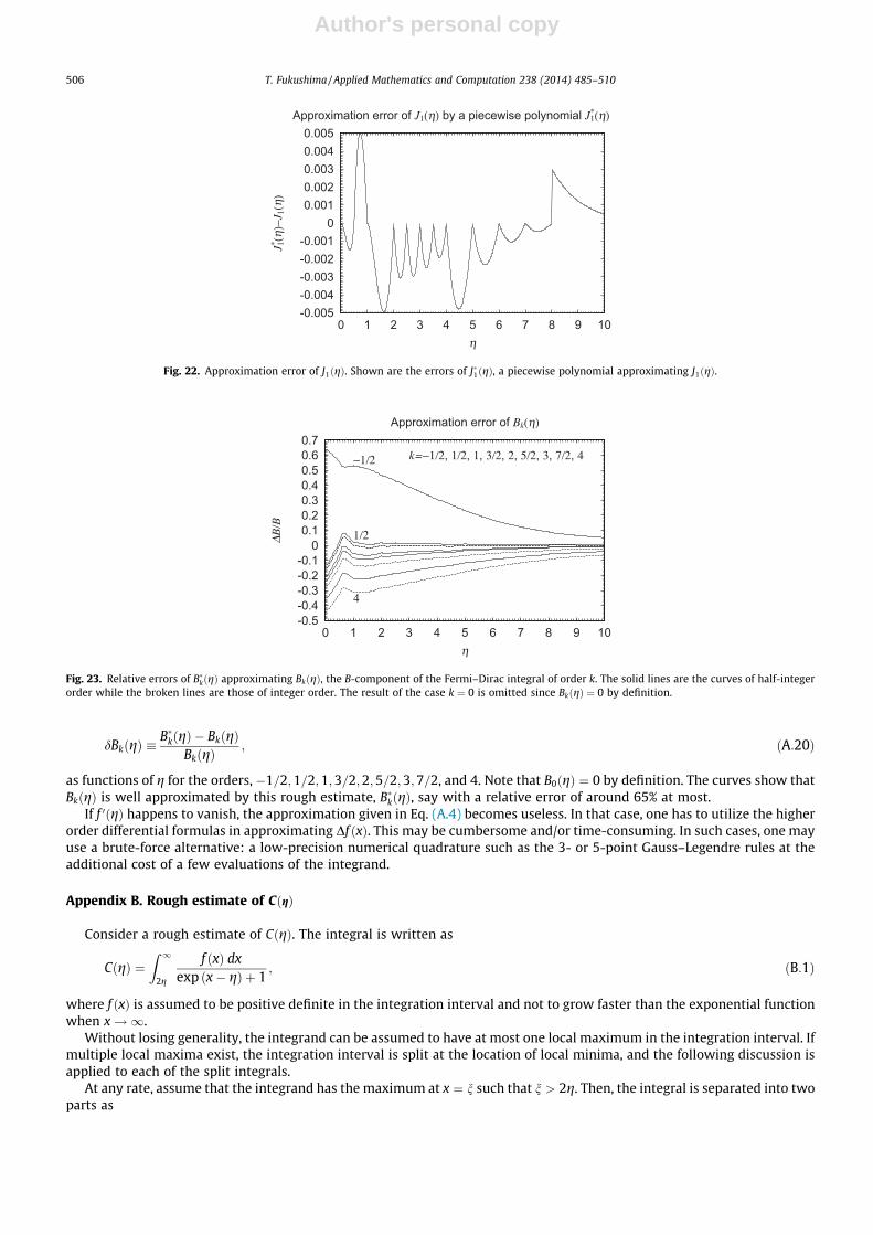
This suggests that the approximation error reduces in proportion to 1=g2 in this case as will be shown in Fig. 23 later.Let us examine the possibility to reduce the computational amount of BðgÞ. The most time-consuming part is the eval-

uation of J1ðgÞ. Since BðgÞ is itself an approximation, there is no necessity of the exact evaluation of its components as longas the total degree of approximation is not degraded significantly. The curve of J1ðgÞ in Fig. 20 indicates that a piecewiseapproximation by a low order polynomial is sufficient for a low precision approximation. Table 1 shows some selected valuesof J1ðgÞ obtained by the quadruple precision numerical integration. Using the numerical values listed in the table, we con-struct an approximation of J1ðgÞ by a composite of (i) a quadratic monomial connecting the points, ð0;0Þ and ð0:5; J1ð0:5ÞÞ,when 0 6 g 6 0:5, (ii) a piecewise linear function connecting the points, 0:5; J1ð0:5Þð Þ through 8:0; J1ð8:0Þð Þ, when0:5 6 g 6 8:0, and (iii) a constant, J1ð1Þ ¼ p2=12, when g > 8:0. The absolute error of the resulting approximation of J1ðgÞis less than 0.005 as illustrated in Fig. 22. This is enough for providing a rough estimate of BðgÞ.

As an example, we consider the Fermi–Dirac integral of order k. In this case, the estimate becomes

BkðgÞ � 2kgk�1J1ðgÞ; ðA:19Þ

where J1ðgÞ is the approximate piecewise polynomial described in the above. Fig. 23 illustrates the relative error of BkðgÞdefined as

0

0.2

0.4

0.6

0.8

1

1.2

0 1 2 3 4 5 6 7 8 9 10x

Behavior of J3(x)/J1(x)

J3(x)/J1(x)

x2/12

7π2/60

Fig. 21. Ratio of two auxiliary integrals, J3ðxÞ=J1ðxÞ, and its two asymptotes; x2=12 and 7p2=60.

Table 1Numerical values of the auxiliary integral J1ðgÞ obtained by the direct numerical quadratureconducted in the quadruple precision environment with an extremely tiny error tolerance,10�33.

g J1ðgÞ

0.0 0.000 000 000 000 000 000.5 0.052 211 261 339 178 621.0 0.170 557 349 502 438 172.0 0.437 598 526 623 744 492.5 0.544 783 428 444 274 193.0 0.627 524 258 364 062 673.5 0.688 368 147 920 279 014.0 0.731 634 872 782 891 305.0 0.782 163 660 101 000 256.0 0.805 135 704 784 287 867.0 0.815 175 094 080 111 248.0 0.819 448 347 942 644 321 0.822 467 033 424 113 22



dBkðgÞ �BkðgÞ � BkðgÞ

BkðgÞ; ðA:20Þ

as functions of g for the orders, �1=2;1=2;1;3=2;2;5=2;3;7=2, and 4. Note that B0ðgÞ ¼ 0 by definition. The curves show thatBkðgÞ is well approximated by this rough estimate, BkðgÞ, say with a relative error of around 65% at most.

If f 0ðgÞ happens to vanish, the approximation given in Eq. (A.4) becomes useless. In that case, one has to utilize the higherorder differential formulas in approximating Df ðxÞ. This may be cumbersome and/or time-consuming. In such cases, one mayuse a brute-force alternative: a low-precision numerical quadrature such as the 3- or 5-point Gauss–Legendre rules at theadditional cost of a few evaluations of the integrand.

Appendix B. Rough estimate of CðgÞ

Consider a rough estimate of CðgÞ. The integral is written as

CðgÞ ¼Z 1

2g

f ðxÞ dxexp x� gð Þ þ 1

; ðB:1Þ

where f ðxÞ is assumed to be positive definite in the integration interval and not to grow faster than the exponential functionwhen x!1.

Without losing generality, the integrand can be assumed to have at most one local maximum in the integration interval. Ifmultiple local maxima exist, the integration interval is split at the location of local minima, and the following discussion isapplied to each of the split integrals.

At any rate, assume that the integrand has the maximum at x ¼ n such that n > 2g. Then, the integral is separated into twoparts as

-0.005-0.004-0.003-0.002-0.001

00.0010.0020.0030.0040.005

0 1 2 3 4 5 6 7 8 9 10

J 1*(η

)−J 1

( η)

η

Approximation error of J1(η) by a piecewise polynomial J1*(η)

Fig. 22. Approximation error of J1ðgÞ. Shown are the errors of J1ðgÞ, a piecewise polynomial approximating J1ðgÞ.

-0.5-0.4-0.3-0.2-0.1

00.10.20.30.40.50.60.7

0 1 2 3 4 5 6 7 8 9 10

ΔB/B

η

Approximation error of Bk(η)

k=−1/2, 1/2, 1, 3/2, 2, 5/2, 3, 7/2, 4−1/2

1/2

4

Fig. 23. Relative errors of BkðgÞ approximating BkðgÞ, the B-component of the Fermi–Dirac integral of order k. The solid lines are the curves of half-integerorder while the broken lines are those of integer order. The result of the case k ¼ 0 is omitted since BkðgÞ ¼ 0 by definition.



CðgÞ ¼ C1 g; nð Þ þ C2 g; nð Þ; ðB:2Þ

where

C1 g; nð Þ �Z n

2g


; ðB:3Þ

C2 g; nð Þ �Z 1

n


: ðB:4Þ

An upper bound of the first part is obtained by replacing the denominator of the integrand by its minimum value, i.e., thevalue when x ¼ 2g, as

C1 g; nð Þ 6 C1 g; nð Þ �Z n

2g

f ðxÞ dxexp 2g� gð Þ þ 1

¼ A nð Þ � Að2gÞeg þ 1

; ðB:5Þ

where AðgÞ is already defined in Eq. (16).In the second part, on the other hand, the integrand decreases monotonically by assumption. Therefore, the integral has

an upper bound obtained by substituting f nð Þ into f ðxÞ as

C2 g; nð Þ 6 C2 g; nð Þ �Z 1

n

f nð Þ dxexpðx� gÞ þ 1

¼ f nð Þ ln½1þ exp g� nð Þ�; ðB:6Þ

where we used a formulaZ 1

a

dyey þ 1

¼ ln 1þ e�að Þ: ðB:7Þ

As a result, an upper bound of CðgÞ is obtained as

CðgÞ 6 C g; nð Þ � C1 g; nð Þ þ C2 g; nð Þ ¼ A nð Þ � Að2gÞeg þ 1

þ f nð Þ ln½1þ exp g� nð Þ�: ðB:8Þ

If there exists no maximum in the integration interval or if n 6 2g, the estimate is simplified by replacing n with 2g as

Cðg; 2gÞ ¼ C2ðg; 2gÞ ¼ f ð2gÞ ln 1þ e�gð Þ; ðB:9Þ

since C1ðg; 2gÞ ¼ 0 by definition. Notice that this approximation is exact if f ðxÞ is constant.As an example, let us take the Fermi–Dirac integral of order k. First, consider the case when k P 0. The integrand has the

unique maximum at x ¼ nk where nk is defined as

nk � kþW0 k expðg� kÞð Þ: ðB:10Þ

Here W0ðzÞ is the primary branch of Lambert W-function [37]. Its fast computing procedure is provided in our recent work[38].

This expression of nk is obtained by solving the equation

0 ¼ ddx

x�k expðx� gÞ þ 1f g�

¼ �kx�k�1 expðx� gÞ þ 1½ � þ x�k expðx� gÞ; ðB:11Þ

which turns out to be the defining equation of the Lambert W-function [4, Formula 4.13.1] as

WeW ¼ z; ðB:12Þ

by using the variable transformation

W � x� k; z � k expðg� kÞ: ðB:13Þ

Since z is positive definite, the real solution of the above equation is limited to the primary branch, W0ðzÞ.When k < 0, on the other hand, the integrand is monotonically decreasing. Then, one may choose Cðg; 2gÞ. However, its

precision of approximation degrades when g is small, say less than 4 or so as illustrated by McDougall and Stoner [15] for thecase F1=2ðgÞ. Then, by setting n�1=2 ¼ 1, we propose adopting the same approximate formula, Eq. (B.8). Since f ðxÞ becomessingular when g! 0 in this case, it is wise to limit the minimum value of the second argument of C2ðg; 2gÞ, say greater than0.01. When k ¼ �1=2, the resulting formula becomes

C2ðg; minð0:01;2gÞÞ ¼ ln½1þ expðminð0:01;2gÞÞ�ffiffiffiffiffiffiffiffiffiffiffiffiffiffiffiffiffiffiffiffiffiffiffiffiffiffiffiffiffiffiminð0:01;2gÞ

p : ðB:14Þ

Fig. 24 illustrates the relative error of thus-computed CkðgÞ, which is defined as

dCkðgÞ �CkðgÞ � CkðgÞ

CkðgÞ; ðB:15Þ



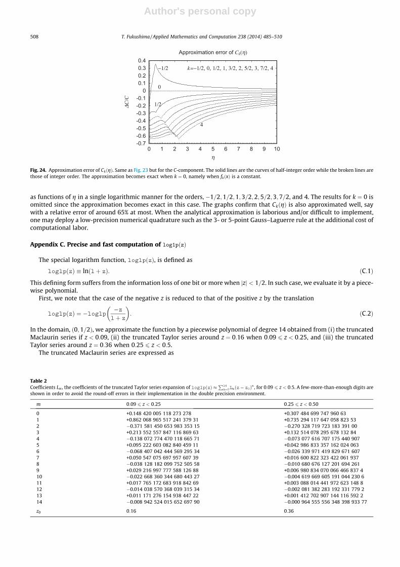
as functions of g in a single logarithmic manner for the orders, �1=2;1=2;1;3=2;2;5=2;3;7=2, and 4. The results for k ¼ 0 isomitted since the approximation becomes exact in this case. The graphs confirm that CkðgÞ is also approximated well, saywith a relative error of around 65% at most. When the analytical approximation is laborious and/or difficult to implement,one may deploy a low-precision numerical quadrature such as the 3- or 5-point Gauss–Laguerre rule at the additional cost ofcomputational labor.

Appendix C. Precise and fast computation of log1pðzÞ

The special logarithm function, log1pðzÞ, is defined as

log1pðzÞ � lnð1þ zÞ: ðC:1Þ

This defining form suffers from the information loss of one bit or more when jzj < 1=2. In such case, we evaluate it by a piece-wise polynomial.

First, we note that the case of the negative z is reduced to that of the positive z by the translation

log1pðzÞ ¼ �log1p �z1þ z

� �: ðC:2Þ

In the domain, ð0;1=2Þ, we approximate the function by a piecewise polynomial of degree 14 obtained from (i) the truncatedMaclaurin series if z < 0:09, (ii) the truncated Taylor series around z ¼ 0:16 when 0:09 6 z < 0:25, and (iii) the truncatedTaylor series around z ¼ 0:36 when 0:25 6 z < 0:5.

The truncated Maclaurin series are expressed as

-0.7-0.6-0.5-0.4-0.3-0.2-0.1

00.10.20.30.4

0 1 2 3 4 5 6 7 8 9 10

ΔC/C

η

Approximation error of Ck(η)

k=−1/2, 0, 1/2, 1, 3/2, 2, 5/2, 3, 7/2, 4−1/2

0

1/2

4

Fig. 24. Approximation error of CkðgÞ. Same as Fig. 23 but for the C-component. The solid lines are the curves of half-integer order while the broken lines arethose of integer order. The approximation becomes exact when k ¼ 0, namely when fkðxÞ is a constant.

Table 2Coefficients Lm , the coefficients of the truncated Taylor series expansion of log1pðzÞ �

P14

m¼0Lm z� z0ð Þm , for 0:09 6 z < 0:5. A few-more-than-enough digits areshown in order to avoid the round-off errors in their implementation in the double precision environment.

m 0:09 6 z < 0:25 0:25 6 z < 0:50

0 +0.148 420 005 118 273 278 +0.307 484 699 747 960 631 +0.862 068 965 517 241 379 31 +0.735 294 117 647 058 823 532 �0.371 581 450 653 983 353 15 �0.270 328 719 723 183 391 003 +0.213 552 557 847 116 869 63 +0.132 514 078 295 678 132 844 �0.138 072 774 470 118 665 71 �0.073 077 616 707 175 440 9075 +0.095 222 603 082 840 459 11 +0.042 986 833 357 162 024 0636 �0.068 407 042 444 569 295 34 �0.026 339 971 419 829 671 6077 +0.050 547 075 697 957 607 39 +0.016 600 822 323 422 061 9378 �0.038 128 182 099 752 505 58 �0.010 680 676 127 201 694 2619 +0.029 216 997 777 588 126 88 +0.006 980 834 070 066 466 837 410 �0.022 668 360 344 680 443 27 �0.004 619 669 605 191 044 230 611 +0.017 765 172 683 918 842 69 +0.003 088 014 441 972 623 148 812 �0.014 038 570 368 039 315 34 �0.002 081 382 283 192 331 779 213 +0.011 171 276 154 938 447 22 +0.001 412 702 907 144 116 592 214 �0.008 942 524 015 652 697 90 �0.000 964 555 556 348 398 933 77

z0 0:16 0:36



log1pðzÞ ¼XMm¼1

zm

m; ðC:3Þ

while the truncated Taylor series are expressed as

log1pðzÞ ¼XMm¼0

Lm z� z0ð Þm; ðC:4Þ

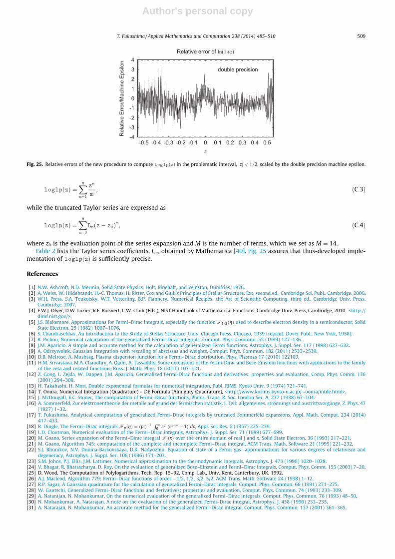
where z0 is the evaluation point of the series expansion and M is the number of terms, which we set as M ¼ 14.Table 2 lists the Taylor series coefficients, Lm, obtained by Mathematica [40]. Fig. 25 assures that thus-developed imple-

mentation of log1pðzÞ is sufficiently precise.

References

[1] N.W. Ashcroft, N.D. Mermin, Solid State Physics, Holt, Rinehalt, and Winston, Dumfries, 1976.[2] A. Weiss, W. Hildebrandt, H.-C. Thomas, H. Ritter, Cox and Giuli’s Principles of Stellar Structure, Ext, second ed., Cambridge Sci. Publ., Cambridge, 2006.[3] W.H. Press, S.A. Teukolsky, W.T. Vetterling, B.P. Flannery, Numerical Recipes: the Art of Scientific Computing, third ed., Cambridge Univ. Press,

Cambridge, 2007.[4] F.W.J. Olver, D.W. Lozier, R.F. Boisvert, C.W. Clark (Eds.), NIST Handbook of Mathematical Functions, Cambridge Univ. Press, Cambridge, 2010. <http://

dlmf.nist.gov/>.[5] J.S. Blakemore, Approximations for Fermi–Dirac integrals, especially the function F1=2ðgÞ used to describe electron density in a semiconductor, Solid

State Electron. 25 (1982) 1067–1076.[6] S. Chandrasekhar, An Introduction to the Study of Stellar Structure, Univ. Chicago Press, Chicago, 1939 (reprint, Dover Publ., New York, 1958).[7] B. Pichon, Numerical calculation of the generalized Fermi–Dirac integrals, Comput. Phys. Commun. 55 (1989) 127–136.[8] J.M. Aparicio, A simple and accurate method for the calculation of generalized Fermi functions, Astrophys. J. Suppl. Ser. 117 (1998) 627–632.[9] A. Odrzywolek, Gaussian integration with rescaling of abscissas and weights, Comput. Phys. Commun. 182 (2011) 2533–2539.

[10] D.B. Melrose, A. Mushtag, Plasma dispersion function for a Fermi–Dirac distribution, Phys. Plasmas 17 (2010) 122103.[11] H.M. Srivastava, M.A. Chaudhry, A. Qadir, A. Tassaddiq, Some extensions of the Fermi-Dirac and Bose-Einstein functions with applications to the family

of the zeta and related functions, Russ. J. Math. Phys. 18 (2011) 107–121.[12] Z. Gong, L. Zejda, W. Dappen, J.M. Aparicio, Generalized Fermi-Dirac functions and derivatives: properties and evaluation, Comp. Phys. Comm. 136

(2001) 294–309.[13] H. Takahashi, H. Mori, Double exponential formulas for numerical integration, Publ. RIMS, Kyoto Univ. 9 (1974) 721–741.[14] T. Ooura, Numerical Integration (Quadrature) – DE Formula (Almighty Quadrature), <http://www.kurims.kyoto-u.ac.jp/�ooura/intde.html>.[15] J. McDougall, E.C. Stoner, The computation of Fermi–Dirac functions, Philos. Trans. R. Soc. London Ser. A. 237 (1938) 67–104.[16] A. Sommerfeld, Zur elektronentheorie der metalle auf grund der fermischen statistik. I. Teil: allgemeines, strömungs und austrittsvorgänge, Z. Phys. 47

(1927) 1–32.[17] T. Fukushima, Analytical computation of generalized Fermi–Dirac integrals by truncated Sommerfeld expansions, Appl. Math. Comput. 234 (2014)

417–433.[18] R. Dingle, The Fermi–Dirac integrals FpðgÞ ¼ ðp!Þ�1 R1

0 ep ee�g þ 1ð Þ de, Appl. Sci. Res. 6 (1957) 225–239.[19] L.D. Cloutman, Numerical evaluation of the Fermi–Dirac integrals, Astrophys. J. Suppl. Ser. 71 (1989) 677–699.[20] M. Goano, Series expansion of the Fermi–Dirac integral FjðxÞ over the entire domain of real j and x, Solid State Electron. 36 (1993) 217–221.[21] M. Goano, Algorithm 745: computation of the complete and incomplete Fermi–Dirac integral, ACM Trans. Math. Software 21 (1995) 221–232.[22] S.I. Blinnikov, N.V. Dunina-Barkovskaya, D.K. Nadyozhin, Equation of state of a Fermi gas: approximations for various degrees of relativism and

degeneracy, Astrophys. J. Suppl. Ser. 106 (1996) 171–203.[23] S.M. Johns, P.J. Ellis, J.M. Lattimer, Numerical approximation to the thermodynamic integrals, Astrophys. J. 473 (1996) 1020–1028.[24] V. Bhagat, R. Bhattacharya, D. Roy, On the evaluation of generalized Bose–Einstein and Fermi–Dirac integrals, Comput. Phys. Comm. 155 (2003) 7–20.[25] D. Wood, The Computation of Polylogarithms, Tech. Rep. 15–92, Comp. Lab., Univ. Kent, Canterbury, UK, 1992.[26] A.J. Macleod, Algorithm 779: Fermi–Dirac functions of order �1/2, 1/2, 3/2, 5/2, ACM Trans. Math. Software 24 (1998) 1–12.[27] R.P. Sagar, A Gaussian quadrature for the calculation of generalized Fermi–Dirac integrals, Comput. Phys. Commun. 66 (1991) 271–275.[28] W. Gautschi, Generalized Fermi–Dirac functions and derivatives: properties and evaluation, Comput. Phys. Commun. 74 (1993) 233–309.[29] A. Natarajan, N. Mohankumar, On the numerical evaluation of the generalized Fermi–Dirac integrals, Comput. Phys. Commun. 76 (1993) 48–50.[30] N. Mohankumar, A. Natarajan, A note on the evaluation of the generalized Fermi–Dirac integral, Astrophys. J. 458 (1996) 233–235.[31] A. Natarajan, N. Mohankumar, An accurate method for the generalized Fermi–Dirac integral, Comput. Phys. Commun. 137 (2001) 361–365.

-4

-3

-2

-1

0

1

2

3

4

-0.5 -0.4 -0.3 -0.2 -0.1 0 0.1 0.2 0.3 0.4 0.5

Rel

ativ

e Er

ror/M

achi

ne E

psilo

n

z

Relative error of ln(1+z)

double precision

Fig. 25. Relative errors of the new procedure to compute log1pðzÞ in the problematic interval, jzj < 1=2, scaled by the double precision machine epsilon.



[32] R. Piessens, E. de Doncker-Kapenga, C. Überhuber, D. Kahaner, QUADPACK, A Subroutine Package for Automatic Integration, Springer, New York, 1983.<http://www.netlib.org/quadpack>.

[33] J.F. Encke, Berliner Astronomisches Jahrbuch für 1857, Königlich Akademie der Wissenschaften, Berlin, 1854.[34] D. Brouwer, G.M. Clemence, Methods of Celestial Mechanics, Academic Press, New York, 1961.[35] T. Fukushima, Generalization of Encke’s method and its application to the orbital and rotational motions of celestial bodies, Astron. J. 112 (1996) 1263–

1277.[36] T.M. Dunster, Uniform asymptotic approximations for incomplete Riemann zeta functions, J. Comput. Appl. Math. 190 (2013) 339–353.[37] R.M. Corless, G.H. Gonnet, D.E.G. Hare, D.J. Jeffrey, D.E. Knuth, On the Lambert W function, Adv. Comput. Math. 5 (1996) 329–359.[38] T. Fukushima, Precise and fast computation of Lambert W-functions without transcendental function evaluations, J. Comput. Appl. Math. 244 (2013)

77–89.[39] T. Fukushima, A fast procedure solving Gauss’ form of Kepler’s equation, Celestial Mech. Dyn. Astron. 70 (1998) 115–130.[40] S. Wolfram, The Mathematica Book, fifth ed., Wolfram Research Inc./Cambridge Univ. Press, Cambridge, 2003.


Computation of a general integral of Fermi-Dirac distribution by McDougall-Stoner method

Documents

Transcript of Computation of a general integral of Fermi-Dirac distribution by McDougall-Stoner method