Comprehensive Study on Air Pollution and Green House ...
334
Comprehensive Study on Air Pollution and Green House Gases (GHGs) in Delhi (Final Report: Air Pollution component) Submitted to Department of Environment Government of National Capital Territory of Delhi and Delhi Pollution Control Committee, Delhi January 2016 Mukesh Sharma; PhD and Onkar Dikshit; PhD Professors, Department of Civil Engineering Indian Institute of Technology Kanpur, Kanpur- 208016
-
Upload
khangminh22 -
Category
Documents
-
view
0 -
download
0
Transcript of Comprehensive Study on Air Pollution and Green House ...

Comprehensive Study on Air Pollution and Green House
Gases (GHGs) in Delhi
(Final Report: Air Pollution component)
Submitted to
Department of Environment
Government of National Capital Territory of Delhi
and
Delhi Pollution Control Committee, Delhi
January 2016
Mukesh Sharma; PhD and Onkar Dikshit; PhD
Professors, Department of Civil Engineering
Indian Institute of Technology Kanpur, Kanpur- 208016
November 2015

Copyright© 2015 by IIT Kanpur, Delhi Pollution Control Committee and
Department of Environment, NCT Delhi. All rights reserved. No part of this
report can be used for any scientific publications in any journal, conferences,
seminars, workshops etc without written permission.
i
Executive Summary
Since the enactment of the Air Act 1981, air pollution control programs have focused on
point and area source emissions, and many communities have benefited from these control
programs. Nonetheless, most cities in the country still face continuing particulate non-
attainment problems from aerosols of unknown origin (or those not considered for
pollution control) despite the high level of control applied to many point sources.
To address the air pollution problem in the city of Delhi by identifying major air pollution
sources, their contributions to ambient air pollution levels and develop an air pollution
control plan, Government of National Capital Territory of Delhi (NCTD) and Delhi
Pollution Control Committee (DPCC), Delhi have sponsored this project “Comprehensive
Study on Air Pollution and Green House Gases in Delhi” to IIT Kanpur. The project has
the following specific major objectives:
Identify and inventorize emission sources (industry, traffic, power plants, local power
generation, small scale industries etc.) in Delhi.
Chemical speciation of particulate matter (PM) and measurement of other air
pollutants;
Perform receptor modeling to establish the source-receptor linkages for PM in ambient
air;
Project emission inventories using mathematical models taking into account vehicle
population/ improvements in vehicle technology, fuel quality changes and other
activities having impact on ambient air quality
Identification of various control options and assessment of their efficacies for air
quality improvements and development of control scenarios consisting of
combinations of several control options; and
Selection of best control options from the developed control scenarios and recommend
implementation of control options in a time-bound manner.
This study has five major components (i) air quality measurements, (ii) emission
inventory, (iii) air quality modeling, (iv) control options and (v) action plan. The
highlights of these components are presented below.

ii
Air Quality: Measurements
Air quality sites were categorized based on the predominant land-use pattern (Table 1) to
cover varying land-use prevailing in the city. PM10 (particulate matter of size less than or
equal to 10 µm), PM2.5 (particulate matter of size less than or equal to 2.5µm), SO2, NO2,
CO, OC (organic carbon), EC (elemental carbon), Ions, Elements and PAHs (poly
aromatic hydrocarbons) were considered for sampling and measurements. The air quality
sampling was conducted for two seasons: winter (2013-14) and summer (2014).
Table 1: Description of Sampling Sites in Delhi
S.
No. Sampling Location
Site
Code
Description of
the site Type of sources
1. DAV School, Dwarka DWK Residential Domestic cooking, vehicles, road
dust
2. Delhi Technical
University, Rohini RHN
Residential
and Industrial
Industries, Domestic cooking,
DG sets, vehicles, road dust,
garbage burning
3. Envirotech, Okhla OKH Industrial Industries, DG sets, vehicles,
road dust
4. Indian Spinal Injuries
Centre, Vasantkunj VKJ
Residential
cum
commercial
Domestic cooking, DG sets,
vehicles, road dust, garbage
burning, restaurants
5.
Arwachin
International School,
Dilshad Garden
DSG Industrial Industries, DG sets, vehicles,
road dust
6. DTEA School, Pusa
Road New Delhi PUS
Residential
cum
commercial
Domestic cooking, DG sets,
vehicles, road dust, garbage
burning, restaurants
Based on the air quality measurements in summer and winter months and critical analyses
of air quality data (Chapter 2), the following inferences and insights are drawn for
understanding current status of air quality. The season-wise, site specific average air
concentrations of PM10, PM2.5 and their compositions (Tables 2.14 (a, b, c, d) and 2.16 (a,
b, c, d)) have been referred to bring the important inferences to the fore.
- Particulate pollution is the main concern in the city where levels of PM10 and
PM2.5 are 4-7 times higher than the national air quality standards in summer
and winter months.

iii
- The chemical composition of PM10 and PM2.5 carries the signature of sources
and their harmful contents. The chemical composition is variable depending on
the size fraction of particles and the season. The PM levels and chemical
composition are discussed separately for two seasons.
Summer - PM10
The overall average concentration of PM10 in summer season is over 500 µg/m3
against the acceptable level of 100 µg/m3.
The crustal component (Si + Al + Fe + Ca) accounts for about 40 percent of total
PM10 in summer. This suggests soil and road dust and airborne flyash are the major
sources of PM10 pollution in summer. The coefficient of variation (CV) is about
0.25, which suggests the sources are consistent all around the city forming a layer
which envelopes the city. The areas of DSG and OKH have the highest crustal
fraction (around 44% of total PM10). It is difficult to pinpoint the crustal sources as
these are wide spread and present all around in Delhi and NCR and are more
prominent in summer when soil and ash-ponds (active or abandoned) are dry and
high speed winds make the particles airborne. It was observed that in summer the
atmosphere looks whitish to grayish which can be attributed to the presence of
large amounts of flyash and dust particles in the atmosphere.
The second important component is the secondary particles (NO₃⁻ + SO₄⁻² +
NH₄⁺), which account for about 13 percent of total PM10 and combustion related
total carbon (EC+OC) accounts for about seven percent. The secondary particles
are formed in the atmosphere because of reaction of precursor gases (SO2, NOx
and NH3) to form NO₃⁻, SO₄⁻², and NH₄⁺. The combustion related contribution is
relatively less in PM10 in summer.
The Cl- content in PM10 in summer is also consistent at 4-6 percent, which is an
indicator of burning of municipal solid waste (MSW).
Summer - PM2.5
The overall average concentration of PM2.5 in summer season is around 300 µg/m3
against the acceptable level of 60 µg/m3.

iv
The crustal component (Si + Al + Fe + Ca) accounts for about 20 percent of total
PM2.5. This suggests soil and road dust and airborne flyash is a significant source
of PM2.5 pollution in summer. The CV is about 0.23, which suggests the source is
consistent all around the city. The area of OKH has the highest crustal fraction
around 28% of total PM2.5.
The second important component is secondary particles (NO₃⁻ + SO₄⁻² + NH₄⁺),
which account for about 17 percent of total PM2.5 and combustion related total
carbon (EC+OC) accounts for about nine percent; both fractions of secondary
particles and combustion related carbons account for a larger fraction in PM2.5 than
in PM10. All three potential sources, crustal component, secondary particles and
combustion contribute consistently to PM2.5 in summer.
The Cl- content in PM2.5 in summer is also consistent at 4-10 percent, which is an
indicator of burning of municipal solid waste (MSW) and has a relatively higher
contribution to PM2.5 than that to PM10.
Winter - PM10
The overall average concentration of PM10 in winter season is around 600 µg/m3
against the acceptable level of 100 µg/m3.
The crustal component (Si + Al + Fe + Ca) accounts for only 13% (much less
compared to 40 percent in summer). This suggests soil and road dust and airborne
flyash have reduced significantly in PM10 in winter. The coefficient of variation
(CV) is about 0.36, which suggests the crustal source is variable and not as
consistent as it was in summer.
The most important component is the secondary particles (NO₃⁻ + SO₄⁻² + NH₄⁺),
which account for about 26 percent of total PM10 and combustion related total
carbon (TC = EC + OC) accounts for about 19 percent; both fraction of secondary
particles and combustion related carbons have increased in winter and account for
45 percent of PM10.

v
The Cl- content in PM10 in winter is also consistent at 4-10 percent, which is an
indicator of burning of municipal solid waste (MSW) and has a relatively higher
contribution in winter.
Winter - PM2.5
The overall average concentration of PM2.5 in winter is 375 µg/m3 against the
acceptable level of 60 µg/m3. The crustal component is reduced dramatically to
only 3.5 percent in PM2.5 in winter.
The single important component is the secondary particles (NO₃⁻ + SO₄⁻² +
NH₄⁺), which account for about 28 percent of total PM2.5 and combustion related
total carbon (EC+OC) accounts for about 23 percent; both secondary particles and
combustion related carbon are consistent contributor to PM2.5 at about 51 percent
having CV of 0.22.
The Cl- content in PM2.5 winter is also consistent at 7 percent, which is an indicator
of burning of municipal solid waste (MSW); which is relatively higher in winter
than in summer
It was observed that in winter the atmosphere looks very hazy and characterized by
smoky and unhealthy air. The consistent and major contributors appear to be
secondary particles and combustion related emission with modest contribution of
burning of MSW.
Potassium levels
In general potassium levels are high and at the same time highly variable; 18 to 7
µg/m3 in PM10 and 15 to 4 µg/m
3 in PM2.5. In general potassium level is less than 2
µg/m3. Potassium is an indicator of biomass burning and high levels and variability
(CV ~ 0.66) show large biomass burning and it is variable. Highest potassium
levels (~ 15 µg/m3) were seen in the beginning of November and early winter
perhaps due to crop residue burning in Punjab and Haryana. Potassium levels
stabilize around 4 µg/m3 (which is also high) in rest of the winter months
suggesting the biomass burning is prevalent throughout winter, locally and
regionally.

vi
NO2 levels
NO2 levels in winter are high and they do exceed national air quality standard of 80
µg/m3 at a few locations; more frequently at PUS sampling site. In addition, high
levels of NO2 are expected to undergo chemical transformation to form fine
secondary particles in the form of nitrates, adding to high levels of existing PM10
and PM2.5. SO2 levels in the city were well within the air quality standard.
General inferences
Levels of PM10, PM2.5 and NO2 are statistically higher (at most locations) in winter
months than in summer months by about 25-30 percent. In general air pollution
levels in ambient air (barring traffic intersections) are uniform across the city
suggesting entire city is stressed under high pollution; in a relative sense, OKH is
most polluted and PUS followed by DWK is the least polluted for PM pollution.
The CO levels are well within the ambient air quality standard during summer
while at PUS, the concentration exceeds the standards during peak traffic hours in
winter.
The entire city is enveloped by pollution layer all around with contribution from
multiple sources within Delhi, nearby region and even from long distances.
It is to be noted that OC3/TC ratio is above 0.22 and highest among ratio of
fraction of OC to TC (Chapter 2). It suggests a significant component of
secondary organic aerosol is formed in atmosphere due to condensation and
nucleation of volatile to semi volatile organic compounds (VOCs and SVOCs),
which again suggests emissions within and outside of Delhi.
Total PAH levels (14 compounds; particulate phase) in winter is very high at 80
ng/m3 and B(a)P at 8 ng/m
3 (annual standard is 1 ng/m
3); the comparison with
annual standard is not advisable due to different averaging times. However, PAH
levels in summer drop significantly to about 15 ng/m3.
In a broad sense, air is more toxic in winter than in summer as it contains much
larger contribution of combustion products in winter than in summer months.

vii
During Diwali days, PM levels nearly double from the average level and organic
content of PM increases more than twice. It is noteworthy that levels of potassium
and barium, the main components of fire crackers can increase by about ten times.
- Limited sampling was undertaken in summer and winter seasons at three sites
in NCR (Noida, Gaziabad and Faridabad), as a part of other study that
indicated the levels in Delhi and NCR are similar and comparable; it suggests
that air pollution levels could be contiguously high in the NCR. To get a
further insight into this matter, a sampling of PM, SO2 and NO2 was also
carried out winter season (2014 -15) and as expected levels in Delhi and NCR
were comparable.
In a broad sense, fractions of secondary particles of both PM10 and PM2.5 in two seasons
were consistent and need to be controlled for better air quality in Delhi and NCR.
Combustion sources, vehicles, biomass burning and MSW burning are other consistent
sources in winter and require a strategy to control these sources. In summer, air quality
cannot be improved unless we find effective control solutions for soil and road dust, fly
ash re-suspension, concrete batching and MSW burning.
Emission Inventory
The overall baseline emission inventory for the entire city is developed for the period
November 2013 to June 2014. The pollutant wise contribution is shown in Figures 1 to 3.
Spatial Distribution of pollutant Emissions from all sources is presented in Figure 4.
The total PM10 emission load in the city is estimated to be 143 t/d (based on average
annual activity data). The top four contributors to PM10 emissions are road dust (56%),
concrete batching (10%), industrial point sources (10%) and vehicles (9%); these are
based on annual emissions. Seasonal and daily emissions could be highly variable. For
example, fugitive road and soil dust re-suspension from ash pond and emission from
concrete batching will be significantly lower in winter than in summer. The estimated
emission suggests that there are many important sources and a composite emission
abatement including most of the sources will be required to obtain the desired air quality.
PM2.5 emission load in the city is estimated to be 59 t/d. The top four contributors to PM2.5
emissions are road dust (38 %), vehicles (20 %), domestic fuel burning (12 %) and

viii
industrial point sources (11%); these are based on annual emissions. Seasonal and daily
emissions could be highly variable.
NOx emissions are even higher than PM10 emission ~ 312 t/d. Nearly 52 % of emissions
are attributed to industrial point source (largely from power plants) followed by vehicular
emissions (36%) that occur at ground level, probably making it the most important
emission. DG sets contributes 6% to NOx emission and is followed by Aircraft emission
(2%). NOx apart from being a pollutant itself, it is important component in formation of
secondary particles (nitrates) and ozone. NOx from vehicles and from industry are
potential sources for controlling of NOx emissions.
SO2 emission load in the city is estimated to be 141 t/d. Industrial point sources account
for above 90 percent of total emission; most of the emissions are from power plants. It
appears there may be a need to control SO2 from power plants. SO2 is known to contribute
to secondary particles (sulfates).
Estimated CO emission is 387 t/d. Nearly 83 % emission of CO is from vehicles, followed
by domestic sources 7 %, MSW burning 3% and about 3 % from industrial point source.
Vehicles could be the main target for controlling CO for improving air quality with respect
to CO.
Spatial variation of emission quantity suggests that for PM10, PM2.5, CO and NOx, the
central down town area, north and east of the city show higher emissions than other parts.
Figure 1: PM10 Emission Load of Different Sources in the City Of Delhi
13681, 10%
12914, 9%
3493, 2%
7381, 5%
54, 0%1614, 1% 1387, 1%
1968, 1% 346, 0%
38, 0%5167, 4%
14370, 10%
79626, 56%
1353, 1%
Industrial Stack Vehicle Hotels/Restaurants Domestic
Aircraft Industries Area DG Set MSW Burning
Cremation Medical Incinerators Construction/Demolition Concrete Batching
Road Dust Agricultural Soil Dust

ix
Figure 2: PM2.5 Emission Load of Different Sources in the City Of Delhi
Figure 3: NOx Emission Load of Different Sources in the City Of Delhi
Figure 4: Spatial Distribution of PM10, PM2.5 and NOx Emissions in the City of Delhi
Air Quality Modeling
Receptor Modeling
Based on the CMB (chemical mass balance) modeling results (Figures 5 and 6) and their
critical analyses, the following inferences and insights are drawn to establish quantified
6576, 11%
11623, 20%
1758, 3%
6940, 12%
54, 0%
1367, 2%1248, 2%
1771, 3%
312, 1%
34, 0%
1292, 2%
3594, 6%
22165, 38%
0, 0%
Industrial Stack Vehicle Hotels/Restaurants Domestic
Aircraft Industries Area DG Set MSW Burning
Cremation Medical Incinerators Construction/Demolition Concrete Batching
Road Dust Agricultural Soil Dust
161838, 52%113443, 36%
1105, 0%
7682, 3%
5416, 2%
1893, 1%
19604, 6%
738, 0%96, 0%
103, 0%
Industrial Stack Vehicle Hotels/Restaurants Domestic Aircraft
Industries Area DG Set MSW Burning Cremation Medical Incinerators

x
source-receptor impacts and to pave the path for preparation of action plan. Tables 4.17 to
4.20 (in Chapter 4), show season-wise, site specific average source contribution to PM10
and PM2.5, and these tables are frequently referred to bring the important inferences to the
fore.
The sources of PM10 and PM2.5 contributing to ambient air quality are different in
summer and winter.
The winter sources (% contribution given in parenthesis for PM10 - PM2.5 to
the ambient air levels) include: secondary particles (25 - 30%), vehicles (20
- 25%), biomass burning (17 – 26%), MSW burning (9 - 8%) and to a
lesser extent soil and road dust. It is noteworthy, in winter; major sources
for PM10 and PM2.5 are generally the same. A significant contribution in
secondary nitrate is from vehicles. It is estimated that secondary nitrate
particles of vehicles origin contribute to 3% of total PM2.5 in ambient air
that makes average vehicle contribution to PM2.5 at about 28%.
The summer sources (% contribution given in parenthesis for PM10 - PM2.5
to the ambient air level) include: coal and flyash (37 - 26%), soil and road
dust (26 – 27%), secondary particles (10 - 15%), biomass burning (7 -
12%), vehicles (6 – 9%) and MSW burning (8 – 7%). It is noteworthy, in
summer also, the major sources for PM10 and PM2.5 are generally the same.
The two most consistent sources for PM10 and PM2.5 in both the seasons are
secondary particles and vehicles. The other sources on average may contribute
more (or less) but their contributions are variable from one day to another. Most
variable source was biomass burning followed by MSW burning. Soil and road
dust and coal and flyash sources were consistent for PM10 but it was not true for
PM2.5.
Consistent presence of secondary and vehicular PM10 and PM2.5 across all sites and
in two seasons, suggests these particles encompass entire Delhi region as a layer.
Similar to the above point, in summer, consistent presence of soil and road dust
and coal and flyash particles encompass entire Delhi region as a layer.
Coal and flyash and road and soil dust in summer contribute 26-37% to PM2.5 and
PM10. It is observed that in summer the atmosphere looks whitish to grayish

xi
indicating presence of large amounts of flyash and dust; re-suspension of dust
appears to be the cause of large contribution of these sources. This hypothesis can
be argued from the fact that the contribution of flyash and road dust reduces
significantly both in PM10 and PM2.5 in winter when winds are low and prevalent
atmospheric conditions are calm.
The contribution of the biomass burning in winter is quite high at 17% (for PM10)
26% (for PM2.5). Biomass burning is prohibited in Delhi and it is not a common
practice at a large scale. The enhanced concentration of PM in October-November
is possibly due to the effect of post-monsoon crop residue burning (CRB). It can be
seen that the biomass contribution in PM10 in the month of November could be as
high as 140 µg/m3 and about 120 µg/m
3 for PM2.5 (mean of contribution in entire
winter season: 97 µg/m3 and 86 µg/m
3 respectively). In all likelihood, the PM from
biomass burning is contributed from CRB prevalent in Punjab and Haryana in
winter. The back trajectory analyses suggest that the CRB and other biomass
emissions may be transported to Delhi from the sources upwind of Delhi (in NW
direction). There is an immediate need to control or find alternatives to completely
eliminate CRB emissions to observe significant improvement in air quality in
Delhi. However, contribution of sizeable biomass burning to PM in December and
January indicates to local sources present in Delhi and nearby areas.
The contribution of MSW burning may surprise many persons. The recent study by
Nagpure et al. (2015) has estimated 190 to 246 tons/day of MSW burning (∼2−3%
of MSW generated; 8390 tons/day). It is clearly seen that MSW burning is a major
source that contributes to both PM10 and PM2.5. This emission is expected to be
large in the regions of economically lower strata of the society which does not
have proper infrastructure for collection and disposal of MSW.

xii
Figure 5: Overall Results of CMB Modeling for PM10 and PM2.5 at six sites
*Solid waste burning refers to MSW burning
Figure 6: City level source contribution to ambient air PM2.5 levels
Dispersion Modeling
A liner relationship between observed and model-computed levels of PM10 and PM2.5 in
winter months with R-square, 0.53 – 0.88 shows that model describes the physics of
dispersion and captures the impact of emission quite well.
What is interesting to note is that the best fit lines have very high intercepts for PM10 (170
µg/m3) and PM2.5 (100 µg/m
3). Since model performance in terms linear association is
established for observed and computed concentrations, the large intercept concentration
can be attributed to the background pollution in Delhi that appears to be contributed from
outside Delhi. In other words, almost about one-third of pollution in PM levels can be
attributed to emissions from outside Delhi. This analysis makes it clear that pollution
control will have to focus both inside and outside Delhi for improvements in air quality
not only in Delhi but also in NCR.
Control Options
The detailed analysis of PM and NOx control options is given in Chapter 6. The proposed
control options are summarized below.
Sec Particle30%
Biomass Burning26%
Coal and Fly Ash5%
Construction Material
2%
Soil and Road Dust
4%
Solid Waste Burning
8%
Vehicles25%
PM2.5: Winter
Sec Particle15%
Biomass Burning
12%
Coal and Fly Ash26%
Construction Material
3%
Soil and Road Dust28%
Solid Waste Burning
7%
Vehicles9%
PM2.5: Summer

xiii
Hotels/Restaurants
There are approximately 9000 Hotels/Restaurants in the city of Delhi, which use
coal (mostly in tandoors). The PM emission in the form of flyash from this source
is large and contributes to air pollution. It is proposed that all restaurants of sitting
capacity more than 10 should not use coal and shift to electric or gas-based
appliances.
Domestic Sector
Although Delhi is kerosene free and 90% of the households use LPG for cooking,
the remaining 10% uses wood, crop residue, cow dung, and coal for cooking
(Census-India, 2012). The LPG should be made available to remaining 10%
households to make the city 100% free from solid fuels.
Coal and flyash
In summer, coal and fly ash contribute about 30 percent of PM10 and unless
sources contributing to flyash are controlled, one cannot expect significant
improvement in air quality. It appears that these sources are more of fugitive in
nature than regular point sources. However, two large power plants in city are also
important sources of flyash. Probably the major part is re-suspension of flyash
from flyash ponds (in use or abandoned) which are not maintained properly and
become dry in summer. Flyash emission from hotels, restaurants and tandoors also
cause large emissions and requires better housekeeping and proper flyash disposal.
MSW burning
One of the reasons for burning MSW is lack of infrastructure for timely collection
of MSW and it is conveniently burned or it may smolder slowly for a long time. In
this regard, infrastructure for collection and disposal (landfill and waste to energy
plants) of MSW has to improve and burning of MSW should be banned
completely.
Construction and Demolition
The construction and demolition emission can be classified as temporary or short
term. In city like Delhi which is high in urban agglomeration, these activities are
frequent. It can be seen from Chapter 3 that this source is the third most contributor
to area source emission in PM10 and importantly it is a consistent source all

xiv
through the year. The control measures for emission may include: wet suppression,
wind speed reduction (for large construction site), proper disposed of waste, proper
handling and storage of raw material and store the waste inside premises with
proper cover. At the time of on-road movement of construction material, it should
be fully covered.
Ready Mix Concrete Batching
The ready mix concrete is used for construction activities. As large amount of
flyash emission is also expected from this source because pozzalan cement used in
the process has about 35 percent flyash in it. The control measures include: wind
breaker, bag filter at silos, enclosures, hoods, curtains, telescopic chutes, covering
of transfer points and conveyer belts.
Vehicular pollution
This source is the second largest source and most consistently contributing source
to PM10 and PM2.5 in winters. Various control options include the implementation
of BS VI, introduction of electric and hybrid vehicles, traffic planning and
restriction of movement of vehicles, retro-fitment in diesel exhaust, improvement
in public transport etc have been proposed and their effectiveness has been
assessed.
Soil and road dust
In summer, this source can contribute about 26% to PM10 and PM2.5. The silt load
on some of the Delhi’s road is very high and silt can become airborne with the
movement of vehicles, particularly in dry summer season. The estimated PM10
emission from road dust is over 65 tons per day. Similarly soil from the open fields
gets airborne in summer. The potential control options can be sweeping and
watering of roads, better construction and maintenance, growing plants, grass etc.
to prevent re-suspension of dust.
Industries and Diesel Generator Sets
Industries: Several measures have been taken to control emissions in the industry
(including relocation), especially in small and medium size industries. However, it is
recommended industries use light diesel oil (LDO) and high speed diesel (HSD) of
sulphur content of 500 ppm or less in boilers or furnaces, if not already being used;

xv
expected PM control will be about 15 to 30 % from this source and SO2 emissions will
become negligible.
Diesel Generator Sets: The primary pollutants from internal combustion engines are
oxides of nitrogen and PM. For Delhi and NCR, the sulphur content should be
reduced to 500 ppm in HSD (if not already in use) as has been done for vehicles; a
reduction of 15 to 30% of PM emission from this source is expected. It will have a
major impact on reduction of SO2 and secondary particles. The DG sets should be
properly maintained and regular inspection should be done. All efforts should be made
to minimize uses of DG sets and regular power supply should be strengthened. Since
small DG sets are used at the ground level and create nuisance and high pollution, it is
recommended that all DG sets of size 2 KVA or less should not be allowed to operate;
solar powered generation, storage and inverter should be promoted.
Secondary particles
What are the sources of secondary particles, the major contributors to Delhi’s PM?
These particles are expected to source from precursor gases (SO2, and NOx) which
are chemically transformed into particles in the atmosphere. Mostly the precursor
gases are emitted from far distances from large sources. For sulfates, the major
contribution can be attributed to large power plants and refineries. The NW wind is
expected to transport SO2 and transformed it into sulfates emitted from large power
plants and refineries situated in the upwind of Delhi. However, contribution of
NOx from local sources, especially vehicles and power plants can also contribute to
nitrates. Behera and Sharma (2010) for Kanpur have concluded that secondary
inorganic aerosol accounted for significant mass of PM 2.5 (about 34%) and any
particulate control strategy should also include control of primary precursor gases.
There are 13 thermal power plants (TPP) with a capacity of over 11000 MW in the
radius of 300km of Delhi, which are expected to contribute to secondary particles.
Based on the study done by Quazi (2013), it was shown that power plants
contribute nearly 80% of sulfates and 50% nitrates to the receptor concentration. A
calculation assuming 90% reduction in SO2 from these plants can reduce 72% of
sulphates. This will effectively reduce PM10 and PM2.5 concentration by about 62
µg/m3 and 35 µg/m
3 respectively. Similarly 90% reduction in NOx can reduce the
nitrates by 45%. This will effectively reduce PM10 and PM2.5 concentration by

xvi
about 37 µg/m3 and 23 µg/m
3 respectively. It implies that control of SO2 and NOx
from power plant can reduce PM10 concentration approximately by 99 µg/m3 and
for PM2.5 the reduction could be about 57 µg/m3.
Secondary Organic Aerosols
The contribution of secondary organic aerosols (SOA) in Delhi has not been done.
However, Behera and Sharma (2010) have estimated that the SOA is about 17
percent of total PM2.5 in Kanpur, another city in Ganga basin. This implies that
emissions of VOCs (volatile organic compounds) need to be controlled both in and
outside of Delhi, as SOA can be formed from VOC sources at far distance from the
receptor. It is recommended that all petrol pumps in Delhi should install vapour
recovery system to reduce VOC emissions both at the time of dispensing
petrol/diesel but also at the time of filling of storage tank at the petrol pumps.
Biomass burning
The enhanced concentration in October-November is possibly due to the effect of
post-monsoon crop residue burning (CRB). The CRB should be minimized if not
completely stopped. All biomass burning in Delhi should be stopped and strictly
implemented. Managing crop residue burning in Haryana, Punjab and other local
biomass burning is important. Potential alternatives to CRB: energy production,
Biogas generation, commercial feedstock for cattle, composting, conversion in
biochar, Raw material for industry
Action Plan
The study recommends that the following control options for improving the air quality,
these must be implemented in a progressive manner.
Stop use of Coal in hotels/restaurants
LPG to all
Stop MSW burning: Improve collection and disposal (landfill and waste to
energy plants)
Construction and demolition: Vertically cover the construction area with
fine screens, Handling and Storage of Raw Material (completely cover the
material), Water spray and wind breaker and store the waste inside premises

xvii
with proper cover. At the time of on-road movement of construction
material, it should be fully covered.
Concrete batching: water spray, wind breaker, bag filter at silos, enclosures,
hoods, curtains, telescopic chutes, cover transfer points and conveyer belts
Road Dust : Vacuum Sweeping of major roads (Four Times a Month),
Carpeting of shoulders, Mechanical sweeping with water wash
Soil Dust: plant small shrubs, perennial forages, grass covers
Vehicles:
Retro Fitment of Diesel Particulate Filter
Implementation of BS – VI for all diesel vehicles including heavy
duty vehicles (non-CNG buses and trucks) and LCVs (non-CNG)
Inspection/ Maintenance of Vehicles
Ultra Low Sulphur Fuel (<10 PPM) ); BS-VI compliant
2-Ws with Multi Point Fuel Injection (MPFI) system or equivalent
Electric/Hybrid Vehicles: 2% of 2-Ws, 10% of 3-Ws and 2% 4Ws:
New residential and commercial buildings to have charging
facilities
Industry and DG Sets:
Reduce sulphur content in Industrial Fuel (LDO, HSD) to less than
500 PPM
Minimize uses, uninterrupted power supply, banning 2-KVA or
smaller DG sets
De-SOx-ing at Power Plants within 300 km radius of Delhi
De-NOx-ing at Power Plants within 300 km radius of Delhi
Controlling Evaporative Loss during fuel unloading and re-fueling through
Vapour Recovery System at petrol pumps
Managing crop residue burning in Haryana, Punjab and other local biomass
burning, Potential alternatives: energy production, Biogas generation,

xviii
commercial feedstock for cattle, composting, conversion in biochar, Raw
material for industry
Wind Breaker, Water Spraying, plantation, reclamation
It appears that even with implementation of all control options (Tables 6.1: Chapter 6),
the national air quality standards will not be achieved for PM10 (100 µg/m3) and PM2.5
(60 µg/m3). With implementation of all control options in Delhi, expected PM10
concentration (including emissions from outside Delhi) would be 200 µg/m3 and for
PM2.5 it would be 115 µg/m3. As a next step towards attaining air quality standards,
since the NCR is a contiguous area with similarities in emitting sources, it is proposed
that the control options (developed for Delhi: Tables 6.1) are implemented for the
entire NCR. With the implementation of control options in Delhi as well as NCR, the
overall air quality in Delhi will improve significantly and expected PM10 levels will be
120 µg/m3 and PM2.5 will be 72 µg/m
3. In addition to the above control options, some
local efforts will be required to ensure that city of Delhi and NCR attain the air quality
standards all through the year and possibly for many years to come.
The above analyses are based on air quality modeling results and calculations by
simplifying some factors. The action plan will certainly be effective in a broad sense
and air quality standard will be attained and health and aesthetic benefits will be
enjoyed by all citizens in NCR including Delhi. The overall action plan that will
ensure compliance with air quality standards for PM10 (100 µg/m3), PM2.5 (60 µg/m
3)
and NO2 (80 µg/m3) is presented Table 1.
It may be noted that this study on air quality management is comprehensive that
provides insight into air quality measurements, emission inventory, source-receptor
impact analyses, dispersion modeling, identification of control options, their efficacies
and action plan for attaining air quality standards. It was observed that NCR is a
contiguous extension of activities similar to that of NCTD. The pollution levels in
NCR were also similar to that of NCTD. It is expected the findings and action plan of
this study are applicable for NCR and will bring air quality improvement in the entire
region. In view of limited financial resources, it is suggested that no separate or
repetitive study is required in NCR and Delhi for re-establishing source-receptor
impacts; the focus should be early implementation of action plan.

xix
Table 1: Action Plan for NCT of Delhi
Source Option
No. Description Option 2016 2017 2018 2019 2020-2023
Percent
improvement
in AQ
Hotels/
Restaurants 1 Stop use of Coal
80.56
Domestic Cooking 2 LPG to all
50.00
MSW Burning 3 Stop MSW burning: Improve collection and disposal
(landfill and waste to energy plants) 100.00
Construction and
Demolition 4
Vertically cover the construction area with fine screens
50.00
Handling and Storage of Raw Material: completely cover
the material
Water spray and wind breaker
Store the waste inside premises with proper cover
Concrete Batching 5
Water Spray
40.00
Wind Breaker
Bag Filter at Silos
Enclosures, Hoods, Curtains, Telescopic Chutes, Cover
Transfer Points and Conveyer Belts
Road Dust and
Soil dust
6.1
Vacuum Sweeping of major roads (Four Times a Month)
70.00 Carpeting of shoulders
Mechanical sweeping with water wash
6.2 plant small shrubs, perennial forages, grass covers in
open areas --
Vehicles
7.1
Electric/Hybrid Vehicles: 2% of 2-Ws, 10% of 3-Ws and
2% 4Ws wef July 2017: New residential and commercial
buildings to have charging facilities
50.0
7.2 Retrofitment of Diesel Particulate Filter: wef July 2018
7.3
Implementation of BS – VI for all diesel vehicles
including heavy duty vehicles (non-CNG buses and
trucks) and LCVs (non-CNG): wef January 2019
7.4 Inspection/ Maintenance of Vehicles
7.5 Ultra Low Sulphur Fuel (<10 PPM); BS-VI compliant:
wef January 2018

xx
Source Option
No. Description Option 2016 2017 2018 2019 2020-2023
Percent
improvement
in AQ
7.6
2-Ws with Multi Point Fuel Injection (MPFI) system or
equivalent: wef January 2019
Industry and DG
Sets
8.1 Reduce sulphur content in Industrial Fuel (LDO, HSD) to
less than 500 PPM 30.00
8.2 Minimize uses, uninterrupted power supply, Banning 2-
KVA or smaller DG sets --
Secondary
Particles
9.1 De-SOx-ing at Power Plants within 300 km of Delhi
90.0
9.2 De-NOx-ing at Power Plants within 300 km of Delhi
90.1
Secondary
Organic Aerosols 10
Controlling Evaporative emissions: Vapour Recovery
System at petrol pumps (Fuel unloading and dispensing) 80.0
Biomass Burning 11
Managing crop residue burning in Haryana, Punjab and
other local biomass burning, Potential alternatives: energy
production, biogas generation, commercial feedstock for
cattle, composting, conversion in biochar, Raw material
for industry: wef July 2016
90.0
Fly Ash 12 Wind Breaker, Water Spraying, plantation, reclamation
--
Notes: for implementation year 2016 may begin from July 2016
Note (1) The above plan is also effective for control of PM10. The expected reduction is about 81% in PM10. (2) The model computed concentrations are 9-month
average. Specific reduction in winter or summer can be estimated from source apportionment in chapter 4 (refer to Tables 4.17 to 4.20).
* Vehicle growth rate calculated for 2019. It is assumed 80% of the vehicles added per year will go out of vehicle fleet because of being 15 years (or more) old.
**Air quality standards cannot be achieved unless stringent measures are also taken at sources outside Delhi. It is recommended that the above actions are implemented
in NCR, else 24-hr PM2.5 levels are likely to exceed 110 µg/m3
.

xxi
Acknowledgments
This project on “Comprehensive Study on Air Pollution and Green House Gases (GHGs) in
Delhi” was sponsored by Department of Environment and Delhi Pollution Control
Committee (DPCC), Government of National Capital Territory of Delhi (NCTD) to Indian
Institute of Technology Kanpur. The project was quite vast in terms of activities including
field sampling, data collection, laboratory analyses, computational work and interpretation of
results. Support of different institutions and individuals at all levels is gratefully
acknowledged. Although it will be an endeavor to remember and acknowledge all those who
assisted in the project, we seek pardon in anticipation, if we err.
We gratefully acknowledge assistance and guidance received from Mr. Ashwani Kumar,
Secretary, Environment, Mr. Sanjiv Kumar and Mr Keshav Chandra, Former Secretaries,
Environment, Mr. Kulanand Joshi, Special Secretary Environment and Mr. Sandip Misra
Former Member Secretary, Govt. of NCTD. Dr. Anil Kumar, Director, Department of
Environment was always available for heeding to all problems and providing workable
solutions; thank you Dr. Anil Kumar. We are thankful to Dr. M. P George, Scientist (DPCC),
Mrs Nigam Agarwal Sr. Scientific Officer, Department of Environment for acting promptly
to all requests and concerns.
We are grateful to Dr. S. Velmurugan, Principal Scientist, Central Road Research Institute,
New Delhi for sharing traffic data for over 50 locations in Delhi. The analytical facilities of
Centre for Environmental Science and Engineering, IIT Kanpur (created under MPLADS,
Govt of India) were of great help in carrying out trace level analyses.
Mr. Pavan Kumar Nagar, P.hD Scholar and Mr. Dhirendra Singh, Senior Project Engineer,
IIT Kanpur worked tirelessly from field sampling to analysis and preparation of report;
thanks to Pavan and Dhirendra for their inestimable support. Sincere thanks are also due to
the entire IITK team engaged in the project including Preeti Singh, Sandhya Anand, Akshay
Singh, Nitish Kumar Verma, Harvendra Singh, Pravin Kumar, Toofan Singh, Gaurav, Gulab
Singh, Saurabh, Deepak Panwar, Durga Prasad Yadav and Virendra. Special thanks to Mr.
Anu N, Assistant Professor, UKF College of Engineering and Technology for his support.

xxii
Table of Contents
Executive Summary i
Acknowledgments xxi
Table of Contents xxii
List of Tables xxviii
List of Figures xxxiv
Chapter 1 Introduction 1
1.1 Background of the Study 1
1.2 General Description of City 3
1.2.1 Demography 3
1.2.2 Climate 3
1.2.3 Emission Source Activities 3
1.3 Need for the Study 4
1.3.1 Current Air Pollution Levels: Earlier Studies 4
1.3.2 Seasonal Variation of Air Quality 6
1.4 Objectives and Scope of Work 8
1.5 Approaches to the Study 9
1.5.1 Selection of sampling: Representation of Urban Land-Use 9
1.5.2 Identification and Grouping of Sources for Emission Inventory 9
1.5.3 Emission Source Profiles 9
1.5.4 Application of Receptor Modeling 10
1.5.5 Application of Dispersion Modeling 10
1.6 Report Structure 10
Chapter 2 Air Quality: Measurements, Data Analyses and Inferences 13
2.1 Introduction 13
2.2 Methodology 13
2.2.1 Site selection and details 13
2.2.2 Instruments and Accessories 16
2.3 Quality Assurance and Quality Control (QA/QC) 19
2.4 Ambient Air Quality - Results 23
2.4.1 Delhi Technical University, Rohini (RHN) 23

xxiii
2.4.1.1 Particulate Matter (PM10, PM2.5) 23
2.4.1.2 Sulphur Dioxide (SO2) and Nitrogen Dioxide (NO2) 24
2.4.1.3 Polycyclic Aromatic Hydrocarbons (PAHs) in PM2.5 26
2.4.1.4 Elemental and Organic Carbon Content (EC/OC) in PM2.5 26
2.4.1.5 Chemical Composition of PM10 and PM2.5 and their correlation
matrix 27
2.4.1.6 Comparison of PM10 and PM2.5 Composition 30
2.4.2 Envrirotech, Okhla (OKH) 37
2.4.2.1 Particulate Matter (PM10, PM2.5) 37
2.4.2.2 Sulphur Dioxide (SO2) and Nitrogen Dioxide (NO2) 38
2.4.2.3 Polycyclic Aromatic Hydrocarbons (PAHs) in PM2.5 39
2.4.2.4 Elemental and Organic Carbon Content (EC/OC) in PM2.5 40
2.4.2.5 Chemical Composition of PM10 and PM2.5 and their correlation
matrix 40
2.4.2.6 Comparison of PM10 and PM2.5 Composition 43
2.4.3 DAV School, Dwarka (DWK) 50
2.4.3.1 Particulate Matter (PM10, PM2.5) 50
2.4.3.2 Sulphur Dioxide (SO2) and Nitrogen Dioxide (NO2) 51
2.4.3.3 Carbon monoxide (CO) 52
2.4.3.4 Polycyclic Aromatic Hydrocarbons (PAHs) in PM2.5 53
2.4.3.5 Elemental and Organic Carbon Content (EC/OC) in PM2.5 53
2.4.3.6 Chemical Composition of PM10 and PM2.5 and their correlation
matrix 54
2.4.3.7 Comparison of PM10 and PM2.5 Composition 57
2.4.4 Indian Spinal Injuries Centre, Vasantkunj (VKJ) 64
2.4.4.1 Particulate Matter (PM10, PM2.5) 64
2.4.4.2 Sulphur Dioxide (SO2) and Nitrogen Dioxide (NO2) 65
2.4.4.3 Polycyclic Aromatic Hydrocarbons (PAHs) in PM2.5 66
2.4.4.4 Elemental and Organic Carbon Content (EC/OC) in PM2.5 67
2.4.4.5 Chemical Composition of PM10 and PM2.5 and their correlation
matrix 68
2.4.4.6 Comparison of PM10 and PM2.5 Composition 70
2.4.5 Arwachin International School, Dilshad Garden (DSG) 77
2.4.5.1 Particulate Matter (PM10, PM2.5) 77

xxiv
2.4.5.2 Sulphur Dioxide (SO2) and Nitrogen Dioxide (NO2) 78
2.4.5.3 Polycyclic Aromatic Hydrocarbons (PAHs) in PM2.5 79
2.4.5.4 Elemental and Organic Carbon Content (EC/OC) in PM2.5 80
2.4.5.5 Chemical Composition of PM10 and PM2.5 and their correlation
matrix 81
2.4.5.6 Comparison of PM10 and PM2.5 Composition 83
2.4.6 DTEA School, Pusa Road (PUS) 90
2.4.6.1 Particulate Matter (PM10, PM2.5) 90
2.4.6.2 Sulphur Dioxide (SO2) and Nitrogen Dioxide (NO2) 91
2.4.6.3 Carbon monoxide (CO) 92
2.4.6.4 Polycyclic Aromatic Hydrocarbons (PAHs) in PM2.5 92
2.4.6.5 Elemental and Organic Carbon Content (EC/OC) in PM2.5 93
2.4.6.6 Chemical Composition of PM10 and PM2.5 and their correlation
matrix 94
2.4.6.7 Comparison of PM10 and PM2.5 Composition 97
2.4.7 Overall Summary and presentation of results 104
2.4.7.1 Particulate Matter (PM10, PM2.5) 104
2.4.7.2 Sulphur Dioxide (SO2) and Nitrogen Dioxide (NO2) 105
2.4.7.3 Carbon monoxide (CO) 105
2.4.7.4 Volatile Organic Compounds – Benzene 106
2.4.7.5 Polycyclic Aromatic Hydrocarbons (PAHs) in PM2.5 106
2.4.7.6 Elemental and Organic Carbon Content (EC/OC) in PM2.5 108
2.4.7.7 Chemical Composition of PM10 and PM2.5 and their correlation
matrix 109
2.4.7.8 Comparison of PM10 and PM2.5 Composition 112
2.5 Statistical Summary 122
2.5.1Box Plot Distribution 122
2.5.2 Statistics of t-Test for Seasonal Comparison 125
Chapter 3 Emission Inventory 132
3.1 Introduction 132
3.2 Methodology 132
3.2.1 Data Collection 133
3.2.2 Digital Data Generation 133
3.3 Area Sources 135

xxv
3.3.3 Municipal Solid Waste 145
3.3.4 Construction and Demolition 149
3.3.5Commercial and Industrial Diesel Generator Sets (DG sets) 151
3.3.6 Cremation 155
3.3.7 Aircraft 156
3.3.8 Bio-Medical Waste Incinerator and Boilers 157
3.3.9 Waste to Energy Plants (MSW) 158
3.3.10 Agricultural Soil Dust 158
3.3.11 Ready Mix Concrete Batching 158
3.3.10 Industries as Area Sources 159
3.3.11 Contribution of Emissions from Area Sources excluding Vehicles and
large Industry (point source) 164
3.4 Point Sources 167
3.5 Vehicular - Line Sources 171
3.5.1 Parking Lot Survey 172
3.5.3 Paved and Unpaved Road Dust 182
3.6 City Level Emission Inventory 185
Chapter 4 Receptor Modeling and Source Apportionment 192
4.1 Receptor Modeling 192
4.2 CMB Modeling: Analysis of Source Apportionment of PM10 and PM2.5 193
4.3 CMB Modeling Results and interpretation 194
4.3.1 Delhi Technical University, Rohini (RHN) 195
4.3.1.1 Winter Season RHN [sampling period: November 03- November
23, 2013] 195
4.3.1.2 Summer Season RHN: [sampling period: April 04 – April 23, 2014] 199
4.3.2 Envirotech, Okhla (OKH) 202
4.3.2.1 Winter Season [sampling period: November 03- November 23,
2013] 202
4.3.2.2 Summer Season OKH [sampling period: April 04-24, 2014] 206
4.3.3 DAV School, Dwarka (DWK) 210
4.3.3.1 Winter Season (DWK) [sampling period: December 02- December
22, 2013] 210
4.3.3.2 Summer Season: [sampling period: May 01- May 24, 2014] 214
4.3.4 Indian Spinal Injuries Centre, Vasantkunj (VKJ) 218

xxvi
4.3.4.1 Winter Season [sampling period: December 15, 2013 - January 04,
2014] 218
4.3.4.2 Summer Season: [sampling period: April 29 - May 19, 2014] 221
4.3.5 Arwachin International School, Dilshad Garden (DSG) 225
4.3.5.1 Winter Season [sampling period: January 24 - Febuary 13, 2014] 225
4.3.5.2 Summer Season [sampling period: May 26, 2014 - June 14, 2014] 229
4.3.6 DTEA School, Pusa Road (PUS) 232
4.3.6.1 Winter Season [sampling period: January 30, 2014 - February 22,
2014] 232
4.3.6.1 Summer Season PUS [sampling period: May 25, 2014 - June 16,
2014] 236
4.4 Break-up Vehicular Contribution: Fuel-wise 239
4.5 Long range transport and contribution 240
4.6. Overall Summary and Source Apportionment at a Glance 241
Chapter 5 Dispersion Modeling for Existing Scenario 255
5.1 Introduction 255
5.2 Meteorological Data 255
5.2 Model Performance 258
Chapter 6 Control options, Analyses and Prioritization for Actions 265
6.1 Air Pollution Scenario in the City of Delhi 265
6.2 Source Control Options 266
6.2.1 Hotels/Restaurant 270
6.2.2 Domestic Sector 270
6.2.3 Municipal Solid Waste (MSW) Burning 270
6.2.4 Construction and Demolition 271
6.2.5 Ready Mix Concrete Batching 271
6.2.6 Road Dust 273
6.2.7 Vehicles 273
6.2.8 Industries and Diesel Generator Sets 275
6.2.9 Secondary Particles: Control of SO2 and NO2 from Large point sources 275
6.2.10 Secondary Organic Aerosols 277
6.2.11 Biomass Burning 277
6.2.12 Fly Ash 279
6.3 Action Plan and Concluding Remarks 280

xxvii
References 284

xxviii
List of Tables
Table 1.1: summary of emissions sources (CPCB, 2010) 6
Table 2.1: Description of Sampling Sites of Delhi 14
Table 2.2: Details of Samplers/Analyzers and Methods 16
Table 2.3: Target Chemical components for Characterization of PM 16
Table 2.4(a): Sampling Days of Various Pollutants in Winter (2013-14) at RHN 20
Table 2.4(b): Sampling Days of Various Pollutants in Winter (2013-14) at OKH 20
Table 2.4(c): Sampling Days of Various Pollutants in Winter (2013-14) at DWK 21
Table 2.4(d): Sampling Days of Various Pollutants in Winter (2013-14) at VKJ 21
Table 2.4(e): Sampling Days of Various Pollutants in Winter (2013-14) at DSG 21
Table 2.4(f): Sampling Days of Various Pollutants in Winter (2013-14) at PUS 21
Table 2.5(a): Sampling Days of Various Pollutants in Summer (2014) at RHN 22
Table 2.5(b): Sampling Days of Various Pollutants in Summer (2014) at OKH 22
Table 2.5(c): Sampling Days of Various Pollutants in Summer (2014) at DWK 22
Table 2.5 (d): Sampling Days of Various Pollutants in Summer (2014) at VKJ 22
Table 2.5 (e): Sampling Days of Various Pollutants in Summer (2014) at DSG 23
Table 2.5 (f): Sampling Days of Various Pollutants in Summer (2014) at PUS 23
Table 2.6(a): Statistical Results of PAHs (ng/m3) in PM2.5 at RHN for Winter
(W) and Summer (S) Seasons 32
Table 2.6(b): Statistical Results of Carbon Contents (µg/m3) in PM2.5 at RHN for
Winter (W) and Summer (S) Seasons 32
Table 2.6(c): Statistical Results of SO2, NO2 and Chemical Characterization
(µg/m3) of PM10 at RHN for Winter (W) Season 33
Table 2.6(d): Statistical Results of SO2, NO2 and Chemical Characterization
(µg/m3) of PM2.5 at RHN for Winter (W) Season 33
Table 2.6(e): Statistical Results of SO2, NO2 and Chemical Characterization
(µg/m3) of PM10 at RHN for Summer (S) Season 34
Table 2.6(f): Statistical Results of SO2, NO2 and Chemical Characterization
(µg/m3) of PM2.5 at RHN for Summer (S) Season 34
Table 2.6(g): Correlation Matrix for PM10 and its composition for Winter (W)
Season 35
Table 2.6(h): Correlation Matrix for PM2.5 and its composition for Winter (W)
Season 35

xxix
Table 2.6(i): Correlation Matrix for PM10 and its composition for Summer (S)
Season 36
Table 2.6(j): Correlation Matrix for PM2.5 and its composition for Summer
Season 36
Table 2.7(a): Statistical Results of PAHs (ng/m3) in PM2.5 at OKH for Winter
(W) and Summer (S) Seasons 45
Table 2.7(b): Statistical Results of Carbon Contents (µg/m3) in PM2.5 at OKH for
Winter (W) and Summer (S) Seasons 45
Table 2.7(c): Statistical Results of SO2, NO2 and Chemical Characterization
(µg/m3) of PM10 at OKH for Winter (W) Season 46
Table 2.7(d): Statistical Results of SO2, NO2 and Chemical Characterization
(µg/m3) of PM2.5 at OKH for Winter (W) Season 46
Table 2.7(e): Statistical Results of SO2, NO2 and Chemical Characterization
(µg/m3) of PM10 at OKH for Summer (S) Season 47
Table 2.7(f): Statistical Results of SO2, NO2 and Chemical Characterization
(µg/m3) of PM2.5 at OKH for Summer (S) Season 47
Table 2.7(g): Correlation Matrix for PM10 and its composition for Winter (W)
Season 48
Table 2.7(i): Correlation Matrix for PM10 and its composition for Summer (S)
Season 49
Table 2.7(j): Correlation Matrix for PM2.5 and its composition for Summer (S)
Season 49
Table 2.8(a): Statistical Results of PAHs (ng/m3) in PM2.5 at DWK for Winter
(W) and Summer (S) Seasons 59
Table 2.8(b): Statistical Results of Carbon Contents (µg/m3) in PM2.5 at DWK
for Winter (W) and Summer (S) Seasons 59
Table 2.8(c): Statistical Results of SO2, NO2 and Chemical Characterization
(µg/m3) of PM10 at DWK for Winter (W) Season 60
Table 2.8(d): Statistical Results of SO2, NO2 and Chemical Characterization
(µg/m3) of PM2.5 at DWK for Winter (W) Season 60
Table 2.8(e): Statistical Results of SO2, NO2 and Chemical Characterization
(µg/m3) of PM10 at DWK for Summer (S) Season 61
Table 2.8(f): Statistical Results of SO2, NO2 and Chemical Characterization
(µg/m3) of PM2.5 at DWK for Summer (S) Season 61

xxx
Table 2.8(g): Correlation Matrix for PM10 and its composition for Winter (W)
Season 62
Table 2.8(h): Correlation Matrix for PM2.5 and its composition for Winter (W)
Season 62
Table 2.8(i): Correlation Matrix for PM10 and its composition for Summer (S)
Season 63
Table 2.8(j): Correlation Matrix for PM2.5 and its composition for Summer (S)
Season 63
Table 2.9(a): Statistical Results of PAHs (ng/m3) in PM2.5 at VKJ for Winter (W)
and Summer (S) Seasons 72
Table 2.9(b): Statistical Results of Carbon Contents (µg/m3) in PM2.5 at VKJ for
Winter (W) and Summer (S) Seasons 72
Table 2.9(c): Statistical Results of SO2, NO2 and Chemical Characterization
(µg/m3) of PM10 at VKJ for Winter (W) Season 73
Table 2.9(d): Statistical Results of SO2, NO2 and Chemical Characterization
(µg/m3) of PM2.5 at VKJ for Winter (W) Season 73
Table 2.9(e): Statistical Results of SO2, NO2 and Chemical Characterization
(µg/m3) of PM10 at VKJ for Summer (S) Season 74
Table 2.9(f): Statistical Results of SO2, NO2 and Chemical Characterization
(µg/m3) of PM2.5 at VKJ for Summer (S) Season 74
Table 2.9(g): Correlation Matrix for PM10 and its composition for Winter (W)
Season 75
Table 2.9(h): Correlation Matrix for PM2.5 and its composition for Winter (W)
Season 75
Table 2.9(i): Correlation Matrix for PM10 and its composition for Summer (S)
Season 76
Table 2.9(j): Correlation Matrix for PM2.5 and its composition for Summer (S)
Season 76
Table 2.10(a): Statistical Results of PAHs (ng/m3) in PM2.5 at DSG for Winter
(W) and Summer (S) Seasons 85
Table 2.10(b): Statistical Results of Carbon Contents (µg/m3) in PM2.5 at DSG
for Winter (W) and Summer (S) Seasons 85
Table 2.10(c): Statistical Results of SO2, NO2 and Chemical Characterization
(µg/m3) of PM10 at DSG for Winter (W) Season 86

xxxi
Table 2.10(d): Statistical Results of SO2, NO2 and Chemical Characterization
(µg/m3) of PM2.5 at DSG for Winter (W) Season 86
Table 2.10(e): Statistical Results of SO2, NO2 and Chemical Characterization
(µg/m3) of PM10 at DSG for Summer (S) Season 87
Table 2.10(f): Statistical Results of SO2, NO2 and Chemical Characterization
(µg/m3) of PM2.5 at DSG for Summer (S) Season 87
Table 2.10(g): Correlation Matrix for PM10 and its composition for Winter (W)
Season 88
Table 2.10(h): Correlation Matrix for PM2.5 and its composition for (W) Winter
Season 88
Table 2.10 (i): Correlation Matrix for PM10 and its composition for Summer (S)
Season 89
Table 2.10(j): Correlation Matrix for PM2.5 and its composition for Summer (S)
Season 89
Table 2.11(a): Statistical Results of PAHs (ng/m3) in PM2.5 at PUS for Winter
(W) and Summer (S) Seasons 99
Table 2.11(b): Statistical Results of Carbon Contents (µg/m3) in PM2.5 at PUS for
Winter (W) and Summer (S) Seasons 99
Table 2.11(c): Statistical Results of SO2, NO2 and Chemical Characterization
(µg/m3) of PM10 at PUS for Winter (W) Season 100
Table 2.11(d): Statistical Results of SO2, NO2 and Chemical Characterization
(µg/m3) of PM2.5 at PUS for Winter (W) Season 100
Table 2.11(e): Statistical Results of SO2, NO2 and Chemical Characterization
(µg/m3) of PM10 at PUS for Summer (S) Season 101
Table 2.11(f): Statistical Results of SO2, NO2 and Chemical Characterization
(µg/m3) of PM2.5 at PUS for Summer (S) Season 101
Table 2.11(g): Correlation Matrix for PM10 and its composition for Winter (W)
Season 102
Table 2.11(h): Correlation Matrix for PM2.5 and its composition for Winter (W)
Season 102
Table 2.11(i): Correlation Matrix for PM10 and its composition for Summer (S)
Season 103
Table 2.11(j): Correlation Matrix for PM2.5 and its composition for Summer (S)
Season 103

xxxii
Table 2.12(a): Overall Summary of Average Concentration of PAHs in PM2.5 all
Sites for Winter Season 114
Table 2.12(b): Overall Summary of Average Concentration of PAHs in PM2.5
for all Sites for Summer Season 114
Table 2.13(a): Overall Summary of Average Concentration of carbon content in
PM2.5 for all Sites for Winter Season 115
Table 2.13(b): Overall Summary of Average Concentration of carbon content in
PM2.5 for all Sites for Summer Season 115
Table 2.14(a): Overall Summary of Average Concentration of Chemical Species
in PM10 for all Sites for Winter Season 116
Table 2.14(b): Overall Summary of Average Concentration of Chemical Species
in PM2.5 for all Sites for Winter Season 117
Table 2.14(c): Overall Summary of Average Concentration of Chemical Species
in PM10 for all Sites for Summer Season 118
Table 2.14(d): Overall Summary of Average Concentration of Chemical Species
in PM2.5 for all Sites for Summer Season 119
Table 2.15: Ratios of Chemical Species of PM2.5 and PM10 for all sites for Winter
(W) and Summer (S) Seasons 120
Table 2.16(a): Mean of major components: PM10, Winter (µg/m3) 120
Table 2.16(b): Statistical summary of major components: PM2.5, Winter (µg/m3) 121
Table 2.16(c): Statistical summary of major components: PM10, Summer (µg/m3) 121
Table 2.16(d): Statistical summary of major components: PM2.5, Summer
(µg/m3) 121
Table 2.17: Statistical Comparison Winter Vs Summer 126
Table 3.1: Emission Load from Construction and Demolition activities (kg/day) 150
Table 3.2: Emission Load from Industries as Area Source (kg/day) 161
Table 3.3: Summary of Emission Load from Area Sources (kg/day) 164
Table 3.4: Emission Load from Point Sources 167
Table 3.5: Data of Vehicles at Entry Points of Delhi (average per day) 174
Table 3.6: Overall Baseline Emission Inventory for the Delhi City (kg/day) 188
Table 4.1: Statistical Summary: RHN, Winter Season 198
Table 4.2: Statistical Summary: RHN, Summer Season 202
Table 4.3: Statistical Summary: OKH, Winter Season 206
Table 4.4: Statistical Summary: OKH, Summer Season 209

xxxiii
Table 4.5: Statistical Summary: DWK, Winter Season 213
Table 4.6: Statistical Summary: DWK, Summer Season 217
Table 4.7: Statistical Summary: VKJ, Winter Season 221
Table 4.8: Statistical Summary: VKJ, Summer Season 224
Table 4.9: Statistical Summary: DSG, Winter Season 228
Table 4.10: Statistical Summary: DSG, Summer Season 232
Table 4.11: Statistical Summary: PUS, Winter Season 235
Table 4.12: Statistical Summary: PUS, Summer Season 239
Table 4.13: Statistical Summary of the Source Apportionment in PM10 for
Winter Season 243
Table 4.14: Statistical Summary of the Source Apportionment in PM10 for
Summer Season 244
Table 4.15: Statistical Summary of the Source Apportionment in PM2.5 for
Winter Season 245
Table 4.16: Statistical Summary of the Source Apportionment in PM2.5 for
Summer Season 246
Table 4.17(a): Concentration Apportionment: Winter PM10 247
Table 4.17(b): Concentration Apportionment: Winter PM2.5 247
Table 4.18(a): Percentage Apportionment: Winter PM10 248
Table 4.18(b): Percentage Apportionment: Winter PM2.5 248
Table 4.19(a): Concentration Apportionment: Summer PM10 249
Table 4.19(b): Concentration Apportionment: Summer PM2.5 249
Table 4.20(a): Percentage Apportionment: Summer PM10 250
Table 4.20(b): Percentage Apportionment: Summer PM2.5 250
Table 6.1: Control Options, Emission Load and Reductions in PM2.5 267
Table 6.2: Control Options, Emission Load and Reductions in NOx 269
Table 6.3: Action Plan for NCT of Delhi 282

xxxiv
List of Figures
Figure 1.1: Average Concentration of Particulate and Gaseous Pollutants at Ten
Sites (Source: CPCB, 2010) 5
Figure 1.2: Seasonal Variation of PM10 7
Figure 1.3: Seasonal Variation of NO2 7
Figure 1.4: Steps for Methodology for Criteria and Toxic Air Pollutants for the
Study 12
Figure 2.1: Photographs of Sampling Sites showing the physical features 14
Figure 2.2: Sampling Location Map of Delhi 15
Figure 2.3: Grid Map Showing Land-use Pattern 15
Figure 2.4: Instruments for Sampling and Characterization 19
Figure 2.5: PM Concentrations at RHN for Winter Season 24
Figure 2.6: PM Concentrations at RHN for Summer Season 24
Figure 2.7: SO2 and NO2 Concentrations at RHN for Winter Season 25
Figure 2.8: SO2 and NO2 Concentrations at RHN for Summer Season 25
Figure 2.9: PAHs Concentrations in PM2.5 at RHN for Winter and Summer
Seasons 26
Figure 2.10: EC and OC Content in PM2.5 at RHN for Winter and Summer
Seasons 27
Figure 2.11: Concentrations of species in PM10 at RHN for Winter and Summer
Seasons 28
Figure 2.12: Concentrations of species in PM2.5 at RHN for Winter and Summer
Seasons 28
Figure 2.13: Percentage distribution of species in PM at RHN for Winter Season 29
Figure 2.14: Percentage distribution of species in PM at RHN for Summer
Season 29
Figure 2.15: Compositional comparison of species in PM2.5 Vs PM10 at RHN for
Winter Season 30
Figure 2.16: Compositional comparison of species in PM2.5 Vs PM10 at RHN for
Summer Season 31
Figure 2.17: PM Concentrations at OKH for Winter Season 37
Figure 2.18: PM Concentrations at OKH for Summer Season 38
Figure 2.19: SO2 and NO2 Concentrations at OKH for Winter Season 38

xxxv
Figure 2.20: SO2 and NO2 Concentrations at OKH for Summer Season 39
Figure 2.21: PAHs Concentrations in PM2.5 at OKH for winter and Summer
Seasons 40
Figure 2.22: EC and OC Content in PM2.5 at OKH for Winter and Summer
Seasons 40
Figure 2.23: Concentrations of species in PM10 at OKH for Winter and Summer
Season 41
Figure 2.24: Concentrations of species in PM2.5 at OKH for Winter and Summer
Season 41
Figure 2.25: Percentage distribution of species in PM at OKH for Winter Season 42
Figure 2.26: Percentage distribution of species in PM at OKH for Summer
Season 43
Figure 2.27: Compositional comparison of species in PM2.5 Vs PM10 at OKH for
Winter Season 44
Figure 2.28: Compositional comparison of species in PM2.5 Vs PM10 at OKH for
Summer Season 44
Figure 2.29: PM Concentrations at DWK for Winter Season 50
Figure 2.30: PM Concentrations at DWK for Summer Season 51
Figure 2.31: SO2 and NO2 Concentrations at DWK for Winter Season 51
Figure 2.32: SO2 and NO2 Concentrations at DWK for Summer Season 52
Figure 2.33: Hourly average concentration of CO at DWK for winter and
summer seasons 52
Figure 2.34: PAHs Concentrations in PM2.5 at DWK for winter and Summer
Seasons 53
Figure 2.35: EC and OC Content in PM2.5 at DWK for Winter and Summer
Seasons 54
Figure 2.36: Concentrations of species in PM10 at DWK for Winter and Summer
Seasons 55
Figure 2.37: Concentrations of species in PM2.5 at DWK for Winter and Summer
Seasons 55
Figure 2.38: Percentage distribution of species in PM at DWK for Winter
Seasons 56
Figure 2.39: Percentage distribution of species in PM at DWK for Summer
Season 56

xxxvi
Figure 2.40: Compositional comparison of species in PM2.5 Vs PM10 at DWK for
Winter Season 57
Figure 2.41: Compositional comparison of species in PM2.5 Vs PM10 at DWK for
Summer Season 58
Figure 2.42: PM Concentrations at VKJ for Winter Season 64
Figure 2.43: PM Concentrations at VKJ for Summer Season 65
Figure 2.44: SO2 and NO2 Concentrations at VKJ for Winter Season 65
Figure 2.45: SO2 and NO2 Concentrations at VKJ for Summer Season 66
Figure 2.46: PAHs Concentrations in PM2.5 at VKJ for winter and Summer
Seasons 67
Figure 2.47: EC and OC Content in PM2.5 at VKJ for Winter and Summer
Seasons 67
Figure 2.48: Concentrations of species in PM10 at VKJ for Winter and Summer
Seasons 68
Figure 2.49: Concentrations of species in PM2.5 at VKJ for Winter and Summer
Seasons 69
Figure 2.50: Percentage distribution of species in PM at VKJ for Winter Season 69
Figure 2.51: Percentage distribution of species in PM at VKJ for Summer Season 70
Figure 2.52: Compositional comparison of species in PM2.5 Vs PM10 at VKJ for
Winter Season 71
Figure 2.53: Compositional comparison of species in PM2.5 Vs PM10 at VKJ for
Summer Season 71
Figure 2.54: PM Concentrations at DSG for Winter Season 77
Figure 2.55: PM Concentrations at DSG for Summer Season 78
Figure 2.56: SO2 and NO2 Concentrations at DSG for Winter Season 78
Figure 2.57: SO2 and NO2 Concentrations at DSG for Summer Season 79
Figure 2.58: PAHs Concentrations in PM2.5 at DSG for winter and Summer
Seasons 80
Figure 2.59: EC and OC Content in PM2.5 at DSG for Winter and Summer
Seasons 80
Figure 2.60: Concentrations of species in PM10 at DSG for Winter and Summer
Seasons 81
Figure 2.61: Concentrations of species in PM2.5 at DSG for Winter and Summer
Seasons 82

xxxvii
Figure 2.62: Percentage distribution of species in PM at DSG for Winter Season 82
Figure 2.63: Percentage distribution of species in PM at DSG for Summer
Season 83
Figure 2.64: Compositional comparison of species in PM2.5 Vs PM10 at DSG for
Winter Season 84
Figure 2.65: Compositional comparison of species in PM2.5 Vs PM10 at DSG for
Summer Season 84
Figure 2.66: PM Concentrations at PUS for Winter Season 90
Figure 2.67: PM Concentrations at PUS for Summer Season 91
Figure 2.68: SO2 and NO2 Concentrations at PUS for Winter Season 91
Figure 2.69: SO2 and NO2 Concentrations at PUS for Summer Season 92
Figure 2.70: Hourly average concentration of CO at PUS for winter and summer
seasons 92
Figure 2.71: PAHs Concentrations in PM2.5 at PUS for Winter and Summer
Seasons 93
Figure 2.72: EC and OC Content in PM2.5 at PUS for Winter and Summer
Seasons 94
Figure 2.73: Concentrations of species in PM10 at PUS for Winter and Summer
Seasons 95
Figure 2.74: Concentrations of species in PM2.5 at PUS for Winter and Summer
Seasons 95
Figure 2.75: Percentage distribution of species in PM at PUS for Winter Season 96
Figure 2.76: Percentage distribution of species in PM at PUS for Summer Season 96
Figure 2.77: Compositional comparison of species in PM2.5 Vs PM10 at PUS for
Winter Season 97
Figure 2.78: Compositional comparison of species in PM2.5 Vs PM10 at PUS for
Summer Season 98
Figure 2.79: Seasonal Comparison of PM10 Concentrations for all Sites 104
Figure 2.80: Seasonal Comparison of PM2.5 Concentrations for all Sites 105
Figure 2.81: Seasonal Comparison of SO2 and NO2 Concentrations for all Sites 105
Figure 2.82: Seasonal comparison of CO 106
Figure 2.83: Variation in PAHs in PM2.5 for Winter Season 107
Figure 2.84: Variation in PAHs in PM2.5 for Summer Season 107
Figure 2.85: Seasonal comparison of in PAHs in PM2.5 108

xxxviii
Figure 2.86: Seasonal Comparison of EC and OC in PM10 for all Sites 109
Figure 2.87: Seasonal Comparison of EC and OC in PM2.5 for all Sites 109
Figure 2.88: Seasonal Comparison of Ionic and Elemental Species
Concentrations in PM10 for all Sites 110
Figure 2.89: Seasonal Comparison of Ionic and Elemental Species
Concentrations in PM2.5 for all Sites 111
Figure 2.90: Compositional comparison of Carbon and Ions Species in PM2.5 Vs
PM10 112
Figure 2.91: Compositional comparison of Elemental Species in PM2.5 Vs PM10 113
Figure 2.92: Box plot distribution of 24-hr average concentration of PM10 during
winter (W) and summer (S) seasons 122
Figure 2.93: Box plot distribution of 24-hr average concentration of PM2.5 during
winter (W) and summer (S) seasons 123
Figure 2.94: Box plot distribution of 24-hr average concentration of NO2 during
winter (W) and summer (S) seasons 123
Figure 2.95: Box plot distribution of 24-hr average concentration of SO2 during
winter (W) and summer (S) seasons 124
Figure 2.96: Box plot distribution of 24-hr average concentration of EC during
winter (W) and summer (S) seasons 124
Figure 2.97: Box plot distribution of 24-hr average concentration of OC during
winter (W) and summer (S) seasons 125
Figure 3.1: Stepwise Methodology adopted for the Study 133
Figure 3.2: Landuse Map of the Study Area 134
Figure 3.3: Grid Map of the City Showing Grid Identity Numbers 134
Figure 3.4: Emission Load from Hotels/Restaurant 136
Figure 3.5: Spatial Distribution of PM10 Emissions from Hotel/Restaurants 137
Figure 3.6: Spatial Distribution of PM2.5 Emissions from Hotel/Restaurants 137
Figure 3.7: Spatial Distribution of NOx Emissions from Hotel/Restaurants 138
Figure 3.8: Spatial Distribution of SO2 Emissions from Hotel/Restaurants 138
Figure 3.9: Spatial Distribution of CO Emissions from Hotel/Restaurants 139
Figure 3.10: Administrative Boundaries of Wards and Village 140
Figure 3.11: Emission Load from domestic sources (kg/day) 141
Figure 3.12:PM10 Emission Load from domestic sources (kg/day, %) 141
Figure 3.13:PM2.5 Emission Load from domestic sources (kg/day, %) 141

xxxix
Figure 3.14: SO2 Emission Load from domestic sources (kg/day, %) 142
Figure 3.15: NOx Emission Load from domestic sources (kg/day, %) 142
Figure 3.16: CO Emission Load from domestic sources (kg/day, %) 142
Figure 3.17: Spatial Distribution of PM10 Emissions from Domestic Sector 143
Figure 3.18: Spatial Distribution of PM2.5 Emissions from Domestic Sector 143
Figure 3.19: Spatial Distribution of NOx Emissions from Domestic Sector 144
Figure 3.20: Spatial Distribution of SO2 Emissions from Domestic Sector 144
Figure 3.21: Spatial Distribution of CO Emissions from Domestic Sector 145
Figure 3.22: Emission Load from MSW (kg/day) 146
Figure 3.23: Spatial Distribution of PM10 Emissions from MSW 146
Figure 3.24: Spatial Distribution of PM2.5 Emissions from MSW 147
Figure 3.25: Spatial Distribution of NOx Emissions from MSW 147
Figure 3.26: Spatial Distribution of SO2 Emissions from MSW 148
Figure 3.27: Spatial Distribution of CO Emissions from MSW 148
Figure 3.28: Construction/Demolition Sites 149
Figure 3.29: Spatial Distribution of PM10 Emissions from
Construction/Demolition 150
Figure 3.30: Spatial Distribution of PM2.5 Emissions from
Construction/Demolition 151
Figure 3.31: Emission Load (kg/day) from DG sets 152
Figure 3.32: Spatial Distribution of PM10 Emissions from DG Sets 152
Figure 3.33: Spatial Distribution of PM2.5 Emissions from DG Sets 153
Figure 3.34: Spatial Distribution of NOx Emissions from DG Sets 153
Figure 3.35: Spatial Distribution of SO2 Emissions from DG Sets 154
Figure 3.36: Spatial Distribution of CO Emissions from DG Sets 154
Figure 3.37: Cremation Sites in City of Delhi 155
Figure 3.38: Emission Load from Cremation Sites 156
Figure 3.39: Spatial Distribution of PM10, PM2.5, NOx, SO2, CO Emissions from
Cremation Sites. 156
Figure 3.40: Emission Load from Aircraft 157
Figure 3.41: Emission Load from Health Care Establishment 158
Figure 3.42: Location of Industrial Areas in Delhi 160
Figure 3.43: Emission Load from Industries as Area Source. 160

xl
Figure 3.44: Spatial Distribution of PM10 Emissions from Industries as Area
Source 162
Figure 3.45: Spatial Distribution of PM2.5 Emissions from Industries as Area
Source 162
Figure 3.46: Spatial Distribution of NOx Emissions from Industries as Area
Source 163
Figure 3.47: Spatial Distribution of SO2 Emissions from Industries as Area
Source 163
Figure 3.48: Spatial Distribution of CO Emissions from Industries as Area
Source 164
Figure 3.49: PM10 Emission Load for area sources (kg/day, %) 165
Figure 3.50: PM2.5 Emission Load for area sources (kg/day, %) 165
Figure 3.51: NOx Emission Load for area sources (kg/day, %) 166
Figure 3.52: SO2 Emission Load for area sources (kg/day, %) 166
Figure 3.53: CO Emission Load for area sources (kg/day, %) 167
Figure 3.54: Locations of Points Sources in the City 168
Figure 3.55: Emission Load from Point Sources 168
Figure 3.56: Spatial Distribution of PM10 Emissions from Point Sources 169
Figure 3.57: Spatial Distribution of PM2.5 Emissions from Point Sources 169
Figure 3.58: Spatial Distribution of NOx Emissions from Point Sources 170
Figure 3.59: Spatial Distribution of SO2 Emissions from Point Sources 170
Figure 3.60: Spatial Distribution of CO Emissions from Point Sources 171
Figure 3.61: Traffic location considered for vehicle emission in the city of Delhi. 172
Figure 3.62: Distribution of 2-Ws in study area (parking lot survey) 173
Figure 3.63: Distribution of 3-Ws in study area (parking lot survey) 173
Figure 3.64: Distribution of 4-Ws in study area (parking lot survey) 174
Figure 3.65: Emission Load from Vehicles (kg/day) 178
Figure 3.66: PM10 Emission Load contribution of each vehicle type in city of
Delhi 178
Figure 3.67: PM2.5 Emission Load contribution of each vehicle type in city of
Delhi 178
Figure 3.68: NOx Emission Load contribution of each vehicle type in city of
Delhi 179

xli
Figure 3.69: SO2 Emission Load contribution of each vehicle type in city of
Delhi 179
Figure 3.70: CO Emission Load contribution of each vehicle type in city of Delhi 179
Figure 3.71: Spatial Distribution of PM10 Emissions from Vehicles 180
Figure 3.72: Spatial Distribution of PM2.5 Emissions from Vehicles 180
Figure 3.73: Spatial Distribution of NOx Emissions from Vehicles 181
Figure 3.74: Spatial Distribution of SO2 Emissions from Vehicles 181
Figure 3.75: Spatial Distribution of CO Emissions from Vehicles 182
Figure 3.76: Road Dust Sampling Location 183
Figure 3.77: Spatial Distribution of PM10 Emissions from Road Dust Re-
suspension 184
Figure 3.78: Spatial Distribution of PM2.5 Emissions from Road Dust Re-
suspension 184
Figure 3.79: PM10 Emission Load of Different Sources in the City Of Delhi 185
Figure 3.80: PM2.5 Emission Load of Different Sources in the City Of Delhi 186
Figure 3.81: SO2 Emission Load of Different Sources in the City Of Delhi 186
Figure 3.82: NOx Emission Load of Different Sources in the City Of Delhi 187
Figure 3.83: CO Emission Load Contribution of Different Sources in the City Of
Delhi 187
Figure 3.84: Spatial Distribution of PM10 Emissions in the City of Delhi 189
Figure 3.85: Spatial Distribution of PM2.5 Emissions in the City of Delhi 189
Figure 3.86: Spatial Distribution of NOx Emissions in the City of Delhi 190
Figure 3.87: Spatial Distribution of PM10 Emissions in the City of Delhi 190
Figure 3.88: Spatial Distribution of CO Emissions in the City of Delhi 191
Figure 4.1: CMB Modeling for PM10 at RHN for Winter Season, 2013-14 197
Figure 4.2: CMB Modeling for PM2.5 at RHN for Winter Season, 2013-14 198
Figure 4.3: Backward trajectories at RHN for Winter Season 199
Figure 4.4: CMB Modeling for PM10 at RHN for Summer Season, 2014 201
Figure 4.5: CMB Modeling for PM2.5 at RHN for Summer Season, 2014 201
Figure 4.6: Backward trajectories at RHN for Summer Season 202
Figure 4.7: CMB Modeling for PM10 at OKH for Winter Season, 2013-14 204
Figure 4.8: CMB Modeling for PM2.5 at OKH for Winter Season, 2013-14 205
Figure 4.9: Backward trajectories at OKH for winter Season 206
Figure 4.10: CMB Modeling for PM10 at OKH for Summer Season, 2014 208

xlii
Figure 4.11: CMB Modeling for PM2.5 at OKH for Summer Season, 2014 209
Figure 4.12: Backward trajectories at OKH for Summer Season 210
Figure 4.13: CMB Modeling for PM10 at DWK Winter Season, 2013-14 212
Figure 4.14: CMB Modeling for PM2.5 at DWK, Winter Season, 2013-14 213
Figure 4.15: Backward trajectories at DWK for Winter Season 214
Figure 4.16: CMB Modeling for PM10 at DWK for Summer Season, 2014 216
Figure 4.17: CMB Modeling for PM2.5 at DWK for Summer Season, 2014 217
Figure 4.18: Backward trajectories at DWK for Summer Season 217
Figure 4.19: CMB Modeling for PM10 at VKJ for Winter Season, 2013-14 219
Figure 4.20: CMB Modeling for PM2.5 at VKJ for Winter Season, 2013-14 220
Figure 4.21: Backward trajectories at VKJ for Winter Season 221
Figure 4.22: CMB Modeling for PM10 at VKJ for Summer Season, 2014 223
Figure 4.23: CMB Modeling for PM2.5 at VKJ for Summer Season, 2014 224
Figure 4.24: Backward trajectories at VKJ for Summer Season 225
Figure 4.25: CMB Modeling for PM10 at DSG for Winter Season, 2013-14 227
Figure 4.26: CMB Modeling for PM2.5 at DSG for Winter Season, 2013-14 228
Figure 4.27: Backward trajectories at DSG for Winter Season 228
Figure 4.28: CMB Modeling for PM10 at DSG for Summer Season, 2014 230
Figure 4.29: CMB Modeling for PM2.5 at DSG for Summer Season, 2014 231
Figure 4.30: Backward trajectories at DSG for Summer Season 232
Figure 4.31: CMB Modeling for PM10 at PUS for Winter Season, 2013-14 234
Figure 4.32: CMB Modeling for PM2.5 at PUS for Winter Season, 2013-14 235
Figure 4.33: Backward trajectories at PUS for Winter Season 236
Figure 4.34: CMB Modeling for PM10 at PUS for Summer Season, 2014 238
Figure 4.35: CMB Modeling for PM2.5 at PUS for Summer Season, 2014 239
Figure 4.36: Backward trajectories at PUS for Winter Season 239
Figure 4.37: Contribution of Fuels in Vehicular Emission 240
Figure 4.38: Overall Results of CMB Modeling for PM10 242
Figure 4.39: Overall Results of CMB Modeling for PM2.5 242
Figure 5.1: Temperature Validation of WRF generated values with IMD values 256
Figure 5.2: Wind Direction Validation of WRF generated values with IMD
values. 256
Figure 5.3: Wind Rose Diagram at Six Air Quality Sampling Locations. 257
Figure 5.4: Observed vs computed PM10 (µg/m3), Winter, RHN 259

xliii
Figure 5.5: Observed vs Predicted of PM10 for Winter, OKH 259
Figure 5.6: Observed vs Predicted of PM10 (µg/m3), for Winter, DWK 259
Figure 5.7: Observed vs Predicted of PM10 (µg/m3), Winter, VKJ 260
Figure 5.8: Observed vs Predicted of PM10 (µg/m3), for Winter, DSG 260
Figure 5.9: Observed vs Predicted of PM10 (µg/m3), Winter, PUS 260
Figure 5.10: Observed vs Predicted of PM2.5 (µg/m3), Winter, RHN 261
Figure 5.11: Observed vs Predicted of PM2.5 (µg/m3), Winter, OKH 261
Figure 5.12: Observed vs Predicted of PM2.5 (µg/m3), Winter, DWK 261
Figure 5.13: Observed vs Predicted of PM2.5 (µg/m3), Winter, VKJ 262
Figure 5.14: Observed vs Predicted of PM2.5 (µg/m3), Winter, DSG 262
Figure 5.15: Observed vs Predicted of PM2.5 (µg/m3), Winter, PUS 262
Figure 5.16: Isopleths of highest 24-hr values of PM10 263
Figure 5.17: Isopleths of highest 24-hr values of PM2.5 263
Figure 6.1: Dust Suppression System; Sprays are used to capture airborne dust 272
Figure 6.2: Windscreen for dust control from storage area 272
Figure 6.3: locations of thermal power plants 276
Figure 6.4: Seasonal Variation of PM10 279
1
Chapter 1
Introduction
1.1 Background of the Study
Air pollution professionals responsible for the development of air pollution control strategies
and other pollution impact analysis programs, have long been faced with the basic need to
understand the relative importance of specific source impacts within air-sheds.
Until recently, traditional approaches to the problem of apportioning source impacts have
been limited to dispersion, or source, models which use emission inventory data (gathered at
emission source) with meteorological data to estimate impacts at the receptor. Unlike source
models, receptor models (especially for particulate matter) deduce source impacts based on
ambient particulate morphology, chemistry and variability information collected at the
receptor. The increased interest in receptor models has resulted from the inability of
dispersion models to assess short-term source impacts or identify sources, which collectively
account for all of measured mass (USEPA, 1991). These shortcomings are largely the result
of difficulty in developing accurate 24-hour particulate emission inventories and
meteorological database. Although traditional techniques using dispersion modelling for
source impact apportionment will remain an important tool in air-shed management, recent
advances in receptor-oriented technique are now beginning to offer an additional useful tool.
Since the enactment of the Air Act 1981, air pollution control programs have focused on
point and area source emissions, and many communities have benefited from these control
programs. Nonetheless, most cities in the country still face continuing particulate non-
attainment problems from aerosols of unknown origin (or those not considered for pollution
control) despite the high level of control applied to many point sources. It is in latter case that
an improved understanding of source-receptor linkages is especially needed if cost effective
emission reductions are to be achieved. Determining the sources of airborne particulate
matter is a difficult problem because of the complexity of urban source mix. The problem is
often compounded by the predominance of non-ducted and widely distributed area (fugitive)
sources and the lack of understanding of the sources of secondary aerosol, their formation
and transport. The advent of receptor modelling and recent developments in the areas of trace
element analysis now permit a much more detailed analysis of ambient aerosol samples. By

2
providing detailed information on the sources of the total, fine and inhalable particles,
receptor models can play a major role in developing strategies for controlling airborne
particulate matter.
It is evident from the above discussions that a receptor modelling is promising tool for source
identification and apportionment in the complex urban condition. This is particularly true
when there are many unorganized activities releasing particulate to atmosphere, which are
typically true for our urban cities. In order to apply receptor modelling, it is essential to
identify sources (small or large), generate emission profile in terms of fingerprints and
elemental composition. The next vital step is the determining the chemical characterization of
collected particulate matter on filter paper. In fact, it is easily conceivable that receptor and
dispersion modelling can complement at each other for better interpretations and decision
making and can be applied at tandem.
Being a major centre of commerce, industry and education, Delhi has experienced a
phenomenal growth in recent years. Like many other large cities, the City of Delhi is
adversely affected by problems of urbanization. The burgeoning population coupled with
rapid growth in terms of vehicles, construction, and energy consumption has resulted in
serious environmental concerns in Delhi.
Air pollution in Delhi is caused mainly by industry and vehicular traffic present both inside
and outside the Delhi. Delhi’s annual average concentration of PM10 is highest among major
Asian cities, and was between three and four times the Indian standard in 2001– 2004 (HEI,
2004). Balachandran et al. (2000) reported that PM10 concentrations exceeded national
standards at all three locations in their study, and that roughly half the PM10 mass in Delhi
could be attributed to fine particulate matter. The number of vehicles in Delhi is ever
increasing causing a great concern regarding concentration of NOx. In some studies, the
pollution levels were reported worse in winter compared to other seasons due to emissions
from heating and unfavourable meteorological conditions for dispersion (Guttikunda and
Gurjar, 2012).
To effectively address the air pollution problem in the city of Delhi by identifying major air
pollution sources, their contributions to ambient air pollution levels and develop an air
pollution control plan, Government of National Capital Territory of Delhi (NCTD) and Delhi
Pollution Control Committee (DPCC), Delhi have sponsored this project “Comprehensive
Study on Air Pollution and Green House Gases in Delhi” to IIT Kanpur. This document

3
constitutes the first draft report that has addressed all important points of scope of work
except inventory and sinks of greenhouse gases.
1.2 General Description of City
1.2.1 Demography
Delhi is situated between the mountain ranges of the Great Himalayas and Aravalis in
northern India with a coordinates of 28.6100° N, 77.2300° E. The total area is 1,483 sq kms
(573.0 sq mi) with a maximum width of 48.48 kms and maximum length of 51.90 kms. It
shares boundaries with the States of Haryana, Uttar Pradesh and Rajasthan. The main
geographical features of the city can be divided in three different parts, the plains, the
Yamuna flood plain, and the ridges part of Aravali hills (Gupta and Mohan, 2013). The
Aravali hill ranges are covered with forest and are called the Ridges; they are the city’s lungs
and help maintain its environment city (Delhi, 2006). In Delhi, key industries include
Telecommunications, Hotels, Information Technology, Tourism, Media and Banking. The
manufacturing and fabrication industries in Delhi are also in large in numbers like automobile
industries, Power plants, Home Textiles sector, Leather industries, Home Consumable
industries sector, Metals and Minerals etc.
The population in Delhi increased rapidly. Current population (in 2011) is 16,779,294
(Census-India, 2012). Literary rate in Delhi is approximately 86%. Delhi is divided into 11
districts and further in sub-divisions. Languages spoken in and around Delhi include Hindi,
English, Urdu and some Bengali and Punjabi.
1.2.2 Climate
The average annual rainfall in Delhi is 714 mm, 3/4th
of which falls in July, August and
September. Heavy rainfall in the catchment area of the Yamuna can result in a dangerous
flood situation for the city (Delhi, 2006). The maximum temperature ranges are experienced
in summer from 41 to 45°C and minimum temperature in winter season is in the range of 3–
6°C in coldest period of December-January (Mohan and Bhati, 2011).
1.2.3 Emission Source Activities
The source activities for air pollution in the city of Delhi can be broadly classified as:
transport sector (motor vehicles and railways), commercial activities, industrial activities,

4
domestic activities, institutional & official activities and fugitive sources. Under commercial
activities, diesel generators and tandoors in restaurants are the most prevailing sources for air
pollution in the city. For transport of men, mostly public transport (buses), tempos and taxies
(CNG-powered) fulfil the transport requirement for the city. The combustion of fuels like
coal, liquefied petroleum gas (LPG) and wood come under the source of domestic activities.
As far as the industrial activities are concerned, the dominant source is the 1000 MW power
generation. Lots of small and medium scale industries are also responsible for the air
pollution. In most of the institutions and offices, the diesel generators are used at the time of
power failure. Unlike other cities, at several locations, garbage burning (mostly in the
morning and evening) is a common practice; it can be an important contributor to air
pollution. The road condition in some parts of the city is quite bad as roads are broken, poorly
maintained and partially paved and it is observed that movements of vehicle may cause non-
exhaust road dust emission in a significant amount.
1.3 Need for the Study
1.3.1 Current Air Pollution Levels: Earlier Studies
PM1, PM2.5 and PM10 concentrations varied seasonally with atmospheric processes and the
anthropogenic activities in Delhi. PM10 decreases during monsoon by ~25–80 μg/m3 and PM1
and PM2.5 by ~10–15 μg/m3 from their pre-monsoon levels. Emissions were from fireworks
during Deepawali in the post-monsoon season increases in PM1, PM2.5 and PM10 levels by
300, 350 and 400 μg/m3, respectively over their monsoon levels (Tiwari et.al, 2012). The
concentration of PAHs, SO2, and CO shows decreasing trend after the implementation of
CNG as an alternative fuel with to petrol or diesel fuelled vehicles, but an increase in NOx
concentration was noticed. The concentrations of BTX, SPM and PM10 show no significant
changes (Ravindra et al., 2006).
Several studies were done for the analysis of ambient air quality of Delhi city. One of the
important analyses was done by CPCB (2010), which shows the snapshot of air quality at that
time for Delhi city. On the basis of this project data, the ambient air quality of Delhi can be
summarized below.
Delhi faces a severe air pollution problem due to the number of sources which are impacting
the ambient air quality. Vehicular pollution in Delhi has grown from 64% to 72% from 1990
to 2000, whereas petrol and diesel consumption have grown by 400% and 300% respectively.

5
Other sources such as biomass burning, refuse burning, construction dust and other
unregulated sources are becoming major sources in some areas of high pollution levels.
Main pollutant which was covered in the CPCB study (CPCB, 2010) was carbon monoxide,
1-3 butadiene benzene, NMHC, aldehydes, alkanes, THC, PM10, PM2.5, ozone, PAHs, SPM,
SO2 and NO2. Ambient air quality status in Delhi with respect to average concentration of
major pollutants is presented in below Figure 1.1.
Figure 1.1: Average Concentration of Particulate and Gaseous Pollutants at Ten Sites
(Source: CPCB, 2010)
In the CPCB (2010) study, Prahladpur site was taken as a background site and it shows that
the level of fine particulate matter and coarse matter exceeds the standard limit. In the same
manner, remaining sites show similar trend for particulate pollution. It is noted that SPM
concentrations were highest in Loni, followed by Anand Vihar, ISBT, SSI, whereas RSPM
concentration were higher at Loni, SSI-GTK and ISBT. SSI-GTK is an industrial site shows
high concentration of PM10 due to large scale industrial density as well as construction
activities. Range of PM10 values at Pitampura and ISBT lies between 200-400 µg/m3. Lowest
value of PM10 concentration is in Dhaula Kuan. At all sites PM2.5 concentrations exceeds the
USEPA standard of 35 µg/m3.
Another pollutant whose value exceeds the CPCB standard is a criteria pollutant NO2 at the
Kerb sites of ISBT and Ashram Chowk, which clearly shows the high movement of vehicles
at these sites. Levels of NO2 & SO2 are in within the limit as per the CPCB norms in
remaining all seven locations.

6
Level of total carbon (TC) and organic carbon (OC) shows highest value at SSI-GTK site.
Value of OC is highest at Pitampura which indicates biomass burning at this site, whereas at
Mayapuri, Naraina and Prahaladpur it shows lower values. SSI site shows higher OC
concentrations followed by ISBT, Ashram Chowk, Pitrampura and Loni Road, whereas lower
at Mayapuri, Naraina and Dhaula Kuan. Higher EC concentration were observed at ISBT,
SSI and lowest at Naraina. Loni shows maximum OC/EC ratio followed by Anand Vihar,
Naraina, Mayapuri and ISBT.
In the CPCB report (2010), it was observed that total PM emission is 147 t/d, major
contributor in PM is by Road dust which is approx. 52.5 % of total estimated pollution. Total
NOx and SO2 emission was approximately 460t/d and 268t/d respectively; major contributors
to these pollutants are Industries which account for 78.4% and 98.8% of total emission.
Similarly CO and HC emissions is approx. 374 t/d and 131 t/d respectively and major
contributor in this pollutant is by vehicles which is approx. 58.2% and 50.7%. Estimated
quantity of the emissions from different sources is presented in Table 1.1.
Table 1.1: summary of emissions sources (CPCB, 2010)
Source Pollutant Emission Rate (kg/day)
PM10 SO2 NOx CO HC
Industrial 32479 264399 360526 23771 4765
Area sources 27730 2608 15332 132552 59968
Vehicular 9750 720 84200 217800 66700
Road Dust 77275 -- -- -- --
Total 147234 267727 460058 374123 131433
To get a clearer picture of the seasonal variability in the concentration of RSPM and NO2,
average, half-monthly concentrations are plotted as an example for air quality data of
Mayapuri.
1.3.2 Seasonal Variation of Air Quality
Figures 1.2 and 1.3 present half monthly mean concentrations averaged over 2005-2013 for
PM10 and NO2 at Mayapuri in Delhi.

7
Figure 1.2: Seasonal Variation of PM10
Figure 1.3: Seasonal Variation of NO2
From the equation, concentration C = k. (Q/(u.H)), it can be seen that concentration, C is
inversely proportional to mixing height (H) and wind speed (u). It is found that mixing height
in Delhi during post-monsoon is about 800m and that during winter is about 500m (CPCB,
2002). Also, the wind speed is found to be the same during both the periods. It is seen, a
sudden increase in PM10 concentration is observed from the latter half of October to the first
half of November, after which it drops gradually during winter. Therefore, from the above
equation it can be concluded that emission rate (Q) during post monsoon is greater than that
during winter.
A second peak is observed in the pre-monsoon season from second half of March to first half
of May. The enhanced concentration in October-November is possibly due to the effect of
post-monsoon crop residue burning. It is plausible to assume that the pre-monsoonal rise in

8
concentration is caused by the dust transport by North-Westerly and Westerly winds (Mishra
and Shibata, 2012) with possible contribution from the crop residue burning during pre-
monsoon season. The PM levels in Delhi do not show significant trend during 2005-2013.
1.4 Objectives and Scope of Work
Objectively the project aims to achieve the following:
Development of GIS-based gridded (2 km × 2 km resolution) air pollution emission
inventory for air pollutants (Particulate Matter less than 10 µm (PM10), Particulate Matter
less than 2.5 µm (PM2.5), Sulphur dioxide (SO2),Carbon monoxide (CO), Oxides of
nitrogen (NOx) and benzene in Delhi;
Compilation and interpretation of the past 10 years ambient air quality data at the
specified sampling sites for PM10, PM2.5, SO2, CO, NOx and benzene (24 hr average data)
and perform time series analyses of air quality data to provide information in terms of
trends such as: (i) significant downward, (ii) significant upward, (iii) firstly decreasing
and then increasing, (iv) firstly increasing then decreasing and (iv) no trend;
Monitoring of above air pollutants and chemical speciation of PM10/PM2.5 in terms of
elements, ions and carbons (inorganic and organic);
Performing receptor modelling to establish the source-receptor linkages of air pollutants;
Chemical speciation of particulates and life cycle analysis of various air pollutants;
Identification of various control options and assessment of their efficacies for air quality
improvements and development of control scenarios consisting of combinations of
several control options;
Selection of best control options from the developed control scenarios and recommend
implementation of control options in a time-bound manner;
Identification of source/sinks of greenhouse gases (GHGs) (CO2, CH4, N2O, and
anthropogenic fluorinated gases);
Development of GIS-based gridded emission inventory of GHGs (2 km × 2 km
resolution) from identified sources;
Estimation of losses of GHGs through various sinks;
Generation of GIS-based carbon emission maps from various sources, such as
transportation, industrial, residential, commercial, and power plants; and

9
Comparative analysis of the results with previous studies and from other geographical
regions.
1.5 Approaches to the Study
The approach of the study is based on attainment of its objectives within the scope of work,
as explained in the section 1.4. The summary of the approach is presented in Figure 1.4. The
overall approach to the study is broadly described below.
1.5.1 Selection of sampling: Representation of Urban Land-Use
It was considered appropriate that six sites in a city like Delhi can represent typical land use
pattern. It needs to be ensured that at all sites there is a free flow of air without any
obstruction (e.g. buildings, trees etc.). In view of the safety of the stations, public buildings
(institutions, and schools) could be better choices as sampling locations. Finalization of sites
was done in consultation with the officials of DPCC, Delhi.
1.5.2 Identification and Grouping of Sources for Emission Inventory
An on-the-field exercise was taken up to physically identify all small and large sources
around the sampling locations. This exercise included emission sources like refuses burning,
road dust, and coal/coke burnt by street vendors/small restaurants to large units like power
plants and various vehicle types. It was necessary to group some of the similar sources to
keep the modeling exercise manageable. It needs to be recognized that particulate emission
sources change from one season to another. Finally the collected data were developed into
emission inventory for the following pollutants: SO2, NOx, CO, PM10 and PM2.5 and software
for emission database and information/data retrieval system were designed and implemented.
1.5.3 Emission Source Profiles
Since for PM2.5, Indian or Delhi specific source profiles are not available except for vehicular
sources (ARAI, 2009), the source profiles for this study were taken from ‘SPECIATE version
3.2’ of USEPA (2006). For vehicular sources, profiles were taken from ARAI (2009).
‘SPECIATE’ is repository of Total Organic Compound (TOC) and PM speciated profiles for
a variety of sources for use in source apportionment studies (USEPA, 2006); care has been
exercised in adopting the profiles for their applicability in Delhi’s environment. For the sake
of uniformity, source profiles for non-vehicular sources for PM10 and PM2.5 were adopted
from USEPA (2006).

10
1.5.4 Application of Receptor Modeling
There are several methods and available commercial software those can be used for
apportioning the sources if the emission profile and measurements are available in the
ambient air particulate in terms of elemental composition. The most common software is
USEPA CMB 8.2 (USEPA, 2004). This model should be able to provide contribution of each
source in the particulate in ambient air. The modeling results should be helpful in identifying
major sources for pollution control. It was important to note that along with source
contribution the model could also provide the associated uncertainties in estimated source
contributions.
1.5.5 Application of Dispersion Modeling
In addition to receptor modeling, dispersion modeling in the study area will also be
undertaken. The hourly meteorological data were generated through WRF “Version 3.4”
model (NCAR, 2012). The emission quantities coupled with predominant meteorological data
of the city were used in dispersion model in estimating the concentration of various pollutants
and examining the contribution of each of the sources. AERMOD View “Version 9.0.” model
(USEPA, 2015) was used for dispersion modeling.
1.6 Report Structure
The overall framework of the study is presented in Figure 1.4. The report is divided into eight
chapters and annexure at the end. The brief descriptions of the chapters are given below.
Chapter 1
This chapter presents background of the study, general description of the city including
demography, climate and sources of air pollution. The current status of the city in term of air
pollution is described by reviewing the previous studies. The objectives, scope and
approaches for this project are also briefly described in this chapter.
Chapter 2
This chapter presents the air quality status of the city on the basis of the monitoring and
chemical characterization results of various air pollutants of all sampling locations for two
seasons, i.e. winter and summer carried out in this study. In addition to the above
information, this chapter also enumerates methodologies adopted for the monitoring,

11
laboratory analyses and quality assessment and quality control (QA/QC). This chapter also
compares the results of all sites both diurnally and seasonally.
Chapter 3
This chapter describes the methodology of developing emission inventory of pollutants at
different grids of the city. The chapter also presents and compares the grid-wise results of
emission inventory outputs for various pollutants. The contributions of various sources
towards air pollution loads (pollutant-wise) are presented. The QA/QC approaches for
emission inventory are also explained in this chapter.
Chapter 4
This chapter presents the methodology used for CMB8.2 modeling for source apportionment
study for PM10 and PM2.5 in summer and winter season.
Chapter 5
This chapter enumerates the methodology used in conducting dispersion modeling
(AERMOD View model). The chapter also describes the results from the above approach of
dispersion modeling for the existing emission scenario of the city
Chapter 6
This chapter describes, explores and analyzes emission of control options and analysis for
various sources based on the modeling results from Chapters 4 and 5.
This chapter also discusses some alternatives for controlling the prominent sources in the city
from management point of view and explains the benefits to be achieved in future

12
Figure 1.4: Steps for Methodology for Criteria and Toxic Air Pollutants for the Study

13
Chapter 2
Air Quality: Measurements, Data Analyses and Inferences
2.1 Introduction
Air pollution has emerged as a major challenge, particularly in urban areas. The problem
becomes more complex due to multiplicity and complexity of air polluting source mix (e.g.,
industries, automobiles, generator sets, domestic fuel burning, road side dusts, construction
activities, etc.). Being a major centre of commerce, industry and education, Delhi has
experienced a phenomenal growth in recent years. Like many other large cities, the City of
Delhi is adversely affected by problems of urbanization. The burgeoning population coupled
with rapid growth in terms of vehicles, construction, and energy consumption has resulted in
serious environmental concerns in Delhi.
Air pollution continues to remain a public health concern despite various actions taken to
control air pollution. Delhi has taken actions in nearly all sectors to control air pollution over
the past two decades – relocation of polluting industries, introduction of improved emission
norms for vehicles, phasing out lead from gasoline, reduction of sulphur in diesel and
benzene in gasoline, city public transport fleet on CNG, banning of 15-year old commercial
vehicles, restriction on transit freight traffic, prohibiting open incineration/combustion,
introduction of metro rail, etc. There is a need to take stock of benefits that have accrued and
ponder on ‘Way Forward’. The further analysis of actions and future needs become even
more important in view of the revised air quality standards that have been notified
(http://www.cpcb.nic.in/National_Ambient_Air_Quality_ Standards.php).
This chapter presents and discusses the current status of air quality of Delhi from the
sampling and chemical analysis results for two seasons carried out under the present project.
2.2 Methodology
2.2.1 Site selection and details
Total six air quality sites were selected to cover varying land-use prevailing in the city. It is
ensured that at all sites, there is a free flow of air without any obstruction (e.g. buildings,
trees etc.). In view of safety of the stations, public buildings (institutions, office buildings,

14
schools etc.) were selected. The sites were selected in consultation with DPCC, Delhi. Table
2.1 describes the sampling sites with prevailing land-use and other features. Figure 2.1 shows
the physical features (photographs) of the sampling sites. Figure 2.2 shows the locations of
the sampling sites on the map and overall land-use pattern of the city is shown in Figure 2.3.
Table 2.1: Description of Sampling Sites of Delhi
S.
No. Sampling Location
Site
Code
Description of
the site Type of sources
1. DAV School, Dwarka DWK Residential Domestic cooking, vehicles, road dust
2. Delhi Technical
University, Rohini RHN
Residential and
Industrial
Industries, Domestic cooking, DG
sets, vehicles, road dust, garbage
burning
3. Envirotech, Okhla OKH Industrial Industries, DG sets, vehicles, road dust
4. Indian Spinal Injuries
Centre, Vasantkunj VKJ
Residential cum
commercial
Domestic cooking, DG sets, vehicles,
road dust, garbage burning, restaurants
5. Arwachin International
School, Dilshad Garden DSG Industrial Industries, DG sets, vehicles, road dust
6. DTEA School, Pusa Road
New Delhi PUS
Residential cum
commercial
Domestic cooking, DG sets, vehicles,
road dust, garbage burning, restaurants
Figure 2.1: Photographs of Sampling Sites showing the physical features
DTU, Rohini
Envirotech, Okhla
ISIC, VasantKunj DTEA, Pusa Road
DAV, Dwarka
AWIS, Dilshad Garden

15
Figure 2.2: Sampling Location Map of Delhi
Figure 2.3: Grid Map Showing Land-use Pattern

16
The parameters for sampling and their monitoring methodologies including type of filter
papers/chemicals and calibration protocols are adopted from CPCB, Delhi
(www.cpcb.nic.in). The entire monitoring programme is divided into two groups, i.e. (i)
gaseous sampling and (ii) particulate matter (PM) sampling (PM10 and PM2.5). Nitrogen
dioxide (NO2), sulphur dioxide (SO2), CO, volatile organic carbon (VOC) etc are among the
gaseous species. The monitoring parameters for this study along with sampling and analytical
methods are presented in Table 2.2 and the targeted chemical components of PM in Table
2.3.
Table 2.2: Details of Samplers/Analyzers and Methods
Sr. No. Parameter Sampler/Analyzing Instrument Method
1. PM10 4-Channel Speciation Sampler (4-CSS) Gravimetric
2. PM2.5 4-Channel Speciation Sampler (4-CSS) Gravimetric
3. SO2 Bubbler/Spectrophotometer West and Gaek
4. NO2 Bubbler/Spectrophotometer Jacob &Hochheiser modified
5. CO Continuous online CO analyzer Non-dispersive infrared
6. OC/EC OC/EC Analyzer Thermal Optical Reflectance
7. Ions Ion-Chromatograph Ion-Chromatography
8. Elements ED-XRF Spectrophotometer/ ICP-MS USEPA
9. PAHs GC-MS Florescence /UV detector
Table 2.3: Target Chemical components for Characterization of PM
Components Required filter
matrix
Analytical
methods
PM10/PM2.5 Teflon filter paper. Gravimetric
Elements (Be, B, Na, Mg, Al, Si, P, K, Ca, Cr, V, Mn,
Fe, Co, Ni, Cu, Zn, As, Se, Rb, Sr, Cd, Cs, Ba and Pb)
Teflon filter paper ED-XRF or ICP-
MS
Ions (F-, Cl
-, Br
-, NO2
-, NO3
-, SO4
2-, K
+, NH4
+, Na
+,
Mg2+
, and Ca2+
)
Teflon filter paper Ion-
chromatography
Carbon Analysis (OC, EC and Total Carbon) Quartz filter
(Prebaked at 600ºC)
TOR/TOT method
2.2.2 Instruments and Accessories
The Partisol®
Model 2300 4-CSS (Thermo Fisher Scientific Inc, USA), USEPA approved
Speciation Samplers are used in this study for monitoring of particulate matter (Figure

17
2.4(a)). A flow rate is 16.7 LPM for PM10 and PM2.5 is used in the sampler. Three channels of
the sampler are utilized: First channel for PM10, second channel for PM2.5 (Teflon filters -
Whatman grade PTFE filters of 47 mm diameter) and third for collection of PM2.5 on quartz
fiber filter (Whatman grade QM-A quartz filters of 47 mm Diameter). PTFE filters are used
for analysis of ions and elements and quartz filters are used for OC-EC and PAHs.
Ecotech AAS 118 (Ecotech, India; flow rate of 1.0 LPM) sampler was used for gaseous
pollutants (SO2 and NO2) and a low flow pump (Pocket pump 210 series; SKC Inc, USA)
was used for sampling of VOCs (flow rate – 50 ml/min).
PM10 and PM2.5 concentrations are determined gravimetrically by weighing the PTFE filters
before and after the sampling using a digital microbalance (Metler-Toledo MX-5, USA;
sensitivity of 1µg; Figure 2.4(b)).
Water soluble ions, are extracted from the teflon filters in ultra-pure Milli-Q water following
the reference method (USEPA, 1999a). Ions analysis of extracted sampled is carried out
using Ion Chromatography (Merohm 882 compact IC, Switzerland; Figure 2.4(e)). Ion
recovery efficiencies were determined by spiking known quantity of ion mass and
reproducibility tests were performed by replicate analysis. Recovery was found between 90%
and 106%, which was within ±10% for all species analyzed.
In addition to conventional pollutants and parameters, this study has analyzed fraction of
organic carbon (OC) and elemental carbon (EC) by thermal optical transmittance (DRI Model
2001A Themal/Optical Carbon Analyzer; Figure 2.4(c)). The explanation of fractions of EC
and OC are given in below:
OC1: Carbon evolved from the filter punch in a He-only (>99.999%) atmosphere
from ambient (~25 °C) to 140 °C.
OC2: Carbon evolved from the filter punch in a He-only (>99.999%) atmosphere
from 140 to 280 °C.
OC3: Carbon evolved from the filter punch in a He-only (>99.999%) atmosphere
from 280 to 480 °C.
OC4: Carbon evolved from the filter punch in a He-only (>99.999%) atmosphere
from 480 to 580 °C.
EC1: Carbon evolved from the filter punch in a 98% He/2% O2 atmosphere at 580 °C.

18
EC2: Carbon evolved from the filter punch in a 98% He/2% O2 atmosphere from 580
to 740 °C.
EC3: Carbon evolved from the filter punch in a 98% He/2% O2 atmosphere from 740
to 840 °C.
OP: The carbon evolved from the time that the carrier gas flow is changed from He to
98% He/2% O2 at 580 °C to the time that the laser-measured filter reflectance (OPR)
or transmittance (OPT) reaches its initial value. A negative sign is assigned if the laser
split occurs before the introduction of O2.
OC: OC1 + OC2 + OC3 + OC4 +OP
EC: TC - OC
Total Carbon (TC): OC1 + OC2 + OC3 + OC4 + EC1 +EC2 + EC3; All carbon
evolved from the filter punch between ambient and 840°C under He and 98% He /2%
O2 atmospheres.
For elemental analysis, PTFE filters were digested in hydrochloric/nitric acid solution using
the microwave digestion system (Anton-Paar, Austria) (USEPA, 1999b). The digested
samples were filtered and diluted to 25 mL with deionized (ultra pure) water. The digested
samples for elements were analyzed using ICP-MS (Thermo fisher Scientific Inc, USA;
Figure 2.4(f)) (USEPA, 1999c).
PAHs were extracted in hexane and dichloromethane (DCM) solvent (1:1v/v) followed by
passing it through silica cartridge (Rajput et al., 2011, USEPA, 1999d). The extracted
samples were concentrated using rotary evaporator (upto 10 mL) and Turbo Vap (Work
Station-II, Caliper Life Sciences, Hopkinton, USA) for final volume of 1 mL. Extracted
samples were analyzed for PAHs using the Gas chromatography-Mass spectrophotometer
(Model Clarus 600 S, Perkin Elmer, USA; Figure 2.4(d)).

19
Figure 2.4: Instruments for Sampling and Characterization
2.3 Quality Assurance and Quality Control (QA/QC)
Quality assurance and quality control (QA/QC) in entire project planning and its
implementation at all levels were designed and hands-on training was imparted to project
team before beginning of any sampling and analysis. During sampling and analysis, a coding
system has been adopted to eliminate any confusion. Separate codes for seasons, site
locations, parameters, time slots are adopted.
For parameters like SO2, NO2, PM10, PM2.5, analyses were done regularly just after the
sampling following the standard operating procedures (SOPs). The analyses for elements,
ions were done immediately after the season capture of the samples. The calibrations for all
samplers were done at regular intervals at the time of sampling. The calibrations of overall
analyses were established by cross-checking with known concentrations of the pollutants.
The major features of QA/QC are briefly described here.
SOPs for entire project planning and implementation were developed, peer reviewed
by other experts and project personnel havebeen trained in the field and in the
laboratory. Whenever necessary, the SOPs were adjusted to meet the field challenges.
SOPs include type of equipment (with specifications), sampling and calibration
methods with their frequency and height and distance of measurement from source.
(c) OC/EC Analyzer
(e) Ion Chromatography (f) ICP-MS
(b) Microbalance
(d) GC-MS with ATD
(a) 4-Channel Speciation
Sampler

20
SOPs for chemical analysis include description of methods, standards to be used,
laboratory and field blanks, internal and recovery standards, data base, screening of
data, record keeping including backups, traceability of calculations and standards.
There are dedicated computers for instruments and data storage with passwords. To ensure
that the computers do not get infected, these computers are not hooked to Internet
connections.
Sampling periods: The sampling has been completed in winter season (November 3, 2013 -
February 20, 2014) and summer season (April 4, 2014 - June 19, 2014). In addition, one day
sampling has been carried out at three locations outside the boundary of Delhi. The analysis
of SO2 and NO2 are carried out daily on a regular basis while gravimetric analysis for
particulate matters was done after completion of the sampling in the season. CO analyzer
(Environment, SA, France) produced the online measurements and data was averaged for
every hour of the day. All efforts were made for 100% achievement of the sampling and
analysis. The details of sampling days for all pollutants at all monitoring locations are
presented in Table 2.4 (Table 2.4(a) to 2.4(f)) and Table 2.5 (Table 2.5(a) to 2.5(f)) for winter
and summer season respectively.
Table 2.4(a): Sampling Days of Various Pollutants in Winter (2013-14) at RHN
Table 2.5(b): Sampling Days of Various Pollutants in Winter (2013-14) at OKH

21
Table 2.6(c): Sampling Days of Various Pollutants in Winter (2013-14) at DWK
Table 2.7(d): Sampling Days of Various Pollutants in Winter (2013-14) at VKJ
Table 2.8(e): Sampling Days of Various Pollutants in Winter (2013-14) at DSG
Table 2.9(f): Sampling Days of Various Pollutants in Winter (2013-14) at PUS

22
Table 2.10(a): Sampling Days of Various Pollutants in Summer (2014) at RHN
Table 2.11(b): Sampling Days of Various Pollutants in Summer (2014) at OKH
Table 2.12(c): Sampling Days of Various Pollutants in Summer (2014) at DWK
Table 2.13(d): Sampling Days of Various Pollutants in Summer (2014) at VKJ

23
Table 2.14(e): Sampling Days of Various Pollutants in Summer (2014) at DSG
Table 2.15(f): Sampling Days of Various Pollutants in Summer (2014) at PUS
2.4 Ambient Air Quality - Results
2.4.1 Delhi Technical University, Rohini (RHN)
The sampling period for winter was November 03- 23, 2013 and for summer it was April 04-
23, 2014.
2.4.1.1 Particulate Matter (PM10, PM2.5)
For sampling of PM10 and PM2.5, the developed SOPs were followed. As a part of QA/QC,
20% of PM-laden filters (of PM10 and PM2.5) were reconditioned for 24 hrs and reweighed.
The variation in the concentration was less than 5%, which was acceptable.
Time series of 24-hr average concentrations of PM10 and PM2.5 are shown for winter (Figure
2.5) and summer (Figure 2.6). Average levels for winter and summer season were 438 and
323 µg/m3 (for PM2.5) and 622 and 534 µg/m
3 (for PM10) respectively; nearly six times
higher than national standards. The air quality standards for both PM10 and PM2.5 are
exceeded. Although winter conditions provide low dispersion and high concentrations, the
levels of PM10 and PM2.5 are alarmingly high. It is to be noted that on Diwali day (November

24
3, 2013), the concentration 655 (for PM2.5) and 894 (for PM10) in µg/m3 were indeed
extremely high. A statistical summary of PM concentrations is presented in Table 2.6 (c),
(d), (e) and (f) for winter and summer season. In summer, PM10 and PM2.5 levels drop (in a
statistical sense at most sites) but continue to be very high in spite of improvement in
meteorology and better dispersion.
Figure 2.5: PM Concentrations at RHN for Winter Season
Figure 2.6: PM Concentrations at RHN for Summer Season
2.4.1.2 Sulphur Dioxide (SO2) and Nitrogen Dioxide (NO2)
Time series of 24-hr average concentrations of SO2 and NO2 are shown for winter (Figure
2.7) and summer (Figure 2.8) seasons. It was observed that SO2 concentrations were low and
meets the air quality standard. However, on Diwali day, a peak concentration of 28 µg/m3
was observed, which is about 3 times higher than normal values. NO2 levels exceed the air

25
quality standard on 5 days in winter with an average of 20 days at 69 µg/m3
for winter and 40
µg/m3
for summer season (Table 2.6(c), (e)). The summer concentration of NO2 dropped
dramatically – in much larger proportion than did the PM levels. The NO2 is certainly matter
of concern and these values can largely be attributed to vehicular pollution and DG sets. Like
for PM pollution, massive efforts will be required to improve the air quality for NO2. NO2 is
showing some episodic behavior which may be due to variability in meteorology and
presence of occasional local sources like DG sets, traffic jams or local open burning etc.
Figure 2.7: SO2 and NO2 Concentrations at RHN for Winter Season
Figure 2.8: SO2 and NO2 Concentrations at RHN for Summer Season

26
2.4.1.3 Polycyclic Aromatic Hydrocarbons (PAHs) in PM2.5
The average concentrations of PAHs (from solid phase only) with some specific markers
were measured for winter and summer seasons. Figure 2.9 shows the measured concentration
of PAHs at RHN. A statistical summary of PAHs is presented in Table 2.6 (a) for winter and
summer seasons. The PAHs compounds analyzed were: (i) Di methyl Phthalate (DmP), (ii)
Di ethyl Phthalate (DEP), (iii) Fluorene (Flu), (iv) Phenanthrene (Phe), (v) Anthracene (Ant),
(vi) Pyrene (Pyr), (vii) Benzo(a)anthracene (B(a)A), (viii) Chrysene (Chr), (ix)
Benzo(b)fluoranthene (B(b)F), (x) Benzo(k)fluoranthene (B(k)F), (xi) Benzo(a)pyrene
(B(a)P), (xii) Indeno(1,2,3-cd)pyrene (InP), (xiii) Dibenzo(a,h)anthracene (D(a,h)A) and
(xiv) Benzo(ghi)perylene (B(ghi)P). It is observed that PAHs concentrations are much higher
in winter season (133 ng/m3) compared to summer season (18 ng/m
3). Major PAHs are
B(ghi)P (28 ng/m3), InP (26 ng/m
3), B(b)F (21 ng/m
3) and Chr ((13 ng/m
3) for winter season
and B(ghi)P (4 ng/m3), InP (3 ng/m
3), B(b)F (3.8 ng/m
3) and Phe (2.3 ng/m
3) for summer
season.
Figure 2.9: PAHs Concentrations in PM2.5 at RHN for Winter and Summer Seasons
2.4.1.4 Elemental and Organic Carbon Content (EC/OC) in PM2.5
Average concentrations of EC, OC (OC1, OC2, OC3 and OC4) and ratio of OC fraction to
TC are shown in Figure 2.10 (a) and (b) for winter and summer seasons. Organic carbon is
observed higher (79 µg/m3) than the elemental carbon (40 µg/m
3). However the ratio of
OC3/TC is observed higher that indicates the formation of secondary organic carbon in
atmosphere at RHN. It is also observed that the OC and EC are higher in winter season than
in summer season. A statistical summary of carbon content (TC, EC, OC; OC1, OC2, OC3

27
and OC4 with fractions OC1/TC, OC2/TC, OC3/TC and OC4/TC) is presented in Table 2.6
(b) for winter and summer seasons.
Figure 2.10: EC and OC Content in PM2.5 at RHN for Winter and Summer Seasons
2.4.1.5 Chemical Composition of PM10 and PM2.5 and their correlation matrix
Graphical presentations of chemical species are shown for winter and summer season for
PM10 (Figure 2.11) and PM2.5 (Figure 2.12). Statistical summary (Mean, maximum,
minimum, standard deviation (SD) and coefficient of variation (CV)) for particulate matter
(PM10 and PM2.5), its chemical composition [carbon content (EC and OC), ionic species (F⁻,
Cl⁻, NO₃⁻, SO₄⁻², Na⁺, NH₄⁺, K⁺, Ca⁺², Mg⁺²) and elements (Be, B, Na, Mg, Al, Si, P, K,
Ca, Cr, V, Mn, Fe, Co, Ni, Cu, Zn, As, Se, Rb, Sr, Cd, Cs, Ba, Pb)] along with mass
percentage (% R) recovered from PM and gaseous pollutant (NO2 and SO2) are presented in
the Table 2.6 (c), (d), (e) and (f) for winter and summer season.
The correlation between different parameters (i.e PM, NO₂, SO₂, TC, OC, EC, F⁻, Cl⁻, NO₃⁻,
SO₄⁻², Na⁺, NH₄⁺, K⁺, Ca⁺², Mg⁺² and Metals (elements) with major species (PM, TC, OC,
EC, NO₃⁻, SO₄⁻², NH₄⁺, Metals) for PM10 and PM2.5 composition is presented in Table 2.6
(g), (h), (i) and (j) for both season. It is seen that most of parameters showed good correlation
(>0.30) with PM10 and PM2.5. The percentage constituent of the PM are presented in Figure
2.13 (a) and (b) for winter season and Figure 2.14 (a) and (b) for summer season.

28
Figure 2.11: Concentrations of species in PM10 at RHN for Winter and Summer Seasons
Figure 2.12: Concentrations of species in PM2.5 at RHN for Winter and Summer
Seasons

29
Figure 2.13: Percentage distribution of species in PM at RHN for Winter Season
Figure 2.14: Percentage distribution of species in PM at RHN for Summer Season

30
2.4.1.6 Comparison of PM10 and PM2.5 Composition
This section presents some important observations from the experimental findings related to
fine particles and coarse particle concentrations. The graphical presentation is the better
option for understanding the compositional variation. Compositional comparison of PM2.5 Vs
PM10 for all species are shown for winter season (Figure 2.15) and summer season (figure
2.16) at RHN.
The chemical species considered for the comparisons are carbon content (TC, OC and EC),
ionic species (F⁻, Cl⁻, NO₃⁻, SO₄⁻², Na⁺, NH₄⁺, K⁺, Ca⁺², Mg⁺²) and elements (Be, B, Na,
Mg, Al, Si, P, K, Ca, Cr, V, Mn, Fe, Co, Ni, Cu, Zn, As, Se, Rb, Sr, Cd, Cs, Ba, Pb). It is
concluded that most portion of PM is having fine mode during winter (70 %) than summer
(60 %). The major species contributing to fine mode are TC, EC, OC, NO₃⁻, SO₄⁻², Na⁺,
NH₄⁺, K⁺, V, Co, Cu, Sr, Cd, Cs and Pb; whereas, major species contributing in coarse mode
are Ca2+
, Mg2+
, Al, Si, Cr, Fe and Ni.
Figure 2.15: Compositional comparison of species in PM2.5 Vs PM10 at RHN for Winter
Season

31
Figure 2.16: Compositional comparison of species in PM2.5 Vs PM10 at RHN for
Summer Season

32
Table 2.16(a): Statistical Results of PAHs (ng/m3) in PM2.5 at RHN for Winter (W) and Summer (S) Seasons
RHN(W) DmP DEP Flu Phe Ant Pyr B(a)A Chr B(b)F B(k)F B(a)P InP D(a,h)A B(ghi)P Total PAHs
Mean 2.07 0.21 0.25 7.21 0.00 4.44 5.53 13.13 21.38 4.54 15.17 26.26 4.64 28.16 133.00
SD 1.89 0.62 0.27 5.72 0.01 6.57 4.10 8.48 10.64 2.70 6.79 14.79 2.81 15.50 72.84
Max 6.95 1.98 0.67 20.84 0.03 23.03 16.59 36.25 40.43 9.20 26.23 53.91 9.04 57.19 288.51
Min 0.26 0.00 0.00 0.00 0.00 1.18 2.16 5.95 10.75 2.01 7.39 10.49 1.99 10.36 64.41
CV 0.92 2.91 1.08 0.79 3.16 1.48 0.74 0.65 0.50 0.59 0.45 0.56 0.61 0.55 0.55
RHN(S) DmP DEP Flu Phe Ant Pyr B(a)A Chr B(b)F B(k)F B(a)P InP D(a,h)A B(ghi)P Total PAHs
Mean 0.37 0.00 0.25 2.34 0.00 1.15 0.18 1.47 3.75 0.08 1.60 3.00 0.07 4.01 18.27
SD 0.22 0.00 0.14 0.60 0.00 0.46 0.29 0.93 2.35 0.19 1.33 2.81 0.21 2.94 11.13
Max 0.68 0.00 0.50 3.64 0.00 1.78 0.89 3.31 7.55 0.62 3.24 7.47 0.67 8.98 35.54
Min 0.02 0.00 0.04 1.50 0.00 0.58 0.00 0.33 0.66 0.00 0.00 0.00 0.00 0.33 5.56
CV 0.61 0.00 0.57 0.26 0.00 0.40 1.60 0.63 0.63 2.58 0.83 0.94 3.12 0.73 0.61
Table 2.17(b): Statistical Results of Carbon Contents (µg/m3) in PM2.5 at RHN for Winter (W) and Summer (S) Seasons
RHN (W) PM2.5 TC EC OC OC1 OC2 OC3 OC4 OC1/TC OC2/TC OC3/TC OC4/TC
Mean 438 119.4 39.9 79.5 9.6 23.4 28.2 18.3 0.079 0.195 0.237 0.156
Max 734 201.9 65.0 137.2 18.5 40.4 50.8 30.3 0.112 0.239 0.287 0.210
Min 261 68.6 23.8 44.8 3.4 12.4 16.7 7.8 0.043 0.173 0.199 0.092
SD 125 32.3 13.3 21.7 4.1 6.9 7.8 5.0 0.020 0.016 0.021 0.034
CV 0.29 0.27 0.33 0.27 0.43 0.30 0.28 0.28 0.252 0.081 0.090 0.218
RHN (S) PM2.5 TC EC OC OC1 OC2 OC3 OC4 OC1/TC OC2/TC OC3/TC OC4/TC
Mean 323 27.2 11.1 16.1 1.0 4.4 5.9 4.8 0.038 0.161 0.221 0.178
Max 598 40.2 19.5 23.9 1.9 7.0 9.5 8.9 0.054 0.192 0.299 0.260
Min 170 15.4 5.8 9.1 0.6 2.6 3.3 2.4 0.019 0.145 0.181 0.115
SD 108 8.2 4.3 4.5 0.4 1.3 1.6 1.7 0.009 0.014 0.032 0.036
CV 0.33 0.30 0.38 0.28 0.43 0.30 0.27 0.35 0.245 0.085 0.147 0.203

33
Table 2.18(c): Statistical Results of SO2, NO2 and Chemical Characterization (µg/m3) of PM10 at RHN for Winter (W) Season
RHN(W) PM₁₀ NO₂ SO₂ OC EC F⁻ Cl⁻ NO₃⁻ SO₄⁻² Na⁺ NH₄⁺ K⁺ Ca⁺² Mg⁺² Be B Na Mg Al Si
Mean 622 69 11 113.5 48.1 0.87 36.23 48.08 36.76 1.59 28.83 15.61 1.46 12.40 0.02 0.91 4.66 5.20 23.60 37.18
Max 1043 136 28 196.0 78.3 2.21 117.89 131.01 104.25 3.13 87.77 94.65 5.98 27.58 0.05 1.87 9.72 12.54 138.66 81.99
Min 363 32 5 64.0 28.7 0.30 15.24 18.37 14.45 0.73 8.75 6.48 0.24 4.44 0.00 0.30 1.98 1.02 4.61 11.49
SD 177 34 5 31.1 16.0 0.56 22.59 26.11 24.73 0.77 18.19 18.87 1.30 6.11 0.02 0.44 2.12 2.93 27.98 20.69
CV 0.28 0.48 0.47 0.27 0.33 0.65 0.62 0.54 0.67 0.49 0.63 1.21 0.89 0.49 0.74 0.48 0.45 0.56 1.19 0.56
RHN(W) P K Ca Cr V Mn Fe Co Ni Cu Zn As Se Rb Sr Cd Cs Ba Pb % R
Mean 1.06 29.01 8.10 0.82 0.56 0.33 12.30 0.12 0.05 1.01 10.92 0.10 0.03 0.07 0.25 0.10 0.11 4.48 2.09 72.4
Max 2.71 159.99 16.98 1.90 1.27 0.67 26.59 0.26 0.17 3.30 39.35 0.24 0.09 0.37 1.74 0.38 0.23 73.66 9.77 91.7
Min 0.34 12.23 2.23 0.28 0.24 0.09 5.32 0.05 0.01 0.12 0.96 0.02 0.01 0.02 0.06 0.01 0.04 0.06 0.16 59.0
SD 0.66 31.48 4.31 0.48 0.34 0.17 6.50 0.07 0.04 0.95 11.67 0.06 0.02 0.07 0.35 0.10 0.07 16.01 2.10 10.4
CV 0.62 1.09 0.53 0.58 0.60 0.50 0.53 0.61 0.82 0.94 1.07 0.67 0.65 1.11 1.38 1.06 0.61 3.57 1.01 0.14
% R is the % recovery of mass of collected particle through compositional analysis
Table 2.19(d): Statistical Results of SO2, NO2 and Chemical Characterization (µg/m3) of PM2.5 at RHN for Winter (W) Season
RHN(W) PM₂.₅ NO₂ SO₂ OC EC F⁻ Cl⁻ NO₃⁻ SO₄⁻² Na⁺ NH₄⁺ K⁺ Ca⁺² Mg⁺² Be B Na Mg Al Si
Mean 438 69 11 79.5 39.9 0.69 27.35 31.11 27.66 1.02 22.47 13.19 0.51 1.93 0.02 0.52 2.72 1.21 7.45 5.70
Max 734 136 28 137.2 65.0 1.93 88.01 103.78 86.56 2.72 73.80 85.10 4.13 4.62 0.04 1.13 6.39 7.57 89.33 14.44
Min 261 32 5 44.8 23.8 0.25 10.10 11.34 12.72 0.32 3.60 4.45 0.13 0.53 0.00 0.15 1.15 0.18 0.54 0.80
SD 125 34 5 21.7 13.3 0.47 16.84 19.73 18.75 0.66 14.96 17.02 0.84 1.34 0.01 0.27 1.27 1.57 18.98 3.97
CV 0.29 0.48 0.47 0.27 0.33 0.69 0.62 0.63 0.68 0.65 0.67 1.29 1.67 0.69 0.76 0.52 0.47 1.30 2.55 0.70
RHN(W) P K Ca Cr V Mn Fe Co Ni Cu Zn As Se Rb Sr Cd Cs Ba Pb % R
Mean 0.60 22.13 2.15 0.11 0.47 0.18 3.26 0.11 0.01 0.74 6.18 0.06 0.02 0.03 0.19 0.07 0.10 2.88 1.56 65.6
Max 2.19 134.84 4.45 0.43 1.14 0.36 8.70 0.23 0.05 2.56 26.79 0.13 0.05 0.27 1.38 0.35 0.21 49.21 7.62 90.9
Min 0.17 8.74 0.66 0.02 0.20 0.07 0.96 0.04 0.00 0.05 0.55 0.02 0.01 0.01 0.05 0.00 0.04 0.03 0.12 49.7
SD 0.47 26.76 1.01 0.09 0.28 0.10 2.03 0.07 0.01 0.71 6.16 0.04 0.01 0.06 0.28 0.08 0.06 10.72 1.65 12.5
CV 0.78 1.21 0.47 0.76 0.60 0.54 0.62 0.62 0.79 0.96 1.00 0.66 0.56 2.01 1.48 1.14 0.62 3.72 1.06 0.19
% R is the % recovery of mass of collected particle through compositional analysis

34
Table 2.20(e): Statistical Results of SO2, NO2 and Chemical Characterization (µg/m3) of PM10 at RHN for Summer (S) Season
RHN(S) PM₁₀ NO₂ SO₂ OC EC F⁻ Cl⁻ NO₃⁻ SO₄⁻² Na⁺ NH₄⁺ K⁺ Ca⁺² Mg⁺² Be B Na Mg Al Si
Mean 536 40 15 23.0 13.4 1.53 49.75 33.36 29.85 2.51 23.06 6.91 1.63 16.30 0.00 0.84 4.88 6.73 30.22 94.94
Max 928 80 28 34.1 23.5 8.14 179.16 61.46 59.83 7.75 60.03 9.95 4.33 44.67 0.00 1.73 8.72 14.40 62.77 183.78
Min 275 10 6 13.0 7.0 0.57 21.44 13.42 12.62 0.66 10.40 4.62 0.16 5.35 0.00 0.24 2.74 2.23 10.60 29.45
SD 166 18 5 6.4 5.1 1.67 35.99 13.82 13.04 1.66 11.60 1.66 1.21 9.33 0.00 0.45 1.56 3.08 12.23 38.43
CV 0.31 0.46 0.37 0.28 0.38 1.09 0.72 0.41 0.44 0.66 0.50 0.24 0.74 0.57 0.51 0.53 0.32 0.46 0.40 0.40
RHN(S) P K Ca Cr V Mn Fe Co Ni Cu Zn As Se Rb Sr Cd Cs Ba Pb % R
Mean 1.72 20.82 13.62 1.16 1.08 0.46 17.32 0.01 0.06 0.80 5.56 0.11 0.03 0.06 0.13 0.08 0.01 0.28 2.20 72.8
Max 3.74 49.66 35.08 3.49 2.34 1.47 43.88 0.03 0.12 1.84 15.36 0.43 0.07 0.12 0.41 0.24 0.03 0.69 6.01 88.1
Min 0.57 7.42 4.40 0.35 0.59 0.12 4.94 0.00 0.01 0.10 1.08 0.04 0.01 0.02 0.04 0.01 0.00 0.08 0.54 45.1
SD 0.75 11.97 6.89 0.67 0.45 0.29 10.54 0.01 0.03 0.52 3.41 0.08 0.01 0.02 0.08 0.06 0.01 0.15 1.23 13.1
CV 0.44 0.57 0.51 0.58 0.42 0.62 0.61 0.70 0.49 0.64 0.61 0.75 0.38 0.36 0.62 0.73 1.27 0.55 0.56 0.18
% R is the % recovery of mass of collected particle through compositional analysis
Table 2.21(f): Statistical Results of SO2, NO2 and Chemical Characterization (µg/m3) of PM2.5 at RHN for Summer (S) Season
RHN(S) PM₂.₅ NO₂ SO₂ OC EC F⁻ Cl⁻ NO₃⁻ SO₄⁻² Na⁺ NH₄⁺ K⁺ Ca⁺² Mg⁺² Be B Na Mg Al Si
Mean 323 40 15 16.1 11.1 0.66 30.92 22.12 22.41 1.07 17.23 4.80 0.43 3.58 0.00 0.52 2.65 2.25 10.48 21.59
Max 598 80 28 23.9 19.5 1.93 110.67 45.97 42.54 2.24 42.39 8.03 1.73 9.52 0.00 1.61 4.27 6.83 30.25 58.97
Min 170 10 6 9.1 5.8 0.32 10.56 8.69 6.67 0.26 2.76 1.83 0.03 0.26 0.00 0.03 1.13 0.34 1.66 4.58
SD 108 18 5 4.5 4.3 0.40 23.22 10.07 10.66 0.57 8.31 1.52 0.45 2.88 0.00 0.42 0.96 1.75 7.83 15.47
CV 0.33 0.46 0.37 0.28 0.38 0.61 0.75 0.46 0.48 0.53 0.48 0.32 1.05 0.80 0.77 0.80 0.36 0.78 0.75 0.72
RHN(S) P K Ca Cr V Mn Fe Co Ni Cu Zn As Se Rb Sr Cd Cs Ba Pb % R
Mean 0.80 15.65 5.52 0.47 0.81 0.21 8.89 0.01 0.03 0.57 3.73 0.06 0.02 0.02 0.06 0.06 0.00 0.09 1.29 62.8
Max 1.57 31.57 12.00 1.24 2.12 0.51 33.97 0.02 0.09 1.64 6.69 0.14 0.06 0.06 0.27 0.23 0.03 0.24 3.13 93.5
Min 0.30 5.58 0.77 0.09 0.42 0.03 0.81 0.00 0.01 0.03 1.03 0.03 0.01 0.01 0.01 0.01 0.00 0.01 0.35 43.7
SD 0.35 7.81 3.19 0.31 0.42 0.12 8.01 0.01 0.02 0.43 1.93 0.02 0.01 0.02 0.07 0.05 0.01 0.07 0.76 14.2
CV 0.44 0.50 0.58 0.66 0.52 0.60 0.90 1.13 0.76 0.74 0.52 0.39 0.48 0.63 1.07 0.89 2.09 0.84 0.59 0.23
% R is the % recovery of mass of collected particle through compositional analysis

35
Table 2.22(g): Correlation Matrix for PM10 and its composition for Winter (W) Season
RHN (W) PM₁₀ NO₂ SO₂ TC OC EC F⁻ Cl⁻ NO₃⁻ SO₄⁻² Na⁺ NH₄⁺ K⁺ Ca⁺² Mg⁺² Metals
PM₁₀ 1.00 0.39 0.51 0.66 0.58 0.66 0.57 0.76 0.64 0.70 0.59 0.64 0.50 0.38 0.40 0.65
TC
0.46 0.19 1.00 0.96 0.85 0.30 0.23 0.13 0.09 0.14 0.19 0.19 0.19 0.27 0.26
OC
0.42 0.12
1.00 0.68 0.27 0.18 0.05 0.04 0.07 0.15 0.15 0.21 0.17 0.16
EC
0.45 0.29
1.00 0.28 0.29 0.24 0.18 0.23 0.24 0.23 0.11 0.40 0.39
NO₃⁻
0.04 0.08
0.59 0.81 1.00 0.54 0.69 0.85 0.01 0.03 0.48 0.26
SO₄⁻²
0.30 0.58
0.53 0.63
1.00 0.47 0.49 0.76 0.58 0.26 0.83
NH₄⁺
-0.10 -0.02
0.78 0.88
0.55 1.00 -0.05 -0.13 0.53 0.24
Metals
0.33 0.71
0.40 0.46
0.51
0.86 0.61 0.41 1.00
Table 2.23(h): Correlation Matrix for PM2.5 and its composition for Winter (W) Season
RHN (W) PM₂.₅ NO₂ SO₂ TC OC EC F⁻ Cl⁻ NO₃⁻ SO₄⁻² Na⁺ NH₄⁺ K⁺ Ca⁺² Mg⁺² Metals
PM₂.₅ 1.00 0.16 0.49 0.46 0.31 0.61 0.50 0.77 0.59 0.72 0.68 0.59 0.54 0.43 -0.32 0.52
TC
0.47 0.20 1.00 0.95 0.87 0.18 0.23 0.20 0.14 0.05 0.16 0.20 0.14 -0.19 0.13
OC
0.42 0.12
1.00 0.68 0.17 0.15 0.10 0.04 -0.02 0.08 0.15 0.09 -0.15 0.09
EC
0.45 0.29
1.00 0.15 0.32 0.32 0.27 0.14 0.24 0.23 0.19 -0.23 0.18
NO₃⁻
-0.01 0.07
0.39 0.81 1.00 0.36 0.62 0.84 -0.10 -0.21 -0.10 -0.07
SO₄⁻²
0.31 0.63
0.44 0.63
1.00 0.50 0.38 0.82 0.75 -0.26 0.82
NH₄⁺
-0.09 -0.09
0.70 0.86
0.60 1.00 -0.11 -0.25 -0.04 -0.08
Metals
0.21 0.70
0.15 0.31
0.33
0.98 0.96 -0.11 1.00

36
Table 2.24(i): Correlation Matrix for PM10 and its composition for Summer (S) Season
RHN (S) PM₁₀ NO₂ SO₂ TC OC EC F⁻ Cl⁻ NO₃⁻ SO₄⁻² Na⁺ NH₄⁺ K⁺ Ca⁺² Mg⁺² Metals
PM₁₀ 1.00 0.17 -0.22 -0.32 -0.29 -0.32 0.17 0.03 0.33 0.41 0.45 0.03 0.73 0.40 0.52 0.80
TC
0.23 0.18 1.00 0.95 0.93 -0.07 0.15 -0.63 0.08 -0.01 0.05 -0.06 -0.45 -0.31 -0.13
OC
0.19 0.21
1.00 0.77 -0.09 0.19 -0.55 0.06 0.08 0.10 0.02 -0.34 -0.27 -0.15
EC
0.24 0.13
1.00 -0.04 0.09 -0.65 0.08 -0.12 -0.02 -0.16 -0.54 -0.33 -0.08
NO₃⁻
-0.10 -0.09
0.49 -0.16 1.00 0.45 0.46 0.06 0.37 0.58 0.71 0.32
SO₄⁻²
0.37 0.13
0.73 -0.35
1.00 0.70 -0.15 0.47 -0.01 0.68 0.70
NH₄⁺
-0.43 -0.39
-0.06 0.91
-0.10 1.00 0.20 0.07 -0.14 -0.25
Metals
0.33 0.09
0.39 -0.29
0.42
0.64 0.17 0.64 1.00
Table 2.25(j): Correlation Matrix for PM2.5 and its composition for Summer Season
RHN (S) PM₂.₅ NO₂ SO₂ TC OC EC F⁻ Cl⁻ NO₃⁻ SO₄⁻² Na⁺ NH₄⁺ K⁺ Ca⁺² Mg⁺² Metals
PM₂.₅ 1.00 0.26 -0.04 0.02 0.10 -0.07 0.38 0.16 0.27 0.38 0.05 0.25 0.47 -0.20 0.11 0.71
TC
0.23 0.18 1.00 0.94 0.94 -0.24 0.21 -0.60 0.12 -0.10 0.18 0.31 -0.29 0.10 0.17
OC
0.19 0.21
1.00 0.77 -0.24 0.29 -0.54 0.03 -0.17 0.26 0.34 -0.30 0.04 0.21
EC
0.24 0.13
1.00 -0.20 0.11 -0.58 0.20 -0.01 0.07 0.25 -0.25 0.14 0.10
NO₃⁻
-0.08 -0.04
0.59 -0.15 1.00 0.45 0.42 0.11 0.23 0.29 -0.02 -0.13
SO₄⁻²
0.48 0.29
0.75 -0.45
1.00 0.58 -0.20 0.61 -0.11 0.12 -0.04
NH₄⁺
-0.38 -0.25
-0.17 0.92
-0.16 1.00 0.26 0.26 -0.19 0.15
Metals
0.25 -0.14
-0.08 0.22
-0.30
0.21 -0.31 0.24 1.00

37
2.4.2 Envrirotech, Okhla (OKH)
The sampling period for winter was November 03 - 23, 2013 and April 04 - 24, 2014 for the
summer Season.
2.4.2.1 Particulate Matter (PM10, PM2.5)
For sampling PM10 and PM2.5, the developed SOPs were followed. As a part of QA/QC, 20%
of PM-laden filters (of PM10 and PM2.5) were reconditioned for 24 hrs and reweighed. The
variation in the concentration was less than 5%, which was acceptable.
Time series of 24-hr average concentrations of PM10 and PM2.5 are shown for winter (Figure
2.17) and summer (Figure 2.18). Average levels for winter and summer seasons are 433 and
412 µg/m3 (for PM2.5) and 721 and 635 µg/m3 (for PM10) respectively. The air quality standards
for both PM10 and PM2.5 are exceeded. Although winter conditions provide low dispersion and
high concentrations, the levels of PM10 and PM2.5 even in summer are alarmingly high. It is to
be noted that the Diwali day (November 3, 2013) shows the concentration 882 (for PM2.5) and
1183 (for PM10) µg/m3 which is about twice of normal concentration. A statistical summary of
PM concentrations is presented in Table 2.7 (c), (d), (e) and (f) for winter and summer seasons.
Figure 2.17: PM Concentrations at OKH for Winter Season

38
Figure 2.18: PM Concentrations at OKH for Summer Season
2.4.2.2 Sulphur Dioxide (SO2) and Nitrogen Dioxide (NO2)
Time series of 24-hr average concentrations of SO2 and NO2 are shown for winter (Figure
2.19) and summer (Figure 2.20). It was observed that SO2 concentrations were low and meet
the air quality standard. However, on Diwali day, a peak concentration of 55 µg/m3
was
observed, which is about 3 times higher than normal values. NO2 levels exceed the air quality
standard. The average NO2 concentration at OKH was 101 µg/m3 for winter and 74 µg/m
3 for
summer season (Table 2.7(c), (e)). The NO2 is certainly matter of concern and these values can
largely be attributed to vehicular pollution and DG sets. Like for PM pollution, massive efforts
will be required to improve the air quality for NO2. The NO2 is showing some episodic
behavior which may be due to variability in meteorology and presence of occasional local
sources like DG sets or open burning etc.
Figure 2.19: SO2 and NO2 Concentrations at OKH for Winter Season

39
Figure 2.20: SO2 and NO2 Concentrations at OKH for Summer Season
2.4.2.3 Polycyclic Aromatic Hydrocarbons (PAHs) in PM2.5
The average concentrations of PAHs with some specific markers were measured in winter and
summer seasons (Figure 2.21) The PAHs compounds analyzed include: (i) Di methyl Phthalate
(DmP), (ii) Di ethyl Phthalate (DEP), (iii) Fluorene (Flu), (iv) Phenanthrene (Phe), (v)
Anthracene (Ant), (vi) Pyrene (Pyr), (vii) Benzo(a)anthracene (B(a)A), (viii) Chrysene (Chr),
(ix) Benzo(b)fluoranthene (B(b)F), (x) Benzo(k)fluoranthene (B(k)F), (xi) Benzo(a)pyrene
(B(a)P), (xii) Indeno(1,2,3-cd)pyrene (InP), (xiii) Dibenzo(a,h)anthracene (D(a,h)A) and (xiv)
Benzo(ghi)perylene (B(ghi)P). It is observed that PAH concentrations are much higher in
winter compared to summer season. Major PAHs are B(ghi)P (19 ng/m3), InP (18 ng/m
3), Phe
(7 ng/m3) and Chr ((13 ng/m
3) for winter season and B(ghi)P (3.4 ng/m
3), B(b)F (3.6 ng/m
3)
and Phe (1.7 ng/m3). The total PAHs were measured much higher in winter (91 ng/m
3)
compared to summer (17 ng/m3). A statistical summary of PAHs concentration is presented in
Table 2.7 (a) for winter and summer season.

40
Figure 2.21: PAHs Concentrations in PM2.5 at OKH for winter and Summer Seasons
2.4.2.4 Elemental and Organic Carbon Content (EC/OC) in PM2.5
Average concentrations of EC, OC (OC1, OC2, OC3 and OC4) and ratio of OC fraction to TC
are shown in Figure 2.22 (a) and (b) for winter and summer season. Organic carbon is observed
higher than the elemental carbon. However the ratio of OC3/TC is observed higher than other
fractions that indicate the formation of secondary organic carbon in atmosphere at OKH. It is
also observed that the OC and EC are higher in winter than in summer season. A statistical
summary carbon content (TC, EC, OC; OC1, OC2, OC3 and OC4 with fractions OC1/TC,
OC2/TC, OC3/TC and OC4/TC) is presented in Table 2.7 (b) for winter and summer seasons.
Figure 2.22: EC and OC Content in PM2.5 at OKH for Winter and Summer Seasons
2.4.2.5 Chemical Composition of PM10 and PM2.5 and their correlation matrix
Graphical presentations of chemical species are shown for winter and summer season for PM10
(Figure 2.23) and PM2.5 (Figure 2.24). Statistical summary (mean, maximum, minimum,

41
standard deviation (SD) and coefficient of variation (CV)) of analysis for particulate matter
(PM10 and PM2.5), its chemical composition [carbon content (EC and OC), ionic species (F⁻,
Cl⁻, NO₃⁻, SO₄⁻², Na⁺, NH₄⁺, K⁺, Ca⁺², Mg⁺²) and elements (Be, B, Na, Mg, Al, Si, P, K, Ca,
Cr, V, Mn, Fe, Co, Ni, Cu, Zn, As, Se, Rb, Sr, Cd, Cs, Ba, Pb)] along with mass percentage (%
R) measured in PM and gaseous pollutant (NO2 and SO2) are presented in the Table 2.7 (c),
(d), (e) and (f) for winter and summer season. The correlation between different parameters
(i.e PM, NO₂, SO₂, TC, OC, EC, F⁻, Cl⁻, NO₃⁻, SO₄⁻², Na⁺, NH₄⁺, K⁺, Ca⁺², Mg⁺² and
Metals (elements) with major species (PM, TC, OC, EC, NO₃⁻, SO₄⁻², NH₄⁺, Metals) for PM10
and PM2.5 composition is presented in Table 2.7 (g), (h), (i) and (j) for both the seasons. It is
seen that most of parameters showed good correlation (>0.30) with PM10 and PM2.5. The
percentage constituent of the PM are presented in Figure 2.25 (a) and (b) for winter season and
Figure 2.26 (a) and (b) for summer season.
Figure 2.23: Concentrations of species in PM10 at OKH for Winter and Summer Season
Figure 2.24: Concentrations of species in PM2.5 at OKH for Winter and Summer Season

42
Figure 2.25: Percentage distribution of species in PM at OKH for Winter Season

43
Figure 2.26: Percentage distribution of species in PM at OKH for Summer Season
2.4.2.6 Comparison of PM10 and PM2.5 Composition
This section presents some important observations from the experimental findings related to
fine particles and coarse particle concentrations. The graphical presentation is a better option
for understanding the compositional variation. Compositional comparisons of PM2.5 Vs PM10
for all species are shown for winter season (Figure 2.27) and summer season (Figure 2.28) at
OKH.
The chemical species considered for the comparisons are carbon content (TC, OC and EC),
ionic species (F⁻, Cl⁻, NO₃⁻, SO₄⁻², Na⁺, NH₄⁺, K⁺, Ca⁺², Mg⁺²) and elements (Be, B, Na,
Mg, Al, Si, P, K, Ca, Cr, V, Mn, Fe, Co, Ni, Cu, Zn, As, Se, Rb, Sr, Cd, Cs, Ba, Pb). The major
species contributing to fine mode are TC, EC, OC, NO₃⁻, SO₄⁻², Na⁺, NH₄⁺, K⁺, V, Co, Cu,
Sr, Cd, Cs and Pb; whereas, major species contributing in coarse mode are Ca2+
, Mg2+
, Al, Si,
Cr, Fe and Ni.

44
Figure 2.27: Compositional comparison of species in PM2.5 Vs PM10 at OKH for Winter
Season
Figure 2.28: Compositional comparison of species in PM2.5 Vs PM10 at OKH for Summer
Season

45
Table 2.26(a): Statistical Results of PAHs (ng/m3) in PM2.5 at OKH for Winter (W) and Summer (S) Seasons
OKH(W) DmP DEP Flu Phe Ant Pyr B(a)A Chr B(b)F B(k)F B(a)P InP D(a,h)A B(ghi)P Total PAHs
Mean 1.36 0.03 0.31 5.02 0.05 2.76 3.51 7.85 14.44 2.90 11.88 18.09 3.75 19.04 91.00
SD 0.70 0.09 0.24 1.38 0.11 1.88 1.91 2.89 5.34 1.32 5.29 8.39 1.66 8.45 34.47
Max 2.99 0.29 0.81 7.74 0.35 7.50 7.29 13.69 26.72 6.03 22.69 37.09 7.29 37.81 169.59
Min 0.59 0.00 0.00 3.05 0.00 1.52 1.82 5.26 9.18 1.60 6.88 11.82 1.90 12.53 63.95
CV 0.51 2.75 0.78 0.27 2.39 0.68 0.55 0.37 0.37 0.45 0.45 0.46 0.44 0.44 0.38
OKH(S) DmP DEP Flu Phe Ant Pyr B(a)A Chr B(b)F B(k)F B(a)P InP D(a,h)A B(ghi)P Total PAHs
Mean 0.44 0.07 0.44 1.69 0.00 1.25 0.29 1.43 3.63 0.07 1.83 2.55 0.00 3.41 17.09
SD 0.40 0.21 0.66 0.86 0.00 0.58 0.48 1.02 2.42 0.21 1.78 2.17 0.00 2.51 10.64
Max 1.23 0.67 2.25 2.87 0.00 2.57 1.37 3.96 9.52 0.66 6.10 7.60 0.00 8.89 43.46
Min 0.00 0.00 0.00 0.35 0.00 0.57 0.00 0.10 0.50 0.00 0.00 0.00 0.00 0.00 4.62
CV 0.90 3.16 1.51 0.51 0.00 0.46 1.61 0.71 0.67 3.16 0.97 0.85 0.00 0.74 0.62
Table 2.27(b): Statistical Results of Carbon Contents (µg/m3) in PM2.5 at OKH for Winter (W) and Summer (S) Seasons
OKH (W) PM2.5 TC EC OC OC1 OC2 OC3 OC4 OC1/TC OC2/TC OC3/TC OC4/TC
Mean 433 114.4 40.5 73.9 12.3 20.2 25.9 15.4 0.104 0.176 0.230 0.143
Max 882 271.2 117.1 154.0 41.5 45.2 47.9 27.5 0.153 0.204 0.290 0.204
Min 240 64.5 19.8 44.4 6.2 10.7 14.8 7.5 0.062 0.144 0.171 0.064
SD 149 46.0 20.8 26.7 7.7 8.4 9.1 4.6 0.024 0.014 0.028 0.039
CV 0.34 0.40 0.51 0.36 0.62 0.42 0.35 0.30 0.233 0.078 0.122 0.272
OKH (S) PM2.5 TC EC OC OC1 OC2 OC3 OC4 OC1/TC OC2/TC OC3/TC OC4/TC
Mean 412 31.0 12.9 18.0 1.4 5.3 6.7 4.6 0.043 0.176 0.225 0.153
Max 704 60.6 28.9 33.0 3.7 9.7 12.1 8.7 0.064 0.211 0.300 0.202
Min 232 13.6 4.2 9.4 0.4 2.9 3.6 2.1 0.023 0.146 0.179 0.101
SD 117 13.0 6.8 6.4 0.9 2.0 2.2 1.6 0.012 0.017 0.028 0.024
CV 0.28 0.42 0.52 0.35 0.63 0.38 0.32 0.35 0.283 0.095 0.123 0.154

46
Table 2.28(c): Statistical Results of SO2, NO2 and Chemical Characterization (µg/m3) of PM10 at OKH for Winter (W) Season
OKH(W) PM₁₀ NO₂ SO₂ OC EC F⁻ Cl⁻ NO₃⁻ SO₄⁻² Na⁺ NH₄⁺ K⁺ Ca⁺² Mg⁺² Be B Na Mg Al Si
Mean 721 101 17 105.5 48.8 0.69 21.86 57.32 39.93 2.09 23.38 18.49 4.85 23.30 0.00 0.55 4.68 8.69 32.98 74.46
Max 1255 136 55 220.0 141.1 2.08 50.48 220.14 127.37 3.42 60.68 136.40 33.58 44.04 0.00 1.12 7.69 30.48 180.26 182.55
Min 408 65 7 63.4 23.9 0.32 9.28 11.91 14.17 0.66 2.40 4.98 0.54 6.31 0.00 0.22 1.99 2.30 7.34 20.42
SD 238 20 12 38.2 25.0 0.42 11.96 46.40 26.81 0.79 13.70 28.78 7.66 10.62 0.00 0.23 1.46 6.04 35.23 41.77
CV 0.33 0.19 0.71 0.36 0.51 0.60 0.55 0.81 0.67 0.38 0.59 1.56 1.58 0.46 3.17 0.42 0.31 0.70 1.07 0.56
OKH(W) P K Ca Cr V Mn Fe Co Ni Cu Zn As Se Rb Sr Cd Cs Ba Pb % R
Mean 1.61 26.21 21.09 1.00 0.49 0.37 19.25 0.12 0.05 0.41 1.87 0.04 0.02 0.12 0.38 0.02 0.11 10.06 1.16 70.2
Max 3.25 173.22 41.80 2.02 1.31 0.72 44.34 0.31 0.12 1.67 4.11 0.09 0.06 0.65 2.89 0.09 0.30 129.02 7.42 92.2
Min 0.63 8.39 4.57 0.24 0.21 0.13 4.63 0.06 0.01 0.10 0.80 0.01 0.01 0.03 0.11 0.00 0.06 0.33 0.21 48.1
SD 0.68 35.03 9.23 0.42 0.26 0.16 9.79 0.06 0.03 0.41 0.94 0.02 0.01 0.13 0.59 0.02 0.06 27.87 1.74 12.4
CV 0.42 1.34 0.44 0.41 0.54 0.43 0.51 0.53 0.66 1.00 0.50 0.62 0.54 1.08 1.54 1.13 0.56 2.77 1.51 0.18
% R is the % recovery of mass of collected particle through compositional analysis
Table 2.29(d): Statistical Results of SO2, NO2 and Chemical Characterization (µg/m3) of PM2.5 at OKH for Winter (W) Season
OKH(W) PM₂.₅ NO₂ SO₂ OC EC F⁻ Cl⁻ NO₃⁻ SO₄⁻² Na⁺ NH₄⁺ K⁺ Ca⁺² Mg⁺² Be B Na Mg Al Si
Mean 433 101 17 73.9 40.5 0.56 16.25 32.84 30.39 1.02 17.81 14.65 1.20 5.23 0.00 0.44 2.18 2.41 13.72 9.05
Max 882 136 55 154.0 117.1 1.82 31.64 62.71 112.23 2.49 40.52 111.62 3.56 18.99 0.00 0.90 4.28 20.10 147.60 28.65
Min 240 65 7 44.4 19.8 0.24 6.51 9.89 9.44 0.24 1.56 3.07 0.15 0.41 0.00 0.17 0.57 0.24 0.78 2.12
SD 149 20 12 26.7 20.8 0.34 7.54 14.73 22.11 0.55 9.26 23.61 0.92 5.10 0.00 0.21 1.07 4.24 31.32 7.58
CV 0.34 0.19 0.71 0.36 0.51 0.61 0.46 0.45 0.73 0.54 0.52 1.61 0.76 0.97 3.24 0.47 0.49 1.76 2.28 0.84
OKH(W) P K Ca Cr V Mn Fe Co Ni Cu Zn As Se Rb Sr Cd Cs Ba Pb % R
Mean 0.71 18.24 4.03 0.21 0.36 0.19 4.06 0.10 0.01 0.17 1.08 0.03 0.02 0.05 0.27 0.01 0.10 6.96 0.64 62.9
Max 1.51 161.05 11.57 0.68 0.59 0.36 9.80 0.29 0.04 0.66 2.60 0.08 0.04 0.53 2.54 0.06 0.27 111.65 4.62 84.2
Min 0.24 2.82 0.83 0.01 0.12 0.07 0.82 0.05 0.00 0.03 0.18 0.01 0.01 0.00 0.07 0.00 0.05 0.01 0.09 45.7
SD 0.44 33.30 3.47 0.19 0.15 0.09 2.88 0.05 0.01 0.17 0.71 0.02 0.01 0.11 0.53 0.01 0.05 24.28 1.01 11.7
CV 0.62 1.83 0.86 0.91 0.41 0.48 0.71 0.50 0.84 0.99 0.65 0.69 0.48 2.12 1.96 1.14 0.52 3.49 1.59 0.19
% R is the % recovery of mass of collected particle through compositional analysis

47
Table 2.30(e): Statistical Results of SO2, NO2 and Chemical Characterization (µg/m3) of PM10 at OKH for Summer (S) Season
OKH(S) PM₁₀ NO₂ SO₂ OC EC F⁻ Cl⁻ NO₃⁻ SO₄⁻² Na⁺ NH₄⁺ K⁺ Ca⁺² Mg⁺² Be B Na Mg Al Si
Mean 635 74 15 25.8 15.6 1.94 39.51 24.90 35.25 3.37 18.60 7.59 1.96 43.24 0.00 1.69 7.39 13.32 53.86 151.70
Max 955 126 24 47.2 34.8 4.44 147.91 64.31 49.70 7.65 45.49 12.92 5.54 83.56 0.01 4.80 11.08 25.77 91.75 250.19
Min 374 53 8 13.5 5.0 0.65 11.42 8.76 18.39 1.31 8.74 3.22 0.31 20.55 0.00 0.62 4.14 5.43 30.29 93.55
SD 169 18 4 9.1 8.1 0.94 30.73 14.28 8.53 1.57 8.17 2.55 1.52 17.07 0.00 0.89 1.98 5.21 15.04 48.36
CV 0.27 0.24 0.30 0.35 0.52 0.49 0.78 0.57 0.24 0.47 0.44 0.34 0.78 0.39 0.48 0.52 0.27 0.39 0.28 0.32
OKH(S) P K Ca Cr V Mn Fe Co Ni Cu Zn As Se Rb Sr Cd Cs Ba Pb % R
Mean 1.94 18.06 40.47 2.83 1.73 0.84 33.93 0.02 0.12 0.52 3.69 0.08 0.03 0.14 0.33 0.12 0.01 1.68 2.10 79.7
Max 5.32 28.77 84.88 5.80 3.18 1.96 57.05 0.05 0.20 2.22 6.45 0.28 0.05 0.29 1.00 0.37 0.01 4.11 3.70 93.1
Min 0.66 10.03 20.76 1.09 0.82 0.30 14.91 0.01 0.06 0.21 1.36 0.04 0.01 0.06 0.13 0.02 0.00 0.31 0.93 55.9
SD 1.01 4.94 17.91 1.26 0.69 0.40 11.74 0.01 0.05 0.43 1.73 0.05 0.01 0.05 0.19 0.10 0.00 0.99 0.82 10.1
CV 0.52 0.27 0.44 0.44 0.40 0.48 0.35 0.50 0.41 0.82 0.47 0.64 0.31 0.39 0.57 0.80 0.32 0.59 0.39 0.13
% R is the % recovery of mass of collected particle through compositional analysis
Table 2.31(f): Statistical Results of SO2, NO2 and Chemical Characterization (µg/m3) of PM2.5 at OKH for Summer (S) Season
OKH(S) PM₂.₅ NO₂ SO₂ OC EC F⁻ Cl⁻ NO₃⁻ SO₄⁻² Na⁺ NH₄⁺ K⁺ Ca⁺² Mg⁺² Be B Na Mg Al Si
Mean 412 74 15 18.0 12.9 1.20 21.41 17.05 27.57 1.36 14.63 5.42 0.82 18.53 0.00 1.13 2.85 2.73 22.76 65.35
Max 704 126 24 33.0 28.9 2.46 56.48 36.76 46.60 4.37 31.27 9.06 3.35 41.73 0.00 3.50 6.85 14.33 51.66 143.41
Min 232 53 8 9.4 4.2 0.51 4.33 6.41 10.51 0.27 1.58 3.04 0.05 3.69 0.00 0.39 1.27 0.54 10.69 26.35
SD 117 18 4 6.4 6.8 0.54 14.38 7.78 8.70 0.99 6.80 1.78 0.83 10.19 0.00 0.73 1.53 3.44 9.96 28.54
CV 0.28 0.24 0.30 0.35 0.52 0.45 0.67 0.46 0.32 0.73 0.46 0.33 1.00 0.55 1.01 0.64 0.54 1.26 0.44 0.44
OKH(S) P K Ca Cr V Mn Fe Co Ni Cu Zn As Se Rb Sr Cd Cs Ba Pb % R
Mean 0.45 8.97 17.22 0.70 1.47 0.24 8.17 0.01 0.04 0.32 2.68 0.05 0.02 0.04 0.07 0.08 0.00 0.27 0.98 61.6
Max 1.32 15.14 49.81 2.24 2.63 0.63 29.17 0.02 0.09 1.68 5.47 0.09 0.04 0.11 0.27 0.22 0.01 0.95 2.18 86.2
Min 0.02 3.59 6.11 0.19 0.64 0.06 2.34 0.00 0.00 0.09 0.94 0.03 0.01 0.01 0.01 0.01 0.00 0.05 0.44 42.5
SD 0.42 3.29 10.64 0.56 0.61 0.16 7.58 0.01 0.03 0.33 1.51 0.02 0.01 0.03 0.07 0.07 0.00 0.26 0.47 10.3
CV 0.94 0.37 0.62 0.79 0.42 0.69 0.93 0.90 0.67 1.02 0.56 0.40 0.38 0.77 1.10 0.87 0.60 0.97 0.48 0.17
% R is the % recovery of mass of collected particle through compositional analysis

48
Table 2.32(g): Correlation Matrix for PM10 and its composition for Winter (W) Season
OKH (W) PM₁₀ NO₂ SO₂ TC OC EC F⁻ Cl⁻ NO₃⁻ SO₄⁻² Na⁺ NH₄⁺ K⁺ Ca⁺² Mg⁺² Metals
PM₁₀ 1.00 0.04 0.65 0.46 0.45 0.44 0.31 0.71 0.18 0.73 0.72 0.53 0.55 0.24 0.51 0.71
TC
0.15 0.23 1.00 0.98 0.95 0.00 0.24 -0.05 0.15 0.38 0.18 0.09 0.65 0.13 0.10
OC
0.19 0.19
1.00 0.87 0.01 0.23 -0.03 0.14 0.34 0.16 0.12 0.56 0.10 0.05
EC
0.07 0.27
1.00 -0.01 0.23 -0.07 0.15 0.42 0.20 0.04 0.73 0.18 0.17
NO₃⁻
0.30 -0.03
0.22 0.12 1.00 -0.05 0.14 0.34 -0.17 0.08 0.46 -0.10
SO₄⁻²
-0.16 0.87
0.18 0.66
1.00 0.64 0.28 0.83 0.05 0.24 0.85
NH₄⁺
0.08 0.12
0.63 0.76
0.55 1.00 -0.16 0.24 0.63 0.13
Metals
-0.21 0.79
0.13 0.59
0.61
0.81 -0.06 0.28 1.00
Table 2.33(h): Correlation Matrix for PM2.5 and its composition for Winter (W) Season
OKH (W) PM₂.₅ NO₂ SO₂ TC OC EC F⁻ Cl⁻ NO₃⁻ SO₄⁻² Na⁺ NH₄⁺ K⁺ Ca⁺² Mg⁺² Metals
PM₂.₅ 1.00 0.00 0.77 0.50 0.47 0.50 0.16 0.59 0.06 0.78 0.71 0.26 0.71 0.77 0.12 0.74
TC
0.14 0.23 1.00 0.98 0.96 0.04 0.34 0.04 0.18 0.55 0.27 0.09 0.56 -0.16 0.02
OC
0.19 0.19
1.00 0.87 0.07 0.33 0.09 0.20 0.50 0.27 0.14 0.46 -0.17 0.04
EC
0.07 0.27
1.00 -0.01 0.32 -0.03 0.14 0.58 0.26 0.03 0.64 -0.13 -0.01
NO₃⁻
0.33 -0.35
0.43 0.30 1.00 -0.08 0.14 0.67 -0.31 0.06 0.38 -0.22
SO₄⁻²
-0.13 0.79
0.06 0.53
1.00 0.52 0.05 0.88 0.48 0.03 0.91
NH₄⁺
0.17 -0.07
0.33 0.60
0.15 1.00 -0.29 0.13 0.37 -0.23
Metals
-0.16 0.75
0.03 0.38
0.45
0.96 0.42 0.03 1.00

49
Table 2.34(i): Correlation Matrix for PM10 and its composition for Summer (S) Season
OKH (S) PM₁₀ NO₂ SO₂ TC OC EC F⁻ Cl⁻ NO₃⁻ SO₄⁻² Na⁺ NH₄⁺ K⁺ Ca⁺² Mg⁺² Metals
PM₁₀ 1.00 0.07 0.36 0.14 0.12 0.17 0.73 -0.03 0.37 0.45 0.29 0.14 0.47 0.27 0.56 0.87
TC
0.23 0.36 1.00 0.99 0.99 0.45 -0.17 -0.32 0.14 -0.08 -0.11 0.18 0.10 -0.04 0.32
OC
0.29 0.37
1.00 0.96 0.43 -0.19 -0.32 0.16 -0.14 -0.16 0.19 0.13 -0.01 0.31
EC
0.17 0.35
1.00 0.46 -0.14 -0.32 0.12 -0.02 -0.06 0.16 0.06 -0.09 0.33
NO₃⁻
0.03 0.02
0.35 -0.01 1.00 0.37 0.29 0.06 0.11 0.42 0.54 0.37
SO₄⁻²
-0.05 0.52
0.39 -0.03
1.00 -0.10 0.11 0.45 0.39 0.65 0.41
NH₄⁺
0.01 -0.01
-0.29 0.78
0.01 1.00 0.47 0.10 -0.05 -0.07
Metals
0.17 0.34
0.87 -0.20
0.23
0.37 0.30 0.55 1.00
Table 2.35(j): Correlation Matrix for PM2.5 and its composition for Summer (S) Season
OKH (S) PM₂.₅ NO₂ SO₂ TC OC EC F⁻ Cl⁻ NO₃⁻ SO₄⁻² Na⁺ NH₄⁺ K⁺ Ca⁺² Mg⁺² Metals
PM₂.₅ 1.00 0.28 0.13 -0.15 -0.15 -0.14 0.73 0.00 0.55 0.17 -0.03 0.23 0.38 0.07 0.63 0.80
TC
0.23 0.36 1.00 0.99 0.99 -0.23 -0.01 -0.35 0.13 0.08 0.05 0.46 0.39 -0.45 -0.15
OC
0.29 0.37
1.00 0.96 -0.20 -0.05 -0.35 0.15 0.06 0.01 0.47 0.42 -0.41 -0.11
EC
0.17 0.35
1.00 -0.25 0.02 -0.34 0.11 0.10 0.09 0.44 0.36 -0.49 -0.18
NO₃⁻
-0.01 0.00
0.55 -0.18 1.00 0.30 0.35 0.03 0.11 0.31 0.53 0.53
SO₄⁻²
-0.13 0.52
0.39 -0.33
1.00 0.14 -0.03 0.51 0.40 0.36 0.07
NH₄⁺
0.24 -0.07
-0.06 0.77
-0.28 1.00 0.39 0.07 -0.12 -0.16
Metals
0.16 0.25
0.76 -0.15
-0.04
0.22 -0.04 0.63 1.00

50
2.4.3 DAV School, Dwarka (DWK)
The sampling period for winter is December 02 - 22, 2013 and May 01- 24, 2014 for Summer
season
2.4.3.1 Particulate Matter (PM10, PM2.5)
For sampling of PM10 and PM2.5, the developed SOPs were followed. As a part of QA/QC,
20% of PM-laden filters (of PM10 and PM2.5) were reconditioned for 24 hrs and reweighed.
The variation in the concentration was less than 5%, which was acceptable.
Time series of 24-hr average concentrations of PM10 and PM2.5 are shown for winter (Figure
2.29) and summer (Figure 2.30). The air quality standards for both PM10 and PM2.5 are
exceeded. Although winter conditions provide low dispersion and high concentrations, the
levels of PM10 and PM2.5 are alarmingly high even in summer months. Average levels for
winter and summer season are 362 and 233 µg/m3 (for PM2.5) and 544 and 458 µg/m
3 (for
PM10) respectively.
Figure 2.29: PM Concentrations at DWK for Winter Season

51
Figure 2.30: PM Concentrations at DWK for Summer Season
2.4.3.2 Sulphur Dioxide (SO2) and Nitrogen Dioxide (NO2)
Time series of 24-hr average concentrations of SO2 and NO2 are shown for winter (Figure
2.31) and summer (Figure 2.32). It was observed that SO2 concentrations were low and meet
the air quality standard. NO2 levels exceed the air quality standard. The average NO2
concentration at DWK was 85 µg/m3 for winter and 40 µg/m
3 for summer season (Table 2.8
(c), (e)). The NO2 is certainly matter of concern and these values can largely be attributed to
vehicular pollution and DG sets. Like for PM pollution, massive efforts will be required to
improve the air quality for NO2. The NO2 is showing some episodic behavior which may be
due to variability in meteorology and presence of occasional local sources like DG sets or open
burning etc.
Figure 2.31: SO2 and NO2 Concentrations at DWK for Winter Season

52
Figure 2.32: SO2 and NO2 Concentrations at DWK for Summer Season
2.4.3.3 Carbon monoxide (CO)
Hourly concentration of CO was observed at DWK for winter and summer seasons. From
Figures 2.33, it can be seen that the maximum concentration is observed during the peak hours
of traffic the day (both in morning as well as evening). It was observed that maximum
concentration occurs at the time peak traffic (winter - 1.9 mg/m3 and summer 1.3 mg/m
3);
higher in evening hours than in morning hours. The levels meet the hourly CO standard (4
mg/m3) at DWK in both the seasons.
Figure 2.33: Hourly average concentration of CO at DWK for winter and summer
seasons

53
2.4.3.4 Polycyclic Aromatic Hydrocarbons (PAHs) in PM2.5
The average concentrations of PAHs with some specific markers measured for winter and
summer season are shown in Figure 2.34. The PAHs compounds analyzed are (i) Di methyl
Phthalate (DmP), (ii) Di ethyl Phthalate (DEP), (iii) Fluorene (Flu), (iv) Phenanthrene (Phe),
(v) Anthracene (Ant), (vi) Pyrene (Pyr), (vii) Benzo(a)anthracene (B(a)A), (viii) Chrysene
(Chr), (ix) Benzo(b)fluoranthene (B(b)F), (x) Benzo(k)fluoranthene (B(k)F), (xi)
Benzo(a)pyrene (B(a)P), (xii) Indeno(1,2,3-cd)pyrene (InP), (xiii) Dibenzo(a,h)anthracene
(D(a,h)A) and (xiv) Benzo(ghi)perylene (B(ghi)P). It is observed that PAHs concentrations are
much higher in winter (89 ng/m3) than in summer (5 ng/m
3) season. Major PAHs are B(ghi)P
(18 ng/m3), InP (17 ng/m
3), B(b)F (14 ng/m
3) and B(a)P ((11 ng/m
3) for winter season and
B(b)F (1.0 ng/m3), B(ghi)P (0.9 ng/m
3), Phe (0.9 ng/m
3) and Pyr (0.6 ng/m
3) for summer
season. A statistical summary of PAHs concentration is presented in Table 2.8 (a) for winter
and summer season.
Figure 2.34: PAHs Concentrations in PM2.5 at DWK for winter and Summer Seasons
2.4.3.5 Elemental and Organic Carbon Content (EC/OC) in PM2.5
Average concentrations of EC, OC (OC1, OC2, OC3 and OC4) and ratio of OC fraction to TC
are shown in Figure 2.35 (a) and (b) for winter and summer season. OC is observed higher than
the EC. However the ratio of OC3/TC is observed higher that indicates the formation of
secondary organic carbon in atmosphere at DWK. It is also observed that the OC and EC are
higher in winter than summer season. A statistical summary of carbon content (TC, EC, OC;
OC1, OC2, OC3 and OC4 with fractions OC1/TC, OC2/TC, OC3/TC and OC4/TC) is
presented in Table 2.8 (b) for winter and summer season.

54
Figure 2.35: EC and OC Content in PM2.5 at DWK for Winter and Summer Seasons
2.4.3.6 Chemical Composition of PM10 and PM2.5 and their correlation matrix
Graphical presentation of chemical species are shown for winter and summer season for PM10
(Figure 2.36) and PM2.5 (Figure 2.37). Statistical summary (mean, maximum, minimum,
standard deviation (SD) and coefficient of variation (CV)) of analysis for particulate matter
(PM10 and PM2.5), its chemical composition [carbon content (EC and OC), ionic species (F⁻,
Cl⁻, NO₃⁻, SO₄⁻², Na⁺, NH₄⁺, K⁺, Ca⁺², Mg⁺²) and elements (Be, B, Na, Mg, Al, Si, P, K, Ca,
Cr, V, Mn, Fe, Co, Ni, Cu, Zn, As, Se, Rb, Sr, Cd, Cs, Ba, Pb)] along with mass percentage (%
R) determined in composition and gaseous pollutant (NO2 and SO2) are presented in the Table
2.8 (c), (d), (e) and (f) for winter and summer season. The correlation between different
parameters (i.e PM, NO₂, SO₂, TC, OC, EC, F⁻, Cl⁻, NO₃⁻, SO₄⁻², Na⁺, NH₄⁺, K⁺, Ca⁺², Mg⁺²
and Metals (elements) with major species (PM, TC, OC, EC, NO₃⁻, SO₄⁻², NH₄⁺, Metals) for
PM10 and PM2.5 composition is presented in Table 2.8 (g), (h), (i) and (j) for both season. It is
seen that most of parameters showed good correlation (>0.30) with PM10 and PM2.5. The
percentage constituent of the PM are presented in Figure 2.38 (a) and (b) for winter season and
Figure 2.39 (a) and (b) for summer season.

55
Figure 2.36: Concentrations of species in PM10 at DWK for Winter and Summer Seasons
Figure 2.37: Concentrations of species in PM2.5 at DWK for Winter and Summer Seasons

56
Figure 2.38: Percentage distribution of species in PM at DWK for Winter Seasons
Figure 2.39: Percentage distribution of species in PM at DWK for Summer Season

57
2.4.3.7 Comparison of PM10 and PM2.5 Composition
This section presents some important observations from the experimental findings related to
fine particles and coarse particle concentrations. The graphical presentation is the better option
for understanding the compositional variation. Compositional comparisons of PM2.5 Vs PM10
for all species are shown for winter season (Figure 2.40) and summer season (Figure 2.41) at
DWK.
The chemical species considered for the comparisons are carbon content (TC, OC and EC),
ionic species (F⁻, Cl⁻, NO₃⁻, SO₄⁻², Na⁺, NH₄⁺, K⁺, Ca⁺², Mg⁺²) and elements (Be, B, Na,
Mg, Al, Si, P, K, Ca, Cr, V, Mn, Fe, Co, Ni, Cu, Zn, As, Se, Rb, Sr, Cd, Cs, Ba, Pb). It is
concluded that most portion of PM is having fine mode during winter (67 %) than summer (51
%). The major species contributing to fine mode are TC, EC, OC, NO₃⁻, SO₄⁻², Na⁺, NH₄⁺,
K⁺, V, Co, Cu, Sr, Cd, Cs and Pb; whereas, major species contributing in coarse mode are
Ca2+
, Mg2+
, Al, Si, Cr, Fe and Ni.
Figure 2.40: Compositional comparison of species in PM2.5 Vs PM10 at DWK for Winter
Season

58
Figure 2.41: Compositional comparison of species in PM2.5 Vs PM10 at DWK for Summer
Season

59
Table 2.36(a): Statistical Results of PAHs (ng/m3) in PM2.5 at DWK for Winter (W) and Summer (S) Seasons
DWK(W) DmP DEP Flu Phe Ant Pyr B(a)A Chr B(b)F B(k)F B(a)P InP D(a,h)A B(ghi)P Total PAHs
Mean 2.22 0.00 0.24 9.17 0.00 2.33 2.80 7.09 13.65 2.97 10.61 17.54 2.95 18.22 89.80
SD 1.95 0.00 0.41 6.55 0.00 1.93 1.52 3.18 6.38 2.27 5.64 8.97 1.82 9.46 42.25
Max 7.13 0.00 1.41 22.83 0.00 7.59 5.59 11.18 23.38 8.62 21.82 29.73 6.12 32.99 146.53
Min 0.64 0.00 0.00 3.26 0.00 0.82 0.98 3.28 5.46 0.67 3.87 5.37 0.57 6.69 37.78
CV 0.88 0.00 1.69 0.71 0.00 0.83 0.54 0.45 0.47 0.76 0.53 0.51 0.62 0.52 0.47
DWK(S) DmP DEP Flu Phe Ant Pyr B(a)A Chr B(b)F B(k)F B(a)P InP D(a,h)A B(ghi)P Total PAHs
Mean 0.39 0.05 0.15 0.90 0.00 0.62 0.24 0.22 1.01 0.00 0.25 0.50 0.00 0.90 5.24
SD 0.47 0.10 0.20 0.54 0.00 0.40 0.75 0.39 1.27 0.00 0.56 0.94 0.00 1.31 5.21
Max 1.22 0.31 0.48 1.94 0.00 1.50 2.38 1.29 4.38 0.00 1.71 2.98 0.00 4.30 19.04
Min 0.00 0.00 0.00 0.23 0.00 0.27 0.00 0.00 0.00 0.00 0.00 0.00 0.00 0.00 1.53
CV 1.20 1.94 1.32 0.60 0.00 0.64 3.16 1.77 1.26 0.00 2.23 1.90 0.00 1.47 0.99
Table 2.37(b): Statistical Results of Carbon Contents (µg/m3) in PM2.5 at DWK for Winter (W) and Summer (S) Seasons
DWK (W) PM2.5 TC EC OC OC1 OC2 OC3 OC4 OC1/TC OC2/TC OC3/TC OC4/TC
Mean 362 80.4 26.8 53.6 6.7 14.0 18.3 14.6 0.077 0.173 0.229 0.193
Max 826 142.7 51.7 94.3 17.5 24.3 34.6 27.9 0.133 0.188 0.264 0.259
Min 202 30.5 8.6 21.9 1.5 5.0 7.8 7.2 0.048 0.161 0.188 0.103
SD 149 33.2 12.5 21.6 4.2 6.0 7.7 5.7 0.022 0.007 0.017 0.052
CV 0.41 0.41 0.47 0.40 0.63 0.43 0.42 0.39 0.291 0.043 0.075 0.270
DWK (S) PM2.5 TC EC OC OC1 OC2 OC3 OC4 OC1/TC OC2/TC OC3/TC OC4/TC
Mean 233 19.3 7.0 12.3 0.6 3.4 4.7 3.6 0.032 0.178 0.241 0.189
Max 392 41.4 19.7 27.1 1.9 6.9 11.0 7.4 0.049 0.236 0.280 0.231
Min 79 11.1 3.7 7.3 0.2 2.0 2.7 1.9 0.015 0.148 0.198 0.125
SD 91 8.2 3.5 5.2 0.4 1.5 2.1 1.4 0.009 0.019 0.021 0.029
CV 0.39 0.42 0.50 0.42 0.64 0.43 0.45 0.40 0.283 0.108 0.088 0.151

60
Table 2.38(c): Statistical Results of SO2, NO2 and Chemical Characterization (µg/m3) of PM10 at DWK for Winter (W) Season
DWK(W) PM₁₀ NO₂ SO₂ OC EC F⁻ Cl⁻ NO₃⁻ SO₄⁻² Na⁺ NH₄⁺ K⁺ Ca⁺² Mg⁺² Be B Na Mg Al Si
Mean 544 85 9 76.6 32.3 0.57 20.52 76.15 61.20 1.98 43.74 7.32 1.72 19.54 0.01 0.64 3.55 4.70 7.18 19.74
Max 981 173 16 134.7 62.3 1.04 44.26 165.55 158.06 3.14 107.23 11.56 6.61 33.55 0.01 1.06 6.00 8.12 11.63 31.46
Min 321 39 7 31.3 10.3 0.24 8.27 25.07 17.81 0.77 15.32 4.09 0.65 4.57 0.00 0.34 1.56 1.25 1.94 5.27
SD 174 37 2 30.8 15.1 0.24 9.03 34.80 40.99 0.69 22.27 2.26 1.37 8.01 0.00 0.22 1.15 1.95 2.92 7.94
CV 0.32 0.44 0.25 0.40 0.47 0.43 0.44 0.46 0.67 0.35 0.51 0.31 0.79 0.41 0.37 0.35 0.32 0.41 0.41 0.40
DWK(W) P K Ca Cr V Mn Fe Co Ni Cu Zn As Se Rb Sr Cd Cs Ba Pb % R
Mean 0.93 10.37 11.48 0.45 0.56 0.26 10.92 0.06 0.03 0.22 2.67 0.04 0.03 0.15 0.13 0.02 0.06 0.25 1.09 70.8
Max 1.47 16.97 21.34 0.75 1.48 0.47 18.01 0.14 0.08 0.57 5.35 0.08 0.06 0.29 0.23 0.08 0.13 0.74 4.00 86.0
Min 0.47 6.23 2.78 0.15 0.30 0.10 2.97 0.04 0.01 0.06 1.22 0.02 0.02 0.09 0.07 0.00 0.04 0.00 0.18 55.7
SD 0.31 2.91 5.55 0.16 0.32 0.11 4.80 0.02 0.02 0.15 1.17 0.02 0.01 0.05 0.04 0.02 0.02 0.19 1.05 8.9
CV 0.34 0.28 0.48 0.37 0.56 0.41 0.44 0.36 0.62 0.68 0.44 0.51 0.43 0.32 0.33 0.85 0.39 0.76 0.96 0.13
% R is the % recovery of mass of collected particle through compositional analysis
Table 2.39(d): Statistical Results of SO2, NO2 and Chemical Characterization (µg/m3) of PM2.5 at DWK for Winter (W) Season
DWK(W) PM₂.₅ NO₂ SO₂ OC EC F⁻ Cl⁻ NO₃⁻ SO₄⁻² Na⁺ NH₄⁺ K⁺ Ca⁺² Mg⁺² Be B Na Mg Al Si
Mean 362 85 9 53.6 26.8 0.44 14.61 53.02 39.63 1.12 34.05 5.97 0.78 3.22 0.01 0.50 1.77 0.71 1.52 3.94
Max 826 173 16 94.3 51.7 0.93 28.17 132.01 96.71 1.97 89.48 8.97 3.83 11.32 0.01 0.87 4.17 2.46 8.43 13.57
Min 202 39 7 21.9 8.6 0.19 6.68 18.23 15.12 0.55 10.39 2.98 0.09 0.48 0.00 0.24 0.55 0.22 0.25 0.66
SD 149 37 2 21.6 12.5 0.19 5.52 24.36 22.18 0.38 17.52 1.82 0.85 3.25 0.00 0.21 0.85 0.65 1.78 3.08
CV 0.41 0.44 0.25 0.40 0.47 0.44 0.38 0.46 0.56 0.34 0.51 0.30 1.10 1.01 0.39 0.41 0.48 0.92 1.17 0.78
DWK(W) P K Ca Cr V Mn Fe Co Ni Cu Zn As Se Rb Sr Cd Cs Ba Pb % R
Mean 0.48 6.88 2.03 0.12 0.40 0.11 1.90 0.06 0.01 0.11 1.40 0.02 0.02 0.12 0.07 0.01 0.05 0.03 0.65 68.9
Max 1.03 13.62 5.49 0.39 1.05 0.34 5.98 0.12 0.02 0.35 3.73 0.04 0.05 0.26 0.16 0.05 0.12 0.08 2.45 84.0
Min 0.13 2.45 0.49 0.02 0.23 0.05 0.57 0.04 0.00 0.03 0.44 0.00 0.01 0.07 0.04 0.00 0.03 0.00 0.13 52.7
SD 0.19 2.57 1.49 0.11 0.19 0.06 1.54 0.02 0.01 0.10 0.83 0.01 0.01 0.04 0.03 0.01 0.02 0.03 0.63 10.1
CV 0.39 0.37 0.73 0.91 0.48 0.60 0.81 0.35 0.76 0.91 0.59 0.57 0.50 0.39 0.39 1.02 0.39 0.85 0.96 0.15
% R is the % recovery of mass of collected particle through compositional analysis

61
Table 2.40(e): Statistical Results of SO2, NO2 and Chemical Characterization (µg/m3) of PM10 at DWK for Summer (S) Season
DWK(S) PM₁₀ NO₂ SO₂ OC EC F⁻ Cl⁻ NO₃⁻ SO₄⁻² Na⁺ NH₄⁺ K⁺ Ca⁺² Mg⁺² Be B Na Mg Al Si
Mean 458 40 8 17.6 8.4 1.00 39.65 10.62 28.42 2.17 16.45 6.84 1.04 22.33 0.00 1.24 4.90 10.75 33.99 113.80
Max 723 61 19 38.7 23.7 1.87 131.76 19.45 53.86 10.14 50.50 15.08 2.00 45.83 0.00 3.29 8.19 21.46 75.24 266.35
Min 163 25 6 10.5 4.4 0.25 2.94 4.60 11.25 0.48 3.90 2.50 0.25 9.69 0.00 0.49 1.73 2.68 7.63 21.48
SD 138 9 3 7.4 4.2 0.51 34.07 4.13 13.69 2.03 12.53 3.25 0.44 11.06 0.00 0.63 1.74 5.66 19.23 64.52
CV 0.30 0.23 0.35 0.42 0.50 0.51 0.86 0.39 0.48 0.93 0.76 0.47 0.42 0.50 0.56 0.51 0.36 0.53 0.57 0.57
DWK(S) P K Ca Cr V Mn Fe Co Ni Cu Zn As Se Rb Sr Cd Cs Ba Pb % R
Mean 1.12 13.99 14.42 1.89 1.30 0.50 22.99 0.01 0.06 0.22 1.43 0.05 0.02 0.10 0.17 0.04 0.00 0.34 0.86 75.4
Max 1.91 27.05 33.43 3.15 2.93 1.17 52.07 0.02 0.11 0.55 2.97 0.09 0.03 0.22 0.31 0.31 0.01 0.76 2.50 93.3
Min 0.47 4.34 3.68 0.74 0.66 0.13 6.15 0.00 0.02 0.04 0.53 0.02 0.01 0.03 0.05 0.00 0.00 0.11 0.10 47.8
SD 0.50 6.41 7.54 0.85 0.56 0.28 13.38 0.01 0.02 0.15 0.84 0.02 0.01 0.05 0.08 0.07 0.00 0.19 0.69 13.9
CV 0.44 0.46 0.52 0.45 0.43 0.57 0.58 0.50 0.44 0.70 0.59 0.48 0.44 0.52 0.46 1.66 0.53 0.54 0.80 0.19
% R is the % recovery of mass of collected particle through compositional analysis
Table 2.41(f): Statistical Results of SO2, NO2 and Chemical Characterization (µg/m3) of PM2.5 at DWK for Summer (S) Season
DWK(S) PM₂.₅ NO₂ SO₂ OC EC F⁻ Cl⁻ NO₃⁻ SO₄⁻² Na⁺ NH₄⁺ K⁺ Ca⁺² Mg⁺² Be B Na Mg Al Si
Mean 233 40 8 12.3 7.0 0.80 19.12 7.47 22.32 1.20 10.83 4.54 0.52 5.65 0.00 0.65 2.48 1.83 9.20 25.36
Max 392 61 19 27.1 19.7 1.61 68.18 13.90 47.75 6.99 34.93 9.60 1.62 19.73 0.00 1.32 4.04 6.47 42.23 113.15
Min 79 25 6 7.3 3.7 0.17 0.10 3.43 2.75 0.17 3.22 0.75 0.04 0.79 0.00 0.21 0.93 0.33 1.78 5.58
SD 91 9 3 5.2 3.5 0.45 19.05 2.61 12.04 1.44 7.78 2.36 0.36 6.01 0.00 0.32 0.79 1.50 8.82 23.69
CV 0.39 0.23 0.35 0.42 0.50 0.56 1.00 0.35 0.54 1.19 0.72 0.52 0.68 1.06 1.03 0.49 0.32 0.82 0.96 0.93
DWK(S) P K Ca Cr V Mn Fe Co Ni Cu Zn As Se Rb Sr Cd Cs Ba Pb % R
Mean 0.59 8.41 4.34 0.74 1.05 0.10 5.47 0.00 0.02 0.14 1.00 0.03 0.01 0.02 0.03 0.03 0.00 0.06 0.44 63.9
Max 1.25 14.85 17.94 1.68 2.45 0.36 17.71 0.01 0.09 0.42 2.36 0.08 0.03 0.07 0.11 0.21 0.00 0.29 1.40 89.0
Min 0.31 2.07 0.99 0.40 0.52 0.03 2.08 0.00 0.01 0.02 0.27 0.01 0.00 0.01 0.01 0.00 0.00 0.01 0.05 41.6
SD 0.26 3.39 3.72 0.35 0.47 0.08 3.35 0.00 0.02 0.11 0.61 0.03 0.01 0.01 0.03 0.05 0.00 0.06 0.34 14.7
CV 0.43 0.40 0.86 0.47 0.45 0.75 0.61 0.83 0.90 0.83 0.61 0.76 0.48 0.59 0.83 1.70 0.62 0.95 0.76 0.23
% R is the % recovery of mass of collected particle through compositional analysis

62
Table 2.42(g): Correlation Matrix for PM10 and its composition for Winter (W) Season
DWK (W) PM₁₀ NO₂ SO₂ TC OC EC F⁻ Cl⁻ NO₃⁻ SO₄⁻² Na⁺ NH₄⁺ K⁺ Ca⁺² Mg⁺² Metals
PM₁₀ 1.00 0.45 0.40 0.82 0.81 0.80 0.69 0.71 0.79 0.73 0.37 0.88 0.73 0.28 0.57 0.32
TC
0.59 0.39 1.00 0.99 0.95 0.65 0.54 0.63 0.46 0.37 0.63 0.69 0.27 0.60 0.32
OC
0.53 0.39
1.00 0.89 0.68 0.56 0.62 0.47 0.31 0.65 0.65 0.24 0.55 0.28
EC
0.67 0.37
1.00 0.53 0.45 0.62 0.42 0.45 0.54 0.71 0.29 0.65 0.39
NO₃⁻
0.38 0.20
0.43 0.56 1.00 0.80 0.28 0.81 0.50 0.42 0.41 0.06
SO₄⁻²
0.20 0.35
0.58 0.59
1.00 0.01 0.84 0.30 0.16 0.13 -0.10
NH₄⁺
0.25 0.37
0.72 0.76
0.32 1.00 0.60 0.28 0.42 0.20
Metals
0.44 0.25
0.14 0.38
0.71
0.64 0.14 0.68 1.00
Table 2.43(h): Correlation Matrix for PM2.5 and its composition for Winter (W) Season
DWK(W) PM₂.₅ NO₂ SO₂ TC OC EC F⁻ Cl⁻ NO₃⁻ SO₄⁻² Na⁺ NH₄⁺ K⁺ Ca⁺² Mg⁺² Metals
PM₂.₅ 1.00 0.34 0.36 0.76 0.79 0.65 0.82 0.76 0.85 0.75 0.56 0.93 0.61 0.31 0.07 0.37
TC
0.60 0.39 1.00 0.99 0.96 0.66 0.55 0.65 0.52 0.46 0.64 0.62 0.19 0.31 0.14
OC
0.53 0.39
1.00 0.89 0.70 0.56 0.65 0.52 0.41 0.66 0.59 0.17 0.24 0.16
EC
0.67 0.37
1.00 0.54 0.48 0.59 0.49 0.51 0.55 0.64 0.21 0.40 0.09
NO₃⁻
0.38 0.25
0.65 0.60 1.00 0.78 0.48 0.87 0.47 0.06 -0.02 0.36
SO₄⁻²
0.23 0.35
0.70 0.53
1.00 0.38 0.90 0.32 0.12 0.02 0.34
NH₄⁺
0.25 0.36
0.78 0.67
0.51 1.00 0.50 0.22 0.00 0.35
Metals
-0.01 0.04
0.33 0.28
0.27
0.09 -0.16 -0.15 1.00

63
Table 2.44(i): Correlation Matrix for PM10 and its composition for Summer (S) Season
DWK (S) PM₁₀ NO₂ SO₂ TC OC EC F⁻ Cl⁻ NO₃⁻ SO₄⁻² Na⁺ NH₄⁺ K⁺ Ca⁺² Mg⁺² Metals
PM₁₀ 1.00 -0.32 -0.17 0.33 0.22 0.47 0.23 -0.05 0.73 0.72 0.16 0.21 0.47 0.55 0.62 0.81
TC
-0.12 0.04 1.00 0.97 0.90 -0.22 0.63 0.22 0.17 0.30 0.53 0.79 0.30 0.04 0.13
OC
-0.09 0.04
1.00 0.77 -0.25 0.57 0.10 0.04 0.25 0.42 0.71 0.24 0.00 0.07
EC
-0.15 0.04
1.00 -0.15 0.64 0.41 0.39 0.34 0.63 0.79 0.35 0.11 0.21
NO₃⁻
-0.28 -0.08
0.54 -0.11 1.00 0.79 0.05 0.22 0.35 0.28 0.59 0.79
SO₄⁻²
-0.31 0.02
0.61 -0.20
1.00 0.23 0.14 0.39 0.41 0.55 0.78
NH₄⁺
-0.08 -0.21
-0.31 0.75
0.11 1.00 0.37 -0.02 -0.33 -0.14
Metals
-0.39 -0.13
0.62 -0.43
0.14
0.37 0.44 0.80 1.00
Table 2.45(j): Correlation Matrix for PM2.5 and its composition for Summer (S) Season
DWK (S) PM₂.₅ NO₂ SO₂ TC OC EC F⁻ Cl⁻ NO₃⁻ SO₄⁻² Na⁺ NH₄⁺ K⁺ Ca⁺² Mg⁺² Metals
PM₂.₅ 1.00 -0.36 -0.26 0.32 0.25 0.38 0.41 0.01 0.65 0.73 0.07 0.27 0.54 0.35 0.38 0.59
TC
-0.12 0.04 1.00 0.96 0.91 -0.24 0.57 0.03 0.10 0.08 0.68 0.67 -0.01 -0.22 -0.06
OC
-0.09 0.04
1.00 0.77 -0.24 0.52 -0.06 -0.03 0.08 0.57 0.57 -0.05 -0.26 -0.07
EC
-0.15 0.04
1.00 -0.20 0.57 0.17 0.28 0.07 0.74 0.73 0.05 -0.14 -0.02
NO₃⁻
-0.20 -0.03
0.60 -0.17 1.00 0.61 0.16 0.01 0.30 0.45 0.29 0.22
SO₄⁻²
-0.21 -0.03
0.51 -0.20
1.00 0.08 0.03 0.51 0.17 0.35 0.63
NH₄⁺
-0.06 -0.18
-0.36 0.79
0.08 1.00 0.54 0.00 -0.07 -0.25
Metals
-0.26 -0.14
0.25 -0.39
-0.07
0.18 0.02 0.33 1.00

64
2.4.4 Indian Spinal Injuries Centre, Vasantkunj (VKJ)
The sampling period for winter is December 15, 2013 to January 04, 2014and April 29, 2014
to May 19, 2014 for summer Season.
2.4.4.1 Particulate Matter (PM10, PM2.5)
For sampling of PM10 and PM2.5, the developed SOPs were followed. As a part of QA/QC,
20% of PM-laden filters (of PM10 and PM2.5) were reconditioned for 24 hrs and reweighed.
The variation in the concentration was less than 5%, which was acceptable.
Time series of 24-hr average concentrations of PM10 and PM2.5 are shown for winter (Figures
2.42) and summer (Figure 2.43). The air quality standards for both PM10 and PM2.5 are
exceeded. Although winter conditions provide low dispersion and high concentrations, the
levels of PM10 and PM2.5 are alarmingly high even in summer. Average levels for winter and
summer season are 315 and 252 µg/m3 (for PM2.5) and 548 and 410 µg/m3 (for PM10)
respectively.
Figure 2.42: PM Concentrations at VKJ for Winter Season

65
Figure 2.43: PM Concentrations at VKJ for Summer Season
2.4.4.2 Sulphur Dioxide (SO2) and Nitrogen Dioxide (NO2)
Time series of 24-hr average concentrations of SO2 and NO2 are shown for winter (Figure
2.44) and summer (Figure 2.45). It was observed that SO2 concentrations were low and meet
the air quality standard but NO2 levels exceed the air quality standard. The average NO2
concentration at VKJ was 78 µg/m3 for winter and 47 µg/m
3 for summer season (Table 2.9 (c),
(e)). The NO2 is certainly matter of concern and these values can largely be attributed to
vehicular pollution and DG sets. Like for PM pollution, massive efforts will be required to
improve the air quality for NO2. The NO2 is showing some episodic behavior which may be
due to variability in meteorology and presence of occasional local sources like DG sets or open
burning etc.
Figure 2.44: SO2 and NO2 Concentrations at VKJ for Winter Season
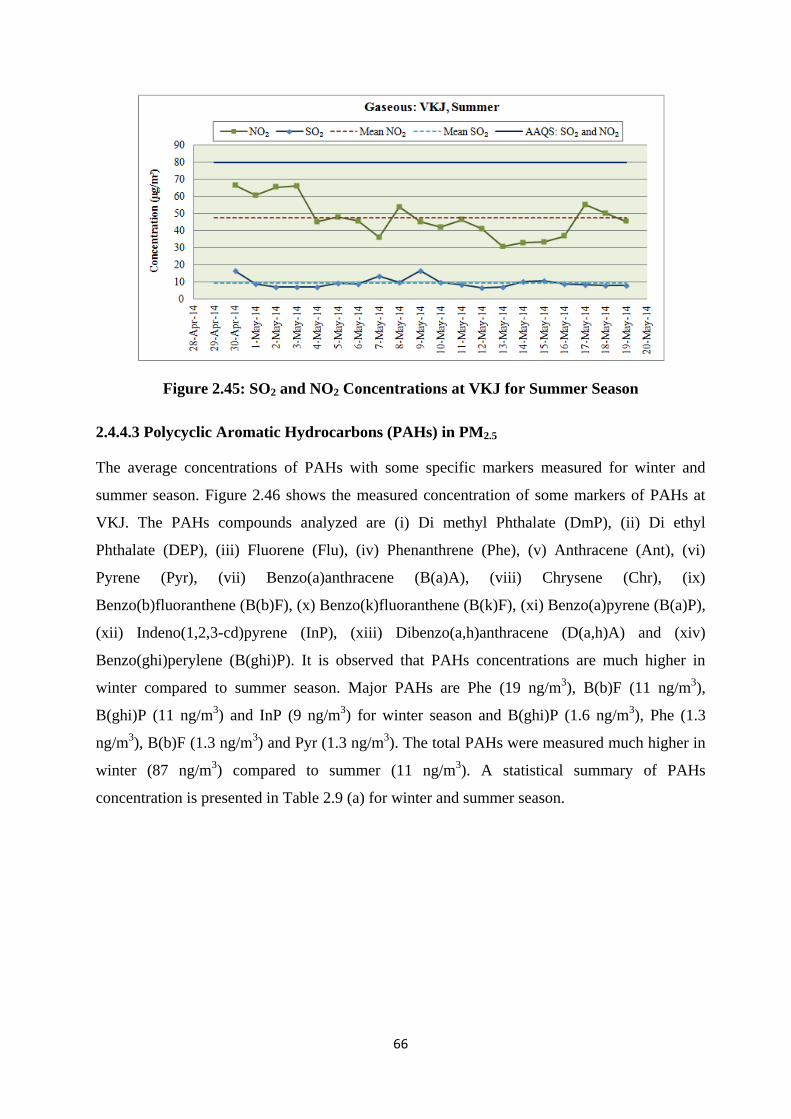
66
Figure 2.45: SO2 and NO2 Concentrations at VKJ for Summer Season
2.4.4.3 Polycyclic Aromatic Hydrocarbons (PAHs) in PM2.5
The average concentrations of PAHs with some specific markers measured for winter and
summer season. Figure 2.46 shows the measured concentration of some markers of PAHs at
VKJ. The PAHs compounds analyzed are (i) Di methyl Phthalate (DmP), (ii) Di ethyl
Phthalate (DEP), (iii) Fluorene (Flu), (iv) Phenanthrene (Phe), (v) Anthracene (Ant), (vi)
Pyrene (Pyr), (vii) Benzo(a)anthracene (B(a)A), (viii) Chrysene (Chr), (ix)
Benzo(b)fluoranthene (B(b)F), (x) Benzo(k)fluoranthene (B(k)F), (xi) Benzo(a)pyrene (B(a)P),
(xii) Indeno(1,2,3-cd)pyrene (InP), (xiii) Dibenzo(a,h)anthracene (D(a,h)A) and (xiv)
Benzo(ghi)perylene (B(ghi)P). It is observed that PAHs concentrations are much higher in
winter compared to summer season. Major PAHs are Phe (19 ng/m3), B(b)F (11 ng/m
3),
B(ghi)P (11 ng/m3) and InP (9 ng/m
3) for winter season and B(ghi)P (1.6 ng/m
3), Phe (1.3
ng/m3), B(b)F (1.3 ng/m
3) and Pyr (1.3 ng/m
3). The total PAHs were measured much higher in
winter (87 ng/m3) compared to summer (11 ng/m
3). A statistical summary of PAHs
concentration is presented in Table 2.9 (a) for winter and summer season.

67
Figure 2.46: PAHs Concentrations in PM2.5 at VKJ for winter and Summer Seasons
2.4.4.4 Elemental and Organic Carbon Content (EC/OC) in PM2.5
Average concentrations of EC, OC (OC1, OC2, OC3 and OC4) and ratio of OC fraction to TC
are shown in Figure 2.47 (a) and (b) for winter and summer season. Organic carbon is observed
higher than the elemental carbon. However the ratio of OC3/TC is observed higher that
indicates the formation of secondary organic carbon in atmosphere at VKJ. It is also observed
that the OC and EC are higher in winter than summer season. A statistical summary of carbon
content (TC, EC, OC; OC1, OC2, OC3 and OC4 with fractions OC1/TC, OC2/TC, OC3/TC
and OC4/TC) is presented in Table 2.9 (b) for winter and summer seasons.
Figure 2.47: EC and OC Content in PM2.5 at VKJ for Winter and Summer Seasons

68
2.4.4.5 Chemical Composition of PM10 and PM2.5 and their correlation matrix
Graphical presentations of chemical species are shown for winter and summer season for PM10
(Figure 2.48) and PM2.5 (Figure 2.49). Statistical summary (Mean, maximum, minimum,
standard deviation (SD) and coefficient of variation (CV)) of analysis for particulate matter
(PM10 and PM2.5), its chemical composition [carbon content (EC and OC), ionic species (F⁻,
Cl⁻, NO₃⁻, SO₄⁻², Na⁺, NH₄⁺, K⁺, Ca⁺², Mg⁺²) and elements (Be, B, Na, Mg, Al, Si, P, K, Ca,
Cr, V, Mn, Fe, Co, Ni, Cu, Zn, As, Se, Rb, Sr, Cd, Cs, Ba, Pb)] along with mass percentage (%
R) estimated in composition and gaseous pollutant (NO2 and SO2) are presented in the Table
2.9 (c), (d), (e) and (f) for winter and summer season. The correlation between different
parameters (i.e PM, NO₂, SO₂, TC, OC, EC, F⁻, Cl⁻, NO₃⁻, SO₄⁻², Na⁺, NH₄⁺, K⁺, Ca⁺², Mg⁺²
and Metals (elements) with major species (PM, TC, OC, EC, NO₃⁻, SO₄⁻², NH₄⁺, Metals) for
PM10 and PM2.5 composition is presented in Table 2.9 (g), (h), (i) and (j) for both season. It is
seen that most of parameters showed good correlation (>0.30) with PM10 and PM2.5. The
percentage constituent of the PM are presented in Figure 2.50 (a) and (b) for winter season and
Figure 2.51 (a) and (b) for summer season.
Figure 2.48: Concentrations of species in PM10 at VKJ for Winter and Summer Seasons

69
Figure 2.49: Concentrations of species in PM2.5 at VKJ for Winter and Summer Seasons
Figure 2.50: Percentage distribution of species in PM at VKJ for Winter Season

70
Figure 2.51: Percentage distribution of species in PM at VKJ for Summer Season
2.4.4.6 Comparison of PM10 and PM2.5 Composition
This section presents some important observations from the experimental findings related to
fine particles and coarse particle concentrations. The graphical presentation is the better option
for understanding the compositional variation. Compositional comparisons of PM2.5 Vs PM10
for all species are shown for winter season (Figure 2.52) and summer season (Figure 2.53) at
VKJ.
The chemical species considered for the comparisons are carbon content (TC, OC and EC),
ionic species (F⁻, Cl⁻, NO₃⁻, SO₄⁻², Na⁺, NH₄⁺, K⁺, Ca⁺², Mg⁺²) and elements (Be, B, Na,
Mg, Al, Si, P, K, Ca, Cr, V, Mn, Fe, Co, Ni, Cu, Zn, As, Se, Rb, Sr, Cd, Cs, Ba, Pb). It is
concluded that most portion of PM is having fine mode during winter (57 %) than summer (61
%). The major species contributing to fine mode are TC, EC, OC, NO₃⁻, SO₄⁻², Na⁺, NH₄⁺,
K⁺, V, Co, Cu, Sr, Cd, Cs and Pb; whereas, major species contributing in coarse mode are
Ca2+
, Mg2+
, Al, Si, Cr, Fe and Ni.
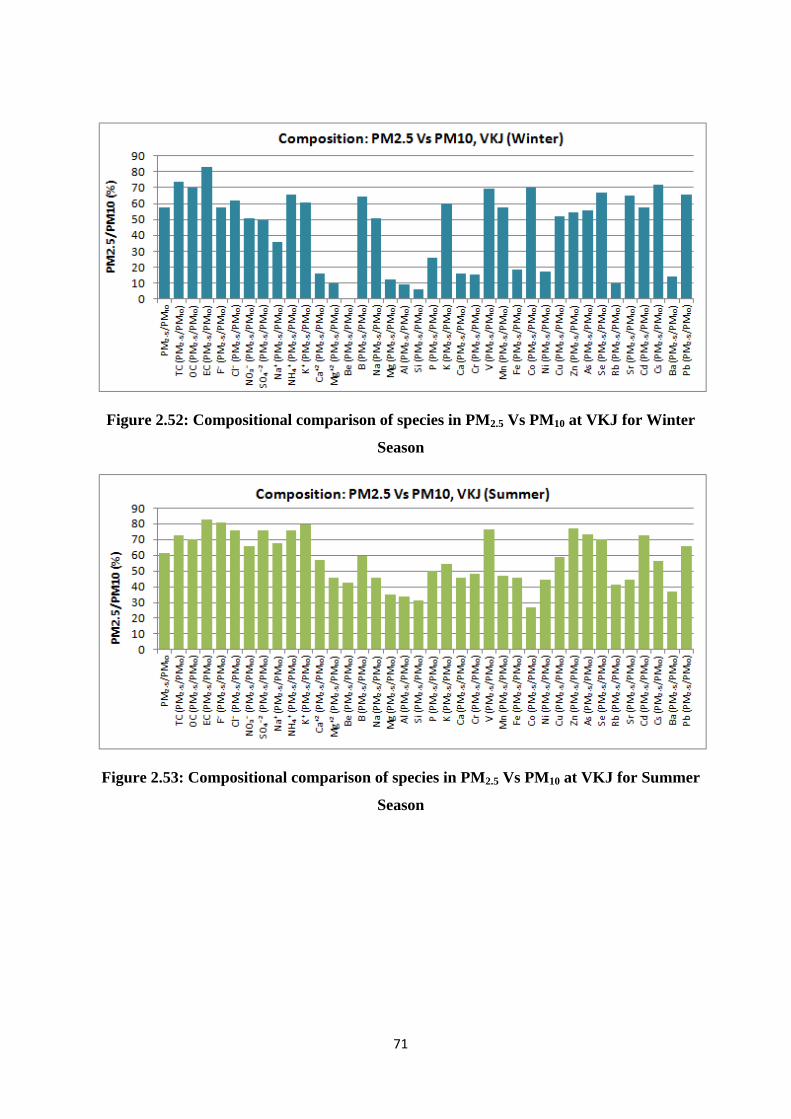
71
Figure 2.52: Compositional comparison of species in PM2.5 Vs PM10 at VKJ for Winter
Season
Figure 2.53: Compositional comparison of species in PM2.5 Vs PM10 at VKJ for Summer
Season

72
Table 2.46(a): Statistical Results of PAHs (ng/m3) in PM2.5 at VKJ for Winter (W) and Summer (S) Seasons
VKJ(W) DmP DEP Flu Phe Ant Pyr B(a)A Chr B(b)F B(k)F B(a)P InP D(a,h)A B(ghi)P Total PAHs
Mean 8.52 0.00 3.23 18.64 0.08 4.04 2.84 7.37 10.91 2.35 6.98 9.35 2.07 10.68 87.05
SD 7.22 0.00 2.68 12.99 0.14 1.88 2.52 3.68 4.92 1.16 4.66 5.84 2.28 5.05 31.11
Max 25.07 0.00 8.47 40.78 0.41 7.87 8.14 14.59 20.99 4.26 16.39 19.57 6.57 19.85 132.07
Min 2.36 0.00 0.78 6.33 0.00 1.65 0.32 3.11 4.73 0.81 2.14 0.95 0.00 3.91 30.83
CV 0.85 0.00 0.83 0.70 1.68 0.47 0.89 0.50 0.45 0.49 0.67 0.62 1.10 0.47 0.36
VKJ(S) DmP DEP Flu Phe Ant Pyr B(a)A Chr B(b)F B(k)F B(a)P InP D(a,h)A B(ghi)P Total PAHs
Mean 1.21 1.23 0.07 1.33 0.07 1.31 0.00 0.66 1.31 0.00 0.72 0.84 0.36 1.64 10.75
SD 0.37 3.17 0.10 0.44 0.10 1.26 0.00 0.67 0.92 0.00 0.90 0.82 0.91 1.29 4.93
Max 2.05 10.17 0.33 2.17 0.27 4.40 0.00 2.33 3.27 0.00 3.03 2.59 2.91 4.35 18.06
Min 0.88 0.00 0.00 0.81 0.00 0.30 0.00 0.08 0.16 0.00 0.00 0.00 0.00 0.00 5.57
CV 0.30 2.58 1.45 0.33 1.53 0.96 0.00 1.01 0.70 0.00 1.25 0.97 2.55 0.78 0.46
Table 2.47(b): Statistical Results of Carbon Contents (µg/m3) in PM2.5 at VKJ for Winter (W) and Summer (S) Seasons
VKJ (W) PM2.5 TC EC OC OC1 OC2 OC3 OC4 OC1/TC OC2/TC OC3/TC OC4/TC
Mean 315 79.1 26.9 52.2 5.4 13.6 18.0 15.2 0.068 0.171 0.226 0.188
Max 574 129.4 39.9 92.1 9.9 24.1 31.0 30.4 0.103 0.198 0.262 0.270
Min 181 37.5 16.0 19.9 1.8 6.2 7.7 4.2 0.042 0.154 0.204 0.103
SD 104 25.4 7.8 19.2 2.2 4.7 6.5 7.5 0.020 0.013 0.016 0.051
CV 0.33 0.32 0.29 0.37 0.41 0.35 0.36 0.49 0.292 0.076 0.073 0.272
VKJ (S) PM2.5 TC EC OC OC1 OC2 OC3 OC4 OC1/TC OC2/TC OC3/TC OC4/TC
Mean 252 22.7 8.7 14.5 0.8 4.0 5.6 3.9 0.035 0.177 0.246 0.178
Max 357 53.6 20.2 33.3 3.2 8.7 15.0 7.8 0.064 0.269 0.361 0.245
Min 120 11.2 4.2 7.0 0.3 1.8 2.7 1.6 0.018 0.153 0.201 0.121
SD 71 11.5 4.3 7.1 0.7 1.9 3.1 1.6 0.012 0.025 0.034 0.030
CV 0.28 0.51 0.50 0.49 0.86 0.49 0.56 0.41 0.354 0.140 0.138 0.166

73
Table 2.48(c): Statistical Results of SO2, NO2 and Chemical Characterization (µg/m3) of PM10 at VKJ for Winter (W) Season
VKJ(W) PM₁₀ NO₂ SO₂ OC EC F⁻ Cl⁻ NO₃⁻ SO₄⁻² Na⁺ NH₄⁺ K⁺ Ca⁺² Mg⁺² Be B Na Mg Al Si
Mean 548 78 13 74.6 32.4 0.74 36.73 70.33 56.32 2.16 43.92 6.59 3.28 18.40 0.00 0.61 2.66 3.20 5.42 16.19
Max 960 125 25 131.5 48.1 2.24 101.38 164.05 154.10 5.18 79.70 11.78 27.15 43.78 0.00 1.14 5.23 6.55 11.04 32.09
Min 254 32 8 28.5 19.2 0.20 11.18 27.18 13.57 0.85 20.71 3.47 0.28 3.54 0.00 0.32 1.31 1.10 1.72 4.60
SD 187 29 5 27.4 9.4 0.50 22.28 38.25 43.00 1.23 18.08 2.72 6.11 11.41 0.00 0.27 1.13 1.63 2.80 8.14
CV 0.34 0.37 0.36 0.37 0.29 0.68 0.61 0.54 0.76 0.57 0.41 0.41 1.86 0.62 0.00 0.43 0.42 0.51 0.52 0.50
VKJ(W) P K Ca Cr V Mn Fe Co Ni Cu Zn As Se Rb Sr Cd Cs Ba Pb % R
Mean 0.55 9.02 8.78 0.32 0.90 0.31 9.19 0.17 0.02 0.17 1.99 0.07 0.03 0.02 0.23 0.04 0.18 0.16 0.96 69.9
Max 1.06 23.87 19.19 0.68 3.11 0.73 20.85 0.59 0.06 0.35 4.59 0.26 0.06 0.06 0.66 0.17 0.61 0.35 4.59 92.7
Min 0.14 4.46 2.87 0.11 0.23 0.12 3.91 0.05 0.01 0.05 0.66 0.02 0.01 0.01 0.09 0.00 0.05 0.05 0.13 53.2
SD 0.28 4.56 4.57 0.16 0.67 0.17 4.91 0.13 0.02 0.09 1.04 0.06 0.01 0.02 0.14 0.04 0.13 0.09 0.99 12.3
CV 0.51 0.51 0.52 0.51 0.75 0.54 0.53 0.75 0.65 0.54 0.52 0.82 0.49 0.62 0.63 0.95 0.75 0.58 1.03 0.18
% R is the % recovery of mass of collected particle through compositional analysis
Table 2.49(d): Statistical Results of SO2, NO2 and Chemical Characterization (µg/m3) of PM2.5 at VKJ for Winter (W) Season
VKJ(W) PM₂.₅ NO₂ SO₂ OC EC F⁻ Cl⁻ NO₃⁻ SO₄⁻² Na⁺ NH₄⁺ K⁺ Ca⁺² Mg⁺² Be B Na Mg Al Si
Mean 315 78 13 52.2 26.9 0.43 22.68 35.77 27.73 0.78 28.77 3.98 0.53 1.86 0.00 0.40 1.36 0.39 0.51 1.02
Max 574 125 25 92.1 39.9 1.22 56.11 91.11 61.44 2.12 53.16 7.61 4.39 8.03 0.00 0.81 3.18 1.57 1.62 3.15
Min 181 32 8 19.9 16.0 0.11 6.48 15.45 6.30 0.19 10.36 2.27 0.08 0.25 0.00 0.14 0.57 0.13 0.20 0.35
SD 104 29 5 19.2 7.8 0.30 15.49 20.47 17.20 0.54 12.43 1.69 0.97 1.80 0.00 0.19 0.63 0.35 0.35 0.64
CV 0.33 0.37 0.36 0.37 0.29 0.70 0.68 0.57 0.62 0.69 0.43 0.43 1.83 0.97 0.00 0.48 0.47 0.91 0.68 0.63
VKJ(W) P K Ca Cr V Mn Fe Co Ni Cu Zn As Se Rb Sr Cd Cs Ba Pb % R
Mean 0.14 5.43 1.40 0.05 0.62 0.18 1.68 0.12 0.00 0.09 1.08 0.04 0.02 0.00 0.15 0.03 0.13 0.02 0.63 67.4
Max 0.30 11.75 2.67 0.12 1.41 0.37 3.79 0.28 0.02 0.23 3.20 0.15 0.03 0.01 0.33 0.13 0.28 0.17 3.30 92.8
Min 0.04 2.20 0.60 0.02 0.22 0.07 0.59 0.04 0.00 0.01 0.46 0.01 0.01 0.00 0.05 0.00 0.04 0.00 0.12 51.2
SD 0.08 2.59 0.70 0.03 0.37 0.10 1.07 0.07 0.00 0.06 0.68 0.03 0.01 0.00 0.09 0.03 0.08 0.03 0.70 11.1
CV 0.56 0.48 0.50 0.60 0.60 0.54 0.64 0.63 1.09 0.69 0.63 0.90 0.43 1.06 0.59 1.12 0.61 1.53 1.11 0.16
% R is the % recovery of mass of collected particle through compositional analysis

74
Table 2.50(e): Statistical Results of SO2, NO2 and Chemical Characterization (µg/m3) of PM10 at VKJ for Summer (S) Season
VKJ(S) PM₁₀ NO₂ SO₂ OC EC F⁻ Cl⁻ NO₃⁻ SO₄⁻² Na⁺ NH₄⁺ K⁺ Ca⁺² Mg⁺² Be B Na Mg Al Si
Mean 410 47 10 20.8 10.5 0.77 21.15 17.42 24.46 1.40 14.53 6.10 1.87 17.95 0.00 0.99 4.86 9.32 28.52 89.33
Max 645 67 17 47.6 24.4 1.70 95.74 52.90 50.50 2.72 69.83 17.82 7.93 31.80 0.00 1.91 7.19 21.47 47.56 150.45
Min 275 31 7 10.0 5.1 0.41 1.78 6.50 10.53 0.47 1.74 1.76 0.50 10.93 0.00 0.18 2.79 3.73 12.34 30.59
SD 89 11 3 10.2 5.2 0.32 20.57 10.84 10.35 0.66 15.87 4.06 1.85 5.37 0.00 0.48 1.34 3.75 9.97 29.56
CV 0.22 0.23 0.31 0.49 0.50 0.42 0.97 0.62 0.42 0.47 1.09 0.66 0.99 0.30 0.69 0.48 0.27 0.40 0.35 0.33
VKJ(S) P K Ca Cr V Mn Fe Co Ni Cu Zn As Se Rb Sr Cd Cs Ba Pb % R
Mean 0.89 12.95 13.29 1.71 0.87 0.46 17.25 0.02 0.07 0.18 1.23 0.03 0.02 0.08 0.15 0.03 0.01 0.30 0.41 73.0
Max 1.59 22.03 20.63 2.93 1.35 0.84 28.80 0.11 0.23 0.51 2.99 0.07 0.07 0.12 0.23 0.13 0.02 0.52 1.02 91.0
Min 0.14 5.63 5.50 0.54 0.43 0.11 4.59 0.00 0.03 0.06 0.64 0.01 0.01 0.03 0.06 0.01 0.00 0.10 0.11 41.4
SD 0.40 4.73 3.75 0.48 0.26 0.20 6.25 0.03 0.04 0.13 0.58 0.02 0.01 0.03 0.05 0.03 0.00 0.11 0.24 13.3
CV 0.45 0.37 0.28 0.28 0.29 0.44 0.36 1.52 0.61 0.70 0.47 0.58 0.59 0.33 0.32 1.05 0.66 0.35 0.59 0.18
% R is the % recovery of mass of collected particle through compositional analysis
Table 2.51(f): Statistical Results of SO2, NO2 and Chemical Characterization (µg/m3) of PM2.5 at VKJ for Summer (S) Season
VKJ(S) PM₂.₅ NO₂ SO₂ OC EC F⁻ Cl⁻ NO₃⁻ SO₄⁻² Na⁺ NH₄⁺ K⁺ Ca⁺² Mg⁺² Be B Na Mg Al Si
Mean 252 47 10 14.5 8.7 0.62 16.08 11.46 18.54 0.94 10.98 4.87 1.06 8.18 0.00 0.59 2.22 3.27 9.61 27.72
Max 357 67 17 33.3 20.2 1.09 68.41 28.47 42.44 2.33 53.39 12.25 7.05 17.98 0.00 1.24 5.84 6.91 18.71 54.88
Min 120 31 7 7.0 4.2 0.23 0.72 3.95 1.27 0.17 1.41 1.32 0.06 1.80 0.00 0.04 0.48 0.63 2.88 8.38
SD 71 11 3 7.1 4.3 0.24 15.87 5.78 10.01 0.55 12.29 3.06 1.56 5.23 0.00 0.35 1.28 2.13 4.73 14.02
CV 0.28 0.23 0.31 0.49 0.50 0.39 0.99 0.50 0.54 0.58 1.12 0.63 1.47 0.64 0.77 0.60 0.58 0.65 0.49 0.51
VKJ(S) P K Ca Cr V Mn Fe Co Ni Cu Zn As Se Rb Sr Cd Cs Ba Pb % R
Mean 0.45 7.03 6.10 0.83 0.66 0.22 7.93 0.01 0.03 0.11 0.95 0.02 0.02 0.03 0.07 0.02 0.00 0.11 0.27 59.8
Max 1.26 17.43 10.81 1.64 1.07 0.53 17.25 0.01 0.07 0.27 2.40 0.05 0.05 0.08 0.17 0.11 0.01 0.28 0.59 89.4
Min 0.08 0.46 1.44 0.11 0.34 0.07 1.99 0.00 0.01 0.02 0.35 0.00 0.00 0.01 0.01 0.01 0.00 0.04 0.07 43.5
SD 0.31 4.03 3.09 0.42 0.20 0.12 4.91 0.00 0.02 0.07 0.48 0.01 0.01 0.02 0.04 0.02 0.00 0.06 0.17 11.6
CV 0.69 0.57 0.51 0.51 0.30 0.56 0.62 0.70 0.57 0.65 0.51 0.69 0.65 0.66 0.64 1.12 1.03 0.58 0.61 0.19
% R is the % recovery of mass of collected particle through compositional analysis

75
Table 2.52(g): Correlation Matrix for PM10 and its composition for Winter (W) Season
VKJ (W) PM₁₀ NO₂ SO₂ TC OC EC F⁻ Cl⁻ NO₃⁻ SO₄⁻² Na⁺ NH₄⁺ K⁺ Ca⁺² Mg⁺² Metals
PM₁₀ 1.00 0.43 -0.21 0.73 0.76 0.52 0.54 0.02 0.74 0.58 0.74 0.75 0.79 0.53 0.65 0.60
TC
0.63 0.03 1.00 0.98 0.84 0.27 -0.20 0.33 0.15 0.44 0.19 0.43 0.30 0.34 0.22
OC
0.57 0.02
1.00 0.72 0.34 -0.25 0.39 0.23 0.49 0.26 0.48 0.33 0.37 0.25
EC
0.65 0.06
1.00 0.01 -0.01 0.08 -0.09 0.20 -0.04 0.17 0.16 0.20 0.06
NO₃⁻
0.42 0.04
0.61 -0.08 1.00 0.78 0.72 0.85 0.84 0.40 0.68 0.66
SO₄⁻²
0.07 -0.17
0.87 -0.14
1.00 0.56 0.78 0.64 0.20 0.43 0.50
NH₄⁺
0.15 -0.26
0.63 0.27
0.67 1.00 0.86 0.43 0.57 0.56
Metals
0.35 0.17
0.47 0.11
0.57
0.72 0.19 0.65 1.00
Table 2.53(h): Correlation Matrix for PM2.5 and its composition for Winter (W) Season
VKJ (W) PM₂.₅ NO₂ SO₂ TC OC EC F⁻ Cl⁻ NO₃⁻ SO₄⁻² Na⁺ NH₄⁺ K⁺ Ca⁺² Mg⁺² Metals
PM₂.₅ 1.00 0.45 -0.33 0.79 0.77 0.70 0.37 0.12 0.68 0.59 0.53 0.70 0.66 0.27 -0.04 0.61
TC
0.64 0.04 1.00 0.98 0.85 0.52 -0.13 0.49 0.37 0.66 0.41 0.60 0.32 0.16 0.54
OC
0.57 0.02
1.00 0.72 0.61 -0.22 0.56 0.44 0.72 0.46 0.64 0.36 0.24 0.60
EC
0.65 0.06
1.00 0.19 0.11 0.24 0.11 0.37 0.19 0.38 0.16 -0.06 0.28
NO₃⁻
0.22 -0.19
0.53 -0.06 1.00 0.73 0.56 0.88 0.87 0.61 0.26 0.85
SO₄⁻²
0.17 -0.30
0.54 -0.24
1.00 0.31 0.83 0.55 0.29 0.33 0.80
NH₄⁺
0.14 -0.30
0.42 0.19
0.49 1.00 0.82 0.45 0.27 0.83
Metals
0.31 -0.19
0.63 -0.11
0.41
0.76 0.29 0.29 1.00

76
Table 2.54(i): Correlation Matrix for PM10 and its composition for Summer (S) Season
VKJ (S) PM₁₀ NO₂ SO₂ TC OC EC F⁻ Cl⁻ NO₃⁻ SO₄⁻² Na⁺ NH₄⁺ K⁺ Ca⁺² Mg⁺² Metals
PM₁₀ 1.00 -0.03 0.09 0.07 0.10 0.03 -0.22 0.48 -0.18 0.24 -0.05 0.41 0.03 -0.46 -0.43 0.11
TC
0.15 0.85 1.00 0.99 0.97 -0.22 0.16 -0.31 0.07 0.55 0.15 0.53 0.11 0.09 0.04
OC
0.21 0.81
1.00 0.94 -0.22 0.19 -0.31 0.07 0.58 0.17 0.54 0.09 0.11 0.05
EC
0.01 0.88
1.00 -0.21 0.11 -0.29 0.05 0.47 0.11 0.48 0.15 0.06 0.03
NO₃⁻
-0.31 -0.10
0.50 0.18 1.00 0.20 0.02 0.10 -0.25 0.31 0.19 -0.58
SO₄⁻²
-0.15 0.13
0.50 0.25
1.00 0.31 0.60 0.53 -0.05 -0.05 -0.20
NH₄⁺
-0.18 0.14
0.09 0.62
0.35 1.00 0.58 -0.09 -0.20 -0.25
Metals
0.45 -0.13
-0.17 -0.48
-0.13
0.05 -0.29 0.23 1.00
Table 2.55(j): Correlation Matrix for PM2.5 and its composition for Summer (S) Season
VKJ (S) PM₂.₅ NO₂ SO₂ TC OC EC F⁻ Cl⁻ NO₃⁻ SO₄⁻² Na⁺ NH₄⁺ K⁺ Ca⁺² Mg⁺² Metals
PM₂.₅ 1.00 -0.09 0.45 0.31 0.36 0.40 0.26 0.26 -0.01 0.41 0.07 0.32 0.43 0.04 0.23 0.61
TC
0.04 0.88 1.00 0.96 0.97 -0.15 0.25 -0.26 -0.05 0.46 0.19 0.66 -0.07 0.16 -0.16
OC
0.21 0.81
1.00 0.94 -0.19 0.24 -0.33 -0.06 0.47 0.20 0.64 -0.11 0.07 -0.10
EC
0.01 0.88
1.00 -0.16 0.18 -0.27 -0.06 0.42 0.13 0.59 -0.04 0.18 -0.04
NO₃⁻
-0.34 -0.10
0.38 0.08 1.00 0.00 -0.11 -0.07 -0.34 0.42 0.01 -0.07
SO₄⁻²
0.01 0.11
0.37 -0.08
1.00 0.11 0.38 0.43 0.00 0.12 0.43
NH₄⁺
-0.19 0.15
0.20 0.68
0.27 1.00 0.53 -0.15 0.08 0.18
Metals
0.17 -0.02
0.40 -0.18
0.18
0.23 0.30 0.51 1.00

77
2.4.5 Arwachin International School, Dilshad Garden (DSG)
The sampling period for winter is January 24, 2014 to February 13, 2014 and May 26, 2014 to
June 14, 2014 for summer season.
2.4.5.1 Particulate Matter (PM10, PM2.5)
For sampling of PM10 and PM2.5, the developed SOPs were followed. As a part of QA/QC,
20% of PM-laden filters (of PM10 and PM2.5) were reconditioned for 24 hrs and reweighed.
The variation in the concentration was less than 5%, which was acceptable.
Time series of 24-hr average concentrations of PM10 and PM2.5 are shown for winter (Figures
2.54) and summer (Figure 2.55). The air quality standards for both PM10 and PM2.5 are
exceeded. Although winter conditions provide low dispersion and high concentrations, the
levels of PM10 and PM2.5 are alarmingly high even in summer. Average levels for winter and
summer season are 435 and 276 µg/m3 (for PM2.5) and 675 and 503 µg/m3 (for PM10)
respectively
Figure 2.54: PM Concentrations at DSG for Winter Season

78
Figure 2.55: PM Concentrations at DSG for Summer Season
2.4.5.2 Sulphur Dioxide (SO2) and Nitrogen Dioxide (NO2)
Time series of 24-hr average concentrations of SO2 and NO2 are shown for winter (Figure
2.56) and summer (Figure 2.57). It was observed that SO2 concentrations were low and meet
the air quality standard. NO2 levels also exceed the air quality standard. The average NO2
concentration at DSG was 75 µg/m3 for winter and 69 µg/m
3 for summer season (Table 2.10
(c), (e)). The NO2 is certainly matter of concern and these values can largely be attributed to
vehicular pollution and DG sets. Like for PM pollution, massive efforts will be required to
improve the air quality for NO2. The NO2 is showing some episodic behavior which may be
due to variability in meteorology and presence of occasional local sources like DG sets or open
burning etc.
Figure 2.56: SO2 and NO2 Concentrations at DSG for Winter Season

79
Figure 2.57: SO2 and NO2 Concentrations at DSG for Summer Season
2.4.5.3 Polycyclic Aromatic Hydrocarbons (PAHs) in PM2.5
The average concentrations of PAHs with some specific markers measured for winter and
summer season. Figure 2.58 shows the measured concentration of some markers of PAHs at
DSG. The PAHs compounds analyzed are (i) Di methyl Phthalate (DmP), (ii) Di ethyl
Phthalate (DEP), (iii) Fluorene (Flu), (iv) Phenanthrene (Phe), (v) Anthracene (Ant), (vi)
Pyrene (Pyr), (vii) Benzo(a)anthracene (B(a)A), (viii) Chrysene (Chr), (ix)
Benzo(b)fluoranthene (B(b)F), (x) Benzo(k)fluoranthene (B(k)F), (xi) Benzo(a)pyrene (B(a)P),
(xii) Indeno(1,2,3-cd)pyrene (InP), (xiii) Dibenzo(a,h)anthracene (D(a,h)A) and (xiv)
Benzo(ghi)perylene (B(ghi)P). It is observed that PAHs concentrations are much higher (46
ng/m3)
in winter than in summer season (10 ng/m
3). Major PAHs are Phe (12 ng/m
3), B(ghi)P
(6 ng/m3), B(b)F (6 ng/m
3) and InP (4 ng/m
3) for winter season and B(ghi)P (2.7 ng/m
3), B(b)F
(1.8 ng/m3), InP (1.7 ng/m
3) and Phe (1.1 ng/m
3). The total PAHs were measured higher in
winter (46 ng/m3) compared to summer (11 ng/m
3). A statistical summary of PAHs
concentration is presented in Table 2.10 (a) for winter and summer season.

80
Figure 2.58: PAHs Concentrations in PM2.5 at DSG for winter and Summer Seasons
2.4.5.4 Elemental and Organic Carbon Content (EC/OC) in PM2.5
Average concentrations of EC, OC (OC1, OC2, OC3 and OC4) and ratio of OC fraction to TC
are shown in Figure 2.59 (a) and (b) for winter and summer season. Organic carbon is observed
higher than the elemental carbon. However the ratio of OC3/TC is observed higher that
indicates the formation of secondary organic carbon in atmosphere at DSG. It is also observed
that the OC and EC are higher in winter than summer season. A statistical summary of carbon
content (TC, EC, OC; OC1, OC2, OC3 and OC4 with fractions OC1/TC, OC2/TC, OC3/TC
and OC4/TC) is presented in Table 2.10 (b) for winter and summer seasons.
Figure 2.59: EC and OC Content in PM2.5 at DSG for Winter and Summer Seasons

81
2.4.5.5 Chemical Composition of PM10 and PM2.5 and their correlation matrix
Graphical presentation of chemical species are shown for winter and summer season for PM10
(Figure 2.60) and PM2.5 (Figure 2.61). Statistical summary (Mean, maximum, minimum,
standard deviation (SD) and coefficient of variation (CV)) of analysis for particulate matter
(PM10 and PM2.5), its chemical composition [carbon content (EC and OC), ionic species (F⁻,
Cl⁻, NO₃⁻, SO₄⁻², Na⁺, NH₄⁺, K⁺, Ca⁺², Mg⁺²) and elements (Be, B, Na, Mg, Al, Si, P, K, Ca,
Cr, V, Mn, Fe, Co, Ni, Cu, Zn, As, Se, Rb, Sr, Cd, Cs, Ba, Pb)] along with mass percentage (%
R) estimated in composition and gaseous pollutant (NO2 and SO2) are presented in the Table
2.10 (c), (d), (e) and (f) for winter and summer season. The correlation between different
parameters (i.e PM, NO₂, SO₂, TC, OC, EC, F⁻, Cl⁻, NO₃⁻, SO₄⁻², Na⁺, NH₄⁺, K⁺, Ca⁺², Mg⁺²
and Metals (elements) with major species (PM, TC, OC, EC, NO₃⁻, SO₄⁻², NH₄⁺, Metals) for
PM10 and PM2.5 composition is presented in Table 2.10 (g), (h), (i) and (j) for both season. It is
seen that most of parameters showed good correlation (>0.30) with PM10 and PM2.5. The
percentage constituent of the PM are presented in Figure 2.62 (a) and (b) for winter season and
Figure 2.63 (a) and (b) for summer season.
Figure 2.60: Concentrations of species in PM10 at DSG for Winter and Summer Seasons

82
Figure 2.61: Concentrations of species in PM2.5 at DSG for Winter and Summer Seasons
Figure 2.62: Percentage distribution of species in PM at DSG for Winter Season

83
Figure 2.63: Percentage distribution of species in PM at DSG for Summer Season
2.4.5.6 Comparison of PM10 and PM2.5 Composition
This section presents some important observations from the experimental findings related to
fine particles and coarse particle concentrations. The graphical presentation is the better option
for understanding the compositional variation. Compositional comparison of PM2.5 Vs PM10
for all species are shown for winter season (Figure 2.64) and summer season (figure 2.65) at
DSG.
The chemical species considered for the comparisons are carbon content (TC, OC and EC),
ionic species (F⁻, Cl⁻, NO₃⁻, SO₄⁻², Na⁺, NH₄⁺, K⁺, Ca⁺², Mg⁺²) and elements (Be, B, Na,
Mg, Al, Si, P, K, Ca, Cr, V, Mn, Fe, Co, Ni, Cu, Zn, As, Se, Rb, Sr, Cd, Cs, Ba, Pb). It is
concluded that most portion of PM is having fine mode during winter (64 %) than summer (65
%). The major species contributing to fine mode are TC, EC, OC, NO₃⁻, SO₄⁻², Na⁺, NH₄⁺,
K⁺, V, Co, Cu, Sr, Cd, Cs and Pb; whereas, major species contributing in coarse mode are
Ca2+
, Mg2+
, Al, Si, Cr, Fe and Ni.

84
Figure 2.64: Compositional comparison of species in PM2.5 Vs PM10 at DSG for Winter
Season
Figure 2.65: Compositional comparison of species in PM2.5 Vs PM10 at DSG for Summer
Season

85
Table 2.56(a): Statistical Results of PAHs (ng/m3) in PM2.5 at DSG for Winter (W) and Summer (S) Seasons
DSG(W) DmP DEP Flu Phe Ant Pyr B(a)A Chr B(b)F B(k)F B(a)P InP D(a,h)A B(ghi)P Total PAHs
Mean 5.16 0.00 1.80 11.71 0.00 1.35 1.15 3.68 6.46 1.74 2.98 4.13 0.54 5.68 46.40
SD 3.57 0.00 1.07 6.19 0.00 0.48 0.96 2.17 3.62 0.94 1.94 3.09 0.67 3.02 19.27
Max 9.72 0.00 3.92 22.94 0.00 2.34 2.94 7.88 14.35 3.88 7.24 10.45 2.08 12.85 88.03
Min 0.76 0.00 0.38 4.30 0.00 0.81 0.00 1.86 3.36 0.58 0.73 0.00 0.00 2.64 25.39
CV 0.69 0.00 0.59 0.53 0.00 0.36 0.84 0.59 0.56 0.54 0.65 0.75 1.24 0.53 0.42
DSG(S) DmP DEP Flu Phe Ant Pyr B(a)A Chr B(b)F B(k)F B(a)P InP D(a,h)A B(ghi)P Total PAHs
Mean 1.25 0.62 0.03 1.13 0.00 0.52 0.00 0.45 1.80 0.00 0.60 1.70 0.02 2.73 10.86
SD 0.31 1.82 0.04 0.20 0.00 0.22 0.00 0.31 1.11 0.00 0.75 1.89 0.07 1.67 6.09
Max 1.83 5.78 0.13 1.45 0.00 0.91 0.00 0.95 4.20 0.00 2.17 5.31 0.22 6.15 22.78
Min 0.86 0.00 0.00 0.85 0.00 0.15 0.00 0.00 0.37 0.00 0.00 0.00 0.00 0.41 3.50
CV 0.25 2.93 1.56 0.18 0.00 0.42 0.00 0.68 0.62 0.00 1.24 1.11 3.16 0.61 0.56
Table 2.57(b): Statistical Results of Carbon Contents (µg/m3) in PM2.5 at DSG for Winter (W) and Summer (S) Seasons
DSG (W) PM2.5 TC EC OC OC1 OC2 OC3 OC4 OC1/TC OC2/TC OC3/TC OC4/TC
Mean 435 61.0 20.6 40.4 2.7 10.2 13.7 12.3 0.042 0.169 0.230 0.210
Max 769 125.2 43.9 83.1 8.7 23.6 29.2 26.0 0.070 0.200 0.255 0.298
Min 158 26.5 8.7 17.8 0.6 4.4 6.4 5.5 0.016 0.092 0.120 0.053
SD 217 29.6 10.9 19.0 1.9 5.2 6.4 5.7 0.014 0.022 0.028 0.050
CV 0.50 0.48 0.53 0.47 0.70 0.51 0.47 0.47 0.322 0.128 0.121 0.238
DSG (S) PM2.5 TC EC OC OC1 OC2 OC3 OC4 OC1/TC OC2/TC OC3/TC OC4/TC
Mean 276 28.7 12.2 17.2 0.7 5.5 5.9 5.1 0.025 0.209 0.209 0.176
Max 467 46.8 19.9 27.2 1.5 18.2 10.7 9.2 0.045 0.984 0.265 0.225
Min 140 12.8 4.3 8.5 0.4 2.7 3.4 1.8 0.015 0.146 0.164 0.143
SD 104 9.8 4.4 5.7 0.2 3.3 2.0 2.1 0.008 0.183 0.020 0.026
CV 0.38 0.34 0.36 0.33 0.34 0.60 0.33 0.41 0.328 0.878 0.094 0.146

86
Table 2.58(c): Statistical Results of SO2, NO2 and Chemical Characterization (µg/m3) of PM10 at DSG for Winter (W) Season
DSG(W) PM₁₀ NO₂ SO₂ OC EC F⁻ Cl⁻ NO₃⁻ SO₄⁻² Na⁺ NH₄⁺ K⁺ Ca⁺² Mg⁺² Be B Na Mg Al Si
Mean 675 75 21 57.8 24.8 1.06 44.87 71.27 88.38 3.04 56.59 7.86 3.45 17.60 0.00 0.94 4.62 5.52 17.82 59.78
Max 1419 140 50 118.7 52.9 2.35 104.62 201.88 275.17 16.36 132.89 15.68 29.42 38.16 0.00 2.63 9.67 11.41 42.14 155.09
Min 280 34 7 25.4 10.5 0.30 8.94 27.40 32.33 1.21 15.74 4.37 0.51 5.52 0.00 0.27 1.94 1.87 4.54 8.26
SD 331 27 11 27.1 13.2 0.59 26.76 44.67 73.09 3.28 31.49 2.95 6.64 8.93 0.00 0.72 2.17 2.67 11.06 41.42
CV 0.49 0.36 0.52 0.47 0.53 0.56 0.60 0.63 0.83 1.08 0.56 0.38 1.93 0.51 0.00 0.77 0.47 0.48 0.62 0.69
DSG(W) P K Ca Cr V Mn Fe Co Ni Cu Zn As Se Rb Sr Cd Cs Ba Pb % R
Mean 1.15 12.06 12.61 0.93 0.96 0.45 17.81 0.21 0.05 1.74 11.13 0.08 0.05 0.04 0.29 1.59 0.22 0.36 1.98 73.8
Max 2.37 25.60 26.00 2.44 1.88 0.86 38.97 0.45 0.26 9.19 58.09 0.20 0.10 0.12 0.54 27.04 0.46 0.88 7.46 90.9
Min 0.45 5.91 3.89 0.29 0.37 0.22 6.18 0.08 0.00 0.15 1.45 0.03 0.02 0.01 0.13 0.01 0.08 0.09 0.53 51.0
SD 0.58 5.96 6.49 0.56 0.45 0.20 9.48 0.11 0.06 2.20 14.81 0.05 0.02 0.03 0.13 6.00 0.11 0.21 1.84 9.7
CV 0.50 0.49 0.51 0.60 0.47 0.45 0.53 0.51 1.28 1.26 1.33 0.60 0.50 0.74 0.43 3.77 0.50 0.57 0.93 0.13
% R is the % recovery of mass of collected particle through compositional analysis
Table 2.59(d): Statistical Results of SO2, NO2 and Chemical Characterization (µg/m3) of PM2.5 at DSG for Winter (W) Season
DSG(W) PM₂.₅ NO₂ SO₂ OC EC F⁻ Cl⁻ NO₃⁻ SO₄⁻² Na⁺ NH₄⁺ K⁺ Ca⁺² Mg⁺² Be B Na Mg Al Si
Mean 435 75 21 40.4 20.6 0.78 31.79 48.53 54.68 1.65 40.50 5.92 1.10 3.96 0.00 0.46 2.55 0.90 1.43 3.30
Max 769 140 50 83.1 43.9 2.12 79.27 124.02 133.71 6.36 91.43 10.53 8.16 13.93 0.00 1.06 5.20 3.14 4.84 8.62
Min 158 34 7 17.8 8.7 0.25 6.34 17.49 20.91 0.41 13.90 2.98 0.15 0.24 0.00 0.20 0.99 0.14 0.30 0.76
SD 217 27 11 19.0 10.9 0.46 20.59 26.99 34.41 1.32 23.58 2.07 1.89 4.53 0.00 0.28 1.13 0.84 1.22 1.96
CV 0.50 0.36 0.52 0.47 0.53 0.59 0.65 0.56 0.63 0.80 0.58 0.35 1.72 1.14 0.00 0.62 0.45 0.93 0.85 0.59
DSG(W) P K Ca Cr V Mn Fe Co Ni Cu Zn As Se Rb Sr Cd Cs Ba Pb % R
Mean 0.46 6.65 2.91 0.11 0.80 0.29 5.54 0.16 0.01 0.96 6.15 0.06 0.04 0.00 0.23 0.66 0.19 0.06 1.55 65.5
Max 0.86 12.78 10.16 0.34 1.66 0.58 17.79 0.44 0.04 5.32 23.46 0.16 0.08 0.01 0.48 9.91 0.44 0.21 6.12 85.5
Min 0.12 2.54 0.79 0.00 0.31 0.11 1.01 0.05 0.00 0.03 0.49 0.01 0.01 0.00 0.09 0.00 0.07 0.01 0.31 41.6
SD 0.24 2.65 2.31 0.10 0.40 0.14 4.19 0.10 0.01 1.32 6.78 0.04 0.02 0.00 0.12 2.19 0.11 0.05 1.60 10.9
CV 0.52 0.40 0.79 0.89 0.50 0.49 0.76 0.63 1.67 1.38 1.10 0.69 0.47 2.46 0.51 3.32 0.55 0.91 1.03 0.17
% R is the % recovery of mass of collected particle through compositional analysis

87
Table 2.60(e): Statistical Results of SO2, NO2 and Chemical Characterization (µg/m3) of PM10 at DSG for Summer (S) Season
DSG(S) PM₁₀ NO₂ SO₂ OC EC F⁻ Cl⁻ NO₃⁻ SO₄⁻² Na⁺ NH₄⁺ K⁺ Ca⁺² Mg⁺² Be B Na Mg Al Si
Mean 503 69 15 24.6 14.7 0.88 21.90 16.64 30.15 3.24 11.40 4.38 1.87 20.98 0.00 0.82 6.83 12.02 38.41 138.44
Max 680 146 30 38.8 24.0 2.04 51.89 51.48 54.88 7.50 34.34 7.68 6.74 35.48 0.00 1.70 10.90 20.28 63.97 229.11
Min 323 42 6 12.2 5.2 0.28 7.45 4.93 13.74 0.97 4.22 2.22 0.50 11.34 0.00 0.28 4.38 6.03 21.49 80.40
SD 113 25 8 8.1 5.4 0.44 15.65 10.96 12.34 1.74 6.87 1.52 1.59 7.15 0.00 0.33 1.94 4.58 14.03 47.19
CV 0.22 0.36 0.52 0.33 0.36 0.50 0.71 0.66 0.41 0.54 0.60 0.35 0.85 0.34 0.28 0.41 0.28 0.38 0.37 0.34
DSG(S) P K Ca Cr V Mn Fe Co Ni Cu Zn As Se Rb Sr Cd Cs Ba Pb % R
Mean 1.19 15.40 17.08 2.10 0.79 0.60 23.92 0.01 0.09 1.87 4.35 0.04 0.02 0.09 0.17 0.62 0.01 0.42 1.60 78.2
Max 2.57 21.06 36.74 3.15 1.91 0.83 36.34 0.03 0.18 7.99 10.46 0.07 0.05 0.14 0.38 4.66 0.02 0.81 3.83 92.6
Min 0.74 9.94 10.16 1.33 0.40 0.35 14.03 0.01 0.04 0.30 1.19 0.02 0.01 0.06 0.10 0.01 0.00 0.27 0.62 42.9
SD 0.41 3.58 6.88 0.58 0.39 0.16 7.25 0.00 0.04 1.97 2.55 0.02 0.01 0.03 0.07 1.16 0.00 0.12 0.76 13.9
CV 0.35 0.23 0.40 0.28 0.50 0.26 0.30 0.38 0.47 1.05 0.59 0.37 0.56 0.29 0.40 1.88 0.72 0.28 0.48 0.18
% R is the % recovery of mass of collected particle through compositional analysis
Table 2.61(f): Statistical Results of SO2, NO2 and Chemical Characterization (µg/m3) of PM2.5 at DSG for Summer (S) Season
DSG(S) PM₂.₅ NO₂ SO₂ OC EC F⁻ Cl⁻ NO₃⁻ SO₄⁻² Na⁺ NH₄⁺ K⁺ Ca⁺² Mg⁺² Be B Na Mg Al Si
Mean 276 69 15 17.2 12.2 0.65 10.48 12.36 24.90 1.55 9.46 3.33 0.85 4.61 0.00 0.46 2.75 2.59 14.23 29.59
Max 467 146 30 27.2 19.9 1.86 46.18 40.98 48.63 4.02 32.91 6.13 4.06 17.12 0.00 1.15 9.06 5.01 27.58 61.93
Min 140 42 6 8.5 4.3 0.18 1.05 4.17 13.22 0.20 2.76 1.47 0.19 0.38 0.00 0.09 1.49 1.50 5.10 11.82
SD 104 25 8 5.7 4.4 0.42 9.71 8.63 10.40 1.13 6.67 1.21 1.08 5.23 0.00 0.28 1.78 1.08 6.28 15.68
CV 0.38 0.36 0.52 0.33 0.36 0.64 0.93 0.70 0.42 0.73 0.71 0.36 1.27 1.13 0.80 0.61 0.65 0.42 0.44 0.53
DSG(S) P K Ca Cr V Mn Fe Co Ni Cu Zn As Se Rb Sr Cd Cs Ba Pb % R
Mean 0.65 6.46 7.89 0.69 0.60 0.16 3.53 0.00 0.02 0.90 2.60 0.03 0.01 0.02 0.06 0.27 0.00 0.07 0.87 61.7
Max 1.47 11.03 23.99 2.02 1.64 0.68 8.31 0.02 0.07 3.26 5.59 0.05 0.04 0.11 0.19 2.30 0.02 0.32 1.70 87.5
Min 0.24 3.35 2.71 0.27 0.28 0.04 1.61 0.00 0.01 0.10 0.65 0.01 0.00 0.01 0.01 0.01 0.00 0.01 0.27 42.6
SD 0.35 2.17 5.47 0.43 0.37 0.16 1.65 0.00 0.02 0.88 1.53 0.01 0.01 0.02 0.04 0.51 0.00 0.07 0.45 14.8
CV 0.54 0.34 0.69 0.62 0.61 0.97 0.47 1.32 0.78 0.98 0.59 0.36 0.57 1.18 0.73 1.89 1.93 1.05 0.52 0.24
% R is the % recovery of mass of collected particle through compositional analysis

88
Table 2.62(g): Correlation Matrix for PM10 and its composition for Winter (W) Season
DSG (W) PM₁₀ NO₂ SO₂ TC OC EC F⁻ Cl⁻ NO₃⁻ SO₄⁻² Na⁺ NH₄⁺ K⁺ Ca⁺² Mg⁺² Metals
PM₁₀ 1.00 0.27 0.26 0.87 0.89 0.79 0.71 0.70 0.63 0.84 0.37 0.83 0.79 0.07 0.58 0.83
TC
0.28 0.19 1.00 0.99 0.98 0.59 0.80 0.45 0.58 0.33 0.55 0.72 0.26 0.70 0.79
OC
0.32 0.21
1.00 0.95 0.63 0.79 0.49 0.62 0.36 0.59 0.73 0.24 0.69 0.80
EC
0.19 0.14
1.00 0.48 0.81 0.34 0.48 0.25 0.45 0.67 0.30 0.69 0.72
NO₃⁻
0.37 0.00
0.78 0.43 1.00 0.55 0.48 0.72 0.45 -0.09 0.30 0.41
SO₄⁻²
0.26 0.39
0.57 0.40
1.00 0.20 0.90 0.66 -0.13 0.32 0.60
NH₄⁺
0.27 0.20
0.65 0.46
0.33 1.00 0.61 -0.06 0.30 0.53
Metals
0.36 0.34
0.69 0.63
0.52
0.71 0.16 0.77 1.00
Table 2.63(h): Correlation Matrix for PM2.5 and its composition for (W) Winter Season
DSG (W) PM₂.₅ NO₂ SO₂ TC OC EC F⁻ Cl⁻ NO₃⁻ SO₄⁻² Na⁺ NH₄⁺ K⁺ Ca⁺² Mg⁺² Metals
PM₂.₅ 1.00 0.42 0.25 0.76 0.80 0.67 0.68 0.49 0.74 0.83 0.52 0.74 0.62 0.36 0.45 0.92
TC
0.28 0.18 1.00 0.99 0.98 0.36 0.76 0.40 0.55 0.44 0.49 0.69 0.53 0.24 0.71
OC
0.32 0.21
1.00 0.95 0.41 0.74 0.46 0.61 0.49 0.53 0.71 0.51 0.25 0.75
EC
0.19 0.14
1.00 0.27 0.79 0.27 0.43 0.35 0.40 0.64 0.53 0.22 0.62
NO₃⁻
0.61 0.25
0.62 0.09 1.00 0.79 0.70 0.80 0.39 -0.06 0.30 0.68
SO₄⁻²
0.40 0.40
0.50 0.25
1.00 0.45 0.89 0.56 -0.04 0.26 0.78
NH₄⁺
0.37 0.35
0.45 0.31
0.43 1.00 0.52 -0.10 0.21 0.72
Metals
0.43 0.26
0.71 0.49
0.55
0.76 0.43 0.56 1.00

89
Table 2.64(i): Correlation Matrix for PM10 and its composition for Summer (S) Season
DSG (S) PM₁₀ NO₂ SO₂ TC OC EC F⁻ Cl⁻ NO₃⁻ SO₄⁻² Na⁺ NH₄⁺ K⁺ Ca⁺² Mg⁺² Metals
PM₁₀ 1.00 0.30 -0.12 -0.35 -0.25 -0.45 0.58 0.25 0.40 0.38 0.66 0.23 0.07 0.27 0.62 0.58
TC
0.36 0.70 1.00 0.96 0.91 -0.61 -0.34 -0.59 0.04 -0.32 -0.16 0.34 -0.44 -0.44 -0.56
OC
0.42 0.75
1.00 0.77 -0.59 -0.37 -0.57 0.06 -0.23 -0.16 0.26 -0.46 -0.40 -0.42
EC
0.26 0.62
1.00 -0.54 -0.25 -0.54 0.02 -0.40 -0.12 0.41 -0.36 -0.43 -0.70
NO₃⁻
-0.28 -0.39
0.66 0.25 1.00 0.20 0.41 0.47 -0.06 0.45 0.67 0.53
SO₄⁻²
0.35 0.28
0.55 0.05
1.00 0.48 0.53 0.44 0.07 0.58 0.29
NH₄⁺
0.00 0.13
0.66 0.52
0.25 1.00 0.12 -0.24 0.39 0.16
Metals
-0.31 -0.54
0.49 0.12
0.66
-0.06 0.49 0.74 1.00
Table 2.65(j): Correlation Matrix for PM2.5 and its composition for Summer (S) Season
DSG (S) PM₂.₅ NO₂ SO₂ TC OC EC F⁻ Cl⁻ NO₃⁻ SO₄⁻² Na⁺ NH₄⁺ K⁺ Ca⁺² Mg⁺² Metals
PM₂.₅ 1.00 -0.29 -0.30 -0.30 -0.45 -0.30 0.57 0.46 0.63 0.57 0.38 0.45 0.27 0.19 0.51 0.73
TC
0.36 0.70 1.00 0.81 0.99 -0.67 -0.32 -0.58 0.05 -0.23 -0.09 0.38 -0.34 -0.41 -0.33
OC
0.42 0.75
1.00 0.77 -0.67 -0.43 -0.63 -0.01 -0.33 -0.15 0.22 -0.40 -0.48 -0.36
EC
0.26 0.62
1.00 -0.70 -0.33 -0.62 -0.03 -0.28 -0.15 0.36 -0.32 -0.40 -0.33
NO₃⁻
-0.25 -0.36
0.83 0.64 1.00 0.27 0.57 0.53 -0.06 0.42 0.53 0.69
SO₄⁻²
0.26 0.20
0.34 0.20
1.00 0.55 0.55 0.42 -0.02 0.25 0.35
NH₄⁺
0.00 0.10
0.54 0.84
0.27 1.00 0.03 -0.18 -0.15 0.24
Metals
-0.38 -0.30
0.62 0.28
0.60
0.49 0.58 0.65 1.00

90
2.4.6 DTEA School, Pusa Road (PUS)
The sampling period for winter is January 30, 2014 to February 22, 2014 and May 25, 2014 to
June 16, 2014 for summer season.
2.4.6.1 Particulate Matter (PM10, PM2.5)
For sampling of PM10 and PM2.5, the developed SOPs were followed. As a part of QA/QC,
20% of PM-laden filters (of PM10 and PM2.5) were reconditioned for 24 hrs and reweighed.
The variation in the concentration was less than 5%, which was acceptable.
Time series of 24-hr average concentrations of PM10 and PM2.5 are shown for winter (Figures
2.66) and summer season (Figure 2.67). The air quality standards for both PM10 and PM2.5 are
exceeded. Although summer conditions (e.g. wind storms, low humidity and high temperature)
provide high turbulence to dispersion, the levels of PM10 and PM2.5 are alarmingly high in
summer for PM10. Average levels for winter and summer season are 278 and 269 µg/m3 (for
PM2.5) and 473 and 534 µg/m3 (for PM10) respectively.
Figure 2.66: PM Concentrations at PUS for Winter Season

91
Figure 2.67: PM Concentrations at PUS for Summer Season
2.4.6.2 Sulphur Dioxide (SO2) and Nitrogen Dioxide (NO2)
Time series of 24-hr average concentrations of SO2 and NO2 are shown for winter (Figure
2.68) and summer (Figure 2.69). It was observed that SO2 concentrations were low and meet
the air quality standard. NO2 levels also exceed the air quality standard. The average NO2
concentration at PUS was 87 µg/m3 for winter and 85 µg/m
3 for summer season (Table 2.11
(c), (e)). The NO2 is certainly matter of concern and these values can largely be attributed to
vehicular pollution and DG sets. Like for PM pollution, massive efforts will be required to
improve the air quality for NO2. The NO2 is showing some episodic behavior which may be
due to variability in meteorology and presence of occasional local sources like DG sets or open
burning etc.
Figure 2.68: SO2 and NO2 Concentrations at PUS for Winter Season

92
Figure 2.69: SO2 and NO2 Concentrations at PUS for Summer Season
2.4.6.3 Carbon monoxide (CO)
Hourly concentration of CO was observed at PUS for winter and summer seasons (Figure
2.45). It can be that the maximum concentration is observed during the peak traffic hours of the
day (both in morning as well as evening). It was observed that maximum concentration peak
(winter – 5.0 mg/m3 and summer - 2.6 mg/m
3) was higher in evening hours than in the morning
hours. The levels exceed the CO standard (4 mg/m3) at PUS in winter season during peak
traffic hours. However in summer CO levels meet the standard.
Figure 2.70: Hourly average concentration of CO at PUS for winter and summer seasons
2.4.6.4 Polycyclic Aromatic Hydrocarbons (PAHs) in PM2.5
The average concentrations of PAHs with some specific markers measured for winter and
summer season. Figure 2.71 shows the measured concentration of some markers of PAHs at

93
PUS. The PAHs compounds analyzed are (i) Di methyl Phthalate (DmP), (ii) Di ethyl
Phthalate (DEP), (iii) Fluorene (Flu), (iv) Phenanthrene (Phe), (v) Anthracene (Ant), (vi)
Pyrene (Pyr), (vii) Benzo(a)anthracene (B(a)A), (viii) Chrysene (Chr), (ix)
Benzo(b)fluoranthene (B(b)F), (x) Benzo(k)fluoranthene (B(k)F), (xi) Benzo(a)pyrene (B(a)P),
(xii) Indeno(1,2,3-cd)pyrene (InP), (xiii) Dibenzo(a,h)anthracene (D(a,h)A) and (xiv)
Benzo(ghi)perylene (B(ghi)P). It is observed that PAHs concentrations are much higher in
winter compared to summer season. Major PAHs are Phe (6.6 ng/m3), B(b)F (4.4 ng/m
3),
B(ghi)P (4.1 ng/m3) and DmP ((2.7 ng/m
3) for winter season and B(ghi)P (2.3 ng/m
3), DEP
(2.1 ng/m3), Phe (1.1 ng/m
3) and InP (0.9 ng/m
3). The total PAHs were measured higher in
winter (29 ng/m3) compared to summer (9 ng/m
3). A statistical summary of PAHs
concentration is presented in Table 2.11 (a) for winter and summer seasons.
Figure 2.71: PAHs Concentrations in PM2.5 at PUS for Winter and Summer Seasons
2.4.6.5 Elemental and Organic Carbon Content (EC/OC) in PM2.5
Average concentrations of EC, OC (OC1, OC2, OC3 and OC4) and ratio of OC fraction to TC
are shown in Figure 2.72 (a) and (b) for winter and summer season. Organic carbon is observed
higher than the elemental carbon. However the ratio of OC3/TC is observed higher that
indicates the formation of secondary organic carbon in atmosphere at PUS. It is also observed
that the OC and EC are higher in winter than summer season. A statistical summary of carbon
content (TC, EC, OC; OC1, OC2, OC3 and OC4 with fractions OC1/TC, OC2/TC, OC3/TC
and OC4/TC) is presented in Table 2.11 (b) for winter and summer seasons.

94
Figure 2.72: EC and OC Content in PM2.5 at PUS for Winter and Summer Seasons
2.4.6.6 Chemical Composition of PM10 and PM2.5 and their correlation matrix
Graphical presentation of chemical species are shown for winter and summer season for PM10
(Figure 2.73) and PM2.5 (Figure 2.74). Statistical summary (Mean, maximum, minimum,
standard deviation (SD) and coefficient of variation (CV)) of analysis for particulate matter
(PM10 and PM2.5), its chemical composition [carbon content (EC and OC), ionic species (F⁻,
Cl⁻, NO₃⁻, SO₄⁻², Na⁺, NH₄⁺, K⁺, Ca⁺², Mg⁺²) and elements (Be, B, Na, Mg, Al, Si, P, K, Ca,
Cr, V, Mn, Fe, Co, Ni, Cu, Zn, As, Se, Rb, Sr, Cd, Cs, Ba, Pb)] along with mass percentage (%
R) estimated in composition and gaseous pollutant (NO2 and SO2) are presented in the Table
2.11 (c), (d), (e) and (f) for winter and summer season. The correlation between different
parameters (i.e PM, NO₂, SO₂, TC, OC, EC, F⁻, Cl⁻, NO₃⁻, SO₄⁻², Na⁺, NH₄⁺, K⁺, Ca⁺², Mg⁺²
and Metals (elements) with major species (PM, TC, OC, EC, NO₃⁻, SO₄⁻², NH₄⁺, Metals) for
PM10 and PM2.5 composition is presented in Table 2.11 (g), (h), (i) and (j) for both season. It is
seen that most of parameters showed good correlation (>0.30) with PM10 and PM2.5. The
percentage constituent of the PM are presented in Figure 2.75 (a) and (b) for winter season and
Figure 2.76 (a) and (b) for summer season.

95
Figure 2.73: Concentrations of species in PM10 at PUS for Winter and Summer Seasons
Figure 2.74: Concentrations of species in PM2.5 at PUS for Winter and Summer Seasons

96
Figure 2.75: Percentage distribution of species in PM at PUS for Winter Season
Figure 2.76: Percentage distribution of species in PM at PUS for Summer Season

97
2.4.6.7 Comparison of PM10 and PM2.5 Composition
This section presents some important observations from the experimental findings related to
fine particles and coarse particle concentrations. The graphical presentation is the better option
for understanding the compositional variation. Compositional comparisons of PM2.5 Vs PM10
for all species are shown for winter season (Figure 2.77) and summer season (Figure 2.78) at
PUS.
The chemical species considered for the comparisons are carbon content (TC, OC and EC),
ionic species (F⁻, Cl⁻, NO₃⁻, SO₄⁻², Na⁺, NH₄⁺, K⁺, Ca⁺², Mg⁺²) and elements (Be, B, Na,
Mg, Al, Si, P, K, Ca, Cr, V, Mn, Fe, Co, Ni, Cu, Zn, As, Se, Rb, Sr, Cd, Cs, Ba, Pb). It is
concluded that most portion of PM is having fine mode during winter (70 %) than summer (60
%). The major species contributing to fine mode are TC, EC, OC, NO₃⁻, SO₄⁻², Na⁺, NH₄⁺,
K⁺, V, Co, Cu, Sr, Cd, Cs and Pb; whereas, major species contributing in coarse mode are
Ca2+
, Mg2+
, Al, Si, Cr, Fe and Ni.
Figure 2.77: Compositional comparison of species in PM2.5 Vs PM10 at PUS for Winter
Season

98
Figure 2.78: Compositional comparison of species in PM2.5 Vs PM10 at PUS for Summer
Season

99
Table 2.66(a): Statistical Results of PAHs (ng/m3) in PM2.5 at PUS for Winter (W) and Summer (S) Seasons
PUS(W) DmP DEP Flu Phe Ant Pyr B(a)A Chr B(b)F B(k)F B(a)P InP D(a,h)A B(ghi)P Total PAHs
Mean 2.67 0.06 0.63 6.59 0.00 1.33 0.82 2.52 4.38 0.84 2.08 2.56 0.18 4.13 28.80
SD 1.88 0.20 0.41 4.14 0.00 1.23 0.63 1.53 2.68 0.50 1.69 2.59 0.45 3.17 17.42
Max 6.53 0.66 1.49 16.90 0.00 4.89 2.13 6.32 9.94 1.84 5.61 8.81 1.49 10.83 70.05
Min 0.86 0.00 0.13 2.30 0.00 0.44 0.00 0.94 1.69 0.31 0.10 0.00 0.00 1.33 9.13
CV 0.71 3.32 0.65 0.63 0.00 0.92 0.77 0.61 0.61 0.60 0.81 1.01 2.49 0.77 0.60
PUS(S) DmP DEP Flu Phe Ant Pyr B(a)A Chr B(b)F B(k)F B(a)P InP D(a,h)A B(ghi)P Total PAHs
Mean 0.47 2.06 0.08 1.12 0.00 0.55 0.00 0.28 0.84 0.00 0.27 0.86 0.00 2.28 8.81
SD 0.22 3.78 0.12 0.55 0.00 0.25 0.00 0.19 0.43 0.00 0.27 0.85 0.00 0.96 4.50
Max 0.76 10.71 0.35 2.36 0.00 0.96 0.00 0.53 1.39 0.00 0.64 2.18 0.00 3.32 19.78
Min 0.13 0.00 0.00 0.57 0.00 0.23 0.00 0.00 0.00 0.00 0.00 0.00 0.00 0.58 1.84
CV 0.5 1.8 1.5 0.5 0.0 0.5 0.0 0.7 0.5 0.0 1.0 1.0 0.0 0.4 0.5
Table 2.67(b): Statistical Results of Carbon Contents (µg/m3) in PM2.5 at PUS for Winter (W) and Summer (S) Seasons
PUS (W) PM2.5 TC EC OC OC1 OC2 OC3 OC4 OC1/TC OC2/TC OC3/TC OC4/TC
Mean 278 54.2 18.6 35.5 2.9 10.2 12.1 10.3 0.050 0.186 0.224 0.196
Max 496 118.7 39.7 78.9 7.2 23.5 27.4 20.8 0.093 0.209 0.261 0.247
Min 127 23.2 8.0 15.2 0.6 4.0 4.8 4.8 0.027 0.165 0.199 0.138
SD 93 25.5 9.0 16.6 2.0 5.1 5.6 4.3 0.017 0.012 0.015 0.032
CV 0.34 0.47 0.48 0.47 0.70 0.50 0.46 0.42 0.329 0.064 0.065 0.161
PUS (S) PM2.5 TC EC OC OC1 OC2 OC3 OC4 OC1/TC OC2/TC OC3/TC OC4/TC
Mean 269 24.0 10.5 13.4 0.5 4.0 5.0 4.0 0.024 0.168 0.218 0.162
Max 578 38.5 20.1 19.8 0.8 5.9 7.3 6.8 0.035 0.192 0.492 0.197
Min 116 11.7 2.8 7.0 0.3 2.0 2.8 1.2 0.015 0.142 0.178 0.094
SD 105 8.3 4.5 4.0 0.1 1.2 1.4 1.6 0.006 0.013 0.065 0.026
CV 0.39 0.35 0.43 0.30 0.22 0.30 0.28 0.40 0.251 0.075 0.299 0.161

100
Table 2.68(c): Statistical Results of SO2, NO2 and Chemical Characterization (µg/m3) of PM10 at PUS for Winter (W) Season
PUS(W) PM₁₀ NO₂ SO₂ OC EC F⁻ Cl⁻ NO₃⁻ SO₄⁻² Na⁺ NH₄⁺ K⁺ Ca⁺² Mg⁺² Be B Na Mg Al Si
Mean 473 87 12 50.8 22.4 0.63 28.35 56.08 42.27 1.41 31.62 5.01 1.41 14.27 0.00 0.75 3.13 3.79 11.38 33.00
Max 757 144 31 112.7 47.9 1.61 88.81 167.49 122.78 4.40 66.72 9.93 3.81 28.19 0.00 1.74 5.86 7.31 25.96 75.23
Min 172 47 7 21.7 9.7 0.20 7.33 14.07 13.59 0.50 11.46 1.88 0.36 3.28 0.00 0.32 1.32 1.05 3.18 8.90
SD 185 25 6 23.7 10.8 0.40 19.22 33.38 23.94 0.90 14.26 2.36 1.10 7.18 0.00 0.37 1.48 1.79 6.01 18.43
CV 0.39 0.29 0.51 0.47 0.48 0.63 0.68 0.60 0.57 0.64 0.45 0.47 0.78 0.50 0.49 0.49 0.47 0.47 0.53 0.56
PUS(W) P K Ca Cr V Mn Fe Co Ni Cu Zn As Se Rb Sr Cd Cs Ba Pb % R
Mean 0.95 8.40 9.19 0.65 0.70 0.29 11.99 0.13 0.02 0.31 2.30 0.02 0.02 0.02 0.18 0.07 0.12 0.34 0.80 68.4
Max 2.08 22.66 17.90 1.37 1.77 0.73 23.27 0.46 0.07 0.88 4.66 0.07 0.05 0.07 0.38 0.34 0.19 1.22 1.99 83.7
Min 0.39 3.18 3.52 0.22 0.28 0.11 3.98 0.06 0.00 0.07 0.80 0.01 0.01 0.00 0.08 0.00 0.06 0.07 0.15 53.0
SD 0.44 4.77 4.48 0.33 0.35 0.15 5.69 0.09 0.02 0.22 1.12 0.01 0.01 0.02 0.08 0.09 0.04 0.27 0.58 8.4
CV 0.47 0.57 0.49 0.51 0.49 0.51 0.47 0.65 0.75 0.71 0.49 0.58 0.43 0.83 0.45 1.31 0.38 0.79 0.72 0.12
% R is the % recovery of mass of collected particle through compositional analysis
Table 2.69(d): Statistical Results of SO2, NO2 and Chemical Characterization (µg/m3) of PM2.5 at PUS for Winter (W) Season
PUS(W) PM₂.₅ NO₂ SO₂ OC EC F⁻ Cl⁻ NO₃⁻ SO₄⁻² Na⁺ NH₄⁺ K⁺ Ca⁺² Mg⁺² Be B Na Mg Al Si
Mean 278 87 12 35.5 18.6 0.43 19.06 34.98 28.87 0.93 23.79 3.76 0.48 2.56 0.00 0.50 1.49 0.31 0.92 1.80
Max 496 144 31 78.9 39.7 1.58 57.92 91.08 60.26 3.60 48.63 7.78 2.65 12.43 0.00 1.25 3.30 0.76 3.15 5.71
Min 127 47 7 15.2 8.0 0.17 3.24 7.35 12.31 0.23 9.04 1.17 0.10 0.16 0.00 0.22 0.62 0.12 0.26 0.45
SD 93 25 6 16.6 9.0 0.30 12.40 17.96 13.57 0.68 10.49 1.88 0.57 3.39 0.00 0.24 0.69 0.18 0.76 1.28
CV 0.34 0.29 0.51 0.47 0.48 0.69 0.65 0.51 0.47 0.73 0.44 0.50 1.18 1.32 0.76 0.47 0.47 0.60 0.83 0.71
PUS(W) P K Ca Cr V Mn Fe Co Ni Cu Zn As Se Rb Sr Cd Cs Ba Pb % R
Mean 0.40 4.58 1.67 0.13 0.61 0.16 3.28 0.11 0.00 0.14 1.34 0.02 0.02 0.00 0.12 0.04 0.10 0.03 0.47 64.2
Max 0.95 8.58 6.26 0.51 1.53 0.42 11.59 0.29 0.00 0.46 3.24 0.04 0.04 0.01 0.20 0.25 0.17 0.12 1.39 86.8
Min 0.17 1.82 0.40 0.03 0.26 0.07 0.55 0.05 0.00 0.02 0.45 0.01 0.01 0.00 0.06 0.00 0.05 0.00 0.14 49.3
SD 0.23 2.11 1.51 0.12 0.30 0.09 2.52 0.06 0.00 0.13 0.72 0.01 0.01 0.00 0.05 0.05 0.04 0.03 0.31 11.0
CV 0.57 0.46 0.91 0.97 0.49 0.53 0.77 0.50 4.69 0.90 0.53 0.56 0.44 3.38 0.39 1.49 0.39 1.32 0.66 0.17
% R is the % recovery of mass of collected particle through compositional analysis

101
Table 2.70(e): Statistical Results of SO2, NO2 and Chemical Characterization (µg/m3) of PM10 at PUS for Summer (S) Season
PUS(S) PM₁₀ NO₂ SO₂ OC EC F⁻ Cl⁻ NO₃⁻ SO₄⁻² Na⁺ NH₄⁺ K⁺ Ca⁺² Mg⁺² Be B Na Mg Al Si
Mean 534 85 8 19.2 12.7 0.97 19.25 24.04 31.03 1.98 12.63 5.09 2.27 22.05 0.00 0.97 7.47 10.20 39.20 89.01
Max 772 116 11 28.2 24.2 1.64 52.44 54.12 53.43 3.81 25.06 11.46 6.94 43.52 0.00 1.47 12.75 18.06 81.35 146.60
Min 285 50 5 10.0 3.4 0.52 3.49 11.24 11.60 0.61 2.18 1.25 0.48 3.69 0.00 0.37 4.74 4.25 15.26 42.14
SD 133 22 2 5.7 5.5 0.36 16.42 13.89 11.93 0.88 6.74 2.23 1.59 8.70 0.00 0.31 2.42 4.30 14.88 30.38
CV 0.25 0.26 0.20 0.30 0.43 0.37 0.85 0.58 0.38 0.44 0.53 0.44 0.70 0.39 0.51 0.32 0.32 0.42 0.38 0.34
PUS(S) P K Ca Cr V Mn Fe Co Ni Cu Zn As Se Rb Sr Cd Cs Ba Pb % R
Mean 1.25 15.60 21.79 1.84 0.93 0.51 22.08 0.05 0.08 0.43 2.64 0.10 0.08 0.10 0.19 0.09 0.05 0.39 1.28 64.1
Max 1.97 27.81 41.62 3.25 1.47 0.91 54.15 0.10 0.12 0.61 4.58 0.18 0.13 0.19 0.36 0.23 0.09 0.70 4.63 82.7
Min 0.58 6.92 11.43 0.81 0.52 0.21 7.40 0.03 0.05 0.27 1.54 0.06 0.05 0.05 0.10 0.03 0.04 0.14 0.45 41.5
SD 0.44 6.03 7.48 0.71 0.26 0.19 10.98 0.02 0.02 0.11 0.78 0.03 0.02 0.04 0.08 0.05 0.02 0.16 0.98 10.7
CV 0.35 0.39 0.34 0.39 0.28 0.37 0.50 0.40 0.25 0.25 0.30 0.32 0.30 0.43 0.42 0.51 0.31 0.40 0.77 0.17
% R is the % recovery of mass of collected particle through compositional analysis
Table 2.71(f): Statistical Results of SO2, NO2 and Chemical Characterization (µg/m3) of PM2.5 at PUS for Summer (S) Season
PUS(S) PM₂.₅ NO₂ SO₂ OC EC F⁻ Cl⁻ NO₃⁻ SO₄⁻² Na⁺ NH₄⁺ K⁺ Ca⁺² Mg⁺² Be B Na Mg Al Si
Mean 269 85 8 13.4 10.5 0.79 11.52 17.62 25.04 1.02 9.93 4.13 1.11 6.96 0.00 0.64 3.32 2.52 8.46 23.31
Max 578 116 11 19.8 20.1 1.39 37.79 45.59 44.74 2.69 21.59 9.47 4.05 21.89 0.00 1.12 6.89 9.62 18.78 46.70
Min 116 50 5 7.0 2.8 0.40 0.96 6.29 9.95 0.24 1.22 1.05 0.07 0.78 0.00 0.12 1.12 0.60 2.81 6.48
SD 105 22 2 4.0 4.5 0.29 11.32 10.78 10.03 0.58 5.81 1.98 1.17 6.12 0.00 0.25 1.51 2.16 4.64 12.02
CV 0.39 0.26 0.20 0.30 0.43 0.36 0.98 0.61 0.40 0.57 0.58 0.48 1.06 0.88 0.35 0.39 0.46 0.86 0.55 0.52
PUS(S) P K Ca Cr V Mn Fe Co Ni Cu Zn As Se Rb Sr Cd Cs Ba Pb % R
Mean 0.56 7.64 6.92 0.75 0.77 0.23 6.24 0.02 0.06 0.27 1.87 0.07 0.04 0.05 0.10 0.06 0.01 0.09 0.98 61.6
Max 1.20 14.37 16.45 1.37 1.35 0.42 18.35 0.04 0.09 0.49 3.47 0.11 0.08 0.10 0.18 0.20 0.02 0.14 4.42 96.4
Min 0.22 2.69 2.80 0.33 0.47 0.12 2.70 0.00 0.03 0.09 0.84 0.02 0.00 0.03 0.05 0.01 0.00 0.03 0.17 40.7
SD 0.23 3.20 3.97 0.27 0.27 0.08 3.90 0.01 0.02 0.12 0.69 0.03 0.02 0.02 0.03 0.04 0.00 0.03 0.92 16.1
CV 0.41 0.42 0.57 0.37 0.34 0.34 0.63 0.62 0.25 0.45 0.37 0.45 0.55 0.30 0.33 0.70 0.51 0.32 0.94 0.26
% R is the % recovery of mass of collected particle through compositional analysis

102
Table 2.72(g): Correlation Matrix for PM10 and its composition for Winter (W) Season
PUS (W) PM₁₀ NO₂ SO₂ TC OC EC F⁻ Cl⁻ NO₃⁻ SO₄⁻² Na⁺ NH₄⁺ K⁺ Ca⁺² Mg⁺² Metals
PM₁₀ 1.00 0.40 0.06 0.66 0.64 0.69 0.64 0.62 0.63 0.57 0.39 0.71 0.80 0.48 0.88 0.90
TC
0.57 0.16 1.00 1.00 0.99 0.75 0.21 0.46 0.44 0.38 0.58 0.73 0.41 0.59 0.65
OC
0.59 0.19
1.00 0.98 0.77 0.21 0.44 0.43 0.38 0.57 0.72 0.39 0.58 0.64
EC
0.52 0.09
1.00 0.71 0.22 0.49 0.45 0.40 0.59 0.74 0.43 0.59 0.65
NO₃⁻
0.33 0.28
0.35 0.05 1.00 0.53 0.07 0.47 0.30 0.21 0.38 0.44
SO₄⁻²
0.40 0.53
0.54 0.05
1.00 -0.07 0.83 0.31 0.08 0.27 0.40
NH₄⁺
0.42 0.31
0.56 0.42
0.13 1.00 0.58 0.34 0.49 0.59
Metals
0.52 0.08
0.68 0.60
0.51
0.86 0.50 0.94 1.00
Table 2.73(h): Correlation Matrix for PM2.5 and its composition for Winter (W) Season
PUS (W) PM₂.₅ NO₂ SO₂ TC OC EC F⁻ Cl⁻ NO₃⁻ SO₄⁻² Na⁺ NH₄⁺ K⁺ Ca⁺² Mg⁺² Metals
PM₂.₅ 1.00 0.51 -0.04 0.80 0.78 0.83 0.44 0.48 0.62 0.59 0.44 0.79 0.73 0.58 0.59 0.63
TC
0.57 0.15 1.00 1.00 0.99 0.75 0.27 0.60 0.61 0.25 0.73 0.74 0.23 0.62 0.58
OC
0.59 0.19
1.00 0.98 0.76 0.27 0.59 0.60 0.23 0.72 0.73 0.20 0.62 0.57
EC
0.52 0.09
1.00 0.72 0.28 0.61 0.61 0.27 0.73 0.74 0.27 0.61 0.59
NO₃⁻
0.67 0.35
0.13 0.04 1.00 0.79 0.18 0.57 0.61 0.09 0.05 0.37
SO₄⁻²
0.57 0.43
0.23 0.02
1.00 0.00 0.81 0.49 0.22 0.28 0.20
NH₄⁺
0.49 0.18
0.42 0.40
0.10 1.00 0.56 0.43 0.62 0.33
Metals
0.26 -0.20
0.68 0.57
0.78
0.78 0.31 0.34 1.00

103
Table 2.74(i): Correlation Matrix for PM10 and its composition for Summer (S) Season
PUS (S) PM₁₀ NO₂ SO₂ TC OC EC F⁻ Cl⁻ NO₃⁻ SO₄⁻² Na⁺ NH₄⁺ K⁺ Ca⁺² Mg⁺² Metals
PM₁₀ 1.00 0.61 -0.05 0.07 0.10 0.04 0.34 0.53 0.35 0.47 0.26 0.48 0.65 0.00 0.52 0.59
TC
0.53 -0.11 1.00 0.98 0.97 -0.14 0.19 -0.48 0.24 -0.30 0.53 -0.09 -0.43 -0.05 0.03
OC
0.58 -0.02
1.00 0.90 -0.11 0.28 -0.52 0.23 -0.26 0.59 -0.09 -0.52 -0.01 0.08
EC
0.45 -0.21
1.00 -0.16 0.10 -0.42 0.25 -0.34 0.43 -0.09 -0.32 -0.09 -0.03
NO₃⁻
-0.18 -0.30
0.16 0.19 1.00 -0.02 0.24 -0.19 0.41 0.71 0.60 0.18
SO₄⁻²
0.59 0.13
0.38 -0.02
1.00 -0.09 0.44 0.72 -0.18 0.19 0.04
NH₄⁺
0.67 0.41
0.37 0.75
-0.17 1.00 0.46 -0.33 0.28 0.12
Metals
0.46 -0.15
-0.10 0.23
0.21
0.08 -0.22 0.58 1.00
Table 2.75(j): Correlation Matrix for PM2.5 and its composition for Summer (S) Season
PUS (S) PM₂.₅ NO₂ SO₂ TC OC EC F⁻ Cl⁻ NO₃⁻ SO₄⁻² Na⁺ NH₄⁺ K⁺ Ca⁺² Mg⁺² Metals
PM₂.₅ 1.00 0.28 -0.20 -0.02 -0.03 0.00 0.41 0.14 0.51 0.42 -0.15 0.15 0.26 0.22 0.22 0.71
TC
0.52 -0.12 1.00 0.97 0.98 -0.25 0.17 -0.48 0.41 -0.35 0.44 -0.05 -0.38 -0.56 -0.39
OC
0.58 -0.02
1.00 0.90 -0.24 0.28 -0.51 0.42 -0.33 0.52 -0.05 -0.46 -0.57 -0.38
EC
0.45 -0.21
1.00 -0.25 0.07 -0.44 0.38 -0.35 0.36 -0.05 -0.29 -0.53 -0.38
NO₃⁻
-0.09 -0.35
0.30 0.06 1.00 -0.21 0.26 -0.18 0.36 0.77 0.72 0.53
SO₄⁻²
0.56 0.19
0.38 0.01
1.00 -0.22 0.52 0.41 -0.33 -0.30 0.21
NH₄⁺
0.64 0.44
0.29 0.78
-0.30 1.00 0.48 -0.18 -0.18 -0.26
Metals
-0.09 -0.22
0.15 -0.13
0.17
-0.03 0.09 0.27 1.00

104
2.4.7 Overall Summary and presentation of results
The sampling period for winter is November 03, 2013 to February 22, 2014 and April 04, 2014
to June 19, 2014 for Summer Season
2.4.7.1 Particulate Matter (PM10, PM2.5)
The seasonal comparison is shown for PM10 (Figure 2.79) and PM2.5 (Figure 2.80) for all sites.
It is observed that the air quality standards for both PM10 and PM2.5 are exceeded. Although
winter conditions provide low dispersion and high concentrations, the levels of PM10 and PM2.5
are quite high during summer also. At PUS concentrations are observed higher in summer. It is
also seen that maximum concentration for PM10 are observed at OKH in both seasons while in
PM2.5 the maximum concentration was observed at DSG (winter) and OKH (summer).
Figure 2.79: Seasonal Comparison of PM10 Concentrations for all Sites

105
Figure 2.80: Seasonal Comparison of PM2.5 Concentrations for all Sites
2.4.7.2 Sulphur Dioxide (SO2) and Nitrogen Dioxide (NO2)
The seasonal comparison for SO2 and NO2 are shown in Figure 2.81 for all sites. It was
observed that SO2 concentrations were low and meets the air quality standard at all sites.
Average NO2 levels are exceeded the air quality standard (80 µg/m3) at OKH, DWK and PUS
in winter and at PUS in summer. The overall average NO2 concentration estimated was
83µg/m3 for winter and 59 µg/m
3 for summer season (Table 2.14 (a) and (c)). The NO2 is
certainly matter of concern and these values can largely be attributed to vehicular pollution and
DG sets. Like for PM pollution, massive efforts will be required to improve the air quality for
NO2. The NO2 is showing some episodic behavior which may be due to variability in
meteorology and presence of occasional local sources like DG sets or open burning etc.
Figure 2.81: Seasonal Comparison of SO2 and NO2 Concentrations for all Sites
2.4.7.3 Carbon monoxide (CO)
Seasonal comparison is presented in Figure 2.82 for average CO levels for DWK and PUS. It
is observed that CO concentration meets the hourly standard.

106
Figure 2.82: Seasonal comparison of CO
2.4.7.4 Volatile Organic Compounds – Benzene
Benzene was estimated for winter and summer seasons at two sites. The measured average
concentrations at (i) DSG is 13.2 ± 8.4 µg/m3 in winter and 38.4 ± 26.1 µg/m
3 in summer and
(ii) PUS is 5.3 ± 6.9 µg/m3 in winter and 39.9 ± 18.8 µg/m
3 in summer. It is observed that the
benzene concentrations are high in summer. The possible reason for higher concentrations in
summer could be high ambient temperature which may cause large evaporative losses from
petrol pumps, solvent industries and fuel tanks of vehicles.
2.4.7.5 Polycyclic Aromatic Hydrocarbons (PAHs) in PM2.5
The average concentrations of PAHs are shown graphically for winter season (Figure 2.83) and
summer season (Figure 2.84) for all sites along with overall average concentration for Delhi.
Average concentrations are shown in Table 2.12 (c) and (d) with the standard deviation and
coefficient of variation CV for Delhi. The PAHs compounds analyzed are (i) Di methyl
Phthalate (DmP), (ii) Di ethyl Phthalate (DEP), (iii) Fluorene (Flu), (iv) Phenanthrene (Phe),
(v) Anthracene (Ant), (vi) Pyrene (Pyr), (vii) Benzo(a)anthracene (B(a)A), (viii) Chrysene
(Chr), (ix) Benzo(b)fluoranthene (B(b)F), (x) Benzo(k)fluoranthene (B(k)F), (xi)
Benzo(a)pyrene (B(a)P), (xii) Indeno(1,2,3-cd)pyrene (InP), (xiii) Dibenzo(a,h)anthracene
(D(a,h)A) and (xiv) Benzo(ghi)perylene (B(ghi)P). It is observed that PAHs concentrations are
much higher in winter compared to summer season. Major PAHs are Phe, Pyr, B(ghi)P, InP,
B(b)F, and Chr. Seasonal comparison is shown in Figure 2.85 which indicates the
concentrations are much higher in winter season compared to summer season. The overall
average total PAHs were measured higher in winter (79 ng/m3) compared to summer (12
ng/m3). B(a)P has annual national standard of 1 ng/m
3. Although the average of 20 days cannot
be compared with annual standard, high levels of B(a)P (i.e. about 10 – 15 ng/m3) suggests that

107
annual levels will exceed the standard by fair margin. B(a)P although has annual standard and
we cannot compare it with levels of 20 days, however levels were are very high and annual
standard is most likely to exceed at all sites in winter season and at RHN and OKH in summer
season.
Figure 2.83: Variation in PAHs in PM2.5 for Winter Season
Figure 2.84: Variation in PAHs in PM2.5 for Summer Season

108
Figure 2.85: Seasonal comparison of in PAHs in PM2.5
2.4.7.6 Elemental and Organic Carbon Content (EC/OC) in PM2.5
The seasonal comparison for OC and EC are presented in Figure 2.86 for PM10 and Figure 2.87
for PM2.5. The PM2.5 contained the quantity of the carbon less than 10% for the all sites. Low
quantity of carbon indicates that non-carbonaceous species are high. There are possible reason
are the combustion based emission decreased but contribution from other local emissions
sources (i.e. local dust, fly ashes, road side dust, construction materials, loose soil) due to high
wind speed and dry weather conditions. It is also observed OC2 and OC3 also higher than the
OC1. The possible reason behind that may be the crop biomass burning significantly
contributed to PM as secondary particles during November and TC decreased later in
December to February when measured at DWK, VKJ, DSG and PUS sites. It is observed that
average TC to PM2.5 ratio were maximum (27%) at RHN followed by OKH and minimum
(14%) at DSG followed by PUS (Table 2.13 (a) and (b)).

109
Figure 2.86: Seasonal Comparison of EC and OC in PM10 for all Sites
Figure 2.87: Seasonal Comparison of EC and OC in PM2.5 for all Sites
2.4.7.7 Chemical Composition of PM10 and PM2.5 and their correlation matrix
Graphical presentation for seasonal comparison for chemical species [(a) Anions, (b) Cations
and (c) Elements) are shown for PM10 (Figure 2.88 (a), (b) and (c)) and PM2.5 (Figure 2.89 (a),
(b) and (c)). Overall summary of average concentrations for all sites along with overall
average, standard deviation (SD) and coefficient of variation (CV) for particulate matter
chemical (PM10 and PM2.5), its composition [carbon content (EC and OC), ionic species (F⁻,
Cl⁻, NO₃⁻, SO₄⁻², Na⁺, NH₄⁺, K⁺, Ca⁺², Mg⁺²) and elements (Be, B, Na, Mg, Al, Si, P, K, Ca,
Cr, V, Mn, Fe, Co, Ni, Cu, Zn, As, Se, Rb, Sr, Cd, Cs, Ba, Pb)] along with mass percentage (%
R) estimated in composition and gaseous pollutant (NO2 and SO2) are presented in the Table
2.13 (a), (b), (c) and (d) for winter and summer seasons.
The statistical summary of the major components (i.e. crustal elements – Si, Ai, Fe, Ca;
Sceondary ions - NO₃⁻, SO₄⁻², NH₄⁺; TC) in PM10 and PM2.5 are presented in Table 2.16 (a),
(b), (c), (d) for winter and summer seasons.

110
Figure 2.88: Seasonal Comparison of Ionic and Elemental Species Concentrations in
PM10 for all Sites

111
Figure 2.89: Seasonal Comparison of Ionic and Elemental Species Concentrations in
PM2.5 for all Sites

112
2.4.7.8 Comparison of PM10 and PM2.5 Composition
This section presents some important observations from the experimental findings related to
fine particles and coarse particle concentrations. The graphical presentation is the better option
for understanding the compositional variation. The major chemical species considered for
overall compositional comparisons are carbon (OC and EC), ions (F⁻, Cl⁻, NO₃⁻, SO₄⁻², Na⁺,
NH₄⁺, K⁺, Ca⁺², Mg⁺²) and elements (Al, Si, Cr, V, Mn, Fe, Co, Ni, Cu, Zn, As, Cd and Pb).
Compositional comparison of PM2.5 Vs PM10 is shown for all major carbon, ions (Figure 2.96)
and elements (Figure 2.97) for all sites and both seasons in Delhi. The overall compositional
comparison is also presented in Table 2.15 for all sites.
It is observed that most portion of PM is having fine mode during winter (70 %) than summer
(60 %). The major species contributing to fine mode are EC, OC, NO₃⁻, SO₄⁻², Na⁺, NH₄⁺,
K⁺, V, Co, Cu, Cd, and Pb; whereas, major species contributing in coarse mode are Ca2+
, Mg2+
,
Al, Si, Cr, Fe and Ni (Figure 2.90 and Figure 2.91).
The average ratio (PM2.5/PM10) were taken from the previous studies (Puxbaum et al., 2004;
Samara et al., 2014; Wang et al., 2014) for TC (0.75), EC (0.70) and OC (0.83) to estimate the
carbon content in PM10. Therefore, the percentage of TC (75%), EC (70%) and OC (83%) are
constant for all sites in PM2.5 to PM10.
Figure 2.90: Compositional comparison of Carbon and Ions Species in PM2.5 Vs PM10

113
Figure 2.91: Compositional comparison of Elemental Species in PM2.5 Vs PM10

114
Table 2.76(a): Overall Summary of Average Concentration of PAHs in PM2.5 all Sites for Winter Season
Winter DmP DEP Flu Phe Ant Pyr B(a)A Chr B(b)F B(k)F B(a)P InP D(a,h)A B(ghi)P Total PAHs
RHN 2.07 0.21 0.25 7.21 0.00 4.44 5.53 13.13 21.38 4.54 15.17 26.26 4.64 28.16 133.00
OKH 1.36 0.03 0.31 5.02 0.05 2.76 3.51 7.85 14.44 2.90 11.88 18.09 3.75 19.04 91.00
DWK 2.22 0.00 0.24 9.17 0.00 2.33 2.80 7.09 13.65 2.97 10.61 17.54 2.95 18.22 89.80
VKJ 8.52 0.00 3.23 18.64 0.08 4.04 2.84 7.37 10.91 2.35 6.98 9.35 2.07 10.68 87.05
DSG 5.16 0.00 1.80 11.71 0.00 1.35 1.15 3.68 6.46 1.74 2.98 4.13 0.54 5.68 46.40
PUS 2.67 0.06 0.63 6.59 0.00 1.33 0.82 2.52 4.38 0.84 2.08 2.56 0.18 4.13 28.80
Overall 3.67 0.05 1.08 9.73 0.02 2.71 2.77 6.94 11.87 2.56 8.28 12.99 2.36 14.32 79.34
SD 2.71 0.08 1.21 4.94 0.03 1.32 1.71 3.73 6.11 1.25 5.18 9.20 1.77 9.17 36.94
CV 0.74 1.63 1.12 0.51 1.59 0.49 0.62 0.54 0.51 0.49 0.63 0.71 0.75 0.64 0.47
Table 2.77(b): Overall Summary of Average Concentration of PAHs in PM2.5 for all Sites for Summer Season
Summer DmP DEP Flu Phe Ant Pyr B(a)A Chr B(b)F B(k)F B(a)P InP D(a,h)A B(ghi)P Total PAHs
RHN 0.37 0.00 0.25 2.34 0.00 1.15 0.18 1.47 3.75 0.08 1.60 3.00 0.07 4.01 18.27
OKH 0.44 0.07 0.44 1.69 0.00 1.25 0.29 1.43 3.63 0.07 1.83 2.55 0.00 3.41 17.09
DWK 0.39 0.05 0.15 0.90 0.00 0.62 0.24 0.22 1.01 0.00 0.25 0.50 0.00 0.90 5.24
VKJ 1.21 1.23 0.07 1.33 0.07 1.31 0.00 0.66 1.31 0.00 0.72 0.84 0.36 1.64 10.75
DSG 1.25 0.62 0.03 1.13 0.00 0.52 0.00 0.45 1.80 0.00 0.60 1.70 0.02 2.73 10.86
PUS 0.47 2.06 0.08 1.12 0.00 0.55 0.00 0.28 0.84 0.00 0.27 0.86 0.00 2.28 8.81
Overall 0.69 0.67 0.17 1.42 0.01 0.90 0.12 0.75 2.06 0.02 0.88 1.58 0.07 2.49 11.84
SD 0.42 0.83 0.15 0.52 0.03 0.38 0.14 0.56 1.30 0.04 0.68 1.02 0.14 1.14 4.97
CV 0.61 1.23 0.90 0.37 2.45 0.42 1.14 0.75 0.63 1.55 0.77 0.65 1.90 0.46 0.42

115
Table 2.78(a): Overall Summary of Average Concentration of carbon content in PM2.5 for all Sites for Winter Season
Winter PM2.5 TC EC OC OC1 OC2 OC3 OC4 OC1/TC OC2/TC OC3/TC OC4/TC
RHN 438 119.4 39.9 79.5 9.60 23.37 28.22 18.29 0.079 0.195 0.237 0.156
OKH 433 114.4 40.5 73.9 12.32 20.17 25.95 15.41 0.104 0.176 0.230 0.143
DWK 362 80.4 26.8 53.6 6.66 13.99 18.31 14.63 0.077 0.173 0.229 0.193
VKJ 315 79.1 26.9 52.2 5.39 13.59 18.01 15.21 0.068 0.171 0.226 0.188
DSG 435 61.0 20.6 40.4 2.68 10.23 13.74 12.27 0.042 0.169 0.230 0.210
PUS 278 54.2 18.6 35.5 2.92 10.22 12.11 10.27 0.050 0.186 0.224 0.196
Overall 377 84.7 28.9 55.8 6.59 15.26 19.39 14.35 0.070 0.178 0.229 0.181
SD 63 24.6 8.6 16.1 3.47 4.92 5.90 2.53 0.020 0.009 0.004 0.024
CV 0.17 0.29 0.30 0.29 0.53 0.32 0.30 0.18 0.289 0.051 0.018 0.131
Table 2.79(b): Overall Summary of Average Concentration of carbon content in PM2.5 for all Sites for Summer Season
Summer PM2.5 TC EC OC OC1 OC2 OC3 OC4 OC1/TC OC2/TC OC3/TC OC4/TC
RHN 323 27.2 11.1 16.1 1.04 4.35 5.90 4.80 0.038 0.161 0.221 0.178
OKH 412 31.0 12.9 18.0 1.40 5.35 6.72 4.58 0.043 0.176 0.225 0.153
DWK 233 19.3 7.0 12.3 0.64 3.41 4.66 3.61 0.032 0.178 0.241 0.189
VKJ 252 22.7 8.7 14.5 0.84 3.97 5.62 3.90 0.035 0.177 0.246 0.178
DSG 276 28.7 12.2 17.2 0.68 5.50 5.94 5.12 0.025 0.209 0.209 0.176
PUS 269 24.0 10.5 13.4 0.53 3.96 5.00 3.95 0.024 0.168 0.218 0.162
Overall 294 25.5 10.4 15.3 0.85 4.42 5.64 4.33 0.033 0.178 0.227 0.173
SD 59 3.9 2.0 2.0 0.29 0.76 0.67 0.54 0.007 0.015 0.013 0.012
CV 0.20 0.15 0.20 0.13 0.34 0.17 0.12 0.12 0.208 0.084 0.056 0.069

116
Table 2.804(a): Overall Summary of Average Concentration of Chemical Species in PM10 for all Sites for Winter Season
Winter PM₁₀ NO₂ SO₂ OC EC F⁻ Cl⁻ NO₃⁻ SO₄⁻² Na⁺ NH₄⁺ K⁺ Ca⁺² Mg⁺² Be B Na Mg Al Si
RHN 622 69 11 113.5 48.1 0.9 36.2 48.1 36.8 1.6 28.8 15.6 1.5 12.4 0.0 0.9 4.7 5.2 23.6 37.2
OKH 721 101 17 105.5 48.8 0.69 21.86 57.32 39.93 2.09 23.38 18.49 4.85 23.30 0.00 0.55 4.68 8.69 32.98 74.46
DWK 544 85 9 76.6 32.3 0.57 20.52 76.15 61.20 1.98 43.74 7.32 1.72 19.54 0.01 0.64 3.55 4.70 7.18 19.74
VKJ 548 78 13 74.6 32.4 0.74 36.73 70.33 56.32 2.16 43.92 6.59 3.28 18.40 0.00 0.61 2.66 3.20 5.42 16.19
DSG 675 75 21 57.8 24.8 1.06 44.87 71.27 88.38 3.04 56.59 7.86 3.45 17.60 0.00 0.94 4.62 5.52 17.82 59.78
PUS 473 87 12 50.8 22.4 0.63 28.35 56.08 42.27 1.41 31.62 5.01 1.41 14.27 0.00 0.75 3.13 3.79 11.38 33.00
Overall 597 83 14 79.78 34.80 0.76 31.43 63.20 54.14 2.05 38.01 10.15 2.69 17.58 0.00 0.73 3.88 5.18 16.40 40.06
SD 93 11 4 25.16 11.29 0.18 9.51 10.93 19.35 0.57 12.26 5.51 1.39 3.87 0.01 0.16 0.89 1.93 10.58 22.86
CV 0.15 0.14 0.30 0.32 0.32 0.24 0.30 0.17 0.36 0.28 0.32 0.54 0.52 0.22 1.78 0.22 0.23 0.37 0.65 0.57
Winter P K Ca Cr V Mn Fe Co Ni Cu Zn As Se Rb Sr Cd Cs Ba Pb % R
RHN 1.1 29.0 8.1 0.8 0.6 0.3 12.3 0.1 0.0 1.0 10.9 0.1 0.0 0.1 0.3 0.1 0.1 4.5 2.1 72.4
OKH 1.61 26.21 21.09 1.00 0.49 0.37 19.25 0.12 0.05 0.41 1.87 0.04 0.02 0.12 0.38 0.02 0.11 10.06 1.16 70.2
DWK 0.93 10.37 11.48 0.45 0.56 0.26 10.92 0.06 0.03 0.22 2.67 0.04 0.03 0.15 0.13 0.02 0.06 0.25 1.09 70.8
VKJ 0.55 9.02 8.78 0.32 0.90 0.31 9.19 0.17 0.02 0.17 1.99 0.07 0.03 0.02 0.23 0.04 0.18 0.16 0.96 69.9
DSG 1.15 12.06 12.61 0.93 0.96 0.45 17.81 0.21 0.05 1.74 11.13 0.08 0.05 0.04 0.29 1.59 0.22 0.36 1.98 73.8
PUS 0.95 8.40 9.19 0.65 0.70 0.29 11.99 0.13 0.02 0.31 2.30 0.02 0.02 0.02 0.18 0.07 0.12 0.34 0.80 68.4
Overall 1.04 15.84 11.87 0.70 0.70 0.33 13.58 0.14 0.04 0.64 5.15 0.06 0.03 0.07 0.24 0.31 0.13 2.61 1.35 70.91
SD 0.35 9.24 4.83 0.27 0.20 0.07 4.01 0.05 0.01 0.62 4.56 0.03 0.01 0.05 0.09 0.63 0.06 4.02 0.55 1.93
CV 0.33 0.58 0.41 0.39 0.28 0.20 0.30 0.36 0.32 0.96 0.89 0.49 0.30 0.74 0.36 2.05 0.43 1.54 0.41 0.03

117
Table 2.81(b): Overall Summary of Average Concentration of Chemical Species in PM2.5 for all Sites for Winter Season
Winter PM₂.₅ NO₂ SO₂ OC EC F⁻ Cl⁻ NO₃⁻ SO₄⁻² Na⁺ NH₄⁺ K⁺ Ca⁺² Mg⁺² Be B Na Mg Al Si
RHN 438 69 11 79.5 39.9 0.7 27.4 31.1 27.7 1.0 22.5 13.2 0.5 1.9 0.0 0.5 2.7 1.2 7.4 5.7
OKH 433 101 17 73.9 40.5 0.56 16.25 32.84 30.39 1.02 17.81 14.65 1.20 5.23 0.00 0.44 2.18 2.41 13.72 9.05
DWK 362 85 9 53.6 26.8 0.44 14.61 53.02 39.63 1.12 34.05 5.97 0.78 3.22 0.01 0.50 1.77 0.71 1.52 3.94
VKJ 315 78 13 52.2 26.9 0.43 22.68 35.77 27.73 0.78 28.77 3.98 0.53 1.86 0.00 0.40 1.36 0.39 0.51 1.02
DSG 435 75 21 40.4 20.6 0.78 31.79 48.53 54.68 1.65 40.50 5.92 1.10 3.96 0.00 0.46 2.55 0.90 1.43 3.30
PUS 278 87 12 35.5 18.6 0.43 19.06 34.98 28.87 0.93 23.79 3.76 0.48 2.56 0.00 0.50 1.49 0.31 0.92 1.80
Overall 377 83 14 55.85 28.88 0.55 21.96 39.37 34.83 1.09 27.90 7.91 0.77 3.13 0.00 0.47 2.01 0.99 4.26 4.13
SD 69 11 4 17.61 9.37 0.15 6.65 9.09 10.72 0.30 8.31 4.77 0.32 1.30 0.01 0.05 0.56 0.77 5.30 2.92
CV 0.18 0.14 0.30 0.32 0.32 0.27 0.30 0.23 0.31 0.27 0.30 0.60 0.42 0.42 1.79 0.10 0.28 0.78 1.24 0.71
Winter P K Ca Cr V Mn Fe Co Ni Cu Zn As Se Rb Sr Cd Cs Ba Pb % R
RHN 0.6 22.1 2.1 0.1 0.5 0.2 3.3 0.1 0.0 0.7 6.2 0.1 0.0 0.0 0.2 0.1 0.1 2.9 1.6 65.6
OKH 0.71 18.24 4.03 0.21 0.36 0.19 4.06 0.10 0.01 0.17 1.08 0.03 0.02 0.05 0.27 0.01 0.10 6.96 0.64 62.9
DWK 0.48 6.88 2.03 0.12 0.40 0.11 1.90 0.06 0.01 0.11 1.40 0.02 0.02 0.12 0.07 0.01 0.05 0.03 0.65 68.9
VKJ 0.14 5.43 1.40 0.05 0.62 0.18 1.68 0.12 0.00 0.09 1.08 0.04 0.02 0.00 0.15 0.03 0.13 0.02 0.63 67.4
DSG 0.46 6.65 2.91 0.11 0.80 0.29 5.54 0.16 0.01 0.96 6.15 0.06 0.04 0.00 0.23 0.66 0.19 0.06 1.55 65.5
PUS 0.40 4.58 1.67 0.13 0.61 0.16 3.28 0.11 0.00 0.14 1.34 0.02 0.02 0.00 0.12 0.04 0.10 0.03 0.47 64.2
Overall 0.47 10.65 2.36 0.12 0.54 0.19 3.29 0.11 0.01 0.37 2.87 0.04 0.02 0.03 0.17 0.14 0.11 1.66 0.92 65.75
SD 0.19 7.53 0.97 0.05 0.16 0.06 1.43 0.03 0.00 0.38 2.55 0.02 0.01 0.05 0.07 0.26 0.05 2.83 0.50 2.14
CV 0.42 0.71 0.41 0.43 0.30 0.32 0.43 0.31 0.67 1.03 0.89 0.50 0.37 1.35 0.43 1.88 0.41 1.70 0.54 0.03

118
Table 2.82(c): Overall Summary of Average Concentration of Chemical Species in PM10 for all Sites for Summer Season
Summer PM₁₀ NO₂ SO₂ OC EC F⁻ Cl⁻ NO₃⁻ SO₄⁻² Na⁺ NH₄⁺ K⁺ Ca⁺² Mg⁺² Be B Na Mg Al Si
RHN 536 40 15 23.0 13.4 1.53 49.75 33.36 29.85 2.51 23.06 6.91 1.63 16.30 0.00 0.84 4.88 6.73 30.22 94.94
OKH 635 74 15 25.8 15.6 1.94 39.51 24.90 35.25 3.37 18.60 7.59 1.96 43.24 0.00 1.69 7.39 13.32 53.86 151.70
DWK 458 40 8 17.6 8.4 1.00 39.65 10.62 28.42 2.17 16.45 6.84 1.04 22.33 0.00 1.24 4.90 10.75 33.99 113.80
VKJ 410 47 10 20.8 10.5 0.77 21.15 17.42 24.46 1.40 14.53 6.10 1.87 17.95 0.00 0.99 4.86 9.32 28.52 89.33
DSG 503 69 15 24.6 14.7 0.88 21.90 16.64 30.15 3.24 11.40 4.38 1.87 20.98 0.00 0.82 6.83 12.02 38.41 138.44
PUS 534 85 8 19.2 12.7 0.97 19.25 24.04 31.03 1.98 12.63 5.09 2.27 22.05 0.00 0.97 7.47 10.20 39.20 89.01
Overall 513 59 11.7 21.83 12.53 1.18 31.87 21.16 29.86 2.44 16.11 6.15 1.77 23.81 0.00 1.09 6.05 10.39 37.37 112.87
SD 77 19 3.4 3.18 2.69 0.45 12.74 7.96 3.51 0.76 4.28 1.21 0.41 9.81 0.00 0.33 1.31 2.28 9.13 26.86
CV 0.15 0.33 0.29 0.15 0.21 0.38 0.40 0.38 0.12 0.31 0.27 0.20 0.23 0.41 0.23 0.30 0.22 0.22 0.24 0.24
Summer P K Ca Cr V Mn Fe Co Ni Cu Zn As Se Rb Sr Cd Cs Ba Pb % R
RHN 1.72 20.82 13.62 1.16 1.08 0.46 17.32 0.01 0.06 0.80 5.56 0.11 0.03 0.06 0.13 0.08 0.01 0.28 2.20 72.8
OKH 1.94 18.06 40.47 2.83 1.73 0.84 33.93 0.02 0.12 0.52 3.69 0.08 0.03 0.14 0.33 0.12 0.01 1.68 2.10 79.7
DWK 1.12 13.99 14.42 1.89 1.30 0.50 22.99 0.01 0.06 0.22 1.43 0.05 0.02 0.10 0.17 0.04 0.00 0.34 0.86 75.4
VKJ 0.89 12.95 13.29 1.71 0.87 0.46 17.25 0.02 0.07 0.18 1.23 0.03 0.02 0.08 0.15 0.03 0.01 0.30 0.41 73.0
DSG 1.19 15.40 17.08 2.10 0.79 0.60 23.92 0.01 0.09 1.87 4.35 0.04 0.02 0.09 0.17 0.62 0.01 0.42 1.60 78.2
PUS 1.25 15.60 21.79 1.84 0.93 0.51 22.08 0.05 0.08 0.43 2.64 0.10 0.08 0.10 0.19 0.09 0.05 0.39 1.28 64.1
Overall 1.35 16.13 20.11 1.92 1.12 0.56 22.91 0.02 0.08 0.67 3.15 0.07 0.03 0.09 0.19 0.16 0.01 0.57 1.41 73.87
SD 0.40 2.87 10.46 0.55 0.35 0.14 6.11 0.01 0.02 0.63 1.70 0.03 0.02 0.03 0.07 0.22 0.02 0.55 0.70 5.54
CV 0.29 0.18 0.52 0.28 0.31 0.26 0.27 0.69 0.30 0.94 0.54 0.49 0.62 0.28 0.37 1.37 1.38 0.96 0.50 0.07

119
Table 2.834(d): Overall Summary of Average Concentration of Chemical Species in PM2.5 for all Sites for Summer Season
Summer PM₂.₅ NO₂ SO₂ OC EC F⁻ Cl⁻ NO₃⁻ SO₄⁻² Na⁺ NH₄⁺ K⁺ Ca⁺² Mg⁺² Be B Na Mg Al Si
RHN 323 40 15 16.1 11.1 0.7 30.9 22.1 22.4 1.1 17.2 4.8 0.4 3.6 0.0 0.5 2.7 2.2 10.5 21.6
OKH 412 74 15 18.0 12.9 1.20 21.41 17.05 27.57 1.36 14.63 5.42 0.82 18.53 0.00 1.13 2.85 2.73 22.76 65.35
DWK 233 40 8 12.3 7.0 0.80 19.12 7.47 22.32 1.20 10.83 4.54 0.52 5.65 0.00 0.65 2.48 1.83 9.20 25.36
VKJ 252 47 10 14.5 8.7 0.62 16.08 11.46 18.54 0.94 10.98 4.87 1.06 8.18 0.00 0.59 2.22 3.27 9.61 27.72
DSG 276 69 15 17.2 12.2 0.65 10.48 12.36 24.90 1.55 9.46 3.33 0.85 4.61 0.00 0.46 2.75 2.59 14.23 29.59
PUS 269 85 8 13.4 10.5 0.79 11.52 17.62 25.04 1.02 9.93 4.13 1.11 6.96 0.00 0.64 3.32 2.52 8.46 23.31
Overall 294 59 11.7 15.28 10.40 0.79 18.26 14.68 23.46 1.19 12.18 4.52 0.80 7.92 0.00 0.66 2.71 2.53 12.45 32.15
SD 65 19 3.4 2.23 2.24 0.21 7.50 5.24 3.10 0.23 3.07 0.72 0.28 5.45 0.00 0.24 0.37 0.48 5.44 16.52
CV 0.22 0.33 0.29 0.15 0.21 0.27 0.41 0.36 0.13 0.19 0.25 0.16 0.34 0.69 0.29 0.36 0.14 0.19 0.44 0.51
Summer P K Ca Cr V Mn Fe Co Ni Cu Zn As Se Rb Sr Cd Cs Ba Pb % R
RHN 0.8 15.6 5.5 0.5 0.8 0.2 8.9 0.0 0.0 0.6 3.7 0.1 0.0 0.0 0.1 0.1 0.0 0.1 1.3 62.8
OKH 0.45 8.97 17.22 0.70 1.47 0.24 8.17 0.01 0.04 0.32 2.68 0.05 0.02 0.04 0.07 0.08 0.00 0.27 0.98 61.6
DWK 0.59 8.41 4.34 0.74 1.05 0.10 5.47 0.00 0.02 0.14 1.00 0.03 0.01 0.02 0.03 0.03 0.00 0.06 0.44 63.9
VKJ 0.45 7.03 6.10 0.83 0.66 0.22 7.93 0.01 0.03 0.11 0.95 0.02 0.02 0.03 0.07 0.02 0.00 0.11 0.27 59.8
DSG 0.65 6.46 7.89 0.69 0.60 0.16 3.53 0.00 0.02 0.90 2.60 0.03 0.01 0.02 0.06 0.27 0.00 0.07 0.87 61.7
PUS 0.56 7.64 6.92 0.75 0.77 0.23 6.24 0.02 0.06 0.27 1.87 0.07 0.04 0.05 0.10 0.06 0.01 0.09 0.98 61.6
Overall 0.58 9.03 8.00 0.70 0.89 0.19 6.70 0.01 0.03 0.38 2.14 0.04 0.02 0.03 0.06 0.09 0.00 0.11 0.80 61.92
SD 0.13 3.37 4.67 0.12 0.32 0.05 2.01 0.00 0.01 0.30 1.08 0.02 0.01 0.01 0.02 0.09 0.00 0.08 0.38 1.37
CV 0.23 0.37 0.58 0.18 0.36 0.27 0.30 0.77 0.43 0.79 0.50 0.43 0.44 0.41 0.35 1.08 0.59 0.69 0.47 0.02

120
Table 2.84: Ratios of Chemical Species of PM2.5 and PM10 for all sites for Winter (W)
and Summer (S) Seasons
Sites (Season) RHN
(W)
RHN
(S)
OKH
(W)
OKH
(S)
DWK
(W)
DWK
(S)
VKJ
(W)
VKJ
(S)
DSG
(W)
DSG
(S)
PUS
(W)
PUS
(S)
PM₁₀ (µg/m³) 622 536 721 635 544 458 548 410 675 503 473 534
PM₂.₅ (µg/m³) 438 323 433 412 362 233 315 252 435 276 278 269
PM₂.₅/PM₁₀ (%) 70 60 60 65 67 51 57 61 64 55 59 50
F⁻ (PM₂.₅/PM₁₀) (%) 79 43 81 62 77 80 58 81 73 74 68 82
Cl⁻ (PM₂.₅/PM₁₀) (%) 76 62 74 54 71 48 62 76 71 48 67 60
NO₃⁻ (PM₂.₅/PM₁₀) (%) 65 66 57 68 70 70 51 66 68 74 62 73
SO₄⁻²(PM₂.₅/PM₁₀) (%) 75 75 76 78 65 79 49 76 62 83 68 81
Na⁺ (PM₂.₅/PM₁₀) (%) 64 43 49 40 57 55 36 68 54 48 66 52
NH₄⁺ (PM₂.₅/PM₁₀) (%) 78 75 76 79 78 66 65 76 72 83 75 79
K⁺ (PM₂.₅/PM₁₀) (%) 85 70 79 71 82 66 60 80 75 76 75 81
Ca⁺² (PM₂.₅/PM₁₀) (%) 35 26 25 42 45 50 16 57 32 45 34 49
Mg⁺² (PM₂.₅/PM₁₀) (%) 16 22 22 43 16 25 10 46 22 22 18 32
Al (PM₂.₅/PM₁₀) (%) 32 35 42 42 21 27 9 34 8 37 8 22
Si (PM₂.₅/PM₁₀) (%) 15 23 12 43 20 22 6 31 6 21 5 26
Cr (PM₂.₅/PM₁₀) (%) 14 40 21 25 26 39 16 48 12 33 19 41
V (PM₂.₅/PM₁₀) (%) 85 75 74 85 71 81 69 76 83 76 87 83
Mn (PM₂.₅/PM₁₀) (%) 55 45 52 28 41 20 58 47 66 28 57 44
Fe (PM₂.₅/PM₁₀) (%) 27 51 21 24 17 24 18 46 31 15 27 28
Co (PM₂.₅/PM₁₀) (%) 88 48 86 37 90 19 70 27 80 26 85 34
Ni (PM₂.₅/PM₁₀) (%) 29 50 24 34 24 37 18 44 16 27 0 71
Cu (PM₂.₅/PM₁₀) (%) 73 72 43 62 49 63 52 59 55 48 45 63
Zn (PM₂.₅/PM₁₀) (%) 57 67 58 73 52 70 54 77 55 60 58 71
As (PM₂.₅/PM₁₀) (%) 63 58 71 67 55 70 56 73 74 69 73 65
Cd (PM₂.₅/PM₁₀) (%) 76 73 57 63 59 67 57 72 41 44 52 69
Pb (PM₂.₅/PM₁₀) (%) 74 59 55 47 60 51 66 66 78 55 58 76
Table 2.85(a): Mean of major components: PM10, Winter (µg/m3)
Winter PM10
Crustal
(Si + Al +
Fe + Ca)
Ratio
Crustal/PM10
Sec Ions
(NO₃⁻ + SO₄⁻² + NH₄⁺)
Ratio Sec
Ions/PM10 TC
Ratio
TC/PM10
RHN 622 81.2 0.130 113.7 0.183 161.6 0.260
OKH 721 147.8 0.205 120.6 0.167 154.3 0.214
DWK 544 49.3 0.091 181.1 0.333 108.8 0.200
VKJ 548 39.6 0.072 170.6 0.311 107.0 0.195
DSG 675 108.0 0.160 216.2 0.320 82.6 0.122
PUS 473 65.6 0.139 130.0 0.275 73.2 0.155
Overall 597 81.9 0.133 155.4 0.265 114.6 0.191
SD 93 40.4 0.048 40.5 0.072 36.4 0.048
CV 0.155 0.493 0.360 0.260 0.273 0.318 0.250

121
Table 2.86(b): Statistical summary of major components: PM2.5, Winter (µg/m3)
Winter PM2.5
Crustal (Si
+ Al + Fe +
Ca)
Ratio
Crustal/PM2.5
Sec Ions
(NO₃⁻ + SO₄⁻² + NH₄⁺)
Ratio Sec
Ions/PM2.5 TC
Ratio
TC/PM2.5
RHN 438 18.6 0.042 81.2 0.186 119.4 0.273
OKH 433 30.9 0.071 81.0 0.187 114.4 0.264
DWK 362 9.4 0.026 126.7 0.350 80.4 0.222
VKJ 315 4.6 0.015 92.3 0.293 79.1 0.251
DSG 435 13.2 0.030 143.7 0.331 61.0 0.140
PUS 278 7.7 0.028 87.6 0.315 54.2 0.195
Overall 377 14.0 0.035 102.1 0.277 84.7 0.224
SD 69 9.5 0.020 26.5 0.073 26.9 0.050
CV 0.184 0.680 0.558 0.260 0.262 0.318 0.224
Table 2.87(c): Statistical summary of major components: PM10, Summer (µg/m3)
Summer PM10
Crustal
(Si + Al +
Fe + Ca)
Ratio
Crustal/PM10
Sec Ions
(NO₃⁻ + SO₄⁻² + NH₄⁺)
Ratio Sec
Ions/PM10 TC
Ratio
TC/PM10
RHN 536 156.1 0.291 86.3 0.161 36.4 0.068
OKH 635 280.0 0.441 78.7 0.124 41.3 0.065
DWK 458 185.2 0.405 55.5 0.121 26.0 0.057
VKJ 410 148.4 0.362 56.4 0.137 31.2 0.076
DSG 503 217.8 0.433 58.2 0.116 39.3 0.078
PUS 534 172.1 0.322 67.7 0.127 31.9 0.060
Overall 513 193.3 0.376 67.1 0.131 34.4 0.067
SD 77 49.0 0.061 12.9 0.016 5.7 0.009
CV 0.150 0.254 0.162 0.192 0.125 0.167 0.127
Table 2.88(d): Statistical summary of major components: PM2.5, Summer (µg/m3)
Summer PM2.5
Crustal
(Si + Al +
Fe + Ca)
Ratio
Crustal/PM2.5
Sec Ions
(NO₃⁻ +
SO₄⁻² +
NH₄⁺)
Ratio Sec
Ions/PM2.5 TC
Ratio
TC/PM2.5
RHN 323 46.5 0.144 61.8 0.191 27.2 0.084
OKH 412 113.5 0.276 59.2 0.144 31.0 0.075
DWK 233 44.4 0.191 40.6 0.174 19.3 0.083
VKJ 252 51.4 0.204 41.0 0.163 22.7 0.090
DSG 276 55.2 0.200 46.7 0.169 28.7 0.104
PUS 269 44.9 0.167 52.6 0.196 24.0 0.089
Overall 294 59.3 0.197 50.3 0.173 25.5 0.088
SD 65 26.9 0.045 9.1 0.019 4.3 0.010
CV 0.221 0.453 0.227 0.180 0.110 0.168 0.110

122
2.5 Statistical Summary
For the comparison of winter and summer air quality levels, box plot and Student t-test
statistics were used. These are discussed in the following sections.
2.5.1Box Plot Distribution
Statistical box plots are shown in Figures 2.92 to 2.97 for all sites for PM2.5, PM10, NO2
and SO2, EC and OC for winter (W) and summer (S) season. These figures show the
mean, median, 25% quartile, 75% quartile and outliers of the data distribution. The outlier
values could possibly due the local activities (i.e. DG sets emission, biomass burning,
traffic congestion etc) near the monitoring stations. It is seen from these plots the
concentrations of various pollutants higher in winter and varying in wider range.
Figure 2.92: Box plot distribution of 24-hr average concentration of PM10 during
winter (W) and summer (S) seasons
Rohini (W)Rohini (S)Okhla (W)Okhla (S)
Dwarka (W)Dwarka (S)
Vasant Kunj (W)Vasant Kunj (S)
Dilshad Garden (W)Dilshad Garden (S)
Pusa Road (W)Pusa Road (S)
200 400 600 800 1000 1200 1400Summer Avg: 513 Winter Avg: 597
Concentration (g/m3)
PM10
Winter Avg: 597 g/m3
Summer Avg: 513 g/m3

123
Figure 2.93: Box plot distribution of 24-hr average concentration of PM2.5 during
winter (W) and summer (S) seasons
Figure 2.94: Box plot distribution of 24-hr average concentration of NO2 during
winter (W) and summer (S) seasons
Rohini (W)
Rohini (S)
Okhla (W)
Okhla (S)
Dwarka (W)
Dwarka (S)
Vasant Kunj (W)
Vasant Kunj (S)
Dilshad Garden (W)
Dilshad Garden (S)
Pusa Road (W)
Pusa Road (S)
0 100 200 300 400 500 600 700 800 900Summer Avg: 294 Winter Avg: 377
Concentration (g/m3)
PM2.5
Winter Avg: 377 g/m3
Summer Avg: 294 g/m3
Rohini (W)
Rohini (S)
Okhla (W)
Okhla (S)
Dwarka (W)
Dwarka (S)
Vasant Kunj (W)
Vasant Kunj (S)
Dilshad Garden (W)
Dilshad Garden (S)
Pusa Road (W)
Pusa Road (S)
0 25 50 75 100 125 150 175 200Summer Avg: 59 Winter Avg: 83
Concentration (g/m3)
NO2
Winter Avg: 83 g/m3
Summer Avg: 59 g/m3

124
Figure 2.95: Box plot distribution of 24-hr average concentration of SO2 during
winter (W) and summer (S) seasons
Figure 2.96: Box plot distribution of 24-hr average concentration of EC during
winter (W) and summer (S) seasons
Rohini (W)
Rohini (S)
Okhla (W)
Okhla (S)
Dwarka (W)
Dwarka (S)
Vasant Kunj (W)
Vasant Kunj (S)
Dilshad Garden (W)
Dilshad Garden (S)
Pusa Road (W)
Pusa Road (S)
0 5 10 15 20 25 30 35 40 45 50 55 60Summer Avg: 12 Winter Avg: 14
Concentration (g/m3)
SO2
Winter Avg: 14 g/m3
Summer Avg: 12 g/m3
Rohini (W)
Rohini (S)
Okhla (W)
Okhla (S)
Dwarka (W)
Dwarka (S)
Vasant Kunj (W)
Vasant Kunj (S)
Dilshad Garden (W)
Dilshad Garden (S)
Pusa Road (W)
Pusa Road (S)
0 10 20 30 40 50 60 70 80 90 100 110 120 130Summer Avg: 10 Winter Avg: 29
Concentration (g/m3)
Elemental Carbon
Winter Avg: 29 g/m3
Summer Avg: 10 g/m3
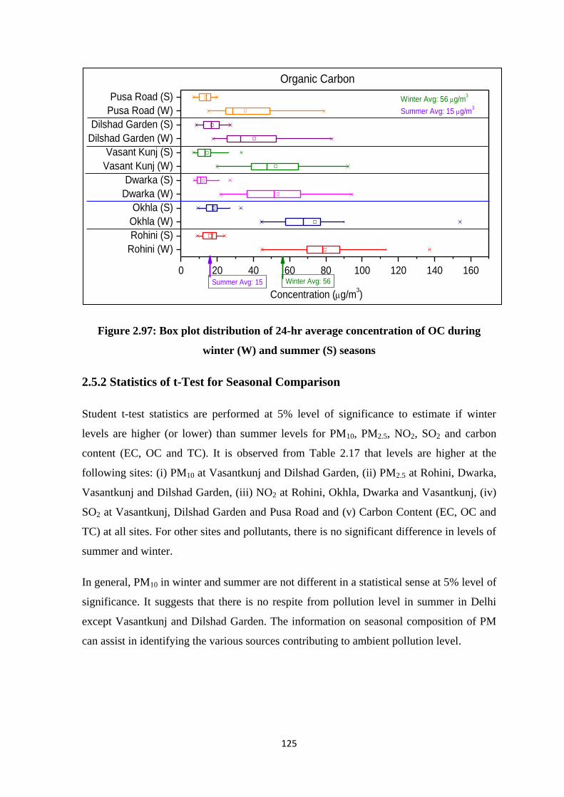
125
Figure 2.97: Box plot distribution of 24-hr average concentration of OC during
winter (W) and summer (S) seasons
2.5.2 Statistics of t-Test for Seasonal Comparison
Student t-test statistics are performed at 5% level of significance to estimate if winter
levels are higher (or lower) than summer levels for PM10, PM2.5, NO2, SO2 and carbon
content (EC, OC and TC). It is observed from Table 2.17 that levels are higher at the
following sites: (i) PM10 at Vasantkunj and Dilshad Garden, (ii) PM2.5 at Rohini, Dwarka,
Vasantkunj and Dilshad Garden, (iii) NO2 at Rohini, Okhla, Dwarka and Vasantkunj, (iv)
SO2 at Vasantkunj, Dilshad Garden and Pusa Road and (v) Carbon Content (EC, OC and
TC) at all sites. For other sites and pollutants, there is no significant difference in levels of
summer and winter.
In general, PM10 in winter and summer are not different in a statistical sense at 5% level of
significance. It suggests that there is no respite from pollution level in summer in Delhi
except Vasantkunj and Dilshad Garden. The information on seasonal composition of PM
can assist in identifying the various sources contributing to ambient pollution level.
Rohini (W)
Rohini (S)
Okhla (W)
Okhla (S)
Dwarka (W)
Dwarka (S)
Vasant Kunj (W)
Vasant Kunj (S)
Dilshad Garden (W)
Dilshad Garden (S)
Pusa Road (W)
Pusa Road (S)
0 20 40 60 80 100 120 140 160Summer Avg: 15 Winter Avg: 56
Concentration (g/m3)
Organic Carbon
Winter Avg: 56 g/m3
Summer Avg: 15 g/m3

126
Table 2.89: Statistical Comparison Winter Vs Summer
2.6 Interpretations and Inferences
Based on the air quality measurements in summer and winter months and critical analyses
of air quality data, the following inferences and insights are drawn for developing causal
relationship between emission and impact through receptor and dispersion modeling
(Chapter 4 and 5). The season-wise, site specific average air concentration of PM10, PM2.5
and their compositions (Tables 2.14 (a, b, c, d) and 2.16 (a, b, c, d)) have been referred to
bring the important inferences to the fore.
- Particulate pollution is the main concern in the city where levels of PM10 and
PM2.5 are 4-7 times higher than the national air quality standards in summer
and winter months.
- The chemical composition of PM10 and PM2.5 carries the signature of sources
and their harmful contents. The chemical composition is variable depending on
the size fraction of particles and the season. The PM levels and chemical
composition are discussed separately for two seasons.
Summer - PM10
The overall average concentration of PM10 in summer season is over 500 µg/m3
against the acceptable level of 100 µg/m3.
The crustal component (Si + Al + Fe + Ca) accounts for about 40 percent of total
PM10 in summer. This suggests soil and road dust and airborne flyash are the major
Parameter
Site PM10 PM2.5 NO2 SO2 EC OC TC
RHN
OKH
DWK
VKJ
DSG
PUS
No significant difference (Levels higher in winter) (Levels lower in winter)
* No pollutant showed lower concentration in winter

127
sources of PM10 pollution in summer. The coefficient of variation (CV) is about
0.25, which suggests the sources are consistent all around the city forming a layer
which envelopes the city. The areas of DSG and OKH have the highest crustal
fraction (around 44% of total PM10). It is difficult to pinpoint the crustal sources as
these are wide spread and present all around in Delhi and NCR and are more
prominent in summer when soil and ash-ponds (active or abandoned) are dry and
high speed winds make the particles airborne. It was observed that in summer the
atmosphere looks whitish to grayish which can be attributed to the presence of
large amounts of flyash and dust particles in the atmosphere.
The second important component is the secondary particles (NO₃⁻ + SO₄⁻² +
NH₄⁺), which account for about 13 percent of total PM10 and combustion related
total carbon (EC+OC) accounts for about seven percent. The secondary particles
are formed in the atmosphere because of reaction of precursor gases (SO2, NOx
and NH3) to form NO₃⁻, SO₄⁻², and NH₄⁺. The combustion related contribution is
relatively less in PM10 in summer.
The Cl- content in PM10 in summer is also consistent at 4-6 percent, which is an
indicator of burning of municipal solid waste (MSW); recall poly vinyl chloride
(PVC) is a major part of MSW.
Summer - PM2.5
The overall average concentration of PM2.5 in summer season is around 300 µg/m3
against the acceptable level of 60 µg/m3.
The crustal component (Si + Al + Fe + Ca) accounts for about 20 percent of total
PM2.5. This suggests soil and road dust and airborne flyash is a significant source
of PM2.5 pollution in summer. The CV is about 0.23, which suggests the source is
consistent all around the city. The area of OKH has the highest crustal fraction
around 28% of total PM2.5.
The second important component is secondary particles (NO₃⁻ + SO₄⁻² + NH₄⁺),
which account for about 17 percent of total PM2.5 and combustion related total
carbon (EC+OC) accounts for about nine percent; both fractions of secondary
particles and combustion related carbons account for a larger fraction in PM2.5 than

128
in PM10. All three potential sources, crustal component, secondary particles and
combustion contribute consistently to PM2.5 in summer.
The Cl- content in PM2.5 in summer is also consistent at 4-10 percent, which is an
indicator of burning of municipal solid waste (MSW) and has a relatively higher
contribution to PM2.5 than that to PM10.
Winter - PM10
The overall average concentration of PM10 in winter season is around 600 µg/m3
against the acceptable level of 100 µg/m3.
The crustal component (Si + Al + Fe + Ca) accounts for only 13% (much less
compared to 40 percent in summer). This suggests soil and road dust and airborne
flyash have reduced significantly in PM10 in winter. The coefficient of variation
(CV) is about 0.36, which suggests the crustal source is variable and not as
consistent as it was in summer.
The most important component is the secondary particles (NO₃⁻ + SO₄⁻² + NH₄⁺),
which accounts for about 26 percent of total PM10 and combustion related total
carbon (TC = EC: elemental carbon + OC: organic carbon) accounts for about 19
percent; both fraction of secondary particles and combustion related carbons have
increased in winter and account for 45 percent of PM10.
The Cl- content in PM10 in winter is also consistent at 4-10 percent, which is an
indicator of burning of municipal solid waste (MSW) and has a relatively higher
contribution in winter.
Winter - PM2.5
The overall average concentration of PM2.5 in winter is 375 µg/m3 against the
acceptable level of 60 µg/m3. The crustal component is reduced dramatically to
only 3.5 percent in PM2.5 in winter.
The single important component is the secondary particles (NO₃⁻ + SO₄⁻² +
NH₄⁺), which account for about 28 percent of total PM2.5 and combustion related
total carbon (EC+OC) accounts for about 23 percent; both secondary particles and

129
combustion related carbon are consistent contributor to PM2.5 at about 51 percent
having CV of 0.22.
The Cl- content in PM2.5 winter is also consistent at 7 percent, which is an indicator
of burning of municipal solid waste (MSW); which is relatively higher in winter
than in summer
It was observed that in winter the atmosphere looks very hazy and characterized by
smoky and unhealthy air. The consistent and major contributors appear to be
secondary particles and combustion related emission with modest contribution of
burning of MSW.
Potassium levels
In general potassium levels are high and at the same time highly variable; 18 to 7
µg/m3 in PM10 and 15 to 4 µg/m
3 in PM2.5. In general potassium level should be
less than 2 µg/m3. Potassium is an indicator of biomass burning and high levels
and variability (CV ~ 0.66) show large biomass burning and it is variable. Highest
potassium levels (~ 15 µg/m3) were seen in the beginning of November and early
winter perhaps due to massive crop residue burning in Punjab and Haryana.
Potassium levels stabilize around 4 µg/m3 (which is also high) in rest of the winter
months suggesting the biomass burning is prevalent throughout winter, locally and
regionally.
NO2 levels
NO2 levels in winter are high and they do exceed national air quality standard of 80
µg/m3 at a few locations; more frequently at PUS sampling site. In addition, high
levels of NO2 are expected to undergo chemical transformation to form fine
secondary particles in the form of nitrates, adding to high levels of existing PM10
and PM2.5. SO2 levels in the city were well within the air quality standard.
General inferences
Levels of PM10, PM2.5 and NO2 are statistically higher (at most locations) in winter
months than in summer months by about 25-30 percent. In general air pollution
levels in ambient air (barring traffic intersections) are uniform across the city
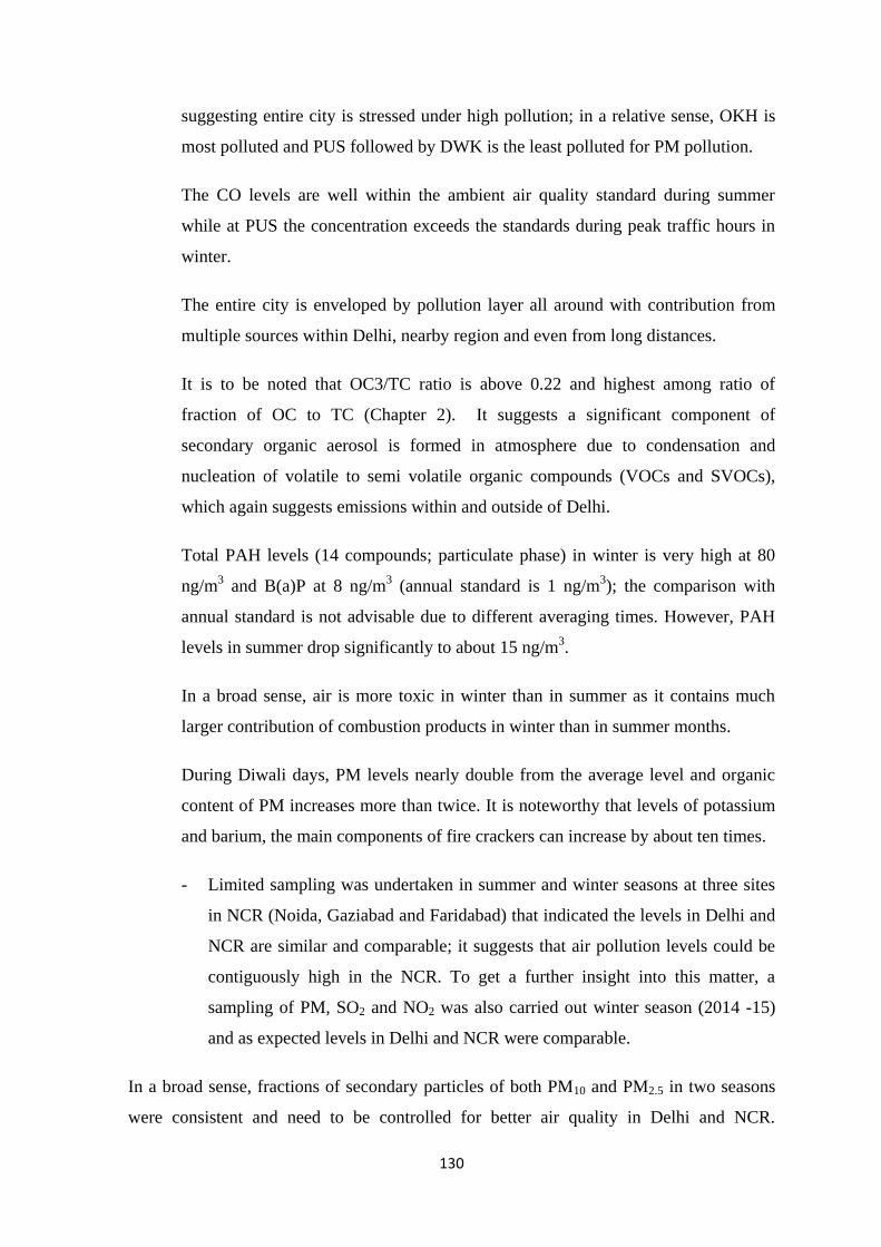
130
suggesting entire city is stressed under high pollution; in a relative sense, OKH is
most polluted and PUS followed by DWK is the least polluted for PM pollution.
The CO levels are well within the ambient air quality standard during summer
while at PUS the concentration exceeds the standards during peak traffic hours in
winter.
The entire city is enveloped by pollution layer all around with contribution from
multiple sources within Delhi, nearby region and even from long distances.
It is to be noted that OC3/TC ratio is above 0.22 and highest among ratio of
fraction of OC to TC (Chapter 2). It suggests a significant component of
secondary organic aerosol is formed in atmosphere due to condensation and
nucleation of volatile to semi volatile organic compounds (VOCs and SVOCs),
which again suggests emissions within and outside of Delhi.
Total PAH levels (14 compounds; particulate phase) in winter is very high at 80
ng/m3 and B(a)P at 8 ng/m
3 (annual standard is 1 ng/m
3); the comparison with
annual standard is not advisable due to different averaging times. However, PAH
levels in summer drop significantly to about 15 ng/m3.
In a broad sense, air is more toxic in winter than in summer as it contains much
larger contribution of combustion products in winter than in summer months.
During Diwali days, PM levels nearly double from the average level and organic
content of PM increases more than twice. It is noteworthy that levels of potassium
and barium, the main components of fire crackers can increase by about ten times.
- Limited sampling was undertaken in summer and winter seasons at three sites
in NCR (Noida, Gaziabad and Faridabad) that indicated the levels in Delhi and
NCR are similar and comparable; it suggests that air pollution levels could be
contiguously high in the NCR. To get a further insight into this matter, a
sampling of PM, SO2 and NO2 was also carried out winter season (2014 -15)
and as expected levels in Delhi and NCR were comparable.
In a broad sense, fractions of secondary particles of both PM10 and PM2.5 in two seasons
were consistent and need to be controlled for better air quality in Delhi and NCR.

131
Combustion sources, vehicles, biomass burning and MSW burning are other consistent
sources in winter and require a strategy to control these sources. In summer, air quality
cannot be improved unless we find effective control solutions for soil and road dust, fly
ash re-suspension, concrete batching and MSW burning. Possible effective mixture of
control options are discussed in Chapter 6.

132
Chapter 3
Emission Inventory
3.1 Introduction
Air pollution has emerged as a major challenge, particularly in urban areas. The problem
becomes more complex due to the multiplicity and complexity of the air polluting source
mix (e.g., industries, automobiles, generators, domestic fuel burning, road side dusts,
construction activities, etc.). Indian cities have experienced a phenomenal growth in terms
of population, industry, and vehicles. The broad emission source categories of air pollution
in an urban area include; (i) transport (motor vehicles and railways), (ii) commercial
establishments, (iii) industrial, (iv) domestic cooking/heating, (v) fugitive dust and (vi)
biomass burning. There could also be some unique or specific sources in a particular area.
Procedures and reliability of emission inventory for regular point, area and line sources are
well-established. However, identification and quantification of fugitive/non-point emission
sources (emissions not released through stacks, vents, ducts or pipes) are quite
challenging.
Emission inventory (EI) is a basic necessity for planning air pollution control activities. EI
provides a reliable estimate of total emissions of different pollutants, their spatial and
temporal distribution, and identification and characterization of main sources. This
information on EI is an essential input to air quality models for developing strategies and
policies. The ultimate goal of the planning process is to identify and achieve emission
patterns that do not result in violations of ambient air quality standards. In this chapter,
emission inventory of the study area for the period of 1st October 2013 to 30
th June 2014 is
presented.
3.2 Methodology
The stepwise methodology adopted for the study is presented in Figure 3.1.

133
Figure 3.1: Stepwise Methodology adopted for the Study
3.2.1 Data Collection
The primary data were collected by IITK team. Parking lane survey at 18 locations was
done to assess types of vehicles on the road. Construction and demolition data was
collected by field survey and validated by satellite imagery. Road dust sampling at 20
locations was conducted. Physical survey of industrial areas was also done. The main
sources of secondary data collection are from DPCC, Delhi Metro Rail Corporation
(DMRC), Census of India, CPCB website, AAI (Airport Authority of India), Indian
Railways, and Central Electricity Authority (CEA). Information has also been collected
through Internet by visiting various websites. Although all possible efforts have been
made to collect the data, some information/data could be missing.
3.2.2 Digital Data Generation
The land-use map of the study area is prepared in terms of settlements, forests, agriculture,
road network, water bodies, etc (Figure 3.2). The entire city was divided into 441 grid cell
of 2 km x 2 km (Figure 3.3).

134
Figure 3.2: Landuse Map of the Study Area
Figure 3.3: Grid Map of the City Showing Grid Identity Numbers

135
At the time of development of the emission inventory for the city, a suitable coding system
has been adopted to avoid the confusion and misrepresentation of results and
interpretation. The map with grid identity numbers is shown in Figure 3.3.
Emission Factor
An emissions factor is a representative value that attempts to relate the quantity of a
pollutant released to the atmosphere with an activity associated with the release of that
pollutant. These factors are usually expressed as the mass of pollutant per unit mass of raw
material, volume, distance travelled, or duration of the activity (e.g., grams of particulate
emitted per kilogram of coal burnt). Such factors facilitate estimation of emissions from
various sources of air pollution. In most cases, these factors are simply averages of all
available data of acceptable quality, and are generally assumed to be representative of
long-term averages for all facilities in the source category.
The general equation for emissions estimation is:
)100/1( EREFAE (3.1)
Where:
E = Emissions;
A = Activity rate;
EF = Emission factor, and
ER = Overall emission reduction efficiency, %
3.3 Area Sources
3.3.1 Hotels/Restaurants
The details of the hotels and restaurants were obtained from DPCC, and related websites.
During the field survey it was observed that hotels, restaurants, etc use coal as fuel in
tandoors. The average consumption of coal in tandoor based on survey was 30 kg/day. The
total number of hotel and restaurant enterprise was 36,099 (Delhi Statistical Hand Book,
2014). We assume that 25% of these enterprises use tandoor for food preparation. The
common fuel other than in tandoor is LPG. The fuel consumption for each fuel type was
estimated for each grid. In most of the cases, it was found that there was no control
devices installed at these activities. The emissions of various parameters such as SO2,

136
NOx, PM10, PM2.5, and CO were estimated from the activity data from each fuel type and
then were summed up in each grid cell. The emission factors given by CPCB (2011) were
used. The overall emission from this area source (Hotels/Restaurants) is presented in
Figure 3.4.
Figure 3.4: Emission Load from Hotels/Restaurant
For spatial distribution of different pollutants, emission per capita, in each ward and
village was calculated, as activity data was available on the basis of per capita. Then the
emission density in terms of kg/day/m2 in each ward was calculated based on population
and area of the ward for different pollutants (PM10, PM2.5, SO2, NOx, and CO); see below.
Emission Density (kg/day/m2) = Emission of Ward (kg/day) / Ward Area (m
2) (3.2)
For calculating emission in a grid which may contain more than one ward, the area of the
fraction of each ward falling inside that grid was calculated and with the help of emission
density of the ward, the missions were calculated, see below.
N
i
EmissionGrid1
(. area of fraction ward i in grid X emission density of ward, i) (3.3)
Where, N= no. of wards in the grid
The spatial distribution of emissions of PM10, PM2.5, NOx, SO2 and CO from
Hotel/Restaurants is presented in Figure 3.5 to 3.9.
3493
1758
1105
2710
6179
0
1000
2000
3000
4000
5000
6000
7000
PM10 PM2.5 NOX SO2 CO
Emis
sio
ns(
kg/d
ay)

137
Figure 3.5: Spatial Distribution of PM10 Emissions from Hotel/Restaurants
Figure 3.6: Spatial Distribution of PM2.5 Emissions from Hotel/Restaurants

138
Figure 3.7: Spatial Distribution of NOx Emissions from Hotel/Restaurants
Figure 3.8: Spatial Distribution of SO2 Emissions from Hotel/Restaurants

139
Figure 3.9: Spatial Distribution of CO Emissions from Hotel/Restaurants
3.3.2 Domestic Sector
The administrative division (2011) map of Delhi was obtained from Census of India and it
was digitized. The NCT of Delhi consists of 113 towns and 112 villages as shown in
Figure3.10. The data on number of household, fuel usage (coal, LPG, crop residue, cow
dung and wood) and population were collected from Census-India (2012). The emission
factors given by CPCB (2011) and AP-42 (USEPA, 2000) were used for each fuel type.
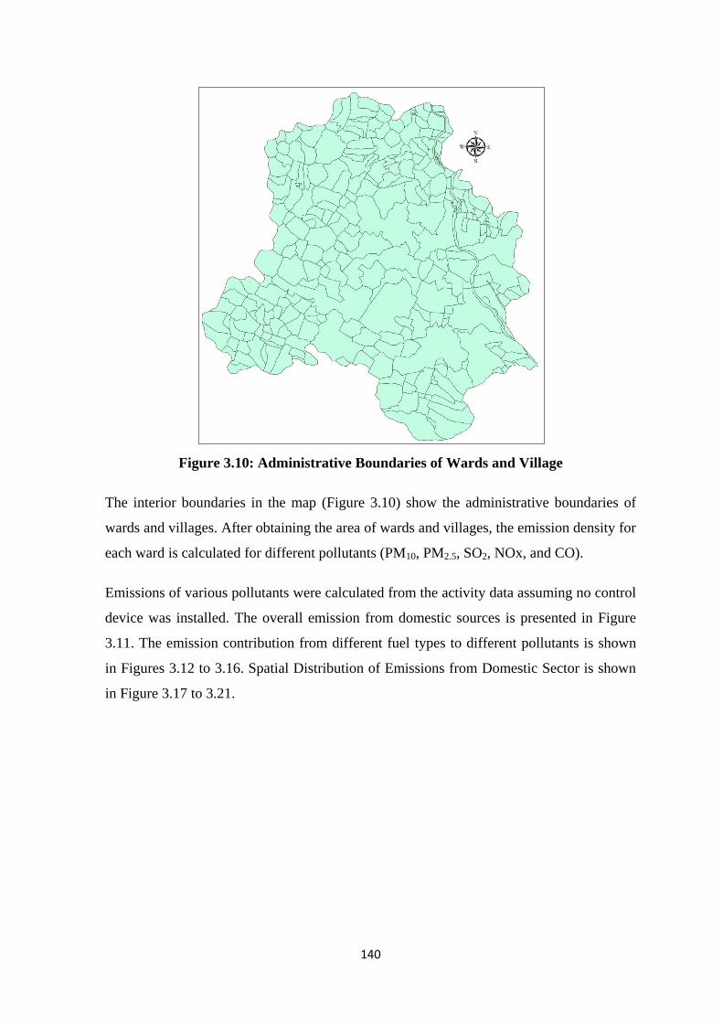
140
Figure 3.10: Administrative Boundaries of Wards and Village
The interior boundaries in the map (Figure 3.10) show the administrative boundaries of
wards and villages. After obtaining the area of wards and villages, the emission density for
each ward is calculated for different pollutants (PM10, PM2.5, SO2, NOx, and CO).
Emissions of various pollutants were calculated from the activity data assuming no control
device was installed. The overall emission from domestic sources is presented in Figure
3.11. The emission contribution from different fuel types to different pollutants is shown
in Figures 3.12 to 3.16. Spatial Distribution of Emissions from Domestic Sector is shown
in Figure 3.17 to 3.21.

141
Figure 3.11: Emission Load from domestic sources (kg/day)
Figure 3.12:PM10 Emission Load from domestic sources (kg/day, %)
Figure 3.13:PM2.5 Emission Load from domestic sources (kg/day, %)
7381 6940 7682
1232
25401
0
5000
10000
15000
20000
25000
30000
PM10 PM2.5 NOX SO2 CO
Emis
sio
ns(
kg/d
ay)
2266, 31%
0, 0%1033, 14%
171, 2%
3912, 53%
Wood Crop Residue Cow Dung Coal LPG
2039, 29%
0, 0%
929, 14%
60, 1%
3912, 56%
Wood Crop Residue Cow Dung Coal LPG

142
Figure 3.14: SO2 Emission Load from domestic sources (kg/day, %)
Figure 3.15: NOx Emission Load from domestic sources (kg/day, %)
Figure 3.16: CO Emission Load from domestic sources (kg/day, %)
216, 18%
0, 0%
98, 8%
173, 14%745, 60%
Wood Crop Residue Cow Dung Coal LPG
629, 8%
9, 0%
287, 4%52, 1%
6705, 87%
Wood Crop Residue Cow Dung Coal LPG
13937, 55%
1064, 4%
6351, 25%
323, 1% 3725, 15%
Wood Crop Residue Cow Dung Coal LPG

143
Figure 3.17: Spatial Distribution of PM10 Emissions from Domestic Sector
Figure 3.18: Spatial Distribution of PM2.5 Emissions from Domestic Sector

144
Figure 3.19: Spatial Distribution of NOx Emissions from Domestic Sector
Figure 3.20: Spatial Distribution of SO2 Emissions from Domestic Sector

145
Figure 3.21: Spatial Distribution of CO Emissions from Domestic Sector
3.3.3 Municipal Solid Waste
Open burning activities are broadly classified into refuse and biomass burning. The refuse
or municipal solid waste (MSW) burning depends on solid waste generation and extent of
disposal and infrastructure for collection. The contribution of MSW burning may surprise
many persons. The recent study by Nagpure et al. (2015), in Delhi has estimated 190 to
246 tons/day of MSW burning (∼2−3% of MSW generated; 8390 tons/day). It is a myth
that MSW is not burned in Delhi. It is clearly seen that MSW burning is a major source
that contributes to both PM10 and PM2.5. This emission is expected to be large in the
regions of economically lower strata of the society which do not have proper infrastructure
for collection and disposal of MSW.
The emission factors given by CPCB (2011) and AP-42 (USEPA, 2000) were used for
estimating the emission from MSW burning using the same procedure of emission density
in a ward or village. The emissions from open burning are presented in Figure 3.22 and
spatial distribution of in Figures 3.23 to 3.27.

146
Figure 3.22: Emission Load from MSW (kg/day)
Figure 3.23: Spatial Distribution of PM10 Emissions from MSW
1968 1771
738123
10332
0
2000
4000
6000
8000
10000
12000
PM10 PM2.5 NOX SO2 CO
Emis
sio
ns(
kg/d
ay)

147
Figure 3.24: Spatial Distribution of PM2.5 Emissions from MSW
Figure 3.25: Spatial Distribution of NOx Emissions from MSW

148
Figure 3.26: Spatial Distribution of SO2 Emissions from MSW
Figure 3.27: Spatial Distribution of CO Emissions from MSW

149
3.3.4 Construction and Demolition
A detailed survey was undertaken to assess construction and demolition activities in the
study area. The construction and demolition locations were then verified with satellite
imagery (Figure 3.28). Information on number of buildings, roads and flyovers under
construction information was collected from DMRC, Public Works Department (PWD),
Central Public Works Department (CPWD), and Delhi Development Authority websites
and sites were physically surveyed. Then areas under construction activities were
calculated on the basis of survey data and GIS. The emissions were estimated using Eq
(3.4) given by AP-42 (USEPA, 2000). The unit of the activity data is m2, i.e. area of these
activities.
E = 1.2 tons/acre/month of activity (tons/m2/month) (3.4)
Figure 3.28: Construction/Demolition Sites
Total emission from construction and demolition activities is presented in Table 3.1. The
spatially resolved map of construction and demolition activities is shown in Figures 3.29
to 3.30.

150
Table 3.1: Emission Load from Construction and Demolition activities (kg/day)
Category TSP PM10 PM2.5
Buildings 16281.72 4070.4301 1017.61
Roads and Flyover 4385.63 1096.4075 274.102
Totals 20667.35 5166.8376 1291.71
Figure 3.29: Spatial Distribution of PM10 Emissions from Construction/Demolition

151
Figure 3.30: Spatial Distribution of PM2.5 Emissions from Construction/Demolition
3.3.5Commercial and Industrial Diesel Generator Sets (DG sets)
DG sets are used as the source of power in shopping complexes and industries during the
power-cut hours. From the results of the survey, it can be concluded that there is minimum
of 2 hours/day power cut in the city, especially in summer. The DG set details were
obtained from DPCC; the DG sets were located on the map.
The unit of the activity data is KWh power generation. The emissions from DG sets
installed in commercial complexes, institutes and industries were estimated and then were
summed up for each grid. The calculation is based on Eq (3.1), where ER, overall
efficiency reduction was taken as zero. The CPCB (2011) emission factors were used for
emission estimation. The total emissions from DG sets are presented in Figure 3.31.
Spatial Distribution of Emissions from DG Sets is shown in Figures 3.32 to 3.36.

152
Figure 3.31: Emission Load (kg/day) from DG sets
Figure 3.32: Spatial Distribution of PM10 Emissions from DG Sets
1387 1248
19604
1293
4234
0
5000
10000
15000
20000
25000
PM10 PM2.5 NOX SO2 CO
Emis
sio
ns(
kg/d
ay)

153
Figure 3.33: Spatial Distribution of PM2.5 Emissions from DG Sets
Figure 3.34: Spatial Distribution of NOx Emissions from DG Sets

154
Figure 3.35: Spatial Distribution of SO2 Emissions from DG Sets
Figure 3.36: Spatial Distribution of CO Emissions from DG Sets

155
3.3.6 Cremation
There are 53 cremation sites in the city of Delhi, which operates in various zones of
Municipal Corporation of Delhi. These cremation sites were located in the grids with the
help of GIS (Figure 3.37). Specific information on number of dead bodies cremated in
each cremation site was not available. The information pertaining to total number of
deaths in Delhi was obtained from Directorate of Economics and Statistics handbook for
the year 2014.
Figure 3.37: Cremation Sites in City of Delhi
The total number of registered death in 2014 for Hindus was 105336. The wood required
for per body for the cremation is taken as 216 kg (Sharma, 2010). The emission factors
for each pollutant for cremation were decided on the basis of CPCB (2011) recommended
emission factors. The total emissions from cremation sites are presented in Figure 3.38.
Spatial Distribution of PM10, PM2.5, NOx, SO2, and CO emissions from cremation sites are
presented in Figure 3.39.

156
Figure 3.38: Emission Load from Cremation Sites
Figure 3.39: Spatial Distribution of PM10, PM2.5, NOx, SO2, CO Emissions from
Cremation Sites
3.3.7 Aircraft
Indira Gandhi International Airport (IATA: DEL, ICAO: VIDP) is the primary airport of
the National Capital Region of Delhi, situated in south-west Delhi, 16 km New Delhi's city
346 312
96 33
2129
0
500
1000
1500
2000
2500
PM10 PM2.5 NOx SO2 CO
Emis
sio
ns(
kg/d
ay)

157
center. Total number of flight (arrival + departure) is approximately 800 per day at IGI
Airport. The aircraft arriving and departing is categorized according to their companies
and engine capacity. The emission factors used have been adopted from ICAO
(International Civil Aviation Organization; http://www.icao.int). From aircrafts most of
the emissions is during the LTO (landing and takeoff) cycle, compared to time of flight
within the Delhi border. The estimated emission is presented in Figure 3.40. This emission
is expected to be dispersing in upper part of atmosphere.
Figure 3.40: Emission Load from Aircraft
3.3.8 Bio-Medical Waste Incinerator and Boilers
There are 32 health care establishments relevant to air pollutant emissions in the city.
These health care establishments are having 14 incinerators (12 (private) and 2 (CBWTF:
Common Bio-medical Waste Treatment Facility) and rest have boilers. For each health
care establishment activity data were taken from DPCC and emissions calculated using
CPCB (2011) (Figure 3.41).
54 54
5416
380
4112
0
1000
2000
3000
4000
5000
6000
PM10 PM2.5 NOX SO2 CO
Emis
sio
ns(
kg/d
ay)

158
Figure 3.41: Emission Load from Health Care Establishment
3.3.9 Waste to Energy Plants (MSW)
There is only one waste to energy plant (Timarpur Okhla Waste Management Co Pvt Ltd)
operating in the city of Delhi. This plant uses 225 ton/day of refuse to derive fuel to
generate energy. The plant is equipped with bag house filter, so the controlled emission
factor of AP-42 (USEPA, 2000) was used to calculate the controlled emissions. The plant
emission is 6.9 kg/day of PM10; 6.9 kg/day of PM2.5; 62.33 kg/day of SO2; 205.86 kg/day
of NOx.
3.3.10 Agricultural Soil Dust
The total agricultural land (50500 ha) was calculated in GIS. The emission factor for crop
type is obtained from EMEP/EEA air pollutant emission inventory guide book (EEA,
2013). The total PM10 emission from agricultural soil dust is estimated to be 1353 kg/day.
The PM2.5 emission is negligible.
3.3.11 Ready Mix Concrete Batching
Concrete is a fixed mixture of water, cement, sand (fine aggregate) and coarse aggregate.
Coarse aggregate consist of gravel, crushed stone or iron blast furnace slag. Cementitious
materials, also called mineral admixtures or pozzolan minerals may be added to make the
concrete mixtures more economical, reduce permeability, increase strength, or influence
other concrete properties (USEPA, 2000).
38 34
103
317
27
0
50
100
150
200
250
300
350
PM10 PM2.5 NOX SO2 CO
Emis
sio
ns(
kg/d
ay)

159
During the study period massive construction activities were found in the study area which
requires concrete batching. There were 60 DMRC locations where construction was under
progress and it was assumed that there will be 40 concrete batching plants of 120 m3/hr
capacities operating for 16 hours. Several medium and small construction activities were
also observed in the city (see section on construction and demolition). The AP-42
(USEPA, 2000) emission factors were used to calculate the emissions from concrete
batching. The total PM10 and PM2.5 emissions from these concrete mix plant estimated to
be 14.37 ton/day and 3.5 ton/day respectively. It may be noted there are a few hundred
concrete batching plants exist in NCR, which may contribute to air quality in Delhi but
these have not been included in emission inventory of Delhi
3.3.10 Industries as Area Sources
There are 25 industrial areas in the city (Figure 3.42). All industries having stack height
below 20 m have been considered as industrial area source. Majority of the industries is
having small boilers and some cupola furnaces were also present. Most of the information
on the industrial areas concerning fuel consumption, stack height, production capacity has
been collected from DPCC. We had to make certain assumptions and made improvements
in the database to make compatibility in fuel consumptions and size of the industry
(production capacity), where no fuel consumption was given minimum consumption per
hour of fuel has been considered. If type of fuel uses were not indicated then it was
assumed that industry used HSD. Ash content in the coal was assumed to be 35% and ‘S’
content as 1.8% for LDO; 1% for HSD (https://www.iocl.com/).CPCB (2011) and AP-42
(USEPA, 2000) emission factors were used to calculate the emissions. Finally all the
emission for each pollutant is summed up. Figure 3.43 presents the overall emissions from
industries as area source. Table 3.2 presents emission from different industrial areas in the
city of Delhi. Spatial Distribution of Emissions from Industries as Area Source is
presented in Figures 3.44 from 3.48.

160
Figure 3.42: Location of Industrial Areas in Delhi
Figure 3.43: Emission Load from Industries as Area Source.
16141367
1893
5616
185
0
1000
2000
3000
4000
5000
6000
PM10 PM2.5 NOX SO2 CO
Emis
sio
ns(
kg/d
ay)

161
Table 3.2: Emission Load from Industries as Area Source (kg/day)
Code Name PM10 PM2.5 SO2 NOx CO
1 ShahzadaBagh 0.98 0.88 12.43 4.36 0.40
2 Naraina Phase 2 1.76 1.58 22.21 7.78 0.71
3 Naraina phase 1 2.44 2.20 31.64 10.13 0.92
4 Mohan Cooperative 6.91 6.22 88.42 29.61 2.69
5 Okhla Industrial Area Phase 1 94.36 84.93 1239.10 373.38 34.48
6 Patparganj IA 8.98 8.08 116.48 36.89 3.35
7 Jhilmil 87.51 27.83 383.45 148.48 9.04
8 Lawrence Road 226.67 204.01 157.73 55.42 5.11
9 GT Karnal Road 8.44 7.60 107.40 36.95 4.27
10 Wazirpur 138.85 124.97 1785.47 587.02 53.59
11 SMA 7.61 6.85 96.37 33.67 3.43
12 SSI 5.73 5.16 75.28 22.69 2.06
13 Rajasthan Udyog 3.79 3.41 50.64 14.19 1.29
14 Badli 13.47 12.12 182.83 47.29 4.31
15 Bawana 431.30 388.35 211.85 102.05 24.95
16 Narela 468.66 401.98 162.77 78.72 5.82
17 Kirti Nagar 8.52 7.67 114.05 31.54 2.87
18 Moti Nagar 0.52 0.46 6.53 2.29 0.21
19 Friends Colony Shahdara 23.25 19.70 123.21 48.74 3.76
20 Mangolpuri 7.72 6.95 98.55 33.34 3.03
21 Udyog Nagar 6.37 5.73 80.62 28.24 2.57
22 Nangloi 1.10 1.00 13.84 5.12 1.10
23 Najafgarh Road 32.86 22.33 218.02 75.60 8.52
24 Mayapuri 26.08 16.06 228.75 76.64 6.28
25 Tilak Nagar 0.62 0.56 7.88 2.76 0.25
Total 1614.50 1366.62 5615.52 1892.88 185.01

162
Figure 3.44: Spatial Distribution of PM10 Emissions from Industries as Area Source
Figure 3.45: Spatial Distribution of PM2.5 Emissions from Industries as Area Source

163
Figure 3.46: Spatial Distribution of NOx Emissions from Industries as Area Source
Figure 3.47: Spatial Distribution of SO2 Emissions from Industries as Area Source

164
Figure 3.48: Spatial Distribution of CO Emissions from Industries as Area Source
3.3.11 Contribution of Emissions from Area Sources excluding Vehicles and large
Industry (point source)
Summary of emissions from various are source categories discussed is presented in Table
3.3.
Table 3.3: Summary of Emission Load from Area Sources (kg/day)
Category PM10 PM2.5 NOx SO2 CO
Hotels/Restaurants 3493 1758 1105 2710 6179
Domestic 7381 6940 7682 1232 25401
Aircrafts 54 54 5416 380 4112
Industries as Area Source 1614 1367 1893 5616 185
DG Set 1387 1248 19604 1293 4234
MSW Burning 1968 1771 738 123 10332
Cremation 346 312 96 33 2129
Construction/Demolition 5167 1292 - - -
Concrete Batching 14370 3594 - - -
Medical Incinerators 38 34 103 317 27
Agricultural Soil Dust 1353 - - - -
Total 37171 18369 36637 11704 52598

165
Figures 3.49 to 3.53 show the break-up of emissions of area sources for PM10, PM2.5,
NOx, SO2 and CO. The major contribution is from concrete batching, followed by
domestic sector and construction and demolition activities for PM10 and PM2.5. For NOx,
the largest sources are DG sets (Figure 3.51).
Figure 3.49: PM10 Emission Load for area sources (kg/day, %)
Figure 3.50: PM2.5 Emission Load for area sources (kg/day, %)
3493, 9%
7381, 20%
54, 0%
1614, 4%
1387, 4%
1968, 5%
346, 1%
5167, 14%
14370, 39%
1353, 4% 38, 0%
Hotels/Restaurants Domestic Aircraft Industries Area
DG Set MSW Burning Cremation Construction/Demolition
Concrete Batching Agricultural Soil Dust Medical Incinerators
1758, 10%
6940, 38%
54, 0%
1367, 7%
1248, 7%
1771, 10%312, 2%
1292, 7%
3594, 19%
0, 0% 34, 0%
Hotels/Restaurants Domestic Aircraft Industries Area
DG Set MSW Burning Cremation Construction/Demolition
Concrete Batching Agricultural Soil Dust Medical Incinerators

166
Figure 3.51: NOx Emission Load for area sources (kg/day, %)
Figure 3.52: SO2 Emission Load for area sources (kg/day, %)
1105, 3%
7682, 21%
5416, 15%
1893, 5%
19604, 54%
738, 2% 96, 0% 103, 0%
Hotels/Restaurants Domestic Airport
Industries as Area Source DG Set MSW Burning
Cremation Medical Incinerators
2710, 23%
1232, 11%
380, 3%
5616, 48%
1293, 11%
123, 1% 33, 0% 317, 3%
Hotels/Restaurants Domestic Airport
Industries as Area Source DG Set MSW Burning
Cremation Medical Incinerators

167
Figure 3.53: CO Emission Load for area sources (kg/day, %)
3.4 Point Sources
The industries having stack height of more than 20 m have been taken as point source. The
information on stacks, fuel and its consumption was obtained from DPCC. The power
plants information was taken from the annual report of Central Electricity Authority
(CEA, 2012). The industries have been numbered and located on the map (Figure 3.54).
The major emission is from coal-based power plants at Badarpur and Rajghat. The AP-42
(USEPA, 2000) emission factors were used to calculate the emission. The emission of
pollutants from large industry and power plant is given in Table 3.4 and Figure 3.55.
Spatial Distribution of Emissions from Point Sources is presented in Figures 3.56 to 3.60.
Table 3.4: Emission Load from Point Sources
Category PM10 PM2.5 NOx SO2 CO
Industries 196 144 225 458 12
Power Plants 13485 6431 161613 128304 11635
6179, 12%
25401, 48%
4112, 8%
185, 0%
4234, 8%
10332, 20%
2129, 4% 27, 0%
Hotels/Restaurants Domestic Airport
Industries as Area Source DG Set MSW Burning
Cremation Medical Incinerators

168
Figure 3.54: Locations of Points Sources in the City
Figure 3.55: Emission Load from Point Sources
136816575
161838
128762
11646
0
20000
40000
60000
80000
100000
120000
140000
160000
180000
PM10 PM2.5 NOX SO2 CO
Emis
sio
ns(
kg/d
ay)

169
Figure 3.56: Spatial Distribution of PM10 Emissions from Point Sources
Figure 3.57: Spatial Distribution of PM2.5 Emissions from Point Sources

170
Figure 3.58: Spatial Distribution of NOx Emissions from Point Sources
Figure 3.59: Spatial Distribution of SO2 Emissions from Point Sources

171
Figure 3.60: Spatial Distribution of CO Emissions from Point Sources
3.5 Vehicular - Line Sources
The average daily flow of vehicles in each hour for 2Ws, 3Ws, 4Ws, LCVs, Buses and
Trucks at 64 locations were obtained from Central Road Research Institute (CRRI, 2015)
(Figure 3.61). Traffic data were modeled to estimate the vehicle plying on road for the
year 2013-14. From these 64 traffic locations, the data were extrapolated for remaining
grid cells. Road lengths in each cell for major and minor roads were calculated from the
digitized maps using the ArcGIS tool, ArcMap and extracted into the grids. The
information on traffic flow from traffic counts was translated into the vehicles on the roads
in each grid. Wherever it was feasible, either traffic flow was taken directly from the
traffic data, and for interior grids, traffic from medium roads going the highways was
taken to flow in the interior part of the city. The emissions from each vehicle category for
each grid is estimated and summed up.

172
Figure 3.61: Traffic location considered for vehicle emission in the city of Delhi.
The emissions from railway locomotives are not taken into considerations, as the
emissions are negligible in comparison with the vehicles and other sources. Most of the
railway tracks in Delhi are of electric traction.
3.5.1 Parking Lot Survey
To obtain the prevalence of vehicle technology types operating in the city and fuel used,
parking lot questionnaire surveys (engine technology and capacity, vehicle age, fuel use,
etc.) were done at 20 locations (Uttam Nagar, Janakpuri, Hauz Khas, Saket, Connaught
Place, Dwarka, PVR Priya, Rajendra Nagar, Kirti Nagar, Barakhamba, Chandni Chowk,
Karkardooma, NDLS Station, Laxmi Nagar, Preet Vihar, Pragati Maidan, Kashmere Gate,
Khan Market, Anand Vihar, and Lajpat Nagar) in the city of Delhi. Out of total 5644
vehicles surveyed, the breakdown was: 1353 2-Ws; 455 3-Ws; 3836 4-Ws. During parking
lot survey, 300 LCVs were surveyed and it was found out that all LCVs runs on CNG fuel
and 99% LCVs are post 2005. All the city buses run on CNG and are of post 2000. The
traffic flow from outside Delhi is also accounted in this inventory. The data from all (127)
toll booth in the city were obtained and is presented in Table 3.5. Approximately 25%
percent of 4-Ws use diesel, 11% uses CNG and the remaining 64% use gasoline. 3-Ws use
compressed natural gas (CNG) and all 2-Ws use gasoline. ARAI (2011) and CPCB (2011)
emission factors were used to calculate the emissions. Figures 3.62 to 3.64 present parking
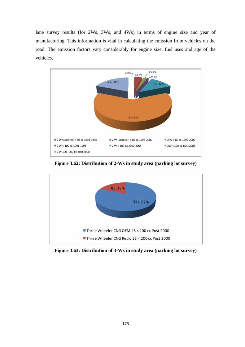
173
lane survey results (for 2Ws, 3Ws, and 4Ws) in terms of engine size and year of
manufacturing. This information is vital in calculating the emission from vehicles on the
road. The emission factors vary considerably for engine size, fuel uses and age of the
vehicles.
Figure 3.62: Distribution of 2-Ws in study area (parking lot survey)
Figure 3.63: Distribution of 3-Ws in study area (parking lot survey)
3, 0%53, 4%
25, 2%
9, 1%
164, 12%
842, 62%
257, 19%
2 W (Scooter) > 80 cc 1991-1995 2 W (Scooter) > 80 cc 1996-2000 2 W > 80 cc 1996-2000
2 W < 100 cc 1991-1996 2 W < 100 cc 2000-2005 2W < 100 cc post 2005
2 W 100 -200 cc post 2000
372, 82%
83, 18%
Three Wheeler CNG OEM 4S < 200 cc Post 2000
Three Wheeler CNG Retro 2S < 200 cc Post 2000

174
Figure 3.64: Distribution of 4-Ws in study area (parking lot survey)
Table 3.5: Data of Vehicles at Entry Points of Delhi (average per day)
S.No. Name of Toll CAT-1 CAT-2 CAT-3 CAT-4 CAT-5 TOTAL
1 Shahdra 1st 635 928 258 304 77 2202
2 Shahdra 2nd 1775 1882 385 690 144 4876
3 Mandooli Main 762 948 297 724 180 2911
4 Mandooli 2nd 12 1 0 0 0 13
5 Loni Main 337 308 375 120 23 1163
6 Loni 2nd 34 16 0 0 0 50
7 Seema Puri 1st 253 161 130 51 16 611
8 Seema Puri 2nd 99 6 0 0 0 105
9 Seema Puri 3rd 139 60 8 10 0 217
10 Chander Nagar 515 216 34 29 5 799
11 Surya Nagar 154 1 0 0 0 155
12 Sonia Vihar 189 148 121 24 3 485
13 Jhilmil 0 0 0 0 0 0
14 Ramprastha 0 17 0 0 0 17
15 Wazirabad 61 120 397 38 3 619
16 Indirapuri 19 10 2 0 0 31
17 Jauhripur 1st 37 40 8 4 0 89
18 Jauhripur 2nd 19 13 0 0 0 32
19 Sewadham 1st 262 75 29 56 14 436
20 Sewadham 2nd 0 0 0 0 0
21 Karawal Nagar 95 90 10 7 0 202
22 Dharamkanta 8 3 1 1 0 13
23 Amit Nagar 15 1 0 0 0 16
482, 13%
1009, 26%
99, 3%
549, 14%
233, 6%
626, 16%
423, 11%
415, 11%
Passenger Cars (Petrol) < 1000 cc Post 2000 Passenger Cars (Petrol) 1000 - 1400 cc Post 2000
Passenger Cars (Petrol) > 1400 cc Post 2000 Passenger Cars (Petrol) > 1400 cc Post 05
Passenger Cars (Diesel)<1600cc Post 2000 Passenger Cars (Diesel)<1600cc Post 2005

175
S.No. Name of Toll CAT-1 CAT-2 CAT-3 CAT-4 CAT-5 TOTAL
24 Shahdara 3rd 0 0 0 0 0
25 Ghazipur Main 4936 1182 259 400 228 7005
26 Old Ghazipur 719 1435 317 551 395 3417
27 Mohan Nagar 537 2282 114 90 18 3041
28 New Kondli 537 507 35 36 6 1121
29 Old Kondli 281 33 2 0 0 316
30 Vasundra 1st 363 110 8 4 2 487
31 Vasundra 2nd 169 41 0 0 0 210
32 Ashok Nagar 1st 232 16 11 4 0 263
33 Ashok Nagar 2nd 25 2 0 0 0 27
34 Between 1st 37 2 0 0 0 39
35 Between 2nd 76 5 0 0 0 81
36 Sabji Mandi 82 10 0 0 0 92
37 Sabji Mandi 2nd 310 19 0 0 0 329
38 Nagarjun 17 0 0 0 0 17
39 Nahar Naks 116 25 0 0 0 141
40 Nahar Naks 2nd 0 0 0 0 0 0
41 Nahar Naks 3rd 0 0 0 0 0 0
42 Mayur Vihar Ph Iii 33 6 0 0 0 39
43 Noida Major 3451 1086 280 282 83 5182
44 Mayur Vihar Cng 41 0 0 0 0 41
45 Cprf 48 0 0 0 0 48
46 Badarpur Main 31 0 0 0 0 31
47 Tuglagabad 516 17 16 10 2 561
48 Prahladpur 1041 269 259 148 23 1740
49 Surajkund 256 127 45 61 47 536
50 Kalindikunj 3628 1924 722 1016 874 8164
51 Jaitpura 1st 71 0 0 0 0 71
52 Jaitpura 2nd 13 1 0 0 0 14
53 Jaitpura 3rd 62 3 3 0 0 68
54 Jaitpura 4th 48 2 1 0 0 51
55 Ballabhgarh 20 2 4 0 0 26
56 Sector 37 1st 11 1 0 0 0 12
57 Sector 37 2nd 4 0 0 0 0 4
58 Sector 37 3rd 9 0 0 0 0 9
59 Sector 37 4th 42 6 3 0 0 51
60 Sector 37 5th 29 0 0 0 0 29
61 Lakkarpur 127 9 6 2 0 144

176
S.No. Name of Toll CAT-1 CAT-2 CAT-3 CAT-4 CAT-5 TOTAL
62 Durga Builder 358 30 8 9 0 405
63 Kapashera 1942 462 193 225 81 2903
64 Ayanagar 4029 332 117 296 126 4900
65 Old Bijwasan 349 43 14 21 7 434
66 New Bijwasan 456 64 21 29 11 581
67 Palam Vihar 656 83 24 26 8 797
68 Bajghera Main 638 158 57 59 17 929
69 Bajghera 2nd 9 1 0 0 0 10
70 Bajghera 3rd 39 4 1 1 0 45
71 Jhatikra 246 68 7 17 1 339
72 Nanakheri 1st 14 3 0 0 0 17
73 Nanakheri 2nd 3 1 0 0 0 4
74 Mandi More 107 53 10 16 3 189
75 Banswara 152 54 30 12 3 251
76 Kapashera B/P 8 0 0 0 0 8
77 Palam B/P 4 0 0 0 0 4
78 Kapashera Cng 6 3 0 0 0 9
79 Kgt Main 4969 4008 1419 1422 528 12346
80 Jaunti 1st 273 211 76 82 29 671
81 Jaunti 2nd 307 242 85 99 27 760
82 Punjab Khore 1st 281 209 79 75 29 673
83 Punjab Khore 2nd 246 214 78 66 21 625
84 Kutubgarh 1st 272 197 73 72 23 637
85 Kutubgarh 2nd 294 212 74 83 29 692
86 Kutubgarh 3rd 31 45 32 13 0 121
87 Mungeshpur 31 27 26 0 0 84
88 Auchandi 1st 70 31 26 52 9 188
89 Auchandi 2nd 9 2 2 0 0 13
90 Harewali 7 1 0 0 0 8
91 Revli 2nd 67 23 7 0 0 97
92 Lampur 111 76 57 122 20 386
93 Bananer 11 3 1 0 0 15
94 Safia Bad 163 78 19 43 10 313
95 Saboli Road 62 20 3 2 0 87
96 Tt Post 255 126 11 11 3 406
97 Kundali 1st 18 11 3 16 2 50
98 Kundali 2nd 235 291 111 160 37 834
99 Singhu School 37 15 4 10 0 66

177
S.No. Name of Toll CAT-1 CAT-2 CAT-3 CAT-4 CAT-5 TOTAL
100 Singhu Gaon 77 8 3 0 0 88
101 Janti Khurd 5 5 4 2 0 16
102 Zero Palla 18 10 0 0 0 28
103 Tajpur 4 2 2 0 0 8
104 Tikri 2957 1778 439 1091 439 6704
105 Jharoda 1st 893 318 64 139 43 1457
106 Jharoda 2nd 9 3 0 15 0 27
107 Dhansa 174 238 44 343 45 844
108 Dorala 1st 201 171 23 107 34 536
109 Dorala 2nd 17 11 5 5 3 41
110 Dorala 3rd 3 0 3 0 0 6
111 Nizampur 1st 118 47 27 33 1 226
112 Nizampur 2nd 117 38 91 6 0 252
113 Bakargarh 43 98 16 41 0 198
114 Badshah Ghalimpur 5 5 0 2 0 12
115 Badshah Ghalimpur 2nd 10 2 0 0 0 12
116 Surakhpur 28 2 0 0 0 30
117 Devarkhana 3 1 0 0 0 4
118 Mundelkalan 1st 25 29 3 5 0 62
119 Mundelkalan 2nd 9 5 1 0 0 15
120 Kairnaka 1st 14 4 1 0 0 19
121 Kairnaka 2nd 2 4 0 0 0 6
122 Chornaka 62 18 4 0 0 84
123 Isapur 2 2 0 0 0 4
124 Head Office 0 0 0 0 0 0
125 Dnd Toll 4051 703 139 277 111 5281
126 Bftc(Badarpur Toll) 6563 2507 1152 1709 663 12594
127 Rajokari 19171 4613 1468 4001 2533 31786
Total 74684 32189 10297 15477 7039 139686
Cat 1: Taxi, Tempo, Tata407 and other commercial vehicles, Cat 2: Bus, Nissan, Canter and other commercial
vehicles, Cat 3: six wheel truck, Cat 4: 10 wheel truck, Cat 5: 14 wheel truck.
The emission from vehicles is shown in Figure 3.65. Emission contribution of each vehicle
type in city of Delhi is presented in Figures 3.66 to 3.70. In the category of 4W cars, it is
estimated that in PM emission, petrol cars contributes about 22% and rest 78% is
contributed by diesel cars; contribution of CNG cars is negligible. The spatial distribution
of emissions from vehicles is presented in Figures 3.71 to 3.75.

178
Figure 3.65: Emission Load from Vehicles (kg/day)
Figure 3.66: PM10 Emission Load contribution of each vehicle type in city of Delhi
Figure 3.67: PM2.5 Emission Load contribution of each vehicle type in city of Delhi
12914 11623
113443
1155
322434
0
50000
100000
150000
200000
250000
300000
350000
PM10 PM2.5 NOX SO2 CO
Emis
sio
ns(
kg/d
ay)
4333, 33%
215, 2%
1362, 10%
489, 4%628, 5%
5888, 46%
2w 3w 4w lcv buses trucks
3900, 33%
194, 2%
1225, 10%
440, 4%565, 5%
5300, 46%
2w 3w 4w lcv buses trucks

179
Figure 3.68: NOx Emission Load contribution of each vehicle type in city of Delhi
Figure 3.69: SO2 Emission Load contribution of each vehicle type in city of Delhi
Figure 3.70: CO Emission Load contribution of each vehicle type in city of Delhi
9859, 9%7177, 6%
19380, 17%
22472, 20%
30136, 27%
24420, 21%
2w 3w 4w lcv buses trucks
230, 20%
0, 0%
659, 57%
16, 2%
142, 12%
108, 9%
2Ws 3Ws 4Ws LCVs Buses Trucks
138462, 43%
14354, 4%
120779, 37%
15020, 5%
18064, 6% 15755, 5%
2w 3w 4w lcv buses trucks

180
Figure 3.71: Spatial Distribution of PM10 Emissions from Vehicles
Figure 3.72: Spatial Distribution of PM2.5 Emissions from Vehicles

181
Figure 3.73: Spatial Distribution of NOx Emissions from Vehicles
Figure 3.74: Spatial Distribution of SO2 Emissions from Vehicles

182
Figure 3.75: Spatial Distribution of CO Emissions from Vehicles
3.5.3 Paved and Unpaved Road Dust
Dust emissions from paved and unpaved roads have been found that these vary with the
‘silt loading’ present on the road surface and average weight of vehicles traveling on the
road. The term silt loading (sL) refers to the mass of the silt-size material (equal to or less
than 75 μm in physical diameter) per unit area of the travel surface. The quantity of dust
emissions from movement of vehicles on a paved or unpaved road can be estimated using
the following empirical expression:
(3.5)
Where
E: particulate emission factor (same units as “k”)
sL: silt load (g m-2
)
W: mean weight of the vehicle fleet (Tons)
k: constant (function of particle size) in g VKT-1
(Vehicle Kilometer Travel) (e.g.
k = 0.62 for PM10).

183
The silt loads (sL) samples from 16 locations were collected (Figure 3.76). Then mean
weight of the vehicle fleet (W) was estimated by giving the weightage to the percentage of
vehicles of all types with their weight. Then emission rate (g VKT-1
) was calculated based
on Eq(3.5). VKT for each grid was calculated by considering the tonnage of each road.
Then finally the emission loads from paved and unpaved roads were found out by using
Eq(3.5). The PM10 and PM2.5 emission from road dust is 79626 kg/day and 22165 kg/day
respectively. Silt load varies a lot. In winter and monsoon season it is less due to moisture
and dew atmospheric condition The Spatial Distribution of Emissions from Road Dust Re-
suspension is presented in Figure 3.77 to 3.78.
Figure 3.76: Road Dust Sampling Location

184
Figure 3.77: Spatial Distribution of PM10 Emissions from Road Dust Re-suspension
Figure 3.78: Spatial Distribution of PM2.5 Emissions from Road Dust Re-suspension

185
3.6 City Level Emission Inventory
The overall baseline emission inventory for the entire city is presented in Table 3.7
(period: November 2013 – June 2014). The pollutant wise contribution is shown in
Figures 3.79 to 3.83. Spatial Distribution of pollutant Emissions from all sources is
presented in figures from 3.84 to 88.
The total PM10 emission load in the city is estimated to be 143 t/d. The top four
contributors to PM10 emissions are road dust (56%), concrete batching (10%), industrial
point sources (10%) and vehicles (9%); these are based on annual emissions. Seasonal and
daily emissions could be highly variable. For example, fugitive road and soil dust re-
suspension from ash pond and emission from concrete batching will be significantly lower
in winter than summer months. The estimated emission suggests that there are many
important sources and a composite emission abatement including most of the sources will
be required to obtain the desired air quality.
Figure 3.79: PM10 Emission Load of Different Sources in the City Of Delhi
13681, 10%
12914, 9%
3493, 2%
7381, 5%
54, 0%1614, 1% 1387, 1%
1968, 1% 346, 0%
38, 0%5167, 4%
14370, 10%
79626, 56%
1353, 1%
Industrial Stack Vehicle Hotels/Restaurants Domestic
Aircraft Industries Area DG Set MSW Burning
Cremation Medical Incinerators Construction/Demolition Concrete Batching
Road Dust Agricultural Soil Dust

186
Figure 3.80: PM2.5 Emission Load of Different Sources in the City Of Delhi
Figure 3.81: SO2 Emission Load of Different Sources in the City Of Delhi
6576, 11%
11623, 20%
1758, 3%
6940, 12%
54, 0%
1367, 2%1248, 2%
1771, 3%
312, 1%
34, 0%
1292, 2%
3594, 6%
22165, 38%
0, 0%
Industrial Stack Vehicle Hotels/Restaurants Domestic
Aircraft Industries Area DG Set MSW Burning
Cremation Medical Incinerators Construction/Demolition Concrete Batching
Road Dust Agricultural Soil Dust
128762, 91%
1155, 1%2710, 2%
1232, 1%380, 0%
5616, 4%1293, 1%
123, 0%33, 0%
317, 0%
Industrial Stack Vehicle Hotels/Restaurants Domestic
Aircraft Industries Area DG Set MSW Burning
Cremation Medical Incinerators

187
Figure 3.82: NOx Emission Load of Different Sources in the City Of Delhi
Figure 3.83: CO Emission Load Contribution of Different Sources in the City Of
Delhi
PM2.5 emission load in the city is estimated to be 59 t/d. The top four contributors to PM2.5
emissions are road dust (38 %), vehicles (20 %), domestic fuel burning (12 %) and
industrial point sources (11%); these are based on annual emissions. Seasonal and daily
emissions could be highly variable.
NOx emissions are even higher than PM10 emission ~ 312 t/d. Nearly 52 % of emissions
are attributed to industrial point source (largely from power plants) followed by vehicular
emissions (36%) that occur at ground level, probably making it the most important
161838, 52%113443, 36%
1105, 0%
7682, 3%
5416, 2%
1893, 1%
19604, 6%
738, 0%96, 0%
103, 0%
Industrial Stack Vehicle Hotels/Restaurants Domestic Aircraft
Industries Area DG Set MSW Burning Cremation Medical Incinerators
11646, 3%322434, 83%
6179, 2%
25401, 7%4112, 1%
185, 0%
4234, 1%
10332, 3%
2129, 0%
Industrial Stack Vehicle Hotels/Restaurants Domestic Aircraft
Industries Area DG Set MSW Burning Cremation Medical Incinerators

188
emission. DG sets contributes 6% to NOx emission and is followed by Aircraft emission
(2%). NOx apart from being a pollutant itself, it is important component in formation of
secondary particles (nitrates) and ozone. NOx from vehicles and from industry are
potential sources for controlling of NOx emissions.
SO2 emission load in the city is estimated to be 141 t/d. Industrial point sources account
for above 90 percent of total emission; most of the emissions are from power plants. It
appears there may be a need to control SO2 from power plants. SO2 is known to contribute
to secondary particles (sulfates).
Estimated CO emission is about 387 t/d. Nearly 83 % emission of CO is from vehicles,
followed by domestic sources 7 %, MSW burning 3% and about 3 % from industrial point
source. Vehicles could be the main target for controlling CO for improving air quality with
respect to CO.
Spatial variation of emission quantity suggests that for PM10, PM2.5, CO and NOx, the
central down town area, north and east of the city show higher emissions than other parts.
Table 3.6: Overall Baseline Emission Inventory for the Delhi City (kg/day)
Category PM10 PM2.5 NOx SO2 CO
Industrial Stack 13681 6576 161838 128762 11646
Vehicle 12914 11623 113443 1155 322434
Road Dust 79626 22165 0 0 0
Hotels/Restaurants 3493 1758 1105 2710 6179
Domestic 7381 6940 7682 1232 25401
Aircraft 54 54 5416 380 4112
Industries Area 1614 1367 1893 5616 185
DG Set 1387 1248 19604 1293 4234
MSW Burning 1968 1771 738 123 10332
Cremation 346 312 96 33 2129
Construction/Demolition 5167 1292 0 0 0
Concrete Batching 14370 3594
Agricultural Soil Dust 1353 0 0 0 0
Medical Incinerators 38 34 103 317 27
Total 143392 58733 311918 141621 386678

189
Figure 3.84: Spatial Distribution of PM10 Emissions in the City of Delhi
Figure 3.85: Spatial Distribution of PM2.5 Emissions in the City of Delhi

190
Figure 3.86: Spatial Distribution of NOx Emissions in the City of Delhi
Figure 3.87: Spatial Distribution of SO2 Emissions in the City of Delhi

191
Figure 3.88: Spatial Distribution of CO Emissions in the City of Delhi

192
Chapter 4
Receptor Modeling and Source Apportionment
4.1 Receptor Modeling
In a complicated urban atmosphere, to identify and quantify contribution of multiple
emitting sources to air quality, is challenging. However, recent advancements in chemical
characterization of PM has made it possible to apportion the sources contributing to air
pollution, especially that of PM. Receptor modeling using source fingerprinting (chemical
composition) can be applied quantitatively to know the sources of origin of particles.
Mathematical models are frequently used to identify and to adopt the source reductions of
environmental pollutants. There are two types of modeling approaches to establish source
receptor linkages:
1. Dispersion Modeling and
2. Receptor source Modeling.
Focus of modeling in this chapter is receptor modeling. Receptor model begins with
observed ambient airborne pollutant concentrations at a receptor and seeks to apportion
the observed concentrations between several source types based on the knowledge of the
compositions of the sources and receptor materials (Cooper and Watson, 1980; Watson,
1984; Javitz et al., 1988). There are two generally recognized classes of receptor Models:
Chemical elemental balance or chemical mass balance (CEM/CMB), and
Multivariate or a statistical.
CMB modeling is preferred if source profiles are known. In this Chapter, CMB technique
has been attempted to fully understand contribution of each source to ambient air PM10 and
PM2.5 concentrations. Positive matrix factorization (PMF) was used to get the first hand
information about possible sources in the study area. However, extensive emission
inventory undertaken in this study gave a good idea of possible sources in the study area.
While (CEM/CMB) methods apportion sources using extensive quantitative source
emission profiles, statistical approaches infer source contribution without a prior need of
quantitative source composition data (Watson et al., 1994). The CMB method assumes
that there is linearity in concentration of aerosol and their mass is conserved from the time

193
a chemical species is emitted from its source to the time it is measured at a receptor. That
is, if p sources are contributing Mj mass of particulates to the receptor (Watson et al.,
2004),
p
j
jMm1
ijij FF '
where, m is the total mass of the particulate collected on a filter at a receptor site, F’ij is the
fraction of chemical species i in the mass from source j collected at the receptor and Fij is
the fraction of chemical i emitted by source j as measured at the source. The mass of the
specific species, mi, is given by the following:
P p j
p
i
ij
p
i
iji MFMm
11
'
Where, Mij is the mass of element i contributed to the receptor from source j. Dividing
both sides of equation by the total mass of the deposit collected at the receptor site, it
follows that
j
p
j
iji SFC
1
where, Ci is the concentration of chemical component i measured at the receptor (air filter)
and Sj is the source contribution; that is, the ratio of the mass contributed from source j to
the total mass collected at receptor site.
If the Ci and Fij at the receptor for all p of the source types suspected of affecting the
receptor are known, and p≤n (n = number of the species), a set of n simultaneous
equations exist from which the source type contribution Sj may be calculated by least
square methods. The software used for CMB 8.2 is developed by USEPA (2004).
4.2 CMB Modeling: Analysis of Source Apportionment of PM10 and
PM2.5
Since for PM2.5, Indian or Delhi specific source profiles are not available except for
vehicular sources (ARAI, 2009), the source profiles for this study were taken from
‘SPECIATE version 3.2’ of USEPA (2006). For vehicular sources, profiles were taken

194
from ARAI (2009). ‘SPECIATE’ is repository of Total Organic Compound (TOC) and
PM speciated profiles for a variety of sources for use in source apportionment studies
(USEPA, 2006); care has been exercised in adopting the profiles for their applicability in
Delhi’s environment. For the sake of uniformity, source profiles for non-vehicular sources
for PM10 and PM2.5 were adopted from USEPA (2006).
The PM10 and PM2.5 monitoring data along with results of chemical speciation (described
in Chapter 2) have been used in the application of CMB 8.2 model of USEPA (2004). The
CMB model was run for each site for each day of sampling for two seasons (summer and
winter) for PM10 and PM2.5 separately. The model results were analyzed in terms of R-
square (model fitting) and model-computed percent mass (compared to the measured
mass). The CMB results for most measurements (over 85 percent) showed the R-square
was above 0.60. Model-computed mass accounted for more than 70 percent of measured
mass. In this study, the degree of freedom (number species – number of sources) being
more than 24, modeling results which gave R-square more than 0.55 were considered for
further analyses. The results of CMB 8.2 at each location for each season are described in
Section 4.3.
HYSPLIT Model (NOAA, 2013) was run for back trajectory analysis to assist in
interpretation of results and to indicate how the sources located in the upwind of Delhi
could impact air quality in Delhi.
4.3 CMB Modeling Results and interpretation
It may be noted that vehicular sources include all vehicles powered by gasoline, diesel and
CNG. Secondary particles include ammonium sulfates and ammonium nitrates which are
formed in atmosphere from precursor gases (SO2, NOx and NH3).The CMB model could
provide contribution of vehicles as a single entity. However, the model could not fully
resolve the source contribution from various vehicular fuels due to colinearity in source
profiles. We have worked out vehicle fuel specific contribution based on emission
inventory of PM10 andPM2.5 from gasoline, diesel and CNG specific to the grid where
measurements were done.

195
4.3.1 Delhi Technical University, Rohini (RHN)
4.3.1.1 Winter Season RHN [sampling period: November 03- November 23, 2013]
At this site, three days, November 3-5, which indicated impact of Diwali fire crackers are
not included and dealt separately.
PM10 (winter)
The average PM10 concentration was 593 µg/m3. Figure 4.1 (a), (b), (c) represents PM10
contribution of sources in terms of concentration, percent contribution of sources and
overall contribution (average over about 20 days) in terms of concentration and percentage
respectively at RHN. Table 4.1 presents summary of performance and acceptability of
CMB model. It is observed that the major PM10 source contributing to PM10 was biomass
burning (174 µg/m3 ~ 28%) followed by vehicular emissions (116 µg/m
3 ~ 19%). The
other major sources are secondary particles, (105 µg/m3 ~ 17%), solid waste burning (74
µg/m3 ~ 12%), coal and flyash (10%) and soil and road dust (11%). Contribution of the
industrial emission was estimated at less than 1% in PM10.
PM2.5 (winter)
The average PM2.5 concentration was 428 µg/m3 (i.e. about 0.70 of PM10). Figure 4.2 (a),
(b), (c) represents PM2.5 contribution of sources in terms of concentration, percent
contribution of sources and overall contribution (average over about 20 days) in terms of
concentration and percentage respectively at RHN. It is observed that the major source
contributing in PM2.5 was biomass burning (137 µg/m3 ~ 34%) followed by vehicular
emission (96 µg/m3 ~ 24%). Other sources are secondary particle formation (81 µg/m
3 ~
20%), solid waste burning (48 µg/m3 ~ 12%) and coal and flyash (5%).
HYSPLIT back trajectories (Figure 4.3) indicate that wind is flowing from NW and
sometimes from West direction. Wind mass as it travels over Punjab, Haryana and parts
of Rajasthan states before entering in Delhi. Winds can pick up the pollutants on the way
especially from large sources (e.g. crop residue burning (CRB)) and tall emitting sources
but these contributions have not been quantifies.
Inferences
The biomass burning has major contribution (29% for PM10 and 35% for PM2.5%)
to the PM at RHN. Biomass burning is prohibited in Delhi and not a common
practice at a large scale. In all likelihood the biomass PM is contributed from CRB

196
prevalent in Punjab and Haryana during this time of the year. The back trajectory
analyses (Figure 4.3) also suggest that the CRB and other biomass emissions may
be transported to Delhi from the states of Punjab and Haryana.
Vehicles contribute significantly to PM10 and PM 2.5 (29% for PM10 and 35% for
PM2.5%).
The secondary particles contribute to PM10 (16%) and PM2.5 (19%). These
particles are expected to source from precursor gases (SO2 and NOx) emitted from
far distances. However, contribution of NOx from local sources, especially vehicles
and power plants can also contribute to nitrates. For sulfates, the major
contribution can be attributed to large power plants and refineries from long
distance. The NW wind is expected to transport SO2 and transformed sulfates
emitted from large power plants and refineries situated in the upwind of Delhi.
The MSW burning contribution has surprised. The recent study by Nagpure et al.
(2015) has estimated 190 to 246 tons/day of MSW burning (∼2−3% of MSW
generated; 8390 tons/day). It is myth that MSW is not burned in Delhi. It is clearly
seen that MSW burning is major source that contributes to PM10 and PM2.5. This
emission is expected to be large from regions of economically lower strata of
society which do not have proper infrastructure for collection and disposal of solid
waste.
The flyash contribution reduced to 5% from 11% in PM10 and similarly the road and soil
dust emission reduced to 2% in PM2.5 compared to 11 % in PM10. These reductions in
emissions during winter season may be due to low wind speed (more calm conditions). It
can be seen that PM2.5 is relatively small in comparison with PM10.
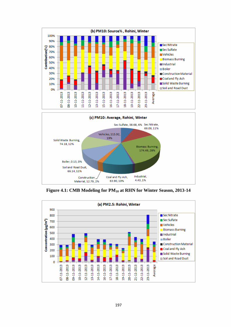
197
Figure 4.1: CMB Modeling for PM10 at RHN for Winter Season, 2013-14

198
Figure 4.2: CMB Modeling for PM2.5 at RHN for Winter Season, 2013-14
Table 4.1: Statistical Summary: RHN, Winter Season
PM10 PM2.5
Parameter Measured Calculated % Mass R² Measured Calculated % Mass R²
Average 592.56 616.71 104.97 0.67 428.45 399.41 92.82 0.66
StdDev 185.43 177.64 8.75 0.07 119.09 142.16 14.57 0.04
CoV 0.31 0.29 0.08 0.10 0.28 0.36 0.16 0.06
Maximum 1043.39 1015.34 123.90 0.75 733.83 813.54 122.10 0.71
Minimum 362.54 413.60 94.10 0.53 261.34 241.52 78.30 0.57

199
Figure 4.3: Backward trajectories at RHN for Winter Season
4.3.1.2 Summer Season RHN: [sampling period: April 04 – April 23, 2014]
PM10 (summer)
The average PM10 concentration was 545µg/m3. Figure 4.4 (a), (b), (c) represents PM10
contribution of sources in terms of concentration, percent contribution of sources and
overall contribution (average over about 20 days) in terms of concentration and percentage
respectively at RHN. Table 4.2 presents summary of performance and acceptability of
CMB model. It is observed that the major PM10 source contributing was soil and road dust
(183 µg/m3 ~ 33%) followed by coal and fly ash (134 µg/m
3 ~ 24%) in PM10. Other
significant sources are secondary particle formation (76 µg/m3 ~ 14%), solid waste
burning (73 µg/m3 ~ 13%), biomass burning (9%), and vehicular emission (4%) in PM10.
Contribution of the industrial emission was estimated less than 1 % in PM10.
PM2.5 (summer)
The average PM2.5 concentration was 337 µg/m3; the PM2.5/PM10 ratio is about 0.6. Figure
4.5 (a), (b), (c) represents PM2.5 contribution of sources in terms of concentration, percent
contribution of sources and overall contribution (average over about 20 days) in terms of
concentration and percentage respectively at RHN. It is observed that the major source
contributing in PM2.5 was soil and road dust (80 µg/m3 ~ 24%) followed by biomass
burning (64 µg/m3 ~ 19%). Other major sources are coal and fly ash (60 µg/m
3 ~ 18%),
secondary particle formation (55 µg/m3 ~ 17%), solid waste burning (11%) and vehicular
emission (7%). Contribution of the industrial emission was estimated less than 1 % in
PM2.5.

200
HYSPLIT back trajectories (Figure 4.6) show that most of the time wind is from NW and
wind mass travels over Punjab and Haryana states before entering in Delhi. These winds
pick up the pollutants on the way especially from tall emitting sources.

201
Figure 4.4: CMB Modeling for PM10 at RHN for Summer Season, 2014
Figure 4.5: CMB Modeling for PM2.5 at RHN for Summer Season, 2014

202
Table 4.2: Statistical Summary: RHN, Summer Season
PM10 PM2.5
Parameter Measured Calculated % Mass R² Measured Calculated % Mass R²
Average 544.71 562.23 104.24 0.67 337.16 329.52 97.98 0.68
StdDev 178.82 177.20 10.87 0.06 114.34 114.61 12.43 0.05
CoV 0.33 0.32 0.10 0.09 0.34 0.35 0.13 0.08
Maximum 927.90 928.68 123.80 0.77 598.44 595.52 122.60 0.77
Minimum 274.78 279.63 75.10 0.58 169.54 154.83 71.70 0.60
Figure 4.6: Backward trajectories at RHN for Summer Season
Inferences
The major sources contributing to PM10 and PM2.5 have dramatically changed. Coal flyash,
road and soil dust have become the major PM10 and PM2.5 sources. It was observed that
atmosphere in summer looked white to gray indicating presence of large amounts of fly
ash and dust which may be due to high speeds wind and very dry conditions which makes
the dust airborne. Occasional dust storm can also contribute to fly and road/soil dust
resuspension.
4.3.2 Envirotech, Okhla (OKH)
4.3.2.1 Winter Season [sampling period: November 03- November 23, 2013]
At this site, three days, November 3-5, 2013, which indicated impact of Diwali fire
crackers are not included here and dealt separately.
PM10 (winter)

203
The average PM10 concentration was 697µg/m3. Figure 4.7 (a), (b), (c) represents PM10
contribution of sources in terms of concentration, percent contribution of sources and
overall contribution (average over about 20 days) in terms of concentration and percentage
respectively at OKH. Table 4.3 presents summary of performance and acceptability of
CMB model. It is observed that the major PM10 source contributing was soil and road dust
(164 µg/m3 ~ 24%) followed by vehicular emission (158 µg/m
3 ~ 23%) in PM10. The other
major sources are biomass burning (109 µg/m3 ~ 16%), coal and flyash (108 µg/m
3 ~
16%), secondary particle formation (14%), construction material (4%) and Solid waste
burning (2.2%) in PM10. Contribution of the industrial emission was estimated less than
1% in PM10.
PM2.5 (winter)
The average PM2.5 concentration was 412 µg/m3. Figure 4.8 (a), (b), (c) represents PM2.5
contribution of sources in terms of concentration, percent contribution of sources and
overall contribution (average over about 20 days) in terms of concentration and percentage
respectively at OKH. It is observed that the major source contributing in PM2.5 was
vehicular emission (109 µg/m3 ~ 29%) followed by biomass burning (108 µg/m
3 ~ 29%).
Other predominant sources are secondary particle formation (76 µg/m3 ~ 20%), coal and
fly ash (39 µg/m3 ~ 10%), soil and road dust (7%) and solid waste burning (3%).
Contribution of the industrial emission was estimated less than 1% in PM2.5.
HYSPLIT back trajectories (Figure 4.9) show that most of the time wind is from NW and
wind mass travels over Punjab and Haryana States before entering in Delhi. These winds
pick up the pollutants on the way especially from large (e.g. crop residue burning (CRB))
and tall emitting sources.

204
Figure 4.7: CMB Modeling for PM10 at OKH for Winter Season, 2013-14

205
Figure 4.8: CMB Modeling for PM2.5 at OKH for Winter Season, 2013-14
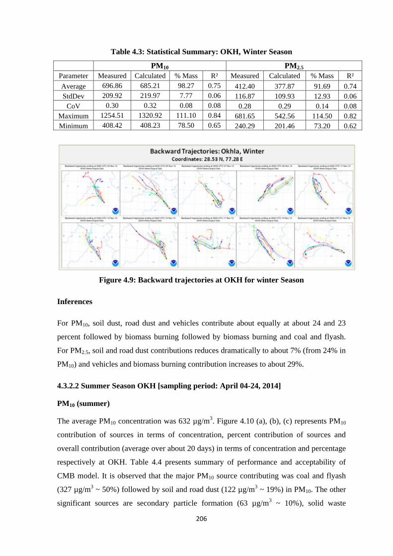
206
Table 4.3: Statistical Summary: OKH, Winter Season
PM10 PM2.5
Parameter Measured Calculated % Mass R² Measured Calculated % Mass R²
Average 696.86 685.21 98.27 0.75 412.40 377.87 91.69 0.74
StdDev 209.92 219.97 7.77 0.06 116.87 109.93 12.93 0.06
CoV 0.30 0.32 0.08 0.08 0.28 0.29 0.14 0.08
Maximum 1254.51 1320.92 111.10 0.84 681.65 542.56 114.50 0.82
Minimum 408.42 408.23 78.50 0.65 240.29 201.46 73.20 0.62
Figure 4.9: Backward trajectories at OKH for winter Season
Inferences
For PM10, soil dust, road dust and vehicles contribute about equally at about 24 and 23
percent followed by biomass burning followed by biomass burning and coal and flyash.
For PM2.5, soil and road dust contributions reduces dramatically to about 7% (from 24% in
PM10) and vehicles and biomass burning contribution increases to about 29%.
4.3.2.2 Summer Season OKH [sampling period: April 04-24, 2014]
PM10 (summer)
The average PM10 concentration was 632 µg/m3. Figure 4.10 (a), (b), (c) represents PM10
contribution of sources in terms of concentration, percent contribution of sources and
overall contribution (average over about 20 days) in terms of concentration and percentage
respectively at OKH. Table 4.4 presents summary of performance and acceptability of
CMB model. It is observed that the major PM10 source contributing was coal and flyash
(327 µg/m3 ~ 50%) followed by soil and road dust (122 µg/m
3 ~ 19%) in PM10. The other
significant sources are secondary particle formation (63 µg/m3 ~ 10%), solid waste

207
burning (50 µg/m3 ~ 8%), vehicular emission (7%) and biomass burning (2%).
Contribution of the industrial emission was estimated less than 2% in PM10.
PM2.5 (summer)
The average PM2.5 concentration was 410 µg/m3; the ratio of PM2.5/PM10 is about 0.57.
Figure 4.11 (a), (b), (c) represents PM2.5 contribution of sources in terms of concentration,
percent contribution of sources and overall contribution (average over about 20 days) in
terms of concentration and percentage respectively at OKH. It is observed that the major
source contributing in PM2.5 was soil and road dust (139 µg/m3 ~ 36%) followed by coal
and fly ash (110 µg/m3 ~ 29%). Other significant sources are secondary particle formation
(54 µg/m3 ~ 14%), vehicular emission (31 µg/m
3 ~ 8%), solid waste burning (7%) and
biomass burning (3%). Contribution of the industrial emission was estimated less than 2%
in PM2.5.
HYSPLIT back trajectories (Figure 4.12) show that most of the time wind is from NW and
wind mass travels over Punjab and Haryana states before entering in Delhi. These winds
pick up the pollutants on the way especially from large (e.g. crop residue burning (CRB))
and tall emitting sources.

208
Figure 4.10: CMB Modeling for PM10 at OKH for Summer Season, 2014

209
Figure 4.11: CMB Modeling for PM2.5 at OKH for Summer Season, 2014
Table 4.4: Statistical Summary: OKH, Summer Season
PM10 PM2.5
Parameter Measured Calculated % Mass R² Measured Calculated % Mass R²
Average 632.43 648.72 103.30 0.68 410.02 383.83 93.51 0.70
StdDev 170.45 168.00 8.92 0.06 119.36 126.62 12.07 0.05
CoV 0.27 0.26 0.09 0.08 0.29 0.33 0.13 0.07
Maximum 954.75 936.80 122.10 0.74 704.02 726.17 120.70 0.78
Minimum 373.84 456.45 86.50 0.51 232.02 240.79 70.20 0.61

210
Figure 4.12: Backward trajectories at OKH for Summer Season
Inference
The sampling site was in the middle of the industrial area which had movement of large
trucks ferrying raw material and finishes products. Poor road conditions and tandoors were
seen in ever by lane. Coal and fly ash is the major contributors in summer both for PM10
and PM2.5, at the same time road and soil dust is prominent both in PM10 and PM2.5.
4.3.3 DAV School, Dwarka (DWK)
4.3.3.1 Winter Season (DWK) [sampling period: December 02- December 22, 2013]
PM10 (winter)
The average PM10 concentration was 544 µg/m3. Figure 4.13 (a), (b), (c) represents PM10
contribution of sources in terms of concentration, percent contribution of sources and
overall contribution (average over about 20 days) in terms of concentration and percentage
respectively at DWK. Table 4.5 presents summary of performance and acceptability of
CMB model. It is observed that the major PM10 source contributing was secondary particle
formation (167 µg/m3 ~ 32%) followed by biomass burning (113 µg/m
3 ~ 21%). The other
significant contributing sources are vehicular emission (105 µg/m3 ~ 20%), soil and road
dust (52 µg/m3 ~ 10%), coal and flyash (7%), solid waste burning (6%) and construction
material (4%). Contribution of the industrial emission was estimated less than 1% in PM10.

211
PM2.5 (winter)
The average PM2.5 concentration was 339 µg/m3. Figure 4.14 (a), (b), (c) represents PM2.5
contribution of sources in terms of concentration, percent contribution of sources and
overall contribution (average over about 20 days) in terms of concentration and percentage
respectively at DWK. It is observed that the major source contributing in PM2.5 was
secondary particle formation (118 µg/m3 ~ 38%) followed by biomass burning (92 µg/m
3
~ 30%). Other major sources are vehicular emission (59 µg/m3 ~ 19%), solid waste
burning (15 µg/m3 ~ 5%), and coal and fly ash (4%). Contributions of minor sources are
soil and road dust (3%), construction material (2%). Contribution of the industrial
emission was estimated to be less than 1% in PM2.5.
HYSPLIT back trajectories (Figure 4.15) show that most of the time wind is from NW and
wind mass travels over Punjab and Haryana states before entering in Delhi. These winds
pick up the pollutants on the way especially from large and tall emitting sources.

212
Figure 4.13: CMB Modeling for PM10 at DWK Winter Season, 2013-14

213
Figure 4.14: CMB Modeling for PM2.5 at DWK, Winter Season, 2013-14
Table 4.5: Statistical Summary: DWK, Winter Season
PM10 PM2.5
Parameter Measured Calculated % Mass R² Measured Calculated % Mass R²
Average 543.85 529.89 97.83 0.64 339.46 311.25 93.18 0.62
StdDev 174.49 168.36 7.70 0.05 156.92 137.13 12.47 0.05
CoV 0.32 0.32 0.08 0.07 0.46 0.44 0.13 0.08
Maximum 981.39 978.12 110.90 0.72 825.90 738.25 117.10 0.70
Minimum 321.00 305.63 85.60 0.51 202.27 177.42 77.90 0.54

214
Figure 4.15: Backward trajectories at DWK for Winter Season
Inferences
Secondary PM (31-38%) and biomass burning (21-29%) are the major sources followed
by vehicular contribution (~20%) – this finding is true for both PM10 and PM2.5. It is bit
surprising that secondary PM has such a high contributors to PM2.5.
4.3.3.2 Summer Season: [sampling period: May 01- May 24, 2014]
PM10 (summer)
The average PM10 concentration was 458 µg/m3. Figure 4.16 (a), (b), (c) represents PM10
contribution of sources in terms of concentration, percent contribution of sources and
overall contribution (average over about 20 days) in terms of concentration and percentage
respectively at DWK. Table 4.6 presents summary of performance and acceptability of
CMB model. It is observed that the major PM10 source contributing was coal and flyash
(174 µg/m3 ~ 39%) followed by soil and road dust (135 µg/m
3 ~ 30%) in PM10. The other
significant sources are secondary particle formation (45 µg/m3 ~ 10%), vehicular emission
(27 µg/m3 ~ 6%), construction material (5%), solid waste burning (4%) and biomass
burning (4%). Contribution of the industrial emission was estimated less than 2% in PM10.
PM2.5 (summer)
The average PM2.5 concentration was 206 µg/m3. Figure 4.17 (a), (b), (c) represents PM2.5
contribution of sources in terms of concentration, percent contribution of sources and
overall contribution (average over about 20 days) in terms of concentration and percentage
respectively at DWK. It is observed that the major source contributing in PM2.5 was coal

215
and flyash (69 µg/m3 ~ 35%) followed by soil and road dust (52 µg/m
3 ~ 26%). Other
significant sources are secondary particle formation (30 µg/m3 ~ 15%), biomass burning
(15 µg/m3 ~ 7%), vehicular emission (6%), construction material (5%), solid waste
burning (4%) and industrial emission (2%).
HYSPLIT back trajectories (Figure 4.18) show that most of the time wind is from NW and
wind mass travels over Punjab and Haryana states before entering in Delhi. These winds
pick up the pollutants on the way especially from large and tall emitting sources.

216
Figure 4.16: CMB Modeling for PM10 at DWK for Summer Season, 2014

217
Figure 4.17: CMB Modeling for PM2.5 at DWK for Summer Season, 2014
Table 4.6: Statistical Summary: DWK, Summer Season
PM10 PM2.5
Parameter Measured Calculated % Mass R² Measured Calculated % Mass R²
Average 457.63 448.51 98.21 0.68 205.62 197.50 96.03 0.68
StdDev 137.91 144.92 11.43 0.06 82.88 89.83 14.30 0.06
CoV 0.30 0.32 0.12 0.09 0.40 0.45 0.15 0.08
Maximum 722.94 756.02 116.20 0.76 356.06 385.38 124.00 0.77
Minimum 163.25 178.70 81.20 0.52 78.69 78.18 69.30 0.57
Figure 4.18: Backward trajectories at DWK for Summer Season
Inference
Coal and flyash, road and soil dusts are the major contributors in summer both for PM10
and PM2.5, at the same time road side dust is prominent both in PM10 and PM2.5.There was
low vehicular density at this site. The station was located at a school point which had play

218
round and it is possible that this site may represent the soil dust emitted from playground
of the school.
4.3.4 Indian Spinal Injuries Centre, Vasantkunj (VKJ)
4.3.4.1 Winter Season [sampling period: December 15, 2013 - January 04, 2014]
PM10 (winter)
The average PM10 concentration was 555 µg/m3. Figure 4.19 (a), (b), (c) represents PM10
contribution of sources in terms of concentration, percent contribution of sources and
overall contribution (average over about 20 days) in terms of concentration and percentage
respectively at VKJ. Table 4.7 presents summary of performance and acceptability of
CMB model. It is observed that the major PM10 source contributing was secondary particle
(163 µg/m3 ~ 32%) followed by vehicular emission (119 µg/m
3 ~ 24%). The other
significant contributing sources are biomass burning (92 µg/m3 ~ 18%), coal and flyash
(43 µg/m3 ~ 9%), soil and road dust (8%), solid waste burning (6%) and construction
material (2.5%). Contribution of the industrial emission was estimated less than 1% in
PM10.
PM2.5 (winter)
The average PM2.5 concentration was 301µg/m3; PM2.5/PM10 ratio was 0.54. Figure 4.20
(a), (b), (c) represents PM2.5 contribution of sources in terms of concentration, percent
contribution of sources and overall contribution (average over about 20 days) in terms of
concentration and percentage respectively at VKJ. It is observed that the major source
contributing in PM2.5 was secondary particle formation (92 µg/m3 ~ 34%) followed by
biomass burning (80 µg/m3 ~ 29%). Other major sources are vehicular emission (76 µg/m
3
~ 28%) and solid waste burning (13 µg/m3 ~ 5%). The minor source are coal and flyash
(1.5%), soil and road dust (1.3%), construction material (<1%) and industrial emission
(<1%) in PM2.5.
HYSPLIT back trajectories (Figure 4.21) show that wind is not stable in any particular
direction and wind mass travel over to neighboring states (i.e Haryana, Uttar Pradesh and
Rajasthan) before entering into Delhi. These winds pick up the pollutants on the way
especially from large and tall emitting sources.

219
Figure 4.19: CMB Modeling for PM10 at VKJ for Winter Season, 2013-14

220
Figure 4.20: CMB Modeling for PM2.5 at VKJ for Winter Season, 2013-14

221
Table 4.7: Statistical Summary: VKJ, Winter Season
PM10 PM2.5
Parameter Measured Calculated % Mass R² Measured Calculated % Mass R²
Average 555.38 502.31 91.86 0.69 300.79 272.47 89.14 0.69
StdDev 188.78 169.40 13.24 0.06 88.70 104.80 12.54 0.05
CoV 0.34 0.34 0.14 0.09 0.29 0.38 0.14 0.07
Maximum 959.63 985.69 118.40 0.76 472.56 495.03 112.40 0.78
Minimum 254.04 264.40 71.50 0.51 180.89 141.14 70.70 0.58
Figure 4.21: Backward trajectories at VKJ for Winter Season
Inference
It is to be noted that at VKJ, secondary particles contribute about 32-33%, vehicles28-24%
and biomass burning 29-18% for PM2.5 and PM10. It signifies that there is need to control
emissions of precursor gases (SO2 and NOx) both from outside and inside of Delhi.
4.3.4.2 Summer Season: [sampling period: April 29 - May 19, 2014]
PM10 (summer)
The average PM10 concentration was 410 µg/m3. Figure 4.22 (a), (b), (c) represents PM10
contribution of sources in terms of concentration, percent contribution of sources and
overall contribution (average over about 20 days) in terms of concentration and percentage
respectively at VKJ. Table 4.8 presents summary of performance and acceptability of
CMB model. It is observed that the major PM10 source contributing was coal and flyash
(133 µg/m3 ~ 33%) followed by soil and road dust (98 µg/m
3 ~ 24%) in PM10. The other
major sources are biomass burning (71 µg/m3 ~ 17%), secondary particle formation (42

222
µg/m3 ~ 10%), vehicular emission (8%), construction material (5%), solid waste burning
(2%) and industrial emission (1%) in PM10.
PM2.5 (summer)
The average PM2.5 concentration was 252 µg/m3; PM2.5/PM10 ratio was 0.6. Figure 4.23
(a), (b), (c) represents PM2.5 contribution of sources in terms of concentration, percent
contribution of sources and overall contribution (average over about 20 days) in terms of
concentration and percentage respectively at VKJ. It is observed that the major source
contributing in PM2.5 was biomass burning (65 µg/m3 ~ 27%) followed by coal and flyash
(58 µg/m3 ~ 24%). Other major sources are Soil and road dust (52 µg/m
3 ~ 21%),
secondary particle formation soil (31 µg/m3 ~ 13%), vehicular emission (9%), solid waste
burning (3%). Other minor sources are construction material (2%) and industrial emission
(1%).
HYSPLIT back trajectories (Figure 4.24) show that most of the time wind is from NW and
wind mass travels over Punjab and Haryana states before entering in Delhi. These winds
pick up the pollutants on the way especially from large and tall emitting sources.

223
Figure 4.22: CMB Modeling for PM10 at VKJ for Summer Season, 2014

224
Figure 4.23: CMB Modeling for PM2.5 at VKJ for Summer Season, 2014
Table 4.8: Statistical Summary: VKJ, Summer Season
PM10 PM2.5
Parameter Measured Calculated % Mass R² Measured Calculated % Mass R²
Average 413.20 409.78 100.03 0.64 252.14 242.67 95.52 0.66
StdDev 90.15 94.78 14.59 0.06 70.72 81.49 11.69 0.05
CoV 0.22 0.23 0.15 0.09 0.28 0.34 0.12 0.08
Maximum 644.79 663.89 123.80 0.75 356.69 416.89 121.90 0.81
Minimum 274.77 274.64 69.20 0.50 120.47 106.16 77.50 0.58

225
Figure 4.24: Backward trajectories at VKJ for Summer Season
Inference
In summer both PM10 and PM2.5 emissions by coal and flyash, road dust and biomass
burning are the major source which requires control in fugitive sources.
4.3.5 Arwachin International School, Dilshad Garden (DSG)
4.3.5.1 Winter Season [sampling period: January 24 - Febuary 13, 2014]
PM10 (winter)
The average PM10 concentration was 688 µg/m3. Figure 4.25 (a), (b), (c) represents PM10
contribution of sources in terms of concentration, percent contribution of sources and
overall contribution (average over about 20 days) in terms of concentration and percentage
respectively at DSG. Table 4.9 presents summary of performance and acceptability of
CMB model. It is observed that the major PM10 source contributing was secondary particle
formation (210 µg/m3 ~ 29%) followed by solid waste burning (127 µg/m
3 ~ 18%). The
other major contributing sources are coal and flyash (106 µg/m3~ 15%), vehicular
emission (104 µg/m3 ~ 14%), soil and road dust (14%), biomass burning (7%) and
construction material (3%).Contribution of the industrial emission was estimated less than
1% in PM10.
PM2.5 (winter)
The average PM2.5 concentration was 425 µg/m3; ratio of PM2.5/PM10 is about 0.58. Figure
4.26 (a), (b), (c) represents PM2.5 contribution of sources in terms of concentration, percent

226
contribution of sources and overall contribution (average over about 20 days) in terms of
concentration and percentage respectively at DSG. It is observed that the major source
contributing in PM2.5 was secondary particle formation (143 µg/m3 ~ 39%) followed by
vehicular emission (88µg/m3 ~ 24%). Other major sources are solid waste burning (54
µg/m3 ~ 15%), biomass burning (43 µg/m
3 ~ 12%), coal and flyash (4%) and soil and road
dust (4%). The minor source are construction material (2%) and industrial emission (<1%)
in PM2.5.
HYSPLIT back trajectories (Figure 4.27) show that most of the time wind is from NW and
wind mass travels over Punjab and Haryana states before entering in Delhi. These winds
pick up the pollutants on the way especially from large and tall emitting sources.

227
Figure 4.25: CMB Modeling for PM10 at DSG for Winter Season, 2013-14

228
Figure 4.26: CMB Modeling for PM2.5 at DSG for Winter Season, 2013-14
Table 4.9: Statistical Summary: DSG, Winter Season
PM10 PM2.5
Parameter Measured Calculated % Mass R² Measured Calculated % Mass R²
Average 687.58 721.03 104.14 0.70 425.49 363.72 88.19 0.68
StdDev 334.96 393.70 13.25 0.05 224.96 186.60 13.10 0.05
CoV 0.49 0.55 0.13 0.08 0.53 0.51 0.15 0.08
Maximum 1418.94 1726.25 124.20 0.77 757.90 742.66 110.90 0.77
Minimum 280.14 300.53 81.00 0.56 157.60 174.73 70.00 0.59
Figure 4.27: Backward trajectories at DSG for Winter Season
Inference
Contributions of secondary particles are consistent high 29% and 39% for PM10 and PM2.5
followed by vehicles at 14 and 24%. Solid waste burning appears to be wide spread and
consistently contributing to both PM10 and PM2.5.

229
4.3.5.2 Summer Season [sampling period: May 26, 2014 - June 14, 2014]
PM10 (summer)
The average PM10 concentration was 531 µg/m3. Figure 4.28 (a), (b), (c) shows PM10
concentration contribution of sources, percent contribution of sources and summary of
sources (average over about 20 days) at DSG. Table 4.10 presents summary of
performance and acceptability of CMB model. It is observed that the major PM10 source
contributing was soil and road dust (185 µg/m3 ~ 34%) followed by coal and flyash (145
µg/m3 ~ 27%). The other major contributing sources are solid waste burning (54 µg/m
3 ~
10%), secondary particle formation (46 µg/m3 ~ 9%), biomass burning (8%), vehicular
emission (7%) and construction material (4%). Contribution of the industrial emission was
estimated less than 1% in PM10.
PM2.5 (summer)
The average PM2.5 concentration was 276 µg/m3. Figure 4.29 (a), (b), (c) represents PM2.5
contribution of sources in terms of concentration, percent contribution of sources and
overall contribution (average over about 20 days) in terms of concentration and percentage
respectively at DSG. It is observed that the major source contributing in PM2.5 was soil and
road dust (74 µg/m3 ~ 28%) followed by coal and flyash (56 µg/m
3 ~ 21%). Other major
sources are secondary particle formation (38 µg/m3 ~ 14%), biomass burning (37 µg/m
3 ~
14%), solid waste burning (9%), vehicular emission (9%) and construction material (3%).
Contribution of the industrial emission was estimated less than 1% in PM2.5.
HYSPLIT back trajectories (Figure 4.30) show that most of the time wind is from NW and
wind mass travels over Punjab and Haryana states before entering in Delhi. These winds
pick up the pollutants on the way especially from large and tall emitting sources.

230
Figure 4.28: CMB Modeling for PM10 at DSG for Summer Season, 2014

231
Figure 4.29: CMB Modeling for PM2.5 at DSG for Summer Season, 2014

232
Table 4.10: Statistical Summary: DSG, Summer Season
PM10 PM2.5
Parameter Measured Calculated % Mass R² Measured Calculated % Mass R²
Average 531.00 539.05 102.21 0.67 276.15 266.09 97.76 0.71
StdDev 98.24 100.13 11.79 0.06 104.44 91.54 8.84 0.05
CoV 0.19 0.19 0.12 0.09 0.38 0.34 0.09 0.07
Maximum 680.28 739.25 123.60 0.77 467.37 441.38 118.60 0.79
Minimum 348.67 371.26 77.80 0.56 140.28 134.25 77.10 0.63
Figure 4.30: Backward trajectories at DSG for Summer Season
Inference
In summer both PM10 and PM2.5 by soil and road dust, coal and flyash, biomass burning
and solid waste burning are the major sources which requires control in fugitive sources.
4.3.6 DTEA School, Pusa Road (PUS)
4.3.6.1 Winter Season [sampling period: January 30, 2014 - February 22, 2014]
PM10 (winter)
The average PM10 concentration was 473 µg/m3. Figure 4.31 (a), (b) and (c) represents
PM10 contribution of sources in terms of concentration, percent contribution of sources
and overall contribution (average over about 20 days) in terms of concentration and
percentage respectively at PUS. Table 4.11 presents summary of performance and
acceptability of CMB model. It is observed that the major PM10 source contributing was
secondary particle formation (119 µg/m3 ~ 26%) followed by vehicular emission (87

233
µg/m3 ~ 19%). The other major contributing sources are soil and road dust (83 µg/m
3 ~
19%), coal and fly ash (66 µg/m3 ~ 15%), biomass burning (11%), solid waste burning
(6%) and construction material (3%). Contribution of the industrial emission was
estimated less than 1% in PM10.
PM2.5 (winter)
The average PM2.5 concentration was 272 µg/m3. Figure 4.32 (a), (b), (c) represents PM2.5
contribution of sources in terms of concentration, percent contribution of sources and
overall contribution (average over about 20 days) in terms of concentration and percentage
respectively at PUS. It is observed that the major source contributing in PM2.5 was
secondary particle formation (76 µg/m3 ~ 32%) followed by vehicular emission (65µg/m
3
~ 28%). Other major sources are biomass burning (47 µg/m3 ~ 20%), soil and road dust
(25 µg/m3 ~ 11%), and solid waste burning (5%). The minor sources are construction
material (2%), coal and flyash (1.3%) and industrial emission (1.2%) in PM2.5.
HYSPLIT back trajectories (Figure 4.33) show that most of the time wind is from NW and
wind mass travels over Punjab and Haryana states before entering in Delhi. These winds
pick up the pollutants on the way especially from large and tall emitting sources.

234
Figure 4.31: CMB Modeling for PM10 at PUS for Winter Season, 2013-14

235
Figure 4.32: CMB Modeling for PM2.5 at PUS for Winter Season, 2013-14
Table 4.11: Statistical Summary: PUS, Winter Season
PM10 PM2.5
Parameter Measured Calculated % Mass R² Measured Calculated % Mass R²
Average 472.79 448.05 95.37 0.71 272.02 236.04 85.62 0.67
StdDev 184.79 177.97 11.77 0.03 73.37 80.95 11.48 0.03
CoV 0.39 0.40 0.12 0.05 0.27 0.34 0.13 0.04
Maximum 757.22 761.72 121.40 0.77 368.26 364.41 109.30 0.71
Minimum 171.93 174.14 70.00 0.65 142.11 121.54 71.10 0.60
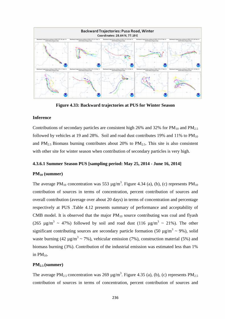
236
Figure 4.33: Backward trajectories at PUS for Winter Season
Inference
Contributions of secondary particles are consistent high 26% and 32% for PM10 and PM2.5
followed by vehicles at 19 and 28%. Soil and road dust contributes 19% and 11% to PM10
and PM2.5 Biomass burning contributes about 20% to PM2.5. This site is also consistent
with other site for winter season when contribution of secondary particles is very high.
4.3.6.1 Summer Season PUS [sampling period: May 25, 2014 - June 16, 2014]
PM10 (summer)
The average PM10 concentration was 553 µg/m3. Figure 4.34 (a), (b), (c) represents PM10
contribution of sources in terms of concentration, percent contribution of sources and
overall contribution (average over about 20 days) in terms of concentration and percentage
respectively at PUS .Table 4.12 presents summary of performance and acceptability of
CMB model. It is observed that the major PM10 source contributing was coal and flyash
(265 µg/m3 ~ 47%) followed by soil and road dust (116 µg/m
3 ~ 21%). The other
significant contributing sources are secondary particle formation (50 µg/m3 ~ 9%), solid
waste burning (42 µg/m3 ~ 7%), vehicular emission (7%), construction material (5%) and
biomass burning (3%). Contribution of the industrial emission was estimated less than 1%
in PM10.
PM2.5 (summer)
The average PM2.5 concentration was 269 µg/m3. Figure 4.35 (a), (b), (c) represents PM2.5
contribution of sources in terms of concentration, percent contribution of sources and

237
overall contribution (average over about 20 days) in terms of concentration and percentage
respectively at PUS. It is observed that the major source contributing in PM2.5 was coal
and fly ash (83 µg/m3 ~ 32%) followed by soil and road dust (80 µg/m
3 ~ 29%). Other
major sources are secondary particle formation (41 µg/m3 ~ 16%), and vehicular emission
(33 µg/m3 ~ 13%), solid waste burning (8%), biomass burning (5%) and construction
material (3%). The minor source is industrial emission (1%) in PM2.5.
HYSPLIT back trajectories (Figure 4.36) show that most of the time wind is from NW and
wind mass travels over Punjab and Haryana states before entering in Delhi. These winds
pick up the pollutants on the way especially from large and tall emitting sources.

238
Figure 4.34: CMB Modeling for PM10 at PUS for Summer Season, 2014

239
Figure 4.35: CMB Modeling for PM2.5 at PUS for Summer Season, 2014
Table 4.12: Statistical Summary: PUS, Summer Season
PM10 PM2.5
Parameter Measured Calculated % Mass R² Measured Calculated % Mass R²
Average 552.53 560.90 101.71 0.70 268.75 260.40 97.90 0.68
StdDev 122.95 145.64 13.06 0.06 104.93 101.54 10.03 0.05
CoV 0.22 0.26 0.13 0.08 0.39 0.39 0.10 0.07
Maximum 771.91 841.47 121.00 0.80 577.81 577.57 114.80 0.75
Minimum 336.65 329.72 73.40 0.58 116.49 109.40 80.50 0.58
Figure 4.36: Backward trajectories at PUS for Winter Season
4.4 Break-up Vehicular Contribution: Fuel-wise
As stated in the beginning of this chapter, due to colinearity in source profiles of vehicular
fuels, CMB modeling could not resolve the contribution of vehicle fuels separately. The

240
results of CMB modeling for vehicular contribution was distributed to fuel specific
contributions based on emission inventory of PM2.5 from gasoline, diesel and CNG
specific to the grid where measurements were done. The vehicle fuel specific contributions
to PM2.5 for summer and winter seasons are given in Figure 4.37 ((a) concentration); (b)
percentage)). Except for RHN site, major contribution is from diesel vehicles – at RNH
diesel vehicle contribution is only 20 percent. While OKH, VKJ, DSG show 70-95%
diesel contribution and at PUS and DWK, diesel contribution is about 60 percent. CNG
contributes a very small (2 to 8 percent) amount of PM2.5 compared to gasoline and diesel
fuels.
4.5 Long range transport and contribution
HYSPLIT back trajectories show that most of the time wind is from NW and sometimes
from west. Wind mass as it travels over Punjab, Haryana and parts of Rajasthan states
before entering in Delhi may pick up the pollutants on the way especially from large
sources (e.g. crop residue burning (CRB)) and tall emitting sources; however these
contributions have not been quantifies. Ghosh et al. (2015) have made some assessment of
the emissions upstream of Delhi and their contribution in Delhi.
Figure 4.37: Contribution of Fuels in Vehicular Emission
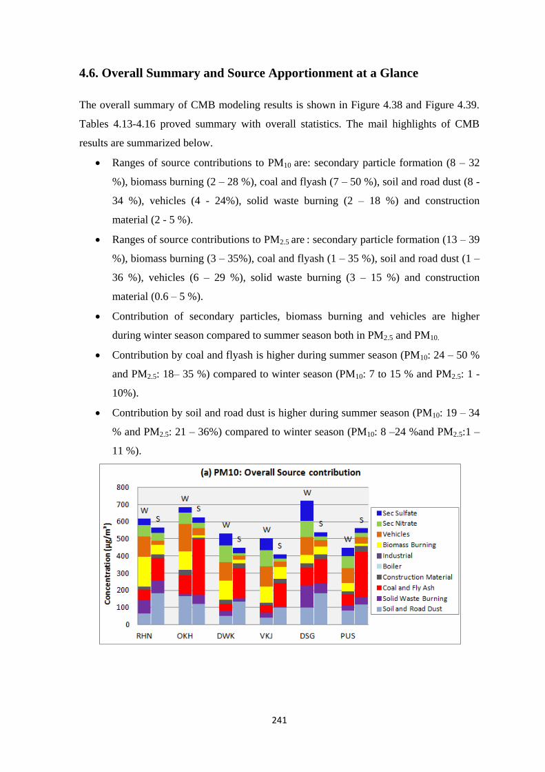
241
4.6. Overall Summary and Source Apportionment at a Glance
The overall summary of CMB modeling results is shown in Figure 4.38 and Figure 4.39.
Tables 4.13-4.16 proved summary with overall statistics. The mail highlights of CMB
results are summarized below.
Ranges of source contributions to PM10 are: secondary particle formation (8 – 32
%), biomass burning (2 – 28 %), coal and flyash (7 – 50 %), soil and road dust (8 -
34 %), vehicles (4 - 24%), solid waste burning (2 – 18 %) and construction
material (2 - 5 %).
Ranges of source contributions to PM2.5 are : secondary particle formation (13 – 39
%), biomass burning (3 – 35%), coal and flyash (1 – 35 %), soil and road dust (1 –
36 %), vehicles (6 – 29 %), solid waste burning (3 – 15 %) and construction
material (0.6 – 5 %).
Contribution of secondary particles, biomass burning and vehicles are higher
during winter season compared to summer season both in PM2.5 and PM10.
Contribution by coal and flyash is higher during summer season (PM10: 24 – 50 %
and PM2.5: 18– 35 %) compared to winter season (PM10: 7 to 15 % and PM2.5: 1 -
10%).
Contribution by soil and road dust is higher during summer season (PM10: 19 – 34
% and PM2.5: 21 – 36%) compared to winter season (PM10: 8 –24 %and PM2.5:1 –
11 %).

242
Figure 4.38: Overall Results of CMB Modeling for PM10
Figure 4.39: Overall Results of CMB Modeling for PM2.5

243
Table 4.13: Statistical Summary of the Source Apportionment in PM10 for Winter Season (Concentration in µg/m3)
Site location Parameter Measure
d PM10
Calculate
d PM10
%
Mass R²
% Source Contribution
Sec
Sulfate
Sec
Nitrate
Biomass
Burning Industrial
Coal and
Fly Ash
Construc
tion
Material
Soil and
Road
Dust
Boiler
Solid
Waste
Burning
Vehicles
RHN
Average 592.56 616.71 104.97 0.67 6.01 10.21 28.91 0.69 11.20 1.98 9.12 0.02 12.76 19.10
StdDev 185.43 177.64 8.75 0.07 3.05 3.39 9.04 0.27 6.92 0.61 9.86 0.03 11.21 7.86
CoV 0.31 0.29 0.08 0.10 0.51 0.33 0.31 0.39 0.62 0.31 1.08 1.72 0.88 0.41
Maximum 1043.39 1015.34 123.90 0.75 10.88 18.39 43.32 1.06 24.68 3.16 25.62 0.09 38.99 32.15
Minimum 362.54 413.60 94.10 0.53 2.66 5.82 17.04 0.31 0.00 1.04 0.00 0.00 0.00 6.52
OKH
Average 696.86 685.21 98.27 0.75 4.35 9.73 17.11 0.47 15.50 4.13 23.13 0.00 2.16 23.42
StdDev 209.92 219.97 7.77 0.06 2.52 3.20 7.81 0.18 7.95 2.38 10.45 0.00 1.64 7.39
CoV 0.30 0.32 0.08 0.08 0.58 0.33 0.46 0.37 0.51 0.58 0.45 0.00 0.76 0.32
Maximum 1254.51 1320.92 111.10 0.84 9.04 15.77 36.13 0.94 30.22 8.99 45.76 0.00 7.01 38.06
Minimum 408.42 408.23 78.50 0.65 0.32 4.27 0.00 0.22 0.00 0.00 5.57 0.00 0.19 11.37
DWK
Average 543.85 529.89 97.83 0.64 12.31 18.04 20.82 0.65 8.16 3.99 10.24 0.03 6.00 19.77
StdDev 174.49 168.36 7.70 0.05 6.35 4.34 7.56 0.20 8.10 1.62 7.82 0.05 3.41 4.93
CoV 0.32 0.32 0.08 0.07 0.52 0.24 0.36 0.32 0.99 0.41 0.76 1.91 0.57 0.25
Maximum 981.39 978.12 110.90 0.72 29.97 26.01 42.13 1.07 29.18 8.07 24.67 0.17 13.96 28.27
Minimum 321.00 305.63 85.60 0.51 5.38 11.19 10.00 0.35 0.00 1.58 1.08 0.00 1.16 10.18
VKJ
Average 555.38 502.31 91.86 0.69 12.69 18.74 19.46 0.64 8.89 2.56 8.03 0.00 5.44 23.55
StdDev 188.78 169.40 13.24 0.06 6.68 5.79 7.14 0.19 6.03 1.78 5.90 0.01 3.40 11.61
CoV 0.34 0.34 0.14 0.09 0.53 0.31 0.37 0.29 0.68 0.70 0.73 3.04 0.63 0.49
Maximum 959.63 985.69 118.40 0.76 28.23 34.94 32.19 1.16 24.73 7.11 20.56 0.05 15.15 43.00
Minimum 254.04 264.40 71.50 0.51 3.54 11.20 7.01 0.44 1.03 0.54 1.58 0.00 0.67 2.58
DSG
Average 687.58 721.03 104.14 0.70 15.30 13.80 7.81 0.67 14.87 3.16 14.39 0.03 15.15 14.82
StdDev 334.96 393.70 13.25 0.05 6.59 4.96 6.29 0.32 7.44 1.71 5.91 0.08 11.00 4.67
CoV 0.49 0.55 0.13 0.08 0.43 0.36 0.81 0.47 0.50 0.54 0.41 3.05 0.73 0.31
Maximum 1418.94 1726.25 124.20 0.77 28.42 26.65 20.78 1.46 31.44 6.58 22.78 0.34 36.64 25.21
Minimum 280.14 300.53 81.00 0.56 7.30 5.76 0.00 0.27 1.06 0.79 0.80 0.00 2.56 5.31
PUS
Average 472.79 448.05 95.37 0.71 11.39 15.56 11.11 0.88 14.69 3.19 17.61 0.01 6.35 19.20
StdDev 184.79 177.97 11.77 0.03 5.13 3.81 4.77 0.30 5.09 0.97 7.79 0.02 3.81 6.66
CoV 0.39 0.40 0.12 0.05 0.45 0.25 0.43 0.34 0.35 0.31 0.44 2.02 0.60 0.35
Maximum 757.22 761.72 121.40 0.77 25.27 24.39 16.66 1.70 24.22 6.00 36.03 0.08 16.07 38.50
Minimum 171.93 174.14 70.00 0.65 4.45 8.33 0.00 0.53 6.23 1.66 0.09 0.00 1.78 10.15

244
Table 4.14: Statistical Summary of the Source Apportionment in PM10 for Summer Season (Concentration in µg/m3)
Site location Parameter Measure
d PM10
Calculate
d PM10
%
Mass R²
% Source Contribution
Sec
Sulfate
Sec
Nitrate
Biomass
Burning Industrial
Coal and
Fly Ash
Construc
tion
Material
Soil and
Road
Dust
Boiler
Solid
Waste
Burning
Vehicles
RHN
Average 544.71 562.23 104.24 0.67 5.81 8.53 10.46 0.78 24.89 2.93 29.77 0.06 12.74 4.76
StdDev 178.82 177.20 10.87 0.06 1.88 4.01 6.78 0.40 12.00 2.56 14.76 0.12 6.85 2.43
CoV 0.33 0.32 0.10 0.09 0.32 0.47 0.65 0.51 0.48 0.87 0.50 2.05 0.54 0.51
Maximum 927.90 928.68 123.80 0.77 9.18 16.32 25.08 1.68 40.28 6.76 66.57 0.48 28.54 8.83
Minimum 274.78 279.63 75.10 0.58 2.90 3.81 0.10 0.21 0.00 0.00 12.00 0.00 0.00 0.25
OKH
Average 632.43 648.72 103.30 0.68 5.41 4.64 2.18 1.31 49.66 - 18.59 0.06 7.58 7.04
StdDev 170.45 168.00 8.92 0.06 2.49 2.29 2.48 0.53 11.92 - 9.28 0.09 3.24 3.33
CoV 0.27 0.26 0.09 0.08 0.46 0.49 1.14 0.40 0.24 - 0.50 1.43 0.43 0.47
Maximum 954.75 936.80 122.10 0.74 11.52 12.01 7.33 2.31 73.58 - 44.52 0.27 14.06 12.74
Minimum 373.84 456.45 86.50 0.51 1.86 2.29 0.00 0.49 27.08 - 5.86 0.00 0.00 1.65
DWK
Average 457.63 448.51 98.21 0.68 7.02 2.99 5.36 1.53 37.37 5.27 30.63 0.02 3.83 5.97
StdDev 137.91 144.92 11.43 0.06 2.64 0.82 5.98 0.86 15.11 2.83 16.16 0.05 2.31 2.75
CoV 0.30 0.32 0.12 0.09 0.38 0.27 1.12 0.56 0.40 0.54 0.53 1.91 0.60 0.46
Maximum 722.94 756.02 116.20 0.76 12.14 5.19 23.74 4.59 64.88 10.44 66.83 0.15 7.77 10.99
Minimum 163.25 178.70 81.20 0.52 2.70 1.63 0.00 0.50 16.14 1.23 1.86 0.00 0.56 1.57
VKJ
Average 413.20 409.78 100.03 0.64 5.65 5.05 18.17 1.33 33.32 4.97 21.40 0.17 2.34 7.60
StdDev 90.15 94.78 14.59 0.06 4.54 3.20 11.60 0.77 15.05 2.75 18.77 0.37 1.20 4.43
CoV 0.22 0.23 0.15 0.09 0.80 0.63 0.64 0.58 0.45 0.55 0.88 2.22 0.51 0.58
Maximum 644.79 663.89 123.80 0.75 15.70 11.60 39.50 3.51 65.36 12.78 74.24 1.68 5.53 19.18
Minimum 274.77 274.64 69.20 0.50 0.00 1.20 1.19 0.28 10.73 0.00 1.85 0.00 0.84 1.51
DSG
Average 531.00 539.05 102.21 0.67 4.90 3.51 9.59 0.81 26.65 4.24 32.96 0.14 9.90 7.30
StdDev 98.24 100.13 11.79 0.06 2.89 2.03 9.91 0.31 10.21 1.69 11.82 0.17 5.22 4.22
CoV 0.19 0.19 0.12 0.09 0.59 0.58 1.03 0.39 0.38 0.40 0.36 1.18 0.53 0.58
Maximum 680.28 739.25 123.60 0.77 10.00 9.80 31.58 1.43 48.53 6.50 57.85 0.61 16.69 14.10
Minimum 348.67 371.26 77.80 0.56 0.41 1.11 0.00 0.27 12.66 1.29 9.91 0.00 0.87 0.67
PUS
Average 552.53 560.90 101.71 0.70 4.67 3.99 2.74 0.94 46.40 5.25 21.02 0.13 7.50 7.37
StdDev 122.95 145.64 13.06 0.06 2.86 1.66 2.48 0.28 15.65 1.59 11.92 0.12 4.45 3.12
CoV 0.22 0.26 0.13 0.08 0.61 0.42 0.90 0.30 0.34 0.30 0.57 0.94 0.59 0.42
Maximum 771.91 841.47 121.00 0.80 10.06 8.23 6.92 1.37 66.12 7.97 44.86 0.41 18.64 15.56
Minimum 336.65 329.72 73.40 0.58 0.53 2.38 0.00 0.36 21.52 2.77 0.00 0.00 1.16 3.62

245
Table 4.15: Statistical Summary of the Source Apportionment in PM2.5 for Winter Season (Concentration in µg/m3)
Site location Parameter Measure
d PM2.5
Calculate
d PM2.5
%
Mass R²
% Source Contribution
Sec
Sulfate
Sec
Nitrate
Biomass
Burning Industrial
Coal and
Fly Ash
Construc
tion
Material
Soil and
Road
Dust
Boiler
Solid
Waste
Burning
Vehicles
RHN
Average 428.45 399.41 92.82 0.66 9.07 10.47 35.34 0.66 5.35 1.34 1.91 0.01 10.90 24.94
StdDev 119.09 142.16 14.57 0.04 3.31 3.53 9.60 0.26 4.13 0.62 1.80 0.01 8.56 12.06
CoV 0.28 0.36 0.16 0.06 0.36 0.34 0.27 0.39 0.77 0.46 0.94 1.74 0.79 0.48
Maximum 733.83 813.54 122.10 0.71 17.42 18.47 51.16 1.32 14.79 2.24 5.14 0.03 26.28 45.95
Minimum 261.34 241.52 78.30 0.57 4.12 3.22 20.06 0.24 0.00 0.00 0.00 0.00 0.00 12.64
OKH
Average 412.40 377.87 91.69 0.74 7.91 12.03 29.86 0.69 9.45 1.90 6.36 0.01 2.53 29.26
StdDev 116.87 109.93 12.93 0.06 3.35 3.59 15.19 0.24 7.10 1.79 7.73 0.03 1.13 7.78
CoV 0.28 0.29 0.14 0.08 0.42 0.30 0.51 0.34 0.75 0.94 1.22 3.02 0.45 0.27
Maximum 681.65 542.56 114.50 0.82 14.33 20.37 54.78 1.22 24.34 4.60 30.07 0.11 5.04 45.13
Minimum 240.29 201.46 73.20 0.62 3.38 5.36 3.02 0.38 0.00 0.00 0.00 0.00 0.51 16.75
DWK
Average 339.46 311.25 93.18 0.62 14.10 22.66 30.52 0.88 4.68 1.76 2.25 0.00 4.76 18.39
StdDev 156.92 137.13 12.47 0.05 4.97 5.03 8.01 0.26 6.52 0.79 1.99 0.01 2.31 8.70
CoV 0.46 0.44 0.13 0.08 0.35 0.22 0.26 0.30 1.39 0.45 0.88 2.39 0.49 0.47
Maximum 825.90 738.25 117.10 0.70 26.80 31.83 40.71 1.32 27.08 3.60 6.15 0.03 9.67 33.03
Minimum 202.27 177.42 77.90 0.54 7.89 11.97 17.45 0.43 0.32 0.00 0.00 0.00 1.97 8.01
VKJ
Average 300.79 272.47 89.14 0.69 14.28 18.44 30.79 0.75 1.63 0.60 1.09 0.00 4.49 27.92
StdDev 88.70 104.80 12.54 0.05 5.54 5.65 12.53 0.17 1.24 0.37 2.19 0.00 2.49 10.58
CoV 0.29 0.38 0.14 0.07 0.39 0.31 0.41 0.23 0.76 0.61 2.01 0.00 0.55 0.38
Maximum 472.56 495.03 112.40 0.78 25.75 29.73 54.50 1.12 4.53 1.40 8.80 0.00 12.67 50.78
Minimum 180.89 141.14 70.70 0.58 6.27 10.89 11.64 0.50 0.00 0.03 0.00 0.00 2.23 13.33
DSG
Average 425.49 363.72 88.19 0.68 21.02 17.39 13.43 0.65 4.50 1.22 3.35 0.02 12.75 25.68
StdDev 224.96 186.60 13.10 0.05 5.95 5.15 10.10 0.19 4.78 0.60 5.00 0.04 9.07 7.43
CoV 0.53 0.51 0.15 0.08 0.28 0.30 0.75 0.30 1.06 0.49 1.49 2.42 0.71 0.29
Maximum 757.90 742.66 110.90 0.77 29.83 31.39 33.23 0.98 17.17 2.21 17.34 0.11 28.94 46.80
Minimum 157.60 174.73 70.00 0.59 11.51 11.07 0.00 0.34 0.00 0.00 0.00 0.00 3.61 16.26
PUS
Average 272.02 236.04 85.62 0.67 15.03 18.31 20.75 1.20 1.12 1.79 9.96 0.01 5.67 26.15
StdDev 73.37 80.95 11.48 0.03 6.39 4.63 7.93 0.36 1.36 0.68 11.65 0.04 2.86 7.56
CoV 0.27 0.34 0.13 0.04 0.42 0.25 0.38 0.30 1.21 0.38 1.17 2.71 0.50 0.29
Maximum 368.26 364.41 109.30 0.71 28.12 25.18 34.75 1.91 4.12 3.62 36.71 0.14 13.10 45.92
Minimum 142.11 121.54 71.10 0.60 5.81 10.74 0.00 0.65 0.00 0.73 0.00 0.00 2.13 17.85

246
Table 4.16: Statistical Summary of the Source Apportionment in PM2.5 for Summer Season (Concentration in µg/m3)
Site location Parameter Measure
d PM2.5
Calculate
d PM2.5
%
Mass R²
% Source Contribution
Sec
Sulfate
Sec
Nitrate
Biomass
Burning Industrial
Coal and
Fly Ash
Construc
tion
Material
Soil and
Road
Dust
Boiler
Solid
Waste
Burning
Vehicles
RHN
Average 337.16 329.52 97.98 0.68 8.33 9.82 21.64 0.85 17.17 2.36 21.42 0.07 11.36 6.98
StdDev 114.34 114.61 12.43 0.05 2.68 5.16 15.55 0.63 8.96 1.64 15.87 0.18 4.87 4.09
CoV 0.34 0.35 0.13 0.08 0.32 0.53 0.72 0.75 0.52 0.69 0.74 2.78 0.43 0.59
Maximum 598.44 595.52 122.60 0.77 12.76 20.95 41.32 2.39 32.07 5.11 49.38 0.73 18.86 13.76
Minimum 169.54 154.83 71.70 0.60 4.16 4.15 3.75 0.08 2.00 0.00 0.00 0.00 3.95 1.31
OKH
Average 410.02 383.83 93.51 0.70 9.35 5.54 3.68 1.40 27.06 - 35.65 0.09 6.70 8.96
StdDev 119.36 126.62 12.07 0.05 3.53 2.37 7.40 0.72 11.83 - 10.68 0.12 2.59 5.47
CoV 0.29 0.33 0.13 0.07 0.38 0.43 2.01 0.51 0.44 - 0.30 1.33 0.39 0.61
Maximum 704.02 726.17 120.70 0.78 17.04 13.10 25.33 3.43 49.99 - 50.74 0.39 14.01 24.14
Minimum 232.02 240.79 70.20 0.61 3.59 2.73 0.00 0.68 7.94 - 14.49 0.00 1.71 1.60
DWK
Average 205.62 197.50 96.03 0.68 12.45 4.85 8.43 1.72 32.93 5.02 24.83 0.02 4.12 5.64
StdDev 82.88 89.83 14.30 0.06 4.92 2.09 13.84 0.82 14.16 1.73 17.85 0.04 1.61 2.75
CoV 0.40 0.45 0.15 0.08 0.39 0.43 1.64 0.48 0.43 0.35 0.72 2.44 0.39 0.49
Maximum 356.06 385.38 124.00 0.77 22.10 9.85 38.30 3.10 69.83 7.94 61.81 0.14 7.53 9.96
Minimum 78.69 78.18 69.30 0.57 5.56 1.44 0.00 0.38 6.54 2.52 0.69 0.00 2.45 1.06
VKJ
Average 252.14 242.67 95.52 0.66 7.62 5.43 27.24 1.23 22.37 2.55 21.50 0.09 2.78 9.20
StdDev 70.72 81.49 11.69 0.05 5.22 2.95 12.49 0.68 13.54 1.87 17.13 0.14 1.25 4.50
CoV 0.28 0.34 0.12 0.08 0.69 0.54 0.46 0.56 0.61 0.73 0.80 1.57 0.45 0.49
Maximum 356.69 416.89 121.90 0.81 19.09 12.45 47.51 3.10 55.74 5.79 66.88 0.54 5.33 19.78
Minimum 120.47 106.16 77.50 0.58 0.00 1.62 0.00 0.19 4.50 0.00 0.00 0.00 0.98 0.06
DSG
Average 276.15 266.09 97.76 0.71 9.80 4.93 13.24 0.94 21.28 4.11 26.12 0.05 9.09 10.44
StdDev 104.44 91.54 8.84 0.05 4.61 2.49 12.86 0.65 10.63 1.89 9.85 0.12 3.78 9.19
CoV 0.38 0.34 0.09 0.07 0.47 0.51 0.97 0.69 0.50 0.46 0.38 2.23 0.42 0.88
Maximum 467.37 441.38 118.60 0.79 18.13 13.15 34.70 2.80 50.55 6.43 39.23 0.40 15.87 32.08
Minimum 140.28 134.25 77.10 0.63 1.83 1.55 0.00 0.32 7.00 1.23 4.39 0.00 3.31 0.00
PUS
Average 268.75 260.40 97.90 0.68 10.36 6.93 5.24 1.42 31.14 3.35 19.56 0.41 7.85 13.74
StdDev 104.93 101.54 10.03 0.05 6.41 5.69 6.70 0.84 12.06 1.36 16.39 0.43 4.32 6.19
CoV 0.39 0.39 0.10 0.07 0.62 0.82 1.28 0.59 0.39 0.41 0.84 1.06 0.55 0.45
Maximum 577.81 577.57 114.80 0.75 22.64 28.76 24.15 3.86 50.33 5.71 75.14 1.75 19.90 32.66
Minimum 116.49 109.40 80.50 0.58 0.00 0.81 0.00 0.40 3.84 0.71 0.26 0.00 2.90 6.34

247
Table 4.17(a): Concentration Apportionment: Winter PM10 (Concentration in µg/m
3)
Site location Measured
PM10 Sec
Particle Biomass
Burning Industrial
Coal and
Fly Ash Construction
Material Soil and
Road Dust Boiler
Solid Waste
Burning Vehicles
RHN 593 105 174 4 64 13 66 0 74 116
OKH 697 99 109 3 108 28 164 0 17 158
DWK 544 167 113 3 38 20 52 0 32 105
VKJ 555 163 92 3 43 13 40 0 30 119
DSG 688 210 49 5 106 20 100 0 127 104
PUS 473 119 48 4 66 14 83 0 27 87
Overall 592 144 97 4 71 18 84 0 51 115
Std 87 43.39 47.14 0.76 29.97 5.95 44.75 0.11 42.12 23.94
Table 4.18(b): Concentration Apportionment: Winter PM2.5 (Concentration in µg/m3)
Site
location Measured
PM2.5 Sec
Particle Biomass
Burning Industrial
Coal and
Fly Ash Construction
Material Soil and
Road Dust Boiler
Solid
Waste
Burning Vehicles
RHN 428 81 137 3 20 6 8 0 48 96
OKH 412 76 108 3 39 8 26 0 10 109
DWK 339 118 92 3 12 5 8 0 15 59
VKJ 301 92 80 2 4 2 4 0 13 76
DSG 425 143 43 2 15 4 13 0 54 88
PUS 272 76 47 3 3 4 25 0 12 65
Overall 363 98 84 3 16 5 14 0 25 82
Std 68 27.31 36.24 0.26 13.08 2.12 9.49 0.02 19.96 19.20

248
Table 4.19(a): Percentage Apportionment: Winter PM10 (Concentration in µg/m
3)
Site location Measured
PM10 Sec
Particle Biomass
Burning Industrial
Coal and
Fly Ash Construction
Material Soil and
Road Dust Boiler
Solid Waste
Burning Vehicles
RHN 593 16.99 28.29 0.72 10.36 2.07 10.72 0.02 12.03 18.80
OKH 697 14.46 15.85 0.45 15.73 4.05 23.96 0.00 2.45 23.06
DWK 544 31.51 21.24 0.62 7.21 3.86 9.73 0.02 5.98 19.83
VKJ 555 32.44 18.27 0.64 8.58 2.51 7.90 0.00 5.99 23.67
DSG 688 29.09 6.82 0.69 14.66 2.80 13.85 0.04 17.61 14.43
PUS 473 26.47 10.68 0.86 14.75 3.15 18.62 0.01 6.02 19.43
Overall 592 24.61 16.68 0.65 12.13 3.08 14.41 0.02 8.75 19.67
Std 87 7.64 7.64 0.14 3.63 0.77 6.11 0.02 5.49 3.33
Table 4.20(b): Percentage Apportionment: Winter PM2.5 (Concentration in µg/m
3)
Site
location Measured
PM2.5 Sec
Particle Biomass
Burning Industrial
Coal and
Fly Ash Construction
Material Soil and
Road Dust Boiler
Solid
Waste
Burning Vehicles
RHN 428 20.28 34.42 0.68 5.10 1.46 1.99 0.01 12.01 24.05
OKH 412 19.99 28.54 0.67 10.24 2.12 6.88 0.01 2.61 28.94
DWK 339 37.82 29.50 0.85 3.95 1.77 2.56 0.00 4.75 18.80
VKJ 301 33.89 29.23 0.77 1.50 0.58 1.32 0.00 4.79 27.92
DSG 425 39.36 11.90 0.66 4.25 1.24 3.70 0.02 14.80 24.08
PUS 272 32.28 19.73 1.20 1.31 1.84 10.68 0.02 5.27 27.68
Overall 363 29.88 25.84 0.78 4.79 1.52 4.29 0.01 7.75 25.14
Std 68 8.51 8.21 0.21 3.25 0.55 3.60 0.01 4.84 3.77

249
Table 4.21(a): Concentration Apportionment: Summer PM10 (Concentration in µg/m
3)
Site
location Measure
PM10 Sec
Particle Biomass
Burning Industrial
Coal and
Fly Ash Construction
Material Soil and
Road Dust Boiler
Solid Waste
Burning Vehicles
RHN 545 76 53 4 134 16 183 0 73 25
OKH 632 63 13 8 327 122 0 50 43
DWK 458 45 19 6 174 23 135 0 18 27
VKJ 413 42 71 5 133 19 98 1 9 31
DSG 531 46 45 4 145 23 185 1 54 38
PUS 553 50 14 5 265 28 116 1 42 40
Overall 522 54 36 6 196 22 140 0 41 34
Std 77 13.16 24.04 1.48 80.91 4.58 36.13 0.24 23.49 7.52
Table 4.22(b): Concentration Apportionment: Summer PM2.5 (Concentration in µg/m3)
Site
location Measure
PM2.5 Sec
Particle Biomass
Burning Industrial
Coal and
Fly Ash Construction
Material Soil and
Road Dust Boiler
Solid Waste
Burning Vehicles
RHN 337 55 64 3 60 8 80 0 37 23
OKH 410 54 12 5 110 115 0 25 31
DWK 206 30 15 3 69 9 52 0 8 11
VKJ 252 31 65 3 58 6 52 0 7 21
DSG 276 38 37 2 56 11 74 0 24 23
PUS 269 41 12 3 83 8 58 1 20 33
Overall 292 42 34 3 73 8 72 0 20 24
Std 72 10.80 25.14 0.96 20.90 1.97 33.21 0.31 11.36 7.78

250
Table 4.23(a): Percentage Apportionment: Summer PM10 (Concentration in µg/m
3)
Site
location Measure
PM10 Sec
Particle Biomass
Burning Industrial
Coal and
Fly Ash Construction
Material Soil and
Road Dust Boiler
Solid Waste
Burning Vehicles
RHN 545 13.54 9.48 0.76 23.91 2.85 32.54 0.06 12.92 4.40
OKH 632 9.67 1.93 1.25 50.39 18.82 0.07 7.70 6.67
DWK 458 9.95 4.26 1.45 38.84 5.21 30.19 0.02 4.09 5.99
VKJ 413 10.37 17.30 1.26 32.57 4.63 23.92 0.15 2.28 7.52
DSG 531 8.54 8.29 0.80 26.84 4.20 34.26 0.14 9.95 6.97
PUS 553 8.88 2.58 0.91 47.28 5.00 20.67 0.11 7.42 7.15
Overall 522 10.15 6.78 1.05 37.20 4.13 26.48 0.09 7.75 6.42
Std 77 1.79 5.76 0.28 10.79 0.94 6.48 0.05 3.85 1.13
Table 4.24(b): Percentage Apportionment: Summer PM2.5
(Concentration in µg/m
3)
Site
location Measure
PM2.5 Sec
Particle Biomass
Burning Industrial
Coal and
Fly Ash Construction
Material Soil and
Road Dust Boiler
Solid Waste
Burning Vehicles
RHN 337 16.74 19.31 0.90 18.12 2.31 24.22 0.07 11.23 7.11
OKH 410 14.06 3.07 1.35 28.65 34.29 0.09 6.57 8.15
DWK 206 15.23 7.46 1.58 34.86 4.76 26.25 0.02 4.14 5.70
VKJ 252 12.96 26.67 1.26 23.95 2.35 21.34 0.08 2.83 8.56
DSG 276 14.42 13.93 0.88 21.00 4.12 27.78 0.05 9.07 8.76
PUS 269 15.80 4.78 1.26 32.06 3.18 22.33 0.35 7.67 12.57
Overall 292 14.89 12.16 1.19 25.95 3.00 27.07 0.11 7.23 8.50
Std 72 1.34 9.20 0.27 6.52 1.08 5.42 0.12 3.11 2.30

251
4.7 Interpretations and Inferences
Based on the CMB modeling results (Figure 4.39 and 4.40) and their critical analyses, the
following inferences and insights are drawn to establish quantified source-receptor impacts
and to pave the path for preparation of action plan. Tables 4.17 to 4.20, show season-wise,
site specific average source contribution to PM10 and PM2.5, and these tables are frequently
referred to bring the important inferences to the fore.
The sources of PM10 and PM2.5 contributing to ambient air quality are different in
summer and winter.
The winter sources (% contribution given in parenthesis for PM10 - PM2.5 to
the ambient air levels) include: secondary particles (25 - 30%), vehicles (20 -
25%), biomass burning (17 – 26%), MSW burning (9 - 8%) and to a lesser
extent soil and road dust. It is noteworthy, in winter; major sources for PM10
and PM2.5 are generally the same.
In the secondary nitrate particles, 50% contribution is attributed to emissions
of NOx within the urban area. Considering approximately 40% emission of
NOx is from vehicles, it is estimated that contribution of vehicles in secondary
nitrates (to ambient air concentration) will be about 3% of total PM2.5: this
makes average vehicle contribution to PM2.5 is about 28% in winter (Quazi,
2013).
The summer sources (% contribution given in parenthesis for PM10 - PM2.5 to
the ambient air level) include: coal and flyash (37 - 26%), soil and road dust
(26 – 27%), secondary particles (10 - 15%), biomass burning (7 - 12%),
vehicles (6 – 9%) and MSW burning (8 – 7%). It is noteworthy, in summer
also, the major sources for PM10 and PM2.5 are generally the same.
The two most consistent sources for PM10 and PM2.5 in both the seasons are secondary
particles and vehicles. The other sources on average may contribute more (or less) but
their contributions are variable from one day to another. Most variable source was
biomass burning followed by MSW burning. Soil and road dust and coal and flyash
sources were consistent for PM10 but it was not true for PM2.5.

252
Consistent presence of secondary and vehicular PM10 and PM2.5 across all sites and in
two seasons, suggests these particles encompass entire Delhi region as a layer.
Similar to the above point, in summer, consistent presence of soil and road dust and
coal and flyash particles encompass entire Delhi region as a layer.
Coal and flyash and road and soil dust in summer contribute 26-37% to PM2.5 and
PM10. It is observed that in summer the atmosphere looks whitish to grayish
indicating presence of large amounts of flyash and dust; re-suspension of dust appears
to be the cause of large contribution of these sources. This hypothesis can be argued
from the fact that the contribution of flyash and road dust reduces significantly both in
PM10 and PM2.5 in winter when winds are low and prevalent atmospheric conditions
are calm.
The contribution of the biomass burning in winter is quite high at 17% (for PM10)
26% (for PM2.5). Biomass burning is prohibited in Delhi and it is not a common
practice at a large scale. The enhanced concentration of PM in October-November is
possibly due to the effect of post-monsoon crop residue (CRB). It can be seen that the
biomass contribution in PM10 in the month of November could be as high as 140
µg/m3 and about 120 µg/m
3 for PM2.5 (mean of contribution in entire winter season:
97 µg/m3 and 86 µg/m
3) respectively. In all likelihood, the PM from biomass burning
is contributed from CRB prevalent in Punjab and Haryana in winter. The back
trajectory analyses suggest that the CRB and other biomass emissions may be
transported to Delhi from the sources upwind of Delhi (in NW direction). There is an
immediate need to control or find alternatives to completely eliminate CRB emissions
to observe any significant improvement in air quality in Delhi. However, presence of
sizeable biomass PM in December and January indicates to local sources present in
Delhi and nearby areas.
The contribution of MSW burning may surprise many persons. The recent study by
Nagpure et al. (2015) has estimated 190 to 246 tons/day of MSW burning (∼2−3% of
MSW generated; 8390 tons/day). It is a myth that MSW is not burned in Delhi. It is
clearly seen that MSW burning is a major source that contributes to both PM10 and
PM2.5. This emission is expected to be large in the regions of economically lower
strata of the society which does not have proper infrastructure for collection and
disposal of MSW.

253
Directions for PM control
Secondary particles
What are the sources of secondary particles, the major contributors to Delhi’s
PM? These particles are expected to source from precursor gases (SO2, and NOx)
which are chemically transformed into particles in the atmosphere. Mostly the
precursor gases are emitted from far distances from large sources. For sulfates, the
major contribution can be attributed to large power plants and refineries. The NW
wind is expected to transport SO2 and transformed into sulfates emitted from large
power plants and refineries situated in the upwind of Delhi. However, contribution
of NOx from local sources, especially vehicles and power plants can also
contribute to nitrates. Behera and Sharma (2010) for Kanpur have concluded that
secondary inorganic aerosol accounted for significant mass of PM 2.5 (about 34%)
and any particulate control strategy should also include control of primary
precursor gases.
Vehicular pollution
This source is the second largest source and most consistently contributing
source to PM10 and PM2.5 in winters. Various control options include the
implementation of Euro VI, introduction of electric and hybrid vehicles, traffic
planning and restriction of movement of vehicles, retro-fitment in diesel
exhaust, improvement in public transport etc. These options are further
discussed in Chapter 5.
Biomass burning
CRB should be minimized if not completely stopped. Possibly it could be
scheduled towards early September. All biomass burning in in Delhi should be
banned and strictly implemented.
MSW burning
One of the reasons for burning MSW is lack of infrastructure for timely
collection of MSW and people conveniently burn or it may smolder slowly for
a long time. In this regard, infrastructure for collection and disposal of MSW
has to improve and burning of MSW should be completely banned
Coal and flyash

254
In summer coal and flyash contribute about 30 percent of PM10 and unless
sources contributing to flyash are controlled, one cannot expect improvement
in air quality. It appears these sources are more of fugitive in nature than
regular point sources. However, two large power plants in city are also
important sources of flyash. Probably the major part is resuspension of fly ash
from flyash ponds (in use or abandoned) which are not maintained properly
and become dry in summer. Flyash emission from hotels, restaurants and
tandoors also cause large emissions and requires better housekeeping and
flyash disposal.
Soil and road dust
In summer this source can contribute about 26% to PM10 and PM2.5. The silt
load on some of the Delhi’s road is very high and silt can become airborne
with the movement of vehicles. The estimated PM10 emission from road dust
is over 65 tons per day. Similarly soil from the open fields gets airborne in
summer. The potential control options can be sweeping and watering of roads,
better construction and maintenance, growing plants, grass etc. to prevent
resuspension of dust.
The effectiveness of the pollution control options and selection of optimal mix of control
options are analyzed in Chapter 5.

255
Chapter 5
Dispersion Modeling for Existing Scenario
5.1 Introduction
USEPA’s AERMOD model (described later) was run for PM10, PM2.5 and NOx to understand
the impact of emissions occurring within Delhi on the ambient air at multiple locations.
Centre of every grid cell (described in Chapter 3) and six sampling sites were the assigned
receptors. This modeling exercise was performed for two seasons (winter and summer) and
the model was calibrated for better predictions. Local meteorological data generated through
WRF (Weather Research and Forecasting) model (described later) were used for the
dispersion modeling and inputs emission inventory (EI) were taken from EI developed in
Chapter 3. The model was first validated against the 20 day measurements carried out at six
sites in each season. A Validated model ensures that physical and chemical description of
atmospheric process are duly accounted and model can be used for assessing the impact and
examining efficacy of pollution control action in terms of air quality improvements.
5.2 Meteorological Data
Hourly wind speed, wind direction, temperature, pressure, cloud cover (opaque),
precipitation, global horizontal radiation and relative humidity for the period of October 1,
2013 - Jun 30, 2014 were generated from WRF (Weather Research and Forecasting) model
at a height of 10 meter from the ground level. This generated data is validated with IMD
observed information (Aryanagar, Delhi) and the results are presented in Figures 5.1 and 5.2.
Windrose as summary of meteorological data are shown for the six air quality sampling sites
for the period of October 1, 2013 - Jun 30, 2014 in Figure 5.1.

256
Figure 5.1: Temperature Validation of WRF generated values with IMD values
Figure 5.2: Wind Direction Validation of WRF generated values with IMD values.
0
5
10
15
20
25
12/2/2013 0:00 12/3/2013 0:00 12/4/2013 0:00 12/5/2013 0:00 12/6/2013 0:00 12/7/2013 0:00 12/8/2013 0:00 12/9/2013 0:00 12/10/2013 0:00
Temperature
Temperature WRF Observed Temperature
0
50
100
150
200
250
300
350
400
12/2/2013 0:00 12/3/2013 0:00 12/4/2013 0:00 12/5/2013 0:00 12/6/2013 0:00 12/7/2013 0:00 12/8/2013 0:00 12/9/2013 0:00 12/10/2013 0:00
Wind Direction
Wind Direction WRF Wind Direcion Observed

257
Figure 5.3: Wind Rose Diagram at Six Air Quality Sampling Locations.
As expected the meteorology does not change much from one location to another. The most
of the time the wind is from NW, NNW and WNN in a narrow channel. However, some wind
is from SE, SSE, and ESE. The wind direction suggests that most of the pollutants will come
from NW sector and some also from SE sector. The average wind speed is 3 m/s. Although
not shown here, the wind speed in winter can be less than 1 m/s causing calm conditions and
resulting in poor dispersion.
AERMOD
American Meteorological Society/Environmental Protection Agency Regulatory Model
(AERMOD) is a dispersion model having the ability to characterize the planetary boundary
layer (PBL) through both surface and mixed layer scaling.
AERMOD Modeling System – It is a steady-state plume model that incorporates air
dispersion based on planetary boundary layer turbulence structure and scaling concepts,
including treatment of both surface and elevated sources, and both simple and complex
terrain (USEPA AERMOD manual). The major components of AERMOD are:
1) AERMET – a meteorological preprocessor

258
2) AERMAP – a terrain data preprocessor
3) AERMOD – a dispersion model
The AERMIC meteorological preprocessor (AERMET) provides AERMOD with the
meteorological information it needs to characterize the PBL. The AERMIC terrain
preprocessor (AERMAP) both characterize the terrain, and generates receptor grids for the
dispersion model (AERMOD). AERMET uses meteorological data and surface
characteristics to calculate boundary layer parameters (e.g. mixing height, friction velocity,
etc.) needed by AERMOD. This data, whether measured off-site or on-site, must be
representative of the meteorology in the modeling domain.
AERMAP uses gridded terrain data for the modeling area to calculate a representative
terrain-influence height associated with each receptor site. The features of the AERMOD
model are: i) concept of plume penetration, ii) estimation of dispersion coefficients, iii)
estimation of plume rise, iv) concentrations predictions in convective layer, v) concentration
predictions in stable layer, vi) handling of downwash, and vii) treatment of simple terrain and
complex terrain.
5.2 Model Performance
Model performance has been examined for seasonal averages (winter and summer) of PM10,
PM2.5 and NOx. The performance of model was shown for PM10 (Figure 5.4 to 5.9) and PM2.5
(Figure 10 to 15). A linear relationship is clearly seen between observed and computed levels
of PM10 and PM2.5 in winter months for each day of measurement. It can be concluded that in
terms of R-square value, model performance is adequate (R-square 0.53 – 0.88). The model
performance for daily observation was not satisfactory for summer months, especially
because of unaccounted for windborne dust which has no well-defined source. The overall
conclusion is that observed PM10 and PM2.5 levels are generally higher than predicted levels
for both PM10, and PM2.5. For NO2 the observed values are higher than predicted value at four
sites, and vice versa for two locations. For PM10 and PM2.5, there is significant part as
background level (which may be coming from outside the political boundary of Delhi or from
missing sources (anthropogenic or non-anthropogenic)). It may be seen in chapter 4 that the
secondary particles contribute 16 % to PM10 and 19% to PM2.5 concentration. The results
suggest that the model is performing satisfactorily in predicting concentrations and can be
used for development of strategies.

259
Figure 5.4: Observed vs computed PM10 (µg/m3), Winter, RHN
Figure 5.5: Observed vs Predicted of PM10 for Winter, OKH
Figure 5.6: Observed vs Predicted of PM10 (µg/m3), for Winter, DWK
y = 2.455x + 201.0R² = 0.881
0
200
400
600
800
1000
1200
0 50 100 150 200 250 300 350 400
Ob
serv
ed
Modeled
y = 3.009x + 195.4R² = 0.538
0
200
400
600
800
1000
1200
1400
0 50 100 150 200 250 300 350
Ob
serv
ed
Modeled
y = 1.634x + 194.7R² = 0.814
0
200
400
600
800
1000
1200
0 100 200 300 400 500 600
Ob
serv
ed
Modeled

260
Figure 5.7: Observed vs Predicted of PM10 (µg/m3), Winter, VKJ
Figure 5.8: Observed vs Predicted of PM10 (µg/m3), for Winter, DSG
Figure 5.9: Observed vs Predicted of PM10 (µg/m3), Winter, PUS
y = 1.652x + 256.9R² = 0.582
0
200
400
600
800
1000
1200
0 50 100 150 200 250 300 350 400
Ob
serv
ed
Modeled
y = 1.223x + 61.15R² = 0.771
0
200
400
600
800
1000
1200
1400
0 200 400 600 800 1000
Ob
serv
ed
Modeled
y = 2.783x - 18.51R² = 0.657
0
200
400
600
800
1000
1200
0 50 100 150 200 250 300 350 400
Ob
serv
ed
Modeled

261
Figure 5.10: Observed vs Predicted of PM2.5 (µg/m3), Winter, RHN
Figure 5.11: Observed vs Predicted of PM2.5 (µg/m3), Winter, OKH
Figure 5.12: Observed vs Predicted of PM2.5 (µg/m3), Winter, DWK
y = 2.087x + 219.7R² = 0.798
0
100
200
300
400
500
600
700
800
0 50 100 150 200 250 300
Ob
serv
ed
Modeled
y = 1.893x + 159.5R² = 0.628
0
50
100
150
200
250
300
350
400
450
500
0 50 100 150 200
Ob
serv
ed
Modeled
y = 2.075x + 46.76R² = 0.871
0
100
200
300
400
500
600
700
800
900
0 50 100 150 200 250 300 350 400
Ob
serv
ed
Modeled

262
Figure 5.13: Observed vs Predicted of PM2.5 (µg/m3), Winter, VKJ
Figure 5.14: Observed vs Predicted of PM2.5 (µg/m3), Winter, DSG
Figure 5.15: Observed vs Predicted of PM2.5 (µg/m3), Winter, PUS
y = 1.541x + 142.9R² = 0.700
0
50
100
150
200
250
300
350
400
450
500
0 50 100 150 200 250
Ob
serv
ed
Modeled
y = 1.800x + 27.99R² = 0.759
0
100
200
300
400
500
600
700
800
900
0 100 200 300 400 500
Ob
serv
ed
Modeled
y = 1.432x + 119.4R² = 0.447
0
50
100
150
200
250
300
350
400
450
0 50 100 150 200 250
Ob
serv
ed
Modeled

263
Figure 5.16 and 5.17 show the highest 24-hr concentration isopleths for PM10 and PM2.5
respectively. Although there are high pollution levels all around in Delhi, this analysis can be
used for finding hotspots in the city. The hot spot for PM level point of view is Shahdara,
East Delhi, Badarpur, Rithala and Badli Samerpur.
Figure 5.16: Isopleths of highest 24-hr values of PM10
Figure 5.17: Isopleths of highest 24-hr values of PM2.5

264
A liner relationship between observed and computed levels of PM10 and PM2.5 in winter
months with R-square 0.53 – 0.88 shows that model describe the physics of dispersion and
captures the impact of emission quite well.
The observed concentrations are much higher 1.6 to 3.0 times for PM10 and 1.4 to 2.8 times
for PM2.5 than the model computed concentrations in terms of slope of the best fit lines
(Figure 5.4 to 5.15). This although not a desirable situation but at the same time not
uncommon that the models under predict (CPCB, 2010; Behera et al., 2011). The model
under prediction suggests incomplete emission inventory and/or missing sources. Although
all efforts we made to account for all sources, uncertainties both in activity data and emission
factor exist. Since the model does not account formation of secondary particles, this provides
a plausible reason for under prediction.
What is interesting to note is that the best fit lines have very high intercepts; 170 µg/m3 and
about 100 µg/m3 for PM2.5. Since model performance in terms linear association is
established for observed and computed concentrations, the large intercept concentration can
be attributed to the background pollution in Delhi that appears to be contributed from outside
Delhi. In other words almost about one-third of pollution PM levels can be attributed to
emissions from outside the Delhi. This analysis makes it clear that pollution control will have
to focus both inside and outside Delhi for improvements in air quality not only in Delhi but
the entire NCR. The pollution control options and their efficacies have been examined in
Chapter 6.

265
Chapter 6
Control options, Analyses and Prioritization for Actions
6.1 Air Pollution Scenario in the City of Delhi
The city of Delhi has a complex urban environment with respect to air pollution and faces
severe air pollution of PM10, PM2.5 and NO2. There are several prominent sources within and
outside Delhi contributing to PM10, PM2.5 and NO2 in ambient air; these pollutants can be
taken as surrogate of other pollutants also, as most of the pollutants coexist and have common
sources. The Chapter 5 has focused on dispersion modeling and has revealed that there are
significant emitting sources both inside and outside Delhi. In other words, an integrated
pollution control approach in the region can only improve the air quality. Chapter 3 presents
the emission inventory and Chapter 4 describes the contributions of sources to the ambient air
concentrations. Based on the comprehensive source apportionment study, the sources of PM10
and PM2.5 contributing to ambient air quality are different in summer and winter. The
highlights of source apportionment study are presented below.
The winter sources (% contribution given in parenthesis for PM10 - PM2.5) include: secondary
particles (25 - 30%), vehicles (20 - 25%), biomass burning (17 – 26%), MSW burning (9 -
8%) and to a lesser extent soil and road dust. It is noteworthy, in winter; major sources for
PM10 and PM2.5 are generally the same.
The summer sources (% contribution given in parenthesis for PM10 - PM2.5) include: coal and
fly ash (37 - 26%), soil and road dust (26 – 27%), secondary particles (10 - 15%), biomass
burning (7 - 12%), vehicles (6 – 9%) and MSW burning (8 – 7%). It is noteworthy, in
summer also, the major sources for PM10 and PM2.5 are generally the same.
Although sources contributing to summer and winter air pollution are different but the overall
action plan should include control of all sources regardless of season. This chapter presents
various air pollution control options and their effectiveness in improving the air quality. At
the end of the chapter, a time sensitive action plan is presented.

266
6.2 Source Control Options
It may be noted that air polluting sources are plenty and efforts are required for every
sector/source. In addition, there is a need to explore various options for controlling air
pollutants for increased emission in future. A list of potential control options that includes
technological and management interventions is presented in Tables 6.1 and 6.2 for PM2.5 and
NO2 respectively. The assessment of efficacies of control options and development of these
tables are outcome of thorough modelling exercise and further analyses and interpretation to
arrive at improvements in ground level air quality throughout the city. The description of
control options is given below.

267
Table 6.1: Control Options, Emission Load and Reductions in PM2.5
A. Immediate Actions (for details see sections 6.2.1 to 6.2.12)
Source Option
No. Description Option
Existing
PM2.5
(kg/day)
Controlled
PM2.5
(kg/day)
Mean Modeled Concentration (µg/m3)
Averaging time: Oct-June
Existing
PM2.5
Controlled
PM2.5
Percent
Change
Hotels/
Restaurants 1 Stop use of Coal 1758 675 3.60 0.70 80.56
Domestic Cooking 2 LPG to all 6940 4111 7.20 3.60 50.00
MSW Burning 3 Stop MSW burning: Improve collection and disposal (landfill
and waste to energy plants) 1771 0 1.80 0.00 100.00
Construction and
Demolition 4
Vertically cover the construction area with fine screens
1292 646 0.80 0.40 50.00
Handling and Storage of Raw Material: completely cover the
material
Water spray and wind breaker
Store the waste inside premises with proper cover
Concrete Batching 5
Water Spray
3594 1797 2.00 1.20 40.00
Wind Breaker
Bag Filter at Silos
Enclosures, Hoods, Curtains, Telescopic Chutes, Cover Transfer
Points and Conveyer Belts
Road Dust and
Soil dust
6.1
Vacuum Sweeping of major roads (Four Times a Month)
22165 6649 36.00 10.80 70.00 Carpeting of shoulders
Mechanical sweeping with water wash
6.2 Plant small shrubs, perennial forages, grass covers in open areas -- -- -- -- --
Sub Total (A)
51.4 16.7 67.5
Notes: (1) The above plan is also effective for control of PM10. The expected reduction is about 67% in PM10. (2) The model computed concentrations are 9-month
average. Specific reduction in winter or summer can be estimated from source apportionment in chapter 4 (refer to Tables 4.17 to 4.20).

268
Table 6.2: Control Options, Emission Load and Reductions in PM2.5 (Continued...)
B. Time-bound Actions (for details see sections 6.2.1 to 6.2.12)
Source Option
No. Description Option
Existing
PM2.5
(kg/day)
Controlled
PM2.5
(kg/day)
Mean Modeled Concentration (µg/m3)
Averaging time: Oct-June
Existing
PM2.5
Controlled
PM2.5
Percent
Change
Vehicles
7.1 Electric/Hybrid Vehicles: 2% of 2-Ws, 10% of 3-Ws and 2% 4Ws wef July
2017: New residential and commercial buildings to have charging facilities
11623 5808 33.2 16.6 50.0
7.2 Retrofitment of Diesel Particulate Filter: wef July 2018
7.3
Implementation of BS – VI for all diesel vehicles including heavy duty
vehicles (non-CNG buses and trucks) and LCVs (non-CNG): wef January
2019
7.4 Inspection/ Maintenance of Vehicles
7.5 Ultra Low Sulphur Fuel (<10 PPM); BS-VI compliant: wef January 2018
7.6 2-Ws with Multi Point Fuel Injection (MPFI) system or equivalent: wef
January 2019 -- -- -- -- --
Industry and DG
Sets
8.1 Reduce sulphur content in Industrial Fuel (LDO, HSD) to less than 500 PPM 1743 1220 3.93 2.751 30.00
8.2 Minimize uses, uninterrupted power supply, Banning 2-KVA or smaller DG
sets -- -- -- -- --
Secondary Particles 9.1 De-SOx-ing at Power Plants within 300 km of Delhi -- 132438 38.5 3.9 90.0
9.2 De-NOx-ing at Power Plants within 300 km of Delhi -- 153349 25.2 2.5 90.1
Secondary Organic
Aerosols 10
Controlling Evaporative emissions: Vapour Recovery System at petrol pumps
(Fuel unloading and dispensing) -- -- 40.1 8.0 80.0
Biomass Burning 11
Managing crop residue burning in Haryana, Punjab and other local biomass
burning, Potential alternatives: energy production, biogas generation,
commercial feedstock for cattle, composting, conversion in biochar, Raw
material for industry: wef July 2016
-- -- 84.0 8.4 90.0
Fly Ash 12 Wind Breaker, Water Spraying, plantation, reclamation -- -- -- -- --
Sub Total (B)
224.9 42.2 81.3
Total (A+B)
276.3 58.9 78.7
Contribution in concentration from outside local sources** 59 13.0 78.0
Overall Total
335.3 71.8 78.6
Notes: (1) The above plan is also effective for control of PM10. The expected reduction is about 81% in PM10. (2) The model computed concentrations are 9-month average. Specific
reduction in winter or summer can be estimated from source apportionment in chapter 4 (refer to Tables 4.17 to 4.20).
* Vehicle growth rate calculated for 2019. It is assumed 80% of the vehicles added per year will go out of vehicle fleet because of being 15 years (or more) old.
**Air quality standards cannot be achieved unless stringent measures are also taken at sources outside Delhi. It is recommended that the above actions are implemented in NCR, else
24-hr PM2.5 levels are likely to exceed 110 µg/m3.

269
Table 6.3: Control Options, Emission Load and Reductions in NOx
Source Option
Number Description Option
Existing NO₂
(kg/day)
Controlled NO₂ (kg/day)
Percent
Change
Hotels/Restaurants 1 Stop use of Coal 1103.0 502.5 54.4
Domestic Cooking 2 LPG to all 7682.0 7047.5 8.3
MSW Burning 3 Stop MSW burning: Improve collection and disposal
(landfill and waste to energy plants) 738.0 0.0 100.0
Vehicles
4.1
Electric/Hybrid Vehicles: 2% of 2-Ws, 10% of 3-
Ws and 2% 4Ws wef July 2017: New residential and
commercial buildings to have charging facilities
113443.0 111264.0 1.9
4.2
Implementation of BS – VI for all diesel vehicles
including heavy duty vehicles (non-CNG buses and
trucks) and LCVs (non-CNG): wef January 2019
119607.0 116558.3 2.5
4.3 Inspection/ Maintenance of Vehicles - - -
4.4 Ultra Low Sulphur Fuel (<10 PPM); BS-VI
compliant: wef January 2018 - - -
4.5 2-Ws with Multi Point Fuel Injection (MPFI) system
or equivalent: wef January 2019 - - -
Power Plants 5.1 De-NOx-ing at Power Plants within Delhi 161612.0 32322.4 80.0
Total -- -- 34
It is expected that with the implementation of control options, the overall NOx emission will reduce by 34%. This implies that average
concentration of NOx will reduce to about 55 µg/m3 and air quality standard of NOx will be achieved throughout the Delhi city.

270
6.2.1 Hotels/Restaurant
There are approximately 9000 Hotels/Restaurants in the city of Delhi, which use coal (mostly
in tandoors). The PM emission in the form of flyash from this source is large (Chapter 3) and
contributes to air pollution. It is proposed that all restaurants of sitting capacity more than 10
should not use coal and shift to electric or gas-based appliances. A careful examination shows
that about 67 % reduction of PM10 (2142 kg/d) and PM2.5 (1083 kg/d) emission from this
source can be achieved by stopping uses of coal. It may be seen that coal and flyash is the
largest contributing sources in summer and this action is expected to reduce ambient air
concentration by 2.7 µg/m3 and 2.9 µg/m
3 in PM10 and PM2.5 respectively.
6.2.2 Domestic Sector
Although Delhi is kerosene free and 90% of the households use LPG for cooking, the
remaining 10% uses wood, crop residue, cow dung, and coal for cooking (Census-India,
2012). The LPG should be made available to remaining 10% households to make the city
100% LPG-fueled. This action is expected to reduce 55% of PM10 (3270 kg/d), 50% of PM2.5
(2829 kg/d) and 4% of NOx (635 kg/d) emissions from domestic sector. This reduction in
emission will reduce the ambient air concentration by 4.4 µg/m3
and 3.6 µg/m3 in PM10 and
PM2.5 respectively.
6.2.3 Municipal Solid Waste (MSW) Burning
The MSW burning is wide spread in Delhi and NCR, more frequent in winter. A recent study
by Nagpure et al. (2015) in Delhi has estimated 190 to 246 tons/day of MSW burning
(∼2−3% of MSW generated; 8390 tons/day). The presence of chloride (see chapter 2) in the
ambient air indicates that along with MSW, plastics and tyres burning could also be taking
place in some areas. The estimated emissions are: 2000 kg/d of PM10 and about 1800 kg/d of
PM2.5. MSW burning contributes to nearly 10% of PM10 and PM2.5 in ambient air (Chapter 4)
in winters. Any form of garbage burning should be strictly stopped and monitored for its
compliance. It will require development of infrastructure (including access to remote and
congested areas) for effective collection of MSW and disposal at landfill site. The other
viable option due to space constraint is to use Waste to Energy technology with effective flue
gas control system to dispose of MSW. A complete ban on MSW burning can almost bring
the emissions from this source to zero and one can see an improvement of 5-10 percent in air
quality.

271
6.2.4 Construction and Demolition
The construction and demolition emission can be classified as temporary or short term. In
city like Delhi which is high in urban agglomeration, these activities are frequent. It can be
seen from Chapter 3 that this source is the third most contributor to area source emission in
PM10 and importantly it is a consistent source all through the year. The control measures for
emission may include:
Wet suppression (Figure 6.1)
wind speed reduction (for large construction site) (Figure 6.2)
Waste should be properly disposed. It should not be kept lying near the roads as it
may contribute to road dust emission.
Proper handling and storage of raw material: covered the storage and provide the
wind breakers
vehicle cleaning and specific fixed wheel washing on leaving site and damping down
of haul routes
Actual construction area is covered by fine screen
No storage (no matter how small) of construction material near road side (up to 10 m
from the edge of road)
The suggested control measures will reduce the emission by 50%. This reduction in emission
will reduce the ambient air concentration by 1.6 µg/m3 (Sharma, 2010). This will also reduce
the road dust and fly ash contribution to ambient air concentration.
6.2.5 Ready Mix Concrete Batching
The ready mix concrete is used for construction activities. In city like Delhi which is high in
urban agglomeration, these activities are frequent. It can be seen from chapter 3 that this
source is the third most contributor to total PM10 emission. As large amount of flyash
generation is also expected from this source because pozzalan cement is used in the process
has about 35 percent fly ash in it. The control measures include:
Wet suppression (Figure 6.1)
Wind speed reduction (Figure 6.2)
The transfer of pozzalan cement and other material to silos is one of the major
emission sources in the plant, and installation of fabric filter should be compulsory.

272
Waste should be properly disposed. It should not be kept lying near the roads as it
may contribute to road dust emission.
Proper handling of raw material (loading, unloading, storage, etc).
Vehicle cleaning and specific fixed wheel washing on leaving site and damping
down of haul routes.
All transfer points and conveyer belts should be covered
Telescopic chute should be used for dropping the raw material
Figure 6.1: Dust Suppression System; Sprays are used to capture airborne dust
Figure 6.2: Windscreen for dust control from storage area
The introduction of fabric filter will reduce the emission by 96% emissions from the silo.
This will also reduce the road dust and fly ash contribution to ambient air concentration.

273
6.2.6 Road Dust
It can be seen from chapters 3 and 4, that the road dust emission and its contribution to
ambient air concentration is consistent and it is one of the largest sources of PM10 and PM2.5
in summer. It was assumed that the observed silt load on road was the result of one month of
accumulation. The following control measures are evaluated and suggested to reduce the dust
emissions on major roads:
1. Mechanical sweeping with water wash: The road dust PM10 emission estimated is 79
ton/day and it depends on the season and moisture on the road. This emission will be
maximum in summer and least in monsoon. Efficiency of mechanical sweeping has
been reported as 55% (Amato et al., 2010). If the sweeping of the main roads is done
twice a month, the road dust emission will be reduced by 23% and if the frequency is
increased to four times in a month, then the road dust emission will be reduced by
52%. This reduction is likely to reduce the ambient air concentration of PM10 by 71
µg/m3 in summer.
2. Vacuum assisted Sweeping: The efficiency of vacuum assisted sweeping is taken as
90% (Amato et al., 2010). If the sweeping is done twice a month, the road dust
emission will be reduced by 42% i.e road dust emission at the end of the month will
be 46 ton/day. If the frequency of sweeping is increased to four times in a month, then
the road dust emission will be reduced by 71% i.e. road dust emission at the end of
the month will be 24 ton/day. This reduction is likely to reduce ambient air
concentration of PM10 by 93 µg/m3 in summer.
3. It is more important that condition of the roads is maintained properly and paved wall
to wall. Broken roads are source of silt accumulation and particle generation.
4. Soil dust could be part of road dust also. It is recommended that open fields should be
kept slightly wet and small shrubs are planted to prevent drift of dust in summer.
6.2.7 Vehicles
It can be seen from Chapters 3 and 4 that the vehicle emission and their contribution to
ambient air concentration is the significant to PM10 and PM2.5 both in winter and summer. In
winter, on average vehicles can contribute 25% to PM2.5 and at certain locations this
contribution could be above 35%. In summer, vehicular contribution is masked by other
prominent sources. There is a significant contribution of diesel vehicles (trucks, buses, LCVs

274
an cars etc) to PM10, PM2.5 and NOx. Therefore, control measures have focused on advanced
technological intervention for diesel vehicles.
1. Retro-fitment of Diesel Particulate Filter (DPF): These filters have PM emission
reduction efficiency of 60-90%. If the diesel vehicle entering in the city has been
equipped with DPF, there is a reduction of 40% emission. This reduction in emission
will reduce the ambient air concentration by 10 µg/m3.
2. Introduction of Electric/Hybrid Vehicles: If electrical and hybrid vehicles are
introduced, it is assumed that by January 2017, 2% of 2-Ws, 10% of 3-Ws and 2%
4Ws will be electric/hybrid vehicles. The percentage reduction in emission estimated
to be 2.3 %. If we assume additional multiplier of 1.5 to electrical and hybrid vehicles
of January 2017, the reduction in PM emission will be about 4.5% and net
improvement in air quality by about 1-2 µg/m3.
3. It is recommended that the sulphur content in diesel should be brought down to 10
ppm or less by end of 2018. This ultra-low sulphur fuel will reduce PM10 and PM2.5
emissions from vehicles by about 6 percent.
4. If the above points (1,2,3) are implemented as scheduled, then there is an effective
reduction of 51 percent of total vehicular emissions.
5. The effectiveness and usefulness of accelerated implementation of BS VI has been
analysed. It is important to introduce BS VI as both PM and NOx emissions are
expected to reduce significantly. Introduction of BS VI will reduce PM10 and PM2.5
emission by 2.4 µg/m3
for the introduction year (2019). The reduction in NO2 control
will help in reducing secondary nitrates and will also prevent formation of ozone.
6. Introduction of 2-Ws with Multi Point Fuel Injection (MPFI) or simply referred to as
Fuel Injection system: This option was not assessed but it can impart significant
reduction in emission from 2-Ws. It is recommended to introduce this technology
from January 2018.
7. Vehicular emission norms/standards are enforced for the new vehicles at the factory.
PUC checks are the means to check emissions from on road vehicles. Emissions from
in-use vehicles also depend on the maintenance and up keep of vehicles. There is a
need to ensure that vehicles are properly maintained as per the recommendation of the
manufacturer. In this regard, it is proposed that each vehicle manufacturing company
should have its own service centers in sufficient number to cater to the need of their
vehicles in the city. The automobiles manufacturing company owned service centers

275
(AMCOSC) should be fully equipped for complete inspection and maintenance of
vehicles ensuring vehicles conforming to emission norms and fuel economy after
servicing.
8. For the long-term sustenance of the air quality, the vehicular population should
stabilize to the level of number of vehicle at the end of 2019, as vehicular emission
reduction in Tables 6.1 and 6.2 are up to December 2019.
6.2.8 Industries and Diesel Generator Sets
Industries
Several measures have been taken to control emissions in the industry (including relocation),
especially in small and medium size industries. It is however recommended industries use
light diesel oil (LDO) and high speed diesel (HSD) of sulphur content of 500 ppm or less in
boilers or furnaces. Expected PM control will be about 15 to 30 % from this source and SO2
emissions will become negligible. No new polluting industry should be allowed in Delhi.
Diesel Generator Sets
For Delhi and NCR, the sulphur content should be reduced to 500 ppm in HSD and LDO to
be used in DG sets. A reduction of 15 to 30% of PM emission from this source is expected
from present emission of about 1400 kg/d, if sulphur content is brought down to 500 ppm. It
will have major impact on reduction of SO2 and secondary particles. The DG sets should be
properly maintained and regular inspection should be done. Emission limit prescribed by
CPCB in Environment (Protection) (Third Amendment) Rules, 2013, should be strictly
followed (MoEF, 2013).
All efforts should be made to minimize uses of DG sets and to strengthen regular power
supply. Since small DG sets are used at the ground level and create nuisance and high
pollution. It is recommended that all DG sets of size 2 KVA or less should not be allowed to
operate; solar powered generation, storage and inverter should be promoted.
6.2.9 Secondary Particles: Control of SO2 and NO2 from Large point sources
What are the sources of secondary particles, the major and consistent contributors to Delhi’s
PM? These particles source from precursor gases (SO2 and NOx), which are chemically

276
transformed into particles in the atmosphere. Mostly, the precursor gases are emitted from far
distances from large sources. For sulfates, the major contribution can be attributed to large
power plants and refineries. The prevalent wind from north-west and south-east can bring in
the secondary sulfates and nitrates from large power plants and refineries almost from all
sides in Delhi. However, contribution of NO2 from local sources, especially vehicles and
power plants can also contribute to nitrates. Behera and Sharma (2010) for Kanpur have
concluded that secondary inorganic aerosol accounted for significant mass of PM 2.5 (about
34%) and any particulate control strategy should also include control of primary precursor
gases. In Delhi, estimated contribution of secondary particles in PM2.5 is 30% and requires
strict controls. What is even more significant, controlling secondary particles through control
of SO2 and NOx will benefit the entire NCR and just not Delhi.
Figure 6.3: Locations of thermal power plants (Numerical number indicates TPPs)
There are 13 thermal power plants (TPPs) (Figure 6.3) with a total capacity of over 11000
MW within the radius of 300 km from Delhi, which are expected to contribute to secondary
particles. Based on the study done by Quazi (2013), it was shown that power plants
contribute nearly 80% of sulfates and 50% nitrates to the receptor concentration. A
calculation assuming 90% reduction in SO2 from these plants can reduce 72% of sulphates.

277
This will effectively reduce PM10 and PM2.5 concentration by about 62 µg/m3 and 35 µg/m
3
respectively. Similarly 90% reduction in NOx can reduce the nitrates by 45%. This will
effectively reduce PM10 and PM2.5 concentration by about 37 µg/m3 and 23 µg/m
3
respectively. It implies that control of SO2 and NOx from power plant can reduce PM10
concentration approximately by 99 µg/m3 and for PM2.5 the reduction could be about 57
µg/m3.
SO2 removal technologies include wet flue gas desulfurization (FGD), dry FGD utilizing a
spray dryer absorber and dry adsorbent (lime and lime stone) injection. Most SO2 removal
processes are engineered oxidation systems which transforms calcium sulfite (CaSO3) formed
by the SO2 removal process to calcium sulfate (CaSO4: gypsum). In a De-NOx-ing (removal
of NO2) system, NO2 is reduced by ammonia (NH3) or urea to nitrogen and water. Based on
economic considerations, a suitable reducing agent can be selected out of ammonia like
materials. This process is called Selective Catalytic Reduction (SCR). SCR De-NOx-ing
system consists of reactor, injection system and catalyst.
6.2.10 Secondary Organic Aerosols
The contribution of secondary organic aerosols (SOA) in Delhi has not been assesssed.
However, Behera and Sharma (2010) have estimated that the SOA is about 17 percent of
Total PM2.5 in Kanpur, another city in Ganga basin. We have assumed 12% of PM10 is SOA
based on PM10/PM2.5 ratio. This implies that emissions of VOCs (volatile organic
compounds) need to be controlled both in and outside of Delhi, as SOA can be formed from
VOC sources at far distance from the receptor. It is recommended that all petrol pumps in
Delhi should install vapour recovery system to reduce VOC emissions both at the time of
dispensing petrol/diesel but also at the time of filling of storage tank at the petrol pump. In
addition, the VOC sources should be controlled in all industry producing, handling and using
solvents in Delhi and NCR. It is also recommended that VOC free paints to be used in
painting works.
6.2.11 Biomass Burning
India being an agrarian country produces a huge amount of crop residue annually, both on
field and off-field, which is estimated to be about 500-550 million tons (Mt) (Indian
Agricultural Research Institute, 2012). Rice crop contributes 36% of total crop residue
whereas wheat contributes 22%. Traditionally, these residues are used for feeding cattle,

278
composting, thatching roofs in rural areas, and fuel for domestic and industrial uses. Uttar
Pradesh (60 Mt) is the largest generator of crop residue followed by Punjab (51 Mt) and
Haryana (28 Mt). According to a study conducted by Pathak et al. (2010) and from the
calculations based on IPCC coefficients, total crop residue burnt per year in the country is
estimated to be over 90 million tones.
In Punjab and Haryana about 80% of rice residue was burned in situ; in Uttar Pradesh it was
about 25%. In Punjab, Haryana and Uttar Pradesh, 23% of wheat and 25% of sugarcane trash
is burnt in the field (Indian Agricultural Research Institute, 2012).
Combine harvesters are used for harvesting both rice and wheat crops, especially in Punjab,
Haryana and Uttar Pradesh. About 80% of straw is left on the field on using combine
harvesters, most of which end up being burnt. The time gap between harvest of rice crop and
sowing of wheat crop in Punjab, Haryana, and Uttar Pradesh during October-November is
typically 15-20 days. In this short time span, farmers prefer burning the straw in the field,
which is quick, easy, and economical, rather than incorporating it for soil enrichment or
harvesting it for any other use. Wheat straw being a highly valued cattle fodder is largely
removed. Consequently, huge amount of paddy straw is burned on the open field during
October-November. The practice is known as stubble burning. Though crop residue burning
(CRB) is banned in these regions, practice still continues. At present, about 70-80 Mt of rice
residue is disposed of through open field burning (Gadde et al., 2009; Badarinath et al., 2009,
2006). The thick cloud of smoke emitted causes atmospheric pollution and poor air quality at
local, global and regional scale and poses serious threat to human health (Kaskaoutis, 2014).
This emission of CRB can certainly impact air quality in Delhi and other cities in the
Gangetic plane.
The CMB modelling (Chapter 4) has clearly identified biomass burning as an important
contributor to Delhi’s PM10 and PM2.5. The data of Mayapuri air quality station, maintained
by CPCB has been analysed and interpreted for 2005 to 2013. From the equation,
concentration C = k. (Q/(u.H)), it can be seen that concentration is inversely proportional to
mixing height (H) and wind speed (u). It is found that mixing height in Delhi during post-
monsoon is about 800m and that during winter is about 500m (CPCB, 2002). Also, the wind
speed is found to be the same during both the periods. At Mayapuri air quality station (Figure
6.4) which shows a sudden increase in PM10 concentration from the latter half of October to
the first half of November, after which it drops gradually during winter. Therefore, from the

279
above equation it can be concluded that emission rate (Q) during post monsoon (Oct – Nov)
is greater than that during winter (QPoM/Qw > (HPoM * uPoM)/(HW * uW)), thus increased Q is
attributed to CRB and peak in November is the impact of CRB in air quality of Delhi.
The enhanced concentration in October-November is possibly due to the effect of post-
monsoon crop residue burning. It can be seen that the biomass contribution in PM10 in the
month of November could be as high as 140 µg/m3 and about 120 µg/m
3 for PM2.5. There is
an immediate need to control perhaps completely eliminate CRB emissions to see any
effective improvement in air quality in Delhi.
A second peak is observed in the pre-monsoon season from second half of March to first half
of May. It is plausible to assume that the pre-monsoonal rise in concentration is caused by the
dust transport by North-Westerly and Westerly winds (Mishra and Shibata, 2012), with
possible contribution from the crop residue burning during pre-monsoon season.
Alternatives to biomass burning
Alternatives to biomass burning include removal of the straw from the field and its use for
other economic activities: energy production, biogas generation, commercial feedstock for
cattle, composting, conversion in biochar, raw material for industry (John A., 2013).
Figure 6.4: Seasonal Variation of PM10
6.2.12 Fly Ash
This study has identified that fly ash is a major contributor especially to PM10 in summer.
This implies that there is more windborne fly ash in the atmosphere. In the earlier
discussions in this chapter, control at other sources (hotels/restaurants and rapid mix plants)

280
were the analysed. In use or abandoned fly ash ponds are also contributing to PM pollution.
There is a possibility of contribution of flyash from brick kilns operating outside Delhi. The
following actions are proposed to reduce the fly ash emissions.
Preventing the wind from entraining the dust particles can be accomplished by keeping the
wind from blowing over the material. This can be done by confinement or by wind control or
by developing a dense green belt all around the ash pond.
Reduction in wind speed, and therefore reduction in emissions can be achieved using one or
more of the many diverse forms of windscreen in addition to enclosing the dust area.
Commercial windscreens are portable and can be placed in front, on top, or any desired
position in respect to a source (Figure 6.2).
The most effective was to avoid fly ash getting airborne is to keep the entire pond moist and
possibly maintained about 1mm of water layer over the entire fly ash pond.
6.3 Action Plan and Concluding Remarks
It appears that even with implementation of all control options (Table 6.1), the national air
quality standards will not be achieved for PM10 (100 µg/m3), and PM2.5 (60 µg/m
3). With
implementation of all control options in Delhi, expected mean PM10 concentration (including
emissions from outside Delhi) is 198 µg/m3 and for PM2.5 it is 117 µg/m
3. It may be recalled
from Chapter 5 that sources outside the Delhi (excluding secondary particles) contribute
about 100 µg/m3 of PM10 and 59 µg/m
3 of PM2.5 in Delhi. As a next step towards attaining air
quality standards, since the NCR is a contiguous area with similarities in emitting sources, it
is proposed that the control options (developed for Delhi: Table 6.1) are implemented for the
entire NCR. With the implementation of control options in Delhi as well as NCR, the overall
air quality in Delhi will improve significantly and expected mean PM10 levels will be 120
µg/m3 and PM2.5 will be 72 µg/m
3. In addition to the above control options, some local efforts
will be required to ensure that city of Delhi and NCR attain the air quality standards all
through the year and possibly for many years to come.
The above analyses are based on air quality modelling results and calculations by simplifying
some factors. The action plan will certainly be effective in a broad sense and air quality
standard will be attained and health and aesthetic benefits will be enjoyed by all citizens in
NCR including Delhi. The overall action plan that will ensure compliance with air quality

281
standards for PM10 (100 µg/m3), PM2.5 (60 µg/m
3) and NO2 (80 µg/m
3) is presented in Table
6.3.
It may be noted that this study on air quality management is comprehensive that provides
insight into air quality measurements, emission inventory, source-receptor impact analyses,
dispersion modeling, identification of control options, their efficacies and action plan for
attaining air quality standards. It was observed that NCR is a contiguous extension of
activities similar to that of NCTD. The pollution levels in NCR were also similar to that of
NCTD. It is expected the findings and action plan of this study are applicable for NCR and
will bring air quality improvement in the entire region. In view of limited financial resources,
it is suggested that no separate or repetitive study is required in NCR and Delhi for re-
establishing source-receptor impacts; the focus should be on early implementation of action
plan.

282
Table 6.4: Action Plan for NCT of Delhi
Source Option
No. Description Option 2016 2017 2018 2019 2020-2023
Percent
improvement
in AQ
Hotels/
Restaurants 1 Stop use of Coal
80.56
Domestic Cooking 2 LPG to all
50.00
MSW Burning 3 Stop MSW burning: Improve collection and disposal
(landfill and waste to energy plants) 100.00
Construction and
Demolition 4
Vertically cover the construction area with fine screens
50.00
Handling and Storage of Raw Material: completely cover
the material
Water spray and wind breaker
Store the waste inside premises with proper cover
Concrete Batching 5
Water Spray
40.00
Wind Breaker
Bag Filter at Silos
Enclosures, Hoods, Curtains, Telescopic Chutes, Cover
Transfer Points and Conveyer Belts
Road Dust and
Soil dust
6.1
Vacuum Sweeping of major roads (Four Times a Month)
70.00 Carpeting of shoulders
Mechanical sweeping with water wash
6.2 plant small shrubs, perennial forages, grass covers in
open areas --
Vehicles
7.1
Electric/Hybrid Vehicles: 2% of 2-Ws, 10% of 3-Ws and
2% 4Ws wef July 2017: New residential and commercial
buildings to have charging facilities
50.0
7.2 Retrofitment of Diesel Particulate Filter: wef July 2018
7.3
Implementation of BS – VI for all diesel vehicles
including heavy duty vehicles (non-CNG buses and
trucks) and LCVs (non-CNG): wef January 2019
7.4 Inspection/ Maintenance of Vehicles
7.5 Ultra Low Sulphur Fuel (<10 PPM); BS-VI compliant:
wef January 2018

283
Source Option
No. Description Option 2016 2017 2018 2019 2020-2023
Percent
improvement
in AQ
7.6
2-Ws with Multi Point Fuel Injection (MPFI) system or
equivalent: wef January 2019
Industry and DG
Sets
8.1 Reduce sulphur content in Industrial Fuel (LDO, HSD) to
less than 500 PPM 30.00
8.2 Minimize uses, uninterrupted power supply, Banning 2-
KVA or smaller DG sets --
Secondary
Particles
9.1 De-SOx-ing at Power Plants within 300 km of Delhi
90.0
9.2 De-NOx-ing at Power Plants within 300 km of Delhi
90.1
Secondary
Organic Aerosols 10
Controlling Evaporative emissions: Vapour Recovery
System at petrol pumps (Fuel unloading and dispensing) 80.0
Biomass Burning 11
Managing crop residue burning in Haryana, Punjab and
other local biomass burning, Potential alternatives: energy
production, biogas generation, commercial feedstock for
cattle, composting, conversion in biochar, Raw material
for industry: wef July 2016
90.0
Fly Ash 12 Wind Breaker, Water Spraying, plantation, reclamation
--
Notes: for implementation year 2016 may begin from July 2016
(1) The above plan is also effective for control of PM10. The expected reduction is about 81% in PM10. (2) The model computed concentrations are 9-month average.
Specific reduction in winter or summer can be estimated from source apportionment in chapter 4 (refer to Tables 4.17 to 4.20).
* Vehicle growth rate calculated for 2019. It is assumed 80% of the vehicles added per year will go out of vehicle fleet because of being 15 years (or more) old.
**Air quality standards cannot be achieved unless stringent measures are also taken at sources outside Delhi. It is recommended that the above actions are implemented
in NCR, else 24-hr PM2.5 levels are likely to exceed 110 µg/m3
.

284
References
Amato, F., Querol, X., Johansson, C., Nagl, C. and Alastuey, A., (2010), A review on the
effectiveness of street sweeping, washing and dust suppressants as urban PM control
methods. Science of the Total Environment 408, 3070–3084
ARAI, (2009), Air Quality Monitoring Project-Indian Clean Air Programme (ICAP):
‘SOURCE PROFILING FOR VEHICULAR EMISSIONS’ as a part of Ambient Air
Quality Monitoring and Emission Source Apportionment Studies. Central Pollution
Control Board, Government of India, Delhi, India, Report No. ARAI/VSP-
III/SP/RD/08-09/60
ARAI, (2011), Indian Emissions Regulations: Limits, Regulations and Measurement of
Exhuast Emissions and Calculation of Fuel Consumption. The Automotive Research
Association of India, Pune, India
Badarinath,K.V.S., Chand, T.R.K., Prasad,V.K. (2006) Agriculture crop residue burning in
the Indo-Gangetic Plains – A study using IRS-P6 AWiFS satellite data. Current
Science, Vol. 91, No. 8, 25
Balachandran, S., Meena, B.R., Khillare, P.S., (2000). Particle size distribution and its
elemental composition in the ambient air of Delhi. Environment International 26, 49 ‐
54
Behara, S. N., Sharma, S., Dikshit, O. and Shukha, S. P., (2011), GIS-Based Emission
Inventory, Dispersion Modeling, and Assessment for Source Contributions of
Particulate Matter in an Urban Environment. Water Air Soil Pollut (2011) 218:423–436
Behera, S. N. and Sharma, M., (2010) Reconstructing Primary and Secondary Components of
PM2.5 Composition for an Urban Atmosphere. Aerosol Science and Technology, 44
(11), 983-992
CEA, (2012), Performance Review of Thermal Power Stations 2011-12, Central Electricity
Authority, Government of India, New Delhi, India
Census-India, (2012). Census of India, 2011. The Government of India, New Delhi, India.
(http://censusindia.gov.in/)

285
Cooper, J.A. and Watson J.G., (1980), Receptor oriented methods of air particulate source
apportionment. JAPCA, 30(10): 1116-1125.
CPCB, (2002), Spatial Distribution of Hourly Mixing Depth over Indian Region. Programme
Objective Series: PROBE/88/2002-03, Central Pollution Control Baord, Government
of India, Delhi, India.
CPCB, (2009), National Ambient Air Quality Standards. Central Pollution Control Board,
Government of India, New Delhi.
CPCB, (2010), Air Quality Monitoring, Emission Inventory and Source Apportionment
Studies for Delhi by NEERI Nagpur. Central Pollution Control Board, Government of
India, Delhi, India.
CPCB, (2011), Air quality monitoring, emission inventory and source apportionment study
for Indian cities. National Summary Report, Central Pollution Control Board,
Government of India, New Delhi, India
Delhi Statistical Hand Book, (2014), Directorate of Economics & Statistics, Government of
National Capital Territory of Delhi. Website : www.des.delhigovt.nic.in
Delhi, (2006). Economic survey of Delhi, 2005-06, http://delhiplanning.nic.in/ economic%
20survey/ es%202005-06/chpt/1.pdf
EEA, (2013). EMEP/EEA air pollutant emission inventory guidebook 2013: Technical
guidance to prepare national emission inventories. European Environment Agengy,
EEA Technical report No 12/2013
Ghosh, S., Biswas, J., Guttikunda, S., Roychowdhury, S. and Nayak, M., (2015), An
investigation of potential regional and local source regions affecting fine particulate
matter concentrations in Delhi, India. Journal of the Air & Waste Management
Association, Vol. 65, 2, 218-231
Ghude, S.D., Fadnavis, S., Beig, G., Polade, S.D. and van der A, R.J. (2008) Detection of
surface emission hot spots, trends, and seasonal cycle from satellite-retrieved NO2 over
India. Journal of Geophysical Research: Atmospheres 113, n/a-n/a.
Gupta, M. and Mohan, M., (2013), Assessment of contribution to PM10 concentrations from
long range transport of pollutants using WRF/Chem over a subtropical urban airshed.
Atmospheric Pollution Research 4, 405‐410

286
Guttikunda, S. and Gurjar, B., (2012), Role of meteorology in seasonality of air pollution in
megacity Delhi, India. Environmental Monitoring and Assessment 184, 3199 - 3211.
HEI, (2004), Health Effects of Outdoor Air Pollution in Developing Countries of Asia: A
Literature Review. HEI, International Scientific Oversight Committee, Special Report
15.
Indian Agricultural Research Institute (2012), Crop Residues Management with Conservation
Agriculture: Potential, Constraints and Policy Needs. Indian Agricultural Research
Institute (IARI), New Delhi.
Javitz, H.S., Watson, J.G. and Robinson, N.F., (1988). Performance of the chemical mass
balance model with simulated local-scale aerosols. Atmos. Environ., 22(10): 2309-
2322.
John, A. (2013), Alternatives to open-field burning on paddy farms. Agricultural and Food
Policy Studies Institute, Malaysia, OPTIONS Vol. 18.
Kaskaoutis, S.K.D.G, D. Sharma, R. P. Singh, S. K. Kharol, M. Sharma, A. K. Singh, S.
Singh, Atinderpal Singh, and D. Singh (2014) Effects of crop residue burning on
aerosol properties, plume characteristics, and long-range transport over northern India.
Journal of Geophysical Research: Atmospheres, 119, 5424–5444
Mishra, A. K. and Shibata, T., (2012): Synergistic analyses of optical and microphysical
properties of agricultural crop residue burning aerosols over the Indo-Gangetic
Basin (IGB), Atmos. Environ., 57, 205–218,.
MoEF, (2013), Environment (Protection) (Third Amendment) Rules, 2013, MoEF
notification PART II—Section 3—Sub-section (i), 11th December, 2013, Ministry of
Environment and Forest, Government of India. India
Mohan, M., Bhati, S., (2011). Analysis of WRF model performance over subtropical region
of Delhi, India. Advances in Meteorology, Volume 2011, art. no. 621235, 13.
Nagpure, A. S., Ramaswami, A. and Russell, A., (2015), Characterizing the Spatial and
Temporal Patterns of Open Burning of Municipal Solid Waste (MSW) in Indian Cities.
Environ. Sci. Technol, DOI: 10.1021/acs.est.5b03243.
NCAR, (2012), WRF Model Version 3.4: UPDATES. Mesoscale and Microscale
Meteorology Division of National Center for Atmospheric Research, Boulder, CO
80307

287
NOAA, (2013), Real-time Environmental Applications and Display sYstem: Providing a
Unique Web-based System for Displaying Meteorological Data. National Oceanic and
Atmospheric Administration, Air Resources Laboratory, College Park, MD 20740
Pathak H., Bhatia A., Jain N., and Agggarwal P.K. (2010) Greenhouse gas emissions and
mitigation in Indian agriculture - A review. ING Bulletins on Regional Assessment of
Reactive Nitrogen, New Delhi, 34 p.
Puxbaum, H., Gomiscek, B., Kalina, M., Bauer, H., Salam, A., Stopper, S., Preining, O. and
Hauck, H., (2004), dual site study of PM2.5 and PM10 aerosol chemistry in the larger
region of Vienna, Austria. Atmospheric Environment 38 (2004) 3949–3958
Quazi, Z. R., (2013), Air Quality Modeling of Kanpur at Higher Resolution: Application of
WRF-CMAQ Modeling Framework. Master Thesis, IIT Kanpur, India
Rajput, P., Sarin, M. and Rengarajan, R., (2011), High-Precision GC-MS Analysis of
Atmospheric Polycyclic Aromatic Hydrocarbons (PAHs) and Isomer Ratios from
Biomass Burning Emissions. Journal of Environmental Protection, 2, 445-453
Ravindra, K., Wauters, E., Tyagi, S.K., Mor, S., Grieken, R. V., (2006), Assessment of air
quality after the implementation of compressed natural gas (CNG) as fuel in public
transport in Delhi, India. Environ Monit Assess., 115(1-3): 405-17.
Samara, C., Voutsa, D., Kouras, A., Eleftheriadis, K., Maggos, T., Saraga, D. and Petrakakis
M., (2013), Organic and elemental carbon associated to PM10 and PM2.5 at urban sites
of northern Greece. Environ Sci Pollut Res, 21:1769 –1785.
Sharma, M., (2010), Air Quality Assessment, Emissions Inventory and Source
Apportionment Studies for Kanpur City. Central Pollution Control Board, Government
of India, New Delhi, India
Sharma, M., (2013), Document on Fly Ash Utilization for the Benefits of Entrepreneurs and
Pollution Contol. Directorate of Environment, Lucknow, U.P.
Tiwari S., Chate, D. M., Srivastava, A. K., Bisht, D. S. and B. Padmanabhamurty (2012).
Assessments of PM1, PM2.5 and PM10 concentrations in Delhi at different mean cycles.
GEOFIZIKA VOL. 29. NO. 2, 125–141
USEPA (2004), Chemical mass balance – CMB8.2, Air Quality Modeling Group. U.S.
Environmental Protection Agency, NC

288
USEPA, (1991), Receptor model technical series, Vol. 1: Overview of receptor model
application to particulate source apportionment. Office of Air Quality Planning and
Standards Research Triangle Park, North Carolina, EPA- 450/4-81-061
USEPA, (1999a), Compendium of Methods for the determination of Inorganic Compounds in
Ambient Air, Compendium Method IO-4.2: Determination of Reactive Acidic and
Basic Gases and Strong Acidity of Atmospheric Fine Particles (<2.5μm) in Ambient
Air. Center for Environmental Research Information Office of Research and
Development, U.S. Environmental Protection Agency, Cincinnati, OH 45268,
EPA/625/R-96/010a1999.
USEPA, (1999b), Compendium of Methods for the determination of Inorganic Compounds in
Ambient Air, Compendium Method IO – 3.1: Selection, Preparation and Extraction of
filter material. Center for Environmental Research Information Office of Research and
Development, U.S. Environmental Protection Agency, Cincinnati, OH 45268,
EPA/625/R-96/010a.
USEPA, (1999c), Compendium of Methods for the determination of Inorganic Compounds in
Ambient Air, Compendium Method IO-3.4: Determination of Metals in Ambient
Particulate Matter using Inductively Coupled Plasma (ICP) Spectroscopy. Center for
Environmental Research Information Office of Research and Development, U.S.
Environmental Protection Agency, Cincinnati, OH 45268, EPA/625/R-96/010a.
USEPA, (1999d), Compendium of Methods for the Determination of Toxic Organic
Compounds in Ambient Air, Compendium Method TO-13A: Determination of
Polycyclic Aromatic Hydrocarbons (PAHs) in Ambient Air Using Gas
Chromatographic/Mass Spectrometry (GC/MS). Center for Environmental Research
Information Office of Research and Development, U.S. Environmental Protection
Agency, Cincinnati, OH 45268, EPA/625/R-96/010b.
USEPA, (2000), AP 42, Fifth Edition, Compilation of Air Pollutant Emission Factors.
http://www3.epa.gov/ttnchie1/ap42/ <last retrieved on November 05, 2015>
USEPA, (2006), SPECIATE-4.0-Speciation Database Development Documentation, U.S.
Environmental Protection Agency, NC, EPA/ 600/ R-06/161
USEPA, (2015), AERMOD View, Gaussian Plume Air Dispersion Model – AERMOD,
Version 9.0 Lakes Environmental Software
289
Wang, W., Maenhaut, W., Yang, W., Liu, X. , Bai Z., Zhang, T., Claeys, M., Cachier, H.,
Dong, S. and Wang, Y., (2014), One–year aerosol characterization study for PM2.5
and PM10 in Beijing. Atmospheric Pollution Research 5, 554‐562
Watson, J.G. (1984), Overview of receptor model principles. JAPCA, 34: 619-623.
Watson, J.G., Chow, J.C., Lu, Z., Fujita, E.M., Lowenthal, D.H., Lawson, D.R., and
Ashbaugh L.L., (1994), Chemical Mass Balance Source Apportionment of PM10 during
the Southern California Air Quality Study. Aerosol Sci. Technol., 21(1): 1-36.
Web Links:
CRRI, (2015). Central Road Research Institute. http://www.crridom.gov.in/
International Civil Aviation Organization (ICAO); http://www.icao.int
Delhi Metro Rail Corporation (DMRC) http://www.delhimetrorail.com/
IOCL, https://www.iocl.com/
Public Works Department (PWD), Delhi, https://pwddelhi.com/
Central Public Works Department (CPWD), http://cpwd.gov.in/
Delhi Development Authority (DDA), https://dda.org.in/ddanew/index.aspx

![[HOUSE OF LORDS]](https://static.fdokumen.com/doc/165x107/6313ad96fc260b71020f33d4/house-of-lords.jpg)