Working Paper Series

Composition of families and subjective economic well-being: An application to Italian context Maria Francesca Cracolici Francesca Giambona Miranda Cuffaro

ECINEQ WP 2011 – 195

ECINEQ 2011-195

April 2011

www.ecineq.org

Composition of families and subjective economic well-being: An application to

Italian context

Maria Francesca Cracolici* Francesca Giambona

Miranda Cuffaro University of Palermo

Abstract

Using Italian data on Income and Living Conditions for the year 2005, the paper explores empirically whether the determinants of subjective economic well-being (SEW) differ (or not) in four representative typologies of households. By means of a Partial Proportional Ordered Logit Model the subjective economic well-being – proxied by the capacity of households to make ends meet – has been explored. Results highlight the variables acting on SEW, common to each typology, are related both to economic status (specifically, the capacity to pay taxes and to afford housing, clothes and holiday expenditures) and to socio-demographic status (specifically, the work-status and the highest level of education). A more in depth analysis, by level of education, shows the economic precariousness of some specific typologies, namely families with one person, with two or more children, and those whose respondent has a very low level of education. Keywords: Economic Well-being, Subjective Approach, Ordered Logit Model JEL Classification:

* Address of correspondence: cracolici@unipa.it (M.F. Cracolici).

3

1. Introduction

In the last two decades the concept of well-being and its measurement have became a relevant and

actual topic in the social, economic and psychological literature, that led to a proliferation of theoretical

and empirical articles on this issue.

According to the subjective approach, in our paper, we focus on household feeling relating to its

economic satisfaction in terms of ability to make ends meet. We call it Subjective Economic Well-being

(SEW). In particular, we analyze SEW for four Italian typologies of households; viz. households with

only one component (H1); households with no children (H2); households with one child (H3), and

households with two or more children (H4).

There are several reasons to investigate the economic well-being of different typologies of

households. Generally, the perceived economic well-being by households reflects partially the

distribution of income among them, and therefore, the assessing of economic well-being is an important

issue to evaluate the economic security of households and their poverty risk. This concern provides

useful insights to policy makers in order to undertake specific actions for different typologies of

families.

Related to Italian situation, it is worth to mention the recent debate on “household impoverishment”,

and on its “increased economic vulnerability”.

Using some subjective indicators on economic conditions from the European Community

Household Panel data, Boeri and Brandolini (2004) showed Italy – in contrast to the others EU partners

– is the only country where the economic conditions of households worsened in the period 1996-2001.

More recently, Pisano and Tedeschi (2007) highlighted that – notwithstanding a stability in the

personal distribution of income – the perception of diminished well-being and an increasing

precariousness of Italian households has growing acute.

The worsening of economic conditions would have partly contribute to a significant change of

household’s structure; as a matter of fact it has been a decreasing of traditional typologies and an

increasing of post-modern ones (Istat, 2009).

The number of couples with more than one child has decreased dramatically, while those households

with one person, with no children, and with only one child have increased and this changing has

regarded all Italian regions. This concern has led us to focus on the main representative typologies

above mentioned.

We presume households with only one person and with two or more children will have lower levels

of economic well-being than families with no children and with one child. Furthermore, we guess

among family typologies the determinants affect differently SEW.

4

Actually, the traditional families have a more solid financial situation as woman can count on

income of her husband and vice versa; on the other hand, households with more children experiment

higher maintenance costs especially when all children are financially dependent.

For our aim, we use the European Survey on Income and Living Conditions (EU-SILC) by

EUROSTAT; it provides a homogeneous information across the European countries on income and

living conditions, and represents a wide database on qualitative and quantitative information relating to

individuals, households and regions. In particular, in this paper we use the Italian dataset for the year

2005.

At our knowledge this is the first time that an analysis on household typologies has been done to

explore the Italian subjective economic well-being. The main recurring fields of research have up to

now been concerned with the objective approach to evaluate the regional or social classes disparities

(Ferrari, 2004; Quintano et al. 2009).

Recently, Ferrari and Maltagliati (2009) made a comparison among Italian families along the

subjective approach considering five geographical macro area and five types of households defined by

the number of components. Their analysis is mainly focused on the ranking of households within each

macro area.

According to this stream of literature, our study aims to investigate the determinants of SEW and to

explore the differences, if any, among the main representative typologies of Italian families. Using a

Partial Proportional Ordered Logit Model (PPOLM), we analyse the relationship between SEW and

some aspects of the economic and social status of households.

The paper is organized as follows. Section 2 presents a short review on well-being concept; in

Section 3 model and data will be presented. Finally, Section 4 and 5 report some empirical findings and

concluding remarks.

2. A Short Review on Well-being

As said above, in the last years the study of well-being has received an increasing interest, and the

different results achieved in the empirical analyses have drew out the need to shift attention from

income or consumption to non-monetary variables able to catch the multi-faceted characteristics of well-

being. In particular, income is often a biased measure due to the reticence of respondents and to

systematic errors on fluctuations of self-employed incomes; definitely, income (or GDP at macro level)

does not capture all aspects of human life. All that, leads to consider a variety of non-monetary

indicators that can take into account better than income different aspects of living conditions.

5

Yet today, an open matter is the absence of an objective criteria in order to identify the various

dimensions of well-being and its connected variables.

Generally, well-being may be described along at least three distinct dimensions: material,

immaterial and emotional attributes. In the literature on development, the first dimension is often

referred to as access to resources; relating to the second one, the literature usually refers to objective

social aspects of life, such as health, education and vocational training, labour market conditions, public

safety and crime, social security, environment, equal justice etc. The emotional dimension refers to the

subjective well-being in terms of individual feelings about satisfaction with the life as a whole or some

specific aspects of life (i.e. family life, job, accommodation, health, social life, education, living

standards).

Regarding to the methodological aspects, the analysis of well-being follows two different and

complementary approaches, viz. the objective and subjective approach.

Along the objective approach, the problem relating to the identification of relevant dimensions has

generally resolved according to Sen’s theory, which conceives well-being in terms of what individual is

able to do or to be. The objective approach assesses well-being by means of cardinal or ordinal

measures following two different paths, that is the non-aggregative strategy and the aggregative

strategy .

The non-aggregative strategy considers the entire vector of dimensions, and in order to manage the

multiple information different techniques – based on the idea of latent variable – can be used (see e.g.

Naga and Bolzani, 2008). Along the aggregative strategy, all information is collapsed to derive an

aggregate indicator of overall well-being or poverty, according for example to Information Theory

Approach (Lugo and Maasouni, 2008), and to Axiomatic Approach (Chakravarty and Silber, 2008);

while according to Fuzzy Set Approach (Betti et al., 2008) the information provided by distinct sets of

elementary indicators – related to different dimensions – is used to derive one synthetic measure for

each dimension of well-being (or poverty).

The subjective approach to the analysis of well-being refers to the evaluation of people regarding to the

life as a whole or to specific aspects of it like financial condition, health, working condition, life

environment, crime and security, social cohesion, etc. (Van Praag and Ferrer-i-Carbonell, 2008).

According to the subjective approach well-being (SWB) is “a broad category of phenomena that

includes people’s emotional responses, domain satisfaction, and global judgements of life satisfaction”

(Diener et al. 1999, p. 277). In this sense, SWB does not have a theoretical background rather it is

conceptualized through one or more answers of people about questions concerning his/her life. In spite

of this “SWB is able to capture people actual experiences in a direct manner and […] this, in turn,

matters because what is experienced does not have to coincide with objective conditions” (Van Hoorn,

2007, p.7).

6

Due to the breath of SWB concept, the economic debate has recently renewed by numerous

contributions on some specific well-being domains, and on the relationship between a person’s life

satisfaction and his/her satisfaction in different areas of life (see e.g. Rojas, 2006; Van Praag et al.

2003). So that, respondents of survey are not only asked how satisfied they are with their life in general,

but also how satisfied they are about their health, social life, accommodation, present job and standard

of living.

Along this line, the First European Quality of Life Survey promoted by European Foundation for the

Improvement of Living and Work Conditions, and the European Survey on Income and Living

Conditions have to be mentioned.

In particular, the first one is focused on satisfaction with the major areas of life ranging from material

to social aspects, and with the functional explanation of the general life satisfaction through these

different areas. Instead, the second survey is mainly focused on social exclusion and living conditions;

the questions about the life satisfaction are limited to the economic aspects and health situation of

individuals.

Finally, a new stream of literature exploring the subjective well-being of specific clusters of people

like older adults (see e.g. Cheli et al., 2002), women (see e.g. Malone et al. 2009), children (Addabbo et

al., 2004; Di Tommaso, 2007) has to be mentioned.

According to the above theoretical background and the availability of data, we focus on a specific

area of SWB; that is the subjective economic well-being explained by the economic and socio-

demographic status. Indeed, in order to overcome the above criticisms linked to income, we consider a

proxy of it, i.e. the economic status, represented by several variables related to financial domain, the

housing conditions and the possession of durables.

In Section 3 our theoretical hypothesis and statistical models will be presented.

3. Model and data

Our idea is to describe SEW through the economic and socio-demographic status of households.

The dependent variable is the assessment of household respondent on the level of difficulty

experienced by the household in making ends meet; it has been assumed as a proxy of the SEW.

According to recent literature, this variable pertains to those one not directly linked to income question

rather to self-rated perception of economic satisfaction (see e.g. Pradhan and Ravallion, 2000). The

evaluation by the respondents was based on an ordinal 3-point scale: 1 (with great difficulty), 2 (with

7

some difficulty), 3 (easily) 1.

We hypothesize these three different point scale correspond to three different levels of subjective

economic well-being; viz. point scale 1, 2 and 3 represent a very unsatisfying, an unsatisfying, and very

satisfying level of SEW, respectively.

The nature of our dependent variable let us to employ an ordered logit model which the general

formulation is the following:

*SEW Xβ ε= + (1)

0 1

1 2

2 3

1

2

3

SEW

ϑ ϑϑ ϑϑ ϑ

≤

= ≤ ≤

*

*

*

if <SEW

if <SEW

if <SEW

(2)

In Eq. 1 SEW* is a latent phenomenon that is linked to the observed outcome, SEW, represented by

the response to the question on the ability to make ends meet. X is the matrix of explanatory variables

relating to the economic and socio-demographic status of household, and ε is the error term. Finally, we

observe SEW which takes the discrete values m = 1, 2, 3, where the cut-off points (mϑ ) need to be

estimated.

Regarding to the explanatory variables, it is worth to mention the economic status has been

considered as ‘capabilities’, be it financial equilibrium, housing conditions, and durable goods (see e.g.

Ferro-Luzzi et al., 2008) or simply the best proxy of income. Indeed, the possession of durable goods

and living conditions “...suffer fewer reporting errors than do income or expenditure…[but]…they still

are subject to measurement errors” (Kolenikov and Angeles, 2009, p. 129). According to these authors,

in order to overcome measurement errors it is preferable to use a considerable number of income

proxies rather than only one.

In the light of that, we consider four domains related to the economic status of household; viz.

financial equilibrium (FE), housing conditions (HC), possession of durable goods (DUR), and quality of

the residence place (RP).

The social and demographic status (SD) of households pertains to the characteristics of households

members; viz. age, gender, level of education, work status. These variables could capture for example

discrimination in the labour market, social exclusion, and also attitudes towards life.

1 The original evaluation by the respondents was based on ordinal 6-point scale; for statistical reasons the variables has been reclassified in 3 ordered outcomes.

8

Finally, a geographic variable to cluster (AREA) (viz. the cluster of Northern, Middle, and Southern

regions) has been used in order to take into account the different conditions of living in the geographical

areas.

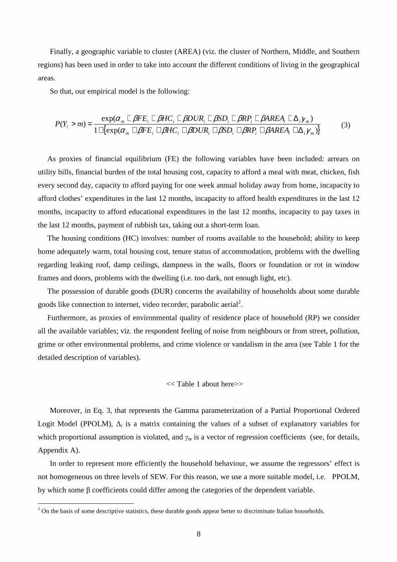
So that, our empirical model is the following:

{ })exp(1

)exp()(

miiiiiiim

miiiiiiimi AREARPSDDURHCFE

AREARPSDDURHCFEmYP

γββββββαγββββββα

∆++++++++∆+++++++

=> (3)

As proxies of financial equilibrium (FE) the following variables have been included: arrears on

utility bills, financial burden of the total housing cost, capacity to afford a meal with meat, chicken, fish

every second day, capacity to afford paying for one week annual holiday away from home, incapacity to

afford clothes’ expenditures in the last 12 months, incapacity to afford health expenditures in the last 12

months, incapacity to afford educational expenditures in the last 12 months, incapacity to pay taxes in

the last 12 months, payment of rubbish tax, taking out a short-term loan.

The housing conditions (HC) involves: number of rooms available to the household; ability to keep

home adequately warm, total housing cost, tenure status of accommodation, problems with the dwelling

regarding leaking roof, damp ceilings, dampness in the walls, floors or foundation or rot in window

frames and doors, problems with the dwelling (i.e. too dark, not enough light, etc).

The possession of durable goods (DUR) concerns the availability of households about some durable

goods like connection to internet, video recorder, parabolic aerial2.

Furthermore, as proxies of environmental quality of residence place of household (RP) we consider

all the available variables; viz. the respondent feeling of noise from neighbours or from street, pollution,

grime or other environmental problems, and crime violence or vandalism in the area (see Table 1 for the

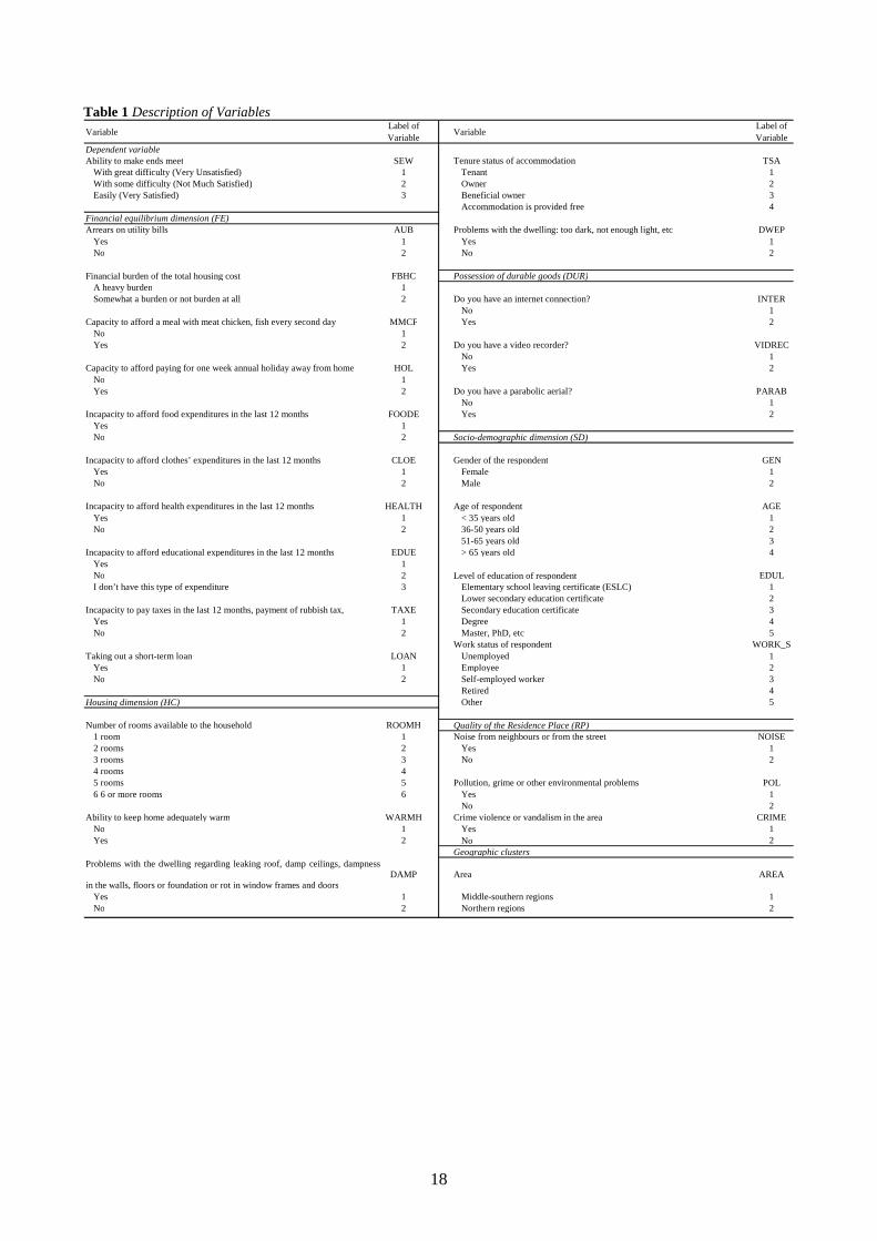
detailed description of variables).

<< Table 1 about here>>

Moreover, in Eq. 3, that represents the Gamma parameterization of a Partial Proportional Ordered

Logit Model (PPOLM), ∆i is a matrix containing the values of a subset of explanatory variables for

which proportional assumption is violated, and γm is a vector of regression coefficients (see, for details,

Appendix A).

In order to represent more efficiently the household behaviour, we assume the regressors’ effect is

not homogeneous on three levels of SEW. For this reason, we use a more suitable model, i.e. PPOLM,

by which some β coefficients could differ among the categories of the dependent variable.

2 On the basis of some descriptive statistics, these durable goods appear better to discriminate Italian households.

9

Eq. 3 has been estimated for the sample of 19,963 Italian households, and for four sub-groups: i)

households with only one component (5,526 obs.); ii ) households with no children (9,054 obs.); iii )

households with one child (2,351 obs.); iv) households with two or more children (3,032 obs.).

In the next Section the results of our empirical models will be illustrated.

4. Empirical Findings

4.1. PPOLM Estimates

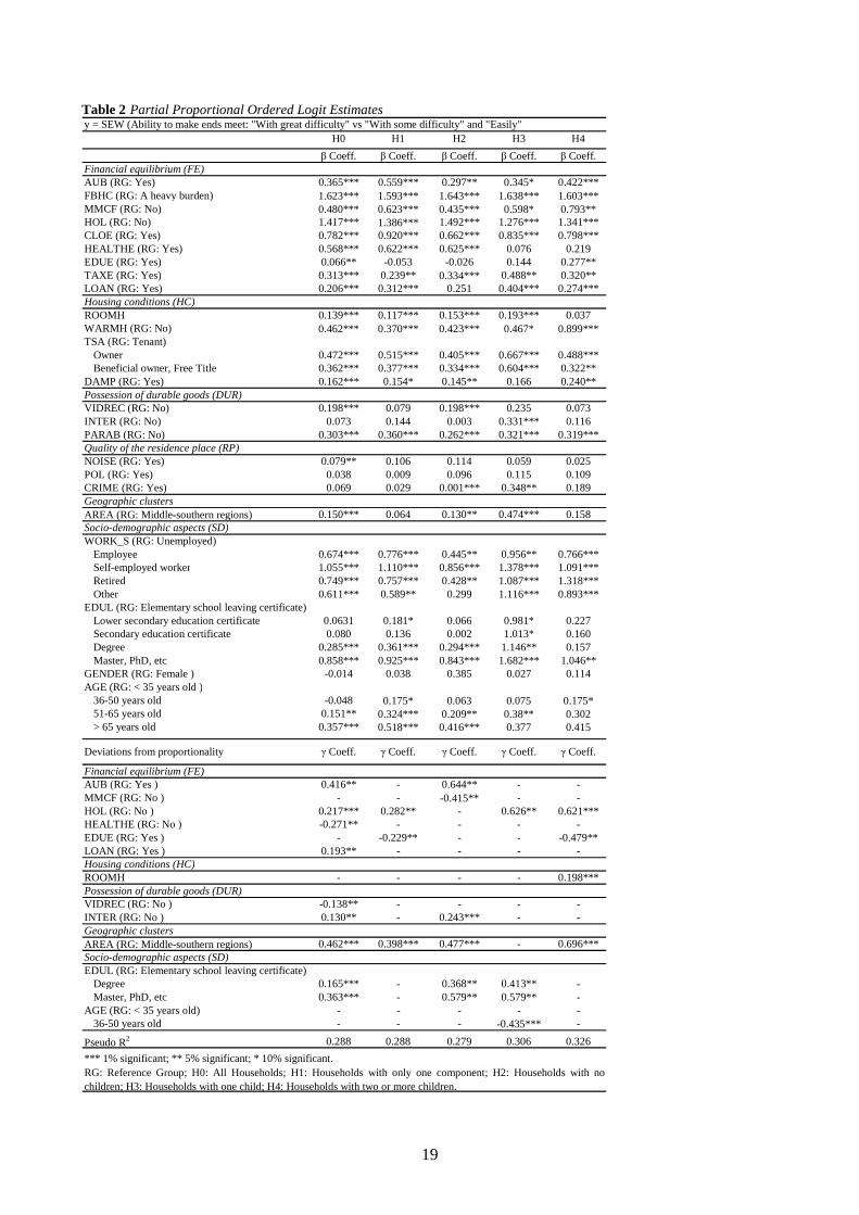
Table 2 reports PPOLM estimates 3. It presents two boxes, the first one contains the β’s and the

second one reports the γ coefficients. In particular, according to the gamma parameterization, in the first

box we have for each explanatory variable one β coefficient concerning the first category of the

dependent variable (i.e. with great difficulty) versus the second and the third one (i.e. with some

difficulty and easily). The β coefficients related to the first and second category versus the third one are

the same to the previous ones, except for those variables for which the parallel-lines assumption is

violated. Regarding to these latter variables, in the bottom box one γ coefficient is reported for each

variable; it is equal to the difference between the β2 (viz. the coefficient related to the first and the

second category of dependent variable versus the third one) and β1 (viz. the coefficient related to the

first category of dependent variable versus the second and the third one).

<< Table 2 about here>>

The estimated models achieved a good fit, and the coefficients of variables – estimated by the

Maximum Likelihood method – possessed the expected signs and effects on the explanation of SEW.

The estimates of the model related to all households and each typology of households show SEW is

positively supported by variables related to the financial equilibrium (e.g. FBHC, HOL, CLOE, TAXE)

and to some socio-demographic variables, viz. work status (WORK_S) and level of education of

respondent (EDUL). In other words estimates show households with no financial burden of the total

housing cost, with a good capacity to afford paying for one week annual holiday away from home,

without problems to afford clothes’ expenditures in the last 12 months, and to pay taxes have more

3 To check the parallel-lines constraint the autofit option of gologit procedure of STATA software was followed. This STATA procedure does a series of Wald tests on each variable to see whether its coefficients differ across equations, e.g., whether the variable meets the parallel-lines assumption. If the Wald test is statistically insignificant for one or more variables, the variable with the least significant value on the Wald test is constrained to have equal effects across equations. A global Wald test is also done of the final model with constraints versus the original unconstrained model; a statistically insignificant test indicates that the final model does not violate the parallel-lines assumption.

10

chances to experiment a higher level of SEW; that is they are very likely satisfied of their economic

situation.

It is worth noticed, a not very necessary need, as the capacity of households to get an holiday, has

positive and strongly significant effect on SEW for all typologies of families. In other words, the

capacity to afford one annual week holiday has became, within the budget of Italian families, a basic

need.

In particular, as hypothesized, HOL does not always respect the parallel-lines assumption, and as

the positive sign of γ coefficient shows, its effect changes when one pass from the lower category of

SEW to the higher. Moreover, γ coefficient is higher for households with at least one child (see Table 2,

columns 5 and 6).

Further, housing conditions, possession of durable goods and environmental quality of residence act

fairly differently on SEW of four typologies. Only the β coefficient of TSA, relating to both owner and

beneficial owner conditions, and that one of PARAB are strongly statistically significant for each

typology. On the contrary, the coefficients of some other variables, are statistically significant only for

some typology (for example, VIDREC for H2; CRIME for H2 and H3) indicating the weak response of

SEW to these variables.

An important issue regards the territorial differences; in other words, the area where household lives

is important only for typologies H2 and H3, indicating households resident in the North of the country

have more chances to experiment a higher level of subjective economic well-being than the households

resident in the Centre-southern area4.

Regarding to the aspects of socio-demographic status, with the exception of GENDER, all variables

are positively related to SEW. With reference to AGE, the β coefficients are significant for the third and

fourth age-class (i.e. 51-65 years old, and equal to or more 65 years old), in particular for H1 and H2

typologies.

Among the other socio-demographic variables, the effect of work status and education level is

particularly interesting. Specifically, the highest level of education and the condition of self-employed

worker represent the most important conditions to have a satisfying SEW, and this aspect regards all

typologies.

4.2. What Kind of Relationship between SEW and Socio-demographic variables does exist?

How are work status and education level related to SEW? In order to better explore this relationship,

we have calculated the average of predicted probability to be very unsatisfying and very satisfying for

4 We explored the effect of regional location by using different aggregation of data; for example North, Centre, South; North-Centre and South; and North and Middle-South, but only the coefficient related to the last aggregation was always statistically different from zero.

11

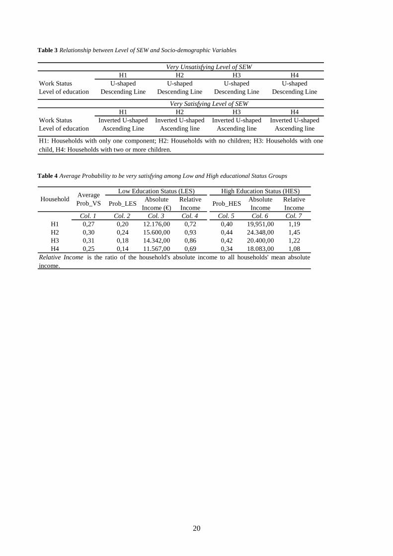
each category of work status and level of education, respectively. In table 3, the shape of such

probabilities has been reported.

<< Table 3 about here>>

As expected, with respect to work status, all typologies of households present an U-shaped and an

inverted U-shaped relationship to SEW for the first and third category of SEW, respectively. In

particular, the self-employed status is a breaking-point; i.e. for all typology of families the probability to

make ends meet with greater difficulty decreases when the family respondent passes from the

unemployed status to the self-employed one; the probability increases again when the family respondent

retires from market labour. While, for the third level of SEW (i.e. very satisfying), the average

probability for all groups of families is inverted U-shaped; viz. the probability to achieve higher level of

SEW increases when one passes from unemployed to the self-employed status; while retired people

have a lower probability to have a satisfying level of SEW.

Relating to the level of education, for all typologies of households the average probability to achieve

an unsatisfying level of SEW decreases for higher level of education. Vice versa, the average probability

of a very satisfying level of SEW increases for higher level of education (i.e. Degree, and Master or

PhD).

4.3. Level of Education and SEW: the Easterlin Considerations

To get some insights on the relation between SEW and level of education we follow the Easterlin

considerations (Easterlin, 2001). He argued, material aspirations rise with increasing level of education;

and low or high levels of education channel likely people into different paths, viz. low income and high

income path. So that, he also stated that people with more education and consequential high level of

income have a higher subjective well-being than those with a lower level of education.

Moreover, it is reasonable to hypothesize people having different levels of education shape their

living standards around different feelings, values, wishes, etc. due to psychological and emotional

differences.

In order to explore the presence of subjective and objective differences among household typologies,

we divide each group of households in two education status groups characterized by low and high

education status (viz. LES and HES), respectively. Within each household typology, LES and HES

identify those families whose respondent has a level of education lower or equal to secondary education

certificate; and degree at least, respectively.

For each typology of household, we compare the average values of predicted probability to be very

12

satisfied for low and high education status; we call these average predicted probabilities Prob_LES and

Prob_HES, respectively. While, we call Prob_VS, the predicted average probability to be very satisfied

for each typology neglecting the education status.

<< Table 4 about here>>

Prob_VS varies slightly among household typologies (see Tab. 4, column 1); this similarity

disappears if we consider the Prob_LES and Prob_HES. With respect to LES group (Tab. 4, column 2),

all households present a Prob_LES ranging from 0.14 to 0.24, for H4 and H2, respectively. While,

Prob_HES (Tab. 4 column 5) is greater and ranges from 0.34 to 0.44, for H4 and H2, respectively.

For each typology of household, Table 4 highlights significant subjective differences on SEW

feeling; in fact, the average value of predicted probability to be very satisfied for HES group is twice

that of LES one. Actually, people with a lower education level have a lower feeling of their SEW, and

vice versa. Moreover, Table 4 shows objective differences exist among households with respect to the

two education status. On average, households belonging to low education status group have a lower

absolute and relative income than the high education status group.

Finally, within each education status group significant differences in terms of average probability can

be appreciated among households; in particular with respect to HES, the highest Prob_HES concerns

households with no children (H2) and with one child (H3); viz. 0.44 and 0.42, respectively.

In synthesis, the analysis for education status lets come out objective and subjective differences

among household groups; moreover, the crossing reading of education status and average probabilities

highlights a different distribution of income inside both each household typology with respect to HES

and LES status, and each education status.

5. Conclusions

By using a Partial Proportional Ordered Logit Model, the effect of composition of household on the

perception of economic well-being has been explored. To this aim, we subdivide the total sample of

19,963 households in four groups, viz. households with only one component, households with no

children, households with one child, and households with two or more children. Five PPOLMs were

estimated, one for all households and four for the different typologies of households, respectively.

Overall, the results are coherent with the recent literature on the Italian household impoverishment.

The estimates generally show households have a very low probability to have satisfying levels of SEW;

13

that is particular evident for households with only one person and households with two or more

children.

In particular, the results give some interesting insights about the relationship between SEW and

some relevant aspects of both economic and socio-demographic status. Regarding to the economic

status, the estimates show the main dimensions affecting SEW is the financial equilibrium. This result is

not surprising, if we consider financial equilibrium is strongly related to income and mirrors the ability

of households to afford ordinary necessities. A more in depth look, shows that the more urgent needs

shared by each typology indifferently are those related to the capacity to pay taxes and to afford

housing, clothes and holydays expenditures, the other ones being differently influential on SEW. So

that, a common life style characterizes the four analyzed typologies of families: to satisfy basic needs

without forgoing holydays!

Regarding to the socio-demographic status, for all typologies of households the probability to

achieve a higher level of SEW increases passing from unemployed status to the self-employed one; and

decreases passing from the last one to the retired status. Relating to the level of education, the

probability to achieve a very satisfying level of well-being increases for higher level of education (i.e.

Degree, and Master or PhD).

In addition, the analysis focused on education status lets us to discover some interesting insights not

evident from β coefficients. In particular, households belonging to the higher education status (i.e.

degree, and PhD and Master) have, on average, a probability to be very satisfying equal to the double

value of those belonging to the low education status. This difference of probability mirrors – within and

between each educational status – subjective and objective disparities in terms of feeling of SEW. As a

matter of fact, level of education takes inside both objective factors (i.e. income) and personal ones (i.e.

feeling or expectation), but also it highlights it is important what people are able to be and not only what

he/she can do or can have.

In conclusion, our analysis on SEW shows using non-monetary variables as proxies of economic

status reveals appreciable differences among typologies of households, not evident if income had been

used; further, a more exhaustive analysis should consider socio-demographic characteristics as

explanatory variables in order to detect objective and subjective discriminant factors among

homogeneous clusters of households.

Moreover, the typology and education status specific analysis appears much more directly policy-

driving. Actually, feasible policies should be defined in order to allow people to achieve a good level of

education as it represents a pre-condition to access to resources leading people to attain higher levels of

well-being. The relevant influence of the latter leads out subjective economic well-being is mostly

related to what people are able to be along his/her life and not only what he/she is able to do, but

14

unfortunately the current policy of the Italian Government is doing the opposite by dramatically

reducing the resources for education.

Appendix A

In the study of the dependence of a response variable on a set of explanatory variables, the choice of

a model is determined by the scale of measurement of the response variable. In this paper, we use an

ordered logit model as the dependent variable, Y – in our case household ability to make ends meet –

takes m ordered values from 1 to M.

The most general logistic model for dependent categorical variable is the Generalized Logistic Model

and can be written as:

{ }exp( )

( ) ( ) , 1,2,..., 11 exp( )

X m i mi m

m i m

XP Y m g m M

X

α ββα β

+> = = = −+ +

, (A1)

where M is the number of categories of the ordinal dependent variable. From Eq. A1, the probability of

Y to take values from 1 to M is the following:

1( 1) 1 ( )i iP Y g Xβ= = − ,

-1( ) ( ) ( ), 2,..., 1i i m i mP Y m g X g X m Mβ β= = − = − ,

-1( ) ( )i i MP Y M g Xβ= =

(A2)

This model is not parsimonious because it involves as many α and β coefficients as the M –1 number of

dependent variable categories.

A more parsimonious model is the Ordered Logit Model that implies the parallel-lines assumption for

all explanatory variables5, viz. the model presents M different α coefficients and the same β coefficients

for each category of dependent variable. This model is called also Proportional Odds Model, and

represents a special case of the Generalized Ordered Model (Eq. A1). It can be written as:

{ }exp( )

( ) ( ) , 1,2,..., 11 exp( )

X m ii

m i

XP Y m g m M

X

α ββα β

+> = = = −+ +

(A3)

As evident, Eq. A3 and Eq. A1, related to the parallel-lines model and the generalized ordered

5 The parallel-lines constraint is satisfied if β1 = β2 = … = βM.

15

model, respectively, are very similar, the only exception being on the β’s, that are the same for all

values of m in Eq. A3. Actually, in the empirical analyses the parallel-lines assumption is often violated

(i.e. one or more β’s could differ across values of m categories).

Therefore, an alternative procedure is to fit a Partial Proportional Ordered Model through which

some β coefficients could differ among the categories of the dependent variable; viz. the proportional

parallel-lines assumption is not satisfied for some explanatory variables.

For example, if we have four explanatory variables (X1, X2, X3 and X4) and X1 and X2 violate the

parallel-lines constraint we will have for X3 and X4 the same β coefficients for all values of m, while

for X1 and X2 the β coefficients are free to differ. In other words:

}{1 2 3 4

1 2 3 4

exp( 1 2 3 4 )P(Y ) = , 1,2,..., -1

1 exp( 1 2 3 4 )m i m i m i i

im i m i m i i

X X X Xm m M

X X X X

α β β β βα β β β β

+ + + +> =+ + + + +

(A4)

To test the parallel-lines assumption a Brant test could be done (Brant, 1990). If Brant test is

significant there will be evidence that the parallel regression assumption has been violated.

Peterson and Harrell (1990), and, recently, Lall et al. (2002) proposed an equivalent parameterization of

the Generalized Ordered Model called the Unconstrained Partial Proportional Odds Model or Gamma

parameterization. Under the Peterson–Harrell parameterization, each explanatory variable has one β

coefficient concerning the first category of dependent variable contrasted to the all other ones; M−2 γ

coefficients that represent the deviation from proportionality; and M-1 α coefficients reflecting the cut-

points:

{ }exp( )

, 1,2,..., -11 exp( )

m i i mi

m i i m

α X β γP(Y m) m M

α X β γ

+ + ∆> = =+ + + ∆

(A5)

where ∆i is a matrix containing the values of a subset of q explanatory variables (q<p, where p are all

the variables) for which proportional assumption is violated, and γm is a vector of regression

coefficients. The test of the proportional assumption, for the q-covariates, is based on the null

hypothesis H0: γm = 0 for all m categories.

There are some advantages to use γ parameterization, it has a more parsimonious layout and provides

an easy way to understand the parallel-lines assumption; for example if we have a dependent variable

with three categories we will have a β coefficient concerning the first category of the dependent variable

contrasted to the other two ones, and one γ coefficient concerning the variables for which the parallel-

lines is violated.

16

References Addabbo, T., Di Tommaso, M.L., Facchinetti, G.: To what Extent Fuzzy Set Theory and Structural

Equation Modelling Can Measure Functionings? An Application to Child Well Being. Working Papers: 30 Child Centre (2004).

Betti, G., Cheli, B., Lemmi, A., Verma, V.: The Fuzzy Set Approach to Multidimensional Poverty: the Case of Italy in the 1990s. In Kakwani, N., Silber, J. (Eds.) Quantitative Approaches to Multidimensional Poverty Measurement, pp. 30–48, Palgrave Macmillan, New York (2008).

Boeri, T., Brandolini, A.: The Age of Discontent: Italian Households at the Beginning of the Decade. Giornale degli Economisti e Annali di Economia 63(3-4):449–487 (2004).

Brant, R.: Assessing Proportionality in the Proportional Odds Model for Ordinal Logistic Regression. Biometrics 46(4):1171–1178 (1990).

Chakravarty, S. R., Silber, J.: Measuring Multidimensional Poverty: The Axiomatic Approach. In Kakwani, N., Silber, J. (Eds.) Quantitative Approaches to Multidimensional Poverty Measurement, pp.192–209, Palgrave Macmillan, New York (2008).

Cheli, B., Lecchini, L., Masserini,L.: An Ordinal Logit Model for Subjective Well-Being Among The Italian Older Adults. In J. Blasius, J. Hox, E. de Leeuw and P. Smidt (eds.) Social Science methodology in the New Millennium, Leske & Budrich, Opladen (2002).

Diener, E., Suh, E.M., Lucas, R.E., Smith, H.L.: Subjective Well-being: Three Decades of Progress. Psychological Bulletin 125:276–302 (1999).

Di Tommaso, M.L.: Children Capabilities: A Structural Equation Model for India. The Journal of Socio-Economics 36:436–450 (2007).

Easterlin, R.A.: Income and Happiness: Towards a Unified Theory. The Economic Journal 111(473): 465–488 (2001).

Ferrari, G.: Using Equivalent Scales as Spatial Deflators: Evidence in Inter-Household Welfare Regional Comparison from Italian HBS Micro-data. In Dagum, C., Ferrari, G. (Eds.) Household Behaviour, Equivalent Scales, Welfare and Poverty, pp.273–294, Physica-Verlag, New York (2004).

Ferrari, G., Maltagliati M.: Cross Region and Economic Profile of Italian Households Well-being Comparisons. Rivista Italiana di Economia, Demografia e Statistica LXIII(1-2): 107–133, (2009).

Ferro Luzzi, G., Flückiger, Y., Weber, S.: A Cluster Analysis of Multidimensional Poverty in Switzerland. In Kakwani, N., Silber, J. (Eds.) Quantitative Approaches to Multidimensional Poverty Measurement, pp.63–79, Palgrave Macmillan, New York (2008).

Fusco, A., Dickes, P.: The Rasch Model and Multidimensional Poverty Measurement. In Kakwani, N., Silber, J. (Eds.) Quantitative Approaches to Multidimensional Poverty Measurement, pp.49–62, Palgrave Macmillan, New York (2008).

Quintano, C., Castellano, R., Regoli, A.: Evolution and decomposition of Income Inequality in Italy, 1991-2004. Statistical Methods and Applications, 18(3):419–443 (2009).

Kolenikov S., Angeles, G.: Socioeconomic Status Measurement with Discrete Proxy Variables: Is principal Component Analysis a Reliable Answer? Review of Income and Wealth, 55(1):128–165 (2009).

ISTAT: Rapporto Annuale, ISTAT, Roma (2009). Lall, R., Campbell, M.J., Walters, S.J., Morgan, K., MRC CFAS Co-operative Institute of Public

Health: A Review of Ordinal Regression Models Applied on Health-related Quality of Life Assessments. Statistical Methods in Medical Research, 11:49–67 (2002).

Lugo, M.A., Maasoumi, E.: Multidimensional Poverty Measures from an Information Theory Perspective. ECINEQ Working Papers, Society for the Study of Economic Inequality (2008).

Malone, K., Stewart, S. D., Wilson, J., Korsching, P. F.: Perceptions of Financial Well-Being among American Women in Diverse Families. Journal of Family and Economic Issue, 31:63–81 (2009).

Naga, R.A., Bolzani, E.: Income, Consumption and Permanent Income: a MIMIC Approach to Multidimensional Poverty Measurement. In Kakwani, N., Silber, J. (Eds.) Quantitative Approaches to Multidimensional Poverty Measurement, pp.104–117, Palgrave Macmillan, New York (2008).

17

Peterson, B., Jr Harrell, F.E.: Partial Proportional Odds Models for Ordinal Response Variables. Applied Statistics, 39:205–217 (1990).

Pisano, E., Tedeschi, S.: Tendenze della Distribuzione dei Redditi in Italia e Impoverimento della Classe Media: Percezione o Realtà? Meridiana, 59/60:131–154 (2007).

Ramos, X.: Using Efficiency Analysis to Measure Individual Well-being With an Illustration for Catalonia. In Kakwani, N., Silber, J. (Eds.) Quantitative Approaches to Multidimensional Poverty Measurement, pp.155–175, Palgrave Macmillan, New York (2008).

Rojas M.: Life satisfaction and satisfaction in domains of life: Is it a simple relationship? Journal of Happiness Studies, 7:467–497 (2006).

Sen, A.: Standard of living, Cambridge University Press, New York (1987). Van Hoorn, A.: A Short Introduction to Subjective Well-being: Its Measurement, Correlates and Policy

Uses. International conference “Is happiness measurable and what do those measures mean for policy, University of Rome Tor Vergata, 1–12 (2007).

Van Praag, B.M.S., Frijtersvan, P., Ferrer-i-Carbonell, A.: The Anatomy of Subjective Well-being”, Journal of Economic Behaviour and Organization, 51:29–49 (2003).

Van Praag, B.M.S., Ferrer-i-Carbonell, A.: The Subjective Approach to Multidimensional Poverty Measurement. In Kakwani, N., Silber, J. (Eds.) Quantitative Approaches to Multidimensional Poverty Measurement, pp.135–54, Palgrave Macmillan, New York (2008).

18

Table 1 Description of Variables Variable

Label of Variable

VariableLabel of Variable

Dependent variableAbility to make ends meet SEW Tenure status of accommodation TSA

With great difficulty (Very Unsatisfied) 1 Tenant 1With some difficulty (Not Much Satisfied) 2 Owner 2Easily (Very Satisfied) 3 Beneficial owner 3

Accommodation is provided free 4Financial equilibrium dimension (FE)Arrears on utility bills AUB Problems with the dwelling: too dark, not enough light, etc DWEP

Yes 1 Yes 1No 2 No 2

Financial burden of the total housing cost FBHC Possession of durable goods (DUR)A heavy burden 1Somewhat a burden or not burden at all 2 Do you have an internet connection? INTER

No 1Capacity to afford a meal with meat chicken, fish every second day MMCF Yes 2

No 1Yes 2 Do you have a video recorder? VIDREC

No 1Capacity to afford paying for one week annual holiday away from home HOL Yes 2

No 1Yes 2 Do you have a parabolic aerial? PARAB

No 1Incapacity to afford food expenditures in the last 12 months FOODE Yes 2

Yes 1No 2 Socio-demographic dimension (SD)

Incapacity to afford clothes’ expenditures in the last 12 months CLOE Gender of the respondent GENYes 1 Female 1No 2 Male 2

Incapacity to afford health expenditures in the last 12 months HEALTH Age of respondent AGEYes 1 < 35 years old 1No 2 36-50 years old 2

51-65 years old 3Incapacity to afford educational expenditures in the last 12 months EDUE > 65 years old 4

Yes 1No 2 Level of education of respondent EDULI don’t have this type of expenditure 3 Elementary school leaving certificate (ESLC) 1

Lower secondary education certificate 2Incapacity to pay taxes in the last 12 months, payment of rubbish tax, TAXE Secondary education certificate 3

Yes 1 Degree 4No 2 Master, PhD, etc 5

Work status of respondent WORK_STaking out a short-term loan LOAN Unemployed 1

Yes 1 Employee 2No 2 Self-employed worker 3

Retired 4Housing dimension (HC) Other 5

Number of rooms available to the household ROOMH Quality of the Residence Place (RP)1 room 1 Noise from neighbours or from the street NOISE2 rooms 2 Yes 13 rooms 3 No 24 rooms 45 rooms 5 Pollution, grime or other environmental problems POL6 6 or more rooms 6 Yes 1

No 2Ability to keep home adequately warm WARMH Crime violence or vandalism in the area CRIME

No 1 Yes 1Yes 2 No 2

Geographic clustersProblems with the dwelling regarding leaking roof, damp ceilings, dampness

in the walls, floors or foundation or rot in window frames and doorsDAMP Area AREA

Yes 1 Middle-southern regions 1No 2 Northern regions 2

19

Table 2 Partial Proportional Ordered Logit Estimates

H0 H1 H2 H3 H4

β Coeff. β Coeff. β Coeff. β Coeff. β Coeff. Financial equilibrium (FE)AUB (RG: Yes) 0.365*** 0.559*** 0.297** 0.345* 0.422***FBHC (RG: A heavy burden) 1.623*** 1.593*** 1.643*** 1.638*** 1.603***MMCF (RG: No) 0.480*** 0.623*** 0.435*** 0.598* 0.793**HOL (RG: No) 1.417*** 1.386*** 1.492*** 1.276*** 1.341***CLOE (RG: Yes) 0.782*** 0.920*** 0.662*** 0.835*** 0.798***HEALTHE (RG: Yes) 0.568*** 0.622*** 0.625*** 0.076 0.219EDUE (RG: Yes) 0.066** -0.053 -0.026 0.144 0.277**TAXE (RG: Yes) 0.313*** 0.239** 0.334*** 0.488** 0.320**LOAN (RG: Yes) 0.206*** 0.312*** 0.251 0.404*** 0.274***Housing conditions (HC)ROOMH 0.139*** 0.117*** 0.153*** 0.193*** 0.037WARMH (RG: No) 0.462*** 0.370*** 0.423*** 0.467* 0.899***TSA (RG: Tenant)

Owner 0.472*** 0.515*** 0.405*** 0.667*** 0.488***Beneficial owner, Free Title 0.362*** 0.377*** 0.334*** 0.604*** 0.322**

DAMP (RG: Yes) 0.162*** 0.154* 0.145** 0.166 0.240**Possession of durable goods (DUR)VIDREC (RG: No) 0.198*** 0.079 0.198*** 0.235 0.073INTER (RG: No) 0.073 0.144 0.003 0.331*** 0.116PARAB (RG: No) 0.303*** 0.360*** 0.262*** 0.321*** 0.319***Quality of the residence place (RP) NOISE (RG: Yes) 0.079** 0.106 0.114 0.059 0.025POL (RG: Yes) 0.038 0.009 0.096 0.115 0.109CRIME (RG: Yes) 0.069 0.029 0.001*** 0.348** 0.189Geographic clustersAREA (RG: Middle-southern regions) 0.150*** 0.064 0.130** 0.474*** 0.158Socio-demographic aspects (SD)WORK_S (RG: Unemployed)

Employee 0.674*** 0.776*** 0.445** 0.956** 0.766***Self-employed worker 1.055*** 1.110*** 0.856*** 1.378*** 1.091***Retired 0.749*** 0.757*** 0.428** 1.087*** 1.318***Other 0.611*** 0.589** 0.299 1.116*** 0.893***

EDUL (RG: Elementary school leaving certificate)Lower secondary education certificate 0.0631 0.181* 0.066 0.981* 0.227Secondary education certificate 0.080 0.136 0.002 1.013* 0.160Degree 0.285*** 0.361*** 0.294*** 1.146** 0.157Master, PhD, etc 0.858*** 0.925*** 0.843*** 1.682*** 1.046**

GENDER (RG: Female ) -0.014 0.038 0.385 0.027 0.114AGE (RG: < 35 years old )

36-50 years old -0.048 0.175* 0.063 0.075 0.175*51-65 years old 0.151** 0.324*** 0.209** 0.38** 0.302> 65 years old 0.357*** 0.518*** 0.416*** 0.377 0.415

Financial equilibrium (FE)AUB (RG: Yes ) 0.416** - 0.644** - -MMCF (RG: No ) - - -0.415** - -HOL (RG: No ) 0.217*** 0.282** - 0.626** 0.621***HEALTHE (RG: No ) -0.271** - - - -EDUE (RG: Yes ) - -0.229** - - -0.479**LOAN (RG: Yes ) 0.193** - - - -Housing conditions (HC)ROOMH - - - - 0.198***Possession of durable goods (DUR)VIDREC (RG: No ) -0.138** - - - -INTER (RG: No ) 0.130** - 0.243*** - -Geographic clustersAREA (RG: Middle-southern regions) 0.462*** 0.398*** 0.477*** - 0.696***Socio-demographic aspects (SD)EDUL (RG: Elementary school leaving certificate)

Degree 0.165*** - 0.368** 0.413** -Master, PhD, etc 0.363*** - 0.579** 0.579** -

AGE (RG: < 35 years old) - - - - -36-50 years old - - - -0.435*** -

Pseudo R2 0.288 0.288 0.279 0.306 0.326

RG: Reference Group; H0: All Households; H1: Households with only one component; H2: Households with nochildren; H3: Households with one child; H4: Households with two or more children.

*** 1% significant; ** 5% significant; * 10% significant.

y = SEW (Ability to make ends meet: "With great difficulty" vs "With some difficulty" and "Easily"

γ Coeff. γ Coeff.Deviations from proportionality γ Coeff. γ Coeff. γ Coeff.

20

Table 3 Relationship between Level of SEW and Socio-demographic Variables

H1 H2 H3 H4Work Status U-shaped U-shaped U-shaped U-shapedLevel of education Descending Line Descending Line Descending Line Descending Line

H1 H2 H3 H4Work Status Inverted U-shaped Inverted U-shaped Inverted U-shaped Inverted U-shapedLevel of education Ascending Line Ascending line Ascending line Ascending line

Very Unsatisfying Level of SEW

Very Satisfying Level of SEW

H1: Households with only one component; H2: Households withno children; H3: Households with onechild, H4: Households with two or more children. Table 4 Average Probability to be very satisfying among Low and High educational Status Groups

Prob_LESAbsolute

Income (€)Relative Income

Prob_HESAbsolute Income

Relative Income

Col. 1 Col. 2 Col. 3 Col. 4 Col. 5 Col. 6 Col. 7H1 0,27 0,20 12.176,00 0,72 0,40 19,951,00 1,19H2 0,30 0,24 15.600,00 0,93 0,44 24.348,00 1,45H3 0,31 0,18 14.342,00 0,86 0,42 20.400,00 1,22H4 0,25 0,14 11.567,00 0,69 0,34 18.083,00 1,08

Household

Relative Incomeis the ratio of the household's absolute income to all households' mean absoluteincome.

Low Education Status (LES) High Education Status (HES)Average Prob_VS