arX

iv:h

ep-p

h/97

1053

5v2

16

Sep

1998

Compositeness and the asymmetries of leptons

at the Z0 peak

R. Dıaz Sanchez.1, R. Martınez1 and J.-Alexis Rodrıguez1,2

1. Depto. de Fısica, Universidad Nacional, Bogota, Colombia

2. Centro Internacional de Fısica, Bogota, Colombia

Abstract

We study the effects on the leptonic asymmetries AFB and ALR

coming from a model of compositeness. We consider the effects comingfrom the self-energies and the vertex correcction to Zl+l−. Thus weuse the Altarelli parametrization of the oblique corrections. We getthe asymptotic limits of these corrections in terms of the parameters(m∗, Λ, f , f ′) and we get bounds for the quotient m∗/Λ with differentvalues of (f , f ′). We conclude that both asymmetries produce boundsfor such quotient when f ′ overweight to f , and this fact is related withthe breakdown of the custodial symmetry.

1 Introduction

Compositeness [1] is regarded as a solution to many problems which are un-solved in the Standard Model, like the fermion mass spectrum, the generationof masses and the large number of parameters. The idea is that some un-derlying structure can explain the quark and lepton family pattern. At thisstage, we shall search for new excited fermions (ψ∗

F ), and for new interactionsoriginated from the constituents.

A signal for a composite structure of fermions could be the productionof excited leptons or quarks, either pairwise, due to their normal gauge cou-plings, or singly, due to radiative transitions between normal and excitedfermions [2] [3]. For instance, excited fermions could be produced in Z de-cays; in fact, there are strong limits coming from the Z0 partial widths.

1

Mass regions up to 45 GeV for u∗ and d∗ as well as 35 − 40 GeV for l∗ andν∗ have been excluded [4]. However, the l∗ limits can be pushed to 46 GeVby searching the decay mode Z → l∗ l∗ → l+l−γγ [4].

Moreover, recently the possibility has been studied that the significant ex-cess from QCD predictions found by the collider detector at Fermilab (CDF)in the inclusive jet cross section for transverse energies ET ≥ 200 GeV couldbe explained by the production of excited bosons or excited quarks in themass region of 1600 GeV and 500 GeV[5] [6], respectively. Other studieshave already been done in order to get the low energy scale Λ for compos-iteness by precise comparison between currently available experimental dataand calculations in the composite model of quarks [7].

On the other hand, radiative corrections are the appropriate place toindirectly look for new physics at low energies [7] [9], because when heavyfermions are coupled to longitudinal components of the gauge bosons thereis no decoupling of the high energy physics from the low energy physics. Inref. [9], radiative corrections at the Z scale have been considered in orderto bound substructure. Our purpose in this paper is to find bounds for themasses of possible excited leptons by using the radiative corrections involvedin the forward-backward and left-right asymmetries for the lepton average.

2 The model

In general, the normal fermions (ψf ) and excited fermions (ψ∗

F ) at low ener-gies can be described by an effective Lagrangian like [3]

Leff =∑

i=γ,Z,W±

viψ∗

FγµV i

µψ∗

F +e

Λψ∗

Fσµν(ciF f − diF fγ5)ψfV

iµν + h.c. , (1)

where V iµν are the field strengths for the gauge bosons and Λ denotes the

compositeness scale. In particular, we choose a specific model which assumesthat excited leptons form a weak isodoublet,

L = (ν∗, l∗) (2)

which couples to the ordinary left handed lepton doublet by the SU(2)L ⊗U(1)Y invariant interaction Lagrangian

L =gf

ΛLσµν τ

2lLWµν +

g′f ′

ΛLσµν Y

2lLBµν + h.c. . (3)

2

Where g and g′ are the SU(2) and U(1) coupling constants respectively, τdenotes the Pauli matrices and Y is the hypercharge.

As for the coefficients ciF f and diF f , in general, g−2 measurements imply|c| = |d|, and also, the absence of dipole moments for the electron and themuon requires c and d to be relatively real [10]. Thus, we have the followingrelations:

cγl∗l = −1

4(f + f ′) ,

cγν∗ν =1

4(f − f ′) ,

cZl∗l = −1

4(f cot θW + f ′ tan θW ) ,

cZν∗ν =1

4(f cot θW + f ′ tan θW ) ,

cW±ν∗l =f

2√

2 sin θW

. (4)

Now, since the excited fermions are doublets, their couplings to photon,Z and W bosons are defined by the following renormalizable Lagrangian

L = Lγµ(gτ

2·W µ +

g′

2Y Bµ)L , (5)

where the coefficients vi from eq.(1) satisfy

vγl∗l = −e ,

vγν∗ν = 0 ,

vZl∗l = − e

2sW cW(1 − 2s2

W ) ,

vZν∗ν =e

2sW cW,

vW+ν∗l =e√2sW

. (6)

3 Self-energy contributions

Once we have the framework setup (eqs. (1)-(6)), we can calculate the con-tribution to the self-energies of the gauge bosons by using dimensional reg-ularization, where the pole d = 4 is identified with ln(Λ2/m2

Z) [8]. In order

3

to simplify the analysis we assume the same mass for the excited leptons,m∗

ν = m∗

l = m∗; this is justified by the fact that we are considering the ex-cited fermion in a linear vectorial representation of the SU(2) × U(1) gaugegroup. The states with equal mass form∗

ν andm∗

l do not break the symmetry.In general the self-energies due to the lagrangians of dimension 5 and 4

are:

Σ(5)ViVj

(q2) = −cVicVjα

9πΛ2F (5)(m∗, q2)

Σ(4)ViVj

(q2) = −vivjα

12π2F (4)(m∗, q2) (7)

where the functions F (m∗, q2) can be written as [9]

F (5)(m∗, q2) = 6m∗4[1 − (m∗2 − q2

q2) ln(

m∗2

m∗2 − q2)]

+ 3m∗2q2[1 + (m∗2 − q2

q2) ln(

m∗2

m∗2 − q2)]

− q4[8 + 3 ln(Λ2

m∗2) − 3(

m∗2 − q2

q2) ln(

m∗2

m∗2 − q2) ,

F (4)(m∗, q2) = q2 lnΛ2

m∗2+ 4m∗2 +

5

3q2

− 2(2m∗2 + q2)

√

4m∗2

q2− 1 arctan(

1√

4m∗2

q2 − 1) . (8)

We have considered the ordinary lepton masses negligible. Therefore, we findthe vacuum polarization tensors for the gauge bosons:

− ΠZ(m2Z) =

α(1 − 2s2W + 2s4

W )

6πm2Zs

2W c

2W

F (4)(m∗, m2Z)

+α

72πm2ZΛ2

(f cot θW + f ′ tan θw)2F (5)(m∗, m2Z) ,

−ΠγZ(m2Z) =

α(1 − 2s2W )

6πsW cWm2Z

F (4)(m∗, m2Z)

+αf

72πΛ2m2Z

(f cot θW + f ′ tan θw)F (5)(m∗, m2Z) ,

−Πγ(m2Z) =

α

3πm2Z

F (4)(m∗, m2Z)

4

+α

72πΛ2m2Z

(f 2 + f ′2)F (5)(m∗, m2Z) , (9)

where ΠW (0) = 0 and Σ′

Z(m2Z) is obtained directly from ΠZ(m2

Z). Theasymptotic limits (m∗,Λ) → ∞ in the functions F (m∗, q2) are

F (5)(m∗, q2)

Λ2= 9

(

m∗

Λ

)2

q2 , (10)

F (4)(m∗, q2) = q2 ln(

Λ

m∗

)2

.

In such limit, Σ(5)ViVj

(q2) approaches a constant value and the physics describedby (3) is non-decoupled.

4 The asymmetries and the new physics

On the other hand, the forward-backward asymmetry AFB and the left-rightasymmetry ALR for leptons in the Z decays are given by

AlFB =

geV g

eA

ge2V + ge2

A

glV g

lA

gl2V + gl2

A

,

ALR =2ge

V geA

ge2V + ge2

A

. (11)

where a Zll amplitude is defined as −igγµ(glV − gl

Aγ5)/4cW and the super-scripts e, l denote electron, lepton respectively. In our case, new physics isincluded in the constants gl

V,A as

glV,A = gSM

V,A + δglV,A (12)

Where the superindex SM denotes the SM coupling with the contribution atone loop level of the top quark and Higgs scalar boson. In this way, δgl

V,A

only contains the new physics contribution. With this prescription we findthat Al

FB and ALR can be written as

AlFB = Al, SM

FB (1 + 2δNP ) ,

ALR = ASMLR (1 + δNP ) , (13)

5

where δNP has the contribution of new physics and

δNP =δgl

A

gSMA

+δgl

V

gSMV

− 2gSM

V δglV + gSM

A δglA

(gSMV )2 + (gSM

A )2. (14)

Additionally, these couplings δglV,A can be expressed in terms of the ǫi

parameters [11],

δgV = =2s2

W

c2W − s2W

ǫ3 − (1

4+

s2W

c2W − s2W

)ǫ1 − ǫl/2 ,

δgA = −1

4ǫ1 − ǫl/2 . (15)

Here, ǫl is the Zl+l− vertex correction given in [9]. The other two parametersǫ1 and ǫ3 can be written as a function of self-energies as given by eq. (9) [11].

We consider the asymmetries for electron and leptonic average. The SMpredicted values are [13]

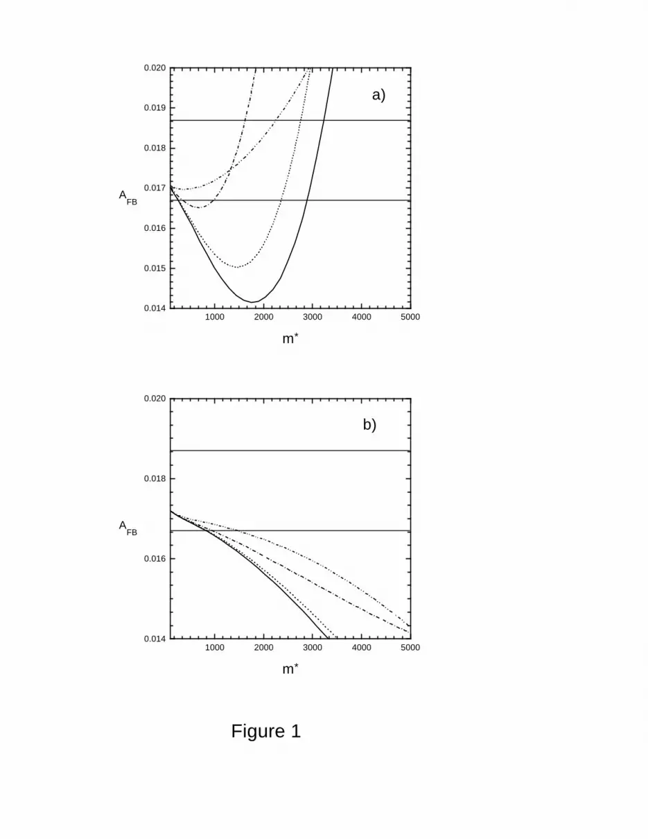
ASMFB = 0.0168 ,

ASMLR = 0.1485 (16)

for α = 1/128.75, mW = 80.35, MH = 100 GeV and mt = 175 GeV. And theexperimental values are [12] :

AlFB = 0.0174 ± 0.0010 ,

ALR = 0.1542 ± 0.0037 . (17)

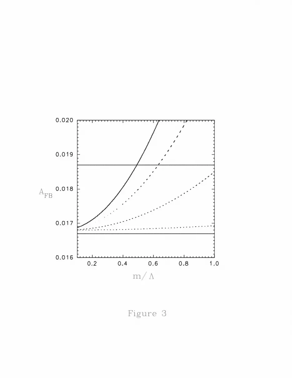
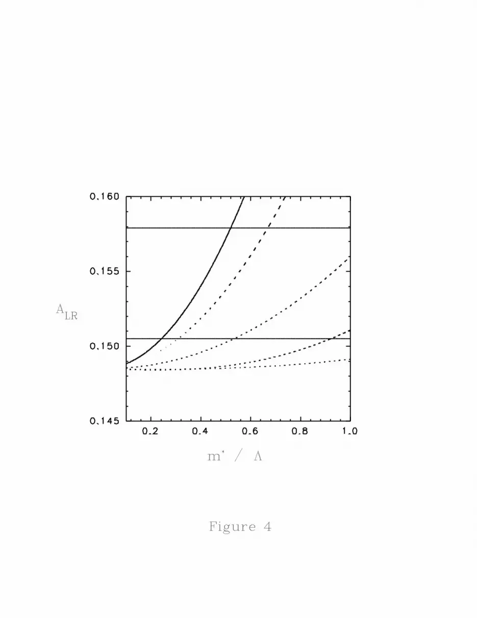
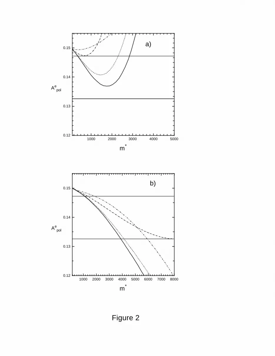
Notice that the standard model value ALR goes 1.54σ out from experi-mental data. Figure 1 shows the AFB as a function of the scale Λ for valuesof m∗ = 100 GeV (a) and m∗ = 500 GeV (b). Different values of the param-eters f and f ′ have been considered. Figure 2 shows ALR as a function ofthe scale Λ for the excited lepton mass of m∗ = 500 GeV (a) and m∗ = 1000GeV (b). In figure 3 we have plotted AFB of the electron versus m∗/Λ, asΛ is the energy scale for new physics, m∗ must be less than Λ, and we havem∗/Λ between 0 and 1. In figure 4 we show the left-right asymmetry versusthe quotient m∗/Λ for different values of f and f ′ couple constants.

We can see that both forward-backward and left-right asymmetries pro-duce bounds for such quotient when f ′ overweight considerably to f, it meansthat custodial symmetry is strongly broken and therefore radiative contribu-tions become higher.

6

5 Conclusion

In conclusion, we have evaluated the contribution of excited lepton states, upto one-loop level, to the oblique parameters. We have included this contri-bution into the leptonic asymmetries AFB and ALR , and we have comparedour results with the precise data on the electroweak observables obtained byLEP and LSD Collaborations [12] [13]. Therefore, we can extract boundson the compositeness scale and the excited lepton mass in the context ofthe phenomenological model under consideration. Further, in equation (3)the term proportional to Bµν breakdowns the custodial symmetry and it isproportional to the constant f ′. Otherwise the new physics is allowed inthe experimental region (1σ), which is satisfied when custodial symmetry isstrongly broken. In order to get this requirement we need that f ′ becomesbigger than f . With this prescription we obtain bounds on the rate m∗/Λ.

6 Acknowlegments

We thank F. Larios for reading the manuscript and useful comments. Weacknowledge the financial support from COLCIENCIAS (Colombia) and thehospitality of CINVESTAV (Mexico) during the realization of this work. R.D. express his acknowledgements to the Fundacion MAZDA Para el Arte yla Ciencia for his fellowship.

References

[1] J. C. Pati, A. Salam: Phys. Rev. Lett. 19 (1967) 1264; Phys. Rev. D8 (1973) 1240; F. Wilczek, A. Zee: Phys. Rev. Lett. 42 (1979) 421; H.Harari: Phys. Reports, 104 (1984) 159.

[2] Baur, Spira, P. Zerwas: Phys. Rev. D42, (1990) 815; J. Khun, P. Zerwas:Phys. Lett. B 147 (1984) 189; Akama, Hattori: Int. J. of Mod. Phys. A9(1994) 3504; N. Cabibbo, L. Maiani, Y. Srivastava: Phys. Lett. B 139(1984) 459; F. Boudjema, A. Djouadi: Phys. Lett. B 240 (1990) 485; F.Boudjema, et. al.: Z. Phys. C 57 (1993) 425; O.J. P. Eboli, et. al.: Phys.Rev. D 53 (1996) 1253

7

[3] Hawigara et.al.: Z Phys. C 49 (1985) 115.

[4] ALEPH Collaboration, D. Decamp, et. al.: Phys. Lett. B 236 (1990) 501;B 250 (1990) 172; L3 Collaboration, O. Adriani, et. al.: Phys. Lett. B288 (1992) 404; L3 Collaboration, M. Acciani, et. al.: Phys. Lett. B353(1995) 136; OPAL Collaboration M. Z. Akrawy et. al.: Phys. Lett. B240 (1990) 497; B 241 (1990) 133; DELPHI Collaboration, P. Abreu,et. al.: Phys. Lett. B 268 (1991) 296; B 327 (1994) 386; Z. Phys. C 53(1992) 4.

[5] S. Catani et. al: Nucl. Phys. B 478 (1996) 273.

[6] Akama, Terazawa: Phys. Rev. D 55, R 2521 (1997). ???

[7] Terazawa, Akama: Mod. Phys. Lett. A 9 (1994) 3423.

[8] K. Hagiwara, S. Ishihara, R. Szalapski, D. Zeppenfeld: Phys. Rev. D 48(1993) 2182; Phys. Lett. B 283 (1992) 353.

[9] J.I. Aranda, O. A. Sampayo, R. Martinez: Z. Phys. C 72 (1996) 479.

[10] F. M. Renard: Phys. Lett. B 116 (1982) 264; F. del Aguila et. al.: Phys.Lett. B 140 (1984) 431; M. Susuki: Phys. Lett. B143 (1984) 237; S. J.Brodsky, S. D. Drell: Phys. Rev. D 22 (1980) 2236.

[11] G. Altarelli, R. Barbieri, S. Jadach: Nucl. Phys.B 369 (1992) 3; Altarelli,R. Barbieri, F. Caravaglios: Nucl. Phys. B 405 (1993) 3; Phys. Lett. B349 (1995) 145.

[12] The LEP Collaborations ALEPH, DELPHI, L3, OPAL, The LEP ELec-troweak Working Group and The SLD Heavy Flavour Group: preprintCERN-PPE/96-183 (December 1996).

[13] For a detailed analysis of data: G. Altarelli: preprint hep-ph/9611239;K. Hawigara, D. Haidt and S. Matsumoto: preprint hep-ph/9706331.

8

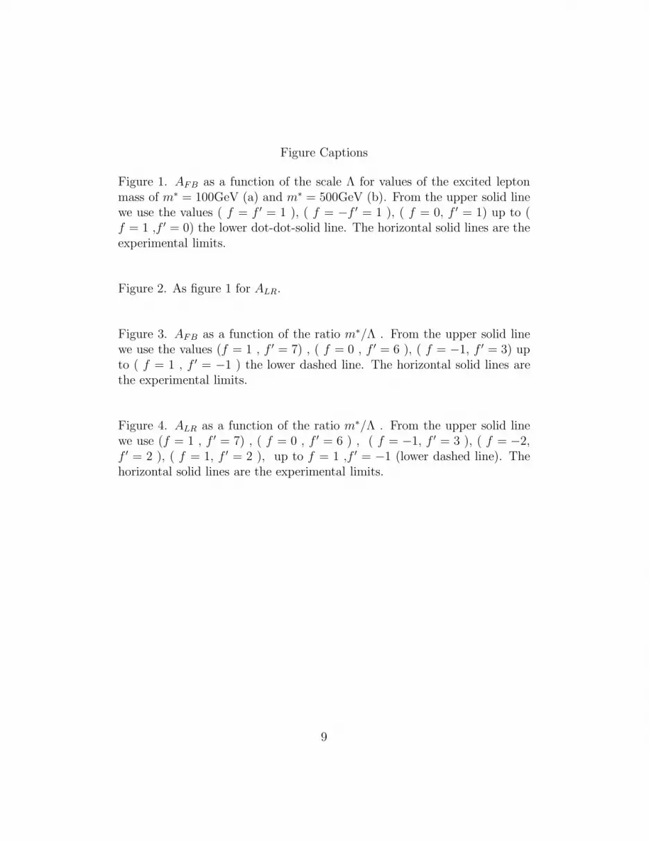
Figure Captions

Figure 1. AFB as a function of the scale Λ for values of the excited leptonmass of m∗ = 100GeV (a) and m∗ = 500GeV (b). From the upper solid linewe use the values ( f = f ′ = 1 ), ( f = −f ′ = 1 ), ( f = 0, f ′ = 1) up to (f = 1 ,f ′ = 0) the lower dot-dot-solid line. The horizontal solid lines are theexperimental limits.

Figure 2. As figure 1 for ALR.

Figure 3. AFB as a function of the ratio m∗/Λ . From the upper solid linewe use the values (f = 1 , f ′ = 7) , ( f = 0 , f ′ = 6 ), ( f = −1, f ′ = 3) upto ( f = 1 , f ′ = −1 ) the lower dashed line. The horizontal solid lines arethe experimental limits.

Figure 4. ALR as a function of the ratio m∗/Λ . From the upper solid linewe use (f = 1 , f ′ = 7) , ( f = 0 , f ′ = 6 ) , ( f = −1, f ′ = 3 ), ( f = −2,f ′ = 2 ), ( f = 1, f ′ = 2 ), up to f = 1 ,f ′ = −1 (lower dashed line). Thehorizontal solid lines are the experimental limits.

9

1000 2000 3000 4000 50000.014

0.016

0.018

0.020

Figure 1

b)

AFB

m*

1000 2000 3000 4000 50000.014

0.015

0.016

0.017

0.018

0.019

0.020

a)

AFB

m*

1000 2000 3000 4000 5000 6000 7000 80000.12

0.13

0.14

0.15b)

Figure 2

Aepol

m*

1000 2000 3000 4000 50000.12

0.13

0.14

0.15a)

Aepol

m*