Complexity of Reasoning over Temporal Data Models

A. Artale1, R. Kontchakov2, V. Ryzhikov1, M. Zakharyaschev2

1 Faculty of Computer ScienceFree University of Bozen-Bolzano

I-39100 Bolzano, Italylastname@inf.unibz.it

2 Department of Computer ScienceBirkbeck College

London WC1E 7HX, UK{roman,michael}@dcs.bbk.ac.uk

Abstract. We investigate the computational complexity of reasoning over tem-poral extensions of conceptual data models. The temporal conceptual models weanalyse include the standard UML/EER ISA between entities and relationships,disjointness and covering, cardinality constraints and their refinements, multi-plicity and key constraints; in the temporal dimension, we have timestamping,evolution and transition constraints, as well as lifespan cardinalities. We give anearly comprehensive picture of the impact of these constraints on the complex-ity of reasoning, which can range from NLOGSPACE to undecidability.

1 Introduction

Temporal conceptual data models [25, 24, 14, 15, 19, 4, 23, 12] extend standard concep-tual schemas with means to visually represent temporal constraints imposed on tempo-ral database instances. According to the glossary [18], such constraints can be dividedinto three categories, to illustrate which we use the temporal data model in Fig. 1.

Timestamping constraints are used to discriminate between those elements of themodel that change over time—they are called temporary—and others that are time-invariant, or snapshot. Timestamping is realised by marking entities, relationships andattributes by T (for temporary) or S (for snapshot), which is then translated into a times-tamping mechanism of the database. In Fig. 1, Employee and Department are snap-shot entities, Name and PaySlipNumber are snapshot attributes and Member a snapshotrelationship. On the other hand, Manager is a temporary entity, Salary a temporary at-tribute and WorksOn a temporary relationship. If no timestamping constraint is imposedon an element, it is left unmarked (e.g., Manages).

Evolution and transition constraints control permissible changes of database states[13, 23, 7]. For entities, we talk about object migration from one entity to another [17].Transition constraints presuppose that migration happens in a fixed amount of time.For example, the dashed arrow marked by TEX in Fig. 1 means that each Project

expires in exactly one year. On the other hand, evolution constraints are qualitative in thesense that they do not restrict the length of migration. In Fig. 1, an AreaManager willeventually become a TopManager (the dashed arrow marked by DEV), each Manager

was once an Employee (DEX−), and a Manager cannot be demoted (PEX).Evolution-related knowledge can also be conveyed through generation relation-

ships [16, 23]. For instance, the generation relationship Propose between Manager

Department S InterestGroup

OrganizationalUnit

d

Member S

(1,∞)

org

mbrEmployee S

Name(String)

S

PaySlipNumber(Integer)

S Salary(Integer)

T

Manager T

TopManagerAreaManager

dex−

dev

pex

WorksOn T

(3,∞)

act

emp

Project

ProjectCode(String)

SPropose gp

(0,1)

Ex-Project tex

Managesman

(1,1)

[0,5]

prj

(1,1)

1

Fig. 1. An ERVT temporal conceptual data model.

and Project (marked by GP, with an arrow pointing to Project) in Fig. 1 means thatmanagers may create new projects.

Lifespan cardinality constraints [14, 23, 24] are temporal counterparts of standardcardinality constraints. While the latter restrict the number of times an object can par-ticipate in a relationship and are evaluated at each moment of time, lifespan cardinalityconstraints are evaluated over the entire existence of the object. According to Fig. 1, forexample, every member of TopManager can manage up to five different projects in itsentire existence, but exactly one project at each moment of time.

The temporal conceptual model ERVT we consider in this paper is a generalisa-tion of the formalisms introduced in [4, 7]. Apart from the temporal constraints dis-cussed above, it includes the standard UML/EER constructs: ISA, disjointness (circledd in Fig. 1) and covering (double arrow) constraints between entities and relationships,cardinality constraints and their refinements, as well as multiplicity constraints for at-tributes and key constraints for entities. The language of ERVT and its model-theoreticsemantics are defined in Section 2. This formalisation of temporal conceptual modelsalso provides us with a rigorous definition of various quality properties of temporal con-ceptual schemas. For instance, a minimal quality requirement for a schema is its con-sistency in the sense that its constraints are not contradictory—or, semantically, haveat least one (nonempty) model. We may also need guarantees that some entities andrelationships in the schema are not necessarily empty (at some or all moments of time)or that one entity (relationship) is not subsumed by another one. To automatically checksuch quality properties, it is essential to provide an effective reasoning support duringthe construction phase of a temporal conceptual model.

The main aim of this paper is to investigate the impact of various types of tem-poral and atemporal constraints on the computational complexity of checking qualityproperties of ERVT temporal conceptual models. First, we distinguish between the full(atemporal) EER language ERfull, its fragment ERbool where ISA can only be used for en-

2

tities (but not relationships), and the fragment ERref thereof where covering constraintsare not available. Reasoning in these (non-temporal) languages is known to be, respec-tively, EXPTIME-, NP- and NLOGSPACE-complete [10, 2]. We then combine each ofthese EER data models with the temporal constraints discussed above and give a nearlycomprehensive classification of their computational behaviour. Of the obtained com-plexity results summarised in Fig. 2 we emphasise here the following:

– It is known [1] that timestamping and evolution constrains together cause unde-cidability of reasoning over ERfull (EXPTIME-completeness, if timestamping is re-stricted to entities [5]). We show in Section 3, however, that reasoning becomesonly NP-complete if the underlying EER language is restricted to ERbool or ERref.

– Timestamping and transition constraints over ERbool result in NP-complete reason-ing; the addition of evolution constraints increases the complexity to PSPACE.

– Evolution constraints over ERref give NP-complete reasoning; transition constraintsresult in PTIME, while timestamping over the same ERref gives only NLOGSPACE.

– Reasoning with both lifespan cardinalities and timestamping is known to be EXP-TIME-complete for ERfull [8]. We show that for ERbool restricted to binary relation-ships the problem becomes NP-complete.

– Reasoning with lifespan cardinalities and transition (or evolution) constraints isundecidable over both ERfull and ERbool.

We prove these results by exploiting the tight correspondence between conceptual mod-elling formalisms and description logics (DLs) [10, 2], the family of knowledge repre-sentation formalisms tailored towards effective reasoning about structured class-basedinformation [9]. DLs form a basis of the Web Ontology Language OWL,1 which is nowin the process of being standardised by the W3C in its second edition OWL 2. We showin Section 3 how temporal extensions of DLs (see [21] for a recent survey) can be usedto encode the different temporal constraints and thus to provide complexity results forreasoning over temporal data models.

2 The Temporal Conceptual Model ERVT

To give a formal foundation to temporal conceptual models, we describe here how toassociate a textual syntax and a model-theoretic semantics with an EER/UML mod-elling language. In particular, we consider the temporal EER model ERVT generalisingthe formalisms of [4, 7] (here VT stands for valid time). ERVT supports timestamp-ing for entities, attributes and relationships, as well as evolution constraints and lifes-pan cardinalities. It is upward compatible (by preserving the non-temporal semanticsof conventional (legacy) conceptual schemas) and sanpshot reducible [20, 23] (at eachmoment of time, all atemporal constraints are verified by the database described by agiven temporal schema). ERVT is equipped with both textual and graphical syntax alongwith a model-theoretic semantics as a temporal extension of the EER semantics [11].We illustrate the formal definition of ERVT using the schema in Fig. 1.

Throughout, by an X-labelled n-tuple over Y we mean any sequence of the form〈x1 : y1, . . . , xn : yn〉, where xi ∈ X with xi 6= xj if i 6= j, and yi ∈ Y .

1 http://www.w3.org/2007/OWL/

3

A signature is a quintuple L = (E ,R,U ,A,D) consisting of disjoint finite sets Eof entity symbols, R of relationship symbols, U of role symbols, A of attribute sym-bols and D of domain symbols. Each relationship R ∈ R is assumed to be equippedwith some k ≥ 1, the arity of R, and a k-tuple REL(R) = 〈U1 : E1, . . . , Uk : Ek〉,where Ei ∈ E and Ui ∈ U with Ui 6= Uj for i 6= j. For example, the binary re-lationship WorksOn in Fig. 1 has two roles: emp ranging over Employee, and act

ranging over Project. Each entity E ∈ E comes equipped with a tuple ATT(E) =〈A1 : D1, . . . , Ah : Dh〉, for some h ≥ 0, where Ai ∈ A, Di ∈ D and Ai 6= Aj fori 6= j. For example, the entity Employee in Fig. 1 has three attributes: Name is of typeString while both PaySlipNumber and Salary are of type Integer. Domain sym-bols D ∈ D are assumed to be associated with pairwise disjoint countably infinite setsBD called basic domains. In Fig. 1, basic domains are the set of integer numbers (forInteger) and the set of strings (for String).

A temporal interpretation of signature L is a structure of the form

I =((Z, <), ∆I , ΛI , {·I(t) | t ∈ Z}

),

where (Z, <) is the intended flow of time, ∆I 6= ∅ is the interpretation domain, ΛI =⋃D∈D Λ

ID with ΛID ⊆ BD and ∆I ∩ ΛI = ∅ is the active domain and ·I(t), for t ∈ Z,

is the interpretation function which assigns a set EI(t) ⊆ ∆I to each E ∈ E , a setRI(t) of U-labelled tuples over ∆I to each relationship R ∈ R, and a binary relationAI(t) ⊆ ∆I × ΛI to each attribute A ∈ A in such a way that the following conditionsare satisfied for all t ∈ Z:

– if ATT(E) = 〈A1 : D1, . . . , Ah : Dh〉, e ∈ EI(t) and (e, a) ∈ AI(t)i , 1 ≤ i ≤ h,then a ∈ ΛIDi

;– if REL(R) = 〈U1 : E1, . . . , Uk : Ek〉 and r ∈ RI(t) then r = 〈U1 : e1, . . . , Uk : ek〉

for ei ∈ EI(t)i , 1 ≤ i ≤ k.

An ERVT conceptual schema of signature L is a finite set of constraints imposed ontemporal interpretations I of signature L. We group these constraints as follows.

Generalisation / specialisation hierarchies (with disjointness and covering) on bothentities and relationships:

– E1 ISA E2, for entities E1 and E2, is satisfied in I if EI(t)1 ⊆ EI(t)2 , for all t ∈ Z.Similarly,R1 ISAR2, for relationshipsR1 andR2, is satisfied in I ifRI(t)1 ⊆ RI(t)2 ,for all t ∈ Z. In Fig. 1, Manager ISA Employee.

– E1 DISJ E2 and R1 DISJ R2 are satisfied in I if EI(t)1 ∩ EI(t)2 = ∅ and, re-spectively, RI(t)1 ∩ RI(t)2 = ∅, for all t ∈ Z. In Fig. 1, disjointness is indicatedby a circled d; that Department and InterestGroup are disjoint sub-entities ofOrganisationalUnit is represented by DepartmentISAOrganisationalUnit,InterestGroup ISA OrganisationalUnit, Department DISJ InterestGroup.

– {E1, . . . , En} COV E and {R1, . . . , Rn} COV R are satisfied in I if, respectively,EI(t) =

⋃ni=1E

I(t)i and RI(t) =

⋃ni=1R

I(t)i , for all t ∈ Z. The double arrow in

Fig. 1 indicates that AreaManager and TopManager cover the entity Manager.

4

It will be convenient for us to assume that the constraint {E1, . . . , En} COV E alwayscomes together with the (implied) constraints Ei ISA E and that the ISA-constraints aretransitive (i.e., if E1 ISAE2 and E2 ISAE3 then we have E1 ISAE3 as well). The sameconcerns ISA for relationships. These assumptions increase the size of the schema atmost quadratically, which has no effect on our complexity results.Cardinality, multiplicity and key constraints:

– Let REL(R) = 〈U1 : E1, . . . , Uk : Ek〉. For 1 ≤ i ≤ k, the cardinality constraintCARDR(R,Ui, Ei) = (α, β) with α ∈ N and β ∈ N ∪ {∞} is satisfied in I if, forall e ∈ EIi and t ∈ Z,

α ≤ ]{(e1, . . . , ei, . . . , ek) ∈ RI(t) | ei = e} ≤ β. (1)

TopManager in Fig. 1 Manages exactly one Project.

– Let REL(R) = 〈U1 : E1, . . . , Uk : Ek〉 and E′i ISA Ei, for some 1 ≤ i ≤ k. Therefinement REF(R,Ui, E

′i) = (α, β) of the cardinality constraint is satisfied in I

if (1) holds for all e ∈ (E′i)I(t) and t ∈ Z.

– Let ATT(E) = 〈A1 : D1, . . . , Ah : Dh〉. For 1 ≤ i ≤ h, the multiplicity constraintCARDA(Ai, E) = (α, β) with α ∈ N and β ∈ N∪ {∞} is satisfied in I if we haveα ≤ ]{a ∈ ΛIDi

| (e, a) ∈ AI(t)i } ≤ β, for all e ∈ EI(t) and t ∈ Z. If the

multiplicity is not given explicitly (as in Fig. 1), it is assumed to be (1, 1).

– Let ATT(E) = 〈A1 : D1, . . . , Ah : Dh〉. The key constraint KEY(E) = Ai is sat-isfied in I if CARDA(E,Ai) = (1, 1) is satisfied in I and, for all a in ΛI andt ∈ Z, we have ]{e ∈ ∆I | (e, a) ∈ AI(t)} ≤ 1. The underlined attributePaySlipNumber in Fig. 1 is a key for Employee. Though PaySlipNumber inFig. 1 is also a time-invariant attribute this is not always the case for key attributes.

If (Ui, Ei) is not an element of REL(R) then CARDR(R,Ui, Ei) is syntactically illegal(similarly for the other constraints). We assume that all numbers are given in binary.Tmestamping constraints (TS). The set of entity symbols E can be partitioned intosets of snapshot (ES), temporary (ET) and implicitly temporal (E I) entities:

– for all E ∈ ES and t ∈ Z, if e ∈ EI(t) then e ∈ EI(t′) for all t′ ∈ Z;– for all E ∈ ET and t ∈ Z, if e ∈ EI(t) then there is t′ ∈ Z with e /∈ EI(t′);– implicitly temporal entities have no restrictions on their interpretation.

Similar partitions can be made on the sets of relationship and attribute symbols. InFig. 1, Employee is a snapshot entity (marked by S), Manager a temporary entity(marked by T) and Project an implicitly temporal one (unmarked). PaySlipNumberand Name are snapshot attributes that do not change their values over time, whereasSalary changes over time, and so is a temporary attribute. Member is a snapshot rela-tionship meaning that an employee is always member of the same organisational unit,while WorksOn is temporary meaning that employees can work on different projects atdifferent times.Evolution constraints (EVO) are grouped into dynamic evolution and persistent evolu-tion constraints. There are three types of dynamic evolution constraints for entities:

5

– E1 DEV E2 is satisfied in I if, for each e ∈ EI(t)1 , t ∈ Z, there exists t′ > t suchthat e ∈ EI(t

′)2 and e /∈ EI(t

′)1 .

– E1 DEX E2 is satisfied in I if, for each e ∈ EI(t)1 , t ∈ Z, there exists t′ > t withe ∈ EI(t

′)2 .

– E1 DEX− E2 is satisfied in I if, for each e ∈ EI(t)1 , t ∈ Z, there exists t′ < t suchthat e ∈ EI(t

′)2 .

In Fig. 1, AreaManager DEV TopManager means that every AreaManager will eventu-ally migrate to TopManager and Manager DEX− Employee means that every Manager

was once an Employee.There are also three types of persistent evolution constraints for entities:

– E1 PEV E2 is satisfied in I if, for each e ∈ EI(t)1 , t ∈ Z, we have e ∈ EI(t′)

2 ande /∈ EI(t

′)1 , for all t′ > t.

– E1 PEX E2 is satisfied in I if, for each e ∈ EI(t)1 , t ∈ Z, we have e ∈ EI(t′)

2 , forall t′ > t.

– E1 PEX− E2 is satisfied in I if, for each e ∈ EI(t)1 , t ∈ Z, we have e ∈ EI(t′)

2 forall t′ < t.

In Fig. 1, Manager PEX Manager reflects the persistent status of Manager (once a man-ager, always a manager).Transition constraints (TRANS) are of three types:

– E1 TEV E2 is satisfied in I if, for each e ∈ EI(t)1 , t ∈ Z, we have e ∈ EI(t+1)2 and

e /∈ EI(t+1)1 .

– E1 TEX E2 is satisfied in I if, for each e ∈ EI(t)1 , t ∈ Z, we have e ∈ EI(t+1)2 .

– E1 TEX− E2 is satisfied in I if, for each e ∈ EI(t)1 , t ∈ Z, we have e ∈ EI(t−1)2 .

In Fig. 1, Project TEX Ex-Project means that every Project will expire in one year.Lifespan cardinality constraints (LFC) and their refinements are defined as follows:

– Let REL(R) = 〈U1 : E1, . . . , Uk : Ek〉. For 1 ≤ i ≤ k, the lifespan cardinalityconstraint L-CARD(R,Ui, Ei) = (α, β) with α ∈ N and β ∈ N ∪ {∞} is satisfiedin I if, for all t ∈ Z and e ∈ EI(t)i ,

α ≤ ][⋃

t′∈Z{(e1, . . . , ei, . . . , ek) ∈ RI(t′) | ei = e}

]≤ β. (2)

In Fig. 1, TopManager can Manage at most five distinct Projects throughout thewhole life.

– Let REL(R) = 〈U1 : E1, . . . , Uk : Ek〉 and E′i ISA Ei, for some 1 ≤ i ≤ k. Therefinement L-REF(R,Ui, E

′i) = (α, β) of the lifespan cardinality constraint is sat-

isfied in I if (2) holds for all t ∈ Z and e ∈ (E′i)I(t).

Generation relationships (GEN) are a sort of evolution constraints conveyed throughrelationships. Suppose R is a binary relationship with REL(R) = 〈s : E1, t : E2〉,where s and t are two fixed role symbols.

6

– A production relationship constraint GP(R) = R′, where R′ is a fresh relationshipwith REL(R′) = 〈s : E1, t : E

′2〉 and E′2 a fresh entity (i.e., R′ do not E′2 occur in

other constraints), is satisfied in I if, for all t ∈ Z, we have EI(t)2 ∩ (E′2)I(t) = ∅

and if r = 〈e1, e2〉 ∈ (R′)I(t) then e1 ∈ EI(t)1 and e2 ∈ (E′2)I(t) ∩ EI(t+1)

2 . InFig. 1, the fact that Managers can create at most one new Project at a time iscaptured by constraining Propose to be a production relationship (marked by GP)together with the (0, 1) cardinality constraint.

– The transformation relationship constraint GT(R) = R′, where R′ is a fresh rela-tionship with REL(R′) = 〈s : E1, t : E

′2〉 and E′2 a fresh entity, is satisfied in I if,

for all t ∈ Z, we have EI(t)2 ∩ (E′2)I(t) = ∅ and if r = 〈e1, e2〉 ∈ (R′)I(t) then

e1 ∈ EI(t)1 , e2 ∈ (E′2)I(t) ∩ EI(t+1)

2 and e1 6∈ EI(t′)

1 , for all t′ > t.

Note that the production relationship constraint GP(R) = R′ can be equivalently re-placed with the disjointness and evolution constraints E′2 DISJ E2 and E′2 TEX E2.Similarly, the transformation relationship constraint GT(R) = R′ can be equivalentlyreplaced with REL(R′) = 〈s : E′1, t : E′2〉,E′2DISJE2,E′2TEXE2,E′1 ISAE1,E′1PEXE′′1and E′′1 DISJ E1, where E′1 and E′′1 are fresh entities. Therefore, in what follows we donot consider generation relationship constraints.

2.1 Reasoning Problems

The basic reasoning problems over temporal data models we are concerned with inthis paper are entity, relationship and schema consistency, and subsumption for entitiesand relationships. To define these problems, suppose that L = (E ,R,U ,A,D) is asignature, E1, E2 ∈ E , R1, R2 ∈ R and Σ is an ERVT schema over L. Σ is said to beconsistent if there exists a temporal interpretation I over L satisfying all the constraintsfrom Σ and such that EI(t) 6= ∅, for some E ∈ E and t ∈ Z. In this case we also saythat I is a model of Σ. The entity E1 (relationship R1) is consistent with respect to Σif there exists a model I of Σ such that EI(t)1 6= ∅ (respectively, RI(t)1 6= ∅), for somet ∈ Z. The entity E1 (relationship R1) is subsumed by the entity E2 (relationship R2)in Σ if any model of Σ is also a model of E1 ISA E2 (respectively, R1 ISA R2).

It is well known that the reasoning problems of checking schema, entity and re-lationship consistency, as well as entity and relationship subsumption are reducible toeach other (see [10, 2] for more details). Note, however, that if the covering constructoris not available, to check schema consistency we have to run, in the worst case, as manyentity satisfiability checks as the number of entities in the schema. In what follows, weonly consider the entity consistency problem.

2.2 Complexity of Reasoning

We investigate the complexity of reasoning not only for full ERVT but also for varioussub-languages obtained by weakening either the EER or the temporal component. Weconsider the three EER fragments identified in [2]:

– ERfull contains all the ERR constraints.

7

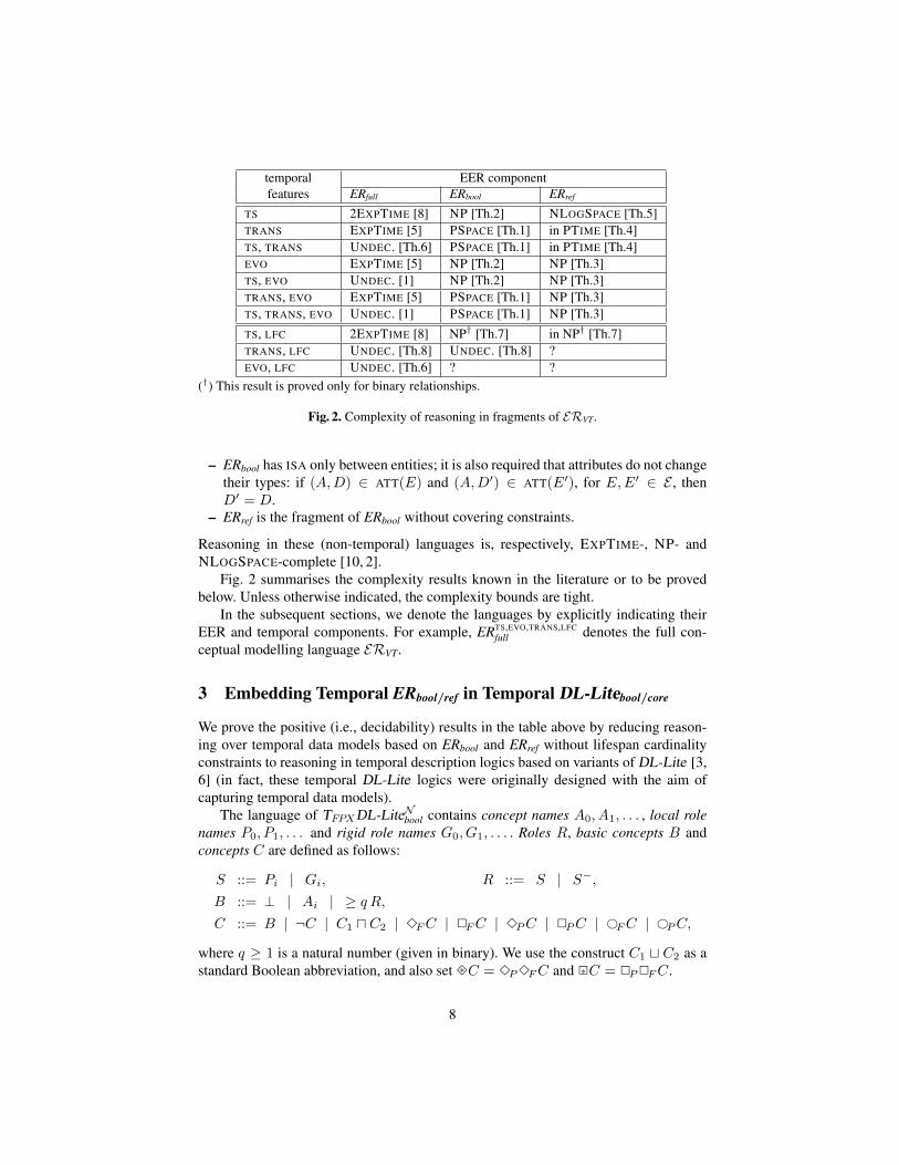
temporal EER componentfeatures ERfull ERbool ERref

TS 2EXPTIME [8] NP [Th.2] NLOGSPACE [Th.5]TRANS EXPTIME [5] PSPACE [Th.1] in PTIME [Th.4]TS, TRANS UNDEC. [Th.6] PSPACE [Th.1] in PTIME [Th.4]EVO EXPTIME [5] NP [Th.2] NP [Th.3]TS, EVO UNDEC. [1] NP [Th.2] NP [Th.3]TRANS, EVO EXPTIME [5] PSPACE [Th.1] NP [Th.3]TS, TRANS, EVO UNDEC. [1] PSPACE [Th.1] NP [Th.3]

TS, LFC 2EXPTIME [8] NP† [Th.7] in NP† [Th.7]TRANS, LFC UNDEC. [Th.8] UNDEC. [Th.8] ?EVO, LFC UNDEC. [Th.6] ? ?

(†) This result is proved only for binary relationships.

Fig. 2. Complexity of reasoning in fragments of ERVT.

– ERbool has ISA only between entities; it is also required that attributes do not changetheir types: if (A,D) ∈ ATT(E) and (A,D′) ∈ ATT(E′), for E,E′ ∈ E , thenD′ = D.

– ERref is the fragment of ERbool without covering constraints.

Reasoning in these (non-temporal) languages is, respectively, EXPTIME-, NP- andNLOGSPACE-complete [10, 2].

Fig. 2 summarises the complexity results known in the literature or to be provedbelow. Unless otherwise indicated, the complexity bounds are tight.

In the subsequent sections, we denote the languages by explicitly indicating theirEER and temporal components. For example, ERTS,EVO,TRANS,LFC

full denotes the full con-ceptual modelling language ERVT.

3 Embedding Temporal ERbool/ref in Temporal DL-Litebool/core

We prove the positive (i.e., decidability) results in the table above by reducing reason-ing over temporal data models based on ERbool and ERref without lifespan cardinalityconstraints to reasoning in temporal description logics based on variants of DL-Lite [3,6] (in fact, these temporal DL-Lite logics were originally designed with the aim ofcapturing temporal data models).

The language of TFPXDL-LiteNbool contains concept names A0, A1, . . . , local rolenames P0, P1, . . . and rigid role names G0, G1, . . . . Roles R, basic concepts B andconcepts C are defined as follows:

S ::= Pi | Gi, R ::= S | S−,B ::= ⊥ | Ai | ≥ q R,C ::= B | ¬C | C1 u C2 | 3FC | 2FC | 3PC | 2PC | ©FC | ©PC,

where q ≥ 1 is a natural number (given in binary). We use the construct C1 t C2 as astandard Boolean abbreviation, and also set 3∗ C = 3P3FC and 2∗C = 2P2FC.

8

A TFPXDL-LiteNbool interpretation I is a function

I(n) =(∆I , A

I(n)0 , . . . , P

I(n)0 , . . . , G

I(n)0 , . . .

), n ∈ Z,

where ∆I 6= ∅, AI(n)i ⊆ ∆I and P I(n)i , GI(n)i ⊆ ∆I ×∆I with GI(n)i = G

I(m)i , for

all m ∈ Z. The role and concept constructs are interpreted in I as follows:

(S−)I(n) = {(y, x) | (x, y) ∈ SI(n)}, ⊥I(n) = ∅, (¬C)I(n) = ∆I \ CI(n),(C1 u C2)

I(n) = CI(n)1 ∩ CI(n)2 , (≥ q R)I(n) =

{x | ]{y | (x, y) ∈ RI(n)} ≥ q

},

(3FC)I(n) =

⋃k>n C

I(k), (3PC)I(n) =

⋃k<n C

I(k),

(2FC)I(n) =

⋂k>n C

I(k), (2PC)I(n) =

⋂k<n C

I(k),

(©FC)I(n) = CI(n+1), (©PC)

I(n) = CI(n−1).

It follows that (3∗ C)I(n) =⋃k∈Z C

I(k) and 2∗C =⋂k∈Z C

I(k).A TFPXDL-LiteNbool TBox, T , is a finite set of concept inclusions (CIs)C1 v C2. (As

usual, instead of two CIs C1 v C2 and C2 v C1 we write C1 ≡ C2.) An interpretationI is a model of T if CI(n)1 ⊆ C

I(n)2 for all n ∈ Z and all CIs C1 v C2 in T . A

concept C is satisfiable with respect to T if there exist a model I of T and n ∈ Zsuch that CI(n) 6= ∅. Concept satisfiability w.r.t. TFPXDL-LiteNbool TBoxes is PSPACE-complete [6].

We now show that entity consistency w.r.t. ERTS,TRANS,EVObool schemas can be reduced to

concept satisfiability w.r.t. TFPXDL-LiteNbool TBoxes. Note that since ERbool has no ISAbetween relationships, without loss of generality we may assume that different relationscannot share the same role in their RELs.

Suppose we are given an ERTS,TRANS,EVObool schema Σ. All entity, relationship and do-

main symbols inΣ will be regarded as concept names in the TFPXDL-LiteNbool TBox TΣwe are about to construct. All role and attribute symbols in Σ will be regarded as rolenames in TΣ . We define TΣ as T 0

Σ ∪ T 1Σ , where T 0

Σ encodes the atemporal constructsand T 1

Σ the temporal ones. T 0Σ contains the following CIs (cf. [2]):

(D) D v ¬C, for C 6= D, where D ∈ D and C ∈ E ∪ R ∪ D;

(A) for ATT(E) = 〈A1 : D1, . . . , Ah : Dh〉 in Σ and 1 ≤ i ≤ h,– ∃A−i v Di,– E v ≥ αAi and E v ≤ β Ai if CARDA(Ai, E) = (α, β);

(R) for REL(R) = 〈U1 : E1, . . . , Uk : Rk〉 in Σ and 1 ≤ i ≤ k,– R ≡ ∃Ui, ≥ 2Ui v ⊥ and ∃U−i v Ei,– Ei v ≥ αU−i and Ei v ≤ β U−i if CARDR(R,Ui, Ei) = (α, β),– E′i v ≥ αU

−i and E′i v ≤ β U

−i if REF(R,Ui, E

′i) = (α, β);

(H) E1 v E2, for E1 ISA E2 in Σ,E1 v ¬E2, for E1 DISJ E2 in Σ,E ≡

⊔ni=1Ei, for {E1, . . . , En} COV E in Σ

(concept inclusions E v ≥ αS with α = 0 and E v ≤ β S with β = ∞ are notincluded in the TBox). The temporal part T 1

Σ contains the following CIs:

9

(TS) E v 2∗E, for snapshot E ∈ ES, and > v 3∗ ¬E, for temporary E ∈ ET,R v 2∗R and roles Ui, 1 ≤ i ≤ k, are rigid, for snapshot R ∈ RS with REL(R) =〈U1 : E1, . . . Uk : Ek〉,the role A is rigid, for snapshot A ∈ AS;

(TRANS) E1 v ©FE2 and E1 v ©F¬E1 for E1 TEV E2,E1 v ©FE2 for E1 TEX E2,E1 v ©PE2 for E1 TEX− E2;

(EVO) E1 v 3F (E2u¬E1) forE1 DEVE2, andE1 v 2FE2u2F¬E1 forE1 PEVE2,E1 v 3FE2 for E1 DEX E2, and E1 v 2FE2 for E1 PEX E2,E1 v 3PE2 for E1 DEX− E2, and E1 v 2PE2 for E1 PEX− E2.

It should be clear that the size of TΣ is polynomial in the size of Σ.

Lemma 1. An entity E is consistent w.r.t. a ERTS,TRANS,EVObool schema Σ if and only if E is

satisfiable w.r.t. to the TFPXDL-LiteNbool TBox TΣ .

The proof of this lemma uses the DL-Lite encoding of atemporal EER schemas [2]and the following lemma showing that we can treat temporary relationships and at-tributes as implicitly temporal:

Lemma 2. Let Σ be an ERTS,TRANS,EVObool schema. If an entity E is consistent w.r.t. Σ then

it is consistent w.r.t. the schema Σ′, which coincides with Σ except that all implicitlytemporal relationships and attributes of Σ are temporary in Σ′.

Proof. Let R1 be an implicitly temporal relationship in Σ. Mark R1 as a temporaryrelationship and denote the resulting schema by Σ1. Let I be a model of Σ such thatEI(t) 6= ∅ for some t ∈ Z. Consider the interpretation J for Σ1 obtained by taking thedisjoint union of two copies of I and then setting

RJ (t)1 =

{{〈e′′1 , e′2, . . . , e′k〉, 〈e′1, e′′2 , . . . , e′′k〉 | 〈e1, e2, . . . , ek〉 ∈ R

I(t)1 }, if t = 0;

{〈e′1, e′2, . . . , e′k〉, 〈e′′1 , e′′2 , . . . , e′′k〉 | 〈e1, e2, . . . , ek〉 ∈ RI(t)1 }, otherwise,

where e′i and e′′i are the two copies of ei ∈ ∆I , 1 ≤ i ≤ k. Clearly, R1 is interpreted asa temporary relationship in J (all other symbols are interpreted in the same way as inI). So, it remains to show that the REL, CARDR and REF constraints involving R1 aresatisfied in J .

REL(R1) = 〈U1 : E1, . . . , Uk : Ek〉 is satisfied in J for every t 6= 0 since J agreeswith the disjoint union of two copies of I. Consider 〈e′′1 , e′2, . . . , e′k〉 ∈ R

J (0)1 . By the

construction, 〈e1, e2, . . . , ek〉 ∈ RI(0)1 , from which ei ∈ EI(0)i and e′i, e′′i ∈ E

J (0)i , for

1 ≤ i ≤ k. Let CARDR(R1, Ui, Ei) = (α, β). It is trivially satisfied for t 6= 0. Considert = 0 and let e′i ∈ E

J (0)i , so that ei ∈ EI(0)i . By the construction,

]{〈e1, e2, . . . , ek〉 ∈ RJ (0)1 | ei = e′i} = ]{〈e1, e2, . . . , ek〉 ∈ RI(0)1 | ei = ei}.

As I satisfies the cardinality constraint, J satisfies it as well. Refinement constraintsREF(R,Ui, E

′i) = (α, β) are considered similarly.

The construction for re-marking implicitly temporal attributes in Σ as temporaryones is analogous. By repeating the above process sufficiently many times we obtainΣ′

containing neither implicitly temporal relationships nor implicitly temporal attributes.

10

Our first application of Lemma 1 is the following:

Theorem 1. Entity consistency for ERTS,TRANS,EVObool , EREVO,TRANS

bool , ERTS,TRANSbool and ERTRANS

boolis PSPACE-complete.

Proof. The upper bound for ERTS,TRANS,EVObool follows from Lemma 1 and PSPACE-com-

pleteness of reasoning in TFPXDL-LiteNbool [6, Theorem 2]. The lower bound for ERTRANSbool

is an immediate consequence of the observation that entity consistency in this language(even without relationships and attributes) is capable of encoding satisfiability of propo-sitional temporal formulas of the form θ ∧ 2∗

∧i(ϕi → ©Fψi), where θ, the ϕi and ψi

are conjunctions of literals. The latter problem is known to be PSPACE-hard [22].

Next, we observe that only the transition constraints TRANS require the next- andprevious-time operators ©F and ©P in TΣ . Without these operators, satisfiability w.r.t.TFPXDL-LiteNbool TBoxes becomes NP-complete [6, Theorem 2], and so we obtain thefollowing:

Theorem 2. Entity consistency for ERTS,EVObool , EREVO

bool and ERTSbool is NP-complete.

Proof. Hardness follows from NP-completeness of entity consistency in ERbool [2].

We consider now temporal extensions of ERref. Note that the Boolean t is neededin TΣ only to encode the covering, and that u in the translation of DEV can be eas-ily eliminated, while the 2∗ (3∗) used to encode TS can be rewritten using 2F and2P (3F ,3P ), e.g., a snapshot entity is translated as E v 2PE and E v 2FE.This gives us an embedding of ERTS,TRANS,EVO

ref into the fragment TFPXDL-LiteNcore ofTFPXDL-LiteNbool, reasoning in which is NP-complete [6, Theorem 3]. Concept inclu-sions of TFPXDL-LiteNcore can only be of the form D1 v D2 and D1 uD2 v ⊥, wherethe Di are defined by the rule:

D ::= B | 3FB | 3PB | 2FB | 2PB | ©FB | ©PB.

Theorem 3. Entity consistency for ERTS,TRANS,EVOref and ERTRANS,EVO

ref is NP-complete.

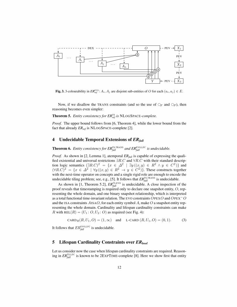
Proof. The NP-hardness is proved by reduction of the NP-complete 3-colourabilityproblem: given a graph G = (V,E) and three colours {1, 2, 3}, decide whether thereis an assignment of colours to the vertices in V such that no two vertices sharing thesame edge have the same colour. To reduce this problem to entity consistency in EREVO

ref ,we need entity symbols O, X1, X2, X3, Y and Ai, for ai ∈ V . One possible way ofencoding the graph G by means of an EREVO

ref schema ΣG is shown in Fig. 3.

Finally, consider ERref extended with timestamping and transition constraints. Inthis case, the embedding into TFPXDL-LiteNcore uses only the next- ©F and previous-time ©P as well as ‘at all moments’ 2∗ and ‘at some moment’ 3∗ temporal operators,which makes reasoning tractable:

Theorem 4. Entity consistency for ERTS,TRANSref is in PTIME.

Proof. The proof can be found in the Appendix.

11

A1 . . .Ai . . .

Aj . . .An

X1

X2

X3Y

O

dd

dd

d

DEX PEV

PEV

PEV

PEV

Fig. 1. 3-colourability in EREVOref : Ai and Aj are disjoint sub-entities of O for each (ai, aj) ∈ E.

1

Fig. 3. 3-colourability in EREVOref : Ai, Aj are disjoint sub-entities of O for each (ai, aj) ∈ E.

Now, if we disallow the TRANS constraints (and so the use of ©F and ©P ), thenreasoning becomes even simpler:

Theorem 5. Entity consistency for ERTSref is NLOGSPACE-complete.

Proof. The upper bound follows from [6, Theorem 4], while the lower bound from thefact that already ERref is NLOGSPACE-complete [2].

4 Undecidable Temporal Extensions of ERfull

Theorem 6. Entity consistency for ERTS,TRANSfull and EREVO,LFC

full is undecidable.

Proof. As shown in [2, Lemma 1], atemporal ERfull is capable of expressing the quali-fied existential and universal restrictions ∃R.C and ∀R.C with their standard descrip-tion logic semantics (∃R.C)I = {x ∈ ∆I | ∃y ((x, y) ∈ RI ∧ y ∈ CI)} and(∀R.C)I = {x ∈ ∆I | ∀y ((x, y) ∈ RI → y ∈ CI)}. These constructs togetherwith the next-time operator on concepts and a single rigid role are enough to encode theundecidable tiling problem; see, e.g., [5]. It follows that ERTS,TRANS

full is undecidable.As shown in [1, Theorem 5.2], ERTS,EVO

full is undecidable. A close inspection of theproof reveals that timestamping is required only to declare one snapshot entity, O, rep-resenting the whole domain, and one binary snapshot relationship, which is interpretedas a total functional time-invariant relation. The EVO constraintsOPEXO andOPEX−Oand the ISA constraintsAISAO, for each entity symbolA, makeO a snapshot entity rep-resenting the whole domain. Cardinality and lifespan cardinality constraints can makeR with REL(R) = (U1 : O,U2 : O) as required (see Fig. 4):

CARDR(R,U1, O) = (1,∞) and L-CARD (R,U1, O) = (0, 1). (3)

It follows that EREVO,LFCfull is undecidable.

5 Lifespan Cardinality Constraints over ERbool

Let us consider now the case when lifespan cardinality constraints are required. Reason-ing in ERTS,LFC

full is known to be 2EXPTIME-complete [8]. Here we show first that entity

12

O R(1, ∗)[0, 1]

1

Fig. 4. Capturing functional total snapshot relationships using L-CARD.

consistency for ERTS,LFCbool with binary relationships only is NP-complete. As in Section 3,

the upper bound is proved by embedding the schema language into an appropriate tem-poral description logic, where traditionally only binary relations are used. So far, weused reification to encode relationships of arbitrary arity; see (R) in Section 3. How-ever, this encoding does not preserve the meaning of timestamped relationships in thepresence of lifespan cardinality constraints. Indeed, Lemma 2 does not hold anymoreand we cannot disregard the difference between temporary and implicitly temporal re-lationships (to see this, note that if we constraint the relationship R in the schema inFig. 4 to be temporary then the schema becomes inconsistent). On the other hand, thereification employed in [8] for capturing n-ary temporary relationships for the ERTS,LFC

fulllanguage was based on a temporal extension ofALC and it does not work for the muchsimpler temporal DL-Lite logics. That is why we restrict the language to binary rela-tionships.

The variant of NP-complete temporal DL-Lite we need is called TRUDL-LiteNbool [6].It uses the ‘universal modalities’ 2∗ and 3∗ on both concepts and roles. The semantics oftemporalised roles 2∗R and 3∗ R (required to encode LFC) is defined as follows:

(2∗R)I(n) =⋂k∈ZR

I(k) and (3∗ R)I(n) =⋃k∈ZR

I(k).

Given an ERTS,LFCbool schemaΣ (with binary relations only), we construct a TRUDL-LiteNbool

TBox TΣ in a way similar to the translation in Section 3. As before, all entity anddomain symbols in Σ are regarded as concept names in TΣ . However, the relationshipand attribute symbols in Σ will now be regarded as role names in TΣ ; the role symbolsin Σ will have no counterparts in TΣ . We define TΣ as T 0

Σ ∪T 1Σ , where T 0

Σ encodes theatemporal constructs and T 1

Σ the temporal ones. T 0Σ is defined as in Section 3 with the

exception of (R) which is replaced with the following:

(R′) for REL(R) = 〈U1 : E1, U2 : E2〉,– ∃R v E1 and ∃R− v E2,– E1 v ≥ αR and E1 v ≤ β R if CARDR(R,U1, E1) = (α, β),– E2 v ≥ αR− and E2 v ≤ β R− if CARDR(R,U2, E2) = (α, β),– E′1 v ≥ αR and E′1 v ≤ β R if REF(R,U1, E

′1) = (α, β),

– E′2 v ≥ αR− and E′2 v ≤ β R− if REF(R,U2, E′2) = (α, β).

The temporal part T 1Σ contains the concept inclusions:

(TS) > v ¬∃2∗R for temporary R ∈ RT; and the role R is rigid for snapshot R ∈ RS,> v ¬∃2∗A for temporary A ∈ AT; and the role A is rigid for snapshot A ∈ AS;

(LFC) for REL(R) = 〈U1 : E1, U2 : E2〉,

13

– E1 v ≥ α3∗ R and E1 v ≤ β3∗ R if L-CARD(R,U1, E1) = (α, β),– E2 v ≥ α3∗ R− and E2 v ≤ β3∗ R− if L-CARD(R,U2, E2) = (α, β),– E′1 v ≥ α3∗ R and E′1 v ≤ β3∗ R if L-REF(R,U1, E

′1) = (α, β),

– E′2 v ≥ α3∗ R− and E′2 v ≤ β3∗ R− if L-REF(R,U2, E′2) = (α, β).

(E v ≥ αS with α = 0 and E v ≤ β S with β =∞ are not included in TΣ .)

Lemma 3. An entity E is consistent w.r.t. an ERTS,LFCbool schema Σ with binary relation-

ships if and only if E is satisfiable w.r.t. the TRUDL-LiteNbool TBox TΣ .

Proof. The proof is straightforward and left to the reader.

Using Lemma 3 and NP-completeness of TRUDL-LiteNbool [6, Theorem 6], we obtain:

Theorem 7. Entity consistency for ERTS,LFCbool with binary relationships is NP-complete.

Proof. The lower bound follows immediately from NP-completeness of ERbool [2].

Unfortunately, if we extend ERLFCbool (with binary relationships) by means of the tran-

sition constraints, the resulting language becomes undecidable.

Theorem 8. Entity consistency for ERTRANS,LFCbool is undecidable.

Proof. We recall from [6, Theorem 5] that if we slightly modify TRUDL-LiteNbool by re-placing the operators 2∗ and 3∗ on concepts with©F , and keeping the same temporalisedroles, then the resulting logic TRXDL-LiteNbool is undecidable. A close inspection of theproof reveals that to prove undecidability we need, apart from a number of conceptnames, a single role name P , which occurs in concepts ∃P and ∃P− and two func-tionality axioms ≥ 23∗ P v ⊥ and ≥ 23∗ P− v ⊥. We show that such a TBox T canbe transformed into an equisatisfiable TBox T ′, which contains the two functionalityaxioms and only CIs of the form > v A and A v C, where C is a concept of the form

C ::= A | ¬A | A1 tA2 | ∃P | ∃P− | ©FA,

and A, A1 and A2 are concept names. Indeed, every CI, C1 v C2, can be rewrittenas > v A and A v ¬C1 t C2, where A is a fresh concept name. We transform theright-hand side of A v ¬C1tC2 into negation normal form and then recursively applythe following rules:

1. A v C1 u C2 is replaced by A v C1 and A v C2,2. A v C1 t C2 is replaced by A v A1 tA2, A1 v C1, A2 v C2 (with fresh Ai),3. A v ©FC is replaced by A v ©FA1 and A1 v C (with fresh A1).

The resulting TBox is the required T ′. Now we show that concept satisfiability w.r.t. T ′can be reduced to entity consistency w.r.t. the ERTRANS,LFC

bool schema ΣT ′ . The reductionis similar to the one used in [10]. Concept names in T ′ are regarded as entity symbols inΣT ′ ; > is represented by a fresh entity symbol O with A ISAO, for each entity symbolA; time-invariance of O is expressed by O TEX O and O TEX− O. The role name P

14

in T ′ is regarded as a relationship symbol P with REL(P ) = 〈U1 : O,U2 : O〉. Thefunctionality of 3∗ P and 3∗ P− is enforced by the constraints, cf. (3):

L-CARD(P,U1, O) = (0, 1) and L-CARD (P,U2, O) = (0, 1).

Concept inclusions of the form > v A and A v A1 are encoded as O ISA A andA ISA A1. For encoding of CIs of the form A v ¬A1 and A v A1 t A2 we refer thereader to [10, Theorem 5.6]. Additionally, we take two fresh entities E∃P and E∃P−and extend the schema with the following constraints:

– A ISA E∃P and REF(P,U1, E∃P ) = (1,∞), for A v ∃P in T ′,– A ISA E∃P− and REF(P,U2, E∃P−) = (1,∞), for A v ∃P− in T ′,– A TEX A1, for A v ©FA in T ′.

Using a technique similar to [10, Theorem 5.6], one can show that, for each conceptname A, A is satisfiable w.r.t. T ′ if and only if A is consistent w.r.t. ΣT ′ .

6 Conclusion

We have investigated the computational complexity of checking quality properties oftemporal conceptual models such as entity, relationship and schema satisfiability or en-tity/relationship subsumption. Although ‘negative’ (undecidability) results were knownfor temporal extensions of the full (atemporal) UML/EER, we have found fragmentswith a much better computational behaviour by considering the language ERbool whereISA between relationships is disallowed, and its sub-language ERref where coveringconstraints are not available. These languages have been extended with timestamp-ing, evolution and transition constraints, and lifespan cardinalities. We have obtaineda nearly comprehensive classification of the computational complexity of reasoningover the resulting temporal conceptual models, which is summarised in Table 2. Threecases involving lifespan cardinalities still remain open. In particular, we do not knowwhether ERref with lifespan cardinalities and transition (or evolution) constraints is de-cidable. Another interesting question we are working on now is whether standard tem-poral provers, quantified Boolean or SAT solvers can be used for efficient practicalreasoning over temporal conceptual models.

References

1. A. Artale. Reasoning on temporal class diagrams: Undecidability results. Annals on Mathe-matics and Artificial Intelligence (AMAI), 46:265–288, 2006. Springer.

2. A. Artale, D. Calvanese, R. Kontchakov, V. Ryzhikov, and M. Zakharyaschev. Reasoningover extended ER models. In Proc. of the 26th Int. Conf. on Conceptual Modeling (ER’07).Lecture Notes in CS, Springer, 2007.

3. A. Artale, D. Calvanese, R. Kontchakov, and M. Zakharyaschev. The DL-Lite family andrelations. Journal of Artificial Intelligence Research, 36:1–69, 2009.

4. A. Artale, E. Franconi, and F. Mandreoli. Description logics for modelling dynamic informa-tion. In Jan Chomicki, Ron van der Meyden, and Gunter Saake, editors, Logics for EmergingApplications of Databases. Lecture Notes in Computer Science, Springer-Verlag, 2003.

15

5. A. Artale, E. Franconi, F. Wolter, and M. Zakharyaschev. A temporal description logicfor reasoning about conceptual schemas and queries. In Proc. of the 8th Joint EuropeanConference on Logics in Artificial Intelligence (JELIA-02), LNAI, 2002.

6. A. Artale, R. Kontchakov, V. Ryzhikov, and M. Zakharyaschev. Past and future of DL-Lite.In Proc. of the 24th AAAI Conf. on Artificial Intelligence (AAAI-10), 2010.

7. A. Artale, C. Parent, and S. Spaccapietra. Evolving objects in temporal information systems.Annals of Mathematics and Artificial Intelligence, 50(1-2):5–38, 2007.

8. A. Artale and D. Toman. Decidable reasoning over timestamped conceptual models. In Proc.of the 21st Int. Workshop on Description Logics (DL-08), Dresden, Germany, May 2008.

9. F. Baader, D. Calvanese, D. McGuinness, D. Nardi, and P. F. Patel-Schneider, editors. De-scription Logic Handbook: Theory, Implementation and Applications. Cambridge UniversityPress, 2002.

10. D. Berardi, D. Calvanese, and G. De Giacomo. Reasoning on UML class diagrams. ArtificialIntelligence, 168(1–2):70–118, 2005.

11. D. Calvanese, M. Lenzerini, and D. Nardi. Unifying class-based representation formalisms.J. of Artificial Intelligence Research, 11:199–240, 1999.

12. C. Combi, S. Degani, and C. S. Jensen. Capturing temporal constraints in temporal ERmodels. In Proc. of the 27th Int. Conf. on Conceptual Modeling (ER’08). LNCS, 2008.

13. O. Etzion, A. Gal, and A. Segev. Extended update functionality in temporal databases. InTemporal Databases - Research and Practice. LNCS, 1998.

14. H. Gregersen and J.S. Jensen. Conceptual modeling of time-varying information. TechnicalReport TimeCenter TR-35, Aalborg University, Denmark, 1998.

15. H. Gregersen and J.S. Jensen. Temporal Entity-Relationship models – a survey. IEEE Trans-actions on Knowledge and Data Engineering, 11(3):464–497, 1999.

16. R. Gupta and G. Hall. An abstraction mechanism for modeling generation. In Proc. ofICDE’92, pages 650–658, 1992.

17. G. Hall and R. Gupta. Modeling transition. In Proc. of ICDE’91, pages 540–549, 1991.18. C. S. Jensen, J. Clifford, S. K. Gadia, P. Hayes, and S. Jajodia et al. The Consensus Glossary

of Temporal Database Concepts. In Temporal Databases - Research and Practice. Springer-Verlag, 1998.

19. C. S. Jensen and R. T. Snodgrass. Temporal data management. IEEE Transactions on Knowl-edge and Data Engineering, 111(1):36–44, 1999.

20. C. S. Jensen, M. Soo, and R. T. Snodgrass. Unifying temporal data models via a conceptualmodel. Information Systems, 9(7):513–547, 1994.

21. C. Lutz, F. Wolter, and M. Zakharyaschev. Temporal description logics: A survey. In Proc.of TIME 2008, 2008.

22. A. Prasad Sistla and Edmund M. Clarke. The complexity of propositional linear temporallogics. In Proc. of the 14th Annual ACM Symposium on Theory of Computing. ACM, 1982.

23. S. Spaccapietra, C. Parent, and E. Zimanyi. Conceptual Modeling for Traditional and Spatio-Temporal Applications—The MADS Approach. Springer, 2006.

24. B. Tauzovich. Towards temporal extensions to the entity-relationship model. In Proc. of theInt. Conf. on Conceptual Modeling (ER’91). Springer-Verlag, 1991.

25. C. Theodoulidis, P. Loucopoulos, and B. Wangler. A conceptual modelling formalism fortemporal database applications. Information Systems, 16(3):401–416, 1991.

16

A Proof of Theorem 4

Theorem 4. Entity consistency for ERTS,TRANSref is decidable in PTIME.

Proof. By Lemma 1, the entity consistency problem can be reduced to concept satisfi-ability with respect to TFPXDL-LiteNbool TBoxes. The latter, in turn, is reducible to thesatisfiability problem in propositional temporal logic; cf. [TR, Theorem 1]. Here wegive a slightly modified version of that reduction (the main difference from [TR] is thatnow the reduction is deterministic).

First, we reduce satisfiability of a TFPXDL-LiteNbool KBK = (T ,A) to satisfiabilityin the one-variable first-order temporal logic in a way similar to [FR]. For each basicconcept B (6= ⊥), we take a fresh unary predicate B∗(x) and encode T as

T † =∧

C1vC2∈T

2∗ ∀x(C∗1 (x)→ C∗2 (x)

),

where the C∗i are the results of replacing each B with B∗(x) (u with ∧, etc.). Weassume that T contains CIs of the form ≥ q R v ≥ q′R, for ≥ q R, ≥ q′R in T suchthat q > q′ and there is no q′′ with q > q′′ > q′ and ≥ q′′R in T . We also assumethat T contains ≥ q R ≡ 2∗ ≥ q R if ≥ q R occurs in T , for a rigid role R (i.e., for Gior G−i ). To take account of the fact that roles are binary relations, we add to T † thefollowing formula, for each role name S,

εS = 2∗(∃x (∃S)∗(x)↔ ∃x (∃S−)∗(x)

)(which says that at each moment of time the domain of S is nonempty iff its range isnonempty). The ABox A is encoded by a conjunction A† of ground atoms of the form©mB∗(a) and©n(≥ q R)∗(a) in the same way as in [FR]. Thus, K is satisfiable iff theformula

K† = T † ∧∧S

εS ∧ A†

is satisfiable.The second step of our reduction is based on the observation that if K† is satisfiable

then it can be satisfied in an interpratation such that

(R0) if (∃S)∗(x) is true at some moment (on some domain element) then it is true at 0(perhaps on a different domain element).

Indeed, if K† is satisfied in I then it is satisfied in the disjoint union I∗ of all In,n ∈ Z, obtained from I by shifting its time line n moments forward. Therefore, if(∃S)∗(x) is true at some moment of time on some element, then there is an elementsuch that (∃S)∗(x) is true on it at 0. It follows then from (R0) that K† is satisfiable iffthe formula

K‡ = T † ∧∧S

((pS → (∃S)∗(dS)

)∧(pS → (∃S−)∗(dS−)

))∧∧

S

2∗ ∀x((

(∃S)∗(x)→ 2∗ pS)∧((∃S−)∗(x)→ 2∗ pS

))∧ A†

17

is satisfiable, where the pS are fresh propositional variables and the dS and dS− arefresh constants (informally, the role S, with pS being false at 0, are always empty,whereas other roles are nonempty at 0, and so are always nonempty). Finally, as K‡contains no existential quantifiers, it can be regarded as a propositional temporal for-mula because all the universal quantifiers can be instantiated by all the constants in theformula, which results only in a polynomial blow-up of K‡.

It turns out that entity consistency in ERTS,TRANSref can in fact be reduced to satisfiabil-

ity of propositional temporal formulas of the form∧Ψ ∧

∧2∗ Φ ∧

∧Θ,

where Ψ and Φ are sets of unary and binary Horn clauses of the form

p, p→ p′, ¬p ∨ ¬p′, p→ ©F p′ or ©F p→ p′

(where p and p′ are propositional variables), 2∗ Φ is the result of prefixing each clausein Φ with 2∗, and Θ is a set of formulas of the form 2∗ p → 2∗ p′. For such formulas wehave the following satisfiability criterion:

Lemma 4. Let ϕ be a propositional temporal formula of the form∧Ψ ∧

∧2∗ Φ ∧

∧Θ

and letΘ0 =

{p′ | 2∗ p→ 2∗ p′ ∈ Θ and

(∧Ψ ∧

∧2∗ Φ)|= 2∗ p

}.

Then ϕ is satisfiable if and only if∧Ψ ∧

∧2∗ Φ ∧

∧2∗Θ0 is satisfiable.

Proof. (⇒) Let M, 0 |= ϕ. Then M, 0 |=∧Ψ ∧

∧2∗ Φ and, by the definition of Θ0,

M |= 2∗ p, for each 2∗ p→ 2∗ p′ ∈ Θ with p′ ∈ Θ0. Therefore, M |=∧

2∗Θ0.(⇐) For each 2∗ p with 2∗ p → 2∗ p′ ∈ Θ and p′ /∈ Θ0, take a model Mp such that

Mp, 0 |=∧Ψ ∧

∧2∗ Φ∧¬2∗ p. Also, take a model M′ satisfying

∧Ψ ∧

∧2∗ Φ∧

∧2∗Θ0

at 0. Construct now a model M by taking the intersection of M′ and the Mp:

M,m |= q iff M′,m |= q and Mp,m |= q, for each 2∗ p,

for all moments m ∈ Z and propositional variables q. Since all clauses in Φ and Ψ areHorn, M, 0 |=

∧Ψ∧∧2∗ Φ. It also follows from the construction that M |= 2∗ p→ 2∗ p′,

for all 2∗ p→ 2∗ p′ ∈ Θ, and so M, 0 |= ϕ.

Similarly to the proof of [TR, Theorem 3], define consmΦ (Ψ) by taking

cons0Φ(Ψ) = {L | Φ ∪ Ψ |= L},consmΦ (Ψ) = {L | Φ |= L′ → ©FL,L

′ ∈ consm−1Φ (Ψ)} ∪ {L | Φ |= L} if m ≥ 1,

consmΦ (Ψ) = {L | Φ |= L′ → ©PL,L′ ∈ consm+1

Φ (Ψ)} ∪ {L | Φ |= L} if m ≤ −1,

where L and L′ are literals (variables or their negations). As in the proof of [TR, Theo-rem 3], since both Φ and Ψ are essentially 2CNFs, we have p ∈ consmΦ (Ψ) if and onlyif M,m |= p, for every M with M, 0 |=

∧Ψ ∧

∧2∗ Φ. Therefore, ϕ is satisfiable just

in case

18

– for each propositional variable q, there is no m ∈ Z with q,¬q ∈ consmΦ∪Θ0(Ψ),

where Θ0 is constructed by taking the set of all p′ such that 2∗ p → 2∗ p′ ∈ Θ and thereis no m ∈ Z with ¬p ∈ consmΦ (Ψ).

It remains to note that the set Θ0 can be constructed and the condition above canbe verified in deterministic polynomial time by solving Diophantine equations for thearithmetic progressions constructed using Unary Finite Automata in the same way as inthe proof of [TR, Theorem 3].

References

[TR] A. Artale, R. Kontchakov, V. Ryzhikov, and M. Zakharyaschev. Temporal conceptual mod-elling with DL-Lite. Technical Report BBKCS-10-02, Department of Computer Science andInformation Systems, Birkbeck, University of London, March 2010.

[FR] A. Artale, R. Kontchakov, V. Ryzhikov, and M. Zakharyaschev. DL-Lite with temporalisedconcepts, rigid axioms and roles. In Proc. of FroCoS, 2009.

19