Complexity and Modeling Power of Insertion-Deletion Systems
131
COMPLEXITY AND MODELING POWER OF INSERTION-DELETION SYSTEMS Alexander Krassovitskiy Dipòsit Legal: T-1370-2011 ADVERTIMENT. La consulta d’aquesta tesi queda condicionada a l’acceptació de les següents condicions d'ús: La difusió d’aquesta tesi per mitjà del servei TDX (www.tesisenxarxa.net ) ha estat autoritzada pels titulars dels drets de propietat intel·lectual únicament per a usos privats emmarcats en activitats d’investigació i docència. No s’autoritza la seva reproducció amb finalitats de lucre ni la seva difusió i posada a disposició des d’un lloc aliè al servei TDX. No s’autoritza la presentació del seu contingut en una finestra o marc aliè a TDX (framing). Aquesta reserva de drets afecta tant al resum de presentació de la tesi com als seus continguts. En la utilització o cita de parts de la tesi és obligat indicar el nom de la persona autora. ADVERTENCIA. La consulta de esta tesis queda condicionada a la aceptación de las siguientes condiciones de uso: La difusión de esta tesis por medio del servicio TDR (www.tesisenred.net ) ha sido autorizada por los titulares de los derechos de propiedad intelectual únicamente para usos privados enmarcados en actividades de investigación y docencia. No se autoriza su reproducción con finalidades de lucro ni su difusión y puesta a disposición desde un sitio ajeno al servicio TDR. No se autoriza la presentación de su contenido en una ventana o marco ajeno a TDR (framing). Esta reserva de derechos afecta tanto al resumen de presentación de la tesis como a sus contenidos. En la utilización o cita de partes de la tesis es obligado indicar el nombre de la persona autora. WARNING. On having consulted this thesis you’re accepting the following use conditions: Spreading this thesis by the TDX (www.tesisenxarxa.net ) service has been authorized by the titular of the intellectual property rights only for private uses placed in investigation and teaching activities. Reproduction with lucrative aims is not authorized neither its spreading and availability from a site foreign to the TDX service. Introducing its content in a window or frame foreign to the TDX service is not authorized (framing). This rights affect to the presentation summary of the thesis as well as to its contents. In the using or citation of parts of the thesis it’s obliged to indicate the name of the author.
-
Upload
khangminh22 -
Category
Documents
-
view
1 -
download
0
Transcript of Complexity and Modeling Power of Insertion-Deletion Systems
COMPLEXITY AND MODELING POWER OF INSERTION-DELETION SYSTEMS
Alexander Krassovitskiy
Dipòsit Legal: T-1370-2011
ADVERTIMENT. La consulta d’aquesta tesi queda condicionada a l’acceptació de les següents condicions d'ús: La difusió d’aquesta tesi per mitjà del servei TDX (www.tesisenxarxa.net) ha estat autoritzada pels titulars dels drets de propietat intel·lectual únicament per a usos privats emmarcats en activitats d’investigació i docència. No s’autoritza la seva reproducció amb finalitats de lucre ni la seva difusió i posada a disposició des d’un lloc aliè al servei TDX. No s’autoritza la presentació del seu contingut en una finestra o marc aliè a TDX (framing). Aquesta reserva de drets afecta tant al resum de presentació de la tesi com als seus continguts. En la utilització o cita de parts de la tesi és obligat indicar el nom de la persona autora. ADVERTENCIA. La consulta de esta tesis queda condicionada a la aceptación de las siguientes condiciones de uso: La difusión de esta tesis por medio del servicio TDR (www.tesisenred.net) ha sido autorizada por los titulares de los derechos de propiedad intelectual únicamente para usos privados enmarcados en actividades de investigación y docencia. No se autoriza su reproducción con finalidades de lucro ni su difusión y puesta a disposición desde un sitio ajeno al servicio TDR. No se autoriza la presentación de su contenido en una ventana o marco ajeno a TDR (framing). Esta reserva de derechos afecta tanto al resumen de presentación de la tesis como a sus contenidos. En la utilización o cita de partes de la tesis es obligado indicar el nombre de la persona autora. WARNING. On having consulted this thesis you’re accepting the following use conditions: Spreading this thesis by the TDX (www.tesisenxarxa.net) service has been authorized by the titular of the intellectual property rights only for private uses placed in investigation and teaching activities. Reproduction with lucrative aims is not authorized neither its spreading and availability from a site foreign to the TDX service. Introducing its content in a window or frame foreign to the TDX service is not authorized (framing). This rights affect to the presentation summary of the thesis as well as to its contents. In the using or citation of parts of the thesis it’s obliged to indicate the name of the author.
Universitat Rovira i Virgili
Departament de Filologies Romaniques
Alexander Krassovitskiy
Complexity and Modeling Power of
Insertion-Deletion Systems
PhD Dissertation
Supervised by:
Yurii Rogozhin
and
Sergey Verlan
Tarragona, 2011
UNIVERSITAT ROVIRA I VIRGILI COMPLEXITY AND MODELING POWER OF INSERTION-DELETION SYSTEMS Alexander Krassovitskiy DL: T.1370-2011
Supervisors:
Professor Yurii Rogozhin
Senior researcher at the Institute of Mathematics and Computer Science
Academy of Sciences of Moldova
Str. Academiei, 5
MD-2028 Chisinau
MOLDOVA
Dr. hab. Sergey Verlan
Associated professor at Departement Informatique
Universite Paris Est
61, Av. General de Gaulle
94010 Creteil
FRANCE
Tutor:
Dr. Gemma Bel-Enguix
Rovira i Virgili University
Research Group on Mathematical Linguistics
Av. Catalunya 35
43002 Tarragona
SPAIN
UNIVERSITAT ROVIRA I VIRGILI COMPLEXITY AND MODELING POWER OF INSERTION-DELETION SYSTEMS Alexander Krassovitskiy DL: T.1370-2011
Abstract
The central notion of the thesis are insertion-deletion systems and their computa-
tional power. More specifically, we study language generating models that use two
string rewriting operations: contextual insertion and contextual deletion.
We approach the questions about the minimal sizes of the insertion-deletion
systems for normal and graph-controlled case. We show that the size of a system
is one of the main parameters determining the computational power of classes of
insertion-deletion systems. Our study consists of four parts, where we study the
power of insertion only, insertion-deletion, graph-controlled, and graph-controlled
systems with priorities, respectively.
In the first part we present equalities between context-free languages and the
languages obtained by insertion systems with one-letter contexts and with specific
squeezing mechanism. We prove the equivalence of these systems and the matrix
languages if a graph-controlled variant is used. We also improve the result from [35]
about the minimal size of computationally complete insertion systems by considering
them in a graph-controlled framework. We also present some results concerning the
semilinearity of Parikh sets of insertion systems.
In the second part we study one-sided and symmetrical insertion-deletion sys-
tems. We solve the last open problem regarding computational completeness of
symmetrical insertion-deletion systems. We introduce and widely use the method
of direct simulation for proving inclusions of families of languages generated by the
insertion-deletion systems. We apply this method to a series of one-sided insertion-
deletion systems and prove the equivalences of their computational power to Turing
machines. We also found that some classes of insertion-deletion systems are not
i
UNIVERSITAT ROVIRA I VIRGILI COMPLEXITY AND MODELING POWER OF INSERTION-DELETION SYSTEMS Alexander Krassovitskiy DL: T.1370-2011
ii ABSTRACT
computationally complete. In the last two parts we study such systems in a graph-
controlled framework, and we show that by this technique the generative power is
strictly increased. At the end, we discuss some open problems raised by our inves-
tigations.
UNIVERSITAT ROVIRA I VIRGILI COMPLEXITY AND MODELING POWER OF INSERTION-DELETION SYSTEMS Alexander Krassovitskiy DL: T.1370-2011
Acknowledgments
It is my pleasure to thank the many people who helped me during this thesis.
First of all, I would like to express sincere gratitude to my supervisor Professor
Yurii Rogozhin who made this work possible. I am in debt to him for providing me
with so many ideas and giving me a lot of inspiration and motivation.
Then, I would like to express my deep gratitude to my second supervisor Dr. hab.
Sergey Verlan. Research visits organized by Sergey have been always very fruitful.
I would also like to thank him for his expertise and patience, not to mention the
proofreading of this work.
I would like to thank the head of our research group, Professor Carlos Martın-
Vide, for his great work in establishing the wonderful environment of the Interna-
tional PhD School in Grammars, Formal Languages and Applications, and for his
help in receiving financial support throughout my PhD. This thesis was made thanks
to the financial support of research grant Ramon i Cajal from the University Rovira
i Virgili, and in part by the project MTM2007-63422 from the Spanish Ministry of
Science and Technology.
I would like to address especial thanks to Dr. Gemma Bel Enguix, who kindly
accepted to be the tutor of my thesis, and for her worthy comments on it. I ap-
preciate a lot that she organized and provided funding for me, necessary to attend
different conferences.
I also address my warm thanks to all professors of the PhD school in Formal
Languages and Applications for presenting so many wonderful topics in Theoretical
Computer Science, and who contributed so much to the organization of the school.
I would like to extend my gratitude to my colleagues Sherzod Turaev, Aretı
iii
UNIVERSITAT ROVIRA I VIRGILI COMPLEXITY AND MODELING POWER OF INSERTION-DELETION SYSTEMS Alexander Krassovitskiy DL: T.1370-2011
iv ACKNOWLEDGMENTS
Panou, Adrian Horia Dediu, Madalina Barbaiani, Catalin Tırnauca, Cristina
Tırnauca, Guangwu Liu, Alexander Perekrestenko, Artiom Alhazov, Peter Leupold
and to all the students of Research Group on Mathematical Linguistics of University
Rovira i Virgili with whom I could feel like at home.
I would like to thank Dr. Lilica Voicu, who has been always very helpful and very
rapid in solving so many administrative problems during all my stay in Tarragona.
I also would like to thank Professor Semen Serovajskiy, whose lectures and dis-
cussions gave me the chance to admire the mathematics and follow the research in
Computer Science.
Last but not the least I wish to express sincerely thanks my parents for their
deep understanding and patience.
UNIVERSITAT ROVIRA I VIRGILI COMPLEXITY AND MODELING POWER OF INSERTION-DELETION SYSTEMS Alexander Krassovitskiy DL: T.1370-2011
Contents
Introduction 1
1 State of the art 5
1.1 Linguistic motivation . . . . . . . . . . . . . . . . . . . . . . . . . . . 5
1.2 Formal languages motivation . . . . . . . . . . . . . . . . . . . . . . 6
1.3 Biological motivation . . . . . . . . . . . . . . . . . . . . . . . . . . . 12
1.3.1 Motivation from DNA computing . . . . . . . . . . . . . . . . 13
1.3.2 Motivation from RNA editing . . . . . . . . . . . . . . . . . . 14
2 Preliminaries 17
2.1 Grammars, automata, and formal languages . . . . . . . . . . . . . . 17
2.2 Graph-controlled systems . . . . . . . . . . . . . . . . . . . . . . . . 21
3 Insertion systems 27
3.1 Definitions . . . . . . . . . . . . . . . . . . . . . . . . . . . . . . . . . 27
3.2 Computational power of pure insertion systems . . . . . . . . . . . . 29
3.3 Graph-controlled insertion systems . . . . . . . . . . . . . . . . . . . 34
4 Insertion-deletion systems 47
4.1 Definitions . . . . . . . . . . . . . . . . . . . . . . . . . . . . . . . . . 47
4.2 Normal form for insertion-deletion systems . . . . . . . . . . . . . . 50
4.3 Basic methods for computational completeness . . . . . . . . . . . . 51
4.4 One-sided insertion-deletion systems . . . . . . . . . . . . . . . . . . 58
4.5 Uncompleteness results . . . . . . . . . . . . . . . . . . . . . . . . . . 64
v
UNIVERSITAT ROVIRA I VIRGILI COMPLEXITY AND MODELING POWER OF INSERTION-DELETION SYSTEMS Alexander Krassovitskiy DL: T.1370-2011
vi CONTENTS
4.6 Descriptional complexity . . . . . . . . . . . . . . . . . . . . . . . . . 79
5 Graph-controlled insertion-deletion systems 83
5.1 Definitions . . . . . . . . . . . . . . . . . . . . . . . . . . . . . . . . . 84
5.2 The computational power of small systems . . . . . . . . . . . . . . . 85
6 Graph-controlled ID systems with priorities 97
6.1 Appearance checking and priorities . . . . . . . . . . . . . . . . . . . 98
6.2 Context-freeness with priorities . . . . . . . . . . . . . . . . . . . . . 100
6.3 Small contextual systems with priorities . . . . . . . . . . . . . . . . 104
Conclusions 109
Bibliography 113
UNIVERSITAT ROVIRA I VIRGILI COMPLEXITY AND MODELING POWER OF INSERTION-DELETION SYSTEMS Alexander Krassovitskiy DL: T.1370-2011
List of Figures
1.1 Inserting by mismatched annealing . . . . . . . . . . . . . . . . . . . 14
1.2 Deleting by mismatched annealing . . . . . . . . . . . . . . . . . . . 15
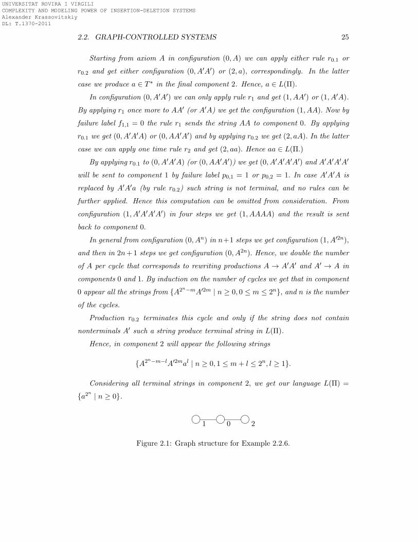
2.1 Graph structure for Example 2.2.6. . . . . . . . . . . . . . . . . . . . 25
3.1 Communication graph for Theorem 3.3.3. . . . . . . . . . . . . . . . 37
3.2 Communication graph for Lemma 3.3.5. . . . . . . . . . . . . . . . . 39
3.3 Communication graph for Theorem 3.3.7. . . . . . . . . . . . . . . . 41
4.1 The situation from Lemma 4.5.15. The derivation tree before the
application of the deletion rule (c, x, ε) (a), intermediate steps (b)
and (c) and after the application (d). . . . . . . . . . . . . . . . . . . 74
4.2 The trees for the derivation of abcdee′d′f from Example 4.5.17. The
derivation in ID (a) and in G1 (b). . . . . . . . . . . . . . . . . . . . 75
5.1 Communication graph for Theorem 5.2.5. . . . . . . . . . . . . . . . 87
6.1 Graph structure for Example 6.1.2. . . . . . . . . . . . . . . . . . . . 99
6.2 Graph structure for Theorem 6.2.2 . . . . . . . . . . . . . . . . . . . 101
6.3 Component structure for Theorem 6.3.3. . . . . . . . . . . . . . . . . 105
vii
UNIVERSITAT ROVIRA I VIRGILI COMPLEXITY AND MODELING POWER OF INSERTION-DELETION SYSTEMS Alexander Krassovitskiy DL: T.1370-2011

UNIVERSITAT ROVIRA I VIRGILI COMPLEXITY AND MODELING POWER OF INSERTION-DELETION SYSTEMS Alexander Krassovitskiy DL: T.1370-2011
Introduction
What could be the most generic tools that helps humans to go through daily obsta-
cles? A possible answer could be described in terms of languages, and information
they pass. We could claim that in every scientific discipline, the understanding of a
subject can be done only by understanding its proper language. Formal languages
often work as a tool that allow researcher to understand in an unambiguous way the
properties of desired system. For example, in order to create a software or hard-
ware one needs a lot of investigations into the subject areas. This, in turn, requires
to describe formally particular components to be implemented, and, of course, the
selection of an adequate language.
Up to now the theory of formal languages has provided formalisms for plenty of
disciplines of human society. We elaborate our thesis around two most interesting
operations of formal languages called insertion and deletion.
The operations of insertion and deletion have a long history. Many linguists
have used various types of string insertion in order to model properties of natural
languages. For example, in Marcus contextual grammars string contextual insertion
are used [47, 24, 58].
Another inspiration for insertion-deletion operation comes from formal language
theory. The insertion operation and its iterated variants are generalized versions
of Kleene’s operation of concatenation [38], while the deletion operation generalizes
the quotient operation. A study of properties of the corresponding operations may
be found in [26, 27, 31].
The third motivation for the study of insertion and deletion comes from the field
of molecular biology. The experimental biology collects a large amount of informa-
1
UNIVERSITAT ROVIRA I VIRGILI COMPLEXITY AND MODELING POWER OF INSERTION-DELETION SYSTEMS Alexander Krassovitskiy DL: T.1370-2011
2 INTRODUCTION
tion about living matter: genes, biological functions, cells, etc. It is clear that the
variety of the biological data needs systematization and understanding. Computer
science have given plenty of efforts in order to understand the functionality of the
living matter. This eventually helps to promote the means of regulations and con-
trols into medicine, biology, and human society. In order to treat the great amount
of raw data formal models are needed. Recently, it was shown that insertion and
deletion correspond to a mismatched annealing of DNA sequences. Such operations
are also present in the evolution processes in the form of point mutations as well as
in RNA editing, see the discussions in [12, 13, 64] and [62]. This biological motiva-
tion of insertion-deletion operations led to their study in the framework of molecular
computing, see, for example, [18, 33, 62, 65].
In general, an insertion operation means adding a substring to a given string,
while a deletion operation means removing a substring of a given string. In our re-
search we mainly consider contextual string insertion and contextual string deletion
operations, i.e., inserted and deleted in specified (left and right) contexts. A con-
textual insertion or contextual deletion rule is defined by a triple (u, x, v) meaning
that x can be inserted between u and v or deleted if it is between u and v. Thus, an
insertion corresponds to the rewriting rule uv → uxv and a deletion corresponds to
the rewriting rule uxv → uv. Further we omit term contextual, whenever it is clear
from the presentation. A finite set of insertion-deletion rules, together with a set of
axioms provide a language generating device: starting from the set of initial strings
and iterating insertion or deletion operations as defined by the given rules one gets
a language. The size of the alphabet, the number of axioms, the size of contexts
and of the inserted or deleted string are natural descriptional complexity measures
for insertion-deletion systems.
The size of an insertion-deletion system is represented as a 6-tuple
(n,m,m′, p, q, q′), where n is a maximal length of the inserted string, m,m′ are
the maximal lengths of the left and right contexts over all insertion rules, p is a
maximal length of the deleted string, and q, q′ are the maximal lengths of the left
and right contexts over all deletion rules. Our research studies those families of
languages which are generated by insertion-deletion systems with different sizes, in
UNIVERSITAT ROVIRA I VIRGILI COMPLEXITY AND MODELING POWER OF INSERTION-DELETION SYSTEMS Alexander Krassovitskiy DL: T.1370-2011
INTRODUCTION 3
particular, those insertion-deletion systems having some of m,m′, q, q′ equal to zero.
It appears that the notion of size becomes one of the central points of the thesis as it
is the main parameter of descriptional complexity of the system. We investigate re-
lation between the computational power of insertion-deletion systems and their size.
Such approach allows to find the borderline between computationally complete and
computationally uncomplete systems. We solved many challenging questions related
to the minimal sizes of the insertion and deletion systems for both graph-controlled
and pure systems. While several interchanges between these parameters allowed to
estimate the borderline for the computationally completeness of our model, for the
uncomplete systems the positions of the generated families in the Chomsky hierarchy
are studied.
The thesis is organized as follows. Chapter 1 gives a brief introduction into
the history of insertion and deletion systems. Here we introduce the main research
areas which gave the inspiration for writing the thesis. The most significant previous
results are summarized in this chapter.
In order to make the thesis accomplished and to fix the notations we introduce
in Chapter 2 the general definitions from formal language theory which are used
throughout the thesis.
Chapter 3 is devoted to pure insertion systems and graph-controlled insertion
systems (all these systems do not use the deletion operation). We present several new
equivalences between the language families in Chomsky hierarchy and the insertion
systems. All these results improve known results from the literature. The material
of this chapter is based on [8, 39, 40].
Chapter 4 deals with systems where both operations of insertion and deletion
are used. Firstly we consider systems where sizes of left and right contexts are
equal and we give an important result concerning the computational completeness
of insertion-deletion systems of size (1, 1, 1; 2, 0, 0).
In this chapter we also investigate one-sided insertion-deletion systems, i.e.
systems whose rules have a left (or right) context only. We show that a one-sided
system can be Turing equivalent, if the sizes of contexts of its rules are sufficiently
large. In this chapter we also give the idea of methods used in the following proofs.
UNIVERSITAT ROVIRA I VIRGILI COMPLEXITY AND MODELING POWER OF INSERTION-DELETION SYSTEMS Alexander Krassovitskiy DL: T.1370-2011
4 INTRODUCTION
We introduce a new method of computational completeness proofs for insertion-
deletion systems that permitted to prove most of the results from this chapter. We
also show a series of computational uncompleteness and decidability results. The
results from this chapter are based on [42, 43, 44]. These results are summarized in
Table 4.1 and Table 4.2.
In Chapter 5 we consider graph-controlled insertion-deletion systems. We take
insertion-deletion systems which are shown to be uncomplete and consider them in a
graph-controller manner. We show that the computational power strictly increases
in these cases. We note, that these systems have their origins from insertion-deletion
P systems firstly considered in [62]. The material of this chapter is based on [7, 41,
43, 44].
The final chapter is devoted to graph-controlled insertion-deletion systems with
priorities corresponding to graph-controlled systems with appearance checking.
More precisely, having an insertion and a deletion rules applicable, then always
the deletion is chosen to be applied. The results on the computational complexity
are given for the classes of languages which can be generated by systems of very
small sizes. We show that this type of priorities is extremely powerful. The results
from this chapter are mostly based on [6, 8, 9].
UNIVERSITAT ROVIRA I VIRGILI COMPLEXITY AND MODELING POWER OF INSERTION-DELETION SYSTEMS Alexander Krassovitskiy DL: T.1370-2011
Chapter 1
State of the art
This chapter gives a short introduction into the history of insertion-deletion systems.
Firstly, we will present the linguistic origins of insertion and deletion operations.
Then, a formal languages motivation is presented. Finally, we give the biological
background for insertion-deletion systems.
1.1 Linguistic motivation
The idea of insertion of one string into another was firstly considered with a linguistic
motivation by Marcus in [47]. It is known that a Chomsky grammar is not a unique
way to represent natural languages. Moreover, for natural languages the models
that use local insertion/deletion may be simpler than models that use top-down
grammatical tree construction of words for a given language. For example, in an
English sentence a noun phrase permits the insertion of an arbitrary number of
adjectives adjacently. This can be represented in a simplified form by an insertion
rule (a, a′, n), where a, a′ ∈ ADJECTIV ES, n ∈ NOUNS. Clearly, the above rule
is easier to express in terms of locality than by syntactical tree.
We would like to cite Marcus concerning the idea that stays behind contextual
string insertion: “Generative grammars are a rupture from the linguistic tradition
of the first half of XX-th century, while analytical models are just the development,
the continuation of this tradition. . . Contextual grammars have their origin in the
attempt to transform some procedures developed within the framework of analytical
5
UNIVERSITAT ROVIRA I VIRGILI COMPLEXITY AND MODELING POWER OF INSERTION-DELETION SYSTEMS Alexander Krassovitskiy DL: T.1370-2011
6 CHAPTER 1. STATE OF THE ART
model into generative devices. The idea of connecting in this way analytical study
with the generative approach to natural languages was one of main problems inves-
tigated in mathematical linguistics in the period from 1957 to 1970.”
Marcus contextual grammars consider couples (x, (u, v)), meaning that words u
and v can be adjoined to the word x. This corresponds in some sense to grammars
having rules of type x→ uxv, i.e., u and v are inserted around the position marked
by x. Such grammars are considered as a generative device that permits insertions
of the given contexts, in cases x satisfies certain conditions, e.g., written by a regular
expression. Many interesting linguistic issues like ambiguity and word duplication
can be captured in this framework.
This idea was later developed in [58, 48], and with particular application in [11].
The fixed size contexts (specified for every rule) were firstly considered in [24].
1.2 Formal languages motivation
In [26, 27] the insertion operation and its iterated variant are introduced with rather
different motivation. The author considers these operations as generalization of
Kleene’s operations of concatenation and closure [38]. The operation of concatena-
tion would produce a string x1x2y from two strings x1x2 and y. By allowing the
concatenation to happen anywhere in the string and not only at its right extremity
a string x1yx2 can be produced, i.e., y is inserted into x1x2. In [31] the deletion is
defined as a right quotient operation which happens not necessarily at the rightmost
end of the string. In the same thesis the duality between the insertion and deletion
is also highlighted: any insertion system generating a language L is at the same
time a deletion system recognizing L. The operations considered in above works
correspond to context-free variants of insertion and deletion operations, because no
contexts are used. In the same place several other variants of insertion and deletion
are introduced and their closure properties are investigated.
In the literature it is possible to find several investigations on the extension of
regular expressions with the operation of insertion. Formally, the extended regular
expressions ExReg are defined as the smallest family of languages which contains the
finite languages and is closed under the operations of union, concatenation, Kleene
UNIVERSITAT ROVIRA I VIRGILI COMPLEXITY AND MODELING POWER OF INSERTION-DELETION SYSTEMS Alexander Krassovitskiy DL: T.1370-2011
1.2. FORMAL LANGUAGES MOTIVATION 7
star and iterated insertion. The article [27] shows that the power of ExReg languages
is strictly between regular and context-free languages. One of the main goals of the
article is to find connections between these languages and context-free languages.
In particular, it verifies whether well-known decidability results for context-free and
regular languages hold as well for the insertion languages. For example, it studies the
decidability problems of emptiness and regularity for an ExReg language given by
its rules as well as the context-freeness of the intersection of two ExReg languages.
The article [29] studies the languages that are closed under insertion. It seems
that the computational power of such languages is rather weak. This is partially due
to the restriction that for every word w ∈ ins(L), ins(L) being the insertion closure
of L, word w must be “insertable” into every word from L and moreover at every
possible position, resulting again a word from L. Hence, L is closed with respect to
insertion if it has some trivial form, for example, a+, the Dyck language, etc.
One of the ways to study the operation of insertion is to apply it on the family
of well-known languages from Chomsky hierarchy. In [31] several types of insertions
are defined:
1. Sequential language insertion SIN of L2 into L1 over alphabet Σ, defined as:
SIN(L1, L2) = {u1vu2 | u1u2 ∈ L1, v ∈ L2}.
2. Parallel language insertion PIN over of L2 into L1 over Σ, defined as:
PIN(L1, L2) = {w ∈ Σ | w = a1v1a2v2 . . . vk1ak, a1, . . . , ak ∈ Σ, a1a2 . . . ak ∈
L1, v1, . . . , vk−1 ∈ L2}.
3. Permuted sequential language insertion PSIN of L2 into L1 over Σ, defined
as: PSIN(L1, L2) = {u1vu2 | u1u2 ∈ L1, there is v′ ∈ L2 such that v ∈
perm(v′)}, where perm(v) is set of permutations of v.
4. Permuted parallel language insertion PPIN of L2 into L1 over Σ, defined
as: PPIN(L1, L2) = {w ∈ Σ | w = a1v1a2v2 . . . vk1ak, a1, . . . , ak ∈ Σ,
a1a2 . . . ak ∈ L1, v1, . . . , vk−1 ∈ Σ∗, there are v′1, . . . , v′k−1 ∈ L2 such that
vi ∈ perm(v′i), 1 ≤ i ≤ k − 1}.
5. Controlled sequential language insertion CSIN, defined via a control function
∆ : Σ → 2Σ∗
. CSIN(L1,∆) = {u1avu2 | u1u2 ∈ L1, a ∈ Σ, v ∈ ∆(a)}.
UNIVERSITAT ROVIRA I VIRGILI COMPLEXITY AND MODELING POWER OF INSERTION-DELETION SYSTEMS Alexander Krassovitskiy DL: T.1370-2011
8 CHAPTER 1. STATE OF THE ART
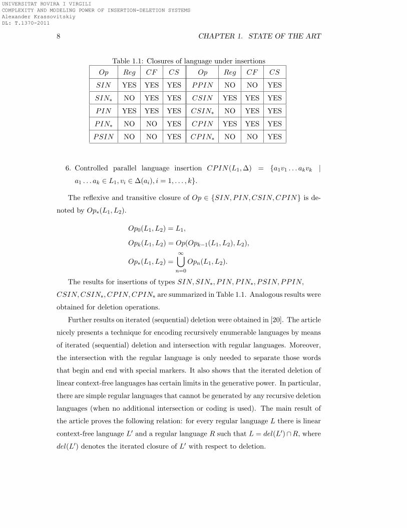
Table 1.1: Closures of language under insertions
Op Reg CF CS Op Reg CF CS
SIN YES YES YES PPIN NO NO YES
SIN∗ NO YES YES CSIN YES YES YES
PIN YES YES YES CSIN∗ NO YES YES
PIN∗ NO NO YES CPIN YES YES YES
PSIN NO NO YES CPIN∗ NO NO YES
6. Controlled parallel language insertion CPIN(L1,∆) = {a1v1 . . . akvk |
a1 . . . ak ∈ L1, vi ∈ ∆(ai), i = 1, . . . , k}.
The reflexive and transitive closure of Op ∈ {SIN, PIN,CSIN,CPIN} is de-
noted by Op∗(L1, L2).
Op0(L1, L2) = L1,
Opk(L1, L2) = Op(Opk−1(L1, L2), L2),
Op∗(L1, L2) =∞⋃
n=0
Opn(L1, L2).
The results for insertions of types SIN, SIN∗, P IN, PIN∗, PSIN, PPIN,
CSIN,CSIN∗, CPIN,CPIN∗ are summarized in Table 1.1. Analogous results were
obtained for deletion operations.
Further results on iterated (sequential) deletion were obtained in [20]. The article
nicely presents a technique for encoding recursively enumerable languages by means
of iterated (sequential) deletion and intersection with regular languages. Moreover,
the intersection with the regular language is only needed to separate those words
that begin and end with special markers. It also shows that the iterated deletion of
linear context-free languages has certain limits in the generative power. In particular,
there are simple regular languages that cannot be generated by any recursive deletion
languages (when no additional intersection or coding is used). The main result of
the article proves the following relation: for every regular language L there is linear
context-free language L′ and a regular language R such that L = del(L′)∩R, where
del(L′) denotes the iterated closure of L′ with respect to deletion.
UNIVERSITAT ROVIRA I VIRGILI COMPLEXITY AND MODELING POWER OF INSERTION-DELETION SYSTEMS Alexander Krassovitskiy DL: T.1370-2011
1.2. FORMAL LANGUAGES MOTIVATION 9
Several investigations pointed out that insertion and deletion may be seen as
particular case of string rewriting manipulations. Shuffle and deletion on trajectories
was studied intensively in [34]. This model has a particular interest because it is easy
to consider the operation of shuffle on trajectories as a generalization of insertion
(with no contexts). Hence, many results that are applicable to systems based on
operations of shuffle and deletion on trajectories are also applicable for the insertion
and deletion systems. For example, as an immediate result one can obtain the
closure of regular languages under the iterated insertion.
In the above article a list of decidability results is given for shuffle and deletion on
trajectories for context-free and regular languages. In particular, it was shown that
for any two regular languages it is decidable whether the language which is resulted
by insertion or deletion of one language into another one is regular. Moreover, this
language may be effectively constructed. In case of regular language being inserted
into (or deleted from) a context-free language this problem is undecidable.
It was shown in [19] how the semantic shuffle and deletion along trajectories
may be used as a generalized model for the contextual insertion and the contextual
deletion. This model has a very clear form for an algorithmic implementation and
can be used to describe many other binary string operations. In a unified form the
techniques presented in the article help to solve many language equations. However,
this technique cannot be applied for the iterative form of the computations (as in the
case of derivations of insertion and deletion systems), because the generating power
of such a model increases significantly, giving a Turing equivalent model. Further
results for restricted variants of the shuffled insertion were obtained in [30].
It was proved in [62] that pure insertion systems having one letter context are
always context-free. Yet, there are insertion systems with two letter context which
generate nonsemilinear languages (see Theorem 6.5 in [62]). On the other hand, it
appears that by using only insertion operations the obtained language classes with
contexts greater than one are incomparable with many known language classes. For
example, there is a simple linear language {anban | n ≥ 1} which cannot be generated
by any insertion system (see Theorem 6.6 in [62]).
In order to overcome this obstacle one can use some codings to “interpret” the
UNIVERSITAT ROVIRA I VIRGILI COMPLEXITY AND MODELING POWER OF INSERTION-DELETION SYSTEMS Alexander Krassovitskiy DL: T.1370-2011
10 CHAPTER 1. STATE OF THE ART
generated strings. The questions about the computational power of insertion systems
with morphisms and intersection with special languages were considered in [55, 56]
and [61]. In [50] two additional mapping relations are used : a morphism h and a
weak coding ϕ. The strings of the language are obtained by applying h−1 ◦ ϕ on
the generated strings. Clearly, the languages obtained in such a way have greater
expressivity, and the corresponding language class is more powerful. It appears that
in this case one can obtain every RE language if insertion rules have sufficiently
large context.
We define the size of an insertion system as a vector (n,m,m′), n > 0,m,m′ ≥ 0,
where n is a maximal length of the inserted strings; m and m′ are equal to the
maximal length of the left and the right contexts of rules of the system. This vector
corresponds to the first three parameters in the definition of size for insertion-deletion
systems. It is proved in [50] that for every recursively enumerable language L there
exists a morphism h, a weak coding ϕ and a language L′ generated by an insertion
system with rules having sizes at most (7, 7, 7), such that, L = h(ϕ−1(L′)). This
result was improved in [54], where it was shown that systems having rules of size at
most (5, 5, 5) are sufficient to encode every recursively enumerable language. This
result was further improved in [70]. Recently, in [35] it was shown that the same
result can be obtained with rules of size equal to (3, 3, 3). We improve this result
by introducing a graph control into the model. In this case the computational
completeness with rules of size (2, 2, 2) is obtained, see Theorem 3.3.7.
Article [36] introduces the operations of contextual insertion and contextual dele-
tion as generalizations of insertion and deletion of words. Closure properties of the
regular and context-free languages under these operations, contextual ins-closed and
del-closed languages, and decidability of existence of solutions to equations involving
these operations are investigated. Based entirely on contextual operations, the in-
sertion and deletion systems have been introduced, where both types of rules can act
simultaneously in the same derivation. Moreover, in this article it was shown that
every Turing machine can be simulated by insertion-deletion systems. This work
also introduces the notion of lengths of contexts as basic computational parameter,
called weight. It corresponds to the 4-tuple (n, m, p, q), where m = max{m,m′},
UNIVERSITAT ROVIRA I VIRGILI COMPLEXITY AND MODELING POWER OF INSERTION-DELETION SYSTEMS Alexander Krassovitskiy DL: T.1370-2011
1.2. FORMAL LANGUAGES MOTIVATION 11
and q = max{q, q′}, where (n,m,m′, p, q, q′) is the size of the system. Since this
work a number of studies have been done in this direction. For example, an attempt
to use the number of symbols of the alphabet as a measure of the (descriptional)
complexity was given in [37]. It is shown there that two symbols are enough to
obtain the power of Turing machine.
We would like to remark one result from [49] where it was proved that even rela-
tively small sized insertion-deletion systems which do not use contexts are computa-
tionally complete. In fact, this article shows that for any type-0 grammar there exists
an insertion-deletion system of size (n, 0, 0;m, 0, 0) which generates the same lan-
guage, where parameters n and m depend on the form of the used grammar. Then,
the result was improved for fixed size insertion-deletion systems by using special
normal forms of RE grammars. More precisely, the inclusions RE ⊆ INS0,03 DEL0,0
2
and RE ⊆ INS0,02 DEL0,0
3 were shown. The article [67] shows that similar results
do not hold for a system of smaller size.
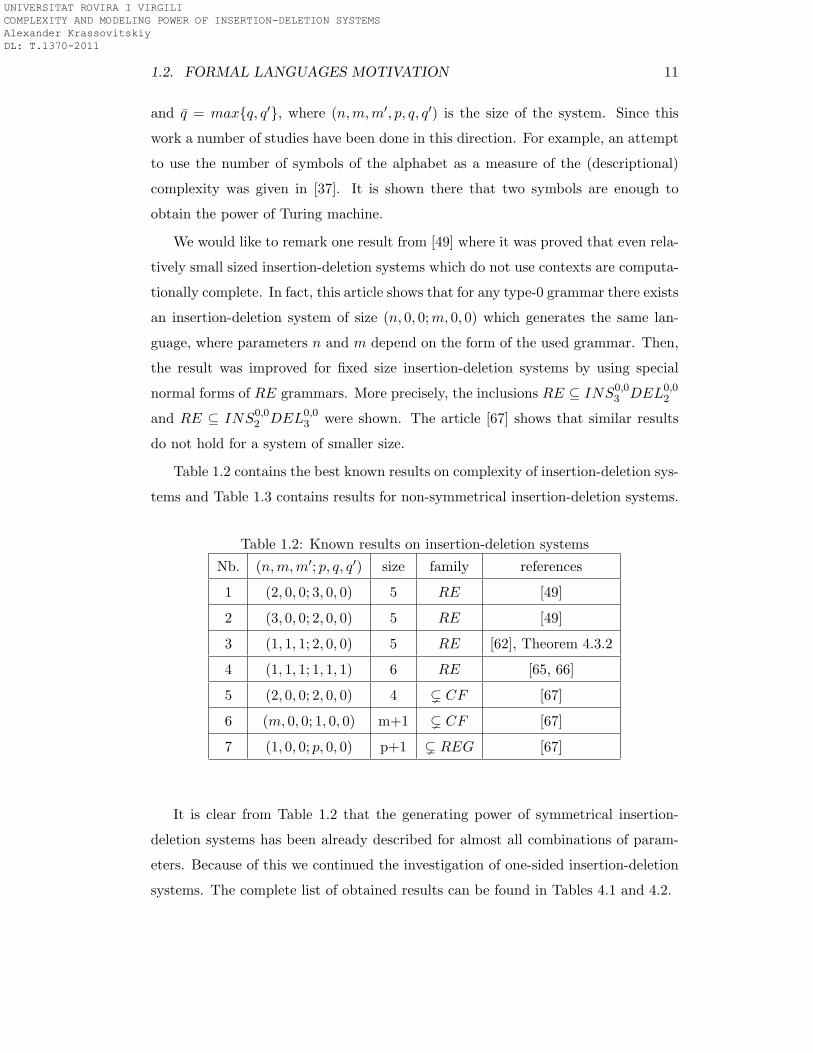
Table 1.2 contains the best known results on complexity of insertion-deletion sys-
tems and Table 1.3 contains results for non-symmetrical insertion-deletion systems.
Table 1.2: Known results on insertion-deletion systems
Nb. (n,m,m′; p, q, q′) size family references
1 (2, 0, 0; 3, 0, 0) 5 RE [49]
2 (3, 0, 0; 2, 0, 0) 5 RE [49]
3 (1, 1, 1; 2, 0, 0) 5 RE [62], Theorem 4.3.2
4 (1, 1, 1; 1, 1, 1) 6 RE [65, 66]
5 (2, 0, 0; 2, 0, 0) 4 ( CF [67]
6 (m, 0, 0; 1, 0, 0) m+1 ( CF [67]
7 (1, 0, 0; p, 0, 0) p+1 ( REG [67]
It is clear from Table 1.2 that the generating power of symmetrical insertion-
deletion systems has been already described for almost all combinations of param-
eters. Because of this we continued the investigation of one-sided insertion-deletion
systems. The complete list of obtained results can be found in Tables 4.1 and 4.2.
UNIVERSITAT ROVIRA I VIRGILI COMPLEXITY AND MODELING POWER OF INSERTION-DELETION SYSTEMS Alexander Krassovitskiy DL: T.1370-2011
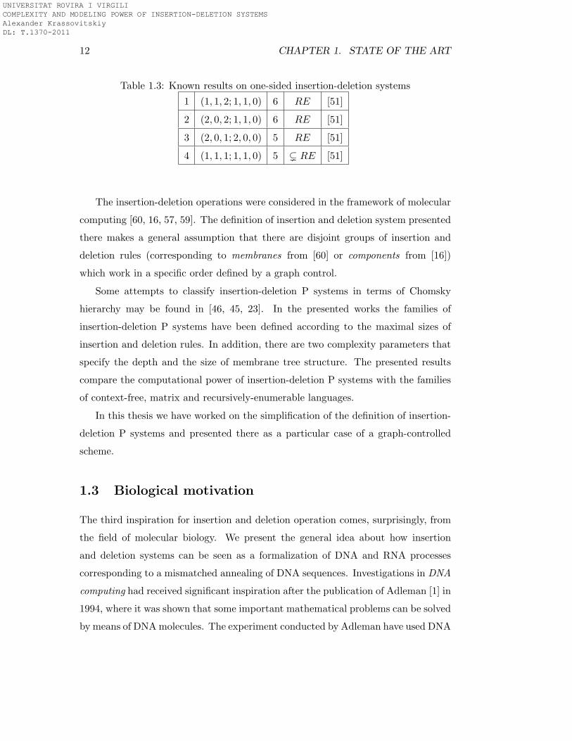
12 CHAPTER 1. STATE OF THE ART
Table 1.3: Known results on one-sided insertion-deletion systems
1 (1, 1, 2; 1, 1, 0) 6 RE [51]
2 (2, 0, 2; 1, 1, 0) 6 RE [51]
3 (2, 0, 1; 2, 0, 0) 5 RE [51]
4 (1, 1, 1; 1, 1, 0) 5 ( RE [51]
The insertion-deletion operations were considered in the framework of molecular
computing [60, 16, 57, 59]. The definition of insertion and deletion system presented
there makes a general assumption that there are disjoint groups of insertion and
deletion rules (corresponding to membranes from [60] or components from [16])
which work in a specific order defined by a graph control.
Some attempts to classify insertion-deletion P systems in terms of Chomsky
hierarchy may be found in [46, 45, 23]. In the presented works the families of
insertion-deletion P systems have been defined according to the maximal sizes of
insertion and deletion rules. In addition, there are two complexity parameters that
specify the depth and the size of membrane tree structure. The presented results
compare the computational power of insertion-deletion P systems with the families
of context-free, matrix and recursively-enumerable languages.
In this thesis we have worked on the simplification of the definition of insertion-
deletion P systems and presented there as a particular case of a graph-controlled
scheme.
1.3 Biological motivation
The third inspiration for insertion and deletion operation comes, surprisingly, from
the field of molecular biology. We present the general idea about how insertion
and deletion systems can be seen as a formalization of DNA and RNA processes
corresponding to a mismatched annealing of DNA sequences. Investigations in DNA
computing had received significant inspiration after the publication of Adleman [1] in
1994, where it was shown that some important mathematical problems can be solved
by means of DNAmolecules. The experiment conducted by Adleman have used DNA
UNIVERSITAT ROVIRA I VIRGILI COMPLEXITY AND MODELING POWER OF INSERTION-DELETION SYSTEMS Alexander Krassovitskiy DL: T.1370-2011
1.3. BIOLOGICAL MOTIVATION 13
molecules in order to solve an instance of well-known NP-complete problem called
Hamiltonian path problem. Since then a big amount of theoretical and practical
investigations has been done giving a growth for such areas as insertion-deletion (P)
systems, splicing systems, sticker systems, Head systems, Watson-Crick automata,
etc., see [62]. We present below how it is theoretically possible to perform the
insertion and the deletion involving molecules of DNA and RNA.
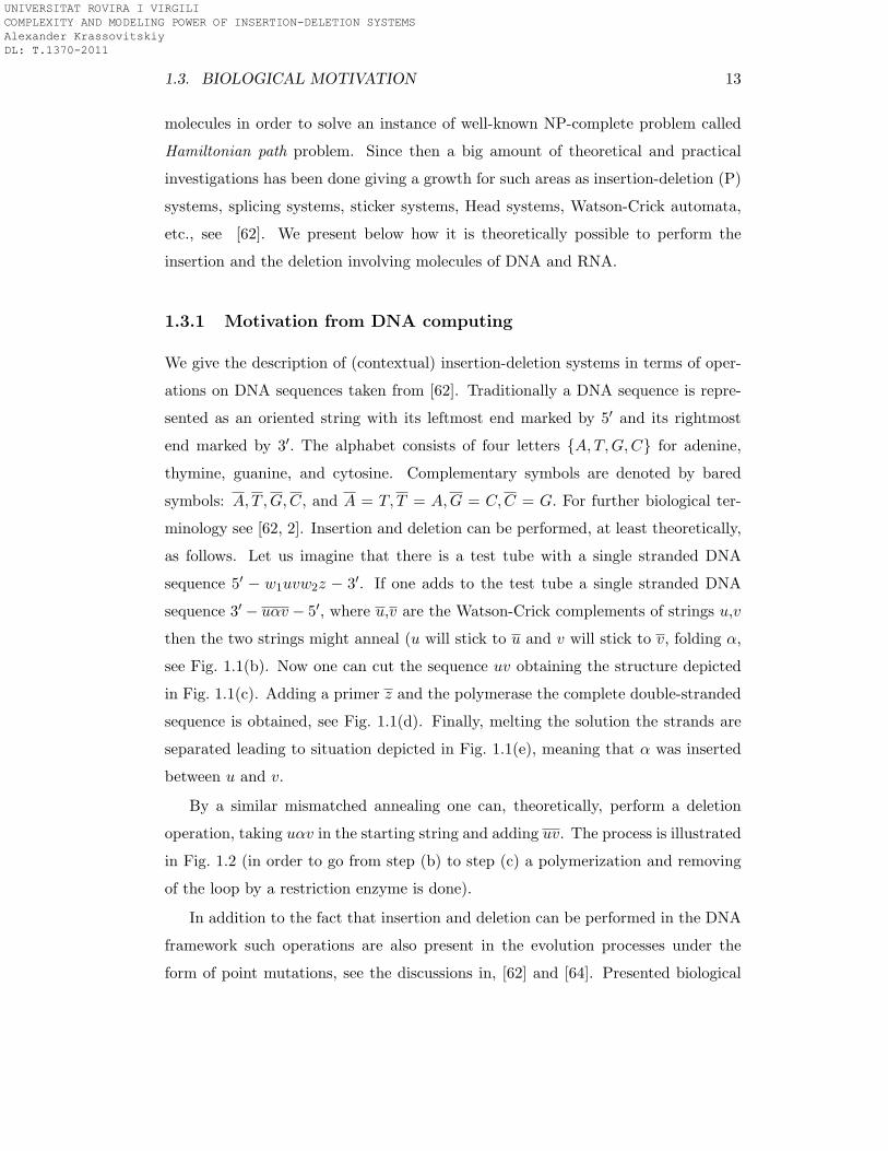
1.3.1 Motivation from DNA computing
We give the description of (contextual) insertion-deletion systems in terms of oper-
ations on DNA sequences taken from [62]. Traditionally a DNA sequence is repre-
sented as an oriented string with its leftmost end marked by 5′ and its rightmost
end marked by 3′. The alphabet consists of four letters {A, T,G,C} for adenine,
thymine, guanine, and cytosine. Complementary symbols are denoted by bared
symbols: A, T ,G,C, and A = T, T = A,G = C,C = G. For further biological ter-
minology see [62, 2]. Insertion and deletion can be performed, at least theoretically,
as follows. Let us imagine that there is a test tube with a single stranded DNA
sequence 5′ − w1uvw2z − 3′. If one adds to the test tube a single stranded DNA
sequence 3′ − uαv − 5′, where u,v are the Watson-Crick complements of strings u,v
then the two strings might anneal (u will stick to u and v will stick to v, folding α,
see Fig. 1.1(b). Now one can cut the sequence uv obtaining the structure depicted
in Fig. 1.1(c). Adding a primer z and the polymerase the complete double-stranded
sequence is obtained, see Fig. 1.1(d). Finally, melting the solution the strands are
separated leading to situation depicted in Fig. 1.1(e), meaning that α was inserted
between u and v.
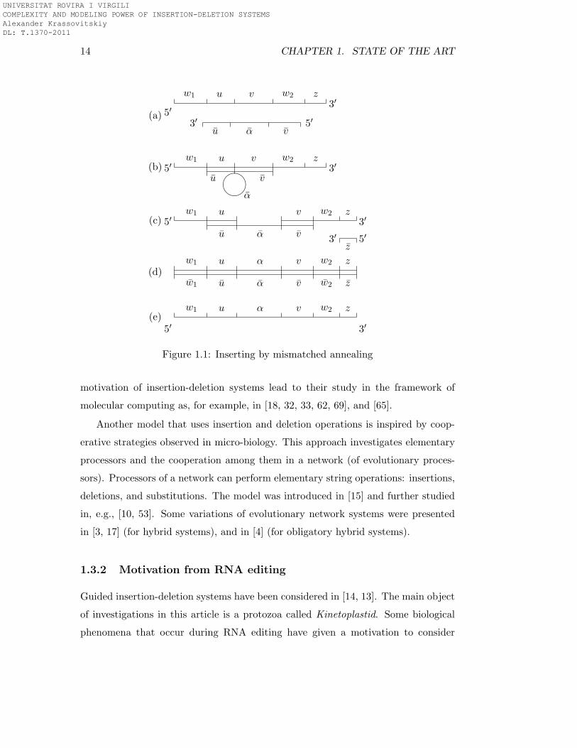
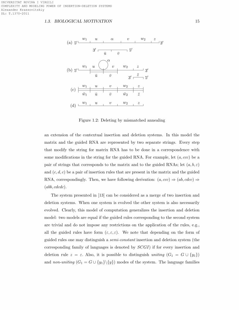
By a similar mismatched annealing one can, theoretically, perform a deletion
operation, taking uαv in the starting string and adding uv. The process is illustrated
in Fig. 1.2 (in order to go from step (b) to step (c) a polymerization and removing
of the loop by a restriction enzyme is done).
In addition to the fact that insertion and deletion can be performed in the DNA
framework such operations are also present in the evolution processes under the
form of point mutations, see the discussions in, [62] and [64]. Presented biological
UNIVERSITAT ROVIRA I VIRGILI COMPLEXITY AND MODELING POWER OF INSERTION-DELETION SYSTEMS Alexander Krassovitskiy DL: T.1370-2011
14 CHAPTER 1. STATE OF THE ART
(d)
(e)5′
w1 u α v w2 z
3′
zw2vαuw1
w1 u α v w2 z
z3′ 5′
3′zw2v
vαu
uw1
5′(c)
����5′(b)
w1 u v w2 z3′
u v
α
5′(a)
w1 u v w2 z3′
5′vαu
3′
Figure 1.1: Inserting by mismatched annealing
motivation of insertion-deletion systems lead to their study in the framework of
molecular computing as, for example, in [18, 32, 33, 62, 69], and [65].
Another model that uses insertion and deletion operations is inspired by coop-
erative strategies observed in micro-biology. This approach investigates elementary
processors and the cooperation among them in a network (of evolutionary proces-
sors). Processors of a network can perform elementary string operations: insertions,
deletions, and substitutions. The model was introduced in [15] and further studied
in, e.g., [10, 53]. Some variations of evolutionary network systems were presented
in [3, 17] (for hybrid systems), and in [4] (for obligatory hybrid systems).
1.3.2 Motivation from RNA editing
Guided insertion-deletion systems have been considered in [14, 13]. The main object
of investigations in this article is a protozoa called Kinetoplastid. Some biological
phenomena that occur during RNA editing have given a motivation to consider
UNIVERSITAT ROVIRA I VIRGILI COMPLEXITY AND MODELING POWER OF INSERTION-DELETION SYSTEMS Alexander Krassovitskiy DL: T.1370-2011
1.3. BIOLOGICAL MOTIVATION 15
w1 u v w2 z
zw2vuw1
w1 u v w2 z(d)
(c)
����
w1 u v
α
w2 z
z3′
5′3′vu
5′(b)
5′(a)w1 u α v w2 z
3′
5′vu
3′
Figure 1.2: Deleting by mismatched annealing
an extension of the contextual insertion and deletion systems. In this model the
matrix and the guided RNA are represented by two separate strings. Every step
that modify the string for matrix RNA has to be done in a correspondence with
some modifications in the string for the guided RNA. For example, let (a, ccc) be a
pair of strings that corresponds to the matrix and to the guided RNAs; let (a, b, ε)
and (c, d, c) be a pair of insertion rules that are present in the matrix and the guided
RNA, correspondingly. Then, we have following derivation: (a, ccc) ⇒ (ab, cdcc) ⇒
(abb, cdcdc).
The system presented in [13] can be considered as a merge of two insertion and
deletion systems. When one system is evolved the other system is also necessarily
evolved. Clearly, this model of computation generalizes the insertion and deletion
model: two models are equal if the guided rules corresponding to the second system
are trivial and do not impose any restrictions on the application of the rules, e.g.,
all the guided rules have form (ε, ε, ε). We note that depending on the form of
guided rules one may distinguish a semi-constant insertion and deletion system (the
corresponding family of languages is denoted by SCGI) if for every insertion and
deletion rule z = ε. Also, it is possible to distinguish uniting (G1 = G ∪ {y1})
and non-uniting (G1 = G ∪ {y1}\{y}) modes of the system. The language families
UNIVERSITAT ROVIRA I VIRGILI COMPLEXITY AND MODELING POWER OF INSERTION-DELETION SYSTEMS Alexander Krassovitskiy DL: T.1370-2011
16 CHAPTER 1. STATE OF THE ART
corresponding to such guided insertion and deletion systems are denoted by uGI
and unGI.
It is known from [13] that the generative capacity of such systems forms a
Chomsky-like hierarchy of languages
Reg ⊂ SCGI ⊂ uGI ⊂ unGI ⊂ RE.
Moreover, the families of languages SCGI and uGI are anti-AFL. From the other
side [14] demonstrates how RNA editing may be accurately modeled by the guided
insertion and deletion systems.
Another form of guided operations of insertion and deletion inspired by RNA
editing was considered in [71]. The author observes that uracil (denoted by 0) is the
only element which is inserted or deleted during RNA transcriptions. The transition
step ⇒G of the corresponding system is defined by using a set of guides G ⊂ V ∗,
where V is the working alphabet. We have usv ⇒G ugv, u, v, s ∈ V ∗, g ∈ G if g
is obtained from s either by insertion or by deletion of one ore more occurrences
of 0 ∈ V. For example, given a sentential form a00a0a0a and a set of guides G′ =
{a0a00a, aaa}. Then we have a00a0a0a ⇒G′ w,w ∈ {a00a0a00a, a0a00aa, a00aaa,
aaa0a}. The main result of this article states that the regular and the context-free
languages are not closed under the operations of guided insertion and deletion.
More details about RNA editing for various biological species may be found, e.g.,
in [12].
UNIVERSITAT ROVIRA I VIRGILI COMPLEXITY AND MODELING POWER OF INSERTION-DELETION SYSTEMS Alexander Krassovitskiy DL: T.1370-2011
Chapter 2
Preliminaries
This chapter introduces the general definitions from the theory of formal languages,
used later in the thesis. Many definitions in this chapter are standard and may be
found in any textbook on formal languages (e.g. [63, 28, 21, 25]).
2.1 Grammars, automata, and formal languages
We denote by N the set of natural numbers {0, 1, 2, . . . } and by N+ the set of strictly
positive integer numbers {1, 2, . . . }. We also denote by ∅ the empty set and by 2X
the set of all subsets of X. The number of elements of a set X is denoted by
Card(X).
An alphabet is a finite non-empty set of symbols which are also called letters or
symbols. A word over the alphabet V is a concatenation of symbols of V . Sometimes
we use term string instead of word. The empty concatenation is called the empty
word and it is denoted by ε. The set of all words over V is denoted by V ∗. The set
of all words over an alphabet V , except the empty word, is denoted by V +. Any
subset of V ∗ is called a language over the alphabet V .
We denote by |w| the length of a word w. For a letter a and a word w we denote
by |w|a the number of letters a in w. We extend this notation to |w|V , where V is
an alphabet, which gives the number of letters from V in w. If A is a set of words,
then we put |A| = maxw∈A
|w|. By alph(w) we denote the set of letters occurring in w.
For a word w ∈ V ∗ we define Perm(w) = {w′ | |w′|a = |w|a for all a ∈
17
UNIVERSITAT ROVIRA I VIRGILI COMPLEXITY AND MODELING POWER OF INSERTION-DELETION SYSTEMS Alexander Krassovitskiy DL: T.1370-2011
18 CHAPTER 2. PRELIMINARIES
V }, and we denote by t⊥ the binary shuffle operation. We recall that x t⊥ y =
{x1y1 . . . xnyn | x = x1 . . . xn, y = y1 . . . yn, xi, yi ∈ V ∗, 1 ≤ i ≤ n}.
In the sequel we will use some normal forms for context-free and type-0 gram-
mars.
Definition 2.1.1. A context-free grammarG = (N,T, S, P ) is said to be in Chomsky
normal form if it has rules of form A→ BC, A→ x, where A,B,C ∈ N , x ∈ T.
Definition 2.1.2. A type-0 grammar G = (N,T, S, P ) is said to be in Pentonnen
normal form if it has rules of form AB → AC, A→ x, where A,B,C ∈ N , A, B, C
being different, x ∈ (N ∪ T )∗ and |x| ≤ 2. We can also assume that x is either ε or
equal to uv, where u, v ∈ N ∪ T and A 6= u, u 6= v, A 6= v.
Definition 2.1.3. A type-0 grammar G = (N,T, S, P ) is said to be in special
Pentonnen normal form if it has rules of form AB → AC, BA → CA, A → AB,
A→ BA, A→ δ, where A,B,C ∈ N are different and δ ∈ N ∪ T ∪ {ε}.
Definition 2.1.4. A type-0 grammar G = (N,T, S, P ) is said to be in Kuroda
normal form if it has rules of form AB → CD, A→ BC, A→ δ, where A,B,C,D ∈
N and δ ∈ T ∪ {ε}.
The Dyck language Dn over Tn = {a1, a1, . . . , an, an}, n ≥ 1 is the context-free
language generated by the grammar
G = ({S}, Tn, S, {S → ε, S → SS} ∪ {S → aiSai | 1 ≤ i ≤ n}).
Intuitively, the pairs (ai, ai), 1 ≤ i ≤ n, can be viewed as parentheses, left and right,
of different kinds. Then Dn consists of all strings of correctly nested parentheses.
Sometimes it is convenient to define the Dyck language D over some alphabet V .
In this case n = Card(V ).
We also recall the following definition from [60]. A context-free matrix grammar
(without appearance checking) is a construct G = (N,T, S,M), where N,T are
disjoint alphabets (of non-terminals and terminals, respectively), S ∈ N (axiom),
and M is a finite set of matrices, that is sequences of the form (A1 → x1, . . . , An →
xn), n ≥ 1, of context-free rules over N ∪T . For a string w, a matrix m : (r1, . . . , rn)
UNIVERSITAT ROVIRA I VIRGILI COMPLEXITY AND MODELING POWER OF INSERTION-DELETION SYSTEMS Alexander Krassovitskiy DL: T.1370-2011
2.1. GRAMMARS, AUTOMATA, AND FORMAL LANGUAGES 19
is executed by applying the productions r1, . . . , rn one after the other, following the
order in which they appear in the matrix. Formally, we write w ⇒m u if there is a
matrix m : (A1 → u1, . . . , An → un) ∈ M and strings w1, w2, . . . , wn+1 ∈ (N ∪ T )∗
such that w = w1, wn+1 = u, and for each i = 1, 2, . . . , n we have wi = w′Aiw′′
and wi+1 = w′uiw′′. If the matrix m is understood, then we write ⇒ instead of
⇒m. As usual, the reflexive and transitive closure of this relation is denoted by ⇒∗.
Then, the language generated by G is L(G) = {w ∈ T ∗ | S ⇒∗ w}. The family
of languages generated by context-free matrix grammars is denoted by MAT λ. It
is well-known fact that every language L ∈ MAT λ can be generated by a matrix
grammar in binary normal form G′ = (N ∪ Q ∪ {S′}, T, S′,M ′), such that L =
L(G′), where Q = {q0, ..., qm},m ≥ 0, N ∩ Q = ∅, matrices M ′ = M ∪ {m0 :
(S′ → Sq0)} having each matrix m ∈M of the following form m : (q → q′, A→ α),
for q, q′, A′ ∈ N,α,∈ (N ∪ T )∗, |α| ≤ 2. Sometimes it is handy to use a modified
binary normal form similarly to the binary normal form, see e.g., [60], having each
matrix m of the following form m : (A → α,A′ → α′), for A,A′ ∈ N,α, α′ ∈
(N ∪ T )∗,max(|α|, |α′|) ≤ 2.
The family of recursively enumerable languages is denoted by RE. The Parikh
image of a language family F is a family of sets of vectors denoted by PsF (we
assume a fixed ordering on the alphabet T = {a1, . . . , an}):
Ps(L) = {(|w|a1 , . . . , |w|an) | w ∈ L},
PsF = {Ps(L) | L ∈ F}.
Definition 2.1.5. A set S ∈ Nk is linear if S can be represented in the form
S = {(x1, . . . , xk) +∑
l=1,...,s
kl · (xl1 , . . . , xlk) | kl ≥ 0}.
Definition 2.1.6. A set S ∈ Nk is semilinear if S is a finite union of linear sets.
Definition 2.1.7. A finite automaton (see, e.g., [21]) is the quintuple
A = (Q, V, q0, F, δ) , where
UNIVERSITAT ROVIRA I VIRGILI COMPLEXITY AND MODELING POWER OF INSERTION-DELETION SYSTEMS Alexander Krassovitskiy DL: T.1370-2011
20 CHAPTER 2. PRELIMINARIES
• Q is a finite set of states,
• V is a finite set of symbols,
• q0 ∈ Q is the initial state,
• F ⊆ Q is the set of final states, and
• δ : Q× V → 2Q is the transition function of the automaton.
We define the transition → in an ordinary way: (q, aw) → (q′, w) if q′ ∈ δ(q, a),
where q, q′ ∈ Q, a ∈ V and w ∈ V ∗. We denote by →∗ the reflexive and transitive
closure of →.
We say that the word w is accepted by A if (q0, w) →∗ (q, ε) and q ∈ F . The
language accepted by A is:
L(A) = {w ∈ V ∗ | (q0, w) →∗ (q, ε), q ∈ F}.
Definition 2.1.8. A register machine (introduced in [52], see also [22]) is a construct
M = (d,Q, q0, h, P ) ,
where
• d is the number of registers,
• Q is a finite set of labels of instructions of P ,
• q0 ∈ Q is the initial label,
• h ∈ Q is the halting label, and
• P is the set of instructions of the following forms:
1. p : (ADD(k), q, s), with p, q, s ∈ Q, 1 ≤ k ≤ d (“increment”-instruction). Add
1 to register k and go to one of the instructions with labels q, s.
2. p : (SUB(k), q, s), with p, q, s ∈ Q, 1 ≤ k ≤ d (“decrement”-instruction).
Subtract 1 from the positive value of register k and go to the instruction with
label q, otherwise (if it is zero) go to the instruction with label s.
UNIVERSITAT ROVIRA I VIRGILI COMPLEXITY AND MODELING POWER OF INSERTION-DELETION SYSTEMS Alexander Krassovitskiy DL: T.1370-2011
2.2. GRAPH-CONTROLLED SYSTEMS 21
3. h : HALT (the halt instruction). Stop the computation of the machine.
For generating languages over T , we use the model of a register machine with output
tape (introduced in [52], see also [5]), which also uses a tape operation:
4. p : (WRITE(A), q), with p, q ∈ Q, A ∈ T .
The configuration of a register machine is given by the (d + 1)-tuple (q, n1, . . . ,
nd), where q ∈ Q and ni ≥ 0, 1 ≤ i ≤ d, describing the current label of the machine
as well as the contents of all registers. A transition of the register machine consists in
updating/checking the value of a register according to an instruction of one of types
above and by changing the current label to another one. We say that the machine
stops if it reaches the label h. A (non-deterministic) register machine M is said
to generate a vector (n1, . . . , nm) of natural numbers if, starting from configuration
(q0, 0, . . . , 0) the machine stops in configuration (h, n1, . . . , nm, 0, . . . , 0). The set of
all vectors generated in this way by M is denoted by Ps(M). It is known (e.g., see
[52], [68]) that register machines generate PsRE. If the WRITE instruction is used,
then RE can be generated.
In the case when a register machine cannot check whether a register is empty
we say that it is partially blind ; the second type of instructions is then written as
p : (SUB(k), q) and the transition is undefined if register k is zero.
Partially blind register machines have an implicit test for zero at the end of a
(successful) computation: counters m + 1, . . . , d should be empty. It is known [22]
that partially blind register machines generate exactly PsMAT λ (Parikh sets of
languages of matrix grammars without appearance checking).
2.2 Graph-controlled systems
Now we introduce the graph-controlled scheme that permits the construction of
systems controlled by a graph.
Definition 2.2.1. Let V be a finite alphabet and op : V ∗ → 2V∗
be an arbitrary
string substitution on V. We call op an operation.
UNIVERSITAT ROVIRA I VIRGILI COMPLEXITY AND MODELING POWER OF INSERTION-DELETION SYSTEMS Alexander Krassovitskiy DL: T.1370-2011
22 CHAPTER 2. PRELIMINARIES
Example 2.2.2. Consider the following (string rewriting) operation op1 which
is given by the rule A → BC and consider the string AAB. Then op1(AAB) =
{BCAB,ABCB}.
If there is no confusion we will not distinguish the operation and its finite rep-
resentation (by rewriting or insertion-deletion rules).
Definition 2.2.3. Let OP = {op1, . . . , opl}, where opi, i ∈ {1 . . . l} is an operation.
We denote by Appl : OP × V ∗ → {TRUE,FALSE} the predicate that checks the
applicability of an operation. Appl(op, w) returns true if op is applicable to the word
w ∈ V ∗, and false otherwise.
Definition 2.2.4. A graph-controlled scheme is a tuple Π = (V, T,A, i0, if , R),
where V is a (working) alphabet, T ⊆ V is a terminal alphabet, A ⊂ V ∗ is a finite
set of axioms, i0 ∈ {1, . . . , n}, n = Card(R) is the initial label, if ∈ {1, . . . , n} is the
final label, R is a set of rules of the following form (i, opi, Pi, Fi), where
• i ∈ {1, . . . , n} is a label for the rule (unique for each rule),
• opi, is a string rewriting operation, and
• Pi, Fi ⊆ {1, . . . , n}. Sets Pi and Fi are called success and failure fields corre-
spondingly.
We note that for different indexes i, i′ the operations opi and opi′ are not neces-
sary distinct.
The configuration of a graph-controlled scheme Π is written as a pair (i, w),
where w ∈ V ∗ and i ∈ {1, . . . , n} is the index of the rule to be applied. A derivation
step (i, w) V (i′, w′) is performed if one of the following conditions hold:
• Appl(opi, w) = true, w′ ∈ opi(w), and i′ ∈ Pi,
• Appl(opi, w) = false, w = w′, and i′ ∈ Fi.
If Fi = ∅ for every i ∈ {1, . . . n} then such scheme is called graph-controlled
scheme without appearance checking. Otherwise, it is called graph-controlled scheme
with appearance checking. When it is not explicitly mentioned we consider graph-
controlled schemes without appearance checking.
UNIVERSITAT ROVIRA I VIRGILI COMPLEXITY AND MODELING POWER OF INSERTION-DELETION SYSTEMS Alexander Krassovitskiy DL: T.1370-2011
2.2. GRAPH-CONTROLLED SYSTEMS 23
As usual the transitive and reflexive closure ofV is denoted asV∗ . The language
generated by graph-controlled scheme Π is defined as follows
L(Π) = {w ∈ T ∗ | (i0, x) V∗ (if , w), x ∈ A}.
We give an alternative definition of the graph-controlled scheme.
Definition 2.2.5. A graph-controlled scheme Π is given by a tuple
(V, T,A, i0, if , R1, . . . , Rn), where elements V, T,A, i0 and if are defined as for the
graph-controlled scheme above. The set of rules forms a partition R = R1∪· · ·∪Rn,
where each Rj is called component. Each rule from Ri has the form (opi,k; pi,k, fi,k),
where
• i ∈ {1, . . . , n} refers to label of the component, k ∈ {1, . . . , Card(Ri)} is a
distinct index of rule in i-th component,
• opi,k is an operation,
• pi,k, fi,k ∈ {1, ..., n}, pi,k and fi,k are called success and failure labels corre-
spondingly.
For a configuration (i, w) of Π we say that the component i is active. A derivation
step (i, w) V (i′, w′) is performed if one of following conditions hold:
• there is k ∈ {1, ..., n}, such that Appl(opi,k, w) = true, w′ ∈ opi,k(w), and
i′ = pi,k,
• for all k ∈ {1, ..., n} Appl(opi,k, w) = false, w = w′ and i′ = fi,k′ , for some
k′ ∈ {1, ..., n}.
The language generated by such a scheme is defined as
L(Π) = {w ∈ T ∗ | (i0, x) V∗ (if , w), x ∈ A}.
Is is easy to see that the second definition of graph-controlled scheme can be
easily transformed to the first one. The converse inclusion is also true and can be
obtained by a subset construction. In what follows we shall consider the graph-
controlled scheme defined as in the second definition.
UNIVERSITAT ROVIRA I VIRGILI COMPLEXITY AND MODELING POWER OF INSERTION-DELETION SYSTEMS Alexander Krassovitskiy DL: T.1370-2011
24 CHAPTER 2. PRELIMINARIES
We define the communication graph of a graph-controlled scheme as a graph
with nodes 1, . . . , n having an edge between node i and j if there exists a rule
(opi,k; pi,k, fi,k) ∈ Ri and either pi,k = j or fi,k = j. We are particularly interested
in schemes whose communication graph has a tree structure.
If not stated otherwise we consider the systems without the appearance checking
mechanism, i.e., every failure label from i−th component is equal to i. In this case
we omit fi,k in the definitions of rules.
Let us consider the following example.
Example 2.2.6. Let T = {a} be a terminal alphabet and V = T ∪ {A,A′} be
a working alphabet. Let operations of the scheme be string rewriting operations.
Appl(Op,w) is true, iff the left hand side of Op is present in w. Consider the fol-
lowing graph-controlled scheme (defined in the sense of definition 2.2.5):
Π = (V, T, {A}, 0, 2, R0, R1, R2}),
where
R0 = {r0.1 : (A→ A′A′; 0, 1), r0.2 : (A→ a; 2, 1)},
R1 = {r1 : (A′ → A; 1, 0)} R2 ={r2 : (A→ a; 2, 2)}.
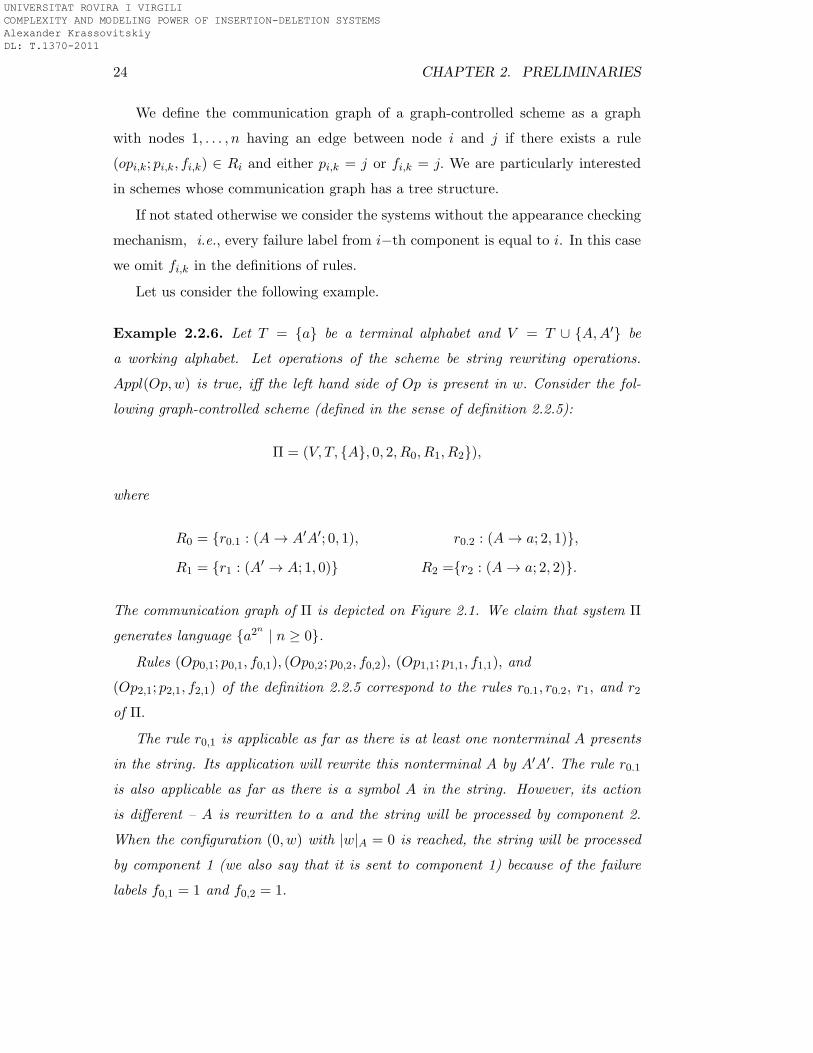
The communication graph of Π is depicted on Figure 2.1. We claim that system Π
generates language {a2n| n ≥ 0}.
Rules (Op0,1; p0,1, f0,1), (Op0,2; p0,2, f0,2), (Op1,1; p1,1, f1,1), and
(Op2,1; p2,1, f2,1) of the definition 2.2.5 correspond to the rules r0.1, r0.2, r1, and r2
of Π.
The rule r0,1 is applicable as far as there is at least one nonterminal A presents
in the string. Its application will rewrite this nonterminal A by A′A′. The rule r0.1
is also applicable as far as there is a symbol A in the string. However, its action
is different – A is rewritten to a and the string will be processed by component 2.
When the configuration (0, w) with |w|A = 0 is reached, the string will be processed
by component 1 (we also say that it is sent to component 1) because of the failure
labels f0,1 = 1 and f0,2 = 1.
UNIVERSITAT ROVIRA I VIRGILI COMPLEXITY AND MODELING POWER OF INSERTION-DELETION SYSTEMS Alexander Krassovitskiy DL: T.1370-2011
2.2. GRAPH-CONTROLLED SYSTEMS 25
Starting from axiom A in configuration (0, A) we can apply either rule r0.1 or
r0.2 and get either configuration (0, A′A′) or (2, a), correspondingly. In the latter
case we produce a ∈ T ∗ in the final component 2. Hence, a ∈ L(Π).
In configuration (0, A′A′) we can only apply rule r1 and get (1, AA′) or (1, A′A).
By applying r1 once more to AA′ (or A′A) we get the configuration (1, AA). Now by
failure label f1,1 = 0 the rule r1 sends the string AA to component 0. By applying
r0.1 we get (0, A′A′A) or (0, AA′A′) and by applying r0.2 we get (2, aA). In the latter
case we can apply one time rule r2 and get (2, aa). Hence aa ∈ L(Π.)
By applying r0.1 to (0, A′A′A) (or (0, AA′A′)) we get (0, A′A′A′A′) and A′A′A′A′
will be sent to component 1 by failure label p0,1 = 1 or p0,2 = 1. In case A′A′A is
replaced by A′A′a (by rule r0.2) such string is not terminal, and no rules can be
further applied. Hence this computation can be omitted from consideration. From
configuration (1, A′A′A′A′) in four steps we get (1, AAAA) and the result is sent
back to component 0.
In general from configuration (0, An) in n+1 steps we get configuration (1, A′2n),
and then in 2n+1 steps we get configuration (0, A2n). Hence, we double the number
of A per cycle that corresponds to rewriting productions A → A′A′ and A′ → A in
components 0 and 1. By induction on the number of cycles we get that in component
0 appear all the strings from {A2n−mA′2m | n ≥ 0, 0 ≤ m ≤ 2n}, and n is the number
of the cycles.
Production r0.2 terminates this cycle and only if the string does not contain
nonterminals A′ such a string produce terminal string in L(Π).
Hence, in component 2 will appear the following strings
{A2n−m−lA′2mal | n ≥ 0, 1 ≤ m+ l ≤ 2n, l ≥ 1}.
Considering all terminal strings in component 2, we get our language L(Π) =
{a2n| n ≥ 0}.
/.-,()*+
1/.-,()*+
0/.-,()*+
2
Figure 2.1: Graph structure for Example 2.2.6.
UNIVERSITAT ROVIRA I VIRGILI COMPLEXITY AND MODELING POWER OF INSERTION-DELETION SYSTEMS Alexander Krassovitskiy DL: T.1370-2011

UNIVERSITAT ROVIRA I VIRGILI COMPLEXITY AND MODELING POWER OF INSERTION-DELETION SYSTEMS Alexander Krassovitskiy DL: T.1370-2011
Chapter 3
Insertion systems
In this chapter we consider systems having only insertion rules. We use an inverse
morphism and a weak coding as specific squeezing mechanisms that filter only those
words of a language that have a “proper” structure. We consider both pure insertion
and graph-controlled insertion systems. One of the main results of this chapter states
the equivalence of generating power between context-free grammars and insertion
systems of size (3, 1, 1) (when obtained languages are encoded by the means of
morphisms). Moreover, in a similar way it is shown an equivalence for the class of
matrix grammars and graph-controlled insertion systems of size (3, 1, 1). Another
important theorem of the chapter proves the equality of graph-controlled insertion
systems having size (2, 2, 2) to the family of recursively enumerable languages.
3.1 Definitions
An insertion system is a construct I = (V,A,R), where V is an alphabet, A is a finite
language over V , and R is a finite sets of triples of the form (u, α, v), where u, α, and
v are strings over V, α 6= ε. The elements of V are working symbols, those of A are
axioms, the triples in R are insertion rules. An insertion rule (u, α, v) ∈ R indicates
that the string α can be inserted between u and v. Stated otherwise, (u, α, v) ∈ R
corresponds to the rewriting rule uv → uαv. We denote by ⇒ the relation defined
by an insertion rule. Formally, x ⇒ y iff x = x1uvx2, y = x1uαvx2, for some
(u, α, v) ∈ I and x1, x2 ∈ V ∗. We denote by =⇒∗ the reflexive and transitive closure
27
UNIVERSITAT ROVIRA I VIRGILI COMPLEXITY AND MODELING POWER OF INSERTION-DELETION SYSTEMS Alexander Krassovitskiy DL: T.1370-2011
28 CHAPTER 3. INSERTION SYSTEMS
of ⇒, and ⇒+ denote its transitive closure.
The language generated by I is defined by
L(I) = {w ∈ V ∗ | x⇒∗ w, x ∈ A}.
The complexity of an insertion system I = (V,A,R) is described by the vector
(n,m,m′) called size, where
n = max{|α| | (u, α, v) ∈ R},
m = max{|u| | (u, α, v) ∈ R},
m′ = max{|v| | (u, α, v) ∈ R}.
We also denote by INSm,m′
n corresponding families of insertion systems. More-
over, we define the total size of the system as the sum of all numbers above:
ψ = n+m+m′.
If some of the parameters n,m,m′ is not specified, then we write instead the sym-
bol ∗. In particular, INS0,0∗ denotes the family of languages generated by insertion
systems with rules having no contexts.
A graph-controlled insertion system is the graph-controlled scheme
Π = (V,A, i0, if , R1, . . . , Rn) (see definition 2.2.5), where for each rule (op, p, f)
from Ri, 1 ≤ i ≤ n the operation op is an insertion rule. By default, Appl(op, w) is
true iff the insertion rule op = (u, α, v) can be performed on w, i.e., w contains a
proper substring uv.
We remark that in the case of insertion systems there is no distinction between
terminal and nonterminal alphabets.
We denote by LSPk(insm,m′
n ) the family of languages generated by graph-
controlled insertion systems with k ≥ 1 components and insertion rules of size at
most (n,m,m′) and whose communication graph has a tree structure. The letter
t is inserted before P to denote classes whose communication graph is arbitrary,
e.g., LStPk(insm,m′
n ). LSPk(insm,m′
n )ac denotes the family of languages generated
by graph-controlled insertion systems having the size (n,m,m′), and having compu-
tation with appearance checking.
We remark that the definition of graph-controlled insertion systems almost co-
incides with the definition of insertion P systems [60]. In Chapter 5 we discuss the
UNIVERSITAT ROVIRA I VIRGILI COMPLEXITY AND MODELING POWER OF INSERTION-DELETION SYSTEMS Alexander Krassovitskiy DL: T.1370-2011
3.2. COMPUTATIONAL POWER OF PURE INSERTION SYSTEMS 29
difference between these two models. Traditionally, in the literature, the term of
insertion P systems is used for graph-controlled insertion systems, however, in what
follows, we will use the latter term, because of a much simpler definition.
Now we give some examples of insertion and graph-controlled insertion systems.
Example 3.1.1. Let I1 = ({a, b, c}, {abc}, I), where
I ={(a, a, ε), (b, b, ε), (c, c, ε)}.
Clearly, this system generates the regular language L(I1) = {a+b+c+}. Indeed, the
axiom abc ∈ L(I1) and the insertion rules can insert an arbitrary number of a, b and
c as long as there is a corresponding letter to the left.
It is possible to consider the above example as a graph-controlled insertion system
with three components with single rule per component, and where the next active
component is determined by a cyclic order. Then the non context-free language
L2 = {anbncn | n ≥ 1} is generated.
Example 3.1.2. Consider the following graph-controlled insertion system Π2 =
({a, b, c}, {abc}, 0, 0, R0, R1, R2), where
R0 ={r0 : (a, a, ε; 1)};
R1 ={r1 : (b, b, ε; 2)};
R2 ={r2 : (c, c, ε; 0)}.
Clearly, Π2 ∈ LStP3(ins1,01 ) and abc ∈ L(Π2). The insertions of a, b and c are
performed when the components 0,1 and 2 are active, correspondingly. This implies
that the number of a, b and c when component 0 is active is the same. Hence,
L(Π2) = {anbncn | n ≥ 1}.
3.2 Computational power of pure insertion systems
It is known that the classes of languages obtained by systems using only insertions,
are incomparable with many known language classes. As an example consider the
linear language {anban | n ≥ 1}. This language cannot be generated by any insertion
UNIVERSITAT ROVIRA I VIRGILI COMPLEXITY AND MODELING POWER OF INSERTION-DELETION SYSTEMS Alexander Krassovitskiy DL: T.1370-2011
30 CHAPTER 3. INSERTION SYSTEMS
system (see Theorem 6.6 in [62]). In order to overcome this “obstacle” we use
some codings to interpret the generated strings. More precisely, firstly an inverse
morphism and then a weak coding are applied to the generated string. Hence, we
consider the languages of the form: ϕ(h−1(L(Π))), where Π is an insertion system,
ϕ is a weak coding and h is a morphism.
We note that in the literature there were also considered another types of codings
when an intersection with a (regular) language is applied to the results of the inser-
tion system instead of the inverse morphism (see, for example, [56, 61]). We mention
that these types of codings are rather simple and can be simulated by a finite state
transducer. Using this method we show several characterizations of language classes
from the Chomsky hierarchy in terms of insertion systems.
We start with the following example where it is shown that a non-regular context-
free language can be generated by an insertion system of size (1, 1, 0) without any
coding.
Example 3.2.1. Consider a system I = (T, {a}, R), where T = {a, b, c, d} and R is
defined as follows: R = {(a, b, ε), (b, c, ε), (c, d, ε), (d, a, ε)}.
Let L be the language generated by I (L = L(I)). It is clear that L can defined
by the following formulas:
L = L1, L1 = aL∗2, L2 = bL∗
3, L3 = cL∗4, L4 = dL∗
1.
By substituting Li, for 2 ≤ i ≤ 4 into the description of Li−1 we obtain:
L1 = a(b(c(dL∗1)
∗)∗)∗.
Let R = {(abcd)∗(dcb)∗}. Consider the language L′′ = L ∩ R. Consider the
word w = abcddcb from R. This word is generated in L as follows (we underline the
inserted symbol):
a⇒ ab⇒ abb⇒ abcb⇒ abccb⇒ abcdcb⇒ abcddcb.
We observe that the generation of the second part of w, the subword dcb, is
related with the generation of its first part abcd, because every letter is inserted two
times: firstly for the second part and after that for the first part. It is also clear
UNIVERSITAT ROVIRA I VIRGILI COMPLEXITY AND MODELING POWER OF INSERTION-DELETION SYSTEMS Alexander Krassovitskiy DL: T.1370-2011
3.2. COMPUTATIONAL POWER OF PURE INSERTION SYSTEMS 31
that this is the only way to generate the subword dcb. Moreover, it can be easily
seen that such a generation leads to a one-to-one correspondence between abcd and
dcb. Now, taking w it is possible to insert a after the first letter d and to continue
in a similar manner as before and so on, which gives wn = (abcd)n(dcb)n, n ≥ 1.
It is also possible to obtain more copies of abcd by performing insertions of four
corresponding letters after d, c, b or a in the first part of wn. Hence, we finally
obtain L′′ = {(abcd)i(dcb)j | j ≤ i}, which is a non-regular context-free language
(by the inverse morphism {abcd → x, dcb → y} it becomes the well-known language
{xiyj | 1 ≤ j ≤ i}). Since the intersection of two regular languages would be regular,
we obtain that L is a non-regular context-free language.
Next theorem is from [62].
Theorem 3.2.2. INS1,1∗ ⊆ CF.
Proof. For an insertion system Π = (T,A, I) consider a context-free grammar G =
(N,T, S, P ) having nonterminal alphabet N = {Da,b | a, b ∈ T ∪ {ε}} and the set of
productions P = P1 ∪ P2 ∪ P3, where
P1 = {S → δ(ε, w, ε) | w ∈ A},
P2 = {Da,b → a | Da,b ∈ N, a, b ∈ T ∪ {ε}},
P3 = {Da1,a2 → δ(a1, w, a2) | (a1, w, a2) ∈ I,
for l = 1, 2 al = al, if al 6= ε and al ∈ T ∪ {ε}, if al = ε},
where for every a1, a2 ∈ T ∪ {ε}, w ∈ T ∗ we denote by δ(a1, w, a2) the following
function
δ(a1, w, a2) =
Da1,a2 , if w = ε
Da1,b1Db1,b2 . . . Dbk−1,bkDbk,a2 , if w = b1 . . . bk.
The rule (a1, b1 . . . bk, a2) ∈ I, a1, a2 ∈ T, b1 . . . bk ∈ T k can be simulated by the
grammar iff the corresponding sentential form contains Da1,a2 . It is clear that non-
terminals in D preserve one symbol left and right contexts. Hence, there is a follow-
ing derivation wDa1,a2w′ ⇒ wDa1,b1Db1,b2 . . . Dbk−1,bkDbk,a2w
′. Since index symbols
are duplicated in adjacent nonterminals we have one symbol context being preserved
UNIVERSITAT ROVIRA I VIRGILI COMPLEXITY AND MODELING POWER OF INSERTION-DELETION SYSTEMS Alexander Krassovitskiy DL: T.1370-2011
32 CHAPTER 3. INSERTION SYSTEMS
in the resulted string. The simulation of rules that have no contexts is performed
by productions from P3 with arbitrary contexts: al ∈ T ∪ {ε}, l = 1, 2.
The simulation starts by the production
S → Dε,b1Db1,b2 . . . Dbk−1,bkDbk,ε ∈ P1
corresponding to the choice of an axiom from A. The terminal string is obtained by
applying rules of P2 at the end of derivation. Hence, we have shown that each step
of derivation in Π can be reproduced by the context-free grammar G.
The other direction L(G) ⊆ L(Π) can be shown as follows. A derivation in G
starts from production from P1 S → δ(ε, w, ε), where δ(ε, w, ε) = Dε,b1Db1,b2 . . .
Dbk−1,bkDbk,ε, and w = b1b2 . . . bk ∈ A. This corresponds to choosing the axiom w
in a derivation of Π. Then either productions from P2 or P3 can be applied. Each
rule Da,b → a ∈ P2 rewrites Da,b by terminal a. In the corresponding derivation
of Π it means that no more insertions can be done between a and b using a as a
left context. (Clearly, for every derivation in G one may consider an equivalent
derivations in which the rules from P2 are applied an the end.)
Each rule Da1,a2 → δ(a1, w, a2) ∈ P3 corresponds to insertion of w between a1
and a2 in the derivation of Π. This captures also the case when the insertion rule
has empty left and/or right contexts.
Since there is a one to one correspondence between derivations in G and Π we
obtain L(Π) = L(G). Hence, INS1,1∗ ⊆ CF.
Next we give a characterization of context-free languages by means of insertion
systems of size (3, 1, 1).
Theorem 3.2.3. A language L is context-free if and only if it can be represented
in the form L = ϕ(h−1(L′)) where L′ ∈ INS1,13 , ϕ is a weak coding and h is a
morphism.
Proof. Taking into account Theorem 3.2.2 and the closure property of context-free
languages with respect to inverse morphisms and weak codings we get the “only if”
part of the statement.
UNIVERSITAT ROVIRA I VIRGILI COMPLEXITY AND MODELING POWER OF INSERTION-DELETION SYSTEMS Alexander Krassovitskiy DL: T.1370-2011
3.2. COMPUTATIONAL POWER OF PURE INSERTION SYSTEMS 33
In order to prove the “if” part of the theorem, it is enough to show that for any
context-free language L there is an insertion system Π of size (3, 1, 1), such that
L = ϕ(h−1(L(Π))), where h is a morphism, and ϕ is a weak coding.
Let G = (N,T, S, P ) be a context-free grammar in the Chomsky normal form
such that L = L(G). Consider the following insertion system Π = (V, {S$}, I), where
V = T ∪ N ∪ {#, $}, I = {(A,#γ, α) | α ∈ V \{#}, A → γ ∈ P, γ ∈ (T ∪ V )∗, 1 ≤
|γ| ≤ 2}. The morphism h and the weak coding ϕ are defined as follows
h(a) =
a#, if a ∈ V \(T ∪ {#}),
a, if a ∈ T ∪ {$},ϕ(a) =
a, if a ∈ T,
ε, if a ∈ V \T.
We claim that L(Π) = L(G). Indeed, each rule (A,#γ, α) ∈ R can be applied to
the sentential form wAαw′ if and only if α 6= #. Hence, a production A → γ ∈ P
can be simulated by the corresponding rule in Π. For the convenience we add a
special symbol $ as the right border.
When every nonterminal is marked and no rules can be applied the output word
can be subjected to the inverse morphism h−1. Indeed, if the system produces a
word having some unmarked nonterminal then h−1 is not defined. At this point h−1
removes all marking symbols, and ϕ removes all nonterminal symbols. This proves
the assertion of the theorem.
Since Parikh image of a context-free language is always semilinear, this implies
that insertion systems of size (n, 1, 1) can generate only languages whose Parikh
image is semilinear. If we drop the contexts then we have a strict inclusion:
Lemma 3.2.4. Ps(INS0,0∗ ) ⊂ SL.
Proof. Consider the following semilinear set
P = {(0, 0) +∑
k≥0
k(0, 1)} ∪ {(0, 0) +∑
k≥0
k(1, 0)}.
We claim that there is no insertion system whose Parikh set is equal to P. We shall
prove this statement by contradiction. Assume that there is an insertion system γ
such that Ps(L(γ)) = P. Let γ have the terminal alphabet {a, b}. Since the language
of axioms is finite the system contains some insertion rules of the form (ε, ak, ε), and
UNIVERSITAT ROVIRA I VIRGILI COMPLEXITY AND MODELING POWER OF INSERTION-DELETION SYSTEMS Alexander Krassovitskiy DL: T.1370-2011
34 CHAPTER 3. INSERTION SYSTEMS
(ε, bl, ε), k, l ≥ 1. Then by applying both rules in a derivation we thus obtain a word
with both letters a and b. This is a contradiction.
On the other hand every linear set can be generated by context-free insertion
systems.
Lemma 3.2.5. For every linear set S there is a language L ∈ INS0,0∗ such that
S = Ps(L).
3.3 Graph-controlled insertion systems
In the remaining of the chapter we consider graph-controlled insertion systems.
We show that these systems have more computational power than pure insertion
systems.
Theorem 3.3.1. LStP∗(ins1,1∗ ) ⊂MAT λ.
Proof. In order to prove the statement it is enough to show that for any graph-
controlled insertion system Π there is a matrix grammar G such that L(Π) = L(G).
We extend the construction of the context-free grammar used in Theorem 3.2.3 for
the case of matrix grammars.
Let Π = (V,A, i0, if , R1, . . . , Rn) be an arbitrary graph-controlled insertion sys-
tem. Consider the matrix grammar G = (N,V, S,M) having nonterminal alphabet
N = Q ∪D, where Q = {Qi | i = 1, . . . , n}, D = {Da,b | a, b ∈ V ∪ {ε}}, and the set
of matrices M =M1 ∪M2 ∪M3, where
M1 ={(S → Qi0δ(ε, w, ε)) | w ∈ A},
M2 ={(Da,b → a) | Da,b ∈ D, a, b ∈ T ∪ {ε}} ∪ {(Qif → ε)},
M3 ={(Qi → Qj , Da1,a2 → δ(a1, w, a2)) | (a1, w, a2; j) ∈ Ri,
for l = 1, 2 al =
al, if al ∈ V,
t, ∀t ∈ V ∪ {ε}, if al = ε},
where for every a1, a2 ∈ V ∪ {ε}, w ∈ V ∗ we denote by δ(a1, w, a2) the following
δ(a1, ε, a2) = Da1,a2 , δ(a1, b1 . . . bk, a2) = Da1,b1Db1,b2 . . . Dbk−1,bkDbk,a2 .
UNIVERSITAT ROVIRA I VIRGILI COMPLEXITY AND MODELING POWER OF INSERTION-DELETION SYSTEMS Alexander Krassovitskiy DL: T.1370-2011
3.3. GRAPH-CONTROLLED INSERTION SYSTEMS 35
The simulation of Π by the matrix grammar G is based on the encoding of
pairs of adjacent letters by nonterminals from D. So, the encoded pair can be used
as a context for an insertion rule. In addition, the label of the active component
is represented by a nonterminal in Q. A rule (a1, b1 . . . bk, a2; j) ∈ Ri, a1, a2 ∈
V ∪ {ε}, b1 . . . bk ∈ V k can be simulated by the grammar iff the sentential form
contains both Qi andDa1,a2 . As a result, the label representing the active component
is rewritten to Qj and Da1,a2 is rewritten to the string Da1,b1Db1,b2 . . . Dbk−1,bkDbk,a2 .
It is clear that the string preserves one symbol (left) context. In order to simulate
rules that have no contexts we introduce productions with an arbitrary contexts:
al ∈ V ∪ {ε}, l = 1, 2.
The simulation of Π by the grammar starts with a nondeterministic choice of an
axiom from A. Then, during the derivation each rule from R1, . . . , Rn having the
context (a1, a2) can be applied iff the productions having Da1,a2 in the left hand
side can be applied. Finally, the string over V can be produced by the grammar as
soon as Qif is deleted from the sentential form. The deletion of Qif specifies that
Π activates the final component. As there is one to one correspondence between
derivations in G and Π we obtain L(Π) = L(G). Hence, LStP∗(ins1,1∗ ) ⊆MAT λ.
The strictness of the inclusion follows from the fact there are languages from
MAT λ which cannot be generated by any insertion P system from LStPm(ins1,1n ),
for any n ≥ 1. Indeed, consider the context-free language La = {cakcakc | k ≥ 0}.
Since every context-free language is a matrix language [63] we have La ∈ MAT λ.
On the other hand, La /∈ LStPm(ins1,1n ), for any n ≥ 1. For the contrary, assume
there is such a system Π′. We note, that the system cannot delete or rewrite any
letter, so every insertion is terminal. As the languages of axioms are finite we need
an insertion rule of letter a. Consider the final insertion step in a derivation which
has at most one step and derives a word w = cakcakc, for some k ≥ n+ 1 :
w0 ⇒∗ w′ ⇒ w,
where w0 is an axiom. Since |w0|c ≤ 3, c may be inserted by the last inser-
tion. Assume, that |w′|c = 3. In the latter case, let ap be the inserted string,
p ≤ n. Because, we may insert ap in the distinct positions of w′ we get that either
cak−pcak+pc ∈ L(Π′) or cak+pcak−pc ∈ L(Π′). This is a contradiction.
UNIVERSITAT ROVIRA I VIRGILI COMPLEXITY AND MODELING POWER OF INSERTION-DELETION SYSTEMS Alexander Krassovitskiy DL: T.1370-2011
36 CHAPTER 3. INSERTION SYSTEMS
Now assume that c is inserted by the last insertion. We note that the insertion
of two c is not possible, since k ≥ n + 1. Consider three cases: (1) the last applied
rule inserts c in the middle, (2) at the end, or (3) at the beginning of w′.
(1) Let wc = ap′
cap′′
be the inserted string, where p′ + p′′ ≤ n − 1. Hence, w′ =
cak′+k′′c, where k′+p′ = k′′+p′′ = k, and k′+k′′ = 2k−p′−p′′ ≥ 2n+2−n+1 ≥ 4.
Obviously, regardless of the contexts of the last insertion rule there are at least two
positions at which wc can be inserted. So, we get a contradiction because either
cak′+p′+1cak
′′+p′′−1c ∈ L(Π′), or cak′+p′−1cak
′′+p′′+1c ∈ L(Π′).
(2) Let aqc be the inserted string, where q ≤ n−1. The corresponding insertion rule
has one of the following forms: (ε, aqc, ε; j) or (a, aqc; ε, j), where j is an index of the
final component. In ether case, aqc may be inserted in w′ before the last letter a.
This is a contradiction. The case (3) is a mirror to the case (2) and can be treated
similarly.
So we proved La /∈ LStPn(ins1,12 ), for any n ≥ 1 and, hence, LStP∗(ins
1,1∗ ) ⊂
MAT λ.
Since a tree is a special case of a graph we get the following result
Corollary 3.3.2. LSP∗(ins1,1∗ ) ⊂MAT λ.
Let us consider graph-controlled insertion systems with left and right contexts
of at most one symbol. This family can characterize the languages generated by
context-free matrix grammars, if a specific squeezing mechanism is used.
Theorem 3.3.3. A language L is in MAT λ if and only if it can be written in the
form L = ϕ(h−1(L′)), where L′ ∈ LSP∗(ins1,12 ), ϕ is a weak coding, h is a morphism.
Proof. Taking into account Theorem 3.3.1 and the fact that the class of languages
generated by context-free matrix grammars is closed under inverse morphisms and
weak codings we get a characterization of MAT λ if we show that for every L ∈
MAT λ there is a weak codings ϕ, a morphism h, and a system Π such that L(Π) ∈
LSP∗(ins1,12 ) and L = ϕ(h−1(L(Π))).
Let us consider a language L ∈ MAT λ. Let G = (N,T, S,M) be a matrix
grammar in the binary normal form such that L = L(G). We assume that matrices
UNIVERSITAT ROVIRA I VIRGILI COMPLEXITY AND MODELING POWER OF INSERTION-DELETION SYSTEMS Alexander Krassovitskiy DL: T.1370-2011
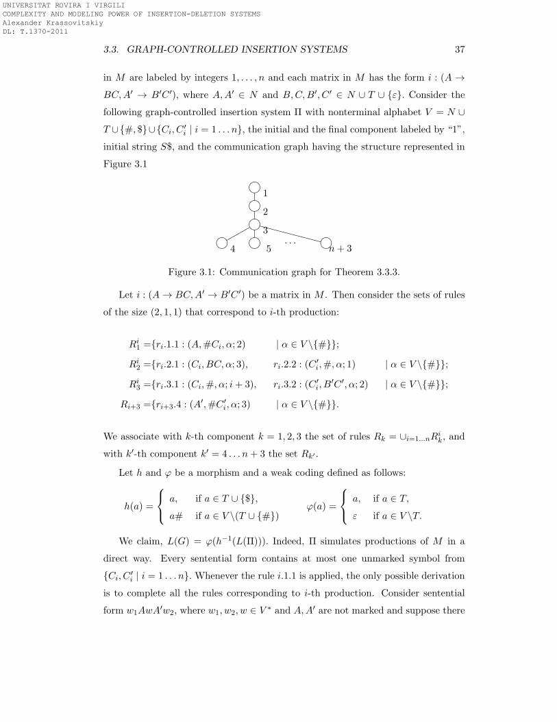
3.3. GRAPH-CONTROLLED INSERTION SYSTEMS 37
in M are labeled by integers 1, . . . , n and each matrix in M has the form i : (A →
BC,A′ → B′C ′), where A,A′ ∈ N and B,C,B′, C ′ ∈ N ∪ T ∪ {ε}. Consider the
following graph-controlled insertion system Π with nonterminal alphabet V = N ∪
T ∪{#, $}∪{Ci, C′i | i = 1 . . . n}, the initial and the final component labeled by “1”,
initial string S$, and the communication graph having the structure represented in
Figure 3.1
/.-,()*+
1/.-,()*+
2/.-,()*+
3qqqqqq
WWWWWWWWWWWWWW
/.-,()*+
4/.-,()*+
5· · · /.-,()*+
n+ 3
Figure 3.1: Communication graph for Theorem 3.3.3.
Let i : (A→ BC,A′ → B′C ′) be a matrix in M . Then consider the sets of rules
of the size (2, 1, 1) that correspond to i-th production:
Ri1 ={ri.1.1 : (A,#Ci, α; 2) | α ∈ V \{#}};
Ri2 ={ri.2.1 : (Ci, BC, α; 3), ri.2.2 : (C ′
i,#, α; 1) | α ∈ V \{#}};
Ri3 ={ri.3.1 : (Ci,#, α; i+ 3), ri.3.2 : (C ′
i, B′C ′, α; 2) | α ∈ V \{#}};
Ri+3 ={ri+3.4 : (A′,#C ′i, α; 3) | α ∈ V \{#}}.
We associate with k-th component k = 1, 2, 3 the set of rules Rk = ∪i=1...nRik, and
with k′-th component k′ = 4 . . . n+ 3 the set Rk′ .
Let h and ϕ be a morphism and a weak coding defined as follows:
h(a) =
a, if a ∈ T ∪ {$},
a# if a ∈ V \(T ∪ {#})ϕ(a) =
a, if a ∈ T,
ε if a ∈ V \T.
We claim, L(G) = ϕ(h−1(L(Π))). Indeed, Π simulates productions of M in a
direct way. Every sentential form contains at most one unmarked symbol from
{Ci, C′i | i = 1 . . . n}. Whenever the rule i.1.1 is applied, the only possible derivation
is to complete all the rules corresponding to i-th production. Consider sentential
form w1AwA′w2, where w1, w2, w ∈ V ∗ and A,A′ are not marked and suppose there
UNIVERSITAT ROVIRA I VIRGILI COMPLEXITY AND MODELING POWER OF INSERTION-DELETION SYSTEMS Alexander Krassovitskiy DL: T.1370-2011
38 CHAPTER 3. INSERTION SYSTEMS
is a matrix rule of the form (A→ BC,A′ → B′C ′).
(1, w1AwA′w2) Vri.1.1 (2, w1A#CiwA
′w2) Vri.2.1
(3, w1A#CiBCwA′w2) Vri.3.1 (4, w
′1A
′w2) Vrn+i.4 (3, w′1A
′#C ′iw2) Vri.3.2
(2, w′1A
′#C ′iB
′C ′w2) Vri.4.2 (1, w′1A
′#C ′i#B
′C ′w2),
where w′1 = w1A#Ci#BCw. Hence, the derivation marks nonterminals A,A′ and
inserts BC, B′C ′ to the right of A# and B#, correspondingly. We note, that we
add one symbol $ to the right end in order to permit the contextual insertion for
the rightmost nonterminal(s). At the end, by applying the inverse morphism and
the weak coding we remove every marked nonterminal. Hence, we have L(G) ⊆
ϕ(h−1(L(Π))).
The inverse inclusion is obvious, because every rule in Π has its counterpart
in G. Moreover the case when the derivation in Π is blocked corresponds to the
case in which the simulation of a matrix cannot be completed. Hence, we get the
L(G) = ϕ(h−1(L(Π))).
Since trees are the special case of graphs we obtain the same result for graph-
controlled systems with an arbitrary structure:
Corollary 3.3.4. A language L ∈ MAT λ if it can be written in the form L =
ϕ(h−1(L′)), where L′ ∈ LStP∗(ins1,12 ), ϕ is a weak coding, h is a morphism.
We mention that a similar result can be obtained with a smaller number of
components but increasing the length of inserted words.
Lemma 3.3.5. For any context-free matrix grammar G′ there is a graph-controlled
insertion system Π′ such that L(Π′) ∈ LSPn+1(ins1,13 ) and L(G′) = L(Π′), where n
is the number of matrices in G′.
Proof. In order to prove the lemma we use the same argument as in the previous
theorem. For a matrix i : (A → BC,A′ → B′C ′) ∈ M, i = 1, . . . , n we consider sets
of rules
R′i1 = {(A,#BC,α; i+ 1)},
R′i+1 = {(A′,#B′C ′, α; 1)}.
UNIVERSITAT ROVIRA I VIRGILI COMPLEXITY AND MODELING POWER OF INSERTION-DELETION SYSTEMS Alexander Krassovitskiy DL: T.1370-2011
3.3. GRAPH-CONTROLLED INSERTION SYSTEMS 39
for every α ∈ V \{#}.
Then, we replace components R1, . . . , Rn+3 from Theorem 3.3.3 by R′1, R
′2, . . . ,
R′n+1, where R
′1 = ∪i=1,...,nR
′i1 .
/.-,()*+
1qqqqqq
WWWWWWWWWWWWWW
/.-,()*+
2/.-,()*+
3· · · /.-,()*+
n+ 1
Figure 3.2: Communication graph for Lemma 3.3.5.
Taking into account that the class of matrix grammars with appearance checking
equals RE we get the following corollary.
Corollary 3.3.6. A language L is RE if and only if it can be written in the form
L = ϕ(h−1(L′)), where L′ ∈ LSP∗(ins1,12 )ac, ϕ is a weak coding, h is a morphism.
In order to prove the next theorem we use the “mark and migration” technique
for insertion systems(see, e.g., [35, 62]). According to this technique, symbols that
have been rewritten are marked (with the marking symbols # and # ). We say that
a letter a is marked in a sentential form waw′ if it is followed by #, i.e., |w′| > 0, and
# is the prefix of w′. For example, in order to simulate a context-free production
A → BC the string #BC is inserted adjacent right to A, assuming that A is not
yet marked. This can be done by the rule (A,#BC,α), α ∈ V \ {#}. As soon as the
derivation of the simulated sentential form is completed, every nonterminal A must
be marked and the pairs A# are subject to the inverse morphism.
In order to simulate a context sensitive production AB → AC we need to bring A
beside B, because they can be separated by a string that consists of marked symbols.
The migration of a symbol A over the marked context is performed stepwise by
means of insertion of new nonterminal FA to the right of the marked symbols. For
example, assume we have to migrate A over X# in the string AX#α. We introduce
the following insertion rules
(AX#, FA, α),
(A,#, X#FAα),
(A#X#FA,#A,α),
UNIVERSITAT ROVIRA I VIRGILI COMPLEXITY AND MODELING POWER OF INSERTION-DELETION SYSTEMS Alexander Krassovitskiy DL: T.1370-2011
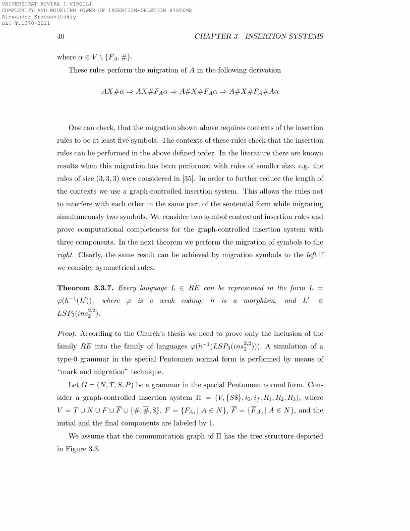
40 CHAPTER 3. INSERTION SYSTEMS
where α ∈ V \ {FA,#}.
These rules perform the migration of A in the following derivation
AX#α⇒ AX#FAα⇒ A#X#FAα⇒ A#X#FA#Aα
One can check, that the migration shown above requires contexts of the insertion
rules to be at least five symbols. The contexts of these rules check that the insertion
rules can be performed in the above defined order. In the literature there are known
results when this migration has been performed with rules of smaller size, e.g. the
rules of size (3, 3, 3) were considered in [35]. In order to further reduce the length of
the contexts we use a graph-controlled insertion system. This allows the rules not
to interfere with each other in the same part of the sentential form while migrating
simultaneously two symbols. We consider two symbol contextual insertion rules and
prove computational completeness for the graph-controlled insertion system with
three components. In the next theorem we perform the migration of symbols to the
right. Clearly, the same result can be achieved by migration symbols to the left if
we consider symmetrical rules.
Theorem 3.3.7. Every language L ∈ RE can be represented in the form L =
ϕ(h−1(L′)), where ϕ is a weak coding, h is a morphism, and L′ ∈
LSP3(ins2,22 ).
Proof. According to the Church’s thesis we need to prove only the inclusion of the
family RE into the family of languages ϕ(h−1(LSP3(ins2,22 ))). A simulation of a
type-0 grammar in the special Pentonnen normal form is performed by means of
“mark and migration” technique.
Let G = (N,T, S, P ) be a grammar in the special Pentonnen normal form. Con-
sider a graph-controlled insertion system Π = (V, {S$}, i0, if , R1, R2, R3), where
V = T ∪N ∪ F ∪ F ∪ {#,#, $}, F = {FA, | A ∈ N}, F = {FA, | A ∈ N}, and the
initial and the final components are labeled by 1.
We assume that the communication graph of Π has the tree structure depicted
in Figure 3.3.
UNIVERSITAT ROVIRA I VIRGILI COMPLEXITY AND MODELING POWER OF INSERTION-DELETION SYSTEMS Alexander Krassovitskiy DL: T.1370-2011
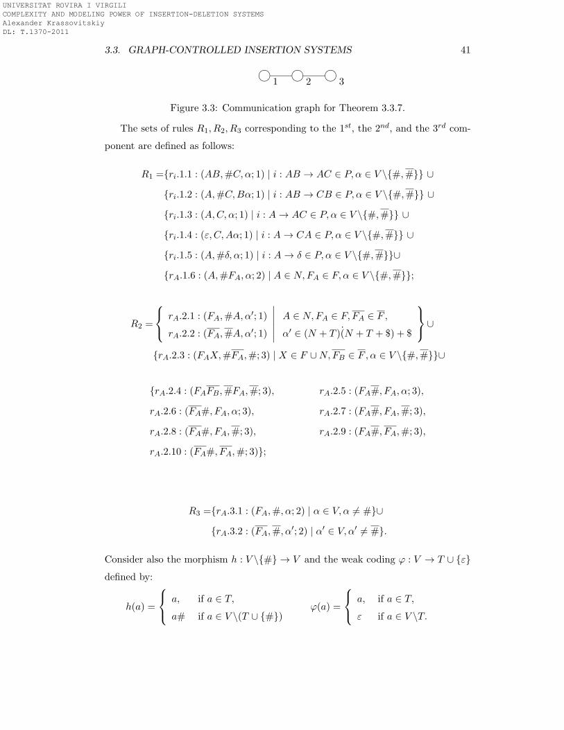
3.3. GRAPH-CONTROLLED INSERTION SYSTEMS 41
/.-,()*+
1/.-,()*+
2/.-,()*+
3
Figure 3.3: Communication graph for Theorem 3.3.7.
The sets of rules R1, R2, R3 corresponding to the 1st, the 2nd, and the 3rd com-
ponent are defined as follows:
R1 ={ri.1.1 : (AB,#C,α; 1) | i : AB → AC ∈ P, α ∈ V \{#,#}} ∪
{ri.1.2 : (A,#C,Bα; 1) | i : AB → CB ∈ P, α ∈ V \{#,#}} ∪
{ri.1.3 : (A,C, α; 1) | i : A→ AC ∈ P, α ∈ V \{#,#}} ∪
{ri.1.4 : (ε, C,Aα; 1) | i : A→ CA ∈ P, α ∈ V \{#,#}} ∪
{ri.1.5 : (A,#δ, α; 1) | i : A→ δ ∈ P, α ∈ V \{#,#}}∪
{rA.1.6 : (A,#FA, α; 2) | A ∈ N,FA ∈ F, α ∈ V \{#,#}};
R2 =
rA.2.1 : (FA,#A,α′; 1)
rA.2.2 : (FA,#A,α′; 1)
∣
∣
∣
∣
∣
∣
A ∈ N,FA ∈ F, FA ∈ F ,
α′ ∈ (N + T )(N + T + $) + $
∪
{rA.2.3 : (FAX,#FA,#; 3) | X ∈ F ∪N,FB ∈ F , α ∈ V \{#,#}}∪
{rA.2.4 : (FAFB,#FA,#; 3), rA.2.5 : (FA#, FA, α; 3),
rA.2.6 : (FA#, FA, α; 3), rA.2.7 : (FA#, FA,#; 3),
rA.2.8 : (FA#, FA,#; 3), rA.2.9 : (FA#, FA,#; 3),
rA.2.10 : (FA#, FA,#; 3)};
R3 ={rA.3.1 : (FA,#, α; 2) | α ∈ V, α 6= #}∪
{rA.3.2 : (FA,#, α′; 2) | α′ ∈ V, α′ 6= #}.
Consider also the morphism h : V \{#} → V and the weak coding ϕ : V → T ∪ {ε}
defined by:
h(a) =
a, if a ∈ T,
a# if a ∈ V \(T ∪ {#})ϕ(a) =
a, if a ∈ T,
ε if a ∈ V \T.
UNIVERSITAT ROVIRA I VIRGILI COMPLEXITY AND MODELING POWER OF INSERTION-DELETION SYSTEMS Alexander Krassovitskiy DL: T.1370-2011
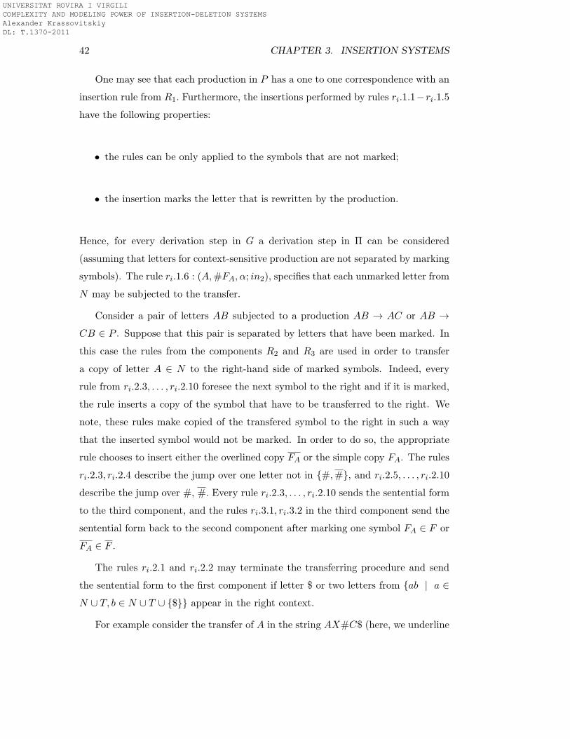
42 CHAPTER 3. INSERTION SYSTEMS
One may see that each production in P has a one to one correspondence with an
insertion rule from R1. Furthermore, the insertions performed by rules ri.1.1−ri.1.5
have the following properties:
• the rules can be only applied to the symbols that are not marked;
• the insertion marks the letter that is rewritten by the production.
Hence, for every derivation step in G a derivation step in Π can be considered
(assuming that letters for context-sensitive production are not separated by marking
symbols). The rule ri.1.6 : (A,#FA, α; in2), specifies that each unmarked letter from
N may be subjected to the transfer.
Consider a pair of letters AB subjected to a production AB → AC or AB →
CB ∈ P . Suppose that this pair is separated by letters that have been marked. In
this case the rules from the components R2 and R3 are used in order to transfer
a copy of letter A ∈ N to the right-hand side of marked symbols. Indeed, every
rule from ri.2.3, . . . , ri.2.10 foresee the next symbol to the right and if it is marked,
the rule inserts a copy of the symbol that have to be transferred to the right. We
note, these rules make copied of the transfered symbol to the right in such a way
that the inserted symbol would not be marked. In order to do so, the appropriate
rule chooses to insert either the overlined copy FA or the simple copy FA. The rules
ri.2.3, ri.2.4 describe the jump over one letter not in {#,#}, and ri.2.5, . . . , ri.2.10
describe the jump over #, #. Every rule ri.2.3, . . . , ri.2.10 sends the sentential form
to the third component, and the rules ri.3.1, ri.3.2 in the third component send the
sentential form back to the second component after marking one symbol FA ∈ F or
FA ∈ F .
The rules ri.2.1 and ri.2.2 may terminate the transferring procedure and send
the sentential form to the first component if letter $ or two letters from {ab | a ∈
N ∪ T, b ∈ N ∪ T ∪ {$}} appear in the right context.
For example consider the transfer of A in the string AX#C$ (here, we underline
UNIVERSITAT ROVIRA I VIRGILI COMPLEXITY AND MODELING POWER OF INSERTION-DELETION SYSTEMS Alexander Krassovitskiy DL: T.1370-2011
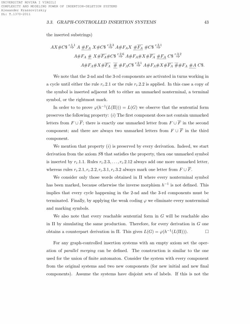
3.3. GRAPH-CONTROLLED INSERTION SYSTEMS 43
the inserted substrings)
AX#C$r.1.1⇒ A #FA X#C$
r.2.3⇒ A#FAX #FA #C$
r.3.1⇒
A#FA # X#FA#C$r.2.6⇒ A#FA#X#FA #FA C$
r.3.2⇒
A#FA#X#FA # #FAC$r.2.1⇒ A#FA#X#FA ##FA #A C$.
We note that the 2-nd and the 3-rd components are activated in turns working in
a cycle until either the rule ri.2.1 or the rule ri.2.2 is applied. In this case a copy of
the symbol is inserted adjacent left to either an unmarked nonterminal, a terminal
symbol, or the rightmost mark.
In order to to prove ϕ(h−1(L(Π))) = L(G) we observe that the sentential form
preserves the following property: (i) The first component does not contain unmarked
letters from F ∪ F ; there is exactly one unmarked letter from F ∪ F in the second
component; and there are always two unmarked letters from F ∪ F in the third
component.
We mention that property (i) is preserved by every derivation. Indeed, we start
derivation from the axiom S$ that satisfies the property, then one unmarked symbol
is inserted by ri.1.1. Rules ri.2.3, . . . , ri.2.12 always add one more unmarked letter,
whereas rules ri.2.1, ri.2.2, ri.3.1, ri.3.2 always mark one letter from F ∪ F .
We consider only those words obtained in Π where every nonterminal symbol
has been marked, because otherwise the inverse morphism h−1 is not defined. This
implies that every cycle happening in the 2-nd and the 3-rd components must be
terminated. Finally, by applying the weak coding ϕ we eliminate every nonterminal
and marking symbols.
We also note that every reachable sentential form in G will be reachable also
in Π by simulating the same production. Therefore, for every derivation in G one
obtains a counterpart derivation in Π. This gives L(G) = ϕ(h−1(L(Π))).
For any graph-controlled insertion systems with an empty axiom set the oper-
ation of parallel merging can be defined. The construction is similar to the one
used for the union of finite automaton. Consider the system with every component
from the original systems and two new components (for new initial and new final
components). Assume the systems have disjoint sets of labels. If this is not the
UNIVERSITAT ROVIRA I VIRGILI COMPLEXITY AND MODELING POWER OF INSERTION-DELETION SYSTEMS Alexander Krassovitskiy DL: T.1370-2011
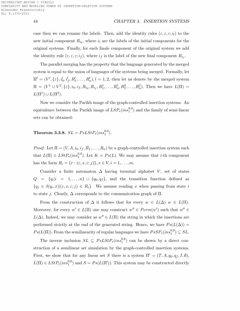
44 CHAPTER 3. INSERTION SYSTEMS
case then we can rename the labels. Then, add the identity rules (ε, ε, ε; il) to the
new initial component Ri0 , where il are the labels of the initial components for the
original systems. Finally, for each finale component of the original system we add
the identity rule (ε, ε, ε; if ), where if is the label of the new final component Rif .
The parallel merging has the property that the language generated by the merged
system is equal to the union of languages of the systems being merged. Formally, let
Πl = (V l, {ε}, il0, ilf , R
l1, . . . , R
ln), l = 1, 2, then let us denote by the merged system
Π = (V 1 ∪ V 2, {ε}, i0, if , Ri0 , Rif , R11, . . . , R
1n, R
21, . . . , R
2n). Then we have L(Π) =
L(Π1) ∪ L(Π2).
Now we consider the Parikh image of the graph-controlled insertion systems. An
equivalence between the Parikh image of LSP∗(ins0,01 ) and the family of semi-linear
sets can be obtained:
Theorem 3.3.8. SL = PsLStP∗(ins0,01 ).
Proof. Let Π = (V,A, i0, if , R1, . . . , Rn) be a graph-controlled insertion system such
that L(Π) ∈ LStP∗(ins0,01 ). Let K = Ps(L). We may assume that i-th component
has the form Ri = {r : (ε, x, ε; j)}, x ∈ V, i = 1, . . . ,m.
Consider a finite automaton ∆ having terminal alphabet V , set of states
Q = {qi|i = 1, . . . , n} ∪ {q0, qf}, and the transition function defined as
{qj ∈ δ(qi, x)|(ε, x, ε; j) ∈ Ri}. We assume reading x when passing from state i
to state j. Clearly, ∆ corresponds to the communication graph of Π.
From the construction of ∆ it follows that for every w ∈ L(∆) w ∈ L(Π).
Moreover, for every w′ ∈ L(Π) one may construct w′′ ∈ Perm(w′) such that w′′ ∈
L(∆). Indeed, we may consider as w′′ ∈ L(Π) the string in which the insertions are
performed strictly at the end of the generated string. Hence, we have Ps(L(∆)) =
Ps(L(Π)). From the semilinearity of regular languages we have PsSP∗(ins0,01 ) ⊆ SL.
The inverse inclusion SL ⊆ PsLStP∗(ins0,01 ) can be shown by a direct con-
struction of a semilinear set simulation by the graph-controlled insertion systems.
First, we show that for any linear set S there is a system Π′ = (T,A, q0, qf , I, ∅),
L(Π) ∈ LStP∗(ins0,01 ) and S = Ps(L(Π′)). This system may be constructed directly
UNIVERSITAT ROVIRA I VIRGILI COMPLEXITY AND MODELING POWER OF INSERTION-DELETION SYSTEMS Alexander Krassovitskiy DL: T.1370-2011
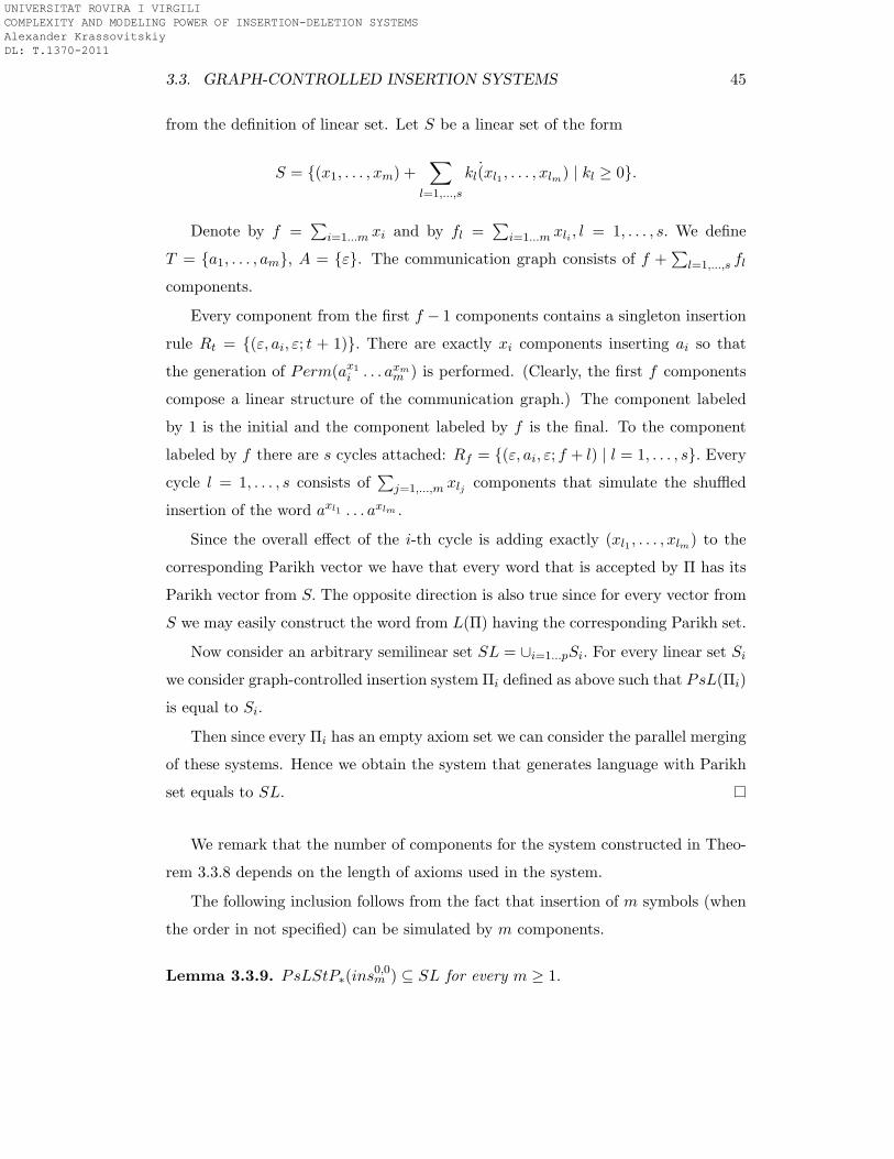
3.3. GRAPH-CONTROLLED INSERTION SYSTEMS 45
from the definition of linear set. Let S be a linear set of the form
S = {(x1, . . . , xm) +∑
l=1,...,s
kl(xl1 , . . . , xlm) | kl ≥ 0}.
Denote by f =∑
i=1...m xi and by fl =∑
i=1...m xli , l = 1, . . . , s. We define
T = {a1, . . . , am}, A = {ε}. The communication graph consists of f +∑
l=1,...,s fl
components.
Every component from the first f − 1 components contains a singleton insertion
rule Rt = {(ε, ai, ε; t + 1)}. There are exactly xi components inserting ai so that
the generation of Perm(ax1
i . . . axmm ) is performed. (Clearly, the first f components
compose a linear structure of the communication graph.) The component labeled
by 1 is the initial and the component labeled by f is the final. To the component
labeled by f there are s cycles attached: Rf = {(ε, ai, ε; f + l) | l = 1, . . . , s}. Every
cycle l = 1, . . . , s consists of∑
j=1,...,m xlj components that simulate the shuffled
insertion of the word axl1 . . . axlm .
Since the overall effect of the i-th cycle is adding exactly (xl1 , . . . , xlm) to the
corresponding Parikh vector we have that every word that is accepted by Π has its
Parikh vector from S. The opposite direction is also true since for every vector from
S we may easily construct the word from L(Π) having the corresponding Parikh set.
Now consider an arbitrary semilinear set SL = ∪i=1...pSi. For every linear set Si
we consider graph-controlled insertion system Πi defined as above such that PsL(Πi)
is equal to Si.
Then since every Πi has an empty axiom set we can consider the parallel merging
of these systems. Hence we obtain the system that generates language with Parikh
set equals to SL.
We remark that the number of components for the system constructed in Theo-
rem 3.3.8 depends on the length of axioms used in the system.
The following inclusion follows from the fact that insertion of m symbols (when
the order in not specified) can be simulated by m components.
Lemma 3.3.9. PsLStP∗(ins0,0m ) ⊆ SL for every m ≥ 1.
UNIVERSITAT ROVIRA I VIRGILI COMPLEXITY AND MODELING POWER OF INSERTION-DELETION SYSTEMS Alexander Krassovitskiy DL: T.1370-2011
46 CHAPTER 3. INSERTION SYSTEMS
Proof. Let Π = (V,A, i0, if , R1, . . . , Rn) be a graph-controlled insertion system such
that L(Π) ∈ LStP∗(ins0,0m ), let K = Ps(L). We may assume that the i-th com-
ponent has the form Ri = {r : (ε, x, ε; j)}, |x| ≤ n, i = 1, . . . ,m. Consider a fi-
nite automaton ∆ having terminal alphabet B = Lab(∪i=1,...,nRi), set of states
Q = {qi|i = 1, . . . , n} ∪ {q0, qf}, and the transition function defined as {qj ∈
δ(qi, r)|r : (ε, x, ε; j) ∈ Ri}. We assume reading the label of insertion rule r when
passing from state i to state j. One may observe that ∆ corresponds to the communi-
cation graph of Π. Consider also a morphism h : B → V ∗, defined as follows h(r) = x,
for every r : (ε, x, ε; j) ∈ Ri. From the construction of ∆ for every w ∈ L(∆) it follows
that h(w) ∈ L(Π). Indeed, performing the insertions w at the rightmost positions we
obtain h(w). Moreover, for every w′ ∈ L(Π) one may construct w′′ ∈ Perm(w′) such
that h−1(w′′) ∈ L(∆). Indeed, we just need to rearrange letters in w′ according to
the insertion rules. Hence, we have Ps(h(L(∆))) = Ps(L(Π)). Since every regular
language is semilinear, and the image of a regular language under a morphism is
also regular we have PsSP∗(ins0,0n ) ⊆ SL.
We conclude the Chapter with following remark:
Remark 3.3.10. We remark, that if we consider only Parikh image of the context-
free insertion languages then the context-free insertion of k symbols can be simulated
by k one-symbol context-free insertions. For example, the rule
r : (ε, a1a2 . . . ak, ε; j) ∈ Ri, i, j ≥ 0 can be simulated as follows:
r1 : (ε, a1, ε; i1) ∈ Ri,
r2 : (ε, a2, ε; i2) ∈ Ri1 , . . . ,
rk : (ε, ak, ε; j) ∈ Rik−1,
where i1, . . . , ik−1 are the indexes of new components. Hence, we get
PsSP∗(ins0,0n ) ⊆ PsSP∗(ins
0,01 ).
UNIVERSITAT ROVIRA I VIRGILI COMPLEXITY AND MODELING POWER OF INSERTION-DELETION SYSTEMS Alexander Krassovitskiy DL: T.1370-2011
Chapter 4
Insertion-deletion systems
In this chapter we consider systems where both operations of contextual string inser-
tion and of contextual string deletion are used (insertion-deletion, for short). Hence,
in addition to the set of insertion rules the set of deletion rules is considered as a part
of the system. Here, we systematically investigate the classes of insertion-deletion
systems with respect to the size of contexts and inserted/deleted strings. We show
several computationally completeness results as well as several classes that are not
computationally complete. In most of the cases we compare the classes of languages
generated by insertion-deletion systems with the classes of the Chomsky hierarchy.
In this chapter we also present the method of direct simulation used in all our
proofs. We show that the computational completeness of many insertion-deletion
systems can be reduced to the problem of modeling of the rules of another complete
insertion-deletion system in the terms of the desired one. The list of results shown
in this chapter is summarized in Tables 4.1 and 4.2.
4.1 Definitions
An insertion-deletion system is a construct ID = (V, T,A, I,D), where V is a (work-
ing) alphabet, T ⊆ V is a terminal alphabet, A is a finite language over V , and I,D
are finite sets of triples of the form (u, α, v), α 6= ε, where u and v are strings over
V .
The elements of T are called terminal symbols. The symbols from V − T are
47
UNIVERSITAT ROVIRA I VIRGILI COMPLEXITY AND MODELING POWER OF INSERTION-DELETION SYSTEMS Alexander Krassovitskiy DL: T.1370-2011
48 CHAPTER 4. INSERTION-DELETION SYSTEMS
called nonterminals. Strings in A ⊂ V ∗ are called axioms, the triples in I are
insertion rules as for insertion systems, and those from D are deletion rules. An
insertion rule (u, α, v) ∈ I indicates that the string α can be inserted between u
and v, while a deletion rule (u, α, v) ∈ D indicates that α can be removed from
the context (u, v). Both types of rules correspond to rewriting rules: uv → uαv for
the insertion rule (u, α, v) ∈ I, and uαv → uv for the deletion rule (u, α, v) ∈ D.
We denote by ⇒ins the relation defined by an insertion rule (formally, x ⇒ins y iff
x = x1uvx2, y = x1uαvx2, for some (u, α, v) ∈ I and x1, x2 ∈ V ∗) and by ⇒del the
relation defined by a deletion rule (formally, x ⇒del y iff x = x1uαvx2, y = x1uvx2,
for some (u, α, v) ∈ D and x1, x2 ∈ V ∗). We refer by ⇒ to any of the relations
⇒ins,⇒del, and denote by ⇒∗ the reflexive and transitive closure of ⇒ (as usual,
⇒+ is its transitive closure).
The language generated by ID is defined by
L(ID) = {w ∈ T ∗ | x⇒∗ w, x ∈ A}.
The complexity of an insertion-deletion system ID = (V, T,A, I,D) is described
by the vector (n,m,m′; p, q, q′) called size, where
n = max{|α| | (u, α, v) ∈ I}, p = max{|α| | (u, α, v) ∈ D},
m = max{|u| | (u, α, v) ∈ I}, q = max{|u| | (u, α, v) ∈ D},
m′ = max{|v| | (u, α, v) ∈ I}, q′ = max{|v| | (u, α, v) ∈ D}.
We also denote by INSm,m′
n DELq,q′
p corresponding families of insertion-deletion
systems. Moreover, we define the total size of the system as the sum of all numbers
above: ψ = n+m+m′ + p+ q + q′.
If some of the parameters n,m,m′, p, q, q′ are not specified, then we write instead
the symbol ∗. If one of the numbers from the couples m, m′ and/or q, q′ is equal
to zero (while the other is not), then we say that corresponding families have a
one-sided context. If all numbers m, m′, q, and q′ are equal to zero, then we call
corresponding language families context-free.
Example 4.1.1. Consider the system ID ∈ INS2,22 DEL2,2
1 defined as follows
UNIVERSITAT ROVIRA I VIRGILI COMPLEXITY AND MODELING POWER OF INSERTION-DELETION SYSTEMS Alexander Krassovitskiy DL: T.1370-2011
4.1. DEFINITIONS 49
ID = ({X,Y, Z, a, b}, {a, b}, {aZa}, I,D), where
I = {1 : (a, aX,Za), 2 : (XZ, Y a, a), 3 : (a, b, Za)};
D = {4 : (ε,X,ZY ), 5 : (aZ, Y, ε), 6 : (b, Z, a)}.
The system ID generates the language L = {anban | n ≥ 0}. Indeed, the system
generates aba as folllows aZa⇒ins abZa⇒del aba. This derivation rewrites Z by b.
The simulation of an insertion of a to the right and to the left of Z can be done by
the following derivation:
aZa ⇒ins aaXZa ⇒ins aaXZY aa ⇒del aaZY aa ⇒del aaZaa.
By repeating the steps above all words of the form akZak, k > 1 can be obtained.
At the end, aZa is rewritten to aba giving akbak ∈ L(ID), k ≥ 1. Moreover, start-
ing from the axiom aZa the only possible sequence of rules that can be applied is
(1, 2, 4, 5)∗(3, 6) (as the contexts of rules make their application almost determinis-
tic) which means that no other words different from those of L can be generated.
We note that the language from Example 4.1.1 cannot be generated by insertion
systems of any size [62].
The same language can be generated by another system.
Example 4.1.2. Consider a system ID1 ∈ INS1,14 DEL0,1
1 ,
ID = ({X,Y, a, b}, {a, b}, {XY }, I,D), where
I ={(X, aXY a, Y ), (X, b, Y )};
D ={(ε,X, a), (ε,X, b), (ε, Y, ε)}.
The system generates aba as follows XY ⇒ins XaXY aY ⇒ins XaXbY aY ⇒4del
aba. This derivation rewrites axiom XY by aba. Similarly, by inserting k-times
aXY b we get the sentential form (Xa)kXY (aY )k. In order to remove all non-
terminals X and Y , symbol b must be inserted in the middle. Hence, we obtain
L(ID) = {akbak | k ≥ 0}.
UNIVERSITAT ROVIRA I VIRGILI COMPLEXITY AND MODELING POWER OF INSERTION-DELETION SYSTEMS Alexander Krassovitskiy DL: T.1370-2011
50 CHAPTER 4. INSERTION-DELETION SYSTEMS
4.2 Normal form for insertion-deletion systems
We present below a normal form for insertion-deletion systems.
Lemma 4.2.1. For any insertion-deletion system ID = (V, T,A, I,D) having the
size (n,m,m′; p, q, q′) it is possible to construct an insertion-deletion system ID2 =
(V ∪ {X,Y }, T, A2, I2, D2 ∪ D′2) having the same size such that L(ID2) = L(ID).
Moreover, all rules from I2 have the form (u, α, v), where |α| = n, |u| = m, |v| = m′,
all rules from D2 have the form (u′, α, v′), where |α| = p, |u′| = q, |v′| = q′ and
D′2 = {(ε,X, ε), (ε, Y, ε)}.
Proof. Consider
A2 ={XiwY tY j | w ∈ A, i = max(m, q), j = max(m′, q′), t = max(p− |w|, 0)},
I2 ={(z1, xYk, z2) | (a, x, b) ∈ I, z1 ∈ {a t⊥ X∗}, z2 ∈ {b t⊥ Y ∗}
and |xY k| = n, k ≥ 0, |z1| = m, |z2| = m′}∪
∪ {(z1, Yn, z2) | z1, z2 ∈ (V ∪ {X,Y })∗, |z1| = m, |z2| = m′},
D2 ={(z1, d, z2) | (a, x, b) ∈ D, z1 ∈ {a t⊥ X∗}, z2 ∈ {b t⊥ Y ∗}, d ∈ {x t⊥ Y ∗}
and |d| = p, |z1| = q, |z2| = q′}.
In fact, any rule having a left (resp. right) context of a smaller size is replaced
by a group of rules, where the left (resp. right) context is a string over V ∪ {X}
(resp. V ∪ {Y }) of needed size. The same holds for the inserted or deleted symbol.
Any axiom w ∈ A is surrounded by X and Y (XiwY tY j) in A2. It is clear that if
w ∈ L(ID) then the word Xiw′Y j , w′ ∈ {w t⊥ Y ∗} will be obtained in ID2 using
corresponding rules and starting from the corresponding axiom. Now symbols X
and Y can be erased by rules from D′2 which implies that w ∈ L(ID2). It is clear
that if rules fromD′2 are used before this step, then at most same w may be obtained.
Hence L(ID) = L(ID2).
Next lemma shows that the deletion of terminal symbols may be excluded.
UNIVERSITAT ROVIRA I VIRGILI COMPLEXITY AND MODELING POWER OF INSERTION-DELETION SYSTEMS Alexander Krassovitskiy DL: T.1370-2011
4.3. BASIC METHODS FOR COMPUTATIONAL COMPLETENESS 51
Lemma 4.2.2. For any insertion-deletion system ID = (V, T,A, I,D) there is a
system ID′ = (V ∪ V ′, T, A ∪ A′, I ∪ I ′, D′) such that L(ID′) = L(ID). Moreover,
for any rule (a, b, c) ∈ D′ it holds that b does not contain letters from T .
Proof. Indeed, we can transform system ID to an equivalent system ID′ as follows.
Let V ′ = {Nt | t ∈ T}. Consider the coding function f : V → V ∪ V ′ defined by
f(x) = Nx if x ∈ T and f(x) = x otherwise. Consider also the following extension
to words (where id is the identity function):
F (a1 . . . an) = {g(a1) . . . g(an) | g ∈ {f, id}}
Now for any rule (a, b, c) in D (resp. in I) we introduce rules (a′, b′, c′) in D′
(resp. I ′), where a′ ∈ F (a), b′ ∈ F (b) and c′ ∈ F (c). For any axiom w ∈ V ∗ we add
F (w) to the axioms. Finally, we remove all rules (a, b, c) ∈ D′ having |b|T 6= 0.
This construction insures that the nonterminal symbolNt acts like an alias for the
symbol t ∈ T , i.e. for any derivation producing w1tw2 there is another derivation
producing w1Ntw2. Hence there is no difference between erasing t or Nt. This proves
the statement of the lemma.
Lemma 4.2.3. For any insertion-deletion system ID = (V, T,A, I,D) having the
size (n,m,m′; p, q, q′) it is possible to construct an insertion-deletion system ID2 =
(V2 ∪ {X,Y }, T, A2, I2, D2 ∪ D′2) having the same size such that L(ID2) = L(ID).
All rules from I2 have the form (u, α, v), where |α| = n, |u| = m, |v| = m′, all rules
from D2 have the form (u′, α′, v′), where |α′| = p, |α′|T = 0, |u′| = q, |v′| = q′ and
D′2 = {(ε,X, ε), (ε, Y, ε)}.
Proof. The assertion of the lemma follows from Lemmas 4.2.1 and 4.2.2.
Definition 4.2.4. We say that an insertion-deletion system ID = (V, T,A, I,D) is
in a normal form, if it has the properties of the system ID2 from Lemma 4.2.3.
4.3 Basic methods for computational completeness
Insertion-deletion systems represent a powerful model of computation. If the size of
the system is not bounded, then an arbitrary grammar can be simulated [36].
UNIVERSITAT ROVIRA I VIRGILI COMPLEXITY AND MODELING POWER OF INSERTION-DELETION SYSTEMS Alexander Krassovitskiy DL: T.1370-2011
52 CHAPTER 4. INSERTION-DELETION SYSTEMS
Theorem 4.3.1. For any type-0 grammar G = (N,T, S, P ) there is an insertion-
deletion system ID = (V, T,A, I,D) such that L(G) = L(ID).
Proof. Let V = N ∪ {#i : 1≤ i≤Card(P )} ∪ {$}. Let k1 = max{|u|, u → v ∈ P}
and k2 = max{|v|, u → v ∈ P}. Consider k = max(k1, k2). The set A is defined
as A = {$kS$k}. For any rule i : u → v ∈ P we add insertion rules (xu,#iv, y),
x, y ∈ (N ∪{$})∗, |xu| = k, |y| = k, to I and a deletion rule (x, u#i, v), x ∈ N ∪{$}
to D. Finally, a rule (ε, $, ε) is added to D.
It is not difficult to see that such system simulates G. Indeed, for any derivation
w1uw2 ⇒ w1vw2 in G there is a two-step derivation $kw1uw2$k ⇒ $kw1u#ivw2$
k ⇒
$kw1vw2$k in ID that simulates the corresponding production of G. If w ∈ L(G)
then the string $kw$k will be obtained in ID. Additional symbols $ can be deleted
at this moment. So w ∈ L(ID).
For the converse inclusion it is enough to observe that if an insertion rule
(xu,#iv, y) is used, then no more insertions inside the corresponding site xu can be
done. Hence the only way to eliminate the symbol #i is to perform the correspond-
ing deletion. Hence the computation in ID can be rearranged in such a way that an
insertion is followed by the corresponding deletion. This corresponds to a derivation
step in G, which completes the proof.
As one can see from the previous theorem, the basic idea of grammar simula-
tion by insertion-deletion systems is a construction of a set of related insertion and
deletion rules that shall be used in some specified sequence, thus performing a gram-
mar rule simulation. Usually, insertion rules introduce new nonterminal symbols in
the string which can be deleted only by the corresponding deletion rules (like the
symbols #i in theorem above). If the correct sequence is not performed, then some
nonterminal symbols that cannot be deleted will remain in the string. In the sub-
sequent sections different variants of this method are shown, thereby decreasing the
size of the insertion and deletion rules.
A simulation of type-0 grammars by insertion-deletion systems is the main
method to prove the computational completeness of insertion-deletion systems.
However, when several such results are established, it is much easier to prove the
computational completeness by simulating other insertion-deletion systems. We call
UNIVERSITAT ROVIRA I VIRGILI COMPLEXITY AND MODELING POWER OF INSERTION-DELETION SYSTEMS Alexander Krassovitskiy DL: T.1370-2011
4.3. BASIC METHODS FOR COMPUTATIONAL COMPLETENESS 53
such simulation a direct simulation. The following theorem shows how a computa-
tionally complete insertion-deletion system can be simulated by another one. This
result was firstly presented in [62], where a grammar in the Geffert normal form was
simulated. Due to some errors in the proof given in the monograph we show the
complete proof of the result.
The theorem uses the following method of simulation: the working (insertion or
deletion) site is delimited by special symbols in order to avoid interactions between
several such sites. Inside the site the sequence of insertions and deletions permits to
simulate exactly one application of the corresponding rule. All additional symbols
are related in such a way that the whole sequence of insertions and deletions shall
be performed in order to eliminate all of them.
Theorem 4.3.2. INS1,11 DEL0,0
2 = RE.
Proof. We prove the theorem by simulating an insertion-deletion systems of size
(1, 1, 1; 1, 1, 1). It is known that these systems are computationally complete, see [65,
66]. Let Π = (V, T,A, I,D) be an insertion-deletion system of size (1, 1, 1; 1, 1, 1) in
normal form. We construct a new system Π′ = (V2, T, A, I2, D2) of size (1, 1, 1; 2, 0, 0)
such that L(Π) = L(Π′). In order to do this, it is enough to show that for every
derivation in Π there is an equivalent derivation in Π′ and conversely, so the systems
generate the same terminal strings. Hence, it is enough to show how a deletion
rule (a, b, c) ∈ D from Π can be simulated using insertion and deletion rules of size
(1, 1, 1; 2, 0, 0). Assume that all rules in D are ordered, n = Card(D), and i denotes
the label of corresponding deletion rule i : (a, b, c). The alphabet of Π′ is defined as
follows: V2 = V ∪ {R1i , R
2i , L
1i , L
2i , Di | i = 1 . . . n}.
For every deletion rule i : (a, b, c) the following insertion rules are added to I2:
(a,R2i , b) (b, R1
i , c) (a, L1i , R
2i )
(L1i , L
2i , R
2i ) (L1
i , Di, L2i )
and the following deletion rules are added to D2:
(ε, L1iR
1i , ε) (ε, L2
iR2i , ε), (ε,Dib, ε).
UNIVERSITAT ROVIRA I VIRGILI COMPLEXITY AND MODELING POWER OF INSERTION-DELETION SYSTEMS Alexander Krassovitskiy DL: T.1370-2011

54 CHAPTER 4. INSERTION-DELETION SYSTEMS
We call these rules i-related. Finally, every insertion rule from I is added to I2.
The deletion rule i : (a, b, c) is simulated as follows. Firstly, R1i , R
2i , L
1i , L
2i , Di
are inserted:
w1abcw2 ⇒ w1aR2i bcw2 ⇒ w1aL
1i bR
1i cw2 ⇒ w1aL
1iR
2i bR
1i cw2 ⇒
w1aL1iL
2iR
2i bR
1i cw2 ⇒ w1aL
1iDiL
2iR
2i bR
1i cw2
Then the pairs L2iR
2i , Dib, and L
1iR
1i are removed.
w1aL1iDiL
2iR
2i bR
1i cw2 ⇒ w1aL
1iDibR
1i cw2 ⇒ w1aL
1iR
1i cw2 ⇒ w1acw2
Hence every derivation in the system Π can be simulated in Π′ we have L(Π) ⊆ L(Π′).
In order to prove that L(Π′) ⊆ L(Π) consider a derivation in the system Π such
that an i-related rule is applied. The only rule that can modify a symbol from V is
the deletion rule (ε,Dib, ε). Assume there is a pair of symbols Dib in a sentential
form wDibw′. We stress the point that each nonterminal from the group of i-related
rules can be only deleted by the rules corresponding to the group. Let us consider
possible derivations preceding the deletion of Dib : w0 ⇒∗ wDibw
′ ⇒del ww′, where
w0 is an axiom. As the only rule that inserts Di is (L1i , Di, R
2i ), we conclude that at
some early point of the derivation we have the corresponding contexts
w0 ⇒∗ w1L
1iDiR
2i bw
′1 ⇒
∗ wDibw′.
As R2i can be removed only in the pair Li
2Ri2, L
i1 have to be inserted at some point,
before the deletion of Dib . In order to insert Li1 we had to apply the rule (a, L1
i , R2i )
which insure that a is present to the left. Also, we may assume that the context R2i is
the same symbol used in the insertion of Di. (Otherwise, we will have some symbols
from V that split L1i and R2
i and which cannot be removed with these contexts.)
Finally, L1i can be removed only if there is R1
i to the right. Since R1i can be only
inserted with the contexts b and c we have that once R1i is inserted it can be used(in
the deletion) only after every symbol to the left before L1i (including b) are deleted.
This implies that b and every interior symbol z, if any, are deleted as follows:
w0 ⇒∗ w2aL
1iDibzbR
1i cw
′2 ⇒
∗ wL1iDibR
1iw
′ ⇒ wL1iR
1iw
′.
UNIVERSITAT ROVIRA I VIRGILI COMPLEXITY AND MODELING POWER OF INSERTION-DELETION SYSTEMS Alexander Krassovitskiy DL: T.1370-2011
4.3. BASIC METHODS FOR COMPUTATIONAL COMPLETENESS 55
We remark that the deletion of each symbol in V requires at least one symbol
contexts from V. Hence, L1i and R1
i meet only if they are separated by b. Since only
oneDi can be inserted, only one b can be removed. Hence, we have that every symbol
from V2\V is removed when all the above steps are performed. This implies that one
symbol b can be removed by the i-related rules if and only if there are corresponding
contexts to the right and to the left. If all the above steps are not performed, then
some of additional symbols will remain in the string, hence it will never become
terminal. So, we get that for every terminal derivation in Π′ there is a terminal
derivation in Π producing the same terminal word. Hence, L(Π′) = L(Π).
We give below another illustration of the method of direct simulation that we
apply for a system whose computational power was not known.
Theorem 4.3.3. INS0,02 DEL1,1
1 = RE.
Proof. The proof of the theorem is based on a simulation of insertion-deletion sys-
tems of size (2, 0, 0; 3, 0, 0). It is known that these systems generate any recursively
enumerable language [49]. Consider ID = (V, T,A, I,D) to be such a system. Now
we construct a system ID2 = (V2, T, A, I2, D2) of size (2, 0, 0; 1, 1, 1) that will gen-
erate same language as ID.
It is clear that in order to show the inclusion L(ID) ⊆ L(ID2) it is sufficient to
show how a deletion rule (ε, abc, ε) ∈ D, with a, b, c ∈ V , may be simulated by using
rules of system ID2, i.e., insertion rules of type (ε, xy, ε) and deletion rules of type
(a′, y′, b′), with a′, b′ ∈ V2 ∪ {ε}, x, y′, y ∈ V2.
We may suppose that any deletion rule (ε, abc, ε) ∈ D satisfies a 6= b 6= c. Indeed,
if this condition does not hold, i.e., we have a rule (a, a, c), then we replace this
rule by an insertion rule (ε,AA′, ε) and two deletion rules (ε, aA, ε) and (ε,A′ac, ε).
If a deletion rule (ε, aaa, ε) is present, then it can be replaced by two insertion rules
(ε,AA′, ε), (ε,BB′, ε) and three deletion rules (ε, aA, ε), (ε,A′aB, ε) and (ε,B′a, ε).
Consider V2 = V ∪ {Li, L′i, Ri, R
′i,Ki,K
′i | 1 ≤ i ≤ Card(D)}.
Let us label all rules from D by integer numbers. Consider now a rule i :
(ε, abc, ε) ∈ D, where 1 ≤ i ≤ Card(D) is the label of the rule. We introduce
following insertion rules in I2:
UNIVERSITAT ROVIRA I VIRGILI COMPLEXITY AND MODELING POWER OF INSERTION-DELETION SYSTEMS Alexander Krassovitskiy DL: T.1370-2011
56 CHAPTER 4. INSERTION-DELETION SYSTEMS
1 : (ε, LiL′i, ε) 2 : (ε,R′
iRi, ε) 3 : (ε,KiK′i, ε)
and following deletion rules in D2 (l,m ∈ V ):
4 : (Li, L′i, a) 5 : (Li, a, b) 6 : (c, R′
i, Ri)
7 : (b, c, Ri) 8 : (Li, b, Ri) 9 : (Ki,K′i, Li)
10 : (Ki, Li, Ri) 11 : (Ki, Ri,m) 12 : (l,Ki,m).
We say that these rules are i-related.
The rule i : (ε, abc, ε) ∈ D is simulated as follows. We first perform two inser-
tions:
w1abcw2 ⇒1 w1LiL
′iabcw2 ⇒
2 w1LiL′iabcR
′iRiw2
Then the following deletions
w1LiL′iabcR
′iRiw2 ⇒
4 w1LiabcR′iRiw2 ⇒
6 w1LiabcRiw2 ⇒5
w1LibcRiw2 ⇒7 w1LibRiw2 ⇒
8 w1LiRiw2
Now we delete symbols LiRi using same technique as above with the help of KiK′i
w1LiRiw2 ⇒3 w1KiK
′iLiRiw2 ⇒
9 w1KiLiRiw2 ⇒10 w1KiRiw2 ⇒
11
w1Kiw2 ⇒12 w1w2
Hence, L(ID) ⊆ L(ID2). Now in order to prove the converse inclusion, we ob-
serve that we perform insertions of nonterminal symbols from V2. After performing
any of these insertions, the whole sequence of insertions and deletions above must
be performed, otherwise some nonterminal symbols are left and cannot be deleted
anymore.
Indeed, assume there is a derivation in which i-related rules result to another
deletion sequence. Firstly, we consider the case when some symbols are inserted
inside of a pair LiL′i, R
′iRi, or KiK
′i. So, Li, Ri and Ki can be used as the contexts
of the deletion rules (5), (7), (8), or (11). We affirm that this will not produce any
new terminal derivations. This affirmation is based on the following assertion.
UNIVERSITAT ROVIRA I VIRGILI COMPLEXITY AND MODELING POWER OF INSERTION-DELETION SYSTEMS Alexander Krassovitskiy DL: T.1370-2011
4.3. BASIC METHODS FOR COMPUTATIONAL COMPLETENESS 57
Assertion 4.3.4. Assume a sentential form is produced, such that, it contains a
nonterminal X ∈ {L′, R′,K ′} and X has no adjacent symbol from {L,R,K} corre-
sponding to the insertion rules (1),(2), and (3). Then in any following derivation,
X will never be removed.
Formally, L(ID′2) = ∅, where ID′
2 = (V2, T, {w0}, I2, D2), and w0 = wdXew′,
w, w′ ∈ V ∗2 , d, e ∈ V,X ∈ V2\V.
Proof. Consider the case for X = L′i, for some i > 0. We have the sentential form
wdL′iew
′, w, w′ ∈ V ∗2 , d, e ∈ V. In order to remove L′
i, we must apply the rule 4 :
(Li, L′i, a). Since d cannot be erased with the right context L′
i, we need to apply the
insertion rule (ε, LiL′i, ε) adjacent left to L
′i. So we have wdL′
iew′ ⇒ wdLiL
′iL
′iew
′.
Next, in order to remove the first L′i the letter a must be inserted (we assume the
worst case: i.e., there is an insertion rule (ε, a, ε) in the system):
wdLiL′iL
′iew
′ ⇒ins wdLiL′iaL
′iew
′ ⇒del wdLiaL′iew
′.
Next, in order to remove a we have to use a deletion rule (α, a, β), α, β ∈ V2. We
have two possibilities: either we remove a by the rule (Li, a, b) from the i-related
group of rules, or a new symbol is inserted such that it in turn is used as a context to
remove a. In the later case the new inserted symbol that follows Li in turn have to be
removed by the similar construction. This gives an infinite repetition path. Hence
a should be removed by the rule (Li, a, b), and, hence, we must have an insertion of
b before L′i.
wdLiaL′iew
′ ⇒ins wdLiabL′iew
′ ⇒ins wdLibL′iew
′.
Now, it is possible to remove b in two cases, either by the rule (Li, b, Ri),
which implies the insertion of Ri by (ε,R′iRi, ε), or by insertion of another sym-
bols between Li and b. The later case gives an infinite repetition of the insertion
and deletion between Li and b (as in the discussion above). Hence, we have the
derivation wdLbL′iew
′ ⇒ins wdLibR′iRiL
′iew
′. This implies that there exists an
insertion of letter c : (ε, c, ε). So, we get the derivation wdLibR′iRiL
′iew
′ ⇒ins
wdLibcR′iRiL
′iew
′ ⇒3del wdLiRiL
′iew
′. Now Li and L′i are separated by Ri. The non-
terminal Ri can be removed only if Ki appears to the left of Ri, which requires
UNIVERSITAT ROVIRA I VIRGILI COMPLEXITY AND MODELING POWER OF INSERTION-DELETION SYSTEMS Alexander Krassovitskiy DL: T.1370-2011
58 CHAPTER 4. INSERTION-DELETION SYSTEMS
another pair of symbols LiL′i to be inserted in order to remove K ′
i.
wdLiRiL′iew
′ ⇒ wdLiKiK′iLiL
′iRiL
′iekw
′ ⇒ wdLiKiLiL′iRiL
′iew
′.
In this form there are two copies of L′i, so the first one can be removed by (only)
the construction presented by the insertion of abc, whereas the second L′ remains
unchanged. Next, we remark that in order to remove Ri the symbol Li must be
removed firstly by the rule (Ki, Li, Ri). But now, in order to remove the remaining
Ki it must be surrounded by some letters from from V : wdLiKiLiL′iRiL
′iew
′ ⇒∗
wdLid′Kie
′L′iew
′ Clearly, this gives a repetition of the sequence of the insertions and
deletions since in this form L′i is surrounded again by symbols from V. Hence there
is no way to place adjacent left to L′i the only nonterminal used for its deletion, the
nonterminal L′i that cannot be further removed.
The cases with the nonterminals X = R′i, or X = K ′
i can be considered similarly.
From the assertion we deduce that if LiL′i is inserted then no other insertions
between Li and L′i are possible. These nonterminals have to be removed at the end
of the terminal derivation(or, at some early point). Clearly, the removal is possible
by rules form the group of i-related rules. Similarly as in the assertion, we conclude
that abc must follow LiL′i, and R
′iRi is necessary inserted adjacent to the right.
Finally, in order to remove LiRi, KiK′i must be inserted adjacent left to it. We
remark, that at the end of the derivation Ki is removed by the rule with the contexts
from V2\V. This implies that no other rules may be applied until the removal of abc
is finished.
4.4 One-sided insertion-deletion systems
In this section we present the results about insertion-deletion systems with one-
sided context, i.e., of size (n,m,m′; p, q, q′) where m +m′ > 0 and m ∗m′ = 0, or
q + q′ > 0 and q ∗ q′ = 0, i.e., one of numbers in some couple is equal to zero. The
proof technique uses the method of direct simulation.
Theorem 4.4.1. INS1,01 DEL1,2
1 = RE.
UNIVERSITAT ROVIRA I VIRGILI COMPLEXITY AND MODELING POWER OF INSERTION-DELETION SYSTEMS Alexander Krassovitskiy DL: T.1370-2011
4.4. ONE-SIDED INSERTION-DELETION SYSTEMS 59
Proof. The proof of the theorem is based on a simulation of insertion-deletion sys-
tems of size (1, 1, 1; 1, 1, 1). It is known that these systems generate any recursively
enumerable language [65]. Consider ID = (V, T,A, I,D) to be such a system in nor-
mal form. Now we construct a system ID2 = (V2, T, A, I2, D2) of size (1, 1, 0; 1, 1, 2)
that will generate the same language as ID.
In order to show the inclusion L(ID) ⊆ L(ID2) it is sufficient to show how
an insertion rule (a, x, b) ∈ I, with a, b, x ∈ V , may be simulated by using rules
of system ID2, i.e., insertion rules of type (a′, x′, ε) and deletion rules of type
(a′, y′, b′c′), with a′, b′, c′ ∈ V2 ∪ {ε}, x′, y′ ∈ V2.
We may suppose that for any rule (a, x, b) ∈ I it holds x 6= b. Indeed, if this is
not the case then this rule may be replaced by two insertion rules (a,B, b), (a, b, B)
and one deletion rule (b, B, b).
Consider V2 = V ∪ {Ai, Bi | 1 ≤ i ≤ Card(I)}.
Let us label all rules from I by integer numbers. Consider now a rule
i : (a, x, b) ∈ I, where 1 ≤ i ≤ Card(I) is the label of the rule. We add follow-
ing insertion rules to I2
(a,Ai, ε), (Ai, x, ε), (Ai, Bi, ε)
and following deletion rules to D2
(x,Bi, b) (a,Ai, xBi).
We say that these rules are i-related. The rule i : (a, x, b) ∈ I is simulated as follows.
We first perform insertions of Ai and x:
w1abw2 ⇒ w1a(Ai)+bw2 ⇒ w1a(AiB
+i )
+bw2 ⇒ w1a(Ai(x+Bi)+)+bw2
After that we perform the deletions (they are applicable to the string w1aAixBibw2)
w1aAixBibw2 ⇒ w1axBibw2 ⇒ w1axbw2.
Hence, L(ID) ⊆ L(ID2). Now in order to prove the converse inclusion, we
observe that we perform insertion of nonterminal symbols Ai and Bi from V2. After
UNIVERSITAT ROVIRA I VIRGILI COMPLEXITY AND MODELING POWER OF INSERTION-DELETION SYSTEMS Alexander Krassovitskiy DL: T.1370-2011
60 CHAPTER 4. INSERTION-DELETION SYSTEMS
performing this insertion, the only way to get rid of these symbols is to erase it with
the introduced deletion rules. But this means that x is inserted between Ai and Bi,
Bi is inserted adjacent left to b, Ai first inserts one Bi and after that one symbol
x. To conclude the proof we remark that if more than one Ai, Bi or x are inserted,
then it is impossible to eliminate the corresponding symbol.
Theorem 4.4.2. INS1,01 DEL0,2
2 = RE.
Proof. The proof of the theorem is based on a simulation of insertion-deletion sys-
tems of size (1, 1, 0; 1, 1, 2) from Theorem 4.4.1. Let ID = (V, T,A, I,D) be such a
system in normal form. Now we construct a system ID2 = (V2, T, A, I2, D2) of size
(1, 1, 0; 2, 0, 2) that will generate the same language as ID.
It is clear that in order to show the inclusion L(ID) ⊆ L(ID2) it is sufficient
to show how a deletion rule (a, x, bc) ∈ D, with a, b, c, x ∈ V , may be simulated by
using rules of system ID2, i.e., insertion rules of type (a, x, ε) and deletion rules of
type (ε, x′y′, b′c′), with b′, c′ ∈ V2 ∪ {ε}, x′, y′ ∈ V2.
We may suppose that for any rule (a, x, bc) ∈ D it does not hold x = b = c.
Indeed, if this is not the case then this rule may be replaced by an insertion rule
(x,Dx, ε) and two deletion rules (a, x,Dxx), (a,Dx, xx).
Consider V2 = V ∪ {Ai | 1 ≤ i ≤ Card(D)}.
Let us label all rules from D by integer numbers. Consider now a rule
i : (a, x, bc) ∈ D, where 1 ≤ i ≤ Card(D) is the label of the rule. We introduce
the insertion rule (a,Ai, ε) to I2 and the deletion rule (ε,Aix, bc) to D2. The rule
i : (a, x, bc) ∈ D is simulated as follows. We first perform insertions of Ai:
w1axbcw2 ⇒+ w1a(Ai)
+xbcw2
Then we perform one deletion (it is applicable to the string w1aAixbcw2)
w1aAixbcw2 ⇒ w1abcw2
Hence, L(ID) ⊆ L(ID2). Now in order to prove the converse inclusion, we ob-
serve that we perform insertion of nonterminal symbol Ai from V2. After performing
UNIVERSITAT ROVIRA I VIRGILI COMPLEXITY AND MODELING POWER OF INSERTION-DELETION SYSTEMS Alexander Krassovitskiy DL: T.1370-2011

4.4. ONE-SIDED INSERTION-DELETION SYSTEMS 61
this insertion, the only way to get rid of this symbol is to erase it with the intro-
duced deletion rule. But this means that x is deleted between a and b. To conclude
the proof we remark that if more than one Ai is inserted, then it is impossible to
eliminate the corresponding symbol Ai.
Theorem 4.4.3. INS0,02 DEL0,1
2 = RE.
Proof. The proof of the theorem is based on a simulation of insertion-deletion sys-
tems of size (2, 0, 0; 3, 0, 0) from [49]. Let ID = (V, T,A, I,D) be such a sys-
tem in normal form. Now we construct a system ID2 = (V2, T, A, I2, D2) of size
(2, 0, 0; 2, 0, 1) that will generate the same language as ID.
It is clear that in order to show the inclusion L(ID) ⊆ L(ID2) it is sufficient to
show how a deletion rule (ε, abc, ε) ∈ D, with a, b, x ∈ V , may be simulated by using
rules of system ID2, i.e., insertion rules of type (ε, xy, ε) and deletion rules of type
(ε, x′y′, b′) or (ε, x′, b′), with b′ ∈ V2 ∪ {ε}, x′, y′ ∈ V2.
Consider V2 = V ∪ {A(j)i , B
(j)i , | j ∈ {1, 2, 3, 4}, 1 ≤ i ≤ Card(D)}.
Let us label all rules from D by integer numbers. Consider now a rule i :
(ε, abc, ε) ∈ D, where 1 ≤ i ≤ Card(D) is the label of the rule. We add following
insertion rules to I2:
1 : (ε,A(1)i B
(1)i , ε) 2 : (ε,A
(2)i B
(2)i , ε) 3 : (ε,A
(3)i B
(3)i , ε)
4 : (ε,A(4)i B
(4)i , ε) 5 : (ε,A
(5)i B
(5)i , ε)
and following deletion rules to D2:
6 : (ε, aA(1)i , B
(1)i ) 7 : (ε, bA
(2)i , B
(2)i ) 8 : (ε, cA
(3)i , B
(3)i )
9 : (ε,B(1)i B
(2)i , A
(5)i ) 10 : (ε,B
(5)i B
(3)i , A
(4)i ) 11 : (ε,A
(5)i A
(4)i , B
(4)i )
12 : (ε,B(4)i , ε)
UNIVERSITAT ROVIRA I VIRGILI COMPLEXITY AND MODELING POWER OF INSERTION-DELETION SYSTEMS Alexander Krassovitskiy DL: T.1370-2011
62 CHAPTER 4. INSERTION-DELETION SYSTEMS
The rule i : (ε, abc, ε) ∈ D is simulated as follows. At first we perform insertions
of A(j)i B
(j)i , j ∈ {1, 2, 3, 4, 5} using rules (1), . . . , (5):
w1abcw2 ⇒+ w1aA
(1)i B
(1)i bA
(2)i B
(2)i A
(5)i B
(5)i cA
(3)i B
(3)i A
(4)i B
(4)i w2
After that deletion rules (6), . . . , (8) are being applied:
w1aA(1)i B
(1)i bA
(2)i B
(2)i A
(5)i B
(5)i cA
(3)i B
(3)i A
(4)i B
(4)i w2 ⇒
+
w1B(1)i B
(2)i A
(5)i B
(5)i B
(3)i A
(4)i B
(4)i w2
Now the remaining introduced symbols are removed:
w1B(1)i B
(2)i A
(5)i B
(5)i B
(3)i A
(4)i B
(4)i w2 ⇒
9,10
w1A(5)i A
(4)i B
(4)i w2 ⇒
11 w1B(4)i w2 ⇒
12 w1w2
Thus, we obtain string w1w2, so we model rule i : (ε, abc, ε) ∈ D correctly.
Hence, L(ID) ⊆ L(ID2). Now in order to prove the converse inclusion, we ob-
serve that we perform insertion of nonterminal symbols A(j)i B
(j)i , j ∈ {1, 2, 3, 4, 5}
from V2. After performing these insertion, the deletion rules above must be per-
formed, otherwise some nonterminal symbol are left and cannot be deleted any
more. More specific, assume ether one a or one b is deleted by corresponding rule
6 or 7. Then it follows that the other rule (7-th or 6-th) is also performed in the
corresponding left or right adjacent position because the only way to remove B(j)i ,
j ∈ {1, 2} is to perform rule 9. From this it follows that rule 5 inserts A(5)i B
(5)i
adjacent right to B(2)i , with the sentential form w1A
(5)i B
(5)i w2. Nonterminal B
(5)i can
be removed only by the rule 10 which assume that rules 3 and 8 were performed
adjacent right to B(5)i . Hence we have w′
1A(5)i A
(4)i B
(4)i w′
2. From there rules 11 and
12 can remove the remaining nonterminals.
Next theorem present a result where insertion and deletion rules have asymme-
tries in the sizes of the left and the right contexts.
Theorem 4.4.4. INS2,01 DEL0,2
1 = RE.
UNIVERSITAT ROVIRA I VIRGILI COMPLEXITY AND MODELING POWER OF INSERTION-DELETION SYSTEMS Alexander Krassovitskiy DL: T.1370-2011
4.4. ONE-SIDED INSERTION-DELETION SYSTEMS 63
Proof. The proof of the theorem is based on a simulation of insertion-deletion sys-
tems of size (1, 1, 0; 1, 1, 2). It is known that these systems generate any recursively
enumerable language, see Theorem 4.4.1. Consider ID = (V, T,A, I,D) to be such
a system in normal form. Now we construct a system ID2 = (V2, T, A, I2, D2) of
size (1, 2, 0; 1, 0, 2) that will generate the same language as ID.
We may suppose that for any rule (a, x, bc) ∈ D it holds a 6= x. If this is not the
case then this rule may be replaced by two deletion rules (B, a, bc), (a,B, bc) and
one insertion rule (a,B, ε), where B is a new nonterminal.
Let us label all rules from D by integer numbers. Consider now a rule
i : (a, x, bc) ∈ D, where 1 ≤ i ≤ Card(D) is the label of the rule. We add the
insertion rule to I2
1 : (ax,Bi, ε)
and the deletion rules
2 : (ε, x,Bib)
3 : (ε,Bi, bc)
to D2. The rule i : (a, x, bC) ∈ D is simulated as follows. We first perform insertions
of Bi:
w1axbcw2 ⇒+ w1ax(Bi)
+bcw2
Then, the deletion of x and Bi (applicable to w1axBibcw2)
w1axBibw2 ⇒ w1aBibcw2 ⇒ w1abcw2
Hence, L(ID) ⊆ L(ID2). Now in order to prove the converse inclusion, we consider
the simulation of the rule (a, x, bc) ∈ D.
Here we insert Bi from V2 corresponding to the deletion rule. It follows from
rule 1 that the insertion of Bi is only possible if ax is at the left. Then there are two
possible cases. The first case is to erase Bi immediately by the rule (ε,Bi, bc). Then
the sentential form remains unchanged. The second case is to erase x by rule 2 and
UNIVERSITAT ROVIRA I VIRGILI COMPLEXITY AND MODELING POWER OF INSERTION-DELETION SYSTEMS Alexander Krassovitskiy DL: T.1370-2011

64 CHAPTER 4. INSERTION-DELETION SYSTEMS
after that erase Bi. If more than one Bi is inserted, we will have to remove every
additional symbol Bi by rule 3. Since we supposed a 6= x, no more than one x can be
deleted. This gives that L(ID2) ⊆ L(ID) and hence we have L(ID2) = L(ID).
As a corollary we obtain the following result.
Corollary 4.4.5. INS0,21 DEL2,0
1 = RE.
4.5 Uncompleteness results
In what follows we show that there are classes of one-sided insertion-deletion systems
that are not computationally complete. We start with the following result.
Theorem 4.5.1. REG \ INS1,01 DEL1,1
1 6= ∅.
Proof. Consider the regular language L = {(ba)+}. We claim that there is no
insertion-deletion system Γ of size (1, 1, 0; 1, 1, 1) in normal form such that L(Γ) = L.
We shall prove the above statement by contradiction. Suppose that there is such
a system Γ = (V, {a, b}, A, I,D) and L(Γ) = L. By Lemma 4.2.2 we can assume
that Γ does not have rules that delete terminal symbols.
Consider a terminal derivation in Γ w ⇒+ wf , where w ∈ A and wf ∈ (ba)+.
Now consider an arbitrary ba block of wf (wf = αbaβ, α, β ∈ (ba)∗) and take its
letter a. Since there are no terminal deletion rules in Γ this letter is either inserted
by an insertion rule or it was a part of an axiom. We may omit the latter case by
taking a derivation that produces a string that is long enough. Now suppose that
this letter was inserted using a rule (z, a, ε) ∈ I, z ∈ V :
w ⇒∗ w1zw2 ⇒ w1zaw2 ⇒∗ αbaβ = wf .
This means that:
w1z ⇒∗ αb
w2 ⇒∗ β
Now we remark that symbol a might be inserted twice:
UNIVERSITAT ROVIRA I VIRGILI COMPLEXITY AND MODELING POWER OF INSERTION-DELETION SYSTEMS Alexander Krassovitskiy DL: T.1370-2011
4.5. UNCOMPLETENESS RESULTS 65
w ⇒∗ w1zw2 ⇒ w1zaw2 ⇒ w1zaaw2.
Hence, we can obtain:
w ⇒∗ w1zaaw2 ⇒∗ αbaaβ.
This contradiction concludes the proof.
A counterpart of this result showing computational uncompleteness of systems
(1,1,1;1,1,0) can be found in [51] In this case a context-free language L = {anbn |
n ≥ 0} cannot be generated.
In the way similar to Theorem 4.5.1 it is possible to show that the language
(ba)+ cannot be generated by systems of size either (1, 1, 0; 2, 0, 0) or (2, 0, 0; 1, 1, 0).
Theorem 4.5.2. REG \ INS1,01 DEL0,0
2 6= ∅.
Proof. Consider the regular language L = (ba)+. We claim that there is no insertion-
deletion system Γ of size (1, 1, 0; 2, 0, 0) such that L(Γ) = L.
We shall prove the above statement by contradiction. Suppose that there is such
a system Γ = (V, {a, b}, A, I,D) in normal form and L(Γ) = L.
Consider a terminal derivation in Γ: w ⇒+ wf , where w ∈ A and wf ∈ (ba)+.
Now consider an arbitrary ba block of wf (wf = αbaβ, α, β ∈ (ba)∗) and take its
letter a. Since there are no terminal deletion rules in Γ this letter is either inserted
by an insertion rule or it was a part of an axiom. We may omit the latter case by
taking a derivation that produces a string that is long enough. Now suppose that
this letter was inserted using a rule (z, a, ε) ∈ I, z ∈ V :
w ⇒∗ w1zw2 ⇒ w1zaw2 ⇒∗ αbaβ = wf . (4.1)
This means that:
w1za⇒∗ αba
aw2 ⇒∗ aβ
(4.2)
and the derivation of w1za does not depend on the derivation of aw2 and vice-versa.
Now we remark that symbol a might be inserted twice:
UNIVERSITAT ROVIRA I VIRGILI COMPLEXITY AND MODELING POWER OF INSERTION-DELETION SYSTEMS Alexander Krassovitskiy DL: T.1370-2011

66 CHAPTER 4. INSERTION-DELETION SYSTEMS
w ⇒∗ w1zw2 ⇒ w1zaw2 ⇒ w1zaaw2. (4.3)
From (4.3) and (4.2) we obtain:
w ⇒∗ w1zaaw2 ⇒∗ αbaaβ.
This is a contradiction.
Theorem 4.5.3. REG \ INS0,02 DEL1,0
1 6= ∅.
Proof. The proof uses similar arguments as Theorem 4.5.2. We consider one more
time the regular language L = (ba)+. We claim there is no insertion-deletion system
Γ of size (2,0,0;1,1,0) in normal form, such that L(Γ) = L.
We shall prove the above statement by contradiction. Suppose there is such a
system Γ = (V, {a, b}, A, I,D) and L(Γ) = L.
Consider a terminal derivation in Γ: w ⇒+ wf , where w ∈ A and wf ∈ (ba)+.
Now consider an arbitrary ba block of wf (wf = αbaβ, α, β ∈ (ba)∗) and take
its letter a. This letter is either inserted by an insertion rule or it was a part of
an axiom. We may omit the latter case by taking a derivation that produces a
string that is long enough. Now, suppose that this letter was inserted by a rule
(ε, Za, ε) ∈ I, Z ∈ V \ {a, b} (the case when a rule (ε, aZ, ε) ∈ I, Z ∈ V \ {a, b} was
used may be considered similarly):
w ⇒∗ w1w2 ⇒ w1Zaw2 ⇒∗ w′
1Zw′aw′
2 ⇒ w′1w
′aw′2 ⇒
∗ αbaβ = wf .
This means that Z is deleted either by the last symbol of w′1 (i.e., w′
1 = w′′1x, and
(x, Z, ε) ∈ D for some x ∈ V ) or, by deletion rule (ε, Z, ε) ∈ D.
Now, consider the derivation
w ⇒∗ w1Zaw2 ⇒ w1ZZaaw2 ⇒∗ w′
1ZZw′aaw′
2
⇒ w′1Zw
′aaw′2 ⇒ w′
1w′aaw′
2 ⇒∗ αbaaβ.
Here we perform twice the insertion of Za. After the deletion of the first letter Z
we delete the second Z by the same rule. Hence we get a contradiction as there is
a terminal derivation w ⇒∗ αbaaβ.
UNIVERSITAT ROVIRA I VIRGILI COMPLEXITY AND MODELING POWER OF INSERTION-DELETION SYSTEMS Alexander Krassovitskiy DL: T.1370-2011
4.5. UNCOMPLETENESS RESULTS 67
Now we shall concentrate on the generative power of the systems of size
(1, 1, 0; 1, 1, 0). Firstly, we show that INS1,01 DEL1,0
1 is included into INS0,02 DEL1,0
1 ∩
INS1,01 DEL0,0
2 .
Lemma 4.5.4. INS1,01 DEL1,0
1 ⊆ INS1,01 DEL0,0
2 .
Proof. In order to prove the lemma it is enough to show that any deletion rule of
size (1, 1, 0) can be simulated by insertion rules of size (1, 1, 0) and deletion rules of
size (2, 0, 0). Assume (a, b, ε), a, b ∈ V is a deletion rule, where V is the alphabet
of the system. Consider the insertion rule (a, a, ε) and the deletion rule (ε, ab, ε),
where a /∈ V. The deletion of b in the left context of a can be simulated as follows:
wabw′ ⇒ins waabw′ ⇒del waw
′, w, w′ ∈ V ∗.
In order to show that no other word can be produced by these rules we mention that
if b is not deleted immediately after insertion of a, we can reorder the rules of the
derivation so that the insertion and the deletion rules are performed consequently.
Indeed, consider such a derivation:
wabw′ ⇒ins waabw′ ⇒1 . . .⇒k w1aabw
′1 ⇒del w1aw
′1, w, w
′, w1, w′1 ∈ V ∗ ,
where i = 1, . . . , k are the steps performed before the deletion of b. Then, we can
consider an equivalent derivation:
wabw′ ⇒1 . . .⇒k w1abw′1 ⇒ins w1aabw
′1 ⇒del w1aw
′1, w, w
′, w1, w′1 ∈ V ∗ ,
giving the same string.
Hence, every system of size (1, 1, 0; 1, 1, 0) can be simulated by a system of size
(1, 1, 0; 2, 0, 0), so we get the assertion of the lemma.
Lemma 4.5.5. INS1,01 DEL1,0
1 ⊆ INS0,02 DEL1,0
1 .
Proof. In order to prove the lemma it is enough to show that any insertion rule of
size (1, 1, 0) can be simulated by insertion rules of size (2, 0, 0) and deletion rules of
size (1, 1, 0). Assume (a, b, ε), a, b ∈ V is an insertion rule, where V is the alphabet
of the system.
UNIVERSITAT ROVIRA I VIRGILI COMPLEXITY AND MODELING POWER OF INSERTION-DELETION SYSTEMS Alexander Krassovitskiy DL: T.1370-2011
68 CHAPTER 4. INSERTION-DELETION SYSTEMS
Consider the insertion rule (ε, bb, ε) and the deletion rule (a, b, ε), where b is a
new symbol that does not belong to V. Clearly, by these rules the insertion of b in
the left context of a can be simulated:
waw′ ⇒ins wabbw′ ⇒del wabw
′, w, w′ ∈ V ∗.
In order to show that no new words can be produced by these rules consider two
cases:
1. Firstly bb is inserted, then letter a appears to the left of b, and finally b is
deleted.
2. Firstly bb is inserted to the right of a, then (maybe not immediately) b is
deleted.
For the both cases we show that it is possible to reorder the rules of the corresponding
derivation such that the insertion rule is followed by the deletion rule. Consider a
derivation for the first case:
ww′ ⇒ins wbbw′ ⇒l1 . . .⇒lk w1bbw
′1 ⇒m1
. . .⇒mkw2abbw
′2 ⇒del w2abw
′2 ,
where w,w1, w2, w′, w′
1, w′2 ∈ V ∗.
Consider a partition of rules l1, . . . , lk of the rules that are performed to the left of
b denoted by li1 , . . . , lik , and to the right of b denoted by lj1 , . . . , ljk . (In the sequences
we respect the order of rules.) Similarly, consider the partition of rules m1, . . . ,mk
of the rules performed to the left and to the right of b, denoted by mi1 , . . . ,mik and
mj1 , . . . ,mjk . We construct the following derivation:
ww′ ⇒li1. . .⇒lik
⇒mi1. . .⇒mik
w2aw′ ⇒ins w2abbw
′ ⇒del
w2abw′ ⇒lj1
. . .⇒ljk⇒mj1
. . .⇒mjkw2abw
′2 .
Clearly, this reordering is possible since the rules of the left of b cannot affect symbols
at the right of b, and the rules at the right of b cannot affect symbols at the left of
b. Moreover, in such a derivation the insertion rule (ε, bb, ε) and the deletion rule
(a, b, ε) are performed together. Hence the derivation does not produce any new
word.
UNIVERSITAT ROVIRA I VIRGILI COMPLEXITY AND MODELING POWER OF INSERTION-DELETION SYSTEMS Alexander Krassovitskiy DL: T.1370-2011
4.5. UNCOMPLETENESS RESULTS 69
Now consider a derivation for the second case:
waw′ ⇒ins wabbw′ ⇒1 . . .⇒k w1abbw
′1 ⇒del w1abw
′1, w, w
′, w1, w′1 ∈ V ∗.
It is clear, that once b being inserted, it can be deleted only in the left context a.
Hence, we can perform the deletion of b immediately after its insertion.
Hence, every system of size (1, 1, 0; 1, 1, 0) can be simulated by the system of size
(2, 0, 0; 1, 1, 0).
We remark, that in the lemma above we order the computation in the similar
way as for the context-free insertion-deletion systems in [49].
Now, we show that the language family generated by insertion-deletion systems
of size (1, 1, 0; 1, 1, 0) is a particular subclass of the family of context-free languages.
We start our investigations by systems that do not contain deletion rules. In the
book [62] it is already shown that the family INS1,1n DEL0,0
0 , n ≥ 1, is a subset of
the family of context-free languages.
Next theorem shows that even a smaller subclass, INS1,01 DEL0,0
0 , having one-
sided insertion rules contains non-regular context-free languages.
Theorem 4.5.6. INS1,01 DEL0,0
0 ∩ (CF \REG) 6= ∅.
Proof. The statement follows from Example 3.2.1.
The below lemma shows that in the case of the family INS1,01 DEL0,0
0 corre-
sponding context-free grammar has a very special form.
Lemma 4.5.7. For any ID ∈ INS1,01 DEL0,0
0 it is possible to construct a context-
free grammar G = ({S} ∪ {Sa | a ∈ T} ∪ T, T, S, P ), generating same language as
ID and having rules of the following form:
S → w w ∈ ({aSa | a ∈ T})∗
Sa → SabSbSa | ε a, b ∈ T.
Proof. Consider any ID = (T, T,A, I, ∅) ∈ INS1,01 DEL0,0
0 . We construct the gram-
mar G = (V, T, S, P ) as follows:
The alphabet V = T ∪{Sx | x ∈ T}. The set of productions is defined as follows.
UNIVERSITAT ROVIRA I VIRGILI COMPLEXITY AND MODELING POWER OF INSERTION-DELETION SYSTEMS Alexander Krassovitskiy DL: T.1370-2011
70 CHAPTER 4. INSERTION-DELETION SYSTEMS
For any (a, b, ε) ∈ I we add following productions to P :
Sa → SabSbSa | ε. (4.4)
For any a1 . . . an ∈ A we add following productions to P :
S → a1Sa1 . . . anSan . (4.5)
It is easy to observe that L(G) = L(ID). Indeed, after each letter a the grammar
G inserts the symbol Sa which may insert (in any order and in any combination) all
possible symbols coming after the letter a. Symbol Sa corresponds to a placeholder,
indicating that at that place can be a letter inserted by a.
We remark that it is possible to extend the previous lemma to systems inserting
a regular language instead of a symbol.
Now we will describe the family INS1,01 DEL1,0
1 . The starting point is the con-
struction given in Lemma 4.5.7, however it is important to show that all possible
deletions may be precomputed. We start with the following definitions.
Definition 4.5.8. For any set of insertion rules I and for a letter a we define
Ia = {x | (a, x, ε) ∈ I}, i.e. the set of all letters that can be inserted next to a.
Definition 4.5.9. We say that a word w is generated by the letter a if there exists
a derivation a⇒∗ aw.
Definition 4.5.10. For an insertion-deletion system ID = (V, T,A, I,D) we denote
by LID(a) the language generated by the system IDa = (V, T, {a}, I,D).
We remark that any word in an insertion-deletion system of size (1, 1, 0; 0, 0, 0)
will have a particular structure: for any word w = w′aw′′ of L(ID) the set of words
{w′a(LID(b))∗w′′}, b ∈ Ia will be also part of L(ID). Hence, a letter a will be
followed by a repetition of blocks LID(b), b ∈ Ia.
The next lemma shows that in order to compute the effect of deletion rules
for a system of size (1, 1, 0; 1, 1, 0) it is enough to take only blocks containing non-
repeating letters, thus giving a limit on the width of a derivation tree that should
be examined in order to compute the effect of deletion rules.
UNIVERSITAT ROVIRA I VIRGILI COMPLEXITY AND MODELING POWER OF INSERTION-DELETION SYSTEMS Alexander Krassovitskiy DL: T.1370-2011
4.5. UNCOMPLETENESS RESULTS 71
Lemma 4.5.11. Consider an insertion-deletion system ID = (V, T,A, I,D) having
the size (1, 1, 0; 1, 1, 0). Take a letter a ∈ V and a letter b ∈ Ia. Consider a derivation
of a word w in ID:
w′ ⇒∗ z′az′′ ⇒∗ z′ a u1b u2b . . . unb un+1 z′′ ⇒∗
⇒∗ z′ a u1by1 u2by2 . . . unbyn un+1 z′′ ⇒∗ w,
where w′ ∈ A, z′, z′′, w, yj , uj ∈ V ∗, |uj |b = 0, 1 ≤ j ≤ n+ 1, and uj is generated by
a and yj is generated by b.
If during the derivation the symbol b from the block uibyi, i ≥ 2 is deleted by
some symbol d ∈ V , belonging to the word u1by1 . . . ui then we may suppose that this
d belongs to ui (ui = u′idu′′i ), i.e. b can be deleted only by a symbol from the same
block.
Proof. We will show that for any derivation that does not fulfill the above property
it is possible to construct another derivation which will satisfy the conditions above.
Let d not be a part of ui. Then there are several possible cases for the position
of d:
1. d belongs to byi−1,
2. d belongs to ui−1,
3. d belongs to ukbyk, k < i− 1,
Consider the first case. Let byi−1 = xdx′. This implies that b ⇒∗ xd, dx′ ⇒∗ d
and duib ⇒∗ d. Then we can rearrange the derivation as follows (below we denote
by v the word ui+1byi+1 . . . unbyn un+1 and we underline the inserted part):
z′ a z′′ ⇒∗ z′ a v z′′ ⇒ z′ a b v z′′ ⇒∗ z′ a b yi v z′′ ⇒∗ z′ a bxd yi v z
′′ ⇒∗
⇒∗ z′ a ui−1bxd yi v z′′ ⇒∗ z′ u1by1 . . . ui−2byi−2ui−1bxd yi v z
′′
The derivation above shows that it is possible to generate directly bxdyi without
generating x′uib.
Now consider the second case. Let ui−1 = xdx′. Then a ⇒∗ xd, dx′byi−1 ⇒∗ d
and dui ⇒∗ d. Then we can rearrange the derivation as follows (below we denote
UNIVERSITAT ROVIRA I VIRGILI COMPLEXITY AND MODELING POWER OF INSERTION-DELETION SYSTEMS Alexander Krassovitskiy DL: T.1370-2011
72 CHAPTER 4. INSERTION-DELETION SYSTEMS
by v the word ui+1byi+1 . . . unbyn un+1 and we underline the inserted part):
z′ a z′′ ⇒∗ z′ a v z′′ ⇒ z′ a b v z′′ ⇒∗ z′ a byi v z′′ ⇒∗
⇒∗ z′ a xd byi v z′′ ⇒ z′ a xd yi v z
′′ ⇒∗ z′ a u1by1 . . . ui−2byi−2 xd yi v z′′
The above derivation satisfies the condition of the lemma, because d belongs to
the same block as b.
The third case can be reduced to the second one by observing that in this case
we do not need to generate the subsequence uk+1byk+1 . . . ui−1byi−1 from a, because
it is erased anyway.
Remark 4.5.12. We remark that the in the case of the first block u1by1, symbol b
may be deleted by a symbol d from u1; in this case we can extend the Lemma 4.5.11 to
i = 1. However, d can be also from z′a and this case is investigated in Lemma 4.5.15.
Definition 4.5.13. For a word w ∈ L(ID) (u ⇒∗ w, u ∈ A) we construct the
derivation tree of w iteratively as follows:
• Initially the tree has a root labeled by ε having children a1, . . . , an, where
u = a1 . . . an. If n = 1, we can consider that the tree is rooted by a1.
• For a transition w′aw′′ ⇒ins w′abw′′ we consider the node corresponding to
the letter a above and add as a left child a node labeled by symbol b.
• For a transition w′abw′′ ⇒del w′aw′′ we consider the node corresponding to
the letter b above and strike it out. In the future, this node is not considered
anymore – it is treated like it is replaced it by its children (corresponding links
from the parent of b to all children should be done).
Having a derivation tree T for w, one can read w by concatenating labels of
vertices from the preordering of T by a depth-first search. Hence, the root corre-
sponds to the first letter of w and the rightmost label of the tree corresponds to
the last letter of w. It is clear that there is a one-to-one correspondence between a
derivation tree for an insertion-deletion system from the family INS1,01 DEL0,0
0 and
the derivation tree for the corresponding context-free grammar constructed as in
Lemma 4.5.7.
UNIVERSITAT ROVIRA I VIRGILI COMPLEXITY AND MODELING POWER OF INSERTION-DELETION SYSTEMS Alexander Krassovitskiy DL: T.1370-2011
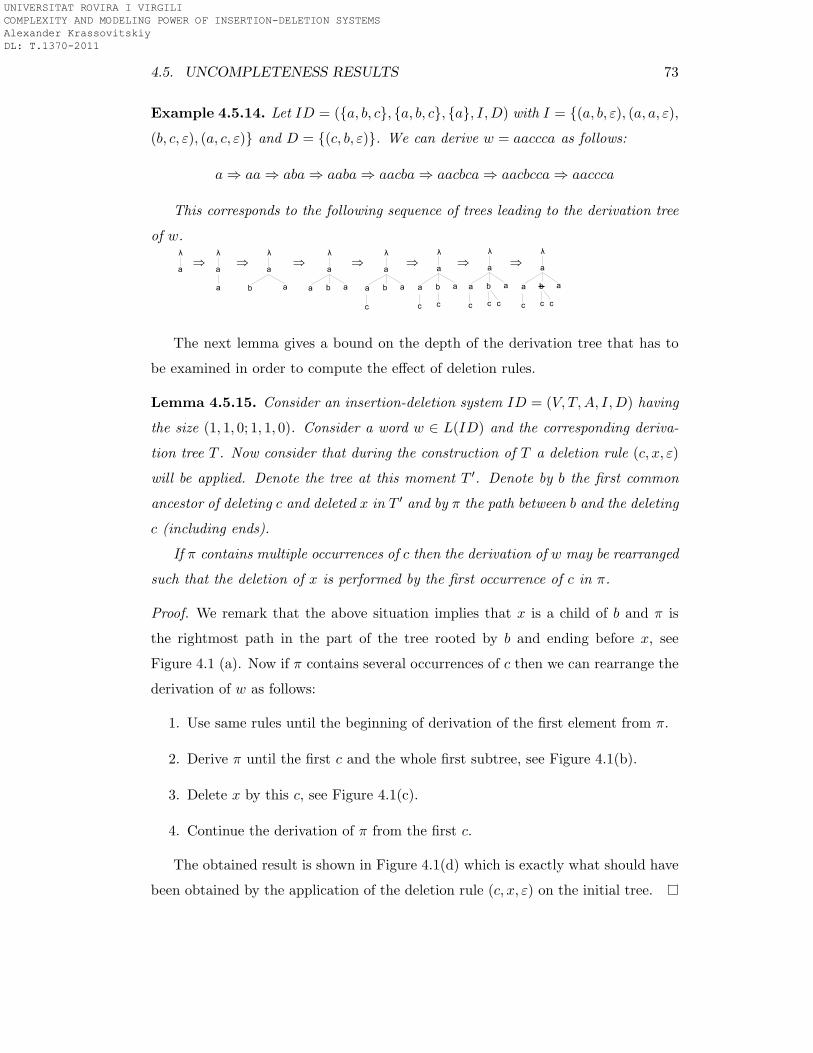
4.5. UNCOMPLETENESS RESULTS 73
Example 4.5.14. Let ID = ({a, b, c}, {a, b, c}, {a}, I,D) with I = {(a, b, ε), (a, a, ε),
(b, c, ε), (a, c, ε)} and D = {(c, b, ε)}. We can derive w = aaccca as follows:
a⇒ aa⇒ aba⇒ aaba⇒ aacba⇒ aacbca⇒ aacbcca⇒ aaccca
This corresponds to the following sequence of trees leading to the derivation tree
of w.
The next lemma gives a bound on the depth of the derivation tree that has to
be examined in order to compute the effect of deletion rules.
Lemma 4.5.15. Consider an insertion-deletion system ID = (V, T,A, I,D) having
the size (1, 1, 0; 1, 1, 0). Consider a word w ∈ L(ID) and the corresponding deriva-
tion tree T . Now consider that during the construction of T a deletion rule (c, x, ε)
will be applied. Denote the tree at this moment T ′. Denote by b the first common
ancestor of deleting c and deleted x in T ′ and by π the path between b and the deleting
c (including ends).
If π contains multiple occurrences of c then the derivation of w may be rearranged
such that the deletion of x is performed by the first occurrence of c in π.
Proof. We remark that the above situation implies that x is a child of b and π is
the rightmost path in the part of the tree rooted by b and ending before x, see
Figure 4.1 (a). Now if π contains several occurrences of c then we can rearrange the
derivation of w as follows:
1. Use same rules until the beginning of derivation of the first element from π.
2. Derive π until the first c and the whole first subtree, see Figure 4.1(b).
3. Delete x by this c, see Figure 4.1(c).
4. Continue the derivation of π from the first c.
The obtained result is shown in Figure 4.1(d) which is exactly what should have
been obtained by the application of the deletion rule (c, x, ε) on the initial tree.
UNIVERSITAT ROVIRA I VIRGILI COMPLEXITY AND MODELING POWER OF INSERTION-DELETION SYSTEMS Alexander Krassovitskiy DL: T.1370-2011
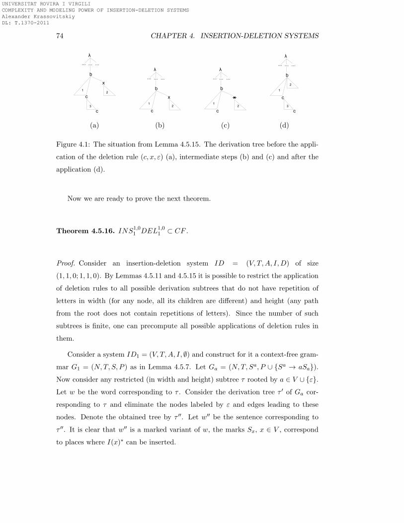
74 CHAPTER 4. INSERTION-DELETION SYSTEMS
(a) (b) (c) (d)
Figure 4.1: The situation from Lemma 4.5.15. The derivation tree before the appli-
cation of the deletion rule (c, x, ε) (a), intermediate steps (b) and (c) and after the
application (d).
Now we are ready to prove the next theorem.
Theorem 4.5.16. INS1,01 DEL1,0
1 ⊂ CF .
Proof. Consider an insertion-deletion system ID = (V, T,A, I,D) of size
(1, 1, 0; 1, 1, 0). By Lemmas 4.5.11 and 4.5.15 it is possible to restrict the application
of deletion rules to all possible derivation subtrees that do not have repetition of
letters in width (for any node, all its children are different) and height (any path
from the root does not contain repetitions of letters). Since the number of such
subtrees is finite, one can precompute all possible applications of deletion rules in
them.
Consider a system ID1 = (V, T,A, I, ∅) and construct for it a context-free gram-
mar G1 = (N,T, S, P ) as in Lemma 4.5.7. Let Ga = (N,T, Sa, P ∪ {Sa → aSa}).
Now consider any restricted (in width and height) subtree τ rooted by a ∈ V ∪ {ε}.
Let w be the word corresponding to τ . Consider the derivation tree τ ′ of Ga cor-
responding to τ and eliminate the nodes labeled by ε and edges leading to these
nodes. Denote the obtained tree by τ ′′. Let w′′ be the sentence corresponding to
τ ′′. It is clear that w′′ is a marked variant of w, the marks Sx, x ∈ V , correspond
to places where I(x)∗ can be inserted.
UNIVERSITAT ROVIRA I VIRGILI COMPLEXITY AND MODELING POWER OF INSERTION-DELETION SYSTEMS Alexander Krassovitskiy DL: T.1370-2011
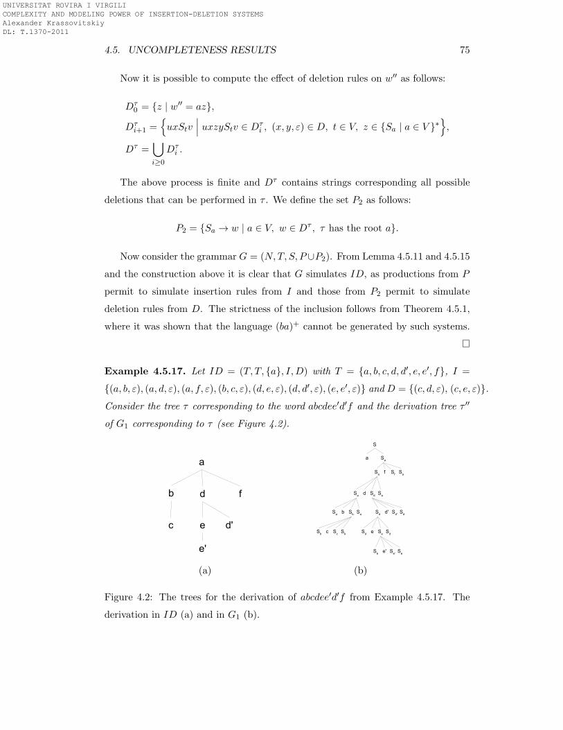
4.5. UNCOMPLETENESS RESULTS 75
Now it is possible to compute the effect of deletion rules on w′′ as follows:
Dτ0 = {z | w′′ = az},
Dτi+1 =
{
uxStv∣
∣
∣uxzyStv ∈ Dτ
i , (x, y, ε) ∈ D, t ∈ V, z ∈ {Sa | a ∈ V }∗}
,
Dτ =⋃
i≥0
Dτi .
The above process is finite and Dτ contains strings corresponding all possible
deletions that can be performed in τ . We define the set P2 as follows:
P2 = {Sa → w | a ∈ V, w ∈ Dτ , τ has the root a}.
Now consider the grammar G = (N,T, S, P∪P2). From Lemma 4.5.11 and 4.5.15
and the construction above it is clear that G simulates ID, as productions from P
permit to simulate insertion rules from I and those from P2 permit to simulate
deletion rules from D. The strictness of the inclusion follows from Theorem 4.5.1,
where it was shown that the language (ba)+ cannot be generated by such systems.
Example 4.5.17. Let ID = (T, T, {a}, I,D) with T = {a, b, c, d, d′, e, e′, f}, I =
{(a, b, ε), (a, d, ε), (a, f, ε), (b, c, ε), (d, e, ε), (d, d′, ε), (e, e′, ε)} and D = {(c, d, ε), (c, e, ε)}.
Consider the tree τ corresponding to the word abcdee′d′f and the derivation tree τ ′′
of G1 corresponding to τ (see Figure 4.2).
(a) (b)
Figure 4.2: The trees for the derivation of abcdee′d′f from Example 4.5.17. The
derivation in ID (a) and in G1 (b).
UNIVERSITAT ROVIRA I VIRGILI COMPLEXITY AND MODELING POWER OF INSERTION-DELETION SYSTEMS Alexander Krassovitskiy DL: T.1370-2011

76 CHAPTER 4. INSERTION-DELETION SYSTEMS
Then we compute w′′ and the application of rules from D to w′′:
Dτ0 = {z | w′′ = az} = {SabSbcScSbSadSdeSee
′Se′SeSdd′Sd′SdSafSfSa},
Dτ1 = {SabSbcSdeSee
′Se′SeSdd′Sd′SdSafSfSa},
Dτ2 = {SabSbcSee
′Se′SeSdd′Sd′SdSafSfSa},
Dτ = Dτ2 ∪Dτ
1 ∪Dτ0 .
Hence following rules shall be added to the grammar G:
Sa → SabSbcSdeSee′Se′SeSdd
′Sd′SdSafSfSa,
Sa → SabSbcSee′Se′SeSdd
′Sd′SdSafSfSa.
Next we present some results for systems having the contexts on the same side
of insertion and deletion rules.
Theorem 4.5.18. REG ⊂ INS2,01 DEL0,0
2 .
Proof. Let A = (Q,Σ, δ, q0, F ) be a finite automaton. Consider the following
insertion-deletion system ID = (V,Σ, A, I,D) of size (1, 2, 0; 2, 0, 0), where
• V = Σ ∪ {Q′i, Q
′′i | qi ∈ Q} ∪ {U}, where U is a new symbol,
• A = {Q′′0Q
′0U},
• for every transition δ(qi, a) = qj we add to I following insertion rules:
(Q′ia,Q
′j , ε), (4.6)
(bQ′i, a, ε), b ∈ Σ, (4.7)
(Q′′i a,Q
′′j , ε); (4.8)
for every a ∈ Σ, δ(q0, a) = qj we add to I the rule:
(Q′′0Q
′0, a, ε), (4.9)
• deletion rules are defined as follows:
D = {(ε,Q′i, ε), (ε,Q
′′i , ε)|qi ∈ Q} (4.10)
∪ {(ε,Q′′rU, ε) | qr ∈ F}. (4.11)
UNIVERSITAT ROVIRA I VIRGILI COMPLEXITY AND MODELING POWER OF INSERTION-DELETION SYSTEMS Alexander Krassovitskiy DL: T.1370-2011
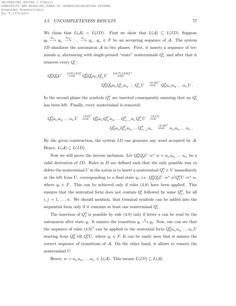
4.5. UNCOMPLETENESS RESULTS 77
We claim that L(A) = L(ID). First we show that L(A) ⊆ L(ID). Suppose
q0ai1−→ qi1
ai2−→ . . .air−→ qir , qir ∈ F be an accepting sequence of A. The system
ID simulates the automaton A in two phases. First, it inserts a sequence of ter-
minals ai alternating with single-primed “state” nonterminals Q′i, and after that it
removes every Q′i :
Q′′0Q
′0U
(4.9),(4.6)=⇒ Q′′
0Q′0ai1Q
′i1U
{(4.7),(4.6)}∗
=⇒
Q′′0Q
′0ai1Q
′i1ai2 . . . Q
′irU
(4.10)∗
=⇒ Q′′0ai1ai2 . . . airU .
In the second phase the symbols Q′′j are inserted consequently ensuring that no Q′
i
has been left. Finally, every nonterminal is removed:
Q′′0ai1ai2 . . . airU
(4.8)∗
=⇒ Q′′0ai1Q
′′i1ai2 . . . Q
′′ir−1
airQ′′irU
(4.11)=⇒
Q′′0ai1Q
′′i1ai2 . . . Q
′′ir−1
air(4.10)∗
=⇒ ai1ai2 . . . air .
By the given construction, the system ID can generate any word accepted by A.
Hence, L(A) ⊆ L(ID).
Now we will prove the inverse inclusion. Let Q′′0Q
′0U ⇒∗ w = ai1ai2 . . . air be a
valid derivation of ID. Rules in D are defined such that the only possible way to
delete the nonterminal U in the axiom is to insert a nonterminal Q′′i ∈ V immediately
at the left from U , corresponding to a final state qi, i.e. Q′′0Q
′0U ⇒∗ w′Q′′
iU ⇒∗ w,
where qi ∈ F . This can be achieved only if rules (4.8) have been applied. This
ensures that the sentential form does not contain Q′i followed by some Q′′
j , for all
i, j = 1, . . . , n. We should mention, that terminal symbols can be added into the
sequential form only if it contains at least one nonterminal Q′i.
The insertion of Q′′j is possible by rule (4.8) only if letter a can be read by the
automaton after state qi. It mimics the transition qia
−→ qj . Now, one can see that
the sequence of rules (4.8)∗ can be applied to the sentential form Q′′0ai1ai2 . . . airU
starting from Q′′0 till Q′′
rU , where qr ∈ F. It can be easily seen that it mimics the
correct sequence of transitions of A. On the other hand, it allows to remove the
nonterminal U.
Hence, w = ai1ai2 . . . air ∈ L(A). This means L(ID) ⊆ L(A).
UNIVERSITAT ROVIRA I VIRGILI COMPLEXITY AND MODELING POWER OF INSERTION-DELETION SYSTEMS Alexander Krassovitskiy DL: T.1370-2011
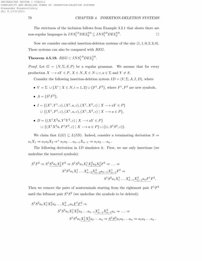
78 CHAPTER 4. INSERTION-DELETION SYSTEMS
The strictness of the inclusion follows from Example 3.2.1 that shows there are
non-regular languages in INS1,01 DEL0,0
0 ⊆ INS2,01 DEL0,0
2 .
Now we consider one-sided insertion-deletion systems of the size (1, 1, 0; 2, 3, 0).
These systems can also be compared with REG.
Theorem 4.5.19. REG ⊂ INS1,01 DEL3,0
2 .
Proof. Let G = (N,Σ, S, P ) be a regular grammar. We assume that for every
production X −→ aY ∈ P , X ∈ N,X ∈ N ∪ ε, a ∈ Σ and Y 6= S.
Consider the following insertion-deletion system ID = (V,Σ, A, I,D), where
• V = Σ ∪ {Xi | X ∈ N, i = 1, 2} ∪ {F 1, F 2}, where F 1, F 2 are new symbols,
• A = {S1F 2},
• I = {(X1, Y 1, ε), (X1, a, ε), (X1, X2, ε) | X −→ aY ∈ P}
∪ {(X1, F 1, ε), (X1, a, ε), (X1, X2, ε) | X −→ a ∈ P},
• D = {(X1X2a, Y 1Y 2, ε) | X −→ aY ∈ P}
∪ {(X1X2a, F 1F 2, ε) | X −→ a ∈ P} ∪ {(ε, S1S2, ε)}.
We claim that L(G) ⊆ L(ID). Indeed, consider a terminating derivation S ⇒
a1X1 ⇒ a1a2X2 ⇒∗ a1a2 . . . an−1Xn−1 ⇒ a1a2 . . . an .
The following derivation in ID simulates it. First, we use only insertions (we
underline the inserted symbols):
S1F 2 ⇒ S1S2a1X11F
2 ⇒ S1S2a1X11X
21a2X
12F
2 ⇒ . . .⇒
S1S2a1X11 . . . X
1n−2X
2n−2an−1X
1n−1F
2 ⇒
S1S2a1X11 . . . X
1n−1X
2n−1anF
1F 2.
Then we remove the pairs of nonterminals starting from the rightmost pair F 1F 2
until the leftmost pair S1S2 (we underline the symbols to be deleted):
S1S2a1X11X
21a2 . . . X
2n−1anF
1F 2 ⇒
S1S2a1X11X
21a2 . . . an−1X
1n−1X
2n−1an ⇒ . . .⇒
S1S2a1X11X
21a2 . . . an ⇒ S1S2a1a2 . . . an ⇒ a1a2 . . . an .
UNIVERSITAT ROVIRA I VIRGILI COMPLEXITY AND MODELING POWER OF INSERTION-DELETION SYSTEMS Alexander Krassovitskiy DL: T.1370-2011

4.6. DESCRIPTIONAL COMPLEXITY 79
Now we prove that L(ID) ⊆ L(G). First, we mention that in any terminating
derivation S1F 2 ⇒∗ w,w ∈ T ∗, F 1 must appear adjacent to F2 since the only
way to remove F2 is to use the rule (Y 1Y 2a, F 1F 2, ε) ∈ D. This rule corresponds
to the production X → a. Now, in order to remove Y 1Y 2 we must use the rule
(X1X2a, Y 1Y 2, ε) corresponding to the production X → aY. Clearly, we perform
the deletions from right to left until we delete S1S2. Hence, every terminal derivation
by ID corresponds to some derivation in G. Thereafter, we obtain L(ID) = L(G).
The strictness of the inclusion follows from Example 3.2.1.
Example 4.5.20.
(ab)+ ∈ INS1,01 DEL2,0
1
Consider the insertion-deletion system ID = (N,T,A, I,D) of size (1, 1, 0, 1, 2, 0)
defined as follows
N ={A,B, F, a, b}, T = {a, b}, A = {abAF};
I ={1 : (A,B, ε), 2 : (A, a, ε), 3 : (B,A, ε), 4 : (B, b, ε)};
D ={5 : (ab,A, ε), 6 : (ba,B, ε), 7 : (ab, F, ε)}.
We claim that L(ID) = (ab)+. The inclusion (ab)+ ⊆ L(ID) can be shown by the
following derivations in ID :
abAF5,7⇒ ab;
and
abAF1,2,5⇒ abaBF
3,4,6⇒ (ab)2AF ⇒ (1,2,5,3,4,6)k−1
... ⇒ (ab)k+1AF5,7⇒ (ab)k+1,
for any k ≥ 1.
Now in order to show that L(ID) ⊆ (ab)+ we mention that rules 5 and 6 require
alternation of the symbols a and b. Otherwise some nonterminals may be left in the
string.
4.6 Descriptional complexity
We collect in tables below our results as well as best known results on insertion-
deletion systems. The first table contains the systems with both contexts of same
UNIVERSITAT ROVIRA I VIRGILI COMPLEXITY AND MODELING POWER OF INSERTION-DELETION SYSTEMS Alexander Krassovitskiy DL: T.1370-2011
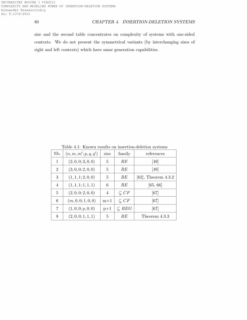
80 CHAPTER 4. INSERTION-DELETION SYSTEMS
size and the second table concentrates on complexity of systems with one-sided
contexts. We do not present the symmetrical variants (by interchanging sizes of
right and left contexts) which have same generation capabilities.
Table 4.1: Known results on insertion-deletion systems
Nb. (n,m,m′; p, q, q′) size family references
1 (2, 0, 0; 3, 0, 0) 5 RE [49]
2 (3, 0, 0; 2, 0, 0) 5 RE [49]
3 (1, 1, 1; 2, 0, 0) 5 RE [62], Theorem 4.3.2
4 (1, 1, 1; 1, 1, 1) 6 RE [65, 66]
5 (2, 0, 0; 2, 0, 0) 4 ( CF [67]
6 (m, 0, 0; 1, 0, 0) m+1 ( CF [67]
7 (1, 0, 0; p, 0, 0) p+1 ( REG [67]
8 (2, 0, 0; 1, 1, 1) 5 RE Theorem 4.3.3
UNIVERSITAT ROVIRA I VIRGILI COMPLEXITY AND MODELING POWER OF INSERTION-DELETION SYSTEMS Alexander Krassovitskiy DL: T.1370-2011
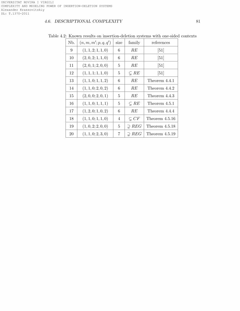
4.6. DESCRIPTIONAL COMPLEXITY 81
Table 4.2: Known results on insertion-deletion systems with one-sided contexts
Nb. (n,m,m′; p, q, q′) size family references
9 (1, 1, 2; 1, 1, 0) 6 RE [51]
10 (2, 0, 2; 1, 1, 0) 6 RE [51]
11 (2, 0, 1; 2, 0, 0) 5 RE [51]
12 (1, 1, 1; 1, 1, 0) 5 ( RE [51]
13 (1, 1, 0; 1, 1, 2) 6 RE Theorem 4.4.1
14 (1, 1, 0; 2, 0, 2) 6 RE Theorem 4.4.2
15 (2, 0, 0; 2, 0, 1) 5 RE Theorem 4.4.3
16 (1, 1, 0; 1, 1, 1) 5 ( RE Theorem 4.5.1
17 (1, 2, 0; 1, 0, 2) 6 RE Theorem 4.4.4
18 (1, 1, 0; 1, 1, 0) 4 ( CF Theorem 4.5.16
19 (1, 0, 2; 2, 0, 0) 5 ) REG Theorem 4.5.18
20 (1, 1, 0; 2, 3, 0) 7 ) REG Theorem 4.5.19
UNIVERSITAT ROVIRA I VIRGILI COMPLEXITY AND MODELING POWER OF INSERTION-DELETION SYSTEMS Alexander Krassovitskiy DL: T.1370-2011

UNIVERSITAT ROVIRA I VIRGILI COMPLEXITY AND MODELING POWER OF INSERTION-DELETION SYSTEMS Alexander Krassovitskiy DL: T.1370-2011
Chapter 5
Graph-controlled
insertion-deletion systems
In the previous chapter it was shown that there are classes of insertion-deletion
systems that cannot generate RE. Making an analogy to context-free grammars, a
natural extension of insertion-deletion systems using the graph-controlled approach
can be done. Such model introduces states (or labels of the program) associated
to every insertion or deletion rule. The transition is performed by applying cor-
responding rule and choosing the new state (thus the rule to be applied) among
a specific set of rules. Another definition of this model in the style of [60] or [16]
can be done. This definition supposes that there are disjoint groups of insertion
and deletion rules (corresponding to membranes from [60] or components from [16]).
The transition is performed by firstly choosing and applying one of applicable rules
from the current group and switching to the next group indicated in the rule de-
scription. This definition can be easily reduced to the first one. This is why we shall
consider that in the subsequent text we use the second definition. We also remark
that the last definition almost coincides with the definition of insertion-deletion P
systems [60]. Moreover, all our results on graph-controlled insertion-deletion sys-
tems were obtained under the name of insertion-deletion P systems. In this chapter
we show that the introduced graph-controlled variant of insertion-deletion systems
permits in most of the cases to increase the computational power of corresponding
83
UNIVERSITAT ROVIRA I VIRGILI COMPLEXITY AND MODELING POWER OF INSERTION-DELETION SYSTEMS Alexander Krassovitskiy DL: T.1370-2011
84 CHAPTER 5. GRAPH-CONTROLLED INSERTION-DELETION SYSTEMS
insertion-deletion systems.
5.1 Definitions
A graph-controlled insertion-deletion system Π = (V, T,A, i0, if , R1, . . . , Rn) is a
particular case of graph-controlled scheme where the set of operations is defined as
a set of contextual insertion-deletion rules. Components Ri, i = 1 . . . n contain rules
of the form r : (u, α, v; j)t ∈ Ri, where i, j ∈ 1 . . . n are labels of components The
triplet (u, α, v) ∈ V ∗ × V ∗ × V ∗ is an insertion rule if t = a, and is a deletion rule if
t = e.
The computation is performed like in the case of graph-controlled insertion sys-
tem. We remark that, as in the case of insertion-deletion systems we may consider
that the insertion and deletion rules are in the normal form.
We would like to note that the presentation of graph-controlled insertion-deletion
systems has much in common with the definition of insertion-deletion P systems [60].
There is one-to-one correspondence between components of graph-controlled and
membranes of P systems on a graph structure. The differences are the following:
axioms of graph-controlled insertion-deletion systems are present only in component
i0, while the initial state of insertion-deletion P systems is determined by the contents
of all membranes; the final component of P systems (in the case of membrane tree
structure) has no rules and considered as the environment of the system.
Another difference is that insertion-deletion P systems are often considered as
a model working in maximal parallel mode, while the graph-controlled insertion-
deletion systems are rather sequential one whose configuration is determined by a
single word in some component. We note that the notions of insertion-deletion P
systems and graph-controlled insertion-deletion systems, can be easily transformed
to each other, however, in what follows, we will use the graph-controlled variant,
because of a much simpler definition, and shorter representation of proofs.
We denote by ELSPk(insm,m′
p , delq,q′
p ) the family of languages generated by
graph-controlled insertion-deletion systems with k ≥ 1 components and insertion
and deletion rules of size at most (n,m,m′; p, q, q′) and whose communication graph
has a tree structure. We omit the letter E if T = V .
UNIVERSITAT ROVIRA I VIRGILI COMPLEXITY AND MODELING POWER OF INSERTION-DELETION SYSTEMS Alexander Krassovitskiy DL: T.1370-2011
5.2. THE COMPUTATIONAL POWER OF SMALL SYSTEMS 85
As in Chapter 4, the letter t is inserted before P to denote classes whose com-
munication graph is arbitrary, e.g., ELStPk(insm,m′
p , delq,q′
p ).
Example 5.1.1. It is easy to see that language {anban | n ≥ 1} is generated by the
following graph-controlled insertion-deletion system
({a, b}, {a, b}, {aba}, 1, 1, R1, R2) ∈ LSP2(ins1,11 , del0,00 ),
where R1 = {(ε, a, b; 2)a}, and R2 = {(b, a, ε; 1)a}.
We remark that the language generated by the system from Example 5.1.1 cannot
be generated by any insertion system of size (n, 1, 1), for any n ≥ 1.
Example 5.1.2. Consider the following example:
Π1 = ({a, b, c}, {a, b, c}, {ε}, 1, 1, R1, R2, R3), where
R1 = {(ε, a, ε; 2)a};R2 = {(ε, b, ε; 3)a};R2 = {(ε, c, ε; 1)a}.
Clearly, Π1 ∈ ELStP3(ins0,01 , del0,00 ). One can see that Π1 generates the non context-
free language. L = {w | |w|a = |w|b = |w|c}. Indeed, every cycle that activates
components 1− 2− 3 inserts exactly one symbol a, b and c.
For the tree case the language {w ∈ {a, b}∗ | |w|a = |w|b} can be generated in a
similar manner.
5.2 The computational power of small systems
We start with the following result.
Theorem 5.2.1. PsStP∗(ins0,01 , del0,01 ) = PsMAT λ.
Proof. The inclusion PsStP∗(ins0,01 , del0,01 ) ⊆ PsMAT λ follows from the simulation
of minimal graph-controlled insertion-deletion without contexts systems by partially
blind register machines [22]. Indeed, any rule (ε, a, ε; q)a ∈ Rp can be simulated by
the instruction p : (ADD(a), q). Similarly, any rule (ε, a, ε; q)e ∈ Rp can be simulated
by the instruction p : (SUB(a), q).
UNIVERSITAT ROVIRA I VIRGILI COMPLEXITY AND MODELING POWER OF INSERTION-DELETION SYSTEMS Alexander Krassovitskiy DL: T.1370-2011

86 CHAPTER 5. GRAPH-CONTROLLED INSERTION-DELETION SYSTEMS
The final component i0 is associated to the final state, while the condition that
a string does not contain non-terminal symbols is represented by requirement that
all register except output ones are zero.
The converse inclusion follows from the simulation of partially blind register ma-
chines by graph-controlled insertion-deletion systems. Indeed, with every instruction
p of the register machine we associate a component. Instruction p : (ADD(Ak), q) is
simulated by rule (ε,Ak, ε; q)a ∈ Rp, and instruction p : (SUB(Ak), q) by
(ε,Ak, ε; q)e ∈ Rp. The requirement that non-output registers are empty corre-
sponds to the condition that the resulting string does not contain non-terminal
symbols.
If the communication graph is a tree, one-way inclusion follows as a particular
case. Non-extended systems are also a particular case.
Corollary 5.2.2. PsSP∗(ins0,01 , del0,01 ) ⊆ PsMAT λ.
In terms of the generated language such systems are not very powerful. Like in
the case of context-free insertion-deletion systems there is no control on the position
of insertion. Hence, the language L = {a∗b∗} cannot be generated, for insertion
strings of any size. Hence we obtain:
Theorem 5.2.3. REG\ELStP∗(ins0,0n , del0,01 ) 6= ∅, for any n > 0.
However, as shown in Example 5.1.2, there are non-context-free languages that
can be generated by such systems (even without deletion).
Now, we show a more general inclusion:
Theorem 5.2.4. ELStP∗(ins0,0n , del0,01 ) ⊂MAT λ, for any n > 0.
Proof. Consider a graph-controlled insertion-deletion system Π = (V, T, w, p0, h, R)
with rules in normal form and H = Lab(R). Such a system can be simulated by the
following matrix grammar G = (V ∪H,T, S, P ).
For every insertion rule (ε, a1 · · · an, ε; q)a in component p, let P contain the
matrix {p → q,D → Da1D · · ·DanD}. For any deletion instruction (ε,A, ε; q)e
in component p, let P contain the matrix {p → q, A → ε}. We also add to P
UNIVERSITAT ROVIRA I VIRGILI COMPLEXITY AND MODELING POWER OF INSERTION-DELETION SYSTEMS Alexander Krassovitskiy DL: T.1370-2011
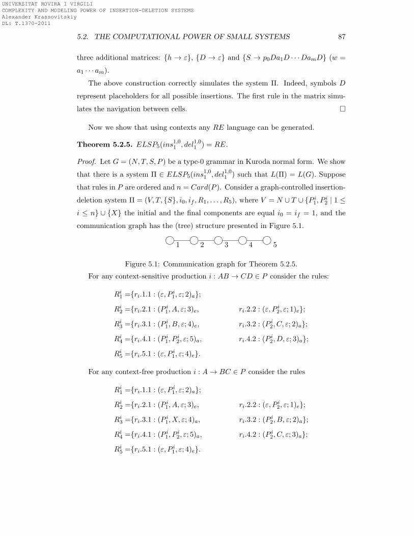
5.2. THE COMPUTATIONAL POWER OF SMALL SYSTEMS 87
three additional matrices: {h → ε}, {D → ε} and {S → p0Da1D · · ·DamD} (w =
a1 · · · am).
The above construction correctly simulates the system Π. Indeed, symbols D
represent placeholders for all possible insertions. The first rule in the matrix simu-
lates the navigation between cells.
Now we show that using contexts any RE language can be generated.
Theorem 5.2.5. ELSP5(ins1,01 , del1,01 ) = RE.
Proof. Let G = (N,T, S, P ) be a type-0 grammar in Kuroda normal form. We show
that there is a system Π ∈ ELSP5(ins1,01 , del1,01 ) such that L(Π) = L(G). Suppose
that rules in P are ordered and n = Card(P ). Consider a graph-controlled insertion-
deletion system Π = (V, T, {S}, i0, if , R1, . . . , R5), where V = N ∪ T ∪ {P i1, P
i2 | 1 ≤
i ≤ n} ∪ {X} the initial and the final components are equal i0 = if = 1, and the
communication graph has the (tree) structure presented in Figure 5.1.
/.-,()*+
1/.-,()*+
2/.-,()*+
3/.-,()*+
4/.-,()*+
5
Figure 5.1: Communication graph for Theorem 5.2.5.
For any context-sensitive production i : AB → CD ∈ P consider the rules:
Ri1 ={ri.1.1 : (ε, P i
1, ε; 2)a};
Ri2 ={ri.2.1 : (P i
1, A, ε; 3)e, ri.2.2 : (ε, P i2, ε; 1)e};
Ri3 ={ri.3.1 : (P i
1, B, ε; 4)e, ri.3.2 : (P i2, C, ε; 2)a};
Ri4 ={ri.4.1 : (P i
1, Pi2, ε; 5)a, ri.4.2 : (P i
2, D, ε; 3)a};
Ri5 ={ri.5.1 : (ε, P i
1, ε; 4)e}.
For any context-free production i : A→ BC ∈ P consider the rules
Ri1 ={ri.1.1 : (ε, P i
1, ε; 2)a};
Ri2 ={ri.2.1 : (P i
1, A, ε; 3)e, ri.2.2 : (ε, P i2, ε; 1)e};
Ri3 ={ri.3.1 : (P i
1, X, ε; 4)a, ri.3.2 : (P i2, B, ε; 2)a};
Ri4 ={ri.4.1 : (P i
1, Pi2, ε; 5)a, ri.4.2 : (P i
2, C, ε; 3)a};
Ri5 ={ri.5.1 : (ε, P i
1, ε; 4)e}.
UNIVERSITAT ROVIRA I VIRGILI COMPLEXITY AND MODELING POWER OF INSERTION-DELETION SYSTEMS Alexander Krassovitskiy DL: T.1370-2011
88 CHAPTER 5. GRAPH-CONTROLLED INSERTION-DELETION SYSTEMS
For any production i : A→ α ∈ P, α ∈ T consider the rules
Ri1 ={ri.1.1 : (ε, P i
1, ε; 2)a};
Ri2 ={ri.2.1 : (P i
1, A, ε; 3)e, ri.2.2 : (ε, P i2, ε; 1)e};
Ri3 ={ri.3.1 : (P i
1, Pi2, ε; 4)a, ri.3.2 : (P i
2, α, ε; 2)a};
Ri4 ={ri.4.1 : (ε, P i
1, ε; 3)e};
Ri5 =∅.
For every production i : A→ ε ∈ P consider the rules
Ri1 = {i.1.1 : (ε,A, ε; 1)e, };R
i2 = Ri
3 = Ri4 = Ri
5 = ∅.
Now associate with k−th component k = 2, . . . , 5 the set of rules
Rk = ∪i=1,...,nRik and with component 1 the set of rules R1 = ∪i=1,...,nR
i1 ∪
{0 : (ε,X, ε; 1)e}. We claim that Π generates the same language as G.
We prove that every step of the derivation in G can be simulated in Π. Consider
as example the production i : AB → CD ∈ R. The simulation of this production
is done as follows. Let a string w1ABw2 is in the component 1. Then, there is the
following derivation
(1, w1ABw2) Vri.1.1 (2, w1Pi1ABw2) Vri.2.1 (3, w1P
i1Bw2) Vri.3.1
(4, w1Pi1w2) Vri.4.1 (5, w1P
i1P
i2w2) Vri.5.1 (4, w1P
i2w2) Vri.4.2
(3, w1Pi2Dw2) Vri.3.2 (2, w1P
i2CDw2) Vri.2.2 (1, w1CDw2).
The simulation of other productions is done in a similar way.
It is easy to see that after the insertion of P i1 by the rule ri.1.1 all rules corre-
sponding to i-th production have to be applied until the rule ri.2.2, otherwise the
derivation will be blocked. We also note that every sentential form has at most one
copy of symbols P i1 and P i
2, i = 1, ..., n and none of them is present if the component
1 is active.
Productions of the form A → BC, where A,B,C ∈ N are controlled by P 1i
that pushes the sequential form “right” from R1 to R5, and by P 2i that controls the
sequence of rules pushing the sequential form “left” from R5 to R1. It is simulated
UNIVERSITAT ROVIRA I VIRGILI COMPLEXITY AND MODELING POWER OF INSERTION-DELETION SYSTEMS Alexander Krassovitskiy DL: T.1370-2011
5.2. THE COMPUTATIONAL POWER OF SMALL SYSTEMS 89
as follows:
(1, w1Aw2) Vri.1.1 (2, w1Pi1Aw2) Vri.2.1 (3, w1P
i1w2) Vri.3.1
(4, w1Pi1P
i2w2) Vri.4.1 (5, w1P
i1P
i2Xw2) Vri.5.1 (4, w1XP
i2w2) Vri.4.2
(3, w1XPi2Cw2) Vri.3.2 (2, w1XP
i2BCw2) Vri.2.2 (1, w1XBCw2).
We mention that one extra symbol X /∈ N ∪ T is introduced by the rule ri.3.1. In
fact the context-free production A→ BC is simulated by two equivalent productions
A → XBC and X → ε with a special nonterminal X. This is due to the fact that
the total number of inserted and deleted symbols must be even. This symbol is
finally deleted by the rule 0 : (ε,X, ε, 1)e ∈ R1.
We use the same technique for productions A→ α,A ∈ N,α ∈ T ∪N :
(1, w1Aw2) Vri.1.1 (2, w1Pi1Aw2) Vri.2.1
(3, w1Pi1w2) Vri.3.1 (4, w1P
i1P
i2w2) Vri.4.1
(3, w1Pi2w2) Vri.3.2 (2, w1P
i2αw2) Vri.2.2 (1, w1αw2)
The result is collected in the final component of the system and the strings are sent
there using the rule (ε,X, ε; 1)e in the first component. To finish the proof we observe
that every correct sentential form has at most one symbol P 1i and P 2
i , i = 1, ..., n.
After the insertion of P 1i in the first component either all rules corresponding to i-th
rule have to be applied (in the defined order) or the derivation is blocked. Hence,
we have L(G) = L(Π).
Symbols P i1 can be inserted by rules with a right context. This gives a char-
acterization of RE languages by the family ELSP5(ins0,11 , del1,01 ), i.e. with con-
texts for insertion and deletion on different sides. In order to achieve this, the
pair of rules ri.2.1, ri.3.1 corresponding to i-th context-sensitive production is re-
placed by new rules ri.2.1 : (ε, P i1, B; 3)e, and ri.3.1 : (ε, P i
1, A; 4)e respectively,
and for every context-free and terminal production j the rule rj .2.1 is replaced by
rj .2.1 : (ε, P i1, A; 3)e. Taking also into account the symmetrical cases we get:
Corollary 5.2.6. ELSP5(ins1,01 , del0,11 ) = ELSP5(ins
0,11 , del1,01 ) =
ELSP5(ins0,11 , del0,11 ) = RE.
UNIVERSITAT ROVIRA I VIRGILI COMPLEXITY AND MODELING POWER OF INSERTION-DELETION SYSTEMS Alexander Krassovitskiy DL: T.1370-2011
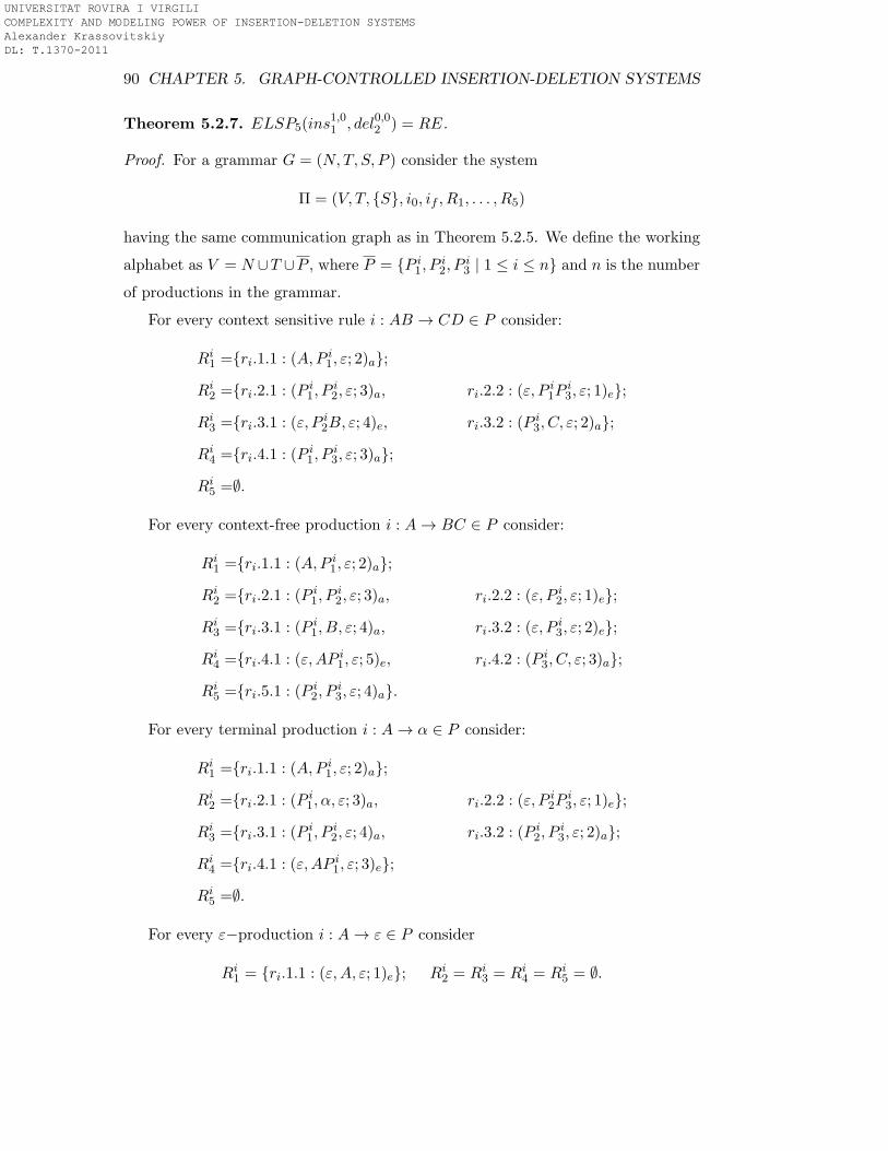
90 CHAPTER 5. GRAPH-CONTROLLED INSERTION-DELETION SYSTEMS
Theorem 5.2.7. ELSP5(ins1,01 , del0,02 ) = RE.
Proof. For a grammar G = (N,T, S, P ) consider the system
Π = (V, T, {S}, i0, if , R1, . . . , R5)
having the same communication graph as in Theorem 5.2.5. We define the working
alphabet as V = N ∪T ∪P , where P = {P i1, P
i2, P
i3 | 1 ≤ i ≤ n} and n is the number
of productions in the grammar.
For every context sensitive rule i : AB → CD ∈ P consider:
Ri1 ={ri.1.1 : (A,P i
1, ε; 2)a};
Ri2 ={ri.2.1 : (P i
1, Pi2, ε; 3)a, ri.2.2 : (ε, P i
1Pi3, ε; 1)e};
Ri3 ={ri.3.1 : (ε, P i
2B, ε; 4)e, ri.3.2 : (P i3, C, ε; 2)a};
Ri4 ={ri.4.1 : (P i
1, Pi3, ε; 3)a};
Ri5 =∅.
For every context-free production i : A→ BC ∈ P consider:
Ri1 ={ri.1.1 : (A,P i
1, ε; 2)a};
Ri2 ={ri.2.1 : (P i
1, Pi2, ε; 3)a, ri.2.2 : (ε, P i
2, ε; 1)e};
Ri3 ={ri.3.1 : (P i
1, B, ε; 4)a, ri.3.2 : (ε, P i3, ε; 2)e};
Ri4 ={ri.4.1 : (ε,AP i
1, ε; 5)e, ri.4.2 : (P i3, C, ε; 3)a};
Ri5 ={ri.5.1 : (P i
2, Pi3, ε; 4)a}.
For every terminal production i : A→ α ∈ P consider:
Ri1 ={ri.1.1 : (A,P i
1, ε; 2)a};
Ri2 ={ri.2.1 : (P i
1, α, ε; 3)a, ri.2.2 : (ε, P i2P
i3, ε; 1)e};
Ri3 ={ri.3.1 : (P i
1, Pi2, ε; 4)a, ri.3.2 : (P i
2, Pi3, ε; 2)a};
Ri4 ={ri.4.1 : (ε,AP i
1, ε; 3)e};
Ri5 =∅.
For every ε−production i : A→ ε ∈ P consider
Ri1 = {ri.1.1 : (ε,A, ε; 1)e}; Ri
2 = Ri3 = Ri
4 = Ri5 = ∅.
UNIVERSITAT ROVIRA I VIRGILI COMPLEXITY AND MODELING POWER OF INSERTION-DELETION SYSTEMS Alexander Krassovitskiy DL: T.1370-2011
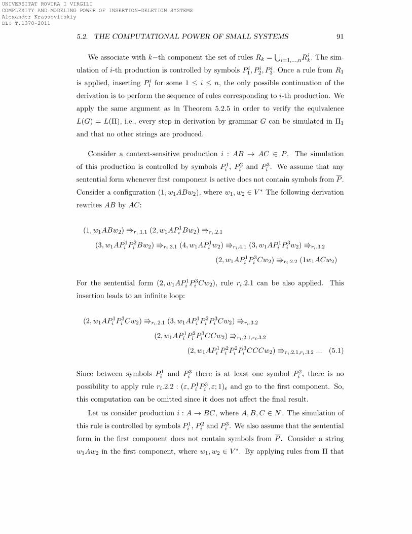
5.2. THE COMPUTATIONAL POWER OF SMALL SYSTEMS 91
We associate with k−th component the set of rules Rk =⋃
i=1,...,nRik. The sim-
ulation of i-th production is controlled by symbols P i1, P
i2, P
i3. Once a rule from R1
is applied, inserting P i1 for some 1 ≤ i ≤ n, the only possible continuation of the
derivation is to perform the sequence of rules corresponding to i-th production. We
apply the same argument as in Theorem 5.2.5 in order to verify the equivalence
L(G) = L(Π), i.e., every step in derivation by grammar G can be simulated in Π1
and that no other strings are produced.
Consider a context-sensitive production i : AB → AC ∈ P . The simulation
of this production is controlled by symbols P 1i , P
2i and P 3
i . We assume that any
sentential form whenever first component is active does not contain symbols from P .
Consider a configuration (1, w1ABw2), where w1, w2 ∈ V ∗ The following derivation
rewrites AB by AC:
(1, w1ABw2) Vri.1.1 (2, w1AP1i Bw2) Vri.2.1
(3, w1AP1i P
2i Bw2) Vri.3.1 (4, w1AP
1i w2) Vri.4.1 (3, w1AP
1i P
3i w2) Vri.3.2
(2, w1AP1i P
3i Cw2) Vri.2.2 (1w1ACw2)
For the sentential form (2, w1AP1i P
3i Cw2), rule ri.2.1 can be also applied. This
insertion leads to an infinite loop:
(2, w1AP1i P
3i Cw2) Vri.2.1 (3, w1AP
1i P
2i P
3i Cw2) Vri.3.2
(2, w1AP1i P
2i P
3i CCw2) Vri.2.1,ri.3.2
(2, w1AP1i P
2i P
2i P
3i CCCw2) Vri.2.1,ri.3.2 ... (5.1)
Since between symbols P 1i and P 3
i there is at least one symbol P 2i , there is no
possibility to apply rule ri.2.2 : (ε, P 1i P
3i , ε; 1)e and go to the first component. So,
this computation can be omitted since it does not affect the final result.
Let us consider production i : A → BC, where A,B,C ∈ N . The simulation of
this rule is controlled by symbols P 1i , P
2i and P 3
i . We also assume that the sentential
form in the first component does not contain symbols from P . Consider a string
w1Aw2 in the first component, where w1, w2 ∈ V ∗. By applying rules from Π that
UNIVERSITAT ROVIRA I VIRGILI COMPLEXITY AND MODELING POWER OF INSERTION-DELETION SYSTEMS Alexander Krassovitskiy DL: T.1370-2011

92 CHAPTER 5. GRAPH-CONTROLLED INSERTION-DELETION SYSTEMS
correspond to i-th production we obtain:
(1, w1Aw2) Vri.1.1 (2, w1AP1i w2) Vri.2.1 (3, w1AP
1i P
2i w2) Vri.3.1
(4, w1AP1i BP
2i w2) Vri.4.1 (4, w1BP
2i w2) Vri.5.1 (4, w1BP
2i P
3i w2) Vri.4.2
(4, w1BP2i P
3i Cw2) Vri.3.2 (4, w1BP
2i Cw2) Vri.2.2 (4, w1BP
2i P
3i Cw2)
The simulation of production i : A→ α, where A ∈ N and α ∈ N ∪T is done in an
analogous manner. Indeed, let (1, w1Aw2) be a sentential form.
(1, w1Aw2) Vri.1.1 (2, w1AP1i w2) Vri.2.1
(3, w1AP1i αw2) Vri.3.1 (4, w1AP
1i P
2i αw2) Vri.4.1
(3, w1P2i αw2) Vri.3.2 (2, w1P
2i P
3i αw2) Vri.2.2 (1, w1αw2)
To finish the proof we observe that every sentential form has at most one symbol
P 1i , P
2i or P 3
i , i = 1, . . . , n. Moreover, the computations for i : A → BC and
i : A → α are deterministic, and additional computation of the form (5.1) for
productions i : AB → AC does not produce new words.
As soon as P 1i is inserted in the first component either all rules corresponding
to i-th rule have to be applied (in the defined order), or the derivation is blocked.
Therefore, there is one-to-one correspondence between sentential forms (in the first
component) and sentential forms of G. Hence, we have L(G) = L(Π1).
The symmetrical case of the right context insertion gives
Corollary 5.2.8. ELSP5(ins0,11 , del0,02 ) = RE.
By a similar simulation we obtain the characterization of RE by exchanging the
size of insertion and deletion rules.
Theorem 5.2.9. ELSP5(ins0,02 , del1,01 ) = ELSP5(ins
0,02 , del0,11 ) = RE.
Proof. As in the previous theorem, we prove the inclusionRE ⊆ ELSP5(ins0,02 del1,01 )
by simulation of type-0 grammar in Penttonen normal form. The reverse inclusion
follows from the Church thesis. Let G = (N,T, S, P ) be a type-0 grammar in
Penttonen normal form. Suppose that rules in P are ordered and n = Card(R).
UNIVERSITAT ROVIRA I VIRGILI COMPLEXITY AND MODELING POWER OF INSERTION-DELETION SYSTEMS Alexander Krassovitskiy DL: T.1370-2011
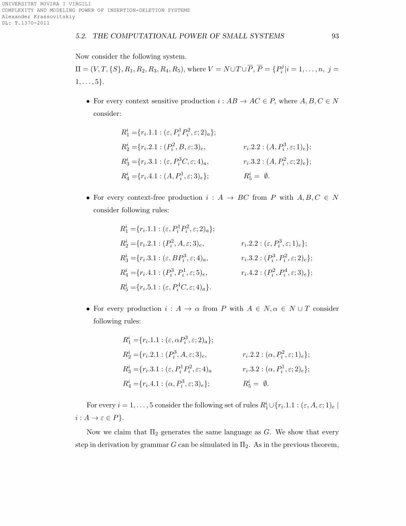
5.2. THE COMPUTATIONAL POWER OF SMALL SYSTEMS 93
Now consider the following system.
Π = (V, T, {S}, R1, R2, R3, R4, R5), where V = N∪T ∪P , P = {P ji |i = 1, . . . , n, j =
1, . . . , 5}.
• For every context sensitive production i : AB → AC ∈ P, where A,B,C ∈ N
consider:
Ri1 ={ri.1.1 : (ε, P 1
i P2i , ε; 2)a};
Ri2 ={ri.2.1 : (P 2
i , B, ε; 3)e, ri.2.2 : (A,P 3i , ε; 1)e};
Ri3 ={ri.3.1 : (ε, P 3
i C, ε; 4)a, ri.3.2 : (A,P 2i , ε; 2)e};
Ri4 ={ri.4.1 : (A,P 1
i , ε; 3)e}; Ri5 = ∅.
• For every context-free production i : A → BC from P with A,B,C ∈ N
consider following rules:
Ri1 ={ri.1.1 : (ε, P 1
i P2i , ε; 2)a};
Ri2 ={ri.2.1 : (P 2
i , A, ε; 3)e, ri.2.2 : (ε, P 3i , ε; 1)e};
Ri3 ={ri.3.1 : (ε,BP 3
i , ε; 4)a, ri.3.2 : (P 3i , P
2i , ε; 2)e};
Ri4 ={ri.4.1 : (P 3
i , P1i , ε; 5)e, ri.4.2 : (P 2
i , P4i , ε; 3)e};
Ri5 ={ri.5.1 : (ε, P 4
i C, ε; 4)a}.
• For every production i : A → α from P with A ∈ N,α ∈ N ∪ T consider
following rules:
Ri1 ={ri.1.1 : (ε, αP 3
i , ε; 2)a};
Ri2 ={ri.2.1 : (P 3
i , A, ε; 3)e, ri.2.2 : (α, P 2i , ε; 1)e};
Ri3 ={ri.3.1 : (ε, P 1
i P2i , ε; 4)a ri.3.2 : (α, P 1
i , ε; 2)e};
Ri4 ={ri.4.1 : (α, P 3
i , ε; 3)e}; Ri5 = ∅.
For every i = 1, . . . , 5 consider the following set of rules Ri1∪{ri.1.1 : (ε,A, ε; 1)e |
i : A→ ε ∈ P}.
Now we claim that Π2 generates the same language as G. We show that every
step in derivation by grammar G can be simulated in Π2. As in the previous theorem,
UNIVERSITAT ROVIRA I VIRGILI COMPLEXITY AND MODELING POWER OF INSERTION-DELETION SYSTEMS Alexander Krassovitskiy DL: T.1370-2011
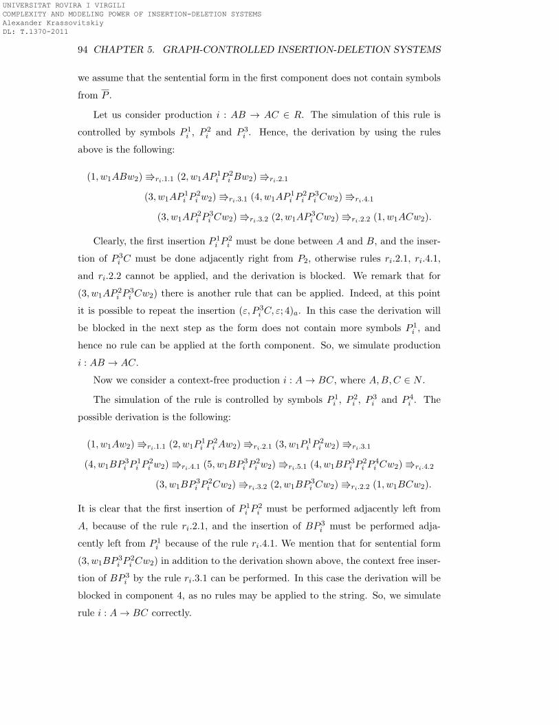
94 CHAPTER 5. GRAPH-CONTROLLED INSERTION-DELETION SYSTEMS
we assume that the sentential form in the first component does not contain symbols
from P .
Let us consider production i : AB → AC ∈ R. The simulation of this rule is
controlled by symbols P 1i , P
2i and P 3
i . Hence, the derivation by using the rules
above is the following:
(1, w1ABw2) Vri.1.1 (2, w1AP1i P
2i Bw2) Vri.2.1
(3, w1AP1i P
2i w2) Vri.3.1 (4, w1AP
1i P
2i P
3i Cw2) Vri.4.1
(3, w1AP2i P
3i Cw2) Vri.3.2 (2, w1AP
3i Cw2) Vri.2.2 (1, w1ACw2).
Clearly, the first insertion P 1i P
2i must be done between A and B, and the inser-
tion of P 3i C must be done adjacently right from P2, otherwise rules ri.2.1, ri.4.1,
and ri.2.2 cannot be applied, and the derivation is blocked. We remark that for
(3, w1AP2i P
3i Cw2) there is another rule that can be applied. Indeed, at this point
it is possible to repeat the insertion (ε, P 3i C, ε; 4)a. In this case the derivation will
be blocked in the next step as the form does not contain more symbols P 1i , and
hence no rule can be applied at the forth component. So, we simulate production
i : AB → AC.
Now we consider a context-free production i : A→ BC, where A,B,C ∈ N .
The simulation of the rule is controlled by symbols P 1i , P
2i , P
3i and P 4
i . The
possible derivation is the following:
(1, w1Aw2) Vri.1.1 (2, w1P1i P
2i Aw2) Vri.2.1 (3, w1P
1i P
2i w2) Vri.3.1
(4, w1BP3i P
1i P
2i w2) Vri.4.1 (5, w1BP
3i P
2i w2) Vri.5.1 (4, w1BP
3i P
2i P
4i Cw2) Vri.4.2
(3, w1BP3i P
2i Cw2) Vri.3.2 (2, w1BP
3i Cw2) Vri.2.2 (1, w1BCw2).
It is clear that the first insertion of P 1i P
2i must be performed adjacently left from
A, because of the rule ri.2.1, and the insertion of BP 3i must be performed adja-
cently left from P 1i because of the rule ri.4.1. We mention that for sentential form
(3, w1BP3i P
2i Cw2) in addition to the derivation shown above, the context free inser-
tion of BP 3i by the rule ri.3.1 can be performed. In this case the derivation will be
blocked in component 4, as no rules may be applied to the string. So, we simulate
rule i : A→ BC correctly.
UNIVERSITAT ROVIRA I VIRGILI COMPLEXITY AND MODELING POWER OF INSERTION-DELETION SYSTEMS Alexander Krassovitskiy DL: T.1370-2011
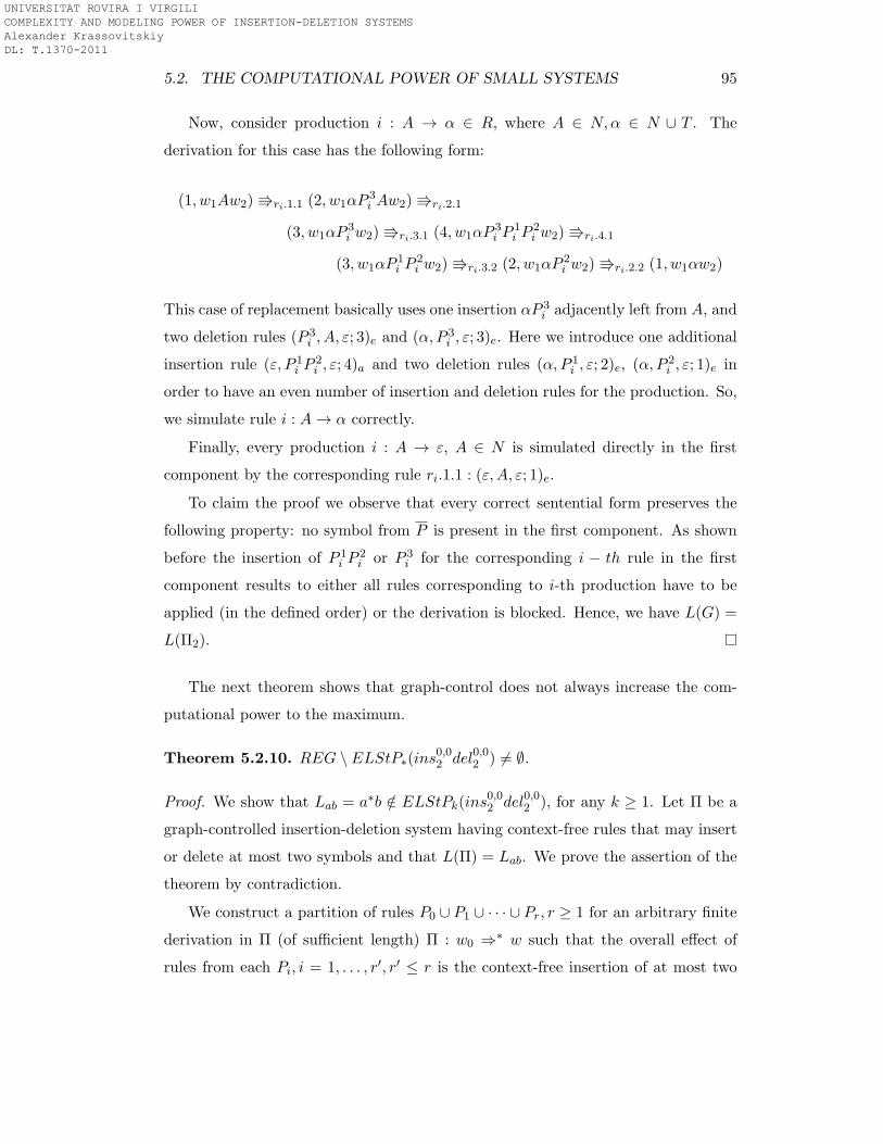
5.2. THE COMPUTATIONAL POWER OF SMALL SYSTEMS 95
Now, consider production i : A → α ∈ R, where A ∈ N,α ∈ N ∪ T . The
derivation for this case has the following form:
(1, w1Aw2) Vri.1.1 (2, w1αP3i Aw2) Vri.2.1
(3, w1αP3i w2) Vri.3.1 (4, w1αP
3i P
1i P
2i w2) Vri.4.1
(3, w1αP1i P
2i w2) Vri.3.2 (2, w1αP
2i w2) Vri.2.2 (1, w1αw2)
This case of replacement basically uses one insertion αP 3i adjacently left from A, and
two deletion rules (P 3i , A, ε; 3)e and (α, P 3
i , ε; 3)e. Here we introduce one additional
insertion rule (ε, P 1i P
2i , ε; 4)a and two deletion rules (α, P 1
i , ε; 2)e, (α, P2i , ε; 1)e in
order to have an even number of insertion and deletion rules for the production. So,
we simulate rule i : A→ α correctly.
Finally, every production i : A → ε, A ∈ N is simulated directly in the first
component by the corresponding rule ri.1.1 : (ε,A, ε; 1)e.
To claim the proof we observe that every correct sentential form preserves the
following property: no symbol from P is present in the first component. As shown
before the insertion of P 1i P
2i or P 3
i for the corresponding i − th rule in the first
component results to either all rules corresponding to i-th production have to be
applied (in the defined order) or the derivation is blocked. Hence, we have L(G) =
L(Π2).
The next theorem shows that graph-control does not always increase the com-
putational power to the maximum.
Theorem 5.2.10. REG \ ELStP∗(ins0,02 del0,02 ) 6= ∅.
Proof. We show that Lab = a∗b /∈ ELStPk(ins0,02 del0,02 ), for any k ≥ 1. Let Π be a
graph-controlled insertion-deletion system having context-free rules that may insert
or delete at most two symbols and that L(Π) = Lab. We prove the assertion of the
theorem by contradiction.
We construct a partition of rules P0 ∪ P1 ∪ · · · ∪ Pr, r ≥ 1 for an arbitrary finite
derivation in Π (of sufficient length) Π : w0 ⇒∗ w such that the overall effect of
rules from each Pi, i = 1, . . . , r′, r′ ≤ r is the context-free insertion of at most two
UNIVERSITAT ROVIRA I VIRGILI COMPLEXITY AND MODELING POWER OF INSERTION-DELETION SYSTEMS Alexander Krassovitskiy DL: T.1370-2011
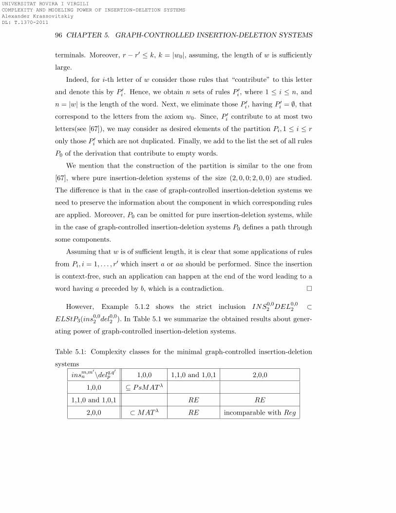
96 CHAPTER 5. GRAPH-CONTROLLED INSERTION-DELETION SYSTEMS
terminals. Moreover, r − r′ ≤ k, k = |w0|, assuming, the length of w is sufficiently
large.
Indeed, for i-th letter of w consider those rules that “contribute” to this letter
and denote this by P ′i . Hence, we obtain n sets of rules P ′
i , where 1 ≤ i ≤ n, and
n = |w| is the length of the word. Next, we eliminate those P ′i , having P
′i = ∅, that
correspond to the letters from the axiom w0. Since, P ′i contribute to at most two
letters(see [67]), we may consider as desired elements of the partition Pi, 1 ≤ i ≤ r
only those P ′i which are not duplicated. Finally, we add to the list the set of all rules
P0 of the derivation that contribute to empty words.
We mention that the construction of the partition is similar to the one from
[67], where pure insertion-deletion systems of the size (2, 0, 0; 2, 0, 0) are studied.
The difference is that in the case of graph-controlled insertion-deletion systems we
need to preserve the information about the component in which corresponding rules
are applied. Moreover, P0 can be omitted for pure insertion-deletion systems, while
in the case of graph-controlled insertion-deletion systems P0 defines a path through
some components.
Assuming that w is of sufficient length, it is clear that some applications of rules
from Pi, i = 1, . . . , r′ which insert a or aa should be performed. Since the insertion
is context-free, such an application can happen at the end of the word leading to a
word having a preceded by b, which is a contradiction.
However, Example 5.1.2 shows the strict inclusion INS0,02 DEL0,0
2 ⊂
ELStP3(ins0,02 del0,02 ). In Table 5.1 we summarize the obtained results about gener-
ating power of graph-controlled insertion-deletion systems.
Table 5.1: Complexity classes for the minimal graph-controlled insertion-deletion
systems
insm,m′
n \delq,q′
p 1,0,0 1,1,0 and 1,0,1 2,0,0
1,0,0 ⊆ PsMAT λ
1,1,0 and 1,0,1 RE RE
2,0,0 ⊂MAT λ RE incomparable with Reg
UNIVERSITAT ROVIRA I VIRGILI COMPLEXITY AND MODELING POWER OF INSERTION-DELETION SYSTEMS Alexander Krassovitskiy DL: T.1370-2011
Chapter 6
Graph-controlled
insertion-deletion systems with
priorities
This chapter is devoted to graph-controlled insertion-deletion systems with priorities.
This model has the following property: if a component contains an insertion and a
deletion rule being both applicable, then the deletion is always chosen to be applied.
Saying otherwise, no insertion rule can be applied if a deletion rule is applicable. We
show that such systems are a particular case of graph-controlled insertion-deletion
systems with appearance checking. The results on computational complexity are
given for the classes of languages which can be generated by such systems of very
small sizes.
The family of languages corresponding to graph-controlled insertion-deletion sys-
tems with priorities is denoted by (E)LSPk(insm,m′
n < delq,q′
p ). As in the previous
section the letter t is inserted before P to denote classes whose communication graph
is arbitrary, e.g., ELStPk(insm,m′
n < delq,q′
p ).
97
UNIVERSITAT ROVIRA I VIRGILI COMPLEXITY AND MODELING POWER OF INSERTION-DELETION SYSTEMS Alexander Krassovitskiy DL: T.1370-2011
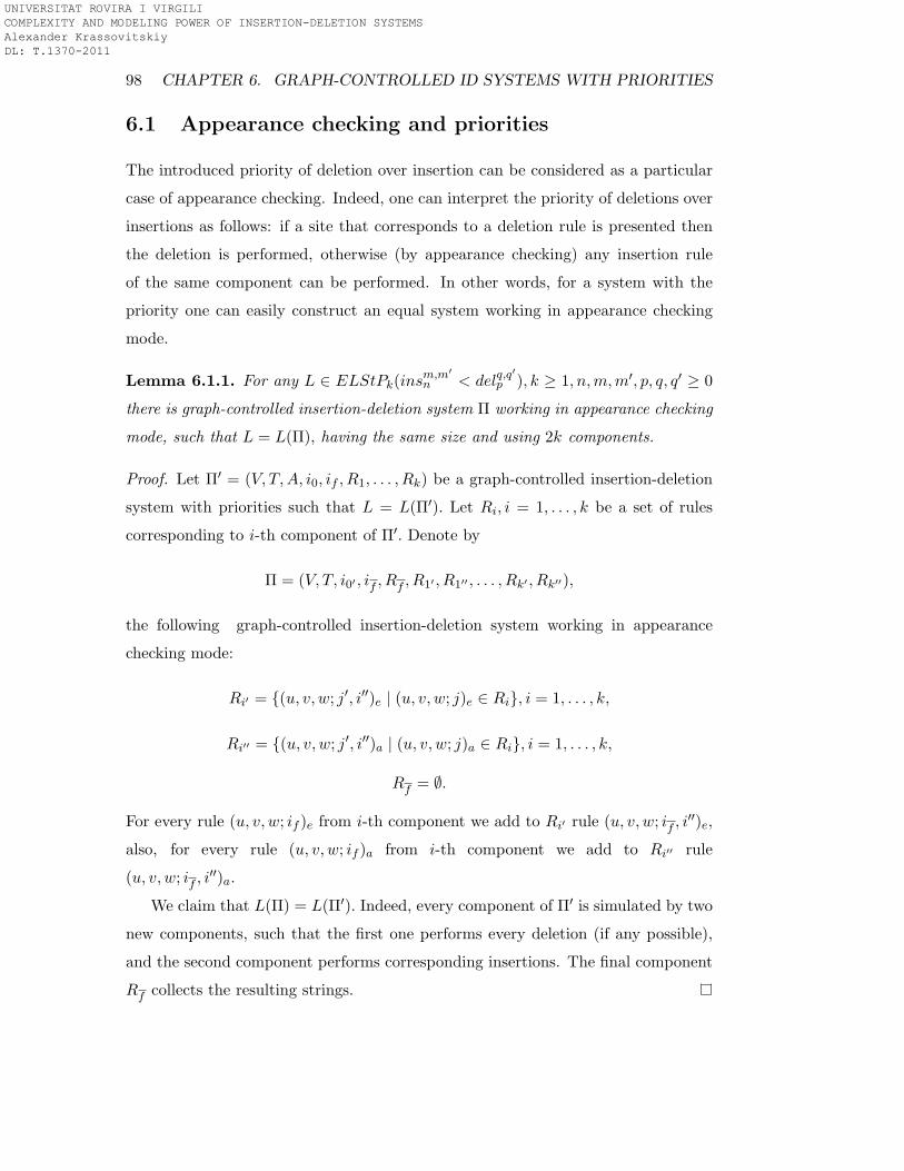
98 CHAPTER 6. GRAPH-CONTROLLED ID SYSTEMS WITH PRIORITIES
6.1 Appearance checking and priorities
The introduced priority of deletion over insertion can be considered as a particular
case of appearance checking. Indeed, one can interpret the priority of deletions over
insertions as follows: if a site that corresponds to a deletion rule is presented then
the deletion is performed, otherwise (by appearance checking) any insertion rule
of the same component can be performed. In other words, for a system with the
priority one can easily construct an equal system working in appearance checking
mode.
Lemma 6.1.1. For any L ∈ ELStPk(insm,m′
n < delq,q′
p ), k ≥ 1, n,m,m′, p, q, q′ ≥ 0
there is graph-controlled insertion-deletion system Π working in appearance checking
mode, such that L = L(Π), having the same size and using 2k components.
Proof. Let Π′ = (V, T,A, i0, if , R1, . . . , Rk) be a graph-controlled insertion-deletion
system with priorities such that L = L(Π′). Let Ri, i = 1, . . . , k be a set of rules
corresponding to i-th component of Π′. Denote by
Π = (V, T, i0′ , if , Rf , R1′ , R1′′ , . . . , Rk′ , Rk′′),
the following graph-controlled insertion-deletion system working in appearance
checking mode:
Ri′ = {(u, v, w; j′, i′′)e | (u, v, w; j)e ∈ Ri}, i = 1, . . . , k,
Ri′′ = {(u, v, w; j′, i′′)a | (u, v, w; j)a ∈ Ri}, i = 1, . . . , k,
Rf = ∅.
For every rule (u, v, w; if )e from i-th component we add to Ri′ rule (u, v, w; if , i′′)e,
also, for every rule (u, v, w; if )a from i-th component we add to Ri′′ rule
(u, v, w; if , i′′)a.
We claim that L(Π) = L(Π′). Indeed, every component of Π′ is simulated by two
new components, such that the first one performs every deletion (if any possible),
and the second component performs corresponding insertions. The final component
Rf collects the resulting strings.
UNIVERSITAT ROVIRA I VIRGILI COMPLEXITY AND MODELING POWER OF INSERTION-DELETION SYSTEMS Alexander Krassovitskiy DL: T.1370-2011
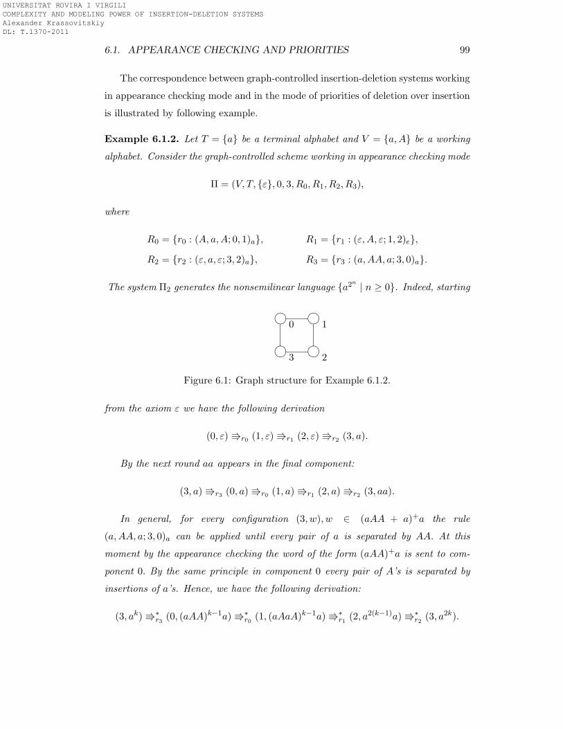
6.1. APPEARANCE CHECKING AND PRIORITIES 99
The correspondence between graph-controlled insertion-deletion systems working
in appearance checking mode and in the mode of priorities of deletion over insertion
is illustrated by following example.
Example 6.1.2. Let T = {a} be a terminal alphabet and V = {a,A} be a working
alphabet. Consider the graph-controlled scheme working in appearance checking mode
Π = (V, T, {ε}, 0, 3, R0, R1, R2, R3),
where
R0 = {r0 : (A, a,A; 0, 1)a}, R1 = {r1 : (ε,A, ε; 1, 2)e},
R2 = {r2 : (ε, a, ε; 3, 2)a}, R3 = {r3 : (a,AA, a; 3, 0)a}.
The system Π2 generates the nonsemilinear language {a2n| n ≥ 0}. Indeed, starting
/.-,()*+
0/.-,()*+
1
/.-,()*+
3/.-,()*+
2
Figure 6.1: Graph structure for Example 6.1.2.
from the axiom ε we have the following derivation
(0, ε) Vr0 (1, ε) Vr1 (2, ε) Vr2 (3, a).
By the next round aa appears in the final component:
(3, a) Vr3 (0, a) Vr0 (1, a) Vr1 (2, a) Vr2 (3, aa).
In general, for every configuration (3, w), w ∈ (aAA + a)+a the rule
(a,AA, a; 3, 0)a can be applied until every pair of a is separated by AA. At this
moment by the appearance checking the word of the form (aAA)+a is sent to com-
ponent 0. By the same principle in component 0 every pair of A’s is separated by
insertions of a’s. Hence, we have the following derivation:
(3, ak) V∗r3
(0, (aAA)k−1a) V∗r0
(1, (aAaA)k−1a) V∗r1
(2, a2(k−1)a) V∗r2
(3, a2k).
UNIVERSITAT ROVIRA I VIRGILI COMPLEXITY AND MODELING POWER OF INSERTION-DELETION SYSTEMS Alexander Krassovitskiy DL: T.1370-2011
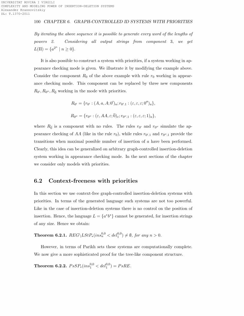
100 CHAPTER 6. GRAPH-CONTROLLED ID SYSTEMS WITH PRIORITIES
By iterating the above sequence it is possible to generate every word of the lengths of
powers 2. Considering all output strings from component 3, we get
L(Π) = {a2n| n ≥ 0}.
It is also possible to construct a system with priorities, if a system working in ap-
pearance checking mode is given. We illustrate it by modifying the example above.
Consider the component R0 of the above example with rule r0 working in appear-
ance checking mode. This component can be replaced by three new components
R0′ , R0′′ , R0 working in the mode with priorities.
R0′ = {r0′ : (A, a,A; 0′)a; r0′.1 : (ε, ε, ε; 0
′′)a},
R0′′ = {r0′′ : (ε,AA, ε; 0)e; r0′′.1 : (ε, ε, ε; 1)a},
where R0 is a component with no rules. The rules r0′ and r0′′ simulate the ap-
pearance checking of AA (like in the rule r0), while rules r0′.1 and r0′′.1 provide the
transitions when maximal possible number of insertion of a have been performed.
Clearly, this idea can be generalized on arbitrary graph-controlled insertion-deletion
system working in appearance checking mode. In the next sections of the chapter
we consider only models with priorities.
6.2 Context-freeness with priorities
In this section we use context-free graph-controlled insertion-deletion systems with
priorities. In terms of the generated language such systems are not too powerful.
Like in the case of insertion-deletion systems there is no control on the position of
insertion. Hence, the language L = {a∗b∗} cannot be generated, for insertion strings
of any size. Hence we obtain:
Theorem 6.2.1. REG\LStP∗(ins0,0n < del0,01 ) 6= ∅, for any n > 0.
However, in terms of Parikh sets these systems are computationally complete.
We now give a more sophisticated proof for the tree-like component structure.
Theorem 6.2.2. PsSP∗(ins0,01 < del0,01 ) = PsRE.
UNIVERSITAT ROVIRA I VIRGILI COMPLEXITY AND MODELING POWER OF INSERTION-DELETION SYSTEMS Alexander Krassovitskiy DL: T.1370-2011
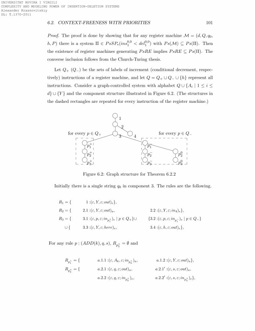
6.2. CONTEXT-FREENESS WITH PRIORITIES 101
Proof. The proof is done by showing that for any register machine M = (d,Q, q0,
h, P ) there is a system Π ∈ PsSP∗(ins0,01 < del0,01 ) with Ps(M) ⊆ Ps(Π). Then
the existence of register machines generating PsRE implies PsRE ⊆ Ps(Π). The
converse inclusion follows from the Church-Turing thesis.
Let Q+ (Q−) be the sets of labels of increment (conditional decrement, respec-
tively) instructions of a register machine, and let Q = Q+ ∪Q− ∪ {h} represent all
instructions. Consider a graph-controlled system with alphabet Q ∪ {Ai | 1 ≤ i ≤
d} ∪ {Y } and the component structure illustrated in Figure 6.2. (The structures in
the dashed rectangles are repeated for every instruction of the register machine.)
/.-,()*+
1/.-,()*+
2KK
KKKK
K
for every p ∈ Q+/.-,()*+
3iiiiiiiiiiiii
UUUUUUUUUUUUU /.-,()*+
4for every p ∈ Q−
/.-,()*+
p+1/.-,()*+
p−1VVVVVVVVVVVVV
/.-,()*+
p+2/.-,()*+
p−2/.-,()*+
p02/.-,()*+
p+3/.-,()*+
p−3/.-,()*+
p03
_ _ _ _�
�
�
�
�
�
�
�
�
�
�
�_ _ _ _
_ _ _ _ _ _ _ _ _ _ _�
�
�
�
�
�
�
�
�
�
�
�_ _ _ _ _ _ _ _ _ _ _
Figure 6.2: Graph structure for Theorem 6.2.2
Initially there is a single string q0 in component 3. The rules are the following.
R1 = { 1 :(ε, Y, ε; out)e},
R2 = { 2.1 :(ε, Y, ε; out)a, 2.2 :(ε, Y, ε; in4)e},
R3 = { 3.1 :(ε, p, ε; inp+
1
)e | p ∈ Q+}∪ {3.2 :(ε, p, ε; inp−
1
)e | p ∈ Q−}
∪ { 3.3 :(ε, Y, ε;here)e, 3.4 :(ε, h, ε; out)e},
For any rule p : (ADD(k), q, s), Rp+3
= ∅ and
Rp+
1
= { a.1.1 :(ε,Ak, ε; inp+
2
)a, a.1.2 :(ε, Y, ε; out)a},
Rp+
2
= { a.2.1 :(ε, q, ε; out)a, a.2.1′ :(ε, s, ε; out)a,
a.2.2 :(ε, q, ε; inp+
3
)e, a.2.2′ :(ε, s, ε; inp+
3
)e},
UNIVERSITAT ROVIRA I VIRGILI COMPLEXITY AND MODELING POWER OF INSERTION-DELETION SYSTEMS Alexander Krassovitskiy DL: T.1370-2011
102 CHAPTER 6. GRAPH-CONTROLLED ID SYSTEMS WITH PRIORITIES
For any rule p : (SUB(k), q, s), Rp−3
= Rp03= ∅ and
Rp−
1
= { e.1.1 :(ε,Ak, ε; inp−
2
)e, e.1.2 :(ε, Y, ε; inp02)a, e.1.3 :(ε, Y, ε; out)e},
Rp−
2
= { e.2.1 :(ε, q, ε; out)a, e.2.2 :(ε, q, ε; inp−
3
)e,
e.2.3 :(ε, s, ε; inp−
3
)e, e.2.4 :(ε, Y, ε;here)a},
Rp02= { e.3.1 :(ε, s, ε; out)a, e.3.2 :(ε, q, ε; inp0
3)e, e.3.3 :(ε, s, ε; inp0
3)e}.
In component 3 configurations (p, x1, . . . , xn) of M are encoded by strings
Perm(pAx1
1 . . . Axnn Y t), t ≥ 0.
We say that such strings have a simulating form. Clearly, in the initial configu-
ration the string is already in the simulating form.
To prove that system Π correctly simulates M we prove the following claims:
1. For any transition (p, x1 . . . xn) ⇒ (q, x′1, . . . , x′n) in M there exist a compu-
tation in Π from the configuration containing Perm(pAx1
1 . . . Axnn Y t) in com-
ponent 3 to the configuration containing Perm(qAx′
1
1 . . . Ax′
nn Y t′), t′ ≥ 0 in
component 3 such that during this computation component 3 is empty on all
intermediate steps and, moreover, this computation is unique.
2. For any successful computation in Π (yielding a non-empty result), com-
ponenet 3 contains only strings of the above form.
3. The result (x1, . . . , xn) in Π is obtained if and only if a string of form
Perm(hAx1
1 . . . Axnn ) appears in component 3.
Now we prove each claim from above. Consider a string Perm(pAx1
1 . . . Axnn Y t),
t ≥ 0 in component 3 of Π. Take an instruction p : (ADD(k), q, s) ∈ P . The only
applicable rule in Π is from the group 3.1 (in the future we simply say rule 3.1)
yielding the string Perm(Ax1
1 . . . Axnn Y t) in component p+1 . After that rule a.1.1
is applied yielding string Perm(Ax1
1 . . . Axk+1k . . . Axn
n Y t) in component p+2 . After
that one of rules a.2.1 or a.2.1′ is applied; then rule a.1.2 yields one of strings
Perm(zAx1
1 . . . Axk+1k . . . Axn
n Y t+1), z ∈ {q, s}, is in the simulating form.
Now suppose that there is an instruction p : (SUB(k), q, s) ∈ P . Then the
only applicable rule in Π is 3.2 which yields the string Perm(Ax1
1 . . . Axnn Y t) in
UNIVERSITAT ROVIRA I VIRGILI COMPLEXITY AND MODELING POWER OF INSERTION-DELETION SYSTEMS Alexander Krassovitskiy DL: T.1370-2011
6.2. CONTEXT-FREENESS WITH PRIORITIES 103
component p−1 . Now if xk > 0, then, due to the priority, rule e.1.1 will be ap-
plied followed by application of rules e.2.4, e.2.1 and e.1.3 which yields the string
Perm(qAx1
1 . . . Axk−1k . . . Axn
n Y t′) that is in the simulating form. If xk = 0, then rule
e.1.2 will be applied (provided that all symbols Y were previously deleted by rule
3.3), followed by rules e.3.1 and e.1.3 which leads to the string Perm(sAx1
1 . . . Axnn )
that is in the simulating form.
To show that component 3 is empty during the intermediate steps, we prove the
following invariant:
Invariant 1. During a successful computation, any visited component p+1 or p−1 is
visited an even number of times as follows: first a string coming from component 3
is sent to an inner component (p+2 , p−2 or p02) and after that a string coming from an
inner component is sent to component 3.
Indeed, since there is only one string in the initial configuration, it is enough to
follow only its evolution. Hence, a sting may visit the node p+1 or p−1 only if on the
previous step symbol p was deleted by one of rules 3.1 or 3.2. If one of rules a.1.2 or
e.1.3 is applied, then component 3 will contain a string of form Perm(Ax1
1 . . . Axnn Y t)
which cannot evolve anymore because all rules in component 3 imply the presence of
symbol from the set Q. Hence, the string is sent to an inner component. In the next
step the string will return from the inner component by one of rules a.2.1, a.2.1′,
e.2.1 or e.3.1 inserting a symbol from Q. If the string enters an inner component
again, then it will be sent to a trap component (p+3 , p−3 or p03) by rules deleting
symbols from Q. Hence the only possibility is to go to component 3 (a string that
visited component p−2 will additionally use rule e.2.4).
For the second claim, it suffices to observe that the invariant above ensures that
in component 3 only one symbol from Q can be present in the string.
The third claim holds since a string may move to component 2 if and only if
the final label h of M appears in component 3. Then, the string is checked for the
absence of symbols Y by rule 2.2 (note that symbols Y can be erased in component 3
by rule 3.3) and sent to the environment by rules 2.1 and 1. Hence, the string sent
to the environment will contain only occurrences of symbols Ai, 1 ≤ i ≤ d.
By induction on the number of computational steps we obtain that Π simulates
UNIVERSITAT ROVIRA I VIRGILI COMPLEXITY AND MODELING POWER OF INSERTION-DELETION SYSTEMS Alexander Krassovitskiy DL: T.1370-2011
104 CHAPTER 6. GRAPH-CONTROLLED ID SYSTEMS WITH PRIORITIES
any computation in M. Claim 1 and 2 imply it is not possible to generate other
strings and Claim 3 implies that the same result is obtained.
We remark that an empty string may be obtained during the proof. This string
can still evolve using insertion rules. If we would like to forbid such evolutions, it
suffices to use a new symbol, e.g. X, in the initial configuration, add new surrounding
component and a rule that deletes X from it.
6.3 Small contextual systems with priorities
Although Theorem 6.2.2 shows that the systems from the previous section are quite
powerful, they cannot generate RE without control on the place where a symbol is
inserted. Once we allow a context in insertion or deletion rules, they can.
Theorem 6.3.1. LSP∗(ins0,11 < del0,01 ) = RE.
Proof. We simulate a register machine with WRITE instructions. We implement
this instruction as an ADD instruction, except the added symbol has to be inserted
to the left of a special marker, deleted at the end, as follows:
• Replace any writing instruction p : (WRITE(A), q, s), A ∈ T of the machine
by instructions p : (ADD(A), q, s), considering output symbols A like new
dummy register. Construct the system Π as in Theorem 6.2.2.
• Change the initial string in component 3 to q0M ;
• Replace rules a.1.1 ((ε,A, ε; inp+2
)a ∈ Rp+1
) by (ε,A,M ; inp+2
)a for A ∈ T ;
• Surround component 1 by a new component o and add to it the following rule
Ro = {(ε,M, ε; out)e}.
It is easy to see that the above construction permits to correctly simulate the register
machine with writing instructions.
Taking M in the left context yields the mirror language. Since RE is closed with
respect to the mirror operation we get the following corollary:
UNIVERSITAT ROVIRA I VIRGILI COMPLEXITY AND MODELING POWER OF INSERTION-DELETION SYSTEMS Alexander Krassovitskiy DL: T.1370-2011
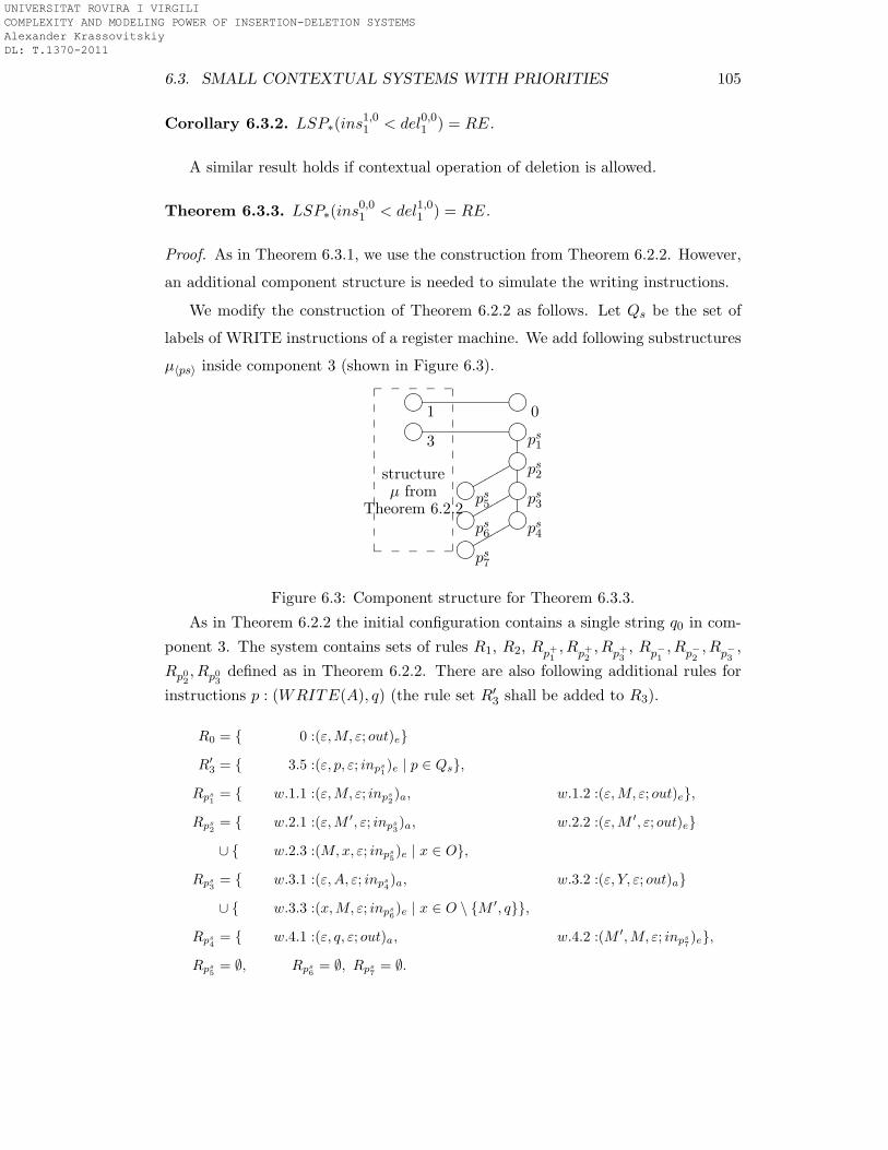
6.3. SMALL CONTEXTUAL SYSTEMS WITH PRIORITIES 105
Corollary 6.3.2. LSP∗(ins1,01 < del0,01 ) = RE.
A similar result holds if contextual operation of deletion is allowed.
Theorem 6.3.3. LSP∗(ins0,01 < del1,01 ) = RE.
Proof. As in Theorem 6.3.1, we use the construction from Theorem 6.2.2. However,
an additional component structure is needed to simulate the writing instructions.
We modify the construction of Theorem 6.2.2 as follows. Let Qs be the set of
labels of WRITE instructions of a register machine. We add following substructures
µ〈ps〉 inside component 3 (shown in Figure 6.3).
/.-,()*+
1/.-,()*+
0/.-,()*+
3/.-,()*+
ps1/.-,()*+
ps2qqqqqq
/.-,()*+
ps5/.-,()*+
ps3qqqqqq
/.-,()*+
ps6/.-,()*+
ps4qqqqqq
/.-,()*+
ps7
_ _ _ _ _�
�
�
�
�
�
�
�
�
�
�
�
�
�
�
�
�
�
�
�
�
�_ _ _ _ _
structureµ from
Theorem 6.2.2
Figure 6.3: Component structure for Theorem 6.3.3.
As in Theorem 6.2.2 the initial configuration contains a single string q0 in com-
ponent 3. The system contains sets of rules R1, R2, Rp+1
, Rp+2
, Rp+3
, Rp−1
, Rp−2
, Rp−3
,
Rp02, Rp0
3defined as in Theorem 6.2.2. There are also following additional rules for
instructions p : (WRITE(A), q) (the rule set R′3 shall be added to R3).
R0 = { 0 :(ε,M, ε; out)e}
R′
3 = { 3.5 :(ε, p, ε; inps
1)e | p ∈ Qs},
Rps
1= { w.1.1 :(ε,M, ε; inps
2)a, w.1.2 :(ε,M, ε; out)e},
Rps
2= { w.2.1 :(ε,M ′, ε; inps
3)a, w.2.2 :(ε,M ′, ε; out)e}
∪ { w.2.3 :(M,x, ε; inps
5)e | x ∈ O},
Rps
3= { w.3.1 :(ε,A, ε; inps
4)a, w.3.2 :(ε, Y, ε; out)a}
∪ { w.3.3 :(x,M, ε; inps
6)e | x ∈ O \ {M ′, q}},
Rps
4= { w.4.1 :(ε, q, ε; out)a, w.4.2 :(M ′,M, ε; inps
7)e},
Rps
5= ∅, Rps
6= ∅, Rps
7= ∅.
UNIVERSITAT ROVIRA I VIRGILI COMPLEXITY AND MODELING POWER OF INSERTION-DELETION SYSTEMS Alexander Krassovitskiy DL: T.1370-2011
106 CHAPTER 6. GRAPH-CONTROLLED ID SYSTEMS WITH PRIORITIES
We simulate the WRITE instruction as follows. Suppose the configuration of
register machine is pAx1
1 . . . Axd
d and the word a1 . . . an is written on the output
tape. The corresponding simulating string in Π will be of form p t⊥ w, where
w = Perm(Ax1
1 . . . Axd
d Yt) t⊥ a1 . . . an, t ≥ 0. After the deletion of the state symbol
p, a markerM is inserted in the string by rule w.1.1. IfM is not inserted at the right
end of the string, in the next step rule w.2.3 is applicable and the string enters the
trap component ps5. In the next step symbol M ′ is inserted in the string. If it is not
inserted before M , then the string is sent to component ps6 by rule w.3.3. Hence, at
this moment the contents of component ps3 is wM ′M . If rule w.3.2 is used, then the
string Y t⊥ w reaches component 3 and no rule is applicable anymore. Otherwise,
symbol A is inserted by rule w.3.1. If it is not between M ′ and M , then rule w.4.2
is applicable and the string enters component ps7. After that q is inserted between
A and M , otherwise the trapping rule w.3.3 is applicable. At this moment, the
configuration of the system consists of the string wtM′AqM in component ps3. Now
if the rule w.3.1 is used, then the string is sent to the trap component by rule w.4.1.
Otherwise, rule w.3.2 should be used followed by the application of rules w.2.2 and
w.1.2, leading to string Y t⊥ wAq in component 3. Hence, the symbol A is appended
at the end of the string. At the end of the computation, all symbols Y are deleted
when the string gets component 0 where the symbol M is further deleted and the
string is sent out. Hence, all symbols from O− T are deleted and a word generated
by M is obtained.
The converse inclusion LSP∗(ins0,01 < del1,01 ) ⊆ RE can be obtained from the
Church-Turing thesis.
Since RE is closed with respect to the mirror operation we obtain:
Corollary 6.3.4. LSP∗(ins0,01 < del0,11 ) = RE.
We remark that the contextual deletion was used only to check for erroneous
evolutions. Therefore we can replace it by a context-free deletion of two symbols.
Theorem 6.3.5. LSP∗(ins0,01 < del0,02 ) = RE.
Proof. We modify the proof of Theorem 6.3.3 as follows.
UNIVERSITAT ROVIRA I VIRGILI COMPLEXITY AND MODELING POWER OF INSERTION-DELETION SYSTEMS Alexander Krassovitskiy DL: T.1370-2011
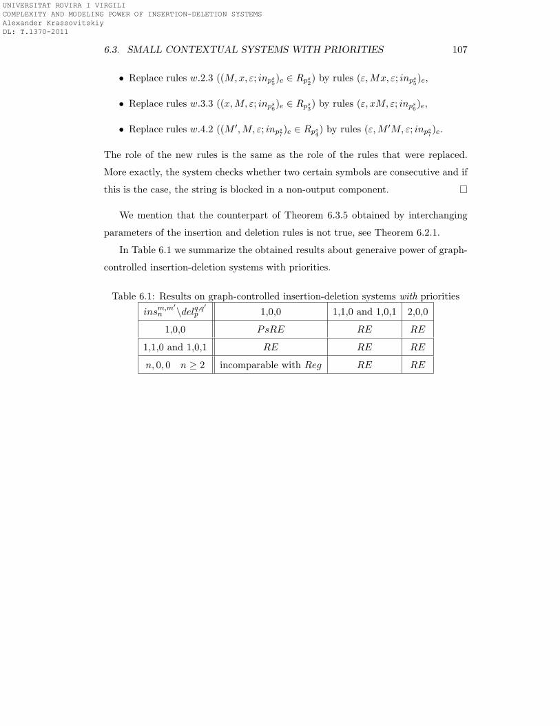
6.3. SMALL CONTEXTUAL SYSTEMS WITH PRIORITIES 107
• Replace rules w.2.3 ((M,x, ε; inps5)e ∈ Rps
2) by rules (ε,Mx, ε; inps
5)e,
• Replace rules w.3.3 ((x,M, ε; inps6)e ∈ Rps
3) by rules (ε, xM, ε; inps
6)e,
• Replace rules w.4.2 ((M ′,M, ε; inps7)e ∈ Rps
4) by rules (ε,M ′M, ε; inps
7)e.
The role of the new rules is the same as the role of the rules that were replaced.
More exactly, the system checks whether two certain symbols are consecutive and if
this is the case, the string is blocked in a non-output component.
We mention that the counterpart of Theorem 6.3.5 obtained by interchanging
parameters of the insertion and deletion rules is not true, see Theorem 6.2.1.
In Table 6.1 we summarize the obtained results about generaive power of graph-
controlled insertion-deletion systems with priorities.
Table 6.1: Results on graph-controlled insertion-deletion systems with priorities
insm,m′
n \delq,q′
p 1,0,0 1,1,0 and 1,0,1 2,0,0
1,0,0 PsRE RE RE
1,1,0 and 1,0,1 RE RE RE
n, 0, 0 n ≥ 2 incomparable with Reg RE RE
UNIVERSITAT ROVIRA I VIRGILI COMPLEXITY AND MODELING POWER OF INSERTION-DELETION SYSTEMS Alexander Krassovitskiy DL: T.1370-2011
UNIVERSITAT ROVIRA I VIRGILI COMPLEXITY AND MODELING POWER OF INSERTION-DELETION SYSTEMS Alexander Krassovitskiy DL: T.1370-2011
Conclusions
In this thesis we have studied insertion-deletion systems and their extensions. We
started our investigation from the pure insertion systems and their extensions by the
graph-controlled scheme. We showed a series of characterizations of known language
classes by the means of such systems.
Next we considered the generative power of insertion-deletion systems. We closed
the last open question for symmetrical insertion-deletion systems concerning compu-
tational completeness of systems of size (2, 0, 0; 1, 1, 1). After that we concentrated
on the study of non-symmetrical insertion-deletion systems. We showed a series of
completeness results for systems of small sizes. The summary of these results is
given in Table 4.2. The most interesting is that we showed that some classes of
insertion-deletion systems are not computationally complete. We also succeeded to
give a characterization to one of them.
Further, for these uncomplete systems we introduced and studied graph-
controlled variants. In all the cases we observed that the computational power of
such systems is increased. Finally, we made another extension of graph-controlled
systems by introducing priorities that are a particular case of appearance check-
ing. This further increases the computational power. Surprisingly, we showed that
it is possible to obtain the whole class PsRE with the system having context-free
one symbol insertion and deletion rules. By introducing contextual insertion and
deletion, any RE language can be generated.
The obtained results permit us to approach the question about the borderline
between computationally complete and uncomplete systems for insertion-deletion
systems.
109
UNIVERSITAT ROVIRA I VIRGILI COMPLEXITY AND MODELING POWER OF INSERTION-DELETION SYSTEMS Alexander Krassovitskiy DL: T.1370-2011
110 CONCLUSIONS
Now, let us formulate some interesting problems raised by our research. First of
all we recall Table 4.2, where the results for one-sided insertion-deletion systems are
collected. It follows from this table that there are several one-sided insertion-deletion
systems for which the generative power is not yet known. Observing the table we
conjecture that for systems of size (n,m,m′, 2, 0, 0), if n +m +m′ ≥ 3, we can get
the computational completeness, while if n+m+m′ < 3 the corresponding systems
are uncomplete. Similarly, we conjecture that systems of size (n,m,m′, 1, 1, 0) are
computationally complete, if n + m + m′ ≥ 4, while in the case n + m + m′ < 4
such systems are likely to be uncomplete. The insertion-deletion systems which
have both contexts (for insertion and for deletion) on the same side, i.e, of the form
(n,m, 0; p, q, 0), n + p ≤ 4,m + q ≥ 1 need further investigation. We think that
the method of direct simulation used in Chapter 4 gives a good way to solve these
problems.
Table 6.2 summarizes the systems for which the question about their computa-
tional complexity has not been answered. Lines 1 and 2 of the table represent the
systems having insertion rules with the maximum length of insertion strings at least
two, while the systems corresponding to lines 3− 8 can insert at most one symbol.
Lines 1− 4 are mirrored copies of lines 5− 8 with respect to insertion and deletion
parts. We omit the cases which correspond to the interchanges of the left and right
sizes of contexts.
Next problem investigated in the thesis refers to uncomplete insertion-deletion
systems. In Chapter 4 we have studied one-sided uncomplete systems of sizes
(1, 1, 0; 1, 1, 0), (1, 1, 0; 2, 0, 0) and (2, 0, 0; 1, 1, 0). While we described the family
INS1,01 DEL1,0
1 , for the latter two families we could only provide some examples of
regular languages that cannot be generated by either of them. On the other hand,
Lemmas 4.5.4 and 4.5.4 show that INS1,01 DEL1,0
1 is a subclass of INS0,02 DEL1,0
1 ∩
INS1,01 DEL0,0
2 . The question whether we could provide more precise characteriza-
tion for these two small families of languages remains open.
In Chapter 5 uncomplete graph-controlled insertion systems of the size
(2, 0, 0; 2, 0, 0) were considered. Insertion-deletion systems of the same size generate
the family of languages which is a proper subclass of context-free languages [67].
UNIVERSITAT ROVIRA I VIRGILI COMPLEXITY AND MODELING POWER OF INSERTION-DELETION SYSTEMS Alexander Krassovitskiy DL: T.1370-2011
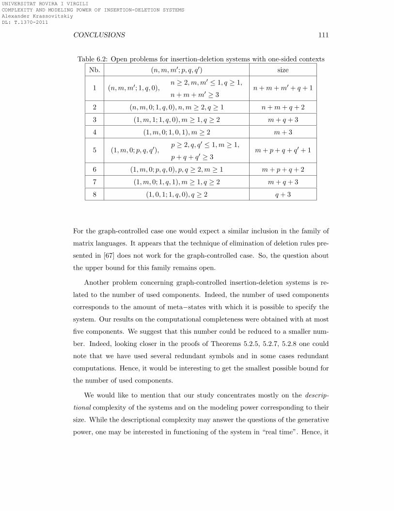
CONCLUSIONS 111
Table 6.2: Open problems for insertion-deletion systems with one-sided contexts
Nb. (n,m,m′; p, q, q′) size
1 (n,m,m′; 1, q, 0),n ≥ 2,m,m′ ≤ 1, q ≥ 1,
n+m+m′ ≥ 3n+m+m′ + q + 1
2 (n,m, 0; 1, q, 0), n,m ≥ 2, q ≥ 1 n+m+ q + 2
3 (1,m, 1; 1, q, 0),m ≥ 1, q ≥ 2 m+ q + 3
4 (1,m, 0; 1, 0, 1),m ≥ 2 m+ 3
5 (1,m, 0; p, q, q′),p ≥ 2, q, q′ ≤ 1,m ≥ 1,
p+ q + q′ ≥ 3m+ p+ q + q′ + 1
6 (1,m, 0; p, q, 0), p, q ≥ 2,m ≥ 1 m+ p+ q + 2
7 (1,m, 0; 1, q, 1),m ≥ 1, q ≥ 2 m+ q + 3
8 (1, 0, 1; 1, q, 0), q ≥ 2 q + 3
For the graph-controlled case one would expect a similar inclusion in the family of
matrix languages. It appears that the technique of elimination of deletion rules pre-
sented in [67] does not work for the graph-controlled case. So, the question about
the upper bound for this family remains open.
Another problem concerning graph-controlled insertion-deletion systems is re-
lated to the number of used components. Indeed, the number of used components
corresponds to the amount of meta−states with which it is possible to specify the
system. Our results on the computational completeness were obtained with at most
five components. We suggest that this number could be reduced to a smaller num-
ber. Indeed, looking closer in the proofs of Theorems 5.2.5, 5.2.7, 5.2.8 one could
note that we have used several redundant symbols and in some cases redundant
computations. Hence, it would be interesting to get the smallest possible bound for
the number of used components.
We would like to mention that our study concentrates mostly on the descrip-
tional complexity of the systems and on the modeling power corresponding to their
size. While the descriptional complexity may answer the questions of the generative
power, one may be interested in functioning of the system in “real time”. Hence, it
UNIVERSITAT ROVIRA I VIRGILI COMPLEXITY AND MODELING POWER OF INSERTION-DELETION SYSTEMS Alexander Krassovitskiy DL: T.1370-2011

112 CONCLUSIONS
could be important to investigate such dynamical properties of the insertion-deletion
systems as length of computations, frequency of visited components, confluence of
the computation, etc.
Our investigation showed that the concept of insertion-deletion systems can be
adapted for the graph-controlled framework. It can be also useful to extend insertion-
deletion systems by other regulations as matrix, (un)ordered, random-context, con-
ditional, valence grammars, etc.
In conclusion, we would like to add that the study of the insertion-deletion
systems is quite inspiring and could give many new opportunities and we expect
many outcomes in the future.
UNIVERSITAT ROVIRA I VIRGILI COMPLEXITY AND MODELING POWER OF INSERTION-DELETION SYSTEMS Alexander Krassovitskiy DL: T.1370-2011
Bibliography
[1] L. M. Adleman. Molecular computation of solutions to combinatorial problems.
Science, 266:1021–1024, 11, 1994.
[2] B. Alberts, A. Johnson, J. Lewis, M. Raff, K. Roberts, and P. Walter. Molecular
Biology of the Cell, Fourth Edition. Garland, 2002.
[3] A. Alhazov, E. Csuhaj-Varju, C. Martın-Vide, and Y. Rogozhin. On the size of
computationally complete hybrid networks of evolutionary processors. Theor.
Comput. Sci., 410(35):3188–3197, 2009.
[4] A. Alhazov, G. B. Enguix, and Y. Rogozhin. Obligatory hybrid networks of
evolutionary processors. In J. Filipe, A. L. N. Fred, and B. Sharp, editors,
Proceedings of the International Conference on Agents and Artificial Intelli-
gence, ICAART 2009, Porto, Portugal, January 19 - 21, 2009, pages 613–618.
INSTICC Press, 2009.
[5] A. Alhazov, R. Freund, and A. Riscos-Nunez. One and two polarizations,
membrane creation and objects complexity in P systems. In SYNASC, vol-
ume Seventh International Symposium on Symbolic and Numeric Algorithms
for Scientific Computing (SYNASC 2005), 25-29 September 2005, Timisoara,
Romania, pages 385–394. IEEE Computer Society, 2005.
[6] A. Alhazov, A. Krassovitskiy, Y. Rogozhin, and S. Verlan. A note on P systems
with small-size insertion and deletion. In Proceedings of the 10th Workshop on
Membr ane Computing, WMC10, Curtea de Arges (Romania), August 24-27,
pages 534–537, 2009.
113
UNIVERSITAT ROVIRA I VIRGILI COMPLEXITY AND MODELING POWER OF INSERTION-DELETION SYSTEMS Alexander Krassovitskiy DL: T.1370-2011
114 BIBLIOGRAPHY
[7] A. Alhazov, A. Krassovitskiy, Y. Rogozhin, and S. Verlan. P systems with
minimal insertion and deletion. In BWMC09, pages 9–22, 2009.
[8] A. Alhazov, A. Krassovitskiy, Y. Rogozhin, and S. Verlan. Small Size Insertion
and Deletion Systems, volume 2. Scientific Applicatioons of Language Methods
of Mathematics, Computing, Language, and Life: Frontiers in Mathematical
Linguistics and Language Theory, pages 459–524. World Scientific, 2010.
[9] A. Alhazov, A. Krassovitskiy, Y. Rogozhin, and S. Verlan. P systems with
minimal insertion and deletion. Theor. Comput. Sci., 412:136–144, 2011.
[10] A. Alhazov, C. Martın-Vide, B. Truthe, J. Dassow, and Y. Rogozhin. On
networks of evolutionary processors with nodes of two types. Fundam. Inform.,
91(1):1–15, 2009.
[11] G. Bel, P. Domosi, and A. Krassovitskiy. Parsing by simple insertion systems.
In Computing Languages with Multi-Agent Systems and Bio-Inspired Devices -
LAMAS 2010 , Special Session of ICAART Valencia, 2010.
[12] R. Benne. RNA Editing: The Alteration of Protein Coding Sequences of RNA.
Ellis Horwood, Chichester, West Sussex, 1993.
[13] F. Biegler, M. J. Burrell, and M. Daley. Regulated RNA rewriting: Modelling
RNA editing with guided insertion. Theor. Comput. Sci., 387(2):103 – 112,
2007. Descriptional Complexity of Formal Systems.
[14] M. J. Burrell. Computational Modelling of Uridine Insertion and Deletion in
Kinetoplasid RNA. PhD thesis, The University of Western Ontario, 2005.
[15] J. Castellanos, C. Martın-Vide, V. Mitrana, and J. M. Sempere. Solving NP-
complete problems with networks of evolutionary processors. In J. Mira and
A. Prieto, editors, Connectionist Models of Neurons, Learning Processes and
Artificial Intelligence, 6th International Work-Conference on Artificial and Nat-
ural Neural Networks, IWANN 2001 Granada, Spain, June 13-15, 2001, Pro-
ceedings, Part I, volume 2084 of Lecture Notes in Computer Science, pages
621–628. Springer, 2001.
UNIVERSITAT ROVIRA I VIRGILI COMPLEXITY AND MODELING POWER OF INSERTION-DELETION SYSTEMS Alexander Krassovitskiy DL: T.1370-2011
BIBLIOGRAPHY 115
[16] E. Csuhaj-Varju and J. Dassow. On cooperating/distributed grammar systems.
Elektronische Informationsverarbeitung und Kybernetik, 26(1/2):49–63, 1990.
[17] E. Csuhaj-Varju, C. Martın-Vide, and V. Mitrana. Hybrid networks of evolu-
tionary processors are computationally complete. Acta Inf., 41(4-5):257–272,
2005.
[18] M. Daley, L. Kari, G. Gloor, and R. Siromoney. Circular contextual
insertions/deletions with applications to biomolecular computation. In
SPIRE/CRIWG, pages 47–54, 1999.
[19] M. Domaratzki. Semantic shuffle on and deletion along trajectories. In
C. Calude, E. Calude, and M. J. Dinneen, editors, Developments in Language
Theory, volume 3340 of Lecture Notes in Computer Science, pages 163–174.
Springer, 2004.
[20] M. Domaratzki and A. Okhotin. Representing recursively enumerable languages
by iterated deletion. Theor. Comput. Sci., 314(3):451–457, 2004.
[21] S. Eilenberg. Automata, Languages, and Machines. Academic Press, Inc.,
Orlando, FL, USA, 1974.
[22] R. Freund, O. Ibarra, G. Paun, and H.-C. Yen. Matrix languages, register
machines, vector addition systems. In Third Brainstorming Week on Membrane
Computing, pages 155–168. Sevilla, 2005.
[23] R. Freund, M. Kogler, Y. Rogozhin, and S. Verlan. Graph-controlled insertion-
deletion systems. In I. McQuillan and G. Pighizzini, editors, Proceedings Twelfth
Annual Workshop on Descriptional Complexity of Formal Systems, Saskatoon,
Canada, 8-10th August 2010, EPTCS 31, pages 88–98, 2010.
[24] B. Galiukschov. Semicontextual grammars. Matem. Logica i Matem. Lingvis-
tika, pages 38–50, 1981. Tallin University, (in Russian).
[25] J. Goldstine, M. Kappes, C. M. R. Kintala, H. Leung, A. Malcher, and D. Wots-
chke. Descriptional complexity of machines with limited resources. J. Universal
Computer Sci., 8(2):193–234, 2002.
UNIVERSITAT ROVIRA I VIRGILI COMPLEXITY AND MODELING POWER OF INSERTION-DELETION SYSTEMS Alexander Krassovitskiy DL: T.1370-2011
116 BIBLIOGRAPHY
[26] D. Haussler. Insertion and Iterated Insertion as Operations on Formal Lan-
guages. PhD thesis, University of Colorado at Boulder, 1982.
[27] D. Haussler. Insertion languages. Information Sciences, 31(1):77–89, 1983.
[28] J. Hopcroft, R. Motwani, and J. Ullman. Introduction to Automata Theory,
Languages, and Computation. Addison-Wesley, Reading, Mass., 2nd edition,
2001.
[29] M. Ito, L. Kari, and G. Thierrin. Insertion and deletion closure of languages.
Theor. Comput. Sci., 183(1):3–19, 1997.
[30] M. Ito and R. Sugiura. n-insertion on languages. In N. Jonoska, G. Paun, and
G. Rozenberg, editors, Aspects of Molecular Computing, volume 2950 of Lecture
Notes in Computer Science, pages 213–218. Springer, 2004.
[31] L. Kari. On Insertion and Deletion in Formal Languages. PhD thesis, University
of Turku, 1991.
[32] L. Kari. From micro-soft to bio-soft: Computing with DNA. In D. Lundh,
B. Olsson, and A. Narayanan, editors, Biocomputing and emergent computation:
Proceedings of BCEC97, pages 146–164. World Scientific, 1997.
[33] L. Kari, G. Paun, G. Thierrin, and S. Yu. At the crossroads of DNA computing
and formal languages: Characterizing RE using insertion-deletion systems. In
Proceedings of 3rd DIMACS Workshop on DNA Based Computing, pages 318–
333. Philadelphia, 1997.
[34] L. Kari and P. Sosık. Aspects of shuffle and deletion on trajectories. Theoretical
Computer Science, 332(1-3):47 – 61, 2005.
[35] L. Kari and P. Sosık. On the weight of universal insertion grammars. Theor.
Comput. Sci., 396(1-3):264–270, 2008.
[36] L. Kari and G. Thierrin. Contextual insertions/deletions and computability.
Inf. Comput., 131(1):47–61, 1996.
UNIVERSITAT ROVIRA I VIRGILI COMPLEXITY AND MODELING POWER OF INSERTION-DELETION SYSTEMS Alexander Krassovitskiy DL: T.1370-2011
BIBLIOGRAPHY 117
[37] I. Katsanyi. A note on restricted insertion-deletion systems. Bulletin of the
EATCS, 83:181–185, 2004.
[38] S. C. Kleene. Representation of events in nerve nets and finite automata. In
C. Shannon and J. McCarthy, editors, Automata Studies, pages 3–41. Princeton
University Press, Princeton, NJ, 1956.
[39] A. Krassovitskiy. On the power of insertion P systems of small size. In
BWMC09, pages 29–44, 2009.
[40] A. Krassovitskiy. On the power of small size insertion P systems. IJCCC,
VI(2):266–277, June 2011. in press.
[41] A. Krassovitskiy, Y. Rogozhin, and S. Verlan. Computational power of P sys-
tems with small size insertion and deletion rules. In T. Neary, D. Woods, A. K.
Seda, and N. Murphy, editors, Complexity of Simple Programs 2008, CSP 2008,
Cork, Ireland, December 6-7, 2008. Proceedings, pages 137–148. Cork Univer-
sity Press, 2008. Invited Paper.
[42] A. Krassovitskiy, Y. Rogozhin, and S. Verlan. Further results on insertion-
deletion systems with one-sided contexts. In C. Martın-Vide, F. Otto, and
H. Fernau, editors, Language and Automata Theory and Applications, Second
International Conference, LATA 2008, Tarragona, Spain, March 13-19, 2008.
Revised Papers, volume 5196 of Lecture Notes in Computer Science, pages 333–
344. Springer, 2008.
[43] A. Krassovitskiy, Y. Rogozhin, and S. Verlan. One-sided insertion and deletion:
Traditional and P systems case. In E. Csuhaj-Varju, R. Freund, M. Oswald, and
K. Salomaa, editors, International Workshop on Computing with Biomolecules,
August 27th, 2008, Wien, Austria, pages 53–64. Druckerei Riegelnik, 2008.
[44] A. Krassovitskiy, Y. Rogozhin, and S. Verlan. Computational power of
insertion-deletion (P) systems with rules of size two. Natural Computing, 2010.
In press: DOI 10.1007/s11047-010-9208-y.
UNIVERSITAT ROVIRA I VIRGILI COMPLEXITY AND MODELING POWER OF INSERTION-DELETION SYSTEMS Alexander Krassovitskiy DL: T.1370-2011
118 BIBLIOGRAPHY
[45] S. N. Krishna. Languages of P Systems: Computability and Complexity. PhD
thesis, Indian Institute of Technology Madras, 2001.
[46] S. N. Krishna and R. Rama. Insertion-deletion P systems. In N. Jonoska
and N. C. Seeman, editors, DNA, volume 2340 of Lecture Notes in Computer
Science, pages 360–370. Springer, 2001.
[47] S. Marcus. Contextual grammars. Rev. Roum. Math. Pures Appl., 14:1525–
1534, 1969.
[48] S. Marcus, G. Paun, and C. Martın-Vide. Contextual grammars as generative
models of natural languages. Computational Linguistics, 24(2):245–274, 1998.
[49] M. Margenstern, G. Paun, Y. Rogozhin, and S. Verlan. Context-free insertion-
deletion systems. Theor. Comput. Sci., 330(2):339–348, 2005.
[50] C. Martın-Vide, G. Paun, and A. Salomaa. Characterizations of recursively
enumerable languages by means of insertion grammars. Theor. Comput. Sci.,
205(1-2):195–205, 1998.
[51] A. Matveevici, Y. Rogozhin, and S. Verlan. Insertion-deletion systems with
one-sided contexts. In J. O. Durand-Lose and M. Margenstern, editors, Ma-
chines, Computations, and Universality, 5th International Conference, MCU
2007, Orleans, France, September 10-13, 2007, Proceedings, volume 4664 of
Lecture Notes in Computer Science, pages 205–217. Springer, 2007.
[52] M. Minsky. Computation: Finite and Infinite Machines. Prentice Hall, NJ,
Englewood Cliffs, 1967.
[53] V. Mitrana and B. Truthe. On accepting networks of evolutionary processors
with at most two types of nodes. In A. H. Dediu, A.-M. Ionescu, and C. Martın-
Vide, editors, Language and Automata Theory and Applications, Third Interna-
tional Conference, LATA 2009, Tarragona, Spain, April 2-8, 2009. Proceedings,
volume 5457 of Lecture Notes in Computer Science, pages 588–600. Springer,
2009.
UNIVERSITAT ROVIRA I VIRGILI COMPLEXITY AND MODELING POWER OF INSERTION-DELETION SYSTEMS Alexander Krassovitskiy DL: T.1370-2011
BIBLIOGRAPHY 119
[54] M. Mutyam, K. Krithivasan, and A. S. Reddy. On characterizing recursively
enumerable languages by insertion grammars. Fundam. Inform., 64(1-4):317–
324, 2005.
[55] K. Onodera. A note on homomorphic representation of recursively enumerable
languages with insertion grammars. Transactions of Information Processing
Society of Japan, 44(5):1424–1427, 2003.
[56] K. Onodera. New morphic characterizations of languages in Chomsky hierarchy
using insertion and locality. In A. H. Dediu, A.-M. Ionescu, and C. Martın-Vide,
editors, Language and Automata Theory and Applications, Third International
Conference, LATA 2009, Tarragona, Spain, April 2-8, 2009., volume 5457 of
Lecture Notes in Computer Science, pages 648–659. Springer, 2009.
[57] G. Paun, G. Rozenberg, and A. Salomaa, editors. The Oxford Handbook of
Membrane Computing. Oxford University Press, 2010.
[58] G. Paun. Marcus Contextual Grammars. Kluwer Academic Publishers, Norwell,
MA, USA, 1997.
[59] G. Paun. Computing with membranes. J. Comput. Syst. Sci., 61(1):108–143,
2000.
[60] G. Paun. Membrane Computing. An Introduction. Springer-Verlag, 2002.
[61] G. Paun, M. J. Perez-Jimenez, and T. Yokomori. Representations and charac-
terizations of languages in Chomsky hierarchy by means of insertion-deletion
systems. Int. J. Found. Comput. Sci., 19(4):859–871, 2008.
[62] G. Paun, G. Rozenberg, and A. Salomaa. DNA Computing: New Computing
Paradigms. Springer, 1998.
[63] G. Rozenberg and A. Salomaa, editors. Handbook of Formal Languages.
Springer-Verlag, Berlin, 1997.
[64] W. D. Smith. DNA computers in vitro and in vivo. In R. Lipton and E. Baum,
editors, Proceedings of DIMACS Workshop on DNA Based Computers, DI-
UNIVERSITAT ROVIRA I VIRGILI COMPLEXITY AND MODELING POWER OF INSERTION-DELETION SYSTEMS Alexander Krassovitskiy DL: T.1370-2011
120 BIBLIOGRAPHY
MACS Series in Discrete Math. and Theoretical Computer Science, pages 121–
185. Amer. Math. Society, 1996.
[65] A. Takahara and T. Yokomori. On the computational power of insertion-
deletion systems. In M. Hagiya and A. Ohuchi, editors, DNA Computing, 8th
International Workshop on DNA Based Computers, DNA8, Sapporo, Japan,
June 10-13, 2002, Revised Papers, volume 2568 of Lecture Notes in Computer
Science, pages 269–280, 2002.
[66] A. Takahara and T. Yokomori. On the computational power of insertion-
deletion systems. Natural Computing, 2(4):321–336, 2003.
[67] S. Verlan. On minimal context-free insertion-deletion systems. Journal of Au-
tomata, Languages and Combinatorics, 12(1-2):317–328, 2007.
[68] D. Wood. Theory of Computation. Harper and Row, 1987.
[69] T. Yokomori. YAC: Yet another computation model of self-assembly. IMACS
Series in Discrete Mathematics and Theoretical Computer Science, 1999.
[70] M. Yong, J. Xiao-gang, S. Xian-chuang, and P. Bo. Minimizing of the only-
insertion insdel systems. J. of Zhejiang University, 6(10):1021–1025, 2005.
[71] H. Zantema. Complexity of guided insertion-deletion in rna-editing. In A. H.
Dediu, H. Fernau, and C. Martın-Vide, editors, Language and Automata Theory
and Applications, 4th International Conference, LATA 2010, Trier, Germany,
May 24-28, 2010. Proceedings, volume 6031 of Lecture Notes in Computer Sci-
ence. Springer, 2010.
UNIVERSITAT ROVIRA I VIRGILI COMPLEXITY AND MODELING POWER OF INSERTION-DELETION SYSTEMS Alexander Krassovitskiy DL: T.1370-2011