arX

iv:h

ep-l

at/9

4121

05v1

27

Dec

199

4

ITP-SB-94-57December, 1994

Complex-Temperature Properties of

the 2D Ising Model with βH = ±iπ/2

Victor Matveev∗ and Robert Shrock∗∗

Institute for Theoretical Physics

State University of New York

Stony Brook, N. Y. 11794-3840

Abstract

We study the complex-temperature properties of a rare example of a statistical mechanical

model which is exactly solvable in an external symmetry-breaking field, namely, the Ising

model on the square lattice with βH = ±iπ/2. This model was solved by Lee and Yang

[1]. We first determine the complex-temperature phases and their boundaries. From a

low-temperature, high-field series expansion of the partition function, we extract the low-

temperature series for the susceptibility χ to O(u23), where u = e−4K . Analysing this series,

we conclude that χ has divergent singularities (i) at u = ue = −(3 − 23/2) with exponent

γ′e = 5/4, (ii) at u = 1, with exponent γ′

1 = 5/2, and (iii) at u = us = −1, with exponent

γ′s = 1. We also extract a shorter series for the staggered susceptibility and investigate its

singularities. Using the exact result of Lee and Yang for the free energy, we calculate the

specific heat and determine its complex-temperature singularities. We also carry this out for

the uniform and staggered magnetisation.

∗email: vmatveev@max.physics.sunysb.edu∗∗email: shrock@max.physics.sunysb.edu

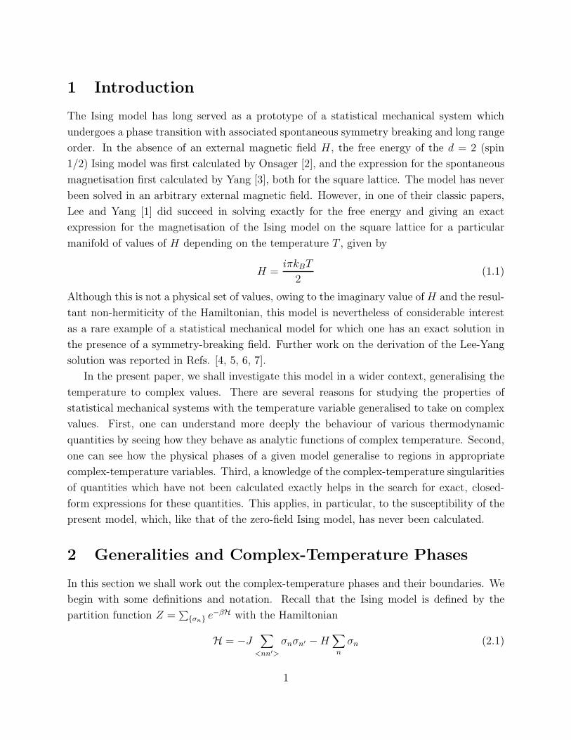
1 Introduction

The Ising model has long served as a prototype of a statistical mechanical system which

undergoes a phase transition with associated spontaneous symmetry breaking and long range

order. In the absence of an external magnetic field H , the free energy of the d = 2 (spin

1/2) Ising model was first calculated by Onsager [2], and the expression for the spontaneous

magnetisation first calculated by Yang [3], both for the square lattice. The model has never

been solved in an arbitrary external magnetic field. However, in one of their classic papers,

Lee and Yang [1] did succeed in solving exactly for the free energy and giving an exact

expression for the magnetisation of the Ising model on the square lattice for a particular

manifold of values of H depending on the temperature T , given by

H =iπkBT

2(1.1)

Although this is not a physical set of values, owing to the imaginary value of H and the resul-

tant non-hermiticity of the Hamiltonian, this model is nevertheless of considerable interest

as a rare example of a statistical mechanical model for which one has an exact solution in

the presence of a symmetry-breaking field. Further work on the derivation of the Lee-Yang

solution was reported in Refs. [4, 5, 6, 7].

In the present paper, we shall investigate this model in a wider context, generalising the

temperature to complex values. There are several reasons for studying the properties of

statistical mechanical systems with the temperature variable generalised to take on complex

values. First, one can understand more deeply the behaviour of various thermodynamic

quantities by seeing how they behave as analytic functions of complex temperature. Second,

one can see how the physical phases of a given model generalise to regions in appropriate

complex-temperature variables. Third, a knowledge of the complex-temperature singularities

of quantities which have not been calculated exactly helps in the search for exact, closed-

form expressions for these quantities. This applies, in particular, to the susceptibility of the

present model, which, like that of the zero-field Ising model, has never been calculated.

2 Generalities and Complex-Temperature Phases

In this section we shall work out the complex-temperature phases and their boundaries. We

begin with some definitions and notation. Recall that the Ising model is defined by the

partition function Z =∑

{σn} e−βH with the Hamiltonian

H = −J∑

<nn′>

σnσn′ − H∑

n

σn (2.1)

1

where σn = ±1 are the Z2 spin variables on each site n of the lattice, β = (kBT )−1, J is the

exchange constant, < nn′ > denote nearest-neighbor pairs, and the units are defined such

that the magnetic moment which would multiply the H∑

n σn is unity. We shall concentrate

here on the square (sq) lattice. We use the standard notation K = βJ , h = βH , v = tanh K,

z = e−2K , u = z2 = e−4K , w = 1/u, and µ = e−2h. Note that v and z are related by the

bilinear conformal transformation

z =1 − v

1 + v(2.2)

It will also be useful to introduce two elliptic moduli. The first is

κ =1

C2=

4u

(1 + u)2(2.3)

which occurs in elliptic integrals in the exact expressions for the internal energy and specific

heat, where we use the abbreviations

C ≡ cosh(2K) (2.4)

S ≡ sinh(2K) (2.5)

We record the symmetry

u → 1/u ⇒ κ → κ (2.6)

The second elliptic modulus,

k< =i

S(S2 + 2)1/2=

4iu

(1 − u)(1 + 6u + u2)1/2(2.7)

occurs in a natural way in the magnetisation.1

The reduced free energy per site is f = −βF = limNs→∞ N−1s ln Z (where Ns denotes

the number of sites on the lattice). In addition to the susceptibility itself, it will also be

convenient to refer to the reduced susceptibility χ = β−1χ.

We begin by discussing the phase boundaries of the model as a function of complex

temperature, i.e. the locus of points across which the free energy is non-analytic. As noted

in Ref. [8], there is an infinite periodicity in complex K under the shift K → K + niπ,

where n is an integer, and, for lattices with even coordination number q, also the shift

K → (2n + 1)iπ/2, as a consequence of the fact that the spin-spin interaction σiσj in H is

an integer. In particular, there is an infinite repetition of phases as functions of complex

K; these repeated phases are reduced to a single set by using the variables v, z, or u (or

variables based on these).

1Note that these differ from the respective elliptic moduli κ0 and k<,0 which occur in the internal energy,specific heat, and spontaneous magnetisation for the Ising model on the square lattice at h = 0.

2

We also note an elementary symmetry involving h for the (spin 1/2) Ising model on a

general lattice Λ. The low-temperature, high-field expansion of Z has the form

Z = e(q/2)NsKeNshZr (2.8)

where

Zr = 1 +∑

n,m

a(Λ)n,mznµm (2.9)

where the only property of Zr that we need is the fact that it is a polynomial in z and µ. In

(2.8), we assume periodic boundary conditions, but for the free energy, in the thermodynamic

limit, this is not essential. Also, parenthetically, we note that for a lattice with even q, only

even powers of z occur in Zr, i.e. Zr is a series in u, but we shall not need this fact here.

Now

h → h + niπ ⇒ µ → µ (2.10)

where n is an integer. Hence, under such a shift, the only change in Z is in the prefactor,

eNsh. Equivalently, in the corresponding (reduced) free energy

f = (q/2)K + h + limNs→∞

N−1s (1 +

∑

n,m

a(Λ)nmznµm) (2.11)

the only change is in the second term, h. Therefore, aside from this term, one may, and we

shall, restrict to the range

− iπ

2< Im(h) ≤ iπ

2(2.12)

without loss of generality. In the present context, we shall consider just the value h = iπ/2;

our results will apply in the same way to h = −iπ/2.

It is useful to review the connection between the square-lattice Ising model with h = iπ/2

and the Ising model on the square lattice in zero field [6, 7]. This is done by first considering

the Ising model on the checkerboard (also called generalised square) lattice, defined by

assigning different couplings Kj, j = 1, ..., 4, to the bonds of the square lattice, as shown

in Fig. 1. Again, for discussions of the partition function, we assume periodic boundary

conditions. The free energy [9] and spontaneous magnetisation [10, 11] are known for the

zero-field checkerboard Ising model. Now recall the identity

ehσ = cosh h + σ sinh h (2.13)

for σ = ±1. For h = iπ/2, this reduces to ehσn = iσn, and hence exp(h∑

n σn) =∏

n(iσn).

Next, consider a dimer site covering of the checkerboard lattice, where by site covering, we

mean that each site is the member of one (and only one) dimer. As is clear from Fig. 1, a

3

simple covering of this sort is provided by each of the bonds of a single type, say those with

the K4 couplings. We may thus associate pairs of the σn’s in the above product with the

dimers of this covering. To do this, we separate one of the two factors of i for such pair and

place it in front of Z. One then has

Zch = iNs/2∑

{σn}

(

∏

<rs>

(iσrσs))

exp(∑

<n,n′>

σnKnn′σn′) (2.14)

where ch denotes checkerboard and Knn′ refers to the appropriate Kj, j = 1, 2, 3, 4 depending

on which bond connects the sites n and n′ (c.f. Fig. 1). Then one can use the identity (2.13)

again to write

Z = iNs/2∑

{σn}

exp(∑

<nn′>

σnK ′n,n′σn′) (2.15)

that is,

Z({Ki}; h = iπ/2)ch = (i)Ns/2Z({K ′i}; h = 0)ch (2.16)

where K ′i = Ki, i = 1, 2, 3, and

K ′4 = K4 +

iπ

2(2.17)

Hence, for the free energy,

f({Ki}; h = iπ/2)ch =iπ

4+ f({K ′

i}; h = 0)ch (2.18)

Then, setting Ki = K, i = 1, 2, 3, 4, one can obtain the Lee-Yang result for f(K, h = iπ/2)

[1] from the (analytic continuation of the) free energy for the zero-field checkerboard lattice

[9]. The same method works for the magnetisation and yields the relation

M({Ki}, h = iπ/2)ch = M({K ′i}, h = 0)ch (2.19)

and for the m-point correlation functions, which satisfy

< σn1 · · · σnm> ({Ki}, h = iπ/2)ch = < σn1 · · · σnm

> ({K ′i}, h = 0)ch (2.20)

Further, it follows from the special case of (2.20) for 2-spin correlation functions, together

with the expression for the susceptibility as a sum over the connected (conn.) 2-spin corre-

lation functions,

χ =∑

r

< σ0σr >conn. (2.21)

(where < σ0σr >conn.≡< σ0σr > −M2) that

χ({Ki}, h = iπ/2)ch = χ({K ′i}, h = 0)ch (2.22)

4

Of course, the Ising model with zero field is not equivalent to one with nonzero field, since

in the former case the partition function and free energy are exactly invariant under the Z2

transformation σn → −σn, whereas in the latter case this symmetry is broken explicitly by

the external field term. This inequivalence is manifested in the fact that eqs. (2.16)-(2.17)

are not Z2-invariant. Thus under the transformation σn → −σn, which is equivalent to

h → −h, the i’s in these equations are replaced by −i. It is also manifested in the fact that

while the zero-field Ising model always has a Z2-symmetric paramagnetic (PM) phase, the

model with nonzero external field h 6= 0 does not have any PM phase. The usefulness of eq.

(2.18) stems from the special feature that for h = ±iπ/2, this non-invariance is localised to

just a constant term in the free energy.

The (reduced) free energy is [1] 2

f(K, h = ±iπ/2) = ±iπ

2+ln 2+

1

4

∫ π

−π

∫ π

−π

dθ1dθ2

(2π)2ln

{

1

2

[

C4+S4−1+S2(

cos(θ1+θ2)−cos(θ1−θ2))

]}

(2.23)

where C and S were defined in (2.4) and (2.5). From U = −∂f/∂β = −J∂f/∂K, one has

the symmetries

U(β, J, H =iπ

2β) = U(β, J, H = − iπ

2β) (2.24)

U(β,−J, h =iπ

2) = U(β, J, h =

iπ

2) (2.25)

U(−β, J, h =iπ

2) = −U(β, J, h =

iπ

2) (2.26)

Similarly, from C = kBK2∂2f/∂K2, one has

C(K, h =iπ

2) = C(K, h = −iπ

2) (2.27)

and

C(K, h =iπ

2) = C(−K, h =

iπ

2) (2.28)

The free energy is trivially divergent at K = ±∞, i.e. u = 0, ∞; however, this will not be

important here since these are isolated points and not part of any phase boundaries. The

curves along which the free energy is non-analytic are given by the locus of points where the

argument of the logarithm in the integrand of eq. (2.23) vanishes. Expressed in terms of the

variable u, f is

f(K, h = ±iπ/2) = ±iπ

2+

1

4ln

[

(1 − u)2

u2

]

+1

4

∫ π

−π

∫ π

−π

dθ1dθ2

(2π)2ln

[

(1+u)2−2uP (θ1, θ2)]

(2.29)

2The Hamiltonian in Ref. [1] was defined with a different zero point of the energy than that used here.

5

where

P (θ1, θ2) = cos θ1 + cos θ2 (2.30)

The above locus of points where the argument of the logarithm vanishes is given by the

solutions of the equation

(1 + u)2 − 2ux = 0 (2.31)

where x = P (θ1, θ2), taking values in the range −2 ≤ x ≤ 2. These are integrable singular-

ities. Since the coefficients in this equation are real, the solutions are either real or consist

of complex conjugate pairs. Moreover, under the replacement u → 1/u, eq. (2.31) retains

its form, up to an overall factor of u−2. Consequently, the locus of solutions is also invariant

under this mapping u → 1/u. The solutions are shown in Fig. 2(a) and consist of the union

of the unit circle

u = eiφ , −π < φ ≤ π (2.32)

and the finite line segment1

ue≤ u ≤ ue (2.33)

where the inner endpoint is

ue = −(3 − 2√

2) = −0.171572875... (2.34)

and the outer endpoint is 1/ue = −(3 + 2√

2) = −5.828427.... Note that ue = −uc, where

uc is the usual critical point in the zero-field square lattice Ising model separating the Z2-

symmetric, paramagnetic (PM) phase from the phase in in the Z2 symmetry is spontaneously

broken by long-range ferromagnetic (FM) long-range order.

It is of interest to see how the solutions to eq. (2.31) are traced out in the complex u

plane as x varies. For x = 2, this equation has a double root at u = 1. As x decreases

from 2 to 0, this root splits into a complex conjugate pair, the members of which move

counterclockwise and clockwise along the unit circle, and finally rejoin to form a double root

at u = −1 when x = 0. As x decreases from 0 to −2, this double root again splits, but

this time into two reciprocal real roots, one of which moves to the right, from u = −1 to

the endpoint ue and the other of which moves leftward to u = 1/ue. The corresponding

phase boundaries in the z plane consist of the unit circle |z| = 1 together with the two line

segments from z = ±ze = ±i(√

2 − 1) upward and downward along the imaginary axis to

z = ∓1/ze = ±i(√

2 + 1), respectively.

The circle (2.32) divides the u plane into two separate phases. A fundamental property of

this model is that the nonzero external field breaks the Z2 symmetry explicitly, so that there

is no Z2-symmetric phase. Even without using the known expression for the magnetisation,

6

one can identify the phases in this diagram as follows. For sufficiently large real K, the

interaction of the external magnetic field with the spins is negligible compared with the

spin-spin interaction, which thus produces a ferromagnetically ordered phase, just as it does

in the model with h = 0. This shows that the neighborhood of the origin in the u (or z) plane

is ferromagnetically ordered. By analytic continuation, it then follows that the entire region

inside the unit circle |u| = 1 is a ferromagnetically ordered phase, and this is so denoted in

Fig. 2(a). Similarly, for sufficiently large negative K, the interaction of the external field

with the spins is again negligible compared with the spin-spin interaction, which produces a

phase with antiferromagnetic (AFM) long-range order. By analogous analytic continuation

arguments, it follows that the entire region outside the unit circle is the AFM phase. This

may be shown as follows. One may think of the phase diagram in the complex variable

w = 1/u. By the u → 1/u symmetry noted above, the phase boundaries in this variable

are the same as those in Fig. 2(a). The above argument shows that the neighborhood of

the origin is antiferromagnetically ordered, and hence, by the same analytic continuation

method, the entire region inside the unit circle |w| = 1 is an AFM phase. Mapping this back

to the u plane, one has shown that the entire region outside of the unit circle |u| = 1 is the

AFM phase. Since the u plane consists of precisely two regions with the property that within

each one can analytically continue from any one point to any other, we have thus obtained

a complete description of the phases in the model. The same reasoning implies that in the z

plane, the phase with |z| < 1 is FM and the phase with |z| > 1 is AFM. In passing, we note

that complex-temperature properties of the h = 0 Ising model on d = 2 lattices have been

studied in Refs. [12, 13, 14, 15, 16, 8, 17, 18, 19, 20]. In the case h = 0 for the square lattice,

the analogous locus of points across which the free energy is singular form a limacon [18]

defined by Re(u) = 1 + 23/2 cos ω + 2 cos 2ω, Im(u) = 23/2 sin ω + 2 sin 2ω for 0 ≤ ω < 2π, or

equivalently, in the z plane, the circles [12] z = ±1 +√

2eiθ, for 0 ≤ θ < 2π.

By the use of the conformal mapping (2.2) on the z plane, or by re-expressing the free

energy in terms of the variable v and again solving for the locus of points where the argument

of the logarithm vanishes, we find that the phase diagram of the model in the v plane is

as shown in Fig. 2(b). The unit circle |z| = 1 is mapped to the imaginary axis in the v

plane, and the respective line segments from z = ±ze to ∓1/ze are mapped to the arcs from

v = e∓iπ/4 to v = e∓3iπ/4. It is interesting that the Re(v) = 0 (i.e. imaginary) axis forms the

boundary between the complex-temperature FM and AFM phases. One may understand

this by recalling that (i) if h were real and positive (negative), this would favor FM (AFM)

ordering, but a pure imaginary value of h does not favor FM over AFM ordering, or vice

versa; (ii) similarly, if the spin-spin coupling K is real and positive (negative), it favors FM

(AFM) ordering, but a pure imaginary value of K (and hence v) does not favor FM over

7

AFM ordering, or vice versa. Therefore, if both h and K are pure imaginary, as is the case

here for the imaginary axis in the v plane, then the system is precisely balanced between FM

and AFM order, so that this axis should be the boundary between the complex-temperature

FM and AFM phases, and this is just what our explicit calculation shows.

The mapping defined by u → κ2, where κ was defined in (2.3), takes the the locus of

points (2.32) and (2.33) to a single semi-infinite line segment extending from 1 to ∞ in the

complex κ2 plane. All points in the κ2 plane are analytically connected to all other points. In

particular, the mapping u → κ2 takes both the complex-temperature FM and AFM phases

in the u plane to the same respective regions in the κ2 plane, as is clear from the symmetry

(2.6) and the fact that the transformation u → 1/u interchanges the FM and AFM phases

in the u plane.

3 Complex-Temperature Behaviour of the Internal En-

ergy and Specific Heat

3.1 Exact Expressions

From the free energy (2.29), it is straightforward to calculate the internal energy U and

specific heat C (per site). In terms of the variable u, we find that

U = −J[

1 + u

1 − u+

(1 − u

1 + u

)(2

π

)

K(κ)]

(3.1.1)

where the elliptic modulus κ was given above in eq. (2.3) and K(k) =∫ π/20 (1−k2 sin2 θ)−1/2dθ

is the complete elliptic integral of the first kind. This expression holds for both the FM

and AFM phases and exhibits the symmetries (2.25) and (2.26). Since either of these has

the effect of taking u → 1/u, and since this mapping takes the interior of the complex-

temperature FM phase to the interior of the complex-temperature AFM phase, the values

of U in these two phases are simply related by (2.25)-(2.26). In the FM phase, the first few

terms of the small-|u| expansion (complex-temperature generalisation of the low-temperature

expansion) are

U = −2J[

1 + 4u2 − 12u3 + 60u4 − 280u5 + O(u6)]

(3.1.2)

In the AFM phase, the corresponding expansion parameter is w = 1/u, and U has the same

expansion as (3.1.2) with J replaced by −J and u replaced by w.

As discussed above, in the limit J → ∞, and hence K → ∞ with fixed H , the spin-spin

interaction overwhelms the contribution of the external field coupling, which therefore has

a negligible effect, to leading order. It follows that in this limit, the value of the internal

8

energy should be the same as the value for h = 0, i.e.,

U(u = 0, h = iπ/2) = U(u = 0, h = 0) (3.1.3)

It is interesting to compare the small-|u| series expansions of these two functions to ascertain

the finite-u corrections to this equality. For this purpose, we recall that [2]

U(K, h = 0) = −J[

1 + u

1 − u+

(1 − 6u + u2)

(1 − u2)

(2

π

)

K(κ0)]

(3.1.4)

where

κ0 =4z(1 − u)

(1 + u)2(3.1.5)

The expression (3.1.10) holds for all phases, PM, FM, and AFM. In the FM phase, it has

the small-|u| expansion

U(h = 0) = −2J[

1 − 4u2 − 12u3 − 36u4 − 120u5 + O(u6)]

(3.1.6)

Clearly, the expansions (3.1.2) and (3.1.6) agree with the relation (3.1.3) for u = 0. U(K, h =

0) also satisfies the symmetries analogous to (2.25) and (2.26), with h = iπ/2 replaced by

h = 0; as a consequence, in the AFM phase, the small-|w| expansion of U(K, h = 0) is given

by (3.1.6) with J replaced by −J and u replaced by w.

For C we get

C

8kBK2= − u

(1 − u)2− (1 + u)2

π(1 + 6u + u2)E(κ) +

(1 + u2)

π(1 + u)2K(κ) (3.1.7)

where K(k) was defined above and E(k) =∫ π/20 (1 − k2 sin2 θ)1/2dθ is the complete elliptic

integral of the second kind. Again, this expression holds for both the FM and AFM phases.

It will also be useful to express C in an equivalent form, using (2.3):

C

8kBK2= − u

(1 − u)2− E(κ)

π(1 + κ)+

(1 + u2)(1 + κ)K(κ)

π(1 + 6u + u2)(3.1.8)

C/K2 has the small-|u| expansion

C

8kBK2= −64u2 + 288u3 − 1920u4 + 11200u5 + O(u6) (3.1.9)

For comparison, the specific heat for the Ising model on the square lattice with h = 0 [2] is

C

kBK2=

4(1 − κ′)

πκ2

[

2{K(κ0) − E(κ0)} − (1 − κ′0){

π

2+ κ′

0K(κ0)}]

(3.1.10)

9

which has the small-|u| expansion

C

kBK2= 64u2 + 288u3 + 1152u4 + 4800u5 + O(u6) (3.1.11)

Of course, in this case, the positivity of the specific heat requires that the coefficient of the

lowest order term must be positive (the first negative coefficient occurs in the u7 term). We

proceed to determine the complex-temperature singularities of U and C for the present case,

h = iπ/2.

3.2 Vicinity of u = ue

As discussed in connection with Fig. 2(a), the point u = ue is the endpoint of the singular line

segment protruding into the complex-temperature extension of the FM phase. All approaches

to this point, except directly from the left along this singular line segment, occur from within

the complex-temperature FM phase. As u → ue = −(3−23/2), κ → −1. The internal energy

diverges likeU

J→

√2

πln(1 − u/ue) , as u → ue (3.2.1)

In the specific heat, the dominant divergence arises from the term in (3.1.7) involving E(κ)

and isC

kBK2→ − 4

√2

π(1 − u/ue), as u → ue (3.2.2)

so that the associated singular exponent for C at u = ue is

α′e,FM ≡ α′

e = 1 (3.2.3)

where the subscript FM indicates the phase from which this point is approached, and the

prime is the standard notation indicating that the approach to this singular point is from

within a broken-symmetry phase. (The last feature is, of course, true of all of the singular

points for h 6= 0.) There is also a weaker, logarithmic divergence arising from the term

involving K(κ). The value of K at ue in (3.2.2) is

Ke = −1

4ln ue = −1

4

[

ln(3 − 23/2) + iπ + 2niπ]

(3.2.4)

where n labels the Riemann sheet used for the evaluation of the logarithm, which we shall

take to be n = 0 below, unless otherwise indicated.

10

3.3 Vicinity of u = 1/ue

The point u = 1/ue is the left end of the singular line segment protruding into the complex-

temperature extension of the AFM phase. Except for the approach directly from the right

along the singular line segment, all approaches to this point occur from within the complex-

temperature AFM phase. As u → 1/ue, κ → −1, as is clear from the previous remarks and

the symmetry (2.6). The internal energy again diverges like

U

J→ −

√2

πln(1 − ueu) , as u → 1

ue(3.3.1)

In the specific heat, the dominant divergence again arises from the term in (3.1.7) involving

E(κ) and isC

kBK2→ 4

√2

π(1 − ueu), as u → 1/ue (3.3.2)

so that the associated singular exponent for C at the outer endpoint (oe) u = 1/ue is

α′oe,AFM ≡ α′

oe = 1 (3.3.3)

The value of K corresponding to u = 1/ue in eq. (3.3.2) is, for the principal Riemann sheet

of the log, Koe = −(1/4)[ln(3 + 23/2) + iπ].

3.4 Vicinity of u = −1

As u → −1 (denoted us), κ diverges; if we set u = −1 + ǫeiφ and let ǫ → 0, then κ ∼−4ǫ−2e−2iφ. One easily sees that U(u = −1) is finite. For C, we observe that the first and

second terms on the right-hand side of eq. (3.1.7) or (3.1.8) are finite. By the use of the

elliptic integral identity (1 + κ)K(κ) = K(2κ1/2/(1 + κ)) (see, e.g. [21]), we can rewrite the

term involving K(κ) in eq. (3.1.8) as

(1 + u2)

π(1 + 6u + u2)K

( 2κ1/2

1 + κ

)

(3.4.1)

As u → −1 and κ diverges, K(2κ1/2/(1 + κ)) → K(0) = π/2, so that C is finite, although

non-analytic, at u = −1. This is true for the approach to u = −1 from either the FM or

AFM phases. We thus have

α′s,FM = α′

s,AFM = 0 (log. finite) (3.4.2)

11

3.5 Vicinity of u = 1

As u → 1, κ → 1. In U the leading potential singularity arises from the first term in (3.1.1)

U

J→ −2

1 − uas u → 1 (3.5.1)

Now K = −(1/4) lnu, so that, if one uses the first Riemann sheet of the logarithm, then

u → 1 maps to K → 0. Recalling that K = βJ , if this zero in K is due to β → 0 at fixed

nonzero J , then eq. (3.5.1) shows that U diverges for u → 1; however, if the zero in K is

due to J → 0 at fixed nonzero β, then, expanding (3.5.1), one finds that U → 1/(2β).

For the specific heat, from (3.1.7), it follows that as u → 1,

k−1B C → 8K2

[

− 1

(1 − u)2+

1

4πln

( 32

(1 − u)2

)

+ ...]

(3.5.2)

where ... refers to less singular terms. If we again use the principal Riemann sheet of the

logarithm, so that u → 1 corresponds to K → 0, then (3.5.2) becomes

k−1B C → −1

2+

2

πK2 ln

( 2

K2

)

+ O(K2) as u → 1 (3.5.3)

That is, C has a finite logarithmic singularity at this point, and hence a corresponding

exponent

α′1,FM = α′

1,AFM = 0 (log. finite) (3.5.4)

In passing, we note that if one were to use a Riemann sheet different than the principal

(n = 0) one in evaluating K = −(1/4) ln(1), so that K = −inπ/2 6= 0, then C would diverge

quadratically at u = 1.

3.6 Elsewhere Along the Singular Curves

We discuss here the behaviour of U and C as one crosses the singular locus of points comprised

by the unit circle (2.32) and the line segment (2.33) away from the points u = ue, 1/ue, −1,

and 1. The singularities which one encounters in this case are associated with passage across

the branch cut of the elliptic integrals in (3.1.1) and (3.1.7). We recall that the elliptic

integrals K(κ) and E(κ) are analytic functions of κ2 in the complex κ2 plane except for

respectively divergent and finite branch points at κ2 = 1 and an associated branch cut,

which is normally taken to run from κ2 = 1 to κ2 = ∞ along the positive real axis in this

plane. To illustrate the nature of the singularities, we shall consider moving outward along a

ray in the u plane defined by u = ρeiθ with ρ increasing from 0 to ∞ at fixed θ, say θ = π/6.

As shown in Fig. 3, the image point in the κ2 plane also moves out from the origin, starting

12

with an angle of π/3 but bending around to the right. As we cross the unit circle in the u

plane, leaving the FM phase and entering the AFM phase, the image point in the κ2 plane

crosses the branch cut moving vertically downward. This branch cut is precisely the image

of the unit circle |u| = 1 (and also of the singular line segment (2.33).) For θ = π/6, the

crossing point is at κ2 = 24(7 − 4√

3) = 1.1487.... In the κ2 plane, one thus passes onto the

second Riemann sheet of the elliptic functions K(κ) and E(κ). If one projects back to the

first Riemann sheet, these functions have discontinuous imaginary parts across this branch

cut. As ρ continues to increase toward ∞, κ2 ∼ 16ρ−2e−2θ so that the image point curves

around finally approaches the origin in a “northwest” direction, at an angle of −π/3, but on

the second Riemann sheet. In Fig. 3 we show the image point for ρ in the range from 0 to

30.

4 Complex-Temperature Behaviour of the Uniform and

Staggered Magnetisation

The magnetisation M is [1, 5]

M(u, h = iπ/2) =(1 + u)1/2

(1 − u)1/4(1 + 6u + u2)1/8(4.1)

Note that (1 + 6u + u2) = (1− u/ue)(1− ueu). By analytic continuation, this formula holds

throughout the complex-temperature extension of the FM phase. The identity discussed

above, and the resultant eq. (2.19) yields the relation

M(u, h = ±iπ/2) = M(−u, h = 0)−1 (4.2)

where [3]

M(u, h = 0) =(1 + u)1/4(1 − 6u + u2)1/8

(1 − u)1/2(4.3)

As is well known, one can express M(u, h = 0) as

M(u, h = 0) = (1 − (k<,0)2)1/8 (4.4)

where

k<,0 =1

sinh2(2K)=

4u

(1 − u)2(4.5)

This quantity also enters in exact expressions for correlation functions in the FM phase of

the h = 0 Ising model [22, 23, 24]. Given the relation (4.2), it is natural to write

M(u, h = iπ/2) = (1 − (k<)2)1/8 (4.6)

13

where the elliptic modulus was introduced in eq. (2.7). The magnetisation for the h = iπ/2

case vanishes continuously at the point u = −1 (denoted us) with exponent

βs =1

2(4.7)

diverges at u = ue with exponent

βe = −1

8(4.8)

and diverges at u = 1 with exponent

β1 = −1

4(4.9)

Elsewhere on the boundary of the complex-temperature extension of the FM phase, i.e., the

unit circle in the u plane, M vanishes discontinously. Note that the apparent divergence at

the point u = 1/ue does not actually occur, since this is outside of the complex-temperature

FM phase, where the above analytic continuation is valid.

The staggered magnetisation Mst does not seem to have been explicitly discussed in the

literature, but one can easily obtain it, as follows. Mst may be defined via

M2st = lim

|r|→∞< σ0σr > (4.10)

where

σr = (−1)p(r)σr (4.11)

where

p(r) =2

∑

i=1

ri (4.12)

i.e. σr = σr for r on the same sublattice as r = 0 and −σr for r on the other sublattice of

the (bipartite) square lattice. To evaluate Mst via eq. (4.10), it suffices to take r = (r, 0)

or (0, r), i.e. the row or column 2-spin correlation function. From the known asymptotic

behaviour of this correlation function [5], one immediately finds that

Mst(w) = M(u → w) (4.13)

where, as before, w = 1/u. This is consistent with eq. (4.6) since (c.f. (2.6)) u → 1/u takes

k< → −k<, and k< enters squared in (4.6). Of course, Mst vanishes identically outside the

complex-temperature extension of the AFM phase. Further, we may immediately conclude

that Mst vanishes continuously at u = −1 with exponent (4.7), diverges at u = 1/ue with

exponent (4.8), and diverges at u = 1 with exponent (4.9). Elsewhere along the bound-

ary of the complex-temperature AFM phase, Mst vanishes discontinuously, with the same

discontinuity as M .

14

It is of interest to compare these results with the behaviour of M and Mst for h = 0

(again on the square lattice). Aside from the physical PM-FM and PM-AFM critical points

u = uc = (3 − 23/2) and 1/uc, where, respectively, M and Mst vanish continuously with

exponent β = 1/8, they also both vanish continuously at the complex-temperature point

u = −1, with the same exponent, β = 1/4. Note that for h = 0 there is only one point, viz.,

u = −1, where the FM and AFM phases are contiguous and M and Mst vanish continuously,

whereas for h = iπ/2 there are two such points, namely, u = −1 and u = 1.

5 Extraction and Analysis of the Low-Temperature Se-

ries for χ

5.1 Generalities

In order to investigate the complex-temperature singularities of the susceptibility χ, we

shall make use of the low-temperature, high-field series expansion for the free energy or

equivalently the partition function of the Ising model on the square lattice [25, 26, 27]. In

Ref. [27], Baxter and Enting calculated this expansion for the partition function to order

O(u23). The series for Zr in eq. (2.9) is

Zr = 1 +∞∑

n=2

∑

m

an,munµm (5.1.1)

where j ≤ m ≤ j2 for n = 2j and j ≤ m ≤ j(j − 1) for n = 2j − 1. We extract the series for

h = iπ/2 by calculating χ = ∂2f/∂h2 and then subsituting µ = −1. This has the form

χ(u, h = iπ/2) = 4u2(∞∑

n=0

cnun) (5.1.2)

The results for the cn are listed in Table 1; the series for Z and the resultant series for χ to

O(u23) yields the cn’s to order n = 21. Parenthetically, we note that χ has been calculated to

O(u28) in Ref. [28] and to O(u38) in Ref. [17], but the low-temperature, high-field expansion

of the partition function as a function of µ = e−2h which would be necessary to extract

χ(h = iπ/2) was not given in these papers (it would be a rather long expression).

We have analysed this series using dlog Pade and differential approximants. For a recent

review of these techniques, see Ref. [29]. Our notation for these approximants follows

Ref. [29] and our earlier work on complex-temperature properties of the h = 0 Ising model

[18, 19, 20]. In particular, we use first order differential approximants (i.e., K = 1 in our

previous notation); as before, we used unbiased approximants so as to be able to use an

15

n cn

0 −11 82 −483 3044 −18635 113686 −688407 4148728 −24904379 1490364810 −8896369611 52993917612 −315120547513 1871018019214 −11094803742415 65716471552016 −388867088659317 2299056643290418 −13581911041678419 80180665158884820 −473048538923826321 27892958533539784

Table 1: Low-temperature series expansion coefficients for χ(u, h = iπ/2) in eq. (5.1.2).

16

extrapolation method for extracting critical exponents. Since the prefactor 4u2 is analytic,

we have actually performed the analysis on the reduced function

χr ≡χ

4u2=

∞∑

n=0

cnun (5.1.3)

As one approaches a generic complex singular point denoted sing from within the complex-

temperature extension of the FM phase, χ is assumed to have the leading singularity

χ ∼ A′sing(1 − u/using)

−γ′

sing

(

1 + a1(1 − u/using) + ...)

(5.1.4)

where A′sing and γ′

sing denote, respectively, the critical amplitude and the corresponding

critical exponent, and the ... represent analytic confluent corrections. One may observe that

we have not included non-analytic confluent corrections to the scaling form in eq. (5.1.4).

The reason is that, as discussed in our earlier work [18], previous studies have indicated that

they are very weak or absent for the 2D Ising model. We proceed to our results.

5.2 Singularity at u = ue

Our dlog Pade results relevant to the singularity in χ(u, h = iπ/2) at u = ue are given

in Table 2. Because of the length of our differential approximant results relevant to the

singularity in χ at u = ue, we list these in the Appendix. From these results, we infer the

location of the singularity to be

using. = −0.17157 ± 0.00001 (5.2.1)

This, together with our knowledge of the exact location of the endpoint of the singular

line segment (2.33), supports the conclusion that the exact location of this singularity is at

u = ue = −0.1715729... given in (2.34). Accepting this conclusion, we plot the values of the

corresponding exponent γ′e for the differential approximants as functions of the normalised

distance from this point, i.e., |using. − ue|/|ue| and extrapolate to zero distance. (This ex-

trapolation method is similar to the use of biased differential approximants; in both of these

approaches, one uses one’s knowledge of the exact position of the singularity.) From our

extrapolation, we obtain

γ′e = 1.25 ± 0.01 (5.2.2)

This strongly supports the following inference for the exact value of this exponent, which we

shall make:

γ′e =

5

4(5.2.3)

17

[N/D] using |using − ue|/|ue| γ′e

[5/3] −0.1716072 2.0 × 10−4 1.2492[4/4] −0.1715705 1.4 × 10−5 1.2464[5/4] −0.1715636 5.4 × 10−5 1.2459[6/4] −0.1715646 4.8 × 10−5 1.2460[3/5] −0.1715802 4.3 × 10−5 1.2471[4/5] −0.1715628 5.8 × 10−5 1.2458[5/5] −0.1715645 4.9 × 10−5 1.2460[6/5] −0.1715598 7.6 × 10−5 1.2457[7/5] −0.1715670 3.4 × 10−5 1.2462[4/6] −0.1715647 4.8 × 10−5 1.2460[5/6] −0.1715674 3.2 × 10−5 1.2462[6/6] −0.1715667 3.6 × 10−5 1.2462[7/6] −0.1715667 3.6 × 10−5 1.2462[8/6] −0.1715665 3.7 × 10−5 1.2462[5/7] −0.1715668 3.6 × 10−5 1.2462[6/7] −0.1715667 3.6 × 10−5 1.2462[7/7] −0.1715670 3.4 × 10−5 1.2462[8/7] −0.1715664 3.8 × 10−5 1.2461[9/7] −0.1715664 3.7 × 10−5 1.2461[6/8] −0.1715672 3.3 × 10−5 1.2462[7/8] −0.1715664 3.8 × 10−5 1.2461[8/8] −0.1715665 3.7 × 10−5 1.2461[9/8] −0.1715754 1.5 × 10−5 1.2501[10/8] −0.1715673 3.2 × 10−5 1.2463[7/9] −0.1715665 3.7 × 10−5 1.2461[8/9] −0.1715666 3.6 × 10−5 1.2462[9/9] −0.1715673 3.2 × 10−5 1.2463[10/9] −0.1715677 3.0 × 10−5 1.2464[11/9] −0.1715696 1.9 × 10−5 1.2470[8/10] −0.1715674 3.2 × 10−5 1.2463[9/10] −0.1715686 2.5 × 10−5 1.2466[10/10] −0.1715699 1.7 × 10−5 1.2471[9/11] −0.1715701 1.6 × 10−5 1.2472

Table 2: Values of pole near ue = −(3 − 23/2) = −0.171572875..., normalised distance fromthis point, |using−ue|/|ue|, and exponent γ′

e from dlog Pade approximants to low-temperatureseries for χr(u, h = iπ/2), starting with the series to O(u9). We list only the approximantswhich satisfy the accuracy criterion |using − ue|/|ue| ≤ 2 × 10−4.

18

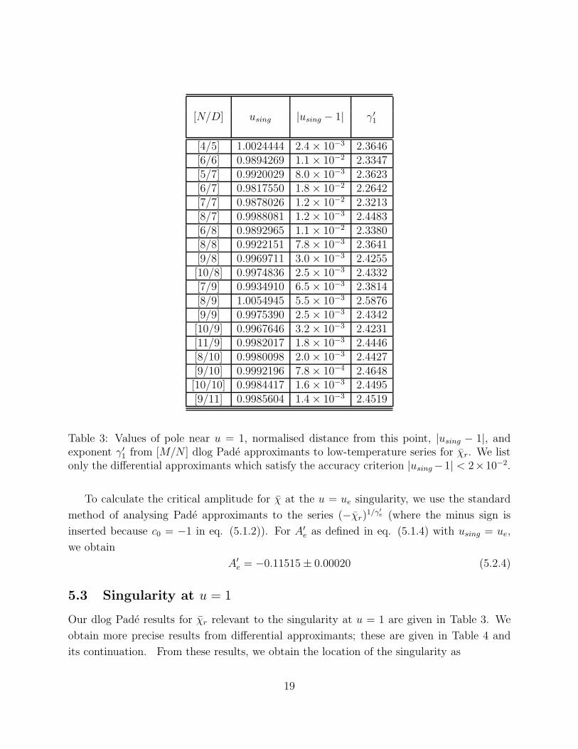
[N/D] using |using − 1| γ′1

[4/5] 1.0024444 2.4 × 10−3 2.3646[6/6] 0.9894269 1.1 × 10−2 2.3347[5/7] 0.9920029 8.0 × 10−3 2.3623[6/7] 0.9817550 1.8 × 10−2 2.2642[7/7] 0.9878026 1.2 × 10−2 2.3213[8/7] 0.9988081 1.2 × 10−3 2.4483[6/8] 0.9892965 1.1 × 10−2 2.3380[8/8] 0.9922151 7.8 × 10−3 2.3641[9/8] 0.9969711 3.0 × 10−3 2.4255[10/8] 0.9974836 2.5 × 10−3 2.4332[7/9] 0.9934910 6.5 × 10−3 2.3814[8/9] 1.0054945 5.5 × 10−3 2.5876[9/9] 0.9975390 2.5 × 10−3 2.4342[10/9] 0.9967646 3.2 × 10−3 2.4231[11/9] 0.9982017 1.8 × 10−3 2.4446[8/10] 0.9980098 2.0 × 10−3 2.4427[9/10] 0.9992196 7.8 × 10−4 2.4648[10/10] 0.9984417 1.6 × 10−3 2.4495[9/11] 0.9985604 1.4 × 10−3 2.4519

Table 3: Values of pole near u = 1, normalised distance from this point, |using − 1|, andexponent γ′

1 from [M/N ] dlog Pade approximants to low-temperature series for χr. We listonly the differential approximants which satisfy the accuracy criterion |using −1| < 2×10−2.

To calculate the critical amplitude for χ at the u = ue singularity, we use the standard

method of analysing Pade approximants to the series (−χr)1/γ′

e (where the minus sign is

inserted because c0 = −1 in eq. (5.1.2)). For A′e as defined in eq. (5.1.4) with using = ue,

we obtain

A′e = −0.11515 ± 0.00020 (5.2.4)

5.3 Singularity at u = 1

Our dlog Pade results for χr relevant to the singularity at u = 1 are given in Table 3. We

obtain more precise results from differential approximants; these are given in Table 4 and

its continuation. From these results, we obtain the location of the singularity as

19

[L/M0; M1] using |using − 1| γ′1

[0/7; 7] 1.0019932 2.0 × 10−3 2.5262[0/7; 9] 0.9983638 1.6 × 10−3 2.4478[0/8; 9] 0.9974253 2.6 × 10−3 2.4337[0/8; 10] 0.9981341 1.9 × 10−3 2.4447[0/9; 9] 0.9999105 0.89 × 10−4 2.4776[0/9; 10] 0.9984608 1.5 × 10−3 2.4502[0/10; 9] 0.9982548 1.7 × 10−3 2.4461[1/4; 5] 1.0013165 1.3 × 10−3 2.4393[1/6; 8] 0.9989524 1.0 × 10−3 2.4554[1/7; 9] 0.9981225 1.9 × 10−3 2.4445[1/8; 8] 1.0019138 1.9 × 10−3 2.5153[1/8; 9] 0.9982128 1.8 × 10−3 2.4460[1/8; 10] 0.9981111 1.9 × 10−3 2.4444[1/9; 9] 0.9990590 0.94 × 10−3 2.4617[2/4; 6] 1.0004562 0.46 × 10−3 2.4545[2/6; 4] 1.0008071 0.81 × 10−3 2.4534[2/6; 6] 1.0012170 1.2 × 10−3 2.4958[2/6; 7] 0.9997299 2.7 × 10−4 2.4678[2/6; 8] 0.9973495 2.7 × 10−3 2.4543[2/7; 6] 0.9996006 4.0 × 10−4 2.4651[2/7; 9] 0.9981442 1.9 × 10−3 2.4450[2/8; 8] 1.0006495 0.65 × 10−3 2.4969[2/8; 9] 0.9985512 1.4 × 10−3 2.4513[2/9; 8] 0.9983746 1.6 × 10−3 2.4474[3/6; 6] 1.0005153 0.52 × 10−3 2.4841[3/6; 7] 0.9973962 2.6 × 10−3 2.4232[3/6; 8] 0.9974009 2.6 × 10−3 2.4201[3/7; 6] 0.9971786 2.8 × 10−3 2.4189[3/7; 7] 0.9977559 2.2 × 10−3 2.4302[3/7; 8] 0.9981732 1.8 × 10−3 2.4407[3/7; 9] 0.9980242 2.0 × 10−3 2.4651[3/8; 6] 0.9975202 2.5 × 10−3 2.4227

Table 4: Values of pole near u = 1, normalised distance from this point, |using − 1|, andexponent γ′

1 from differential approximants to low-temperature series for χr. We list onlythe differential approximants which satisfy the accuracy criterion |using − 1| ≤ 2 × 10−3.

20

[3/8; 7] 0.9980148 2.0 × 10−3 2.4375[3/8; 8] 0.9986544 1.3 × 10−3 2.4508[3/9; 7] 0.9991902 0.81 × 10−3 2.4621[4/4; 4] 1.0024665 2.5 × 10−3 2.4681[4/5; 7] 0.9979715 2.0 × 10−3 2.4379[4/6; 8] 0.9998460 1.5 × 10−4 2.4832[4/7; 5] 0.9982928 1.7 × 10−3 2.4505[4/7; 7] 0.9989074 1.1 × 10−3 2.4584[4/7; 8] 0.9990659 0.93 × 10−3 2.4624[4/8; 7] 0.9990450 0.96 × 10−3 2.4618[5/4; 5] 1.0009762 0.98 × 10−3 2.4429[5/5; 7] 0.9987068 1.3 × 10−3 2.4543[5/6; 7] 0.9993881 0.61 × 10−3 2.4709[5/6; 8] 0.9991317 0.87 × 10−3 2.4644[5/7; 6] 1.0014642 1.5 × 10−3 2.5280[5/7; 7] 0.9990811 0.92 × 10−3 2.4629[5/8; 6] 1.0000180 1.8 × 10−5 2.4888[6/4; 6] 0.9993653 0.63 × 10−3 2.5040[6/5; 7] 1.0002641 2.6 × 10−4 2.4944[6/6; 7] 0.9991189 0.88 × 10−3 2.4641[6/7; 5] 1.0003178 3.2 × 10−4 2.4956[6/7; 6] 0.9993080 0.69 × 10−3 2.4698[7/5; 6] 0.9990014 1.0 × 10−3 2.4565[7/6; 5] 0.9983233 1.7 × 10−3 2.4405[8/4; 6] 0.9993253 0.67 × 10−3 2.4757[8/5; 5] 0.9987939 1.2 × 10−3 2.4448[8/5; 6] 0.9994784 0.52 × 10−3 2.4852[8/6; 5] 0.9981646 1.8 × 10−3 2.4390[9/4; 6] 0.9986630 1.3 × 10−3 2.4600

Table 5: Continuation of table of differential approximants for the singularity in χr at u = 1.

21

using = 0.999 ± 0.001 (5.3.1)

From this and our determination of the phase boundaries (2.32)-(2.33), we infer that the

exact location of this singularity is at u = 1. Given this conclusion, we then plot the values

of γ′1 as a function of the distance from u = 1 and extrapolate to zero distance. This yields

the value

γ′1 = 2.50 ± 0.01 (5.3.2)

This strongly supports the following inference that we shall make for the exact value of this

exponent:

γ′1 =

5

2(5.3.3)

Hence, in particular,

γ′1 = 2γ′

e (5.3.4)

We note that the relation (5.3.4) can be understood if one re-expresses χ as a function of the

elliptic modulus variable k< in eq. (2.7), since k< diverges at u = 1 with an exponent which

is twice as large as the exponent describing its divergence at u = ue, i.e., k< ∼ (1 − u)−1 as

u → 1, while k< ∼ (1 − u/ue)−1/2 as u → ue.

5.4 Singularity at u = −1

We have studied the singularity in χ at u = −1 (denoted us) by using the series for χ in the

variable u and also transforming this series to one in the elliptic modulus variable k<. The

series in k< showed a greater sensitivity to this singularity, and therefore we concentrate on

the results from our analysis of this series. The reason for this greater sensitivity is clear;

the series in u is strongly affected by the fact that, as one can see from Fig. 2(a), there is

an intervening singular line segment protruding into the FM phase and ending at u = ue,

in front of the point u = −1 as one moves out from the origin along the negative Re(u)

axis. The transformation from u to k< maps the singular endpoint at u = ue away to −∞and maps the singularity at u = 1 to ∞ in the k< plane, thereby leaving the singularity at

u = −1 as the nearest to the origin. Specifically, the image of the singular line segment from

u = ue leftward to u = −1 is the semi-infinite line segment from −∞ to −1 in the k< plane.

The line segment from u = 1/ue to u = −1 has the same image, again the segment from

−∞ to −1 in the k< plane, while the unit circle |u| = 1 maps to the line segment from 1 to

∞ in this plane. The series in k< has the form χ = (1/4)(k<)2 ∑∞n=0 c′n(k<)n, and, as before,

we actually analyse the reduced function χr = 4(k<)−2χ. Using the Taylor series expansion

of k< near u = −1,

k< = −1 − 2−5(1 + u)4 + O((1 + u)5) (5.4.1)

22

it follows that as k< → −1 and u → −1, the singular form χ ∼ (1 + k<)−γ′

s,k< corresponds

to χ ∼ (1 + u)−γ′

s, with

γ′s = 4γ′

s,k<(5.4.2)

Our results from the differential approximants for this series are given in Table 6 and its

continuation. Because the actual pole positions have small imaginary parts, typically a few

times 10−4 of the size of the real part, there are resultant imaginary parts in the values of the

corresponding exponent γ′s from the differential approximants. Since the exact singularity

in χ(u) is at the real value u = −1, and since χ(u, h = iπ/2) is real for real u, we know that

γ′s at u = (k<) = −1 is real. Given this and the relation (5.4.2), it follows that we may take

only the real parts of the exponents from the differential approximants to the series in k<,

and we do so.

From this study, we obtain for the position of the singularity

(k<)sing = −0.9993 ± 0.0001 (5.4.3)

consistent with the expectation (k<)sing = −1, or equivalently, using = us = −1. As is

evident, the values of Re(γ′s) are almost all slightly below 0.25; however, when we carry out

our method of plotting the values as a function of the distance |(k<) + 1| and extrapolating

to zero distance from the exact singularity, the extrapolated value is actually slightly above

0.25. Accordingly, we give a conservative estimate

γ′s,k< = 0.250 ± 0.020 (5.4.4)

and hence, using (5.4.2),

γ′s = 1.00 ± 0.08 (5.4.5)

This supports the conclusion, which we shall draw, that the exact value of this exponent is

γ′s = 1 (5.4.6)

We show our summary of exponents in table 8. The exponent relation α′u,ph.+2β ′

u+γ′u,ph. = 2

is evidently satisfied at all three of the singularities u = ue, u = 1, and u = −1.

6 Extraction and Analysis of Low-Temperature Series

for χ(a)

We have also investigated the complex-temperature singularities in the staggered suscep-

tibility χ(a) for the present model. To do this, we have extracted and analysed the low-

temperature series expansion for this function, using the low-temperature, high staggered

23

[L/M0; M1] (k<)sing |(k<)sing + 1| Re(γ′s,k<

)

[3/6; 7] −0.9992689 − 0.0002556i 7.7 × 10−4 0.2195[3/7; 6] −0.9992875 − 0.0002801i 7.7 × 10−4 0.2204[3/7; 8] −0.9992627 + 0.0004390i 8.6 × 10−4 0.2230[3/7; 9] −0.9993572 + 0.0003351i 7.2 × 10−4 0.2283[3/8; 7] −0.9992612 + 0.0004332i 8.6 × 10−4 0.2228[3/8; 8] −0.9991777 + 0.0000793i 8.3 × 10−4 0.2147[3/9; 7] −0.9993502 + 0.0003284i 7.3 × 10−4 0.2277[4/5; 7] −0.9992779 − 0.0001344i 7.3 × 10−4 0.2205[4/7; 5] −0.9992970 − 0.0001857i 7.3 × 10−4 0.2213[4/7; 8] −0.9992847 + 0.0002823i 7.7 × 10−4 0.2232[4/8; 7] −0.9992808 + 0.0002780i 7.7 × 10−4 0.2229[5/6; 8] −0.9992436 + 0.0002910i 8.1 × 10−4 0.2207[5/7; 7] −0.9994218 + 0.0003067i 6.5 × 10−4 0.2319[5/8; 6] −0.9992426 + 0.0002845i 8.1 × 10−4 0.2206[6/5; 5] −0.9990412 + 0.0000501i 9.6 × 10−4 0.2087[6/6; 6] −0.9991672 + 0.0005305i 9.9 × 10−4 0.2178[6/6; 7] −0.9994966 + 0.0002217i 5.5 × 10−4 0.2368[6/7; 6] −0.9994911 + 0.0002243i 5.6 × 10−4 0.2364

Table 6: Values of pole (k<)sing near k< = −1, i.e. u = −1 (denoted us), distance from thispoint, |(k<)sing + 1|, and real part of exponent, Re(γ′

s,k<) from differential approximants to

low-temperature series for χr(k<, h = iπ/2). We list only the approximants which satisfythe accuracy criterion |(k<)sing + 1| < 1 × 10−3.

24

[7/4; 6] −1.0004373 + 0.0006097i 7.5 × 10−4 0.2916[7/5; 6] −0.9993254 + 0.0004203i 7.9 × 10−4 0.2269[7/5; 7] −0.9993665 + 0.0002981i 7.0 × 10−4 0.2286[7/6; 4] −0.9998382 + 0.0005474i 5.7 × 10−4 0.2573[7/6; 5] −0.9993332 + 0.0004066i 7.8 × 10−4 0.2273[7/6; 6] −0.9993588 + 0.0003212i 7.2 × 10−4 0.2285[7/7; 5] −0.9993650 + 0.0003025i 7.0 × 10−4 0.2286[8/4; 6] −0.9993815 + 0.0001580i 6.4 × 10−4 0.2286[8/5; 6] −0.9993680 + 0.0002999i 7.0 × 10−4 0.2287[8/6; 4] −0.9993746 + 0.0002485i 6.7 × 10−4 0.2288[8/6; 5] −0.9993660 + 0.0003035i 7.0 × 10−4 0.2287[9/4; 5] −0.9992599 + 0.0000684i 7.4 × 10−4 0.2199[9/4; 6] −1.0005762 + 0.0005457i 7.9 × 10−4 0.3106[9/5; 4] −0.9992690 + 0.0001240i 7.4 × 10−4 0.2209[9/5; 5] −0.9992719 + 0.0002258i 7.6 × 10−4 0.2218[9/6; 4] −0.9995104 + 0.0003921i 6.3 × 10−4 0.2390[10/4; 4] −0.9994550 − 0.0001668i 5.7 × 10−4 0.2311[10/4; 5] −0.9991991 + 0.0001605i 8.2 × 10−4 0.2164[10/5; 4] −0.9992330 + 0.0001856i 7.9 × 10−4 0.2189

Table 7: Continuation of table of differential approximants for χr series in the variable k<

near u = k< = −1.

u α′u,FM α′

u,AFM βu γ′u α′

u,ph. + 2β ′u + γ′

u,ph.

ue = −(3 − 23/2) 1 − −1/8 5/4 21 0 finite∗ 0 finite∗ −1/4 5/2 2

us = −1 0 finite 0 finite 1/2 1 2

Table 8: Exponents at singularities in the 2D Ising model with h = ±iπ/2. The results forα′

u and βu are exact; the results for γ′u are our conclusions for the exact values from our series

analysis. The notation − indicates that the point cannot be approached from within thegiven phase. For the singularity of C at u = 1 (marked with a ∗), the values of α′ correspondto evaluating K = −(1/4) ln(1) = 0 on the principal Reimann sheet of the logarithm, asdiscussed in the text.

25

field series expansions for the free energy of the Ising model on the square lattice calculated

by the King’s College group [30, 25]. These are denoted antiferromagnetic polynomials in

these papers and were calculated to order O(w11) in Ref. [25], where, as before, w = 1/u is

the low-temperature expansion variable in the AFM phase. The antiferromagnetic polyno-

mials were apparently not calculated to higher order subsequently [31]. We have extracted

from these the resultant low-temperature series expansion for χ(a) for h = iπ/2, which is

χ(a)(h = iπ/2) = 4w2[

− 1 − 8w2 + 24w3 − 135w4 + 648w5 − 3336w6

+17240w7 − 90501w8 + 479192w9 + O(w10)]

(6.1)

For reference, we recall that the series for χ(a) for h = 0 on this lattice is [30, 25]

χ(a)(h = 0) = 4w2[

1+4w2+8w3+39w4+152w5+672w6+3016w7+13989w8+66664w9+O(w10)]

(6.2)

The series (6.1) is much shorter than the one which we extracted for χ, given by eq. (5.1.2)

and Table 1, and hence one does not expect to derive results for χ(a) which are as precise

as those which we obtained for χ. As before, we have used both dlog Pade and differential

approximants for this analysis.

We study first the vicinity of the singular point w = 1. In Table 9 we list the pole locations

and resultant exponents for the approximants which satisfy the accuracy requirement |wsing−1| ≤ 0.05. One would not normally expect a dlog Pade approximant of such low order as [1/2]

to yield an accurate result; however, it happens that the denominator of this approximant

is ∝ (1 − w)(1 − (11/2)w), so that it produces a location for the pole which is exact.

For this reason, it yields a much better determination of the associated exponent than

would otherwise have been the case. This fortuitously accurate approximant, and the best

differential approximant, [3/2; 2], both give γ′1,a values of about 2.5. From the full set, we

infer the crude result

γ′1,a = 2.5 ± 0.5 (6.3)

This is consistent with the exact value γ′1,a = 5/2 and hence with the equality γ′

1,a = γ′1.

However, clearly the results for γ′1,a are much less precise than our determination of γ′

1.

We also studied the series in the vicinity of the singular endpoint w = we = −(3 − 23/2)

(i.e., u = uoe = 1/ue = −(3 + 23/2)). To optimise the sensitivity, we calculated and analysed

series in transformed variables to map the singularity at w = 1 away. We required these

variables to be equal to w for small w and to map w = ±∞ to ±∞, respectively. Two

such variables were w′ = w(1 + w/8)(1 − w)−1 and w′′ = w(1 − w)−1 sinh w. The series

in the transformed variables did slightly better in locating the pole positions in w′e and w′′

e

corresponding to we. The dlog Pade and differential approximants indicated that χ(a) has a

26

PA or DA wsing |wsing − 1|/ γ′1,a

[1/2] 1 0 2.462[2/3] 1.04562 4.6 × 10−2 2.626[2/4] 0.950447 5.0 × 10−2 2.063[4/4] 0.956193 4.4 × 10−2 2.063[3/5] 0.969809 3.0 × 10−2 2.162

[0/3; 4] 0.955169 4.5 × 10−2 2.057[0/4; 2] 0.955792 4.4 × 10−2 2.172[2/2; 2] 0.999046 0.95 × 10−3 2.554[3/2; 2] 0.952282 4.8 × 10−2 2.357

Table 9: Values of pole near w = 1 (denoted w1), normalised distance from this point, |wsing−1|, and exponent γ′

1,a from dlog Pade and differential approximants to low-temperature series

for χ(a)r . We list only the Pade and differential approximants which satisfy the accuracy

criterion |wsing − 1| ≤ 0.05.

divergent singularity at we and yielded values for the associated exponent γ′oe,a in the range

from about 0.2 to 0.4. Given our exact results α′oe = 1 for the specific heat and βoe = −1/4

for the staggered magnetisation, a value within the above range for γ′oe,a would indicate a

violation of the exponent relation α′oe +2βoe+γ′

oe = 2. In this context, it is of interest to note

that we have already found violations of the relation α+2β +γ = 2 at complex-temperature

singularities, e.g., in the zero-field Ising model on the square lattice at u = us = −1, as

approached from within the PM phase, where αs = 0, βs = 1/4, and γs < 0 (since χ has a

finite non-analyticity for the approach from within the PM phase) [18], and in the zero-field

Ising model on the honeycomb lattice, at the point z = zℓ = −1, as approached from within

the FM phase, where α′ℓ = 2, βℓ = −1/4, and γ′

ℓ = 5/2, so that α′ℓ + 2βℓ + γ′

ℓ = 4 [20].

7 Complex-Temperature Behaviour of the Correlation

Length

In this section we shall study the complex-temperature behaviour of the correlation length.

To do this, we make use of a calculation of the asymptotic form of the spin-spin correlation

function along a row (or equivalently, column), < σ0,0σn,0 >, for large n [5] (where, without

loss of generality, one may take n > 0. From this calculation, carrying out an analytic

27

continuation to complex temperature, we obtain, for n → ∞,

< σ0,0σn,0 >conn.∼ −(2/π)(1 − u2)−1M2n−1u(−u)n

= −(2/π)(1 − u)−3/2(1 + 6u + u2)−1/4n−1u(−u)n (7.1)

where we have used the exact expression for M , (4.1). This analytic continuation ap-

plies within the FM phase. Extracting the correlation length ξ in the usual way as ξ−1 =

− limr→∞ r−1 ln(< σ0σr >conn.), where r ≡ |r|, we find

ξ−1row = − ln(−u) (7.2)

For usual physical second-order critical points, one can use the connected 2-spin correlation

function for any r, with |r| → ∞, to extract the correlation length ξ. However, in our

previous work [18, 19], we found that at the complex-temperature singular point u = us = −1

in the zero-field Ising model on the square lattice, the correlation length defined from the

diagonal connected 2-spin correlation function diverges with a different exponent, ν ′s,diag = 2,

than the exponent ν ′s = 1 describing the divergence in the correlation length defined from

off-diagonal (e.g., row) correlation functions. In view of this, we include the suffix row in

(7.2) for clarity. We now consider three particular singular points which can be approached

from within the complex-temperature FM phase, viz., u = ue, u = −1, and u = 1. As

u → ue, the 2-spin correlation function (7.1) diverges, like (1 − u/ue)−1/4, because of the

divergence in the prefactor M2, but the correlation length ξrow remains finite, with ξ−1row =

− ln(−ue) = 1.7627... at u = ue. If this feature of a finite correlation length applied to

all of the connected 2-spin correlation functions, precisely at u = ue as well as for points

approaching ue from within the complex-temperature FM phase, then by the same argument

as was used in Ref. [8], it would follow that the only singularity in χ would arise from the

divergent M2 prefactor.3 We know, however, that the above premise cannot be true, since

then the susceptibility exponent at ue (as approached from within the FM phase) would

be 1/4, whereas we found that γ′e = 5/4. The fact that the susceptibility diverges with an

exponent different from that arising from the divergent M2 prefactor shows that at least

some connected 2-spin correlation functions must decay like a power law, i.e. the associated

correlation length must be divergent, at u = ue. To get more information on this, it would

be useful to carry out analytic calculations of the asymptotic forms of the general 2-spin

correlation functions < σ0,0σm,n > in the present model, near to and at this singular point.

3Define < σ0σr > = M2c(r). Then χ = M2∑

rc(r). For purposes of analysing divergences, the asymp-

totic behaviour of the sum can be approximated by that of the integral∫

d2r c(r) for large r (with ashort-distance cutoff on the latter). If c(r) ∼ r−pe−r/ξ as r → ∞, this integral is finite. Therefore, adivergence in χ would arise solely from a divergence in the prefactor M2. This was noted in Ref. [19].

28

As u → 1, the 2-spin correlation function (7.1) again diverges, like (1 − u)−3/2, and

the correlation length ξrow is finite: ξ−1row = − ln(−1) = −iπ (for the principal Riemann

sheet of the logarithm). This is a case similar that discussed in [8] where Re(ξ−1) = 0 but

Im(ξ−1) 6= 0.

As u → −1, each 2-spin correlation function is finite, but the correlation length does

diverge, with exponent

ν ′s = 1 (7.3)

If one were to use the exponent relation γ′s = ν ′

s(2−ηs), then with our inference γ′s = 1 in eq.

(5.4.6), it would follow that ηs = 1. However, we have shown previously [18] that one must

use caution in trying to apply such exponent relations at complex-temperature singularities,

since different connected spin-spin correlation functions may be characterised by correlation

lengths which diverge with different exponents ν.

This type of analysis can also be done with the staggered 2-spin correlation functions

(c.f. (4.11))

< σ0,0σn,0 >conn. = (−1)n < σ0,0σn,0 >conn. (7.4)

In particular, as u → 1/ue (i.e., w → we), these correlation functions diverge, like (1 −w/we)

−1/4, because of the divergent prefactor M2st. However, the correlation length ξrow,AFM

remains finite. If this behaviour characterised all of the staggered 2-spin correlation functions,

at we as well as in the vicinity of we, then the only divergence in χ(a) would arise from the

M2st prefactor, and hence γ′

e,a = 1/4. This value is consistent with our results from the

analysis of the low-temperature series for χ(a). This merits further study.

8 Exact Solution at u = 1 for Arbitrary H

In the body of this paper, we have investigated singularities in the square lattice Ising model

as functions of complex-temperature, for the fixed value of external magnetic field, h = iπ/2

(or h = −iπ/2). It is also of interest to study the complementary problem of singularities

as a function of h for fixed K or u. Indeed, in pursuing such a study, Yang and Lee were

led to their celebrated circle theorem on the zeros of the partition function for the Ising

model in the complex e2h plane [1, 32]. Here, we would like to mention some elementary

results which elucidate how various quantities become singular at a particularly simple point,

u = 1, as h is varied. These results may be combined with our determination of the exact

singularities in f , U , C, and M as one approaches this point by varying u. At J = 0, hence

K = 0 and u = 1, the partition function reduces to a single-site problem, which can easily be

calculated exactly for arbitrary H , dimensionality, and lattice type. We find, independent

29

of the dimensionality and lattice type,

f(u = 1, h) = ln(2 cosh h) (8.1)

U = −H tanh h (8.2)

k−1B C =

h2

cosh2 h(8.3)

M = tanh h (8.4)

χ =1

cosh2 h(8.5)

Further, the m-point correlation functions factorise trivially and are independent of the

positions of the spins:

< σr1· · · σrm

> = < σr1>m = Mm = (tanhh)m (8.6)

To study the singularities of these functions, we must define new exponents, since the usual

critical exponents apply to singularities of thermodynamic quantities as functions of T . To

avoid a profusion of new symbols, we shall use the same Greek letters as for the respective T -

dependent singularities in thermodynamic quantities, but use a superscript (h) to indicate

that they describe the singularity as a function of h for K = 0. Thus, for the leading

singularity in the specific heat, as a function of h, at the point h = hs (s denotes a generic

singularity here) for fixed K = 0 (hence u = 1), we shall write

C(h)sing. ∼ A(h)C,s,dir.(h − hs)

−α(h)s,dir. (8.7)

where dir. denotes the direction, in the complex h plane, from which one approaches the

singular point hs. Similarly, we shall write

χsing. ∼ A(h)χ,s,dir.(h − hs)

γ(h)s,dir. (8.8)

and so forth for the singularities in other quantities. From (8.3), it is evident that C diverges

for

h = (2n + 1)iπ

2, n ∈ Z (8.9)

with corresponding exponent

α(h)1 = 2 (8.10)

for any direction of approach to any of the singular points (8.9). The internal energy itself

also diverges at these points, with the exponent α(h)1 − 1 = 1 and vanishes at the set

h = niπ , n ∈ Z (8.11)

30

The magnetisation vanishes and diverges at the same set of points as the internal energy U

(c.f. eqs. (8.11) and (8.9) with the respective exponents

β(h)1,zero = 1 (8.12)

and

β(h)1,div = −1 (8.13)

again, independent of the direction of approach to these points in the complex h plane. The

susceptibility diverges at the points (8.9) with exponent

γ(h)1 = 2 (8.14)

It is useful to evaluate the general results above for the interesting special case of complex

h = hr + iπ/2 where hr is real. For this case, we have

f = ln(2i sinh hr) (8.15)

U = − H

tanh hr(8.16)

k−1B C = −(hr + iπ/2)2

sinh2 hr

(8.17)

M =1

tanh hr

(8.18)

χ = − 1

sinh2 hr

(8.19)

and

< σr1· · · σrm

> = (tanhhr)−m (8.20)

As hr → 0 so that h → iπ/2, we recover our previous results, that U and M diverge linearly

while C and χ diverge quadratically.

For loose-packed lattices, it is straightforward to extend these results to consider a stag-

gered rather than uniform external field, Hst, i.e. to consider the partition function

Z =∑

{σn}

exp(∑

n

(−1)p(n)hstσn) (8.21)

where p(n) was defined in eq. (4.12) and hst = βHst. Since the summations over the spins

on the even and odd sublattices are decoupled, one finds the same equations as before, but

with H replaced by Hst, i.e., f = ln(2 cosh hst), U = −Hst tanh hst, C = kBh2st/ cosh2 hst,

and Mst = tanhhst. The staggered susceptibility is χ(a) = 1/ cosh2 hst.

31

9 Conclusions

In this paper, we have studied a natural generalisation of an exactly solved model from real

non-negative temperature to complex temperature. This is the Ising model on the square

lattice in an external magnetic field given by βH = ±iπ/2, first solved by Lee and Yang

[1]. We have worked out the complex-temperature phase boundaries, as shown in Fig. 2.

We have also extracted a low-temperature series expansion for the susceptibility, χ. From

an analysis of this series using dlog Pade and differential approximants, we conclude that

χ has divergent singularities at u = ue = −(3 − 23/2) with exponent γ′e = 5/4, at u = 1

with exponent γ′1 = 5/2, and at u = us = −1 with exponent γ′

s = 1. We have also

studied the staggered susceptibility. Using exact results, we have determined the complex-

temperature singularities of the specific heat and the uniform and staggered magnetisation.

We are currently in the process of extending our studies to other 2D lattices. The findings

show again that even though the Ising model has a very simple Hamiltonian, it exhibits a

fascinating richness of properties.

This research was supported in part by the NSF grant PHY-93-09888. One of us (R.S.)

thanks Prof. C. N. Yang for a discussion of Ref. [1] and Profs. D. S. Gaunt and A. J.

Guttmann for discussions of the current status of low-temperature series expansions.

32

References

[1] Lee, T. D. and Yang, C. N. 1952 Phys. Rev. 87 410.

[2] Onsager, L. 1944 Phys. Rev. 65 117.

[3] Yang, C. N. 1952 Phys. Rev. 85 808.

[4] Baxter, G. 1965 J. Math. Phys. 6 1015; 1966 J. Math. Phys. 8 399.

[5] McCoy, B. and Wu, T. T. 1967 Phys. Rev. 155 438.

[6] Merlini, D. 1974 Lett. Nuovo Cim. 9 100.

[7] Lin, K. Y. and Wu, F. Y. 1988 Int. J. Mod. Phys. B 4 471.

[8] Marchesini, G. and Shrock, R. E. 1989 Nucl. Phys. B 318 541.

[9] Utiyama, T. 1951 Prog. Theor. Phys. 6 907.

[10] Syozi, I. and Naya, S. 1960 Prog. Theor. Phys. 23 374; ibid. 24 829.

[11] Baxter, R. J. 1986 Proc. Roy. Soc. Lond. A404 1.

[12] Fisher, M. E. 1965 Lectures in Theoretical Physics (Univ. of Colorado Press, Boulder),

vol. 12C, p. 1.

[13] Thompson, C. J., Guttmann, A. J., Ninham, B. W. 1969 J. Phys. C 2 1889; Guttmann,

A. J. 1969 ibid, 1900.

[14] Domb, C. and Guttmann, A. J. 1970 J. Phys. C 3 1652.

[15] Guttmann, A. J. 1975 J. Phys. A: Math. Gen. 8 1236.

[16] Itzykson, C., Pearson, R., and Zuber, J.B. 1983 Nucl. Phys. B 220 415.

[17] Enting, I. G., Guttmann, A. J., and Jensen, I. 1994 J. Phys. A: Math. Gen. 27 6963.

[18] Matveev, V. and Shrock, R., “Complex-Temperature Singularities of the Susceptibil-

ity in the d = 2 Ising Model. I. Square Lattice” ITP-SB-94-37 (Aug. 1994) (hep-

lat/9408020), J. Phys. A: Math. Gen., in press.

[19] Matveev, V. and Shrock, R., “Complex-Temperature Singularities in the d = 2 Ising

Model. II. Triangular Lattice” ITP-SB-94-53 (Nov. 1994) (hep-lat/9411023), submitted

to J. Phys. A: Math. Gen..

33

[20] Matveev, V. and Shrock, R., “Complex-Temperature Singularities in the d = 2 Ising

Model. III. Honeycomb Lattice” ITP-SB-9454 (Dec. 1994) (hep-lat/9412076), submitted

to J. Phys. A: Math. Gen..

[21] Gradshteyn, I. and Ryzhik, I. 1980 Table of Integrals, Series, and Products (Academic,

New York), eq. 8.126.3.

[22] Kaufmann, B. and Onsager, L. 1949 Phys. Rev. 76 1244.

[23] Montroll, E. W., Potts, R. B., and Ward, J. C. 1963 J. Math. Phys. 4 308.

[24] Ghosh, R. K. and Shrock, R. E. 1984 Phys. Rev. B 30 3790; 1985 J. Stat. Phys. 38 473;

1985 Phys. Rev. B 31 1486.

[25] Sykes, M. F., Gaunt, D. S., Martin, J. L, Mattingly, S. R., and Essam, J. W. 1973 J.

Math. Phys. A: Math. Gen. 14 1071.

[26] Sykes, Watts, M. G., and Gaunt, D. S. 1975 J. Math. Phys. A: Math. Gen. 8 1448.

[27] Baxter, R. J. and Enting, I. G. 1979 J. Stat. Phys. 21 103.

[28] Briggs, K. M., Enting, I. G., and Guttmann, A. J. 1994 J. Phys. A: Math. Gen. 27

1503 (hep-lat/9312082).

[29] Guttmann, A. J. 1989 in Phase Transitions and Critical Phenomena, Domb, C. and

Lebowitz, J., eds. (Academic Press, New York) vol. 13.

[30] Sykes, M. F., Essam, J. W., Gaunt, D. S. 1965 J. Math. Phys. 6 283 and references

therein.

[31] Gaunt, D. S. 1994 private communication.

[32] Yang, C. N. and Lee, T. D. 1952 Phys. Rev. 87 404.

34

Appendix

Here we list our differential approximant results relevant for the singularity in χ(u, h =

iπ/2) at u = ue.

35

[L/M0; M1] using |using − ue|/|ue| γ′e

[0/4; 6] −0.1715614 6.7 × 10−5 1.2455[0/5; 5] −0.1715743 8.1 × 10−6 1.2474[0/5; 6] −0.1715716 7.2 × 10−6 1.2470[0/5; 7] −0.1715696 1.9 × 10−5 1.2467[0/6; 4] −0.1715688 2.4 × 10−5 1.2466[0/6; 5] −0.1715717 6.6 × 10−6 1.2470[0/6; 7] −0.1715661 3.9 × 10−5 1.2461[0/6; 8] −0.1715659 4.1 × 10−5 1.2460[0/7; 5] −0.1715706 1.3 × 10−5 1.2469[0/7; 6] −0.1715662 3.9 × 10−5 1.2461[0/7; 7] −0.1715659 4.1 × 10−5 1.2460[0/7; 8] −0.1715660 4.0 × 10−5 1.2460[0/7; 9] −0.1715628 5.8 × 10−5 1.2456[0/8; 6] −0.1715658 4.1 × 10−5 1.2460[0/8; 7] −0.1715660 4.0 × 10−5 1.2460[0/8; 8] −0.1715654 4.3 × 10−5 1.2459[0/8; 10] −0.1715690 2.2 × 10−5 1.2469[0/9; 7] −0.1715599 7.6 × 10−5 1.2456[0/9; 8] −0.1715549 1.0 × 10−4 1.2468[0/9; 9] −0.1715754 1.5 × 10−5 1.2505[0/9; 10] −0.1715716 7.2 × 10−6 1.2481[0/10; 8] −0.1715584 8.5 × 10−5 1.2456[0/10; 9] −0.1715718 6.4 × 10−6 1.2482[1/5; 5] −0.1715621 6.3 × 10−5 1.2449[1/5; 6] −0.1715609 7.0 × 10−5 1.2447[1/5; 7] −0.1715625 6.0 × 10−5 1.2450[1/6; 5] −0.1715609 7.0 × 10−5 1.2446[1/6; 6] −0.1715615 6.7 × 10−5 1.2448[1/6; 7] −0.1715649 4.7 × 10−5 1.2457[1/6; 8] −0.1715676 3.1 × 10−5 1.2466[1/7; 5] −0.1715624 6.1 × 10−5 1.2450[1/7; 6] −0.1715647 4.8 × 10−5 1.2457

Table 10: Values of pole near ue = −(3 − 23/2) = −0.171572876..., normalised distancefrom this point, |using − ue|/|ue|, and exponent γ′

e from differential approximants (DA’s) tolow-temperature series for χr. We list only the differential approximants which satisfy theaccuracy criterion |using − ue|/|ue| ≤ 1 × 10−4.

36

[1/7; 7] −0.1715669 3.5 × 10−5 1.2463[1/7; 8] −0.1715682 2.7 × 10−5 1.2468[1/7; 9] −0.1715702 1.6 × 10−5 1.2475[1/8; 6] −0.1715676 3.1 × 10−5 1.2466[1/8; 7] −0.1715682 2.7 × 10−5 1.2468[1/8; 8] −0.1715690 2.2 × 10−5 1.2471[1/8; 9] −0.1715700 1.7 × 10−5 1.2474[1/8; 10] −0.1715701 1.6 × 10−5 1.2475[1/9; 7] −0.1715769 2.4 × 10−5 1.2513[1/9; 8] −0.1715699 1.7 × 10−5 1.2474[1/9; 9] −0.1715704 1.4 × 10−5 1.2476[1/10; 8] −0.1715702 1.5 × 10−5 1.2475[2/4; 4] −0.1715557 1.0 × 10−4 1.2435[2/4; 5] −0.1715555 1.0 × 10−4 1.2434[2/4; 6] −0.1715609 7.0 × 10−5 1.2446[2/5; 4] −0.1715555 1.0 × 10−4 1.2434[2/5; 5] −0.1715609 7.0 × 10−5 1.2446[2/5; 6] −0.1715612 6.8 × 10−5 1.2445[2/5; 7] −0.1715651 4.5 × 10−5 1.2460[2/6; 4] −0.1715609 7.0 × 10−5 1.2446[2/6; 5] −0.1715612 6.8 × 10−5 1.2446[2/6; 6] −0.1715671 3.4 × 10−5 1.2479[2/6; 7] −0.1715658 4.2 × 10−5 1.2466[2/6; 8] −0.1715686 2.5 × 10−5 1.2466[2/7; 5] −0.1715649 4.6 × 10−5 1.2459[2/7; 6] −0.1715657 4.2 × 10−5 1.2467[2/7; 7] −0.1715701 1.6 × 10−5 1.2463[2/7; 8] −0.1715688 2.4 × 10−5 1.2465[2/7; 9] −0.1715698 1.8 × 10−5 1.2473[2/8; 6] −0.1715685 2.6 × 10−5 1.2466[2/8; 7] −0.1715688 2.4 × 10−5 1.2465[2/8; 8] −0.1715686 2.5 × 10−5 1.2459[2/8; 9] −0.1715737 4.5 × 10−6 1.2501[2/9; 7] −0.1715693 2.1 × 10−5 1.2468[2/9; 8] −0.1715785 3.3 × 10−5 1.2506[3/4; 4] −0.1715556 1.0 × 10−4 1.2434[3/4; 5] −0.1715619 6.4 × 10−5 1.2449[3/4; 6] −0.1715632 5.6 × 10−5 1.2452

Table 11: Continuation of DA Table for ue Singularity.

37

[3/5; 3] −0.1715648 4.7 × 10−5 1.2455[3/5; 4] −0.1715616 6.6 × 10−5 1.2448[3/5; 5] −0.1715628 5.8 × 10−5 1.2451[3/5; 6] −0.1715657 4.2 × 10−5 1.2460[3/5; 7] −0.1715672 3.3 × 10−5 1.2463[3/6; 4] −0.1715637 5.3 × 10−5 1.2454[3/6; 5] −0.1715656 4.2 × 10−5 1.2460[3/6; 6] −0.1715660 4.0 × 10−5 1.2466[3/6; 7] −0.1715689 2.3 × 10−5 1.2463[3/6; 8] −0.1715687 2.4 × 10−5 1.2464[3/7; 5] −0.1715672 3.3 × 10−5 1.2463[3/7; 6] −0.1715690 2.3 × 10−5 1.2463[3/7; 7] −0.1715686 2.5 × 10−5 1.2463[3/7; 8] −0.1715699 1.7 × 10−5 1.2478[3/7; 9] −0.1715697 1.9 × 10−5 1.2464[3/8; 6] −0.1715687 2.4 × 10−5 1.2464[3/8; 7] −0.1715696 1.9 × 10−5 1.2474[3/8; 8] −0.1715619 6.4 × 10−5 1.2297[3/9; 7] −0.1715680 2.8 × 10−5 1.2436[4/4; 3] −0.1715679 2.9 × 10−5 1.2462[4/4; 4] −0.1715608 7.0 × 10−5 1.2446[4/4; 5] −0.1715630 5.7 × 10−5 1.2452[4/4; 6] −0.1715669 3.5 × 10−5 1.2464[4/5; 3] −0.1715628 5.9 × 10−5 1.2451[4/5; 4] −0.1715632 5.6 × 10−5 1.2452[4/5; 5] −0.1715648 4.7 × 10−5 1.2458[4/5; 6] −0.1715670 3.4 × 10−5 1.2465[4/5; 7] −0.1715686 2.5 × 10−5 1.2454[4/6; 4] −0.1715663 3.8 × 10−5 1.2462[4/6; 5] −0.1715673 3.2 × 10−5 1.2464[4/6; 6] −0.1715689 2.3 × 10−5 1.2465[4/6; 7] −0.1715690 2.3 × 10−5 1.2468[4/6; 8] −0.1715635 5.5 × 10−5 1.2360[4/7; 5] −0.1715685 2.5 × 10−5 1.2480[4/7; 6] −0.1715689 2.3 × 10−5 1.2466[4/7; 7] −0.1715770 2.4 × 10−5 1.2503[4/7; 8] −0.1715900 1.0 × 10−4 1.2273[4/8; 6] −0.1715674 3.2 × 10−5 1.2441

Table 12: Continuation of DA Table for ue Singularity.

38

[5/4; 3] −0.1715611 6.9 × 10−5 1.2446[5/4; 4] −0.1715611 6.9 × 10−5 1.2446[5/4; 5] −0.1715654 4.4 × 10−5 1.2459[5/4; 6] −0.1715670 3.4 × 10−5 1.2465[5/5; 3] −0.1715607 7.1 × 10−5 1.2445[5/5; 4] −0.1715653 4.4 × 10−5 1.2459[5/5; 5] −0.1715674 3.2 × 10−5 1.2462[5/5; 6] −0.1715754 1.4 × 10−5 1.2488[5/5; 7] −0.1715682 2.7 × 10−5 1.2456[5/6; 4] −0.1715673 3.3 × 10−5 1.2465[5/6; 5] −0.1715662 3.9 × 10−5 1.2490[5/6; 6] −0.1715688 2.4 × 10−5 1.2466[5/6; 8] −0.1715835 6.2 × 10−5 1.2433[5/7; 5] −0.1715698 1.8 × 10−5 1.2478[5/7; 6] −0.1715665 3.7 × 10−5 1.2427[5/7; 7] −0.1715882 8.9 × 10−5 1.2325[5/8; 6] −0.1715723 3.5 × 10−6 1.2495[6/4; 2] −0.1715686 2.5 × 10−5 1.2473[6/4; 3] −0.1715610 6.9 × 10−5 1.2446[6/4; 4] −0.1715642 5.1 × 10−5 1.2455[6/4; 5] −0.1715667 3.6 × 10−5 1.2463[6/4; 6] −0.1715683 2.7 × 10−5 1.2472[6/5; 3] −0.1715655 4.3 × 10−5 1.2459[6/5; 4] −0.1715666 3.6 × 10−5 1.2463[6/5; 5] −0.1715697 1.9 × 10−5 1.2464[6/5; 6] −0.1715689 2.3 × 10−5 1.2468[6/5; 7] −0.1715662 3.9 × 10−5 1.2420[6/6; 4] −0.1715685 2.5 × 10−5 1.2469[6/6; 5] −0.1715689 2.3 × 10−5 1.2467[6/6; 6] −0.1715686 2.5 × 10−5 1.2460[6/6; 7] −0.1715819 5.3 × 10−5 1.2461[6/7; 5] −0.1715630 5.8 × 10−5 1.2355[6/7; 6] −0.1715746 9.9 × 10−6 1.2505[7/4; 2] −0.1715853 7.2 × 10−5 1.2519[7/4; 3] −0.1715648 4.7 × 10−5 1.2457[7/4; 4] −0.1715679 2.9 × 10−5 1.2466[7/4; 5] −0.1715679 2.9 × 10−5 1.2466[7/4; 6] −0.1715707 1.3 × 10−5 1.2495

Table 13: Continuation of DA Table for ue Singularity.

39

[7/5; 3] −0.1715664 3.8 × 10−5 1.2462[7/5; 4] −0.1715679 2.9 × 10−5 1.2466[7/5; 5] −0.1715687 2.4 × 10−5 1.2464[7/5; 6] −0.1715678 2.9 × 10−5 1.2446[7/5; 7] −0.1715709 1.2 × 10−5 1.2483[7/6; 4] −0.1715691 2.2 × 10−5 1.2471[7/6; 5] −0.1715672 3.3 × 10−5 1.2433[7/6; 6] −0.1715652 4.5 × 10−5 1.2388[7/7; 5] −0.1715689 2.3 × 10−5 1.2458[8/4; 2] −0.1715791 3.6 × 10−5 1.2505[8/4; 3] −0.1715670 3.4 × 10−5 1.2464[8/4; 4] −0.1715679 2.9 × 10−5 1.2466[8/4; 5] −0.1715683 2.7 × 10−5 1.2465[8/4; 6] −0.1715609 7.0 × 10−5 1.2283[8/5; 3] −0.1715677 3.0 × 10−5 1.2467[8/5; 4] −0.1715682 2.7 × 10−5 1.2465[8/5; 5] −0.1715691 2.2 × 10−5 1.2464[8/6; 4] −0.1715700 1.7 × 10−5 1.2476[8/6; 5] −0.1715621 6.3 × 10−5 1.2310[9/4; 2] −0.1715693 2.1 × 10−5 1.2472[9/4; 3] −0.1715676 3.1 × 10−5 1.2467[9/4; 4] −0.1715684 2.6 × 10−5 1.2466[9/4; 5] −0.1715692 2.2 × 10−5 1.2471[9/4; 6] −0.1715572 9.1 × 10−5 1.2152[9/5; 3] −0.1715658 4.1 × 10−5 1.2458[9/5; 4] −0.1715691 2.2 × 10−5 1.2469[9/5; 5] −0.1715690 2.3 × 10−5 1.2460[9/6; 4] −0.1715709 1.1 × 10−5 1.2483[10/4; 2] −0.1715630 5.7 × 10−5 1.2448[10/4; 3] −0.1715686 2.5 × 10−5 1.2470[10/4; 4] −0.1715681 2.8 × 10−5 1.2457[10/4; 5] −0.1715643 5.0 × 10−5 1.2385[10/5; 3] −0.1715698 1.8 × 10−5 1.2476[11/4; 2] −0.1715688 2.4 × 10−5 1.2471[11/4; 3] −0.1715692 2.2 × 10−5 1.2473[11/4; 4] −0.1715669 3.5 × 10−5 1.2433[11/5; 3] −0.1715707 1.2 × 10−5 1.2481

Table 14: Continuation of DA Table for ue Singularity.

40

Figure Caption

Fig. 1. Assignment of couplings Ki, i = 1, 2, 3, 4 to links (bonds) of the checkerboard

lattice.

Fig. 2. (a) Phases and associated boundaries in the complex u plane for the Ising model

on the square lattice with h = ±iπ/2. The boundaries are given by eqs. (2.32) and (2.33)

in the text. In particular, the line segment extends from ue as given in eq. (2.34) off the

figure to the left, ending at 1/ue = −(3 + 2√

2) ≃ −5.828. FM and AFM refer to phases in

which M 6= 0, Mst = 0 and M = 0, Mst 6= 0, respectively. (b) Complex-temperature phase

diagram in the v plane.

Fig. 3. Path of κ2 corresponding to u = ρeiθ for θ = π/6, as ρ varies from 0 to 30.

Horizontal and vertical axes are the Re(κ2) and Im(κ2) axes. The image of the singular

curve (2.32) and line segment (2.33) is the dark line from κ2 = 1 to κ2 = ∞.

41

This figure "fig1-1.png" is available in "png" format from:

http://arXiv.org/ps/hep-lat/9412105v1

K

K

K K

K

K

K K K

K K K

1

3

1

3

1

3

4 2 4

2 4 2

K

K

K K

K

K

K K K

K K K

1

3

1

3

1

3

4 2 4

2 4 2

This figure "fig1-2.png" is available in "png" format from:

http://arXiv.org/ps/hep-lat/9412105v1

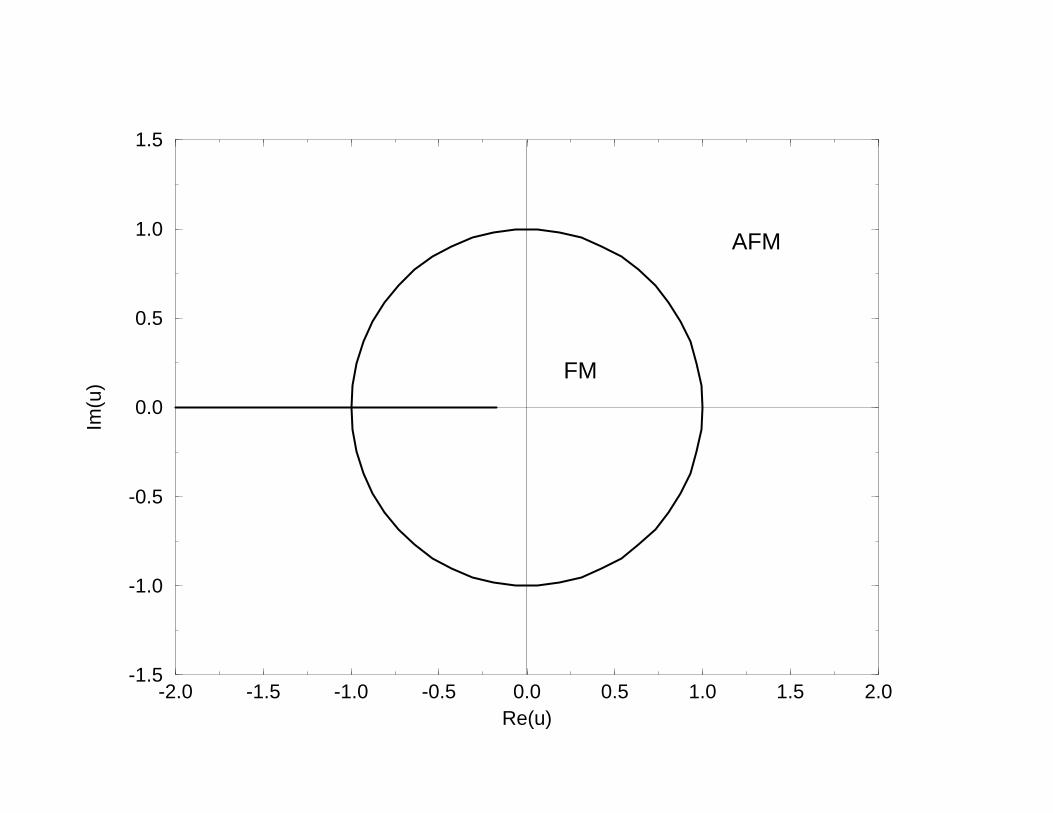
-2.0 -1.5 -1.0 -0.5 0.0 0.5 1.0 1.5 2.0Re(u)

-1.5

-1.0

-0.5

0.0

0.5

1.0

1.5

Im(u

)

FM

AFM

-2.0 -1.5 -1.0 -0.5 0.0 0.5 1.0 1.5 2.0Re(v)

-1.5

-1.0

-0.5

0.0

0.5

1.0

1.5

Im(v

) AFM FM

This figure "fig1-3.png" is available in "png" format from:

http://arXiv.org/ps/hep-lat/9412105v1

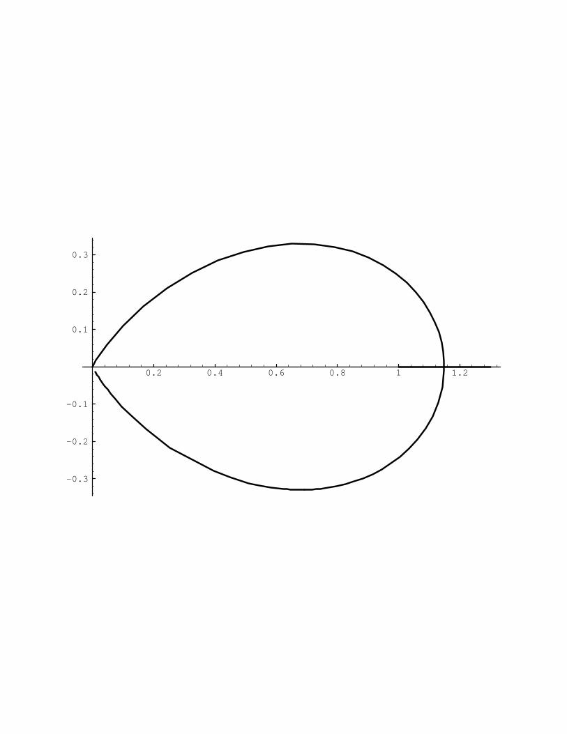
0.2 0.4 0.6 0.8 1 1.2

-0.3

-0.2

-0.1

0.1

0.2

0.3

This figure "fig1-4.png" is available in "png" format from:

http://arXiv.org/ps/hep-lat/9412105v1