Complete Issue - International Journal of Environmental and ...
123
-
Upload
khangminh22 -
Category
Documents
-
view
0 -
download
0
Transcript of Complete Issue - International Journal of Environmental and ...
Page | i
Preface
We would like to present, with great pleasure, the inaugural volume-3, Issue-3, March 2017, of a scholarly
journal, International Journal of Environmental & Agriculture Research. This journal is part of the AD
Publications series in the field of Environmental & Agriculture Research Development, and is devoted to
the gamut of Environmental & Agriculture issues, from theoretical aspects to application-dependent studies
and the validation of emerging technologies.
This journal was envisioned and founded to represent the growing needs of Environmental & Agriculture as
an emerging and increasingly vital field, now widely recognized as an integral part of scientific and
technical investigations. Its mission is to become a voice of the Environmental & Agriculture community,
addressing researchers and practitioners in below areas
Environmental Research:
Environmental science and regulation, Ecotoxicology, Environmental health issues, Atmosphere and
climate, Terrestric ecosystems, Aquatic ecosystems, Energy and environment, Marine research,
Biodiversity, Pharmaceuticals in the environment, Genetically modified organisms, Biotechnology, Risk
assessment, Environment society, Agricultural engineering, Animal science, Agronomy, including plant
science, theoretical production ecology, horticulture, plant, breeding, plant fertilization, soil science and
all field related to Environmental Research.
Agriculture Research:
Agriculture, Biological engineering, including genetic engineering, microbiology, Environmental impacts
of agriculture, forestry, Food science, Husbandry, Irrigation and water management, Land use, Waste
management and all fields related to Agriculture.
Each article in this issue provides an example of a concrete industrial application or a case study of the
presented methodology to amplify the impact of the contribution. We are very thankful to everybody within
that community who supported the idea of creating a new Research with IJOEAR. We are certain that this
issue will be followed by many others, reporting new developments in the Environment and Agriculture
Research Science field. This issue would not have been possible without the great support of the Reviewer,
Editorial Board members and also with our Advisory Board Members, and we would like to express our
sincere thanks to all of them. We would also like to express our gratitude to the editorial staff of AD
Publications, who supported us at every stage of the project. It is our hope that this fine collection of articles
will be a valuable resource for IJOEAR readers and will stimulate further research into the vibrant area of
Environmental & Agriculture Research.
Mukesh Arora
(Editor-in Chief)
Dr. Bhagawan Bharali
(Managing Editor)
Page | ii
Fields of Interests Agricultural Sciences
Soil Science Plant Science
Animal Science Agricultural Economics
Agricultural Chemistry Basic biology concepts
Sustainable Natural Resource Utilisation Management of the Environment
Agricultural Management Practices Agricultural Technology
Natural Resources Basic Horticulture
Food System Irrigation and water management
Crop Production
Cereals or Basic Grains: Oats, Wheat, Barley, Rye, Triticale,
Corn, Sorghum, Millet, Quinoa and Amaranth
Oilseeds: Canola, Rapeseed, Flax, Sunflowers, Corn and
Hempseed
Pulse Crops: Peas (all types), field beans, faba beans, lentils,
soybeans, peanuts and chickpeas. Hay and Silage (Forage crop) Production
Vegetable crops or Olericulture: Crops utilized fresh or whole
(wholefood crop, no or limited processing, i.e., fresh cut salad);
(Lettuce, Cabbage, Carrots, Potatoes, Tomatoes, Herbs, etc.)
Tree Fruit crops: apples, oranges, stone fruit (i.e., peaches,
plums, cherries)
Tree Nut crops: Hazlenuts. walnuts, almonds, cashews, pecans Berry crops: strawberries, blueberries, raspberries
Sugar crops: sugarcane. sugar beets, sorghum Potatoes varieties and production.
Livestock Production
Animal husbandry Ranch
Camel Yak
Pigs Sheep
Goats Poultry
Bees Dogs
Exotic species Chicken Growth
Aquaculture
Fish farm Shrimp farm
Freshwater prawn farm Integrated Multi-Trophic Aquaculture
Milk Production (Dairy)
Dairy goat Dairy cow
Dairy Sheep Water Buffalo
Moose milk Dairy product
Forest Products and Forest management
Forestry/Silviculture Agroforestry
Silvopasture Christmas tree cultivation
Maple syrup Forestry Growth
Mechanical
General Farm Machinery Tillage equipment
Harvesting equipment Processing equipment
Hay & Silage/Forage equipment Milking equipment
Hand tools & activities Stock handling & control equipment
Agricultural buildings Storage
Page | iii
Agricultural Input Products
Crop Protection Chemicals Feed supplements
Chemical based (inorganic) fertilizers Organic fertilizers
Environmental Science
Environmental science and regulation Ecotoxicology
Environmental health issues Atmosphere and climate
Terrestric ecosystems Aquatic ecosystems
Energy and environment Marine research
Biodiversity Pharmaceuticals in the environment
Genetically modified organisms Biotechnology
Risk assessment Environment society
Theoretical production ecology horticulture
Breeding plant fertilization
Page | iv
Board Members
Mukesh Arora(Editor-in-Chief)
BE(Electronics & Communication), M.Tech(Digital Communication), currently serving as Assistant Professor in the
Department of ECE.
Dr. Bhagawan Bharali (Managing Editor)
Professor & Head, Department of Crop Physiology, Faculty of Agriculture, Assam Agricultural University, Jorhat-
785013 (Assam).
Dr. Josiah Chidiebere Okonkwo
PhD Animal Science/ Biotech (DELSU), PGD Biotechnology (Hebrew University of Jerusalem Senior Lecturer,
Department of Animal Science and Technology, Faculty of Agriculture, Nau, AWKA.
Dr. Sunil Wimalawansa
MD, PhD, MBA, DSc, is a former university professor, Professor of Medicine, Chief of Endocrinology, Metabolism
& Nutrition, expert in endocrinology; osteoporosis and metabolic bone disease, vitamin D, and nutrition.
Dr. Rakesh Singh
Professor in Department of Agricultural Economics, Institute of Agricultural Sciences, Banaras Hindu University,
Also Vice President of Indian Society of Agricultural Economics, Mumbai
Dr. Ajeet singh Nain
Working as Professor in GBPUA&T, Pantnagar-263145, US Nagar, UK, India.
Prof. Salil Kumar Tewari
Presently working as Professor in College of Agriculture and Joint Director, Agroforestry Research Centre (AFRC) /
Program Coordinator in G.B. Pant University of Agric. & Tech.,Pantnagar - 263 145, Uttarakhand (INDIA).
Goswami Tridib Kumar
Presently working as a Professor in IIT Kharagpur from year 2007, He Received PhD degree from IIT Kharagpur in
the year of 1987.
Dr. Mahendra Singh Pal
Presently working as Professor in the dept. of Agronomy in G. B. Pant University o Agriculture & Technology,
Pantnagar-263145 (Uttarakhand).
Jiban Shrestha
Scientist (Plant Breeding & Genetics)
Presently working as Scientist (Plant Breeding and Genetics) at National Maize Research Programme (NMRP),
Rampur, Chitwan under Nepal Agricultural Research Council (NARC), Singhdarbar Plaza, Kathmandu, Nepal.
Page | v
Dr. V K Joshi
Professor V.K.Joshi is M.Sc., Ph.D. (Microbiology) from Punjab Agricultural University, Ludhiana and Guru Nanak
Dev University, Amritsar, respectively with more than 35 years experience in Fruit Fermentation Technology,
Indigenous fermented foods, patulin ,biocolour ,Quality Control and Waste Utilization. Presently, heading the dept.
of Food Science and Technology in University of Horticulture and Forestry, Nauni-Solan (HP), India.
Mr. Aklilu Bajigo Madalcho
Working at Jigjiga University, Ethiopia, as lecturer and researcher at the College of Dry land Agriculture, department
of Natural Resources Management.
Dr. Vijay A. Patil
Working as Assistant Research Scientist in Main Rice Research Centre, Navsari Agricultural University, Navsari.
Gujarat- 396 450 (India).
Dr. S. K. Jain
Presently working as Officer Incharge of All India Coordinated Sorghum Improvement Project, S. D. Agricultural
University, Deesa, Gujarat.
Dr. Salvinder Singh
Presently working as Associate Professor in the Department of Agricultural Biotechnology in Assam Agricultural
University, Jorhat, Assam.
Dr. Salvinder received MacKnight Foundation Fellowship for pre-doc training at WSU, USA – January 2000- March
2002 and DBT oversease Associateship for Post-Doc at WSU, USA – April, 2012 to October, 2012.
Mr. Anil Kumar
Working as Junior Research Officer/Asstt. Prof. in the dept. of Food Science & Technology in Agriculture &
Technology, Pantnagar.
Table of Contents
S.No Title Page
No.
1
Effect of Grazing Land Improvement Practices on Herbaceous production, Grazing
Capacity and their Economics: Ejere district, Ethiopia Authors: Abule Ebro, Azage Tegegne, Fekadu Nemera, Adisu Abera, Yared Deribe
Digital Identification Number: Paper-March-2017/IJOEAR-FEB-2017-8
01-06
2
CdTe quantum dots/Poly (diallyl dimethyl ammonium chloride) multilayer films:
preparation and application for gaseous sensors Authors: Shichao Xu, Kai Dong, Junnan Wen, Nan Jiang, Jiangjiang Wang, Chunming Zheng,
Shihuai Zhao, Jimei Zhang
Digital Identification Number: Paper-March-2017/IJOEAR-FEB-2017-16
07-14
3
Biosorption of Malathion pesticide using Spirogyra sp. Authors: Chhunthang Liani, SS Katoch
Digital Identification Number: Paper-March-2017/IJOEAR-MAR-2017-1
15-20
4
The Relationship between Soil Moisture and Temperature Vegetation on Kirklareli City
Luleburgaz District A Natural Pasture Vegetation Authors: Canan Sen, Ozan Ozturk
Digital Identification Number: Paper-March-2017/IJOEAR-MAR-2017-2
21-29
5
Comparison of Resistance to Fusarium wilts disease in Seeded and Regenerated Sesame
(Sesamum indicum L.) Authors: Firoozeh Chamandoosti
Digital Identification Number: Paper-March-2017/IJOEAR-MAR-2017-6
30-34
6
Radial variation in microfibril angle of Acacia mangium. Authors: N. Lokmal, Mohd Noor A.G.
Digital Identification Number: Paper-March-2017/IJOEAR-NOV-2016-10
35-42
7
Atmospheric Deposition of Nitrogen compounds in Assam (India) Authors: Bhagawan Bharali, Bhupendra Haloi
Digital Identification Number: Paper-March-2017/IJOEAR-MAR-2017-3
43-55
8
The Influence of Vermiculite on the Uptake of Silver Nanoparticles in a Terrestrial System Authors: Sara A. Pappas, Uday Turaga, Naveen Kumar, Seshadri Ramkumar, Ronald J. Kendall
Digital Identification Number: Paper-March-2017/IJOEAR-MAR-2017-5
56-64
9
Analysis of Trend and Variability of Temperature in Ebonyi State, South-eastern Nigeria,
1984-2015 Authors: Bridget Diagi, Vincent Weli
Digital Identification Number: Paper-March-2017/IJOEAR-MAR-2017-9
65-71
10
Analyzing Marketing Margins and the Direction of Price Flow in the Tomato Value Chain
of Limpopo Province, South Africa Authors: Kudzai Mandizvidza
Digital Identification Number: Paper-March-2017/IJOEAR-MAR-2017-13
72-82
11
Genome–Wide Analysis and Expression Pattern of the AP2/ERF Gene Family in Kiwifruit
under Waterlogging Stress Treatment Authors: Ji-Yu Zhang, De-Lin Pan, Gang Wang, Ji-Ping Xuan, Tao Wang, Zhong-Ren Guo
Digital Identification Number: Paper-March-2017/IJOEAR-MAR-2017-15
83-90
12
New banana genotypes and cultivars more productive for southern Minas, Brazil Authors: Lair Victor Pereira, José Clélio de Andrade, Ângelo Albérico Alvarenga, Marcelo
Ribeiro Malta, Paulo Márcio Norberto, Sebastião de Oliveira e Silva
Digital Identification Number: Paper-March-2017/IJOEAR-MAR-2017-16
91-97
13
Agricultural Waste Management in order to sustainable agriculture in Karnataka Authors: Omid Minooei, S. Mokshapathy
Digital Identification Number: Paper-March-2017/IJOEAR-FEB-2017-15
98-103
14
Uptake of Silver from Polyvinylpyrrolidine Coated Silver Nanoparticles in a Terrestrial
System Authors: Sara A. Pappas, Uday Turaga, Naveen Kumar, Seshadri Ramkumar, Ronald J. Kendall
Digital Identification Number: Paper-March-2017/IJOEAR-MAR-2017-19
104-114
International Journal of Environmental & Agriculture Research (IJOEAR) ISSN:[2454-1850] [Vol-3, Issue-3, March- 2017]
Page | 1
Effect of Grazing Land Improvement Practices on Herbaceous
production, Grazing Capacity and their Economics: Ejere
district, Ethiopia Abule Ebro
1, Azage Tegegne
2, Fekadu Nemera
3, Adisu Abera
4, Yared Deribe
5
1,2,4,5Livestock and Irrigated Value Chains for Ethiopian Smallholders Project—International Livestock Research Institute
(ILRI), P.O. Box 5689, Addis Ababa, Ethiopia 3Adami Tulu Research Center, P. O. Box, 35, Zeway, Ethiopia
Abstract— The effects of different grazing land improvement practices on herbaceous production, grazing capacities and
their economics were studied in Ejere district, west Shoa zone, Ethiopia. Four different treatments, i.e., application of Urea
and Diammonium phosphate (DAP), cattle manure, wooden ash, and a control/no application) were randomly applied to the
study plots in three replications for each treatment. All experimental plots were fenced throughout the study period. The
application of urea and DAP significantly increased grass (3620.86 kg ha-1
) and total biomass production (5742.93 kg ha-1
).
Of the 6 herbaceous species recorded in the Urea and DAP plots, four of them were grasses with Setaria verticellata having
the highest percentage composition (35.54%) while the control plot was dominated by Cyperus rotundus (31.5%) and
Cerastium octandrum (31.5%). Less land is required to maintain a tropical livestock unit (TLU) in Urea and DAP applied
plots (0.03 ha TLU-1
) than in plots applied with other treatments (mean = 0.09 ha TLU-1
). Similar to the result of the
biological data, the participants of the grassland day rated the Urea and DAP applied treatment best because of the high
production of grass. Considering total biomass production, application of manure was advantageous to the farmers due to
increased net benefits and the marginal rate of return is above the minimum accetable rate for this sort of treatment. On the
other hand, considering grass production alone, application of Urea and DAP was more profitable for farmers as far as
they store and sell it in the dry seasons. In conclusion, we recommend a long-term study to examine the effects of the
different treatments on productivity of grazing lands, herbaceous species composition, grazing capacities, livestock, the
environment, and their economics.
Keywords— Ash, grazing land improvement, manure, Urea, DAP.
I. INTRODUCTION
Ethiopia holds the largest livestock population in Africa estimated at about 54 million heads of cattle, 25.5 million sheep,
24.06 million goats, 0.92 million camels, 4.5 million donkeys, 1.7 million horses, 0.33 million mules, 54 million chicken and
4.9 million beehives [1]. It is also among the 28 smaller countries (25 in Africa) where grazing land accounts greater than
60% of the total land area [2]. Despite these huge resources, the productivity of livestock in general is low and its
contribution to the national economy is below expected. Among the major problems affecting livestock production and
productivity in Ethiopia, feed shortage in terms of quantity and quality is the leading problem [1].
The major feed resources in Ethiopia are natural pasture (grasslands) and crop residues with varying proportion among the
different zones of the country. Similar to the other parts of Ethiopia, the role of grazing lands as a major livestock feed
resources is diminishing from time to time because of natural and human induced factors (increased conversion of grazing
lands to crop land) which created heavy grazing pressure on the remaining grazing lands although the extent of degradation
varies from site to site [4, 5, 6]. In addition, grazing land improvement practices are relatively less common particularly in
the highlands of Ethiopia owing to the lack of awareness and appropriate training, lack of appropriate improvement methods
and little attention given to grazing lands by the agricultural extension system. The pressure is likely to intensify in the
coming decades creating more pressure on the remaining grazing lands justifying the need to improve the available
remaining grazing lands to increase their livestock holding capacity [1]. Thus, the current study examined the effect of
applying different grazing land improvement techniques on biomass production and herbaceous species composition, grazing
capacities of the grazing lands and the economics of the different treatments. This paper will contribute to better
understanding of grazing land rehabilitation techniques in Ethiopia and for similar ecosystem elsewhere.
International Journal of Environmental & Agriculture Research (IJOEAR) ISSN:[2454-1850] [Vol-3, Issue-3, March- 2017]
Page | 2
II. MATERIALS AND METHODS
2.1 Description of the study area
This study was carried out in Ejere district, West Shoa zone, Ethiopia. The district was selected due to its potential for
livestock production (dairy, small ruminant, poultry and apiculture) and it is one of the intervention districts for Livestock
and Irrigation Value Chain for Ethiopian smallholders (LIVES) project of the International Livestock Research Institute
(ILRI). The altitude ranges from 2063 to 3158 meters above sea level (m.a.s.l). The rainfall of the area is distinctly bimodal
pattern, viz-a-viz. the main rainy season occurs from June to end of September and the short and small rainy season is in
February and March. The mean annual rainfall ranges from 900 to 1200 mm.
The livelihood of the communities in the study district is based on mixed crop-livestock production system and the human
population is about 104 709 (49 829 males and 55 057 females) [1]. The livestock population is estimated to be: 119 854
cattle, 37 423 sheep, 11 600 goats, 9436 mule, 356 donkey, 10 117 horses and 43 125 poultry. Crop residues, natural pasture,
improved forage, hay, agro-industrial by-products and others contribute as livestock feed [1]. The district has upland and
wetland grazing areas. In addition to grazing, the wetlands are the sources of water for livestock and irrigation for lower
riparian’s [6]. Particularly, the Berga wetland is one of the two known breeding sites (Weserbi-near Sululta and Berga) for
the globally threatened White-winged Fluff tail Sarothrura ayresi [7]. With regard to grazing land ownership, there are two
types, i.e., private and communal although the former is larger (80%) than the latter in terms of area coverage (20%) at the
current moment while the opposite was true in the past. The private grazing lands (0.25 to 0.5 ha/household on average) are
used for hay making and/or grazing [8].
2.2 Site selection
In site selection for the study, which was undertaken with the help of farmers, livestock experts and development agents, the
representativeness of the site for grazing lands in the mid altitude (2378 m.a.s.l), and poor herbaceous production condition
of the site was taken into consideration.
The treatments described in this study are mainly based on locally available resources (manure, wood ash, enclosing) except
Urea and DAP which is imported and can be purchased at the service cooperative level in the villages. Fifteen plots of 4 m x
4 m were laid out to apply 4 treatments (Urea and DAP, wooden ash, cow manure, and untreated/control) randomly in 3
replications. All plots were fenced during the main growing season (June to November, 2015). The distance between plots
and replications/blocks was 1 and 2 meters, respectively. The amount of urea and DAP, ash and dry manure applied on 16 m-
2 plots were 0.24 kg and 0.16 kg, 4.8 kg and 12 kg, respectively. The plots were ripped to incorporate the treatment materials
into the soil. The manure, obtained from farmers was decomposed for three months at backyards of farmers and dissolved in
water and added into the soil in form of slurry. Wood Ash from farmers was scattered over the plots. Urea and DAP was over
sown by broadcasting. The treatments were applied after the beginning of main rainy season. At the end of the growing
season, the different plots were harvested using hand sickles and sorted into grass, and non-grass components. Furthermore,
they were sorted into different species using field guide [9] and experienced technician from Adami Tulu research center,
Ethiopia. The sorted materials were oven-dried at 65 ᵒC for 72 hours.
2.3 Organization of grassland day and field assessment
Thirty male and nine female model farmers and 23 male and 2 female extension staff drawn from 4 districts (Ejere,
AdaBerga, Meta-Robi and Dendi of west Shoa zone) and west Shoa zonal office attended the grassland day which was
organized with the objective of creating awareness on the importance of improved grazing land management for the public.
2.4 Statistical and economic analyses
Analysis of variance (ANOVA) was conducted to verify the significant differences among the treatments using the
STATA/SE 14 program. The formula proposed by Moore et al. [10], modified by Moore and Odendaal (1987) [11] and
Moore (1989) [12], was used for grazing capacity estimation by taking in account the grass and total biomass yields. The
equation is as follows:
Y= d/(DM x f)r
where Y is the grazing capacity (ha TLU-1
), d the number of days in a year (365), DM the grass and total biomass DM yield
(kg ha-1
), f is the utilization factor, r the daily grass DM required. The grazing capacity was calculated using tropical
livestock unit (TLU) which is an animal weighing 250 kg and consuming 2.5% of its body weight. Thus, each TLU will
consume 6.25 kg of forage dry matter daily and utilization factor of 0.5 (50%) was used [13].
International Journal of Environmental & Agriculture Research (IJOEAR) ISSN:[2454-1850] [Vol-3, Issue-3, March- 2017]
Page | 3
The partial budget analysis (economic analysis) was done according to Upton 1979 [14] and CIMMYT 1988 [15] to
determine economic benefit of the different treatments. Total variable cost, total return (TR), net benefit (NB), change in net
benefit and marginal rate of return (%) were calculated for total biomass and grass production separately as grass is the most
important feed resource for cattle and sheep. Furthermore, the economic analysis was undertaken considering the price of
baled hay at harvest time and during the dry season.
III. RESULTS
3.1 Biomass production, herbaceous species composition and grazing capacities
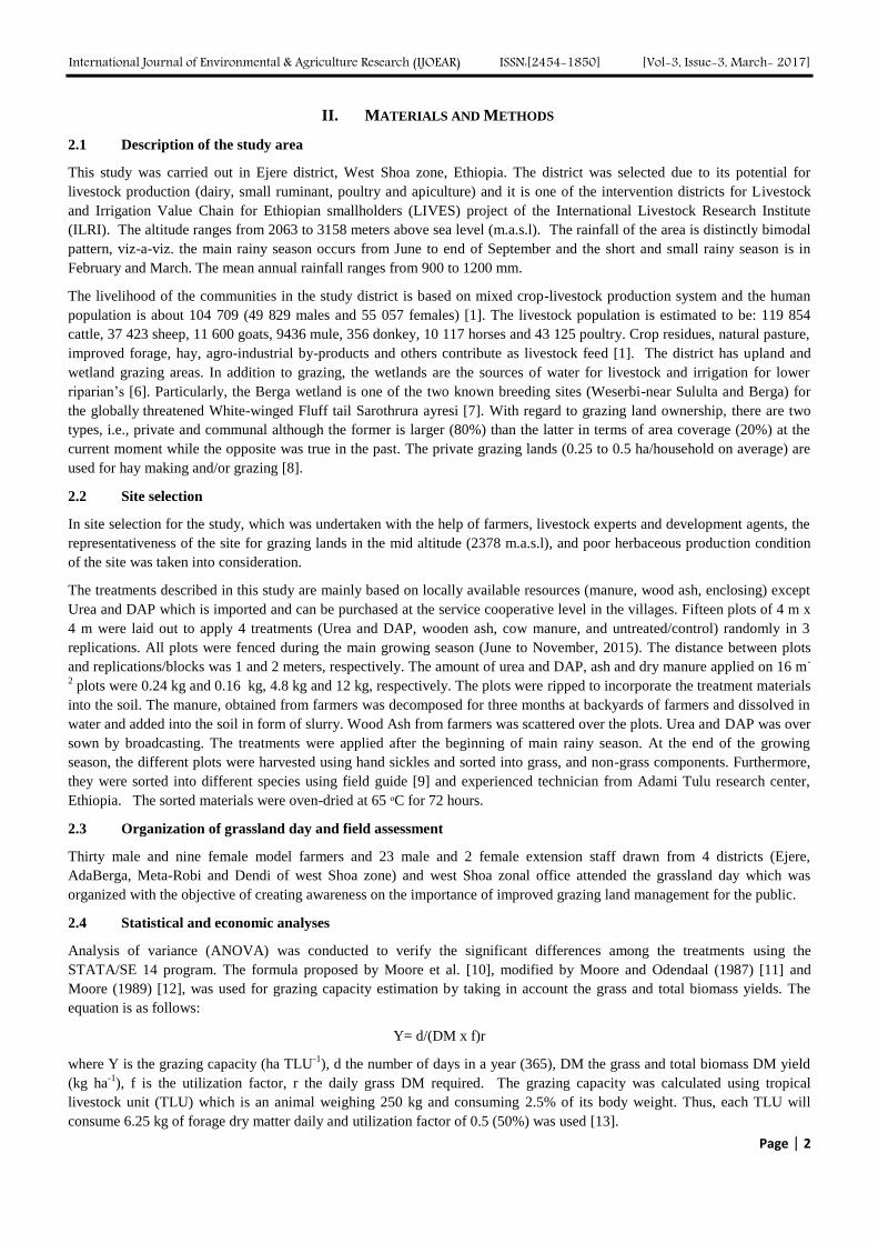
Grass dry matter yield was highest (P<0.02) in Urea and DAP treated plots (Table 1). Compared with the control, application
of ash or manure increased grass production although it was non-significant (P>0.05). On the other hand, the non-grass
biomass was the highest in manure-treated plots although not significant (P<0.05). Application of ash produced more non-
grass biomass than the control. Urea and DAP application significantly increased (P<0.02) total biomass production (TBP).
While the control was the least in TBP, ash and manure applications were comparable in TBP.
TABLE 1
APPLICATION OF DIFFERENT TREATMENTS ON MEAN HERBACEOUS DRY MATTER PRODUCTION (kg ha-1
) AND
GRAZING CAPACITIES (ha TLU-1
)
Treatments Grass Non-grass Total biomass
(TB)
GC (grass)
(ha/TLU)
GC (TB)
(ha/TLU)
Control (no treatment) 1042.7b 1786.7
b 2829.3
c 0.11 0.04
Ash 1170.7b 2773.3
b 3944
bc 0.09 0.03
Urea and DAP 3620.80a 2122.13
b 5742.93
a 0.03 0.02
Manure (cow) 1716b 2986.7
b 4702.7
ab 0.07 0.03
SEM 151 121.6 178
Significance level 0.0155 0.2361 0.0168
Means with different letters down the column are significantly different (P<0.05); SEM= standard error of the mean.
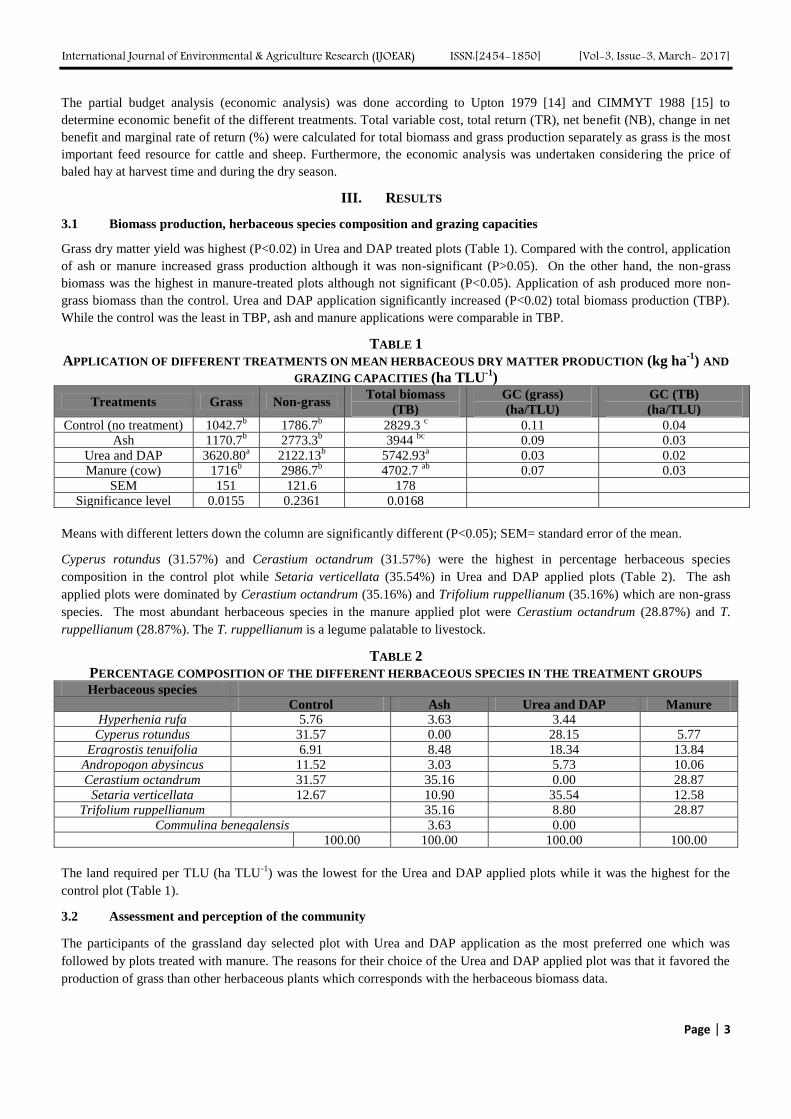
Cyperus rotundus (31.57%) and Cerastium octandrum (31.57%) were the highest in percentage herbaceous species
composition in the control plot while Setaria verticellata (35.54%) in Urea and DAP applied plots (Table 2). The ash
applied plots were dominated by Cerastium octandrum (35.16%) and Trifolium ruppellianum (35.16%) which are non-grass
species. The most abundant herbaceous species in the manure applied plot were Cerastium octandrum (28.87%) and T.
ruppellianum (28.87%). The T. ruppellianum is a legume palatable to livestock.
TABLE 2
PERCENTAGE COMPOSITION OF THE DIFFERENT HERBACEOUS SPECIES IN THE TREATMENT GROUPS Herbaceous species
Control Ash Urea and DAP Manure
Hyperhenia rufa 5.76 3.63 3.44
Cyperus rotundus 31.57 0.00 28.15 5.77
Eragrostis tenuifolia 6.91 8.48 18.34 13.84 Andropogon abysincus 11.52 3.03 5.73 10.06
Cerastium octandrum 31.57 35.16 0.00 28.87
Setaria verticellata 12.67 10.90 35.54 12.58 Trifolium ruppellianum
35.16 8.80 28.87
Commulina benegalensis 3.63 0.00
100.00 100.00 100.00 100.00
The land required per TLU (ha TLU-1
) was the lowest for the Urea and DAP applied plots while it was the highest for the
control plot (Table 1).
3.2 Assessment and perception of the community
The participants of the grassland day selected plot with Urea and DAP application as the most preferred one which was
followed by plots treated with manure. The reasons for their choice of the Urea and DAP applied plot was that it favored the
production of grass than other herbaceous plants which corresponds with the herbaceous biomass data.
International Journal of Environmental & Agriculture Research (IJOEAR) ISSN:[2454-1850] [Vol-3, Issue-3, March- 2017]
Page | 4
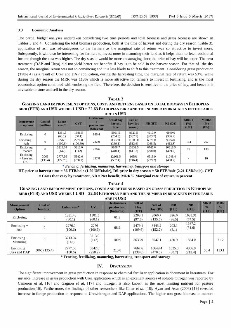
3.3 Economic Analysis
The partial budget analyses undertaken considering two time periods and total biomass and grass biomass are shown in
Tables 3 and 4. Considering the total biomass production, both at the time of harvest and during the dry season (Table 3),
application of ash was advantageous to the farmers as the marginal rate of return was so attractive to invest more.
Subsquently, it will also be interesting for farmers to invest more in manuring their land as it helps them to fetch additional
income though the cost was higher. The dry season would be more encauraging since the price of hay will be better. The next
treatment (DAP and Urea) did not yield better net benefits if hay is to be sold in the harvest season. For that of the dry
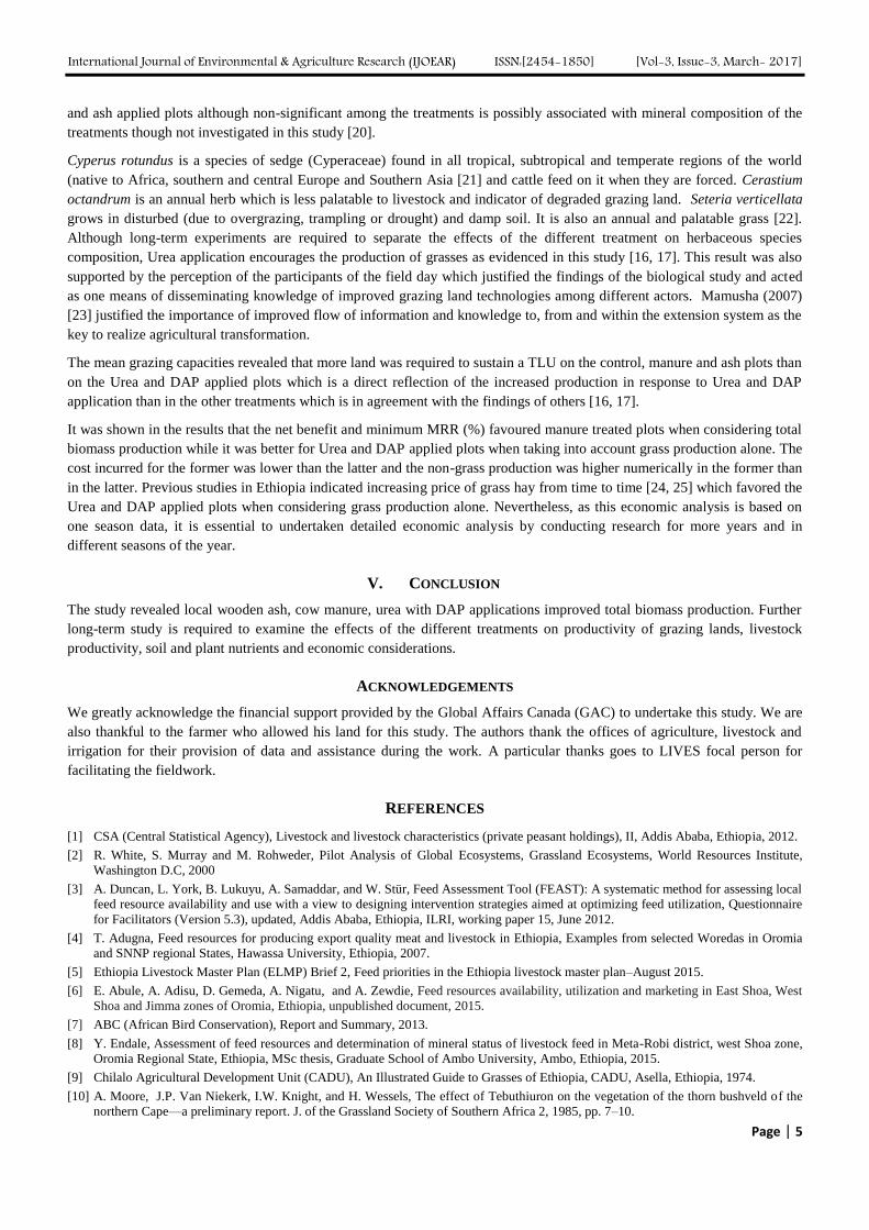
season, the marginal return was not so convincing and it is less likely to shift to this treatment. Considering grass production
(Table 4) as a result of Urea and DAP application, during the harvesting time, the marginal rate of return was 53%, while
during the dry season the MRR was 113% which is more attractive for farmers to invest in fertilizing, and is the most
economical option combined with enclosing the field. Therefore, the decision is sensitive to the price of hay, and hence it is
advisable to store and sell in the dry season.
TABLE 3
GRAZING LAND IMPROVEMENT OPTIONS, COSTS AND RETURNS BASED ON TOTAL BIOMASS IN ETHIOPIAN
BIRR (ETB) AND USD WHERE 1 USD = 22.63 ETHIOPIAN BIRR AND THE NUMBER IN BRACKETS IN THE TABLE
ARE IN USD
Improveme
nt options
Cost of
fertilizer
Labor
cost * CVT
Herbaceou
s
production
(bales/ha)
Sell of hay
harvest
time
Sell of
hay (dry
season)
NB (HT) NB (DS)
MRR1
(%)
(HT)
MRR2
(%)
(DS)
Enclosing 0 1381.5
(60.1)
1381.5
(60.1) 166.4
5991.5
(264.8)
8321.5
(367.7)
4610.0
(203.7)
6940.0
(306.7)
Enclosing +
Ash 0
2276.0
(100.6)
2276.0
(100.60) 232.0
8352.0
(369.1)
11600.0
(512.6)
6076.0
(268.5)
9324.0
(412.8) 164 267
Enclosing
+ manure 0
3213.04
(142)
3213.0
(142) 276.6
9958.7
(440.1)
13831.5
(611.2)
6745.6
(298.0)
10618.5
(469.2) 72 138
Enclosing
+ Urea and
DAP
3065
(135.4)
2777.56
(122.70)
5842.6
(258.1) 337.8
12161.5
(537.4)
16891
(746.4)
6318.9
(279.2)
11048.4
(488.2) - 16
* Fencing, fertilizing, manuring, harvesting, transport and storage
HT-price at harvest time = 36 ETB/bale (1.59 USD/bale), DS-price in dry season = 50 ETB/bale (2.21 USD/bale), CVT
= Costs that vary by treatment, NB = Net benefit, MRR% Marginal rate of return in percent
TABLE 4
GRAZING LAND IMPROVEMENT OPTIONS, COSTS AND RETURNS BASED ON GRASS PRDUCTION IN ETHIOPIAN
BIRR (ETB) AND USD WHERE 1 USD = 22.63 ETHIOPIAN BIRR AND THE NUMBER IN BRACKETS IN THE TABLE
ARE IN USD
Management
Option
Cost of
fertilizer Labor cost* CVT
Herbaceous
production
(bales/ha)
Sell of
Hay
(HT)
Sell of
Hay (DS)
NB
(HT)
NB
(DT)
MRR
%
(HT)
MRR
%
(DT)
Enclosing 0 1381.46
(60.1)
1381.5
(60.1) 61.3
2208.1
(97.5)
3066.7
(135.5)
826.6
(36.5)
1685.31
(74.5)
Enclosing +
Ash 0
2276.0
(100.6)
2276
(100.6) 68.9
2479.1
(109.6)
3443.2
(152.2)
203.1
(8.1)
1167.2
(51.6)
Enclosing +
Manuring 0
3213.04
(142)
3213.0
(142)
100.9 3633.9 5047.1 420.9 1834.0
71.2
Enclosing +
Urea and DAP 3065 (135.4)
2777.56
(100.6)
5842.6
(258.2) 213.0
7667.6
(338.8)
10649.4
(470.6)
1825.0
(80.7)
4806.9
(212.4) 53.4 113.1
* Fencing, fertilizing, manuring, harvesting, transport and storage
IV. DISCUSSION
The significant improvement in grass production in response to chemical fertilizer application is document in literatures. For
instance, increase in grass production with Urea application which is an excellent sources of soluble nitrogen was reported by
Cameron et al. [16] and Gagnon et al. [17] and nitrogen is also known as the most limiting nutrient for pasture
production[16]. Furthermore, the findings of other researchers like Cinar et al. [18]; Ayan and Acar (2008) [19] revealed
increase in forage production in response to Urea/nitrogen and DAP applications. The higher non-grass biomass in manure
International Journal of Environmental & Agriculture Research (IJOEAR) ISSN:[2454-1850] [Vol-3, Issue-3, March- 2017]
Page | 5
and ash applied plots although non-significant among the treatments is possibly associated with mineral composition of the
treatments though not investigated in this study [20].
Cyperus rotundus is a species of sedge (Cyperaceae) found in all tropical, subtropical and temperate regions of the world
(native to Africa, southern and central Europe and Southern Asia [21] and cattle feed on it when they are forced. Cerastium
octandrum is an annual herb which is less palatable to livestock and indicator of degraded grazing land. Seteria verticellata
grows in disturbed (due to overgrazing, trampling or drought) and damp soil. It is also an annual and palatable grass [22].
Although long-term experiments are required to separate the effects of the different treatment on herbaceous species
composition, Urea application encourages the production of grasses as evidenced in this study [16, 17]. This result was also
supported by the perception of the participants of the field day which justified the findings of the biological study and acted
as one means of disseminating knowledge of improved grazing land technologies among different actors. Mamusha (2007)
[23] justified the importance of improved flow of information and knowledge to, from and within the extension system as the
key to realize agricultural transformation.
The mean grazing capacities revealed that more land was required to sustain a TLU on the control, manure and ash plots than
on the Urea and DAP applied plots which is a direct reflection of the increased production in response to Urea and DAP
application than in the other treatments which is in agreement with the findings of others [16, 17].
It was shown in the results that the net benefit and minimum MRR (%) favoured manure treated plots when considering total
biomass production while it was better for Urea and DAP applied plots when taking into account grass production alone. The
cost incurred for the former was lower than the latter and the non-grass production was higher numerically in the former than
in the latter. Previous studies in Ethiopia indicated increasing price of grass hay from time to time [24, 25] which favored the
Urea and DAP applied plots when considering grass production alone. Nevertheless, as this economic analysis is based on
one season data, it is essential to undertaken detailed economic analysis by conducting research for more years and in
different seasons of the year.
V. CONCLUSION
The study revealed local wooden ash, cow manure, urea with DAP applications improved total biomass production. Further
long-term study is required to examine the effects of the different treatments on productivity of grazing lands, livestock
productivity, soil and plant nutrients and economic considerations.
ACKNOWLEDGEMENTS
We greatly acknowledge the financial support provided by the Global Affairs Canada (GAC) to undertake this study. We are
also thankful to the farmer who allowed his land for this study. The authors thank the offices of agriculture, livestock and
irrigation for their provision of data and assistance during the work. A particular thanks goes to LIVES focal person for
facilitating the fieldwork.
REFERENCES
[1] CSA (Central Statistical Agency), Livestock and livestock characteristics (private peasant holdings), II, Addis Ababa, Ethiopia, 2012.
[2] R. White, S. Murray and M. Rohweder, Pilot Analysis of Global Ecosystems, Grassland Ecosystems, World Resources Institute,
Washington D.C, 2000
[3] A. Duncan, L. York, B. Lukuyu, A. Samaddar, and W. Stür, Feed Assessment Tool (FEAST): A systematic method for assessing local
feed resource availability and use with a view to designing intervention strategies aimed at optimizing feed utilization, Questionnaire
for Facilitators (Version 5.3), updated, Addis Ababa, Ethiopia, ILRI, working paper 15, June 2012.
[4] T. Adugna, Feed resources for producing export quality meat and livestock in Ethiopia, Examples from selected Woredas in Oromia
and SNNP regional States, Hawassa University, Ethiopia, 2007.
[5] Ethiopia Livestock Master Plan (ELMP) Brief 2, Feed priorities in the Ethiopia livestock master plan–August 2015.
[6] E. Abule, A. Adisu, D. Gemeda, A. Nigatu, and A. Zewdie, Feed resources availability, utilization and marketing in East Shoa, West
Shoa and Jimma zones of Oromia, Ethiopia, unpublished document, 2015.
[7] ABC (African Bird Conservation), Report and Summary, 2013.
[8] Y. Endale, Assessment of feed resources and determination of mineral status of livestock feed in Meta-Robi district, west Shoa zone,
Oromia Regional State, Ethiopia, MSc thesis, Graduate School of Ambo University, Ambo, Ethiopia, 2015.
[9] Chilalo Agricultural Development Unit (CADU), An Illustrated Guide to Grasses of Ethiopia, CADU, Asella, Ethiopia, 1974.
[10] A. Moore, J.P. Van Niekerk, I.W. Knight, and H. Wessels, The effect of Tebuthiuron on the vegetation of the thorn bushveld of the
northern Cape—a preliminary report. J. of the Grassland Society of Southern Africa 2, 1985, pp. 7–10.
International Journal of Environmental & Agriculture Research (IJOEAR) ISSN:[2454-1850] [Vol-3, Issue-3, March- 2017]
Page | 6
[11] A. Moore, A. Odendaal, Die ekonomiese implikasies en bosbeheer soos van toepassing op ‘n speenkalfproduksiestelsel in die
doringbosveld van die Molop-gebied (Afrikaans), J. of the Grassland Society of Southern Africa 4, 1987, pp. 139–142.
[12] A, Moore, Die ekologie en ekofisiologie van Rhigozum trichotomum, PhD Thesis, University of Port Elizabeth, South Africa,1989,
pp. 210.
[13] ILCA (International Livestock Center for Africa), Livestock Systems Research Manual, Vol.1. ILCA Working Paper 1,1990, ILCA,
Addis Ababa, Ethiopia.
[14] M. Upton, Farm management in Africa, the principle of production and planning, Oxford University Press, 1979, pp. 380.
[15] CIMMYT, From Agronomic Data to Farmer Recommendations, an Economics Workbook, Mexico, D.F. CIMMYT, 1988.
[16] K. Cameron, H. J.Di, J. Moir, R. Christie, and R. Pellow, Using Nitrogen: What is Best Practice?, South Island Dairy Event (SIDE)
Proceedings, Lincoln University, June, 2005.
[17] B. Gagnon, N. Ziadi, G. Bélanger, and G. Parent, Urea-based fertilizer assessment in forage grass production in eastern Canada,
Proceedings of the 2016 International Nitrogen Initiative Conference, "Solutions to improve nitrogen use efficiency for the world", 4 –
8 December, 2016, Melbourne, Australia. www.ini2016.com
[18] S, Cinar, M. Avci, R. Hatipoglu, K. Kokten, I. Atis, T. Tukel, S. Aydemir, and H. Yucel, A research on effects of nitrogen and
phosphorus fertilization on botanical composition, hay yield and quality in slope part of Hanyeri village rangeland (Tufanbeyli
Adana), Turkey Vi, Field Crops Congress, 2005, pp. 873-877.
[19] I. Ayan, and Z. Acar, Methods for improving rangelands in the Black Sea Region of Turkey, Journal of Fac Of Agric 23, 2008,pp.
145-151.
[20] J. Lickaez, Wood ash: An alternative liming material for agricultural soils, Http//www/Agric.Gov.ab.ca, 2002, 534-2.
[21] M.Z. Imam, and C.D. Sumi, Evaluation of antinociceptive activity of hydromethanol extract of Cyperus rotundus in mice, The official
journal of the International Society for Complementary Medicine Research (ISCMR), 2014, 14: 83.
[22] V.P. Oudtshoorn, Guide to Grasses of Southern Africa, Briza Publication, Pretoria, South Africa, 1999, pp. 288.
[23] L. Mamusha, The agricultural knowledge system in Tigray, Ethiopia: Recent History and Actual Effectiveness. Margraf Publishers,
Weikersheim, 2007.
[24] G. Berhanu, H. Adane, and B. Kahsay, Feeding market in Ethiopia: Results of rapid market appraisal, Working paper No. 15, 2009.
[25] T. Adugna, feed Resources Availability and Quality vs Animal Productivity. In: Tolera, A., Yami, A. and Alemu, D. (Eds.). Livestock
Feed Resources in Ethiopia: Challenges, Opportunities and the Need for Transformation. Ethiopian Animal Feed Industry
Association, Addis Ababa, 2012, pp. 37-46.
International Journal of Environmental & Agriculture Research (IJOEAR) ISSN:[2454-1850] [Vol-3, Issue-3, March- 2017]
Page | 7
CdTe quantum dots/Poly (diallyl dimethyl ammonium chloride)
multilayer films: preparation and application for gaseous sensors Shichao Xu
1 , Kai Dong
2, Junnan Wen
3, Nan Jiang
4, Jiangjiang Wang
5, Chunming
Zheng6, Shihuai Zhao
7, Jimei Zhang
8
1,6,7,8State Key Laboratory of Hollow Fiber Membrane Materials and Processes, Tianjin Polytechnic University, Tianjin,
300387, China 1,2,3,4,5,6,7,8
School of Environmental and Chemical Engineering, Tianjin Polytechnic University, Tianjin, 300387, China 1,6,7,8
TianJin Engineering Center for Safety Evaluation of Water Quality & Safeguards Technology, Tianjin Polytechnic
University, Tianjin 300387, China
Abstract— CdTe quantum dots (QDs)/Poly (diallyldimethylammonium chloride) (PDDA) multilayer films (QDMF) have
been self-assembled by layer-by-layer (LBL) technique. CdTe quantum dots (QDs) were synthesized by using Te, NaBH4, and
CdCl2 as precursors and mercaptopropionic acid (MPA) as stabilizer. The as-prepared composites were characterized by
transmission electron microscope (TEM), Fourier transform infrared spectroscopy (FTIR), UV-vis adsorption spectrum(UV-
vis), and Fluorescence spectrum(FS), respectively. It was shown that the self-assembled QDMF in this study could be used as
gaseous sensors for detecting organic gases, such as ammonia, acetone, methanol and formaldehyde. The quenching
mechanism of CdTe QDs multilayer films by formaldehyde was studied in detail and The detection limit was 10-236ppm.
Keywords— CdTe quantum dots, gaseous sensor; PDDA, QDMF.
I. INTRODUCTION
A trend in current sensor development is miniaturization to obtain inexpensive and compact gas sensors that are robust and
safe, have low power consumption and enable multiplexing of sensor arrays and remote sensing [1, 2]. Gas sensors play a
key role in a variety of fields , such as environmental pollution monitoring, industrial process monitoring, leak detection of
explosive gases, and medical breath analysis. In order to increase sensitivity, devices with nanostructure for gas sensors has
shown lots of advantages[3].
From previous literatures, we can find that there are many gas detecting methods so far. But, compared with those traditional
gas detection techniques, which are often costly, low sensitivity and time-consuming, semiconductor sensors have drawn a
great deal of attention in recent years for its unique optical advantages. Semiconductor luminescent nanocrystals, known as
“quantum dots” (QDs), exhibit unique optical and electronic properties, including high luminescent quantum yields, tunable
emission, high photostability and relatively long emission lifetime. All these advantages explain the reason of its presence
[4]. Furthermore, it has been used for energy conversion and storage[5-8], fabrication of optoelectronic device[9], and
particularly, sensor applications[10-12].
Recently, a number of QD-based sensors have been reported for ions, [13] biomacromolecules, [14-16] and small organic
molecules. [17] And, CdTe QDs have been proved to be a promising material as elemental building blocks for the next
generation of nanodevices [18, 19]. Self-assembled multilayers by layer-by-layer (LBL) method are stable, well-ordered,
easy to prepare and low cost, and have been extensively applied for the constructions of chemo- and bio-sensors [20, 21].
Another important feature of LBL is recharging of the surface at every step of the adsorption self-assembly, which results in
oppositely charged molecules to be adsorbed in the next step with molecular order during the films fabrication process.
Therefore the stable LBL method can encapsulate the QDs efficiently into flexible nanofilms (thickness below 60 nm) [22]. It
has been also successfully applied to the preparation of multiplayer films of polyelectrolytes with other materials such as
proteins, graphite oxides, gold colloids, dyes and nanoparticles [23]. Many groups have developed QDs-based sensing
systems for the detection of Hg2+
[24-26] and Cu2+
[27-29] based on the fluorescence quenching of QDs.
In this paper, CdTe QDs multilayer films was fabricated by the standard LBL assembly technique. The CdTe nanoparticles
with negative charged in the presence of MPA can serve as the anionic entity needed in the multilayer fabrication technique.
International Journal of Environmental & Agriculture Research (IJOEAR) ISSN:[2454-1850] [Vol-3, Issue-3, March- 2017]
Page | 8
Besides, The effects of assembling methods, concentration of PDDA and layer number of films on fluorescence intensity of
QDMF have been studied.
II. MATERIALS AND METHODS
2.1 Materials
Cadmium chloride (A. R.), sodium borohydride (NaBH4, A. R.), tellurium powder (H.R.), mercaptopropinic acid (MPA,
>90%) and sodium hydride (A. R.) were purchased from Sinopharm Chemical Reagent Company, Tianjin Guangfu Fine
Chemical Research Institute, Tianjin Delan Fine Chemical Factory, Shanghai Jifeng Biotechnology Company and Tianjin
Kermel Chemical Reagent company respectively. Poly (diallyl dimethyl ammonium chloride) (PDDA, G. R.) was obtained
from Sigma Chemical Co. All regents were used as received without further purification.
2.2 Synthesis of CdTe QDs coped with MPA
The method for the preparation of NaHTe was described elsewhere[30,31] with a few modifications. 40 mg of sodium
borohydride was put into a small flask, followed by adding 0.5mL of secondary distilled water. After 15 mg of tellurium
powder was added in the flask, the reacting flask was rapidly sealed via a rubber plug with a small long syringe pinhead
inserted into the flask to discharge pressure from the resulting hydrogen. After 4-5 hours, the black tellurium powder
disappeared and a white sodium tetraborate precipitate appeared at the bottom of the flask. The resulting NaHTe aqueous
solution with light pink was obtained.
The CdTe QDs were prepared using a simple refluxing route in aqueous solution with some improvement [32]. The
synthesized NaHTe was added into CdCl2 (0.173 mmol/mL) solution at pH 9.1 in the presence of MPA (80 μL) in N2
atmosphere. The CdTe precursor solution was heated to 96℃ at different refluxing times. The whole process was carried out
in N2 atmosphere.
2.3 Preparation of CdTe quantum dots/ Poly (diallyl dimethyl ammonium chloride) Multilayer films (QDMF)
The glass substrates were pretreated according to the literature [33]with some modifications. The glass chips were
ultrasonically washed with pure water and boiled for 30 min, after being immersed in H2SO4 /H2O2 solution with the volume
ratio of 7:3. Finally, the chips were washed with DI water and dried with nitrogen. QDMF were prepared using a layer-by-
layer procedure[34]. The chips were dipped in a PDDA aqueous solution for 20 min to modify a monolayer of positive
PDDA. Then the modified substrates were rinsed with DI water several times to remove the physically absorbed PDDA, and
dried under a stream of nitrogen. Then the chips were immersed in CdTe QDs aqueous solution to charge negatively QDMF
were formed by repeating these steps in a cyclic fashion. The principle of multilayers’ self-assembling was based on the
electrostatic interaction between negatively charged QDs and positively charged PDDA.
2.4 Characterization
The transmission electron microscope (TEM) images were taken with a Hitachi-7650 electron microscope operated at an
acceleration voltage of 100kV. Fourier transform infrared spectroscopy (FTIR) was performed using a FTIR-650
spectrometer. The UV-vis adsorption spectral values were measured on a Helios- spectrophotometer. Fluorescence
experiments were performed with the help of F-380 spectrofluorimeter.
2.5 Quenching
In this process, the prepared QDMF was taken in a bottle containing a certain amount of organic gases. After 40 minutes'
standing, the change of fluorescence intensity of QDMF was detected by spectrofluorimeter to investigate the concentration
of organic gases. Finally, the result of the detection reflects sensitivity of prepared samples.
International Journal of Environmental & Agriculture Research (IJOEAR) ISSN:[2454-1850] [Vol-3, Issue-3, March- 2017]
Page | 9
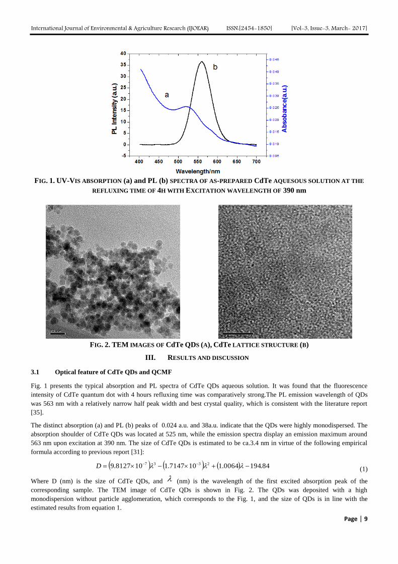
FIG. 1. UV-VIS ABSORPTION (a) and PL (b) SPECTRA OF AS-PREPARED CdTe AQUESOUS SOLUTION AT THE
REFLUXING TIME OF 4H WITH EXCITATION WAVELENGTH OF 390 nm
FIG. 2. TEM IMAGES OF CdTe QDS (A), CdTe LATTICE STRUCTURE (B)
III. RESULTS AND DISCUSSION
3.1 Optical feature of CdTe QDs and QCMF
Fig. 1 presents the typical absorption and PL spectra of CdTe QDs aqueous solution. It was found that the fluorescence
intensity of CdTe quantum dot with 4 hours refluxing time was comparatively strong.The PL emission wavelength of QDs
was 563 nm with a relatively narrow half peak width and best crystal quality, which is consistent with the literature report
[35].
The distinct absorption (a) and PL (b) peaks of 0.024 a.u. and 38a.u. indicate that the QDs were highly monodispersed. The
absorption shoulder of CdTe QDs was located at 525 nm, while the emission spectra display an emission maximum around
563 nm upon excitation at 390 nm. The size of CdTe QDs is estimated to be ca.3.4 nm in virtue of the following empirical
formula according to previous report [31]:
84.1940064.1107147.1108127.9 2337 D (1)
Where D (nm) is the size of CdTe QDs, and (nm) is the wavelength of the first excited absorption peak of the
corresponding sample. The TEM image of CdTe QDs is shown in Fig. 2. The QDs was deposited with a high
monodispersion without particle agglomeration, which corresponds to the Fig. 1, and the size of QDs is in line with the
estimated results from equation 1.
International Journal of Environmental & Agriculture Research (IJOEAR) ISSN:[2454-1850] [Vol-3, Issue-3, March- 2017]
Page | 10
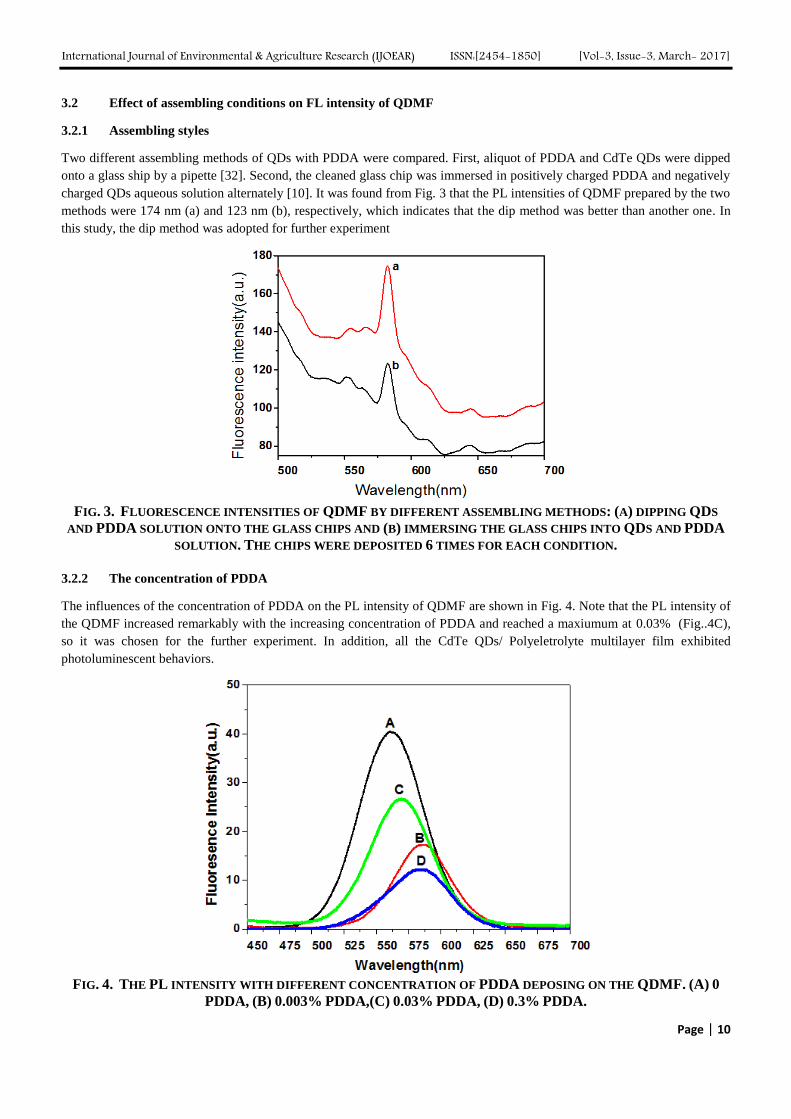
3.2 Effect of assembling conditions on FL intensity of QDMF
3.2.1 Assembling styles
Two different assembling methods of QDs with PDDA were compared. First, aliquot of PDDA and CdTe QDs were dipped
onto a glass ship by a pipette [32]. Second, the cleaned glass chip was immersed in positively charged PDDA and negatively
charged QDs aqueous solution alternately [10]. It was found from Fig. 3 that the PL intensities of QDMF prepared by the two
methods were 174 nm (a) and 123 nm (b), respectively, which indicates that the dip method was better than another one. In
this study, the dip method was adopted for further experiment
FIG. 3. FLUORESCENCE INTENSITIES OF QDMF BY DIFFERENT ASSEMBLING METHODS: (A) DIPPING QDS
AND PDDA SOLUTION ONTO THE GLASS CHIPS AND (B) IMMERSING THE GLASS CHIPS INTO QDS AND PDDA
SOLUTION. THE CHIPS WERE DEPOSITED 6 TIMES FOR EACH CONDITION.
3.2.2 The concentration of PDDA
The influences of the concentration of PDDA on the PL intensity of QDMF are shown in Fig. 4. Note that the PL intensity of
the QDMF increased remarkably with the increasing concentration of PDDA and reached a maxiumum at 0.03% (Fig..4C),
so it was chosen for the further experiment. In addition, all the CdTe QDs/ Polyeletrolyte multilayer film exhibited
photoluminescent behaviors.
FIG. 4. THE PL INTENSITY WITH DIFFERENT CONCENTRATION OF PDDA DEPOSING ON THE QDMF. (A) 0
PDDA, (B) 0.003% PDDA,(C) 0.03% PDDA, (D) 0.3% PDDA.
International Journal of Environmental & Agriculture Research (IJOEAR) ISSN:[2454-1850] [Vol-3, Issue-3, March- 2017]
Page | 11
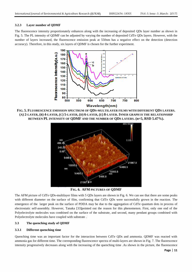
3.2.3 Layer number of QDMF
The fluorescence intensity proportionately enhances along with the increasing of deposited QDs layer number as shown in
Fig. 5. The PL intensity of QDMF can be adjusted by varying the number of deposited CdTe QDs layers. However, with the
number of layers increased, the fluorescence emission peak at 550nm has a negative effect on the detection (detection
accuracy). Therefore, in this study, six layers of QDMF is chosen for the further experiment.
FIG. 5. FLUORESCENCE EMISSION SPECTRUM OF QDS-MULTILAYER FILMS WITH DIFFERENT QDS LAYERS.
(A) 2-LAYER, (B) 4-LAYER, (C) 5-LAYER, (D) 6-LAYER, (E) 8-LAYER. INNER GRAPH IS THE RELATIONSHIP
BETWEEN PL INTENSITY OF QDMF AND THE NUMBER OF QDS LAYERS. (n=5, RSD 5.47%).
FIG. 6. AFM PICTURES OF QDMF
The AFM picture of CdTe QDs-multilayer films with 5 QDs layers are shown in Fig. 6. We can see that there are some peaks
with different diameter on the surface of film, confirming that CdTe QDs were successfully grown in the reaction. The
emergence of the larger peak on the surface of PDDA may be due to the aggregation of CdTe quantum dots in process of
electrostatic self-assembly. However, Tanaka [33]pointed out the reason for this phenomenon. First, only one end of the
Polyelectrolyte molecules was combined on the surface of the substrate, and second, many pendant groups combined with
Polyelectrolyte molecules have coupled with substrate .
3.3 The quenching study of QDMF
3.3.1 Different quenching time
Quenching time was an important factor for the interaction between CdTe QDs and ammonia. QDMF was reacted with
ammonia gas for different time. The corresponding fluorescence spectra of multi-layers are shown in Fig. 7. The fluorescence
intensity progressively decreases along with the increasing of the quenching time .As shown in the picture, the fluorescence
International Journal of Environmental & Agriculture Research (IJOEAR) ISSN:[2454-1850] [Vol-3, Issue-3, March- 2017]
Page | 12
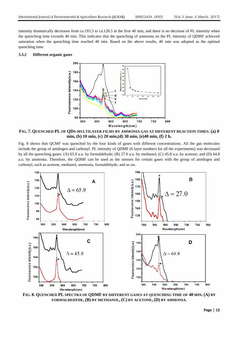
intensity dramatically decreases from ca.193.3 to ca.128.5 in the first 40 min, and there is no decrease of PL intensity when
the quenching time exceeds 40 min. This indicates that the quenching of ammonia on the PL intensity of QDMF achieved
saturation when the quenching time reached 40 min. Based on the above results, 40 min was adopted as the optimal
quenching time.
3.3.2 Different organic gases
FIG. 7. QUENCHED PL OF QDS-MULTILAYER FILMS BY AMMONIA GAS AT DIFFERENT REACTION TIMES. (a) 0
min, (b) 10 min, (c) 20 min,(d) 30 min, (e)40 min, (f) 2 h.
Fig. 8 shows that QCMF was quenched by the four kinds of gases with different concentrations. All the gas molecules
include the group of amidogen and carbonyl. PL intensity of QDMF (6 layer numbers for all the experiments) was decreased
by all the quenching gases: (A) 65.9 a.u. by formaldehyde; (B) 27.0 a.u. by methanol; (C) 45.8 a.u. by acetone; and (D) 64.8
a.u. by ammonia. Therefore, the QDMF can be used as the sensors for certain gases with the group of amidogen and
carbonyl, such as acetone, methanol, ammonia, formaldehyde, and so on.
FIG. 8. QUENCHED PL SPECTRA OF QDMF BY DIFFERENT GASES AT QUENCHING TIME OF 40 MIN. (A) BY
FORMALDEHYDE, (B) BY METHANOL, (C) BY ACETONE, (D) BY AMMONIA.
International Journal of Environmental & Agriculture Research (IJOEAR) ISSN:[2454-1850] [Vol-3, Issue-3, March- 2017]
Page | 13
3.3.3 The fluorescence image of QDMF
FIG. 9. THE FLUORESCENCE IMAGE OF QDMF, BEFORE EXCITATION(a),UV(365nm) excitation(b),
UV(365nm) EXCITATION AFTER QUENCHED BY METHANOL(c).
In our previous work, a preliminary study on the detection effect of the current sensor has been implemented. In this process,
commercial UV light is used to detect prepared samples under conventional conditions(without the aid of fluorescence
spectrometer and other advanced instruments).Fig.9 shows that the prepared sensors have high detection ability for
formaldehyde and other harmful gases. As a result, the family self-detection could be initially realized and the market has
huge potentiality.
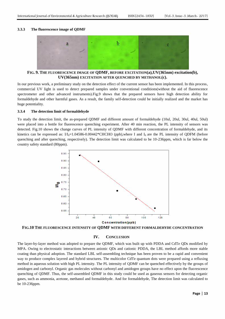
3.3.4 The detection limit of formaldehyde
To study the detection limit, the as-prepared QDMF and different amount of formaldehyde (10ul, 20ul, 30ul, 40ul, 50ul)
were placed into a bottle for fluorescence quenching experiment. After 40 min reaction, the PL intensity of sensors was
detected. Fig.10 shows the change curves of PL intensity of QDMF with different concentration of formaldehyde, and its
kinetics can be expressed as: I/I0=1.04586-0.00442*CHCHO (ppb),where I and I0 are the PL intensity of QDFM (before
quenching and after quenching, respectively). The detection limit was calculated to be 10-236ppm, which is far below the
country safety standard (80ppm).
FIG.10 THE FLUORESCENCE INTENSITY OF QDMF WITH DIFFERENT FORMALDEHYDE CONCENTRATION
IV. CONCLUSION
The layer-by-layer method was adopted to prepare the QDMF, which was built up with PDDA and CdTe QDs modified by
MPA. Owing to electrostatic interactions between anionic QDs and cationic PDDA, the LBL method affords more stable
coating than physical adoption. The standard LBL self-assembling technique has been proven to be a rapid and convenient
way to produce complex layered and hybrid structures. The multicolor CdTe quantum dots were prepared using a refluxing
method in aqueous solution with high PL intensity. The PL intensity of QDMF can be quenched effectively by the groups of
amidogen and carbonyl. Organic gas molecules without carbonyl and amidogen groups have no effect upon the fluorescence
quenching of QDMF. Thus, the self-assembled QDMF in this study could be used as gaseous sensors for detecting organic
gases, such as ammonia, acetone, methanol and formaldehyde. And for formaldehyde, The detection limit was calculated to
be 10-236ppm.
International Journal of Environmental & Agriculture Research (IJOEAR) ISSN:[2454-1850] [Vol-3, Issue-3, March- 2017]
Page | 14
ACKNOWLEDGEMENTS
The current research was funded by Tianjin National Science Foundation of the PRC (No.11JCZDJC22300 and
No.13JCQNJC02600), Program of Introducing Talents of Discipline to Universities of Tianjin Administration of Foreign
Experts Affairs (No.Y2012061), and the Innovative Training Program of Ministry of the PRC (No. 2012100580019).
REFERENCES
[1] A. Airoudj, D. Debarnot, B. Be che, F. Poncin-Epaillard. Anal. Chem. 80 ((2008)) 9188.
[2] M. El-Sherif, L. Bansal, J. Yuan. Sensors. 7 (2007) 3100.
[3] S. Varghese, S. Lonkar, K. K. Singh, S. Swaminathan, A. Abdala. Sens. Actuators, B. 218(2015)160.
[4] M. Hasani, A. M. Coto Garc¨ªa, J. M. Costa-Fern¨¢ndez, A. Sanz-Medel. Sens. Actuators, B. 144 (2010) 198.
[5] R. J.Ellingson, M. C.Beard, J. C.Johnson, P. R.Yu, O.I.Micic, A. J.Nozik, A.Shabaev,A. L.Efros. Nano Lett. 5(2005)865
[6] R. D.Schaller, V. I.Klimov.Phys. Rev. Lett. 92 (2004)1866011
[7] R.Plass, S.Pelet, J.Krueger, M. r t el, U. J. Bach. Phys.Chem. B. 106 (2002) 7578
[8] A. J.Nozik. Physica .E . 14 (2002), 115
[9] P. V. J.Kamat. Phys. Chem. C .111 (2007) 2834
[10] P. T.Snee, R. C.Somers, G.Nair, J. P. Zimmer, M.G.Bawendi, D. G. J.Nocera.. Am. Chem. Soc. 128(2006)13320
[11] G. W. Walker, V. C.Sundar, C. M.Rudzinski, A. W.Wun, M. G.Bawendi, D. G.Nocera, Appl. Phys. Lett. 83 (2003) 3555
[12] N. Hildebrandt. ACS Nano. 5 (2011) 5286
[13] Ali, E.; Zheng, Y.; Yu, H.; Ying, J. Anal. Chem. 2007, 79, 9452−9458.
[14] Dong, H.; ao, W.; Yan, F.; Ji, H.; Ju, H. Anal. Chem. 2010, 82,5511−5517.
[15] Xu, X.; Liu, X.; Nie, Z.; Pan, Y.; uo, M.; Yao, S. Anal. Chem.2011, 83, 52−59.
[16] Wang, Y. Q.; Chen, L. X. J. Nanomed. Nanotechnol. 2011, 7, 385−402.
[17] Liu, M.; Xu, L.; Cheng, W.; Zeng, Y.; Yan, Z. Spectrochim. Acta,Part A 2008, 70,1198−1202.
[18] C. Bertoni, D. Gallardo, S. Dunn, N. Gaponik, A. Eychm¨¹ller. Appl. Phys. Lett. 90 (2007) 034107.
[19] J. Li, D. Bao, X. Hong, D. Li, Y. Bai, T. Li. Colloids Surf., A: Physicochemical and Engineering Aspects. 257 (2005) 267.
[20] J. J. Gooding, F. Mearns, W. Yang, J. Liu. Electroanalysis. 15 (2003) 81.
[21] S. Flink, F. C. J. M. van Veggel, D. N. Reinhoudt. Adv. Mater. 12 (2000) 1315.
[22] D. Zimnitsky, C. Jiang, J. Xu, Z. Lin, L. Zhang, V. V. Tsukruk. Langmuir. 23 (2007) 10176.
[23] J. W. Ostrander, A. A. Mamedov, N. A. Kotov. J. Am. Chem. Soc. 123 (2001) 1101.
[24] B. Chen, Y. Yu, Z. Zhou, P. Zhong. Chem. Lett. 33 (2004) 1608.
[25] Z. X. Cai, H. Yang, Y. Zhang, X. P. Yan. Anal. Chim. Acta. 559 (2006) 234.
[26] J. Chen, Y. C. Gao, Z. B. Xu, G. H. Wu, Y. C. Chen, C. Q. Zhu. Anal. Chim. Acta. 577 (2006) 77.
[27] M. Liu, H. Zhao, S. Chen, H. Yu, Y. Zhang, X. Quan. Chem. Commun. (2011)
[28] K. M. Gatt¨¢s-Asfura, R. M. Leblanc. Chem. Commun. (2003) 2684.
[29] M. T. Fern¨¢ndez-Arg¨¹elles, W. J. Jin, J. M. Costa-Fern¨¢ndez, R. Pereiro, A. Sanz-Medel. Anal. Chim. Acta. 549 (2005) 20.
[30] D. L. Klayman, T. S. Griffin. J. Am. Chem. Soc. 95 (1973) 197.
[31] C. Dong, H. Qian, N. Fang, J. Ren. J. Phys. Chem. B. 110 (2006) 11069.
[32] L. Zhang, X. Zou, E. Ying, S. Dong. J. Phys. Chem. C. 112 (2008) 4451.
[33] F. Yang, Q. Ma, W. Yu, X. Su. Talanta. (2011)
[34] Q. Ma, H. Cui, X. Su. Biosensors and Bioelectronics. 25 (2009) 839.
[35] C. Wang, Q. Ma, X. Su. Journal of Nanoscience and Nanotechnology. 8 (2008) 4408.
[36] W. W. Yu, L. Qu, W. Guo, X. Peng. Chem. Mater. 15 (2003) 2854.
[37] L. Jin, L. Shang, J. Zhai, J. Li, S. Dong. J. Phys. Chem. C. 114 (2009) 803.
[38] Tanaka M, Mochizuki A, Motomura T, et al. Colloid. Surf. A:Physicochem. Eng. Asp.,2001,193(1-3):145-152.
International Journal of Environmental & Agriculture Research (IJOEAR) ISSN:[2454-1850] [Vol-3, Issue-3, March- 2017]
Page | 15
Biosorption of Malathion pesticide using Spirogyra sp.
Chhunthang Liani1, SS Katoch
2
Centre for Energy and Environmental Engineering, National Institute of Technology, Hamirpur, Himachal Pradesh, India
177005
Abstract— The biosorption of Malathion from aqueous solution by green algal biomass was investigated. The green algae
used were of the species Spirogyra and was collected from Neugal river near Sujanpur, Himachal Pradesh. Batch
biosorption experiments were performed to examine the effect of contact time, pH, biomass concentration and initial
Malathion concentration. The concentration of residual Malathion concentration after biosorption was determined using
UV-Vis Spectrophotometer at a wavelength of 309 nm. The maximum adsorption was found to be at pH 7 after a contact time
of 5 hours with initial Malathion concentration of 100 mg/L and biomass of weight 75 mg. The equilibrium biosorption data
were analyzed using Langmuir and Freundlich isotherm. Freundlich isotherm was found to be more favorable than
Langmuir isotherm.
Keywords— algae, biosorption, isotherm, Malathion, pesticide.
I. INTRODUCTION
The use of pesticide is essential for the modern agricultural practice. Pesticides not only kill unwanted pests and insects, they
also increase the productivity of agriculture. In India, agricultural production increased by 100% while the cropping land
increased by only 20% [1]. Pesticide residues that get released into the environment tend to stay in the environment for a
very long time, and get accumulated throughout the food chain, making it hazardous to the environment. The U.S. Geological
Survey conducted a study from which they reported that more than 90% of the water and fish samples that they collected
from major rivers or water streams were contaminated with pesticides. The rivers and streams which were contaminated by
pesticides were influenced by agriculture and urban land use [2]. Currently, India ranks 10th in the world pesticide
consumption list [3] and the Indian agrochemical market is expected to reach U.S $ 6.3 billion by 2020 [4].
Pesticides are classified into many classes, out of which, organophosphates and organochlorines are deemed the most
important ones. Malathion is an organophosphorus pesticide which is most commonly used in agriculture all over the world.
It is used for killing insects on agricultural crops and stored products. It is also widely used for killing mosquitos in urban and
residential areas. It is also used for the control of flies, household insects and head and body lice. In 2006, it was reported that
approximately 15 million pounds of Malathion were used worldwide annually [5]. The Environmental Protection Agency has
identified Malathion as a toxicity class III pesticide and a general use pesticide (GUP). Malathion interferes with the normal
function of the nervous system and thus indirectly affects the function of other organs. The effect of exposure to Malathion
on human health may include, but not limited to, difficulty in breathing, vomiting, diarrhoea, headaches, dizziness and loss of
consciousness and death [6].
Several methods have been proposed for the removal/treatment of Malathion from raw water and wastewater such as
electrocoagulation, advanced oxidation and coagulation/flocculation [7, 8, 9]. The limitations to these methods are that they
are quiet expensive and the chemicals used for these methods require constant observation and it is preferable that they be
handled by a skilled person. Adsorption with activated carbon is an easy and cost effective method for the removal of
pesticides and has been extensively studied for the removal of Malathion [10- 11]. In recent years, studies about the removal
of Malathion by biological materials have increased due to their easy availability, low cost and efficiency. Biosorption by
activated sludge, isolated bacillus sp., Rhizopus oryzae, nanocellulose, algal biomass of Chlorella vulgaris, chesnut shells
and the fungal biomass of Phanerochaete chrysosporium has been studied with positive results [12, 13, 14, 15, 16, 17, 18].
Either live or dead biomass can be used in biosorption process. Live biomass has been used for the removal of heavy metals
in the past [19- 20]. The use of dead biomass is more desirable than the live ones as dead biomass do not require nutrients to
sustain them and can be stored to be used later. While using live biomass, sorption as well as biodegradation may also occur
and it is very difficult to distinguish which one of them has more contribution.
International Journal of Environmental & Agriculture Research (IJOEAR) ISSN:[2454-1850] [Vol-3, Issue-3, March- 2017]
Page | 16
The present study investigates Malathion removal from aqueous solution by biosorption using green algal biomass of species
Spirogyra, which is abundant in fresh water lakes and rivers. Laboratory batch experiments were carried out using a shaker-
incubator at a constant temperature to determine the optimum contact time, pH, weight of biomass and initial Malathion
concentration for maximum removal. Langmuir and Freundlich isotherms were used for determining the sorption capacity of
Spirogyra sp.
II. MATERIALS AND METHOD
2.1 Malathion solution
Commercially available Malathion 50% E.C, Osothion, was used in this study.
2.2 Biomass
The green algae, Spirogyra sp., used in this study was collected from Neugal River near Sujanpur, located at 31.83ºN
76.50ºE, Himachal Pradesh. The algae was washed with distilled water to remove dirt and other impurities after which it was
sundried for 6 hours and then it was kept in an oven for 48 hours at 130º C to make sure it was completely dead. The dead
biomass was grounded using a pestle and mortar to get fine powder. The powdered biomass was kept in a crucible and stored
in a desiccator until used.
2.3 Measurement of residual Malathion concentration
Pure solution of Malathion was scanned in an UV-Vis Spectrophotometer from Aligent Technology, Cary Series to
determine the wavelength with maximum absorbance. Maximum absorbance was found at wavelength 309 nm. Using this
wavelength, a standard curve of Malathion solution of known concentration (50 – 250 mg/L) was prepared. This data was
used to determine the unknown concentration of residual Malathion concentration.
2.4 Batch Kinetic Study
Batch kinetic study was performed by taking 100 mL of Malathion solution in 250 mL Erlenmeyer flasks. Optimum removal
of Malathion from the solution was determined based on contact time, pH, amount of biomass kept in contact with the
pesticide solution and initial Malathion concentration. The flasks were kept in a shaker-incubator for a specific amount of
time at 130rpm and the temperature of the incubator was kept at 27 ± 2º C. The pH of the solution was adjusted using 0.1M
NaOH and 5% HCl. The final residual concentration of Malathion in the solution was determined using UV-Vis
Spectrophotometer as mentioned before.
The amount of Malathion adsorbed by the algal biomass was calculated using the formula
Qe = (C0 – Ce) V/m (1)
Where,
Qe (mg/g) is the amount of Malathion adsorbed per unit weight of the algal biomass.
C0 (mg/L) is the initial Malathion concentration.
Ce (mg/L) is the Malathion concentration at equilibrium
V (L) is the amount of Malathion solution.
m (g) is the amount of biomass used.
All tests were performed in triplets and their average was taken for the actual calculation.
2.5 Biosorption isotherm
To evaluate the biosorption performance, a graph between the sorbate in the solution and the amount of sorbate sorbed on the
biosorbent is plotted. There are various isotherm models which have been proposed and used throughout the years. In this
study, Langmuir and Freundlich isotherm are studied to evaluate the data.
The equation for Langmuir isotherm is
International Journal of Environmental & Agriculture Research (IJOEAR) ISSN:[2454-1850] [Vol-3, Issue-3, March- 2017]
Page | 17
Qe = QmbCe / (1+b.Ce) (2)
Where,
Qe is the amount of Malathion adsorbed (mg/g)
Qm is the maximum Malathion adsorbed per unit biomass (mg/g)
Ce is the equilibrium concentration of Malathion (mg/L)
b is the Langmuir equilibrium constant (L/mg) and it explains the affinity between the sorbent and sorbate..
The Langmuir isotherm equation can be arranged into linear form
Ce/Qe = 1/b.Qm + Ce/Qm (3)
Which can be further rearranged into?
1/Qe = 1/b.Qm Ce + 1/Qm (4)
A plot between 1/Qe and 1/Ce will give intercept 1/Qm and slope 1/b.Qm.
The Freundlich isotherm is described by the following equation
Qe = k.Ce1/n (5)
Where,
k and n represents Freundlich constants. k indicates the adsorption/binding capacity (L/g) and n indicates the intensity of the
adsorption i.e. the affinity between the sorbent and sorbate.
The linearized form of equation (4) can be written by taking logarithm on both sides
ln Qe = 1/n ln Ce + ln k (6)
III. RESULTS AND DISCUSSION
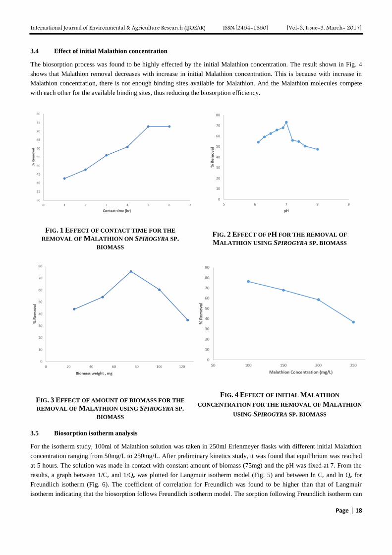
3.1 Effect of contact time
After performing batch biosorption study, it was observed that with the increase in time, the percentage removal of
Malathion increases. Highest Malathion removal was observed at 5 hours after which, the removal percentage remained
constant. This can be explained by the fact that after 5 hours, all the active biosorption sites have been occupied by
Malathion. The result of the contact time test is shown in Fig. 1.
3.2 Effect of pH
After performing biosorption test with different pH, it was found that highest amount of Malathion removal was achieved at
pH 7, after which the removal percentage starts to decrease again, suggesting that at lower and higher pH, all the functional
groups responsible for biosorption have bounded, thus resulting in lower biosorption. While, at neutral pH, the functional
groups are free for biosorption. The result of Malathion removal with respect to pH is shown in Fig. 2.
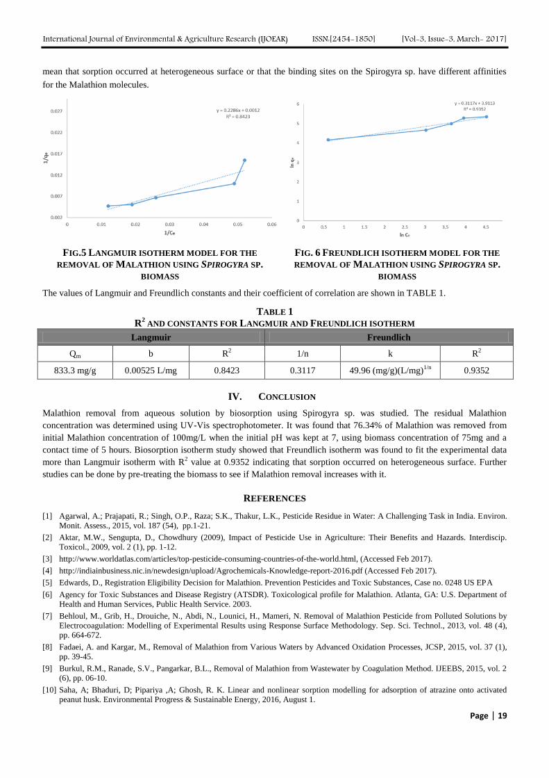
3.3 Effect of biomass weight
Batch biosorption studies were done to determine the effect of weight of biomass made in contact with the Malathion
solution for the removal of Malathion with varying weight of biomass. It was found that the removal of Malathion increased
with increase in biomass concentration till 75 mg after which the removal decreased again, making 75 mg the optimum dose
of biomass. This can be explained by the fact that with less amount of biomass, the amount of Malathion was much more
such that there were not enough biomass surfaces where Malathion could bind on to. While at higher biomass concentration,
all available sorption sites were not utilized causing agglomeration of the biomass which in turn decreases the amount of
adsorption sites available. The result is shown in Fig. 3.
International Journal of Environmental & Agriculture Research (IJOEAR) ISSN:[2454-1850] [Vol-3, Issue-3, March- 2017]
Page | 18
3.4 Effect of initial Malathion concentration
The biosorption process was found to be highly effected by the initial Malathion concentration. The result shown in Fig. 4
shows that Malathion removal decreases with increase in initial Malathion concentration. This is because with increase in
Malathion concentration, there is not enough binding sites available for Malathion. And the Malathion molecules compete
with each other for the available binding sites, thus reducing the biosorption efficiency.
FIG. 1 EFFECT OF CONTACT TIME FOR THE
REMOVAL OF MALATHION ON SPIROGYRA SP.
BIOMASS
FIG. 2 EFFECT OF PH FOR THE REMOVAL OF
MALATHION USING SPIROGYRA SP. BIOMASS
FIG. 3 EFFECT OF AMOUNT OF BIOMASS FOR THE
REMOVAL OF MALATHION USING SPIROGYRA SP.
BIOMASS
FIG. 4 EFFECT OF INITIAL MALATHION
CONCENTRATION FOR THE REMOVAL OF MALATHION
USING SPIROGYRA SP. BIOMASS
3.5 Biosorption isotherm analysis
For the isotherm study, 100ml of Malathion solution was taken in 250ml Erlenmeyer flasks with different initial Malathion
concentration ranging from 50mg/L to 250mg/L. After preliminary kinetics study, it was found that equilibrium was reached
at 5 hours. The solution was made in contact with constant amount of biomass (75mg) and the pH was fixed at 7. From the
results, a graph between 1/Ce and 1/Qe was plotted for Langmuir isotherm model (Fig. 5) and between ln Ce and ln Qe for
Freundlich isotherm (Fig. 6). The coefficient of correlation for Freundlich was found to be higher than that of Langmuir
isotherm indicating that the biosorption follows Freundlich isotherm model. The sorption following Freundlich isotherm can
International Journal of Environmental & Agriculture Research (IJOEAR) ISSN:[2454-1850] [Vol-3, Issue-3, March- 2017]
Page | 19
mean that sorption occurred at heterogeneous surface or that the binding sites on the Spirogyra sp. have different affinities
for the Malathion molecules.
FIG.5 LANGMUIR ISOTHERM MODEL FOR THE
REMOVAL OF MALATHION USING SPIROGYRA SP.
BIOMASS
FIG. 6 FREUNDLICH ISOTHERM MODEL FOR THE
REMOVAL OF MALATHION USING SPIROGYRA SP.
BIOMASS
The values of Langmuir and Freundlich constants and their coefficient of correlation are shown in TABLE 1.
TABLE 1
R2 AND CONSTANTS FOR LANGMUIR AND FREUNDLICH ISOTHERM
Langmuir Freundlich
Qm b R2 1/n k R
2
833.3 mg/g 0.00525 L/mg 0.8423 0.3117 49.96 (mg/g)(L/mg)1/n
0.9352
IV. CONCLUSION
Malathion removal from aqueous solution by biosorption using Spirogyra sp. was studied. The residual Malathion
concentration was determined using UV-Vis spectrophotometer. It was found that 76.34% of Malathion was removed from
initial Malathion concentration of 100mg/L when the initial pH was kept at 7, using biomass concentration of 75mg and a
contact time of 5 hours. Biosorption isotherm study showed that Freundlich isotherm was found to fit the experimental data
more than Langmuir isotherm with R2 value at 0.9352 indicating that sorption occurred on heterogeneous surface. Further
studies can be done by pre-treating the biomass to see if Malathion removal increases with it.
REFERENCES
[1] Agarwal, A.; Prajapati, R.; Singh, O.P., Raza; S.K., Thakur, L.K., Pesticide Residue in Water: A Challenging Task in India. Environ.
Monit. Assess., 2015, vol. 187 (54), pp.1-21.
[2] Aktar, M.W., Sengupta, D., Chowdhury (2009), Impact of Pesticide Use in Agriculture: Their Benefits and Hazards. Interdiscip.
Toxicol., 2009, vol. 2 (1), pp. 1-12.
[3] http://www.worldatlas.com/articles/top-pesticide-consuming-countries-of-the-world.html, (Accessed Feb 2017).
[4] http://indiainbusiness.nic.in/newdesign/upload/Agrochemicals-Knowledge-report-2016.pdf (Accessed Feb 2017).
[5] Edwards, D., Registration Eligibility Decision for Malathion. Prevention Pesticides and Toxic Substances, Case no. 0248 US EPA
[6] Agency for Toxic Substances and Disease Registry (ATSDR). Toxicological profile for Malathion. Atlanta, GA: U.S. Department of
Health and Human Services, Public Health Service. 2003.
[7] Behloul, M., Grib, H., Drouiche, N., Abdi, N., Lounici, H., Mameri, N. Removal of Malathion Pesticide from Polluted Solutions by
Electrocoagulation: Modelling of Experimental Results using Response Surface Methodology. Sep. Sci. Technol., 2013, vol. 48 (4),
pp. 664-672.
[8] Fadaei, A. and Kargar, M., Removal of Malathion from Various Waters by Advanced Oxidation Processes, JCSP, 2015, vol. 37 (1),
pp. 39-45.
[9] Burkul, R.M., Ranade, S.V., Pangarkar, B.L., Removal of Malathion from Wastewater by Coagulation Method. IJEEBS, 2015, vol. 2
(6), pp. 06-10.
[10] Saha, A; Bhaduri, D; Pipariya ,A; Ghosh, R. K. Linear and nonlinear sorption modelling for adsorption of atrazine onto activated
peanut husk. Environmental Progress & Sustainable Energy, 2016, August 1.
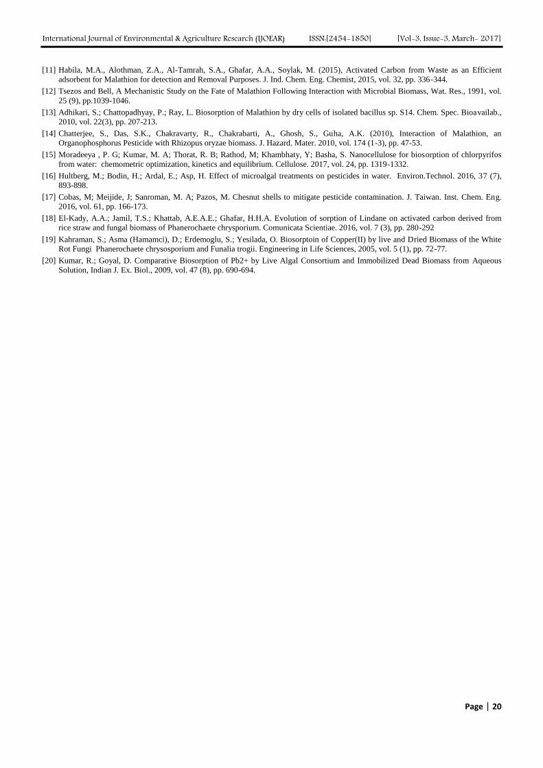
International Journal of Environmental & Agriculture Research (IJOEAR) ISSN:[2454-1850] [Vol-3, Issue-3, March- 2017]
Page | 20
[11] Habila, M.A., Alothman, Z.A., Al-Tamrah, S.A., Ghafar, A.A., Soylak, M. (2015), Activated Carbon from Waste as an Efficient
adsorbent for Malathion for detection and Removal Purposes. J. Ind. Chem. Eng. Chemist, 2015, vol. 32, pp. 336-344.
[12] Tsezos and Bell, A Mechanistic Study on the Fate of Malathion Following Interaction with Microbial Biomass, Wat. Res., 1991, vol.
25 (9), pp.1039-1046.
[13] Adhikari, S.; Chattopadhyay, P.; Ray, L. Biosorption of Malathion by dry cells of isolated bacillus sp. S14. Chem. Spec. Bioavailab.,
2010, vol. 22(3), pp. 207-213.
[14] Chatterjee, S., Das, S.K., Chakravarty, R., Chakrabarti, A., Ghosh, S., Guha, A.K. (2010), Interaction of Malathion, an
Organophosphorus Pesticide with Rhizopus oryzae biomass. J. Hazard. Mater. 2010, vol. 174 (1-3), pp. 47-53.
[15] Moradeeya , P. G; Kumar, M. A; Thorat, R. B; Rathod, M; Khambhaty, Y; Basha, S. Nanocellulose for biosorption of chlorpyrifos
from water: chemometric optimization, kinetics and equilibrium. Cellulose. 2017, vol. 24, pp. 1319-1332.
[16] Hultberg, M.; Bodin, H.; Ardal, E.; Asp, H. Effect of microalgal treatments on pesticides in water. Environ.Technol. 2016, 37 (7),
893-898.
[17] Cobas, M; Meijide, J; Sanroman, M. A; Pazos, M. Chesnut shells to mitigate pesticide contamination. J. Taiwan. Inst. Chem. Eng.
2016, vol. 61, pp. 166-173.
[18] El-Kady, A.A.; Jamil, T.S.; Khattab, A.E.A.E.; Ghafar, H.H.A. Evolution of sorption of Lindane on activated carbon derived from
rice straw and fungal biomass of Phanerochaete chrysporium. Comunicata Scientiae. 2016, vol. 7 (3), pp. 280-292
[19] Kahraman, S.; Asma (Hamamci), D.; Erdemoglu, S.; Yesilada, O. Biosorptoin of Copper(II) by live and Dried Biomass of the White
Rot Fungi Phanerochaete chrysosporium and Funalia trogii. Engineering in Life Sciences, 2005, vol. 5 (1), pp. 72-77.
[20] Kumar, R.; Goyal, D. Comparative Biosorption of Pb2+ by Live Algal Consortium and Immobilized Dead Biomass from Aqueous
Solution, Indian J. Ex. Biol., 2009, vol. 47 (8), pp. 690-694.
International Journal of Environmental & Agriculture Research (IJOEAR) ISSN:[2454-1850] [Vol-3, Issue-3, March- 2017]
Page | 21
The Relationship between Soil Moisture and Temperature
Vegetation on Kirklareli City Luleburgaz District A Natural
Pasture Vegetation Canan Sen
1, Ozan Ozturk
2
1Department of Field Crops Agricultural Faculty, University of Namik Kemal, Tekirdag-Turkey
2Ataturk Soil Water and Agricultural Meteorology Research Institute, Kirklareli-Turkey
Abstract— This study was realized in 2014 – 2015 in two different sections of Kirklareli city Luleburgaz district Sakizkoy
village natural pasture in order to research the effect of soil moisture and soil temperature on area covered by vegetation,
plant species and dry yield. As research area, study was conducted in two different sections defined as A and B located to the
north and south of village coppice forest area located within the borders of Kirklareli city Luleburgaz district Sakizkoy
village. By this study, the relation between soil moisture and temperature with plant species were evaluated by CANOCO 4.5
computer program. Accordingly, the effect of ecological values on vegetative properties was presented. According to
research results, soil moisture and temperature have significant effect on vegetation. In the first year when soil moisture was
high, hay yield was 2901.9 kg/ha while the yield was detected as 480.1 kg/ha after soil temperature (which is inversely
correlated with soil moisture) increased in the second year. It was determined that Lolium perenne (one of the dominant
species of vegetation) is common in parcels with high moisture while Chrysopogon gryllus is common in parcels where soil
temperature is high.
Keywords— pasture, dry yield, soil moisture, soil temperature, CANOCO 4.5.
I. INTRODUCTION
Climate change is expected to affect agriculture very differently in different parts of the world (Parry et al., 2004). Climate
change impacts on crop yield are often integrated with its effects on water productivity and soil water balance. Global
warming will influence temperature and rainfall, which will directly have effects on the soil moisture status and groundwater
level (Kang et al.2009). According to Valentine, (1990), livestock products provide the major economic return from most
range and pasture lands and compared with harvested or purchased feeds, pastures and pasture provide a relatively
inexpensive and energy-efficient feed source for livestock. Climate change is change the community structure of grasslands
(Buckland et al., 2001; Lüscher et al., 2004). Grasslands will differ in their response to climate change depending on their
type (species, soil type, management) (Olesen , 2006 ). Management and species richness of grasslands may increase their
resilience to change (Duckworth et al., 2000). Particularly climatic factors, like mean annual precipitation and precipitation
variability, have a huge impact on rangeland condition and fodder production (Williams and Albertson, 2006). Climate
change in the form of decreasing mean annual precipitation accompanied by increasing variability has important
consequences for rangeland productivity and thus pastoral livelihood security (Martin et al.2013). Soil moisture plays a key
role in vegetation restoration and ecosystem stability in arid and semiarid regions. The response of soil moisture to rainfall
pulses is an important hydrological process, which is strongly influenced by land use during the implementation of
vegetation restoration. Soil moisture depended strongly on precipitation (Yu et al.2015). Soil moisture is a key rangeland
health parameter as it is the principal limiting factor in semi-arid ecosystems (Weber and Gokhale, 2010) . Soil moisture and
temperature are together referred to as "soil climate". The effects of soil climate are mainly the basic determining criteria that
separate range ecosystems from other natural ecosystems. In addition, soil climate affects all soil-plant relationships in range
ecosystems. Rooting depth, water potentials, nutrient intake and nutrient element distribution are affected by the amount and
time of moisture availability associated with the critical temperatures at which the root activity is observed. The temperature
and moisture near the soil surface affect the germination of range plants. Besides germination, settlement and continuity also
depend on the temperature and moisture of the soil (Altin et al. 2011). Temperature is an important feature that has a
significant effect on the biological events that take place in the soil and directs the physical and chemical processes. The root
development of most plants ceases at temperatures below 5˚C. The availability of soil and air temperature data is necessary
to understand plant-soil relationships and to be able to make comments on the use of the soil (Dinc and Senol, 1998) and
therefore will create a basis for the projections to be drawn for range management and improvement in the future. The
objective of this study is to determine the effects of I) different pasture sites and II) soil moisture and temperature on
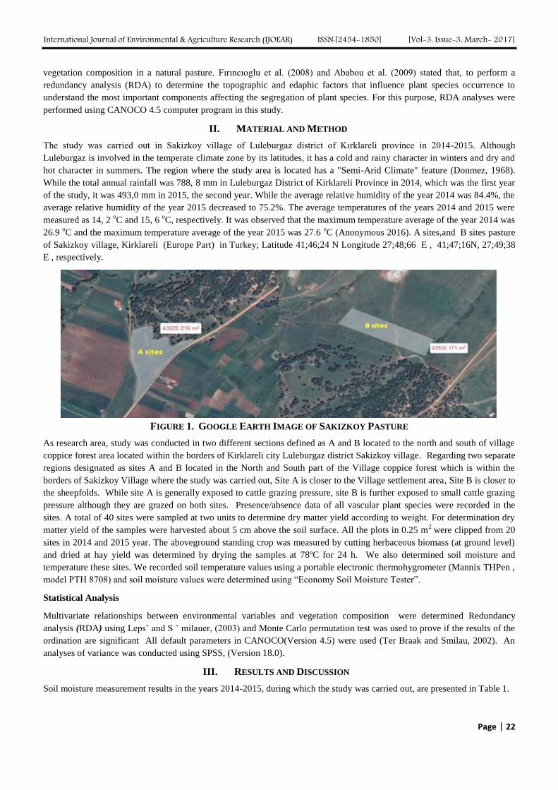
International Journal of Environmental & Agriculture Research (IJOEAR) ISSN:[2454-1850] [Vol-3, Issue-3, March- 2017]
Page | 22
vegetation composition in a natural pasture. Fırıncıoglu et al. (2008) and Ababou et al. (2009) stated that, to perform a
redundancy analysis (RDA) to determine the topographic and edaphic factors that influence plant species occurrence to
understand the most important components affecting the segregation of plant species. For this purpose, RDA analyses were
performed using CANOCO 4.5 computer program in this study.
II. MATERIAL AND METHOD
The study was carried out in Sakizkoy village of Luleburgaz district of Kırklareli province in 2014-2015. Although
Luleburgaz is involved in the temperate climate zone by its latitudes, it has a cold and rainy character in winters and dry and
hot character in summers. The region where the study area is located has a "Semi-Arid Climate" feature (Donmez, 1968).
While the total annual rainfall was 788, 8 mm in Luleburgaz District of Kirklareli Province in 2014, which was the first year
of the study, it was 493,0 mm in 2015, the second year. While the average relative humidity of the year 2014 was 84.4%, the
average relative humidity of the year 2015 decreased to 75.2%. The average temperatures of the years 2014 and 2015 were
measured as 14, 2 oC and 15, 6
oC, respectively. It was observed that the maximum temperature average of the year 2014 was
26.9 oC and the maximum temperature average of the year 2015 was 27.6
oC (Anonymous 2016). A sites,and B sites pasture
of Sakizkoy village, Kirklareli (Europe Part) in Turkey; Latitude 41;46;24 N Longitude 27;48;66 E , 41;47;16N, 27;49;38
E , respectively.
FIGURE 1. GOOGLE EARTH IMAGE OF SAKIZKOY PASTURE
As research area, study was conducted in two different sections defined as A and B located to the north and south of village
coppice forest area located within the borders of Kirklareli city Luleburgaz district Sakizkoy village. Regarding two separate
regions designated as sites A and B located in the North and South part of the Village coppice forest which is within the
borders of Sakizkoy Village where the study was carried out, Site A is closer to the Village settlement area, Site B is closer to
the sheepfolds. While site A is generally exposed to cattle grazing pressure, site B is further exposed to small cattle grazing
pressure although they are grazed on both sites. Presence/absence data of all vascular plant species were recorded in the
sites. A total of 40 sites were sampled at two units to determine dry matter yield according to weight. For determination dry
matter yield of the samples were harvested about 5 cm above the soil surface. All the plots in 0.25 m2
were clipped from 20
sites in 2014 and 2015 year. The aboveground standing crop was measured by cutting herbaceous biomass (at ground level)
and dried at hay yield was determined by drying the samples at 78ºC for 24 h. We also determined soil moisture and
temperature these sites. We recorded soil temperature values using a portable electronic thermohygrometer (Mannix THPen ,
model PTH 8708) and soil moisture values were determined using “Economy Soil Moisture Tester”.
Statistical Analysis
Multivariate relationships between environmental variables and vegetation composition were determined Redundancy
analysis (RDA) using Lepsˇ and S ˇ milauer, (2003) and Monte Carlo permutation test was used to prove if the results of the
ordination are significant All default parameters in CANOCO(Version 4.5) were used (Ter Braak and Smilau, 2002). An
analyses of variance was conducted using SPSS, (Version 18.0).
III. RESULTS AND DISCUSSION
Soil moisture measurement results in the years 2014-2015, during which the study was carried out, are presented in Table 1.
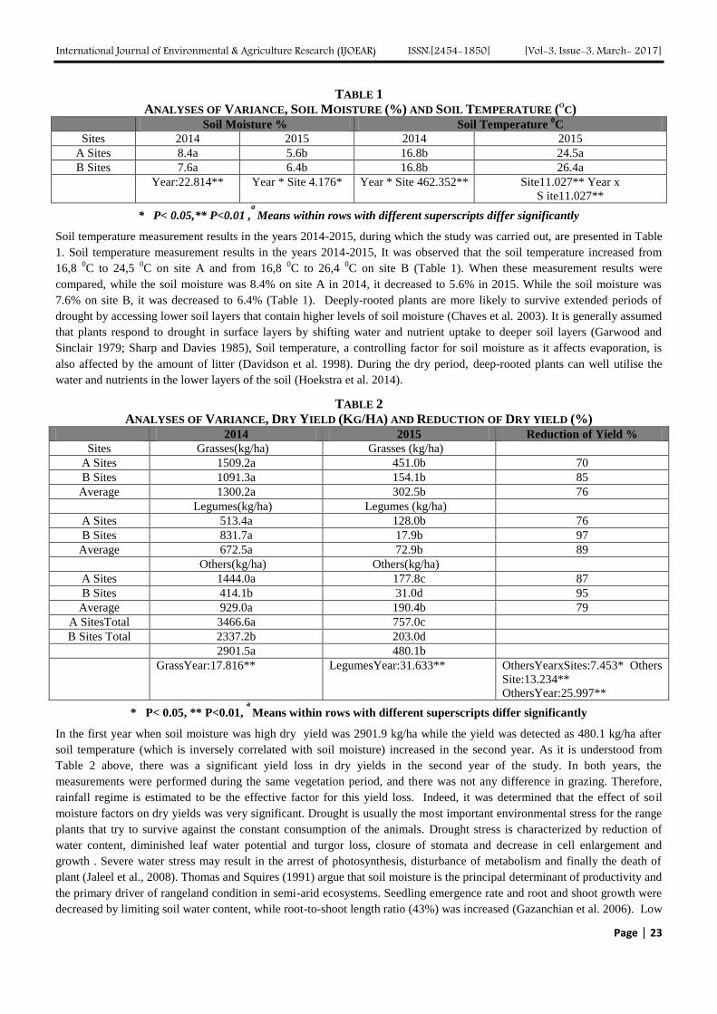
International Journal of Environmental & Agriculture Research (IJOEAR) ISSN:[2454-1850] [Vol-3, Issue-3, March- 2017]
Page | 23
TABLE 1
ANALYSES OF VARIANCE, SOIL MOISTURE (%) AND SOIL TEMPERATURE (OC)
Soil Moisture % Soil Temperature 0C
Sites 2014 2015 2014 2015
A Sites 8.4a 5.6b 16.8b 24.5a
B Sites 7.6a 6.4b 16.8b 26.4a
Year:22.814** Year * Site 4.176* Year * Site 462.352** Site11.027** Year x
S ite11.027**
* P< 0.05,** P<0.01 ,a
Means within rows with different superscripts differ significantly
Soil temperature measurement results in the years 2014-2015, during which the study was carried out, are presented in Table
1. Soil temperature measurement results in the years 2014-2015, It was observed that the soil temperature increased from
16,8 0C to 24,5
0C on site A and from 16,8
0C to 26,4
0C on site B (Table 1). When these measurement results were
compared, while the soil moisture was 8.4% on site A in 2014, it decreased to 5.6% in 2015. While the soil moisture was
7.6% on site B, it was decreased to 6.4% (Table 1). Deeply-rooted plants are more likely to survive extended periods of
drought by accessing lower soil layers that contain higher levels of soil moisture (Chaves et al. 2003). It is generally assumed
that plants respond to drought in surface layers by shifting water and nutrient uptake to deeper soil layers (Garwood and
Sinclair 1979; Sharp and Davies 1985), Soil temperature, a controlling factor for soil moisture as it affects evaporation, is
also affected by the amount of litter (Davidson et al. 1998). During the dry period, deep-rooted plants can well utilise the
water and nutrients in the lower layers of the soil (Hoekstra et al. 2014).
TABLE 2
ANALYSES OF VARIANCE, DRY YIELD (KG/HA) AND REDUCTION OF DRY YIELD (%) 2014 2015 Reduction of Yield %
Sites Grasses(kg/ha) Grasses (kg/ha)
A Sites 1509.2a 451.0b 70
B Sites 1091.3a 154.1b 85
Average 1300.2a 302.5b 76
Legumes(kg/ha) Legumes (kg/ha)
A Sites 513.4a 128.0b 76
B Sites 831.7a 17.9b 97
Average 672.5a 72.9b 89
Others(kg/ha) Others(kg/ha)
A Sites 1444.0a 177.8c 87
B Sites 414.1b 31.0d 95
Average 929.0a 190.4b 79
A SitesTotal 3466.6a 757.0c
B Sites Total 2337.2b 203.0d
2901.5a 480.1b
GrassYear:17.816** LegumesYear:31.633** OthersYearxSites:7.453* Others
Site:13.234**
OthersYear:25.997**
* P< 0.05, ** P<0.01, a
Means within rows with different superscripts differ significantly
In the first year when soil moisture was high dry yield was 2901.9 kg/ha while the yield was detected as 480.1 kg/ha after
soil temperature (which is inversely correlated with soil moisture) increased in the second year. As it is understood from
Table 2 above, there was a significant yield loss in dry yields in the second year of the study. In both years, the
measurements were performed during the same vegetation period, and there was not any difference in grazing. Therefore,
rainfall regime is estimated to be the effective factor for this yield loss. Indeed, it was determined that the effect of soil
moisture factors on dry yields was very significant. Drought is usually the most important environmental stress for the range
plants that try to survive against the constant consumption of the animals. Drought stress is characterized by reduction of
water content, diminished leaf water potential and turgor loss, closure of stomata and decrease in cell enlargement and
growth . Severe water stress may result in the arrest of photosynthesis, disturbance of metabolism and finally the death of
plant (Jaleel et al., 2008). Thomas and Squires (1991) argue that soil moisture is the principal determinant of productivity and
the primary driver of rangeland condition in semi-arid ecosystems. Seedling emergence rate and root and shoot growth were
decreased by limiting soil water content, while root-to-shoot length ratio (43%) was increased (Gazanchian et al. 2006). Low
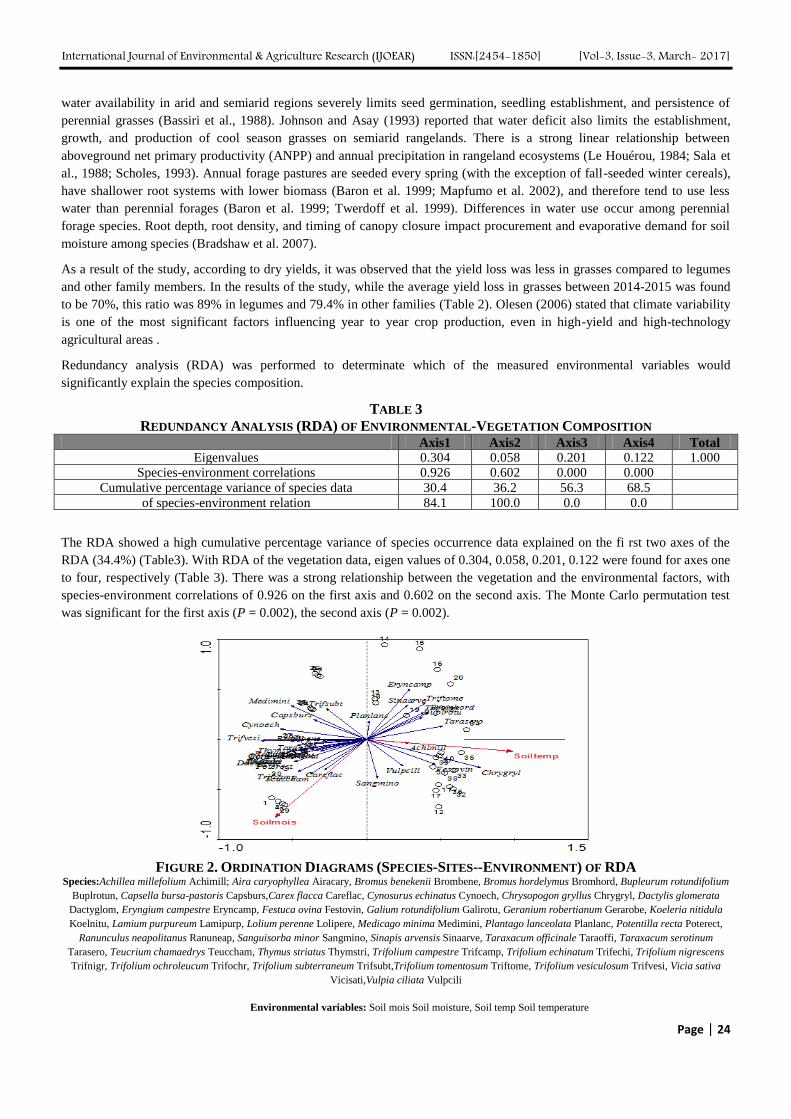
International Journal of Environmental & Agriculture Research (IJOEAR) ISSN:[2454-1850] [Vol-3, Issue-3, March- 2017]
Page | 24
water availability in arid and semiarid regions severely limits seed germination, seedling establishment, and persistence of
perennial grasses (Bassiri et al., 1988). Johnson and Asay (1993) reported that water deficit also limits the establishment,
growth, and production of cool season grasses on semiarid rangelands. There is a strong linear relationship between
aboveground net primary productivity (ANPP) and annual precipitation in rangeland ecosystems (Le Houérou, 1984; Sala et
al., 1988; Scholes, 1993). Annual forage pastures are seeded every spring (with the exception of fall-seeded winter cereals),
have shallower root systems with lower biomass (Baron et al. 1999; Mapfumo et al. 2002), and therefore tend to use less
water than perennial forages (Baron et al. 1999; Twerdoff et al. 1999). Differences in water use occur among perennial
forage species. Root depth, root density, and timing of canopy closure impact procurement and evaporative demand for soil
moisture among species (Bradshaw et al. 2007).
As a result of the study, according to dry yields, it was observed that the yield loss was less in grasses compared to legumes
and other family members. In the results of the study, while the average yield loss in grasses between 2014-2015 was found
to be 70%, this ratio was 89% in legumes and 79.4% in other families (Table 2). Olesen (2006) stated that climate variability
is one of the most significant factors influencing year to year crop production, even in high-yield and high-technology
agricultural areas .
Redundancy analysis (RDA) was performed to determinate which of the measured environmental variables would
significantly explain the species composition.
TABLE 3
REDUNDANCY ANALYSIS (RDA) OF ENVIRONMENTAL-VEGETATION COMPOSITION Axis1 Axis2 Axis3 Axis4 Total
Eigenvalues 0.304 0.058 0.201 0.122 1.000 Species-environment correlations 0.926 0.602 0.000 0.000
Cumulative percentage variance of species data 30.4 36.2 56.3 68.5
of species-environment relation 84.1 100.0 0.0 0.0
The RDA showed a high cumulative percentage variance of species occurrence data explained on the fi rst two axes of the
RDA (34.4%) (Table3). With RDA of the vegetation data, eigen values of 0.304, 0.058, 0.201, 0.122 were found for axes one
to four, respectively (Table 3). There was a strong relationship between the vegetation and the environmental factors, with
species-environment correlations of 0.926 on the first axis and 0.602 on the second axis. The Monte Carlo permutation test
was significant for the first axis (P = 0.002), the second axis (P = 0.002).
FIGURE 2. ORDINATION DIAGRAMS (SPECIES-SITES--ENVIRONMENT) OF RDA Species:Achillea millefolium Achimill; Aira caryophyllea Airacary, Bromus benekenii Brombene, Bromus hordelymus Bromhord, Bupleurum rotundifolium
Buplrotun, Capsella bursa-pastoris Capsburs,Carex flacca Careflac, Cynosurus echinatus Cynoech, Chrysopogon gryllus Chrygryl, Dactylis glomerata
Dactyglom, Eryngium campestre Eryncamp, Festuca ovina Festovin, Galium rotundifolium Galirotu, Geranium robertianum Gerarobe, Koeleria nitidula
Koelnitu, Lamium purpureum Lamipurp, Lolium perenne Lolipere, Medicago minima Medimini, Plantago lanceolata Planlanc, Potentilla recta Poterect,
Ranunculus neapolitanus Ranuneap, Sanguisorba minor Sangmino, Sinapis arvensis Sinaarve, Taraxacum officinale Taraoffi, Taraxacum serotinum
Tarasero, Teucrium chamaedrys Teuccham, Thymus striatus Thymstri, Trifolium campestre Trifcamp, Trifolium echinatum Trifechi, Trifolium nigrescens
Trifnigr, Trifolium ochroleucum Trifochr, Trifolium subterraneum Trifsubt,Trifolium tomentosum Triftome, Trifolium vesiculosum Trifvesi, Vicia sativa
Vicisati,Vulpia ciliata Vulpcili
Environmental variables: Soil mois Soil moisture, Soil temp Soil temperature
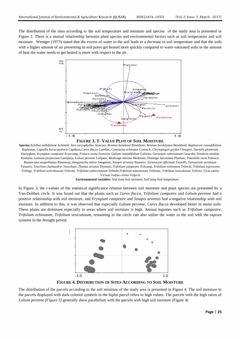
International Journal of Environmental & Agriculture Research (IJOEAR) ISSN:[2454-1850] [Vol-3, Issue-3, March- 2017]
Page | 25
The distribution of the sites according to the soil temperature and moisture and species of the study area is presented in
Figure 2. There is a mutual relationship between plant species and environmental factors such as soil temperature and soil
moisture. Weniger (1973) stated that the excess of water in the soil leads to a decrease in soil temperature and that the soils
with a higher amount of air presenting in soil pores get heated more quickly compared to water-saturated soils as the amount
of heat the water needs to get heated is more with respect to the air.
FIGURE 3. T- VALUE PLOT OF SOIL MOISTURE
Species:Achillea millefolium Achimill; Aira caryophyllea Airacary, Bromus benekenii Brombene, Bromus hordelymus Bromhord, Bupleurum rotundifolium
Buplrotun, Capsella bursa-pastoris Capsburs,Carex flacca Careflac, Cynosurus echinatus Cynoech, Chrysopogon gryllus Chrygryl, Dactylis glomerata
Dactyglom, Eryngium campestre Eryncamp, Festuca ovina Festovin, Galium rotundifolium Galirotu, Geranium robertianum Gerarobe, Koeleria nitidula
Koelnitu, Lamium purpureum Lamipurp, Lolium perenne Lolipere, Medicago minima Medimini, Plantago lanceolata Planlanc, Potentilla recta Poterect,
Ranunculus neapolitanus Ranuneap, Sanguisorba minor Sangmino, Sinapis arvensis Sinaarve, Taraxacum officinale Taraoffi, Taraxacum serotinum
Tarasero, Teucrium chamaedrys Teuccham, Thymus striatus Thymstri, Trifolium campestre Trifcamp, Trifolium echinatum Trifechi, Trifolium nigrescens
Trifnigr, Trifolium ochroleucum Trifochr, Trifolium subterraneum Trifsubt,Trifolium tomentosum Triftome, Trifolium vesiculosum Trifvesi, Vicia sativa
Vicisati,Vulpia ciliata Vulpcili
Environmental variables: Soil mois Soil moisture, Soil temp Soil temperature
In Figure 3, the t-values of the statistical significance relation between soil moisture and plant species are presented by a
Van-Dobben circle. It was found out that the plants such as Carex flacca, Trifolium campestre and Lolium perenne had a
positive relationship with soil moisture, and Eryngium campestre and Sinapis arvensis had a negative relationship with soil
moisture. In addition to this, it was observed that especially Lolium perenne, Carex flacca developed better in moist soils.
These plants are dominant especially in areas where soil moisture is high. Annual legumes such as Trifolium campestre,
Trifolium echinatum, Trifolium vesiculosum, remaining in the circle can also utilise the water in the soil with the taproot
systems in the drought period.
-1.0 1.0
-0.4
0.6
FIGURE 4. DISTRIBUTION OF SITES ACCORDING TO SOIL MOISTURE
The distribution of the parcels according to the soil moisture of the study area is presented in Figure 4. The soil moisture in
the parcels displayed with dark-colored symbols in the biplot parcel refers to high values. The parcels with the high ratios of
Lolium perenne (Figure 5) generally show parallelism with the parcels with high soil moisture (Figure 4)
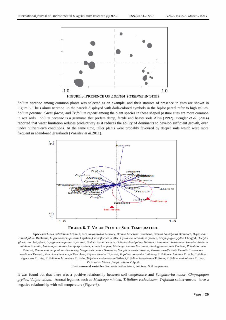
International Journal of Environmental & Agriculture Research (IJOEAR) ISSN:[2454-1850] [Vol-3, Issue-3, March- 2017]
Page | 26
-1.0 1.0
-0.4
0.6
FIGURE 5. PRESENCE OF LOLIUM PERENNE IN SITES
Lolium perenne among common plants was selected as an example, and their statuses of presence in sites are shown in
Figure 5. The Lolium perenne in the parcels displayed with dark-colored symbols in the biplot parcel refer to high values.
Lolium perenne, Carex flacca, and Trifolium repens among the plant species in these shaped pasture sites are more common
in wet soils. Lolium perenne is a graminae that prefers damp, fertile and heavy soils Altin (1992). Dengler et al. (2014)
reported that water limitation reduces productivity as it reduces the ability of dominants to develop sufficient growth, even
under nutrient-rich conditions. At the same time, taller plants were probably favoured by deeper soils which were more
frequent in abandoned grasslands (Vassilev et al.2011).
FIGURE 6. T- VALUE PLOT OF SOIL TEMPERATURE
Species:Achillea millefolium Achimill; Aira caryophyllea Airacary, Bromus benekenii Brombene, Bromus hordelymus Bromhord, Bupleurum
rotundifolium Buplrotun, Capsella bursa-pastoris Capsburs,Carex flacca Careflac, Cynosurus echinatus Cynoech, Chrysopogon gryllus Chrygryl, Dactylis
glomerata Dactyglom, Eryngium campestre Eryncamp, Festuca ovina Festovin, Galium rotundifolium Galirotu, Geranium robertianum Gerarobe, Koeleria
nitidula Koelnitu, Lamium purpureum Lamipurp, Lolium perenne Lolipere, Medicago minima Medimini, Plantago lanceolata Planlanc, Potentilla recta
Poterect, Ranunculus neapolitanus Ranuneap, Sanguisorba minor Sangmino, Sinapis arvensis Sinaarve, Taraxacum officinale Taraoffi, Taraxacum
serotinum Tarasero, Teucrium chamaedrys Teuccham, Thymus striatus Thymstri, Trifolium campestre Trifcamp, Trifolium echinatum Trifechi, Trifolium
nigrescens Trifnigr, Trifolium ochroleucum Trifochr, Trifolium subterraneum Trifsubt,Trifolium tomentosum Triftome, Trifolium vesiculosum Trifvesi,
Vicia sativa Vicisati,Vulpia ciliata Vulpcili
Environmental variables: Soil mois Soil moisture, Soil temp Soil temperature
It was found out that there was a positive relationship between soil temperature and Sanguisorba minor, Chrysopogon
gryllus, Vulpia ciliata. Annual legumes such as Medicago minima, Trifolium vesiculosum, Trifolium subterraneum have a
negative relationship with soil temperature (Figure 6).
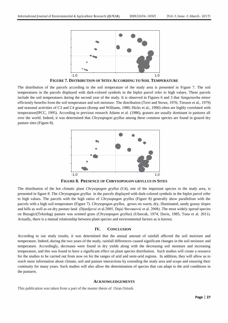
International Journal of Environmental & Agriculture Research (IJOEAR) ISSN:[2454-1850] [Vol-3, Issue-3, March- 2017]
Page | 27
-1.0 1.0
-0.4
0.6
FIGURE 7. DISTRIBUTION OF SITES ACCORDING TO SOIL TEMPERATURE
The distribution of the parcels according to the soil temperature of the study area is presented in Figure 7. The soil
temperatures in the parcels displayed with dark-colored symbols in the biplot parcel refer to high values. These parcels
include the soil temperatures during the second year of the study. It is observed in Figures 6 and 3 that Sanguisorba minor
efficiently benefits from the soil temperature and soil moisture. The distribution (Terri and Stowe, 1976; Tieszen et al., 1979)
and seasonal activities of C3 and C4 grasses (Kemp and Williams, 1980; Hicks et al., 1990) often are highly correlated with
temperature(IPCC, 1995). According to previous research Adams et al. (1986), grasses are usually dominant in pastures all
over the world. Indeed, it was determined that Chrysopogon gryllus among these common species are found in grazed dry
pasture sites (Figure 8).
-1.0 1.0
-0.4
0.6
FIGURE 8. PRESENCE OF CHRYSOPOGON GRYLLUS IN SITES
The distribution of the hot climatic plant Chrysopogon gryllus (C4), one of the important species in the study area, is
presented in figure 8. The Chrysopogon gryllus in the parcels displayed with dark-colored symbols in the biplot parcel refer
to high values. The parcels with the high ratios of Chrysopogon gryllus (Figure 8) generally show parallelism with the
parcels with a high soil temperature (Figure 7). Chrysopogon gryllus, grows on warm, dry, illuminated, sandy grassy slopes
and hills as well as on dry pasture land (Djurdjevıć et al.2005, Dajıć Stevanovıć et al. 2008). The most widely spread species
on Buzagici(Tekirdag) pasture was scented grass (Chrysopogon gryllus) (Uluocak, 1974; Davis, 1985; Tuna et al. 2011).
Actually, there is a mutual relationship between plant species and environmental factors as is known.
IV. CONCLUSION
According to our study results, it was determined that the annual amount of rainfall affected the soil moisture and
temperature. Indeed, during the two years of the study, rainfall differences caused significant changes in the soil moisture and
temperature. Accordingly, decreases were found in dry yields along with the decreasing soil moisture and increasing
temperature, and this was found to have a significant effect on plant species distribution. Such studies will create a resource
for the studies to be carried out from now on for the ranges of arid and semi-arid regions. In addition, they will allow us to
reach more information about climate, soil and pasture interactions by extending the study area and scope and ensuring their
continuity for many years. Such studies will also allow the determination of species that can adapt to the arid conditions in
the pastures.
ACKNOWLEDGEMENTS
This publication was taken from a part of the master thesis of Ozan Ozturk.

International Journal of Environmental & Agriculture Research (IJOEAR) ISSN:[2454-1850] [Vol-3, Issue-3, March- 2017]
Page | 28
REFERENCES
[1] AbabouA., Chouıeb M., Khader M., Mederbal K., Saıdı D. and Bentayeb Z., 2009. Multıvarıate analysıs of vegetatıon of the salted
Lower-Chelıff Plaın, Algerıa Bol.Soc.Bot.Méx. 85: 59-69 .
[2] Adams J.B, Smith M.O, Johnson P.E., 1986. Spectral mixture modelling: a new analysis of rock and soil types at the Viking Lander 1
Site. J. Geophy. Res., 91(B8): 8098-8112.
[3] Altin M., 1992. Improvement of Meadow and Pasture. T.U Facult of Agricultural Press. No: 152 ,13, s. 29.
[4] Altin M., Gokkus A., Koc A. 2011. Pasture and Meadow Management. Republic of Turkey Ministry of Food, Agriculture and
Livestock, Plant Production Department , Ankara.
[5] Anonymous 2016. http://www.mgm.gov.tr/FILES/resmi-istatistikler/iklim_metaveri.pdf
[6] Baron V. S., Mapfumo, E., Naeth, M. A. and Chanasyk, D. S. 1999. Sustainable grazing systems for perennial and annual forages on
sloped lands. Canada-Alberta Environmentally Sustainable Agriculture Agreement (CAESA) Final Rep. RES-024-93. 160 pp.
[7] Bassiri M., Wilson A.M., and Grand B. 1988 . Root excision and temporary dehydration effects on emergence and seedling growth of
4 range species. J. Range Management 41
[8] Bradshaw D. L., Chanasyk, D. S., Baron, V. S. and Naeth, M. A. 2007. Soil water regimes of annual and perennial forages during
drought years in the Aspen Parkland ecoregion of Alberta. Can. J. Soil Sci. 87: 523–533.
[9] Buckland S.M., Thompson, K., Hodgson, J.G. & Grime, J.P. 2001. Grassland invasions: effects of manipulations of climate and
management. Journal of Applied Ecology, 38, 301–309.
[10] Carey P D, Watkinson A R & Gerard F F O 1995. The determinants of the distribution and abundance of the winter annual grass
Vulpia ciliata ssp. Ambigua. Journal of Ecology, 83, 177–187.
[11] Chaves M M, Maroco J. P and Pereira J .S, 2003. Understanding plant responses to drought – from genes to the whole plant, Funct.
Plant Biol., 30, 239–264.
[12] Dajıć Stevanovıć, Z., Peeters A., Vrbnıčanın S., Šoštarıć I., and Aćıć S., 2008. Long term grassland vegetation changes: Case study
Nature Park Stara Planina (Serbia). – Community Ecol. 9: 23–31.
[13] Davidson E., Belk E. and Boone R. D . 1998. Soil Water Content and Temperature as Independent or Confounded Factors
Controlling Soil Respiration in a Temperate Mixed Hardwood Forest. Global Change Biology 4: 217–227
[14] Davis PH ,1985. Flora of Turkey and The East Aegean Islands,1-9. Edinburg University Press.
[15] Dengler J, Janiˇsova M., Torok P., Wellstein C., 2014. Biodiversity of palaearctic grasslands: a synthesis Agriculture, Ecosystems
and Environment 182:1–14.
[16] Dinc U. and Senol, S. 1998. Soil study and Maps. CU. Faculty of Agricultural Press No: 161, A-50 ,Adana 23,
[17] Djurdjevıć L., Mıtrovıć M., Pavlovıć P., Perıšıć S., and Mačukanovıć-Jocıć M., 2005 .Total phenolics and phenolic acids content in
low (Chrysopogon gryllus) and mediocre quality (Festuca vallesiaca) forage grasses of Deliblato Sands meadow-pasture communities
in Serbia Czech J. Anim. Sci., 50, 2005 2: 54–59.
[18] Donmez Y. 1968. Geography of plant in Trakya region. Univ. of Istanbul Geography Ins. Press No: 132 , 51.
[19] Duckworth JC, Bunce RGH and Malloch AJC 2000. Modelling the potential effects of climate change on calcareous grasslands in
Atlantic Europe. J. Biogeog. 27, 347-358.
[20] Firincioglu H. K., Şahin B., Seefeld S., Mert F., Hakyemez B.H., and Vural M., 2008. Pilot study for an Assessment of Vegetation
Structure for Steppe Rangelands of Central Anatolia Turk J Agric For 32 : 401-414 .
[21] Garwood E. A., and Sinclair, J., 1979. Use of water by six grass species. II. Root distribution anduse of soil water. Journal of
Agricultural Science, 93, 25-35.
[22] Gazanchian A, Khosh Kholgh Sima NA, Malboobi MA and Heravan EM 2006. Relationships between emergence and soil water
content for perennial cool season grasses native to Iran. Crop Sci., 46: 544-553
[23] Hicks R.A., D.D. Briske, C.A. Call, and R.J. Ansley. 1990: Co-existence of a perennial C3 bunchgrass in a C4 dominated grassland:
an evaluation of gas exchange characteristics. Photosynthetica, 24, 63-74.
[24] Hoekstra N J, Finn J A, Hofer D, ve Lüscher A 2014. The effect of drought and interspecific interactions on depth of water uptake in
deep- and shallow-rooting grassland species asdetermined by _18O natural abundance Biogeosciences, 11, 4493–4506.
[25] IPCC 1995. Impacts, Adaptation and Mitigation Options. IPCC, Working Group II, Cambridge: Cambridge University Press, 878 pp.
[26] JaleelC.A., Manivannan P., Lakshmanan G.M.A., Gomathinayagam M. and Panneerselvam R., 2008. Alterations in morphological
parameters and photosynthetic pigment responses of Catharanthus roseus under soil water deficits. Colloids Surf. B: Biointerfaces,
61: 298–303
[27] Johnson D.A. Assay K.H., 1993. Viewpoint. Selection for improved drought response in cool -season grasses J. Range management
46, 194-202.
[28] Kang Y., Khan S., Ma X. 2009 . Climate change impacts on crop yield, crop water productivity and food security – A review
Progress in Natural Science 19 ,1665–1674
[29] KempP. R., Williams, G. J.,1980. A physiological basis for niche separation between Agropyron smithii (C3) and Bouteloua gracilis
(C4). - Ecology 61: 846- 858
[30] Le Houérou HN 1984. Rain use efficiency: a unifying concept in arid-land ecology. J Arid Environ 7:213–247
[31] Lepsˇ J. and Sˇmilauer, P., 2003. Multivariate analysis of ecological data using CANOCO. Cambridge University Press, Cambridge.
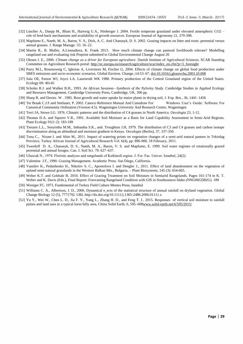
International Journal of Environmental & Agriculture Research (IJOEAR) ISSN:[2454-1850] [Vol-3, Issue-3, March- 2017]
Page | 29
[32] Lüscher A., Daepp M., Blum H., Hartwig U.A., Nösberger J. 2004. Fertile temperate grassland under elevated atmospheric CO2 –
role of feed-back mechanisms and availability of growth resources. European Journal of Agronomy 21, 379-398.
[33] Mapfumo E., Naeth, M. A., Baron, V. S., Dick, A. C. And Chanasyk, D. S. 2002. Grazing impacts on litter and roots: perennial versus
annual grasses. J. Range Manage. 55: 16–22.
[34] Martin R., B. Muller, A.Linstadtera, K. Frank 2013. How much climate change can pastoral livelihoods tolerate? Modelling
rangeland use and evaluating risk Preprint submitted to Global Environmental Change August 26
[35] Olesen J. E., 2006. Climate change as a driver for European agriculture. Danish Institute of Agricultural Sciences. SCAR Standing
Committee on Agriculture Research portal: http://ec.europa.eu/research/agriculture/scar/index_en.cfm?p=3_foresight
[36] Parry M.L, Rosenzweig C, Iglesias A, Livermore M, Fischer G, 2004. Effects of climate change on global food production under
SRES emissions and socio-economic scenarios. Global Environ. Change.;14:53–67. doi:10.1016/j.gloenvcha.2003.10.008
[37] Sala OE, Parton WJ, Joyce LA, Lauenroth WK 1988. Primary production of the Central Grassland region of the United States.
Ecology 69: 40±45
[38] Scholes R.J. and Walker B.H., 1993. An African Savanna—Synthesis of the Nylsvley Study. Cambridge Studies in Applied Ecology
and Resource Management, Cambridge University Press, Cambridge, UK, 306 pp.
[39] Sharp R. and Davies W . 1985. Root growth and water uptake by maize plants in drying soil, J. Exp. Bot., 36, 1441–1456
[40] Ter Braak C.J.F.and Smilauer, P. 2002. Canoco Reference Manual And Canodraw For Windows User’s Guide: Software For
Canonical Community Ordination (Version 4.5). Wageningen University And Research Centre, Wageningen
[41] Terri JA, Stowe LG. 1976. Climatic patterns and the distribution of C4 grasses in North America. Oecologia 23, 1-12.
[42] Thomas D.A. and Squires V.R., 1991. Available Soil Moisture as a Basis for Land Capability Assessment in Semi-Arid Regions.
Plant Ecology 91(1-2): 183-189
[43] Tieszen L.L., Senyimba M.M., Imbamba S.K., and. Troughton J.H, 1979. The distribution of C3 and C4 grasses and carbon isotope
discrimination along an altitudinal and moisture gradient in Kenya. Oecologia (Berlin), 37, 337-350.
[44] Tuna C., Nizam I. and Altin M., 2011. Impact of watering points on vegetation changes of a semi-arid natural pasture in Tekirdag
Province, Turkey African Journal of Agricultural Research Vol. 6(4), pp. 896-900, 18 February, 2011.
[45] Twerdoff D. A., Chanasyk, D. S., Naeth, M. A., Baron, V. S. and Mapfumo, E. 1999. Soil water regimes of rotationally grazed
perennial and annual forages. Can. J. Soil Sci. 79: 627–637.
[46] Uluocak N., 1974. Floristic analyses and rangelands of Kırklareli region. J. For. Fac. Univer. Istanbul, 24(2).
[47] Valentine J.F., 1990. Grazing Management. Academic Press. San Diego, California.
[48] Vassilev K., Pedashenko H., Nikolov S. C., Apostolova I. and Dengler J., 2011. Effect of land abandonment on the vegetation of
upland semi-natural grasslands in the Western Balkan Mts., Bulgaria. – Plant Biosystems, 145 (3): 654-665.
[49] Weber K.T. and Gokhale B. 2010. Effect of Grazing Treatment on Soil Moisture in Semiarid Rangelands. Pages 161-174 in K. T.
Weber and K. Davis (Eds.), Final Report: Forecasting Rangeland Condition with GIS in Southeastern Idaho (NNG06GD82G). 189
[50] Weniger FC. 1973. Fundemental of Turkey Field Culture Mentes Press, Istanbul
[51] Williams C. A., Albertson, J. D., 2006. Dynamical e_ects of the statistical structure of annual rainfall on dryland vegetation. Global
Change Biology 12 (5), 777{792. URL http://dx.doi.org/10.1111/j.1365-2486.2006.01111.x
[52] Yu Y., Wei W., Chen L. D., Jia F. Y., Yang L., Zhang H. D., and Feng T. J.. 2015. Responses of vertical soil moisture to rainfall
pulses and land uses in a typical loess hilly area, China Solid Earth, 6, 595–608www.solid-earth.net/6/595/2015/
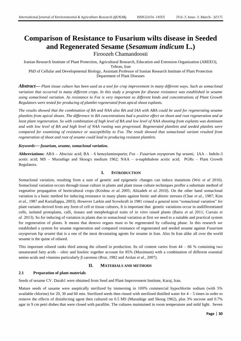
International Journal of Environmental & Agriculture Research (IJOEAR) ISSN:[2454-1850] [Vol-3, Issue-3, March- 2017]
Page | 30
Comparison of Resistance to Fusarium wilts disease in Seeded
and Regenerated Sesame (Sesamum indicum L.) Firoozeh Chamandoosti
Iranian Research Institute of Plant Protection, Agricultural Research, Education and Extension Organization (AREEO),
Tehran, Iran
PhD of Cellular and Developmental Biology, Assistant Professor of Iranian Research Institute of Plant Protection
Department of Plant Diseases
Abstract— Plant tissue culture has been used as a tool for crop improvement in many different ways. Such as somaclonal
variation that occurred in many different crops. In this study a program for disease resistance was established in sesame
using somaclonal variation. As resistance to Fos is very important so different kinds and concentrations of Plant Growth
Regulators were tested for producing of plantlet regenerated from apical shoot explants.
The results showed that the combination of BA and NAA also BA and IAA with ABA could be used for regenerating sesame
plantlets from apical shoots. The difference in BA concentrations had a positive effect on shoot and root regeneration and at
least plant regeneration. So with combination of high level of BA and low level of NAA shooting from explants was dominant
and with low level of BA and high level of NAA rooting was progressed. Regenerated plantlets and seeded planlets were
compared for examining of resistance or susceptibility to Fos. The result showed that somaclonal variant resulted from
regeneration of shoot and root of sesame could lead to producing resistant plantlets.
Keywords— fusarium, sesame, somaclonal variation.
Abbreviations: ABA – Abscisic acid; BA – 6 benzylaminopurin; Fos – Fusarium oxysporum fsp sesami, IAA – Indole-3
acetic acid; MS – Murashige and Skoog,s medium 1962; NAA – α-naphthalene acetic acid; PGRs – Plant Growth
Regulators.
I. INTRODUCTION
Somaclonal variation, resulting from a sum of genetic and epigenetic changes can induce mutations (Wei et al 2016).
Somaclonal variation occurs through tissue culture in plants and plant tissue culture techniques proffer a substitute method of
vegetative propagation of horticultural crops (Krishna et al. 2005; Alizadeh et al. 2010). On the other hand somaclonal
variation is a basic method for inducing resistance in many plants against biotic and abiotic stresses (Chae et al., 1987; Kim
et al., 1987 and Kariallappa, 2003). However Larkin and Scowkraft in 1981 coined a general term “somaclonal variation” for
plant variants derived from any form of cell or tissue cultures, It is important that genetic variations occur in undifferentiated
cells, isolated protoplasts, calli, tissues and morphological traits of in vitro raised plants (Bairu et al. 2011; Currais et
al. 2013). So for inducing of variation in plants duo to somaclonal variation at first we need to a suitable and practical system
for regeneration of plants. It means that denovo organs must to be regenerated by callusing phase. In this research we
established a system for sesame regeneration and compared resistance of regenerated and seeded sesame against Fusarium
oxysporum fsp sesami that is a one of the most devastating agents for sesame in Iran. Also In Iran alike all over the world
sesame is the quine of oilseed.
This important oilseed ranks third among the oilseed in production. Its oil content varies from 44 – 66 % containing two
unsaturated fatty acids – oleic and linoleic together account for 85% (Maximum) with a combination of different essential
amino acids and vitamins particularly β carotene (Brar, 1982 and Arslan et al., 2007).
II. MATERIALS AND METHODS
2.1 Preparation of plant materials
Seeds of sesame CV. Darab1 were obtained from Seed and Plant Improvement Institute, Karaj, Iran.
Mature seeds of sasame were aseptically sterilized by immersing in 100% commercial hypochlorite sodium (with 5%
available chlorine) for 20, 30 and 60 min. Sterilized seeds then rinsed with sterilized distilled water for 4 – 5 times in order to
remove the effects of disinfecting agent then cultured on 0.5 MS (Murashige and Skoog 1962), plus 3% sucrose and 0.7%
agar in 9 cm petri dishes that were closed with parafilm. The cultures maintained in room temperature and mild light. Seven
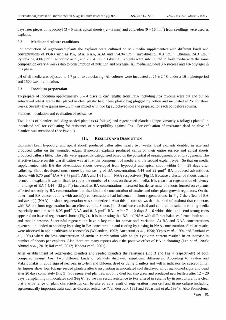
International Journal of Environmental & Agriculture Research (IJOEAR) ISSN:[2454-1850] [Vol-3, Issue-3, March- 2017]
Page | 31
days later pieces of hypocotyl (3 – 5 mm), apical shoots ( 2 – 3 mm) and cotyledon (9 – 16 mm2) from seedlings were used as
explants.
2.2 Media and culture conditions
For production of regenerated plants the explants were cultured on MS media supplemented with different kinds and
concentrations of PGRs such as BA, IAA, NAA, ABA and 554.94 µm-1
myo-Inositol, 0.3 µml-1
Thiamin, 24.3 µml-1
Pyridoxine, 4.06 µml-1
Nicotinic acid , and 26.64 µml-1
Glycine. Explants were subcultured to fresh media with the same
composition every 4 weeks duo to consumption of nutrition and oxygene. All media included 3% sucrose and 4% phytagel in
this phase.
pH of all media was adjusted to 5.7 prior to autoclaving. All cultures were incubated at 25 ± 2 º C under a 16-h photoperiod
and 1500 Lux illumination.
2.3 Inoculum preparation
To prepare of inoculum approximately 3 – 4 discs (1 cm2 length) from PDA including Fos mycelia were cut and put on
autoclaved wheat grains that placed in clear plastic bag. Clear plastic bag plugged by cotton and incubated at 25º for three
weeks. Seventy five grams inoculum was mixed with two kg autoclaved soil and prepared for each pot before sowing.
Plantlets inoculation and evaluation of resistance
Two kinds of plantlets including seeded plantlets (4 foliage) and regenerated plantlets (approximately 4 foliage) planted in
inoculated soil for evaluating for resistance or susceptibility against Fos. For evaluation of resistance dead or alive of
plantlets was mentioned (See Pavlou)
III. RESULTS AND DISSCUTION
Explants (Leaf, hypocotyl and apical shoot) produced callus after nearly two weeks. Leaf explants doubled in size and
produced callus on the wounded edges. Hypocotyl explants produced callus on their entire surface and apical shoots
produced callus a little. The calli were apparently categorised based on the potential of organogenesis or embryogenesis. The
effective factore on this classification was at first the component of media and the second explant type. So that on media
supplemented with BA the adventitious shoots developed from hypocotyl and apical shoot within 14 – 28 days after
callusing. Shoot developed much more by increasing of BA concentration. 4.44 and 22 µml-1
BA produced adventitious
shoots with 5.70 µml-1
IAA + 3.78 µml
-1 ABA and 1.61 µml
-1 NAA respectively (Fig 1). Because a cluster of shoots usually
formed on explants it was difficult to count the number of shoots on these two media. It is clear that regeneration efficiency
in a range of BA ( 4.44 – 22 µml-1
) increased as BA concentrations increased but dense mass of shoots formed on explants
affected not only by BA concentrations but also kind and concentration of auxins and other plant growth regulators. On the
other hand BA concentrations with auxin(s) concentrations had influence in shoot regenerations. In Fig 7 the effect of BA
and auxin(s) (NAA) on shoot regeneration was summerized. Also this picture shows that the kind of auxin(s) that cooperats
with BA on shoot regeneration has an effective role. Shoots (1 – 2 cm) were excised and cultured on suitable rooting media
especially medium with 8.05 µml-1
NAA and 0.13 µml-1
BA. After 7 - 10 days 5 – 6 white, thick and semi strong roots
appeared on base of regenerated shoots (Fig 2). It is interesting that BA and NAA with different balances formed both shoot
and root in sesame. Successful regeneration have a key role for somaclonal variation. At BA and NAA concentrations
regeneration tended to shooting by rising in BA concentration and rooting by rinsing in NAA concentration. Similar results
were observed in apple cultivars or rootstocks (Welanders, 1992; Ancherani et al., 1990; Yepes et al., 1994 and Famiani et
al., 1994) where the low concentration of auxin in combination with height cytokinin content resulted in an increase in
number of shoots per explants. Also there are many reports about the positive effect of BA in shooting (Lee et al., 2003;
Ahmad et al., 2010; Rai et al., 2012; Kadota et al., 2001).
After establishment of regenerated plantlets and seeded plantlets the resistance (Fig 3 and Fig 4 respectively) of both
compared against Fos. Two different kinds of plantlets displayed significant differences. According to Pavlou and
Vakalounakis in 2005 sign of necrosis in xylem and phloem, dead or dying plantlets and wilt is indicator for susceptibility.
As figures show four foliage seeded planlets after transplanting in inoculated soil displayed all of mentioned signs and dead
after 20 days completely (Fig 5). So regenerated plantlets not only died but also grew and produced new leaflets after 12 – 20
days transplanting in inoculated soil (Fig 6). So we can result resistance to Fos altered in sesame by tissue culture. It is clear
that a wide range of plant characteristics can be altered as a result of regeneration from cell and tissue culture including
agronomacally important traits such as diseases resistance (Van den bulk 1991 and Sebastiani et al., 1994). Also Somaclonal
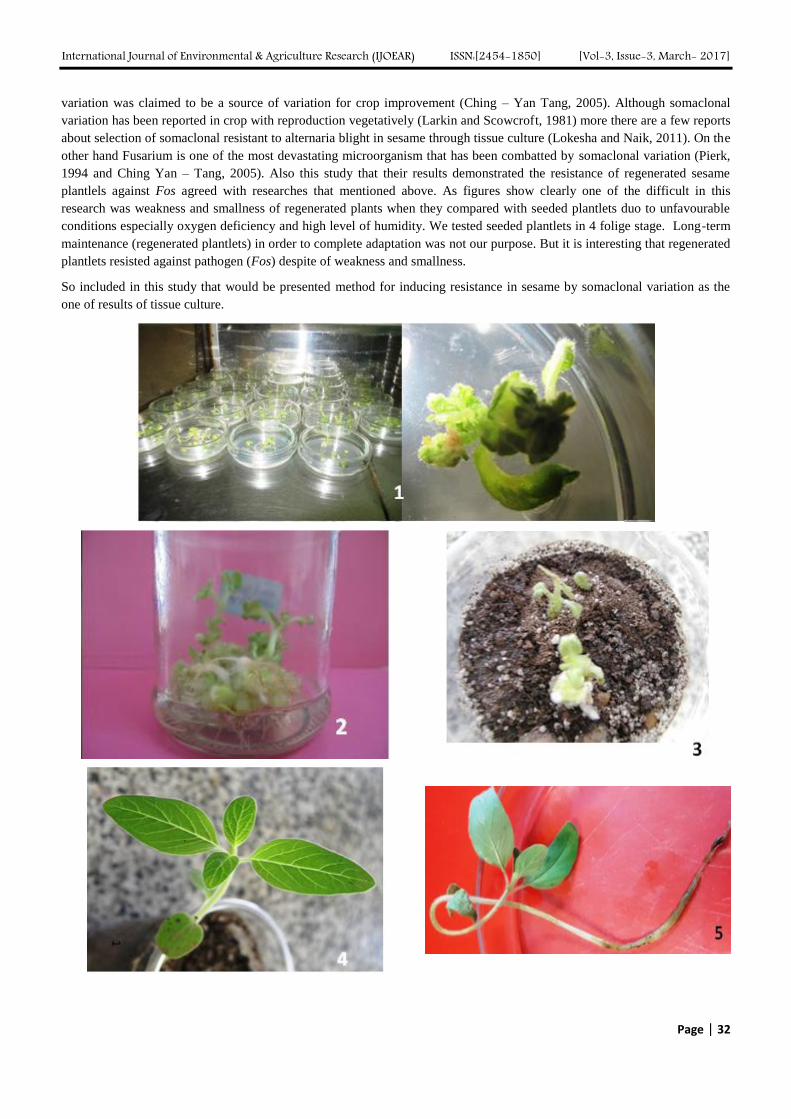
International Journal of Environmental & Agriculture Research (IJOEAR) ISSN:[2454-1850] [Vol-3, Issue-3, March- 2017]
Page | 32
variation was claimed to be a source of variation for crop improvement (Ching – Yan Tang, 2005). Although somaclonal
variation has been reported in crop with reproduction vegetatively (Larkin and Scowcroft, 1981) more there are a few reports
about selection of somaclonal resistant to alternaria blight in sesame through tissue culture (Lokesha and Naik, 2011). On the
other hand Fusarium is one of the most devastating microorganism that has been combatted by somaclonal variation (Pierk,
1994 and Ching Yan – Tang, 2005). Also this study that their results demonstrated the resistance of regenerated sesame
plantlels against Fos agreed with researches that mentioned above. As figures show clearly one of the difficult in this
research was weakness and smallness of regenerated plants when they compared with seeded plantlets duo to unfavourable
conditions especially oxygen deficiency and high level of humidity. We tested seeded plantlets in 4 folige stage. Long-term
maintenance (regenerated plantlets) in order to complete adaptation was not our purpose. But it is interesting that regenerated
plantlets resisted against pathogen (Fos) despite of weakness and smallness.
So included in this study that would be presented method for inducing resistance in sesame by somaclonal variation as the
one of results of tissue culture.
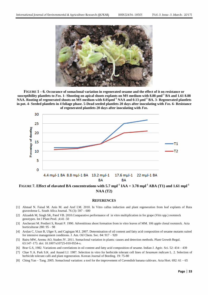
International Journal of Environmental & Agriculture Research (IJOEAR) ISSN:[2454-1850] [Vol-3, Issue-3, March- 2017]
Page | 33
FIGURE 1 – 6. Occurance of somaclonal variation in regenerated sesame and the effect of it on resistance or
susceptibility plantlets to Fos. 1- Shooting on apical shoots explants on MS medium with 8.88 µml-1
BA and 1.61 8.88
NAA. Rooting of regenerated shoots on MS medium with 8.05µml-1
NAA and 0.13 µml-1
BA. 3- Regenerated plantlets
in pot. 4- Seeded plantlets in 4 foliage phase. 5-Dead seeded plantlets 20 days after inoculating with Fos. 6- Resistance
of regenerated plantlets 20 days after inoculating with Fos.
FIGURE 7. Effect of elavated BA concentrations with 5.7 mµl-1
IAA + 3.78 mµl-1
ABA (T1) and 1.61 mµl-1
NAA (T2)
REFERENCES
[1] Ahmad N. Faisal M. Anis M. and Aref I.M. 2010. In Vitro callus induction and plant regeneration from leaf explants of Ruta
graveolense L. South Afica Journal. 76 (3): 597 – 600
[2] Alizadeh M, Singh SK, Patel VB. 2010.Comparative performance of in vitro multiplication in for grape (Vitis spp.) rootstock
genotypes. Int J Plant Prod. ;4:41–50
[3] Ancherani M. Predieri S, Rosati P. 1990. Adventitious shoot formation from in vitro leaves of MM. 106 apple clonal rootstock. Acta
horticulturae 280: 95 – 98
[4] Arslan C, Uzun B, Ulger S, and Cagirgan M.I. 2007. Determination of oil content and fatty acid composition of sesame mutants suited
for intensive management conditions. J. Am. Oil Chem. Soc. 84: 917 – 920
[5] Bairu MW, Aremu AO, Staden JV. 2011. Somaclonal variation in plants: causes and detection methods. Plant Growth Regul.
63:147–173. doi: 10.1007/s10725-010-9554-x.
[6] Brar G.S, 1982. Variations and correlations in oil content and fatty acid composition of sesame. Indian J. Agric. Sci. 52: 434 – 439
[7] Chae Y.A. Park S.K. and Anand I.J. 1987. Selection in vitro for herbicide tolerant cell lines of Sesamum indicum L. 2. Selection of
herbicide tolerant calli and plant regeneration. Korean Journal of Beeding. 19: 75-80
[8] Ching Yan – Tang. 2005. Somaclonal variation: a tool for the improvement of Cavendish banana cultivars. Acta Hort. 692: 61 – 65
International Journal of Environmental & Agriculture Research (IJOEAR) ISSN:[2454-1850] [Vol-3, Issue-3, March- 2017]
Page | 34
[9] Currais L, Loureiro J, Santos C, Canhoto JM. 2013. Ploidy stability in embryogenic cultures and regenerated plantlets of
tamarillo. Plant Cell Tissue Organ Cult. 114:149–159. doi: 10.1007/s11240-013-0311-5
[10] Famiani F. Ferradini N. Staffolani P. Standardi A. 1994. effect of leaf excision time and age, BA concentration and dark treatments on
in vitro shoot regeneration of M26 apple rootstock. Journal of horticultural Science. 69 (4): 679 – 685
[11] Kadota M. Lmizu K. and Hirano T. 2001. Double-phase in vitro culture using sorbitol increases shoot proliferation and reduces
hyperhydricity in Japanese pear. Scientica Horticulturae. 89 (3): 207 – 2015
[12] KariyallappaD.K. 2003. In vitro regeneration and cell line selection for Alternaria resistant callus in Sesame (Sesamum indicum L.).
M.Sc. (Agri.) Thesis, University of Agricultural Sciences, Dharwad.
[13] Kim M.K. Park S.K. and Chae Y.A. 1987. Selection in vitro for herbicide tolerant cell lines of Sesamum indicum: Effects of explants
and hormone combination on callus induction. Korean Journal of Plant Breeding 19: 70-94
[14] Krishna H, Singh SK, Sharma RR, Khawale RN, Minakshi Patel VB. 2005 Biochemical changes in micropropagated grape (Vitis
vinifera L.) plantlets due to arbuscular-mycorrhizal fungi (AMF) inoculation during ex vitro acclimatization. Sci Hortic. 106: 554 –
567
[15] Larkin P, Scowcroft W. 1981.Somaclonal variation—a novel source of variability from cell cultures for plant improvement. Theor
Appl Genet. 60:197–214
[16] Lee Y.K, Chung, W. and Ezura H. 2003. Efficient plant regeneration via organogenesis in winter squash (Cucurbita maxima Duch.).
Plant Science. 164 (3): 413 – 418
[17] Lokesha R. and Naik M.K. 2011. Selection of somaclonals resistant to Alternaria blight in sesame (Sesamum indicum L.) through in
vitro cell line method. Indian Journal of Fundamental and Applied Life Sciences. 1(4): 338 – 346
[18] Murashige T. and Skoog F. 1962. A revised medium for rapid growth and bioassays with tobacco tissue cultures. Phyiol. Plant. 15:
473 – 497
[19] Pavlou, G. C and Vakalounakis D. J. 2005. Biological control of root and stem rot of greenhouse cucumber, caused by Fusarium
oxysporum f.sp. radicis-cucumerinum, by lettuce soil amendment. Crop Protection, 24: 135-140
[20] Pierik R.L.M. 1997. In Vitro Culture of Highrt Plants. Kluwer Acadamic Publishers
[21] Rai G. K, Rai N. P, Kumar S. yadav A, and Rathaur S. 2012. Effects of explant age, germination medium, pre-culture parameters,
inoculation medium, pH, washing medium, and selection regime on Agrobacterium-mediated transformation of tomato. In Vitro
Cellular and Developmental Biology. 48: 565 – 578
[22] Sebastiani L. Lenzi, A. PugliesiC. and Fambrini M. 1994. Somaclonal variation for resistance to Verticillium dahliae in potato plants
regenerated from callus. Euphytica. 80: 5 – 11
[23] Van den bulk, R.W. 1991. Application of cell and tissue culture and and in vitro selection for disease resistance breeding – a review.
Euphytica. 56: 269 – 285
[24] Wei Fu-Jin, Lin-Yun Kuang , Hui-Min Oung . Sin-Yuan Cheng , Hshin-Ping Wu . Lin-Tzu Huang Yi-Tzu. Tseng Wan-Yi Chiou1,
Vicki Hsieh-Feng , Cheng-Han Chung, , Su-May Yu , Lan-Ying Lee , Stanton B. Gelvin and Yue-Ie C. Hsing, 2016. Somaclonal
variation does not preclude the use of rice transformants for genetic screening. The Plant Journal. 85, 648–659
[25] Welander M. Maheswaran. G. 1992. Shoot regeneration from leaf explants of dwarfing apple rootstocks. Journal of Plant Physiology.
140: 223 – 228
[26] Yepes. L.M. Aldwinckle. H.S. 1994. Micropropagatin of thirteen Malus cultivars and rootstocks, and effect of antibiotics on
proliferation. Plant growth Regulation 15: 55 – 67
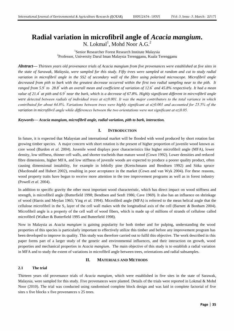
International Journal of Environmental & Agriculture Research (IJOEAR) ISSN:[2454-1850] [Vol-3, Issue-3, March- 2017]
Page | 35
Radial variation in microfibril angle of Acacia mangium. N. Lokmal
1, Mohd Noor A.G.
2
1Senior Researcher Forest Research Institute Malaysia
2Professor, University Darul Iman Malaysia Terengganu, Kuala Terengganu
Abstract— Thirteen years old provenance trials of Acacia mangium from five provenances were established at five sites in
the state of Sarawak, Malaysia, were sampled for this study. Fifty trees were sampled at random and cut to study radial
variation in microfibril angle in the SS2 of secondary wall of the fibre using polarised microscope. Microfibril angle
decreased from pith to bark with the greatest decrease occurred within the first two radial sampling near to the pith. It
ranged from 5.9° to 28.8
° with an overall mean and coefficient of variation of 12.6
° and 45.8% respectively. It had a mean
value of 21.4 at pith and 6.9
near the bark, which is a decrease of 67.8%. Highly significant different in mircrofibril angle
were detected between radials of individual trees at α≥0.001. It was the major contributors to the total variance in which
contributed for about 64.8%. Variations between trees were highly significant at α≥0.001 and accounted for 25.5% of the
variation in microfibril angle while differences between the two orientations were not significant at α≤0.05.
Keywords— Acacia mangium, microfibril angle, radial variation, pith to bark, interaction.
I. INTRODUCTION
In future, it is expected that Malaysian and international market will be flooded with wood produced by short rotation fast
growing timber species. A major concern with short rotation is the present of higher proportion of juvenile wood known as
core wood (Burdon et al. 2004). Juvenile wood displays poor characteristics like higher microfibril angle (MFA), lower
density, low stiffness, thinner cell walls, and shorter tracheids than mature wood (Cown 1992). Lower densities and reduced
fibre dimensions, higher MFA, and low stiffness of juvenile woods are expected to produce a poorer quality product, often
causing dimensional instability, for example in loblolly pine (Kretschmann and Bendtsen 1992) and Sitka spruce
(Macdonald and Hubert 2002), resulting in poor acceptance in the market (Cown and van Wyk 2004). For these reasons,
wood property traits have begun to receive more attention in the tree improvement programs as well as in forest industry
(Powell et al. 2004).
In addition to specific gravity the other most important wood characteristic, which has direct impact on wood stiffness and
strength, is microfibril angle (Butterfield 1998; Bendtsen and Senft 1986; Cave 1969). It also has an influence on shrinkage
of wood (Harris and Meylan 1965; Ying et al. 1994). Microfibril angle (MFA) is referred to the mean helical angle that the
cellulose microfibril in the S2 layer of the cell wall makes with the longitudinal axis of the cell (Barnett & Bonham 2004).
Microfibril angle is a property of the cell wall of wood fibers, which is made up of millions of strands of cellulose called
microfibril (Walker & Butterfield 1995 and Butterfield 1998).
Now in Malaysia as Acacia mangium is gaining popularity for both timber and for pulping, understanding the wood
properties of this species is particularly important to effectively utilize this timber and before any improvement program has
been developed to improve its quality. This study was therefore carried out to fulfil this objective. The work described in this
paper forms part of a larger study of the genetic and environmental influences, and their interaction on growth, wood
properties and mechanical properties in Acacia mangium. The main objective of this study is to establish a radial variation
in MFA and to study the extent of variations in microfibril angle between trees, orientations and radial subsamples.
II. MATERIALS AND METHODS
2.1 The trial
Thirteen years old provenance trials of Acacia mangium, which were established in five sites in the state of Sarawak,
Malaysia, were sampled for this study. Five provenances were planted. Details of the trials were reported in Lokmal & Mohd
Noor (2010). The trial was conducted using randomised complete block design and was laid in complete factorial of five
sites x five blocks x five provenances x 25 trees.
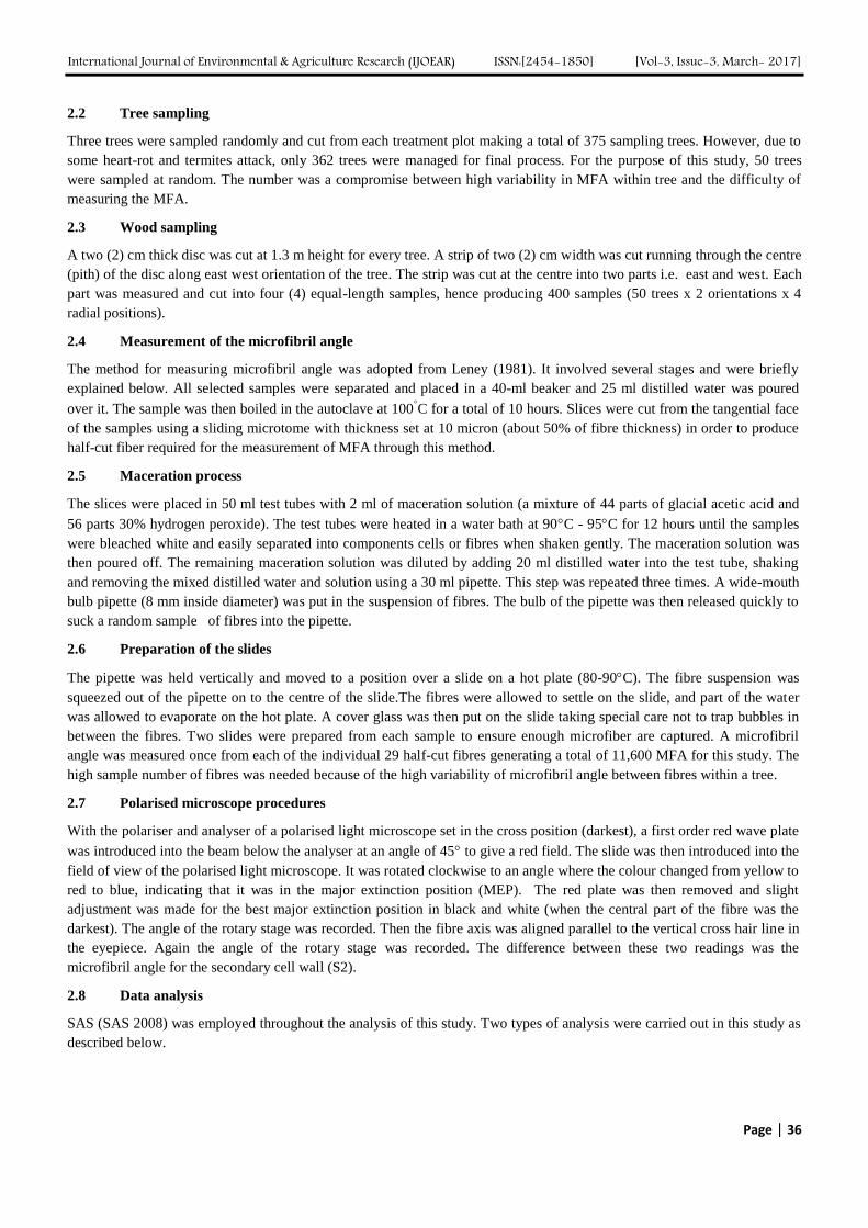
International Journal of Environmental & Agriculture Research (IJOEAR) ISSN:[2454-1850] [Vol-3, Issue-3, March- 2017]
Page | 36
2.2 Tree sampling
Three trees were sampled randomly and cut from each treatment plot making a total of 375 sampling trees. However, due to
some heart-rot and termites attack, only 362 trees were managed for final process. For the purpose of this study, 50 trees
were sampled at random. The number was a compromise between high variability in MFA within tree and the difficulty of
measuring the MFA.
2.3 Wood sampling
A two (2) cm thick disc was cut at 1.3 m height for every tree. A strip of two (2) cm width was cut running through the centre
(pith) of the disc along east west orientation of the tree. The strip was cut at the centre into two parts i.e. east and west. Each
part was measured and cut into four (4) equal-length samples, hence producing 400 samples (50 trees x 2 orientations x 4
radial positions).
2.4 Measurement of the microfibril angle
The method for measuring microfibril angle was adopted from Leney (1981). It involved several stages and were briefly
explained below. All selected samples were separated and placed in a 40-ml beaker and 25 ml distilled water was poured
over it. The sample was then boiled in the autoclave at 100C for a total of 10 hours. Slices were cut from the tangential face
of the samples using a sliding microtome with thickness set at 10 micron (about 50% of fibre thickness) in order to produce
half-cut fiber required for the measurement of MFA through this method.
2.5 Maceration process
The slices were placed in 50 ml test tubes with 2 ml of maceration solution (a mixture of 44 parts of glacial acetic acid and
56 parts 30% hydrogen peroxide). The test tubes were heated in a water bath at 90C - 95C for 12 hours until the samples
were bleached white and easily separated into components cells or fibres when shaken gently. The maceration solution was
then poured off. The remaining maceration solution was diluted by adding 20 ml distilled water into the test tube, shaking
and removing the mixed distilled water and solution using a 30 ml pipette. This step was repeated three times. A wide-mouth
bulb pipette (8 mm inside diameter) was put in the suspension of fibres. The bulb of the pipette was then released quickly to
suck a random sample of fibres into the pipette.
2.6 Preparation of the slides
The pipette was held vertically and moved to a position over a slide on a hot plate (80-90C). The fibre suspension was
squeezed out of the pipette on to the centre of the slide.The fibres were allowed to settle on the slide, and part of the water
was allowed to evaporate on the hot plate. A cover glass was then put on the slide taking special care not to trap bubbles in
between the fibres. Two slides were prepared from each sample to ensure enough microfiber are captured. A microfibril
angle was measured once from each of the individual 29 half-cut fibres generating a total of 11,600 MFA for this study. The
high sample number of fibres was needed because of the high variability of microfibril angle between fibres within a tree.
2.7 Polarised microscope procedures
With the polariser and analyser of a polarised light microscope set in the cross position (darkest), a first order red wave plate
was introduced into the beam below the analyser at an angle of 45 to give a red field. The slide was then introduced into the
field of view of the polarised light microscope. It was rotated clockwise to an angle where the colour changed from yellow to
red to blue, indicating that it was in the major extinction position (MEP). The red plate was then removed and slight
adjustment was made for the best major extinction position in black and white (when the central part of the fibre was the
darkest). The angle of the rotary stage was recorded. Then the fibre axis was aligned parallel to the vertical cross hair line in
the eyepiece. Again the angle of the rotary stage was recorded. The difference between these two readings was the
microfibril angle for the secondary cell wall (S2).
2.8 Data analysis
SAS (SAS 2008) was employed throughout the analysis of this study. Two types of analysis were carried out in this study as
described below.
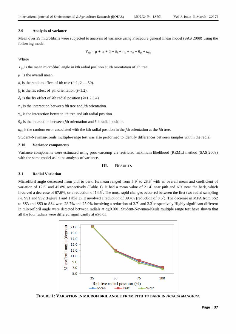
International Journal of Environmental & Agriculture Research (IJOEAR) ISSN:[2454-1850] [Vol-3, Issue-3, March- 2017]
Page | 37
2.9 Analysis of variance
Mean over 29 microfibrils were subjected to analysis of variance using Procedure general linear model (SAS 2008) using the
following model:
ijk = + αi + βj + δk + ij + ik + θjk + ijk
Where
ijk is the mean microfibril angle in kth radial position at jth orientation of ith tree.
is the overall mean.
αi is the random effect of ith tree (i=1, 2 .... 50).
βj is the fix effect of jth orientation (j=1,2).
δk is the fix effect of kth radial position (k=1,2,3,4)
ij is the interaction between ith tree and jth orientation.
ik is the interaction between ith tree and kth radial position.
θjk is the interaction between jth orientation and kth radial position.
ijk is the random error associated with the kth radial position in the jth orientation at the ith tree.
Student-Newman-Keuls multiple-range test was also performed to identify differences between samples within the radial.
2.10 Variance components
Variance components were estimated using proc varcomp via restricted maximum likelihood (REML) method (SAS 2008)
with the same model as in the analysis of variance.
III. RESULTS
3.1 Radial Variation
Microfibril angle decreased from pith to bark. Its mean ranged from 5.9° to 28.8
° with an overall mean and coefficient of
variation of 12.6° and 45.8% respectively (Table 1). It had a mean value of 21.4
near pith and 6.9
near the bark, which
involved a decrease of 67.6%, or a reduction of 14.5. The most rapid changes occurred between the first two radial sampling
i.e. SS1 and SS2 (Figure 1 and Table 1). It involved a reduction of 39.4% (reduction of 8.5). The decrease in MFA from SS2
to SS3 and SS3 to SS4 were 28.7% and 25.0% involving a reduction of 3.7 and 2.3
respectively.Highly significant different
in mircrofibril angle were detected between radials at α≥0.001. Student-Newman-Keuls multiple range test have shown that
all the four radials were differed significantly at α≥0.05.
FIGURE 1: VARIATION IN MICROFIBRIL ANGLE FROM PITH TO BARK IN ACACIA MANGIUM.

International Journal of Environmental & Agriculture Research (IJOEAR) ISSN:[2454-1850] [Vol-3, Issue-3, March- 2017]
Page | 38
TABLE 1
VARIATION IN MICROFIBRIL ANGLE FROM PITH TO BARK IN ACACIA MANGIUM.
Radial Mean Min Max CV (%) Std error
SS1 21.4°a
16.6° 28.8
° 15.1 0.32
SS2 12.9°b
11.5° 15.5
° 7.2 0.09
SS3 9.2°c
7.6° 11.6
° 10.4 0.10
SS4 6.9°d
5.9° 8.8
° 9.10 0.06
Overall 12.6° 5.9
° 28.8
° 45.8 0.29
Notes: SS1 sample nearest to pith; SS4 sample closest to bark; Mean with the same letter are not significantly different at
α≤0.05 via Student Newman Keuls.
3.2 Variation between trees
Mean of individual tree varied from 11.0 to 15.3
with an average and coefficient of variation of 12.6
and 9.7% respectively.
Differences between trees were also highly significant at α≥0.001 (Table 2). Student-Newman-Keuls multiple-range test was
performed and separated all trees in to 22 significantly distinct groups reinforced the high variation between trees. Tree
accounted for 25.5% of the total variance in MFA.
3.3 Variation between orientations
Mean of MFA for east and west orientation 12.8 and 12.4
respectively. The differences between the two orientations were
not significant at α≤0.05 (Table 2 and Figure 3).
TABLE 2
ANALYSIS OF VARIANCE AND VARIANCE COMPONENT FOR MICROFIBRIL ANGLE
Source df Mean square Variance Variance (%)
Tree (T) 49 12.1***
11.0 25.5
Orientation (O) 1 16.8ns
0.1 0.1
Radial (R) 3 4015.1***
28.1 64.8
TXO 49 0.4ns
0.1 0.1
TXR 147 3.6***
2.6 6.0
OXR 3 4.2***
1.1 2.5
error 147 0.4 0.4 0.9
Total 399 43.3 100.0
Notes: *,
**,
*** significant at p≥0.05, p≥0.01 and p≥0.001.
ns not significant at p≤0.05
3.4 Interaction between Trees and Orientations
Interaction between trees and orientations was not significant (Table 2). Although there was highly significant different
between trees, the different between both orientations for individual tree was very small (Figure 3).
3.5 Interaction between Trees and Radials
Interaction between trees and radials was highly significant (Table 2). Further examinations have shown that the interaction
was due to different rate of reduction in microfibril angle within each radial of individual tree (Figure 2). This was very
obvious especially within the first quarter from pith where tremendous change in MFA occurred.
3.6 Interaction between orientations and radials
Interaction between orientations and radials were highly significant (Table 2). Further examinations have shown that the
interaction was due to different rate of reduction in microfibril angle within each radial of different orientations especially in
the region of 50%-75% from pith.
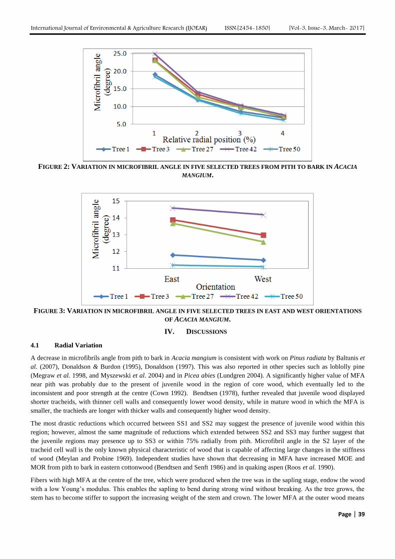
International Journal of Environmental & Agriculture Research (IJOEAR) ISSN:[2454-1850] [Vol-3, Issue-3, March- 2017]
Page | 39
FIGURE 2: VARIATION IN MICROFIBRIL ANGLE IN FIVE SELECTED TREES FROM PITH TO BARK IN ACACIA
MANGIUM.
FIGURE 3: VARIATION IN MICROFIBRIL ANGLE IN FIVE SELECTED TREES IN EAST AND WEST ORIENTATIONS
OF ACACIA MANGIUM.
IV. DISCUSSIONS
4.1 Radial Variation
A decrease in microfibrils angle from pith to bark in Acacia mangium is consistent with work on Pinus radiata by Baltunis et
al. (2007), Donaldson & Burdon (1995), Donaldson (1997). This was also reported in other species such as loblolly pine
(Megraw et al. 1998, and Myszewski et al. 2004) and in Picea abies (Lundgren 2004). A significantly higher value of MFA
near pith was probably due to the present of juvenile wood in the region of core wood, which eventually led to the
inconsistent and poor strength at the centre (Cown 1992). Bendtsen (1978), further revealed that juvenile wood displayed
shorter tracheids, with thinner cell walls and consequently lower wood density, while in mature wood in which the MFA is
smaller, the trachieds are longer with thicker walls and consequently higher wood density.
The most drastic reductions which occurred between SS1 and SS2 may suggest the presence of juvenile wood within this
region; however, almost the same magnitude of reductions which extended between SS2 and SS3 may further suggest that
the juvenile regions may presence up to SS3 or within 75% radially from pith. Microfibril angle in the S2 layer of the
tracheid cell wall is the only known physical characteristic of wood that is capable of affecting large changes in the stiffness
of wood (Meylan and Probine 1969). Independent studies have shown that decreasing in MFA have increased MOE and
MOR from pith to bark in eastern cottonwood (Bendtsen and Senft 1986) and in quaking aspen (Roos et al. 1990).
Fibers with high MFA at the centre of the tree, which were produced when the tree was in the sapling stage, endow the wood
with a low Young’s modulus. This enables the sapling to bend during strong wind without breaking. As the tree grows, the
stem has to become stiffer to support the increasing weight of the stem and crown. The lower MFA at the outer wood means
International Journal of Environmental & Agriculture Research (IJOEAR) ISSN:[2454-1850] [Vol-3, Issue-3, March- 2017]
Page | 40
the tree has higher Young’s modulus which enables them to fulfill the role. The other possibility is probably due to its
colonising habit (Wiemann & Williamson, 1988), which combine rapid early growth in stature with the production of a weak
stem due to high microfibril angle. As the tree grows, reducing microfibril angle in inevitable as to increase stem stiffness to
maintain structural stability. These changes are probably associated with the ecological habit of pioneer species of wet
tropical lowland forest. Differences in mircrofibril angle between radial was highly significant at P0.001. This is in contrast
with the work by Lima et al. (2004) on 11 clones of hybrid between Eucalyptus grandis and E. urophylla who found no
significant different in microfibril angle between radials.
The decreasing radial variation alone contributed for 64.1% of the total variation in MFA, implied that the wood strength in
the region of core wood would be low and caused further problem during wood processing. This was consistence with the
finding by Butterfield (1998) who concluded that MFA was the dominant wood characteristics underlying the poor wood
quality in many fast-grown and short-rotation plantation softwoods. However this situation creates an opportunity in tree
improvement by reducing the MFA in the central regions. This will result in improved wood quality at the central hence
improve wood strength. Evans & Ilic (2001) found that MFA accounted for 96% of the variation in modulus of elasticity of
Eucalyptus delegatensis. The scenario was unwelcome as in future most timbers reaching the markets were most likely will
be coming from fast grown short rotation with high proportion of juvenile wood.
4.2 Variation between trees
Effect of trees was significant and contributed for 25.5% toward the total variation in MFA. Though the amount was only a
third of radial variance, it was substantial to ensure a successful gain in tree selection. Very high MFA variation between
radials within trees implicated that attempts to improve MFA must take this into account and must make sure that
considerable variation between trees exists. Similar observation was reported in Pinus radiata (Donaldson & Burdon 1995).
Differences among trees, a large part of observed variation was probably attributed to the differences in genetic makeup of
the individual tree provenance which was not taking care during sampling and microclimate surrounding the individual tree.
Evans et al. (2000) also found very large variation in microfibril angle between hardwood trees of red alder (Alnus rubra)
and proposed for tree selection for steeper MFA in the central region. The same strategy was suggested by Donaldson &
Burdon (1995) following their work in Pinus radiata.
4.3 Variation between orientations
There was no effect of orientation on MFA in this study. Although there was some variation in MFA between east and west
orientation, it was very small and was not significant. The small variation observed in this study was probably an inherent. It
may also due to the influence of strong wind blow which came from the east direction annually during heavy-rain monsoon
season which also triggered formation of new fiber. To our knowledge, there was no work been done comparing the MFA
between two opposite direction to compare with this study.
4.4 Interaction between trees and orientations
Interaction between trees and orientations was not significant and only accounted for 1% of the total variance in MFA. Since
there was no significant different between orientations, the interaction between trees and orientations is probably and solely
due to highly significant differences in microfibril angle between trees (Table 2). To our knowledge, there was no work been
done comparing the MFA between trees and orientations to compare with this study.
4.5 Interaction between trees and radials
Interaction between trees and radials was highly significant (Table 2). Further examination of the data proved that the
interaction was due to differences in rate of reductions between radials of different trees (Figure 2). To our knowledge, there
was no work been done comparing the MFA between trees and radials to compare with this study.
4.6 Interaction between orientations and radials
Interaction between orientations and radials was significant (Table 2). Further examination of the data proved that the
interaction was due to different rate of reductions in MFA between radials of both orientations (Figure 1). To our knowledge,
there was no work been done comparing the MFA between orientations and radials to compare with this study?
V. CONCLUSIONS
All trees exhibited the same decreasing pattern of microfibril angle radially from pith to bark. The largest decrease occurred
International Journal of Environmental & Agriculture Research (IJOEAR) ISSN:[2454-1850] [Vol-3, Issue-3, March- 2017]
Page | 41
in the first two sub samples from pith followed by a gradual decrease in the last two sub samples towards bark. Radial
variation in microfibril angel is the most important factor affecting variation in MFA. It accounted for 61% of the total
variation. Variation between trees is substantial and contributed for 22.3% of the total variation. Although this variation is
only one third of the radial variation, it provides a basis for an improvement in MFA hence the wood strength in Acacia
mangium.
ACKNOWLEDGEMENT
I thank Professor Dr Saidi Moin of UPM for his kind review and assistance in the statistical analysis. I extend my thanks to
Abang Abdul Hamid Abang Abdul Karim and the staff of Forest Research Centre, Forestry Department of Sarawak for the
permission, and logistic and invaluable field assistance during the course of my assessment and sample collection throughout
the state of Sarawak. I especially thank Mr. Ling Wang Choon and the staff of Timber Research and Technical Training
Centre, Forestry Department of Sarawak for their invaluable assistance during the wood sample processing. I thank En.
Abdul Rahman Mansor and the staff of Similajau National Park, Bintulu for making my stays during tree sampling works
pleasant. I sincerely thank Dr Daniel Baskaran for his continuous moral supports and helps in preparing this dissertation. To
my staff in the Tree Improvement, FRIM, i.e. Amir Sharifuddin, CikMi, Asri, Sam, Rosli, Amran, Ramli and Ida, I thank
them for their excellent field and lab assistance.
REFERENCES
[1] Baltunis BS, Wu HX & Powell MB 2007. Inheritance of density, microfibril angle, and modulus of elasticity in juvenile wood of
Pinus radiata at two locations in Australia. Canadian Journal Forest Research 37:2164-2174.
[2] Barnett JR & Bonham VA 2004. Cellulose microfibril angle in the cell wall of wood fibers. Biology Review 79:461-472.
[3] Barrett JD, AP Schniewind & RL Taylor 1972. Theoretical shrinkage model for wood cell walls. Wood Science 4(3):178-192.
[4] Bendtsen BA & Senft J 1986. Mechanical and anatomical properties in individual growth rings of plantation-grown eastern cotton
wood and loblolly pine. Wood and Fibre Sciences 18: 23-38.
[5] Bouriaud O, Breda N, Le Moguedec G & Nepveu G 2004. Modelling variability of wood density in beech as affected by ring age,
radial growth and climate. Trees Structure and Function 18:264-275.
[6] Boyd JD. 1983. Anisotropic shrinkage of wood: Identification of dominant determinants. Mokuzai Gakkaishi 20(10):473-482.
[7] Burdon, R.D., Kibblewhite, R.P., Walker, J.C.F., Megraw, R.A., Evans, R., and Cown, D.J. 2004. Juvenile versus mature wood: a
new concept, orthogonal to corewood versus outer wood, with special reference to Pinus radiata and P. taeda. Forest Science 50:399-
415.
[8] Butterfield BG 1998 Editorial notes. In Butterfield BG (ed.) Proceeding of the IAWA/IUFRO International Workshop on the
Significance of Microfibril Angle to Wood Quality, November 1997, Westport, New Zealand.
[9] Cave ID 1969. The longitudinal modulus of Pinus radiata. Wood Science and Technology 3:40-48.
[10] Cown DJ 1992. Corewood (juvenile wood) in Pinus radiata – Should we be concerned? New Zealand Journal of Forest Science
22(1):87-95.
[11] Cown, D., and van Wyk, L. 2004. Profitable wood processing -hat does it require? Good wood! New Zealand Journal of Forestry 49:
10-15.
[12] Donaldson LA & Burdon RD 1995. Clonal variation and repeatability of microfibril angle in Pinus radiata. New Zealand Journal of
Forest Science 25:164-174.
[13] Donaldson LA 1997. Microfibril angle: its influence on wood properties, and prospects for improvement in radiata pine. Proceedings
of the Wood Quality Workshop 1995. New Zealand Forest Research Institute, Rotorua, New Zealand. Forest Research Institute
Bulletin 201: 20-25.
[14] Evans J.W., J.F. Senft, D.W. Green 2000. Juvenile wood effect in Red alder: analysis of physical And mechanical data to delineate
Juvenile and mature wood zones Forest Products Journal Vol. 50, No. 7/8 75-87
[15] Evans R, & Ilic J 2001. Rapid prediction in wood stiffness from microfibril angle and density. Forest Product Journal 51: 27-33.
[16] Harris JM & BA Meylan 1965. The influence of microfibril angle on longitudinal and tangential shrinkage in Pinus radiata.
Holzforschung 19(5):144-153.
[17] Kretschmann, D.E., and Bendtsen, B.A. 1992. Ultimate tensile strength and modulus of elasticity of fast-grown plantation loblolly
pine lumber. Wood Fiber Science. 24: 189-203.
[18] Leney L 1981. A technique for measuring fibril angle using polarized light microscope. Wood and Fiber 13: 13-16.
[19] Lima JT, Breese MC & Cahalan CM 2004. Variation in microfibril angle in Eucalyptus clones. Holzforschung 58: 160-166.
[20] Lokmal N & Ernest COK (1995). Genotype and environment interaction and it’s stability in Acacia mangium Journal of Tropical
Forest Science 8:247-254.
[21] Lokmal N, Darus A & Ernest COK (1993). Genotype and Environment Interaction in Acacia mangium. In Rao V, Henson IE &
Rajanaidu N (eds.) Proceeding of the International Symposium on Genotype and Environment Interaction on Perennial Species.
Hilton Hotel, Kuala Lumpur, 12-13 September 1991.
International Journal of Environmental & Agriculture Research (IJOEAR) ISSN:[2454-1850] [Vol-3, Issue-3, March- 2017]
Page | 42
[22] Lokmal N. and Mohd Noor A.G. 2010. Variation of Specific Gravity in Acacia mangium. J. Agrobiotech. Food Sci. 1(1):60-68.
[23] Lundgren C 2004. Microfibril angle and density patterns of fertilized and irrigated Norway spruce. Silva Fennical 38: 107-117.
[24] MacDonald E, Hubert J 2002. A review of the effects of silviculture on timber quality of Sitka spruce. Journal of Forestry 75:107–
138
[25] Megraw RA, Leaf G & Bremer D 1998. Longitudinal shrinkage and microfibril angle in loblolly pine. In Butterfield BG (ed.)
Proceeding of the IAWA/IUFRO International Workshop on the Significance of Microfibril Angle to Wood Quality, November 1997,
Westport, New Zealand.
[26] Meylan. B.A and M.C. Probine. 1969. Microfibril angle as a parameter in timber quality assessment. Forest Product Journal 19(4):30-
34.
[27] Myszewski JH, Bridgewater FE, Lowe WJ, Byram TD & Megraw RA 2004. Genetic variation in the microfibril angle of loblolly pine
from two test sites. Southern Journal of Applied Forestry 28: 196-204.
[28] Powell, M.B., McRae, T.A., Wu, H.X., Dutkowski, G.W., and Pilbeam, D.J. 2004. Breeding strategy for Pinus radial in Australia. In
Forest Genetics and Tree Breeding in the Age of Genomics: Progress and Future, Proceedings of the 2004 IUFRO Joint Conference of
Division 2, 1-5 November 2004, Charleston, South Carolina. Edited by B. Li and S. McKeand. (Available from
http://www.ncsu.edu/feop/iufro-genetics2004/proceedings.pdf).
[29] Roos, K.D., J.E. Shottafer, and R.K. Shepard, 1990. The relationship between selected mechanical properties and age in quaking
aspen. Forest Prod. J. 40(7\8):54-56.
[30] SAS 2008
[31] Sarén MP, Serimaa R, Anderson S, Saranpää P, Keckes J & Fratzl P 2004. Effect of growth rate on mean microfibril angle and cross-
sectional shape of tracheids of Norway spruce. Trees Structure and Function 18: 354-362.
[32] Walker JCR & Butterfield BG 1995. The importance of microfibril angle for the processing industries. New Zealand Forestry 40: 34-
40.
[33] Watt MS, Downes GM, Whitehead D, Mason EG, Richardson B, Grace JC & Moore JR 2005. Wood properties of juvenile Pinus
radiata growing in the presence and absence of competing under storey vegetation at a dry land site. Trees Structure and Function 19:
580-586.
[34] Wiemann MC & Williamson GB 1988. Extreme radial changes in wood specific gravity in some tropical pioneers. Wood and Fiber
Science 203: 344-349.
[35] Xu P & Walker J 2004. Stiffness gradient in radiata pine trees. Wood Science and Technology 38: 1-9.
[36] Ying L, DE Kretschmann & BA Bendtsen 1994. Longitudinal shrinkage in fast grown loblolly pine plantation wood. Forest Products
Journal 44(1):58-62.
[37] Zobel BJ, & Buijtenen J (1989). Wood variation. Its causes and control. Springer, Berlin Heidelberg New York.
International Journal of Environmental & Agriculture Research (IJOEAR) ISSN:[2454-1850] [Vol-3, Issue-3, March- 2017]
Page | 43
Atmospheric Deposition of Nitrogen compounds in Assam (India) Bhagawan Bharali
1, Bhupendra Haloi
2
Department of Crop Physiology, Assam Agricultural University, Jorhat-785013, Assam (India)
Abstract— The study comprises estimate of wet deposited nitrogenous compounds in Assam (India). Deposition has been
estimated from a survey works (2010-11) at urban and peri-urban areas of Assam. Air samples were collected by clinical
syringe (10 cm3) for Oxides of Nitrogen (NO, NO2: NOx) and reduced Nitrogen (NH3, NH4
+: NHy). The samples were
diffused into 10 cm3 each of distilled water and 0.1N HCl respectively for estimation of mean concentration of weighted
hydrogen (µeql-1
), quantity of elemental nitrogen (N) or nitrate (NO3-1
) and ammonium (NH4+) ions expressed in mg l
-1 or kg
ha-1
y-1
. The measured concentrations of the nitrogenous compounds were interpolated with a properly used Kriging
Technique on a 1km x 1km grid covering districts characterised by varying congestions of population, vehicular transport
and of industrial evidences. There were many fold variations of these air quality parameters among the major sites and
locations of the pollutants e.g. nitrogen deposited through aerosol of its oxides ranged from 6.0-38 kg ha-1
yr-1
, whereas
nitrogen accumulation from the reduced aerosol was 7-24 kg ha-1
yr-1
. Tissue nitrogen in some indicator plant species
(e.g.Pinus longifolia, Ficus benjamina), collected from the square grids of polluted areas was also elevated. Thus, the
hypothesis that the North-east India, especially Assam is also facing with enrichment of nitrogenous pollution due to
anthropogenic activities, mass vehicular and industrial growth, was tested.
Keywords— Oxides of nitrogen, reduced nitrogen, weighted hydrogen, aerosols, pollution.
I. INTRODUCTION
The inputs of reactive N (termed here as NHx:NH3 and NH4+, NOx :(NO + NO2), and nitrate (NO3
-) and nitrite (N2O) are
through increased biological fixation of atmospheric N2 in certain crops, combustion of fossil fuels and release of NOx, and
production of synthetic fertilizer nitrogen (Galloway et al., 1994, 1995). There is an additional release of reactive N from
stable soil organic matter as a result of soil disturbance for crop production that is not readily quantifiable (Edu Dorland et
al., 2013).
Nitrogen oxides have increased in importance in recent decades as atmospheric pollutants in rapidly growing urban and its
surrounding areas of India (Bharali et al., 2012; Vitousek et. al., 1997). Deposition of gaseous Ammonia and particulate
NH4+ may also contribute to the acidification of the ecosystem (Mohan and Kumar, 1998; McClean et. al. 2011). The wet
and dry deposited oxides of N redistribute nitrogen throughout the environment. Ammonia as an atmospheric pollutant can
contribute to a substantial portion of total deposition of nitrogen (Sutton, Moncrieff and Fowler, 1992). In fact, emissions of
ammonia and nitrogen oxides have been strongly increased globally since the 1950s (Galloway et. al. 2008). The source of
volatilised Ammonia is the intensive agricultural systems related to dairy farming, animal husbandry, whereas nitrogen
oxides are linked to mainly anthropogenic activities viz., burning of fossil fuel by traffic, industry and households. So, many
natural and semi-natural ecosystems across the world are deposited with the atmospheric nitrogen as a result of short- and
long-range transport of the nitrogenous pollutants (Bobbink et. al. 2010). Since 1990s, areas recognised historically with high
atmospheric N deposition (20–100kgNha−1
year−1
) have been the central and western Europe, eastern USA, eastern Asia and
India. Estimated background inputs (pre-1900s) ranged between 1 and 3 kgNha−1
year−1
(e.g. Asman et. al. 1998; Dentener
et. al. 2006; Galloway and Cowling 2002). Thus, atmospheric nitrogen deposition and climate variability are both measured
as major components of global change (Gaudnik et al. 2011). The exploration for possibilities of current deposition of
nitrogen in the province of Assam by virtue of any reason needs a strong attention.
II. MATERIALS AND METHODS
Collection of Air (by clinical syringe,) and vegetation samples during October 2010 to January 2011 for their analyses: Air
samples were collected for NO2 concentrations based on diffusion tube measurement (Hyvarinen and Crittenden, 1998) by
dissolving 10 cm3 of it into equal volume of double distilled water, and NH3 concentrations based on trapping 10 cm
3 air into
a 10 ml of 0.1N HCl to analyse NH4+ (Harrison et. al., 1989). The places for collection of air samples in Northeast India
(Latitude 26o
North, Longitude 92oE, Altitude 86.6 meter above the mean sea level) were from Guwahati (district of Kamrup
Metro), Jagiroad (Morigaon), Jorhat-Titabor (Jorhat) and Namrup (Dibrugarh). The sites comprised of the highly populated,
most traffic congested areas in the cities and towns, factories and industrial complexes (e.g.Pulp and paper industry at
Jagiroad, Fertilizer manufacturing complexes at Namrup), Oil refinery at Guwahati). The Kriging Technique (Zapletal, 1998)
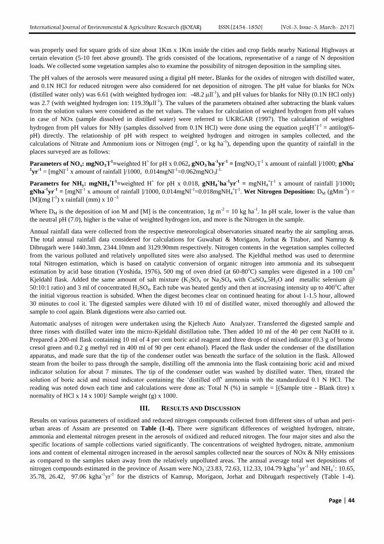
International Journal of Environmental & Agriculture Research (IJOEAR) ISSN:[2454-1850] [Vol-3, Issue-3, March- 2017]
Page | 44
was properly used for square grids of size about 1Km x 1Km inside the cities and crop fields nearby National Highways at
certain elevation (5-10 feet above ground). The grids consisted of the locations, representative of a range of N deposition
loads. We collected some vegetation samples also to examine the possibility of nitrogen deposition in the sampling sites.
The pH values of the aerosols were measured using a digital pH meter. Blanks for the oxides of nitrogen with distilled water,
and 0.1N HCl for reduced nitrogen were also considered for net deposition of nitrogen. The pH value for blanks for NOx
(distilled water only) was 6.61 (with weighted hydrogen ion: -48.2 ll-1
), and pH values for blanks for NHy (0.1N HCl only)
was 2.7 (with weighted hydrogen ion: 119.39ll-1
). The values of the parameters obtained after subtracting the blank values
from the solution values were considered as the net values. The values for calculation of weighted hydrogen from pH values
in case of NOx (sample dissolved in distilled water) were referred to UKRGAR (1997). The calculation of weighted
hydrogen from pH values for NHy (samples dissolved from 0.1N HCl) were done using the equation eqH+l-1
= antilog(6-
pH) directly. The relationship of pH with respect to weighted hydrogen and nitrogen in samples collected, and the
calculations of Nitrate and Ammonium ions or Nitrogen (mgl-1
, or kg ha-1
), depending upon the quantity of rainfall in the
places surveyed are as follows:
Parameters of NOx: mgNO3-l-1
=weighted H+
for pH x 0.062, gNO3-ha
-1yr
-1 = [mgNO3
-l-1
x amount of rainfall ]/1000; gNha-
1yr
-1 = [mgNl
-1 x amount of rainfall ]/1000, 0.014mgNl
-1=0.062mgNO3l
-1.
Parametrs for NHy: mgNH4+l-1
=weighted H+ for pH x 0.018, gNH4
+ha
-1yr
-1 = mgNH4
+l-1
x amount of rainfall ]/1000;
gNha-1
yr-1
= [mgNl-1
x amount of rainfall ]/1000, 0.014mgNl-1
=0.018mgNH4+l-1
. Wet Nitrogen Deposition: DM (gMm-2
) =
[M](mg l-1
) x rainfall (mm) x 10 -3
Where DM is the deposition of ion M and [M] is the concentration, 1g m-2
= 10 kg ha-1
. In pH scale, lower is the value than
the neutral pH (7.0), higher is the value of weighted hydrogen ion, and more is the Nitrogen in the sample.
Annual rainfall data were collected from the respective meteorological observatories situated nearby the air sampling areas.
The total annual rainfall data considered for calculations for Guwahati & Morigaon, Jorhat & Titabor, and Namrup &
Dibrugarh were 1440.3mm, 2344.10mm and 3129.90mm respectively. Nitrogen contents in the vegetation samples collected
from the various polluted and relatively unpolluted sites were also analysed. The Kjeldhal method was used to determine
total Nitrogen estimation, which is based on catalytic conversion of organic nitrogen into ammonia and its subsequent
estimation by acid base titration (Yoshida, 1976). 500 mg of oven dried (at 60-80oC) samples were digested in a 100 cm
3
Kjeldahl flask. Added the same amount of salt mixture (K2SO4 or Na2SO4 with CuSO4.5H2O and metallic selenium @
50:10:1 ratio) and 3 ml of concentrated H2SO4. Each tube was heated gently and then at increasing intensity up to 400oC after
the initial vigorous reaction is subsided. When the digest becomes clear on continued heating for about 1-1.5 hour, allowed
30 minutes to cool it. The digested samples were diluted with 10 ml of distilled water, mixed thoroughly and allowed the
sample to cool again. Blank digestions were also carried out.
Automatic analyses of nitrogen were undertaken using the Kjeltech Auto Analyzer. Transferred the digested sample and
three rinses with distilled water into the micro-Kjeldahl distillation tube. Then added 10 ml of the 40 per cent NaOH to it.
Prepared a 200-ml flask containing 10 ml of 4 per cent boric acid reagent and three drops of mixed indicator (0.3 g of bromo
cresol green and 0.2 g methyl red in 400 ml of 90 per cent ethanol). Placed the flask under the condenser of the distillation
apparatus, and made sure that the tip of the condenser outlet was beneath the surface of the solution in the flask. Allowed
steam from the boiler to pass through the sample, distilling off the ammonia into the flask containing boric acid and mixed
indicator solution for about 7 minutes. The tip of the condenser outlet was washed by distilled water. Then, titrated the
solution of boric acid and mixed indicator containing the ‘distilled off’ ammonia with the standardized 0.1 N HCl. The
reading was noted down each time and calculations were done as: Total N (%) in sample = [(Sample titre - Blank titre) x
normality of HCl x 14 x 100]/ Sample weight (g) x 1000.
III. RESULTS AND DISCUSSION
Results on various parameters of oxidized and reduced nitrogen compounds collected from different sites of urban and peri-
urban areas of Assam are presented on Table (1-4). There were significant differences of weighted hydrogen, nitrate,
ammonia and elemental nitrogen present in the aerosols of oxidized and reduced nitrogen. The four major sites and also the
specific locations of sample collections varied significantly. The concentrations of weighted hydrogen, nitrate, ammonium
ions and content of elemental nitrogen increased in the aerosol samples collected near the sources of NOx & NHy emissions
as compared to the samples taken away from the relatively unpolluted areas. The annual average total wet depositions of
nitrogen compounds estimated in the province of Assam were NO3-:23.83, 72.63, 112.33, 104.79 kgha
-1yr
-1 and NH4
+: 10.65,
35.78, 26.42, 97.06 kgha-1
yr-1
for the districts of Kamrup, Morigaon, Jorhat and Dibrugarh respectively (Table 1-4).
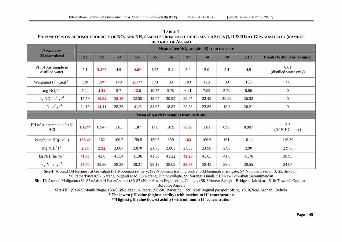
International Journal of Environmental & Agriculture Research (IJOEAR) ISSN:[2454-1850] [Vol-3, Issue-3, March- 2017]
Page | 45
TABLE 1
PARAMETERS ON AEROSOL PRODUCTS OF NOX AND NHy SAMPLES FROM EACH THREE MAJOR SITES (I, II & III) AT GUWAHATI CITY (KAMRUP
DISTRICT OF ASSAM)
Parameters
(Mean values)
Mean of ten NOx samples (S) from each site
S1 S2 S3 S4 S5 S6 S7 S8 S9 S10 Blank (Without air sample)
PH of Air sample in
distilled water 5.1 5.3** 4.9 4.8* 4.97 5.1 5.0 5.0 5.1 4.9
6.61
(distilled water only)
Weighjted H+ (eql
-1) 120 70* 140 207** 173 93 103 113 93 130 < 0
mg NO3-l-1
7.44 4.34 8.7 12.8 10.75 5.79 6.41 7.03 5.79 8.06 0
kg NO3-ha
-1yr
-1 17.59 10.94 38.16 32.55 19.07 20.92 29.85 22.49 20.92 26.52 0
kg N ha-1
yr-1
24.19 14.11 28.23 41.7 34.95 18.82 20.83 22.85 18.8 26.21 0
Mean of ten NHy samples from each site
PH of Air sample in 0.1N
HCl 1.12** 0.947 1.03 1.07 1.06 10.9 0.89 1.01 0.98 0.987
2.7
(0.1N HCl only)
Weighjted H+(eql
-1) 158.4* 162 160.2 159.5 159.6 159 163 160.6 161. 161.1 119.39
mg NH4+ l
-1 2.85 2.92 2.887 2.870 2.873 2.863 2.933 2.890 2.90 2.90 2.975
kg NH4+ha
-1yr
-1 41.07 42.0 41.54 41.36 41.38 41.22 42.26 41.65 41.8 41.76 30.95
kg N ha-1
yr-1
37.94 38.86 38.38 38.21 38.18 38.03 39.06 38.45 38.6 38.55 24.07
Site-I: Around Oil Refinery at Guwahati (S1:Noonmati refinery, (S2:Noonmati training centre, S3:Noonmati main gate, S4:Noonmati sector 3, S5:Birkuchi,
S6:Patherkuwari,S7:Narengi oughuli road, S8:Narengi Junior college, S9:Narengi Tiniali, S10:New Guwahati Baminimaidan
Site-II: Around Maligaon: (S1-S5):Adabari Buses’ stand-(S6-S7):Near Assam Engineering College, (S8-S9):near Sarighat Bridge at Jalukbari, S10: Towards Gopinath
Bordoloi Airport
Site-III: (S1-S2):Manik Nagar, (S3-S5):Rajdhani Nursery, (S6-S8):Baisistha, (S9):Near Reginal passport office, (S10)Near Arohan , Beltola
* The lowest pH value (highest acidity) with maximum H+ concentration
**Highest pH value (lowest acidity) with minimum H+ concentration
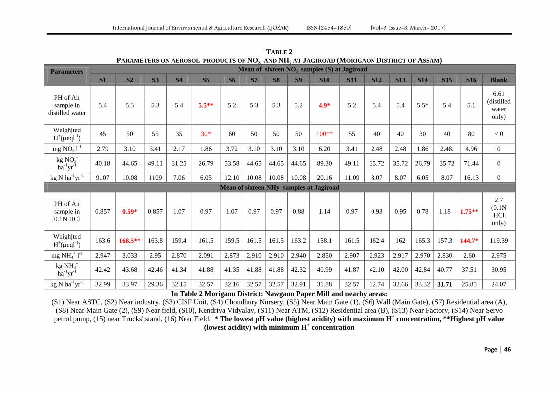
International Journal of Environmental & Agriculture Research (IJOEAR) ISSN:[2454-1850] [Vol-3, Issue-3, March- 2017]
Page | 46
TABLE 2
PARAMETERS ON AEROSOL PRODUCTS OF NOX AND NHy AT JAGIROAD (MORIGAON DISTRICT OF ASSAM)
Parameters Mean of sixteen NOx samples (S) at Jagiroad
S1 S2 S3 S4 S5 S6 S7 S8 S9 S10 S11 S12 S13 S14 S15 S16 Blank
PH of Air
sample in
distilled water
5.4 5.3 5.3 5.4 5.5** 5.2 5.3 5.3 5.2 4.9* 5.2 5.4 5.4 5.5* 5.4 5.1
6.61
(distilled
water
only)
Weighjted
H+(eql
-1)
45 50 55 35 30* 60 50 50 50 100** 55 40 40 30 40 80 < 0
mg NO3-l-1
2.79 3.10 3.41 2.17 1.86 3.72 3.10 3.10 3.10 6.20 3.41 2.48 2.48 1.86 2.48. 4.96 0
kg NO3-
ha-1
yr-1
40.18 44.65 49.11 31.25 26.79 53.58 44.65 44.65 44.65 89.30 49.11 35.72 35.72 26.79 35.72 71.44 0
kg N ha-1
yr-1
9..07 10.08 1109 7.06 6.05 12.10 10.08 10.08 10.08 20.16 11.09 8.07 8.07 6.05 8.07 16.13 0
Mean of sixteen NHy samples at Jagiroad
PH of Air
sample in
0.1N HCl
0.857 0.59* 0.857 1.07 0.97 1.07 0.97 0.97 0.88 1.14 0.97 0.93 0.95 0.78 1.18 1.75**
2.7
(0.1N
HCl
only)
Weighjted
H+(eql
-1)
163.6 168.5** 163.8 159.4 161.5 159.5 161.5 161.5 163.2 158.1 161.5 162.4 162 165.3 157.3 144.7* 119.39
mg NH4+ l
-1 2.947 3.033 2.95 2.870 2.091 2.873 2.910 2.910 2.940 2.850 2.907 2.923 2.917 2.970 2.830 2.60 2.975
kg NH4+
ha-1
yr-1
42.42 43.68 42.46 41.34 41.88 41.35 41.88 41.88 42.32 40.99 41.87 42.10 42.00 42.84 40.77 37.51 30.95
kg N ha-1
yr-1
32.99 33.97 29.36 32.15 32.57 32.16 32.57 32.57 32.91 31.88 32.57 32.74 32.66 33.32 31.71 25.85 24.07
In Table 2 Morigaon District: Nawgaon Paper Mill and nearby areas:
(S1) Near ASTC, (S2) Near industry, (S3) CISF Unit, (S4) Choudhury Nursery, (S5) Near Main Gate (1), (S6) Wall (Main Gate), (S7) Residential area (A),
(S8) Near Main Gate (2), (S9) Near field, (S10), Kendriya Vidyalay, (S11) Near ATM, (S12) Residential area (B), (S13) Near Factory, (S14) Near Servo
petrol pump, (15) near Trucks' stand, (16) Near Field. * The lowest pH value (highest acidity) with maximum H+ concentration, **Highest pH value
(lowest acidity) with minimum H+ concentration
International Journal of Environmental & Agriculture Research (IJOEAR) ISSN:[2454-1850] [Vol-3, Issue-3, March- 2017]
Page | 47
TABLE 3
PARAMETERS ON AEROSOL PRODUCTS OF NOX AND NHy AT TWO SITES OF JORHAT DISTRICT (SITE 1:TITABOR &SITE2:JORHAT) OF ASSAM
Parameters
Mean of ten NOx samples (S) each at Jorhat and Titabor
S1 S2 S3 S4 S5 S6 S7 S8 S9 S10
Blank
(Without air
sample)
PH of Air sample in
distilled water 5.317 5.26 5.66** 5.54 5.46 5.01 5.08 5.42 4.99 4.67*
6.61
(distilled
water only)
Weighjted H+(eql
-1) 39.33 66.67 26.67* 33.33 43.33 50.00 58.33 66.67 130.0 193.33** < 0
mg NO3-l-1
3.93 4.13 1.65 2.07 2.69 3.10 3.62 3.24 8.54 11.99 0
kg NO3-ha
-1yr
-1 92.04 96.89 98.75 48.45 62.98 72.67 84.78 96.89 188.9 280.99 0
kg N ha-1
yr-1
20.783 21.877 8.75 17.14 19.65 23.22 26.29 29.34 35.13 55.92 0
Mean of ten NHy samples each at Jorhat and Titabor
PH of Air sample in
0.1N HCl 1.26* 1.38 1.39 1.43 1.44 1.45 1.55 1.60 1.68** 1.49
2.7
(0.1N HCl
only)
Weighjted H+(eql
-1) 155.6** 152.9 152.7 151.9 151.4 151.3 149.3 148.1 146.2* 150.5 119.39
mg NH4+ l
-1 2.797 2.750 2.750. 2.733 2.723 2.723 2.687 2.670 2.633 2.713 2.975
kg NH4+ha
-1yr
-1 66.65 64.51 64.44 64.11 63.91 63.84 62.98 62.50 61.70 63.52 30.95
kg N ha-1
yr-1
51.06 50.18 50.12 49.86 49.70 49.65 48.98 48.61 47.99 49.41 24.07
SiteI: Rice growing areas towards Titabor: (S1) Namghar area , Titabor, (S2):Regional Rice research station Titabor, (S3): Titabor tiniali,, (S4):Titalbaor Chariali,
(S5):Chinamora tiniali, (S6): Gatany factory, (S8-S10): ONGC area, Cinnamora;
Site II: Jorhat town: (S1):Samples from Cinnamora railgate, :Cinamora petrol pupm, (S2): Lahoti petrol pump, (S3):AT Road, Joraht town, (S4): Bhogdoi bridge, & AT
Road, Borpool, (S5):samples from Garali, Dos & Co. (S6): Borbheta Tiniali,, Rowraia chariali, Civil Hospital, Jorhat, (S7):Baruah chariali, ASTC, Jorhat, (S8): Malowali
Tiniali, (S9):Tarajan, Byepass, (S10): Dikha Nursery & Moubandha,
* The lowest pH value (highest acidity) with maximum H+ concentration, **Highest pH value (lowest acidity) with minimum H
+ concentration
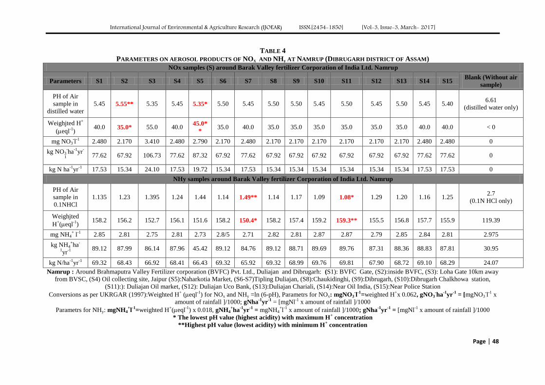
International Journal of Environmental & Agriculture Research (IJOEAR) ISSN:[2454-1850] [Vol-3, Issue-3, March- 2017]
Page | 48
TABLE 4
PARAMETERS ON AEROSOL PRODUCTS OF NOX AND NHy AT NAMRUP (DIBRUGARH DISTRICT OF ASSAM)
NOx samples (S) around Barak Valley fertilizer Corporation of India Ltd. Namrup
Parameters S1 S2 S3 S4 S5 S6 S7 S8 S9 S10 S11 S12 S13 S14 S15 Blank (Without air
sample)
PH of Air
sample in
distilled water
5.45 5.55** 5.35 5.45 5.35* 5.50 5.45 5.50 5.50 5.45 5.50 5.45 5.50 5.45 5.40 6.61
(distilled water only)
Weighjted H+
(eql-1
) 40.0 35.0* 55.0 40.0
45.0*
* 35.0 40.0 35.0 35.0 35.0 35.0 35.0 35.0 40.0 40.0 < 0
mg NO3-l-1
2.480 2.170 3.410 2.480 2.790 2.170 2.480 2.170 2.170 2.170 2.170 2.170 2.170 2.480 2.480 0
kg NO3-ha
-1yr
-
1
77.62 67.92 106.73 77.62 87.32 67.92 77.62 67.92 67.92 67.92 67.92 67.92 67.92 77.62 77.62 0
kg N ha-1
yr-1
17.53 15.34 24.10 17.53 19.72 15.34 17.53 15.34 15.34 15.34 15.34 15.34 15.34 17.53 17.53 0
NHy samples around Barak Valley fertilizer Corporation of India Ltd. Namrup
PH of Air
sample in
0.1NHCl
1.135 1.23 1.395 1.24 1.44 1.14 1.49** 1.14 1.17 1.09 1.08* 1.29 1.20 1.16 1.25 2.7
(0.1N HCl only)
Weighjted
H+(eql
-1)
158.2 156.2 152.7 156.1 151.6 158.2 150.4* 158.2 157.4 159.2 159.3** 155.5 156.8 157.7 155.9 119.39
mg NH4+ l
-1 2.85 2.81 2.75 2.81 2.73 2.8/5 2.71 2.82 2.81 2.87 2.87 2.79 2.85 2.84 2.81 2.975
kg NH4+ha
-
1yr
-1
89.12 87.99 86.14 87.96 45.42 89.12 84.76 89.12 88.71 89.69 89.76 87.31 88.36 88.83 87.81 30.95
kg N/ha-1
yr-1
69.32 68.43 66.92 68.41 66.43 69.32 65.92 69.32 68.99 69.76 69.81 67.90 68.72 69.10 68.29 24.07
Namrup : Around Brahmaputra Valley Fertilizer corporation (BVFC) Pvt. Ltd., Duliajan and Dibrugarh: (S1): BVFC Gate, (S2):inside BVFC, (S3): Loha Gate 10km away
from BVSC, (S4) Oil collecting site, Jaipur (S5):Naharkotia Market, (S6-S7)Tipling Duliajan, (S8):Chaukidinghi, (S9):Dibrugarh, (S10):Dibrugarh Chalkhowa station,
(S11):): Duliajan Oil market, (S12): Duliajan Uco Bank, (S13):Duliajan Chariali, (S14):Near Oil India, (S15):Near Police Station
Conversions as per UKRGAR (1997):Weighted H+ (eql
-1) for NOx and NHy =ln (6-pH), Parametrs for NOx: mgNO3
-l-1
=weighted H+x 0.062, gNO3
-ha
-1yr
-1 = [mgNO3
-l-1
x
amount of rainfall ]/1000; gNha-1
yr-1
= [mgNl-1
x amount of rainfall ]/1000
Parametrs for NHy: mgNH4+l-1
=weighted H+(eql
-1) x 0.018, gNH4
+ha
-1yr
-1 = mgNH4
+l-1
x amount of rainfall ]/1000; gNha-1
yr-1
= [mgNl-1
x amount of rainfall ]/1000
* The lowest pH value (highest acidity) with maximum H+ concentration
**Highest pH value (lowest acidity) with minimum H+ concentration
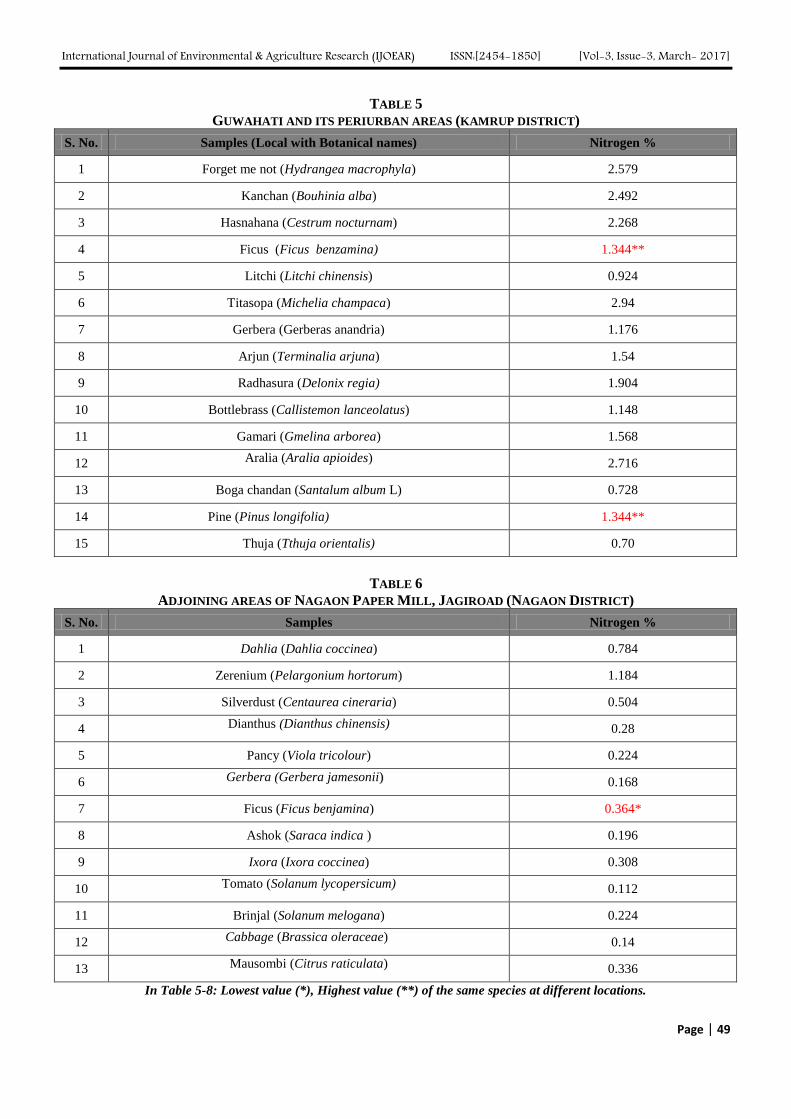
International Journal of Environmental & Agriculture Research (IJOEAR) ISSN:[2454-1850] [Vol-3, Issue-3, March- 2017]
Page | 49
TABLE 5
GUWAHATI AND ITS PERIURBAN AREAS (KAMRUP DISTRICT)
S. No. Samples (Local with Botanical names) Nitrogen %
1 Forget me not (Hydrangea macrophyla) 2.579
2 Kanchan (Bouhinia alba) 2.492
3 Hasnahana (Cestrum nocturnam) 2.268
4 Ficus (Ficus benzamina) 1.344**
5 Litchi (Litchi chinensis) 0.924
6 Titasopa (Michelia champaca) 2.94
7 Gerbera (Gerberas anandria) 1.176
8 Arjun (Terminalia arjuna) 1.54
9 Radhasura (Delonix regia) 1.904
10 Bottlebrass (Callistemon lanceolatus) 1.148
11 Gamari (Gmelina arborea) 1.568
12 Aralia (Aralia apioides)
2.716
13 Boga chandan (Santalum album L) 0.728
14 Pine (Pinus longifolia) LONGIFOLIA 1.344**
15 Thuja (Tthuja orientalis) 0.70
TABLE 6
ADJOINING AREAS OF NAGAON PAPER MILL, JAGIROAD (NAGAON DISTRICT)
S. No. Samples Nitrogen %
1 Dahlia (Dahlia coccinea) 0.784
2 Zerenium (Pelargonium hortorum) 1.184
3 Silverdust (Centaurea cineraria) 0.504
4 Dianthus (Dianthus chinensis)
0.28
5 Pancy (Viola tricolour) 0.224
6 Gerbera (Gerbera jamesonii)) )
0.168
7 Ficus (Ficus benjamina) 0.364*
8 Ashok (Saraca indica ) 0.196
9 Ixora (Ixora coccinea) 0.308
10 Tomato (Solanum lycopersicum)
0.112
11 Brinjal (Solanum melogana) 0.224
12 Cabbage (Brassica oleraceae)) 0.14
13 Mausombi (Citrus raticulata)
0.336
In Table 5-8: Lowest value (*), Highest value (**) of the same species at different locations.
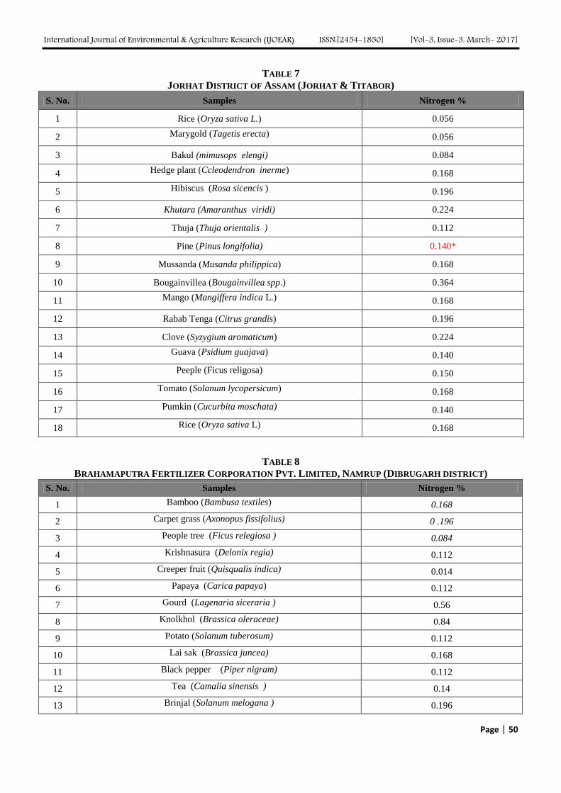
International Journal of Environmental & Agriculture Research (IJOEAR) ISSN:[2454-1850] [Vol-3, Issue-3, March- 2017]
Page | 50
TABLE 7
JORHAT DISTRICT OF ASSAM (JORHAT & TITABOR)
S. No. Samples Nitrogen %
1 Rice (Oryza sativa L.) 0.056
2 Marygold (Tagetis erecta)
0.056
3 Bakul (mimusops elengi) 0.084
4 Hedge plant (Ccleodendron inerme) 0.168
5 Hibiscus (Rosa sicencis ) 0.196
6 Khutara (Amaranthus viridi) 0.224
7 Thuja (Thuja orientalis ) 0.112
8 Pine (Pinus longifolia) 0.140*
9 Mussanda (Musanda philippica) 0.168
10 Bougainvillea (Bougainvillea spp.) 0.364
11 Mango (Mangiffera indica L.) 0.168
12 Rabab Tenga (Citrus grandis) 0.196
13 Clove (Syzygium aromaticum) 0.224
14 Guava (Psidium guajava) 0.140
15 Peeple (Ficus religosa) 0.150
16 Tomato (Solanum lycopersicum) 0.168
17 Pumkin (Cucurbita moschata) 0.140
18 Rice (Oryza sativa L) 0.168
TABLE 8
BRAHAMAPUTRA FERTILIZER CORPORATION PVT. LIMITED, NAMRUP (DIBRUGARH DISTRICT)
S. No. Samples Nitrogen %
1 Bamboo (Bambusa textiles) 0.168
2 Carpet grass (Axonopus fissifolius) 0 .196
3 People tree (Ficus relegiosa )
0.084
4 Krishnasura (Delonix regia)
0.112
5 Creeper fruit (Quisqualis indica)
0.014
6 Papaya (Carica papaya)
0.112
7 Gourd (Lagenaria siceraria )
0.56
8 Knolkhol (Brassica oleraceae)
0.84
9 Potato (Solanum tuberosum)
0.112
10 Lai sak (Brassica juncea)
0.168
11 Black pepper (Piper nigram)
0.112
12 Tea (Camalia sinensis )
0.14
13 Brinjal (Solanum melogana )
0.196
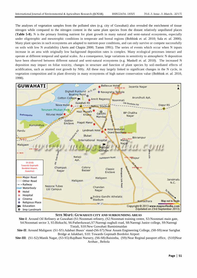
International Journal of Environmental & Agriculture Research (IJOEAR) ISSN:[2454-1850] [Vol-3, Issue-3, March- 2017]
Page | 51
The analyses of vegetation samples from the polluted sites (e.g. city of Guwahati) also revealed the enrichment of tissue
nitrogen while compared to the nitrogen content in the same plant species from the distant relatively unpolluted places
(Table 5-8). N is the primary limiting nutrient for plant growth in many natural and semi-natural ecosystems, especially
under oligotrophic and mesotrophic conditions in temperate and boreal regions (Bobbink et. al. 2010; Sala et. al. 2000).
Many plant species in such ecosystems are adapted to nutrient-poor conditions, and can only survive or compete successfully
on soils with low N availability (Aerts and Chapin 2000; Tamm 1991). The series of events which occur when N inputs
increase in an area with originally low background deposition rates is complex. Many ecological processes interact and
operate at different temporal and spatial scales. As a consequence, large variations in sensitivity to atmospheric N deposition
have been observed between different natural and semi-natural ecosystems (e.g. Maskell et. al. 2010). The increased N
deposition may impact on foliar toxicity, changes in structure and function of plant species by soil-mediated effects of
acidification, such as stunted root growth by NHy. All these may largely linked to significant changes in the N cycle, in
vegetation composition and in plant diversity in many ecosystems of high nature conservation value (Bobbink et. al. 2010,
1998).
SITE MAP1: GUWAHATI CITY AND SURROUNDING AREAS
Site-I: Around Oil Refinery at Guwahati (S1:Noonmati refinery, (S2:Noonmati training centre, S3:Noonmati main gate,
S4:Noonmati sector 3, S5:Birkuchi, S6:Patherkuwari,S7:Narengi oughuli road, S8:Narengi Junior college, S9:Narengi
Tiniali, S10:New Guwahati Baminimaidan
Site-II: Around Maligaon: (S1-S5):Adabari Buses’ stand-(S6-S7):Near Assam Engineering College, (S8-S9):near Sarighat
Bridge at Jalukbari, S10: Towards Gopinath Bordoloi Airport
Site-III: (S1-S2):Manik Nagar, (S3-S5):Rajdhani Nursery, (S6-S8):Baisistha, (S9):Near Reginal passport office, (S10)Near
Arohan , Beltola
SII (S10) Towards Gopinath Bordoloi Airport,
Guwahati
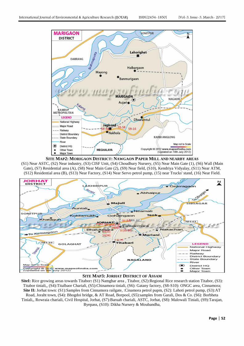
International Journal of Environmental & Agriculture Research (IJOEAR) ISSN:[2454-1850] [Vol-3, Issue-3, March- 2017]
Page | 52
SITE MAP2: MORIGAON DISTRICT: NAWGAON PAPER MILL AND NEARBY AREAS
(S1) Near ASTC, (S2) Near industry, (S3) CISF Unit, (S4) Choudhury Nursery, (S5) Near Main Gate (1), (S6) Wall (Main
Gate), (S7) Residential area (A), (S8) Near Main Gate (2), (S9) Near field, (S10), Kendriya Vidyalay, (S11) Near ATM,
(S12) Residential area (B), (S13) Near Factory, (S14) Near Servo petrol pump, (15) near Trucks' stand, (16) Near Field.
SITE MAP3: JORHAT DISTRICT OF ASSAM
SiteI: Rice growing areas towards Titabor: (S1) Namghar area , Titabor, (S2):Regional Rice research station Titabor, (S3):
Titabor tiniali,, (S4):Titalbaor Chariali, (S5):Chinamora tiniali, (S6): Gatany factory, (S8-S10): ONGC area, Cinnamora;
Site II: Jorhat town: (S1):Samples from Cinnamora railgate, :Cinamora petrol pupm, (S2): Lahoti petrol pump, (S3):AT
Road, Joraht town, (S4): Bhogdoi bridge, & AT Road, Borpool, (S5):samples from Garali, Dos & Co. (S6): Borbheta
Tiniali,, Rowraia chariali, Civil Hospital, Jorhat, (S7):Baruah chariali, ASTC, Jorhat, (S8): Malowali Tiniali, (S9):Tarajan,
Byepass, (S10): Dikha Nursery & Moubandha,
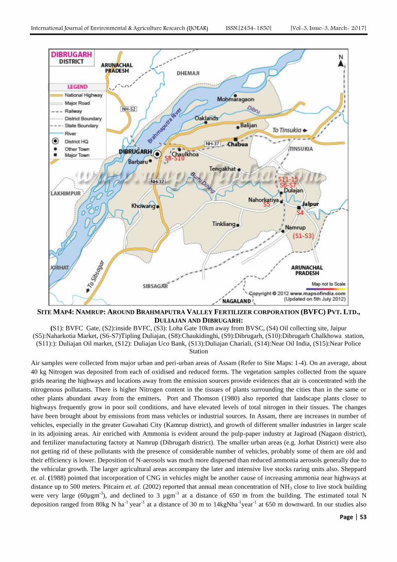
International Journal of Environmental & Agriculture Research (IJOEAR) ISSN:[2454-1850] [Vol-3, Issue-3, March- 2017]
Page | 53
SITE MAP4: NAMRUP: AROUND BRAHMAPUTRA VALLEY FERTILIZER CORPORATION (BVFC) PVT. LTD.,
DULIAJAN AND DIBRUGARH: (S1): BVFC Gate, (S2):inside BVFC, (S3): Loha Gate 10km away from BVSC, (S4) Oil collecting site, Jaipur
(S5):Naharkotia Market, (S6-S7)Tipling Duliajan, (S8):Chaukidinghi, (S9):Dibrugarh, (S10):Dibrugarh Chalkhowa station,
(S11):): Duliajan Oil market, (S12): Duliajan Uco Bank, (S13):Duliajan Chariali, (S14):Near Oil India, (S15):Near Police
Station
Air samples were collected from major urban and peri-urban areas of Assam (Refer to Site Maps: 1-4). On an average, about
40 kg Nitrogen was deposited from each of oxidised and reduced forms. The vegetation samples collected from the square
grids nearing the highways and locations away from the emission sources provide evidences that air is concentrated with the
nitrogenous pollutants. There is higher Nitrogen content in the tissues of plants surrounding the cities than in the same or
other plants abundant away from the emitters. Port and Thomson (1980) also reported that landscape plants closer to
highways frequently grow in poor soil conditions, and have elevated levels of total nitrogen in their tissues. The changes
have been brought about by emissions from mass vehicles or industrial sources. In Assam, there are increases in number of
vehicles, especially in the greater Guwahati City (Kamrup district), and growth of different smaller industries in larger scale
in its adjoining areas. Air enriched with Ammonia is evident around the pulp-paper industry at Jagiroad (Nagaon district),
and fertilizer manufacturing factory at Namrup (Dibrugarh district). The smaller urban areas (e.g. Jorhat District) were also
not getting rid of these pollutants with the presence of considerable number of vehicles, probably some of them are old and
their efficiency is lower. Deposition of N-aerosols was much more dispersed than reduced ammonia aerosols generally due to
the vehicular growth. The larger agricultural areas accompany the later and intensive live stocks raring units also. Sheppard
et. al. (1988) pointed that incorporation of CNG in vehicles might be another cause of increasing ammonia near highways at
distance up to 500 meters. Pitcairn et. al. (2002) reported that annual mean concentration of NH3 close to live stock building
were very large (60µgm-3
), and declined to 3 µgm-3
at a distance of 650 m from the building. The estimated total N
deposition ranged from 80kg N ha-1
year-1
at a distance of 30 m to 14kgNha-1
year-1
at 650 m downward. In our studies also
International Journal of Environmental & Agriculture Research (IJOEAR) ISSN:[2454-1850] [Vol-3, Issue-3, March- 2017]
Page | 54
the mean deposition of nitrogen by NOx was 6-38kgha-1
yr-1
, whereas by NHy was 7-24kgha-1
yr-1
from all the sites. The
annual average of total deposition of nitrogen compounds in state has been computed as the sum of the annual averages of
wet deposited nitrogen in the representative districts of Assam. Thus, a total maximum deposition of N through oxidized and
reduced forms of Nitrogen together is about 18-46 kg ha-1
yr-1
. Spatial distribution of total respective depositions of NOx and
NHy on a 1km x 1 km grid in 2010-11 is shown as sites (urban and peri-urban areas) of sample collections in the district
maps for better orientation. Several significantly different gradients for NOx and NHy were recognized for the sites as well
as the locations of sample collections. Plausibly, the total deposition of the former was especially influenced by their
emissions from populated cities and larger vehicular traffic congested areas. The reasons for the later were mostly influenced
by depositions from industries (e.g. pulp & paper factory at Jagiroad, fertilizer factory at Namrup), and intensive cultivable
as well as animal rearing hot spots of the urban and peri-urban areas in the state.
IV. CONCLUSION
The wet deposited nitrogen (NOx, NHy and their compounds) was estimated following a square grid (1km x1km) resolution
in a few major districts of Assam. The deposition had been assessed from the measured and modeled concentrations of
acidifying compounds in the atmosphere and the precipitations with reference to UKRGR (1997).Net deposition of Nitrogen
through its oxides ranged from 6.0-38kgha-1
yr-1
, whereas net deposition of nitrogen by ammonia was in between 7-24 kgha-
1yr
-1. A total maximum deposition of N through oxidized and reduced forms of Nitrogen together is about 18-46 kg ha
-1yr
-1.
The hypothesis that Assam (especially Guwahati and its adjoining areas) is also facing with enrichment of nitrogenous
pollution due to anthropogenic activities and mass vehicular and industrial growth was tested positive.
ACKNOWLEDGEMENTS
The authors express sincere sense of gratitude to the Ministry of Environment and Forests, Govt. of India for financial
support for accomplish the research work. Special thanks are extended to the Authority of Assam Agricultural University,
Jorhat (Assam) for providing all kinds of facilities pertaining to the field and laboratory works under the project.
REFERENCES
[1] Aerts, R., & Chapin, F. S. (2000). The mineral nutrition of wild plants revisited: a re-evaluation of processes and patterns. Advances
in Ecological Research, 30, 1–67.
[2] Asman, W. A. H., Sutton, M. A., & Schjorring, J. K. (1998).Ammonia: emission, atmospheric transport and deposition. New
Phytologist, 139, 27–48.
[3] Bharali, B., Haloi. B., Chutia, J., Dey, P.C. (2012) Atmosperic deposition of Nitrogen in North-east India and productivity of winter
cereals’ Published in the Web BALWOIS 12 (www.balois.com), the 5th International Conference on Water, Climate and
Environment- held from 28th May -2nd June 2012 at Ohrid, The Republic of Macedonia.
[4] Bobbink, R., Hicks, K., Galloway, J., Spranger, T., Alkemade, R., Ashmore, M., et. al. (2010). Global assessment of nitrogen
deposition effects on terrestrial plant diversity: a synthesis. Ecological Applications, 20, 30–59.
[5] Bobbink, R., Hornung, M., & Roelofs, J. G. M. (1998). The effects of air-borne nitrogen pollutants on species diversity in natural and
semi-natural European vegetation. Journal of Ecology, 86, 717–738. Water Air Soil Pollut. (2013) 224:1664
[6] Dentener, F., Drevet, J., Lamarque, J. F., Bey, I., Eickhout, B., Fiore, A. M., et. al. (2006). Nitrogen and sulfur deposition on regional
and global scales: a multimodel evaluation. Global Biogeochemical Cycles, 20.
[7] Edu Dorland & Carly J. Stevens & Cassandre Gaudnik & Emmanuel Corcket & Suzanne Rotthier & Katherine Wotherspoon & Mari
Jokerud & Vigdis Vandvik & Merel B. Soons & Mariet M. Hefting Per Arild Aarrestad & Didier Alard & Martin Diekmann &
Cecilia Duprè & Nancy B. Dise & David J. G. Gowing & Roland Bobbink (2013) Differential Effects of Oxidised and Reduced
Nitrogen on Vegetation and Soil Chemistry of Species-Rich Acidic Grasslands. Water Air Soil Pollut (2013) 224:1664
[8] Galloway, J., & Cowling, E. B. (2002). Reactive nitrogen and the world: 200 years of change. Ambio, 31, 64–71.
[9] Galloway J N, Levy II H and Kasibhatla P S (1994) Year 2020: consequences of population growth and development on the
decomposition of oxidized nitrogen. Ambio 23, 120-123.
[10] Galloway J N, Schlesinger WH, Levy II H, Michaels A and Schnoor J L (1995) Nitrogen fixation: Anthropogenic
enhancementenvironmental response. Global Biogeochem. Cycles 9, 235-252.
[11] Galloway, J. N., Townsend, A. R., Erisman, J. W., Bekunda, M., Cai, Z., Freney, J. R., et. al. (2008). Transformation of the nitrogen
cycle: recent trends, questions and potential solutions. Science, 320, 889–892.
[12] Gaudnik, C., Corcket, E., Clement, B., Delmas, C.L., Gombert, C.S., Muller, S., Stevens, C.J. and Alard, D. (2011) Detecting the foot
print of changing atmospheric nitriogen deposition loads on acid grassland in the context of climate change. Global Climate Change
Biology Vol. 17, Issue 11, Pages 3351-3365.
[13] Harrison, R.M., Rapsomanikis, S. and Turnbull, A.(1989) Land surface exchange in a chemically reactive system; surface fluxes of
HNO3, HCL and NH3. Atmospheric Environment, 23:1795-1800.
International Journal of Environmental & Agriculture Research (IJOEAR) ISSN:[2454-1850] [Vol-3, Issue-3, March- 2017]
Page | 55
[14] Hyvarinen, M. and Crittenden, P.D. (1998) Relationships between atmospheric nitrogen inputs and the vertical nitrogen and
phosphorous concentration gradients in the lichen Cladonia portentosa. New Phytologist, 140:519-530.
[15] Maskell, L. C., Smart, S. M., Bullock, J. M., Thompson, K., & Stevens, C. J. (2010). Nitrogen deposition causes widespread species
loss in British Habitats. Global Change Biology, 16, 671–679
[16] Mc Clean, C. J., van den Berg, L. J. L., Ashmore, M. R. and Preston, C. D. (2011) Atmospheric nitrogen deposition explains patterns
of plant species loss. Global Change Biology, 17: 2882–2892.
[17] Mohan, M. and Kumar, S. (1998) Review of Acid rain potential in India: Future threats and remedial measures. Current science.
75:6:579-593.
[18] Pitcairn, C.E.R., Skiba, U.M., Sutton, M.A., Fowler, D., Munro, R., and Kennedy, V. (2002) Defining the spatial impacts of poultry
farm ammonia emission on species composition of adjacent woodland groundflora using Ellenberg, Nitrogen index, nitrous oxide and
nitric oxide emissions and foliar nitrogen as marker variables. Environmental Pollution, Vol. 119, Issue 1, Pages 9-21.
[19] Port, G.R. and Thomson, J.R. (1980) Outbreak of insect herbivores on plants along motorways in the United Kingdom, Journal of
Applied Ecology 17, 649-656.
[20] Sala, O. E., Chapin, F. S., Armesto, J. J., Berlow, E., Bloomfield, J., Dirzo, R., et. al. (2000). Biodiversity—global biodiversity
scenarios for the year 2100. Science, 287, 1770–1774.
[21] Sheppard, L.J., Leith, I.D., Crossley, A. Van Dijk, N., Fowler, D., Sutton, M.A., Woods, C. (2008) Stress responses of Calluna
vulgaris to reduced and oxidised N applied under ‘real world conditions’. Environmental Pollution 154, 404-413.
[22] Sutton, MA., Moncrieff, JB. Fowler, D. (1992) Deposition of atmospheric ammonia to moorlands. Environmental Pollution, 75:15-
24.
[23] Tamm, C. O. (1991). Nitrogen in terrestrial ecosystems: questions of productivity, vegetational changes, and ecosystem stability.
Berlin: Springer.
[24] UKRGAR, (1997) Acid Deposition in the United Kingdom, 1992-1994. The United Kingdom Review Group on Acid Rain,
Department of Environment, London. Page 173-174
[25] Vitousek P M, Aber J, Howarth R W, Likens G E, Matson P A, Schindler D W, Schlesinger W H, and Tilman D G 1997 Human
alteration of the global nitrogen cycle: Causes and Consequences. Issues in Ecology 1, 1-15.
[26] Yoshida, S. and Douglas, A., Forno, Jamessa, Cock Kwanchai, A, Gomez, A. (1976) Laboratory Manual for Physiological Studies of
Rice, page 1-73, Published by Intl. Rice Res. Inst. Los Banos, Philipines.
[27] Zapletal, M. (1998) Atmospheric deposition of nitrogen compounds in the Czech Republic. Environmental Pollution 102 A1: 305-
311.
International Journal of Environmental & Agriculture Research (IJOEAR) ISSN:[2454-1850] [Vol-3, Issue-3, March- 2017]
Page | 56
The Influence of Vermiculite on the Uptake of Silver
Nanoparticles in a Terrestrial System Sara A. Pappas
1, Uday Turaga
2, Naveen Kumar
3, Seshadri Ramkumar
4,
Ronald J. Kendall5
1,2,3,5The Wildlife Toxicology Laboratory, Department of Environmental Toxicology, The Institute of Environmental and
Human Health, Texas Tech University, Lubbock, TX USA 4The Nonwovens and Advanced Materials Laboratory, Department of Environmental Toxicology, The Institute of
Environmental and Human Health, Texas Tech University, Lubbock, TX USA
Abstract— The uptake of silver from silver nanoparticles in soil was investigated in the presence of increasing
concentrations of Vermiculite, typical 2:1 clay. Two insect species, Acheta domesticus and Tenebrio molitor, and two plant
species, Helianthus annuus and Sorghum vulgare, were exposed to silver nanoparticles in the presence of increasing
concentrations of Vermiculite in soil. Silver nanoparticles were characterized using techniques including transmission
electron microscopy, dynamic light scattering, and powder X-ray diffraction. The levels of silver in test species exposed to
silver nanoparticles were measured using an inductively coupled plasma-optical emission spectrometer. An increase in the
cation exchange capacity of soil was observed with the increase in the concentration of vermiculite in soil. The results
suggested a decrease in the uptake of silver from silver nanoparticles in soil by Acheta domesticus as a function of
increasing concentrations of Vermiculite in soil. No apparent trend was observed in the remaining species. Both plant
species were found to accumulate silver in their roots. The translocation of silver to stems and leaves was observed in the
case of Helianthus annuus. Results from this study suggest that the presence of Vermiculite in soil could possibly decrease
the uptake of silver from silver nanoparticles.
Keywords— Silver nanoparticles, Acheta domesticus, Tenebrio molitor, Helianthus annus, Sorghum vulgare, inductively
coupled plasma-optical emission spectrometer, Cation exchange capacity.
I. INTRODUCTION
The widespread use of silver nanoparticles (Ag NPs) for a variety of applications has resulted in an increase in the
concentrations of Ag NPs in terrestrial ecosystems. Typically, Ag NPs find their way into terrestrial ecosystems through the
application of sewage sludge as fertilizer to land [1-3]. The environmental behavior, fate, and ecotoxicity of metal-based
nanoparticles in a terrestrial ecosystem are known to be influenced by the physicochemical characteristics of both the
nanoparticles themselves and the soil. Physical properties include size and shape of nanoparticles while the chemical
characteristics include acid-base character, aqueous solubility and surface coatings, if any [4]. The physicochemical
properties of soil can influence the mobility, bioavailability and toxicity of pollutants in a terrestrial ecosystem. These
properties include pH, soil texture, organic matter, and cation exchange capacity (CEC), etc [5,6].
The texture of a soil is comprised of sand, silt, and clay. The particle size of sand, silt, and clay are > 50 μm, 2-50 μm, and <
2 μm respectively [7,8]. Clay particles belong to a group of minerals described as hydrous silicates [9]. Clay particles
typically have a negative charge [10]. Additionally, clay particles considerably contribute to the CEC of soil. CEC of soil is
the quantity of positively charged ions that could be held by the negatively charged surface of clay minerals [9]. The CEC of
a soil provides electrostatic binding sites for cations like silver ions (Ag+) thus rendering them electrostatically immobilized
[11]. The negative charge of clay minerals, the high surface area of clay due to small particle size [12] and the contribution of
clay minerals to the CEC of soil [9] play a key role in determining the fate of metal contaminants in soil. The four major
groups of clay minerals include: 1) the kaolinite group; 2) the mont-morillonite/smectite group; 3) the illite group and 4) the
chlorite group [9]. The mont-morillonite/smectite group of clay minerals are known to possess high surface area and CEC
compared to the remaining three groups of clay minerals. The general formula of mont-morillonite/smectite group of clay
minerals is (Ca,Na,H)(Al,Mg,Fe,Zn)2(Si,Al)4O10(OH)2-XH2O [9].
A member of the mont-morillonite/smectite group of clay minerals, Vermiculite, is used in the present study. The effect of
increasing concentrations of Vermiculite in soil on the uptake of silver from Ag NPs in a terrestrial system was investigated.
Terrestrial isopods have been used as model organisms to understand the uptake, kinetics and transformation of metal
nanoparticles [13-15]. The uptake of nanoparticles in terrestrial isopods occurs exclusively through the oral route. Negligible
International Journal of Environmental & Agriculture Research (IJOEAR) ISSN:[2454-1850] [Vol-3, Issue-3, March- 2017]
Page | 57
surface uptake of nanoparticles is observed in terrestrial isopods facilitating the uptake and transformation studies of metal
nanoparticles [16]. However, it is equally important to investigate the uptake of metals from metal nanoparticles by other
components of terrestrial ecosystems that serve a crucial link in the metal transport chains between trophic levels in the food
web.
Two species of insects, Acheta domesticus and Tenebrio molitor, and two species of plants, Helianthus annuus (a dicot plant)
and Sorghum vulgare (a monocot plant) were used. The insect and plant species were exposed to Ag NPs in soil containing a
range of concentrations of Vermiculite. Insects serve an important role in the metal-transport chains between trophic levels in
food webs [17]. For instance, during the breeding season, insects and larvae constitute an important food source for
insectivorous birds [18]. Therefore, it is important to determine if insects are able to bioaccumulate Ag from Ag NPs in soil.
As seeds are another important food source for granivorous birds [19], the possibility of translocation of Ag to plant tissues
was investigated. Results from this study would help understand the role of plants in bioaccumulation of metal nanoparticles.
II. MATERIAL AND METHOD
2.1 Soil collection and preparation
Soil used in the present study was collected 40 minutes south of Colorado City, Texas at an elevation of 684 m above sea
level. Exact coordinates were as follows: Universal Transverse Mercator 14 S 0319752 mE 3557792 mN. All soil was
collected from the top 10 cm of soil, shoveled into clean plastic containers and transported back to The Institute of
Environmental and Human Health (TIEHH) at Texas Tech University (TTU) in Lubbock, TX. The soil was processed for
homogeneity at TIEHH. All large rocks, roots, living organisms, and other organic matter were removed first and large
clumps of soil were crushed. The soil was then sifted through a 2 mm wire screen into another clean plastic storage container.
Processed soil was covered and stored indoors until ready for use.
2.2 Soil analysis
The characterization of soil samples was performed at Midwest Laboratories Inc. (Omaha, NE). Soil samples were
characterized by evaluating parameters such as soil texture, percent humic matter, percent organic matter, exchangeable
cations (K+, Mg
2+, Ca
2+), available phosphorus (P), soil pH, percent base saturation of cations (K
+, Mg
2+, Ca
2+, H
+), CEC, and
sulfur (S) content.
Nanoparticle Characterization
Uncoated silver nanoparticles (30-50 nm) were purchased from US Research Nanomaterials, Inc. (Houston, TX). All silver
nanoparticles were reported by US Research Nanomaterial, Inc (www.us-nano.com) to consist of > 99.99% Ag.
In order to confirm the size range and shape of the nanoparticles, transmission electron microscopy (TEM) was used.
Samples were prepared by dispersing the Ag NP powder in ethanol (EtOH) and sonicated for 10 minutes before being drop
cast onto a carbon coated copper grid. Samples were air dried before analysis. TEM (Hitachi H-8100 TEM) images were
taken at 200 kV using a tungsten filament side-mounted camera.
Dynamic light scattering (DLS) was used as an additional method to confirm the size Ag NPs. The sample preparation
process for DLS involved placing approximately 10 mg of Ag NP powder in 10 mL of reagent grade acetone (Fisher
Scientific, MA, USA). Samples were sonicated until Ag NPs remained suspended in solution. Samples were analyzed using a
Nanotrac NPA252 Combination (Microtrac Inc. Montgomery, PA) and Mictrotrac Flex Software (Version: 10.3.14).
Powder x-ray diffraction (PXRD) was used to confirm the composition of Ag NPs. A Rigaku Ultima III X-Ray
Diffractometer was used for this purpose. Samples were analyzed using Cu Kα radiation as x-ray source. The Ag NPs were
analyzed using the following instrument parameters: parallel-beam geometry was used with a step width of 0.03° and a count
time of one second; the divergence, scattering, and receiving slits were set at one. Once completed, the diffraction patterns
were compared and matched to the phases in the International Center for Diffraction Data (ICDD) powder diffraction file
(PDF) database.
2.3 Insect treatment groups
Two 37.8 L terrariums were prepared for each insect treatment group, including a control group. The clay content of soil was
adjusted before the terrariums were spiked with Ag NPs. The required amount of clay (Sta-Green®
vermiculite) was weighed
International Journal of Environmental & Agriculture Research (IJOEAR) ISSN:[2454-1850] [Vol-3, Issue-3, March- 2017]
Page | 58
out to constitute 1, 5, 10, 15, and 20% of clay (by weight) in 2.5 kg soil for each treatment group. Each terrarium was spiked
with 62.5 mg of uncoated 30-50 nm Ag NPs so that a final soil concentration of 25 µg/g Ag NPs was obtained.
Once the terrariums were prepared, insects were purchased from Reptilefood (reptilefoods.com, Ohio, USA). Each terrarium
received either 300 small crickets or 400 large mealworms. Insects were provided with fresh food and water as needed for the
duration of the 28-day exposure period. After 28 days, insects were carefully extracted from the terrariums and placed in
glass jars. The jars were then placed in a -80°C freezer until all the insects were deceased. Insects were then freeze dried
(FreeZone 2.5 Liter Freeze Dry System, Labconco, Corp. Kansas City, MO) for at least 48 hours to ensure the removal of all
moisture. Freeze dried insects were then crushed into a fine powder and stored in a freezer until further analysis.
2.4 Plant treatment groups
Commercially available 7.6 L plastic nursery containers were purchased and filled with approximately two inches of
commercial pond pebbles to aid in proper drainage. The clay content in the soil was adjusted as was done with the insect
treatment groups. This soil was then spiked to have a final soil concentration of 25 µg/g Ag NPs in soil. The spiked soil was
transferred into the plastic nursery containers.
Seeds of each plant species were planted into the prepared nursery containers and were transported to the TTU greenhouse.
The plants remained in the greenhouse until maturity, approximately three months for H. annuus and six months for S.
vulgare. While in the greenhouse, plants received shaded sunlight and were maintained at 60°F or above. To prevent the soil
from drying out, plants were misted for three minutes every eight hours in a day. Once plants reached maturity, the entire
plant was harvested. The roots were separated from the remainder of the plant and rinsed using tap water for a full minute to
remove all attached soil. The shoot system of the plant was separated into leaves, stems, and seeds. The plant samples were
stored in a freezer until further analysis.
2.5 Sample digestions
Three identical samples were weighed out using the insect samples collected from each terrarium. For each plant treatment
group, four samples were prepared from each nursery container: a root sample, a leaf sample, a stem sample, and a seed
sample. For each sample, either plant or insect, approximately 1 grams were weighed into a 100 mL beaker. Wet weights
(ww) were taken into account in the case of plants samples. 10 ml of 70% nitric acid (HNO3, reagent grade) was added to
each sample. This was followed by an addition of 10 ml of 30% hydrogen peroxide (H2O2, reagent grade). A solution
containing 10 ml HNO3 and 10 ml H2O2 was used as the reagent blank. All beakers were covered with a Teflon watch glass
and placed on hot plates overnight for sample digestions. All samples were slowly heated in increments of 50 ˚C until the
solutions began to reflux gently. Care was taken to ensure that none of the solutions boiled over resulting in a loss of sample.
All samples were swirled periodically during the reflux process to aid in the digestion of the samples. The digestions were
considered complete when the volume of samples in the beaker was reduced to approximately 5 ml. Once complete, beakers
were removed from the hot plate and placed in an ice bath to cool. Cooling was followed by filtering the samples into 50 ml
centrifuge tubes (Corning CentriStar TM
, Corning, NY) using ashless filter paper (Whatman No. 41, Fisher Scientific, PA).
This was to ensure all remaining solids and/or digested lipids were removed from the samples. The original sample beakers
were then rinsed twice with 10 ml of 5% HNO3 and the rinse contents were added to the centrifuge tubes. The centrifuge
tubes with sample extracts were stored at room temperature until analysis by Inductively Coupled Plasma-Optical Emission
Spectrometry (ICP-OES).
2.6 ICP-OES analysis
All samples were analyzed using a Teledyne Instruments (Hudson, New Hampshire) Prodigy High Dispersion ICP-OES. The
samples were analyzed for silver at three wavelengths: 224.643, 328.068, and 338.289 nm. The three wavelengths were
aligned using a 10 ppm silver standard solution (SPEX CetriPrep). The instrument was calibrated using a range of silver
concentrations from 0-20 ppm.
2.7 Statistical Analysis
All data was compared using ANOVA with Rstudio software [20]. The Shapiro test was used to test the normality of data
[21]. All statistical analysis was compared with 95 % confidence interval. Data was analyzed using a one-way ANOVA,
followed by a multiple comparison test (Tukey HSD) to identify significant differences among the treatment groups
(α<0.05).
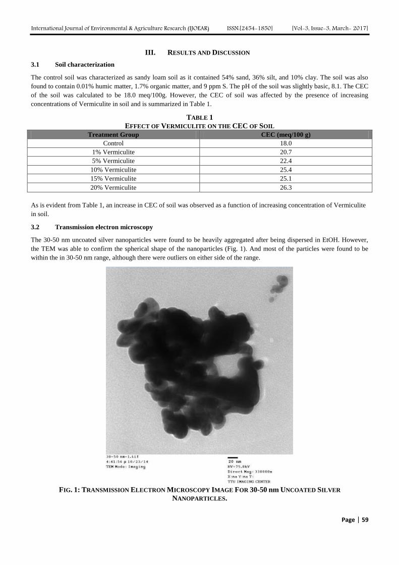
International Journal of Environmental & Agriculture Research (IJOEAR) ISSN:[2454-1850] [Vol-3, Issue-3, March- 2017]
Page | 59
III. RESULTS AND DISCUSSION
3.1 Soil characterization
The control soil was characterized as sandy loam soil as it contained 54% sand, 36% silt, and 10% clay. The soil was also
found to contain 0.01% humic matter, 1.7% organic matter, and 9 ppm S. The pH of the soil was slightly basic, 8.1. The CEC
of the soil was calculated to be 18.0 meq/100g. However, the CEC of soil was affected by the presence of increasing
concentrations of Vermiculite in soil and is summarized in Table 1.
TABLE 1
EFFECT OF VERMICULITE ON THE CEC OF SOIL
Treatment Group CEC (meq/100 g)
Control 18.0
1% Vermiculite 20.7
5% Vermiculite 22.4
10% Vermiculite 25.4
15% Vermiculite 25.1
20% Vermiculite 26.3
As is evident from Table 1, an increase in CEC of soil was observed as a function of increasing concentration of Vermiculite
in soil.
3.2 Transmission electron microscopy
The 30-50 nm uncoated silver nanoparticles were found to be heavily aggregated after being dispersed in EtOH. However,
the TEM was able to confirm the spherical shape of the nanoparticles (Fig. 1). And most of the particles were found to be
within the in 30-50 nm range, although there were outliers on either side of the range.
FIG. 1: TRANSMISSION ELECTRON MICROSCOPY IMAGE FOR 30-50 nm UNCOATED SILVER
NANOPARTICLES.
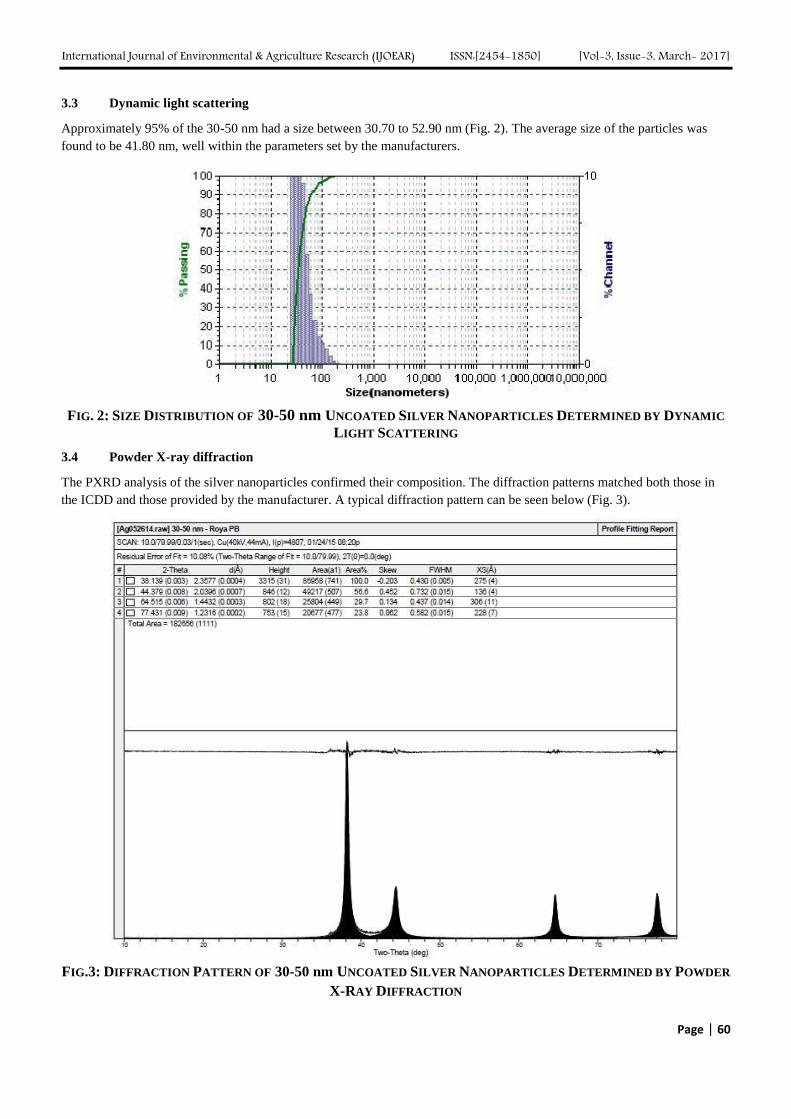
International Journal of Environmental & Agriculture Research (IJOEAR) ISSN:[2454-1850] [Vol-3, Issue-3, March- 2017]
Page | 60
3.3 Dynamic light scattering
Approximately 95% of the 30-50 nm had a size between 30.70 to 52.90 nm (Fig. 2). The average size of the particles was
found to be 41.80 nm, well within the parameters set by the manufacturers.
FIG. 2: SIZE DISTRIBUTION OF 30-50 nm UNCOATED SILVER NANOPARTICLES DETERMINED BY DYNAMIC
LIGHT SCATTERING
3.4 Powder X-ray diffraction
The PXRD analysis of the silver nanoparticles confirmed their composition. The diffraction patterns matched both those in
the ICDD and those provided by the manufacturer. A typical diffraction pattern can be seen below (Fig. 3).
FIG.3: DIFFRACTION PATTERN OF 30-50 nm UNCOATED SILVER NANOPARTICLES DETERMINED BY POWDER
X-RAY DIFFRACTION
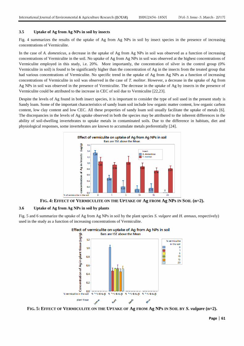
International Journal of Environmental & Agriculture Research (IJOEAR) ISSN:[2454-1850] [Vol-3, Issue-3, March- 2017]
Page | 61
3.5 Uptake of Ag from Ag NPs in soil by insects
Fig. 4 summarizes the results of the uptake of Ag from Ag NPs in soil by insect species in the presence of increasing
concentrations of Vermiculite.
In the case of A. domesticus, a decrease in the uptake of Ag from Ag NPs in soil was observed as a function of increasing
concentrations of Vermiculite in the soil. No uptake of Ag from Ag NPs in soil was observed at the highest concentrations of
Vermiculite employed in this study, i.e. 20%. More importantly, the concentration of silver in the control group (0%
Vermiculite in soil) is found to be significantly higher than the concentration of Ag in the insects from the treated group that
had various concentrations of Vermiculite. No specific trend in the uptake of Ag from Ag NPs as a function of increasing
concentrations of Vermiculite in soil was observed in the case of T. molitor. However, a decrease in the uptake of Ag from
Ag NPs in soil was observed in the presence of Vermiculite. The decrease in the uptake of Ag by insects in the presence of
Vermiculite could be attributed to the increase in CEC of soil due to Vermiculite [22,23].
Despite the levels of Ag found in both insect species, it is important to consider the type of soil used in the present study is
Sandy loam. Some of the important characteristics of sandy loam soil include low organic matter content, low organic carbon
content, low clay content and low CEC. All these properties of sandy loam soil usually facilitate the uptake of metals [6].
The discrepancies in the levels of Ag uptake observed in both the species may be attributed to the inherent differences in the
ability of soil-dwelling invertebrates to uptake metals in contaminated soils. Due to the difference in habitats, diet and
physiological responses, some invertebrates are known to accumulate metals preferentially [24].
FIG. 4: EFFECT OF VERMICULITE ON THE UPTAKE OF Ag FROM Ag NPs IN SOIL (n=2).
3.6 Uptake of Ag from Ag NPs in soil by plants
Fig. 5 and 6 summarize the uptake of Ag from Ag NPs in soil by the plant species S. vulgare and H. annuus, respectively)
used in the study as a function of increasing concentrations of Vermiculite.
FIG. 5: EFFECT OF VERMICULITE ON THE UPTAKE OF Ag FROM Ag NPs IN SOIL BY S. vulgare (n=2).
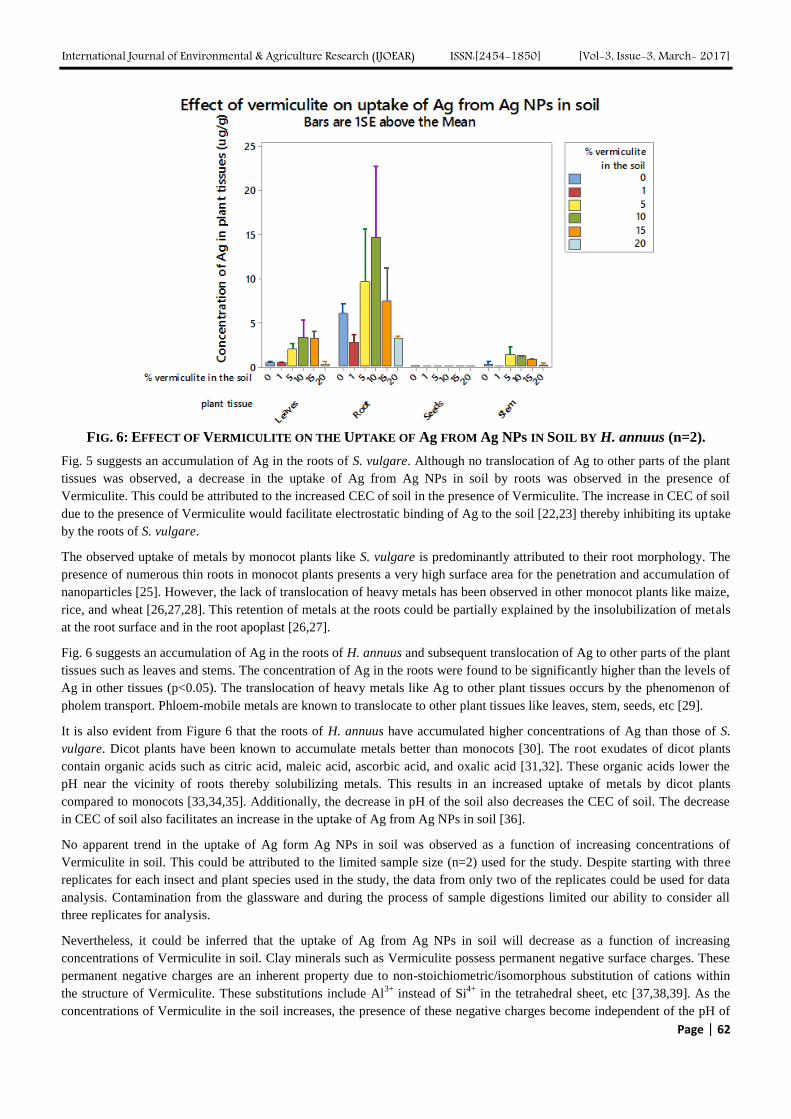
International Journal of Environmental & Agriculture Research (IJOEAR) ISSN:[2454-1850] [Vol-3, Issue-3, March- 2017]
Page | 62
FIG. 6: EFFECT OF VERMICULITE ON THE UPTAKE OF Ag FROM Ag NPs IN SOIL BY H. annuus (n=2).
Fig. 5 suggests an accumulation of Ag in the roots of S. vulgare. Although no translocation of Ag to other parts of the plant
tissues was observed, a decrease in the uptake of Ag from Ag NPs in soil by roots was observed in the presence of
Vermiculite. This could be attributed to the increased CEC of soil in the presence of Vermiculite. The increase in CEC of soil
due to the presence of Vermiculite would facilitate electrostatic binding of Ag to the soil [22,23] thereby inhibiting its uptake
by the roots of S. vulgare.
The observed uptake of metals by monocot plants like S. vulgare is predominantly attributed to their root morphology. The
presence of numerous thin roots in monocot plants presents a very high surface area for the penetration and accumulation of
nanoparticles [25]. However, the lack of translocation of heavy metals has been observed in other monocot plants like maize,
rice, and wheat [26,27,28]. This retention of metals at the roots could be partially explained by the insolubilization of metals
at the root surface and in the root apoplast [26,27].
Fig. 6 suggests an accumulation of Ag in the roots of H. annuus and subsequent translocation of Ag to other parts of the plant
tissues such as leaves and stems. The concentration of Ag in the roots were found to be significantly higher than the levels of
Ag in other tissues (p<0.05). The translocation of heavy metals like Ag to other plant tissues occurs by the phenomenon of
pholem transport. Phloem-mobile metals are known to translocate to other plant tissues like leaves, stem, seeds, etc [29].
It is also evident from Figure 6 that the roots of H. annuus have accumulated higher concentrations of Ag than those of S.
vulgare. Dicot plants have been known to accumulate metals better than monocots [30]. The root exudates of dicot plants
contain organic acids such as citric acid, maleic acid, ascorbic acid, and oxalic acid [31,32]. These organic acids lower the
pH near the vicinity of roots thereby solubilizing metals. This results in an increased uptake of metals by dicot plants
compared to monocots [33,34,35]. Additionally, the decrease in pH of the soil also decreases the CEC of soil. The decrease
in CEC of soil also facilitates an increase in the uptake of Ag from Ag NPs in soil [36].
No apparent trend in the uptake of Ag form Ag NPs in soil was observed as a function of increasing concentrations of
Vermiculite in soil. This could be attributed to the limited sample size (n=2) used for the study. Despite starting with three
replicates for each insect and plant species used in the study, the data from only two of the replicates could be used for data
analysis. Contamination from the glassware and during the process of sample digestions limited our ability to consider all
three replicates for analysis.
Nevertheless, it could be inferred that the uptake of Ag from Ag NPs in soil will decrease as a function of increasing
concentrations of Vermiculite in soil. Clay minerals such as Vermiculite possess permanent negative surface charges. These
permanent negative charges are an inherent property due to non-stoichiometric/isomorphous substitution of cations within
the structure of Vermiculite. These substitutions include Al3+
instead of Si4+
in the tetrahedral sheet, etc [37,38,39]. As the
concentrations of Vermiculite in the soil increases, the presence of these negative charges become independent of the pH of
International Journal of Environmental & Agriculture Research (IJOEAR) ISSN:[2454-1850] [Vol-3, Issue-3, March- 2017]
Page | 63
soils. Additionally, the phenomenon of cation adsorption in expandable clay minerals such as Vermiculite occurs
predominantly in inter-layer spaces, not on the relatively inactive planar surfaces [38].
IV. CONCLUSION
The influence of a clay mineral, Vermiculite, on the uptake of Ag from Ag NPs in soil by insect and plant species was
investigated. The presence of Vermiculite resulted in an increase in the cation exchange capacity of soil. The presence of
Vermiculite has also potentially resulted in a decrease in the uptake of Ag from Ag NPs in soil by insect and plant species.
The increase in CEC of soil due to the presence of clay minerals, the increased surface area of clay minerals due to their
small particle size, and the negative charge of clay minerals may cumulatively result in a decrease in the uptake of Ag from
Ag NPs in soil. Consequently, clay minerals may be used as sorbents for heavy metals in soil thereby decreasing the
possibility of their entrance into food webs.
ACKNOWLEDGEMENTS
The authors would like to thank Sematech, TX for their financial contribution to this project. We also would like to thank Dr.
Melanie A Barnes, Department of Geosciences, Texas Tech University, Ms. Roya Baghi, Department of Chemistry &
Biochemistry, Texas Tech University, and Michael T Abel, Trace Analysis, Inc., Lubbock, Texas, for all their valuable
expertise, time and help with this project. Finally, we would like to extend our appreciation to the prospective Editors and
Reviewers.
REFERENCES
[1] Cornelis G, Kirby JK, Beak B, Chittleborough D, McLaughlin MJ. A Method for Determination of Retention of Silver and Cerium
Oxide Manufactured Nanoparticles in Soils. Environ Chem. 2010; 7: 298–308.
[2] Unrine JM, Hunyadi SE, Tsyusko OV, Rao W, Shoults-Wilson WA, Bertsch PM. Evidence for Bioavailability of Au Nanoparticles
from Soil and Biodistribution within Earthworms (Eisenia Fetida). Environ Sci Technol. 2010; 44:8308–8313.
[3] Unrine JM, Shoults-Wilson WA, Zhurbich O, Bertsch PM, Tsyusko OV. Trophic Transfer of Au Nanoparticles from Soil along a
Simulated Terrestrial Food Chain. Environ Sci Technol. 2012; 46:9753–9760.
[4] Tourinho PS, Van Gestel CA, Lofts S, Svendsen C, Soares AM, Loureiro S. Metal‐based Nanoparticles in Soil: Fate, Behavior,
and Effects on Soil Invertebrates. Environ Toxicol Chem. 2012; 31:1679–1692.
[5] Babich H, Stotzky G, Ehrlich, HL. Environmental Factors that Influence the Toxicity of Heavy Metal and Gaseous Pollutants to
Microorganisms. CRC Cr Rev Microbiol. 1980; 8:99-145.
[6] Shoults-Wilson WA, Reinsch BC, Tsyusko OV, Bertsch P M , Lowry GV, Unrine JM. 2011. Role of Particle Size and Soil Type
in Toxicity of Silver Nanoparticles to Earthworms. Soil Sci Soc Am J. 2011; 75:365–377.
[7] Qian J, Shan X-Q, Wang, Z-J, Tu Q. Distribution and plant availability of heavy metals in different particle-size fractions of soil.
Sci Total Environ. 1996; 187:131-141.
[8] Bradl HB. Adsorption of heavy metal ions on soils and soils constituents. J Colloid Interf Sci. 2004; 277: 1-18.
[9] Uddin F. Clays, Nanoclays, and Montmorillonite minerals. MetallMater Trans A. 2008; 39A:2804-2814.
[10] Dube A, Zbytniewski R, Kowalkowski T, Cukrowska E, Buszewski B. Adsorption and migration of heavy metals in soil. Pol J
Environ Stud. 2001; 10:1-10.
[11] Gao J, Powers K, Wang Y, Zhou H, Roberts SM, Moudgil BM, Koopman B, Barber DS. 2012. Influence of suwanee river humic
acid on particle properties and toxicity of silver nanoparticles. Chemosphere. 2012; 89: 96-101.
[12] Malandrino M, Abollino O, Giacomino A, Aceto M, Mentasti E. Adsorption of heavy metals on vermiculite: Influence of pH and
organic ligands. J Colloid Interf Sci. 2006; 299:537-546.
[13] Romih T, Drasler B, Jemec A, Drobne D, Novak S, Golobic M, Makovec D, Susic R, Kogej K. Bioavailability of cobalt and iron
from citric-acid-adsorbed CoFe2O4 nanoparticles in the terrestrial isopod Porcellio scaber. Sci Total Environ. 2015; 508:76-84.
[14] Tourinho PS, Van Gestel CAM, Jurkschat K, Soares AM, Loureiro S. Effects of soil and dietary exposure to Ag nanoparticles and
AgNO3 in the terrestrial isopod Porcellionides pruinosus. Environ Pollut. 2015; 205:170-177.
[15] Tourinho PS, Van Gestel CAM, Morgan AJ, Kille P, Svendsen C, Jurkschat K, Mosselmans JFW, Soares AMVM, Loureiro S.
Toxicokinetics of Ag in the terrestrial isopod Porcellionides pruinosus exposed to Ag NPs and AgNO3 via soil and food.
Ecotoxicology. 2016; 25:267-278.
[16] Vijver MG, Wolterbeek HT, Vink JP, Van Gestel CAM. Surface adsorption of metals onto the earthworm Lumbricus rubellus and
the isopod Porcellio scaber is negligible compared to absorption in the body. Sci Total Environ. 2005; 340:271-280.
[17] Dauwe T, Janssens E, Bervoets L, Blust R, Eens M. Relationships between metal concentration in great tit nestlings and their
environment and food. Environ Pollut. 2004; 131:373-380.
[18] Winter S, Streit B. Organichlorine compounds in a three-step terrestrial food chain. Chemosphere. 1992; 24:1765-1774.
[19] Shuman TW, Robel RJ, Zimmerman JL, Kemp KE. Variance in Digestve Efficinces of Four Sympatric Avian Granivores. The Auk.
International Journal of Environmental & Agriculture Research (IJOEAR) ISSN:[2454-1850] [Vol-3, Issue-3, March- 2017]
Page | 64
1989; 106:324-326.
[20] Rstudio Team (2015). Rstudio: Integrated Development for R. Rstudio Inc., Boston, MA. http://www.rstudio.com/.
[21] Shapiro SS, Wilk MB. An analysis of variance test for normality (complete samples). Biometrika. 1965; 52:591-611.
[22] Oromieh AG. 2011. Evaluating solubility, aggregation and sorption of nanosilver particles and silver ions in soils. MS Thesis in
Environmental Science, Swedish University of Agricultural Sciences, Department of Soil and Environment, Uppsala, Sweden.
[23] Benoit R, Wilkinson KJ, Sauve S. Partitioning of silver and chemical speciation of free Ag in soils amended with nanoparticles.
Chem Cent J. 2013; 7:75.
[24] Gall JE, Boyd RS, Rajakaruna N. Transfer of heavy metals through terrestrial food webs: a review. Environ Monit Assess. 2015;
187:1-21.
[25] Lee WM, An YJ, Yoon H, Kweon HS. Toxicity and bioavailability of copper nanoparticles to the terrestrial plants mung bean
(Phaseolus radiates) and wheat (Triticum aestivum): Plant agar test for water insoluble nanopartilces. Environ Toxicol Chem. 2008;
27: 1915-1921.
[26] Kosegarten H, Koyro HW. Apoplastic accumulation of iron in the epidermis of maize (Zea mays) roots grown in calcareous soil.
Physiol Plant. 2001; 113:515-522.
[27] Bravin MN, Travassac F, Le Floch M, Hinsinger P, Garnier JM. Oxygen input control the spatial and temporal dynamics of arsenic
at the surface of a flooded paddy soil and in the rhizosphere of lowland rice (Oryza Sativa L): A microcosm study. Plant Soil. 2008;
312:207-218.
[28] Page V, Feller U. Selective transport of zinc, manganese, nickel, cobalt and cadmium in the root system and transfer to the leaves in
young wheat plants. Ann. Bot. 2005; 96:425-434.
[29] Page V, Feller U. Heavy metals in crop plants: Transport and redistribution processes on the whole plant level. Agrnomoy. 2015;
5:447-463.
[30] Sauerbeck DR. Plant element and soil properties governing uptake and availability of heavy metals derived from sewage sludge.
Water Air Soil Poll. 1991; 57:227-237.
[31] Wang H, Inukai Y, Yamauch A. Root Development and Nutrient Uptake. Crit Rev Plant Sci. 2006; 25:279–301.
[32] Koo BJ, Chang AC, Crowley DE, Page AL, Taylor A. Availability and Plant Uptake of Biosolid-Borne Metals. Appl Environ Soil
Sci. 2013. Article ID 892036, 10 pages.
[33] Reddy MR Dunn SJ. Accumulation of Heavy Metals by Soybean from Sludge-Amended Soil. Environ Pollut B. 1984; 7:281–295.
[34] Raskin I, Nanda Kumar PBA, Dushenkov S, Salt DE. Bioconcentration of Heavy Metals by Plants. Curr Opin Biotech. 1994;
5:285–290.
[35] Yin L, Cheng Y, Espinasse B, Colman BP, Auffan M, Wiesner M, Rose J, Liu J Bernhardt ES. More than the Ions: The Effects of
Silver Nanoparticles on Lolium Multiflorum. Environ Sci Technol. 2011; 45:2360–2367.
[36] Mishra S, Singh HB. Biosynthesized silver nanoparticles as a nanoweapon against phytopathogens: exploringtheir scope and
potential in agriculture. Appl Microbiol Biotechnol. 2014; 99:1097-1107.
[37] Foth HD. 1978. Fundamentals of soil science. 6th Edition John Wiley and Sons, NY.
[38] Kinniburgh DG, Jackson ML. 1981. Cation adsorption by hydrous metal oxides and caly. In:Adsorption of Inorganics at Solid-
Liquid Interfaces. Eds. Anderson MA and Rubin AJ. Ann Arbor Science, MI.
[39] Rieuwerts JS, Thornton I, Farago ME, Ashmore MR. Factors influencing metal bioavailability in soils:preliminary investigations
for the development od a critical loads approach for metals. Chem Spec Bioavailab. 1998; 10:61-75.
International Journal of Environmental & Agriculture Research (IJOEAR) ISSN:[2454-1850] [Vol-3, Issue-3, March- 2017]
Page | 65
Analysis of Trend and Variability of Temperature in Ebonyi State,
South-eastern Nigeria, 1984-2015 Bridget Diagi
1, Vincent Weli
2
Department of Geography and Environmental Management, University of Port Harcourt, Nigeria
Email:[email protected]
Department of Geography and Environmental Management, University of Port Harcourt, Nigeria
Email:[email protected]
Abstract— Temperature being one of the indicators of climate change has become one of the most important discussions of
recent times. Changes in temperature influence a variety of processes directly or indirectly which cut across every aspect of man
existences. This paper therefore examined the trend in temperature as tools of climate change over Ebonyi State, South-Eastern
Nigeria, which is an area well known for crop agriculture. Temperature data covering a period of 31 years (1984-2015) were
collected and analyzed using mean, moving average, standard deviation coefficient of variation and linear regression. Result
revealed that there is a positive trend in temperature over the study period and that the area is getting warmer by 0.0037oc
annually, which is an Indication that Ebonyi State is experiencing a rise in air surface temperature. Since most of the inhabitants
are dependent on economic activities that are temperature sensitive like farming, the study therefore recommends that measures
should be taken by all stakeholders including the government, individuals and cooperate bodies to take the issue of climate
variability serious in the study area in order to mitigate its impact in the long run.
Keywords— Climate Change, Ebonyi, Trend, Temperature, Agriculture.
I. INTRODUCTION
Issues related to climate change and global warming arising from anthropogenic emission of greenhouse gases have emerge as
one of the most important environmental issues in the past few decades (Singh et al., 2013). Human activities at present are
altering the carbon cycle by adding more CO2 to the atmosphere and also by influencing the ability of natural sinks, like forests,
to remove CO2 from the atmosphere. The emission of carbon dioxide comes from a variety of natural sources; but human-related
emissions are responsible for the increase that has occurred in the atmosphere since the industrial revolution. Evidence has shown
that the level of carbon dioxide in earth’s atmosphere presently is higher than at any time in the last 800,000 years. For instance
in 2014, global CO2 emissions were projected to increase by an additional 2.5% over the 2013 level (USNCDC, 2013). Other
sources of these emissions include water vapour, chlorofluorocarbons (CFCs), methane, tropospheric ozone and nitrous oxide.
These gases are released into the atmosphere due to human activities such as burning of fossil fuel, gas flaring and deforestation
amongst others .These gases are termed greenhouse gases, because they act as the glass of a greenhouse or sunroom which is
relatively transparent to solar radiation which is in short wavelength but absorbs and emits terrestrial radiation which is in long
wavelength, and thereby increasing the temperature within the glass house or room. The continuous built up of greenhouse gases
may induce changes in climatic system including increases in mean global temperatures. The global mean surface air temperature
has risen by about 0.74°C from 1906 to 2005 and this rise has been attributed mostly to a rise in greenhouse gases (IPCC, 2007).
Changes in temperature influence a variety of processes directly or indirectly for example the hydrological process. Temperature
increases causes intensification of the hydrological cycle due to increase in evaporation and precipitation(Jain and Kumar, 2012;
Tshiala et al., 2011) Temperature changes can also lead to changing patterns of precipitation, the spatial and temporal distribution
of runoff, soil moisture, and groundwater reserves as well as increased frequency of drought and flood occurrences (Tshiala et al.,
2011). Changing temperature patterns could also have effects on soil and plant growth characteristics since temperature and
water content are important physical factors for plant growth especially in Ebonyi State were majority are engaged in one form of
agriculture or another as their source of livelihood. Non-optimum levels of water and temperature conditions can strongly perturb
plant development, especially at the early stages of growth such as seed germination and emergence (Tshiala et al., 2011).
Changes in climate may also impact the water availability and water needs for agriculture. If temperature increases and more
sporadic rainfall events result from global warming, this will increase the demand irrigation needs in the future. The increasing
number of heat-related deaths worldwide over the last few decades have portrayed an alarming picture of the extreme weather
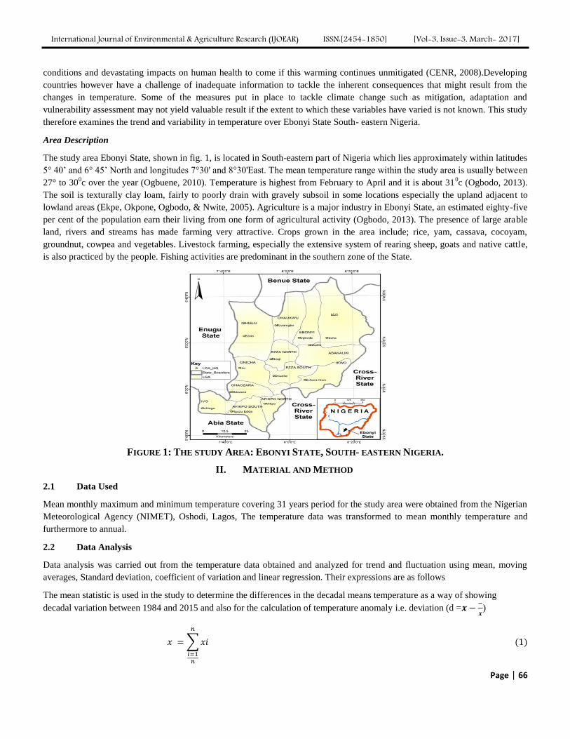
International Journal of Environmental & Agriculture Research (IJOEAR) ISSN:[2454-1850] [Vol-3, Issue-3, March- 2017]
Page | 66
conditions and devastating impacts on human health to come if this warming continues unmitigated (CENR, 2008).Developing
countries however have a challenge of inadequate information to tackle the inherent consequences that might result from the
changes in temperature. Some of the measures put in place to tackle climate change such as mitigation, adaptation and
vulnerability assessment may not yield valuable result if the extent to which these variables have varied is not known. This study
therefore examines the trend and variability in temperature over Ebonyi State South- eastern Nigeria.
Area Description
The study area Ebonyi State, shown in fig. 1, is located in South-eastern part of Nigeria which lies approximately within latitudes
5° 40’ and 6° 45’ North and longitudes 7°30' and 8°30'East. The mean temperature range within the study area is usually between
27° to 300c over the year (Ogbuene, 2010). Temperature is highest from February to April and it is about 31
0c (Ogbodo, 2013).
The soil is texturally clay loam, fairly to poorly drain with gravely subsoil in some locations especially the upland adjacent to
lowland areas (Ekpe, Okpone, Ogbodo, & Nwite, 2005). Agriculture is a major industry in Ebonyi State, an estimated eighty-five
per cent of the population earn their living from one form of agricultural activity (Ogbodo, 2013). The presence of large arable
land, rivers and streams has made farming very attractive. Crops grown in the area include; rice, yam, cassava, cocoyam,
groundnut, cowpea and vegetables. Livestock farming, especially the extensive system of rearing sheep, goats and native cattle,
is also practiced by the people. Fishing activities are predominant in the southern zone of the State.
FIGURE 1: THE STUDY AREA: EBONYI STATE, SOUTH- EASTERN NIGERIA.
II. MATERIAL AND METHOD
2.1 Data Used
Mean monthly maximum and minimum temperature covering 31 years period for the study area were obtained from the Nigerian
Meteorological Agency (NIMET), Oshodi, Lagos, The temperature data was transformed to mean monthly temperature and
furthermore to annual.
2.2 Data Analysis
Data analysis was carried out from the temperature data obtained and analyzed for trend and fluctuation using mean, moving
averages, Standard deviation, coefficient of variation and linear regression. Their expressions are as follows
The mean statistic is used in the study to determine the differences in the decadal means temperature as a way of showing
decadal variation between 1984 and 2015 and also for the calculation of temperature anomaly i.e. deviation (d =
)

International Journal of Environmental & Agriculture Research (IJOEAR) ISSN:[2454-1850] [Vol-3, Issue-3, March- 2017]
Page | 67
Where i runs from 1 to n; x, the temperature or rainfall values, and n, the number of years.
Moving average is a smoothing method that is needed to check out some up and down i.e. in finding trend that might exit in data
as trends tend to be obscured by the random errors. The simplest way of smoothing a time series data is to use a moving average.
An average value is computed by using only a specified set of values. In this study, a 10-year moving average is used.
The 10- years moving average is written as:
Where n is 10 years order and y the variable in this case temperature
Standard deviation is one of the simplest ways of measuring climate variability by using the standard deviation estimator in
measuring dispersion. It is used in this study to show the absolute variability in temperature from 1984 to 2015. Sample standard
deviation Sx is given as
where = the estimator of the standard deviation of a climate variable X
It is not easy to interpret the standard deviation as a measure of dispersion on its own. This is because a small value for standard
deviation shows that the dispersion of the dataset is low. Nevertheless, the magnitude of these values depends on what is being
analysed. Therefore, a method to overcome this difficulty of interpreting the standard deviation is to take into account the value
of the mean of the data and employ the use of coefficient of variation. It is used in this study to show the relative variability of
temperature over time. The coefficient of variation, , is a relative measure of variability and is defined as follows (Waller,
2008):
The least squares regression is used to model the trends in temperature data over the 31 years period. The result helps to
determine the overall average rates of change in trends of annual temperature in the study area.
The equation for least square regression is
Where
and
a is the intercept; b the regression coefficient or slope;
y =the temperature values (dependent variable);
x=the time in years ;( independent variable)
= the mean time; and
= the mean temperature value.
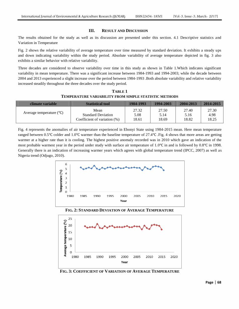
International Journal of Environmental & Agriculture Research (IJOEAR) ISSN:[2454-1850] [Vol-3, Issue-3, March- 2017]
Page | 68
III. RESULT AND DISCUSSION
The results obtained for the study as well as its discussion are presented under this section. 4.1 Descriptive statistics and
Variation in Temperature
Fig. 2 shows the relative variability of average temperature over time measured by standard deviation. It exhibits a steady ups
and down indicating variability within the study period. Absolute variability of average temperature depicted in fig. 3 also
exhibits a similar behavior with relative variability.
Three decades are considered to observe variability over time in this study as shown in Table 1.Which indicates significant
variability in mean temperature. There was a significant increase between 1984-1993 and 1994-2003; while the decade between
2004 and 2013 experienced a slight increase over the period between 1984-1993 .Both absolute variability and relative variability
increased steadily throughout the three decades over the study period.
TABLE 1
TEMPERATURE VARIABILITY FROM SIMPLE STATISTIC METHODS
Fig. 4 represents the anomalies of air temperature experienced in Ebonyi State using 1984-2015 mean. Here mean temperature
ranged between 0.5℃ colder and 1.0℃ warmer than the baseline temperature of 27.4℃ .Fig. 4 shows that more areas are getting
warmer at a higher rate than it is cooling. The highest positive anomaly recorded was in 2010 which gave an indication of the
most probable warmest year in the period under study with surface air temperature of 1.0℃ in and is followed by 0.8℃ in 1998.
Generally there is an indication of increasing warmer years which agrees with global temperature trend (IPCC, 2007) as well as
Nigeria trend (Odjugo, 2010).
FIG. 2: STANDARD DEVIATION OF AVERAGE TEMPERATURE
FIG. 3: COEFFICIENT OF VARIATION OF AVERAGE TEMPERATURE
climate variable Statistical tool 1984-1993 1994-2003 2004-2013 2014-2015
Average temperature (℃)
Mean
Standard Deviation
Coefficient of variation (%)
27.32
5.08
18.61
27.50
5.14
18.69
27.40
5.16
18.82
27.30
4.98
18.25
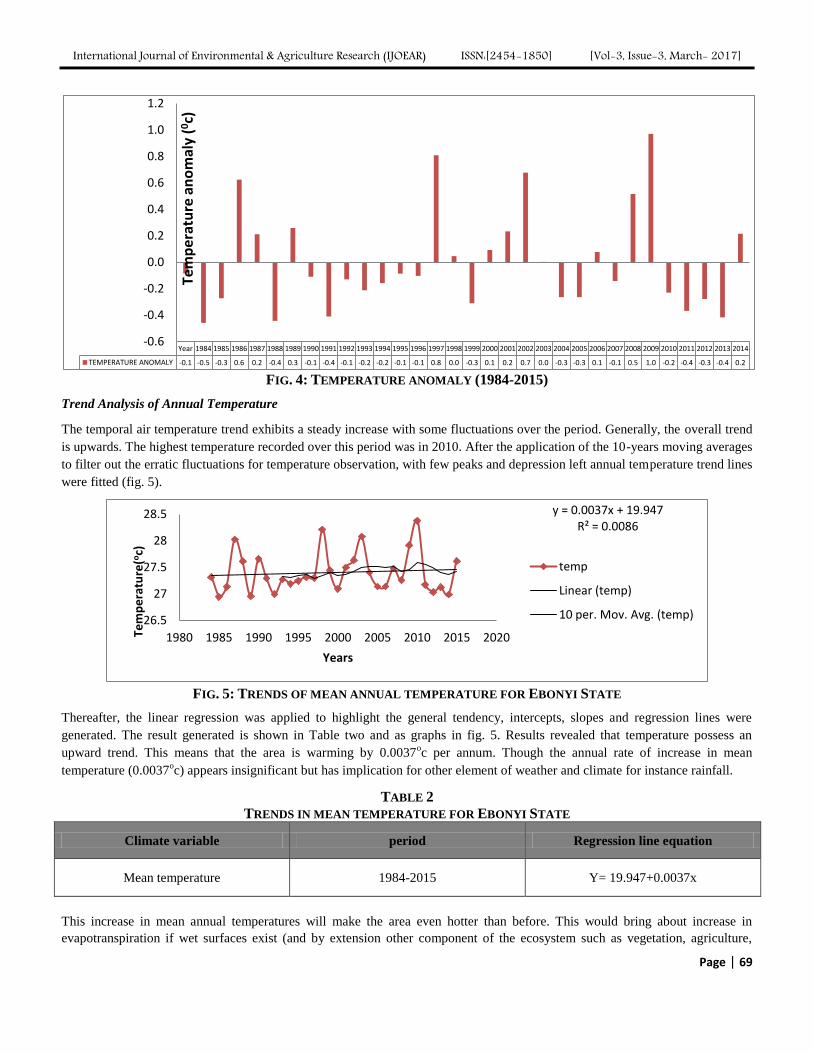
International Journal of Environmental & Agriculture Research (IJOEAR) ISSN:[2454-1850] [Vol-3, Issue-3, March- 2017]
Page | 69
FIG. 4: TEMPERATURE ANOMALY (1984-2015)
Trend Analysis of Annual Temperature
The temporal air temperature trend exhibits a steady increase with some fluctuations over the period. Generally, the overall trend
is upwards. The highest temperature recorded over this period was in 2010. After the application of the 10-years moving averages
to filter out the erratic fluctuations for temperature observation, with few peaks and depression left annual temperature trend lines
were fitted (fig. 5).
FIG. 5: TRENDS OF MEAN ANNUAL TEMPERATURE FOR EBONYI STATE
Thereafter, the linear regression was applied to highlight the general tendency, intercepts, slopes and regression lines were
generated. The result generated is shown in Table two and as graphs in fig. 5. Results revealed that temperature possess an
upward trend. This means that the area is warming by 0.0037oc per annum. Though the annual rate of increase in mean
temperature (0.0037oc) appears insignificant but has implication for other element of weather and climate for instance rainfall.
TABLE 2
TRENDS IN MEAN TEMPERATURE FOR EBONYI STATE
Climate variable period Regression line equation
Mean temperature 1984-2015 Y= 19.947+0.0037x
This increase in mean annual temperatures will make the area even hotter than before. This would bring about increase in
evapotranspiration if wet surfaces exist (and by extension other component of the ecosystem such as vegetation, agriculture,
Year 1984 1985 1986 1987 1988 1989 1990 1991 1992 1993 1994 1995 1996 1997 1998 1999 2000 2001 2002 2003 2004 2005 2006 2007 2008 2009 2010 2011 2012 2013 2014
TEMPERATURE ANOMALY -0.1 -0.5 -0.3 0.6 0.2 -0.4 0.3 -0.1 -0.4 -0.1 -0.2 -0.2 -0.1 -0.1 0.8 0.0 -0.3 0.1 0.2 0.7 0.0 -0.3 -0.3 0.1 -0.1 0.5 1.0 -0.2 -0.4 -0.3 -0.4 0.2
-0.6
-0.4
-0.2
0.0
0.2
0.4
0.6
0.8
1.0
1.2
Tem
per
atu
re a
no
mal
y (0
c)
y = 0.0037x + 19.947 R² = 0.0086
26.5
27
27.5
28
28.5
1980 1985 1990 1995 2000 2005 2010 2015 2020 Tem
pe
ratu
re(o
c)
Years
temp
Linear (temp)
10 per. Mov. Avg. (temp)
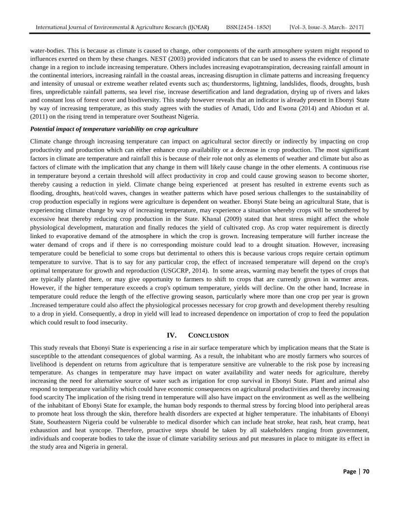
International Journal of Environmental & Agriculture Research (IJOEAR) ISSN:[2454-1850] [Vol-3, Issue-3, March- 2017]
Page | 70
water-bodies. This is because as climate is caused to change, other components of the earth atmosphere system might respond to
influences exerted on them by these changes. NEST (2003) provided indicators that can be used to assess the evidence of climate
change in a region to include increasing temperature. Others includes increasing evapotranspiration, decreasing rainfall amount in
the continental interiors, increasing rainfall in the coastal areas, increasing disruption in climate patterns and increasing frequency
and intensity of unusual or extreme weather related events such as; thunderstorms, lightning, landslides, floods, droughts, bush
fires, unpredictable rainfall patterns, sea level rise, increase desertification and land degradation, drying up of rivers and lakes
and constant loss of forest cover and biodiversity. This study however reveals that an indicator is already present in Ebonyi State
by way of increasing temperature, as this study agrees with the studies of Amadi, Udo and Ewona (2014) and Abiodun et al.
(2011) on the rising trend in temperature over Southeast Nigeria.
Potential impact of temperature variability on crop agriculture
Climate change through increasing temperature can impact on agricultural sector directly or indirectly by impacting on crop
productivity and production which can either enhance crop availability or a decrease in crop production. The most significant
factors in climate are temperature and rainfall this is because of their role not only as elements of weather and climate but also as
factors of climate with the implication that any change in them will likely cause change in the other elements. A continuous rise
in temperature beyond a certain threshold will affect productivity in crop and could cause growing season to become shorter,
thereby causing a reduction in yield. Climate change being experienced at present has resulted in extreme events such as
flooding, droughts, heat/cold waves, changes in weather patterns which have posed serious challenges to the sustainability of
crop production especially in regions were agriculture is dependent on weather. Ebonyi State being an agricultural State, that is
experiencing climate change by way of increasing temperature, may experience a situation whereby crops will be smothered by
excessive heat thereby reducing crop production in the State. Khanal (2009) stated that heat stress might affect the whole
physiological development, maturation and finally reduces the yield of cultivated crop. As crop water requirement is directly
linked to evaporative demand of the atmosphere in which the crop is grown. Increasing temperature will further increase the
water demand of crops and if there is no corresponding moisture could lead to a drought situation. However, increasing
temperature could be beneficial to some crops but detrimental to others this is because various crops require certain optimum
temperature to survive. That is to say for any particular crop, the effect of increased temperature will depend on the crop's
optimal temperature for growth and reproduction (USGCRP, 2014). In some areas, warming may benefit the types of crops that
are typically planted there, or may give opportunity to farmers to shift to crops that are currently grown in warmer areas.
However, if the higher temperature exceeds a crop's optimum temperature, yields will decline. On the other hand, Increase in
temperature could reduce the length of the effective growing season, particularly where more than one crop per year is grown
.Increased temperature could also affect the physiological processes necessary for crop growth and development thereby resulting
to a drop in yield. Consequently, a drop in yield will lead to increased dependence on importation of crop to feed the population
which could result to food insecurity.
IV. CONCLUSION
This study reveals that Ebonyi State is experiencing a rise in air surface temperature which by implication means that the State is
susceptible to the attendant consequences of global warming. As a result, the inhabitant who are mostly farmers who sources of
livelihood is dependent on returns from agriculture that is temperature sensitive are vulnerable to the risk pose by increasing
temperature. As changes in temperature may have impact on water availability and water needs for agriculture, thereby
increasing the need for alternative source of water such as irrigation for crop survival in Ebonyi State. Plant and animal also
respond to temperature variability which could have economic consequences on agricultural productivities and thereby increasing
food scarcity The implication of the rising trend in temperature will also have impact on the environment as well as the wellbeing
of the inhabitant of Ebonyi State for example, the human body responds to thermal stress by forcing blood into peripheral areas
to promote heat loss through the skin, therefore health disorders are expected at higher temperature. The inhabitants of Ebonyi
State, Southeastern Nigeria could be vulnerable to medical disorder which can include heat stroke, heat rash, heat cramp, heat
exhaustion and heat syncope. Therefore, proactive steps should be taken by all stakeholders ranging from government,
individuals and cooperate bodies to take the issue of climate variability serious and put measures in place to mitigate its effect in
the study area and Nigeria in general.
International Journal of Environmental & Agriculture Research (IJOEAR) ISSN:[2454-1850] [Vol-3, Issue-3, March- 2017]
Page | 71
ACKNOWLEDGEMENTS
The Authors expresses deep appreciation to the anonymous reviewers of this study and this Journal platform for the opportunity
granted it to publish this paper.
REFERENCES
[1] B.J. Abiodun, A.T. Salami, and M. Tadross, “Climate change scenarios for Nigeria: understanding the biophysical impacts”: A Report by the
climate systems Analysis Group, Cape Town, for building Nigerian’s response to climate change project.
[2] S.O. Amadi, S.O. Udo, and I.O Ewona, “Trends and variations of monthly mean minimum and maximum temperature data over Nigeria
for the period 1950-2012”. International Journal of pure and applied Physics. Vol. 2, No. 4, pp.1-27, 2014.
[3] Committee on the Environment and Natural Resources (CENR), “Scientific Assessment of the Effects of Global Change on the United
States”, 2008.
[4] I.I. Ekpe, E.G. Okpone, E.N. Ogbodo, and J.N. Nwite, “Physico-chemical properties of four ultisor under different vegetation cover in
South-eastern Nigeria.” Journal of Science of Agriculture, Food Technology and Environment. Vol 5, pp74-78, 2005.
[5] IPCC, “Climate Change 2007”: impacts, adaptation and vulnerability: contribution of Working Group II to the fourth assessment
report of the Intergovernmental Panel on Climate Change, Cambridge University Press, Cambridge, UK, 2007.
[6] IPCC, “Climate Change 2013: The Physical Science Basis”. Contribution of Working Group I to the Fifth Assessment Report of
the Intergovernmental Panel on Climate Change [Stocker, T.F., D. Qin, G.-K. Plattner, M. Tignor, S.K. Allen, J. Boschung, A. Nauels,
Y. Xia, V. Bex and P.M. Midgley (eds.)]. Cambridge University Press, Cambridge, United Kingdom and New York, NY, USA, 2013.
[7] S.K. Jain and V. Kumar, “Trend analysis of rainfall and temperature data for India.Current Science”, Vol 102(1), pp37 – 49, 2012.
[8] Nigerian Environmental Study/Action Team (NEST), “Climate Change in Nigeria. A Communication Guide for Reporters and
Educators”. Ibadan: NEST. 5-16, 2003.
[9] P.A.O. Odjugo, “Regional evidence of climate change in Nigeria”. Journal of Geography and Regional Planning”, Vol 3(6), pp142-150,
2010.
[10] E.N. Ogbodo, “Assessment and management strategies for the receding watersheds of Ebonyi State, Southeast Nigeria”. Journal of
environment and earth Science, vol 13, no3, 2013.
[11] E.B. Ogbuene, “Impact of Meteorological Parameters on Rice Yield: An Approach for Environmental Resource Sustainability in Ebonyi
Rice Farmland”. Journal of environmental issues and agriculture in developing countries, vol 2, No 2 and 3, 2010.
[12] O. Singh, P.O. Arya, and B.S. Chaudhary, “On rising temperature trends at Dehradun in Doon Valley of Uttarakhand, India”, J. Earth
Syst.Sci., vol 122(3), pp613-622, 2013.
[13] M.F. Tshiala, J.M. Olwoch, and F.A. Engelbrecht, “Analysis of temperature trends over Limpopo Province, South Africa”, Journal of
Geography and Geology, vol3 (1), pp13-21, 2011.
[14] D.L. Waller, “Statistics for Business”, Butterworth- Heinemann: Amsterdam.
[15] R.C. Khanal, ‘’Climate change and organic agriculture” The journal of agriculture and environment, vol.10, pp 100-110, 2009
[16] USGCRP ,J.G. Hatfield, R.Takle, P. Grotjahn, R.C.Holden, T.Izaurralde, E. Mader, Marshall, &D. Liverman, : Agriculture. Climate
Change Impacts in the United States: The Third National Climate Assessment, J. M. Melillo, Terese (T.C.) Richmond, and G. W. Yohe,
Eds., U.S. Global Change Research Program, 150-174,2014.
International Journal of Environmental & Agriculture Research (IJOEAR) ISSN:[2454-1850] [Vol-3, Issue-3, March- 2017]
Page | 72
Analyzing Marketing Margins and the Direction of Price Flow in
the Tomato Value Chain of Limpopo Province, South Africa Kudzai Mandizvidza
Development Economist and International Consultant, Beijing, China
Email: [email protected]
Abstract— The Limpopo Province is home to South Africa’s tomato farming giants, some of whom also occupy the position
of the largest producers of the commodity in the Southern Hemisphere. Regardless of its importance in the tomato industry of
the country, there are few studies analysing the mechanism through which prices of tomatoes are determined and transmitted
from the farm gate in Limpopo to the various provincial, local and international markets. This study attempts to fill the
knowledge gap on the performance of Limpopo Province’s tomato markets by examining the marketing margins and the
direction of price flow amongst the successive tomato marketing levels. By means of the Concurrent Marketing Margin
Analysis approach, it was established that the farmers’ portion of the consumer’s Rand is low. About 85.1% of the
consumer’s Rand goes to pay for marketing margins. Granger causality tests show that both the wholesale and retail prices
are caused by farm gate prices. The farm level is therefore key to tomato price determination in Limpopo Province of South
Africa and pertinent policies that improve the commodity’s primary sector may potentially enhance the other sectors in value
chain that depend on tomato production.
Keywords— Limpopo Province, market dominance, marketing margins, price flow, tomato markets, vertical price
linkage.
I. INTRODUCTION
Agricultural productivity has improved throughout history because of economic progression, innovation, specialization,
research and development (Fuglie et al., 2007; Fuglie and Nin-Pratt, 2012; Nin-Pratt, 2013). This has increased the
productive capacities of farmers who in time have been able to produce in excess of what is needed for home consumption
and subsistence. Such developments augmented the significance and complexity of marketing and have seen the
establishment of arenas to facilitate the exchange of marketable surplus between producers and consumers.
In the context of the tomato industry of South Africa, it is highlighted in Department of Agriculture, Forestry and Fisheries
(DAFF) (2011) that production of tomato occurs in all the nine provinces of South Africa by both commercial and emerging
farmers. However, different provinces produce varied volumes due to environmental disparities amongst other factors. The
Limpopo Province with its warmer climate plays the most vital role in the country’s tomato production. According to DAFF
(2011) the province contributes about 3 590 ha to the country’s total area planted to tomatoes. Limpopo Tourism and Parks
Board (2011), suggests that almost 60% of the country’s tomatoes are produced in Limpopo Province which is responsible
for about 45% of the Johannesburg Fresh Produce Market’s annual turnover. However, the Limpopo Province’s tomato
producing industry’s concentration is high which in economics sense means that a large share of total production is
dominated by a few large producers. Limpopo Tourism and Parks Board (2011), indicates that only one farming company is
responsible for about 40% of the province’s 60% contribution to South Africa’s total tomato production.
Even though the majority of tomato is produced in the Limpopo Province, the commodity is consumed in all parts of the
country and is also exported thus; there is some degree of spatial separation between production and consumption. Such
spatial distribution calls for the need for an efficient and effective marketing system to facilitate the movement of tomatoes
from the point of production to the end user. Bringing the agricultural product from the agricultural enterprise to the
consumer according to Saccomandi (1998), involves a series of functions and productive activities that interconnect. The
process also depends on the current state of technology, the organization of productive activities and the spatial distribution
of production and consumption.
II. PROBLEM STATEMENT
There is high industry concentration in the tomato producing industry of the Limpopo Province. Such a situation where the
industry is dominated by a few large firms paves way to major producers potentially using their market power to influence
pricing strategies from time to time. As to which of the participants in the chain will consequently suffer or benefit from
International Journal of Environmental & Agriculture Research (IJOEAR) ISSN:[2454-1850] [Vol-3, Issue-3, March- 2017]
Page | 73
impending price shocks depends on the degree to which market players adjust to price signals. It also depends on the timing
in response and the extent to which their adjustment to price shocks is asymmetric as shown in Vavra and Goodwin (2005).
Particular aspects of participants’ response to price movements may also have important implications on marketing margins
of several players in the marketing chain of tomato in Limpopo Province. While farmers may view their proportion of the
consumer’s Rand as low, tomato consumers on the other hand experience continual rising prices of this commodity. It may
be questioned therefore, as to whom in the marketing chain sits at point(s) of price determination. It may also be of interest to
determine the direction of price causality along the marketing chain for tomato in Limpopo Province so as to guide any
pricing policy in the respective food market.
III. AIM AND OBJECTIVES
This study seeks to analyze marketing margins and the direction of price flow in the tomato value chain of Limpopo Province
South Africa so as to determine the performance of tomato markets in the region. It’s is imperative to estimate the point(s) of
price determination and direction of causality along the marketing chain for tomato in Limpopo Province so as to guide food
marketing and pricing policies.
IV. RESEARCH HYPOTHESES
1. Price and direction of causality along the marketing chain for tomato in Limpopo Province are determined beyond the
farm gate.
2. The proportion of the consumer’s dollar that goes to pay for marketing margins is uncertain.
V. LITERATURE REVIEW
According to FAO (2002), the percentage share of the final price, which is taken up by the marketing functions, is what is
known as the marketing margin. Guvheya et al. (1998) treated the concept of marketing margins as differences between
prices at different levels in the marketing channel which capture the proportion of the final selling price that a particular
agent in the marketing chain adds. Elitzak (1996) characterize marketing margins or the farm-to-retail price spread as the
difference between the farm value and retail price that represents payments for all assembling, processing, transporting and
retailing charges added to farm products. Cox (2009) noted that producers often wonder about the large difference between
the prices that consumers pay for food and the prices that farmers receive. However, high marketing margins can be justified
by costs involved in distributing the product from point of production to the final consumer. It can be argued though, that too
high a percentage reflects some exploitation of either farmers or consumers. Wohlgenant (2001) investigated marketing
margins and identified some of the questions that are frequently asked about the issue. These questions, which have attracted
considerable interest across literature and amongst researchers and policy makers, include; Are marketing margins too large?
What is the incidence of marketing costs on retail prices and farm prices? How quickly are farm prices transmitted to the
retail level and how quickly are retail price changes transmitted to farmers? In order to have a thorough and exact
investigation, Mojtaba et al. (2010) recommended that the marketing margin be divided into two smaller portions namely
Retailer Margin (RM) and Wholesaler Margin (WM). RM refers to the difference between the price paid by consumers and
the price that retailers pay to the wholesalers. WM refers to the difference between the price at which wholesalers sell their
product and the price that they pay to the farmers.
While price represents the equilibrium point where demand and supply meet in the market place, Schnepf (2006) emphasizes
that the general price level of an agricultural commodity, at any stage, is influenced by a variety of market forces that can
alter the current or expected balance between supply and demand. According to Holland (1998) price determination for many
consumer products is in most cases a function of the cost of production and a desired level of mark-up. Price determination
by this desired level of mark-up is what is referred to as cost-plus pricing, mark-up pricing or full-cost pricing which in
Salvatore (1993) is related to three rules of thumb. The first is termed; mark-up percent, which is the proportion of profit to
total cost. The second is the gross margin percent, which is the proportion of profit to the selling price, and lastly, profit
margin, which is the difference in selling price and total cost.
VI. STUDY AREA, DATA COLLECTION AND SAMPLING TECHNIQUE
This study is based mainly on the Limpopo Province which is the northernmost province of South Africa covering a total
surface area of 123,910 km2 making it the fifth largest province amongst the country’s nine provinces. Limpopo Province
can be described as the garden of South Africa due to its rich fruit and vegetable production. Apart from being South Africa’s
International Journal of Environmental & Agriculture Research (IJOEAR) ISSN:[2454-1850] [Vol-3, Issue-3, March- 2017]
Page | 74
main tomato producer Limpopo Province is responsible for about 75% of the country’s mangoes, 65% of its papayas, 36% of
its tea, 25% of its citrus, bananas, and litchis, 60% of its avocados, 285 000 tons of potatoes, and 35% of its oranges. Most of
tomato production in the province is done by a private corporation, who is also the largest tomato farmer in South Africa.
The province is also involved in the production of coffee, nuts, guavas, sisal, cotton, tobacco, sunflower, maize, wheat,
grapes and timber. Livestock production and game ranching is also prominent particularly in most of the higher-lying areas
(vanNiekerk, 2012; Limpopo Tourism and Parks Board, 2011).
This study used both primary and secondary data of time series in nature. Daily tomato prices were collected synchronously
at farm gate, wholesale and retail levels for mixed grades of cooking tomatoes to achieve a sample size of 50 observations.
Semi structured interviews and desk studies were also conducted to explore the procurement and marketing procedures
followed by various participants in tomato marketing in the Limpopo Province.
VII. MARKETING MARGIN ANALYSIS
In analysing the marketing margins, the Concurrent Margin Method was used. As described by Singh (1998) the method is a
static analysis of the distributive margin usually adopted to calculate the price spread in one market town by considering
differences between prices prevailing at successive stages of marketing at a given point of time.
The model is defined as thus;
Mt = P t,L – Pt,L-1 where; (1)
Mt= Marketing margin between market level (L) and its preceding level (L-1) at time (t)
Pt,L = Price at market level (L) at time (t)
Pt,L-1 = Price at market level (L-1) at time (t)
Where marketing margins at different levels of the marketing chain are compared, Guvheya et al. (1998) emphasizes the use
of consumer price as the common denominator for all margins.
The two indices that were used in this study are Total Gross Marketing Margin (TGMM) and Producers’ Gross Marketing
Margin (GMMp) as given in Scott (1995) where Gross Marketing Margin is the difference between consumer’s price and
farmer’s price. TGMM and GMMp were calculated as;
TGMM = ’
x 100, (2)
and
GMMp =
x 100 (3)
VIII. TESTING FOR UNIT ROOT NON-STATIONARITY
The Augmented Dickey Fuller test was performed on each of the logarithmic series of farm prices (FP), wholesale prices
(WP) and retail prices (RP) to formally ascertain whether they contained a unit root.
IX. PRICE DETERMINATION AND DIRECTION OF CAUSALITY
In assessing the points of price determination and the direction of causality along the major marketing channels for tomato in
Limpopo Province, Granger causality tests (Granger, 1969) were performed.
Three sets of Vector Autoregressive (VAR) models were formulated and estimated;
(a) Testing causality between farm gate and wholesale levels:
lnFPt = α1 + ilnWPt-i +
ilnFPt-i + U1t
lnWPt = α2 + ilnWPt-i +
ilnFPt-i + U2t (5)

International Journal of Environmental & Agriculture Research (IJOEAR) ISSN:[2454-1850] [Vol-3, Issue-3, March- 2017]
Page | 75
(b) Testing causality between wholesale and retail levels:
lnWPt = α1 + ilnRPt-i +
ilnWPt-i + U1t
lnRPt = α2 + ilnRPt-i +
ilnWPt-i + U2t (6)
(c) Testing causality between farm and retail levels:
lnFPt = α1 + ilnRPt-i +
ilnFPt-i + U1t
lnRPt = α2 + ilnRPt-i +
ilnFPt-i + U2t (7)
*where; ln is the natural logarithm of each respective price series
FPt is the farm price at time (t)
WPt is the wholesale price at time (t)
RPt is the retail price at time (t)
FPt-i is lagged farm gate price
WPt-i is lagged wholesale price
RPt-i is lagged retail price
n is the upper limit set at the optimal lag length
ai, bi, ci, and di are coefficients to be estimated using the ordinary Least squares method and α1 and α2 are intercepts
U1t and U2t are error terms that are assumed uncorrelated and white noise
The inference in the first mathematical statement of equation 5 is that current farm prices are dependent on past farm prices
and past and present wholesale prices.
Likewise, the second mathematical statement postulates that current wholesale prices are dependent on past farm prices and
past and present wholesale prices.
The inference in the first mathematical statement of equation 6 is that current wholesale prices are dependent on past
wholesale prices and past and present retail prices.
Likewise, the second mathematical statement postulates that current retail prices are dependent on past wholesale prices and
past and present retail prices.
The inference in the first mathematical statement of equation 7 is that current farm gate prices are dependent on past farm
prices and past and present retail prices.
Likewise, the second mathematical statement postulates that current retail prices are dependent on past farm gate prices and
past and present retail prices.
In each of the cases (a), (b) and (c), four causality relationships were tested by placing the appropriate restrictions on each
model. P-values and F-tests were used to confirm statistical significance of the causality relationships.
For instance, in case (a) the following were the causality relationships tested between farm gate and wholesale prices;
(i) A unidirectional causality from wholesale to farm gate levels would be concluded if;
i ≠ 0 and
i = 0
(ii) A unidirectional causality from farm gate to wholesale levels would be concluded if,
i = 0 and
i ≠ 0
(iii) An absence of a causal relationship between the variables that is independence would be concluded if both
i = 0 and
i = 0
This would imply that both sets of the lagged exogenous variables were not statistically different from zero.
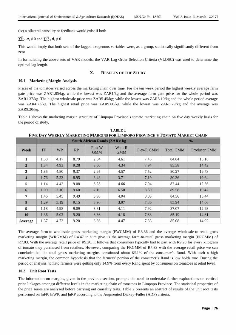
International Journal of Environmental & Agriculture Research (IJOEAR) ISSN:[2454-1850] [Vol-3, Issue-3, March- 2017]
Page | 76
(iv) a bilateral causality or feedback would exist if both
i ≠ 0 and
i ≠ 0
This would imply that both sets of the lagged exogenous variables were, as a group, statistically significantly different from
zero.
In formulating the above sets of VAR models, the VAR Lag Order Selection Criteria (VLOSC) was used to determine the
optimal lag length.
X. RESULTS OF THE STUDY
10.1 Marketing Margin Analysis
Prices of the tomatoes varied across the marketing chain over time. For the ten week period the highest weekly average farm
gate price was ZAR1.85/kg, while the lowest was ZAR1/kg and the average farm gate price for the whole period was
ZAR1.37/kg. The highest wholesale price was ZAR5.45/kg; while the lowest was ZAR3.10/kg and the whole period average
was ZAR4.73/kg. The highest retail price was ZAR9.60/kg, while the lowest was ZAR8.79/kg and the average was
ZAR9.20/kg.
Table 1 shows the marketing margin structure of Limpopo Province’s tomato marketing chain on five day weekly basis for
the period of study.
TABLE 1
FIVE DAY WEEKLY MARKETING MARGINS FOR LIMPOPO PROVINCE’S TOMATO MARKET CHAIN
South African Rands (ZAR)/ kg %
Week FP WP RP F-to-W
GMM
W-to-R
GMM F-to-R GMM Total GMM Producer GMM
1 1.33 4.17 8.79 2.84 4.61 7.45 84.84 15.16
2 1.34 4.93 9.28 3.60 4.34 7.94 85.58 14.42
3 1.85 4.80 9.37 2.95 4.57 7.52 80.27 19.73
4 1.76 5.23 8.95 3.48 3.71 7.19 80.36 19.64
5 1.14 4.42 9.08 3.28 4.66 7.94 87.44 12.56
6 1.00 3.10 9.60 2.10 6.50 8.60 89.58 10.42
7 1.46 5.45 9.49 3.98 4.04 8.03 84.56 15.44
8 1.29 5.19 9.15 3.90 3.97 7.86 85.94 14.06
9 1.18 4.98 9.09 3.81 4.11 7.92 87.07 12.93
10 1.36 5.02 9.20 3.66 4.18 7.83 85.19 14.81
Average 1.37 4.73 9.20 3.36 4.47 7.83 85.08 14.92
The average farm-to-wholesale gross marketing margin (FWGMM) of R3.36 and the average wholesale-to-retail gross
marketing margin (WRGMM) of R4.47 in sum give us the average farm-to-retail gross marketing margin (FRGMM) of
R7.83. With the average retail price of R9.20, it follows that consumers typically had to part with R9.20 for every kilogram
of tomato they purchased from retailers. However, comparing the FRGMM of R7.83 with the average retail price we can
conclude that the total gross marketing margins constituted about 85.1% of the consumer’s Rand. With such a high
marketing margin, the common hypothesis that the farmers’ portion of the consumer’s Rand is low holds true. During the
period of analysis, tomato farmers were getting only 14.9% from every Rand spent by consumers on tomatoes at retail level.
10.2 Unit Root Tests
The information on margins, given in the previous section, prompts the need to undertake further explorations on vertical
price linkages amongst different levels in the marketing chain of tomatoes in Limpopo Province. The statistical properties of
the price series are analysed before carrying out causality tests. Table 2 presents an abstract of results of the unit root tests
performed on lnFP, lnWP, and lnRP according to the Augmented Dickey-Fuller (ADF) criteria.
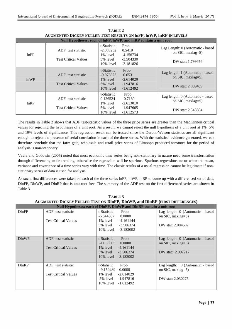
International Journal of Environmental & Agriculture Research (IJOEAR) ISSN:[2454-1850] [Vol-3, Issue-3, March- 2017]
Page | 77
TABLE 2
AUGMENTED DICKEY FULLER TEST RESULTS ON lnFP, lnWP, lnRP IN LEVELS Null Hypotheses: each of lnFP, lnWP, and lnRP contain a unit root
lnFP
ADF test statistic
Test Critical Values
t-Statistic Prob.
-2.083252 0.5419
1% level -4.156734
5% level -3.504330
10% level -3.181826
Lag Length: 0 (Automatic - based
on SIC, maxlag=5)
DW stat: 1.799676
lnWP
ADF test statistic
Test Critical Values
t-Statistic Prob
-0.073823 0.6531
1% level -2.614029
5% level -1.947816
10% level -1.612492
Lag length: 1 (Automatic - based
on SIC, maxlag=5)
DW stat: 2.089489
lnRP
ADF test statistic
Test Critical Values
t-Statistic Prob
0.126524 0.7180
1% level -2.613010
5% level -1.947665
10% level -1.612573
Lag length: 0 (Automatic - based
on SIC, maxlag=5)
DW stat: 2.548604
The results in Table 2 shows that ADF test-statistic values of the three price series are greater than the MacKinnon critical
values for rejecting the hypotheses of a unit root. As a result, we cannot reject the null hypothesis of a unit root at 1%, 5%
and 10% levels of significance. This regression result can be trusted since the Durbin-Watson statistics are all significant
enough to reject the presence of serial correlation in each of the three series. With the statistical evidence generated, we can
therefore conclude that the farm gate, wholesale and retail price series of Limpopo produced tomatoes for the period of
analysis is non-stationary.
Vavra and Goodwin (2005) noted that most economic time series being non-stationary in nature need some transformation
through differencing or de-trending, otherwise the regression will be spurious. Spurious regressions occur when the mean,
variance and covariance of a time series vary with time. The classic results of a usual regression cannot be legitimate if non-
stationary series of data is used for analysis.
As such, first differences were taken on each of the three series lnFP, lnWP, lnRP to come up with a differenced set of data,
DlnFP, DlnWP, and DlnRP that is unit root free. The summary of the ADF test on the first differenced series are shown in
Table 3.
TABLE 3
AUGMENTED DICKEY FULLER TEST ON DlnFP, DlnWP, and DlnRP (FIRST DIFFERENCES) Null Hypotheses: each of DlnFP, DlnWP and DlnRP contain a unit root
DlnFP ADF test statistic
Test Critical Values
t-Statistic Prob
-6.644587 0.0000
1% level -4.161144
5% level -3.506374
10% level -3.183002
Lag length: 0 (Automatic - based
on SIC, maxlag=3)
DW stat: 2.004682
DlnWP ADF test statistic
Test Critical Values
t-Statistic Prob
-11.33005 0.0000
1% level -4.161144
5% level -3.506374
10% level -3.183002
Lag length: 0 (Automatic - based
on SIC, maxlag=5)
DW stat: 2.097217
DlnRP ADF test statistic
Test Critical Values
t-Statistic Prob
-9.150489 0.0000
1% level -2.614029
5% level -1.947816
10% level -1.612492
Lag length: : 0 (Automatic - based
on SIC, maxlag=5)
DW stat: 2.030275
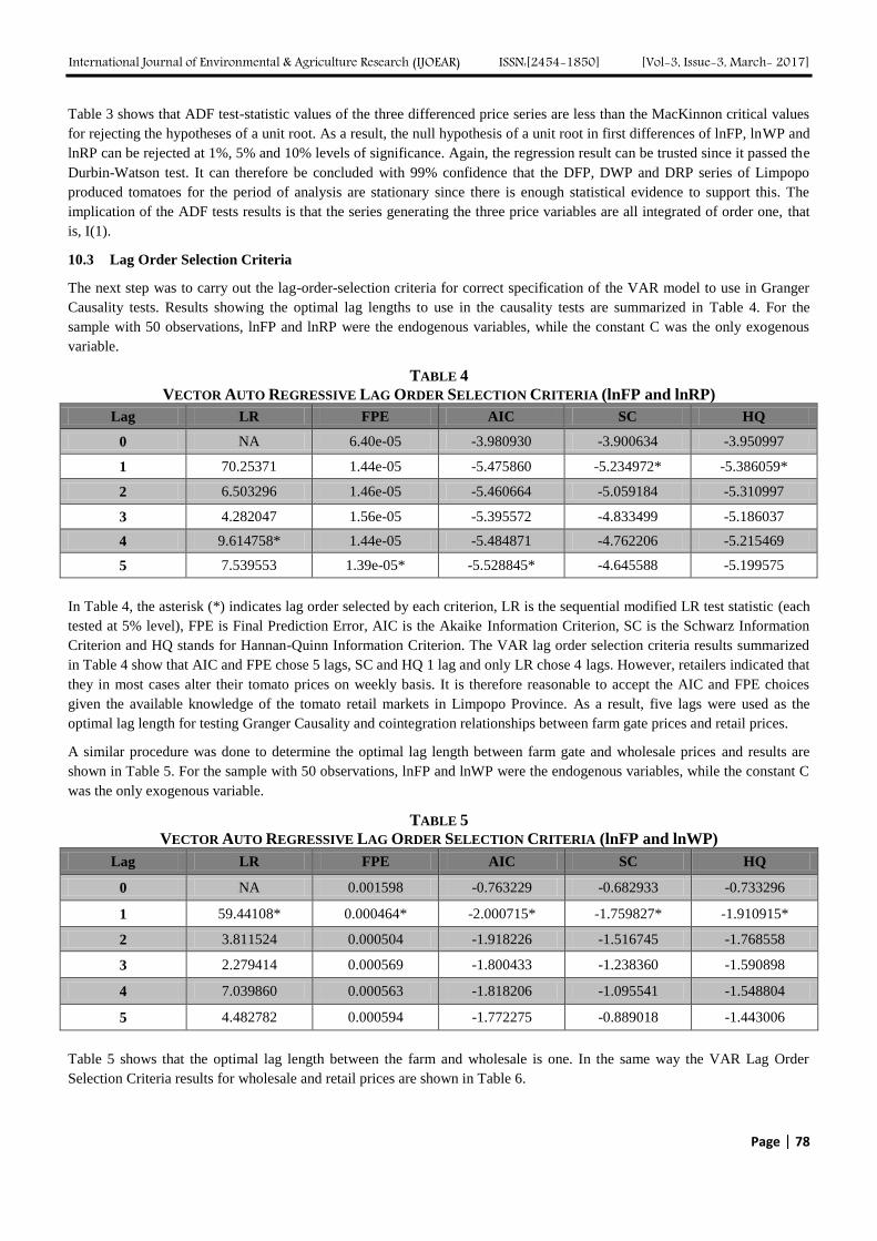
International Journal of Environmental & Agriculture Research (IJOEAR) ISSN:[2454-1850] [Vol-3, Issue-3, March- 2017]
Page | 78
Table 3 shows that ADF test-statistic values of the three differenced price series are less than the MacKinnon critical values
for rejecting the hypotheses of a unit root. As a result, the null hypothesis of a unit root in first differences of lnFP, lnWP and
lnRP can be rejected at 1%, 5% and 10% levels of significance. Again, the regression result can be trusted since it passed the
Durbin-Watson test. It can therefore be concluded with 99% confidence that the DFP, DWP and DRP series of Limpopo
produced tomatoes for the period of analysis are stationary since there is enough statistical evidence to support this. The
implication of the ADF tests results is that the series generating the three price variables are all integrated of order one, that
is, I(1).
10.3 Lag Order Selection Criteria
The next step was to carry out the lag-order-selection criteria for correct specification of the VAR model to use in Granger
Causality tests. Results showing the optimal lag lengths to use in the causality tests are summarized in Table 4. For the
sample with 50 observations, lnFP and lnRP were the endogenous variables, while the constant C was the only exogenous
variable.
TABLE 4
VECTOR AUTO REGRESSIVE LAG ORDER SELECTION CRITERIA (lnFP and lnRP)
Lag LR FPE AIC SC HQ
0 NA 6.40e-05 -3.980930 -3.900634 -3.950997
1 70.25371 1.44e-05 -5.475860 -5.234972* -5.386059*
2 6.503296 1.46e-05 -5.460664 -5.059184 -5.310997
3 4.282047 1.56e-05 -5.395572 -4.833499 -5.186037
4 9.614758* 1.44e-05 -5.484871 -4.762206 -5.215469
5 7.539553 1.39e-05* -5.528845* -4.645588 -5.199575
In Table 4, the asterisk (*) indicates lag order selected by each criterion, LR is the sequential modified LR test statistic (each
tested at 5% level), FPE is Final Prediction Error, AIC is the Akaike Information Criterion, SC is the Schwarz Information
Criterion and HQ stands for Hannan-Quinn Information Criterion. The VAR lag order selection criteria results summarized
in Table 4 show that AIC and FPE chose 5 lags, SC and HQ 1 lag and only LR chose 4 lags. However, retailers indicated that
they in most cases alter their tomato prices on weekly basis. It is therefore reasonable to accept the AIC and FPE choices
given the available knowledge of the tomato retail markets in Limpopo Province. As a result, five lags were used as the
optimal lag length for testing Granger Causality and cointegration relationships between farm gate prices and retail prices.
A similar procedure was done to determine the optimal lag length between farm gate and wholesale prices and results are
shown in Table 5. For the sample with 50 observations, lnFP and lnWP were the endogenous variables, while the constant C
was the only exogenous variable.
TABLE 5
VECTOR AUTO REGRESSIVE LAG ORDER SELECTION CRITERIA (lnFP and lnWP)
Lag LR FPE AIC SC HQ
0 NA 0.001598 -0.763229 -0.682933 -0.733296
1 59.44108* 0.000464* -2.000715* -1.759827* -1.910915*
2 3.811524 0.000504 -1.918226 -1.516745 -1.768558
3 2.279414 0.000569 -1.800433 -1.238360 -1.590898
4 7.039860 0.000563 -1.818206 -1.095541 -1.548804
5 4.482782 0.000594 -1.772275 -0.889018 -1.443006
Table 5 shows that the optimal lag length between the farm and wholesale is one. In the same way the VAR Lag Order
Selection Criteria results for wholesale and retail prices are shown in Table 6.
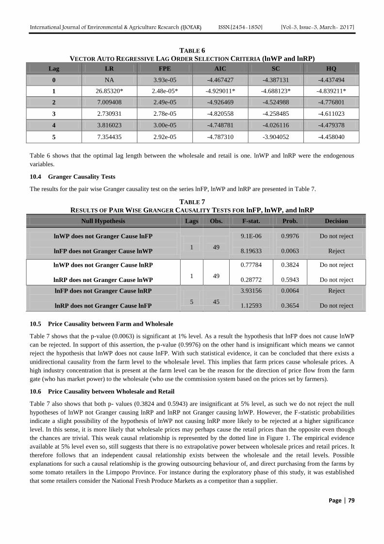
International Journal of Environmental & Agriculture Research (IJOEAR) ISSN:[2454-1850] [Vol-3, Issue-3, March- 2017]
Page | 79
TABLE 6
VECTOR AUTO REGRESSIVE LAG ORDER SELECTION CRITERIA (lnWP and lnRP)
Lag LR FPE AIC SC HQ
0 NA 3.93e-05 -4.467427 -4.387131 -4.437494
1 26.85320* 2.48e-05* -4.929011* -4.688123* -4.839211*
2 7.009408 2.49e-05 -4.926469 -4.524988 -4.776801
3 2.730931 2.78e-05 -4.820558 -4.258485 -4.611023
4 3.816023 3.00e-05 -4.748781 -4.026116 -4.479378
5 7.354435 2.92e-05 -4.787310 -3.904052 -4.458040
Table 6 shows that the optimal lag length between the wholesale and retail is one. lnWP and lnRP were the endogenous
variables.
10.4 Granger Causality Tests
The results for the pair wise Granger causality test on the series lnFP, lnWP and lnRP are presented in Table 7.
TABLE 7
RESULTS OF PAIR WISE GRANGER CAUSALITY TESTS FOR lnFP, lnWP, and lnRP
Null Hypothesis Lags Obs. F-stat. Prob. Decision
lnWP does not Granger Cause lnFP
lnFP does not Granger Cause lnWP
1
49
9.1E-06
8.19633
0.9976
0.0063
Do not reject
Reject
lnWP does not Granger Cause lnRP
lnRP does not Granger Cause lnWP
1
49
0.77784
0.28772
0.3824
0.5943
Do not reject
Do not reject
lnFP does not Granger Cause lnRP
lnRP does not Granger Cause lnFP
5
45
3.93156
1.12593
0.0064
0.3654
Reject
Do not reject
10.5 Price Causality between Farm and Wholesale
Table 7 shows that the p-value (0.0063) is significant at 1% level. As a result the hypothesis that lnFP does not cause lnWP
can be rejected. In support of this assertion, the p-value (0.9976) on the other hand is insignificant which means we cannot
reject the hypothesis that lnWP does not cause lnFP. With such statistical evidence, it can be concluded that there exists a
unidirectional causality from the farm level to the wholesale level. This implies that farm prices cause wholesale prices. A
high industry concentration that is present at the farm level can be the reason for the direction of price flow from the farm
gate (who has market power) to the wholesale (who use the commission system based on the prices set by farmers).
10.6 Price Causality between Wholesale and Retail
Table 7 also shows that both p- values (0.3824 and 0.5943) are insignificant at 5% level, as such we do not reject the null
hypotheses of lnWP not Granger causing lnRP and lnRP not Granger causing lnWP. However, the F-statistic probabilities
indicate a slight possibility of the hypothesis of lnWP not causing lnRP more likely to be rejected at a higher significance
level. In this sense, it is more likely that wholesale prices may perhaps cause the retail prices than the opposite even though
the chances are trivial. This weak causal relationship is represented by the dotted line in Figure 1. The empirical evidence
available at 5% level even so, still suggests that there is no extrapolative power between wholesale prices and retail prices. It
therefore follows that an independent causal relationship exists between the wholesale and the retail levels. Possible
explanations for such a causal relationship is the growing outsourcing behaviour of, and direct purchasing from the farms by
some tomato retailers in the Limpopo Province. For instance during the exploratory phase of this study, it was established
that some retailers consider the National Fresh Produce Markets as a competitor than a supplier.
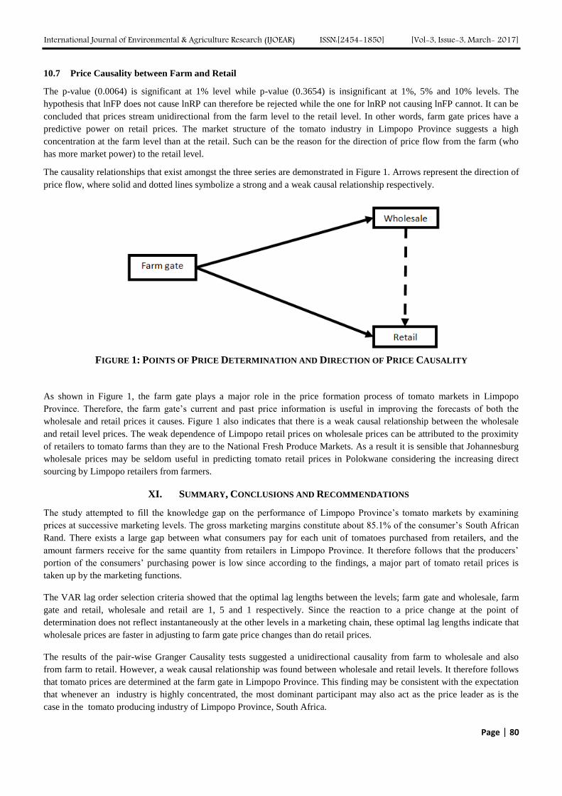
International Journal of Environmental & Agriculture Research (IJOEAR) ISSN:[2454-1850] [Vol-3, Issue-3, March- 2017]
Page | 80
10.7 Price Causality between Farm and Retail
The p-value (0.0064) is significant at 1% level while p-value (0.3654) is insignificant at 1%, 5% and 10% levels. The
hypothesis that lnFP does not cause lnRP can therefore be rejected while the one for lnRP not causing lnFP cannot. It can be
concluded that prices stream unidirectional from the farm level to the retail level. In other words, farm gate prices have a
predictive power on retail prices. The market structure of the tomato industry in Limpopo Province suggests a high
concentration at the farm level than at the retail. Such can be the reason for the direction of price flow from the farm (who
has more market power) to the retail level.
The causality relationships that exist amongst the three series are demonstrated in Figure 1. Arrows represent the direction of
price flow, where solid and dotted lines symbolize a strong and a weak causal relationship respectively.
FIGURE 1: POINTS OF PRICE DETERMINATION AND DIRECTION OF PRICE CAUSALITY
As shown in Figure 1, the farm gate plays a major role in the price formation process of tomato markets in Limpopo
Province. Therefore, the farm gate’s current and past price information is useful in improving the forecasts of both the
wholesale and retail prices it causes. Figure 1 also indicates that there is a weak causal relationship between the wholesale
and retail level prices. The weak dependence of Limpopo retail prices on wholesale prices can be attributed to the proximity
of retailers to tomato farms than they are to the National Fresh Produce Markets. As a result it is sensible that Johannesburg
wholesale prices may be seldom useful in predicting tomato retail prices in Polokwane considering the increasing direct
sourcing by Limpopo retailers from farmers.
XI. SUMMARY, CONCLUSIONS AND RECOMMENDATIONS
The study attempted to fill the knowledge gap on the performance of Limpopo Province’s tomato markets by examining
prices at successive marketing levels. The gross marketing margins constitute about 85.1% of the consumer’s South African
Rand. There exists a large gap between what consumers pay for each unit of tomatoes purchased from retailers, and the
amount farmers receive for the same quantity from retailers in Limpopo Province. It therefore follows that the producers’
portion of the consumers’ purchasing power is low since according to the findings, a major part of tomato retail prices is
taken up by the marketing functions.
The VAR lag order selection criteria showed that the optimal lag lengths between the levels; farm gate and wholesale, farm
gate and retail, wholesale and retail are 1, 5 and 1 respectively. Since the reaction to a price change at the point of
determination does not reflect instantaneously at the other levels in a marketing chain, these optimal lag lengths indicate that
wholesale prices are faster in adjusting to farm gate price changes than do retail prices.
The results of the pair-wise Granger Causality tests suggested a unidirectional causality from farm to wholesale and also
from farm to retail. However, a weak causal relationship was found between wholesale and retail levels. It therefore follows
that tomato prices are determined at the farm gate in Limpopo Province. This finding may be consistent with the expectation
that whenever an industry is highly concentrated, the most dominant participant may also act as the price leader as is the
case in the tomato producing industry of Limpopo Province, South Africa.
International Journal of Environmental & Agriculture Research (IJOEAR) ISSN:[2454-1850] [Vol-3, Issue-3, March- 2017]
Page | 81
An important conclusion drawn from the causal relationships between the farm gate, wholesale and retail prices is that the
farm level is key to tomato price determination in Limpopo Province. It therefore means that current and past information on
farm gate prices is useful in improving estimations of both wholesale and retail prices it causes. According to Guvheya et al.
(1998), information on causality shows the direction of price flow between levels and thus helps in the identification of
points of price determination along the marketing chain. In the light of this assertion, it can be concluded that tomato prices
in Limpopo Province are determined at the farm level. With the farm level being key to tomato price determination in
Limpopo Province of South Africa, pertinent policies that improve the commodity’s primary sector may by the ripple effect,
potentially benefit the other sectors in the value chain who are also dependent on tomato production.
This this study has shown the importance of the farm level at deciding the market price for food. Governments in the
developing economies such as South Africa are encouraged to intensify small scale farmers support programs so as to reduce
industry concentrations as well as encourage fairer competition in the food producing sectors of their respective economies.
This will ensure that agricultural produce prices will not be determined by a few major producers. A scenario where only one
producer dominates a market potentially leads to situation where all price movements are influenced by this single player
while the other farmers are simply price takers regardless of their cost structures.
XII. AREAS FOR FURTHER STUDY
The study established that the gross marketing margins of tomato in Limpopo Province are high. However the source of such
huge marketing margins has not been ascertained between marketing costs and retailers’ profits. This study only managed to
alert on the existence of high marketing margins that constitute the major portion of the consumer’s Rand. It is therefore
recommended that further research be undertaken to establish whether the retailers’ profits are unfairly high or peradventure
whether the marketing margins are as a result of high marketing costs. Such a complementary study will assist in identifying
the actual basis of the high marketing margins so that corrective policy measures can be directed appropriately and more
specifically.
ACKNOWLEDGEMENTS
Sincere appreciation goes to Mrs L. C Muchopa and Dr. P. Chaminuka for their grooming and guidance. Heartfelt gratitude
goes to Mrs Glenda (nee Nyanhongo) Mandizvidza, Mukundinashe Thaniel Kudzai and Ms. N. Shylletti Tsivai for their
support and inspiration.
REFERENCES
[1] Cox, L. (2009). Direct marketing of your agricultural products. Retrieved May 12, 2012, from
http://www.ctahr.hawaii.edu/sustainag/news/articles/V2-Cox- DM.pdf
[2] Department of Agriculture, Forestry and Fisheries (DAFF). (2011). A profile of the South African tomato market value chain.
Retrieved November 12, 2012, from http://www.nda.agric.za/docs/AMCP/TOMATOMVC2012.pdf
[3] Elitzak, H. (1996). Food cost review. Washington D.C: U.S Department of Agriculture.
[4] Food and Agriculture Organisation (FAO). (2002). Agricultural Marketing Extension. FAO TCP/SAF/0065, No 1 Pg1-24.
Retrieved February 04, 2011, from http://www.nda.agric.za/docs/GenPub/ 1AgriMarketExtension.pdf
[5] Fuglie, K. O., Macdonald, J. M., & Ball, E. (2007). Productivity Growth in U.S. Agriculture. Retrieved May 20, 2013, from United
States Department of Agriculture Economic Research Service: http://www.ers.usda.gov/media/201 254/eb9_1_.pdf
[6] Fuglie, K., & Nin-Pratt, A. (2012). 2012 Global Food Policy Report: A Changing Global Harvest. Retrieved May 20, 2013, from
International Food Policy Research Institute: http://www.ifpri.org/gfpr/2012/agricultural-productivity
[7] Granger, C. W. (1969). Investigating causal relationships by econometric models and cross-spectral methods. Econometrica: 37, 424-
38.
[8] Guvheya, G., Mabaya, E., & Christy, D. R. (1998)."Horticultural marketing in Zimbabwe:", Margins, price transmission and
spatial marketIntegration. Staff Paper. New York, Ithaca, U.S.A: Department of Agricultural, Resource, and Managerial
Economics Cornell University.
[9] Holland, R. (1998). Selling price, gross margin &mark-updetermination. ADC info# 12. Agricultural Extension Centre, The
University of Tennessee.
[10] Limpopo Tourism and Parks Board. (2011). Limpopo Province, South Africa's food basket. Retrieved November 5, 2011,from
http://www.golimpopo.com/fact-details_2_5.html
[11] Mojtaba, A., Farhad, S. B., & Hussein, E. (2010). Efficiency of date marketing system in Sistan & Bluchestan of Iran; A
marketing margin approach. Agric. Econ. – Czech, 56, 2010 (1) , 43-50.

International Journal of Environmental & Agriculture Research (IJOEAR) ISSN:[2454-1850] [Vol-3, Issue-3, March- 2017]
Page | 82
[12] Nin-Pratt, A. (2013). Agricultural Productivity: Good and Bad News. Retrieved May 20, 2013, from International Food Policy
Research Institute:
http://www.ifpri.org/blog/agricultural-productivity-good-and-bad-news
[13] Saccomandi, V. (1998). Agricultural Market Economics:A Neo-Institutional Analysis of the Exchange, Circulation and Distribution
of Agricultural Products. Netherlands: Van Gorcum & Comp. B. V.
[14] Salvatore, D. (1993). Managerial Economics In A Global Economy. McGraw-Hill.
[15] Schnepf, R. (2006). Price determination in agricultural commodity markets: A Primer. U.S: Congressional Research Service.
[16] Scott, G. J. (1995). Prices, product and people: Analysing agricultural markets in developing countries. Colorado: Lynne Rienner
Publishers, Inc.
[17] Singh, B. (1998). Production and marketing of wheat in India. New Delhi: Mittal Publications.
[18] van Niekerk, L. (2012). South Africa Yearbook 2011/12- Land and its people. Pretoria: Government of South Africa.
[19] Vavra, P., & Goodwin, B. (2005). "Analysis of Price Transmission Along the Food Chain". OECD Food, Agriculture and Fisheries
Working Papers, No. 3. OECD Publishing doi:10.1787/752335872456.
[20] Wohlgenant, M. K. (2001). Marketing Margins: Empirical Analysis. Department of Agricultural & Resource Economics, North
Carolina State University, Raleigh NC.
International Journal of Environmental & Agriculture Research (IJOEAR) ISSN:[2454-1850] [Vol-3, Issue-3, March- 2017]
Page | 83
Genome–Wide Analysis and Expression Pattern of the AP2/ERF
Gene Family in Kiwifruit under Waterlogging Stress Treatment Ji-Yu Zhang
1, De-Lin Pan
2, Gang Wang
3, Ji-Ping Xuan
4, Tao Wang
5, Zhong-Ren Guo
6
Institute of Botany, Jiangsu Province & Chinese Academy of Sciences, Nanjing 210014 China
Abstract—APETALA2/ethylene response factor (AP2/ERF) transcription factors play important roles in the response to
abiotic stresses. It is now possible to identify all of the AP2/ERF genes in the kiwifruit genome because the kiwifruit genome
project has been completed. 183 AP2/ERF genes were identified and compared with AP2/ERF genes from Arabidopsis in
this study. The 183 AP2/ERF kiwifruit genes were classified into four subfamilies: DREB (64), ERF (94), AP2 (19) and RAV
(5), as well as one soloist. RNA-sequence and Quantitative RT-PCR (qRT-PCR) analysis results showed that 20 genes were
responsive to waterlogging stress, suggesting that AP2/ERF transcription factors play important roles in the response to
waterlogging stress in kiwifruit
Keywords—AP2/ERF, kiwifruit, waterlogging stress.
I. INTRODUCTION
The APETALA2/ethylene response factor (AP2/ERF) superfamily is defined by the AP2/ERF domain which consists of
about 60 to 70 amino acids, and can be classified into at least five subfamilies: AP2 (containing two repeated AP2/ERF
domains), DREB (dehydration responsive element binding, containing a single AP2/ERF domain), ERF (containing a single
AP2/ERF domain), RAV (containing a B3domain and a single AP2/ERF domain), and others(Zhang et al. 2012b). The ERF
and DREB subfamilies can be further divided into six subfamilies: the B1–6 subfamilies and A1–6 subfamilies,
respectively(Zhang et al. 2012b). It has been demonstrated that AP2/ERF play important roles in the plant cell cycle, growth
and development, as well as the response to biotic and abiotic stresses (Zhang et al. 2012b).
Waterlogging is one of the most common stresses affecting plant growth and development. Many important crop plants are
sensitive to waterlogging conditions caused by heavy rain. Waterlogging and submergence conditions impose a variety of
challenges on the plants(Hinz et al. 2010). Previous research has shown that the AP2/ERF genes play an important role in the
regulation of gene expression during waterlogging stress. RAP2.2 is induced in shoots by ethylene and functions in an
ethylene-controlled signal transduction pathway and the overexpression of RAP2.2 resulted in improved plant survival under
hypoxia (low-oxygen) stress, whereas lines containing T-DNA knockouts of the gene had poorer survival rates than the wild
type(Hinz et al. 2010). The RAP2.2 gene plays a significant role in the metabolic adaptation to flooding stress in
Arabidopsis(Hinz et al. 2010). The SUB1A-1 allele could reduce elongation growth and carbohydrate consumption, and to
confer submergence tolerance (Fukao 2006; Xu et al. 2006; Jung et al. 2010). Flooding sensitive japonica cultivar over-
expressing SUB1A -1 could increase ADH1 expression and flooding tolerance(Fukao 2006; Xu et al. 2006). Four ERF
subfamily genes in Arabidopsis, namely RAP2.2 (At3g14230), RAP2.12 (At1g53910), HRE1 (At1g72360), and HRE2
(At2g47520) have been documented that play important role in the response to hypoxia (Hinz et al. 2010; Licausi et al.
2010). HRE1 over-expressing plants showed an increased activity in the fermentative enzymes pyruvate decarboxylase and
alcohol dehydrogenase together with increased ethanol production under hypoxia, showed an improved tolerance of anoxia
(Licausi et al. 2010). RAP2.2 was induced in shoots by ethylene and functions in an ethylene-controlled signal transduction
pathway(Hinz et al. 2010). Overexpression of RAP2.2 resulted in improved plant survival under hypoxia stress, whereas
lines containing T-DNA knockouts of the gene had poorer survival rates than the wild type(Hinz et al. 2010). Deepwater rice
requires SNORKEL1 (SK1) and SK2 ERF transcription factors to elongate stem internodes and extend the hollow stems to
the water surface for survival (Hattori et al. 2009). Du et al. reported (Du et al. 2014) that 38 of 184 AP2/ERF transcript
factor genes were responsive to waterlogging stress and 25 genes were ERF subfamily.
Kiwifruit is a major fruit worldwide. However, the majority of currently growing kiwifruit cultivars, like ‘Hongyang’, are
susceptible to waterlogging stress in East China. A thorough knowledge of kiwifruit resistance mechanisms will help to limit
crop loss due to waterlogging stress, and to decrease the economic losses. It’s known to us that AP2/ERF transcript factor
play important roles in the response to waterlogging stresses. It is possible to identify the AP2/ERF genes in many species as
these plant genome projects have been completed. Previous studies showed that there are 147, 184, 132, 200, and 116
AP2/ERF genes in the Arabidopsis (Nakano 2006) , maize(Du et al. 2014), grapevine(Zhuang et al. 2009), poplar(Zhuang et
International Journal of Environmental & Agriculture Research (IJOEAR) ISSN:[2454-1850] [Vol-3, Issue-3, March- 2017]
Page | 84
al. 2008), and Chinese plum (Du et al. 2013), respectively. However, few reports of the AP2/ERF superfamily are available
in kiwifruit. Kiwifruit genome projects have been completed(Huang and al. 2013). In this article, AP2-like genes from
kiwifruit were surveyed and comparatively analyzed. Here, 183 AP2/ERF transcription factors were identified from the
kiwifruit genome database and the transcriptome sequencing database (Zhang et al., 2015). The expressions of kiwifruit
AP2/ERF genes under waterlogged stress were performed. These analyses will be valuable to isolate and understand the
molecular mechanism of AP2/ERF genes responded to waterlogging stress in kiwifruit.
II. MATERIAL AND METHOD
2.1 Plant Material and Treatment
The kiwifruit cultivars ‘Jinkui’ were obtained from the Institute of Botany, Jiangsu Province & Chinese Academy of
Sciences, China. Plants were grown in pots containing a 2:1 mixture of garden soil and vermiculite without any added
fertilizer, and were maintained in a plant growth chamber. The growth chamber conditions were: relative humidity of ~ 60%,
160μmol m−2
s−1
PAR, photoperiod of 12 h light/12 h dark for 24 h, and 25°C average temperature. Seedlings, already grown
to the 8–10 node stage were selected for uniformity. The waterlogging treatment was performed as described previously (Yin
et al. 2009a). The pots were flooded by standing in a 28 cm×14 cm×14 cm container filled with tap water to 2.5 cm above the
level of the soil surface. The tap water had a pH of 7.3. The water temperature was held at ~25°C. Roots were sampled at 0,
24, 48, and 96 h after treatment, frozen in liquid nitrogen and stored at -80°C, which were later used for quantitative real
time-PCR (qRT–PCR) for studying the expression profile of AP2 TF genes. Each treatment was repeated three times and
there were 10 plants per treatment in every biological replication.
2.2 Database
Kiwifruit Genome Database (http://bioinfo.bti.cornell.edu/cgi-bin/kiwi/home.cgi) and transcriptome sequencing database
(NCBI, Accession number: SRR2048539) were mined to identify members of the AP2/ERF. The amino acid sequence of the
AP2/ERF domain (IYRGVRQRNSGKWVSEVREPNKKTRIWLGTFQTAEMAARAHDVAALALRGRSACLNF) from
Arabidopsis AtCBF1 (also named AtDREB1B; accession number AT4G25490) was used as queries to search against the
databases from Kiwifruit Genome Database Web site (http://bioinfo.bti.cornell.edu/cgi-bin/kiwi/home.cgi) using the
BLASTP program at the e-value of 1e-3 to avoid false positives.
2.3 Phylogenetic Tree Construction
Phylogenetic trees of the aligned kiwifruit AP2/ERF protein sequences were constructed using MEGA version 5.0 (Tamura
et al. 2011)(http://www.megasoftware.net) via the neighborjoining (NJ) method with the following parameters: Poisson
correction, pairwise deletion, and bootstrap (1,000 replicates; randomseed).
2.4 Differentially expressed analysis of AP2/ERF family genes under waterlogging stress
We have previously conducted the transcriptome sequencing of kiwifruit under waterlogging. The number of reads per
kilobase per exon region in a given gene per million mapped fragments (RPKM) was performed to identify AP2/ERF family
genes are regulated by waterlogging stress(Chen et al. 2014). Differentially expressed AP2/ERF family genes of 0h and 96h
were identified by the R program(Chen et al. 2014). We applied the Pearson’s chi-squared test to assess the lane effect. The
p-value was computed for each gene. The Benjamini–Hochberg false discovery rate (FDR) was then applied to correct the
results for the q-value. The FDR method is generally used in deep-sequencing studies to identify over-representative
AP2/ERF family genes (Junttila et al. 2013). If the FDR-adjusted q-value was ≤ 0.05, the AP2/ERF family genes were
considered to be differentially expressed. Heatmap were performed using the software of MEV (Multi Experiment Viewer).
Color scale represents reads per kilobase per million normalized log2 transformed counts where blue indicates low level and
red indicate high level.
2.5 Quantitative RT-PCR (qRT-PCR) Analysis
Quantitative RT-PCR (qRT-PCR) was used to determine the expression of AP2/ERF family genes in kiwifruit under
waterlogging. Total RNA isolation, DNase I treatment, First strand cDNA synthesise, and qRT-PCR assay were performed
as described by Zhang et al (Zhang et al. 2012a). The relative levels of genes to control AdActin (Yin et al. 2009b; Yin et al.
2012) mRNAs were analysed using the ABI-7300 system software and the 2−ΔΔCt
method (Livak and Schmittgen 2001).
Gene-specific primers used in the qRT-PCR were listed in Table 1. Data analyses were conducted using SPSS version 17.0
statistical software. For all analyses, the level of significance between different time points was set at P<0.05. Heatmap were
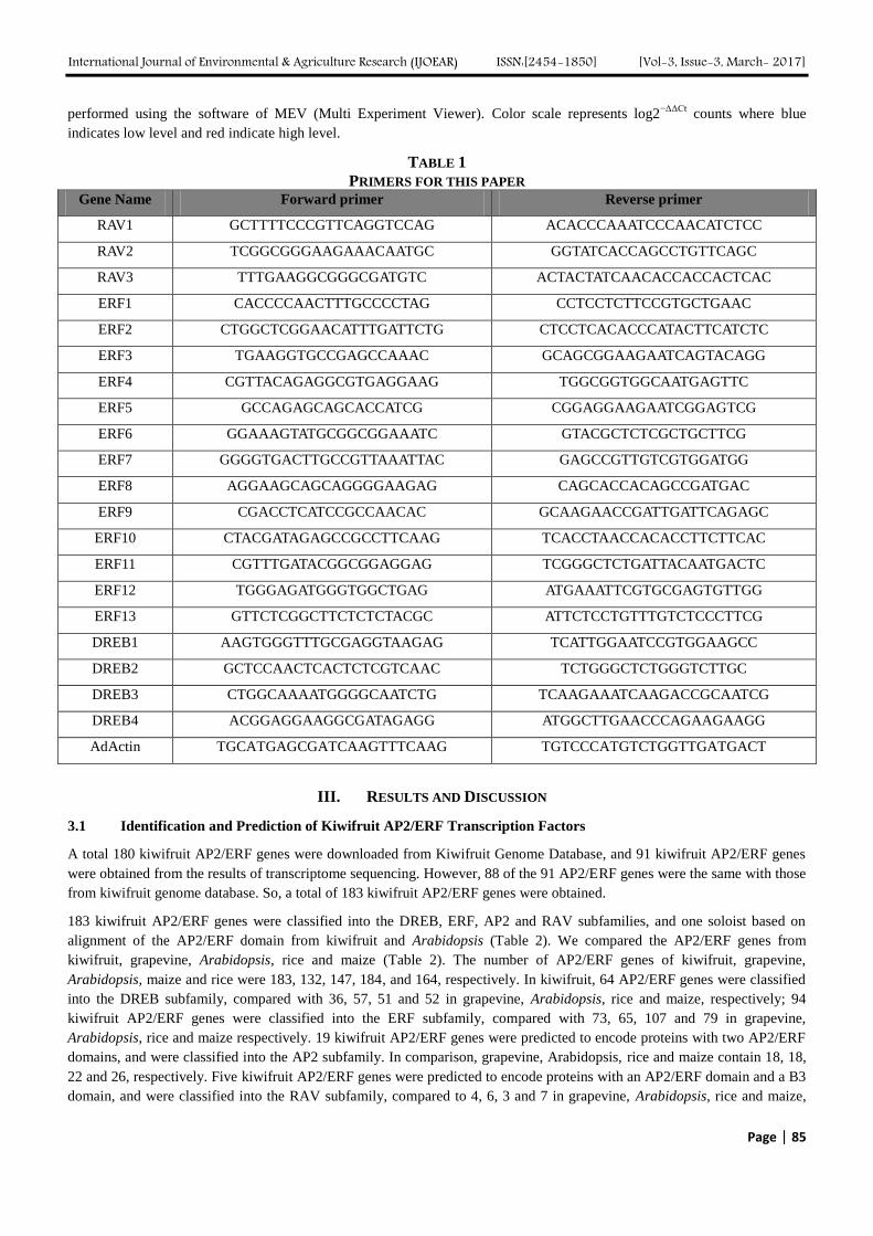
International Journal of Environmental & Agriculture Research (IJOEAR) ISSN:[2454-1850] [Vol-3, Issue-3, March- 2017]
Page | 85
performed using the software of MEV (Multi Experiment Viewer). Color scale represents log2−ΔΔCt
counts where blue
indicates low level and red indicate high level.
TABLE 1
PRIMERS FOR THIS PAPER Gene Name Forward primer Reverse primer
RAV1 GCTTTTCCCGTTCAGGTCCAG ACACCCAAATCCCAACATCTCC
RAV2 TCGGCGGGAAGAAACAATGC GGTATCACCAGCCTGTTCAGC
RAV3 TTTGAAGGCGGGCGATGTC ACTACTATCAACACCACCACTCAC
ERF1 CACCCCAACTTTGCCCCTAG CCTCCTCTTCCGTGCTGAAC
ERF2 CTGGCTCGGAACATTTGATTCTG CTCCTCACACCCATACTTCATCTC
ERF3 TGAAGGTGCCGAGCCAAAC GCAGCGGAAGAATCAGTACAGG
ERF4 CGTTACAGAGGCGTGAGGAAG TGGCGGTGGCAATGAGTTC
ERF5 GCCAGAGCAGCACCATCG CGGAGGAAGAATCGGAGTCG
ERF6 GGAAAGTATGCGGCGGAAATC GTACGCTCTCGCTGCTTCG
ERF7 GGGGTGACTTGCCGTTAAATTAC GAGCCGTTGTCGTGGATGG
ERF8 AGGAAGCAGCAGGGGAAGAG CAGCACCACAGCCGATGAC
ERF9 CGACCTCATCCGCCAACAC GCAAGAACCGATTGATTCAGAGC
ERF10 CTACGATAGAGCCGCCTTCAAG TCACCTAACCACACCTTCTTCAC
ERF11 CGTTTGATACGGCGGAGGAG TCGGGCTCTGATTACAATGACTC
ERF12 TGGGAGATGGGTGGCTGAG ATGAAATTCGTGCGAGTGTTGG
ERF13 GTTCTCGGCTTCTCTCTACGC ATTCTCCTGTTTGTCTCCCTTCG
DREB1 AAGTGGGTTTGCGAGGTAAGAG TCATTGGAATCCGTGGAAGCC
DREB2 GCTCCAACTCACTCTCGTCAAC TCTGGGCTCTGGGTCTTGC
DREB3 CTGGCAAAATGGGGCAATCTG TCAAGAAATCAAGACCGCAATCG
DREB4 ACGGAGGAAGGCGATAGAGG ATGGCTTGAACCCAGAAGAAGG
AdActin TGCATGAGCGATCAAGTTTCAAG TGTCCCATGTCTGGTTGATGACT
III. RESULTS AND DISCUSSION
3.1 Identification and Prediction of Kiwifruit AP2/ERF Transcription Factors
A total 180 kiwifruit AP2/ERF genes were downloaded from Kiwifruit Genome Database, and 91 kiwifruit AP2/ERF genes
were obtained from the results of transcriptome sequencing. However, 88 of the 91 AP2/ERF genes were the same with those
from kiwifruit genome database. So, a total of 183 kiwifruit AP2/ERF genes were obtained.
183 kiwifruit AP2/ERF genes were classified into the DREB, ERF, AP2 and RAV subfamilies, and one soloist based on
alignment of the AP2/ERF domain from kiwifruit and Arabidopsis (Table 2). We compared the AP2/ERF genes from
kiwifruit, grapevine, Arabidopsis, rice and maize (Table 2). The number of AP2/ERF genes of kiwifruit, grapevine,
Arabidopsis, maize and rice were 183, 132, 147, 184, and 164, respectively. In kiwifruit, 64 AP2/ERF genes were classified
into the DREB subfamily, compared with 36, 57, 51 and 52 in grapevine, Arabidopsis, rice and maize, respectively; 94
kiwifruit AP2/ERF genes were classified into the ERF subfamily, compared with 73, 65, 107 and 79 in grapevine,
Arabidopsis, rice and maize respectively. 19 kiwifruit AP2/ERF genes were predicted to encode proteins with two AP2/ERF
domains, and were classified into the AP2 subfamily. In comparison, grapevine, Arabidopsis, rice and maize contain 18, 18,
22 and 26, respectively. Five kiwifruit AP2/ERF genes were predicted to encode proteins with an AP2/ERF domain and a B3
domain, and were classified into the RAV subfamily, compared to 4, 6, 3 and 7 in grapevine, Arabidopsis, rice and maize,
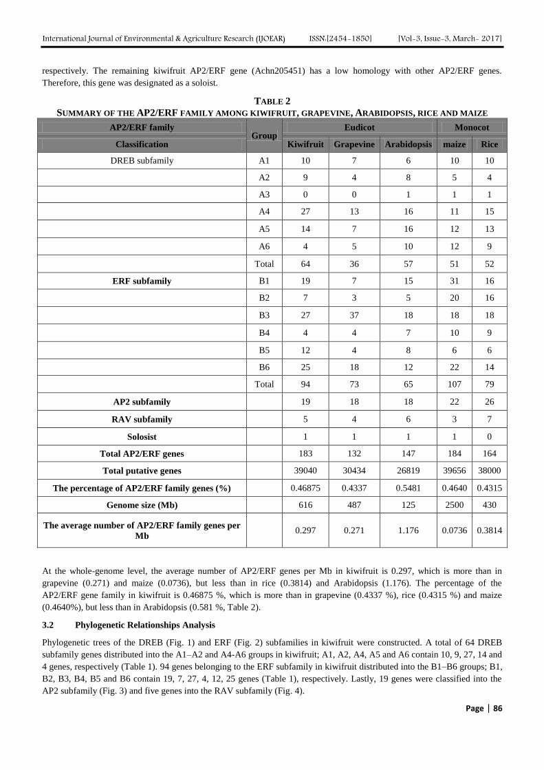
International Journal of Environmental & Agriculture Research (IJOEAR) ISSN:[2454-1850] [Vol-3, Issue-3, March- 2017]
Page | 86
respectively. The remaining kiwifruit AP2/ERF gene (Achn205451) has a low homology with other AP2/ERF genes.
Therefore, this gene was designated as a soloist.
TABLE 2
SUMMARY OF THE AP2/ERF FAMILY AMONG KIWIFRUIT, GRAPEVINE, ARABIDOPSIS, RICE AND MAIZE
AP2/ERF family Group
Eudicot Monocot
Classification Kiwifruit Grapevine Arabidopsis maize Rice
DREB subfamily A1 10 7 6 10 10
A2 9 4 8 5 4
A3 0 0 1 1 1
A4 27 13 16 11 15
A5 14 7 16 12 13
A6 4 5 10 12 9
Total 64 36 57 51 52
ERF subfamily B1 19 7 15 31 16
B2 7 3 5 20 16
B3 27 37 18 18 18
B4 4 4 7 10 9
B5 12 4 8 6 6
B6 25 18 12 22 14
Total 94 73 65 107 79
AP2 subfamily 19 18 18 22 26
RAV subfamily 5 4 6 3 7
Solosist 1 1 1 1 0
Total AP2/ERF genes 183 132 147 184 164
Total putative genes 39040 30434 26819 39656 38000
The percentage of AP2/ERF family genes (%) 0.46875 0.4337 0.5481 0.4640 0.4315
Genome size (Mb) 616 487 125 2500 430
The average number of AP2/ERF family genes per
Mb 0.297 0.271 1.176 0.0736 0.3814
At the whole-genome level, the average number of AP2/ERF genes per Mb in kiwifruit is 0.297, which is more than in
grapevine (0.271) and maize (0.0736), but less than in rice (0.3814) and Arabidopsis (1.176). The percentage of the
AP2/ERF gene family in kiwifruit is 0.46875 %, which is more than in grapevine (0.4337 %), rice (0.4315 %) and maize
(0.4640%), but less than in Arabidopsis (0.581 %, Table 2).
3.2 Phylogenetic Relationships Analysis
Phylogenetic trees of the DREB (Fig. 1) and ERF (Fig. 2) subfamilies in kiwifruit were constructed. A total of 64 DREB
subfamily genes distributed into the A1–A2 and A4-A6 groups in kiwifruit; A1, A2, A4, A5 and A6 contain 10, 9, 27, 14 and
4 genes, respectively (Table 1). 94 genes belonging to the ERF subfamily in kiwifruit distributed into the B1–B6 groups; B1,
B2, B3, B4, B5 and B6 contain 19, 7, 27, 4, 12, 25 genes (Table 1), respectively. Lastly, 19 genes were classified into the
AP2 subfamily (Fig. 3) and five genes into the RAV subfamily (Fig. 4).
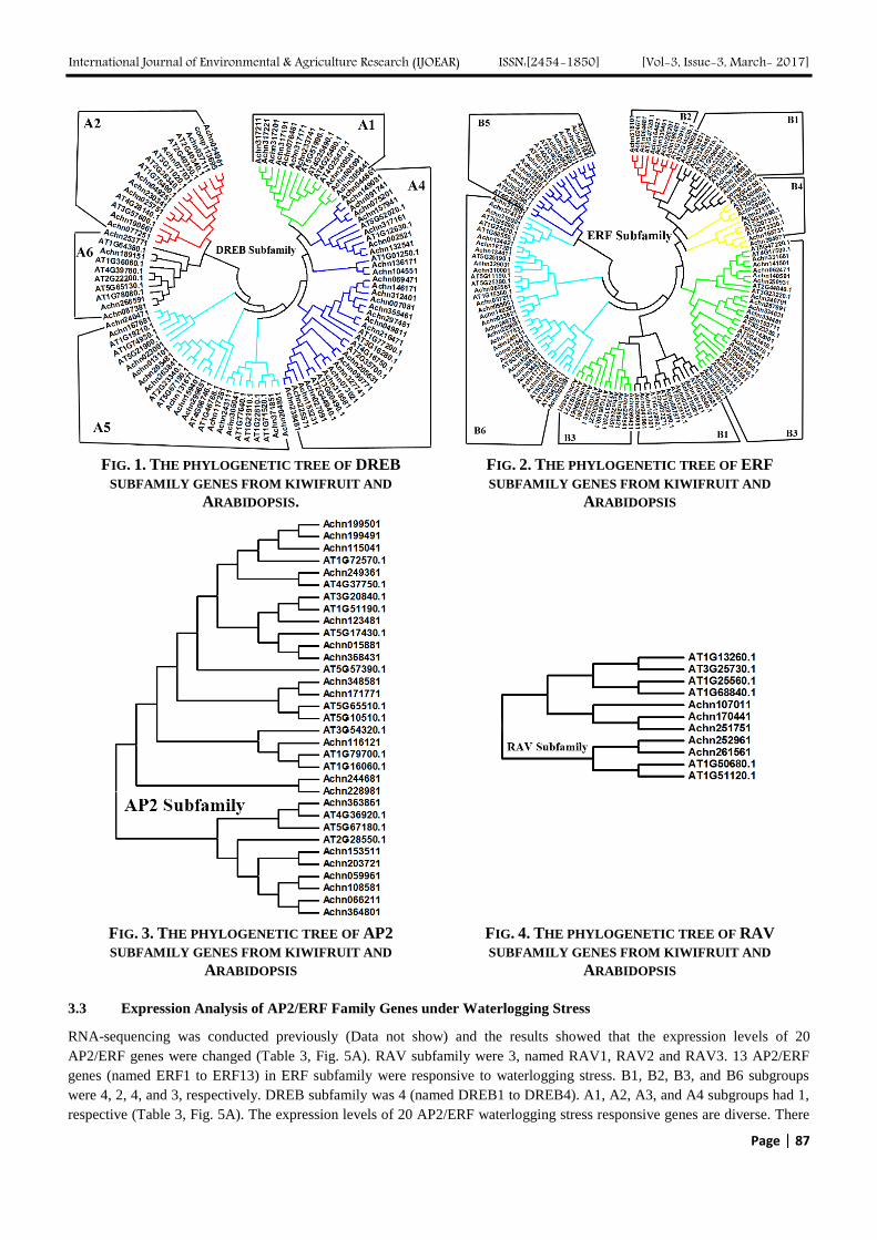
International Journal of Environmental & Agriculture Research (IJOEAR) ISSN:[2454-1850] [Vol-3, Issue-3, March- 2017]
Page | 87
FIG. 1. THE PHYLOGENETIC TREE OF DREB
SUBFAMILY GENES FROM KIWIFRUIT AND
ARABIDOPSIS.
FIG. 2. THE PHYLOGENETIC TREE OF ERF
SUBFAMILY GENES FROM KIWIFRUIT AND
ARABIDOPSIS
FIG. 3. THE PHYLOGENETIC TREE OF AP2
SUBFAMILY GENES FROM KIWIFRUIT AND
ARABIDOPSIS
FIG. 4. THE PHYLOGENETIC TREE OF RAV
SUBFAMILY GENES FROM KIWIFRUIT AND
ARABIDOPSIS
3.3 Expression Analysis of AP2/ERF Family Genes under Waterlogging Stress
RNA-sequencing was conducted previously (Data not show) and the results showed that the expression levels of 20
AP2/ERF genes were changed (Table 3, Fig. 5A). RAV subfamily were 3, named RAV1, RAV2 and RAV3. 13 AP2/ERF
genes (named ERF1 to ERF13) in ERF subfamily were responsive to waterlogging stress. B1, B2, B3, and B6 subgroups
were 4, 2, 4, and 3, respectively. DREB subfamily was 4 (named DREB1 to DREB4). A1, A2, A3, and A4 subgroups had 1,
respective (Table 3, Fig. 5A). The expression levels of 20 AP2/ERF waterlogging stress responsive genes are diverse. There
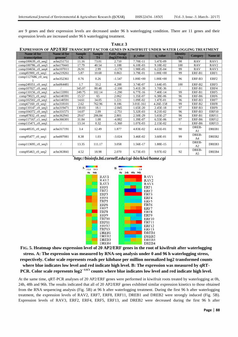
International Journal of Environmental & Agriculture Research (IJOEAR) ISSN:[2454-1850] [Vol-3, Issue-3, March- 2017]
Page | 88
are 9 genes and their expression levels are decreased under 96 h waterlogging condition. There are 11 genes and their
expression levels are increased under 96 h waterlogging treatment.
TABLE 3
EXPRESSION OF AP2/ERF TRANSCRIPT FACTOR GENES IN KIWIFRUIT UNDER WATER LOGGING TREATMENT Name id for
transcription
Name id for
genome*
Sample
CK
Sample
T4
Fold_change
(log2(T4/ck)) p_value q_value
Identity
(%) Category Name id
comp100639_c0_seq2 achn251751 11.16 73.01 2.710 7.70E-11 5.47E-09 98 RAV RAV1
comp100786_c0_seq3 achn170441 17.79 40.54 1.188 6.10E-03 9.18E-02 100 RAV RAV2
comp104656_c0_seq4 achn107011 26.91 2.99 -3.170 1.98E-05 6.22E-04 99 RAV RAV3
comp81900_c0_seq1 achn219261 5.87 10.68 0.863 3.79E-01 1.00E+00 99 ERF-B1 ERF1
comp1127686_c0_seq
1 achn352361 0.76 0.26 -1.547 1.00E+00 1.00E+00 96 ERF-B3 ERF2
comp249351_c0_seq1 achn064481 1.7 33.2 4.288 3.74E-07 1.64E-05 100 ERF-B2 ERF3
comp107027_c0_seq1 / 345.07 80.48 -2.100 5.41E-39 1.70E-36 / ERF-B1 ERF4
comp110156_c0_seq1 achn133991 249.75 102.14 -1.290 6.77E-16 7.40E-14 99 ERF-B1 ERF5
comp79023_c0_seq1 achn140391 15.57 65 2.062 1.35E-07 6.38E-06 96 ERF-B6 ERF6
comp102502_c0_seq1 achn140591 14.61 34.05 1.221 1.09E-02 1.47E-01 96 ERF-B3 ERF7
comp67160_c0_seq1 achn318101 2.62 762.96 8.186 3.01E-161 4.26E-158 99 ERF-B2 ERF8
comp110147_c0_seq3 achn319471 130.03 18.1 -2.845 1.65E-20 2.45E-18 97 ERF-B3 ERF9
comp104372_c0_seq3 achn331571 14.07 2.09 -2.751 5.32E-03 8.21E-02 96 ERF-B3 ERF10
comp87832_c0_seq1 achn362941 29.67 206.84 2.801 2.50E-29 5.65E-27 96 ERF-B1 ERF11
comp117167_c1_seq1 achn366301 31.84 1.08 -4.882 1.39E-07 6.55E-06 97 ERF-B6 ERF12
comp115471_c0_seq1 / 13.14 0.32 -5.360 1.07E-03 2.15E-02 / ERF-B6 ERF13
comp48535_c0_seq1 achn317191 3.4 12.49 1.877 4.83E-02 4.61E-01 90 DREB-
A1 DREB1
comp95477_c0_seq1 achn007081 8.38 1.03 -3.024 3.46E-02 3.60E-01 99 DREB-
A4 DREB2
comp113695_c0_seq3 / 13.35 111.17 3.058 1.56E-17 1.88E-15 / DREB-
A2 DREB3
comp95463_c0_seq2 achn363841 4.52 18.98 2.070 6.73E-03 9.97E-02 92 DREB-
A5 DREB4
*http://bioinfo.bti.cornell.edu/cgi-bin/kiwi/home.cgi
FIG. 5. Heatmap show expression level of 20 AP2/ERF genes in the root of kiwifruit after waterlogging
stress. A: The expression was measured by RNA-seq analysis under 0 and 96 h waterlogging stress,
respectively. Color scale represents reads per kilobase per million normalized log2 transformed counts
where blue indicates low level and red indicate high level. B: The expression was measured by qRT-
PCR. Color scale represents log2−ΔΔCt
counts where blue indicates low level and red indicate high level.
At the same time, qRT-PCR analyses of 20 AP2/ERF genes were performed in kiwifruit roots treated by waterlogging at 0h,
24h, 48h and 96h. The results indicated that all of 20 AP2/ERF genes exhibited similar expression kinetics to those obtained
from the RNA sequencing analysis (Fig. 5B) at 96 h after waterlogging treatment. During the first 96 h after waterlogging
treatment, the expression levels of RAV2, ERF7, ERF8, ERF11, DREB1 and DREB2 were strongly induced (Fig. 5B).
Expression levels of RAV3, ERF2, ERF4, ERF5, ERF13, and DREB2 were decreased during the first 96 h after
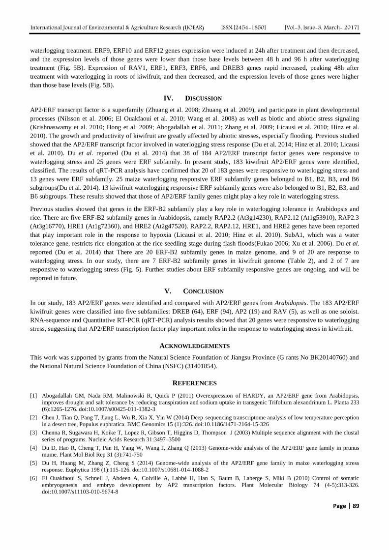
International Journal of Environmental & Agriculture Research (IJOEAR) ISSN:[2454-1850] [Vol-3, Issue-3, March- 2017]
Page | 89
waterlogging treatment. ERF9, ERF10 and ERF12 genes expression were induced at 24h after treatment and then decreased,
and the expression levels of those genes were lower than those base levels between 48 h and 96 h after waterlogging
treatment (Fig. 5B). Expression of RAV1, ERF1, ERF3, ERF6, and DREB3 genes rapid increased, peaking 48h after
treatment with waterlogging in roots of kiwifruit, and then decreased, and the expression levels of those genes were higher
than those base levels (Fig. 5B).
IV. DISCUSSION
AP2/ERF transcript factor is a superfamily (Zhuang et al. 2008; Zhuang et al. 2009), and participate in plant developmental
processes (Nilsson et al. 2006; El Ouakfaoui et al. 2010; Wang et al. 2008) as well as biotic and abiotic stress signaling
(Krishnaswamy et al. 2010; Hong et al. 2009; Abogadallah et al. 2011; Zhang et al. 2009; Licausi et al. 2010; Hinz et al.
2010). The growth and productivity of kiwifruit are greatly affected by abiotic stresses, especially flooding. Previous studied
showed that the AP2/ERF transcript factor involved in waterlogging stress response (Du et al. 2014; Hinz et al. 2010; Licausi
et al. 2010). Du et al. reported (Du et al. 2014) that 38 of 184 AP2/ERF transcript factor genes were responsive to
waterlogging stress and 25 genes were ERF subfamily. In present study, 183 kiwifruit AP2/ERF genes were identified,
classified. The results of qRT-PCR analysis have confirmed that 20 of 183 genes were responsive to waterlogging stress and
13 genes were ERF subfamily. 25 maize waterlogging responsive ERF subfamily genes belonged to B1, B2, B3, and B6
subgroups(Du et al. 2014). 13 kiwifruit waterlogging responsive ERF subfamily genes were also belonged to B1, B2, B3, and
B6 subgroups. These results showed that those of AP2/ERF family genes might play a key role in waterlogging stress.
Previous studies showed that genes in the ERF-B2 subfamily play a key role in waterlogging tolerance in Arabidopsis and
rice. There are five ERF-B2 subfamily genes in Arabidopsis, namely RAP2.2 (At3g14230), RAP2.12 (At1g53910), RAP2.3
(At3g16770), HRE1 (At1g72360), and HRE2 (At2g47520). RAP2.2, RAP2.12, HRE1, and HRE2 genes have been reported
that play important role in the response to hypoxia (Licausi et al. 2010; Hinz et al. 2010). SubA1, which was a water
tolerance gene, restricts rice elongation at the rice seedling stage during flash floods(Fukao 2006; Xu et al. 2006). Du et al.
reported (Du et al. 2014) that There are 20 ERF-B2 subfamily genes in maize genome, and 9 of 20 are response to
waterlogging stress. In our study, there are 7 ERF-B2 subfamily genes in kiwifruit genome (Table 2), and 2 of 7 are
responsive to waterlogging stress (Fig. 5). Further studies about ERF subfamily responsive genes are ongoing, and will be
reported in future.
V. CONCLUSION
In our study, 183 AP2/ERF genes were identified and compared with AP2/ERF genes from Arabidopsis. The 183 AP2/ERF
kiwifruit genes were classified into five subfamilies: DREB (64), ERF (94), AP2 (19) and RAV (5), as well as one soloist.
RNA-sequence and Quantitative RT-PCR (qRT-PCR) analysis results showed that 20 genes were responsive to waterlogging
stress, suggesting that AP2/ERF transcription factor play important roles in the response to waterlogging stress in kiwifruit.
ACKNOWLEDGEMENTS
This work was supported by grants from the Natural Science Foundation of Jiangsu Province (G rants No BK20140760) and
the National Natural Science Foundation of China (NSFC) (31401854).
REFERENCES
[1] Abogadallah GM, Nada RM, Malinowski R, Quick P (2011) Overexpression of HARDY, an AP2/ERF gene from Arabidopsis,
improves drought and salt tolerance by reducing transpiration and sodium uptake in transgenic Trifolium alexandrinum L. Planta 233
(6):1265-1276. doi:10.1007/s00425-011-1382-3
[2] Chen J, Tian Q, Pang T, Jiang L, Wu R, Xia X, Yin W (2014) Deep-sequencing transcriptome analysis of low temperature perception
in a desert tree, Populus euphratica. BMC Genomics 15 (1):326. doi:10.1186/1471-2164-15-326
[3] Chenna R, Sugawara H, Koike T, Lopez R, Gibson T, Higgins D, Thompson J (2003) Multiple sequence alignment with the clustal
series of programs. Nucleic Acids Research 31:3497–3500
[4] Du D, Hao R, Cheng T, Pan H, Yang W, Wang J, Zhang Q (2013) Genome-wide analysis of the AP2/ERF gene family in prunus
mume. Plant Mol Biol Rep 31 (3):741-750
[5] Du H, Huang M, Zhang Z, Cheng S (2014) Genome-wide analysis of the AP2/ERF gene family in maize waterlogging stress
response. Euphytica 198 (1):115-126. doi:10.1007/s10681-014-1088-2
[6] El Ouakfaoui S, Schnell J, Abdeen A, Colville A, Labbé H, Han S, Baum B, Laberge S, Miki B (2010) Control of somatic
embryogenesis and embryo development by AP2 transcription factors. Plant Molecular Biology 74 (4-5):313-326.
doi:10.1007/s11103-010-9674-8
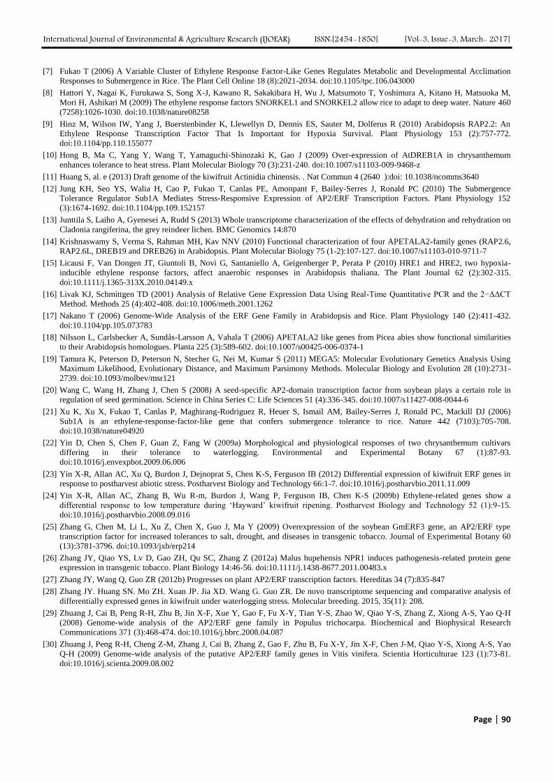
International Journal of Environmental & Agriculture Research (IJOEAR) ISSN:[2454-1850] [Vol-3, Issue-3, March- 2017]
Page | 90
[7] Fukao T (2006) A Variable Cluster of Ethylene Response Factor-Like Genes Regulates Metabolic and Developmental Acclimation
Responses to Submergence in Rice. The Plant Cell Online 18 (8):2021-2034. doi:10.1105/tpc.106.043000
[8] Hattori Y, Nagai K, Furukawa S, Song X-J, Kawano R, Sakakibara H, Wu J, Matsumoto T, Yoshimura A, Kitano H, Matsuoka M,
Mori H, Ashikari M (2009) The ethylene response factors SNORKEL1 and SNORKEL2 allow rice to adapt to deep water. Nature 460
(7258):1026-1030. doi:10.1038/nature08258
[9] Hinz M, Wilson IW, Yang J, Buerstenbinder K, Llewellyn D, Dennis ES, Sauter M, Dolferus R (2010) Arabidopsis RAP2.2: An
Ethylene Response Transcription Factor That Is Important for Hypoxia Survival. Plant Physiology 153 (2):757-772.
doi:10.1104/pp.110.155077
[10] Hong B, Ma C, Yang Y, Wang T, Yamaguchi-Shinozaki K, Gao J (2009) Over-expression of AtDREB1A in chrysanthemum
enhances tolerance to heat stress. Plant Molecular Biology 70 (3):231-240. doi:10.1007/s11103-009-9468-z
[11] Huang S, al. e (2013) Draft genome of the kiwifruit Actinidia chinensis. . Nat Commun 4 (2640 ):doi: 10.1038/ncomms3640
[12] Jung KH, Seo YS, Walia H, Cao P, Fukao T, Canlas PE, Amonpant F, Bailey-Serres J, Ronald PC (2010) The Submergence
Tolerance Regulator Sub1A Mediates Stress-Responsive Expression of AP2/ERF Transcription Factors. Plant Physiology 152
(3):1674-1692. doi:10.1104/pp.109.152157
[13] Junttila S, Laiho A, Gyenesei A, Rudd S (2013) Whole transcriptome characterization of the effects of dehydration and rehydration on
Cladonia rangiferina, the grey reindeer lichen. BMC Genomics 14:870
[14] Krishnaswamy S, Verma S, Rahman MH, Kav NNV (2010) Functional characterization of four APETALA2-family genes (RAP2.6,
RAP2.6L, DREB19 and DREB26) in Arabidopsis. Plant Molecular Biology 75 (1-2):107-127. doi:10.1007/s11103-010-9711-7
[15] Licausi F, Van Dongen JT, Giuntoli B, Novi G, Santaniello A, Geigenberger P, Perata P (2010) HRE1 and HRE2, two hypoxia-
inducible ethylene response factors, affect anaerobic responses in Arabidopsis thaliana. The Plant Journal 62 (2):302-315.
doi:10.1111/j.1365-313X.2010.04149.x
[16] Livak KJ, Schmittgen TD (2001) Analysis of Relative Gene Expression Data Using Real-Time Quantitative PCR and the 2−ΔΔCT
Method. Methods 25 (4):402-408. doi:10.1006/meth.2001.1262
[17] Nakano T (2006) Genome-Wide Analysis of the ERF Gene Family in Arabidopsis and Rice. Plant Physiology 140 (2):411-432.
doi:10.1104/pp.105.073783
[18] Nilsson L, Carlsbecker A, Sundås-Larsson A, Vahala T (2006) APETALA2 like genes from Picea abies show functional similarities
to their Arabidopsis homologues. Planta 225 (3):589-602. doi:10.1007/s00425-006-0374-1
[19] Tamura K, Peterson D, Peterson N, Stecher G, Nei M, Kumar S (2011) MEGA5: Molecular Evolutionary Genetics Analysis Using
Maximum Likelihood, Evolutionary Distance, and Maximum Parsimony Methods. Molecular Biology and Evolution 28 (10):2731-
2739. doi:10.1093/molbev/msr121
[20] Wang C, Wang H, Zhang J, Chen S (2008) A seed-specific AP2-domain transcription factor from soybean plays a certain role in
regulation of seed germination. Science in China Series C: Life Sciences 51 (4):336-345. doi:10.1007/s11427-008-0044-6
[21] Xu K, Xu X, Fukao T, Canlas P, Maghirang-Rodriguez R, Heuer S, Ismail AM, Bailey-Serres J, Ronald PC, Mackill DJ (2006)
Sub1A is an ethylene-response-factor-like gene that confers submergence tolerance to rice. Nature 442 (7103):705-708.
doi:10.1038/nature04920
[22] Yin D, Chen S, Chen F, Guan Z, Fang W (2009a) Morphological and physiological responses of two chrysanthemum cultivars
differing in their tolerance to waterlogging. Environmental and Experimental Botany 67 (1):87-93.
doi:10.1016/j.envexpbot.2009.06.006
[23] Yin X-R, Allan AC, Xu Q, Burdon J, Dejnoprat S, Chen K-S, Ferguson IB (2012) Differential expression of kiwifruit ERF genes in
response to postharvest abiotic stress. Postharvest Biology and Technology 66:1-7. doi:10.1016/j.postharvbio.2011.11.009
[24] Yin X-R, Allan AC, Zhang B, Wu R-m, Burdon J, Wang P, Ferguson IB, Chen K-S (2009b) Ethylene-related genes show a
differential response to low temperature during ‘Hayward’ kiwifruit ripening. Postharvest Biology and Technology 52 (1):9-15.
doi:10.1016/j.postharvbio.2008.09.016
[25] Zhang G, Chen M, Li L, Xu Z, Chen X, Guo J, Ma Y (2009) Overexpression of the soybean GmERF3 gene, an AP2/ERF type
transcription factor for increased tolerances to salt, drought, and diseases in transgenic tobacco. Journal of Experimental Botany 60
(13):3781-3796. doi:10.1093/jxb/erp214
[26] Zhang JY, Qiao YS, Lv D, Gao ZH, Qu SC, Zhang Z (2012a) Malus hupehensis NPR1 induces pathogenesis-related protein gene
expression in transgenic tobacco. Plant Biology 14:46-56. doi:10.1111/j.1438-8677.2011.00483.x
[27] Zhang JY, Wang Q, Guo ZR (2012b) Progresses on plant AP2/ERF transcription factors. Hereditas 34 (7):835-847
[28] Zhang JY. Huang SN. Mo ZH. Xuan JP. Jia XD. Wang G. Guo ZR. De novo transcriptome sequencing and comparative analysis of
differentially expressed genes in kiwifruit under waterlogging stress. Molecular breeding. 2015, 35(11): 208.
[29] Zhuang J, Cai B, Peng R-H, Zhu B, Jin X-F, Xue Y, Gao F, Fu X-Y, Tian Y-S, Zhao W, Qiao Y-S, Zhang Z, Xiong A-S, Yao Q-H
(2008) Genome-wide analysis of the AP2/ERF gene family in Populus trichocarpa. Biochemical and Biophysical Research
Communications 371 (3):468-474. doi:10.1016/j.bbrc.2008.04.087
[30] Zhuang J, Peng R-H, Cheng Z-M, Zhang J, Cai B, Zhang Z, Gao F, Zhu B, Fu X-Y, Jin X-F, Chen J-M, Qiao Y-S, Xiong A-S, Yao
Q-H (2009) Genome-wide analysis of the putative AP2/ERF family genes in Vitis vinifera. Scientia Horticulturae 123 (1):73-81.
doi:10.1016/j.scienta.2009.08.002
International Journal of Environmental & Agriculture Research (IJOEAR) ISSN:[2454-1850] [Vol-3, Issue-3, March- 2017]
Page | 91
New banana genotypes and cultivars more productive for
southern Minas, Brazil
Lair Victor Pereira1, José Clélio de Andrade
2, Ângelo Albérico Alvarenga
3, Marcelo
Ribeiro Malta4, Paulo Márcio Norberto
5, Sebastião de Oliveira e Silva
6
1,2,3,4,5Agricultural Research Company of Minas Gerais (EPAMIG), Lavras, MG, CP 176, CEP: 37200-000, Brazil
Email: [email protected] 6PVNS/Capes/UFRB, Cruz das Almas, BA, CEP: 44380-000, Brazil
Abstract— Southern of Minas state, is a important producer of banana, especially the cultivars Prata-Anã, Nanicão and
Maçã. These cultivars present low productivity, great plant height and are susceptible to major banana diseases. The
objective of this study was to evaluate the vegetative and productive behavior of banana cultivars as Prata, Nanicão and
Maçã, in Lavras, MG, Brazil to select those with the best features, of bunch and fruit size, lower production cycle and
disease resistance in high land conditions. Were evaluated the following materials: type: ‘Prata’: ‘Prata-Anã’ (control),
‘BRS Maravilha’, ‘BRS Vitoria’, PA 94-01; type ‘Nanicão’: ‘Grande Naine’ (control) and FHIA 17 and type ‘Maçã’:
‘Maçã’ (control) and YB 42-03. The experiment was conducted in a completely randomized block design with three
replications and 16 plants per plot. Regarding the type ‘Prata-Anã’, ‘BRS Maravilha’ and PA 94-01 are recommended by
their greater productivity, plant height, production cycle, flavor and fruit appearance in relation to cv ‘Prata-Anã’
traditionally grown in region. PV 94-01 and ‘Vitoria’, despite the greats plant height, are recommended due to the greater
productivity. The YB 42-03 genotype is an alternative to ‘Maçã’ because it is similar to productivity, size and production
cycle.
Keywords— Musa, Banana, Production cycle, Yield.
I. INTRODUCTION
There are more than 125 countries that are dedicated to the cultivation of bananas in the world. This fruit stands out in the
first position of the world ranking around 106.5 million tons in 2011, according to Vieira (2015).
The banana is the second most consumed fruit in the world with 11.4 kg/hab/year, losing only to the orange with 12.2
kg/hab/year (FAO, 2014). The expansion of banana farming in most countries from 35 million tonnes in 1978 to 106.5
million tonnes in 2011 was made possible thanks to the intensive use of technologies (VIEIRA, 2015).
The productivity of banana growing in Minas Gerais increased from 14.103 t ha-1 in 2001 to 16.936 t ha-1 in 2012 (IBGE,
2013). This increase in productivity is mainly due to the adoption of new technologies such as fertirrigation, adequate crop
management, and the introduction of new, more productive cultivars.
Several banana cultivars have been evaluated and recommended in all regions of Brazil. Among these, there are those of the
type ‘Prata’: ‘Pioneira’, ‘Prata Graúda’, ‘BRS Pacovan Ken’, ‘BRS Maravilha’, ‘BRS Platina’, ‘BRS Conquista’, ‘BRS
Vitória’; tipo ‘Maçã’: ‘Thap Maeo’, ‘Mysore’ e ‘Caipira’; type ‘Ouro’: ‘Prata Baby’ or ‘Nam’ and type ‘Nanicão’: ‘Grande
Naine’ (SILVA; PEREIRA; RODRIGUES, 2008).
However, obtaining new, more productive banana cultivars is not enough to determine success in terms of adoption by
producers. Besides the agronomic aspects, the new cultivars must present fruits with good market characteristics (Silva, et
al., 2013). An improved cultivar should increase productivity, reduce production costs due to the decrease in the use of
pesticides, thus increasing the income of the producer (Amorim et al., 2011).
The cultivar BRS Maravilha in dry conditions was more productive than Prata-Anã, its mother in the first two cycles in Jataí
(GO) (SANTOS; CARNEIRO, 2012), in Goiânia (GO) (MENDONÇA et al., 2013), in Aquidauana (GO) (VIEIRA, 2011), in
Botucatu (SP) (RAMOS et al., 2009) and in Lavras (MG) (PEREIRA et al., 2003).
Borges et al. (2011) report that the genotype FHIA 17 was highlighted in rainy conditions in production among the 14
genotypes evaluated in northern Paraná and that the cultivars BRS Maravilha, PV 94-01 and YB 42-03 presented similar
behavior to the cultivars of the Same type Prata-Anã, Pacovan and Maçã, respectively.
International Journal of Environmental & Agriculture Research (IJOEAR) ISSN:[2454-1850] [Vol-3, Issue-3, March- 2017]
Page | 92
According to the Capixaba Institute for Research, Technical Assistance and Rural Extension - INCAPER (2010); SILVA et
al. (2008) and PEREIRA et al. (2005) the BRS Vitória cultivar was more productive than Prata and Pacovan in the states of
Espírito Santo, Bahia and Amazonas, respectively. In irrigated conditions the ‘BRS Maravilha’ presented superior yield
twice as much as the cultivar Prata-Anã in the Jaíba projects (MG) (RODRIGUES et al., 2006) and Gorutuba (MG) (SOUTO
et al., 2001).
The influence of the environment, mainly temperature, on the banana production cycle, can be observed in experiments
conducted in Lavras (MG), Maria da Fé (MG) and Jaíba (MG). In Lavras, with average annual minimum temperatures of
15.4ºC and altitude of 900 m, the ‘Prata-Anã’ cycle was 510 days (PEREIRA et al., 2002). In Maria da Fé, with an average
annual minimum temperature of 10.7ºC and altitude of 1270 m, the production cycle of Prata-Anã was 620 days (PEREIRA
et al., 2002). On the other hand, in Jaíba with a minimum annual average temperature of 18.5ºC and altitude of 500 m, the
production cycle of this cultivar was 320 days (RODRIGUES; SOUTO; SILVA, 2006).
This work was conducted with the objective of evaluating new cultivars and genotypes of bananas of the types Prata,
Nanicão and Maçã in the southern region of the state of Minas Gerais, Brazil, regarding the increase of productivity and fruit
quality.
II. MATERIAL AND METHOD
The experiment was conducted at the Experimental Farm of AGROTESTE in Lavras (MG), Brazil, from January 2013 to
December 2015, and the first two cycles were evaluated. The altitude of the place is 918 m.
According to the climatic classification of Koppen (DANTAS; CARVALHO; FERREIRA, 2007), the climate of Lavras -
MG is cwa, that is, temperate rainy season (mesothermic) with dry winter and subtropical rainy summer. The average
temperature of the coldest month is below 18ºC and the hottest month is over 22ºC, with the average annual temperature of
19.4ºC and relative humidity of 76.2%. The average annual rainfall is 1,529 mm, with the driest months being from June to
September.
Soil of the experimental area was classified as type 3, Red Latosol Ferric 62, 15 and 23 dag kg-1 of clay, silt and sand,
respectively.
The experiment was installed in randomized blocks with three replications and plots with 16 plants per cultivar or genotype
planted in the 3.0 x 3.0 m spacing.
The following genotypes and cultivars were evaluated: Prata type: Prata Anã (control), BRS Maravilha and PA 94-01
(genitor Prata Anã), BRS Vitória and PV 94-01 (Pacovan); Nanicão type: Grande Naine (control, Cavendish type), FHIA 17
(Hybrid of Gros Michel), and Type Maçã: Maçã (control) and YB 42-03.
The cycle of production of the mother and daughter plants and the accumulated one (from the planting of the mother plant to
the harvest of the daughter plant) were evaluated, the periods being expressed in months. Production characteristics were as
follows: fresh mass of the bunch (kg), number of fruits per bunch, length and diameter of the fruit (cm) and fresh mass of the
fruit (g) of the medium bunch. The bunches were harvested when the fruits presented without pistils or floral remains, sharp
corners, that is, ideal point of cut for the local market.
Plant development data were taken by measuring the diameter of the pseudocaule (cm) at 50 cm of the soil level and height
of the plant (m), at the time of flowering.
It was also evaluated the incidence of yellow Sigatoka in the mother plant in flowering and harvest, through the number of
leaves attacked, leaves without symptoms and leaves functional or alive. It was considered as functional leaf that presented in
the flowering and harvest at least 2/3 of leaf area totally green.
Statistical analysis was performed using the Variance Analysis System software for the SISVAR balanced data (FERREIRA,
2011) and the comparison of means of treatments was performed using the Scott-Knott test at 5% probability.
III. RESULTS AND DISCUSSION
The results concerning the bunch and the fruit weight, number of fruits per bunch, length and diameter of these in the two
cycles of the evaluated cultivars and genotypes are in Table 1.
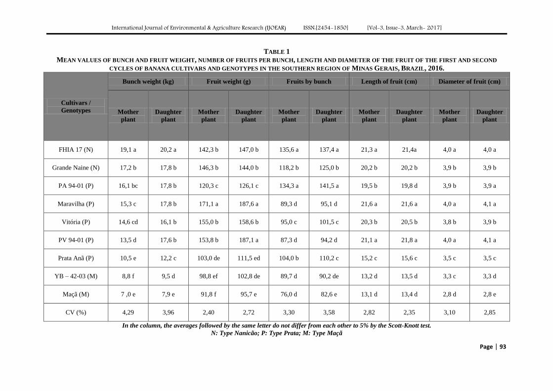
International Journal of Environmental & Agriculture Research (IJOEAR) ISSN:[2454-1850] [Vol-3, Issue-3, March- 2017]
Page | 93
TABLE 1
MEAN VALUES OF BUNCH AND FRUIT WEIGHT, NUMBER OF FRUITS PER BUNCH, LENGTH AND DIAMETER OF THE FRUIT OF THE FIRST AND SECOND
CYCLES OF BANANA CULTIVARS AND GENOTYPES IN THE SOUTHERN REGION OF MINAS GERAIS, BRAZIL, 2016.
Cultivars /
Genotypes
Bunch weight (kg) Fruit weight (g) Fruits by bunch Length of fruit (cm) Diameter of fruit (cm)
Mother
plant
Daughter
plant
Mother
plant
Daughter
plant
Mother
plant
Daughter
plant
Mother
plant
Daughter
plant
Mother
plant
Daughter
plant
FHIA 17 (N) 19,1 a 20,2 a 142,3 b 147,0 b 135,6 a 137,4 a 21,3 a 21,4a 4,0 a 4,0 a
Grande Naine (N) 17,2 b 17,8 b 146,3 b 144,0 b 118,2 b 125,0 b 20,2 b 20,2 b 3,9 b 3,9 b
PA 94-01 (P) 16,1 bc 17,8 b 120,3 c 126,1 c 134,3 a 141,5 a 19,5 b 19,8 d 3,9 b 3,9 a
Maravilha (P) 15,3 c 17,8 b 171,1 a 187,6 a 89,3 d 95,1 d 21,6 a 21,6 a 4,0 a 4,1 a
Vitória (P) 14,6 cd 16,1 b 155,0 b 158,6 b 95,0 c 101,5 c 20,3 b 20,5 b 3,8 b 3,9 b
PV 94-01 (P) 13,5 d 17,6 b 153,8 b 187,1 a 87,3 d 94,2 d 21,1 a 21,8 a 4,0 a 4,1 a
Prata Anã (P) 10,5 e 12,2 c 103,0 de 111,5 ed 104,0 b 110,2 c 15,2 c 15,6 c 3,5 c 3,5 c
YB – 42-03 (M) 8,8 f 9,5 d 98,8 ef 102,8 de 89,7 d 90,2 de 13,2 d 13,5 d 3,3 c 3,3 d
Maçã (M) 7 ,0 e 7,9 e 91,8 f 95,7 e 76,0 d 82,6 e 13,1 d 13,4 d 2,8 d 2,8 e
CV (%) 4,29 3,96 2,40 2,72 3,30 3,58 2,82 2,35 3,10 2,85
In the column, the averages followed by the same letter do not differ from each other to 5% by the Scott-Knott test.
N: Type Nanicão; P: Type Prata; M: Type Maçã
International Journal of Environmental & Agriculture Research (IJOEAR) ISSN:[2454-1850] [Vol-3, Issue-3, March- 2017]
Page | 94
The genotype FHIA 17 produced higher fresh weight, number of fruits per bunch, length and diameter of the fruit, being
overcome in fresh weight only by PV 94-01 and ‘BRS Maravilha’, in the second cycle.
The length and diameter of the fruits of the genotypes of FHIA 17, PV 94-01 and cultivar BRS Maravilha were significantly
higher than the other evaluated materials.
The values of bunch and fruit weight, number of fruits per bunch, length and diameter of fruits observed in this study were
significantly lower than those reported by Borges et al. (2011). These differences can be attributed to management, soil
fertility and annual distribution and amount of rainfall (ALVES, 1999), since the trials were conducted in fairly distinct
edaphoclimatic regions.
The cultivar Grande Naine, unique of the Cavendish type, produced bunches with superior weight to the genotypes of the
‘Prata’ type, only in the first cycle and number of fruits per cluster inferior to the one of PA 94-01, in the two cycles. The
weight of the fruit was also lower than that of PV 94-01 and cultivar BRS Maravilha. The values of bunch and fruit weight
and number of fruits per bunch of ‘Grande Naine’ obtained in this study are lower than those obtained by Donato et al.
(2006) in Guanambi (BA), under irrigation and those reported by Silva, Pereira and Rodrigues (2008) in Cruz das Almas
(BA) and by Borges et al. (2011) in Andirá (PR) under rainfed conditions. It is noteworthy that in Lavras (MG) and in much
of the state of Minas Gerais, rainfall has been very low, even in the rainy season (from October to March). This causes water
deficit in the soil and, consequently, lower utilization of fertilizers by plants.
Regarding the production of ‘Prata’ type materials, genotypes PV 94-01 and PA 94-01 and cultivars BRS Maravilha and
BRS Vitória produced larger bunches and fruits in terms of weight than the cultivar Prata-Anã in the two cycles evaluated.
The PV 94-01 along with the cultivar BRS Maravilha had the largest increases in bunch weight and fruit size from the first to
the second cycle.
Among the materials of the ‘Prata’ type, PA 94-01 was the one that produced clusters with the highest number of fruits being
these, similar in appearance and taste to the cultivar Prata-Anã.
Analyzing plant height, pseudocaule diameter and PA 94-01 production cycle (Table 2), it can be observed that this genotype
was similar to the Prata-Anã cultivar. Although the plant height, pseudocaule diameter and number of live leaves in
flowering PA 94-01 were considered adequate. However, Nomura et al. (2013) report that the production cycle of this
genotype was later, resulting in lower productivity. The BRS Maravilha cultivar in terms of bunch weight, together with PA
94-01, were superior to BRS Vitória and PV 94-01 only in the first production cycle.
As regards weight, length and diameter, BRS Maravilha and PV 94-01, cultivar BRS Maravilha presented the highest weight
in both cycles, and in the second cycle the fruits of PV 94-01 produced larger fruits in weight, length and weight. Diameter in
the two cycles evaluated. The highest weight of the bunch and size of the BRS Maravilha fruits in relation to the Prata-Anã
obtained in this work in dry conditions are confirmed by the reports of Silva et al. (2003) in Lavras (MG), by Ramos et al.
(2009) in Botucatu (SP), by Vieira (2011) in Aquidauana (MS), by Santos and Carneiro (2012) in Jataí (GO) and by
Mendonça et al. (2013) in Goiânia (GO). BRS Maravilha also surpassed Prata-Anã in the region of Jaíba (MG)
(RODRIGUES; SOUTO; SILVA, 2006) and in southwestern Bahia (DONATO et al., 2009).
The genotype PV 94-01 and cultivar BRS Maravilha had the largest increases in bunch and fruit weight and number of fruits
per bunch in the second cycle. This increase is also reported by Rodrigues, Souto e Silva (2006) for BRS Maravilha, SH 36-
40 (Prata Graúda MG).
The genotype YB 42-03 and the cultivar Maçã produced the smallest clusters and fruits in terms of size, number of fruits per
cluster. The YB 42-03 was slightly higher in these characteristics than the cultivar Maçã, its similar. These results
corroborate with those reported by Silva, Pereira and Rodrigues (2008).
The cultivars Grande Naine and Prata Anã showed the lowest heights, inferior to 2.3 m in the mother plant and 2.7 m in the
daughter plant (Table 2), results similar to those reported by Nomura et al. (2013). The largest size of these BRS Vitória
cultivars was 3.5 m and 4.1 m followed by the PV 94-01 genotype with 3.1 m and 3.8 m, respectively, in the 1st and 2nd
cycle. The larger size of the cultivars Vitória and PV 94-01 were also reported by Nomura et al. (2013). These results are
already expected, since this characteristic is inherited from her mother-in-law Pacovan.
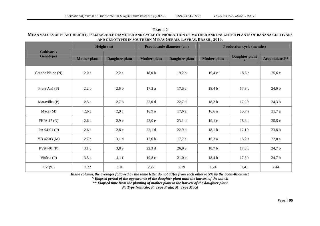
International Journal of Environmental & Agriculture Research (IJOEAR) ISSN:[2454-1850] [Vol-3, Issue-3, March- 2017]
Page | 95
TABLE 2
MEAN VALUES OF PLANT HEIGHT, PSEUDOCAULE DIAMETER AND CYCLE OF PRODUCTION OF MOTHER AND DAUGHTER PLANTS OF BANANA CULTIVARS
AND GENOTYPES IN SOUTHERN MINAS GERAIS. LAVRAS, BRAZIL, 2016.
Cultivars /
Genotypes
Height (m) Pseudocaule diameter (cm) Production cycle (months)
Mother plant Daughter plant Mother plant Daughter plant Mother plant Daughter plant
* Accumulated**
Grande Naine (N) 2,0 a 2,2 a 18,0 b 19,2 b 19,4 c 18,5 c 25,6 c
Prata Anã (P) 2,2 b 2,6 b 17,2 a 17,5 a 18,4 b 17,3 b 24,0 b
Maravilha (P) 2,5 c 2,7 b 22,0 d 22,7 d 18,2 b 17,2 b 24,3 b
Maçã (M) 2,6 c 2,9 c 16,9 a 17,6 a 16,6 a 15,7 a 21,7 a
FHIA 17 (N) 2,6 c 2,9 c 23,0 e 23,1 d 19,1 c 18,3 c 25,5 c
PA 94-01 (P) 2,6 c 2,8 c 22,1 d 22,9 d 18,1 b 17,1 b 23,8 b
YB 42-03 (M) 2,7 c 3,1 d 17,6 b 17,7 a 16,3 a 15,2 a 22,0 a
PV94-01 (P) 3,1 d 3,8 e 22,3 d 26,9 e 18,7 b 17,8 b 24,7 b
Vitória (P) 3,5 e 4,1 f 19,8 c 21,0 c 18,4 b 17,5 b 24,7 b
CV (%) 3,22 3,16 2,27 2,79 1,24 1,41 2,44
In the column, the averages followed by the same letter do not differ from each other to 5% by the Scott-Knott test.
* Elapsed period of the appearance of the daughter plant until the harvest of the bunch
** Elapsed time from the planting of mother plant to the harvest of the daughter plant
N: Type Nanicão; P: Type Prata; M: Type Maçã
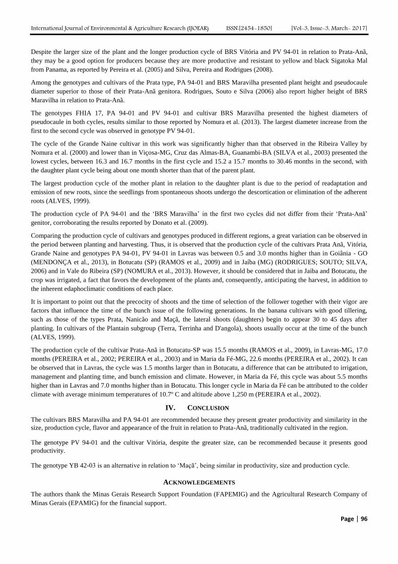
International Journal of Environmental & Agriculture Research (IJOEAR) ISSN:[2454-1850] [Vol-3, Issue-3, March- 2017]
Page | 96
Despite the larger size of the plant and the longer production cycle of BRS Vitória and PV 94-01 in relation to Prata-Anã,
they may be a good option for producers because they are more productive and resistant to yellow and black Sigatoka Mal
from Panama, as reported by Pereira et al. (2005) and Silva, Pereira and Rodrigues (2008).
Among the genotypes and cultivars of the Prata type, PA 94-01 and BRS Maravilha presented plant height and pseudocaule
diameter superior to those of their Prata-Anã genitora. Rodrigues, Souto e Silva (2006) also report higher height of BRS
Maravilha in relation to Prata-Anã.
The genotypes FHIA 17, PA 94-01 and PV 94-01 and cultivar BRS Maravilha presented the highest diameters of
pseudocaule in both cycles, results similar to those reported by Nomura et al. (2013). The largest diameter increase from the
first to the second cycle was observed in genotype PV 94-01.
The cycle of the Grande Naine cultivar in this work was significantly higher than that observed in the Ribeira Valley by
Nomura et al. (2000) and lower than in Viçosa-MG, Cruz das Almas-BA, Guanambi-BA (SILVA et al., 2003) presented the
lowest cycles, between 16.3 and 16.7 months in the first cycle and 15.2 a 15.7 months to 30.46 months in the second, with
the daughter plant cycle being about one month shorter than that of the parent plant.
The largest production cycle of the mother plant in relation to the daughter plant is due to the period of readaptation and
emission of new roots, since the seedlings from spontaneous shoots undergo the descortication or elimination of the adherent
roots (ALVES, 1999).
The production cycle of PA 94-01 and the ‘BRS Maravilha’ in the first two cycles did not differ from their ‘Prata-Anã’
genitor, corroborating the results reported by Donato et al. (2009).
Comparing the production cycle of cultivars and genotypes produced in different regions, a great variation can be observed in
the period between planting and harvesting. Thus, it is observed that the production cycle of the cultivars Prata Anã, Vitória,
Grande Naine and genotypes PA 94-01, PV 94-01 in Lavras was between 0.5 and 3.0 months higher than in Goiânia - GO
(MENDONÇA et al., 2013), in Botucatu (SP) (RAMOS et al., 2009) and in Jaíba (MG) (RODRIGUES; SOUTO; SILVA,
2006) and in Vale do Ribeira (SP) (NOMURA et al., 2013). However, it should be considered that in Jaiba and Botucatu, the
crop was irrigated, a fact that favors the development of the plants and, consequently, anticipating the harvest, in addition to
the inherent edaphoclimatic conditions of each place.
It is important to point out that the precocity of shoots and the time of selection of the follower together with their vigor are
factors that influence the time of the bunch issue of the following generations. In the banana cultivars with good tillering,
such as those of the types Prata, Nanicão and Maçã, the lateral shoots (daughters) begin to appear 30 to 45 days after
planting. In cultivars of the Plantain subgroup (Terra, Terrinha and D'angola), shoots usually occur at the time of the bunch
(ALVES, 1999).
The production cycle of the cultivar Prata-Anã in Botucatu-SP was 15.5 months (RAMOS et al., 2009), in Lavras-MG, 17.0
months (PEREIRA et al., 2002; PEREIRA et al., 2003) and in Maria da Fé-MG, 22.6 months (PEREIRA et al., 2002). It can
be observed that in Lavras, the cycle was 1.5 months larger than in Botucatu, a difference that can be attributed to irrigation,
management and planting time, and bunch emission and climate. However, in Maria da Fé, this cycle was about 5.5 months
higher than in Lavras and 7.0 months higher than in Botucatu. This longer cycle in Maria da Fé can be attributed to the colder
climate with average minimum temperatures of 10.7º C and altitude above 1,250 m (PEREIRA et al., 2002).
IV. CONCLUSION
The cultivars BRS Maravilha and PA 94-01 are recommended because they present greater productivity and similarity in the
size, production cycle, flavor and appearance of the fruit in relation to Prata-Anã, traditionally cultivated in the region.
The genotype PV 94-01 and the cultivar Vitória, despite the greater size, can be recommended because it presents good
productivity.
The genotype YB 42-03 is an alternative in relation to ‘Maçã’, being similar in productivity, size and production cycle.
ACKNOWLEDGEMENTS
The authors thank the Minas Gerais Research Support Foundation (FAPEMIG) and the Agricultural Research Company of
Minas Gerais (EPAMIG) for the financial support.
International Journal of Environmental & Agriculture Research (IJOEAR) ISSN:[2454-1850] [Vol-3, Issue-3, March- 2017]
Page | 97
REFERENCES
[1] ALVES, E.J. (1999) A cultura da bananeira: aspectos técnicos, socioeconômicos e agroindustriais. 2. ed. Brasília:
EMBRAPA/CNPMF. 585 p.
[2] AMORIM, E.P. et al. (2011) Banana Breeding: Progress and Challenger. New York: CRC Press, p. 252-280.
[3] BORGES, R.S. et al. (2011) Avaliação de genótipos de bananeira no norte do Estado do Paraná. Revista Brasileira de Fruticultura,
v.33, n.1, p.291-296.
[4] CENTRAL DE ABASTECIMENTO DE MINAS GERAIS – CEASAMINAS (2015). Oferta de produtos/variedades: banana.
Disponível em www.ceasaminas.com.br. Accessed in june 30, 2015.
[5] DANTAS, A.A.; CARVALHO, L.G.; FERREIRA, E. (2007) Classificação e tendências climáticas em Lavras, MG. Ciência e
Agrotecnologia, v.31, n.6, p.186-1866.
[6] DONATO, S.L.R.; ARANTES, A.M.; SILVA, S.O.; CORDEIRO, Z.J.M. (2009) Comportamento fitotécnico da bananeira ‘Prata-
Anã’ e de seus híbridos. Pesquisa Agropecuária Brasileira, v.44, n.12, p. 1608-1615.
[7] FOOD AGRICULTURE ORGANIZATION OF THE UNITED NATIONS (FAO) (2014). Faostat 2014. Disponivel em
http://www.faostat3.fao.org. Accessed in june 10, 2015.
[8] FERREIRA, D.F. (2011) Sisvar: a computer statistical analysis system. Ciência e Agrotecnologia, v.35, n.6, p.1039-1042.
[9] INSTITUTO BRASILEIRO DE GEOGRAFIA E ESTATISTICA – IBGE (2013). Banco de dados. Produção agrícola municipal.
Disponível em <http//www.sidra.ibge.gov.br/bda/agric>. Accessed in dec. 10, 2015.
[10] INSTITUTO CAPIXABA DE PESQUISA, ASSISTÊNCIA TÉCNICA E EXTENSÃO RURAL – INCAPER (2010). Bananas
‘Japira’ e ‘Vitória’ resistentes às doenças. Incaper em revista. Vitória, Informativo especial, ano 1, n.1, jan./dez.2010. Disponível em
<http//incaes.web407.unis.net/revista.php?ideap=97> Accessed in july 27, 2015.
[11] MENDONÇA, K.H.; DUARTE, D.A.S.; COSTA, V.A.M.; MATOS, G.R.; SELEGUINI, A. (2013) Avaliação de genótipos de
bananeira em Goiânia, Estado de Goiás. Revista Ciência Agronômica, v.44, n.3, p.652-660.
[12] NOMURA, E.S.; DAMATTO JUNIOR, E.R.; FUZITANI, E.J.; AMORIM, E.P.; SILVA, S.O. (2013) Avaliação agronômica de
genótipos de bananeira em condições subtropicais do Vale da Ribeira, São Paulo. Revista Brasileira de Fruticultura, v.35, n.1, p.111-
122.
[13] PEREIRA, L.V.; ALVARENGA, A.A.; MATOS, L.E.S; SILVA, C.R.R. (2002) Avaliação de cultivares de bananeira (Musa sp.,
AAB) em três locais do Estado de Minas Gerais. Ciência e Agrotecnologia, Edição Especial, p.1373-1382.
[14] PEREIRA, L.V.; SILVA, S.O.; ALVES, E.J.; SILVA, C.R.R. (2003) Avaliação de cultivares e híbridos de bananeira em Lavras, MG.
Ciência e Agrotecnologia, v.27, n.1, p.17-25.
[15] PEREIRA, J.C.R.; GASPAROTTO, L.; PEREIRA, M.C.N. (2005) BRS Vitória: nova cultivar de bananeira do subgrupo Prata para o
agronegócio no Estado do Amazonas. Brasília: Embrapa, 2p. (Embrapa. Comunicado Técnico, 34).
[16] RAMOS, D.P.; SARITA, L.; MISHAM, M.M.; DAMATTA JUNIOR, E.R. (2009) Avaliação de genótipos de bananeira em Botucatu,
SP. Revista Brasileira de Fruticultura, v.31, n.4, p.1092-1101.
[17] RODRIGUES, M.G.V.; SOUTO, R.F.; SILVA, S.O. (2006) Avaliação de genótipos de bananeira sob irrigação. Revista Brasileira de
Fruticultura, v.28, n.3, p.449-453.
[18] SANTOS, S.C.; CARNEIRO, C.C. (2012) Desempenho de genótipos de bananeira na região de Jataí-GO. Revista Brasileira de
Fruticultura, v.34, n.3, p.783-791.
[19] SILVA, S.O.; PASSOS, A.R.; DONATO, S.L.R.; SALOMÃO, L.C.C.; PEREIRA, L.V.; RODRIGUES, M.G.V.; LIMA NETO, F.P.;
LIMA, M.B. (2003) Avaliação de genótipos de bananeira em diferentes ambientes. Ciência e Agrotecnologia, v.27, n.4, p.737-748.
[20] SILVA, S.O.; PEREIRA, L.V.; RODRIGUES, M.G.R. (2008) Variedades. Informe Agropecuário, v.29, n.245, p.78-83.
[21] SILVA, S.O.; AMORIM, E.P.; SANTOS-SEREJO, J.A.; FERREIRA, C.F.; RODRIGUEZ, M.A.D. (2013) Melhoramento genético
da bananeira: estratégias e tecnologias disponíveis. Revista Brasileira de Fruticultura, v.35, n.3, p. 919-931.
[22] VIEIRA, L.C.R. (2011) Avaliação de cultivares de bananeira na microrregião de Aquidauana-MS. Dissertação de Mestrado. Unidade
Universitária de Aquidauana, Universidade Estadual do Mato Grosso do Sul, Aquidauana, 36p.
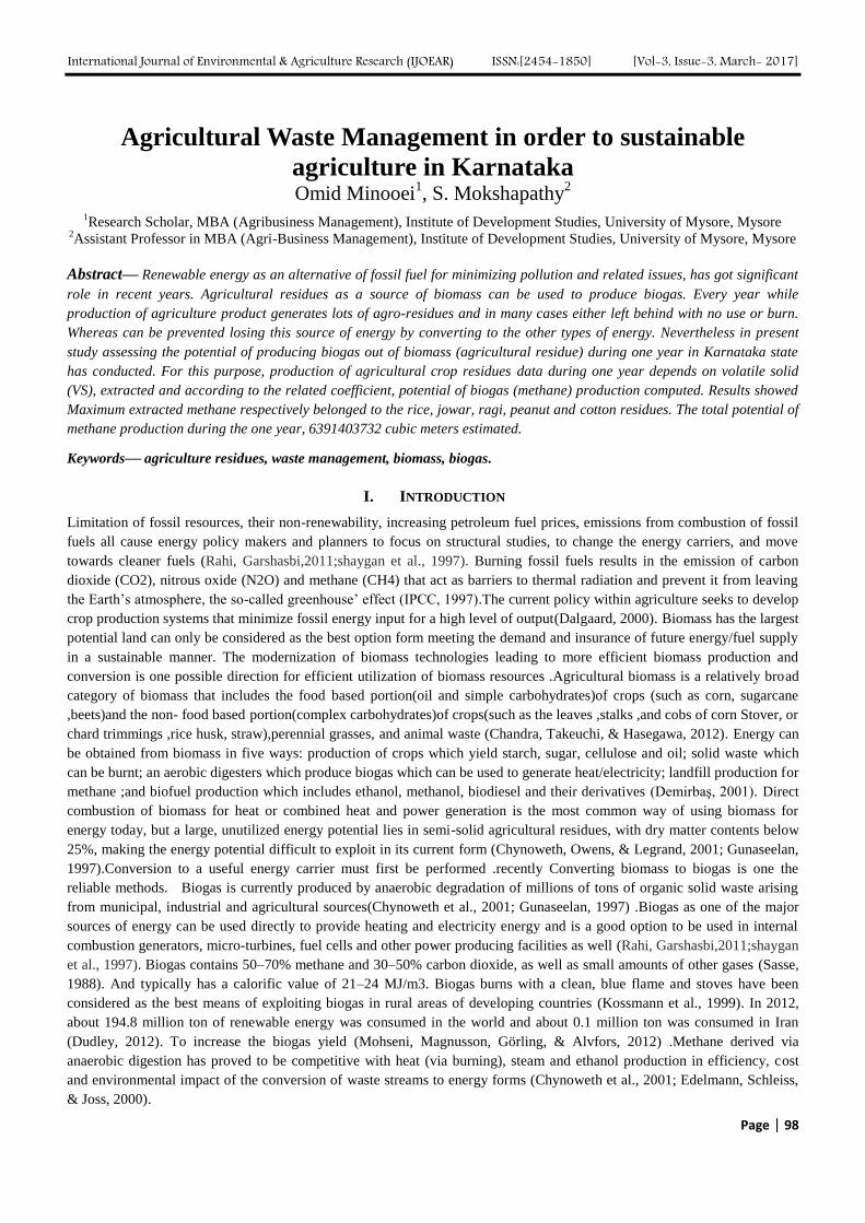
International Journal of Environmental & Agriculture Research (IJOEAR) ISSN:[2454-1850] [Vol-3, Issue-3, March- 2017]
Page | 98
Agricultural Waste Management in order to sustainable
agriculture in Karnataka
Omid Minooei1, S. Mokshapathy
2
1Research Scholar, MBA (Agribusiness Management), Institute of Development Studies, University of Mysore, Mysore
2Assistant Professor in MBA (Agri-Business Management), Institute of Development Studies, University of Mysore, Mysore
Abstract— Renewable energy as an alternative of fossil fuel for minimizing pollution and related issues, has got significant
role in recent years. Agricultural residues as a source of biomass can be used to produce biogas. Every year while
production of agriculture product generates lots of agro-residues and in many cases either left behind with no use or burn.
Whereas can be prevented losing this source of energy by converting to the other types of energy. Nevertheless in present
study assessing the potential of producing biogas out of biomass (agricultural residue) during one year in Karnataka state
has conducted. For this purpose, production of agricultural crop residues data during one year depends on volatile solid
(VS), extracted and according to the related coefficient, potential of biogas (methane) production computed. Results showed
Maximum extracted methane respectively belonged to the rice, jowar, ragi, peanut and cotton residues. The total potential of
methane production during the one year, 6391403732 cubic meters estimated.
Keywords— agriculture residues, waste management, biomass, biogas.
I. INTRODUCTION
Limitation of fossil resources, their non-renewability, increasing petroleum fuel prices, emissions from combustion of fossil
fuels all cause energy policy makers and planners to focus on structural studies, to change the energy carriers, and move
towards cleaner fuels (Rahi, Garshasbi,2011;shaygan et al., 1997). Burning fossil fuels results in the emission of carbon
dioxide (CO2), nitrous oxide (N2O) and methane (CH4) that act as barriers to thermal radiation and prevent it from leaving
the Earth’s atmosphere, the so-called greenhouse’ effect (IPCC, 1997).The current policy within agriculture seeks to develop
crop production systems that minimize fossil energy input for a high level of output(Dalgaard, 2000). Biomass has the largest
potential land can only be considered as the best option form meeting the demand and insurance of future energy/fuel supply
in a sustainable manner. The modernization of biomass technologies leading to more efficient biomass production and
conversion is one possible direction for efficient utilization of biomass resources .Agricultural biomass is a relatively broad
category of biomass that includes the food based portion(oil and simple carbohydrates)of crops (such as corn, sugarcane
,beets)and the non- food based portion(complex carbohydrates)of crops(such as the leaves ,stalks ,and cobs of corn Stover, or
chard trimmings ,rice husk, straw),perennial grasses, and animal waste (Chandra, Takeuchi, & Hasegawa, 2012). Energy can
be obtained from biomass in five ways: production of crops which yield starch, sugar, cellulose and oil; solid waste which
can be burnt; an aerobic digesters which produce biogas which can be used to generate heat/electricity; landfill production for
methane ;and biofuel production which includes ethanol, methanol, biodiesel and their derivatives (Demirbaş, 2001). Direct
combustion of biomass for heat or combined heat and power generation is the most common way of using biomass for
energy today, but a large, unutilized energy potential lies in semi-solid agricultural residues, with dry matter contents below
25%, making the energy potential difficult to exploit in its current form (Chynoweth, Owens, & Legrand, 2001; Gunaseelan,
1997).Conversion to a useful energy carrier must first be performed .recently Converting biomass to biogas is one the
reliable methods. Biogas is currently produced by anaerobic degradation of millions of tons of organic solid waste arising
from municipal, industrial and agricultural sources(Chynoweth et al., 2001; Gunaseelan, 1997) .Biogas as one of the major
sources of energy can be used directly to provide heating and electricity energy and is a good option to be used in internal
combustion generators, micro-turbines, fuel cells and other power producing facilities as well (Rahi, Garshasbi,2011;shaygan
et al., 1997). Biogas contains 50–70% methane and 30–50% carbon dioxide, as well as small amounts of other gases (Sasse,
1988). And typically has a calorific value of 21–24 MJ/m3. Biogas burns with a clean, blue flame and stoves have been
considered as the best means of exploiting biogas in rural areas of developing countries (Kossmann et al., 1999). In 2012,
about 194.8 million ton of renewable energy was consumed in the world and about 0.1 million ton was consumed in Iran
(Dudley, 2012). To increase the biogas yield (Mohseni, Magnusson, Görling, & Alvfors, 2012) .Methane derived via
anaerobic digestion has proved to be competitive with heat (via burning), steam and ethanol production in efficiency, cost
and environmental impact of the conversion of waste streams to energy forms (Chynoweth et al., 2001; Edelmann, Schleiss,
& Joss, 2000).
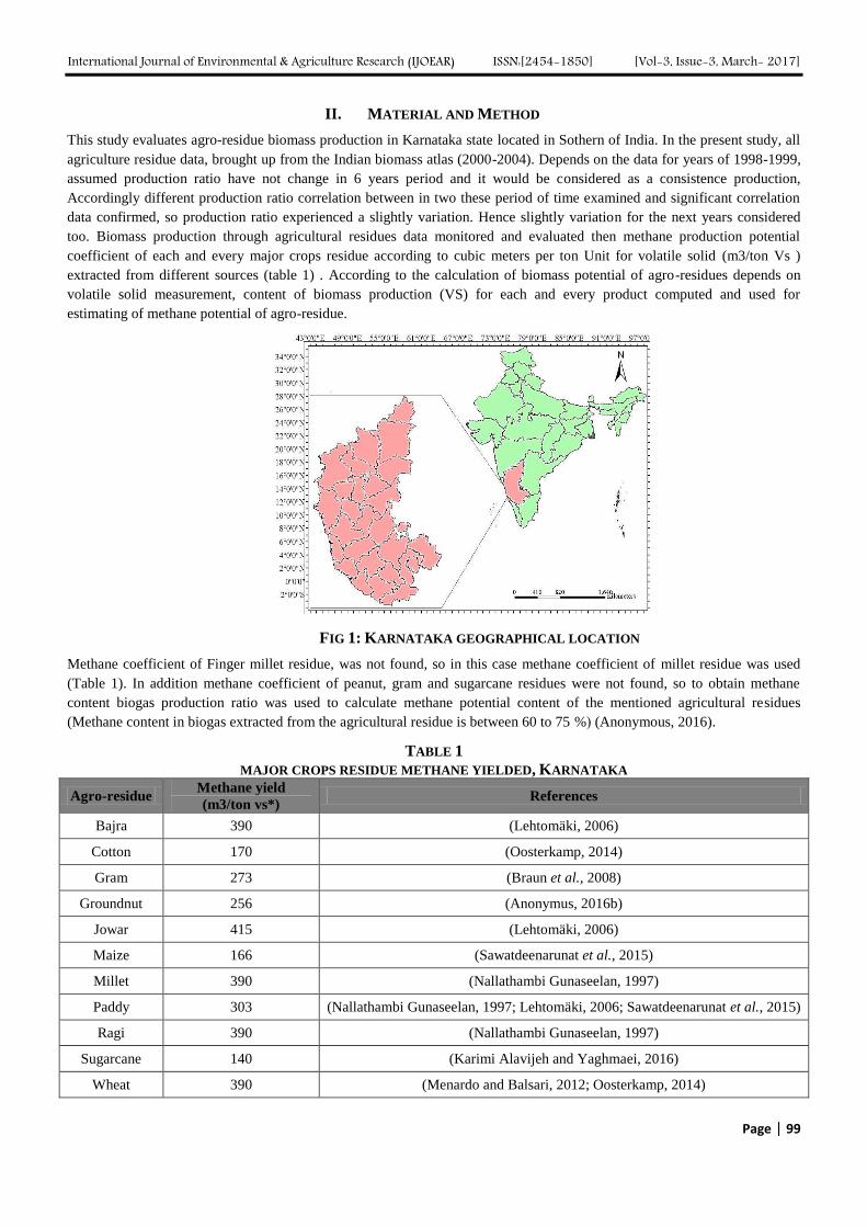
International Journal of Environmental & Agriculture Research (IJOEAR) ISSN:[2454-1850] [Vol-3, Issue-3, March- 2017]
Page | 99
II. MATERIAL AND METHOD
This study evaluates agro-residue biomass production in Karnataka state located in Sothern of India. In the present study, all
agriculture residue data, brought up from the Indian biomass atlas (2000-2004). Depends on the data for years of 1998-1999,
assumed production ratio have not change in 6 years period and it would be considered as a consistence production,
Accordingly different production ratio correlation between in two these period of time examined and significant correlation
data confirmed, so production ratio experienced a slightly variation. Hence slightly variation for the next years considered
too. Biomass production through agricultural residues data monitored and evaluated then methane production potential
coefficient of each and every major crops residue according to cubic meters per ton Unit for volatile solid (m3/ton Vs )
extracted from different sources (table 1) . According to the calculation of biomass potential of agro-residues depends on
volatile solid measurement, content of biomass production (VS) for each and every product computed and used for
estimating of methane potential of agro-residue.
FIG 1: KARNATAKA GEOGRAPHICAL LOCATION
Methane coefficient of Finger millet residue, was not found, so in this case methane coefficient of millet residue was used
(Table 1). In addition methane coefficient of peanut, gram and sugarcane residues were not found, so to obtain methane
content biogas production ratio was used to calculate methane potential content of the mentioned agricultural residues
(Methane content in biogas extracted from the agricultural residue is between 60 to 75 %( (Anonymous, 2016).
TABLE 1
MAJOR CROPS RESIDUE METHANE YIELDED, KARNATAKA
Agro-residue Methane yield
(m3/ton vs*) References
Bajra 390 (Lehtomäki, 2006)
Cotton 170 (Oosterkamp, 2014)
Gram 273 (Braun et al., 2008)
Groundnut 256 (Anonymus, 2016b)
Jowar 415 (Lehtomäki, 2006)
Maize 166 (Sawatdeenarunat et al., 2015)
Millet 390 (Nallathambi Gunaseelan, 1997)
Paddy 303 (Nallathambi Gunaseelan, 1997; Lehtomäki, 2006; Sawatdeenarunat et al., 2015)
Ragi 390 (Nallathambi Gunaseelan, 1997)
Sugarcane 140 (Karimi Alavijeh and Yaghmaei, 2016)
Wheat 390 (Menardo and Balsari, 2012; Oosterkamp, 2014)
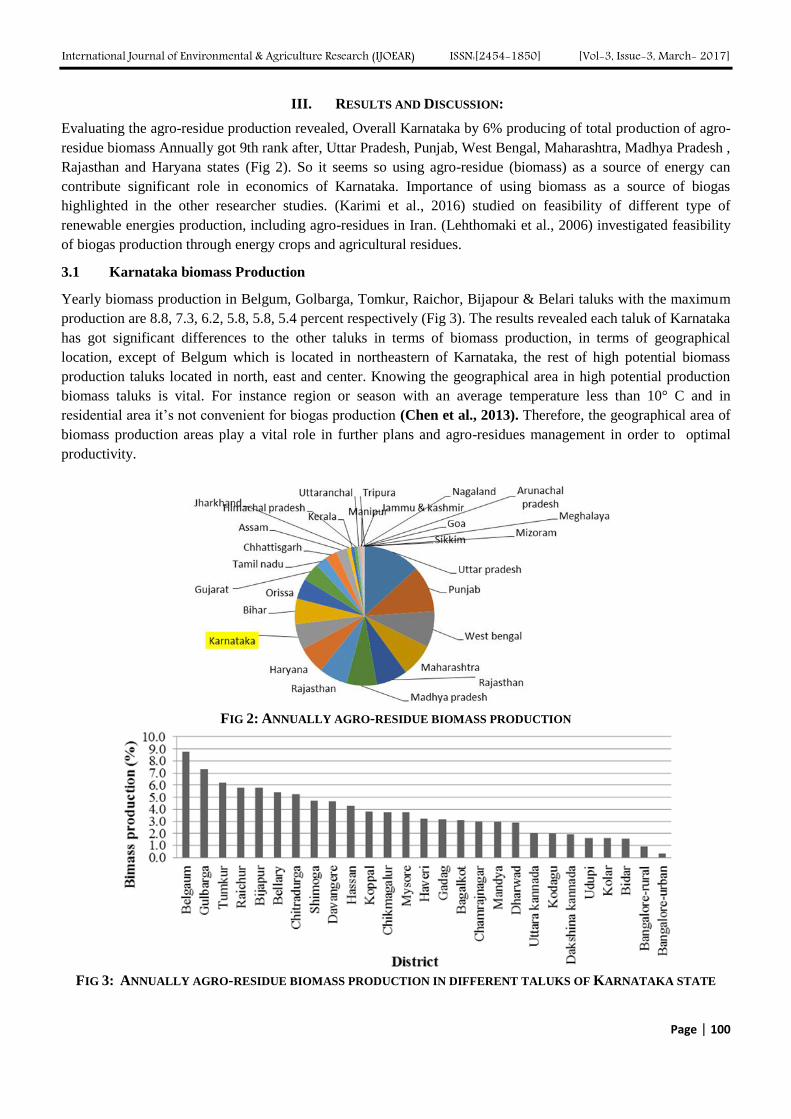
International Journal of Environmental & Agriculture Research (IJOEAR) ISSN:[2454-1850] [Vol-3, Issue-3, March- 2017]
Page | 100
III. RESULTS AND DISCUSSION:
Evaluating the agro-residue production revealed, Overall Karnataka by 6% producing of total production of agro-
residue biomass Annually got 9th rank after, Uttar Pradesh, Punjab, West Bengal, Maharashtra, Madhya Pradesh ,
Rajasthan and Haryana states (Fig 2). So it seems so using agro-residue (biomass) as a source of energy can
contribute significant role in economics of Karnataka. Importance of using biomass as a source of biogas
highlighted in the other researcher studies. (Karimi et al., 2016) studied on feasibility of different type of
renewable energies production, including agro-residues in Iran. (Lehthomaki et al., 2006) investigated feasibility
of biogas production through energy crops and agricultural residues.
3.1 Karnataka biomass Production
Yearly biomass production in Belgum, Golbarga, Tomkur, Raichor, Bijapour & Belari taluks with the maximum
production are 8.8, 7.3, 6.2, 5.8, 5.8, 5.4 percent respectively (Fig 3). The results revealed each taluk of Karnataka
has got significant differences to the other taluks in terms of biomass production, in terms of geographical
location, except of Belgum which is located in northeastern of Karnataka, the rest of high potential biomass
production taluks located in north, east and center. Knowing the geographical area in high potential production
biomass taluks is vital. For instance region or season with an average temperature less than 10° C and in
residential area it’s not convenient for biogas production (Chen et al., 2013). Therefore, the geographical area of
biomass production areas play a vital role in further plans and agro-residues management in order to optimal
productivity.
FIG 2: ANNUALLY AGRO-RESIDUE BIOMASS PRODUCTION
FIG 3: ANNUALLY AGRO-RESIDUE BIOMASS PRODUCTION IN DIFFERENT TALUKS OF KARNATAKA STATE
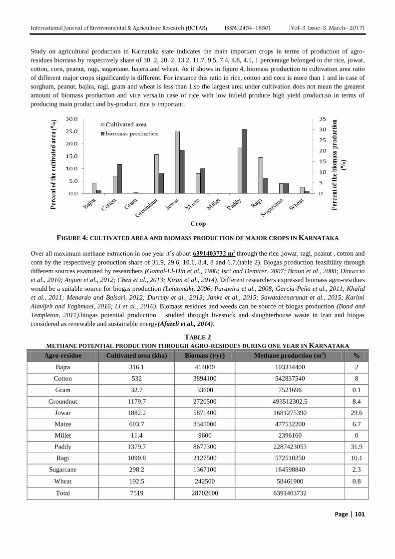
International Journal of Environmental & Agriculture Research (IJOEAR) ISSN:[2454-1850] [Vol-3, Issue-3, March- 2017]
Page | 101
Study on agricultural production in Karnataka state indicates the main important crops in terms of production of agro-
residues biomass by respectively share of 30. 2, 20. 2, 13.2, 11.7, 9.5, 7.4, 4.8, 4.1, 1 percentage belonged to the rice, jowar,
cotton, corn, peanut, ragi, sugarcane, bajera and wheat. As it shows in figure 4, biomass production to cultivation area ratio
of different major crops significantly is different. For instance this ratio in rice, cotton and corn is more than 1 and in case of
sorghum, peanut, bajira, ragi, gram and wheat is less than 1.so the largest area under cultivation does not mean the greatest
amount of biomass production and vice versa.in case of rice with low infield produce high yield product.so in terms of
producing main product and by-product, rice is important.
FIGURE 4: CULTIVATED AREA AND BIOMASS PRODUCTION OF MAJOR CROPS IN KARNATAKA
Over all maximum methane extraction in one year it’s about 2373043936 m3 through the rice ,jowar, ragi, peanut , cotton and
corn by the respectively production share of 31.9, 29.6, 10.1, 8.4, 8 and 6.7.(table 2). Biogas production feasibility through
different sources examined by researchers (Gamal-El-Din et al., 1986; Isci and Demirer, 2007; Braun et al., 2008; Dinuccio
et al., 2010; Anjum et al., 2012; Chen et al., 2013; Kiran et al., 2014). Different researchers expressed biomass agro-residues
would be a suitable source for biogas production (Lehtomäki, 2006; Parawira et al., 2008; Garcia-Peña et al., 2011; Khalid
et al., 2011; Menardo and Balsari, 2012; Durruty et al., 2013; Janke et al., 2015; Sawatdeenarunat et al., 2015; Karimi
Alavijeh and Yaghmaei, 2016; Li et al., 2016). Biomass residues and weeds can be source of biogas production (Bond and
Templeton, 2011).biogas potential production studied through livestock and slaughterhouse waste in Iran and biogas
considered as renewable and sustainable energy(Afazeli et al., 2014).
TABLE 2
METHANE POTENTIAL PRODUCTION THROUGH AGRO-RESIDUES DURING ONE YEAR IN KARNATAKA
Agro-residue Cultivated area (kha) Biomass (t/yr) Methane production (m3) %
Bajra 316.1 414000 103334400 2
Cotton 532 3894100 542837540 8
Gram 32.7 33600 7521696 0.1
Groundnut 1179.7 2720500 493512302.5 8.4
Jowar 1882.2 5871400 1681275390 29.6
Maize 603.7 3345000 477532200 6.7
Millet 11.4 9600 2396160 0
Paddy 1379.7 8677300 2287423053 31.9
Ragi 1090.8 2127500 572510250 10.1
Sugarcane 298.2 1367100 164598840 2.3
Wheat 192.5 242500 58461900 0.8
Total 7519 28702600 6391403732
International Journal of Environmental & Agriculture Research (IJOEAR) ISSN:[2454-1850] [Vol-3, Issue-3, March- 2017]
Page | 102
IV. CONCLUSION
Besides of Limited fusil fuels and energy crisis, extensively non-renewable energy using results to the environmental issues
and global warming. So one of the initial actions for the saving our environmental from global warming and related issues is
replacing of non-renewable energy to the renewable form of energy. Biomass as a source of renewable energy because of
variety of advantages highly suggested by researchers. One of the biomass sources is agricultural residues that left largely
unused on the agriculture field and can be consider as a main important sources for renewable energies. Out of biomass, bio-
methane/biogas would be produced and its valuable as natural gas or other type of fossil fuel are. Biogas can use to produce
electricity or even heating, cooling, pumping, or used as vehicle fuel.
According to the results, agricultural crop residues considered as reliable source for renewable energy production in form of
biogas in Karnataka. Results shows 91.6 % of total methane production obtain from rice, jowar, ragi, peanut, cotton, corn
residues. Factors such a climate, (temperature above 20 ° C), solar energy and biomass resources have a key role in optimum
methane extraction. (chen et al ., 2013) . According to diversified climate of Karnataka and high production of agro-residue
biomass, it seems to biomass as a renewable energy can be considered for supplying some part of demanded energy in
Karnataka.
REFERENCES
[1] Afazeli, H., Jafari, A., Rafiee, S., & Nosrati, M. (2014). An investigation of biogas production potential from livestock and
slaughterhouse wastes. Renewable and Sustainable Energy Reviews, 34, 380–386.
[2] Alavijeh, M. K., & Yaghmaei, S. (2016). Biochemical production of bioenergy from agricultural crops and residue in Iran. Waste
Management, 52, 375–394.
[3] Anjum, M., Khalid, A., Mahmood, T., & Arshad, M. (2012). Anaerobic co-digestion of municipal solid organic waste with melon
residues to enhance biodegradability and biogas production. Journal of Material Cycles and Waste Management, 14(4), 388–395.
[4] Anonymus,2016b.Gas Yields and Methane Contents for Various Substrates. https://energypedia.info/wiki/Gas Yields and Methane
Contents for Various Substrates.
[5] Bond, T., & Templeton, M. R. (2011). History and future of domestic biogas plants in the developing world. Energy for Sustainable
Development, 15(4), 347–354.
[6] Braun, R., Weiland, P., & Wellinger, A. (2008). Biogas from energy crop digestion. In IEA bioenergy task (Vol. 37, pp. 1–20).
[7] Chandra, R., Takeuchi, H., & Hasegawa, T. (2012). Methane production from lignocellulosic agricultural crop wastes: A review in
context to second generation of biofuel production. Renewable and Sustainable Energy Reviews, 16(3), 1462–1476.
[8] Chynoweth, D. P., Owens, J. M., & Legrand, R. (2001). Renewable methane from anaerobic digestion of biomass. Renewable
Energy, 22(1–3), 1–8. https://doi.org/http://dx.doi.org/10.1016/S0960-1481 (00)00019-7
[9] Dalgaard, T. (2000). Farm types-How can they be used to structure, model and generalise farm data? In Agricultural data for life
cycle assessments. Agricultural economics research Institute (LEI).
[10] Demirbaş, A. (2001). Biomass resource facilities and biomass conversion processing for fuels and chemicals. Energy Conversion and
Management, 42(11), 1357–1378.
[11] Dimpl, E. (2010). Small-scale electricity generation from biomass. Part II: Biogas. Deutsche Gesellschaft Für Technische
Zusammenarbeit (GTZ)-HERA.
[12] Dimpl, E., & from Biomass, S. E. G. (2010). Part II: Biogas. Deutsche Gesellschaft Für Technische Zusammenarbeit (GTZ)-HERA.
[13] Dinuccio, E., Balsari, P., Gioelli, F., & Menardo, S. (2010). Evaluation of the biogas productivity potential of some Italian agro-
industrial biomasses. Bioresource Technology, 101(10), 3780–3783.
[14] Dudley, B. (2012). BP statistical review of world energy. June 2012. London, UK.
[15] Durruty, I., Zaritzky, N. E., & González, J. F. (2013). Organic fractions influence on biogas generation from potato residues. Kinetic
model generalization. Biomass and Bioenergy, 59, 458–467.
[16] Edelmann, W., Schleiss, K., & Joss, A. (2000). Ecological, energetic and economic comparison of anaerobic digestion with different
competing technologies to treat biogenic wastes. Water Science and Technology, 41(3), 263 LP-273. Retrieved from
http://wst.iwaponline.com/content/41/3/263.abstract
[17] Rahi A, Garshasbi M. Biogas production process and manufacturing biogas plants for distributed. In: Proceedings of the first
bioenergy conference. Iran; 2011
[18] Gamal-El-Din, H., El-Bassel, A., & El-Badry, M. (1986). Biogas Production from Some Organic Wastes. In Biogas Technology,
Transfer and Diffusion (pp. 463–473). Springer.
[19] Garcia-Peña, E. I., Parameswaran, P., Kang, D. W., Canul-Chan, M., & Krajmalnik-Brown, R. (2011). Anaerobic digestion and co-
digestion processes of vegetable and fruit residues: Process and microbial ecology. Bioresource Technology, 102(20), 9447–9455.
https://doi.org/10.1016/j.biortech.2011.07.068
[20] Garcia-Peña, E. I., Parameswaran, P., Kang, D. W., Canul-Chan, M., & Krajmalnik-Brown, R. (2011). Anaerobic digestion and co-
digestion processes of vegetable and fruit residues: process and microbial ecology. Bioresource Technology, 102(20), 9447–9455.
International Journal of Environmental & Agriculture Research (IJOEAR) ISSN:[2454-1850] [Vol-3, Issue-3, March- 2017]
Page | 103
[21] Gunaseelan, V. N. (1997). Anaerobic digestion of biomass for methane production: a review. Biomass and Bioenergy, 13(1–2), 83–
114.
[22] Intergovernmental Panel on Climate Change (IPCC)., 1997. In: Houghton, J.T. (Ed.), Greenhouse Gas Inventory Reference Manual,
vol. 3. IPCC Technical Support Unit, London
[23] Isci, A., & Demirer, G. N. (2007). Biogas production potential from cotton wastes. Renewable Energy, 32(5), 750–757.
[24] Khalid, A., Arshad, M., Anjum, M., Mahmood, T., & Dawson, L. (2011). The anaerobic digestion of solid organic waste. Waste
Management, 31(8), 1737–1744.
[25] Kiran, E. U., Trzcinski, A. P., Ng, W. J., & Liu, Y. (2014). Bioconversion of food waste to energy: a review. Fuel, 134, 389–399.
[26] Kossmann, W., Pönitz, U., Habermehl, S., Hoerz, T., Krämer, P., Klingler, B., Krieg, A. (1999). Biogas Digest, Volume II–Biogas–
Application and Product Development. Information and Advisory Service on Appropriate Technology, Eschborn.
[27] Lehtomäki, A. (2006). Biogas production from energy crops and crop residues. University of Jyväskylä.
[28] Menardo, S., & Balsari, P. (2012). An analysis of the energy potential of anaerobic digestion of agricultural by-products and organic
waste. BioEnergy Research, 5(3), 759–767.
[29] Mohseni, F., Magnusson, M., Görling, M., & Alvfors, P. (2012). Biogas from renewable electricity–Increasing a climate neutral fuel
supply. Applied Energy, 90(1), 11–16.
[30] Nallathambi Gunaseelan, V. (1997). Anaerobic digestion of biomass for methane production: A review. Biomass and Bioenergy,
13(1), 83–114. https://doi.org/http://dx.doi.org/10.1016/S0961-9534(97)00020-2
[31] Oosterkamp, W. J. (2014). Use of volatile solids from biomatter for energy production. Bioenergy Research: Advances and
Applications” Elsevier, Chennai, India.
[32] Parawira, W., Read, J. S., Mattiasson, B., & Björnsson, L. (2008). Energy production from agricultural residues: high methane yields
in pilot-scale two-stage anaerobic digestion. Biomass and Bioenergy, 32(1), 44–50.
[33] Shaygan J, Mehdizadeh H, Ghavipanjeh F. Convert organic waste into methane using anaerobic purification. First biogas seminar.
Iran; 1997. p. 32–46.
[34] Sawatdeenarunat, C., Surendra, K. C., Takara, D., Oechsner, H., & Khanal, S. K. (2015). Anaerobic digestion of lignocellulosic
biomass: Challenges and opportunities. Bioresource Technology, 178, 178–186.
[35] Singal, R., & Grimes, S. R. (2001). New Microsoft Word Document (2). Biotechniques. https://doi.org/Chronic ischaemic mitral
regurgitation. Current treatment results and new mechanism-based surgical approaches.
International Journal of Environmental & Agriculture Research (IJOEAR) ISSN:[2454-1850] [Vol-3, Issue-3, March- 2017]
Page | 104
Uptake of Silver from Polyvinylpyrrolidine Coated Silver
Nanoparticles in a Terrestrial System Sara A. Pappas
1, Uday Turaga
2, Naveen Kumar
3, Seshadri Ramkumar
4,
Ronald J. Kendall5*
1,2,3,5The Wildlife Toxicology Laboratory, The Institute of Environmental and Human Health, Texas Tech University,
Lubbock, TX, USA 4Nonwovens and Advanced Materials Laboratory, The Institute of Environmental and Human Health. Texas Tech
University, Lubbock, TX, USA
Abstract— The widespread use of silver nanoparticles (Ag NPs) has facilitated their uninterrupted entry into various
ecosystems. Nanoparticles are stabilized using a variety of approaches for various applications. The present study has
investigated the uptake of polyvinylpyrrolidine (PVP) coated Ag NPs in a terrestrial system. Two insect (Acheta domesticus
and Tenebrio molitor) and two plant species (Sorghum vulgare and Helianthus annuus) were used in the study. The effect of
concentration and size of PVP-coated Ag NPs was investigated. The test species were maintained in soil spiked with 0, 1, 5,
25, 125, and 625 mg/kg PVP-coated 30-50 nm Ag NPs to test the effect of concentration of Ag NPs on uptake. Similarly, the
test species were maintained in soil spiked with 25 mg/kg of 20, 30-50, and 50-80 nm PVP-coated Ag NPs to study the effect
of size of nanoparticles on uptake. The PVP-coated Ag NPs were characterized using transmission electron microscopy,
dynamic light scattering and powder X-ray diffraction techniques. The levels of silver in test samples were measured using
inductively coupled plasma-optical emission spectroscopy. A concentration dependent increase in the levels of Ag in both the
insect species was observed as a function of increasing concentrations of coated Ag NPs in soil. An increase in the levels of
Ag as a function of increasing size of coated Ag NPs was observed with Acheta domesticus. No apparent trend was observed
with Tenebrio molitor species. A concentration dependent increase in the levels of Ag in the roots of both the plants was
observed as a function of increasing concentrations of coated Ag NPs in soil. Additionally, the translocation of Ag to other
plant tissues was observed in Helianthus annuus, a dicot plant.
Keywords— Silver nanoparticles, polyvinylpyrrolidine, Acheta domesticus, Tenebrio molitor, Sorghum vulgare,
Helianthus annuus, inductively coupled plasma-optical emission spectroscopy.
I. INTRODUCTION
The widespread use of silver nanoparticles (Ag NPs) for a variety of consumer, industrial and medical applications has
resulted in an increase in the anthropogenic release of silver in to the environment [1,2]. Silver from many Ag NP containing
products is predicted to enter into the wastewater streams and eventually wastewater treatment plants [3]. Much of the silver
at the treatment plants is partitioned in to sewage sludge [2,4,5]. Ag NPs eventually find their way in to the terrestrial
ecosystems through the application of sewage sludge to agricultural lands [4].
The colloidal stability of nanoparticles significantly affects their mobility, uptake/bioavailability, and toxicity in a given
ecosystem [6]. Environmental conditions present in an ecosystem such as pH, ionic strength, background electrolyte
composition, etc. affect the colloidal stability of nanoparticles. Additionally, the presence of capping agents/coatings on
nanoparticles also influences their colloidal stability [7,8]. Ag NPs are highly reactive due to their high surface area-to-
volume ratio. This leads to phenomenon such as particle aggregation and settling in Ag NPs, unless stabilized/protected by
suitable coatings [9,10]. Coatings prevent the aggregation of nanoparticles through electrostatic repulsions, steric repulsions,
and a combination of both [9,11]. Coatings that are commonly used during the synthesis of Ag NPs include chemicals such
as citrate, sodium borohydride (NaBH4), and polyvinylpyrrolidine (PVP) [9,11].
PVP coatings are known to sterically stabilize Ag NPs. The mechanism of steric stabilization of nanoparticles involves the
adsorption of uncharged polymer on the surface of nanoparticles [6,12,13]. Another mechanism involves the formation of
weak coordinative bonds between PVP and Ag+ ions [14,15]. The effect of surface coatings on the stability, transformation,
uptake, and toxicity of nanoparticles has been discussed in literature [13, 16-21]. The present study investigates the uptake of
PVP-coated Ag NPs (henceforth referred to as coated Ag NPs) in a terrestrial system by two insect (Acheta domesticus and
Tenebrio molitor) and plant species (Sorghum vulgare and Helianthus annuus). PVP-coated Ag NPs were chosen as they
demonstrated excellent shape and size stability characteristics in an ecotoxicological medium compared to other charge
stabilized (citrate coated) Ag NPs [13]. The insect and plant species selected for the study were found to be native to the
region where the soil was collected. Therefore, investigating the uptake of Ag NPs by these species would help us understand
International Journal of Environmental & Agriculture Research (IJOEAR) ISSN:[2454-1850] [Vol-3, Issue-3, March- 2017]
Page | 105
the role of these species in the transport of metal contaminants along the food chain of native insectivorous and granivorous
species.
II. MATERIAL AND METHOD
2.1 Soil collection and preparation
All soil used during the insect and plant exposure experiments were collected in Mitchell County, Texas at an elevation of
684 m above sea level. The soil was collected from the top 10 cm of soil and is shoveled into clean plastic containers. Once
transported to The Institute of Environmental and Human Health (TIEHH) at Texas Tech University (TTU) in Lubbock, TX,
the soil was processed for homogeneity. Large clumps of soil were crushed. Large rocks, roots, living organisms, and other
organic matter were removed. This was followed by sieving of the soil through a 2 mm wire screen into another clean plastic
storage container. Once processed, the soil was covered and stored indoors until ready for use.
2.2 Soil analysis
The analysis of various characteristics of soil samples was performed at the Midwest Laboratories Inc. (Omaha, NE). Soil
texture, percent humic matter, percent organic matter, exchangeable cations (K+, Mg
2+, Ca
2+), available phosphorus (P), soil
pH, percent base saturation of cations (K+, Mg
2+, Ca
2+, H
+), cation exchange capacity (CEC), and sulfur (S) content were all
analyzed in order to fully characterize the soil.
2.3 Nanoparticle Characterization
Silver nanoparticles coated with 0.2% PVP (20, 30-50, and 50-80 nm) were purchased from US Research Nanomaterials,
Inc. (www.us-nano.com, Houston, TX). The US Research Nanomaterial, Inc reported that all Ag NPs consisted of > 99.99%
Ag.
Transmission electron microscopy (TEM) was used to confirm the size range and shape of the coated and uncoated Ag NPs.
The preparation of samples involved the dispersion of Ag NP powder in ethanol (EtOH). Samples were sonicated for 10
minutes before being drop cast onto a carbon coated copper grid. Samples were air dried prior to analysis and TEM (Hitachi
H-8100 TEM) images were taken at 200 kV using a tungsten filament side-mounted camera.
The size of Ag NPs was also confirmed using Dynamic light scattering (DLS). A mixture of 10 mg of Ag NP powder in 10
ml of reagent grade acetone (Fisher Scientific, MA, USA) was sonicated until Ag NPs remained suspended in solution.
Samples were analyzed using a Nanotrac NPA252 Combination (Microtrac Inc. Montgomery, PA) and Mictrotrac Flex
Software (Version: 10.3.14).
The composition of Ag NPs was confirmed using Powder x-ray diffraction (PXRD). A Rigaku Ultima III X-Ray
Diffractometer was used. Ag NPs were analyzed using a Cu Kα radiation as x-ray source. The following instrument
parameters were used to analyze the Ag NPs: parallel-beam geometry was used with a step width of 0.03° and a count time
of one second; the divergence, scattering, and receiving slits were set at one. Once completed, the diffraction patterns were
compared and matched to the phases in the International Center for Diffraction Data (ICDD) powder diffraction file (PDF)
database.
2.4 Exposure of insects to coated Ag NPs
Two 37.8 L terrariums were prepared for each insect treatment group. Exactly 2.5 kg of prepared soil was weighed out into
each clean terrarium. The insect species were maintained in soil spiked with a range of concentrations of 30-50 nm coated Ag
NPs (0, 1, 5, 25, 125, and 625 mg/kg) to understand the effect of concentration of Ag NPs on uptake. Additionally, the effect
of size of nanoparticles (20, 30-50, and 50-80 nm) on their uptake by the test species was investigated by spiking the soil
with 25 mg/kg coated Ag NPs. Once the terrariums were prepared, insects were purchased from Reptilefood
(reptilefoods.com, Ohio, USA). Either 300 small crickets or 400 large mealworms were placed in each of the terratiums and
were provided with fresh food and water as needed for the duration of the 28 day exposure period. After the 28 day exposure
had run to completion, insects were carefully extracted from the terrariums and placed in glass jars. The jars were then placed
in a -80°C freezer until all the insects were deceased. Freeze drying of the insects (FreeZone 2.5 Liter Freeze Dry System,
Labconco, Corp. Kansas City, MO) for at least 48 hours was performed to ensure the removal of all moisture. Finally, the
freeze dried insects were then crushed into a fine powder and stored in a freezer until further use.
2.5 Exposure of plants to coated Ag NPs
This set of experiments was performed in commercially available 7.6 L plastic nursery containers. The containers were filled
with approximately two inches of commercial pond pebbles to aid in proper drainage. As detailed in the insect sample
International Journal of Environmental & Agriculture Research (IJOEAR) ISSN:[2454-1850] [Vol-3, Issue-3, March- 2017]
Page | 106
section above, the plant species were maintained in soil spiked with a range of concentrations of 30-50 nm coated Ag NPs (0,
1, 5, 25, 125, and 625 mg/kg) to understand the effect of concentration of Ag NPs on uptake. Additionally, the effect of size
of nanoparticles (20, 30-50, and 50-80 nm) on their uptake by the test species was investigated by spiking the soil with 25
mg/kg coated Ag NPs.
Seeds for the two plant species were planted into their own completed nursery containers and were transported to the TTU
greenhouse. The plants were maintained in the TTU greenhouse until maturity, approximately three months for H. annuus
and six months for S. vulgare. The plants received shaded sunlight and were maintained at 60°F or above in the TTU
greenhouse. The entire plant was harvested after it reached maturity. The roots of the plants were separated rinsed using tap
water for one minute to remove all attached soil. The shoot system of the plant was separated into leaves, stems, and seeds.
The plant samples were stored in a freezer until further use.
2.6 Sample digestions
Three identical samples were weighed out using the insect samples collected from each terrarium. For each plant treatment
group, four samples were prepared from each nursery container: a root sample, a leaf sample, a stem sample, and a seed
sample, if possible. Dry weights were used in the case of insects and wet weights were used in the case of plants. 10 ml of
70% nitric acid (HNO3, reagent grade) was added to 1 gm of insect or plant samples in a 100 ml beaker. 10 ml of 30%
hydrogen peroxide (H2O2, reagent grade) was added to this mixture. The beakers were covered with a Telfon watch glass and
the samples were heated in increments of 50 ˚C until the solutions begin to reflux gently. To aid in the effective digestion of
all samples, the beakers were periodically swirled. The digestions were stopped when the volume of sample in each of the
beakers reduced to approximately 5 ml. This was followed by placing the beakers in an ice bath to cool. The samples were
then filtered into 50 ml centrifuge tubes (Corning CentriStar TM
, Corning, NY) using ashless filter paper (Whatman No. 41,
Fisher Scientific, PA). Filtering at this step ensures all lipids and other solids were removed from the samples. The original
sample beakers were additionally rinsed twice with 10 ml of 5% HNO3 and the rinse contents were added to the 50 ml
centrifuge tube. The extracts were stored at room temperature until further analysis. A solution containing 10 ml HNO3 and
10 ml H2O2 was used as the reagent blank during the analysis of samples.
2.7 ICP-OES analysis
The samples were analyzed using a Teledyne Instruments (Hudson, New Hampshire) Prodigy High Dispersion Inductively
Coupled Plasma Optical Emission Spectrometer (ICP-OES). The analysis of samples was performed at three wavelengths:
224.643, 328.068, and 338.289 nm. A 10 ppm silver standard solution (SPEX CetriPrep) was used to align all the three
wavelengths of interest. Ultimately, the data from 338.289 nm was chosen for analysis.
2.8 Statistical analysis
A duplicate analysis of samples was performed in the present study (n=2). A normality check was performed and the data
was normalized using Johnson transformation approach (p=0.05). ANOVA was performed on Ag concentrations more than
0.005 μg/g. Samples that contained silver concentrations below instrument detection limits (<0.005 μg/g) were treated as
zeroes. All statistical analysis was performed with 95% confidence interval. The ANOVA test was followed by a multiple
comparison test (Tukey) to identify the significant difference among the treatment groups. Statistical analyses were
performed using MINITAB 17 [Minitab 17 Statistical Software (2010). Computer software, State College, PA: Minitab, Inc.
www.minitab.com].
III. RESULTS AND DISCUSSION
3.1 Soil characterization
The control soil was found to contain 54% sand, 36% silt, and 10% clay. This type of soil is classified as a sandy loam. The
additional tests found the soil to contain 0.01% humic matter, 1.7% organic matter, and 9 ppm S. The pH of the control soil
was slightly basic, 8.1. And the CEC of the soil was calculated to be 18.0 meq/100g. Other data from soil analysis is
summarized in Table 1.
3.2 Transmission electron microscopy
A representative TEM image of coated 20 nm Ag NPs is presented in Fig. 1. As expected with the presence of PVP coatings,
the phenomenon of aggregation is observed to be minimal. The presence of bulk organic materials like PVP on the surface of
Ag NPs prevents the phenomenon of aggregation of nanoparticles through steric repulsions [6,12,13]. A reduction in
aggregation of coated Ag NPs may likely facilitate their uptake in the test species. Additionally, the TEM image confirmed
the spherical shape of coated Ag NPs.
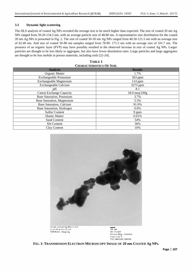
International Journal of Environmental & Agriculture Research (IJOEAR) ISSN:[2454-1850] [Vol-3, Issue-3, March- 2017]
Page | 107
3.3 Dynamic light scattering
The DLS analysis of coated Ag NPs revealed the average size to be much higher than expected. The size of coated 20 nm Ag
NPs ranged from 39.20-154.3 nm, with an average particle size of 48.80 nm. A representative size distribution for the coated
20 nm Ag NPs is presented in Fig. 2. The size of coated 30-50 nm Ag NPs ranged from 40.50-121.5 nm with an average size
of 62.40 nm. And size of coated 50-80 nm samples ranged from 78.90- 171.5 nm with an average size of 101.7 nm. The
presence of an organic layer (PVP) may have possibly resulted in the observed increase in size of coated Ag NPs. Larger
particles are thought to be less likely to aggregate, but also have lower dissolution rates. Large particles and large aggregates
are thought to be less mobile in porous materials, including soils [22-24].
TABLE 1
CHARACTERISTICS OF SOIL Analysis Results
Organic Matter 1.7%
Exchangeable Potassium 263 ppm
Exchangeable Magnesium 114 ppm
Exchangeable Calcium 3273 ppm
pH 8.1
Cation Exchange Capacity 18.0 meq/100g
Base Saturation, Potassium 3.7%
Base Saturation, Magnesium 5.3%
Base Saturation, Calcium 91.0%
Base Saturation, Hydrogen 0.0%
Sulfur Content 9 ppm
Humic Matter 0.01%
Sand Content 54%
Slit Content 36%
Clay Content 10%
FIG. 1: TRANSMISSION ELECTRON MICROSCOPY IMAGE OF 20 nm COATED Ag NPs.
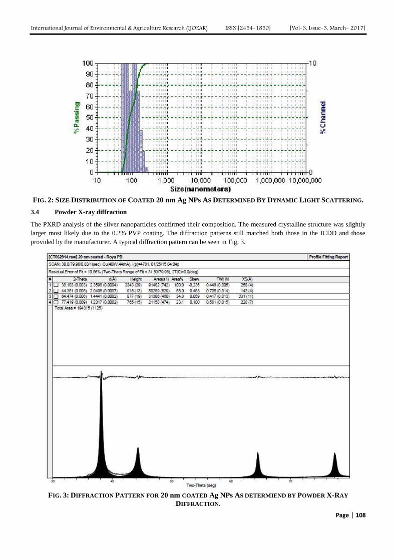
International Journal of Environmental & Agriculture Research (IJOEAR) ISSN:[2454-1850] [Vol-3, Issue-3, March- 2017]
Page | 108
FIG. 2: SIZE DISTRIBUTION OF COATED 20 nm Ag NPs AS DETERMINED BY DYNAMIC LIGHT SCATTERING.
3.4 Powder X-ray diffraction
The PXRD analysis of the silver nanoparticles confirmed their composition. The measured crystalline structure was slightly
larger most likely due to the 0.2% PVP coating. The diffraction patterns still matched both those in the ICDD and those
provided by the manufacturer. A typical diffraction pattern can be seen in Fig. 3.
FIG. 3: DIFFRACTION PATTERN FOR 20 nm COATED Ag NPs AS DETERMIEND BY POWDER X-RAY
DIFFRACTION.
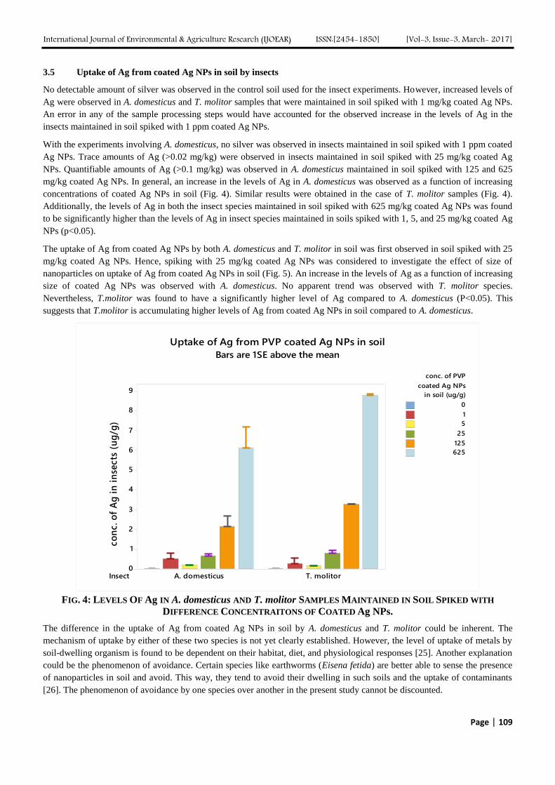
International Journal of Environmental & Agriculture Research (IJOEAR) ISSN:[2454-1850] [Vol-3, Issue-3, March- 2017]
Page | 109
3.5 Uptake of Ag from coated Ag NPs in soil by insects
No detectable amount of silver was observed in the control soil used for the insect experiments. However, increased levels of
Ag were observed in A. domesticus and T. molitor samples that were maintained in soil spiked with 1 mg/kg coated Ag NPs.
An error in any of the sample processing steps would have accounted for the observed increase in the levels of Ag in the
insects maintained in soil spiked with 1 ppm coated Ag NPs.
With the experiments involving A. domesticus, no silver was observed in insects maintained in soil spiked with 1 ppm coated
Ag NPs. Trace amounts of Ag (>0.02 mg/kg) were observed in insects maintained in soil spiked with 25 mg/kg coated Ag
NPs. Quantifiable amounts of Ag (>0.1 mg/kg) was observed in A. domesticus maintained in soil spiked with 125 and 625
mg/kg coated Ag NPs. In general, an increase in the levels of Ag in A. domesticus was observed as a function of increasing
concentrations of coated Ag NPs in soil (Fig. 4). Similar results were obtained in the case of T. molitor samples (Fig. 4).
Additionally, the levels of Ag in both the insect species maintained in soil spiked with 625 mg/kg coated Ag NPs was found
to be significantly higher than the levels of Ag in insect species maintained in soils spiked with 1, 5, and 25 mg/kg coated Ag
NPs (p<0.05).
The uptake of Ag from coated Ag NPs by both A. domesticus and T. molitor in soil was first observed in soil spiked with 25
mg/kg coated Ag NPs. Hence, spiking with 25 mg/kg coated Ag NPs was considered to investigate the effect of size of
nanoparticles on uptake of Ag from coated Ag NPs in soil (Fig. 5). An increase in the levels of Ag as a function of increasing
size of coated Ag NPs was observed with A. domesticus. No apparent trend was observed with T. molitor species.
Nevertheless, T.molitor was found to have a significantly higher level of Ag compared to A. domesticus (P<0.05). This
suggests that T.molitor is accumulating higher levels of Ag from coated Ag NPs in soil compared to A. domesticus.
Insect T. molitorA. domesticus
9
8
7
6
5
4
3
2
1
0
co
nc. o
f A
g i
n i
nse
cts
(u
g/g
)
0
1
5
25
125
625
in soil (ug/g)
coated Ag NPs
conc. of PVP
Uptake of Ag from PVP coated Ag NPs in soil
Bars are 1SE above the mean
FIG. 4: LEVELS OF Ag IN A. domesticus AND T. molitor SAMPLES MAINTAINED IN SOIL SPIKED WITH
DIFFERENCE CONCENTRAITONS OF COATED Ag NPs.
The difference in the uptake of Ag from coated Ag NPs in soil by A. domesticus and T. molitor could be inherent. The
mechanism of uptake by either of these two species is not yet clearly established. However, the level of uptake of metals by
soil-dwelling organism is found to be dependent on their habitat, diet, and physiological responses [25]. Another explanation
could be the phenomenon of avoidance. Certain species like earthworms (Eisena fetida) are better able to sense the presence
of nanoparticles in soil and avoid. This way, they tend to avoid their dwelling in such soils and the uptake of contaminants
[26]. The phenomenon of avoidance by one species over another in the present study cannot be discounted.
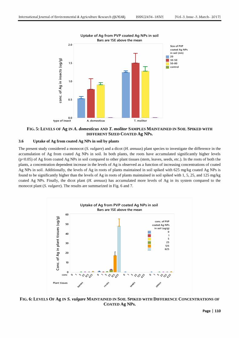
International Journal of Environmental & Agriculture Research (IJOEAR) ISSN:[2454-1850] [Vol-3, Issue-3, March- 2017]
Page | 110
type of insect T. molitorA. domesticus
2.0
1.5
1.0
0.5
0.0
co
nc. o
f A
g i
n i
nse
cts
(u
g/g
)20
30-50
50-80
control
in soil (nm)
coated Ag NPs
Size of PVP
Uptake of Ag from PVP coated Ag NPs in soil
Bars are 1SE above the mean
FIG. 5: LEVELS OF Ag IN A. domesticus AND T. molitor SAMPLES MAINTAINED IN SOIL SPIKED WITH
DIFFERENT SIZED COATED Ag NPs.
3.6 Uptake of Ag from coated Ag NPs in soil by plants
The present study considered a monocot (S. vulgare) and a dicot (H. annuus) plant species to investigate the difference in the
accumulation of Ag from coated Ag NPs in soil. In both plants, the roots have accumulated significantly higher levels
(p<0.05) of Ag from coated Ag NPs in soil compared to other plant tissues (stem, leaves, seeds, etc.). In the roots of both the
plants, a concentration dependent increase in the levels of Ag is observed as a function of increasing concentrations of coated
Ag NPs in soil. Additionally, the levels of Ag in roots of plants maintained in soil spiked with 625 mg/kg coated Ag NPs is
found to be significantly higher than the levels of Ag in roots of plants maintained in soil spiked with 1, 5, 25, and 125 mg/kg
coated Ag NPs. Finally, the dicot plant (H. annuus) has accumulated more levels of Ag in its system compared to the
monocot plant (S. vulgare). The results are summarized in Fig. 6 and 7.
Plant tissues
conc
stem
s
seed
s
root
s
leav
es
625
12525510
625
12525510
62512
52551062512
525510
60
50
40
30
20
10
0
Co
nc. o
f A
g i
n p
lan
t ti
ssu
es
(ug
/g)
0
1
5
25
125
625
in soil (ug/g)
coated Ag NPs
conc. of PVP
Uptake of Ag from PVP coated Ag NPs in soil
Bars are 1SE above the mean
FIG. 6: LEVELS OF Ag IN S. vulgare MAINTAINED IN SOIL SPIKED WITH DIFFERENCE CONCENTRATIONS OF
COATED Ag NPs.
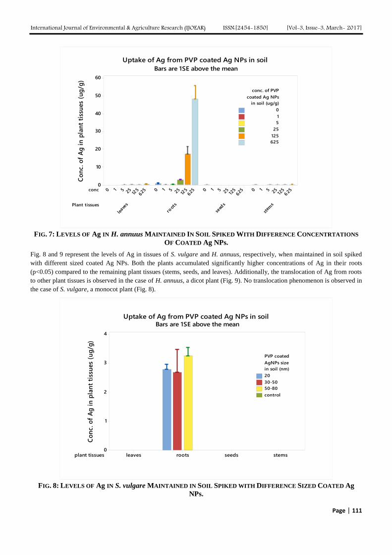
International Journal of Environmental & Agriculture Research (IJOEAR) ISSN:[2454-1850] [Vol-3, Issue-3, March- 2017]
Page | 111
Plant tissues
conc
stem
s
seed
s
root
s
leav
es
625
12525510
625
12525510
62512
52551062512
525510
60
50
40
30
20
10
0
Co
nc. o
f A
g i
n p
lan
t ti
ssu
es
(ug
/g)
0
1
5
25
125
625
in soil (ug/g)
coated Ag NPs
conc. of PVP
Uptake of Ag from PVP coated Ag NPs in soil
Bars are 1SE above the mean
FIG. 7: LEVELS OF Ag IN H. annuus MAINTAINED IN SOIL SPIKED WITH DIFFERENCE CONCENTRTATIONS
OF COATED Ag NPs.
Fig. 8 and 9 represent the levels of Ag in tissues of S. vulgare and H. annuus, respectively, when maintained in soil spiked
with different sized coated Ag NPs. Both the plants accumulated significantly higher concentrations of Ag in their roots
(p<0.05) compared to the remaining plant tissues (stems, seeds, and leaves). Additionally, the translocation of Ag from roots
to other plant tissues is observed in the case of H. annuus, a dicot plant (Fig. 9). No translocation phenomenon is observed in
the case of S. vulgare, a monocot plant (Fig. 8).
plant tissues stemsseedsrootsleaves
4
3
2
1
0
Co
nc. o
f A
g i
n p
lan
t ti
ssu
es
(ug
/g)
20
30-50
50-80
control
in soil (nm)
AgNPs size
PVP coated
Uptake of Ag from PVP coated Ag NPs in soilBars are 1SE above the mean
FIG. 8: LEVELS OF Ag IN S. vulgare MAINTAINED IN SOIL SPIKED WITH DIFFERENCE SIZED COATED Ag
NPs.
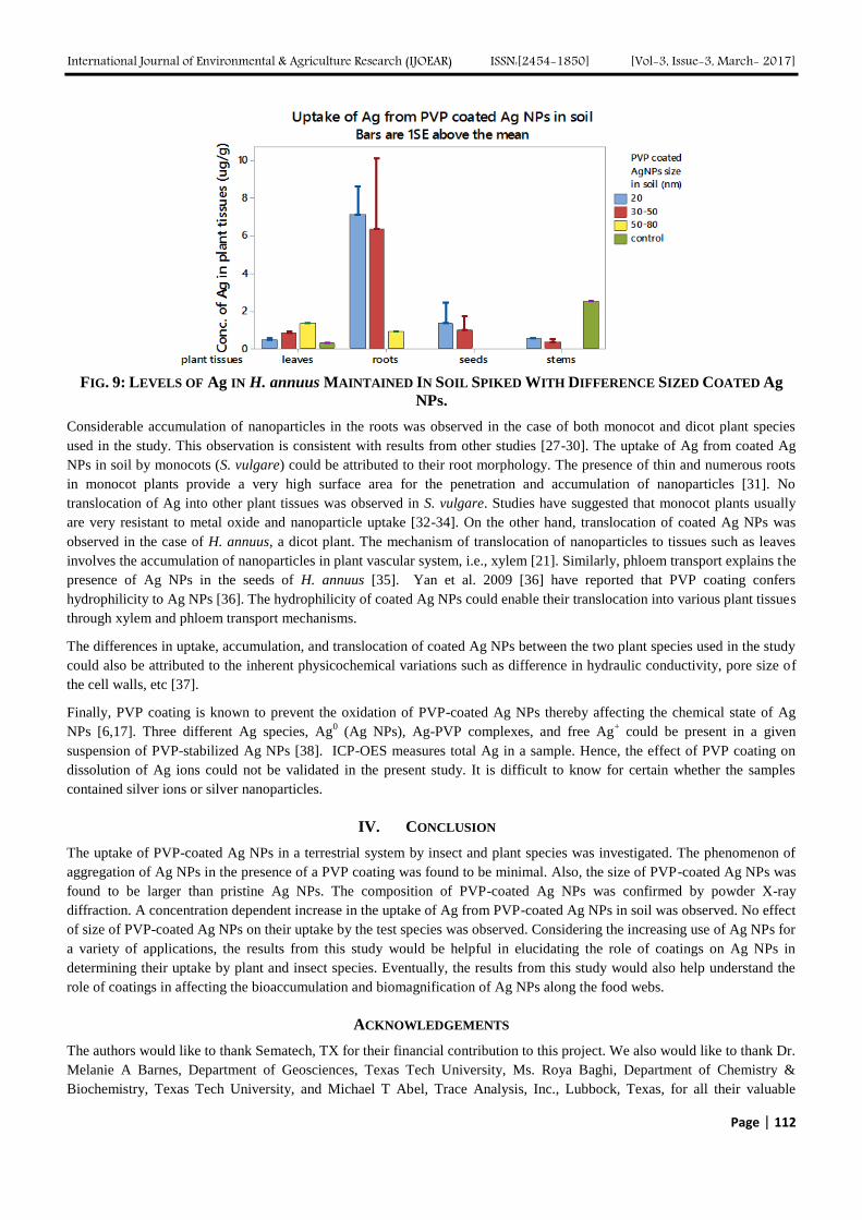
International Journal of Environmental & Agriculture Research (IJOEAR) ISSN:[2454-1850] [Vol-3, Issue-3, March- 2017]
Page | 112
FIG. 9: LEVELS OF Ag IN H. annuus MAINTAINED IN SOIL SPIKED WITH DIFFERENCE SIZED COATED Ag
NPs.
Considerable accumulation of nanoparticles in the roots was observed in the case of both monocot and dicot plant species
used in the study. This observation is consistent with results from other studies [27-30]. The uptake of Ag from coated Ag
NPs in soil by monocots (S. vulgare) could be attributed to their root morphology. The presence of thin and numerous roots
in monocot plants provide a very high surface area for the penetration and accumulation of nanoparticles [31]. No
translocation of Ag into other plant tissues was observed in S. vulgare. Studies have suggested that monocot plants usually
are very resistant to metal oxide and nanoparticle uptake [32-34]. On the other hand, translocation of coated Ag NPs was
observed in the case of H. annuus, a dicot plant. The mechanism of translocation of nanoparticles to tissues such as leaves
involves the accumulation of nanoparticles in plant vascular system, i.e., xylem [21]. Similarly, phloem transport explains the
presence of Ag NPs in the seeds of H. annuus [35]. Yan et al. 2009 [36] have reported that PVP coating confers
hydrophilicity to Ag NPs [36]. The hydrophilicity of coated Ag NPs could enable their translocation into various plant tissues
through xylem and phloem transport mechanisms.
The differences in uptake, accumulation, and translocation of coated Ag NPs between the two plant species used in the study
could also be attributed to the inherent physicochemical variations such as difference in hydraulic conductivity, pore size of
the cell walls, etc [37].
Finally, PVP coating is known to prevent the oxidation of PVP-coated Ag NPs thereby affecting the chemical state of Ag
NPs [6,17]. Three different Ag species, Ag0 (Ag NPs), Ag-PVP complexes, and free Ag
+ could be present in a given
suspension of PVP-stabilized Ag NPs [38]. ICP-OES measures total Ag in a sample. Hence, the effect of PVP coating on
dissolution of Ag ions could not be validated in the present study. It is difficult to know for certain whether the samples
contained silver ions or silver nanoparticles.
IV. CONCLUSION
The uptake of PVP-coated Ag NPs in a terrestrial system by insect and plant species was investigated. The phenomenon of
aggregation of Ag NPs in the presence of a PVP coating was found to be minimal. Also, the size of PVP-coated Ag NPs was
found to be larger than pristine Ag NPs. The composition of PVP-coated Ag NPs was confirmed by powder X-ray
diffraction. A concentration dependent increase in the uptake of Ag from PVP-coated Ag NPs in soil was observed. No effect
of size of PVP-coated Ag NPs on their uptake by the test species was observed. Considering the increasing use of Ag NPs for
a variety of applications, the results from this study would be helpful in elucidating the role of coatings on Ag NPs in
determining their uptake by plant and insect species. Eventually, the results from this study would also help understand the
role of coatings in affecting the bioaccumulation and biomagnification of Ag NPs along the food webs.
ACKNOWLEDGEMENTS
The authors would like to thank Sematech, TX for their financial contribution to this project. We also would like to thank Dr.
Melanie A Barnes, Department of Geosciences, Texas Tech University, Ms. Roya Baghi, Department of Chemistry &
Biochemistry, Texas Tech University, and Michael T Abel, Trace Analysis, Inc., Lubbock, Texas, for all their valuable
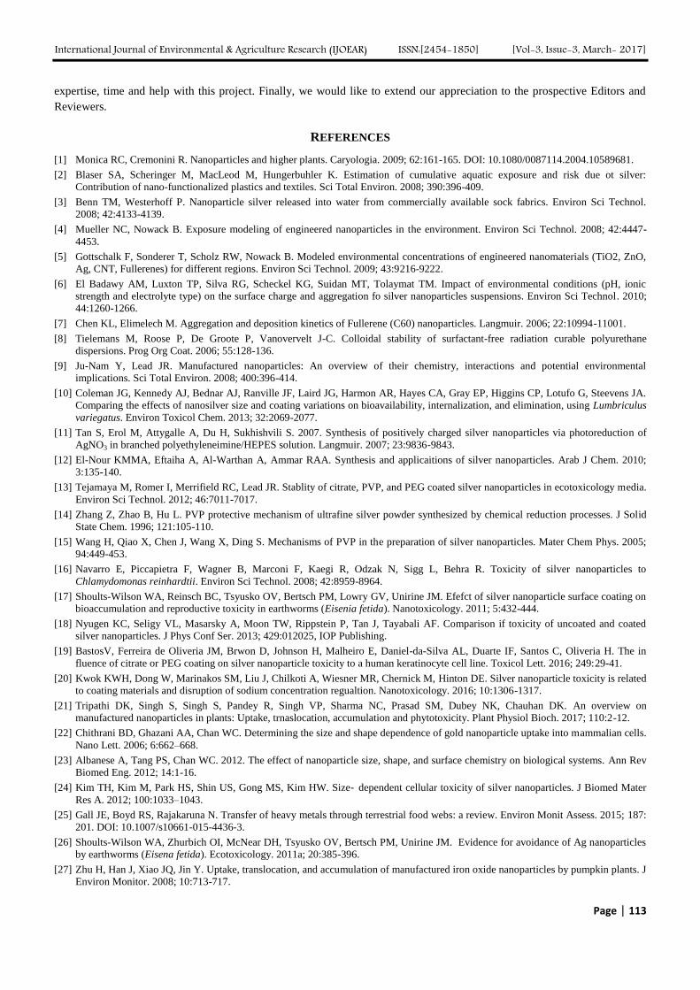
International Journal of Environmental & Agriculture Research (IJOEAR) ISSN:[2454-1850] [Vol-3, Issue-3, March- 2017]
Page | 113
expertise, time and help with this project. Finally, we would like to extend our appreciation to the prospective Editors and
Reviewers.
REFERENCES
[1] Monica RC, Cremonini R. Nanoparticles and higher plants. Caryologia. 2009; 62:161-165. DOI: 10.1080/0087114.2004.10589681.
[2] Blaser SA, Scheringer M, MacLeod M, Hungerbuhler K. Estimation of cumulative aquatic exposure and risk due ot silver:
Contribution of nano-functionalized plastics and textiles. Sci Total Environ. 2008; 390:396-409.
[3] Benn TM, Westerhoff P. Nanoparticle silver released into water from commercially available sock fabrics. Environ Sci Technol.
2008; 42:4133-4139.
[4] Mueller NC, Nowack B. Exposure modeling of engineered nanoparticles in the environment. Environ Sci Technol. 2008; 42:4447-
4453.
[5] Gottschalk F, Sonderer T, Scholz RW, Nowack B. Modeled environmental concentrations of engineered nanomaterials (TiO2, ZnO,
Ag, CNT, Fullerenes) for different regions. Environ Sci Technol. 2009; 43:9216-9222.
[6] El Badawy AM, Luxton TP, Silva RG, Scheckel KG, Suidan MT, Tolaymat TM. Impact of environmental conditions (pH, ionic
strength and electrolyte type) on the surface charge and aggregation fo silver nanoparticles suspensions. Environ Sci Technol. 2010;
44:1260-1266.
[7] Chen KL, Elimelech M. Aggregation and deposition kinetics of Fullerene (C60) nanoparticles. Langmuir. 2006; 22:10994-11001.
[8] Tielemans M, Roose P, De Groote P, Vanovervelt J-C. Colloidal stability of surfactant-free radiation curable polyurethane
dispersions. Prog Org Coat. 2006; 55:128-136.
[9] Ju-Nam Y, Lead JR. Manufactured nanoparticles: An overview of their chemistry, interactions and potential environmental
implications. Sci Total Environ. 2008; 400:396-414.
[10] Coleman JG, Kennedy AJ, Bednar AJ, Ranville JF, Laird JG, Harmon AR, Hayes CA, Gray EP, Higgins CP, Lotufo G, Steevens JA.
Comparing the effects of nanosilver size and coating variations on bioavailability, internalization, and elimination, using Lumbriculus
variegatus. Environ Toxicol Chem. 2013; 32:2069-2077.
[11] Tan S, Erol M, Attygalle A, Du H, Sukhishvili S. 2007. Synthesis of positively charged silver nanoparticles via photoreduction of
AgNO3 in branched polyethyleneimine/HEPES solution. Langmuir. 2007; 23:9836-9843.
[12] El-Nour KMMA, Eftaiha A, Al-Warthan A, Ammar RAA. Synthesis and applicaitions of silver nanoparticles. Arab J Chem. 2010;
3:135-140.
[13] Tejamaya M, Romer I, Merrifield RC, Lead JR. Stablity of citrate, PVP, and PEG coated silver nanoparticles in ecotoxicology media.
Environ Sci Technol. 2012; 46:7011-7017.
[14] Zhang Z, Zhao B, Hu L. PVP protective mechanism of ultrafine silver powder synthesized by chemical reduction processes. J Solid
State Chem. 1996; 121:105-110.
[15] Wang H, Qiao X, Chen J, Wang X, Ding S. Mechanisms of PVP in the preparation of silver nanoparticles. Mater Chem Phys. 2005;
94:449-453.
[16] Navarro E, Piccapietra F, Wagner B, Marconi F, Kaegi R, Odzak N, Sigg L, Behra R. Toxicity of silver nanoparticles to
Chlamydomonas reinhardtii. Environ Sci Technol. 2008; 42:8959-8964.
[17] Shoults-Wilson WA, Reinsch BC, Tsyusko OV, Bertsch PM, Lowry GV, Unirine JM. Efefct of silver nanoparticle surface coating on
bioaccumulation and reproductive toxicity in earthworms (Eisenia fetida). Nanotoxicology. 2011; 5:432-444.
[18] Nyugen KC, Seligy VL, Masarsky A, Moon TW, Rippstein P, Tan J, Tayabali AF. Comparison if toxicity of uncoated and coated
silver nanoparticles. J Phys Conf Ser. 2013; 429:012025, IOP Publishing.
[19] BastosV, Ferreira de Oliveria JM, Brwon D, Johnson H, Malheiro E, Daniel-da-Silva AL, Duarte IF, Santos C, Oliveria H. The in
fluence of citrate or PEG coating on silver nanoparticle toxicity to a human keratinocyte cell line. Toxicol Lett. 2016; 249:29-41.
[20] Kwok KWH, Dong W, Marinakos SM, Liu J, Chilkoti A, Wiesner MR, Chernick M, Hinton DE. Silver nanoparticle toxicity is related
to coating materials and disruption of sodium concentration regualtion. Nanotoxicology. 2016; 10:1306-1317.
[21] Tripathi DK, Singh S, Singh S, Pandey R, Singh VP, Sharma NC, Prasad SM, Dubey NK, Chauhan DK. An overview on
manufactured nanoparticles in plants: Uptake, trnaslocation, accumulation and phytotoxicity. Plant Physiol Bioch. 2017; 110:2-12.
[22] Chithrani BD, Ghazani AA, Chan WC. Determining the size and shape dependence of gold nanoparticle uptake into mammalian cells.
Nano Lett. 2006; 6:662–668.
[23] Albanese A, Tang PS, Chan WC. 2012. The effect of nanoparticle size, shape, and surface chemistry on biological systems. Ann Rev
Biomed Eng. 2012; 14:1-16.
[24] Kim TH, Kim M, Park HS, Shin US, Gong MS, Kim HW. Size‐ dependent cellular toxicity of silver nanoparticles. J Biomed Mater
Res A. 2012; 100:1033–1043.
[25] Gall JE, Boyd RS, Rajakaruna N. Transfer of heavy metals through terrestrial food webs: a review. Environ Monit Assess. 2015; 187:
201. DOI: 10.1007/s10661-015-4436-3.
[26] Shoults-Wilson WA, Zhurbich OI, McNear DH, Tsyusko OV, Bertsch PM, Unirine JM. Evidence for avoidance of Ag nanoparticles
by earthworms (Eisena fetida). Ecotoxicology. 2011a; 20:385-396.
[27] Zhu H, Han J, Xiao JQ, Jin Y. Uptake, translocation, and accumulation of manufactured iron oxide nanoparticles by pumpkin plants. J
Environ Monitor. 2008; 10:713-717.
International Journal of Environmental & Agriculture Research (IJOEAR) ISSN:[2454-1850] [Vol-3, Issue-3, March- 2017]
Page | 114
[28] Wang Z, Xie X, Zhao J, Liu X, Feng W, White JC, Xing B. Xylem- and Phloem-based transport of CuO nanoparticles in maize (Zea
Mays L.). Envriron Sci Technol. 2012; 46:4434-4441.
[29] Raliya R, Franke C, Chavalmane S, Nair R, Reed N, Biswas P. Quantitative understanding of nanoparticle uptake in watermelon.
Front Plant Sci. 2016; 7:1288. DOI: 10.3389/fpls.2016.01288.
[30] Wang P, Lombi E, Sun S, Scheckel KG, Malysheve A, Mckenna BA, Menzies NW, Zhao F-J, Kopittke PM. Characterizing the
uptake, accumulation and toxicity of silver sulfide nanoparticles. Environmental Science Nano. 2017; 4:448-460. DOI:
10.1039/c6en00489.
[31] Lee W-M, An Y-J, Kweon H-S. Toxicity and bioavailability of copper nanoparticles to the terestrial plants Mung Bean (Phaseolus
radiatus) and Wheat (Triticum aestivum): Plant agar test for water-insoluble nanoparticles. Environ Toxicol Chem. 2008; 27:1915-
1921.
[32] Ma Y, Kuang L, He X, Bai W, Ding Y, Zhang Z, Zhao Y, Chai Z. Effects of rare earth oxide nanoparticles on root elongation of
plants. Chemosphere. 2010; 78:273-279.
[33] Judy JD, Unrine JM, Rao W, Wirick S, Bertsch PM. 2012. Bioavailability of gold nanomaterials to plants: Importance of particle size
and surface coating. Environ Sci Technol. 2012; 46:8467-8474.
[34] Nadiminti PP, Dong YD, Sayer C, Hay P, Rookes JE, Boyd BJ, Cahill DM. Nanostructured liquid crystalline particles as an
alternative delivery vehicle for plant agrochemicals. ACS Appl Mater Interfaces. 2013; 5: 1818-1826.
[35] Page V, Feller U. Heavy metals in crop plants: Transport and redistribution processes on the whole plant level. Agron. 2015; 5:447-
463. DOI: 10.3390/agrnomy5030447.