arX

iv:0

912.

3571

v1 [

quan

t-ph

] 1

8 D

ec 2

009

Complete analysis of measurement-induced entanglement localization on a

three-photon system

Miroslav Gavenda,1 Radim Filip,1 Eleonora Nagali,2 Fabio Sciarrino,2, 3 and Francesco De Martini2, 4

1Department of Optics, Palacky University, 17. listopadu 12, 771 46 Olomouc, Czech Republic2Dipartimento di Fisica, Sapienza Universita di Roma, piazzale Aldo Moro 5, 00185 Roma, Italy

3Istituto Nazionale di Ottica Applicata, Largo E. Fermi 6, 50125 Firenze, Italy4Academia Nazionale dei Lincei, Via della Lungara 10, 00165 Roma, Italy

We discuss both theoretically and experimentally elementary two-photon polarization entangle-ment localization after break of entanglement caused by linear coupling of environmental photonwith one of the system photons. The localization of entanglement is based on simple polarizationmeasurement of the surrounding photon after the coupling. We demonstrate that non-zero entan-glement can be localized back irrespectively to the distinguishability of coupled photons. Further,it can be increased by local single-copy polarization filters up to an amount violating Bell inequal-ities. The present technique allows to restore entanglement in that cases, when the entanglementdistillation does not produce any entanglement out of the coupling.

PACS numbers: 03.67.Hk, 03.67.Pp, 42.50.Dv

I. INTRODUCTION

Quantum entanglement, the fundamental resource inquantum information science, is extremely sensitive tocoupling to surrounding systems. By this coupling theentanglement is reduced or even completely vanishes.In the case of partial entanglement reduction, quantumpurification and distillation protocols can be adopted[1, 2, 3, 4, 5]. In quantum distillation protocols, en-tanglement can be increased without any operation onthe surrounding systems. Using a collective procedure,the distillation probabilistically transforms many copiesof less entangled states to a single more entangled state,using a collective procedure just at the output of thecoupling [6]. Fundamentally, the distillation requires atleast a bit of residual entanglement passing through thecoupling.

When the coupling with the environment completelydestroys the entanglement, both purification and distil-lation protocols can not be exploited. Hence anotherbranch of methods like unlocking of hidden entanglement[7] or entanglement localization [8, 9, 10, 11, 12] must beused. In reference [7] there has been estimated that in or-der to unlock the hidden entanglement from a separablemixed state of two subsystems an additional bit or bitsof classical information is needed to determine which en-tangled state is actually present in the mixture. Howeverno strategy was presented in order to extract this infor-mation from the system of interest or the environment.Latter, to retrieve the entanglement, the localization pro-tocols [8, 9, 10, 11, 12] have been introduced working onthe principle of getting some nonzero amount of bipar-tite entanglement from some multipartite entanglement.That means performing some kind of operation on themultipartite system (or on its part) may induce bipartiteentanglement between subsystems of interest.

We can say that the entanglement breaks because itis so inconveniently redistributed among system of inter-

est and environment that it is transformed into gener-ally complex multipartite entanglement. Entanglementcan be localized back for the further application justby performing suitable measurement on the surroundingsystem and the proper feed-forward quantum correction.The measurement and feed-forward operation substitute,at least partially, a full inversion of the coupling whichrequires to keep very precise interference with the sur-rounding systems. For many-particle systems, the maxi-mal value of the localizable entanglement depends on thecoupling and also on initial states of surrounding systems.

To understand the mechanism of the entanglement lo-calization, we simplify the complex many particle cou-pling process to a set of sequential couplings with a sin-gle particle representing an elementary surrounding sys-tem E [13]: see FIG. 1. Then, our focus is just on thethree-qubit entanglement produced by this elementarycoupling of one qubit from maximally entangled state oftwo qubits A and B to a third surrounding qubit E. Be-fore the coupling to the qubit B, we have typically nocontrol on the quantum state of qubit E, hence consid-ered to be unknown. Further, the qubit E is typicallynot interfering or weakly interfering with the qubit B.Recently Sciarrino et al. [14] reported the entanglementlocalization after the coupling to an incoherent noisy sys-tem.In this paper, we report the study in depth of the keyrole of two-photon interference in the process of entan-glement localization presented in our previous paper [14].In particular we focus on the theory of the localizationprotocol, both considering a distinguishable and an in-distinguishable photon coupling with the environment.The experimental implementation of such processes willbe presented as well, with large attention to the experi-mental setup. In order to carry out our analysis on thedynamic of the localization protocol, we have considereda simple process for the interaction between the signalphoton and the surrounding one. To be specific, we as-sume a polarization insensitive linear coupling between

2

EPRM

IXIN

G

Alice

Bob

Measurement

Filter B

Filter A

Environment

(E)

a)

MIXING MEASUREMENT FILTRATION

b)

E’E

B’

B

BUN PBS

!"

!#

$x $xF

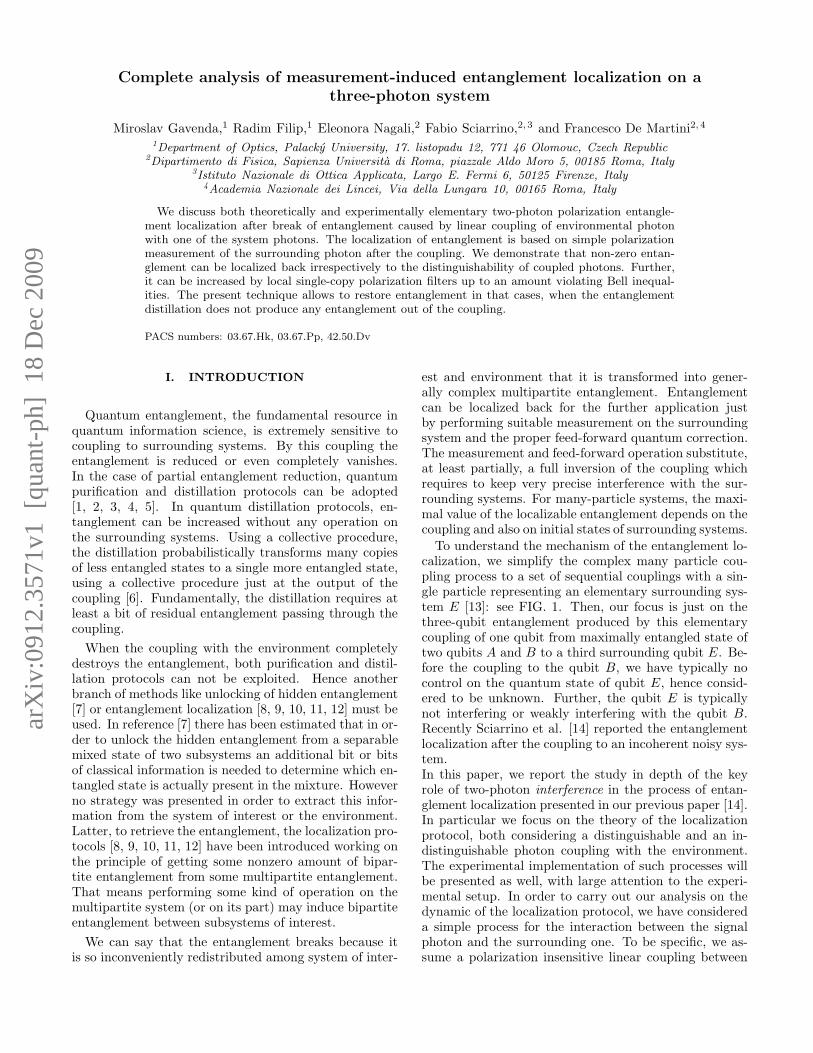
FIG. 1: (Color online) a) Schematic representation of thelocalization protocol. b) Detailed representation of the threesteps of the localization procedure.

distinguishable or partially distinguishable surroundingunpolarized single photon E and single photon B fromthe photon pair A, B maximally entangled in the polar-ization degree of freedom. After this coupling, the stateof two entangled photons A, B turns to be a mixture ofthe two-photon maximally entangled state and the sep-arable two unpolarized photons. For some value of thecoupling, this state gets separable and the entanglementis completely redirected to the surrounding system. Wetheoretically prove that for any linear coupling, it is al-ways possible to localize a non-zero entanglement backto the photon pair A, B just by a polarization sensitivedetection of the photon E. Interestingly, this qualita-tive result can be obtained irrespectively to the level ofdistinguishability and noise in the surrounding photonE. We discuss the impact of distinguishability in theentanglement localization more in details and give phys-ical explanation of the differences between the localiza-tion for distinguishable or partial distinguishable photonE. The performance of this localization can be furtherenhanced using a simple single-copy distillation method[15, 16, 17, 18, 19, 20, 21, 22, 23, 24], up to a state violat-ing Bell inequalities [25, 26], independently on the noiseand distinguishability of the photon E.

The paper is organized as follows. In Sec. II we discusstheory of the polarization entanglement localization, fora comparison, first for the coupling of fully indistinguish-able photons (Sec. II.A) and then for realistic linear cou-

pling of partially distinguishable photons (Sec. II.B). InSec. III, the experimental results are discussed in details.The Sec. III.A describes the experimental setup and thestate preparation. The Sec. III.B contains the experi-mental result about the localization for the coupling offully distinguishable photons, the Sec. III.C presents theresults of localization for the coupling of indistinguish-able photon whereas the Sec. III.D reports on results oflocalization for the coupling of partially indistinguishablephotons. The summary is done in the Conclusion. In theAppendix A, a modification of the entanglement local-ization for the polarizing linear coupling is described.

II. THEORY

Let us assume that we generate a maximally entangledpolarization state |Ψ−〉AB = (|HV 〉 − |V H〉)/

√2 of two

photons A and B. The form of the maximally entangledstate is not relevant, as the same results can be obtainedfor any maximally entangled state. The first photon iskept by Alice and second is coupled to the surroundingphoton E in an unknown state, ρE = 11/2 (completelyunpolarized state), by a simple linear polarization in-sensitive coupling (a beam splitter with transmissivityT ). After the coupling, three possible situations can beobserved: both photons B and E go simultaneously toeither mode k′

B or mode k′E , or only a single photon is

separately presented in both output modes k′B or k′

E (seeFIG. 1). We will focus only on the last case, that is asingle photon output from the coupling. In this case,it is in principle not possible to distinguish whether theoutput photon is the one from the entangled pair (B) orthe unpolarized photon E. We investigate in detail, theimpact of the distinguishability of the surrounding sys-tem on the localization procedure. Note that the systemE can be also produced by the entanglement source andthen coupled to the entangled state through a subsequentpropagation. Therefore, it is not fundamentally impor-tant whether E is produced by truly independent sourceor not.

A. Coupling of indistinguishable photons

To understand the role of partial distinguishability inthe entanglement localization, let us first assume thatboth photons B and E are perfectly indistinguishable.Then, if both the photons leave the linear polarization-insensitive coupling separately, the coupling transforma-tion can be written for any polarization state |Ψ〉B as:

|Ψ〉B|Ψ〉E → (T − R)|Ψ〉B|Ψ〉E ,

|Ψ〉B|Ψ⊥〉E → T |Ψ〉B|Ψ⊥〉E − R|Ψ⊥〉B|Ψ〉E . (1)

Both the singlet state |Ψ−〉AB as well as ρE can be writ-ten in the general basis |Ψ〉 and |Ψ⊥〉, namely: |Ψ−〉AB =

(|ΨΨ⊥〉AB − |Ψ⊥Ψ〉AB)/√

2 and ρE = (|Ψ〉E〈Ψ| +

3

|Ψ⊥〉E〈Ψ⊥|)/2. Therefore, it is simple to find that theoutput state σI

ind (tracing over photon E) is exactly amixture of the entangled state with the unpolarized noise(Werner state) [27]:

σIind =

4Find − 1

3|Ψ−〉AB〈Ψ−|+

(1 − Find)

311A⊗11B, (2)

where the fidelity Find, that is the overlap with the singletstate |Ψ−〉AB, takes values 0 ≤ Find ≤ 1 and reads:

Find =(1 − 3T )2

4 (1 − 3T (1 − T )). (3)

The state is entangled only if 1/2 < F ≤ 1 and theconcurrence [28] reads Cind = 2Find − 1. If Find < 1/2the entanglement is completely lost and the state (2) isseparable. The explicit formula for concurrence is

CIind = max

(0,

3T 2 − 1

2 (1 − 3T (1 − T ))

). (4)

The probability of this situation is P Iind =(

T 2 + (T − R)2 + R2)/2 and the condition for en-

tanglement breaking channel is T < 1/√

3. In orderto achieve a maximal violation of Bell inequalities [29],we have to refer to the quantity BI

ind given by theexpression

BIind =

2√

2T |1 − 2T |1 − 3T (1− T )

(5)

The violation appears only for T > 0.68, imposing a con-dition on the coupling even more strict.

More generally, all the result that will be presentedin the paper can be directly extended for general pas-sive coupling between two modes. It can be representedby Mach-Zehnder interferometer consisting to two unbal-anced beam splitters (with transmissivity T1 and T2) andtwo phase shifts −φ and φ separately in arms inside theinterferometer. All the results depends only on a singleparameter: the probability T that the entangled photonwill leave the coupling as the signal, which is explicitlyequal to:

T = T1 + T2 − 2T1T2 +√

T1T2R1R2 cos 2φ. (6)

Thus all results, here simply discussed for a beam splitter,are valid for any passive coupling between two photons.

After the measurement of polarization on photon E,let us say by the projection on an arbitrary state |Ψ〉E ,the state of photons A, B is transformed into

σIIind =

1

P IIind

((T 2 + (T − R)2)|T 〉〈T |+ R2|Ψ⊥Ψ⊥〉〈Ψ⊥Ψ⊥|

)

(7)where the state |T 〉 represents the unbalanced singletstate:

|T 〉 =1√

T 2 + (T − R)2(T |ΨΨ⊥〉 − (T − R)|Ψ⊥Ψ〉)

(8)

and P IIind = T 2 + (T −R)2 + R2. Calculating the concur-

rence as measure of entanglement, we found

CIIind =

T |2T − 1|1 − 3(1 − T )T

(9)

which is always larger than zero if T 6= 0, 1/2. It is worthnotice that, irrespective to polarization noise in the qubitE, it is possible to probabilistically localized back to theoriginal photon pair A and B a non-zero entanglementfor all T 6= 0, 1/2.

The basic principle of this process can be understoodby comparing Eq. (2) and Eq. (7). The unpolarized noisein Eq. (2) has been transformed to a fully correlated po-larized noise in Eq. (7) just by the measurement on E.This measurement can be arbitrary and does not dependon the coupling strength T . Thus, it is not necessary toestimate the channel coupling before the measurement.The positive result comes from the observation that afully correlated and polarized noise is less destructive tomaximal entanglement than the completely depolarizednoise. Further, the entanglement localization effect per-sists even if an arbitrary phase or amplitude dampingchannel affects photon E after the coupling. If there isstill a preferred basis in which the same classical corre-lation can be kept, it is sufficient for the entanglementlocalization. Unfortunately, the localized state is entan-gled but the localization itself is not enough to produce astate violating Bell inequalities. The maximal Bell factorBII

ind is identical to (5) although the state has completelychanged its structure.

However if T is known then the entanglement of state(7) and the Bell inequality violation can be further in-creased by the single-copy distillation [15, 16, 17]. First,a local polarization filter can be used to get the balancedsinglet state in the mixture. An explicit constructionof the single local filter at Bob’s side is given by |Ψ〉 →(T−R)/T |Ψ〉, |Ψ⊥〉 → |Ψ⊥〉 for T > 1/3. If T < 1/3 thena different filtering |Ψ〉 → |Ψ〉, |Ψ⊥〉 → T/(T − R)|Ψ⊥〉has to be applied. Thus the Werner state (2) is con-ditionally transformed to a maximally entangled mixedstate (MEMS)[30, 31, 32, 37]:

((T − R)2|Ψ−〉〈Ψ−| + R2|Ψ⊥Ψ⊥〉〈Ψ⊥Ψ⊥|

)

(T − R)2 + R2(10)

where the probability of success is given by (T−R)2+R2.Due to symmetry, the same situation arises if the state|Ψ⊥〉 is detected, just replacing the state Ψ ↔ Ψ⊥. If thelocal filtering on Bob’s side is applied according to theprojection, it is possible to reach the MEMS with twiceof success probability. Now, a difference between Eq.(10)and Eq. (2) is only in an additive fully correlated polar-ized noise. Such result can be achieved by an operationon the photon B, while a processing on other photon isnot required.

Further local filtration performed on both photons Aand B can give maximal entanglement achievable froma single copy. Both Alice and Bob should implement

4

the filtration |Ψ〉 → |Ψ〉 and |Ψ⊥〉 → √ǫ|Ψ⊥〉, where

0 < ǫ ≤ 1. The filtered state is then

σIIIind =

1

4P IIIind

(ǫ(2T − 1)2|Ψ−〉〈Ψ−|+

ǫ2(1 − T )2|Ψ⊥Ψ⊥〉〈Ψ⊥Ψ⊥|)

(11)

where P IIIind =

(ǫ(2T − 1)2 + ǫ2(1 − T )2

)/4 is probability

of success. The state has the following concurrence forT 6= 0, 1/2

CIIIind (ǫ) =

1

1 + ǫ (1−T )2

2(1−2T )2

(12)

As ǫ goes to zero, the concurrence approaches unity, ex-cept for T = 0, 1/2, where it vanishes. Thus we can getentanglement arbitrarily close to its maximal value forany T (except T = 0, 1/2). For T = 1/2, it could notappear due to bunching effect between the photons atthe beam splitter. Such result can be achieved since wecan completely eliminate the fully correlated polarizednoise, which is actually completely orthogonal to the sin-gle state |Ψ−〉. We stress once again that maximal en-tanglement was probabilistically approached irrespectiveto the initial polarization noise of the photon E, just byits single-copy localization measurement and single-copydistillation.

If ǫ → 0 we get simply BIIIind = 2

√2 for any T , ex-

cept T = 0, 1/2. Since the maximal entanglement allowsideal teleportation of unknown state we can concludethat the linear coupling to the distinguishable photoneven in an unknown state could be practically proba-bilistically reversed. It is interesting to make a compar-ison with the deterministic localization procedure. Toachieve it, we need perfect control of the state of pho-ton E before the coupling. We can know it either apriori or by a measurement on the more complex sys-tems predicting pure state of E. Being |Ψ〉E the stateof E after coupling, three-photon state is proportional to|Ψ〉A (T |Ψ⊥Ψ〉BE − R|ΨΨ⊥〉BE)− (T −R)|Ψ⊥ΨΨ〉ABE.This belongs to not-symmetrical W-state, rather than toGHZ states, therefore the maximal entanglement can notbe obtained deterministically. It can be done by the pro-jection on |Ψ〉E followed by the single-copy distillation.From this point of view, the unpolarized noise of photonE does not qualitatively change the result of the local-ization, but only decreases the success rate.

B. Coupling of partially distinguishable photons

Up to now, we have assumed that both photons Band E are indistinguishable in the linear coupling. Onthe other hand, if they are partially or fully distinguish-able), then it is in principle possible to perfectly filterout surrounding photons from the signal photons afterthe coupling. Although they are in principle partiallyor fully distinguishable, any realistic attempt to discrim-inate them would be typically too noisy to offer such

0.2 0.4 0.6 0.8 1T

0.2

0.4

0.6

0.8

1C

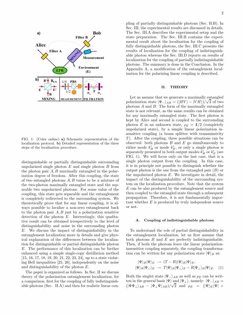
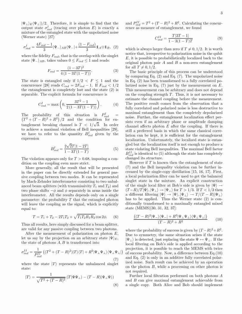
FIG. 2: Concurrence for indistinguishable photon E (p = 1):CI

ind without measurement (dotted), CII

ind with measurement(dashed), CIII

ind with measurement and LOCC filtration (full),for ǫ = 0.005.

0.2 0.4 0.6 0.8 1T

0.2

0.4

0.6

0.8

1C

FIG. 3: Concurrence for distinguishable photon (p = 0):CI

dis without measurement (dotted), CII

dis with measurement(dashed), CIII

dis with measurement and LOCC filtration (full)

information. Here we are interested in the opposite sit-uation, when distinguishable photon B and surroundingphoton E cannot be practically distinguished after thecoupling. It is an open question whether the entangle-ment localization method can still help us. For simplicity,let us assume a mixture of the previous case with a sit-uation where both the photons B and E are completelydistinguishable. The state is mixture pσind + (1− p)ρdis,where only with probability p the photons are indistin-guishable. After the coupling and tracing over photonE, the output state is once more a Werner state (2) withfidelity

F (p) =(4p + 5)T 2 − 2(2p + 1)T + 1

4 (1 − (2 + p)T (1 − T ))(13)

and success probability P (p) = 1− (2 + p)T (1−T ). Theconcurrence is given by C(p) = 2F (p)−1. The entangle-ment between A and B is lost if

p >T 2 + 2T − 1

2T (1− T )(14)

5

and thus for T <√

2 − 1, the entanglement between Aand B is lost for any p. The maximal Bell factor

B(p) = 2√

2T|T − p(1 − T )|

1 − (p + 2)(1 − T )T(15)

gives violation of Bell inequalities only if p ∈ [0, 1] satis-fies

p <√

2 +1

1 − T− 1 +

√2

T. (16)

Let us discuss first the entanglement localization forthe fully distinguishable photon case (p = 0). In thislimit, after the coupling the fidelity reads:

Fdis =5T 2 − 2T + 1

4 (1 − 2T (1 − T )), (17)

and the concurrence and the maximal violation of Bellinequalities are

CIdis =

T 2 + 2T − 1

2(1 − 2T (1 − T )), BI

dis = 2√

2T 2

T 2 + (1 − T )2.

(18)

The concurrence vanishes for T <√

2 − 1 and theviolation of Bell inequalities disappears for T < 1 +1√2

(1 −

√1 +

√2)≈ 0.608. In both cases, the thresh-

olds are lower than for the coupling of indistinguishablephotons; the distinguishability of photon E leads to lessrobust transmission of the quantum resources.

If the projection on |Ψ〉E is performed on the envi-ronmental photon after the coupling, the resulting statereads

ρIIdis =

1

P IIdis

(T 2

2|Ψ−〉AB〈Ψ−| +

R2

2|Ψ⊥〉A〈Ψ⊥| ⊗ 11/2B)

(19)where P II

dis = (T 2 + R2)/2. Clearly, the additive noisyterm in the Eq.(19) is separable and the full correlationin the partially polarized noise (7) does not arise here, incomparison with the fully indistinguishable case. Exceptfor T = 0, this state is exhibiting non-zero concurrence

CIIdis =

T 2

2T 2 − 2T + 1(20)

which is a decreasing function of T . The state just afterthe localization does not violate Bell inequalities, sincethe maximal Bell factor is the same as after the mixingBII

dis = BIdis.

Similarly to the previous discussion, projecting on|Ψ⊥〉E , we get an identical state, only replacing Ψ ↔ Ψ⊥.This means that even for completely non-interfering pho-tons B and E, a polarization measurement on the photonE can localize entanglement back to photons A and B.To approach it with maximal success rate, local unitarytransformations doing Ψ ↔ Ψ⊥ have to be applied if|Ψ⊥〉 is measured. Similarly to previous indistinguish-able case, the photon E is not affected by the amplitude

or phase damping channel. It is only important to keepa preferred basis without any noise influence.

The physical mechanism which models the localizationprocess for coupling of distinguishable photons is differ-ent from the previous case. Here, the three-photon mixedstate after the coupling is proportional to

T 2|Ψ−〉AB〈Ψ−| ⊗ 11/2E + R2|Ψ−〉AE〈Ψ−| ⊗ 11/2B (21)

describing just a random swap of the photons B and Eat the beam splitter. Although there is no correlationgenerated by the coupling between photons A and B,contrary to previous case, still a correlation between pho-tons A and E will appear in the second part of expressiondue to the initial entangled state. It is used to condition-ally transform the locally completely depolarized state ofphoton A to a fully polarized state. Of course, it doesnot have any impact on the local state of photon B. Butit is fully enough to localize entanglement for any T afterthe projection on photon E. It is rather a non-local cor-relation effect where the polarization noise is correctednot at photon B but at photon A.

The entanglement can be further enhanced using localfiltration and classical communication; in the limit ǫ → 0and introducing optimal filtering given by

|Ψ⊥Ψ〉 → T√2T 2 − 2T + 1

|Ψ⊥Ψ〉,

|Ψ⊥Ψ⊥〉 → ǫ|Ψ⊥Ψ⊥〉 (22)

(whereas all other basis states are preserved) the finalstate approaches

ρIIIdis =

1

2|ΨΨ⊥〉AB〈ΨΨ⊥| +

1

2|Ψ⊥Ψ〉AB〈Ψ⊥Ψ|

− T

2√

2T 2 − 2T + 1(|ΨΨ⊥〉〈Ψ⊥Ψ| + h.c.) .(23)

The filtrations turns the state (19) into state (23) whichappears as a result of the action of phase damping chan-nel on the input singlet state. The filtrations eliminatedthe noise component |Ψ⊥Ψ⊥〉AB〈Ψ⊥Ψ⊥| from the state(19) and this ensures the violation of Bell inequalities forthe final state (23).

The concurrence approaches CIIIdis =

√CII

dis, at cost of

a decreasing success rate. But, at contrary to the case oftwo perfectly interfering photons, maximal entanglementcannot be approached for any T < 1. This is caused bylack of interference in the entanglement localization fordistinguishable photons. Of course, the collective proto-cols can be still used, since all entangled two-qubit statesare distillable to maximally entangled state [15].

A maximal value of the Bell factor

BIIIdis = 2

√1 +

T 2

T 2 + (1 − T )2(24)

can be achieved if ǫ → 0 for any T. Although Bell in-equalities are violated in this case for any T > 0 the fullentanglement cannot be recovered at any single copy.

6

Also here it is instructive to make a comparison withthe case in which the photon E is in the known purestate |Ψ〉E . Then after the coupling the three-photonstate is proportional to T 2|Ψ−〉AB〈Ψ−| ⊗ |Ψ〉E〈Ψ| +R2|Ψ−〉AE〈Ψ−| ⊗ |Ψ〉B〈Ψ| and after the projection on|Ψ〉E , it transforms to T 2|Ψ−〉AB〈Ψ−|+ 1

2R2|Ψ⊥〉A〈Ψ⊥|⊗|Ψ〉B〈Ψ|. Since both the contributions are not orthogo-nal there is no local filtration procedure which could fil-ter out the |Ψ−〉AB from the noise contribution. There-fore, although we could have a complete knowledge aboutpure state of the photon E, its distinguishability does notallow to achieve maximal entanglement from the singlecopy distillation.

For the mixture of both the distinguishable and indis-tinguishable photons, the concurrence after the measure-ment is

CI(p) = max

(0,

|(1 + p)T 2 − pT |1 − (2 + p)T (1 − T )

), (25)

which is positive if p 6= T/(1 − T ) and

p <1 − T

T+

T

1 − T. (26)

Except T = 0, p/(1 + p), the last condition is always sat-isfied since right side has minimum equal to two. Evenif the noise is a mixture of distinguishable and indistin-guishable photons, it is possible to localize entanglementjust by a measurement for almost all the cases. After theapplication of LOCC polarization filtering, the concur-rence can be enhanced up to

CIII(p, ǫ) =2T 2|T − p(1 − T )|√

1 − 2(1 + p)(1 − T )T (ǫ(1 − T )2 + 2T 2).

(27)In the limit of ǫ → 0, it approaches

CIII(p) = max

(0,

|T − p(1 − T )|√1 − 2(1 + p)T (1 − T )

)(28)

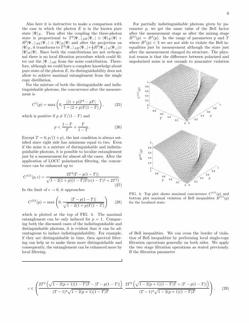
which is plotted at the top of FIG. 4. The maximalentanglement can be only induced for p = 1. Compar-ing both the discussed cases of the indistinguishable anddistinguishable photons, it is evident that it can be ad-vantageous to induce indistinguishability. For example,if they are distinguishable in time, then spectral filter-ing can help us to make them more distinguishable andconsequently, the entanglement can be enhanced more bylocal filtering.

For partially indistinguishable photons given by pa-rameter p, we get the same value of the Bell factorafter the measurement stage as after the mixing stageBII(p) = BI(p). In the range of parameters p and Twhere BI(p) < 2 we are not able to violate the Bell in-equalities just by measurement although the state justafter the measurement changed its structure. The phys-ical reason is that the difference between polarized andunpolarized noise is not enough to guarantee violation

0

0.2

0.4

0.6

0.8

1

00.2

0.40.6

0.810

0.2

0.4

0.6

0.8

1

pT

CIII(p

)

0

0.2

0.4

0.6

0.8

1

00.2

0.40.6

0.812

2.2

2.4

2.6

2.8

3

pT

BIII(p

)

FIG. 4: Top plot shows maximal concurrence CIII(p) andbottom plot maximal violation of Bell inequalities BIII(p)for the localized state.

of Bell inequalities. We can cross the border of viola-tion of Bell inequalities by performing local single-copyfiltration operations generally on both sides. We applythe two stage filtration operations as stated previously.If the filtration parameter

ǫ ∈

2T 2(√

1 − 2(p + 1)(1 − T )T − |T − p(1 − T )|)

(T − 1)2√

1 − 2(p + 1)(1 − T )T,2T 2

(√1 − 2(p + 1)(1 − T )T + |T − p(1 − T )|

)

(T − 1)2√

1 − 2(p + 1)(1 − T )T

, (29)

7

then we get following Bell factor

BIII(p, ǫ) =4√

2T 2|p(T − 1) + T |√2(p + 1)(T − 1)T + 1 (2T 2 + (T − 1)2ǫ)

(30)otherwise we get

BIII(p, ǫ) =2√

4T 4(p(T−1)+T )2

2(p+1)(T−1)T+1 + ((T − 1)2ǫ − 2T 2)2

2T 2 + (T − 1)2ǫ.

(31)The particular cases of Bell factors given previously canbe obtained from the above relations setting p = 0 (p =1) for coupling of distinguishable (indistinguishable) pho-tons and additionally the maximal value of the Bell factoris obtained if ǫ goes to zero. In order to get violation ofthe Bell inequalities BIII(p, ǫ) > 2 the filtration param-

eter needs to be for the (30) ǫ < T 2(p(T−1)+T )2

2(T−1)2(2(p+1)(T−1)T+1)

and for the (31) ǫ < 2T 2

(T−1)2

( √2|p(T−1)+T |√

2(p+1)(T−1)T+1− 1

). In

both the cases, value of ǫ should rapidly decrease as Tis smaller. In other words, it means that for a given ǫ,the state violates Bell inequalities only if p is sufficientlylarge. For any p and T , there is always some ǫ > 0 belowthe region given by (29), therefore as ǫ → 0, the maximalviolation

BIII(p) = 2

√

1 +(p(T − 1) + T )2

2(p + 1)(T − 1)T + 1. (32)

comes from the Eq. (30) since it is higher than the limitexpression from Eq. (31). The maximal violation of Bellinequalities is plotted at the bottom of FIG. 4. Generally,for ǫ > 0 we have to compare the (30) and (31) to findout which gives higher BIII(p).

III. EXPERIMENTAL IMPLEMENTATION

Let us now describe the experimental implementationof the localization protocol both for fully distinguishableand partially indistinguishable photons.

A. Experimental setup

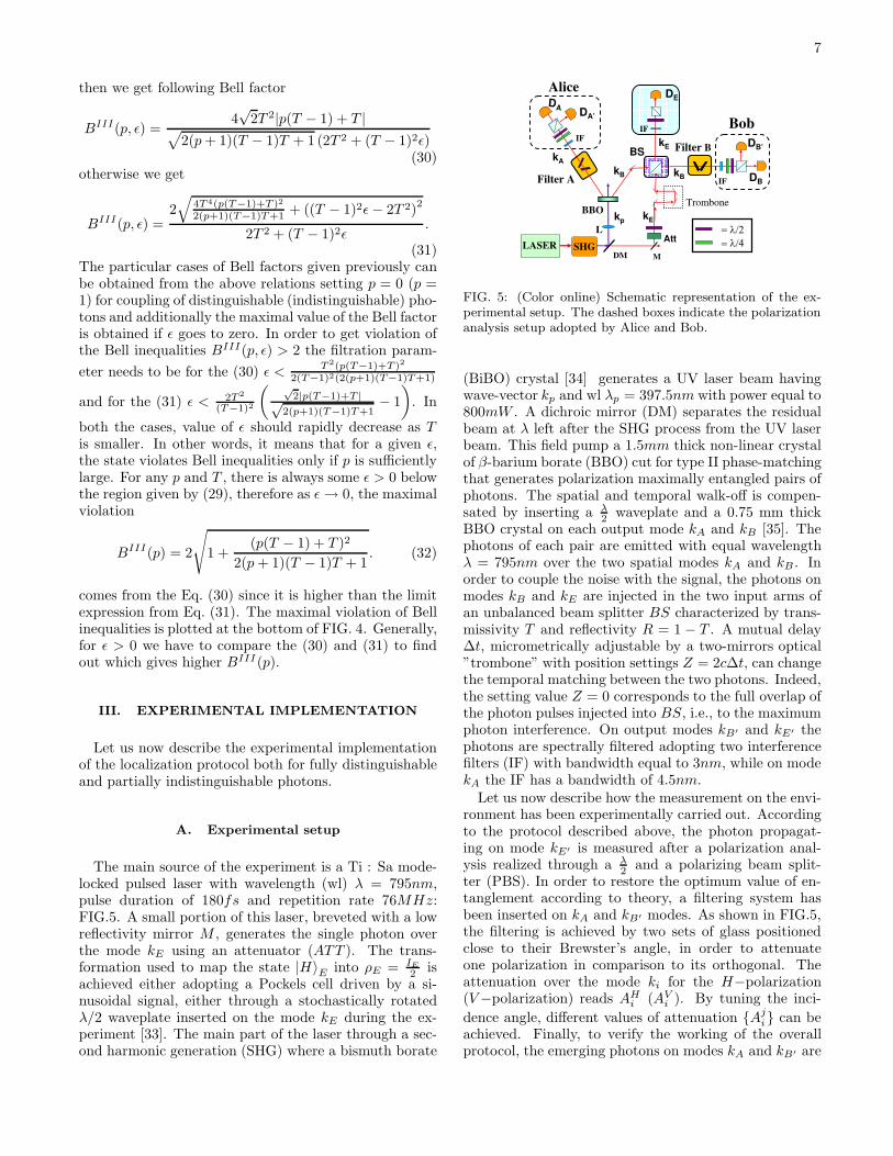
The main source of the experiment is a Ti : Sa mode-locked pulsed laser with wavelength (wl) λ = 795nm,pulse duration of 180fs and repetition rate 76MHz:FIG.5. A small portion of this laser, breveted with a lowreflectivity mirror M , generates the single photon overthe mode kE using an attenuator (ATT ). The trans-formation used to map the state |H〉E into ρE = IE

2 isachieved either adopting a Pockels cell driven by a si-nusoidal signal, either through a stochastically rotatedλ/2 waveplate inserted on the mode kE during the ex-periment [33]. The main part of the laser through a sec-ond harmonic generation (SHG) where a bismuth borate

kB

kA

kE

TromboneBBO

AttL

IF

DA’

Alice

BS

IF

DE

IF

DA

Filter A

Filter B

kB

kE

DMLASER

kp

MSHG

DB’

DB

Bob

FIG. 5: (Color online) Schematic representation of the ex-perimental setup. The dashed boxes indicate the polarizationanalysis setup adopted by Alice and Bob.

(BiBO) crystal [34] generates a UV laser beam havingwave-vector kp and wl λp = 397.5nm with power equal to800mW . A dichroic mirror (DM) separates the residualbeam at λ left after the SHG process from the UV laserbeam. This field pump a 1.5mm thick non-linear crystalof β-barium borate (BBO) cut for type II phase-matchingthat generates polarization maximally entangled pairs ofphotons. The spatial and temporal walk-off is compen-sated by inserting a λ

2 waveplate and a 0.75 mm thickBBO crystal on each output mode kA and kB [35]. Thephotons of each pair are emitted with equal wavelengthλ = 795nm over the two spatial modes kA and kB . Inorder to couple the noise with the signal, the photons onmodes kB and kE are injected in the two input arms ofan unbalanced beam splitter BS characterized by trans-missivity T and reflectivity R = 1 − T . A mutual delay∆t, micrometrically adjustable by a two-mirrors optical”trombone” with position settings Z = 2c∆t, can changethe temporal matching between the two photons. Indeed,the setting value Z = 0 corresponds to the full overlap ofthe photon pulses injected into BS, i.e., to the maximumphoton interference. On output modes kB′ and kE′ thephotons are spectrally filtered adopting two interferencefilters (IF) with bandwidth equal to 3nm, while on modekA the IF has a bandwidth of 4.5nm.

Let us now describe how the measurement on the envi-ronment has been experimentally carried out. Accordingto the protocol described above, the photon propagat-ing on mode kE′ is measured after a polarization anal-ysis realized through a λ

2 and a polarizing beam split-ter (PBS). In order to restore the optimum value of en-tanglement according to theory, a filtering system hasbeen inserted on kA and kB′ modes. As shown in FIG.5,the filtering is achieved by two sets of glass positionedclose to their Brewster’s angle, in order to attenuateone polarization in comparison to its orthogonal. Theattenuation over the mode ki for the H−polarization(V −polarization) reads AH

i (AVi ). By tuning the inci-

dence angle, different values of attenuation {Aji} can be

achieved. Finally, to verify the working of the overallprotocol, the emerging photons on modes kA and kB′ are

8

analyzed in polarization through a λ2 waveplate (wp), a

λ4 and a PBS. Then the photons are coupled to a singlemode fiber and detected by single photon counting mod-ule (SPCM) {DA, DA′ , DB′ , DB}. The output signals ofthe detectors are sent to a coincidence box interfacedwith a computer, which collects the double coincidencerates ([DA, DB], [DA, DB′ ], [DA′ , DB], [DA′ , DB′ ]) andtriple coincidence rates ([DA, DB, DE ], [DA, DB′ , DE ],[DA′ , DB, DE ], [DA′ , DB′ , DE]). The detection of triplecoincidence ensures the presence of one photon per modeafter the BS. In order to determine all the elements ofthe two-qubit density matrix, an overcomplete set of ob-servables is measured by adopting different polarizationsettings of the λ

2 wp and λ4 wp positions [36]. The uncer-

tainties on the different observables have been calculatedthrough numerical simulations of counting fluctuationsdue to the Poissonian distributions. Here and after, wewill distinguish the experimental density matrix from thetheoretical one by adding a ”tilde” .

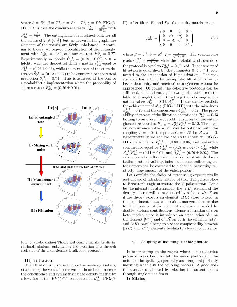
As first experimental step, we have characterized theinitial entangled state generated by the NL crystal onmode kA and kB, that is the signal to be transmit-ted through the noisy channel. The overall coincidencerate is equal to about 8.000 coincidences per second.The experimental quantum state tomography of ρin

ABis reported in FIG.7-a, to be compared with the the-oretical one ρin

AB =∣∣Ψin

⟩AB

⟨Ψin

∣∣AB

, where |Ψin〉 =

(|HV 〉 + i|V H〉)/√

2 (FIG.6-a). Although the generatedstate differs from the singlet state, all the conclusionsfrom the previous section remains valid. We found avalue of the concurrence Cin = (0.869 ± 0.005) and a

linear entropy Sin = (0.175 ± 0.005), where the un-certainty on the concurrence has been calculated ap-plying the Monte-Carlo method on the experimentaldensity matrix. The fidelity with the entangled state∣∣Ψin

⟩AB

is F(ρinAB ,

∣∣Ψin⟩

AB) =

⟨Ψin

∣∣AB

ρinAB

∣∣Ψin⟩

AB=

(0.915 ± 0.002). The discrepancy between theory andexperiment is mainly attributed to double pairs emis-sion. Indeed by subtracting the accidental coincidences

we obtain a concurrence equal to C′in = (0.939 ± 0.006)

and a linear entropy of S′in = (0.091 ± 0.006). The fi-

delity with the entangled state |Psiin〉AB is then equalto F ′(ρin

AB , |Psiin〉AB) = (0.949 ± 0.003). Minor sourcesof imperfections related to the generation of our entan-gled state are the presence of spatial and temporal walk-off due to the non linearity of the BBO crystal as wellas a correlation in wavelength of the generated pairs ofphotons.

B. Coupling of distinguishable photons

The experiment with distinguishable photons has beenachieved by injecting a single photon E with a randomlychosen mutual delay with photon B of ∆t >> τind =300fs. We note that the resolution time tdet of the de-tector is tdet >> ∆t, hence it is not technologically pos-

sible to individuate whether the detected photon belongsto the environment or to the entangled pair. To carryout the experiment we adopted a beam splitter withT = 0.40 which, according to the theoretical prediction(see FIG. 3), allows to study the entanglement localiza-tion process.Since multi-photon contributions represent the mainsource of imperfections in our calculations, we have sub-tracted their contributions in all the experimental datareported for the density matrices of each step of the pro-tocol.

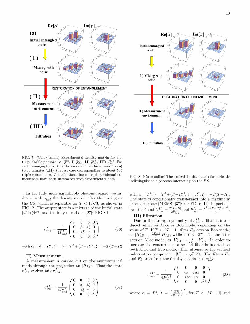
I) MixingWithout any access to the environmental photon, af-

ter the mixing on the BS, once there is one pho-ton per output mode, the theoretical input stateρin = |Ψin〉〈Ψin| evolves into a noisy state repre-sented by the density matrix ρI

dis, written in the basis{|HH〉, |HV 〉, |V H〉, |V V 〉, } as:

ρIdis =

1

4P Idis

α 0 0 00 β iξ 00 −iξ γ 00 0 0 δ

(33)

with α = δ = R2, β = γ = R2 + 2T 2, ξ = 2T 2 andP I

dis = R2+T 2, where R = 1−T indicates the reflectivityof the beam splitter. This matrix, shown in FIG.(6-I), ex-

hibits theoretically concurrence CIdis = max(0, 2T 2−R2

2PI

).

Because of the interaction with noise, ρIdis does not ex-

hibit entanglement (CIdis = 0) and is highly mixed with

linear entropy equal to SIdis = 0.90. Afterwards we ana-

lyze experimentally how the entangled state is corrupteddue to the coupling with the photon E. In this case no-polarization selection is performed on mode kE . The ex-perimental density matrix ρI

dis is shown in FIG.(7-I). As

expected, it exhibits CIdis = 0, and SI

dis = (0.89 ± 0.01).

The fidelity with theory is high: F Idis = F (ρI

dis, ρIdis) =

(0.997 ± 0.006), with F (ρ, σ) = Tr2[(√

ρσ√

ρ)1/2

]. In

this case, due to the coupling the entanglement is com-pletely redirected and no quantum distillation protocolcan be applied to restore entanglement between photonsA and B.

II) MeasurementAs no selection has been performed on the photon E

before the coupling, a multi-mode photon E interactswith the entangled photon B. After the interaction, asingle mode fiber has been inserted on the output mode ofthe BS in order to select only the output mode connectedwith the entanglement breaking. Let us consider the casein which the photon on mode kE is measured in the state|H〉E . After the measurement, the density matrix ρI

disevolves into an entangled one described by the densitymatrix ρII

dis

ρIIdis =

1

4P IIdis

0 0 0 00 β iξ 00 −iξ γ 00 0 0 δ

(34)

9

where δ = R2, β = T 2, γ = R2 + T 2, ξ = T 2: FIG.(6-

II). In this case the concurrence reads CIIdis = T 2

2P II

dis

with

P IIdis =

P I

dis

2 . The entanglement is localized back for all

the values of T 6= {0, 12} but, as shown in the graph, the

elements of the matrix are fairly unbalanced. Accord-ing to theory, we expect a localization of the entangle-ment with CII

dis = 0.32, and success rate P IIdis = 0.27.

Experimentally we obtain CIIdis = (0.19 ± 0.02) > 0, a

fidelity with the theoretical density matrix ρIIdis equal to

F IIdis = (0.96±0.03), while the mixedness of the state de-

creases SIIdis = (0.72±0.02) to be compared to theoretical

prediction SIIdis = 0.74 . This is achieved at the cost of

a probabilistic implementation where the probability of

success reads: P IIdis = (0.26 ± 0.01).

HH

HV

VH

VV

HH

HV

VH

VV

-0.5

-0.25

0

0.25

0.5

HH

HV

VH

VV

HH

HV

VH

VV

HH

HV

VH

VV

HH

HV

VH

VV

-0.5

-0.25

0

0.25

0.5

HH

HV

VH

VV

HH

HV

VH

VVRe Im

I ) Mixing with

noise

II ) Measurement

environment

III ) Filtration

RESTORATION OF ENTANGLEMENT

HH

HV

VH

VV

HH

HV

VH

VV

-0.5

-0.25

0

0.25

0.5

HH

HV

VH

VV

HH

HV

VH

VV

HH

HV

VH

VV

HH

HV

VH

VV

-0.5

-0.25

0

0.25

0.5

HH

HV

VH

VV

HH

HV

VH

VV

HH

HV

VH

VV

HH

HV

VH

VV

-0.5

-0.25

0

0.25

0.5

HH

HV

VH

VV

HH

HV

VH

VV

HH

HV

VH

VV

HH

HV

VH

VV

-0.5

-0.25

0

0.25

0.5

HH

HV

VH

VV

HH

HV

VH

VV

HH

HV

VH

VV

HH

HV

VH

VV

-0.5

-0.25

0

0.25

0.5

HH

HV

VH

VV

HH

HV

VH

VV

Initial entangled

state

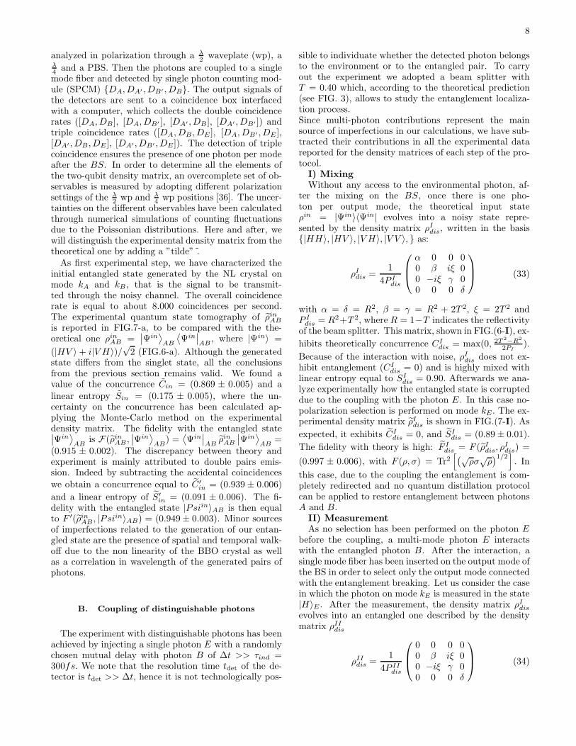
FIG. 6: (Color online) Theoretical density matrix for distin-guishable photons, enlightening the evolution of ρ througheach step of the entanglement localization protocol.

III) FiltrationThe filtration is introduced onto the mode kA and kB,

attenuating the vertical polarization, in order to increasethe concurrence and symmetrizing the density matrix bya lowering of the |V V 〉〈V V | component in ρII

dis: FIG.(6-

II). After filters FA and FB, the density matrix reads:

ρIIIdis =

0 0 0 00 ǫβ iǫξ 00 −iǫξ ǫβ 00 0 0 ǫ2δ

(35)

where β = T 2, δ = R2, ξ = T 3

√T 2+R2

. The concurrence

reads CIIIdis = 2ǫξ

2ǫβ+ǫ2δ while the probability of success of

the protocol is equal to P IIIdis = 2ǫβ+ǫ2δ. The intensity of

filtration is quantified by the parameter 0 < ǫ ≤ 1, con-nected to the attenuation of V polarization. The con-currence has a limit for asymptotic filtration (ǫ → 0)lower than unity and maximal entanglement cannot beapproached. Of course, the collective protocols can bestill used, since all entangled two-qubit state are distil-lable to a singlet one. By setting the following atten-uation values AV

A = 0.33, AHA = 1, the theory predicts

the achievement of ρIIIdis (FIG.(6-III)) with the mixedness

SIIIdis = 0.76 and the concurrence CIII

dis = 0.42. The prob-ability of success of the filtration operation is P III

dis = 0.43leading to an overall probability of success of the entan-glement restoration Ptotal = P II

disPIIIdis = 0.12. The high-

est concurrence value which can be obtained with thecoupling T = 0.40 is equal to C = 0.55 for Ptotal → 0.Experimentally we achieve the state shown in FIG.(7-

III with a fidelity F IIIdis = (0.89 ± 0.06) and measure a

concurrence equal to CIIIdis = (0.28 ± 0.02) > CII

dis while

P IIIdis P II

dis = (0.11 ± 0.01) and SIIIdis = (0.70 ± 0.02). The

experimental results shown above demonstrate the local-ization protocol validity, indeed a channel redirecting en-tanglement can be corrected to a channel preserving rel-atively large amount of the entanglement.

Let’s explain the choice of introducing experimentallyjust one set of filtration instead of two. The glasses closeto Brewster’s angle attenuate the V polarization. Let ǫbe the intensity of attenuation, the |V H〉 element of thedensity matrix will be attenuated by a factor

√ǫ. Even

if the theory expects an element |HH〉 close to zero, inthe experimental case we obtain a non-zero element dueto the intensity of the coherent radiation, revealed bydouble photons contributions. Hence a filtration of ǫ onboth modes, since it introduces an attenuation of ǫ onthe element |V V 〉 and of

√ǫ on both the elements |HV 〉

and |V H〉, would bring to a wider comparability between|HH〉 and |HV 〉 elements, leading to a lower concurrence.

C. Coupling of indistinguishable photons

In order to exploit the regime where our localizationprotocol works best, we let the signal photon and thenoise one be spatially, spectrally and temporal perfectlyindistinguishable in the coupling process. A good spa-tial overlap is achieved by selecting the output modesthrough single mode fibers.

I) Mixing.

10

HH

HV

VH

VV

HH

HV

VH

VV

-0.5

-0.25

0

0.25

0.5

HH

HV

VH

VV

HH

HV

VH

VV

HH

HV

VH

VV

HH

HV

VH

VV

-0.5

-0.25

0

0.25

0.5

HH

HV

VH

VV

HH

HV

VH

VV

HH

HV

VH

VV

HH

HV

VH

VV

-0.5

-0.25

0

0.25

0.5

HH

HV

VH

VV

HH

HV

VH

VV

HH

HV

VH

VV

HH

HV

VH

VV

-0.5

-0.25

0

0.25

0.5

HH

HV

VH

VV

HH

HV

VH

VV

HH

HV

VH

VV

HH

HV

VH

VV

-0.5

-0.25

0

0.25

0.5

HH

HV

VH

VV

HH

HV

VH

VV

HH

HV

VH

VV

HH

HV

VH

VV

-0.5

-0.25

0

0.25

0.5

HH

HV

VH

VV

HH

HV

VH

VV

HH

HV

VH

VV

HH

HV

VH

VV

-0.5

-0.25

0

0.25

0.5

HH

HV

VH

VV

HH

HV

VH

VV

Re Im

RESTORATION OF ENTANGLEMENT

HH

HV

VH

VV

HH

HV

VH

VV

-0.5

-0.25

0

0.25

0.5

HH

HV

VH

VV

HH

HV

VH

VV

Mixing with

noise

Measurement

environment

Filtration

( II )

( I )

(a)

( III )

Initial entangled

state

FIG. 7: (Color online) Experimental density matrix for dis-tinguishable photons: a) ρin, I) ρI

dis, II) ρII

dis, III) ρIII

dis . Foreach tomographic setting the measurement lasts from 5 s (a)to 30 minutes (III), the last case corresponding to about 500triple coincidence. Contributions due to triple accidental co-incidences have been subtracted from experimental data.

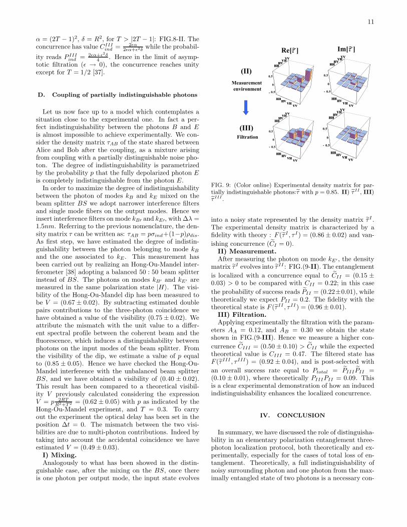
In the fully indistinguishable photons regime, we in-dicate with σI

ind the density matrix after the mixing on

the BS, which is separable for T < 1/√

3, as shown inFIG. 2. The output state is a mixture of the initial state|Ψin〉〈Ψin| and the fully mixed one [27]: FIG.8-I.

σIind =

1

4P Iind

α 0 0 00 β iξ 00 −iξ γ 00 0 0 δ

(36)

with α = δ = R2, β = γ = T 2+(T −R)2, ξ = −T (T −R)

II) Measurement.A measurement is carried out on the environmental

mode through the projection on |H〉E′ . Thus the stateσI

ind evolves into σIIind:

σIIind =

1

4P IIind

0 0 0 00 β iξ 00 −iξ γ 00 0 0 δ

(37)

HH

HV

VH

VV

HH

HV

VH

VV

-0.5

-0.25

0

0.25

0.5

HH

HV

VH

VV

HH

HV

VH

VV

HH

HV

VH

VV

HH

HV

VH

VV

-0.5

-0.25

0

0.25

0.5

HH

HV

VH

VV

HH

HV

VH

VVRe Im

Initial entangled

state

I ) Mixing with

noise

II ) Measurement

environment

III ) Filtration

RESTORATION OF ENTANGLEMENT

HH

HV

VH

VV

HH

HV

VH

VV

-0.5

-0.25

0

0.25

0.5

HH

HV

VH

VV

HH

HV

VH

VV

HH

HV

VH

VV

HH

HV

VH

VV

-0.5

-0.25

0

0.25

0.5

HH

HV

VH

VV

HH

HV

VH

VV

HH

HV

VH

VV

HH

HV

VH

VV

-0.5

-0.25

0

0.25

0.5

HH

HV

VH

VV

HH

HV

VH

VV

HH

HV

VH

VV

HH

HV

VH

VV

-0.5

-0.25

0

0.25

0.5

HH

HV

VH

VV

HH

HV

VH

VV

HH

HV

VH

VV

HH

HV

VH

VV

-0.5

-0.25

0

0.25

0.5

HH

HV

VH

VV

HH

HV

VH

VV

HH

HV

VH

VV

HH

HV

VH

VV

-0.5

-0.25

0

0.25

0.5

HH

HV

VH

VV

HH

HV

VH

VV

FIG. 8: (Color online) Theoretical density matrix for perfectlyindistinguishable photons interacting on the BS.

with β = T 2, γ = T 2+(T −R)2, δ = R2, ξ = −T (T −R).The state is conditionally transformed into a maximallyentangled state (MEMS) [37]: see FIG.(9-II). In particu-

lar, it is found CIIind = T |T−R|

2P II

ind

and P IIind = T 2+(T−R)2+R2

4 .

III) FiltrationDue to the strong asymmetry of σII

ind a filter is intro-duced either on Alice or Bob mode, depending on thevalue of T . If T > |2T − 1|, filter FB acts on Bob mode,as |H〉B → 2T−1

T |H〉B, while if T < |2T − 1|, the filter

acts on Alice mode, as |V 〉A → T2T−1 |V 〉A. In order to

increase the concurrence, a second filter is inserted onboth Alice and Bob mode, which attenuates the verticalpolarization component: |V 〉 → √

ǫ|V 〉. The filters FA

and FB transform the density matrix into σIIIind :

σIIIind =

1

4P IIIind

0 0 0 00 ǫα iǫα 00 −iǫα ǫα 00 0 0 ǫ2δ

(38)

where α = T 2, δ =(

TRR−T

)2

, for T < |2T − 1| and

11

α = (2T − 1)2, δ = R2, for T > |2T − 1|: FIG.8-II. Theconcurrence has value CIII

ind = 2ǫα2ǫα+ǫ2δ while the probabil-

ity reads P IIIind = 2ǫα+ǫ2δ

4 . Hence in the limit of asymp-totic filtration (ǫ → 0), the concurrence reaches unityexcept for T = 1/2 [37].

D. Coupling of partially indistinguishable photons

Let us now face up to a model which contemplates asituation close to the experimental one. In fact a per-fect indistinguishability between the photons B and Eis almost impossible to achieve experimentally. We con-sider the density matrix τAB of the state shared betweenAlice and Bob after the coupling, as a mixture arisingfrom coupling with a partially distinguishable noise pho-ton. The degree of indistinguishability is parametrizedby the probability p that the fully depolarized photon Eis completely indistinguishable from the photon E.

In order to maximize the degree of indistinguishabilitybetween the photon of modes kB and kE mixed on thebeam splitter BS we adopt narrower interference filtersand single mode fibers on the output modes. Hence weinsert interference filters on mode kB′ and kE′, with ∆λ =1.5nm. Referring to the previous nomenclature, the den-sity matrix τ can be written as: τAB = pσind+(1−p)ρdis.As first step, we have estimated the degree of indistin-guishability between the photon belonging to mode kB

and the one associated to kE . This measurement hasbeen carried out by realizing an Hong-Ou-Mandel inter-ferometer [38] adopting a balanced 50 : 50 beam splitterinstead of BS. The photons on modes kB′ and kE′ aremeasured in the same polarization state |H〉. The visi-bility of the Hong-Ou-Mandel dip has been measured tobe V = (0.67 ± 0.02). By subtracting estimated doublepairs contributions to the three-photon coincidence wehave obtained a value of the visibility (0.75 ± 0.02). Weattribute the mismatch with the unit value to a differ-ent spectral profile between the coherent beam and thefluorescence, which induces a distinguishability betweenphotons on the input modes of the beam splitter. Fromthe visibility of the dip, we estimate a value of p equalto (0.85 ± 0.05). Hence we have checked the Hong-Ou-Mandel interference with the unbalanced beam splitterBS, and we have obtained a visibility of (0.40 ± 0.02).This result has been compared to a theoretical visibil-ity V previously calculated considering the expressionV = p 2RT

R2+T 2 = (0.62 ± 0.05) with p as indicated by theHong-Ou-Mandel experiment, and T = 0.3. To carryout the experiment the optical delay has been set in theposition ∆t = 0. The mismatch between the two visi-bilities are due to multi-photon contributions. Indeed bytaking into account the accidental coincidence we haveestimated V = (0.49 ± 0.03).

I) Mixing.Analogously to what has been showed in the distin-

guishable case, after the mixing on the BS, once thereis one photon per output mode, the input state evolves

Measurement

environment

Filtration

(II)

(III)

HHHV

VHVV

HHHV

VHVV

- 0.5

0

0.5

HHHV

VHVV

HHHV

VHVV

HHHV

VHVV

HHHV

VHVV

- 0.5

0

0.5

HHHV

VHVV

HHHV

VHVV

]~Re[ ]~Im[

HHHV

VHVV

HHHV

VHVV

- 0.5

0

0.5

HHHV

VHVV

HHHV

VHVV

HHHV

VHVV

HHHV

VHVV

- 0.5

0

0.5

HHHV

VHVV

HHHV

VHVV

-

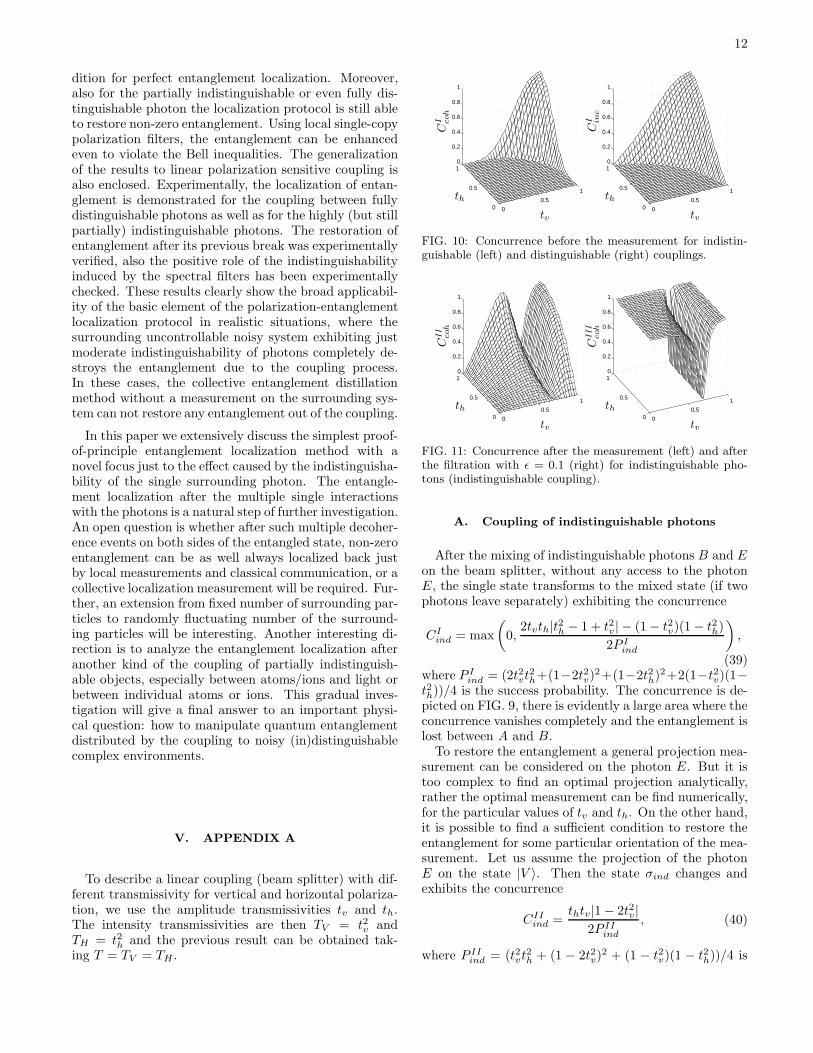
FIG. 9: (Color online) Experimental density matrix for par-tially indistinguishable photons:τ with p = 0.85. II) τ II , III)τ III .

into a noisy state represented by the density matrix τI .The experimental density matrix is characterized by afidelity with theory : F (τI , τI) = (0.86 ± 0.02) and van-

ishing concurrence (CI = 0).II) Measurement.After measuring the photon on mode kE′ , the density

matrix τI evolves into τII : FIG.(9-II). The entanglement

is localized with a concurrence equal to CII = (0.15 ±0.03) > 0 to be compared with CII = 0.22; in this case

the probability of success reads PII = (0.22±0.01), whiletheoretically we expect PII = 0.2. The fidelity with thetheoretical state is F (τII , τII) = (0.96 ± 0.01).

III) Filtration.Applying experimentally the filtration with the param-

eters AA = 0.12, and AB = 0.30 we obtain the stateshown in FIG.(9-III). Hence we measure a higher con-

currence CIII = (0.50 ± 0.10) > CII while the expectedtheoretical value is CIII = 0.47. The filtered state hasF (τIII , τIII) = (0.92 ± 0.04), and is post-selected with

an overall success rate equal to Ptotal = PIII PII =(0.10 ± 0.01), where theoretically PIIIPII = 0.09. Thisis a clear experimental demonstration of how an inducedindistinguishability enhances the localized concurrence.

IV. CONCLUSION

In summary, we have discussed the role of distinguisha-bility in an elementary polarization entanglement three-photon localization protocol, both theoretically and ex-perimentally, especially for the cases of total loss of en-tanglement. Theoretically, a full indistinguishability ofnoisy surrounding photon and one photon from the max-imally entangled state of two photons is a necessary con-

12

dition for perfect entanglement localization. Moreover,also for the partially indistinguishable or even fully dis-tinguishable photon the localization protocol is still ableto restore non-zero entanglement. Using local single-copypolarization filters, the entanglement can be enhancedeven to violate the Bell inequalities. The generalizationof the results to linear polarization sensitive coupling isalso enclosed. Experimentally, the localization of entan-glement is demonstrated for the coupling between fullydistinguishable photons as well as for the highly (but stillpartially) indistinguishable photons. The restoration ofentanglement after its previous break was experimentallyverified, also the positive role of the indistinguishabilityinduced by the spectral filters has been experimentallychecked. These results clearly show the broad applicabil-ity of the basic element of the polarization-entanglementlocalization protocol in realistic situations, where thesurrounding uncontrollable noisy system exhibiting justmoderate indistinguishability of photons completely de-stroys the entanglement due to the coupling process.In these cases, the collective entanglement distillationmethod without a measurement on the surrounding sys-tem can not restore any entanglement out of the coupling.

In this paper we extensively discuss the simplest proof-of-principle entanglement localization method with anovel focus just to the effect caused by the indistinguisha-bility of the single surrounding photon. The entangle-ment localization after the multiple single interactionswith the photons is a natural step of further investigation.An open question is whether after such multiple decoher-ence events on both sides of the entangled state, non-zeroentanglement can be as well always localized back justby local measurements and classical communication, or acollective localization measurement will be required. Fur-ther, an extension from fixed number of surrounding par-ticles to randomly fluctuating number of the surround-ing particles will be interesting. Another interesting di-rection is to analyze the entanglement localization afteranother kind of the coupling of partially indistinguish-able objects, especially between atoms/ions and light orbetween individual atoms or ions. This gradual inves-tigation will give a final answer to an important physi-cal question: how to manipulate quantum entanglementdistributed by the coupling to noisy (in)distinguishablecomplex environments.

V. APPENDIX A

To describe a linear coupling (beam splitter) with dif-ferent transmissivity for vertical and horizontal polariza-tion, we use the amplitude transmissivities tv and th.The intensity transmissivities are then TV = t2v andTH = t2h and the previous result can be obtained tak-ing T = TV = TH .

0

0.5

1

0

0.5

10

0.2

0.4

0.6

0.8

1

tv

th

CI coh

0

0.5

1

0

0.5

10

0.2

0.4

0.6

0.8

1

tv

th

CI in

c

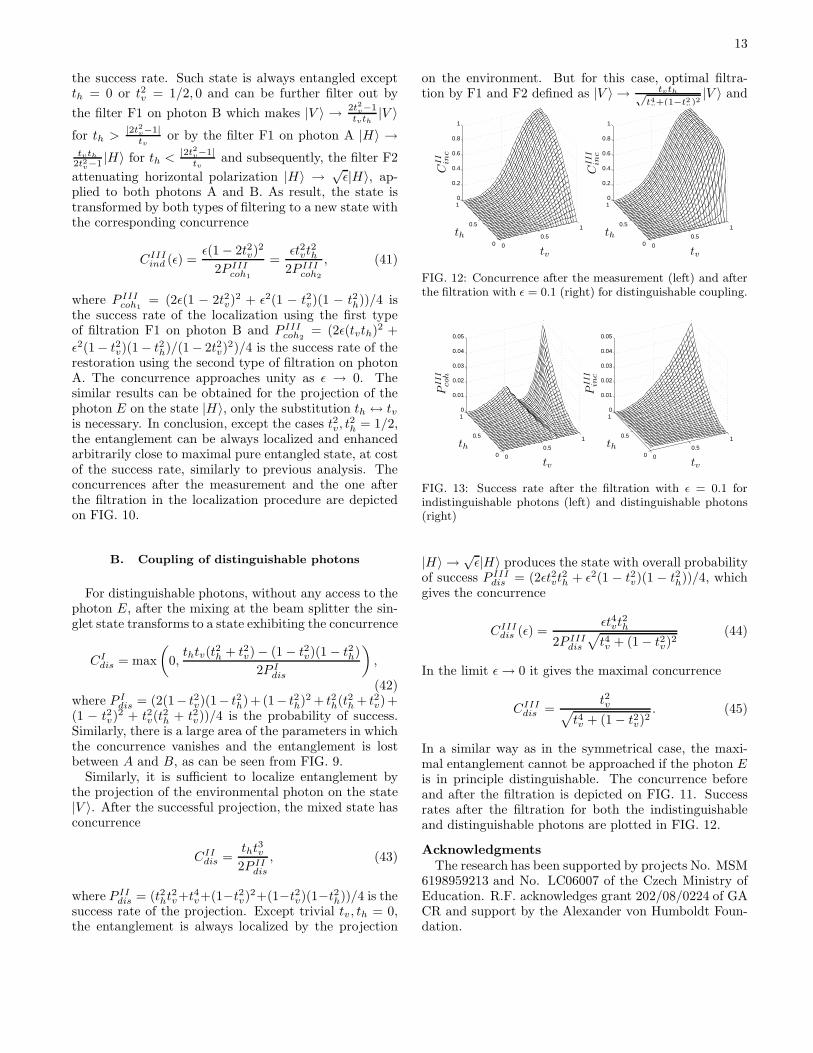
FIG. 10: Concurrence before the measurement for indistin-guishable (left) and distinguishable (right) couplings.

0

0.5

1

0

0.5

10

0.2

0.4

0.6

0.8

1

tv

th

CII

coh

0

0.5

1

0

0.5

10

0.2

0.4

0.6

0.8

1

tv

th

CIII

coh

FIG. 11: Concurrence after the measurement (left) and afterthe filtration with ǫ = 0.1 (right) for indistinguishable pho-tons (indistinguishable coupling).

A. Coupling of indistinguishable photons

After the mixing of indistinguishable photons B and Eon the beam splitter, without any access to the photonE, the single state transforms to the mixed state (if twophotons leave separately) exhibiting the concurrence

CIind = max

(0,

2tvth|t2h − 1 + t2v| − (1 − t2v)(1 − t2h)

2P Iind

),

(39)where P I

ind = (2t2vt2h+(1−2t2v)

2+(1−2t2h)2+2(1−t2v)(1−t2h))/4 is the success probability. The concurrence is de-picted on FIG. 9, there is evidently a large area where theconcurrence vanishes completely and the entanglement islost between A and B.

To restore the entanglement a general projection mea-surement can be considered on the photon E. But it istoo complex to find an optimal projection analytically,rather the optimal measurement can be find numerically,for the particular values of tv and th. On the other hand,it is possible to find a sufficient condition to restore theentanglement for some particular orientation of the mea-surement. Let us assume the projection of the photonE on the state |V 〉. Then the state σind changes andexhibits the concurrence

CIIind =

thtv|1 − 2t2v|2P II

ind

, (40)

where P IIind = (t2vt2h + (1 − 2t2v)

2 + (1 − t2v)(1 − t2h))/4 is

13

the success rate. Such state is always entangled exceptth = 0 or t2v = 1/2, 0 and can be further filter out by

the filter F1 on photon B which makes |V 〉 → 2t2v−1

tvth

|V 〉for th >

|2t2v−1|

tvor by the filter F1 on photon A |H〉 →

tvth

2t2v−1 |H〉 for th <

|2t2v−1|

tv

and subsequently, the filter F2

attenuating horizontal polarization |H〉 → √ǫ|H〉, ap-

plied to both photons A and B. As result, the state istransformed by both types of filtering to a new state withthe corresponding concurrence

CIIIind (ǫ) =

ǫ(1 − 2t2v)2

2P IIIcoh1

=ǫt2vt

2h

2P IIIcoh2

, (41)

where P IIIcoh1

= (2ǫ(1 − 2t2v)2 + ǫ2(1 − t2v)(1 − t2h))/4 is

the success rate of the localization using the first typeof filtration F1 on photon B and P III

coh2= (2ǫ(tvth)2 +

ǫ2(1− t2v)(1 − t2h)/(1− 2t2v)2)/4 is the success rate of the

restoration using the second type of filtration on photonA. The concurrence approaches unity as ǫ → 0. Thesimilar results can be obtained for the projection of thephoton E on the state |H〉, only the substitution th ↔ tvis necessary. In conclusion, except the cases t2v, t

2h = 1/2,

the entanglement can be always localized and enhancedarbitrarily close to maximal pure entangled state, at costof the success rate, similarly to previous analysis. Theconcurrences after the measurement and the one afterthe filtration in the localization procedure are depictedon FIG. 10.

B. Coupling of distinguishable photons

For distinguishable photons, without any access to thephoton E, after the mixing at the beam splitter the sin-glet state transforms to a state exhibiting the concurrence

CIdis = max

(0,

thtv(t2h + t2v) − (1 − t2v)(1 − t2h)

2P Idis

),

(42)where P I

dis = (2(1− t2v)(1− t2h)+ (1− t2h)2 + t2h(t2h + t2v)+(1 − t2v)2 + t2v(t

2h + t2v))/4 is the probability of success.

Similarly, there is a large area of the parameters in whichthe concurrence vanishes and the entanglement is lostbetween A and B, as can be seen from FIG. 9.

Similarly, it is sufficient to localize entanglement bythe projection of the environmental photon on the state|V 〉. After the successful projection, the mixed state hasconcurrence

CIIdis =

tht3v2P II

dis

, (43)

where P IIdis = (t2ht2v+t4v+(1−t2v)2+(1−t2v)(1−t2h))/4 is the

success rate of the projection. Except trivial tv, th = 0,the entanglement is always localized by the projection

on the environment. But for this case, optimal filtra-tion by F1 and F2 defined as |V 〉 → tvth√

t4v+(1−t2

v)2|V 〉 and

0

0.5

1

0

0.5

10

0.2

0.4

0.6

0.8

1

tv

th

CII

inc

0

0.5

1

0

0.5

10

0.2

0.4

0.6

0.8

1

tv

th

CIII

inc

FIG. 12: Concurrence after the measurement (left) and afterthe filtration with ǫ = 0.1 (right) for distinguishable coupling.

0

0.5

1

0

0.5

10

0.01

0.02

0.03

0.04

0.05

tv

thP

III

coh

0

0.5

1

0

0.5

10

0.01

0.02

0.03

0.04

0.05

tv

th

PIII

inc

FIG. 13: Success rate after the filtration with ǫ = 0.1 forindistinguishable photons (left) and distinguishable photons(right)

|H〉 → √ǫ|H〉 produces the state with overall probability

of success P IIIdis = (2ǫt2vt

2h + ǫ2(1 − t2v)(1 − t2h))/4, which

gives the concurrence

CIIIdis (ǫ) =

ǫt4vt2h

2P IIIdis

√t4v + (1 − t2v)2

(44)

In the limit ǫ → 0 it gives the maximal concurrence

CIIIdis =

t2v√t4v + (1 − t2v)

2. (45)

In a similar way as in the symmetrical case, the maxi-mal entanglement cannot be approached if the photon Eis in principle distinguishable. The concurrence beforeand after the filtration is depicted on FIG. 11. Successrates after the filtration for both the indistinguishableand distinguishable photons are plotted in FIG. 12.

AcknowledgmentsThe research has been supported by projects No. MSM

6198959213 and No. LC06007 of the Czech Ministry ofEducation. R.F. acknowledges grant 202/08/0224 of GACR and support by the Alexander von Humboldt Foun-dation.

14

[1] C. H. Bennett, G. Brassard, S. Popescu, B. Schumacher,J. A. Smolin, and W. K. Wootters, Phys. Rev. Lett. 76,722 (1996).

[2] D. Deutsch, A. Ekert, R. Jozsa, Ch. Macchiavello, S.Popescu and Anna Sanpera, Phys. Rev. Lett. 77, 2818(1996).

[3] Z. Zhao, T. Yang, Y. A. Chen, A. N. Zhang, and J. W.Pan, Phys. Rev. Lett. 90 207901 (2003).

[4] J. W. Pan, S. Gasparoni, R. Ursin, G. Weihs and A.Zeilinger, Nature 423, 417 (2003).

[5] P. Walther, K. J. Resch, . Brukner, A. M. Steinberg, J.W. Pan, and A. Zeilinger, Phys. Rev. Lett. 94 040504(2005).

[6] P. G. Kwiat, S. Barraza-Lopez, A. Stefanov, and N.Gisin, Nature (London) 409, 1014 (2001).

[7] O. Cohen, Phys. Rev. Lett. 80, 2493 (1998).[8] D. P. DiVincenzo et al, Lecture Notes in Computer Sci-

ence 1509 (Springer- Verlag, Berlin, 1999), pp. 247-257(2004).

[9] F. Verstraete, M. Popp and J.I. Cirac, Phys. Rev. Lett.

92, 027901 (2004).[10] J. A. Smolin, F. Verstraete, and A. Winter, Phys. Rev.

A 72, 052317 (2005).[11] M. Popp, F. Verstraete, M. A. Martin- Delgado and J. I.

Cirac, Phys. Rev. A 71, 042306 (2005).[12] G. Gour and R.W. Spekkens, Phys. Rev. A 73, 062331

(2006).[13] W. H. Zurek, Rev. Mod. Phys. 75, 715 (2003).[14] F. Sciarrino, E. Nagali, F. De Martini, M. Gavenda, and

R. Filip, Phys. Rev. A 79, 060304(R) (2009).[15] M. Horodecki, P. Horodecki and R. Horodecki, Phys. Rev.

Lett. 78, 574 (1997).[16] N. Linden, S. Massar, and S. Popescu, Phys. Rev. Lett.

81, 3279 (1998).[17] A. Kent, N. Linden, and S. Massar, Phys. Rev. Lett. 83,

2656 (1999).[18] M. Horodecki, P. Horodecki, and R. Horodecki, Phys.

Rev. A 60, 1888 (1999).[19] F. Verstraete, J. Dehaene and B. DeMoor, Phys. Rev. A

64, 010101 (2001).[20] L. X. Cen, N. J. Wu, F. H. Yang, and J. H. An, Phys.

Rev. A 65 052318 (2002).[21] F. Verstraete and M. M. Wolf, Phys. Rev. Lett. 89 170401

(2002).[22] N. A. Peters, J. B. Altepeter, D. Branning, E. R. Jeffrey,

T. C. Wei, and P. G. Kwiat, Phys. Rev. Lett. 92, 133601(2004).

[23] Z. W. Wang, X. F. Zhou, Y. F. Huang, Y. S. Zhang, X. F.Ren, and G. C. Guo, Phys. Rev. Lett. 96 220505 (2006).

[24] Y. C. Liang, L. Masanes, and A. C. Doherty, Phys. Rev.A 77 012332 (2008).

[25] J. S. Bell, Physics 1, 195 (1964).[26] J. F. Clauser, M. A. Horne, A. Shimony and R. A. Holt,

Phys. Rev. Lett. 23, 80 (1969).[27] R.F. Werner, Phys. Rev. A 40, 4277 (1989).[28] W. Wootters, Phys. Rev. Lett. 80, 2245 (1998).[29] R. Horodecki, P. Horodecki and M. Horodecki, Phys.

Lett. A 200, 340 (1995).[30] S. Ishizaka and T. Hiroshima, Phys. Rev. A 62, 022310

(2000).[31] T. C. Wei, K. Nemoto, P. M. Goldbart, P. G. Kwiat, W.

J. Munro, and F. Verstraete, Phys. Rev. A 67, 022110(2003).

[32] C. Cinelli, G. Di Nepi, F. De Martini, M. Barbieri, andP. Mataloni, Phys. Rev. A 70, 022321 (2004).

[33] F. Sciarrino, C. Sias, M. Ricci, and F. De Martini, Phys.

Rev. A 70, 052305 (2004).[34] M. Ghotbi, M. Ebrahim-Zadeh, A. Majchrowski, E.

Michalski, I.V. Kityk, Optics Letters 29, 21 (2004).[35] P. G. Kwiat, K. Mattle, H. Weinfurter, A. and Zeilinger,

Phys. Rev. Lett. 75, 4337 (1995).[36] D. F. V. James, P.G. Kwiat, W. J. Munro, and A. G.

White, Phys. Rev. A 64, 052312 (2001).[37] F. Verstraete, K. Audenaert, T. De Bie, and B. De Moor,

Phys. Rev A 64, 012316 (2001).[38] C K.Z. Hong, Y. Ou, and L. Mandel, Phys. Rev. Lett.

59, 2044 (1987).