Competitive Equilibrium with Moral Hazard inEconomies With Multiple Commodities.

Alessandro CitannaGroupe HEC - Paris, 78351 Jouy-en-Josas, France

and GSIA, Carnegie Mellon University, Pittsburgh, PA, 15213, USA.

Antonio Villanacci¤

DiMAD, Universita’ di Firenze, 50134, Italy.

First draft: December 1996.This version: January 2000.

Abstract

We study an economy with competitive commodity markets and ex-clusive pairwise contractual relations with moral hazard, where both theprincipal and the agent can be risk averse. We show existence of equilibriaand their generic constrained suboptimality, by means of a change in thecompensation schemes. Such suboptimality occurs provided the number ofcommodities is su¢ciently large relative to the number of states and pairtypes, and there are at least three future states of the world.

JEL classi…cation: D51, D52, D82Keywords: general equilibrium, moral hazard, constrained suboptimal-

ity

¤We thank Piero Gottardi and Heraclis Polemarchakis for helpful discussions. Antonio Vil-lanacci acknowledges the hospitality and …nancial support of the University of Geneva throughan EC fellowship.

1. Introduction

In this paper we embed the principal-agent model into the Arrow-Debreu frame-work of uncertainty and perfect competition, and show existence of equilibria.While previous attempts, for instance Prescott and Townsend (1984) and Ben-nardo (1996), consider contractual pairs in which risk-neutral principals design thecontract but have no bargaining power, we study principal-agent pairs in whichthe principal has all the bargaining power, following the partial equilibrium tra-dition (see Grossman and Hart (1983), e.g.). Our assumption can be justi…ed forexample if, when contractual pairs are formed, it is too costly for the agents toswitch to another principal if the contract conditions are judged to be unfavorable.In fact, it can be considered that in our economies contractual pairs are …xed fromthe beginning, and we study the e¤ects of their interaction through competitivecommodity markets. The case analyzed in the literature is polar opposite to ours,assuming that competition across principals leaves them with no surplus, i.e., zeroexpected pro…ts. While their assumption translates into a zero expected pro…tcondition for the principals, in our model principals o¤er utility-maximizing con-tracts, and both the principal and the agent can be risk averse: if the principalacts in her own interest (as an individually-owned …rm), the assumption of riskneutrality is clearly restrictive in the space of preferences. As a consequence ofour modeling strategy, the incentive and participation conditions must be directlyincorporated into the principal maximization problem, and nonconvexities arise.We overcome these di¢culties in a way that does not prevent the use of smoothanalysis for the assessment of the welfare properties of equilibria, essentially ex-tending the approach of Grossman and Hart (1983) to the general equilibriumsetting. It should be noted that risk neutrality of the principal together withthe zero pro…t condition substantially simpli…es the existence problem, in essencereducing the search for competitive equilibria when some states are unobservableto appending some conditions to the usual incomplete markets equilibrium, andtherefore totally bypasses the nonconvexity problems which arise instead in ourframework.

As in the relevant literature, our economy exhibits a …nite number of types ofcontractual pairs, but in…nitely many ex ante identical individuals for each type.However, in each pair optimal contracts are deterministic, and there is no con-sumption randomization. The bilateral contract concerns sharing an uncertainoutput, and this uncertainty is idiosyncratic to the contractual pair; that is, out-put generates individual risk. To focus on the agency problem, we assume no risk

2

in the aggregate. This assumption is totally innocuous, as it will be seen, and itis made only to simplify the exposition: provided the additional aggregate risk isindependent from individual e¤ort, it could be added to our economy. Althoughour model encompasses several examples of contractual relations under incom-plete information (insurer-insuree, security designer-trader, lender-investor), wewill focus on the traditional case of …rms and workers, paired in independent pro-duction units. Output is then exchanged on the commodity markets, which arecompetitive in the sense that individuals take commodity prices as given. Theprice taking behavior depends on the assumption of atomistic individuals, whosestrategic choice of e¤ort does not a¤ect aggregate statistics such as prices.

In our model, principals do not trade linear …nancial contracts. Introducingasset (insurance) markets would generate the same existence problems …rst high-lighted by Helpman and La¤ont (1975). Linear (and nonexclusive) contracts ofthis form are compatible with competitive equilibrium if asset trading constraintsare imposed, as shown by Bisin and Gottardi (1999). Whether …nancial contractsare nonlinear or with trading constraints, the bottom line is that with moralhazard, asset markets will be incomplete. Hence we can expect the welfare conse-quences of the presence of asymmetric information to be complicated by the pricee¤ects in a model with multiple commodities and incomplete …nancial markets.We carry out the study of the welfare properties of our competitive equilibriaunder the assumption of no …nancial markets.

We study the welfare e¤ects caused by changes in the principal’s direct deci-sion variable (e.g.: the compensation scheme, the insurance coverage, the assetpayo¤s), while leaving endowments …xed. In other words, we examine the welfareconsequences directly attributable to the contractual imperfections. We showthat the conclusions derived in a partial equilibrium framework, or with a sin-gle commodity (i.e. constrained optimality, see Prescott and Townsend (1984)),can be reversed with multiple goods and individuals’ risk aversion, provided theprice e¤ects are predominant (that is, when the number of commodities and ofstates is su¢ciently large). The intuition behind the result is all contained in theprice e¤ects that arise with incomplete …nancial markets when there are multiplecommodities (see Geanakoplos and Polemarchakis (1986) and, for an extensionof their results, Citanna, Kajii and Villanacci (1998)). In a competitive econ-omy, the principal designs a contract without taking into account the equilibriumrepercussions on prices. Hence there is room to gain e¢ciency by changing thecompensation scheme. However, and as a di¤erence with Geanakoplos and Pole-marchakis, in our case constrained suboptimality arises even if traders are not

3

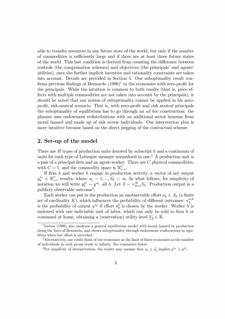
able to transfer resources in any future state of the world, but only if the numberof commodities is su¢ciently large and if there are at least three future statesof the world. This last condition is derived from counting the di¤erence betweencontrols (the compensation schemes) and objectives (the principals’ and agents’utilities), once the further implicit incentive and rationality constraints are takeninto account. Details are provided in Section 5. Our suboptimality result con-…rms previous …ndings of Bennardo (1996)1 in the economies with zero-pro…t forthe principals. While the intuition is common to both results (that is, price ef-fects with multiple commodities are not taken into account by the principals), itshould be noted that our notion of suboptimality cannot be applied in his zero-pro…t, risk-neutral scenario. That is, with zero-pro…t and risk neutral principalsthe suboptimality of equilibrium has to go through an ad hoc construction: theplanner uses endowment redistributions with an additional sector immune frommoral hazard and made up of risk averse individuals. Our intervention plan ismore intuitive because based on the direct pegging of the contractual scheme.

2. Set-up of the model

There are H types of production units denoted by subscript h and a continuum ofunits for each type of Lebesgue measure normalized to one.2 A production unit isa pair of a principal-…rm and an agent-worker. There are C physical commodities,with C > 1; and the commodity space is RC++:

If …rm h and worker h engage in production activity, a vector of net outputyshh 2 RC++ results; where sh = 1; :::; Sh < 1: In what follows, for simplicity ofnotation we will write yshh = ysh ; all h. Let S = £Hh=1Sh. Production output is apublicly observable outcome3.

Each worker can put in the production an unobservable e¤ort ah 2 Ah (a …niteset of cardinality K), which in‡uences the probability of di¤erent outcomes: ¼shkhis the probability of output ysh if e¤ort akh is chosen by the worker. Worker h isendowed with one indivisible unit of labor, which can only be sold to …rm h orconsumed at home, obtaining a (reservation) utility level Vh 2 R.

1Lisboa (1996) also analyzes a general equilibrium model with moral hazard in productionalong the lines of Bennardo, and shows suboptimality through endowment reallocations in equi-libria when low e¤ort is provided.

2Alternatively, one could think of our economies as the limit of …nite economies as the numberof individuals in each group tends to in…nity. See comments below.

3For simplicity of interpretation, the reader may assume that sh ¸ s0h implies ysh ¸ ys0

h :

4

Each …rm proposes a contract to the worker, that is a vector wh = (wshh )Shsh=1,such that if the individual state sh is observed the wage wshh is paid. We assumethat wages are o¤ered as baskets of commodities, instead of being expressed innominal terms. As it is customary with the principal-agent literature, the labormarket is modeled as a take-it-or-leave-it exchange of one unit of labor.

We are going to model output uncertainty at the …rm level as individual risk,and no uncertainty will be derived at the aggregate level. This is accomplished asfollows. All units of each type are assumed to be di¤erent only with respect to theoutput realization and the chosen level of e¤ort. Hence they are ex ante identical.Therefore, aggregate states (as functions from [0; 1]H into S) are equivalent if theycorrespond to the same frequencies of output levels for each type (an argumentsimilar to Malinvaud’s (1973))

Once we …x the proportion of units of type h who choose e¤ort level k, denotedby µkh, the frequency of output level sh, f shh , is determined by

f shh =X

k

µkhfshkh

where f shkh is the frequency of output level sh given e¤ort level akh. Note that forgiven e¤ort level akh, the probability ¼shkh is also the frequency f shkh as a consequenceof the presence of a continuum of individuals for each type and of the Law ofLarge Numbers (see Uhlig (1996)). Therefore f shkh is given as a primitive of theeconomy.4

Although µkh will be determined in equilibrium, individuals take it as given,as they do with future spot commodity prices. This entails a stronger notionof rational expectations. Therefore, from the individual viewpoint the frequencyf shh is also given and unique. This is equivalent to the absence of aggregaterisk in this economy. Although independent aggregate risk could be added tothe speci…cation of uncertainty faced by individuals, this would only complicatethe notation without adding anything substantial to the analysis. Hence we willassume no further independent aggregate risk in the economy.

4Note also that using a continuum of agents in each group guarantees consistency of price-taking behavior on the commodity markets, but does not yield proper market clearing conditions,e¤ective at every realization of uncertainty, but only on (L2¡) average. The interpretation à laMalinvaud based on limit economies would result in e¤ective market clearing, since in that casewe could use Kolmogorov’s Strong Law of Large Numbers. However, in either way any largebut …nite economy would only have approximate market clearing, so we use the continuum ofagents to make our model similar to others used in the literature.

5

For simplicity of exposition we assume K = 2; so that Ah = fa1h; a2hg µ R2++:

However, in what follows we will sometimes keep the use of K to denote thenumber of e¤orts, and this to help the reader identify where the dimensionality ofvectors comes from. De…ne A ´ £Hh=1Ah; with generic element a, and

¡Vh

¢Hh=1 ´

V . Firm h is endowed with a sure vector of goods eh 2 RC+ and an uncertainvector of production yh 2 RCSh++ .

Let ¼kh =³¼shkh

´Shsh=1; and ¼h =

¡¼hk

¢Kk=1 : Moreover, for h = 1; :::;H, denote

by xshcih 2 R++ the consumption in individual state sh of good c by …rm h (wheni = f) and worker h (when i = w). De…ne also (xshcih )Cc=1 = x

shih ; (x

shih )sh = xih; for

i = f;w and (xfh; xwh)Hh=1 = x: Finally, the price of good c is denoted by pc 2 R++

and (pc)Cc=1 = p:We introduce the basic assumptions of the model. First, we impose standard

restrictions on probabilities, that is, …rst order stochastic dominance of the high-level e¤ort over the low-level.

Assumption 1 (stochastic dominance) For any k = 1; 2; ¼kh belongs to theopen Sh ¡ 1-dimensional simplex Sh =

n¼ 2 RSh++ :

PShs=1 ¼

s = 1o

and ¼h 2Sh£Sh is such that, if ak0 ¸ ak;

X

sh·s¼shhk ¸

X

sh·s¼shhk0

for all s 2 Sh; with strict inequality for some s.

Let ¦h be the set of such vectors ¼h: De…ne ¦ = £Hh=1¦h. We then assume that…rms and workers’ utility functions are constant across all output realizations, andsatisfy standard smooth assumptions.

Assumption 2 (risk-averse principal)5 The utility function for …rm h is Uh :Ah £ RShC++ ! R; where

5With only minor changes in the model (namely, allowing for RC+ as the consumption space

and assuming simple di¤erential concavity of the utility functions, de…ned without the boundarycondition and dropping the unboundedness-from-below assumption) we could accomodate forrisk neutrality and still show existence. The test economy that we selected is still valid. Sincethe extension is trivial and only makes the notation cumbersome, we prefer to concentrate onthe case of strict convexity, i.e., of risk aversion for both the principal and the agent. However,the reader can safely apply the existence results to the risk-neutral case.

6

Uh :¡akh; xfh

¢7!

X

sh

¼shkh ¢ uh¡xshfh

¢´ Ukh ;

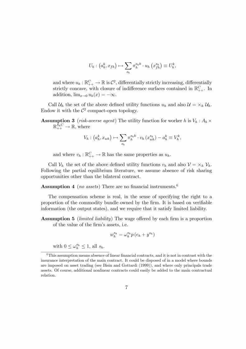
and where uh : RC++ ! R is C2, di¤erentially strictly increasing, di¤erentiallystrictly concave, with closure of indi¤erence surfaces contained in RC++. Inaddition, limx!0 uh(x) = ¡1:

Call Uh the set of the above de…ned utility functions uh and also U = £h Uh.Endow it with the C2 compact-open topology.

Assumption 3 (risk-averse agent) The utility function for worker h is Vh : Ah£RShC++ ! R; where

Vh :¡akh; xwh

¢7!

X

sh

¼shkh ¢ vh (xshwh) ¡ akh ´ V kh ;

and where vh : RC++ ! R has the same properties as uh.

Call Vh the set of the above de…ned utility functions vh and also V = £h Vh.Following the partial equilibrium literature, we assume absence of risk sharingopportunities other than the bilateral contract.

Assumption 4 (no assets) There are no …nancial instruments.6

The compensation scheme is real, in the sense of specifying the right to aproportion of the commodity bundle owned by the …rm. It is based on veri…ableinformation (the output states), and we require that it satisfy limited liability.

Assumption 5 (limited liability) The wage o¤ered by each …rm is a proportionof the value of the …rm’s assets, i.e.

wshh = !shh p (eh + ysh)

with 0 · !shh · 1; all sh:6This assumption means absence of linear …nancial contracts, and it is not in contrast with the

insurance interpretation of the main contract. It could be disposed of in a model where boundsare imposed on asset trading (see Bisin and Gottardi (1999)), and where only principals tradeassets. Of course, additional nonlinear contracts could easily be added to the main contractualrelation.

7

The timing of the model is simple. First, each pair h of …rm and worker ex-change a contract (wh; ah). Then the worker chooses a level of e¤ort ah; productiontakes place and an individual state sh for each individual arises. Owners of …rmsand workers go to the market with their share of production and/or endowmentsand exchange them at the prevailing price.

The objective of each worker is to choose an e¤ort, and then buy goods inorder to maximize his utility. The objective of each …rm is to choose a contractand the e¤ort to be given by the worker, and then buy goods in order to maximizeits utility.

Worker h ’s maximization problem is

maxakh;xwh Vh¡akh; xwh

¢s:t:

¡pxshwh + !shh p (eh + ysh) ¸ 0 for all sh(2.1)

for given p; y; eh and !h: Firm h ’ s maximization problem is

maxakh;xwh;!h;xfh Uh¡akh; xfh

¢s:t:

(1) ¡pxshfh + (1 ¡ !shh ) p (ysh + eh) ¸ 0 ; for all sh,(2) 0 · !shh · 1; for all sh(3)

¡akh; xwh

¢= argmax Vh (eah; exwh) s:t: ¡ pexshwh + !shh p (eh + ysh) ¸ 0

for all sh(4) Vh

¡akh; xwh

¢¡ V h ¸ 0:

(2.2)for given p; y; eh: Constraints (3) and (4) are the incentive and participation con-straint, respectively. Observe that at this stage the problem of the worker is solvedalso by the …rm.

We need to make the individual e¤ort choice consistent with the de…nition ofµkh: First, let µh = (µkh)Kk=1 and let µ = (µh)Hh=1. Since µkh represents the proportionof individuals choosing e¤ort k, and it is an endogenous quantity, an equilibriummust require that µkh be equal to one (zero) if the corresponding e¤ort dominates(is dominated by) the other at given prices, and that µkh be in between only ifboth e¤orts are utility maximizers for each …rm in unit h.

Hence for each type h we …rst split problems 2.1 and 2.2 into K maximizationproblems

max(xkwh)Psh ¼

shkh ¢ vh

³xshkwh

´(2.3)

8

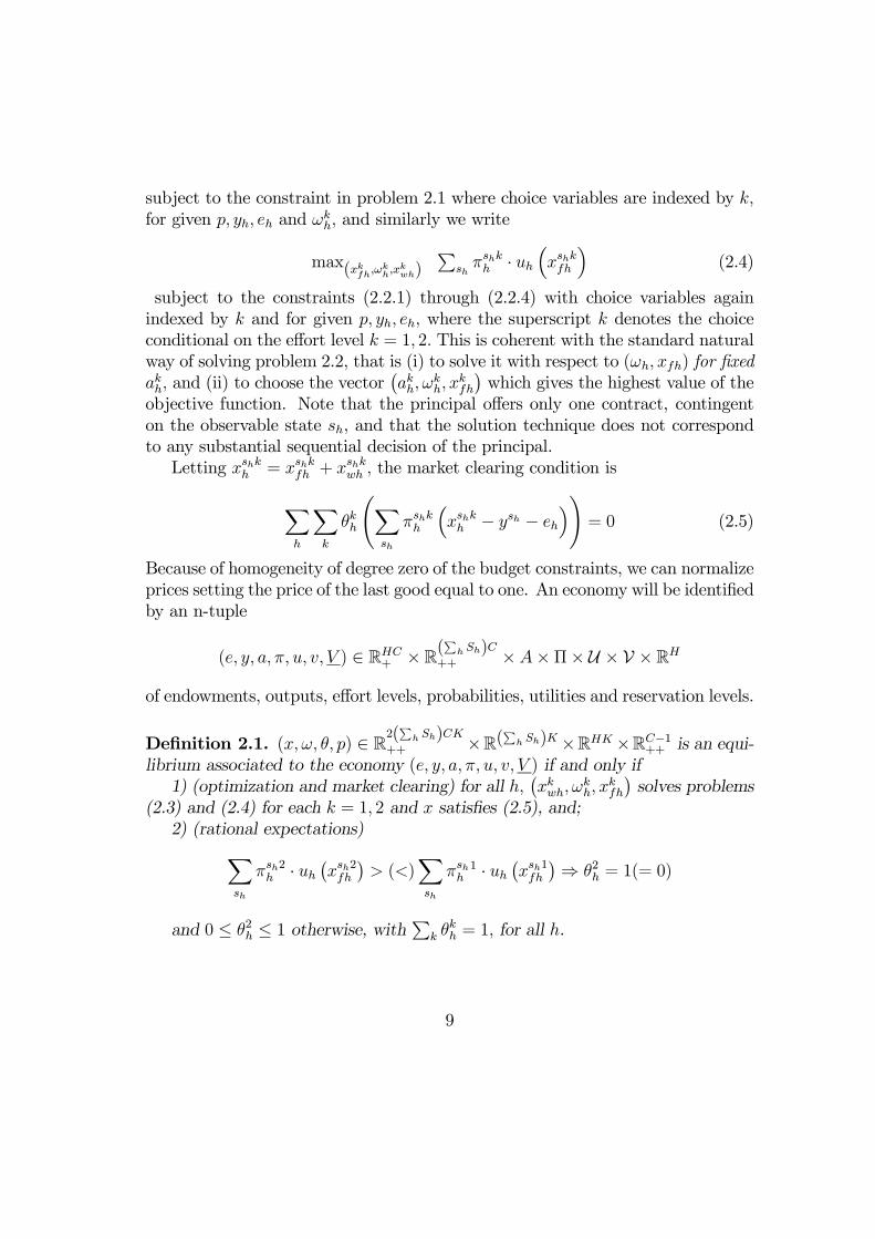
subject to the constraint in problem 2.1 where choice variables are indexed by k;for given p; yh; eh and !kh; and similarly we write

max(xkfh;!kh;xkwh)Psh ¼

shkh ¢ uh

³xshkfh

´(2.4)

subject to the constraints (2.2.1) through (2.2.4) with choice variables againindexed by k and for given p; yh; eh; where the superscript k denotes the choiceconditional on the e¤ort level k = 1; 2: This is coherent with the standard naturalway of solving problem 2.2, that is (i) to solve it with respect to (!h; xfh) for …xedakh; and (ii) to choose the vector

¡akh; !kh; xkfh

¢which gives the highest value of the

objective function. Note that the principal o¤ers only one contract, contingenton the observable state sh, and that the solution technique does not correspondto any substantial sequential decision of the principal.

Letting xshkh = xshkfh + xshkwh ; the market clearing condition is

X

h

X

k

µkh

ÃX

sh

¼shkh³xshkh ¡ ysh ¡ eh

´!= 0 (2.5)

Because of homogeneity of degree zero of the budget constraints, we can normalizeprices setting the price of the last good equal to one. An economy will be identi…edby an n-tuple

(e; y; a; ¼; u; v; V ) 2 RHC+ £ R(Ph Sh)C++ £A£ ¦ £ U £ V £ RH

of endowments, outputs, e¤ort levels, probabilities, utilities and reservation levels.

De…nition 2.1. (x; !; µ; p) 2 R2(Ph Sh)CK++ £R(Ph Sh)K £RHK £RC¡1++ is an equi-

librium associated to the economy (e; y; a; ¼; u; v; V ) if and only if1) (optimization and market clearing) for all h;

¡xkwh; !kh; xkfh

¢solves problems

(2.3) and (2.4) for each k = 1; 2 and x satis…es (2.5), and;2) (rational expectations)

X

sh

¼sh2h ¢ uh¡xsh2fh

¢> (<)

X

sh

¼shh1 ¢ uh

¡xsh1fh

¢) µ2h = 1(= 0)

and 0 · µ2h · 1 otherwise, withPk µkh = 1; for all h.

9

Before proving existence, we need to add assumptions that make the economicproblem interesting, by ruling out the case of empty constraint sets. In particular,we want to make sure that the agent can be asked to participate. Given that weare using a di¤erentiable approach to existence, we will make assumptions tofurther require that this can be done by staying in the interior of the constraintset. This is so accomplished.

Assumption 6 For any h, let ¡h ½ RC+ £ RCSh++ £Ah£¦h £ Vh £ R be the set of°h ´ (eh; y; ah; ¼h; vh; V h) such that

vh (ysh + eh) >1

mins:j¼s1h ¡¼s2h j>0 j¼s1h ¡ ¼s2h j max©a1h + V h; a

2h + V h;

¯̄a2h ¡ a1h

¯̄ª;

all sh:

Assumption 6 in essence says that in any state sh the agent’s utility can beset high enough with the given resources of the …rm, yet without fully utilizingthem.

We will use ¡ = £h¡h and U as our parameter spaces. De…ne it as ­ = ¡£U .In order to apply degree theory, we will need the following property for the set¡h:

Lemma 2.2. ¡h is nonempty and path-connected, all h:

This lemma is technical, although straightforward, and its proof notationallycumbersome, hence it is omitted and is available from the authors upon request.An immediate consequence of Lemma 2.2 is the following result.

Corollary 2.3. ­ is nonempty and path-connected.

Proof. U is path-connected (see Smale (1974)). Path-connectedness of ¡ followsfrom Lemma 2.2. Nonemptiness also is either trivial or follows from the samelemma.

We move now to the analysis of the maximization problems in greater detail.

10

3. The two maximization problems

It is pretty straightforward to see that problems 2.1 and 2.2 can be solved usingthe method …rst suggested by Grossman and Hart (1983). Consider the problem,for given p; y; eh and !h;

maxxshwh vh (xshwh) s:t:

¡pxshwh + !shh p (ysh + eh) ¸ 0:(3.1)

De…ne the smooth value function to the above problem as evh (!shh ; p; ysh ; eh). It isobvious that

¡ak¤h ; x¤wh

¢solves 2.1 if and only if xsh¤wh solves 3.1 for all sh; and ak¤h

solves

maxakh

X

sh

¼shk ¢ evh (!shh ; p; ysh ; eh) ¡ akh:

Also from basic consumer theory we know that, for any (!shh ; p; ysh ; eh), D!shevh >

0 and D2!shevh < 0: Fix a vector y. Because of strict monotonicity of evh; for

any given p the restriction of evh (!shh ; p; ysh ; eh) at this commodity price vectoradmits (smooth) inverse, say Áh (:; p; ysh ; eh) : De…ne zshh = evh (!shh ; p; ysh ; eh) ; thenÁh (z

shh ; p; ysh ; eh) = !shh . Since D!shevh > 0 and D2

!shevh < 0, then DzshÁh =1

D!sh evh > 0 and D2zshÁh = ¡D

2!sh

evhD!sh evh > 0: Here we are heavily exploiting both

utility state separability and the exclusive nature of the contract.Using the above remarks, we have that

¡akh; xwh; !h; xfh

¢is a solution to prob-

lems 2.1 and 2.2 i¤ for any sh; xshwh solves problem 3.1, and¡akh; !h; xfh

¢solves

maxakh;!h;xfh Uh¡akh; xfh

¢s:t: (1) ; (2) and

(3)Psh ¼

shkh ¢ evh (!shh ; p; ysh ; eh) ¡ akh ¸P

sh ¼shk0h ¢ evh (!shh ; p; ysh ; eh) ¡ ak0h ; all k; k0 2 K

(4)Psh ¼

shk ¢ evh (!shh ; p; ysh ; eh) ¡ akh ¡ V h ¸ 0:

(3.2)

for given p; y; eh and ~vh: Observe that (3) implies that the …rm’s choice of ah isthe one carried out by the worker.

After substituting everywhere Áh (zshh ; p; ysh; eh) for !shh in (1) through (4) ; and

after splitting problem 3.2 according to what previously done in Section 2, we canrewrite problems 3.1 and 3.2 as

maxxshkwhvh

³xshkwh

´s:t:

¡pxshkwh + Áh³zshkh ; p; ysh ; e

´p (eh + ysh) ¸ 0:

(3.3)

11

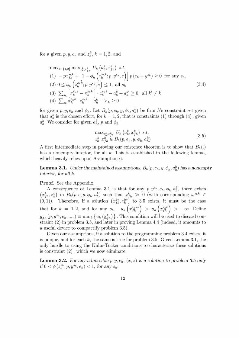
for a given p; y; eh and zkh; k = 1; 2; and

maxk2f1;2gmaxzkh;xkfh Uh¡akh; xkfh

¢s:t:

(1) ¡ pxshkfh +h1 ¡ Áh

³zshkh ; p; ysh ; e

´ip (eh + ysh) ¸ 0 for any sh,

(2) 0 · Áh³zshkh ; p; ysh ; e

´· 1; all sh

(3)Psh

h¼shkh ¡ ¼shk0h

i¢ zshkh ¡ akh + ak

0h ¸ 0; all k0 6= k

(4)Psh ¼

shkh ¢ zshkh ¡ akh ¡ V h ¸ 0

(3.4)

for given p; y; eh and Áh: Let Bh(p; eh; y; Áh; akh) be …rm h’s constraint set giventhat akh is the chosen e¤ort, for k = 1; 2; that is constraints (1) through (4) ; givenakh: We consider for given akh; p and Áh

maxzkh;xkfh Uh¡akh; xkfh

¢s:t:

zkh; xkfh 2 Bh(p; eh; y; Áh; akh)(3.5)

A …rst intermediate step in proving our existence theorem is to show that Bh(:)has a nonempty interior, for all k: This is established in the following lemma,which heavily relies upon Assumption 6.

Lemma 3.1. Under the maintained assumptions, Bh(p; eh; y; Áh; akh) has a nonemptyinterior, for all k:

Proof. See the Appendix.A consequence of Lemma 3.1 is that for any p; ysh ; eh; Áh; akh, there exists¡

xkfh; zkh¢

in Bh(p; e; y; Áh; akh) such that xkfh À 0 (with corresponding !shk 2(0; 1)). Therefore, if a solution

¡xk¤fh; zk¤h

¢to 3.5 exists, it must be the case

that for k = 1; 2; and for any sh; uh³xshk¤fh

´> uh

³xshkfh

´> ¡1: De…ne

ufh (p; ysh ; eh; :::; ) ´ mink©uh

¡xkfh

¢ª: This condition will be used to discard con-

straint (2) in problem 3.5, and later in proving Lemma 4.4 (indeed, it amounts toa useful device to compactify problem 3.5).

Given our assumptions, if a solution to the programming problem 3.4 exists, itis unique, and for each k; the same is true for problem 3.5. Given Lemma 3.1, theonly hurdle to using the Kuhn-Tucker conditions to characterize these solutionsis constraint (2) ; which we now eliminate.

Lemma 3.2. For any admissible p; y; eh; (x; z) is a solution to problem 3.5 onlyif 0 < Á (zshh ; p; y

sh ; eh) < 1; for any sh:

12

Proof. See the Appendix.Problem 3.5 satis…es both necessary and su¢cient conditions to apply Kuhn-

Tucker Theorem (see Mangasarian (1969), e.g.): all constraints and the objectivefunction are pseudoconcave and the constraint set has nonempty interior fromLemmas 3.1 and 3.2.

We conclude this section establishing regularity of the solution to problem 3.5,all k.

Lemma 3.3. The solution to problem 3.5 is a smooth function of the parameters,outside borderline cases.

Proof. See the Appendix.

4. Existence of an equilibrium

We want to show existence of an equilibrium by using the associated system ofKuhn-Tucker and market clearing equations. For ease of notation, we set

f shk1h (:) = ¡pxshkfh +³1 ¡ Áh

³zshkh ; :

´´p(ysh + eh)

fk2h (:) =X

sh

(¼shkh ¡ ¼shk0h )zshk ¡ akh + ak0h

fk3h (:) =X

sh

¼shkh zshk ¡ akh ¡ V h

gshkh (:) = ¡pxshkwh + Áh³zshkh ; p; ysh ; eh

´p(ysh + eh)

and call ®shkh the multiplier associated with f shk1h ; ¯kh the multiplier associated with

fk3h; ±kh ¸ 0 the multiplier associated with fk2h, and …nally ´

hand ´h the multipliers

associated with the constraints µ2h ¸ 0 and 1¡µ2h ¸ 0; respectively. As we observedin the proof of Lemma 3.3, both ®shkh > 0 and f shk1h = 0; and ¯kh > 0 and fk3h = 0;all sh; k; h. Also, let ½shkh be the multiplier associated with the constraint gshkh in3.3, again with ½shkh > 0 and gshkh = 0. Using the …rst order conditions for the twoproblems, an equilibrium must be a solution to the following system of equations:

13

¼shkh Duh³xshkfh

´¡ ®shkh p = 0; all sh; k; h (1)

¡®shkh DÁh¡zshk; :

¢p(ysh + eh) + ¯kh¼

shkh + ±kh(¼

shkh ¡ ¼shk0h ) = 0; all sh; k; h (2)

U2h ¡ U1

h + ´h ¡ ´h = 0; all h (3)

minn´h; µ2h

o= 0; all h (4)

min©´h; 1 ¡ µ2h

ª= 0; all h (5)

f shk1h (:) = 0; all sh; k; h (6)min

©±kh; fk2h (:)

ª= 0; all k; h (7)

fk3h (:) = 0; all k; h (8)¼shkh Dvh

³xshkwh

´¡ ½shkh p = 0; all sh; k; h (9)

gshkh (:) = 0; all sh; k; h (10)Ph[(1 ¡ µ2h)

Psh ¼

sh1h

³xsh1nh ¡ yshn ¡ enh

´+ µ2h

Psh ¼

sh2h

³xsh2nh ¡ yshn ¡ enh

´] = 0 (11)(4.1)

Observe that in (4.1) we have deleted the last market clearing equation, corre-sponding to the numeraire commodity C; using Walras law. In order to …nda solution to system (4:1) we apply a degree theorem (see Lloyd (1978)). LetF°;u : ¥ ! Rº; with º = dim¥; be the function de…ning the equations in system(4:1): Here ¥ is the space of “endogenous” variables, which is a product of openspaces, or manifolds without boundaries. Note that we have actually parametrizeda family of such functions, and by Corollary 2.3 we can build a continuous homo-topy H : ¥ £ [0; 1] ! Rº between any two such functions, that is between anytwo economies (°; u); (°0; u0) 2 ­: In order for deg2 F°;u to be well de…ned at thevalue zero for these functions, we prove that the set H¡1(0) is compact. We thencan construct a test economy (°¤; u¤) for the case of Sh = S = 2 for all h, witha unique equilibrium (x; z; µ; p) ; and show that the test economy is regular, thatis, F°¤;u¤ is continuously di¤erentiable at least locally around the unique point »such that F°¤;u¤(») = 0; and with full-ranked derivative D»F°¤;u¤ : The applicationof the degree theorem is completed after constructing another homotopy betweenthe function de…ning the equilibrium for an economy with an arbitrary (…nite)number of states and a related economy with two states.

These facts will lead to the key statement of the paper.

Theorem 4.1. For any economy (°; u) 2 ­; an equilibrium exists.

The proof follows from the four subsequent lemmas, which establish the prop-erties we just summarized.

14

We build the test economy. Although the test economy is simpli…ed and isbased on the assumption that Sh = S = 2; it captures the fundamental elements ofthe model and will be used to extend the existence result to any …nite Sh (Lemma4.5). Assuming S = 2 allows us to easily show regularity, especially regarding theincentive and participation constraint equations (see Lemma 4.3).

Lemma 4.2. There exists an economy (°¤; u¤) with a unique associated equilib-rium »¤ = (x; z; µ; p) :

Proof. Recall that °h = (eh; y; ah; ¼h; vh; V h) : Assume without loss of generalitythat Sh = S, all h. Moreover, take S = 2. For all h, take uh (xfh) = vh (xwh) =1C

PCc=1 log x

c. Also, take eh = eh ¢ 1; with eh > 0; as the endowments, and for allh and all s take ysh = eys ¢ 1; with eys > 0: De…ne ys = eys + eh. Choose eh and ~yssuch that ys = 100 and y~s = 1000, for the states s and ~s. Take

a1h = log 1 = 0; and a2h = log e = 1:

to be the e¤ort levels for all h: As probabilities, take

¼s1h =23; ¼s2h =

13

Finally, set V h = log 1 = 0, for all h.Now we show that there is a unique equilibrium for the above-chosen economy

(°; u): Consider the associated standard exchange economy with individuals hav-ing initial allocation ysh + eh; all s. Under the assumed separability of the utilityfunctions and the absence of …nancial markets, their state-by-state maximizationproblem is

maxxh

1C

CX

c=1

log xs;ch s:t: p (xsh ¡ ysh ¡ eh) = 0

Let ¹sh be the associated Lagrange multiplier. The …rst order conditions give

¹sh =1

p(ysh + eh)and xs;ch =

p(ysh + eh)Cpc

:

Observe that if p = 1, then

15

¹sh =1Cysh

; xs;ch =Cysh

C= ys

h; uh (xsh) = log ys

h:

[(xsh = ysh

¢ 1; ¹sh = 1Cysh)h; p = 1] is a no-trade walrasian equilibrium, therefore

it is the unique equilibrium associated to the (full information) Pareto optimalallocation (ysh + eh)s;h. In other words, any initial allocation which is equal acrosscommodities for each household is a Pareto optimal allocation with associatedunique equilibrium price equal to 1. Hence, in these economies any sharing of theinitial allocation is also Pareto optimal. This is the key observation. Take

xskwh = !skh ys ¢ 1 and xskfh =

¡1 ¡ !skh

¢ys ¢ 1:

and let p = 1: Once !skh is given and unique, the uniqueness of equilibrium pricesand allocations follows from a standard argument: there cannot be an equilibriumvector of consumption other than the one just computed because, due to the strictconcavity of the utility function, this other vector of consumption would violatePareto optimality; but if that is the case, then prices and multipliers are unique,too.

Once !skh is given; it is immediately shown that equations (4.1.6) and (4.1.10)are satis…ed. If also µ2h = 1; as we will show, equation (4.1.11) is automaticallysatis…ed. Now letting ½skh = ¼skh

C!skh ys ; even equation (4.1.9) is satis…ed, mirroring

the …rst order condition in the walrasian equilibrium for each state s; and for eachk. Similarly, equation (4.1.1) is satis…ed once we set ®skh = ¼skh ¢ Ds;k;Cuh

¡xskfh

¢.

Observe that we can uniquely determine zskh = log!skh ys:We are therefore left with checking existence and uniqueness of !skh ; for all s; k

and h; satisfying system (4:1); and in particular the remaining equations (4.1.2)through (4.1.5), and equations (4.1.7) and (4.1.8), and with showing that µ2h = 1;all h: Note that this entails determining uniquely also the remaining variables ¯; ±and ´ (all indexes are dropped). Using the envelope condition,

@evh@!skh

¡!skh ; :

¢=

1!shkh

(4.2)

Moreover, uh¡xskfh

¢= log

¡1 ¡ !skh

¢ys and

Ds;k;Cuh¡xskfh

¢= ¹skfh =

1C

¡1 ¡ !skh

¢ys: (4.3)

16

Substituting for ®skh in equation (4.1.2) and using (4:2) and (4:3), we get

¼skh ¯kh + ±

kh(¼skh ¡ ¼sk0h ) = ¼skh ¢ !skh

1 ¡ !skh(4.4)

for k = 1; 2 and with k0 6= k. Therefore, dropped the subscript h, the maingoal now is to show that there is a unique solution

¡¯k; ±k; !1k; :::; !Sk

¢k=1;2 with

!sk 2 (0; 1) all s; k; to the system of equations: (4.4), for all s; k; and (4:1:7),(4:1:8).

If, as we will show, U1h < U2

h ; then, from (4.1.3) we get ´h¡´h < 0; from (4.1.4)

it follows that ´h > ´h

¸ 0 , and, …nally, from (4.1.5), we get that µ2h = 1, all h,as desired. Now from equation (4.1.4), the only solution will be ´h = 0: Equation(4.1.3) is then an equation in one unknown, ´h; clearly with a unique solution,di¤erent from zero. A sketch of the computations is provided in the Appendix.

Di¤erentiability and full rank of the derivative with respect to the endogenousvariables now follow from the observation that the derivative of our system isessentially equivalent, after a change of basis, to the derivative of a standardincomplete markets economy, with no …nancial markets.

Lemma 4.3. (°¤; u¤) is a regular economy.

Proof. See the Appendix.It is maintained that Sh ¸ 2 for all h.

Lemma 4.4. The set H¡1 (0) is compact.

Proof. See the Appendix.Finally, here is the result that links economies with Sh = 2 to any …nite Sh;

all h:

Lemma 4.5. There is a continuous homotopy · from economies with Sh = 2and economies with Sh > 2 (and …nite), all h: The set ·¡1(0) is compact, and theeconomy (°¤; u¤) is still a regular test economy.

Proof. See the Appendix.

17

5. Constrained suboptimality

In this section we establish the generic constrained suboptimality of the equilib-rium allocations. In particular, we consider a central authority who could choosezshkh (which is tantamount to choosing !shkh ) in lieu of the principals.7 Let zshkhbe the control variables, and z 2 RKSH the corresponding vector. With a slightmodi…cation from Citanna, Kajii and Villanacci (1998), the possibility of Paretoimproving over the equilibrium outcome occurs if the following system of equationshas no solution

F (»; °; u) = 0

cT·D ~FDG

¸= 0

cT c¡ 1 = 0

(5.1)

where: a) ~F (~»; z; z; ¯; °; u) = 0 represents system (4.1) without equations (2) and(8) ; with ~» = »n(z; ¯); while z is kept at the equilibrium level, that is, z solvesF (»; °; u) = 0 (i.e., (4.1)), and everywhere in (4.1) we substitute for zshkh + zshkhwhenever only zshkh appeared; b) G(»), the utility function vector, is given by

G(») = [:::;X

k

µkhUkh ; ¼

1h(z

1h + z

1h); ¼

2h(z

2h + z

2h); :::];

c) the derivatives are taken with respect to ~» and z, and; d) c is a vector of realcoe¢cients. For z = 0; ~F (~»; z; z; ¯; °; u) = 0 and equation (4.1.2) and (4.1.8)are equivalent to F (»; °; u) = 0: If we kept the participation constraint, overallthe agent would not be a¤ected by the change in z. This way we could onlycare to show that the principals can be made better o¤. However, we drop theparticipation constraint and make sure that the agents, as well as the principals,can be made better o¤.

Evidently, system (5.1) is well de…ned if ~F is di¤erentiable, at least locallyaround an equilibrium, which is true if there are no corner solutions at the mini-mum functions in (4.1). We will …rst assume that to be the case, and show thatthis restriction is weakly generic in the space of parameters. As usual, a propertyis weakly generic if it holds in an open and dense subset of the parameter space.

7It is clear that the methodology applies to a wider range of interventions on the equilibriumoutcome. For instance, it is easier to establish that endowment reallocations through taxes andtransfers would also lead to a Pareto improvement over the equilibrium outcome.

18

Given Theorem 4.1, system (5.1) has no solution if and only if the last twogroups of equations have no solution. We write them explicitly as

ck1hD2Ukh + (¡1)kc3hDUkh ¡ ck6hª+ c11~µkhXknh + c12h~µ

khDUkh = 0 (1)

¡ck1hªT = 0 (2)ck7hÂ[±kh=0] = 0 (3)c4hÂ[µ2h=0] ¡ c5hÂ[µ2h=1] + c11³

nfh + c12h(U

2h ¡ U1

h) = 0 (4)c3h + c4h(1 ¡ Â[µ2h=0]) = 0 (5)¡c3h + c5h(1 ¡ Â[µ2h=1]) = 0 (6)ck9hD2V kh ¡ ck10hª+ c11~µ

khXkh = 0 (7)

¡ck9hªT = 0 (8)PhPk(ck1hP k¤fh + ck6hZkfh + ck9hP k¤wh + ck10hZkwh) = 0 (9)

¡ck6hÁ0kT + ck7h(¼k ¡ ¼k0)T (1 ¡ Â[±kh=0]) + ck10hÁ0k + ck13h¼kh = 0 (10)

cT c¡ 1 = 0 (11)

(5.2)

where: Â is the indicator function which is one on the set in brackets and zero onits complement; ~µ

2= µ2; ~µ

1= 1 ¡ µ2.8 Counting equations and unknowns, note

that there are KSH equations (10) (corresponding to the derivatives with respectto zh), but that we have added the 3H extra variables (the rows DG) c12h, andck13h; for k = 1; 2, all h: Moreover, notice that at any equilibrium where ±kh 6= 0;we also lose equations (3) in (5.2). Hence, throwing away equations (3), we haveKSH¡KH¡3H+1 too many equations. This number is positive provided thatS ¸ 3.

We are now ready to state the main result of this section.

Theorem 5.1. For an open and dense subset of ­; if S ¸ 3 and C ¡ 1 ¸ KSH;the equilibrium allocation is constrained suboptimal.

8Also, cih is the coe¢cient for equation i in (4.1), and³n

h =P

s ¼s2h (xs2n ¡ ysn ¡ en

h) ¡ Ps ¼s1

h (xs1n ¡ ysn ¡ enh)

while

P k¤fh =

·¡®1kIn

¡®2kIn

¸and P k¤

wh =·

¡½1kIn

¡½2kIn

¸

andZk

fh =h¡xshkc

fh +³1 ¡ ©h

³zshkh ; :

´´(yshc + ec

h)i

s=1;:::;S;c6=C

Zkwh =

h¡xshkc

wh + ©h

³zshkh ; :

´(yshc + ec

h)i

s=1;:::;S;c6=C

19

Openness follows from the properness of the natural projection (Lemma 4.4).To prove density in Theorem 5.1, we will use a standard strategy to show that(5.1) has no solution, involving a transversality argument based on perturbationsof system (5.1). This usually entails showing regularity of the equilibrium system…rst, and then applying quadratic perturbations of utility functions to show thatthe derivative of (5.2) with respect to c; and the parameters e; u; has full rank.Instead, mainly for compactness of exposition, we will establish the full rankproperty directly in one step, and then will make use of a transversality argumentfor in…nite dimensional spaces to conclude that also the derivative of system (5.1)with respect to c and the endogenous variables would be full generically, butthe resulting manifold with negative dimension is then empty. Hence the …rststep toward proving genericity of constrained suboptimality is to construct theperturbation technology for the in…nite dimensional case.

5.1. The perturbation technology

We parametrize utilities in the following way. For any given economy (°; u), we…x y and e, and the components of ° other than utilities, call them °0, with°00 = (u; v). We restrict our attention to a compact subset of RC++ containingyshh + eh in its interior; all sh and all h; and therefore bounded away from theaxes of RC++: Then the space U (and V) of utilities previously de…ned and nowrestricted to such a compact set is a Banach space for a bounded metric inducedby the C2 compact-open topology.9 Then ­°0 is also a Banach space. If a propertyis dense with respect to the set ­°0, then it is also dense with respect to ­: This isbecause density is essentially a local property, and we can imagine the functionsin ­°0 to be extended to the original domain in the following way. If an economydoes not satisfy the property, we wiggle the utilities de…ned over the compact setpreviously constructed, and keep them unchanged outside an open set containingthis compact set. Clearly, if two functions are close in the topology on ­°0 thenthey are close in ­; given our construction and the metric on ­°0. Given this,from now on we drop the reference to the point °0 and simply write ­ for ­°0.

Given our economy (°; u) and a corresponding function uh 2 Uh; we considerfor each equilibrium (in particular, for each x¤h 2 F¡1°;u(0))

uh(xs;kfh ) = uh(xs;kfh ) + ·

s;kfh + a

s;kfh (x

s;kfh ¡ xs;k¤fh ) + (xs;kfh ¡ xs;k¤fh )TAs;kfh (x

s;kfh ¡ xs;k¤fh )

9This is true because U (and V) are G± subsets of the space of C2 functions (for a proof, seeAllen (1981), e.g.), and G± subsets are topologically complete (see Hocking and Young (1961)).

20

as a perturbed utility function, with ·s;kfh 2 R, as;kfh 2 RC and As;kfh a C £ Csymmetric, negative de…nite matrix. All parameters ·s;kfh ; a

s;kfh andAs;kfh are assumed

to be small in norm, so that d(uh; uh) < "; for a given " > 0; and where d(:) is thedistance induced by the C2 sup norm in Uh: With this formulation, the set of alluh so obtained is a linear subspace of Uh. Similar conclusions hold for Vh. Thatis so provided we are able to perturb utilities without transforming them fromstate-independent to state-dependent. This can be accomplished in steps. First,we use this parametrization on the subset of parameters where in equilibriumxs;kih 6= xs0;k0ih ; when either s 6= s0 or k 6= k0, all i = f; w and all h: This allowsperturbations of utilities in the form expressed above without altering their state-independence. Then we show that the set of parameters for which in equilibriumxs;kih = xs

0;k0ih ; some s; s0; k; k0; i and h; with s 6= s0 or k 6= k0 is meager. An iterative

procedure would then show that the condition xs;kih = xs0;k0ih ; all s; s

0; k; k0; i and h isalso nongeneric. This is in essence the analogue of dealing with corner solutions.

Since the left hand side of (5.1) is a function © from a Banach space intoRº (with º < 1), it su¢ces to show that D»;c;°00©(»; c; °00), computed at allvalues such that ©(»; c; °00) = 0, is onto when restricted to the particular linearsubspace of U (and V) identi…ed by the above parametrization. Note that thissubspace is …nite for given x¤; but not necessarily so as we move x¤; since wedo not know at this point that the number of equilibria is …nite. The need touse the in…nite dimensional version of the transversality theorem arises from the(uncountably) in…nite dimensionality of this subspace, which in turn derives fromthe need to independently perturb the utility gradient and Hessian, hence to centerthe perturbation around x¤.

Once it is established that rank of the derivative is full, i.e. rank D»;c;°00© = º;we can apply the Sard-Smale theorem (see Smale (1965) or Abraham et al. (1988),Theorem. 3.6.15) to establish transversality, that is, we conclude that there is adense subset of ­ such that rank D»;c©°;u(»; c) = º; for all °; u in this subset.

We can apply the theorem since the projection ¼ : ©¡1(0) ! ­ is a Fredholmmap. It is a continuous linear map, in fact a smooth map, if we establish that rankD»;c;°00© = D© = º; so that ©¡1(0) is a Banach smooth submanifold of ¥£C£­,a Lindelöf manifold, and:

a) ¼ is (proper over a Hausdor¤, locally compact and …rst countable topologicalspace, hence) closed;

b) ¥ £ C is …nite dimensional;c) ©¡1(0) is a closed subspace of …nite codimension (a consequence of codim

©¡1(0) = dimRº)

21

Then the statement on ¼ follows from Abraham et al (1988), Lemma 3.6.24,and:

d) ¼ has …nite kernel, since dimker¼ = dim[(¥ £ C) \ ©¡1(0)] = º; and,e) ¼ has …nite co-kernel, a consequence of Abraham et al:, Lemma 3.6.23.Hence, by the Sard-Smale theorem, the set of regular values of ¼ is open and

dense in ­: The transversality proof is then concluded like in the standard …nitedimensional case.

5.2. Density

We are now ready to prove the second part of Theorem 5.1, the density statement.Proof. Assume conditions A) through D), that is:

A) csk1h 6= 0; and csk9h 6= 0; all s; k; h:B) Writing equations

X

h

X

k

ck6hZkfh = 0 (5.3)

in matrix form as Ab = 0;where

A =

26666664

¢ ¢ ¢ xsk1fh ¡ [(1 ¡ Á(zskh )]~ys1 + @©h@p1 p

1eys1 ¢ ¢ ¢...

¢ ¢ ¢ xskcfh ¡ [(1 ¡ Á(zskh )]~ysc + @©h@p1 p

ceysc ¢ ¢ ¢...

¢ ¢ ¢ xsk(C¡1)fh ¡ [(1 ¡ Á(zskh )]~ys(C¡1) + @©h@p1 p

C¡1eysC¡1 ¢ ¢ ¢

37777775

is a (C¡1)£KSH-dimensional matrix of individual excess demands, ~ys = ys+eh;and for ease of notation s = sh; while b = (¢ ¢ ¢ ; csk6h; ¢ ¢ ¢) is a KSH-dimensionalvector. There exists a square submatrix of A with KSH rows, and full rank,denoted by A0: This explains why we assume that C ¡ 1 ¸ KSH:

C) There exists at least a household h such that³nh ´ P

s ¼s2h (xs2n ¡ ysn ¡ enh) ¡ P

s ¼s1h (xs1n ¡ ysn ¡ enh) 6= 0:

D) In equilibrium, there are no corner solutions, and xs;kih 6= xs0;k0ih ; when eithers 6= s0 or k 6= k0, all i = f;w and all h;

First observe that if A), and after throwing out (H ¡ 1) of equations (4) ; andequation (11), which under our assumptions we do without compromising theexcess number of equations in the system, the following perturbation of system(5.2) works:

22

Afh; all k; h (1)cskC1h ; all s; k; h (2)cc11; some c (4)c3h if µ2h = 0; c4h otherwise; all h (5)c3h if µ2h = 1; c5h otherwise, all h (6)Awh; all k; h (7)cskC9h ; all s; k; h (8)csknC9h ; some h; s; k (9)csk6h; all s; k; h (10)

(5.4)

Note that (4) is perturbed using condition C). The next step is to show thatD»;°00Fhas full rank (without using ®s0k0h0 ), which would imply that rank D»;c;°00© = º:Wecan apply the transversality theorem to state that system (5.1) has no solution asdesired, provided the stated conditions hold. This is immediately veri…ed usingthe following sketched perturbations:

¢as;k;cfh (1)¢®s;kh (2)¢·s;kfh ; some s; k (3)¢´h

or ¢µ2h [if µ2h > 0 or = 0; resp.] (4)¢´h or ¢µ2h [if µ2h < 1 or = 1; resp.] (5)¢xs;k;Cfh (6)¢±kh or ¢zkh [if f2h > 0 or = 0; resp.] (7)¢zkh (8)³¢xs;kwh; ¢½

s;kh

´(9) ; (10)

¢xs;k;cfh ; some s; k; h all c 6= C (11)

(5.5)

Note that equations (11) do not contain the market clearing condition forc = C.

As for condition A), observe that if ck1h = 0 and ck9h = 0, all h; k; then alsock10h = 0; and c11 = 0, using the numéraire commodity normalization. Usingequations (4.1.1) and (5.2.1), we have

csk6h = ®skh (c12h~µ

k+ (¡1)kc3h) (5.6)

Concentrating on equations (5.2.9), one can see that these form the subsystem(5.3). Under condition B), if C ¡ 1 ¸ KSH; (5.3) has a unique solution, that is,

23

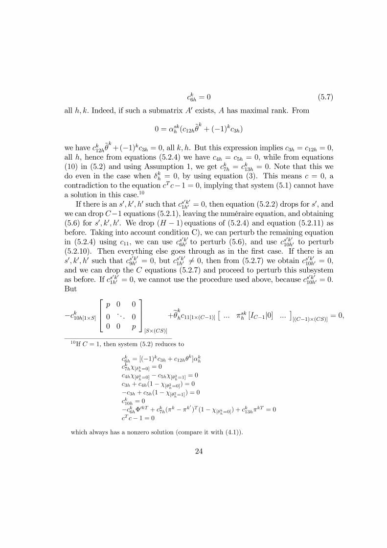
ck6h = 0 (5.7)

all h; k: Indeed, if such a submatrix A0 exists, A has maximal rank. From

0 = ®skh (c12h~µk+ (¡1)kc3h)

we have ck12h~µk+(¡1)kc3h = 0; all k; h. But this expression implies c3h = c12h = 0;

all h, hence from equations (5.2.4) we have c4h = c5h = 0; while from equations(10) in (5.2) and using Assumption 1, we get ck7h = ck13h = 0: Note that this wedo even in the case when ±kh = 0; by using equation (3). This means c = 0; acontradiction to the equation cT c¡1 = 0; implying that system (5.1) cannot havea solution in this case:10

If there is an s0; k0; h0 such that cs0k01h0 = 0; then equation (5.2.2) drops for s0, andwe can drop C¡1 equations (5.2.1), leaving the numéraire equation, and obtaining(5.6) for s0; k0; h0. We drop (H ¡ 1) equations of (5.2.4) and equation (5.2.11) asbefore. Taking into account condition C), we can perturb the remaining equationin (5.2.4) using c11; we can use cs0k06h0 to perturb (5.6), and use cs0k010h0 to perturb(5.2.10). Then everything else goes through as in the …rst case. If there is ans0; k0; h0 such that cs0k09h0 = 0; but cs0k01h0 6= 0, then from (5.2.7) we obtain cs0k010h0 = 0;and we can drop the C equations (5.2.7) and proceed to perturb this subsystemas before. If cs0k01h0 = 0, we cannot use the procedure used above, because cs0k010h0 = 0:But

¡ck10h[1£S]

264p 0 0

0 . . . 00 0 p

375[S£(CS)]

+eµkhc11[1£(C¡1)]£::: ¼skh [IC¡1j0] :::

¤[(C¡1)£(CS)] = 0;

10If C = 1, then system (5.2) reduces to

ck6h = [(¡1)kc3h + c12hµk]®k

hck7hÂ[±k

h=0] = 0c4hÂ[µ2

h=0] ¡ c5hÂ[µ2h=1] = 0

c3h + c4h(1 ¡ Â[µ2h=0]) = 0

¡c3h + c5h(1 ¡ Â[µ2h=1]) = 0

ck10h = 0

¡ck6h©0kT + ck

7h(¼k ¡ ¼k0)T (1 ¡ Â[±k

h=0]) + ck13h¼kT = 0

cT c ¡ 1 = 0

which always has a nonzero solution (compare it with (4.1)).

24

and

¡ck0s010h0ps0 + ¼s

0k0h0

eµk0

h0 ¢ c11[1£(C¡1)] [[IC¡1j0]][(C¡1)£C] = 0;

and also

¼s0k0h0

eµk0

h0 ¢ c11[1£(C¡1)] [[IC¡1j0]][(C¡1)£C] = 0;

which implies that c11 = 0, if eµk0

h0 6= 0; so we gain an extra degree of freedom, andthrow away the one equation among (5.2.4), (5.2.1) and (5.2.7) which we cannotperturb. If eµk

0

h0 = 0; we lose the equation we are not able to perturb:Finally, we show that conditions B), C) and D) hold generically. The argument

is standard and is sketched in the Appendix (see Regularity results). To conclude,we obtain a dense subset of parameters where system (5.1) has no solution, as wewere to show.

25

A. Proof of Lemma 3.1

Drop the subscript h: The set B(p; e; y; Á; ak) could be empty because of con-straints (3) and (4) : Indeed, for any s; once !s is given; if xsf = (1¡!s)(ys+ e)=2then (1) is satis…ed as a strict inequality. We distinguish the cases when k = 1 ork = 2: Without loss of generality assume a2 ¸ a1:

a) First, we examine the constraint set for k = 1; and with a2 > a1: We notethat

z = mins0

ev³!s

0= 1; p; ys

0; e

´> a1 + V

by Assumption 6 and by de…nition of indirect utility. By continuity and mono-tonicity of ~v, for all s there exists an !s 2 (0; 1) such that z > ~v(!s; p; ys; e) >a1 + V : Let z = mins0 ev

¡!s0 ; p; ys0 ; e

¢: Since ~v is a di¤eomorphism, for all s there

exists an !s such that z = ~v(!s; p; ys; e); and !s < 1 by construction and !s > 0by Assumption 3. So (2) is also satis…ed with strict inequalities. Let zs = z and!s = !s: Then (4) is immediately satis…ed and nonbinding, since

X

s

¼s1z ¡ a1 ¡ V = z ¡ a1 ¡ V > 0

As for (3) ; we observe thatX

s

[¼s1 ¡ ¼sh2)]z ¡ a1 + a2 = a2 ¡ a1 > 0

by assumption.b) If k = 1 but a2 = a1; let s be a state such that ¼s2 ¡ ¼s1 > 0 and

~s a state where ¼~s2 ¡ ¼~s1 < 0. Such states exist by Assumption 1. Sincelim!!0 ev (!; p; ys; e) = ¡1 and, by Assumption 6, for any s;

v (ys + e) >¯̄a2 ¡ a1

¯̄= 0

the continuity of ev and the connectedness of [0; 1] imply that for all s there existsan !s 2 (0; 1) such that ev (!s; p; ys; e) = 0: Let !s = !s and zs = ev (!s; p; ys; e) = 0for all s 6= ~s: Then (3) and (4) are satis…ed with inequalities. By Assumption6, there exists a !~s and a corresponding z~s = ev

¡!~s; p; ys; e

¢such that the above

inequalities are satis…ed in a strict sense and such that !~s = Á(z~s; p; y~s; e) 2 (0; 1);so that (2) is satis…ed too.

26

c) Finally, for k = 2; again for all s there exists an !s 2 (0; 1) such thatev (!s; p; ys; e) = 0: Let zs = 0 and !s = !s for all s 6= s; where s is as above: UsingAssumption 6, again we immediately can choose zs such that both constraints(3) and (4) are satis…ed with strict inequalities (this is where the full power ofAssumption 6 is used). Then, letting !s = Á(zs; p; ys; e); we have 0 < !s < 1; andconstraint (2) is satis…ed and nonbinding.

B. Proof of Lemma 3.2

>From the participation constraint (4) it must be that !shh > 0; because

lim!shh !0

evh (!shh ; p; ysh; eh) = ¡1:

Hence at an optimum for problem 3.5, the constraint Áh (zshh ; p; ysh ; eh) ¸ 0 is

never binding. Similarly, it must be that !shh < 1:We know that the …rm can lockin the utility uh

³xshkfh

´in each state, as a consequence of Lemma 3.1. Recall that

xshkfh is obtained with !shkh < 1: Moreover, for any sh; uh¡xshfh

¢< uh (xfh) < +1,

where xfh =¡xcfh

¢Cc=1

and xcfh = p(ysh+eh)minc pc

: (This last statement shows that thevery low utility in state sh can be compensated by a very high utility in the otherstates only up to a given extent.). Now assume that there is k and sh such that!shkh ! 1: Then xshkfh ! 0; and by Assumption 2,

limxshfh!0

uh(xshkfh ) = ¡1:

which ends our proof.

C. Proof of Lemma 3.3.

The Kuhn-Tucker conditions for problem 3.5 are

27

xshkh ¼shkh Dxshkuh³xshkfh

´¡ ®shkh p = 0 (1)

zshkh ¡®shkh Á0h³zshkh ; :

´p(ysh + eh) + ¯kh¼

shkh + ±kh(¼

shkh ¡ ¼shk0h ) = 0 (2)

®shkh minf®shkh ;¡pxshkfh +³1 ¡ Áh

³zshkh ; :

´´p(ysh + eh)g = 0 (3)

±kh minn±kh;

Psh(¼

shkh ¡ ¼shk0h ) ¢ zshkh ¡ akh + ak

0h

o= 0 (4)

¯kh minf¯kh;Psh ¼

shkh z

shkh ¡ a1h ¡ V hg = 0 (5)

(C.1)

One immediately sees that ®shkh > 0; all sh; k; h; that ¯kh > 0 all k; h: To show¯kh > 0; solve for ®shkh in (C:1:1) and substitute it into (C:1:2) to get

¼shkh ¯kh + ±

kh(¼shkh ¡ ¼shk0h )

=³¼shkh Dshkuh

³xshkfh

´(ysh + eh)

´Á0h

¡zshk; :

¢

Suppose ¯1h = 0: If ±kh > 0, there is a state s such that ¼skh ¡ ¼sk0h < 0, while theright-hand side is always positive, clearly an absurd. Similarly, with ±kh = 0; wewould have the absurd that the right-hand side is both positive and zero: Hence¯kh > 0.

We limit ourselves to showing that if it is not the case that constraint (3) holdswith equality and ±kh = 0, then the derivative of system (C.1) with respect to thechoice variables and the multipliers (listed to the left-hand side of the system) hasfull row rank. Hereafter, we drop the subscript h and …x a k:

If ±k > 0 andPs(¼sk ¡ ¼sk0) ¢ zsk ¡ ak + ak0 = 0; taking the derivative, we get

the CS + 2S + 2- dimensional square matrix

Mk =

266664

D2k 0 ¡ªT 0 0

0 ¡Á00k ¡Á0k ¼k ¡ ¼k0 ¼k¡ª ¡Á0kT 0 0 00 (¼k ¡ ¼k0)T 0 0 00 ¼kT 0 0 0

377775

where

ª =

264p 0 0

0 . . . 00 0 p

375 ;

28

an S £ CS matrix of prices, and D2k; Á

0k and Á00k are matrices of dimensionSC£SC (the …rst) and S£S (the last two) with zeros o¤ the diagonal, and withgeneric diagonal elements D2

sk = ¼skD2u¡xskf

¢; Á0sk = Á0(zsk; p; ys; e)p(ys+e) and

Á00sk = ®sk ¢D2skÁ

¡zsk; p; ys; e

¢¢ p(ys+ e); respectively. Note that Á00sk > 0; all s; k.

If ±k = 0 andPs(¼sk ¡ ¼sk0) ¢ zsk ¡ akh + ak

0h > 0; the matrix of derivatives has

the same rank of

Mk0 =

2664

D2k 0 ¡ªT 0

0 ¡Á00k ¡Á0k ¼k¡ª ¡Á0kT 0 00 ¼kT 0 0

3775

We want to show both that 0 =Mk¢; where ¢ = (¢x;¢z;¢®;¢±;¢¯) impliesthat ¢ = 0; and that 0 = Mk0¢0 where ¢0 = (¢x;¢z;¢®;¢¯) implies ¢0 = 0:The argument is standard, based on the convexity of preferences, and the detailsare left to the reader.

D. Proof of Lemma 4.2.

Drop the subscript h: The relevant subsystem composed of equations (4.4) and(4.1.7) and (4.1.8) is written more compactly as

(1) ¼s1¯1 + [¼s1 ¡ ¼s2] ±1 = ¼s1ks1(2)

Ps(¼s1 ¡ ¼s2) log!s1ys ¡ a12 ¸ 0

(3)Ps ¼s1 log!s1ys = a1

(4) ¼s2¯2 + [¼s2 ¡ ¼s1] ±2 = ¼s2ks2(5)

Ps(¼s1 ¡ ¼s2) log!s2ys ¡ a12 · 0

(6)Ps ¼s2 log!s2ys = a2

(D.1)

where (1) and (4) correspond to equations (4.1.2), (2) and (5) correspond to equa-tions (4.1.7) and (3) and (6) correspond to equations (4.1.8), once it is understoodthat ±k ¸ 0; for k = 1; 2, and that if (2) is a strict inequality, ±1 = 0; and if (8) isa strict inequality, ±2 = 0: Also, we have de…ned

ksk =!sk

1 ¡ !sk > 0;

a12 = a1 ¡ a2;

29

and y = ysyes = 1=10: Once the parameters are …xed, system (D.1) is formed of two

independent blocks, expressions (1) through (3) ; and expressions (4) through (6) :Moreover, each block can be solved recursively. The strategy to solve the abovesystem is decomposed in steps (all equation numbers refer to system (D.1), unlessotherwise stated):

(i) Since (2) cannot hold as equality, and therefore ±1 = 0, solve for ¯1; ±1; !s1;all s, from equations (1) and (3) and verify that (2) is satis…ed.

(ii) Since (5) cannot hold as inequality, solve …rst for¡log!s2ys; log!~s2y~s

¢and

hence for !s2 and !~s2 from equations (5) and (6).

(iii) Solve for ¯2, ±2 as functions of !s2; for s = s; ~s; from equation (4), checkingthat ±2 > 0.

(iv) Check that the restrictions on !s2 are satis…ed.

(v) Check that Ufh¡x1fh

¢< Ufh

¡x2fh

¢, so that µ2h = 1; for all h:

The details of the computation are available from the authors upon request.

E. Proof of Lemma 4.3.

The derivative of the extended system F°¤;u¤ (»¤) with respect to »¤ is summarizedbelow as

26666664

M10h 0 0 0 0 P 1

fhB1h Dh B2

h 0 0 00 0 M2

h 0 0 P 2fh

C1h 0 0 W 1

h 0 P 1wh

0 0 C2h 0 W 2

h P 2wh

0 0 X2h 0 X2

h 0

37777775

(E.1)

where:a) Mkh = Mk; the previously de…ned matrix (see Lemma 3.3) of derivatives

of the principal’s …rst order conditions, and similarly, Mk0h is Mk0 with the addedcolumn of the derivative with respect to ±k and the row corresponding to equation(4:1:7) (calculations in Lemma 4.2 show that ±1h = 0 while f12h(:) = 0, all h, and±2h > 0).

30

b) Bkh is a 3£(CSh+2Sh+2) matrix of zeros, except for the …rst CSh elementsof the …rst row, which are equal to the vector (:::; ¼s1Du(xs1); :::), if k = 1, andto (:::;¡¼s2Du(xs2); :::); if k = 2.

c) Dh is the 3 £ 3 matrix of derivatives of equations11 (3) ; (4) and (5) withrespect to µ2h; ´h and ´h; that is

Dh =

24

0 1 ¡10 1 0¡1 0 0

35

d) Ckh is a (CSh+Sh)£(CSh+2Sh+2) matrix of derivatives of the agent’s …rstorder conditions (equations (9) and (10)) with respect to the principal’s choicevariables, for k = 1; 2. In particular, it has all zeros except for the derivative ofequation (10) with respect to zskh .

e) Finally,W kh =·D2vkh ¡ªT¡ª 0

¸; the matrix of derivatives of the agent’s …rst

order conditions with respect to xskwh and ½skh , for k = 1; 2: X2h =

£::: ¼s2h InT :::

¤

(recall that µ2h = 1; all h), while

P kfh =

2664

¡®1kIn¡®2kIn¤kh0

3775 and P kwh =

24

¡½1kIn¡½2kIn0

35

are a (CSh+2Sh+2)£(C¡1) and a (CSh+Sh)£(C¡1); respectively, matrices ofprice derivatives. Here InT =

£I 0

¤; a (C ¡ 1)£C matrix, with a last column

of zeros, and I is the usual (C ¡ 1) square identity matrix.The simple idea of the proof is to …rst perform some elementary operations

on rows and columns of (E.1) (that is, without a¤ecting its rank) and then toobserve that the obtained matrix has full row rank, as a consequence of a knownresult. Namely, and for each h:

1. Using the full rank ofDh, clean12 the matrices Bkh of their nonzero elements,for k = 1; 2:

2. Using the super-columns of (x1wh; ½1h) ; and the fact that W 1h has full row

rank, clean C1h of its nonzero elements. Keep in mind that µ2h = 1.

11All equation numbers refer to system (4.1), unless otherwise stated.12By “clean” we mean: use an appropriate linear combination of columns (or rows) of the

given matrix and add it to the targeted matrix (or row(s), or column(s)), so that the result iszero.

31

3. For k = 2; the matrix of derivatives of (7) and (8) with respect to zs2h hasfull rank (recall that S = 2). Hence we use it to clean ¡Á002 and ¡Á02T in M2

h ;and the nonzero elements of C2

h. Similarly, the matrix of derivatives of (2) withrespect to ¯2h and ±2h has full rank. Hence we use it to clean the rows of ¡Á02 inM2h (i.e. the derivatives of equation (2) with respect to ®s2h ), and ¤2h; a matrix of

nonzero derivatives in P kfh.4. Because of Lemma 3.3, we can use M10

h to clean the matrix P 1fh:

Rearranging rows and columns, the transformed matrix (E.1) is shown to havefull rank if and only if the following matrix has full row rank (zeros are omitted):

D2u2h ¡ªT·

¡®12h In¡®22h In

¸

¡ª

D2u2wh ¡ªT ¡½12h In¡½22h In

¡ªX2h X2

h

where D2u2h (D2u2wh) is the Hessian of the utility function of …rm (worker) ife¤ort k = 2 is chosen. The above matrix has the same structure of the analogousderivative for a standard exchange economy with completely incomplete …nancialmarkets computed at a no trade equilibrium and therefore it has full row rank.

F. Proof of Lemma 4.4

In what follows, “Converges” means “converges (or so does a subsequence) to anelement which belongs to the set containing the sequence”. Consider a pair ofeconomies (°; u) and (°¤; u¤) and any sequence

fxn; zn; µn; ®n; ¯n; ±n; ´n; ½n; pn; tng1n=1 ½ H¡1(0):

Then:©¡µ2h

¢nª1n=1 Converges, say to µh; because it is contained in the compact set

[0; 1] : For a similar reason, ftng1n=1 Converges to t: For at least one k,©xknwh

ª1n=1 is

bounded above by total resources and below by zero, all h. Since for any s we havezsknh = v(xsknwh ); using the participation constraint and the boundary condition onpreferences it is easily seen that xknwh Converges to xkwh.

n(½shkh )n

o1n=1

Converges

32

because of (4:1:9) and the fact that pC = 1: fpng1n=1 Converges because ½shk doesand because of equations (4:1:9): Now equation (4.1.10) shows that

©xk0nwh

ªalso

Converges for k0 6= k (a necessary step if µh 2 f0; 1g): Since zshknh = vh¡xsknwh

¢,

then fzshnh g1n=1 Converges. On the other hand, fxnfhg is bounded above by totalresources and below away from the axes as a consequence of Lemmas 3:1 and3:2; and the convergence of pn; then xnfh Converges, using the boundary condition

on preferences:n(®shkh )n

o1n=1

Converges because of the price normalization and of(4:1:1):

f¯nhg1n=1 and f±nhg1n=1 Converge because of equations (4:1:2) = 0, i.e.,·¯n

±n¸=

[A (¼n)]¡1 Ân - with obvious notation - and A (¼n) is a square matrix (recall thatSh ¸ 2; all h) which has full rank along the sequence and in the limit and ÂnConverges.

According to the value of µ2h; either ´nh

! 0 or ´nh ! 0 (or both), whilethe other Converges from (4:1:4) and (4:1:5): More precisely, if µh = 0; sinceminf´nh; 1¡(µ2h)ng = 0; all n, then 0 = limn!+1minf´nh; 1¡(µ2h)ng = limn!+1 ´n:Then, from (4:1:3); limn!+1 ´n = limn!+1 U (1; n)¡U (2; n) ; a converging limit,with obvious notation. The same argument works in the remaining cases, andcompletes the proof.

G. Proof of Lemma 4.5

The proof of existence by homotopy is carried through inductively. It is enoughto show that a homotopy exists between economies with S = 2 and S = 3. De…ne¼h 2 ¦h µ R2

++ and ¼¤h 2 ¦¤h µ R3

++; where the two probability spaces satisfy theassumptions of the paper in the case in which the number of the states is 2 and3, respectively. Moreover, let

¼kh(t) = (1 ¡ t)¡¼kh; 0

¢+ t¼k¤h :

De…ne the space of endogenous variables of an economy with S states as ¥S andlet dim¥S = n (S) : Let ­S be the space of exogenous variables of an economywith S states (which for S = 3 includes both ¼h and ¼¤h): Fix " 2 R++: Considerthe function

· : ¥3 £ [0; 1] ! Rn(3)

33

de…ned:a) by the left-hand side of equations (4.1.4) and (4.1.5), and of equations

(4.1.1), (4.1.2), (4.1.6), (4.1.9), (4.1.10), but only for sh = 1; 2; replacing every-where ¼shkh by ¼shkh (t);while the corresponding equations for sh = 3 are given bythe left-hand side of the following system:

(1 ¡ t)(x3kfh ¡ "1) + t[¼3kh (t)Duh¡x3kfh

¢¡ ®3kh p] = 0; all k; h (1)

(1 ¡ t)z3kh + t[¡®s3kh DÁh¡z3k; :

¢p(y3 + eh) + ¯kh¼3kh (t) + ±

kh(¢¼3h(t)] = 0; 13 all k; h (2)

(1 ¡ t)®3kh + t£¡px3kfh +

¡1 ¡ Áh(vh(x3kwh))

¢p(y3 + eh)

¤= 0; all k; h (6)

(1 ¡ t)¡x3kwh ¡ "1

¢+ t[¼3kh (t)Dvh

¡x3kwh

¢¡ ½3kh p] = 0; all k; h (9)

(1 ¡ t)½3kh + th¡px3k;wh + Áh

¡z3kh ; p; y3; eh

¢p(y3 + eh)

i= 0; all k; h (10)

(G.1)b) by transforming equations (4.1.3), (4.1.7), (4.1.8) and (4.1.11) into

tPk(¡1)k¼3k¤h u(x3kfh) +

Psh ¼

sh2h (t)uh

¡xsh2fh

¢¡ P

sh ¼sh1h (t)uh

¡xsh1fh

¢+ ´

h¡ ´h = 0; all h (3)

minn±kh;

Ps=1;2¢¼

sh(t)zskh + t¢¼3¤h zskh ¡ ak + ak0

o= 0; all k; h (7)

t¼3k¤h vh(x3kwh) +Ps=1;2 ¼

skh (t)zskh ¡ ak ¡ V h = 0; all k; h (8)

Ph[(1 ¡ µ2h)

Ps=1;2¼s1h (t)

³xsh1nh ¡ yshn ¡ enh

´+ µ2h

Ps=1;2¼s2h (t)

³xsh2nh ¡ yshn ¡ enh

´]

+tPk µkhPh ¼

3k¤h

³x3knh ¡ y3n ¡ enh

´= 0

(11

(G.2)Observe that for t = 0; we get the system de…ning equilibrium for the case oftwo states of the world, plus some values related to a “fake” third state; as aconsequence, uniqueness and regularity of the test economy are not a¤ected bythe extension of the original function de…ning the equilibrium (the left-hand sideof (4.1)). For t = 1; we get the system de…ning the equilibrium for the case ofthree states.

We claim that the set ·¡1 (0) is compact. As in Lemma 4.4, in what follows“Converges” means “converges (or so does a subsequence) to an element whichbelongs to the set containing the sequence”. Consider a pair (°; u) 2 ­3 and(°¤; u¤) 2 ­3; and any sequence

fxn; zn; µn; ®n; ¯n; ±n; ´n; ½n; pn; tng1n=1 ½ ·¡1(0):13Only in this proof, ¢¼h = ¼k

h ¡ ¼k0h :

34

We denote the limit of the sequence of a given variable by that variable withan upper bar: Since t 2 [0; 1] ; ftng1n=1 Converges. Although we would need toconsider three distinct cases, when t = 0; t = 1 or t 2 (0; 1), the …rst two cases es-sentially amount to repeating the proof of Lemma 4.4. We consider the remainingcase t 2 (0; 1) : [Note that we are omitting the other homotopy parameter, whichlinks (°; u) to (°¤; u¤): this part repeats the proof as in Lemma 4.4, and that iswhy it is omitted.]

First, since t 2 (0; 1) ; ¼knh (tn) ! ¼kh(t) À 0:©¡µ2h

¢nª1n=1 Converges, say to

µh; because it is contained in the compact set [0; 1] : For at least one k;©xknwh

ª1n=1

is bounded above by equation (G:2:11) and below by zero. Observe that fors = 1; 2; we have zsknh = vh

¡xsknwh

¢and we repeat the argument in Lemma 4.4, to

obtain Convergence of fxsknwh g1n=1. Similarly, for s = 1; 2; ½skh n Converges becauseof (4:1:9) and the fact that pC = 1: From equation (4:1:9); fpng1n=1 Converges to

¼shkh (t)Dvh³xshkwh

´³½shkh

´¡1À 0: As for the other k; using equation (4.1.10) and

convergence of prices, we get Convergence of fxsknwh g1n=1for s = 1; 2.For s = 1; 2; since zsknh = vh

¡xskwh

¢; we have that fzsknh g1n=1 Converges. Again

for at least one k,©xknfh

ªis bounded above by total resources and below by zero.

Moreover, for any s = 1; 2; any h; n

u¡xsknfh

¢¸ u

¡[1 ¡ Áh

¡zsknh

¢] (ysn + en)

¢

and therefore

u¡xskfh

¢¸ u

¡¡1 ¡ Áh

¡zsk

¢(ys + e)

¢¢

>From the boundary condition xsknfh ! xskfh À 0; i.e., fxsknfh g1n=1 Converges, andf®sknfh g1n=1 Converges, for s = 1; 2.

For s = 3; observe that fx3knwh g1n=1 Converges because of (G.2.8) and of theboundary condition on preferences. Also, ½3kh n ! 1¡t

t

¡x3kwh ¡ "1

¢+¼3kh (t)Dvh

¡x3kwh

¢Q

0; and therefore Converges: Then we use (G.1.1) and (G.1.6) to get, for c =1; :::; C;

0 = (1 ¡ t)(x3kcfh ¡ ") + (G.3)

t[¼3kh (t)Dcuh¡x3kfh

¢¡ t

1 ¡ t£px3kfh ¡

¡1 ¡ Áh

¡vh

¡x3kwh

¢¢¢p(y3 + eh)

¤pc]

Then if there exists c such that x3kcnfh ! 0; by Assumption 2 we have

35

limx3kcnfh !0

Dcuh¡xskfh

¢= +1

and from (G:3) we get a contradiction. Therefore, fx3knfh g1n=1 Converges. Thenf®3knh g1n=1 Converges because of the price normalization and of (4.1.1) and (G.1.1):

As for z3knh ; observe the following. If ±knh ! +1 or ±knh ! ±kh > 0; from

equation (G.2.7); z3knh Converges. If ±knh ! ±kh = 0; then from equation (4:1:2) ;¯knh converges. Now if z3knh ! +1; then, by Assumption 3, Áh

¡z3knh

¢! +1;

which contradicts equation (G:1:10) : If z3knh ! ¡1; then again by Assumption3 Á0h

¡z3knh

¢! 0; which contradicts equation (G:1:2) : f¯nhg1n=1 and f±nhg1n=1 Con-

verge because of equations (G:1:2), i.e.,·¯n

±n¸= [A (¼n; ¼¤n)]¡1 Ân

with obvious notation - and A (¼n; ¼¤n) has full rank along the sequence and inthe limit and Ân Converges. The remaining of the argument is identical to thatof Lemma 4.4.

H. Regularity results

First, assume smoothness and that there is h; k and s; s0 with s 6= s0such that,say, xs;kfh = xs

0;kfh : Then these equations and, from (4.1.1),

¼skh Duh¡xskfh

¢¡ ®skh p = 0

¼s0kh Duh¡xs0kfh

¢¡ ®s0kh p = 0 (H.1)

are equivalent to

¼skh Duh¡xskfh

¢¡ ®skh p = 0

¼skh =®skh ¡ ¼s0kh =®s0kh = 0

xs;kfh = xs0;kfh

(H.2)

After substituting equations (H.2) for (H.1) in (4.1), we count one too manyequations. It is immediate now that we can essentially perturb this modi…edequation system as in (5.5), with the additional use of ¼skh ; and therefore concludethat there is an open and dense subset of the parameters where the function F issmooth and for which no solution to system (4.1) exists when xs;kfh = xs

0;kfh :

36

Second, we remove the smoothness assumption. At any solution to (4.1): (i)either ´h = 0 or µ2h = 0; all h; (ii) either ´h = 0 or µ2h = 1; all h; (iii) either ±kh = 0or fk2h(:) = 0; all k; h; and never both.

It is su¢cient to consider one case, say (i), as all the others follow the sameway, and they are at most …nitely many combinations.

Suppose that ´h = 0 and µ2h = 0; some h: Then we can write system (4.1)equivalently by substituting equation (4.1.4) and adding the equations µ2h = 0.Let F 0 = 0 represent this modi…ed system. We know we can perturb this modi…edsystem (this is trivially shown) and apply transversality to obtain a dense subsetof ­ where DF 0°;u has full rank. Hence for °; u in this dense subset, F 0¡1°;u (0) is amanifold of negative dimension, or the empty set. To see this, simply notice thatin system (4:1) the number of equations and unknowns is equal, so that in themodi…ed system F 0°;u = 0 there is one too many equations. Of course, ±1h = 0 andf12h (:) > 0 in equilibrium for all economies, a standard result for principal-agentsmodels.

To show that conditions B) holds generically, we proceed as follows. We ap-pend the equations °A0 = 0; with ° 2 RC¡1 and bT b = 1 to (4.1). Then, using aperturbation of the gradient of the agent utility function which leaves unchangedthe direct and indirect utility function at equilibrium, we show that the augmentedversion of (4.1) generically has no solution. A standard argument applies to showthe genericity of condition C).

References

[1] Abraham, R, J.E. Marsden and T. Ratiu, 1988, Manifolds, tensor analysis,and applications (Springer-Verlag, Berlin).

[2] Allen, B., 1981, Utility perturbations and the equilibrium price set, Journalof Mathematical Economics 8, 277-307.

[3] Bennardo, A., 1996, Existence and pareto properties of competitive equilibriaof a multicommodity economy with moral hazard, mimeo.

[4] Bisin, A. and P. Gottardi, 1999, General competitive analysis with asymmet-ric information, Journal of Economic Theory 87, 1-48.

37

[5] Citanna, A., A. Kajii and A. Villanacci, 1998, Constrained suboptimalityin incomplete markets: A general approach and two applications, EconomicTheory 11, 495-521.

[6] Geanakoplos, J. and H. Polemarchakis, 1986, Existence, Regularity and Con-strained Suboptimality of Competitive Allocations when the Asset Market isIncomplete, in Heller, W., Starr, R., Starrett, D. (eds) “Uncertainty, Infor-mation and Communication”, Cambridge: Cambridge University Press.

[7] Grossman, S. and O. Hart, 1983, An analysis of the principal-agent problem,Econometrica 51, 7-44.

[8] Helpman, E. and J.J. La¤ont, 1975, On moral hazard in general equilibriumtheory, Journal of Economic Theory 10, 8-23.

[9] Hocking, J.G. and G.S. Young, 1961, Topology (Dover Publications, NewYork).

[10] Lisboa, M., 1996, Moral hazard and nonlinear pricing in a general equilibriummodel, mimeo.

[11] Lloyd, N., 1978, Degree Theory (Cambridge University Press, Cambridge).

[12] Malinvaud, E., 1973, Markets for an exchange economy with individual risks,Econometrica 41, 383-410.

[13] Mangasarian, O., 1969, Nonlinear Programming (McGraw-Hill, New York).

[14] Prescott, E. and P. Townsend, 1984, Pareto optima and competitive equilibriawith adverse selection and moral hazard, Econometrica 52, 21-45.

[15] Smale, S., 1965, An in…nite dimensional version of Sard’s theorem, AmericanJournal of Mathematics 87, 861-866.

[16] Smale, S., 1974, Global analysis and economics IIA: extension of a theoremof Debreu, Journal of Mathematical Economics 1, 1-14.

[17] Uhlig, H., 1996, A law of large numbers for large economies, Economic Theory8, 41-50.

38