Comparison of Deep Reinforcement Learning Algorithms in a Self-Play Setting

by

Sunil KumarB.Tech., National Institute of Technology Durgapur, India, 2014

A Thesis Submitted in Partial Fulfillment of theRequirements for the Degree of

Master of Science

in the Department of Computer Science

© Sunil Kumar, 2021University of Victoria

All rights reserved. This thesis may not be reproduced in whole or in part, byphotocopying or other means, without the permission of the author.

ii

Comparison of Deep Reinforcement Learning Algorithms in a Self-Play Setting

by

Sunil KumarB.Tech., National Institute of Technology Durgapur, India, 2014

Supervisory Committee

Dr. Hausi A. Müller, Supervisor(Department of Computer Science)

Dr. Alex Thomo, Departmental Member(Department of Computer Science)

iii

ABSTRACT

In this exciting era of artificial intelligence and machine learning, the success of Al-phaGo, AlphaZero, and MuZero has generated a great interest in deep reinforcementlearning, especially under self-play settings. The methods used by AlphaZero arefinding their ways to be more useful than before in many different application areas,such as clinical medicine, intelligent military command decision support systems, andrecommendation systems. While specific methods of reinforcement learning with self-play have found their place in application domains, there is much to be explored fromexisting reinforcement learning methods not originally intended for self-play settings.

This thesis focuses on evaluating performance of existing reinforcement learningtechniques in self-play settings. In this research, we trained and evaluated the perfor-mance of two deep reinforcement learning algorithms with self-play settings on gameenvironments, such as the games Connect Four and Chess.

We demonstrate how a simple on-policy, policy-based method, such as REIN-FORCE, shows signs of learning, whereas an off-policy value-based method such asDeep Q-Networks does not perform well with self-play settings in the selected envi-ronments. The results show that REINFORCE agent wins 85% of the games aftertraining against a random baseline agent and 60% games against the greedy baselineagent in the game Connect Four. The agent’s strength from both techniques was mea-sured and plotted against different baseline agents. We also investigate the impactof selected significant hyper-parameters in the performance of the agents. Finally,we provide our recommendation for these hyper-parameters’ values for training deepreinforcement learning agents in similar environments.

iv

Contents

Supervisory Committee ii

Abstract iii

Contents iv

List of Tables vi

List of Figures vii

Acknowledgements ix

1 Introduction 11.1 Motivation . . . . . . . . . . . . . . . . . . . . . . . . . . . . . . . . . 21.2 Problem Definition and Research Questions . . . . . . . . . . . . . . 31.3 Research Methodology and Approach . . . . . . . . . . . . . . . . . . 41.4 Contributions . . . . . . . . . . . . . . . . . . . . . . . . . . . . . . . 51.5 Thesis Outline . . . . . . . . . . . . . . . . . . . . . . . . . . . . . . . 5

2 Background and Related Work 72.1 Theoretical Background . . . . . . . . . . . . . . . . . . . . . . . . . 7

2.1.1 Machine learning . . . . . . . . . . . . . . . . . . . . . . . . . 72.1.2 Reinforcement learning . . . . . . . . . . . . . . . . . . . . . . 92.1.3 Deep Learning . . . . . . . . . . . . . . . . . . . . . . . . . . . 142.1.4 Deep Reinforcement Learning . . . . . . . . . . . . . . . . . . 182.1.5 Deep Learning Frameworks . . . . . . . . . . . . . . . . . . . 20

2.2 Binomial Test: Measuring differences in strength . . . . . . . . . . . . 212.3 Related Work . . . . . . . . . . . . . . . . . . . . . . . . . . . . . . . 222.4 Game Environments . . . . . . . . . . . . . . . . . . . . . . . . . . . 26

2.4.1 Chess . . . . . . . . . . . . . . . . . . . . . . . . . . . . . . . 27

v

2.4.2 Connect Four . . . . . . . . . . . . . . . . . . . . . . . . . . . 282.5 Chapter Summary . . . . . . . . . . . . . . . . . . . . . . . . . . . . 29

3 Algorithm Architecture and Implementation 303.1 The Environments . . . . . . . . . . . . . . . . . . . . . . . . . . . . 30

3.1.1 Chess . . . . . . . . . . . . . . . . . . . . . . . . . . . . . . . 313.1.2 Connect Four . . . . . . . . . . . . . . . . . . . . . . . . . . . 32

3.2 The Convolutional Neural Network Architecture . . . . . . . . . . . . 333.3 The Choice for Base Algorithms . . . . . . . . . . . . . . . . . . . . . 343.4 Value-based DRL Method: DQN . . . . . . . . . . . . . . . . . . . . 35

3.4.1 Hyper-Parameters in DQN . . . . . . . . . . . . . . . . . . . . 363.5 Policy-based DRL Method: REINFORCE . . . . . . . . . . . . . . . 39

3.5.1 Hyper-Parameters in REINFORCE . . . . . . . . . . . . . . . 413.6 Comparing Models . . . . . . . . . . . . . . . . . . . . . . . . . . . . 433.7 Chapter Summary . . . . . . . . . . . . . . . . . . . . . . . . . . . . 43

4 Evaluation, Results and Discussion 444.1 Experimental Setup . . . . . . . . . . . . . . . . . . . . . . . . . . . . 444.2 Agent’s Strength Comparison . . . . . . . . . . . . . . . . . . . . . . 45

4.2.1 The Baselines . . . . . . . . . . . . . . . . . . . . . . . . . . . 454.2.2 DQN Agent Results . . . . . . . . . . . . . . . . . . . . . . . . 454.2.3 REINFORCE Agent Results . . . . . . . . . . . . . . . . . . . 464.2.4 Final Results . . . . . . . . . . . . . . . . . . . . . . . . . . . 47

4.3 Impact of Hyper-Parameter on Training . . . . . . . . . . . . . . . . 474.3.1 Impact of Number of Epochs . . . . . . . . . . . . . . . . . . 484.3.2 Impact of Number of Self-Play Games . . . . . . . . . . . . . 494.3.3 Impact of Neural Network Size . . . . . . . . . . . . . . . . . 514.3.4 Impact of Learning Rate . . . . . . . . . . . . . . . . . . . . . 52

4.4 Chapter Summary . . . . . . . . . . . . . . . . . . . . . . . . . . . . 52

5 Conclusions 545.1 Contributions . . . . . . . . . . . . . . . . . . . . . . . . . . . . . . . 545.2 Future work . . . . . . . . . . . . . . . . . . . . . . . . . . . . . . . . 55

Bibliography 57

vi

List of Tables

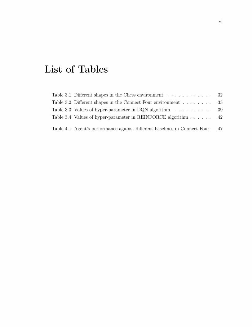
Table 3.1 Different shapes in the Chess environment . . . . . . . . . . . . 32Table 3.2 Different shapes in the Connect Four environment . . . . . . . . 33Table 3.3 Values of hyper-parameter in DQN algorithm . . . . . . . . . . 39Table 3.4 Values of hyper-parameter in REINFORCE algorithm . . . . . . 42

Table 4.1 Agent’s performance against different baselines in Connect Four 47

vii

List of Figures

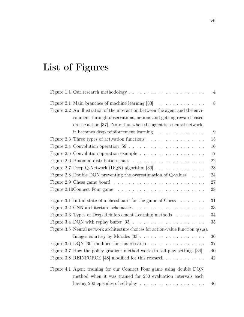
Figure 1.1 Our research methodology . . . . . . . . . . . . . . . . . . . . . 4

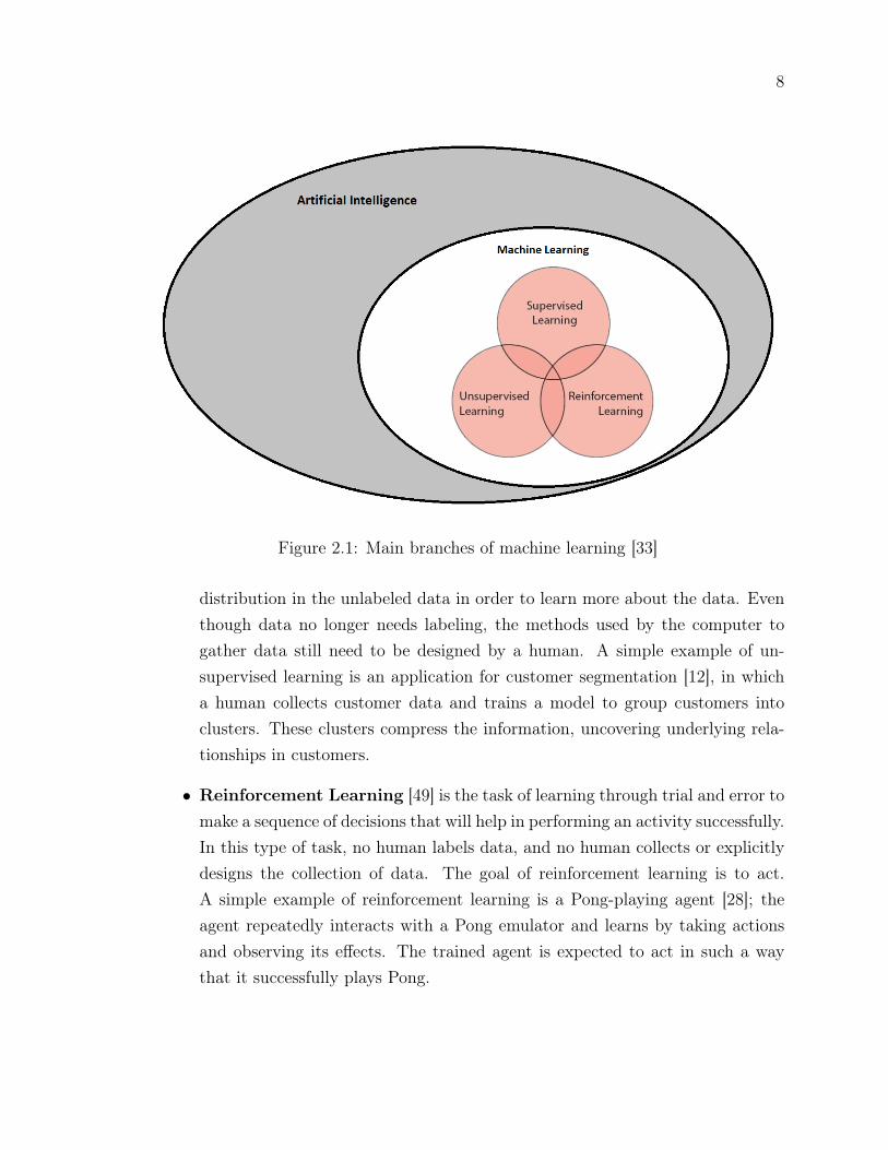
Figure 2.1 Main branches of machine learning [33] . . . . . . . . . . . . . 8Figure 2.2 An illustration of the interaction between the agent and the envi-

ronment through observations, actions and getting reward basedon the action [37]. Note that when the agent is a neural network,it becomes deep reinforcement learning . . . . . . . . . . . . . 9

Figure 2.3 Three types of activation functions . . . . . . . . . . . . . . . . 15Figure 2.4 Convolution operation [59] . . . . . . . . . . . . . . . . . . . . . 16Figure 2.5 Convolution operation example . . . . . . . . . . . . . . . . . . 17Figure 2.6 Binomial distribution chart . . . . . . . . . . . . . . . . . . . . 22Figure 2.7 Deep Q-Network (DQN) algorithm [30] . . . . . . . . . . . . . . 23Figure 2.8 Double DQN preventing the overestimation of Q-values . . . . 24Figure 2.9 Chess game board . . . . . . . . . . . . . . . . . . . . . . . . . 27Figure 2.10Connect Four game . . . . . . . . . . . . . . . . . . . . . . . . 28

Figure 3.1 Initial state of a chessboard for the game of Chess . . . . . . . 31Figure 3.2 CNN architecture schematics . . . . . . . . . . . . . . . . . . . 33Figure 3.3 Types of Deep Reinforcement Learning methods . . . . . . . . 34Figure 3.4 DQN with replay buffer [33] . . . . . . . . . . . . . . . . . . . . 35Figure 3.5 Neural network architecture choices for action-value function q(s,a).

Images courtesy by Morales [33] . . . . . . . . . . . . . . . . . . 36Figure 3.6 DQN [30] modified for this research . . . . . . . . . . . . . . . . 37Figure 3.7 How the policy gradient method works in self-play settings [34] 40Figure 3.8 REINFORCE [48] modified for this research . . . . . . . . . . . 42

Figure 4.1 Agent training for our Connect Four game using double DQNmethod when it was trained for 250 evaluation intervals eachhaving 200 episodes of self-play . . . . . . . . . . . . . . . . . . 46

viii

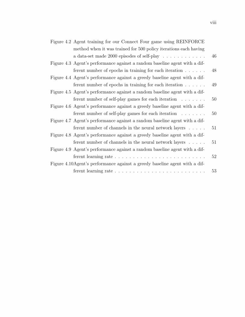
Figure 4.2 Agent training for our Connect Four game using REINFORCEmethod when it was trained for 500 policy iterations each havinga data-set made 2000 episodes of self-play . . . . . . . . . . . . 46

Figure 4.3 Agent’s performance against a random baseline agent with a dif-ferent number of epochs in training for each iteration . . . . . . 48

Figure 4.4 Agent’s performance against a greedy baseline agent with a dif-ferent number of epochs in training for each iteration . . . . . . 49

Figure 4.5 Agent’s performance against a random baseline agent with a dif-ferent number of self-play games for each iteration . . . . . . . 50

Figure 4.6 Agent’s performance against a greedy baseline agent with a dif-ferent number of self-play games for each iteration . . . . . . . 50

Figure 4.7 Agent’s performance against a random baseline agent with a dif-ferent number of channels in the neural network layers . . . . . 51

Figure 4.8 Agent’s performance against a greedy baseline agent with a dif-ferent number of channels in the neural network layers . . . . . 51

Figure 4.9 Agent’s performance against a random baseline agent with a dif-ferent learning rate . . . . . . . . . . . . . . . . . . . . . . . . . 52

Figure 4.10Agent’s performance against a greedy baseline agent with a dif-ferent learning rate . . . . . . . . . . . . . . . . . . . . . . . . . 53

ix

ACKNOWLEDGEMENTS

I would like to express my gratitude to my supervisors Dr. Hausi A. Müller for thecontinuous support, mentoring, patience, and encouragement to pursue research inhis group.

I would like to thank Dr. Ulrike Stege for her support and Dr. Alex I. Thomofor his help and mentoring in my research.

I would like to thank my lab mates for all the insightful discussions we’ve had and forproviding such a collaborative atmosphere. I have learnt so much at the Rigi Lab.

I’m grateful to my family for everything—for encouraging and inspiring me to followmy dreams. I could not have done this without you.

Chapter 1

Introduction

In the 1950s, behavioral psychology gave rise to the main idea behind ReinforcementLearning: all animals learn to perform better in specific tasks if they receive positiverewards after the completion of such tasks [49]. However, the applications of this ideawere restricted to simple low-dimensional problems until recently. Nowadays, theincrease in computational power, availability of compute and storage clouds, as wellas the rapid growth of research in the area of reinforcement learning led researchersto address many unsolved challenges such as autonomous driving [24], resource man-agement in computer clusters [29], traffic light control systems [54], security patrolsystems [56], optimizing chemical reactions [60], and recommendation systems [58].

Reinforcement Learning (RL) is a type of machine learning (ML), which is afield of science that studies computer algorithms that improve automatically throughgaining experience. Generally, these algorithms require a large amount of data to workeffectively. In RL the algorithm collects its own data through interactions with theenvironment. It is different from existing popular ML techniques, such as supervisedlearning and unsupervised learning. The first difference is that the feedback in RL isincomplete, and most rewards are delayed. That is, a reward is given after performingmultiple steps in the training process, instead of each step. The second difference isthat the aim of RL is not to find a hidden pattern in unlabeled random data, but tomaximize the reward solely.

When deep learning (i.e., the use of artificial neural network) is combined with RL,it is called Deep Reinforcement Learning (DRL). A popular technique in modern DRLis Self-play. In this technique the algorithm learns through interactions with copiesof itself within an environment without requiring any direct supervision. However,most of the existing techniques in DRL are only made and evaluated in settings

2

where the agent acts against a fixed environment [43]. It is unclear which of the DRLtechniques are most promising in a self-play setting, and which ones are better fits forsuch settings. Popular methods for DRL in self-play settings, such as AlphaZero [45],depend on the Monte Carlo tree search [8] to improve the policy, which requires aperfect-information environment. This would mean that when each player is makinga decision, it is aware of all the events that have previously occurred, complete currentstate and the future does not depend on any randomness or chance factor. Hence,DRL methods, such as AlphaZero [45], cannot be applied to imperfect-informationenvironments, such as the real world, effectively.

1.1 Motivation

Over the past decade, we have witnessed a rapid growth in Artificial Intelligence (AI)applications based on RL. For instance, Google’s DeepMind team created the MuZero[40] algorithm, a successor of AlphaZero [45], that set a new record for games such asGo and Chess. It has also become the state of the art for many Atari 2600 Games,setting a new landmark in AI research. Both MuZero and AlphaZero are based ontraining a DRL agent in a self-play setting, which does not use any data-set or humanknowledge. In addition, the OpenAI team created AI for the Dota2 game [4] usinga similar DRL technique in a self-play setting that defeated the world’s best team ofDota in a 5v5 game. More recently, DeepMind came up with AlphaStar [2], the firstAI system to defeat a top professional player at StarCraft II. AlphaGo [46] also hasapplications in other areas than games, such as intelligent military command decisionsupport [23], and clinical medicine [57].

Today, RL is a very active field of study. Hence, many reinforcement learningbased environments have been created to help researchers develop and compare theirRL algorithms. Examples of such environments could be OpenAI’s Gym,1 Atari 2600Games [31, 32], StarCraft II Learning Environment [51], Pommerman,2 or the 3Denvironment based on the game Doom [26]. However, most of them use settingswhere agents play against a fixed environment, meaning that there are no readilyavailable environments for a self-play setting. It remains largely undetermined whichof the known DRL techniques are most effective in a self-play setting, especially forenvironments where Monte Carlo tree search (MCTS) cannot be used. This thesis

1OpenAI Gym: https://gym.openai.com/2Pommerman: AI research into multi-agent learning, 2018. https://www.pommerman.com/

3

aims to provide a better understanding of DRL when applied to self-play settingsalong with the demonstration of the impact of essential hyper-parameters present inthese methods.

1.2 Problem Definition and Research Questions

According to Kun Shao et al. [43], the majority of DRL techniques developed overthe last few years are evaluated only in a setting where the agent plays against afixed environment, such as Atari 2600 Games. Hence the effectiveness of these DRLalgorithms in a self-play setting has yet to be explored. In this research, we striveto find the performance of two different types of DRL algorithms—value-based andpolicy-based—when applied in a self-play setting. We selected the Deep Q-Network(DQN) algorithm, which is a value-based DRL algorithm and REINFORCE which isa policy-based DRL algorithm for our experiments. We aim to investigate which ofthese techniques are most suited for a self-play setting. Similar to all machine learningmethods, DRL algorithms also employ parameters, referred to as hyper-parameters,which determine the actual neural network structure and affect the training processof DRL models. Hence, we also investigate the effect of selected hyper-parameters inthese DRL algorithms for self-play settings.The overall objectives of this thesis are as follows:

• Explore the applicability and performance of selected DRL methods for a self-play setting

• Investigate the effect of important hyper-parameters on the training of a DRLagent for self-play settings

To accomplish the above objectives, this thesis follows the steps described below:

• Implement DQN and REINFORCE methods for self-play settings

• Compare the performance of the agents trained using these methods

• Demonstrate the effect of selected hyper-parameters on the training of the DRLagent for self-play settings

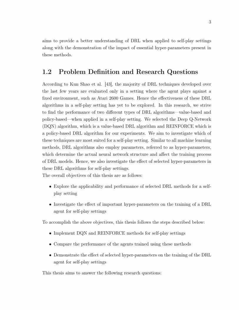
This thesis aims to answer the following research questions:

4

RQ1. How can DRL methods like DQN and REINFORCE be applied in environmentssupporting self-play settings?

RQ2. Which of the two method, DQN and REINFORCE, is better suited for gameenvironments similar to Connect Four in self-play settings?

RQ3. What are the important hyper-parameters and their initial values while inves-tigating in DRL for game environments in a self-play setting?

1.3 Research Methodology and Approach

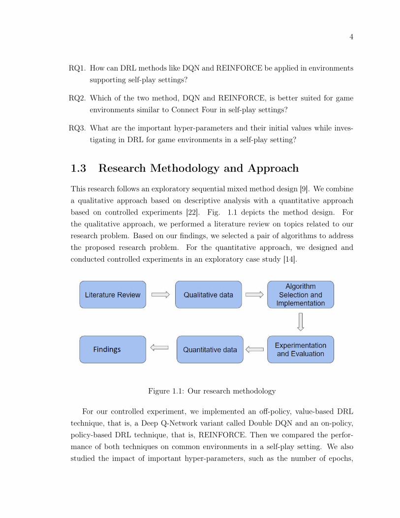
This research follows an exploratory sequential mixed method design [9]. We combinea qualitative approach based on descriptive analysis with a quantitative approachbased on controlled experiments [22]. Fig. 1.1 depicts the method design. Forthe qualitative approach, we performed a literature review on topics related to ourresearch problem. Based on our findings, we selected a pair of algorithms to addressthe proposed research problem. For the quantitative approach, we designed andconducted controlled experiments in an exploratory case study [14].

Figure 1.1: Our research methodology

For our controlled experiment, we implemented an off-policy, value-based DRLtechnique, that is, a Deep Q-Network variant called Double DQN and an on-policy,policy-based DRL technique, that is, REINFORCE. Then we compared the perfor-mance of both techniques on common environments in a self-play setting. We alsostudied the impact of important hyper-parameters, such as the number of epochs,

5

number of self-play games, learning-rate, and neural network depth in the perfor-mance of such techniques in self-play settings. We then compared the performanceof trained agents against different baselines explained. Chapters 3 and 4 describe theimplementation and evaluation details, respectively.

1.4 Contributions

The contributions of this thesis are as follows:

• Design and implementation of implementing the REINFORCE method for anenvironment that supports self-play.

• Demonstration of a simple Policy Gradient method that shows signs of learningin a self-play setting, in contrast to DQN which shows no sign of learning.

• Demonstration of the effects of hyper-parameters, such as the number of epochs,number of self-play games, learning-rate, and neural network depth, on the DRLagent’s training.

• Recommendation of initial values for the hyper-parameters in DRL with self-play settings on similar environments.

• Open-source code—the code developed for this research is open-sourced forfuture work by other researchers.

1.5 Thesis Outline

This chapter presented the motivation behind our research, stated the research ques-tions that guide this research, and outlined the contributions of this research. Theremaining chapters are organized as follows.

Chapter 2 formalizes key concepts for this research, describes the background, andsummarizes state-of-the-art literature related to this thesis.

Chapter 3 details the architecture and implementation of different components ofthis research.

Chapter 4 describes the evaluation conditions and discusses the results of the ex-periments.

6

Chapter 5 summarizes our research and discusses avenues for future research.

7

Chapter 2

Background and Related Work

2.1 Theoretical Background

Deep reinforcement learning is a machine learning approach in the field of ArtificialIntelligence (AI). AI is a branch of computer science involved in the creation of com-puter programs capable of demonstrating intelligence [33]. Traditionally, any pieceof software that displays cognitive abilities such as perception, search, planning, andlearning is considered to be part of AI.

2.1.1 Machine learning

Machine learning is an area of AI that is concerned with creating computer programswith the ability to automatically learn and improve from experience without being ex-plicitly programmed. There are three main branches of machine learning: supervised,unsupervised, and reinforcement learning as depicted in Fig. 2.1 below.

• Supervised Learning is the task of learning a mapping function from input tooutput from labeled data. In supervised learning, a human decides which datato collect and how to label it. The goal of supervised learning is to generalize.A canonical example of supervised learning is recognizing handwritten digits;humans gather images of handwritten digits, then label those images, and traina model to recognize and classify the digits in the images correctly [13]. Thetrained model is expected to generalize and correctly classify handwritten digitsin new images.

• Unsupervised Learning is the task of learning the underlying structure or

8

Figure 2.1: Main branches of machine learning [33]

distribution in the unlabeled data in order to learn more about the data. Eventhough data no longer needs labeling, the methods used by the computer togather data still need to be designed by a human. A simple example of un-supervised learning is an application for customer segmentation [12], in whicha human collects customer data and trains a model to group customers intoclusters. These clusters compress the information, uncovering underlying rela-tionships in customers.

• Reinforcement Learning [49] is the task of learning through trial and error tomake a sequence of decisions that will help in performing an activity successfully.In this type of task, no human labels data, and no human collects or explicitlydesigns the collection of data. The goal of reinforcement learning is to act.A simple example of reinforcement learning is a Pong-playing agent [28]; theagent repeatedly interacts with a Pong emulator and learns by taking actionsand observing its effects. The trained agent is expected to act in such a waythat it successfully plays Pong.

9

2.1.2 Reinforcement learning

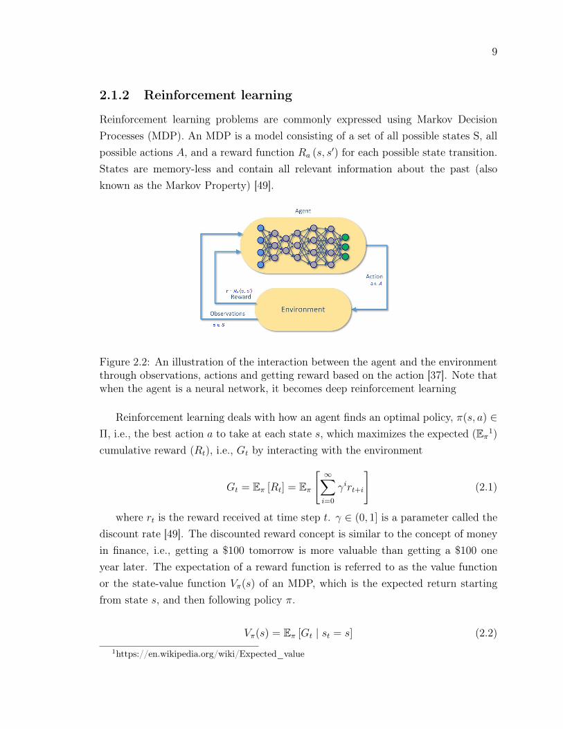
Reinforcement learning problems are commonly expressed using Markov DecisionProcesses (MDP). An MDP is a model consisting of a set of all possible states S, allpossible actions A, and a reward function Ra (s, s′) for each possible state transition.States are memory-less and contain all relevant information about the past (alsoknown as the Markov Property) [49].

Figure 2.2: An illustration of the interaction between the agent and the environmentthrough observations, actions and getting reward based on the action [37]. Note thatwhen the agent is a neural network, it becomes deep reinforcement learning

Reinforcement learning deals with how an agent finds an optimal policy, π(s, a) ∈Π, i.e., the best action a to take at each state s, which maximizes the expected (Eπ1)cumulative reward (Rt), i.e., Gt by interacting with the environment

Gt = Eπ [Rt] = Eπ

[∞∑i=0

γirt+i

](2.1)

where rt is the reward received at time step t. γ ∈ (0, 1] is a parameter called thediscount rate [49]. The discounted reward concept is similar to the concept of moneyin finance, i.e., getting a $100 tomorrow is more valuable than getting a $100 oneyear later. The expectation of a reward function is referred to as the value functionor the state-value function Vπ(s) of an MDP, which is the expected return startingfrom state s, and then following policy π.

Vπ(s) = Eπ [Gt | st = s] (2.2)1https://en.wikipedia.org/wiki/Expected_value

10

We can also define an action-value function Qπ(s, a), which is the expected returnstarting from state s, taking action a, and then following policy π.

Qπ(s, a) = Eπ [Gt | st = s, at = a] (2.3)

Following the above definitions, we can also say

Vπ(s) =∑a∈A

π(a | s)Qπ(s, a) (2.4)

where A is a set of actions, the agent can choose.Reinforcement learning methods can be divided into off-policy and on-policy meth-

ods. When we carry out the training on the actions sampled from the target/learnedpolicy, it is called on-policy reinforcement learning algorithms. Whereas, when thetraining is done on the distribution of episodes produced by a different behaviorpolicy rather than that produced by the target/learned policy, it is called off-policyreinforcement learning algorithms.

Reinforcement learning methods can also be divided into value-based and policy-based methods. In value-based methods, the agents update the value function tolearn suitable policy, and in policy-based methods, agents learn the policy directly.

Bellman Equations

Bellman’s Equations help us define the behavior of the agent mathematically in aMarkov decision process. According to Bellman, the state-value function can also bedecomposed into immediate reward plus discounted value of the successor state whichmodifies the Equation 2.2 and therefore becomes an Equation 2.5

Vπ(s) = Eπ [Rt+1 + γVπ (st+1) | st = s] (2.5)

Similarly, we can decompose the action-value function too.

Qπ(s, a) = Eπ [Rt+1 + γQπ (st+1, at+1) | st = s, at = a] (2.6)

Equations 2.5 and 2.6 are known as the Bellman Expectation Equations. To arriveat another Bellman Equation, we need to define the optimal state-value function V∗(s),

11

which is the maximum value function over all policies.

V∗(s) = maxπ

Vπ(s) (2.7)

Similarly, the optimal action-value function Q∗(s, a) is the maximum action-valuefunction over all policies.

Q∗(s, a) = maxπ

Qπ(s, a) (2.8)

Here we can introduce the transition probability Pass′ (probability of transitioningto state s′ from s, a) and achieve the Bellman Optimality Equations which express thefact that the value of a state under an optimal policy must be equal to the expectedreturn for the best action from that state [49].

V∗(s) = maxa∈A(s)

Qπ∗(s, a)

= maxa

Eπ∗ [Gt | st = s, at = a]

= maxa

Eπ∗[∞∑k=0

γkRt+k+1 | st = s, at = a

]

= maxa

Eπ∗[Rt+1 + γ

∞∑k=0

γkRt+k+2 | st = s, at = a

]= max

aE [Rt+1 + γV∗ (st+1) | st = s, at = a]

= maxa∈A(s)

∑s′,r

Pass′ [r + γV∗ (s′)]

= maxaRas + γ

∑s′∈S

Pass′V∗ (s′)

(2.9)

and similarly, we can get

Q∗(s, a) = Ras + γ

∑s′∈S

Pass′ maxa′

Q∗ (s′, a′) (2.10)

where s = st, a = at, s′ = st+1, a

′ = at+1

Bellman Equations are the foundation for many reinforcement learning algorithmssuch as SARSA and Q-learning.

12

Exploitation vs Exploration

In reinforcement learning, there is a trade-off between exploration and exploitation[36], that is, whether an agent should trust the learned values of Q enough to selectactions based only on it, or should the agent try other actions hoping that it mightresult in a better reward. This happens because the agent is optimizing actions in anunknown environment, which requires a large amount of information to be collectedfor estimation Pass′ before the action-value function converges. If the Q function tendsto be stable before the environment has been fully explored, the performance of themodel would be far from satisfactory, especially in a high action space situation.

To deal with the exploration vs. exploitation dilemma, ε− greedy selection [49] isintroduced to ensure that the agent makes enough exploration before the convergenceof the action-value function. Instead of choosing the best action estimated by theQ function, there is a probability for ε to randomly select from all actions. Themathematical expression of this method is as follows.

π(a | s) =

ε/m+ 1− ε if a∗ = arg maxa∈A

q(s, a)

ε/m otherwise(2.11)

where m is the number of actions. This method may affect the agent’s performanceat the first set of episodes during the training, but it can widen the horizon of theagent in the long run.

Q-Learning

Q-learning [53] is a typical off-policy, value-based method in which the goal is tomaximize the total discounted reward. Now, in order to do that, we need to obtainan optimal action-selection policy function Qπ(s, a) that predicts the best action a instate s. The following Bellmen Equation is used for such cases:

Qπ(s, a) = r + γmaxa′

Q (s′, a′) (2.12)

Here r is an instant reward, and the remaining part of the equation is the futurereward. The optimized Q function is obtained by minimizing the total expected lossfunction described as the difference between the predicted reward at a state and the

13

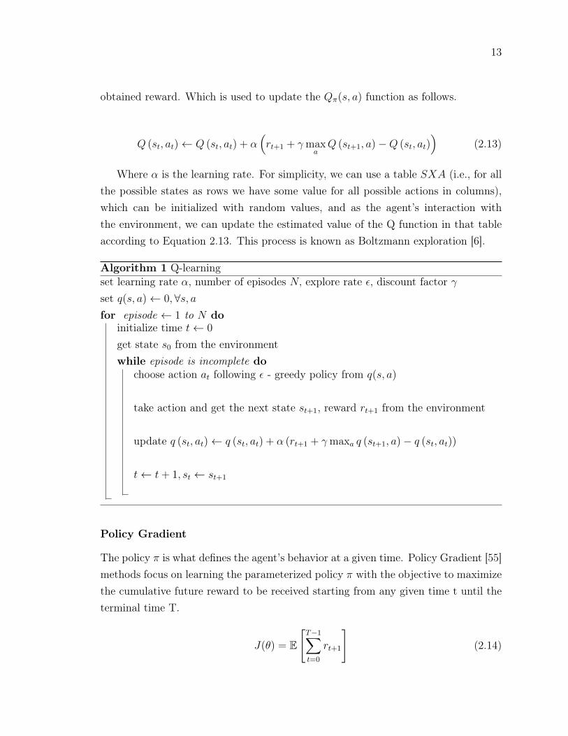
obtained reward. Which is used to update the Qπ(s, a) function as follows.

Q (st, at)← Q (st, at) + α(rt+1 + γmax

aQ (st+1, a)−Q (st, at)

)(2.13)

Where α is the learning rate. For simplicity, we can use a table SXA (i.e., for allthe possible states as rows we have some value for all possible actions in columns),which can be initialized with random values, and as the agent’s interaction withthe environment, we can update the estimated value of the Q function in that tableaccording to Equation 2.13. This process is known as Boltzmann exploration [6].

Algorithm 1 Q-learningset learning rate α, number of episodes N, explore rate ε, discount factor γset q(s, a)← 0,∀s, afor episode ← 1 to N do

initialize time t← 0

get state s0 from the environmentwhile episode is incomplete do

choose action at following ε - greedy policy from q(s, a)

take action and get the next state st+1, reward rt+1 from the environment

update q (st, at)← q (st, at) + α (rt+1 + γmaxa q (st+1, a)− q (st, at))

t← t+ 1, st ← st+1

Policy Gradient

The policy π is what defines the agent’s behavior at a given time. Policy Gradient [55]methods focus on learning the parameterized policy π with the objective to maximizethe cumulative future reward to be received starting from any given time t until theterminal time T.

J(θ) = E

[T−1∑t=0

rt+1

](2.14)

14

A simple method such as REINFORCE performs this by adding randomness tothe probabilities of the action given by the policy and experience of the environmentwith this updated policy. If the new total output reward is better, we increase thelikelihood of those actions from those states and vice-versa.

Sparse Rewards System

Generally, an environment has multiple possible actions with one ultimate final goalfor which reward is given. For example, in a chess environment, a single reward isgiven after hundreds of moves by the agent, depending on whether it won the game ornot. This causes a problem known as Sparse Rewards System [35], which arises mainlydue to too many actions required before receiving the reward, making it difficult todo just the random action to receive a successful reward with a positive gradienttoward the optimal solution. To tackle this sparse reward system, we perform rewardshaping (manually design and assigning rewards for some particular actions), whichmakes it easy to converge to a solution. For example, in a chess environment, we cangive rewards based on piece capture. However, there are downsides to reward shapingas well. First, it is a custom process; it has to be re-done for every new environment;for example, all Atari games require separate personalized optimal Reward Shaping.So this is also not scalable. Secondly, Reward Shaping give rise to the AlignmentProblem2 in which an agent will find many way to obtain little useless rewards withoutachieving the ultimate goal. Moreover, this reward shaping is optimized based onhuman behaviors that might not be optimal for many environments, such as in thegame of Go, where we want to surpass human knowledge.

2.1.3 Deep Learning

Deep Learning [27] is a technique of using multi-layered non-linear function approxi-mation, typically an artificial neural network model to solve a complex problem suchas speech recognition, visual object recognition, and so forth. Deep learning is basedon the theory of brain development and is used to learn data representation. Althoughthe term ‘deep learning’ was introduced in 1986 [10], the use-cases were very limitedbecause of a lack of data and incapable computation hardware. However, with theavailability of large-scale datasets and capable hardware, a big revolution occurs indeep learning [39].

2https://ai-alignment.com/the-reward-engineering-problem-30285c779450

15

There are two kinds of deep learning models that have been widely used in recentyears. Convolutional Neural Network (CNN) [25] is a type of deep neural networkwhich is mainly used in computer vision problems such as object detection and imageclassification. The CNN is a shift-invariant based on shared-weights architecture andis inspired by biological processes. Recurrent Neural Network (RNN) is another typeof deep neural network mainly used for natural language processing. Long Short TermMemory (LSTM) is a special kind of RNN [20] which is capable of learning long-termdependencies.

Activation Function in Deep Neural Network

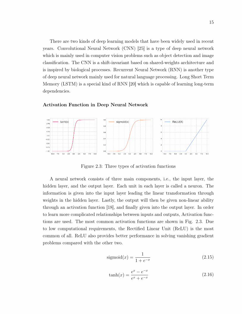
Figure 2.3: Three types of activation functions

A neural network consists of three main components, i.e., the input layer, thehidden layer, and the output layer. Each unit in each layer is called a neuron. Theinformation is given into the input layer leading the linear transformation throughweights in the hidden layer. Lastly, the output will then be given non-linear abilitythrough an activation function [18], and finally given into the output layer. In orderto learn more complicated relationships between inputs and outputs, Activation func-tions are used. The most common activation functions are shown in Fig. 2.3. Dueto low computational requirements, the Rectified Linear Unit (ReLU) is the mostcommon of all. ReLU also provides better performance in solving vanishing gradientproblems compared with the other two.

sigmoid(x) =1

1 + e−x(2.15)

tanh(x) =ex − e−x

ex + e−x(2.16)

16

ReLU(x) = max(x, 0) (2.17)

Convolutional Layer in Convolutional Neural Network

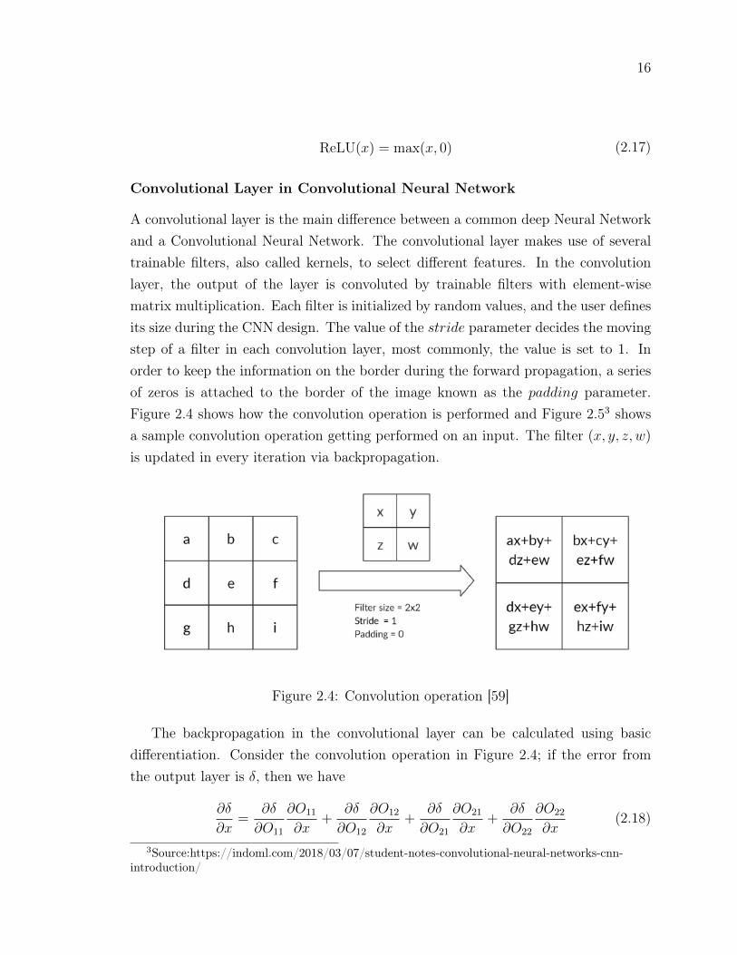
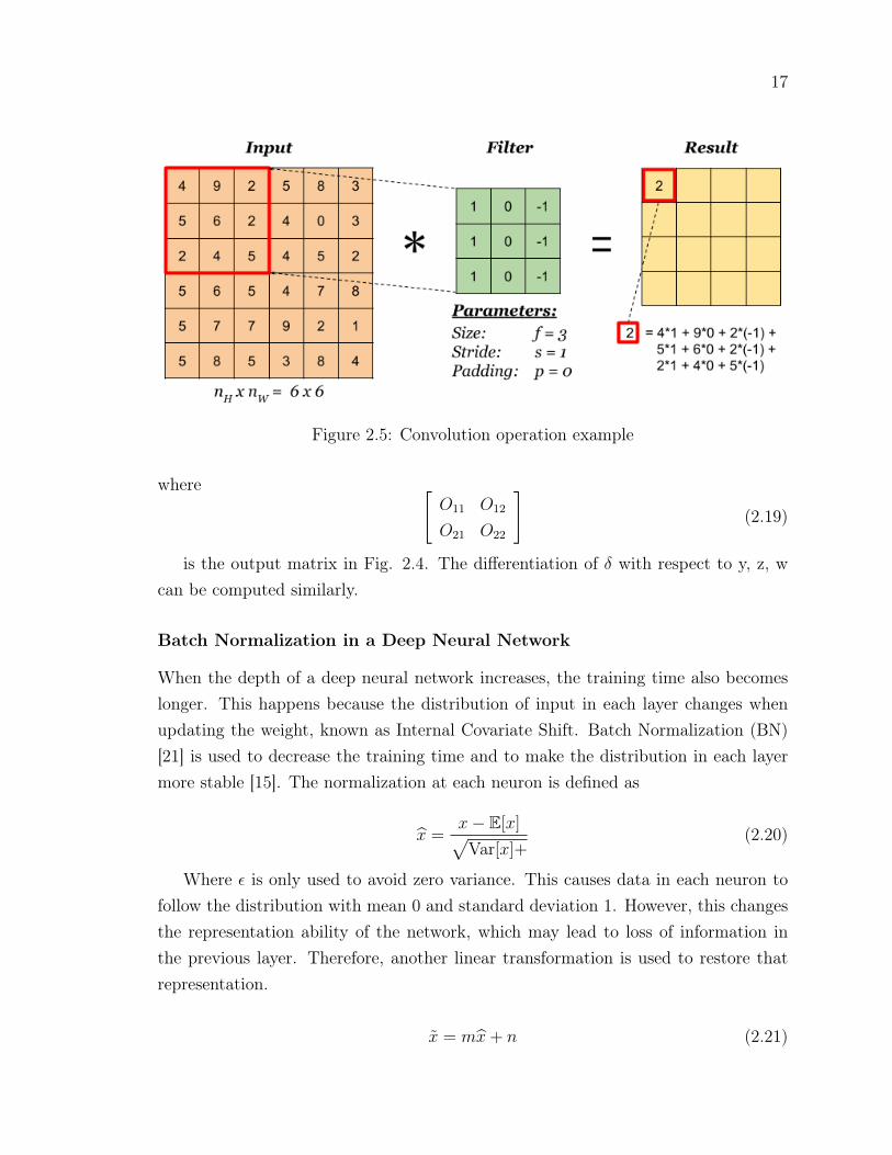
A convolutional layer is the main difference between a common deep Neural Networkand a Convolutional Neural Network. The convolutional layer makes use of severaltrainable filters, also called kernels, to select different features. In the convolutionlayer, the output of the layer is convoluted by trainable filters with element-wisematrix multiplication. Each filter is initialized by random values, and the user definesits size during the CNN design. The value of the stride parameter decides the movingstep of a filter in each convolution layer, most commonly, the value is set to 1. Inorder to keep the information on the border during the forward propagation, a seriesof zeros is attached to the border of the image known as the padding parameter.Figure 2.4 shows how the convolution operation is performed and Figure 2.53 showsa sample convolution operation getting performed on an input. The filter (x, y, z, w)

is updated in every iteration via backpropagation.

Figure 2.4: Convolution operation [59]

The backpropagation in the convolutional layer can be calculated using basicdifferentiation. Consider the convolution operation in Figure 2.4; if the error fromthe output layer is δ, then we have

∂δ

∂x=

∂δ

∂O11

∂O11

∂x+

∂δ

∂O12

∂O12

∂x+

∂δ

∂O21

∂O21

∂x+

∂δ

∂O22

∂O22

∂x(2.18)

3Source:https://indoml.com/2018/03/07/student-notes-convolutional-neural-networks-cnn-introduction/

17

Figure 2.5: Convolution operation example

where [O11 O12

O21 O22

](2.19)

is the output matrix in Fig. 2.4. The differentiation of δ with respect to y, z, wcan be computed similarly.

Batch Normalization in a Deep Neural Network

When the depth of a deep neural network increases, the training time also becomeslonger. This happens because the distribution of input in each layer changes whenupdating the weight, known as Internal Covariate Shift. Batch Normalization (BN)[21] is used to decrease the training time and to make the distribution in each layermore stable [15]. The normalization at each neuron is defined as

x̂ =x− E[x]√

Var[x]+(2.20)

Where ε is only used to avoid zero variance. This causes data in each neuron tofollow the distribution with mean 0 and standard deviation 1. However, this changesthe representation ability of the network, which may lead to loss of information inthe previous layer. Therefore, another linear transformation is used to restore thatrepresentation.

x̃ = mx̂+ n (2.21)

18

Here m and n are learnable parameters. Note, the result is the same as theoriginal when m =

√Var[x] and n = E[x]. The mean and variance during the

training will be stored and will be treated as the mean of the variance of test data.Batch Normalization also mitigates vanishing gradient problems along with dealingwith Internal Covariate Shift problems [21].

2.1.4 Deep Reinforcement Learning

Deep Reinforcement Learning (DRL) [16] is a combination of deep learning and rein-forcement learning. The specific property of DRL programs is the learning throughtrial and error from feedback that is simultaneously sequential, evaluative, and sam-pled by leveraging powerful non-linear function approximation [33]. In DRL, thecomputer programs that solve complex decision-making problems under uncertaintyare called agents. This means that if we are training a robot to pick up objects, therobot arm is not part of the agent. Only the code that makes decisions is referred toas the agent.

The two major types of DRLs are Model-based learning and Model-free learning.In Model-based learning, the agent is required to learn a model that describes how theenvironment works from its observations and then plan a solution using that model.Model-free learning is when an agent can directly derive an optimal policy from itsinteractions with the environment without having to create a model in advance.

Deep Q Network

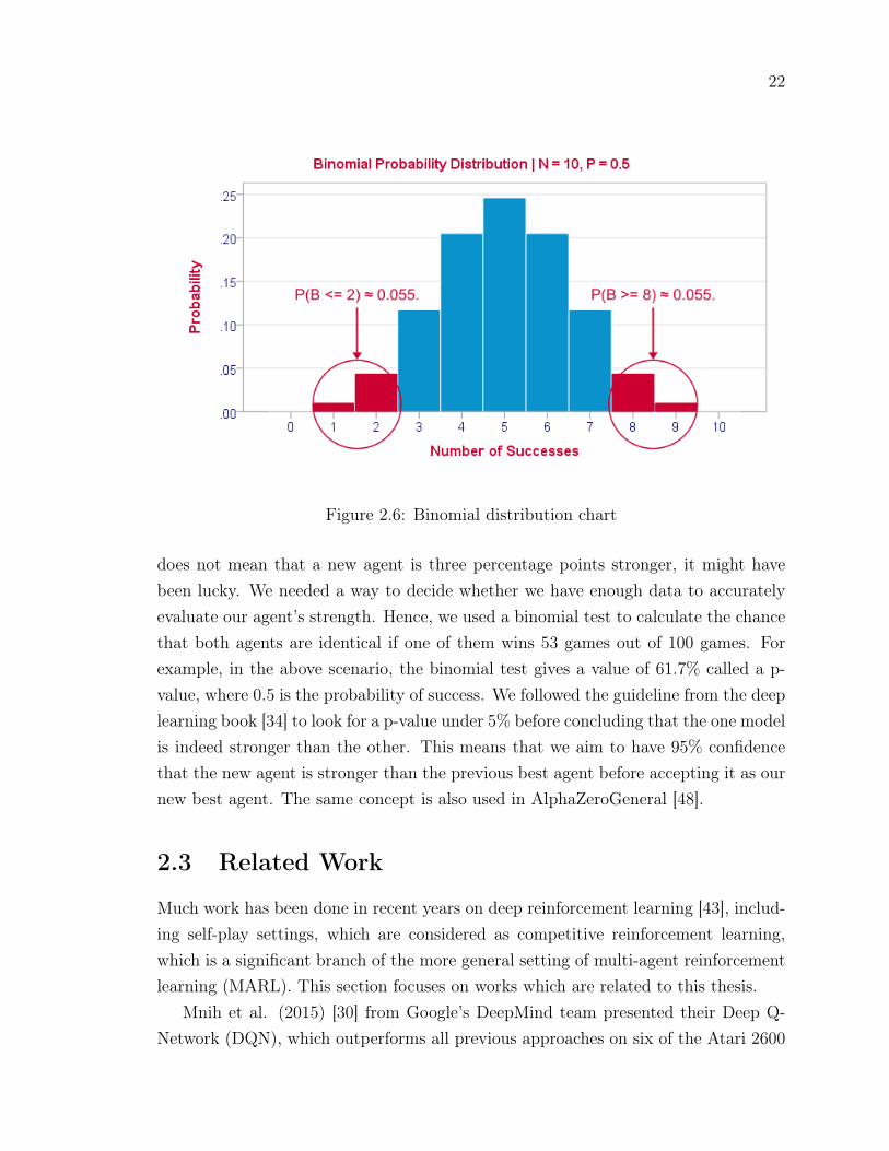
Q-learning is a robust algorithm designed to solve simple reinforcement learning prob-lems. However, it is unable to deal with continuous states, continuous actions, or aproblem with a large state-action space. To solve the former problem, a deep learningmethod can be used to approximate the action-value function. Generally, states areimage data observed by the agent, and a convolutional neural network is an effectiveway to extract features from this kind of data in convolution layers and feed theminto the fully connected layer to approximate the Q function. Fig. 2.7 shows the basicDQN algorithm by DeepMind used for Arcade Learning Environment [3] to becomethe new state-of-the-art solution in the field.

DeepMind introduced experience replay buffer, which stores the experience [St, At,

Rt, St+1] in the memory and randomly samples from it to optimize the neural networkmodel [30]. Their combination of Q-learning, deep learning, and the experience replay

19

memory formed Deep Q Network (DQN); according to their paper, this outperformsall previous approaches on six of the Atari games and surpasses a human expert onthree of them.

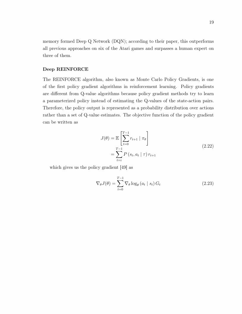
Deep REINFORCE

The REINFORCE algorithm, also known as Monte Carlo Policy Gradients, is oneof the first policy gradient algorithms in reinforcement learning. Policy gradientsare different from Q-value algorithms because policy gradient methods try to learna parameterized policy instead of estimating the Q-values of the state-action pairs.Therefore, the policy output is represented as a probability distribution over actionsrather than a set of Q-value estimates. The objective function of the policy gradientcan be written as

J(θ) = E

[T−1∑t=0

rt+1 | πθ

]

=T−1∑t=i

P (st, at | τ) rt+1

(2.22)

which gives us the policy gradient [49] as

∇θJ(θ) =T−1∑t=0

∇θ logθ (at | st)Gt (2.23)

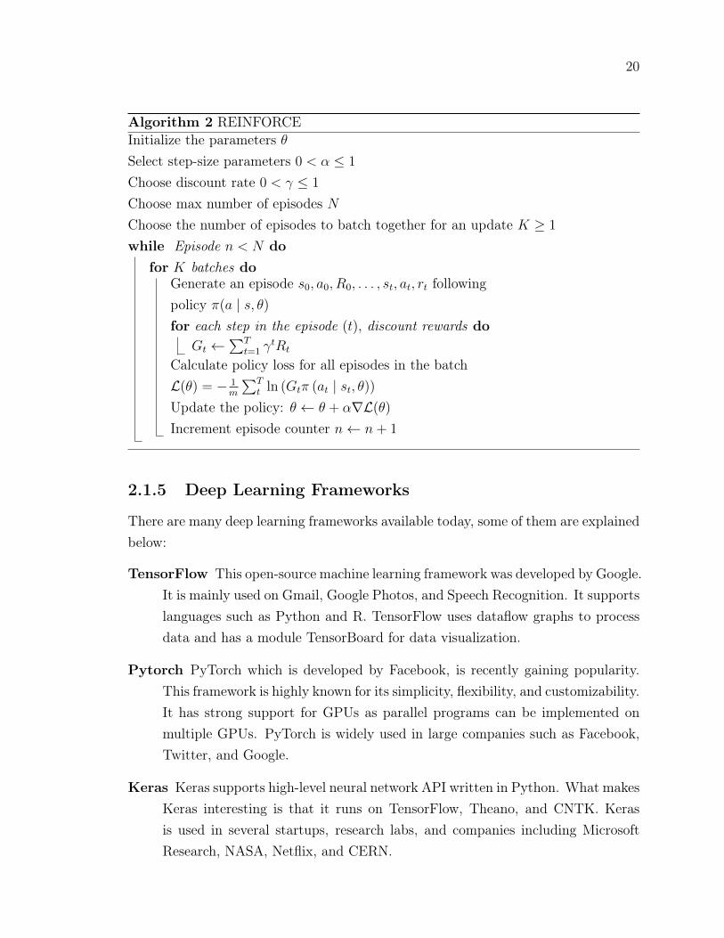
20

Algorithm 2 REINFORCEInitialize the parameters θSelect step-size parameters 0 < α ≤ 1

Choose discount rate 0 < γ ≤ 1

Choose max number of episodes NChoose the number of episodes to batch together for an update K ≥ 1

while Episode n < N dofor K batches do

Generate an episode s0, a0, R0, . . . , st, at, rt followingpolicy π(a | s, θ)for each step in the episode (t), discount rewards do

Gt ←∑T

t=1 γtRt

Calculate policy loss for all episodes in the batchL(θ) = − 1

m

∑Tt ln (Gtπ (at | st, θ))

Update the policy: θ ← θ + α∇L(θ)

Increment episode counter n← n+ 1

2.1.5 Deep Learning Frameworks

There are many deep learning frameworks available today, some of them are explainedbelow:

TensorFlow This open-source machine learning framework was developed by Google.It is mainly used on Gmail, Google Photos, and Speech Recognition. It supportslanguages such as Python and R. TensorFlow uses dataflow graphs to processdata and has a module TensorBoard for data visualization.

Pytorch PyTorch which is developed by Facebook, is recently gaining popularity.This framework is highly known for its simplicity, flexibility, and customizability.It has strong support for GPUs as parallel programs can be implemented onmultiple GPUs. PyTorch is widely used in large companies such as Facebook,Twitter, and Google.

Keras Keras supports high-level neural network API written in Python. What makesKeras interesting is that it runs on TensorFlow, Theano, and CNTK. Kerasis used in several startups, research labs, and companies including MicrosoftResearch, NASA, Netflix, and CERN.

21

Caffe Developed at BAIR or Berklee Artificial Intelligence Research, Caffe standsfor Convolutional Architecture for Fast Feature Embedding. Caffe is writtenin C++ with a Python Interface and is generally used for image detection andclassification.

Theano The University de Montreal developed Theano, which was written in Pythonand centers around NVIDIA CUDA, allowing users to integrate it with GPS.

DL4J A machine learning group led by Adam Gibson developed this Deep LearningFramework Deeplearning4j. Written in java and scala, DL4J supports differentneural networks, such as CNN, RNN, and LSTM.

2.2 Binomial Test: Measuring differences in strength

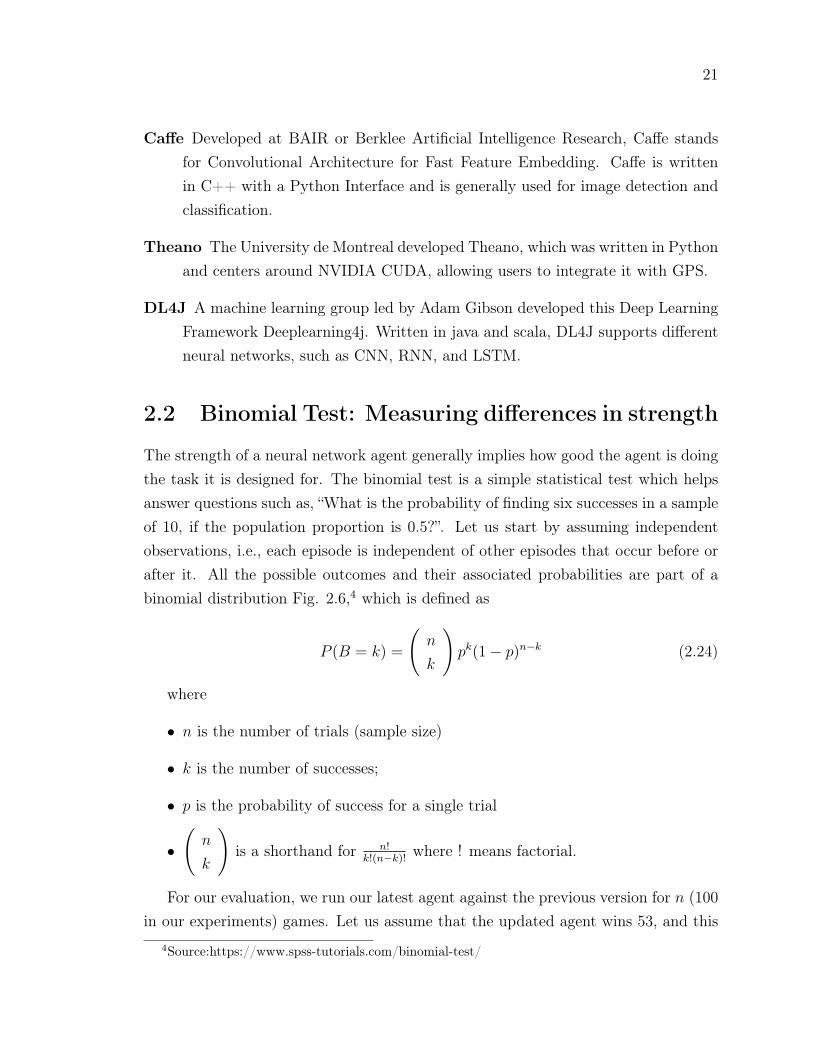
The strength of a neural network agent generally implies how good the agent is doingthe task it is designed for. The binomial test is a simple statistical test which helpsanswer questions such as, “What is the probability of finding six successes in a sampleof 10, if the population proportion is 0.5?”. Let us start by assuming independentobservations, i.e., each episode is independent of other episodes that occur before orafter it. All the possible outcomes and their associated probabilities are part of abinomial distribution Fig. 2.6,4 which is defined as

P (B = k) =

(n

k

)pk(1− p)n−k (2.24)

where

• n is the number of trials (sample size)

• k is the number of successes;

• p is the probability of success for a single trial

•

(n

k

)is a shorthand for n!

k!(n−k)! where ! means factorial.

For our evaluation, we run our latest agent against the previous version for n (100in our experiments) games. Let us assume that the updated agent wins 53, and this

4Source:https://www.spss-tutorials.com/binomial-test/

22

Figure 2.6: Binomial distribution chart

does not mean that a new agent is three percentage points stronger, it might havebeen lucky. We needed a way to decide whether we have enough data to accuratelyevaluate our agent’s strength. Hence, we used a binomial test to calculate the chancethat both agents are identical if one of them wins 53 games out of 100 games. Forexample, in the above scenario, the binomial test gives a value of 61.7% called a p-value, where 0.5 is the probability of success. We followed the guideline from the deeplearning book [34] to look for a p-value under 5% before concluding that the one modelis indeed stronger than the other. This means that we aim to have 95% confidencethat the new agent is stronger than the previous best agent before accepting it as ournew best agent. The same concept is also used in AlphaZeroGeneral [48].

2.3 Related Work

Much work has been done in recent years on deep reinforcement learning [43], includ-ing self-play settings, which are considered as competitive reinforcement learning,which is a significant branch of the more general setting of multi-agent reinforcementlearning (MARL). This section focuses on works which are related to this thesis.

Mnih et al. (2015) [30] from Google’s DeepMind team presented their Deep Q-Network (DQN), which outperforms all previous approaches on six of the Atari 2600

23

games from the Arcade Learning Environment [3] and outperforms human experts inthree of the games. Atari 2600 is still considered a standard testbed for evaluation ofperformance for most reinforcement learning algorithms. Their agent used high di-mensional input, specifically 84 × 84 × 4 images as input, which does not include anygame-specific information or hand-designed visual features in a convolutional neuralnetwork (CNN) and produces a single value for each valid action. They used a variantof an online Q-learning algorithm, with a stochastic gradient descent, to update theweights. This approach uses an experience replay buffer to store all the transitionsand then samples randomly from it to smoothen the training distribution over manypast experiences, as shown in Fig. 3.4. During the training on the evaluation, thenetwork architecture and all hyper-parameters were not changed at all. Fig. 2.7shows the algorithms used. The first method we chose in this thesis is DQN as thevalue-based off-policy method.

Figure 2.7: Deep Q-Network (DQN) algorithm [30]

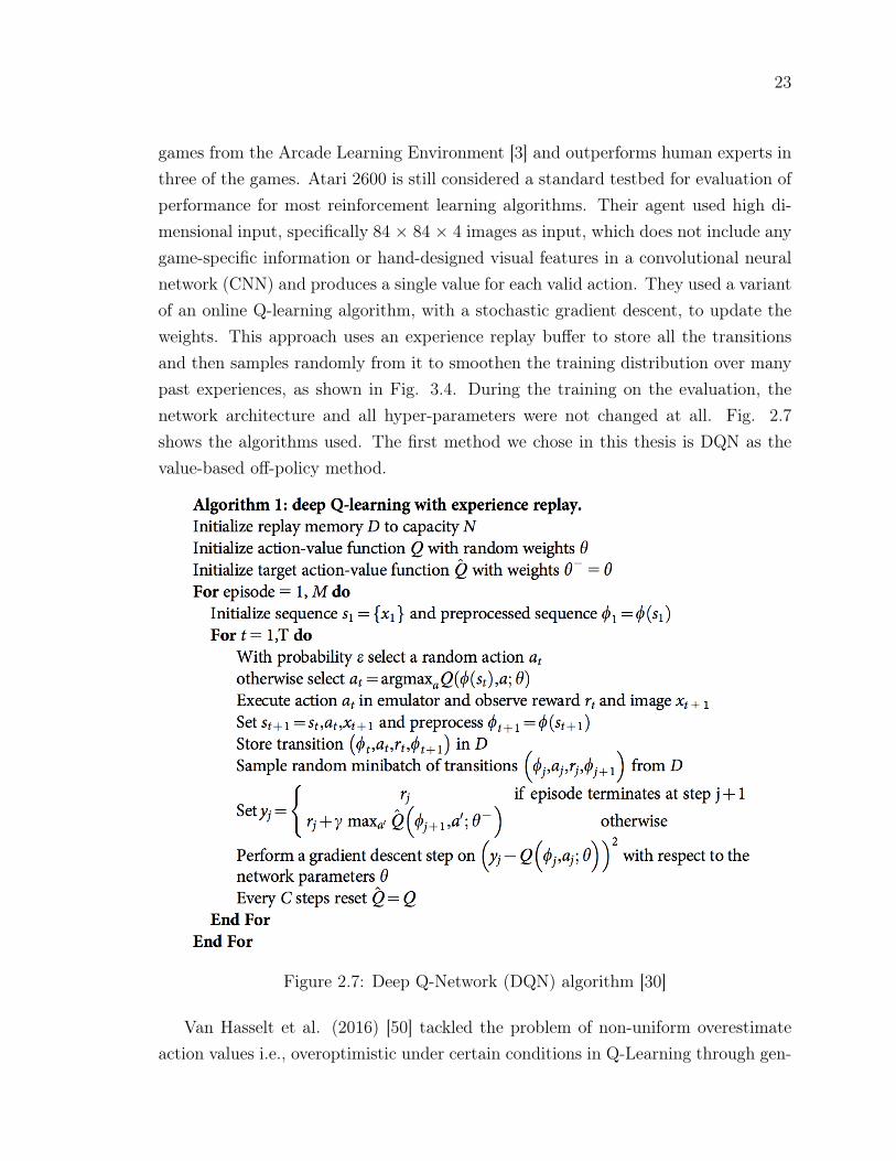
Van Hasselt et al. (2016) [50] tackled the problem of non-uniform overestimateaction values i.e., overoptimistic under certain conditions in Q-Learning through gen-

24

eralizing the idea behind Double Q-learning [17], hence constructed a new algorithmknown as Double DQN. They showed that the non-uniform overestimation occursin DQN while testing on Atari 2600 games and also showed that their methods sig-nificantly reduced this overestimation and improved performance in several games.They were obtaining state-of-the-art results in the Atari domain. The idea of DoubleDQN is to have a target network as a frozen copy of the original online network, andevaluate the greedy policy based on the online network but using the target networkto estimate its value. The target network will be updated periodically after every tsteps. For this thesis, we thought it would be a good idea to include this variant toobecause it was a small change in the implementation and it promises better results.

Figure 2.8: Double DQN preventing the overestimation of Q-values

Schaul et al. (2016) [38] from Google’s DeepMind team further improved their ex-periences replay mechanism because some experiences are more important for learningthan others, and hence, they should have higher priority while sampling from experi-ence replay memory. Until now, most variants of DQN were uniformly sampling thetransition batch from the experience replay memory. Prioritized Experience Replaywith DQN won 41 out of 49 games and achieved a new state-of-the-art. They used abinary heap data structure so that sampling from experiences replay memory can bedone in O(1), and in updating the priority in the buffer in O(logN). With priorityp = |error| + offset, they defined the probability of sampling a transition from thememory as P (i) =

pαi∑k p

αk, where pi > 0 is the priority of transition i and α is the

priority scaling constant which determines how much of the priority is used. DoubleDeep Q-Network combined with Prioritized Experience Replay is the first methodwe used as a value-based deep reinforcement learning to be applied on a self-playsetting. All of the above methods were applied and evaluated mainly on Atari 2600games. Hence, performance on a self-play setting for these is unknown. We also triedPrioritized Experience Replay in our DQN implementation, but with no success.

Schulman et al. (2015) [41] modified a standard policy gradient method andachieved monotonic improvement of the policy called Trust Region Policy Optimiza-

25

tion (TRPO). KL-Divergent is a measure of the difference between two probabilitydistributions. In a policy gradient method, a policy output from a network offersthe probabilities of performing actions at any state, and they used KL-Divergent tostop receiving newly learned policies that are too different from the current knownpolicy. The idea is straightforward to understand—we only accept the learning if itis consistent with the reason for trust in our known learned policy. Complete im-plementation of the method was difficult to achieve due to the complexity; also, themethod introduced many new hyper-parameters.

Schulman et al. (2017) [42] further proposed a policy gradient method calledproximal policy optimization (PPO) based on a similar idea known as TRPO, i.e., toimprove training stability by avoiding parameter updates that change the policy toomuch at a single step. PPO simplifies it by using a clipped surrogate objective whileretaining similar performance. They used clip(r(θ), 1 − ε, 1 + ε) function to cut theratio of old policy and new policy within [1− ε, 1 + ε], where ε is a hyper-parameterbetween 0 and 1. The objective function of PPO is modified with an error term onthe value estimation and an entropy term to encourage good exploration.

Silver et al. (2017) [44, 47] started with supervised learning on human data totrain a model for the game of Go. Then they further improved their model usingreinforcement learning in a self-play setting and Monte Carlo tree search on the valueand policy networks for the game of Go. Their method (AlphaGo) achieved a 99.8%winning rate against other Go programs and defeated the human European Go cham-pion by 5 games to 0. After that, they initialized their model from the scratch withoutany supervised learning, they used reinforcement learning in a self-play setting; theMonte Carlo tree search resulted in an even more robust game AI named AlphaGoZero, which won all 100 games against the previously published, AlphaGo method.They exploited the fact that Go is a perfect information game, and hence, the MCTSmethod could be used in this case. In our thesis, we are trying to study the perfor-mance of deep reinforcement learning methods for environments where informationis imperfect.

Silver et al. (2017) [45] used AlphaZero techniques, which is a general reinforce-ment learning algorithm. It performed exceptionally well on the three games forwhich it was tested: chess, shogi, and Go. They used data generated from the self-play setting of the model, indicating an entirely random behavior. The convolutionneural network had two endpoints, one giving the policy as an output and the othergiving a single value corresponding to winning chances of that player from that state.

26

Heinrich et al. (2016) [19] combined fictitious self-play with deep reinforcementlearning and came up with Neural Fictitious Self-Play (NFSP). Their method learnsto approximate Nash equilibria of imperfect-information games from self-play. Theyapplied NFSP on a small poker game and showed that it worked where other DRLtechniques such as DQN greedy did not work. This work is similar to the work donein this thesis, because we also explored DRL in self-play settings.

Charlesworth et al. (2018) [7] applied PPO DRL method to train an AI model toplay a four-player imperfect information card game known as ’Big 2’, in which eachplayer aim to play all of their cards as quickly as possible. Their results showcasedthat the network’s performance against three random opponents improved over timeand the final network significantly outperformed human players. Their ’Big 2’ novelenvironment also could be used as a test-bed for other DRL methods.

Wang et al. (2020) [52] investigated and analyzed important hyper-parameters andcombinations of loss-functions in an AlphaZero-like self-play algorithm and evaluatehow these parameters contribute to the training. They selected all perfect informationgames and used MCTS similar to AlphaZero to improve the network predictions.They found that a higher number of the outer self-play iterations is more promisingthan higher numbers of the inner training epochs. This work is similar to the workreported in this thesis; they used the AlphaZero algorithm while analyzing the hyper-parameter, whereas we are using DQN and REINFORCE methods.

Brown et al. (2020) [5] from the Facebook AI Research team presented a generalframework for self-play setting in games with imperfect-information using deep rein-forcement learning and search similar to AlphaZero called ReBeL (Recursive Belief-based Learning). The goal was similar to the work done in this thesis, but in a moregeneral setting. The framework was tested on two games, namely Poker and Liar’sDice, and showed superhuman performance for both of them. According to the paper,ReBeL’s theoretical guarantees for convergence to a Nash equilibrium are limited onlyto two-player zero-sum games which creates some gaps for future research.

2.4 Game Environments

We use the following games as case studies with the aim to understand the working ofthe original deep reinforcement learning techniques for self-play settings, which doesnot have an MCTS in them. We will not exploit the fact that these fall into theperfect information game category, for which Monte Carlo tree search (MCTS) could

27

be used to improve the move selection similar to what has been done in Alpha-Zerolike implementations.

2.4.1 Chess

Figure 2.9: Chess game board

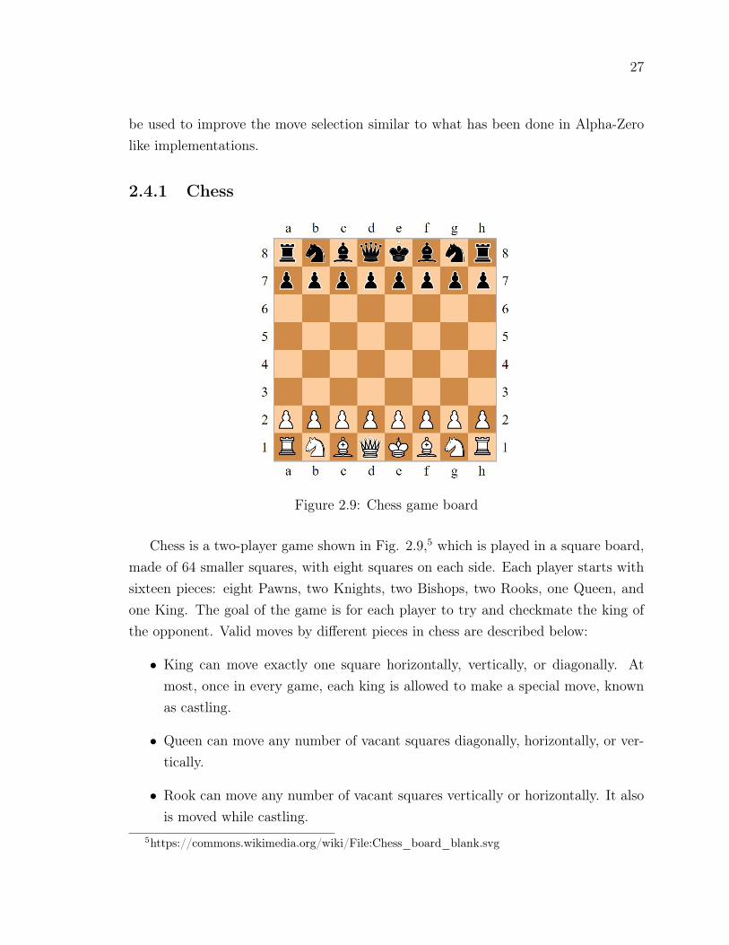
Chess is a two-player game shown in Fig. 2.9,5 which is played in a square board,made of 64 smaller squares, with eight squares on each side. Each player starts withsixteen pieces: eight Pawns, two Knights, two Bishops, two Rooks, one Queen, andone King. The goal of the game is for each player to try and checkmate the king ofthe opponent. Valid moves by different pieces in chess are described below:

• King can move exactly one square horizontally, vertically, or diagonally. Atmost, once in every game, each king is allowed to make a special move, knownas castling.

• Queen can move any number of vacant squares diagonally, horizontally, or ver-tically.

• Rook can move any number of vacant squares vertically or horizontally. It alsois moved while castling.

5https://commons.wikimedia.org/wiki/File:Chess_board_blank.svg

28

• Bishop can move any number of vacant squares in any diagonal direction.

• Knight can move one square along with any rank or file and then at an angle.The knight’s movement can also be viewed as an “L” or “7” laid out at anyhorizontal or vertical angle.

• Pawns can move forward one square, if that square is unoccupied. If it has notyet moved, the pawn has the option of moving two squares forward, providedboth squares in front of the pawn are unoccupied. They can capture an enemypiece on either of the two spaces adjacent to the space in front of them (i.e., thetwo squares diagonally in front of them) but cannot move to these spaces if theyare vacant. The pawn is also involved in the two special moves en passant andpromotion. A pawn attacking a square crossed by an opponent’s pawn whichhas advanced two squares in one move from its original square may capture thisopponent’s pawn as though the latter had been moved only one square. Thiscapture is only legal on the move following this advance and is called an ’enpassant’ capture.

2.4.2 Connect Four

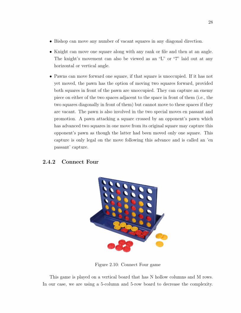
Figure 2.10: Connect Four game

This game is played on a vertical board that has N hollow columns and M rows.In our case, we are using a 5-column and 5-row board to decrease the complexity.

29

Each column has a hole in the upper part of the board, where pieces are introduced.There is a window for every square so that pieces can be seen from both sides.

Both players aim to make a straight line of four own pieces; the line can be vertical,horizontal, or diagonal.

Before starting, players randomly decide which of them will be the beginner; movesare made alternatively, one by turn. Moves entail placing new pieces on the board;pieces slide downwards from upper holes, falling down to the last row or piling up onthe last piece introduced in the same column. So, in every turn, the introduced piecemay be placed at most on five different squares.

The first player to get a straight line made with four own pieces and no gapsbetween them wins.

2.5 Chapter Summary

This chapter introduced concepts, terms and notations used in this thesis. First, itdescribed what reinforcement learning is and how it is different from other machinelearning methods. Second, it explained deep learning and deep reinforcement learningalong with common concepts used in these methods. Third, it further summarisedrelated research work done in the field and how it is related to this research. Finally,we introduced the rules for the selected environments for our research.

30

Chapter 3

Algorithm Architecture andImplementation

This chapter focuses on the architecture and design choices made for this research.Section 3.1 explains the design of the game environments used in our experiment.Section 3.2 illustrates the CNN architecture used in both DRL algorithms. Section3.3 describes the reasoning behind the selection of algorithms used in this research.Sections 3.4 and 3.5 explain the selected algorithms implementation details alongwith the role of their important hyper-parameters. Finally, Section 3.6 explains themechanism of comparing two neural network models during training.

3.1 The Environments

Most of the environments publicly available are for agents playing against a fixedenvironment. We needed environments for self-play settings where an agent is playingagainst itself and from which we can utilize the experiences of both the agents, i.e.,the agent who wins and the agent who loses. Due to our interest in the game ofchess, which fits the requirements, we created a chess environment taking motivationfrom Alpha-Zero for chess [45]. Chess turns out to be very hard to model, and thetraining process was much slower than expected. Hence, we chose another gamefrom AlphaZeroGeneral [48] called Connect Four, which is much simpler, and thetraining process is much faster compared to chess. Note that both Chess and ConnectFour are perfect information environments, but the agent and the algorithm do nottake advantage of this fact. Thus, we are treating them as imperfect-information

31

environments.

3.1.1 Chess

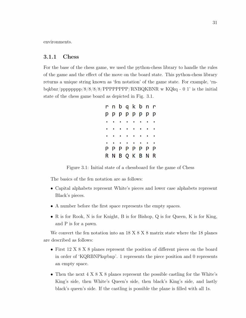
For the base of the chess game, we used the python-chess library to handle the rulesof the game and the effect of the move on the board state. This python-chess libraryreturns a unique string known as ‘fen notation’ of the game state. For example, ‘rn-bqkbnr/pppppppp/8/8/8/8/PPPPPPPP/RNBQKBNR w KQkq - 0 1’ is the initialstate of the chess game board as depicted in Fig. 3.1.

Figure 3.1: Initial state of a chessboard for the game of Chess

The basics of the fen notation are as follows:

• Capital alphabets represent White’s pieces and lower case alphabets representBlack’s pieces.

• A number before the first space represents the empty spaces.

• R is for Rook, N is for Knight, B is for Bishop, Q is for Queen, K is for King,and P is for a pawn.

We convert the fen notation into an 18 X 8 X 8 matrix state where the 18 planesare described as follows:

• First 12 X 8 X 8 planes represent the position of different pieces on the boardin order of ‘KQRBNPkqrbnp’. 1 represents the piece position and 0 representsan empty space.

• Then the next 4 X 8 X 8 planes represent the possible castling for the White’sKing’s side, then White’s Queen’s side, then black’s King’s side, and lastlyblack’s queen’s side. If the castling is possible the plane is filled with all 1s.

32

• The 17th 1 X 8 X 8 plane is filled with the number of moves since the last pawnmove or capture for the fifty-move-rule.

• the last 1 X 8 X 8 plane carries 1 on the position where en passant is possible.

This converted matrix represents a state in the algorithm and is used as the inputto the model, i.e., a convolution neural network.

The action space represents all possible moves on 8 X 8 board by any chess piece.This also includes pawn promotion to Queen, Rook, Bishop, Knight. The calculationfor the total action space is described below:

• pawn promotions: from 8 (columns) * 2 (black and white) * 4 (type of promo-tion) * 3 (direction) - 4 (corner columns only have 2 directions) * 4 (type ofpromotion) = 192 - 16 = 176 possible moves

• normal move: from each square position on the board a piece can move eitherhorizontally (7), vertically (7), diagonally (min 7 to max 14) or a knight’s move(min 2 to max 8). computing all the above possible moves for all 64 square willgive us 1792 possible moves.

• total possible moves in chess = 1792 + 176 = 1968

Average game length in terms of number of moves for professional chess games isaround 40. But when two random agents play a game of chess they finish a gamein around 200-500 moves. We will be forcing a decision based on the pieces on theboard in 100 moves.

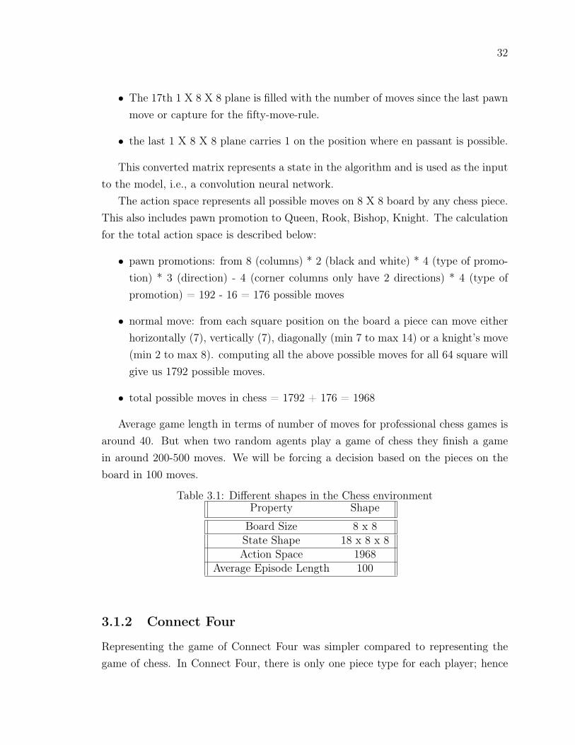
Table 3.1: Different shapes in the Chess environmentProperty Shape

Board Size 8 x 8State Shape 18 x 8 x 8Action Space 1968

Average Episode Length 100

3.1.2 Connect Four

Representing the game of Connect Four was simpler compared to representing thegame of chess. In Connect Four, there is only one piece type for each player; hence

33

only one 2D matrix with +1 for player one and -1 for player two was sufficient torepresent all the information about the game state.

Action Space was equal to the number of columns. We decided to keep the boardsmall, and hence we are using a square board with five rows and five columns. Hence,the Action Space is five for the five columns on the board.

Table 3.2: Different shapes in the Connect Four environmentProperty Shape

Board Size 5 x 5State Shape 1 x 5 x 5Action Space 5

Average Episode Length 25

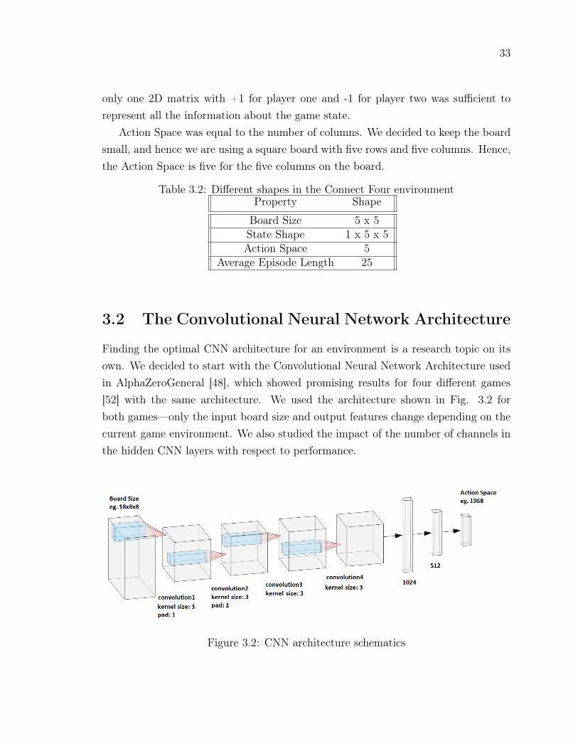
3.2 The Convolutional Neural Network Architecture

Finding the optimal CNN architecture for an environment is a research topic on itsown. We decided to start with the Convolutional Neural Network Architecture usedin AlphaZeroGeneral [48], which showed promising results for four different games[52] with the same architecture. We used the architecture shown in Fig. 3.2 forboth games—only the input board size and output features change depending on thecurrent game environment. We also studied the impact of the number of channels inthe hidden CNN layers with respect to performance.

Figure 3.2: CNN architecture schematics

34

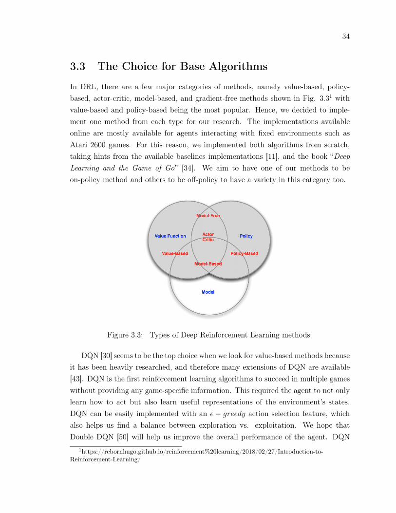
3.3 The Choice for Base Algorithms

In DRL, there are a few major categories of methods, namely value-based, policy-based, actor-critic, model-based, and gradient-free methods shown in Fig. 3.31 withvalue-based and policy-based being the most popular. Hence, we decided to imple-ment one method from each type for our research. The implementations availableonline are mostly available for agents interacting with fixed environments such asAtari 2600 games. For this reason, we implemented both algorithms from scratch,taking hints from the available baselines implementations [11], and the book “DeepLearning and the Game of Go” [34]. We aim to have one of our methods to beon-policy method and others to be off-policy to have a variety in this category too.

Figure 3.3: Types of Deep Reinforcement Learning methods

DQN [30] seems to be the top choice when we look for value-based methods becauseit has been heavily researched, and therefore many extensions of DQN are available[43]. DQN is the first reinforcement learning algorithms to succeed in multiple gameswithout providing any game-specific information. This required the agent to not onlylearn how to act but also learn useful representations of the environment’s states.DQN can be easily implemented with an ε − greedy action selection feature, whichalso helps us find a balance between exploration vs. exploitation. We hope thatDouble DQN [50] will help us improve the overall performance of the agent. DQN

1https://rebornhugo.github.io/reinforcement%20learning/2018/02/27/Introduction-to-Reinforcement-Learning/

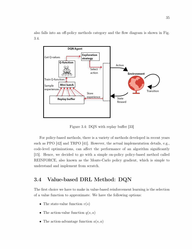
35

also falls into an off-policy methods category and the flow diagram is shown in Fig.3.4.

Figure 3.4: DQN with replay buffer [33]

For policy-based methods, there is a variety of methods developed in recent yearssuch as PPO [42] and TRPO [41]. However, the actual implementation details, e.g.,code-level optimizations, can affect the performance of an algorithm significantly[15]. Hence, we decided to go with a simple on-policy policy-based method calledREINFORCE, also known as the Monte-Carlo policy gradient, which is simple tounderstand and implement from scratch.

3.4 Value-based DRL Method: DQN

The first choice we have to make in value-based reinforcement learning is the selectionof a value function to approximate. We have the following options:

• The state-value function v(s)

• The action-value function q(s, a)

• The action-advantage function a(s, a)

36

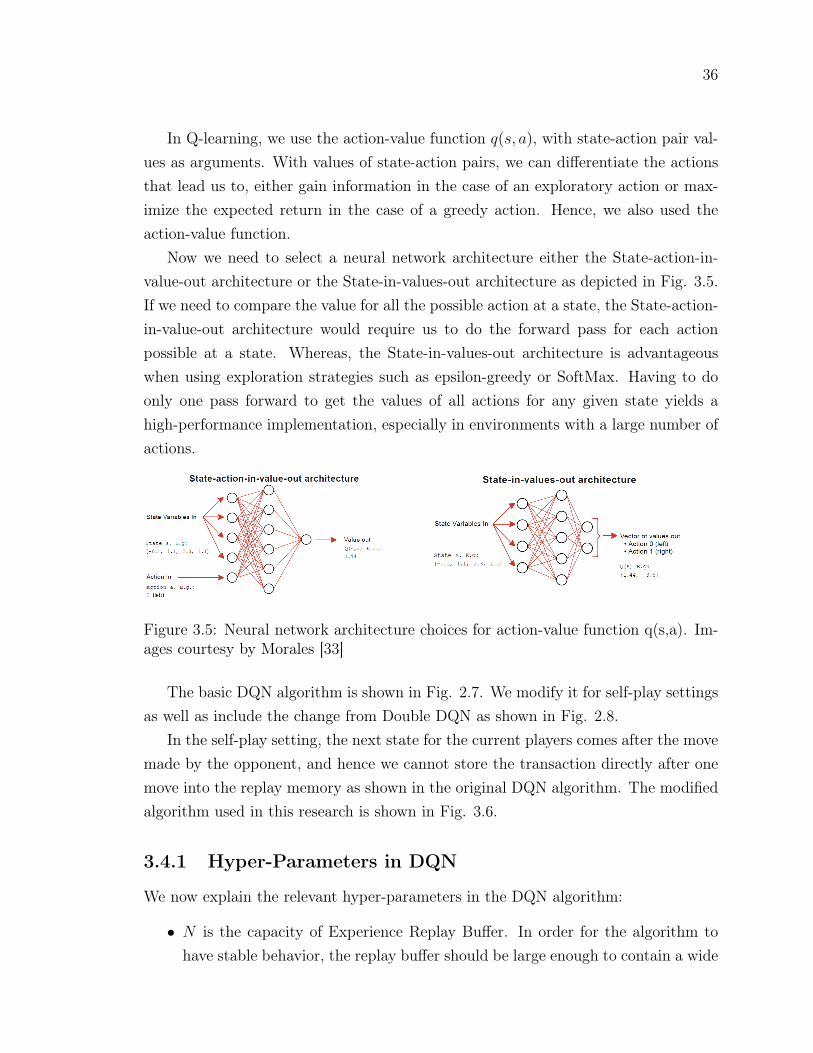
In Q-learning, we use the action-value function q(s, a), with state-action pair val-ues as arguments. With values of state-action pairs, we can differentiate the actionsthat lead us to, either gain information in the case of an exploratory action or max-imize the expected return in the case of a greedy action. Hence, we also used theaction-value function.

Now we need to select a neural network architecture either the State-action-in-value-out architecture or the State-in-values-out architecture as depicted in Fig. 3.5.If we need to compare the value for all the possible action at a state, the State-action-in-value-out architecture would require us to do the forward pass for each actionpossible at a state. Whereas, the State-in-values-out architecture is advantageouswhen using exploration strategies such as epsilon-greedy or SoftMax. Having to doonly one pass forward to get the values of all actions for any given state yields ahigh-performance implementation, especially in environments with a large number ofactions.

Figure 3.5: Neural network architecture choices for action-value function q(s,a). Im-ages courtesy by Morales [33]

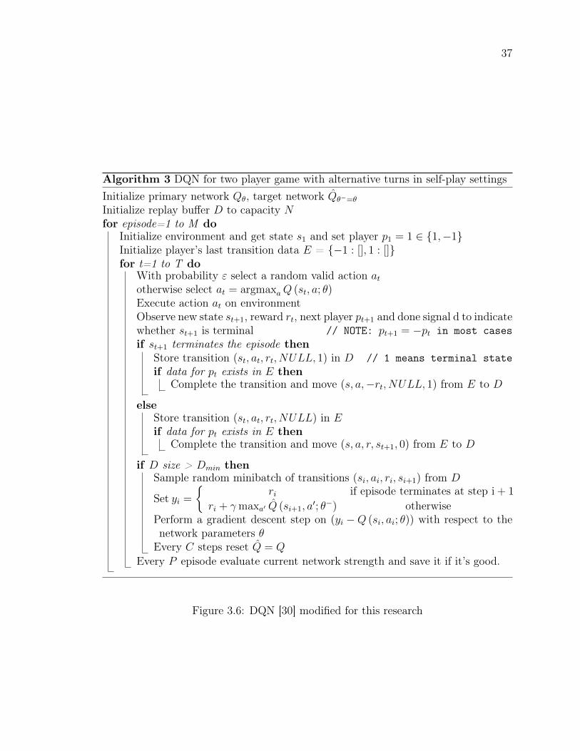
The basic DQN algorithm is shown in Fig. 2.7. We modify it for self-play settingsas well as include the change from Double DQN as shown in Fig. 2.8.

In the self-play setting, the next state for the current players comes after the movemade by the opponent, and hence we cannot store the transaction directly after onemove into the replay memory as shown in the original DQN algorithm. The modifiedalgorithm used in this research is shown in Fig. 3.6.

3.4.1 Hyper-Parameters in DQN

We now explain the relevant hyper-parameters in the DQN algorithm:

• N is the capacity of Experience Replay Buffer. In order for the algorithm tohave stable behavior, the replay buffer should be large enough to contain a wide

37

Algorithm 3 DQN for two player game with alternative turns in self-play settingsInitialize primary network Qθ, target network Q̂θ−=θ

Initialize replay buffer D to capacity Nfor episode=1 to M do

Initialize environment and get state s1 and set player p1 = 1 ∈ {1,−1}Initialize player’s last transition data E = {−1 : [], 1 : []}for t=1 to T do

With probability ε select a random valid action atotherwise select at = argmaxaQ (st, a; θ)Execute action at on environmentObserve new state st+1, reward rt, next player pt+1 and done signal d to indicatewhether st+1 is terminal // NOTE: pt+1 = −pt in most casesif st+1 terminates the episode then

Store transition (st, at, rt, NULL, 1) in D // 1 means terminal stateif data for pt exists in E then

Complete the transition and move (s, a,−rt, NULL, 1) from E to D

elseStore transition (st, at, rt, NULL) in Eif data for pt exists in E then

Complete the transition and move (s, a, r, st+1, 0) from E to D

if D size > Dmin thenSample random minibatch of transitions (si, ai, ri, si+1) from D

Set yi =

{ri if episode terminates at step i + 1

ri + γmaxa′ Q̂ (si+1, a′; θ−) otherwise

Perform a gradient descent step on (yi −Q (si, ai; θ)) with respect to thenetwork parameters θEvery C steps reset Q̂ = Q

Every P episode evaluate current network strength and save it if it’s good.

Figure 3.6: DQN [30] modified for this research

38

range of experiences, but it may not always be good to keep everything. If youonly use the most recent data, you will overfit to that and the algorithm will notwork out; if you use too much experience, you may slow down your learning [1].We set it to 5,000 times the average episode length, i.e., 125,000 for ConnectFour. This needs tuning to get to a good size for the replay buffer.

• Dmin is the minimum replay memory size to fill before training can start. Weassume 2,000 games of memory should be enough to start. Thus, we start witha 25 x 2,000 i.e. 50,000 minimum replay memory size for the Connect Fourgame environment.

• γ is the discount factor needed to calculate target Q values. Generally, a valuebetween 0.9-0.99 is used in most algorithms we have seen. We set the discountfactor value to 0.97 initially.

• M is the number of games to be executed for the training. We expect to obtainmeaningful results with 100,000 games but to be on the safe side we set M to300,000. We periodically save the intermediate trained agent’s model and theevaluation of its strength compare to the baseline agents.

• LearningRate is the learning rate for the neural network gradient update. Avalue near 0.001 is sufficient. The learning rate controls the learning speed ofthe neural network model, too large a value will result in divergence and toosmall a value may double the training time.

• C is the target network update frequency. We are using 1,000 steps as our initialvalue for this parameter. This means that after every 1,000 batches of trainingthe target network will be replaced with the online network.

• batchsize is the size of one batch during the neural network training step. Weexperiment with small and large batch sizes and an initial value of 128.

• ε is used for the epsilon greedy policy in which a value of ε represents thelikelihood of a random action instead of best action using the online network.This parameter is controlled by three values Initial εθ (explore probability atthe start of the training), Final ε′ (The endpoint for the explore probability inε decay) and Explore steps (The number of steps for ε decay from εθ to ε′).

39

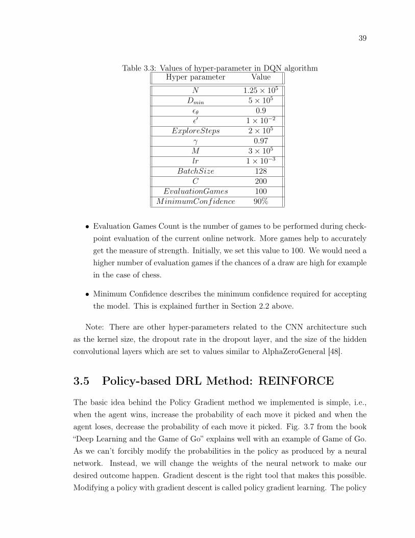
Table 3.3: Values of hyper-parameter in DQN algorithmHyper parameter Value

N 1.25× 105

Dmin 5× 105

εθ 0.9ε′ 1× 10−2

ExploreSteps 2× 105

γ 0.97M 3× 105

lr 1× 10−3

BatchSize 128C 200

EvaluationGames 100MinimumConfidence 90%

• Evaluation Games Count is the number of games to be performed during check-point evaluation of the current online network. More games help to accuratelyget the measure of strength. Initially, we set this value to 100. We would need ahigher number of evaluation games if the chances of a draw are high for examplein the case of chess.

• Minimum Confidence describes the minimum confidence required for acceptingthe model. This is explained further in Section 2.2 above.

Note: There are other hyper-parameters related to the CNN architecture suchas the kernel size, the dropout rate in the dropout layer, and the size of the hiddenconvolutional layers which are set to values similar to AlphaZeroGeneral [48].

3.5 Policy-based DRL Method: REINFORCE

The basic idea behind the Policy Gradient method we implemented is simple, i.e.,when the agent wins, increase the probability of each move it picked and when theagent loses, decrease the probability of each move it picked. Fig. 3.7 from the book“Deep Learning and the Game of Go” explains well with an example of Game of Go.As we can’t forcibly modify the probabilities in the policy as produced by a neuralnetwork. Instead, we will change the weights of the neural network to make ourdesired outcome happen. Gradient descent is the right tool that makes this possible.Modifying a policy with gradient descent is called policy gradient learning. The policy

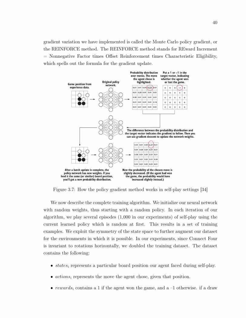
40

gradient variation we have implemented is called the Monte Carlo policy gradient, orthe REINFORCE method. The REINFORCE method stands for REward Increment= Nonnegative Factor times Offset Reinforcement times Characteristic Eligibility,which spells out the formula for the gradient update.

Figure 3.7: How the policy gradient method works in self-play settings [34]

We now describe the complete training algorithm. We initialize our neural networkwith random weights, thus starting with a random policy. In each iteration of ouralgorithm, we play several episodes (1,000 in our experiments) of self-play using thecurrent learned policy which is random at first. This results in a set of trainingexamples. We exploit the symmetry of the state space to further augment our datasetfor the environments in which it is possible. In our experiments, since Connect Fouris invariant to rotations horizontally, we doubled the training dataset. The datasetcontains the following:

• statesi represents a particular board position our agent faced during self-play.

• actionsi represents the move the agent chose, given that position.

• rewardsi contains a 1 if the agent won the game, and a –1 otherwise. if a draw

41

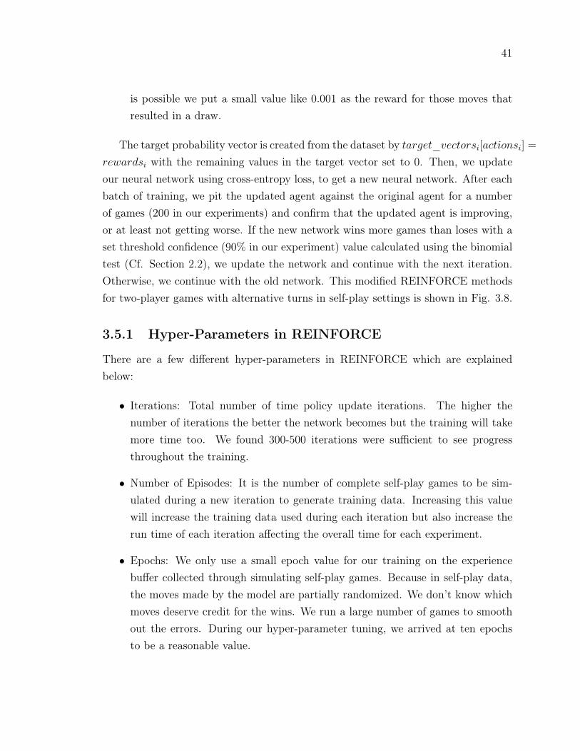
is possible we put a small value like 0.001 as the reward for those moves thatresulted in a draw.

The target probability vector is created from the dataset by target_vectorsi[actionsi] =

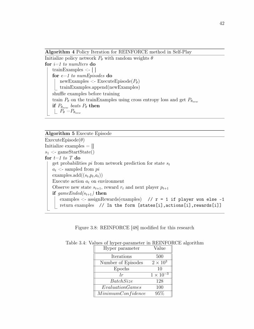
rewardsi with the remaining values in the target vector set to 0. Then, we updateour neural network using cross-entropy loss, to get a new neural network. After eachbatch of training, we pit the updated agent against the original agent for a numberof games (200 in our experiments) and confirm that the updated agent is improving,or at least not getting worse. If the new network wins more games than loses with aset threshold confidence (90% in our experiment) value calculated using the binomialtest (Cf. Section 2.2), we update the network and continue with the next iteration.Otherwise, we continue with the old network. This modified REINFORCE methodsfor two-player games with alternative turns in self-play settings is shown in Fig. 3.8.

3.5.1 Hyper-Parameters in REINFORCE

There are a few different hyper-parameters in REINFORCE which are explainedbelow:

• Iterations: Total number of time policy update iterations. The higher thenumber of iterations the better the network becomes but the training will takemore time too. We found 300-500 iterations were sufficient to see progressthroughout the training.

• Number of Episodes: It is the number of complete self-play games to be sim-ulated during a new iteration to generate training data. Increasing this valuewill increase the training data used during each iteration but also increase therun time of each iteration affecting the overall time for each experiment.

• Epochs: We only use a small epoch value for our training on the experiencebuffer collected through simulating self-play games. Because in self-play data,the moves made by the model are partially randomized. We don’t know whichmoves deserve credit for the wins. We run a large number of games to smoothout the errors. During our hyper-parameter tuning, we arrived at ten epochsto be a reasonable value.

42

Algorithm 4 Policy Iteration for REINFORCE method in Self-PlayInitialize policy network Pθ with random weights θfor i=1 to numIters do

trainExamples <- [ ]for e=1 to numEpisodes do

newExamples <- ExecuteEpisode(Pθ)trainExamples.append(newExamples)

shuffle examples before trainingtrain Pθ on the trainExamples using cross entropy loss and get Pθnewif Pθnew beats Pθ then

Pθ =Pθnew

Algorithm 5 Execute EpisodeExecuteEpisode(θ)Initialize examples = []s1 <- gameStartState()for t=1 to T do

get probabilities pi from network prediction for state stat <- sampled from piexamples.add((st,pt,at))Execute action at on environmentObserve new state st+1, reward rt and next player pt+1

if gameEnded(st+1) thenexamples <- assignRewards(examples) // r = 1 if player won else -1return examples // In the form [states[i],actions[i],rewards[i]]

Figure 3.8: REINFORCE [48] modified for this research

Table 3.4: Values of hyper-parameter in REINFORCE algorithmHyper parameter Value

Iterations 500Number of Episodes 2× 103

Epochs 10lr 1× 10−3

BatchSize 128EvaluationGames 100

MinimumConfidence 95%

43

3.6 Comparing Models

We pit agents against each other in a series of matches in which half of the matchesagent 1 plays first and in the rest, it plays second. The implementation is based onthe Arena from AlphaZeroGeneral [48] with some changes as we are not using MCTSin our methods. During each evaluation cycle, we also evaluate the strength of thecurrent agent with respect to the baseline agents like a random agent and a greedyagent (Cf. Chapter 4). This helps us plot a graph that shows clearly if the agent isimproving or not.

3.7 Chapter Summary

This chapter explained the core design of the algorithms and environments used in ourresearch. It also introduced in detail the changes required in the existing algorithmsto adapt them for self-play settings. Finally, we listed hyper-parameters present inthe algorithm and their expected impact on the training of the DRL neural networkmodel.

44

Chapter 4

Evaluation, Results and Discussion

The overall evaluation of this research aims to investigate the effectiveness of the DRLalgorithms on a setting for which they were not originally designed. In our research,we consider an exploratory case study which allows us to conduct our investigationbased on our research questions.

This chapter defines the methods used to evaluate the goals of this research alongwith a discussion of the actual results collected throughout our experiments. Section4.1 specifies the actual hardware and software used during the controlled experiment.Section 4.2 explains the baseline agents for the neural network strength evaluationand discusses the results obtained from the agent’s training with both algorithms.Finally, Section 4.3 describes the hyper-parameters on which our research focusedand then demonstrates their impact on the performance of the agent.

4.1 Experimental Setup

We used the Python programming language for this implementation, consideringthe readability of the code along with the availability of widely used deep learningframeworks such as PyTorch and TensorFlow. We also used Numpy, which is a usefulPython library that accelerates matrix operations with the C programming language.This allows us to write efficient scientific computing code with Python. We decidedto use Pytorch for our deep learning operations, due to its simplicity.

The experiments were done on a single computer system. There were some lim-itations such as 8GB GPU memory that limit the size of the Neural network andbatch sizes. Therefore, parameters related to hardware limitations will be suitably

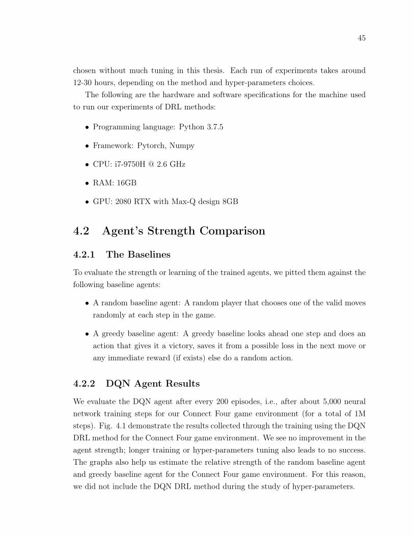
45

chosen without much tuning in this thesis. Each run of experiments takes around12-30 hours, depending on the method and hyper-parameters choices.

The following are the hardware and software specifications for the machine usedto run our experiments of DRL methods:

• Programming language: Python 3.7.5

• Framework: Pytorch, Numpy

• CPU: i7-9750H @ 2.6 GHz

• RAM: 16GB

• GPU: 2080 RTX with Max-Q design 8GB

4.2 Agent’s Strength Comparison

4.2.1 The Baselines

To evaluate the strength or learning of the trained agents, we pitted them against thefollowing baseline agents:

• A random baseline agent: A random player that chooses one of the valid movesrandomly at each step in the game.

• A greedy baseline agent: A greedy baseline looks ahead one step and does anaction that gives it a victory, saves it from a possible loss in the next move orany immediate reward (if exists) else do a random action.

4.2.2 DQN Agent Results

We evaluate the DQN agent after every 200 episodes, i.e., after about 5,000 neuralnetwork training steps for our Connect Four game environment (for a total of 1Msteps). Fig. 4.1 demonstrate the results collected through the training using the DQNDRL method for the Connect Four game environment. We see no improvement in theagent strength; longer training or hyper-parameters tuning also leads to no success.The graphs also help us estimate the relative strength of the random baseline agentand greedy baseline agent for the Connect Four game environment. For this reason,we did not include the DQN DRL method during the study of hyper-parameters.

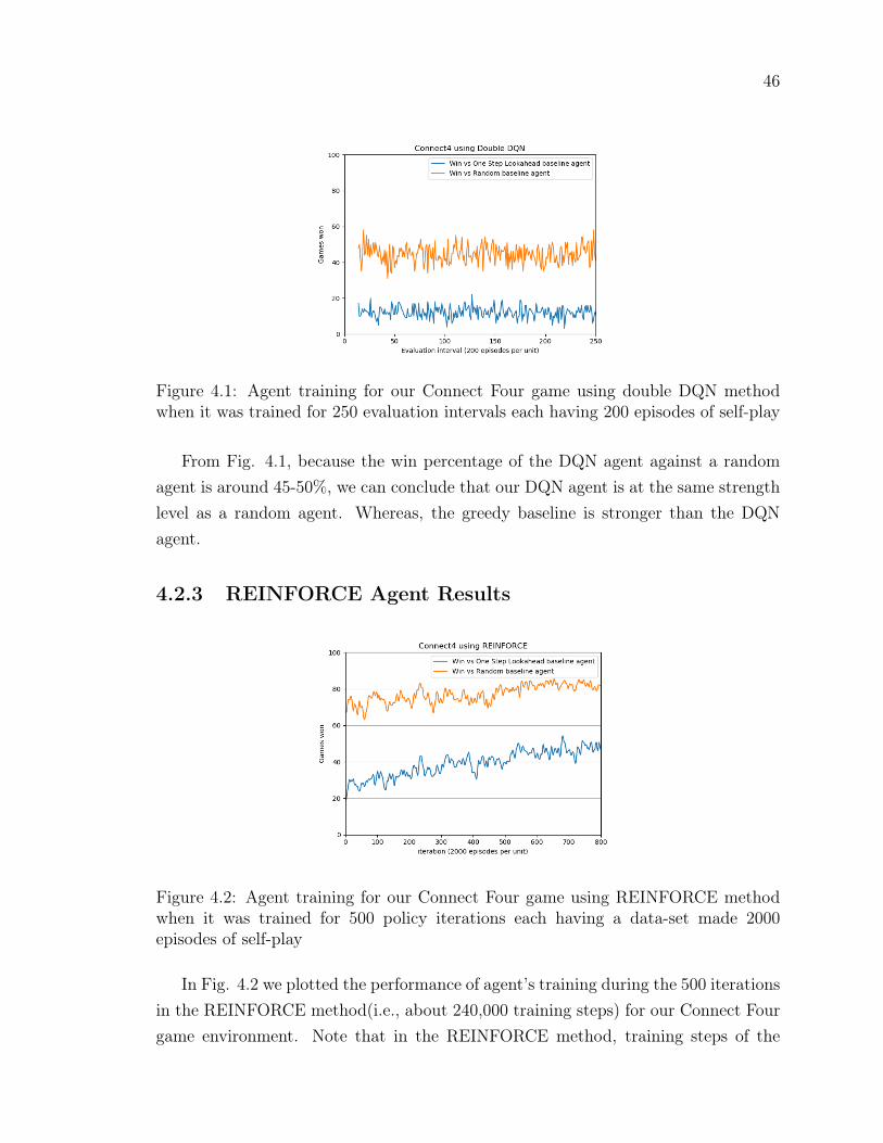
46

Figure 4.1: Agent training for our Connect Four game using double DQN methodwhen it was trained for 250 evaluation intervals each having 200 episodes of self-play

From Fig. 4.1, because the win percentage of the DQN agent against a randomagent is around 45-50%, we can conclude that our DQN agent is at the same strengthlevel as a random agent. Whereas, the greedy baseline is stronger than the DQNagent.

4.2.3 REINFORCE Agent Results

Figure 4.2: Agent training for our Connect Four game using REINFORCE methodwhen it was trained for 500 policy iterations each having a data-set made 2000episodes of self-play

In Fig. 4.2 we plotted the performance of agent’s training during the 500 iterationsin the REINFORCE method(i.e., about 240,000 training steps) for our Connect Fourgame environment. Note that in the REINFORCE method, training steps of the

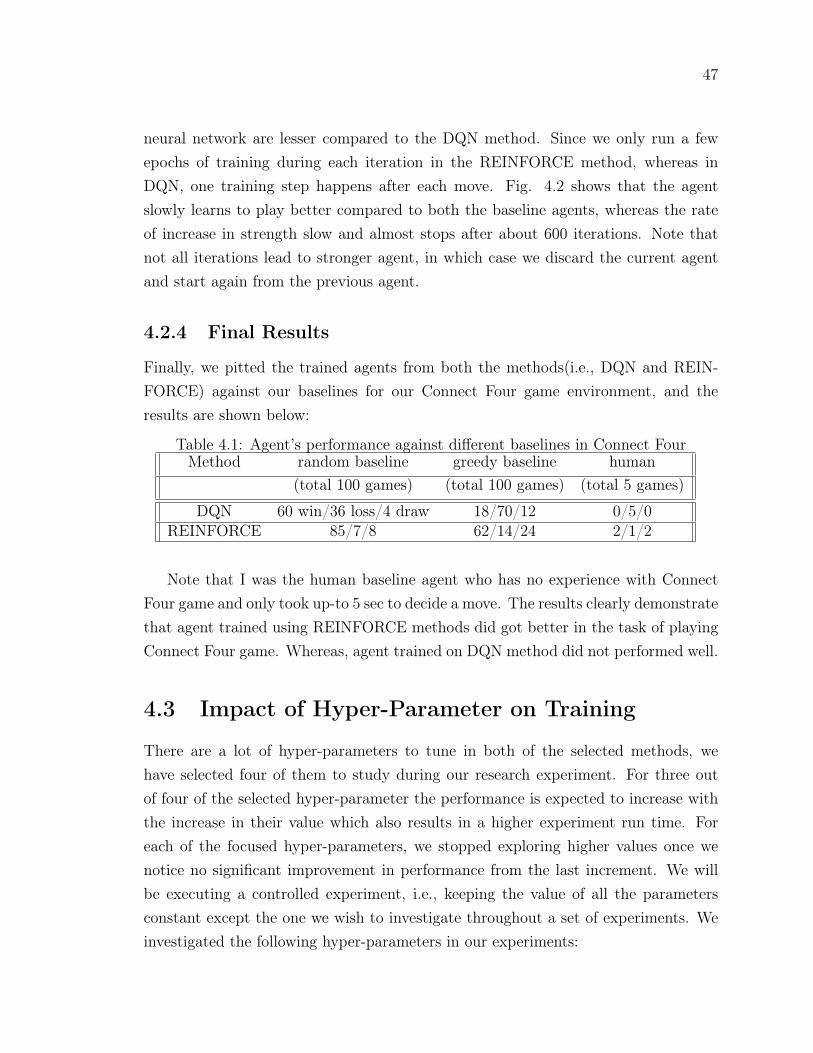
47

neural network are lesser compared to the DQN method. Since we only run a fewepochs of training during each iteration in the REINFORCE method, whereas inDQN, one training step happens after each move. Fig. 4.2 shows that the agentslowly learns to play better compared to both the baseline agents, whereas the rateof increase in strength slow and almost stops after about 600 iterations. Note thatnot all iterations lead to stronger agent, in which case we discard the current agentand start again from the previous agent.

4.2.4 Final Results

Finally, we pitted the trained agents from both the methods(i.e., DQN and REIN-FORCE) against our baselines for our Connect Four game environment, and theresults are shown below:

Table 4.1: Agent’s performance against different baselines in Connect FourMethod random baseline greedy baseline human

(total 100 games) (total 100 games) (total 5 games)

DQN 60 win/36 loss/4 draw 18/70/12 0/5/0REINFORCE 85/7/8 62/14/24 2/1/2

Note that I was the human baseline agent who has no experience with ConnectFour game and only took up-to 5 sec to decide a move. The results clearly demonstratethat agent trained using REINFORCE methods did got better in the task of playingConnect Four game. Whereas, agent trained on DQN method did not performed well.

4.3 Impact of Hyper-Parameter on Training

There are a lot of hyper-parameters to tune in both of the selected methods, wehave selected four of them to study during our research experiment. For three outof four of the selected hyper-parameter the performance is expected to increase withthe increase in their value which also results in a higher experiment run time. Foreach of the focused hyper-parameters, we stopped exploring higher values once wenotice no significant improvement in performance from the last increment. We willbe executing a controlled experiment, i.e., keeping the value of all the parametersconstant except the one we wish to investigate throughout a set of experiments. Weinvestigated the following hyper-parameters in our experiments:

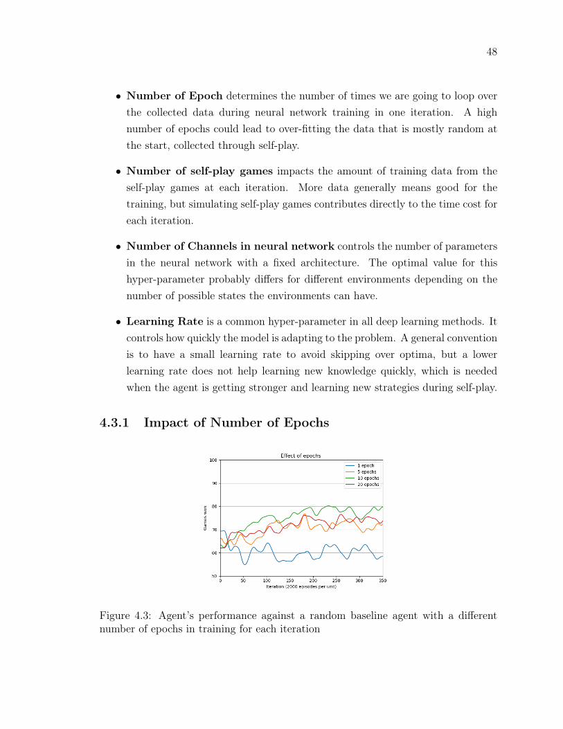
48

• Number of Epoch determines the number of times we are going to loop overthe collected data during neural network training in one iteration. A highnumber of epochs could lead to over-fitting the data that is mostly random atthe start, collected through self-play.

• Number of self-play games impacts the amount of training data from theself-play games at each iteration. More data generally means good for thetraining, but simulating self-play games contributes directly to the time cost foreach iteration.

• Number of Channels in neural network controls the number of parametersin the neural network with a fixed architecture. The optimal value for thishyper-parameter probably differs for different environments depending on thenumber of possible states the environments can have.

• Learning Rate is a common hyper-parameter in all deep learning methods. Itcontrols how quickly the model is adapting to the problem. A general conventionis to have a small learning rate to avoid skipping over optima, but a lowerlearning rate does not help learning new knowledge quickly, which is neededwhen the agent is getting stronger and learning new strategies during self-play.

4.3.1 Impact of Number of Epochs

Figure 4.3: Agent’s performance against a random baseline agent with a differentnumber of epochs in training for each iteration

49

Figure 4.4: Agent’s performance against a greedy baseline agent with a differentnumber of epochs in training for each iteration

According to the literature [34], we should not do too many epochs on the datacollected through self-play; the recommended values range from 1 to 3. Because inself-play data, the moves made by the agents are partially randomized, and we don’tknow which moves deserve credit for the wins. We are counting on a huge numberof games to smooth out the errors. Note that increasing the value for this hyper-parameter does increase the training time in each iteration, causing a significantincrease in the overall time for one experiment.

Figs. 4.3 and 4.4 shows the results obtained with different values for the epochhyper-parameter and keeping all the other hyper-parameter constant. We can seein the figures that 10 epochs giving the best results and increasing or decreasingthe value decreases the overall performance. The optimal value for the epoch hyper-parameter turns out to be more than what was recommended in the literature. Notethat the optimal value for the epoch hyper-parameter could depend on the environ-ment complexity, which could be a direction for future research.

4.3.2 Impact of Number of Self-Play Games

The number of self-play games contributes to the training data for each iteration;the more data we have the better would be the agent after each iteration. Butincreasing the number of self-play games increases the total time to simulate thesegames, and resulted in an increase in data that increases the training time of theagent. Hence overall, this hyper-parameter contributes heavily to the overall time forthe experiment. So, we want the value to be good enough to give us a good result for

50

Figure 4.5: Agent’s performance against a random baseline agent with a differentnumber of self-play games for each iteration

Figure 4.6: Agent’s performance against a greedy baseline agent with a differentnumber of self-play games for each iteration

each iteration and not cost us too much time.Figs. 4.5 and 4.6 show the results obtained with different values for the self-play

games and keeping all the other hyper-parameter constant. We note that against therandom baseline, there is no significant improvement between 2,000 games and 5,000games, and against the greedy baseline also the improvement from 2,000 games to5,000 games is less than 5%. Note that the time cost for 5,000 games per iterationis twice then 2,000 games, which suggest that 2000 self-play games would be thebest value for this hyper-parameter.

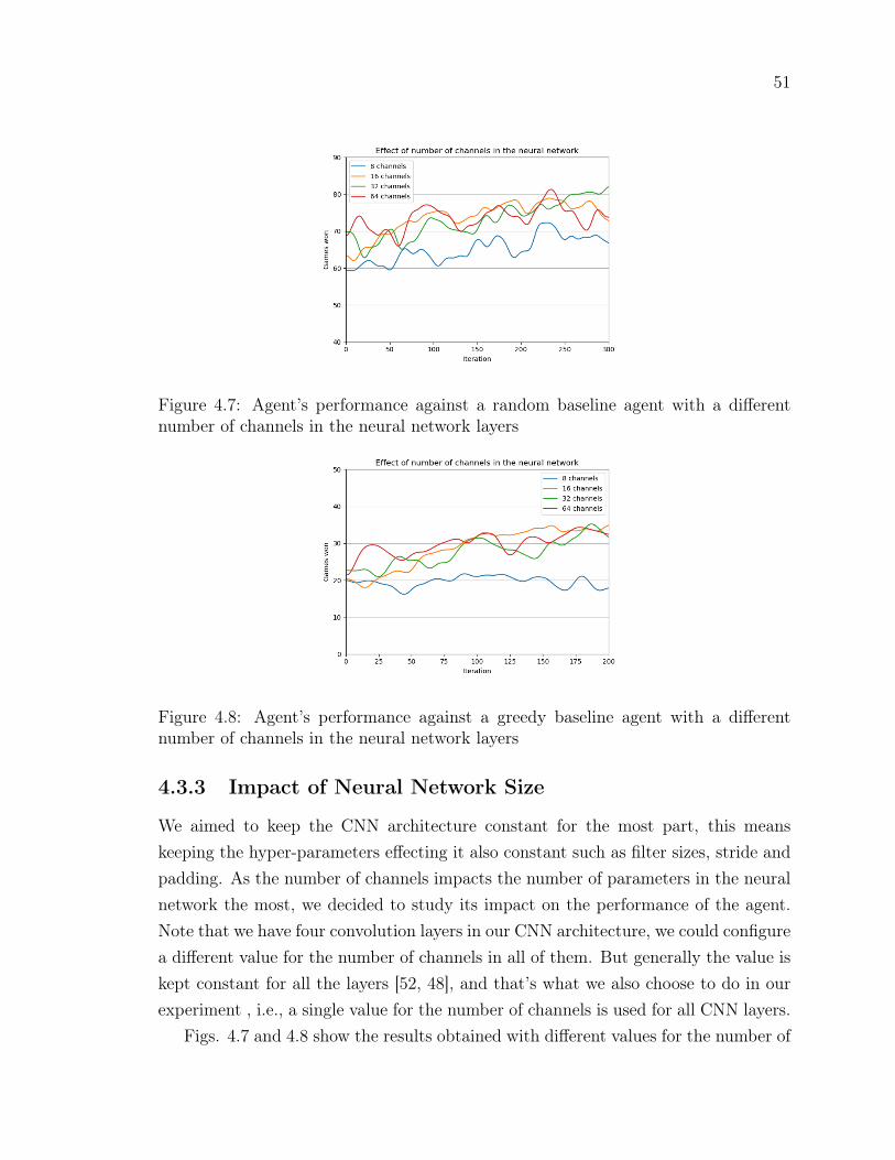
51

Figure 4.7: Agent’s performance against a random baseline agent with a differentnumber of channels in the neural network layers

Figure 4.8: Agent’s performance against a greedy baseline agent with a differentnumber of channels in the neural network layers

4.3.3 Impact of Neural Network Size

We aimed to keep the CNN architecture constant for the most part, this meanskeeping the hyper-parameters effecting it also constant such as filter sizes, stride andpadding. As the number of channels impacts the number of parameters in the neuralnetwork the most, we decided to study its impact on the performance of the agent.Note that we have four convolution layers in our CNN architecture, we could configurea different value for the number of channels in all of them. But generally the value iskept constant for all the layers [52, 48], and that’s what we also choose to do in ourexperiment , i.e., a single value for the number of channels is used for all CNN layers.

Figs. 4.7 and 4.8 show the results obtained with different values for the number of

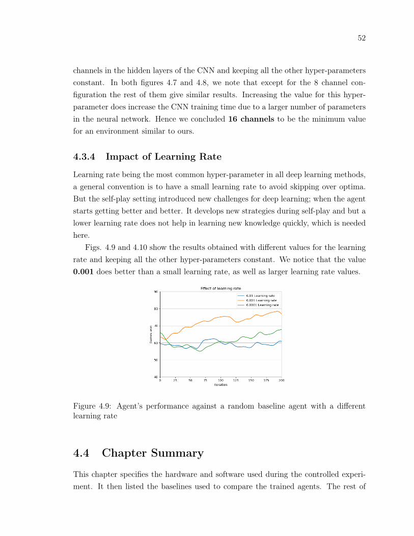
52

channels in the hidden layers of the CNN and keeping all the other hyper-parametersconstant. In both figures 4.7 and 4.8, we note that except for the 8 channel con-figuration the rest of them give similar results. Increasing the value for this hyper-parameter does increase the CNN training time due to a larger number of parametersin the neural network. Hence we concluded 16 channels to be the minimum valuefor an environment similar to ours.

4.3.4 Impact of Learning Rate

Learning rate being the most common hyper-parameter in all deep learning methods,a general convention is to have a small learning rate to avoid skipping over optima.But the self-play setting introduced new challenges for deep learning; when the agentstarts getting better and better. It develops new strategies during self-play and but alower learning rate does not help in learning new knowledge quickly, which is neededhere.

Figs. 4.9 and 4.10 show the results obtained with different values for the learningrate and keeping all the other hyper-parameters constant. We notice that the value0.001 does better than a small learning rate, as well as larger learning rate values.

Figure 4.9: Agent’s performance against a random baseline agent with a differentlearning rate

4.4 Chapter Summary

This chapter specifies the hardware and software used during the controlled experi-ment. It then listed the baselines used to compare the trained agents. The rest of

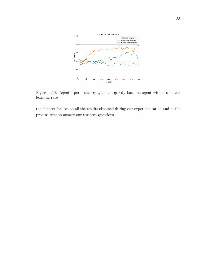
53

Figure 4.10: Agent’s performance against a greedy baseline agent with a differentlearning rate

the chapter focuses on all the results obtained during our experimentation and in theprocess tries to answer our research questions .

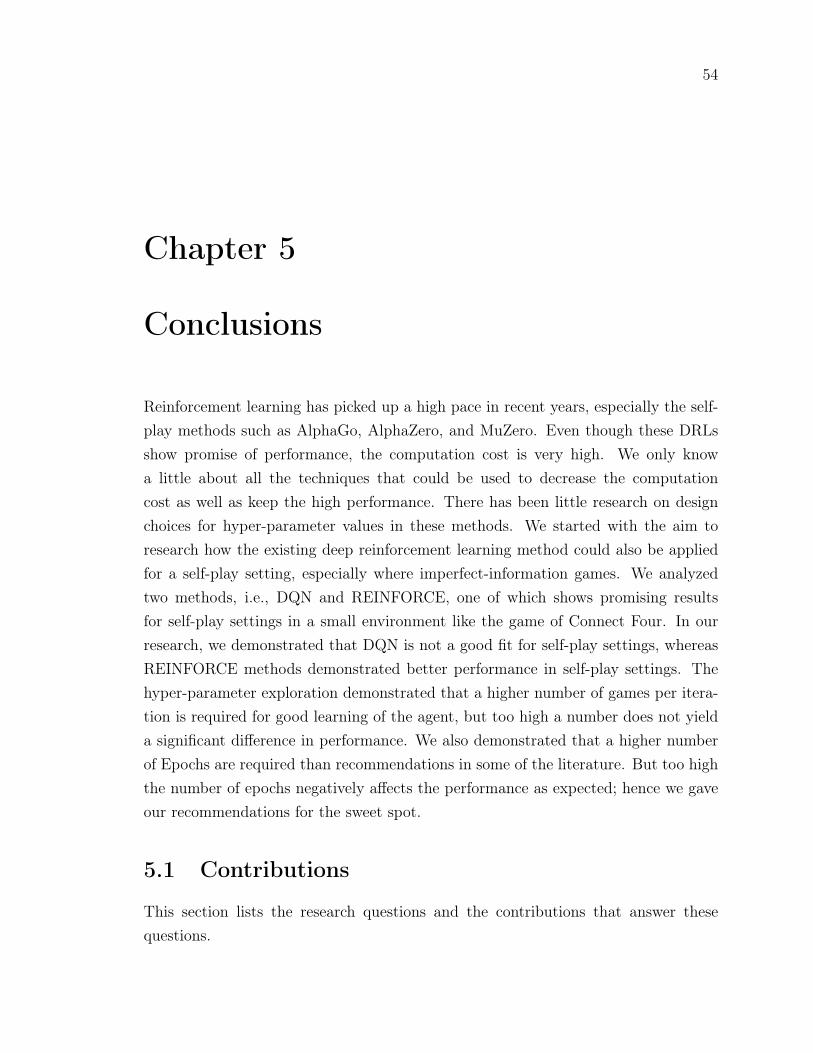
54

Chapter 5

Conclusions

Reinforcement learning has picked up a high pace in recent years, especially the self-play methods such as AlphaGo, AlphaZero, and MuZero. Even though these DRLsshow promise of performance, the computation cost is very high. We only knowa little about all the techniques that could be used to decrease the computationcost as well as keep the high performance. There has been little research on designchoices for hyper-parameter values in these methods. We started with the aim toresearch how the existing deep reinforcement learning method could also be appliedfor a self-play setting, especially where imperfect-information games. We analyzedtwo methods, i.e., DQN and REINFORCE, one of which shows promising resultsfor self-play settings in a small environment like the game of Connect Four. In ourresearch, we demonstrated that DQN is not a good fit for self-play settings, whereasREINFORCE methods demonstrated better performance in self-play settings. Thehyper-parameter exploration demonstrated that a higher number of games per itera-tion is required for good learning of the agent, but too high a number does not yielda significant difference in performance. We also demonstrated that a higher numberof Epochs are required than recommendations in some of the literature. But too highthe number of epochs negatively affects the performance as expected; hence we gaveour recommendations for the sweet spot.

5.1 Contributions

This section lists the research questions and the contributions that answer thesequestions.

55

RQ1. How can DRL methods such as DQN and REINFORCE be applied in environ-ments supporting self-play settings?

C1. Chapter 3 explains both algorithms in detail along with the changes requiredto collect all the data for the case of self-play settings.

RQ2. Which of the two methods, DQN and REINFORCE, is better suited for gameenvironments similar to Connect Four in self-play settings?

C2. Chapter 4 demonstrated that the REINFORCE method is more promising forself-play settings.

RQ3. What are the important hyper-parameters and their initial values for traininga DRL agent on game environments in a self-play settings?

C3. Chapter 4 demonstrated the impact of the four hyper-parameters and sharedrecommendations for them.

5.2 Future work

This section proposes avenues where the work presented in this thesis could be furtherexplored.

Actor-critic methods

Actor-critic reinforcement learning methods improve the policy gradient with a value-based critic. They are, in a way a combination of value-based and policy-basedmethods. It would be worthwhile to investigate how one of these methods works inself-play settings.

Environments with various complexities

The complexity of the environment may affect the optimal values for the hyper-parameters. This would require a few different customize-able experimental environ-ments with varying difficulties/complexities. This kind of research would give a betteridea for the values of hyper-parameters for a new unknown environment.

56

Impact of CNN architectures

Obviously different CNN architectures will result in different behaviour and perfor-mance in any application area. Hence, the impact of different CNN architecturescould be explored, leading to a more effective general CNN architecture for self-playsettings.

57

Bibliography

[1] Joshua Achiam. Spinning Up in Deep Reinforcement Learning. 2018. (page 38)

[2] Kai Arulkumaran, Antoine Cully, and Julian Togelius. AlphaStar: An Evolu-tionary Computation Perspective. February 2019. (page 2)

[3] Marc G Bellemare, Yavar Naddaf, Joel Veness, and Michael Bowling. The arcadelearning environment: An evaluation platform for general agents. Journal ofArtificial Intelligence Research, 47:253–279, 2013. (page 18, 23)

[4] Christopher Berner, Greg Brockman, Brooke Chan, Vicki Cheung, PrzemysławDębiak, Christy Dennison, David Farhi, Quirin Fischer, Shariq Hashme, ChrisHesse, et al. Dota 2 with large scale deep reinforcement learning. arXiv preprintarXiv:1912.06680, 2019. (page 2)

[5] Noam Brown, Anton Bakhtin, Adam Lerer, and Qucheng Gong. Combiningdeep reinforcement learning and search for imperfect-information games, 2020.(page 26)

[6] Nicolò Cesa-Bianchi, Claudio Gentile, Gábor Lugosi, and Gergely Neu. Boltz-mann Exploration Done Right. May 2017. (page 13)

[7] Henry Charlesworth. Application of self-play reinforcement learning to a four-player game of imperfect information. CoRR, abs/1808.10442, 2018. (page 26)

[8] Guillaume Maurice Jean-Bernard Chaslot Chaslot. Monte-carlo tree search.Maastricht University, 2010. (page 2)

[9] John W Creswell and J David Creswell. Research design: Qualitative, quantita-tive, and mixed methods approaches. Sage publications, 2017. (page 4)

58

[10] Rina Dechter. Learning while searching in constraint-satisfaction-problems. InProceedings of the Fifth AAAI National Conference on Artificial Intelligence,AAAI’86, page 178–183. AAAI Press, 1986. (page 14)

[11] Prafulla Dhariwal, Christopher Hesse, Oleg Klimov, Alex Nichol, Matthias Plap-pert, Alec Radford, John Schulman, Szymon Sidor, Yuhuai Wu, and PeterZhokhov. Openai baselines. https://github.com/openai/baselines, 2017.(page 34)

[12] J Du Toit, R Davimes, A Mohamed, K Patel, and JM Nye. Customer seg-mentation using unsupervised learning on daily energy load profiles. Journal ofAdvances in Information Technology Vol, 7(2):69–75, 2016. (page 8)

[13] Anuj Dutt and Aashi Dutt. Handwritten digit recognition using deep learning.Int J AdvRes Comput Eng Technol, 6(7):990–997, 2017. (page 7)

[14] Steve Easterbrook, Janice Singer, Margaret-Anne Storey, and Daniela Damian.Selecting empirical methods for software engineering research. In Guide to ad-vanced empirical software engineering, pages 285–311. Springer, 2008. (page 4)

[15] Logan Engstrom, Andrew Ilyas, Shibani Santurkar, Dimitris Tsipras, FirdausJanoos, Larry Rudolph, and Aleksander Madry. Implementation matters indeep policy gradients: A case study on PPO and TRPO. arXiv preprintarXiv:2005.12729, 2020. (page 35)

[16] Vincent Francois-Lavet, Peter Henderson, Riashat Islam, Marc G. Bellemare, andJoelle Pineau. An Introduction to Deep Reinforcement Learning. Foundationsand Trends in Machine Learning, 11(3-4):219–354, 2018. arXiv: 1811.12560.(page 18)

[17] Hado V. Hasselt. Double q-learning. In J. D. Lafferty, C. K. I. Williams, J. Shawe-Taylor, R. S. Zemel, and A. Culotta, editors, Advances in Neural InformationProcessing Systems 23, pages 2613–2621. Curran Associates, Inc., 2010. (page 24)

[18] Soufiane Hayou, Arnaud Doucet, and Judith Rousseau. On the impact ofthe activation function on deep neural networks training. arXiv preprintarXiv:1902.06853, 2019. (page 15)

59

[19] Johannes Heinrich and David Silver. Deep reinforcement learning from self-play in imperfect-information games. arXiv preprint arXiv:1603.01121, 2016.(page 26)

[20] Sepp Hochreiter and Jürgen Schmidhuber. Long short-term memory. NeuralComputation, 9(8):1735–1780, 1997. (page 15)

[21] Sergey Ioffe and Christian Szegedy. Batch normalization: Accelerating deepnetwork training by reducing internal covariate shift. CoRR, abs/1502.03167,2015. (page 17, 18)

[22] Andreas Jedlitschka, Marcus Ciolkowski, and Dietmar Pfahl. Reporting exper-iments in software engineering. In Guide to advanced empirical software engi-neering, pages 201–228. Springer, 2008. (page 4)

[23] X. Jin. Research on command decision support system AI problem decompo-sition. In 2018 10th International Conference on Intelligent Human-MachineSystems and Cybernetics (IHMSC), volume 02, pages 96–100, 2018. (page 2)

[24] B Ravi Kiran, Ibrahim Sobh, Victor Talpaert, Patrick Mannion, Ahmad A. AlSallab, Senthil Yogamani, and Patrick Pérez. Deep reinforcement learning forautonomous driving: A survey. IEEE Transactions on Intelligent TransportationSystems, 2021. (page 1)

[25] Alex Krizhevsky, Ilya Sutskever, and Geoffrey E. Hinton. Imagenet classificationwith deep convolutional neural networks. Commun. ACM, 60(6):84–90, May2017. (page 15)

[26] Guillaume Lample and Devendra Singh Chaplot. Playing FPS games with deepreinforcement learning. CoRR, abs/1609.05521, 2016. (page 2)

[27] Yann LeCun, Yoshua Bengio, and Geoffrey Hinton. Deep learning. Nature,521(7553):436–444, May 2015. (page 14)

[28] Ilya Makarov, Andrej Kashin, and Alisa Korinevskaya. Learning to play pongvideo game via deep reinforcement learning. In AIST (Supplement), pages 236–241, 2017. (page 8)

60

[29] Hongzi Mao, Mohammad Alizadeh, Ishai Menache, and Srikanth Kandula. Re-source management with deep reinforcement learning. In Proceedings of the 15thACM Workshop on Hot Topics in Networks, pages 50–56, 2016. (page 1)

[30] Volodymyr Mnih, Koray Kavukcuoglu, David Silver, Alex Graves, IoannisAntonoglou, Daan Wierstra, and Martin Riedmiller. Playing atari with deepreinforcement learning. arXiv preprint arXiv:1312.5602, 2013. (page vii, 18, 22,23, 34, 37)

[31] Volodymyr Mnih, Koray Kavukcuoglu, David Silver, Alex Graves, IoannisAntonoglou, Daan Wierstra, and Martin Riedmiller. Playing Atari with DeepReinforcement Learning. December 2013. (page 2)

[32] Volodymyr Mnih, Koray Kavukcuoglu, David Silver, Andrei A. Rusu, Joel Ve-ness, Marc G. Bellemare, Alex Graves, Martin Riedmiller, Andreas K. Fid-jeland, Georg Ostrovski, Stig Petersen, Charles Beattie, Amir Sadik, IoannisAntonoglou, Helen King, Dharshan Kumaran, Daan Wierstra, Shane Legg, andDemis Hassabis. Human-level control through deep reinforcement learning. Na-ture, 518(7540):529–533, February 2015. (page 2)

[33] Miguel Morales. Grokking Deep Reinforcement Learning. Manning Publications,2018. (page vii, 7, 8, 18, 35, 36)

[34] Max Pumperla and Kevin Ferguson. Deep Learning and the Game of Go. Man-ning Publications, 2019. (page vii, 22, 34, 40, 49)

[35] Martin A. Riedmiller, Roland Hafner, Thomas Lampe, Michael Neunert, JonasDegrave, Tom Van de Wiele, Volodymyr Mnih, Nicolas Heess, and Jost TobiasSpringenberg. Learning by playing—solving sparse reward tasks from scratch.CoRR, abs/1802.10567, 2018. (page 14)

[36] Leslie A. Rusch. Exploration-exploitation trade-off in deep reinforcement learn-ing. 2018. (page 12)

[37] Otabek Sattarov, Azamjon Muminov, Cheol Won Lee, Hyun Kyu Kang, Ryum-duck Oh, Junho Ahn, Hyung Jun Oh, and Heung Seok Jeon. Recommendingcryptocurrency trading points with deep reinforcement learning approach. Ap-plied Sciences, 10(4), 2020. (page vii, 9)

61

[38] Tom Schaul, John Quan, Ioannis Antonoglou, and David Silver. Prioritizedexperience replay. arXiv preprint arXiv:1511.05952, 2015. (page 24)

[39] Jürgen Schmidhuber. Deep learning in neural networks: An overview. CoRR,abs/1404.7828, 2014. (page 14)

[40] Julian Schrittwieser, Ioannis Antonoglou, Thomas Hubert, Karen Simonyan,Laurent Sifre, Simon Schmitt, Arthur Guez, Edward Lockhart, Demis Hassabis,Thore Graepel, et al. Mastering atari, go, chess and shogi by planning with alearned model. arXiv preprint arXiv:1911.08265, 2019. (page 2)

[41] John Schulman, Sergey Levine, Philipp Moritz, Michael I. Jordan, and PieterAbbeel. Trust region policy optimization. CoRR, abs/1502.05477, 2015. (page 24,35)

[42] John Schulman, Filip Wolski, Prafulla Dhariwal, Alec Radford, and Oleg Klimov.Proximal policy optimization algorithms. CoRR, abs/1707.06347, 2017. (page 25,35)

[43] Kun Shao, Zhentao Tang, Yuanheng Zhu, Nannan Li, and Dongbin Zhao. Asurvey of deep reinforcement learning in video games. arXiv, abs/1912.10944,2019. (page 2, 3, 22, 34)

[44] David Silver, Aja Huang, Chris J. Maddison, Arthur Guez, Laurent Sifre,George van den Driessche, Julian Schrittwieser, Ioannis Antonoglou, Veda Pan-neershelvam, Marc Lanctot, Sander Dieleman, Dominik Grewe, John Nham,Nal Kalchbrenner, Ilya Sutskever, Timothy Lillicrap, Madeleine Leach, KorayKavukcuoglu, Thore Graepel, and Demis Hassabis. Mastering the game of Gowith deep neural networks and tree search. Nature, 529(7587):484–489, January2016. (page 25)

[45] David Silver, Thomas Hubert, Julian Schrittwieser, Ioannis Antonoglou,Matthew Lai, Arthur Guez, Marc Lanctot, Laurent Sifre, Dharshan Kumaran,Thore Graepel, et al. Mastering chess and shogi by self-play with a general rein-forcement learning algorithm. arXiv preprint arXiv:1712.01815, 2017. (page 2,25, 30)

[46] David Silver, Thomas Hubert, Julian Schrittwieser, Ioannis Antonoglou,Matthew Lai, Arthur Guez, Marc Lanctot, Laurent Sifre, Dharshan Kumaran,

62

Thore Graepel, Timothy Lillicrap, Karen Simonyan, and Demis Hassabis. Mas-tering Chess and Shogi by Self-Play with a General Reinforcement LearningAlgorithm. December 2017. (page 2)

[47] David Silver, Julian Schrittwieser, Karen Simonyan, Ioannis Antonoglou, AjaHuang, Arthur Guez, Thomas Hubert, Lucas Baker, Matthew Lai, AdrianBolton, Yutian Chen, Timothy Lillicrap, Fan Hui, Laurent Sifre, George van denDriessche, Thore Graepel, and Demis Hassabis. Mastering the game of Go with-out human knowledge. Nature, 550(7676):354–359, October 2017. (page 25)

[48] N. Surag. Alpha zero general. https://github.com/suragnair/

alpha-zero-general, 2018. (page vii, 22, 30, 33, 39, 42, 43, 51)

[49] Richard S. Sutton and Andrew G. Barto. Reinforcement Learning: An Introduc-tion, volume 16. 1988. (page 1, 8, 9, 11, 12, 19)

[50] Hado van Hasselt, Arthur Guez, and David Silver. Deep reinforcement learningwith double q-learning. CoRR, abs/1509.06461, 2015. (page 23, 34)

[51] Oriol Vinyals, Timo Ewalds, Sergey Bartunov, Petko Georgiev, Alexander SashaVezhnevets, Michelle Yeo, Alireza Makhzani, Heinrich Küttler, John Agapiou,Julian Schrittwieser, John Quan, Stephen Gaffney, Stig Petersen, Karen Si-monyan, Tom Schaul, Hado van Hasselt, David Silver, Timothy Lillicrap, KevinCalderone, Paul Keet, Anthony Brunasso, David Lawrence, Anders Ekermo, Ja-cob Repp, and Rodney Tsing. StarCraft II: A New Challenge for ReinforcementLearning. August 2017. (page 2)

[52] Hui Wang, Michael Emmerich, Mike Preuss, and Aske Plaat. Analysis of hyper-parameters for small games: Iterations or epochs in self-play? arXiv preprintarXiv:2003.05988, 2020. (page 26, 33, 51)

[53] Christopher J. C. H. Watkins and Peter Dayan. Q-learning. Machine Learning,8(3):279–292, May 1992. (page 12)

[54] Marco A Wiering. Multi-agent reinforcement learning for traffic light control.In Machine Learning: Proceedings of the Seventeenth International Conference(ICML 2000), pages 1151–1158, 2000. (page 1)

63

[55] Ronald J. Williams. Simple statistical gradient-following algorithms for con-nectionist reinforcement learning. Mach. Learn., 8(3–4):229–256, May 1992.(page 13)

[56] S. Yasuyuki, O. Hirofumi, M. Tadashi, and H. Maya. Cooperative capture bymulti-agent using reinforcement learning application for security patrol systems.In 2015 10th Asian Control Conference (ASCC), pages 1–6, May 2015. (page 1)

[57] Zhongheng Zhang. When doctors meet with alphago: potential application ofmachine learning to clinical medicine. Annals of Translational Medicine, 4(6),2016. (page 2)

[58] Xiangyu Zhao, Liang Zhang, Zhuoye Ding, Dawei Yin, Yihong Zhao, and Jil-iang Tang. Deep reinforcement learning for list-wise recommendations. CoRR,abs/1801.00209, 2018. (page 1)

[59] Yue Zheng. Reinforcement learning and video games. arXiv preprintarXiv:1909.04751, 2019. (page vii, 16)

[60] Zhenpeng Zhou, Xiaocheng Li, and Richard N. Zare. Optimizing Chemical Reac-tions with Deep Reinforcement Learning. ACS Central Science, 3(12):1337–1344,December 2017. Publisher: American Chemical Society. (page 1)