comparative analysis of okumura-hata and cost 231 path loss ...
47
Department of Electronics and Communications Engineering COMPARATIVE ANALYSIS OF OKUMURA-HATA AND COST 231 PATH LOSS MODELS FOR WIRELESS MOBILE COMMUNICATIONS Prepared By Eliza Khatun ID: 2013-2-50-015 Sohifa Binte Masud Era ID: 2013-2-50-017 Dept. of ECE East West University Supervised By Md. Asif Hossain Assistant Professor, Dept. of ECE April 2017
-
Upload
khangminh22 -
Category
Documents
-
view
1 -
download
0
Transcript of comparative analysis of okumura-hata and cost 231 path loss ...

Department of Electronics and Communications Engineering
COMPARATIVE ANALYSIS OF OKUMURA-HATA
AND COST 231 PATH LOSS MODELS FOR
WIRELESS MOBILE COMMUNICATIONS
Prepared By
Eliza Khatun
ID: 2013-2-50-015
Sohifa Binte Masud Era
ID: 2013-2-50-017
Dept. of ECE
East West University
Supervised By
Md. Asif Hossain
Assistant Professor, Dept. of ECE
April 2017

Letter of Transmittal
To
Md. Asif Hossain
Assistant Professor
Department of Electronics and Communication Engineering
East West University
Subject: Submission of Project Report as (ICE-498)
Dear Sir,
We are pleased to let you know that we have completed our thesison “Comparative Analysis of
Okumura-Hata and COST 231 Path Loss Models for Wireless Mobile Communications”. The
attachment contain of the thesis that has been prepared for your evaluation and consideration. Working on
this thesis has given us some new concepts. By applying those concept we have tried to make something
innovative by using our theoretical knowledge which we have acquired since last four years from you and
the other honorable faculty members of EWU. This thesis would be a great help for us in future.
We are very grateful to you for your guidance, which helped us a lot to complete my project and acquire
practical knowledge.
Thanking You.
Yours Sincerely
Eliza Khatun
ID: 2013-2-50-015
Sohifa Binte Masud Era
ID: 2013-2-50-017
Dept. of ECE
East West University

Declaration
This is certified that the project is done by us under the course “Thesis (ICE-498)”. The thesis of
“Comparative Analysis of Okumura-Hata and COST 231 Path Loss Models for Wireless Mobile
Communications” has not been submitted elsewhere for the requirement of any degree or any other
purpose except for publication.
Eliza Khatun
ID: 2013-2-50-015
Sohifa Binte Masud Era
ID: 2013-2-50-017
Acceptance
This thesis paper is submitted to the Department of Electronics and Communications
Engineering, East West University is submitted in partial fulfillment of the requirements for the
degree of B.Sc. in Information& Communications Engineering under complete supervision of
the undersigned.
________________
Md. Asif Hossain
Assistant Professor
Dept. of ECE
East West University
Abstract
Wireless mobile communication is key factor the next generation communication systems. But it faces
several impairments in transmission such as attenuation, fading, distortion and absorption. Path loss is
happened due to these problems. To minimize such path loss in transmission, different path loss models
have been used. This project deals with the two prominent empirical path loss models: Okumura-Hata and
COST 231. Various operating frequencies, base station height, receiver height, distance and various
environments have been considered in the analysis.
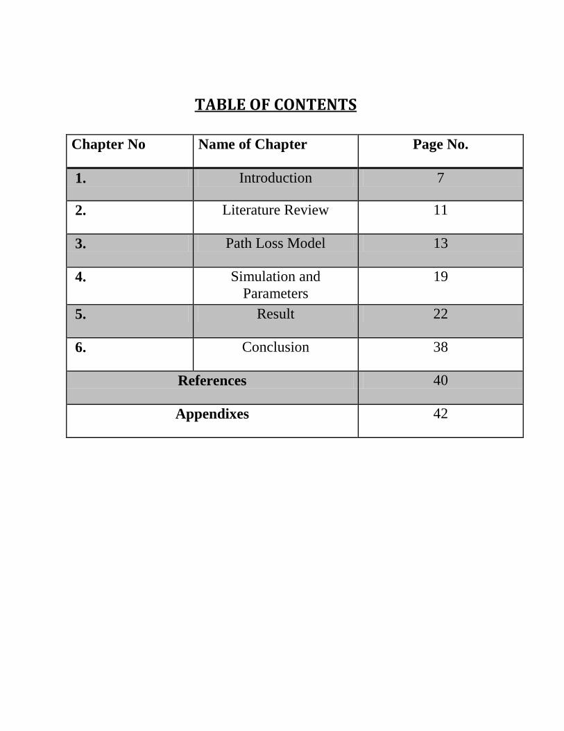
TABLE OF CONTENTS
Chapter No Name of Chapter Page No.
1. Introduction 7
2. Literature Review 11
3. Path Loss Model 13
4. Simulation and
Parameters
19
5. Result 22
6. Conclusion 38
References 40
Appendixes 42

7
CHAPTER 1
INTRODUCTION

8
Path loss is the decrease in power density or attenuation of an electromagnetic wave as it transmits
through space. Path loss is a major factor in the analysis and design of the link budget of a
telecommunication system. Path loss used in wireless communications a signal propagation. Path
loss may be due to many things, such as free-space loss, refraction, diffraction, reflection, aperture-
medium coupling loss, and absorption. Path loss is also influenced by environment contours,
environment (urban or rural, vegetation and foliage), propagation medium (dry or moist air), the
space between the transmitter and the receiver, and the height and position of antennas.
Path loss can be denoted by the path loss exponent, whose value is normally in the range of 2 to 4
(where 2 is for propagation in free space, 4 is for relatively loss environments and for the case of
full specular reflection from the earth surface called flat earth model). In some states, such as
buildings, stadiums and other indoor states, the path loss exponent can reach values in the range of
4 to 6. On the other hand, a channel may act as a waveguide, resulting in a path loss exponent less
than 2. Path loss is usually expressed in dB
In its simplest form, the path loss can be calculated by using this formula which is:
L=10nlog10 (d+C) --------- (1)
Where
L is the path loss in decibel, n is the path loss exponent, d is the distance between the transmitter
and the receiver, usually measured in meter. C is a constant which accounts for system losses.
OKUMURA MODEL:
Okumura's model is one of the most broadly used models for signal prediction in urban areas. This
model is valid for frequencies in the range 150–1920 MHz and distances of 1–100 km. It can be
used for base-station antenna heights ranging from 30–1000 m. The Okumura model is a Radio
propagation model that was built using the data collected in the city of Tokyo, Japan. The model is
ideal for using in cities with many urban buildings but not many tall blocking structures. The model
functioned as a base for the Hata Model.
Okumura model was founded into three modes.The one for urban, other for suburban and open
areas. The model for urban areas was built first and used as the base for others.
9
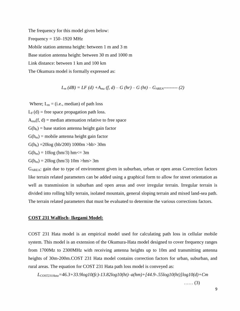
The frequency for this model given below:
Frequency = 150–1920 MHz
Mobile station antenna height: between 1 m and 3 m
Base station antenna height: between 30 m and 1000 m
Link distance: between 1 km and 100 km
The Okumura model is formally expressed as:
Lm (dB) = LF (d) +Amu (f, d) – G (hr) – G (ht) – GAREA--------- (2)
Where; Lm = (i.e., median) of path loss
LF (d) = free space propagation path loss.
Amu(f, d) = median attenuation relative to free space
G(hb) = base station antenna height gain factor
G(hm) = mobile antenna height gain factor
G(hb) =20log (hb/200) 1000m >hb> 30m
G(hm) = 10log (hm/3) hm<= 3m
G(hm) = 20log (hm/3) 10m >hm> 3m
GAREA: gain due to type of environment given in suburban, urban or open areas Correction factors
like terrain related parameters can be added using a graphical form to allow for street orientation as
well as transmission in suburban and open areas and over irregular terrain. Irregular terrain is
divided into rolling hilly terrain, isolated mountain, general sloping terrain and mixed land-sea path.
The terrain related parameters that must be evaluated to determine the various corrections factors.
COST 231 Walfisch- Ikegami Model:
COST 231 Hata model is an empirical model used for calculating path loss in cellular mobile
system. This model is an extension of the Okumura-Hata model designed to cover frequency ranges
from 1700Mz to 2300MHz with receiving antenna heights up to 10m and transmitting antenna
heights of 30m-200m.COST 231 Hata model contains correction factors for urban, suburban, and
rural areas. The equation for COST 231 Hata path loss model is conveyed as:
LCOST231Hata=46.3+33.9log10(fc)-13.82log10(ht)–a(hm)+[44.9-.55log10(ht)]log10(d)+Cm
…… (3)
10
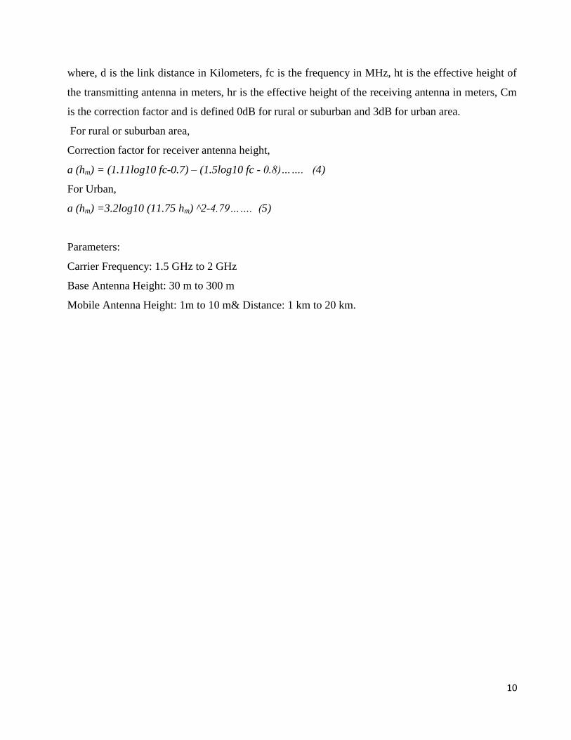
where, d is the link distance in Kilometers, fc is the frequency in MHz, ht is the effective height of
the transmitting antenna in meters, hr is the effective height of the receiving antenna in meters, Cm
is the correction factor and is defined 0dB for rural or suburban and 3dB for urban area.
For rural or suburban area,
Correction factor for receiver antenna height,
a (hm) = (1.11log10 fc-0.7) – (1.5log10 fc - 0.8)……. (4)
For Urban,
a (hm) =3.2log10 (11.75 hm) ^2-4.79……. (5)
Parameters:
Carrier Frequency: 1.5 GHz to 2 GHz
Base Antenna Height: 30 m to 300 m
Mobile Antenna Height: 1m to 10 m& Distance: 1 km to 20 km.

11
CHAPTER 2
Literature Review

12
In [1], the authors have compared three prominent channel models which would be used in LTE.
They have compared between Stanford University Interim (SUI) models, Okumura model, Hata
COST 231 model, COST Walfisch-Ikegami & Ericsson 9999 model.
In [2], the authors investigates different empirical propagation models for Long Term Evolution -
Advanced (LTE-A) in the 2GHz band.
In [3], the author analyzed about the empirically based path loss channel model differences. It
applies to distances and base antenna heights not well-covered by existing models. The
characterization used is a linear curve fitting the decibel path loss to the decibel-distance, with a
Gaussian random variation about that curve due to shadow fading. The resulting path loss model
applies to base antenna heights from 10 to 80 m, base-to-terminal distances from 0.1 to 8 km, and
three distinct terrain categories
In [4], the paper presents results of a measurement campaign carried out to examine applicability of
the Okumura-Hata model in our region in various VHF/UHF frequency bands. It provided good
approximation in the urban areas; the Okumura-Hata model gave significant errors in rural areas.
Therefore paper describes an advance which allows changes to the Okumura-Hata model through
statistical examination of the measurement results with application of the least squares method.
In [5], Radio propagation is essential for emerging technologies with appropriate design,
deployment and management strategies for any wireless network. It is heavily site specific and can
vary significantly depending on terrain, frequency of operation, velocity of mobile terminal,
interface sources and other dynamic factor in these two channel model.
Similarworks have been done in [5-12].

13
CHAPTER 3 PATH LOSS MODEL
14
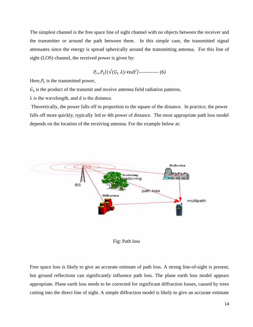
The simplest channel is the free space line of sight channel with no objects between the receiver and
the transmitter or around the path between them. In this simple case, the transmitted signal
attenuates since the energy is spread spherically around the transmitting antenna. For this line of
sight (LOS) channel, the received power is given by:
[ /4πd)2]------------ (6)
Here, is the transmitted power,
is the product of the transmit and receive antenna field radiation patterns,
λ is the wavelength, and d is the distance.
Theoretically, the power falls off in proportion to the square of the distance. In practice, the power
falls off more quickly, typically 3rd or 4th power of distance. The most appropriate path loss model
depends on the location of the receiving antenna. For the example below at:
Fig: Path loss
Free space loss is likely to give an accurate estimate of path loss. A strong line-of-sight is present,
but ground reflections can significantly influence path loss. The plane earth loss model appears
appropriate. Plane earth loss needs to be corrected for significant diffraction losses, caused by trees
cutting into the direct line of sight. A simple diffraction model is likely to give an accurate estimate

15
of path loss. Loss prediction fairly difficult and unreliable since multiple diffraction is present.
Path loss for different environment:
Okumura model:
The Okumura model for urban areas is a Radio propagation model that was built using the data
collected in the city of Tokyo, Japan. This model is applicable for frequencies in the range of 150
MHz to 1920 MHz and distances of 1 km to 100 km. It can be used for the base stations antenna
heights ranging from 30 m to 1000 m. To determine path loss using Okumara’s model, the free
space path loss between the points of interest is first determined and then the value of Amu(f, d) is
added to it along with correction factors according to the type of terrain. The model can be
expressed as:
L50(dB) = LF + Amu(f, d) – G (hte) – G (hre) - ------------- (7)
Where,
L50is the 50th percentile path loss in dB
LF is the free space propagation loss in dB
Amu(f, d) is median attenuation in dB
G (hte) is the base station antenna height gain factor.
G (hre) is the mobile antenna height gain factor.
is the gain due to the type of environment moving from urban to suburban or open area.
(
)
(
)
16
(
)
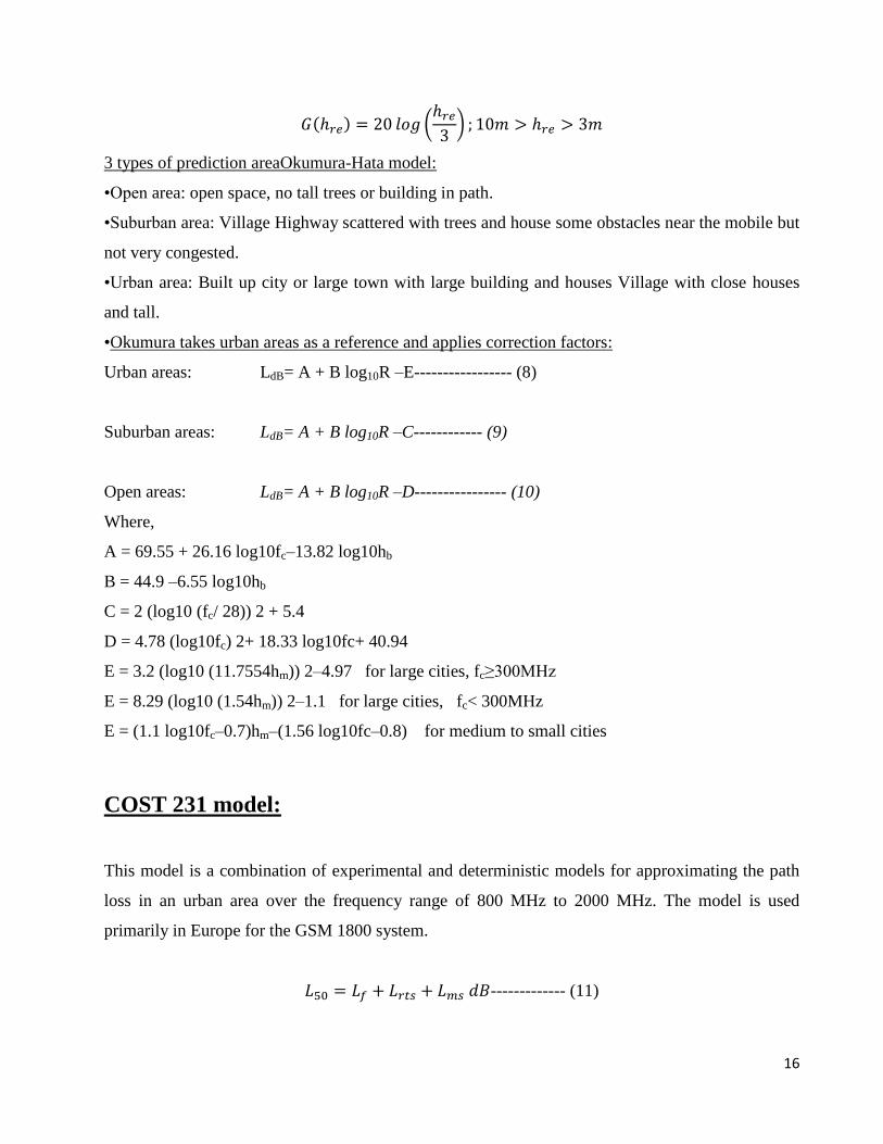
3 types of prediction areaOkumura-Hata model:
•Open area: open space, no tall trees or building in path.
•Suburban area: Village Highway scattered with trees and house some obstacles near the mobile but
not very congested.
•Urban area: Built up city or large town with large building and houses Village with close houses
and tall.
•Okumura takes urban areas as a reference and applies correction factors:
Urban areas: LdB= A + B log10R –E----------------- (8)
Suburban areas: LdB= A + B log10R –C------------ (9)
Open areas: LdB= A + B log10R –D---------------- (10)
Where,
A = 69.55 + 26.16 log10fc–13.82 log10hb
B = 44.9 –6.55 log10hb
C = 2 (log10 (fc/ 28)) 2 + 5.4
D = 4.78 (log10fc) 2+ 18.33 log10fc+ 40.94
E = 3.2 (log10 (11.7554hm)) 2–4.97 for large cities, fc≥300MHz
E = 8.29 (log10 (1.54hm)) 2–1.1 for large cities, fc< 300MHz
E = (1.1 log10fc–0.7)hm–(1.56 log10fc–0.8) for medium to small cities
COST 231 model:
This model is a combination of experimental and deterministic models for approximating the path
loss in an urban area over the frequency range of 800 MHz to 2000 MHz. The model is used
primarily in Europe for the GSM 1800 system.
------------- (11)
17
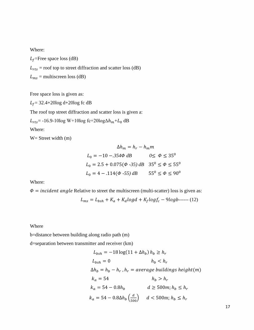
Where:
=Free space loss (dB)
= roof top to street diffraction and scatter loss (dB)
= multiscreen loss (dB)
Free space loss is given as:
= 32.4+20log d+20log fc dB
The roof top street diffraction and scatter loss is given a:
= -16.9-10log W+10log fc+20logΔ + dB
Where:
W= Street width (m)
.354 dB 0
-35) dB
-55) dB
Where:
Relative to street the multiscreen (multi-scatter) loss is given as:
------ (12)
Where
b=distance between building along radio path (m)
d=separation between transmitter and receiver (km)
(
) m;

18
Both increase path loss with lower base station antenna height.
(
)for mid size city and suburbun area with moderate tree density
for metropolitan area
The range of parameters for which the COST 231 model is valid is:
The following default values may be used in the model:
b=20-50m
W=b/2
Roof=3m for pitched roof and 0m for flat roof,
And (number of floor) + roof
This model is restricted to the following range of parameters:
Carrier Frequency 1.5 GHz to 2 GHz
Base Antenna Height 30 m to 300 m
Mobile Antenna Height 1m to 10 m
Distance d 1 km to 20 km
COST 321-Hata model is designed for large and small macro-cells, i.e., base station antenna heights
above rooftop levels adjacent to base station.

19
CHAPTER 4
SIMULATIONS AND PARAMETERS

20
All of our results have been found after done the simulations in MATLAB R2016a software.
MATLAB is a high-performance language for technical calculating. It integrates calculation,
visualization, and programming in an easy-to-use situation where problems and solutions are
expressed in familiar mathematical notation. Typical uses include:
Math and computation
Algorithm development
Modeling, simulation, and prototyping
Data analysis, exploration, and visualization
Scientific and engineering graphics
Application development, including Graphical User Interface building
MATLAB is an communicating system whose basic data component is an array that does not
require dimensioning. This permits you to solve many technical calculating problems, particularly
those with matrix and vector designs, in a fraction of the time it would take to write a program in a
scalar no communicating language such as C or FORTRAN.
21
MATLAB use for attitudes matrix laboratory. MATLAB was initially written to provide easy
access to matrix software industrialized by the LINPACK and EISPACK projects, which composed
characterize the state-of-the-art in software for matrix computation.MATLAB has evolved over a
period of years with input from many users. In university environments, it is the standard
instructional tool for introductory and advanced courses in mathematics, engineering, and science.
In industry, MATLAB is the tool of choice for high-productivity exploration, development, and
analysis.MATLAB features a family of application-specific keys called toolboxes. Very important
to most users of MATLAB, toolboxes allow you to study and apply specialized technology.
Toolboxes are comprehensive collections of MATLAB functions (M-files) that extend the
MATLAB environment to solve specific classes of problems. Areas in which toolboxes are
accessible include signal processing, control systems, neural networks, fuzzy logic, wavelets,
simulation, and many others.
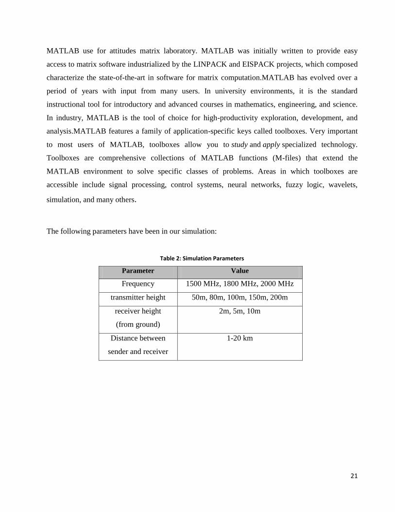
The following parameters have been in our simulation:
Table 2: Simulation Parameters
Parameter Value
Frequency 1500 MHz, 1800 MHz, 2000 MHz
transmitter height 50m, 80m, 100m, 150m, 200m
receiver height
(from ground)
2m, 5m, 10m
Distance between
sender and receiver
1-20 km

22
CHAPTER 5
RESULTS

23
This section deals with the result obtained after the simulations.
In Fig. 1, the Path-loss vs. distance for 1500 MHz has been displayed. Here, the transmitter
height has been considered as 50 meter while received height is 2 meter. In this figure, the Hata
model shows the lower path loss than the Cost231 model. Hata model for both medium sized
city and metropolitan city give the identical results but in case of Cost model the performance
can be differentiated. If we consider the value of distance, d= 10 km then the path loss by Hata
model is around 163 dB (for both medium sized city and metropolitan city) while by Cost
model is around 204 dB medium sized city and 210 dB for metropolitan city.
Fig. 1 Path-loss vs distance for 1500 MHz, transmitter height=50m and receiver height=2m
24
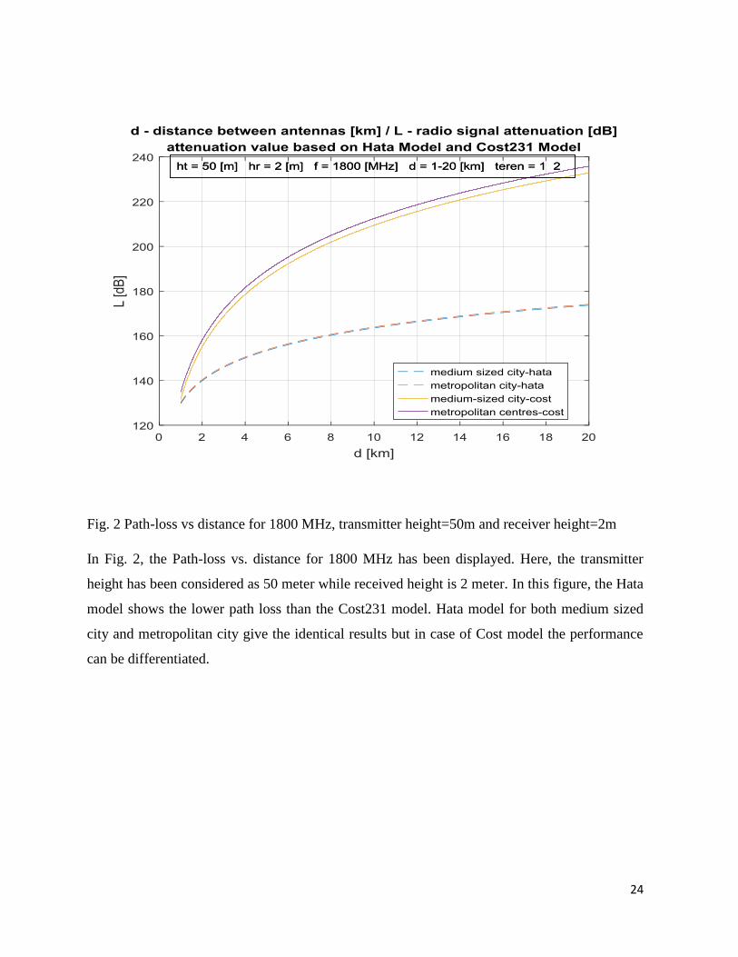
Fig. 2 Path-loss vs distance for 1800 MHz, transmitter height=50m and receiver height=2m
In Fig. 2, the Path-loss vs. distance for 1800 MHz has been displayed. Here, the transmitter
height has been considered as 50 meter while received height is 2 meter. In this figure, the Hata
model shows the lower path loss than the Cost231 model. Hata model for both medium sized
city and metropolitan city give the identical results but in case of Cost model the performance
can be differentiated.

25
Fig. 3 Path-loss vsdistance for 2000 MHz, transmitter height=50m and receiver height=2m
Similar results have been found in In Fig. 3 though frequency used here is 2000 MHz. So,
changing the frequency would not affect the path loss by both the models. In this fig, the Path-
loss vs. distance for 2000MHz has been displayed. Here, the transmitter height has been
considered as 50 meter while received height is 2 meter.
In Fig. 3, the Path-loss vs distance for 2000 MHz has been displayed. Almost similar results to
Fig.2 have been found in Fig. 3. Here Hata model also shows the better results..

26
Fig. 4 Path-loss vsdistance for 1500 MHz, transmitter height=80m and receiver height=2m
In Fig. 4, the Path-loss vs. distance for 1500 MHz has been displayed. Here, the transmitter
height has been considered as 80 meter while received height is 2 meter. In this figure, the Hata
model shows the lower path loss than the Cost231 model. Hata model for both medium sized
city and metropolitan city give the identical results but in case of Cost model the act can be
differentiated.

27
Fig. 5 Path-loss vsdistance for 1500 MHz, transmitter height=100m and receiver height=2m
In Fig. 5, the Path-loss vs. distance for 1500 MHz has been displayed. Here, the transmitter
height has been considered as 100 meter while received height is 2 meter. In this figure, the
Hata model shows the lower path loss than the Cost231 model. Hata model for both medium
sized city and metropolitan city give the identical results but in case of Cost model the act can
be differentiated.
28
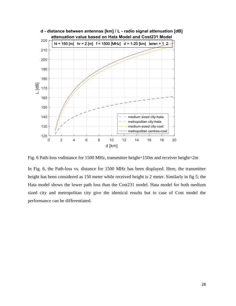
Fig. 6 Path-loss vsdistance for 1500 MHz, transmitter height=150m and receiver height=2m
In Fig. 6, the Path-loss vs. distance for 1500 MHz has been displayed. Here, the transmitter
height has been considered as 150 meter while received height is 2 meter. Similarly in fig 5; the
Hata model shows the lower path loss than the Cost231 model. Hata model for both medium
sized city and metropolitan city give the identical results but in case of Cost model the
performance can be differentiated.

29
Fig. 7 Path-loss vsdistance for 1500 MHz, transmitter height=80m and receiver height=2m
Now, we have changed the parameter for the simulation. Here we have considered the
transmitter height as 80 meter. Hata model for both medium sized city and metropolitan city
give the identical results but in case of Cost model the performances almost the same for both
the cases. From this Fig.5 we can conclude that increasing the transmitter height from 50 meter
to 80 meter will lead the path loss in decreasing.

30
Fig.8 Path-loss vs distance for 1500 MHz, transmitter height=200m and receiver height=5m
In Fig. 8, the Path-loss vsdistance for 1500 MHz has been displayed. Here, the transmitter
height has been considered as 200 meter while received height is 5meter. In this figure, the
Hata model shows the lower path loss than the Cost231 model. Hata model for both medium
sized city and metropolitan city give the identical results but in case of Cost model the act can
be differentiated. If we consider the value of distance, d= 10 km then the path loss by Hata
model is around 153 dB (for both medium sized city and metropolitan city) while by Cost
model is around 204 dB medium sized city and 210 dB for metropolitan city.

31
Fig. 9 Path-loss vs distancefor 1500 MHz, transmitter height=100m and receiver height=2m
From Fig.9, it is observable that the increasing in transmitter height from 80 meter to 100 meter
will not lead the significant decrease in path loss compare to the previous case. But if we
increase the transmitter height as 150 meter than the path loss found significantly lower than
the case of 100 meter or 80 meter cases (Fig. 8). But still Hata model performs the better. Same
observation can be found in Fig. 10.

32
Fig. 10 Path-loss vsdistance for 1500 MHz, transmitter height=150m and receiver height=2m
In this figure, the Hata model shows the lower path loss than the Cost231 model. Hata model
for both medium sized city and metropolitan city give the identical results but in case of Cost
model the performance can be differentiated.
33
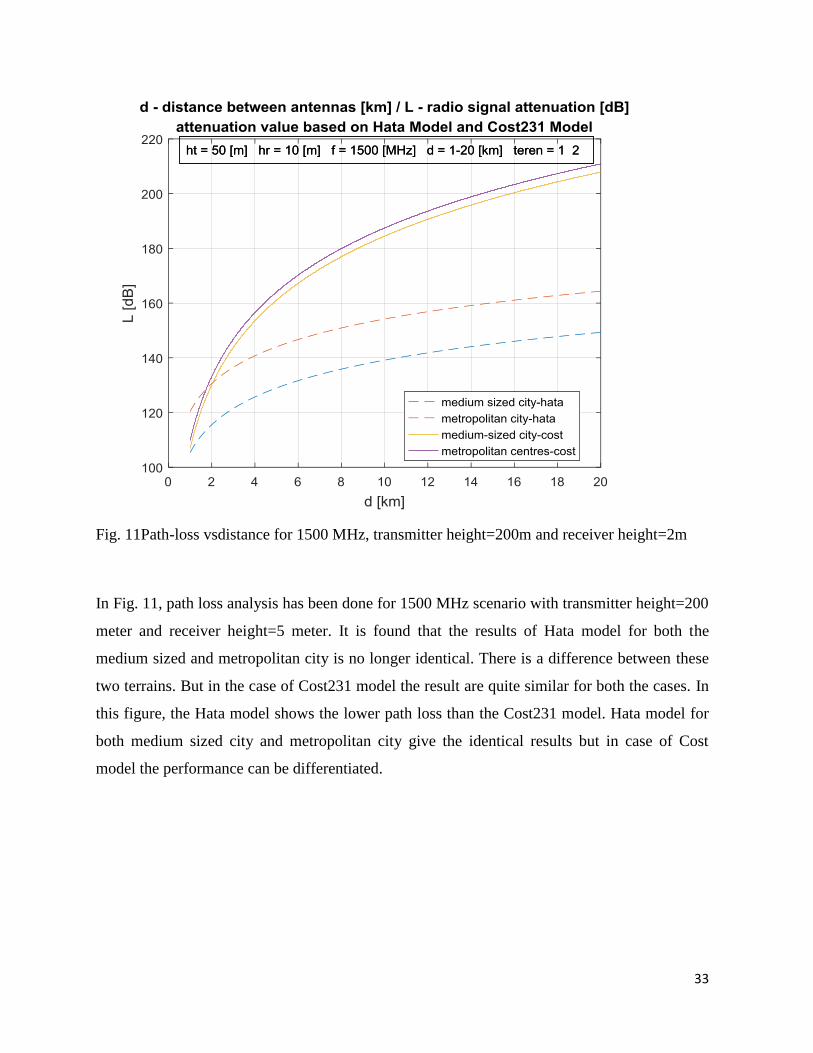
Fig. 11Path-loss vsdistance for 1500 MHz, transmitter height=200m and receiver height=2m
In Fig. 11, path loss analysis has been done for 1500 MHz scenario with transmitter height=200
meter and receiver height=5 meter. It is found that the results of Hata model for both the
medium sized and metropolitan city is no longer identical. There is a difference between these
two terrains. But in the case of Cost231 model the result are quite similar for both the cases. In
this figure, the Hata model shows the lower path loss than the Cost231 model. Hata model for
both medium sized city and metropolitan city give the identical results but in case of Cost
model the performance can be differentiated.

34
Fig. 12 Path-loss vs distance for 1500 MHz, transmitter height=200m and receiver height=5m
In Fig. 12, path loss analysis has been done for 1500 MHz scenario with transmitter height=200
meter and receiver height=5 meter. It is found that the results of Hata model for both the
medium sized and metropolitan city is no longer identical. There is a difference between these
two terrains. But in the case of Cost231 model the result are quite similar for both the cases.

35
Fig. 13 Path-loss vsdistance for 1500 MHz, transmitter height=200m and receiver height=10m
Now if we increase the height of the receiver antenna the path loss difference between the
medium sized and metropolitan city of Hata models are also increased but the overall path loss
is decreasing. The phenomena have been found in Fig. 14.
36
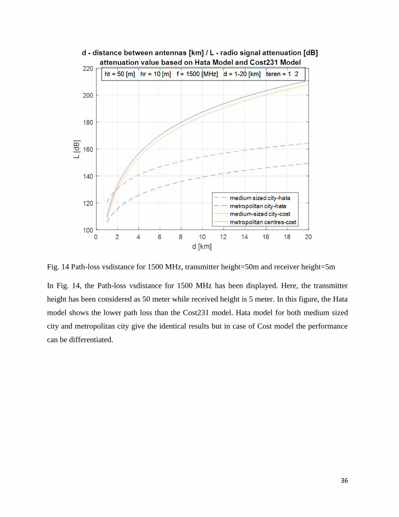
Fig. 14 Path-loss vsdistance for 1500 MHz, transmitter height=50m and receiver height=5m
In Fig. 14, the Path-loss vsdistance for 1500 MHz has been displayed. Here, the transmitter
height has been considered as 50 meter while received height is 5 meter. In this figure, the Hata
model shows the lower path loss than the Cost231 model. Hata model for both medium sized
city and metropolitan city give the identical results but in case of Cost model the performance
can be differentiated.
37
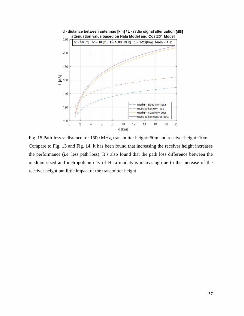
Fig. 15 Path-loss vsdistance for 1500 MHz, transmitter height=50m and receiver height=10m
Compare to Fig. 13 and Fig. 14, it has been found that increasing the receiver height increases
the performance (i.e. less path loss). It’s also found that the path loss difference between the
medium sized and metropolitan city of Hata models is increasing due to the increase of the
receiver height but little impact of the transmitter height.

38
CHAPTER 6
CONCLUSION

39
In this paper, the path loss performances of Hata model and Cost231 model have been analyzed
for different scenarios. In all the cases, Hata model’s performances are found better than the
Cost 231 model. It’s also found that increasing the frequency is not changing the path loss
value remarkably. But, if we increase the transmitter height than the path loss is decreasing in
all the cases. Again, if we increase the receiver height the performance of both the model is also
increased. The performances of Hata model for medium sized city and metropolitan city almost
identical for any frequency change and transmitter height change, but it creates difference when
the receiver height is changed. Similar change for Cost231 case has been found when we
change the frequency, but it’s not impacted when change the transmitter or receiver height. In a
conclusion, for the better performance, Hata model should be used with proper transmitter and
receiver height consideration.
40
References [1] Shabbir, Noman, Muhammad T. Sadiq, HasnainKashif, and RizwanUllah. "Comparison of
radio propagation models for long term evolution (Lte) network." arXiv preprint arXiv:
1110.1519 (2011).
[2] Ahmad, Yassir A., Walid A. Hassan, and Tharek Abdul Rahman. "Studying different
propagation models for LTE-A system." In Computer and Communication Engineering
(ICCCE), 2012 International Conference on, pp. 848-853. IEEE, 2012.
[3] Erceg, Vinko, Larry J. Greenstein, Sony Y. Tjandra, Seth R. Parkoff, Ajay Gupta, Boris
Kulic, Arthur A. Julius, and Renee Bianchi. "An empirically based path loss model for wireless
channels in suburban environments." IEEE Journal on selected areas in communications 17,
no.7 (1999):1205-1211.
4] Roslee, Mardeni Bin, and KokFoong Kwan. "Optimization of Hata propagation prediction
model in suburban area in Malaysia." Progress In Electromagnetics Research C 13 (2010): 91-
106.
[5] Singh, Yuvraj. "Comparison of okumura, hata and cost-231 models on the basis of path loss
and signal strength."International journal of computer applications 59, no. 11 (2012).
[6] [Okumura1968] T. Okumura, E. Ohmore, and K. Fukuda, "Field strength and its variability
in VHF and UHF land mobile service," Rev. Elec. Communes. Lab., pp. 825-73, September-
October 1968.
[7] [Hata1980] M. Hata, "Empirical formula for propagation kiss ubkabdnibukeradui services,"
IEEE Trans. Veh. Tech., pp. 317-25, August 1980. [COST231] European Cooperative in the
Field of Science and Technical Research EURO-COST 231, "Urban transmission loss models
for mobile radio in the 900- and 1,800 MHz bands
[8] [Erceg1999] V. Erceget. al, An empirically based path loss model for wireless channels in
suburban environments, IEEE JSAC, vol. 17, no. 7, July 1999, pp. 1205-1211.
[9] Dinesh Sharma, R.K.Singh, “The Effect of Path Loss on QoS at NPL” International Journal
of Engineering Science and Technology Vol. 2(7), 2010, 3018-3023.
[10]Jean-Paul M. G. Linmartz's, Wireless Communication, The Interactive Multimedia CD-
ROM, Baltzer Science Publishers, P.O.Box 37208, 1030 AE Amsterdam, ISSN 1383 4231,
Vol. 1 (1996), No.1
41
[11] Theodore.S.R., 2006, “Wireless Communications Principles and Practice”, Prentice-Hall,
India.
[12] Walfisch, J., and Bertoni, H. L. “A Theoretical Model of UHF Propagation in Urban
Environment.” IEEE Transactions, Antennas & Propagation, AP-36:1788– 1796,
October 1988.

42
Appendixes
Matlab codes
%___________________________________________________________________
% for the cost231
function [hL50dB] = cost231hata(hBSef, hMS, f, d, area)
%COST231Hata - function returns signal attenuation value based on
% COST231-Hata Model
%
% hL50dB = cost231hata(hBSef, hMS, f, d, area)
%
% hL50dB - radio signal attenuation [dB]
%
% hBSef - effective base station antenna height [m]
% 30 <= hBS,ef<= 200 m
% hMS - mobile station antenna height [m]
% 1 <= hMS<= 10 m
% f - frequency [MHz]
% 1500 <= f <= 2000 MHz
% d - distance between antennas [km]
% 1 <= d <= 20 km
% area - area type: {1, 2}
% 1 - medium-sized city 2 - metropolitan centres
n = 0;
for i = (area)
n = n + 1;
if((min(f)>=1500)&&(max(f)<=2000))
if((min(hBSef)>=30)&&(max(hBSef)<=200))
if((min(hMS)>=1)&&(max(hMS)<=10))
if((i==1)||(i==2))
if((min(d)>=1)&&(max(d)<=20))
ahMS = (1.1 * log10(f) - 0.7) * hMS - (1.56 * log10(f) - 0.8);
if(i==1)
43
C = 0;
end
if(i==2)
C = 3;
end
L50dB = 46.3 + 33.9 * log10(f) - 13.82 * log10(hBSef) - ahMS + (44.9 - 6.55 *
log10(hBSef)) * log(d) + C;
hL50dB(n,:) = L50dB;
else
disp('ERROR: required distance between antennas = 1 <= d <= 20 km');
end
else
disp('ERROR: required area type = 1 lub 2');
end
else
disp('ERROR: required mobile station antenna height = 1 <= hMS<= 10 m');
end
else
disp('ERROR: required effective base station antenna height = 30 <= hBS,ef<= 200 m');
end
else
disp('ERROR: required frequency = 1500 <= f <= 2000 MHz');
end
end
end
%___________________________________________________________________
%___________________________________________________________________
function [hL50dB] = hata(hBSef, hMS, f, d, area)
%Hata - function returns signal attenuation value based on Hata Model
%
% hL50dB = hata(hBSef, hMS, f, d, area)
%
% hL50dB - radio signal attenuation [dB]
44
%
% hBSef - effective base station antenna height [m]
% 30 <= hBS,ef<= 200 m
% hMS - mobile station antenna height [m]
% 1 <= hMS<= 10 m
% f - frequency [MHz]
% 150 <= f <= 1800 MHz
% d - distance between antennas [km]
% 1 <= d <= 20 km
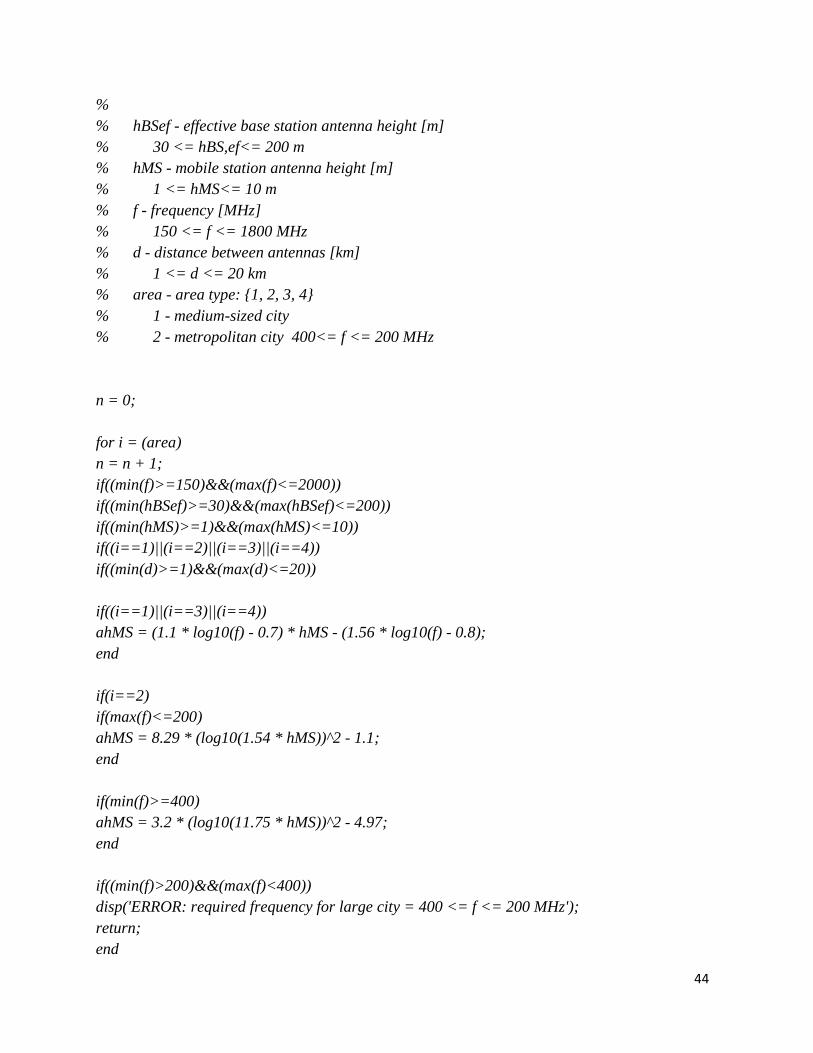
% area - area type: {1, 2, 3, 4}
% 1 - medium-sized city
% 2 - metropolitan city 400<= f <= 200 MHz
n = 0;
for i = (area)
n = n + 1;
if((min(f)>=150)&&(max(f)<=2000))
if((min(hBSef)>=30)&&(max(hBSef)<=200))
if((min(hMS)>=1)&&(max(hMS)<=10))
if((i==1)||(i==2)||(i==3)||(i==4))
if((min(d)>=1)&&(max(d)<=20))
if((i==1)||(i==3)||(i==4))
ahMS = (1.1 * log10(f) - 0.7) * hMS - (1.56 * log10(f) - 0.8);
end
if(i==2)
if(max(f)<=200)
ahMS = 8.29 * (log10(1.54 * hMS))^2 - 1.1;
end
if(min(f)>=400)
ahMS = 3.2 * (log10(11.75 * hMS))^2 - 4.97;
end
if((min(f)>200)&&(max(f)<400))
disp('ERROR: required frequency for large city = 400 <= f <= 200 MHz');
return;
end
45
end
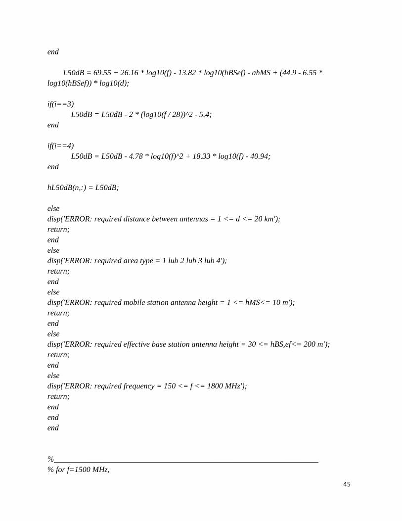
L50dB = 69.55 + 26.16 * log10(f) - 13.82 * log10(hBSef) - ahMS + (44.9 - 6.55 *
log10(hBSef)) * log10(d);
if(i==3)
L50dB = L50dB - 2 * (log10(f / 28))^2 - 5.4;
end
if(i==4)
L50dB = L50dB - 4.78 * log10(f)^2 + 18.33 * log10(f) - 40.94;
end
hL50dB(n,:) = L50dB;
else
disp('ERROR: required distance between antennas = 1 <= d <= 20 km');
return;
end
else
disp('ERROR: required area type = 1 lub 2 lub 3 lub 4');
return;
end
else
disp('ERROR: required mobile station antenna height = 1 <= hMS<= 10 m');
return;
end
else
disp('ERROR: required effective base station antenna height = 30 <= hBS,ef<= 200 m');
return;
end
else
disp('ERROR: required frequency = 150 <= f <= 1800 MHz');
return;
end
end
end
%___________________________________________________________________
% for f=1500 MHz,

46
clear all;
% hBSef - effective base station antenna height [m]
% 30 <= hBS,ef<= 200 m
ht = 50; %[m]
% hMS - mobile station antenna height [m]
% 1 <= hMS<= 10 m
hr = 2; %[m]
% f - frequency [MHz]
% 1500 <= f <= 2000 MHz
f = 1500; %[MHz]
% d - distance between antennas [km]
% 1 <= d <= 20 km
from = 1; %[km]
to = 20; %[km]
precision = 0.01; %[km]
d = from:precision:to; %[km]
area = [1,2];
% hL50dB = hata(hBSef, hMS, f, d, area)
L = hata(ht, hr, f, d, area);
% hL50dB = cost231hata(hBSef, hMS, f, d, area)
L1 = cost231hata(ht, hr, f, d, area);
clf reset;
plot(d, L,'--');
desc = ['ht = ',num2str(ht),' [m] hr = ',num2str(hr),' [m] f = ',...
num2str(f),' [MHz] d = ',num2str(from),'-',num2str(to),' [km] teren = ', num2str(area)];
annotation('textbox',[0.15 0.7 0.2 0.2],'String',{desc},'FitBoxToText','on');
hold on

47
plot(d, L1,'-');
desc = ['ht = ',num2str(ht),' [m] hr = ',num2str(hr),' [m] f = ',...
num2str(f),' [MHz] d = ',num2str(from),'-',num2str(to),' [km] teren = ', num2str(area)];
annotation('textbox',[0.15 0.7 0.2 0.2],'String',{desc},'FitBoxToText','on');
grid on;
axis auto;
title({'d - distance between antennas [km] / L - radio signal attenuation [dB]';...
'attenuation value based on Hata Model and Cost231 Model'});
xlabel('d [km]');
ylabel('L [dB]');
legend('medium sized city-hata','metropolitan city-hata','medium-sized city-
cost','metropolitancentres-cost','location','Best');
%___________________________________________________________________