Common Shareholding in Europe - JRC Publications Repository

Common Shareholding in Europe

Rosati, N.

Bomprezzi, P.

Ferraresi, M.

Frigo, A.

Nardo, M.

2020

EUR 30312 EN

This publication is a Technical report by the Joint Research Centre (JRC), the European Commission’s science and knowledge service. It aims to provide evidence-based scientific support to the European policymaking process. The scientific output expressed does not imply a policy position of the European Commission. Neither the European Commission nor any person acting on behalf of the Commission is responsible for the use that might be made of this publication. For information on the methodology and quality underlying the data used in this publication for which the source is neither Eurostat nor other Commission services, users should contact the referenced source. Thedesignations employed and the presentation of material on the maps do not imply the expression of any opinion whatsoever on the part of the European Union concerning the legal status of any country, territory, city or area or of its authorities, or concerning the delimitationof its frontiers or boundaries.

EU Science Hubhttps://ec.europa.eu/jrc

JRC121476

EUR 30312 EN

PDF ISBN 978-92-76-20876-1 ISSN 1831-9424 doi:10.2760/734264

Luxembourg: Publications Office of the European Union, 2020

© European Union, 2020

The reuse policy of the European Commission is implemented by the Commission Decision 2011/833/EU of 12 December 2011 on the reuse of Commission documents (OJ L 330, 14.12.2011, p. 39). Except otherwise noted, the reuse of this document is authorised under the Creative Commons Attribution 4.0 International (CC BY 4.0) licence (https://creativecommons.org/licenses/by/4.0/). This means that reuse is allowed provided appropriate credit is given and any changes are indicated. For any use or reproduction of photos or other material that is not owned by the EU, permission must be sought directly from the copyright holders.

All content © European Union, 2020, except: except: Figure 3.1, page 53, reproduction of Fig. 1 on p. 2675 of He, J., and Huang, J. (2017) "Product Market Competition in a World of Cross-Ownership: Evidence from Institutional Blockholdings". The Review of Financial Studies, vol. 30, no. 8, pp. 2674-2718.; permission granted by Oxford University Press on Jul 22, 2020 by License Number 4874220513731.

How to cite this report: Rosati, N., Bomprezzi, P., Ferraresi, M., Frigo, A., Nardo, M., Common Shareholding in Europe, EUR 30312 EN, Publications Office of the European Union, Luxembourg, 2020, ISBN 978-92-76-20876-1, doi:10.2760/734264, JRC121476

JRC TECHNICAL REPORT

Common Shareholding in Europe

Rosati, N.

Bomprezzi, P.

Ferraresi, M.

Frigo, A.

Nardo, M.

2020

Contents

Acknowledgments 1

Abstract 2

Executive Summary 4

1 Introduction 15

2 Measuring Common shareholding 25

2.1 Existing measures of common shareholding . . . . . . . . . . . . . . . . . . . . . . . . . 26

2.2 Towards new common shareholding indices . . . . . . . . . . . . . . . . . . . . . . . . . . 30

2.2.1 General framework . . . . . . . . . . . . . . . . . . . . . . . . . . . . . . . . . . . . . 30

2.2.2 A simple example . . . . . . . . . . . . . . . . . . . . . . . . . . . . . . . . . . . . . . 31

2.2.3 Measurement issues . . . . . . . . . . . . . . . . . . . . . . . . . . . . . . . . . . . . . 33

2.2.4 Assessing the extent of common shareholding . . . . . . . . . . . . . . . . . . . . 35

2.3 Data availability . . . . . . . . . . . . . . . . . . . . . . . . . . . . . . . . . . . . . . . . . . . . 36

2.3.1 The Orbis database . . . . . . . . . . . . . . . . . . . . . . . . . . . . . . . . . . . . . 38

2.3.2 The ad hoc dataset . . . . . . . . . . . . . . . . . . . . . . . . . . . . . . . . . . . . . 40

2.4 Some new common shareholding indices . . . . . . . . . . . . . . . . . . . . . . . . . . . 41

2.4.1 Shareholder indices . . . . . . . . . . . . . . . . . . . . . . . . . . . . . . . . . . . . . 42

2.4.2 Market indices . . . . . . . . . . . . . . . . . . . . . . . . . . . . . . . . . . . . . . . . . 45

2.4.3 Indices based on block-holdings . . . . . . . . . . . . . . . . . . . . . . . . . . . . . 46

3 Common Shareholding in the EU 51

3.1 Results for listed firms active in the EU in 2007-2016 . . . . . . . . . . . . . . . . . . . 51

i

3.2 Top-ranking investors . . . . . . . . . . . . . . . . . . . . . . . . . . . . . . . . . . . . . . . . 57

3.3 Major Portfolios . . . . . . . . . . . . . . . . . . . . . . . . . . . . . . . . . . . . . . . . . . . . 59

4 Common Shareholding in Selected Industries 65

4.1 Energy sector - Oil&Gas . . . . . . . . . . . . . . . . . . . . . . . . . . . . . . . . . . . . . . 66

4.2 Energy sector - Electricity . . . . . . . . . . . . . . . . . . . . . . . . . . . . . . . . . . . . . 77

4.3 Trading Platforms for Financial Instruments sector - Trading Platforms operators . . 86

4.4 Telecommunication sector - Mobile Network Operators and their parents . . . . . . . 96

4.5 Beverages sector - Manufacturers . . . . . . . . . . . . . . . . . . . . . . . . . . . . . . . . 107

5 Block-holdings in Investors’ Portfolios in the EU 127

5.1 Outline of holdings in the five sectors . . . . . . . . . . . . . . . . . . . . . . . . . . . . . 128

5.2 Effects of thresholds on firms-investors relations . . . . . . . . . . . . . . . . . . . . . . 131

5.2.1 Firms cross-held by block-holders . . . . . . . . . . . . . . . . . . . . . . . . . . . . 132

5.2.2 Densities of block-holdings . . . . . . . . . . . . . . . . . . . . . . . . . . . . . . . . 134

5.3 Thresholds in networks relations . . . . . . . . . . . . . . . . . . . . . . . . . . . . . . . . . 135

5.3.1 Network indices for firms . . . . . . . . . . . . . . . . . . . . . . . . . . . . . . . . . . 137

5.3.2 Network indices for investors . . . . . . . . . . . . . . . . . . . . . . . . . . . . . . . 140

5.4 The ’Big Three’ . . . . . . . . . . . . . . . . . . . . . . . . . . . . . . . . . . . . . . . . . . . . 143

6 Linking Common Shareholding and Competition 149

6.1 Modelling the link . . . . . . . . . . . . . . . . . . . . . . . . . . . . . . . . . . . . . . . . . . . 150

6.2 Measurement and data issues . . . . . . . . . . . . . . . . . . . . . . . . . . . . . . . . . . . 151

6.2.1 Market identification . . . . . . . . . . . . . . . . . . . . . . . . . . . . . . . . . . . . . 151

6.2.2 Measures of common shareholding . . . . . . . . . . . . . . . . . . . . . . . . . . . 152

6.2.3 Measures of competition . . . . . . . . . . . . . . . . . . . . . . . . . . . . . . . . . . 154

6.3 Markup . . . . . . . . . . . . . . . . . . . . . . . . . . . . . . . . . . . . . . . . . . . . . . . . . . 155

6.3.1 Calculation of markup . . . . . . . . . . . . . . . . . . . . . . . . . . . . . . . . . . . . 157

6.3.2 Lerner index . . . . . . . . . . . . . . . . . . . . . . . . . . . . . . . . . . . . . . . . . . 158

6.4 Econometric approach . . . . . . . . . . . . . . . . . . . . . . . . . . . . . . . . . . . . . . . . 159

6.5 Candidate sectors for the econometric analysis . . . . . . . . . . . . . . . . . . . . . . . 161

6.5.1 The ’Big Three’ and the BlackRock-BGI merger . . . . . . . . . . . . . . . . . . . . 162

ii

6.5.2 Ownership changes between primary and secondary investors . . . . . . . . . 165

6.5.3 Towards an application . . . . . . . . . . . . . . . . . . . . . . . . . . . . . . . . . . . 166

7 Effects of the BlackRock-BGI Merger on Beverages Manufacturers 167

7.1 The Beverages manufacturing industry . . . . . . . . . . . . . . . . . . . . . . . . . . . . . 168

7.1.1 Data description . . . . . . . . . . . . . . . . . . . . . . . . . . . . . . . . . . . . . . . 171

7.2 The main causal model . . . . . . . . . . . . . . . . . . . . . . . . . . . . . . . . . . . . . . . 172

7.3 Model variables . . . . . . . . . . . . . . . . . . . . . . . . . . . . . . . . . . . . . . . . . . . . 173

7.3.1 Competitive outcomes . . . . . . . . . . . . . . . . . . . . . . . . . . . . . . . . . . . 174

7.3.2 Treatment variables . . . . . . . . . . . . . . . . . . . . . . . . . . . . . . . . . . . . . 174

7.3.3 Firm-level controls . . . . . . . . . . . . . . . . . . . . . . . . . . . . . . . . . . . . . . 175

7.4 Sample description . . . . . . . . . . . . . . . . . . . . . . . . . . . . . . . . . . . . . . . . . . 176

7.5 Empirical results . . . . . . . . . . . . . . . . . . . . . . . . . . . . . . . . . . . . . . . . . . . 180

7.5.1 Preliminary evidence . . . . . . . . . . . . . . . . . . . . . . . . . . . . . . . . . . . . 180

7.5.2 Results from Difference-in-Differences model . . . . . . . . . . . . . . . . . . . . 182

7.5.3 Who drives the effect? . . . . . . . . . . . . . . . . . . . . . . . . . . . . . . . . . . . 186

7.6 Robustness checks . . . . . . . . . . . . . . . . . . . . . . . . . . . . . . . . . . . . . . . . . 187

7.6.1 Event study analysis . . . . . . . . . . . . . . . . . . . . . . . . . . . . . . . . . . . . . 187

7.6.2 Alternative sample selection . . . . . . . . . . . . . . . . . . . . . . . . . . . . . . . 190

7.6.3 Different definitions of the treatment and control groups . . . . . . . . . . . . . 192

7.6.4 Falsification and other tests . . . . . . . . . . . . . . . . . . . . . . . . . . . . . . . . 193

7.7 Hetereogeneous effects . . . . . . . . . . . . . . . . . . . . . . . . . . . . . . . . . . . . . . . 196

7.7.1 Long-term effects . . . . . . . . . . . . . . . . . . . . . . . . . . . . . . . . . . . . . . 196

7.7.2 Intensity of the exposure . . . . . . . . . . . . . . . . . . . . . . . . . . . . . . . . . . 200

7.8 Final remarks . . . . . . . . . . . . . . . . . . . . . . . . . . . . . . . . . . . . . . . . . . . . . . 204

8 Conclusions 211

References 217

List of Abbreviations and Definitions 228

List of Boxes 229

iii

List of Figures 231

List of Tables 235

Annexes 237

A The Database of EU Ownership 239

A.1 Structure of the Orbis database . . . . . . . . . . . . . . . . . . . . . . . . . . . . . . . . . . 240

A.2 Extraction of companies . . . . . . . . . . . . . . . . . . . . . . . . . . . . . . . . . . . . . . 241

A.2.1 Identification of listed companies active in the EU . . . . . . . . . . . . . . . . . 242

A.2.2 Identification of sectors of economic activity . . . . . . . . . . . . . . . . . . . . . 243

A.3 Selection of relevant company information . . . . . . . . . . . . . . . . . . . . . . . . . . 247

A.3.1 General company information . . . . . . . . . . . . . . . . . . . . . . . . . . . . . . 247

A.3.2 Ownership information . . . . . . . . . . . . . . . . . . . . . . . . . . . . . . . . . . . 250

A.3.3 Financial information . . . . . . . . . . . . . . . . . . . . . . . . . . . . . . . . . . . . 254

A.4 Organisation and cleaning of data . . . . . . . . . . . . . . . . . . . . . . . . . . . . . . . . 259

A.4.1 The legal information . . . . . . . . . . . . . . . . . . . . . . . . . . . . . . . . . . . . 259

A.4.2 The industry classification . . . . . . . . . . . . . . . . . . . . . . . . . . . . . . . . . 260

A.4.3 The ownership links . . . . . . . . . . . . . . . . . . . . . . . . . . . . . . . . . . . . . 260

A.4.4 The financial information . . . . . . . . . . . . . . . . . . . . . . . . . . . . . . . . . . 263

A.4.5 Definition of new variables . . . . . . . . . . . . . . . . . . . . . . . . . . . . . . . . . 264

A.4.6 Note on cleaning procedures . . . . . . . . . . . . . . . . . . . . . . . . . . . . . . . 266

A.5 Dataset descriptive statistics . . . . . . . . . . . . . . . . . . . . . . . . . . . . . . . . . . . 267

A.6 Comparison with official statistics . . . . . . . . . . . . . . . . . . . . . . . . . . . . . . . . 270

B Common Shareholding Indices 273

B.1 Sparsity . . . . . . . . . . . . . . . . . . . . . . . . . . . . . . . . . . . . . . . . . . . . . . . . . 274

B.1.1 Measuring sparsity . . . . . . . . . . . . . . . . . . . . . . . . . . . . . . . . . . . . . . 274

B.1.2 Application to the common shareholding framework . . . . . . . . . . . . . . . . 278

B.2 Network methods . . . . . . . . . . . . . . . . . . . . . . . . . . . . . . . . . . . . . . . . . . . 288

B.2.1 Network representation of the common shareholding framework . . . . . . . . 290

B.2.2 Alternative representations for one-mode matrices . . . . . . . . . . . . . . . . . 294

iv

B.2.3 Network measures . . . . . . . . . . . . . . . . . . . . . . . . . . . . . . . . . . . . . . 297

B.2.4 Modified indices for weighted networks . . . . . . . . . . . . . . . . . . . . . . . . 302

B.2.5 Other matrix summary indices . . . . . . . . . . . . . . . . . . . . . . . . . . . . . . 303

C Identification of Sectors 304

C.1 Selection of companies and definition of sectors . . . . . . . . . . . . . . . . . . . . . . . 304

C.2 Energy sector, split into Oil&Gas and Electricity . . . . . . . . . . . . . . . . . . . . . . . 305

C.3 Trading Platforms for Financial Instruments . . . . . . . . . . . . . . . . . . . . . . . . . . 306

C.4 Telecommunications - Mobile networks . . . . . . . . . . . . . . . . . . . . . . . . . . . . 307

C.5 Beverages manufacturers . . . . . . . . . . . . . . . . . . . . . . . . . . . . . . . . . . . . . 309

D Complements to the Econometric Analysis 311

D.1 Ownership changes between investors . . . . . . . . . . . . . . . . . . . . . . . . . . . . . 311

D.2 Sample exclusion due to missing values . . . . . . . . . . . . . . . . . . . . . . . . . . . . 316

D.3 Evolution of ownership over time . . . . . . . . . . . . . . . . . . . . . . . . . . . . . . . . . 317

D.4 Alternative competition measure . . . . . . . . . . . . . . . . . . . . . . . . . . . . . . . . . 319

D.5 Heterogeneity of exposure . . . . . . . . . . . . . . . . . . . . . . . . . . . . . . . . . . . . . 320

v

Acknowledgments and disclaimer

This document is the conclusive report of the project "Possible anti-competitive effects of com-

mon ownership (PACECO)", Parts 1 and 2, developed under the Administrative Arrangements

No. COMP/2017/022 and No. COMP/2018/014.

This report has been prepared by researchers of the Joint Research Centre (JRC), the European

Commission’s science and knowledge service. The JRC aims to provide evidence-based scien-

tific support to the EU policy making process. The scientific output exposed in this report does

not imply a policy position of the European Commission. Neither the European Commission

nor any person acting on behalf of the Commission is responsible for the use that might be

made of this publication.

The analysis in this report is based on firm-level information on companies, mostly listed,

active in the countries of the European Union in the period 2007-2016. All firms’ information -

regarding their ownership, financial performance, area of activity, and other characteristics -

is extracted from the Orbis commercial database, provided by Bureau van Dijk.

The identification of the relevant companies representing specific industries of interest fol-

lowed an ad hoc process that benefitted from crucial input from specialist teams at the

Directorate-General for Competition (DG COMP), which we gratefully acknowledge.

In particular, the authors would like to thank the following DG COMP colleagues who pro-

vided valuable input into the development of the project and the shaping of this document:

Azevedo João, Bergevin Jean, Bjorkroth Tom, Chauve Philippe, Despott Maria Elena, Elías Cabr-

era José Enrique, Greenaway Sean, Hariton Cyril, Jelinski Igor, Materia Francesco, Porumbrica

Ana, Schmidt Cornelius, and Sikora-Wittnebel Joanna.

The authors would also like to thank the following JRC colleagues, who gave valuable contri-

butions at different stages of the development of the project: Bellia Mario, Bellucci Andrea,

Ferrara Antonella, Giua Ludovica, Gucciardi Gianluca, Hallak Issam, Marcucci Andrea, Panzica

Roberto, Pericoli Filippo, and Wingender Anthea.

1

Abstract

Common shareholding is the simultaneous ownership of shares in many firms active in the

same market. Common shareholders are typically institutional investors (banks, pension

funds, insurance companies or mutual investment funds), who hold stakes below the level

of control and do not actively participate in firms’ decisions. Although traditionally common

shareholding has not been seen as an antitrust issue, in recent years researchers and policy

makers have started to consider its potential anticompetitive effects.

Scholars have raised concerns that common shareholding could have anticompetitive effects

when a common owner has a majority control over at least one of the firms, and minority

stakes in competing companies. Nevertheless, little is known about common shareholding

by institutional investors, whose control seems to be limited to minority voting rights. Such

institutional investors have historically implemented a passive investment strategy, whereby

fund managers invest the assets of their customers following an index. At the same time,

they collect the voting rights of their customers and potentially gain some influence over the

management decisions of the firms they are mandated to invest in. As a result, fund managers

have acquired substantial shares - always on behalf of their customers - in a large number of

firms that in many cases are direct competitors, creating a new corporate governance setup.

Common shareholders can indeed acquire a broad level of participation across a market; for

example, in 2016 we find that the firms in BlackRock’s portfolio in the EU Oil&Gas industry

represented roughly 90% of Total Assets for this market. Moreover, common shareholding has

become increasingly prevalent in recent years. For instance, 60% of US public firms in 2014

had common shareholders that held at least 5% both in the firm itself and in a competitor. This

occurred in only 10% of cases back in 1980 (He and Huang, 2017). In Europe, we find that

common shareholding with at least 5% participation involved 67% of the listed companies in

2016.

Although the existence of the phenomenon is widely witnessed across the globe, little evi-

dence is available to date about European markets. The Finance & Economy Unit of the JRC,

on request of DG COMP,� undertook an extensive analysis of common shareholding in Europe.

To the best of our knowledge, this is the first comprehensive study on this topic in Europe,

including not only listed firms but also a series of relevant unlisted corporations in select in-

dustries.§

�Project: "Possible anti-competitive effects of common ownership (PACECO)", Parts 1 and 2, developed under theAdministrative Arrangements No. COMP/2017/022 and No. COMP/2018/014.

§Recent reports by the Monopolies Commission (2018) and by the European Parliament (2020) also investigate theextent of common shareholding in Europe, however their investigation is limited in scope to specific geographic areasor industries. See more details in Chapter 1.

2

The aspects of common shareholding investigated in this study are:

(A) Measuring common shareholding: analysis of methodological and measurement issues;

(B) Common shareholding indices: derivation of new indicators (and respective properties)

to overcome the criticisms of the current measures of the phenomenon;

(C) Ownership structure of EU listed firms: construction of a database comprising all listed

firms active in the EU in 2007-2016, with historical ownership data, industry classification,

legal and financial information;

(D) Identification of industries of interest: construction of ad-hoc lists of firms identifying all

relevant actors active in five specific EU markets during 2007-2016 (Electricity, Oil&Gas,

Mobile Telecoms, Trading Platforms and Beverages);

(E) Common shareholding and common shareholders: picture of the extent and trends of

common shareholding in the last decade for the listed firms active in the EU and the five

chosen markets;

(F) Top players: closer look at ownership of top competitors of each industry, and at portfolios

of the largest institutional investors;

(G) Holding thresholds: analysis of level of participation as an expression of effective monitor-

ing of shareholders on companies; effects of holding thresholds on common shareholding

indicators;

(H) Linking common shareholding and market performance of companies: development of a

methodology for testing the link between the level of common shareholding and firms’

performance, with an application to EU data for the Beverages sector (this topic is par-

tially developed in collaboration with the Competence Centre on Microeconomic Evalua-

tion of the JRC).

3

Executive Summary

The debate on common shareholding - and its potential antitrust effects - is currently on the

agenda of all major think tanks and institutions worldwide. Common horizontal shareholders

are usually institutional investors - e.g. pension funds and asset managers - holding concomi-

tant shareholdings in a given market.

In the last two decades, these investment funds have grown substantially in Europe and world-

wide, both in total size and concentration, especially channeling savings towards investment

strategies that replicate the performance of stock market indices, such as the S&P500 or the

FTSE100. As a result, wealth fund managers have acquired substantial shares - always on be-

half of their customers - in a large number of firms that in many cases are direct competitors,

creating a new corporate governance setup. According to the Financial Timesi “BlackRock,

Vanguard and State Street, the three biggest index-fund managers, control about 80 per cent

of the US equity ETF market, about $1.6tn in total. Put together, the trio would be the largest

shareholder of 88 per cent of all S&P 500 companies”.

Despite claiming a so-called passive engagement strategy (not intervening directly in firm’s

decisions), institutional investors in fact collect, together with the shares, the associated voting

rights of their customers. This has led some economists to worry about the effects of this

concentration of power, as well as the influence exerted on the management decisions of the

firms that common shareholders are mandated to invest in.

As shown in the seminal paper by Azar, Schmalz and Tecu,ii a major concern is that these

common shareholdings, though in minority shares, may create competition distortions in cer-

tain sectors. However, the possible effects of common shareholders on market efficiency and

competition have only been investigated in a small number of specific industries, and no con-

sensus has been reached concerning a more general effect on the economy.

In the literature, common shareholders are mostly known as “common owners”. The term

“common owners” is somehow misleading, as these investors do not actually own compa-

nies, they rather own (usually small) participations in many companies. In this report, to be

consistent with the literature, the terms common owners and common shareholders are used

interchangeably. Moreover, this reports looks at shareholding participations in the same mar-

ket (horizontal), disregarding concomitant participation in upstream or downstream related

companies.

Over the past months, the debate on common shareholding has continued to gain increasing

attention from academic and policy actors, having generated several interventions and round-

tables, as well as published research in the areas of corporate governance and antitrust law.

iFinancial Times, “Common ownership of shares faces regulatory scrutiny”, January 22, 2019.iiAzar, J., Schmalz, M. C., and Tecu, I., 2018, "Anti-Competitive Effects of Common Ownership", Journal of Finance,

Vol. 73, No. 4, pp. 1513-1565.

4

Even though common shareholding is widely witnessed across the globe, little evidence is

available to date about European markets. Moreover, consistent results are still lacking on its

actual implications, such as possible anticompetitive practices and other negative externalities

affecting firms’ performance and managerial decisions. The present report - to the best of

our knowledge - is the first comprehensive study on common shareholding in Europe and its

possible anticompetitive effects, including not only listed firms but also many relevant unlisted

corporations in selected industries.iii

The investigation of a causal link between the presence of common shareholding in a market

and its competitive outcomes poses several challenges. First of all, the definition of a market

of reference; secondly, the measurement of common shareholding itself; furthermore, the

choice of an appropriate competition indicator, be it based on market power and/or market

concentration; lastly, however no less important, data availability at firm or even product

level. This report principally addresses these questions. Below is a summary of the main

findings.

Common shareholding and common shareholders in the EUiv

The overall results for listed firms activev in the EU in 2007-2016 show that the number of

common shareholders increases over time, from around 14 thousand in 2007 to above

16 thousand in 2016 (Table I).vi

The total number of registered shareholders has also been increasing over the ten years,

reaching a value of almost 127 thousand in 2016. However, the large majority of shareholders

only hold participation in one of the listed firms, being therefore "single" shareholders (more

than 85% of the cases).

The number of listed firms that are cross-held by block-holdersvii has been increasing, going

from around 15.5 thousand to around 17.5 thousand. In relative terms, 67% of all listed

firms active in the EU are cross-held by common shareholders holding at least 5%

in each company, that is more than two-thirds of all listed firms active in the EU are thus

linked to at least one other firm through a common shareholder that holds a non-negligible

amount of shares in both. These results for Europe are in line with those for the US: about

iiiRecent reports by the Monopolies Commission (2018) and by the European Parliament (2020) also investigate theextent of common shareholding in Europe, however their investigation is limited in scope to specific geographic areasor industries, and is kept at a descriptive level. See more details in Chapter 1.

ivIn this context the term EU comprises the 28 countries of the EU as of 2017, excluding candidate countries andcountries which are simply associates of the European Economic Area (EEA).

vEither registered in the EU, or registered outside, but holding shares in at least one EU firm.viWe recall that a common shareholder by definition is an investors holding participation in at least two firms in a

given market, otherwise it is labelled as a "single" shareholder.viiAn investor is defined as being a block-holder of a firm if holding at least 5% of the shares of the firm. Two firms

are cross-held by a block-holder if the investor holds at least 5% of shares in both firms. This definition, coming fromthe US literature on common shareholding, will be maintained also in the sectoral analyses.

5

60% of US public firms in 2014 had common shareholders that held at least 5% both in the

firm itself and in a competitor. This occurred in only 10% of cases back in 1980.viii

Table I: Summary statistics for listed firms active in the EU in 2007-2016.NOTE - Number of firms; number and percentage of firms cross-held by block-holders (BH) at minimum5%; total number of shareholders (SH); number and percentage of common shareholders (i.e. share-holders with more than one firm in their portfolio).

Year Number Number (%) Firms Number Number (%)of Firms Cross-held by BH of SH Common SH

2007 23,624 15,454 (65.41) 97,578 14,570 (14.93)2008 24,453 15,891 (64.99) 100,856 14,799 (14.67)2009 24,910 15,883 (63.76) 101,190 14,959 (14.78)2010 25,307 16,001 (63.23) 105,803 15,398 (14.55)2011 25,493 16,059 (62.99) 104,798 14,772 (14.10)2012 25,515 16,203 (63.50) 105,237 14,733 (14.00)2013 26,090 17,800 (68.23) 107,430 14,991 (13.95)2014 26,375 18,235 (69.14) 113,071 15,599 (13.80)2015 26,282 17,678 (67.26) 120,307 16,196 (13.46)2016 25,995 17,460 (67.17) 126,810 16,236 (12.80)

The distribution of the size and intensity of portfoliosix varies enormously, and only a lim-

ited group of top investors presents significant values. Table II reports the indices measuring

common shareholding for the top portfolio in terms of market penetration.

The top portfolio holds as many as 25% of the firms in the market x (column “Density”

in Table II), i.e. more than 6 thousand companies, steadily through the decade. Additionally,

the value-based indices (column “Tot. assets density”) reveal that the firms included in the

largest portfolios represent a significant proportion of the total value of the market, reaching a

coverage of above 80% of Total Assets and more than 90% of Market Capitalisation in almost

all years (column “MKT CAP density”). This means that the top investors not only hold shares

in a considerable number of firms, but also typically choose the largest enterprises, leaving

out only minor players - which together do not account for more than 10-20% of the market

value. Also of note is that both indices have been increasing over time, showing that the

preference for the largest market players has become stronger over time.

Looking at the weighted indices (which account for the concomitant shareholding and the

value of the companies held), we see that the proportion of market value held by the

top common shareholder through its participation shares is rather tangible, showing values

above 3% - and increasing - for Market Capitalisation. For Total Assets even higher

values are observed, with a steep increase in the last years to values above 6%.viiiSee He, J., and Huang, J., 2017, "Product Market Competition in a World of Cross-Ownership: Evidence from

Institutional Blockholdings". The Review of Financial Studies, vol. 30, no. 8, pp. 2674-2718.ixA portfolio is defined by the set of firms where an investor holds shares in a specific market. The size of a portfolio

reflects the number of included firms, while the intensity is determined by the amount of shares held in each firm.xThe term “market” refers, here and onwards, to the set of listed firms active in the EU, unless otherwise stated.

6

Table II: Common shareholding indices for listed firms active in the EU: top player.NOTE - Density: Proportion of firms in a shareholder’s portfolio relative to the total number of anal-ysed firms. Tot. assets density: Proportion of Total Assets of the analysed firms represented by thefirms in portfolio. Weighted Tot assets density: Proportion of Total Assets of the analysed firms held byshareholder through participation shares. MKT CAP density: Proportion of Market Capitalisation of theanalysed firms represented by the firms in portfolio. Weighted MKT CAP density: Proportion of MarketCapitalisation of the analysed firms held by shareholder through participation shares.

Year Density Tot. assets Weighted tot. MKT CAP Weighted MKTdensity assets density density CAP density

2007 25.29 75.86 2.29 86.74 2.342008 25.79 79.78 3.62 85.95 2.382009 25.42 79.04 4.11 89.20 3.112010 26.02 81.71 3.21 91.20 3.382011 25.81 83.91 2.88 91.84 3.332012 25.59 83.83 2.87 90.32 3.112013 24.84 85.01 5.52 91.50 3.422014 23.92 86.97 5.82 91.16 3.432015 23.85 87.65 6.27 91.38 3.672016 23.87 88.37 6.32 92.58 3.86

The portfolio composition of common shareholders varies largely with the investor in terms

of nationality of the firms held. For companies based in the EU, the most frequent countries

of registration are the UK, Germany, France and Italy. However, many firms active in the EU

are registered outside Europe (around 40%), with a large representation of the US. Given that

the major common shareholders hold large participation stakes in US-based corpo-

rations, they could be able in turn to influence the European industries through the

firms that US companies hold in the EU. This adds to the direct participation that such

investors hold in EU-based companies, completing the picture of their potential influence in

the EU. Table III summarises some key figures about the top investors in the EU market. The

so-called "Big Three" (BlackRock, State Street and Vanguard) are highlighted in bold.

Four large funds stand out with portfolios currently including more than 20% of the listed firms

active in Europe, namely BlackRock, Dimensional Fund, Norwayxi and Vanguard. In terms of

time trend, both BlackRock and Vanguard show an increase in size over time, while Dimen-

sional has been shrinking a little, and Norway is overall stable. Positioned only slightly behind

are Axa, Deutsche Bank, Fidelity (FMR) and JP Morgan Chase, which started out above 20% at

the beginning of the period of observation, but have decreased their number of firms held over

time, currently holding between 12.5% and 16.2%. On a lower but stable level are Bank of

New York Mellon, State Street and Teachers Insurance, with around 17%, while Credit Suisse,

Goldman Sachs and Invesco show smaller declining portfolios, currently standing at 13%.

xiThe term "Norway" (the state) is used as an abbreviation to indicate the Norwegian Sovereign Fund. The same isintended for the references to other states, where France or Sweden, for instance, refer to the respective sovereignfunds.

7

Table III: Top investors - size and intensity of portfolios of listed firms active in the EU in 2016 (orderedby % of TOAS held). "Big Three" highlighted in bold.NOTE - Size of portfolios (number of listed firms active in the EU owned by each investor); Relative sizeof portfolios (% of listed firms active in the EU owned by each investor); Intensity of portfolio (Averageparticipation shares); Proportion of TOAS held in portfolio (through participations in listed firms active inthe EU); Proportion of MKT CAP held in portfolio (through participations in listed firms active in the EU).

Name Country No. Firms % Firms Avg. shares % TOAS % Mkt Cap

BLACKROCK US 6052 23.3 3.26 2.69 3.86VANGUARD US 6006 23.1 2.84 2.04 3.46STATE STREET US 4346 16.7 1.37 1.14 2.03NORWAY NO 5316 20.5 1.27 0.89 1.05FMR LLC US 3378 13.0 2.87 0.68 1.44JP MORGAN CHASE US 4208 16.2 1.12 0.61 0.77INVESCO BM 3335 12.8 1.56 0.42 0.60DIMENSIONAL FUND US 6204 23.9 1.40 0.41 0.46BANK OF NY MELLON US 4289 16.5 0.83 0.39 0.74UBS CH 3331 12.6 0.85 0.37 0.47NORTHERN TRUST US 3081 11.9 0.83 0.32 0.57TEACHERS INSURANCE US 3885 15.0 0.60 0.26 0.52DEUTSCHE BANK DE 3474 13.4 0.70 0.26 0.40AXA FR 3261 12.5 0.97 0.23 0.35MORGAN STANLEY US 2976 11.5 0.74 0.22 0.41GOLDMAN SACHS US 3447 13.3 0.72 0.21 0.37BNP PARIBAS FR 2070 8.0 0.75 0.20 0.21CREDIT SUISSE CH 3378 13.0 0.46 0.18 0.26ALLIANZ DE 2651 10.2 1.00 0.15 0.24BARCLAYS UK 1841 7.1 0.82 0.10 0.09

Sectoral results

This report analyses in more detail five sectors: Oil&Gas, Electricity, Mobile Telecoms, Trading

Platforms and Beverages. The relative concentration (limited number of firms with large mar-

ket shares) and the existence of a topical expertise on market players (due to recent antitrust

or merger investigations) motivated the choice. For these industries, common shareholding

patterns more or less mirror the general trends found for the listed firms active in the EU.

Portfolios of common shareholders continue to be very large in all five sectors, in some cases

including between 30% to 40% of active companies (Electricity and Oil&Gas sectors). Again,

in all studied sectors the inclusion of firms in the portfolios of common shareholders continues

to be based on size, with excluded firms only representing around 10% of the industry Total

Assets. Once weighted by the respective holdings, the top investors show joint ownership of

large portions of the considered industries, as depicted in Figure I for the Big Three (BlackRock,

State Street and Vanguard).

8

Figure I: Total market shares (%) held jointly by the "Big three" - BlackRock, State Street and Vanguard.Based on Total Assets and Market Capitalisation, over 2007-2016.

0

2

4

6

8

10

12

2007 2009 2011 2013 2015

OilGas

0

2

4

6

8

10

12

2007 2009 2011 2013 2015

Electricity

0

2

4

6

8

10

12

2007 2009 2011 2013 2015

Trading Platforms

0

2

4

6

8

10

12

2007 2009 2011 2013 2015

Telecoms

0

2

4

6

8

10

12

2007 2009 2011 2013 2015

Beverages

Based on Total Assets and Market CapitalisationMarket shares of 'Big Three' (%)

Total Assets Market Capitalisation

The comparison of portfolios of large investors also highlights:

� a wide overlap of strategies, in many cases without evidence of differential investments.

The largest funds (BlackRock, Vanguard and State Street) show almost coincident portfo-

lios, investing in the same companies, with correlations as high as 90% repeatedly over

the years, in all considered sectors;

� State-owned funds also play a major role in the EU, especially in Norway and in Sweden,

but also in France in the Oil&Gas, Electricity and Telecoms sectors;

� the Energy sectors see the appearance of further public players such as China, Russia

and Korea, especially in Electricity.

As an example, Figure II reports the trend in portfolio sizes of top investors in the Beverages

industry over the decade of observation. The funds steadily hold stakes in between 20 and

25% of the market players, while banks have been diminishing their holdings, initially reaching

about 25% of the market, while currently down to 10-15% of the players. The acquisition

of part of Barclays’ portfolio under the BlackRock-Barclays Global Investors merger of 2009

emerges clearly from the picture.

9

Figure II: Beverages Manufacturers sector - Top investors. Relative size of portfolios over 2007-2016:proportion of firms in market owned by each investor (%).

Thresholds of holdings

A final note examines the intensity of the investments, i.e. specific thresholds for the level of

participation. Recent literaturexii investigated the role of block-holders as effective monitors

of the firms held. Particular attention has been given to investors whose portfolios present

multiple block-holdings, suggesting strong links to the common shareholding investigation.

The very few existing empirical studies on common shareholding, all based on non-EU firms,

consider block-holding as defined by thresholds of 5%. This is mostly due to data availability

and not to a specific economic meaning of the chosen value. In the interest of truly under-

standing the full extent of this phenomenon, particularly in the context of the EU, this report

experiments with new thresholds in the definition of block-holders, namely using minimum

equity investments of 1, 3 and 5 per cent. We perform the analysis only for the five sectoral

studies.

xiiKang, J. K., Luo, J., and Na, H. S., 2018, "Are institutional investors with multiple blockholdings effective monitors?",Journal of Financial Economics, 128(3), pp. 576-602.

10

The proportion of firms cross-held in each of the markets, for different levels of minimum

holding, continues to be very high, as in the case of the general analysis for the listed firms.

Figure III shows that in most markets, more than half of the firms are connected to at least

one competitor through a common shareholder holding 5% or more shares in both companies

(this grows to 60-70% if we consider common holdings above 3%). Only in Beverages is this

proportion slightly lower (about 45%), while in Telecoms we see higher interconnection of firms

through corporate groups.

The general picture suggests a strong presence of common shareholding in all industries, and

in particular the existence of a considerable number of investors with high-intensity portfolios,

influencing a large number of firms even when applying higher holding thresholds.

Figure III: Proportion (%) of firms cross-held over 2007-2016 by one or more investors, relative to totalnumber of firms in each market. Different thresholds of minimum holdings.

40

50

60

70

80

2007 2009 2011 2013 2015

OilGas

40

50

60

70

80

2007 2009 2011 2013 2015

Electricity

40

50

60

70

80

2007 2009 2011 2013 2015

Trading Platforms

40

50

60

70

80

2007 2009 2011 2013 2015

Telecoms

40

50

60

70

80

2007 2009 2011 2013 2015

Beverages

Proportion of firms cross-held (%)at certain minimum levels of shares

shares>1% shares>3% shares>5%

11

Linking common shareholding and market performance of companies

The investigation of a causal link between the presence of common shareholding in a market

and its competitive outcomes poses several challenges. The first is the definition of a market

of reference (i.e. the identification of companies belonging to that market). The official code

of activity (NACE code) has proven to be insufficient in identifying the main players in all of

the five analysed markets; the NACE code does not exist for specific activities, such as trading

platforms or mobile telecoms, for example. Therefore, together with specialists, we have

manually identified the relevant companies belonging to each of the five markets.

The second challenge has been the measurement of common shareholding itself. The most

popular tool used in the academic literature to assess the effects of common shareholding

is the so-called Modified Herfindahl-Hirschman Index (MHHI), which captures the increase in

effective market concentration introduced by the presence of common shareholders. Never-

theless, it fails to measure directly the extent of common shareholding itself. As alternatives,

the few existing empirical studies have generally limited the measurement of common share-

holding to a small set of descriptive measures. Examples include the proportion of common

shareholders among all the investors present in a market; or the proportion of firms that are

cross-held by a common holder, for a certain level of ownership. Still, several other aspects

of investors’ behaviour and of portfolios’ composition can help to draw a more precise picture

of the phenomenon. The same applies to the analysis of the firms’ shareholding structures,

which can reveal interesting patterns of overlap in a given market. For these reasons, in the

present investigation, we used techniques based on two main groups of methodologies, com-

ing from the Sparsity and Network literature respectively, to derive new indicators for the

overall investigation of common shareholding and for the econometric analysis.

The choice of an appropriate competition indicator has been another challenge in linking com-

mon shareholding to firms’ performances. The ideal candidate would be the use of prices.xiii

However, data (un)availability at product level, or the extremely high cost of these data, may

compel the consideration of alternative measures of market power and/or market concentra-

tion based on balance sheet information at the firm level. Finally, additional issues need to be

addressed in the specification of an econometric strategy that allows for the identification of

a causal relationship.xiv

Although the economic literature finds some evidence of the existence of an effect of common

shareholding on market performance in specific US industries, overall the results are mixed

and difficult to generalise to other markets/countries. At the EU level, there are only a couple

of studies looking at a few top players in specific industries, and a sector-wide analysis is still

xiiiThe seminal paper of Azar and co-authors use the airlines prices to show to what extent an increase in commonshareholding influences competition.

xivAmong others: exogenous variation of common shareholding that can induce a shift in market competition; theassessment of the degree of exposure of firms active in the market to the common shareholding variation; and thechoice of appropriate control variables to account for firms’ and market characteristics.

12

missing. In this report a tentative empirical model is estimated based on Beverages data, in

which a selection of the new common shareholding indicators is used.

An application: effects of the BlackRock-BGI merger on Beverages manufacturers

The study considers the exogenous shock in ownership that followed the BlackRock-Barclays

Global Investors (BGI) merger of 2009. The impact of the change in common shareholding

induced by the BlackRock-BGI merger is estimated using a difference-in-differences approach.

We compare - before and after the event - the markup of firms exposed to the merger (treated

group) to that of firms that did not have any pre-merger relations with BlackRock and/or BGI

(control group). The markup is measured through the relative price-cost margin, also known

as the Lerner Index.

The specific market under investigation is defined by the set of Beverages manufacturers

active in the EU between 2007 and 2016, namely either through being registered in the EU, or

holding shares in at least one firm in this geographic area. The study includes a set of selected

beverages products, namely soft drinks, mineral waters, juices and beers. Observations over

the two years before the merger permits the study of the degree of dependence of the firms on

each of the two institutional investors, as well as the determination of analogies of behaviour

between such firms and those not connected to any of the investors before 2009.

The estimations performed indicate that the merger between BlackRock and BGI did in fact

have an effect on markups of the firms in their portfolios. After the merger, firms that were

already held by BlackRock and/or BGI show - on average - a Lerner index 0.07 points higher

than that of firms without any participation by BlackRock/BGI, suggesting that the merger trig-

gered an increase in profitability of firms already exposed to BlackRock and/or BGI. Analogous

results are obtained using an alternative competition measure as an outcome. We find that

the increase in profitability seems to be driven more by an increase in revenues rather than a

decrease in costs.

We also find that the impact of the merger seems to be positively related to time, as the

Lerner Index significantly increases with the number of years. Two and three years on from

the merger, treated firms show a Lerner Index approximately 0.06 points larger than that of

control firms, reaching the maximum value of 0.08 difference after 7 years, while disappearing

in the 8th year. The main intuition behind these findings is that the merger event prompted

a sizable increase in the Lerner Index in treated firms during the first years, after which the

market self-correction took place. We also explored the possibility that the degree of exposure

to the merger may influence the actual extent of the effect. We find that the effect is larger

for those companies which were only marginally part of the BlackRock or BGI portfolios before

the merger, having benefitted most from the event. In particular, the impact of the merger

for a firm held at 1% by BGI and/or BlackRock leads to an increase in the Lerner Index of

13

0.10 points on average. Such an impact significantly reduces to 0.05 if the pre-merger quota

held increases to 4%. For firms with minority holdings of 5% or more, there seems to be no

significant impact on the Lerner Index.

Our results would appear to suggest a positive association between common shareholding and

the market power of firms. However, the findings of this study should be treated with caution;

in particular, the following caveats should be considered. First, earlier data on the common

shareholding structure of firms would help confirm that BlackRock and BGI in 2007 did not

specifically target companies that would have performed well after the crisis. We do not find

evidence of this, but our sample is limited. In a similar vein, multiple observations prior to the

merger would strengthen the evidence of a common trend between treated and control firms

- a key identifying assumption of the difference-in-differences design underlying the analysis.

Second, the study focuses only on the beverages sector, however, while carefully accounting

for other industries’ specificities and potential data shortcomings, the present methodology

could be applied to possible future investigations in other markets. Third, the Lerner Index

is used, following the literature, as a proxy of market competition; however, data on prices

or other outcome of the competitive process would help reinforce the evidence on common

shareholding and competitive outcomes, as it would facilitate controlling for the heterogeneity

of products sold by firms. Moreover, any country/product specific changes in the market could

be factored in.

A final observation is due, concerning possible unobservable factors that may have affected

profitability, other than the merger under consideration. There are a series of possible mech-

anisms of influence through which asset managers may affect a firm’s competitive outcome.

Typically, such mechanisms include network effects, general policy consensus between asset

managers, or even a specific threshold in ownership that allows for effective leverage, under

which a shareholder in practice does not have a strong impact. These factors were not directly

observable in the present study and potentially could be further investigated, depending on

the availability of additional specific data. In reality, the phenomenon of common sharehold-

ing proved to be particularly complex, and disentangling its various effects continues to be

challenging. Given that the literature in this area has not yet investigated in depth the chan-

nels through which influence is exerted, this certainly constitutes a good candidate for future

research.

14

Chapter 1

Introduction

Multiple academic papers point out to common shareholding as a new potential anticompet-

itive device, and policy makers acknowledge that the issue merits to be monitored. Scholars

have raised concerns that common shareholding can have anticompetitive effects when the

owners have majority control over at least one of the firms they own in the same compet-

ing market. Yet, little is known about common shareholding by institutional investors: their

control seems to be limited to minority shareholdings; however, they collect the voting rights

of their customers, therefore gaining some influence over the management decisions of the

firms they are mandated to invest in. These funds have grown considerably both in total size

and concentration. As a result, wealth fund managers have acquired substantial shares - al-

ways on behalf of their customers - in a large number of firms that are in many cases direct

competitors, creating a new corporate governance setup.

As shown in the papers published recently by José Azar and Michael Schmalz,1 a major concern

is that these common shareholdings, though in minority shares, may create competition dis-

tortions in certain sectors. However, the possible effects of common shareholders on market

efficiency and competition have only been investigated in a small number of specific indus-

tries, and no consensus has been reached concerning a more general effect on the economy.

Minority shareholders

The case that recently attracted the attention of scholars and policy makers typically refers to

common shareholders of competing firms according to the following distinctive setting: (i) they

legally own shares of stock in a public or private corporation, holding a minority of the given

corporation’s outstanding shares with less than 50% of the voting rights (also called minority1See for example Azar et al. (2017, 2018, 2019), Schmalz (2017, 2018).

15

interest or non-controlling interest), and (ii) they adopt a passive engagement style. Minority

shareholders can take the form of both individual retail investors, or institutional investors

(for example pension funds, mutual funds, hedge funds, endowment funds, investment banks,

insurance companies and commercial trusts).

There are a number of features differentiating institutional investors from individual share-

holders. First, institutional shareholders account for half of the volume of trades on many

Stock Exchanges, and - moving large blocks of shares - have an enormous influence on the

stock market’s movements and prices. Due to their substantial resources and specialised

knowledge, institutional investors are able to extensively research a variety of investment op-

tions not directly accessible to retail investors. Second, the institutional players invest other

people’s financial resources not directly raised by themselves. In addition, being considered

as knowledgeable by Securities and Stock Exchange Commissions, institutional investors are

generally subject to fewer of the protective regulations usually applied to other individual

financial players.

Due to their stakes positions and the power they exert on capital markets, institutional in-

vestors may influence management decisions, such as the election or removal of officers in

the board of directors, or vote or veto against board decisions. In reality, asset management

funds (AMF) are showing growing interest in taking further control over the decisions of firms

they are mandated to invest in.2 The boom in the amount of assets under management

(AUMs) of these funds, together with the enhanced concentration of the industry, is a striking

phenomenon taking place on stock markets.3 As a side effect, the increasing share of interna-

tional savings invested in stock markets and managed by a handful of institutional investors

- together with their associated voting rights - has shaped a new landscape of corporate con-

trol, and the impact of AMFs on the corporate governance of listed firms has received growing

attention. In particular, just as AMFs seek to influence listed firms’ CEOs in favour of socially

sensitive issues, one may wonder whether AMFs influence managerial decisions in other areas

- deliberately or not.

AMFs are typically assumed to be passive shareholders. A passive shareholder is a share-

holder who does not actively attempt to influence managerial decisions, but rather diversifies

her portfolio and adopts a “vote with one’s feet” attitude. A passive fund manager is subject

to two major restrictions, however. First, she must invest in a pre-determined class of stocks

stated in the statutes of the fund, e.g. geography, industry, firm size. Second, AMFs shares2See, for instance, the statement issued by Laurence Fink, CEO of BlackRock, Inc., in his January 2018 Letter to

CEOs: “Society is demanding that companies, both public and private, serve a social purpose. [...] We must beactive, engaged agents on behalf of the clients invested with BlackRock, who are the true owners of your company.This responsibility goes beyond casting proxy votes at annual meetings - it means investing the time and resourcesnecessary to foster long-term value.”

3For instance BlackRock holding is estimated to ca. $7.4 trillion AUMs. In their latest report, BlackRock displays two-thirds of AUMs in stock markets, which would represent 5% of the estimated $90 trillion world market capitalization.Besides, ca. $2 trillion of the BlackRock AUMs are invested in active management funds, ten times as much as thefair value of stocks held by Berkshire Hathaway - ca. $200 billion as of December 31, 2019 - whose CEO and mainowner Warren Buffet is renowned for his influence on financial markets.

16

must remain within the stated asset class, and derivatives instruments and short sales are

typically disallowed. The so called passively managed funds are the index funds, whereby

investments are distributed across companies in the same proportions as the stock index,

whatever the amounts received from customers. On the other hand, managers of so-called

“actively” managed funds may freely select firms within the predetermined class of stocks;

their performance is eventually compared with the stock class’ market benchmarks.4 In par-

ticular, passively managed funds were assumed to be passive shareholders, however this

statement is contradicted by the large passive funds such as BlackRock, Vanguard or States

Street, which claim to be ‘passive investors, but active owners’. For example, Glenn Booraem,

controller of Vanguard, states in 2013: “We believe that our active engagement on all man-

ner of issues demonstrates that passive investors don’t need to be passive owners”.5 Similar

statements about active engagement have been made by other major funds.6

Possible effects of common shareholding

common shareholding may induce anticompetitive effects stemming from a number of mech-

anisms. First, reducing competition may be explicit, through personal engagement with man-

agers. Softened competition allows common shareholders to extract consumers’ utility through

cartels and maximise corporate profits, just as monopolistic firms would do. Through a related,

but non-explicit mechanism, AMFs may systematically vote in favour of less competitive dy-

namics because, as a diversified shareholder, they control votes across firms. José Azar and

Martin Schmalz rather emphasise this latter mechanism (see for instance the chronicle in Azar

et al., 2017).

Both mechanisms assume that the gains a firm may extract from additional market shares

are taken away from another firm, and diversified AMFs would thus be even overall. For

instance, the design and development of a new car model may be less relevant to diversified

AMFs, since the new model would take away market shares from another car producer, rather

than increasing the overall industry sales and enhancing shareholders’ profits. CEOs know

this, and thus expend less efforts in outperforming competitors. Evidence provided in the4It is important to note that active management fund managers are not shareholder activists. Shareholder activists

typically are unregulated hedge funds that publicly and “actively” demand changes in management decisions and takeaction through, e.g., media campaigns and proxy voting. Activists typically ask for short-term decisions including cash-holdings distribution and tender offer acceptance, even board members change. Activists are hostile to entrenchedmanagers and enhance shareholder rights. Also, activists target a few companies and are little diversified. Examplesof famous activists are Elliott Associates and Icahn Associates. Studies that looked at the effects of hedge fund attacksinclude Brav et al. (2008) and Bebchuk et al. (2015).

5See article “Passive Investors, Not Passive Owners” by Glenn Booraem in April 2013, availableat Vanguard’s corporate site https://global.vanguard.com/portal/site/institutional/ch/en/articles/research-and-commentary/topical-insights/passive-investors-passive-owners-tlor

6The Financial Times presented similar views by State Street on 6 April 2014 in the article “Passive investment,active ownership” and by Dimensional Fund on 16 March 2013 in “Challenging Management (but Not the Market)”.For an overview, see Appel (2016).

17

https://global.vanguard.com/portal/site/institutional/ch/en/articles/research-and-commentary/topical-insights/passive-investors-passive-owners-tlor


literature, showing that CEOs compensation schemes are indexed to industry rather than firm

performances, supports such a hypothesis.7

Another effect relates to the previously mentioned shareholder activists. By establishing a

compact and stable pool of shareholders, AMFs may create a disincentive for shareholder

activists. Activists are viewed as a major instrument against entrenched managers; AMFs may

deter such attacks and reduce shareholders’ rights, not just competition.

The literature on the effects of common shareholding finds its motivation in the theoretical

papers on partial ownership developed by Bresnahan and Salop (1986) and O’Brien and Salop

(2000) in which they design an economic framework for the analysis of the competitive effects

of partial ownership of common shares. The analysis depends on two separate and distinct

elements, i.e. financial interest and corporate control in determining a firms’ pricing incen-

tives. Compared to a merger analysis, which assumes that the acquiring firm automatically

controls the acquired entity, in partial ownership the corporate control and financial interests

are separable elements and their interplay may harm competition in a greater or lesser way

than the case of a complete merger. As highlighted in O’Brien and Waehrer (2017), the theory

of partial ownership in the above papers encompasses what this line of research calls “com-

mon ownership”, as a case where two or more competing firms have a common shareholder

that partially owns each of them.

The empirical literature usually refers to a set of papers that analyse the level of common

shareholding of US publicly-listed companies in certain selected industries. For instance, the

paper of Azar et al. (2018), henceforth “AST airline paper,” analyses the effects of minority

common shareholdings on airfares. Using fixed-effect panel regressions, they show a correla-

tion between common shareholding concentration and an increase in airfares for some airlines

routes of around 3-7% on average, compared to the case under separate ownership. Alongside

higher prices, reduced incentives to compete due to common shareholding generate a lower

output, with a large decrease in market efficiency and a transfer from consumers to firms.

Recently, Dennis et al. (2019) further tested the empirical evidence on the relationship be-

tween airfares and common shareholding in the airline industry documented in the AST paper.

Adjusting for several aspects, such as (i) cash flow and control rights of equity holders, (ii) the

measure of control rights to apply only to shares for which the institutions have unique voting

rights, and (iii) accounting for the endogeneity of market concentration and prices, they found

no relationship between common shareholding and prices in this industry.

The paper of Azar et al. (2019), henceforth “ARS banking paper”, analyses whether variations

in bank concentration due to common shareholding help to explain the variation of prices

in the banking market. The authors use a dataset containing information on interest rates

and fees on deposit accounts at branch-level in the US credit market from 2003 to 2013,

finding that changes in the HHI do not correlate with changes in either fees, thresholds, or7See for instance Antón et al. (2018), Gilje et al. (2019).

18

deposit spreads. In particular, they also show that monopsony power of depository institutions

generated through common shareholding and cross-ownership links has a strong correlation

with prices in the market for deposits.

In their paper, Antón et al. (2018) (henceforth, “AEGS paper”) examine variation in the extent

to which different shareholders in the US industry have different economic incentives to induce

their firms to compete, and whether managerial incentives reflect these shareholder prefer-

ences. The AEGS paper shows that the sensitivity between a top manager’s wealth and their

firm’s performance is weaker when the firm’s largest shareholders are also large shareholders

of competitors. The wealth-performance relationship for managers is steeper when firms are

owned by shareholders without significant stakes in competitors.

In a related paper, Appel et al. (2016) examined whether passive institutional investors in-

fluenced firms’ governance structures and their performance. The study exploits variations

in the ownership - by passive mutual funds - of US firms associated with stock assignments

to the Russell 1000 and 2000 indexes. The authors show that passive institutional investors

are not active owners in the traditional sense of buying or selling shares with the purpose

of influencing management, but they are not passive owners either. In particular, ownership

by passively-managed mutual funds was associated with more independent directors, fewer

takeover defensive movements, and more equal voting rights. These funds are attentive to

firms’ corporate governance, and they use their large voting blocks to exercise voice and ex-

ert influence. Companies with greater ownership by passive funds exert influence, exhibit

improvements in long-term performance, and are less likely to be targeted for activism by

active hedge funds.

These studies, however, have been subject to harsh criticism from wealth fund managers.

In their ViewPoint document (BlackRock, 2017) BlackRock top management members ex-

plain that the wealth management business model hardly matches the mechanisms described

above. The document highlights the complex mechanisms present in the voting decisions of

AMFs. In particular, AMFs are composed of a variety of funds with various objectives. Bylaws

of index funds constrain the latter to invest in index companies and represent long-term and

stable shareholders. The authors emphasise how they differ from activists who are short-term

investors. The document stresses that “engagement is a way to influence and monitor firms

on best practices in advance of using the ultimate sanctions – voting against particular pro-

posals or directors – and consequently engagement and voting go hand-in-hand in carrying

out an assert manager’s responsibilities.” The authors argue that they promote corporate

governance using engagement techniques rather than public hostility; similar arguments are

found in Larry Fink’s 2018 Letter to CEOs.8

8In Fink (2018): “Where activists do offer valuable ideas [...] we encourage companies to begin discussions early,to engage with shareholders like BlackRock, and to bring other critical shareholders to the table. But when a companywaits until a proxy proposal to engage or fails to express its long-term strategy in a compelling manner, we believethe opportunity for meaningful dialogue has often already been missed.”

19

The current debate


agenda of all major think tanks and institutions worldwide. In December 2017 Paris hosted an

OECD Competition Policy Roundtable on "Common ownership by institutional investors and its

impact on competition", which built on a previous roundtable held in 2008 entitled "Minority

Shareholdings and Interlocking Directorates". According to the OECD event report,9 in the last

ten years several developments occurred, including a "rapid growth in passively-managed

investment funds, [which] has had a significant impact on the ownership structure of large

firms in several industries". It is also stated that "Recent econometric studies have expressed

differing views of the likely impact on competitive conditions of common ownership by insti-

tutional investors or other large financial firms. However, measuring the impact of common

ownership and using competition policy to address any associated competition problems can

be challenging".

More recently, in May 2018, the European Corporate Governance Institute (ECGI) dedicated a

focus panel of its Annual Members’ Meeting to "Common Ownership: Antitrust Meets Corpo-

rate Governance". The session was open to the public and comprised interventions by Barbara

Novick, BlackRock’s Vice-Chairman; Greg Medcraft, Director of the OECD Directorate for Finan-

cial and Enterprise Affairs; and Xavier Vives, professor of Economics and Finance, Abertis Chair

of Regulation, Competition and Public Policy, at IESE Business School. According to the ECGI

Event Report,10 "The discussion brought out very clearly the tension between increased stew-

ardship and governance involvement on the one hand, and concerns about potential collusion

between competing firms having the same shareholders."

The last "Viewpoint" of the International Corporate Governance Network issued in October

2018 (see ICGN, 2018) states that "the reality of common ownership is not in dispute, but its

impacts are".

Finally, in the US, the Federal Trade Commission (FTC) organised a public hearing on common

shareholding in December 2018. While the representatives of relevant US federal agencies

(the FTC and the Securities and Exchange Commissions) considered that changes in antitrust

and corporate governance regulations would be premature at this stage, they declared nev-

ertheless that the effects of common concentrated ownership on competition across the US

economy deserve close and careful study.11

All discussions point to the increased need of sound studies that allow for the measurement

of such potential impacts. The main existing empirical studies are limited to specific sectors

such as airlines (Azar et al., 2018; Kennedy et al., 2017; Dennis et al., 2019; Schmalz, 2018),9See http://www.oecd.org/daf/competition/common-ownership-and-its-impact-on-competition.htm

10See https://ecgi.global/sites/default/files/events/2018_annual_members_meeting.pdf11US Federal Trade Commission public hearing on “Common ownership”, 6 December 2018, see https://www.ftc.

gov/news-events/events-calendar/ftc-hearing-8-competition-consumer-protection-21st-century.

20

http://www.oecd.org/daf/competition/common-ownership-and-its-impact-on-competition.htm

https://ecgi.global/sites/default/files/events/2018_annual_members_meeting.pdf

https://www.ftc.gov/news-events/events-calendar/ftc-hearing-8-competition-consumer-protection-21st-century

https://www.ftc.gov/news-events/events-calendar/ftc-hearing-8-competition-consumer-protection-21st-century

banking (Azar et al., 2019; Schmalz, 2018) or pharmaceuticals (Newham et al., 2018). Some

scholars also began to debate measurement issues in order to improve on the state-of-the-art

Modified Herfindahl-Hirschman Index (MHHI) (see Gilje et al., 2019).

Data on ownership is generally limited to US publicly-listed firms. Nevertheless, European

markets are equally in danger of a steep rise in passive investment. As stated by John Authers

in the Financial Times12 in September 2018: "As passive is a far bigger share of the US mar-

kets than of any counterpart elsewhere in the world, this looks like an invitation for passive

providers to pile into the rest of the world". However, not much empirical evidence is currently

available on institutional investments and common shareholding in Europe. Seldeslacht et al.

(2017) present an overview of ownership of German companies by institutional investors in

selected industries. Pagliari and Graham (2019) propose the analysis of a counter-shock in

ownership, i.e. the case of two commonly held airports whose ownership was separated. Re-

cent reports by the Monopolies Commission (2018) and by the European Parliament (2020)

investigated the extent of common shareholding in Europe, however their investigation is lim-

ited in scope to specific geographic areas or industries.

The Monopolies Commission in Germany, an independent expert advisory body, analysed the

situation of common shareholding at national level and across certain other Member States in

its 2018 report.13 The report indicates that many institutional investors hold several portfo-

lio companies active in a given economic sector. Moreover, several companies can be found

simultaneously in the portfolio of several of the largest institutional investors. The Monopo-

lies Commission concluded that there is considerable potential for competition distortion and

recommended a close monitoring of the situation at the European level.

The study on common shareholding commissioned by the European Parliament’s Committee

on Economic and Monetary Affairs (ECON) is aimed at providing supporting analysis for the

ECON members.14 The ECON study contains a brief case study describing common sharehold-

ings in the banking sector, considering the first 15 largest shareholders for a sample of 25 of

the largest publicly listed banks in Europe (in the time window 2012-2015). Contrary to the

present report, the European Parliament study does not perform an econometric analysis of

links between the levels of common shareholding and firms’ competitive performance. It fo-

cuses, instead, on providing some measures of common shareholdings in the banking sector,

together with a very brief description of voting and engagement policies of the main com-

mon shareholders. The study acknowledges that common shareholding is well present in the

banking sector, with BlackRock being the largest common shareholder. The largest part of the

ECON study is devoted to an overview of the key arguments in the debate about potential

theories of harm relating to common shareholdings (unilateral and coordinated effects). The12See Opinion "The long view" of 1st September 2018 entitled "Have we seen a peak in passive investing for the

US?", https://www.ft.com/content/99d13606-ad2a-11e8-94bd-cba20d67390c13Available at https://www.monopolkommission.de/images/HG22/Main_Report_XXII_Common_Ownership.pdf14See Frazzani et al. (2020), available at https://www.europarl.europa.eu/RegData/etudes/STUD/2020/

652708/IPOL_STU(2020)652708_EN.pdf

21

https://www.ft.com/content/99d13606-ad2a-11e8-94bd-cba20d67390c

https://www.monopolkommission.de/images/HG22/Main_Report_XXII_Common_Ownership.pdf

https://www.europarl.europa.eu/RegData/etudes/STUD/2020/652708/IPOL_STU(2020)652708_EN.pdf


study assesses how these potential effects could be captured by EU competition law (merg-

ers control, but also application of Articles 101 and 102 TFEU) and recalls in particular the

debate around possible modification of the EU Merger Regulation to capture non-controlling

shareholdings. However, it is important to note that the study does not support any potential

policy/legislative initiatives. The ECON study concludes that “whether and in which circum-

stances common ownership is beneficial or deleterious for competition, innovation, and, ulti-

mately, citizen welfare is still an open debate” and that more research is needed to understand

this. The authors caution that, “unless there is evidence that common ownership does indeed

negatively impact competition in the EU banking sector, amending the current competition law

toolbox to address any as yet unproven competition law concerns about such a phenomenon

could be premature”.

The present report represents, to the best of our knowledge, the first comprehensive study on

firms’ ownership in the EU, shedding light upon the picture of common shareholding and iden-

tifying the main investors in all listed firms active in the EU15 and in five strategic industries:

Oil&Gas, Electricity, Telecommunications, Trading Platforms and Beverages Manufacturers.

The study of the five selected sectors is not limited to publicly listed companies, but includes

all major players - public and private - active in the EU, i.e. either registered in the EU,

or registered outside but holding participations in European firms. This includes major non-

EU corporations that exert influence on the European markets, which in turn are influenced

by several common minority shareholders. The role of such shareholders, therefore, is not

enacted solely through direct participation in European firms, but also indirectly via foreign

investments.

Additionally, the present report also includes an attempt to measure through an econometric

model the possible effect of common shareholding on firms’ profitability. Specifically, the

study presents an empirical analysis of the effects of the BlackRock-Barclays Global Investors

(BGI) merger on profitability of the manufacturers of beverages (soft drinks, waters, juices and

beers) active in the EU during 2007-2016.

Report overview

The report starts by considering some possible methodological strategies for the measurement

of common shareholding. We first review the current knowledge, together with its growing cri-

tiques. We then present a general framework for the analysis of common shareholding, where

we define the assumptions underlying the market and the players under analysis, identifying

the main measurement issues to be tackled.15We recall that in this context the term EU comprises the 28 countries of the EU as of 2017, excluding candidate

countries and countries which are simply associates of the European Economic Area (EEA).

22

A series of new indices of common shareholding are proposed, based on balance sheet and

ownership firm-level data available for this study. The indicators are linked to two main sets of

statistical methodologies, coming from the literature on sparsity and on networks, respectively.

The new indices cover both the firm and the investor’s perspectives, and are then aggregated

at market level to obtain suitable industry indicators.

The proposed common shareholding measures are then applied to firm-level data to illus-

trate the picture of common shareholding in the EU. The availability and suitability of data to

conduct the analysis is assessed. All firms’ information - regarding their ownership, financial

performance, area of activity, and other characteristics - is extracted from the Orbis commer-

cial database, provided by Bureau van Dijk, covering the period 2007-2016. A first overview of

the phenomenon is obtained considering all listed firms active in Europe in the given period,

i.e. all those registered in the EU territory plus any listed firm that is registered elsewhere but

holds shares in at least one firm registered in the EU. After the general picture, the analysis

focuses on five specific industries: Oil&Gas, Electricity, Mobile Telecommunications, Trading

Platforms and Beverages.

A series of indicators is presented, describing the investment behaviour of shareholders both

at industry-level and at investor-level. The strength of relationships within the networks of

firms and of investors is also studied. Special attention is devoted to the top investors within

the EU overall and within each industry, and a brief overview of cross-investments within

industries is also reported, when relevant. Finally, specific indicators are calculated for the

’Big Three’ - BlackRock, State Street and Vanguard - whose investment behaviour is looked at

in detail.

The sectoral studies continue with the analysis of the intensity of shareholders’ investments

(level of holdings), and its effects on various common shareholding indicators, both at investor

and at market-level. The study considers different thresholds of a firm’s ownership, namely

holdings of minimum 1, 3, 5 and 10 percent of shares. New indicators of common shareholding

based on thresholds are also constructed for individual investors and for the overall network

of shareholders.

Several issues are then considered to test causality between common shareholding and com-

petition, including suitable firms’ competitive outcomes, and the calculation of alternative

indicators. Various econometric strategies are proposed, following alternative choices of com-

petition measures and of specifications of the possible anticompetitive effects. The five sectors

are then compared as possible candidates for the econometric analysis, which aims to assess

a possible causal link between common shareholding and competition.

The final part of the report presents an empirical analysis of the effects of the BlackRock-

Barclays Global Investors (BGI) merger on the profitability of manufacturers of beverages (soft

drinks, waters, juices and beers) active in the EU during 2007-2016. Besides changes in the

ownership of firms as generated by the merger, several other characteristics of firms are taken

23

into account, such as the shareholding structure, the interconnectedness with competitors

through shareholders, the detailed industry classification, the size, and the pre- and post-

merger listing status.

The remainder of the report is organised as follows: Chapter 2 discusses the main issues

involved in the measurement of common shareholding, and proposes some new indicators.

Chapter 3 presents the general picture of common shareholding in the EU, while Chapter 4

reports the five sectoral studies dedicated to common shareholding in Oil&Gas, Electricity,

Telecommunications, Trading Platforms and Beverages. Chapter 5 looks at the intensity of

ownership in the five sectors, analysing the presence of block-holdings in investors’ portfolios.

Chapter 6 discusses possible avenues to follow in order to analyse the link between common

shareholding and competition. With the purpose of applying a thorough and solid econometric

model to the EU data, alternative specifications of causal models are proposed; the five sectors

are subsequently re-analysed as possible candidates for the empirical study. Finally, Chapter 7

presents the chosen econometric model, as well as its application to the EU Beverages sector.

Some further technical details are reported in the annexes, concerning, respectively, the

database construction (Appendix A); the proposed framework for the measurement of com-

mon shareholding (Appendix B); the identification of the five industries for the sectoral studies

(Appendix C); and finally some complements to the econometric analysis (Appendix D).

24

Chapter 2

Measuring Common shareholding

The most popular tool used in the academic literature to assess the effects of common share-

holding is the so-called Modified Herfindahl-Hirschman Index (MHHI), which captures the dis-

tortion introduced in market competition by the presence of common shareholders. It does so

by correcting the Herfindahl-Hirschman Index (HHI) of competition according to the ownership

and control shares of common shareholders in competing companies. Nevertheless, it fails to

measure directly the extent of common shareholding itself.

As alternatives, the few existing empirical studies have generally limited the measurement of

common shareholding to a small set of descriptive measures. Examples are the proportion

of common shareholders among all the investors present in a market; or the proportion of

firms that are cross-held by a common holder, at a certain level of ownership. However,

several other aspects of investors’ behaviour and of portfolios’ composition can help draw

a more precise picture of the phenomenon. The same applies to the analysis of the firms’

shareholding structures, which can reveal interesting patterns of overlap in a given market.

In the present investigation, a series of statistical techniques are analysed, with the objec-

tive of identifying new indices of the extent of common shareholding that explore the above

dimensions.

The remainder of this Chapter is organised as follows: Section 2.1 reviews the existing mea-

sures of common shareholding used in the empirical analyses, highlighting limitations and

critiques recently raised by scholars. Section 2.2 prepares the framework for the pursuit of a

measure of the extent of common shareholding, defining working assumptions and pointing

out the main measurement issues to be tackled. It also illustrates them through a simple mar-

ket example. Section 2.3 describes briefly the firm-level information available for this study.

A set of new indices of common shareholding, based upon the available firm variables, is pro-

posed in Section 2.4. A full account of the database structure can be found in Appendix A,

while more technical details about the construction of the indices are reported in Appendix B.

25

2.1 Existing measures of common shareholding

Studies investigating the effects of common shareholding have presented a series of descrip-

tive measures of the phenomenon, such as the number of competitors linked through a com-

mon shareholder, the proportion of a firm’s shares held by common shareholders, or still the

shares held by common shareholders in a firm’s competitors, and so on (see for instance,

He and Huang, 2017). Such descriptive measures have been used as firm-level explanatory

variables in models trying to capture the effect of common shareholding on markets, together

with other measures capturing the corporate ownership structure, such as the proportion of

atomistic shareholders of a firm.

One index which has become increasingly popular in the empirical studies on common share-

holding is the so-called Modified Herfindahl-Hirschmann Index (MHHI), a modified version of

the Herfindahl-Hirschmann Index (HHI). The MHHI is a measure of competition that controls

for common shareholding across firms in the same industry. Its difference with respect to

the HHI - called the “delta” MHHI - has often been used as a proxy for the measurement of

common shareholding. As a matter of fact, it is not a direct measure of the level of common

shareholding in an industry, but rather of the distortion that the common shareholding of com-

peting firms may generate on competition in markets. Nevertheless, given its centrality and

its widespread use in the empirical literature on common shareholding, the MHHI will be briefly

presented here, together with its shortcomings.

The HHI assumes that market dispersion is a factor of competition, and equals the sum of

squared market shares (sj) of each firm j in a selected industry, i.e. HH =∑

j s2j. The HHI

is constructed in a competition setting à la Cournot, where firms compete in the market by

setting quantities. In such an environment, each firm j in the industry maximises the profit

of the shareholder, which does not have any other financial stakes in rival firms, and the

consequent markup - the ratio between the selling prices and cost prices - is proportional to

the firms’ HHI.

Under the assumption of constant marginal costs for competing firms in the industry - i.e., each

firm bears constant additional costs to increment an additional unit of product - the formula

predicts a positive correlation between greater concentration (high HHI) and higher prices in

the market. However, there is mixed evidence of a correlation between higher concentration

and prices. For instance, a firm may gain in production efficiency, while marginal costs de-

crease, yet eventually gain in market power; the HHI thus increases without an increase in

prices. In addition, the correlation between the HHI and prices does not reliably identify the

economic power of each player, leading to a possible bias in the assessment of the effective

competition in the market.

The HHI suffers from many weaknesses, such as (i) a strong sensitivity to the market defi-

nition, (ii) the lack of assigning the appropriate weights to smaller firms in the market, (iii)

26

the inability to make product market and quality distinctions among competitors, and more

recently, and especially (iv) the failure to accurately reflect the real level of competition in the

presence of common shareholding, where common shares of institutional investors in multiple

competing firms are not accounted for. The consideration of shares held by a common share-

holder in competing firms is crucial, since it may affect their incentives to compete, lessening

competition in targeted markets and moving their equilibria closer to less competitive and less

efficient models such as oligopoly or monopoly. In particular, the assignment of lower weights

to firms having smaller market power but that are commonly owned by the same stockholder

may underestimate the importance of such firms in potential anticompetitive behaviours.

To overcome the problem of common stockholders, Bresnahan and Salop (1986) proposed a

modification of the HHI controlling for common shareholding across firms in the same industry.

The modified index was named MHHI (Modified HHI), and was first proposed in a theoretical

model to account for the change in competitive incentives of stockholders produced by an hor-

izontal joint venture. When the profits of the joint venture are shared by parent stockholders,

then parent’s incentives to expand output by lowering prices would be reduced, under certain

conditions. Later, O’Brien and Salop (2000) derived a formula to analyse the degree of mar-

ket concentration in a setting where competing firms were partially acquired by competitors

(cross-ownership). The general formula is given by:

MHH =∑

j

∑

k

sjsk

∑

γj.β

k

∑

γj.β

j

=∑

j

s2j+∑

j

∑

k 6=jsjsk

∑

γj.β

k

∑

γj.β

j

= HH + ΔMHH

(2.1)

Following the notation in the AST airline paper, coefficient βj denotes the ownership shares of

firm j held by shareholder , and βk

the analogous quantity for firm k 6= j. On the other hand,

γj is the control share in firm j held by shareholder .

The MHHI breaks down the total market concentration into two parts (i) the standard industry

concentration, as measured by HHI, capturing the number and the relative dimension of com-

petitors; and (ii) the common shareholding concentration, called ΔMHHI, which captures how

natural competitors are connected by common shareholding. The MHHI represents the level

of concentration after the ownership’ acquisitions by common shareholders, and the change

of concentration “delta” is the difference between the post-ownership’ acquisition MHHI and

the pre-ownership’ acquisition HHI.

The recent empirical literature uses mainly the ΔMHHI as a measure of the lower incentive

of commonly-owned firms to compete. For example, assuming competing firms have distinct

27

shareholders, then the ΔMHHI equals zero – the maximization of profits depends on the market

share of each firm and MHH = HH. On the other hand, supposing firms are commonly owned,

the ΔMHHI will then capture the difference in the level of concentration in the market due to

changes in ownership shares (βj) and the control shares of the shareholder (γj) in each firm

j, taking into account the ownership shares that the shareholder owns in competitors (βk).

Just like the HHI, the MHHI assumes that firms maximise the profits of their shareholders. Yet,

firms also maximise their profits taking into account the diversity among their shareholders

and their respective stakes in competing firms. The larger the share of ownership held by

common shareholders, the greater the financial interests of shareholders that a firm has to

maximise.

Shareholders may influence the objective production function of controlled firms to pursue

their financial interests by exerting their control shares and voting rights. Hence, ownership

and voting shares have implications for the mechanisms of corporate governance and conse-

quently for shareholders’ incentives to compete.

One of the main instruments utilised by shareholders to exert influence over corporate gov-

ernance is the so-called “voice.” The investors can communicate their financial, investment

and strategic plans regarding product markets to firms’ management through private or pub-

lic engagement meetings.1 Although it is still not clear if these possible strategies come from

engagement meetings of investors, or directly from members requested to sit on boards to

determine such strategies, the “voice” is proportional to the degree of ownership (βj) that the

shareholder holds in (partially) owned firms’ j.

The last powerful instrument, or the last resort, utilised by shareholders to exert influence

on corporate strategies is the “vote” against firm’s management - as stated by the Black-

Rock proxy voting guidelines indicating that they vote against when direct engagement fails.2

The higher is the share of shareholders voting rights (γj), the greater will be the influence of

investors over management’s strategies.

The above analysis of the structure of the MHHI highlights two difficulties that can be encoun-

tered in its calculation. First, computing the market shares of the firms is not a straightforward

exercise, given that they can be based on different market variables, and that the definition of

the market itself is sometimes blurred. Moreover, the control weights of shareholders in firms

are also difficult to determine, due to the different possible assumptions on the type of control

exerted by the shareholder, which is not always easy to assess.1The active engagement approach is openly supported by the main investment funds, as discussed earlier in

Chapter 1. See, for example, article “Passive Investors, Not Passive Owners” by Glenn Booraem in April 2013, avail-able at Vanguard’s corporate site https://global.vanguard.com/portal/site/institutional/ch/en/articles/research-and-commentary/topical-insights/passive-investors-passive-owners-tlor. The Financial Timespresented similar views by State Street on 6 April 2014 in the article “Passive investment, active ownership” and byDimensional Fund on 16 March 2013 in “Challenging Management (but Not the Market)”. For an overview, see Appel(2016).

2See, for example, the document “BlackRock Investment Stewardship - Corporate governance and proxy votingguidelines for U.S. securities”, January 2020, available at https://www.blackrock.com/corporate/literature/fact-sheet/blk-responsible-investment-guidelines-us.pdf.

28



https://www.blackrock.com/corporate/literature/fact-sheet/blk-responsible-investment-guidelines-us.pdf

https://www.blackrock.com/corporate/literature/fact-sheet/blk-responsible-investment-guidelines-us.pdf

Besides the problems in the calculation of the MHHI, the actual use of the index has also been

subject to some criticism, especially by O’Brien and Waehrer (2017). The first major issue is

the misspecification problem in the equations generally used in the empirical literature, which

may generate a (positive) correlation between price and the adopted measure of common

shareholding, even in the absence of a causal effect of common shareholding on price. Thus,

a possible implication is that these correlations do not establish that common shareholding

through minority shareholdings raises prices. Specifically, the MHHI depends on product mar-

ket shares, which depend in turn on the same factors that drive prices. In that case, both

market shares and the MHHI may be endogenous. If market shares and the MHHI are related

to factors that affect price, but such factors are not included as explanatory variables, the

estimated regressions are likely to cause a positive relationship between the MHHI and prices

for reasons not directly related to common shareholding.

A second critique of the use of MHHI relates to the issue that some of the factors that drive

prices may also affect institutional investors’ stock purchasing decisions, and consequently the

financial shares of investors. In their AST airline paper Azar et al. (2018) accounted for possible

endogeneity of common shareholding, but not of the industry market shares. This is the main

critique formulated by Kennedy et al. (2017) and O’Brien and Waeher (2017). By considering

the industry shares as endogenous, the effect on prices becomes statistically insignificant.

The above authors use instruments for common shareholding similar to the AST airline paper,

namely the merger between BlackRock’s acquisition of Barclays Global Investors in 2009, and

add the number of airlines in the Russell 1000 index for each market quarter. Shares of airline

companies that appear in the Russell 1000 stock market index are more likely to be held

by passive investors. Kennedy et al. (2017) find evidence that instrumentalised common

shareholding results in lower prices. This exercise demonstrates the complexity and high

relevance of identifying the determinants of all components of the MHHI that are unrelated to

the dependent variable, in this case product market prices.

The above considerations revealed several shortcomings in the existing common shareholding

measures: the limitation of the descriptive measures of common shareholding, the difficulties

in the calculation of the MHHI, the inadequacy of the MHHI as a measurement of the extent of

common shareholding, and finally its controversial use in econometric models due to possible

endogeneity and misspecification problems. This analysis suggests that measures of common

shareholding are still incomplete and require further investigation. The next sections suggest

new avenues for measuring common shareholding.

29

2.2 Towards new common shareholding indices

2.2.1 General framework

The identification of possible methodologies to be applied in order to construct an index of the

extent of common shareholding is based on the assumptions outlined below, which both define

the structure of common shareholding considered in the present study, as well as identify

characteristics of the agents and markets involved in the analysis.

The assumptions have been inspired in part by the structure of the database that will be

used in real-world applications of this project - the Bureau van Dijk Orbis historical ownership

database. Nevertheless, they constitute a general framework applicable to any set of corpo-

rate ownership data. For more details about the Orbis database see Bureau van Dijk (2018a).

Assumptions underlying the common shareholding analysis

A.1 The index measuring the extent of common shareholding will be based on ownership

shares alone, and will not consider other aspects of market structure of a given industry

or economy.

A.2 We will consider the case of competing firms presenting the same shareholder that is a

third entity, therefore excluding the case of cross-ownership.

A.3 The entities involved in the analysis belong to one and only one of two categories: either

shareholders or firms owned.

A.4 The firms owned must be identified by a common characteristic, such as an industry or

geographic area, which we will denote from now on as “market”. The measurement of

common shareholding will be limited to the specified market.

A.5 The measurement of common shareholding will refer to a specific point in time, i.e. it will

be of cross-sectional nature.

A.6 Independent firms, or firms with no recorded shareholders, will not be considered in the

analysis of ownership structure. The same will apply to potential shareholders with no

recorded shares in any of the market firms’. Their presence and characteristics in a

given market will be considered separately from the common shareholding analysis, and

integrated therein if applicable.

A.7 Possible relationships between shareholders are not considered in the common share-

holding analysis, focussing only on the relationship between each shareholder and the

firms in the given market. Possible links between shareholders will be considered sepa-

rately from the common shareholding analysis, and integrated therein if applicable.

30

A.8 The shareholders’ nature will not be limited to a given set of entity types, and can include,

for instance, companies, institutions, states, individuals, and so on.

A.9 The ownership shares may be direct or indirect (total) shares, as applicable.

In this report, the identification and proposal of methodologies for the measurement of com-

mon shareholding will be based on these assumptions, some of which may be relaxed later if

necessary.

The typical information available on ownership relationships between entities should include,

at least, the identification of the firm, the shareholder and the existence of a link between the

two. Ideally, the actual amount of ownership shares owned by the shareholder, either directly

or indirectly, should also be available.

In many real-world databases, the reported shareholder structure is simplified, covering only

the main shareholders. This is especially true for listed companies, where the long list of

atomistic shareholders is often summarised into only one item (named “Public” in the Orbis

database), whose value of shares corresponds to the sum of the shares owned by all atomistic

shareholders together. The simplified ownership structure can also be due to lack of data, or

to an explicit choice of the researcher, deciding to limit the study to shareholders owning at

least a certain amount of shares. Given these possible scenarios, we will add an additional

working assumption:

A.10 If reported direct ownership shares do not sum to 100%, we will assume that the remain-

ing shares are either self-owned or are owned by atomistic shareholders, with a negligible

individual ownership.

From assumptions A1-A10, a simplified representation of the ownership structure of a given

market can be obtained through a table, where each row corresponds to a shareholder and

each column to a firm. The elements of the table can either report the corresponding owner-

ship share, in which case we name it ownership matrix (OM), or simply report a value of

one if a link exists between a firm and a shareholder, zero otherwise (relation matrix - RM).

2.2.2 A simple example

This section presents a simple numerical example to help illustrate the common shareholding

problem and highlight the different facets that might be of interest. This example will be used

throughout the document to help illustrate the different methodologies, by applying them to

the common shareholding context, and test the alternative measurement proposals.

Consider a fictitious “market” with four firms (denoted by F1-F4) and eight shareholders (de-

noted by O1-O8). According to assumption A3, the firms and the shareholders constitute two

31

separate groups, i.e. there are twelve distinct players, and relationships are only possible

across the two groups, and not within (assumptions A2 and A7). Table 2.1 reports the own-

ership information of the four firms active in the market, while Tables 2.2-2.3 display the cor-

responding ownership and relation matrices. Italics denote indirect ownership shares; “n.a.”

indicates information about the existence of a link between a shareholder and a firm, without

knowledge of the actual percentage of ownership shares.

Table 2.1: Ownership structure displaying the links between the firms in a given market and theirrespective owners. Direct and indirect (total) ownership shares reported.

Firm Owner Direct share (%) Indirect share (%)F1 O1 13.1 -F1 O2 8.6 -F1 O3 - 5.2F2 O3 - n.a.F2 O4 27.4 -F3 O2 10.4 -F3 O3 4.8 -F3 O5 66.3 -F3 O6 18.5 -F4 O1 - 1.6F4 O3 - 6.8F4 O7 54.3 -F4 O8 12.7 -

The ownership matrix in Table 2.2 shows immediately the presence of three common share-

holders in the market, namely O1-O3, one of them (O3) creating a link between all four firms

in the market. The remaining shareholders (O4-O8) only hold shares in one of the four firms,

therefore are not common shareholders. Each column represents the ownership structure of

the respective firm, with the total shown at the bottom. Notice that direct and indirect owner-

ship shares are not summed, to avoid possible duplications.

The total amount of direct shares is the proportion of the firm directly held by the reported

shareholders; according to assumption A10, the remaining proportion is either self-owned, or

owned by atomistic shareholders with a negligible individual ownership, unlikely to have a

large impact on the firm. Total indirect ownership represents the amount of shares of each

firm owned by shareholders through some intermediate entities. It can be considered, besides

direct ownership, as an index of the influence of a specific shareholder on the firm.

In each column, the sum of shares relative to O1-O3 corresponds to the proportion of the firm’s

shares held by common shareholders. For example, in the case of F3 common shareholders

control 15.2% of the shares. On the other hand, in each line the total amount of shares held

by a common shareholder in a firm’s competitors can be identified. For instance, O2 holds

10.4% of F1’s competitor F3, and holds 8.6% of F3’s competitor F1.

32

Table 2.2: Ownership matrix (OM) of the market example from Table 2.1. Indirect ownership shares initalics.

F1 F2 F3 F4O1 13.1 1.6O2 8.6 10.4O3 5.2 n.a. 4.8 6.8O4 27.4O5 66.3O6 18.5O7 54.3O8 12.7

Total 21.7 27.4 100 675.2 n.a. 8.4

The relation matrix is shown in Table 2.3, reporting a value of one whenever a link is reported

in the ownership information. Notice that, in the case of F2 and O3, the existence of a link was

detected, although without the specification of the actual ownership share. In this case, the

relation matrix still shows a value of one, even if the reported link had incomplete information.

The row totals of the relation matrix show how many firms in the market are owned by each

shareholder, allowing for the immediate identification of the common shareholders (row total

greater than one). The column total identifies the number of reported shareholders of each

firm. The sum of rows O1-O3 counts the number of common shareholders present in each

firm’s ownership structure, indicating a degree of inter-dependence of each firm on the rest of

the market. For example, F1 shows a strong presence of common shareholders (3/3), while F4

has only two of its four shareholders in common with other firms.

The overall total shows the number of links between shareholders and firms present in the

economy, in this case thirteen. The minimum number of possible links, arising in a case with

no common shareholders, would be eight; in this case, each shareholder only invests in one

firm, so we would have only one link for each shareholder (eight in total). On the other hand,

in the opposite extreme case where all shareholders own shares in all four firms, the total

number of links would reach its maximum of 8 × 4 = 32, that is the number of shareholders

times the number of firms.

2.2.3 Measurement issues

Through the construction of the ownership and relation matrices (OM and RM), it is possible

to identify and compute some of the most common descriptive measures of the extent of

common shareholding, as described above, comprising:

33

Table 2.3: Relation matrix (RM) of the market example from Table 2.1.

F1 F2 F3 F4 TotalO1 1 0 0 1 2O2 1 0 1 0 2O3 1 1 1 1 4O4 0 1 0 0 1O5 0 0 1 0 1O6 0 0 1 0 1O7 0 0 0 1 1O8 0 0 0 1 1

Total 3 2 4 4 13

1. Number of reported shareholders with shares in more than one firm of the given market

(number of reported common shareholders)

2. For each common shareholder, number of competitors held

3. For each firm, number/proportion of common shareholders among its reported sharehold-

ers

4. For each firm, proportion of shares held by common shareholders

5. For each firm, shares of equity holders tail (atomistic shareholders)

6. For each firm, shares held by common shareholders in their competitors

As a matter of fact, these are the main measures used in the empirical studies on common

shareholding outlined previously. They describe firms’ and shareholders’ characteristics with

regard to common shareholding at an individual level, and are therefore helpful in a regression

setting, in order to incorporate the structure of common shareholding when seeking to study

the effects on a certain market measure such as prices.

However, these measures are unable to describe the overall extent of the phenomenon at

market level, unless they are aggregated over agents according to certain criteria, for example

computing sums or averages. Still, it is unclear which measure should be chosen over the

others, and what would be the best aggregation strategy.

The representation of the ownership structure of a market through a matrix, be it ownership or

relation matrix, suggests as a natural starting point the investigation of methods that charac-

terise matrices’ structures. Several different statistical techniques that extract patterns from

given matrices are available, both for the case of numerical and of relational/binary matri-

ces. Such techniques allow for the identification of matrices’ characteristics, as well as for

the calculation of indices quantifying specific aspects of the relationships represented in the

matrix. Given the multiplicity of possible matrix aspects to be considered, we shall analyse in

34

this work the measures related to the concept of sparsity (or sparseness) of a matrix, which

is more directly linked to the common shareholding problem. In fact, the concept of sparsity

has to do with the representation of a phenomenon where only a small number of coefficients

contain a large proportion of the total information. The remaining elements of the representa-

tion are negligible, in most cases considered just noise. In matrix language, a sparse matrix

or vector is such that most of its elements are zero, similar to the structure of the ownership

and relation matrices introduced above.

The distance or similarity between matrices will also be analysed. The similarity between

matrices is defined according to a specific metric used to determine the distance between two

given matrices. If one of the two matrices is a benchmark - for example the most sparse matrix

in a specific context - the distance or similarity measure can be used to identify the degree

of a certain phenomenon with respect to the given benchmark. In the study of common

shareholding, a specific benchmark matrix can be easily defined, representing for instance

the absence of common shareholding, rather than total interconnection between shareholders

and firms, or any other market structure of interest.

In the following sections, the aforementioned concepts and statistical methods will be re-

viewed, and their relevance in the context of common shareholding measurement analysed.

Network methods will also be considered, given that many indices used in this context are

derived from matrix methods, applied to the matrix representation of the network links. The

discussion of the various methods will be illustrated based on the previous numerical example.

2.2.4 Assessing the extent of common shareholding

Describing the phenomenon of common shareholding through a unique indicator is somewhat

a reductive exercise, given that the investment behaviour of shareholders in a specific market

touches many different aspects. Of all the shortcomings of the existing common shareholding

measures highlighted in the previous sections, particular attention will be devoted here to a

specific issue, that is the pursuit of a measure of the mere extent of common shareholding in

a market, before considering its possible effects on economic variables.

A first evaluation of the market ownership structure can be obtained through descriptive statis-

tics such as the proportion of common shareholders (relative to the total number of share-

holders), or the fraction of firms that are cross-held3 (possibly defining a threshold of block-

holding). Such statistics are an important quantification of the extent of common shareholding

in a market, and can reveal interesting patterns over time. He and Huang (2017) apply these

two measures to US data in the period 1980-2014, obtaining evidence of a large increase in3An investor is considered to be a block-holder of a certain level - say, for example, at a 5% level - if she holds at

least 5% of the shares of a company. Two firms are cross-held by the block-holder if the investor holds a block of atleast 5% of shares in both firms.

35

the phenomenon since the beginning of the observation period until 2006, where a peak is

reached, followed by a more stable period afterwards.

A general overview of the degree of connectedness of a market due to the presence of com-

mon shareholders is a starting point, but several other issues are of interest, stemming from

the individual behaviour of the investors. First, the investment decisions are driven by a variety

of objectives, which determine not only how many and which firms to include in an investor’s

portfolio, but also the amount to be held in each of the chosen companies. Furthermore, the

distribution of investments within a portfolio can also vary, being more or less concentrated

around few players rather than equally spread across all chosen firms. As a consequence,

the degree of uniformity of a portfolio can reveal different shareholders’ strategies. Another

aspect of interest is the comparison of portfolios of concurrent investors. This allows for the

analysis of possible market-level structures, in particular considering whether a market is split

into segments allotted to different stakeholders or - on the opposite side - total access to any

company is available to all potential investors. Finally, the consideration of the shareholders’

type (such as industrial company, financial company, public authority, individual, etc.) is also

of interest to investigate possible differentiation of investments across certain groups.

2.3 Data availability

Keeping all the above points in mind, the building of new measures should start with the

careful consideration of the available data, in order to propose indicators that are feasible

to be calculated. Orbis, a database compiled by Bureau van Dijk (BvD), was chosen as our

main data source for several reasons. First, it provides standardised company information

for most world countries, also allowing for historical analyses. The worldwide coverage is

key to be able to analyse not only EU firms, but also their shareholders, which are many times

registered outside the EU. Second, it constitutes a very rich source of firm-level data, collecting

many different aspects of companies, such as legal information, industry classification, trade

description, full historical reported ownership, and financial accounts. Third, Orbis is a well

acknowledged database, widely used in the financial economics and corporate finance fields.

Indeed, several empirical studies investigating firms’ financial information are based on Orbis

data.4 Lastly, the representativeness of Orbis is generally considered satisfying both for the

financial panel data and the historical ownership (See Kalemli-Oezcan et al., 2015).

An ad hoc dataset was extracted from Orbis on purpose for this study, including all firms’ fi-

nancial and ownership main variables, needed as building blocks for the common shareholding

indices. Although balance sheet data are available for many years back in time, the owner-

ship structure of companies only became available more recently. Hence, the ad hoc dataset4See, for instance, Altomonte and Nicolini (2012), Gal (2013), Andrews et al. (2014), Asdrubali and Signore (2015),

and Bravo-Biosca et al. (2016).

36

covers firm-level information from 2007 to 2016, all available years at the time of the study.

In order to build the common shareholding indices, two main sets of variables are necessary.

On one side, a full account of the shareholders’ structure of companies, allowing to describe

in detail the relationships between investors and firms operating in the market. For instance,

using this information it is possible to identify firms that are linked through a common share-

holder. Orbis includes information on the percentage held by a shareholder, associated to each

firm in its portfolio, as well as the name and country of registration of both parties. Moreover,

the reported ownership shares come together with the date of validity, the source from which

BvD has received the information, and, above all, the classification of the firm-shareholder

type of relation.5 Finally, Orbis differentiates between direct and total ownership shares, with

the first documenting a direct participation of the shareholder in the firm, while the second

also taking into account participations mediated through a third company.

On the other side, variables proxying firms’ size are needed to adjust common shareholding

measures for firms’ value in the market. For example, we can calculate the value (in monetary

terms) of the firms’ shares in an investor’s portfolio. Orbis historical financial information con-

tains a large amount of variables coming from firms’ accounts. To proxy firms’ market size, we

adopted two measures: Total Assets (TOAS) and Market Capitalisation (MKT CAP). TOAS rep-

resents the total amount of assets owned by a firm expressed at its market value, including

cash, marketable securities, inventory, fixed assets, intangibles and goodwill. Market Capital-

isation is the value of a company that is traded on the stock market, calculated by the total

number of shares times the present share price. While data on Market Capitalization is only

available for listed firms, Total Assets figures are available for most of firms. Nevertheless, in

principle both variables describe the size of the firm from the monetary perspective, hence will

be alternatively used in the common shareholding analysis, also depending on the availability

of data. Further financial variables related to firms’ risk, performance, efficiency, profitability

and growth are also retrieved.

The aforementioned two groups of variables constitute the basis for the construction of a mea-

sure of common shareholding. Nevertheless, the ad hoc dataset is complemented with other

firms’ characteristics, such as the listing status of the enterprise, or its sector of economic ac-

tivity, identified through the NACE (Nomenclature générale des Activités économiques dans les

Communautés Européennes) industry classification.6 The identification of five broad groups

of shareholders of interest is also considered, namely Funds, States, Banks, Insurance Com-

panies and finally Cross-Investors, i.e. shareholders whose main activity falls within the same

market under analysis.

We describe briefly below our main source of data and the characteristics of the final ad

hoc dataset. Further details on the Orbis database and on the extraction of the relevant5Such as Domestic or Global Ultimate Owner (DUO or GUO) – see detailed definitions in Appendix A.6Section A.2.2 in Appendix A presents a discussion of different systems of industry classification, and a summary

description of the NACE system. Full details about the NACE codes and classification can be found in Eurostat (2008).

37

information into the ad hoc dataset are described in Appendix A. There, we report a description

of the data provider, the identification and selection of the companies of interest, all details

about the variables enclosed in the dataset, the data organisation and cleaning, and some

descriptive statistics of the dataset.

2.3.1 The Orbis database

Presentation of the database

The Orbis database comprises standardised company information compiled by Bureau van

Dijk (BvD). According to the BvD official presentation:7

Orbis has information on more than 365 million companies across the globe. It’s the

resource for company data. And we make it simple to compare companies internation-

ally. Use Orbis to find, analyse and compare companies for better decision making and

increased efficiency.

We go further than just providing information, we carefully capture a wide variety of data,

then we treat, append and standardise it to make it richer, more powerful and easier to

interrogate. In fact, we capture and treat data from more than 160 separate providers,

and hundreds of our own sources, to create Orbis.

Orbis provides data on firms’ financial and production activity from balance sheets and income

statements, together with all known firms’ ownership information, as well as other company

related information (intellectual property, auditors, etc.) A detailed list of all the services BvD

provides can be found in their business presentation. Orbis has been designed as a commer-

cial database focused mainly on business activities (such as the screening of new suppliers),

and was not originally designed for academic research. Therefore, some characteristics of

the database need to be carefully considered, when constructing a database for research pur-

poses.

BvD collects part of the data itself, but mostly combines and harmonises the data provided

by national information providers. An overview of the national information providers can be

found in the BvD Orbis Brochure (Bureau van Dijk, 2018a). Not all of the providers cover

a single country, but rather several (regional) countries. For example, the provider Cortera

provides ownership information for the US and Canada, Creditreform is the provider for Austria,

Germany and Luxembourg, and so on.

The financial and balance sheet information comes from the national Chambers of Commerce,

to which the companies are obliged to file their accounting information (into the respective7See https://www.bvdinfo.com/en-gb/our-products/data/international/orbis

38

https://www.bvdinfo.com/en-gb/our-products/data/international/orbis

business register). The information is then relayed to Orbis via one of its providers. It is BvD’s

declared goal to harmonise the respective information and make it internationally comparable.

Hence, it provides the financial data in a so-called “global format”, which has been derived

from the prevailing formats used for the presentation of business accounts in Europe.

Orbis-based academic research

Several empirical studies use data coming from the Orbis database, mainly on the firms’ fi-

nancial information. Among others, Altomonte and Nicolini (2012), Gal (2013), Andrews et al.

(2014), Asdrubali and Signore (2015), and Bravo-Biosca et al. (2016). Some of these stud-

ies develop a series of weights to correct the Orbis-based estimates for representativeness

according to the objective of the study. Such analyses can be used as a benchmark for the

specification of econometric models in the study of the effects of common shareholding on the

markets. Altomonte et al. (2018) use Orbis to explore the structure of business groups.

Other papers describe and discuss methodological aspects of the use of Orbis data, like the

aforementioned Kalemli-Oezcan et al. (2015), or Ribeiro et al. (2010), where some of the

differences between Orbis administrative data and the methodological framework used by

National Statistical Offices are discussed. Ragoussis and Gonnard (2012) and Schild (2016)

describe methodologies used to extract from Orbis specific datasets for use in subsequent

empirical studies. For example, the Ragoussis and Gonnard dataset is the basis for the study

in Andrews et al. (2014) cited above. Harasztosi (2018) gives a thorough and updated account

of the representativeness of the Orbis database according to employment and value added

variables.

Since Kalemli-Oezcan et al. (2015) is a reference on Orbis included in many empirical studies,

we summarise briefly here their main findings. First, they give a detailed description of the

challenges and shortcomings of the Orbis database and concrete instructions regarding the

download, the methodology and the cleaning process in the construction of panel datasets

from Orbis.

Furthermore, the authors test the representativeness of the financial dataset and the owner-

ship structure represented in Orbis with data from Eurostat and OECD, respectively. The firms

contained in Orbis are set in comparison to the firms presented in the official statistics by

Eurostat/ OECD based on

� the amount of gross output the respective firms represent in a given economy

� the number of firms

� and the size and the sector distribution of firms

The authors conclude that the representativeness of Orbis is satisfying for the financial panel

data as well as the historic ownership file. In terms of gross output, the Orbis data covers

39

80-90% of the gross output represented in the Eurostat information. In all other cases the

coverage of the Orbis data is at least higher than 50%. The results are confirmed when looking

at a smaller subsample (the manufacturing sector).

2.3.2 The ad hoc dataset

A historical dataset containing all listed companies active in the EU8 in the period 2007-2016

is constructed: this includes all listed firms registered in the EU, plus all listed companies reg-

istered elsewhere, but holding shares in at least one firm registered in the EU.9 The average

number of firms observed each year is 26,560 - as displayed in Table 2.4 - where about 57%

are registered in the EU countries, the rest being registered outside the EU. The proportion of

EU versus Non-EU registered companies remains roughly constant over time. The total num-

ber of observed firms increases slightly over the years, except for the last, where due to the

reporting lag the number of covered firms is slightly smaller than in the previous year. Overall,

a set of 31,864 different firms are observed.

Table 2.4: Sample composition by country of registration and year.

Country 2007 2008 2009 2010 2011 2012 2013 2014 2015 2016

EU 14,434 14,849 15,000 15,122 15,171 15,125 15,479 15,564 15,336 15,086

Non-EU 10,423 10,819 11,169 11,398 11,581 11,710 11,756 11,846 11,877 11,856

Total 24,857 25,668 26,169 26,520 26,752 26,835 27,235 27,410 27,213 26,942

The largest groups of EU companies are registered in the UK and Spain (around 20% in each

country), followed by Romania (9%), Germany (8,5%), France (7,5%), Poland (5,5%) and Swe-

den (5%). Again, the distribution stays roughly constant over time. Most of the companies

registered outside the EU are located in the US (30%), Japan (9.7%), Canada (6.78%) and

Australia (6.6%), while 4,83% of the companies are from India.

Although not all companies are observed in all years, due to the natural life cycle of firms,

generally the sample is rather stable. About 68% of the companies have complete records,

i.e. they are present throughout the whole 10 years of the period under analysis, and 80% are

observed during at least 7 years; a small percentage of firms (15%) were recorded maximum

during half of the period, i.e. at most for 5 years.

The bulk of firms are concentrated in few industries. In Table 2.5 the proportion of firms active

in the main NACE Sections are reported, with “Manufacturing” (Section C) and “Financial and8In this context the term EU comprises the 28 countries of the EU as of 2017, excluding candidate countries and

countries which are simply associates of the European Economic Area (EEA).9More details about the selection procedure are reported in Section A.2.

40

insurance activities” (Section K) comprising the largest number of firms. Each one of the

remaining unreported Sections represented less than 2.5% of the total sample.

Table 2.5: Proportion of firms active in the main NACE Sections

Section Description No Firms %

C Manufacturing 10,242 32.69

K Financial and insurance activities 7,713 24.62

J Information and communication 3,002 9.58

G Wholesale and retail trade 1,889 6.03

M Professional, scientific and technical activities 1,486 4.74

L Real estate activities 1,151 3.67

B Mining and quarrying 1,119 3.57

The dataset contains 6,070,111 ownership links. On average, each company has about 22

shareholders per year. However, 50% of the companies have at most 7 shareholders in a

given year, while 9,5% of the companies even have only one shareholder. The number of total

links per year rises slightly from 604,385 in 2007 to 617,353 in 2016.

Every year, on average over 87% of the companies report an ultimate owner of some type.10

The percentage rises slightly over the sample period from 83.24% in 2007 to 88.49% in 2016.

About 60% of companies have a domestic GUO50, with non-EU companies showing a larger

share (70%) compared to EU (56%).

Overall, 64% of the firm-shareholder links are recorded between entities registered in the same

country (domestic shareholders), the remaining cases denoting a shareholder located abroad.

The proportion is rather similar in the case of EU or non-EU based companies.

2.4 Some new common shareholding indices

Some descriptive measures of the presence of common shareholding have been used in the

past, as mentioned earlier, but a unifying index evaluating the overall extent of common

shareholding is still to be investigated. Based on the considerations presented in the previous

sections, a series of alternative indices of common shareholding is proposed. The chosen

indicators are constructed on participation shares alone, considered as the main expression of

a shareholder’s influence on a firm.10Such as Domestic or Global Ultimate Owner (DUO or GUO) – see detailed definitions in Appendix A.

41

The indices are derived through applying two different approaches to the common sharehold-

ing framework, coming from the Sparsity and Network literature, respectively. The first set of

methods looks at the shareholder-firm relationships. The second one, instead, analyses only

links between agents of the same type, i.e. firm-firm or investor-investor, looking separately at

the respective networks. The relationships in these last two groups are not direct, but induced

by the presence of an external agent making a connection – a common shareholder linking

two firms, or a firm present in two investors’ portfolios, creating an overlap.

Details about the derivation and properties of the sparsity and network indices are explained in

Appendix B. There, the indices are applied to the appropriate matrices, following the simplified

market example introduced earlier. In one case the matrices represent shareholders-firms

relationships (sparsity methods), in the other case they correspond to the two separate groups

of firms or shareholders (networks methods).

It follows that the set of indices calculated for the sectoral analyses is constituted by two

groups of indices: the first is based on the analysis of each shareholders’ portfolio, then ag-

gregated at market level according to different criteria; the second set looks instead at sim-

ilarities between portfolios of pairs of shareholders, or at overlaps of shareholders structures

for pairs of firms. The market level aggregation of these last indicators gives rise to network

indices, assessing the strength of connectedness of the networks of shareholders or firms,

respectively.

Moreover, following examples in the literature (see for instance Seldeslachts et al., 2017, or

Fichtner et al., 2017), some new indicators based on the number of block-holdings have been

added, for different definitions of blocks (minimum 1%, 3%, 5% and 10% of shares held).

Some previous shareholders’ indicators have also been aggregated at market level in new

ways. For example, the joint market shares of the ’Big Three’ portfolios (BlackRock, State

Street and Vanguard) have been calculated based on Total Assets (TOAS) or Market Capitali-

sation (MKT CAP), aggregating the respective weighted densities.

The construction and meaning of all above indicators are briefly recalled in Tables 2.6 and 2.7.

Their interpretation in the light of the current study is presented in the next Sections. For

further details about their statistical derivation and properties please refer to Appendix B.

2.4.1 Shareholder indices

Assessing the size of an investor’s portfolio is a crucial exercise; this is needed to understand

the potential strength of connections induced by the shareholder in the commonly held firms

present in her portfolio. We present below a series of indices capturing different aspects of

portfolio size and strength, reflecting alternative measurements of the extent and strength of

common shareholding induced in a market by the portfolio. In turn, the behaviour of specific

42

shareholders, which dominate in some sense the industry, will characterise at market level

the extent of common shareholding.

The first type of index used to study portfolios of investors is the so-called density of invest-

ments, representing the share of the market in the hands of a specific shareholder, according

to different definitions. This index comes from the literature on sparsity of matrices, and

is based on the shareholder-firm relationships represented through an ownership matrix or

through an incidence/relation matrix.

The density can be calculated based on the headcount of firms in a portfolio, or according

to their value, expressed in terms of some financial indicator of firm size. In this study, the

value-based densities have referred to the total assets (TOAS), available for most firms, or to

the market capitalisation (MKT CAP) - only for listed firms. Moreover, the density can also be

weighted by the actual participation shares held by the shareholder in each firm, giving rise

to a weighted density. All-together, this originates five different indicators as follows:

� Density = Nsubs/Nfirms

No. of firms in a shareholder’s portfolio over total no. of firms in the market

Represents the share of the market to which an investor has access through sharehold-

ing. For example, a density of 12% means that a shareholder holds shares in 12% of the

firms in the market under consideration. This index does not take into account the actual

amount of participation, but only whether the investor is present in a certain firm or not.

� TOAS density = Total TOAS subs/Total market TOAS

Sum of the TOAS of all firms in a shareholder’s portfolio over sum of TOAS of all firms in

the market

Represents the relative weight of the firms chosen by a specific investor over the whole

market. For instance, a value of 65% means that the firms chosen by the investor rep-

resent 65% of the market in terms of TOAS. Even if the density is low (i.e. the portfolio

includes few companies), the TOAS density can still be high, if the chosen companies are

all large enterprises. The opposite can also occur (high density with low TOAS density, in

case the portfolio includes only small firms).

� MKT CAP density = Total MKT CAP subs/Total market MKT CAP

Sum of the MKT CAP of all listed firms in a shareholder’s portfolio over sum of MKT CAP

of all listed firms in the market

Interpretation is the same as above, but refers to market capitalisation. Notice that, since

this variable is only available for listed companies, the index will include only listed firms,

and the market total is computed only on listed firms.

43

� TOAS weighted density = Sum weighted TOAS subs/Total market TOAS

Sum of the TOAS of firms in portfolio, each weighted by the actual ownership share of

investor, over sum of TOAS of all firms in the market

Represents the actual share of TOAS of the market in the hand of an investor through

the specific ownership shares held. For example, if a shareholder has a weighted TOAS

density of 2%, this means that the shares held in the various firms of the portfolio amount

to 2% of the total market TOAS.

� MKT CAP weighted density = Sum weighted MKT CAP subs/Total market MKT CAP

Sum of the MKT CAP of listed firms in portfolio, each weighted by the actual ownership

share of investor, over sum of MKT CAP of all listed firms in the market

Same as above, but refers to market capitalisation. Again computed only for listed firms

(see note for MKT CAP density).

Shareholders scoring exceptional values in the above indicators (so-called top investors) are

deemed to dominate the market in some respect, and therefore are subject to further analysis.

Among them, a group of particular interest is that of companies active in the market itself,

which hold shares in concurrent firms, therefore constituting a group. Such shareholders, in

case they present high values of the above indices, are denoted top cross investors.

Another index describing the type of investment strategy is the so-called uniformity index:11

� Uniformity = 1 -

p∑

shres2∑

shres

One minus the following ratio: (Square root of the) Sum of the squares of the shares in

portfolio, over sum of all shares in portfolio.

The index is based on the shares held by an investor in each company in the market, and

assesses the relative weight of larger participation shares over the shares total, showing

smaller values for more concentrated distributions. A value of the index closer to one

denotes an even distribution of investments within the portfolio (uniformity).12

In the limit, if the investor only holds shares in one company, and zero shares in all remaining

companies, the uniformity index will have a value of zero. On the other hand, when an investor

holds participation in all firms of the given market, and all with equal shares ("democratic"

investor), the index attains its highest value, equal to one. The smaller the values of the

index, the more concentrated the investment strategy of a shareholder, i.e. the more the

shareholder discriminates between different companies and chooses only some, typically with

large participation shares. A large value of uniformity instead generally corresponds to many

firms, all held with small shares.11This index is derived from the ℓ2/ ℓ1 norm, as defined in Appendix B.12For further details see Appendix B, and examples therein.

44

2.4.2 Market indices

Once we compute the above indices for each shareholder’s portfolio, we can look at their dis-

tribution across the population of shareholders, identifying for instance the average, median

or maximum density, or some percentiles of interest. Such values, and their evolution

over time, will reveal some characteristics of the market ownership structure, leading to the

subsequent analysis of specific cases of interest.

Further insight into the market structure comes from the analysis of the shareholder-shareholder

relationships, which are explored through the network representation of the market. The pro-

jection of the two-mode links between firms and shareholders into the one-more network of

shareholders allows us to implement network indices revealing the interconnectedness of port-

folios. The main index used for this purpose is the correlation between pairs of portfolios,

which reveals the level of overlap between two shareholders’ investments.

Several market indices can be obtained from the above, such as the proportion of non-zero

correlations, measuring the overall degree of overlap of portfolios; this proportion can only

be calculated for shareholders with high densities, who hold a considerable number of firms

in the market. The proportion of highly correlated high-density portfolios is a signal of

the degree of overlap in the investment behaviour of top shareholders.

A similar analysis can be performed within the network of firms, through the projection of the

ownership links into the firm-firm relationships induced by common shareholders. Here, the

object of study is the shareholders’ structure of a firm, and the assessment of the degree of

overlap with other competitors’ ownership information computed through their correlation.

The higher the correlation between two firms, the greater the similarity of the respective

shareholders’ structures, both in terms of the identity of the shareholders and of the quanti-

ties of participation they hold in each competitor. For example, even though two firms have

several shareholders in common, if they choose to hold rather different amounts of shares

in each company, the correlation between the two firms may not be very high. A value of

100% of correlation denotes total coincidence of the two ownership structures, both in terms

of shareholders and of quantities held. On the opposite side, in a case where two firms are

not cross-held, the correlation between their respective ownership structures is zero, there-

fore the proportion of non-zero correlations is again a useful indicator of the degree of

connectedness of the firms’ network.

In order to consider only relevant participations, the index above can be calculated only taking

into consideration the main shareholders for each firm, i.e. investors that hold at least a certain

percentage of shares - for example the threshold of 5%. In this case, the index is identical to

a common shareholding measure presented in Chapter 6 of Azar (2012), based on the density

of the network of firms, which computes the proportion of firm-firm connections existing

between pairs of competitors in a given market, due to the presence of a common block-holder.

45

Notice that all proposed indices can only be computed if the amount of shares held by an

investor is known, so it is thus crucial to have the maximum possible information about partic-

ipation shares. Since there is a non-negligible fraction of recorded shareholder-firm links that

do not specify the actual amount of participation, an imputation strategy has been adopted in

order to fill in the missing information, where possible. Details on the imputation procedure

are reported in Section A.4.

2.4.3 Indices based on block-holdings

A final note regards the intensity of the investments, i.e. specific thresholds for the level

of participation. Recent literature investigated the role of block-holders as effective monitors

of the firms held (see, for example, Kang et al., 2018). An investor is considered to be a

block-holder of a certain level - say, for example, at a 5% level - if she holds at least 5% of

the shares of a company. Particular attention has been given to investors whose portfolios

present multiple block-holdings, suggesting strong links to the common shareholding investi-

gation. It follows that the analysis of the intensity of investments by common shareholders,

as represented by block-holdings, can shed further light on the common shareholding puzzle.

The very few existing empirical studies on common shareholding, all based on non-EU firms,

consider block-holding as defined by thresholds of 5%. This is mostly due to data availability

and not due to a specific economic meaning of the chosen value. In the interest of truly under-

standing the full extent of this phenomenon, particularly in the context of the EU, this study

experiments with new thresholds in the definition of block-holders, namely using minimum

equity investments of 1, 3, 5, and 10 percent. We present some new indicators of common

shareholding based on thresholds of block-holdings.

A first group of indices computes the number and proportion of firms cross-held by

block-holders, for different levels of holdings. Two firms are cross-held by a block-holder if

the investor holds a block of at least x% of shares in both firms. When the threshold of 5% is

used, we match the indicators used in the US-based research of He and Huang (2017). This

threshold is used in the overview of listed firms active in the EU and in the sectoral studies, for

ease of comparison with the cited literature. However, the same indicator is then reproposed

with alternative thresholds.

New threshold-based versions of common shareholding indices

In the first part of the study, several common shareholding indices are developed based on

all holdings in each market. Some of them are re-proposed here with a new definition, where

only holdings above certain thresholds are considered. First, the density of portfolios, i.e.

the proportion of market firms included in a single investor’s portfolio, is computed looking at

46

the most intensive holdings only, namely with minimum 1%, 3%, 5% and 10%. These indices

represent the fraction of firms active in an industry which are held with a large participation

by a single shareholder, i.e. measures the extent of cross-holding of competitors in blocks of

certain value. They are also compared to the previous values based on all holdings.

As for the network indices, the interconnection between firms has been assessed looking

only at the largest participations in each firm’s shareholders structure. Looking at one pair

of firms at a time, these indices quantify the degree of similarity between the shareholder

structures of each pair, where the shareholders for the two firms are limited to the investors

with more intensive participation, namely larger than x%. When two firms have no common

block-holder, then they are not connected, and the index for the pair equals zero. According

to this definition, the overall proportion of existing connections in the firms’ network measures

the density of links between firms, links induced by common shareholders that hold consid-

erable participations in pairs of competitors. With a threshold of minimum 5% of shares, the

index coincides with a common shareholding measure presented in Chapter 6 of Azar (2012)

(density of the network of firms). In the present analysis, we compute the same indices for

different levels of block-holding, namely at 1%, 3%, 5% and 10%.

In the case of the investors’ network, the links between pairs of portfolios have been computed

considering all firms held by an investor, regardless of the level of participation. Here we

propose alternative definitions of the same index, where only the largest holdings are retained

in each portfolio, in order to compare structures only of major investments.

Additional descriptive indicators of block-holding

In addition to the previous indicators, some new indices based on thresholds are proposed,

following some recent studies. For example, Fichtner et al. (2017) presents the number of

block-holdings of top global investors for holdings of minimum 3%, 5% and 10% re-

spectively, highlighting specifically results for the ’Big Three’ - BlackRock, State Street and

Vanguard. Similarly, Seldeslachts et al. (2017) present the number of block-holdings at 1% of

selected institutional investors in German listed companies.

In accordance with these studies, we present the calculation of the number of block-holdings

for the ’Big Three’ in each market under analysis for 1%, 3% and 5% levels; we add the

proportion of such block-holdings relative to the total portfolio of the investors in each industry.

Finally, we compute the total number of block-holdings at 1%, 3%, 5% and 10% for all investors

in each market. These indices reveal interesting patterns of industry-specific intensities of

investment by shareholders.

47

Table 2.6: common shareholding indicators for shareholders’ portfolios, and market level counterparts.

Indicator Definition InterpretationMarketlevel

Density Nsubs/Nfirms

Number of firms in a shareholder’s portfolio over totalnumber of firms in the market. Represents the shareof the market to which an investor has access throughshareholding.

Average,median,maximum,percentiles

TOASdensity

Total TOAS subs/Totalmarket TOAS

Sum of the TOAS of all firms in a shareholder’s port-folio over sum of TOAS of all firms in the market. Rep-resents the relative weight of the firms chosen by aspecific investor over the whole market.


TOASweighteddensity

Sum weighted TOASsubs/Total market

TOAS

Sum of the TOAS of firms in portfolio, each weightedby the actual ownership share of investor, over sumof TOAS of all firms in the market. Represents theactual share of TOAS of the market in the hand of aninvestor through the specific ownership shares held.

Average,median,maximum,percentiles,sum for ’Big 3’

MKTCAP

density

Total MKT CAPsubs/Total market MKT

CAP

Sum of the MKT CAP of all listed firms in a share-holder’s portfolio over sum of MKT CAP of all listedfirms in the market. Interpretation is same as forTOAS density, but refers to market capitalisation.Only listed firms in portfolio.


MKTCAP

weighteddensity

Sum weighted MKTCAP subs/Total market

MKT CAP

Sum of the MKT CAP of listed firms in portfolio, eachweighted by the actual ownership share of investor,over sum of MKT CAP of all listed firms in the market.Interpretation is same as for TOAS weighted density,but refers to market capitalisation. Only listed firms

in portfolio.

Average,median,maximum,percentiles,sum for ’Big 3’

Uniformity 1 -

p∑

shres2∑

shres

One minus the following ratio: (Square root of the)Sum of the squares of the shares in portfolio, oversum of all shares in portfolio. Index assesses the rel-ative weight of larger participation shares over theshares total, showing smaller values for more concen-trated distributions.


Numberof

Block-holdings

Number of holdings> p%

Number of participations in portfolios with sharevalue above a certain percentage p. Represents thenumber of more intensive investments of portfolio.Computed for p = 3,5,10.

Sum for ’Big3’, sum for allSH

48

Table 2.7: common shareholding indicators for shareholders’ and firms’ networks.

Shareholders’ network

Indicator Definition Interpretation

Correlation Pearson’s ρPearson’s correlation coefficient ρ between pairs of port-folios. Reveals the level of overlap between two share-holders’ investments.

Proportion ofnon-zero

correlations

No. non−zero ρn(n−1)/2

Number of non-zero correlations over total number ofpossible connections between pairs of portfolios. n is thetotal number of portfolios. Represents the proportion ofexisting links in the shareholders’ network, i.e. the net-work’s density.

Number ofhighly correlated

high-densityportfolios

No. of ρ >80%

Number of correlations higher than 80% between pairsof large (high density) portfolios (holding more than 10%of the market’s firms). Counts the number of very stronglinks among large shareholders’ portfolios.

Proportion ofhighly correlated

high-densityportfolios

No. ρ>80%k(k−1)/2

Number of correlations higher than 80%, over total num-ber of possible connections between pairs of large (highdensity) portfolios (holding more than 10% of the mar-ket’s firms). k is the total number of high density port-folios. Represents the proportion of very strong linksamong large shareholders’ portfolios, i.e. the degree ofsimilarity of their investments.

Firms’ network (only block-holdings at min. 5%)

Indicator Definition Interpretation

Correlation Pearson’s ρPearson’s correlation coefficient ρ between pairs of SHstructures of firms. Reveals the level of overlap betweentwo firms’ SH structures.

Proportion ofnon-zero

correlations

No. non−zero ρn(n−1)/2

Number of non-zero correlations over total number ofpossible connections between pairs of firms. n is the to-tal number of firms. Represents the proportion of firmsthat are connected through some common shareholder,i.e. the firms’ network density.

Number ofhighly correlated

SH structuresNo. of ρ>80%

Number of correlations higher than 80% between pairsof firms. Counts the number of very strong links amongfirms’ SH structures.

Proportion ofhighly correlated

SH structures

No. ρ>80%k(k−1)/2

Number of correlations higher than 80%, over total num-ber of non-zero connections between pairs of firms. k isthe total number of connected firms. Represents the pro-portion of very strong links among connected firms, i.e.the degree of similarity of SH structure.

49

Chapter 3

Common Shareholding in the EU

Before proceeding with the identification and analysis of the five industries of interest, we

present here a brief overview of the overall structure of ownership in Europe. The figures are

based on the dataset of all listed firms active in the EU,1 introduced earlier.

Given the very large number of recorded shareholders in the EU (above a hundred thousand

per year), the market indices based on networks – which compare two-by-two all possible pairs

of agents – were not calculated, and will be left for the sectoral analyses. Therefore this first

overview will present the indices based on density and uniformity, as well as some descriptive

statistics of the ownership structure of Europe.2

The Chapter is organised as follows: Section 3.1 presents the overall results of common share-

holding indicators for listed companies active in the EU between 2007 and 2016. Section 3.2

identifies the investors presenting top values of the common shareholding indices in the EU,

while Section 3.3 outlines the summary statistics on the largest EU portfolios.

3.1 Results for listed firms active in the EU in 2007-2016

Table 3.1 presents an overview of the market structure, reporting the number of listed firms

active in the EU in 2007-2016, and the number of their respective recorded shareholders. We

recall that the definition of this set of firms includes two groups of companies: (i) listed firms

registered in one of the EU countries, and (ii) listed firms registered elsewhere, but holding

shares in firms registered in the EU territory. As for the shareholders, some types that are

recorded collectively – and hence cannot be identified – were discarded in this analysis.3

1We recall that in this context the term EU comprises the 28 countries of the EU as of 2017, excluding candidatecountries and countries which are simply associates of the European Economic Area (EEA).

2For the definition of the indicators, see Section 2.4.3The discarded shareholder types correspond to the following categories, as classified in Bureau van Dijk’s user

guide to the ownership databases (see BvD, 2018b): Public (Shareholder type "Z"), and Aggregated unnamed share-

51

Table 3.1 highlights also the number and proportion of common shareholders, as well as of

companies cross-held by block-holders. A common shareholder by definition is an investor

holding participation in at least two firms in a given market, otherwise it is labelled as a

"single" shareholder. As before, an investor is defined as being a block-holder of a firm if

holding at least 5% of the shares of the firm. Two firms are cross-held by a block-holder if the

investor holds at least 5% in both firms. This definition will be maintained also in the sectoral

analyses.

Table 3.1: Summary statistics for listed firms active in the EU between 2007 and 2016: number offirms; number and percentage of firms cross-held by block-holders (BH) at minimum 5%; total numberof shareholders; number and percentage of common shareholders (i.e. shareholders with more than onefirm in their portfolio); number and percentage of single owners (holding shares only of one firm).

Year Number Number (%) Firms Number Number (%) Number (%)Firms Cross-held by BH of SH Common SH Single SH

2007 23,624 15,454 (65.41) 97,578 14,570 (14.93) 83,008 (85.07)2008 24,453 15,891 (64.99) 100,856 14,799 (14.67) 86,057 (85.33)2009 24,910 15,883 (63.76) 101,190 14,959 (14.78) 86,231 (85.22)2010 25,307 16,001 (63.23) 105,803 15,398 (14.55) 90,405 (85.45)2011 25,493 16,059 (62.99) 104,798 14,772 (14.10) 90,026 (85.90)2012 25,515 16,203 (63.50) 105,237 14,733 (14.00) 90,504 (86.00)2013 26,090 17,800 (68.23) 107,430 14,991 (13.95) 92,439 (86.05)2014 26,375 18,235 (69.14) 113,071 15,599 (13.80) 97,472 (86.20)2015 26,282 17,678 (67.26) 120,307 16,196 (13.46) 104,111 (86.54)2016 25,995 17,460 (67.17) 126,810 16,236 (12.80) 110,574 (87.20)

The figures show a slight increase in the number of listed firms over time (from less than

24,000 to about 26,000). The total number of reported shareholders is also increasing over

the years, reaching a value of almost 127 thousand in 2016. However, the large majority of

shareholders only hold participation in one of the listed firms, being therefore "single" share-

holders (more than 85% of the cases). Although the number of common shareholders has

been increasing in the ten years of observation, their proportion has been declining, from

about 15% in 2007 to less than 13% in 2016.

Another interesting indicator of the extent of common shareholding is given by the quantifica-

tion of the presence of common block-holders. The number of listed firms that are cross-held

by block-holders has been increasing from about 15.5 thousand to about 17.5 thousand, and

their proportion over the whole set of firms has been oscillating, but is now rather stable on

higher values around 67%.

The above results are very close to US-based indicators calculated for the same period in He

and Huang (2017). In their research, the two authors present a calculation of the above indices

from 1980 to 2014, showing a noticeable increase in all indicators, reaching a peak in 2007,

holders (types "L" and "D"). See Appendix A for details.

52

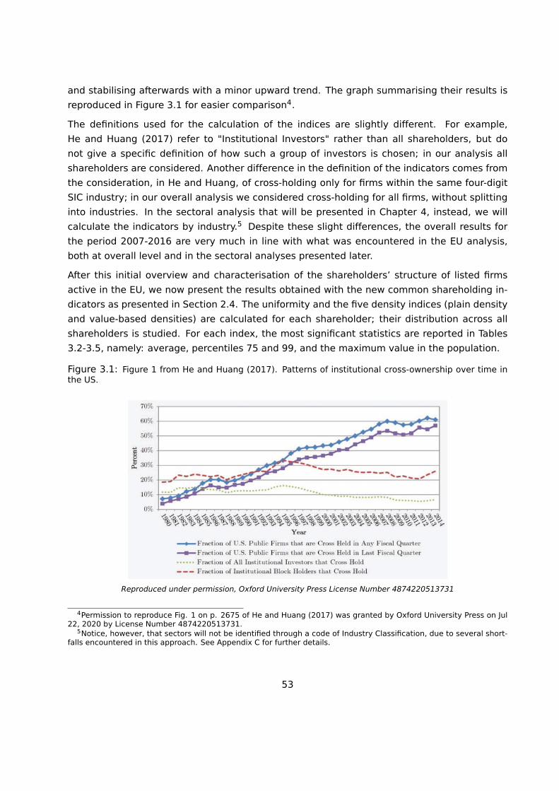
and stabilising afterwards with a minor upward trend. The graph summarising their results is

reproduced in Figure 3.1 for easier comparison4.

The definitions used for the calculation of the indices are slightly different. For example,

He and Huang (2017) refer to "Institutional Investors" rather than all shareholders, but do

not give a specific definition of how such a group of investors is chosen; in our analysis all

shareholders are considered. Another difference in the definition of the indicators comes from

the consideration, in He and Huang, of cross-holding only for firms within the same four-digit

SIC industry; in our overall analysis we considered cross-holding for all firms, without splitting

into industries. In the sectoral analysis that will be presented in Chapter 4, instead, we will

calculate the indicators by industry.5 Despite these slight differences, the overall results for

the period 2007-2016 are very much in line with what was encountered in the EU analysis,

both at overall level and in the sectoral analyses presented later.

After this initial overview and characterisation of the shareholders’ structure of listed firms

active in the EU, we now present the results obtained with the new common shareholding in-

dicators as presented in Section 2.4. The uniformity and the five density indices (plain density

and value-based densities) are calculated for each shareholder; their distribution across all

shareholders is studied. For each index, the most significant statistics are reported in Tables

3.2-3.5, namely: average, percentiles 75 and 99, and the maximum value in the population.

Figure 3.1: Figure 1 from He and Huang (2017). Patterns of institutional cross-ownership over time inthe US.

Reproduced under permission, Oxford University Press License Number 4874220513731

4Permission to reproduce Fig. 1 on p. 2675 of He and Huang (2017) was granted by Oxford University Press on Jul22, 2020 by License Number 4874220513731.

5Notice, however, that sectors will not be identified through a code of Industry Classification, due to several short-falls encountered in this approach. See Appendix C for further details.

53

The summary statistics for the plain density index are presented in Table 3.2. The average

market share held by investors has declined over time, from about 0.025% in 2007 to 0.018%

in 2016. However, such yearly averages are greatly influenced by some large values corre-

sponding to the top investors, while in fact the majority of shareholders present much lower

values. In fact, recalling that about 85% of the owners hold only one firm in their portfo-

lio, and considering that there are about 26 thousand firms per year in the market, for most

shareholders the density is extremely low (≈ 0.004% = 1/26,000).

The portfolios have non-negligible sizes only for a very small fraction of investors: many of

the portfolios in the top 1% of the distribution still do not even encompass as much as 0.5%

of the firms (the 99th percentiles is around 0.2%), but the maximum density value shows that

there are shareholders holding as many as 25% of the firms in the market, i.e. more than 6000

companies. Due to these very high values, the top shareholders will be briefly analysed later

in Sections 3.2-3.3, looking at the sizes of their portfolios over time, their composition in terms

of country of registration of the firms, and their weight as assessed by the average share value.

Table 3.2: Density of investments: Proportion of firms in a shareholder’s portfolio relative to the totalnumber of firms in the market. Summary Statistics by year (percentage points): mean, 75th percentile(p75), 99th percentile (p99), maximum (max).

Year Density

mean p75 p99 max

2007 0.0252 0.0042 0.2751 25.29212008 0.0235 0.0041 0.2413 25.79232009 0.0225 0.0040 0.2369 25.41952010 0.0222 0.0040 0.2331 26.02052011 0.0216 0.0039 0.2197 25.81492012 0.0210 0.0039 0.2077 25.59282013 0.0204 0.0038 0.2108 24.83712014 0.0198 0.0038 0.2047 23.91662015 0.0189 0.0038 0.1940 23.84522016 0.0179 0.0038 0.1770 23.8661

In the case of uniformity, reported in Table 3.3, more than three quarters of the shareholders

present a value of zero, given that they only own shares in one firm. This also justifies the

very low mean value, showing high concentration of the investments of the shareholders.

However, the top values for this index are rather high, with the percentile 99 showing a unifor-

mity above 80%, and the maximum observed value being about 99% throughout the years of

observation. This shows that the shareholders with the larger portfolios tend to invest equally

among the chosen firms, rather than giving priority to specific companies through buying

higher shares. This is usually reflected by a low value for the average share, as will be seen

later in the section dedicated to the top owners.

54

Table 3.3: Uniformity of investments: relative weight of larger participation shares over the shares totalin the portfolio. Small values denote concentrated investment. Summary Statistics by year (percentagepoints, index values between 0 and 1): mean, 75th percentile (p75), 99th percentile (p99), maximum(max).

Year Uniformity

mean p75 p99 max

2007 6.8517 0.0000 82.5517 98.63622008 6.6227 0.0000 81.7706 98.63132009 6.4407 0.0000 81.2290 98.74722010 6.3770 0.0000 81.4345 98.77842011 6.1674 0.0000 81.0806 98.70482012 5.9699 0.0000 80.2010 98.66372013 6.0062 0.0000 80.3506 98.70832014 6.0396 0.0000 80.4744 98.80712015 5.9612 0.0000 80.0559 98.80452016 5.7440 0.0000 79.0219 98.7994

For the density indices based on financial variables, the distributions present a large amount

of values very close to zero, as shown in Table 3.4 for values based on Total Assets, and Table

3.5 for indices calculated from Market Capitalisation. This is in line with the presence of a large

number of single shareholders, but adds the information that the single firms in their portfolios

are generally also small in size.

However, looking at the common shareholders, it is striking that the firms included in the

largest portfolios represent a significant proportion of the total value of the market, reaching a

coverage of above 80% of Total Assets and more than 90% of Market Capitalisation in almost

all years. This means that the top investors not only hold shares in a considerable number

of firms (we have seen values around 25% in Table 3.2), but also typically choose the largest

enterprises, leaving out only minor players - which together do not account for more than

10-20% of the market value. Also of note is that both indices have been increasing steadily

over time, showing that the preference for the largest players has become stronger over time.

Looking at the weighted indices, in the right panels of Tables 3.4 and 3.5, again we observe

the majority of portfolios producing negligible values. However, the proportion of market value

held by top investors through their participation shares is rather tangible, showing maximum

values above 3% - and increasing - for Market Capitalisation. For Total Assets even higher

maximum values are observed, with an average of about 4.3% and, also increasing, displaying

a steep rise from 2012 onwards in particular.

55

Table 3.4: Density indices based on Total Assets of firms in portfolio. Left: TOAS density - proportion oftotal assets of the market represented by the firms in portfolio. Right: Weighted TOAS density - proportionof total assets of the market held by shareholder through participation shares. Summary Statistics byyear (percentage points): mean, 75th percentile (p75), 99th percentile (p99), maximum (max).

Year TOAS density

mean p75 p99 max

2007 0.0843 0.0017 0.6643 75.86322008 0.0850 0.0014 0.6213 79.77782009 0.0745 0.0013 0.6136 79.03592010 0.0737 0.0012 0.6201 81.70662011 0.0784 0.0012 0.9931 83.91192012 0.0764 0.0012 1.0032 83.83382013 0.0707 0.0012 0.7367 85.00712014 0.0673 0.0013 0.7632 86.97242015 0.0640 0.0012 0.7076 87.65142016 0.0596 0.0012 0.7024 88.3695

Year Weighted TOAS density

mean p75 p99 max

2007 0.0011 0.0000 0.0145 2.29062008 0.0011 0.0000 0.0130 3.61922009 0.0012 0.0000 0.0130 4.10822010 0.0011 0.0000 0.0126 3.21332011 0.0012 0.0000 0.0139 2.87982012 0.0011 0.0000 0.0134 2.87152013 0.0012 0.0000 0.0132 5.51662014 0.0011 0.0000 0.0118 5.82172015 0.0011 0.0000 0.0116 6.26752016 0.0010 0.0000 0.0110 6.3193

Table 3.5: Density indices based on Market Capitalisation of firms in portfolio. Left: MKT CAP density -proportion of market capitalisation of the market represented by the firms in portfolio. Right: WeightedMKT CAP density - proportion of market capitalisation of the market held by shareholder through par-ticipation shares. Summary Statistics by year (percentage points): mean, 75th percentile (p75), 99thpercentile (p99), maximum (max).

Year MKT CAP density

mean p75 p99 max

2007 0.0832 0.0009 0.6613 86.73682008 0.0833 0.0008 0.6335 85.95462009 0.0857 0.0011 0.6446 89.19572010 0.0882 0.0012 0.6664 91.19852011 0.0854 0.0012 0.6274 91.84132012 0.0841 0.0012 0.6629 90.32372013 0.0843 0.0015 0.7311 91.50062014 0.0806 0.0017 0.6475 91.16262015 0.0795 0.0021 0.6328 91.37582016 0.0754 0.0021 0.5716 92.5755

Year Weighted MKT CAP density

mean p75 p99 max

2007 0.0011 0.0000 0.0157 2.33742008 0.0010 0.0000 0.0134 2.38232009 0.0011 0.0000 0.0150 3.11142010 0.0010 0.0000 0.0137 3.38042011 0.0010 0.0000 0.0138 3.32702012 0.0010 0.0000 0.0135 3.11212013 0.0010 0.0000 0.0134 3.42282014 0.0010 0.0000 0.0127 3.43102015 0.0010 0.0000 0.0120 3.67132016 0.0009 0.0000 0.0112 3.8560

56

3.2 Top-ranking investors

After the consideration of the general results, it is worth having a closer look at the share-

holders that present maximum values in the density-based indices presented earlier. In fact,

although in many cases the investors scoring higher values in one index also score high in the

remaining ones, there are some exceptions.

In particular, we observe cases of small portfolios that include very large enterprises with

very large participation shares, therefore presenting top values for the weighted indices, even

though their non-weighted indices are negligible. Given the possible strategic relevance of

their investments, we summarise the main findings in Table 3.6.

The table presents, for each top-ranking investor, the country of registration and the number

of listed firms active in the EU included in the respective portfolio; the last five columns report

the number of years in 2007-2016 when the investor presented one of the top 20 values in

the five indices. A blank corresponds to cases where the investor was never in the top 20 for

the specific index.

The top panel summarises the information on the largest portfolios, most of which present top

values for the Density index throughout the 10 years of observation. Given the large number

of firms held and their size, the value-based indices also present very high values in most

cases, both in terms of Total Assets and of Market Capitalisation. As was mentioned earlier,

these large portfolios generally encompass all the largest companies, representing in many

cases more than 80% of the market value.

As for the weighted indices, not all portfolios present high values, given that the average

shares held are rather small in some cases, therefore producing a smaller value for these

indices. Still, a good number of investors score very high also on the weighted indices for

the entire period of 2007-2016, namely Bank of New York Mellon, BlackRock, Fidelity, JP Mor-

gan Chase, Norway6, State Street and Vanguard. From these preliminary figures, these large

groups - mainly US-based (except Norway) - show a clear dominance over the set of listed

firms active in Europe.

The bottom panel of Table 3.6 reports other portfolios, of generally smaller size, but still scor-

ing high in one or more of the value-based indices. In many cases this is still due to the

considerable number of firms held (hundreds or even thousands), but few investors hold a

rather small portfolio (few dozens of firms). These few cases generally correspond to investors

holding very high stakes of some large companies, therefore producing high weighted indices.

The corresponding non-weighted indices are always negligible.6We recall that the term "Norway" (the state) is used as an abbreviation to indicate the Norwegian Sovereign Fund.

The same is intended for the references to other states, such as France or Sweden, meaning the respective sovereignfunds.

57

Table 3.6: Top-ranking investors. Number of years in 2007-2016 an investor appears in the top 20 forthe five density-based indices. Blanks correspond to cases where investor was never in the top 20.

Name Cou

ntr

y

No

Sub

s2

01

6

Den

sity

TOA

Sd

ensi

ty

MKT

CA

Pd

ensi

ty

TOA

Sw

den

sity

MKT

CA

Pw

den

sity

Largest portfolios No years ranking in top 20

ALLIANZ DE 2651 9 10 8AXA FR 3261 10 9 10 4 7BANK OF NEW YORK MELLON US 4289 10 10 10 10BARCLAYS UK 1841 5 4 5BLACKROCK US 6052 9 9 9 9 10BNP PARIBAS FR 2070 4 5 5CREDIT SUISSE CH 3378 10 7DEUTSCHE BANK DE 3474 10 10 10DIMENSIONAL FUND US 6204 10 6FMR LLC US 3378 10 10 10 10 10GOLDMAN SACHS US 3447 10 5INVESCO BM 3335 9 9 9 7JP MORGAN CHASE US 4208 10 10 10 8 10MORGAN STANLEY US 2976 10 9NORTHERN TRUST US 3081 5 7NORWAY NO 5316 10 10 10 9 10STATE STREET US 4346 10 10 10 10 10TEACHERS INSURANCE US 3885 9 10 10UBS CH n.a. 8 8 8 6VANGUARD US 6006 10 10 10 10 10

Other portfolios No years ranking in top 20

CAPITAL GROUP US 1451 10 9 10 10CENTRAL HUIJIN INVESTMENT CN 47 8CHINA-PEOPLE’S REPUBLIC CN 472 8 8FRANKLIN RESOURCES US 1748 10HKSCC NOMINEES LIMITED CN 52 7HSBC CUSTODY NOMINEES (AUSTRALIA) AU 433 5ING GROEP NL 380 6LLOYDS BANKING GROUP UK 25 9REGERINGSKANSLIET - SWEDEN SE 1872 8 10SCHRODERS UK 2644 7STICHTING PENSIOENFONDS NL 1790 9 10SUN LIFE FINANCIAL CA 1447 5T ROWE PRICE GROUP US 1831 9TEMASEK HOLDINGS SG 39 5WELLINGTON MANAGEMENT US 1929 10

58

3.3 Major Portfolios

Following the general overview of the shareholders’ structure in the EU, this section gives

a closer look at portfolios of the major common shareholders present in the area. Twenty

shareholders were considered for this analysis, selected according to the size of their portfolio

over the entire period of observation, and for their presence in the top ranks of all indices

analysed earlier, i.e. they correspond to the largest portfolios presented in the top panel of

Table 3.6.

The chosen shareholders all have in their portfolio more than 3000 listed companies active in

the EU, for at least 5 years in the period 2007-2016.7 The main results are presented in Tables

3.7 and 3.8, in which an outline of the characteristics of portfolios in terms of size and shares

are reported, as well as the geographical area of registration of firms held in each portfolio.

From the top and middle panels of Table 3.7, four large funds stand out with portfolios currently

including more than 20% of the listed firms active in Europe, namely BlackRock, Dimensional

Fund, Norway and Vanguard. In terms of time trend, both BlackRock and Vanguard show an

increase in size over time, while Dimensional has been shrinking a little, and Norway is overall

stable.

Positioned only slightly behind are Axa, Deutsche Bank, Fidelity (FMR LLC) and JP Morgan

Chase, which started out above 20% at the beginning of the period of observation, but have

decreased their number of firms held over time, currently holding between 12.5% and 16.2%.

On a lower but stable level are Bank of New York Mellon, State Street and Teachers Insurance,

with around 17%, while Credit Suisse, Goldman Sachs and Invesco show smaller declining

portfolios, currently standing at around 13%. The remaining investors hold smaller portfolios,

generally having diminished in relative size over the years.

7The only exception is BNP PARIBAS, which has more than 3000 firms in portfolio only in three years.

59

Table 3.7: Summary indicators for portfolios of major common shareholders over 2007-2016.

Year ALLIA

NZAXA

BANKOF

NYMEL

LON

BARCLA

YSBLA

CKROCK

BNPPA

RIBAS

CREDIT

SUIS

SE

DEUTS

CHEBANK

DIMEN

SIONAL

FUND

FMR

LLC

GOLDMAN

SACHS

INVES

COJP

MORGANCHASE

MORGANST

ANLEY

NORTHER

NTR

UST

NORWAY

STAT

EST

REET

TEAC

HERS

INSU

RANCE

UBS VANGUARD

Size of portfolios (number of listed firms active in the EU owned by each investor)

2007 3746 5431 3637 5975 3055 2242 4198 4841 5962 4913 3920 1804 4942 4107 3120 4095 3937 2990 4749 38522008 3809 5376 3837 6142 4038 2316 4141 4658 6307 4952 4092 3445 5173 3985 3133 5206 4232 3183 4586 40222009 3686 5484 4144 5512 5547 3359 3808 4464 6332 4880 3875 3663 5092 3660 3005 5242 4253 4017 4138 39932010 3679 5411 4329 3187 5927 3453 4044 4553 6585 5009 3897 3962 5191 3636 2966 5310 4502 4420 4162 40432011 3390 5001 4268 3042 6049 3159 3943 4246 6581 4915 3687 3948 4980 3352 2871 5252 4572 4682 3956 59472012 3231 4672 4208 2714 5910 2856 3747 4036 6530 4728 3524 3800 4682 3226 2767 5077 4657 4639 3656 59682013 3135 4201 4292 2278 6016 2637 3614 3924 6480 4576 3545 3705 4604 3108 2856 5305 4643 4688 3466 58202014 2897 3969 4384 2240 6187 2357 3581 3799 6308 4321 3663 3620 4582 3330 2943 5484 4772 4635 3331 58842015 2786 3630 4429 2044 6217 2254 3496 3693 6267 3592 3626 3491 4402 3180 3025 5469 4612 4495 n.a. 60082016 2651 3261 4289 1841 6052 2070 3378 3474 6204 3378 3447 3335 4208 2976 3081 5316 4346 3885 n.a. 6006

Relative size of portfolios (% of listed firms active in the EU owned by each investor)

2007 15.9 23.0 15.4 25.3 12.9 9.5 17.8 20.5 25.2 20.8 16.6 7.6 20.9 17.4 13.2 17.3 16.7 12.7 20.1 16.32008 15.6 22.0 15.7 25.1 16.5 9.5 16.9 19.1 25.8 20.3 16.7 14.1 21.2 16.3 12.8 21.3 17.3 13.0 18.8 16.52009 14.8 22.0 16.6 22.1 22.3 13.5 15.3 17.9 25.4 19.6 15.6 14.7 20.4 14.7 12.1 21.0 17.1 16.1 16.6 16.02010 14.5 21.4 17.1 12.6 23.4 13.6 16.0 18.0 26.0 19.8 15.4 15.7 20.5 14.4 11.7 21.0 17.8 17.5 16.5 16.02011 13.3 19.6 16.7 11.9 23.7 12.4 15.5 16.7 25.8 19.3 14.5 15.5 19.5 13.2 11.3 20.6 17.9 18.4 15.5 23.32012 12.7 18.3 16.5 10.6 23.2 11.2 14.7 15.8 25.6 18.5 13.8 14.9 18.4 12.6 10.8 19.9 18.3 18.2 14.3 23.42013 12.0 16.1 16.5 8.7 23.1 10.1 13.9 15.0 24.8 17.5 13.6 14.2 17.7 11.9 11.0 20.3 17.8 18.0 13.3 22.32014 11.0 15.1 16.6 8.5 23.5 8.9 13.6 14.4 23.9 16.4 13.9 13.7 17.4 12.6 11.2 20.8 18.1 17.6 12.6 22.32015 10.6 13.8 16.9 7.8 23.7 8.6 13.3 14.1 23.9 13.7 13.8 13.3 16.8 12.1 11.5 20.8 17.6 17.1 n.a. 22.92016 10.2 12.5 16.5 7.1 23.3 8.0 13.0 13.4 23.9 13.0 13.3 12.8 16.2 11.5 11.9 20.5 16.7 15.0 n.a. 23.1

Average participation shares

2007 1.01 1.78 1.01 2.53 1.43 0.74 0.95 1.25 1.18 3.31 1.40 1.68 1.37 1.23 0.75 0.46 1.30 0.63 1.17 1.562008 1.02 1.56 0.96 2.62 1.28 0.81 0.85 1.10 1.17 2.86 1.29 1.43 1.20 1.23 0.77 0.65 1.28 0.60 1.09 1.712009 0.94 1.30 1.02 2.18 3.25 1.22 0.66 0.95 1.14 2.93 0.86 1.30 1.11 1.01 0.95 0.80 1.33 0.52 0.88 1.972010 0.89 1.00 0.97 2.08 3.16 0.98 0.56 0.91 1.06 2.88 0.71 1.49 1.00 0.82 0.96 0.90 1.26 0.49 0.88 2.132011 0.97 0.94 0.99 1.41 3.04 0.83 0.51 0.82 1.07 2.73 0.67 1.37 1.02 0.72 1.02 1.00 1.26 0.47 0.83 1.682012 1.01 0.88 0.95 1.36 2.96 0.77 0.52 0.74 1.12 2.66 0.68 1.36 1.02 0.69 1.11 1.07 1.29 0.46 0.77 1.842013 1.00 0.87 0.98 0.92 3.13 0.81 0.49 0.69 1.18 2.70 0.65 1.43 1.08 0.63 1.07 1.19 1.31 0.46 0.80 1.972014 1.04 0.88 0.91 0.87 3.04 0.78 0.50 0.72 1.25 2.68 0.67 1.50 1.16 0.69 0.90 1.23 1.28 0.56 0.85 2.172015 1.07 0.90 0.90 0.91 3.09 0.76 0.49 0.80 1.36 2.96 0.71 1.58 1.11 0.74 0.88 1.21 1.30 0.56 n.a. 2.522016 1.00 0.97 0.83 0.82 3.26 0.75 0.46 0.70 1.40 2.87 0.72 1.56 1.12 0.74 0.83 1.27 1.37 0.60 n.a. 2.84

60

Considering the average quantities held (bottom panel of Table 3.7), the ranking is slightly

different, with the average share of BlackRock and Fidelity consistently representing around

3%, followed by Vanguard with about 2% (increasing), and Invesco, Dimensional and State

Street with about 1% to 1.5%. They are followed in turn by Allianz, Axa, Bank of New York

Mellon, Norway and JP Morgan Chase, where the average share of annual portfolios is close to

1%, and slightly increasing. The remaining common shareholders currently present portfolios

whose average share is below 1%.

In terms of the geographical composition of portfolios, Table 3.8 reports some overall statistics

for the whole period of observation. Compared to the complete set of listed firms active in the

EU during 2007-2016 - where roughly 43% of companies are registered outside Europe - the

firms included in the portfolios of the top 20 shareholders show a much higher proportion of

cases registered outside the EU (70%).

Looking at the countries of registration of the firms in the portfolios, we find that the most

frequent ones are the US, the UK, Japan, Germany, France and Italy (in decreasing order).

Depending on the investor, though, the proportion of firms in the portfolio coming from each

of the mentioned countries varies largely. For example, Northern Trust invests almost uniquely

in firms from the US (≈ 70% of portfolio) and from the UK (≈ 18%), almost disregarding Japan

and the other EU countries.

On the other hand, Japan attracts large attention from many of the major common sharehold-

ers, covering in many cases more than one-tenth of their portfolio (Axa, Bank of New York

Mellon, BlackRock, Dimensional, Fidelity, Goldman Sachs, JP Morgan Chase, Norway, State

Street, Teachers Insurance and Vanguard).

UK-based firms have in general a large weight in all portfolios, second only to the US, but they

are privileged by Barclays, where they represent about one-third of the chosen companies

over the years.

As for the three remaining European countries, they are present in small proportions in all

portfolios, but they are clearly preferred by home investors: Allianz and Deutsche Bank port-

folios present, respectively, 6% and 5% of companies based in Germany, while 7.67% of firms

held by BNP Paribas are French.

61

Table 3.8: Composition of portfolios of major common shareholders, by geographical area and countryof registration. N = Number of links to listed firms active in the EU over 2007-2016; p = proportion oflinks (%) in portfolio related to listed firms active in the EU registered in indicated area/country.

Name of Shareholder Area Country of registrationNon-EU EU US UK JP DE FR IT

ALLIANZ N 19,215 13,795 11,488 3,518 1,433 1,965 2,016 865p (%) 58.21 41.79 34.80 10.66 4.34 5.95 6.11 2.62

AXA N 30,152 16,284 17,140 7,335 4,670 1,352 1,752 993p (%) 64.93 35.07 36.91 15.80 10.06 2.91 3.77 2.14

BANK OF NY MELLON N 32,553 9,264 19,984 4,376 3,817 801 756 550p (%) 77.85 22.15 47.79 10.46 9.13 1.92 1.81 1.32

BARCLAYS N 21,563 13,412 14,905 10,331 1,369 469 545 287p (%) 61.65 38.35 42.62 29.54 3.91 1.34 1.56 0.82

BLACKROCK N 40,342 14,656 20,269 7,043 5,419 1,209 1,174 714p (%) 73.35 26.65 36.85 12.81 9.85 2.20 2.13 1.30

BNP PARIBAS N 13,364 13,339 7,278 4,949 1,330 840 2,048 712p (%) 50.05 49.95 27.26 18.53 4.98 3.15 7.67 2.67

CREDIT SUISSE N 26,348 11,602 18,266 6,030 1,940 1,293 756 619p (%) 69.43 30.57 48.13 15.89 5.11 3.41 1.99 1.63

DEUTSCHE BANK N 27,732 13,956 18,466 6,531 1,458 2,122 880 502p (%) 66.52 33.48 44.30 15.67 3.50 5.07 2.11 1.20

DIMENSIONAL FUND N 45,848 17,708 18,433 4,661 6,584 2,107 1,957 1,298p (%) 72.14 27.86 29.00 7.33 10.36 3.32 3.08 2.04

FMR LLC N 33,286 11,978 15,923 5,024 4,433 1,055 1,361 758p (%) 73.54 26.46 35.18 11.10 9.79 2.33 3.01 1.67

GOLDMAN SACHS N 28,138 9,138 18,934 6,085 3,640 513 448 285p (%) 75.49 24.51 50.79 16.32 9.76 1.38 1.20 0.76

INVESCO N 25,518 9,255 15,647 4,712 2,086 796 815 315p (%) 73.38 26.62 45.00 13.55 6.00 2.29 2.34 0.91

JPMORGAN CHASE N 33,364 14,492 17,555 6,305 4,753 1,350 1,340 877p (%) 69.72 30.28 36.68 13.17 9.93 2.82 2.80 1.83

MORGAN STANLEY N 26,349 8,211 19,188 5,229 1,185 485 464 224p (%) 76.24 23.76 55.52 15.13 3.43 1.40 1.34 0.65

NORTHERN TRUST N 23,381 6,386 20,808 5,437 188 116 106 45p (%) 78.55 21.45 69.90 18.27 0.63 0.39 0.36 0.15

NORWAY N 36,986 14,770 13,693 4,210 6,753 1,446 1,709 1,173p (%) 71.46 28.54 26.46 8.13 13.05 2.79 3.30 2.27

STATE STREET N 33,530 10,996 19,398 4,850 4,976 903 1,002 647p (%) 75.30 24.70 43.57 10.89 11.18 2.03 2.25 1.45

TEACHERS INSURANCE N 32,723 8,911 18,614 2,939 4,969 939 951 530p (%) 78.60 21.40 44.71 7.06 11.93 2.26 2.28 1.27

UBS N 20,873 11,474 12,922 6,489 1,342 1,157 1,106 451p (%) 64.53 35.47 39.95 20.06 4.15 3.58 3.42 1.39

VANGUARD N 40,853 10,690 21,225 3,304 5,401 1,012 1,208 744p (%) 79.26 20.74 41.18 6.41 10.48 1.96 2.34 1.44

Box 3.1: Main results of EU analysis - Overall evidence

� Baseline analysis is done on a historical dataset containing all listed companies active in

the EU in the period 2007-2016: this includes all listed firms registered in the EU, plus

all listed companies registered elsewhere, but holding participation in at least one firm

registered in the EU. The average number of firms observed each year is 26,560 (from

24,857 in 2007 to 26,942 in 2016) - where about 57% are registered in EU countries,

the rest being registered outside the EU. The proportion of EU versus Non-EU registered

companies remains roughly constant over time.

� In 2016, 87.2% of all shareholders of companies in our dataset held participation in only

one company (85.1% in 2007). Common shareholders therefore make up 12.8% of all

shareholders (14.9% in 2007). The number of listed firms that are cross-held by block-

holders (common shareholders with at least 5% participation in more than one company)

has been increasing, growing from around 15.5 thousand in 2007 to around 17.5 thousand

in 2016. Around 67% of the analysed companies are cross-held by block-holders with at

least 5% participation.

� Looking at portfolios, the top common shareholders hold as many as 25% of the firms

in the market, representing more than 6,000 companies overall. They tend to invest

equally among the chosen firms, rather than prioritising specific companies through buy-

ing higher percentages of shares.

� The firms included in the largest portfolios represent a significant proportion of the total

value of the market, reaching a coverage of above 80% of Total Assets and more than 90%

of Market Capitalisation in almost all years. This means that the top investors not only

hold shares in a considerable number of firms (around 25%), but also typically choose

the largest enterprises, leaving out only minor players - which together do not account

for more than 10-20% of the market value. The preference for the largest market players

has become stronger over time.

� When both the Total Assets and Market Capitalisation are multiplied by the percentage of

shares actually held, we find that in 2016 the top common shareholders holds within its

grasp 3.8% of total Market Capitalisation and 6.6% of the Total Assets in the EU. These

percentages were 2.3 and 3.6 respectively in 2008; An acceleration in the control of Total

Assets or MarketCap can be observed as of 2012.

�

63

Box 3.2: Main results of EU analysis - Focus on big players

� Four large funds stand out with portfolios currently including more than 20% of the listed

firms active in Europe, namely BlackRock, Dimensional Fund, Norway (short for The Nor-

wegian Sovereign Fund) and Vanguard. In terms of time trend, both BlackRock and Van-

guard show an increase in size over time, while Dimensional has been shrinking a little,

and Norway is overall stable.

� Positioned only slightly behind are Axa, Deutsche Bank, Fidelity (FMR LLC) and JP Morgan

Chase, which all started out holding above 20% of the listed firms active in Europe at

the beginning of the period of observation, but have decreased their number of firms

held over time, currently holding between 12.5% and 16.2% of listed firms. On a lower

but stable level are Bank of New York Mellon, State Street and Teachers Insurance, with

holdings in around 17% of listed firms active in Europe, while Credit Suisse, Goldman

Sachs and Invesco show smaller declining portfolios, currently comprising at around 13%

of the firms under analysis.

� Considering the quantities held in portfolio, BlackRock and Fidelity have average shares

which consistently represent around 3%, followed by Vanguard with about 2% (increas-

ing), and Invesco, Dimensional and State Street with about 1% to 1.5% average holdings.

They are followed in turn by Allianz, Axa, Bank of New York Mellon, Norway and JP Morgan

Chase, where the average share of annual portfolios is close to 1%, and slightly increas-

ing. The remaining common shareholders currently present portfolios whose average

share is below 1%.

� The top 20 common shareholders tend to invest in companies registered outside the EU

(70% of the cases), mostly in the US and Japan. The top EU target countries in 2007-

2016 were the UK, Germany, France and Italy. Some common shareholders show a clear

geographical preference: for example, Northern Trust invests almost uniquely in firms

from the US (≈ 70% of portfolio) and from the UK (≈ 18%), almost disregarding Japan and

the other EU countries.

�

64

Chapter 4

Common Shareholding in

Selected Industries

Following the general overview of all firms active in the EU, five industries of interest are

considered, namely Oil&Gas, Electricity, Mobile Telecommunications, Trading Platforms and

Beverages.1 For each industry, the identification of the relevant companies representing the

market followed an ad hoc process.

It should be noted that, similarly to the study on listed firms, the analysis of the five industries

encompasses all firms active in the EU in the specified sectors of economic activity, regardless

of their country of registration. In reality, a large proportion of companies active in these

sectors are subsidiaries of mother companies registered outside the EU, mainly in the US, but

also in countries such as Canada, Russia and China.

Starting from the comprehensive database of all listed companies active in the EU between

2007 and 2016, an initial selection of firms was conducted according to the international codes

of industry classification. The industry classification used to identify the economic activity

of firms followed the NACE system.2 Each firm can present more than one NACE code of

economic activity, classified as either "Core", "Primary" or "Secondary" activity. In many cases

it was necessary to consider all levels of activity, given that many corporations are active in

additional economic fields beyond their core business.

Unfortunately, this procedure did not manage to fully identify the set of relevant players in

each market, calling for further refinements. Several non-listed firms of relevance were also

integrated into each market. The final identification of each industry benefitted from the

crucial input of specialist teams at DG COMP, which we gratefully acknowledge.1The relative concentration (limited number of firms with large market shares) and the existence of a topical

expertise on market players (due to recent antitrust or merger investigations) motivated the choice.2NACE stands for Nomenclature générale des Activités économiques dans les Communautés Européennes (Euro-

pean Classification of Economic Activities). For further details see Eurostat (2008).

65

The selection procedure of each industry is briefly commented upon in each sectoral analysis.

Full details are reported in Appendix C. Sections 4.1-4.5 report the results for each industry.

The relatively large time span of available observations, covering ten years between 2007 and

2016, enables the identification of a shift in investment behaviour among the top investors in

some industries, both in terms of the size of portfolios and the amount of participation in

individual firms. In particular, the increase in investment coming from Funds and States may

raise some concerns in strategic sectors such as those considered in the present analysis.

All aspects considered above are measured through the application of some of the indices

presented in Chapter 2.

4.1 Energy sector - Oil&Gas

All companies that presented at least one NACE code in Section "D" (Electricity, gas, steam and

air conditioning supply) among Core, Primary or Secondary activities were initially selected as

potential candidates for the Energy sector. We noticed the importance of considering also the

Secondary codes, especially in the Oil&Gas sector to capture relevant companies having their

Core and Primary codes in Mining or Manufacturing.

After this first selection, firms were allocated to the "Electricity" or "Oil&Gas" sectors according

to specific classifications appearing among Core or first three Primary codes (see Table C.1 in

Appendix C for details). As suggested by our colleagues in DG COMP, we removed transmission

system operators (TSOs) from the list, given that transmission is a highly regulated activity.

Nearly a hundred unlisted firms were added to complement the dataset, based on expert

opinion.

The Oil&Gas industry, identified according to the procedure described above, is composed by

153 distinct corporations active in the EU during the period 2007-2016. Of these, 73% are

listed. All-together, in 2016 the Total Assets of the selected firms amount to 3309 Bn Euro,

while the listed firms have a total value of Market Capitalisation of 1811 Bn Euro for the same

year. Although most firms are active throughout the whole period of observation, some are

recorded during a shorter period of time, either due to a later entry into the market or to exit

due to M&A, dissolution or other reasons. Therefore the panel of firms is not constant over

time, oscillating during the ten years of observation between 125 and 139 firms per year (on

average 134).

An overview of the summary statistics is outlined in Table 4.1. The number of recorded share-

holders varies little during 2007-2016, ranging between 1578 and 1884 per year, with the

proportion of common shareholders rather stable around 33%, much higher than the overall

figure of about 14%. On the other hand, the proportion of firms cross-held by block-holders is

in line with the general picture of listed firms in the EU, i.e. rather stable around 63%.

66

Table 4.1: Summary statistics for firms active in the EU in the Oil&Gas sector between 2007 and 2016:number of firms; number and percentage of firms cross-held by block-holders (BH) at minimum 5%; totalnumber of shareholders; number and percentage of common shareholders (i.e. shareholders with morethan one firm in their portfolio); number and percentage of single owners (holding shares only of onefirm).


2007 125 75 (60.00) 1,655 535 (32.33) 1,120 (67.67)2008 129 84 (65.11) 1,639 535 (32.64) 1,104 (67.36)2009 132 77 (58.33) 1,578 544 (34.47) 1,034 (65.53)2010 134 87 (64.93) 1,802 621 (34.46) 1,181 (65.54)2011 134 87 (64.93) 1,822 605 (33.21) 1,217 (66.79)2012 137 90 (65.69) 1,659 617 (37.19) 1,042 (62.81)2013 139 86 (61.87) 1,832 597 (32.59) 1,235 (67.41)2014 139 86 (61.87) 1,835 606 (33.02) 1,229 (66.98)2015 136 85 (62.50) 1,884 598 (31.74) 1,286 (68.26)2016 135 82 (60.74) 1,741 565 (32.45) 1,176 (67.55)

About 46% of the firms are registered outside the EU, almost half of which are in the US,

followed by Canada, Australia and a smaller number from China, Japan, Norway and Russia.

More than half of the firms (52%) report as their core activity the Nace code "3522: Distribu-

tion of gaseous fuels through mains", while 12% have as their principal classification "3513:

Distribution of electricity", and another 12% present "1920: Manufacture of refined petroleum

products". About 9% of firms are active in "610: Extraction of crude petroleum" and 5% in

"3523: Trade of gas through mains". The remaining companies declare their main activities in

Section D (Electricity, Gas and Steam Supply), or other related activities (wholesale of fuels or

transport via pipeline). A summary of the main economic activities is reported in Table 4.2.

Table 4.2: Main areas of economic activity of firms active in the EU in the Oil&Gas sector between 2007and 2016: Core Nace code, description of area of activity, and percentage of firms presenting such Corecode.

Core Nace Description % firms

3522 Distribution of gaseous fuels through mains 521920 Manufacture of refined petroleum products 123513 Distribution of electricity 120610 Extraction of crude petroleum 93523 Trade of gas through mains 5

Other: mainly from Section D (Electricity, Gas and Steam Supply), 10Wholesale of fuels or Transport via pipeline

67

Main players

Before looking at the overall results for the whole market, we report here some figures relative

to the largest enterprises active in this sector. Table 4.3 reports the ten largest companies

registered in the EU and the ten largest from outside, reporting their size in terms of Total

Assets for 2016, the country of registration, and the percentage of shares held in 2016 by the

four top institutional investors, namely BlackRock, Vanguard, State Street and Norway3.

The size of the largest companies is comparable across the two groups, although those reg-

istered outside the EU 28 tend to show somewhat larger Total Assets for 2016. In terms

of country of registration, the UK, France, Italy and Spain prevail in Europe, while outside

most companies are based in North America (US or Canada), followed by Russia, Norway and

Venezuela.

The presence of the four funds is widespread in both groups of firms, in some cases presenting

very high participation (above 6%). In terms of shares, BlackRock dominates in the EU-based

companies, with values generally much higher than the remaining three investors. State

Street concentrates mainly on UK firms, while Norway and Vanguard invest more evenly in

all top companies. Outside the EU, Vanguard’s presence is of a similar level to Blackrock,

although slightly higher in this case, followed at some distance by State Street. Norway marks

its presence in almost all top firms, although with rather small shares. The only exception is

Petroleos De Venezuela, where the funds are absent, being wholly owned by the State.

Density and uniformity

The first common shareholding indices to be presented are the shareholders indices derived

from each investor’s ownership information. Their respective distribution will be analysed to

infer market-level indicators. The results for the Oil&Gas industry are displayed in Table 4.4.

The six indices are those based on plain density, on the value-based densities calculated from

Total Assets and Market Capitalisation, with their corresponding share-weighted versions, and

finally the index of uniformity of investments portfolios.

On average, the portfolios of investors in this market hold about 2.5% of the firms, i.e. ap-

proximately 3 firms. However, given the very large number of single shareholders (about two

thirds), the distribution of the size of portfolios is very asymmetric: the majority of investors

(75%) only hold participation in 2 firms or less, that is 1.5% of the market, as we see from

the 75th percentile. Things change dramatically for the largest portfolios, where the top 1%

hold on average more than 38 firms (≈ 28% of the market). All these figures are rather stable

over the ten years of observation. The maximum size of portfolios is very large, with portfolios3We recall that the term "Norway" (the state) is used as an abbreviation to indicate the Norwegian Sovereign Fund.

The same is intended for the references to other states, such as France or Sweden, meaning the respective sovereignfunds.

68

Table 4.3: Largest firms of Oil&Gas sector and selected ownership data on their main common share-holders. Top 10 largest enterprises in the EU and outside the EU, by country of registration. Size mea-sured by Total Assets in 2016 (Bn Euros). Direct or indirect participation shares (%) held in 2016.

Cou

ntr

y

TOA

S2

01

6(B

ne

)

Bla

ckR

ock

Nor

way

Sta

teS

tree

t

Vang

uar

d

Registered in the EU Shares held in 2016 (%)

ROYAL DUTCH SHELL PL UK 390.17 6.92 2.35 3.38 2.73BP PLC UK 249.80 5.51 1.70 3.33 2.52TOTAL S.A. FR 128.17 5.07 1.67 0.74 1.92ENI S.P.A. IT 83.36 2.27 1.51 0.57 1.48ENGIE FR 80.56 1.74 1.46 0.49 1.28GAS NATURAL SDG, S.A ES 32.08 1.16 0.79 0.18 0.68CENTRICA PLC UK 25.55 6.75 1.91 2.52 2.44REPSOL S.A. ES 23.74 3.04 1.24 0.36 1.61OMV AG AT 17.35 1.07 1.57 0.51 0.99HERA SPA IT 6.17 0.42 1.75 0.90 0.97

Registered outside the EU Shares held in 2016 (%)

EXXON MOBIL CORP US 313.36 5.87 0.87 4.63 6.83CHEVRON CORP US 246.73 6.41 0.98 6.04 6.97GAZPROM PJSC RU 216.66 1.25 0.47 0.11 1.46PETROLEOS DE VENEZUELA VE 179.93ROSNEFT OIL COM PJSC RU 155.67 0.27 0.12 0.34STATOIL ASA NO 85.96 0.80 67.00 0.22 0.70CONOCOPHILLIPS CO US 85.16 6.55 0.96 4.84 6.91KINDER MORGAN INC US 76.18 4.78 0.64 3.99 5.80ENERGY TRANSFER US 66.59 0.19TRANSCANADA CORP CA 62.21 0.60 0.11 2.06

69

encompassing 40% or more of the firms in the market being observed every year. This fig-

ure has been increasing over time, reaching a peak of 45% in 2016, i.e. about 60 competing

companies.

As for the uniformity index, rather low average values are observed in all years (around 14%),

showing that investors tend to distinguish between the firms in their portfolio through an

uneven distribution of shares. However, the top values of the index are always above 85%,

with a maximum above 90% and increasing, revealing that there are shareholders holding an

almost equal amount of shares in all firms held.

The value-based indices are calculated from the Total Assets or the Market Capitalisation of

the firms in a portfolio. Given that the last variable is only available for listed firms, the two

indices present slightly different values, given that they are not calculated using the same

pool of firms. However, the general trend is rather similar in the two cases. Looking first at

the unweighted indices, we find that the firms in the portfolios represent on average about

6% of the market, but again this distribution is very skewed: the 75th percentile shows that

three quarters of portfolios include firms that represent at most a minor share of the market

value (a stable figure of about 3.5% of Market Capitalisation, and an increasing share of Total

Assets, currently reaching 6.5%). This suggests that the majority of portfolios include either

a limited number of medium firms, or a larger number of small firms, in either case not being

very relevant for the overall market. When we move towards the upper end of the distribution,

however, we see that the top portfolios include participation in almost all relevant firms, rep-

resenting more than 70% of the market value in terms of Total Assets, and more than 85% of

Market Capitalisation (on average over the ten years). The largest observed values are close

to 90% for TOAS and almost 100% for MKT CAP, revealing that the largest portfolios hand-pick

all firms with the largest value in the market.

Once we consider actual firm ownership, weighting the value of the firms by the respective

participation shares, we find that 99% of portfolios hold less than 1% of the value of the market

through their participation shares, both in terms of TOAS and of MKT CAP. However, there are

top investors that hold in their hands large amounts of market value, given that the shares

they hold in the firms in their portfolio amount to about 5-6% of the market TOAS or MKT CAP.

70

Table 4.4: Oil&Gas sector common shareholding indices. Summary Statistics by year (percentagepoints, index values between 0 and 100): mean, 75th percentile (p75), 99th percentile (p99), maxi-mum (max). Density: Proportion of firms in a shareholder’s portfolio relative to the total number offirms in the market. Uniformity: Relative weight of larger participation shares over the shares total inthe portfolio. Small values denote concentrated investment. TOAS density: Proportion of total assetsof the market represented by the firms in portfolio. Weighted TOAS density: Proportion of total assetsof the market held by shareholder through participation shares. MKT CAP density: Proportion of marketcapitalisation of the market represented by the firms in portfolio. Weighted MKT CAP density: Proportionof market capitalisation of the market held by shareholder through participation shares.

Year Density

mean p75 p99 max

2007 2.4933 1.6000 28.8000 40.80002008 2.5838 1.5504 31.0078 42.63572009 2.6256 1.5152 31.0606 41.66672010 2.5366 1.4925 28.3582 44.02992011 2.4780 1.4925 29.1045 44.02992012 2.5444 2.1898 27.7372 40.87592013 2.3334 1.4388 26.6187 43.16552014 2.4159 1.4388 27.3381 43.16552015 2.3409 1.4706 27.2059 44.11762016 2.4281 1.4815 25.9259 45.1852

Year Uniformity

mean p75 p99 max

2007 14.2029 28.9559 84.7759 88.652008 14.2989 28.7194 85.0252 89.682009 15.0344 29.8343 85.2258 90.122010 14.9557 30.3018 85.4537 90.502011 14.4327 29.1845 84.9744 90.522012 15.9969 31.7066 84.9540 90.372013 13.9317 28.2429 84.7570 90.972014 14.5752 29.9732 85.3394 90.972015 13.5395 27.3938 85.1052 90.602016 14.1145 28.4073 86.0875 91.01

Year TOAS density

mean p75 p99 max

2007 5.5368 3.0749 72.1366 84.93002008 5.8669 3.6807 74.1782 86.37552009 5.9431 3.7569 77.2302 86.23092010 5.8955 3.4620 78.6741 86.92122011 5.5879 2.7858 77.5357 87.94542012 5.7378 3.3057 72.9714 84.74972013 5.7177 4.6072 68.7842 85.10072014 5.7448 5.8130 69.8872 87.69382015 5.6280 5.2626 70.2692 88.77882016 5.9754 6.5469 68.6473 89.2991


mean p75 p99 max

2007 0.0536 0.0161 0.8886 4.12022008 0.0518 0.0160 0.8091 3.97012009 0.0576 0.0179 1.0858 5.13982010 0.0500 0.0148 0.8719 5.31732011 0.0467 0.0130 0.8057 5.58012012 0.0511 0.0148 0.8601 5.81392013 0.0524 0.0134 0.8213 6.36512014 0.0517 0.0149 0.7790 4.87452015 0.0543 0.0160 0.8331 4.71992016 0.0538 0.0163 0.9077 5.7510


mean p75 p99 max

2007 5.9102 3.0433 80.0996 97.89272008 6.4627 3.7682 89.2018 99.01732009 6.4209 4.2629 86.2573 99.39722010 6.3556 4.7061 91.0768 99.47502011 5.9074 3.7030 87.0212 99.44292012 6.0933 4.1428 84.1377 97.60222013 6.1213 4.6127 82.8554 97.45762014 6.3079 3.4487 84.0280 98.85872015 6.0392 3.3678 83.6435 98.76712016 6.3439 3.6858 82.1542 97.5925


mean p75 p99 max

2007 0.0542 0.0102 1.1636 5.51742008 0.0468 0.0086 1.0094 2.97452009 0.0597 0.0118 1.1059 6.22902010 0.0500 0.0095 0.9359 6.06842011 0.0445 0.0090 0.7262 5.16732012 0.0483 0.0117 0.8850 5.36932013 0.0463 0.0112 0.8567 4.42872014 0.0463 0.0133 0.8548 4.67922015 0.0474 0.0137 0.8731 4.74522016 0.0476 0.0136 0.8101 4.9134

Common shareholding indices for top investors

Given the asymmetries of the density indices observed above, it is worth investigating what

happens at the top levels. For this reason, a group of investors has been selected according

to the values scored in the various indices in 2007-2016, and their behaviour has been looked

at in detail. The "Top Investors" are defined as being the shareholders that present, over the

ten years of observation, at least five times a value of density, Weighted TOAS density or

Weighted MKT CAP density in the top 20. This selection makes it possible to distinguish the

largest portfolios, i.e. those holding the largest number of firms, or the most valuable ones,

such as those portfolios with a limited number of large firms but each one held with a large

participation share, thus securing a large overall share of market value into the hand of the

investor.

In fact, the top investors tend to be the same over the entire period, therefore scoring the

largest values in the indices across all years. Given that the MKT CAP variable is not available

for all firms, Table 4.5 summarises, for the sake of the example, some figures concerning the

shareholders with the top Weighted TOAS density. The Table reports the size of portfolios

(number of firms in portfolio and density) in 2016, and the two TOAS-based indices, together

with the largest firms held and respective participation shares reported in 2016.

In the first position we find the Russian Government, which holds almost 6% of the Total Assets

of the market, given that it is the majority owner of two of the largest companies in Oil&Gas

(Gazprom and Rosneft). The usual top three funds follow, respectively BlackRock, Vanguard

and Norway, each having invested in more than 40% of the firms in the market; even with

small participation, they hold approximately between 3% and 4% of the market value. State

Street and Capital Group follow closely behind, again with numerous firms held, including most

larger players. Last, Jupiter Dividend, with participations in only 3 firms, manages to control

1.56% of the market value, due to large shares in the largest firms.

The evolution of the indices over 2007-2016 is reported for top investors in Figure 4.1, by in-

vestor type (Funds, States, Banks, Insurance). In general, over the years Banks and Insurance

companies have maintained or decreased the number of firms held in the Oil&Gas industry.

Yet, the proportion of firms in portfolio is rather high, constituting between 15% and 40% of

companies active in the industry. The share of market value, both in terms of TOAS and of

MKT CAP, is almost always below 1% throughout the period of observation for both types of

investors.

States present more stable values, with Norway and Sweden holding the largest number of

firms (about 42% and 28% on average respectively), but in terms of market value are beaten

by Russia, as reported earlier. As for the funds, BlackRock, Vanguard and State Street dominate

over all remaining investors of this type, showing increasing trends in all indicators during

2007-2016, and scoring the top three values in each index in 2016.

72

Table 4.5: Top Investors in Oil&Gas sector: Investors whose portfolios present the top values of theWeighted TOAS density index in 2016. Country of shareholder (SH); number of firms held in Oil&Gasindustry; Density (share of firms held); TOAS density (share of market TOAS represented by firms held);Weighted TOAS density (share of market TOAS held through participation shares); firms with largestTOAS in portfolio and respective quantity of shares held, ordered by decreasing TOAS. All figures refer tothe year 2016. MO = Majority Owner.

Shareholder Name SH

countr

y

No.

Firm

sH

eld

Den

sity

TOA

Sd

ensi

ty

Wei

ghte

dTO

AS

den

sity

Largest firms and shares held (%)

GOVERNMENT OFTHE RUSSIAN FED-ERATION

RU 7 5.19 11.51 5.75 GAZPROM (MO); ROSNEFT (MO)

BLACKROCK US 61 45.19 89.21 4.19

ROYAL DUTCH SHELL (6.92); EXXON(5.87); BP PLC (5.51); CHEVRON(6.41); GAZPROM (1.25); ROSNEFT(0.27); TOTAL (5.07)

VANGUARD US 57 42.22 87.51 3.42

ROYAL DUTCH SHELL (2.73); EXXON(6.83); BP (2.52); CHEVRON (6.97);GAZPROM (1.46); ROSNEFT (0.34);TOTAL (1.92)

NORWAY NO 54 40.00 85.68 2.72

ROYAL DUTCH SHELL (2.35); EXXON(0.87); BP (1.7); CHEVRON (0.98);GAZPROM (0.47); ROSNEFT (0.12);TOTAL (1.67); STATOIL (67.00)

STATE STREET US 45 33.33 80.21 2.55ROYAL DUTCH SHELL (3.38); EXXON(4.63); BP (3.33); CHEVRON (6.04);GAZPROM (0.11); TOTAL (0.74)

CAPITAL GROUP US 27 20.00 65.78 1.91ROYAL DUTCH SHELL (5.45); EXXON(1.47); BP PLC (2.17); CHEVRON(3.79); TOTAL (2.49)

JUPITER DIVIDEND UK 3 2.22 20.11 1.56 ROYAL DUTCH SHELL (7.1); BP PLC(9.2); CENTRICA(3.4)

73

Figure 4.1: Common shareholding indices for Top Investors in Oil Gas sector. Top panel: Density -Proportion of firms in a shareholder’s portfolio relative to the total number of firms in the market. Bottompanel: Weighted TOAS density - Proportion of total assets of the market held by shareholder throughparticipation shares.

10

15

20

25

30

35

40

45

2007 2009 2011 2013 2015

BLACKROCK

DIMENS. FUND

FMR LLC

NORTHERN TRUST

STATE STREET

VANGUARD

Funds

2007 2009 2011 2013 2015

NORWAY

SWEDEN

States

2007 2009 2011 2013 2015

BANK NY ME

BARCLAYS

BNP PARIBAS

CREDIT SUISSE

DEUTSCHE BANK

GOLDMAN SACHS

JPMORGAN CHASE

Banks

2007 2009 2011 2013 2015

ALLIANZ SE

AXA SA

STICHTING PENSIOEN

TEACHERS INSUR

Insurance

Density (%)

0

1

2

3

4

5

6

2007 2009 2011 2013 2015

BLACKROCK

DIMENS. FUND

FMR LLC

NORTHERN TRUST

STATE STREET

VANGUARD

Funds

2007 2009 2011 2013 2015

FRANCE

NORWAY

RUSSIA

States

2007 2009 2011 2013 2015

BANK NY ME

BARCLAYS

BNP PARIBAS

CREDIT SUISSE

DEUTSCHE BANK

GOLDMAN SACHS

JPMORGAN CHASE

Banks

2007 2009 2011 2013 2015

ALLIANZ SE

AXA SA

STICHTING PENSIOEN

TEACHERS INSUR

Insurance

Weighted TOAS Density (%)

74

Network indices

This Section presents common shareholding indices calculated inside the two separate net-

works of Shareholders and Firms, measuring the strength of the relationships induced between

actors of the same type due to a link with an actor of the other type. Namely, two firms can

be linked by a common shareholder, while two shareholders are connected through ownership

of shares in the same firm.

The higher the number of firms that two investors have in common, and the closer the amount

of shares held in each of them, the stronger the link between the two investors. On the other

hand, the higher the number of shareholders that appear in two firms’ ownership structures,

and the more similar the values of the shares held, the closer the firms will be considered

to be. In both networks, the strength of the link is measured through the calculation of the

coefficients of correlation between either portfolios (for shareholders) or ownership structures

(in the case of firms).

In the shareholders’ network, however, high correlations can be observed between two port-

folios that comprise the same firms with similar shares, but with a very small number of firms.

Given that in general the portfolios tend to be rather small,4 it makes sense to select the most

significant portfolios before looking at the strength of their link. For this industry, a threshold

of at least 10% of density has been chosen, defining the so-called "high density portfolios".

In the case of the firms’ network, no selection was necessary based on the number of share-

holders, since the average ownership structure includes about 12 owners, giving rise to a

reasonable number of links to analyse between any pair of firms. On the other hand, to avoid

possible spurious links generated by very small participations, only block-holdings have been

considered, i.e. links generated by ownership of at least 5% of shares. If the participation is

below 5%, it is ignored for the calculation of these indices.

Tables 4.6 and 4.7 report the yearly results for the two networks. Only about 4% of all possible

owner-owner connections are detected, i.e. the vast majority of shareholders have no firms in

common. Such proportion is rather constant over time, slightly decreasing in the last years.

Considering all existing links between large "high density" portfolios, less than 2% of con-

nected high density shareholders have a strong correlation of investment behaviour (above

80%). Still, it is striking that some large portfolios show an almost coinciding behaviour; even

though they are few, they cannot be ignored and should be further analysed.

In the firms’ network, we observe an increasing proportion of connections of pairs of firms

through block-holders present in their ownership structures. This fraction was below 2% in

2007, but has currently more than doubled to above 5%, witnessing an increase in extensive

block-holding by large investors. Among the connected firms, above 10% show strong links,

with correlations of more than 80% between their respective block-holding structures, con-4We recall that 75% of portfolios hold at most 2 firms, and the average portfolio size is of 3 firms, as seen in earlier.

75

firming there is a large overlap of investment preferences among top investors. However, this

indicator has not shown a particular pattern over time.

Table 4.6: Network indices for Oil&Gas sector. Shareholders’ network. Total number of common share-holders; proportion of non-zero correlations between pairs of portfolios, i.e. proportion of connectionsbetween two shareholders induced by common shareholding of a same firm; number of high correlations(>80%) between pairs of high-density portfolios (both densities >10%); proportion of high correlationsbetween pairs of high-density portfolios.

Tot No. Prop Non-Zero No. High Corr. Prop. High Corr.Year Comm SH Correlations High Dens. High Dens.

2007 535 3.87 69 1.782008 535 4.02 87 2.082009 544 4.35 97 2.232010 621 4.03 94 1.662011 605 3.96 96 1.902012 617 4.72 73 1.472013 597 3.59 73 1.502014 606 3.93 96 1.862015 598 3.45 63 1.302016 565 3.63 70 1.57

Table 4.7: Network indices for Oil&Gas sector. Firms’ network. Total number of firms cross-held by block-holders (holding at least 5%); proportion of non-zero correlations between shareholders’ structures ofpairs of firms (only shares >5%); number of high correlations between shareholders’ structures of pairsof firms (only shares >5%); proportion of high correlations (>80%) among the non-zero correlations.

Tot. No. Firms Prop Non-Zero No. of High Prop. of HighYear Cross-Held by BH Correlations Correlations Correlations

2007 75 1.70 18 13.642008 84 2.24 28 15.142009 77 4.98 63 14.622010 87 4.65 59 14.252011 87 4.23 44 11.672012 90 3.57 50 15.022013 86 3.60 30 8.702014 86 4.09 39 9.952015 85 4.52 41 9.882016 82 5.40 69 14.14

76

4.2 Energy sector - Electricity

The Electricity sector has been selected according to the general procedure for the Energy

sectors (see Section 4.1). This industry includes 396 firms active in the EU area, of which

39% are registered outside, mainly in the US, Canada, Switzerland and Russia. The number

of active firms per year has been increasing steadily from 275 in 2007 to 353 in 2016, with

an average of 325 firms per year. The large majority (89%) of the selected firms is listed.

In 2016, the sector totaled 3330 Bn Euro of Total Assets, while the listed firms had a Market

Capitalisation of 864 Bn Euro.

The number of shareholders has also been increasing over time, totalling 3596 investors in

2016 against the 2429 present in 2007. Although the number of common shareholders has

been rather stable over time (on average about 690 per year), their proportion has been

drastically diminishing, having observed a steep rise in single shareholders, which currently

amount to 80% of the investors. In 2007, this proportion was as low as 71%. Table 4.8 presents

some yearly statistics.

Although the number of firms cross-held by block investors has been increasing since 2007,

their proportion had decreased around 7 percentage points (from 62.5 to 55.5) by the end of

2016, given the rapid growth of the size of this industry.

Table 4.8: Summary statistics for firms active in the EU in the Electricity sector between 2007 and 2016:number of firms; number and percentage of firms cross-held by block-holders (BH) at minimum 5%; totalnumber of shareholders; number and percentage of common shareholders (i.e. shareholders with morethan one firm in their portfolio); number and percentage of single owners (holding shares only of onefirm).


2007 275 172 (62.55) 2,429 704 (28.98) 1,725 (71.02)2008 285 177 (62.11) 2,545 722 (28.37) 1,823 (71.63)2009 303 171 (56.44) 2,566 697 (27.16) 1,869 (72.84)2010 321 188 (58.57) 2,925 759 (25.95) 2,166 (74.05)2011 325 186 (57.23) 2,842 677 (23.82) 2,165 (76.18)2012 333 191 (57.36) 2,732 644 (23.57) 2,088 (76.43)2013 340 184 (54.12) 2,815 663 (23.55) 2,152 (76.45)2014 346 194 (56.07) 2,975 645 (21.68) 2,330 (78.32)2015 350 204 (58.29) 3,028 693 (22.89) 2,335 (77.11)2016 353 196 (55.52) 3,596 712 (19.80) 2,884 (80.20)

All of the firms’ economic activity falls within Group 35.1 of the Nace classification (Electric

power generation, transmission and distribution), as shown in Table 4.9. The large majority

of firms (73%) have as their main activity "Production of electricity" (Nace Core code 3511),

followed by "3512: Transmission of electricity" (16%), "3513: Distribution of electricity" (7%)

and "3514: Trade of electricity" (4%).

77

Table 4.9: Main areas of economic activity of firms active in the EU in the Electricity sector between2007 and 2016: Core Nace code, description of area of activity, and percentage of firms presenting suchCore code.


3511 Production of electricity 733512 Transmission of electricity 163513 Distribution of electricity 73514 Trade of electricity 4

Main players

The picture of the main players as shown in Table 4.10 again indicates a strong presence of

the four main funds. Additionally, France plays a major role in this market, holding very large

stakes in three of the top ten EU-based corporations, together with a minor presence in some

additional firms. Of the remaining four investors, BlackRock holds the highest shares, followed

by Norway and Vanguard on similar levels, and finally by State Street. As for companies based

outside the EU, all three American investors show very large participation, while Norway is

present in most companies, but with low shares, and France is completely absent, having

focused only on EU top players.

In this sector there are more companies which are totally State-owned: EnBW (Energie Baden-

Württemberg), whose majority shareholders are the state of Baden-WÜrttemberg and the

Oberschwäbischen Elektrizitätswerken - a municipal association of regional and local authori-

ties; Vattenfall AB, wholly owned by Sweden; and China Huadian, wholly owned by China.


The shareholders’ indices based on densities and uniformity present a picture of investors’

portfolios which is rather different from the other Energy industry analysed in Section 4.1,

namely the Oil&Gas market. In fact, the larger (and increasing) number of firms active in

Electricity implies that even sizeable portfolios represent a smaller share of the market in

terms of headcount. Besides the very large fraction of single shareholders (above 80% in

2016), we can see from Table 4.11 that only 1% of investors hold more than 9% of the firms

active in the market in 2016, i.e. about 30 firms. This figure has been diminishing over

time, as has the maximum density, which currently stands at around 28%; however, given the

large number of firms in this industry, this apparently small fraction - when compared to the

maximum density of 45% in Oil&Gas - amounts to about one hundred Electricity companies.

Compared to Oil&Gas, the lower average value of the uniformity index shows a more con-

centrated behaviour in terms of amount of shares held, that is to say that investors tend to

78

Table 4.10: Largest firms of Electricity sector and selected ownership data on their main commonshareholders. Top 10 largest enterprises in the EU and outside the EU, by country of registration. Sizemeasured by Total Assets in 2016 (Bn Euros). Direct or indirect participation shares (%) held in 2016.

Cou

ntr

y

TOA

S2

01

6(B

ne

)

Bla

ckR

ock

Fran

ce

Nor

way

Sta

teS

tree

t

Vang

uar

d


ELECTRICITE DE FRANCE FR 198.93 0.25 84.50 0.57 0.14 0.30ENEL SPA IT 155.60 5.04 1.57 0.59 1.63ENGIE FR 80.56 1.74 36.10 1.46 0.49 1.28E.ON SE DE 63.70 6.03 0.15 2.03 1.84 2.05ELECTRABEL BE 52.08 25.01IBERDROLA SA ES 48.31 3.00 0.11 3.21 0.75 1.92RWE AG DE 45.97 4.72 0.12 1.93 1.03 1.73ENBW DE 30.90SSE PLC UK 27.86 2.93 2.95 2.62 2.56VATTENFALL AB SE 27.42


DUKE ENERGY CORP US 125.95 5.97 0.60 4.93 6.74EXELON CORP US 109.01 7.68 0.90 5.92 6.25CHINA HUADIAN CN 106.36TOKYO ELECTRIC POWER JP 92.03 0.76 0.52 0.13 0.90KOREA ELECTRIC POWER KR 82.73 1.18 0.84AMERICAN ELECTRIC POWER US 60.21 6.83 5.19 6.22CENTRAIS ELETRICAS BRASILEIRAS BR 49.64 0.98 1.01 0.52THE KANSAI ELECTRIC POWER JP 48.71 1.46 1.06 0.18 1.61EDISON INTERNATIONAL US 48.69 7.16 1.40 7.98 7.91ENTERGY CORP US 43.55 8.74 1.40 5.60 10.90

79

privilege a few companies in their portfolios, buying larger shares, while the remaining chosen

firms are only held with minor participations. Even at the upper end of the distribution, we

find values much lower than in the other Energy market, except for the maximum, which is

rather similar around 90%. Notably, that the 75th percentile drops to zero in 2011, which is not

surprising since the fraction of single owners exceeds three quarters from that year onwards

(a single owner by definition has the maximum concentration of investments, i.e. a value of

0% uniformity).

If we look at the representativeness of the portfolios in terms of TOAS and MKT CAP, we see that

even in the largest portfolios the chosen firms tend to cover smaller fractions of the market

value: for example, looking at the TOAS density, we see that currently only 1% of portfolios

hold firms whose value represents more than 30% of the market, the largest portfolios reaching

a maximum just above 66%. The equivalent figures in Oil&Gas were of about 70% and 90%

respectively in 2016, having increased over time, while in Electricity a drop in this indicator is

evident. Again, this difference can be attributed to the fact that the number of firms active in

Electricity has been increasing steadily over time, while in Oil&Gas it is rather constant.

As for the density based on market capital, we observe that on average portfolios hold listed

firms that represent between 2% and 3% of the market value. Still, the top portfolios comprise

as much as 90% of the market value, having clearly hand-picked the most relevant companies.

Compared to the TOAS density, the index based on MKT CAP shows larger shares; this can

partly depend on the reduced number of firms for which this last variable is available, but it

could also be due to a mismatch between Assets and Market value in this industry. In fact,

the same was not observed in the Oil&Gas, where the indicators based on both variables were

almost identical.

Looking now at the weighted densities, we find portfolios holding large amount of participation

in very large firms, therefore controlling a remarkable fraction of the market’s Total Assets

or Market Capitalisation. Although this is true only for the very largest portfolios (the 99th

percentile is still very low, around 0.5%), in 2016 we observe investors holding about 7%

of the market’s Total Assets through their participation shares, and about 3.5% of Market

Capitalisation. While for TOAS the values are rather stable over time, for MKT CAP we observe

a decline, especially in recent years, but this could be due not only to changes in ownership,

but also to possible changes in the listing status of large companies.

80

Table 4.11: Electricity sector common shareholding indices. Summary Statistics by year (percentagepoints, index values between 0 and 100): mean, 75th percentile (p75), 99th percentile (p99), maximum(max). Density: Proportion of firms in a shareholder’s portfolio relative to the total number of firms in themarket. Uniformity: Relative weight of larger participation shares over the shares total in the portfolio.Small values denote concentrated investment. TOAS density: Proportion of total assets of the marketrepresented by the firms in portfolio. Weighted TOAS density: Proportion of total assets of the marketheld by shareholder through participation shares. MKT CAP density: Proportion of market capitalisationof the market represented by the firms in portfolio. Weighted MKT CAP density: Proportion of marketcapitalisation of the market held by shareholder through participation shares.

Year Density

mean p75 p99 max

2007 1.0635 0.7273 14.5455 28.36362008 1.0495 0.7018 14.3860 32.98252009 0.9703 0.6601 14.8515 33.33332010 0.8840 0.6231 12.1495 33.64492011 0.8269 0.3077 11.0769 31.07692012 0.7699 0.3003 10.2102 27.92792013 0.7379 0.2941 9.1176 29.70592014 0.7189 0.2890 8.9595 29.19082015 0.7258 0.2857 9.7143 28.00002016 0.6520 0.2833 8.7819 28.6119

Year Uniformity

mean p75 p99 max

2007 11.4758 18.0206 79.7464 91.032008 11.3280 17.0530 79.9821 91.152009 10.9425 9.4204 79.7225 90.262010 10.3508 2.5943 78.3367 89.842011 9.6477 0.0000 77.3420 89.962012 9.3177 0.0000 77.7962 89.042013 9.1434 0.0000 76.4534 89.392014 8.5811 0.0000 76.1050 90.132015 8.8894 0.0000 76.9485 90.432016 7.6547 0.0000 75.4472 90.35

Year TOAS density

mean p75 p99 max

2007 2.1784 1.4514 38.8681 64.29942008 2.2075 1.5575 37.6497 73.70392009 1.9902 1.2598 35.7006 69.55482010 1.9819 1.7400 33.5341 75.14482011 1.8313 0.9804 32.9652 75.57212012 1.7416 0.9607 30.7829 69.83892013 1.4364 0.7711 25.1298 61.32292014 1.4196 0.6757 25.2061 60.84842015 1.4816 0.7645 27.9182 61.11372016 1.3715 0.5439 29.2677 66.8575


mean p75 p99 max

2007 0.0361 0.0091 0.6896 6.45232008 0.0340 0.0094 0.6419 5.49202009 0.0358 0.0087 0.5736 8.14482010 0.0332 0.0071 0.5625 8.00282011 0.0323 0.0073 0.5335 5.70062012 0.0336 0.0090 0.6108 7.86432013 0.0302 0.0077 0.5185 7.10672014 0.0283 0.0064 0.4660 6.55532015 0.0276 0.0066 0.4522 6.67462016 0.0259 0.0045 0.4230 6.6986


mean p75 p99 max

2007 2.8789 2.3382 52.7401 86.66052008 2.8798 1.8094 53.2521 93.75942009 2.7628 2.1126 53.4902 92.69582010 2.6516 2.4864 46.6519 93.89922011 2.5396 2.2393 45.7196 91.65452012 2.5180 1.5586 47.2062 88.33412013 2.3336 1.2352 40.1832 90.57332014 2.3432 0.9714 43.4761 90.85462015 2.3770 1.0705 45.4337 90.28712016 2.0593 0.7743 42.3846 92.9233


mean p75 p99 max

2007 0.0376 0.0074 0.5643 14.65612008 0.0348 0.0062 0.6301 8.93902009 0.0377 0.0077 0.6842 11.53642010 0.0368 0.0057 0.6988 8.74822011 0.0330 0.0062 0.7082 4.43052012 0.0350 0.0081 0.6466 5.53262013 0.0340 0.0079 0.6214 7.75762014 0.0301 0.0071 0.5407 6.43152015 0.0312 0.0080 0.5583 4.39892016 0.0279 0.0048 0.5063 3.4891


Table 4.12 reports the major owners of this industry in 2016, in terms of share of market Total

Assets held through participation shares (weighted TOAS density). The Electricity sector is

characterised by a strong presence of state-owned companies, with States holding very large

shares or in many cases even being the majority owners of their national providers, as in the

case of France, Sweden, China and Korea. The usual US-based funds are still present as top

investors, but rather for the large number of firms in their portfolios, each held with minority

shares. The graphs in Figure 4.2 highlight the contrast between the large size of the portfolios

of Funds and their relatively small fraction of market TOAS held. The opposite is true for States,

especially France, presenting a small but very valuable portfolio.

The Banks are no longer important players in this market, having observed over time a shrink-

age of the size of their portfolios, both in terms of number of firms and of TOAS held, as is

evident from Figure 4.2. Similar findings, even at lower levels, are evident for the Insurance

companies investing in this industry, currently playing a minor role.

Network indices

The indices of connectedness calculated on the two networks of shareholders and firms are

shown in Tables 4.13 and 4.14 respectively. In both cases, we observe a much lower number

of links between actors in each network compared to Oil&Gas, and with diminishing trends in

time.

While in 2007 about 1.7% of possible connections between pairs of investors were active, in

2016 we observe only 0.65%, showing that the market has moved towards a structure with

more independent investors. In Oil&Gas the degree of connectedness among shareholders

was always above 3.5% throughout the whole period of observation. As for the strength of

those links, the fraction of high correlations (above 80%) between large portfolios (at least

10% of firms held) is small, but increasing: starting at about 0.35%, it is currently at 2.15%,

suggesting that the largest portfolios have experienced a convergence of investment strate-

gies.

As for the firms’ network, we observe few links derived from cross-ownership by block-holders,

almost always below 1%, but a large proportion of them are strong: about 21% of the links

existing in 2106 had a correlation larger than 80%.

82

Table 4.12: Top Investors in Electricity sector: Investors whose portfolios present the top values of theWeighted TOAS density index in 2016. Country of shareholder (SH); number of firms held in Electricityindustry; Density (share of firms held); TOAS density (share of market TOAS represented by firms held);Weighted TOAS density (share of market TOAS held through participation shares); firms with largestTOAS in portfolio and respective quantity of shares held, ordered by decreasing TOAS. All figures refer tothe year 2016.

SH Name SH

countr

y

No.

Firm

sH

eld

Den

sity

TOA

Sd

ensi

ty

WTO

AS

den

s.


FRANCE FR 20 5.67 16.84 6.70 EDF (84.5); ENGIE (36.1); E.ON (0.15); ELEC-TRABEL (25.01); IBERDROLA (0.11); RWE (0.12)

CHINA-PEOPLE’SREPUBLIC

CN 6 1.70 6.54 3.23CHINA HUADIAN CORP (100); SSE (0.84); SDICPOWER HOLDINGS (0.12); CENTRICA (0.83);EDP (3.02); SHANGHAI ELECT. POWER (1.62)

BLACKROCK US 99 28.05 66.04 2.41EDF (0.25); ENEL (5.04); DUKE ENERGY (5.97);EXELON (7.68); TOKYO ELECT. POWER (0.76);KOREA ELECT. POWER (1.18); ENGIE (1.74)

VANGUARDGROUP US 101 28.61 66.86 1.98

EDF (0.3); ENEL (1.63); DUKE ENERGY (6.74);EXELON (6.25); TOKYO ELECT. POWER (0.9);KOREA ELECT. POWER (0.84); ENGIE (1.28)

REPUBLICKOREA KR 14 3.97 21.01 1.22

DUKE ENERGY (0.11); EXELON (0.23); KOREAELECT. POWER (18.2); AMERICAN ELECTRIC(0.16); EDISON (0.15); ENTERGY (0.12); KOREAHYDRO & NUCLEAR POWER (50.01)

STATESTREET US 69 19.55 58.22 1.18

EDF (0.14); ENEL (0.59); DUKE ENERGY (4.93);EXELON (5.92); TOKYO ELECT. POWER (0.13);ENGIE (0.49); E.ON (1.84)

NORWAY NO 90 25.50 56.66 1.13EDF (0.57); ENEL (1.57); DUKE ENERGY (0.6);EXELON (0.9); TOKYO ELECT. POWER (0.52);ENGIE (1.46); E.ON (2.03)

SWEDEN SE 48 13.60 41.93 1.06

ENEL (0.18); DUKE ENERGY (0.17); EXELON(0.12); E.ON (0.11); AMERICAN ELECTRIC(0.14); KANSAI ELECTRIC (0.14); EDISON(0.19); VATTENFALL (100)

CAPITALGROUP US 23 6.52 32.19 0.82

EDF (0.2); ENEL (1.34); DUKE ENERGY (3.12);EXELON (3.9); ENGIE (1.82); AMERICAN ELEC-TRIC (0.29); IBERDROLA (2.39)

83

Figure 4.2: Common shareholding indices for Top Investors in Electricity sector. Top panel: Density -Proportion of firms in a shareholder’s portfolio relative to the total number of firms in the market. Bottompanel: Weighted TOAS density - Proportion of total assets of the market held by shareholder throughparticipation shares.

5

10

15

20

25

30

2007 2009 2011 2013 2015

BLACKROCK

DIMENS. FUND

FMR LLC

STATE STREET

VANGUARD

Funds

2007 2009 2011 2013 2015

FRANCE

NORWAY

SWEDEN

States

2007 2009 2011 2013 2015

BANK NY CORP

BARCLAYS

BNP PARIBAS

CREDIT SUISSE

DEUTSCHE BANK

JPMORGAN CHASE

Banks

2007 2009 2011 2013 2015

ALLIANZ SE

AXA SA

STICHTING PENSIOENFO

TEACHERS INSUR

Insurance

Density index (%)

0

1

2

3

4

5

6

7

8

2007 2009 2011 2013 2015

BLACKROCK

DIMENS. FUND

FMR LLC

STATE STREET

VANGUARD

Funds

2007 2009 2011 2013 2015

CHINA-PEOPLE'S REP.

FRANCE

KOREA

NORWAY

RUSSIAN FED GOVT

SWEDEN

States

2007 2009 2011 2013 2015

BANK NY CORP

BARCLAYS

BNP PARIBAS

CREDIT SUISSE

DEUTSCHE BANK

JPMORGAN CHASE

Banks

2007 2009 2011 2013 2015

ALLIANZ SE

AXA SA

STICHTING PENSIOENFO

TEACHERS INSUR

Insurance

Weighted TOAS Density index (%)

84

Table 4.13: Network indices for Electricity sector. Shareholders’ network. Total number of commonshareholders; proportion of non-zero correlations between pairs of portfolios, i.e. proportion of con-nections between two shareholders induced by common shareholding of a same firm; number of highcorrelations (>80%) between pairs of high-density portfolios (both densities >10%); proportion of highcorrelations between pairs of high-density portfolios.


2007 704 1.73 3 0.352008 722 1.66 2 0.272009 697 1.47 1 0.172010 759 1.26 2 0.322011 677 1.08 2 0.402012 644 1.03 5 1.422013 663 1.00 3 1.432014 645 0.94 4 1.452015 693 0.96 3 0.852016 712 0.65 7 2.15

Table 4.14: Network indices for Electricity sector. Firms’ network. Total number of firms cross-held byblock-holders (holding at least 5%); proportion of non-zero correlations between shareholders’ structuresof pairs of firms (only shares >5%); number of high correlations between shareholders’ structures of pairsof firms (only shares >5%); proportion of high correlations (>80%) among the non-zero correlations.

Tot. No. Firms Prop Non-Zero No. of High Prop. of HighYear Cross-Held Correlations Correlations Correlations

2007 172 1.31 93 18.792008 177 0.95 75 19.582009 171 1.27 86 14.752010 188 1.11 85 14.962011 186 0.91 96 20.132012 191 0.77 91 21.362013 184 0.72 81 19.612014 194 0.68 96 23.822015 204 0.81 96 19.472016 196 0.77 102 21.29

85

4.3 Trading Platforms for Financial Instruments sector -

Trading Platforms operators

The initial attempt of capturing through NACE codes the industry of Trading Platforms for Finan-

cial Instruments (Trading Platforms for short) failed to identify the relevant companies. Given

that a specific NACE code for Trading Platforms does not actually exist, possible codes have

been selected based on what was reported by the main players of this sector. Unfortunately,

such categories were either too broad ("Other credit granting"; "Other financial service activi-

ties, except insurance and pension funding n.e.c.") or too narrow ("Administration of financial

markets"; "Security and commodity contracts brokerage"), and therefore were of no help for

the identification of the other players in the industry.

As a consequence, the list of trading venues and systematic internalisers operating in the EU

has been constructed manually using the list of markets maintained by the European Secu-

rities Market Authorities (ESMA). First, four separate lists for different categories of trading

venues were compiled: regulated markets, multilateral trading facilities, organised trading fa-

cilities, and systematic internalisers. Then, together with colleagues in DG COMP, we identified

a single list of 176 companies operating such platforms in EU. The Trading Platforms operators

reflect the actual players active in this industry, and are hence considered the relevant com-

panies for this sector. Only 27% of the selected operators are listed. The sector’s Total Assets

in 2016 amounted to 11729 Bn Euro, while the 2016 total Market Capitalisation for listed firms

was 590 Bn Euro. The large majority (89%) of the operators are registered in one of the EU

countries. Of the few operators registered outside, ten come from the US, six from Norway,

two from Canada and two from Switzerland.

Table 4.15: Summary statistics for firms active in the EU in the Trading Platforms sector between 2007and 2016: number of firms; number and percentage of firms cross-held by block-holders (BH) at minimum5%; total number of shareholders; number and percentage of common shareholders (i.e. shareholderswith more than one firm in their portfolio); number and percentage of single owners (holding shares onlyof one firm).


2007 124 80 (64.52) 1,584 425 (26.83) 1,159 (73.17)2008 130 88 (67.69) 1,600 464 (29.00) 1,136 (71.00)2009 136 86 (63.24) 1,630 403 (24.72) 1,227 (75.28)2010 137 90 (65.69) 1,655 386 (23.32) 1,269 (76.68)2011 138 90 (65.22) 1,594 373 (23.40) 1,221 (76.60)2012 143 89 (62.24) 1,503 352 (23.42) 1,151 (76.58)2013 148 103 (69.59) 1,433 366 (25.54) 1,067 (74.46)2014 152 102 (67.11) 1,474 394 (26.73) 1,080 (73.27)2015 156 104 (66.67) 1,607 401 (24.95) 1,206 (75.05)2016 159 105 (66.04) 1,662 384 (23.10) 1,278 (76.90)

86

As shown in Table 4.15, on average there are 142 firms per year, constantly increasing from

124 in 2007 to 159 in 2016. The total number of shareholders, on the other hand, has been

rather stable, with an average just below 1600 investors per year. The proportion of common

shareholders has also shown a constant value of about 25%, again higher than the overall EU

figure. In this sector, we observe a growth in both the number and the proportion of com-

petitors commonly block-held by investors: currently about two thirds of the Trading Platforms

operators have some shareholder in common with another operator, both with participations

higher than 5%.

The classification of economic activity of the trading platform operators is summarised in Table

4.16. The largest group of firms (39%) present the Core Nace code "6419: Other monetary in-

termediation", followed by "6612: Security and commodity contracts brokerage" (19%), "6611:

Administration of financial markets" (15%) and "6499: Other financial service activities, except

insurance and pension funding n.e.c." (9%). Smaller groups are classified as "6420: Activities

of holding companies" (5%) and "6619: Other activities auxiliary to financial services, except

insurance and pension funding" (4%), the remaining companies having registered activities

either in the Financial area, or as Head offices/Business support services (less than 2% each).

Only three firms are classified in the field of Information and Communication.

Table 4.16: Main areas of economic activity of firms active in the EU in the Trading Platforms sec-tor between 2007 and 2016: Core Nace code, description of area of activity, and percentage of firmspresenting such Core code.


6419 Other monetary intermediation 396612 Security and commodity contracts brokerage 196611 Administration of financial markets 156499 Other financial service activities n.e.c. 96420 Activities of holding companies 56619 Other activities auxiliary to financial services 4

Other: mainly from Section K (Financial and Insurance Activities), 9Business support services or Information and communication

Main players

Of the set of 176 firms that operate Trading Platforms in the EU, the largest are banks or

financial intermediaries devoted to auxiliary financial activities (Core Nace codes 6611 and

6612, see Table 4.16), whose names are reported in the first column of Table 4.17.

In many cases, even the operators that are registered in the EU are actually foreign compa-

nies wholly owned by homonymic firms based outside the EU area. In other cases, they are

87

controlled subsidiaries of very large corporations, again mainly based outside Europe. If that

is the case, looking at the shareholder structure of the firm in the first column is of no help,

necessitating the investigation of the parent or controlling companies. As a consequence, Ta-

ble 4.17 reports an additional column with the name of the parent, in case the operator is a

controlled subsidiary or foreign company. For such cases, the reported shares held by the four

funds are the participation shares of the controlling corporation, not of the original firm.

In general, a very strong participation of BlackRock and Vanguard is evident, followed closely

by State Street and to a lesser extent Norway.


The Trading Platforms industry has some peculiarities that should be pointed out before pro-

ceeding to the analysis of the common shareholding indicators. The set of firms operating the

Trading Platforms is rather heterogeneous, not only in terms of area of activity, as seen ear-

lier, but also in terms of Total Assets and Market Capitalisation. For example, the Total Assets

of a bank are incomparably higher than those of a stock exchange, and even more so than

those of a digital platform or technology firm. On the other hand, even companies with little

assets can have a large Market Cap, but overall the amount of listed firms in the identified set

of operators is minor. This will cause a certain discrepancy between the TOAS and MKT CAP

indicators, as will be highlighted later.

88

Table 4.17: Largest firms of Trading Platforms sector and selected ownership data on their main common shareholders. Top 10 largestenterprises in the EU and outside the EU, by country of registration. Size measured by Total Assets in 2016 (Bn Euros). Direct or indirectparticipation shares (%) held in 2016. In case a firm is controlled or is a foreign company, reported shares are those of the parent.

Cou

ntr

y

TOA

S2

01

6(B

ne

)

Bla

ckR

ock

Nor

way

Sta

teS

tree

t

Vang

uar

d

Operators registered in the EU Foreign company of/Controlled by Shares held in 2016 (%)

BANK OF AMERICA NA UK 2069.37 BANK of AMERICA CORPORATION (US) 6.01 0.86 4.04 6.26BARCLAYS BANK PLC UK 1416.76 BARCLAYS PLC 5.45 3.00 2.40 2.47CITYBANK N.A. UK 1276.58 CITIGROUP INC (US) 6.34 0.86 4.10 5.82LLOYDS BANK PLC UK 969.74 LLOYDS BANKING GROUP PLC 5.14 3.01 2.04 2.29GOLDMAN SACHS INTERNATIONAL UK 883.78 GOLDMAN SACHS GROUP, INC (US) 5.79 0.63 4.78 5.41LONDON STOCK EXCHANGE GROUP PLC UK 659.15 8.66 1.49 3.05 2.59AUSTRALIA AND NZ BANKING GROUP UK 625.91 AUSTRALIA AND NZ BANKING GROUP (AU) 1.78 1.34 0.46 2.64STANDARD CHARTERED BANK UK 612.85 STANDARD CHARTERED PLC 5.04 1.81 1.93 1.98BANCO SANTANDER SA ES 461.24 5.03 0.94 0.45 1.09BANCO BILBAO VIZCAYA ES 418.45 5.00 1.52 0.93 2.16

Operators registered outside the EU Foreign company of/Controlled by Shares held in 2016 (%)

JPMORGAN CHASE BANK US 1975.91 JPMORGAN CHASE & CO 6.34 0.90 4.28 6.50UBS AG CH 873.37 UBS GROUP AG 4.89 3.17 0.82 2.00TORONTO DOMINION BANK CA 802.24 0.13 0.87 0.11 1.90DNB BANK ASA NO 258.44 25.01INTERCONTINENTAL EXCHANGE, INC. US 77.79 6.06 0.71 3.87 5.74RBC INVESTOR SERVICES TRUST CA 17.26 ROYAL BANK of CANADA 0.34 0.82 0.11 1.88NASDAQ, INC. US 13.42 5.58 1.12 2.90 6.59BGC PARTNERS INC US 4.79 2.38 0.61 1.53 5.48INVESTMENT TECHNOLOGY GROUP INC US 0.74 9.68 1.78 2.23 8.06MARKETAXESS HOLDINGS INC. US 0.50 7.58 1.10 2.47 7.09

89

Another characteristic of this industry is that many of the companies active in this sector are

controlled by large groups, presenting therefore a very concentrated ownership structure with

large participation shares in the hands of few - or even only one - investor. This implies that in

some cases the weighted indices show values very close to the unweighted ones, given that

the shares can get very close to 100%.

Table 4.18 displays the results of the density and uniformity indices. The relative size of

portfolios has been decreasing over time, not only in terms of mean but also at any other

level of the distribution. The maximum firms’ share declined from 26.6% in 2007 to 21.38%

in 2016, corresponding to about 34 firms in the largest portfolio. The average investor holds

about 1.5% of the firms in the industry, i.e. about two companies.

The average uniformity presents a small, stable value of about 8%, with the maximum uni-

formity reaching about 83% in the later years. This shows a rather "democratic" investment

behaviour of top investors, holding in general similar minor shares in most companies in their

portfolio.

As for the TOAS based densities, there are no investors whose portfolio represents a very large

share of the market value, as in the other markets under analysis, given that some of the firms

present extremely high values of TOAS as shown earlier in Table 4.17, thus the market total

is extremely high. Overall, firms cross-held by the largest common shareholders represent at

most about 30% of the market value; however, given that these companies are held with large

participations, the weighted TOAS index is rather high, witnessing in some cases investors who

hold as much as 20% of the market Total Assets through their shares. This is particularly true

of some major investors, which will be analysed in more detail below.

Alternatively, in the case of Market Capitalisation, we observe a behaviour similar to the other

industries, with the largest portfolios including all relevant players covering almost all the

market value, however once we weight according to the shares held, we encounter at most

about 3% of the market value in the hands of a single investor. The large difference, compared

to the TOAS based indices, is principally due to the fact that the fraction of quoted firms is

rather small in this industry (about 27%), so that the indices based on MKT CAP are calculated

on a rather restricted set of operators. In particular, many large banks - whose Total Assets

are huge - are not listed, since they are part of larger groups, wholly owned by listed parent

companies. Therefore, many large players end up being excluded from the calculation of the

MKT CAP indicators.

90

Table 4.18: Trading Platforms sector common shareholding indices. Summary Statistics by year (per-centage points, index values between 0 and 100): mean, 75th percentile (p75), 99th percentile (p99),maximum (max). Density: Proportion of firms in a shareholder’s portfolio relative to the total numberof firms in the market. Uniformity: Relative weight of larger participation shares over the shares totalin the portfolio. Small values denote concentrated investment. TOAS density: Proportion of total assetsof the market represented by the firms in portfolio. Weighted TOAS density: Proportion of total assetsof the market held by shareholder through participation shares. MKT CAP density: Proportion of marketcapitalisation of the market represented by the firms in portfolio. Weighted MKT CAP density: Proportionof market capitalisation of the market held by shareholder through participation shares.

Year Density

mean p75 p99 max

2007 1.8136 1.6129 18.5484 26.61292008 1.7125 1.5385 17.6923 24.61542009 1.5327 0.7353 15.4412 22.79412010 1.5140 0.7299 15.3285 22.62772011 1.5009 0.7246 15.2174 23.18842012 1.4370 0.6993 14.6853 23.07692013 1.4970 1.3514 14.1892 23.64862014 1.4630 1.3158 15.7895 23.02632015 1.3786 0.6410 14.1026 21.79492016 1.3358 0.6289 13.8365 21.3836

Year Uniformity

mean p75 p99 max

2007 9.5876 6.2989 73.6539 83.682008 10.1073 11.3614 74.2729 82.812009 8.8353 0.0000 72.2638 81.782010 8.4081 0.0000 70.3008 82.892011 8.1140 0.0000 69.8677 80.792012 8.0586 0.0000 71.6145 80.982013 8.9990 0.0000 69.8792 83.252014 9.3877 0.9769 72.9298 81.712015 9.1083 0.0000 73.7728 84.142016 8.5076 0.0000 70.6782 83.85

Year TOAS density

mean p75 p99 max

2007 0.4389 0.0466 6.3910 29.60572008 0.4611 0.0994 6.2391 32.19522009 0.5860 0.0656 8.0627 37.54202010 0.7589 0.0916 10.1345 32.91292011 4.5037 6.7067 28.2688 39.16592012 3.4188 5.8499 24.6123 27.47662013 2.5138 4.9271 22.2890 25.89392014 1.9307 3.3851 18.2272 21.72422015 2.0172 3.3320 18.3522 22.83702016 1.7800 3.5675 17.1748 27.7510


mean p75 p99 max

2007 0.0750 0.0002 2.5414 22.45762008 0.0800 0.0002 2.3012 23.80472009 0.0916 0.0002 2.6735 23.86542010 0.1008 0.0004 2.9524 28.23082011 0.0942 0.0017 2.5829 21.80072012 0.0801 0.0018 1.9380 16.79442013 0.0933 0.0030 2.7622 17.69592014 0.0696 0.0024 1.5450 15.39822015 0.0949 0.0018 2.7502 16.85882016 0.0970 0.0012 2.3591 17.9481


mean p75 p99 max

2007 5.1203 6.4321 71.5485 84.89132008 5.1975 1.3291 88.6810 91.92052009 4.8121 1.0343 86.8470 90.10222010 4.8709 0.7086 88.0968 90.87472011 7.6239 12.5216 75.1979 97.40712012 7.1208 9.0928 74.4122 97.83642013 7.2721 11.4601 78.8032 99.68702014 7.0214 10.7205 74.9539 93.11602015 6.6428 8.7194 81.5364 99.58942016 6.3330 7.1437 76.3403 99.6206


mean p75 p99 max

2007 0.0522 0.0078 1.1656 6.43212008 0.0451 0.0023 1.1934 4.28422009 0.0409 0.0007 0.7801 5.31942010 0.0411 0.0016 0.7514 5.60362011 0.0486 0.0078 0.9468 4.28312012 0.0488 0.0079 0.9800 2.16742013 0.0547 0.0138 0.9872 2.88382014 0.0527 0.0163 0.9790 2.72342015 0.0515 0.0163 0.9384 3.26632016 0.0489 0.0109 0.9614 3.3583


The picture of top investors in the Trading Platforms industry is largely dominated by banks,

while funds tend to drop to lower positions in the ranking of shareholders. All top investors in

2016 (except Barclays) are registered outside the EU, but hold in turn foreign companies (FC)

or controlled subsidiaries registered in Europe, as reported in Table 4.19.

To give a few examples, US-based Goldman Sachs Group Inc majority owns Goldman Sachs

International and wholly owns Goldman Sachs International Bank, both registered in the UK;

the Japanese Nomura Holdings Inc wholly owns UK-based Nomura International; finally, Morgan

Stanley is registered in the US but is the majority owner of Morgan Stanley & Co. International

PLC, which is based in the UK. The list could continue with several similar examples.

In 2016, the big funds tended to hold very similar portfolios in terms of firms held, but the

level of participation varies. For example, BlackRock holds a large share (8.66%) of the London

Stock Exchange, while State Street and Vanguard have about 3% each. On the other hand,

State Street has a strong presence in the Spanish banks Santander (8.34%) and Banco Bilbao

Vizcaya (10.87), while BlackRock holds about half of that and Vanguard even less (about 1%

and 2% respectively).

It is worth commenting briefly on the results presented in Tables 4.17 and 4.19, since they

seem to show - at first sight - some inconsistencies. Compared to the picture of the main play-

ers in Table 4.17, we see that some main operators based in the EU, such as Bank of America,

Citibank or Lloyds, are not reported here among the largest firms held by top investors in Table

4.19. This is because, as previously reported, they are not held directly by such top investors,

but are instead controlled by groups which are in turn held by top investors, according to

the ownership displayed information; however, they do not in general have such large Total

Assets, and therefore do not appear among the largest firms in portfolio in Table 4.19.

In terms of time trends of the indicators, Figure 4.3 reports the density and the weighted TOAS

density indices. The decreasing trend of density for all types of investors shows an overall

tendency to invest in a smaller proportion of firms over time. However, the shrinkage of such

a proportion can be due to the increase in the number of firms active in this industry in 2007-

2016, while the actual number of firms in each portfolio has remained stable. Overall, the

size of the portfolios does not differ much across the four types of investors presented in the

graphs, with Sweden, Funds, Banks and Insurance companies all fluctuating within the range

of 15%-20%, while Norway highlights a consistently higher value of above 20%, holding the

largest portfolio in 2016 (34 firms).

As for the Total Assets, the portfolios of Banks present values way above any other type of

investor, due to both the large amount of Assets of the firms participated in, and to the

high shares held. Still, we observe a certain decreasing trend over time, again potentially

attributable to the enlargement of the market in recent years.

92

Table 4.19: Top Investors in Trading Platforms sector: Investors whose portfolios present the top valuesof the Weighted TOAS density index in 2016. Country of shareholder (SH); number of firms held in TradingPlatforms industry; Density (share of firms held); TOAS density (share of market TOAS represented byfirms held); Weighted TOAS density (share of market TOAS held through participation shares); firms withlargest TOAS in portfolio and respective quantity of shares held, ordered by decreasing TOAS. All figuresrefer to the year 2016.

SH Name SH

countr

y

No.

Firm

sH

eld

Den

sity

TOA

Sden

sity

WTO

AS

den

.


BARCLAYSPLC UK 9 5.66 19.50 12.46

BARCLAYS BANK PLC (98); LSE (0.32); INTERCONT. EXCH.(0.15); BARCLAYS CAPITAL SEC (100); TP ICAP (0.13); IN-VESTEC (0.15); DEUTSCHE BOERSE (0.52)

GOLDMANSACHS US 22 13.84 22.88 4.20

GOLDMAN SACHS INTERN. (50.01); LSE (1.09); SAN-TANDER (0.14); BANCO BILBAO VIZCAYA (0.11); IN-TERCONT. EXCH. (1.91); JYSKE BANK (0.11); GOLDMANSACHS INTERN. BANK (100)

CREDITSUISSE CH 23 14.47 17.38 2.89

LSE (0.57); SANTANDER (2.87); BANCO BILBAO VIZCAYA(1.75); CREDIT SUISSE INTERN. (100); INTERCONT. EXCH.(0.23); TP ICAP (0.22); INVESTEC (0.27)

NOMURAHOLD. JP 11 6.92 8.78 2.36

LSE (0.74); NOMURA INTERN. (100); INTERCONT. EXCH.(1.03); NASDAQ INC (0.11); DEUTSCHE BOERSE (0.13);INVESTM. TECHN. (0.12); MARKETAXESS HOLD. (1.32)

DNB ASA NO 9 5.66 4.37 1.88DANSKE BANK (0.13); DNB BANK (100); OSLO BORS(19.81); ABG SUNDAL COLLIER (0.21); SOCIETE GEN-ERALE (0.12); SWEDBANK (0.19)

MORGANSTANLEY US 14 8.81 17.39 1.76

LSE (0.78); SANTANDER (0.14); BANCO BILBAO VIZCAYA(0.11); MORGAN STANLEY INTERN. (50.01); INTERCONT.EXCH. (0.22); NASDAQ INC (0.44); DEUTSCHE BOERSE(0.17)

STATESTREET US 33 20.75 19.49 1.23

LSE (3.05); SANTANDER (8.34); BANCO BILBAO VIZCAYA(10.87); DANSKE BANK (0.29); STATE STREET BANK FC -UK (100); INTERCONT. EXCH. (3.87); JYSKE BANK (0.11);OSLO BORS (4.16)

BLACKROCK US 30 18.87 17.56 0.98LSE (8.66); SANTANDER (5.03); BANCO BILBAO VIZCAYA(5.00); DANSKE BANK (2.02); INTERCONT. EXCH. (6.06);JYSKE BANK (0.54); TP ICAP (1.72)

NORWAY NO 34 21.38 19.44 0.73LSE (1.49); SANTANDER (0.94); BANCO BILBAO VIZCAYA(1.52); DANSKE BANK (2.13); DNB BANK (25.01); INTER-CONT. EXCH. (0.71); JYSKE BANK (1.6)

BANK NYMELLON US 23 14.47 14.78 0.44

LSE (0.27); SANTANDER (4.8); BANCO BILBAO VIZCAYA(4.19); INTERCONT. EXCH. (1.85); TP ICAP (0.18); IN-VESTEC (0.13); SYDBANK (0.18)

VANGUARDGROUP US 31 19.50 17.56 0.37

LSE (2.59); SANTANDER (1.09); BANCO BILBAO VIZCAYA(2.16); DANSKE BANK (1.6); INTERCONT. EXCH. (5.74);JYSKE BANK (1.5); TP ICAP (0.97)

INVESCO BM 25 15.72 13.35 0.31LSE (4.84); BANCO BILBAO VIZCAYA (0.19); DANSKEBANK (0.68); INTERCONT. EXCH. (0.24); JYSKE BANK(0.38); TP ICAP (2.26); SYDBANK (0.11)

Figure 4.3: Common shareholding indices for Top Investors in Trading Platforms sector. Top panel:Density - Proportion of firms in a shareholder’s portfolio relative to the total number of firms in the market.Bottom panel: Weighted TOAS density - Proportion of total assets of the market held by shareholderthrough participation shares.

10

15

20

25

2007 2009 2011 2013 2015

BLACKROCK

DIMENS. FUND

FMR LLC

STATE STREET

VANGUARD

Funds

2007 2009 2011 2013 2015

NORWAY

SWEDEN

States

2007 2009 2011 2013 2015

BANK NY

BARCLAYS

BNP PARIB

CREDIT SUISSE

DEUTSCHE BANK

DNB ASA

GOLDMAN S

JPMORGAN

Banks

2007 2009 2011 2013 2015

ALLIANZ SE

AXA SA

STICHTING PENSIOEN

TEACHERS INSUR

Insurance

Density (%)

0

5

10

15

20

25

30

2007 2009 2011 2013 2015

BLACKROCK

DIMENS. FUND

FMR LLC

STATE STREET

VANGUARD

Funds

2007 2009 2011 2013 2015

NORWAY

SWEDEN

States

2007 2009 2011 2013 2015

BARCLAYS

CREDIT SUISSE

DNB ASA

GOLDMAN S

NOMURA HOLD

Banks

2007 2009 2011 2013 2015

ALLIANZ SE

AXA SA

STICHTING PENSIOEN

TEACHERS INSUR

Insurance


94

Network indices

The network indices show a weak connection among shareholders, where only about 2% of

possible links are active, and among the connected large portfolios (density>10%), less than

1% show strong links with correlations above 80%. These results point toward a more frag-

mented market (compared for instance to the Energy cases), where shareholders tend to take

hold of different parts of the industry, with little overlap in terms of investment strategies.

In the firms’ network, the active links due to block-holdings are few (less than 1% all over

2008-2016), but the firms that are linked show in general a strong similarity of ownership

structures, with more than 30% of cases recording a very high correlation (above 80%).

Table 4.20: Network indices for Trading Platforms sector. Shareholders’ network. Total number ofcommon shareholders; proportion of non-zero correlations between pairs of portfolios, i.e. proportion ofconnections between two shareholders induced by common shareholding of a same firm; number of highcorrelations (>80%) between pairs of high-density portfolios (both densities >10%); proportion of highcorrelations between pairs of high-density portfolios.


2007 425 2.48 7 0.552008 464 2.50 7 0.682009 403 1.99 5 0.642010 386 1.93 5 0.752011 373 1.91 2 0.362012 352 1.89 2 0.402013 366 2.22 2 0.492014 394 2.30 4 0.862015 401 2.02 3 0.602016 384 1.86 3 0.69

Table 4.21: Network indices for Trading Platforms. Firms’ network. Total number of firms cross-held byblock-holders (holding at least 5%); proportion of non-zero correlations between shareholders’ structuresof pairs of firms (only shares >5%); number of high correlations between shareholders’ structures of pairsof firms (only shares >5%); proportion of high correlations (>80%) among the non-zero correlations.


2007 80 1.19 20 21.982008 88 0.73 28 45.902009 86 0.87 24 30.002010 90 0.94 29 32.952011 90 0.84 34 43.042012 89 0.76 27 35.062013 103 0.84 30 32.972014 102 0.71 22 26.832015 104 0.79 28 29.472016 105 0.93 33 28.21

95

4.4 Telecommunication sector - Mobile Network Opera-

tors and their parents

The NACE industry classification does not supply a specific code for mobile telecommunica-

tions. The NACE codes "60: programming and broadcasting activities" and "61: telecom-

munications" have been used as base to select, in each EU country, the initial list of Mobile

Network Operators (MNOs). Colleagues in DG COMP supplied an additional list of Mobile Vir-

tual Network Operators (MVNOs) for each EU country. After some preliminary analyses,5 the

MVNOs were eventually left out given their small size. The parent companies of the MNOs

were added to the list of firms defining the Mobile Telecoms market. This was considered ad-

visable for at least two reasons. First, large telecoms companies often operate in the mobile

sector through specialised subsidiaries dedicated to this segment of their activity. Therefore,

they would not be included in the industry if merely looking at Mobile Operators.6 Second, the

large investors (and likely common shareholders) tend to show more interest in the parents of

corporate groups, rather than in their controlled subsidiaries. Therefore, the ownership struc-

ture of Mobile Operators alone is likely to underestimate the actual influence of large investors

in this industry, exerted indirectly through the parents.

Altogether, we identified 105 Mobile Network Operators (MNOs) active in the EU in the pe-

riod 2007-2016, and additional 72 controlling parents. The parents are identified with the

Orbis definition of "GUO50", i.e. the Global Ultimate Owner characterised by a minimum of

50% ownership shares in the path from the subsidiary to the ultimate owner.7 These parents

are partly companies active in the telecoms industry, partly holding or financial companies.

Adding the parents to the list of MNOs, we obtain a final list of 177 companies that represent

all firms active in or influencing mobile telecoms in the EU over 2007-2016. This set of firms

in 2016 totaled 1236 Bn Euro in Total Assets and 521 Bn Euro in Market Capitalisation.

The large majority of the firms are registered in Europe (93%), with the largest share in Lux-

embourg (10%), followed by the Netherlands with about 8%. As shown in Table 4.22, most

of the companies (70%) classify their core activity in the Nace Division "61: Telecommunica-

tions", mainly with codes "6190: Other telecommunications activities" (33%), "6120: Wireless

telecommunications activities" (28%) and "6110: Wired telecommunications activities" (6%),

the remaining 3% being classified generically as "6100: Telecommunications". Holding com-

panies represent 11% of the sample. The remaining 19% of firms are scattered across a series

of different activities, mainly in business support services or management consulting activities.

5Results available upon request. The identification process of the relevant MVNOs is described in Appendix C.6For example, DEUTSCHE TELEKOM AG is not an MNO, but controls several mobile operators, such as T-MOBILE

AUSTRIA GMB, T-MOBILE NETHERLANDS and TELEKOM DEUTSCHLAND. DEUTSCHE TELEKOM AG would be excludedfrom the list of firms active in the mobile sector, if merely selecting MNOs.

7For details about the GUO definition, see Appendix A.

96

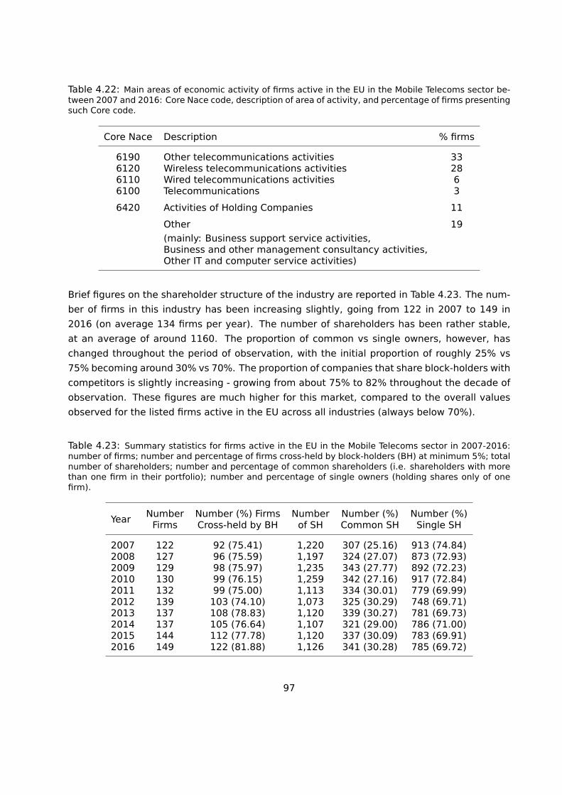
Table 4.22: Main areas of economic activity of firms active in the EU in the Mobile Telecoms sector be-tween 2007 and 2016: Core Nace code, description of area of activity, and percentage of firms presentingsuch Core code.


6190 Other telecommunications activities 336120 Wireless telecommunications activities 286110 Wired telecommunications activities 66100 Telecommunications 3

6420 Activities of Holding Companies 11

Other 19(mainly: Business support service activities,Business and other management consultancy activities,Other IT and computer service activities)

Brief figures on the shareholder structure of the industry are reported in Table 4.23. The num-

ber of firms in this industry has been increasing slightly, going from 122 in 2007 to 149 in

2016 (on average 134 firms per year). The number of shareholders has been rather stable,

at an average of around 1160. The proportion of common vs single owners, however, has

changed throughout the period of observation, with the initial proportion of roughly 25% vs

75% becoming around 30% vs 70%. The proportion of companies that share block-holders with

competitors is slightly increasing - growing from about 75% to 82% throughout the decade of

observation. These figures are much higher for this market, compared to the overall values

observed for the listed firms active in the EU across all industries (always below 70%).

Table 4.23: Summary statistics for firms active in the EU in the Mobile Telecoms sector in 2007-2016:number of firms; number and percentage of firms cross-held by block-holders (BH) at minimum 5%; totalnumber of shareholders; number and percentage of common shareholders (i.e. shareholders with morethan one firm in their portfolio); number and percentage of single owners (holding shares only of onefirm).


2007 122 92 (75.41) 1,220 307 (25.16) 913 (74.84)2008 127 96 (75.59) 1,197 324 (27.07) 873 (72.93)2009 129 98 (75.97) 1,235 343 (27.77) 892 (72.23)2010 130 99 (76.15) 1,259 342 (27.16) 917 (72.84)2011 132 99 (75.00) 1,113 334 (30.01) 779 (69.99)2012 139 103 (74.10) 1,073 325 (30.29) 748 (69.71)2013 137 108 (78.83) 1,120 339 (30.27) 781 (69.73)2014 137 105 (76.64) 1,107 321 (29.00) 786 (71.00)2015 144 112 (77.78) 1,120 337 (30.09) 783 (69.91)2016 149 122 (81.88) 1,126 341 (30.28) 785 (69.72)

97

Main players

Most of the firms are registered in the EU, with only a few large players from outside. Therefore,

in the analysis of the main firms active in this industry fourteen EU-based companies vs only

four non-EU corporations will be considered. Summary information is displayed in Table 4.24.

BlackRock dominates this industry, with rather large shares in some of the top players; Van-

guard and Norway lag behind, with relatively small participations, while State Street plays only

a minor role. France is also present, with a large participation in the French company Orange,

but also some smaller shares in other top competitors.

Table 4.24: Largest firms of Mobile Telecoms sector and selected ownership data on their main commonshareholders. Top 14 largest enterprises in the EU and top 4 outside the EU, by country of registration.Size measured by Total Assets in 2016 (Bn Euros). Direct or indirect participation shares (%) held in 2016.

Cou

ntr

y

TOA

S2

01

6(B

ne

)

Bla

ckR

ock

Fran

ce

Nor

way

Sta

teS

tree

t

Vang

uar

d


VODAFONE GROUP PLC UK 180.17 8.14 0.17 2.26 2.83 2.42DEUTSCHE TELEKOM AG DE 103.18 4.65 0.13 1.52 1.28 1.49ORANGE FR 92.59 1.98 21.00 1.51 0.53 1.57TELEFONICA SA ES 83.26 5.22 0.10 1.48 0.65 1.84LIBERTY GLOBAL PLC UK 65.16 3.06 0.75 1.98 1.53TELECOM ITALIA S.P.A IT 61.70 2.10 1.46 0.22 1.19BT GROUP PLC UK 49.35 6.72 1.38 1.80 2.1VIVENDI FR 27.01 3.94 3.12 1.62 2.12 1.83TELIA COMPANY AB SE 22.53 1.27 0.88 0.24 1.28PROXIMUS SA BE 16.49 2.60 0.21 0.79 0.31 0.92KONINKLIJKE KPN NV NL 14.74 6.53 0.19 2.01 0.29 1.59BOUYGUES SA FR 13.77 1.32 0.14 1.10 0.20 1.19TELEFONICA DEUTSCHLAND DE 10.88 0.84 0.43 0.70 0.11 0.50TDC A/S DK 8.64 2.05 2.76 0.44 2.10


CK HUTCHISON HOLDING KY 123.99 1.39 1.11 0.95 1.51AMERICA MOVIL MX 69.33 1.98 0.26 0.12 1.35MTN GROUP LIMITED ZA 18.63 1.78 0.30 0.36 2.88TELENOR ASA NO 13.62 0.82 5.55 0.58 0.99

98


The summary statistics on the density-based and uniformity indicators for Mobile Network

Operators are reported in Table 4.25. The distribution of investors portfolios is heavily skewed,

with the top 1% of portfolios having an equity interest in above 13% of the firms on the market

in 2016, albeit in a declining trend with respect to previous years. Maximum values are also

significantly high, around 24% on average for the period. This is again due to the presence,

in this industry, of large groups mothered by Telecom giants such as Vodafone, Orange or

Deutsche Telecom, which have little if no overlap in their portfolios, and have more or less

partitioned the set of firms active in this industry into independent groups.

The presence of large global investors lowers the uniformity indices, where the maximum

reaches 87% in 2016. This is because these investors have very widespread interests both in

subsidiaries as well as in the mother groups themselves.

In terms of value-based indices, there are some differences in level between TOAS and MKT

CAP results, given that the set of listed firms in this industry is rather reduced, and therefore

the second set of indices is calculated on a very restricted part of the market. We see that the

top 1% of investors hold firms that represent roughly 70% or more of the Total Assets of the

industry, showing that such top investors tend to privilege the largest enterprises. The TOAS

market shares, represented by the weighted TOAS, reach values of about 3% of the market

Total Assets through their participation shares. As we will see further down in the analysis

dedicated to top investors, it is mostly certain individual shareholders - alongside funds such as

BlackRock - that control the largest amounts of assets weighted by their participation shares,

while the telecom groups and other shareholders control smaller and smaller portions.

A similar picture holds for listed firms, where the largest portfolios (mainly the Funds) hold

firms representing almost the entire market Market Capitalisation, and through their participa-

tions control about 3% of the market value.


The final ownership in the Mobile Network Operators industry in 2016 is concentrated in the

hands of select individuals and associated holding groups, alongside large investment man-

agement firms such as Blackrock or Vanguard Group. These global shareholders hold signifi-

cant investments in large pan-European telecom groups such as Vodafone and Orange, as well

as national providers. Together, these groups and providers compose almost the entirety of

the European mobile telecommunication market. For example, Table 4.26 shows the reach of

individuals such as Mr. Carlos Slim Helú in Mexico or Mr. Victor Li Tzar Kuoi on Hong Kong, with

controlling interests in European national telecom providers, both directly and through their

controlled holdings.

99

Table 4.25: Telecoms sector common shareholding indices. Summary Statistics by year (percentagepoints, index values between 0 and 100): mean, 75th percentile (p75), 99th percentile (p99), maximum(max). Density: Proportion of firms in a shareholder’s portfolio relative to the total number of firms in themarket. Uniformity: Relative weight of larger participation shares over the shares total in the portfolio.Small values denote concentrated investment. TOAS density: Proportion of total assets of the marketrepresented by the firms in portfolio. Weighted TOAS density: Proportion of total assets of the marketheld by shareholder through participation shares. MKT CAP density: Proportion of market capitalisationof the market represented by the firms in portfolio. Weighted MKT CAP density: Proportion of marketcapitalisation of the market held by shareholder through participation shares.

Year Density

mean p75 p99 max

2007 1.9793 1.6393 19.6721 22.13112008 2.0221 1.5748 19.6850 22.83462009 1.9521 1.5504 20.1550 23.25582010 1.9423 1.5385 19.2308 23.84622011 1.9392 1.5152 18.9394 23.48482012 1.7969 1.4388 17.2662 22.30222013 1.7596 1.4599 16.7883 24.08762014 1.7401 1.4599 16.7883 24.81752015 1.6778 1.3889 15.9722 24.30562016 1.5896 1.3423 13.4228 24.1611

Year Uniformity

mean p75 p99 max

2007 11.3223 0.0000 79.9896 83.352008 12.0384 15.3604 80.0174 85.502009 12.3053 20.5333 79.8603 84.992010 11.9752 16.3526 80.1282 83.882011 12.7353 25.9924 79.2355 85.532012 12.6269 26.2247 79.7097 85.142013 12.3826 26.2024 77.5718 86.932014 12.0850 23.2642 77.7652 87.122015 12.0788 24.5015 78.9143 87.512016 12.0780 23.6421 76.5931 87.34

Year TOAS density

mean p75 p99 max

2007 7.4309 7.4203 69.8989 78.47162008 8.3073 7.8860 74.8037 79.16962009 7.8094 7.5798 74.3395 78.97112010 7.9720 7.8477 71.1840 78.18842011 7.6715 7.7347 70.0327 75.65232012 7.8307 11.6326 67.1252 75.92082013 7.4921 7.9090 67.7414 77.88502014 7.7871 8.3077 68.4811 79.38062015 8.7723 9.5516 73.6521 81.99152016 8.1432 10.0338 69.7344 82.4209


mean p75 p99 max

2007 0.0860 0.0359 1.5411 4.55592008 0.0925 0.0426 1.6098 3.96372009 0.0879 0.0385 1.4706 3.02562010 0.0930 0.0406 1.4843 3.38772011 0.0926 0.0435 1.3986 3.16492012 0.1016 0.0474 1.7398 3.61712013 0.0952 0.0486 1.3742 3.59392014 0.1014 0.0497 1.4447 4.04982015 0.1042 0.0479 1.4203 4.00092016 0.1058 0.0490 1.5877 3.2686


mean p75 p99 max

2007 7.7725 6.2385 85.8200 96.79532008 10.4532 16.4621 92.7547 98.43062009 9.8064 17.0676 91.4586 98.19872010 9.7489 14.0196 91.2640 97.95732011 10.4767 12.4617 90.9646 98.22892012 10.6983 10.9133 87.2116 96.16432013 9.2160 11.3131 85.0667 99.32752014 9.4158 11.0683 85.5496 96.72832015 9.2643 11.8521 85.8330 99.33242016 8.7866 8.5342 83.3435 99.1699


mean p75 p99 max

2007 0.0750 0.0276 1.2486 4.12362008 0.0800 0.0291 1.3366 3.82362009 0.0788 0.0282 1.4514 3.38802010 0.0753 0.0313 1.2841 3.67042011 0.0853 0.0415 1.3257 4.38552012 0.0909 0.0433 1.3286 4.55462013 0.0811 0.0403 1.0815 4.25212014 0.0898 0.0452 1.4224 3.82892015 0.0916 0.0412 1.5243 3.57032016 0.0925 0.0377 1.7629 3.7309

Investment management groups such as Blackrock Inc are also major shareholders in Euro-

pean telecom groups such as Vodafone, where Blackrock holds 8.14%. Vodafone Group PLC

is a major player in the market, holding more than 8% of undertakings active in the sector

through its full ownership of subsidiaries in Spain, Italy, Romania, Check Republic, Hungary,

Netherlands, Germany, and so on. Similarly, Orange controls subsidiaries in Spain, Poland,

Belgium, Romania and Slovakia. Note that not all subsidiaries of these groups are shown for

conciseness. As Table 4.26 shows, the top global shareholders in the sector often hold signifi-

cant portions of Total Assets. In particular, the aforementioned Carlos Slim Helú, Victor Li Tzar

Kuoi, and Blackrock each hold 3.26%, 3.09%, and 3.18% of weighted Total assets respectively.

Also rather important are the States, with France and Norway ranking amongst the top in-

vestors. While Total Assets are less significant in comparison to other shareholders (about 1%

weighted Total Assets for the two), the number of undertakings invested in is significant, reach-

ing 24.16% for Norway. Table 4.26 presents all these top shareholders, based on weighted

Total Assets, reporting first the individuals and their associated holdings, and then the funds,

telecom groups, and states.

The time trends of the common shareholding indices are reported for the usual four groups

of shareholders’ types (Funds, States, Banks and Insurance companies) as well as for the top

cross investors, that is, the most important telecom groups with significant assets or sub-

sidiaries active in the EU. Figures 4.4 and 4.5 report the results for density and weighted TOAS

density for the top investors and top cross-investors, respectively.

We observe rather constant density for Funds and States, while Banks and Insurance com-

panies seem to be divesting in this sector. The largest portfolios in terms of undertakings

invested in remain those of Norway and Sweden. However, as Table 4.26 previously demon-

strated, the biggest shareholders in terms of weighted Total Assets density remain the funds,

in particular Blackrock with more than 3%, followed by the individuals mentioned in Table 4.26

but not shown here. In terms of Total Assets, Banks and Insurance confirm a decline in quanti-

ties held. The remaining Funds, such as Vanguard Group are located at much lower levels for

the entire period, finishing just above 1% but steadily increasing.

Looking at cross-owners in Figure 4.5, we see that the relative size of the portfolios of the

Telecom groups has been stable throughout the period (between 4% and 10%). Vodafone and

Deutsche Telekom remain important players from this perspective, because of the number

of national subsidiaries that are wholly or significantly owned. Looking at the share of total

assets weighted by participation, however, the values have been converging to between 1%

and 2% for all the groups. The shares of total assets are not very high, due to the fact that

parent companies and large global shareholders are included, diluting the share of controlled

total assets.

101

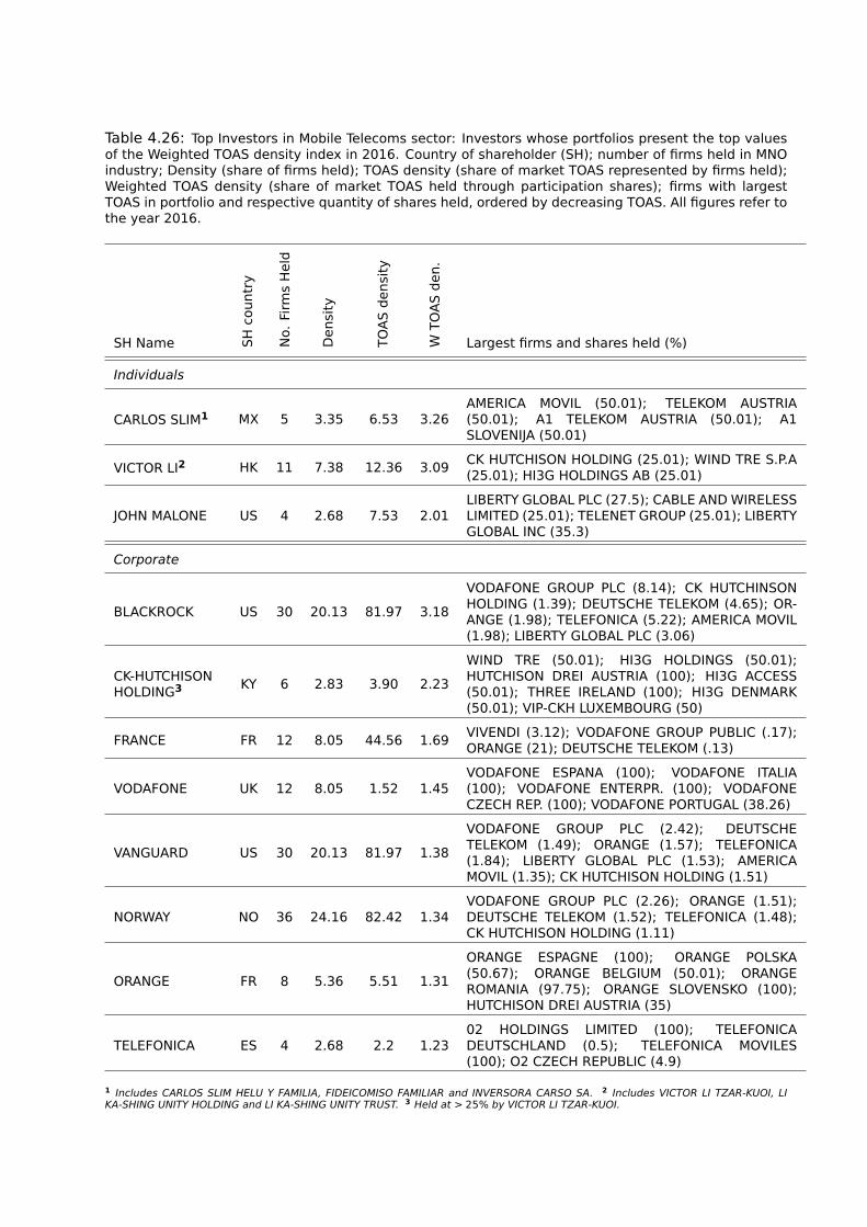
Table 4.26: Top Investors in Mobile Telecoms sector: Investors whose portfolios present the top valuesof the Weighted TOAS density index in 2016. Country of shareholder (SH); number of firms held in MNOindustry; Density (share of firms held); TOAS density (share of market TOAS represented by firms held);Weighted TOAS density (share of market TOAS held through participation shares); firms with largestTOAS in portfolio and respective quantity of shares held, ordered by decreasing TOAS. All figures refer tothe year 2016.

SH Name SH

countr

y

No.

Firm

sH

eld

Den

sity

TOA

Sden

sity

WTO

AS

den

.


Individuals

CARLOS SLIM1 MX 5 3.35 6.53 3.26AMERICA MOVIL (50.01); TELEKOM AUSTRIA(50.01); A1 TELEKOM AUSTRIA (50.01); A1SLOVENIJA (50.01)

VICTOR LI2 HK 11 7.38 12.36 3.09 CK HUTCHISON HOLDING (25.01); WIND TRE S.P.A(25.01); HI3G HOLDINGS AB (25.01)

JOHN MALONE US 4 2.68 7.53 2.01LIBERTY GLOBAL PLC (27.5); CABLE AND WIRELESSLIMITED (25.01); TELENET GROUP (25.01); LIBERTYGLOBAL INC (35.3)

Corporate

BLACKROCK US 30 20.13 81.97 3.18

VODAFONE GROUP PLC (8.14); CK HUTCHINSONHOLDING (1.39); DEUTSCHE TELEKOM (4.65); OR-ANGE (1.98); TELEFONICA (5.22); AMERICA MOVIL(1.98); LIBERTY GLOBAL PLC (3.06)

CK-HUTCHISONHOLDING3 KY 6 2.83 3.90 2.23

WIND TRE (50.01); HI3G HOLDINGS (50.01);HUTCHISON DREI AUSTRIA (100); HI3G ACCESS(50.01); THREE IRELAND (100); HI3G DENMARK(50.01); VIP-CKH LUXEMBOURG (50)

FRANCE FR 12 8.05 44.56 1.69 VIVENDI (3.12); VODAFONE GROUP PUBLIC (.17);ORANGE (21); DEUTSCHE TELEKOM (.13)

VODAFONE UK 12 8.05 1.52 1.45VODAFONE ESPANA (100); VODAFONE ITALIA(100); VODAFONE ENTERPR. (100); VODAFONECZECH REP. (100); VODAFONE PORTUGAL (38.26)

VANGUARD US 30 20.13 81.97 1.38

VODAFONE GROUP PLC (2.42); DEUTSCHETELEKOM (1.49); ORANGE (1.57); TELEFONICA(1.84); LIBERTY GLOBAL PLC (1.53); AMERICAMOVIL (1.35); CK HUTCHISON HOLDING (1.51)

NORWAY NO 36 24.16 82.42 1.34VODAFONE GROUP PLC (2.26); ORANGE (1.51);DEUTSCHE TELEKOM (1.52); TELEFONICA (1.48);CK HUTCHISON HOLDING (1.11)

ORANGE FR 8 5.36 5.51 1.31

ORANGE ESPAGNE (100); ORANGE POLSKA(50.67); ORANGE BELGIUM (50.01); ORANGEROMANIA (97.75); ORANGE SLOVENSKO (100);HUTCHISON DREI AUSTRIA (35)

TELEFONICA ES 4 2.68 2.2 1.2302 HOLDINGS LIMITED (100); TELEFONICADEUTSCHLAND (0.5); TELEFONICA MOVILES(100); O2 CZECH REPUBLIC (4.9)

1 Includes CARLOS SLIM HELU Y FAMILIA, FIDEICOMISO FAMILIAR and INVERSORA CARSO SA. 2 Includes VICTOR LI TZAR-KUOI, LIKA-SHING UNITY HOLDING and LI KA-SHING UNITY TRUST. 3 Held at > 25% by VICTOR LI TZAR-KUOI.

Figure 4.4: Common shareholding indices for Top Investors in Mobile Telecoms sector. Top panel: Density- Proportion of firms in a shareholder’s portfolio relative to the total number of firms in the market.Bottom panel: Weighted TOAS density - Proportion of total assets of the market held by shareholderthrough participation shares.

0

5

10

15

20

25

2007 2009 2011 2013 2015

BLACKROCK

DIMENS. FUND

FMR LLC

STATE STREET

VANGUARD

Funds

2007 2009 2011 2013 2015

BELGIUM

FRANCE

NORWAY

SWEDEN

States

2007 2009 2011 2013 2015

BANK NY ME

BARCLAYS

BNP PARIBAS

CREDIT SUISSE

DEUTSCHE BANK

JPMORGAN CHASE

Banks

2007 2009 2011 2013 2015

ALLIANZ SE

AXA SA

STICHTING PENSIOEN

TEACHERS INSUR

Insurance

Density (%)

0

.5

1

1.5

2

2.5

3

3.5

2007 2009 2011 2013 2015

BLACKROCK

DIMENS. FUND

FMR LLC

STATE STREET

VANGUARD

Funds

2007 2009 2011 2013 2015

BELGIUM

FRANCE

NORWAY

SWEDEN

States

2007 2009 2011 2013 2015

BANK NY ME

BARCLAYS

BNP PARIBAS

CREDIT SUISSE

DEUTSCHE BANK

JPMORGAN CHASE

Banks

2007 2009 2011 2013 2015

ALLIANZ SE

AXA SA

STICHTING PENSIOEN

TEACHERS INSUR

Insurance


103

Figure 4.5: Common shareholding indices for Top Cross Investors in Mobile Telecoms sector. Top panel:Density - Proportion of firms in a shareholder’s portfolio relative to the total number of firms in the market.Bottom panel: Weighted TOAS density - Proportion of total assets of the market held by shareholderthrough participation shares.

0

2

4

6

8

10

2007 2009 2011 2013 2015

DEUTSCHE TELEKOM

ORANGE

SFR GROUP

TELEFONICA

VIVENDI

VODAFONE

Density index (%)

0

1

2

3

4

2007 2009 2011 2013 2015

DEUTSCHE TELEKOM

ORANGE

SFR GROUP

TELEFONICA

VIVENDI

VODAFONE

Weighted TOAS Density index (%)

104

Network indices

The Mobile Telecoms industry shows stronger interconnections between actors of the same

type, comparable to the values observed in the Oil&Gas sector, evidently higher than the

cases of Electricity or Trading Platforms. The results on shareholders’ and firms’ networks are

reported in Tables 4.27 and 4.28, respectively.

The proportion of portfolios that are linked through commonly held firms has been increasing

over time, from about 2.82% to 3.15%. On the other hand, among the large connected port-

folios (density>10%) the links are weaker with respect to the previous definition of the sector,

with about 1.99% of these owners showing a correlation of 80% or higher in 2106.

The firms’ network is also highly interconnected through block-holders, with about 2.75% of

active links in 2016, and of which about half present a high correlation of more than 80%. This

very high fraction of highly-correlated ownership structures is likely the result of the presence

of clusters of firms belonging to the large Telecoms groups, which are almost all wholly owned

or at least controlled by the parent, showing therefore very similar shareholders’ structures.

Table 4.27: Network indices for Mobile Telecoms sector. Shareholders’ network. Total number of com-mon shareholders; proportion of non-zero correlations between pairs of portfolios, i.e. proportion ofconnections between two shareholders induced by common shareholding of a same firm; number ofhigh correlations (>80%) between pairs of high-density portfolios (both densities >10%); proportion ofhigh correlations between pairs of high-density portfolios.


2007 324 2.82 16 1.252008 347 3.41 12 0.782009 367 3.29 12 0.982010 363 3.22 3 0.332011 360 3.83 6 0.702012 352 3.69 8 1.722013 365 3.41 2 0.532014 347 3.34 6 1.852015 358 3.27 11 3.132016 363 3.15 7 1.99

105

Table 4.28: Network indices for Mobile Telecoms sector. Firms’ network. Total number of firms cross-held by block-holders (holding at least 5%); proportion of non-zero correlations between shareholders’structures of pairs of firms (only shares >5%); number of high correlations between shareholders’ struc-tures of pairs of firms (only shares >5%); proportion of high correlations (>80%) among the non-zerocorrelations.


2007 92 2.76 99 48.532008 96 2.99 124 51.882009 98 3.19 129 49.052010 99 3.05 124 48.442011 99 2.96 117 45.702012 103 3.04 142 48.632013 108 2.82 134 50.952014 105 2.79 111 42.692015 112 2.82 118 40.692016 122 2.75 142 46.86

106

4.5 Beverages sector - Manufacturers

The focus is on the manufacture of beverages, rather than their wholesale, although some

of the companies considered perform both types of activities. Only certain types of products

were included, namely Soft Drinks, Waters, Juices and Beers.

The set of firms active in the sector was delineated according to two steps. First, a selection

was made based on specific NACE codes of industry classification for beverages manufac-

turing: "Manufacture of beer", "Manufacture of soft drinks; production of mineral waters and

other bottled waters", and "Manufacture of fruit and vegetable juice". All listed firms active

in the EU which presented at least one of the above classifications as primary or secondary

activity were included in the sample.

Following this initial selection, a number of unlisted relevant players was added based on the

expert opinion of colleagues from DG COMP, representing unlisted companies with significant

market share or presence in European countries. All-together, we obtain a list of 290 firms, of

which 214 are listed manufacturers of Soft Drinks and/or Waters, Beer or Juices. The remaining

76 firms are the relevant unlisted players. The sector’s Total Assets in 2016 were worth 1309

Bn Euro, while the Market Capitalisation totaled 1352 Bn Euro.

Roughly two-thirds of the firms are registered in the EU (69.15%), with Germany accounting

for about 20%, then followed by France and United Kingdom at around 5%. Outside, the US is

the largest country represented, with 8.81% of firms in the sample registered there.

As shown in Table 4.29, the majority of companies (69%) classify their core activity in the Nace

Division "11: Manufacture of Beverages", divided evenly between codes "1105: Manufacture

of beer" (33%) and "1107: Manufacture of soft drinks; production of mineral waters" (32%); a

smaller percentage (4%) are occupied in "1102: Manufacture of wine from grape".

Table 4.29: Main areas of activity of firms active in the EU in the Beverages sector in 2007-2016: CoreNace code, description of area of activity, and percentage of firms presenting such Core code.


1105 Manufacture of beer 331107 Manufacture of soft drinks; production of mineral waters 321102 Manufacture of wine from grape 41089 Manufacture of other food products n.e.c. 31032 Manufacture of fruit and vegetable juice 2

4634 Wholesale of beverages 3

Other 23(mainly: Distilling, rectifying and blending of spirits,Other processing and preserving of fruit and vegetables,Activities of head offices)

107

Products such as fruit juices were also included in the sample, but they comprise a significantly

smaller portion of the sector, just 5% between codes 1089 and 1032. Instead 26% of firms

are scattered across a series of different but related activities under their core Nace, such as

wholesale or distillation.

In terms of shareholder structure of the industry, some summary data is reported in Table

4.30. The number of firms in this industry has been increasing slightly, from 241 in 2007 to

261 in 2016. Similarly, the number of shareholders has been steadily increasing, albeit not

drastically, over the same period. The initial proportion of common vs single shareholders,

although slightly declining, has not changed much throughout the period (28% and 72% vs

26% and 74% roughly). A similar pattern can be observed when considering block-holdings

of 5%, where the number (and proportion) of firms cross-held by a block-holder has remained

rather stable, just below 45% throughout most of the period. These levels are slightly below

the EU average observed for other sectors.

Table 4.30: Summary statistics for firms active in the EU in the Beverages sector between 2007 and2016: number of firms; number and percentage of firms cross-held by block-holders (BH) at minimum5%; total number of shareholders; number and percentage of common shareholders (i.e. shareholderswith more than one firm in their portfolio); number and percentage of single owners (holding shares onlyof one firm).


2007 241 104 (43.15) 1,902 533 (28.02) 1,369 (71.98)2008 245 113 (46.12) 1,874 563 (30.04) 1,311 (69.96)2009 250 113 (45.20) 1,987 607 (30.55) 1,380 (69.45)2010 257 113 (43.97) 2,058 610 (29.64) 1,448 (70.36)2011 259 111 (42.86) 2,073 572 (27.59) 1,501 (72.41)2012 259 111 (42.86) 2,035 574 (28.21) 1,461 (71.79)2013 263 116 (44.11) 2,096 580 (27.67) 1,516 (72.33)2014 264 115 (43.56) 2,079 567 (27.27) 1,512 (72.73)2015 264 118 (44.70) 2,152 567 (26.35) 1,585 (73.65)2016 261 118 (45.21) 2,152 561 (26.07) 1,591 (73.93)

Main players

Table 4.31 shows the main players in this sector, selected on the basis of their declared total

assets (in billions of euros) in 2016, alongside some of the more relevant shareholders for the

purpose of this exercise. As previously stated, about two-thirds of the firms in the sample

are registered in the EU. Among these, the biggest of these firms, Anheuser-Busch InBev, is

almost four times as big as its next largest competitor. The top ’international’ competitors on

the other hand, are far more similar in size and typically also larger than their EU counterparts.

108

Table 4.31: Largest firms active in the EU in the Beverages sector, and selected ownership data ontheir main common shareholders. Top 15 largest enterprises registered in the EU and top 15 registeredoutside the EU, by country of registration. Size measured by Total Assets in 2016 (Bn Euros). Direct orindirect participation shares (%) held in 2016.

Cou

ntr

y

TOA

S2

01

6(B

ne

)

Bla

ckR

ock

Nor

way

Sta

teS

tree

t

Vang

uar

d


ANHEUSER-BUSCH INBEV BE 192.99 0.76 0.95 1.05 0.85GRAND METROPOLITAN LTD (DIAGEO PLC) UK 55.41 7.09 1.58 2.59 2.49DANONE FR 40.96 5.40 1.50 0.69 1.88HEINEKEN NV NL 39.32 0.89 0.80 0.20 0.81UNILEVER NV NL 38.14 2.98 1.72 0.66 1.98COCA-COLA EUROPEAN PARTNERS PLC UK 18.57 0.15 0.48 0.44 0.28CADBURY LIMITED (MONDELEZ) UK 12.05 5.76 0.99 4.23 5.94GREENE KING PLC UK 7.19 2.87 1.98 0.86 2.39CARLSBERG A/S DK 6.27 4.99 1.24 0.20 1.48MARSTON’S PLC UK 3.25 2.25 1.45 0.76 2.31DAVIDE CAMPARI IT 3.18 0.71 1.08 0.13 0.99NESTLE WATERS (NESTLE S.A.) FR 2.41 3.70 2.56 0.50 2.12REFRESCO GROUP N.V. NL 1.96 0.46 5.67 1.25BRITVIC PLC UK 1.90 5.01 2.66 1.02 2.20JERONIMO MARTINS SGP PT 1.43 2.41 1.02 0.14 0.85


NESTLE S.A. CH 122.94 3.70 2.56 0.50 2.12THE COCA-COLA COMPANY US 82.79 5.42 0.87 3.93 6.37PEPSICO INC US 69.72 5.53 0.94 4.36 1.43MONDELEZ INTERNATIONATIONAL US 58.38 5.76 0.99 4.23 5.94QUINENCO S.A. CL 52.32 0.18SWIRE PACIFIC LIMITED HK 45.70 0.98 0.82 0.49 0.75MOLSON COORS BREWING US 27.84 4.96 0.50 3.47 7.24FOMENTO ECONOMICO MEXICANO MX 24.97 0.83 0.16 0.32SAN MIGUEL CORPORATION PH 24.89AMBEV SA (ANHEUSER-BUSCH INBEV) BR 24.41 1.28 0.30 0.13 0.98GENERAL MILLS INC US 19.47 6.69 0.92 5.96 5.80BEIJING ENTERPRISES HK 17.70 2.22 0.31 0.15 1.31KIRIN HOLDINGS JP 13.71 4.90 1.13 0.54 1.87DR PEPPER SNAPPLE GROUP INC US 9.29 8.82 1.01 4.57 9.35ASAHI GROUP HOLDINGS JP 9.01 2.19 1.07 0.59 1.62

109

The last four columns show the participation of the shareholders considered most relevant in

terms of common shareholding positions. BlackRock dominates this industry, with rather large

shares in most of the top players, reaching up to 8.82%. The others lag behind, with relatively

small participations. State Street in particular is a minor player for the observed year.


The summary statistics on the density-based and uniformity indicators are reported in Table

4.32. Across all reported quantiles, the share of firms held by investors is declining. Even

though the top investor holds almost 25% of all firms in the sector, the remaining investors

are trimming their portfolio density. This pattern is evident when looking at the top 1% of

investors, which in 2007 held above 14% of firms in the sector; in 2016 this declined to 11.2%.

While the distribution of investors portfolios is still skewed, this is less so when compared to

other sectors analysed earlier, showing at first a more diversified shareholder network.

On the other hand, the uniformity index remains more or less stable throughout the period,

with the average (around 10%) indicating that most shareholders are concentrated on few

firms in their investment decisions. The years 2015 and 2016 show a slightly larger number

of investors with non-reported shares (about 1.3% compared to less than 1% in the previous

years), yielding a slightly larger proportion of single owners (with zero uniformity index). For

this reason the values of the 75th percentile drop in these two years.

In terms of value-based indices, there are some differences in level between TOAS and MKT

CAP results due to the fact that some firms in the sample are not listed. The table shows that

the top 1% of investors hold firms that represent at least between 53% and 60% of the Total

Assets of the industry depending on the year (declining trend), while the top investor per year

has held an increasing share of the Total Assets of the sector, up to 82% in 2016. Such values

are in line with expectations on investor behaviour, since top investors tend to privilege the

largest enterprises. However, when this index is weighted according to the participation share

of investors, the trend inverts, and it can be seen how the largest investor holds a slightly

decreasing share of weighted Total Assets. Given the results from the unweighted Total Assets

density, it would seem that top investors, and other investors in general, are diluting their

investment concentration among more firms.

A similar picture holds for listed firms, where the largest portfolios hold firms representing

almost the industry’s entire Market Capitalisation, and through their participations control

about 4% of the market value. In 2016, the top value for the Total Asset index corresponds

to Stichting Anheuser-Busch InBev, which holds a large direct participation in only one firm,

Anheuser-Busch InBev, the largest player in the market; this single participation amounts to

5% of the market total assets.8

8This investor did not appear in Table 4.33, since it is not a common shareholder.

110

Table 4.32: Beverages sector common shareholding indices. Summary Statistics by year (percentagepoints, index values between 0 and 100): mean, 75th percentile (p75), 99th percentile (p99), maximum(max). Density: Proportion of firms in a shareholder’s portfolio relative to the total number of firms in themarket. Uniformity: Relative weight of larger participation shares over the shares total in the portfolio.Small values denote concentrated investment. TOAS density: Proportion of total assets of the marketrepresented by the firms in portfolio. Weighted TOAS density: Proportion of total assets of the marketheld by shareholder through participation shares. MKT CAP density: Proportion of market capitalisationof the market represented by the firms in portfolio. Weighted MKT CAP density: Proportion of marketcapitalisation of the market held by shareholder through participation shares.

Year Density

mean p75 p99 max

2007 1.1737 0.8299 13.6929 23.23652008 1.2223 0.8163 14.6939 24.48982009 1.1539 0.8000 14.0000 23.20002010 1.0830 0.7782 13.6187 23.34632011 1.0464 0.7722 12.3552 23.93822012 1.0538 0.7722 12.7413 24.32432013 1.0148 0.7605 12.1673 25.85552014 1.0014 0.7576 11.3636 24.24242015 0.9827 0.7576 11.7424 23.48482016 0.9673 0.7663 11.1111 23.7548

Year Uniformity

mean p75 p99 max

2007 11.6126 18.0240 80.08 87.472008 12.6035 23.8995 80.39 88.872009 12.3630 23.2265 80.05 88.792010 11.9174 21.4334 78.82 88.872011 11.1801 13.8747 78.27 87.382012 11.3974 15.7820 78.49 88.692013 11.2386 15.1230 77.83 89.632014 11.1712 14.9939 78.38 89.182015 10.6359 4.7023 77.66 89.712016 10.3846 0.0000 77.26 88.44

Year TOAS density

mean p75 p99 max

2007 3.3957 1.8235 54.2706 68.75802008 3.6018 1.6250 59.4013 76.07632009 3.3997 1.7581 59.6992 75.31832010 3.4720 1.4321 59.4506 77.15182011 3.5727 2.1656 57.6684 77.68102012 3.4596 2.0395 55.4596 81.43822013 3.4603 3.1643 55.0004 81.90812014 3.3045 1.2180 54.8999 81.81912015 3.2564 1.7686 53.0278 79.77912016 3.4460 1.9012 55.0029 81.7071


mean p75 p99 max

2007 0.0526 0.0123 0.9355 9.73322008 0.0472 0.0115 0.9804 7.58682009 0.0453 0.0104 1.0497 6.81322010 0.0426 0.0094 0.8014 5.90342011 0.0451 0.0121 1.1049 5.18562012 0.0469 0.0121 0.9054 5.47382013 0.0522 0.0130 1.0894 5.42752014 0.0464 0.0100 1.0640 5.23382015 0.0481 0.0112 1.0125 4.94682016 0.0448 0.0090 0.9203 5.0550


mean p75 p99 max

2007 4.5776 0.6308 79.1511 91.68802008 4.7761 0.6713 80.9224 92.88852009 4.5231 0.9838 84.2562 92.56052010 4.3595 0.8348 81.4195 93.18192011 4.5801 1.0658 81.8512 94.30822012 4.0444 0.9599 69.3285 87.01252013 4.2028 1.3411 73.1618 94.31782014 4.0458 0.8432 72.3251 92.32302015 4.3344 1.0635 69.9960 94.71392016 4.5102 1.2788 69.6414 96.1065


mean p75 p99 max

2007 0.0404 0.0040 0.6531 5.71542008 0.0366 0.0049 0.6580 4.41772009 0.0380 0.0057 0.6928 4.22232010 0.0365 0.0049 0.6492 3.36662011 0.0393 0.0085 0.6704 3.71312012 0.0410 0.0089 0.5933 7.40802013 0.0489 0.0099 0.8511 7.45822014 0.0392 0.0056 0.7480 4.44572015 0.0423 0.0079 0.7056 4.71102016 0.0401 0.0077 0.6559 4.3167


The list of top common investors9 presented in Table 4.33 ranks these shareholders based on

their weighted Total Assets density for 2016, i.e. the share of total market TOAS held through

the stakes of firms in their portfolios. It is immediately evident that the main investors are

the sector-specific corporate groups with many controlled subsidiaries. Diageo Plc, L’Arche

Green, and Anheuser-Busch InBev are just three of those large corporate groups responsible

for well-known brands, such as the case of L’Arche Green and Heineken. In fact, the table

hints at the heterogeneity within the Beverage sector, where those groups or firms involved in

the production and/or distribution of alcoholic products are structured in a similar manner to

what was seen in Telecoms, with large corporate groups and many cross-holdings. The other

beverage producers instead tend to be defined as smaller enterprises with local markets and

a limited shareholder structure.

Alongside these corporate groups, the large investment management funds are also present

as main investors. As will be highlighted in greater detail in the following sections, Black-

Rock leads among these funds under every observed metric. In terms of weighted total asset

density, BlackRock in 2016 accounted for 2.33% of the market’s total assets, not far off from

one of the leading corporate groups, Anheuser-Busch InBev with 2.92%. Vanguard and State

Street enter into the ranks of top investors, but fall short of these values. Observing the port-

folio composition of these investment management funds, there is evidence of an appetite for

investment in larger corporate groups or holdings as opposed to individual or smaller produc-

ers: some of the biggest corporate groups such as Anheuser-Busch InBev appear alongside

some of the bigger producers of beverages such as The Coca-Cola Company.

Finally, it should be noted that other financial institutions are missing from the ranks of top

investors. Large banks or insurance companies do not appear, a trend which is repeated over

different sectors and can be confirmed when looking at the time series for ownership indices

across different investor classes. State participation is also missing, excluding the Norwegian

sovereign fund which presents a portfolio similar in composition to that of the other large

funds mentioned earlier, with investments in corporate groups such as Anheuser-Busch InBev

or Nestle SA.

As a final comment, there are several comparisons that can be drawn between the top in-

vestors of this sector and that of Mobile Telecoms, when defined as Mobile Network Operators

and Parents (see Section 4.4). In particular, cross-investing is prevalent in both these sectors.

The time trends of the common shareholding indices are reported for the usual four groups of

shareholders’ types (Funds, States, Banks and Insurance companies). Figure 4.6 reports the

results for density and weighted TOAS density for the top investors.

9Only investors with more than one firm in portfolio are reported.

112

Table 4.33: Top Common Investors in Beverages sector: Investors with more than one firm in portfolio,whose portfolios present the top values of the Weighted TOAS density index in 2016. Country of share-holder (SH); number of firms held in MNO industry; Density (share of firms held); TOAS density (shareof market TOAS represented by firms held); Weighted TOAS density (share of market TOAS held throughparticipation shares); firms with largest TOAS in portfolio and respective quantity of shares held, orderedby decreasing TOAS. All figures refer to the year 2016.

SH Name SH

countr

y

No.

Firm

sH

eld

Den

sity

TOA

Sden

sity

WTO

AS

den

.


DIAGEO PLC UK 3 1.15 4.28 4.25 GRAND METROPOLITAN LTD (100); EASTAFRICAN BREWERIES LTD (50.03)

L’ARCHEGREEN NL 6 2.30 6.71 3.40

HEINEKEN HOLDING NV (51.71); HEINEKENNV (50.01); SCOTTISH & NEWCASTLE (50.01);HEINEKEN ASIA PACIFIC (50.01)

ANHEUSER-BUSCH INBEV BE 10 3.83 3.89 2.92

AMBEV SA (61.95); ABI SAB GROUP HOLDING(100); ANADOLU EFES BIRACIL (24); SUN IN-TERBREW PLC (99.95); BANKS HOLDINGS LTD(34.09); FOSTER’S GROUP (100); LÖWENBRÄUAG (100)

BLACKROCK US 62 23.75 78.29 2.33

ANHEUSER-BUSCH INBEV (0.76); NESTLE S.A.(3.70); THE COCA-COLA COMPANY (5.42); PEP-SICO INC (5.53); MONDELEZ INTERNATIONAL(5.76); SWIRE PACIFIC LTD (0.98); DANONE (5.4)

VANGUARD US 59 22.61 78.06 1.86

ANHEUSER-BUSCH INBEV (0.85); NESTLE S.A.(2.12); THE COCA-COLA COMPANY (6.73); PEP-SICO INC (1.43); MONDELEZ INTERNATIONAL(5.94); SWIRE PACIFIC LTD (0.75); DANONE(1.88)

FOMENTOECONOMICO MX 3 1.15 6.98 1.44 HEINEKEN HOLDING NV (14.94); HEINEKEN NV

(12.53); COCA-COLA FEMSA SAB (63)

STATE STREET US 44 16.86 72.04 1.21

ANHEUSER-BUSCH INBEV (1.05); NESTLE S.A.(0.50); THE COCA-COLA COMPANY (3.93); PEP-SICO INC (4.36); MONDELEZ INTERNATIONAL(4.23); SWIRE PACIFIC LTD (0.49); DANONE(0.69)

CAPITALGROUP US 22 8.43 42.86 0.95

NESTLE S.A. (1.98); THE COCA-COLA COMPANY(5.51); PEPSICO INC (0.65); MONDELEZ INTER-NATIONAL (1.65); DANONE (0.30); UNILEVERNV (0.61); AMBEV SA (0.12)

NORWAY NO 58 22.22 81.71 0.89

ANHEUSER-BUSCH INBEV (0.95); NESTLE S.A.(2.56); THE COCA-COLA COMPANY (0.87); PEP-SICO INC (0.94); MONDELEZ INTERNATIONAL(0.99); QUINENCO S.A. (0.18); SWIRE PACIFICLTD (0.82)

FMR LLC US 38 14.56 65.81 0.69

ANHEUSER-BUSCH INBEV (0.77); NESTLE S.A.(0.64); THE COCA-COLA COMPANY (1.57); PEP-SICO INC (0.59); MONDELEZ INTERNATIONAL(1.38); QUINENCO S.A. (0.15); DANONE (0.15)

As previously noted in other sectors, Funds and States (only Norway in this case) remain

relatively stable in the share of total firms held in their portfolios, while Banks and Insurance

companies seem to be divesting in this sector. The largest portfolios in terms of undertakings

invested in remains that of BlackRock, which peaked above 25%. Indeed, BlackRock has

consistently appeared among the funds as the investor with the greatest reach. Even when

considering the weighted Total Assets density, BlackRock is still considerably ahead of its

competitors, holding more than 2.5% of weighted total assets from 2009 to 2016. Table 4.33

also confirms these findings. In terms of Total Assets, Banks and Insurance confirm a decline

to levels well below BlackRock. The remaining Funds, such as Vanguard Group, are located at

much lower levels for the entire period, finishing just above 2% but steadily increasing.

As mentioned previously, cross-investment - that is the participation of corporate groups or

ultimate owners among each other - defines investment behaviour in this sector. Figure 4.7

therefore looks at the top cross-investors for this sector. When considering the proportion of

firms that a top investor holds in its portfolio for the observed year, corporate groups such

as Anheuser-Busch InBev (also known as AB InBev) and L’Arche Green - which control brands

such as Becks and Heineken respectively - dominate the market with respect to competitors.

In 2016, AB InBev boasts participations in almost 4% of total firms.

However, when considering a weighted measure of total assets controlled, there are new play-

ers in the market to consider, such as Diageo Plc, responsible for the production of alcoholic

beverages, especially liquors and spirits (with Guinness, Baileys and Johnnie Walker among

the main brands). While the Diageo group boasted almost 10% of weighted total assets at the

beginning of the period, this value has been declining and converging towards values more

in line with other top cross-investors. When considering weighted total assets density, these

top cross-investors account for a greater share of the market with respect to funds or other

financial institutions. For example, both AB InBev and Diageo Plc account for roughly 4% of

weighted total assets in 2016, while BlackRock (the biggest of the funds) peaks at 2.5%. This

is the result of a sector, as stated before, characterised on one end by large corporate groups

with many subsidiaries.

114

Figure 4.6: Common shareholding indices for Top Investors in Beverages sector. Top panel: Density -Proportion of firms in a shareholder’s portfolio relative to the total number of firms in the market. Bottompanel: Weighted TOAS density - Proportion of total assets of the market held by shareholder throughparticipation shares.

0

5

10

15

20

25

2007 2009 2011 2013 2015

BLACKROCK

DIMENS. FUND

FMR LLC

STATE STREET

VANGUARD

Funds

__ NORWAY

2007 2009 2011 2013 2015

States

2007 2009 2011 2013 2015

BANK NY ME

BARCLAYS

BNP PARIBAS

CREDIT SUISSE

DEUTSCHE BANK

GOLDMAN SACHS

JPMORGAN CHASE

Banks

2007 2009 2011 2013 2015

ALLIANZ SE

AXA SA

STICHTING PENSIOEN

TEACHERS INSUR

Insurance

Density (%)

-1

-.5

0

.5

1

1.5

2

2.5

2007 2009 2011 2013 2015

BLACKROCK

DIMENS. FUND

FMR LLC

STATE STREET

VANGUARD

Funds

__NORWAY

2007 2009 2011 2013 2015

States

2007 2009 2011 2013 2015

BANK NY ME

BARCLAYS

BNP PARIBAS

CREDIT SUISSE

DEUTSCHE BANK

GOLDMAN SACHS

JPMORGAN CHASE

Banks

2007 2009 2011 2013 2015

ALLIANZ SE

AXA SA

STICHTING PENSIOEN

TEACHERS INSUR

Insurance


115

Figure 4.7: Common shareholding indices for Top Cross Investors in Beverages sector. Left panel:Density - Proportion of firms in a shareholder’s portfolio relative to the total number of firms in the market.Right panel: Weighted TOAS density - Proportion of total assets of the market held by shareholder throughparticipation shares.

0

.5

1

1.5

2

2.5

3

3.5

4

2007 2009 2011 2013 2015

Density (%)

0

2

4

6

8

10

2007 2009 2011 2013 2015


Beverages Sector - Cross Investors

ANHEUSER-BUSCH INBEV DIAGEO PLC FOMENTO ECONOMICO ME L'ARCHE GREEN N.V.

Network indices

The summary statistics regarding shareholders’ and firms’ networks are presented in Tables

4.34 and 4.35, respectively. Several key details should be pointed out regarding these tables.

In the shareholders’ network, only the largest portfolios are considered for the calculation

of correlations, to avoid obtaining very high irrelevant values. For example, if we consider

two coincident small portfolios, both holding the same amount of shares in two very small

firms, their correlation would be maximum, but the two investors are not interesting players.

Therefore, we look at correlations only for investors whose portfolios hold at least 10% of the

firms active in the market.

Applying a similar reasoning, in the case of the firms’ network a minimum value of 5% invest-

ment by the shareholder is used in calculating the correlations among shareholding structures

of firms. Fundamentally, the attention is restricted only to those investors with more intensive

presence in the firm, with block-holdings of minimum 5%. An analysis of alternative levels of

block-holding is reported later in Chapter 5.

116

Due to the heterogeneity of firms, with large corporate groups mixed among smaller regional

producers, the strength of the shareholders’ network is less evident. For this reason as well,

the proportion of portfolios that are linked through commonly held firms has been decreas-

ing over time, from about 2.34% to 1.83%. On the other hand, among those high-density

portfolios (density>10%), the number of high correlations between said portfolios is small and

decreasing over time. This could be due to those corporate groups such as AB InBev with large

portfolios consisting of fully controlled subsidiaries.

At the given level of block-holdings (5%), the firms’ network is less interconnected in compari-

son to other sectors, with less than 1% of possible connections between shareholder structures

presenting some correlation. In turn, the proportion of these correlations that could be con-

sidered high (>80%) was only 23.53% in 2016. The presence of many regional firms with

niche markets in this sample helps explain some of these lower correlations in the networks,

but equally the presence of corporate groups with large vertical investments results in weaker

correlations across the shareholder structures.

Table 4.34: Network indices for Beverages sector. Shareholders’ network. Total number of commonshareholders; proportion of non-zero correlations between pairs of portfolios, i.e. proportion of con-nections between two shareholders induced by common shareholding of a same firm; number of highcorrelations (>80%) between pairs of high-density portfolios (both densities >10%); proportion of highcorrelations between pairs of high-density portfolios.


2007 552 2.34 4 0.632008 587 2.69 6 0.632009 627 2.57 5 0.582010 629 2.53 4 0.672011 590 2.48 4 0.922012 594 2.52 2 0.492013 599 2.38 1 0.262014 588 2.20 3 0.792015 590 1.95 2 0.362016 582 1.83 2 0.49

117

Table 4.35: Network indices for Beverages sector. Firms’ network. Total number of firms cross-held byblock-holders (holding at least 5%); proportion of non-zero correlations between shareholders’ structuresof pairs of firms (only shares >5%); number of high correlations between shareholders’ structures of pairsof firms (only shares >5%); proportion of high correlations (>80%) among the non-zero correlations.


2007 115 0.77 59 26.582008 124 0.69 74 35.752009 123 0.88 87 31.752010 123 0.86 78 27.562011 126 0.74 76 30.772012 128 0.85 72 25.352013 130 0.79 65 23.992014 125 0.71 68 27.532015 128 0.72 75 30.002016 129 0.80 64 23.53

118

Box 4.1: Focus on markets - Oil&Gas

� The Oil&Gas industry is composed of 153 distinct corporations active in the EU during the

period 2007-2016, of which 73% are listed. Although most firms are active throughout

the whole period of observation, some are active for a shorter period of time, either due

to a later entry into the market or to an exit resulting from M&A, dissolution or other

reasons. Therefore, the set of firms is not constant over time, oscillating between 125

and 139 firms per year (on average 134) during the ten years of observation. About 46%

of the firms are registered outside the EU, almost half of which are in the US, followed by

Canada and Australia, with yet a smaller proportion coming from China, Japan, Norway

and Russia.

� The proportion of firms cross-held by block-holders is in line with the general picture of

listed firms in the EU, i.e. rather stable at around 63%.

� The majority of investors (75%) in companies in the Oil&Gas sector only hold participation

in 2 firms or less. This changes dramatically when looking at the largest portfolios, where

the top 1% of common shareholders hold more than 38 firms on average (≈ 28% of the

market). All these figures remain rather stable over the ten years of observation. The

maximum size of portfolios is very large, with portfolios encompassing 40% or more of

the firms in the market being observed in every year. This figure has been increasing

over time, reaching a peak of 45% in 2016, i.e. about 60 competing companies (out of

the 135 composing the market).

� The largest (top 1%) common shareholders include participation in almost all relevant

firms, representing more than 70% of the market value in terms of Total Assets (TOAS

is roughly 3309 Bn Euro in 2016), and more than 85% of Market Capitalisation (roughly

1811 Bn Euro in 2016), on average over the ten years. The most comprehensive portfolio

holds participations in firms which represent close to 90% of TOAS and almost 100% of

MKT CAP, revealing that the largest investors hand-pick all the firms with the largest value

in the market.

� Once we consider the percentage of shares actually owned by common shareholders, we

find that 99% of portfolios hold less than 1% of the value of the market through their

participation shares, both in terms of TOAS and of MKT CAP.

� However, top common shareholders BlackRock, Vanguard, State Street and Norway (short

for the Norwegian Sovereign Fund) hold large amounts of market value within their grasp:

in 2016 their shares in companies in portfolio amounted to about 12.88% of the TOAS

(approximately 426 Bn Euro).

Cont. next page

119

Box 4.1 (cont.): Focus on markets - Oil&Gas

� In terms of shares, BlackRock dominates with investments in the largest EU-registered

companies, with participated values up to 6.9% in 2016, generally much higher than

the remaining three investors (Vanguard, State Street and Norway). In 2016, the firms

participated in by BlackRock constituted roughly 90% of Total Assets of the Oil&Gas mar-

ket (about 3309 Bn), with about 4.2% of TOAS also controlled by BlackRock through its

participations.

� Among firms registered in the EU, State Street principally concentrates its investments in

UK companies, with participations between 0.18% and 3.38% in 2016. However, it holds

larger stakes in top US-based companies, such as Exxon and Chevron, with approximately

5-6% holdings. The companies in its portfolio represent 80.2% of the TOAS in the market,

and State Street controls approximately 2.55% of the market TOAS.

� In the last year of observation (2016), Norway only holds minority stakes in EU-based

firms (between 0.79% and 2.35%), but controls national Statoil with a participation of

67%, whilst also holding stakes in several US giants. Overall, this amounts to controlling

about 2.72% of the TOAS, with firms in the portfolio representing 86% of the market

value. Vanguard has small participations in EU firms (between 0.68% and 2.73%), and

holds several larger stakes (around 7%) in top US-based Oil companies; it controls 3.42%

of the TOAS of the Oil&Gas market.

� A peculiar case is the Russian Government, which holds almost 6% of the Total Assets of

the market in 2016 via its subsidiaries Gazprom and Rosneft, but has little if no participa-

tions in other companies.

�

120

Box 4.2: Focus on markets - Electricity

� The Electricity sector includes 396 firms active in the EU, of which 39% are registered

outside, mainly in the US, Canada, Switzerland and Russia. Most firms are listed (89%).

In 2016, the selected firms totaled 3330 Bn Euro of Total Assets, while the listed firms

had a Market Capitalisation of 864 Bn Euro.

� The number of active firms per year has been increasing steadily, going from 275 in

2007 to 353 in 2016, with an average of 325 firms per year. The Electricity sector is

characterised by the strong presence of state-owned companies, with Sovereign Funds

holding very large shares in their national providers - in many cases even being the

majority owners - as in the case of France, China, Korea and Sweden.

� Although the absolute number of firms cross-held by block investors has been increasing

since 2007, their proportion had decreased about 7 percentage points (from 62.5 in 2007

to 55.5 in 2016), given the rapid growth of the size of this industry. In 2016, the largest

shareholders (top 1%) held more than 30 firms active in the market (corresponding to

9% of the total number of firms). The top portfolio had participations in 29% of the firms,

approximately 100 companies.

� The top 1% of portfolios hold shares in firms whose value represents more than 30% of

the market (in terms of Total Assets) and more than 42% in terms of Market Capitali-

sation. This is a much lower percentage than in the Oil&Gas sector, and is due to the

larger number of firms active in the Electricity sector, and their steady increase over time

(comparatively, in Oil&Gas the number of companies is less than half that observed in

Electricity, and rather constant across time). The largest portfolio encompasses firms

covering more than 66% of TOAS and roughly 93% of MKT CAP. The top portfolio holds

about 7% of the market’s Total Assets through its participation shares, and about 3.5% of

Market Capitalisation.

� France plays a major role in this market, holding very large stakes in three of the top ten

EU-based companies, and minor participations in some additional firms. Overall in 2016

the French Sovereign Fund controlled about 6.7% of the Total Assets of this market.

� China, mainly via its subsidiary CHINA HUADIAN, controls 3.23% of market TOAS in 2016.

� The usual US-based funds (BlackRock, State Street and Vanguard) are still present as top

investors, but rather for the large number of firms in their portfolios (around one hundred

for BlackRock and Vanguard), each held with minority shares. Altogether, they control

5.57% of market TOAS in 2016.

� In 2016, Norway held minority stakes in 90 firms active in the market, controlling 1.13%

of the market TOAS.�

121

Box 4.3: Focus on markets - Trading Platforms for Financial Instruments

� This sector is defined by the companies that operate Trading Platforms. The selection

of such operators led to the identification of 176 distinct firms active in the EU between

2007 and 2016 (increasing from 124 in 2007 to 159 in 2016), 89% of which are registered

in one of the EU countries. Of the few operators registered outside, ten come from the

US, six from Norway, two from Canada and two from Switzerland. Of the set of 176 firms

that operate Trading Platforms in the EU, the largest are banks or financial intermediaries

devoted to auxiliary financial activities. Only 27% of the operators are listed.

� The Trading Platforms sector has some peculiarities that should be highlighted. The set

of firms operating the Trading Platforms is rather heterogeneous, both in terms of area

of activity, but equally in terms of Total Assets and Market Capitalisation. For example,

the Total Assets of a bank are incomparably higher than those of a stock exchange, and

even more so than those of a digital platform or technology firm. On the other hand,

even companies with few assets can have a large Market Cap, even if the amount of

listed firms in the identified set of operators is minor. Many of the companies active in

this sector are controlled by large groups, thus presenting a very concentrated ownership

structure with large participation shares in the hands of few - or even only one - investor.

� In 2016, about two thirds of the Trading Platforms operators have some shareholder in

common with another operator, both with participations higher than 5%.

� The largest portfolio invests in 26.6% of the companies in the market in 2007; due to

the increase in operators over time, the share of the largest portfolio declines to 21.38%

by 2016, corresponding to about 34 firms. The average investor holds about 1.5% of

the firms in the industry, i.e. about two companies. The top investors show a rather

"democratic" investment behaviour, generally holding similar minority shares in most

companies in their portfolio.

� Taking into account the Total Assets, there are no investors whose portfolio represents a

very large share of the market value (11729 Bn Euro in 2016), in contrast to the other

markets under analysis. In fact, firms cross-held by the largest common shareholders

represent altogether at most around 30% of the market value.

� This market is characterised by the presence of highly intensive portfolios, for example

large banking groups, which can control through their shares as much as 20% of the

market value.

Cont. next page

122

Box 4.3 (cont.): Focus on markets - Trading Platforms for Financial Instruments

� The picture of top investors in the Trading Platforms industry is largely dominated by

banks, while funds tend to drop to lower positions in the ranking of common sharehold-

ers. In 2016, the top common shareholder in terms of TOAS control is Barclays: through

participations in only nine firms it controls 12.5% of the market TOAS. All other top in-

vestors in 2016 (except Barclays) are registered outside the EU.

� In 2016, the big funds tended to hold very similar portfolios in terms of firms held, but the

level of participation varies. For example, BlackRock holds a large share (8.66%) in the

London Stock Exchange, while State Street and Vanguard have about 3% each. On the

other hand, State Street has a strong presence in the Spanish banks Santander (8.34%)

and Banco Bilbao Vizcaya (10.87), while BlackRock holds about half of that and Vanguard

even less (about 1% and 2% respectively).

� Overall, the size of the portfolios - in terms of number of firms held - does not differ much

across top investors. Portfolios held by Sweden, Funds, Banks and Insurance companies

include approximately 15% to 20% of the firms active in this market, while Norway dis-

plays a consistently higher value, of above 20%, holding the largest portfolio in 2016 (34

firms).

�

123

Box 4.4: Focus on markets - Mobile Telecoms: MNOs and their parents

� Overall, in 2007-2016 we identified 105 Mobile Network Operators (MNOs) active in the

EU, and an additional 72 controlling parent companies. The parents are either companies

active in the telecoms industry, or holding/financial companies. They have been included

in the set of firms defining this industry because: (i) they have a strong influence on the

mobile market through their controlled subsidiaries and (ii) large investors often reach

the subsidiaries active in this market indirectly through their parents. In adding the

parents to the initial list of MNOs, we obtain a final list of 177 companies that represent

all firms active in or influencing mobile telecoms in the EU during 2007-2016.

� The number of firms in this industry has been increasing slightly, going from 122 in

2007 to 149 in 2016. The large majority of the firms are registered in Europe (93%),

mostly in Luxembourg (10%), followed by the Netherlands with about 8%. The sector is

characterised by large groups mothered by telecom giants such as Vodafone, Orange or

Deutsche Telecom, which have little if no overlap in their portfolios, and have more or

less partitioned the set of firms active in this industry into independent domains.

� The proportion of common vs single owners has changed throughout the period of

observation, with the initial proportion of roughly 25% vs 75% becoming roughly 30%

vs 70%. The proportion of companies that share block-holders with competitors is

increasing, growing from about 75% to 82% through the decade of observation.

� The ownership in the Mobile Telecoms industry at the end of the observation period in

2016 is concentrated in the hands of select individuals and associated holding groups,

alongside large investment management firms such as Blackrock or Vanguard. These

global shareholders hold significant investments in large pan-European telecom groups

such as Vodafone and Orange, as well as in national providers. Together, these groups

and providers compose almost the entirety of the European mobile telecoms market.

� In 2016, individuals such as Carlos Slim Helú (Mexico), Victor Li Tzar Kuoi (Hong

Kong/China), and J. Malone (US) controlled - directly or indirectly - 3.26%, 3.09% and

2.01% of the Total Assets in the market, respectively (1236 Bn Euro).

� Besides individuals, BlackRock dominates this industry, with rather large shares in some

of the top players (over 8% in Vodafone, almost 7% in BT GROUP PLC and about 6% in

KONINKLIJKE KPN NV). Overall BlackRock controlled about 3.18% of Total Assets in 2016.

� Vanguard and Norway lag behind, with relatively small participations, while State Street

plays only a minor role. France is also present, with a large participation in the French

company Orange, but also some smaller shares in other top competitors. This industry

is also characterised by cross-ownership of the companies in the market, with Vodafone,

Orange and Telefonica appearing among the top common shareholders.�

124

Box 4.5: Focus on markets - Beverages Manufacturers

� The focus is on the manufacture of beverages, rather than their wholesale, although

some of the companies considered conduct both types of activity. Only some types of

products were included, namely Soft Drinks, Waters, Juices and Beers.

� Altogether, we identified 290 distinct firms active in the EU in the manufacturing of Soft

Drinks and/or Waters, Beer or Juices, over the period 2007-2016. Of these, 214 are listed

and the remaining are the relevant unlisted players (76 firms ).

� In this industry, the number of firms has been increasing slightly, going from 241 in

2007 to 261 in 2016. Roughly two-thirds of the firms are registered in the EU (69.15%),

with Germany accounting for about 20%, followed by France and the United Kingdom at

around 5%. Outside, the US is the largest country represented, with 8.81% of firms in the

sample registered there.

� The Beverages market is rather heterogeneous, with a set of large firms are involved in

the production and/or distribution of alcoholic products structured in a similar manner

to what was seen in Telecoms, with large corporate groups and many cross-holdings.

Comparatively, the other beverage producers tend to be smaller enterprises with local

markets and a limited shareholder structure.

� The initial proportion of common vs single shareholders, although slightly declining, has

not changed much throughout the period (28% and 72% in 2007 vs 26% and 74% roughly

in 2016). A similar pattern can be observed when considering block-holdings of 5%, where

the number (and proportion) of firms cross-held by a block-holder has remained rather

stable, just below 45% throughout most of the period. These levels are slightly below the

EU average observed for other sectors.

� The top 1% of investors in 2007 held more than 14% of firms in the sector; by 2016 this

number declined to 11.2%. These investors hold firms that represent between 53% and

60% of the Total Assets of the industry, depending on the year (declining trend). The top

common shareholder has invested in companies representing up to 82% of the TOAS of

the sector in 2016 (1309 Bn Euro). Such values are in line with expectations, since the top

investors tend to privilege the largest enterprises. However, when this index is weighted

according to the participation share of investors, the trend inverts, demonstrating that

the largest investor holds a slightly decreasing share of weighted Total Assets. It would

seem that top investors (but this holds for other investors in general) are diluting their

investment concentration among more firms.

Cont. next page

125

Box 4.5 (cont.): Focus on markets - Beverages Manufacturers

� Cross-investment - that is, the participation of corporate groups or ultimate owners

among each other - defines investment behavior in this sector. The first three common

shareholders in terms of weighted total assets in the beverages are also part of the mar-

ket: DIAGEO PLC (UK) with 4.25% of the market TOAS, L’ARCHE GREEN (NL) with 3.40%

and ANHEUSER-BUSCH INBEV (BE) with 2.92%.

� BlackRock is the first common shareholder external to the market, with rather large

shares in most of the top players, reaching up to 8.82% shares in a single firm. Overall

BlackRock’s portfolio accounted for 2.33% of the market’s total assets in 2016. Vanguard

and State Street lag behind, with relatively small participations. State Street in particular

is a minor player for the observed year. The portfolio composition of these investment

management funds would indicate evidence of an appetite for investment in larger cor-

porate groups or holdings, as opposed to individual or smaller producers: some of the

biggest corporate groups such as Anheuser-Busch InBev appear alongside some of the

bigger producers of beverages such as The Coca-Cola Company.

� Other financial institutions, such as large banks or insurance companies, are missing from

the ranks of top common shareholders. State participation is also missing, with the ex-

ception of the Norwegian sovereign fund which presents a portfolio similar in composition

to that of the other large funds.

�

126

Chapter 5

Block-holdings in Investors’

Portfolios in the EU

An investor is defined as a block-holder of a firm if holding at least a certain percentage of the

shares of the firm (block). The threshold defining the block is an indicator of the “intensity”1 of

the investment of the shareholder in a given firm. Kang et al. (2018) study the relationship be-

tween holding blocks in investors’ portfolios and their monitoring effectiveness on firms held.

Their results, based on US data, suggest that "information advantages and governance experi-

ence obtained from multiple block-holdings are important channels through which institutions

perform effective monitoring". The authors also state that "these results are particularly evi-

dent when institutions have multiple block-holdings in the same industry". Using a threshold

for ownership blocks at minimum 5%, they find that in 1993-2010 an institutional investor on

average holds blocks in five competing firms.2

Such evidence is closely linked to the common shareholding debate; hence a careful consid-

eration of block-holdings in investors’ portfolios in the EU provides a more detailed picture of

the phenomenon of common shareholding in Europe.

The EU-level analyses and the sectoral studies reported in the previous chapters presented

some common shareholding indices with a threshold of block-holding of minimum 5%, to al-

low for comparison with existing literature. The same common shareholding indicators are

re-calculated here, utilizing different levels of block-holdings, namely thresholds of 1, 3, 5,

and 10 percent equity holdings by the investors. Moreover, some common shareholding in-

dicators that were previously calculated over all holdings are proposed here in new versions,

where only larger block-holdings are considered. Finally, new threshold-based measures of1Throughout this report, we have often referred to the magnitude of an investment using the term “intensity”,

namely the level of shares held by an investor in a specific firm.2Based on Thomson Reuters Institutional Holdings (13F) data.

127

common shareholding are presented, following some recent academic studies. The main fea-

tures of the threshold-based common shareholding indices used for the sectoral analyses are

briefly summarised in Chapter 2, Section 2.4.3, where the link with existing literature is also

highlighted. More details on their interpretation and implications for the measurement of com-

mon shareholding will be provided during the presentation of the empirical results on the five

industries.

The remainder of this Chapter is organised as follows: Section 5.1 presents the summary

statistics on average holdings and block-holdings during 2007-2016 in the five industries under

analysis. Section 5.2 presents the empirical results on the common shareholding threshold-

based indices for firm-investor market relations, while Section 5.3 analyses links between

agents in the two separate networks of firms and of shareholders. Section 5.4 looks at the

dynamics of the portfolios of the ’Big three’ (BlackRock, State Street and Vanguard) over the

period of observation, looking at average holdings and at the trends in block-holdings for

different threshold levels. Not only is the total number of firms block-held in each industry

analysed, but equally the proportion that they represent in terms of the overall portfolio of

firms held in each market by such investors.

5.1 Outline of holdings in the five sectors

The identification of the Oil&Gas, Electricity, Trading Platforms, Telecoms and Beverages sec-

tors has been discussed earlier.3 However, one aspect should be underlined here: the Electric-

ity sector is much larger than the remaining industries, both in terms of number of firms and

number of investors. This difference should be taken into account when interpreting some of

the empirical results, and will be recalled later, where appropriate.

Table 5.1 reports the summary statistics on the average participation shares per portfolio, by

market, where the statistics are calculated on the portfolios of all investors present in each

market. Such average holdings reflect the level of intensity of each portfolio in the markets.4

In all industries the median intensity is below 1% throughout 2007-2016, showing that more

than half of investors hold portfolios of very little intensity, with average holdings of less than

1%. The mean portfolio holds about 5-6% shares on average in its firms; only Oil&Gas shows

lower levels, while Telecoms stands on slightly higher values, given the strong presence of

high-participation corporate groups.

3An overview can be found in the sectoral analyses of Chapter 4. Full details in Appendix C, where the main featuresof the five markets are recalled in Table C.1.

4We recall that a portfolio is defined by the set of firms where an investor holds shares in a specific market. Thesize of a portfolio reflects the number of included firms, while the intensity is determined by the amount of sharesheld in each firm.

128

Table 5.1: Average participation shares in investors’ portfolios. All investors, by market and year.

Oil&Gas

Year mean median p90 p99

2007 2.66 0.52 2.57 62.052008 2.56 0.51 2.56 60.002009 2.66 0.51 2.56 63.052010 2.50 0.49 2.36 59.452011 2.46 0.47 2.34 59.452012 2.60 0.50 2.56 62.052013 2.66 0.51 2.56 67.492014 2.57 0.51 2.56 66.132015 2.68 0.52 3.01 69.702016 2.67 0.51 2.89 70.01

Electricity


2007 3.97 0.70 5.67 78.852008 3.97 0.70 5.65 77.952009 4.26 0.70 5.98 77.952010 4.43 0.70 6.29 78.652011 4.70 0.70 7.23 80.522012 5.29 0.76 10.90 82.572013 5.41 0.74 10.47 87.912014 5.15 0.76 9.89 87.912015 5.17 0.76 9.89 89.382016 5.20 0.74 9.18 89.94

Trading Platforms


2007 5.30 0.95 11.45 89.202008 5.47 0.84 11.59 91.002009 5.46 0.77 10.08 98.002010 5.63 0.81 10.49 98.002011 5.87 0.87 11.59 98.002012 6.16 0.90 11.59 98.252013 6.18 0.83 11.59 98.802014 6.51 0.89 11.59 99.432015 6.38 0.85 11.59 99.432016 6.57 0.89 11.74 99.43

Telecoms


2007 6.21 0.51 4.99 100.002008 6.37 0.48 5.24 100.002009 6.44 0.50 5.32 100.002010 6.35 0.49 5.28 100.002011 7.16 0.52 7.79 100.002012 8.19 0.55 15.60 100.002013 8.09 0.54 14.72 100.002014 8.35 0.55 17.11 100.002015 8.85 0.54 24.81 100.002016 9.73 0.54 36.46 100.00

Beverages


2007 4.67 0.64 5.01 96.142008 4.61 0.63 4.70 95.532009 4.85 0.65 5.01 96.952010 4.93 0.64 5.75 96.952011 5.09 0.65 5.99 97.212012 5.14 0.66 6.39 98.542013 5.41 0.67 7.05 99.532014 5.41 0.67 7.00 99.232015 5.51 0.67 7.23 99.332016 5.60 0.67 7.05 98.99

129

Looking at the 90th percentile, we still find that in most industries 90% of investors barely reach

an investment intensity of 10% of average holdings (in Oil&Gas it is actually remarkably lower,

with values around 3% average shareholdings). Overall this pattern is rather stable, except for

the Telecoms sector, where we observe a sudden rise after 2012; the increase in investment

intensity may be due to the upsurge in large corporate groups with large participations in

their subsidiaries. Moreover, with the partial exception of the Oil&Gas sector, a clear trend

emerges among shareholders to increase the intensity of investments in their portfolios. The

distribution of average shares in this table reflects the usual composition of the shareholder

structure: many small investors and few investors with larger participation.

All the distributions of (average) shareholdings are very skewed, and we observe at the top

end some very intensive portfolios. Such top investors are normally linked to corporate groups,

where the parent company controls or even wholly owns the respective subsidiaries. This

pattern is consistent across sectors and throughout the period of observation. In some cases,

such as the Telecoms sector, the presence of large corporate groups with many fully owned

subsidiaries amplifies this. It is likely that other large average participations are investors with

small but ’intensive’ portfolios. This initial portrait demonstrates how, in reality, the majority

of investors favour small shareholdings.

Figure 5.1 shows the block-holdings of all investors active in each market. The total number of

block-holdings for all investors in an industry is an index of the intensity of investments among

the sector’s active firms. Given that the total number of firms is rather stable in all sectors,

an increase in the number of block-holdings reveals either more intensive investment in each

company, or an increase in the number of investors holding blocks of shares in the market.

The levels in the Electricity sector are higher due to the greater (and increasing) number of

firms in the sample. Here the large differences in the indicators for the chosen thresholds

suggest that the investments in this industry vary in intensity. For example, the number of

block-holdings at 1% level are around double those for a 3% threshold, and about four times

more than those at 10%.

In the Oil&Gas and Trading Platforms industries, although the number of active firms has been

slightly increasing throughout 2007-2016, the overall number of block-holdings has remained

rather stable over the years, for all levels of shares considered. Again, the intensity of in-

vestments varies, with about a 4:1 ratio of block-holdings at 1% vs. those at 10%, in both

sectors.

Overall, the Telecoms sector shows lower numbers of block-holdings for small values of par-

ticipation; there is also little variation across thresholds, indicating that in general the invest-

ments in this sector are rather intensive. The block-holdings at 1% are around double those

of the 10% counterpart, confirming a much lower dispersion than in the other industries. Still,

the 10% blocks are as numerous as in the other industries (except Electricity, for the reasons

explained above).

130

Figure 5.1: Number of block-holdings for all investors at different thresholds.

0

500

1000

1500

2000

2500

2007 2009 2011 2013 2015

OilGas

0

500

1000

1500

2000

2500

2007 2009 2011 2013 2015

Electricity

0

500

1000

1500

2000

2500

2007 2009 2011 2013 2015

Trading Platforms

0

500

1000

1500

2000

2500

2007 2009 2011 2013 2015

Telecoms

0

500

1000

1500

2000

2500

2007 2009 2011 2013 2015

Beverages

at certain levels of sharesNumber of block-holdings of all investors

BH > 1% BH > 3% BH > 5% BH > 10%

Lastly, in the Beverages Manufacturers sector, the levels remain stable throughout the period

in two respects: on the one hand, the number of firms remains relatively stable, and on the

other hand, the intensity of the investment does not change significantly. In fact, the ratio

between block-holdings at 1% and 10% remains almost the same from 2007 to 2016.

5.2 Effects of thresholds on firms-investors relations

The application of thresholds to the indices based on firm-investor relations limits the ob-

servation only to stronger links between the two groups of agents, therefore considering all

low-intensity connections negligible.

The identification of the firms that are cross-held by a block-holder, i.e. where the investor has

a high intensity of holding in both companies, was performed in previous analyses at a level

of 5%. Here we extend it to lower levels of holdings, namely 1 and 3 percent.

Besides this indicator, we propose here an additional new index, measuring the weight of

intensive investments of each shareholder’s portfolio. This new index is a threshold-based

version of the density of investments presented in the previous sectoral analyses, and repre-

sents the proportion of firms in a shareholder’s portfolio that are block-held with a minimum

amount of shares, relative to the total number of firms in the market. The index is presented

for several block-holding thresholds, as well as for all the holdings, i.e. the original density

index, for the sake of comparison.

131

5.2.1 Firms cross-held by block-holders

Figure 5.2 presents the results on the number and proportion of cross-held firms (CHF), for

different levels of block-holding. In all sectors, the number of CHF remains very stable and

similar across the different levels, over the whole period of observation. The slight exception

is the Telecoms sector, where the presence of a few, large corporate groups with many sub-

sidiaries drives up the proportion of CHF in the market. This can be seen both in the bottom

(proportion of CHF) and in the top (number of CHF) panels, where the differential between the

number of cross-held firms for different thresholds of block-holdings is minimal in Telecoms.

The number of cross-held firms in this sector where the block-holder held minimum 1%, 3%,

or 5% of equity in both firms was almost as high as the number of total CHF, indicating that

cross-holders in this sector have much larger equity interests spread out among firms with

respect to other sectors.

On the opposite side stands the case of the Electricity sector, where the ratio of the total num-

ber of firms to the number of CHF where the equity held is 5% or above is roughly 2:1. For

example, in 2009 there were about 300 CHF in the sector, of which about 150 have common

shareholders with shares of at least 5% in both firms. The large number of firms in this sector

also helps to explain the greater number of CHF, but in terms of proportion the values are

dropping over the period to levels closer to those seen in the other sectors. Similar results

emerge for the Beverages Manufacturers sector. Indeed, considering all active firms - com-

pared to those cross-held with shares greater than or equal to 5% - the ratio stands at about

2.5 times on average throughout the period. Compared to the results of threshold analysis

for the other sectors, this difference is significantly larger than in sectors such as Oil&Gas or

Telecoms, showing that in beverages there is a smaller proportion of cross-holdings at a high

intensity of investment.

When looking at the proportion of firms cross-held by block-holders, the values are significant

across the sectors. On average, more than 50% of firms in each sector are cross-held by one

or more investor with shares greater than 5%. The proportion of cross-held firms reaches up to

80% when considering lower thresholds of equity investments. Nevertheless, the Beverages

Manufacturers sector shows a slightly different performance from the average. In fact, for

block-holdings of 5%, the proportion of CHF as a share of total active firms peaks at 45% in

2016, while for all other sectors this figure was steadily above 50% throughout the period

of observation. Moreover, for block-holdings of 1%, the proportion is in decline, going from a

high of 61% in 2008 to about 55% in 2016. This is an indication that the links existing between

shareholder structures are likely constituted through smaller block-holdings than those used

in the reference literature, and in general this is in line with the presence of clusters of firms

represented by corporate groups with little or no interconnections.

Despite these slightly different levels, the overall trends are very similar in all sectors, showing

a flat pattern over time, with a rather stable level throughout the period of observation.

132

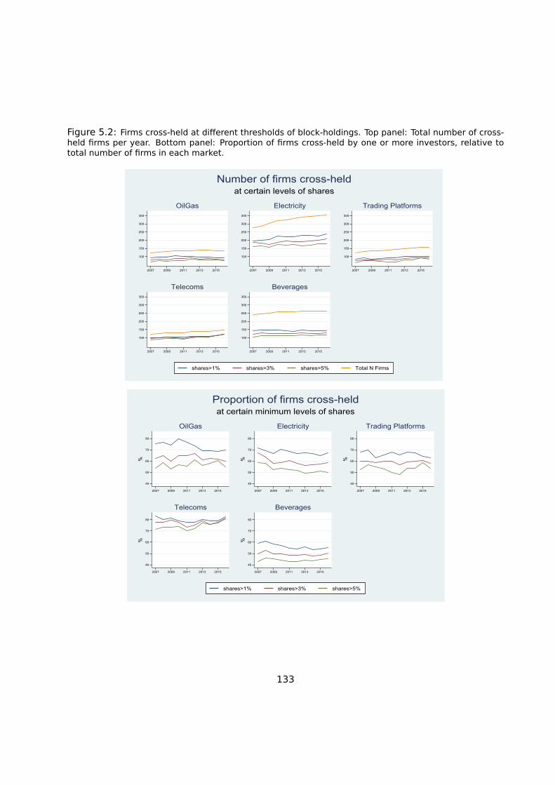
Figure 5.2: Firms cross-held at different thresholds of block-holdings. Top panel: Total number of cross-held firms per year. Bottom panel: Proportion of firms cross-held by one or more investors, relative tototal number of firms in each market.

100

150

200

250

300

350

2007 2009 2011 2013 2015

OilGas

100

150

200

250

300

350

2007 2009 2011 2013 2015

Electricity

100

150

200

250

300

350

2007 2009 2011 2013 2015

Trading Platforms

100

150

200

250

300

350

2007 2009 2011 2013 2015

Telecoms

100

150

200

250

300

350

2007 2009 2011 2013 2015

Beverages

at certain levels of sharesNumber of firms cross-held

shares>1% shares>3% shares>5% Total N Firms

40

50

60

70

80

%

2007 2009 2011 2013 2015

OilGas

40

50

60

70

80

%

2007 2009 2011 2013 2015

Electricity

40

50

60

70

80

%

2007 2009 2011 2013 2015

Trading Platforms

40

50

60

70

80

%

2007 2009 2011 2013 2015

Telecoms

40

50

60

70

80

%

2007 2009 2011 2013 2015

Beverages

at certain minimum levels of sharesProportion of firms cross-held

shares>1% shares>3% shares>5%

133

5.2.2 Densities of block-holdings

The densities of block-holdings represent the proportion of companies in a shareholder’s port-

folio corresponding to a certain threshold of holding (no threshold, 1, 3, 5, 10 percent), relative

to the total number of firms in the market, thus evaluating the market share of firms held with

a certain intensity by a given shareholder. Figure 5.3 shows the results on the top 1% of more

"intensive" portfolios (top panel), as well as the maximum value attained by the most intensive

investor for the various thresholds (bottom panel).

Looking at the top 1% of portfolios holdings, across all sectors the proportion of block-holdings

per portfolio is declining or stable over the period, irrespective of the threshold of equity in-

vestment considered. In general, portfolio densities are below 20% for all levels of investment,

but the differential between non-threshold (all holdings) and threshold densities is large, sug-

gesting that this cohort of investors concentrate their investments in a limited number of firms

where they block-hold at larger values, the remainder of the portfolio presenting smaller partic-

ipations. The exception is the Oil&Gas sector where, considering all equity investments held,

portfolio densities reach noticeably higher levels, illustrating that investors with the largest

portfolios spread out their investments across more firms, even with large intensities.

Observing instead the investors with the maximum values for portfolio density, the trends

are slightly different. Here the maximum value refers to the portfolio holding the largest

proportion of block-holdings in the market, relative to the total number of firms. This top

portfolio represents the most ’intensive’ investor in the market; for example, if we look at the

5% threshold (yellow line), we see in Oil&Gas that the top investor holds a minimum of 5% of

shares in almost 20% of the market firms. The levels of density are clearly higher than in the

top panel of Figure 5.3, but are also slightly increasing, particularly in Oil&Gas. In the other

sectors values are not as high, with the top portfolio including between 5 and 10% of firms at a

block-holding level of 5% shares. Across sectors the distribution of investors measured by the

size of their portfolios is highly skewed, with a very small share of investors increasing their

presence in the market. The same is applicable even when considering different thresholds for

block-holdings. A case in point is the Telecoms sector, where the investor with the maximum

(largest) portfolio density holds at least a 10% equity investment in close to 10% of the firms

in the sample over the period. Still, what is common to all sectors is the flat pattern across the

ten years, where the values for 2007 remain almost unchanged until 2016.

It should be noted that this ’top investor’ described above is not necessarily the same across

years or for different thresholds of block-holdings. Observing for example the Oil&Gas sector,

the top - most "intensive" - investor holds shares equal to or above 10% for roughly 5% of the

firms in the market (light blue line); this is likely to be a corporate group or a holding company

with very sector-specific interests. Instead, the top investor who holds shares of 3% or above

for about 20% of the firms in the market (green line) is likely to be a fund or investment group

with a more diversified portfolio across the sector. For example, looking at the Beverages Man-

134

ufacturers sector - as reported in Table 4.33 - funds such as BlackRock have a specific interest

in larger corporate groups, but the top-scoring investor may vary across years. Other larger

investors, such as Morgan Stanley or certain insurance groups, have smaller participations but

have a greater presence across corporate groups as well as in smaller firms in the market,

and thus might in turn overtake the top funds in specific periods in terms of block-holdings.

Among those investors that have significant block-holdings (>10%) for a share of the firms in

the sample, such as those represented by the light blue line, corporate groups with fully-owned

subsidiaries are likely to fall below them.

In conclusion, taking into consideration the different levels of block-holdings, the density of

portfolios has remained relatively stable throughout the period and across the sectors, follow-

ing a decline with respect to initial values. Nevertheless, these figures confirm the presence

of investors with large shares across a wide section of firms in the sectors.

5.3 Thresholds in networks relations

The following sections revisit the shareholder and firms’ network common shareholding indices

used in the previous chapters, allowing for different thresholds of equity investments. The

application of a threshold for block-holding has different effects in the two networks. In the

firms’ case, it limits the shareholding structure of each company only to the most intensive

investments, i.e. only to the most "present" shareholders. On the other hand, in the investors’

network the companies in each portfolio are restricted according to the respective holding

intensity. This exercise substantially resizes the larger portfolios, which usually have a more

dispersed holding structure, while smaller intensive portfolios become more relevant. This

difference in the two networks’ nature must be kept in mind throughout the analysis, in order

to correctly interpret the results.

For each network, four indicators are presented: the number and proportion of links between

each pair of agents in a network, assessing the extent of connectedness of each group; the

total number of strong links, i.e. those presenting a correlation above 80%; and finally the

proportion of strong links over the total number of existing connections, assessing the strength

of the network’s cohesion.

In the case of the firms, the four indicators replicate those used in previous sectoral analyses

with a 5% threshold, adding two further block-holding levels; this allows for different selec-

tions of investors to be considered for the analysis of similarities between firms’ shareholder

structures. In the case of the shareholders’ network, all indices are new, in the sense that they

have never previously been calculated using a threshold, but rather considering all holdings

in each portfolio. Here only the largest holdings of an investor are retained for each threshold

instead.

135

Figure 5.3: Summary statistics of portfolio density; proportion of block-held firms in a shareholder’sportfolio relative to the total number of firms in the market, considering different thresholds for block-holdings. Top panel: 99th percentile (top 1% of investors). Bottom panel: maximum value (top investor).

0

10

20

30

40

%

2007 2009 2011 2013 2015

OilGas

0

10

20

30

40

%

2007 2009 2011 2013 2015

Electricity

0

10

20

30

40

%

2007 2009 2011 2013 2015

Trading Platforms

0

10

20

30

40

%

2007 2009 2011 2013 2015

Telecoms

0

10

20

30

40

%

2007 2009 2011 2013 2015

Beverages

at certain levels of sharesDensity of block-holdings, percentile 99

All holdings BH > 1% BH > 3% BH > 5% BH > 10%

0

10

20

30

40

50

%

2007 2009 2011 2013 2015

OilGas

0

10

20

30

40

50

%

2007 2009 2011 2013 2015

Electricity

0

10

20

30

40

50

%

2007 2009 2011 2013 2015

Trading Platforms

0

10

20

30

40

50

%

2007 2009 2011 2013 2015

Telecoms

0

10

20

30

40

50

%

2007 2009 2011 2013 2015

Beverages

at certain levels of sharesDensity of block-holdings, maximum

All holdings BH > 1% BH > 3% BH > 5% BH > 10%

136

Another important difference with respect to previous sectoral studies is that the analysis of

high correlations between portfolios is now extended to all pairs of portfolios, and not only to

larger ones. Previous analyses only considered portfolios encompassing at least 10% of the

firms in each market, to avoid picking cases of non-relevant high correlations. For example,

two very small portfolios with very low participations in a limited number of coinciding firms

would present a very high correlation, given their strong similarity, but in reality do not rep-

resent relevant investors in the market. Once we apply minimum thresholds for the holdings,

this is no longer a concern, because low-intensity investments are automatically dropped and

there is no need to restrict them further. Therefore, in the present analysis for the sharehold-

ers’ network we keep all portfolios for all levels of block-holdings, so that the reference pool of

portfolios is constant throughout the calculations.

In order to allow for a clear interpretation of the effects of a change in thresholds, four refer-

ence values are initially calculated on all holdings and held fixed as the thresholds are moved:

the total number of firms per sector/year, representing the size of the firms’ network; the total

number of investors per sector/year, representing the size of the shareholders’ network; the

number of firms in a shareholders’ portfolio, representing the shareholder-firm connections

that generate overlaps between investors; and finally the number of shareholders in a firm’s

ownership structure, generating connections with other firms in the market.

5.3.1 Network indices for firms

The firms’ network reveals the correlations between the ownership structures of the firms in

a sector. Figures 5.4 and 5.5 display these correlations across the period for all five sectors,

looking both at non-zero and only high correlations. Non-zero total correlations represents the

overall degree of connectedness of the firms by their shareholders in the given market. High

correlations instead represent correlations of 80% or above between the ownership structures

of firms, only considering shareholders with shares above 1, 3, or 5 percent. This sheds light

upon the most connected firms in each sector. Since in previous calculations of the firms’

network only shareholders with block-holdings of 5% minimum were used, this study expands

on this by considering values of 1% and 3% as alternative thresholds.

Observing the number of non-zero correlations in the top panel of Figure 5.4, the results show

that the total overlaps between firms’ shareholder structures remain relatively stable over the

period across sectors (except Electricity at 1%), with only slightly increasing trends. In the

case of the Oil&Gas sector, the overall degree of connectedness among firms remains gen-

erally higher than other sectors; in this industry, the share of non-zero correlations over total

correlations stays consistently above 12% (see bottom panel of Figure 5.4), highlighting that

there are numerous links between firms induced by common shareholders.

137

For the remaining sectors, correlations between shareholder structures remain close to or be-

low 5%, depending on the threshold for minimum investment used. Within the Beverages

Manufacturers sector the values are slightly lower than in the others. Even at the minimum

investment of 1%, the share of non-zero correlations never rises above 5% of total possible

connections. For more significant investments, such as 5%, the share is never above 1%.

Figure 5.4: Non-zero correlations between shareholder structures of pairs of firms, considering onlyinvestments with shares above certain minimums. Top panel: Number of non-zero correlations for differ-ent thresholds. Bottom panel: Proportion of non-zero correlations relative to the total number of possibleconnections between pairs of firms for different thresholds.

0

1000

2000

3000

4000

2007 2010 2013 2016

OilGas

0

1000

2000

3000

4000

2007 2010 2013 2016

Electricity

0

1000

2000

3000

4000

2007 2010 2013 2016

Trading Platf.

0

1000

2000

3000

4000

2007 2010 2013 2016

Telecoms

0

1000

2000

3000

4000

2007 2010 2013 2016

Beverages

(only shares above a certain minimum %)Number of non-zero correlations - Firms' network

shares > 1% shares > 3% shares > 5%

0

5

10

15

%

2007201020132016

OilGas

0

5

10

15

2007 2010 2013 2016

Electricity

0

5

10

15

2007 2010 2013 2016

Trading Platf.

0

5

10

15

2007 2010 2013 2016

Telecoms

0

5

10

15

2007 2010 2013 2016

Beverages

(only shares above a certain minimum %)Proportion of non-zero correlations - Firms' network


138

This limited linkage between the shareholder structures is likely due, as previously mentioned,

to the type of firms in the sample - a mixture of large corporate groups with fully-owned sub-

sidiaries and small local enterprises with few owners. The overall result is that of a sector with

many ’vertical’ investments and few horizontal investors.

Figure 5.5: High correlations between shareholders structures of pairs of firms, considering only in-vestments with shares above certain minimums. Top panel: Number of high correlations for differentthresholds. Bottom panel: Proportion of high correlations relative to the total number of non-zero corre-lations between pairs of firms for different thresholds.

0

50

100

150

2007 2010 2013 2016

OilGas

0

50

100

150

2007 2010 2013 2016

Electricity

0

50

100

150

2007 2010 2013 2016

Trading Platf.

0

50

100

150

2007 2010 2013 2016

Telecoms

0

50

100

150

2007 2010 2013 2016

Beverages

(only shares above a certain minimum %)Number of high correlations (>80%) - Firms' network


0

10

20

30

40

50

%

2007201020132016

OilGas

0

10

20

30

40

50

2007 2010 2013 2016

Electricity

0

10

20

30

40

50

2007 2010 2013 2016

Trading Platf.

0

10

20

30

40

50

2007 2010 2013 2016

Telecoms

0

10

20

30

40

50

2007 2010 2013 2016

Beverages

(only shares above a certain minimum %)Proportion of high correlations (>80%) - Firms' network


139

Concerning the proportion of high correlations among the shareholder structures (see bottom

panel of Figure 5.5), Telecoms is again the outlier because of the presence of large corporate

groups with fully owned subsidiaries. The time series for Trading Platforms, although more

volatile, also shows that the proportion of high correlations over total correlations reaches

peaks comparable to Telecoms. This suggests that the top shareholders in this sector are also

further concentrating their investments. As the considered intensity of investment increases,

the proportion of high correlations between connected firms rises substantially, meaning that

those firms that are connected at higher investment intensity more frequently show a stronger

overlap of shareholding structures. In terms of total number of strong links (top panel), Elec-

tricity also present some higher figures, but mainly due to the larger size of its network.

5.3.2 Network indices for investors

Figure 5.6 and Figure 5.7 present indices related to the shareholders’ network, which demon-

strates the correlations between the portfolio structure of investors. The interpretation is

analogous to that of the firms’ network, and in general confirms a strong connectedness in all

markets.

When considering very low thresholds such as 1%, the number of non-zero correlations indi-

cates a high overall degree of overlap between investor portfolios (top panel of Figure 5.6),

but with a tendency to decline over the period of observation.

As the threshold becomes more stringent, the number of connections becomes more stable

over the period, but exhibits a dramatic drop; about ten-fold if comparing the 1% to the 5%

figures. This may again be due, as in the Telecoms sector, to large corporate groups that

fully own many subsidiaries and do not cross invest as much. Therefore, the likelihood of

correlations between portfolios decreases, and depends mostly on the cross-investments of

institutional investors such as funds, which in general hold smaller shares.

As for the proportion of connections existing in the shareholders’ network, the trends are very

similar to those of the absolute figures, the only difference being in the 1% threshold, where a

more evident decline is observed. It is important to note that the proportion of connections is

calculated over the total number of potential shareholder-shareholder links; considering that

each market has thousands of investors per year, the possible two-by-two links are in the

order of several millions, which yields very small proportions even when the number of non-

zero correlations is high. This was not the case in the firms network, of much smaller size,

where the possible links were a few thousand, even in the largest market (Electricity).

Alternatively, Figure 5.7 shows the high correlations between investor portfolios, where the

proportion of high correlations is now calculated over the total number of existing investor-

investor connections. The index therefore highlights on the most strongly connected investors

per sector. As the threshold for block-holdings increases, this proportion increases, because

140

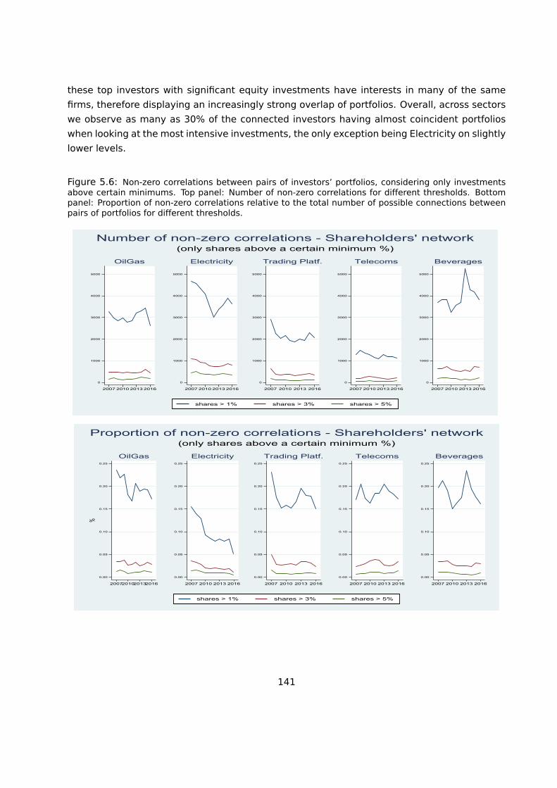
these top investors with significant equity investments have interests in many of the same

firms, therefore displaying an increasingly strong overlap of portfolios. Overall, across sectors

we observe as many as 30% of the connected investors having almost coincident portfolios

when looking at the most intensive investments, the only exception being Electricity on slightly

lower levels.

Figure 5.6: Non-zero correlations between pairs of investors’ portfolios, considering only investmentsabove certain minimums. Top panel: Number of non-zero correlations for different thresholds. Bottompanel: Proportion of non-zero correlations relative to the total number of possible connections betweenpairs of portfolios for different thresholds.

0

1000

2000

3000

4000

5000

2007 2010 2013 2016

OilGas

0

1000

2000

3000

4000

5000

2007 2010 2013 2016

Electricity

0

1000

2000

3000

4000

5000

2007 2010 2013 2016

Trading Platf.

0

1000

2000

3000

4000

5000

2007 2010 2013 2016

Telecoms

0

1000

2000

3000

4000

5000

2007 2010 2013 2016

Beverages

(only shares above a certain minimum %)Number of non-zero correlations - Shareholders' network


0.00

0.05

0.10

0.15

0.20

0.25

%

2007201020132016

OilGas

0.00

0.05

0.10

0.15

0.20

0.25

2007 2010 2013 2016

Electricity

0.00

0.05

0.10

0.15

0.20

0.25

2007 2010 2013 2016

Trading Platf.

0.00

0.05

0.10

0.15

0.20

0.25

2007 2010 2013 2016

Telecoms

0.00

0.05

0.10

0.15

0.20

0.25

2007 2010 2013 2016

Beverages

(only shares above a certain minimum %)Proportion of non-zero correlations - Shareholders' network


141

Looking only at the sheer number, high correlations occur less often when the thresholds for

block-holding become more stringent. Even at 1%, the number of high correlations is usually

between 200 and 400, only a fraction of all the non-zero correlations. This suggests that many

of the existing links between shareholder portfolios are driven by small equity holdings by

investors.

Figure 5.7: High correlations between pairs of investors’ portfolios, considering only investments withshares above certain minimums. Top panel: Number of high correlations for different thresholds. Bottompanel: Proportion of high correlations relative to the total number of non-zero correlations between pairsof portfolios for different thresholds.

0

200

400

600

2007 2010 2013 2016

OilGas

0

200

400

600

2007 2010 2013 2016

Electricity

0

200

400

600

2007 2010 2013 2016

Trading Platf.

0

200

400

600

2007 2010 2013 2016

Telecoms

0

200

400

600

2007 2010 2013 2016

Beverages

(only shares above a certain minimum %)Number of high correlations (>80%) - Shareholders' network


0

10

20

30

40

%

2007201020132016

OilGas

0

10

20

30

40

2007 2010 2013 2016

Electricity

0

10

20

30

40

2007 2010 2013 2016

Trading Platf.

0

10

20

30

40

2007 2010 2013 2016

Telecoms

0

10

20

30

40

2007 2010 2013 2016

Beverages

(only shares above a certain minimum %)Proportion of high correlations (>80%) - Shareholders' network


142

5.4 The ’Big Three’

In the interest of understanding how certain big investors, that is those with wide portfolios,

have increased their common shareholding across the sectors of interest over the years, Table

5.2 presents statistics on average participation shares for BlackRock Inc., The Vanguard Group,

and State Street Corporation, referred to as the ’Big Three’. BlackRock in particular stands

out since, following the 2009 merger with Barclays Global Investors, its average ownership

increased dramatically across sectors. This stylised fact can also be seen in the time series

showing the evolution of block-holdings for the ’Big Three’ in Figures 5.8 and 5.9.

In the Oil&Gas industry, all these funds hold average participation shares that are close to or

above a 3% level of block-holding, making them very relevant actors in the market. BlackRock

and Vanguard have a similar behaviour in Trading Platforms, but State Street is left behind

in this sector, with average holdings just above 1% throughout the period. The investment

intensity in Electricity is rather uniform for the three funds, at around 1.5%, with only Black-

Rock at slightly higher levels, around 2%. The Telecoms sector presents the lowest intensity in

investments of all considered industries, with both State Street and Vanguard well below 1%

average holdings. BlackRock stands at a higher level, with around 2% average. In the Bev-

erages Manufacturers sector, BlackRock experiences a significant jump after its acquisition

of Barclays Global Investors in 2009. Vanguard similarly increases its average participation,

but not due to capital operations. State Street remains the laggard again with respect to its

competitors. This trend is comparable to the other sectors of interest, with BlackRock and

Vanguard always edging out State Street in terms of average participation size.

Figures 5.8 and 5.9 show the number of firms block-held by each fund and the proportion

of their portfolios composed by block-holdings. These are reported as usual for block-holding

levels of 1, 3, and 5 percent. Of these ’Big Three’ investors, BlackRock is the most active across

sectors and over the period. A large part of this is again due to the 2009 acquisition of Barclays

Global Investors, which created a money management juggernaut and vastly increased the

portfolio holdings of BlackRock.

The levels of block-holdings are comparable across the sectors for these top investors, with

BlackRock and Vanguard increasing their block-holdings over the period while State Street

remains steady but well below. In certain sectors, such as Telecoms, the presence of large

corporate groups (for example Vodafone) with many fully owned subsidiaries pushes down the

number of block-holdings for other investors, while in Electricity the large number of firms in

the sample with respect to the other sectors results in an increased number of block-holdings.

Due to these circumstances, the ’Big Three’ lean towards a block-holding style of investment

in the energy sectors (Oil&Gas, and Electricity), while maintaining smaller equity holdings in

Trading Platforms or Telecoms.

143

Table 5.2: Average participation shares in investors’ portfolios. Results for ’Big three’: BlackRock, StateStreet and Vanguard, by market and year.

Oil&Gas

Year BlackRock State Street Vanguard

2007 0.96 2.24 1.862008 0.82 1.98 1.902009 3.97 2.00 2.012010 3.85 2.12 2.232011 3.52 1.96 2.052012 3.32 2.17 2.202013 3.43 2.34 2.582014 3.51 2.32 2.812015 3.54 2.64 3.442016 3.91 2.98 3.87

Electricity


2007 1.05 1.48 1.082008 1.03 1.28 1.032009 2.55 1.38 1.202010 2.24 1.28 1.262011 2.10 1.36 1.182012 1.90 1.25 1.182013 2.06 1.20 1.342014 2.31 1.20 1.522015 2.32 1.24 1.772016 2.40 1.30 2.00

Trading Platforms


2007 0.61 1.04 0.762008 0.73 0.71 0.892009 2.44 0.64 0.962010 2.95 0.81 1.112011 2.69 0.71 1.192012 2.46 0.71 1.412013 3.54 0.92 1.742014 2.76 1.00 1.942015 3.17 1.13 2.262016 3.46 1.03 2.43

Telecoms


2007 0.29 0.50 0.402008 0.45 0.51 0.432009 2.65 0.54 0.542010 2.84 0.54 0.722011 2.49 0.51 0.802012 1.99 0.58 0.862013 2.57 0.57 0.922014 1.90 0.54 0.982015 1.99 0.60 1.232016 2.29 0.63 1.38

Beverages


2007 1.07 1.38 1.142008 0.65 1.33 1.312009 2.64 1.36 1.372010 2.78 1.29 1.482011 2.41 1.51 1.362012 2.48 1.68 1.632013 2.52 1.46 1.792014 2.72 1.46 1.902015 2.73 1.38 2.212016 2.59 1.26 2.38

144

The proportion of block-holdings in the total investments (overall investor’s portfolio) per sec-

tor by each of the ’Big Three’ is presented in Figure 5.9. These stylised facts show the prefer-

ence for intensity of investment by these top funds. Indeed, in certain sectors such as Oil&Gas,

over 40% of BlackRock’s equity holdings are of 5% or greater during the entire period anal-

ysed. This preference for intensity of investment is very sector specific; in other markets such

as Telecoms, the majority of shares held in the portfolios of each of the ’Big Three’ is smaller.

BlackRock for example, has between 60% and 80% of its equity investments in Telecoms

greater than or equal to 1%, while its remaining shares held in Telecom firms are therefore

smaller than 1%. State Street is in a reverse situation, with only just below 20% of shares in

its Telecoms portfolio being greater than or equal to 1%, and the vast majority of its share

holdings in the sector being below 1%. In this specific sector, only BlackRock holds shares

above the other thresholds. Lastly, in the Beverages Manufacturers sector, when considering

conventional levels of 5%, almost 20% of BlackRock and Vanguard’s portfolios in 2016 are

composed by block-holdings, values higher than in the others sectors with the exception of

Oil&Gas.

145

Figure 5.8: Number of block-holdings for the ’Big Three’ at different thresholds.

0

10

20

30

40

50

60

2007 2010 2013 2016

OilGas

0

10

20

30

40

50

60

2007 2010 2013 2016

Electricity

0

10

20

30

40

50

60

2007 2010 2013 2016

Trading Platf.

0

10

20

30

40

50

60

2007 2010 2013 2016

Telecoms

0

10

20

30

40

50

60

2007 2010 2013 2016

Beverages

Number of block-holdings > 1%

BLACKROCK INC STATE STREET CORP VANGUARD GROUP INC

0

5

10

15

20

25

30

2007 2010 2013 2016

OilGas

0

5

10

15

20

25

30

2007 2010 2013 2016

Electricity

0

5

10

15

20

25

30

2007 2010 2013 2016

Trading Platf.

0

5

10

15

20

25

30

2007 2010 2013 2016

Telecoms

0

5

10

15

20

25

30

2007 2010 2013 2016

Beverages



0

5

10

15

20

25

30

2007 2010 2013 2016

OilGas

0

5

10

15

20

25

30

2007 2010 2013 2016

Electricity

0

5

10

15

20

25

30

2007 2010 2013 2016

Trading Platf.

0

5

10

15

20

25

30

2007 2010 2013 2016

Telecoms

0

5

10

15

20

25

30

2007 2010 2013 2016

Beverages



146

Figure 5.9: Proportion of block-holdings in portfolios of ’Big Three’ at different thresholds.

0

20

40

60

80

100

%

2007201020132016

OilGas

0

20

40

60

80

100

2007 2010 2013 2016

Electricity

0

20

40

60

80

100

2007 2010 2013 2016

Trading Platf.

0

20

40

60

80

100

2007 2010 2013 2016

Telecoms

0

20

40

60

80

100

2007 2010 2013 2016

Beverages

Proportion of block-holdings > 1%


0

10

20

30

40

50

60

%

2007201020132016

OilGas

0

10

20

30

40

50

60

2007 2010 2013 2016

Electricity

0

10

20

30

40

50

60

2007 2010 2013 2016

Trading Platf.

0

10

20

30

40

50

60

2007 2010 2013 2016

Telecoms

0

10

20

30

40

50

60

2007 2010 2013 2016

Beverages



0

10

20

30

40

50

%

2007201020132016

OilGas

0

10

20

30

40

50

2007 2010 2013 2016

Electricity

0

10

20

30

40

50

2007 2010 2013 2016

Trading Platf.

0

10

20

30

40

50

2007 2010 2013 2016

Telecoms

0

10

20

30

40

50

2007 2010 2013 2016

Beverages



147

Chapter 6

Linking Common Shareholding

and Competition

The link between common shareholding and competition is related to a firm’s objective func-

tion. As noticed by Azar et al. (2018), if a firm acts in the interest of its main shareholder,

then what should be maximised is not the firm’s own value but the shareholder’s utility. With

institutional investors, this corresponds to the maximization of their portfolio value. Clearly,

firms’ profit maximization and portfolio maximization do not always coincide; in particular, an

aggressive price behaviour could benefit a firm’s own profit but reduce the value of common

shareholders’ portfolios.

To what extent common shareholders possessing small fractions of shares in many firms of the

same market are able to actually influence market outcome is still an open question. O’Brien

and Salop (2000) show that if a firm maximises its shareholders’ portfolio profits (and not its

own profit), industry markup1 is proportional to a modified Herfindahl-Hirschman Index (HHI),

where the markup depends on the density of the network of ownership and control of the firms

in the considered market. When this is the case, higher markup should be observed in markets

with higher common shareholding (Azar et al., 2018).

Previous chapters have discussed in detail the various measures of common shareholding that

were developed for the purpose of this exercise.2 The different firm and market level indices,

aside from offering viable alternatives to the standard literature indices such as the HHI or the

modified HHI, also gave valuable insight into the structure of the five sectors considered for

the analysis, namely Oil&Gas, Electricity, Mobile Telecoms, Trading Platforms and Beverages.3

1Markup is given by (price - marginal costs)/price.2See Chapter 2 for a general overview and Appendix B for more technical details.3See sectoral results in Chapters 4 and 5.

149

This chapter deals with the measurement, data and econometric issues arising when assess-

ing the link between common shareholding and competition. In what follows, rather than

reviewing thoroughly the research on this topic, we will briefly detail the requirements and

possible way forward for an empirical measurement of such possible effect. It is worth recall-

ing, though, that the econometric modelling still has several challenges ahead, principally the

lack of an established theory showing how common shareholding affects managers, and from

there competitive outcomes.

Section 6.1 recalls the main modelling challenges. Section 6.2 discusses measurement and

data issues related to market identification, the measurement of common shareholding and of

competitive outcomes. Section 6.3 presents and discusses different market power indicators

of competition, while Section 6.4 proposes an econometric strategy for the test of causality

between common shareholding and competition. Finally, Section 6.5 recalls the main sectoral

results, to help choose a suitable candidate industry for the econometric analysis.

6.1 Modelling the link

The first ingredient of the recipe linking competition to common shareholding is how the rela-

tionship is actually modelled.

One could look at markets where common shareholders are not present and compare them

with markets where common shareholding is observed (He and Huang, 2017). Azar (2012)

uses a panel of 210 industries to regress average industry markup on the density of common

shareholders (plus controls, including industry fixed effects). He finds a significant and pos-

itive relation between markup and within-industry density. Cross-industry comparison, while

appealing in theory, has limited utility as very different aspects - e.g. the different cost-

structures, different nature of activity, and so on - might play a crucial role in shaping causal

effects (Schmalz, 2018).

An additional difficulty in industry comparisons is the amount of data and effort needed to de-

fine market boundaries and proximity. On the other hand, the analysis of common sharehold-

ing in vertically linked markets could be worth exploring, since there common shareholding

could have a beneficial effects on markups (Azar’s results go in this direction).

Given the theoretical and empirical problems in working with many markets, the analysis of a

single market has been the choice mostly followed by the literature (Schmalz, 2018). Ideally,

to measure the effect of common shareholding within the same market one would need a

change in market conditions with the emergence of a set of common shareholders either

previously not there, or present but with different percentages of shares. One could then

analyse the pre and post margins for the whole industry - or for the affected firms - and see if

common shareholding has indeed influenced markups.

150

Our data span from 2007 to 2016, and in that period we never observe the switch between

the absence and the presence of common shareholders in the EU overall and in any of the five

analysed markets.4 We observe, instead, changes in the identity of common shareholders (for

example, evidence suggests that large funds substitute banks as common shareholders of the

electricity market from 2009-2010), or in the proportion of the market assets held.

Within markets, the literature usually looks at variables such as market share or profitability of

companies with common shareholders (He and Huang, 2017, among others). Changes in prof-

its or margins are associated to common shareholding also by Azar (2012), once confounding

factors are accounted for. Notice that sharp empirical evidence for efficiency gains arising

from common shareholding is still lacking (Schmalz, 2017).

Finally, the effects of common shareholding on variables other than competition, such as in-

novation, have been also analysed (López and Vives, 2017; Antón et al., 2018; Shelegia and

Spiegel, 2017), showing that common shareholding can also be welfare improving. The link

between common shareholding and investments is explored by Gutierrez and Philippon (2017).

6.2 Measurement and data issues

No matter the model chosen, the empirical testing of the relation between common share-

holding and competition is not straightforward, due to several measurement and data issues.

Here we discuss the main points, including concerns related to the market identification and

the measurement of common shareholding. The choice of possible measures of competition

is also discussed, looking at both market power and market concentration indicators.

6.2.1 Market identification

First the definition of market boundaries. The literature has used official codes of economic

activity (NACE for Europe, NAICS, SIC for the US5) to define market boundaries. The main

issue is that this classification is not precise for all firms and markets. In Europe, NACE codes

are assigned according to the value added produced by the company and this classification is

generally quite stable in time, reflecting changes in company’s activity only with delay. This

is crucial for firms and sectors where technological progress is rapidly changing production

and products. An additional complication is the presence of large conglomerates with multiple

and very different activities (thus uncertain industrial classification) which operate in different

markets. Finally, for certain types of activities there is no correspondence to a specific code,4See overall picture of common shareholding in the EU in Chapter 3 and sectoral results in Chapters 4 and 5.5The codes of economic activity are referred to, respectively, as the NACE (Nomenclature générale des Activités

économiques dans les Communautés Européennes - European Classification of Economic Activities), the NAICS (NorthAmerican Industry Classification System), and the SIC (Standard Industrial Classification).

151

and even looking at the main players they tend to be classified according to a variety of dif-

ferent activities. For example, in the definition of the Trading Platforms industry presented in

Chapter 4, the companies that operate the trading platforms are classified not only as devel-

oping financial services activities or administration of financial markets, but also as banking

(monetary intermediation), holding activities, business support services or even IT services.

An underestimated complication resides in the fact that the availability of NACE classifica-

tion for firms depends on national legislation. In some countries, like Denmark, firms are

given the option to indicate ’no sectoral code’ when producing their accounts and this in-

flated the number of firms for which the NACE code is not available. Other countries foresee

simplified accounting rules (without the indication of NACE) for certain categories of firms.

Non-exhaustive examples are, in France, Société en nom collectif (SNC), Affaires Personnelles,

Coopératives, Administration, Associations, GIE (groupement d’intérêt économique); in Lux-

embourg, enterprise individual, SECS (Société en commandite simple), SNC, Etablissement

public, foundation, GIE; in the Netherlands Sole Traders, Federations, Foundations and partici-

pations, which are consolidated in holdings. Two countries - UK and Cyprus - explicitly mention

exceptions to NACE declaration related to foreign controlled firms. UK grants exceptions for

NACE declaration to Unlimited, LP, Royal Charter, European Economic Interest Grouping, and

foreign companies. Cyprus grants exceptions to partnerships and business names, and to

overseas companies (branches of foreign companies) if not taxed in Cyprus.

A further issue, when dealing with data coming from different classifications (typically NACE

for Europe and NAICS or SIC for US) is that the correspondence of sectors at 4 (or even 3) digit

level is not assured. For example, in the Electricity sector the US-SIC classification presents

a rather comprehensive category of "Electric Services" (code 4911), while the NACE distin-

guishes between Production (code 3511), Transmission (3512), Distribution (3513) and Trade

(3514) of Electricity. Similar, but not identical detailed classification can be encountered in the

NAICS system, where different codes identify Electric Power Generation (22111), Electric Bulk

Power Transmission and Control (221121) and Electric Power Distribution (221122), but none

refers to trade.

6.2.2 Measures of common shareholding

An empirical testing of the link between common shareholding and competition requires us-

able variables for the measurement of both phenomena.

The literature has so far mainly recurred to the modified HHI delta as a measure of common

shareholding (HHI delta is the additional variation in concentration arising because of common

shareholding). This implies several challenges. Firstly, data challenges, with the need to have

firm-level and market-level data. Secondly, endogeneity problems (see discussion in O’Brien

and Waehrer, 2017). Finally, a logical issue also exists: common shareholding is measured with

152

the MHHI, an endogenous measure of concentration that depends on common shareholding

and market share.

To solve the endogeneity problem, Azar et al. (2018) use changes in route-level prices and

the purchase of Barclays Global Investors in 2009 by BlackRock as an instrument to estimate

the impact of enhanced concentration on specific airfares. The use of prices, while extremely

appealing to measure competitive pressure, is rather challenging in practice. It requires the

identification of a homogeneous good supplied by all (most of) the companies in the market,

for which the price-company data is actually observed and collected for a sufficiently long

period to allow meaningful quantitative analysis. While standard surveys on product-market-

price data and quantities typically take years to be conducted and validated, the use of web-

scrapers to record on-line prices could constitute a possible alternative.6

Azar (2012) offers an alternative to the modified HHI, constructing a measure of density of

common shareholders in a market. Azar’s defines density as

Densty =

∑n=1

∑

j< yj

n(n − 1)/2

where yj is equal to 1 if firms and j are connected by a block-holder (i.e. if they have a

common shareholder holding at least 5% shares in each firm), zero otherwise. He and Huang

(2017) also offer measures of intensity of common shareholding based on the number of firms,

within a market, that are cross-held. These indicators are firm-centred in the sense that they

look at the ownership structure of firms, identifying possible shareholders’ overlaps with their

competitors. On the other hand, additional owner-oriented common shareholding indicators

have been developed in Chapter 2 (and applied to the EU in Chapters 3-5), adding a new

dimension to the measurement of the phenomenon. The new indices analyse the portfolio

structure of investors, and the overlap between investment strategies of different owners

active in a given market, highlighting whether the common shareholders tend to target the

same companies or rather split the market into selected ownership subsets.

Another (unavoidable) limitation of all the analyses of common shareholding resides in the use

of shares to infer control. The percentage of the shares held is only an imperfect substitute for

the control exercised, when e.g. dual-class share or golden shares are present. Data issues

complicate this point. To the best of our knowledge, no firm-level data (not Orbis, nor Dun &

Bradstreet7 or Compustat8 for listed firms) distinguish explicitly shareholders in terms of the

type of shares they hold. Therefore, we are obliged to assume a 1:1 correspondence between

control rights and percentage of shares.9

6An example of web scrapers to infer prices is The billion prices project (http://www.thebillionpricesproject.com/our-research/). Notice that the Commission developed a tool, the European media monitor (EMM - https://ec.europa.eu/jrc/en/scientific-tool/europe-media-monitor-newsbrief), that could be adapted to the purpose.EMM scrapes the web in 70 languages according to given keywords and runs sentiment analysis in 14 languages.

7See https://www.dnb.com/8See https://www.spglobal.com/marketintelligence/en/campaigns/i-need-data-to-make-informed-decisions9An additional issue with papers using US data (e.g. all the papers by Azar and Schmalz) is that they rely on data

153

http://www.thebillionpricesproject.com/our-research/

http://www.thebillionpricesproject.com/our-research/

https://ec.europa.eu/jrc/en/scientific-tool/europe-media-monitor-newsbrief

https://ec.europa.eu/jrc/en/scientific-tool/europe-media-monitor-newsbrief

https://www.dnb.com/

https://www.spglobal.com/marketintelligence/en/campaigns/i-need-data-to-make-informed-decisions

Schmalz (2018) suggests associating also the number of board seats to the percentage of

shareholding. Orbis contains information on board members obtained from balance sheet

data, hence with a delay of about 2 years, but does not contain information on which com-

pany/shareholder each board member represents. The dataset BoardEx10 contains updated

biographical information on board members and senior executives for about 1.7 million com-

panies around the world, but it requires manual matching of companies when it is used in

tandem with financial statements from Orbis (or from other datasets).

6.2.3 Measures of competition

A third challenge is the measurement of competition. Structural forces at play in the global

economy, including the ICT revolution, globalization, and delocalisation of supply chains, are

uprooting industrial organization in many countries. Policymakers, and for this purpose those

worried about consumer welfare, need to adjust their policy objectives to capture the new

possible anticompetitive effects resulting from these changes. For these reasons, it is crucial

to choose an appropriate measure of competition. In order to establish a causal relationship

between common shareholding and competition, the options explored include measures of

market power or market concentration, as well as considering directly the effect on prices.

Prices remain the preferred indicator for changes in competitive forces on the market, however

obtaining data on prices at the required level of specificity is still a challenge.

The literature on common shareholding offers two possibilities, either a measure of market

power or a measure of market concentration. Market power refers to the ability of a company

to raise and maintain the price above the level that would prevail under perfect competition

(see OECD, 1993). The indicator mostly used in practical measures is the Lerner index based

on industry markup, i.e. the wedge between prices and marginal costs. As neither prices nor

marginal costs are actually observed in firm-level data, the Lerner index is approximated by a

profitability index either based on the difference between sales and variable costs or the differ-

ence between operating profits and financial costs, to account for fixed costs (for a summary

of the measures see Santos et al., 2018). Still, this approach has pros and cons. The major

limitation is that it is based on average costs rather than on costs at the margin. The advan-

tage is that they can be calculated using standard accounting data. Although not perfect, the

Orbis dataset remains the best possible option for an empirical analysis when accompanied by

a correct definition of the reference market and its main players. Orbis variables from balance

sheet and profit-loss accounts are widely used in the literature to approximate markups and

are good candidates for empirical testing.11

coming from the 13F filings (a quarterly report filed by institutional managers to the Security Exchange Commission),thus limited to equity assets under management of at least 100 million US$ in value. Azar et al. (2018) complementthese data with hand-collected non-institutional ownership data for owners with a stake above 5% of outstandingshares.

10See http://corp.boardex.com/data/11See Appendix A, and specifically definitions of available balance sheet and profit&loss account variables in Tables

154

http://corp.boardex.com/data/

Market concentration relates to the idea that a limited number of players may implicitly

control the market, while a larger number of players is likely to increase the competitive pres-

sure on competitors. The HHI is the common measure of concentration used in the literature

(Hallak and Rosati, 2018), as it computes the relative size of a firm in an industry in terms of

the proportion of total output (see OECD, 1993, and OECD, 2012). Sales are generally used as

a proxy of firms’ economic activity, as they are a standard measure in product market strength

literature and are less subject to manipulation than reported earnings (He and Huang, 2017).

A major empirical shortcoming of both approaches is related to the use of accounting data from

consolidated (versus unconsolidated) accounts. Consolidated sales refer to the entire activity

of the company, regardless of the sector in which it is undertaken. Apportioning sales/value

added to sectors is not an easy task and is subject to ad hoc assumptions. An additional short-

coming of using consolidated accounts is that even if one assumed that a company is active

in a single sector, multinational firms will report all international sales within a single consol-

idated account; this is likely to artificially inflate the share of multinational firms if compared

to the shares of domestic ones.

As the typology of balance sheet produced (unconsolidated vs consolidated) depends on legal

requirements (hence also on national legislation), in some cases consolidated balance sheet

is the only available option within firm-level datasets. The Orbis database allows differenti-

ating between consolidated and unconsolidated accounts, and accounting for ownership. By

using as much as possible unconsolidated country-level firms’ accounts, we are able to be

more precise in sector and geographic area.12 Furthermore, we avoid inflating the data with

international sales or sales of the group in other markets. Whenever unconsolidated accounts

are not available, we consider consolidated accounts without apportioning sales or assets to

single markets to avoid ad hoc assumptions.13

6.3 Markup

Through a survey of the relevant literature and a recap of the main terminology, we discuss

more in detail the potential indicators for competition, in particular linking them to the im-

portance of new policy objectives. We focus mainly on the firm markup, and present the

methodology for how it is calculated.14

Over the past 20 years, economies in the Western world have seen major structural shifts

driven by the rapid diffusion of ICT, the globalization of supply chains, or the delocalization

A.8 and A.9.12See Hallak and Rosati (2018) and discussion therein.13Notice that in the case of the listed firms included in the initial database, most of the accounts (70%) are con-

solidated (see Section A.5 in Appendix A for further details). In the case of the unlisted firms - added manually tointegrate the definition of the five industries - the large majority of accounts are unconsolidated.

14Concentration measures are not explored further for being at market rather than at firm level.

155

of production, for example. These forces are responsible for market outcomes that now com-

mand attention from academics and policymakers alike. No market trend, however, has gar-

nered as much attention in recent years as the apparent increase in industry concentration

and the corresponding decline in competition. Both U.S and European antitrust authorities -

arguably the two most influential entities of their kind in the world - have brought (or begun)

in recent years antitrust actions against major market players such as Google, Facebook, or

Amazon.

The evidence seems to back up the claims of the authorities. Reports by the OECD (2018)

find that markups and profits, especially in the U.S, have increased globally. Others such as

Gutiérrez and Philippon (2017), Baqaee and Farh (2020), and Diez et al. (2019) have found

similar results. This last work calculates that global markups have increased by 6% between

2000 and 2015, driven by high-markup firms in advanced countries. Again, De Loecker et

al. (2020) report similar findings, where the upper tail of the distribution drives increasing

markups in the U.S. There is therefore consensus in the literature on the evolution of industry

concentration, but less so when it comes to concentration and its effects on competition for

a specific market within an industry. The authors mentioned above, alongside others such as

Gutiérrez and Philippon (2018), conclude that, while competition has declined in the U.S, the

trend in Europe is less evident. Because of the structural changes mentioned above, observed

changes such as increasing industry concentration do not necessarily lead to greater market

concentration, and hence lower competition. Properly assessing the economic outcomes due

to changes in common shareholding requires that the policymaker focuses instead on more

specific indicators such as prices, profits, or markups (OECD, 2018).

In Europe, Weche and Wambach (2018) have also observed increasing markups in the years

after the financial crisis of 2007. The distinguishing factor is that the authors observed increas-

ing markups along the entire distribution - as opposed to the U.S, where the large firms with

higher markups gained more market share. The results also showed heterogeneity among

European countries, with some experiencing this increase in markups more than others.

These stylised facts could be indicators of anticompetitive behaviour going on in the market.

Several authors, such as Kwoka (2013) and Blonigen and Pierce (2016), have shown that ar-

rangements like mergers, which result in increased market concentration, are correlated to

increasing markups or declining competition. It is therefore possible that through these merg-

ers or other similar agreements, firms are extending their market power with anticompetitive

behavior or conduct. This includes not only price setting, but also rent-seeking behaviour

through intense lobbying for regulatory protection or favoritism. Even where anticompetitive

mergers are not observed, increasing markups should still be of concern to policymakers. As

outlined before, structural changes are weakening the link between concentration and higher

profits. For example, superstar firms such as Google or Facebook operate in sectors with ex-

ceptionally low marginal costs with respect to their revenue, something seen among all new

156

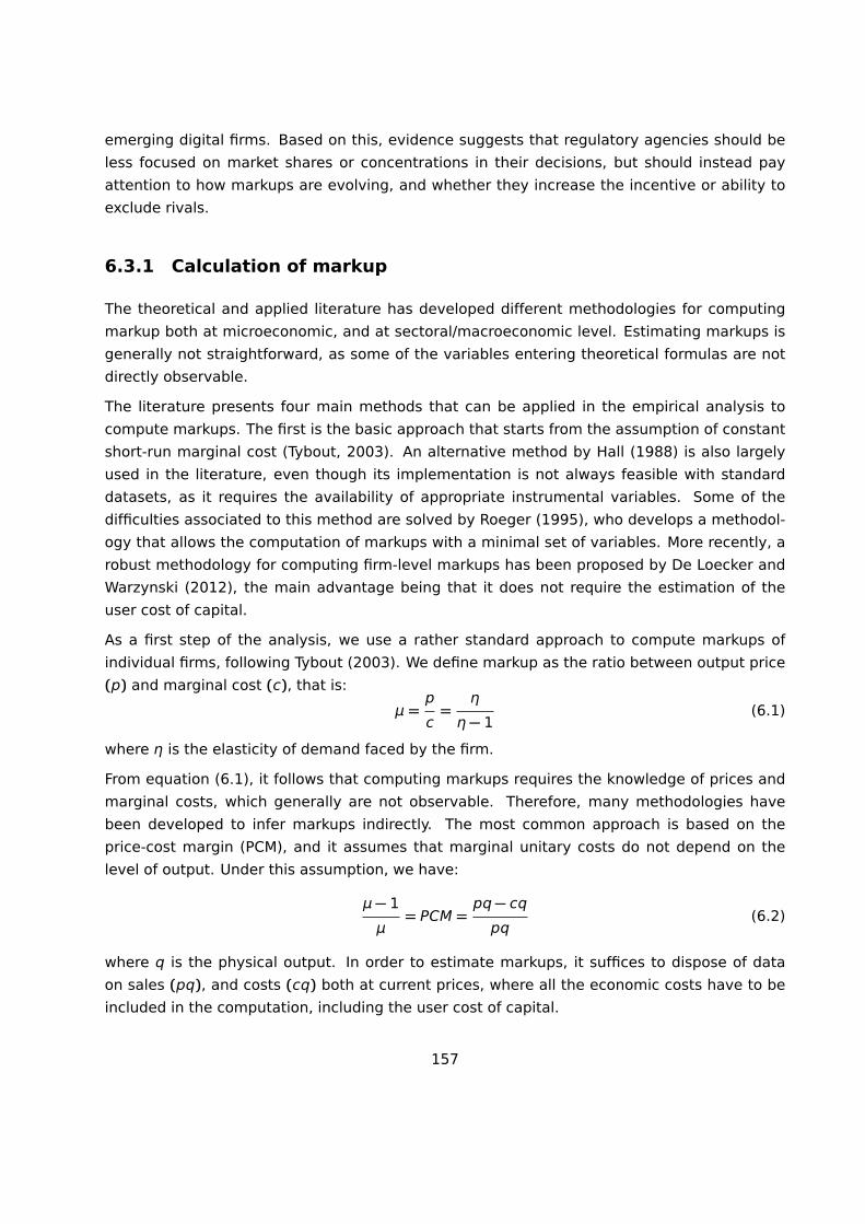
emerging digital firms. Based on this, evidence suggests that regulatory agencies should be

less focused on market shares or concentrations in their decisions, but should instead pay

attention to how markups are evolving, and whether they increase the incentive or ability to

exclude rivals.

6.3.1 Calculation of markup

The theoretical and applied literature has developed different methodologies for computing

markup both at microeconomic, and at sectoral/macroeconomic level. Estimating markups is

generally not straightforward, as some of the variables entering theoretical formulas are not

directly observable.

The literature presents four main methods that can be applied in the empirical analysis to

compute markups. The first is the basic approach that starts from the assumption of constant

short-run marginal cost (Tybout, 2003). An alternative method by Hall (1988) is also largely

used in the literature, even though its implementation is not always feasible with standard

datasets, as it requires the availability of appropriate instrumental variables. Some of the

difficulties associated to this method are solved by Roeger (1995), who develops a methodol-

ogy that allows the computation of markups with a minimal set of variables. More recently, a

robust methodology for computing firm-level markups has been proposed by De Loecker and

Warzynski (2012), the main advantage being that it does not require the estimation of the

user cost of capital.

As a first step of the analysis, we use a rather standard approach to compute markups of

individual firms, following Tybout (2003). We define markup as the ratio between output price

(p) and marginal cost (c), that is:

μ =p

c=

η

η − 1(6.1)

where η is the elasticity of demand faced by the firm.

From equation (6.1), it follows that computing markups requires the knowledge of prices and

marginal costs, which generally are not observable. Therefore, many methodologies have

been developed to infer markups indirectly. The most common approach is based on the

price-cost margin (PCM), and it assumes that marginal unitary costs do not depend on the

level of output. Under this assumption, we have:

μ − 1

μ= PCM =

pq − cq

pq(6.2)

where q is the physical output. In order to estimate markups, it suffices to dispose of data

on sales (pq), and costs (cq) both at current prices, where all the economic costs have to be

included in the computation, including the user cost of capital.

157

In detail, once the costs associated to capital are taken into account, the price-cost margin of

firm at date t - and thus the markup - can be estimated as follows:

PCMt =πt

pt qt+(rt + δ) ktpt qt

(6.3)

where πt is the profit of firm at date t, rt is the interest rate at date t, δ is the depreciation

rate of capital, and kt is the stock of capital of firm at time t. This computation is relatively

straightforward within the ORBIS dataset. Indeed, the database includes firm-level data on

the revenues ptqt, and on the costs associated to labour and intermediate inputs, which

determine the level of current profit πt. Moreover, ORBIS reports the stock of tangible assets

kt. The only elements missing in the computation are the interest rate and the depreciation

rate of capital, which can be obtained from other statistical sources.

The interest rate can be computed as the difference between the nominal interest rate and

the inflation rate, to get a proxy of the real ex-ante interest rate. The series are available, for

example, from the Statistical Data Warehouse of the European Central Bank. With regards to

the depreciation rate, Konigs and Vandenbussche (2005) assume a fixed parameter, and find

that their results are not significantly affected by its value.

Applying equation (6.3), it is possible thus to estimate the markup level of each firm included

in the ORBIS dataset year by year, provided data on the four key variables are available: sales

(TURN), cost of labour (STAF), cost of intermediate inputs (MATE) and stock of assets (TFAS).

Tables A.8 and A.9 in Appendix A report the detailed definition of these variables, as well as of

other main financial variables present in the Orbis dataset.

6.3.2 Lerner index

An alternative measure of markets’ competition, largely used in the literature (see, among

others, Aghion et al., 2005; Grullon et al., 2019; and Gutiérrez and Philippon, 2017) is given

by the Lerner index. This index is in practice a monotone transformation of the markup, the

main difference being the expression of their respective formulas, which allow their calculation

starting from different items of the balance sheet and profit & loss account. The Lerner Index

was formalised by Abba Lerner in 1934, and is defined as follows:

L =P − MC

P(6.4)

where P are prices and MC are marginal costs for a given firm. The indicator varies from zero to

one, with zero being the situation of perfect competition in which prices are equal to marginal

costs.

The interpretation of the two alternative measures is the following: while the markup gives the

158

percentage amount for which prices exceed marginal costs (and should be equal to one under

perfect competition), the Lerner Index is a normalised measure that varies between zero and

one. The value zero - as mentioned above - represents the case of perfect competition, while

the index takes value one in the extreme situation where the monopolist faces zero marginal

costs and it is able to charge a positive price. In this sense, the Lerner index is a measure of

how much the discretion in firm’s price setting is far away from the social optimum.15

Nevertheless, as for the markup, prices and marginal costs are not observable. Hence, to

overcome this problem, it is possible to compute the index at firm level as the ratio between

the earnings before interests and taxes (EBT) and the amount of sales (TURN).16 While this

indicator can be considered as a good proxy of the firms’ market power, it does not contain the

cost of capital,17 which can be subtracted from the EBT to obtain a more realistic measure of

markets’ competition.

6.4 Econometric approach

Building on the previous discussion, the purpose of this Section is to propose a model at the

sector level that shows the causal relationship of common shareholding on competitive out-

comes. The most straightforward way is by leveraging exogenous events that occur in the

market that affect the degree of common shareholding. However, as commented earlier,

there are no clear occurrences where the market passes from an absence to a presence of

common shareholding in the period under observation (2007-2016). In fact, the phenomenon

of common shareholding in this period is already quite widespread across the EU, and its in-

tensity is rather stable throughout the period.18 On the other hand, as mentioned earlier, we

observe substitutions among the classes of common shareholders, as funds tend to replace

banks along the observation period, especially driven by the BlackRock-BGI merger. We recall

also that, with the data at hand, cross-industry regressions are not suitable for establishing

a causal link between common shareholding and competitive outcomes, since there are too

many sectoral differentiating factors that are difficult to control for. The analyses of the pre-

vious Chapters will help choose one of such sectors for the application of the econometric

analysis.

Keeping these issues in mind, a possible sectoral model can be built on the large literature

that uses the Difference-in-Differences (DiD) method to investigate the net impact of a pol-

icy/programme on given outcomes. The standard case for applying the DiD is when a change

in regulation/law (treatment) affects only a group of units (the treated units) and there is an-15See Lerner (1934).16For detailed definition of these and other variables, see Tables A.8 and A.9 in Appendix A.17A comprehensive review of the main strengths and weaknesses in using the Lerner Index as a measure of com-

petitiveness is provided by Elzinga et al. (2011).18See overall picture of common shareholding in the EU in Chapter 3.

159

other group (the control) which is similar in all respects but is not affected by the policy. Both

groups are observed over a period of time which includes the year of the adoption of the policy.

Then, it is natural to measure the policy effect by comparing the change in the mean outcome

of the treated cases with the change in the mean outcome for the untreated. This approach

can, under some conditions, identify the causal effect of the policy on the outcome of interest.

In this specific case, there is no clear shock affecting common shareholding, namely neither

a regulation, nor an intervention that has affected common shareholding at the European

level in the period of observation. As a consequence, it is also not straightforward to identify

possible treated and control units.

Hence, to overcome these issues, and in order to induce a sort of "exogenous" variation in

the common shareholding, we exploit the decision of BlackRock to acquire Barclays Global

Investors (BGI) in 2009. The presence of this merger event not only allows a pre and a post

period to be defined, but also permits the identification of treated and control groups. That is,

we can create a measure of a firm’s exposure to the merger event based on their dependency

on BlackRock and BGI before the merger. The intuition being that the more a firm was held by

BlackRock and/or BGI, the more a firm is expected to be "exposed" to the merger and, hence,

the higher the impact. Of course, firms that did not have any relations with BlackRock and/or

BGI would not be directly affected by the merger, and hence would act as control units.

The simplest exposure indicator can be a dummy variable assessing whether a firm was part

of BlackRock or BGI portfolios before the merger. A more sophisticated indicator, measuring

different degrees of exposure, is given by the relative share held by BlackRock and BGI in

each firm. It follows that the impact of common shareholding is estimated, under the two

alternative exposure indicators, by comparing changes in the markup of firms (more) exposed

to the merger to those that are not (less) affected, before and after the merger.

Markup can be influenced by country-specific macroeconomic shocks, such as changes in

institutional setting and/or consumer tastes. However, financial variables are in general not

country-specific,19 so they do not allow to account for country effects. Similarly, heterogeneity

of the products in a given sector cannot be captured by a firm’s aggregate balance sheet,

hence product-specific unobserved effects cannot be factored in.

An alternative solution would be relying on product-level data on consumption (prices and

quantities) in each country. This data can then be linked to firms, providing information on the

average quantities and prices of the products sold by each firm in each country. In this case,

the analysis would be based on the measure of exposure and its interaction with the average

quantities sold, so as to capture the relative weight of each firm in the market. Moreover, this

type of data would allow to add other combinations of fixed effects to eliminate any remaining

source of bias due to correlation between unobserved factors that are constant over time

(firms, products, country and year fixed effects) and our exposure variable.19See discussion about consolidated vs unconsolidated financial accounts in Section 6.2.3.

160

Several options for price data for the five sectors were investigated, unfortunately with no

success. In some cases there was an additional challenge related to the identification of a

“product” itself (e.g. in the Trading Platforms case), and hence the definition of a possible

price. In other cases, wholesale prices could have been retrieved (e.g. in Electricity markets),

but not retail prices, which are those more likely to be affected in case of harmed market com-

petition. For the Beverages sector, where a product was more easily identified, unfortunately

product-level data covering the pre- and post-merger periods were not available, at the time

of the study. For these reasons, the empirical analysis is kept at the firm level.

6.5 Candidate sectors for the econometric analysis

Five sectoral studies have been reported in Chapter 4, analysing respectively the Oil&Gas,

Electricity, Mobile Telecoms, Trading Platforms and Beverages industries. Specifically, results

on market definition and shareholding structure were presented, with a detailed identification

of main corporations and top investors, with respective portfolio information. Special attention

has been devoted to minority shareholders and their role as block-holders, in particular to the

so-called ’Big Three’, the largest US-based funds BlackRock, State Street and Vanguard; the

analyses looked at their portfolios, at trends of investment ’intensity’ (amount of shares held

in firms in portfolio), as well as changes in portfolio size and number of block-holdings. Evi-

dence on the interconnections within each market has been investigated looking at a series of

common shareholding indices based on firm-shareholder relations; moreover, the networks of

firms and shareholders have been studied separately, identifying the presence and strength of

links between firms (induced by common shareholders), and connections across shareholders

(due to partially overlapping portfolios). Lastly, a comparative analysis of some of the indices

above has been presented for all the sectors in Chapter 5, with the assessment of the effect

of holding thresholds on the chosen indices.

The objective of this section is to analyse various ownership patterns in the five sectors, in or-

der to identify suitable variation in the common shareholding indicators that can help capture

the possible effects on competition. Besides the relevant earlier findings on the five sectors,

here we discuss two new types of variations of ownership that can be of particular value in the

development of the econometric analysis. First, evidence is presented on the BlackRock-BGI

merger in 2009, accompanied by the contemporaneous analysis of the investment behaviour

of close players, namely State Street, Vanguard and Barclays PLC. Second, additional sig-

nificant ownership changes between investors in the period of observation are considered,

looking at both increase and decrease in participation of top investors in ’secondary’ investors

- which can be likely targets of M&As strategy from the large institutional investors.

161

6.5.1 The ’Big Three’ and the BlackRock-BGI merger

The overall results from the sectoral analyses do not show a very specific trend over the pe-

riod of observation. As already commented earlier, at first sight this seems to signal a lack

of dynamics in the ownership structure of the sectors. However, looking at a selection of top

investors, the sectoral studies revealed that, while the top values of common shareholding in-

dicators were stable in the last decade, a change in the identity of the main players took place.

In particular, it was witnessed the rising of the large investment funds and a contemporaneous

drop in the participation of banks and insurance companies.20

In Chapter 5 additional indices have been computed for the ’Big Three’ (BlackRock, State

Street and Vanguard), looking at both their market shares (in terms of Total Assets and Market

Capitalisation) and the intensity of their investments (number of block-holdings). Here such

indices are recalled for all five sectors, while analogous figures are shown also for Barclays

Global Investors (BGI) and Barclays PLC. The reason why these two investors are added is to

monitor the effect of the 2009 merger of BlackRock with BGI, which is the largest ’substitution’

event between funds and banks. This event had unprecedented proportions in the history of

mergers between asset management funds, and has therefore played a crucial role in shaping

the various studies on common shareholding.

The BlackRock acquisition of Barclays Global Investors was announced 10 years ago to date,

propelling the asset management fund to the top of global rankings, ahead of its competitors

such as State Street and Fidelity Investments. It created what was at the time a behemoth of

almost $3 trillion in assets, in what was just the latest in a series of acquisitions beginning with

Merrill Lynch Investment Management. The sheer magnitude and speed at which BlackRock

expanded has made it an interesting case study as well as instrument in impact evaluation

models. Often these acquisitions do not occur independently of other events. In fact, the

sale of BGI to BlackRock by Barclays was used to finance the acquisition of Lehman Brother’s

assets. In the meanwhile, BlackRock has grown to be the largest asset management fund in

the world, and has gone from being a primarily fixed income business to a diversified business

with interests in exchange traded funds, government consulting, and even a provider of risk

and operations platforms for others in the industry.

The effects of the BlackRock-BGI merger are clearly visible in the databases of the five sectors.

For the sake of comparison, Figure 6.1 presents the number of block-holdings at minimum 1%

of participation in the portfolio of the ’Big Three’ and of both BGI and Barclays PLC. The reason

why Barclays PLC is also object of this investigation is because BGI has few links to the firms

in each sector, while most of the participation of the group appears through Barclays PLC.

Table 6.1 compares the average participation shares in the portfolios of BlackRock and Bar-20See in Chapter 4 the specific sections analysing the common shareholding indices for top investors, where evi-

dence of this substitution effects between funds and banks is reported.

162

Figure 6.1: Number of block-holdings for the ’Big Three’ (top) and Barclays/BGI (bottom) at 1% level.

0

10

20

30

40

50

60

2007 2010 2013 2016

OilGas

0

10

20

30

40

50

60

2007 2010 2013 2016

Electricity

0

10

20

30

40

50

60

2007 2010 2013 2016

Trading Platf.

0

10

20

30

40

50

60

2007 2010 2013 2016

Telecoms

0

10

20

30

40

50

60

2007 2010 2013 2016

Beverages



0

5

10

15

20

25

30

35

2007 2010 2013 2016

OilGas

0

5

10

15

20

25

30

35

2007 2010 2013 2016

Electricity

0

5

10

15

20

25

30

35

2007 2010 2013 2016

Trading Platf.

0

5

10

15

20

25

30

35

2007 2010 2013 2016

Telecoms

0

5

10

15

20

25

30

35

2007 2010 2013 2016

Beverages


BARCLAYS PLC BGI

163

clays PLC,21 while Figure 6.2 reports the total market shares held jointly by BlackRock, State

Street and Vanguard against the Barclays/BGI joint market shares. Market shares are based

on the Total Assets or Market Capitalisation22 of the firms in each portfolio, weighted by the

respective participation shares. At the time of the merger, all dimensions - the number of firms

in portfolio, the intensity of the participation and the market shares - dropped dramatically for

BGI/Barclays PLC.

Table 6.1: Average participation shares in investors’ portfolios. Results for Barclays PLC (BARC) andBlackRock (BR), by market and year.

2007 2008 2009 2010 2011 2012 2013 2014 2015 2016

Oil&Gas BARC 3.02 2.96 1.79 1.38 0.85 0.80 0.52 0.48 0.55 0.65BR 0.96 0.82 3.97 3.85 3.52 3.32 3.43 3.51 3.54 3.91

Electricity BARC 1.75 1.63 1.39 1.14 0.82 0.81 0.85 0.75 1.08 1.07BR 1.05 1.03 2.55 2.24 2.10 1.90 2.06 2.31 2.32 2.40

Stock Mkts BARC 2.16 1.89 1.37 1.59 1.37 1.41 0.26 0.28 0.77 0.23BR 0.61 0.73 2.44 2.95 2.69 2.46 3.54 2.76 3.17 3.46

Telecoms BARC 1.51 1.54 1.08 1.50 0.47 0.43 1.29 1.25 1.19 1.39BR 0.29 0.45 2.65 2.84 2.49 1.99 2.57 1.90 1.99 2.29

Beverages BARC 2.68 2.10 1.70 1.44 0.85 0.62 0.66 0.71 0.63 0.67BR 1.07 0.65 2.64 2.78 2.41 2.48 2.52 2.72 2.73 2.59

21Analogous figures for State Street and Vanguard have already been presented in Table 5.2 in the previous Chapter.As for BGI, the ownership of this fund is often reported under Barclays PLC, hence its specific information is ratherlimited.

22For listed firms only.

164

Figure 6.2: Total market shares held jointly by BlackRock, State Street and Vanguard vs Barclays/BGIjoint market shares.

05

1015

2007 2009 2011 2013 2015year

OilGas

02

46

8

2007 2009 2011 2013 2015year

Electricity

010

2030

2007 2009 2011 2013 2015year

Trading Platforms

02

46

2007 2009 2011 2013 2015year

Telecoms0

24

68

2007 2009 2011 2013 2015year

Beverages

Based on Total Assets and Market CapitalisationMarket shares of 'Big Three' and BGI/Barclays (%)

Total Assets B3 Market Capitalisation B3Total Assets BGI/Bar Market Capitalisation BGI/Bar

6.5.2 Ownership changes between primary and secondary investors

Given that the BlackRock-BGI merger represented a once-in-a-lifetime event, we investigated

the possible existence of other minor changes in ownership at the investors’ level, which in

turn may have provoked a relevant change in the degree of common shareholding of the firms

active in each sector.

In each of the five markets, besides the usual set of top global investors,23 a second group

of relevant shareholders holding slightly smaller portfolios has been identified; this second

group of investors represents a possible target of M&A from the largest investors, therefore

being likely candidates of changes in ownership events. Overall, the patterns of ownership

changes are similar to those already seen in the discussion specific to the ’Big Three’ and the

BlackRock-BGI merger. In almost every sector there is a sharp increase in ownership jumps of

BlackRock in the sector, driven by its acquisition of BGI, and in turn a sharp sell-off on behalf

of Barclays as they sell their division. By far these ownership jumps are the most significant in

each sector.23See Chapter 3.

165

This evidence is in line with the results of a similar investigation presented in Massa et al.

(2018), where a series of asset management mergers is considered besides the BlackRock-

BGI case. The authors comment that “While these other mergers are considerably smaller in

magnitude and scale, the analysis is helpful for at least two reasons. First, it clarifies to what

extent the results from the BlackRock-BGI merger generalise to a broader setting. Second, it

addresses any residual concern that the results we document are impacted by the financial

crisis of 2008, the subsequent market recovery that took place during the BlackRock-BGI

merger period, or any long-term trends around that time.” Their empirical analysis finds that

the statistical and economic significance of the effects of these minor mergers is “an order of

magnitude smaller” than that of the BlackRock-BGI event. The authors argue that “this was to

be expected, as no other merger led to the same increase in ownership concentration.”

For these reasons, no other ownership changes between investors are pursued further, con-

centrating our econometric analysis on the BlackRock-BGI merger. The selection procedure of

the ’secondary top investors’ is reported in Appendix D, together with an investigation of own-

ership changes between primary and secondary investors during the period of observation.

6.5.3 Towards an application

This Chapter analysed several features of a possible causal model linking common sharehold-

ing and competition, and considered specific aspects of the five sectors, with the purpose of

assessing their suitability as candidates for the econometric analysis.

The overall picture of ownership and common shareholding indicators is rather similar across

sectors. The evidence of the BlackRock-BGI merger is also strongly present in all considered

industries, which were all equally affected. Hence, the choice of the sector for the application

of the econometric model is based rather on an overall interest, than on empirical grounds.

The food sector has been the object of much competition concern in the past decade, having

seen many Commission initiatives investigating the food supply chain. Therefore, it seemed

interesting to investigate further the Beverages sector. The next Chapter presents the applica-

tion of the causal model to the industry of Beverages manufacturers. Section 7.1 describes in

detail this market, and the various aspects which led to its choice for the econometric analysis.

The empirical results are then reported, together with a series of robustness checks.

166

Chapter 7

Effects of the BlackRock-BGI

Merger on Beverages

Manufacturers

The merger between BlackRock and Barclays Global Investors (BGI) in 2009 generated an

unprecedented shock in ownership of large corporations worldwide, having exogenously in-

creased common shareholding of competitors across several industries. The effect of the

merger on airlines has been analysed in the reference study of Azar et al. (2018), which

generated a lively discussion and a number of additional studies in response.1 This series

of research, based on US data, has raised several antitrust concerns related to the potential

distortion introduced by common shareholding. The present analysis falls within the above

framework, providing one of the first attempts at assessing the possible anticompetitive ef-

fects of common shareholding in the EU.

To date, there are very few studies looking at common shareholding in Europe. Seldeslacht

et al. (2017) present an overview of ownership of German companies, in particular looking

at the presence of institutional investors and of their growing role in selected industries, both

in terms of value held and of number of block-holdings. Recent reports by the Monopolies

Commission (2018) and by the European Parliament (2020) investigate the extent of common

shareholding in Europe, however their investigation is limited in scope to specific geographic

areas or industries, and is kept at a descriptive level.2 Pagliari and Graham (2019) propose the

analysis of a counter-shock in ownership, i.e. the case of two commonly held airports whose

ownership was separated; the authors provide evidence on how this change in ownership

has affected the competition between the two airports, in terms of traffic, charges, prices,1See, for example, the literature cited in the Introduction to the report.2See more details in Chapter 1.

167

strategy, and other performance indicators. However, no market-level impact of the split in

ownership can be gauged from this analysis.

Furthermore, all above studies remain at a descriptive level, and do not propose an econo-

metric model for the measurement of potential causality between common shareholding and

competition. Therefore, to the best of our knowledge, this is the first investigation of such

potential antitrust effect based on firm-level data in the EU. The chosen industry for the anal-

ysis is the Beverages sector, constituted by the manufacturers of soft drinks, mineral waters,

juices and beers active in the EU between 2007 and 2016.

Section 7.1 describes in detail the Beverages market, and the reasons behind its choice for the

econometric analysis. Section 7.2 presents the main econometric model chosen to investigate

causality between common shareholding and competition. Section 7.3 illustrates the main

variables (outcomes and treatments), and the firm-level controls used in the analysis. Section

7.4 discusses the availability of the required variables in the observed sample, highlighting

some structural limitations. Section 7.5 presents and discusses the main empirical results,

while Section 7.6 reports alternative specifications used to test the robustness of the main

model. The presence of heterogeneous effects is investigated in Section 7.7, and Section

7.8 reports some final remarks. Appendix D includes some complements to the econometric

analysis.

7.1 The Beverages manufacturing industry

The monitoring of the food sector has raised several competition concerns in the past decade,

with a number of actions taken towards antitrust enforcement in this area. The European

Commission launched several initiatives to investigate the food supply chain. Some of the

main points are summarised below; for further details please refer to Schmidt (2013), Cassels

and Whiddingtion (2012), Collinson and Woodward-Carlton (2012) and European Commission

press release (2018).

Starting as back as 2008, we witness the publication of the communication "Tackling the Chal-

lenge of Rising Food Prices" in May,3 followed in December by the interim report "Food Prices

in Europe".4 In the same year the High Level Group on the Agro-Food Industry was formed,

whose first findings gave basis for the Communication "A Better Functioning Food Supply Chain

in Europe" in October 2009,5 accompanied by the "Staff Working Document on Competition in

the Food Supply Chain" issued by DG COMP.6

3Commission Communication on "Tackling the challenge of rising food prices - Directions for EU action", COM (2008)321, May 20, 2008.

4Commission Communication on "Food Prices in Europe", COM (2008) 821, December 9, 2008.5Commission Communication "A better functioning food supply chain in Europe", COM(2009) 591, October 28, 20096Commission Staff Working Document, "Competition in the food supply chain", accompanying document to the

Communication "A better functioning food supply chain in Europe", October 28, 2009

168

In 2010 the High Level Forum for a Better Functioning Food Supply Chain was set up; within

the Forum, the "Business to Business (B2B) Platform" proposed in 2011 and 2013 principles of

good practice in B2B relationships in the whole food supply chain.7,8 In January 2012 a Task

Force was established within DG COMP to oversee competition within the food sector.

In May 2012 the European Competition Network publishes the "Report on competition law en-

forcement and market monitoring activities by European competition authorities in the food

sector", a compilation of contributions from national competition authorities of the EU and

DG COMP, describing antitrust investigations for the period 2004-2011. The following years

(2012-2017) are covered in the recently released report "The application of the Union compe-

tition rules to the agricultural sector" (October 2018), accompanied by the Commission Staff

Working Document with additional information on the investigations.

In 2012 DG COMP commissioned a study on the economic impact of modern retail on choice

and innovation in the EU food sector. The study was conducted between May 2013 and

September 2014 by EY, together with Arcadia International and Cambridge Econometrics. The

results were published by the Commission in the "modern retail study" in 2014 (see EC, 2104),

highlighting the presence and power of large retailers, with growing concentration. Their role

in the food supply chain, and their interplay with the other parts of the chain, are discussed in

Chauve et al. (2014) and Chauve and Renkens (2015), where several competition issues are

analysed. In particular, the authors suggest that "innovation is more likely to be hampered by

highly concentrated food manufacturers than by powerful retailers" , and that "the spotlight

of competition enforcement is on retailers but the processing and manufacturing part of the

chain is the largest source of antitrust cases", pointing to the need of more attention on the

manufacturing part of the food supply chain.

The present analysis focuses precisely on manufacturers and their ownership structure, look-

ing at both common and cross-ownership. Within the broader food sector, the study inves-

tigates the Beverages industry, more specifically looking at manufacturers of Soft Drinks,

Bottled Waters, Juices and Beers, active in the EU territory. In the soft drinks category all

carbonated (cola and non-cola) drinks are included, as well as sports drinks and energy drinks.

The brewery industry has been included given its role as potential entry point in the soft drinks

market. Manufacturers of other alcoholic drinks such as wine or spirits are not object of the

present investigation. The wholesalers of Beverages have also been excluded, being active at

a different level of the supply chain.

The choice of the Beverages industry within the food sector has been based on the consider-

ation of several aspects, in cooperation with DG COMP. On the one hand the market is very

dynamic - the entry into the segment is technically rather straightforward (although strong7Core Members of B2B Platform: “Vertical relationships in the Food Supply Chain: Principles of Good Practice”,

November 29, 2011.8B2B Platform (industry and retailers without farmers): “Framework for the implementation and enforcement of the

principles of good practice in vertical relations in the food supply chain”, January 25, 2013.

169

brands are present) - and has experienced several changes during 2007-2016: the share of

bottled waters has been increasing over total consumption, with a gradual uptake of flavoured

and sweetened waters; changes in consumers’ preferences are visible in growth of consump-

tion of smoothies and juices, with a clear consumers’ trend toward healthier food/drinks; the

popularity of energy drinks largely increased;9 changes in regulation about beverages (e.g.

"sugar tax") or related issues such as packaging materials and food information took place

during the period of observation.10

On the other hand, looking at concentration and common shareholding structures,11 several

points are of interest in this industry, among which the following: there is very high market

concentration, with the top three soft drinks champions (CocaCola, Pepsico and Mondelez)

covering the main part of world market in soda; the top players present major common share-

holding by institutional investors; there are quite significant changes, both in relative and in

absolute terms, in the shares owned by key institutional shareholders, such as BlackRock and

Vanguard, in the period of observation; cross-ownership is also widely present, due to several

large corporate groups; there are many companies active in the EU, but registered outside,

with a strong foreign ownership structure; and, finally, common shareholding is also present

where manufacturing of soft drinks is a secondary activity (e.g. Danone).

The "intensity" of investments is also quite high in this industry, with the average participation

shares in all investors’ portfolios growing over time during the decade of observation. In 2016,

the top 10% of investors held on average stakes of about 7% or more in the firms in their

portfolios. This is in line with the presence of large corporate group, where the participation

level in the subsidiaries is very high. Even the investments of the ’Big Three’ (BlackRock, State

Street and Vanguard) reach high and increasing levels, with BlackRock and Vanguard holding

in 2016 stakes of 5% or more in about one fifth of firms in their EU Beverages portfolio. The

joint market share of the ’Big Three’ also increases steadily over time, in 2016 amounting to

more than 5% of the industry’s Total Assets.

Overall, the proximity of portfolios among institutional investors is very high, giving rise to

strong interconnections between shareholders. At the same time, most of the firms are linked

through common shareholders that invest intensely in them, about 45% of firms being cross-

held by block-holders with minimum 5% stakes, steadily through the whole period of observa-

tion.9"Globally, the energy drink industry has gone from a $3.8-billion business in 1999, to a $27.5-billion business" in

2013. Source: Ferdman (2014).10For example: Commission Regulation (EC) No 282/2008 on recycled plastic materials and articles intended to come

into contact with foodstuffs; Directive 2009/54/EC of the European Parliament and of the Council of 18 June 2009 onthe exploitation and marketing of natural mineral waters; Commission Regulation (EU) No 115/2010 laying down theconditions for use of activated alumina for the removal of fluoride from natural mineral waters and spring waters;Regulation (EU) No 1169/2011 of the European Parliament and of the Council of 25 October 2011 on the provision offood information to consumers (e.g. the mandatory nutrition declaration).

11See dedicated sectoral analysis in Chapter 4.

170

7.1.1 Data description

The set of firms investigated in the present study has been identified following an ad-hoc pro-

cess that benefitted from crucial input from DG COMP.12 The selected period of analysis is

dictated by data availability: all firms’ information - regarding their ownership, financial per-

formance, area of activity, and other characteristics - is extracted from the Orbis commercial

database provided by Bureau van Dijk, covering the period 2007-2016. The main features of

the dataset are recalled below.

The set of manufacturers in the Beverages market relevant for the present analysis is com-

posed by all listed firms active13 in the EU between 2007 and 2016, classified with the following

NACE codes14 of industrial activity: manufacture of beer (1105); manufacture of soft drinks,

production of mineral waters and other bottled waters (1107); manufacture of fruit and veg-

etable juice (1032). Few dozens of extra unlisted firms were added based on expert opinion.

All-together, we obtain a list of 290 firms, of which 214 are listed (or delisted15) manufactur-

ers. The remaining 76 firms are the relevant unlisted players. Of the selected firms, 33% are

classified as manufacturers of beer (as core activity), 32% of soft drinks and mineral waters,

and 2% of juices. The remaining firms present a core activity of other nature, including whole-

sale of beverages, distilling, rectifying and blending of spirits, other processing and preserving

of fruit and vegetables, activities of head offices, and so on.16

Roughly two-thirds of the firms are registered in the EU (69.15%), with Germany accounting for

about 20% of the sample, followed by France and the United Kingdom at around 5%. Outside

EU, the US are the largest country represented, with 8.81% of firms in the sample registered

there.

The selected firms present different types of shareholding structures. Along the ten years of

observation, there are 5498 different reported shareholders, on average around two thousand

per year. Among these, roughly 30% are common shareholders steadily throughout the pe-

riod. Looking at investors’ portfolios, the average participation shares increased continuously

from 4.67% in 2007 to 5.60% in 2016, and the number of block-holdings also increases in

the decade of observation for all considered levels of participation (minimum 1, 3, 5 and 10

percent).12For further details see Appendix C.13Firm active in the EU: either registered in the EU, or registered outside the EU but holding shares in at least one

firm registered in the EU.14Among Core, or first four Primary codes, or first twenty Secondary codes.15The term "delisted" indicates firms that were listed at some point during the period of observation, but were later

delisted.16In these cases the beverages manufacturing activity will appear not as a core, but as primary or secondary activity.

171

7.2 The main causal model

Looking for an appropriate model to establish causal effects of market structure on competi-

tion, the choice was ultimately narrowed down to a Difference-in-Differences (DiD) approach

(see full discussion in Section 6.4).

Despite being the most suitable model for the purpose of this exercise, there are certain

considerations to be taken into account if a DiD approach is to be used. First, there is no

clear policy shock or regulation that would directly affect common shareholding; second -

as a consequence - the splitting of the sample between treated and control units is not as

straightforward in the present context as in a standard DiD policy exercise.

The event of a merger, and in particular the 2009 BlackRock-BGI merger, has been used

before in a similar setting by Azar et al. (2018), as recalled earlier. In a similar fashion, in

our application the treatment group will consist of the firms exposed to (i.e. held by) BGI

or BlackRock before 2009. Therefore, we can leverage the 2009 merger between the two

investors as the exogenous policy event that introduces variation to the indices of common

shareholding in the market.17 The control group will include all firms which were held neither

by BlackRock nor by BGI prior to the merger.

In terms of econometric strategy, this merger allows both to define a “pre” and a “post” period,

as well as to identify a treated and a control group, therefore establishing the essential items

for a DiD approach. The main DiD model estimated in this study is specified as follows:

yƒ t = α + γ tretedƒ2007 × postt + δ ƒ t + ƒt + ƒƒ + ƒ t (7.1)

where yƒ t is the markup of firm ƒ in year t; tretedƒ2007 is a dummy variable that equals

one if a firm ƒ , in year 2007, was held by BlackRock and/or Barclays BGI, and zero otherwise;

since the merger was announced on June 11, 2009 we define postt as a binary variable that is

equal to one from 2009 onwards and zero otherwise; ƒ t is a vector of firm-level explanatory

variables; ƒt are time fixed effects that capture macroeconomic shocks common to all firms in

year t, and ƒƒ are firms fixed effects that control for unobserved heterogeneity between firms.

Finally, ƒ t is the error term, clustered at the firm level to control for the impact of residual

unobservable shocks.

The model presented above represents the baseline econometric approach for studying the

causal effects of common shareholding. In particular, the impact of the change in common

shareholding induced by the merger is estimated by comparing the markup - before and after

the event - of firms exposed to the merger to that of firms that did not have any relations with

BlackRock and/or BGI. In terms of Eq. (7.1), such an effect is measured by the coefficient γ: a

positive sign of this parameter would indicate that the merger led to a higher markup in firms17See Massa et al., (2018) for a discussion of the exogeneity of the BlackRock/BGI merger event.

172

dependent on BlackRock and/or BGI as compared to those not dependent on either investor.

Furthermore, it is worth noting that we measure the treatment indicator in 2007, and keep

the value fixed for all periods in the sample. The use of a pre-determined treatment variable

assures that such an indicator does not vary with common and unobservable shocks which

could simultaneously impact the firms’ markup, generating reverse-causality type of issues.

Finally, notwithstanding that the BlackRock-BGI merger can be considered as a quasi-natural

experiment, a remaining concern is that the treatment status is not randomly allocated across

firms. In other words, the status could be correlated with other firm’s characteristics that in

turn are influenced by the merger event. If this were the case, the exogeneity conditions of

the included control variables would be violated after the merger, leading to biased estimates

(Lechner, 2011). Hence, to overcome this concern, besides the inclusion of time-varying firm

characteristics (ƒ t), we allow for interactions between the variables in ƒ t and the postt event

indicator. This helps ruling out that results are driven by changes in observable firm charac-

teristics and not by the merger event itself (see a similar approach in Massa et al., 2018).

7.3 Model variables

Measures to assess common shareholding and the level of competition in our sample were

extensively discussed in previous Chapters. Different firm and market level indices were con-

structed, offering viable alternatives to the indices commonly used in the literature, such as

the Herfindahl-Hirschman Index. In our empirical model, some of these new indices are used

to pursue the econometric strategy.

Regarding the dependent variable, prices were the first choice for an indicator of changes in

the competitive forces on the market. However, due to the difficulty in gathering the data

on prices at the required level of specificity, other suitable measures of competition were

developed. The discussion of the various measures was outlined in Chapter 6, and the Lerner

Index was established as the best alternative. The model specification uses a series of firm-

level control variables and fixed effects, as well as other ownership-based indices; some of

these have been employed previously in the literature as relevant factors to discern potential

causal effects of the ’policy’ experiment under consideration.

Both outcome and control variables related to firms’ financial statements refer to end-of-year

accounts; for example, data points labelled “2010” correspond to 31.12.2010. Furthermore,

the financial database reports one account per firm, reflecting global operations. In fact, each

firm corresponds to one legal entity, whose balancesheet is presented to local authorities

without geographical or activity break-down, regardless of its corporate organizational struc-

ture. In some cases, we could wish more disaggregated information, such as in the case of

multinationals or large multi-activity corporations, but also for smaller enterprises producing a

173

series of different products. However, this level of detail is not available, since the global for-

mat reflects the actual reporting of financial statements in the official records of the Business

Registers. Notice also that the accounts are harmonised according to international standards,

hence providing a good term of comparison across firms.

7.3.1 Competitive outcomes

In order to gauge variations in competitiveness, and as a way to calculate the markup of firms,

we adopt the Lerner Index. In the literature, this index is frequently considered as replacement

of the markup, because it bypasses many of the impracticalities associated to calculating the

markup directly (see IMF, 2019).

Estimating markups from a theoretical point of view would require variables that are often

not directly observable, such as prices or marginal costs. The Lerner Index is in practice a

monotone transformation of the markup, and can be constructed using different items of the

balance sheet and profit & loss account. Specifically:

Lerner ndex =Operting profits nd losses

Operting revenes

where: “operating revenues” (Orbis variable18 OPRE) include net sales, other operating rev-

enues and stock variations; while “operating profits and losses” are given by variable EBT.

This definition of the index is consistent with that of IMF (2019), also based on Orbis firm-level

financial variables. The advantage is that a viable index is obtained using available data.

As a robustness check, an adjusted Lerner Index is also constructed, defined as:

Adjsted Lerner ndex =Operting profits nd losses − Cost of cpitl

Operting revenes

which accounts for the cost of capital. The latter has been computed by multiplying all tangible

assets (Orbis TFAS) with the nominal interest rate, and subtracting the average expected

inflation of 2% (following Konigs and Vandenbussche, 2005).

7.3.2 Treatment variables

The treatment is defined in different ways according to the various specifications of the DiD

model, and can be summarised as follows:

� Treted: dummy variable that equals one if a firm was held by BlackRock and/or Bar-

clays BGI in 2007, zero otherwise;18For this and other Orbis variables, see definition in Appendix A.

174

� BG&BR: dummy variable that equals one if a firm was jointly held in 2007 by both

BlackRock and Barclays BGI, zero otherwise;

� Shres owned: the amount of shares of a firm held by BlackRock or Barclays BGI in

2007 (or their sum if the firm was jointly held); the purpose is to capture the degree of

exposure to BlackRock and/or Barclays BGI before the merger.

7.3.3 Firm-level controls

Several controls have been used to explicitly account for heterogeneity of firm-level charac-

teristics, besides what captured by the fixed effects. Their definition is as follows:

� Totl ssets: total assets (fixed assets + current assets);

� Shreholders′ HH: index of concentration of the shareholders’ structure of a firm; it is

obtained as an Herfindahl-Hirschman Index (HHI) computed on the set of shares held by

recorded shareholders with direct participation;

� Shres top 4 owners: total shares held by the four recorded shareholders with largest

direct participation (excluding aggregated shareholders);

� Shres owned by Big2: total shares held jointly by State Street and Vanguard (Big2);

� Firm′s integrtion: degree of integration of firm with remaining firms in the market

through owners (average correlation between shareholding structures of given firm with

competitors).

While the Total Assets are the usual proxy for firm size, the remaining controls are worth a

short note. The link between shareholding structure and corporate performance has been

investigated in the past, for example in Demsetz and Villalonga (2001); in such work, based

on 511 US firms from all sectors of economy observed in 1976-1980, no significant relation is

found, mainly due to the presence of diffuse ownership. Nevertheless the period of observation

is rather back in time, and is based on different geographical and industry references, hence

we believe that the issue is still worth investigating in our current dataset. For the effect,

we choose three indicators, namely two indices of concentration of ownership (Shareholders’

HHI and Shares top 4 owners, as defined above), and an index of presence of other main

institutional investors among the shareholders (total shares held jointly by State Street and

Vanguard). Similar indices have been investigated in Seldeslacht et al. (2017) and in Fichtner

et al. (2017), among others.

The last control variable accounts for the cross-links in shareholding structures between a firm

and its competitors, a measure of the firm’s integration in the market through its owners.

175

Although the measure is computed in a different manner, the logic behind this indicator is

similar to that of Backus et al. (2018), where "profit weights" are computed for each pair of

firms, starting from their shareholding structures. Such weights give rise to some "cooperation

matrices" reflecting the interactions of pairs of firms generated by their ownership overlaps.

7.4 Sample description

The ownership information is complete for almost all the sample and over the entire period of

the analysis. However, the requirements on balance sheet reporting vary according to differ-

ing country legal frameworks and firms’ listing status. In some cases this leads to absence of

financial information for given corporations. For this reason, part of the selected sample can-

not be included in the econometric analysis due to missing data. The issue of missing financial

data and how this may influence the econometric strategy is discussed in further detail below.

Table 7.1 reports the number of cases excluded from the analysis, out of the total number of

available firms per year.19 The second column shows that there are 664 observations for which

financial data are missing, either on the dependent or on control variables. This amounts to

66 firms per year, on average.

Table 7.1: Summary of dropped observations due to non-reported financial variables (Missing financials)or Lerner Index outside the [-1, 1] interval (Trimmed Lerner Ind.), by year.

Number Missing Trimmed FinalYear of obs. financials Lerner Ind. sample

2007 241 63 7 171

2008 245 63 12 170

2009 250 64 13 173

2010 257 66 8 183

2011 259 66 6 187

2012 259 59 5 195

2013 263 62 8 193

2014 264 66 8 190

2015 264 70 7 187

2016 261 85 4 172

Total 2563 664 78 1821

19Notice that in general not all 290 firms in the overall sample are available each year, due to their natural life-cycle.Moreover, given that the individual firm we refer to is a unique legal entity, a company may appear as "absent" fromthe sample after a change its legal identity - for example due to a restructuring (e.g. takeover) - even if not ceasingto exist in practice.

176

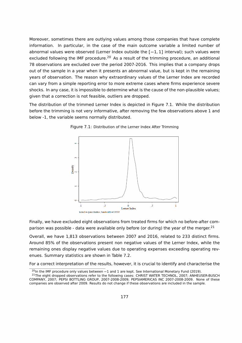
Moreover, sometimes there are outlying values among those companies that have complete

information. In particular, in the case of the main outcome variable a limited number of

abnormal values were observed (Lerner Index outside the [−1,1] interval); such values were

excluded following the IMF procedure.20 As a result of the trimming procedure, an additional

78 observations are excluded over the period 2007-2016. This implies that a company drops

out of the sample in a year when it presents an abnormal value, but is kept in the remaining

years of observation. The reason why extraordinary values of the Lerner Index are recorded

can vary from a simple reporting error to more extreme cases where firms experience severe

shocks. In any case, it is impossible to determine what is the cause of the non-plausible values;

given that a correction is not feasible, outliers are dropped.

The distribution of the trimmed Lerner Index is depicted in Figure 7.1. While the distribution

before the trimming is not very informative, after removing the few observations above 1 and

below -1, the variable seems normally distributed.

Figure 7.1: Distribution of the Lerner Index After Trimming

Finally, we have excluded eight observations from treated firms for which no before-after com-

parison was possible - data were available only before (or during) the year of the merger.21

Overall, we have 1,813 observations between 2007 and 2016, related to 233 distinct firms.

Around 85% of the observations present non negative values of the Lerner Index, while the

remaining ones display negative values due to operating expenses exceeding operating rev-

enues. Summary statistics are shown in Table 7.2.

For a correct interpretation of the results, however, it is crucial to identify and characterise the20In the IMF procedure only values between −1 and 1 are kept. See International Monetary Fund (2019).21The eight dropped observations refer to the following cases: CHRIST WATER TECHNOL, 2007; ANHEUSER-BUSCH

COMPANY, 2007; PEPSI BOTTLING GROUP, 2007-2008-2009; PEPSIAMERICAS INC 2007-2008-2009. None of thesecompanies are observed after 2009. Results do not change if these observations are included in the sample.

177

companies that are excluded or that drop out occasionally due to outliers. Appendix D presents

and discusses summary statistics on the excluded firms, and characterises them in terms of

country of registration and listing status, in order to capture possible distortions introduced

by these specificities. As shown in Appendix D, it can be observed that a large proportion of

companies with missing financial information belong in general to countries with less stringent

reporting requirements (such as Germany). On the other hand, the presence of outliers in the

outcome variables seems to be more randomly spread in terms of country and NACE codes,

even if most of the companies trimmed on the basis of outliers are non-listed.

Table 7.2: Summary statistics over the entire period of observation

No. obs. mean sd min max

Lerner Index 1813 0.10 0.24 -0.97 1.00

Treated 1813 0.27 0.44 0.00 1.00

Post 1813 0.82 0.39 0.00 1.00

(log) Total assets 1813 19.28 2.74 9.20 25.99

Shareholders’ HHI 1813 3807.55 3580.25 0.00 10000

Shares top 4 owners 1813 62.66 34.27 0.00 100

Firm’s Integration 1813 0.26 0.36 0.00 1.00

Shares owned by Big2 1813 0.76 2.13 0.00 15.68

Finally, Table 7.3 reports the composition of the treated firms in the final sample. Of the firms

observed in 2007, 53 are treated; among these, three firms are held only by BlackRock (the

average share owned is equal to 0.37), 27 are held only by BGI (with average shares of 1.99%)

and 23 are held by both BlackRock and BGI (the average total share is 4.15%).

Table 7.3: Average shares owned by BGI and/or BlackRock (BR) in 2007 in different sets of firms

Obs. Held by BR Held by BGI Held by BR & BGI

Treated firms 53

of which: 3 27 23

Shares held by BR/BGI 0.37 1.99 4.15

To complement the above baseline information, the evolution of ownership of the treated and

control groups over the following years is inspected. Figures 7.2 and 7.3 report the average

shares owned by Barclays/BGI and BlackRock, respectively, in three sub-groups over the time

frame under analysis: firms jointly owned by the two investors, firms owned only by either

of them, and firms owned by neither. While in the first figure the importance of BGI in the

shareholders’ composition decreases, BlackRock appears to gain a larger share, especially

178

among the firms that in 2007 where jointly held by both investors. It is also noteworthy that

companies that were not owned by neither BGI nor BlackRock in 2007 do not experience large

acquisitions by the two in the following 9 years. Detailed results on ownership of key players

of the market can be found in Appendix D.

Figure 7.2: Average shares owned by Barclays/BGI

Figure 7.3: Average shares owned by BlackRock

179

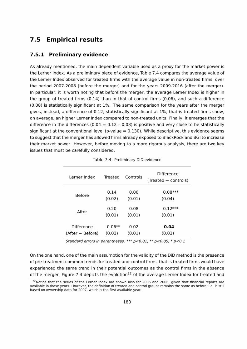
7.5 Empirical results

7.5.1 Preliminary evidence

As already mentioned, the main dependent variable used as a proxy for the market power is

the Lerner Index. As a preliminary piece of evidence, Table 7.4 compares the average value of

the Lerner Index observed for treated firms with the average value in non-treated firms, over

the period 2007-2008 (before the merger) and for the years 2009-2016 (after the merger).

In particular, it is worth noting that before the merger, the average Lerner Index is higher in

the group of treated firms (0.14) than in that of control firms (0.06), and such a difference

(0.08) is statistically significant at 1%. The same comparison for the years after the merger

gives, instead, a difference of 0.12, statistically significant at 1%, that is treated firms show,

on average, an higher Lerner Index compared to non-treated units. Finally, it emerges that the

difference in the differences (0.04 = 0.12 – 0.08) is positive and very close to be statistically

significant at the conventional level (p-value = 0.130). While descriptive, this evidence seems

to suggest that the merger has allowed firms already exposed to BlackRock and BGI to increase

their market power. However, before moving to a more rigorous analysis, there are two key

issues that must be carefully considered.

Table 7.4: Preliminary DiD evidence

Lerner Index Treated ControlsDifference

(Treated − controls)

Before0.14 0.06 0.08***

(0.02) (0.01) (0.04)

After0.20 0.08 0.12***

(0.01) (0.01) (0.01)

Difference 0.06** 0.02 0.04

(After − Before) (0.03) (0.01) (0.03)

Standard errors in parentheses. *** p<0.01, ** p<0.05, * p<0.1

On the one hand, one of the main assumption for the validity of the DiD method is the presence

of pre-treatment common trends for treated and control firms, that is treated firms would have

experienced the same trend in their potential outcomes as the control firms in the absence

of the merger. Figure 7.4 depicts the evolution22 of the average Lerner Index for treated and22Notice that the series of the Lerner Index are shown also for 2005 and 2006, given that financial reports are

available in those years. However, the definition of treated and control groups remains the same as before, i.e. is stillbased on ownership data for 2007, which is the first available year.

180

non-treated firms. Although purely suggestive, it can be noticed that trends look similar before

the merger, since the confidence intervals overlap, while differ after the merger was in place,

with the value of Lerner Index being particularly pronounced for treated firms in the years

2013 and 2014.

Figure 7.4: Naive evidence of the common trend: average Lerner Index (±2SD) in treated (eposed)and control (not eposed) groups.

On the other hand, since the assignment to the treatment group is not random, there might

be firms’ observable characteristics that determine the probability of being treated. In other

words, the treated firms, namely those held by BGI and/or BlackRock in 2007, could be very

different in terms of observable characteristics, such as size, turnover, etc., from those in the

control group, thus any observed effects on the Lerner Index might be simply due to these

different characteristics rather than the merger event. Were it the case, the exclusion of these

characteristics from the regression would lead to biased estimates.

To account for this, a mean comparison test between treated and control firms is carried out

on pre-treatment data23 for the observable characteristics described in the previous section.

Results are shown in Table 7.5, showing that the level of total assets and total share owned23For most firms, the ownership and financial values used for the tests are those from the year 2007. However, for

four treated firms and 10 control firms, financial data are only present from 2008. It follows that they are includedin the empirical analyses only from 2008, and that for these cases the tests presented in Table 7.5 are run on 2007ownership data but on 2008 financial data.

181

by the "big two" (State Street and Vanguard) are significantly larger on average for treated

firms as compared to control units. On the contrary, control units show a higher HHI index

and share of top 4 owners with respect to treated firms. It seems that there is no difference

in terms of integration between treated and control firms. Finally, while the initial level of the

Lerner Index for treated firms appears to be larger than that observed for control firms, such

a difference is weakly statistically significant (p-value = 0.071).

Table 7.5: Pre-treatment comparison between treated and control units

Difference

Variable Treated Controls (Treated−controls)

Lerner Index 0.14 0.06 0.08 *

(0.04) (0.02) (0.04)

(log) Total assets 21.73 18.24 3.49 ***

(0.23) (0.19) (0.30)

Shareholders’ HHI 1021.98 4542.58 -3520.60 ***

(178.94) (315.10) (362.37)

Shares top 4 owners 35.59 69.04 -33.45 ***

(3.75) (2.86) (4.71)

Firm’s Integration 0.26 0.27 -0.01

(0.04) (0.03) (0.05)

Shares owned by Big2 1.67 0.02 1.65 ***

(0.33) (0.02) (0.33)

Number of firms 53 128

Standard errors in parentheses. *** p<0.01, ** p<0.05, * p<0.1

7.5.2 Results from Difference-in-Differences model

The first round of DiD results is reported in Table 7.6. Here, the results of the estimation of

Eq. (7.1) are displayed under different specifications: column (1) reports the model without

control variables; in columns (2) and (3) the analysis is replicated by including controls and

their interaction with the post indicator, respectively. Central to the issues at hand is the

coefficient of treted × post, which is positive (0.069) and statistically significant at 5% level

in the specification in col. (1), and it is very similar (0.072) when controls are included. When

we interact controls with post (col. 3), the coefficient of interest is larger than those in the

previous specifications24 (0.113), and it statistically different form zero at a 5% level.24Such an increase in the size of the coefficient might indicate that estimations in col. (2) are affected by a negative

correlation between treted × post and the control variables observed after the merger. Furthermore, it is worth

182

While for column (2) the implicit assumption is that the dummy for post years has a different

effect only for the treated, in column (3) we postulate that all covariates might have different

effects after the merger, compared to their effect before, which remains the reference point.

In other words, the coefficient for each non-interacted firm characteristic has to be interpreted

as the marginal effect for that variable only for the reference years before the merger.

Table 7.6: Main results

Dep. var.: Lerner Index (1) (2) (3)

Treated*post 0.069** 0.072** 0.113**(0.034) (0.035) (0.049)

(log) Total assets -0.007 -0.007(0.009) (0.011)

Shareholders’ HHI 0.004 -0.006(0.007) (0.008)

Shares top 4 owners 0.010 0.049(0.049) (0.079)

Firm’s Integration 0.007 -0.003(0.035) (0.044)

Shares owned by Big2 -0.501 0.631(0.664) (1.105)

(log) Total assets*post 0.001(0.007)

Shareholders’ HHI*post 0.012**(0.005)

Shares top 4 owners*post -0.042(0.077)

Firm’s Integration*post 0.015(0.036)

Shares owned by Big2*post -0.952(0.777)

Observations 1,813 1,813 1,813Treated 483 483 483Controls 1,330 1,330 1,330

Year fixed effects yes yes yesFirm fixed effects yes yes yesR-squared within 0.015 0.019 0.026R-squared overall 0.614 0.615 0.618

Robust standard errors, clustered at the firm levels, in parentheses*** p<0.01, ** p<0.05, * p<0.1

noting that, although the estimated coefficient of treted × post in col. (3) is larger than the one estimated in col.(2), its 95% confidence interval ranges from 0.02 to 0.21 which includes 0.72, the point estimate of the specificationreported in col. (2).

183

As usual, the interaction term between post and each predictor represents the difference in

the coefficients between the reference period and the post period.25

None of the control variables is statistically significant in the specification of col. (2). When the

controls are interacted with post, only Shrehoders′ HH is statistically significant, indicating

that firms with more concentrated shareholders’ structures experience a positive impact on

the Lerner Index after the merger.

The results indicate that firms held by BlackRock and/or BGI in 2007 show a Lerner Index on

average 0.07 points higher than control firms after the merger, suggesting that the merger

triggered an increase in profitability of firms already exposed to BlackRock and/or BGI.

Analogous results are obtained using as outcome the alternative competition measure de-

scribed earlier, i.e. the Lerner Index adjusted for cost of capital. Results are presented in

Appendix D. Notice that in this case the sample is slightly more reduced, given that not all

firms report the necessary financial variables for the calculation of this adjusted outcome.

While the results indicate an increase of the Lerner Index associated with the merger, nothing

is said on whether such an effect is driven by changes in revenues and/or costs.26 To closely

inspect which component of the Lerner Index pushes more the effect, we plot the (average)

evolution of revenues and costs for treated (Figure 7.5a) and control (Figure 7.5b) firms, before

and after the merger. In the case of treated firms, both revenues and costs move along

the same path before the merger, and immediately after we observe a sharper increase in

revenues as compared to costs, while moving again along a similar trend from 2010 onwards.

Regarding control firms, both revenues and costs follow a similar – almost identical – path,

before and after the merger. What emerges is that the increase in the Lerner Index seems to

be driven more by a marked increase in revenues rather than a decrease in costs.

While this exercise represents a first attempt to link common shareholding with a measure of

firm’s competitive outcome, other ex-post studies evaluated the impact of merger decisions on

prices. Kwoka (2013) collects 46 merger cases in the US and presents the average price effects

estimated by this sample of studies. It turns out that in 38 cases the merger led to a price

increase of approximately 9.85%, while in only 8 cases a decrease in prices was found (around

4.83%). Turning to Europe, a recent report commissioned by the European Commission to a

team of academics at the Centre for Competition Policy, University of East Anglia, reviews ex-

post evaluations of the impact of merger decisions by EU competition authorities.27 According

to the report, it emerged that post-merger prices increased in 14 studies, with such an effect

being estimated at around 8.24%, while, on the contrary, in 7 studies a decrease in the level25Note that estimating a fully interacted model is very similar to estimating two separate models - the so-called

split sample - one before and one after the treatment, and it would be perfectly equivalent if we did not includefixed effects. However, we prefer to run the interacted estimation rather than the split sample estimator because thep-value for each interaction term provides a significance test for the difference in those coefficients.

26The revenues variable corresponds to the OPRE variable from Orbis, while the costs are obtained by subtractingrevenues (OPRE) from the EBT variable.

27See Ormosi et al. (2015).

184

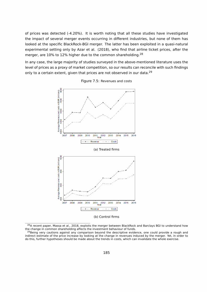
of prices was detected (-4.20%). It is worth noting that all these studies have investigated

the impact of several merger events occurring in different industries, but none of them has

looked at the specific BlackRock-BGI merger. The latter has been exploited in a quasi-natural

experimental setting only by Azar et al. (2018), who find that airline ticket prices, after the

merger, are 10% to 12% higher due to the common shareholding.28

In any case, the large majority of studies surveyed in the above-mentioned literature uses the

level of prices as a proxy of market competition, so our results can reconcile with such findings

only to a certain extent, given that prices are not observed in our data.29

Figure 7.5: Revenues and costs

(a) Treated firms

(b) Control firms

28A recent paper, Massa et al., 2018, exploits the merger between BlackRock and Barclays BGI to understand howthe change in common shareholding affects the investment behaviour of funds.

29Being very cautions against any comparison beyond the descriptive evidence, one could provide a rough andindirect estimate of the price increase by looking at the change in revenues induced by the merger. Yet, in order todo this, further hypotheses should be made about the trends in costs, which can invalidate the whole exercise.

185

7.5.3 Who drives the effect?

In the figures below, a visual overview of the relevance of each treated firm in the baseline

estimation is provided. In Figure 7.6, firms held in 2007 either by BlackRock (the first three

data points from the left) or by Barclays/BGI (the remaining from the fourth onwards) are

dropped from the sample one at a time. The same exercise is conducted in Figure 7.7 focusing

on firms held in 2007 by both BGI and BlackRock.

In case a deviation from the main trend is observed, this signals that the specific dropped

firm played a pivotal role in driving the estimates of our original baseline specification. For

instance, this might be due to an exceptionally high or low Lerner Index. Overall, the value of

the impact is rather constant and does not suffer from notable changes when single firms are

dropped from the sample.

Figure 7.6: Effect of treatment excluding, one at a time, firms owned by either BGI or BlackRock. Firstthree firms on the left are held by BlackRock; firms on the right, are held by BGI.

186

Figure 7.7: Effect of treatment excluding, one at a time, firms jointly owned by BGI and BlackRock

7.6 Robustness checks

In this section, the validity of the previous results is confirmed by a battery of robustness

checks, intended to address possible issues related to the research design, which could bias

the baseline estimates. First, the traditional event-study analysis on the Lerner Index is car-

ried out. Then, several sensitivity checks are performed on alternative specifications of the

sample and on a different definition of the groups of treated and control firms. Finally, some

falsification tests are conducted.

7.6.1 Event study analysis

The existence of a common trend is the key identifying assumption for DiD estimates to be

unbiased. In the framework of this analysis, the assumption implies that - in the absence

of the treatment - firms held by BGI and/or BlackRock in 2007 would have experienced the

187

same trends in their potential Lerner Index as the control firms. While this is not testable, an

event-study analysis can shed some light on the validity of the research design. Specifically,

following Autor (2003), the interactions of the time dummies and the treatment indicator for

pre-treatment periods are added to the baseline specification of Eq. (7.1). If the trends in the

Lerner Index in treatment and control groups are the same, then the interactions should be not

statistically significant, i.e. the DiD coefficient should not be significantly different between the

two groups in the pre-treatment period. An attractive feature of this test is that the interactions

of the time dummies after the treatment (up to several years) with the treatment indicator are

informative, and can show whether the treatment effect changes over time. In detail, the

following specification is estimated:

yƒ t = α +2007∑

π=2007

γπ(tretedƒ × yerπ)+2016∑

τ=2009

γτ(tretedƒ × yerτ) + δƒ t + ƒƒ + ƒt + ƒ t (7.2)

where the year 2008 is omitted, coinciding with the period immediately preceding the merger.

This specification allows to test for the presence of parallel trends in the pre-treatment period,

namely, if the coefficient associated to the lead (γπ, for 2007) is not statistically different from

zero. As already anticipated, this approach is convenient to understand whether the treatment

effect fades, increases or stays constant over time, depending on the estimated coefficients

of the lags γτ , with τ going from 2009 to 2016.

Table 7.7 reports the estimates of Eq. (7.2), with and without control variables. According to

the point estimates in col. (1), where controls are not included, there is no difference in the

Lerner Index between treated and control units in the pre-treatment period. On the contrary,

coefficients associated to lags turn out to be positive and statistically significant from 2 up

to 5 years after the merger, indicating that the Lerner Index is growing over time for treated

firms if compared to control ones. Results remain qualitatively the same in columns (2) and

(3), where controls and controls interacted with post are included.

The estimates from column (3) and their 95% confidence intervals are plotted in Figure 7.8.

Taken together, these results seem to validate the research design, as there is no evidence

against the presence of a common trend between treated and control units.

188

Table 7.7: Autor test. Reference year 2008, one year before the merger.

Dep. var.: Lerner Index (1) (2) (3)

2 yrs prior -0.027 -0.027 -0.024(0.030) (0.030) (0.030)

merger -0.019 -0.019 0.023(0.027) (0.027) (0.041)

1 yr after 0.042 0.045 0.089(0.038) (0.039) (0.057)

2 yrs after 0.080** 0.082** 0.124**(0.037) (0.038) (0.052)

3 yrs after 0.095** 0.102** 0.144**(0.047) (0.049) (0.063)

4 yrs after 0.103** 0.104** 0.145**(0.047) (0.048) (0.062)

5 yrs after 0.097* 0.100* 0.141**(0.050) (0.052) (0.064)

6 yrs after 0.037 0.043 0.083(0.052) (0.055) (0.067)

7 yrs after 0.018 0.024 0.063(0.053) (0.056) (0.065)

(log) Total assets -0.006 -0.006(0.009) (0.011)

Shareholders’ HHI 0.003 -0.007(0.006) (0.008)

Shares top 4 owners 0.018 0.056(0.049) (0.079)

Firm’s Integration 0.004 -0.005(0.034) (0.044)

Shares owned by Big2 -0.607 0.507(0.746) (1.079)

(log) Total assets*post 0.001(0.007)

Shareholders’ HHI*post 0.012**(0.005)

Shares top 4 owners*post -0.041(0.076)

Firm’s Integration*post 0.013(0.036)

Shares owned by Big2*post -0.924(0.763)

Observations 1,813 1,813 1,813

Treated 483 483 483

Controls 1,330 1,330 1,330

Year fixed effects yes yes yes

Firm fixed effects yes yes yes

R-squared within 0.028 0.032 0.038

R-squared overall 0.619 0.621 0.623

Robust standard errors, clustered at the firm level, in parentheses; *** p<0.01, ** p<0.05, * p<0.1

Figure 7.8: Event study

7.6.2 Alternative sample selection

In Table 7.8, other methods for sample selection have been tested. In the first three columns,

companies that were not present in the 2007 sample are not considered in the estimation,

resulting in a smaller sample size. This means that the control units are constant over time, not

introducing any newly created company in the sample. As a result, the sample is composed

by 1,513 observations, including all 483 observations from treated firms. The coefficient of

interest remains positive and significant at the conventional level.

Yet, another source of concern might derive from the use of an unbalanced sample, which

could lead to biased results.30 Therefore, we replicate our main results by relying on a bal-

anced sample of firms, keeping only those with recorded observations along the entire time-

span of the analysis. We have full 10-year information on 105 firms (1,050 observations), of

which 36 are treated.31 Results of this analysis are reported in Table 7.8, col. (4)−(6) and,30The concern about unbalanced panels lies in the possible reason behind missing information. If the data are

non-randomly missing, findings are likely to be biased. In our setting, the reasons for the missing data are quite wellknown, such as firms exiting the market due to their natural life-cycle, or non-reporting of balance sheet informationdue to lack of legal obligation. Therefore, a good robustness check can come from the comparison of the resultsobtained with the full unbalanced sample with those obtained using a balanced one. If estimates yield similar results,this suggests that findings are not biased (Baltagi, 2008; Cameron and Trivedi, 2005).

31As a reference, note that 82% of the firms of the full sample present data for at least 5 years, which is a quite longtime span to capture the effects under study. More in detail, 25% of the companies present between 5 and 8 years ofobservation, 12% of the firms are observed for 9 years, and 45% have full information for the whole 10 years.

190

reassuringly, indicate that the coefficient of treted × post is statistically significant across

models and pretty similar to that obtained in the baseline specification.

A final alternative sample definition is used in the last three columns. Here, instead of trim-

ming Lerner Index observations outside the [−1,1] interval, these are kept in the sample, but

their values are set equal to the thresholds of −1 and +1. In this case, the sample counts

1,884 observations, of which 489 are related to treated firms. Columns (7)−(9) show the re-

sults with this specification, which are consistent with the main model and slightly larger in

magnitude.

Table 7.8: Alternative sample definitions

Existing in 2007 Balanced Sample Replacing if > 1 or < −1Dep. var.: Lerner Index (1) (2) (3) (4) (5) (6) (7) (8) (9)

Treated*post 0.071** 0.073** 0.120** 0.072** 0.080** 0.101*** 0.080** 0.085** 0.126**

(0.034) (0.035) (0.048) (0.033) (0.034) (0.038) (0.037) (0.038) (0.056)

(log) Total assets 0.002 0.003 -0.011 -0.014 0.005 0.006

(0.005) (0.008) (0.014) (0.016) (0.011) (0.013)

Shareholders’ HHI 0.002 -0.007 0.002 -0.003 -0.021 -0.136

(0.008) (0.009) (0.009) (0.010) (0.076) (0.089)

Shares top 4 owners -0.017 0.024 0.009 0.047 0.027 0.100

(0.052) (0.081) (0.064) (0.082) (0.069) (0.100)

Firm’s Integration -0.002 -0.007 -0.039 -0.044 0.007 -0.009

(0.039) (0.046) (0.044) (0.046) (0.036) (0.050)

Shares owned by Big2 -0.336 1.157 -0.439 1.426 -0.010 0.001

(0.567) (0.944) (0.835) (1.206) (0.007) (0.011)

(log) Total assets*post -0.001 0.003 -0.002

(0.007) (0.006) (0.008)

Shareholders’ HHI*post 0.012** 0.007 0.139**

(0.006) (0.005) (0.062)

Shares top 4 owners*post -0.043 -0.046 -0.088

(0.078) (0.061) (0.090)

Firm’s Integration*post 0.008 0.004 0.021

(0.038) (0.027) (0.046)

Shares owned by Big2*post -1.209 -1.515* -0.010

(0.758) (0.814) (0.008)

Observations 1,513 1,513 1,513 1,050 1,050 1,050 1,884 1,884 1,884

Treated 483 483 483 360 360 360 489 489 489

Controls 1,030 1,030 1,030 690 690 690 1,395 1,395 1,395

Year fixed effects yes yes yes yes yes yes yes yes yes

Firm fixed effects yes yes yes yes yes yes yes yes yes

R-squared within 0.018 0.019 0.026 0.037 0.045 0.051 0.095 0.015 0.014

R-squared overall 0.605 0.605 0.608 0.667 0.670 0.617 0.617 0.626 0.627

Robust standard errors, clustered a the firm level, are shown in parentheses. *** p<0.01, ** p<0.05, * p<0.1

In col. (1), (2) and (3) we exclude firms which were not in the sample in 2007

In col. (4), (5) and (6) we keep only firms with 10 years of observation

In col. (7), (8) and (9) values of Lerner Index below -1 or above 1 are replaced with such thresholds.

191

7.6.3 Different definitions of the treatment and control groups

So far, the definition of the treated group included three types of "exposed" firms, according

to the 2007 ownership structure: i) firms held only by BlackRock; ii) firms held only by BGI and

iii) firms held by both BlackRock and BGI. The assumption was that all the above three groups

of firms were equally exposed to the merger, and could therefore be considered as "treated".

However, the interpretation of the role of these three groups might vary, and lead eventually

to alternative definitions of the treatment and control groups.

A possible argument could be the following: while the first two groups of firms are fully entitled

to be considered treated, the latter may be shifted into the control group. In fact, it might be

reasonable to assume that for this set of firms the merger did not produce any effects, given

that it is composed by companies already held by both BlackRock and BGI before the merger.

In order to understand potential differences of roles of these three groups of firms, and whether

this is reflected in any differential effect on profitability after the merger, an alternative specifi-

cation of treated and control groups has been experimented. In particular, we split the original

group of treated firms into two, separating the 23 companies jointly held by BlackRock and BGI

from the rest. A dummy variable, BG&BR, measured in 2007, is built to account for this issue,

equal to one if a firm was held by both BlackRock and BGI, and zero otherwise. Then, this new

variable is interacted with the treted variable in a model taking the following form:

yƒ t = α+γtretedƒ2007× postt+ λtretedƒ2007× postt×BG&BRƒ2007+ δƒ t+ ƒƒ + ƒt+ ƒ t (7.3)

where the variable treted includes all firms held in 2007 by BlackRock and/or BGI, i.e. all

three groups i), ii) and iii) defined above. It follows that coefficient γ accounts for the effect of

the merger for all treated firms, while λ captures the differential effect of the merger for the

firms jointly held by BGI and BlackRock in 2007.

If λ in Eq. (7.3) turns out to be statistically significant, then the impact of the merger on firms

held by both BlackRock and BGI is different from that on firms held by BlackRock or BGI only. In

this case, the treatment variable would need to be redefined, including only firms held either

by BlackRock or by BGI. Instead, if λ is not statistically significant, the impact of the merger

for firms held by both BlackRock and BGI is not different from the rest of treated firms. Hence,

in this case, there would be no need to change the definition of treated and control groups.

According to estimates shown in the first three columns of Table 7.9, the coefficient λ is nega-

tive (−0.030) but not statistically significant in the specification that does not include controls

(col. 1). Similarly, it is negative and indistinguishable from zero both in the model where con-

trols are included (−0.026; col. 2), and in the last case where we account for the interaction

between controls and post (−0.003; col. 3). Therefore, in light of these results, there is no

evidence against the inclusion of these firms, namely those held in 2007 by both BlackRock

and BGI, in the definition of treated firms.

192

7.6.4 Falsification and other tests

Placebo test

A common way to conduct a placebo tests in the context of DiD analysis is that of focusing

on the span prior to the merger, that is to simulate what would have happened to the Lerner

Index if a fake year of the merger were used. More in detail, we assume that the merger

between BlackRock and BGI occurred in 2008, and the main analysis is replicated on the period

2007-2008. If the coefficient associated to tretedƒ2007 × (ƒke)post2008 turns out positive

and significant, it would suggest that before the true year of the merger, treated firms were

already experiencing an increase in the Lerner Index compared to control ones, thus casting

doubts on the validity of previous results.

Reassuringly, the effect of placebo exercise does not lead to any effect on the Lerner Index

as the γ coefficient turns out to be indistinguishable from zero in the specification without

controls (Table 7.9, col. 4), and in both the specifications where controls are included (Table

7.9; col. 5), and interacted with (ƒke)post (Table 7.9; col. 6).

Different definition of the treatment year

The results discussed so far have been based on the indicator of dependence from BlackRock

and/or BGI using figures from 2007, a period coinciding with the beginning of the financial

crisis. This could raise the concern that BGI and BlackRock could have targeted companies

in 2007, which would perform particularly well after the crisis. In other words, it might be

the case that BGI and BlackRock – in light of the financial crisis – have decided to invest

in "healthier" and more performing firms in 2007, thus questioning the definition of treated

and control group, and therefore of the results. In principle, the best solution to tackle this

issue would be building our treatment indicator on earlier ownership data, long before the

financial crisis. By doing so, we would have a proxy for exposure to BGI and BlackRock which

is less subject to possible selection bias. In fact, it would be unrelated to the shareholding

strategies of the two financial institutions preparing for the merger and/or the financial crisis.

Unfortunately, data on ownership is not available before 2007.

However, there are some ways to mitigate this concern. To begin with, recall that in all esti-

mations we control for year fixed effects that are meant to capture macroeconomic shocks,

such as the financial crisis, common to all firms. In this regard, one could claim that treated

and control firms could have responded differently to the crisis even in the absence of the

merger event. Were it the case, the inclusion of years fixed effect would not be sufficient for

obtaining unbiased estimates. Nevertheless, as pointed out by Lewellen and Lowry (2020), it

is a major concern only if firms in the control group belong to different sectors than treatment

firms, which does not apply in our context as we restricted the analysis to firms operating in

the Beverages market.

193

Second, as discussed in Section 7.2, the possibly non-random allocation of treated and control

units can be correlated with other firms’ characteristics and/or with the financial crisis, but the

introduction of the interaction between controls variables and post in the estimates should

attenuate the potential bias. In fact, if more performing firms were acquired by BGI and

BlackRock in 2007 in light of the crisis, the control variables - which are meant to capture

firms’ characteristics - interacted with post should have picked up this effect, leading to a

coefficient of treted × post indistinguishable from zero. However, as shown in Table 7.6, col.

3, the coefficient of treted × post is positive and statistically significant at 1%.

Finally, one could argue that the financial crisis produced its effect in Europe starting from

2008.32 It follows that, in the spirit of a further robustness test, an alternative treatment has

been computed according to 2008 ownership data. If the definition of treated and control

groups were undermined by the strategic behavior of BGI/BlackRock reacting to the financial

crisis, we would observe very different results with respect to those obtained with the treat-

ment indicator based on 2007.

The last three columns of Table 7.9 display the results of this analysis and indicate that the

coefficient of interest is positive (0.071) and statistically significant at 5% level when controls

are excluded (col. 7), and it is slightly larger, 0.77 and 0.125 respectively, when controls and

controls interacted with post are included (col. 8 and 9).

The fact that the coefficient of interest remains stable indicates that the two financial insti-

tutions did not substantially alter their portfolio in anticipation of the financial and economic

turmoil caused by the Great Recession. Taken together, these results are stable across speci-

fications and do not seem to be much affected by the choice of the year used for determining

the treated status of firms, thus lessening the concerns that BGI and BlackRock could have

targeted only the more performing companies in 2007.

32In late 2008 the crisis developed into a number of European bank failures, declines in various stock indexes, largereductions in the market value of equities, a decrease in international trade. The currency crisis spread at the end ofOctober 2008.

194

Table 7.9: Robustness tests

Dep. var.: Lerner Index (1) (2) (3) (4) (5) (6) (7) (8) (9)

Treated*post 0.082* 0.075 0.120**(0.050) (0.048) (0.056)

Treated*post*(BGI&BR) -0.030 -0.026 -0.003(0.060) (0.058) (0.069)

Treated*(fake)post 0.019 0.019 0.011(0.029) (0.028) (0.041)

(2008)Treated*post 0.071** 0.077** 0.125**(0.035) (0.037) (0.054)

(log) Total assets -0.005 -0.003 0.025 0.028 -0.009 -0.007(0.009) (0.009) (0.025) (0.026) (0.009) (0.011)

Shareholders’ HHI 0.004 -0.007 -0.012 -0.007 0.009 0.000(0.007) (0.007) (0.012) (0.013) (0.007) (0.010)

Shares top 4 owners 0.018 0.064 -0.036 -0.035 -0.026 -0.021(0.047) (0.071) (0.109) (0.128) (0.055) (0.115)

Firm’s integration 0.010 -0.003 0.019 0.035 0.032 0.032(0.035) (0.043) (0.031) (0.041) (0.038) (0.051)

Shares owned by Big2 -0.151 0.919 -4.797*** -4.137*** -0.918 -0.365(0.548) (1.374) (1.406) (1.407) (0.805) (1.289)

(log) Total assets*post -0.002 -0.002(0.002) (0.007)

Shareholders’ HH*Ipost 0.013** 0.009(0.005) (0.008)

Shares top 4 owners*post -0.049 0.001(0.069) (0.109)

Firm’s Integration*post 0.017 0.001(0.035) (0.040)

Shares owned by Big2*post -0.916 -0.401(1.018) (0.862)

(log) Total assets*(fake)post -0.002(0.006)

Shareholders’ HHI*(fake)post -0.003(0.008)

Shares top 4 owners*(fake)post -0.019(0.107)

Integration*(fake)post -0.034(0.033)

Shares owned by Big2*(fake)post -0.300(0.900)

Observations 1,813 1,813 1,813 335 335 335 1,646 1,646 1,646Treated 483 483 483 101 101 101 434 434 434Controls 1,330 1,330 1,330 234 234 234 1,212 1,212 1,212

Year fixed effects yes yes yes yes yes yes yes yes yesFirm fixed effects yes yes yes yes yes yes yes yes yesR-squared within 0.016 0.014 0.020 0.005 0.041 0.058 0.014 0.024 0.028R-squared overall 0.614 0.616 0.618 0.613 0.615 0.616 0.629 0.633 0.634

Robust standard errors, clustered at the firm level, are shown in parentheses. *** p<0.01, ** p<0.05, * p<0.1

We include, in column (1), (2) and (3), the differential effect of firms that are held by both shareholders; in column (4), (5) and (6), a placeboyear of the merger; in column (7), (8) and (9) a different definition of year of treatment.

195

7.7 Hetereogeneous effects

The baseline results have shown a positive relationship between the Lerner Index after the

merger and the exposure to the merger itself. However, these results can be explained in light

of two additional aspects not yet considered in the analysis. On the one hand, the merger

may take time to materialise its effect on the Lerner Index. On the other hand, the degree of

exposure to the merger may influence the actual extent of the effect.

7.7.1 Long-term effects

A significant role could be played by the time elapsed since the merger, as its effects may

take some time to materialise. To account for this possibility, a new variable, duration, has

been included in the model, measuring the time since the merger took place (1 to 8 years).

Its quadratic term (drton2) is also included, allowing the effect to be a non-linear function

of time. Therefore, the following model is estimated:

yƒ t = α + tretedƒ2007 × postt × (γ + λ drtont + π drton2t) + δƒ t + ƒƒ + ƒt + ƒ t (7.4)

Results of this analysis are reported in Table 7.10. Columns (1)-(3) show the estimates of the

linear specification, where the coefficient π in Eq. (7.4) is set equal to zero. Columns (4)-(6),

instead, present the estimates of the full quadratic specification. As usual, the three columns

for each specification correspond to estimation of models without controls, with controls, and

with controls interacted with post.

To better understand its dynamics, the aggregate effect has been computed for the years after

the merger. The estimated coefficients of Table 7.10 have been used to compute the following

combinations: γ+λ×yer in the case of the linear specification, and γ+λ×yer+π×yer2 for

the quadratic specification, for each post-merger year (duration from 1 to 8). The estimated

values of the effects are reported in Table 7.11, for the plain model (cols. 1 and 4), and for

the models with controls (cols. 2 and 5) and controls interacted with the post dummy (cols. 3

and 6). To ease the interpretation of the results, the combinations described above have been

plotted against the number of years in Figure 7.9, for the specifications with controls.

196

Table 7.10: Long-term effects

Dep. var.: Lerner Index (1) (2) (3) (4) (5) (6)

Treated*post 0.050* 0.049* 0.091** -0.043 -0.046 -0.005

(0.030) (0.030) (0.045) (0.031) (0.032) (0.041)

Treated*duration 0.005 0.006 0.005 0.064*** 0.066*** 0.066***

(0.008) (0.008) (0.008) (0.024) (0.024) (0.024)

Treated*duration2 -0.007*** -0.007*** -0.007***

(0.002) (0.002) (0.002)

(log) Total assets -0.007 -0.008 -0.008 -0.008

(0.009) (0.011) (0.009) (0.011)

Shareholders’ HHI 0.003 -0.007 0.003 -0.007

(0.006) (0.008) (0.006) (0.008)

Shares top 4 owners 0.009 0.049 0.012 0.051

(0.049) (0.079) (0.049) (0.079)

Firm’s Integration 0.007 -0.003 0.005 -0.004

(0.035) (0.044) (0.034) (0.044)

Shares owned by Big2 -0.675 0.424 -0.659 0.427

(0.738) (1.039) (0.746) (1.067)

(log) Total assets*post 0.001 0.001

(0.007) (0.007)

Shareholders’ HHI*post 0.012** 0.012**

(0.005) (0.005)

Shares top 4 owners*post -0.044 -0.043

(0.077) (0.077)

Firm’s Integration*post 0.015 0.014

(0.036) (0.037)

Shares owned by Big2*post -0.916 -0.905

(0.752) (0.755)

Observations 1,813 1,813 1,813 1,813 1,813 1,813

Treated 483 483 483 483 483 483

Controls 1,330 1,330 1,330 1,330 1,330 1,330

Year fixed effects yes yes yes yes yes yes

Firm fixed effects yes yes yes yes yes yes

R-squared within 0.016 0.021 0.027 0.024 0.028 0.035

R-squared overall 0.614 0.616 0.619 0.617 0.619 0.622

Robust standard errors, clustered at the firm level, are shown in parentheses.

*** p<0.01, ** p<0.05, * p<0.1

In columns (1)-(3) and (4)-(6) we control for the duration after the merger and its square, respectively.197

In the linear specification, the impact of the merger seems to be positively related to time,

as the Lerner Index significantly increases with the number of years, and after 6 years the

effect vanishes. Looking at the point estimates reported in Table 7.11, col. (1), it emerges

that after 2 and 3 years of the merger treated firms show a Lerner Index approximately 0.06

points larger than that of control firms (an estimate statistically significant at 5%), reaching

the maximum value of 0.08 difference after 7 years (coefficients are statistically significant at

10%) while disappearing in the 8th year. Results do not change if controls and their interaction

with post are included, as displayed in col. (2) and (3) of the same table.

Figure 7.9: Long term effects

(a) Linear specification

(b) Quadratic specification

198

However, a more reliable picture emerges when a quadratic term is introduced, which has a

concave effect. In fact, as shown in Figure 7.9b, one additional year after the merger is asso-

ciated to a larger effect on the Lerner Index. According to estimates of Table 7.11, col. (4), the

effect is statistically significant after 2 years and increases up to 5 years from the merger. It

slowly decreases and then, after 6 years disappears. Similar results are observed if controls

and its interaction with post are included (Table 7.11, col. 5 and 6). The main intuition behind

these findings is that the merger event prompted a sizable increase of the Lerner Index in

treated firms during the first years after which the market self-correction took place.

Table 7.11: Effects in models including linear or quadratic time trends

Linear Quadratic

Years (1) (2) (3) (4) (5) (6)

1 year 0.06** 0.06** 0.010** 0.01 0.01 0.06

(0.03) (0.03) (0.04) (0.02) (0.02) (0.04)

2 years 0.06** 0.06** 0.010** 0.06** 0.06** 0.10**

(0.03) (0.03) (0.04) (0.03) (0.03) (0.04)

3 years 0.06** 0.07** 0.011** 0.09** 0.09** 0.13***

(0.03) (0.03) (0.05) (0.04) (0.04) (0.05)

4 years 0.07** 0.07** 0.011** 0.10** 0.11** 0.15***

(0.03) (0.03) (0.05) (0.04) (0.04) (0.06)

5 years 0.07* 0.08* 0.012** 0.11** 0.11** 0.15**

(0.04) (0.04) (0.05) (0.05) (0.05) (0.06)

6 years 0.08* 0.08* 0.012** 0.09** 0.10** 0.14**

(0.04) (0.04) (0.06) (0.05) (0.05) (0.06)

7 years 0.08* 0.08* 0.013** 0.07 0.07 0.11*

(0.05) (0.05) (0.06) (0.05) (0.05) (0.06)

8 years 0.08 0.09 0.013** 0.03 0.04 0.08

(0.06) (0.06) (0.06) (0.05) (0.05) (0.06)

Robust standard errors in parentheses. *** p<0.01, ** p<0.05, * p<0.1

Plain model (cols. 1 and 4), with controls (cols. 2 and 5), controls

interacted with post (cols. 3 and 6)

199

7.7.2 Intensity of the exposure

In the main analysis all treated firms receive the same weights. However, it might be that the

impact of the merger on profitability depends on the extent of a firm’s exposure to BlackRock

and/or BGI in 2007. For example, the impact of the merger for a firm held at 1% by BG and/or

BlackRock in 2007 could be different from that experienced by a firm held, say, at 3%.

To investigate whether there has been a heterogeneous response according to the intensity

of exposure, we build a continuous variable, shareowned, corresponding to the value of par-

ticipation of BGI and/or BlackRock in 2007 (sum of the respective shares). This indicator is

interacted with tretedƒ2007 × post2007, and a quadratic specification is also considered. The

estimated model is a generalised version of Eq. (7.1), taking the following form:

yƒ t = α+ tretedƒ2007 × postt × (γ+ λ shreonedƒ07 + π shreoned2ƒ07) + δƒ t + ƒƒ + ƒt + ƒ t

(7.5)

Results of estimation for this model are reported in Table 7.12. Columns (1)-(3) show the

estimates of the linear specification, where coefficient π in Eq. (7.5) is set equal to zero.

Columns (4)-(6) present instead the estimates of the quadratic specification. Like before, each

set of three columns corresponds to model without controls, with controls, and with controls

interacted with post.

The quadratic effect is given by the full combination γ+λ×shreonedƒ2007+π shreoned2ƒ07,

while in the linear specification the impact corresponds to γ + λ × shreonedƒ2007; in both

cases the effect depends on the specific value of the variable shareowned. In practice, it

is possible to compute the impact for any value of exposure. For the sake of the example,

the linear and quadratic combined effects are computed using the estimated coefficients for

some chosen levels of exposure (see Table 7.13). The same results are also plotted in Figure

7.10. Apparently, in the linear specification reported in Figure 7.10a, larger shares owned by

BGI and/or BlackRock in 2007 seem to be associated with a reduction on the Lerner Index,

however the significance fades for very large values of exposure, rarely observed in practice.

More in detail, the impact of the merger for a firm held at 1% by BGI and/or BlackRock leads

to an increase of the Lerner Index of 0.10, an estimation statistically significant at 5%. Such

an impact significantly reduces to 0.05 if the held quota increases to 4% (Table 7.13 col. 1).

After 5%, there seems to be no significant impact on the Lerner Index.

Regarding the quadratic specification, although in the visual depiction (Figure 7.10b) and in

the opposite sign of the polynomial coefficients (see Table 7.12, col. 4 to 6) there seems to be

a U-shape pattern, this has no sufficient statistical power.

Further complements to the present exposure analysis are reported in Appendix D.

200

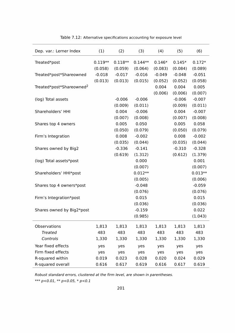
Table 7.12: Alternative specifications accounting for exposure level

Dep. var.: Lerner Index (1) (2) (3) (4) (5) (6)

Treated*post 0.119** 0.118** 0.144** 0.146* 0.145* 0.172*

(0.058) (0.059) (0.064) (0.083) (0.084) (0.089)

Treated*post*Shareowned -0.018 -0.017 -0.016 -0.049 -0.048 -0.051

(0.013) (0.013) (0.015) (0.052) (0.052) (0.058)

Treated*post*Shareowned2 0.004 0.004 0.005

(0.006) (0.006) (0.007)

(log) Total assets -0.006 -0.006 -0.006 -0.007

(0.009) (0.011) (0.009) (0.011)

Shareholders’ HHI 0.004 -0.006 0.004 -0.007

(0.007) (0.008) (0.007) (0.008)

Shares top 4 owners 0.005 0.050 0.005 0.058

(0.050) (0.079) (0.050) (0.079)

Firm’s Integration 0.008 -0.002 0.008 -0.002

(0.035) (0.044) (0.035) (0.044)

Shares owned by Big2 -0.336 -0.141 -0.310 -0.328

(0.619) (1.312) (0.612) (1.379)

(log) Total assets*post 0.000 0.001

(0.007) (0.007)

Shareholders’ HHI*post 0.012** 0.013**

(0.005) (0.006)

Shares top 4 owners*post -0.048 -0.059

(0.076) (0.076)

Firm’s Integration*post 0.015 0.015

(0.036) (0.036)

Shares owned by Big2*post -0.159 0.022

(0.985) (1.043)

Observations 1,813 1,813 1,813 1,813 1,813 1,813

Treated 483 483 483 483 483 483

Controls 1,330 1,330 1,330 1,330 1,330 1,330

Year fixed effects yes yes yes yes yes yes

Firm fixed effects yes yes yes yes yes yes

R-squared within 0.019 0.023 0.028 0.020 0.024 0.029

R-squared overall 0.616 0.617 0.619 0.616 0.617 0.619

Robust standard errors, clustered at the firm level, are shown in parentheses.

*** p<0.01, ** p<0.05, * p<0.1

201

Table 7.13: Heterogeneous effects on the Lerner Index, according to different levels of exposure toBlackRock and/or BGI. The effects are calculated, for the sake of the example, at some chosen levels ofexposure (shares owned).

Exposure Linear Quadratic

(Shares owned) (1) (2) (3) (4) (5) (6)

1% 0.10** 0.10** 0.13** 0.10** 0.10** 0.13**

(0.05) (0.05) (0.053) (0.05) (0.05) (0.05)

2% 0.08** 0.08** 0.11** 0.07* 0.07* 0.09*

(0.04) (0.04) (0.05) (0.04) (0.04) (0.05)

3% 0.07** 0.07** 0.10** 0.04 0.04 0.06

(0.03) (0.03) (0.04) (0.04) (0.04) (0.06)

4% 0.05* 0.05* 0.08* 0.02 0.02 0.04

(0.03) (0.03) (0.05) (0.05) (0.05) (0.07)

5% 0.03 0.04 0.07 0.01 0.01 0.04

(0.03) (0.02) (0.05) (0.04) (0.04) (0.07)

6% 0.02 0.02 0.06 0.01 0.01 0.04

(0.03) (0.03) (0.06) (0.04) (0.04) (0.06)

7% 0.02 0.01 0.04 0.01 0.02 0.05

(0.04) (0.04) (0.06) (0.05) (0.05) (0.07)

8% -0.01 -0.00 0.03 0.03 0.04 0.07

(0.05) (0.05) (0.07) (0.09) (0.09) (0.10)

Robust standard errors in parentheses. *** p<0.01, ** p<0.05, * p<0.1

Plain model (cols. 1 and 4), with controls (cols. 2 and 5), controls

interacted with post (cols. 3 and 6)

202

Figure 7.10: Marginal effects of the exposure to BlackRock and/or BGI. The effects are calculated, forthe sake of the example, at some chosen levels of exposure (shares owned).

(a) Linear specification

(b) Quadratic specification

203

7.8 Final remarks

This analysis presents a first attempt to measure the possible effects of common shareholding

on competition in the Beverages industry. The study considers the exogenous shock in own-

ership given by the BlackRock-BGI merger of 2009. The merger is exploited in a difference-in-

differences setting so as to determine a possible causal effect on market competition.

The specific market under investigation is defined by the set of beverages manufacturers

active in the EU territory between 2007 and 2016, namely either registered in the EU, or

holding participation in at least one firm registered in Europe. The range of manufactured

products considered in the study includes soft drinks, mineral waters, juices and beers.

The first evidence collected in this study points to the direction of enhanced market power

for the manufacturers that experienced increased common shareholding due to the merger.

Moreover, it should be noted that an increase in the Lerner Index - the competitive outcome

used in the analysis - appears to be driven more by a marked increase in revenues, rather

than a decrease in costs. The effect is larger for those companies which were only marginally

participated in by BlackRock or BGI before the merger, having benefitted most from the event.

On the other hand, those manufacturers which were more strongly held by either fund pre-

merger show a positive but smaller improvement in profitability. The effect is present soon

after the merger, but reaches its peak between four and five years after the event, becoming

negligible later on. The empirical evidence found in this study is robust to a certain number of

checks, including alternative specifications of the outcome and treatment variables. Overall,

the findings presented in this chapter seem to confirm similar results obtained by scholars

using US data for other industries. This constitutes, to the best of our knowledge, the first

investigation using EU data, and the first on the Beverages industry.

These results would appear to suggest a positive association between common shareholding

and the market power of firms. However, the findings of this study should be treated with

caution; in particular, the following caveats should be considered:

i) The small sample size and the short period of observation are potentially responsible

for the limited power of some statistical results, which will require further investigation.

In this respect, earlier data on the common shareholding structure of firms would help

confirm that BlackRock and BGI in 2007 did not specifically target companies that would

have performed well after the crisis. In a similar vein, multiple observations prior to the

merger would strengthen the evidence of a common trend between treated and control

firms - a key identifying assumption of the difference-in-differences design underlying the

analysis.

ii) The study focuses only on the Beverages sector, but while carefully accounting for other

industries’ specificities as well as possible data shortcomings, the present methodology

could be applied to possible future investigations in other markets.

204

iii) The Lerner Index is used - following the literature - as a proxy of market competition;

however, data on prices would help reinforce the evidence on common shareholding and

competitive outcomes, as it would facilitate controlling for the heterogeneity of products

sold by firms. Moreover, any country/product specific changes in the market could have

been factored-in.












research.

205

Box 7.1: Econometrics - Strategy

� We excluded a multi-industry econometric analysis, due to the product and structural

heterogeneity of different sectors, and opted instead for a single sector analysis.

� In the definition of the most appropriate econometric strategy, we observed that results

from the sectoral analyses did not show a very specific trend. The extent of common

shareholding at overall industry level was already high when our observation started in

2007, and remained roughly unchanged until 2016.

� However, looking at a selection of top investors, the sectoral reports revealed that a

change in the identity of the main players took place. In particular, we saw the rise of the

large investment funds and a contemporaneous drop in the participation of banks and

insurance companies.

� In particular, the 2009 merger of BlackRock with BGI, is the largest ’substitution’ event

between funds and banks. This event was of unprecedented proportions in the history

of mergers between asset management funds, and has therefore played a crucial role in

shaping the various studies on common shareholding.

� Given that the BlackRock-BGI merger represented a once-in-a-lifetime event, we also

investigated the possible existence of other minor changes in ownership at the investors’

level, which in turn may have provoked a relevant change in the degree of common

shareholding of the firms active in each sector.

� Others have encountered the same finding, that the statistical and economic significance

of the effects of these minor mergers is there but “an order of magnitude smaller” than

that of the BlackRock-BGI event. We therefore privileged this latter event, in order to

analyse possible links between common shareholding and competitive outcomes.

�

206

Box 7.2: Econometrics - Modelling

� Challenges. The econometric modelling has several challenges ahead, principally the

lack of an established theory showing how common shareholding affects managers, and

from there competitive outcomes. Additional challenges are:

– Defining market boundaries and proximity. The NACE classification is suited to

identify well established sectors, but is unable to capture markets in rapid change

where new technologies and products emerge. Instead, we used expert knowledge

to define exactly the players in each of the analysed markets.

– Using a common shareholding measure that overcomes the drawbacks of the

MHHI. We develop new measures taken from the literature on sparse matrices and

networks.

– Using a relevant measure of competition. Prices remain the preferred indicator for

changes in competitive forces on the market, however obtaining data on prices

at the required level of specificity is still a challenge. Instead, we used measures

of market power and market concentration. Market power is approximated by the

Lerner index, calculated either on the difference between sales and variable costs or

on the difference between operating profits and financial costs, to account for fixed

costs. Market concentration: the HHI is the typical measure of concentration used in

the literature, as it computes the relative size of a firm in an industry in terms of the

proportion of total output.

– A major empirical shortcoming relates to the use of accounting data from consoli-

dated vs unconsolidated accounts. We use unconsolidated accounts whenever avail-

able to be more precise in targeting the sector and the geographic area of activity.

� The sample. The Beverage sector was chosen for the empirical analysis: the set of

beverages manufacturers active in the EU territory between 2007 and 2016, namely

either registered in the EU, or holding participations in at least one firm registered in

Europe. The range of manufactured products considered in the study includes soft

drinks, mineral waters, juices and beers.

� The model. The impact of the change in common shareholding - induced by the

BlackRock-BGI merger - is estimated using a difference-in-differences approach. The

change in markup, before and after the event, for firms exposed to the merger (“treated”

group) is compared to that of firms that did not have any pre-merger relations with Black-

Rock and/or BGI (“control” group). We refine the estimated model through accounting

for several confounding factors, which could distort the measured link between common

shareholding and profitability. In particular, we account for the heterogeneity of relevant

firm-level characteristics, such as the dimension of the company, the shareholding struc-

ture, and the integration of the firm with competitors through common shareholders.�

207

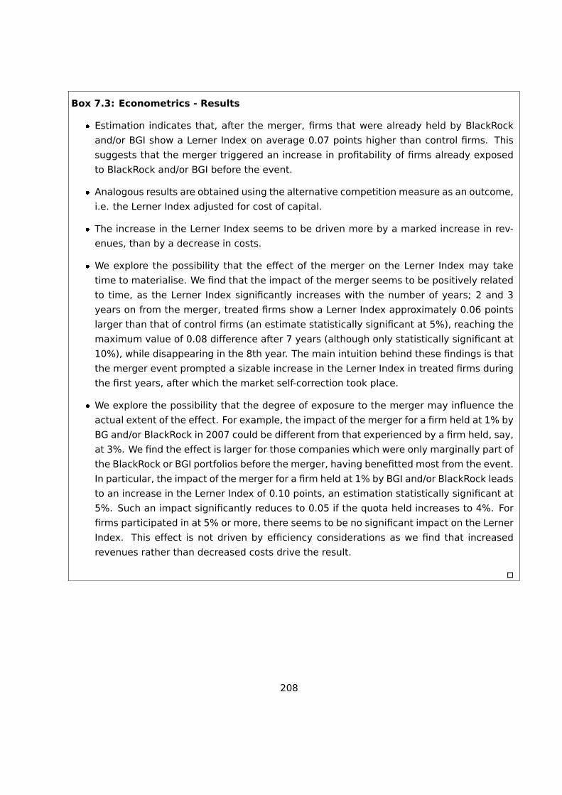
Box 7.3: Econometrics - Results

� Estimation indicates that, after the merger, firms that were already held by BlackRock

and/or BGI show a Lerner Index on average 0.07 points higher than control firms. This

suggests that the merger triggered an increase in profitability of firms already exposed

to BlackRock and/or BGI before the event.

� Analogous results are obtained using the alternative competition measure as an outcome,

i.e. the Lerner Index adjusted for cost of capital.

� The increase in the Lerner Index seems to be driven more by a marked increase in rev-

enues, than by a decrease in costs.

� We explore the possibility that the effect of the merger on the Lerner Index may take

time to materialise. We find that the impact of the merger seems to be positively related

to time, as the Lerner Index significantly increases with the number of years; 2 and 3

years on from the merger, treated firms show a Lerner Index approximately 0.06 points

larger than that of control firms (an estimate statistically significant at 5%), reaching the

maximum value of 0.08 difference after 7 years (although only statistically significant at

10%), while disappearing in the 8th year. The main intuition behind these findings is that

the merger event prompted a sizable increase in the Lerner Index in treated firms during

the first years, after which the market self-correction took place.

� We explore the possibility that the degree of exposure to the merger may influence the

actual extent of the effect. For example, the impact of the merger for a firm held at 1% by

BG and/or BlackRock in 2007 could be different from that experienced by a firm held, say,

at 3%. We find the effect is larger for those companies which were only marginally part of

the BlackRock or BGI portfolios before the merger, having benefitted most from the event.

In particular, the impact of the merger for a firm held at 1% by BGI and/or BlackRock leads

to an increase in the Lerner Index of 0.10 points, an estimation statistically significant at

5%. Such an impact significantly reduces to 0.05 if the quota held increases to 4%. For

firms participated in at 5% or more, there seems to be no significant impact on the Lerner

Index. This effect is not driven by efficiency considerations as we find that increased

revenues rather than decreased costs drive the result.

�

208

Box 7.4: Econometrics - Robustness checks

Several sensitivity checks are performed on alternative specifications of the sample, and on

a different definition of the groups of treated and control firms (firms directly affected by the

merger, and firms whose shareholding structure is not touched by the merger, respectively).

� Is an outlier driving the result? No, the value of the impact does not suffer from notable

changes when single firms are dropped from the sample.

� Without the merger, would firms held by BGI and/or BlackRock in 2007 have experienced

the same growth in their potential Lerner Index? No, our statistical tests suggest that

this would not have happened; i.e. the firms would not have experienced a higher Lerner

index, if the merger had not taken place.

� Is the result robust to changes of the sample? Yes, we replicate our main results by relying

on a balanced sample of firms, keeping only those with recorded observations along the

entire time-span of the analysis. Results are confirmed and the estimated coefficient is

even higher.

� In our analysis we had: i) firms held only by BlackRock; ii) firms held only by BGI and

iii) firms held by both BlackRock and BGI. The assumption was that all the above three

groups of firms were equally exposed to the merger, and could therefore be considered

as "treated". However, the interpretation of the role of these three groups might vary,

and lead eventually to alternative definitions of the treatment and control groups. Is the

result robust to these changes? Yes, estimations are not sensitive to the definition of the

treated group.

� We also ran a series of falsification tests to validate our model, all with negative results. In

particular, we looked into the possibility that BlackRock/BGI, anticipating the 2008 crisis,

could have targeted only the better performing companies in 2007. We find that the

two financial institutions did not substantially alter their portfolio in anticipation of the

financial and economic turmoil.

�

209

Box 7.5: Econometrics - Additional comments and limitations of the analysis

� The short period of observation before the merger is probably responsible for the limited

power of some statistical results, which will need further investigation. In this respect,

earlier data on the common shareholding structure of firms would help confirm that Black-

Rock and BGI in 2007 did not specifically target companies that would have performed

well after the crisis. In a similar vein, multiple observations prior to the merger would

strengthen the evidence of a common trend between treated and control firms - a key

identifying assumption of the difference-in-differences design underlying the analysis.

� The study focuses only on the Beverages sectors, but while carefully accounting for other

industries’ specificities, as well as possible data shortcomings, the present methodology

could be applied to possible future investigations in other markets.

� The Lerner Index is used - following the literature - as a proxy of market competition;

however, data on prices would help reinforce the evidence on common shareholding and

competitive outcomes, as it facilitates controlling for the heterogeneity of products sold

by firms. Moreover, any country/product specific changes in the market could have been

factored-in.

� Additional unobservable factors, other than the merger under consideration, may have

affected profitability. There are a series of possible mechanisms of influence through

which asset managers may affect a firm’s competitive outcome. Typically, such mech-

anisms include network effects, general policy consensus between asset managers, or

even a specific threshold in ownership that allows for effective leverage, under which a

shareholder in practice does not have a strong impact. These factors were not directly

observable in the present study and potentially could be further investigated, depending

on the availability of additional specific data.

The phenomenon of common shareholding proved to be particularly complex, and disentan-

gling its various effects continues to be challenging. Given that the literature in this area has

not yet investigated in depth the channels through which influence is exerted, this certainly

constitutes a good candidate for future research.

�

210

Chapter 8

Conclusions


agenda of all major think tanks and institutions worldwide. Common shareholders are typi-

cally institutional investors - e.g. pension funds and asset managers - holding concomitant

shareholdings in a given market. In the last two decades, these investment funds have grown

substantially in total size and concentration, both in Europe and worldwide, especially those

channeling savings towards investment strategies that replicate the performance of stock

market indices, such as the S&P500 or the FTSE100. Despite claiming a so-called passive

engagement strategy (not intervening directly in firm’s decisions), institutional investors col-

lect, together with the shares, the associated voting rights of their customers. This has led

economists (and policy makers) to analyse the effects of this concentration of power, as well as

the influence exerted on the management decisions of the firms which common shareholders

are mandated to invest in.

This report provides a comprehensive analysis of common shareholding in Europe with a spe-

cific focus on five industries/markets, namely Oil&Gas, Electricity, Trading Platforms, Telecom-

munications and Beverages. Based on firm-level balance sheet and ownership data, a set of

new indices of common shareholding is used to describe the investment behavior of share-

holders at both industry and investor level. The strength of relationships within the networks

of firms and of investors is also studied. Special attention is devoted to the top investors in

the EU overall as well as in each industry, and a brief overview of cross-investments within

industries is also reported, when relevant. Our baseline analysis is conducted on a historical

dataset containing all listed companies active in the EU in the period 2007-2016: this includes

all listed firms registered in the EU, plus all listed companies registered elsewhere, but holding

shares in at least one firm registered in the EU. The average number of firms observed each

year is 26,560 (24,857 in 2017 to 26,942 in 2016) - where on average about 57% are regis-

tered in the EU countries, the rest being registered outside the EU.

211

We find that in 2016, 87.2% of all shareholders of companies in our dataset hold participation

in only one company (85.7% in 2007). Common shareholders therefore constitute 12.8% of all

shareholders (14.9% in 2007). The number of listed firms that are cross-held by block-holders

(common shareholders with at least 5% participation in more than one company) has been

increasing, rising from about 15.5 thousand in 2007 to about 17.5 thousand in 2016. Around

67% of the analysed companies are cross-held by block-holders with at least 5% participation.

Looking at portfolios, top common shareholders hold shares in as many as 25% of the firms

in the market, i.e. more than 6,000 companies overall. They tend to invest equally among

the chosen firms, rather than giving priority to certain specific companies by buying higher

percentages of shares. The firms included in the largest portfolios represent a significant

proportion of the total value of the market, reaching a coverage of above 80% of Total Assets

(TOAS) and more than 90% of Market Capitalisation in almost all years. This means that the

top investors not only hold shares in a considerable number of firms (around 25%), but also

typically choose the largest enterprises, leaving out only minor players - which together do

not account for more than 10-20% of the market value. The preference for the largest market

players has become stronger over time. When both Total Assets and Market Capitalisation are

multiplied by the percentage of shares actually held, we find that in 2016 the top common

shareholder holds within its grasp 3.8% of total weighted Market Capitalisation and 6.6% of

the weighted TOAS in the EU. These percentages were 2.3 and 3.6 respectively in 2008; an

acceleration in the control of Total Assets or MarketCap can be observed as of 2012.

As to specific industries, we find that more than half of investors hold portfolios of very little

intensity, with average holdings of less than 1%. The mean portfolio holds shares of about

5-6% on average in the held firms; only Oil&Gas shows lower levels, while Telecoms stands on

slightly higher values, given the strong presence of high-participation corporate groups. Top

common shareholders are the usual suspects in all sectors (top banks and large asset man-

agement funds), except in Telecoms where individuals and large corporate groups dominate

via their cross-shareholdings in other companies in the same sector.

In the Oil&Gas sector BlackRock, Vanguard, State Street and Norway hold large amounts of

market value in their grasp: their shares in the held companies amount to about 12.88% of

the TOAS in 2016. A peculiar case is the Russian Government, which holds almost 6% of the

Total Assets of the market in 2016 via its subsidiaries Gazprom and Rosneft, but has little or

no participations in other companies.

In the Electricity market top common shareholders hold about 7% of the market’s Total As-

sets through their participation shares, and about 3.5% of Market Capitalisation. France plays

a major role in this market, holding very large stakes in three of the top ten EU-based cor-

porations, together with a minor presence in some additional firms. Overall in 2016 France

controlled about 6.7% of the Total Assets of this market. China is also a major player, mainly

via its subsidiary CHINA HUADIAN CORP, controlling about 3.23% of market TOAS. The usual

212

US-based funds (BlackRock, State Street and Vanguard) are still present as top investors, but

rather for the large number of firms in their portfolios, each held with minority shares. Overall,

together they control 5.57% of market TOAS.

The Trading Platforms sector presents some peculiarities. The set of firms operating the trad-

ing platforms (stock exchanges, banks, tech companies) is rather heterogeneous, not only in

terms of area of activity but also in terms of Total Assets and Market Capitalisation. Banks usu-

ally have a value of Total Assets which is incomparably higher than that of a traditional stock

exchange, and even more so than a digital platform or technology firm. On the other hand,

even companies with few assets can have a large Market Cap (even if the amount of listed

firms in the identified set of operators is minor). Many of the companies active in this sector

are controlled by large groups, thus presenting a very concentrated ownership structure with

large participation shares in the hands of few - or even only one - investors. The picture of

top investors in this industry is largely dominated by banks, while funds tend to drop to lower

positions in the ranking of common shareholders. In 2016, the big funds appeared to hold

very similar portfolios in terms of firms held, but the level of participation varies. For example,

BlackRock holds a large share (8.66%) of the London Stock Exchange, while State Street and

Vanguard have about 3% each. On the other hand, State Street has a strong presence in the

Spanish banks Santander (8.34%) and Banco Bilbao Vizcaya (10.87%), while BlackRock holds

about half of that and Vanguard even less (about 1% and 2% respectively). Overall, the size

of the portfolios - in terms of the number of firms - does not differ much across investors, with

Sweden, Funds, Banks and Insurance companies each fluctuating within the range 15%-20%,

while Norway displays a consistently higher value, of above 20%, holding the largest portfolio

in 2016 (34 firms).

In 2016, ownership in the Mobile Telecoms industry is concentrated in the hands of select indi-

viduals and associated holding groups, alongside large investment management firms such as

Blackrock or Vanguard Group. These global shareholders hold significant investments in large

pan-European telecom groups such as Vodafone and Orange, as well as national providers.

Together, these groups and providers compose almost the entirety of the European mobile

telecommunication market. The Telecoms sector exhibits some distinctiveness with respect to

the other sectors, notably cross-ownership (the telecoms companies themselves are common

shareholders). Another peculiarity of the Telecoms sector is the presence of individuals as com-

mon shareholders. Mr. Carlos Slim Helú (Mexico), Mr. Victor Li Tzar Kuoi (Hong Kong/China),

and J. Malone (US) control, directly or indirectly, 3.26%, 3.09% and 2.01% of the Total Assets

in the market, respectively. Among the funds, BlackRock dominates this industry, with rather

large shares in some of the top players (over 8% in Vodafone, almost 7% in BT GROUP PLC and

about 6% in KONINKLIJKE KPN NV); overall BlackRock controlled about 3.18% of Total Assets

in 2016. Vanguard and Norway lag behind, with relatively small participations, while State

Street plays only a minor role. France is also present, with a large participation in the French

company Orange, but also with some smaller stakes in other top competitors.

213

The Beverages market is rather heterogeneous. Relatively small enterprises with local markets

and a limited shareholder structure coexist with a set of large firms producing and/or distribut-

ing alcoholic products, structured in complex corporate groups with many cross-holdings (as

in the Telecoms sector). The top 1% of investors in 2007 held above 14% of the firms in the

sector, and in 2016 this declined to 11.2%. These investors hold firms that represent at least

between 53% and 60% of the Total Assets of the industry depending on the year (declining

trend). The top common shareholder has invested in companies representing up to 82% of the

TOAS of the sector in 2016. Such values are in line with expectations, since top investors tend

to privilege the largest enterprises. However, when this index is weighted according to the par-

ticipation share of investors, the trend inverts, demonstrating that the largest investor holds

a slightly decreasing share of weighted Total Assets. It would seem that top investors (but

this holds for other investors in general) are diluting their investment concentration amongst

a larger number of firms.

Likewise, cross-investment also characterises investment behavior in this sector. The first

three common shareholders in terms of weighted total assets in the Beverages sector are also

part of the market: DIAGEO PLC (UK) with 4.25% of the market TOAS, L’ARCHE GREEN (NL)

with 3.40% and ANHEUSER-BUSCH INBEV (BE) with 2.92%. BlackRock is the first common

shareholder external to the market, with rather large shares in most of the top players, reach-

ing up to 8.82% in a single firm. Overall, in 2016 BlackRock accounted for 2.33% of the market

TOAS. Vanguard and State Street lag behind, with relatively small participations. State Street

in particular is a minor player for the observed year.

This report also explores the link between common shareholding and competition, notably the

idea that higher markups should be observed in markets with higher common shareholding

(Azar et al., 2018). The phenomenon was already present when our observation started in

2007, and remained stable throughout the period of observation, so no specific trend for over-

all common shareholding could be explored for our econometric strategy. Instead, a change

in the identity of the main players is clearly detected, exhibited through the rise of the large

investment funds and a contemporaneous drop in the participation of banks and insurance

companies. Therefore, the proposed model exploits this feature for the econometric identi-

fication. In particular, the 2009 merger of BlackRock with BGI was the largest ’substitution’

event between funds and banks. This event was of unprecedented proportions in the history of

mergers between asset management funds, and has therefore played a crucial role in shaping

the various studies on common shareholding. This is true for all analysed markets, including

Beverages, the market eventually used as test case for the econometric analysis.

The econometric modelling posed several challenges, principally (not addressed in this report)

the lack of an established theory showing how common shareholding affects managers, and

thus competitive outcomes. Additional challenges addressed include (i) the definition of mar-

ket boundaries and proximity, done in collaboration with experts in the field, (ii) the use of a

214

measure for common shareholding that overcomes the drawbacks of the measure mostly used

in the literature (the modified HHI) - for this we developed new measures taken from the liter-

ature on sparse matrices and networks; and finally (iii) the use of an appropriate measure of

competition. Although prices remain the preferred indicator for changes in competitive forces

on the market, obtaining data on prices at the required level of specificity is still a challenge.

Instead, we used a measure of market power, approximated by the Lerner index.

The impact of the change in common shareholding induced by the BlackRock-BGI merger is

estimated using a difference-in-differences approach, by comparing - before and after the

event - the markup of firms exposed to the merger (treated group of treated firms) to that

of firms that did not have any pre-merger relations with BlackRock and/or BGI (control group

or control firms). The markup is measured through the Lerner Index, calculated either on the

difference between sales and variable costs or on the difference between operating profits

and financial costs, to account for fixed costs.

The estimations performed indicate that the merger between BlackRock and BGI did in fact

have an effect on markups of the firms in their portfolios. After the merger, firms that were

already held by BlackRock and/or BGI show a Lerner Index on average 0.07 points higher than

control firms, suggesting that the merger triggered an increase in profitability of firms already

exposed to BlackRock and/or BGI. Analogous results are obtained using an alternative compe-

tition measure as the outcome, the Lerner Index adjusted for cost of capital. We find that the

increase in the Lerner Index seems to be driven more by a marked increase in revenues rather

than a decrease in costs. We also find that the impact of the merger seems to be positively

related to time, as the Lerner Index significantly increases with the number of years; 2 and 3

years on from the merger, treated firms show a Lerner Index approximately 0.06 points larger

than that of control firms, reaching the maximum value of a difference of 0.08 points after 7

years, while disappearing in the 8th year. The main intuition behind these findings is that the

merger event prompted a sizable increase in the Lerner Index in treated firms during the initial

years, after which the market self-correction took place. We also explored the possibility that

the degree of exposure to the merger may influence the actual extent of the effect. We find

that the effect is larger for those companies which were only marginally part of the BlackRock

or BGI portfolios before the merger, having benefitted most from the event. In particular, the

impact of the merger for a firm held at 1% by BGI and/or BlackRock leads to an increase of

the Lerner Index of 0.10 points on average. Such an impact significantly reduces to 0.05 if

the shares held increase to 4%. For firms participated in at 5% or more, there seems to be no

significant impact on the Lerner Index.

Our results would appear to suggest a positive association between common shareholding and

the market power of firms. However, the findings of this study should be treated with caution;

in particular, the following caveats should be considered. First, earlier data on the common

shareholding structure of firms would help confirm that BlackRock and BGI in 2007 did not

215

specifically target companies that would have performed well after the crisis. We do not find

evidence of this, but our sample is limited. In a similar vein, multiple observations prior to the

merger would strengthen the evidence of a common trend between treated and control firms

- a key identifying assumption of the difference-in-differences design underlying the analysis.

Second, the study focuses only on the Beverages sectors, however, while carefully accounting

for other industries’ specificities and possible data shortcomings, the present methodology

could be applied to possible future investigations in other markets. Third, the Lerner Index

is used - following the literature - as a proxy of market competition; however, data on prices

would help reinforce the evidence on common shareholding and competitive outcomes, as

it would enable controlling for the heterogeneity of products sold by firms. Moreover, any

country/product specific changes in the market could be factored-in.












research.

216

Bibliography

[1] Aghion P., Bloom N., Blundell R., Griffith R., Howitt P. (2005) "Competition and Innovation:

an Inverted-U Relationship", The Quarterly Journal of Economics, vol. 120, pp. 701-28.

[2] Altomonte, C., and Nicolini, M. (2012) "Economic integration and the dynamics of firms’

competitive behavior", Structural Change and Economic Dynamics, vol. 23, no. 4, pp.

383-402.

[3] Altomonte, C., Ottaviano, G. and Rungi, A. (2018) "Business Groups as Knowledge-based

Hierarchies", Working Paper No. 12.

[4] Andrews, D., Criscuolo, C. and Menon, C. (2014) "Do resources flow to patenting firms?

Cross-country evidence from firm level data", OECD Economic Department Working Pa-

pers, n. 1127.

[5] Antón, M., Ederer, F., Giné, M., and Schmalz, M. C. (2017) "Common ownership, com-

petition, and top management incentives", Ross School of Business Paper No. 1328;

European Corporate Governance Institute (ECGI) - Finance Working Paper No. 511/2017.

Available at SSRN: https://ssrn.com/abstract=2802332

[6] Antoniou, I. E., and Tsompa, E. T. (2008) "Statistical analysis of weighted networks",

Discrete dynamics in Nature and Society, vol. 2008, Article ID 375452, 16 pages,

doi:10.1155/2008/375452.

[7] Appel, I. R., Gormley, T. A., and Keim, D. B. (2016) "Passive investors, not passive own-

ers", Journal of Financial Economics, vol. 121, no. 1, pp. 111-141.

[8] Asdrubali, P., and Signore, S. (2015) "The Economic Impact of EU Guarantees on Credit

to SMEs Evidence from CESEE Countries", No. 002/2015, Directorate General Economic

and Financial Affairs (DG ECFIN), European Commission.

[9] Autor, D.H. (2003) "Outsourcing at Will: The Contribution of Unjust Dismissal Doctrine

to the Growth of Employment Outsourcing", Journal of Labor Economics, vol. 21, no. 1,

pp. 1-42.

217

https://ssrn.com/abstract=2802332

[10] Azar, J. (2012) "A new look at oligopoly: Implicit collusion through portfolio diversifica-

tion.", PhD Dissertation, Princeton University.

[11] Azar, J., Raina, S., and Schmalz, M. C. (2019) "Ultimate ownership and bank competi-

tion", Manuscript. Available at SSRN: https://ssrn.com/abstract=2710252

[12] Azar J., Schmalz M.C. (2017) "Common ownership of competitors raises antitrust con-

cerns", Journal of European Competition Law and Practice, vol. 8, pp. 329-332.

[13] Azar, J., Schmalz, M. C., and Tecu, I. (2017) "Why Common Ownership Creates Antitrust

Risks", CPI Antitrust Chronicle, June 2017.

[14] Azar, J., Schmalz, M. C., and Tecu, I. (2018) "Anti-Competitive Effects of Common Own-

ership", Journal of Finance, vol. 73, no. 4, pp. 1513-1565.

[15] B2B Platform (2011) "Vertical relationships in the Food Supply Chain: Principles of Good

Practice", November 29, 2011. Available at https://www.supplychaininitiative.eu/

sites/default/files/b2b_principles_of_good_practice_in_the_food_supply_

chain.pdf

[16] B2B Platform (2013) “Framework for the implementation and enforcement of the prin-

ciples of good practice in vertical relations in the food supply chain”, January 25,

2013. Available at https://www.supplychaininitiative.eu/sites/default/files/

b2b_voluntary_initiative_-framework.pdf

[17] Backus, M., Conlon, C., and Sinkinson, M. (2018) "Common ownership and competi-

tion in the ready-to-eat cereal industry", New York University Stern Working Paper,

Available for download from http://www.law.northwestern.edu/research-faculty/

clbe/events/antitrust/documents/sinkinson_cereal.pdf.

[18] Baltagi, B. (2008) Econometric analysis of panel data, John Wiley & Sons.

[19] Baqaee, D. and E. Farhi (2020) "Productivity and Misallocation in General Equilibrium",

The Quarterly Journal of Economics, vol. 135, no. 1, pp. 105-163.

[20] Bebchuk, L. A., Brav, A., and Jiang, W. (2015) "The Long-Term Effects of Hedge Fund

Activism", Columbia Law Review, pp. 1085-1155.

[21] Bernard, H. R. (2012) Social research methods: Qualitative and quantitative approaches,

Sage.

[22] BlackRock (2017) "Index investing and common ownership theories", BlackRock View-

point.

[23] Blonigen, B. and J. Pierce (2016) "Evidence for the Effects of Mergers on Market Power

and Efficiency", Working Papers 16-43, Center for Economic Studies, U.S. Census Bu-

reau.

218


https://www.supplychaininitiative.eu/sites/default/files/b2b_principles_of_good_practice_in_the_food_supply_chain.pdf



https://www.supplychaininitiative.eu/sites/default/files/b2b_voluntary_initiative_-framework.pdf

https://www.supplychaininitiative.eu/sites/default/files/b2b_voluntary_initiative_-framework.pdf

http://www.law.northwestern.edu/research-faculty/clbe/events/antitrust/documents/sinkinson_cereal.pdf

http://www.law.northwestern.edu/research-faculty/clbe/events/antitrust/documents/sinkinson_cereal.pdf

[24] Bonaccorsi, A., and Giuri, P. (2001) "Network structure and industrial dynamics. The

long-term evolution of the aircraft-engine industry", Structural Change and Economic

Dynamics, vol. 12, no. 2, pp. 201-233.

[25] Bonacich, P. (1991) "Simultaneous group and individual centralities", Social networks,

vol. 13, no. 2, pp. 155-168.

[26] Bonacich, P., and Lloyd, P. (2015) "Eigenvector centrality and structural zeroes and ones:

When is a neighbor not a neighbor?", Social Networks, vol. 43, pp. 86-90.

[27] Borgatti, S. P. (2012) "Social network analysis, two-mode concepts in", In Computational

complexity, pp. 2912-2924, Springer New York.

[28] Borgatti, S. P., Mehra, A., Brass, D. J., and Labianca, G. (2009) "Network analysis in the

social sciences", Science, vol. 323, pp. 892-895.

[29] Borgatti, S. P., and Everett, M. G. (1997) "Network analysis of 2-mode data", Social

networks, vol. 19, no. 3, pp. 243-269.

[30] Borgatti, S. P., Everett, M. G., and Johnson, J. C. (2018) Analyzing social networks, Sage.

[31] Borgatti, S. P., and Halgin, D. S. (2011) "Analyzing affiliation networks", In The Sage

handbook of social network analysis, vol. 1, pp. 417-433.

[32] Boyd, S. and Vandenberghe, L. (2018) Introduction to Applied Linear Algebra - Vectors,

Matrices, and Least Squares. Cambridge University Press.

[33] Brav, A., Jiang, W., Partnoy, F., and Thomas, R. (2008) "Hedge fund activism, corporate

governance, and firm performance", The Journal of Finance, vol. 63, no. 4, pp. 1729-

1775.

[34] Bravo-Biosca, A., Criscuolo, C., and Menon, C. (2016) "What drives the dynamics of

business growth?", Economic Policy, vol. 31, no. 88, pp. 703-742.

[35] Bresnahan, T. F., and Salop, S. C. (1986) "Quantifying the competitive effects of pro-

duction joint ventures", International Journal of Industrial Organization, vol. 4, no. 2, pp.

155-175.

[36] Bureau van Dijk (2018a), "Orbis Brochure", Bureau van Dijk - A Moody’s Analytics Com-

pany. Available for download from https://www.bvdinfo.com/en-gb/our-products/

data/international/orbis

[37] Bureau van Dijk (2018b), "Bureau van Dijk historical ownership databases - User Guide -

2017 Q4", Bureau van Dijk - A Moody’s Analytics Company. Available with the purchase

of the Orbis Ownership database.

219



[38] Cameron, A. C., and Trivedi, P. K. (2005) Microeconometrics: methods and applications,

Cambridge university press.

[39] Cassels, J. and Whiddingtion, C. (2012) "EU: food sector antitrust task force" Field Fisher

Waterhouse Publications, 11 January 2012, available from https://www.fieldfisher.

com/publications/2012/01/eu-food-sector-antitrust-task-force

[40] Chauve, P., Parera, A., and Renckens, A. (2014) "Agriculture, Food and Competition Law:

Moving the Borders", Journal of European Competition Law & Practice, vol. 5, no. 5, pp.

304-313.

[41] Chauve, P., and Renckens, A. (2015) "The European Food Sector: Are Large Retailers a

Competition Problem?", Journal of European Competition Law & Practice, vol. 6, no. 7,

pp. 513-529.

[42] Collinson, A. and Woodward-Carlton, J. (2012) "Action by DG Competition’s food sec-

tor ’task force’ still pending" Lexology, 30 March 2012, available from https://www.

lexology.com/library/detail.aspx?g=a6cb8be2-f928-4dce-bb05-a94335d7672f

[43] Costa, L. D. F., Rodrigues, F. A., Travieso, G., and Villas Boas, P. R. (2007) "Characteri-

zation of complex networks: A survey of measurements". Advances in physics, vol. 56,

no. 1, pp. 167-242.

[44] Dalton, H. (1920) "The measurement of the inequality of incomes", The Economic Jour-

nal, vol. 30, no. 119, pp. 348-361.

[45] De Loecker J., J. Eeckhout, and G. Unger (2020) "The Rise of Market Power and the

Macroeconomic Implications", NBER Working Paper n. 23687. The Quarterly Journal of

Economics, vol. 135, no. 2, pp. 561-644.

[46] De Loecker J., and Warzynski, F. (2012) "Markups and Firm-Level Export Status", Ameri-

can Economic Review, vol. 102, no. 6, pp. 2437-2471.

[47] Demsetz, H., and Villalonga, B. (2001) "Ownership structure and corporate perfor-

mance", Journal of Corporate Finance, vol. 7, no. 3, pp. 209-233.

[48] Dennis, P., Gerardi, K., and Schenone, C. (2019) "Common Ownership Does Not Have

Anti-Competitive Effects in the Airline Industry", Manuscript, Available at SSRN: https:

//ssrn.com/abstract=3063465 or http://dx.doi.org/10.2139/ssrn.3063465

[49] Diez, M. F. J., Fan, J., and C. Villegas-Sánchez (2019) "Global Declining Competition", IMF

Working Paper No. 19/82.

[50] Egghe, L., and Rousseau, R. (2003) " A measure for the cohesion of weighted networks".

Journal of the Association for Information Science and Technology, vol. 54, no. 3, pp.

193-202.

220

https://www.fieldfisher.com/publications/2012/01/eu-food-sector-antitrust-task-force

https://www.fieldfisher.com/publications/2012/01/eu-food-sector-antitrust-task-force

https://www.lexology.com/library/detail.aspx?g=a6cb8be2-f928-4dce-bb05-a94335d7672f

https://www.lexology.com/library/detail.aspx?g=a6cb8be2-f928-4dce-bb05-a94335d7672f



http://dx.doi.org/10.2139/ssrn.3063465

[51] Elzinga K., David E. M. (2011) "The Lerner index of monopoly power: origins and uses",

The American Economic Review, vol. 101, pp. 558-64.

[52] European Commission (2008) Commission Communication on "Tackling the challenge of

rising food prices - Directions for EU action", COM (2008) 321, May 20, 2008.

[53] European Commission (2008) Commission Communication on "Food Prices in Europe",

COM (2008) 821, December 9, 2008.

[54] European Commission (2009) Commission Communication "A better functioning food

supply chain in Europe", COM(2009) 591, October 28, 2009.

[55] European Commission (2009) Commission Staff Working Document, "Competition in the

food supply chain", accompanying document to the Communication "A better function-

ing food supply chain in Europe", SEC(2009) 1449, October 28, 2009.

[56] European Commission (2014) Report "The economic impact of modern retail on

choice and innovation in the EU food sector". Available at https://ec.europa.eu/

competition/sectors/agriculture/retail_study_report_en.pdf

[57] European Commission (2018) Commission Report "The application of the Union compe-

tition rules to the agricultural sector", COM(2018) 706, October 26, 2018.

[58] European Commission (2018) Commission Staff Working Document, accompanying doc-

ument to the Communication "The application of the Union competition rules to the

agricultural sector", SWD(2018) 450, October 26, 2018.

[59] European Commission (2018) "Competition/Agriculture: Commission publishes report

on application of competition rules in the agricultural sector", Press release, 26 October

2018, available from http://europa.eu/rapid/press-release_IP-18-6182_en.htm

[60] European Parliament (2020) See Frazzani et al. (2020)

[61] European Competition Network (2012) "Report on competition law enforcement and

market monitoring activities by European competition authorities in the food sector".

Available at https://ec.europa.eu/competition/ecn/food_report_en.pdf

[62] Eurostat (2008) "NACE Rev. 2. Statistical Classification of Economic Activities in the Eu-

ropean Community", Eurostat Methodologies and Working papers, Office for Official Pub-

lications of the European Communities, Luxembourg.

[63] Everett, M. G., and Borgatti, S. P. (2013) "The dual-projection approach for two-mode

networks", Social Networks, vol. 35, no. 2, pp. 204-210.

[64] Ferdman, R. A. (2014) "The American energy drink craze in two highly caf-

feinated charts", Quartz, 26 March 2014, available from https://qz.com/192038/

221

https://ec.europa.eu/competition/sectors/agriculture/retail_study_report_en.pdf

https://ec.europa.eu/competition/sectors/agriculture/retail_study_report_en.pdf

http://europa.eu/rapid/press-release_IP-18-6182_en.htm

https://ec.europa.eu/competition/ecn/food_report_en.pdf

https://qz.com/192038/the-american-energy-drink-craze-in-two-highly-caffeinated-charts/#/h/56821,2/



the-american-energy-drink-craze-in-two-highly-caffeinated-charts/#/h/

56821,2/

[65] Fichtner, J., Heemskerk, E. M., and Garcia-Bernardo, J. (2017) "Hidden power of the Big

Three? Passive index funds, re-concentration of corporate ownership, and new financial

risk", Business and Politics, vol. 19, no. 2, pp. 298-326.

[66] Fink, L. D. (2018) "A sense of purpose", Annual letter to CEOs.

[67] Frazzani, S., Noti, K., Schinkel, M. P., Seldeslachts, J., Banal-Estañol, A., Boot, N., An-

gelici, C., (2020) “Barriers to Competition through Common Ownership by Institutional

Investors”, Study for the Committee on Economic and Monetary Affairs, Policy Depart-

ment for Economic, Scientific and Quality of Life Policies, European Parliament, Luxem-

bourg, 2020, Available at https://www.europarl.europa.eu/RegData/etudes/STUD/

2020/652708/IPOL_STU(2020)652708_EN.pdf

[68] Gal, P. N. (2013) "Measuring total factor productivity at the firm level using OECD-

ORBIS", OECD Economic Department Working Papers, n. 1049.

[69] Gilje, E., Gormley, T. A. and Levit, D. (2018) "Who’s Paying Attention? Measuring Com-

mon Ownership and Its Impact on Managerial Incentives", Journal of Financial Eco-

nomics, Forthcoming.

[70] Grullon G., Yelena L., Michaely R. (2019) "Are US industries becoming more concen-

trated?", Review of Finance, vol. 23, no. 4, pp. 697–743.

[71] Gutiérrez, G. and T. Philippon (2017) "Investmentless Growth: An Empirical Investiga-

tion", Brookings Papers on Economic Activity, 89-169.

[72] Gutiérrez, G. and T. Philippon (2018) "How EU Markets Became More Competitive Than

US Markets: A Study of Institutional Drift", NBER Working Papers 24700, National Bureau

of Economic Research, Inc.

[73] Hall, R. (1988) "The Relation between Price and Marginal Cost in the U.S. Industry",

Journal of Political Economy, vol. 96, no. 5, pp. 921-947.

[74] Hallak I., Rosati N. (2018) "Market Concentration in Europe", JRC Technical Report.

[75] Harasztosi, P. (2018) "Representativeness of ORBIS database", JRC Technical Report.

[76] He, J., and Huang, J. (2017) "Product Market Competition in a World of Cross-Ownership:

Evidence from Institutional Blockholdings". The Review of Financial Studies, vol. 30, no.

8, pp. 2674-2718.

[77] Hurley, N., and Rickard, S. (2009) "Comparing measures of sparsity", IEEE Transactions

on Information Theory, vol. 55, no. 10, pp. 4723-4741.

222







[78] ICGN (2018) "Common ownership: do institutional investors really promote anti-

competitive behaviour?", ICGN Viewpoint, October 2018, International Corporate Gov-

ernance Network.

[79] International Monetary Fund (2019) "The rise of corporate market power and

its macroeconomic effects", IMF - World Economic Outlook, Chapter 2. Available

at https://www.imf.org/~/media/Files/Publications/WEO/2019/April/English/

Ch2Annex.ashx?la=en

[80] Kalemli-Ozcan, S., Sorensen, B., Villegas-Sanchez, C., Volosovych, V., and Yesiltas, S.

(2015) "How to construct nationally representative firm level data from the ORBIS global

database", National Bureau of Economic Research Working Paper, No. w21558, Avail-

able at http://www.nber.org/papers/w21558

[81] Kang, J. K., Luo, J., and Na, H. S. (2018) "Are institutional investors with multiple block-

holdings effective monitors?", Journal of Financial Economics, vol. 128, no. 3, pp. 576-

602.

[82] Karvanen, J., and Cichocki, A. (2003) "Measuring sparseness of noisy signals", 4th Inter-

national Symposium on Independent Component Analysis and Blind Signal Separation,

pp. 125-130.

[83] Kennedy, P., O’Brien, D. P., Song, M. and Waehrer, K. (2017) "The Competitive Effects

of Common Ownership: Economic Foundations and Empirical Evidence", July 24 (2017)

Available at SSRN: https://ssrn.com/abstract=3008331

[84] König M. D. and Battiston, S. (2009) "From graph theory to models of economic net-

works. A tutorial", In Networks, Topology and Dynamics, pp. 23-63, Springer, Berlin,

Heidelberg.

[85] Konigs J., and Vandenbussche H. (2005) "Antidumping Protection and Markups of Do-

mestic Firms", Journal of International Economics, vol. 65, pp. 151-165.

[86] Kwoka, J. (2013) "Does merger control work? A retrospective on U.S. enforcement ac-

tions and merger outcomes", Antitrust Law Journal, vol. 78, no. 3, pp. 619-650.

[87] Latapy, M., Magnien, C., and Del Vecchio, N. (2008) "Basic notions for the analysis of

large two-mode networks", Social networks, vol. 30, no. 1, pp. 31-48.

[88] Lechner, M. (2011) “The estimation of causal effects by difference-in-difference meth-

ods”, Foundations and Trends in Econometrics, vol. 4, no. 3, pp. 165-224.

[89] Lerner Abba P. (1934) "Economic Theory and socialist economy", Review of Economic

Studies, vol. 2, pp.51-61.

223

https://www.imf.org/~/media/Files/Publications/WEO/2019/April/English/Ch2Annex.ashx?la=en

https://www.imf.org/~/media/Files/Publications/WEO/2019/April/English/Ch2Annex.ashx?la=en

http://www.nber.org/papers/w21558


[90] Lewellen, K. and Lowry, M. B. (2020) “Does Common Ownership Really Increase Firm

Coordination?”, Tuck School of Business Working Paper No. 3336343. Available at SSRN:


[91] Lopez A.L., Vives X. (2017) "Cross-ownership, R&D spillovers and antitrust policy", CE-

Sifo Working Paper Series No. 5935. Available at SSRN: https://ssrn.com/abstract=

2805398

[92] Massa, M., Schumacher, D. and Wang, Y. (2018) “Who Is Afraid of BlackRock?”, INSEAD

Working Paper No. 2015/60/FIN. Available at SSRN: https://ssrn.com/abstract=

2641078

[93] Monopolies Commission (2018) “Common ownership”, Excerpt from Chapter II of the

XXII Biennial Report of the Monopolies Commission (“Competition 2018”) in accordance

with Section 44 Paragraph 1 Sentence 1 of the German Act against Restraints of Compe-

tition. Available at https://www.monopolkommission.de/images/HG22/Main_Report_

XXII_Common_Ownership.pdf

[94] Newham, M., Seldeslachts, J. and Banal-Estañol, A. (2018) "Common Ownership and

Market Entry: Evidence from the Pharmaceutical Industry", DIW Berlin Discussion Paper,

No. 1738. Available at SSRN: https://ssrn.com/abstract=3194394

[95] Newman, M. E. (2003) "The structure and function of complex networks". SIAM review,

vol. 45, no. 2, pp. 167-256.

[96] O’Brien, D. P., and Salop, S. C. (2000) "Competitive effects of partial ownership: Financial

interest and corporate control", Antitrust Law Journal, vol. 67, pp. 559-614.

[97] O’Brien, D. P., and Waehrer, K. (2017) "The Competitive Effects of Common Ownership:

We Know Less Than We Think", Manuscript. Available at SSRN: https://ssrn.com/

abstract=2922677

[98] OECD (1993) “Glossary of Industrial Organisation Economics and Competition Law”,

compiled by R.S. Khemani, and D.M. Shapiro, available at http://www.oecd.org/

regreform/sectors/2376087.pdf.

[99] OECD (2012) Proceedings of the 2012 Policy Roundtable on Market Definition, available

at http://www.oecd.org/daf/competition/Marketdefinition2012.pdf

[100] OECD (2018) "Market Concetration". Issue paper, 6-8 June 2018, http://www.oecd.

org/daf/competition/market-concentration.htm

[101] Opler, T., Pinkowitz, L., Stulz, R., and Williamson, R. (1999) "The determinants and im-

plications of corporate cash holdings", Journal of financial economics, vol. 52, no. 1, pp.

3-46.

224











http://www.oecd.org/regreform/sectors/2376087.pdf

http://www.oecd.org/regreform/sectors/2376087.pdf

http://www.oecd.org/daf/competition/Marketdefinition2012.pdf

http://www.oecd.org/daf/competition/market-concentration.htm

http://www.oecd.org/daf/competition/market-concentration.htm

[102] Opsahl, T., Agneessens, F., and Skvoretz, J. (2010) "Node centrality in weighted net-

works: Generalizing degree and shortest paths", Social networks, vol. 32, no. 3, pp.

245-251.

[103] Ormosi, P., Havell, R. and Mariuzzo, F. (2015) “A review of merger decisions in the EU:

What can we learn from ex-post evaluations?” European Commission. ISBN 978-92-79-

51935-2, doi: 10.2763/84342

[104] Pagliari, R., and Graham, A. (2019) "An exploratory analysis of the effects of ownership

change on airport competition", Transport Policy, vol. 78, pp. 76-85.

[105] Pastor, G., Mora-Jiménez, I., Jäntti, R., and Caamano, A. J. (2013) "Sparsity-Based criteria

for entropy measures", Wireless Communication Systems (ISWCS 2013), Proceedings of

the Tenth International Symposium, pp. 1-5.

[106] Pastor, G., Mora-Jiménez, I., Jäntti, R., and Caamano, A. J. (2015) "Mathematics of spar-

sity and entropy: Axioms core functions and sparse recovery", Manuscript available at

arXiv preprint arXiv:1501.05126.

[107] Quéré, R., and Frélicot, C. (2012) "A new index based on sparsity measures for compar-

ing fuzzy partitions". In Joint IAPR International Workshops on Statistical Techniques in

Pattern Recognition (SPR) and Structural and Syntactic Pattern Recognition (SSPR), pp.

291-300. Springer, Berlin, Heidelberg.

[108] Ragoussis, A., and E. Gonnard (2012) "The OECD-ORBIS database treatment and bench-

marking procedures", document interne, Éditions OCDE, Paris.

[109] Rajan, R. G., and Zingales, L. (1995) "What do we know about capital structure? Some

evidence from international data", The journal of Finance, vol. 50, no. 5, pp. 1421-1460.

[110] Ribeiro, S. P., Menghinello, S., and De Backer, K. (2010) "The OECD ORBIS database:

Responding to the need for firm-level micro-data in the OECD", OECD Statistics Working

Papers, 2010(1), 1.

[111] Rickard, S., and Fallon, M. (2004) "The Gini index of speech", Proceedings of the 38th

Conference on Information Science and Systems (CISS’04).

[112] Robins, G., and Alexander, M. (2004) "Small worlds among interlocking directors: Net-

work structure and distance in bipartite graphs", Computational & Mathematical Orga-

nization Theory, vol. 10, no. 1, pp. 69-94.

[113] Roeger W. (1995) "Can Imperfect Competition Explain the Difference between the Primal

and Dual Productivity Measures? Estimates for U.S. Manufacturing", Journal of Political

Economy, vol. 103, no. 2, pp. 316-330.

225

[114] Santos A., Cincera M., Neto P., Serrano M.M. (2018) "Competition effect on innovation

and productivity, the Portuguese case", Public Policy Portuguese Journal, vol. 3, no. 2,

pp. 52-84.

[115] Shelegia S., and Spiegel Y. (2017) "Bertrand competition when firms hold passive own-

ership stakes in one another", Economic letters, vol. 114, pp. 136-138.

[116] Schild, C. J. (2016) "Linking ‘Orbis’ Company Data with Establishment Data from the

German Federal Employment Agency", German Record Linkage Center Working Paper,

No. WP-GRLC-2016-02.

[117] Schmalz M.C. (2017) "Common ownership and competition: facts, misconceptions and

what to do about it", Manuscript. Background paper for the 128th meeting of the OECD

Competition committee.

[118] Schmalz, M. C. (2018) "Common Ownership, Concentration and Corporate Conduct",

Annual Review of Financial Economics, vol. 10, pp. 413-448.

[119] Schmidt, J. P. (2013) "Antitrust developments in the food sector in the EU", European

Competition Law Review, vol. 34, no. 5, pp. 274-279.

[120] Scott, J. (2017) Social network analysis, Sage.

[121] Seldeslachts, J., Newham, M., and Banal-Estañol, A. (2017) "Changes in common owner-

ship of German companies", DIW Economic Bulletin, vol. 7, no. 30, pp. 303-311.

[122] Tybout, J. (2003) "Plant- and firm-level evidence on ’New’ trade theories". In: Choi, K.,

Harrigan, J. (Eds.), Handbook of International Trade, Basil Blackwell, UK, Oxford and US,

MA.

[123] Weche, J.P., and A. Wambach (2018) "The fall and rise of market power in Europe", ZEW

Discussion Papers 18-003, ZEW - Leibniz Centre for European Economic Research.

[124] Zhang, X. D (2017) Matrix analysis and applications, Cambridge University Press.

[125] Zonoobi, D., Kassim, A. A., and Venkatesh, Y. V. (2011) "Gini index as sparsity measure

for signal reconstruction from compressive samples", IEEE Journal of Selected Topics in

Signal Processing, vol. 5, no. 5, pp. 927-932.

226

List of Abbreviations and Definitions

AEGS Antón, Ederer, Giné and Schmalz

AMF Asset Management Funds

ARS Azar, Raina and Schmalz

AST Azar, Schmalz and Tecu

AUM Assets Under Management

BGI Barclays Global Investors

Big2 State Street and Vanguard

Big Three BlackRock, State Street and Vanguard

BR BlackRock

BvD Bureau van Dijk

CEO Chief Executive Officer

CHF Cross-Held Firm

DUO Domestic Ultimate Owner

EBITDA Earnings Before Interest, Taxes, Depreciation and Amortization

EEA European Economic Area

EMM European Media Monitor

ECGI European Corporate Governance Institute

EP European Parliament

ESMA European Securities Market Authorities

EU European Union

FTC Federal Trade Commission

GUO Global Ultimate Owner

HHI Herfindahl-Hirschman Index

ICGN International Corporate Governance Network

ISO International Organization for Standardization

227

MHHI Modified Herfindahl-Hirschman Index

MKT CAP Market Capitalisation

MNO Mobile Network Operator

MO Majority Owner

MVNO Mobile Virtual Network Operator

NACE European Classification of Economic Activities (Nomenclature générale des Activités

économiques dans les Communautés Européennes)

OECD Organisation for Economic Co-operation and Development

NAICS North American Industry Classification System

ROA Return on Assets

ROE Return on Equity

SH Shareholder

SIC Standard Industrial Classification

TFEU Treaty on the Functioning of the European Union

TOAS Total Assets

TSO Transmission System Operator

228

List of Boxes

3.1 Main results of EU analysis - Overall evidence . . . . . . . . . . . . . . . . . . . . . . . . . . . . . . . . . . . . . . 63

3.2 Main results of EU analysis - Focus on big players . . . . . . . . . . . . . . . . . . . . . . . . . . . . . . . . . .64

4.1 Focus on markets - Oil&Gas . . . . . . . . . . . . . . . . . . . . . . . . . . . . . . . . . . . . . . . . . . . . . . . . . . . . . . . . . 119

4.2 Focus on markets - Electricity . . . . . . . . . . . . . . . . . . . . . . . . . . . . . . . . . . . . . . . . . . . . . . . . . . . . . . .121

4.3 Focus on markets - Trading Platforms . . . . . . . . . . . . . . . . . . . . . . . . . . . . . . . . . . . . . . . . . . . . . . 122

4.4 Focus on markets - Telecoms . . . . . . . . . . . . . . . . . . . . . . . . . . . . . . . . . . . . . . . . . . . . . . . . . . . . . . . .124

4.5 Focus on markets - Beverages . . . . . . . . . . . . . . . . . . . . . . . . . . . . . . . . . . . . . . . . . . . . . . . . . . . . . . 125

7.1 Econometrics - Strategy . . . . . . . . . . . . . . . . . . . . . . . . . . . . . . . . . . . . . . . . . . . . . . . . . . . . . . . . . . . . . 206

7.2 Econometrics - Modelling . . . . . . . . . . . . . . . . . . . . . . . . . . . . . . . . . . . . . . . . . . . . . . . . . . . . . . . . . . . .207

7.3 Econometrics - Results . . . . . . . . . . . . . . . . . . . . . . . . . . . . . . . . . . . . . . . . . . . . . . . . . . . . . . . . . . . . . . 208

7.4 Econometrics - Robustness checks . . . . . . . . . . . . . . . . . . . . . . . . . . . . . . . . . . . . . . . . . . . . . . . . . 209

7.5 Econometrics - Additional comments and limitations of the analysis . . . . . . . . . . . .210

229

List of Figures

I Joint market shares for "Big Three" . . . . . . . . . . . . . . . . . . . . . . . . . . . . . . . 9

II Beverages sector . . . . . . . . . . . . . . . . . . . . . . . . . . . . . . . . . . . . . . . . . . . 10

III Proportion of firms cross-held . . . . . . . . . . . . . . . . . . . . . . . . . . . . . . . . . . . 11

3.1 Figure 1 from He and Huang (2017) . . . . . . . . . . . . . . . . . . . . . . . . . . . . . . . 53

4.1 Common shareholding indices for Top Investors in Oil Gas . . . . . . . . . . . . . . . . 74

4.2 Common shareholding indices for Top Investors in Electricity . . . . . . . . . . . . . . 84

4.3 Common shareholding indices for Top Investors in Trading Platforms . . . . . . . . . 94

4.4 Common shareholding indices for Top Investors in Mobile Telecoms . . . . . . . . . . 103

4.5 Common shareholding indices for Top Cross Investors in Mobile Telecoms . . . . . . 104

4.6 Common shareholding indices for Top Investors in Beverages . . . . . . . . . . . . . . 115

4.7 Common shareholding indices for Top Cross Investors in Beverages . . . . . . . . . . 116

5.1 Number of block-holdings all investors . . . . . . . . . . . . . . . . . . . . . . . . . . . . . 131

5.2 Firms cross-held by block-holders . . . . . . . . . . . . . . . . . . . . . . . . . . . . . . . . 133

5.3 Portfolio densities of block-holdings . . . . . . . . . . . . . . . . . . . . . . . . . . . . . . . 136

5.4 Non-zero correlations in firms’ network . . . . . . . . . . . . . . . . . . . . . . . . . . . . . 138

5.5 High correlations in firms’ network . . . . . . . . . . . . . . . . . . . . . . . . . . . . . . . . 139

5.6 Non-zero correlations in shareholders’ network . . . . . . . . . . . . . . . . . . . . . . . 141

5.7 High correlations in shareholders’ network . . . . . . . . . . . . . . . . . . . . . . . . . . 142

5.8 Number of block-holdings of ’Big three’ . . . . . . . . . . . . . . . . . . . . . . . . . . . . 146

5.9 Proportion of block-holdings of ’Big three’ . . . . . . . . . . . . . . . . . . . . . . . . . . . 147

6.1 Number of block-holdings of ’Big three’ and Barclays/BGI . . . . . . . . . . . . . . . . . 163

230

6.2 Joint market shares for ’Big Three’ and Barclays/BGI . . . . . . . . . . . . . . . . . . . . 165

7.1 Distribution of Lerner Index . . . . . . . . . . . . . . . . . . . . . . . . . . . . . . . . . . . . 177

7.2 Average shares owned by Barclays/BGI . . . . . . . . . . . . . . . . . . . . . . . . . . . . . 179

7.3 Average shares owned by BlackRock . . . . . . . . . . . . . . . . . . . . . . . . . . . . . . 179

7.4 Naive evidence of the common trend . . . . . . . . . . . . . . . . . . . . . . . . . . . . . . 181

7.5 Revenues and costs . . . . . . . . . . . . . . . . . . . . . . . . . . . . . . . . . . . . . . . . . 185

7.6 Effect of treatment excluding firms owned by either BGI or BlackRock . . . . . . . . . 186

7.7 Effect of treatment excluding firms jointly owned by BGI and BlackRock . . . . . . . 187

7.8 Event study . . . . . . . . . . . . . . . . . . . . . . . . . . . . . . . . . . . . . . . . . . . . . . . 190

7.9 Long term effects . . . . . . . . . . . . . . . . . . . . . . . . . . . . . . . . . . . . . . . . . . . 198

7.10Marginal effects of the exposure to BlackRock and/or BGI . . . . . . . . . . . . . . . . . 203

A.1 Ownership of Investor A on Firm B. Left: direct, right: indirect through Firm C . . . . 251

D.1 Ownership changes - Oil&Gas . . . . . . . . . . . . . . . . . . . . . . . . . . . . . . . . . . . 313

D.2 Ownership changes - Electricity and Trading Platforms . . . . . . . . . . . . . . . . . . . 314

D.3 Ownership changes - Telecoms and Beverages . . . . . . . . . . . . . . . . . . . . . . . . 315

D.4 Evolution of ownership among some largest firms active in the EU . . . . . . . . . . . 317

D.5 Evolution of ownership among some largest firms active in the EU (cont.) . . . . . . 318

D.6 Treated firms by shares owned by merging investors . . . . . . . . . . . . . . . . . . . . 321

231

List of Tables

I Summary statistics for listed firms active in the EU in 2007-2016 . . . . . . . . . . . . 6

II Common shareholding indices for listed firms active in the EU . . . . . . . . . . . . . . 7

III Top investors . . . . . . . . . . . . . . . . . . . . . . . . . . . . . . . . . . . . . . . . . . . . . . 8

2.1 Ownership structure . . . . . . . . . . . . . . . . . . . . . . . . . . . . . . . . . . . . . . . . . 32

2.2 Ownership matrix (OM) . . . . . . . . . . . . . . . . . . . . . . . . . . . . . . . . . . . . . . . 33

2.3 Relation matrix (RM) . . . . . . . . . . . . . . . . . . . . . . . . . . . . . . . . . . . . . . . . . 34

2.4 Sample composition by country of registration and year . . . . . . . . . . . . . . . . . 40

2.5 Proportion of firms active in the main NACE Sections . . . . . . . . . . . . . . . . . . . . 41

2.6 common shareholding indicators . . . . . . . . . . . . . . . . . . . . . . . . . . . . . . . . . 48

2.7 Network indicators . . . . . . . . . . . . . . . . . . . . . . . . . . . . . . . . . . . . . . . . . . 49

3.1 Summary statistics for listed firms active in the EU in 2007-2016 . . . . . . . . . . . . 52

3.2 Density of investments in listed firms active in the EU in 2007-2016 . . . . . . . . . . 54

3.3 Uniformity of investments in listed firms active in the EU in 2007-2016 . . . . . . . . 55

3.4 Density indices based on Total Assets of listed firms active in the EU in 2007-2016 56

3.5 Density indices based on Market Capitalisation of listed firms active in the EU in

2007-2016 . . . . . . . . . . . . . . . . . . . . . . . . . . . . . . . . . . . . . . . . . . . . . . . 56

3.6 Top-ranking investors in 2007-2016 . . . . . . . . . . . . . . . . . . . . . . . . . . . . . . . 58

3.7 Major portfolios of common shareholders over 2007-2016 . . . . . . . . . . . . . . . . 60

3.8 Geographical composition of portfolios of major common shareholders . . . . . . . . 62

4.1 Summary statistics for Oil&Gas sector between 2007 and 2016 . . . . . . . . . . . . . 67

4.2 Main areas of economic activity of firms in Oil&Gas sector . . . . . . . . . . . . . . . . 67

4.3 Selected ownership data for largest firms in Oil&Gas sector . . . . . . . . . . . . . . . 69

232

4.4 Density and Uniformity of investments in Oil&Gas sector . . . . . . . . . . . . . . . . . 71

4.5 Top Investors in Oil&Gas sector . . . . . . . . . . . . . . . . . . . . . . . . . . . . . . . . . . 73

4.6 Shareholders’ network indices for Oil&Gas sector . . . . . . . . . . . . . . . . . . . . . . 76

4.7 Firms’ network indices for Oil&Gas sector . . . . . . . . . . . . . . . . . . . . . . . . . . . 76

4.8 Summary statistics for Electricity sector between 2007 and 2016 . . . . . . . . . . . 77

4.9 Main areas of economic activity of firms in Electricity sector . . . . . . . . . . . . . . . 78

4.10Selected ownership data for largest firms in Electricity sector . . . . . . . . . . . . . . 79

4.11Density and Uniformity of investments in Electricity sector . . . . . . . . . . . . . . . . 81

4.12Top Investors in Electricity sector . . . . . . . . . . . . . . . . . . . . . . . . . . . . . . . . . 83

4.13Shareholders’ network indices for Electricity sector . . . . . . . . . . . . . . . . . . . . . 85

4.14Firms’ network indices for Electricity sector . . . . . . . . . . . . . . . . . . . . . . . . . . 85

4.15Summary statistics for Trading Platforms sector between 2007 and 2016 . . . . . . 86

4.16Main areas of economic activity of firms in Trading Platforms sector . . . . . . . . . . 87

4.17Selected ownership data for largest firms in Trading Platforms sector . . . . . . . . . 89

4.18Density and Uniformity of investments in Trading Platforms sector . . . . . . . . . . . 91

4.19Top Investors in Trading Platforms sector . . . . . . . . . . . . . . . . . . . . . . . . . . . . 93

4.20Shareholders’ network indices for Trading Platforms sector . . . . . . . . . . . . . . . . 95

4.21Firms’ network indices for Trading Platforms sector . . . . . . . . . . . . . . . . . . . . . 95

4.22Main areas of economic activity of firms in Mobile Telecoms sector . . . . . . . . . . . 97

4.23Summary statistics for Mobile Telecoms sector between 2007 and 2016 . . . . . . . 97

4.24Selected ownership data for largest firms in Mobile Telecoms sector . . . . . . . . . . 98

4.25Density and Uniformity of investments in Telecoms sector . . . . . . . . . . . . . . . . 100

4.26Top Investors in Mobile Network Operators sector . . . . . . . . . . . . . . . . . . . . . . 102

4.27Shareholders’ network indices for Mobile Telecoms sector . . . . . . . . . . . . . . . . 105

4.28Firms’ network indices for Mobile Telecoms sector . . . . . . . . . . . . . . . . . . . . . . 106

4.29Main areas of activity of firms in Beverages sector . . . . . . . . . . . . . . . . . . . . . 107

4.30Summary statistics for Beverages sector between 2007 and 2016 . . . . . . . . . . . 108

4.31Selected ownership data for largest firms in Beverages sector . . . . . . . . . . . . . . 109

4.32Density and Uniformity of investments in Beverages sector . . . . . . . . . . . . . . . 111

4.33Top Common Investors in Beverages sector . . . . . . . . . . . . . . . . . . . . . . . . . . 113

233

4.34Shareholders’ network indices for Beverages sector . . . . . . . . . . . . . . . . . . . . 117

4.35Firms’ network indices for Beverages sector . . . . . . . . . . . . . . . . . . . . . . . . . 118

5.1 Average participation shares, all investors . . . . . . . . . . . . . . . . . . . . . . . . . . . 129

5.2 Average participation shares of ’Big three’ . . . . . . . . . . . . . . . . . . . . . . . . . . 144

6.1 Average participation shares of BlackRock and Barclays . . . . . . . . . . . . . . . . . . 164

7.1 Summary of dropped observations . . . . . . . . . . . . . . . . . . . . . . . . . . . . . . . . 176

7.2 Summary statistics . . . . . . . . . . . . . . . . . . . . . . . . . . . . . . . . . . . . . . . . . . 178

7.3 Average shares owned by BGI and/or BlackRock (BR) in 2007 . . . . . . . . . . . . . . 178

7.4 Preliminary DiD evidence . . . . . . . . . . . . . . . . . . . . . . . . . . . . . . . . . . . . . . 180

7.5 Pre-treatment comparison between treated and control units . . . . . . . . . . . . . . 182

7.6 Main results . . . . . . . . . . . . . . . . . . . . . . . . . . . . . . . . . . . . . . . . . . . . . . 183

7.7 Autor test . . . . . . . . . . . . . . . . . . . . . . . . . . . . . . . . . . . . . . . . . . . . . . . . 189

7.8 Alternative sample definitions . . . . . . . . . . . . . . . . . . . . . . . . . . . . . . . . . . . 191

7.9 Robustness tests . . . . . . . . . . . . . . . . . . . . . . . . . . . . . . . . . . . . . . . . . . . 195

7.10Long-term effects . . . . . . . . . . . . . . . . . . . . . . . . . . . . . . . . . . . . . . . . . . . 197

7.11Effects in models including linear or quadratic time trends . . . . . . . . . . . . . . . . 199

7.12Alternative specifications accounting for exposure level . . . . . . . . . . . . . . . . . . 201

7.13Heterogeneous effects . . . . . . . . . . . . . . . . . . . . . . . . . . . . . . . . . . . . . . . 202

A.1 Structure of the Orbis database . . . . . . . . . . . . . . . . . . . . . . . . . . . . . . . . . . 242

A.2 NACE Codes . . . . . . . . . . . . . . . . . . . . . . . . . . . . . . . . . . . . . . . . . . . . . . 245

A.3 Sections and Divisions of NACE Rev. 2 . . . . . . . . . . . . . . . . . . . . . . . . . . . . . 246

A.4 Entity Types . . . . . . . . . . . . . . . . . . . . . . . . . . . . . . . . . . . . . . . . . . . . . . 249

A.5 Construction of the Direct and Total shares . . . . . . . . . . . . . . . . . . . . . . . . . . 252

A.6 Shareholder types . . . . . . . . . . . . . . . . . . . . . . . . . . . . . . . . . . . . . . . . . . 253

A.7 Ultimate Owners Types . . . . . . . . . . . . . . . . . . . . . . . . . . . . . . . . . . . . . . . 253

A.8 List and definition of Balance Sheet variables collected by Orbis . . . . . . . . . . . . 257

A.9 List and definition of Profit & Loss Account variables collected by Orbis . . . . . . . . 258

A.10Example of raw ownership information . . . . . . . . . . . . . . . . . . . . . . . . . . . . . 261

234

A.11Example of cleaned ownership information . . . . . . . . . . . . . . . . . . . . . . . . . . 262

A.12Firm’s summarised ownership information . . . . . . . . . . . . . . . . . . . . . . . . . . . 262

A.13Construction of the "current listing status" variable for year . . . . . . . . . . . . . . . 265

A.14Sample composition by country of registration and year . . . . . . . . . . . . . . . . . 267

A.15Structure of the Database . . . . . . . . . . . . . . . . . . . . . . . . . . . . . . . . . . . . . 268

A.16Current listing status of firms, by year . . . . . . . . . . . . . . . . . . . . . . . . . . . . . 268

A.17Proportion of firms active in the main NACE Sections . . . . . . . . . . . . . . . . . . . . 269

A.18NACE Codes . . . . . . . . . . . . . . . . . . . . . . . . . . . . . . . . . . . . . . . . . . . . . . 270

A.19Coverage in Comparison To World Bank . . . . . . . . . . . . . . . . . . . . . . . . . . . . 272

B.1 Some common sparsity measures and their properties . . . . . . . . . . . . . . . . . . 277

B.2 Ownership (OM) and relation (RM) matrices of a market example . . . . . . . . . . . . 280

B.3 Matrix sparsity measures . . . . . . . . . . . . . . . . . . . . . . . . . . . . . . . . . . . . . . 283

B.4 Example of matrix sparsity measures for OM and RM . . . . . . . . . . . . . . . . . . . . 285

B.5 Some common matrix norms . . . . . . . . . . . . . . . . . . . . . . . . . . . . . . . . . . . 287

B.6 Differences between incidence matrix and benchmark matrices . . . . . . . . . . . . 288

B.7 Relation matrix (RM) . . . . . . . . . . . . . . . . . . . . . . . . . . . . . . . . . . . . . . . . . 291

B.8 Projection matrices of the relation matrix . . . . . . . . . . . . . . . . . . . . . . . . . . . 292

B.9 Bipartite adjacency matrix . . . . . . . . . . . . . . . . . . . . . . . . . . . . . . . . . . . . . 293

B.10Matrix of pairwise overlaps . . . . . . . . . . . . . . . . . . . . . . . . . . . . . . . . . . . . . 294

C.1 Definition of markets . . . . . . . . . . . . . . . . . . . . . . . . . . . . . . . . . . . . . . . . . 310

D.1 Primary and secondary investors . . . . . . . . . . . . . . . . . . . . . . . . . . . . . . . . . 312

D.2 Firms with missing values . . . . . . . . . . . . . . . . . . . . . . . . . . . . . . . . . . . . . 316

D.3 Main results . . . . . . . . . . . . . . . . . . . . . . . . . . . . . . . . . . . . . . . . . . . . . . 319

D.4 Number of firms by relevant shareholder composition in 2007 . . . . . . . . . . . . . . 320

D.5 Summary statistics of exposure classes . . . . . . . . . . . . . . . . . . . . . . . . . . . . 321

D.6 Summary firm’s characteristics by exposure classes . . . . . . . . . . . . . . . . . . . . 323

235

Annexes

237

Appendix A

The Database of EU Ownership

A dataset comprising the ownership information of companies is a rich resource that can be

used to investigate several research questions about the structure of corporate groups. Such

a dataset also allows to obtain relevant empirical evidence, which can help make informed

decisions based on deeper knowledge of market structures.

Despite the availability of large commercial databases of firm-level micro data, the extraction

and cleaning of the relevant information is in itself a hard task, given the huge size of the data

involved, the complexity of the ownership information, and the need to match it with several

additional firm’s characteristics. The challenge is not new in applied research, as reported, for

instance, in Ribeiro et al. (2010), or Kalemli-Ozcan et al. (2015). However, given the specific

focus of each empirical study, different purposely-built sets of data may be needed, rather

than a comprehensive all-inclusive database.

The present Appendix describes the procedure followed in the construction of an ad hoc

dataset with ownership information on a specific target group, i.e. the listed companies active

in the EU between 2007 and 2016. All firm-level data are extracted from Bureau van Dijk’s

Orbis database, which will be presented in detail later.

The set of firms selected for the current study includes not only listed firms registered in one

of the EU countries, but also listed firms registered elsewhere, but holding stakes in EU firms.

Overall, a set of 31,864 different firms are observed, with an average of 26,560 per year;

of these, roughly four in ten are registered outside the EU. The shareholding structures of

these firms comprise more than 100,000 distinct reported owners per year, with over 6 million

shareholder-firm links registered over the period of observation.

The Appendix highlights the challenges encountered in the development of the ad hoc owner-

ship dataset, and discusses the choices made along the way. The final dataset is constructed

with the immediate purpose of specific applications, such as drawing the picture of common

shareholding in the EU, or measuring the possible effect of common shareholding on the mar-

239

ket. However, the dataset is rather general and is suitable for several other empirical studies

on firms and their ownership structure.

The procedure used for the construction of the dataset is also quite general, following some

overall principles that are justified and detailed in this Appendix. Such procedure can easily

be adapted - with minor modifications - to the extraction of similar information for different

target groups of companies, or different geographical regions.

The Appendix is organised as follows: Section A.1 presents the structure of the Orbis database.

Section A.2 describes the method of identification and selection of the companies of interest,

i.e. the listed companies which were active in the EU between 2007 and 2016. The same

section also discusses the procedure of firms’ selection used to identify different sectors of

economic activity. Section A.3 describes the Orbis variables that were extracted to be enclosed

in the database, ranging from general company information, to financial variables and finally

to ownership information. Section A.4 describes the organisation and cleaning of the different

parts of the database, which contain, respectively, the legal and the ownership information,

the industry classification and the financial variables. A short version of the ownership data

is also constructed, containing summarised ownership information suitable to be merged with

the financial and industry data. Some new variables defined for the current purpose, which

were constructed based on the Orbis variables, are also presented. Section A.5 contains some

descriptive statistics of the various parts of the database, while Section A.6 compares them to

evidence from official statistics.

A.1 Structure of the Orbis database

BvD provides online access to the Orbis information, with the possibility of downloading a

certain amount of selected data. However, the download process has several shortcomings, as

reported for instance in Kalemli-Oezcan et al. (2015). For example, the presence of a download

cap makes the online consultation more appropriate for a search on a specific (limited) set of

companies rather than for a massive download of a whole country or industry. Moreover,

the occasional reclassification of companies’ identifiers (so-called BvD IDs) makes sometimes

difficult to match companies’ information downloaded at different points in time, since their

identifier might have changed. Although BvD provides a“correspondence table” of BvD IDs,

the task does not always have an easy solution. Finally, some online ownership information

only presents the current situation (such as the current Global Ultimate Owner), but does not

allow to reconstruct the previous historical information.

As an alternative, BvD provides the Orbis data twice a year through the release of flat files,

which mirror the online information at a specific point in time. The flat files information has

the advantage of being consistent in terms of companies’ identifiers, and also provides the full

240

historical ownership information. Although the large size of the files calls for the need to split

them into smaller sets of data, there is no imposed cap on the amount of data that can be

processed, being dependent only on the computer’s capacity. A reasonable machine allows to

process much more information at a time than the download. For these (and other) reasons

the present database is constructed starting from the flat files.

BvD provides the data not in a single dataset, but via a number of files, each containing differ-

ent parts of the Orbis database. This is due to the very large dimension of the data provided,

which would make a single database unmanageable.1 BvD provides also an accompanying

document with the list of variables included in each one of the files, together with a brief

explanation on their definition. Hence, the initial key task is to locate and extract from the

various files the information that is needed.

The present database is based on the last release at the time of the study, available since

February 2018, which refers to information updated to December 2017. However, companies’

financial statements for the year 2017 were still not available on that date, as well as many

other variables which need more time to be processed.2 Therefore the present database will

contain only information relative to the period 2007-2016.

Table A.1 provides an overview of the different flat files that compose the Orbis database, and

reports the main variables they contain. The first batch of files provides descriptive information

of the companies. The second batch provides the accounting data (Global Format and Ratios).

Further files provide information on the directorates of a company, its advisors and the stock

market where a company is listed, respectively. Lastly, additional files contain the historical

information on ownership and (current) names and types of all entities.

A.2 Extraction of companies

In order to compose the relevant database for the analysis, the extraction of information from

Orbis should undergo two selection procedures, one relative to the units to be included in

the sample (firms), the other relative to the choice of economic variables to be retained.

This section discusses the selection procedure for firms, while relevant variables retention is

described in Section A.3.

Since the present project refers to the population of listed companies that are active in the EU,

we should first define how this characteristic is identified. Subsequently, we shall discuss how

to identify the industries of interest for the sectoral studies.1For example, the file with the financial information alone reaches a size of about 100 Gigabytes, while the owner-

ship information (2007-2016) occupies about 330 Gigabytes. Any empirical analysis needs the availability of a verycapable server, with a considerable amount of RAM memory, in order to be able to store, read in and analyse thedata.

2Notice that the release of microdata suffers generally a two-year delay in most common databases.

241

Table A.1: Structure of the Orbis database (for acronyms, see p. 227)

Files Main Variables

Contact Info/All Addresses Address, Telephone/Additional Addresses of the Firm

Identifiers/BvD9 Identification numbers/BvD-Identification number, BvD9

Legal Information Listing Status, Delisting Date, Main Exchange

Additional Company Informa-tion

Changes in the Company Name

Industry Classification NACE Code, US SIC, NAICS

Trade Description Peer Group Specification

Overviews Business lines, Brand names, Production site

Key Financial Indicators Total Assets, Cash Flows, Turnover

Global Format & Financial Ra-tios

Fixed Assets, Current Assets, EBITDA, ROA, ROE

Directorates Current/Previous Name, Educational Degree, Salary

Bankers Current/Previous Name, Appointment Date

Advisors/Other Advisors Cur-rent

Name, Appointment Date, Resignation Date

Stock data Stock exchange and Stock Index

Ownership Structure Shareholder Information, Ownership Shares, UltimateOwner

Entities BvD-Identification number, Name, ISO Code, Entity Type

A.2.1 Identification of listed companies active in the EU

First, the current listing status of all global companies is obtained from the Legal Informa-

tion file. Only companies that are currently classified as “Listed” or “Delisted” are retained,

whereas all those that are classified as “Unlisted” are discarded.3

Subsequently, the population of “listed companies active in the EU” is extracted from the

previous selection, comprising in the present study two sets of listed/delisted companies:

1. listed/delisted companies registered in one of the EU countries;

2. listed/delisted companies registered outside the EU, but holding shares in at least one

firm registered in the EU in the period 2007-2016.3“Delisted” status denotes a company that is currently not listed in any exchange, but was listed at some point in

the past; “Unlisted” indicates a company that has never been listed in any exchange.

242

In order to identify the companies in group 2., the list of all quoted companies registered

outside the EU is compared with the yearly ownership files. If any of the quoted companies

in this list appears as shareholder of one or more EU firm between 2007 and 2016, then it is

considered “active” in the EU.

The country of registration of listed/delisted companies and of the firms they participate in is

obtained again from the Legal Information file, through the company identifier. In this context

the term EU comprises the 28 countries of the EU as of 2017, excluding candidate countries

and countries which are simply associates of the European Economic Area (EEA).

A.2.2 Identification of sectors of economic activity

There are several international systems of classification of the economic activity of firms,

among which the US-SIC (US Standard Industrial Classification), the I-SIC (International Stan-

dard Industrial Classification), the NAICS (North American Industry Classification System), and

finally the NACE (Nomenclature générale des Activités économiques dans les Communautés

Européennes).

The Orbis database reports, in the Industry Classification file, the NACE, the US-SIC and the

NAICS codes for each company, describing the set of industries where the firm is active at the

time of release of the database, i.e. as of December 2017. Previous industry classifications

or changes in the current classification are not recorded, although for most companies the

economic activities are rather stable over time.

The NACE industry classification is the European statistical classification for economic activi-

ties, and therefore will be the chosen classification system in the present project. The NACE

classification has evolved over time, since previous versions were based on existing national

classification and lacked international compatibility. The present analysis refers to the most

updated version (NACE Revision 2), which has been introduced in the year 2007. This revised

version accounts for the rise of new activities in recent years and guarantees an international

compatibility, due to its alignment with the ISIC codes, the international classification of eco-

nomic activity.

We summarise in the following the main features of this industrial classification, as well as

any further aspects considered relevant for the current project. A detailed description and

discussion of the NACE Rev. 2 codes can be found in Eurostat (2008).

The NACE Codes are composed by four digits, reflecting a hierarchical structure of Sections,

Divisions, Groups and Classes, as detailed below:

- Level 1 - Section: Sections are defined by an alphabetical code, given by letters A-U.

The NACE Rev. 2 classification contains 21 sections, such as Agriculture, Forestry and

Fishing (A), Manufacturing (C), Construction (F), and so on.

243

- Level 2 - Division: The divisions are identified by the first two digits of the NACE code,

ranging from 01 to 99. The divisions separate different broad areas of activity within

each Section. For example, within Section A (Agriculture, Forestry and Fishing), division

01 corresponds to “Crop and animal production, hunting and related service activities”,

division 02 to “Forestry and logging”, while division 03 to “Fishing and aquaculture”.

There are 88 Divisions in total.

- Level 3 - Group: Groups are identified by the first three digits of the NACE code, sep-

arating further the activities within each Division. There are 272 Groups in the current

revision.

- Level 4 - Class: Classes are identified by the full four-digit NACE Code, and represent

the most detailed definition of economic activity (615 classes in total).

The NACE Code does not include the alphabetical identifier of the Section. Table A.2 reproduces

an excerpt from Section A, providing an example of the hierarchical structure of the NACE

Code. The full list of the 21 sections and corresponding divisions is reported in Table A.3. The

ISIC and NACE codes contain the same classification at higher levels of the hierarchy, however

the NACE is more detailed in the subgroups.

A single company can present several NACE codes, if involved in more than one economic

activity. The NACE codes reported in Orbis can be of three types: the so-called core code,

which uniquely identifies the main activity of the company according to certain criteria;4 up to

four primary codes, denoting other sectors of activity with a high weight in the total activity of

the firm; and a series of secondary codes identifying further activities of smaller size. Although

in general most companies do not present more than four secondary codes, some companies

can present dozens of them.

Regarding the present analysis, the possible identification of sectors of interest through suit-

able NACE codes has been assessed as follows. First, the NACE classification has been in-

spected, identifying possible codes defining each market at a two-digit level. Divisions 35

(Electricity, gas, steam and air conditioning supply) and 61 (Telecommunications) seem a nat-

ural choice for the first two industries. However, in the case of stock markets no specific

Division seems to correspond to the industry. Subsequently, some key players of each of the

three sectors have been identified in the EU, and the respective four-digit core NACE codes

extracted from Orbis. The following core NACE codes have been observed:

� Energy Generation: codes

- 0610 - Extraction of crude petroleum

- 3511 - Production of electricity

- 3523 - Trade of gas through mains4For more details about the identification of the core industry of activity, see Chapter 3 in Eurostat (2008).

244

Table A.2: NACE Codes

Section Division Group Class Description NACE Code

A Agriculture, Forestry and Fishing

01 Crop and animal production, hunting and 0100related service activities

...

02 Forestry and logging 0200

...

03 Fishing and aquaculture 0300

03.1 Fishing 0310

03.11 Marine fishing 031103.12 Freshwater fishing 0312

03.2 Aquaculture 0320

03.21 Marine Aquaculture 032103.22 Freshwater aquaculture 0322

� Stock Markets: codes

- 6492 - Other credit granting

- 6499 - Other financial service activities, except insurance and pension funding n.e.c.

- 6611 - Administration of financial markets

- 6612 - Security and commodity contracts brokerage

� Telecommunications: code 6190 - Other telecommunications activities

The previously highlighted Divisions for the energy and the telecommunication markets seem

to be confirmed (35 and 61), although in the energy market an additional division appears,

06 - Extraction of crude petroleum and natural gas. On the other hand, in the case of stock

markets Divisions 64 (Financial service activities, except insurance and pension funding) and

66 (Activities auxiliary to financial services and insurance activities) are very general and com-

prise a wide range of financial services beyond stock markets. For this industry we might wish

to consider the three-digit level, i.e. the Group; for example, Group 66.1 (Activities auxiliary

245

Table A.3: Sections and Divisions of NACE Rev. 2

Section Title Divisions

A Agriculture, forestry and fishing 01 – 03

B Mining and quarrying 05 – 09

C Manufacturing 10 – 33

D Electricity, gas, steam and air conditioning supply 35

E Water supply; sewerage, waste management and reme-diation activities

36 – 39

F Construction 41 – 43

G Wholesale and retail trade; repair of motor vehicles andmotorcycles

45 – 47

H Transportation and storage 49 – 53

I Accommodation and food service activities 55 – 56

J Information and communication 58 – 63

K Financial and insurance activities 64 – 66

L Real estate activities 68

M Professional, scientific and technical activities 69 – 75

N Administrative and support service activities 77 – 82

O Public administration and defence; compulsory social se-curity

84

P Education 85

Q Human health and social work activities 86 – 88

R Arts, entertainment and recreation 90 – 93

S Other service activities 94 – 96

T Activities of households as employers; undifferentiatedgoods- and services-producing activities of householdsfor own use

97 – 98

U Activities of extraterritorial organisations and bodies 99

to financial services, except insurance and pension funding) includes both Classes 6611 and

6612 listed above, which seem to better identify the given industry. A similar reasoning ap-

plies to Group 64.9 (Other financial service activities, except insurance and pension funding).

Analogous reasoning was followed in the identification of beverages manufacturers. Details of

all sectors’ definitions are reported in Appendix C.

For the identification of a specific market, all companies presenting the chosen NACE code as

core, primary or secondary can be considered as active in that specific industry. However,

this very comprehensive criterion can be restricted - for example - only to core, primary and

first n secondary codes. In this case, a company that declares the chosen activity as being

246

its secondary activity of order > n would not be considered as having an important role in the

industry, and therefore would be excluded. The value of n can be decided according to the

purposes of the study.

A.3 Selection of relevant company information

The company information relevant for this project is extracted from five different datasets

within the Orbis database. Starting from the files listed in Table A.1, some general company

information is retrieved from the Legal Information and Entities files, the NACE codes are

obtained from the Industry Classification file, the Global format & Financial Ratios file provides

the financial variables, and the shareholders’ structure comes from the Ownership file.

Some variables from the Legal Information and Industry Classification files have already been

described earlier, in Section A.2, given that they were used for the selection of the relevant

companies to be included in the database. The remaining variables are presented in the

remainder of this section.

A.3.1 General company information

Company ID and definition of country of reference

All files contain the so-called BvD identification number (BvDID), which identifies uniquely each

firm in Orbis, and allows to merge information from different files. The first two digits of the

BvDID mirror the ISO code of the country where the entity is incorporated. Therefore in the

present analysis whenever a firm or a market is identified by country, it should be interpreted

always as the country of registration. Notice that this does not necessarily coincide with the

trading market of the company.

The rest of the BvDID is constituted by the company’s fiscal identification number, if known.

Otherwise the internal identification number of the provider, which has provided the informa-

tion regarding this particular entity, is employed. In the case of shareholders, some may be

individuals rather than firms, in which case the personal fiscal identification number is used.

If the information is retrieved by BvD itself, the latter compose an identification number with

the ISO country code, an asterisk, followed by numerical digits. Whenever BvD cannot identify

the ISO code, the latter is replaced with YY for companies and WW for individuals.

Listed/Delisted/Unlisted variable

The Legal Information file provides a variable classifying each company in one of the following

three categories, as mentioned earlier: “Listed”, “Delisted” or “Unlisted”. This classification

247

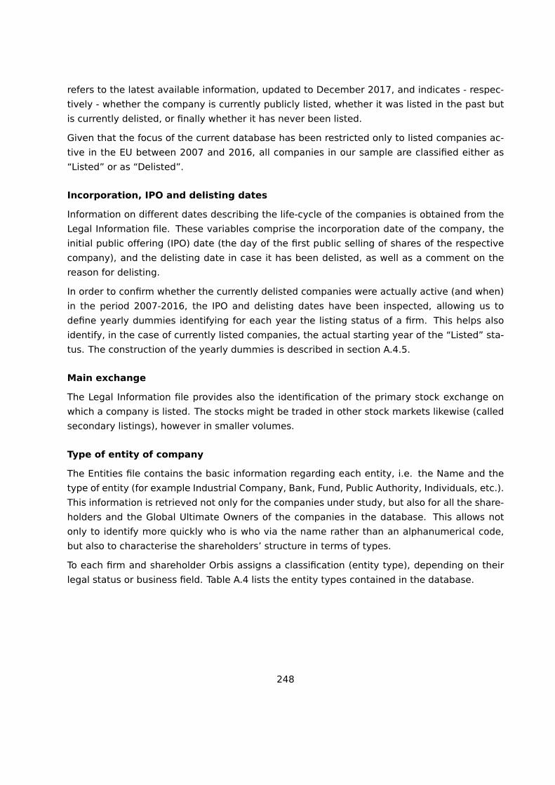
refers to the latest available information, updated to December 2017, and indicates - respec-

tively - whether the company is currently publicly listed, whether it was listed in the past but

is currently delisted, or finally whether it has never been listed.

Given that the focus of the current database has been restricted only to listed companies ac-

tive in the EU between 2007 and 2016, all companies in our sample are classified either as

“Listed” or as “Delisted”.

Incorporation, IPO and delisting dates

Information on different dates describing the life-cycle of the companies is obtained from the

Legal Information file. These variables comprise the incorporation date of the company, the

initial public offering (IPO) date (the day of the first public selling of shares of the respective

company), and the delisting date in case it has been delisted, as well as a comment on the

reason for delisting.

In order to confirm whether the currently delisted companies were actually active (and when)

in the period 2007-2016, the IPO and delisting dates have been inspected, allowing us to

define yearly dummies identifying for each year the listing status of a firm. This helps also

identify, in the case of currently listed companies, the actual starting year of the “Listed” sta-

tus. The construction of the yearly dummies is described in section A.4.5.

Main exchange

The Legal Information file provides also the identification of the primary stock exchange on

which a company is listed. The stocks might be traded in other stock markets likewise (called

secondary listings), however in smaller volumes.

Type of entity of company

The Entities file contains the basic information regarding each entity, i.e. the Name and the

type of entity (for example Industrial Company, Bank, Fund, Public Authority, Individuals, etc.).

This information is retrieved not only for the companies under study, but also for all the share-

holders and the Global Ultimate Owners of the companies in the database. This allows not

only to identify more quickly who is who via the name rather than an alphanumerical code,

but also to characterise the shareholders’ structure in terms of types.

To each firm and shareholder Orbis assigns a classification (entity type), depending on their

legal status or business field. Table A.4 lists the entity types contained in the database.

248

Table A.4: Entity Types

Entity Type Description

A Insurance Company

B Bank

C Industrial Company

D Unnamed private shareholders, aggregated

E Mutual & Pension Fund/ Nominee/ Trust/ Trustee

F Financial Company

H Self Ownership

I One or more known individuals or families

J Foundation/ Research Institute

LUnnamed shareholders (companies or a mixture of companies and private

owners)

M Employees/ Managers/ Directors

P Private Equity Firms

Q Branch

S Public authorities, States, Governments

V Venture Capital

W Marine Vessels

Y Hedge Fund

Z Public

Notice that “Public” (Z) comprises atomistic shareholders of publicly listed companies. In

contrast, “Unnamed Private Shareholders” (D) and “Unnamed Shareholder (Companies and

Private Owners)” (L) represent atomistic shareholders of non-publicly listed companies. Given

249

the present company selection only Z is relevant. Since atomistic shareholder cannot individ-

ually exert control over a company, they are aggregated.

A.3.2 Ownership information

The historical Ownership file defines the relationships (links) between a “subsidiary” and its

shareholders for a given year. The term “subsidiary” here denotes any firm in portfolio,

independent of the quantity held. The information includes

� the BvD ID of both subsidiary and shareholder

� the percentage the shareholder holds (direct and total ownership shares),

� the source from which BvD has received the information,

� the date of the validity of the information,

� a classification of the subsidiary-shareholder relationship (the “type of relation”)

� the ultimate owners according to several definitions

A link with a shareholder is present for a given year whenever the shareholder information has

been confirmed in that year, or when it has been confirmed for the previous and the subse-

quent years. Older shareholder information, which has not been updated in the current year

is considered as still being valid and kept in the database. However, any previous shareholder

that no longer holds shares in the present year is dismissed.

The historical files are updated twice a year, the number of recorded links having increased

after each update. The files contain ownership links from the year 2007 onwards.

Direct and Total ownership shares

Orbis differentiates between direct and total ownership shares. A direct ownership documents

a direct participation of the shareholder in the subsidiary, as it is shown in Figure A.1 a). In

other words, the shareholder owns shares of the subsidiary directly and not via its participa-

tion in a third, intermediate company as depicted in Figure A.1 b) (total ownership).

Whenever the shareholder distinguishes between voting and non voting shares, Orbis reports

the former. Sometimes the direct and total ownership shares are reported using non-numerical

values (direct and total %). The variable “direct % & total % only figures” transforms these

qualitative ownership indications into numeric values according to the conversion in Table A.5.

250

Figure A.1: Ownership of Investor A on Firm B. Left: direct, right: indirect through Firm C.

Direct Ownership

A

B

Indirect Ownership

A

C

B

Type of relation

The variable type of relation defines the characteristic of each subsidiary-shareholder link.

It comprises four general types of relationship between the subsidiary and the shareholder

(reported in Table A.6), and various categories describing different types of ultimate owners.

The ultimate owner (UO) is the first independent shareholder in the hierarchy above the sub-

sidiary that holds a minimum percentage of ownership shares (direct or total), according to a

specific value of interest (for example 25%). An entity is defined to be independent when none

of its shareholders holds more than the chosen percentage of its shares. Additionally, all share-

holders belonging to one of the following three entity types are also considered independent:

Individuals and Families, Public authorities/State, or Employees/Managers/Directors.

BvD distinguishes UOs based on their country of registration, defining the Domestic Ultimate

Owner (DUO) as one located in the same country as the respective subsidiary, while the

Global Ultimate Owner (GUO) can be located worldwide. A further distinction is given by

limiting the choice of the UO among only some types of entities, namely banks and finan-

cial/insurance/industrial companies. In such cases the respective UOs are indicated with an

additional “c”, i.e. as GUOc/DUOc.

As for the possible choices of percentages, Orbis presents the options of UOs based on a mini-

mum of 25% or 50% of ownership. Any shareholder that is located in the hierarchy in-between

the subsidiary and the UO must in turn likewise hold either minimum 25% or 50% of the shares

of its subsidiary, i.e. the chosen percentage defines the minimum ownership of all companies

appearing in the path to the UO.

251

Table A.5: Construction of the Direct % and Total % - Only Figures

Non-Numeric ValueDirect% and Total %

Corresponds to:Direct% and Total %

only figures

WO - wholly owned >=98.1-% 98%

MO - majority owned >=50.01% 50.01%

JO - jointly owned =50.00% 50.00%

NG - negligible <=0.01% -

CQ+1 50.00% + 1 share 50.01%

GP - General Partner -

BR - Branch 100.00%

F - Foreign Company 100.00%

T - Sole Trader 100.00%

n.a./ - -

’>X X+0.01%

’<X X-0.01%

+/- X X

All-together, the choice of the percentage of interest, the location of the UO, and its entity type

give rise to eight possible different definitions, that are reported in Table A.7. In some cases

the UOs are not reported simply because they do not exist according to the chosen definitions.

For example, if a firm does not have any shareholder holding more that 25% of its shares, then

none of the above eight types of UOs will exist. On the other hand, if some of its shareholders

hold more than 25% but none more than 50%, then the GUOs/DUOs based on a 25% definition

might exist, while those based on a 50% threshold are not defined.

252

Table A.6: Shareholder types

Type Definition

SHH Any kind of shareholder, which has been reported to BvD. The direct and totalownership shares might be known or not. It can hold any amount of ownershipshares.

ISH A shareholder who directly owns the subsidiary and is in turn directly or indi-rectly owned by the ultimate owner of that particular subsidiary.

HQ Is the single shareholder of the subsidiary (headquarter), implying that the sub-sidiary is a branch or foreign company of the shareholder.

CTP A shareholder with both direct and indirect participation, whose total ownershipshares have been obtained by the Calculated Total Percentage method.

Table A.7: Ultimate Owners Types

Type Definition

DUO25 Domestic Ultimate Owner characterised by a minimum of 25% ownership sharesin the path from the subsidiary to the ultimate owner

GUO25 Global Ultimate Owner characterised by a minimum of 25% ownership shares inthe path from the subsidiary to the ultimate owner

DUO50 Same as DUO25, but using a minimum 50% definition

GUO50 Same as GUO25, but using a minimum 50% definition

DUO25C Same as DUO25, but UO only bank or financial/insurance/industrial company

GUO25C Same as GUO25, but UO only bank or financial/insurance/industrial company

DUO50C Same as DUO50, but UO only bank or financial/insurance/industrial company

GUO50C Same as GUO50, but UO only bank or financial/insurance/industrial company

253

A.3.3 Financial information

To estimate the plausible causal effect of common shareholding in the analysis, we take into

account firms’ characteristics and their economic and financial performances based on finan-

cial and non-financial measures. The main objective of profit seeking entities is the maximiza-

tion of shareholders’ wealth since shareholders are the legal owners of a company and their

interests should be prioritised. Generally, the shareholders’ wealth maximization is achieved

thought different objectives such as (i) to make profits, since shareholders are interested in

current and future earnings, and (ii) to maintain firm’s growth and development. Both objec-

tives are driven by the financial performance of the firm and can be identified in a number

of ways both financial and non-financial. The most common financial indicators used in the

financial empirical literature refer to profitability, revenues, return on investment, cash flow,

whereas the most used non-financial measures relate to the total sales, number of employees

and market shares.

A first important measure capturing firm’s size is represented by Total Assets (TA). TA refers to

the total amount of assets owned by the firm at its market value. TA includes cash, marketable

securities, inventory, fixed assets, intangibles and goodwill. According to the time taken to

be converted - more or less quickly - into cash, they are classified either current assets or

long-term assets. The balance sheet composition of total assets is very relevant for potential

acquirors, in particular if the value stated in the balance sheet corresponds to its current value.

In case the firm’s asset has a higher current value compared to that reported in the balance

sheet, possible acquirors may have greater incentive to invest in the firm. As a result, we

expect larger firms with higher current and future values to be targeted by large investors,

whereby their investments are distributed across larger companies in the market in the same

proportions as the stock index.

A relevant financial variable, generally considered in empirical financial literature, is Leverage.

Leverage represents how a firm uses debt to finance its activities and asset purchases, and it

is computed as the sum of long-term debt and debt in current liabilities divided by total assets.

Generally, firms with higher leverage are considered riskier and may not be able to increase

the share of debt in their liabilities. However, the optimal capital structure differs across firms

and industries. Empirical evidences predict a positive relationship between firm’s size and

leverage (Rajan and Zingales, 1995) and the main explanation is that large companies suffer

less of asymmetry information problems so that they have an easier access to the market of

debt financing.

A financial variable measuring firm’s performance is the Cash Flow. Cash flow is the net

amount of cash and cash-equivalents flowing in - from customers who buy firm’s products or

services - and out of a firm - for all the payments in the accounting year. We define Cash Flow

as the ratio of earnings after interest and taxes plus depreciation minus common dividends to

Total Assets. Following the pecking order theory, investments should preferably be financed

254

with the internal funds, then with debt and finally with equity. As a result, more cash should

be accumulated in companies with the positive cash flow.

Efficiency measures

An alternative variable considered in literature as a substitute for liquid assets (Opler et al.,

1999) is Net Working Capital (NWC). NWC measures firm’s efficiency and indicates if a firm

has enough short term assets to cover its short term debt. NWC is defined as the ratio of

the current assets minus current liabilities and minus savings to assets net of savings. A ratio

below one indicates a negative NWC whereas a ratio higher than two could mean that the firm

is not investing its excess of cash.

As an additional measure of company’s efficiency use of capital is Operational Efficiency (OE),

which shows the ability of firm’s management to generate profit if revenues decrease. OE is

defined as the ratio between operating expense to net sales. This measure is commonly used

to identify the trend of operational efficiency or inefficiency in a firm over a period of time.

When in a trend the ratio goes up it means that the operating environment is working inef-

ficiently and might need to implement cost controls for margin improvement. Conversely, a

decrease in the ratio indicates an efficient operating environment in which operating expenses

represent an increasingly smaller percentage of sales.

Profitability measures

As a measure of firm’s profitability we consider (i) the Net Income (NI), (ii) the Return on

Equity (ROE), (iii) earnings before interest, taxes, depreciation and amortization (EBITDA) and

(iv) Return on Assets (ROA).

The net income (NI) is an indicator that measures how profitable is a firm over a certain

period of time. NI is computed subtracting from total revenues all the business expenses

and operating costs other than taxes that firm a incurred in doing business. The net income

is relevant because it can be used to compute the earnings for share and consequently the

earnings of each shareholder on the basis of the shares they own.

The variable Return on Equity (ROE) shows how many profits a firm has generated with in-

vestments in capital made by shareholders. ROE represents the amount of profits returned

as a percentage of shareholders’ equity. The ROE is useful for comparing the profitability of

a company to that of other firms operating in the same industry. It illustrates how effective

the company is at turning the cash put into the business into greater gains and growth for the

company and investors. The higher the ROE, the more efficient the company’s operations are

making use of those funds.

As additional metric of profitably we consider the earnings before interest, taxes, depreciation

and amortization (EBITDA). EBIDTA is computed by adding to operating profits (i.e. earnings

255

before interest and tax) the firms’ depreciation and amortization expenses. This measure

has the benefit of removing the distorting effects of taxes on profits, interest income and

expenses but also remove the effect of investments in capital in the company. This measure

also provides a picture of a firm’s short-term operational efficiency showing that the firm is

generating enough earnings for payment back of its debt. EBIDTA is also widely used by

investors to analyse capital-intensive and high leveraged companies and compare them in

sectors of activities where depreciation rates and interest payments on debt are larger with

respect to other sectors, such as utilities or telecommunications companies, and in the case

of acquisition targets.

The last profitability measures we consider in the analysis is ROA. Such a metric is informative

about how many earnings the firm generated with the invested capital (assets) or, saying dif-

ferently, how effective the company has been in converting its investments into net income.

ROA is computed as net income (NI) over total assets. Due to high variation of its value across

firms and sectors, ROA is more suitable for a comparison of publicly-traded companies with

similar characteristics that operate in the same industry.

Growth measures

To proxy for a firm’s growth opportunities in their business, we consider several measures.

A first measure refers to “Research and Development expenses” (R&D) and represents the

operating expenses that a firm incurs into to develop new products or services in a year. In

some industries - i.e., technological, industrial, pharmaceutical - R&D expenses are usually

higher compared to those of other sectors. The main reason is that firms have to reinvest

a significant portion of their profits in R&D activities to continuously grow, allowing them to

maintain their market positions or find new areas of opportunistic growth that diversify their

business activities. Firms with higher R&D expenditures are expected to have greater growth

opportunities.

A second measure for growth opportunities is the variable Book-to-Market Ratio. The Book-

to-Market Ratio of listed companies reflects the management’s ability to effectively use firms’

assets to grow, and it is computed as the ratio between common shareholders’ equity at the

book value and the market capitalization determined in the stock market where the firm is

publicly listed. Book-to-Market Ratio is also used to determine whether the market value of a

publicly traded company reflects its real value or just an investor speculation.

The last measure of firm’s growth we consider is the variable Employment. Employment rep-

resents the total number of full time employees of a company in a certain year. An increase in

the job creation means that the firm is growing in its business activities.

256

Definition of main financial variables from the Orbis dataset

Tables A.8 and A.9 report the specific definitions of some main financial variables collected in

the Orbis dataset, from the balance sheet and the profit&loss account.

Table A.8: List and definition of Balance Sheet variables collected by Orbis

Acronym Label/Formula Definition

FIASFixed Assets Total amount (after depreciation) of non current assets

IFAS+TFAS+OFAS(Intangible assets + Tangible assets + Other fixed as-

sets)

IFAS Intangible Fixed Assets

All intangible assets such as formation expenses, re-

search expenses, goodwill, development expenses

and all other expenses with a long term effect

TFAS Tangible Fixed Assets All tangible assets such as buildings, machinery, etc.

OFAS Other Fixed AssetsAll other fixed assets such as long term investments,

shares and participations, pension funds etc.

CUASCurrent Assets Total amount of current assets

STOK+DEBT+OCAS (Stocks + Debtors + Other current assets)

STOK StocksTotal inventories (raw materials + in progress + fin-

ished goods)

DEBT Debtors Trade receivables (from clients and customers only)

OCAS Other Current Assets

All other current assets such as receivables from other

sources (taxes, group Companies), short term invest-

ment of money and Cash at bank and in hand.

TOASTotal Assets Total assets

FIAS+CUAS (Fixed assets + Current assets)

257

Table A.9: List and definition of Profit & Loss Account variables collected by Orbis

Acronym Label/Formula Definition

OPREOperating revenue Total operating revenues. The figures do not include VAT.

(Turnover) (Net sales + Other operating revenues+ Stock variations)

TURN Sales Net sales

COST Cost of Goods Sold

Cost of sold goods, production, services. Costs directly

related to the production of the goods sold + depreciation

of those costs

GROSGross Profit

Operating revenue - Cost of goods soldOPRE-COST

MATE Material CostsDetail of the purchases of goods (raw materials + fin-

ished goods). No services.

STAF Cost of EmployeesDetail of all the employees costs of the Company (includ-

ing pension costs)

EBIT Operating P/LAll operating revenues - all operating expenses (Gross

profit-Other operating expenses)

DEPRDepreciation

Total amount of depreciation and amortization of the assets& Amortization

AV Added ValueProfit for period + Depreciation + Taxation + Interests

paid + Cost of employees

EBTAEBITDA

Operating profit + DepreciationEBIT+DEPR

258

A.4 Organisation and cleaning of data

The selection of firms and of variables according to the procedures described in the previous

sections allowed us to extract from Orbis a large amount of data used in the empirical analyses

of the project. This section describes the structures used to organise the data, together with

the cleaning procedures used to treat the raw data.

Due to the heterogeneous format of the various parts of the data, the final firm-level data for

the analysis is organised in four separate datasets containing, respectively, the legal informa-

tion, the industry classification, the ownership links and the financial variables. The legal and

industry information refer to the firms’ situation in December 2017, while the financial and

ownership data are available yearly for the period 2007-2016.

The contents of the four datasets, as well as the choices made in their construction, are

reported in the following. Some descriptive statistics of the data are presented in Section A.5

An assessment of the coverage of the data is presented in Section A.6, where figures from the

present datasets are compared to official statistics.

Unless stated otherwise, all variables contained in the four datasets have been earlier de-

scribed in detail in Section A.3 All datasets can be linked using the BvD ID, the unique firm’s

identifier, according to the specific needs.

A.4.1 The legal information

The first set of data contains for each firm the following information: the firm’s identifier, the

name (trimmed to first 20 characters due to space constraints), the date of incorporation, the

country of registration, a dummy for the EU area, the type of entity, plus a series of variables

about the listing information (listing status as of December 2017, IPO date, main exchange,

delisted date and delisted comment - for delisted companies only).

The firms included in this dataset constitute the population of all listed companies recorded

in Orbis that are or were active in the EU during the period 2007-2016. The selection of this

group of companies from the general Orbis database has been described in Section A.2.

The list of firms’ identifiers can be used as the basis of companies’ selection or searches in

order to extract information of interest from any of the files constituting the Orbis database.

As mentioned earlier, the present project extracted information only from five of those files,

but many more are available for possible use.

259

A.4.2 The industry classification

The second set of data reports all NACE codes classifying the sector of economic activity of

each firm in December 2017. Together with the NACE Section (A-U), the core NACE code is

reported, as well as the four primary codes and all twenty available secondary codes. For a

detailed description of the NACE industry classification system, see Section A.2.

The information contained in this dataset can be used to create lists of selected companies

exerting activity in different sectors or industries.

A.4.3 The ownership links

The third set of data is the largest and constitutes the core of the database for the project. For

each year between 2007 and 2016, all available ownership information about the population

of quoted firms active in the EU is retained, independent of their listing status in that specific

year. The decision of whether to use only the firms listed in a specific year can be taken later,

given that firms can be selected easily using the purpose-built dummy variable on the “current

listing status” (see description in Section A.4.5).

Not all firms in our population have ownership information available in all years. This can be

due to several reasons:

(i) the firm did not exist in the specific year - if needed, this can be confirmed through the

date of incorporation in the legal information dataset;

(ii) the firm was independent in the given year, i.e. did not have any shareholders;

(iii) the firm had some shareholders in the given year, but no provider supplied ownership

information to BvD, and BvD itself did not manage to obtain any information.

Case (iii) may occur only if a firm has not yet entered the Orbis database; in fact, if the firm has

some previous ownership information, and no update is available for the year of interest, BvD

still provides ownership for the given year, namely maintains the last available information.

This situation can be identified through the variable “date of information”, when the date

refers to older years.

In each year, a firm can present information on dozens of shareholders, but some firms even

present hundreds of them. Each shareholder can have several roles in its relationship with

a subsidiary, for example it can be the GUO25 and also the DUO25. All different roles are

recorded in the variable “type of relation” presented earlier, implying that for each subsidiary-

shareholder pair several links can be present in Orbis, one for each role.

Table A.10 reports an excerpt of raw ownership data for a given company in 2008, where

the actual firm’s and shareholders’ identifiers have been replaced by fictitious values. The

260

example shows the case of multiple links between the subsidiary and some of its sharehold-

ers (second and third blocks), which in this case fulfill several definitions of Ultimate Owner

each, therefore appearing in different UO roles. Notice also that not all dates of information

are updated to the end of 2008, showing that for some shareholders the information was not

provided in the given year, and previous information has been maintained.

Table A.10: Example of raw ownership information. SH=shareholder.

Date of Type of GUO GUO GUO GUOFirm SH Direct Total information relation 25 50 25C 50C

IT00 CH11 . 46.1 13mar2008 SHH CH33 CH33 CH33 CH33

IT00 IT22 65.73 . 31dec2008 SHH CH33 CH33 CH33 CH33IT00 IT22 65.73 . 31dec2008 ISH CH33 CH33 CH33 CH33IT00 IT22 65.73 . 31dec2008 DUO 25 CH33 CH33 CH33 CH33IT00 IT22 65.73 . 31dec2008 DUO 50 CH33 CH33 CH33 CH33IT00 IT22 65.73 . 31dec2008 DUO 25C CH33 CH33 CH33 CH33IT00 IT22 65.73 . 31dec2008 DUO 50C CH33 CH33 CH33 CH33

IT00 CH33 . 65.73 31dec2008 GUO 25 CH33 CH33 CH33 CH33IT00 CH33 . 65.73 31dec2008 GUO 50 CH33 CH33 CH33 CH33IT00 CH33 . 65.73 31dec2008 GUO 25C CH33 CH33 CH33 CH33IT00 CH33 . 65.73 31dec2008 GUO 50C CH33 CH33 CH33 CH33

IT00 IT44 . 4.99 06dec2006 SHH CH33 CH33 CH33 CH33

IT00 LU55 4.66 . 19sep2008 SHH CH33 CH33 CH33 CH33

IT00 FR66 . . 11may2005 SHH CH33 CH33 CH33 CH33

IT00 DE77 . 1.99 14oct2008 SHH CH33 CH33 CH33 CH33

In order to eliminate redundant or duplicate information from the raw data, all cases where

a subsidiary-shareholder link is appearing multiple times undergo the following cleaning pro-

cess: only one record is kept with the subsidiary and shareholder identifiers, the total and

direct ownership share information and the date of information, while all roles recorded in the

variable “type of relation” are registered in additional variables named after the several UO

definitions, where the corresponding shareholder’s identifier will appear. The variable “type of

relation” is then dropped. Table A.11 reports the result of previous example after the cleaning

procedure, where only one link per shareholder appears.

The “current listing status” variable mentioned in Section A.4.5 is then added, together with

the name, entity type and country of registration of each of the shareholders and ultimate

261

Table A.11: Example of cleaned ownership information. SH=shareholder.

Date of GUO GUO GUO GUO DUO DUO DUO DUOFirm SH Direct Total information 25 50 25C 50C 25 50 25C 50C

IT00 CH11 . 46.1 13mar2008 CH33 CH33 CH33 CH33 IT22 IT22 IT22 IT22IT00 IT22 65.73 . 31dec2008 CH33 CH33 CH33 CH33 IT22 IT22 IT22 IT22IT00 CH33 . 65.73 31dec2008 CH33 CH33 CH33 CH33 IT22 IT22 IT22 IT22IT00 IT44 . 4.99 06dec2006 CH33 CH33 CH33 CH33 IT22 IT22 IT22 IT22IT00 LU55 4.66 . 19sep2008 CH33 CH33 CH33 CH33 IT22 IT22 IT22 IT22IT00 FR66 . . 11may2005 CH33 CH33 CH33 CH33 IT22 IT22 IT22 IT22IT00 DE77 . 1.99 14oct2008 CH33 CH33 CH33 CH33 IT22 IT22 IT22 IT22

owners. A dummy is also created to identify “independent” firms, i.e. those for which the

ultimate owners’ are not defined or coincide with the firm itself.

In a second stage, the ownership structure of a subsidiary is summarised into one link per

subsidiary with all essential information, in order to be able to merge it with other parts of

the dataset. For each year of observation, the essential ownership information is summarised

through the minimum and maximum values of direct and total ownership shares owned by

the shareholders, and through the identification number of all ultimate owners. The result is

shown in Table A.12.

The minimum and maximum of “direct” and “total” variables can be used to perform checks

in cases where ultimate owners are not defined - in such cases the maximum of the ownership

shares held should always be less than 25% or 50%. Additional summary information can be

added, such as the total number of shareholders for the given year, or the identification of the

largest shareholder, and so on.

This summarised ownership information of each firm is very useful if we wish to merge it

with the corresponding listing, financial or industry classification data, without having to carry

around the full list of shareholders and their shares, which can be consulted separately.

Table A.12: Firm’s summarised ownership information.

Dir Dir Tot Tot GUO GUO GUO GUO DUO DUO DUO DUOFirm Min Max Min Max 25 50 25C 50C 25 50 25C 50C

IT00 4.66 65.73 1.99 65.73 CH33 CH33 CH33 CH33 IT22 IT22 IT22 IT22

262

A.4.4 The financial information

The last set of data contains about a hundred financial variables coming from the yearly bal-

ance sheets of the firms. The main ones have been described earlier, but many more are

available for selection. For each year, a firm can present more than one account, therefore it

is necessary to set some criteria to select only one account per firm per year.

Accounts may differ according to the type of consolidation, the closing date, the number

of months of reference and the accounting practice. Moreover, not all accounts are equally

populated, so further checks are needed in order to include accounts where the main variables

of interested are not missing. The accounts with closing date in the first quarter of a certain

year are considered to be referring to the financial activity of the previous year.

The criteria used for the selection of the appropriate account for the current project are as

follows (in order of importance):

A) Consolidation type: Orbis presents six possible classifications of the consolidation type

of an account:

- C1 = Consolidated account of a company-headquarter of a group, aggregating all companies

belonging to the group (affiliates, subsidiaries, etc.), where the company-headquarter has

no unconsolidated account

- C2 = Consolidated account as above, but where the company-headquarter also presents an

unconsolidated account

- U1 = Unconsolidated account of a company with no consolidated account

- U2 = Unconsolidated account of a company with a consolidated account

- LF = Limited number of financial items

- NF = No financial items at all

In the construction of the financial database, priority is given to accounts in the order C1, C2,

U1, U2, LF, NF.

B) Number of months: When different accounts for the same year refer to periods of differ-

ent length, the account covering the highest number of months is chosen.

C) Missing variables: Priority is given to accounts with minimum missing values on the fol-

lowing ten variables: total assets, shareholders funds, number of employees, sales, operating

revenue (turnover), net income, EBITDA, Research & Development expenses, ROE and ROA.

263

D) Accounting practice: Accounts are reported either by IFRS (International Financial Re-

porting Standards) or GAAP (US Generally Accepted Accounting Principles) standards. Priority

is given to IFRS practice.

A.4.5 Definition of new variables

Annual dummies for current listing status

In each year of the sample, say t, it is important to identify whether a firm is listed or not;

in fact, the listing status of the firms for a specific year is not directly available, since the

Listed/Delisted variable described above gives the last available status (in our case referring

to December 2017).

For this purpose, a indicator variable has been defined for each year, named “current listing

status”. It refers to the year t in which the ownership link is reported, and is derived from

the listing/delisting information of the firm. The full IPO and listing dates are available, but

only the corresponding year is retained for the construction of the yearly listing status. The

assignment rules for different values of the yearly dummies are summarised in Table A.13.

The first case occurs when the IPO year of the firm lies in the past, or at most coincides with

year t itself; if the delisting year lies in the future, the value 1 is assigned to the company,

indicating that it is currently active in the stock market. The assigned value is 0 if both the

IPO and the delisting year are in the past. We assume that a missing indication of the delisting

year is due to the fact that the company has not yet been delisted, therefore in this case the

status variables takes value 1 too.

A second possibility is that the link is recorded before the IPO year, in which case the current

listing status is equal to 0, independent of the delisting year. In other words the company is

not listed in the year of observation.

Whenever the IPO Date is missing, while the delisting year is given, the company is assumed

to having been listed a long time ago, before year t. Therefore the listing status in determined

according to the same criteria as in the first case above.

If both the IPO and the listing dates are missing, but the firm is still listed in 2017, we assume

again that the company was listed a long time ago, and therefore that is listed throughout the

period of observation. On the other hand, if both dates are missing and the firm is delisted

in 2017, then the current status variable is not defined, i.e. is recorded as missing. Specific

assumptions can be considered in order to assign an actual 0/1 value.

In only two cases the delisting date was prior to the IPO date, probably denoting companies

that re-entered the market at a later stage. In such cases they were considered as still listed

in 2017, hence listed in all years after the IPO date (as if the delisting date was missing).

264

Table A.13: Construction of the "current listing status" variable for year t.

IPO year Delisting yearListing Status Current Listing Status

in 2017 in year t

≤ t≥ t any 1

n.a. any 1

< t any 0

> t any any 0

n.a ≥ t any 1

< t any 0

n.a n.a Listed 1

n.a n.a Delisted –

DUOs and ISH Variables

The Ownership database contains the variables GUO50, GUO50C, GUO25, GUO25C, which

report for every subsidiary-shareholder link the respective global ultimate owner of the sub-

sidiary in that particular year, according to the definitions in Table A.7, in case they exist.

In order to enhance the analysis, we construct similar variables reporting the DUO50, DUO50C,

DUO25, DUO25C and ISH of the subsidiary for the given year (when present), derived from the

variable “type of relation” presented earlier.

Minimum and maximum total and direct ownership percentage

Four new variables are created, reporting for each subsidiary the amount of direct or total

ownership shares held by its biggest and smallest shareholder in that particular year. The

variables are invariant for all links of a respective subsidiary in a given year. Such variables

are useful in analysing the shareholders’ structure of a company, and can also be used to

test the correctness of the ultimate owner information presented in the database. For exam-

ple, whenever the largest shareholder holds less than 50%/25% of the shares, the subsidiary

cannot have an ultimate owner at the 25% or 50% level, or vice-versa.

265

A.4.6 Note on cleaning procedures

Since there is a non-negligible fraction of recorded shareholder-subsidiary links that do not

specify the actual amount of participation, an imputation strategy has been adopted in order

to fill in the missing information, where possible.

The imputation criteria adopted for the ownership information are as follows: if there is a non-

reporting for one or two consecutive periods, but the amount of shares is available before or

after, then the missing share is replaced by the value recorded in the previous or following

year. This is a rather conservative operation, given that in general the value of the shares

held is rather stable. In case of a gap of more than two years, no action is taken, considering

that the closest reported amount of shares is too far in time to be considered reliable.

After this first round of imputation, the values that are still missing are filled according to

extra information available from Orbis. If the shareholder is declared to be the GUO (Global

Ultimate Owner) or DUO (Domestic Ultimate Owner) according to a definition of minimum 50%

or 25% of shares, then the missing share is replaced by 50.01% or 25.01%, respectively. If

the shareholder is not the GUO or DUO, then all its portfolio is analysed, and the average

share held in the portfolio is considered to be representative of the shareholder’s investing

behaviour, and is therefore imputed in the missing cases, but these are very few.

After all this procedure, there are still some links with no available share (about 3%). They cor-

respond to the cases where the shareholder is not the GUO or DUO of the subsidiaries, where

for all the years of observation the shareholder-subsidiary link has been recorded with no share

available, and where no average share for the shareholder’s portfolio is available, since for all

subsidiaries of that shareholder no share information is available. This is usually the case of

single shareholders with small participation (<25%), being linked to only one subsidiary in the

market, but with no share information, so in general they are not very important players. For

these cases, the information about the existence of a shareholder-firm link can still be used,

but the indicators requiring the quantification of the shares held cannot be calculated.

As for financial variables, there are no major issues of missing data on the main variables (Total

Assets and Market Capitalisation). The Total Assets are basically almost available. Neverthe-

less, in case of non-reporting in some years, values are imputed from previous or following

years, giving a final coverage of 99% of firm-year. As for Market Capitalisation, it is not always

available, due to the fact that the listing status of firms can change throughout the period of

observation. Therefore, the missing values are mainly related to years where the companies

were still unlisted or have been delisted, hence no imputation is performed on this variable.

266

A.5 Dataset descriptive statistics

Following the selection procedure outlined in Section A.2, a historical dataset containing all

listed companies active in the EU in the period 2007-2016 is obtained. The average number of

firms observed each year is 26,560 - as displayed in Table A.14 - where on average about 57%

are registered in the EU countries, the rest being registered outside the EU. The proportion

of EU versus Non-EU registered companies remains roughly constant over time. The total

number of observed firms increases slightly over the years, except for the last, where due to

the reporting lag the number of covered firms is slightly smaller than in the previous year.

Overall, a set of 31,864 different firms are observed.

Table A.14: Sample composition by country of registration and year.

Country 2007 2008 2009 2010 2011 2012 2013 2014 2015 2016

EU 14,434 14,849 15,000 15,122 15,171 15,125 15,479 15,564 15,336 15,086

Non-EU 10,423 10,819 11,169 11,398 11,581 11,710 11,756 11,846 11,877 11,856

Total 24,857 25,668 26,169 26,520 26,752 26,835 27,235 27,410 27,213 26,942

The largest groups of EU companies are registered in the UK and Spain (around 20% in each

country), followed by Romania (9%), Germany (8,5%), France (7,5%), Poland (5,5%) and Swe-

den (5%). Again, the distribution stays roughly constant over time. Most of the companies

registered outside the EU are in the US (30%), followed by Japanese companies (9.7%), Cana-

dian (6.78%) and Australian companies (6.6%), while 4,83% of the companies are from India.

Table A.15 reports - for the total sample of 31,864 firms - the coverage of the ownership

information, the NACE industry classification and the financial indicators in the sample. The

number of firms for which none of the information is available is negligible. As an additional

note, 77.78% of such firms have been delisted from the stock markets by the year 2017. On

the other hand, 97.3% of companies present ownership data, and complete ownership, NACE

and financial information is available for 28,931 firms - 91% of the sample.

Although not all companies are observed all years, due to the natural birth and death pro-

cesses of firms, generally the sample is rather stable. About 68% of the companies have

complete records, i.e. they are present throughout the whole 10 years of the period under

analysis, and 80% are observed during at least 7 years; a small percentage of firms (15%)

were recorded maximum during half of the period, i.e. at most for 5 years.

Table A.16 reports the listing status of companies in each year of observation. On average,

every year around 83% of the companies are listed. In about 3.5% of the cases it was not

possible to determine the listing status of the firms by year, given that both the IPO date and

delisting dates were missing, and the firms were classified as "Delisted" in 2017. Over time

267

Table A.15: Structure of the Database

No Financials Financials

No Nace Nace Total No Nace Nace Total

No Ownership 63 523 586 4 272 276

Ownership 218 1649 1867 204 28931 29135

Total 231 2172 2453 208 29203 29411

the proportion of quoted companies in a given year decreases slightly. While initially 89% of

the companies were listed, the share drops to 78% in 2016. Among the currently delisted

firms, the large majority (89%) have been listed before or in 2007. i.e. before the beginning of

the period of observation. Only very few companies are listed and delisted within the sample

period. A large proportion of firms (68%) are always listed in all years when they are observed.

Table A.16: Current listing status of firms, by year. If both IPO date and delisting dates are missing, thelisting status is not available (NA).

Year Delisted Listed NA Total

2007 1,602 22,218 1,037 24,857

2008 2,254 22,377 1,037 25,668

2009 3,055 22,070 1,044 26,169

2010 3,477 22,023 1,020 26,520

2011 3,827 22,008 917 26,752

2012 4,122 21,826 887 26,835

2013 4,438 21,938 859 27,235

2014 4,524 22,038 848 27,410

2015 4,515 21,883 815 27,213

2016 5,236 20,914 792 26,942

The bulk of firms are concentrated in few industries. In Table A.17 the proportion of firms active

in the main NACE Sections are reported, with “Manufacturing” (Section C) and “Financial and

insurance activities” (Section K) comprising the largest number of firms. Each one of the

remaining Sections represented less than 2.5% of the total sample.

Table A.18 pictures the number of companies which are classified as being active in any of

268

Table A.17: Proportion of firms active in the main NACE Sections

Section Description No Firms %

C Manufacturing 10,242 32.69

K Financial and insurance activities 7,713 24.62

J Information and communication 3,002 9.58

G Wholesale and retail trade 1,889 6.03

M Professional, scientific and technical activities 1,486 4.74

L Real estate activities 1,151 3.67

B Mining and quarrying 1,119 3.57

the sectors of interest identified by the eight Nace Codes discussed in Section A.2. The Core

Nace Codes were inspected, as well as all four Primary Nace Codes (Prim) and the first four

Secondary Nace Codes (Second), respectively. None of the companies presented any of the

eight codes as their third or fourth Primary Codes, therefore they are omitted.

The first Primary Nace Code coincides with the Core Nace Code of the company. The bulk of

firms is classified in these categories by their Core Nace Code or first Secondary Nace Code.

The number of firms who are active in these categories as a second, third or fourth activity is

small. An exception are the classifications “Other financial service activities, except insurance

and pension funding” (Nace Code 6499) and “Security & Commodity Contracts Brokerage”

(Nace Code 6612), where a lot of companies are active as a side activity.

Overall, most of the companies that present some of the eight core Nace Codes are active in

“Other Credit Granting” (Nace Code 6492). This might be due to the fact that this categoriza-

tion is very broad, and therefore not very selective.

The dataset contains 6,070,111 ownership links. On average, each company has about 22

shareholders per year. However, 50% of the companies have at most 7 shareholders in a

given year, while 9,5% of the companies even have only one shareholder. The number of total

links per year rises slightly from 604,385 in 2007 to 617,353 in 2016.

Every year, on average over 87% of the companies report an ultimate owner of some type.

The percentage rises slightly over the sample period from 83.24% in 2007 to 88.49% in 2016.

About 60% of companies have a domestic GUO50, with non-EU companies showing a larger

share (70%) compared to EU (56%).

Overall, 64% of the subsidiary-shareholder links are recorded between entities registered in

the same country (domestic shareholders), the remaining cases denoting a shareholder lo-

cated abroad. The proportion is rather similar in the case of EU or non-EU based companies.

269

Table A.18: NACE Codes

Code Core 1 Prim 2 Prim 1 Second 2 Second 3 Second 4 Second

0610 237 237 38 1

3511 273 273 57 5 8

3523 14 1 2

6190 593 593 132 43 23 9

6492 3,029 3,029 33 1,179 50 36 13

6499 236 236 22 501 239 59 648

6611 45 45 32 20 5 3

6612 310 310 327 305 706 5

In terms of financial information, only 1% of the reported accounts presents limited financial

information. Most of the accounts (70%) are consolidated, either of type C1 or C2, while

all remaining are unconsolidated. For what concerns the time and variable coverage, 75% of

accounts refer to a time period of 12 months, and 95% present at least six of the main financial

indicators. The most frequent accounting standard is the GAAP (62%), while the IFRS practice

is used in the remaining cases.

A.6 Comparison with official statistics

The World Bank provides information on the number of listed companies in individual coun-

tries, as well as regions (e.g Europe & Asia/ Arabian World). The data is obtained from the

World Federation of Exchange.

The data include either companies that are either incorporated in the same country as their

exchange, or foreign companies which are exclusively registered in that particular stock mar-

ket. Hence, in comparison to the present dataset, foreign companies which holds shares in a

firm in the EU but are quoted outside the EU are not reported. Nevertheless, we consider it a

good base for comparison.

Table A.19 reports the ratio of the numbers of firms present in our dataset per country and year

compared to the data provided by the World Bank. The ratios are displayed in percentage

points, and only European countries are considered. The latter is the case, as we consider

the number of firms which are foreign but have their exclusive exchange in Europe to be

small. Hence, with this approach companies which are registered and active in Europe are set

270

in comparison. Unfortunately, the World bank does not provide listing information for 5 EU

countries (Denmark, Estonia, Finland, Latvia, Lithuania, Sweden). Overall, the present dataset

contains a higher number of companies in comparison to the data provided by the World Bank.

271

Table A.19: Coverage of our dataset in comparison to World Bank (ratio in %)

2007 2008 2009 2010 2011 2012 2013 2014 2015 2016

Austria 128 134 136 147 147 150 154 150 152 166

Belgium 122 131 138 139 146 150 188 195 184 184

Bulgaria 130 122 128 132 132 135 135

Croatia 96 98 130 153 157 171 188 182 188 216

Cyprus 125 138 151 156 161 171 179 179 205 214

Czech Republic 346 289 338 313 340 306 373 400 367 373

Denmark Not Contained in the World Bank Data

Estonia Not Contained in the World Bank Data

Finland Not Contained in the World Bank Data

France 168 178 183 192 199 201 226 223 221 220

Germany 163 172 184 188 194 196 202 220 229 237

Greece 114 113 112 114 110 108 116 110 111 123

Hungary 115 115 107 106 100 100 100 104 113 119

Ireland 202 212 222 246 260 312 329 319 330 343

Italy 123 127 143 146 135 135 144 141 141 139

Latvia Not Contained in the World Bank Data

Lithuania Not Contained in the World Bank Data

Luxembourg 221 255 307 324 400 436 483 492 448 414

Malta 94 89 95 110 138 141 130 133 148 148

Netherlands 124 135 172 185 193 204 290 288 277 264

Poland 147 137 153 142 122 114 112 111 112 113

Portugal 167 164 169 177 178 184 200 196 191 198

Romania 2617 2265 1943 1900 1800 1784 1675 1649 1629 1562

Slovak Republic 26 48 97 150 93 200 206

Slovenia 93 101 125 133 147 159 176 186 198 237

Spain 84 84 85 87 86 87 98 96 87 87

Sweden Not Contained in the World Bank Data

United Kingdom 120 134 148 151 160 169 168 168 166 164

272

Appendix B

Common Shareholding Indices

Chapter 2 overviewed the main tools used in the academic literature to assess the effects of

common shareholding, highlighting pros and cons. It also set up a framework for the analysis

of ownership data, introducing a simplified market example and discussing several measure-

ment issues. Finally, it translated sparsity and network indicators into the common sharehold-

ing context, proposing feasible measures to be computed in the empirical analysis, according

to our data restrictions. In the present technical annex, the above statistical methodologies are

analysed, setting the theoretical background for the identification of new indices of the extent

of common shareholding. The proposed methods explore several new aspects of investors’

behaviour and of portfolios’ composition, which can help us draw a more precise picture of the

phenomenon. The same applies to the analysis of the firms’ shareholding structures, which

can reveal interesting patterns of overlap in a given market.

Although several methodologies were considered, many present limited applicability to the

common shareholding study. Hence, the focus of subsequent developments has been re-

stricted to techniques based on two main groups of methods, coming from the Sparsity and

Network literature respectively. Their applicability to the measurement of common sharehold-

ing is discussed in detail, and the implementation of the proposed measures is illustrated

through a simple example of a fictitious market. Measures that allow comparison with bench-

mark scenarios are also considered. Further insight will be available later from the real-data

applications for listed firms and for the five industries under study.

The concept of sparsity is generally found in the literature on inequality or diversity, and

studies the distribution of a certain phenomenon in a given population, e.g. of income, in

particular in the aspects related to its concentration in the hands of a small number of players.

The higher the concentration of the variable in the population, the higher the inequality of the

distribution. By contrast, a low concentration denotes higher diversity of the phenomenon in

the population. This framework extends easily to the common shareholding analysis, applying

273

the relevant concepts to the distribution of the investments of shareholders across firms in

a given market. Here, a low concentration signals diversification of investments across the

market and therefore goes in the direction of common shareholding.

The second approach comes from the literature on the analysis of networks. This field stud-

ies the empirical structure of the relationships that exist between elements of a population.

Such relationships induce flows of information within the population according to its level of

connectedness, and additionally allow to identify the most important or central players. Con-

sidering the population of the firms and owners of a market, the corporate ownership structure

can naturally be represented through a network, where the network relations are given by the

ownership links between firms and their shareholders.

Section B.1 presents the concept of sparsity and related indices, coming from the inequality

literature, and applies them to the common shareholding analysis. Section B.2 approaches

the market structure as a network of owner-firms relations, adapting network measures to the

current research objective. The real data applications will be of value in determining the best

measure to be used.

B.1 Sparsity

The concept of sparsity is often linked to definitions of inequality or diversity, giving rise to

different interpretations and measures.1 However, a common agreement is that a distribution

with all its information concentrated in one coefficient, and all other zero, is the most sparse.

On the other hand, there is agreement that the least sparse distribution is found when the

information is evenly spread over all coefficients. In the following, this will be the reference

definition of sparsity.

In the inequality literature, maximum and minimum sparsity would correspond to the most un-

equal case and to perfect equality, respectively. In the case of corporate ownership, a sparse

investment behaviour would correspond generically to a high concentration of ownership in

few hands (or few firms), while low sparsity would be observed in case of more widespread in-

vestments across the market. A more detailed analysis of the application of sparsity concepts

to corporate ownership will be discussed in Section B.1.2 below.

B.1.1 Measuring sparsity

There is a large set of sparsity measures in the literature, coming mainly from the fields of

signal processing and information theory. The most common are the Kurtosis, the Gini Index,

the Hoyer measure, the pq-means, the ℓp norms and their combinations. These and other

1A comprehensive review of these and other fields of application can be found in Hurley and Rickard (2009).

274

measures are discussed, for instance, in Karvanen and Cichocki (2003), Rickard and Fallon

(2004), Hurley and Rickard (2009), Zonoobi et al. (2011), Pastor et al. (2013), and Pastor et

al. (2015).

Before presenting the details of each measure, it is important to focus on desirable properties

of a generic sparsity function, in order to be able to choose between alternatives. Desirable

criteria that a sparsity measure should fulfill are, among others, the so-called “Robin Hood”

property, the scaling or homogeneity, the “rising tide” property, and the “cloning” property.

These four criteria were initially proposed by Dalton (1920) in the financial setting of inequality

measurement of wealth distribution, but are nowadays generally recognised to be minimum

criteria a “good” measure of sparsity should satisfy, being referred to as “Dalton’s Laws”.

More recently, Rickard and Fallon (2004) added two extra properties, named “Bill Gates” and

“Babies”, respectively, which will be defined below, together with Dalton’s Laws. Additional

axioms and attributes, whose analysis goes beyond the scope of this report, can be found in

Pastor et al. (2013, 2015).

Properties of sparsity measures

- Robin Hood: A “fair” readjustment of coefficients decreases sparsity. Taking some

amount from the larger coefficients and “redistributing” towards smaller coefficients

yields a less concentrated i.e. more equal distribution.

- Scaling: A change in scale of the coefficients does not change sparsity. Multiplying

wealth of all units by an equal factor does not change the level of (in)equality of the

distribution.

- Rising Tide: An identical increase in all coefficients decreases sparsity. Adding a fixed

amount to each coefficient reduces the relative difference between large and small val-

ues, i.e. yields a more equal distribution.

- Cloning: Doubling the number of coefficients by cloning the same values does not

change sparsity. If a second population is cloned, reproducing the same values as the

first one, then the level of (in)equality of the merged populations equals that of the initial

population.

- Bill Gates: A significant increase in one coefficient increases sparsity. When one coeffi-

cient becomes very large, the level of inequality increases.

- Babies: The addition of extra zero coefficients increases sparsity. Adding individuals

with zero wealth to a population increases inequality, by concentrating the (positive)

total wealth in the hands of a smaller share of individuals.

275

More details about the above properties can be found in Hurley and Rickard (2009); the paper

also presents sixteen sparsity measures and prove which of them satisfy which properties.

The main result is that only two measures satisfy all six properties, namely the Gini Index and

the pq-means (see below), while all remaining measures satisfy some, but not all of them.

Some common sparsity measures

Table B.1 below presents some among the most common sparsity measures, and reports their

properties. For easier reference in the following, the measures will be sometimes referred to

according to the numbering presented in the table, rather than their full names. The coeffi-

cients of the distribution under analysis are denoted by ck, k = 1 . . . , N, while their ordered

set is indicated by c(k) (in increasing order). Measures 1-4 and 6-7 are presented in their nor-

malised version, which accounts for the length N of the vector representing the distribution.

The normalised versions in general satisfy more properties than the original measures. Prop-

erties only satisfied in the normalised version of the measures, and not in the original ones,

are indicated in brackets.

The measures in Table B.1 do not present a unified notation in the literature; we follow here

the suggestions of Hurley and Rickard (2009), where some measures have been modified -

either with a minus sign or by changing the direction of some inequality - in order to obtain

an homogeneous interpretation in the sense that an increase in sparsity yields a positive

increase in the corresponding measure. In particular, notice that measure 1 is usually defined

in the literature as the count of non-zero values, but this would go in the opposite direction,

increasing when sparsity decreases. For this reason here the definition is reversed, counting

the number of zeros instead. For all these measures, the less sparse the distribution, the

smaller the value of the index, the value increasing with sparsity.

As we can see from Table B.1, most measures fulfill many of the presented properties, if

not all. Karvanen and Cichocki (2003) compare measures 1-4 and 6-7. Quéré and Frélicot

(2012) compare 7 and 8 through a set of simulations on binary (0-1) distributions, testing their

performance in the context of fuzzy partitions. Measure 10 is considered, among others, in

Rickard and Fallon (2004) and Zonoobi et al. (2011). Hurley and Rickard (2009) and Pastor et

al. (2015) propose more comprehensive accounts of original and normalised measures, other

additional measures and properties not discussed here, as well as proofs of the fulfillment of

the respective properties.

Measures 1 and 2 simply compute the proportion of zero or negligible elements of the dis-

tribution; the higher the proportion, the more concentrated the distribution, i.e. the higher

the sparsity. In measure 6, any zero coefficient gives a zero log value in the summation, con-

tributing towards a smaller total; the minus sign reverts the direction of this effect, so that the

more the null coefficients in the sum, the higher the sparsity measure. Measure 7 is based on

276

Table B.1: Some common sparsity measures and their properties. Measures 1-4 and 6-7 presentedin version normalised wrt N; ck, k = 1 . . . , N are the distribution’s coefficients; c(k) denote the orderedcoefficients (increasing). Properties as presented earlier: RH = Robin Hood; Sc = Scaling; RT = RisingTide; Cl = Cloning; BG = Bill Gates; Ba = Babies. Properties in brackets are only valid for the normalisedversion of the measures.

No. Measure Definition RH Sc RT Cl BG Ba

1. ℓ0/N #{k : ck = 0}/N Ø (Ø) Ø

2. ℓ0ε/N #{k : ck ≤ ε}/N (Ø) Ø

3. −ℓ1/N − 1N∑

k ck Ø (Ø) (Ø)

4. −ℓp/N − 1N�

∑

k cpk

�1/p, 0 < p < 1 Ø Ø (Ø)

5. ℓ2/ ℓ1Ç

∑

k c2k /�∑

k ck�

Ø Ø Ø

6. − log/N − 1N∑

k log(1 + c2k) Ø (Ø) (Ø)

7. Nκ4 N∑

k c4k/�

∑

k c2k

�2Ø Ø (Ø) Ø (Ø)

8. Hoyer 1pN−1

�

pN −

∑

k ckÇ

∑

k c2k

�

Ø Ø Ø Ø Ø

9. pq-mean−�

1N

∑

k cpk

�1/p/�

1N

∑

k cqk

�1/qp ≤ 1, q > 1 Ø Ø Ø Ø Ø

p < q

10. Gini 1 − 2N∑

ck

∑Nk=1(N − k +

12 ) c(k) Ø Ø Ø Ø Ø Ø

the Kurtosis coefficient κ4 - named by analogy to the measure of peakedness of a probability

distribution - while measure 10 is the well-known Gini Coefficient of inequality.

Measures 3-5 and 8-9 are based on ℓp-type norms, which are sums of the coefficients each

raised to a certain power p, sum that in turn is raised to the power 1/p in order to go back

to the original scale of the coefficients. The ℓp-type norms do not have in general an intuitive

interpretation, except for the ℓ1 norm which is simply the average. However, a special note

should be devoted to two measures, namely ℓ0 and ℓ2, from which several other measures in

the table are derived.

The ℓ0 index is the base for the popular density measure, i.e. the proportion of non-zero el-

ements of a vector. The density concept is complementary to sparseness, and has several

applications both to matrices and to networks, which will be discussed later. Measure 2 re-

stricts the attention to relevant coefficients only, thus ignoring all those of a negligible size. A

corrected density index can be proposed according to this more restrictive exclusion criterion,

only considering values above a certain threshold.

277

The ℓ2 norm is also known as Euclidean norm, and for vector C = (c1, . . . , cN) of coefficients is

given by:

ℓ2(C) =

√

√

√

√

N∑

k=1

c2k

This is one of the most popular norms in several fields of application; it is commonly used

to compute the “length” of vectors of size N, since it corresponds to the distance from the

origin (the null vector) to the point C in an N-dimensional space. The vectors presenting

larger coefficients will have a larger ℓ2 norm, showing that they are further away from the

origin. Based on this norm, several distance measures have been developed, especially in

error minimisation contexts, such as the least squares criterion (which minimises the square

of the ℓ2 norm), or the mean square error measurement (divides by N the square of the ℓ2

norm).

Notice that the ℓ2 norm gives higher weight to larger coefficients, by squaring their values,

contrary to the simple average ℓ1. For this reason, the derived measure number 5, given by

the ratio of ℓ2 to ℓ1, can be seen as assessing the relative weight of larger coefficients over

the coefficients’ total, hence showing larger values for more concentrated distributions, i.e.

for higher sparsity. For example, considering three distributions with same total value and

increasing concentration - say (2, 2, 2), (4, 1, 1) and (5, 1, 0) - measure ℓ2/ ℓ1 takes values

0.58, 0.71 and 0.85 respectively. In the sparsest case, i.e. (6, 0, 0), we get ℓ2/ ℓ1 = 1.

B.1.2 Application to the common shareholding framework

In order to apply the sparsity concept to the common shareholding problem, and in particular

to the two matrices defined in Chapter 2 - Ownership Matrix (OM) and Relation Matrix (RM) -

it is necessary to identify the most and least sparse scenarios and their meaning. The main

issue to be considered is the applicability of the sparsity concept to a matrix, since the concept

itself, as well as the measures, were initially developed in relation to a vector of coefficients -

representing the distribution of wealth.

The extension of a vector measurement to a matrix can be done in three different ways, which

in turn give rise to different benchmark scenarios, as discussed below. Let index = 1, . . . , denote the owners, and j = 1, . . . , J the firms. The sparsity of a given ownership structure can

be studied looking at the following dimensions in the OM and RM:

(1) column dimension: sparsity of the shareholders’ distribution for a given firm.

In the analysis of a column, the maximum sparsity is achieved when a given firm j

presents only one owner who holds 100% of the shares, the least sparse distribution

corresponding instead to having nj shareholders, each with a proportion of 1/nj of the

278

shares. For the RM, these cases correspond, respectively, to a vector with one unit ele-

ment and all the rest zero, or to a vector of all ones.

(2) row dimension: sparsity of the investment distribution of a given owner into the firms

constituting the market.

If we look at a row, the sparsest case occurs when an owner only holds shares of one firm

in the market (whatever the percentage), the minimum sparsity being achieved when the

owner owns shares in all firms in the market, at a constant percentage (does not show

preference for any firm in particular).

(3) overall dimension: global sparsity of the market.

In the overall analysis of the matrices we can define maximum sparsity either of all the

rows (one firm only per each owner, for all owners; one firm can have more owners,

≥ J), or of all the columns (one owner only per each firm, for all firms; the owner can be

common to other firms, ≤ J), or of both at the same time (square diagonal matrix, one

owner only per each firm and one firm only per each owner, = J).Defining maximum sparsity of a matrix looking at the column dimension would consider

only the shareholders’ structure of a given firm, and not the inter-linking between firms

caused by common shareholders, so does not correspond to the primary objective of our

study. However, this approach can be used to assess other market characteristics in a

later stage. The last approach (joint maximum sparsity of both rows and columns) again

imposes the column maximum sparsity, which is not of central interest at this stage, so

it will be left for later analyses.

It follows that the row-wise approach for the definition of overall maximum sparsity of a

matrix seems more appropriate for our case, as being directly connected to the study of

common shareholding. In fact, in this approach the most sparse matrix corresponds to

the absence of common shareholders, i.e. each row only presents one non-zero element,

while the opposite happens when each row is completely filled with positive and equal

values, that is each owner being linked to all firms in the economy with equal shares (least

sparse scenario). Notice that this last case, being repeated for all owners, implies that

the shareholder structure of all firms is identical. The relative weight of each shareholder

in a firm is not constrained to a specific value, however it will depend on its financial

capacity.

Following these considerations, the most and least sparse versions of the OM and RM of the

initial example are computed in Table B.2, according to the overall dimension (3) above, with

row-wise maximum sparsity definition. These will be the benchmark matrices for the present

study, even though other reference scenarios can be considered according to the different

approaches presented above, if the research objective changes.

Looking at Table B.2, in the least sparse scenario of the OM the shares are not specified

279

Table B.2: Ownership (OM) and relation (RM) matrices of the market example from Table 2.1. Maximum(left) and minimum (right) sparsity. Row-wise approach for the definition of overall sparsity: maximumsparsity corresponds to absence of common shareholders; minimum sparsity implies equal shareholderstructure for all firms.

OM, maximum sparsity

F1 F2 F3 F4O1 p1O2 p2O3 p3O4 p4O5 p5O6 p6O7 p7O8 p8

OM, minimum sparsity

F1 F2 F3 F4O1 p1 p1 p1 p1O2 p2 p2 p2 p2O3 p3 p3 p3 p3O4 p4 p4 p4 p4O5 p5 p5 p5 p5O6 p6 p6 p6 p6O7 p7 p7 p7 p7O8 p8 p8 p8 p8

RM, maximum sparsity

F1 F2 F3 F4O1 1 0 0 0O2 1 0 0 0O3 1 0 0 0O4 0 1 0 0O5 0 0 1 0O6 0 0 1 0O7 0 0 0 1O8 0 0 0 1

RM, minimum sparsity

F1 F2 F3 F4O1 1 1 1 1O2 1 1 1 1O3 1 1 1 1O4 1 1 1 1O5 1 1 1 1O6 1 1 1 1O7 1 1 1 1O8 1 1 1 1

numerically, given the arbitrariness of their value, but they are simply indicated as p for

owner = 1, . . . ,8, with∑8=1 p ≤ 100%. On the other hand, the representation of the RM is

unique in both scenarios, so that the actual values of the coefficients are reported.

Properties of sparsity measures revisited

Given that the properties of sparsity measures were initially considered in a welfare inequality

context, they need to be critically reassessed in the common shareholding framework, specif-

ically in the sense discussed above, i.e. looking at row-wise sparsity (increase in sparsity =

decrease of the extent of common shareholding; decrease in sparsity = stronger presence

of common shareholding). Each property will be analysed initially looking at a change in be-

haviour of one single owner, subsequently extending the same behaviour to all owners in the

market (if meaningful) in order to assess the overall effect on the OM and RM. This exercise

will also help exclude sparsity measures that are inappropriate for our purpose.

Robin Hood: in case an owner holding a large share in a firm decides to divest, redirecting the

investment towards other firms where it holds smaller (or zero) shares, the measure captures

280

the change as a decrease in sparsity, i.e. a movement from absence or low level of common

shareholding towards a higher level of common shareholding. The same applies if all owners

change their behaviour in an analogous way: the measure would detect a reduction in sparsity.

This is a desirable property as it goes in the direction of the effect we would like to measure.

Therefore sparsity measures that fulfill the Robin Hood property are appropriate in our context.

Scaling: If an owner, say, doubles the ownership shares held in all the firms participated in, the

measure does not detect a change in sparsity, i.e. the extent of common shareholding is con-

sidered unchanged. For a single row, this change in investment does not alter the presence of

common shareholding, since the number of existing links is unchanged. However, given that

the strength of the links increased, and that the column sum of the shares is constrained to be

≤ 100%, this implies a decrease of the strength of the links other owners have with the same

firms. Such decrease in the limit could even lead to a zero share, therefore eliminating an

existing link, and altering the sparsity. It follows that this property is somewhat controversial,

especially in the case of the OM, which might suffer an (undetected) readjustment of all rows

when one owner changes its investments. The property seems more acceptable for the RM,

which in general will be unchanged under this scenario, although in an extreme case the actual

number of links might be affected, as mentioned earlier. Therefore, a measure fulfilling this

property raises some concerns, and should be tested further. The situation where all owners

would double their shares is an impossible event given the above constraint on the column

totals, therefore is not analysed.

Rising Tide: If an owner increases its ownership shares by k > 0 points in all firms in the mar-

ket (even in those where it had previously no shares), then the sparsity decreases. In the limit,

an owner that only owned shares in one firm, becomes common shareholder of all companies

in the economy, so there is a change toward an increased level of common shareholding. This

property is in line with the dynamics of common shareholding, therefore is acceptable for our

study. If all owners made a similar change in investments, the RM would immediately become

the sparsest one proposed earlier, therefore going again in the direction of this property; how-

ever, in the case of the OM we cannot add indefinitely extra shares to all elements, due to the

column total constraint, so this case will not be contemplated.

Cloning: If the number of firms in the market doubles, and an owner invests in the new firms

exactly the same amounts of shares held in the original set of firms, sparsity does not change.

Duplicating (“cloning”) the initial vector of investments does not change their relative concen-

tration, since the proportion of firms held by the owner is unchanged. However, the absolute

number of firms linked by the owner doubled, introducing more inter-connections between

firms. In the most extreme case, an owner who had invested only in one firm (and there-

fore who was not a common shareholder) will introduce a connection between two firms, and

become a common shareholder. Therefore, measures with this property are acceptable if we

281

seek to measure the relative extent of common shareholding, but are less suitable for absolute

measurements.

Bill Gates: If one owner increases largely its investment in one firm, sparsity increases. The

owner will have to divest with respect to other firms held, in order to move funds massively to

that specific firm. Therefore all remaining existing links of that owner will decrease in strength,

some even reaching a zero value, i.e. some links may disappear. The same will happen at col-

umn level, as a larger share held by the owner under consideration makes all other shares of

that specific firm decrease largely, again possibly causing some links of that firm with other

owners to vanish. In both cases this implies an increase in sparsity, therefore the property is

in line with the market dynamics and is acceptable for our analysis.

Babies: Adding an extra firm in the market whose owners are not common to any other firm

increases sparsity. This amounts to adding a new column with the shareholders’ structure of

the added firm, and some new lines corresponding to the new added owners, which were not

present before in the market, since they are not common to any other firms. Therefore, the

column will be filled with zeros, except for the last few elements containing the shares held by

the new owners. This implies that each line corresponding to an existing owner will have an

extra zero, hence increasing the sparsity of that line. On the other hand, since the new owners

are not common to other firms, the degree of common shareholding decreases. It follows that

the market dynamics in this scenario goes in the direction predicted by the property, which

therefore is admissible in the common shareholding framework.

Summarising, all six properties of sparseness measures are overall still meaningful in the

context of common shareholding, although the scaling and cloning properties show some lim-

itations when applied to the OM, being less problematic in the RM case.

Extension of sparsity measures to ownership and relation matrices

Consider now the application of the sparsity measures to either the OM or RM matrix, say X,

whose elements shall be denoted by j; as before, index = 1 . . . , spans the rows i.e. the

owners, and index j = 1 . . . , J the firms in the columns. Recall that the elements represent,

respectively, either the ownership share or the presence/absence of a owner-firm link.

Given the row-wise maximum sparsity definition discussed above, any of the sparsity mea-

sures of Table B.1 can be applied to each row of X, and then aggregated across rows accord-

ing to some criterion. Denoting generically by S() a sparsity measure applied to row (i.e.

to elements j, with fixed ), an overall measure of row-wise sparsity for matrix X is given by

S(X) defined as follows:

S(X) =∑

=1

S()

282

This type of aggregation is mentioned in Rickard and Fallon (2004) as a common measure of

matrix sparsity, however other ways of summarising rows information can be considered.

Table B.3 proposes some alternative aggregation methods of row sparsity indices S(), dis-

cussing the interpretation of the resulting matrix measures. Besides the sum of row indices,

the average across rows is considered, as well as the median and other relevant percentiles; as

alternatives, the maximum or minimum row sparsity are also of interest, representing, respec-

tively, the value of sparsity corresponding to the owner with most concentrated investments

(in the limit not a common shareholder), and to the most “democratic” owner, investing more

equally across firms in the market (in principle a common shareholder). In general, low val-

ues of S(X) raise concerns in the common shareholding context, showing more evenly spread

investments of owners across firms in the market, going in the direction of common share-

holding.

Table B.3: Matrix sparsity measures S(X) constructed applying different row aggregation criteria. S()denotes a generic sparsity measure for the investment behaviour of owner .

No. Criterion S(X) Interpretation

1. Sum∑

=1S()

Total owners’ sparsity. A high value denotes high concentration inthe investment behaviour, i.e. owners tend to hold shares of fewfirms. A low value denotes tendency of owners to distribute invest-ments across firms.

2. Average 1

∑

=1S()

Average owners’ sparsity. Same as above, but normalised by , thenumber of owners in the market.

3. Median Med S()

Median sparsity. 50% of owners have an investment behaviour withsparsity lower than S(X). If S(X) is high, then owners do not diversifymuch investments; if low, there is stronger tendency for commonshareholding.

4. pth percentile Qp S()Same as above, with now p% of owners having investments withsparsity lower than S(X). Threshold that determines the degree ofsparsity of the p% most “democratic” owners.

5. Minimum min S()Sparsity of most “democratic” market owner, holding a very similarproportion of shares in all market firms.

6. Maximum mx S()Sparsity of most “unequal” market owner, holding very differentproportion of shares across market firms, in the limit having in-vested only in one firm.

Among the possible row-sparsity measures that can be used to construct the matrix indices,

measure 5 from Table B.1 will be used to illustrate the application to the OM and RM matrices,

the remaining measures presenting in general analogous interpretations. The special case of

measure 1, given its links with other fields in the literature, will be discussed separately below.

283

Measure 5 is the ℓ2/ ℓ1 sparsity index; the expression applied to one row of the OM or RM is

given by:

S() =ℓ2()

ℓ1()=

√

√

√

J∑

j=12j

J∑

j=1j

The general meaning of this measure was discussed in Section B.1.1; in the common share-

holding application, the ℓ2 measure considers one owner at a time, sums the squares of the

shares the owner holds in each firm j in the market - giving more weight to larger shares -

and finally takes the square root of the total. This measures the (Euclidean) “distance” of the

owner’s investment behaviour from the “null” owner, i.e. an owner that holds zero (or negli-

gible) shares in all firms in the market. The ratio of ℓ2 to the ℓ1 measure (simple sum of the

shares held by the owner in all the firms in portfolio), re-scales such distance according to the

owner’s total investment, giving a relative measure of how concentrated is the owner’s invest-

ment behaviour across the market. Such individual behaviour can then aggregated according

to any method proposed in Table B.3.

The row-wise calculation of the ℓ2/ ℓ1 sparsity index for the OM and RM of our example is given

in Table B.4, together with the overall matrix measures obtained according to the various

aggregation criteria discussed earlier.2 Looking at the row indices, we notice that all owners

that hold shares of only one firm have maximum sparsity score of one in both the RM and OM.

On the other hand, the common shareholders can be ranked according to the scores, where

the RM only accounts for the number of investments among the market firms, while OM adds

the information about the intensity of the investments and their relative distribution. Common

shareholders O1 and O2 are equivalent in terms of number of investments (from matrix RM

both score 0.707), but the values obtained in the OM reveal that O1 has a more concentrated

investment behaviour, having a higher sparsity index (0.898 vs 0.710). Owner O3 scores the

lowest among the common shareholders in both matrices, given not only that it invests in

more firms, but also that the level of investment is rather even across firms; this is the most

“democratic” owner in the market, and its scores will correspond to the minimum criterion

for the matrix measures. Notice that in the case of O3, the actual shares held in firm F2 are

not available, so that the OM score has been computed based only on the three firms where

shares were known.

Among the remaining matrix measures, the sum aggregation criterion is not very meaningful

for this specific sparsity index, while its standardised version given by the average has a more

intuitive interpretation. The average values indicate for both matrices that the investment

behaviour is rather concentrated, while the median shows that at least 50% of the owners are

single owners (have maximum sparsity index). The maximum criterion being equal to one is2Except percentiles, which were not computed due to the very small number of observations.

284

not very informative, simply indicating that the owner with the most concentrated investment

behaviour is actually owner of a single firm.

Table B.4: Matrix sparsity measures for OM and RM of Tables 2.2-B.7, based on ℓ2/ ℓ1 row-sparsity index.Row index = 1, . . . ,8.

Row measures

RM OM

ℓ2 ℓ1 ℓ2/ ℓ1 ℓ2 ℓ1 ℓ2/ ℓ1

1p2 2 0.707 13.197 14.7 0.898

2p2 2 0.707 13.495 19 0.710

3p4 4 0.5 9.81 16.8 0.584

4 1 1 1 1 1 15 1 1 1 1 1 16 1 1 1 1 1 17 1 1 1 1 1 18 1 1 1 1 1 1

Matrix measures based on ℓ2/ ℓ1

Sum 6.9140 7.1922Average 0.8643 0.8990Median 1 1

Min 0.5 0.5842Max 1 1

A little more attention should be devoted to measure 1, whose link to the vector density

measure was discussed in Section B.1.1. If we choose S() = ℓ0/ J i.e. the proportion of null

elements of row , then the average aggregation criterion would give:

S(X) =1

∑

=1

S() =1

∑

=1

#{j : j = 0}

J=#{(, j) : j = 0}

J

This is the overall proportion of null elements of the X matrix, the complement of the well-

known matrix density index - an index very widely used in matrix analysis and also in the

networks literature - i.e. the proportion of non-zero elements of the matrix:

density(C) =#{(, j) : j 6= 0}

J

A thorough discussion of this index in the analysis of networks will follow in Section B.2.3.

285

In the ownership application, however, Assumption A6 above implies that all lines of the OM or

RM must have at least one non-zero element, i.e. each owner is included in the matrix if and

only if it owns at least one firm in the market. Therefore, the sparsity index for each row should

compute the proportion of null row elements excluding those that are structurally non-zero,

i.e. should take the expression S() = ℓ0/(J − 1), otherwise the row index would never reach

the maximum of one in the case of maximum sparsity (absence of common shareholding).

This yields the following common shareholding-corrected matrix sparsity measure:

SCS(X) =#{(, j) : j = 0}

(J − 1)

For the same reason, a common shareholding variation of the matrix density index should also

be considered as follows:

densityCS(X) =#{(, j) : j 6= 0} −

(J − 1)

which computes the proportion of non-zero elements only among the entries in the matrix

which can actually be zero, thus excluding the cases that are bound to be non-zero. This

modified density index will reach the minimum value of zero in case of absence of common

shareholders, hence allowing to have a zero-density benchmark for a market with only single

owners.

In both cases, matrices RM and OM in Tables 2.2-B.7 present 19 null elements, therefore

SCS(X) = 19/(8 × 3) = 0.7917, showing a high level of sparsity, in line with the results based

on the ℓ2/ ℓ1 metric. The corrected density, eliminating all “structural” links, accounts only for

(13 − 8) = 5 non-zero entries, out of (J − 1), i.e. densityCS(X) = 5/24 = 0.2083 = 1 − SCS(X).

Similarity measures for comparison to benchmark scenarios

A possible alternative approach to the measurement of the extent of common shareholding,

as mentioned earlier, is the comparison of the observed market structure with an hypothetical

benchmark scenario of interest. As long as it is possible to express the desired benchmark

through a specific matrix - as was illustrated in Table B.2 for our example - then the compar-

ison with the benchmark can be performed through the computation of a similarity measure

between the benchmark matrix and the matrix representing the actual market.

Matrix similarity measures are intended to assess the “distance” d(A,B) between two matrices

A and B, with identical number of rows and columns, not necessarily square. Similarity mea-

sures are usually calculated entry-wise, that is the elements of the two matrices in the same

position are compared (usually calculating differences), and these values are then aggregated

through a matrix norm, a matrix measure similar to the vector measures considered earlier.

286

In order to compute a matrix norm, the matrix is basically treated as a long vector, where the

columns (or rows) have been stacked together; the norms treat a × J matrix as a vector of size

J, and apply any vector measure to it. Among the most popular, we have the ℓp-type norms,

the Frobenius norm and the more general family of Lp,q-norms, whose formulas are given in

Table B.5. The structure of these norms is very similar to the sparsity measures presented

earlier, the main differences being that summation is now performed over the two row and

column indices, and j respectively, to span all elements of the matrix.

Both the L2,1 and the Frobenius norm are particular cases of the family of Lp,q norms, since

the Frobenius is actually an L2,2 norm. The L2,1 norm is a popular error function used in robust

data analysis and in sparse coding, given that the error for each data point (the matrix row in

this case) is not raised to any power, but simply summed over all points (rows).

The Frobenius norm is also rather popular, being the Euclidean norm on the × J space of

matrix elements. It is invariant under rotations of rows and/or columns, i.e. the order in which

the firms and the owners are arranged into the matrix is irrelevant. For a full account of matrix

theory and applications, see for instance Zhang (2017), or Boyd and Vandenberghe (2018).

For the calculation of the distance between matrices, the chosen norm is not applied to the

original matrices, but to the transformed matrix (of differences). In the right column of Table

B.5, the norms presented above are used for the measurement of matrices similarity, based

on the matrix of differences A − B.

Table B.5: Some common matrix norms, applied either to a single matrix C (left), or to a pair of matricesA and B (right) in order to determine their distance d(A,B). The elements of the reference matrix aredenoted by pj, = 1 . . . , , j = 1 . . . , J, were p = , b or c, according to the case.

No. Norm Definition d(A,B)

1. ℓp-type�

∑

∑

j |cj|p�1/p �

∑

∑

j |j − bj|p�1/p

2. L2,1∑

Ç

∑

j |cj|2∑

Ç

∑

j |j − bj|2

3. FrobeniusÇ

∑

∑

j |cj|2Ç

∑

∑

j |j − bj|2

4. Lp,q

�

∑

�

∑

j |cj|p�q/p

�1/q �

∑

�

∑

j |j − bj|p�q/p

�1/q

For the sake of the example, we shall compute the similarity measures no. 2 and 3 from

Table B.5 between the usual incidence matrix X of Table B.7 and the two benchmark scenarios

seen before. Denote the maximum and minimum sparsity relation matrices RM by MAR and

MR, as presented earlier in Table B.2, bottom left and bottom right respectively. The matrix

differences X − MAR and X − MR are displayed in Table B.6, together with the quantities

necessary for the calculation of the L2,1 and the Frobenius norms. The L2,1 norm gives the

287

following values: d(X,MAR) = 3.7320 and d(X,MR) = 11.4887, while the Frobenius norms

yields d(X,MAR) = 2.236 and d(X,MR) = 4.359. The distance of the incidence matrix from

the maximum sparsity scenario is smaller under both measures, if compared to the distance

from the opposite benchmark, showing that the market considered in the example is closer

to the case of absence of common shareholding than to the case of completely connected

market. This result is in line with the findings obtained through the matrix sparsity indices

analysed earlier, i.e. the market does not show a strong presence of common shareholding.

Table B.6: Differences between incidence matrix X and benchmark matrices MAR and MR represent-ing relation matrices under maximum and minimum sparsity respectively. Elements of the differencematrices are denoted generically by dj. Similarity indices computed according to L2,1 and Frobeniusnorms.

∑

j |dj|2

X − MAR =

0 0 0 1 10 0 1 0 10 1 1 1 30 0 0 0 00 0 0 0 00 0 0 0 00 0 0 0 00 0 0 0 0

L2,1 = 3.7320

Frobenius = 2.236

∑

j |dj|2

X − MR =

0 -1 -1 0 20 -1 0 -1 20 0 0 0 0

-1 0 -1 -1 3-1 -1 0 -1 3-1 -1 0 -1 3-1 -1 -1 0 3-1 -1 -1 0 3

L2,1 = 11.4887

Frobenius = 4.359

If we wish to use the density index (or its variation presented earlier) in the case of comparison

of matrices, we can either compute the densities of the two matrices and then compare them,

or compute directly the density of the matrix of differences. Since the density is not a linear

operator, in general Density(A) − Density(B) 6= Density(A − B) (unless A = B, in which case

they are both null). In the first computation on the left-hand side, we assess the difference in

sparsity between A and B; if the difference is positive, then matrix A is more dense i.e. has

more non-zero elements than B, the reverse applying in case of a negative value. On the other

hand, the density of A−B will always be a positive value, computing the proportion of non-zero

values of the difference matrix, i.e. the proportion of cases for which the elements of A and B

are not equal. A small value indicates that the two matrices coincide in most entries, while a

value close to one means that most of the elements of the two matrices are different, hence

producing non-zero entries in the difference matrix.

B.2 Network methods

Social network analysis studies the empirical structure of social relations and associations

that may be expressed in network form. It can therefore be applied to the analysis of the

288

corporate ownership structure of a market, which can be easily represented through a network

of relationships between owners and firms.

A light introduction to social networks can be found in Borgatti et al. (2009), while König and

Battiston (2009) present the main features of models of economic networks. For a compre-

hensive account of social networks analysis see, for instance, Scott (2017) or Borgatti et al.

(2018).

A social network is constituted by a set of nodes (also denoted vertices or actors), and a set

of ties (also edges or links) that connect pairs of nodes. There are several measures that can

help characterise features of a given network, based on concepts such as centrality, the study

of the importance of a node based on its position, or cohesion, the extent of connectedness

of the network. Extensive surveys of network measurements can be found, for example, in

Newman (2003) and in Costa et al. (2007).

The nodes can be all of the same type, for example when studying relationships between in-

dividuals, giving rise to a so-called one-mode network. However, in many cases the interest

is in studying the links between actors of different nature, such as individuals and organisa-

tions (affiliation networks), or individuals and events. These kinds of data present several

facets of interactions, considering that - for example - belonging to the same organisation

or club creates links between individuals, but on the other hand common members can also

create mutual influence among organisations. This kind of data can be represented through a

two-mode network, also known as bipartite network. Two interesting applications of bipartite

network methods are developed in the empirical studies by Bonaccorsi and Giuri (2001) and

by Robins and Alexander (2004), where network indices are utilised for the characterisation of

industry dynamics and corporate interlocking, respectively.

The network nodes and ties can be represented through a matrix, where rows and columns

can represent the same set of entities (one-mode matrix), or two distinct groups of actors,

such as individuals and organisations (two-mode matrices), in this case the nodes from one

group being arranged on the rows and those from the other group on the columns. The entries

of the matrices represent the presence (or absence) of a tie or link between the nodes; in the

case of a two-mode network, a tie exists only between one entity of one set and one entity of

the other set, but not between entities belonging to the same set. For example, in the case

of affiliation networks, links are defined only between individuals and organisations, but not

between individuals or between organizations. Links between nodes within each group can

then be derived from the initial links recorded across groups.

289

B.2.1 Network representation of the common shareholding frame-

work

In the study of common shareholding, the structure of the market presented in Section 2.2.1,

and in particular assumptions A2-A3 and A7 therein, yielded a natural division of the actors

into the two groups of firms and owners, whose links have been represented through matrices

OM and RM there defined. This structure corresponds precisely to the concept of two-mode

data referred above, and to a two-mode matrix representation; therefore in the following our

attention will focus on two-mode network methods.

Although a common representation of networks is given by graphs, the matrix representation

is preferred in the present approach, given the framework and example introduced in Sections

2.2.1-2.2.2, and the connection to the matrix methods presented in Section B.1, which will be

made explicit later. For the sake of simplicity, the initial presentation of the methods will be

generally based on presence/absence of ties, i.e. on the RM, and not on the complete OM.

The actual value (weight) of the tie will be considered later, with reference to the weighted

networks literature.

The network analysis of two-mode data can be performed according to two different ap-

proaches. The first is a unimodal or separate approach, which projects the data into one-mode

and then looks at relationships within one group of actors at a time; the second approach is bi-

modal or joint, where the two groups of actors are analysed together. The two approaches are

referred to, respectively, as “conversion” and “direct” approach in Borgatti and Halgin (2011).

The direct approach has been preferred in the recent years, on the basis that the conversion

or projection procedure to one-mode would lead to loss of structural information. A discussion

of both approaches is presented in Everett and Borgatti (2013), where the conversion method

is actually revalued and considered equally valid when compared to the direct approach, as

long as both projections to one-mode dimensions are used jointly in the analysis. Moreover,

the authors highlight that the conversion approach can provide different insights compared to

the direct analysis. For these reasons, both approaches will be presented, and subsequently

illustrated with reference to our initial example. For a more comprehensive review of two-

mode network analysis, see for instance Borgatti and Everett (1997) and Borgatti (2012).

Unimodal approach

With reference to the market example introduced in Section 2.2.2, and in particular to the

relation matrix (RM) presented in Table 2.3, let us compute the projection of the ties in the RM

onto each of the groups of agents, namely the owners and the firms.

For easier reference, the Table is reproduced below:

290

Table B.7: (Reproduction of Table 2.3) Relation matrix (RM) of the market example from Table 2.1.

F1 F2 F3 F4 TotalO1 1 0 0 1 2O2 1 0 1 0 2O3 1 1 1 1 4O4 0 1 0 0 1O5 0 0 1 0 1O6 0 0 1 0 1O7 0 0 0 1 1O8 0 0 0 1 1

Total 3 2 4 4 13

Table B.8 presents the two projections into one-mode matrices, with the owners represented

in the left panel, and the firms in the right one. Intuitively, the projection matrices allow us to

capture similarities between owners in terms of their participation into firms, and similarities

between firms due to the shared owners. If the RM matrix is denoted as usual by X (also

referred to as incidence matrix), then the two one-mode projections matrices can be obtained,

respectively, as the products XX′ and X′X, where X′ is the transpose of matrix X.

The one-mode matrices are symmetric, and represent the overlaps between actors belonging

to the same groups, that is, respectively, the number of firms common to each pair of owners

(left), and the number of owners common to each pair of firms (right). The values on the

diagonal represent the number of firms owned by each owner, and the number of owners of

each firm, respectively, i.e. they correspond to row and column totals in Table B.7.

The pairwise overlaps between two distinct actors correspond also to the number of 2-step

paths between them, as pointed out in Borgatti (2012); for example, the fact that F1 and F3

have two owners in common means that we can reach F3 from F1 through two different 2-step

paths, one going through O2 (F1 → O2 → F3) and the other through O3 (F1 → O3 → F3). Of

course the same applies the other way around, that is considering paths from F3 to F1.

Let us consider first the projection into the owners’ group, recalling that owners O1-O3 were

common across more than one firm, while O4-O8 only owned one firm. It follows that the

expected number of ties in the left panel for the non-common shareholders O4-O8 cannot

exceed one, since they can only share one firm with another owner. For example, O5 shares

one firm with O2, one with O3 and one with O6, which incidentally is the same firm F3, the

only one it holds. On the other hand, the common shareholders O1-O3 might share more than

one firm with other owners, therefore the recorded number of ties can be larger than one. This

is highlighted in the left panel, where values relative to the common shareholders are shown

in italics. For example, O1 shares ownership of one firm with O2 (that is F1), and one with O7

and O8 (that is firm F4), while has two firms in common with O3 (both F1 and F4).

291

Table B.8: Projection matrices of the relation matrix X from Table B.7. Values in the matrices representthe number of overlapping ties for any pair of actors in each group. Left: projection into the owners’group (XX′); on the diagonal number of firms owned by each owner, off-diagonal number of firms sharedby each pair of owners. Right: projection into the firms’ group (X′X); on the diagonal number of recordedowners per firm, off-diagonal number of owners common to each pair of firms.

O1 O2 O3 O4 O5 O6 O7 O8O1 2 1 2 0 0 0 1 1O2 1 2 2 0 1 1 0 0O3 2 2 4 1 1 1 1 1O4 0 0 1 1 0 0 0 0O5 0 1 1 0 1 1 0 0O6 0 1 1 0 1 1 0 0O7 1 0 1 0 0 0 1 1O8 1 0 1 0 0 0 1 1

F1 F2 F3 F4F1 3 1 2 2F2 1 2 1 1F3 2 1 4 1F4 2 1 1 4

Notice that the maximum possible number of ties corresponds to the total number of firms in

the market, in this example being four. Since we observe that one of the ties actually reaches

the maximum value, in the case of O3 with itself, this fact highlights that O3 owns shares

in all firms in the market, therefore creating a strong interconnection between the firms. A

comparison of the maximum observed tie with the maximum possible value can therefore be

an informative index of the degree of interconnection present in the market.

In the firms’ projection in the right panel, the values off the main diagonal represent the

strength of the ties between firms induced by the presence of common shareholders. In this

simple example, all firms are connected, as all values are non-zero, either through one com-

mon shareholder - like for instance in the case of F1 and F2, which share O3 - or through more

than one common shareholder, as in the case of F1 and F4, which share both O1 and O3.

In case a firm does not share any holder with the rest of the firms in the market, the corre-

sponding line and column would present all zero elements (except on the diagonal). This would

represent a “stand alone” firm, i.e. disconnected from the rest of the actors in the group.

Other patterns can arise from the analysis of this second projection, when for instance distinct

clusters of firms can be identified, having strong internal interconnections induced by common

shareholders, but not sharing any owners with other clusters. This situation would give rise

to blocks filled with null entries in the firms’ matrix, after appropriate rearrangement of the

firms’ order in the rows/columns.

In this cursory overview, the two projection matrices provide a useful summary of the owner-

ship information, suggesting that an appropriate analysis of the sparseness of these matrices

can lead to a quantification of the extent of common shareholding, and more in general of

the strengths of interconnections existing in the market. The analysis can be applied to the

whole matrices, or also to specific blocks of the matrices with a relevant meaning - such as

the top-left block in the owners’ matrix, which was highlighted in italics in Table B.8 - or any

other which could be of interest.

292

Besides sparsity indices, other measures can be applied to the unimodal analysis, namely

indices coming from the network literature, linked to the concept of centrality or cohesion

mentioned earlier. Since such measures can be used also in the bimodal approach, they will

be discussed later, after presenting the bimodal framework.

Bimodal approach

In this approach both modes are analysed jointly, via the construction of a so-called bipartite

adjacency matrix, say B, where both groups (owners and firms) appear on the rows and on

the columns. Matrix B is symmetrical and is composed of four blocks, one of them being the

original incidence matrix X displayed in Table B.7, and another its transpose X′, all remaining

elements of the B matrix being zero. The bipartite adjacency matrix for our example is shown

in Table B.9, where X appears in the top-right block, and X′ in the bottom-left. The remaining

blocks are null, since no ties are recorded between actors belonging to the same mode.

Table B.9: Bipartite adjacency matrix B constructed from the relation matrix X of Table B.7.

O1 O2 O3 O4 O5 O6 O7 O8 F1 F2 F3 F4O1 0 0 0 0 0 0 0 0 1 0 0 1O2 0 0 0 0 0 0 0 0 1 0 1 0O3 0 0 0 0 0 0 0 0 1 1 1 1O4 0 0 0 0 0 0 0 0 0 1 0 0O5 0 0 0 0 0 0 0 0 0 0 1 0O6 0 0 0 0 0 0 0 0 0 0 1 0O7 0 0 0 0 0 0 0 0 0 0 0 1O8 0 0 0 0 0 0 0 0 0 0 0 1F1 1 1 1 0 0 0 0 0 0 0 0 0F2 0 0 1 1 0 0 0 0 0 0 0 0F3 0 1 1 0 1 1 0 0 0 0 0 0F4 1 0 1 0 0 0 1 1 0 0 0 0

The pairwise overlaps displayed in the projection matrices of the unimodal approach can be

easily obtained through multiplication of the B matrix by itself. The resulting matrix is still

square and symmetric, say BB, and is divided into four blocks, two of them null, and two of

them corresponding to the two projection matrices. The BB matrix for our example is displayed

in Table B.10.

Contrary to the projection matrices of the unimodal approach, the BB matrix presents several

“structural” zeros, since there are no 2-step paths that can link actors of different modes (re-

member that, as noted earlier, pairwise overlaps correspond to 2-step paths). Therefore any

analysis of such matrix should take this into account. For example, in the calculation of a spar-

sity measure or other connectedness metric, the structural zeros should be distinguished from

the actual zeros denoting absence of a tie between actors of different groups. Unfortunately,

293

Table B.10: Matrix BB of pairwise overlaps, giving the number of 2-step paths between nodes.

O1 O2 O3 O4 O5 O6 O7 O8 F1 F2 F3 F4O1 2 1 2 0 0 0 1 1 0 0 0 0O2 1 2 2 0 1 1 0 0 0 0 0 0O3 2 2 4 1 1 1 1 1 0 0 0 0O4 0 0 1 1 0 0 0 0 0 0 0 0O5 0 1 1 0 1 1 0 0 0 0 0 0O6 0 1 1 0 1 1 0 0 0 0 0 0O7 1 0 1 0 0 0 1 1 0 0 0 0O8 1 0 1 0 0 0 1 1 0 0 0 0F1 0 0 0 0 0 0 0 0 3 1 2 2F2 0 0 0 0 0 0 0 0 1 2 1 1F3 0 0 0 0 0 0 0 0 2 1 4 1F4 0 0 0 0 0 0 0 0 2 1 1 4

few techniques have been developed specifically for this purpose, and most analyses apply

standard network techniques to the bipartite matrices of two-mode data.

An exception is the measurement of centrality, where some specific two-mode measures have

been proposed (see for instance Bonacich, 1991). Besides the problem of occurrence of struc-

tural zeros, Bonacich and Lloyd (2015) underline another feature to be taken into account in

the case of centrality measures of a bipartite network: if the two groups are of different size,

actors of the smaller group have more possible ties available (given by the size of the larger

group) and consequently may appear to be more central. The authors also warn about the

possible existence of exogenous ties (“structural ones”) within a certain group of actors, such

as in the case of siblings in a same classroom, or the case of scientific collaboration between

PhD student and advisor. In the common shareholding problem this could arise when, for

instance, two firms belong to the same corporate group, or two owners are linked by some

structural relationship. In all such cases, appropriate corrections may be introduced; some

possible proposals for centrality measures are given by Bonacich and Lloyd (2015), where the

original error minimisation criteria are adjusted excluding structural zeros and ones.

As an alternative, the results from standard techniques can be corrected a posteriori, for ex-

ample normalising by dividing metrics by bipartite maxima, as discussed in Borgatti (2012).

B.2.2 Alternative representations for one-mode matrices

Borgatti (2012) presents some alternative representations of the one-mode projections, lead-

ing to matrices similar to those in Table B.8, where elements are computed according to dif-

ferent methods that re-scale the mere counts presented there.

Two of such alternatives are discussed below, and can be considered in the analysis of com-

294

mon shareholding. For the sake of the example, the alternative methods will be presented

here with reference to the projection matrix of the owners’ group, i.e. the left panel of Table

B.8, analogous reasoning holding for the firms’ projection matrix. Besides the suggestions in

Borgatti (2012), some further alternatives for binary matrices are also considered below.

Following the notation in Borgatti (2012), let X be the original relation matrix (RM), and let

A = XX′ be the projection matrix into the rows’ space (owners); denote by j the correspond-

ing elements of A, counting the number of ties between owners and j. The maximum number

of ties between two owners is J, i.e. the total number of firms in the market.

(1) A first alternative to the projection in A is given by the matrix of Pearson correlations among

the rows of X, say R, whose entries rj are related to the j as follows:

rj =j/ J − j

ssj

Here j/ J represents the proportion of common ties between two owners, relative to the maxi-

mum possible number of ties, while the and s elements are used to standardise the previous

measure, and represent, respectively, the mean and standard deviation of the corresponding

row of X. The row means can be interpreted as the proportion of links each owner has with

the firms in the market, with respect to the total number of firms. For example, in our case O2

would have = 0.5, since it owns shares in two out of four firms.

The Pearson correlation coefficient rj varies between −1 and 1, where the two values indicate,

respectively, maximum negative and maximum positive association between the ownership

choices of the two owners. A value of zero denotes absence of association between the two

behaviours. Notice that in case of zero ties existing between two owners (i.e. j = 0), the

value of rj will always be negative, indicating that the two owners go in opposite directions in

their choices, given that they do own some firms, but never the same ones. The analysis of

this matrix, and of the signs of its elements, can reveal further features of the interaction of

owners in the market.

(2) The second alternative to projection matrix A proposed by Borgatti (2012) is a matrix, say

C, whose elements are given by the Jaccard coefficients cj defined below. Such coefficients

are obtained starting from a cross-tabulation of row and j of the original relation matrix X

(shown below right), which shows the number of firms owned by both owners (), the number

not owned by any of them (d), and the number owned by one but not the other owner (b and

c respectively):

cj =

+b+c

Row j

1 0

Row 1 b

0 c d

295

The Jaccard coefficient cj measures the degree of association between the choices of the two

owners, since is computes the proportion of firms owned by both owners over the total number

of firms owned by any of the two.

The coefficient varies between a minimum of zero (there is no firm in the market that is owned

by both owners, i.e. = 0), and a maximum of one (all firms owned by owner are also held

by owner j and vice-versa (b = c = 0). Contrary to the case of matrix R, the elements of C

cannot take up negative values, although the qualitative picture of the association of owners’

behaviour is similar. Incidentally, notice that element of the contingency table for owners

and j displayed above corresponds to the previously defined entry j of matrix A, so the cj

coefficients are again a normalisation of the values of A.

Besides the coefficients presented in Borgatti (2012), many other measures of similarity or

association between pairs of rows/columns are available in the case of a binary matrix, like

the RM analysed above. In general, they are based on the contingency table representation

introduced above, like for instance the Goodman and Kruskal’s gamma, or its special case

called Yule’s Q association coefficient, defined as:

Q =d − bc

d + bc

where elements , . . . , d are those from the contingency table.

For this binary case, the Pearson correlation coefficient introduced earlier has itself a simplified

expression, called Pearson’s coefficient:

ϕ =d − bc

p

( + c)(b + d)( + b)(c + d)

again based on elements , . . . , d as above. For more association measures for 2 × 2 contin-

gency table, see for instance Bernard (2012).

In principle, it should be possible to apply these suggestions in the bimodal approach too. In

fact, bipartite matrices can be constructed starting from the adjacency matrix B, following the

alternatives given above for the unimodal problem, i.e. the one-mode blocks appearing in the

BB pairwise overlaps matrix of Table B.10 can be replaced by alternative one-mode matrices

representing, for instance, the Jaccard coefficients or the Pearson correlations discussed ear-

lier. The calculation of appropriate indices starting from these alternative matrices - and their

interpretation in the unimodal and bimodal approaches - will be discussed in Section B.2.3.

296

B.2.3 Network measures

The previous sections proposed an overview of various matrix representations that can origi-

nate from the initial relation matrix of a network, both in the unimodal and bimodal approaches

to bipartite networks. From any of the matrices presented above, different measures can be

calculated in order to capture certain network characteristics. Their meaning and interpre-

tation will vary according to the underlying chosen matrix, and to the selected approach, as

discussed in the following. For the sake of simplicity, the measures will be presented and

interpreted here with reference to either incidence matrices or projections matrices based on

counts of links between nodes.

Applications to alternative representations of projection matrices - such as the matrices based

on Pearson coefficients or other nodes’ association measures presented in B.2.2 - are also

possible, but will not be discussed thoroughly in the present note. The application to such

alternative matrices will be analogous to that of the counts matrices, but might require the

modification of the indices accordingly, or the adoption of different indices. A first simple ex-

ample is given in Section B.2.5 below, where a new network index is proposed for the Pearson

coefficients’ matrix, drawing from the measures presented earlier in the sparsity context. Fur-

ther cases can be considered according to the need. Notice that care should also be taken in

the interpretation of the resulting indices, given that the underlying matrices have a different

informational content.

In this section, two sets of measures taken from the network literature will be presented -

respectively cohesion and centrality measures. For a thorough account of network measures,

see for instance the aforementioned reference works of Scott (2017) or Borgatti et al. (2018).

A specific discussion of network measures for large two-mode networks can be found in Latapy

et al. (2008).

The general purpose of centrality and cohesion measures was introduced earlier, namely on

the one hand studying the importance of a node based on its position, and on the other

hand assessing the extent of connectedness of the network, respectively. In the common

shareholding measurement, the focus is more on a global evaluation of the strength of the

ties in the whole network induced by common shareholding, rather than the analysis of the

importance of single actors, or their individual contribution to the cohesiveness of the network.

For this reason, cohesion measures arise as a natural candidate in this context, and their

possible application to the common shareholding problem is straightforward. However, some

centrality measures can also be applied to the common shareholding study, as long as they

are interpreted as a global characteristic of the network, and not used to assess individual

performance of actors. Below the two most common measures of cohesion and centrality are

presented, density and degree, respectively. Their interpretation in the common shareholding

context is discussed, and illustrated based on our fictitious market example. The connection

of each measure to the previous matrix methods is also highlighted and commented upon.

297

Network cohesion

The most popular network cohesion measure is the so-called density, defined as the proportion

of actual links known in the network over the theoretical number of possible relationships.

This measure evaluates the degree of connectedness between the nodes of a network, and

consequently the extent to which different paths facilitate circulation of information among

network’s participants.

The minimum value of the density is zero, corresponding to a totally disconnected network,

while the maximum of one represents a network where all possible links are actually present.

A low value corresponds to a sparse network, where information flows are weaker, since nodes

are less cohesive. As the number of nodes increases, the density tends to decrease, given that

in a larger network the number of possible links increases fast.

The calculation of the density measure varies according to the type of network. For example,

in a simple one-group network a “connection” of a node to itself does not count, since the

relevant ties in such network are only those that link two different nodes; if the network is

constituted by n nodes, then the maximum number of ties is n(n − 1). On the other hand, in

a two-mode network only links across two different groups are possible, therefore the maxi-

mum number of possible ties exclude all within-group connections; if n1 and n2 represent the

number of nodes of each group, then the maximum possible number of connections is n1n2.

The ratio of the actual number of connections to these maxima will measure the density of

the network. The minimum number of connections in the two cases is usually considered to

be zero, i.e. a set of “stand alone” actors in the case of one group, and two separate sets of

actors with no interconnections in the case of a bipartite network.

When a matrix representation of the network is adopted, as in our approach, the density can

be computed with respect to different matrices, obtaining different insights and interpretations

of a network’s properties. For example, in the case of a bipartite network the density index can

be calculated with respect either to the original incidence matrix X, taking into account the

direct (one-step) links between the two groups, or also be applied to the one-mode projection

matrices, evaluating the density of the (two-step) links induced within each group by the

connections in X. Notice that, even if the X matrix is rather sparse (and hence presents low

density), it is sufficient to have one element of a group having links to all members of the

second group to obtain a totally (two-step) connected second group. This is exactly the case

of owner O3 in our example, which “links” all four firms in the market, giving rise to a totally

connected one-mode firms matrix, as shown in Table B.8 (right), whose density is one.

The calculation of the density index of a network matrix will differ in the case of one-mode and

of two-mode matrices, as discussed in the following.

298

In a one-mode matrix - say A - like those in Table B.8, all self-links should be ignored, i.e. all

elements on the diagonal are excluded. It follows that the density for a one-mode matrix with

n nodes is given by a corrected version of the expression introduced in Section B.1.2, namely:

d1M =#{(, j), 6= j : j 6= 0}

n(n − 1)

As pointed out earlier, in the common shareholding framework the additional specificity of

the matrices deriving from Assumption A6 should be taken into account, i.e. that all actors

of one group must have at least one link to one actor of the other group. For the one-mode

density, the only effect is on the interpretation of the index, not on the formula above (which

is still valid): the measure applied to the two projection matrices will then refer to the density

of links between all owners in the market, but will represent the density of connections only

between the non-independent firms of the market, i.e. only between firms that have at least

one recorded owner, therefore should not be interpreted as density of the whole market firms.

The two projection matrices of our example (Table B.8) present 28 and 12 non-zero off-diagonal

elements, in the owners’ and firms’ case respectively; given that the size of the two matrices is

8 for the owners and 4 for the firms, it follows that one-mode densities are computed according

to the above formula as doners1M = 28/(8 × 7) = 0.5 and dƒ rms1M = 12/(4 × 3) = 1, as expected.

In our bipartite network, these values refer to two-step links within the groups, induced by

the direct links observed across groups; therefore the computed densities reveal that the

cross-groups connections induce only 50% of all possible links between owners in the market,

while activate all possible interconnections between (non-independent) firms, in line with what

observed earlier.

In terms of a two-mode matrix of a general network, all recorded links are of interest, therefore

the density can be calculated with the usual matrix density expression of Section B.1.2. For a

two-mode incidence matrix in the common shareholding context, the modified density index

proposed in Section B.1.2 should be adopted, again due to Assumption A6. Assuming without

loss of generality that ≥ J, i.e. that there are more owners than firms, then the minimum

possible number of ties in the incidence matrix X equals - the number of owners. Hence we

subtract from the recorded number of ties the number of owners, in order to attain the desired

minimum value of zero in case of absence of common shareholding. Therefore, the density of

X is given by:

d2M =#{(, j) : j 6= 0} −

(J − 1)

As for the density of the two-mode incidence matrix X, we have 13 non-zero entries (Table

B.7), with = 8 and J = 4, giving a density of dX2M = (13 − 8)/(8 × 3) = 0.21, i.e. the market

presents only 21% of the possible “extra” links of owners beyond the first firm they own,

denoting a low overall level of common shareholding. This result seems to be in contrast

with the higher densities obtained within groups, but we should keep in mind that index dX2M

299

measures the density of the direct connections between the two sets of entities, while the

previous indices assesses the intra-group induced cohesion for each set of actors separately,

therefore measuring a different dimension of the market structure.

It is easy to confirm that in the two benchmark scenarios of minimum and maximum sparsity

of Table B.2, the above formula gives the expected values of zero density for absence of

common shareholders (RM, maximum sparsity), and unit density for the totally connected

minimum sparsity case.

In case the bimodal approach is adopted, the structural zeros present in the bipartite adja-

cency matrix B or in the BB matrix of pairwise overlaps should be accounted for, modifying

formulas accordingly.

Node centrality

An alternative common network characteristic is the degree of a node - which is a centrality

measure - given by the number of connections or ties that a node has to other nodes. The

degree can be normalised dividing by the maximum number of possible ties; this normalisation

is even more relevant in a bipartite network, since the maximum number of ties of a node

depends on the group the node belongs to. In fact, as mentioned earlier, nodes in the smaller

group would look more central without normalisation, given the larger number of possible ties

(equal to the size of the larger group).

Notice that the row and column totals of the incidence matrix X of a bipartite network corre-

spond exactly to the number of connections of the nodes in the two groups, i.e. to the degree

of each node. The same values can also be read on the diagonal of the two projection matrices

into the one-mode spaces, as mentioned earlier.

If we denote by d and dj the degree of owner or firm j of X, respectively, then the normalised

degree of the nodes in the bipartite network is given by:

d∗=d

Jnd d∗

j=dj

For example, in our simplified market the maximum possible ties of an owner are J = 4 (one

for each firm), while a firm j can present at most = 8 ties (one for each owner). The maximum

degree in our example is observed for owner O3, which is linked to all four firm (100% degree),

while the firms with highest degree are F3 and F4, each presenting links to four of the eight

owners (50% degree). The actor (firm or owner) presenting highest degree is considered to be

the most central actor.

Although the degree in itself is usually computed as a measure of the centrality of one node,

in order to identify the most important actors, this measure can be useful also in identifying

general patterns in the network. This can be achieved by analysing the distribution of the

300

degree over the whole network, called the degree distribution, giving for each integer k the

proportion pk of nodes with degree equal to k. Many aspects of this distribution can be stud-

ied, such as the average or its maximum value, which represents the maximum number of

connections stemming from a single actor. The distribution is generally very asymmetric, with

a long right tail, due to the heterogeneity of real-world networks, where the majority of nodes

have a low degree, but still some nodes can present a very high degree.

In a bipartite network, the degree distribution of each group of actors should be analysed

separately, giving rise to two different degree distributions, for example one for the firms and

one for the owners. A high degree in one distribution does not necessarily correspond to a

high value in the other; for example, a market can present complete absence of common

shareholding, so that all owners have degree one, but each firm can have a large number of

owners, therefore showing large values for the firms’ degree distribution. The average degree

for each group of actors can be a useful indicator of the level of connectedness of the network.

In our example, the degrees for the four firms in the market are (3,2,4,4) respectively, with

a quite even distribution around the middle of the possible values (range between 1 and 8).

The average is 3.25 out of 8, showing a medium level of centrality of firms. For the case of

owners, the degrees are (2,2,4,1,1,1,1,1), a much more asymmetric distribution, with the

majority of the owners having minimum degree of one, but one firm achieving the maximum

degree of four. The average degree for the owners is 1.625 connections out of 4. The average

values tend to hide the difference in symmetry between the two distributions, so different

measures such as the range, minimum or maximum can be more useful in characterising

the distributions. In particular, the maximum degree is a popular network measure, which in

general will depend on the network size, as noticed earlier (see for instance Newman, 2003,

and Costa et al., 2007).

A full characterisation of the degree distribution of a network can also be achieved, based on

certain probability distributions. The study of the parameters governing such distributions can

be of help in identifying the behaviour of the network through the degree. Several scholars

model the degree distribution pk , k = 0,1, . . . by fitting a power law, where pk ∼ k−α; the value

of the exponent α summarises in one coefficient the behaviour of the network connectedness.

The power law is widely recognised as being an appropriate representation of the degree

distribution for large real-world networks; Latapy et al. (2008) report that empirically the

exponent α takes values between 2 and 3.5, reflecting an heterogeneous degree behaviour

with a typical long right tail.

Further details about the degree distribution and power laws, as well as other degree measures

such as average or maximum degree, can be found, for example, in Newman (2003).

301

B.2.4 Modified indices for weighted networks

Some of the previous indices have been modified in the context of weighted networks, i.e.

when the ties between nodes are characterised by a weight representing the strength of the

tie, rather than a simple binary indicator of presence/absence. Such weighted representation

of the network resembles the representation of corporate ownership through the full own-

ership information of matrix OM, hence some additional indices of the market structure can

be derived from this literature. The popular node strength index, extension of the node de-

gree presented above, will be discussed here. For further indices see for instance Egghe and

Rousseau (2003), Antoniou and Tsompa (2008) or Opsahl et al. (2010).

The node strength is defined as the sum of the weights of all ties stemming from one node,

i.e. the total strength of all relationships of that node. In the simple (unweighted) network all

ties have weight one, therefore the node strength simply counts the number of ties per node,

i.e. corresponds to the node degree as defined earlier. If j represent the strength of the

relationship between node and node j, the node strength is obtained, respectively, as:

s =J∑

j=1

j nd sj =∑

=1

j

corresponding to the row and column total of the weighted network matrix representation.

The definition is valid both for a one-mode and a two-mode network.

Given that the information about the total strength of the ties is complementary to the number

of ties, both should be accounted for in the analysis of a node’s centrality. Opsahl et al. (2010)

propose a degree centrality measure that combines both aspects, given by:

Cα= d

�

s

d

�α

where d is the degree of node and s the node strength. The exponent α is a positive tuning

parameter, whose value is chosen according to the research objectives. If 0 < α < 1, a high

degree is taken as favourable, while the opposite occurs if α > 1. Further details about this

measure can be found in Opsahl et al. (2010).

In our application, the rows and columns refer to the owners and firms, respectively, so that

the row and column totals of matrix OM correspond exactly to the nodes’ strength. In Table 2.2

column totals were displayed, since they had the direct meaning of the proportion of shares

held by recorded shareholders of a firm. The firm with highest strength is firm F3 with a

total weight of 100%. The row totals were not displayed, as not having a specific economic

interpretation, but nevertheless gain this new meaning in the network context. In this case,

the owner with highest strength is O5, with a total weight of 66.3%. Notice that the row totals

can exceed 100%, since they sum ownership shares on different firms, while the total (direct)

shares owned by the different owners of a firm are bounded above by 100%.

302

B.2.5 Other matrix summary indices

Additional indices coming from the matrix literature presented in Section B.1 can be consid-

ered in the study of networks. The main advantage of such indices is that they can be applied

to any kind of matrix, i.e. not only to the relation matrix recording presence or absence of

owner-firm links, or its derived matrices.

For example, if we consider the alternative matrix representations for one-mode groups - such

as the case of the matrix R of Pearson correlation coefficients between actors rj - interest

could lie only on non-zero correlations that pass a specific threshold, rather than considering

all non-zero elements.

In this case, an alternative definition of density based on the sparsity measure ℓ0ε

(see measure

2 in Table B.1) could be considered, giving rise to the following one-mode index:

d′1M =#{(, j), 6= j : rj ≥ ε}

n(n − 1)

This index evaluates the proportion of actors in the group presenting a “high” correlation in

their investment behaviour (or in their ownership structure), where threshold ε will determine

the relevant correlation strength.

Additionally, notice that matrix or sparsity indices can also be applied to the full ownership

matrix, taking into account the actual shares involved in each ownership link. For example,

the above modified density could be applied to a matrix with Pearson correlations based on

the full ownership information in OM, or to a matrix whose elements are given by the Euclidean

distance between the rows (or columns) of the OM.

303

Appendix C

Identification of Sectors

C.1 Selection of companies and definition of sectors

Any meaningful analysis of common shareholding crucially depends on the correct identifica-

tion of the firms operating in each of the analysed sectors. At first, for each sector and EU

country, the identification of companies has been done using the official NACE-four digit code

of economic activity associated to each of the listed firms, active in Europe (core, primary and

secondary NACE codes1). The rationale behind the choice of using also Secondary Codes was

that of minimising the probability of losing important market players by having the largest

possible set of firms.

In a successive step, we then trimmed this list excluding possibly irrelevant companies. In

fact, the broad definition of some NACE categories led to the selection of some companies

that - despite being related to the field of interest - did not match precisely the actual defi-

nition sought in terms of economic activity. For example, in the Energy market transmission

system operators had to be excluded, given that transmission is a highly regulated activity.

In many cases, this refinement involved manual checks of companies to verify their precise

trade description.

To the original set of listed firms active in the EU, we also added a variable number of unlisted

companies to be sure to include the main market players. The final list of companies for each

sector has been constructed in agreement and collaboration with our colleagues at DG COMP,

taking advantage of their detailed field knowledge.

As possible complement to the above selection, we also explored the possibility to link com-

pany identification to its dimension (measured with assets or turnover), thereby trimming all

firms with a low asset value. In order to check the impact of this selection procedure on the1Each firm can have, besides one Core NACE code, many Primary and Secondary codes depending on the value

added coming from its different productive activities.

304

reliability of common shareholding indicators, we computed the common shareholding indices

based on matrix methods both on the original set of firms and on the reduced set (after ex-

cluding firms with low or absent turnover). We performed the check for both the Electricity and

the Oil&Gas markets. In both sets, the indices gave an analogous picture; in fact, for the in-

dices based on financial values, the firms with no record are automatically dropped, and those

with small assets have a very low impact, so that they do not alter the general results. For

indices based on headcount (e.g. share of firms in a common shareholder’s portfolio, etc.), the

inclusion of small firms changed the scale but not the time trends; relative values remained

unaffected.

These results confirm that the crucial issue remains the inclusion of relevant players and not

the exclusion of irrelevant ones. For the first, we finally discarded a refinement simply based

on assets, preferring that based on NACE codes, expert judgments and on manual verification

of firms’ identity and importance. This also acknowledges the fluid nature of some of these

markets. We present below the peculiarities of firms’ selection for each sector.

C.2 Energy sector, split into Oil&Gas and Electricity

All companies that presented at least one NACE code starting with "35" (Electricity, gas, steam

and air conditioning supply) among Core, Primary or Secondary have been initially selected

as potential candidates for the Energy sector. We noticed the importance to consider also

the Secondary codes especially in the Oil&Gas sector to capture relevant companies having

their Core and Primary codes in Mining (610, 620) or Manufacturing (1920). Firms were then

classified into the "Electricity" or "Oil&Gas" sectors according to the following criteria:

1. Electricity: codes 3511, 3512, 3513, 3514 among Core or first three Primary codes

� production of electricity (NACE: 3511)

� transmission of electricity (NACE: 3512)

� distribution of electricity (NACE: 3513)

� trade of electricity (NACE: 3514)

2. Oil&Gas: codes 0610, 0620, 1920, 3521, 3522, 3523 among Core or first three Primary

codes, corresponding to:

� extraction of crude petroleum (NACE: 0610)

� extraction of natural gas (NACE: 0620)

� manufacture of refined petroleum products (NACE: 1920)

� manufacture of gas (NACE: 3521)

305

� distribution of gaseous fuels through mains (NACE: 3522)

� trade of gas through mains (NACE: 3523)

According to the selection outlined above, we obtained 360 firms active in the EU for the Elec-

tricity sector. As for the Oil&Gas, this procedure selected 112 firms. Of these, 19 firms actually

met both criteria 1) and 2) above, i.e. were active both in the Electricity and in the Oil&Gas

sectors, so they were included in both datasets. As suggested by our colleagues in DG COMP,

we removed transmission system operators (TSOs) from the list, given that transmission is

a highly regulated activity. This implied the removal of six companies from the Electricity

dataset and one from the Oil&Gas.

Additional 42 unlisted firms for Electricity and 42 for Oil&Gas were added to complement the

dataset, based on expert opinion. For unlisted firms we proceeded to the extraction of all

available financial and ownership information, which was not included in the original database

of only listed firms. The final dataset used for the analysis has 396 companies for the Electricity

sector and 153 companies for the Oil&Gas sector.

C.3 Trading Platforms for Financial Instruments

The initial attempt of capturing through NACE codes the industry of Trading Platforms for Fi-

nancial Instruments failed to identify the relevant companies. Given that a specific NACE code

for Trading Platforms does not actually exist, possible codes have been selected based on

what reported by the main players of this sector. Unfortunately, such categories were either

too broad ("6492: Other credit granting"; "6499: Other financial service activities, except

insurance and pension funding n.e.c.") or too narrow ("6611: Administration of financial mar-

kets"; "6612: Security and commodity contracts brokerage"), therefore were of no help for the

identification of the other players of the industry.

As a consequence, the list of Trading Venues and Systematic Internalisers operating in the EU

has been constructed manually, using the list of markets maintained by the European Secu-

rities Market Authorities (ESMA). First, four separate lists for different categories of Trading

Venues were compiled: Regulated Markets, Multilateral Trading Facilities, Organised Trading

Facilities, and Systematic Internalisers. Then, together with colleagues in DG COMP, we iden-

tified a single list of 176 companies operating such platforms in the EU. The Trading Platforms

operators reflect the actual players active in this industry, and are hence considered the rele-

vant companies for this sector.

This list entailed the manual check of each company name and the match with its BvD iden-

tifier. Of the identified operators, only 48 were listed companies, and therefore present in

the original database; for the remaining 128 unlisted operators, all financial and ownership

information had to be extracted anew.

306

C.4 Telecommunications - Mobile networks

The NACE codes "60: programming and broadcasting activities" and "61: telecommunica-

tions" have been used as base to select, in each EU country, the initial list of Mobile Network

Operators (MNOs). This list was updated and complemented by our colleagues in DG COMP by

trimming unrelated companies and adding additional MNOs and 153 Mobile Virtual Network

Operators (MVNOs).

For all 255 companies finally selected we had to manually match firm’s name and BvD iden-

tifier. Only in a limited number of cases, in fact, the MNOs or the MVNOs corresponded to

the initial list provided by DG COMP, as we privileged mobile telecom operators rather than

mother companies when the operator was an active commercial firm. For example, the sec-

ond MNO in Austria is T-Mobile Austria, part of the Deutsche Telekom group. This company is

actually present on Orbis as T-MOBILE AUSTRIA GMBH, so we included this company in the list

and discarded Deutsche Telekom for Austria.

Most of the MVNOs were not actually identifiable companies but rather commercial initiatives.

In that case, we included preferably the mother companies at the country level - when clas-

sified as telecoms - or the international conglomerate when a national reference company

operating in the telecom sector was not available. We never included public bodies (govern-

ment and its departments) as mother companies. In some cases, domestic operators were

subsidiaries of large international conglomerates operating in very different fields (e.g. large

retails such as MediaMarkt, COOP or SPAR holding). In that case, we retained the largest

controlling company operating in the telecom sector if available.

In a few cases, we had to select the company among a list of very similar names (e.g. Telnet,

Telnet holding, Telnet group, all located in Belgium, the first classified as telecom, the second

as financial holding, the third as post and telecoms). In that case, again, we selected the

last controlling domestic company classified as telecoms. Finally, four companies currently

dissolved but with financial data for the period 2007-2016 were also included.

Of the 255 operators included in the country-level list, some are repeated due to one (or

both) of the following reasons: (i) they are active in more than one country (for example, A1

TELEKOM AUSTRIA is active both in Austria and in Bulgaria as an MNO); (ii) they are active in

a same country both as an MNO and as an MVNO (taking again the example of A1 TELEKOM

AUSTRIA, which is a MNO in Austria, but also operates in the same country the MVNO "Ge

org!"). After removing the repeated operators, we obtain a final list of 231 firms.

This list is a first attempt to define this industry. It may benefit from further refinements,

for example dropping minor companies (especially MNVOs). Since the MVNOs are smaller

entities, sometimes representing only a specific mobile package and not an actual identifiable

company, for the sake of robustness we also adopt an alternative definition of the sector which

does not include them. All-together, we are left with 105 MNOs active in the EU. The set of

307

MNOs is then complemented with the corresponding controlling parents in the period 2007-

2016, so as to include all relevant companies that exert influence in the industry, even though

they are not directly mobile operators.

The choice of including the controlling parents has several facets. Indeed, it is usually the

case that big investors and potential common shareholders choose to hold shares in the par-

ent company, through which they manage to influence all subject companies, rather than

investing directly in the smaller subsidiaries. It is also often the case that the parent com-

pany is listed, while the other firms in the corporate group are unlisted, hence the investor’s

preference can also be linked to the listing status. Moreover, several parent companies exert

influence in the industry even though they are not directly mobile operators. For example,

DEUTSCHE TELEKOM AG is not an MNO, but controls several mobile operators, such as T-

MOBILE AUSTRIA GMB, T-MOBILE NETHERLANDS and TELEKOM DEUTSCHLAND. Some other

parent companies may even not be active directly in the telecoms, being holding or financial

companies; nevertheless, being controlling parents of MNOs they still influence the market. It

follows that, in order to study the extent of common shareholding in the mobile market, the

inclusion of such mother companies and the analysis of their ownership structure is crucial.

The choice of the relevant parent company has been based on the definition of Global Ultimate

Owner (GUO), according to a minimum participation of 50% (GUO50). The GUO50 is provided

directly in the Orbis database, and is not reconstructed manually from the ownership informa-

tion. Nevertheless, several quality checks have been performed on this variable, having found

it consistently defined and reliable.

Orbis defines the GUO50 as being the Global Ultimate Owner characterised by a minimum of

50% ownership shares in the path from the subsidiary to the ultimate owner. If the GUO holds

direct participation in the subsidiary, then it owns more than 50% of shares. If there are any

intermediate ownership steps between the company and the GUO, all of them present more

than 50% of ownership.

The types of GUOs considered for this analysis are only banks or financial/insurance/industrial

companies, i.e. only entities of types A, B, C and F according to Orbis definition (see Table

A.4 in Appendix A). This definition implies that entities such as individuals, states or public

administrations are not considered as controlling parents, given that these last entities would

not present any ownership structure themselves.

In general the GUO50 is rather constant over the ten years of observation, but there are

occasional changes when there is a change in ownership due to either a merger or acquisition,

or simply an increase/decrease in participation.

All-together, in 2007-2016 we identified 107 controlling parents for the 105 MNOs. Some of the

parents are themselves MNOs (35 companies), so they are already included in the initial list.

The remaining 72 parents are partly companies active in the telecoms industry, partly holding

or financial companies. Adding these parents to the initial list of MNOs, we obtain a final list

308

of 177 companies that represent all firms active in or influencing mobile telecommunications

in the EU over 2007-2016.

In this report, we will discuss our metrics according to the second industry definition. Results

including the smaller entities (MVNOs) are qualitatively the same (available upon request).

C.5 Beverages manufacturers

The set of firms active in the Beverages sector in the EU has been obtained in two steps,

following the criteria explained below.

First, a selection has been made starting from the database of listed firms, based on the

following NACE codes for beverages manufacturing: code 1105 (Manufacture of beer); code

1107 (Manufacture of soft drinks; production of mineral waters and other bottled waters); and

code 1032 (Manufacture of fruit and vegetable juice). All listed firms active in the EU which

present at least one of the above codes as primary or secondary activity2 are included in the

sample.

Following this initial selection, a number of unlisted relevant players has been added based

on the expert opinion of colleagues from DG COMP, representing unlisted companies with

significant market share or presence in European countries. In some cases the added firms

are part of larger corporate groups, partially owned by one or more firms from the initial group

of listed enterprises. In general, the added unlisted companies presented at least one of the

above NACE codes as primary or secondary activity.

After this selection, a manual check was performed on firms classified as manufacturers of

beverages only as secondary activity, to ensure that they are actually active in the market.

Following this investigation, five cases were excluded from the sample, due to the following

situations: some companies had a beverages business in the past, but had sold it before 2007,

and are currently concentrating on other activities as their core business; in a couple of cases

we were unable to trace any link to beverages manufacturing - these were dropped supposing

that the industry classification in one of the NACE codes above might be a strategy to "hoard"

codes for possible future needs, and does not reflect an actual current activity in the market.

All-together, we obtain a list of 290 firms, of which 214 are listed (or delisted) manufacturers

of Soft Drinks, Beer or Juices. The remaining 76 firms are the relevant unlisted players.

The main features of the five markets are summarised in Table C.1.

2Up to 20 secondary activities.

309

Table C.1: Definition of the five markets under analysis. Total number of distinct firms active over 2007-2016. Total number of distinct shareholders investing in market over 2007-2016. Criteria for inclusion offirms in each market.

MarketNo.firms

No.SH

Inclusion criteria

Oil&Gas 153 4882

All listed firms active in the EU1 classified with the following NACE codesamong Core or first three Primary codes of industrial activity: extraction ofcrude petroleum (0610); extraction of natural gas (0620); manufacture ofrefined petroleum products (1920); manufacture of gas (3521); distributionof gaseous fuels through mains (3522); trade of gas through mains (3523).Removed transmission system operators (TSOs). Few extra unlisted firmsadded based on expert opinion.

Electricity 396 9115

All listed firms active in the EU1 classified with the following NACE codesamong Core or first three Primary codes of industrial activity: productionof electricity (3511); transmission of electricity (3512); distribution of elec-tricity (3513); trade of electricity (3514). Removed transmission systemoperators (TSOs). Few extra unlisted firms added based on expert opinion.

TradingPlatforms 176 4165

All companies (listed and unlisted) operating trading venues in the EU. Thelist of Trading Platforms was supplied by the European Securities MarketAuthorities (ESMA), and includes regulated markets, multilateral trading fa-cilities, organised trading facilities, and systematic internalisers. The list ofcompanies operating each platform was supplied by DG COMP.

Telecoms 177 3199

All Mobile Network Operators (MNOs) active in the EU, together with theirrespective controlling parents throughout 2007-2016. The controlling parentis identified with the GUO502. The list of MNOs was supplied by DG COMP,while the identification of the controlling parent was obtained from Orbisdata.

Beverages 290 5498

All listed firms active in the EU1 classified with the following NACE codes ofindustrial activity (among Core, or first four Primary codes, or first twentySecondary codes): manufacture of beer (1105); manufacture of soft drinks,production of mineral waters and other bottled waters (1107); manufactureof fruit and vegetable juice (1032). Few dozens of extra unlisted firms addedbased on expert opinion.

1 Definition of firm active in the EU: either registered in the EU, or registered outside the EU but holding shares in at least one firmregistered in the EU.2 Orbis defines the GUO50 as being the Global Ultimate Owner characterised by a minimum of 50% ownership shares in the path fromthe subsidiary to the ultimate owner.

310

Appendix D

Complements to the Econometric

Analysis

D.1 Ownership changes between investors

Given that the BlackRock-BGI merger represented a once-in-a-lifetime event, we investigated

the possible existence of other minor changes in ownership at the investors’ level, which in

turn might have caused a relevant change in the degree of common shareholding of the firms

active in each sector. In each of the five markets, besides the usual set of top global investors,1

a second group of relevant shareholders holding slightly smaller portfolios has been identified;

this second group of investors represents a possible target of M&A from the largest investors,

therefore being likely candidates of changes in ownership events.

The selection procedure for these “secondary top investors” (or alternatively, sector specific

top investors) occurred based on two criteria: a threshold for minimum investments of at

least x% in at least y% of firms over the entire period. This selection procedure has been

applied to the set of shareholders of each sector, after eliminating the global main investors.

As a robustness check, the selection procedure has also been applied to the whole set of

shareholders, and all primary investors resulted in the list of extracted shareholders, indicating

that the selection criteria is robust.

The global main investors are the usual 20 top shareholders used in previous ownership-based

analysis, with the addition of four new global main investors for the purpose of this exercise.

These additional four were funds that resulted comparable in size to the other 20, and were

not included in the original list only for the cutoff imposed at 20. When looking at ownership

jumps between investors, they behave similarly to the top global 20.1Also denoted as “primary investors”. See previous dedicated sections in Chapter 4.

311

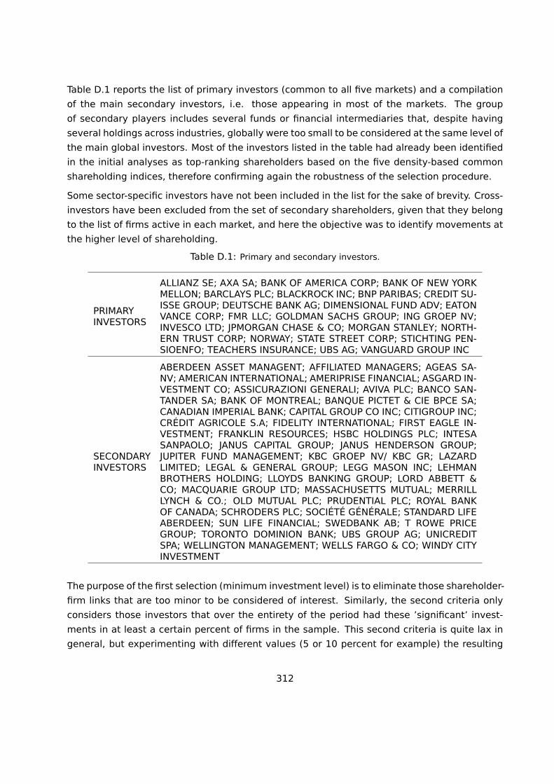
Table D.1 reports the list of primary investors (common to all five markets) and a compilation

of the main secondary investors, i.e. those appearing in most of the markets. The group

of secondary players includes several funds or financial intermediaries that, despite having

several holdings across industries, globally were too small to be considered at the same level of

the main global investors. Most of the investors listed in the table had already been identified

in the initial analyses as top-ranking shareholders based on the five density-based common

shareholding indices, therefore confirming again the robustness of the selection procedure.

Some sector-specific investors have not been included in the list for the sake of brevity. Cross-

investors have been excluded from the set of secondary shareholders, given that they belong

to the list of firms active in each market, and here the objective was to identify movements at

the higher level of shareholding.

Table D.1: Primary and secondary investors.

PRIMARYINVESTORS

ALLIANZ SE; AXA SA; BANK OF AMERICA CORP; BANK OF NEW YORKMELLON; BARCLAYS PLC; BLACKROCK INC; BNP PARIBAS; CREDIT SU-ISSE GROUP; DEUTSCHE BANK AG; DIMENSIONAL FUND ADV; EATONVANCE CORP; FMR LLC; GOLDMAN SACHS GROUP; ING GROEP NV;INVESCO LTD; JPMORGAN CHASE & CO; MORGAN STANLEY; NORTH-ERN TRUST CORP; NORWAY; STATE STREET CORP; STICHTING PEN-SIOENFO; TEACHERS INSURANCE; UBS AG; VANGUARD GROUP INC

SECONDARYINVESTORS

ABERDEEN ASSET MANAGENT; AFFILIATED MANAGERS; AGEAS SA-NV; AMERICAN INTERNATIONAL; AMERIPRISE FINANCIAL; ASGARD IN-VESTMENT CO; ASSICURAZIONI GENERALI; AVIVA PLC; BANCO SAN-TANDER SA; BANK OF MONTREAL; BANQUE PICTET & CIE BPCE SA;CANADIAN IMPERIAL BANK; CAPITAL GROUP CO INC; CITIGROUP INC;CRÉDIT AGRICOLE S.A; FIDELITY INTERNATIONAL; FIRST EAGLE IN-VESTMENT; FRANKLIN RESOURCES; HSBC HOLDINGS PLC; INTESASANPAOLO; JANUS CAPITAL GROUP; JANUS HENDERSON GROUP;JUPITER FUND MANAGEMENT; KBC GROEP NV/ KBC GR; LAZARDLIMITED; LEGAL & GENERAL GROUP; LEGG MASON INC; LEHMANBROTHERS HOLDING; LLOYDS BANKING GROUP; LORD ABBETT &CO; MACQUARIE GROUP LTD; MASSACHUSETTS MUTUAL; MERRILLLYNCH & CO.; OLD MUTUAL PLC; PRUDENTIAL PLC; ROYAL BANKOF CANADA; SCHRODERS PLC; SOCIÉTÉ GÉNÉRALE; STANDARD LIFEABERDEEN; SUN LIFE FINANCIAL; SWEDBANK AB; T ROWE PRICEGROUP; TORONTO DOMINION BANK; UBS GROUP AG; UNICREDITSPA; WELLINGTON MANAGEMENT; WELLS FARGO & CO; WINDY CITYINVESTMENT

The purpose of the first selection (minimum investment level) is to eliminate those shareholder-

firm links that are too minor to be considered of interest. Similarly, the second criteria only

considers those investors that over the entirety of the period had these ’significant’ invest-

ments in at least a certain percent of firms in the sample. This second criteria is quite lax in

general, but experimenting with different values (5 or 10 percent for example) the resulting

312

investors extracted are often the same ones identified in earlier phases of the study.

This analysis required then the extraction of the ownership information for each secondary

investor selected. With this information, we were able to check all the jumps in ownership

that the global main investors made into our secondary sector specific investors per year,

separating by positive and negative investment jumps. Figures D.1-D.3 below plot this, where

the selection of the secondary investors has been based on thresholds of minimum 5% invest-

ment in at least 10% of the firms active in the decade of observation. The only exception was

the MNOs and Parents sector, where 1% and 5% cut-offs were used; the different thresholds

were necessary due to the strongest presence of corporate groups, as noted earlier. Further

fine-tuning of the selection thresholds can be applied.

The ownership jumps were weighted by a proxy of the size of the secondary investor, based

on an index of TOAS density of its respective portfolio. This information for TOAS density was

previously calculated from ORBIS financial data for all shareholders, as one of the density-

based common shareholding indices (see definition in previous sectoral analyses). For those

investors where ORBIS did not provide information on portfolio Total Assets, as can happen for

some of these smaller financial firms, an average of the yearly TOAS density of shareholders of

the same entity type was calculated, and used as a substitute where the weight was missing.

The patterns in the graphs are similar to those already seen in the discussion specific to the

’Big Three’ and the BlackRock-BGI merger in Chapters 5 and 6. In almost every sector there

is a sharp increase in ownership jumps of BlackRock in the sector, driven by its acquisition of

BGI, and in turn a sharp sell-off on behalf of Barclays as they sell their division. By far these

ownership jumps are the most significant in each sector.

Figure D.1: Ownership changes between primary and secondary investors - Oil&Gas sector.

020

4060

80Su

m ow

nersh

ip jum

ps

2008 2009 2010 2012 2013 2014 2015 2016

primary_to_secondary shareholdersOilGas sum of positive ownership jumps between shareholders

AXA SA BANK OF AMERICA CORP

BARCLAYS PLC BLACKROCK INC

BNP PARIBAS CREDIT SUISSE GROUP

FMR LLC INVESCO LTD

JPMORGAN CHASE & CO UBS AG

VANGUARD GROUP INC

-250

-200

-150

-100

-500

2008 2009 2010 2011 2012 2013 2014 2015 2016

primary_to_secondary shareholdersOilGas sum of negative ownership jumps between shareholders



BNP PARIBAS CREDIT SUISSE GROUP

FMR LLC INVESCO LTD


VANGUARD GROUP INC

primary_to_secondary shareholdersOilGas sum of positive and negative ownership jumps between shareholders

313

Figure D.2: Ownership changes between primary and secondary investors - Electricity and TradingPlatforms sectors.

020

4060

Sum

owne

rship

jumps

2008 2009 2010 2011 2012 2013 2014 2015 2016

primary_to_secondary shareholdersElectricity sum of positive ownership jumps between shareholders



CREDIT SUISSE GROUP FMR LLC

INVESCO LTD JPMORGAN CHASE & CO

STICHTING PENSIOENFO UBS AG-15

0-10

0-50

0

2008 2009 2010 2011 2012 2013 2014 2015 2016

primary_to_secondary shareholdersElectricity sum of negative ownership jumps between shareholders





STICHTING PENSIOENFO UBS AG

primary_to_secondary shareholdersElectricity sum of positive and negative ownership jumps between shareholders

020

4060

Sum

owne

rship

jumps

2008 2009 2010 2011 2012 2013 2014 2015 2016

Trading Platf. sum of positive ownership jumps between shareholders primary_to_secondary shareholders

ALLIANZ SE AXA SA

BANK OF AMERICA CORP BARCLAYS PLC

BLACKROCK INC FMR LLC

ING GROEP NV INVESCO LTD


-150

-100

-500

2008 2009 2010 2011 2012 2013 2014 2015 2016

Trading Platf. sum of negative ownership jumps between shareholders primary_to_secondary shareholders

ALLIANZ SE AXA SA

BANK OF AMERICA CORP BARCLAYS PLC

BLACKROCK INC FMR LLC

ING GROEP NV INVESCO LTD


Trading Platf. sum of pos. and neg. ownership jumps between shareholders primary_to_secondary shareholders

314

Figure D.3: Ownership changes between primary and secondary investors - Telecoms and Beveragessector.

05

1015

20Su

m ow

nersh

ip jum

ps

2008 2009 2010 2011 2012 2013 2014 2015 2016

primary_to_secondary shareholderspositive ownership jumps


BANK OF NEW YORK MEL BARCLAYS PLC

BLACKROCK INC BNP PARIBAS

CREDIT SUISSE GROUP EATON VANCE CORP

FMR LLC GOLDMAN SACHS GROUP

ING GROEP NV JPMORGAN CHASE & CO

NORWAY STATE STREET CORP

UBS AG-15

-10-5

0

2008 2009 2010 2011 2012 2013 2014 2015 2016

primary_to_secondary shareholdersnegative ownership jumps


BANK OF NEW YORK MEL BARCLAYS PLC


CREDIT SUISSE GROUP EATON VANCE CORP

FMR LLC GOLDMAN SACHS GROUP

ING GROEP NV JPMORGAN CHASE & CO

NORWAY STATE STREET CORP

UBS AG

primary_to_secondary shareholdersMNOs_and_Parents sum of positive and negative ownership jumps between shareholders

010

2030

4050

Sum

owne

rship

jumps

2008 2009 2010 2011 2012 2013 2014 2015 2016

primary_to_secondary shareholdersBeverages sum of positive ownership jumps between shareholders

AXA SA BARCLAYS PLC





-150

-100

-500

2008 2009 2010 2011 2012 2013 2014 2015 2016

primary_to_secondary shareholdersBeverages sum of negative ownership jumps between shareholders

AXA SA BARCLAYS PLC





primary_to_secondary shareholdersBeverages sum of positive and negative ownership jumps between shareholders

315

D.2 Sample exclusion due to missing values

Table 7.1 reported the number of observations which were dropped each year from the analy-

sis, due to unavailable data on either the response variable or the controls. Few extra values

were dropped once the outcome variable was limited to the interval [−1,1], following IMF

(2019).

In order to understand possible implications on the empirical results, the excluded observa-

tions were studied so as to identify possible concerns. Table D.2 below reports some descrip-

tive statistics about the observations excluded from the sample.

The first column reports the number of years (out of ten) a firm was excluded from the analysis

due to missing or trimmed values. In the large majority of cases, firms are excluded only for

a limited number of years. An exception is given by a set of firms which are systematically

excluded from the sample for the whole period of observation. For this group we observe that

almost all firms were delisted or unlisted in 2017, and registered in Germany. This suggests

that exclusion from the sample may be due to total absence of financial data, given the less

stringent reporting obligations of this type of firms and legal framework. Even for those firms

missing for a smaller number of years, it is still predominant the unlisted/delisted status, as

well as registration in Germany.

Table D.2: Number of firms with missing values, by listing status and country of registration

No years No. Listing status in 2017 Countrymissing firms

Listed Delist./Unlist. DE Other

1 37 19 18 11 262 23 8 15 2 213 17 8 9 5 124 14 4 10 4 105 8 3 5 0 86 7 2 5 0 77 3 0 3 0 38 7 1 6 2 59 9 0 9 1 8

10 31 3 28 26 5

Total 156 48 108 51 105

316

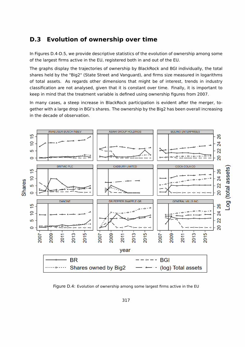
D.3 Evolution of ownership over time

In Figures D.4-D.5, we provide descriptive statistics of the evolution of ownership among some

of the largest firms active in the EU, registered both in and out of the EU.

The graphs display the trajectories of ownership by BlackRock and BGI individually, the total

shares held by the "Big2" (State Street and Vanguard), and firms size measured in logarithms

of total assets. As regards other dimensions that might be of interest, trends in industry

classification are not analysed, given that it is constant over time. Finally, it is important to

keep in mind that the treatment variable is defined using ownership figures from 2007.

In many cases, a steep increase in BlackRock participation is evident after the merger, to-

gether with a large drop in BGI’s shares. The ownership by the Big2 has been overall increasing

in the decade of observation.

Figure D.4: Evolution of ownership among some largest firms active in the EU

317

Figure D.5: Evolution of ownership among some largest firms active in the EU (cont.)

318

D.4 Alternative competition measure

Table D.3: Adjusted Lerner Index as dependent variable

Dep. var.: Lerner Index Adjusted (1) (2) (3)

Treated*post 0.091** 0.093** 0.147***

(0.036) (0.037) (0.049)

(log) Total assets 0.000 -0.001

(0.006) (0.009)

Shareholders’ HHI -0.001 -0.007

(0.006) (0.008)

Shares top 4 owners 0.001 -0.007

(0.043) (0.080)

Firm’s Integration -0.009 0.016

(0.030) (0.046)

Shares owned by Big2 -0.318 1.524

(0.552) (0.992)

(log) Total assets*post 0.001

(0.008)

Shareholders’ HHI*post 0.008

(0.006)

Shares top 4 owners*post 0.017

(0.078)

Firm’s Integration*post -0.031

(0.040)

Shares owned by Big2*post -1.452*

(0.798)

Observations 1,730 1,730 1,730

Year fixed effects yes yes yes

Firm fixed effects yes yes yes

R-squared within 0.031 0.032 0.042

R-squared overall 0.917 0.917 0.917

Number of firms 225 225 225

Robust standard errors, clustered at the firm levels, are shown in parentheses

*** p<0.01, ** p<0.05, * p<0.1

319

D.5 Heterogeneity of exposure

Ownership of companies exposed to the merger

We further inspect the relative size of ownership between BGI and BlackRock. The composition

of the overall exposure to the merger is examined in particular for firms that are held by both

BGI and BlackRock, and few other relevant players with high participations by one of them.

The cross-section distribution of the treated firms in 2007 is reported in Table D.4, where the

number of treated firms is grouped into classes according to the relative size of the ownership

of BGI and BlackRock. This joint distribution is also instrumental to interpret the relevance of

the shock in the sample under analysis and the (in)ability to measure its effect with sufficient

precision.

Table D.4: Number of firms by relevant shareholder composition in 2007

Shares held by BlackRock

0% 0-1% 1- 2% 2-3% 3-5% 5-7% 7-10% >10% Total

Sh

are

sh

eld

by

BG

I

0% 118 3 0 0 0 0 0 0 121

0-1% 12 5 0 0 0 1 0 0 18

1-2% 6 2 2 0 0 0 0 0 10

2-3% 0 1 0 0 0 0 0 0 1

3-5% 5 2 4 0 1 0 0 0 12

5-7 % 1 3 1 0 0 0 0 0 5

7-10% 2 1 0 1 0 0 0 0 4

>10% 0 0 0 0 0 0 0 0 0

Total 144 17 7 1 1 1 0 0 171

The same pattern emerges in the Figure D.6, with BGI having a more sizeable ownership in

most cases. This is not surprising because the portfolio of BlackRock in the late 2000s was not

as large as that of Barclays/BGI. Companies with a more sizeable participation of BGI and/or

BlackRock among their shareholders are identified explicitly in the graph.

Table D.5 reports some summary statistics of classes of exposure, where classes are defined

according to the sum of the shares held by BlackRock and BGI in 2007. We display the number

of firms and the number of observations belonging to the specific exposure class over the

entire period of observation. Please note that the panel structure of the available data is not

perfectly balanced and hence the number of observations can be smaller than 10 times the

number of unique firms.

320

Figure D.6: Treated firms by shares owned by merging investors

Among the descriptive statistics for each class, Table D.5 reports the average size of firms (as

measured by the log of Total Assets), and the number of firms in the class that are breweries

(core NACE code = 1105) or manufacturers of soft drinks/mineral waters (core NACE code =

1107). A detailed description of the firms belonging to each exposure class, including among

others size and industry is provided in Table D.6.

Table D.5: Summary statistics of exposure classes

Exposure Nr. of obs. Nr. of firms (log) assets Breweries Sodas/waters

0-1% 162 19 20.99 10 2

1-2% 81 9 22.16 2 2

2-3% 26 3 22.91 1 0

3-4% 60 6 22.26 2 4

4-5% 64 7 21.53 1 2

5-12% 98 13 22.12 6 5

321

Firm Nace % BR % BGI Assets Global Ultimate Owner

Exposure class [ 0% ; 1% )

ANADOLU EFES BIRACIL 1105 0.25 0.11 21.54 ANADOLU EFES BIRACIL

ANHEUSER-BUSCH INBEV 1105 0 0.34 23.22 ANHEUSER-BUSCH INBEV

ARCA CONTINENTAL SAB 1107 0.34 0 20.80 ARCA CONTINENTAL SAB

BARRY CALLEBAUT AG 1082 0.22 0 21.38 JACOBS HOLDING AG

CHINA HUIYUAN JUICE 1031 0.55 0 20.28 CHINA HUIYUAN JUICE

CHRIST WATER TECHNOL 3600 0.31 0.23 18.56 CHRIST WATER TECHNOL

COMPANHIA DE BEBIDAS 1105 0.73 0.2 23.33 ANHEUSER-BUSCH INBEV

DATACOLOR AG 1105 0 0.16 18.89 DATACOLOR AG

DAVIDE CAMPARI - MIL 1101 0.36 0.11 21.04 DAVIDE CAMPARI - MIL

GRUPO MODELO, S.A.B. 1105 0 0.72 22.55 GRUPO MODELO, S.A.B.

HEINEKEN NV 1105 0 0.52 23.20 L’ARCHE GREEN N.V.

HITE JINRO HOLDINGS 1105 0 0.52 21.42 HITE JINRO HOLDINGS

IHLAS HOLDING A.S. 8690 0 0.13 20.04 IHLAS HOLDING A.S.

JERONIMO MARTINS SGP 4711 0 0.11 20.88 SOCIEDADE FRANCISCO

SAPPORO HOLDINGS LIM 1105 0 0.99 21.93 SAPPORO HOLDINGS LIM

SUMOL+COMPAL, S.A. 1107 0 0.33 18.56 REFRIGOR, S.A.

TAKARA HOLDINGS INC 1102 0 0.67 21.00 TAKARA HOLDINGS INC

TSINGTAO BREWERY COM 1105 0 0.3 20.38 TSINGTAO BREWERY COM

YOUNG & CO’S BREWERY 1105 0 0.51 19.73 YOUNG & CO’S BREWERY


ABI SAB GROUP HOLDIN 1105 0 1.89 23.84 ABI SAB GROUP HOLDIN

C&C GROUP PLC 1102 0 1.27 20.54 C&C GROUP PLC

COCA-COLA FEMSA SAB 1107 0 1.2 22.37 FOMENTO ECONOMICO

DANONE 1051 0.26 1.25 23.64 DANONE

FOSTER’S GROUP PTY L 1105 0 1.15 22.51 FOSTER’S GROUP PTY L

NESTLE S.A. 1089 0.37 0.64 24.96 NESTLE S.A.

NICHOLS PLC 1107 0 1.17 17.76 NICHOLS PLC

SWIRE PACIFIC LIMITE 6831 0 1.1 23.53 JOHN SWIRE & SONS LI

WIMM-BILL-DANN FOODS 1051 0 1.46 20.26 WIMM-BILL-DANN FOODS


CAMPBELL SOUP CO 1089 0.45 2.08 22.15 CAMPBELL SOUP CO

FRASER & NEAVE LTD 1105 0.97 1.91 22.53 FRASER & NEAVE LTD

UNILEVER NV 1089 1.33 1.08 24.04 UNILEVER NV

322

Firm Nace % BR % BGI Assets Global Ultimate Owner


COCA COLA BOTTLING C 1107 0 3.14 20.59 COCA COLA BOTTLING C

COCA-COLA CO 1107 0.61 2.92 24.10 COCA-COLA CO

COTT CORP 1107 0 3.45 20.47 COTT CORP

FOMENTO ECONOMICO 1107 1.24 1.8 23.06 FOMENTO ECONOMICO

KIRIN HOLDINGS CO., 1105 0.28 3.58 23.41 KIRIN HOLDINGS CO.,

MARSTON’S PLC 1105 0 3.35 21.94 MARSTON’S PLC


A.G. BARR P.L.C. 1107 0 4.24 18.93 A.G. BARR P.L.C.

DEAN FOODS CO 1052 1.12 3.19 22.29 DEAN FOODS CO

FULLER SMITH & TURNE 1105 0 4.23 19.98 FULLER SMITH & TURNE

KRAFT HEINZ FOODS CO 1039 1.26 3.33 22.72 KRAFT HEINZ FOODS CO

LANDEC CORP 2016 0.17 3.97 18.39 LANDEC CORP

MONDELEZ INTERNATION 1051 1.18 3.12 24.56 ALTRIA GROUP INC

PEPSICO INC 1107 0.73 3.98 23.88 PEPSICO INC


ANHEUSER-BUSCH CO 1105 0.49 5.67 23.18 ANHEUSER-BUSCH CO

ASAHI GROUP HOLDINGS 1105 1.27 6.11 22.58 ASAHI GROUP HOLDINGS

BEIJING ENTERPRISES 1105 6.76 0.39 22.08 BEIJING ENTERPRISES

BRITVIC PLC 1107 0 7.07 20.72 BRITVIC PLC

CHIQUITA BRANDS INTE 1031 1.08 4.69 21.32 CHIQUITA BRANDS INTE

COCA-COLA AMATIL LIM 1107 0.21 5.53 21.75 COCA-COLA AMATIL LIM

GENERAL MILLS INC 1089 2.28 5.4 23.23 GENERAL MILLS INC

GREENE KING PLC 1105 0 6.27 22.15 GREENE KING PLC

MOLSON COORS BREW 1105 0.54 6.2 22.94 MOLSON COORS BREW

MONSTER BEVERAGE 1107 4.05 3.55 19.73 MONSTER BEVERAGE

PEPSI BOTTLING GROUP 1107 2.36 9.47 22.91 PEPSI BOTTLING GROUP

PEPSIAMERICAS INC 1107 0.97 8.88 22.01 PEPSIAMERICAS INC

SCOTTISH & NEWCASTLE 1105 0 7.4 22.98 SCOTTISH & NEWCASTLE

Table D.6: Summary of firm’s characteristics by exposure classes. Nace core classification. Values ofshares held by BlackRock (BR) and BGI, (log) Assets and GUO refer to the year 2007.

323

GETTING IN TOUCH WITH THE EU

In person

All over the European Union there are hundreds of Europe Direct information centres. You can find the address of the centre nearest you at: https://europa.eu/european-union/contact_en

On the phone or by email

Europe Direct is a service that answers your questions about the European Union. You can contact this service:

- by freephone: 00 800 6 7 8 9 10 11 (certain operators may charge for these calls),

- at the following standard number: +32 22999696, or

- by electronic mail via: https://europa.eu/european-union/contact_en

FINDING INFORMATION ABOUT THE EU

Online

Information about the European Union in all the official languages of the EU is available on the Europa website at: https://europa.eu/european-union/index_en

EU publicationsYou can download or order free and priced EU publications from EU Bookshop at: https://publications.europa.eu/en/publications. Multiple copies of free publications may be obtained by contacting Europe Direct or your local information centre (see https://europa.eu/european-union/contact_en).

KJ-NA-30312-EN

-N

doi:10.2760/734264

ISBN 978-92-76-20876-1

Common Shareholding in Europe - JRC Publications Repository

Documents

Transcript of Common Shareholding in Europe - JRC Publications Repository