Electronic copy available at: http://ssrn.com/abstract=1858879

Commodity Price Changes and Their Impacts on Poverty in Developing Countries: the Brazilian Case

Carlos Azzoni1, Joaquim Guilhoto2, Eduardo Haddad3, Tatiane Menezes4, Fernando Silveira5, Marcos M. Hasegawa6

PRELIMINARY VERSION

SUBJECT TO CHANGES

Abstract

The objective of the paper is to provide an estimative of the impacts that changes in

international prices of agricultural commodities will have on income distribution and poverty in

Brazil. To do so, a Social Accounting Matrix is constructed and applied, using a Leontief-

Miyazawa type model framework. The SAM is defined for 40 products, being 17 raw

agricultural products, 15 agricultural processed products, 3 industrial agricultural inputs, 2 other

industrial products, trade, transport, and services. Households are allocated to 10 groups, being 6

agricultural (4 types of family farmers, commercial farmers, and agricultural labor), and 4 urban

(income quartiles). Demand elasticities (price and income) for the products defined in the SAM

are considered, as well as limitations on the supply of agricultural inputs. The knowledge of the

possible impacts of changes in international commodity prices on income distribution and

poverty is very important for policy design within developing countries. Given the estimated

impacts on different groups of producers, different sorts of cushioning policies can be designed.

1 Departamento de Economia FEA -USP, e Pesquisador do CNPq. 2 Departamento de Economia FEA -USP, Regional Economics Applications Laboratory (REAL), e Pesquisador do CNPq. 3 Departamento de Economia FEA -USP, Regional Economics Applications Laboratory (REAL), e Pesquisador do CNPq. 4 Universidade Federal de Pernambuco (UFPE). 5 Instituto de Pesquisa Econômica Aplicada ( IPEA). 6 Universidad Catolica del Norte – UCN, Chile.

Electronic copy available at: http://ssrn.com/abstract=1858879

2

1. Introduction

Producers and households in developing countries are affected by the prices of products

involved in international transactions. The impacts of agricultural policy and structural reforms

leading to changes in international prices of goods and services are expected to be differentiated

across households and producers, depending on how they are involved in the circular flow of

goods and services within the country of residence. As such, it might be expected that these

reforms will affect income distribution and poverty levels within those countries. Considering

the supply side, units producing commodities facing price increases in the international markets

will benefit, since their product will become more valuable; those using imported inputs whose

prices increased as a result of the structural reforms will lose. As for households, those working

in sectors with increased international prices could experience income gains, and those working

in other sectors could rest unaffected in terms of income. However, since some prices would rise,

households not working for gaining sectors could suffer a decrease in real income. A general

price increase could also result, thus affecting all sorts of households.

Therefore, structural reforms that can change international prices are expected to produce

important changes in income distribution in all countries involved in international trade. Since

the impacts will vary according to the role played by different agents in the production and

distribution of national income, it is important to produce a detailed analysis of such impacts.

The objective of the paper is to provide an estimate the impacts of changes in international prices

of agricultural commodities on income distribution and poverty in Brazil, considering not only

the first round (direct) effects but also their spillovers (indirect effects) across the circula r flow of

income. The introduction of the second and higher round effects is important, for the initial

effects could either be mitigated or empowered by the indirect effects. The knowledge of such

compounded effects is important in the design of alternative policies for cushioning the

measured adverse impacts of reforms on poor people. It is possible that an increase in the price

of a very important export product of a country does not necessarily benefit all households

equally. As a matter of fact, some may be badly hurt, if the prices of products with high

participation in their consumption basket increased as a result of the second and higher order

effects in the national economy, and if they do not work in sectors benefited by the initial price

increase.

3

The paper is organized in 6 sections, including this introduction. Section 2 presents

details of the SAM and its sectoral disaggregation. The next section deals with the procedures

used to solve the model. In section 4 we discuss the estimation of input supply restrictions and of

demand elasticities. Examples of how the model can be used to estimate distributive impacts of

price shocks are presented in section 5. Finally, in the last section the concluding remarks are

presented.

2. Methodology and data sources

Given the study objectives, the SAM makes a distinction between the agricultural and

nonagricultural activities and agents in the economy, and takes into consideration the relations

that occur between them. At the same time, the SAM takes into consideration the relationships of

agricultural and nonagricultural activities and agents with the rest of the world economy. The

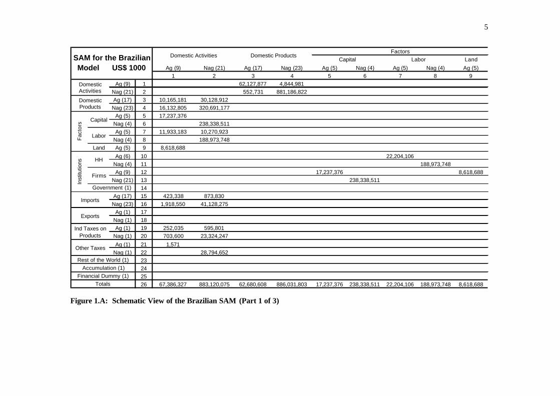
structure of SAM is described below, and is portrayed in Figures 1.A to 1.C. The first two

columns show, among other elements, the inputs from agricultural and nonagricultural goods and

agents that are needed to produce the agricultural and nonagricultural goods available in the

economy (rows 1 and 2). Rows 3 and 4 show the destination of the agricultural and

nonagricultural goods (columns 3 and 4). Rows 5 to 9 show how income generated by the

domestic activities is allocated among factors of production, and columns 5 to 9 show how this

income is allocated to institutions in the economy. Rows 10 to 14 show the different institutions,

while the corresponding columns 10 to 14 show how this income is spent. Columns 15 and 16

show the composition of the total value imports, while rows 15 and 16 show the destination of

imports. The composition of total value of exports is displayed in columns 17 and 18, which are

allocated to the rest of the world, in rows 17 and 18. Rows 19 to 22 show the source of taxes

received by government, while columns 19 to 22 show that these values are allocated directly to

government row (row 14). The transactions with the rest of the world are displayed into row 23

and column 23. Accumulation is displayed into row 24 and column 24, while row 25 and column

25 represent the financial dummy that is used to make the final adjust, closing in this way the

values for the SAM. It must be emphasized that the aggregate values are taken from the official

National Accounts for the country, so that any row or column sum will provide the official figure

for that case.

4

Previous applications of models of this type for the Brazilian economy can be found in

Fonseca and Guilhoto (1987), and Guilhoto, Conceição, and Crocomo (1996). The input-output

matrices released by the Brazilian Statistical Institute (IBGE) only take into consideration

Agriculture as a whole and 7 food processing industries, of a total of 42 sectors. The most recent

data released from IBGE refers to 1996; this matrix was constructed for the year 1999, following

the methodology developed by Guilhoto and Sesso Filho (2004), based on Brazilian national

accounting data. The SAM is defined for 40 products, being 17 raw agricultural products, 15

agricultural processed products, 3 industrial agricultural inputs, 2 other industrial products, trade,

transport, and services

The agribusiness activities in Brazil accounted for around 27% of total national GDP in

1999, in spite of the fact that Brazil is a major world producer of several products. This reflects

the fact that Brazil presents a large and diversified economy. Export-oriented sectors, such as

coffee, sugar, and soybean, compete in the international market and are prone to be the first

affected by different conditions in the world food market. On the other hand, sectors oriented

towards the local market, such as rice, beans, manioc, beef, dairy, etc., will lead important

internal distributional impacts in case of changes in world prices.

The definition of farm types is based on two different data sets: the Agricultural Census

of 1996/97 and the Pesquisa Padrão de Vida (PPV) of 1996 (Living Standard Survey), both from

IBGE. The first source is more comprehensive and allows for more information across states,

farm sizes, technology, etc. The second source provides more information on household

characteristics, consumption structures, etc. Our definition of household types is be based on a

study by the Ministry of Agrarian Reform/Incra and FAO, in which Brazilian farms were split

into family and non- family based on size, use of hired labor, market orientation, income levels

etc. Based on the objectives of this study, and on our analysis of characteristics of family and

non- family farms, we have decided to work with four groups of family farms, and to deal with

non- family farms as a group. Since consumption structures will come from different surveys, it is

important to analyze the matching of those two in terms of general characteristics of farmers.

Comparing the proportions of area, number of farms and number of people working in the

different farm types, it can be seen that the distributions in the two data sets are quite similar. In

other words, PPV consists of a good sample for the census results.

5

Land

Ag (9) Nag (21) Ag (17) Nag (23) Ag (5) Nag (4) Ag (5) Nag (4) Ag (5)1 2 3 4 5 6 7 8 9

Ag (9) 1 62,127,877 4,844,981Nag (21) 2 552,731 881,186,822Ag (17) 3 10,165,181 30,128,912Nag (23) 4 16,132,805 320,691,177

Ag (5) 5 17,237,376Nag (4) 6 238,338,511Ag (5) 7 11,933,183 10,270,923

Nag (4) 8 188,973,748Land Ag (5) 9 8,618,688

Ag (6) 10 22,204,106Nag (4) 11 188,973,748Ag (9) 12 17,237,376 8,618,688

Nag (21) 13 238,338,51114

Ag (17) 15 423,338 873,830Nag (23) 16 1,918,550 41,128,275

Ag (1) 17Nag (1) 18Ag (1) 19 252,035 595,801

Nag (1) 20 703,600 23,324,247

Ag (1) 21 1,571Nag (1) 22 28,794,652

23242526 67,386,327 883,120,075 62,680,608 886,031,803 17,237,376 238,338,511 22,204,106 188,973,748 8,618,688

Capital Labor

Rest of the World (1)Accumulation (1)

Financial Dummy (1)Totals

Imports

Exports

Ind Taxes on Products

Other Taxes

Inst

itutio

ns HH

Firms

Government (1)

Domestic Activities

Domestic Products

Fac

tors

Capital

Labor

FactorsDomestic Activities Domestic ProductsSAM for the Brazilian

Model US$ 1000

Figure 1.A: Schematic View of the Brazilian SAM (Part 1 of 3)

6

Ag (6) Nag (4) Ag (9) Nag (21) Ag (17) Nag (23) Ag (1) Nag (1)10 11 12 13 14 15 16 17 18

Ag (9) 1 413,469Nag (21) 2 1,380,523Ag (17) 3 3,888,010 10,550,602 0 1,703,642Nag (23) 4 30,623,941 252,889,500 102,399,488 49,933,409

Ag (5) 5Nag (4) 6Ag (5) 7

Nag (4) 8Land Ag (5) 9

Ag (6) 10 15,370,156 8,617,840Nag (4) 11 145,615,740 60,235,599Ag (9) 12 1,822,974

Nag (21) 13 23,890,68214

Ag (17) 15 71,707 190,988Nag (23) 16 2,283,019 15,305,757

Ag (1) 17Nag (1) 18Ag (1) 19 124,188 337,000 59,330 69,770

Nag (1) 20 1,950,161 16,104,238 8,116,803 3,472,323Ag (1) 21 4,025,760 1,713,245

Nag (1) 22 58,994,997 16,231,15823 1,635,143 15,491,222 1,805,352 61,649,63624 3,225,316 40,452,006 6,791,997 64,346,886 -32,028,57625 2,168,497 20,544,18726 46,192,102 394,825,087 27,679,038 262,229,193 166,732,000 1,864,683 69,766,440 1,773,412 53,405,733

Rest of the World (1)Accumulation (1)

Financial Dummy (1)Totals

Imports

Exports

Ind Taxes on Products

Other Taxes

Inst

itutio

ns HH

Firms

Government (1)

Domestic Activities

Domestic Products

Fac

tors

Capital

Labor

ExportsHouseholds FirmsGov (1)

ImportsSAM for the Brazilian Model US$ 1000

Figure 1.B: Schematic View of the Brazilian SAM (Part 2 of 3)

7

Ag (1) Nag (1) Ag (1) Nag (1)19 20 21 22 23 24 25 26

Ag (9) 1 67,386,327Nag (21) 2 883,120,075Ag (17) 3 6,244,262 62,680,608

Nag (23) 4 90,648,798 22,712,684 886,031,803Ag (5) 5 17,237,376Nag (4) 6 238,338,511Ag (5) 7 22,204,106Nag (4) 8 188,973,748

Land Ag (5) 9 8,618,688Ag (6) 10 46,192,102Nag (4) 11 394,825,087Ag (9) 12 27,679,038

Nag (21) 13 262,229,19314 1,455,063 55,515,554 5,740,576 104,020,807 166,732,000

Ag (17) 15 304,820 1,864,683Nag (23) 16 9,130,838 69,766,440

Ag (1) 17 1,773,412 1,773,412Nag (1) 18 53,405,733 53,405,733Ag (1) 19 16,939 1,455,063Nag (1) 20 1,844,182 55,515,554Ag (1) 21 5,740,576Nag (1) 22 104,020,807

23 80,581,35424 25,402,209 108,189,83825 22,712,68426 1,455,063 55,515,554 5,740,576 104,020,807 80,581,354 108,189,838 22,712,684

Rest of the World (1)Accumulation (1)

Financial Dummy (1)Totals

Imports

Exports

Ind Taxes on Products

Other Taxes

Inst

itutio

ns HH

Firms

Government (1)

Domestic Activities

Domestic Products

Fac

tors

Capital

Labor

Acc. (1)Financial

Dummy (1) TotalsInd Taxes on Products Other Taxes

ROW (1)SAM for the Brazilian Model US$ 1000

Figure 1.C: Schematic View of the Brazilian SAM (Part 3 of 3)

8

It was pointed out before that different sectors present different linkages within the

production system, be it through technical relationships with other sectors, or through income

generation and distribution, and, hence, through consumption, as a feed-back mechanism.

Therefore, it is important to take into consideration how wages and value added are distributed to

different groups of income. As an example, from all wage income received by the lowest income

group, farm sectors are responsible for 20%, increasing to 24% in the next decile, and decreasing

there on. For rich people, wages coming from farm producing sectors are less important. The

participation of different income groups in food manufacturing sectors is quite different, with the

very poor receiving a smaller portion of income from these sectors. This contrast in the two types

of sectors producing food products illustrates the need to consider how different sectors can

influence income distribution. It is also clear from the data that food directed to the consumption

of the local population are more important in the income generation of poor people, both in terms

of wages and value added. Soybean production is more important for employees and producers

in the middle-income range. Therefore, a price shock in this sector tends to affect this group of

households more intensively than poor households, at least in the first round of effects.

Since income is distributed differently across sectors, households associated to each

sector are expected to have a different consumption structure. This is especially true when

considering the differences in consumption between urban and rural families. Therefore, an

important step towards constructing a SAM is the consideration of how families spend their

income. The data sources for this part of the study are the 1987 and 1995/96 Household

Expenditure Surveys developed by IBGE. For urban households, we use the household surveys

of 1987 and 1995/96 (POF); we consider 4 groups of households, defined according to income

levels. For rural households, we use the 1996 PPV. The five categories of farms presented before

will be considered. Thus, we have consumption structures for 10 types of consumers, 6 rural (5

farmers, 1 employees), and 4 urban. The data show that poorer households spend a higher

proportion of their income on agricultural raw food. As expected, rural households present more

self-consumption than urban households, and the proportion decreases from family farms 1

through 4; urban households spend a larger share of their income with housing. In general, both

housing and education expenditure shares rise from low- income households to high- income

ones.

9

3. Solving the Model

The goal of this section is to describe the various relationships embedded in the model. Its

solution considers reactions of consumers to price and income changes, and reactions of

producers to input price changes. It does not include, however, substitution effects between

products and sectors. It is structured in five stages, as described below. The sum of the results

calculated in these stages, partially considering the reactions of agents to price and quantity

stimuli, comes close to a full general equilibrium model. In Chapter 6, the results of the

simulations using this SAM-based model are compared, in aggregate terms (global GDP,

employment, price indexes, etc.) to a general equilibrium model which does not have the sectoral

and product details of this study. It will be shown that the disaggregated results provided by the

model estimated in this study are compatible, at the aggregate level, with the ones resulting from

the CGE model. On the other hand, the model presented here provides details on the impacts

across farm types that is impossible to achieve within that CGE model.

3.1. Model solution mechanics

As a result of structural reforms in international trade, prices of commodities exported by

the Brazilian economy are expected to change. It is expected that the international supply curve

of protected commodities will shift upwards, leading to increases in international prices, as

portrayed in Figure 3.1 below.

Figure 3.1 – Expected effects in the World Market

International Prices

Volume traded

World Supply

World Demand

10

Some countries will be negatively affected by the changes, some countries positively. It is

expected that the demand for Brazilian exports will increase, as portrayed in Figure 3.2 below.

The effects on domestic prices will depend on the elasticity of domestic supply. In the case of a

flat domestic supply curve, such as S1, there will be no increase in the domestic price of the

commodity, and thus no reduction in domestic consumption, and total production will increase

by the amount of exports (arrow b in the figure). In the most probable case of some price

transmission to the domestic market, such as in the case of a positive slope supply curve such as

S2, the domestic price is expected to increase (arrow c in the figure), leading to a reduction in the

domestic consumption. Thus, the final increase in production will not be the full amount of

exports, as before, but a smaller amount (arrow a in the figure). It will be equal to the increased

amount of exports, less the decreased amount of domestic consumption (assuming this domestic

price increase will not affect the country’s competitiveness in the international market).

Figure 4.2 – Effects of a positive-slopped domestic supply

Domestic Prices

c S1

S2

Domestic Production a

b

11

In order to estimate the impacts of this chain of events, the first stage of the model

estimation simulates a situation in which the supply curve is such as S1, that is, the whole

increase in export volume is used to shock the model, ignoring any price increases. No restriction

is imposed on the supply of inputs either. In other words, this stage simulates an increase in

exported quantities at the previous price level. The results of this stage indicate the upper bound

effect on national production, admitting that the additional production does not cause any price

effect on the domestic market. Additional exports will be added to the previous production,

imposing direct, indirect and induced effects on the system.

The price transmission from international to domestic prices considered is the one

obtained from the resulting scenarios from OECD, i.e., results from the GTAP model. These

estimates present expected international price changes as well as domestic price changes. This

domestic price change for a product is supposed to spread to all prices in the economy through a

Leontief-type price transmission mechanism. For example, an increase in the domestic price of

soybeans will affect in the first place the prices of all sectors utilizing this product as an input, at

fixed coefficients. In later stages, all prices will be affected in some way through the indirect

effects generated by the original price increases.

The estimated domestic price changes will increase or decrease the production value of

the specific product, depending on the price-elasticity of that product’s demand. For a product

with price- inelastic demand, which is the case of almost all food products, a domestic price

increase will result in increased production value and income for that activity. In order to keep

total income constant in the system, this extra income is transferred from all other sectors in the

economy, whose incomes will fall proportionately to their participation in total production.

Considering these changed incomes and the price changes, nominal and real income changes are

calculated. Using estimated income-elasticities, the income changes will be transformed into

production value changes, adding another element to the estimation. At this stage, still no factor

supply restriction is imposed, that is, a flat supply curve is supposed.

So far two results have been obtained. The first indicates the maximum effect of

increased exports without any restriction on the supply side of the economy. Price effects have

been introduced in the second stage, indicating the negative impacts on economic activity of the

estimated price increases. In the third stage these results are just summed-up, to come up to the

net results, still ignoring input supply restrictions.

12

Increased production of goods means increased use of inputs. If goods are produced with

flat cost curves, there would be no effect on prices from the supply side; if production faces

positive sloped cost curves, some supply reactions are to be expected. A way to consider this

effect is to estimate product supply elasticities and include these factors in the estimation of the

impacts. However, data limitations made it impossible to do it this way. The alternative used was

to estimate the expected increases in input prices as a consequence of increased production, and

to spread these price increases to the economy with a Leontief-type price transmission

mechanism. The same chain of income and price changes described in the second stage is

estimated.

As a matter of fact, the estimated model is not exactly as portrayed in Figure 3.2, but the

one displayed in Figure 3.3 below, which reproduces the demands for Brazilian goods, and the

flat domestic supply curve S1 from Figure 3.2. As input prices rise, production costs go up in all

sectors using these inputs, and the flat domestic supply curve moves upward, to S3. This shift in

supply affects the quantity transactioned in the same way as the reactions of producers in the

upward slopped supply curve displayed in Figure 3.2, but the quantitative effects might be

different. Thus, although the choice of this methodology to introduce domestic supply responses

was determined by data restrictions alone, the input supply limitations introduced via the

Leontief-type price transmission mechanism partially takes care of the problem. Off course, the

two alternatives most probably will lead to different quantitative results, but the direction of

change is the same.

Finally, the fifth stage just consolidates the upper-bound effect of the first stage, the

influence of price transmission, and the influence of input limitations, coming up with the net

effects on the national economy. Figure 3.4 summarizes the mechanics of the model solution.

13

Figure 4.3 Effects on the domestic market with a Leontief-type price transmission mechanism

Domestic Prices

c S1 S3

a

b

Figure 3.4 – Model solution schematics

40 products

Land Labor Capital

10 household types(6 rural, 4 urban)

10 consumptionstructures

(40 products)

Domestic purchases

International purchases

Change inInternationalDemand

Income andprice elasticities

Pass-through todomestic prices

Internationalprice changes

Leontief-type pricemultipliers

Inputsupply

limitations

Cons. Price IndexGeneral Price Index

14

4. Input supply and product demand elasticities

4.1. Input supply

According to the mechanism described above, input supply restrictions are incorporated

in the Fourth Stage. Given the additional input demand calculated in Stage III, input price

changes are estimated, based on estimates of input supply price elasticities. The overall effect of

these price changes are considered in the economy as a whole, diminishing the restriction- free

previous income estimates.

Land is abundant in Brazil. It is true that quality varies (location included in quality), but

nevertheless one should bear in mind that, contrary to developed country cases, the supply of

land should be more price-elastic in Brazil. The last available agricultural census, referring to the

year 1995, revealed that less than 50 million hectares were cultivated. In this same year, the

amount of idle productive 7 area, including resting land, amounted to almost 25 million hectares.

A study by Olivete et al (2002) indicates that the main supplier of area to production-expanding

products in the last part of the 90s was natural pasture. The study also shows that the main area-

demanding product is cultivated pasture: soybean demanded 2,165 million extra hectares, while

cultivated pasture demanded 9,773 million. Adding to this supply of idle area, total pasture area

in 1995 amounted to almost 178 million hectares. That is, at that time, expanding production

could very easily use idle area without concerns with price increases, suggesting a flat land

supply curve. In the year 2003, the amount of cultivated area grew to almost 57 million hectares,

14.5% higher than in 1995. This land use increase produced a 56.2% increase in the amount of

production (in tons), revealing that the recent increase in Brazilian agricultural production was

produced mainly by productivity growth. As Gasques et all (2002) show, Total Factor

Productivity grew 4.51% in the 90s, and 4.25 between 2000 and 2002. As for land prices, a sharp

decrease was observed from 1995 to 2000, when the price of a hectare costed only 45% of the

price in 1995. Since then, prices are increasing steadily, with a jump between 2002 and 2003.

These numbers allow for the calculation of an estimate of land supply elasticity. Taking

the period 1996-2003 (skipping the relatively high land prices in 1995), the price-elasticity of 7 Idle productive area does not include forests or land inadequate for cultivation.

15

land supply would be of 1. Considering the 2000-03 period (including the peak prices of 2003), it

would be 0.43, in line with the numbers used by OECD for European countries, USA and Japan.

Eliminating the peak year of 2003, the number would be 0.54. Considering the mechanics of

simulation within the model, the results of stages I-III will be expressed in output variations

(monetary values). Therefore, it is necessary to associate input price increases to output

variations. For a 56.2% increase in production from 1996 to 2003, cultivated area expanded by

only 15%, providing an area-production elasticity of 0.27 (for every 1% increase in production,

area increased by 0.27%). During this period, land supply price-elasticity was unitary, implying

an output price-elasticity of 0.27. Considering more recent years, in which land price-elasticity

was lower, the output elasticity would also be lower, between 1.35 and 1.69. For the purpose of

calculations, an output elasticity of 2 will be used. This elasticity will only apply to agricultural

products. No land price increase will apply to poultry and eggs, cattle ranching, hog and pig

farming and other animal production.

As for manufactured inputs, the model considers fertilizers, defensives, and tractors. The

first two are mainly imported, and tractors are even exported. Considering the evolution of

fertilizer prices and quantities between 1996 and 2003, it is observed that quantities increased by

86%, while real prices increased by 24%. The implied elasticity in these numbers is 3.62.

Ignoring the strong variations of 2003, and computing averages of initial and end years, the

elasticity would be slightly higher, 3.85. Contrary to the case of land, in which the area-

production elasticity was lower than unity, in the case of manufactured input it is higher.

Between 1996 and 2003, for every extra 1% in production, the quantity of fertilizers increased by

1.53%. Considering the supply price-elasticity of 3.62, the output elasticity would be of 2.36. For

the period 2000-2003, any 1% extra production caused an increase of only 1.03% in input use.

This additional input use was accompanied by a 0.49% increase in input prices, leading to an

output-elasticity of 2.0. These numbers are clearly influenced by the values for 2003.

Considering the sensitivity of results to the period chosen, a number of 2.5 for the output

elasticity should be chosen. Due to lack of data for other manufactured inputs, the same elasticity

will be used for defensives and tractors.

There is a long lasting decreasing trend in labor absorption in Brazilian agriculture. Even

in the 70s, when employment in general was growing strongly, agriculture released workers. In

recent years, with the already demonstrated growth in production, employment is not following.

16

That would be only a partial view, if other sectors were demanding labor from agriculture.

However, that is not the case, for unemployment rates are widespread across sectors and regions

of the Brazilian economy, at high levels. For an increase of 56.2% in agricultural production

between 1996 and 2003, the number of employed persons in agriculture decreased by around

10%, and real wages decreased by around 4%. It is reasonable thus to suppose that any additional

worker needed in agriculture in the near future will be available at the current market wage level.

In summary, the price effects due to input supply limitations used in the model will be

Input A 1% increase in agricultural output will increase input prices by

Land 0.5% Manufactured inputs 0.4% Labor 0

4.2. Demand Elasticities

A pseudo panel was constructed to calculate own-price, cross-price and income

elasticities for a disaggregated list of food products, as well as for aggregated groups of non-food

products. A two-stage demand function model commonly used in agricultural studies was

constructed, with a more sophisticated estimation procedure. Household expenditure data were

used to construct a three-dimension pseudo panel with: time, region and income bracket. This

procedure allows for the control for effects that vary with time, but are constant across regions

(random effects), as well as for effects fixed in time, but which vary across regions (fixed

effects), effects which, when not specified, are included in the omitted variables, biasing the

parameter estimators.

Data used came from the 1987/88 and 1995/96 POF – Pesquisa de Orçamentos

Familiares, household expenditure surveys produced by IBGE, the Brazilian official statistics

office. They consist of surveys covering expenditure of 14,000 families in 1987/88 and 16,000

families in 1995/96, for the most important metropolitan areas in Brazil: Belém (North),

Fortaleza, Recife and Salvador (Northeast), Belo Horizonte, Rio de Janeiro and São Paulo

(Southeast), Curitiba and Porto Alegre (South), and Brasília (Center-West). Only families with

some expenditure with some of those items were included in the study, resulting in samples of

17

404.366 observations in 1987/88 and 347,569 in 1995/96. The product groups are as follows:

home maintenance - cleaning items, such as soap, detergents, etc.; accessories - bags, belts,

wallets and bijouterie; transportation - urban bus, fuel and labor; personal care - shampoo, soap,

toilet paper etc.; personal expenditure - maids, hairdresser and sewing professionals; recreation -

movies, clubs, magazines and non-academic books; and education - tuition for elementary and

high schools, books and stationery.

In the first stage a pseudo panel was constructed aggregating consumption items into

those 13 groups, with observations for 10 income brackets (income deciles), 10 metropolitan

regions and 2 years. In the second stage expenditure with the 19 food products was also

disaggregated into the 10 x 10 x 2 fashion. Therefore, each step considered 200 observations.

Within the TSBS, it is assumed that, in the first stage, consumers chose how to spend their

income among the following groups of products: food, housing, home maintenance, apparel,

shoes, accessories, transportation, health services and drugs, leisure and tobacco, personal

hygiene, personal expenditures, and education. In the second stage, the expenditure allocated to

food products will be attributed to 19 food products: sugar, rice, banana, potato, coffee, onion,

wheat flour, manioc flour, beans, chicken, orange, milk, pasta, margarine, vegetable oils, bread,

cheese, and tomato.

The estimation method employed is the Interactive Seemingly Unrelated Regression

(ISUR), which is equivalent to the Full Information Maximum Likelihood method (FILM).

When ISUR is employed to estimate a LAIDS model, the property of additivity of the demand

function makes the variance and covariance matrix singular. To solve for that, any one of the

equations is taken off of the system. In order to keep the homogeneity property, all prices must

be normalized by the price referring to equation excluded. The coefficients for this equation are

recuperated, given the additivity property. Symmetry is imposed in the estimation process.

Table 1 below presents the estimated own-price, cross-price, and income elasticities for

19 commodities. Both own-price and income elasticities present the expected signs, with all but

one commodity in the inelastic portion of the demand function (wheat flower shows a price

elasticity of –1.172).

18

Table 1 – Own-Price, Cross-Price, and Income Elasticities

Price Elascitities

Sugar Rice BananaPotato Coffee Meat Onion Manioc Flower

Wheat Flower Beans Chicken Orange Milk Pasta Margarine Oil Bread Cheese Tomato

ei1 -0.77 ei2 -0.21 -0.83 ei3 0.11 -0.05 -0.94 ei4 0.12 -0.03 -0.05 -0.88 ei5 0.27 0.14 0.02 0.14 -0.45 ei6 0.18 0.30 0.05 0.46 -0.83 -0.58 ei7 0.05 -0.01 0.01 -0.07 0.11 -0.01 -0.74 ei8 0.17 0.16 -0.03 0.06 -0.03 -0.08 0.32 -0.68 ei9 -0.21 0.06 -0.07 -0.25 0.09 -0.02 0.39 0.11 -1.17 ei10 0.09 0.06 0.08 0.30 0.04 -0.08 -0.08 -0.11 0.21 -0.74 ei11 0.14 -0.14 0.17 -0.44 0.19 0.05 0.15 0.20 -0.33 -0.05 -0.90 ei12 0.06 -0.02 0.05 -0.04 0.03 0.00 -0.06 0.11 -0.02 0.07 0.05 -1.08 ei13 -0.49 0.13 -0.21 0.35 0.35 -0.22 -0.19 0.72 0.58 0.12 0.13 -0.01 -1.07 ei14 0.05 0.03 -0.05 0.17 -0.01 0.01 -0.37 0.02 -0.46 0.03 0.02 0.08 0.04 -1.08 ei15 0.08 -0.08 0.02 -0.33 0.02 0.13 -0.21 -0.39 -0.11 -0.14 0.00 0.01 0.02 0.14 -0.92 ei16 0.16 -0.14 0.07 0.10 -0.01 0.09 0.07 -0.19 -0.08 -0.08 0.01 0.10 0.05 -0.01 -0.18 -0.92 ei17 -0.03 -0.02 0.32 0.04 0.09 -0.04 0.10 0.36 -0.24 0.28 0.00 -0.20 0.05 -0.07 0.13 -0.34 -0.52 ei18 0.13 0.00 0.09 0.05 -0.08 -0.04 -0.06 0.09 -0.25 0.29 0.11 -0.09 -0.13 0.28 0.18 0.27 -0.08 -0.79 ei19 0.23 0.00 0.03 0.06 0.09 0.02 0.01 0.17 0.01 0.11 0.05 0.00 0.00 -0.06 -0.16 -0.01 -0.02 0.10 -0.99

Expenditure Elasticities

Ei 0.19 0.16 0.62 0.59 0.24 0.65 0.51 -0.06 0.42 0.00 0.30 0.85 0.56 0.32 0.59 0.42 0.16 0.94 0.52

19

As expected, the cross-price elasticities are low, and complementarity and substitutability

among goods are observed in general. As for income-elasticity, all commodities present low

values, which was expected for food products. The higher values for the elasticities are observed

for cheese (0.942), orange (0.853), and beef (0.651), which are relatively more expensive than

the other items. Beans and manioc flower, very basic products in the typical diet of the Brazilian

poor, exhibit negative income elasticities, although very close to zero.

5. Policy Simulations

In this section a more realistic situation is simulated. Given the framework presented

above, it is expected that trade liberalization will change the international prices of agricultural

commodities, with effects on rural and urban families in Brazil. Since different types of rural and

urban households are involved in the productive process in different ways, it is expected that the

international price changes will affect them differently. The aim of this chapter is to present the

expected impacts for the different household types, hence on inequality and poverty.

5.1. Expected changes in international commodity prices

As presented in Section 4, the international and domestic changes in product prices are

exogenous to this study. They were calculated independently using a Computable General

Equilibrium model (CGE) of the world economy, in which the flow of trade between countries is

considered. This world model is used to simulate a situation in which all forms of subsidies are

reduced by half in every country (including Brazil, whenever it is the case). The estimated

expected price changes are displayed in Table 5.1, which presents the impacts on the domestic

prices, export prices, import prices, and export volume. All food products exported by Brazil are

expected to experience domestic price increases of over 2%, with a maximum of 5.68%.

20

GTAP Products Domestic Prices Export Prices Import Prices Export volumePaddy rice 2.62 3.24 0.45 94.52Horticulture 2.44 3.24 0.59 -6.52Sugar cane & beet 2.52 0,00 -14.24 -69.51Plant fibres and other crops 2.76 3.39 0.14 -3.94Wheat 1.64 2.41 1.14 -11.53Coarse grains 2.95 3.6 0.85 0.26Oilseeds 2.43 3.18 1.28 1.21Bovine cattle, sheeps 5.68 6.34 1.81 -6.35Raw milk 3.16 3.76 1.98 -31.43Non-ruminants 3.88 4.56 0.82 -8.4Dairy 3.03 3.03 3.10 17.31Sugar 2.01 2.01 1.57 7.24Bovine meat 3.96 3.96 1.44 163.85Pig&Poultry meat 3.99 3.99 1.27 1.29Other processed food 2.3 2.3 -0.77 3.28Manfuactures -0.03 -0.03 -0.13 7.22Textiles, wearing apparel, leather 0.02 0.02 -0.48 -0.04Services 0.99 0.99 0.10 -2.15

Table 6.1 - GTAP expected changes in prices and export volumes (%)

5.2. Aggregate impacts on the Brazilian economy

Aggregate results are presented in Table 5.2. As a consequence of increases in prices and export

volumes, real aggregate GDP is expected to grow by 1.6%, real household income by 1.58%, and

employment level by 1.41%. These are quite low values, reflecting the fact that Brazilian

economy is highly diversified, with agricultural activities and food processing industries taking a

small share of total activity, as explained in Chapter 2. Besides that, exports are a small share of

total production. For raw agricultural products, it represented only 3% of total production in

1999. Within this group, soybeans presented the largest export share, 31.1%, in spite of the

importance of the Brazilian production in the international market. For processed food products

as a group, the export share was 13.6%, with the largest shares belonging to sugar (35.6%), and

coffee products (32.1%). The importance of the domestic market explains the low impacts of the

simulated export increases, and also the fact that all types of families end-up receiving the

benefits of increased exports, as will be shown later on in this chapter.

21

Table 5.2 – Aggregate results

%

Real GDP 1.60161

Real Household Income 1.57591

Consumer Price Index 1.63406

GDP Deflator 1.27965

Employment 1.40686

5.3. Global results sensitivity to input limitation parameters

The parameters that represent the effects of increased production on input prices were

presented in Chapter 4. The model estimates Leontief-type price multipliers that spread the

effects of input price increases throughout the economic system. These price increases affect real

income and hence domestic demand. Since their estimation was made without the sophisticated

econometric techniques applied to demand elasticities, it is important to check whether or not

results are sensitive to their values. For that, the parameters were changed, with the resulting

changes in real GDP, real household income, consumer price index, general domestic price

deflator, and employment are show in table 5.3.

It can be seen that the model results are not sensitive to these parameters, since the

differences are all small. For example, if both parameters are set to their lowest level, implying

less price sensitivity of input supply, real DGP growth would go up by 0.00029 percentage

points (from 1.60161% to 1.60132%). Since the price transmission mechanism is linear, a similar

increase in the parameter values will produce the same quantitative results, only in the other

direction. The largest impacts are on employment: from 1.40686% to 1.40578%, a change of

0.00108 percentage points, still negligible. Therefore, there is no basis to suspect that the

aggregate results presented would change significantly if different limitations on the input side

were imposed to the model.

22

Table 5.3 – Sens itivity of aggregate results to changes in input limitation parameters

5.4. Global results sensitivity to the allocation of additional exports to farm types

The results on Table 5.2 consider that additional exports will be allocated to the five farm

types proportionally to their previous shares in production. One might argue that these extra

exports are probably to be served by large producers, since they are the ones more

entrepreneurial and market-oriented, and that this could lead to different results in comparison to

the ones presented. Thus, in this section simulations were made considering different allocation

of exports across farm types. In Table 5.4 three situations are portrayed. In the first, the increased

international demand is to be served by all types of farmers, proportionally to their participation

in production. The second considers that only farmers of types 4 and 5 (large family and

commercial farmers) will export and provide inputs to exporting sectors (for example, only large

producers will provide sugar cane as inputs to the manufacturing of sugar). The third situation

considers that only the three first types of family farmers will sell abroad and provide inputs to

food processing activities.

It will be shown in a later section tha t these three situations will produce differences in

distributive effects, but at the aggregate level, the impacts are really small, as the results

Parameter values Model (a) (b) (c) (d) (e) (f)

Manufactured inputs 0.4 0.2 0.6 0.4 0.4 0.2 0.6Land 0.5 0.5 0.5 0.3 0.7 0.3 0.7Labor 0 0 0 0 0 0 0

Results (% changes)

Real GDP 1.60161 1.60173 1.60149 1.60177 1.60144 1.60189 1.60132Real Household Income 1.57591 1.57608 1.57574 1.57614 1.57568 1.57631 1.57551CPI 1.63406 1.63406 1.63406 1.63406 1.63406 1.63406 1.63406GDP Deflator 1.27965 1.27965 1.27965 1.27965 1.27965 1.27965 1.27965Employment 1.40686 1.40637 1.40735 1.40627 1.40745 1.40578 1.40794

Changes in results

Real GDP - 0.00012 -0.00012 0.00017 -0.00017 0.00029 -0.00029Real Household Income - 0.00017 -0.00017 0.00023 -0.00023 0.00040 -0.00040CPI - 0.00000 0.00000 0.00000 0.00000 0.00000 0.00000GDP Deflator - 0.00000 0.00000 0.00000 0.00000 0.00000 0.00000Employment - -0.00049 0.00049 -0.00059 0.00059 -0.00108 0.00108

23

displayed in Table 5.4 indicate. This is explained by the important role of domestic demand

originated in the urban sector of the Brazilian economy. As presented in Chapter 2, the share of

urban population is around 80%, and the share of urban income is around 90%. Thus, an increase

in the exports of agricultural goods will end-up affecting the income of urban households, which

in turn will purchase agricultural products from all types of farms. Thus, these results indicate

that the results are quite robust to different allocation of exports to farm types.

Table 5.4 – Sensitivity of global results to different export profiles

Allocation of additional exports

Change in aggregate Household Income

Difference (% points)

Proportional to shares in production 1.5759% -

Large family and commercial farms only 1.5713% 0.0046

Small family farms only 1.5694% 0.0065

5.5. Distributive aspects

In this section the impacts are analyzed considering their different effects across

household types. The aggregate results presented before are detailed as they accrue to different

households, and some synthetic indicators are used to consider the impacts on poverty and

inequality.

5.5.1 Effects across household types

Table 5.5 shows the expected changes in income received by households resulting from

the GTAP scenario of domestic price changes derived from international adjustments. It shows

that agricultural employees and commercial farmers are the ones expected to have the largest

positive impacts (+2.95% and +2.84%). In general, rural households will benefit more than urban

households. The two poorest rural household types will receive the lowest positive impacts

among rural households (+1.91%), but this is larger than the best case of urban households

(+1.49%). The best case within agricultural farmers is a positive impact of 2.11% (type D), still

0.8 percentage point below commercial farmers.

24

Table 5.5 - Impacts on household income across family types

Family type Household Income growth (%)

Family Agriculture 1 1.9066 Family Agriculture 2 1.9217 Family Agriculture 3 2.0576 Family Agriculture 4 2.1130 Commercial Farmers 2.8458 Agricultural Employees 2.9522 Urban 1 1.4564 Urban 2 1.4830 Urban 3 1.4871 Urban 4 1.4785 All Households 1.5759

Table 5.6 illustrates the various stages in the estimation of the model, as presented

in section 4. Column F is exactly the same as in Table 5.5, exhibiting the final effects. Column E

indicates the effects on income of increased exported volumes, without considering any price

changes. All changes are positive, for it shows the effects on the economy of increasing the

production of the respective sectors, at the previous price levels (except for input price changes,

displayed in the column D). Comparing these two columns, it is clear that rural households

increase their numbers when going from E to F, and urban households present decreasing values.

This is expected, for urban households face more negative price impacts, given their

consumption baskets and income sources.

Column A presents income changes due to increased product prices, and column

B shows income compensation, that is, income that was distributed to other household types in

order to keep total income constant in the system. The sum of these two columns results in

positive numbers for rural households, and negative for urban families, indicating a net transfer

of income from urban to rural sectors due to an overall increase in the price of agricultural goods

(all price- inelastic). Thus, while all households benefit from increased exports, rural families

25

receive positive effects of price and income compensation, while urban families have to face

increased agricultural prices. Column C displays the effects on income of input price restrictions

(land and manufac tured inputs), and column D introduces the income compensation for the

resulting price changes.

Income change due to increased product prices

Income compensation for

changes in product prices

Income change due to land and manufactured inputs supply restrictions

Income compensation for changes in prices

of land and manufactured

inputs

Changes in exported volume

Total

A B C D E F

Family agriculture 1 0,45 -0,32 0,02 -0,02 1,77 1,91Family agriculture 2 0,45 -0,31 0,02 -0,02 1,78 1,92Family agriculture 3 0,50 -0,30 0,02 -0,02 1,85 2,06Family agriculture 4 0,52 -0,30 0,03 -0,02 1,88 2,11

Commercial farmers 0,83 -0,28 0,04 -0,01 2,28 2,85Agricultural Employees 0,87 -0,29 0,04 -0,01 2,34 2,95

Urban Households 1 0,24 -0,32 0,01 -0,02 1,54 1,46Urban Households 2 0,25 -0,32 0,01 -0,02 1,55 1,48Urban Households 3 0,25 -0,31 0,01 -0,02 1,55 1,49Urban Households 4 0,24 -0,31 0,01 -0,02 1,55 1,48

All households 0,29 -0,31 0,01 -0,02 1,60 1,58

Table 6.6 - Changes in household income, by estimation stage

5.5.2 Sensitivity to different allocations of additional exports

Even if the largest impacts accrue to commercial farmers and large family farmers, it is

observed that all family farm types receive positive effects. As mentioned in section 5.4, this is

related to the share of demand originated in the urban sector of the Brazilian economy, implying

that any increase in exports will affect urban households, which in turn will purchase agricultural

products from all types of farms. Adding to that, the GTAP simulation forecasts an increase in

manufacturing exports, which is much larger, in size, than the increased value of food products

exports. In order to illustrate that, the final effect was decomposed into the direct effect, and the

total effect (direct, indirect, induced, and price effects). In the first step, only the direct impact of

the increased export values are considered, ignoring the indirect (purchases of inputs from other

sectors) and induced (consumer purchases) by the initial impact. In the second step, these

26

indirect and induced effects are included, as well as the effects of domestic prices on real income

all over the economy.

The same two extreme cases commented on Section 5.4, referring to different allocations

of additional exports across farm types, are considered here. The first considers that only

household types 4 and 5, that is, large family and commercial farmers will produce the additio nal

exports, both of final products and agricultural inputs to export sectors. The second allocates all

additional exports to small family farmers. Table 5.7 presents the results of the standard run, and

the two extreme cases. The global changes were already discussed in Section 5.4, and are very

small, but the changes to specific household types are now important. Family farmers of type 1

(small) can get income changes varying from 1.45% to 3.15%, with a standard run scenario of

1.91%; commercial farmers’ income changes vary between 1.6% and 3.08%, with a standard run

value of 2.84%. These scenarios practically do not affect income growth for urban households.

Table 5.7 – Impacts on household income growth of different allocations of additional

exports (Changes in household income, %)

These simulations illustrate the point already made in Section 5.4, on the importance of domestic

demand. Considering the case in which only large farms can export, it can be seen that the direct

impacts on the first three categories of family farmers is null. However, the indirect and induced

effects coming from the increased activity in the economy at large imply income increases for

Direct Total Direct Total Difference Direct Total Difference

Family Agriculture 1 0.3706 1.9066 0.0 1.4551 -0.4515 1.4497 3.1501 1.2436Family Agriculture 2 0.3969 1.9217 0.0 1.4517 -0.4701 1.4733 3.1582 1.2364Family Agriculture 3 0.4509 2.0576 0.0 1.5395 -0.5182 1.8796 3.6984 1.6407

Family Agriculture 4 0.4659 2.1130 0.6105 2.2493 0.1363 0.0 1.6045 -0.5085Commercial Farmers 0.7592 2.8458 1.0214 3.0881 0.2424 0.0 2.1179 -0.7279Agricultural Employees 0.8148 2.9522 0.9341 3.0752 0.1230 0.0 1.9570 -0.9951

Urban Family 1 0.2374 1.4564 0.2389 1.4578 0.0014 0.2381 1.4479 -0.0085Urban Family 2 0.2643 1.4830 0.2657 1.4838 0.0008 0.2649 1.4752 -0.0078Urban Family 3 0.2674 1.4871 0.2688 1.4878 0.0007 0.2680 1.4794 -0.0076Urban Family 4 0.2638 1.4785 0.2659 1.4806 0.0021 0.2648 1.4709 -0.0076

All households 0.2970 1.5759 0.2956 1.5713 -0.0046 0.2963 1.5694 -0.0065

Standard run Large farms only Small farms only

27

these households of over 1.45%. In the standard run case, the total effect for these three family

groups is over 1.91%, from a direct effect between 0.37% and 0.45% only. Given the small

farmers minor share in production, the allocation of extra exports to them produces large

increases in their growth rates. This indicates that the distributive effects will differ between the

cases. These changes in distributive impacts are displayed in table 5.1, in which the same

synthetic inequality and poverty indicators shown in Table 5.7 are presented.

Figure 6.1 Impacts of exports allocation

0,0

1,0

2,0

3,0

4,0

Family

Agricu

lture

1

Family

Agricu

lture 2

Family

Agricu

lture

3

Family

Agricu

lture

4

Commerc

ial Fa

rmers

Agricu

ltural

Emplo

yees

Urban F

amily

1

Urban

Family

2

Urban F

amily

3

Urban

Family

4

All ho

useh

olds

Inco

me

gro

wth

(%)

Standard run Large farms only Small farms only

5.5.3. Impacts on poverty and inequality

In this section the impacts of the changes simulated in the model are considered with the

use of synthetic indicators of poverty and inequality. Income inequality is portrayed through Gini

and Theil coefficients, which are calculated for the whole income distribution, and separately for

urban, rural, and family agricultural households. As for poverty indicators, changes in the

percentage of indigents and in the number of poor people are considered. For this, households

from PNAD 2003 were allocated to the same ten categories employed in this study and the

28

additional income coming from the simulations were summed to their previous incomes 8. Since

impacts are differentiated across household types, the aggregate income distribution changes,

leading to new Gini and Theil coefficients.

Results are presented in Table 5.8, in which column A presents the basic case, referring

to the situation present in the SAM. Column B shows the impacts on income distribution of the

standard run of the model (additional exports proportional to previous shares in production). It

can be seen that the price changes simulated in the standard run of this model leads to a marginal

reduction in the general Gini index, from 0.58735 to 0.58708. Inequality within urban

households is practically unchanged, and inequality within rural households, and even within

family agriculture households, increases marginally. As expected, if additional exports are sold

by large family and commercial farmers only (column C), Gini and Theil coefficients are

reduced by less than in the previous case, and inequality within rural families increases more

than before, although still marginally. Finally, if only small farms export the additional products

purchased by foreign demand, income inequality is reduced in the rural area, although still only

slightly. Similar results are achieved with the Theil index.

The bottom part of Table 5.8 presents headcounts of population in extreme poverty, that

is, people that do not receive income to buy food compatible with a minimum diet of calories and

proteins 9. State-specific conservative poverty lines were used, meaning that the number of poor

is smaller than if other poverty lines available were used10. Therefore, the impacts on the number

of poor presented here are to be taken as maximum values. Again, results are very modest, for a

number between 334,000 and 427,000 people would be taken away from extreme poverty,

representing changes between 2.98% and 3.81% of the total number of people in that situation.

There is an important regional aspect here, for in the Northeast region changes will be much

larger (between 4.75% and 6.19%), with over 75% of people moving away from extreme poverty

coming from this region.

8 The necessary correction for price changes between 1999 and 2003 was applied. 9 Taken from Rocha, S. and Albuquerque, R. C. “Geografia da pobreza extrema e vulnerabilidade à fome”, Seminário Especial Fome e Pobreza – Fórum Nacional, Rio de Janeiro, Set 2003 (www.forumnacional.org.br/publi/ep/EP0054.pdf) 10 For a discussion, see Takagy, M., Grazziano da Silva, J. and Del Grossi, M. “Pobreza e fome: em busca de uma metodologia para quantificação do problema no Brasil, Campinas IE/UNICAMP, Texto para Discussão N. 101, Jul 2001, and Silveira, F. G. et. all. “Insuficiência alimentar nas grandes regiões urbanas brasileiras: estimativas a partir da POF 1995/96-IBGE” Economia Aplicada, Vol. 8, N. 3, Jul 2003

29

These minor impacts on income inequality and poverty are expected, given the small

aggregate effects on GDP, household income and employment, and the large share of the urban

economy in Brazil. Since most changes only affect rural households, and these are only a small

part of Brazilian population, these changes end-up presenting only small impacts on aggregate

income distribution.

Table 6.8 - Effects of different export scenarios on poverty and distribution

Proportional to share in

production

Large family and commercial

farms only

Small family farms only

A B C D (B - A ) (C - A ) (D - A )

Gini Index Geral 0,58735 0,58708 0,58721 0,58680 -0,00027 -0,00014 -0,00055 Urban 0,56912 0,56913 0,56913 0,56913 0,00001 0,00001 0,00001 Rural 0,54465 0,54515 0,54594 0,54309 0,00050 0,00129 -0,00156 Family agriculture 0,50357 0,50392 0,50491 0,50105 0,00035 0,00134 -0,00252

T - Theil Index Geral 0,70498 0,70440 0,70468 0,70383 -0,00058 -0,00030 -0,00115 Urban 0,65291 0,65291 0,65291 0,65291 0,00000 0,00000 0,00000 Rural 0,66532 0,66708 0,66932 0,66130 0,00176 0,00400 -0,00402 Family agriculture 0,48364 0,48431 0,48663 0,47743 0,00067 0,00299 -0,00621

Population in extreme poverty Number 11.187.966 10.827.744 10.854.230 10.761.177 -360.222 -333.736 -426.789 Share 6,68% 6,46% 6,48% 6,42% -0,22% -0,20% -0,25% Percentage change -3,22% -2,98% -3,81%

Basic case

Export scenarios

Changes

5. Concluding remarks

By including different farm types, their differentiated products mix, their received

income, and their consumption structure, it is possible to estimate how changes in specific prices

will affect income distribution within the rural sector. Considering the urban sector, it is also

possible to estimate how different groups of urban households will be affected by the price

changes, given their income sources and consumption structures. As a result, after any price

change in the system, the model will provide a new picture of the income distribution in the

country. This information is very important for assessing the consequences of trade

liberalization, for example, for in that case international prices will tend to change, with

consequences for inequality and poverty in developing countries. Given the estimated impacts on

30

different groups of producers and consumers, different sorts of cushioning policies can be

designed.

References

Guilhoto, J.J.M., P.H.Z. da Conceição, e F.C. Crocomo (1996). “Estrutura de Produção,

Consumo, e Distribuição de Renda na Economia Brasileira: 1975 e 1980 Comparados”.

Economia & Empresa. 3(3):1-126.

Guilhoto, J.J.M., U.A. Sesso Filho (2004). “Estimação da Matriz Insumo-Produto à Partir de

Dados Preliminares das Contas Nacionais”. Economia Aplicada. In Printing.

Fonseca, M.A.R., e J. J. M. Guilhoto (1987). "Uma Análise dos Efeitos Econômicos de

Estratégias Setoriais". Revista Brasileira de Economia. Vol. 41. N. 1. Jan-Mar. pp. 81-98.

Olivette, M. P. A., Caser, D. V. and Camargo, A. M. M. P. (2002) “Distribuição da Área

Agrícola: as grandes regiões do Brasil na década de 90”, Agricultura em São Paulo,

49(1):95-125

Gasquez, J. G., Rezende, G. C., Villa-Verde, C. M., Conceição, J. C. P. R., Carvalho, J. C. S. and

Salerno, M. S. (2003) “Desempenho e crescimento do agronegócio no Brasil” mimeo,

IPEA