1

Combining docking pose rank and structure with deep learning im-

proves protein-ligand binding mode prediction

Joseph A. Morrone*, Jeffrey K. Weber, Tien Huynh, Heng Luo, Wendy D. Cornell

Healthcare & Life Sciences Research, IBM TJ Watson Research Center

1101 Kitchawan Road, Yorktown Heights, NY 10598, USA

ABSTRACT: We present a simple, modular graph-based convolutional neural network that takes structural information from pro-tein-ligand complexes as input to generate models for activity and binding mode prediction. Complex structures are generated by a standard docking procedure and fed into a dual-graph architecture that includes separate sub-networks for the ligand bonded topology and the ligand-protein contact map. This network division allows contributions from ligand identity to be distinguished from effects of protein-ligand interactions on classification. We show, in agreement with recent literature, that dataset bias drives many of the promising results on virtual screening that have previously been reported. However, we also show that our neural network is capable of learning from protein structural information when, as in the case of binding mode prediction, an unbiased dataset is constructed. We develop a deep learning model for binding mode prediction that uses docking ranking as input in combination with docking structures. This strategy mirrors past consensus models and outperforms the baseline docking program in a variety of tests, including on cross-docking datasets that mimic real-world docking use cases. Furthermore, the magnitudes of network predictions serve as reliable measures of model confidence.

I. INTRODUCTION

Computational techniques have long played a role in drug dis-covery efforts. These methods often involve training QSAR models that relate molecular features to targeted activities 1-3 or leveraging structure-based approaches that make use of the binding mode (pose), a three-dimensional description of the lig-and interacting with the target protein. Protein-ligand docking programs, structure-based tools that are widely used by drug discovery modeling groups, 4-8 sample an ensemble of binding modes with the aim of optimizing a scoring function. Scoring functions are typically physics-based or physics-inspired, with emphasis on approximating trends in protein-ligand binding.

Techniques that combine neural networks with structure-based pose predictions have appeared in the literature 9-11. Three-di-mensional image-based convolutional neural networks 12-16 and, more recently, graph-based approaches 16-18 have been devel-oped and applied to a variety of classification and regression tasks related to protein-ligand binding. When applied in con-junction with docking, the newer approaches take binding modes sampled by docking programs as input and ‘rescore’ them using a deep learning model. While initial results trained on popular ‘benchmarking for docking’ datasets such as DUD (Database of Useful (Docking) Decoys) 19 and DUD-E (Data-base of Useful (Docking) Decoys - Enhanced) 20 appeared promising, recently reported 21,22 comparisons with purely lig-and-based informatics methods showed that purported virtual screening improvements were arising from ligand information alone. The fact that protein structural information has no de-monstrable impact on classification points to bias in these da-tasets when used for deep learning.

We here present a simple, modular, graph-based deep learning architecture that allows for the ligand and protein-ligand contact information to be treated as inputs within a predictive model. This architecture is trained on two related tasks: (1) virtual screening (classifying ligands according to their activities) and (2) binding mode prediction (identifying a correct binding mode, given a protein-ligand pair). Since the effects of the lig-and chemical structure and those of the protein-ligand binding model are readily separable within this framework, our model offers a clear paradigm for assessing the impact of these two feature types on performance. We show, in agreement with re-cent work 21,22, that for virtual screening tasks benchmarked on the DUD-E dataset, no significant improvement is observed when using protein-ligand complex structures as deep learning descriptors as opposed to purely two-dimensional ligand-based features.

The issue of bias in the virtual screening results motivates the identification of a task for which deep neural networks can suc-cessfully learn from the interactions present in protein-ligand complexes. We therefore develop a model for binding mode prediction, where ligand chemical structure alone cannot be predictive as, by construction, correct and incorrect binding modes are associated with each ligand. We show that our pro-tein-ligand contact network can be trained on the PDBbind 2017 refined set 23,24 to yield a predictive model. While this model performs admirably according to the area under the receiver-operator characteristics curve (AUC, a metric that assesses how well models distinguish between classes), it does not show im-provement over the baseline docking program in ranking the binding modes of individual target-ligand-pairs.

In order to show significant improvement over the baseline pro-duced by docking results, we introduce an additional feature

2

into our architecture: the docking pose rank. A model incorpo-rating this feature with the above-described structural infor-mation is shown to improve performance over the baseline docking program on 5 of 6 independent test sets considered. This network serves as a consensus model between the repre-sentation learned from the three-dimensional complex and the pose-ranked output of docking. In particular, this model yields improvement for two cross-docking datasets taken from the lit-erature 25,26. In cross docking, a ligand is docked into an alter-native target crystal structure that was not solved in co-complex with that specific ligand 27; as such, cross docking is considered more difficult than the “self-docking” tasks the network is trained upon, since ligand-specific induced fit effects are not captured in cross-docking target structures.

Finally, estimating errors within machine learning models is an important, but often overlooked, objective28. The magnitude of the output classifier is shown to be useful in filtering out low-confidence poses based on an assessment of model precision.

This article is organized as follows. In Section II, we detail our method and parameter choices. In Section III, we present the results and insights from the model. Finally, in Section IV, we provide further discussion and conclusions.

II. METHODS AND DETAILS

As in related deep learning-based approaches 11-13,18, docking programs are used to generate binding mode(s) for each target-ligand combination of interest. The binding modes are then taken as input into our deep neural network; as we will discuss later, additional inputs may also be considered. The output, i.e. the prediction of the model, can vary depending on the problem of interest. In this work, we develop networks to train on two different yet related binary classification tasks: compound ac-tivity against a target (virtual screening) or binding mode pre-diction. All deep learning models are written in Python using the TensorFlow library 29.

1. Neural network architecture

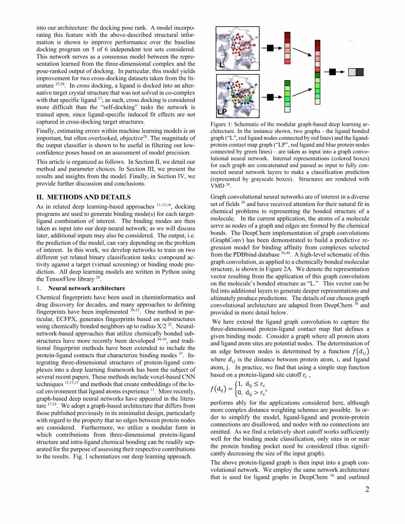
Chemical fingerprints have been used in cheminformatics and drug discovery for decades, and many approaches to defining fingerprints have been implemented 30-33. One method in par-ticular, ECFPX, generates fingerprints based on substructures using chemically bonded neighbors up to radius X/2 32. Neural-network-based approaches that utilize chemically bonded sub-structures have more recently been developed 34-36, and tradi-tional fingerprint methods have been extended to include the protein-ligand contacts that characterize binding modes 37. In-tegrating three-dimensional structures of protein-ligand com-plexes into a deep learning framework has been the subject of several recent papers. These methods include voxel-based CNN techniques 12,13,15 and methods that create embeddings of the lo-cal environment that ligand atoms experience 11. More recently, graph-based deep neural networks have appeared in the litera-ture 17,18. We adopt a graph-based architecture that differs from those published previously in its minimalist design, particularly with regard to the property that no edges between protein nodes are considered. Furthermore, we utilize a modular form in which contributions from three-dimensional protein-ligand structure and intra-ligand chemical bonding can be readily sep-arated for the purpose of assessing their respective contributions to the results. Fig. 1 schematizes our deep learning approach.

Figure 1: Schematic of the modular graph-based deep learning ar-chitecture. In the instance shown, two graphs - the ligand bonded graph (“L”, red ligand nodes connected by red lines) and the ligand-protein contact map graph (“LP”, red ligand and blue protein nodes connected by green lines) – are taken as input into a graph convo-lutional neural network. Internal representations (colored boxes) for each graph are concatenated and passed as input to fully con-nected neural network layers to make a classification prediction (represented by grayscale boxes). Structures are rendered with VMD 38.

Graph convolutional neural networks are of interest in a diverse set of fields 39 and have received attention for their natural fit in chemical problems to representing the bonded structure of a molecule. In the current application, the atoms of a molecule serve as nodes of a graph and edges are formed by the chemical bonds. The DeepChem implementation of graph convolutions (GraphConv) has been demonstrated to build a predictive re-gression model for binding affinity from complexes selected from the PDBbind database 36,40. A high-level schematic of this graph convolution, as applied to a chemically bonded molecular structure, is shown in Figure 2A. We denote the representation vector resulting from the application of this graph convolution on the molecule’s bonded structure as “L.” This vector can be fed into additional layers to generate deeper representations and ultimately produce predictions. The details of our chosen graph convolutional architecture are adapted from DeepChem 36 and provided in more detail below.

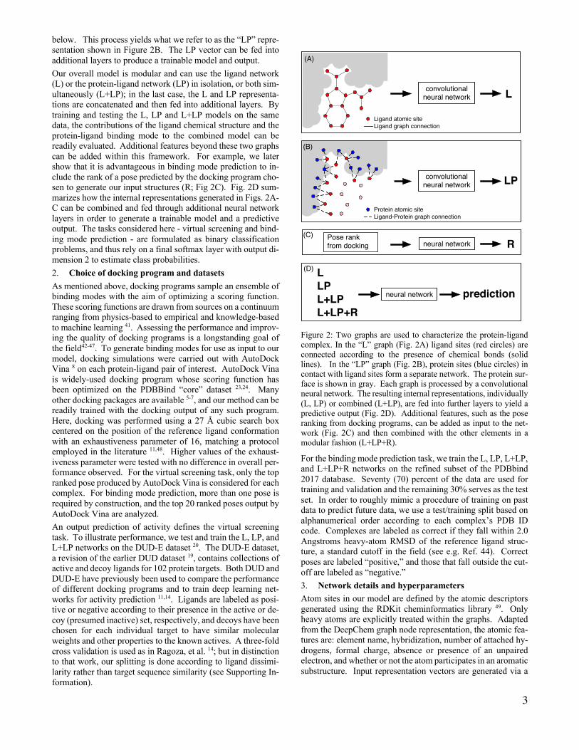
We here extend the ligand graph convolution to capture the three-dimensional protein-ligand contact map that defines a given binding mode. Consider a graph where all protein atom and ligand atom sites are potential nodes. The determination of an edge between nodes is determined by a function !"#$%& where #$% is the distance between protein atom, i, and ligand atom, j. In practice, we find that using a simple step function based on a protein-ligand site cutoff () ,

!"d+,& = .1, d+, ≤ r30, d+, > r3,

performs ably for the applications considered here, although more complex distance weighting schemes are possible. In or-der to simplify the model, ligand-ligand and protein-protein connections are disallowed, and nodes with no connections are omitted. As we find a relatively short cutoff works sufficiently well for the binding mode classification, only sites in or near the protein binding pocket need be considered (thus signifi-cantly decreasing the size of the input graph). The above protein-ligand graph is then input into a graph con-volutional network. We employ the same network architecture that is used for ligand graphs in DeepChem 36 and outlined

L

LP

3

below. This process yields what we refer to as the “LP” repre-sentation shown in Figure 2B. The LP vector can be fed into additional layers to produce a trainable model and output.

Our overall model is modular and can use the ligand network (L) or the protein-ligand network (LP) in isolation, or both sim-ultaneously (L+LP); in the last case, the L and LP representa-tions are concatenated and then fed into additional layers. By training and testing the L, LP and L+LP models on the same data, the contributions of the ligand chemical structure and the protein-ligand binding mode to the combined model can be readily evaluated. Additional features beyond these two graphs can be added within this framework. For example, we later show that it is advantageous in binding mode prediction to in-clude the rank of a pose predicted by the docking program cho-sen to generate our input structures (R; Fig 2C). Fig. 2D sum-marizes how the internal representations generated in Figs. 2A-C can be combined and fed through additional neural network layers in order to generate a trainable model and a predictive output. The tasks considered here - virtual screening and bind-ing mode prediction - are formulated as binary classification problems, and thus rely on a final softmax layer with output di-mension 2 to estimate class probabilities.

2. Choice of docking program and datasets

As mentioned above, docking programs sample an ensemble of binding modes with the aim of optimizing a scoring function. These scoring functions are drawn from sources on a continuum ranging from physics-based to empirical and knowledge-based to machine learning 41. Assessing the performance and improv-ing the quality of docking programs is a longstanding goal of the field42-47. To generate binding modes for use as input to our model, docking simulations were carried out with AutoDock Vina 8 on each protein-ligand pair of interest. AutoDock Vina is widely-used docking program whose scoring function has been optimized on the PDBBind “core” dataset 23,24. Many other docking packages are available 5-7, and our method can be readily trained with the docking output of any such program. Here, docking was performed using a 27 Å cubic search box centered on the position of the reference ligand conformation with an exhaustiveness parameter of 16, matching a protocol employed in the literature 11,48. Higher values of the exhaust-iveness parameter were tested with no difference in overall per-formance observed. For the virtual screening task, only the top ranked pose produced by AutoDock Vina is considered for each complex. For binding mode prediction, more than one pose is required by construction, and the top 20 ranked poses output by AutoDock Vina are analyzed.

An output prediction of activity defines the virtual screening task. To illustrate performance, we test and train the L, LP, and L+LP networks on the DUD-E dataset 20. The DUD-E dataset, a revision of the earlier DUD dataset 19, contains collections of active and decoy ligands for 102 protein targets. Both DUD and DUD-E have previously been used to compare the performance of different docking programs and to train deep learning net-works for activity prediction 11,14. Ligands are labeled as posi-tive or negative according to their presence in the active or de-coy (presumed inactive) set, respectively, and decoys have been chosen for each individual target to have similar molecular weights and other properties to the known actives. A three-fold cross validation is used as in Ragoza, et al. 14; but in distinction to that work, our splitting is done according to ligand dissimi-larity rather than target sequence similarity (see Supporting In-formation).

Figure 2: Two graphs are used to characterize the protein-ligand complex. In the “L” graph (Fig. 2A) ligand sites (red circles) are connected according to the presence of chemical bonds (solid lines). In the “LP” graph (Fig. 2B), protein sites (blue circles) in contact with ligand sites form a separate network. The protein sur-face is shown in gray. Each graph is processed by a convolutional neural network. The resulting internal representations, individually (L, LP) or combined (L+LP), are fed into further layers to yield a predictive output (Fig. 2D). Additional features, such as the pose ranking from docking programs, can be added as input to the net-work (Fig. 2C) and then combined with the other elements in a modular fashion (L+LP+R).

For the binding mode prediction task, we train the L, LP, L+LP, and L+LP+R networks on the refined subset of the PDBbind 2017 database. Seventy (70) percent of the data are used for training and validation and the remaining 30% serves as the test set. In order to roughly mimic a procedure of training on past data to predict future data, we use a test/training split based on alphanumerical order according to each complex’s PDB ID code. Complexes are labeled as correct if they fall within 2.0 Angstroms heavy-atom RMSD of the reference ligand struc-ture, a standard cutoff in the field (see e.g. Ref. 44). Correct poses are labeled “positive,” and those that fall outside the cut-off are labeled as “negative.”

3. Network details and hyperparameters

Atom sites in our model are defined by the atomic descriptors generated using the RDKit cheminformatics library 49. Only heavy atoms are explicitly treated within the graphs. Adapted from the DeepChem graph node representation, the atomic fea-tures are: element name, hybridization, number of attached hy-drogens, formal charge, absence or presence of an unpaired electron, and whether or not the atom participates in an aromatic substructure. Input representation vectors are generated via a

convolutionalneural network L

(A)

Pose rankfrom docking neural network R

(C)

LLPL+LPL+LP+R

neural network prediction

(D)

Ligand atomic siteLigand graph connection

convolutionalneural network LP

Protein atomic siteLigand-Protein graph connection

(B)

4

concatenation of one-hot encoded vectors over all atomic fea-tures.

The graph topology is represented as a connectivity list that specifies the nearest neighbors of each node. The graph convo-lutional network architecture adapted from DeepChem is com-posed of alternating nearest-neighbor convolution and pooling layers. Convolution and pooling units can be repeated an arbi-trary number of times, but a depth of 3 was deemed sufficient for many tasks in the original implementation 36. A single dense neural layer follows the final pooling layer in the network; the dense node dimension is reduced using a gather operation that takes both the mean and maximum across nodes. A more de-tailed discussion of this architecture can found in Altae-Tran, et al. 36. In our modular approach, this representation can be com-bined with the results from other inputs (graphical or other) and fed to further dense layers, ultimately yielding an output predic-tion. A schematic of the network is given in Figure S1.

Initial hyperparameters for the “L” network were adopted from DeepChem and were also used as an initial hyperparameter state for the LP model. L2 regularization was applied with a scaling coefficient of 0.0005, as determined by exploration of several parameter choices.

For the “L+LP+R” network, select hyperparameters of the net-work (see SI) are optimized more systematically using random exploration of hyperparameter space 50. In this procedure, eight validation sets were generated from random 10%/90% splits of the training set; independent models were trained on the 90% partition of each splitting. This training program was repeated for 200 sets of parameters. Hyperparameters were chosen to maximize the fraction of correct top ranked binding modes when averaged over the eight (10%) validation sets. Hy-perparameter values are given in Table S1. Results reported for L+LP+R on the PDBbind test set (Section III-2) are averaged over output from the eight trained models corresponding to the chosen hyperparameter set. Results reported for L+LP+R in Section III-3 are averaged over five training instances using the full PDBbind refined set.

III. RESULTS

1. Role of protein structure in virtual screening and bind-

ing mode prediction tasks

Table 1 reports the area under the receiver-operator curve (AUC) observed for the ligand-only (L) 36, ligand-protein (LP), and combined dual graph L+LP approaches measured against baseline AutoDock Vina results for virtual screening (training and testing on DUD-E) and binding mode prediction (training and testing on PDBbind refined). The AUC represents the in-tegral of the true positive rate as a function of the false positive rate for an ordered list of model predictions. AUCs are particu-larly useful for evaluating performance on the unbalanced da-tasets that one typically encounters in drug discovery classifi-cation tasks, where active ligands are often in the minority.

The pitfalls of using DUD-E to evaluate structure-based deep learning models can been seen upon inspection of the AUCs given in the first column of Table 1. The top-ranked poses pro-duced by AutoDock Vina yield an AUC of 0.70, which is in fair agreement with previously reported values14. Three of the four machine learning methods show a significant improvement over Vina, in agreement with the results of other deep learning approaches in the literature 11,14. However, as we show below and as seen in very recent work 21,22, the observed improvement is not due to learning from 3D structural information.

Because of the modular nature of our network, we can use the L and LP networks independently to test the relative contribu-tions of ligand identity alone (through internal bonded struc-ture) and the contacts between ligand and protein sites that de-fine the binding mode. For virtual screening tasks trained and tested on the DUD-E dataset, the L network significantly out-performs the LP network. Therefore, it is shown that ligand-identity is driving the performance of the combined (L+LP) model. Furthermore, standard cheminformatics representations such as the Morgan circular fingerprint (analogous to ECFP4) 32 available in the popular package RDKIT 49 fed into a random forest classifier produce similar results to the “L” network, and far surpass the result where the ligand-protein graph serves as the sole input. Thus, while virtual screening/DUD-E bench-marks are intended to demonstrate that deep learning methods learn from the 3D structures of protein-ligand complexes, those models are actually learning from ligand-only information and produce equivalent results to traditional cheminformatics ap-proaches.

As noted in recent work 21,22 this result is likely due to some bias in choosing active and decoy molecules in the DUD-E da-taset that can be readily “solved” by machine learning models. In other words, machine learning models can identify active and decoy molecules in the DUD-E datasets independent of their protein interactions. Similar issues related to applying machine learning techniques to such datasets have appeared in the liter-ature 51,52. This finding is also apparent upon close examination of the hyperparameter optimization of the DeepVS model of Pe-reira, et al. which shows that even if protein structural infor-mation is left out of the feature set, the performance on the DUD dataset worsens only slightly 11.

We next consider the task of binding mode prediction in the context of training and testing on structures in the PDBbind refined dataset 23,24 (second column of Table 1). These results show that the choice of dataset and/or task, and not a failure in network architecture, limits learning from protein-ligand inter-actions in DUD-E/virtual screening. In the case of binding mode prediction, the labels are related to the “3D” RMSDs of binding modes rather than the “1D” activities of protein-ligand combinations, and so the L+P network is encouraged to learn from protein ligand contacts rather than ligand identities. In-deed, the “L” network (which only takes chemical structures of the ligand as input) cannot distinguish the three-dimensional orientations that define binding modes. In this case, it can be seen (Table 1, second column) that the LP network significantly outperforms the L network. The “L” network yields a result close to random (AUC: 0.54). Though the L network might still be gleaning some information from the general “dockability” of ligands (which may relate to size or other properties), the LP network (AUC: 0.83) clearly captures the fundamentals of bind-ing mode prediction that the L network cannot. The combined L+LP network primarily reflects the LP results, although it reaches slightly higher values (AUC: 0.86).

Table 1 also shows that the binding mode prediction AUC re-ported for AutoDock Vina is significantly lower than the AUC achieved by our model. However, this result is not indicative of real-world performance, which is usually measured accord-ing to the ranking of binding modes for a single target-ligand pair. Instead, these data show that the probabilities output by our model are, as absolute numbers, more predictive of pose correctness than docking-generated scores or “binding ener-gies” across different sets of targets and ligands. Thus, the

5

output probability can be thought to provide a measure of con-fidence for a given binding mode. We will return to this point below.

Table 1: Comparative performance (as measured by AUC)

of methods trained and applied on virtual screening and

binding mode prediction tasks.

Virtual Screening – DUD-E

Binding Mode Pre-diction – PDBbind

AutoDock Vina 0.70 0.66

Morgan Radius 2 / RF

0.83 ---

L 0.84 0.54

LP 0.64 0.83

L+LP 0.82 0.86

2. Improving binding mode prediction from docking us-

ing a novel architecture

Having demonstrated that the 3D structures of protein-ligand binding poses can be used to train a binding mode prediction model, we next tested if such models could improve upon the results generated by the initial docking program.

In Table 2, we report, in addition to the AUC, the percentage of top ranked (ranked “1”) binding modes that are correct. The condition of correct is met when a binding mode falls within 2.0 Å RMSD of the heavy-atom reference ligand coordinates. It can be seen that in terms of this metric, which is often of most interest to the end user, Vina outperforms the L+LP model’s ‘re-scoring’ of its binding modes. This result is generally in agreement with published results for a voxel-based deep learn-ing model 13. This single ligand-protein pair test yields results more favorable to the docking program than the AUC measure, as the AUC indicates how well docking scores/energies rank all poses in the test set (see Table 2).

We next introduce the subnetwork schematized in Figure 2C to include pose ranking as an additional feature of our model. The output of a simple pose rank-fed sub-network is combined with the internal representations generated by the L and LP sub-net-works (Figures 2A and 2B); this combined representation is di-rected through a final set of three dense layers to yield a predic-tion that describes a “consensus” of the inputs. Consensus mod-els have been developed that use multiple docking programs to generate an improved result 53,54. Here, we use deep learning to combine protein-ligand structural features with the docking rank to produce a new prediction. We label this model “L+LP+R.” Hyperparameters for this system were optimized as discussed in Section II-3.

Table 2: Comparison of model performance on the inde-

pendent test set drawn from the PDBbind database, as

measured by AUC and the fraction of correct top ranked

binding modes.

AUC top ranked fraction correct

Autodock Vina 0.66 0.364

L+LP 0.86 0.306 (0.003)

L+LP+R 0.90 0.380 (0.004)

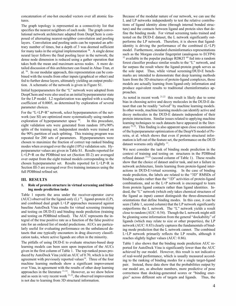
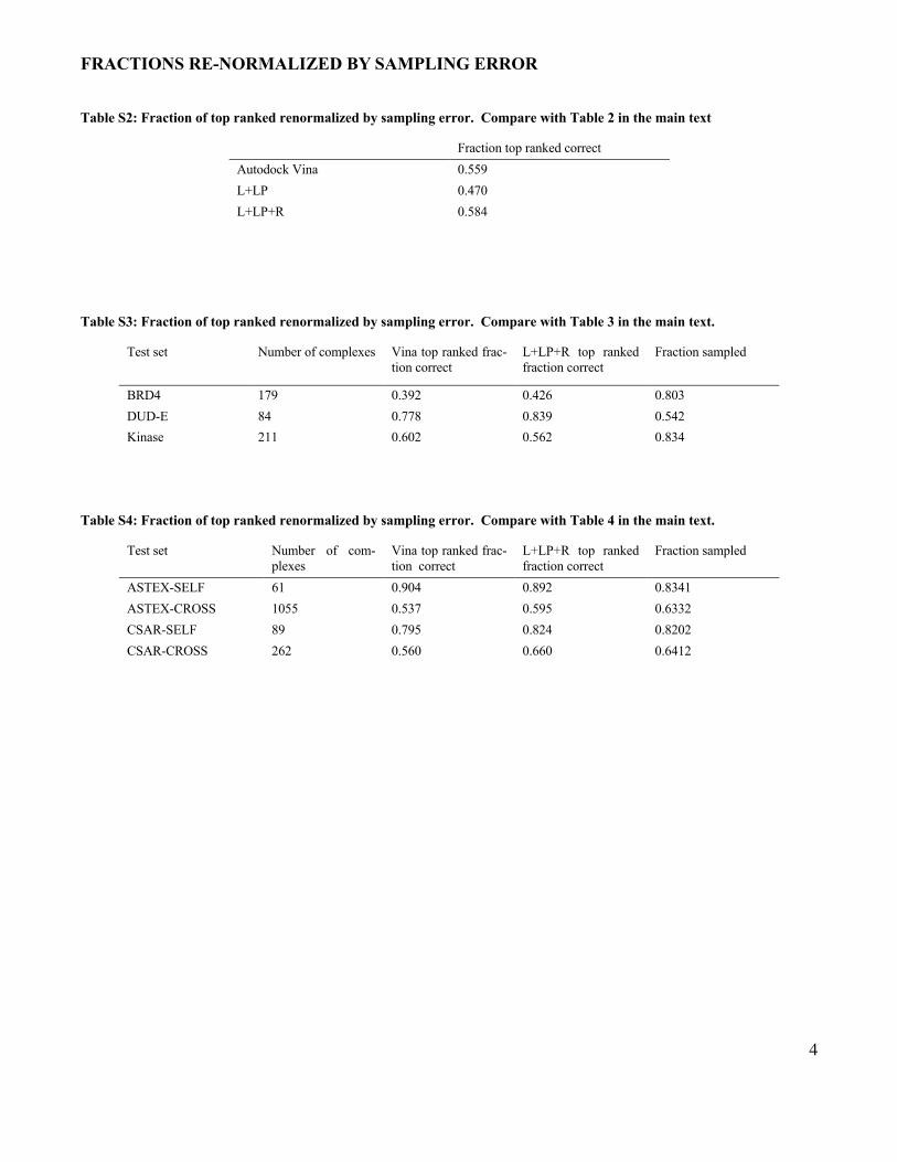
The results of the “L+LP+R” model on our PDBbind test set are given in Table 2 and Figure 3. It can be seen that the “L+LP+R” model is the top performer, significantly improving on the “L+LP” model and improving the Vina result by roughly 5 per-cent with respect to the fraction of top ranked poses that are correct (Table 2). Figure 3 shows the cumulative fraction of systems that contain at least one correct pose up to a given pose number. For example, at x=5, the y-values indicate the fraction of systems that have at least one “positive” pose in the top 5 according to the rankings specified by each model. It can be seen that the “L+LP+R” model maintains roughly the advantage seen on the first pose until approximately x=10, where all plots in Figure 3 start to level off. In 65% of systems in our test set, the docking program samples a correct mode in at least one of the 20 rank positions. As our model only re-ranks docking out-put, improvement in sampling error 44 is beyond the scope of our method. Results renormalized by this sampling error are in-cluded in Table S2.

A very recent publication 18 claimed to achieve a 5-7% improve-ment over baseline docking results on the PDBbind 2018 da-taset, seemingly outperforming our L+LP model and roughly matching the results of our L+LP+R model. However, unlike in the present results, the training and testing datasets in Ref. 18 omit borderline poses with RMSDs between 2 Å and 4 Å. In other words, positive poses in that study have RMSDs less than 2 Å and negative poses have RMSDs greater than 4 Å. Mar-ginal poses are presumably some of the most important yet dif-ficult to classify in real world applications. If these poses are filtered from our dataset, we find that the L+LP model exhibits increases in AUC and the fraction top ranked metric and shows an ~12% relative improvement over our docking baseline (Ta-bles S5 and S6 in the Supporting Information), results compa-rable to those presented in Ref. 18. The results produced by the L+LP+R model using the filtered dataset are also boosted (roughly 30% above our docking baseline). However, we feel these seemingly positive results do not adequately reflect model performance in production environments, as exclusion of valid but difficult-to-classify data points is not recommended for building robust machine learning models.

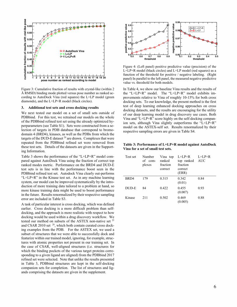
The values of the probabilities output by our model are also good measures of the model’s confidence in those predictions. This fact can be seen by evaluating the positive predictive value (precision) of the model over various thresholds (see Figure 4, left panel). Further details of how this plot is generated is given in the Supporting Information. Using a threshold of 0.9 the “L+LP+R” model has a precision of approximately 90%. Neg-ative pose prediction is shown in Figure 4, right panel. As the dataset is unbalanced, the overall higher negative predictive value is expected given our AUC measurements.

6

Figure 3: Cumulative fraction of results with crystal-like (within 2 Å RMSD) binding mode plotted versus pose number as ranked ac-cording to AutoDock Vina (red squares) the L+LP model (green diamonds), and the L+LP+R model (black circles).

3. Additional test sets and cross docking results

We next tested our model on a set of small sets outside of PDBbind. For this test, we retrained our models on the whole of the PDBbind refined test set using the already optimized hy-perparameters (see Table S1). Sets were constructed from a se-lection of targets in PDB database that correspond to bromo-domain 4 (BRD4), kinases, as well as the PDBs from which the targets of the DUD-E dataset 20 are drawn. Complexes that were repeated from the PDBbind refined set were removed from these test sets. Details of the datasets are given in the Support-ing Information.

Table 3 shows the performance of the “L+LP+R” model com-pared against AutoDock Vina using the fraction of correct top ranked modes metric. Performance on the BRD4 and DUD-E test sets is in line with the performance boost seen in the PDBbind refined test set. Autodock Vina clearly out-performs “L+LP+R” in the Kinase test set. As in any machine learning system, our model can be improved systematically by the intro-duction of more training data tailored to a problem at hand, so more kinase training data might be used to boost performance in the future. Results renormalized by their respective sampling error are included in Table S3.

A task of particular interest is cross docking, which was defined earlier. Cross docking is a more difficult problem than self-docking, and the approach is more realistic with respect to how docking would be used within a drug discovery workflow. We tested our method on subsets of the ASTEX non-native set 25 and CSAR 2010 set 26, which both contain curated cross dock-ing examples from the PDB. For the ASTEX set, we used a subset of structures that we were able to successfully dock and featurize within our trained model, ignoring, for example, struc-tures with atomic properties not present in our training set. In the case of CSAR, well-aligned structures (i.e. structures for which the binding pockets of the various target proteins corre-sponding to a given ligand are aligned) from the PDBbind 2017 refined set were selected. Note that unlike the results presented in Table 3, PDBbind structures are kept in the self-docking companion sets for completion. The list of structures and lig-ands comprising the datasets are given in the supplement.

Figure 4: (Left panel) positive predictive value (precision) of the L+LP+R model (black circles) and L+LP model (red squares) as a function of the threshold for positive / negative labeling. (Right panel) In parallel to the left panel, the measured negative predictive value vs. threshold for both models.

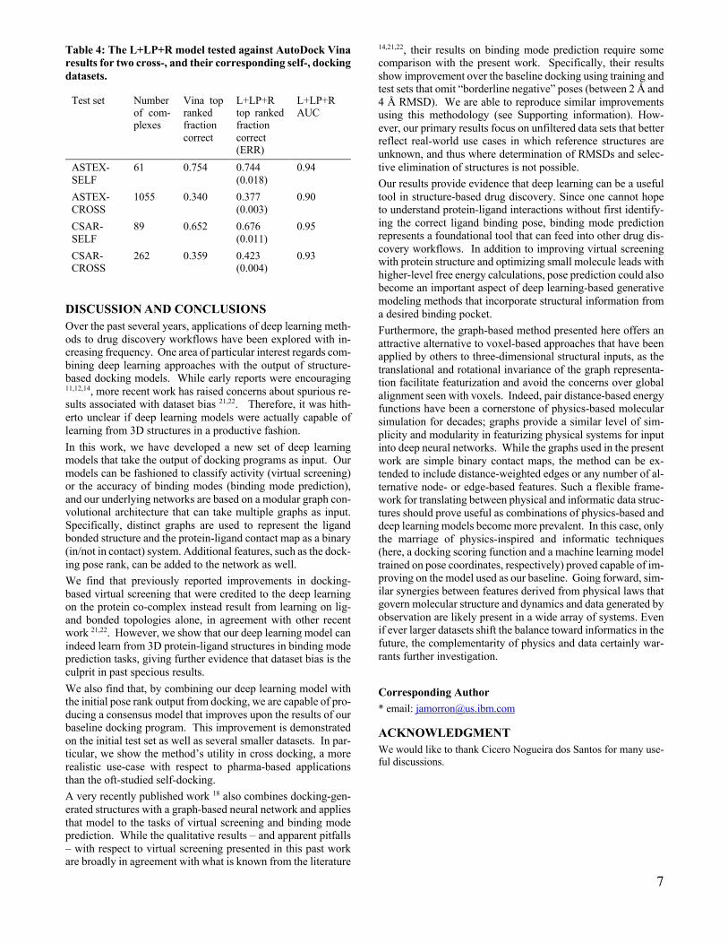
In Table 4, we show our baseline Vina results and the results of the “L+LP+R” model. The “L+LP+R” model exhibits im-provements relative to Vina of roughly 10-15% for both cross docking sets. To our knowledge, the present method is the first test of deep learning enhanced docking approaches on cross docking datasets, and the results are encouraging for the utility of our deep learning model in drug discovery use cases. Both Vina and “L+LP+R” score highly on the self-docking compan-ion sets, although Vina slightly outperforms the “L+LP+R” model on the ASTEX-self set. Results renormalized by their respective sampling errors are given in Table S4.

Table 3: Performance of L+LP+R model against AutoDock

Vina for a set of small test sets.

Test set Number of com-plexes

Vina top ranked fraction correct

L+LP+R top ranked fraction correct (ERR)

L+LP+R AUC

BRD4 179 0.315 0.342 (0.01)

0.84

DUD-E 84 0.422 0.455 (0.007)

0.93

Kinase 211 0.502 0.469 (0.005)

0.88

1 2 3 4 5 6 7 8 9 10 11 12 13 14 15 16 17 18 19 20pose number as ranked according to model

0.30

0.35

0.40

0.45

0.50

0.55

0.60

0.65cu

mul

ativ

e fr

actio

n of

resu

lts w

ith x

tal-l

ike

pose

AutoDock VinaL+LPL+LP+R 0.5 0.6 0.7 0.8 0.9

threshold0.4

0.5

0.6

0.7

0.8

0.9

posi

tive

pred

ictiv

e va

lue

L+LP+RL+LP

0.1 0.2 0.3 0.4 0.5threshold

0.95

0.96

0.97

0.98

0.99

nega

tive

pred

ictiv

e va

lue

7

Table 4: The L+LP+R model tested against AutoDock Vina

results for two cross-, and their corresponding self-, docking

datasets.

Test set Number of com-plexes

Vina top ranked fraction correct

L+LP+R top ranked fraction correct (ERR)

L+LP+R AUC

ASTEX-SELF

61 0.754 0.744 (0.018)

0.94

ASTEX-CROSS

1055 0.340 0.377 (0.003)

0.90

CSAR-SELF

89 0.652 0.676 (0.011)

0.95

CSAR-CROSS

262 0.359 0.423 (0.004)

0.93

DISCUSSION AND CONCLUSIONS

Over the past several years, applications of deep learning meth-ods to drug discovery workflows have been explored with in-creasing frequency. One area of particular interest regards com-bining deep learning approaches with the output of structure-based docking models. While early reports were encouraging 11,12,14, more recent work has raised concerns about spurious re-sults associated with dataset bias 21,22. Therefore, it was hith-erto unclear if deep learning models were actually capable of learning from 3D structures in a productive fashion.

In this work, we have developed a new set of deep learning models that take the output of docking programs as input. Our models can be fashioned to classify activity (virtual screening) or the accuracy of binding modes (binding mode prediction), and our underlying networks are based on a modular graph con-volutional architecture that can take multiple graphs as input. Specifically, distinct graphs are used to represent the ligand bonded structure and the protein-ligand contact map as a binary (in/not in contact) system. Additional features, such as the dock-ing pose rank, can be added to the network as well.

We find that previously reported improvements in docking-based virtual screening that were credited to the deep learning on the protein co-complex instead result from learning on lig-and bonded topologies alone, in agreement with other recent work 21,22. However, we show that our deep learning model can indeed learn from 3D protein-ligand structures in binding mode prediction tasks, giving further evidence that dataset bias is the culprit in past specious results.

We also find that, by combining our deep learning model with the initial pose rank output from docking, we are capable of pro-ducing a consensus model that improves upon the results of our baseline docking program. This improvement is demonstrated on the initial test set as well as several smaller datasets. In par-ticular, we show the method’s utility in cross docking, a more realistic use-case with respect to pharma-based applications than the oft-studied self-docking.

A very recently published work 18 also combines docking-gen-erated structures with a graph-based neural network and applies that model to the tasks of virtual screening and binding mode prediction. While the qualitative results – and apparent pitfalls – with respect to virtual screening presented in this past work are broadly in agreement with what is known from the literature

14,21,22, their results on binding mode prediction require some comparison with the present work. Specifically, their results show improvement over the baseline docking using training and test sets that omit “borderline negative” poses (between 2 Å and 4 Å RMSD). We are able to reproduce similar improvements using this methodology (see Supporting information). How-ever, our primary results focus on unfiltered data sets that better reflect real-world use cases in which reference structures are unknown, and thus where determination of RMSDs and selec-tive elimination of structures is not possible.

Our results provide evidence that deep learning can be a useful tool in structure-based drug discovery. Since one cannot hope to understand protein-ligand interactions without first identify-ing the correct ligand binding pose, binding mode prediction represents a foundational tool that can feed into other drug dis-covery workflows. In addition to improving virtual screening with protein structure and optimizing small molecule leads with higher-level free energy calculations, pose prediction could also become an important aspect of deep learning-based generative modeling methods that incorporate structural information from a desired binding pocket.

Furthermore, the graph-based method presented here offers an attractive alternative to voxel-based approaches that have been applied by others to three-dimensional structural inputs, as the translational and rotational invariance of the graph representa-tion facilitate featurization and avoid the concerns over global alignment seen with voxels. Indeed, pair distance-based energy functions have been a cornerstone of physics-based molecular simulation for decades; graphs provide a similar level of sim-plicity and modularity in featurizing physical systems for input into deep neural networks. While the graphs used in the present work are simple binary contact maps, the method can be ex-tended to include distance-weighted edges or any number of al-ternative node- or edge-based features. Such a flexible frame-work for translating between physical and informatic data struc-tures should prove useful as combinations of physics-based and deep learning models become more prevalent. In this case, only the marriage of physics-inspired and informatic techniques (here, a docking scoring function and a machine learning model trained on pose coordinates, respectively) proved capable of im-proving on the model used as our baseline. Going forward, sim-ilar synergies between features derived from physical laws that govern molecular structure and dynamics and data generated by observation are likely present in a wide array of systems. Even if ever larger datasets shift the balance toward informatics in the future, the complementarity of physics and data certainly war-rants further investigation.

Corresponding Author

* email: jamorron@us.ibm.com

ACKNOWLEDGMENT

We would like to thank Cicero Nogueira dos Santos for many use-ful discussions.

8

REFERENCES

(1) Peter Gedeck; Bernhard Rohde, A.; Bartels, C. QSAR − How Good Is It in Practice? Comparison of Descriptor Sets on an Un-biased Cross Section of Corporate Data Sets. J. Chem. Inf. Model. 2006, 46 (5), 1924–1936.

(2) Butkiewicz, M.; Lowe, E., Jr.; Mueller, R.; Mendenhall, J.; Teixeira, P.; Weaver, C.; Meiler, J. Benchmarking Ligand-Based Vir-tual High-Throughput Screening with the PubChem Database. Mole-cules 2013, 18 (12), 735–756.

(3) Xu, Y.; Ma, J.; Liaw, A.; Sheridan, R. P.; Svetnik, V. De-mystifying Multitask Deep Neural Networks for Quantitative Struc-ture–Activity Relationships. J. Chem. Inf. Model. 2017, 57 (10), 2490–2504.

(4) Kuntz, I. D.; Blaney, J. M.; Oatley, S. J.; Langridge, R.; Fer-rin, T. E. A Geometric Approach to Macromolecule-Ligand Interac-tions. J Mol Biol 1982, 161 (2), 269–288.

(5) Verdonk, M. L.; Cole, J. C.; Hartshorn, M. J.; Murray, C. W.; Taylor, R. D. Improved Protein–Ligand Docking Using GOLD. Proteins 2003, 52 (4), 609–623.

(6) Richard A Friesner; Jay L Banks; Robert B Murphy; Thomas A Halgren; Jasna J Klicic; Daniel T Mainz; Matthew P Repasky; Eric H Knoll; Mee Shelley; Jason K Perry; David E Shaw; Francis, P.; and Shenkin, P. S. Glide:  a New Approach for Rapid, Accurate Docking and Scoring. 1. Method and Assessment of Docking Accuracy. J. Med. Chem. 2004, 47 (7), 1739–1749.

(7) Moustakas, D. T.; Lang, P. T.; Pegg, S.; Pettersen, E.; Kuntz, I. D.; Brooijmans, N.; Rizzo, R. C. Development and Validation of a Modular, Extensible Docking Program: DOCK 5. J Comput Aided Mol Des 2006, 20 (10-11), 601–619.

(8) Trott, O.; Olson, A. J. AutoDock Vina: Improving the Speed and Accuracy of Docking with a New Scoring Function, Efficient Op-timization, and Multithreading. J. Comput. Chem. 2009, 65 (2), 455–461.

(9) Durrant, J. D.; McCammon, J. A. NNScore: a Neural-Net-work-Based Scoring Function for the Characterization of Protein−Lig-and Complexes. J. Chem. Inf. Model. 2010, 50 (10), 1865–1871.

(10) Durrant, J. D.; Friedman, A. J.; Rogers, K. E.; McCammon, J. A. Comparing Neural-Network Scoring Functions and the State of the Art: Applications to Common Library Screening. Journal of Chem-ical … 2013, 53 (7), 1726–1735.

(11) Pereira, J. C.; Caffarena, E. R.; Santos, dos, C. N. Boosting Docking-Based Virtual Screening with Deep Learning. J. Chem. Inf. Model. 2016, 56 (12), 2495–2506.

(12) Wallach, I.; Dzamba, M.; Heifets, A. AtomNet: a Deep Con-volutional Neural Network for Bioactivity Prediction in Structure-Based Drug Discovery. arXiv:1510.02855, 2015.

(13) Ragoza, M.; Hochuli, J.; Idrobo, E.; Sunseri, J.; Koes, D. R. Protein–Ligand Scoring with Convolutional Neural Networks. J. Chem. Inf. Model. 2017, 57 (4), 942–957.

(14) Ragoza, M.; Turner, L.; Koes, D. R. Ligand Pose Optimiza-tion with Atomic Grid-Based Convolutional Neural Networks. arxiv:1710.07400, 2017.

(15) Jiménez, J.; Škalič, M.; Martínez-Rosell, G.; De Fabritiis, G. KDEEP: Protein–Ligand Absolute Binding Affinity Prediction via 3D-Convolutional Neural Networks. J. Chem. Inf. Model. 2018, 58 (2), 287–296.

(16) Nguyen, D. D.; Cang, Z.; Wu, K.; Wang, M.; Cao, Y.; Wei, G.-W. Mathematical Deep Learning for Pose and Binding Affinity Pre-diction and Ranking in D3R Grand Challenges. J Comput Aided Mol Des 2019, 33 (1), 71–82.

(17) Feinberg, E. N.; Sur, D.; Wu, Z.; Husic, B. E.; Mai, H.; Li, Y.; Sun, S.; Yang, J.; Ramsundar, B.; Pande, V. S. PotentialNet for Molecular Property Prediction. ACS Cent. Sci. 2018, 4 (11), 1520–1530.

(18) Lim, J.; Ryu, S.; Park, K.; Choe, Y. J.; Ham, J.; Kim, W. Y. Predicting Drug–Target Interaction Using a Novel Graph Neural Net-work with 3D Structure-Embedded Graph Representation. J. Chem. Inf. Model. 2019, 59 (9), 3981–3988.

(19) Huang, N.; Shoichet, B. K.; Irwin, J. J. Benchmarking Sets for Molecular Docking. J. Med. Chem. 2006, 49 (23), 6789–6801.

(20) Mysinger, M. M.; Carchia, M.; Irwin, J. J.; Shoichet, B. K. Directory of Useful Decoys, Enhanced (DUD-E): Better Ligands and Decoys for Better Benchmarking. J. Med. Chem. 2012, 55 (14), 6582–6594.

(21) Sieg, J.; Flachsenberg, F.; Rarey, M. In Need of Bias Con-trol: Evaluating Chemical Data for Machine Learning in Structure-Based Virtual Screening. J. Chem. Inf. Model. 2019, 59 (3), 947–961.

(22) Chen, L.; Cruz, A.; Ramsey, S.; Dickson, C. J.; Duca, J. S.; Hornak, V.; Koes, D. R.; Kurtzman, T. Hidden Bias in the DUD-E Da-taset Leads to Misleading Performance of Deep Learning in Structure-Based Virtual Screening. PLoS ONE 2019, 14 (8), e0220113–e0220122.

(23) Li, Y.; Liu, Z.; Li, J.; Han, L.; Liu, J.; Zhao, Z.; Wang, R. Comparative Assessment of Scoring Functions on an Updated Bench-mark: 1. Compilation of the Test Set. J. Chem. Inf. Model. 2014, 54 (6), 1700–1716.

(24) Li, Y.; Han, L.; Liu, Z.; Wang, R. Comparative Assessment of Scoring Functions on an Updated Benchmark: 2. Evaluation Meth-ods and General Results. J. Chem. Inf. Model. 2014, 54 (6), 1717–1736.

(25) Verdonk, M. L.; Mortenson, P. N.; Hall, R. J.; Hartshorn, M. J.; Murray, C. W. Protein−Ligand Docking Against Non-Native Pro-tein Conformers. J. Chem. Inf. Model. 2008, 48 (11), 2214–2225.

(26) Dunbar, J. B.; Smith, R. D.; Yang, C.-Y.; Ung, P. M.-U.; Lexa, K. W.; Khazanov, N. A.; Stuckey, J. A.; Wang, S.; Carlson, H. A. CSAR Benchmark Exercise of 2010: Selection of the Protein-Lig-and Complexes. J. Chem. Inf. Model. 2011, 51 (9), 2036–2046.

(27) Hartshorn, M. J.; Verdonk, M. L.; Chessari, G.; Brewerton, S. C.; Mooij, W. T. M.; Mortenson, P. N.; Murray, C. W. Diverse, High-Quality Test Set for the Validation of Protein−Ligand Docking Performance. J. Med. Chem. 2007, 50 (4), 726–741.

(28) Sheridan, R. P. The Relative Importance of Domain Ap-plicability Metrics for Estimating Prediction Errors in QSAR Varies with Training Set Diversity. J. Chem. Inf. Model. 2015, 55 (6), 1098–1107.

(29) Abadi, M.; Agarwal, A.; Barham, P.; Brevdo, E.; Chen, Z.; Citro, C.; Corrado, G. S.; Davis, A.; Dean, J.; Devin, M.; Ghemawat, S.; Goodfellow, I.; Harp, A.; Irving, G.; Isard, M.; Jia, Y.; Jozefowicz, R.; Kaiser, L.; Kudlur, M.; Levenberg, J.; Mane, D.; Monga, R.; Moore, S.; Murray, D.; Olah, C.; Schuster, M.; Shlens, J.; Steiner, B.; Sutskever, I.; Talwar, K.; Tucker, P.; Vanhoucke, V.; Vasudevan, V.; Viegas, F.; Vinyals, O.; Warden, P.; Wattenberg, M.; Wicke, M.; Yu, Y.; Zheng, X. TensorFlow: Large-Scale Machine Learning on Hetero-geneous Distributed Systems. March 14, 2016.

(30) Carhart, R. E.; Smith, D. H.; Venkataraghavan, R. Atom Pairs as Molecular Features in Structure-Activity Studies: Definition and Applications. J. Chem. Inf. Model. 1985, 25 (2), 64–73.

(31) Nilakantan, R.; Bauman, N.; Dixon, J. S.; Venkataraghavan, R. Topological Torsion: a New Molecular Descriptor for SAR Appli-cations. Comparison with Other Descriptors. J. Chem. Inf. Model. 1987, 27 (2), 82–85.

(32) Rogers, D.; Hahn, M. Extended-Connectivity Fingerprints. J. Chem. Inf. Model. 2010, 50 (5), 742–754.

(33) Cereto-Massagué, A.; Ojeda, M. J.; Valls, C.; Mulero, M.; Garcia-Vallvé, S.; Pujadas, G. Molecular Fingerprint Similarity Search in Virtual Screening. Methods 2015, 71, 58–63.

(34) Duvenaud, D.; Maclaurin, D.; Aguilera-Iparraguirre, J.; Gómez-Bombarelli, R.; Hirzel, T.; Aspuru-Guzik, A.; Adams, R. P. Convolutional Networks on Graphs for Learning Molecular Finger-prints. arXiv:1509.09292, 2015.

(35) Kearnes, S.; McCloskey, K.; Berndl, M.; Pande, V.; Riley, P. Molecular Graph Convolutions: Moving Beyond Fingerprints. J Comput Aided Mol Des 2016, 30 (8), 595–608.

(36) Altae-Tran, H.; Ramsundar, B.; Pappu, A. S.; Pande, V. Low Data Drug Discovery with One-Shot Learning. ACS Cent. Sci. 2017, 3 (4), 283–293.

(37) Da, C.; Kireev, D. Structural Protein–Ligand Interaction Fingerprints (SPLIF) for Structure-Based Virtual Screening: Method and Benchmark Study. J. Chem. Inf. Model. 2014, 54 (9), 2555–2561.

(38) Humphrey, W.; Dalke, A.; Schulten, K. VMD -- Visual Mo-lecular Dynamics. Journal of Molecular Graphics 1996, 14, 33–38.

9

(39) Wu, Z.; Pan, S.; Chen, F.; Long, G.; Zhang, C.; Yu, P. S. A Comprehensive Survey on Graph Neural Networks. arXiv:1901:00596. 2019.

(40) Wu, Z.; Ramsundar, B.; Feinberg, E. N.; Gomes, J.; Ge-niesse, C.; Pappu, A. S.; Leswing, K.; Pande, V. MoleculeNet: a Bench-mark for Molecular Machine Learning. Chemical Science 2017, 00 (11), 1–18.

(41) Sousa, S. F.; Fernandes, P. A.; Ramos, M. J. Protein–Ligand Docking: Current Status and Future Challenges. Proteins 2006, 65 (1), 15–26.

(42) Warren, G. L.; Andrews, C. W.; Capelli, A.-M.; Clarke, B.; LaLonde, J.; Lambert, M. H.; Lindvall, M.; Nevins, N.; Semus, S. F.; Senger, S.; Tedesco, G.; Wall, I. D.; Woolven, J. M.; Peishoff, C. E.; Head, M. S. A Critical Assessment of Docking Programs and Scoring Functions. J. Med. Chem. 2006, 49 (20), 5912–5931.

(43) McGaughey, G. B.; Sheridan, R. P.; Bayly, C. I.; Culberson, J. C.; Kreatsoulas, C.; Lindsley, S.; Maiorov, V.; Truchon, J.-F.; Cor-nell, W. D. Comparison of Topological, Shape, and Docking Methods in Virtual Screening. J. Chem. Inf. Model. 2007, 47 (4), 1504–1519.

(44) Brozell, S. R.; Mukherjee, S.; Balius, T. E.; Roe, D. R.; Case, D. A.; Rizzo, R. C. Evaluation of DOCK 6 as a Pose Generation and Database Enrichment Tool. J Comput Aided Mol Des 2012, 26 (6), 749–773.

(45) Bjerrum, E. J. Machine Learning Optimization of Cross Docking Accuracy. Computational Biology and Chemistry 2016, 62, 133–144.

(46) Wang, Z.; Sun, H.; Yao, X.; Li, D.; Xu, L.; Li, Y.; Tian, S.; Hou, T. Comprehensive Evaluation of Ten Docking Programs on a Di-verse Set of Protein–Ligand Complexes: the Prediction Accuracy of

Sampling Power and Scoring Power. Phys Chem Chem Phys 2016, 18 (18), 12964–12975.

(47) Gaieb, Z.; Parks, C. D.; Chiu, M.; Yang, H.; Shao, C.; Wal-ters, W. P.; Lambert, M. H.; Nevins, N.; Bembenek, S. D.; Ameriks, M. K.; Mirzadegan, T.; Burley, S. K.; Amaro, R. E.; Gilson, M. K. D3R Grand Challenge 3: Blind Prediction of Protein-Ligand Poses and Af-finity Rankings. J Comput Aided Mol Des 2019, 33 (1), 1–18.

(48) Arciniega, M.; Lange, O. F. Improvement of Virtual Screen-ing Results by Docking Data Feature Analysis. J. Chem. Inf. Model. 2014, 54 (5), 1401–1411.

(49) RDKit: Open-Source Cheminformatics. (50) Bergstra, J.; Bengio, Y. Random Search for Hyper-Parame-

ter Optimization. Journal of Machine Learning Research 2012, 13 (Feb), 281–305.

(51) Gabel, J.; Desaphy, J.; Rognan, D. Beware of Machine Learning-Based Scoring Functions—on the Danger of Developing Black Boxes. J. Chem. Inf. Model. 2014, 54 (10), 2807–2815.

(52) Wallach, I.; Heifets, A. Most Ligand-Based Classification Benchmarks Reward Memorization Rather Than Generalization. J. Chem. Inf. Model. 2018, 58 (5), 916–932.

(53) Hsin, K.-Y.; Ghosh, S.; Kitano, H. Combining Machine Learning Systems and Multiple Docking Simulation Packages to Im-prove Docking Prediction Reliability for Network Pharmacology. PLoS ONE 2013, 8 (12), e83922–e83929.

(54) Perez-Castillo, Y.; Sotomayor-Burneo, S.; Jimenes-Vargas, K.; Gonzalez-Rodriguez, M.; Cruz-Monteagudo, M.; Armijos-Jara-millo, V.; Cordeiro, M. N. D. S.; Borges, F.; Sánchez-Rodríguez, A.; Tejera, E. CompScore: Boosting Structure-Based Virtual Screening Performance by Incorporating Docking Scoring Function Components Into Consensus Scoring. J. Chem. Inf. Model. 2019, 59 (9), 3655–3666.

Supporting information for “Combining docking pose rank and struc-ture with deep learning improves protein-ligand binding mode predic-tion” Joseph A. Morrone*, Jeffrey K. Weber, Tien Huynh, Heng Luo, Wendy D. Cornell

Healthcare & Life Sciences Research, IBM TJ Watson Research Center

1101 Kitchawan Road, Yorktown Heights, NY 10598, USA

Figure S1: Schematic for the graph convolutional neural network used in this study. This element of our network is adapted from DeepChem. The graph is composed of molecular connectivity (topology) and the atomic features that define the nodes. Features are passed into a set of alternating nearest neighbor convolution and pooling layers. A depth of 3 is used here and in the original implementation. After a single dense layer, a gather operation combines the output from all previous nodes.

Table S1 Hyperparameters for L+LP+R model

Nconv 1 Nconv 2 Nconv 3 N dense N final 1 N final 2 L2

L+LP 64 128 64 128 --- --- 0.0005

L+LP+R opt. 256 32 192 336 208 288 0.0003

graph representation

atomic features

andgraph

topology

nearset neighbor convolutionnearest neighbor poolingdense layer

gather

2

DEFINITION OF AUC

The AUC computation involves counting the number of negative entries (inactive or decoy ligands) that are ranked in the top N+ entries where N+ is the number of positives (active ligands). The formula is given as:

AUC = 1 − $%+∑ %-

'

%-

%+()$ .

DEBIASED DUD-E SPLITTING

Our goal in generating debiased train/test splits for DUD-E involves splitting the target sets into test and training sets in a way that minimizes the difference between active and decoy (presumed inactive) ligands across target sets. The splitting uses dataset bias ideas similar to those expressed in Ref. 52 in the main text.

1. Ligands are represented by an ECFP4-like fingerprint using RDKit (Ref. 49 in main text).

2. Ligands are separated into groups according to their associated target.

3. The distribution of Tanimoto similarities is computed between ligands in target sets X and Y, and then also split according to their labels (A=active, I=decoy/presumed inactive): ρ++,-, ρ+.,-, ρ.+,-, ρ..,-.

4. The bias between two target sets is sensitive to the difference between the respective active and inactive distributions and is given by the following equation:

/012,- = KL(ρ++,-, ρ+.,-) + KL(ρ+.,-, ρ++,-) + KL(ρ..,-, ρ.+,-) + KL(ρ.+,-, ρ..,-)

where KL(a,b) is the Kullback-Leibler divergence between distributions a and b.

KL(1, /) =71( 89 :1(/(;

(

5. The splitting is chosen to minimize the global bias (the sum of the target-pairwise biases) using a Monte Carlo procedure.

DEFINITION OF POSITIVE PREDICTIVE VALUE AND NEGATIVE PREDICTIVE VALUE

The positive predictive value (PPV) or precision and negative predictive value are defined as:

PPV = <=><=> + <?>

NPV = <=%<=% + <?%

where NAB, NCB, NAD,  19FNCD are the number of true positive, false positive, true negative and false negatives, respectively. The boundary between positively and negatively classified samples is set by the threshold which is varied on the x-axis of Fig. 4 in the main text.

4

FRACTIONS RE-NORMALIZED BY SAMPLING ERROR

Table S2: Fraction of top ranked renormalized by sampling error. Compare with Table 2 in the main text

Fraction top ranked correct Autodock Vina 0.559 L+LP 0.470 L+LP+R 0.584

Table S3: Fraction of top ranked renormalized by sampling error. Compare with Table 3 in the main text.

Test set Number of complexes Vina top ranked frac-tion correct

L+LP+R top ranked fraction correct

Fraction sampled

BRD4 179 0.392 0.426 0.803 DUD-E 84 0.778 0.839 0.542 Kinase 211 0.602 0.562 0.834

Table S4: Fraction of top ranked renormalized by sampling error. Compare with Table 4 in the main text.

Test set Number of com-plexes

Vina top ranked frac-tion correct

L+LP+R top ranked fraction correct

Fraction sampled

ASTEX-SELF 61 0.904 0.892 0.8341 ASTEX-CROSS 1055 0.537 0.595 0.6332 CSAR-SELF 89 0.795 0.824 0.8202 CSAR-CROSS 262 0.560 0.660 0.6412

5

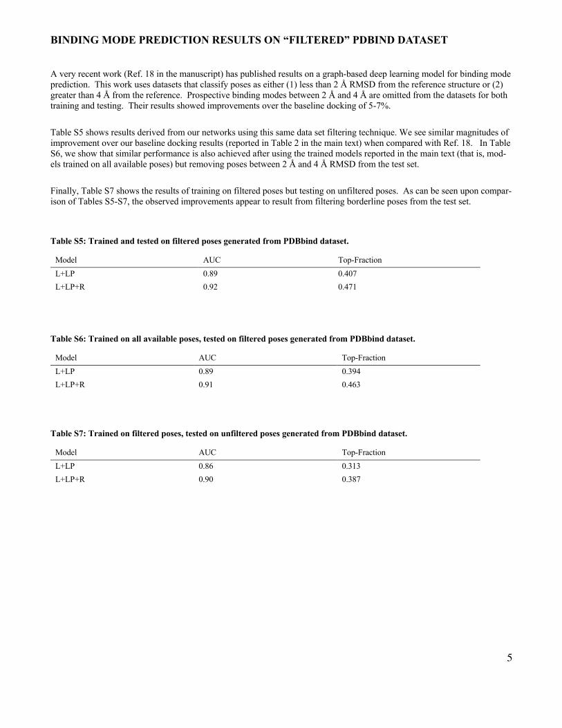
BINDING MODE PREDICTION RESULTS ON “FILTERED” PDBIND DATASET

A very recent work (Ref. 18 in the manuscript) has published results on a graph-based deep learning model for binding mode prediction. This work uses datasets that classify poses as either (1) less than 2 Å RMSD from the reference structure or (2) greater than 4 Å from the reference. Prospective binding modes between 2 Å and 4 Å are omitted from the datasets for both training and testing. Their results showed improvements over the baseline docking of 5-7%.

Table S5 shows results derived from our networks using this same data set filtering technique. We see similar magnitudes of improvement over our baseline docking results (reported in Table 2 in the main text) when compared with Ref. 18. In Table S6, we show that similar performance is also achieved after using the trained models reported in the main text (that is, mod-els trained on all available poses) but removing poses between 2 Å and 4 Å RMSD from the test set.

Finally, Table S7 shows the results of training on filtered poses but testing on unfiltered poses. As can be seen upon compar-ison of Tables S5-S7, the observed improvements appear to result from filtering borderline poses from the test set.

Table S5: Trained and tested on filtered poses generated from PDBbind dataset.

Model AUC Top-Fraction L+LP 0.89 0.407 L+LP+R 0.92 0.471

Table S6: Trained on all available poses, tested on filtered poses generated from PDBbind dataset.

Model AUC Top-Fraction L+LP 0.89 0.394 L+LP+R 0.91 0.463

Table S7: Trained on filtered poses, tested on unfiltered poses generated from PDBbind dataset.

Model AUC Top-Fraction

L+LP 0.86 0.313

L+LP+R 0.90 0.387