University of Texas at El Paso University of Texas at El Paso

ScholarWorks@UTEP ScholarWorks@UTEP

Open Access Theses & Dissertations

2019-01-01

Combination Of Resampling Based Lasso Feature Selection And Combination Of Resampling Based Lasso Feature Selection And

Ensembles Of Regularized Regression Models Ensembles Of Regularized Regression Models

Abhijeet R. Patil University of Texas at El Paso

Follow this and additional works at: https://scholarworks.utep.edu/open_etd

Part of the Bioinformatics Commons, and the Biostatistics Commons

Recommended Citation Recommended Citation Patil, Abhijeet R., "Combination Of Resampling Based Lasso Feature Selection And Ensembles Of Regularized Regression Models" (2019). Open Access Theses & Dissertations. 2886. https://scholarworks.utep.edu/open_etd/2886

This is brought to you for free and open access by ScholarWorks@UTEP. It has been accepted for inclusion in Open Access Theses & Dissertations by an authorized administrator of ScholarWorks@UTEP. For more information, please contact lweber@utep.edu.

COMBINATION OF RESAMPLING BASED LASSO FEATURE SELECTION

AND ENSEMBLES OF REGULARIZED REGRESSION MODELS

ABHIJEET R PATIL

Master’s Program in Computational Science

APPROVED:

Sangjin Kim, Ph.D., Chair

Ming-Ying Leung, Ph.D., Co-Chair

Sourav Roy, Ph.D.

Lin Li, Ph.D.

Stephen Crites, Ph.D.Dean of the Graduate School

c©Copyright

by

Abhijeet R Patil

2019

to my

MOTHER and FATHER

with love

COMBINATION OF RESAMPLING BASED LASSO FEATURE SELECTION

AND ENSEMBLES OF REGULARIZED REGRESSION MODELS

by

ABHIJEET R PATIL, B.E., M.Tech

THESIS

Presented to the Faculty of the Graduate School of

The University of Texas at El Paso

in Partial Fulfillment

of the Requirements

for the Degree of

MASTER OF SCIENCE

Computational Science Program

THE UNIVERSITY OF TEXAS AT EL PASO

December 2019

Acknowledgements

I would like to express my most sincere gratitude to my advisor, Dr. Sangjin Kim for his

wise guidance, constant encouragement, and advice throughout my research. I sincerely

appreciate his generous time and ideas. I would like to thank my co-advisor, Dr. Ming-

Ying Leung for her constant support, supervision in my study and thesis. I am indebted

and thankful to both of my advisors. I have greatly benefited from their expertise. I could

never reach to this point without enormous help from them.

I would also like to thank my committee members; Dr. Sourav Roy of Biological Sciences

Department and Dr. Lin Li of Physics Department, all at The University of Texas at El

Paso. Their encouragement, insightful comments, additional guidance were invaluable to

my research. I am also thankful to Dr. Jonathon E Mohl for his valuable suggestions and

support.

I will forever be thankful to my undergraduate mentor, Prof. A.M. Padma Reddy. He

has always been helpful in providing advice many times during my engineering. I still think

fondly of my time as an undergraduate student in his classes. His enthusiasm and love for

teaching is contagious. Padma Reddy sir is the reason i decided to go to pursue a career

in teaching and research.

I especially thank my father Revansiddappa.S.Patil, my mother Jyothi.R.Patil, brother

Shankar.R.Patil, sister Preeti.R.Patil, and my wife Dikshita.A.Patil for their constant in-

spiration, loving support and encouragement in all my decisions. I undoubtedly could not

have done this without you all.

v

Abstract

In high-dimensional data, the performance of various classifiers is largely dependent on

the selection of important features. Most of the individual classifiers using existing feature

selection (FS) methods do not perform well for highly correlated data. Obtaining important

features using the FS method and selecting the best performing classifier is a challenging

task in high throughput data. In this research, we propose a combination of resampling

based least absolute shrinkage and selection operator (LASSO) feature selection (RLFS)

and ensembles of regularized regression models (ERRM) capable of handling data with

the high correlation structures. The ERRM boosts the prediction accuracy with the top-

ranked features obtained from RLFS. The RLFS utilizes the LASSO penalty with sure

independence screening condition to select the top k ranked features. The ERRM includes

five individual penalty based methods: LASSO, adaptive LASSO (ALASSO), elastic net

(ENET), smoothly clipped absolute deviations (SCAD), and minimax concave penalty

(MCP). It is built on the idea of bagging and rank aggregation. Upon performing simulation

studies and applying to smokers cancer gene expression data, we demonstrated that the

proposed combination of ERRM with RLFS achieved superior performance in accuracy

and geometric mean.

vi

Table of Contents

Page

Acknowledgements . . . . . . . . . . . . . . . . . . . . . . . . . . . . . . . . . . . . v

Abstract . . . . . . . . . . . . . . . . . . . . . . . . . . . . . . . . . . . . . . . . . . vi

Table of Contents . . . . . . . . . . . . . . . . . . . . . . . . . . . . . . . . . . . . . vii

List of Tables . . . . . . . . . . . . . . . . . . . . . . . . . . . . . . . . . . . . . . . ix

List of Figures . . . . . . . . . . . . . . . . . . . . . . . . . . . . . . . . . . . . . . x

Chapter

1 Introduction . . . . . . . . . . . . . . . . . . . . . . . . . . . . . . . . . . . . . . 1

2 Literature Review . . . . . . . . . . . . . . . . . . . . . . . . . . . . . . . . . . . 4

2.1 Feature Selection . . . . . . . . . . . . . . . . . . . . . . . . . . . . . . . . 4

2.1.1 Filter-based Methods . . . . . . . . . . . . . . . . . . . . . . . . . . 4

2.1.2 Embedded-based Methods . . . . . . . . . . . . . . . . . . . . . . . 5

2.1.3 Wrapper-based Methods . . . . . . . . . . . . . . . . . . . . . . . . 5

2.2 Classification Methods . . . . . . . . . . . . . . . . . . . . . . . . . . . . . 6

2.2.1 Supervised Classification . . . . . . . . . . . . . . . . . . . . . . . . 6

2.2.2 Unsupervised Clustering . . . . . . . . . . . . . . . . . . . . . . . . 6

3 Materials and Methods . . . . . . . . . . . . . . . . . . . . . . . . . . . . . . . . 8

3.1 Rank Based Feature Selection Methods . . . . . . . . . . . . . . . . . . . . 8

3.1.1 The Proposed Resampling based Lasso Feature Selection . . . . . . 9

3.1.2 Information Gain . . . . . . . . . . . . . . . . . . . . . . . . . . . . 10

3.1.3 Chi-square test . . . . . . . . . . . . . . . . . . . . . . . . . . . . . 11

3.1.4 Minimum Redundancy Maximum Relevance . . . . . . . . . . . . . 11

3.2 Classification Algorithms . . . . . . . . . . . . . . . . . . . . . . . . . . . . 12

3.2.1 The Proposed Ensembles of Regularized Regression Models . . . . . 12

3.2.2 Logistic Regression . . . . . . . . . . . . . . . . . . . . . . . . . . . 13

vii

3.2.3 Regularized Regression Models . . . . . . . . . . . . . . . . . . . . 16

3.2.4 Random Forests . . . . . . . . . . . . . . . . . . . . . . . . . . . . . 18

3.2.5 Support Vector Machines . . . . . . . . . . . . . . . . . . . . . . . . 19

3.2.6 Adaboost . . . . . . . . . . . . . . . . . . . . . . . . . . . . . . . . 19

3.3 Evaluation Metrics . . . . . . . . . . . . . . . . . . . . . . . . . . . . . . . 20

4 Results . . . . . . . . . . . . . . . . . . . . . . . . . . . . . . . . . . . . . . . . . 21

4.1 Simulation Results . . . . . . . . . . . . . . . . . . . . . . . . . . . . . . . 21

4.1.1 Simulation Scenario (S1): low correlation 0.2 . . . . . . . . . . . . . 22

4.1.2 Simulation Scenario (S2): medium correlation 0.5 . . . . . . . . . . 24

4.2 Experimental Results . . . . . . . . . . . . . . . . . . . . . . . . . . . . . . 29

5 Discussion . . . . . . . . . . . . . . . . . . . . . . . . . . . . . . . . . . . . . . . 36

6 Conclusion and Future Work . . . . . . . . . . . . . . . . . . . . . . . . . . . . . 38

6.1 Conclusion . . . . . . . . . . . . . . . . . . . . . . . . . . . . . . . . . . . . 38

6.2 Future Work . . . . . . . . . . . . . . . . . . . . . . . . . . . . . . . . . . . 38

6.2.1 Data . . . . . . . . . . . . . . . . . . . . . . . . . . . . . . . . . . . 39

6.2.2 Modified adaptive lasso with proposed weights in high-throughput

microarray data . . . . . . . . . . . . . . . . . . . . . . . . . . . . . 40

6.2.3 Adaptive K-Nearest-Neighbor with proposed weights in high-dimensional

microarray data . . . . . . . . . . . . . . . . . . . . . . . . . . . . . 41

6.2.4 Analyze the performance of FS and classification methods for high-

dimensional multi-class classification problem. . . . . . . . . . . . . 42

6.2.5 Timeline . . . . . . . . . . . . . . . . . . . . . . . . . . . . . . . . . 43

References . . . . . . . . . . . . . . . . . . . . . . . . . . . . . . . . . . . . . . . . . 44

Appendix

A Simulation Scenario: S3 . . . . . . . . . . . . . . . . . . . . . . . . . . . . . . . 52

B The RLFS-ERRM Program . . . . . . . . . . . . . . . . . . . . . . . . . . . . . 55

Curriculum Vitae . . . . . . . . . . . . . . . . . . . . . . . . . . . . . . . . . . . . . 85

viii

List of Tables

4.1 Average values taken over 100 iterations in simulation scenario: S1 . . . . . 26

4.2 Average values taken over 100 iterations in simulation scenario: S2 . . . . . 28

4.3 Average values taken over 100 iterations in experimental data SMK-CAN-187 32

4.4 Comparison of proposed ERRM with and without bootstrapping . . . . . . 34

4.5 Comparison of regularized regression models used in the ERRM with and

without FS screening . . . . . . . . . . . . . . . . . . . . . . . . . . . . . . 35

6.1 Timeline for completion of this work . . . . . . . . . . . . . . . . . . . . . 43

A.1 Average values taken over 100 iterations in simulation scenario: S3 . . . . . 53

ix

List of Figures

3.1 The complete workflow depicting the proposed combination of RLFS-ERRM frame-

work . . . . . . . . . . . . . . . . . . . . . . . . . . . . . . . . . . . . . . . 15

4.1 True number of features selected among top k-SIS ranked features and the average

of this taken over 100 iterations for three different scenarios . . . . . . . . . . . 23

4.2 Boxplot showing the accuracies of Classifiers with FS methods in simulation sce-

nario: S1 . . . . . . . . . . . . . . . . . . . . . . . . . . . . . . . . . . . . . 27

4.3 Boxplot showing the accuracies of Classifiers with FS methods in simulation sce-

nario: S2 . . . . . . . . . . . . . . . . . . . . . . . . . . . . . . . . . . . . . 29

4.4 Boxplot showing the accuracies of Classifiers with FS methods in experimental

data SMK-CAN-187 . . . . . . . . . . . . . . . . . . . . . . . . . . . . . . . 33

A.1 Boxplot showing the accuracies of Classifiers with FS methods in simulation sce-

nario: S3 . . . . . . . . . . . . . . . . . . . . . . . . . . . . . . . . . . . . . 54

x

Chapter 1

Introduction

With the advances of high throughput technology in biomedical research, large volumes

of high-dimensional data are being generated [1, 2, 3]. Some of the examples of such

data can be found in microarray gene expression [4, 5, 6] data, RNA-seq [7], genome-wide

association study (GWAS) [8, 9] data, and DNA-methylation [10, 11]. These data are high

dimensional in nature, where the total count of features is significantly larger than the

number of samples (p >> n) and termed as the curse of dimensionality. Although this

is one of the major problems, there are many other problems such as noise, redundancy

and over parameterization. To deal with these problems, many two-stage approaches of FS

and classification algorithms have been proposed in machine learning over the last decade.

While the FS methods are used to reduce the dimensionality of data by removing noisy

and redundant features that help in selecting the truly important features, the classification

algorithms help increase the prediction performance.

The FS methods are classified into rank-based and subset methods [12, 13]. Rank-based

methods rank all the features with respect to their importance based on some criteria.

Although there is a lack of threshold to select the optimal number of top-ranked features,

this can be solved using Sure Independence screening (SIS) [14] condition. Some of the

popular rank-based FS methods used in bioinformatics are Information Gain [15], Chi-

square [16] and Minimum Redundancy Maximum Relevance [17]. Subset methods [18] are

the ones where the subset of features are selected with some pre-determined threshold based

on some criteria but these methods need more computational time in high-dimensional data

setting and lead to an NP-hard problem [19]. Some of the popular subset methods include

Boruta [20], Fisher score [21] and Relief [22].

1

For the classification of gene expression data, there are non-parametric based popular

algorithms used, such as Random Forests [23], Adaboost [24], and Support Vector Ma-

chines [25]. While the Random Forests and Adaboost are based on the concept of decision

trees, the Support Vector Machines is based on the idea of hyperplanes. In addition to

the above, there are parametric machine learning algorithms such as penalized logistic re-

gression (PLR) models that have five different penalties which are predominantly popular

in high-dimensional data. The first two classifiers are Lasso [26] and Ridge [27] that are

based on L1 and L2 penalties. The third classifier is a combination of these and is termed

as elastic net [28]. The other two PLR classifiers are SCAD [29] and MCP [30] which are

based on non-concave and concave respectively. All these individual classifiers are very

common in machine learning and bioinformatics [31]. However, in highly correlated gene

expression data, these individual classifiers do not perform well in terms of prediction ac-

curacy. To overcome the issue of individual classifiers, ensembles classifiers are proposed

[32, 33]. The ensemble classifiers are bagging and aggregating methods [34, 35] that are

employed to improve the accuracy of several ”weak” classifiers [36]. The tree-based method

Classification by ensembles from random partitions (CERP) [37] showed good performance

but is computer-intensive. The ensembles of logistic regression models (LORENS) [38]

for high-dimensional data were proven to be good for classification. However, they de-

crease in performance when there are small number of true important variables in the

high-dimensional space because of random partition.

In this research, we introduce the proposed combination of FS and classifier, the resam-

pling based Lasso Feature Selection (RLFS) method for ranking the features and Ensembles

of Regularized Regression Models (ERRM) for classification purposes. The resampling ap-

proach is proven to be one of the best FS screening step in a high-dimensional data setting

[13]. The RLFS uses the selection probability with lasso penalty and the threshold for se-

lecting the top-ranked features is set using k-SIS condition and these selected features are

applied to the ERRM to achieve the best prediction accuracy. The ERRM uses five individ-

ual regularization models, Lasso, Adaptive lasso (Alasso), Elastic Net (ENET), SCAD, and

2

MCP. These methods are used in each individual tree with the bootstrapped samples from

the training data in the learning phase. This step is repeated for t times. The combination

of bagging and weighted rank aggregation is employed along with majority voting to select

the best performing classification method Mi given the bootstrap sample Bi.

The rest of the thesis is organized as follows. In Chapter 3, the RLFS and ERRM along

with the other FS and classification methods are explained in detail. In Chapter 4 we show

that the proposed combined framework of RLFS and ERRM has superior performance in

comparison to other combinations of existing FS methods and individual classifiers. In

Chapter 4.1 we show the results with explanation of our extensive simulation studies and

in Chapter 4.2 we show the performance of our proposed methods outperforming all other

methods on the gene expression smokers cancer (SMK-CAN-187) data. We discuss our

findings briefly in the Chapter 5 and finally Chapter 6 concludes the thesis.

3

Chapter 2

Literature Review

This chapter describes the various feature selection and classification algorithms used in

high-dimensional data. The first section explains the different types of feature selection and

the computational algorithms involved. In the second section, we will discuss the different

classification algorithms used in machine learning.

2.1 Feature Selection

There are many challenges faced when we deal with high-dimensional data, such as high-

performance computing, overfitting, and redundant features. To overcome such problems,

in high-dimensional data, two-stage approaches of filtering and classification was proposed

[13]. Feature selection (FS) is a process of removing the noisy and redundant features from

the data. It helps in boosting the performance of a classification algorithm not just in

terms of accuracy but also in computational time.

There Feature selection can be divided into three different categories namely filter-based,

embedded, and wrapper methods.

2.1.1 Filter-based Methods

The filter-based approaches are independent of the classification methods; therefore, they

are computationally faster than the wrapper and embedded methods. The relevant fea-

tures are selected based on distances, entropy, and uncertainty. There are many algorithms

developed. Some of the best examples include Relief [22], which uses the distance-based

metric function. The ReliefF [39], which is a modified version of Relief, is developed to han-

4

dle the multi-class problems. The minimum redundancy maximum relevance (MRMR) [17]

and mutual information-based feature selection method (MIFS) [40] are the FS methods

that rely on mutual information criteria. The mutual information is calculated between the

individual feature and response label. The FS method conditional mutual information max-

imization (CMIM) [41] recursively chooses the features that provide the maximum mutual

information with the response class. The various entropy-based methods are developed,

Information gain [15], gain ratio, and symmetrical uncertainty.

2.1.2 Embedded-based Methods

The embedded-based methods incorporate the FS process inside the classification method,

which helps in performing the gene selection and classification simultaneously. It helps

reduce the computational time than the wrapper method; however, it is expensive when

compared to filter-based methods. The embedded method includes the pruning method,

built-in mechanism, and regularization methods. In the pruning method, all the features

are considered during the training phase for building the classification model. The features

with lower correlation coefficient values are removed recursively using the support vector

machines. In the built-in FS method, the important features are ranked based on their

importance. The variable importance (varImp) measure in the random forest method is

the best example of a built-in measure. In the regularized methods, the penalized regres-

sion models are based on penalties and are popular in high-dimensional data for variable

selection and classification purposes. Some of the examples of the sparse variable selection

models include lasso, adaptive lasso, elastic net, SCAD, and MCP. These methods are

discussed in Chapter 3.

2.1.3 Wrapper-based Methods

Wrapper-based selects the feature subsets using classification algorithm and searching tech-

niques. The examples of the former approach include forward selection, backward elimi-

5

nation, and recursive feature elimination. The latter approach includes hill climbing and

best-first search strategies using the decision trees and naive Bayes classifiers. The wrap-

per methods are computationally expensive because the features are selected based on the

performance of the classifiers or the searching techniques, which is a recursive process.

2.2 Classification Methods

Depending on the type of data, the classification algorithms are classified into two cate-

gories, supervised classification and unsupervised clustering.

2.2.1 Supervised Classification

There is a broad range of algorithms that can be applied for labeled data such as tree-based

methods, discriminant analysis, and penalized regression models. The popular tree-based

methods include random forest and adaptive boosting. The random forests are built on

the concept of decision trees. The idea is to operate as an ensemble method instead of

relying on a single method. It is based on the concept of bagging and majority voting. The

Adaptive boosting method is an ensemble learning technique where it improves the single

weak boosting algorithm through an iterative process. The support vector machines detect

the maximum margin hyperplane by maximizing the distance between the hyperplane and

the closest dot. The maximum margin indicates that the classes are well separable and

correctly classified. These methods are discussed in Chapter 3.

2.2.2 Unsupervised Clustering

In this section, the various unsupervised machine learning methods used for unlabeled data

are discussed. Some of the examples include; K-Nearest-Neighbor and K-means clustering.

Clustering algorithms group the samples based on some sort of similarity metric that is

computed for features. In the context for gene expression data, genes represented as fea-

6

tures are grouped into classes on the terms of similarity in their expression profiles across

tissues, cases or condition [42]. Clustering algorithms divide the samples into a prede-

termined number of groups in a way that maximizes a specific function. Although there

are many such clustering methods for handling the unlabelled data, most of them do not

work well in a high-dimensional setting. Therefore reducing the size of data through the

various dimensionality reduction methods becomes a necessity. After the reduced data is

obtained, the cluster-based models can be applied for prediction purposes. Some of the

popular dimensionality reduction techniques include principal component analysis and lin-

ear discriminant analysis [3]. These methods reduce the size of data by transforming the

original features in high-dimensional space to fewer dimensions.

The KNN classifier is known for its non-parametric (It is a quasi model where there are

underlying assumptions made) behavior. It can be used for supervised and unsupervised

learning. It is a lazy algorithm, which means that there is no explicit training phase as

the decisions are made on entire training data. The downside of this algorithm is that it is

computationally expensive in terms of cost and time.

7

Chapter 3

Materials and Methods

This section is divided mainly into three sections. The first section describes the FS meth-

ods, the second section explains the classification algorithms and the third section shows

the metrics used for measuring the performance of the models. In section 3.1, the RLFS

method is explained followed by a brief description of the other commonly used rank based

FS methods in binary classification problems such as Information Gain (IG), Chi-squared

(Chi2) and Minimum Redundancy Maximum Relevance (MRMR). In section 3.2, we first

explain in detail the ERRM method followed by brief description of the popular classifica-

tion algorithms in the field of bioinformatics.

The performance of ERRM is compared with the support vector machines, embedded

logistic regression models, and tree-based ensemble methods such as random forests and

adaptive boosting classifiers. The programs for all the experiments are written using R

software [43]. The FS and Classification is performed with the packages [44, 45, 46, 47, 48,

49] obtained from CRAN. The weighted rank aggregation is evaluated with RankAggreg

package obtained from [50]. The SMK-CAN-187 data is obtained from [51], some of the

applications of the data can be found in the articles [52, 53] where the importance of

screening approach in high dimensional data is elaborated.

3.1 Rank Based Feature Selection Methods

With the gain in popularity of high dimensional data in bioinformatics, the challenges to

deal with it also grows. In gene expression data, having large p and small n problems, the

n represents the samples as patients and p represents the features as genes. Dealing with

8

such a large number of genes that are generated by conducting large biological experiments

involves computationally intensive tasks that become too expensive to handle. The perfor-

mance drops when such a large number of genes are added to the model. To overcome this

problem, employing FS methods becomes a necessity. In statistical machine learning, there

are many FS methods developed to deal with the gene expression data. But most of the ex-

isting algorithms aren’t completely robust applications to the gene expression data. Hence,

we propose an FS method that ranks the features based on some criteria explained in the

next section. We also explain some other popular FS methods in classification problems

such as IG, Chi2, and MRMR.

3.1.1 The Proposed Resampling based Lasso Feature Selection

From [13] we see that the resampling based FS is relatively more efficient in comparison to

the other existing FS methods in gene expression data. The RLFS method is based on the

lasso penalized regression method and resampling approach employed to obtain the ranked

important features using the frequency.

The Least absolute shrinkage and selection operator (Lasso) [26] estimator is based on

L1-regularization. The L1-regularization method limits the size of coefficients pushes the

unimportant regression coefficients to zero by using the L1 penalty. Due to this property,

variable selection is achieved. It plays a key role in achieving better prediction accuracy

along with the gene selection in bioinformatics.

The lasso penalty is shown below:

βlasso = argminβ

[−

n∑i=1

{yilog(π(yi = 1|xi))+(1−yi)log(1−π(yi = 1|xi))}+λp∑i=1

|βi|

](3.1)

The selection probability Sp(f) of the features based on the lasso is shown in the below

equation.

S(fp) =1

R

R∑i=1

1

L

L∑j=1

I(βijp 6= 0), for f = 1, 2, ..., p (3.2)

9

The k-SIS criteria to select the top k ranked features is defined by,⌈k × n

log(n)

⌉(3.3)

where R is defined by the total number of resampling, L is total number of λ values, p

is defined by index of features, n is total number of samples, βi,j,p is defined as regression

coefficient of pth index of feature f and I() indicator variable. For each of the R number

of resampling and L number of values of λ are considered to build the variable selection

model. The 10-fold cross validation is considered while building the model.

After ranking the features using the RLFS method, we employ the k-SIS approach to

select the top features based on (3.3) where k is set to 2. The number of true important

variables selected among the top k-SIS ranked features are calculated in each iteration and

the average of this is taken over 100 iterations.

3.1.2 Information Gain

The Information Gain (IG) [15] is simple and one of the widely used FS methods. This

univariate FS method is used to assess the quantity of information shared between the

feature space X and the response variable Y. It provides an ordered ranking of all the

features having a strong correlation with the response variable that helps to obtain good

classification performance. The information gain between the i-th feature Xi and the

response labels Y are given as follows:

IG(Xi,Y) = H(Xi)− H(Xi|Y) (3.4)

where H(Xi) is entropy of Xi and H(Xi|Y ) is entropy of Xi given Y . The entropy [54] of

X is defined by the following equation:

H(Xi) =∑xi∈X

π(xi)log2(π(xi)) (3.5)

10

where xi indicates discrete random variable X, P (xi) gives the probability of xi on all values

of x.

Given the random variable Y, the conditional entropy of X is:

H(Xi|Y) =∑yj∈Y

π(yj)∑xi∈X

π(xi|yj)log2(π(xi|yj)) (3.6)

where π(yi) is the prior probability of yi, π(xi|yj) is conditional probability of xi in a given

yj that shows the uncertainty of X given Y .

3.1.3 Chi-square test

Chi-square test (Chi2) [16, 55, 56, 54, 57] is a statistical test of independence used to

determine the significant relationship between two categorical variables. The basic rule

is that the features having a strong dependency on the class labels are selected and the

features independent of the class labels are ignored. Two events X and Y are said to be

independent of each other if:

π(XY ) = π(X)π(Y ) or π(X|Y ) = π(X) and π(Y |X) = π(Y ) (3.7)

These events corresponds to the occurrence of feature and the response variable. Based on

the following equation, we can rank the terms.

χ2(fi, y) =∑

ef∈{0,1}

∑ey∈{0,1}

(Nejey − Eejey)2

Eejey(3.8)

where ef and ey are the feature term and the response class respectively, N is the observed

frequency, and E is the expected frequency.

3.1.4 Minimum Redundancy Maximum Relevance

The minimum redundancy and maximum relevance method (MRMR) [17] is built on opti-

mization criteria of mutual information (redundancy and relevance) hence it is also defined

under mutual information based methods. The MRMR criterion is defined as follows:

11

JMRMR(Xk) = I(Xk;Y )− 1

|S|∑Xj∈S

I(Xk;Xj) (3.9)

where Xk represents each feature, Y represent the response variable, and S represents the

subspace containing the features. The importance of feature Xk is represented by the value

of J(Xk). Higher the value of J(Xk), more important the feature.

3.2 Classification Algorithms

Along with gene selection, improving prediction accuracy when dealing with high-dimensional

data has always been a challenging task. There is a wide range of popular classification

algorithms used when dealing with high throughput data such as tree-based methods [58],

support vector machines, and penalized regression models [59]. These popular models are

discussed briefly in this section.

3.2.1 The Proposed Ensembles of Regularized Regression Models

We firstly divided the original data Xn×pinto 70% of training and 30% of the testing set.

The classifiers are fitted on Xt×p and the class labels y as training data set to predict the

classification of y using X(n−t)×p of test set.

The detailed procedure is as follows. The training data Xt×p is given to the proposed RLFS

and the new reduced feature set Xt×f is obtained which is used as new training data for

the proposed ERRM model. Here, t is the samples included in training data, n − t is the

samples included in testing data, p is the total count og features and f is the reduced

number of features after FS.

Lasso, Alasso, ENET, SCAD, and MCP are the five individual regularized regression

models included as base learners in our ERRM. The role of bootstrapped aggregation or

bagging is to reduce the variance through averaging over an “ensemble” of trees which will

improve the performance of weak classifiers. B = Bk1 , ...., B

kM is the number of random

12

bootstrapped samples obtained from reduced training set Xt×f with corresponding class

label y. The fived regularized regression models are trained on each bootstrapped sample B

named as sub-training data leading to 5×B models. These five regularized models are then

trained using the 10-fold cross validation to predict the classes on the out of bag samples

called sub-testing data where the best model fit in each of the five regularized regression

model is obtained. Henceforth, in each of the five regularized model, the best model is

selected and the testing data X(n−t)×p is applied to obtain the final list of predicted classes

for each of these models. For binary classification problems, in addition to accuracy, the

sensitivity and specificity are largely sought. The J evaluation metrics are computed for

each of these best models of five regularized models. In order to get an optimized classifier

using all the evaluation measures J is important and this is achieved using weighted rank

aggregation. Here, each of the regularized models are ranked based on the performance of J

evaluation metrics. The models are ranked based on the increasing order of performance, in

case of matching score of accuracy of two or more models, other metrics such as sensitivity

and specificity will be considered. The best performing model amongst the five models is

obtained based on these ranks. This procedure is repeated to obtain the best performing

model in each of the tree T . Finally, majority voting procedure is applied over the T trees

to obtain a final list of predicted classes. The test class label is applied to measure the final

J measures for assessing the performance of the proposed ensembles. The majority voting

is defined as: argmaxc

∑5i=1 I(yi = c).

The complete workflow of the proposed RLFS-ERRM framework is shown in Figure

3.1.

3.2.2 Logistic Regression

Logistic regression (LR) is perhaps one of the basic and popular models used while dealing

with binary classification problems [60]. Logistic regression for dealing with more than two

classes is called multinomial logistic regression. The primary focus here is on the binary

classification. Given the set of inputs, the output is a predicted probability that the given

13

Algorithm 1 Proposed ERRM

Step 1: Obtain new training data Xt×f with most informative features using the proposed

RLFS method.

Step 2: Draw bootstrap samples from Xt×f and apply it to each of the regularized

methods to be fitted with 10-fold cross validation.

Step 3: Apply out of bag samples (OOB) not used in bootstrap samples to the above

fitted models to choose the best model using J performance metrics.

Step 4: Repeat steps 2 and 3 untill getting 100 bootstrap models.

Step 5: Apply testing set X(n−t)×f to each of 100 models to aggregate votes of classifica-

tion.

Step 6: Predict classification of each sample by the rule of majority voting in the testing

set.

14

Data Matrix:

features X: x1, x2, ....., xp and

class labels Y: 0 or 1

Training set

70% of samples

Testing set

30% of samples

Proposed RLFS method starts here

Lasso method

λ1 λ2 ... λ100

β1 ... ... ... ...

β2 ... ... ... ...

... ... ... ... ...

βp ... ... ... ...

Count non-zero βi

Rank variables with

highest selection probability

Select top k ∗ nlog(n)

Proposed RLFS ends here

returning the ranked features

Proposed ERRM classifier

starts here

using reduced features

bootstrap samples

for each tree T

Run the sub-training data

on five models with 10-fold CV.

best model is selected

in each of five regularized models

The testing data is applied

Evaluation metrics are recorded

Rank Aggregation is performed

The final best regularized model

among the five regularized models

in each tree T is selected.

Majority voting is applied

on T = 100 best individual models

Predict output and

obtain J evaluation metrics

Repeat

100

times

Bootstrap

100

times

Figure 3.1: The complete workflow depicting the proposed combination of RLFS-ERRMframework 15

input point belongs to a particular class. The output is always between [0, 1]. Logistic

regression is based on the assumption that the original input space can be divided into two

separate regions, one for each class, by a plane. This plane helps to discriminate between

the dots belonging to different classes and is called as linear discriminant or linear boundary.

One of the limitation is the number of parameters that can be estimated needs to be

smaller and should not exceed the number of samples.

3.2.3 Regularized Regression Models

Regularization is a technique used in logistic regression by employing penalties to overcome

the limitations of dealing with high-dimensional data. Here, we discuss the PLR models

such as Lasso, Adaptive lasso, ENET, SCAD, and MCP. These five methods are included in

the proposed ERRM and also tested as independent classifiers for comparing performance

with the ERRM.

Let the expression levels of features in ith sample be represented as Xi = (xi1, xi2, ....., xip)

for i = 1, ....., n and p is the number of features. The response variables, yi ∈ {0, 1} where

yi=0 means that ith individual is in the non disease group and yi=1 is disease group.

The logistic regression equation:

log

(π(yi = 1|xi)

1− π(yi = 1|xi)

)= β0 + βx (3.10)

where i = 1....n and β = (β1...βp)T .

From logistic regression (3.10), the log-likelihood estimator is shown as below:

L(β0, β) =n∑i=1

{yilog(π(yi = 1|xi)) + (1− yi)log(1− π(yi = 1|xi))}. (3.11)

Logistic regression offers the benefit by simultaneous estimation of the probabilities π(xi)

and 1-π(xi) for each class. The criterion for prediction is I{π(xi) ≥ 0.5}, where I(·) is an

indicator function. The penalty term is added to the negative log-likelihood function:

Lplr(β0, β) = L(β0, β) + p(βi). (3.12)

16

where p(βi) is a penalty function.

The parameters for PLR is estimated by minimizing above function:

βplr = argminβ

[− Lplr(β0, β)

], (3.13)

The lasso penalized regression method is defined in the (3.1). It is a widely used method

in variable selection and classification purpose in high dimensional data. It is one of the

five methods used in the proposed ERRM for classification purposes.

The oracle property [29] is having consistency in variable selection and asymptotic

normality. The lasso works well in subset selection, however, it lacks the oracle property.

To overcome this, different weights are assigned to different coefficients and this is termed

as weighted lasso called adaptive lasso. The adaptive lasso penalty is shown below:

βalasso = argminβ

[− L(β0, β) + λ

p∑i=1

wi|βi|

], (3.14)

The ridge estimator [27] uses L2 regularization method which obtains the size of coef-

ficients by adding the L2 penalty. The ENET [61] is the combination of lasso which uses

L1 penalty and ridge which uses L2 penalty. The sizeable number of variables are obtained

which helps in avoiding the model turning into excessively sparse model.

The ENET penalty is defined as:

βenet = argminβ

[− L(β0, β) + λ

(1− α

2

p∑i=1

|βi|2 + α

p∑i=1

|βi|

)], (3.15)

The smoothly clipped absolute deviation penalty (SCAD) [29] is sparse logistic regres-

sion model with a non-concave penalty function. It improves the properties of L1 penalty.

The regression coefficients are estimated by minimizing the log-likelihood function:

βscad = argminβ

[− L(β0, β) + λ

p∑i=1

pλ(βi)

], (3.16)

17

In (3.16) the pλ(βi) is defined by:

|βi|I(|βi|≤λ) +

({(b2 − 1)λ2 − (bλ− |βi|)2+}I(λ ≤ |βi|)

2(b− 1)

), b > 2 and λ ≥ 0 . (3.17)

Minimax concave penalty (MCP) [30] is very similar to the SCAD. However, the MCP

relaxes the penalization rate immediately while for SCAD the rate remains smooth before

it starts decreasing. The MCP equation is given as follows:

βmcp = argminβ

[− L(β0, β) + λ

p∑i=1

pλ(βi)

]. (3.18)

In (3.18) the pλ(βi) is defined as:

(2bλ|βi| − β2i

2b

)I(|βi| ≤ bλ) +

(bλ22

)I(|βi| > bλ), for λ ≥ 0 and b > 1. (3.19)

3.2.4 Random Forests

Random Forests (RF) [23] is a simple and interpretive method commonly used for classi-

fication purpose in bioinformatics. It is also known for its variable importance ranking in

high dimensional data sets. RF is built on the concept of decision trees. Decision trees are

usually more decipherable when dealing with binary responses. The idea of RF is to operate

as an ensemble instead of relying on single model. RF is a combination of a large number

of decision trees where each individual tree has some random subset of features obtained

from the data by allowing repetitions. This process is called bagging. The majority voting

scheme is applied by aggregating all the tree models and obtain one final prediction.

Given a training set Xi with responses yi, grow each tree on a independent bootstrap sam-

ple from the training data. For b = 1, ..., B :, at every node, out of the p variables select m

variables at random then detect the best split on these m variables. Output the ensemble

of trees {fb}B1 . The predictions from all the individual regression trees on new data xt can

be made by:

18

f =1

B

B∑b=1

fb(xt) (3.20)

3.2.5 Support Vector Machines

Support vector machines (SVM) [25] is well known amongst most of the mainstream algo-

rithms in supervised learning. The main goal of SVM is to choose a hyperplane that can

best divide the data in the high dimensional space. This helps to avoid overfitting. SVM

detects the maximum margin hyperplane, the hyperplane that maximizes the distance be-

tween the hyperplane and the closest dots [62]. The maximum margin indicates that the

classes are well separable and correctly classified. It is represented as a linear combination

of training points. As a result, the decision boundary function for classifying points as to

hyperplane only involves dot products between those points. Given the training data, the

feature set Xi and class label yi ∈ {−1,+1}. The inner product is defined by:

w · x =d∑j=1

w(j) · x(j). (3.21)

For the i-th data point:

γi = (w · xi + a)yi (3.22)

Solve for γ such that, maxw

miniγi, where the margin of γi is as large as possible.

The goal is to find γ such that the margin of the training data is at least γ and written as

optimization problem:

maxw,γ

γ

s.t.∀ i, yi(w · xi + a) ≥ γ

(3.23)

3.2.6 Adaboost

Adaboost is also known as adaptive boosting (ABOOST) [24]. It improves the performance

of particular weak boosting classifier through an iterative process. This ensemble learning

19

algorithm can be extensively applied to classification problems. The primary objective here

is to assign more weights to the patterns that are harder to classify. Initially, the same

weights are assigned to each training item. The weights of the wrongly classified items are

incremented while the weights of the rightly classified items are decreased in each iteration.

Hence, with the additional iterations and more classifiers, the weak learner is bound to cast

on the challenging samples of the training set.

3.3 Evaluation Metrics

We evaluated the results of combinations of FS methods with the classifier using accuracy

(Acc) and geometric mean (Gmean). The metrics are detailed with respect to true positive

(TP), true negative (TN), false negative (FN), and false positive (FP). The equations for

accuracy and Gmean are as follows:

Accuracy =TP + TN

TP + TN + FP + FN

Gmean =√Sensitivity × Specificity

(3.24)

where the sensitivity and specificity are given by:

Sensitivity =TP

TP + FNand Specificity =

TN

TN + FP(3.25)

20

Chapter 4

Results

4.1 Simulation Results

The data is generated based on a random multivariate normal distribution where the mean

is assigned as 0 and the variance-covariance matrix∑

X adapts a compound symmetry

structure with the diagonal items set to 1 and the off-diagonal items being ρ values.

∑X

=

1 ρ · · · ρ

ρ 1 · · · ρ...

.... . .

...

ρ ρ · · · 1

p×p

(4.1)

The class labels are generated using the Bernoulli trails with the following probability:

πi(yi = 1|xi) =exp(xiβ)

1 + exp(xiβ)(4.2)

The data matrix xi ∼ Np(0,∑

x) is generated using the random multivariate normal

distribution and the response variable yi is generated by binomial distribution as shown in

(4.1) and (4.2) respectively. For sufficient comparison of the performance of the model and

subsidizing the effects of the data splits, all of the regularized regression models were built

using the 10-fold cross validation procedure, the averages were taken over 100 partitioning

times referred as 100 iterations in this paper. The data generated are high-dimensional

in nature with the number of samples, n = 100 and total features, p = 1000. The true

regression coefficients are set to 25 which are generated using uniform distribution with the

min and max values 2 and 4, respectively.

21

With this set up of high-dimensional data, we simulated three different types of data

each with correlation structures ρ = 0.2, 0.5 and 0.8 respectively. These values show the

low, medium and high correlation structures in the data sets which are significantly similar

to what we usually see in the gene expression or others among many types of data in the

field of bioinformatics.

The prediction performance of any given model is largely dependent on the type of

features. The features having an effect on the class will help in attaining the best prediction

accuracies. In Figure 4.1 we see the RLFS method with the top-ranked features based on

the k-SIS criterion includes the more true number of important features than other existing

FS methods such as IG, Chi2, and MRMR used for comparison in this study. The proposed

RLFS is performing consistently better across low, medium and highly correlated simulated

data and the positive effect of having more number of true important variables is seen in

all three simulation scenarios and further explained in detail.

4.1.1 Simulation Scenario (S1): low correlation 0.2

The predictors are generated having a low correlation structure with ρ = 0.2. The pro-

posed classifier ERRM is performing better than existing classifier on all the FS methods:

proposed RLFS, IG, Chi2 and MRMR. In addition, the proposed combination of RLFS

method and ERRM classifier, with the accuracy and Gmean, each of which is 0.8606 and

0.8626 with the standard deviations (SD) of 0.049 and 0.073 respectively, is relatively better

in comparison to other combinations of FS method and classifier such as RLFS-LASSO,

RLFS-ALASSO, RLFS-ENET and the other remaining combinations as observed in Figure

4.2. The combination of the FS method IG with proposed ERRM with accuracy and SD of

0.8476 and 0.052 is also seen performing better than IG-LASSO, IG-ALASSO, IG-ENET,

IG-SCAD, IG-MCP, IG-ABOOST, IG-RF, IG-LR, and IG-SVM. Similarly, the combina-

tion of Chi2-ERRM with an accuracy of 0.8538 and a SD of 0.053 is seen better than FS

method Chi2 with the other remaining classifiers. The results are reported in Table 4.1.

The combination of MRMR-ERRM has an accuracy of 0.8550 and Gmean of 0.8552 is

22

better than the combination of FS method MRMR with the rest of the nine classifiers.

The performance of proposed ERRM shows that ensembles approach is better than using

individual classifiers.

0.0

0.1

0.2

0.3

0.4

0.5

FS Methods

True

FS

Ave

rage

Correlation 0.2

0.0

0.1

0.2

0.3

0.4

0.5

FS Methods

True

FS

Ave

rage

Correlation 0.5

0.0

0.1

0.2

0.3

0.4

0.5

FS Methods

True

FS

Ave

rage

Correlation 0.8

FS Methods

RLFS

IG

Chi2

MRMR

Figure 4.1: True number of features selected among top k-SIS ranked features and theaverage of this taken over 100 iterations for three different scenarios

All the classifiers with the features obtained from RLFS method achieved best accuracies

23

in comparison to other FS methods. The combination of RLFS with SVM showed the

second-best performance. It explains the characteristic of SVM working well with the

proposed RLFS as it selected the best features in comparison to other FS methods. In

general, the SVM classifier showed very competitive performance with all the FS methods.

The ENET method which is a combination of L1 and L2 penalty showed best perfor-

mance among all the regularized regression models with all the FS methods, and the best

accuracy obtained with RLFS. This can be justified because of the known characteristic of

ENET performing well in the high dimensional setting.

In summary, when we compare the average accuracies across all the combinations of

FS method and classifiers, the proposed combination of RLFS-ERRM is having better

performance than the other existing combinations of the FS and classifier without the

proposed FS method RLFS and classifier ERRM itself. For example, the existing FS

methods IG, Chi2, and MRMR with the eight existing individual classifiers performance

are lower than the proposed RLFS-ERRM combination shown in the Table 4.1.

4.1.2 Simulation Scenario (S2): medium correlation 0.5

The predictor variables are generated using medium correlation structure with ρ = 0.5.

The proposed combination of RLFS method and ERRM classifier, with the accuracy and

Gmean, each of which is 0.9256 and 0.9266 with the standard deviations (SD) of 0.037 and

0.053. respectively, attained relatively better performance compared to other combinations

of FS method and classifier such as RLFS-LASSO, RLFS-ALASSO, RLFS-ENET and the

other remaining combinations. The results are shown in Table 4.2. From Figure 4.3, we

see that the proposed ensemble classifier ERRM with other FS methods such as IG, Chi2,

and MRMR is performing best compared to the other nine individual classifiers.

The SVM and ENET classifiers with the RLFS method attained accuracies of 0.9256

and 0.9244 respectively. These accuracies are almost similar to the combination of ERRM-

RLFS but the combination of ERRM-RLFS, with the Gmean of 0.9266 and SD of 0.053,

outperforms the SVM and ENET classifiers. The average SD of the proposed combination

24

of the ERRM-RLFS is smaller than other combination of FS method and classifier. This

shows the robustness of the proposed combination. The accuracies of SVM and ENET

with the IG method are 0.9128 and 0.9150 respectively. These are relatively low compared

to the accuracy of 0.9184 achieved by ERRM with IG. Similarly, the ERRM with the

Chi2 method having an accuracy of 0.9160 showed relatively better performance than the

competitive classifiers ENET and SVM which acquired an accuracy of 0.9122 and 0.9098

respectively. Further, the ERRM classifier with the MRMR method having an accuracy of

0.9174 showed better performance than ENET, SVM, and other top-performing individual

classifiers. While the SVM and ENET classifiers showed promising performance on the

RLFS that had a good number of important features failed to show the same consistency on

the other FS methods where there was more noise. On the other hand, the ensembles ERRM

showed robust behavior, with being able to withstand the noise that helps in attaining

better prediction accuracies and Gmean, not only with the RLFS method but also with

other FS methods such as IG, Chi2, and MRMR.

In summary, when we compare all the combinations of the FS methods and classifiers,

the proposed combination of the RLFS-ERRM is seen performing relatively better than

any other existing combination of FS and classifiers. The accuracies of the combination of

proposed method and other existing methods are very close ranging between 1% to 2%.

Similar results are also found in the Simulation Scenario (S3): which is having the highly

correlated data with ρ set to 0.8. The results for this scenario are described in the Appendix

A.

25

Table 4.1: Average values taken over 100 iterations in simulation scenario: S1

FS

+

Classifier

Proposed RLFS IG Chi2 MRMR

Acc

(SD)

Gmean

(SD)

Acc

(SD)

Gmean

(SD)

Acc

(SD)

Gmean

(SD)

Acc

(SD)

Gmean

(SD)

Proposed

ERRM

0.8606

(0.049)

0.8626

(0.073)

0.8476

(0.052)

0.8483

(0.079)

0.8538

(0.053)

0.8551

(0.071)

0.8550

(0.049)

0.8552

(0.075)

LASSO0.8486

(0.052)

0.8504

(0.075)

0.8316

(0.054)

0.8335

(0.083)

0.8310

(0.052)

0.8323

(0.071)

0.8388

(0.051)

0.8393

(0.077)

ALASSO0.8402

(0.054)

0.8416

(0.077)

0.8198

(0.051)

0.8217

(0.079)

0.8160

(0.053)

0.8171

(0.075)

0.8304

(0.051)

0.8313

(0.079)

ENET0.8564

(0.048)

0.8584

(0.072)

0.8424

(0.054)

0.8441

(0.081)

0.8494

(0.046)

0.8509

(0.067)

0.8508

(0.052)

0.8508

(0.077)

SCAD0.8440

(0.054)

0.8457

(0.080)

0.8264

(0.057)

0.8283

(0.086)

0.8226

(0.061)

0.8239

(0.077)

0.8330

(0.056)

0.8336

(0.081)

MCP0.8078

(0.049)

0.8095

(0.081)

0.8050

(0.062)

0.8074

(0.088)

0.7936

(0.060)

0.7952

(0.085)

0.8110

(0.060)

0.8126

(0.082)

ABOOST0.8390

(0.051)

0.8224

(0.077)

0.8314

(0.060)

0.8328

(0.080)

0.8422

(0.054)

0.8435

(0.075)

0.8432

(0.054)

0.8437

(0.075)

RF0.8432

(0.057)

0.8467

(0.084)

0.8414

(0.052)

0.8435

(0.078)

0.8498

(0.053)

0.8520

(0.075)

0.8522

(0.051)

0.8534

(0.077)

LR0.8474

(0.050)

0.8489

(0.076)

0.8330

(0.053)

0.8346

(0.080)

0.8370

(0.054)

0.8380

(0.073)

0.8394

(0.051)

0..8394

(0.080)

SVM0.8582

(0.049)

0.8595

(0.070)

0.8312

(0.052)

0.8320

(0.083)

0.8404

(0.054)

0.8416

(0.074)

0.8388

(0.049)

0.8378

(0.084)

26

0.7

0.8

0.9

1.0

Classifier

Accu

racy

RLFS

0.7

0.8

0.9

1.0

Classifier

Accu

racy

IG

0.7

0.8

0.9

1.0

Classifier

Accu

racy

Chi2

0.7

0.8

0.9

1.0

Classifier

Accu

racy

MRMR

Classifier

ERRM

LASSO

ALASSO

SCAD

MCP

ENET

AB

RF

LR

SVM

Figure 4.2: Boxplot showing the accuracies of Classifiers with FS methods in simulationscenario: S1

27

Table 4.2: Average values taken over 100 iterations in simulation scenario: S2

FS

+

Classifier

Proposed RLFS IG Chi2 MRMR

Acc

(SD)

Gmean

(SD)

Acc

(SD)

Gmean

(SD)

Acc

(SD)

Gmean

(SD)

Acc

(SD)

Gmean

(SD)

Proposed

ERRM

0.9256

(0.037)

0.9266

(0.053)

0.9184

(0.039)

0.9195

(0.059)

0.9160

(0.038)

0.9165

(0.056)

0.9174

(0.042)

0.9176

(0.056)

LASSO0.9146

(0.037)

0.9155

(0.053)

0.9034

(0.045)

0.9046

(0.061)

0.9020

(0.043)

0.9029

(0.063)

0.9066

(0.045)

0.9065

(0.062)

ALASSO0.9056

(0.039)

0.9062

(0.056)

0.8956

(0.044)

0.8966

(0.065)

0.8948

(0.046)

0.8954

(0.065)

0.8984

(0.046)

0.8982

(0.062)

ENET0.9244

(0.038)

0.9253

(0.052)

0.9150

(0.044)

0.9163

(0.061)

0.9122

(0.039)

0.9130

(0.060)

0.9158

(0.043)

0.9155

(0.058)

SCAD0.9102

(0.041)

0.9110

(0.060)

0.8974

(0.046)

0.8986

(0.0630

0.8964

(0.045)

0.8972

(0.065)

0.9030

(0.045)

0.9030

(0.059)

MCP0.8850

(0.047)

0.8855

(0.066)

0.8798

(0.050)

0.8813

(0.068)

0.8772

(0.045)

0.8782

(0.065)

0.8738

(0.049)

0.8738

(0.070)

ABOOST0.9158

(0.035)

0.9166

(0.050)

0.9014

(0.046)

0.9027

(0.065)

0.9102

(0.040)

0.9112

(0.060)

0.9072

(0.047)

0.9075

(0.062)

RF0.9148

(0.039)

0.9166

(0.055)

0.9186

(0.041)

0.9199

(0.059)

0.9154

(0.042)

0.9167

(0.060)

0.9116

(0.043)

0.9127

(0.060)

LR0.9124

(0.037)

0.9127

(0.054)

0.9054

(0.043)

0.9063

(0.061)

0.9018

(0.045)

0.9024

(0.063)

0.9092

(0.043)

0.9084

(0.060)

SVM0.9256

(0.038)

0.9261

(0.054)

0.9128

(0.038)

0.9135

(0.056)

0.9098

(0.043)

0.9099

(0.061)

0.9126

(0.045)

0.9120

(0.062)

28

0.75

0.80

0.85

0.90

0.95

1.00

Classifier

Accu

racy

RLFS

0.75

0.80

0.85

0.90

0.95

1.00

Classifier

Accu

racy

IG

0.75

0.80

0.85

0.90

0.95

1.00

Classifier

Accu

racy

Chi2

0.75

0.80

0.85

0.90

0.95

1.00

Classifier

Accu

racy

MRMR

Classifier

ERRM

LASSO

ALASSO

SCAD

MCP

ENET

AB

RF

LR

SVM

Figure 4.3: Boxplot showing the accuracies of Classifiers with FS methods in simulationscenario: S2

4.2 Experimental Results

To test the performance of the proposed combination of ERRM with RLFS, and compare

with the rest of the combinations of FS and classifiers, the gene expression data SMK-CAN-

187 is analyzed. The data includes 187 samples and 19993 genes obtained from smokers,

which included 90 samples with lung cancer and 97 samples without lung cancer. This data

is high-dimensional in nature with the number of genes being 19993. The pre-processing

29

procedures were performed to handle this high-dimensional data. As first filtering step

to overcome the redundant noisy features, the marginal maximum likelihood estimation

(MMLE) was performed, the genes are ranked based on their level of significance. These

ranked significant genes are further applied on the FS methods as the final filtering step and

final list of truly significant genes are obtained. These significant genes are applied to all

the classification models. The average classification accuracy and Gmean of our proposed

framework is tested. At first, the data was divided into training and testing set with 70%

and 30% of samples respectively. 70% of the training data is given to the FS methods

which rank the genes with respect to their importance and then the top-ranked genes are

selected based on k-SIS condition. The selected genes are applied in all the classifiers. For

standard comparison and mitigating the effects of the data splitting, all of the regularized

regression models were built using the 10-fold cross validation, the models were assessed for

testing the performance using different metrics and averages were taken over 100 splitting

times referred as 100 iterations.

Figure 4.4 shows the box plot of average accuracies taken over 100 iterations for all

the combinations of FS and classifiers. Each of the sub-figures in the figure shows the

classifiers with the corresponding FS method. In simulation studies, we set the number

of true important significant Chi2 when we generate the synthetic data and then after

applying the FS methods, we estimate the average number of true important features as

seen in section 3.1. However, the significant genes cannot be known apriori. But, based

on the simulation results in section 4.1, where we saw that a higher number of significant

features in the model leads to better prediction accuracy. From this, we can see that if

the accuracy of classifiers is better then there is a higher number of significant genes in

the model. The average number of true important features showed in Figure 4.1 proved

that the RLFS method selects more significant features. Likewise, the RLFS has more

significant genes than the other FS methods, when we see in Table 4.3, the performance of

all the individual classifiers when applied on the RLFS method, the accuracy and Gmean

are relatively much better than the accuracies of the individual classifiers when applied on

30

the IG, Chi2, and MRMR methods.

When we look at the performance of all the classifiers with the IG method in comparison

to other FS method, there is much variation in the accuracies. The SVM classifier which

attained the accuracy of 0.7026 with the RLFS method drops to 0.6422 with IG method,

this shows that the IG is a very poorly performed FS method among all.

The proposed combination of the RLFS with ERRM classifier achieved the highest av-

erage accuracy of 0.7161 and Gmean of 0.7127. The RLFS method is also a top-performed

FS method on all individual classifiers. However, among the other FS methods, the MRMR

method when applied to all the individual classifiers showed relatively much better perfor-

mance than the application of IG and Chi2 methods to the individual classifiers.

In summary, the proposed combination of the RLFS-ERRM outperformed the rest of

the combination of the FS method and classifier. We can also note that the proposed

combination is much better than other combinations of the existing FS and classifiers. For

example, the proposed RLFS-ERRM is observed to have accuracy of 0.7161 whereas the

other combinations such as Chi2-SVM is recorded with 0.6422. This explains that the

proposed framework performs much better when the predictor variables are significantly

correlated. The second best performed method is the RLFS-ENET combination. The

lowest performance among all the combinations of FS method and classifier is shown by

SVM classifier with the IG method.

31

Table 4.3: Average values taken over 100 iterations in experimental data SMK-CAN-187

FS

+

Classifier

Proposed RLFS IG Chi2 MRMR

Acc

(SD)

Gmean

(SD)

Acc

(SD)

Gmean

(SD)

Acc

(SD)

Gmean

(SD)

Acc

(SD)

Gmean

(SD)

Proposed

ERRM

0.7161

(0.053)

0.7127

(0.082)

0.6789

(0.056)

0.6791

(0.091)

0.6807

(0.056)

0.6808

(0.091)

0.7035

(0.056)

0.7024

(0.087)

LASSO0.7073

(0.064)

0.7058

(0.087)

0.6726

(0.060)

0.6725

(0.095)

0.6680

(0.057)

0.6680

(0.090)

0.6859

(0.061)

0.6871

(0.097)

ALASSO0.6878

(0.065)

0.6869

(0.091)

0.6715

(0.060)

0.6714

(0.094)

0.6696

(0.064)

0.6698

(0.092)

0.6800

(0.059)

0.6803

(0.092)

ENET0.7138

(0.061)

0.7116

(0.085)

0.6733

(0.057)

0.6722

(0.093)

0.6733

(0.052)

0.6726

(0.090)

0.6998

(0.061)

0.6992

(0.095)

SCAD0.7114

(0.054)

0.7098

(0.083)

0.6735

(0.056)

0.6732

(0.090)

0.6670

(0.058)

0.6669

(0.091)

0.6894

(0.059)

0.6901

(0.091)

MCP0.6880

(0.010)

0.6870

(0.082)

0.6673

(0.057)

0.6663

(0.089)

0.6647

(0.059)

0.6639

(0.092)

0.6866

(0.057)

0.6874

(0.089)

ABOOST0.6991

(0.064)

0.6958

(0.087)

0.6673

(0.054)

0.6634

(0.086)

0.6605

(0.058)

0.6583

(0.094)

0.6929

(0.050)

0.6897

(0.083)

RF0.6975

(0.056)

0.6933

(0.089)

0.6729

(0.045)

0.6691

(0.078)

0.6738

(0.054)

0.6703

(0.090)

0.6942

(0.055)

0.6902

(0.088)

LR0.7001

(0.065)

0.6987

(0.089)

0.6761

(0.058)

0.6662

(0.097)

0.6770

(0.059)

0.6769

(0.094)

0.7008

(0.058)

0.7000

(0.086)

SVM0.7026

(0.058)

0.7014

(0.086)

0.6422

(0.059)

0.6430

(0.099)

0.6459

(0.066)

0.6477

(0.105)

0.6668

(0.058)

0.6658

(0.092)

32

0.5

0.6

0.7

0.8

Classifier

Accu

racy

RLFS

0.5

0.6

0.7

0.8

Classifier

Accu

racy

IG

0.5

0.6

0.7

0.8

Classifier

Accu

racy

Chi2

0.5

0.6

0.7

0.8

Classifier

Accu

racy

mRMR

Classifier

ERRM

LASSO

ALASSO

SCAD

MCP

ENET

AB

RF

LR

SVM

Figure 4.4: Boxplot showing the accuracies of Classifiers with FS methods in experimen-tal data SMK-CAN-187

For assessing the importance of bootstrapping and FS screening of the proposed frame-

work, we measured the performance of ERRM without FS screening. The results shows

the ensembles method with and without bootstrapping procedure. In the former approach

the bootstrapped samples were used and in the latter technique resampled samples were

used. In Table 4.4 we see that the ERRM with bootstrapping procedure attains relatively

better accuracy in comparison to other ERRM without bootstrapping.

33

Table 4.4: Comparison of proposed ERRM with and without bootstrapping

Bootstrapping Accuracy (SD) Gmean (SD)

ERRM

without

FS screening Yes 0.7129 (0.053) 0.7093 (0.091)

ERRM

without

FS screening No 0.6947 (0.057) 0.6944 (0.089)

The performance of the regularized regression models used in the proposed ensembles

algorithm is tested with the FS screening step and without FS screening step. In the former

approach, the regularized regression models were built and tested using the proposed RLFS

screening step with selected amount of significant features, whereas in the latter approach,

the regularized models used all the features for building the model. The FS screening step

is necessary for boosting the performance of the model in terms of accuracy and geometric-

mean. The results are shown in Table 4.5.

34

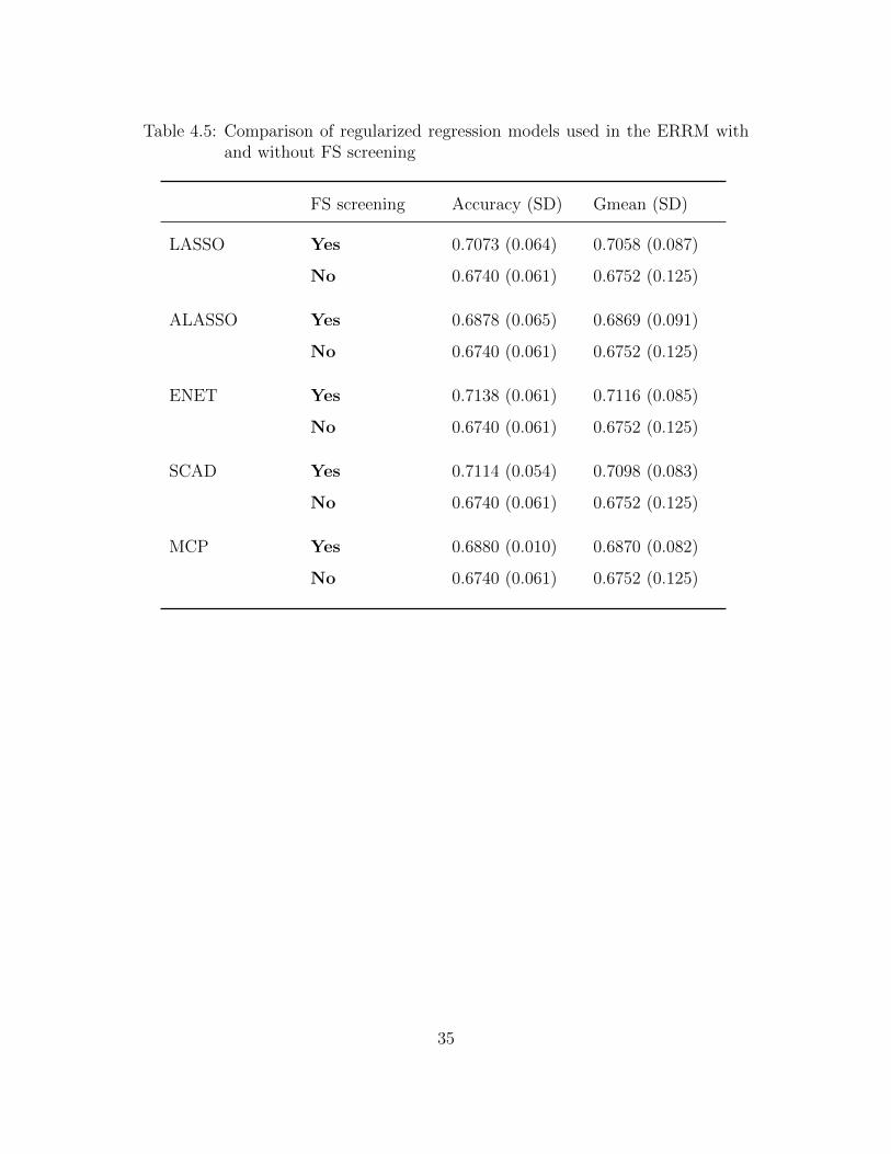
Table 4.5: Comparison of regularized regression models used in the ERRM withand without FS screening

FS screening Accuracy (SD) Gmean (SD)

LASSO Yes 0.7073 (0.064) 0.7058 (0.087)

No 0.6740 (0.061) 0.6752 (0.125)

ALASSO Yes 0.6878 (0.065) 0.6869 (0.091)

No 0.6740 (0.061) 0.6752 (0.125)

ENET Yes 0.7138 (0.061) 0.7116 (0.085)

No 0.6740 (0.061) 0.6752 (0.125)

SCAD Yes 0.7114 (0.054) 0.7098 (0.083)

No 0.6740 (0.061) 0.6752 (0.125)

MCP Yes 0.6880 (0.010) 0.6870 (0.082)

No 0.6740 (0.061) 0.6752 (0.125)

35

Chapter 5

Discussion

In this research, we proposed the combination of RLFS and ERRM that are used for feature

selection and classification respectively. The RLFS method ranks the features by employing

the lasso method with resampling approach and the k-SIS criteria to set the threshold for

selecting the optimal number of features and these features are applied on the ERRM

classifier, which uses bootstrapping and rank aggregation, to select the best performing

model across the bootstrapped samples and helps in attaining the best prediction accuracy

in a high dimensional setting. The ensembles framework ERRM is built using five different

regularized regression models. The regularized regression models are known for their best

performance in terms of variable selection and prediction accuracy on the gene expression

data.

To show the performance of our framework we used three different simulation scenarios

with low, medium and high correlation structures that matches the gene expression data.

To further illustrate our point, we also used SMK-CAN-187 data. Figure 4.1 shows the

boxplots of the average number of true important features, where the RLFS shows higher

detection power than the other FS methods such as IG, Chi2, and MRMR. From the results,

of both simulation studies and experimental data, we show that all the individual classifiers

with RLFS method performed much better compared to the IG, Chi2, and MRMR. We

also observed that all the individual classifiers showed a lot of instability with the other

three FS methods. This means that the individual classifiers do not work well with more

noise and less true important variables in the model. The SVM and ENET classifiers

with all the FS methods performed a little better among all the classifiers. However, the

performance was relatively still low in comparison to the proposed ERRM classifier with

36

every FS method. The tree-based ensemble methods RF and ABOOST with RLFS also

attained good accuracies but were not the best compared to the ERRM classifier.

The proposed ERRM method is assessed with the FS screening and without FS screening

step along with the bootstrapping option. The ERRM with FS screening and bootstrapping

approach works better than ERRM without the FS screening and bootstrapping technique.

Also, the results from Table 4.4 shows that the ensembles with bootstrapping is better

approach on both the filtered and unfiltered data. On comparing the performance of the

individual regularized regression models used in the ensembles, the individual models with

proposed RLFS screening step showed comparatively better accuracy in comparison to the

individual regularized regression models without the FS screening. This means that using

the reduced number of significant features with RLFS is better approach instead of using

all the features from the data.

The ERRM showed better overall performance not only with the RLFS but also with

the other FS methods compared in this study. This means that the ERRM is robust and

works much better on the highly correlated gene expression data. The rule of thumb in

attaining the best prediction accuracy is that more the true important variables, better

the prediction accuracy. Henceforth, from the results of simulation and experimental data

we see that the proposed combination of RLFS-ERRM has a superior compared to the

other existing combinations of FS and classifiers as seen in the Tables 4.1, 4.2 and 4.3. The

proposed ERRM classifier showed the best performance across all the FS methods, with

the highest performance achieved with RLFS method. However, the minor drawback in

the framework is that the performance of ERRM would have been much better if the RLFS

method had better selection average in retaining the significant features.

37

Chapter 6

Conclusion and Future Work

In this chapter, I conclude my M.S thesis project and propose problems for my Ph.D

dissertation.

6.1 Conclusion

In this research, through extensive simulation studies, we showed the superior performance

of RLFS with the k-SIS condition has a higher selection average in detecting the true

important features than other competitive FS methods. The ensemble classifier ERRM

also showed better average prediction accuracy with the RLFS, IG, Chi2, and MRMR

compared to other classifiers with these FS methods. On comparing the ensembles, the

proposed ERRM with bootstrapping showed better accuracy in comparison to the ERRM

without bootstrapping. In both the simulation study and the experimental data SMK-

CAN-187, the superior performance was achieved by the proposed combination of RLFS

-ERRM compared to all other combinations of FS and classifiers.

6.2 Future Work

As future work, we will further develop methodologies to deal with binary and multi-class

classification in high-throughput data.

38

6.2.1 Data

We will obtain datasets from GEO which are publicly available for testing the performance

of our methods. We will also generate the synthetic data to further evaluate the perfor-

mance of the proposed methods and the existing popular machine learning algorithms.

Simulation data

The synthetic data can be generated in many different ways. We simulate the data with

conditions that match the real microarray gene expression data. The microarray data usu-

ally have high complex correlation structures, to deal with such data is always challenging.

We plan to develop different simulation data types to the real microarray data. Some of

the approaches are as follows:

1. Compound Symmetry structure

2. Autoregressive (AR(1)) structure

3. Block correlation structure

In each of these different types of simulation data, we will test the proposed algorithms

for different scenarios of the data based on the correlation structures.

Real Data

Because of the advancement of high-throughput technology in biomedical research, large

volumes of high-dimensional data are being generated. Some of the classic examples of such

data include microarray gene expression data and DNA-methylation data. These data sets

are deposited and made publicly available in the Gene expression Omnibus - National

Center for Biotechnological Information (GEO - NCBI) website. Several datasets will be

obtained from GEO, and these datasets will undergo various pre-processing steps and finally

will be used for analyzing the performance of our proposed methods. We also intend to

perform a similar procedure for several of the publicly available benchmark datasets.

39

Some of the gene expression dataset for binary classification includes breast cancer data

obtained from GEO with accession number GEO2034 having 286 samples and 22284 genes,

colon cancer data with sample size of 62 and 2000 genes, Leukemia data with 72 number

of samples and 7129 genes, Lung cancer data from GEO with accession number GSE10072

having 107 samples and 22283 genes, and GSE20189 having 162 samples and 22278 genes.

Some of the gene expression data from GEO for multi-class classification problem includes

GSE60, GSE1825, and GSE5460.

Dealing with gene expression data is challenging because of the curse of dimensionality.

There are several algorithms available to deal with this problem; one of such algorithms

include PLR models. One of the other problems of gene expression data includes missing

information. The data pre-processing is a crucial step in gene expression data to handle

such an issue. Although most of the data are having complete information, because of

the nature of experiments conducted, some of the datasets might be having missing in-

formation and it becomes a necessity to address this issue. Handling the missing values

(MVs) in a high-dimensional setting is an extremely challenging problem. There is a lack

of research in this domain; few of the existing approaches for handling MVs are not reliable

as there is no complete information about the suitability of those algorithms in handling

large datasets. Some of the algorithms for handling MVs are as follows, K-nearest-Neighbor

imputation (KNNImpute), Gene Ontology imputation (GOImpute), Multivariate imputa-

tions by chained reactions (MICE), regularized and Bayesian lasso regression. We would

use one of these approaches for handling the datasets with MVs.

6.2.2 Modified adaptive lasso with proposed weights in high-

throughput microarray data

The adaptive lasso method is widely used for variable selection and classification purposes in

the high-dimensional setting. In Chapter 4 we described the performance of the adaptive

lasso method. The adaptive lasso method uses weights from ridge regression [27]. The

40

performance of the adaptive lasso can be improved by modifying the weights with different

approaches instead of using the standard weights from ridge regression. We plan to propose

variants of the adaptive lasso method with new weights from FS and resampling procedures

in the high-dimensional setting. In the first variant, the weights will be calculated based on

the regression coefficients from the FS methods. We will compare the performance of the FS

method with various classifiers including the proposed classification method. In the second

variant, we will propose a new weight-based on the resampling technique for the adaptive

lasso method. The aim is to compare the performance of the proposed adaptive lasso

method with the existing adaptive lasso method. In Chapter 4.1, the compound symmetry

structure was introduced for measuring the performance of the proposed framework in

this thesis. Develop the simulation study with an auto-regressive structure with different

correlation scenarios and apply this data to the proposed framework. We will also find the

real high-dimensional microarray data from GEO and measure the performance.

6.2.3 Adaptive K-Nearest-Neighbor with proposed weights in

high-dimensional microarray data

In addition to the penalized regression models, random forest, and support vector ma-

chines described in Chapter 3.2. KNN method is popularly used for binary classification

problems [63]. The KNN method faces the problem of the curse of dimensionality in a high-

dimensional setting. We will analyze the performance of the K-Nearest-Neighbor (KNN)

algorithm for dealing with such problems by reducing the features using the applicable

FS methods [64]. There are also studies conducted on the modification of KNN, adding

weights to the method [65]. We plan to propose adaptive KNN with the average radius

as weights for dealing with binary classification. The performance of the KNN and the

proposed KNN will be tested through simulation and real data applications.

41

6.2.4 Analyze the performance of FS and classification methods

for high-dimensional multi-class classification problem.

We plan to extend the development of the methodology for multi-class classification in high-

dimensional data. A two-stage approach is used for dealing with high-dimensional data

where the first stage is FS and the second stage is regarded as classification [66, 67]. The

popular FS methods in multi-class classification problems include Fisher’s score, MRMR,

Chi2, Correlation-based FS, Information Gain, Symmetrical Uncertainty, and SVM-RFE.

The classification methods such as KNN, Naive Bayes, decision trees, neural networks

and support vector machines can be used. The aim is to propose the ensembles of FS and

classifiers in a multi-class context. For measuring the performance of the proposed method,

firstly, we have to develop a simulation study with a multi-class response. Secondly, we have

to find the multi-label microarray data from GEO. With these data sets, The performance

of the proposed method will be compared with various existing individual FS and classifiers

in multi-class classification problems.

All the algorithms and codes for the developed methodologies will be deposited in an

online repository and will be granted access to public for usage.

42

6.2.5 Timeline

Table 6.1 shows the tentative timeline for the future work to be completed.

Table 6.1: Timeline for completion of this work

Date Tasks to complete Goals

Jan. - May. 2020 Modified adaptive lasso with

proposed weights in

high-throughput microarray

data

Submit manuscript

Jun. - Aug. 2020 Adaptive K-Nearest-Neighbor

with proposed weights in

high-dimensional microarray

data

Submit manuscript

Sep. - Dec. 2020 Develop methodology for

high-dimensional multi-class

classification problem

Present at a conference

Feb. 2021 Complete the first draft of

dissertation

Submit first dissertation draft

Mar. 2021 Complete the revised draft of

dissertation

Submit revised dissertation draft

Apr. 2021 Defend dissertation Dissertation defense

May. 2021 Complete the final version of

dissertation

Submit final dissertation

43

References

[1] Hassan Tariq, Elf Eldridge, and Ian Welch. An efficient approach for feature construc-

tion of high-dimensional microarray data by random projections. PLOS ONE, 13:1–8,

04 2018.

[2] Abhishek Bhola and Shailendra Singh. Gene selection using high dimensional gene

expression data: An appraisal. Current Bioinformatics, 13(3):225–233, 2018.

[3] Jian J. Dai, Linh H. Lieu, and David M. Rocke. Dimension reduction for classification

with gene expression microarray data. Statistical applications in genetics and molecular

biology, 5:Article6, 2006.

[4] Jun Lu, Robnet T. Kerns, Shyamal D. Peddada, and Pierre R. Bushel. Principal

component analysis-based filtering improves detection for affymetrix gene expression

arrays. In Nucleic acids research, 2011.

[5] Richard Bourgon, Robert Gentleman, and Wolfgang Huber. Reply to talloen et al.:

Independent filtering is a generic approach that needs domain specific adaptation.

Proceedings of the National Academy of Sciences, 107(46):E175–E175, 2010.

[6] Richard Bourgon, Robert Gentleman, and Wolfgang Huber. Independent filtering

increases detection power for high-throughput experiments. Proceedings of the National

Academy of Sciences of the United States of America, 107 21:9546–51, 2010.

[7] Daniel Ramskold, Eric T. Wang, Christopher B. Burge, and Rickard Sandberg. An

abundance of ubiquitously expressed genes revealed by tissue transcriptome sequence

data. In PLoS Computational Biology, 2009.

[8] Lin Li, Michael Kabesch, Emmanuelle Bouzigon, Florence Demenais, Martin Farrall,

Miriam Moffatt, Xihong Lin, and Liming Liang. Using eqtl weights to improve power

44

for genome-wide association studies: a genetic study of childhood asthma. Frontiers

in Genetics, 4:103, 2013.

[9] M. L. Calle, V. Urrea, G. Vellalta, N. Malats, and K. V. Steen. Improving strategies

for detecting genetic patterns of disease susceptibility in association studies. Statistics

in Medicine, 27(30):6532–6546, 2008.

[10] Christoph Bock. Analysing and interpreting dna methylation data. Nature Reviews

Genetics, 13:705–719, 2012.

[11] Hokeun Sun and Shuang Wang. Penalized logistic regression for high-dimensional dna

methylation data with case-control studies. Bioinformatics, 28 10:1368–75, 2012.

[12] S Kim and S Halabi. High dimensional variable selection with error control. BioMed

Research International, 2016:1–11, 2016.

[13] Sangjin Kim and Jong-Min Kim. Two-stage classification with sis using a new filter

ranking method in high throughput data. Mathematics, 7(6), 2019.

[14] Jianqing Fan and Jinchi Lv. Sure independence screening for ultrahigh dimensional

feature space. Journal of the Royal Statistical Society Series B, 70(5):849–911, Novem-

ber 2008.

[15] J. Ross Quinlan. C4.5: Programs for Machine Learning. Morgan Kaufmann Publishers

Inc., San Francisco, CA, USA, 1993.

[16] Isabelle Guyon and Andre Elisseeff. An introduction to variable and feature selection.

J. Mach. Learn. Res., 3:1157–1182, March 2003.

[17] Hanchuan Peng, Fuhui Long, and Chris Ding. Feature selection based on mutual

information criteria of max-dependency, max-relevance, and min-redundancy. IEEE

Transactions on Pattern Analysis and Machine Intelligence, 27:1226–1238, 2003.

45

[18] Gregory Ditzler, J Calvin Morrison, Yemin Lan, and Gail L Rosen. Fizzy: feature

subset selection for metagenomics. BMC bioinformatics, 16:358, November 2015.

[19] Chao-Ton Su and Chien-Hsin Yang. Feature selection for the svm: An application to

hypertension diagnosis. Expert Systems with Applications, 34(1):754 – 763, 2008.

[20] Miron B. Kursa and Witold R. Rudnicki. Feature selection with the boruta package.

2010.

[21] Um Okeh and Ica Oyeka. Estimating the fisher’s scoring matrix formula from logistic

model. 2013.

[22] Ryan J. Urbanowicz, Melissa Meeker, William La Cava, Randal S. Olson, and Jason H.

Moore. Relief-based feature selection: Introduction and review. Journal of biomedical

informatics, 85:189–203, 2017.

[23] Leo Breiman. Random forests. Mach. Learn., 45(1):5–32, October 2001.

[24] Yoav Freund. An adaptive version of the boost by majority algorithm. Machine

Learning, 43(3):293–318, Jun 2001.

[25] M. A. Hearst, S. T. Dumais, E. Osuna, J. Platt, and B. Scholkopf. Support vector

machines. IEEE Intelligent Systems and their Applications, 13(4):18–28, July 1998.

[26] Robert Tibshirani. Regression shrinkage and selection via the lasso. Journal of the

Royal Statistical Society. Series B (Methodological), 58(1):267–288, 1996.

[27] Donald W. Marquardt and Ronald D. Snee. Ridge regression in practice. The American

Statistician, 29(1):3–20, 1975.

[28] Xin-Guang Yang and Yongjin Lu. Informative gene selection for microarray clas-

sification via adaptive elastic net with conditional mutual information. ArXiv,

abs/1806.01466, 2018.

46

[29] Jianqing Fan and Runze Li. Variable selection via nonconcave penalized likelihood

and its oracle properties. 2001.

[30] Cun-Hui Zhang. Nearly unbiased variable selection under minimax concave penalty.

The Annals of Statistics, 38(2):894–942, Apr 2010.

[31] Trevor Hastie, Robert Tibshirani, and Jerome Friedman. The elements of statistical

learning: data mining, inference and prediction. Springer, 2 edition, 2009.

[32] Thomas G. Dietterich. Ensemble methods in machine learning. In Proceedings of the

First International Workshop on Multiple Classifier Systems, MCS ’00, pages 1–15,

London, UK, UK, 2000. Springer-Verlag.

[33] Richard Maclin and David W. Opitz. Popular ensemble methods: An empirical study.

CoRR, abs/1106.0257, 2011.

[34] Leo Breiman. Bagging predictors. Mach. Learn., 24(2):123–140, August 1996.

[35] Yoav Freund and Robert E Schapire. A decision-theoretic generalization of on-line

learning and an application to boosting. J. Comput. Syst. Sci., 55(1):119–139, August

1997.

[36] Susmita Datta, Vasyl Pihur, and Somnath Datta. An adaptive optimal ensemble

classifier via bagging and rank aggregation with applications to high dimensional data.

In BMC Bioinformatics, 2010.

[37] Hongshik Ahn, Hojin Moon, Melissa J. Fazzari, Noha Lim, James J. Chen, and

Ralph L. Kodell. Classification by ensembles from random partitions of high-

dimensional data. Computational Statistics Data Analysis, 51:6166–6179, 2007.

[38] Noha Lim, Hongshik Ahn, Hojin Moon, and James J. Chen. Classification of high-

dimensional data with ensemble of logistic regression models. Journal of biopharma-

ceutical statistics, 20 1:160–71, 2009.

47

[39] Igor Kononenko. Estimating attributes: Analysis and extensions of relief. In ECML,

1994.

[40] Roberto Battiti. Using mutual information for selecting features in supervised neural

net learning. IEEE transactions on neural networks, 5 4:537–50, 1994.

[41] Francois Fleuret. Fast binary feature selection with conditional mutual information.

J. Mach. Learn. Res., 5:1531–1555, 2004.

[42] Mehdi Pirooznia, Jack Y. Yang, Mary Qu Yang, and Youping Deng. A comparative

study of different machine learning methods on microarray gene expression data. BMC

Genomics, 9:S13 – S13, 2008.

[43] R Development Core Team. R: A Language and Environment for Statistical Comput-

ing. R Foundation for Statistical Computing, Vienna, Austria, 2008. ISBN 3-900051-

07-0.

[44] Andy Liaw and Matthew Wiener. Classification and regression by randomforest. R

News, 2(3):18–22, 2002.

[45] Miron B. Kursa. praznik: Collection of Information-Based Feature Selection Filters,

2018. R package version 5.0.0.

[46] Frank Pessler Frank Klawonn Natalia Novoselova, Junxi Wang. Biocomb: Feature

Selection and Classification with the Embedded Validation Procedures for Biomedical

Data Analysis, 2018. R package version 0.4.

[47] Jerome Friedman, Trevor Hastie, and Robert Tibshirani. Regularization paths for gen-

eralized linear models via coordinate descent. Journal of Statistical Software, 33(1):1–

22, 2010.

[48] Patrick Breheny and Jian Huang. Coordinate descent algorithms for nonconvex pe-

nalized regression, with applications to biological feature selection. Annals of Applied

Statistics, 5(1):232–253, 2011.

48

[49] David Meyer, Evgenia Dimitriadou, Kurt Hornik, Andreas Weingessel, and Friedrich

Leisch. e1071: Misc Functions of the Department of Statistics, Probability Theory

Group (Formerly: E1071), TU Wien, 2019. R package version 1.7-1.

[50] Vasyl Pihur, Somnath Datta, and Susmita Datta. RankAggreg: Weighted Rank Aggre-

gation, 2018. R package version 0.6.5.

[51] Feature Selection Datasets. http://featureselection.asu.edu/old/datasets.php. Ac-

cessed: 13-Oct-2019.

[52] Veronica Bolon-Canedo, Noelia Sanchez-Marono, Amparo Alonso-Betanzos,

Jose Manuel Benıtez, and Francisco Herrera. A review of microarray datasets

and applied feature selection methods. Inf. Sci., 282:111–135, 2014.

[53] Mingyuan Wang and Adrian Barbu. Are screening methods useful in feature selection?

an empirical study. In PloS one, 2018.

[54] Jundong Li, Kewei Cheng, Suhang Wang, Fred Morstatter, Robert P. Trevino, Jiliang

Tang, and Huan Liu. Feature selection: A data perspective. ACM Comput. Surv.,

50:94:1–94:45, 2017.

[55] In-Hee Lee, Gerald H. Lushington, and Mahesh Visvanathan. A filter-based feature

selection approach for identifying potential biomarkers for lung cancer. In Journal of

Clinical Bioinformatics, 2010.

[56] Borja Seijo-Pardo, Veronica Bolon-Canedo, and Amparo Alonso-Betanzos. Using a

feature selection ensemble on dna microarray datasets. In ESANN, 2016.

[57] Xin Jin, Anbang Xu, Rongfang Bie, and Ping Guo. Machine learning techniques and

chi-square feature selection for cancer classification using sage gene expression profiles.

In BioDM, 2006.

49

[58] Xiao Dong Chen and Hemant Ishwaran. Random forests for genomic data analysis.

Genomics, 99 6:323–9, 2012.

[59] Concha Bielza, V. Robles, and Pedro Larranaga. Regularized logistic regression with-

out a penalty term: An application to cancer classification with microarray data.

Expert Syst. Appl., 38:5110–5118, 2011.

[60] J. G. Liao and Khew-Voon Chin. Logistic regression for disease classification using

microarray data: model selection in a large p and small n case. Bioinformatics, 23

15:1945–51, 2007.

[61] Hui Zou and Trevor Hastie. Regularization and variable selection via the elastic net.

Journal of the Royal Statistical Society. Series B (Statistical Methodology), 67(2):301–

320, 2005.

[62] Li Ying, Zhang Yu, and Zhao Shishun. Gender classification with support vector

machines based on non-tensor pre-wavelets. 2010 Second International Conference on

Computer Research and Development, pages 770–774, 2010.

[63] R. Mitch Parry, W. Jones, Todd H. Stokes, Jeff Phan, Richard A. Moffitt, Hengfu

Fang, L Shi, Aloys Oberthuer, Margit Bistrup Fischer, Weida Tong, and May D.

Wang. k-nearest neighbor models for microarray gene expression analysis and clinical

outcome prediction. In The Pharmacogenomics Journal, 2010.

[64] Mukesh Kumar, Nitish Kumar Rath, Amitav Swain, and Santanu Kumar Rath. Sci-

encedirect eleventh international multi-conference on information processing-2015 (

imcip-2015 ) feature selection and classification of microarray data using mapreduce

based anova and k-nearest neighbor. 2015.

[65] Klaus Hechenbichler and Klaus Schliep. Weighted k-nearest-neighbor techniques and

ordinal classification. 2004.

50

[66] Junshan Yang, Jiarui Zhou, Zexuan Zhu, Xiaoliang Ma, and Zhen Ji. Iterative en-

semble feature selection for multiclass classification of imbalanced microarray data. In

Journal of Biological Research-Thessaloniki, 2016.

[67] Tao Li, Chengliang Zhang, and Mitsunori Ogihara. A comparative study of feature

selection and multiclass classification methods for tissue classification based on gene

expression. Bioinformatics, 20 15:2429–37, 2004.

51

Appendix A

Simulation Scenario: S3

The data is generated based on high correlation data structure with rho = 0.8. The

performance of proposed combination of RLFS-ERRM is relatively better than the other

combinations of the FS methods and classifiers. The results for simulation scenario S3 are

shown in Figure A.1. The average accuracy and Gmean for all the FS and classifiers are

noted in the Table A.1. The SVM and ENET classifiers with all the FS methods showed

a little better performance among all individual the classifiers. However, the accuracy and

Gmean attained by the proposed ensemble classifier ERRM with the FS methods RLFS,

IG and Chi2 was relatively better compared to the individual classifiers with FS methods.

In summary, the best performance is achieved by the proposed RLFS-ERRM combination

with accuracy of 0.9586 and Gmean of 0.9596. The second best performing combination is

MRMR-SVM. The lowest performance in terms of accuracy and the Gmean is shown by

Chi2-MCP. The MCP classifier is having the lowest accuracies with all the FS methods.

This explains that the MCP does not perform well when the predictor variables are highly

correlated

52

Table A.1: Average values taken over 100 iterations in simulation scenario: S3

FS

+

Classifier

Proposed RLFS IG Chi2 MRMR

Acc

(SD)

Gmean

(SD)

Acc

(SD)

Gmean

(SD)

Acc

(SD)

Gmean

(SD)

Acc

(SD)

Gmean

(SD)

Proposed

ERRM

0.9586

(0.025)

0.9596

(0.039)

0.9556

(0.027)

0.9565

(0.041)

0.9530

(0.034)

0.9544

(0.045)

0.9560

(0.024)

0.9558

(0.037)

LASSO0.9482

(0.033)

0.9493

(0.050)

0.9442

(0.030)

0.9194

(0.045)

0.9428

(0.037)

0.9447

(0.051)

0.9444

(0.032)

0.9442

(0.042)

ALASSO0.9420

(0.031)

0.9425

(0.051)

0.9376

(0.030)

0.9379

(0.047)

0.9328

(0.041)

0.9342

(0.056)

0.9388

(0.033)

0.9389

(0.047)

ENET0.9576

(0.025)

0.9587

(0.039)

0.9538

(0.029)

0.9546

(0.042)

0.9532

(0.034)

0.9546

(0.045)

0.9566

(0.024)

0.9562

(0.036)

SCAD0.9464

(0.031)

0.9475

(0.049)

0.9422

(0.030)

0.9428

(0.045)

0.9386

(0.043)

0.9401

(0.055)

0.9414

(0.031)

0.9408

(0.043)

MCP0.9256

(0.040)

0.9270

(0.062)

0.9262

(0.038)

0.9269

(0.055)

0.9210

(0.041)

0.9221

(0.058)

0.9224

(0.034)

0.9223

(0.048)

ABOOST0.9454

(0.032)

0.9469

(0.047)

0.9494

(0.030)

0.9501

(0.044)

0.9470

(0.034)

0.9482

(0.046

0.9480

(0.029)

0.9481

(0.040)

RF0.9540

(0.030)

0.9557

(0.043)

0.9560

(0.029)

0.9565

(0.043)

0.9542

(0.032)

0.9556

(0.044)

0.9508

(0.027)

0.9510

(0.039)

LR0.9478

(0.029)

0.9482

(0.045)

0.9462

(0.030)

0.9469

(0.044)

0.9418

(0.038)

0.9432

(0.050)

0.9438

(0.028)

0.9437

(0.041)

SVM0.9560

(0.027)

0.9568

(0.041)

0.9522

(0.030)

0.9527

(0.043)

0.9520

(0.031)

0.9526

(0.042)

0.9594

(0.026)

0.9587

(0.037)

53

0.80

0.85

0.90

0.95

1.00

Classifier

Accu

racy

RLFS

0.80

0.85

0.90

0.95

1.00

Classifier

Accu

racy

IG

0.80

0.85

0.90

0.95

1.00

Classifier

Accu

racy

Chi2

0.80

0.85

0.90

0.95

1.00

Classifier

Accu

racy

MRMR

Classifier

ERRM

LASSO

ALASSO

SCAD

MCP

ENET

AB

RF

LR

SVM

Figure A.1: Boxplot showing the accuracies of Classifiers with FS methods in simulationscenario: S3

54

Appendix B

The RLFS-ERRM Program

l ibrary (mvtnorm)

l ibrary ( d o P a r a l l e l )

l ibrary ( class )

l ibrary ( adabag )

l ibrary ( t i d y v e r s e )

l ibrary ( Biocomb )

l ibrary ( prazn ik )

l ibrary ( randomForest )

l ibrary ( glmnet )

l ibrary ( ncvreg )

l ibrary ( e1071 )

l ibrary ( c a r e t )

l ibrary ( RankAggreg )

l ibrary ( ggp lot2 )

## Functions to c a l c u l a t e performance metr i c s

## accuracy

accuracy <− function ( truth , p r ed i c t ed )

{

i f ( length ( t ruth ) > 0)

sum( t ruth==pred i c t ed )/length ( t ruth ) else

55

return (0 )

}

## s e n s i t i v i t y

s e n s i t i v i t y <− function ( truth , p r ed i c t ed )

{

i f (sum( t ruth==1) > 0)

sum( p r ed i c t ed [ t ruth==1]==1)/sum( t ruth==1) else

return (0 )

}

## s p e c i f i c i t y

s p e c i f i c i t y <− function ( truth , p r ed i c t ed )

{

i f (sum( t ruth==0) > 0)

sum( p r ed i c t ed [ t ruth==0]==0)/sum( t ruth==0) else

return (0 )

}

## genera te the f e a t u r e s e t

f e a t u r e set = function ( nsample , p , seed . index , beta , c o r s )

{

set . seed ( seed . index )

cor .mat = matrix (1 , nrow = p , ncol = p)

cor .mat [ lower . t r i ( cor .mat)]= co r s

# cor . mat [ upper . t r i ( cor . mat)]= cors

cor .mat=t ( cor .mat)

cor .mat [ lower . t r i ( cor .mat ) ] = co r s

mu. vec=rep (0 , p )

56

dat = rmvnorm(n = nsample , mean = mu. vec ,

sigma = cor .mat , method = ”svd” )

# change to e igen or c h o l or svd i f needed

return ( dat )

}

## genera te response

generate response data = function ( nsample , p , cors , theta0 )

{

cnt = 0

case . dat = NULL

control . dat = NULL

# genera te response o f e q u a l c o n t r o l and case

while ( cnt==0)

{

seed . va l = sample (1 : 1000000 ,1 )

data . set = f e a t u r e set ( nsample , p , seed . val , beta , c o r s )

data . set = scale (data . set )

f e t a = data . set%∗%theta0

fprob = exp( f e t a )/(1+exp( f e t a ) )

y = rbinom( nsample , 1 , fprob )

idx = which( y == 1)

i f ( ( length ( idx)==(nsample/ 2 ) ) )

#& ( l e n g t h ( i d x )<=((nsample/2)+20)))

{

r e s u l t = l i s t (y , data . set , seed . va l )

cnt = 100

57

return ( r e s u l t )

}

}

}

data . gen <− function ( )

{

nsample = 200 ; co r s = 0 . 2 ;

p = 1000 ; num. beta = 25

beta = runif (num. beta , 2 , 4 )

t rue . c o e f s = beta

t rue . c o e f s . idx = c ( 1 :num. beta )

# i n d i c e s o f the t r u e r e g r e s s i o n c o e f s

theta0 = rep (0 , p )

# genera te the empty l i s t o f v a l u e s

theta0 [ c ( t rue . c o e f s . idx ) ] = c ( t rue . c o e f s )

obj <− generate response data ( nsample = nsample , p ,

co r s = cors , theta0 = theta0 )

y1 = obj [ [ 1 ] ] # response v a r i a b l e

x1 = data . frame ( obj [ [ 2 ] ] ) # data s e t

df <− data . frame ( x1 , y1 )

colnames ( df)=paste ( ”v” , 1 : ncol ( df ) , sep=”” )

colnames ( df ) [ ncol ( df ) ]<− ”y”

true . var .names = paste ( ”v” , c ( t rue . c o e f s . idx ) , sep=”” )

return ( df )

58

}

## r e a l data g e n e r a t i o n f u n c t i o n

data . gen <− function ( )

{

data .SMK CAN 187 <− readMat ( ”SMK CAN 187 . mat” )

x1 <− as . matrix (data .SMK CAN 187$X)

y1 <− as . numeric (data .SMK CAN 187$Y)

y1 <− replace ( y1 , y1==1, 0)

y1 <− replace ( y1 , y1==2, 1)

s . idx <− sample ( 1 :nrow( x1 ) , as . integer (nrow( x1 )∗ . 7 ) , replace = F)

t r a i n . y = y1 [ s . idx ]

t r a i n . x = x1 [ s . idx , ]

t e s t . x = x1[− s . idx , ]

t e s t . y = y1[− s . idx ]

data . t r a i n <− data . frame ( t r a i n . x , t r a i n . y )

data . t e s t <− data . frame ( t e s t . x , t e s t . y )

return ( l i s t (data . t ra in , data . t e s t ) )

}

## Function to conver t s c o r e s

conver tScore s <− function ( s c o r e s )

{

s c o r e s <− t ( s c o r e s )

59

ranks <− matrix (0 , nrow( s c o r e s ) , ncol ( s c o r e s ) )

weights <− ranks

for ( i in 1 :nrow( s c o r e s ) ){

ms <− sort ( s c o r e s [ i , ] , decr=TRUE, ind=TRUE)

ranks [ i , ] <− colnames ( s c o r e s ) [ ms$ i x ]

weights [ i , ] <− ms$x

}

l i s t ( ranks = ranks , weights = weights )

}

## Function to c a l c u l a t e the PLR models

## l a s s o

l a s s o = function (x , y )

{

cv . l a s s o <− cv . glmnet ( y = y , x = x , alpha =1, family=” binomial ” )

return ( cv . l a s s o )

}

## a l a s s o

a l a s s o = function (x , y )

{

## Ridge Regress ion to c r e a t e the Adaptive Weights Vector

cv . r i dg e <− cv . glmnet ( y = y , x = x , alpha =0, family=’ binomial ’ )

w3 <− 1/abs (matrix ( coef ( cv . r idge ,

s=cv . r i dg e $lambda .min ) [ , 1 ] [ 2 : ( ncol ( x )+1)] ) )ˆ1

## Using gamma = 1

w3 [ w3 [ , 1 ] == I n f ] <− 999999999

## Replac ing v a l u e s es t imated as I n f i n i t e f o r 999999999

## Adaptive Lasso

60

cv . a l a s s o <− cv . glmnet ( y = y , x = x , alpha =1,

family=” binomial ” , pena l ty . factor = w3)

return ( cv . a l a s s o )

}

## b r i d g e

enet = function (x , y )

{

cv . enet <− cv . glmnet ( y=y , x= x , alpha =0.5 , family=” binomial ” )

return ( cv . enet )

}

## scad

scad = function (x , y )

{

cv . scad <− cv . ncvreg (x , y , family=” binomial ” , pena l ty=”SCAD” )

return ( cv . scad )

}

## mcp

mcp = function (x , y )

{

cv . mcp <− cv . ncvreg (x , y , family=” binomial ” , pena l ty=”MCP” )

return ( cv . mcp)

}

## Function to perform f e a t u r e s e l e c t i o n

f e a t u r e . s e l e c t i o n = function ( method , data )

{

df <− data

61

## S p l i t the data i n t o t r a i n i n g and t e s t i n g s e t

bound <− f loor ( (nrow( df )/4)∗3)

df <− df [ sample (nrow( df ) ) , ] #sample rows

df . t r a i n <− df [ 1 : bound , ] #g e t t r a i n i n g s e t

df . t e s t <− df [ ( bound+1):nrow( df ) , ]

##−−−−−−−−−−−−−−−−−−−−−−−−−−−−−−−−−−−−−−−−−−−−−−−−−−

t r a i n . x <−data . matrix ( df . t r a i n [ ,−( ncol ( df . t r a i n ) ) ] )

t r a i n . y <− as . numeric ( df . t r a i n [ , ( ncol ( df . t r a i n ) ) ] )

# Test s e t s e p e r a t e d i n t o data matrix and response v a r i a b l e

t e s t . x <− data . matrix ( df . t e s t [ ,−( ncol ( df . t e s t ) ) ] )

t e s t . y <− as . numeric ( df . t e s t [ , ( ncol ( df . t e s t ) ) ] )

data . t r a i n <− data . frame ( t r a i n . x , t r a i n . y )

# Last column name i s t r a i n . y

data . t e s t <− data . frame ( t e s t . x , t e s t . y )

# Last column name i s t e s t . y

i f ( method == ” resampl ing ” )

{

f i n a l l a s s o <− main ( t r a i n . x = t r a i n . x , t r a i n . y = t r a i n . y ,

method = ” l a s s o ” )

set l a s s o <− names( f i n a l l a s s o [ 1 : top ] )

idx <− match( set l a s so , names(data . t r a i n ) )

}

i f ( method==” in fo rmat ion ” )

{

data . t r a i n [ , ncol (data . t r a i n ) ]

62

<− as . factor (data . t r a i n [ , ncol (data . t r a i n ) ] )

d i s c<−” equal i n t e r v a l width”

a t t r s . nominal <− numeric ( )

f i t . i n f o =

s e l e c t . i n f . ga in (data . t ra in , d i s c . method=

disc , a t t r s . nominal=a t t r s . nominal )

idx <− as . integer ( f i t . i n f o $NumberFeature ) [ 1 : top ]

}

i f ( method==” ch i2 ” )

{

data . t r a i n [ , ncol (data . t r a i n ) ]<−as . factor

(data . t r a i n [ , ncol (data . t r a i n ) ] )

d i s c<−” equal i n t e r v a l width”

a t t r s . nominal <− numeric ( )

f i t . ch i2 <− s e l e c t . i n f . ch i2 (data . t ra in , d i s c . method=

disc , a t t r s . nominal=a t t r s . nominal )

idx <− as . integer ( f i t . ch i2$NumberFeature ) [ 1 : top ]

}

i f ( method==”mrmr” )

{

f i t . mrmr = MRMR(data . t r a i n [ ,−ncol (data . t r a i n ) ] ,

data . t r a i n [ , ncol (data . t r a i n ) ] , k=ncol (data . t r a i n

[ ,−ncol (data . t r a i n ) ] ) )

fm<− f i t . mrmr$ s co r e

set <− names( fm ) [ 1 : top ]

idx <− match( set , names(data . t r a i n ) )

63

}

return ( l i s t (data . t ra in , data . t e s t , idx ) )

}

## Function to c a l c u l a t e Resampling method

f r e q . matrix = function ( t r a i n . x , t r a i n . y , method )

{

i f ( method==” l a s s o ” )

{

f i t = glmnet ( as . matrix ( t r a i n . x ) , t r a i n . y , alpha =1,

family=” binomial ” )

beta . matrix = f i t $beta

}

i f ( method==” br idge ” )

{

f i t = glmnet ( as . matrix ( t r a i n . x ) , t r a i n . y , alpha=(1/2) ,

family=” binomial ” )

beta . matrix = f i t $beta

}

i f ( method==” scad ” )

{

f i t = ncvreg ( as . matrix ( t r a i n . x ) ,

t r a i n . y , family=” binomial ” , pena l ty=”SCAD” )

beta . matrix = f i t $beta[−c ( 1 ) , ]

}

i f ( method==”mcp” )

64

{

f i t = ncvreg ( as . matrix ( t r a i n . x ) ,

t r a i n . y , family=” binomial ” , pena l ty=”MCP” )

beta . matrix = f i t $beta[−c ( 1 ) , ]

}

r e s u l t . matrix = c o e f s . matrix = matrix (0 ,nrow=ncol

( beta . matrix ) ,

ncol=nrow( beta . matrix ) )

colnames ( r e s u l t . matrix ) = rownames( beta . matrix )

for ( i in 1 :nrow( r e s u l t . matrix ) )

{

idx = which( beta . matrix [ , i ] !=0)

r e s u l t . matrix [ i , idx ] = 1

c o e f s . matrix [ i , idx ] = beta . matrix [ idx , i ]

}

# return f requency matrix

return ( l i s t ( r e s u l t . matrix , c o e f s . matrix ) )

}

resampl ing = function ( t r a i n . x , t r a i n . y , method )

{

idx = sample ( 1 :nrow( t r a i n . x ) , as . integer (nrow( t r a i n . x )∗ 0 . 7 ) )

s . x = t r a i n . x [ idx , ]

s . y = t r a i n . y [ idx ]

i f ( method==” l a s s o ” )

{

obj = f r e q . matrix ( s . x , s . y , method )

65

}

i f ( method==” br idge ” )

{

obj = f r e q . matrix ( s . x , s . y , method )

}

i f ( method==” scad ” )

{

obj = f r e q . matrix ( s . x , s . y , method )

}

i f ( method==”mcp” )

{

obj = f r e q . matrix ( s . x , s . y , method )

}

# return f requency matrix and c o e f i c i e n t s matrix

return ( obj )

}

add = function ( obj .mat , opt ion )

{

i f ( opt ion==” frequency ” ){ s = apply ( obj .mat , 2 ,sum)}

i f ( opt ion==” c o e f ” ){ s = apply ( obj .mat , 2 , function ( x )max(abs ( x ) ) )}

return ( s )

}

#################################################################

resampl ing r e s u l t s = function ( t r a i n . x , t r a i n . y , method )

{

# 100 resampl ing

# re turn f requency and c o e f f i c i e n t s

66

# f o r each v a r i a b l e s

mat0 = matrix (0 ,nrow=100 ,ncol=ncol ( t r a i n . x ) )

mat1 = matrix (0 ,nrow=100 ,ncol=ncol ( t r a i n . x ) )

colnames ( mat0 ) = colnames ( mat1 ) = colnames ( t r a i n . x )

l e n s = NULL

for ( i in 1 : 100 ) ###########################################

{

# l a s s o

obj0 = resampl ing ( t r a i n . x , t r a i n . y , method=method )

l e n s = c ( l ens ,nrow( obj0 [ [ 1 ] ] ) )

mat0 [ i , ] = add( obj0 [ [ 1 ] ] , ” f requency ” )

mat1 [ i , ] = add( obj0 [ [ 2 ] ] , ” c o e f ” )

}

f r e q . vec = apply (mat0 , 2 ,sum)/sum( l e n s )

coef . vec = apply (mat1 , 2 , function ( x )max(abs ( x ) ) )

return ( l i s t ( f r e q . vec , coef . vec ) )

}

main = function ( t r a i n . x , t r a i n . y , method )#, d i r e c t o r y )

{

r e s u l t s = resampl ing r e s u l t s ( t r a i n . x , t r a i n . y , method )

mu. vec = r e s u l t s [ [ 1 ] ]

max. c o e f s . vec = r e s u l t s [ [ 2 ] ]

s .mu. vec = sort (mu. vec , d e c r ea s ing=T, index . return=T)

rank .mu. vec = mu. vec [ s .mu. vec$ i x ]

return (rank .mu. vec )

}

67

t e s t . function <− function ( f e a t u r e . idx , method )

{

f s <− f e a t u r e . idx

data . t r a i n <− f s [ [ 1 ] ]

data . t e s t <− f s [ [ 2 ] ]

idx <− f s [ [ 3 ] ]

###################################

reduced . t r a inx <− data . t r a i n [ , idx ]

reduced . t r a iny <− as . factor (data . t r a i n [ , ncol (data . t r a i n ) ] )

t e s t . x <− data . t e s t [ , idx ]

t e s t . y <− as . factor (data . t e s t [ , ( ncol (data . t e s t ) ) ] )

###################################

dat . t r a i n <− data . frame ( reduced . t ra inx , reduced . t r a i ny )

###################################

n <− length ( reduced . t r a iny )

nalg <− length ( a lgor i thms )

nvm <− length ( v a l i d a t i o n )

ly <− levels ( reduced . t r a iny )

f i t t edMode l s <− l i s t ( ) #to keep the f i t t e d a l g o r i t h m s

c o e f s .mat = f r e q .mat = matrix (0 ,nrow=M,

ncol=ncol ( reduced . t r a inx ) )

colnames ( c o e f s .mat)=colnames ( f r e q .mat)=

colnames ( reduced . t r a inx )

bes t . methods=NULL

mat . r e s u l t = matrix (0 ,nrow=nrow( t e s t . x ) , ncol=M)

68

i f ( method==” ensemble ” )

{

for ( k in 1 :M)

{

repeat

{ # to make sure t h a t a t l e a s t more than

# two c l a s s e s are p r e s e n t

s <− sample (n , replace=TRUE)

i f ( length ( table ( reduced . t r a iny [ s ] ) ) >= 2

& length ( table ( reduced . t r a iny [− s ] ) ) >= 2)

break

}

f s <− 1 : ncol ( reduced . t r a inx )

sub . t r a i n i n g x <− reduced . t r a inx [ s , f s ]

sub . t e s t i n g x <− reduced . t r a inx [−unique ( s ) , f s ]

sub . t r a i n i n g y <− reduced . t r a iny [ s ]

sub . t e s t i n g y <− reduced . t r a iny [−unique ( s ) ]

p r ed i c t ed <− l i s t ( )

Res <− l i s t ( )

# t r a i n a l l a l g o r i t h m s on the s u b s e t

# Fi t the model and p r e d i c t

for ( j in 1 : nalg )

{

Res [ [ j ] ]<− switch ( a lgor i thms [ j ] ,

69

” l a s s o ” = {

f i t . l a s s o = l a s s o ( as . matrix

(sub . t r a i n i n g x ) , sub . t r a i n i n g y )

l a s s o . idx = which(abs ( coef ( f i t . l a s s o )

[ ,1 ])>0) [− c ( 1 ) ]

l a s s o .m. idx = match(names( l a s s o . idx ) ,

colnames (sub . t e s t i n g x ) )

l a s s o . xb =

as . matrix (cbind (1 , as . matrix

(sub . t e s t i n g x [ , l a s s o .m. idx ] ) ) )%∗%as . matrix

( coef ( f i t . l a s s o ) [ c (1 , l a s s o . idx ) , 1 ] )

l a s s o . pred = exp( l a s s o . xb )/(1+exp( l a s s o . xb ) )

l a s s o . pred <− i f e l s e ( l a s s o . pred >0.5 , 1 , 0)

p r ed i c t ed [ [ j ] ] <− as . character ( l a s s o . pred [ , 1 ] )

} ,

” a l a s s o ” = {

f i t . a l a s s o = a l a s s o ( as . matrix

(sub . t r a i n i n g x ) , sub . t r a i n i n g y )

a l a s s o . idxwhich (abs ( coef ( f i t . a l a s s o ) [ ,1 ] ) >0) [− c ( 1 ) ]

a l a s s o .m. idx =

match(names( a l a s s o . idx ) , colnames (sub . t e s t i n g x ) )

a l a s s o . xb = as . matrix (cbind (1 ,

as . matrix (sub . t e s t i n g x [ , a l a s s o .m. idx ] ) ) )

%∗%as . matrix ( coef ( f i t . a l a s s o ) [ c (1 , a l a s s o . idx ) , 1 ] )

a l a s s o . pred = exp( a l a s s o . xb )/(1+exp( a l a s s o . xb ) )

70

a l a s s o . pred <− i f e l s e ( a l a s s o . pred >0.5 , 1 , 0)

p r ed i c t ed [ [ j ] ] <− as . character ( a l a s s o . pred [ , 1 ] )

} ,

” br idge ” = {

f i t . enet = enet ( as . matrix (sub . t r a i n i n g x ) , sub . t r a i n i n g y )

enet . idx = which(abs ( coef ( f i t . enet ) [ ,1 ] ) >0) [− c ( 1 ) ]

enet .m. idx = match(names( enet . idx ) ,

colnames (sub . t e s t i n g x ) )

enet . xb = as . matrix (cbind (1 , as . matrix (

sub . t e s t i n g x [ , enet .m. idx ] ) ) )%∗%as . matrix

( coef ( f i t . enet ) [ c (1 , enet . idx ) , 1 ] )

enet . pred = exp( enet . xb )/(1+exp( enet . xb ) )

enet . pred <− i f e l s e ( enet . pred >0.5 , 1 , 0)

p r ed i c t ed [ [ j ] ] <− as . character ( enet . pred [ , 1 ] )

} ,

” scad ” = {

f i t . scad = scad ( as . matrix (sub . t r a i n i n g x ) , sub . t r a i n i n g y )

scad . idx = which(abs ( coef ( f i t . scad ))>0)[−c ( 1 ) ]

scad .m. idx = match(names( scad . idx ) ,

colnames (sub . t e s t i n g x ) )

scad . xb = as . matrix (cbind (1 , as . matrix (

sub . t e s t i n g x [ , scad .m. idx ] ) ) )%∗%as . matrix (

coef ( f i t . scad ) [ c (1 , scad . idx ) ] )

scad . pred = exp( scad . xb )/(1+exp( scad . xb ) )

71

scad . pred <− i f e l s e ( scad . pred >0.5 , 1 , 0)

p r ed i c t ed [ [ j ] ] <− as . character ( scad . pred [ , 1 ] )

} ,

”mcp” = {

f i t . mcp = mcp( as . matrix (sub . t r a i n i n g x ) , sub . t r a i n i n g y )

mcp . idx = which(abs ( coef ( f i t . mcp))>0)[−c ( 1 ) ]

mcp .m. idx = match(names(mcp . idx ) , colnames (sub . t e s t i n g x ) )

mcp . xb = as . matrix (cbind (1 , as . matrix (

sub . t e s t i n g x [ , mcp .m. idx ] ) ) )%∗%as . matrix

( coef ( f i t . mcp ) [ c (1 ,mcp . idx ) ] )

mcp . pred = exp(mcp . xb )/(1+exp(mcp . xb ) )

mcp . pred <− i f e l s e (mcp . pred >0.5 , 1 , 0)

p r ed i c t ed [ [ j ] ] <− as . character (mcp . pred [ , 1 ] )

}

)

attr ( Res [ [ j ] ] , ” a lgor i thm ” ) <− a lgor i thms [ j ]

}

# compute v a l i d a t i o n measures

s c o r e s <− matrix (0 , nalg , nvm)

rownames( s c o r e s ) <− a lgor i thms

colnames ( s c o r e s ) <− v a l i d a t i o n

for ( i in 1 : nalg )

for ( j in 1 :nvm)

72

s c o r e s [ i , j ] <− switch ( v a l i d a t i o n [ j ] ,

” accuracy ” = accuracy (sub . t e s t ingy ,

factor ( p r ed i c t ed [ [ i ] ] , levels=ly ) ) ,

” s e n s i t i v i t y ” = s e n s i t i v i t y (sub . t e s t ingy ,

factor ( p r ed i c t ed [ [ i ] ] , levels=ly ) ) ,

” s p e c i f i c i t y ” = s p e c i f i c i t y (sub . t e s t ingy ,

factor ( p r ed i c t ed [ [ i ] ] , levels=ly ) )

)

## Rank a g g r e g a t i o n to s e l e c t the b e s t model

## based on the performance metr ic s

convScores <− conver tScore s ( s c o r e s )

##−−−−−−−−−−−−−−−−−−−−−−−−−−−−−−−−−−−−−−−−−−−

i f (nvm > 1 && nalg <= 5)

i f (weighted )

f i t t edMode l s [ [ k ] ] <− Res [ [ which(

a lgor i thms == BruteAggreg ( convScores$ranks ,

nalg , convScores$weights ,

distance=distance )$top . l i s t [ 1 ] ) ] ]

##−−−−−−−−−−−−−−−−−−−−−−−−−−−−−−−−−−−−−−−−−−−−

bestAlg <− unlist ( sapply ( f i t t edMode l s ,

FUN = function ( x ) attr (x , ” a lgor i thm ” ) ) )

newdata<− t e s t . x

p r ed i c t ed sub <− l i s t ( )

Res sub<− l i s t ( )

## b e s t A l g = b e s t . methods

for ( s in 1 : nalg )

73

{

Res sub [ [ s ] ]<− switch ( bestAlg [ s ] ,

” l a s s o ” = {

r e s l a s s o sub <− predict ( f i t . l a s so ,

newx = as . matrix ( newdata ) , type = ” c l a s s ” )

p r ed i c t ed sub [ [ s ] ]<− r e s l a s s o sub [ , 1 ]

} ,

” a l a s s o ” = {

r e s a l a s s o sub <− predict ( f i t . a l a s so ,

newx = as . matrix ( newdata ) , type = ” c l a s s ” )

p r ed i c t ed sub [ [ s ] ]<− r e s a l a s s o sub [ , 1 ]

} ,

” br idge ” = {

r e s e n e t sub <− predict ( f i t . enet ,

newx = as . matrix ( newdata ) , type = ” c l a s s ” )

p r ed i c t ed sub [ [ s ] ]<− r e s e n e t sub [ , 1 ]

} ,

” scad ” = {

r e s s cad sub <− predict ( f i t . scad ,

X = as . matrix ( newdata ) , type = ” c l a s s ” )

p r ed i c t ed sub [ [ s ] ]<− r e s s cad sub

} ,

”mcp” = {

resmcp sub <− predict ( f i t . mcp ,

X = as . matrix ( newdata ) , type = ” c l a s s ” )

p r ed i c t ed sub [ [ s ] ]<− resmcp sub

}

)

74

}

#s t o r e p r e d i c t e d c l a s s i f i c a t i o n

mat . r e s u l t [ , k ] = Res sub [ [ 1 ] ]

# some output

verbose=T

i f ( verbose )

cat ( ” I t e r ” , k , ”\n” )

}

major i ty . vote = apply (mat . r e s u l t , 1 , function ( x )

names( table ( x ) ) [ which .max( table ( x ) ) ] )

acc . ens <− accuracy ( t e s t . y , major i ty . vote )∗100

sens . ens <− s e n s i t i v i t y ( t e s t . y , major i ty . vote )∗100

spec . ens <− s p e c i f i c i t y ( t e s t . y , major i ty . vote )∗100

p e r f <− c ( acc . ens , sens . ens , spec . ens )

}

else i f ( method==” l a s s o ” )

{

f i t . l a s s o . ind = l a s s o ( as . matrix ( reduced . t r a inx ) ,

reduced . t r a iny )

l a s s o . idx . ind = which(abs ( coef (

f i t . l a s s o . ind ) [ ,1 ] ) >0) [− c ( 1 ) ]

l a s s o .m. idx . ind = match(names( l a s s o . idx . ind ) ,

colnames ( t e s t . x ) )

l a s s o . xb . ind = as . matrix (cbind (1 , as . matrix (

t e s t . x [ , l a s s o .m. idx . ind ] ) ) )%∗%as . matrix ( coef (

f i t . l a s s o . ind ) [ c (1 , l a s s o . idx . ind ) , 1 ] )

75

l a s s o . pred . ind = exp( l a s s o . xb . ind )/(1+exp( l a s s o . xb . ind ) )

l a s s o . pred . ind <− i f e l s e ( l a s s o . pred . ind >0.5 , 1 , 0)

p r ed i c t ed . l a s s o . ind <− as . character ( l a s s o . pred . ind [ , 1 ] )

acc . l a s s o <− accuracy ( t e s t . y , p r ed i c t ed . l a s s o . ind )∗100

sens . l a s s o <− s e n s i t i v i t y ( t e s t . y , p r ed i c t ed . l a s s o . ind )∗100

spec . l a s s o <− s p e c i f i c i t y ( t e s t . y , p r ed i c t ed . l a s s o . ind )∗100

p e r f <− c ( acc . l a s so , sens . l a s so , spec . l a s s o )

}

else i f ( method==” a l a s s o ” )

{

f i t . a l a s s o . ind = a l a s s o ( as . matrix (

reduced . t r a inx ) , reduced . t r a i ny )

a l a s s o . idx . ind = which(abs ( coef (

f i t . a l a s s o . ind ) [ ,1 ] ) >0) [− c ( 1 ) ]

a l a s s o .m. idx . ind = match(names(

a l a s s o . idx . ind ) , colnames ( t e s t . x ) )

a l a s s o . xb . ind = as . matrix (cbind (1 , as . matrix (

t e s t . x [ , a l a s s o .m. idx . ind ] ) ) )%∗%as . matrix (

coef ( f i t . a l a s s o . ind ) [ c (1 , a l a s s o . idx . ind ) , 1 ] )

a l a s s o . pred . ind = exp( a l a s s o . xb . ind )/(1+exp( a l a s s o . xb . ind ) )

a l a s s o . pred . ind <− i f e l s e ( a l a s s o . pred . ind >0.5 , 1 , 0)

p r ed i c t ed . a l a s s o . ind <− as . character ( a l a s s o . pred . ind [ , 1 ] )

acc . a l a s s o <− accuracy ( t e s t . y , p r ed i c t ed . a l a s s o . ind )∗100

sens . a l a s s o <− s e n s i t i v i t y ( t e s t . y , p r ed i c t ed . a l a s s o . ind )∗100

spec . a l a s s o <− s p e c i f i c i t y ( t e s t . y , p r ed i c t ed . a l a s s o . ind )∗100

76

p e r f <− c ( acc . a l a s so , sens . a l a s so , spec . a l a s s o )

}

else i f ( method==” br idge ” )

{

f i t . enet . ind = enet ( as . matrix ( reduced . t r a inx ) ,

reduced . t r a iny )

enet . idx . ind = which(abs ( coef

( f i t . enet . ind ) [ ,1 ] ) >0) [− c ( 1 ) ]

enet .m. idx . ind = match(names

( enet . idx . ind ) , colnames ( t e s t . x ) )

enet . xb . ind = as . matrix (cbind (1 , as . matrix

( t e s t . x [ , enet .m. idx . ind ] ) ) )%∗%as . matrix

( coef ( f i t . enet . ind ) [ c (1 , enet . idx . ind ) , 1 ] )

enet . pred . ind = exp( enet . xb . ind )/(1+exp( enet . xb . ind ) )

enet . pred . ind <− i f e l s e ( enet . pred . ind >0.5 , 1 , 0)

p r ed i c t ed . enet . ind <− as . character ( enet . pred . ind [ , 1 ] )

acc . enet <− accuracy ( t e s t . y , p r ed i c t ed . enet . ind )∗100

sens . enet <− s e n s i t i v i t y ( t e s t . y , p r ed i c t ed . enet . ind )∗100

spec . enet <− s p e c i f i c i t y ( t e s t . y , p r ed i c t ed . enet . ind )∗100

p e r f <− c ( acc . enet , sens . enet , spec . enet )

}

else i f ( method==” scad ” )

{

f i t . scad . ind = scad ( as . matrix ( reduced . t r a inx ) ,

reduced . t r a iny )

77

scad . idx . ind = which(abs

( coef ( f i t . scad . ind ))>0)[−c ( 1 ) ]

scad .m. idx . ind = match(names( scad . idx . ind ) ,

colnames ( t e s t . x ) )

scad . xb . ind = as . matrix (

cbind (1 , as . matrix ( t e s t . x [ , scad .m. idx . ind ] ) ) )%∗%as . matrix (

coef ( f i t . scad . ind ) [ c (1 , scad . idx . ind ) ] )

scad . pred . ind = exp( scad . xb . ind )/(1+exp( scad . xb . ind ) )

scad . pred . ind <− i f e l s e ( scad . pred . ind >0.5 , 1 , 0)

p r ed i c t ed . scad . ind <− as . character ( scad . pred . ind [ , 1 ] )

acc . scad <− accuracy ( t e s t . y , p r ed i c t ed . scad . ind )∗100

sens . scad <− s e n s i t i v i t y ( t e s t . y , p r ed i c t ed . scad . ind )∗100

spec . scad <− s p e c i f i c i t y ( t e s t . y , p r ed i c t ed . scad . ind )∗100

p e r f <− c ( acc . scad , sens . scad , spec . scad )

}

else i f ( method==”mcp” )

{

f i t . mcp . ind = mcp( as . matrix ( reduced . t r a inx ) , reduced . t r a iny )

mcp . idx . ind = which(abs ( coef ( f i t . mcp . ind ))>0)[−c ( 1 ) ]

mcp .m. idx . ind = match(names(mcp . idx . ind ) , colnames ( t e s t . x ) )

mcp . xb . ind = as . matrix (cbind (1 , as . matrix (

t e s t . x [ , mcp .m. idx . ind ] ) ) )%∗%as . matrix (

coef ( f i t . mcp . ind ) [ c (1 ,mcp . idx . ind ) ] )

mcp . pred . ind = exp(mcp . xb . ind )/(1+exp(mcp . xb . ind ) )

mcp . pred . ind <− i f e l s e (mcp . pred . ind >0.5 , 1 , 0)

p r ed i c t ed . mcp . ind <− as . character (mcp . pred . ind [ , 1 ] )

78

acc . mcp <− accuracy ( t e s t . y , p r ed i c t ed . mcp . ind )∗100

sens . mcp <− s e n s i t i v i t y ( t e s t . y , p r ed i c t ed . mcp . ind )∗100

spec . mcp <− s p e c i f i c i t y ( t e s t . y , p r ed i c t ed . mcp . ind )∗100

p e r f <− c ( acc . mcp , sens . mcp , spec . mcp)

}

else i f ( method==”svm . l i n ” )

{

## Support Vector Machine l i n e a r

modelsvm . l i n <− svm( reduced . t ra inx ,

reduced . t ra iny , k e rne l = ” l i n e a r ” )

pred c lasssvm . l i n <− predict ( modelsvm . l i n , t e s t . x )

## From l i b r a r y c a r e t to c a l c u l a t e performance metr ic s

accuracy svm . l i n <− accuracy ( t e s t . y , pred c lasssvm . l i n )∗100

s e n s i v i t i y svm . l i n <− s e n s i t i v i t y ( t e s t . y , pred c lasssvm . l i n )∗100

s p e c i f i c i t y svm . l i n <− s p e c i f i c i t y ( t e s t . y , pred c lasssvm . l i n )∗100

p e r f <− c ( accuracy svm . l i n , s e n s i v i t i y svm . l i n ,

s p e c i f i c i t y svm . l i n )

}

else i f ( method==” r f ” )

{

## Random Forest −−−−−−−−−−

r fmodel <− randomForest ( reduced . t ra inx , reduced . t ra iny ,

n t r ee= R)

pred c l a s s r f <− predict ( rfmodel , t e s t . x , type= ” c l a s s ” )

79

accuracy r f <− accuracy ( t e s t . y , pred c l a s s r f )∗100

s e n s i t i v i t y r f <− s e n s i t i v i t y ( t e s t . y , pred c l a s s r f )∗100

s p e c i f i c i t y r f <− s p e c i f i c i t y ( t e s t . y , pred c l a s s r f )∗100

p e r f <− c ( accuracy rf , s e n s i t i v i t y rf , s p e c i f i c i t y r f )

}

else i f ( method==” l r ” )

{

## l o g i s t i c r e g r e s s i o n−−−−−−−−−−

glm l r <− cv . glmnet ( as . matrix ( reduced . t r a inx ) ,

reduced . t ra iny , family=” binomial ” )

pred l r <− predict (glm l r , newx = as . matrix ( t e s t . x ) ,

s = ”lambda . min” , type = ” c l a s s ” )

accuracy l r <− accuracy ( t e s t . y , pred l r )∗100

s e n s i t i v i t y l r <− s e n s i t i v i t y ( t e s t . y , pred l r )∗100

s p e c i f i c i t y l r <− s p e c i f i c i t y ( t e s t . y , pred l r )∗100

p e r f <− c ( accuracy l r , s e n s i t i v i t y l r , s p e c i f i c i t y l r )

}

else i f ( method==”adab” )

{

## Ada Boost −−−−−−−−−−−−−−−−−−−−−−−−−−−−−−−−−−−

model adab <− boost ing ( reduced . t r a i ny ˜ . , data = dat . t ra in ,

boos=TRUE, mf ina l= R)

pred adab <− predict (model adab , as . data . frame ( t e s t . x ) )

accuracy adab <− accuracy ( t e s t . y , pred adab$class )∗100

80

s e n s i t i v i t y adab <− s e n s i t i v i t y ( t e s t . y , pred adab$class )∗100

s p e c i f i c i t y adab <− s p e c i f i c i t y ( t e s t . y , pred adab$class )∗100

p e r f <− c ( accuracy adab , s e n s i t i v i t y adab , s p e c i f i c i t y adab )

}

return ( p e r f )

}

## Function to c a l c u l a t e performance metr ic s

p e r f . met r i c s <− function ( r e s u l t s )

{

ens . acc <− r e s u l t s [ , 1 ] /100 ; l a s s o . acc <− r e s u l t s [ , 4 ] /100 ;

a l a s s o . acc <− r e s u l t s [ , 7 ] /100 ;

enet . acc <− r e s u l t s [ , 1 0 ] /100 ; scad . acc <− r e s u l t s [ , 1 3 ] /100 ;

mcp . acc <− r e s u l t s [ , 1 6 ] /100 ; svm . l i n . acc <− r e s u l t s [ , 1 9 ] /100 ;

r f . acc <− r e s u l t s [ , 2 2 ] /100 ;

l r . acc <− r e s u l t s [ , 2 5 ] /100 ; adab . acc <− r e s u l t s [ , 2 8 ] /100 ;

model <− data . frame ( Methods = c ( rep ( ”ERRM” , reps ) ,

rep ( ”LASSO” , reps ) , rep ( ”ALASSO” , reps ) ,

rep ( ”ENET” , reps ) , rep ( ”SCAD” , reps ) , rep ( ”MCP” , reps ) ,

rep ( ”SVM” , reps ) , rep ( ”RF” , reps ) , rep ( ”LR” , reps ) ,

rep ( ”AB” , reps ) ) ,

Accuracy = c ( ens . acc , l a s s o . acc , a l a s s o . acc , enet . acc ,

scad . acc , mcp . acc , svm . l i n . acc , r f . acc , l r . acc , adab . acc ) )

ensemble . accuracy <− c (mean( r e s u l t s [ , 1 ] ) , sd ( r e s u l t s [ , 1 ] ) )

81

ensemble . s e n s i t i v i t y <− c (mean( r e s u l t s [ , 2 ] ) , sd ( r e s u l t s [ , 2 ] ) )

ensemble . s p e c i f i c i t y <− c (mean( r e s u l t s [ , 3 ] ) , sd ( r e s u l t s [ , 3 ] ) )

l a s s o . accuracy <− c (mean( r e s u l t s [ , 4 ] ) , sd ( r e s u l t s [ , 4 ] ) )

l a s s o . s e n s i t i v i t y <− c (mean( r e s u l t s [ , 5 ] ) , sd ( r e s u l t s [ , 5 ] ) )

l a s s o . s p e c i f i c i t y <− c (mean( r e s u l t s [ , 6 ] ) , sd ( r e s u l t s [ , 6 ] ) )

a l a s s o . accuracy <− c (mean( r e s u l t s [ , 7 ] ) , sd ( r e s u l t s [ , 7 ] ) )

a l a s s o . s e n s i t i v i t y <− c (mean( r e s u l t s [ , 8 ] ) , sd ( r e s u l t s [ , 8 ] ) )

a l a s s o . s p e c i f i c i t y <− c (mean( r e s u l t s [ , 9 ] ) , sd ( r e s u l t s [ , 9 ] ) )

enet . accuracy <− c (mean( r e s u l t s [ , 1 0 ] ) , sd ( r e s u l t s [ , 1 0 ] ) )

enet . s e n s i t i v i t y <− c (mean( r e s u l t s [ , 1 1 ] ) , sd ( r e s u l t s [ , 1 1 ] ) )

enet . s p e c i f i c i t y <− c (mean( r e s u l t s [ , 1 2 ] ) , sd ( r e s u l t s [ , 1 2 ] ) )

scad . accuracy <− c (mean( r e s u l t s [ , 1 3 ] ) , sd ( r e s u l t s [ , 1 3 ] ) )

scad . s e n s i t i v i t y <− c (mean( r e s u l t s [ , 1 4 ] ) , sd ( r e s u l t s [ , 1 4 ] ) )

scad . s p e c i f i c i t y <− c (mean( r e s u l t s [ , 1 5 ] ) , sd ( r e s u l t s [ , 1 5 ] ) )

mcp . accuracy <− c (mean( r e s u l t s [ , 1 6 ] ) , sd ( r e s u l t s [ , 1 6 ] ) )

mcp . s e n s i t i v i t y <− c (mean( r e s u l t s [ , 1 7 ] ) , sd ( r e s u l t s [ , 1 7 ] ) )

mcp . s p e c i f i c i t y <− c (mean( r e s u l t s [ , 1 8 ] ) , sd ( r e s u l t s [ , 1 8 ] ) )

svm . l i n . accuracy <− c (mean( r e s u l t s [ , 1 9 ] ) , sd ( r e s u l t s [ , 1 9 ] ) )

svm . l i n . s e n s i t i v i t y <− c (mean( r e s u l t s [ , 2 0 ] ) , sd ( r e s u l t s [ , 2 0 ] ) )

svm . l i n . s p e c i f i c i t y <− c (mean( r e s u l t s [ , 2 1 ] ) , sd ( r e s u l t s [ , 2 1 ] ) )

r f . accuracy <− c (mean( r e s u l t s [ , 2 2 ] ) , sd ( r e s u l t s [ , 2 2 ] ) )

r f . s e n s i t i v i t y <− c (mean( r e s u l t s [ , 2 3 ] ) , sd ( r e s u l t s [ , 2 3 ] ) )

r f . s p e c i f i c i t y <− c (mean( r e s u l t s [ , 2 4 ] ) , sd ( r e s u l t s [ , 2 4 ] ) )

l r . accuracy <− c (mean( r e s u l t s [ , 2 5 ] ) , sd ( r e s u l t s [ , 2 5 ] ) )

l r . s e n s i t i v i t y <− c (mean( r e s u l t s [ , 2 6 ] ) , sd ( r e s u l t s [ , 2 6 ] ) )

l r . s p e c i f i c i t y <− c (mean( r e s u l t s [ , 2 7 ] ) , sd ( r e s u l t s [ , 2 7 ] ) )

adab . accuracy <− c (mean( r e s u l t s [ , 2 8 ] ) , sd ( r e s u l t s [ , 2 8 ] ) )

adab . s e n s i t i v i t y <− c (mean( r e s u l t s [ , 2 9 ] ) , sd ( r e s u l t s [ , 2 9 ] ) )

82

adab . s p e c i f i c i t y <− c (mean( r e s u l t s [ , 3 0 ] ) , sd ( r e s u l t s [ , 3 0 ] ) )

ensemble . performance <− l i s t ( ensemble . accuracy ,

ensemble . s e n s i t i v i t y , ensemble . s p e c i f i c i t y )

names( ensemble . performance ) <− c ( ” ensemble accuracy ” ,

” ensemble s e n s i t i v i t y ” , ” ensemble s p e c i f i c i t y ” )

l a s s o . performance <− l i s t ( l a s s o . accuracy ,

l a s s o . s e n s i t i v i t y , l a s s o . s p e c i f i c i t y )

names( l a s s o . performance ) <− c ( ” l a s s o accuracy ” ,

” l a s s o s e n s i t i v i t y ” , ” l a s s o s p e c i f i c i t y ” )

a l a s s o . performance <− l i s t ( a l a s s o . accuracy ,

a l a s s o . s e n s i t i v i t y , a l a s s o . s p e c i f i c i t y )

names( a l a s s o . performance ) <− c ( ” a l a s s o accuracy ” ,

” a l a s s o s e n s i t i v i t y ” , ” a l a s s o s p e c i f i c i t y ” )

enet . performance <− l i s t ( enet . accuracy , enet . s e n s i t i v i t y ,

enet . s p e c i f i c i t y )

names( enet . performance ) <− c ( ” enet accuracy ” ,

” enet s e n s i t i v i t y ” , ” enet s p e c i f i c i t y ” )

scad . performance <− l i s t ( scad . accuracy ,

scad . s e n s i t i v i t y , scad . s p e c i f i c i t y )

names( scad . performance ) <− c ( ” scad accuracy ” ,

” scad s e n s i t i v i t y ” , ” scad s p e c i f i c i t y ” )

mcp . performance <− l i s t (mcp . accuracy ,

mcp . s e n s i t i v i t y , mcp . s p e c i f i c i t y )

names(mcp . performance ) <− c ( ”mcp accuracy ” ,

”mcp s e n s i t i v i t y ” , ”mcp s p e c i f i c i t y ” )

svm . l i n . performance <− l i s t (svm . l i n . accuracy ,

svm . l i n . s e n s i t i v i t y , svm . l i n . s p e c i f i c i t y )

83

names(svm . l i n . performance ) <− c ( ”svm . l i n accuracy ” ,

”svm . l i n s e n s i t i v i t y ” , ”svm . l i n s p e c i f i c i t y ” )

r f . performance <− l i s t ( r f . accuracy , r f . s e n s i t i v i t y ,

r f . s p e c i f i c i t y )

names( r f . performance ) <− c ( ” r f accuracy ” , ” r f s e n s i t i v i t y ” ,

” r f s p e c i f i c i t y ” )

l r . performance <− l i s t ( l r . accuracy , l r . s e n s i t i v i t y ,

l r . s p e c i f i c i t y )

names( l r . performance ) <− c ( ” l r accuracy ” , ” l r s e n s i t i v i t y ” ,

” l r s p e c i f i c i t y ” )

adab . performance <− l i s t ( adab . accuracy , adab . s e n s i t i v i t y ,

adab . s p e c i f i c i t y )

names( adab . performance ) <− c ( ”adab accuracy ” ,

”adab s e n s i t i v i t y ” , ”adab s p e c i f i c i t y ” )

return ( l i s t ( ensemble . performance , l a s s o . performance ,

a l a s s o . performance , enet . performance , scad . performance ,

mcp . performance , svm . l i n . performance , r f . performance ,

l r . performance , adab . performance , model ) )

}

84

Curriculum Vitae

Abhijeet R Patil was born on June 29, 1990. The second son of Revansiddappa S Patil and

Jyothi R Patil, he entered Sai Vidya Institute of Technology (SVIT), Bangalore, India, in

the fall of 2008, he obtained his bachelor’s degree in Computer Science and Engineering in

the summer of 2012. In the fall of 2012, he entered R.V. College of Engineering, Bangalore,

India. While pursuing a master’s degree in Bioinformatics, he worked as a Teaching Assis-

tant in the Biotechnology department. In 2015 he joined Sharnbasva University (previously

called Appa Institute of Engineering and Technology), he worked as Assistant Professor

where he taught various computer science and engineering courses over two years. He has

been granted sabbatical by the institution from August 2017 till August 2021 for pursuing

his Ph.D. studies in the USA. Abhijeet got accepted in the Computation Science program at

The University of Texas at El Paso to pursue his Doctoral degree in fall 2017 and currently

resides in El Paso with his wife.

Email address: arpatil@miners.utep.edu

85