A resampling procedure for generating conditioned daily weather sequences

A resampling procedure for generating conditioned daily weather

sequences

Martyn P. Clark,1 Subhrendu Gangopadhyay,1,2 David Brandon,3 Kevin Werner,3

Lauren Hay,4 Balaji Rajagopalan,5,6 and David Yates7

Received 7 October 2003; revised 10 February 2004; accepted 27 February 2004; published 28 April 2004.

[1] A method is introduced to generate conditioned daily precipitation and temperaturetime series at multiple stations. The method resamples data from the historical record‘‘nens’’ times for the period of interest (nens = number of ensemble members) andreorders the ensemble members to reconstruct the observed spatial (intersite) andtemporal correlation statistics. The weather generator model is applied to 2307 stationsin the contiguous United States and is shown to reproduce the observed spatialcorrelation between neighboring stations, the observed correlation between variables(e.g., between precipitation and temperature), and the observed temporal correlationbetween subsequent days in the generated weather sequence. The weather generatormodel is extended to produce sequences of weather that are conditioned onclimate indices (in this case the Nino 3.4 index). Example illustrations of conditionedweather sequences are provided for a station in Arizona (Petrified Forest, 34.8�N,109.9�W), where El Nino and La Nina conditions have a strong effect on winterprecipitation. The conditioned weather sequences generated using the methodsdescribed in this paper are appropriate for use as input to hydrologic models toproduce multiseason forecasts of streamflow. INDEX TERMS: 1833 Hydrology:

Hydroclimatology; 1869 Hydrology: Stochastic processes; 1894 Hydrology: Instruments and techniques;

KEYWORDS: hydroclimatology, prediction, stochastic hydrology

Citation: Clark, M. P., S. Gangopadhyay, D. Brandon, K. Werner, L. Hay, B. Rajagopalan, and D. Yates (2004), A resampling

procedure for generating conditioned daily weather sequences, Water Resour. Res., 40, W04304, doi:10.1029/2003WR002747.

1. Introduction

[2] Accurate streamflow forecasts are vital for watermanagers to meet the competing demands for increasinglyscarce fresh water resources. The U.S. National WeatherService (NWS) uses the extended streamflow prediction(ESP) procedure for streamflow forecasting [Day, 1985].In the traditional implementation of this approach, ahydrologic model is driven with inputs of observedprecipitation and temperature data up to the beginningof the forecast (e.g., 1 January) and is then run usinginputs of precipitation and temperature for the same datesover the forecast lead time from all past years in the

historical record. This provides an ensemble of possibleoutcomes given the modeled hydrologic conditions (e.g.,soil moisture, water equivalent of the accumulated snow-pack) at the start of the forecast. Forecast accuracy isentirely dependent on accurate specification of conditionsover the basin at the start of the forecast and theinfluence of those conditions on the basin hydrologicresponse. The approach works well in river systemswhere significant lag times are introduced due to storageof water in snowpack or subsurface and groundwaterreservoirs.[3] Much effort has been devoted toward modifying the

historical sequences of precipitation and temperature usedin ESP in order to include information from meteorologicalforecasts and climate outlooks. As a first step in thisdirection, Hamlet and Lettenmaier [1999] modified theESP approach by restricting attention to years (ensemblemembers) that were similar in terms of the phase of the ElNino-Southern Oscillation (ENSO) and the phase of thePacific Decadal Oscillation (PDO). In most cases thisprovided a set of ensembles that were more tightlyclustered, and closer to observed runoff, than the fullensemble. However, when attention is restricted to a smallsubset of years, or when some years are weighted moreheavily than others, the resultant probabilistic streamflowforecasts may be overwhelmed by unusual conditions inany of the selected years.[4] The NWS Advanced Hydrologic Prediction Service

[see, e.g., Connelly et al., 1999] seeks to improve opera-

1Center for Science and Technology Policy Research, CooperativeInstitute for Research in Environmental Sciences, University of Colorado,Boulder, Colorado, USA.

2Also at Department of Civil, Environmental, and ArchitecturalEngineering, University of Colorado, Boulder, Colorado, USA.

3"Colorado Basin River Forecast Center, Salt Lake City, Utah, USA.4Water Resources Division, United States Geological Survey, Lakewood,

Colorado, USA.5Department of Civil, Environmental, and Architectural Engineering,

University of Colorado, Boulder, Colorado, USA.6Also at Center for Science and Technology Policy Research,

Cooperative Institute for Research in Environmental Sciences, Universityof Colorado, Boulder, Colorado, USA.

7Research Applications Program, National Center for AtmosphericResearch, Boulder, Colorado, USA.

Copyright 2004 by the American Geophysical Union.0043-1397/04/2003WR002747$09.00

W04304

WATER RESOURCES RESEARCH, VOL. 40, W04304, doi:10.1029/2003WR002747, 2004

1 of 15

tional streamflow forecasts in the United States. NWSefforts to date have developed methods to use the officialClimate Prediction Center (CPC) climate outlooks topreadjust historical precipitation and temperature timeseries that are used as input to the ESP system (J. Schaake,NWS Office of Hydrologic Development, personal com-munication, 2002) and methods to postprocess the clima-tological ESP traces (L. Rundquist, NWS Alaska-PacificRiver Forecast Center, personal communication, 2003).The CPC forecasts are very conservative, and the depar-ture from the climatological ESP forecasts are often verysmall.[5] The family of stochastic methods used to generate

synthetic sequences of weather [e.g., Wilks and Wilby,1999, and references therein] provides an interestingalternative to the approaches above. Such methods,commonly known as ‘‘weather generators,’’ providenew weather sequences that compensate for inadequaciesin the length of station records. Weather generatormodels typically contain separate treatments for precipita-tion occurrence and intensity [e.g., Gabriel and Neumann,1962; Todorovic and Woolhiser, 1975; Foufoula-Georgiouand Lettenmaier, 1987; Hay et al., 1991; Wilks, 1998]. Forexample, Wilks [1998] used a Markov chain process togenerate the sequence of wet and dry days. Conditionalprobabilities are calculated for the cases (precipitation onday t, given no precipitation on day t � 1) and (precip-itation on day t, given precipitation on day t � 1). In thegenerated weather sequence, the transition from wet-to-dryand dry-to-wet days is determined if a random numberpulled from a uniform distribution is less than or equal tothe appropriate conditional probability. That is, if day t isdry, day t + 1 is modeled as a wet day if the uniformrandom number is less than or equal to the conditionalprobability for the case (precipitation on day t j noprecipitation on day t � 1). Wilks [1998] generatedprecipitation intensities on wet days by randomly selectinga value from a mixed distribution that is fitted for nonzeroprecipitation amounts.[6] Another set of methods generates weather by

resampling data from the historical record [e.g., Young,1994; Rajagopalan and Lall, 1999; Buishand andBrandsma, 2001; Yates et al., 2003]. These methodscompare a vector of weather variables for day t againsta vector of same variables from similar dates in thehistorical record. The k (k =

ffiffiffin

p) most similar days are

taken as the k-nearest neighbors (n is the number ofsimilar dates used in the comparison). One of theseneighbors is randomly selected, and the day followingthe selected neighbor is taken as the next simulated day(day t + 1).[7] Unfortunately, many existing weather generator

methods have problems with under-prediction of precipi-tation when they are extended to multiple sites [e.g.,Jothityangkoon et al., 2000; Buishand and Brandsma,2001; Yates et al., 2003]. The objectives of this paper aretwofold: (1) to introduce an approach for generatingweather that preserves the mean, standard deviation,and skewness of the generated precipitation and temper-ature time series, while also preserving the temporalpersistence, and intersite and intervariable correlations,and (2) to introduce methods for conditioning the weather

generator on climate indices and probabilistic climateforecasts.[8] The weather generator method presented in this

paper is based on the resampling-type weather generators[Young, 1994; Rajagopalan and Lall, 1999; Buishandand Brandsma, 2001; Yates et al., 2003] but uses theensemble-member reordering method, which was recentlyintroduced by Clark et al. [2004] for downscaling ofnumerical weather prediction model output, to reconstructthe observed space-time variability in generated weathersequences. The overall goal of this paper is to develop arobust method for generating weather sequences, repre-senting estimates of future climate conditions, that canbe used as input to hydrologic models to forecaststreamflow.

2. Data

[9] This study uses daily precipitation and maximumand minimum temperature data from the National Weath-er Service (NWS) cooperative network of climate ob-serving stations across the contiguous United States(Figure 1). These data were extracted from the NationalClimatic Data Center (NCDC) ‘‘Summary of the Day’’(TD3200) data set by Jon Eischeid, NOAA ClimateDiagnostics Center, Boulder, Colorado [Eischeid et al.,2000]. Quality control performed by NCDC includes theprocedures described by Reek et al. [1992] that flagquestionable data based on checks for (1) extremevalues, (2) internal consistency among variables (e.g.,maximum temperature less than minimum temperature),(3) constant temperature (e.g., 5 or more days with thesame temperature are suspect), (4) excessive diurnal tem-perature range, (5) invalid relations between precipitation,snowfall, and snow depth, and (6) unusual spikes intemperature time series. Records at most of these stationsstart in 1948 and continue through to the present. Attentionis restricted to stations with less than 10% missing orquestionable data during the period 1950–1999 (2307stations; Figure 1).

3. The Weather Generator Method

[10] The method for generating weather sequences can bedescribed in two main steps:[11] 1. Data sequences from individual stations are

resampled from the historical record ‘‘nens’’ times, wherenens is the number of ensemble members. For a givensimulated day (e.g., 14 January 2004), data are selectedfrom days in the time series for which the Julian day iswithin ±x days of the simulated day (if x = 7, data areresampled from the period 7–21 January). Data may beselected from all years (for the generation of climatolog-ical weather sequences), or data may be preferentiallyselected from a subset of years (for the generation ofconditioned weather sequences). Resampling of data isnot dependent on previous simulated days (as in otherweather generator methods), so it is not constrained atthis stage to preserve the temporal persistence in stationtime series. Such bootstrap methods have been proven inmany instances to preserve the moments (mean, standard

2 of 15

W04304 CLARK ET AL.: GENERATING CONDITIONED DAILY WEATHER SEQUENCES W04304

deviation, and skewness) of station time series [e.g.,Efron, 1979].[12] 2. For a given generated day, the ensemble members

are re-ordered so as to preserve the space-time variability inhistorical time series. The major difference between thismethod and other weather generator models is that thespace-time variability is not preserved intrinsically, but isreconstructed as a post-processing step.[13] The ensemble reordering methodology (‘‘the

Schaake shuffle’’) was introduced recently by Clark etal. [2004] and requires further explanation. For a givensimulated day, the starting point is a three-dimensionalmatrix of preferentially selected historical station obser-vations Xi,j,k, where i refers to each ensemble member,j refers to each station, and k refers to each variable. Tocorrespond to the matrix X, we construct an identicallysized three-dimensional matrix Yi,j,k; also derived fromhistorical station observations of the respective variables,where i refers to an index of dates in the historical timeseries, and, as in X, j refers to each station and k refers toeach variable.[14] The Y matrix is used as a base to reconstruct the

spatiotemporal variability of the preferentially selected his-torical station observations inX. The differences between theX andYmatrices are (1) the observations used to populate theY matrix are selected from all years in the historical record,whereas the observations in the X matrix may be preferen-tially selected from a subset of years (e.g., those reflectingfuture climate conditions); (2) for a given ensemble memberi, the observations used to populate the Y matrix for the

stations j and variables k are taken from the same dates inthe historical record, whereas the observations used topopulate the j and k dimensions of the X matrix can comefrom a mix of different dates; and (3) the dates used topopulate the Y matrix are persisted for subsequentsimulated days.[15] For a given station j and variable k, the ensemble

reordering method can be formulated as follows. Let ~X be avector of n preferentially selected observations x and let ~cbe the sorted vector of ~X , that is,

~X ¼ x1; x2; . . . ; xnð Þ; ð1Þ

~c ¼ x 1ð Þ; x 2ð Þ; . . . ; x nð Þ� �

; x 1ð Þ � x 2ð Þ . . . � x nð Þ: ð2Þ

Also, let ~Y be a vector of n historical observations that areselected from all years y, and let~g be the sorted vector of ~Y ,that is,

~Y ¼ y1; y2; . . . ; ynð Þ; ð3Þ

~g ¼ y 1ð Þ; y 2ð Þ; . . . ; y nð Þ� �

; y 1ð Þ � y 2ð Þ . . . � y nð Þ: ð4Þ

Furthermore, let ~B be the vector of indices describing theoriginal observation number that corresponds to the valuesin the ordered vector ~g.[16] As an example, preferential resampling maximum

temperature for 10 ensemble members at a given station on

Figure 1. Location of stations used in this study. The squares depict stations used in the optimizationstudy (see section 4.2.2 for more details).

W04304 CLARK ET AL.: GENERATING CONDITIONED DAILY WEATHER SEQUENCES

3 of 15

W04304

a given date (~X ); and the corresponding selection ofhistorical observations from all years (~Y ), may providevectors of ~X , ~c, ~Y , ~g, and ~B that are

~X ¼ 15:3; 11:2; 8:8; 11:9; 7:5; 9:7; 8:3; 12:5; 10:3; 10:1ð Þ;

~c ¼ 7:5; 8:3; 8:8; 9:7; 10:1; 10:3; 11:2; 11:9; 12:5; 15:3ð Þ;

~Y ¼ 10:7; 9:3; 6:8; 11:3; 12:2; 13:6; 8:9; 9:9; 11:8; 12:9ð Þ;

~g ¼ 6:8; 8:9; 9:3; 9:9; 10:7; 11:3; 11:8; 12:2; 12:9; 13:6ð Þ;

~B ¼ 3; 7; 2; 8; 1; 4; 9; 5; 10; 6ð Þ:

In this example, data from the first date selected from thehistorical record (10.7 in vector ~Y ) is ranked fifth lowest ofthe 10 ensemble members, as shown in the vectors~g and ~B.Data from the second date are ranked third lowest (9.3 invector ~Y ); and data from the third date selected from thehistorical record are ranked lowest of all 10 ensemblemembers (6.8 in vector ~Y ).[17] Now the final step is to construct the reordered

vector ~XSS, which is the final reordered output:

~XSS ¼ xss1 ; x

ss2 ; . . . ; x

ssn

� �; ð5Þ

where

xssq ¼ x rð Þ; ð6Þ

q ¼ ~B r½ ; ð7Þ

r ¼ 1; . . . ; n: ð8Þ

Recall that the subscripts in parentheses refer to theelements in the sorted vector ~c. Following through withthe numbers from the example above provides

xss3 ¼ x 1ð Þ ¼ 7:5;

xss7 ¼ x 2ð Þ ¼ 8:3;

xss2 ¼ x 3ð Þ ¼ 8:8;

and so on. Hence, in this example,

~XSS ¼ 10:1; 8:8; 7:5; 10:3; 11:9; 15:3; 8:3; 9:7; 11:2; 12:5ð Þ:

[18] The ensemble reordering approach is demonstratedgraphically in Figure 2 through an example. Figure 2

Figure 2. The ensemble reordering method for a hypothetical ensemble of 10 members, and for a givenvariable (e.g., maximum temperature) for 14 January 2004, showing (a) the ranked ensemble of generatedweather for three stations (c), (b) a random selection of historical observations for the three stations (Y),(c) the ranked historical observations (g), and (d) the final reordered output (XSS). See text for furtherdetails.

4 of 15


outlines example results for three stations (j = 3) and onevariable (e.g., maximum temperature) that are extractedfrom the matrices X and Y that were described at thebeginning of this section. Figure 2a describes the rankedpreferentially selected observations for the three examplestations (the vectors ~c defined earlier). Figure 2b describesthe observations selected from all years in the historicalrecord (the vectors ~Y defined earlier), and Figure 2c showsthe ranked historical observations (the vectors ~g definedearlier). Also in Figure 2c is the vector~B, which is the indexof the original ensemble member that corresponds to thevalues in the ordered vector ~g. Figure 2d describes the finalshuffled output (the vectors ~X

SS).

[19] The dark ellipses in Figure 2 correspond to the firstensemble member extracted from the historical record.When this is not sorted (i.e., the vector ~Y ), the values are10.7, 10.9, and 13.5, for stations one, two, and three,respectively (Figure 2b). When these values are sorted withrespect to all other ensemble members, the first observedensemble is ranked fifth for station one, sixth for stationtwo, and fourth for station three (Figure 2c). For the firstensemble member, the ranks 5, 6, and 4 are actually thevalues of the index (r) for the three stations (equation (6));

values for the first ensemble member, once resorted (xqss =

x(r)), are 10.1 at station one (x1ss = x(5); see Figure 2a), 9.3 at

station two (x1ss = x(6)), and 14.5 at station three (x1

ss = x(4)).Also consider the second ensemble in Figure 2 (the shadedellipses). Ensemble 2 from the historical record is rankedthird, second, and fifth for stations one, two, and three,respectively (Figure 2c), such that the final shuffled outputfor ensemble 2 is 8.8 (station one), 7.2 (station two), and15.6 (station three).[20] This approach works because it preserves the Spear-

man Rank correlation structure between station pairs, andbetween climate variables. Consider first the correlationbetween station pairs. If observed data at two neighboringstations are similar (i.e., a high correlation between sta-tions), then the observations at the two stations on a given(randomly selected) day are likely to have a similar rank.The rank of each preferentially selected observation (i.e.,the resampled weather, in the vector ~c) at the two stations ismatched with the rank of each observation in the vector ~g,meaning that for all ensemble members, the rank of theresampled realizations will be similar at the two stations.When this process is repeated for all simulated days, theranks of a given ensemble member will on average be

Figure 3. Comparison of the seasonal cycles of generated and observed precipitation (top row),maximum temperature (middle row), and minimum temperature (bottom row), for an example station inArizona (Petrified Forest; 34.8�N, 109.9�W). The thin line with diamonds illustrates the observations,and the box-and-whiskers illustrate the minimum, lower quartile, median, upper quartile, and maximumof the generated weather sequences. Results are based on weather generated for the period 1950–1999.


5 of 15

W04304

similar for the two stations, and the spatial correlation willbe reconstructed once the vector ~c is resorted. This reason-ing is identical for intervariable correlations.[21] An ordered selection of dates from the historical

record enables preservation of temporal persistence. Therandom selection of dates that are used to populate thematrix Yi,j,k are only used for the first day in the generatedsequence, and are persisted for subsequent forecast leadtimes. In the example presented in Figure 2, the dates for thenext simulated day would be 9 January 1996 for the firstensemble member, 18 January 1982 for ensemble two,14 January 2000 for ensemble three, and so on. Hightemporal persistence (e.g., as measured through lag-1correlation statistics) means that the historical observationsfor subsequent days will, on average, have a similar rank.Because the (ranked) preferentially selected observations inthe vector ~c are matched with the rank of successiveobservations in the vector ~g, the temporal persistence isreconstructed once the ensemble output is resorted.[22] The main assumption in this approach is that the

spatiotemporal correlation structure, as computed using alldays in the historical record, is appropriate to reconstruct thespatiotemporal correlation structure for a subset of data. For

unconditioned simulations this method generates sequencesof weather that are similar (but not identical) to observedsequences. For conditioned simulations the method gener-ates unique weather sequences (i.e., sequences of weatherthat have hitherto been unobserved).

4. Results

4.1. Summary Statistics of Generated Precipitationand Temperature Fields

[23] A necessary quality of any weather generator methodis its capability to reproduce the summary statistics of theobserved precipitation and temperature fields. Figure 3shows box-and-whisker plots of the generated mean (leftcolumn), variance (middle column), and skewness (rightcolumn) for precipitation (top row), maximum temperature(middle row), and minimum temperature (bottom row), forall months of the year for an example station in centralArizona (Petrified Forest; 34.8�N, 109.9�W). The generateddistribution is based on an ensemble of 50 weather sequencesfor the period 1950–1999. The observed mean, variance, andskewness are depicted in Figure 3 as the solid line with

Figure 4. Comparison of generated and observed summary statistics for all stations in the contiguousUnited States (shown in Figure 1), for the month of January. The plots show comparisons of the stationmean (left column), standard deviation (middle column), and skewness (right column), for precipitation(top row) maximum temperature (middle row), and minimum temperature (bottom row).

6 of 15


diamonds. The statistical moments at Petrified Forest are allproduced well.[24] Generating weather for a single station, however, is

not a very robust test of the capabilities of the weathergenerator model. To extend this analysis, an ensemble of50 daily weather sequences was generated for the period1950–1999 for each station in Figure 1 (2307 stations). Themean, standard deviation, skewness, lag-1 correlation, andintervariable correlations were then computed for all gener-ated ensemble members at each station. Spatial correlationsof generated time series between station pairs were alsocomputed for each ensemble member, but only for caseswhere the interstation separation is less than 500 km (spatialcorrelations were only computed for every fifth station,resulting in 47,105 valid station pairs). For distances greaterthan 500 km, the spatial correlation is very small. Themedian of the summary statistics of all ensemble members(mean, standard deviation, skewness, lag-1 correlation, andintervariable and intersite correlation) was computed foreach station (or valid station pair) and compared againstthe observed summary statistic at that station or station pair.[25] Figures 4 and 5 portray comparisons of the mean,

standard deviation, and skewness from the generated andobserved time series for the months of January and July,respectively, for all stations (Figure 1) in the contiguous

United States. The top rows in Figures 4 and 5 present thecomparison of the generated and observed precipitationtime series. The mean (left column), standard deviation(middle column), and skewness (right column) are alladequately reproduced, although the skewness in the gen-erated time series is lower than the corresponding statisticsin the observed time series (Figures 4 and 5). The middleand bottom rows in Figures 4 and 5 present the comparisonfor the generated and observed maximum and minimumtemperature time series. Similar to the results for PetrifiedForest, the mean, standard deviation, and skewness of thetemperature time series are all reproduced accurately.[26] The results in Figures 3–5 are not altogether unex-

pected; unconditioned resampling of data from all years inthe historical record should preserve the statistical momentsof historical time series. A bigger challenge for the weathergenerator is an adequate depiction of the observed space-timevariability in the generated precipitation and temperaturefields. Figures 6 and 7 illustrate the observed and generatedtemporal (lag-1) Pearson correlations (top rows), and thespatial Pearson correlations between valid station pairs (bot-tom rows), for all stations in the contiguous United States.Results are shown for the months of January (Figure 6) andJuly (Figure 7). Correlations of generated precipitationare lower than the observed correlations (left columns of

Figure 5. As in Figure 4, except for the month of July.


7 of 15

W04304

Figures 6 and 7). This occurs because the ensemble reorder-ing method has difficulties dealing with the intermittentproperties of precipitation. When the ensemble of generatedweather for a given day has less zero precipitation ensemblemembers than the ensemble from the persisted observed data,the generated ensemblemembers with zero precipitation daysare matched with observed precipitation amounts, and theirassignment to a given ensemble member is entirely random(see Clark et al. [2004] for more details).[27] The generated maximum and minimum temperature

time series reproduce the observed correlation structurefairly well (middle and right columns of Figures 6 and 7),although the generated lag-1 correlations are slightly lowerthan the observed correlations. This discrepancy could bedue to bad data (e.g., when temperature sensors are ‘‘stuck’’and the same temperature value is repeated for subsequentdays) or to the lag-1 Pearson correlations being consistentlylower than the Spearman Rank correlation (note that theensemble-reordering method is only guaranteed to preservethe Spearman Rank correlation). Nevertheless, differencesbetween observed and generated temperature correlationsare very small.[28] Figure 8 illustrates comparisons between generated

and observed inter-variable correlations for all stations in thecontiguous United States (shown in Figure 1), for the monthsof January (top row) and July (bottom row). The left andmiddle columns in Figure 8 portray correlations betweenprecipitation and maximum temperature, and between pre-cipitation and minimum temperature, respectively. The neg-ative correlations indicate a tendency for lower temperatureson precipitation days (most pronounced for the precipitationand maximum temperature correlations in July), and thisprocess is reproduced well by the weather generator model.The right column in Figure 8 portrays (high) correlations

between maximum and minimum temperature, and thesecorrelations are also reproduced well.

4.2. Conditioning on Climate Indices

4.2.1. Conditioning the Weather Generator onENSO Indices[29] Extending the weather generator to produce condi-

tional weather sequences is fairly straightforward [e.g.,Yates et al., 2003]. Instead of resampling data from allyears, one can rank the years (e.g., in terms of the similarityof a climate index), from most similar (highest rank) to leastsimilar (lowest rank), and preferentially select certain years(iyear) based on weighting and selection criteria:

iyear ¼ INT ulN

a

� �þ 1 ð9Þ

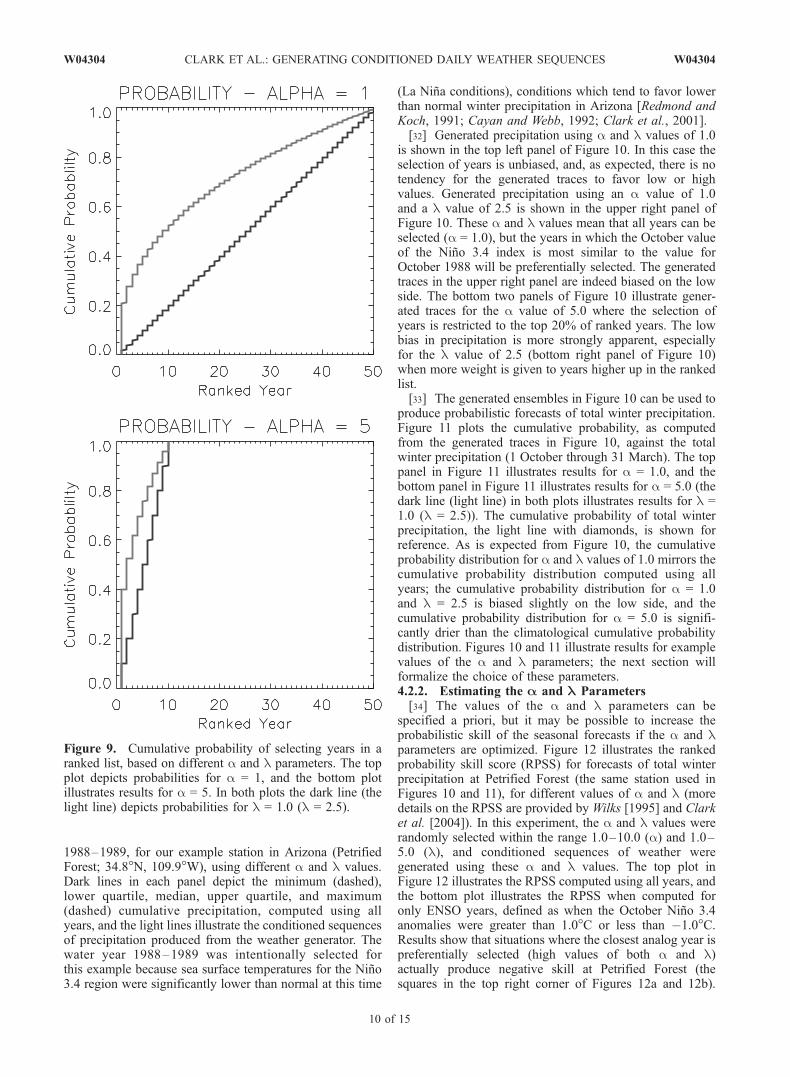
In equation (9), u � U(0, 1) is a random number selectedfrom a uniform distribution ranging from zero to one, l is aweighting parameter, a is a selection parameter, N is thenumber of years in the time series, and INT is the integeroperator. Values of l greater than 1 shift the uniformrandom number closer to zero, meaning years higher in theranked list will be preferentially selected. Values of agreater than 1 will restrict the selection of years to a subsetof years (e.g., if a = 5, attention will be restricted to the top20% of ranked years). The selection of years is unbiased ifboth l and a are equal to 1. The probability of preferentiallyselecting different ranked years for selected a and l valuesis illustrated graphically in Figure 9.[30] This approach is implemented in this study as

follows: (1) Years are ranked in terms of the similarity ofthe October value of the Nino 3.4 index, and (b) equation (9)is applied by selecting iyear 100 times, and using theselection of iyears to obtain the subset of days from which

Figure 6. Comparison of generated and observed lag-1 correlations (top row) and intersite correlations(bottom row) for all stations in the contiguous United States (shown in Figure 1), for the month ofJanuary. The plots show comparisons for precipitation (left column), maximum temperature (middlecolumn), and minimum temperature (right column).

8 of 15


data are resampled. An additional random component isintroduced by using a different random selection of yearsfor each generated day. The Nino 3.4 index represents seasurface temperature (SST) anomalies in the centralequatorial Pacific Ocean (5�N–5�S; 170�W–120�W);strong positive values of the Nino 3.4 index depict El Ninoevents, and strong negative values of the Nino 3.4 indexdepict La Nina events. The use of October Nino 3.4conditions to rank the years means that the generated

precipitation and temperature sequences are conditionedwith respect to SST conditions at the beginning of winter; ifthe SST anomalies persist throughout winter, then they canaffect the wintertime atmospheric circulation (and surfaceclimate) over North America. The generated weathersequences thus can be considered forecasts initialized inOctober.[31] Figure 10 illustrates 50 sequences of cumulative

precipitation conditioned using equation (9) for water year

Figure 7. As in Figure 6, except for the month of July.

Figure 8. Comparison of generated and observed intervariable correlations, for all stations in thecontiguous United States (shown in Figure 1). The plots show correlations between precipitation andmaximum temperature (left column), between precipitation and minimum temperature (middle column),and between maximum temperature and minimum temperature (right column). The top plots depictresults for January, and the bottom plots depict results for July.


9 of 15

W04304

1988–1989, for our example station in Arizona (PetrifiedForest; 34.8�N, 109.9�W), using different a and l values.Dark lines in each panel depict the minimum (dashed),lower quartile, median, upper quartile, and maximum(dashed) cumulative precipitation, computed using allyears, and the light lines illustrate the conditioned sequencesof precipitation produced from the weather generator. Thewater year 1988–1989 was intentionally selected forthis example because sea surface temperatures for the Nino3.4 region were significantly lower than normal at this time

(La Nina conditions), conditions which tend to favor lowerthan normal winter precipitation in Arizona [Redmond andKoch, 1991; Cayan and Webb, 1992; Clark et al., 2001].[32] Generated precipitation using a and l values of 1.0

is shown in the top left panel of Figure 10. In this case theselection of years is unbiased, and, as expected, there is notendency for the generated traces to favor low or highvalues. Generated precipitation using an a value of 1.0and a l value of 2.5 is shown in the upper right panel ofFigure 10. These a and l values mean that all years can beselected (a = 1.0), but the years in which the October valueof the Nino 3.4 index is most similar to the value forOctober 1988 will be preferentially selected. The generatedtraces in the upper right panel are indeed biased on the lowside. The bottom two panels of Figure 10 illustrate gener-ated traces for the a value of 5.0 where the selection ofyears is restricted to the top 20% of ranked years. The lowbias in precipitation is more strongly apparent, especiallyfor the l value of 2.5 (bottom right panel of Figure 10)when more weight is given to years higher up in the rankedlist.[33] The generated ensembles in Figure 10 can be used to

produce probabilistic forecasts of total winter precipitation.Figure 11 plots the cumulative probability, as computedfrom the generated traces in Figure 10, against the totalwinter precipitation (1 October through 31 March). The toppanel in Figure 11 illustrates results for a = 1.0, and thebottom panel in Figure 11 illustrates results for a = 5.0 (thedark line (light line) in both plots illustrates results for l =1.0 (l = 2.5)). The cumulative probability of total winterprecipitation, the light line with diamonds, is shown forreference. As is expected from Figure 10, the cumulativeprobability distribution for a and l values of 1.0 mirrors thecumulative probability distribution computed using allyears; the cumulative probability distribution for a = 1.0and l = 2.5 is biased slightly on the low side, and thecumulative probability distribution for a = 5.0 is signifi-cantly drier than the climatological cumulative probabilitydistribution. Figures 10 and 11 illustrate results for examplevalues of the a and l parameters; the next section willformalize the choice of these parameters.4.2.2. Estimating the A and L Parameters[34] The values of the a and l parameters can be

specified a priori, but it may be possible to increase theprobabilistic skill of the seasonal forecasts if the a and lparameters are optimized. Figure 12 illustrates the rankedprobability skill score (RPSS) for forecasts of total winterprecipitation at Petrified Forest (the same station used inFigures 10 and 11), for different values of a and l (moredetails on the RPSS are provided by Wilks [1995] and Clarket al. [2004]). In this experiment, the a and l values wererandomly selected within the range 1.0–10.0 (a) and 1.0–5.0 (l), and conditioned sequences of weather weregenerated using these a and l values. The top plot inFigure 12 illustrates the RPSS computed using all years, andthe bottom plot illustrates the RPSS when computed foronly ENSO years, defined as when the October Nino 3.4anomalies were greater than 1.0�C or less than �1.0�C.Results show that situations where the closest analog year ispreferentially selected (high values of both a and l)actually produce negative skill at Petrified Forest (thesquares in the top right corner of Figures 12a and 12b).

Figure 9. Cumulative probability of selecting years in aranked list, based on different a and l parameters. The topplot depicts probabilities for a = 1, and the bottom plotillustrates results for a = 5. In both plots the dark line (thelight line) depicts probabilities for l = 1.0 (l = 2.5).

10 of 15


Positive skill occurs in situations in which the weightingfunction is relaxed (Figure 12b). The shuffled complexevolution (SCE) method of Duan et al. [1992, 1993, 1994]was used to optimize the a and l parameters by maximizingthe RPSS (restricting attention to ENSO years). The SCEoptimization provided parameter values of a = 5.550 andl = 1.106 (RPSS = 0.365).[35] Attention is now directed to optimizing a and l

parameters for forecast applications. Figure 12 illustratesthe dependence of probabilistic forecast skill on thestrength of ENSO conditions; RPSS values are muchhigher when attention is restricted to ENSO years (El Ninoplus La Nina). This is fairly intuitive. In years where there

is weak ENSO forcing, assigning more weight to years thathave similar values of the Nino 3.4 index is unlikely toresult in an increase in probabilistic forecast skill. In otherwords, the a and l parameters should depend on thestrength of the Nino 3.4 index. The a and l parametersshould therefore be optimized locally, using years wherethe value of the Nino 3.4 index is similar to the year beingforecast.[36] The SCE optimization program [Duan et al., 1992,

1993, 1994] was configured to maximize the RPSS valuefor the 10 years in which values of the Nino 3.4 index aremost similar to the year being forecast. For a given wateryear, a function evaluation for a given a and l parameter set

Figure 10. Fifty generated ensemble members of cumulative precipitation for water year 1988–1989,for the example station in Arizona used for Figure 3 (Petrified Forest; 34.8�N, 109.9�W), for differenta and l parameters.


11 of 15

W04304

involves (1) generating probabilistic forecasts of total winterprecipitation, based on an ensemble of 50 generated weathersequences (1 October through 31 March) for each of the10 years that have the most similar Nino 3.4 conditions, and(2) calculating the RPSS value for these 10 probabilisticforecasts. Function evaluations are repeated until the globaloptimal RPSS value is identified, or after 200 functionevaluations, whichever occurs first. Results are crossvalidated; that is, data for a given water year are not usedto estimate the a and l parameters that are used to producethe optimized generated weather sequence for that wateryear. The optimization program has a high computational

Figure 12. Topology of the ranked probability skill score(RPSS) score, using different a and l parameters, for thePetrified Forest station in Arizona (34.8�N, 109.9�W). Thetop plot depicts RPSS values computed using all years;the bottom plot depicts RPSS values computed using ElNino-Southern Oscillation (ENSO) years (defined as whenthe October value of the Nino 3.4 index was >1.0�C or<�1.0�C).

Figure 11. Probabilistic forecasts of total winter precipita-tion (1 October through 31 March) for water year 1988–1989, for Petrified Forest (34.8�N, 109.9�W), for differenta and l parameters. See text for further details.

12 of 15


burden, which was reduced by limiting the maximumnumber of function evaluations to 200, by restrictinganalysis to ENSO years, and by restricting attention to thestations in the contiguous United States where thecorrelation between the October value of the Nino 3.4index and total 1 October through 31 March precipitationexceeds 0.5 (92 stations).[37] Figure 13 compares the RPSS values using opti-

mized a and l parameters against RPSS values for thedefault a and l parameters used in previous figures.Recall that analysis is restricted to ENSO years. Eachsymbol in Figure 13 illustrates the probabilistic forecastskill for a station in the contiguous United States thatmeets the selection criteria defined above. On the whole,the optimized a and l parameters provide generatedweather sequences with higher probabilistic skill than thedefault parameters of a = 1.0 and l = 2.5 (top plot inFigure 13). However, the default parameters of a = 5.0and l = 1.0 and a = 5.0 and l = 2.5 (middle and bottomplots in Figure 13) provide generated weather sequenceswith equivalent probabilistic forecast skill to the optimizeda and l parameters. The lower optimized RPSS valuescan be interpreted as arising from situations where thesample size is insufficient to provide stable a and lestimates. Results suggest parameters of a = 5.0 and l =2.5 can be effectively used to condition the weathergenerator on ENSO indices.

5. Summary and Discussion

[38] A new approach for generating weather has beenintroduced that preserves the mean, standard deviation, andskewness of the generated precipitation and temperaturesequences, while also preserving the temporal persistenceand intersite and intervariable correlations. The methodresamples data from the historical record ‘‘nens’’ times(nens is the number of ensemble members), and reordersthe ensemble members to reconstruct the observed space-time variability in precipitation and temperature fields. Theweather generator method has been applied to 2307stations in the contiguous Unites States. When generatedsequences are examined for all of these stations, resultsshow that the weather generator reproduces the summarystatistics (mean, standard deviation, skewness) very well.Intersite correlations from the weather generator are slightlylower than observed intersite correlations, due to difficul-ties in accurately reproducing the intermittent properties ofprecipitation [see also Clark et al., 2004]. Intersitecorrelations for temperature are preserved very well. Insummary, the weather generator reproduces the statisticalmoments at individual stations well and acceptably

Figure 13. Comparison of the RPSS when weathersequences are generated using optimized a and lparameters, and when weather sequences are generatedusing default a and l parameters. The plots illustrate resultsfor the parameters a = 1.0 and l = 2.5, a = 5.0 and l = 1.0,and a = 5.0 and l = 2.5, for the top, middle, and bottomplots, respectively. Results are shown for the 92 stations inthe contiguous United States where the correlation betweenthe October value of the Nino 3.4 index and total winterprecipitation exceeds 0.5.


13 of 15

W04304

duplicates the observed lag-1, intersite, and intervariablecorrelations.[39] Methods are introduced to extend the weather

generator model to generate weather sequences that reflectEl Nino and La Nina conditions. Instead of resamplingdata from all years in the historical record, data arepreferentially resampled from a set of years that are similarin terms of values of the Nino 3.4 index. The resultant setof years are identified using weighting and selectionparameters. The weighting parameter gives more weightto years higher up in the ranked list, and the selectionparameter restricts attention to a subset of years (e.g., thetop 20% of years in the ranked list). The weighting andselection parameters are optimized, and default parametersare suggested for future studies. Example forecasts areprovided for a station in Arizona (Petrified Forest; 34.8�N,109.9�W) where El Nino and La Nina conditions have astrong effect on winter precipitation. The conditionedweather sequences generated using the methods describedin this paper are appropriate for use as input to hydrologicmodels to produce multiseason forecasts of streamflow.Future work will assess the skill of multiseason hydrologicforecasts in numerous small river basins in the contiguousUnites States.[40] It is possible to use the a and l parameters

discussed in this paper to produce climate change scenar-ios (e.g., by ranking years from warmest to coldest, as

done by Yates et al. [2003]). However, it is recommendedthat this be done cautiously. When conditioning is based ona list of years that are ranked from warmest to coldest, the aand l parameters will alter not only the mean of thedistribution, but the standard deviation and skewness aswell. This may not be desired. For example, Figure 14shows the interannual standard deviation of Januarymaximum temperature at Petrified Forest, constructed usingdifferent a and l values. As expected, the standarddeviation decreases when the selection of data is biasedtoward warm years. If the standard deviation and skewnessare important attributes for the construction of climatechange scenarios, then alternative methods for conditioningthe weather generator must be developed and used. Moreresearch is needed in this area.

[41] Acknowledgments. This work is part of a collaborative effortbetween the University of Colorado and the Colorado Basin River ForecastCenter that seeks to improve operational streamflow forecasts on intra-seasonal to seasonal timescales. The work was funded by the NationalOceanic and Atmospheric Administration (NOAA) Office of Global Pro-grams (OGP) under awards NA16GP1587 and NA17RJ1229. The authorsare grateful to Marina Timofeyeva for comments on an earlier draft of thismanuscript.

ReferencesBuishand, T. A., and T. Brandsma (2001), Multisite simulation of dailyprecipitation and temperature in the Rhine basin by nearest neighborresampling, Water Resour. Res., 37, 2761–2776.

Cayan, D. R., and R. H. Webb (1992), El Nino/Southern Oscillation andstreamflow in the western United States, in El Nino: Historical andPaleoclimatic Aspects of the Southern Oscillation, edited by H. Diazand V. Markgraf, pp. 29–68, Cambridge Univ. Press, New York.

Clark, M. P., M. C. Serreze, and G. J. McCabe (2001), Historical effects ofEl Nino and La Nina events on the seasonal evolution of the montanesnowpack in the Columbia and Colorado River Basins, Water Resour.Res., 37, 741–757.

Clark, M. P., S. Gangopadhyay, L. E. Hay, B. Rajagopalan, and R. L. Wilby(2004), The Schaake shuffle: A method for reconstructing space-timevariability in forecasted precipitation and temperature fields, J. Hydro-meteorol., 5, 243–262.

Connelly, B. A., D. T. Braatz, J. B. Halquist, M. M. DeWeese, L. Larson,and J. J. Ingram (1999), Advanced hydrologic prediction system,J. Geophys. Res., 104(D16), 19,655–19,660.

Day, G. N. (1985), Extended streamflow forecasting using NWSRFS,J. Water. Resour. Plann. Manage., 111, 157–170.

Duan, Q., S. Sorooshian, and V. K. Gupta (1992), Effective and efficientglobal optimization for conceptual rainfall-runoff models, Water Resour.Res., 28, 1015–1031.

Duan, Q., V. K. Gupta, and S. Sorooshian (1993), A shuffled complexevolution approach of effective and efficient optimization, J. Optim.Theory Appl., 76, 501–521.

Duan,Q., S. Sorooshian, andV.K.Gupta (1994), Optimal use of the SCE-UAglobal optimization method for calibrating watershed models, J. Hydrol.,158, 265–284.

Efron, B. (1979), Bootstrap methods: Another look at the jackknife, Ann.Stat., 7, 1–26.

Eischeid, J. K., P. A. Pasteris, H. F. Diaz, M. S. Plantico, and N. J. Lott(2000), Creating a serially complete, national daily time series of tem-perature and precipitation for the western United States, J. Appl.Meteorol., 39, 1580–1591.

Foufoula-Georgiou, E., and D. P. Lettenmaier (1987), A Markov renewalmodel for rainfall occurrences, Water Resour. Res., 23, 875–884.

Gabriel, K. R., and J. Neumann (1962), A Markov chain model fordaily rainfall occurrence at Tel Aviv, Q. J. R. Meteorol. Soc., 88,90–95.

Hamlet, A. F., and D. P. Lettenmaier (1999), Columbia River streamflowforecasting based on ENSO and PDO climate signals, J. Water Resour.Plann. Manage., 125, 333–341.

Hay, L. E., G. J. McCabe, D. M. Wolock, and M. A. Ayers (1991), Simula-tion of precipitation by weather-type analysis, Water Resour. Res., 27,493–501.

Figure 14. Interannual standard deviation of Januarymaximum temperature at Petrified Forest, for different aand l parameters, for the case where years at PetrifiedForest are ranked from warmest to coldest. The plotillustrates results for l values ranging from 1.0 to 5.0; thedark line with diamonds shows results for a = 1.0, and thelight line with triangles shows results for a = 5.0. The thickhorizontal light line depicts the observed interannualstandard deviation in January maximum temperature atPetrified Forest.

14 of 15


Jothityangkoon, C., M. Sivapalan, and N. R. Viney (2000), Tests of a space-time model of daily rainfall in southwestern Australia based on nonho-mogeneous random cascades, Water Resour. Res., 36, 267–284.

Rajagopalan, B., andU. Lall (1999), A k-nearest neighbor simulator for dailyprecipitation and other variables, Water Resour. Res., 35, 3089–3101.

Redmond, K. T., and R. W. Koch (1991), Surface climate and streamflowvariability in the western United States and their relationship with large-scale circulation indices, Water Resour. Res., 27, 2381–2399.

Reek, T., S. R. Doty, and T. W. Owen (1992), A deterministic approach tothe validation of historical daily temperature and precipitation data fromthe cooperative network, Bull. Am. Meteorol. Soc., 73, 753–762.

Todorovic, P., and D. A. Woolhiser (1975), A stochastic model of n-dayprecipitation, J. Appl. Meteorol., 14, 17,024.

Wilks, D. S. (1995), Statistical Methods in the Atmospheric Sciences: AnIntroduction, 467 pp., Academic, San Diego, Calif.

Wilks, D. D. (1998), Multi-site generalizations of a daily stochastic weathergeneration model, J. Hydrol., 210, 178–191.

Wilks, D. S., and R. L. Wilby (1999), The weather generation game: Areview of stochastic weather models, Prog. Phys. Geogr., 23, 329–357.

Yates, D., S. Gangopadhyay, B. Rajagopalan, and K. Strzepek (2003),A technique for generating regional climate scenarios using a nearest

neighbor algorithm, Water Resour. Res., 39(7), 1199, doi:10.1029/2002WR001769.

Young, K. C. (1994), A multivariate chain model for simulating climaticparameters from daily data, J. Appl. Meteorol., 33, 661–671.

��D. Brandon and K. Werner, Colorado Basin River Forecast Center, 2242

W North Temple, Salt Lake City, UT 84116, USA.

M. P. Clark and S. Gangopadhyay, Center for Science and TechnologyPolicy Research, Cooperative Institute for Research in EnvironmentalSciences, 1333 Grandview Avenue, Campus Box 488, University ofColorado, Boulder, CO 80309-0488, USA. ([email protected])

L. Hay, United States Geological Survey, Water Resources Division, Box25046, MS 412, Denver Federal Center, Lakewood, CO 80225, USA.

B. Rajagopalan, Department of Civil, Environmental, and ArchitecturalEngineering, Campus Box 428, University of Colorado at Boulder,Boulder, CO 80309-0428, USA.

D. Yates, Research Applications Program, National Center for Atmo-spheric Research, 3450 Mitchell Lane, Boulder, CO 80301, USA.


15 of 15

W04304

A resampling procedure for generating conditioned daily weather sequences

Documents

Transcript of A resampling procedure for generating conditioned daily weather sequences