A Vervaat-like path transformationfor the re ected Brownian bridgeconditioned on its local time at 0Philippe Chassaing1 & Svante Janson2October 19, 1999AbstractWe describe a Vervaat-like path transformation for the re ected Brownian bridgeconditioned on its local time at 0: up to random shifts, this process equals the twoprocesses constructed from a Brownian bridge and a Brownian excursion by addinga drift and then taking the excursions over the current minimum. As a consequence,these three processes have the same occupation measure, which is easily found.The three processes arise as limits, in three di�erent ways, of pro�les associated tohashing with linear probing, or, equivalently, to parking functions.1 IntroductionWe regard the Brownian bridge b(t) and the normalized (positive) Brownian excursione(t) as de�ned on the circle R=Z, or, equivalently, as de�ned on the whole real line, beingperiodic with period 1. We de�ne, for a � 0, the operator a on the set of boundedfunctions on the line byaf(t) = f(t)� at� inf�1<s�t(f(s)� as)= sups�t (f(t)� f(s)� a(t� s)): (1.1)If f has period 1, then so has af ; thus we may also regard a as acting on functions onR=Z. Evidently, af is nonnegative.In this paper, we prove that, for every a � 0, the three following processes can beobtained (in law) from each other by random shifts, that we will describe explicitly:� Xa, which denotes the re ecting Brownian bridge jbj conditioned to have local timeat level 0 equal to a;� Ya = ab ;� Za = ae.We will �nd convenient to use the following formulas for Ya and Za:Ya(t) = b(t)� at+ supt�1�s�t(as� b(s)); (1.2)Za(t) = e(t)� at+ supt�1�s�t(as� e(s)): (1.3)1Institut Elie Cartan, BP 239, 54 506 Vandoeuvre Cedex, France.2Uppsala University, Department of Mathematics, PO Box 480, 751 06 Uppsala, Sweden1

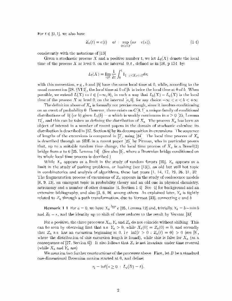
For t 2 [0; 1], we also haveZa(t) = e(t)� at+ sup0�s�t(as� e(s)); (1.4)consistently with the notations of [13].Given a stochastic process X and a positive number t, we let Lt(X) denote the localtime of the process X at level 0, on the interval [0; t], de�ned as in [10, p.154] by:Lt(X) = lim"#0 12" Z t0 1f�"<Xs<"gds;with this convention, e.g., b and jbj have the same local time at 0, while, according to theusual convention [28, xVI.2], the local time at 0 of jbj is twice the local time at 0 of b. Whenpossible, we extend L(X) to t 2 (�1; 0), in such a way that Lb(X) � La(X) is the localtime of the process X at level 0, on the interval [a; b], for any choice �1 < a < b < +1.The de�nition above of Xa is formally not precise enough, since it involves conditioningon an event of probability 0. However, there exists on C[0; 1] a unique family of conditionaldistributions of jbj (or b) given L1(b) = a which is weakly continuous in a � 0 [25, Lemma12], and this can be taken as de�ning the distribution of Xa. The process Xa has been anobject of interest in a number of recent papers in the domain of stochastic calculus: itsdistribution is described in [27, Section 6] by its decomposition in excursions. The sequenceof lengths of the excursions is computed in [7], using [24]. The local time process of Xais described through an SDE in a recent paper [25] by Pitman, who in particular provesthat, up to a suitable random time change, the local time process of Xa is a Bessel(3)bridge from a to 0 [25, Lemma 14]. (See also [5], where a Brownian bridge conditioned onits whole local time process is decribed.)While Xa appears as a limit in the study of random forests [25], Za appears as alimit in the study of parking problems, or hashing (see [13]), an old but still hot topicin combinatorics and analysis of algorithms, these last years [1, 14, 17, 19, 26, 31, 32].The fragmentation process of excursions of Za appears in the study of coalescence models[8, 9, 13], an emergent topic in probability theory and an old one in physical chemistry,astronomy and a number of other domains [4, Section 1.4]. See [4] for background and anextensive bibliography, and also [3, 6, 16] among others. As explained later, Ya is tightlyrelated to Za through a path transformation, due to Vervaat [33], connecting e and b.Remark 1.1 For a = 0, we have X0 law= e [25, Lemma 12] and, trivially, Y0 = b�min band Z0 = e, and the identity up to shift of these reduces to the result by Vervaat [33].For a positive, the three processesXa, Ya and Za do not coincide without shifting. Thiscan be seen by observing �rst that a.s. Ya > 0, while Xa(0) = Za(0) = 0, and secondlythat Za a.s. has an excursion beginning at 0, i.e. infft > 0 : Za(t) = 0g > 0 (see [8],where the distribution of this excursion length is found), while this is false for Xa (as aconsequence of [27, Section 6]). It also follows that Za is not invariant under time reversal(while Xa and Ya are).We mention two further constructions of the processes above. First, let B be a standardone-dimensional Brownian motion started at 0, and de�ne:�t = inffs � 0 : Ls(B) = tg:2

Then Xa can also be seen as the re ected Brownian motion jBj conditioned on �a = 1, seee.g. [25, the lines following (11)] or [27, identity (5.a)].Secondly, de�ne ~b(t) = b(t) � R 10 b(s) ds. It is easily veri�ed that ~b is a stationaryGaussian process (on R=Z or on R), for example by calculating its covariance functionCov(~b(s);~b(t)) = 1� 6js� tj(1� js� tj)12 ; js� tj � 1:Since b and ~b di�er only by a (random) constant, Ya = a(~b) too. This implies that Ya isa stationary process. (Xa and Za are not, again because they vanish at 0.)We may similarly de�ne ~e(t) = e(t) � R 10 e(s) ds, and obtain Za = a(~e), but we donot know any interesting consequences of this.Precise statements of the relations between the three processes Xa, Ya and Za aregiven in Section 2. The three processes arise as limits, under three di�erent conditions,of pro�les associated with parking schemes (also known as hashing with linear probing).This is described in Sections 3 and 4. The proofs are given in the remaining sections.2 Main resultsIn this section we give precise descriptions of the shifts connecting the three processes Xa,Ya and Za, in all six possible directions. Let a � 0 be �xed.First, assume that the Brownian bridge b is built from e using Vervaat's path trans-formation [10, 11, 33]: given a uniform random variable U , independent of e,b(t) = e(U + t)� e(U): (2.1)Then ab(t) = ae(U + t);so that:Theorem 2.1 For U uniform and independent of Za,Za(U + �) law= Ya:As a consequence, Ya is a stationary process on the line, or on the circle R=Z, as was seenabove in another way. A far less obvious result is:Theorem 2.2 For U uniform on [0; 1] and independent of Xa,Xa(U + �) law= Ya:The proof will be given later. The case a = 0 of Theorem 2.2 is just Vervaat's pathtransformation, since, as remarked above, X0 law= e. In [10], one can �nd a host of similarpath transformations connecting the Brownian bridge, excursion and meander.3

Corollary 2.3 The occupation measures of Xa, Ya and Za coincide, and have thedistribution function 1� e�2ax�2x2 :This is also the distribution function of Ya(t) for any �xed t.Recall that a random variable W is Rayleigh distributed if Pr(W � x) = e�x2=2. Theoccupation measure of Xa (or Ya, Za) is then the law of half the residual life at time a ofW : Pr((W � a)=2 � x jW � a) = e�2ax�2x2 . For a = 0 we recover the Durrett{Iglehartresult for the occupation measure of the Brownian excursion: it is the law of W=2 [15].Proof of Corollary 2.3. By de�nition, the occupation measure of Xa is the law ofXa(U), so, from Theorem 2.2, it is also the law of Ya(0). The same is true for Za byTheorem 2.1, and for Ya because it is stationary. We haveYa(0) = sup�1�s�0(as� b(s))law= sup0�t�1(b(t)� at)law= sup0�t�1((1 � t)B t1�t � at)= sup0�u�+1�Bu � au1 + u �:For positive numbers � and �, setT�;� = inffu � 0;Bu � �u+ �g:Using the exponential martingale exp(2�Bu � 2�2u), it is easy to derive thatPr(T�;� < +1) = e�2��;see [28, Exercise II.3.12]. We have thus:Pr(Ya(0) � x) = Pr�9 u � 0 such that Bu � au1 + u � x�= Pr(Ta+x;x < +1)= e�2ax�2x2 : }Problem 2.4 What are the laws of Xa(t) and Za(t) (which depend on t)?We need an additional notation to de�ne a random shift from Ya or Za to Xa: letT (X) denote the inverse process of L(X).Theorem 2.5 Suppose a > 0. Let U be uniformly distributed on [0; 1] and independentof Za or Ya. Set � = TaU (Za);~� = TaU (Ya):4

We have: Xa law= Za(� + �)law= Ya(~� + �):Note that as a di�erence with Theorems 2.1 and 2.2, here � (resp. ~�) depends on Za (resp.Ya).Thus we obtain Xa by shifting any of the processes uniformly in local time, while wehave seen above that we obtain Ya by shifting uniformly in real time.Theorem 2.6 Suppose a > 0.(i). Almost surely, t 7! Lt(Xa) � at reaches its maximum at a unique point V in [0; 1)and Xa(V + �) law= Za:(ii). Almost surely, t 7! Lt(Ya) � at reaches its maximum at a unique point ~V in [0; 1)and Ya( ~V + �) law= Za:Moreover, ~V is uniform on [0; 1] and independent of Ya( ~V + �).In contrast, and as an explanation, t 7! Lt(Za) � at reaches its maximum at 0, see theproof in Section 11. It is easily veri�ed that V is not uniformly distributed.Remark 2.7 For a = 0, Theorems 2.5 and 2.6 hold if we instead de�ne � = 0, V = 0and ~� = ~V as the unique points where Z0, X0 and Y0, respectively, attain their minimumvalue 0, see Remark 1.1.Finally, we observe that it is possible to invert a and recover the Brownian bridge bfrom Ya = ab and the excursion e from Za = ae using local times.Theorem 2.8 For any t,b(t) = Ya(t)� Ya(0)� Lt(Ya) + atand e(t) = Za(t)� Lt(Za) + at:Combining Theorems 2.6 and 2.8, we can construct Brownian excursions from Xa andYa too.Corollary 2.9 Let V and ~V be as in Theorem 2.6. Thene0(t) = Xa(V + t) + at� LV+t(Xa) + LV (Xa)and e00(t) = Ya( ~V + t) + at� L ~V+t(Ya) + L ~V (Ya);respectively, de�ne normalized Brownian excursions.In the case of Ya, in addition, e00 and ~V are independent.The problem of possible other shifts is adressed in the concluding remarks.5

3 Parking schemes and associated spacesA parking scheme ! describes how m cars c1, c2, . . . park on n places f1; 2; : : : ; ng. Wewrite ! = (!k)1�k�m;where each !k 2 f1; : : : ; ng. According to !, car c1 parks on place !1. Then car c2 parkson place !2 if !2 is still empty, else it tries !2 + 1, !2 + 2, . . . , until it �nds an emptyplace, and so on. We adopt the convention that n+ 1 = 1, and more generally n+ k = k.We consider only the case 1 � m < n.14 12 4 3

6

678 9

9

10

11 11

11

12

13

5 12

13

13

14

14

15

16

1617 1819 20

21

22

23

24

20

2121 21 21 21

14 12 4 3

6

678 9

9

10

11 11

11

12

13

5 12

13

13

14

14

15

16

1617 1819 2021

2121 21 21 21

14 12 4 3

6

678 9

9

10

11 11

11

12

13

5 12

13

13

14

14

15

16

1617 1819 202122

22

23 23 2323 23 23

23 232121 21 21 21

14 12 4 3

6

68 10

11 11

11

12

5 12

14

14

15

16

1617 1819 202122

22 9

7 9

23

23

23

23

13

13

13

23 23 2323 23 23

23 232121 21 21 21

14 12 4 3

6

68 10

11 11

11

12

5 12

14

14

15

16

1617 1819 202122

22 9

7 9

23

23

23

23

13

13

13

24 24

24 24 2424 24

24

24

24 24

24

24

24

24Figure 1: Elements of P25;m, m = 20; � � � ; 24.The interest of combinatorists to parking schemes is born from a paper by Konheim& Weiss [21], in 1966, about hashing with linear probing, a popular search method, thathad also been studied, notably, by Don Knuth, in 1962 (see the historical notes in his 1999paper [19], or pages 526{539 in his book [18]). The metaphore of parking was already usedby Konheim & Weiss. The two recent and beautiful papers by Flajolet, Poblete & Viola[17] and Knuth [19] drew the attention of the authors to the connection between parkingschemes and Brownian motion (see also [13, 14]). For a similar connection between treesand Brownian motion, see [2, 6, 25, 30], among others.Let Pn;m denote the set of all parking schemes of m cars on n places, and let CPn;mdenote the subset of con�ned parking schemes, con�ned meaning that the last place is6

assumed to be left empty. We have#Pn;m = nm and #CPn;m = nm�1(n�m);the last can be seen as follows. For ! 2 Pn;m, we de�ne the shift (rotation)r! = (�1 + !k)1�k�m;moving all cars back one place (modulo n); the action of r on Pn;m draws nm�1 orbits ofn elements, each of them containing n�m elements of CPn;m.Let Yk(!) be the number of cars whose �rst try is on place k, according to ! 2 Pn;m.For any natural integer k, set Sk+1(!) = Sk(!) + Yk+1(!);with S0(!) = 0. Our convention extends to Yk+n = Yk, so that Sk+n = Sk +m. Set:W (!; i) = Si(!)� imn ; (3.1)and note that W (!; k + n) =W (!; k). We haveProposition 3.1 There exists at least an element of CPn;m, x(�), in each orbit �,such that W (x(�); �) is nonnegative.Proof. Let ! denote an element of Pn;m. Since S(rj!; k) = S(!; k + j) � S(!; k)and thus W (rj!; k) = W (!; k + j) � W (!; k), W (rj!; �) is nonnegative if and only ifW (!; j) = minkW (!; k). This proves that x(�) = rj! exists in Pn;m. We postpone theproof that in fact rj! 2 CPn;m to Proposition 5.4 (see also [13]). }In general, in the same orbit � , there are several elements z such that W (z; �) isnonnegative: we let x(�) be one particular choice, and let En;m be the set of the nm�1elements x(�). (This set is thus to some extent arbitrary, but the results below hold forany choice.)4 Convergence resultsFor ! in Pn;m, let Hk(!) denote the number of cars that try, successfully or not, to parkon place k. (We regard Hk as de�ned for all integers k, with Hk+n = Hk.) We rescale Hkhn(t)

t

128 7 9

912

13

5 12

13

13 4 3

6

6

11 11

11

14

14

14 15 10

16

16

Figure 2: Pro�le.7

and de�ne hn(k=n; !) = Hk(!)=pn; hn is then extended to a continuous periodic functionon R, that we call the pro�le of !, by linear interpolation, i.e.hn(t; !) = (1 + bntc � nt)Hbntc(!) + (nt� bntc)H1+bntc(!)pn :Let �n;` (resp. ~�n;`, �n;`) denote the law of (hn(t))0�t�1 when ! is drawn at random inPn;n�` (resp. CPn;n�`, En;n�`).Central to our results are the following theorems:Theorem 4.1 If `=pn! a � 0, then�n;` weakly�! Ya:Theorem 4.2 If `=pn! a � 0, then~�n;` weakly�! Xa:Theorem 4.3 If `=pn! a � 0, then�n;` weakly�! Za:Theorem 4.3 was also proved, by similar methods, in [13, Lemma 5.11].As will be seen in detail later, Theorems 2.1 and 2.2 can be seen as consequences ofthe preceding convergence results, combined with the evident relationhn(t; rj!) = hn�t+ jn; !�and with the following obvious statement: the random rotation of a random element ofCPn;m or of En;m gives a random element of Pn;m. More formally:Proposition 4.4 If ! is random uniform on Pn;m, CPn;m or on En;m, and U isuniform on [0; 1] and independent of !, then rdnUe! is random uniform on Pn;m.A di�erent kind of random rotation gives Theorem 2.5: let ! be random in Pn;m or inEn;m and choose randomly an empty place j of !. Then rj! is random in CPn;m. Moreformally, let us de�ne an operator R from Pn;m to CPn;m as shifting to the next emptyplace: R! = rj!;where j � 1 is the �rst place left empty by !. Thus Rd(n�m)Ue! (with U random uniform)is a rotation of ! to a random empty place, i.e. to a random element of the correspondingorbit in CPn;m, and we have:Proposition 4.5 If ! is random uniform on Pn;m, CPn;m or on En;m, and U isuniform on [0; 1] and independent of !, then Rd(n�m)Ue! is random uniform on CPn;m.8

For Theorem 2.5 we use also the convergence of the number of empty places in a giveninterval of f1; 2; : : : ; ng to the local time of Xa, Ya or Za in the corresponding interval of[0; 1].More precisely, let Vj;k(!) denote the number of empty places in the set fj + 1; j +2; : : : ; kg, according to the parking scheme !, and de�ne, in analogy with hn above, acorresponding continuous function vn on [0; 1] by rescaling and linear interpolation sothat vn(k=n) = V0;k=pn for integers k, i.e.vn(t; !) = (1 + bntc � nt)V0;bntc(!) + (nt� bntc)V0;1+bntc(!)pn ; 0 � t � 1:We then have the following extension of Theorems 4.1{4.3, yielding joint convergence ofthe processes hn and vn.Theorem 4.6 Suppose `=pn! a � 0. On [0; 1], the following hold:(i). If ! is drawn at random in Pn;n�`, then (hn(�; !); vn(�; !)) law�! (Ya; L(Ya)).(ii). If ! is drawn at random in CPn;n�`, then (hn(�; !); vn(�; !)) law�! (Xa; L(Xa)).(iii). If ! is drawn at random in En;n�`, then (hn(�; !); vn(�; !)) law�! (Za; L(Za)).5 Results on parking schemesConsider a �xed ! 2 Pn;m. As remarked above, we regard the functions Yk, Sk, W (!; k)and Hk as de�ned for all integers k; Sk+n = Sk +m and the three others have period n.Note that, among the cars that visit place k, only one will not visit place k + 1, so:Proposition 5.1 Hk+1 = (Hk � 1)+ + Yk+1:This recursion does not de�ne fully Hk, given (Yk)0�k�n, as the recursion starts nowhere.In order to circumvent this di�culty, we have to �nd a place left empty by !. Let�k = maxi�k (i� Si) = max�n+k<i�k(i� Si): (5.1)Proposition 5.2 For a given ! and place k, there are two cases:(i). k is left empty, Hk = 0, k � Sk = �k�1 + 1 and �k = �k�1 + 1.(ii). k is occupied, Hk � 1, k � Sk � �k�1 and �k = �k�1.Proof. Clearly k is left empty if and only if Hk = 0.Next, observe that if Sk�Sj � k� j for some j < k, then at least k� j cars have triedto park after j, and there is not room enough for all of them to park on fj+1; : : : ; k� 1g,so one of them will park on k. Conversely, suppose that some car parks on k, and let j bethe last empty place before k. Then the k � j places fj + 1; : : : ; kg are all occupied, andthe cars on them must all have made their �rst try in the same set, so Sk � Sj � k � j.9

Consequently, k is empty if and only if Sk�Sj < k�j for all j < k, which is equivalentto k � Sk > maxj<k(j � Sj) = �k�1 and thus also to �k > �k�1.Finally, note that always k�Sk � k�Sk�1 � 1+�k�1, and thus �k�1 � �k � �k�1+1.} This leads to an explicit formula for Hk, given Yk.Proposition 5.3 For any integer k,Hk = 1 + Sk � k +�k�1:Proof. First observe that by Proposition 5.2, both sides vanish if k is empty. We thenproceed by induction, beginning at any empty place (both sides have period n). Goingfrom k to k + 1, if k is occupied, then the left hand side increases by Proposition 5.1 byHk+1�Hk = Yk+1� 1 while the right hand side increases by Yk+1� 1+�k��k�1, whichby Proposition 5.2 equals Yk+1 � 1 too. Similarly, if k is empty, then both sides increaseby Yk. Hence the equality holds for every k. }We can also now complete the proof of Proposition 3.1.Proposition 5.4 If W (!; j) = minkW (!; k), then place j is empty.Proof. For every i < j,Sj � Si =W (!; j)�W (!; i) + (j � i)mn � (j � i)mn < j � iand thus j�Sj > maxi<j(i�Si) = �j , so the result follows by Proposition 5.2. }Let Vj;k(!) denote the number of empty places in the set fj+1; j+2; : : : ; kg, accordingto the parking scheme !. As another immediate consequence of Proposition 5.2 we obtain:Proposition 5.5 For j � k, Vj;k = �k ��j:Further similar results are given in [13, Section 5].We end this section with a discrete analog of Theorem 2.6, which would lead to a proofof Theorem 2.6 through the convergence theorems of Section 4. The proof of Theorem 2.6that we give is however more direct, and we will not use this result in the sequel.For ! in Pn;m, and k � 0, let C(!; k) be de�ned by:C(!; k) = k(n�m)n � V0;k(!):Clearly C(!; k+n) = C(!; k), and we may use this to extend the de�nition to all integersk. Proposition 5.6 For ! in Pn;m, assertions C(!; j) = mink C(!; k) and W (!; j) =minkW (!; k) are equivalent. For ! in En;m, C(!; �) is nonnegative.10

Proof. According to Proposition 5.4, W (!; j) = minkW (!; k) insures that place j isempty. The �rst assertion also insures that place j is empty, since it implies C(!; j� 1) �C(!; j) and thus V0;j > V0;j�1.As a simple consequence of Propositions 5.2 and 5.5, see also [13], for an empty placej and for k � j, we have:Vj;k = maxj�i�k(i� Si)� j + Sj= maxj�i�k�W (!; j)�W (!; i) + (i� j)n�mn �:As a consequence, for k � j, we have:C(!; k)� C(!; j) = (k � j)(n�m)n � V j; k= minj�i�k�(k � i)(n�m)n +W (!; i)�W (!; j)�� W (!; k)�W (!; j):By periodicity, the inequality persists for all integers j and k. This shows �rst that ifj is a minimum point for C, so that the left hand side is nonnegative for all k, then jis a minimum point for W too. Moreover, if there is another minimum point k for W ,then W (!; k) =W (!; j), and the inequality shows that C(!; k) = C(!; j), so k is anotherminimum point for C too.The �nal assertion follows because if ! 2 En;m, then 0 is a minimum point for W , andthus also for C, and C(!; 0) = 0. }6 Convergence results: proofs6.1 Proof of Theorem 4.1.Let U (m) = (U (m)k )1�k�m denote a sequence of m independent random variables, uniformon [0; 1]. For m � n, the sequence U (m) generates the parking scheme !(m) 2 Pn;m de�nedby !(m)k = dnU (m)k e:The nm possible parking schemes generated this way are clearly equiprobable.Consider the empirical process �m(t) associated with U (m), de�ned on [0; 1] by�m(t) = m�1=2(#fk : U (m)k � tg �mt): (6.1)As m ! 1, the processes �m converge in distribution, as random elements of the spaceD[0; 1], to a Brownian bridge [12, Theorem 16.4]. Due to the Skorohod representationtheorem, see e.g. [29, II.86.1], we may thus assume that the variables U (m) are such that,as m!1, �m(t)! b(t); uniformly on [0; 1]: (6.2)11

We have m = n � ` = n � anpm, where an ! a. Then, by (3.1), for any integer j(extending �m periodically),W (!(m); j) = pm �m� jn�; (6.3)Sj � j = pm ��m� jn�� an jn�: (6.4)Hence, as n!1 and thus m!1 too,1pn(Sbntc � bntc)! b(t)� at;uniformly on [�1; 1], say. By (5.1), this implies1pn�bntc ! supt�1�s�t(as� b(s)) = sups�t (as� b(s)); (6.5)uniformly on [0; 1], and thus by Proposition 5.3 and (1.2) we obtain:1pnHbntc(!(m))! b(t)� at+ sups�t (b(s)� as) = Ya(t);uniformly for all real t (by periodicity), which implies that:Proposition 6.1 With the assumptions above, there is almost surely uniform conver-gence of hn(�; !(m)) to Ya(�).6.2 Proof of Theorem 4.3.We draw a random element !(m) in Pn;m using U (m), as in Subsection 6.1. Let p(!(m)) =rJ!(m) be its projection in En;m. Thus J is one of the points where W (!(m); �) attains itsminimum, and by (6.1) and (6.3), it follows that �m almost attains its minimum at J=n;more precisely, �m(J=n) = infk �m(k=n) < inft �m(t) +m�1=2: (6.6)We can always assume that 1 � J � n.Moreover, we may assume that b is constructed from a Brownian excursion e by Ver-vaat's relation (2.1). This entails that b has almost surely a unique minimum in [0; 1] atthe point 1�U . Still assuming m = n� ` = n� anpm, the uniform convergence (6.2) of�m(t) to b(t) and (6.6) imply that limn!1 Jn = 1� U: (6.7)Since Hk(p(!(m))) = Hk+J(!(m)) and thus hn(t; p(!(m))) = hn(t + J=n; !(m)), which byProposition 6.1 and (6.7) converges uniformly to ab(t+ 1� U) = ae(t), we haveProposition 6.2 With the assumptions above, there is almost surely uniform conver-gence of hn(�; p(!(m))) to Za(�).See Subsections 5.1 and 5.2 of [13] for more details.12

6.3 Proof of Theorem 4.2.The sequence Sj � j may be seen as a certain random walk (with �xed endpoint Sn �n = m � n.) Considering only parking sequences means conditioning the random walkSj � j on ending at a minimum at Sn � n. This random walk should, after rescaling,converge to a Brownian bridge b(t)� at from 0 to �a, conditioned on its minimum being�a, or, equivalently, a Brownian motion B(t) conditioned on B(1) = M(1) = �a, withM(t) = mins�tB(s); the corresponding process hn would then, through Proposition 5.3,converge to B�M with the same condition. By L�evy [28, Theorem VI.2.3], (B�M;�M)equals (in law) (jBj; L), so this is the same as jB(t)j conditioned on B(1) = 0, L(1) = a,or, equivalently, jb(t)j conditioned on L(1) = a.However we have not been able to make such an argument rigorous, and we ratherproceed as in [6, Section 5]: we use the fact that the sequence of excursion lengths of Xa isthe weak limit of the sequence of block lengths, suitably normalized, in a random con�nedparking scheme of CPn;n�`. Then we take advantage of the fact that the excursions ofXa appear in random order, independently of their shape and length, as explained in[27, Section 6], while the blocks of a random con�ned parking scheme have the sameproperty. This allows us to build on the same space a sequence of random variablesgn = (gn(t))0�t�1, distributed according to ~�n;`, and a random variable X = (X(t))0�t�1,with the same distribution as Xa, in such a way that we can prove gn ! X.Sizes of blocks and lengths of excursionsFor y 2 Pn;m, let us de�ne R(y) = (R(k)(y))k�1 as the sequence of block lengths when theblocks are sorted by increasing date of birth (in increasing order of �rst arrival of a car:for instance, on the next �gure, for n = 25 and m = 16, R(y) = (2; 5; 5; 1; 2; 1; 0; : : :)).12 4 3

6

678 9

9

10

11 11

11

12

13

5 12

13

13

13

12 4 3

6

678 9

9

10

11 11

11

12

13

5 12

13

13

14

14

14

14

12 4 3

6

678 9

9

10

11 11

11

12

13

5 12

13

13

14

14

14 15

16

16

16

12 4 3

6

678 9

9

10

11 11

11

12

13

5 12

13

13

14

14

14 15

16

1617 1819

19Figure 3: Elements of P25;m, m = 13; � � � ; 19.Let �n denote the law of R(y)=n when y is drawn at random in Pn;n�` or in CPn;n�`.Theorems 1.1 and 1.2 of [13] assert that, assuming i=pn! a,�n weakly�! J? = (J?k )k�1;13

in which J? is de�ned, for k � 1, given a sequence of independent standard Gaussiandistributed random variables (Nk)k�1, byJ?1 + J?2 + � � �+ J?k = N21 +N22 + � � � +N2ka2 +N21 +N22 + � � �+N2k : (6.8)Assume a > 0 and let �a = Ta(B), where B is the standard linear Brownian motion startedat 0. It is well known that (�t)t�0 is a stable subordinator with index 1=2, meaning that,for any k and any k-tuple of positive numbers (ti)1�i�k:(�t1+t2+:::+ti)1�i�k law= � t21N21 + t22N22 + � � � + t2iN2i �1�i�k:Setting ~�t = �at=a2, an immediate consequence is(~�t)t�0 law= (�t)t�0:It is also well known that (�t)t�0 is a pure jump process, whose jump-sizes in the interval[0; t] are precisely the lengths of excursions, of the underlying Brownian motion, that endbefore time �t [28, xXII.2].Let ~J1 � ~J2 � � � � (resp. J1 � J2 � � � � and J1 � J2 � � � �) be the ranked jump-sizesof ~� over the interval [0; 1] (resp. the ranked jump-sizes of � over the interval [0; a] andthe ranked excursion lengths of Xa over the interval [0; 1]). As we have ~�1 = �a=a2 and~Jk = Jk=a2, � ~J1~�1 ; ~J2~�1 ; : : : ��� ~�1 = 1a2� law= �J1�a ; J2�a ; : : : ��� �a = 1�law= (J1; J2; : : : j �a = 1)law= (J1; J2; : : :);the last identity due to the fact that, as remarked in Section 1, Xa has the same distributionas the re ected Brownian motion conditioned on �a = 1 [27, (5.a)]. In view of theseidentities, [7, Corollary 5] asserts that the size-biased random permutation of (J1; J2; � � �)has the same distribution as J? given by (6.8).Incidentally, Theorem 1.4 of [13] shows that the sequences of excursion lengths of Xaand Za have the same distribution, suggesting partly Theorems 2.5 and 2.6 of this paper.The fact that the sequence of lengths of excursions has the same distribution for Za as forXa was noticed simultaneously in [8, 13], and leads to conjecture an interesting alternative(through the fragmentation process of excursions of ae) for the original construction,given by Aldous and Pitman in [6], of the additive coalescent (see [8, 2nd version] for theproof). In [13], it is shown that the process, with time parameter a, of blocks lengths ofa random element ! 2 Pn;n�bapnc, converges to the same fragmentation process. Thisparallels the behavior observed in [3] for the sizes of connected components of the randomgraph during the phase transition.14

Order of excursionsLet us adopt the notation of [34, Lecture 4] for the Brownian scaling of a function f overthe interval [a; b]: f [a;b] = � 1pb� af(a+ t(b� a)); 0 � t � 1�:According to the theory of excursions (see [27, Section 6] for details and references), we canbuild a copy X of Xa by applying the in�nite analog of a random shu�e to the excursionsof Xa.More formally, let (ek)k�1 be a sequence of independent random variables distributedas the normalized Brownian excursion e, and let (Uk)k�1 be a sequence of independentrandom variables, uniform on [0; 1]. Moreover J?, (ek)k�1 and (Uk)k�1 are assumed to beindependent. Set G(k) = Xi : Ui<Uk J?i (6.9)D(k) = Xi : Ui�Uk J?i : (6.10)With probability 1, Ui = Uj =) i = j and the terms of J? add up to 1, so the stochasticprocess X that is zero outside [k�1 [G(k);D(k)], and satis�esX [G(k);D(k)] = ek;for k � 1, is well de�ned and continuous, and has the same distribution as Xa [27]. Notethat a.s. LG(k)(X) = LD(k)(X) = aUk;with the notations of Theorem 2.6. The de�nition of G(k) and D(k) re ects the fact thatthe excursions of X are ranked from left to right in increasing order of their number Uk,generating thus a random shu�e of the excursions, independently of their shapes ek andtheir lengths J?k .Order of blocksLet us give a di�erent formulation, more convenient for our purposes, of the well knownfact that a random shu�e of the blocks of a random con�ned parking scheme still producesa random con�ned parking scheme: we only keep track of this shu�e on the pro�le of theparking scheme.Let Hk = (h(k)j )j�1 be independent sequences of possibly dependent random variablesh(k)j , distributed according to ~�j;1. Assuming y is drawn at random in CPn;n�`, indepen-dently of the sequences Hk, let us add 1 to each of the ` �rst coordinates of R(y): thisoperation produces a new sequence of random variables jn = (jn(k))k�1, whose terms addup to n; these can be regarded as lengths of blocks including a �nal empty place (allowingempty blocks consisting only of one empty place). Note that jn(k) > 0 if and only if k � `,and that Jn(k) = jn(k)=n still satis�esJn weakly�! J?:15

Let, in analogy with (6.9) and (6.10),G(k; n) = Xi : Ui<Uk Jn(i) (6.11)D(k; n) = Xi : Ui�Uk Jn(i); (6.12)and let gn be de�ned by: g[G(k;n);D(k;n)]n = h(k)jn(k); k � `:The h(k)jn(k) are thus sorted by increasing order of the attached Uk. It is easily seen thata random shu�e of the blocks (including a trailing empty place) in a random con�nedparking scheme produces a new random con�ned parking scheme with the same distribu-tion, and that the structure of each block of length j is distributed according to CPj;j�1.Hence, checking that our scalings match properly, gn is distributed according to ~�n;`.Proof of Theorem 4.2From [14] (or as a very special case of Theorem 4.3, since CPn;n�1 = En;n�1), we knowthat ~�n;1 weakly�! e;so the Skorohod representation theorem provides the existence, on some probability space~, of a Brownian excursion e and of a sequence H = (hj)j�1 of possibly dependent randomvariables hj, distributed according to ~�j;1, such that, almost surely, hj converges uniformlyto e. The same Theorem provides the existence, on some probability space , of randomvariables Jn and J?, distributed as above, and such that, almost surely, for any k � 1,limn Jn(k) = J?k : (6.13)Finally, by a denumerable product of copies of [0; 1], ~ and , we build on somespace , simultaneously, random variables ek, Hk = (h(k)j )j�1, Uk, Jn and J?, wherek; n = 1; 2; : : :, with the distributions given above, such that for each k � 1 (6.13) holdsand h(k)j uniformly�! ek; as j !1; (6.14)moreover, the variables (ek;Hk), Uk, and ((Jn)n�1; J?) are all independent of each other.De�ne X and gn as above, and de�ne further, for N � 1, XN and gn;N in the sameway, but using only excursions (blocks) with index k � N . Thus e.g. XN = X on[N1 [G(k);D(k)], whileXN = 0 outside this set. Since the excursion lengthsD(k)�G(k)!0, andX is (uniformly) continuous on [0; 1], XN ! X in C[0; 1] (i.e. uniformly) as N !1.Note that as both Jn and J? have nonnegative terms that add up to 1, (6.13) yields`1-convergence of Jn to J?; and thus by (6.9), (6.10), (6.11), (6.12), G(n; k) ! G(k) andD(n; k) ! D(k) for every k, which together with (6.14) and jn(k) = nJn(k) ! 1 easilyimplies that, for �xed N , gn;N ! XN a.s. in C[0; 1] as n!1.Informally, we now let N !1. In order to justify this, we need the following estimate,which will be proved below.16

Proposition 6.3 For every � > 0,limN!1 lim supn!1 Pr(kgn;N � gnk > �) = 0;where kfk = supt jf(t)j denotes the norm in C[0; 1].Now, let � > 0. ThenPr(kgn �Xk > 3�) � Pr(kgn � gn;Nk > �) + Pr(kgn;N �XNk > �) + Pr(kXN �Xk > �);where by Proposition 6.3 and the comments above, all three terms on the right hand sidecan be made arbitrarily small by �rst choosing N and then n large enough. Consequently,gn ! X (uniformly) in probability, which completes the proof of Theorem 4.2. (Seealso [12, Theorem 4.2] where the same type of argument is stated for convergence indistribution.)Proof of Proposition 6.3. The Dvoretsky-Kiefer-Wolfowitz inequality impliessupj Ekhjk2 <1(see [14, Section 3.2]). Denote this supremum by A. Then, given Jn, by Chebyshev'sinequality, Pr(kgn;N � gnk > �) = Pr(maxk>N qJn(k)kh(k)jn(k)k > �)� Xk>N Pr(qJn(k)kh(k)jn(k)k > �)� Xk>N ��2AJn(k);and thus, unconditionally,Pr(kgn;N � gnk > �) � E(min(1; A��2 Xk>N Jn(k))):Hence, by dominated convergence,lim supn!1 Pr(kgn;N � gnk > �) � limn!1E(min(1; A��2 Xk>N Jn(k)))= E(min(1; A��2 Xk>N J�k ));which tends to 0 as N !1 by dominated convergence again. }7 Proof of Theorem 2.2Due to the Skorohod representation theorem, and to Theorem 4.2, there exist on someprobability space, a sequence fn of random variables distributed according to ~�n;bapnc+1,and a continuous copy X of Xa such that, almost surely, fn(t) converges, uniformly for17

t 2 [0; 1], to X(t). Possibly at the price of enlarging the probability space, consider arandom variable U , uniform on [0; 1] and independent of (fn)n�1 and X.On the one hand, almost surely:fn�t+ dnUen � uniformly�! X(t+ U):On the other hand, according to Proposition 4.4, fn��+ dnUen � is distributed according to�n;bapnc+1. Thus, owing to Theorem 4.1,X(�+ U) law= Ya: }8 Proof of Theorem 2.8Theorem 2.8 follows from (1.1){(1.4) and the following formulas for the local times of Yaand Za.Proposition 8.1 With Ya = ab, for any t,Lt(Ya) = sup�1�s�tfas� b(s)g � sup�1�s�0fas� b(s)g: (8.1)With Za = be, for any t, Lt(Za) = sup�1�s�tfas� e(s)g (8.2)and for t 2 [0; 1], Lt(Za) = sup0�s�tfas� e(s)g: (8.3)Proof. By a well known theorem of Paul L�evy [28, Theorem VI.2.3], a.s., on [0;+1)Lt(Bt � inf0�s�tBs) = � inf0�s�tBs;or, with the notation �0(X)t = � inf0�s�tXs,Lt(B +�0(B)) = �0(B)t:On any interval [0; 1� �], the Brownian bridge b has an absolutely continuous distributionw.r.t. the distribution of B, and so has b(t) � at. Consequently, for 0 � t < 1, writingb(a) = b(t)� at, Lt(b(a) +�0(b(a))) = �0(b(a))t: (8.4)This extend by continuity to t = 1. Now, de�ne�(X)t = � inf�1�s�tXs;and observe that �0(b(a))t � �(b(a))t18

with equality if and only if t is larger or equal than the �rst nonnegative zero t0 of theprocess Ya = b(a) +�(b(a)). On [t0; 1], we have thusYa(t) = b(a)(t) + �0(b(a))t:As a consequence, on [t0; 1], (8.4) yieldsLt(Ya) = Lt(Ya)� Lt0(Ya)= �0(b(a))t � �0(b(a))t0= �(b(a))t � �(b(a))t0= �(b(a))t � �(b(a))0: (8.5)This proves (8.1) for t 2 [t0; 1]. The formula extends easily to [0; 1], since both sides vanishon [0; t0], and due to the periodicity of Ya and b, to the whole line.For the assertions on Za, let b(t) = e(t + U) � e(U), where as usual U is uniform on[0; 1] and independent of e. Then, Za(t) = Ya(t � U) and thus, using (8.1) or (8.5) and�(b(a)) = Ya � b(a),Lt(Za) = Lt�U (Ya)� L�U (Ya)= �(b(a))t�U � �(b(a))�U= Ya(t� U)� b(t� U) + a(t� U)� Ya(�U) + b(�U)� aU= Za(t)� e(t) + at;which yields (8.2) and (8.3). }9 Proof of Theorem 4.6(i,iii)We assume that a random parking scheme !(m) in Pn;m is constructed as in Subsection6.1, so that the processes �m de�ned there converge a.s. uniformly to a Brownian bridgeb(t). Then, by Proposition 6.1, hn(�; !(m)) converges a.s. uniformly to Ya = ab.Moreover, by Proposition 5.5 and (6.5),V0;bntcpn = �bntc ��0pn ! sups�t (as� b(s))� sups�0(as� b(s));uniformly on [0; 1], and thus vn(t; !(m)) has the same uniform limit. By Proposition8.1, the right hand side equals the local time Lt(Ya), and we have proved the followingcomplement to Proposition 6.1:Proposition 9.1 With the assumptions above, there is almost surely uniform conver-gence of vn(�; !(m)) to L(Ya) on [0; 1].Propositions 6.1 and 9.1 together yield Theorem 4.6(i).For Part (iii), we use the additional assumptions of Subsection 6.2, and obtain theneasily from Proposition 9.1, using vn(t; p(!(m))) = vn(t+ J=n; !(m))� vn(J=n; !(m)), thefollowing analogue for Za:Proposition 9.2 With the assumptions above, there is almost surely uniform conver-gence of vn(�; p(!(m))) to L(Za) on [0; 1].19

10 Proofs of Theorem 2.5 and 4.6(ii)In view of Theorem 4.2, the proof of Theorem 2.5 reduces to the proof ofTheorem 10.1 If a > 0, and � and ~� are de�ned as in Theorem 2.5, then~�n;bapnc weakly�! Za(� + �)law= Ya(~� + �):Proof. Set m = n� bapnc and de�ne Mn and ~Mn 2 [0; 1] byRd(n�m)Uep(!) = rnMnp(!);Rd(n�m)Ue! = rn ~Mn!:By the de�nition of R and r on Pn;m, we havevn( ~Mn; !) = vn(Mn; p(!)) = d(n�m)Uepn : (10.1)Due to Proposition 8.1, s �! `(s) = Ls(Za), s 2 [0; 1], is continuous and nondecreasingfrom 0 to a, with the consequences that the set A = fx 2 [0; a] : #`�1(x) > 1g isdenumerable, and that, furthermore, for x =2 A, `�1 is uniquely de�ned and continuous: ifyn 2 [0; 1] with `(yn) ! x =2 A, then yn ! `�1(x). Assume again that ! = !(m) is as inSubsections 6.1 and 6.2. Due to (10.1),j`(Mn)� aU j � 2pn + kvn(�; p(!)) � `k1;which a.s. converges to zero as n ! 1 by Proposition 9.2, and thus, if aU =2 A, that is,almost surely, limn!1Mn = `�1(aU) = �:For the same reasons lim ~Mn = ~� a.s..As a consequence, using Propositions 6.1 and 6.2 again, almost surely, hn(Rd(n�m)Ue!; �)[resp. hn(Rd(n�m)Uep(!); �)] converges uniformly to Ya(~�+ �) [resp. Za(�+ �)]. On the otherhand, according to Proposition 4.5, Rd(n�m)Ue! and Rd(n�m)Uep(!) are random uniformon CPn;m, with the consequence that both hn(Rd(n�m)Ue!; �) and hn(Rd(n�m)Uep(!); �)are distributed according to ~�n;bapnc. }Similarly, for Theorem 4.6 (ii), we consider a copy X = Ya(~� + �) of Xa, and we notethat, due to Proposition 9.1, vn(Rd(n�m)Ue!; t) converges uniformly to L~�+t(Ya)�L~� (Ya) =Lt(X). }20

11 Proof of Theorem 2.6If 0 < t < 1, Proposition 8.1 yieldsLt(Za) = sup0�s�tfas� e(s)g < at;since s 7! as � e(s) is a continuous function and as� e(s) < at for every s 2 [0; t]. As aconsequence, t 7! �(t) = Lt(Za)� at, which has period 1, reaches its maximum 0 exactlyat the integers.By Theorem 2.1, we can assume that Ya = Za(U + �), and thenLt(Ya)� at = LU+t(Za)� LU (Za)� at= �(U + t)� �(U):Hence Lt(Ya) � at reaches its maximum exactly at fn � U : n 2 Zg, so ~V = 1 � U andYa( ~V + t) = Za(t), which proves (ii).The proof for Xa is done the same way, using either Theorem 2.5, or the result justproved for Ya and Theorem 2.2. }12 Concluding remarksConcerning the problem of possible other shifts, note that there exist only one shift fromXa or Ya to Za. Actually there is no nontrivial shift from Za to itself, while Ya is stationary,i.e. invariant under any nonrandom shift, and Xa is invariant under shifts Tx(Xa) for anyx. This last point follows from Theorem 2.5, but it can also be seen more directly on thede�nition of Xa based on the sequences (e; J; U) of shapes, lengths and sorting numbersof its excursions: if we replace the sorting numbers U = (Ui)i�1 by U (x) = (fUi � xg)i�1,it produces a new process which is just Xa(Tx(Xa) + �). ButU law= U (x):This paper deals with more or less the same stochastic processes as [6, 7, 25]. Maybeless apparent, but somewhat expected, they deal with combinatorial notions that aretightly related: the one-to-one correspondence between labeled trees and elements ofCPn;n�1 (see [14] and the references therein) extends easily to a one-to-one correspondencebetween random forests �a la Pavlov [20, 22, 23] with n�m roots andm leaves and elementsof CPn;m, in which trees are in correspondence with parking blocks (see Figure 4). Theserandom forests can be seen as the set of genealogical trees of a Galton-Watson branchingprocess started with n�m individuals, with Poisson o�spring, conditioned to have totalprogeny equal to n [20]. As such, they are also considered in [6, Lemma 18] and [25,Section 3].Finally we remark that the shifts studied in this paper, together with the constructionin Section 6, imply the following improved version of Theorem 4.1 in [13].Let U be a random variable uniformly distributed on [0; 1] and independent of a processX that stands indi�erently for Xa, Ya or Za. Let D (resp. F ) denote the last zero of Xbefore U (resp. the �rst zero of X after U), and let � = F � D. Set, using Brownianscaling as in Section 6, f = X [D;F ] and r = X [F;D+1].21

128 4 3

6

6

11 11

11107 9

912

13

5 12

13

13

I II III IV V VI VII VIII

8

1

2

I II

5

7 9

12

13

III IV V

10

VI VII

4

11

6

3

VIIIFigure 4: Correspondence CP13;21 $ Pavlov's forests.Theorem 12.1 We have:(i). � has the same distribution as N2a2+N2 , in which N is standard Gaussian;(ii). f is a normalized Brownian excursion, independent of (F;D);(iii). Given (�; f), r is distributed as Xa=p1��.AcknowledgementsThanks to Philippe Flajolet for putting the two authors in contact with each other, andto Don Knuth for making this possible by �rst putting the second author in contact withPhilippe Flajolet. A starting point of this paper were discussions with Marc Yor, andspecially one about the possible relation between parking and process Xa. Thanks alsoto him for pointing to us many interesting papers, such as [8, 25, 27]. Thanks to JeanBertoin for giving an early access to the second version of [8] and to [9].References[1] D. Aldous, Hashing with linear probing, under non-uniform probabilities. Probab.Eng. Inform. Sci., 2 (1988), 1-14.[2] D. Aldous, The continuum random tree. II: An overview. Stochastic Analysis, Proc.Symp., Durham/UK 1990, Lond. Math. Soc. Lect. Note Ser. 167 (1991), 23{70.[3] D.J. Aldous, Brownian excursions, critical random graphs and the multiplicative co-alescent. Ann. Probab. 25 (1997), no.2, 812{854.[4] D.J. Aldous, Deterministic and stochastic models for coalescence (aggregation andcoagulation): a review of the mean-�eld theory for probabilists. Bernoulli 5 (1999),no. 1, 3{48.[5] D.J. Aldous, Brownian excursion conditioned on its local time. Electron. Comm.Probab. 3 (1998), no. 10, 79{90.22

[6] D.J. Aldous & J. Pitman, Brownian bridge asymptotics for random mappings. Ran-dom Structures Algorithms 5 (1994), no. 4, 487{512.[7] D.J. Aldous & J. Pitman, The standard additive coalescent. Ann. Probab. 26 (1998),1703{1726.[8] J. Bertoin, A fragmentation process connected with Brownian motion. Pr�epublication487, Laboratoire de Probabilit�es, Universit�e de Paris VI & VII, 4, pl. Jussieu, Feb.1999, available at: http://www.proba.jussieu.fr/mathdoc/textes/PMA-487.dvi[9] J. Bertoin, Clustering statistics for sticky particles with Brownian initial velocity.Pr�epublication 514, Laboratoire de Probabilit�es, Universit�e de Paris VI & VII, 4, pl.Jussieu, June 1999, available at: http://www.proba.jussieu.fr/mathdoc/textes/PMA-514.dvi[10] J. Bertoin & J. Pitman, Path transformations connecting Brownian bridge, excursionand meander. Bull. Sci. Math. 118 (1994), no. 2, 147{166.[11] Ph. Biane, Relations entre pont et excursion du mouvement brownien r�eel. Ann. Inst.H. Poincar�e Probab. Statist. 22 (1986), no. 1, 1{7.[12] P. Billingsley, Convergence of Probability Measures. John Wiley & Sons, Inc., NewYork-London-Sydney, 1968.[13] P. Chassaing & G. Louchard, Phase transition for parking blocks, Brownian ex-cursion and coalescence. In preparation, 1999, available at: http://altair.iecn.u-nancy.fr/�chassain[14] P. Chassaing & J.F. Marckert, Parking functions, empirical processes and the widthof rooted labelled trees. Pr�epublication 99/22 de l'Institut Elie Cartan, Apr. 1999,available at: http://altair.iecn.u-nancy.fr/�chassain[15] R. Durrett & D.L. Iglehart, Functionals of Brownian meander and Brownian excur-sion. Ann. Probab. 5 (1977), 130{135.[16] S.N. Evans & J. Pitman, Construction of Markovian coalescents. Ann. Inst. H.Poincar�e Probab. Statist. 34 (1998), no. 3, 339{383.[17] P. Flajolet, P. Poblete & A. Viola, On the analysis of linear probing hashing. Algo-ritmica 22 (1998), no. 4, 490{515.[18] D.E. Knuth, The Art of Computer Programming. Vol. 3: Sorting and Searching. 2nded., Addison-Wesley 1998.[19] D.E. Knuth, Linear probing and graphs. Algoritmica 22 (1998), no. 4, 561{568.[20] V.F. Kolchin, Random Mappings. Nauka, Moscow 1984 (Russian). English transl.:Optimization Software, New York 1986.[21] A.G. Konheim & B. Weiss, An occupancy discipline and applications. SIAM J. Appl.Math. 14 (1966), no. 6, 1266{1274.23

[22] Yu. L. Pavlov, The asymptotic distribution of maximum tree size in a random forest.Th. Probab. Appl. 22 (1977), 509{520.[23] Yu. L. Pavlov, Random forests. Karelian Centre Russian Acad. Sci., Petrozavodsk1996 (Russian).[24] M. Perman, J. Pitman, M. Yor, Size-biased sampling of Poisson point processes andexcursions. Probab. Th. Rel. Fields 92 (1992), no. 1, 21{39.[25] J. Pitman, The SDE solved by local times of a Brownian excursion or bridge derivedfrom the height pro�le of a random tree or forest. Ann. Probab. 27 (1999), no.1,261{283.[26] J. Pitman & R. Stanley, A polytope related to empirical distributions,plane trees, parking functions, and the associahedron. Technical Report 560,Dept. Statistics, U.C. Berkeley, June 1999, available at: http://stat-www.berkeley.edu/users/pitman/bibliog.html[27] J. Pitman & M. Yor, Arcsine laws and interval partitions derived from a stable sub-ordinator. Proc. London Math. Soc. (3) 65 (1992), no. 2, 326{356.[28] D. Revuz & M. Yor, Continuous Martingales and Brownian Motion. 3rd edition,Springer 1999.[29] L.C.G. Rogers & D. Williams, Di�usions, Markov Processes, and Martingales. Vol. 1.Foundations. Second edition. Wiley Series in Probability and Mathematical Statistics:Probability and Mathematical Statistics. John Wiley & Sons, Ltd., Chichester, 1994.[30] J. Spencer, Enumerating graphs and Brownian motion. Commun. Pure Appl. Math.50 (1997), no. 3, 291{294.[31] R. Stanley, Parking functions and noncrossing partitions. Electron. J. Comb. 4 (1997),no. 2.[32] R. Stanley, Hyperplane arrangements, parking functions, and tree inversions, inMathematical Essays in Honor of Gian-Carlo Rota (B. Sagan and R. Stanley, eds.),Birkh�auser, Boston/Basel/Berlin (1998), 259-375.[33] W. Vervaat, A relation between Brownian bridge and Brownian excursion. Ann.Probab. 7 (1979), no. 1, 143{149.[34] M. Yor, Local times and excursions for Brownian motion: a concise introduction.Lecciones en Matem�aticas, Universidad Central de Venezuela (1995).

24