Collaborative Research between DoE Labs and Tokyo Tech ...

Collaborative Research between

DoE Labs and Tokyo Tech GSIC on Extreme Scale Computing -

Success Stories Satoshi Matsuoka

Professor Global Scientific Information and Computing (GSIC) Center

Tokyo Institute of Technology Fellow, Association for Computing Machinery (ACM)　& ISC

AICS Symposium

AICS-Riken, Kobe Japan 20160222

Successful Model of DoE Lab / Tokyo Tech Collabora8on •  1. Ini'al agreement on collabora'on area w/DoE group

•  Funding on both sides not mandated but desirable

•  2. Send a Ph.D. guinea pig student for short-‐term (2mo) exploratory hard labor internship

•  3. Usually Tokyo Tech student performs extremely well => tangible collabora've research advance

•  4. Student asked back for longer-‐term (6 mo or greater) more hard labor internship

•  5. Papers published, OSS deliverables, awards, … •  6. Student obtains Ph.D. => hired as postdoc at DoE Lab (much higher salary than being hired in Japan!)

Tokyo Tech Collabora8on Topics with DoE Labs in the recent years •  Exascale Resiliece (Leonardo Bau'sta-‐Gomez@ANL, Kento Sato@LLNL)

• Performance of OpenMP-‐MPI Hybrid Programming on Many-‐Core (Abdelhalim Amer@ANL)

• Performance Visualiza'on (Kevin Brown@LLNL) • Performance Modeling of Tee Code with ASPEN (Keisuke Fukuda@ORNL)

•  Large-‐Scale Graph Store in NVM (Keita Iwabuchi@LLNL) • OpenACC Data Layout Extensions (Tetsuya Hoshino@ORNL)

• More to come…

LLNL-‐PRES-‐664262 4

[SC11, EuroPar12 & Cluster12 (Leonardo Bautista-‐‑Gomez et al.)] Internship at ANL => PostDoc at ANL

4

ckpt A3

ckpt A2

ckpt A1

Parity 1

Parity 4

ckpt D3

ckpt D2

ckpt D1

Node 1 Node 2 Node 3 Node 4

•  Diskless checkpoint: –  Create redundant data across local

storages on compute nodes using a encoding technique such as Reed-‐solomon, XOR

•  Scalable by using distributed disks –  Can restore lost checkpoints on a failure

caused by small # of nodes like RAID-‐5

Diskless checkpoin'ng

ckpt B3

ckpt B2

Parity 2

ckpt B1

ckpt C3

Parity 3

ckpt C2

ckpt C1

Diskless checkpoint run'me library using Reed-‐Solomon encoding

Ø  FTI implements a scalable Reed-‐Solomon encoding algorithm by u'lizing local storages such as SSD Ø  FTI analyzes the topology of the system and create encoding clusters that increase the resilience

API

Architecture

Modeling

Analysis

FTI (Multilevel checkpointing)

λ FTI is a multilevel checkpointing library with 4 levels of reliability. It has over 8000 lines of c/c++ (with Fortran bindings) under GPL2.1. λ Download at http://www.github.com/leobago/fti and you can access the documentation at http://leobago.github.io/fti λ FTI discovers the location of the processes in the hardware and creates topology-aware virtual rings to enhance reliability. λ FTI can protect dynamic datasets, where the size, pointers or structure of the dataset changes during the runtime. λ FTI offers the option to dedicate one process per node for fault tolerance to minimize the checkpoint overhead. λ While using dedicated processes for asynchronous tasks FTI allows the user to do a fine-grained selection about the tasks to offload. λ While using dedicated processes, FTI splits the global communicator and returns a new communicator to isolate the FT-dedicate ranks. λ FTI monitors the timestep length and can dynamically adapt the checkpointing interval during runtime, keeping a consistent state. λ Applications ported: HACC, CESM (ice module), LAMMPS, GYSELA5D, SPECFEM3D (CUDA version), HYDRO.

API and code example

int main(int argc, char **argv) { MPI_Init(&argc, &argv); FTI_Init(“conf.fti”, MPI_COMM_WORLD); double *grid; int i, steps=500, size=10000; initialize(grid); FTI_Protect(0, &i, 1, FTI_INTG); FTI_Protect(1, grid, size,FTI_DFLT); for (i=0; i<steps; i++) { FTI_Snapshot(); kernel1(grid); kernel2(grid); comms(FTI_COMM_WORLD); } FTI_Finalize(); MPI_Finalize(); return 0; }

File System: Classic Ckpt. Slowest of all levels.

The most reliable. Power outage.

RS Encoding: Ckpt. Encoding. Slow for large checkppoints.

Reliable, multiple node crashes.

Partner Copy: Ckpt. Replication. Fast copy to neighbor node.

It tolerates single node crashes.

Local Storage: SSD, PCM, NVM. Fastest checkpoint level.

Low reliability, transient failures.

0

5

10

15

20

25

30

35

40

600 1200 2400 4800 7200 9600

Che

ckpo

intin

g ov

erhe

ad (%

)

Numbers of cores

Weak Scaling Checkpointing Overhead

No ckpt. FTI L1 FTI L2 FTI L3 FTI L4 PFS ckpt.

λ Weak scaling on MIRA (BG\Q) λ LAMMPS, Lennard-Jones simulation of 1.3 billion atoms λ 512 nodes, 64 MPI processes per node ( 32,678 processes) λ Power monitoring and checkpoint every ~5 minutes λ Less than 5% overhead on time to completion

λ Weak scaling to ~10k proc. λ CURIE supercomputer in France λ SSD on the compute nodes λ HYDRO scientific application λ Checkpointing every ~6 minutes

FTI scaling

Extreme-Scale Resilience for Billion-Way Parallelism

•  Coordinators –  US: Kento Sato, Kathryn Mohror, Adam Moody,

Todd Gamblin, Bronis R. de Sipinski (LLNL) –  JP: Satoshi Matsuok (Tokyo Tech), Naoya

Maruyama (RIKEN) •  Description

–  The Tokyo Tech group creates resilience APIs for transparent and fast recovery, resilience modeling for optimizing environment, and resilience architecture for scalable and reliable checkpoint/restart, then feeds back to SCR, the production resilience library developed at LLNL. The production library will be deployed in TSUBAME3.0

•  How to collaborate –  Biweekly meeting –  Student / young researchers exchange

•  Deliverables –  Pre-standardization of Resilience API –  Production resilience interface, SCR

8

•  Schedule (DRAFT) 2015 2016 2017 2018 2019 2020

Q1

Q2

Q3

Q4

Q1

Q2

Q3

Q4

Q1

Q2

Q3

Q4

Q1

Q2

Q3

Q4

Q1

Q2

Q3

Q4

Q1

Q2

Q3

Q4

TSUBAME2.5 TSUBAME3.0 TSUBAME3.X

Continuous update to production software upon feedbacks

Pre-standardized API Standardized API Modeling for next generation systems 3.X Modeling for next generation systems 4.X

New arch. for next generation systems 3.X New arch. for next generation systems 4.X

US JP

Checkpoint Cost a

nd Resliency

Low

H

igh

Local

Partner

⊕ XOR

Stable Storage

Level 1

Level 2

Level 3 Parallel file system

Compute nodes

Resilience APIs

Resilience Modeling

Resilience Architecture:

Feedback to production

Scalable Checkpoint/Restart

Burst buffers

LLNL-PRES-665006

Kento Sato LLNL Internship Now LLNL PostDoc

9

int main (int *argc, char *argv[]) { FMI_Init(&argc, &argv); FMI_Comm_rank(FMI_COMM_WORLD, &rank); /* Application’s initialization */ while (( ) < numloop) { /* Application’s program */ } /* Application’s finalization */ FMI_Finalize(); }

FMI example code

n = FMI_Loop(…)

•  FMI_Loop enables transparent recovery and roll-‐back on a failure

–  Periodically write a checkpoint –  Restore the last checkpoint on a failure

[IPDPS2014, Kento Sato et al.]

0

500

1000

1500

2000

2500

0 500 1000 1500

Perf

orm

ance

(GFl

ops)

# of Processes (12 processes/node)

MPI FMI MPI + C FMI + C FMI + C/R

Chapter 4: FMI: Fault Tolerant Messaging Interface 57

0

50

100

150

200

250

300

350

0 500 1000 1500

C/R

Thro

ughp

ut (G

B/se

cond

s)

# of Processes

Checkpoint (XOR encoding) Restart (XOR decoding)

Figure 4.13: Checkpoint/Restart scalability with 6 GB/node checkpoints, 12 process-es/node

the performance of FMI with an MPI implementation. For those experiments, we used

MVAPICH2 version 1.2 running on top of SLURM [76].

4.6.1 FMI Performance

Table 4.2: Ping-Poing Performance of MPI and FMI

1-byte Latency Bandwidth (8MB)MPI 3.555 usec 3.227 GB/sFMI 3.573 usec 3.211 GB/s

We measured the point-to-point communication performance on Sierra, and compare

FMI to MVAPICH2. Table 4.2 shows the ping-pong communication latency for 1-byte

messages, and bandwidth for a message size of 8 MB. Because FMI can intercept MPI

calls, we compiled the same ping-pong source for both MPI and FMI. The results show

that FMI has very similar performance compared to MPI for both the latency and the

bandwidth. The overhead for providing fault tolerance in FMI is negligibly small for

messaging.

Because failure rates are expected to increase at extreme scale, checkpoint/restart for

failure recovery must be fast and scalable. To evaluate the scalability of checkpoint/restart

in FMI, we ran a benchmark which writes checkpoints (6 GB/node), and then recovers

P2P communication performance

Even with the high failure rate, FMI incurs only a 28% overhead

MTBF: 1 minute

FMI directly writes checkpoints via memcpy, and can exploit the

bandwidth

API

Architecture

Modeling

Analysis

Example code & Evaluation

LLNL-‐PRES-‐665006

0"

0.1"

0.2"

0.3"

0.4"

0.5"

0.6"

0.7"

0.8"

0.9"

1"

Failure"rate"x1"" Failure"rate"x2" Failure"rate"x10"

Efficie

ncy(

L2"cost"x1"/"Non=blocking"

L2"cost"x1"/"Blocking"





90% of efficiency in most cases

[SC12, Kento Sato et al.]

API

Architecture

Modeling

Analysis

•  Objective: Minimize checkpoint overhead to PFSo  Minimize CPU usage, memory and network bandwidth

•  Proposed method: Implementation and modeling Non-blocking checkpointingo  Asynchronously write checkpoints to PFS through Staging nodes using

RDMAo  Determine the optimal checkpoint interval on the asynchronous

checkpoint scheme

8%

Failure analysis on TSUBAME2.0

8-‐12% of failures s'll requires PFS checkpoint

x Computation state followed by level-x checkpoint

x Recovery state from level-x checkpoint

Transition to a recovery state by level-2 failure

Transition to a computation state by level-2 recovery

1 2

1

1 1 1

1 1

2

1 1 1

1 1L2-0

1

1 2

1

1 1 1

1 1

2

1

2 1 1 1

1 1

L2-1 L2-2

Incomplete segment 1

Complete segment 2

Incomplete segment 2

Complete segment 3

Async. checkpoin'ng model


IPSJ SIG Technical Report

SSD#2# SSD#3# SSD#4#SSD#1# SSD#1# SSD#2# SSD#3# SSD#4#

Compute#node#1#

Compute#node#2#

Compute#node#3#

Compute#node#4#

Compute#node#1##

Compute#node#2#

Compute#node#3#

Compute#node#4#

PFS#(Parallel#file#system)# PFS#(Parallel#file#system)#

A single node

Fig. 2 (a) Left: Flat buffer system (b) Right: Burst buffer system

ging overhead. In addition, if we apply uncoordinated check-pointing to MPI applications, indirect global synchronization canoccur. For example, process(a2) in cluster(A) wants to send amessage to process(b1) in cluster(B), which is writing its check-point at that time. Process(a2) waits for process(b1) because pro-cess(b1) is doing I/O and can not receive or reply to any mes-sages, which keeps process (a1) waiting to checkpoint with pro-cess (a2) in Figure 1. If such a dependency propagates across allprocesses, it results in indirect global synchronization. Many MPIapplications exchange messages between processes in a shorterperiod of time than is required for checkpoints, so we assumeuncoordinated checkpointing time is same as coordinated check-pointing one in the model in Section 4.

2.4 Target Checkpoint/Restart StrategiesAs discussed previously, multilevel and asynchronous ap-

proaches are more efficient than single and synchronous check-point/restart respectively. However, there is a trade-off betweencoordinated and uncoordinated checkpointing given an applica-tion and the configuration. In this work, we compare the ef-ficiency of multilevel asynchronous coordinated and uncoordi-nated checkpoint/restart. However, because we have alreadyfound that these approaches may be limited in increasing applica-tion efficiencies at extreme scale [29], we also consider storagearchitecture approaches.

3. Storage designsOur goal is to achieve a more reliable system with more effi-

cient application executions. Thus, we consider not only a soft-ware approach via checkpoint/restart techniques, but also con-sider different storage architectures. In this section, we introducean mSATA-based SSD burst buffer system (Burst buffer system),and explore the advantages by comparing to a representative cur-rent storage system (Flat buffer system).

3.1 Current Flat Buffer SystemIn a flat buffer system (Figure 2 (a)), each compute node has

its dedicated node-local storage, such as an SSD, so this designis scalable with increasing number of compute nodes. Severalsupercomputers employ this flat buffer system [13], [22], [24].However this design has drawbacks: unreliable checkpoint stor-age and inefficient utilization of storage resources. Storing check-points in node-local storage is not reliable because an applica-tion can not restart its execution if a checkpoint is lost due to afailed compute node. For example, if compute node 1 in Figure2 (a) fails, a checkpoint on SSD 1 will be lost because SSD 1is connected to the failed compute node 1. Storage devices canbe underutilized with uncoordinated checkpointing and message

logging. While the system can limit the number of processes torestart, i.e., perform a partial restart, in a flat buffer system, lo-cal storage is not utilized by processes which are not involved inthe partial restart. For example, if compute node 1 and 3 are in asame cluster, and restart from a failure, the bandwidth of SSD 2and 4 will not be utilized. Compute node 1 can write its check-points on the SSD of compute node 2 as well as its own SSD inorder to utilize both of the SSDs on restart, but as argued earlierdistributing checkpoints across multiple compute nodes is not areliable solution.

Thus, future storage architectures require not only efficient butreliable storage designs for resilient extreme scale computing.

3.2 Burst Buffer SystemTo solve the problems in a flat buffer system, we consider a

burst buffer system [21]. A burst buffer is a storage space tobridge the gap in latency and bandwidth between node-local stor-age and the PFS, and is shared by a subset of compute nodes.Although additional nodes are required, a burst buffer can offera system many advantages including higher reliability and effi-ciency over a flat buffer system. A burst buffer system is morereliable for checkpointing because burst buffers are located ona smaller number of dedicated I/O nodes, so the probability oflost checkpoints is decreased. In addition, even if a large numberof compute nodes fail concurrently, an application can still ac-cess the checkpoints from the burst buffer. A burst buffer systemprovides more efficient utilization of storage resources for partialrestart of uncoordinated checkpointing because processes involv-ing restart can exploit higher storage bandwidth. For example, ifcompute node 1 and 3 are in the same cluster, and both restartfrom a failure, the processes can utilize all SSD bandwidth unlikea flat buffer system. This capability accelerates the partial restartof uncoordinated checkpoint/restart.

Table 1 Node specificationCPU Intel Core i7-3770K CPU (3.50GHz x 4 cores)

Memory Cetus DDR3-1600 (16GB)M/B GIGABYTE GA-Z77X-UD5HSSD Crucial m4 msata 256GB CT256M4SSD3

(Peak read: 500MB/s, Peak write: 260MB/s)SATA converter KOUTECH IO-ASS110 mSATA to 2.5’ SATA

Device Converter with Metal FramRAID Card Adaptec RAID 7805Q ASR-7805Q Single

To explore the bandwidth we can achieve with only commod-ity devices, we developed an mSATA-based SSD test system. Thedetailed specification is shown in Table 1. The theoretical peakof sequential read and write throughput of the mSATA-based SSDis 500 MB/sec and 260 MB/sec, respectively. We aggregate theeight SSDs into a RAID card, and connect two the RAID cardsvia PCE-express(x8) 3.0. The theoretical peak performance ofthis configuration is 8 GB/sec for read and 4.16 GB/sec for writein total. Our preliminary results showed that actual read band-width is 7.7 GB/sec (96% of peak) and write bandwidth is 3.8GB/sec (91% of peak) [32] . By adding two more RAID cards,and connecting via high-speed interconnects, we expect to be ableto build a burst buffer machine using only commodity deviceswith 16 GB/sec of read, and 8.32 GB/sec of write throughput.

c⃝ 2013 Information Processing Society of Japan 3


SSD#2# SSD#3# SSD#4#SSD#1# SSD#1# SSD#2# SSD#3# SSD#4#

Compute#node#1#

Compute#node#2#

Compute#node#3#

Compute#node#4#

Compute#node#1##

Compute#node#2#

Compute#node#3#

Compute#node#4#

PFS#(Parallel#file#system)# PFS#(Parallel#file#system)#

A single node

Fig. 2 (a) Left: Flat buffer system (b) Right: Burst buffer system

ging overhead. In addition, if we apply uncoordinated check-pointing to MPI applications, indirect global synchronization canoccur. For example, process(a2) in cluster(A) wants to send amessage to process(b1) in cluster(B), which is writing its check-point at that time. Process(a2) waits for process(b1) because pro-cess(b1) is doing I/O and can not receive or reply to any mes-sages, which keeps process (a1) waiting to checkpoint with pro-cess (a2) in Figure 1. If such a dependency propagates across allprocesses, it results in indirect global synchronization. Many MPIapplications exchange messages between processes in a shorterperiod of time than is required for checkpoints, so we assumeuncoordinated checkpointing time is same as coordinated check-pointing one in the model in Section 4.

2.4 Target Checkpoint/Restart StrategiesAs discussed previously, multilevel and asynchronous ap-

proaches are more efficient than single and synchronous check-point/restart respectively. However, there is a trade-off betweencoordinated and uncoordinated checkpointing given an applica-tion and the configuration. In this work, we compare the ef-ficiency of multilevel asynchronous coordinated and uncoordi-nated checkpoint/restart. However, because we have alreadyfound that these approaches may be limited in increasing applica-tion efficiencies at extreme scale [29], we also consider storagearchitecture approaches.

3. Storage designsOur goal is to achieve a more reliable system with more effi-

cient application executions. Thus, we consider not only a soft-ware approach via checkpoint/restart techniques, but also con-sider different storage architectures. In this section, we introducean mSATA-based SSD burst buffer system (Burst buffer system),and explore the advantages by comparing to a representative cur-rent storage system (Flat buffer system).

3.1 Current Flat Buffer SystemIn a flat buffer system (Figure 2 (a)), each compute node has

its dedicated node-local storage, such as an SSD, so this designis scalable with increasing number of compute nodes. Severalsupercomputers employ this flat buffer system [13], [22], [24].However this design has drawbacks: unreliable checkpoint stor-age and inefficient utilization of storage resources. Storing check-points in node-local storage is not reliable because an applica-tion can not restart its execution if a checkpoint is lost due to afailed compute node. For example, if compute node 1 in Figure2 (a) fails, a checkpoint on SSD 1 will be lost because SSD 1is connected to the failed compute node 1. Storage devices canbe underutilized with uncoordinated checkpointing and message

logging. While the system can limit the number of processes torestart, i.e., perform a partial restart, in a flat buffer system, lo-cal storage is not utilized by processes which are not involved inthe partial restart. For example, if compute node 1 and 3 are in asame cluster, and restart from a failure, the bandwidth of SSD 2and 4 will not be utilized. Compute node 1 can write its check-points on the SSD of compute node 2 as well as its own SSD inorder to utilize both of the SSDs on restart, but as argued earlierdistributing checkpoints across multiple compute nodes is not areliable solution.

Thus, future storage architectures require not only efficient butreliable storage designs for resilient extreme scale computing.

3.2 Burst Buffer SystemTo solve the problems in a flat buffer system, we consider a

burst buffer system [21]. A burst buffer is a storage space tobridge the gap in latency and bandwidth between node-local stor-age and the PFS, and is shared by a subset of compute nodes.Although additional nodes are required, a burst buffer can offera system many advantages including higher reliability and effi-ciency over a flat buffer system. A burst buffer system is morereliable for checkpointing because burst buffers are located ona smaller number of dedicated I/O nodes, so the probability oflost checkpoints is decreased. In addition, even if a large numberof compute nodes fail concurrently, an application can still ac-cess the checkpoints from the burst buffer. A burst buffer systemprovides more efficient utilization of storage resources for partialrestart of uncoordinated checkpointing because processes involv-ing restart can exploit higher storage bandwidth. For example, ifcompute node 1 and 3 are in the same cluster, and both restartfrom a failure, the processes can utilize all SSD bandwidth unlikea flat buffer system. This capability accelerates the partial restartof uncoordinated checkpoint/restart.

Table 1 Node specificationCPU Intel Core i7-3770K CPU (3.50GHz x 4 cores)

Memory Cetus DDR3-1600 (16GB)M/B GIGABYTE GA-Z77X-UD5HSSD Crucial m4 msata 256GB CT256M4SSD3

(Peak read: 500MB/s, Peak write: 260MB/s)SATA converter KOUTECH IO-ASS110 mSATA to 2.5’ SATA

Device Converter with Metal FramRAID Card Adaptec RAID 7805Q ASR-7805Q Single

To explore the bandwidth we can achieve with only commod-ity devices, we developed an mSATA-based SSD test system. Thedetailed specification is shown in Table 1. The theoretical peakof sequential read and write throughput of the mSATA-based SSDis 500 MB/sec and 260 MB/sec, respectively. We aggregate theeight SSDs into a RAID card, and connect two the RAID cardsvia PCE-express(x8) 3.0. The theoretical peak performance ofthis configuration is 8 GB/sec for read and 4.16 GB/sec for writein total. Our preliminary results showed that actual read band-width is 7.7 GB/sec (96% of peak) and write bandwidth is 3.8GB/sec (91% of peak) [32] . By adding two more RAID cards,and connecting via high-speed interconnects, we expect to be ableto build a burst buffer machine using only commodity deviceswith 16 GB/sec of read, and 8.32 GB/sec of write throughput.


Interconnect :Mellanox FDR HCA (Model No.: MCX354A-FCBT) 11

TSUBAME3.0 EBD Prototype mSATA High I/O BW, low power & cost

mSATA ☓ 8 (Read: 500MB/s, Write: 260MB/s)

Adaptec RAID ☓ 1

mSATA mSATA mSATA mSATA mSATA mSATA mSATA mSATA

EBD I/O

•  Provide POSIX-‐like I/O interfaces –  open, read, write and close –  Client can open any files on any servers

•  IBIO use ibverbs for communica'on between clients and servers

–  Exploit network bandwidth of infiniBand

0

0.5

1

1.5

2

2.5

3

3.5

4

4.5

0 2 4 6 8 10 12 14 16

Read

/Wri

te th

roug

hput

(GB/

sec)

# of Processes

Read - Peak Read - Local Read - IBIO Read - NFS Write - Peak Write - Local Write - IBIO Write - NFS

CCGrid2014 Best Paper Award

(Kento Sato, Kathryn Mohror, Adam Moody, Todd Gamblin, Bronis R. de Supinski, Naoya

Maruyama & Satoshi Matsuoka)

[CCGrid2014 (Best Paper Award), Kento Sato et al.]

API

Architecture

Modeling

Analysis


Resilience modeling overview

12

To find out the best checkpoint/restart strategy for systems with burst buffers, we model checkpoin'ng strategies

Hi Compute node

Si

i = 0 i > 0

1 2 mi Hi-1 Hi-1 Hi-1

Storage Model: HN {m1, m2, . . . , mN }

Recursive structured storage model C/R strategy model

Li = Ci + Ei Oi = Ci + Ei (Sync.)

Ii (Async.)

Ci or Ri = < C/R date size / node >☓ <# of C/R nodes per Si

* >

< write perf. ( wi ) > or <read perf. ( ri ) >

+

1

1

1 1

2

1 11 1

1

1 1

2

1

2

1 1

11 2

1 1

1 1 1

1 1

1 1 21

k p0 (t + ck )t0 (t + ck )

k pi (t + ck )ti (t + ck )i

k

k i

p0 (rk )

pi (rk )

p0 (rk )t0 (rk )

ti (rk )

Duration t + ck rk

No failure

Failure

λi : i -level checkpoint time

: c -level checkpoint time rc : c -level recovery time

cct : Interval

k 1

k

Successful Level-k recovery

Successful Computation

Level k Failures during

recovery

! Level < k Failures during

recovery

Level k Failures during computation or checkpointing

!

Level < k Failures during computation or checkpointing

1 Successful

Computation

Figure 6: The basic structure of the non-blocking checkpointing model

constructed on a top of an existing one, we include theassumptions made in the existing model [4]. We highlightthe important assumptions here.

We assume that failures are independent across compo-nents and occur following a Poisson distribution. Thus, afailure within a job does not increase the probability of suc-cessive failures. In reality, some failures can be correlated.For example, failure of a PSU can take out multiple nodes.The XOR encoding can actually handle failures category 2and even higher. In fact, using topology-aware techniques,the probability of those failures affecting processes in thesame XOR set is very low. In such cases you don’t need torestart from the PFS. SCR also exclude problematic nodesfrom restarted runs. Thus, the assumption implies that theaverage failure rates do not change and dynamic checkpointinterval adjustment is not required during application exe-cution.

We also assume that the costs to write and read check-points are constant throughout the job execution. In reality,I/O performance can fluctuate because of contention forshared PFS resources. However, staging nodes serve as abuffer between the compute nodes and the PFS. Thus, oursystem mitigates the performance variability of the PFS.

If a failure occurs during non-blocking checkpointing,we assume that checkpoints cached on failed nodes havenot been written to the PFS. Thus, we need to recover thelost checkpoint data from redundant stores on the computenodes, if possible, and if not, locate an older checkpoint torestart the application. This could be an older checkpointcached on compute nodes, assuming multiple checkpointsare cached, or a checkpoint on the PFS.

B. Basic model structure

As employed in the existing model [4], we use aMarkov model to describe run time states of an application.We construct the model by combining the basic structuresshown in Figure 6. The basic structure has computation(white circle) and recovery (blue circle) states labeled by acheckpoint level. The computation states represent periodsof application computation followed by a checkpoint at thelabeled level. The recovery state represents the period of

restoring from a checkpoint at the labeled level.If no failures occur during a compute state, the application

transitions to the next right compute state. We denote thecheckpoint interval between checkpoints as t, the cost of alevel c checkpoint as cc, and rate of failure requiring level kcheckpoint as λk. The probability of transitioning to the nextright compute state and the expected time before transitionare p0(t + cc) and t0(t + cc) where:

p0(T ) = e−λT

t0(T ) = T

We denote λ as the summation of all levels of failurerates, i.e., λ =

!Li=1 λi where L represents the highest

checkpoint level. If a failure occurs on during a computestate, the application transitions to the most recent recoverystate which can handle the failure. If the failure requires leveli checkpoint or less to recover and the most recent recoverstate is at level k where i ≤ k, the application transitions tothe level k recovery state. The expected probability of andrun time before the transition from the compute state c tothe recovery state k are pi(t + cc) and ti(t + cc) where:

pi(T ) =λi

λ(1 − e−λT )

ti(T ) =1 − (λT + 1) · e−λT

λ · (1 − e−λT )During recovery, if no failures occur, the application

transitions to the compute state that directly follows thecompute state that took the checkpoint that was used forrecovery. If cost of recovery from a level k checkpoint is rk,the expected probability of the transition and the expectedrun time are given by p0(rk) and t0(rk). If a failure requiringi level checkpoint occurs while recovering, and i < k, weassume the current recovery state can retry the recovery.However, if i ≥ k, we assume the application must transitionto a higher-level recovery state. The expected probabilitiesand times of failure during recovery are pi(rk) and ti(rk).We also assume that the highest level recovery state (levelL) that uses checkpoints on the PFS, can be restarted in theevent of any failure i ≤ L.

C. Non-blocking checkpoint modelWe describe our model of non-blocking checkpointing by

combining the basic structures from Figure 6. We showa two level example in Figure 7. If no failures occurduring execution, the application simply transitions acrossthe compute states in sequence (Figure 7(a)). In this ex-ample, level 1 (L1) checkpoints (e.g., XOR checkpoints)are taken as blocking checkpoints, and level 2 (L2) check-points (e.g., PFS checkpoints) are taken as non-blockingcheckpoints. With blocking checkpointing, the checkpointbecomes available at the completion of the correspondingcompute state. Thus, if an L1 failure occurs, the applicationtransitions to the most recent L1 recovery state (Figure

6

k 1

k

Successful Level-k recovery

Successful Computation

Level k Failures during

recovery

! Level < k Failures during

recovery

Level k Failures during computation or checkpointing

!

Level < k Failures during computation or checkpointing

1 Successful

Computation

Figure 6: The basic structure of the non-blocking checkpointing model

constructed on a top of an existing one, we include theassumptions made in the existing model [4]. We highlightthe important assumptions here.

We assume that failures are independent across compo-nents and occur following a Poisson distribution. Thus, afailure within a job does not increase the probability of suc-cessive failures. In reality, some failures can be correlated.For example, failure of a PSU can take out multiple nodes.The XOR encoding can actually handle failures category 2and even higher. In fact, using topology-aware techniques,the probability of those failures affecting processes in thesame XOR set is very low. In such cases you don’t need torestart from the PFS. SCR also exclude problematic nodesfrom restarted runs. Thus, the assumption implies that theaverage failure rates do not change and dynamic checkpointinterval adjustment is not required during application exe-cution.

We also assume that the costs to write and read check-points are constant throughout the job execution. In reality,I/O performance can fluctuate because of contention forshared PFS resources. However, staging nodes serve as abuffer between the compute nodes and the PFS. Thus, oursystem mitigates the performance variability of the PFS.

If a failure occurs during non-blocking checkpointing,we assume that checkpoints cached on failed nodes havenot been written to the PFS. Thus, we need to recover thelost checkpoint data from redundant stores on the computenodes, if possible, and if not, locate an older checkpoint torestart the application. This could be an older checkpointcached on compute nodes, assuming multiple checkpointsare cached, or a checkpoint on the PFS.

B. Basic model structure

As employed in the existing model [4], we use aMarkov model to describe run time states of an application.We construct the model by combining the basic structuresshown in Figure 6. The basic structure has computation(white circle) and recovery (blue circle) states labeled by acheckpoint level. The computation states represent periodsof application computation followed by a checkpoint at thelabeled level. The recovery state represents the period of

restoring from a checkpoint at the labeled level.If no failures occur during a compute state, the application

transitions to the next right compute state. We denote thecheckpoint interval between checkpoints as t, the cost of alevel c checkpoint as cc, and rate of failure requiring level kcheckpoint as λk. The probability of transitioning to the nextright compute state and the expected time before transitionare p0(t + cc) and t0(t + cc) where:

p0(T ) = e−λT

t0(T ) = T

We denote λ as the summation of all levels of failurerates, i.e., λ =

!Li=1 λi where L represents the highest

checkpoint level. If a failure occurs on during a computestate, the application transitions to the most recent recoverystate which can handle the failure. If the failure requires leveli checkpoint or less to recover and the most recent recoverstate is at level k where i ≤ k, the application transitions tothe level k recovery state. The expected probability of andrun time before the transition from the compute state c tothe recovery state k are pi(t + cc) and ti(t + cc) where:

pi(T ) =λi

λ(1 − e−λT )

ti(T ) =1 − (λT + 1) · e−λT

λ · (1 − e−λT )During recovery, if no failures occur, the application

transitions to the compute state that directly follows thecompute state that took the checkpoint that was used forrecovery. If cost of recovery from a level k checkpoint is rk,the expected probability of the transition and the expectedrun time are given by p0(rk) and t0(rk). If a failure requiringi level checkpoint occurs while recovering, and i < k, weassume the current recovery state can retry the recovery.However, if i ≥ k, we assume the application must transitionto a higher-level recovery state. The expected probabilitiesand times of failure during recovery are pi(rk) and ti(rk).We also assume that the highest level recovery state (levelL) that uses checkpoints on the PFS, can be restarted in theevent of any failure i ≤ L.

C. Non-blocking checkpoint modelWe describe our model of non-blocking checkpointing by

combining the basic structures from Figure 6. We showa two level example in Figure 7. If no failures occurduring execution, the application simply transitions acrossthe compute states in sequence (Figure 7(a)). In this ex-ample, level 1 (L1) checkpoints (e.g., XOR checkpoints)are taken as blocking checkpoints, and level 2 (L2) check-points (e.g., PFS checkpoints) are taken as non-blockingcheckpoints. With blocking checkpointing, the checkpointbecomes available at the completion of the correspondingcompute state. Thus, if an L1 failure occurs, the applicationtransitions to the most recent L1 recovery state (Figure

6

p0 (T )t0 (T )

: No failure for T seconds : Expected time when p0 (T )

pi (T )

ti (T ): i - level failure for T seconds : Expected time when pi (T )

MLC model

[CCGrid2014 (Best Paper Award), Kento Sato et al.]


Table 3 Simulation configuration

level 1 level 2ri 16 GB/sec 10 GB/secwi 8.32 GB/sec 10 GB/sec

Flat buffer Burst bufferH2 {v1, v2} H2 {1, 1088} H2 {32, 34}{F1, F2} {2.13 × 10−6, 4.27 × 10−7} {2.13 × 10−6, 7.61 × 10−8}

Checkpoint size per node (D) 5GBEncoding rate node (e1) 400MB/sec

0"

0.1"

0.2"

0.3"

0.4"

0.5"

0.6"

0.7"

0.8"

0.9"

1"

1" 2" 10" 50" 100"

Efficie

ncy(

Scale(factor((xF, xL2)(

Flat"Buffer6Coordinated" Flat"Buffer6Uncoordinated"Burst"Buffer6Coordinated" Burst"Buffer6Uncoordinated"

Fig. 3 Efficiency of multi-level coordinated and uncoordinated check-point/restart on a flat buffer system and a burst buffer system

compute nodes.Failure rates(F) are based on failure analysis using pF3D [8].

The failure analysis shows that average failure rates of a singlecompute node requiring LOCAL is 1.96×10−10, XOR is 1.77×10−9,PFS is 3.93 × 10−10. In a flat buffer system, each failure rateis calculated by multiplying the each failure rate by the num-ber of compute nodes, i.e., 1088 nodes. This leads to failurerates of Failure rate of a single Coastal nodes is We use fail-ure analysis in 2.14 × 10−7 for LOCAL, 1.92 × 10−6 for XOR,and 4.27 × 10−7 for PFS. Actually, if a level-i failure rate islower than a level-i+ 1 one, the optimal level i checkpoint countsis zero because level i can be recovery level i + 1 checkpoint,which is written more frequently than level i. If a compute nodesfailure occurs, a flat buffer system lose checkpoint data on thefailed compute node, so XOR is required to restore the lost check-point data. Thus, we use 2 level checkpoint/restart where level1 is XOR, and level 2 is PFS, and each level of failure rate is{F1, F2} = {2.14 × 10−7 + 1.92 × 10−6, 4.27 × 10−7}.

In a burst buffer system, 34 burst buffer nodes are used, so fail-ure rate of entire burst buffer nodes is calculated as 6.67 × 10−8,failure rate requiring PFS as 1.33 × 10−8. Even on a com-pute nodes failure, a burst buffer nodes can keep checkpointdata, so LOCAL checkpoint is enough to tolerate a compute nodefailure. Thus, we use 2 level checkpoint/restart where level 1is LOCAL, and level 2 is PFS, and each level of failure rate is{F1, F2} = {2.14×10−7 +1.92×10−6, 6.28×10−8 +1.33×10−8}for burst buffer system.

5.2 ResultsAt extreme systems will be larger, overall failure rates and

checkpoint size are expected to increase. To explore the effects,we increase failure rates and level 2 checkpoint costs by factorsof 1, 2, 10, 50 and 100, and compare efficiency between multi-level coordinated and uncoordinated checkpoint/restart on a flatbuffer system and a burst buffer system. We do not change level1 checkpoint cost, since the performance of flat and burst bufferis expected to scale with system size.

As Figure 3 shows the efficiency under different failure ratesand checkpoint costs. When we computes the efficiency, we op-timize level-1 and 2 checkpoint frequency (v1 and v2), and inter-val between checkpoints (T ) using our multi-level asynchronouscheckpoint/restart model, which yields the maximal efficiency.The burst buffer system always achieves higher efficiency thanthe flat buffer system. The efficiency gap becomes more apparentwith higher failure rates and higher checkpoint cost because theburst buffer system integrate checkpoints into the fewer numberof burst buffer nodes than compute nodes, which decrease proba-bility of losing checkpoints, and restarting from a slower PFS.

Table 4 Allowable message logging overhead

Flat buffer Burst bufferscale factor Allowable message scale factor Allowable message

logging overhead logging overhead1 0.0232% 1 0.00435%2 0.0929% 2 0.0175%

10 2.45% 10 0.468%50 84.5% 50 42.0%100 ≈ 100% 100 99.9%

The efficiency in Figure 3 does not include message loggingoverhead, so validity of uncoordinated checkpoint/restart dependson degree of message logging overhead. Table 4 shows allowablemessage logging overhead. To achieve higher efficiency than co-ordinated checkpoint/restart, the logging overhead must be belowa few percent in a current and a 10 times scaled system. In sys-tems whose failure rates and checkpoint costs is 50 times higherthan a current system, uncoordinated checkpoint/restart is neces-sary even with high logging overhead. By using uncoordinatedcheckpoint/restart, we can leverage a burst buffer, and achieve70% of efficiency even on two order of magnitude larger scalesystems because partial restart of uncoordinated checkpoint canexploit bandwidth of both burst buffers and a PFS, and acceleraterestart time.

Building a reliable data center or supercomputer, and maxi-mizing system efficiency are significant given fixed amount ofcost. To explore which tiers of storage can impact system ef-ficiency improvement, we increase performance of each tier ofstorage failure by factors of 1, 2, 10 and 20. Figure 4 showsefficiency in increasing scale factor of performance of level-1checkpoint/restart in 100 times scaled systems in Figure 3. Asshown, improvement of flat buffer and burst buffer performancedoes not impact the system efficiency. But, as in Figure 5, in-creasing PFS performance improve the system efficiency, and wecan achieve over 80% efficiency with both coordinated and unco-ordinated checkpoint/restart on the burst buffer system. The both


MTBF = days a day 2, 3H 1H

API

Architecture

Modeling

Analysis


Publications

•  Kento Sato, Kathryn Mohror, Adam Moody, Todd Gamblin, Bronis R. de Supinski, Naoya Maruyama and Satoshi Matsuoka, "A User-level InfiniBand-based File System and Checkpoint Strategy for Burst Buffers", In Proceedings of the 14th IEEE/ACM International Symposium on Cluster, Cloud and Grid Computing (CCGrid2014), Chicago, USA, May, 2014. (Best Paper Award !!)

•  Kento Sato, Adam Moody, Kathryn Mohror, Todd Gamblin, Bronis R. de Supinski, Naoya Maruyama and Satoshi Matsuoka, "FMI: Fault Tolerant Messaging Interface for Fast and Transparent Recovery", In Proceedings of the International Conference on Parallel and Distributed Processing Symposium 2014 (IPDPS2014), Phoenix, USA, May, 2014.

•  Kento Sato, Satoshi Matsuoka, Adam Moody, Kathryn Mohror, Todd Gamblin, Bronis R. de Supinski and Naoya Maruyama, "Burst SSD Buffer: Checkpoint Strategy at Extreme Scale", IPSJ SIG Technical Reports 2013-HPC-141, Okinawa, Sep, 2013

•  Kento Sato, Adam Moody, Kathryn Mohror, Todd Gamblin, Bronis R. de Supinski, Naoya Maruyama and Satoshi Matsuoka, "Design and Modeling of a Non-blocking Checkpointing System", In Proceedings of the International Conference on High Performance Computing, Networking, Storage and Analysis 2012 (SC12), Salt Lake, USA, Nov, 2012.

•  Kento Sato, Adam Moody, Kathryn Mohror, Todd Gamblin, Bronis R. de Supinski, Naoya Maruyama and Satoshi Matsuoka, "Towards a Light-weight Non-blocking Checkpointing System", In HPC in Asia Workshop in conjunction with the International Supercomputing Conference (ISC'12), Hamburg, Germany, June, 2012 (Poster)

•  Kento Sato,Adam Moody,Kathryn Mohror,Todd Gamblin,Bronis R. de Supinski, Naoya Maruyama and Satoshi Matsuoka, "Design and Modeling of a Non-Blocking Checkpoint System", In ATIP - A*CRC Workshop on Accelerator Technologies in High Performance Computing, Singapore, March, 2012. (Poster)

•  Kento Sato, Adam Moody, Kathryn Mohror, Todd Gamblin, Bronis R. de Supinski, Naoya Maruyama and Satoshi Matsuoka, "Design and Modeling of an Asynchronous Checkpointing System", IPSJ SIG Technical Reports 2012-HPC-135 (SWoPP 2012), Tottori, Aug, 2012.

•  Kento Sato, Adam Moody, Kathryn Mohror, Todd Gamblin, Bronis R. de Supinski, Naoya Maruyama and Satoshi Matsuoka, "Towards an Asynchronous Checkpointing System", IPSJ SIG Technical Reports 2011-ARC-197 2011-HPC-132 (HOKKE-19), Hokkaido, Nov, 2011.

IEEE/ACM CCGrid2014 Best Paper Award


Tokyo Tech Billion Way Relience Project

Graph500 ランキング 3位大規模グラフ処理ベンチマークGraph500 のTSUBAME 2.0 における挑戦鈴村豊太郎　　上野晃司

SC'11テクニカル・ペーパーPhysis: ヘテロジニアススパコン向けステンシル計算フレームワーク丸山直也　　野村達男　　佐藤賢斗　　松岡聡

SC'11テクニカル・ペーパー（最高得点獲得）FTI :ヘテロジニアススパコン向け耐障害インタフェース～100TFlops超　東北地方太平洋沖地震シミュレーション～Leonardo Bautista-Gomez Dimitri Komatitch 丸山直也坪井誠司Franck Cappello 松岡聡中村武

14

23

18

SC11 Technical Paper Perfect Score Award (Leonardo Batista Gomez, Seiji

Tsuboi, Dimitri Komatitsch, Frank Cappello, Naoya Maruyama &

Satoshi Matsuoka)

NVM Energy Model [FTXS2013]

FTI: Fault Tolerance Interface [SC11, EuroPar12, Cluster12]

FMI: Fault Tolerant Messaging Interface [IPDPS2014]

Fault-in-Place Network Architecture [SC14]

NVCR: GPU C/R library [HCW2011]

Async. C/R [SC12]

Async. Model [SC12]

API software

Architecture

Model

Analysis Failure Monitoring [IPSJ Tech Report]

FP Compression [Submitted to IPDPS2015]

API to resource manager & scheduler

Failure Prediction

Failure Analysis w/ Machine Learning

NVM Durability model

Standardization of failure log

IBIO: Infiniband I/O [CCGrid2014]

Burst buffer architecture [CCGrid 2014]

Storage Model [CCGrid2014]

CCGrid2014 Best Paper Award

(Kento Sato, Kathryn Mohror, Adam Moody, Todd Gamblin, Bronis R. de Supinski, Naoya

Maruyama & Satoshi Matsuoka)

§  Visits –  Abdelhalim Amer, PhD. Student at Tokyo

Ins'tute of Technology –  Sept 2013 – Nov 2013 (Tokyo Tech à ANL)

•  Characterizing lock conten'on in mul'threaded MPI applica'ons

–  Nov 2013 – Apr 2013 (ANL à Tokyo Tech) •  Develop hybrid MPI kernels relying on

mul'threaded communica'on

15

OpenMP-MPI Performance collaboration w/ANL - Abdelhalim Amer

–  Apr 2014 -‐ Sep2014 (Tokyo Tech à ANL) •  Large scale analysis of hybrid MPI graph traversal kernels •  Characterize and mi'gate thread arbitra'on issues to enhance communica'on

progress

–  Apr 2015 ~: Postdoc at ANL. Planning for future collabora'ons/visits §  Outcome

–  Two publica'ons (PPoPP’15 and PPMM’) –  Sorware contribu'on to the MPICH library –  Ongoing collabora'on

Abdelhalim Amer (Halim) Postdoctoral Researcher, ANL

Research and Achievements Summary

§  Characterizing state-‐of-‐the-‐art MPI+Threads run'mes –  Applica'on and run'me perspec'ves –  Large scale analysis (512K cores on Mira)

§  Exposing thread-‐synchroniza'on issues the MPI-‐run'me §  Develop MPI-‐aware thread-‐synchroniza'on to improve run'me performance

Pros and Cons of MPI+Threads at Large Scale?

Run:me Conten:on in Mul:threaded MPI due to

Thread-‐Safety

Reducing Conten:on by Improving Cri:cal Sec:on

Arbitra:on [ACM PPoPP’ 15]

Characterizing Large Scale MPI + Threads [PPMM’15]

App

s +

Run

time

Run

time

Syst

em

[ACM PPOPP’15] Abdelhalim Amer, Huiwei Lu, Yanjie Wei, Pavan Balaji and Satoshi Matsuoka. MPI+Threads: Run:me Conten:on and Remedies. ACM SIGPLAN Symposium on Principles and Prac:ce of Parallel Programming (PPoPP) [PPMM’15] Abdelhalim Amer, Huiwei Lu, Pavan Balaji, and Satoshi Matsuoka. Characterizing MPI and Hybrid MPI+Threads Applica:ons at Scale: Case Study with BFS. Workshop on Parallel Programming Model for the Masses (PPMM)

This small, synthetic graph was generated by a method called Kronecker multiplication. (Jeremiah Willcock, Indiana University)

Large-Scale MPI+Threads Graph Analytics Characterization on BG/Q [PPMM’15]

0 0.5

1 1.5

2 2.5

3 3.5

4 4.5

128 1024 8192 65536 524288

Perf

orm

ance

(GTE

PS)

Number of Cores

Processes

Hybrid

0

2

4

6

8

10

12

14

16

128 1024 8192 65536 524288

Perf

orm

ance

(GTE

PS)

Number of Cores

MPI-Only Hybrid MPI-Only-Optmized Hybrid-Optmized

Core-to-Core vs. Node-to-Node Data Movement: •  MPI+Threads does better

but cannot do miracles!

Process-level scalability optimizations: •  MPI+Threads

experiences overheads

0

5

10

15

20

25

128 1024 8192 65536 524288 Pe

rfor

man

ce (G

TEPS

) Number of Cores

Processes+LP+IB Hybrid+LP+IB Hybrid+LP+IB+FG

Thread-synchronization optimization: •  Fine-grained locking

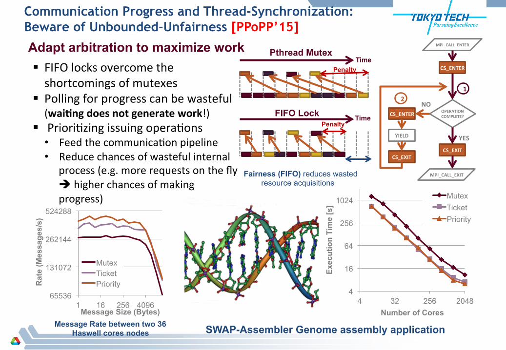
Communication Progress and Thread-Synchronization: Beware of Unbounded-Unfairness [PPoPP’15]

§  FIFO locks overcome the shortcomings of mutexes

§  Polling for progress can be wasteful (wai:ng does not generate work!)

§  Priori'zing issuing opera'ons •  Feed the communica'on pipeline •  Reduce chances of wasteful internal

process (e.g. more requests on the fly è higher chances of making progress)

MPI_CALL_ENTER

MPI_CALL_EXIT

CS_ENTER

CS_ENTER

CS_EXIT CS_EXIT

YIELD

OPERATION COMPLETE?

YES

NO 2

1

Time Penalty

Fairness (FIFO) reduces wasted resource acquisitions

Time Penalty

Pthread Mutex

FIFO Lock

Adapt arbitration to maximize work

65536

131072

262144

524288

1 16 256 4096

Rat

e (M

essa

ges/

s)

Message Size (Bytes)

Mutex Ticket Priority

Message Rate between two 36 Haswell cores nodes SWAP-Assembler Genome assembly application

4

16

64

256

1024

4 32 256 2048

Exec

utio

n Ti

me

[s]

Number of Cores

Mutex Ticket Priority

2

Insightul Analysis of Performance Metrics on Fat-‐tree Networks[Kevin Brown, ICPADS15]

source port

dest. port

traffic (kb)

a b 5 b a 15

process 2

app

Open MPI library

network hardware

app

Open MPI library

network hardware

process 1 network communica'on profile

Profiler Non-‐intrusive collec'on of performance metrics w/ our ibprof profiler •  Low overhead •  Captures links traffic

Hardware-‐centric traffic visualiza'on BoxFish for FatTree

compute nodes

switches

1

Tree-‐topology viz. design

Insightul Analysis of Performance Metrics on Fat-‐tree Networks

3 Tree-‐topology viz. design Adjacency matrix viz. design

Each element represents a link ü  No occlusion of data ü  Space efficient design ü  More link design op'ons

Square

Bisected square Triangle pair

Data (traffic, load, etc.) is encoded in the size, shape, color, and/or hue of the links

ibprof’s Profiling Overhead

21 21 25 210 215 220 223

0

20

40

60

80

100

Message Size (bytes)

Ove

rhea

d(%

)

bcastreduceping-pong

21 25 210 215 220 223

�2

0

2

4

6

8

10


alltoall scattergather allgatherallreduce

(a) Intel MPI Bencharmark

ft is cg mg bt sp lu

�0.6

�0.4

�0.2

0

0.2

0.4

0.6

-32ms

56ms

0.3ms

-39ms

14ms47ms 58ms

Kernels & Psuedo Apps

kernel

pseudo app

(b) NAS Parallel Benchmarks

Fig. 5. Runtime overhead of communication profiling. Subfigure (5a) shows the percentage increase in communication latency for the various IMB benchmarks.These results are separated into two charts for increased readability. Subfigure (5b) shows the increase in runtime of NPB kernels and pseudo applications. Theheight of each bar represents the overhead as a percentage of the communication runtime and the bars annotation states the actual change in communicationruntime.

2) Increase in Communication Latency: Figure 5 shows theresults of our experiments. These graphs represent the increasein communication latency caused by our profiler and does not re-flect the time for dumping profiles. Results were averaged acrossall 100 pairs of runs with standard errors <1% in all cases. Theaverage overhead was 11.6%, 3.4%, and 1.3% for MPI_Bcast,MPI_Reduce, and MPI_Scatter, respectively, over allmessage sizes while other IMB benchmarks averaged below1% overhead. Similarly, all NPB benchmarks averaged below1%, with the communication-bound FT benchmark reportingthe highest value of 0.46%.

The averaged runtime differences were in the order ofmicroseconds for the IMB benchmarks and milliseconds forthe NPB benchmark. Because such small differences couldbe attributed to jitters in the system, we ran similar exper-iments at different times over several days for verification.Similar trends were observed in the results with some runsoccasionally reporting negative overheads and all overheadsremaining negligible except for spikes in the MPI_Bcastand MPI_Reduce results for the message sizes shown. Weconfirmed that the spike in the MPI_Bcast can be attributedto Open MPI switching from the send/receive semantics toRDMA pipeline protocol when the message size surpasses256 KB. We ran a set of MPI_Bcast trials with the RDMApipeline size limit changed from 256 KB to 1 MB and thepipeline send length changed from 1 MB to 4 MB. As expected,we observed additional spikes for messages between 1 MB and4 MB in size. Further research is being planned to ascertainthe cause of this phenomenon.

3) Increase in Application Runtime: The total increase inapplication runtime when ibprof is used is equal to theincrease in communication latency plus the time taken to writeprofiles. On our system, the time taken for a complete profiledump was less than 1 seconds, irrespective of the applicationor communication pattern. This time is dependent on the IOsubsystem’s performance, which is beyond the scope of thiswork.

VI. CASE STUDY

In this Section, we showcase the usability of our profilingapproach and analysis toolchain. We analyze the execution of

samplesort, a popular sorting algorithm for parallel systems,and we also compare the performance of different MPI libraryversions. Experiments were conducted on TSUBAME2.5, whichutilizes two independent IB subnets and each compute nodehas a link to each subnet.

A. Visualizing Traffic Patterns and Contention in Samplesort

Samplesort, as described in [19], is a sorting algorithm fordistributed memory environments. The main idea behind thealgorithm is to find a set splitters to partition the input keys intop buckets corresponding to p processes in such a way that everyelement in the i

th bucket is less than or equal to each of theelements in the (i+ 1)th bucket. Because splitters are selectedrandomly, the resulting bucket sizes may be uneven. This couldresult in communication and computation imbalances whenkeys are shuffled and sorted, respectively.

For our experiment, we used the samplesort code presentedin [19] 1. We executed samplesort with 128 MPI processes,using a 1:1 process-to-node mapping. Each process startedwith 1 GB of unsorted integers, randomly generated with auniform distribution. The same random number seed wasused in all cases. Fig. 6 shows a typlical process-centricvisualization of samplesort’s main communication routines over128 nodes using Paraver. We are unable to extract any networkperformance insights from this and other similar visualizationsthat are generated using PMPI-based instrumentation tools.

1) Performance Analysis using our ibprof Profiler andour Boxfish Module: We profiled an execution of samplesortusing ibprof and visualized the network traffic in ourBoxfish fat tree module. Segments of the code were manuallyinstrumented to enable the identification of the code blockwhere the all-to-all key exchange is conducted in order toperform a meaningful analysis. Fig. 7 shows the network trafficgenerated by the main communication routines of samplesort.This section of the profile reflects the traffic generated by thesegment of the program highlighted in Fig. 6.

The red links that are visible in area C of Fig. 7 representlinks that were carrying the most traffic during the commu-nication block of the code. By exploring the visualization

1Source code: http://users.ices.utexas.edu/˜hari/talks/hyksort.html

21 25 210 215 220 223

0

20

40

60

80

100


Ove

rhea

d(%

)


21 25 210 215 220 223

�2

0

2

4

6

8

10





�0.6

�0.4

�0.2

0

0.2

0.4

0.6

-32ms

56ms

0.3ms

-39ms

14ms47ms 58ms


kernel

pseudo app






VI. CASE STUDY










(avg: 11.6) (avg: 3.4)

21 25 210 215 220 223

0

20

40

60

80

100


Ove

rhea

d(%

)


21 25 210 215 220 223

�2

0

2

4

6

8

10





�0.6

�0.4

�0.2

0

0.2

0.4

0.6

-32ms

56ms

0.3ms

-39ms

14ms47ms 58ms


kernel

pseudo app






VI. CASE STUDY










•  All NPB apps averaged < 1% •  Peak overhead occurred with MPI_Bcast when Open MPI switched from send/recv to RDMA

•  All other collec'ves averaged < 5%

Ove

rhea

d (%

)O

verh

ead

(%)

Intel MPI Benchmarks NAS Parallel Benchmarks

Process-‐centric Visualiza'ons vs. Boxfish Fat Tree Visualiza'on

22

Paraver Does not show network traffic hotspots

Boxfish Capable of highligh'ng network hotspots and traffic pazerns

Samplesort on 128 nodes of TSUBAME2.5

vs.

Visualizing the Traffic Pazerns of Different Open MPI Library version

23

v1.82

v1.65 Open MPI v1.65 balances traffic over both subnets ofTSUBAME2.5 with the default configura'on

Open MPI v1.82 uses a single subnet per opera'on with the

default configura'ons on TSUBAME2.5

Publica'ons

Poster (Prior to internship but using LLNL’s work): Kevin A. Brown, Jens Domke, and Satoshi Matsuoka. “Tracing Data Movements within MPI Collec>ves”. In Proceedings of the 21st European MPI Users' Group Mee'ng (EuroMPI/ASIA '14).

Paper:

Brown, K.A.; Domke, J.; Matsuoka, S., "Hardware-‐Centric Analysis of Network Performance for MPI Applica>ons”. In 2015 IEEE 21st Interna'onal Conference on Parallel and Distributed Systems (ICPADS)

Challenges to model a tree-‐based irregular applica8ons with Aspen

Keisuke Fukuda (Ph.D Student) Research Internship @ORNL

•  2013 Sep-‐Nov •  2014 Oct-‐Nov

•  Now long-‐term intern at AICS 2015 Oct-‐2016 Sep

Challenges in modeling irregular applica8ons •  Performance modeling of applica'on is used to:

•  Run'me (power, memory) es'ma'on •  Hardware/machine design

•  Conven'onal, ad-‐hoc mathema'cal modeling is not suitable if irregular data structure (e.g. tree) and control flows affect the performance

•  How to model such applica'ons? •  We focus on the Fast Mul'pole Method

0

1

2

3

4

0 200 400 600 Time [s]

Ncrit

La~ce

Plummer

(this figure will be shown anddescribed again)

Each plot point representsa particular shape of tree

Performance variationcaused by “shape” of a treefor a fixed number of particles

Examples of tree shapes

26

• Applied Aspen modeling language to FMM •  Run'me es'ma'on for la~ce, sphere, plummer distribu'on, Ncrit = 16〜512

•  Es'ma'on errror was 7-‐13% error in avg.

• Room for op'miza'on for find-‐grained kernels and in deriving constants

• Aspen requires large 'me and memory to evaluate the models

27

Whole-‐app model of ExaFMM

28

0"

0.1"

0.2"

0.3"

0.4"

0.5"

0.6"

16"

32"

48"

64"

80"

96"

112"

128"

144"

160"

176"

192"

208"

224"

240"

256"

272"

288"

304"

320"

336"

352"

368"

384"

400"

416"

432"

448"

464"

480"

496"

512"

Time%[s]�

Ncrit�

Aspen%Model%vs.%Actual%run8me%La:ce%distribu8on%%50,000%par8cles�

Model"

Actual"

Error: avg 7.7%, max 33.2%, min 3.7%

Whole-‐app model of ExaFMM

29

0"

0.1"

0.2"

0.3"

0.4"

0.5"

0.6"

0.7"

0.8"

16"

32"

48"

64"

80"

96"112"

128"

144"

160"

176"

192"

208"

224"

240"

256"

272"

288"

304"

320"

336"

352"

368"

384"

400"

416"

432"

448"

464"

480"

496"

512"

Time[s]�

Ncrit�

Aspen/Model/vs./Actual/run8me"Sphere/distribu8on//50,000/par8cles/

�

Model"

Actual"

Error: avg 12.8%, max 26.9%, min 4.0%

Dynamic Graphs (temporal graph) •  the structure of a graph

changes dynamically over time •  many real-world graphs are

classified into dynamic graph

•  Most studies for large graphs have not focused on a dynamic graph data structure, but rather a static one, such as Graph 500

•  Even with the large memory capacities of HPC systems, many graph applications require additional out-of-core memory (this part is still at an early stage)

Sparse Large Scale-free •  social network, genome

analysis, WWW, etc. •  e.g., Facebook manages

1.39 billion active users as of 2014, with more than 400 billion edges

Distributed Large-Scale Dynamic Graph Data Store Keita Iwabuchi1, 2, Scott Sallinen3, Roger Pearce2,

Brian Van Essen2, Maya Gokhale2, Satoshi Matsuoka1 1.  Tokyo Institute of Technology (Tokyo Tech)

2. Lawrence Livermore National Laboratory (LLNL) 3. University of British Columbia

Source: Jakob Enemark and Kim Sneppen, “Gene duplica'on models for directed networks with limits on growth”, Journal of Sta's'cal Mechanics: Theory and Experiment 2007

Controller / Partitioner

Comp. Node

Comp. Node

Distributed Dynamic Graph Data Store

share.sandia.gov

Comp. Node

Graph Application

Comp. Node

Comp. Node

Developing a distributed dynamic graph store for data intensive supercomputers equipped with locally attached NVRAM

Streaming edges

Degree Aware Dynamic Graph Data Store (DegAwareRHH)

Robin Hood Hashing1

[1] P. Celis, “Robin hood hashing,” Ph.D. dissertation, 1986. Designed to maintain a small average probe distance

w1

w5 v1 p1

v3 p3

w2

v4 p4

w3

w6

v2 p2

v1 p1

v2 p2

v3 p3

v4 p4

Vertex-table

v2 w1 v3 w2

v4 w3

v1 w4 v3 w5

Edge-list

v: vertex p: vertex property data w: edge weight

Vertex-table : tree, hash table Edge-list : vector, linked-list

v1 v4 p1 p4

v1 v3 w5 w6

{v2,v4}

{v3,v4}

p2 p3 w3 w4

w4

Low-‐degree table

Mid-‐high degree table

DegAwareRHH Degree Aware Graph Data Structure

Each table is composed of Robin Hood Hashing

Extend DegAwareRHH for distributed-‐memory using a async. MPI communica'on framework[2][3]

•  Degree aware data structures, where low-‐degree ver'ces are compactly represented

•  Use Robin Hood Hashing[1] because of its locality proper'es to minimize the number of accesses to NVRAM, reducing page misses.

v2 v3 w1 w2

Vertex ID Vertex property Edge weight

[2] R. Pearce, et al, “Scaling techniques for massive scale-free graphs in distributed (external) memory,” IPDPS’ 13 [3] R. Pearce, et al, “Faster parallel traversal of scale free graphs at extreme scale with vertex delegates, ” SC’ 14

RMAT 25 graph: #vertices 32M, #edges 1B

#nodes (24 processes per node)

Million Re

quests/sec.

•  STINGER: a state-of-the-art shared-memory dynamic graph processing framework developing at Georgia Tech

•  Baseline: a baseline model using Boost.Interprocess •  DegAwareRHH: our proposed dynamic graph store

Dynamic Large-‐Scale Graph Construc'on (on-‐memory)

Edge inser'on and dele'on (single node, 24 threads/processes)

total #edges: 1 billion

Edge inser'on total #edges: 128 billion

Bezer

Billion

Req

uests/sec.

16x than Baseline

121x than STINGER

over 2 billion insertions/

sec. overperforms Baseline by 30.69 %

Due to a skewness of the data set (RMAT graph), DegAwareRHH overperforms the both implementa'ons significantly

2016/2/3

Publica'on list •  Keita Iwabuchi, Roger A. Pearce, Brian Van Essen, Maya Gokhale, Satoshi Matsuoka,

“Design of a NVRAM Specialized Degree Aware Dynamic Graph Data Structure”, SC 2015 Regular, Electronic, and Educa'onal Poster, Interna'onal Conference for High Performance Compu'ng, Networking, Storage and Analysis 2015 (SC ’15), Nov. 2015

•  Keita Iwabuchi, Roger A. Pearce, Brian Van Essen, Maya Gokhale, Satoshi Matsuoka, “Design of a NVRAM Specialized Degree Aware Dynamic Graph Data Structure”, 7th Annual Non-‐Vola'le Memories Workshop 2016, Mar. 2016

An OpenACC Extension for Data Layout Transforma'on w/ORNL

Tetsuya Hoshino(Ph.D Student) Research Internship @ORNL 2014 Sep-‐Nov

Now: Assistant Professor @ Supercompu'ng Center,

The University of Tokyo

Why the extension is needed? •  An OpenACC program can be

executed on any devices –  mul'-‐core CPU, Xeon Phi, GPUs

•  OpenACC target devices have different performance characteris'cs especially about memory access –  ex. SoA and AoS

•  Data layout of real-‐world applica'ons is complicated and is shared in the whole program –  Auto-‐tuning is required

0

0.1

0.2

0.3

0.4

0.5

0.6

0.7

0.8

0.9

1

Original AoS SoA

Elap

sed :m

e/1 :m

e step

[sec]

Viscosity and Convec:on phases

Intel Xeon (6 core)

K20X GPU

The graph shows the result of manual data layout transforma'on for the viscosity and convec'on phases of a real-‐world CFD applica'on UPACS (Hoshino et al. “CUDA vs OpenACC: Performance Case Studies with Kernel Benchmarks and a Memory-‐Bound CFD Applica'on”, CCGrid13)

An OpenACC extension #pragma acc transform

•  Specifica'on

•  Clause list

–  transpose( array_name::transpose_rule ) •  for mul'-‐dimensional array •  A[Z][Y][X][3] → A’[3][Z][Y][X] (transpose rule :: [4,1,2,3])

–  redim( array_name::redim_rule ) •  for 1 dimensional array •  B[Z*Y*X*3] → B’[Z][Y][X][3] → B’’[3][Z][Y][X] (by transpose clause)

–  expand( derived_type_array_name ) •  for array of structures •  C[Z][Y][X].c[3] → C’[Z][Y][X][3] → C’’[3][Z][Y][X] (by transpose clause)

37

#pragma acc transform [clause [[,] clause] …] new-‐line structured block

Collaborate with ORNL •  Implement the direc've top on OpenARC that is an Open-‐source

OpenACC compiler developed by ORNL –  Source-‐to-‐Source translator

•  Input : Extended OpenACC program •  Output : OpenACC program

–  It is on going work

Our Translator

Extended OpenACC

.c input OpenARC generates

AST

analyze direc'ves

transform structures output

OpenACC

.c

Evaluate with Himeno benchmark (27-‐point stencil program)

•  Apply transpose to coefficient arrays of Himeno benchmark –  But the transforma'on is

applied by hands –  Transformed program is

same as the output program that OpenARC should output

•  Performance evalua'on –  CPU : Original is the best –  GPU : 24% up –  MIC : more than 60% down

•  Translator change the coefficient mul'dimensional array to 1-‐dimensional array, it disturbs prefetching

0

0.2

0.4

0.6

0.8

1

1.2

Original A[Z][Y][X][4] ([4] is

innermost)

A[Z][Y][4][X] A[Z][4][Y][X] A[4][Z][Y][X] ([4] is

outermost)

Rela:v

e pe

rforman

ce (O

riginal == 1)

Intel Xeon (12cores)

Intel Xeon Phi

NVIDIA K20X GPU

Lessons Learned

•  Sending actual Ph.D. students to DoE labs extremely produc've for both sides for tangible collabra'on

•  Tokyo Tech Ph.D. students are extremely good and well trained by global standards – they usually survive the filtering of summer interns and produce tangible results

• Many students end up being hired by DoE labs. Others go to Japanese univ. & labs, etc. => great talent pool

•  Some administra've obstacles, esp. travel and funding from both ends – need more flexibility in purpose, airlines, gaps in travel i'nerary, etc.

41

Tokyo Tech Research on Big Data Convergence JST-‐CREST “Extreme Big Data” Project (2013-‐2018)

Supercomputers Compute&Batch-Oriented

More fragile

Cloud　IDC Very low BW & Efficiency Highly available, resilient

Convergent Architecture (Phases 1~4) Large Capacity NVM, High-Bisection NW

PCB

TSV Interposer

High Powered Main CPU

Low Power CPU

DRAM DRAM DRAM

NVM/Flash

NVM/Flash

NVM/Flash

Low Power CPU

DRAM DRAM DRAM

NVM/Flash

NVM/Flash

NVM/Flash

2Tbps HBM 4~6HBM Channels 1.5TB/s DRAM & NVM BW 30PB/s I/O BW Possible 1 Yottabyte / Year

EBD System Software incl. EBD Object System

Introduction

Problem

Dom

ain

Inmostlivingorganism

sgeneticinstructions

used

intheirdevelopm

entarestored

inthelong

polym

eric

moleculecalledDNA.

DNAconsists

oftwolong

polym

ersof

simpleun

its

callednu

cleotides.

The

four

basesfoun

din

DNAareadenine(abbreviated

A),cytosine

(C),guanine(G

)andthym

ine(T

).

AleksandrDrozd

,NaoyaMaruyama,SatoshiMatsuoka

(TIT

ECH)

AMultiGPU

Rea

dAlig

nmen

tAlgorithm

withModel-basedPerform

ance

Optimization

Nove

mber

1,2011

5/54

Large Scale Metagenomics

Massive Sensors and Data Assimilation in Weather Prediction

Ultra Large Scale Graphs and Social Infrastructures

Exascale Big Data HPC

Co-Design

Future Extreme Big Data Scientific Apps

Graph Store

EBD Bag Co-Design 13/06/06 22:36日本地図

1/1 ページfile:///Users/shirahata/Pictures/日本地図.svg

1000km

KVS

KVS

KVS

EBD KVS

Cartesian Plane Co-Design

Given a top-‐class supercomputer, how fast can we accelerate next genera>on big data c.f. Clouds?

World-‐leading results: -‐  #1 Graph 500

2014, 2015 -‐  #1 Green Graph

500 (TsubameKFC)

-‐  GPU sort scalable to ~30Petabyte/s on future SCs

-‐  OSSs in dev.

The Graph500 – June 2014 and June/Nov 2015 K Computer #1 Tokyo Tech[EBD CREST] Univ. Kyushu

[Fujisawa Graph CREST], Riken AICS, Fujitsu

List Rank GTEPS Implementation

November 2013 4 5524.12 Top-down only

June 2014 1 17977.05 Efficient hybrid

November 2014 2 Efficient hybrid

June/Nov 2015 1 38621.4 Hybrid + Node Compression

*Problem size is weak scaling

“Brain-class” graph

88,000 nodes, 700,000 CPU Cores 1.6 Petabyte mem 20GB/s Tofu NW

≫

LLNL-IBM Sequoia 1.6 million CPUs 1.6 Petabyte mem

0

500

1000

1500

64 nodes (Scale 30)

65536 nodes

(Scale 40)

Elap

sed

Tim

e (m

s)

Communic73% total exec

time wait in communication

43

TSUBAME3.0

2006 TSUBAME1.0 80 Teraflops, #1 Asia #7 World “Everybody’s Supercomputer”

2010 TSUBAME2.0 2.4 Petaflops #4 World

“Greenest Production SC”

2013 TSUBAME2.5

upgrade 5.7PF DFP /17.1PF SFP 20% power reduction

2013 TSUBAME-KFC #1 Green 500

2017 TSUBAME3.0 15~20PF(DFP) ~4PB/s Mem BW 9~10GFlops/W power efficiency Big Data & Cloud Convergence

Large Scale Simulation Big Data Analytics

Industrial Apps 2011 ACM Gordon Bell Prize

2017 Q1 TSUBAME3.0+2.5 Towards Exa & Big Data

1.   “Everybody’s Supercomputer” – High Performance (15~20 Petaflops, ~4PB/s Mem, ~1Pbit/s NW), innova:ve high cost/performance packaging & design, in mere 100m2…

2.   “Extreme Green” – 9~10GFlops/W power-‐efficient architecture, system-‐wide power control, advanced cooling, future energy reservoir load leveling & energy recovery

3.   “Big Data Convergence” – Extreme high BW &capacity, deep memory hierarchy, extreme I/O accelera:on, Big Data SW Stack for machine learning /DNN, graph processing, …

4.   “Cloud SC” – dynamic deployment, container-‐based node co-‐loca:on & dynamic configura:on, resource elas:city, assimila:on of public clouds…

5.   “Transparency” -‐ full monitoring & user visibility of machine & job state, accountability via reproducibility

43

Big Data and HPC Convergent Infrastructure=> “Big Data & Supercomputing Convergent Center” （Tokyo Tech GSIC）

•  “Big Data” currently processed managed by domain laboratories => No longer scalable •  HPCI HPC Center => Converged HPC and Big Data Science Center •  People convergence: domain scientists + data scientists + CS/Infrastructure => Big data science center •  Data services including large data handling, big data structures e.g. graphs, ML/DNN/AI services…

2013 TSUBAME2.5 Upgrade

5.7Petaflops 17PF DNN

2017Q1 TSUBAME3.0+2.5 upgrade Green&Big Data 100+PF DNN

HPCI Leading Machine Ultra-fast memory

network, I/O

Mid-tier Parallel FS

Storage

Archival Long-Term

Object Store

Big Data Science Applica'ons

Introduction

Problem

Dom

ain

Inmostlivingorganism

sgeneticinstructions

used

intheirdevelopm

entarestored

inthelong

polym

eric

moleculecalledDNA.

DNAconsists

oftwolong

polym

ersof

simpleun

its

callednu

cleotides.

The

four

basesfoun

din

DNAareadenine(abbreviated

A),cytosine

(C),guanine(G

)andthym

ine(T

).

AleksandrDrozd

,NaoyaMaruyama,SatoshiMatsuoka

(TIT

ECH)

AMultiGPU

Rea

dAlig

nmen

tAlgorithm

withModel-basedPerform

ance

Optimization

Nove

mber

1,2011

5/54

Na:onal Labs With Data

Present old style data science Domain labs segregated data facili'es

No mutual collabora'ons Inefficient, not scalable with Not enough data scien'sts

Convergence of top-‐>er HPC and Big Data Infrastructure

Data Management Big Data Storage Deep Learning SW Infrastructure

Virtual Mul>-‐Ins>tu>onal Data Science => People Convergence

Goal 100 Petabytes

100Gbps L2 Connec'on to commercial clouds

Main reason: We have shared resource HPC centers but no

“Data Center” per se

New collabora8ons under considera8on •  Fault tolerance towards exascale

•  Modeling & analyzing sor errors with “realis'c” machine fault models (Kobayashi)

•  General system-‐level GPU checkpoin'ng (Suzuki)

• Big Data / IoT / Machine Learning-‐AI & HPC Convergence •  Modeling deep learning algorithms performance (Ooyama) •  Counterpart to Tokyo Tech Extreme Big Data (EBD) Project w/DENSO

• Post-‐Moore compu'ng •  Programming / Performance modeling future FPGAs (also w/Riken AICS Naoya Maruyama (Hamid)

•  FLOPS to BYTES – from compute intensive to bandwidth/capacity intensive compu'ng (w/Kengo Nakajima, Toshio Endo et. al.)

• ADAC (Accelerated Data Analy'cs and Compu'ng) Ins'tute – ORNL – ETH/CSCS – Tokyo Tech GSIC

To be presented @ DoE/MEXT workshop)

Collaborative Research between DoE Labs and Tokyo Tech ...

Documents

Transcript of Collaborative Research between DoE Labs and Tokyo Tech ...