COBRA-SFS: A Thermal-Hydraulic Analysis Code for Spent ...
346
. .. .~ . . . - . . . . , , .. . ; . ._.- . .- ,. . ... .., - . . ., .. _.. .: . . . OSTI COBRA-SFS: A Thermal-Hydraulic Analysis Code for Spent Fuel Storage And Transportation Casks T. E. Michener D. R. Rector J. M. Cuta R. E; Dodge C. W. Enderlin September 1995 -. Prepared for the U.S. Department of ,Energy- -- - . - under Contract DE-AC06-76RLO 1530 Pacific Northwest Laboratory Operated for the U.S. Department vf Energy by Baaelle Memorial Institute ' '0 PNL-10782 UC-800 ..... <. I - . ,
-
Upload
khangminh22 -
Category
Documents
-
view
0 -
download
0
Transcript of COBRA-SFS: A Thermal-Hydraulic Analysis Code for Spent ...

. .. .~ . . . - .
. . . , , .. . ; . ._.- . . -
, . . . . . .., - .
. ., . . _.. . : . . .
O S T I
COBRA-SFS: A Thermal-Hydraulic Analysis Code for Spent Fuel Storage And Transportation Casks T. E. Michener D. R. Rector J. M. Cuta
R. E; Dodge C. W. Enderlin
September 1995
- .
Prepared for the U.S. Department of ,Energy- -- - . - under Contract DE-AC06-76RLO 1530
Pacific Northwest Laboratory Operated for the U.S. Department vf Energy by Baaelle Memorial Institute
' ' 0 PNL-10782 UC-800
..... < . I
- ... ,

PNL-10782 UC-800
COB RA-S FS : A Thermal-Hydraulic Analysis Code for Spent Fuel Storage And Transportation Casks
Documentation for Cycle 2
T. E. Michener D. R. Rector J. M. Cuta R. E. Dodge C. W. Enderlin
September 1995
Prepared for the U.S. Department of Energy under Contract DE-AC06-76RLO 1830
Pacific Northwest Laboratory Richland, Washington 99352

DISCLAIMER
This report was prepared as an account of work sponsored by an agency of the United States Government. Neither the United StatesGovernment nor any agency thereof, nor Battelle Memorial Institute, nor any of their employees, makes any warranty, express or implied, or assumes any legal liability or responsibility for the accuracy, completeness, or usefulness of any information, apparatus, product, or process disclosed, or represents that its use would not infringe privately owned rights. Reference herein to any specific commercial product, process, or service by trade name, trademark, manufacturer, or otherwise does not necessarily constitute or imply its endorsement, recommendation, or favoring by the United States Government or any agency thereof, or Battelle Memorial Institute. The views and opinions of authors expressed herein do not necessarily state or reflect those of the United States Government or any agency thereof.
PACIFIC NORTHWEST LABORATORY operated by
BATTELLE MEMORIAL INSTiTUTE for the
UNITED STATES DEPARTMENT OF ENERGY under Contract DE-ACO6-76RLO 1830
Printod in tho Unitod Statu of Anwrica
Avaikbk to DOE ond DOE controctorr from the Offico of Sciontific and Technical Information. P.O. Box 62. Oak Ridgo. TN 37831;
p r i m availah from (615) 5768401.
Available to tho public from tha National Toctwriul Information Servico, US. Dopartmont of Commercw. 5286 Port Royd Rd., Springfmld. VA 22161
@ This document was printed on recycled paper.

DISCLAIMER
Portions of this document may be illegible electronic image products. Images are produced from the best available original document.

Abstract
COBRA-SFS is a general thermal-hydraulic analysis computer code for prediction of material temperatures and fluid conditions in a wide variety of systems. The code has been validated for analysis of spent fuel storage systems, as part of the Commercial Spent Fuel Management Program of the U.S. Department of Energy. The code solves finite volume equations representing the conservation equations for mass, moment, and energy for an incompressible single-phase heat transfer fluid. The fluid solution is coupled to a finite volume solution of the conduction equation in the solid structure of the system.
This document presents a complete description of Cycle 2 of COBRA-SFS, and consists of three main parts. Part I describes the conservation equations, constitutive models, and solution methods used in the code. Part 11 presents the User Manual, with guidance on code applications, and complete input instructions. This part also includes a detailed description of the auxiliary code RADGEN, used to generate grey body view factors required as input for radiative heat transfer modeling in the code. Part I11 describes the code structure, platform dependent coding, and program hierarchy. Installation instructions are also given for the various platform versions of the code that are available.
iii


Acknowledgments
The authors would like to thank Leroy Stewart and Jeff Williams of the U.S. Department of Energy for sponsoring this work. Thanks are also extended to Mike McKinnon, Jim Creer, and Max Kreiter of the Pacific Northwest Laboratory Commercial Spent Fuel Management Program Office, who have provided support during this endeavor. In addition, the authors would like to acknowledge the Nuclear Regulatory Commission (NRC) Technical Review team for their through review of the COBRA-SFS computer code and documentation set. Finally, thanks go to Frank Ryan, Technical Editor, for his efforts in the preparation of this manuscript, and Zen Antoniak for his independent technical review.
V

e
e

Nomenclature
A
A -
channel cross-sectional area (ft2) in the axial direction
surface area for generalized control volume (ft2)
average cross-sectional area (ft2) over the subchannel control volume
surface area of generalized control volume (fi2)
axial cross-sectional area of fuel (ft2)
axial cross-sectional area of cladding (ft2)
area of the interface between two solid nodes for heat transfer (e2) surface area of slab node (ft2)
black body view factor from surface k to surface i for radiative heat transfer (dimensionless)
fraction of power generated in the coolant
specific heat at constant pressure (Btu/lbm- O F )
turbulent momentum factor (dimensionless empirical parameter)
average hydraulic diameter of lateral control volume (ft)
hydraulic diameter of subchannel, based on wetted perimeter (ft)
hydraulic diameter of subchannel, based on heated perimeter (ft)
diameter of fuel (ft)
outside diameter of fuel rod (ft)
diameter of kth condunction heat transfer node in fuel or cladding (ft)
local mass continuity error at level j (lbdsec)
energy per unit mass (BtuAbm)
vii

g
g
gc
G
Gr
H
-
body force vector per unit mass (1bQca)
fluid surface area for generalized control volume (ft2)
body force due to turbulent mixing (lbm-ft/sec2)
grey body view factor from surface n to surface m for radiative heat transfer (dimensionless)
axial friction factor, Darcy formulation (dimensionless)
friction for lateral flow, Darcy formulation (dimensionless)
acceleration of gravity vector, (ft/sec2)
scalar gravitational acceleration constant, (ft/sec2)
force/mass conversion constant for English engineering units, (32.2 lbm-ft/lbm-sec')
average axial mass velocity in lateral control volume, (lbmlsec-ft2)
Grashof Number (dimensionless)
heat transfer coefficient, (Btu/sec-ft2-'F)
condunctance across the fuel-cladding gap (Btdsec-ft2- F)
H, surface heat transfer coefficient (Btu/sec-ft2- F)
h
I A
1
K
I(G
saturation enthalpy for the liquid phase, (Btu/lbm)
latent heat of vaporization, (h, - ~ ) , (Btu/lbm)
saturation enthalpy for the vapor phase (Btu/lbm)
enthalpy (Btdlbm)
Identity tensor
internal thermal energy per unit mass (Btullbm)
form drag for axial flow (dimensionless)
form drag for lateral flow (dimensionless)
(a) To properly balance units in all terms in the integral formlation of the energy conservation equation, the force vector F must be diviede by the proportionality factor J, relating the ft-lbf force to thermal energy in units of Btu, as J = 778 ft-lbf/Btu.
viii

k thermal conductivity (Btukec-ft-OF)
centroid length for gap k (ft)
m axial mass flow rate (Ibdsec)
n
n,
n,
Nu Nusselt number (dimensionless)
P pressure (psia)
unit vector, outward normal to A
unit vector, normal to subchannel axial flow area A
unit vector, normal to gap lateral flow area, SAX
P,
Ph
Pr Prandtl number (dimensionless)
wetted perimeter of subchannel control volume (ft)
heated perimeter of subchannel control volume (ft)
q heat flux vector (Btu/sec-ft*)
q' linear heat rate (Btu/sec-ft)
q" surface heat flux (Btuhec-ft2)
q"'
q,
volumetric heat generation rate (Btu/sec-ft3)
energy deposited per unit volume (Btulsec-ft3)
Q,
Q,
Q,
Q,,,
R thermal conduction resistance (Btu/sec-ft2-"F)
Re Reynolds number (dimensionless)
energy deposited per unit length (Btu/sec-ft)
turbulent energy exchange source term (Btu/sec)
energy deposited per unit length from the heated surfaces, (Btu/sec-ft)
total energy input due to turbulent mixing (Btu/sec)
internal heat generation rate per unit mass(Btu/lbm-sec)
S width (ft) of gap k connecting channel ii to channel jj
ix

t time (sec)
T temperature ( O F )
Tclad cladding surface temperature ( O F )
T, temperature of the fuel surface ( O F )
Ti fluid temperature in current node of subchannel i ( O F )
TRuid average fluid temperature seen by rod n ( O F )
T, wall surface temperature ( O F )
T,,, wall surface temperature ( O F )
Tb
T
tCld cladding thickness (ft)
bulk fluid temperature in the subchannel control volume (OF)
tensor of surface stresses acting on the fluid A
U
U
scalar velocity (ft/sec) in the axial direction
local axial velocity vector (ft/sec) - Uj average axial velocity at j for momentum cell (ft/sec)
U composite thermal conductance (Btuhec-OF)
V local lateral velocity vector, (ft/sec)
V
V
- volume of generalized control volume (ft3)
scalar velocity in the lateral direction (fthec) - Vk
W -
average lateral velocity in gap k for momentum cell (ft/sec)
wall surface area for generalized control volume (ft2)
W mass flow rate in the lateral direction, per unit length (lbmlsec-ft)
w' 'turbulent crossflow for momentum and enthalpy exchange between adjacent channels (Ibdft- sec)
axial distance (ft) X
Zk empirical shape factor for conduction length of gap k (dimensionless)
X

Greek symbols :
a m
AX
Ah
Ar
AU
At
e
E
Eik
empirical mixing coefficient for turbulent crossflow model (dimensionless)
axial node length (ft)
change in enthalpy (BtuAbm)
radial increment in fuel noding (ft)
axial velocity difference between adjacent channels for turbulent mixing momentum exchange (ftkec)
transient time increment (sec)
angle of channel axial orientation relative to vertical (degrees)
surface emissivity of a solid node (dimensionless)
sign determiner for lateral velocity in gap k with respect to channel i.
ii
CL
P
(T
4ll
c kei
Eik = 1.0 if i = ii -1.0 if i = j j
where ii < jj
eddy difisivity for turbulence (ft2/sec)
Kronecker-delta function
shear stress tensor
viscosity, (lbm/sec-ft2)
density (Ibm/ft3)
Stefan-Boltzmann constant; 4.76( 10-13) BtuI~ec-ft2-R~
fraction of perimeter of rod n facing a given subchannel (dimensionless)
summation on all gaps k connected to channel i
xi

c men summation on all channels m facing rod n
c nci summation on all rods n with heat transfer surfaces, facing channel i
c nek summation on all gaps n connected to gap k for lateral momentum transport
C ne(N+ 1)
summation on all rod surface nodes n seen by cladding node N+ 1
C me(N + 1)
summation on all slab nodes m seen by cladding node N + 1
Subscripts:
C
fi
.. 11
j
J
jj
k
P
L
S
t
W
e
cladding material property
fuel material property
lower-numbered channel of a pair connected by gap k
axial level index number
axial level index for lateral momentum transport, (i.e., J = j + 1/2)
higher-numbered channel of a pair connected by gap k
gap index number
laminar flow
laminar flow
slab node property
turbulent flow
wall
circumferential angle for radial fuel noding (radians)
xii

superscripts:
n previous time-step value
o current iteration value
N current time step value
‘I’ per unit cell quantity (e3)
xiii

a

Contents
... Abstract . . . . . . . . . . . . . . . . . . . . . . . . . . . . . . . . . . . . . . . . . . . . . . . . . . . . . . . . 111
Acknowledgments . . . . . . . . . . . . . . . . . . . . . . . . . . . . . . . . . . . . . . . . . . . . . . . . . . V
Nomenclature . . . . . . . . . . . . . . . . . . . . . . . . . . . . . . . . . . . . . . . . . . . . . . . . . . . vii
1 . 0 Introduction . . . . . . . . . . . . . . . . . . . . . . . . . . . . . . . . . . . . . . . . . . . . . . . . . . 1.1
2.0 Conservation Equations . . . . . . . . . . . . . . . . . . . . . . . . . . . . . . . . . . . . . . . . . . 2.1
2.1 Integral Balance Laws . . . . . . . . . . . . . . . . . . . . . . . . . . . . . . . . . . . . . . . 2.1
2.2 Subchannel Partial Differential Equations . . . . . . . . . . . . . . . . . . . . . . . . . . . 2.4
2.3 Finite Difference Equations . . . . . . . . . . . . . . . . . . . . . . . . . . . . . . . . . . . . 2.13 2.3.1 Conservation of Mass . . . . . . . . . . . . . . . . . . . . . . . . . . . . . . . . 2.15 2.3.2 Conservation of Axial Momentum . . . . . . . . . . . . . . . . . . . . . . . . . 2.16 2.3.3 Conservation of Lateral Momentum . . . . . . . . . . . . . . . . . . . . . . . . 2.18 2.3.4 Conservation of Energy for the Fluid . . . . . . . . . . . . . . . . . . . . . . . 2.20
2.4 Energy Conservation in Fuel Rods and Solid Structures . . . . . . . . . . . . . . . . . . 2.22 2.4.1 Rod Energy Equation . . . . . . . . . . . . . . . . . . . . . . . . . . . . . . . . . 2.22 2.4.2 Solid Structure Energy Equation . . . . . . . . . . . . . . . . . . . . . . . . . . 2.27
3.0 Constitutive Models . . . . . . . . . . . . . . . . . . . . . . . . . . . . . . . . . . . . . . . . . . . . 3.1
3.1 Fluid Flow Models . . . . . . . . . . . . . . . . . . . . . . . . . : . . . . . . . . . . . . . . . 3.1 3.1.1 Wall Friction . . . . . . . . . . . . . . . . . . . . . . . . . . . . . . . . . . . . . . 3.1 3.1.2 Form Drag Models . . . . . . . . . . . . . . . . . . . . . . . . . . . . . . . . . . 3.3 3.1.3 Turbulent Mixing Models . . . . . . . . . . . . . . . . . . . . . . . . . . . . . . 3.4
. 3.2 Energy Exchange Models . . . . . . . . . . . . . . . . . . . . . . . . . . . . . . . . . . . . . 3.5 3.2.1 Convective Heat Transfer Correlations . . . . . . . . . . . . . . . . . . . . . . 3.5 3.2.2 Fluid Conduction Shape Factor . . . . . . . . . . . . . . . . . . . . . . . . . . 3.6 3.2.3 Solid-to-Solid Conduction . . . . . . . . . . . . . . . . . . . . . . . . . . . . . . 3.6 3.2.4 Radiation Exchange Factors . . . . . . . . . . . . . . . . . . . . . . . . . . . . . 3.8
4.0 Numerical Solution Methods . . . . . . . . . . . . . . . . . . . . . . . . . . . . . . . . . . . . . . . 4.1
4.1 Fluid Flow Solution . . . . . . . . . . . . . . . . . . . . . . . . . . . . . . . . . . . . . . . . 4.1 4.1.1 Tentative Flow Solution . . . . . . . . . . . . . . . . . . . . . . . . . . . . . . . 4.3 4.1.2 Pressure and Linearized Flow Solution . . . . . . . . . . . . . . . . . . . . . . 4.6
xv
4.2 Energy Solution . . . . . . . . . . . . . . . . . . . . . . . . . . . . . . . . . . . . . . . . . . . 4.12 4.2.1 Fluid and Slab Energy Solution . . . . . . . . . . . . . . . . . . . . . . . . . . 4.12 4.2.2 Fuel Rod Energy Solution . . . . . . . . . . . . . . . . . . . . . . . . . . . . . . 4.14
5.0 Boundary Conditions . . . . . . . . . . . . . . . . . . . . . . . . . . . . . . . . . . . . . . . . . . . 5.1
5.1 Fluid Flow Boundary Conditions . . . . . . . . . . . . . . . . . . . . . . . . . . . . . . . 5.1 5.1.1 Inlet Mass Flow Rate Boundary Condition Options . . . . . . . . . . . . . . 5.2 5.1.2 Inlet Pressure Boundary Condition Options . . . . . . . . . . . . . . . . . . . 5.3
5.2 Thermal Boundary Conditions . . . . . . . . . . . . . . . . . . . . . . . . . . . . . . . . . 5.5
5.2.2 Plenum Boundary Conditions . . . . . . . . . . . . . . . . . . . . . . . . . . . . 5.7 5.2.1 Side Thermal Boundary Conditions . . . . . . . . . . . . . . . . . . . . . . . . 5.6
5.3 Transient Forcing Functions . . . . . . . . . . . . . . . . . . . . . . . . . . . . . . . . . . 5.10
6.0 User Manual . . . . . . . . . . . . . . . . . . . . . . . . . . . . . . . . . . . . . . . . . . . . . . . . . 6.1
6.1 User Guidance on Code Applications . . . . . . . . . . . . . . . . . . . . . . . . . . . . . 6.1 6.1.1 COBRA-SFS Cask Model Optimization . . . . . . . . . . . . . . . . . . . . . 6.1 6.1.2 Summary of Applications of COBRA-SFS . . . . . . . . . . . . . . . . . . . . 6.8 6.1.3 WhatToDoWhentheCodeFails . . . . . . . . . . . . . . . . . . . . . . . . . 6.10
6.2 Input Instructions for COBRA-SFS . . . . . . . . . . . . . . . . . . . . . . . . . . . . . . . 6.16 6.2.1 Problem Initiation Input . . . . . . . . . . . . . . . . . . . . . . . . . . . . . . . 6.17 6.2.2 Group PROP.. Fluid and Material Properties . . . . . . . . . . . . . . . . . . 6.19 6.2.3 Group CHAN.. Flow Field Geometry . . . . . . . . . . . . . . . . . . . . . . . 6.21 6.2.4 Group VARY.. Geometry Variations . . . . . . . . . . . . . . . . . . . . . . . . 6.29 6.2.5 Group RODS.. Fuel Rod Geometry . . . . . . . . . . . . . . . . . . . . . . . . 6.31 6.2.6 Group SLAB.. Solid Structure Geometry . . . . . . . . . . . . . . . . . . . . . 6.39
6.2.8 Group HEAT.. Heat Transfer Correlations . . . . . . . . . . . . . . . . . . . . 6.54 6.2.9 6.2.10 Group BDRY..T herma1 Boundary Conditions . . . . . . . . . . . . . . . . . . 6.69 6.2.11 Group OPER.. Operating Conditions . . . . . . . . . . . . . . . . . . . . . . . 6.80 6.2.12 Group CALC.. Calculational Parameters . . . . . . . . . . . . . . . . . . . . . 6.91 6.2.13 Group OUTP.. Output Options . . . . . . . . . . . . . . . . . . . . . . . . . . . 6.95 6.2.14 Termination of Input File . . . . . . . . . . . . . . . . . . . . . . . . . . . . . . 6.100
7.0 Validation for Cycle 2 . . . . . . . . . . . . . . . . . . . . . . . . . . . . . . . . . . . . . . . . . . . 7.1
7.1 Benchmark Test: Cycle 1 to Cycle 2 . . . . . . . . . . . . . . . . . . . . . . . . . . . . . . 7.1
7.2 Single-Assembly Test Cases . . . . . . . . . . . . . . . . . . . . . . . . . . . . . . . . . . . 7.2
7.2.2 Mitsubishi 15 x 15 PWR Test Assembly . . . . . . . . . . . . . . . . . . . . . 7.8 7.2.3 BNFL 16 x 16 PWR Test Assembly . . . . . . . . . . . . . . . . . . . . . . . 7.11
6.2.7 Group RADG.. Radiative Heat Transfer Exchange Factors . . . . . . . . . . 6.48
Group DRAG.. Friction Factors and Loss Coefficients 6.59
7.2.1 SAHTT 15 x 15 PWR Test Assembly . . . . . . . . . . . . . . . . . . . . . . . 7.3
xvi

7.3 Multiple-Assembly Shipping/Storage Cask Test Cases . . . . . . . . . . . . . . . . . . . 7.3.1 TN24P with Unconsolidated Fuel . . . . . . . . . . . . . . . . . . . . . . . . . 7.3.2 PSN Concrete Cask . . . . . . . . . . . . . . . . . . . . . . . . . . . . . . . . . .
7.4 Validation on Alternative Platforms . . . . . . . . . . . . . . . . . . . . . . . . . . . . . . .
8.0 Code Structure and Installation . . . . . . . . . . . . . . . . . . . . . . . . . . . . . . . . . . . . .
8.1 Functional Hierarchy of COBRA-SFS . . . . . . . . . . . . . . . . . . . . . . . . . . . . 8.1.1 Input Routines . . . . . . . . . . . . . . . . . . . . . . . . . . . . . . . . . . . . . 8.1.2 Solution Routines . . . . . . . . . . . . . . . . . . . . . . . . . . . . . . . . . . . 8.1.3 Output Routines . . . . . . . . . . . . . . . . . . . . . . . . . . . . . . . . . . . .
8.2 Subroutine Descriptions . . . . . . . . . . . . . . . . . . . . . . . . . . . . . . . . . . . . .
8.3 Dimension Parameters . . . . . . . . . . . . . . . . . . . . . . . . . . . . . . . . . . . . . .
8.4 Platform-Dependent Coding . . . . . . . . . . . . . . . . . . . . : . . . . . . . . . . . . . .
8.5 Installation Guide . . . . . . . . . . . . . . . . . . . . . . . . . . . . . . . . . . . . . . . 8.5.1 Code Transmittal Package . . . . . . . . . . . . . . . . . . . . . . . . . . . . . . 8.5.2 Installation Instructions . . . . . . . . . . . . . . . . . . . . . . . . . . . . . . . 8.5.3 Redimensioning COBRA-SFS and RADGEN . . . . . . . . . . . . . . . . . .
9.0 References . . . . . . . . . . . . . . . . . . . . . . . . . . . . . . . . . . . . . . . . . . . . . . . . . .
Appendix A . Common Block Variables . . . . . . . . . . . . . . . . . . . . . . . . . . . . . . . . . : .
xvii
7.13 7.14 7.26
7.38
8.1
8.1 8.1 8.1 8.2
8.3
8.14
8.19
8.32 8.32 8.34 8.37
9.1
A.1

Figures
2.1
2.2
2.3
Relation of Subchannel Control Volume to Storage System
Subchannel Control Volume . . . . . . . . . . . . . . . . . . . . . . . . . . . . . . . . . . . . .
. . . . . . . . . . . . . . . . .
Lateral Momentum Control Volume . . . . . . . . . . . . . . . . . . . . . . . . . . . . . . . .
2.4
2.5
2.9
2.4 Subchannel Computational Cell . . . . . . . . . . . . . . . . . . . . . . . . . . . . . . . . . . 2.14
2.5
2.6
2.7
3.1
4.1
COBRA-SFS Finite-Volume Fuel Rod Model with Central Void . . . . . . . . . . . . . . 2.24
COBRA-SFS Finite-Volume Fuel Rod Model Without Central Void . . . . . . . . . . . . 2.25
Solid Control Volume . . . . . . . . . . . . . . . . . . . . . . . . . . . . . . . . . . . . . . . . 2.28
Solid-to-Solid Resistance Network . . . . . . . . . . . . . . . . . . . . . . . . . . . . . . . . .
Flow Chart of the RECIRC Solution Scheme . . . . . . . . . . . . . . . . . . . . . . . . . .
5.1 Schematic Description of the Network Model for Pressure Drop Through the Reactor Vessel . . . . . . . . . . . . . . . . . . . . . . . . . . . . . . . . . . . . . . . . . . .
3.7
4.2
5.5
5.2 Simple Illustration of a COBRA-SFS Cask Model . . . . . . . . . . . . . . . . . . . . . . . 5.9
5.3 . Example of COBRA-SFS Plenum Model . . . . . . . . . . . . . . . . . . . . . . . . . . . . . 5.10
5.4 Example of Channels Used to Model a Plenum in COBRA-SFS . . . . . . . . . . . . . . 5.11
6.1 TN24P Cask Cross Section . . . . . . . . . . . . . . . . . . . . . . . . . . . . . . . . . . . .
6.2 TN24P One-Half Section of Symmetry Cask Model . . . . . . . . . . . . . . . . . . . . . .
6.3
6.4
6.3 TN24P One-Eighth Section of Symmetry Cask Model . . . . . . . . . . . . . . . . . . . . 6.5
6.4 Rod-and-Subchannel Model for Fuel Assembly . . . . . . . . . . . . . . . . . . . . . . . . . 6.6
6.5 Lumped Rod and Channel Model for Fuel Assembly . . . . . . . . . . . . . . . . . . . . . 6.7
7.1 Diagram of SAHTT Assembly . . . . . . . . . . . . . . . . . . . . . . . . . . . . . . . . . . .
7.2 COBRA-SFS subchannel model of SAHTT Assembly . . . . . . . . . . . . . . . . . . . . .
7.4
7.5
7.3(a) Comparison of COBRA-SFS Results with SAHTT Data: Rod Temperature Profiles on the Diagonal . . . . . . . . . . . . . . . . . . . . . . . . . . . . . . . . . . . . . . . . . . . . . 7.7
xviii

7-3(b) Comparison of COBRA-SFS Results with SAHTT Data: Rod Temperature Profiles; Top Face to Bottom Face . . . . . . . . . . . . . . . . . . . . . . . . . . . . . . . . . . . . . . 7.7
7.4 COBRA-SFS Subchannel Model of Mitsubishi Test Assembly . . . . . . . . . . . . . . . 7.9
7.5(a) Mitsubishi Results for SICOH-3D Code . . . . . . . . . . . . . . . . . . . . . . . . . . . . . 7.10
7.5(b) Mitsubishi Results for COBRA-SFS. Cycle 2 . . . . . . . . . . . . . . . . . . . . . . . . . . 7.10
7.6 Cross-Section of BNFL Test Assembly . . . . . . . . . . . . . . . . . . . . . . . . . . . . . . 7.12
7.7(a) Comparison of COBRA.SFS. Cycle 2 Results with BNFL Data: Rod Temperature Profile on the Diagonal . . . . . . . . . . . . . . . . . . . . . . . . . . . . . . . . . . . . . . . . . . . . 7.13
7.7(b) Comparison of COBRA-SFS Results with BNFL Data: Rod Temperature Profiles; Top Face to Bo . . . . . . . . . . . . . . . . . . . . . . . . . . . . . . . . . . . . . . . . . . . . . 7.13
7.8 TN24P PWR Spent Fuel Storage Cask . . . . . . . . . . . . . . . . . . . . . . . . . . . . . . 7.15
7.9 TN24P PWR Spent Fuel Storage Cask Cross-section . . . . . . . . . . . . . . . . . . . . . 7.16
7.10 Axial Noding for COBRA-SFS Model of TN24P Cask . . . . . . . . . . . . . . . . . . . . 7.18
7.11 COBRA-SFS Model of One-Eighth Section of Symmetry of TN24P Cask . . . . . . . . . 7.19
7.12 Subchannel Model of One-Half Section of Fuel Assembly . . . . . . . . . . . . . . . . . . 7.20
7.13 Lumped Channel and Rod Model of Fuel Assembly . . . . . . . . . . . . . . . . . . . . . . 7.21
7.14 COBRA-SFS Model of One-Half Section of Symmetry of TN24P Cask . . . . . . . . . 7.22
7.15(a) Comparison of COBRA-SFS Calculations with Measured Temperatures in the Center Assembly of the TN24P Cask (vertical orientation. helium back-fill) . . . . . . . . . . . . . . . . . . . . . . . . . . . . . . . . . . . . . . . . . . . . . . . . . 7.24
7.15(b) Comparison of COBRA-SFS Calculations with Measured Temperatures in the Outer Assembly of the TN24P Cask (vertical orientation. helium back-fill . . . . . 7.24
7.16 COBRA-SFS Calculation of Top-to-Bottom Peak Temperature Profile Through the Centerline of the Cross-Section of the Horizontal TN24P Cask. Compared with Measured Temperatures . . . . . . . . . . . . . . . . . . . . . . . . . . . . . . . . . . . . 7.25
7.17 Diagram of PSNNSC-17 Cask Structure . . . . . . . . . . . . . . . . . . . . . . . . . . . . 7.27
7.18 PSNNSC-17 Cask Multi-Assembly Sealed Basket . . . . . . . . . . . . . . . . . . . . . . . 7.28
7.19 Cross-section of Consolidated Fuel Assembly . . . . . . . . . . . . . . . . . . . . . . . . . 7.29
xix

7.20
7 . 21
7.22
7.23
7.24
7.25
Axial Noding for COBRA-SFS Model of PSN/VSC-17 Cask . . . . . . . . . . . . . . . . 7.31
COBRA-SFS Model of PSN/VSC-17 Cask: Half-Section of Symmetry . . . . . . . . . . 7.32
COBRA-SFS Model of Structures Within the MSB in the PSN Cask 7.33
COBRA-SFS Model of Consolidated Fuel Assemblies in PSN Cask . . . . . . . . . . . . 7.34
Comparison of COBRA-SFS Calculations with Measured Temperatures in the
. . . . . . . . . . .
PSN/VSC-17 Cask; vertical orientation. vents open. helium back-fill . . . . . . . . . . . 7.37
PSNNSC-17 Cask; vertical orientation. vents open. nitrogen back-fill . . . . . . . . . . 7.37 Comparison of COBRA-SFS Calculations with Measured Temperatures in the

Tables
4.1 . Flow Derivatives with Respect to Pressure . . . . . . . . . . . . . . . . . . . . . . . . . . . . . 4.7
4.2 Continuity Error Derivatives with Respect to Pressure . . . . . . . . . . . . . . . . . . . . . 4.8
4.3 Definitions of Coefficients in the A Matrix . . . . . . . . . . . . . . . . . . . . . . . . . . . . . 4.16
4.4 Definitions of Terms in the Y Matrix . . . . . . . 1 . . . . . . . . . . . . . . . . . . . . . . . . . 4.17
6.1
6.2
6.3
7.1
7.2
7.3
7.4
7.5
7.6
8.1
8.2
Single-Assembly Validation of the COBRA-SFS Code . . . . . . . . . . . . . . . . . . . . . . 6.9
Multi-Assembly Validation of COBRA-SFS Code . . . . . . . . . . . . . . . . . . . . . . . . . 6.10
Input and Output Files in RADGEN . . . . . . . . . . . . . . . . . . . . . : . . . . . . . . . . . 6.16
Comparison of COBRA-SFS Predictions to Measured Temperatures for SAHTT Test No . 12 . . . . . . . . . . . . . . . . . . . . . . . . . . . . . . . . . . . . . . . . 7.8
TN24P Cask Test Matrix and Peak Temperatures . . . . . . . . . . . . . . . . . . . . . . . . . . 7.17
Peak Temperature Predictions for TN24P Cask Tests . . . . . . . . . . . . . . . . . . . . . . 7.23
PSNNSC-17 Cask Test Matrix and Peak Temperatures . . . . . . . . . . . . . . . . . . . . . 7.30
Peak Temperature Predictions for PSNNSC-17 Cask Tests . . . . . . . . . . . . . . . . . . . 7.36
Run Time on Alternative Platforms . . . . . . . . . . . . . . . . . . . . . . . . . . . . . . . . . . 7.38
Dimension Parameters for COBRA-SFS Code . . . . . . . . . . . . . . . . . . . . . . . . . . . 8.15
Dimension Parameters for RADGEN Code . . . . . . . . . . . . . . . . . . . . . . . . . . . . 8.18
8.3 COBRA-SFS Code Package . . . . . . . . . . . . . . . . . . . . . . . . . . . . . . . . . . . . . . . 8.33
xxi

1 .O Introduction
COBRA-SFS (Spent Fuel Storage)("), is a computer program that performs thermal-hydraulic analyses of multi-assembly spent-fuel storage and transportation systems, '(Rector 1986a; Rector et al 1986a; Lombardo et al. 1986a; Rector and Michener 1989). It uses a lumped-parameter, finitediffer- ence approach to predict flow and temperature distributions in spent fuel storage systems and fuel assemblies, under forced and natural convection heat transfer conditions, in both steady-state and transients. Derived from the COBRA family of codes @owe 1973; Stewart et al. 1977; George et al. 1980; Khan et al. 198l), which have been extensively evaluated against in-pile and out-of-pile data, COBRA-SFS retains all the important features of the COBRA codes for single-phase analysis@), and extends the range of application to problems with two-dimensional radiative and three-dimensional conductive heat transfer. With these added capabilities, COBRA-SFS has been used to analyze various single- and multi-assembly spent fuel storage systems containing unconsolidated and consolidated fuel, with a variety of fill media (Cuta et al. 1984; Lombardo et al. 1986b; Cuta and Creer 1986; Wiles et al. 1986; Rector et al. 1986b; Rector et al. 1986a; McKinnon et al. 1986; Wheeler et al. 1986).
Cycle 0 of COBRA-SFS was released in 1986. Subsequent applications of the code required the development of additional capabilities, leaduing to the release of Cycle 1 in February 1989. Since then, the code has been subjected to an independent technical review as part of a submittal to the Nuclear Regulatory Commission (NRC) a generic license to apply the code to spent fuel storage system analysis. Minor modifications and error corrections were developed in response to the reviewers' recommendations. In addition, new capabilities and improvements to the code have been developed, and these changes have been combined to form a new release of the code, Cycle 2.
This report constitutes the documentation of Cycle 2 of COBRA-SFS. Much of its content has been reported elsewhere, in documentation of specific applications of the code and in validation and documentation of Cycle 1. However, to make life easier for the user, particularly the new user of the code, this report endeavors to be "the only COBRA-SFS manual you will ever need" for Cycle 2. It presents a complete description of the mathematical modeling and solution methods used in the code, documents the validation of Cycle 2, and guides the user through various applications of the code, and the input instructions. As a result, the report may at first glance seem intimidatingly large and complicated, containing rather more than one might really want to know about the code.
(a) The acronym COBRA stands for Coolant Boiling in Rod Arrays, and was originally coined to describe the code's application to thermal-hydraulic analysis of fuel rod bundles and reactor cores. COBRA-SFS uses essentially the same subchannel formulation, but with modifications and improvements for application to single-phase gas-cooled spent fuel storage casks with radiative, convective and conductive heat transfer. COBRA-SFS is not applicable to two-phase flow analysis as currently formulated. The models for subcooled boiling, the effect of phase change on the energy equation, and momentum effects of phase slip have been removed.
(b)
1.1

The organization of this manual, however, is intended to make it relatively easy to use. It is divided into three parts: a theory manual, a user guide, and a programmer’s manual, organized as follows:
I. Theory Manual Section 2.0 Conservation Equations Section 3 .O Constitutive Models Section 4.0 Numerical Solution Methods
11. Users Guide Section 5.0 Boundary Conditions Section 6.0 User Manual
111. Programmer’s Manual Section 7.0 Validation for Cycle 2 Section 8.0 Code Structure and Installation
In brief, Part I shows the user what sort of problems the code is suited for. Part I1 shows how to use the code to solve a problem. Part I11 presents some reassuring evidence that the code’s results can be trusted to be reasonably accurate, and describes the code structure. This part also gives installation instructions for the code, and describes platform dependent programming required to allow the code to run on various workstations.
Part I describes the mathematical modeling and numerical solution methods used in the code. In Section 2.0, the formulation of the conservation equations for the working fluid and the equations for energy exchange with solid structures are described in detail. The constitutive models required to achieve closure of the equation set are presented in Section 3.0, for both the fluid equations and the energy equations. The numerical solution methods used to solve the fluid conservation equations and the energy equation for the solid structures are described in Section 4.0.
It is recommended that the user develop at least a passing familiarity with the equations solved in the COBRA-SFS code and the methods by which the solution is accomplished. This will aid the user in assessing the applicability of the code to new problems, and perhaps help develop insight into the most efficient way to model a given problem. However, an intimate acquaintance with the inner workings of the code is not required to actually use it in practical applications.
Applications information is covered in, Part 11, consisting of Sections 5.0 and 6.0. Speci- fication of boundary conditions for COBRA-SFS calculations are described in detail in Section 5.0. COBRA-SFS has a wide variety of options for specification of boundary conditions, including thermal-hydraulic boundary conditions on the working fluid and thermal boundary conditions on the solid structures. The user has a great deal of flexibility in specifying the boundary conditions for a problem, but that freedom comes at a price. The user must understand the workings of the boundary conditions options well enough to make rational choices which suit the particular problem at hand. The code includes some built-in checks on the boundary conditions, primarily to avoid inconsistent specifications, but there is no way to design an automatic check to verify that the boundary conditions specijed are what the user actually intended.
1.2

The input instructions for the code are given in Section 6.0. As guidance for the new user, this section also includes a summary of previous applications of the code, with a list of previously published reports that document those applications. It provides examples of what to expect from the code, and demonstrates some appropriate ways to model various shipping cask and storage configuration problems. An earnest attempt has been made to make the input instructions as clear as possible, but COBRA-SFS is a complicated code which requires of the new user a significant investment of time on the learning curve, It is strongly recommended that the user carefully study the examples of previous code applications before attempting to set up a new problem.
Section 6.0 also includes a subsection describing how to use the RADGEN code. This is an auxiliary code that generates grey-body view factors for the radiative heat transfer modeling in COBRA-SFS. The view-factor information is merely another element of the code input, and it could come from any source that generates the view factors in a manner consistent with the way they are used in the code. In actuality, however, it is generally not practical to obtain them for rod arrays by any other means than the RADGEN code.
The Programmer’s Manual, Part 111, is also of interest to the practical code user, although it is perhaps somewhat less compelling than the User Guide in Part 11. Validation of the Cycle 2 release is documented in Section 7.0. There is one “benchmark” test, comparing the results obtained with Cycle 2 to those obtained with the previous release, Cycle 1. In addition, three single-assembly test cases are presented, with data comparisons from test sections consisting of electrically heated rod bundles. Three test cases consisting of multi-assembly shipping or storage casks are also presented. The results are compared to measured data, and to previously reported results obtained with interim versions of the code.
Section 8.0 presents a description of the code structure and organization, including a summary of the program flow, and a brief description of each subroutine. It also describes the dimension parameters in the code, and explains how they may be changed to tailor the size of the code to a particular application. The COBRA-SFS code is designed to run on a variety of platforms, and Section 8.0 also describes how to obtain the various versions from the released source, and how to install the code on the various platforms.
1.3

1.
2.0 Conservation Equations
The governing equations for flow of a single-component mixture can be formulated on an arbitrary fixed Eulerian control volume (Slattery 1972). This approach is used to develop the conservation equations solved in the COBRA-SFS code. Integral balances for mass, energy, and linear momentum are formed on the arbitrary Eulerian control volume, then applied to subchannel modeling with appropriate definitions and simplifications, and converted to partial differential equations over the subchannel control volume. The resulting system of subchannel equations is then expressed in finite-difference form, to be solved numerically using the procedures described in Section 4.0. The following subsections describe the integral balance laws, and show the simpli- fications and assumptions used to convert them to the subchannel partial differential equations. The final subsections show the approximation of these subchannel equations with the finite difference equations that are solved in the code.
2.1 Integral Balance Laws
Starting with an arbitrary Eulerian control volume, 1, bounded by a fixed surface A, (which may consist of both fluid and solid boundaries), the integral balance for an arbitrary mixture property, Q, can be expressed as
a -$ Q dV + $ Q(U*n) dA = a t Y - A
The sum of all sources and sinks, S , of Q within the volume and on the surface A must equal the sum of the change in Q inside integral balance can also be expressed in terms of the total derivatives, using Green’s theorem, as
and the rate at which Q moves across the surface A. This
d -$ QdV = $,SydV- - $(S;n)dA dt y - A -
In the COBRA-SFS, the appropriate mixture property Q for each of the conservation equations is as follows:
mass conservation equation -- fluid density energy conservation equation -- density times fluid internal energy momentum equation -- density times the velocity vector.
2.1

The general form of the conservation equations, therefore, can be expressed as
energy:
+ [ ( y e U) - q] . n dA
[A
momentum:
(2.4)
A number of simplifying assumptions are applied to these integral balance laws, consistent with the intended application of the code. Chief among these are the following:
1.
2.
3.
4.
5 .
6.
The flow is at sufficiently low velocity so that kinetic and potential energy are negligible compared to internal thermal energy.
Work done by body forces and shear stresses is small compared to surface heat transfer and convective energy transport in the energy equation.
Gravity is the only significant body force in the momentum equation.
The fluid is incompressible but thermally expandable, so that density and transport properties vary only with the local temperature.
The radioactive energy source in the fuel is sufficiently decayed so that direct energy deposition in the fluid is negligible, and there is no significant gamma heating.
There is normally no lateral cross-coupling for momentum. (Note: this assumption can be superseded by special modeling options in the code.)
Considering the geometries that COBRA-SFS will be used to model, the surface integral over - A can be separated into a fluid component, F, - with fluid transport across the face, and a wall
2.2

component, W, where the unit normal velocity vector is zero. The surface stresses can be similarly treated as consisting of a hydrostatic pressure component and a shear tensor component, such that
.i= - p i + f f
Applying assumption No. 1 above, the fluid energy, e, can be expressed as
Using the definition of enthalpy, the fluid energy can be written as
ph = pi + P = p e + P
In substituting this relation for e in the integral balance for energy, it is assumed that the time derivative of the pressure over the volume is small enough with respect to surface heat transfer terms to be neglected.
These assumptions and simplifications allow the final form of the integral balance equations to be written as
mass:
energy:
momentum:
(2.7)
2.3

2.2 Subchannel Partial Differential Equations
In COBRA-SFS, the Eulerian control volume is the fluid subchannel in the rod array. Fluid flow i s constrained by the surfaces of the closely spaced fuel rods. and on a small scale, the fuel rods partition the flow area into many subchannels that communicate laterally by crossflow through narrow gaps. This geometry is illustrated in Figure 2.1. which shows the subchannel in relation to the assembly. Applying the integral balance relations (Eqs. [2.5], [2.6], and [2.7]) to the subchannel control volume yields a set of subchannel equations which can be approximated in finite difference form.
The volume and surface area of the control volume comprising the subchannel are defined as shown in Figure 2.2, where A denotes the axial area for flow. Lateral flow occurs through the gaps between the fuel rods forming the subchannel. The subchannel illustrated in Figure 2.2 has three gaps, each of which with a lateral flow area given by SAX. Assuming linear variation in A over axial distance (Le., the distance along the main axis of the rod bundle), the volume, V,. of the subchannel control volume is given by
V = A A X 1 where = -(Ax + A,& 2
Storage System Subchannel
Fuel Assembly Control Volume 59503052.1
Figure 2.1. Relation of Subchannel Control Volume to Storage System
2.4

U Fuel Rod I
59503052.2 V d
Figure 2.2. Subchannel Control Volume
The total fluid surface E of the control volume consists of the axial flow area A at the top and bottom of the control volume, plus the lateral flow areas of the gaps between the fuel rods, S d X . The solid surface W of the control volume is defined by the surfaces of the rods forming the subchannels.
For each rod (of which there are three in Figure 2.2; note that the third one has been “cut away’’ so that the subchannel itself can be seen), the area of the solid surface is given by ( ~ D , ) # l l ~ ’
It is assumed that the flow field is space- and time-averaged in such a way that the quantities of interest, ( p , pU, pV, ph) have continuous derivatives. In addition, the volume and surface averages must be defined in terms of the volume and surface integrals. For example, the density and mass fluxes are defined as
2.5

Substituting these definitions into the integral balance equation for mass continuity yields
The summation for the lateral flow is over all gaps k of the subchannel I, and the term E& is a function to determine the sign of the flow. (See Section 2.3 and the Nomenclature for a complete explanation.)
This equation can be expressed in partial differential form by dividing by AX and taking the limit as Ax becomes small. Therefore, the subchannel equation for mass continuity is
(2.9)
A similar set of definitions can be made for the energy equation, so that the integrals relate to the averaged quantities as
ph(U m) dE <pVh> E 1
In addition, energy entering or leaving the control volume through the wall surfaces can be characterized by a summation over the rod surfaces facing the subchannel control volume. This yields the following convenient definition for the wall heat flux integral,
The average heat flux, < q" > , is defined by an empirical heat transfer coefficient and the difference between the wall or rod surface temperature and the bulk fluid temperature. (See Section 3.0 for further discussion of constitutive models required for closure of the equation set.)
2.6

It should also be noted at this point that the surface integrals for energy transport, as defined above with the averaged quantities, do not take into account the effect of energy transport due to turbulent mixing. This is neglected in the definition, but because it is not always an insignificant portion of the energy exchanged between subchannels, it is included explicitly as an additional term that is determined using an empirical model. A time-fluctuating crossflow, w‘, is defined as an equal mass exchange between adjacent control volumes, and related to the eddy diffinivity by
The total energy input due to turbulent mixing, Q,,, is treated as a source term in the energy balance,
Q,,, = -AXCw’Ah kci
Substituting these relations and definitions into the integral balance equation for energy, (Eq. [2.6]), yields
If the above equation is divided by AX and the limit taken as AX approaches zero, the result is a partial differential equation of the form
A-<< a ph>> + -< a pU h>A + eik< pV h>S at ax kci
= CP 4 <s’ j - C w / A h w n
(2.11)
w i ki
The flowing enthalpy is defined as a function of the averaged energy and mass fluxes, such that
This allows consistent treatment of energy transport for both axial and lateral flow.
Consideration of axial and lateral momentum transport requires the development of separate equations for the axial and lateral components. The axial equation considers transport of momentum in the direction parallel to the longitudinal axis of the fuel rods. The lateral equation considers flow perpendicular to the fuel rods, through the gaps (see Figure 2.1). In most applications, the axial direction is vertical, with positive flow defined in the upward direction, while the lateral direction is
a 2.7

horizontal. However, COBRA-SFS has the capability to model horizontal or inclined assemblies and casks, and can correctly account for the buoyancy forces in both the axial and lateral directions.
Defining the momentum balance law integrals in terms of space- and time-averaged quantities over the subchannel control volume yields .
P n d F E -<P>AXcAx + 8 > A X - SE
P n d y E <6(A,+, , - Ax)
The gravity force is decomposed into axial and lateral components as
pg dV_ = -[AAX << p>>cosO]naxia1 - [ S AX C <<~>>sinO]nlat,,, L! The volume and surface integrals for axial momentum consider the flux of axial momentum
through all fluid surfaces of the control volume. These averaged quantities are defined in terms of the integrals as
A modified control volume is used to define the corresponding quantities for the lateral component of the momentum equation. It consists of the volume defined by the gap width and centroid length, as illustrated in Figure 2.3.
2.8

Subchannels
Jl
S9503052.3
Figure 2.3. Lateral Momentum Control Volume
Using this control volume, the integrals for lateral momentum fluxes can be defined as
The remaining integral terms in the balance equations must be defined using empirical relations. Shear stresses consist of wall shear and an optional fluid-fluid shear term for detailed modeling of large open flow regions with several channels.
The solid surface stress integral is approximated with empirical wall friction correlations and form loss coefficients. Axial wall and form drag is approximated as
This formula is generally applicable to rod bundle geometries, and has been well validatec such cases. However, when channels are used to represent a large open flow region, the shear
2.9
for

stresses are primarily fluid-to-fluid. The wall shear stress is seen only by the outermost channel, and is more properly expressed as a function of channel velocity than as a friction factor. In such channels, the wall shear stress integral can be approximated as
The shear stress term on the "sides" of the channels that do not see the wall is fluid-fluid shear, and the fluid surface stress integral is applied. Axial momentum is transferred between adjacent channels through the lateral gap connections, and the integral is approximated as
When fluid-fluid shear is considered, it is no longer appropriate to neglect the fluid-to-fluid lateral transfer of momentum between adjacent lateral control volumes. Therefore, Flaterd terms in the above approximation of the fluid shear integral includes*empirical terms for the lateral transport of lateral momentum and the axial transport of lateral momentum. The definitions of these terms depend on the subchannel .formulation of the conservation equations presented in Section 2.3.3.
Wall shear stress for lateral momentum exchange is treated as a lateral form drag for lateral flow between adjacent channels, and is approximated as
1 2
(fi.n)dW = - -K,<pV2>S AX
Momentum exchange due to turbulent mixing is also modeled empirically, in the same manner as in the energy equation. The total axial force, F,, on the control volume as a result of turbulent mixing is defined as
F, = - C T A X c ~ ' A U h i
2.10

Using these definitions, the axial component of the integral momentum balance (Eq. 12.71) can be expressed as
A X - < < ~ U > > A a < ~ u ~ > A , + ~ , - < ~ u ~ > A , + AXE e i k < p u v > s at k e i
A K ) < ~ u ~ > A - A X C , ~ W / A U - -(- 1 fAX * 2 D, k a
The lateral component of Eq. (2.7) can be similarly expressed as
(2.13) 1 2
= - -K,< pV2>S AX + SAX[<P>ii - <Pjj] - S AX<<p>>g sin0
. Equations (2.12) and (2.13) apply to rod bundles or other geometries similar to rod arrays. In applications where large open flow regions are modeled, in which fluid-fluid shear must be included, these equations appear as shown below. The axial component of the momentum equation with fluid- fluid shear is
- A X C , ~ w J ~ ~ ki
2.11
(2.12a)

The lateral component of the momentum equation with fluid-fluid shear can be expressed as
= - -KG<pV2>S 1 AX + SAX[<P>,, - <P>,,] (2.13a)
- S AX<<p>> gsin0 t Flatera) termS
2 -
Equations (2.12) and (2.13) can be treated in the same manner as the mass continuity and energy equations. The subchannel partial differential equations are obtained by dividing by AX and taking the limit as AX goes to zero. For the axial momentum equation, this yields
(2.14)
The corresponding subchannel equation for the lateral component of momentum is
The same thing can be done for Eqs. (2.12a) and (2.13a), which yields subchannel partial differential equations of the following form. For the axial component;
2.12
(2.14a)

The corresponding lateral equation is
S <pvu> s = -(<e, - <p>..) s -<<pv>>s f - at ax Q !J
(2.15a)
The following subsection shows how these subchannel partial differential equations for mass continuity (Eq. [2.9]), for fluid energy conservation (Eq. [2.1 l]), and for momentum conservation (Eqs. [2.14] and [2.15], or Eqs. [2.14a] and [2-15a]) are approximated as finite difference equations for solution in the code. However, it should be noted that the equations derived here are applicable to more general problems than simply subchannel analysis. They can be used to model any flow field that can be adequately represented as a set of parallel channels with predominantly axial flow which communicate through lateral flow paths connecting the channels. The only requirement is that the assumptions and simplifications described above for subchannel modeling are not violated.
2.3 Finite Difference Equations
To develop the finite difference equations, the control volume is represented by the computa- tional cell shown in Figure 2.4, with the computational variables located as shown. The state varia- bles of density, p , and enthalpy, h, are defined at the cell center and are indexed by the node number. The axial flow rate (pTJA), the pressure, P, and axial flow area, A, are defined at the upper and lower cell boundaries, and are indexed by the corresponding axial levels, j and j-1. For a given gap k, the gap width, S,, and the crossflow per unit length, (p*VS,), are defined on the transverse cell boundary midway between the axial levels and are indexed by the gap number and axial level of the upper face, j , of the cell.
The subchannel equations are formulated using velocity as the transportive variable. However, within the code the solution is expressed in terms of the mass flow rates (m and w for the axial and lateral directions, respectively). This requires some additional definitions to specify the flow rates and momentum flux terms with appropriate donor cell quantities. The positive direction for the axial velocity, U, is the direction from the channel inlet to the exit, along the main axis of the fuel rods. For the conventional application to vertically oriented fuel bundles, this is the upward flow direction. Negative axial velocities define flow in the opposite direction.
The sign convention on the lateral velocity, however, does not have such a convenient refer- ence as gravity, and so is less intuitively obvious. The lateral velocity in gap k, V,, is defined as positive when flow is from the lower-numbered subchannel of the pair forming the gap (denoted ii), into the higher-numbered channel of the pair (denoted jj). It is negative if flow is in the opposite
2.13

t pi
j
j-1
p* Uj-1 Aj-1 S9503052.4
Figure 2.4. Subchannel Computational Cell
direction. This convention is implemented by means of the unitary switch function, E&, which is applied as a multiplier on terms containing the lateral velocity, V. It is defined for gap k such that
eik = 1.0, if i = ii = -1.0, if i = j eik
Employing the above definitions for positive and negative flow directions, the donor cell convention for convected quantities results in the following definitions of the momentum flux terms;
for Uj 2 0.0, p'Uj = pjUj for UJ< 0.0, p*Uj = pj+lUj for V, 2 0.0, p*V, = piiV, for V, < 0.0, p* V, = piiVk
The axial flow rate can then be defined generally as
m. = p*U.A. J J J
2.14

Similarly, the general definition for the lateral flow rate (which is by convention, treated on a per unit length basis to accommodate variable axial noding) is
Wk = p*V,S,
Using these definitions, the subchannel partial differential equations, (Eqs. [2.9], [2. 111, [2.14], and [2.15]), can be expressed in terms of flow rates.
mass:
energy:
axiai momentum:
ap am at ax kd
A- + - + Ce,w, = o
- -(- I f + K)lml- m - ApgcosO - C , c wfkAU 2 Dh PA kei
lateral momentum:
(2.16)
(2.17)
(2.18)
(2.19)
The finite difference equations are derived from these subchannel equations by approximating the time derivative with the time step, At, and the spatial derivative with the noding increment, Ax, as shown in the following subsections.
2.3.1 Conservation of Mass
The assumptions made in the derivation of the continuity equation are that the channel area changes linearly with distance over the length of the control volume, the fluid density is uniform throughout the control volume, the axial and lateral velocities are uniform over the respective areas, and the lateral connection width is constant over the length of the control volume.
2.15

The final form of the equation for conservation of mass in the COBRA-SFS code is
- AX, A - (p - P”)~ + m, - mJ-l + AX1 etk wk = 0
At k€l
(2.20)
2.3.2 Conservation of Axial Momentum
The time and space derivatives for the flow rates can be approximated for the momentum equations in the same way as for the mass continuity equation. The derivative of the pressure is slightly more complicated, however. It is approximated by assuming a linear pressure variation such that
- Pj + Pj-l -p = 2
The pressure difference can then be written as
Pj_lAj-l - PjAj = P (Aj-, - Aj) + A Cpj-l - Pj)
The pressure force resulting from the area change is canceled, and
In addition to the definition of the axial and transverse flow rates (m and w) and the convective terms defined above, appropriate averaging across node boundaries must be defined for the axial and lateral convection of axial momentum. For the axial convection of axial momentum, the transporting velocity is the velocity at the cell center, which is defined as the average of the velocity at j and j + 1, such that
- u . = J
This velocity convects either mj or m,+l, depending on its direction, so that
2.16
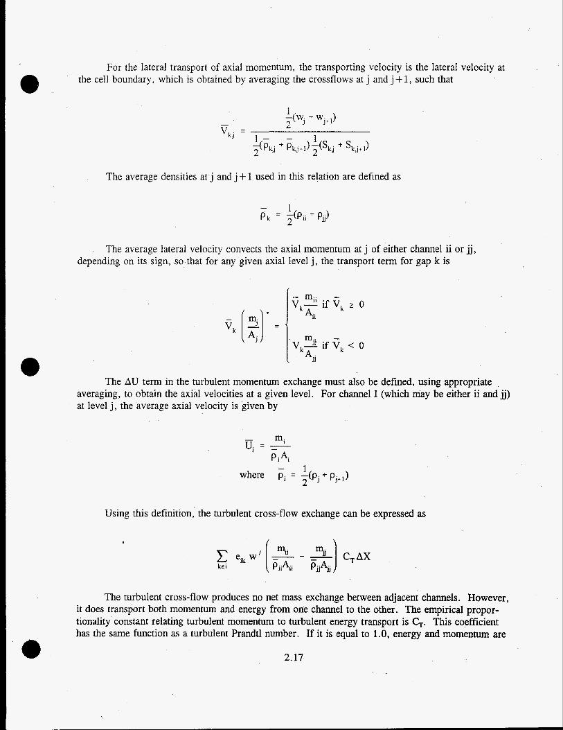
For the lateral transport of axial momentum, the transporting velocity is the lateral velocity at the cell boundary, which is obtained by averaging the crossflows at j and j + 1 , such that
The average densities at j and j + 1 used in this relation are defined as
- 1 P k = $3, + PJ
The average lateral velocity convects the axial momentum at j of either channel ii or jj , depending on its sign, so that for any given axial level j, the transport term for gap k is
The AU term in the turbulent momentum exchange must also be defined, using appropriate averaging, to obtain the axial velocities at a given level. For channel I (which may be either ii and jj) at level j , the average axial velocity is given by
- m. u. = 1 pi Ai
1 -
- 1 p. = -(pj + pj+l) l 2
where
Using this definition, the turbulent cross-flow exchange can be expressed as
The turbulent cross-flow produces no net mass exchange between adjacent channels. However, it does transport both momentum and energy from one channel to the other. The empirical propor- tionality constant relating turbulent momentum to turbulent energy transport is G. This coefficient has the same function as a turbulent Prandtl number. If it is equal to 1.0, energy and momentum are
2.17

exchanged at equal rates. If it is set to 0.0, there is no lateral momentum exchange due to turbu- lence. The actual value used in the code is determined by user input.
When the above definitions and approximations are used in the subchannel equation for axial momentum, Eq. (2.1 €9, the finite difference form of the axial momentum equation is
(2.21)
In applications where fluid-fluid shear must be included in the axial momentum equation, the finite difference form is derived from Eq. (2.14a) rather than Eq. (2.14). All of the terms are the same as shown in Eq. (2.21), except for the wall shear stress term. The finite difference form in this case is expressed as follows;
piiAii p. .A.. U U kai
(2.2 1 a)
2.3.3 Conservation of Lateral Momentum
As with the axial momentum equation, average velocities for momentum transport must be defined in order to formulate the finite difference equation. In the axial convection of transverse momentum, the transporting velocity is defined as
1 - u. =
2.18

The cross-flow convected by this average velocity defines the transport term as
UJ wJ if uj 2 o - I - UJ wj+, if Uj < 0
UJ w = =
When the above definitions are substituted into Eq. (2.15), the final form of the finite differ- ence equation for lateral momentum becomes
(2.22) 1 W AX.
- Sj!AX.p gsin8 - - KG/&I wj 2 J J 2 Pjsj c
In applications where fluid-fluid shear must be included in the lateral momentum equation, the finite difference form is derived from Eq. (2.15a) rather than Eq. (2.15). All of the terms are the same as shown in Eq. (2.22) above, except for the additional fluid shear stress terms.
The axial transport of lateral momentum, Fad, is defined as
I
The viscosities are calculated by averaging between the values of the adjacent channels connected by the gap at the axial levels j and j-1, and at j and j + 1, as follows:
1 4
pJ = -[piij + p... + p... + p... ] I I J l I J + l JJJ+1
1 pJ-] = - [ p i i i + p . . . + p . . . +p... 3 4 JJJ xu-1 JJJ-1
2.19

The lateral transport of lateral momentum, F,,,, is defined as
In the summation, n is the index of a gap connected to gap k by fluid-fluid shear. The average viscosity is calculated at a given axial level as
The F,,,,,,, termS defined above are substituted into the lateral momentum equation for the case with fluid-fluid shear. The finite difference form is in therefore expressed as follows:
(2.22a)
The lateral fluid-fluid shear term is incorporated into the COBRA-SFS code in a manner that permits only two other cross-flows to be connected to a given gap, k, for the exchange of lateral momentum.
2.3.4 Conservation of Energy for the Fluid
The finite difference approximation of the subchannel equation for fluid energy, Eq. (2.17), can be written directly, using the definitions and assumptions noted above for the mass conservation equation. The only significant differences are that the axial and lateral flows (m and w) convect
2.20

enthalpy rather than density in this equation, and there are energy fluxes through the solid surfaces as well as the fluid surfaces of the control volume. The finite difference form of the energy equation is, therefore,
+ 4 X , x elk w,h * = P,,.@,AXJ q " k a n a
(2.23)
- (T,i - TjJj + eik Sj AXj k, + 4Xj eik w 'j (hii - hjj)j
ku c Z, k i
In the actual solution of the energy equation in COBRA-SFS, however, it is necessary to separate the mass continuity error from the energy error. This is done by the simple expedient of multiplying the mass continuity equation by the flowing enthalpy and subtracting the result from the energy equation. So the final form of the finite difference equation for the fluid energy in COBRA- SFS is
+ m j @ * -h j ) - mj-,(h*-hj-,) (Ph - <Ph>")j xj AXj At
+ AX, eik wj(h * - hj) = P, @"AXj 9'' ki x i
(2.24)
-(Tii - T..). + eikSj AXj k JJ '
+ AX. 1 . eikw 'j Pii - h,Jj k a Qz, ka
The heat flux through the solid surfaces of the control volume, denoted by q" in the above equation, is the surface-averaged convective heat flux over the given node. If the conduction model is not used, the heat flux is simply a boundary condition specified by user input. When the conduction model is used, however, the heat flux is a calculated quantity determined in the solution of the con- duction equation for heat transfer in the fuel rods or solid structure nodes (see Section 2.4). Heat transfer between the fluid and wall is modeled using empirical heat transfer coefficients, such that
The surface temperature of the rod or slab node, T,, is solved for in the solid conduction energy equation (see Section 2.4). The sink temperature for the heat flux calculation is the fluid temperature corresponding to the enthalpy of the subchannel in that node.
a 2.21
2.4 Energy Conservation in Fuel Rods and Solid Structures
Heat transfer in the fuel rods and other solid structures is determined in COBRA-SFS using the following conduction equation:
q// = -kVT
It is approximated using a control volume formulation, consistent with the finite difference formulation of the fluid conservation equations. In these structures, surface area of the control volume is defined by the product of the axial height of the adjacent fluid control volume (AXj, as used in Eq. [2.24]), and the segment of the rod or wall perimeter that is connected to the fluid node. (This information is specified by user input.) A surface temperature is determined for each node by solving the energy equation. The user also has the option of modeling internal nodes within the solid structure, and solving for the local temperatures of these nodes.
For steady-state problems in which radiative heat transfer can be neglected, the noding of the fuel rods is used only to define the surface heat flux into the fluid control volumes (Le., the sub- channels). Unheated solid structures are not modeled in the heat transfer solution, but are treated simply as adiabatic surfaces. This is the simplest form of the heat transfer solution in COBRA-SFS, and there are very few cases where it is an adequate representation of the problem. More often, it is necessary to include radiation exchange between the rods and conduction through walls, support baskets, and other unheated structures in contact with the fluid.
Conduction through unheated structures is modeled in COBRA-SFS with the “slab” energy equation, which is simply the conduction equation with boundary conditions defined by the fluid temperature and user-specified heat transfer coefficients at the node surfaces. These surfaces can also exchange energy with each other and with the fuel rods via radiation. There are two options available for modeling heat conduction in the fuel rods. For steady-state problems, it may be sufficient to solve a simplified form of the conduction equation for the cladding only to obtain surface tempera- tures of the fuel rods. In transient calculations, or if fuel centerline temperatures are needed, it is necessary to solve the conduction equation for the fuel pellet as well as for the cladding.
The following subsections describe these heat transfer models and their formulation in COBRA- SFS. ‘They are coupled to the fluid conservation equations via the energy flux terms for heat transfer to the fluid, which are expressed in terms of the fluid temperature and appropriate heat transfer coef- ficients. The manner in which these equations are solved together is described in Section 4.0.
2.4.1 Rod Energy Equation
When the heat generation in the fuel rods is treated as a simple heat flux boundary condition on the fluid, it is not necessary to solve the conduction equation for the fuel rods. In that case, the surface heat flux for the fluid energy equation is calculated as
2.22

The heat flux, 9". is calculated for each rod from the input values for rod geometry and the fuel volumetric heat generation rate, q"'.
If thermal radiation is important for a given problem, however, it is necessary to determine the surface temperatures of the fuel rods. For steady-state problems, it is often sufficient to solve the conduction equation over the cladding only, treating the heat generated in the fuel as a source term at the inner boundary. The total heat removed by convection varies as a function of fluid temperature and the surface heat transfer coefficient. The radiation term includes contributions from slabs and other rods within the same assembly. It is assumed that slabs and rod surfaces exchange radiant energy only in the same plane. This greatly simplifies the determination of the appropriate view factors for radiation exchange. since these are therefore needed only in two dimensions. Given the axial uniformity of fuel bundles. this is a reasonable assumption for most geometries to which COBRA-SFS is likely to be applied.
When using the option for the cladding surface conduction only, it is assumed that there is no axial heat transfer, and that the temperature is uniform around the circumference of the rod at a given axial level. The rod energy equation for the clad alone can therefore be expressed as
(2.25)
The rod heat transfer model represented by Eq. (2.25) is adequate for nearly all steady-state applications of COBRA-SFS. For transient applications, or cases where the internal rod temperature distribution is important, a forniulation of the conduction equation must be used that includes internal nodes for the fuel rods. In this model, separate conduction equations are written for the cladding and for the fuel. The cladding is represented with a single node, but the fuel is divided into a number of radial rings, as illustrated in Figure 2.5 (for fuel with a central void), and in Figure 2.6 (for fuel without a central void). The number of fuel nodes in a given case is determined by user input, and the nodes are assumed to be of equal radial thickness, except for the innermost and outermost nodes, which are one-half the thickness of the other nodes.
The conduction equation for heat transfer in the cladding is similar to Eq. (2.25), except that in this formulation the time-dependent energy storage term cannot be neglected, and the energy entering the cladding from the fuel does so via conduction, rather than as a source term. With these changes, the conduction equation for the cladding becomes
(2.26)
2.23

S9503052.5
Figure 2.5. COBRA-SFS Finite-Volume Fuel Rod Model with Central Void
The clad conduction equation is coupled to the fuel conduction equation through the gap heat transfer coefficient, Hgap, and the temperature difference across the gap between the fuel pellet and the clad. The gap heat transfer coefficient is an empirical parameter, defined by user input. In the clad node, heat transfer is considered in the radial direction only, with a uniform temperature distribution radially around the circumference of the rod. This is the usual approach in the fuel pellet, as well, but the conduction equations are formulated to allow consideration of azimuthal as well as radial noding. Nodes in the circumferential direction are counted with the variable No, and in the radial direction with N. The fuel pellet node temperatures are identified as Tkm where k is the radial location (1 to N), and m is the circumferential location (1 to No).
2.24

59503052.6
Figure 2.6. COBRA-SFS Finite-Volume Fuel Rod Model Without Central Void
2.25

The set of conduction equations in finite-difference form for each of the N fuel nodes and the cladding node, N+ 1, can be written as follows:
Fuel node 1 (inner-most node):
Fuel nodes 2 through N- 1 :
Fuel node N (fuel surface node):
(2.27)
(2.28)
(2.29)
2.26

Cladding Node N + 1 : *
*
a
(2.30)
In this model, it is assumed that axial heat transfer is negligible, heat is generated uniformly throughout the fuel at a given axial location, and material properties of the fuel do not vary signifi- cantly with the radial variation in temperature.
2.4.2 Solid Structure Energy Equation
The heat transfer model for the solid structure nodes is formulated for an arbitrary control volume that can exchange energy with the fluid and with other solid structure nodes via conductive or radiative heat transfer. In addition, the solid structure nodes’can exchange energy with the rods by means of radiation. The generic control volume for a solid structure node, (also called a “slab” node, to differentiate it from a fuel rod node), is illustrated in Figure 2.7. The axial length of the control volume is denoted by Axj, which corresponds to axial noding of the fluid subchannels. The cross- sectional area for axial heat transfer from a slab node is defined by user input. A slab control volume may have any number of surfaces connected to adjacent slab nodes or fluid subchannels. These connections and their dimensions are defined by user input.
In addition to conductive and convective heat transfer between the slab node and adjacent slab or fluid nodes, the control volume can also exchange energy via thermal radiation with the surfaces of fuel rods and other slabs. Given the above assumptions and definitions, the conduction equation for the slab node can be written in finite difference form as
2.27
(2.31)

A, (transverse face: may see other slab nodes) S9503052.7
Figure 2.7. Solid Control Volume
As with the rod equation, radiation is assumed to occur only in a given axial plane. Conduction between two slab nodes is modeled using a composite thermal conductance, U, which accounts for the heat transfer area, the thermal conductivity of the slab materials, and any gap resistance or thermal radiation at the slab interface. In the axial direction, a composite thermal conductance through the top and the bottom of the slab node is calculated, denoted as Uj and Uj-,, respectively. The actual values used in a given problem are determined from user input of appro- priate empirical conduction resistances for the various node connections. (See Section 3.2 for a discussion of the composite thermal conductance as a constitutive model in the code, and to Section 6.2.6 for the group SLAB input instructions.)
2.28

3.0 Constitutive Models
The three-equation model presented in Section 2.0 fully describes the fluid behavior in systems modeled using COBRA-SFS i n terms of the independent variables of pressure, mass flow rate, and fluid enthalpy. With the addition of the heat transfer models for the fuel rods and other solid structures, a complete flow and heat transfer system can be described. To solve the equations, however, closure relations are required to define terms in the equations that are not amenable to calculation from first principles. This section presents the empirical models used in COBRA-SFS to achieve closure of the equation set. These models are reasonable within the intended application of the code, and every attempt has been made to adequately verify the formulation. However, it must be noted that constitutive models are empirical approximations, and can always be improved. They should be used with careful consideration of their range of applicability, and it is to be hoped that eventually some state-of-the-art advances will come along and make them obsolete. In that happy event, it should be a relatively simple matter to replace the existing models with the improved ones. This is made particularly simple by the fact that most of the empirical models in the code are defined by user input.
3.1 Fluid Flow Models
The momentum exchange terms are a primary source of empiricism in the fluid flow equations in COBRA-SFS. As discussed in Section 2.2 in the derivation of the subchannel partial differential equations for momentum, the solid surface stress tensor is represented by wall friction and form drag correlations. The fluid stress tensor is replaced by velocity-dependent models for fluid-fluid shear. Energy and momentum exchange due to turbulent mixing must also be represented by empirical models, since turbulence is neglected in the primary formulation of the mixture balance laws over the control volume. The following subsections describe these constitutive models as currently implemented in COBRA-SFS.
3.1.1 Wall Friction
The shear stress terms in the axial momentum equation for rod bundle geometries were defined in Section 2.2 by an approximation of the shear stress integral in the momentum balance. In the normal subchannel formulation, this integral was approximated by a wall friction term that included an empirical friction factor, f, as shown in Eqs. (2.12) and (2.14). An alternative formulation was also presented for wall shear in channels modeling an open flow region. This formulation is a function of fluid properties and geometry only, and was presented in Eqs. (2.12a) and (2.14a). Although the fluid shear stress terms in these equations are approximations of the mathematical model for shear stress, they are not constitutive models in the usual sense of the term, since they are not based on fits to data. Therefore, the friction factor is the only constitutive relation used in the wall shear stress term. The friction factor used in COBRA-SFS is the Darcy-Weisback friction factor, a dimensionless number determined from experimental measurements of axial pressure drop in a wide range of geometries and flows. These data are primarily for flow in pipes and tubes, but it is assumed that these flow geometries scale to subchannel flow by means of the hydraulic diameter.
3.1

The friction factor correlation for turbulent flow is expressed in COBRA-SFS as
f = aRe cRed + e (3.1)
The coefficients a, b, c, d, and e are empirical constants specified by user input, and Re is the local subchannel Reynolds number, defined as
The user has the option of specifying several friction factor correlations of the form shown in Eq. (3. l), in order to model different friction losses in different subchannels within the problem (refer to Section 6.2.9, which contains the input instructions for group DRAG).
The friction factor correlation for laminar flow is expressed in COBRA-SFS as
4 = a,Reb' + ct (3.3)
As in the correlation for turbulent flow above, the empirical constants a,, b,, and c, are speci- fied by user input. The actual value of the friction factor used in the axial momentum equation for a given subchannel node is determined as the maximum of the laminar and turbulent correlation values at the local Reynolds number.
The friction factor correlations described by Eqs. (3.1) and (3.3) are based on a Reynolds number defined with the subchannel-averaged fluid viscosity. There is in reality a distribution of viscosity due to the subchannel radial temperature profile in the fluid. As an option specified by user input, COBRA-SFS includes an empirical correlation to account for the viscosity variation near a heated surface. The relationship used is that developed by Tong (Tong 1968), and has the form
= f [ 1.0 + [ [ !qa6 - pbulk
The viscosity at the wall, pWd, is determined from the fluid properties using an estimated fluid temperature at the wall. This temperature is calculated from a simple heat balance as
It is important to note that the calculated wall temperature used in this correlation is based on the total heat input to the channel in the given node, over the total heated perimeter of the channel. It is assumed for the purposes of this calculation that the heat input to the channel is uniform over the
3.2

perimeter, when in fact the heat inputs from the various rods surrounding the channel may be different. However, these differences will in most cases be relatively small. Any error this might introduce into the approximation will probably be quite small, at least in relation to the uncertainty inherent in the Tong viscosity correction correlation itself.
The user should also take note of the fact that the Tong viscosity correction correlation was derived from data obtained with water as the working fluid. In most COBRA-SFS applications, the coolant is a gas such as air, nitrogen, argon. or helium. The correlation is formulated in terms of the fluid properties, and therefore should be applicable to different fluids, but it has not been validated for fluids other than water. In general, the wall viscosity correction will be very small, and in many cases it will make more sense to ignore it. It is not usually needed for cases where the working fluid is a gas with a high thermal conductivity, such as helium.
3.1.2 Form Drag Models
In addition to the momentum effects of friction at the wall, local obstructions to the flow due to structures such as grid spacers, orifice plates, and local. variations in the flow area result in axial pressure losses. The reversible component of such losses is calculated in the axial momentum equa- tion, if the area change is included in the COBRA-SFS model. The irreversible component must be explicitly included by means of the constitutive model for form drag.
The pressure drop across a local obstruction is expressed as
The loss coefficient K is an empirical parameter determined from measured data in similar structures. In COBRA-SFS, these local loss coefficients can be modeled as constants or as functions of the local Reynolds number with a form similar to that of the wall friction correlation in Eq. (3.1). Refer to Section 6.2.9 for the input instructions for group DRAG.
In the formulation in Eq. (3.4), the cross-sectional area A refers to the nominal channel flow area, and not to the flow area at the obstruction itself. The user must be aware of this definition when determining appropriate input values for K from pressure drop measurement data. In some cases, the reported K values are determined based on the flow area at the obstruction. When using such values as input for a COBRA-SFS model, the measured loss coefficients must be scaled by the area ratio, so that the input loss coefficient is defined as
The shear stress integral for the lateral momentum equation is modeled with a simpler approxi- mation than that used for the axial momentum equation. Both wall friction and form drag are treated
3.3

with a single approximation of the pressure loss coefficient. This permits formulation of the pressure loss in terms of known geometric quantities, such that
KJ w(w AP= (3.5)
2gcps’
In rod assemblies, the coefficient I(G can be thought of as the form loss for flow through the gap between two adjacent fuel rods. The value for K, is dependent on the geometry of the given problem and must be specified by user input (refer to the input instructions for group DRAG, in Secrion 6.2.9).
3.1.3 Turbulent Mixing Models
The turbulent mixing model in COBRA-SFS approximates the momentum effects of turbulence by defining a fluctuating cross-flow per unit length, w’, that represents an equal mass exchange between adjacent channels. This fluctuating cross-flow is related to the turbulent eddy diffusivity by the definition
e -
The local value of this fluctuating cross-flow is not determined directly from the eddy diffu- sivity, however, since this is not an easily determined quantity over the flow field as modeled in subchannel analysis. Instead, the fluctuating cross-flow is calculated from an empirical relation using the geometry of the gap, the average axial flow rate in the gap, and experimentally determined mixing coefficients.
There are four such turbulent mixing correlations included in COBRA-SFS (Rogers and Todreas 1968; Ingesson and Hedberg 1970; Rogers and Rosehart 1972). They are selected by user input, and are formulated as follows:
wT = a S k G
wT = a Reb 6 G
s, -- w T = a R e b - D G
‘k
3.4

wT = a Re bS, G
where _- G D Re = -
P
E = 4 (Aii + Ajj)/(Pw + P, ) I , u
G = (mi, + mjJ/(Aii + Ajj)
The user may specify different correlations or different coefficients for each assembly type (refer to the input instructions for group HEAT, in Section 6.2.8).
3.2 Energy Exchange Models
As formulated in Section 2.0 above, it is implicitly assumed that the surface heat flux terms that appear in the fluid energy equation and in the conduction equations for the fuel rods and solid structures are known, or can be calculated from known quantities. ,In actual practice, these heat fluxes depend on convective heat transfer, radiative heat transfer, and contact conductance, all of which can be determined only with the aid of empirical heat transfer models. Constitutive relation- ships are required for surface heat transfer coefficients, radiation exchange factors, and contact conductance. The following subsections describe how these models are implemented in COBRA-SFS. e 3.2.1 Convective Heat Transfer Correlations
Convective heat transfer is modeled in COBRA-SFS using a heat transfer coefficient defined in terms of the Nusselt number. The heat transfer coefficient is defined by the expression
The Nusselt number is defined as a function of Reynolds number and Prandtl number, using the empirical relation
Nu = AReaPrb + B
The local heat transfer coefficient is calculated in the code using this formula. The values for the empirical constants are specified by user input, and different correlations can be specified for different channels (refer to Section 6.2.8, containing the input instructions for group HEAT).
a 3.5

3.2.2 Fluid Conduction Shape Factor
Conduction in the fluid is modeled directly in the formulation of the fluid energy equation in COBRA-SFS, but only in the lateral direction. Axial conduction is assumed negligible. Lateral conduction is calculated through the gaps over the centroid length between the subchannels. How- ever, the exact length of the centroid is a matter of definition, and may or may not be the appropriate length for the conduction path. The fluid conduction model in COBRA-SFS therefore includes an option to specify the centroid length for conduction as a value different from that used for the lateral momentum equation. This is implemented by defining the conduction length e, in terms of the centroid length i' using an empirical shape factor,
4, = cz,
The appropriate value for Z, is problem-dependent, and general guidelines are not readily available. Experience has shown that with air or helium as the working fluid, a value near unity gives good agreement with experimental data.
3.2.3 Solid-to-Solid Conduction
In theory, the heat transfer due to conduction between adjacent solid nodes can be calculated exactly using the conduction equation as formulated in Section 2.4. In practice, the contact conduc- tance at the interface between adjacent structures is not always known with great accuracy. Since this contact conductance (or resistance, if considered as a reciprocal) plays a large part in determining the rate of heat transfer, accurate characterization of this parameter becomes a very important modeling consideration.
In COBRA-SFS, contact conductance between adjacent solid structure nodes is modeled using a composite thermal conductance, U. This conductance includes the heat transfer area of the interface and the thermal conductivity of the node materials. In addition, it also accounts for any gap resis- tance due to imperfect contact between the two surfaces, and includes thermal radiation across the gap. The components of the total thermal resistance are shown schematically in Figure 3.1. The terms R, and R2 denote the thermal resistance from the center of each slab node to the interface between them, and are defined by user input. The total series resistance of the solid portion of the heat transfer path between the two slab nodes is given by
The resistance for node n is defined as
3.6

Solid Node #I 'Solid Node #2
R i I I I I
R2
-2 Y Conductivity Length L, Conductivity Length L,
59503052.6
Figure 3.1. Solid-to-Solid Resistance Network
The values of L, and A, are determined from user input, where is the distance from the center of the slab node to the interface (as shown in Figure 3. l), and A, is the area of the interface between the two nodes.
The radiative heat transfer across the interface is approximated as radiation between two parallel plates where the surfaces are assumed to be grey bodies. The thermal resistance is given by the relation
a 1 1 - + - - I
oA(TI2 + T:)(T1 + T2) - €1 €2
RRAD -
In this formula, T, and T2 are absolute temperatures (in the code, the units are degrees Rankine), E , and constant.
are the surface emissivities of the slab nodes, and ~7 is the Stefan-Boltzmann
In parallel with the radiation across the gap, the conduction resistance is also calculated based on the user-specified material properties for the fluid in the gap. The total gap resistance, therefore, can be expressed as
The overall thermal conductance between the adjacent slab nodes can be calculated as
e 1 u =
Rsom + RGAP
3.7

This formulation is used for heat transfer between slab nodes in both the transverse and the axial directions, as shown in Eq. (2.31). The appropriate composite conductance U for any given connection is calculated from the user-specified definitions of solid-to-solid connections and slab node geometry (refer to the input instructions for group SLAB in Section 6.2.6).
3.2.4 Radiation Exchange Factors
The radiation heat transfer between surfaces is modeled using radiation exchange factors. The net rate of radiant energy outflow from surface I to surface j , denoted by Qij, is defined in terms of an exchange factor, F,,, such that
Q.. ?I = AiF..a(Tf 'J - T:)
The quantity F,, defines the fraction of the total amount of radiant energy emitted from surface I that actually reaches surface j and is absorbed. This includes all the paths by which radiation may reach surface j from surface I, including direct and reflective paths. This has been termed a grey body view factor, and gives a much more realistic estimate of the energy exchange between surfaces due to radiation than can be obtained using standard 'black-body' view factors. Black body view factors, as the name implies, assume that all incident radiation is absorbed, and none reflected. For surfaces with an emissivity of 1.0, the grey body view factors reduce to the black body factors, since an emissivity of 1 .O implies black surfaces for radiation heat transfer, by definition.
The radiation exchange factors F, can be calculated from the geometry of a particular problem and the ideal black body view factors for the given surfaces. However, this is not a trivial calculation for a geometry of any complexity, such as a fuel rod array in a canister. The preferred means for calculating these values for input to COBRA-SFS is to use the auxiliary code RADGEN, which solves the set of equations (Cox 1977);
n 1.0-E. 8ki x p ki .(-) - -IF.. 'J = -B kj E . k~ i = l 'i 'i
Every surface I sees every surface j = 1,2,3,.. .n, and by reflection sees every surface k= 1,2,3, ... n, where n is the total number of surfaces radiation.
from each surface j, also that can exchange energy by
For enclosures that consist simply of wall nodes, the system of equations can be solved in the COBRA-SFS code, as part of the input processing. The user supplies only the black body view factors for the surfaces, and their emissivities. The code calculates the appropriate grey body view factors internally. For enclosures that include rods, however, the code expects the grey body view factors as input. These must be calculated before-hand, using the RADGEN code, or any similar code that produces the grey body view factors in the appropriate format. Correct and consistent input for the grey body view factors is absolutely essential for the radiation model in COBRA-SFS to work properly. Where possible, input checks have been installed in the code, but the conscientious user would be well advised to study carefully the input instructions for the RADG group of the COBRA- SFS input (see Section 6.2.7), and those for the RADGEN code (see Section 6.3).
3.8

a 4.0 Numerical Solution Methods
The solution of the governing equations for fluid flow and heat transfer in COBRA-SFS is fully implicit and proceeds iteratively through a series of steps that addresses each of the conservation equations in turn. Within an iteration, the code solves the momentum equations for the velocity field, then the energy equations for the temperatures and enthalpies, and then the mass continuity equation for the pressure field. Within this simplistic description, however, lies a wealth of intricate detail.
The basic fluid solution is applicable to single-phase flow at very low velocities, with or with- out buoyancy-driven natural circulation. The code is also capable of resolving the flow and pressure fields for systems in which the net flow is zero. This calculational flexibility is a feature of the numerical solution method for the fluid equations that COBRA-SFS has inherited from its immediate predecessor, COBRA-WC (George et al. 1980). In spent fuel assemblies and storage or shipping casks, the flow field may be fairly simple to obtain, but the strong coupling of the fluid energy equa- tion and the heat transfer models for the solid structures presents special problems of stability and convergence rates. In particular. the energy equations for the fluid and solid structure nodes must be solved simultaneously, and the rate of convergence of the temperature solution tends to dominate convergence behavior, rather than the elimination of momentum or mass conservation errors.
The following subsections describe the flow and energy solutions in the code in some detail. Section 4.1 presents the fluid flow solution. and Section 4.2 the solution of the energy equations. It should be borne in mind, however, that although the solutions are described separately, they are performed together within an iteration of the solution procedure.
4.1 Fluid Flow Solution
The finite difference equations for mass continuity, (Eq. [2.20]), momentum, (Eqs. [2.21] and [2.22]), and energy, (Eq. [2 .23]) for the fluid are solved using the RECIRC solution method, adapted from the COBRA-WC code. In this method, the set of equations is solved iteratively to obtain the flow and pressure fields. The primary advantage of the RECIRC method is that it is applicable to reverse and recirculating flows, such as those occurring in storage systems cooled by natural circu- lation. RECIRC uses .a Newton-Raphson technique similar to the one developed by Hirt (Hirt and Cook 1972) to solve the conservation equations, but it has been made implicit in time, as was done in the SABRE code (Gosman et al. 1973). The solution method is quite complex, and it is summarized here before examining each separate step in detail.
The RECIRC flow field solution is divided into two parts: a tentative flow solution and a pressure solution. The tentative flow solution is achieved by iteratively sweeping the bundle from inlet to exit. In each sweep, tentative axial flows, rii, and cross-flows, W, are computed for the bundle by evaluating the two linearized momentum equations with current values for pressure and other independent variables. After all tentative flows and cross-flows have been computed at all axial levels, the flows and pressures are adjusted to satisfy continuity by a Newton-Raphson method. The flow field obtained in this pressure solution is then used in the energy equation to obtain an enthalpy and fluid properties distribution for the next axial sweep. A flow chart of this procedure is shown in Figure 4.1. The tentative flow solution is described in more detail in Section 4.1.1 and the pressure solution is described in Section 4.2.2.
4.1

Level
1 Begin External Iteration
A4 I Begin Axial Sweep from Bottom to Top 1
1 Solve Energy Equation * I Calculate Current Fluid Properties, Friction Factors,
and Heat Transfer Coefficients c 1 Solve Momentum Equation for Tentative Axial
and Lateral Flows * Yes
Begin Pressure Loop 1 I %
- I Next Level
Top to Bottom
Perform 1-D Solution Every Third External Iteration Option
Active
I
I Evaluate Current Continuity Error in Each Node
Solve Continuity Equation for Pressure Adjustment; Level-by-Level then Channel-by-Channel *
* I
Calculate New Axial and Lateral Flows that Satisfy Continuity
V
Number of Iterations
Yes Yes v I Calculate New Pressures I
Evaluate Current Maximum Energy, Momentum, and Continuity Errors
A
\
I . .- .- . . . U
Figure 4.1. Flow Chart of the RECIRC Solution Scheme
4.2

4.1.1 Tentative Flow Solution
The first step in the RECIRC flow field solution is to solve the axial and transverse momentum equations for the tentative flow rates rii and W. Since the axial flow in channel I is affected by axial flows in adjacent channels through the crossflow terms, the tentative flows, mj, in all channels must be solved for simultaneously at an axial level. The axial momentum equation, (Eq. [2.21]), is linear- ized and applied to all channels at a level to form a system of N equations, where N is the number of channels, such that
The diagonal elements of [A] are defined by
The switch function, depends of the direction of flow and is defined as
(4.2)
- 0 if eikVk I 0
1 if eikVk > o Q, =
The off-diagonal elements of [A] contain zeros except for the columns representing channels adjacent to channel I, where the elements are defined as
- SkAhx. w I 4, = (1-63 ei, Vk J - - AXj An pn An
(4.3)
4.3

In this definition, the subscript n refers to a channel adjacent to I, connected through a gap k such that I is either the ii or jj channel of the pair. The index for n, therefore, is defined as n = ii + jj - I.
The vector [B] consists of the source terms, and is calculated as
The pressures and flow rates in Eq. (4.4) are those generated during the previous pressure iteration, except for mkt, which is the predicted axial flow rate obtained in the solution for the previous level. To ensure that friction effects have the proper weight when differentiating Eq. (4.1) with respect to pressure, the linearized pressure loss is defined as
The matrices of Eq. (4.1) are stored in arrays consisting of only the non-zero elements, and is solved by direct elimination at each level.
Once a set of tentative axial flows, ffi, has been obtained, the tentative cross-flows, W, are calculated. Since the transverse momentum equation does not depend on cross-flows in other gaps, a simultaneous solution is not necessary. The tentative cross-flows in each gap are calculated using the linearized form of Eq. (2.22), as
where
4.4

The pressures and flow rates used in Eq. (4.5) are those generated during the previous pressure iteration, except for the axial velocities at j-1, which are based on the flow rate predicted for the previous axial level in the current iteration. The tentative flow field is determined for each channel and gap by sweeping the assembly from inlet to exit. The resulting tentative flows and cross-flows satisfy the linearized momentum equations, but they do not, in general, satisfy continuity.
The efficiency of the overall solution can be enhanced if the flow rate used to define the donor cell axial momentum flux is forced to satisfy continuity during the tentative flow axial sweep. This is accomplished by defining a set of "predicted" axial flows mj at level j that are used to evaluate the tentative flow rate at level j + 1. The predicted flows are determined by solving the combined linear- ized momentum and continuity equations while assuming that the previous axial level flows are fixed. At level j only, the continuity error for each cell is calculated as
Ej = ij AXJAt(p - pP)j +hj -mj'-l +AXj + eikWjL1 (4.6)
The predicted flows, mi-, and w;-~, are calculated at the previous axial level and mj is the just- computed tentative axial flow. It is then possible to calculate an estimate of the pressure changes needed to satisfy continuity, using the derivatives of the tentative flows with respect to pressure, from the Newton-Raphson expression
The above equation is written for a given channel I, and n in the summation represents a channel connected to I through a gap k, such that n = (ii+jj)-1. The form of the pressure derivatives is described below, in Section 4.1.2, with the discussion of the pressure and continuity solution.
Once a set of estimated pressure changes has been calculated, the predicted flows to be used in the donor momentum flux terms for the next axial level are calculated using
(4.7)
4.5

The tentative flows and pressures at j are not updated using this information, however. These predicted flows are used only to provide a better estimate of the donor momentum flux distribution to the momentum equations at the next axial level.
The predicted average axial velocity in the gap, used in Eq:(4.5), is calculated as
For forced convection problems, the convergence is substantially improved if the predicted value for the axial momentum flux is used. For problems with negative flows or buoyancy-dominated flows, however, the use of predicted momentum flux can be counterproductive. For this reason, the calculation of a predicted momentum flux is automatically skipped in the solution procedure if nega- tive flows occur in an assembly.
4.1.2 Pressure and Linearized Flow Solution
After all tentative axial flows and crossflows have been computed at all axial levels in all assemblies, the pressures and flows are adjusted to satisfy continuity. For a given boundary condi- tion, the flow and pressure field in each assembly are locally independent of all the other assemblies. Therefore, the equations for flow and pressure are solved on an assembly-by-assembly basis. The first step in this process is to compute the continuity error, Ej, in all cells, using the expression
- AX = A 2 (p - pn), + 6. - fi. + AX^ eik +j
ki A t J J-1 (4.9)
The adjustments in axial flows and crossflows necessary to satisfy continuity are defined as
Am = m. - fij J J
Amj-l = mj-l - fij-,
4.6

Substituting these expressions into Eq. (4.9) and subtracting Eq. (2.20), it can be seen that the flow adjustments must satisfjr the expression
Ani, - Ani ,_ i AXJ elk Awj = - EJ k E i
(4.10)
Assuming that m and w are functions of pressure only, the flow corrections can be expressed as
The subscript n on the pressure terms in the equation for Awj above refers to the channel con- nected to channel I through gap k. The expressions for the flow and crossflow derivatives are derived from the linearized form of the axial and transverse momentum equations (Eq. [4.1] and [4.5]) and are presented in Table 4.1. e
The term A,, in the definitions in Table 4.1 is from Eq. (4.2), and the G term stands for the denominator of the right-hand side of Eq. (4.5).
Table 4.1. Flow Derivatives with Respect to Pressure
4.7

After substituting these definitions for the flow derivatives into the above equations for the flow corrections and rearranging, the general form for Eq. (4.10) becomes
1
(4.11)
This is equivalent to
(4.12)
The partial derivatives of the continuity error E, with respect to pressure are defined in terms of the computational variables, as shown in Table 4.2.
Table 4.2. Continuity Error Derivatives with Respect to Pressure
Error Derivative
"J-1
Definition
+ AX^ C eik - kei aPjj-l
4.8

When the expression presented in Eq. (4.12) if evaluated for all axial nodes and all flow channels for a given assembly, the coefficient matrix consists of M equations, where M is the total number of cells in the assembly (M = number of axial nodes times the number of channels). The matrix equation has the form
0
E . . . . - dE ,
. . . (4.13)
Since it is generally not possible to solve a matrix of this size directly, the matrix is solved in pieces. An alternating direction iterative solution is implemented that performs a level-by-level sweep followed by a channel-by-channel sweep for each iteration in the pressure loop. The solution pro- ceeds as described below.
First, the pressure change in each channel in the assembly is determined at each axial level, using current values of pressure change in adjacent axial levels. The equation for continuity error becomes
%j -1 aEJ
*pI,J-, + - aEl 8
aPI,J- I keg aPnJ_1 (4.14)
dE . aEJ 6PiP,-, - J 6P0. = - E l - - 'Pij -2 aPij
Note that the most recent values of the pressure change, denoted by the superscript 0, are used at the axial levels at the current level, j , and at the previous level, j-1.
4.9

For all N channels in the assembly at axial level j , Eq. (4.14) produces a system of N equa- tions having the form
. . . (4.15)
This matrix is solved by direct inversion to obtain new 6P values for the current level j.
On the second sweep of the assembly, the pressure changes at all axial levels are determined for each channel of the assembly. using current values for the pressure changes in adjacent channels. This equation for continuity error is
(4.16)
Considering all J axial levels in a given channel i, Eq. (4.16) forms a tridiagonal system of J equations for channel i, of the form
' aEi,J+l aEi,J+ 1 -- ap~,.l -1 api,J
This matrix equation is solved to obtain new 6P values for the current channel.
4.10
(4.17)

The pressure solution is a potentially time-consuming process for large problems. To solve the equation more efficiently. an axial rebalancing step is performed every third iteration, which consists of a one-dimensional axial approximation of the problem. To form the one-dimensional tridiagonal matrix equation, the total continuity error at each level j is calculated by summing over all N chan- nels, as
N E = Eij
J i =1
A tridiagonal matrix is then formed as follows:
This equation is then solved to obtain an average pressure correction at each level, which is then applied to the individual channel pressures at that level. During the pressure loop, the compu- tational mesh is repeatedly swept. level-by level and channel-by-channel, solving for 6P, until the change in all of the 6P values falls below a specified convergence criteria.
After the solution to the pressure equation has converged, the resulting pressure changes, the 6P values, represent adjustments to the pressure field that make the flow field satisfy continuity. The pressures and flows are than updated using
= P,Oj + 6Pij
a fij 1 = m , + - (6Pi3-, - 6Pij)
'Pij -1
At this point, the flow solution satisfies both momentum and continuity for the current set of erties and boundary conditions for the given assembly. The procedure is repeated for each
assembly in the problem domain. This new flow field is then used in the energy solution to deter- mine the convective heat transfer to the fluid, as described in detail in Section 4.2.
4.11

4.2 Energy Solution
The energy solution for the fluid and solid structures has been divided into the following steps:
1. The coefficient matrices representing the individual rod equations are decomposed by lower- upper (LU) triangular factorization to determine Tclad as a function of TflUid.
2. The fluid and slab equations are solved simultaneously using successive over-relaxation io obtain a fluid enthalpy and slab temperature distribution.
3. The rod temperature distribution is determined by back substitution of the new fluid temperatures.
The simultaneous solution of the fluid and slab energy equations is described in detail in Section 4.2.1. The rod energy solution, which consists of steps 1 and 3 above, is described in Section 4.2.2.
4.2.1 Fluid and Slab Energy Solution
The fluid energy equation (Eq. [2.24]) and the slab energy equation (Eq. 12.311) are generally so tightly coupled in COBRA-SFS applications that they must be solved simultaneously. The con- struction of the matrix equation describing each fluid and slab node at a given axial level is described below, followed by a description of the solution of both sets of equations.
The fluid energy equation (Eq. [2.24]) is written in terms of fluid enthalpy. However, certain terms require the fluid temperature to calculate the heat transfer due to fluid conduction and convec- tion. Therefore, the fluid temperatures are converted to enthalpies by the following approximation:
11 -ho
cP
T = T o + -
In this definition, the reference temperature and enthalpy are chosen arbitrarily as the current values of T and h from the previous iteration. The cladding temperature T,,, can be represented by solving Eq. (2.26) as
(4.18)
When these two expressions are substituted 'into the fluid energy equation (Eq. [2.24]), an equation is obtained that is linear in enthalpy. This system of N equations, (one for each subchannel i at level j), forms the matrix equation,
4.12
(4.19)

Q
0
a
The matrix [L] is an N x N coefficient matrix, N being the number of channels. The source vector is ( S , ) , and (hIj consists of the fluid enthalpies at level j. For large problems, the matrix b] is sparse, and in the interests of computational efficiency, only the non-zero elements are stored.
The only temperature terms in the fluid energy equation that are not expressed in terms of enthalpy are the slab temperatures T,. These temperatures are obtained from the solution of the solid structure energy equation and are included in the source vector {S , , ] . After each energy iteration, the terms containing slab temperatures are updated to reflect the values for the current iteration.
The slab energy equation presented in Eq. (2.31) is written in terms of temperature. However, the terms describing radiative heat transfer are a function of temperature to the fourth power. Rather than treat these terms explicitly, they are written for slab node i as
= A, OH,, (T, - T)
3 whereH,, = E,T,
T = Fi, T,,4 + Fin TCn4)/ewT: ( mei nei
The terms H, and T are evaluated using current iterate values and the resulting linear expres- sion is substituted into the slab energy equation (Eq. [2.31]). This yields an equation that is linear in temperature at level j. The equations for every slab at level j are combined to form the matrix equation
The matrix [u] is an M x M coefficient matrix, where M is the number of slabs (S,) is the source vector, and is sparse, and in the interest of computational efficiency, only the nonzero elements are stored.
contains the slab temperatures at level j. For large problems, the matrix m]
The slab energy equation consists of terms containing not only slab temperatures, but also fluid temperatures, Ti, and composite radiation temperatures, T. Fluid temperatures are obtained from the fluid energy equation and are represented in the source vector (Sw). After each fluid energy iteration, the source terms containing fluid temperatures are updated to reflect the current iteration values. The
4.13

composite radiation temperature is derived as a summation of terms containing slab and cladding temperatures to the fourth power. The cladding portion of this composite temperature is not updated during the fluid and slab solution, but the slab portion is updated after every slab energy iteration.
Both the fluid and slab matrix equations are solved by successive overrelaxation, with a default relaxation factor of 1.2. A single iteration consists of one sweep through the fluid equations, followed by one sweep through the slab equations. The iteration is repeated until the changes in fluid enthalpy and slab temperature are both less than user-specified convergence criteria. Alternatively, convergence may be defined as obtaining an asymptotic limit for the temperature field, but this requires some insight on the part of the user in examining the overall results calculated for the problem.
Once the fluid and slab energy solutions have both converged, the fluid temperatures are obtained using the fluid equation of state. The fluid temperatures are substituted into Eq. (4.18) to obtain the rod cladding temperatures. If a detailed rod model is used, the fuel temperatures are also back-calculated, using Eq. (4.21), as described in the solution of the fuel rod energy equation in Section 4.2.2.
For problems with several nodes'and significant heat transfer in the radial direction, the energy solution may take hundreds of iterations to converge. To speed up the convergence rate, energy rebalancing is performed on both the fluid and slab matrix equations.
4.2.2 Fuel Rod Energy Solution
To expedite the energy solution, the rod surface temperature is described as a function of fluid temperature in the form
The constants K1, K,, and & are generated by performing an LU decomposition on the fuel rod finite-volume equations. If radiative heat transfer is not considered, the constants are generated only once. If it is considered, the cladding temperature of a particular rod is dependent on the tem- peratures of other rods, and the rod equations are solved iteratively using the fluid and slab tempera- ture distribution from the previous fluid temperature iteration. When the constants K,, K,, and K3 have been determined, the above expression for cladding temperature is substituted into the fluid energy equation (Eq. [2.24]) before solving the fluid and slab energy equations.
In order to perform the decomposition, the fuel rod finite-volume equations (Eqs. r2.273 through [2.30]) are cast into a tridiagonal matrix of the form shown in Eq. (4.21). Here a rod model with one cladding node and four fuel nodes is used in the following example:
(4.21)
4.14

The elements are ordered i n a manner that allows storage of the coefficients in a 3 x 5 array. The subscripts in Eq. (4-21) are the index values of the storage array in COBRA-SFS rather than the matrix indices.
The terms in the coefficient matrix A are defined in Table 4.3 and the terms in the source vector y are defined in Table 4.4. If the coolant temperature distribution T, were known, Eq. (4.21) could be solved directly for the rod temperature distribution. However, since T, is unknown, matrix A is factored into an upper and lower triangular matrix, B and C, respectively, as shown in Eq. (4.22). As in Eq. (4.21). the subscripts in Eq. (4.22) represent storage locations rather than matrix indices.
- A =
1 0 0 0 0
-. ’3 I 1 0 0 0
0 c;, 1 0 0
0 0 c,, 1 0
0 0 0 cj, I
Performing the indicated matrix multiplication gives
0
0 C41B31
0
0 0
0 . O
B32 0
B42 ‘4 1 B32 +B4 1
‘5IB41 C,,B4*+B,,
By inspection, the terms of the stored A matrix can be defined in terms of the B and C matrices as
A,, = B,, A23 = Bu A33 = a, A43 = B42 A53 = 0
(4.22)
(4.23)
4.15

Table 4.3. Definitions of Coefficients in the A Matrix
I1 Element I Definition
d7 - kf
A13 A rN,
ArN, k f AZ1 and A3,
- d i
Using elementary matrix algebra, an algebraic expression relating Tcld and TRuid can be determined, as
let AT = Y
and Y = CZ
then ?%T = Y - CBT = CZ
thus BT = Z
4.16

Table 4.4. Definitions of Terms in the Y Matrix
Since B is upper triangular. only Z must be found to solve for T. The elements of B and C are given as follows:
4.17

Since y = CZ, Z can be evaluated in terms of C and Y as
z, = Y l
z, = Y , - z,ql
z; = Y ; - z,c;, ~
z, = Y, - Z&
Z j = Y j - Z,C5, + f(TJ
Since BT = Z. the expression for the clad temperature is determined as
Bj , Tj = 2,
Tj = Zj/Bj,
In more general terms of N fuel nodes, this is
This is equivalent to the cladding temperature expression
'clad = Kl + K, + K3 Hsurf 'fluid
This decomposition allows the cladding and fuel temperatures to be expressed as functions of fluid temperature. If there is no heat transfer by thermal radiation or by circumferential conduction, and if there is no rod-to-rod contact, then the rod solution is complete. However, if any of these effects are present, a change in temperature results in a change in terms of the source matrix Y , which requires iteration on the rod temperatures. When the constants K,, K2, and & have been determined, the expression for cladding temperature is substituted into the fluid energy equation before solving the Auid and slab energy equations.
4.18

5 .O Boundary Conditions
The COBRA-SFS code has great flexibility in the manner in which boundary conditions may be applied to a given problem. This reflects the wide range of possible applications of the code, and the complex geometries and heat transfer systems that it can be used to analyze. This flexibility, although necessary and desirable, places something of a burden on the user, however. The user must make logical and consistent selections in the boundary condition input, or risk falling prey to the merciless “gigo” law of computer programming; that is, “garbage in; garbage out.” This section presents an overview of the boundary condition specification options in the code, and explains how they can be used to model different sorts of problems. It is highly recommended that the user study this section carefully before attempting to set up any problems for COBRA-SFS analysis.
The boundary conditions for the code fall rather neatly into two classes: flow boundary conditions and thermal boundary conditions. The distinction between the two types becomes a bit blurred, however, when the optional plenum model is used. The plenum regions (top or bottom or both) provide a boundary on the flow, and also on the heat transfer to the environment beyond the boundary of the system as represented in the COBRA-SFS input model. The following subsections present these two types of boundary conditions separately, and also discuss in some detail how they interact and how they can be used in conjunction with one another. Section 5.1 discusses the fluid flow boundary condition options. Section 5.2 presents the thermal boundary condition options, including the optional plenum model. Transient forcing functions, by means of which the various boundary conditions can be varied over time, are described in Section 5.3.
5.1 Fluid Flow Boundary Conditions
COBRA-SFS derives from the COBRA family of subchannel codes, and in these codes, boundary condition specification is a relatively straightforward affair. They were designed to model flow in a fuel assembly or reactor core. Their main purpose is to determine what enters at the bottom and exits at the top of the core. The side boundary is assumed impermeable, isothermal, and generally ignorable. The boundary conditions are specified with a uniform exit pressure seen by all subchannels, and either a specified inlet flow (in which case the code calculates the resulting inlet pressure), or a specified inlet pressure (in which case the code determines the required inlet flow). This happy state of affairs can still be modeled using COBRA-SFS, but in general it is not adequate for typical applications of the code, even neglecting for the moment the added complication of the top and bottom plenum model option.
COBRA-SFS still operates under the assumption that the channels all see a uniform exit pressure. The user has considerable flexibility, however, in specifying what happens at the inlet. Basically, there are two options, which can be summarized as follows:
i . The total inlet mass flow is specified, and the code calculates the resulting inlet pressure distribution.
5.1

2. The inlet pressure is specified (by specifying the exit pressure and the desired pressure drop), and the code calculates the resulting inlet flow.
The first option is basically the same option as in the original COBRA code, but as implemented in COBRA-SFS, the user has considerable flexibility in specifying the distribution of the inlet flow. These variations are discussed in Section 5.1.1. The variations on the specified pressure drop option are discussed in Section 5:1.2.
5.1.1 Inlet Mass Flow Rate Boundary Condition Options
The user has the option of specifying different boundary conditions for different assemblies. Whether a given assembly will be treated with an inlet flow or a pressure drop boundary condition is determined by user input for each assembly (with input variable ITDPAWASS) on CHAN.6 (see Section 6.2.3). When specifying the inlet mass flow rate as a boundary condition for a given assembly, the user enters the global average inlet mass flux (in Mlbm/hr-ft*, input variable GIN on line OPER.2; refer to Section 6.2.11). This must be the overall average inlet mass flux for all channels in all assemblies with flow boundary conditions, and is assumed to be the sum of all subchannel flows divided by the sum of their inlet flow areas.
In order to specify how this global average mass flux is distributed among the subchannels, however, the user has the following four different options:
1.
2.
3.
4.
GIN is the average inlet mass flux, and local subchannel inlet flows are calculated based on the subchannel inlet area (specified by IG=O on OPER.l).
GIN is the average inlet mass flux, but the user will specify by input the relative fraction of flow for each assembly. Within each assembly, the local subchannel flow will be calculated on the basis of the subchannel areas, assuming a uniform mass flux over the assembly inlet (specified by IG=2 on OPER. 1).
GIN is the average inlet mass flux, but the user will specify by input the relative fraction of flow in each subchannel, for specified assemblies (specified by IG=3 on OPER.l).
GIN is the average inlet mass flux, but the user will specify by input the relative fraction of flow to each assembly, and within specified assemblies will also specify the fraction of flow in each subchannel (specified by IG=4 on OPER. 1).
It should be noted that these options do not really represent different boundary conditions. They are simply variations on the inlet flow boundary condition, which allow the user some control over the inlet flow distribution.
Another variation on the inlet flow boundary condition option can be obtained by requiring the code to calculate the appropriate inlet flow distribution that will give a uniform mass flux in all subchannels of the assembly. This is obtained by specifying IDTPA(NASS)=2, and defining the
5.2

desired uniform mass flux in GIN, on OPER.2. The code will use the values specified for the total system pressure drop DPS to obtain a first guess at the inlet pressure, but will then solve for inlet pressure values that give the desired uniform mass flux in the channels by adding DPS to the exit pressure PREF, (DPS and PREF are specified by input on OPER.2; see Section 6.2.11).
The user also has the option of specifying the total inlet flow rate, using input variable FTOTAL on OPER.2. The code will calculate the required inlet pressure for each channel to produce a uniform pressure drop across all channels at the specified total flow rate, FTOTAL. When this option is used, all assemblies must have the same boundary condition option, for obvious reasons. It is specified by setting ITDPA(NASS)=3 on CHAN.6 for all assemblies, or setting ITDP=3 on OPER.l (NOTE: this option has been tested only with FTOTAL=O.O; see Sections 6.2.3 and 6.2.11).
In addition to the above, there is one more flow boundary condition option that represents something of a departure from the standard assumption of a specified inlet flow and calculated exit flow. The user may specify a zero flow boundary condition at the top and bottom of the assembly (This is accomplished by setting ITDPAWASS) to 4 on CHAN.6 for that assembly; see Section 6.2.3). This option allows modeling of a sealed enclosure in which there are no plena at top or bottom. A number of electrically heated test sections simulating spent fuel rod arrays are of this configuration. Obviously, the uniform exit pressure assumption cannot be strictly adhered to in applying this boundary condition, or the problem would be over-specified. In this option, the specified exit pressure is used as the reference pressure for the fluid properties calculations, but the actual exit pressure seen by a given channel is whatever is required to give zero flow across the boundary.
5.1.2 Inlet Pressure Boundary Condition Options
The options to specify an inlet pressure in COBRA-SFS are implemented in terms of specifying a pressure drop for an assembly or group of assemblies. These are the options for a uniform pressure drop and the optional network model, which are described in detail below, in Sections 5.1.2.1 and 5.1.2.2, respectively.
5.1.2.1 Uniform Pressure Drop Boundary Option
The inlet pressure boundary condition option in COBRA-SFS is implemented as a specified uniform pressure drop (which is specified in variable DPS on OPER.2; see Section 6.2.11). This boundary condition can be applied to the entire problem, or to selected assemblies within the problem, by specifying input variable ITDPAWASS) = 1 on CHAN.6. It will be applied to all assemblies if ITDP= 1 on OPER. 1. When this boundary condition is selected for an assembly, the inlet pressure for each subchannel is defined as
P, = PREF+ DPS
* Note that the reference pressure PREF and total pressure drop DPS are specified by input on OPER.2.
5.3

When this option is used, the inlet flow for each subchannel in the assembly is calculated by the code. The value specified in GIN is used to determine the 'first guess' at the inlet flow rate, but the final converged value will in general be different.
5.1.2.2 Network Model
The specified total pressure drop boundary condition is generally applied uniformly to all channels. However, for some unusual modeling situations in which the COBRA code is applied to a reactor core, it may be desirable to allow the code to calculate the flow distribution between assemblies based on the orificing and assembly arrangement. The network model was developed for the COBRA code to model the pressure losses above and below the channel region in the Fast Flux Test Facility. This model has been retained in CO3RA-SFS, and could be used to model a storage cask system, if it were configured as arrays of parallel assemblies with plena above and below. However, the code has not been validated for such an application.
In most cases, it would probably be more efficient to use the plenum model in COBRA-SFS, rather than the network model. If the plenum model is used, the network model is superfluous. However, the network model is available in the code, and could be used if the user wished to undertake an appropriate validation effort. When the network model is used, a single pressure drop is specified (which may vary as a function of time), and the subchannel flow rates are adjusted so that the pressure drop through each flow path matches the specified uniform pressure drop @PS on OPER.2).
Figure 5.1 is a schematic description of the network model for a three-assembly problem with a bypass channel. The conservation equations described in the previous section are solved only for the region containing the three assemblies, as noted in Figure 5.1. This region represents the assemblies, consisting of rods and subchannels, where flow resistance is determined by wall friction factors and local form loss coefficients. The gravitational head is also accounted for in this region. Along the additional portions of the flow paths, a reduced momentum equation is solved, which takes into account only the flow resistance due to friction and form losses and the gravitational head. No inertia terms are included, and it is assumed that the transport time through the network model is essentially zero.
In the example described by Figure 5.1, the resistances marked RMN and RAOm are the flow resistances associated with the assembly inlet orifices and the outlet hardware (handling socket, etc.), respectively. The loss Coefficients can be made dependent on Reynolds number by means of input option selections. A gravitational pressure drop can also be modeled by supplying head lengths at the inlet and outlet. (These are noted as HA in Figure 5.1.) The assembly inlet gravitational head is calculated using the inlet temperature to define the density. The outlet gravitational head is calculated using the mixed mean assembly outlet temperature to determine the density.
The assembly group dynamic loss coefficients, R,,, and Rmm, represent the flow resistances from a common plenum to the assembly group plena or to the downcomer region. The group dynamic loss coefficients are assumed to be independent of Reynolds number. Here too, gravitational losses may be modeled by supplying head lengths. One additional term, RT, may be used to represent the dynamic loss coefficient for flow from the inlet nozzle to the common plenum.
5.4

J S9503052.10
Figure 5.1. Schematic Description of the Network Model for Pressure Drop Through the Reactor Vessel
For most problems, the actual loss coefficients for each of these resistances will not be known, but the flow and corresponding pressure drop across each resistance should be available. The effective loss coefficients may then be calculated as
For R, which may be dependent on Reynolds number, it is necessary to supply a wetted perimeter so the Reynolds number can be calculated from the flow rate. The wetted perimeter need not have any physical significance, but should be chosen so that the correct loss is obtained for a given flow rate when using the specified resistance versus Reynolds number curve.
5.2 Thermal Boundary Conditions
In addition to the fluid boundary conditions described above, the COBRA-SFS code also contains options for defining heat transfer boundary conditions. In many applications, there is significant heat loss radially out the sides of the canister or cask being modeled, and often out the top
5.5

and bottom of the structure, as well. The assumption of adiabatic boundaries for heat transfer is generally not adequate for spent fuel cask analysis. The user must be able to specify heat transfer boundaries on the sides, top, and bottom. The manner in which this capability is implemented in COBRA-SFS is described in Section 5.2.1 for the side boundary.
Top and bottom boundary conditions must be specified when a shipping cask or multi-assembly storage container has a lower or upper plenum within which the coolant mixes due to natural circulation. The physical structures of the cask above and below the fuel assemblies can also provide important heat transfer paths to the environment, in addition to the heat lost radially out the sides or transported by the working fluid. There also may be heat loading on the cask from the environment, due to solar insolation, external fires, etc. The top and bottom structures are modeled in COBRA- SFS using the plenum model. Boundary conditions for the plenum regions can be specified for the axial and radial directions in both plena. The expressions for heat transfer used in these boundary . conditions can include conduction, thermal radiation, and natural convection, or a combination of all three. It is also possible to specify heat sources by defining local heat fluxes at the boundary. The thermal boundary conditions for the plenum regions are described in Section 5.2.2.
5.2.1 Side Thermal Boundary Conditions
The default in the code is to assume that there are no side thermal boundary conditions. The outside boundary at each axial level is considered as adiabatic. The user has the option, however, of specifying a heat transfer boundary on the outermost wall node at each axial level. This is done by defining a onedimensional thermal connection, or series of connections from the node to some boundary temperature, ,that will permit heat transfer radially from the node. The user specifies a boundary temperature for the connection, along with a set of empirical coefficients for a heat flux correlation of the form
The empirical coefficients, C,, G, and C, are specified by input for each connection type. If the effect of radiative heat transfer is to be included, the surface emissivities must also be specified. The outermost boundary temperatures are also specified by input, and the user has the option of defining variations in the boundary temperatures, both axially and circumferentially. The expression in Eq. (5.1) allows for modeling of heat transfer modes that are not linear in temperature (such as natural convection, which is expressed in terms of a Grashof or Rayleigh number).
The user has a great deal of flexibility in specifying the side thermal boundary nodes, and the input has been made as general as possible to permit modeling of a wide range of cask and canister geometries. Examples of how this option can be used are illustrated by the validation calculations presented in Section 7.0. These examples include the relatively straightforward case of a single assembly with a specified temperature on the outside of the test section wall, as well as the more
5.6

complicated case of large multi-assembly storage casks with complex heat transfer paths through support baskets, shielding, insulation layers and cask shell structures. The user would be well- advised to study these examples carefully before attempting to set up the input to specify the thermal boundary conditions for a new application of the code.
Heat transfer through the specified side boundary connections is calculated as part of the energy solution. At each axial level, the temperatures in the boundary regions are estimated using slab temperatures from the previous iteration, before the rod, fluid, and slab energy equations are solved. The one-dimensional series of equations for each boundary connection are solved iteratively for a radial temperature distribution in the boundary region. After the boundary solution has converged, a linear composite resistance is constructed to represent the total connection between the outermost slab node and the specified boundary temperature. This resistance and the boundary temperature are then implemented in the solid structure energy equation (Eq. [2.31]). After all boundary resistances at an axial level have been computed, the energy equations for that level are solved. The iteration proceeds in this manner until convergence is achieved, or until the user- specified iteration limit is reached.
5.2.2 Plenum Boundary Conditions
In an ordinary COBRA subchannel model, the axial flow can convect fluid energy out the top of the assembly, but it is assumed that there is no axial transport by conduction from slab and rod nodes at the top boundary. If flow reverses at the exit, it is assumed that the incoming fluid is drawn from an essentially infinite reservoir above the channel exit, at an enthalpy and pressure defined by input. Similar assumptions are made for the inlet conditions. There is no conduction heat loss out the bottom, and the inlet flow enthalpy is defined by input. But in many applications the storage canister or cask is in some way sealed at the top and bottom. It may have an open plenum at the top and bottom, where the flow streams from different channels or assemblies can communicate with each other, providing flow paths for natural circulation. In addition, there may be structures that can conduct heat from the flow channels and internal structure nodes through the end caps to the surrounding environment.
In COBRA-SFS, these top and bottom structures can be represented using the plenum model. The user can model both the top and bottom plenum, or the bottom plenum only, or the top plenum only. When both top and bottom plenum are modeled, the channel inlet conditions and outlet flow are calculated in the code as required to satisfy overall mass conservation in the system and any specified assembly pressure drop boundary conditions. When only the bottom plenum is modeled, with no top plenum, the channel outlet conditions are determined from the flow calculated for the uniform exit pressure specified in the input. When only the top plenum is modeled, without a bottom plenum, the channel inlet flow is specified according to the selected boundary condition option, as discussed in Section 5.1. The outlet conditions are calculated to satisfy mass continuity at the exit, and for heat conduction through the end cap to the ambient boundary temperature.
Specific examples of COBRA-SFS models of shippinghtorage casks are presented in Section 7.0 as part of the validation of Cycle 2. In order to properly represent the heat transfer paths through the plena in these cask designs, the models are quite detailed, but the basic idea is relatively simple. This is illustrated by the 'typical' cask model shown in Figure 5.2. This model consists of an upper plenum, a channel region, and a lower plenum, with natural circulation paths established through the
5.7

channel region between the plena. The plenum model represents the fluid with a single node. It is assumed that the flow entering the plenum mixes instantaneously and completely. The resulting pressure and mixed temperature provides the fluid transport properties for flow from the plenum into the channels, as required to complete the natural circulation loop shown in Figure 5.3.
The plenum model assumes a one-dimensional node for the fluid, but the conduction heat transfer paths in the plenum regions can be radially and axially nonuniform. It is possible to include heat losses through the sides of the plenum region, & well as through the top or bottom. Fluid enters the top plenum as positive flow at the channel exit, and enters the lower plenum as negative flow at the channel inlet. Because the flow is assumed to mix completely and instantaneously in each plenum, positive flow into the channels from the lower plenum convects the mixed enthalpy into the channels, and negative flow into the channels from the upper plenum convects the mixed enthalpy of that plenum. The plenum mixture temperature is also the temperature that is used to determine the rate of heat loss to the environment through the top and sides of the plenum region, through the axial and radial conduction regions specified by user input.
The conduction heat transfer from the fluid in each plenum is modeled using one-dimensional thermal connections in the axial and radial directions. These are defined by input using the relation in Eq. (5.1), and may consist of a series of regions, with each region having a different expression for heat transfer (see the input instructions for group BDRY, in Section 6.2.10). Different boundary temperatures may also be specified for the radial and axial directions. In addition, conduction heat transfer paths through each plenum region can be modeled with thermal connections to solid structure nodes of the channel region in the axial level adjacent to the plenum. These connections represent axial heat transfer from the cask body, or heat transfer from the basket to the bottom or top of the cask. Radial and axial conduction paths through the plena can have different boundary temperatures, to appropriately represent the external environment seen by the cask. For example, a cask sitting on a solid surface would probably see different temperatures on the bottom and sides of the lower plenum.
As with the side boundary specification, this option for the top and bottom plenum has been designed to permit the user great flexibility in modeling these structures. Examples of plenum models are included in some of the validation cases presented in Section 7.0, and the user should study these closely before setting up the input to describe a specific application.
The fluid enthalpies and flow rates entering the plenum, and the temperatures of the solid structure nodes connected to the plenum, are computed in the energy solution for the axial level adjacent to the plenum. These values are then held fixed while the plenum equations are solved. The resulting plenum structure temperatures and plenum fluid enthalpy are then used to define the boundary conditions for the next iteration of the rod, fluid and slab energy solution.
If a detailed representation of the flow field in the plenum is required, however, this one- dimensional plenum model is not appropriate, since it represents the fluid in the plenum with a single temperature and pressure. An alternative to the plenum model is simply to extend the region modeled by the channels to include the plenum. This is illustrated in Figure 5.4, in which the onedimensional plenum region of the example in Figure 5.3 is represented with four channels and five axial levels.
5.8

a
A
Upper Plenum
Lower Plenum
S9503052.11
Figure 5.2. Simple Illustration of a COBRA-SFS Cask Model
5.9

I I
Channel Region 1 Lower Plenum
S9503052.12
Figure 5.3. Example of COBRA-SFS Plenum Model
The necessary zero-flow boundary at each channel inlet (for the lower plenum), and at each channel outlet (for the upper plenum), is obtained with the boundary conditions specification in group OPER (the value of ITDP is specified as 4; see Section 6.2.11). If the plenum region is an open reservoir, the option for fluid-fluid shear can be used for the lateral flow connections between channels. This makes it possible to properly account for momentum losses in the open region of the plenum when it is modeled with several channels.
5.3 Transient Forcing Functions
The conservation equations in the COBRA-SFS code include the time-dependent terms, and are therefore applicable to transient analysis. The numerical solution method in the code is fully implicit in time, and has no time-step size limitation for stability. However, the constitutive models in the code for flow and heat transfer (described in Section 3.0) are based almost exclusively on steady-state data and on models that were derived assuming steady conditions. The code has not been validated for transient applications. If a user wishes to apply the code to transient analysis, it is recommended that appropriate validation be performed for the constitutive models that will be employed in the calculation, to verify their applicability to the problem.
5.10

111
I I I Channel Region
59503052.13
Figure 5.4. Example of Channels Used to Model a Plenum in COBRA-SFS
This caveat notwithstanding, the COBRA-SFS code can simulate transients in which the inlet enthalpy, total heat generation rate, system pressure, or inlet flow rate vary as a function of time. The transient forcing functions on these boundary conditions are implemented in the code by reading input tables of time versus relative (or actual) value for each parameter to be varied. Linear interpolation is used to obtain the current forcing function value at a time step between specified table entries. The value of parameter P at time t is computed as
P(t) = F(t)P(o)
where F(t) is the factor interpolated from the input transient table at time t and P(o) is the steady-state value of parameter P. Alternatively, the actual value of the parameter may be used in the table, so that
P(t) = F(t)
where F(t) is the value interpolated from the table at time t.
The factors entered in the forcing functions tables apply to any of the input options available for the given parameter. For example, the inlet enthalpy forcing function table applies to average inlet enthalpy, average inlet temperature, or to individual channel inlet enthalpy or temperature, depending on the input option selected.
5.1'1

Flow forcing functions may be used with any inlet flow option, including the uniform inlet pressure gradient option. Alternatively, a forcing function may be specified for the uniform pressure drop option. If the pressure drop is specified, a flow forcing function becomes the pressure drop forcing function and the inlet flows are computed in response to the pressure boundary condition. For obvious reasons, the forcing functions on flow cannot be applied when the total flow, zero flow, or plenum boundary condition options are used.
a
5.12

6.0 User Manual
This section is intended to serve as the basic user’s manual for COBRA-SFS, Cycle 2. It contains guidance for the user concerning the important parameters to consider in developing an input model for the code, and a summary of validated applications. A listing of all documented applica- tions of the code is also provided. This user guidance is presented in Section 6.1. The input instruc- tions for the Cycle 2 version of the code are presented in Section 6.2. The auxiliary code RADGEN, used to generate view factor input for the radiative heat transfer model, is described in Section 6.3. This section includes the input instructions for RADGEN.
6.1 User Guidance on Code Applications
The COBRA code uses the subchannel modeling approac,,, and was originally designed for thermal-hydraulic analysis of reactor fuel bundles. Subsequent generations of the code retained this modeling philosophy, but have been tailored to specific applications. The COBRA-SFS code is designed to analyze multi-assembly spent fuel storage systems, such as shipping casks and storage canisters. The subchannel modeling approach is intrinsically flexible, and as a result the code is not tailored to a specific cask geometry. It has been applied to a wide variety of cask and canister designs, and has successfully accommodated a wide range of geometric configurations.
The flexibility of the subchannel modeling approach and the deliberate generality of the input structure in the code, however, require that the user know what he is about in setting up the input model for a given analysis. The validation test cases for Cycle 2 (see Section 7.0) serve as examples of how the code can be applied to various problems, from single assembly test sections to multiple assembly shipping/storage casks. In addition to these handy examples, Section 6.1.1 discusses cask modeling optimization, and illustrates some of the main considerations in setting up a cask model. A summary of all previously published reports on COBRA-SFS applications is given in Section 6.1 2. Guidance on how to deal with a calculation in which the code fails is presented in Section 6.1.3.
6.1.1 COBRA-SFS Cask Model Optimization
A detailed study of COBRA-SFS modeling optimization has been published elsewhere (Rector and Michener 1989). This section summarizes the results and recommendations of that study, and presents parts of the discussion that might be of interest to a new user of the code. In general, the modeling flexibility and extensive capabilities of the code often tempt the inexperienced user into setting up a more complicated and detailed model than is actually required for the application. By developing a basic understanding of the modeling features in the code, the user can learn to construct a model that will give the best results for the least effort, both in setup time and computation time.
The accuracy of an analysis with a COBRA-SFS model of a spent fuel storage system is highly dependent on noding distribution and the number and locations of temperature points in the system. Although the code can handle very large problems consisting of hundreds of channels, rods, and axial levels, there is a practical upper limit on model size, generally dictated by computer memory require- ments. Also, the larger the problem, the longer it will take to set up and verify the input and the
6.1

longer it will take to run; these are constraints in both time and memory costs. Experience has shown that the resolution afforded by detailed rod-and-subchannel modeling is not always necessary for an accurate representation of the flow and temperature field in a fuel assembly. Acceptable results can, in many cases, be obtained with much coarser representations of the assembly geometry (Rector et al. 1986).
There are basically two areas in model development where the user has significant choices that affect computational efficiency. These are in the geometry modeling for assembly, channel, slab, and axial nodalization, and in the optimization of the numerical solution. The following subsections discuss the considerations and trade-offs to be made in model optimization for these two areas.
6.1 .1.1 Cask Model Optimization: Geometry Considerations.
The accuracy of the results depends on having enough nodes to adequately resolve the problem, but cost and memory requirements increase in direct proportion to the number of nodes. Therefore, the objective of model optimization as far as the geometry is concerned is to obtain the desired level of accuracy with the minimum number of nodes. There are basically two ways to reduce problem size: 1) reduce the actual problem to be solved by modeling only a section of symmetry rather than the whole system, and 2) select the noding such that a given node represents the largest possible region that can be characterized with a single temperature (or in the case of a fluid node, a single temperature, velocity, and pressure).
A COBRA-SFS cask model is constructed by dividing the cask into a set of finite volumes or nodes, consisting of assemblies which are made up of channels to represent the fluid flow paths and rods to represent the fuel. The channels are bounded by slabs that represent the solid material of the cask, such as assembly canisters, support baskets, shielding layers, and inner and outer structural shells. Most cask designs can be described as basically consisting of a large right circular cylinder containing an array of baskets to hold spent fuel assemblies or the fuel rods from disassembled bundles. The number of nodes required for adequate resolution of the system is highly problem dependent, but in many cases one may take advantage of inherent symmetries in the cross-section to reduce the volume of system that must be represented.
There are three conditions that must be satisfied for symmetry in the model. The geometry must be symmetric, the decay heat generation must be the same in geometrically symmetric regions, and the boundary conditions must be the same on geometrically symmetric regions. Geometric symmetry is readily verified by inspection of a cross-sectional diagram of the system. Figure 6.1 shows a diagram of the TN24P cask, which has geometric symmetry on four different axes. Examples of noding patterns that take advantage of this symmetry are shown for a half-section of the cask in Figure 6.2, and for an eighth-section in Figure 6.3. All other things being equal, the eighth- section model would give the same results as a full cask model for one-eighth the number of nodes. Alternatively, a more detailed model could be constructed for the one-eighth section using the same number of nodes as would be required for a coarser full cask model.
6.2

Figure 6.1. TN24P Cask Cross Section
Symmetry in the distribution of the decay heat generation rates throughout the cask is usually more problematical than geometric symmetry. In general, the fuel loading will not be symmetric, but it will probably be done with an eye to making it as uniform as possible in order to minimize hot spots in the heat loading of the cask. If the distribution is relatively uniform, it can be treated as if it were symmetric, and an average heat generation rate used for assemblies in the same relative position in each of the sections of symmetry. A more conservative approach would be to use the heat genera- tion rate of the hottest of the assemblies in the same relative position at each location in the selected section of symmetry.
In general, the external boundary conditians on a cask can be treated as symmetric, especially if the cask is simply sitting alone in a relatively benign environment. The resistance to thermal conduction around the circumference of the cask will usually be significantly less than the resistance to the ambient temperature. If local boundary conditions are imposed on the exterior of the cask, however, such as a fire or exposure to the sun on one side only, this assumed symmetry can be destroyed. Even with a uniform ambient temperature, the boundary conditions may not be symme- trical if the cask is horizontal rather than vertical. Contact with the ground or other supporting structures can significantly affect the boundary conditions, and must be considered when determining the appropriate section of symmetry to represent the cask in the COBRA-SFS model.
Once an appropriate section of symmetry has been selected for the model, the detail required for resolution of the flow field and temperatures within the assemblies and cask structure must be determined. The level of detail needed in the model depends on the type of information to be
6.3

0"
180" S9505005.8
FigWe 6.2. TN24P One-Half Section of Symmetry Cask Model
6.4

i t 3
Steel Body
Neutron Shield
Shell
s9505005.7
Figure 6.3. TN24P One-Eighth Section of Symmetry Cask Model
obtained from the analysis. Typically, the user wants to determine the peak clad temperature, and often the radial and axial distributions of temperature. To obtain an accurate peak clad temperature, it is usually necessary to model the hot assembly in detail, as illustrated in Figure 6.4 for a half- section of a full bundle.
For regions where the temperature is likely to be lower because of lower heat generation rates, it may be sufficient to model the assembly using lumped rods and channels, as illustrated in Figure 6.5. This sort'of lumped noding may give adequate answers for peak clad temperatures even in the hot assembly, if the decay heat generation rates are relatively uniform. Sensitivity studies are advisable for very large models, to determine the minimum level of detail that will still give accept- able results. In general, so long as the assembly noding is sufficient to provide reasonably correct average channel flows and temperatures to the plena, an accurate modeling of the resistances to radial heat flow in the slab noding is more important in obtaining accurate radial temperature profiles than is excessive detail in the assembly noding.
6.5

4
@ TC Lance Location
S9503052.14
Figure 6.4. Rod-and-Subchannel Model for Fuel Assembly, (Half-Section of Symmetry)
The importance of accurate representation of the conduction paths requires that sufficient slab nodes be included in the model. Heat transfer between slab nodes is modeled by assuming a constant heat flux between node points, which implies a linear temperature gradient over that length, if the nodes have the same thermal conductivity. If the heat flux or temperature gradient in a region is relatively constant, then a single node-to-node connection may be sufficient, but in general the slab noding must be detailed enough to resolve any significant non-uniformity in the temperature gradient through the material. The thermal properties of the material being modeled are the best guide to determining the appropriate slab noding resolution, but in some cases sensitivity studies may be useful as well.
6.6

Figure 6.5. Lumped Rod and Channel Model for Fuel Assembly
6.1.1.2 Cask Model Optimization: Solution Parameters
The calculation time required for the numerical solution can be affected by several user- specified parameters. The most important of these are the acceleration parameters for the rod and slab energy equations and the axial rebalancing of the fluid energy solution. The COBRA-SFS numerical solution spends about 80% of the total calculation time in the energy solution, so even a small change in the rate of convergence of this part of the solution can have a significant impact on the overall cost of the simulation.
The acceleration parameters are applied to calculational variables as
X ” = ax” + ( l . o - a ) x ~ - ’
where X = calculational variable CY = acceleration factor, (input) n = current iteration number.
The fluid and solid structure energy equations, which are solved simultaneously for all nodes at each axial level, use acceleration factors ACCELH and ACCELW (both defined on CALC.2). The default value for these two acceleration factors is 1.2, and for most problems this is a reasonable
6.7

value. However, the optimum value can be as high as 1.5 to 1.6, and may decrease the computation time by as much as 20%. For very large cask models, or if a large number of simulations will be run with a given model, it may be wise to run a few sensitivity cases to determine an optimum value for these factors.
The rod energy equation is solved for all nodes at an axial level, with the new fluid enthalpies and slab temperatures held fixed. If the rods are not thermally coupled, either by direct contact conductance or radiative heat transfer, the solution of the rod energy equation requires only one iteration, and the value of the rod solution acceleration factor is irrelevant. If the rods are coupled primarily by contact conductance, the rod energy solution may converge faster if the solution is accelerated by specifying a value for ACCROD that is greater than 1.0. If the rods are coupled by radiative heat transfer, however, it may be necessary to damp the solution because of the highly non- linear T4 terms. .
Experience has shown that the value of ACCROD should probably be less than 0.8 for most problems with radiative heat transfer, and it might need to be as low as 0.5 or 0.4 for stability, in some cases. It is recommended that a conservatively low value be selected for ACCROD. The solu- tion computation time does not seem to be readily decreased by adjustments to this parameter, but if it is too large, the solution can become unstable.
Axial rebalancing is done to accelerate the axial propagation of thermal disturbances in the flow field. It is sometimes useful in speeding up convergence, but since axial transport of energy is not generally a dominant heat transfer mechanism in cask thermal-hydraulics, the effect of such accelera- tion on overall convergence is often very minor. The default value of 1.0 for ACCAX is usually sufficient, and the factor has very little effect on convergence rates for most problems.
6.1.2 Summary of Applications of COBRA-SFS
The basic conservation equations in COBRA-SFS are applicable to any thermal-hydraulic problem that can be adequately described using the assumptions of the subchannel modeling philos- ophy. The constitutive relations required to achieve closure of the equation set, however, are for the most part far less general, and usually have a limited range of applicability. As a result, the question of whether or not COBRA-SFS can be used to analyze a particular problem is one that should be approached with some caution. As a general rule, the code should not be applied without first ascertaining its suitability for the analysis by appropriate data comparisons.
The COBRA-SFS code has been extensively validated for application to single assembly anal- ysis, by means of data comparisons with electrically heated test sections. Compared to shipping casks and storage canisters, these are relatively simple geometries, and as such provide a check on the basic solution method and the formulation of the conservation equations in the code. The code’s ability to accurately predict temperature distributions for these tests shows that the conservation equations are in the proper form in the code, and that they correctly model the physical processes of heat transfer and momentum exchange. Documentation of this validation work includes the reports listed in Table 6.1.
6.8

Table 6.1 Single-Assembly Validation of the COBRA-SFS Code
ID number I Date I Title
PNL-6049; Vol. 111 COBRA-SFS: A Thermal-Hydraulic Analysis I 1986 I Computer Code; Vol. 111: Validation Assessments
EPRI-NP-3764 I 1984 Thermal-Hydraulic Analysis of Consolidated Spent PWR Fuel Rods
PNL-578 1
EPRI-NP-4593
COBRA-SFS Predictions of Single-Assembly Spent Fuel Heat Transfer Data
Comparisons of COBRA-SFS Calculations to Data from Electrically Heated Test Sections Simulating Unconsolidated and Consolidated BWR Spent Fuel
Validation of multi-assembly casks and storage systems is rather more difficult than simulation of single-assembly tests. Due to the greater complexity of the geometry, and the sheer number of nodes that must be included, the possibility of compensating errors is vastly increased. As part of the code validation for multi-assembly applications, COBRA-SFS has been used to obtain pre-test predic- tions for a number of cask test programs, such as the CASToR-V/21, the TN24P, the Westinghouse MC-10, and the VSC-17 casks.
These calculations were made essentially 'blind', in that in many cases the COBRA-SFS runs were made before the tests were conducted. In most cases, discrepancies between the pre-test predic- tions produced by the code, and the actual test results could be traced to deviations of the experimen- tal design or procedure from the test plan. When the code input was modified to make the model more representative of the actual test conditions, the predictions were generally in excellent agreement with the data. Table 6.2 lists the documentation of the multi-assembly validation work performed on COBRA-SFS Cycle 1, and on various subsequent interim developmental versions of the code.
As a result of the validation work that has been performed with COBRA-SFS, the code can be applied with confidence to analyses of unconsolidated or consolidated rod arrays, in single assembly canisters or multi-assembly storage casks, oriented vertically or horizontally, with gas or vacuum back-fill. Boundary conditions describing external conditions can be defined on the top, bottom and sides of the system, including source terms due to external heating.
Capabilities exist in the code to model heat transfer due to forced or free convection, conduc- tion, and thermal radiation in unconsolidated and consolidated spent fuel rods in single assemblies or casks. The code can also model the effects of inlet and outlet plena, the structures of the cask walls and support structures, and the external environment. The user is assured of a reasonable expectation that the code will be able to calculate such problems successfully, but the worth of those results can only be judged in light of the results of an appropriate validation of the code for such an application.
6.9

Table 6.2. Multi-Assembly Validation of COBRA-SFS Code
1986
1992 I
ID number
COBRA-SFS Thermal-Hydraulic Analysis of the CASTOR-1C and REA 2023 BWR Storage Casks Containing Consolidated Spent Fuel
Performance Testing and Analyses of the VSC-17 Ventilated Concrete Cask
PNL-59 17 EPRI-NP-4887
PNL-6054 EPRI-NP-5 128
PNL-663 1 EPRI-NP-619 1
PNL-5777, Vol. I1
PNL-5974
PNL-5802
PNL-7839 EPRI-TP-100305
6.1.3 What To Do When the Code Fails
It may be humbling to have to admit it, but it is usually the user’s own fault when the code fails. The COBRA-SFS code has seen a great deal of use in a wide variety of applications. Most of the more obvious bugs and errors have been worked out of the code. When it fails in a particular calculation, the problem can usually be traced to something incorrect in the input (e.g., inadvertent errors in the input values, misapplication of particular models, or inappropriate boundary conditions). Therefore, the first step in investigating any problem with the code’s performance should be a cold- eyed, relentless scrutiny of the input file.
Numerous examples of code applications are presented in Section 7.0 with the validation test cases. Most of the models in the code are exercised in one way or another in these problems. In addition, the input instructions in Section 6.2 give detailed explanations of the form and usage of each input line in the code. Where necessary, interrelationships between different parts of the input stream are pointed out, and any incompatibilities are noted. There is also some internal checking for errors within the code. But because the input is so extremely flexible, there is a definite limit to how effective this can be. The code checks for violations of the dimension parameter specifications, and for inconsistencies in the view factor input for radiative heat transfer. Some checking is done on the
6.10

specification of the channel and slab node interconnections, to make certain that the input conventions have not been violated. But the code has no means of divining what the geometry should look like, as compared to how the input describes it.
If careful examination of the input uncovers no obvious errors, incompatible modeling specifi- cations, or inappropriate boundary conditions, the next step is to see how far the solution behavior managed to get before failing. The flow and heat transfer problems solved by the code are generally quite complex, and in many cases highly nonlinear. There are two basic ways the solution can get into trouble: 1) by driving toward a solution far outside the expected reasonable range of the answer, or 2) by being unable to converge on an answer even after many iterations. If there are no input errors, the underlying cause of the failure is similar in both cases; non-linearities in the problem are interfering with the orderly procession of the solution toward convergence. How to deal with the matter, however, is slightly different in each case, as described below.
6.1.3.1 Code Fails with a Cryptic Error Message
The error message is "some variable is not being interpolated properly by subroutine curve. " In most cases, the variable is the fluid enthalpy, and the problem is not with the interpolation algo- rithm in the code, as the message seems to imply. The interpolation algorithm is probably working fine; the message simply means that the variable has exceeded the range of the properties table for the fluid, as specified in input group PROP (see Section 6.2.2). The user should first check the input to determine if the specified range of the table is large enough to accommodate the full range of condi- tions expected in the problem. If the range seems a little narrow, it might be a good idea to add a line or two to the properties table and try running the case again.
If the problem occurs on the very first iteration, there is only a slight possibility that increasing the range of the fluid properties table will take care of matters and let the iteration proceed to a proper solution. For a problem with a specified pressure drop boundary condition (with or without the plenum model), this error message on the first iteration might simply mean that the initial condi- tions are a very bad guess. If the value specified in GIN on OPER.2 for the flow rate is significantly less than the final value, unrealistically high fluid temperatures may be calculated in the first itera- tion. In such a case, it may help to increase the specified flow rate to a value closer to the expected final value.
If, however, the problem occurs after a number of iterations, the trouble is probably more serious, and may indicate an instability in the solution of either the conductive or radiative heat transfer energy exchange. The thermal connections between different slab nodes, and between the slab nodes and the fluid, are implicit within a given axial level. They are connected only semi- implicitly for radiative heat transfer within a given axial level, and for conduction to the axial levels above and below a given level. The heat transfer solution for a case in which slab nodes have strong semi-implicit thermal connections, in comparison to their implicit connections, may experience an instability.
This instability can be diagnosed by running the case again with the maximum number of iterations set to one less than the value at which the code printed the error message. The resulting output for a slab node that is experiencing this instability will show a saw-tooth temperature profile in the axial direction. The problem can usually be dealt with by specifying some degree of damping for
6.11
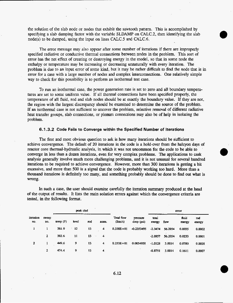
the solution of the slab node or nodes specifying a slab damping factor with node(s) to be damped, using the input
that exhibit the sawtooth pattern. This is accomplished by the variable SLDAMP on CALC.2, then identifying the slab on lines CALC.5 and CALC.6.
The error message may also appear after some number of iterations if there are improperly specified radiative or conductive thermal connections between nodes in the problem. This sort of error has the net effect of creating or destroying energy in the model, so that in some node the enthalpy or temperature may be increasing or decreasing unnaturally with every iteration. The problem is due to an input error of some kind, but it may be rather difficult to find the node that is in error for a case with a large number of nodes and complex interconnections. One relatively simple way to check for this possibility is to perform an isothermal test case.
To run an isothermal case, the power generation rate is set to zero and all boundary tempera- tures are set to some uniform value. If all thermal connections have been specified properly, the temperature of all fluid, rod and slab nodes should be at exactly the boundary value. If they are not, the region with the largest discrepancy should be examined to determine the source of the problem. If an isothermal case is not sufficient to uncover the problem, selective removal of different radiative heat transfer groups, slab connections, or plenum connections may also be of help in isolating the problem.
6.1.3.2 Code Fails to Converge within the Specified Number of Iterations
The first and most obvious question to ask is how many iterations should be sufficient to achieve convergence. The default of 20 iterations in the code is a hold-over from the halcyon days of reactor core thermal-hydraulic analysis, in which it was not uncommon for the code to be able to converge in less than a dozen iterations, even for very complex problems. The applications to cask analysis generally involve much more challenging problems, and it is not unusual for several hundred iterations to be required to achieve convergence. However, more than 300 iterations is getting a bit excessive, and more than 500 is a signal that the code is probably working too hard. More than a thousand iterations is definitely too many, and something probably should be done to find out what is wrong.
In such a case, the user should examine carefully the iteration summary produced at the head of the output of results. It lists the main solution errors against which the convergence criteria are tested, in the following format.
peak clad error
iteration sweep Totalflow pressure total fluid rod no. no. temp (F) level rod assm. (Ibds) drop (psi) energy flow energy energy
1 1 381.9 12 13 4 0.338E+01 -0.2353495 -2.3474 56.2054 0.0035 0.0002
2 382.6 1 1 13 4 -2.0857 56.2054 0.0233 0.0001
2 1 449.6 9 13 4 0.253E+01 0.0054958 -1.0128 3.0014 0.0780 0.0038
2 474.4 9 13 4 -0.8751 3.0014 0.1611 0.0007
6.12

This example shows the first two iterations for a calculation that took 214 iterations to converge (see Section 7.3.2, PSN concrete cask with nitrogen back-fill). In examining the conver- gence behavior of a given case, the significant items of interest in the iteration summary are the four error terms, which are tested against the convergence criteria specified by the user in the input for group CALC, on line CALC.2. The total energy error is tested against the input variable QERROR. The flow error is tested against the input variable FERROR. The fluid energy error is tested against the input variable HERROR. The fluid continuity solution is also tested against the input variable WERRY during the inner iteration, but no information is printed on this in the iteration summary (see Section 6.2.12, input group CALC, line CALC.2 for a complete discussion of this input).
In general, these error terms should show a monotonically decreasing trend. If the errors are oscillating (i.e., jumping between nearly the same values over the course of two or three iterations), the behavior may be due to the stability problem described above. Strong semi-implicit coupling along with relatively weak implicit coupling between nodes for the heat transfer solution may not be severe enough in some cases to cause the code to actually fail. It can, however, result in very slow rates of convergence, or oscillation of the solution about an asymptote that may or may not be approaching the correct solution. In such a case, the problem can be diagnosed in the same way as described above, and much the same action needs to be taken to fix the problem. That is, by looking at the output for saw-tooth patterns in the axial temperature profiles, and damping any nodes that exhibit such behavior.
If the total energy error is not oscillating, but appears to be stuck on some value that does not change from iteration to iteration, the problem may be improperly specified thermal connections. This sort of input error can cause the code to fail, as noted above in Section 6.1.3.1, if the resulting energy error is large enough. But alternatively, it may simply create a source of energy error that cannot be iterated away. The problem can usually be diagnosed using the same procedures as outlined above, starting with running an isothermal case to determine the existence of an energy source or sink somewhere in the problem.
If the error summary shows steadily decreasing values, but they are going down at an irrita- tingly slow rate, there are a number of possible causes of the problem and different actions to be taken. Some of the more likely possibilities are discussed below, with suggestions for appropriate action.
If the problem is starting with an initial guess that is too far from the final solution, it may take an abnormally long time to reach convergence. In such a case, the best thing to do is to start with a better initial guess, as defined with the operating conditions in group OPER on line OPER.2. If the case uses a uniform pressure drop boundary condition for a specified total flow (with or without the plenum model), it may be helpful to start with an initial specified flow rate (entered as GIN on OPER.2) that is closer to the expected final value. It may also be helpful to adjust the initial enthalpy (entered as HIN on OPER.2).
Another possible cause of a slow convergence rate is that the specified damping factors on CALC.2 are too conservative for a particular case. These can be reduced or eliminated by appro- priate changes in the input for CALC.2. If the damping is not needed, the code will almost always converge more rapidly without the damping factors. However, removing the damping factors could in some cases cause the code to fail due to instabilities, as described above. As disastrous as this
6.13

result might seem to the user, it is actually a useful improvement over very slow convergence rates. If the failure is due to instabilities of the type described above, the user will be motivated to search out the specific nodes that are hindering convergence. Appropriate damping factors can then be applied specifically to the troublesome nodes, using the damping factor input variable SLDAMP on CALC.2 and identifying the specific nodes to be damped on CALC.5 and CALC.6. This allows damping to be applied where it is needed, without unnecessarily impacting the global convergence rate for the problem.
The optional axial energy rebalancing can sometimes result in a dramatic improvement in the convergence rate. This feature is specified by setting the variable ACCAX to a non-zero value on CALC.2. Axial energy rebalancing consists of performing a one-dimensional energy solution for the system every three iterations, and using the results to make a global adjustment in all nodes at all axial levels. In many cases this will propagate changes through the system much more rapidly than the node-by-node solution, and can result in much faster convergence. It can, however, destabilize the solution, and so should not be used unless it can be shown to be a definite help. The results of the axial rebalancing calculation can be seen directly by setting the variable IPREP on OUTP. 1 in group OUTP. However, this yields a very large amount of output even for problems of moderate size, and probably would not be useful except for debugging purposes.
One last option to consider if the code fails to converge is to examine the values selected for the convergence criteria. If they are unnecessarily stringent, they could be forcing the code to calculate many iterations with no real change in the solution. A quick and easy check to determine if the code is doing more iterations than it really needs is to look at the peak clad temperature in the iteration summary. If it is not changing between iterations, this indicates that no substantial changes are occurring in the solution. In such a case, the additional iterations are probably a waste of time, and it would be appropriate to relax the convergence criteria slightly.
The appropriateness of relaxed convergence criteria can be evaluated by comparing the results obtained with different values for the convergence criteria. If more relaxed convergence criteria yield essentially the same results as the same case with tighter convergence criteria, and does so in fewer iterations, then the relaxed convergence criteria are probably appropriate for the problem. Some degree of judgement is required from the user to determine what constitutes the appropriate standard of convergence for a given application. In general, it is sufficient for a calculated answer to be approximately as accurate as the measured value with which it is validated.
6.2 Input Instructions for COBRA-SFS
The input instructions for COBRA-SFS are provided in this section. The code input is listed line by line, with the definition of each input variable. Each set of instructions is preceded by an explanatory paragraph. However, users unfamiliar with COBRA-SFS should refer to Section 6.1 for a discussion of the modeling capabilities and limitations of the code, and the list of references docu- menting the various applications and validation calculations performed with the code. These reports are intended in part to provide guidance and examples for the code user in developing new input files and applications.
6.14

COBRA-SFS input is organized into groups identified by unique four-character flags. The groups are defined by function and reflect a generalized logical approach to setting up input for a problem. COBRA-SFS input falls into the following five basic categories:
1. the physical properties of the solid materials and working fluid 2. the flow channel geometry and solid node structure 3. the constitutive models for the flow and heat transfer solutions 4. the boundary conditions 5 . solution control parameters and output options.
The various input groups under these five categories are listed below. Note that many of the input groups are optional.
Case Control Data
Problem identification and initialization
Thermodynamic and Material Properties
Group PROP - Fluid and Solid Material Properties
Geometry Description
Group CHAN - Flow Field Geometry Group VARY - Geometry Variations (optional) Group RODS - Fuel Rod Geometry (optional) Group SLAB - Solid Structure Geometry (optional) Group RADG - Thermal Radiation Exchange Factors (optional)
Constitutive Models
Group HEAT - Heat Transfer Correlations Group DRAG - Friction Factors and Pressure Loss Coefficients
Boundary Conditions
Group BDRY - Thermal Boundary Conditions (optional) Group OPER - Operating Conditions
Code Control
Group CALC - Calculational Parameters Group OUTP - Output Options
The information required to initiate a COBRA-SFS calculation is described in Section 6.2.1. The fluid and solid material properties are read in group PROP, which is described in Section 6.2.2. Note that input group PROP is not optional; properties of the fluid must be supplied in all cases.
6.15

The geometry of the problem is described in group CHAN, which is a required input group, and in optional groups VARY, RODS, SLAB, and RADG. The flow field geometry, described in input group CHAN, defines the flow regions within the problem. This input group is described in Section 6.2.3. Group VARY can be used to describe variations of flow channel areas and connec- tions with respect to axial location. This optional input group is described in Section 6.2.4.
The fuel rod geometry input in group RODS is required only if there are heat generating rods in the problem. The input for this group is described in Section 6.2.5. Section 6.2.6 describes the input for optional group SLAB, which is used to describe heat-conducting solid structures in the system. When thermal radiation is modeled, the geometric viewfactor information in group RADG is required input. This group is described in Section 6.2.7.
The constitutive models required by the energy and flow field solutions are described in groups HEAT and DRAG, respectively. The input for group HEAT, described in Section 6.2.8, specifies the heat transfer correlations used in the energy equations. The input for group DRAG, described in Section 6.2.9, specifies the friction factor correlations and pressure loss coefficients used in the momentum equations.
The boundary conditions for the problem are described in groups BDRY and OPER. The input for group BDRY, described in Section 6.2.10, defines the thermal boundary conditions applied to the problem. The input for group OPER, described in Section 6.2.11, defmes the boundary operating conditions for the flow solution and the transient forcing functions.
The parameters controlling various functions of the code are read in groups CALC and OUTP. The input for group CALC, described in Section 6.2.12, defines the calculational parameters con- trolling the numerical solution procedure. The input for group OUTP, described in Section 6.2.13, defines the parameters controlling the various output options.
Input is terminated by entering ENDD for the group flag. This signals the code to stop looking for additional input groups.
The new user would be well advised to read through the input instructions entirely before attempting to set up the input for a particular problem. It is important for the user to have a reason- ably complete picture of the overall structure of the COBRA-SFS input, as it will give order to the large array of options available.
The general format of the input instructions is to give a complete description of all variables in each line of input, including the format for reading the data. Some input lines are repeated, and some groups of lines are repeated in sequence as a set. These repetitive patterns are noted in the instruc- tions, both in the format for the line and in the descriptive text accompanying the input. In many instances, later input will depend on values specified in earlier input lines. These flags are noted on the input line, with a reference to the line on which the flag was defined. For example, the variable defining the number of channels in an assembly, NCHANA, is read on input line CHAN.5. In all subsequent instructions that refer to NCHANA, the origin of this flag is denoted by specifying the variable as NCHANA[CHANS].
6.16

6.2.1 Problem Initiation Input
Input records COBRA.1 and COBRA.4 are required at the beginning of every COBRA-SFS input file. COBRA.l defines the execution time allotted for the problem, and offers the user the opportunity to restart a previously executed problem from the TAPE8 restart dump. The case title is specified on COBRA.4. This title is printed on the output file, and serves as the case identifier, for easy reference. The date and time of the calculation are also written to the output file along with the title. If the restart option is flagged, COBRA.2 must also be read, to define the restarted calculation.
COBRA.l MAXT,IECHO FORMAT( 215)
Columns Variable Descriution 1-5 MAXT CPU time limit (sec.) for problem execution. For restart cases,
enter MAXT as a negative number (ABS(MAXT) will be used to define the time limit).
(NOTE: The value entered for MAXT cannot supersede any execution time limit specified in the job control language in a batch submittal. The user must ascertain that any such time limits are compatible with the input value of MAXT.)
6-10 IECHO Flag for printout of input file;
= 0; the input file will be printed on the output file (default).
= 1; the input file will not be printed on the output file.
COBRA.2 NJUMP,NA,IT,NTT,TTT Read only if MAXT < 0 on COBRA.l FORMAT(415,F5.0)
Columns Variable Descriution 1-5 NJUMP Restart option flag;
= 1; continue calculation from a previous steady state or transient solution; new input may be read in to define a new case, with the previous calculation as the first guess.
= 2; not a restart; print output information from a previous calculation on tapes.
6.17

6-10 NA
11-15 IT
Number of iterations for restarted case;
- for a steady-state calculation, number of additional iterations.
- for a transient calculation, number of iterations per time step
(NOTE: If new input is read for group CALC, the value for NA will be superseded by the new value for NTFUES on CALC.3 .)
Flag to define type of restart:
= 0; restart and continue the previous solution; - continue iterating in a steady-state case - continue time steps in a transient case
= 1; restart a steady-state case and initiate a transient
(NOTE: Input to define the transient must be specified by new input for group CALC. Forcing functions may be specified in group OPER, either with new input or in the original input file.)
16-20 NTT Number of transient time steps for the restarted calculation.
2 1-25 TTT Total transient time (seconds) for the restarted calculation.
All cases, including a restart case, must have a title, which is read on line COBRA.3. This is an alphanumeric identifier that will be printed on each page of the output file, along with the date and time of the run.
COBRA3 J 1 ,(TEXT(I),I = 1,17) FORMAT(SX,IS, 17A4)
Columns Variable Description 1-5 Blank
6-10 J1 flag for option controlling output of input data;
I 1; print all processed input data from the current input file.
= 10; print all processed input data from the current input file, then stop execution.
11-78 TEXT(1) Title for problem identification, for label printed at top of each page in the output file (maximum of 68 characters).
6.18

When doing a restart calculation, (i.e., NJUMP= l), the user has the opportunity to modify the input by specifying new data for the input groups PROP, VARY, RADG, HEAT, DRAG, BDRY, OPER, and OUTP. The problem geometry, however, which is specified in groups CHAN, RODS, and SLAB, cannot be changed on a restart. Changes in these groups constitute a whole new problem, and a restart is neither useful nor appropriate. After all modified groups have been entered, or if no changes or modifications are needed in the input on a restart, the user must enter the ENDD group flag to terminate the search for new input for the restart.
COBRA.4 AGROUP Read only if NJUMP > 0 FORMAT( A4)
Columns Variable Description 1-4 AGROUP Enter ENDD, to signal end of input stream for this restart case.
6.2.2 Group PROP--Fluid and Material Properties
This group is used to define thermodynamic and heat transfer properties for the fluid and solid materials included in the problem. Properties can be specified for only two different fluids, but any number of solid material properties can be specified in a problem. Properties for fluids are defined on PROP.2 and PROP.3; solid material properties are defined on PROP.4. At least one fluid must be specified to define the coolant, but properties for solid materials are optional.
PROP. 1 AGROUP,NPROP,NSPROP FORMAT( A4,l X ,215)
Columns Variable DescriDtion 1-4 AGROUP Enter PROP.
6-10 NPROP Number of elements in fluid properties table.
Enter 0 to use option for two sets of fluid properties. (The number of elements for each table will be specified on PROP.2.)
11-15 NSPROP Number of solid materials for which properties will be entered on PROP. 3.
Fluid Properties
If the coolant is a liquid, properties are entered as saturated liquid values for the pressure PLIQ(1). If the coolant is a gas, properties are entered for temperatures at the system pressure (which is specified on OPER.2), and variable PLIQ(1) is not used. Fluid properties for at least two reference temperatures are required to allow interpolation.
Different fluids can be specified for different parts of a given case. When this option is used, NPROP[PROP.l] is set equal to zero, and the number of elements for each of the two fluid properties
a 6.19
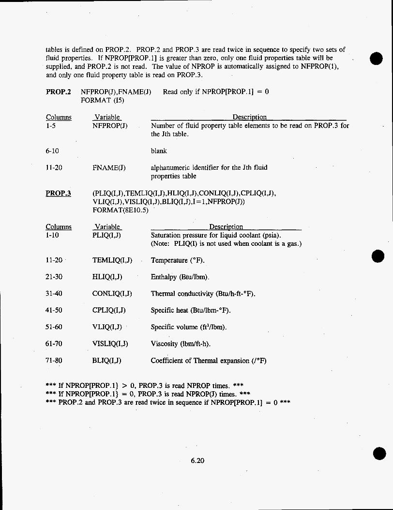
tables is defined on PROP.2. PROP.2 and PROP.3 are read twice in sequence to specify two sets of fluid properties. If NPROP[PROP.l] is greater than zero, only one fluid properties table will be supplied, and PROP.2 is not read. The value of NPROP is automatically assigned to NFPROP(l), and only one fluid property table is read on PROP.3.
PROP.2 NFPROP(J),FNAME(J) Read only if NPROP[PROP.l] = 0 FORMAT (15)
Columns 1-5
6-10
1 1-20
PROP.3
Columns 1-10
11-20
21-30
3 1-40
4 1-50
51-60
61-70
71-80
Variable NFPROP(J)
FNAME(J)
Description Number of fluid property table elements to be read on PROP.3 for the Jth table.
blank
alphanumeric identifier for the Jth fluid properties table
(PLIQ(I,J),TEMLIQ(I,J),HLIQ(I,J),CONLIQ(I,J),CPLIQ(I,J), VLIQ(1, J),VISLIQ(I , J) ,BLIQ(I, J),I = 1 ,NFPROP(J)) FORMAT(8E10.5)
Description Saturation pressure for liquid coolant (psia). (Note: PLIQ(1) is not used when coolant is a gas.)
TEMLIQ(1, J) Temperature ( O F ) .
HLIQ(1, J) Enthalpy (Btu/lbm).
CONLIQ(1, J) Thermal conductivity (Btu/h-&-OF).
CPLIQ(1,J) Specific heat (Btu/lbm-"F).
VLIQ(1, J) Specific volume (ft3/lbm).
Viscosity (lbdft-h).
Coefficient of Thermal expansion (/OF)
*** If NPROP[pROP.l} > 0, PROP.3 is read NPROP times. *** *** If NPROP[pROP.l} = 0, PROP.3 is read NPROP(3) times. *** *** PROP.2 and PROP.3 are read twice in sequence if NPROP[pROP.l] = 0 ***
6.20

Solid Material Properties
Solid material properties are specified for NSPROPPROP. 13 materials. This input is optional, and is read only if NSPROP on PROP. 1 is greater than zero. Properties are assumed constant for all temperatures. The material type number is used to identify the material properties of the various solid structure nodes input in groups SLAB and BDRY. Material property types must be numbered sequentially from 1 to NSPROP.
PROP.4 (IMAT(I),ANAME(I),CPSOL(I),RHOSOL(I),CONO(I),CONl(I),CON2(I),CON3(I), NQVT(I),I= 1 ,NSPROPFROP. 11)
Read only if NSPROP > 0 on PROP.l FORMAT (I5 ,A5,6E 10 .0,15)
Columns 1-5
6-10
11-20
21-30
3 1-40 41-50 5 1-60 6 1-70
71-75
Variable IMAT(1)
ANAME(1)
CPSOL(1)
RHOSOL(1)
CONO(1) CONl(1) CON2(I) CON3(I)
Description Solid material type identification number.
Solid material name (for user convenience).
Specific heat (Btullbm-OF) (for transient calculations).
Density (lbm/ft3) (for transient calculations).
Coefficients of an expression for solid thermal conductivity (Btuh-ft-OF) that has the form:
k = CONO(1) + CONl(I)*T + CON2(I)*T2 + CON3(I)*P
where T is the temperature in OR.
Transient heating rate forcing function. Corresponds to profiles read in OPER.14 and 15.
*** PROP.4 is read NSPROP[PROP.l] times. ***
6.2.3 Group CHAN-Flow Field Geometry
This group is read to define the flow field geometry. The basis of the problem geometry is subchannel modeling, in which the flow field is represented as an array of channels that can commun- icate laterally by crossflow. For convenience in modeling fuel bundles and casks, the channels are grouped into assemblies; a group of channels that can communicate laterally comprise an assembly. Channels of one assembly cannot communicate by crossflow with the channels of other assemblies.
6.21

Axial Geometry
The axial geometry of the channel region is defined by the axial length, Z, entered on CHAN.23 and the number of axial nodes, NDX, entered on CHAN. 1. have the same axial length, and the same axial noding. The default in the code is a uniform axial node size, which is calculated as DX = Z/NDX. The user has the option, however, of specifying axial nodes of varying sizes, by setting NAZONE on CHAN.l and reading in a variable axial node size table on CHAN.4.
All channels in all assemblies
cHAN.1
Columns 1-4
6-10
11-15
16-20
21-25
26-30
3 1-35
AGROUP,NASSEM ,NDX ,NAZONE,ISHEAR,NSHEAR,NANGLT FORMAT(A4,1X,615)
Variable AGROUP
NASSEM
NDX
NAZONE
ISHEAR
NSHEAR
NANGLT
Description Enter CHAN.
Number of assemblies.
Number of axial nodes.
Flag for variable axial node sizes;
= 0; uniform axial nodes (default).
> 0; number of regions in variable axial node size table (read on CHAN.4).
Flag for fluid shear stress (NOTE: used only when modeling plenum regions with multiple channels);
= 0; fluid shear stress not considered.
= 1; fluid shear stress included.
Number of pairs of gaps that are connected by fluid-fluid shear in the lateral direction.
Number of lateral control volume orientation angles (read on CHAN.2 below) (NOTE: this input is needed for the fluid-fluid shear option, but it is also used to define the direction of the gravity vector for lateral momentum transport in a horizontal or tilted geometries .)
6.22

CHAN.2 (ANGLE(I),I= l,NANGLT(CHAN. I)) Read only if NANGLT[CHAN.l] > 0 FORMAT (8e10.5)
Columns Variable DescriDtion 1-10 ANGLE(1) Orientation angle for lateral flow, in degrees from 1 1-20 etc. CHAN.9.
vertical; to be assigned to specific gaps on
(NOTE: this input is used only if fluid-fluid shear is included in the model (Le., ISHEAR=l on CAN.l), or if modeling lateral gravity terms in a horizontal or tilted geometry.)
cHAN.3
Columns 1-10
11-20
cHA.N.4
Columns 1-5, 11-15, etc.
6-10, 16-20, etc .
Z ,THETA FORMAT(2F 10-5)
Variable Description Z Axial length of the channel region (in.).
THETA Channel orientation, in degrees from vertical (Default is 0.0. Used to calculate gravity term in the momentum equation).
(NSTEPS(I),VDX(I),I = 1 ,NAZONE) Read only if NAZONE > 0 on CAN. 1 FORMAT(8(15 ,E5 .O))
Variable Descriution NSTEPS (I) Number of nodes in zone I. (Note: the total number
of nodes, C NSTEPO), must be equal to NDX, specified on CAN.1.)
VDX(1) Axial node length (in.) in zone I. (Note: the sum of all nodes must be equal to Z on CHAN.2.)
**** up to four pairs of NSTEPS,VDX data may be entered per record. **** **** If NAZONE is greater than 4, CHAN.4 is read repeatedly until **** **** all NAZONE pairs of data have been specified. ****
Assembly Geometry Description
The input lines CHAN.5 through CHAN.7 are read in sequence as a set NASSEMCCHAN.11 times, once for each assembly in the problem. All channels are identified in this manner, assembly by assembly. An assembly may contain any number of channels. The assembly number and the assembly type number are read on CHAN.5. Each assembly must have a unique number (1 through NASSEM), but different assemblies can have the same assembly type number, if they have the same geometry. An assembly type is defined by the number of channels and their interconnections, as
6.23

specified by input on CHAN.7. It is necessary to enter the geometry data for an assembly type only once, with the CHAN.7 input for the first assembly of that type. For subsequent assemblies of that type, the value entered for ITYPA on CHAN.5 is recognized as a previously defined type, and CHAN.7 is not read. The geometry input for any subsequent assembly of the same type is automati- cally copied into the appropriate arrays.
The flow and heat transfer correlations to be used must be defined separately for each assem- bly, however. This information is supplied on CHAN.6, along with the index of the axial heat gen- eration profile table (if the assembly contains heated rods).
CHAN.5 NASS ,ITYPA, NCHANA,INTAPE,IFREE,TMNCVL(NASS) FORMAT(415,E5.0)
Columns 1-5
6-10
11-15
16-20
2 1-25
26-30
Variable NASS
ITYPA
NCHANA
INTAPE
IFREE
DescriDtion Assembly number.
Assembly type number (corresponding to a channel geometry description entered on CHAN.7).
Number of channels in assembly NASS.
Flag for 110 unit source of the channel geometry input on CHAN.6 for assembly NASS:
= 0; read from the input file (default).
= N; read from 1/0 unit N.
Flag for specifying wall shear boundary condition option for assembly NASS:
= 0; wall shear specified by friction factor correlation (default).
= 1; laminar zero-slip wall boundary condition. NOTE: this option is used only when modeling large open plenum regions where fluid-fluid shear must be taken into account.)
TMNCVL(NASS) Factor to adjust transverse momentum control volume length in assembly NASS so that the length is defined as bm = P,ITMNCVL(NASS) in the calculation of the turbulent crossflow, w'. (Default for TMNCVL(NASS) is 0.0, so that bAss = 1.0 for W'.)
6.24

CHAN.6 NAFLX(NASS), NFLMC(NASS),NHFVT(NASS) ,NPFVT(NASS),MDFLT, NFASSCNASS,.ITDPA(NASS) FORMAT(715)
Columns 1-5
6-10
11-15
16-20
21-25
26-30
3 1-35
Variable NAFLX(NASS)
NFLMC(NASS)
NHFVT(NASS)
NPFVT(NASS)
MDFLT
NFASS(NASS)
ITDPA(NASS)
Description Identification number of the axial heat flux rofile table [specified
Identification number of the heat transfer coefficient correlation [specified on HEAT.21 for assembly NASS (default is 1).
on OPER.16 and OPER.171 for assembly P f ASS (default is 1).
(NOTE: If NTHEAT > 0 on HEAT. 1, this is also the identification number of the heat transfer coefficient correlation for lateral flow in assembly NASS. IF NFHEAT > 0 on HEAT. 1, this is also the identification number of the heat transfer coefficient correlation for free convection in assembly NASS .)
Identification number of the heat generation versus time forcing function [specified on OPER. 13 and OPER. 141 to use in assembly NASS durin a transient (default is 0; initial value is used throughout t f e transient.)
Identification number of the pressure drop or flow versus time forcin function [s ecified on OPER. 11 and OPER. 121 for
transient).
Identification number for the friction factor correlation(s) [specified on DRAG.2 for axial flow and optionally on DRAG.13 for lateral flow], to be used in assembl NASS (default is 1).
s cifying a non-zero value for N on CHAN.7 for an individual
assem ly NASS ( B efault is 0; initial value is used throughout the
(NOTE: This value can be superse B ed in a given channel by
c R" annel of this assembly type.)
Identification number of the fluid properties table [specified on PROP.31 for assembly NASS. (Default is table 1.)
Flag for flow or pressure drop boundary condition for assembly NASS:
= 0; specified flow boundary condition.
= 1; uniform pressure drop (specified in OPER).
= 2; pressure drop resulting in uniform inlet mass flu.
= 3; uniform pressure dro calculated for total mass flow rate (FTO ! AL on OPER.2).
= 4; zero flow at both top and bottom boundaries.
(NOTE: ITDPA(NASS) is needed only if*different assemblies have different boundary conditions. If all assemblies see the same boundary condition, ITDPA(NASS) for each assembly, and the appropriate option is then specified with variable assemblies.)
6.25

cHAN.7
Columns 1
2-5
6-10
11-15
16-20
21, 36, 51, 66
22-25
52-55, 67-70
37-40,
26-30,
56-60, 7 1-75
31-35, 46-50, 61-65, 76-80
41-45,
(N,I,AC,PW ,PH,(NANGLE(K),LC(K),GAPS(K),DIST(K),K = 1,4),
Read only for a new value of assembly type in ITYPA[CHANS]. FORMAT(I1 ,14,3E5.3,4(11 ,I4,2E5.2))
I= 1 ,NCHANA[CHAN.S])
Variable N
I
AC
PW
PH
NANGLE(K)
DIST(K)
Description Index number of friction factor correlation to be applied to channel I; must correspond to a correlation entered on DRAG.2. Default is MDFLT, entered on CHAN.6, for all channels in the assembly.
(NOTE: if the option for lateral friction factor correlations is used, N also must correspond to the index number of a lateral friction factor correlation entered on DRAG. 13. See group DRAG input instructions.)
Channel identification number (must be entered sequentially, 1 through NCHANA[CHAN .5]).
Channel nominal area (in.*).
Channel nominal wetted perimeter (in.).
Channel nominal heated perimeter (in.).
Identification number of a lateral control volume orientation angle read on CHAN.2.
(NOTE: this input is optional, and is needed only when the option for fluid-fluid shear or gravity forces in the transverse direction are modeled; see Section 6.1.2.)
Identification number of adjacent channel for the Lth connection to channel I, where LC(K) > I (each connection should be identified only once, as a connection from the lower-numbered channel to the higher- numbered channel).
Width of flow connection between channel I and channel LC(K), (in.).
Transverse control volume length (in.) between channel I and channel LC(K).
(NOTE: This input is optional. It defines the transverse length of the momentum cell and also the conduction length in the transverse direction. A default value for this distance can be defined for all flow connections by specifying the variable SL on CHAN.8. If this option is used, DIST(K) can be entered as zero.)
*** CHAN.7 is read NCHANA[CHAN.S] times for a given assembly type. *** *** CHAN.5 through CHAN.7 are read sequentially NASSEM[CHAN. 11 times. ***
6.26

Lateral Flow Connection Parameters
All lateral flow connections between the channels within each assembly are defined in the input on CHAN.7. The flow solution for these connections requires an empirical term to define the cross- flow resistance (refer to the description of the lateral momentum equation in Section 2.3.3). For analysis of rod bundle arrays using subchannel modeling, a single number is usually sufficient to characterize all lateral connections. This input is read on CHAN.8. The user also has the option of specifying different loss coefficients for different gaps, as appropriate to model problems in which the lateral control volumes are not all essentially identical. This input is supplied in group DRAG. However, a value still must be entered for JSIJ(1) on CHAN.8, for use in gaps where the lateral resistance is not defined in subsequent input. Even if lateral resistance values will be defined for all gaps in subsequent input, CHAN.8 must be read in. The code cannot look ahead in the input stream to see whether or not this input will be required.
A value must also be entered for the width-to-length ratio SL, to be used to define the centroid length for any gap that is not specified with a non-zero value for DIST(K) on CHAN.7. If all gaps have a non-zero DIST(K) value specified, SL is not used, and therefore can be entered as zero.
The index numbers of pairs of gaps that exchange momentum due to fluid-fluid shear must be identified by input on CHAN.9, if this option has been specified by input on CHAN. 1. The user must understand the gap numbering convention in COBRA-SFS in order to correctly define this input. The gaps are numbered automatically in the code, in the order in which they are specified by input on CHAN.7. For example, in an array of subchannels such as that shown in Figure 6.4 for a fuel assembly, the input for CHAN.7 for subchannels 1 through 6 is as follows;
NANGLE LC NANGLE LC N I AC PW PH C C GAPS DISTC C GAPS DIST 123456789012345678901234567890123456789012345678901234567890123456789012345 0 1.0663.5750.16570 2.1984 .4860
0 2.3OO41.226.66290 3.1410 .4860 4.1984 .563
0 3.0885.6630.66300 5.1410 S630
0 4.30041.226.66290 5.1410 .4860 7.1984 .563
0 5.17701.3261.3260 6.1410 .5630 8.1410 .563
0 6.0768.7115.49720. 9.0790 S630
6.27

By the COBRA-SFS gap number convention, the gaps are automatically numbered as follows:
This pattern is continued until all subchannels have been identified by input on CHAN.7.
CHAN. 7 line 1 2
3 4
5
6
subchannel XI 1 2 2 3 4 4 5 5 6
subchannel JJ 2 3 4 5 5 7 6 8 9
pap number 1 2 3 4 5 6 7 8 9
CHAN.8 KIJ(l),SL,FTM FORMAT(3ES.O)
Columns Variable Description 1-5 KIJ(1) Nominal flow resistance in lateral connections between channels
(default is 0.5).
6-10 SL Width-to-length ratio for transverse momentum control volume. (NOTE: This is used only for gaps where DIST(K) is entered as zero on CHAN.7 default is 0.5).
11-15 FTM Factor for turbulent mixing of momentum and energy (default is 0.0).
CHAN.9 (III(L),JJJ(L),L= 1 ,NSHEAR[CHAN. 11) Read only if NSHEAR > 0 FORMAT (1215)
Columns Variable DescriDtion 1-5, W L ) Identification numbers of one gap in a pair that 11-15 are connected by lateral fluid shear. etc. (NOTE: refer to Section 6.1.2 for an explanation
of the gap numbering convention in the code.)
6-10, JJJ(L) 16-20 etc .
Identification numbers of the other gap in a pair that are connected by lateral fluid shear.
**** Up to six pairs of II1,JJJ channel numbers may be entered per record. **** **** If NSHEAR is greater than six, repeat this line until all NSHEAR **** **** pairs of data have been specified. ****
6.28

6.2.4 Group VARY--Geometry Variations
This group is used to specify axial variations in channel flow area and lateral flow connection width. It is optional. If this group is not used, all channel areas and lateral flow connection widths are assumed constant over the entire axial length.
VARY.l AGROUP,NAFACT,NAXL,NARAMP,NGAPS,NGXL FORMAT(A4,1X,515)
Columns 1-4
6-10
11-15
16-20
21-25
26-30
Variable AGROUP
NAFACT
NAXL
NARAMP
NGAPS
NGXL
Channel Area Variations
DescriDtion Enter VARY.
Number of channels with area variations.
Number of axial locations for channel area variations. (NOTE: All area variation tables use the same table of axial locations .)
Number of iterations for gradual insertion of area variations into the calculation (default is 1).
Number of lateral flow connections for which the width varies axially.
Number of axial locations for lateral flow connection width variations.
(NOTE: All gap width variation tables use the same axial locations.)
The channel area variations are read only if NAFACT and NAXL on VARY. 1 are both greater than zero. The channel area variations are specified on VARY.2 through VARY.4. VARY.2 is read once to define the axial locations of the area variations, then the input lines VARY.3 and VARY.4 are read sequentially, NAFACT times, to define the area variations and the channels affected. Line VARY.3 is read to specify the assembly number and index number of a channel in the assembly that has area variations, then VARY.4 is read to define the table of area variation factors in that channel, at the locations defined by input on VARY.2.
6.29

VARY.2 (AXL(J),J = 1 ,NAXLvARY. 11) Read only if NFACT > 0 and NAXL > 0 on VARY.l FORMAT( 12F5.3)
Columns 1-5, 6-10, etc.
Variable AXL(J)
DescriDtion Relative axial location (x/L) of the Jth channel area variation.
VARY .3 NASS,I Read only if NAFACT > 0 and NAXL > 0 on VARY, 1 FORMAT(215)
Columns 1-5
6-10
Variable NASS
I
DescriDtion Identification number of assembly containing channel I.
Identification number of channel in assembly NASS for which area variations are being specified.
VARY.4 (AFACT(L,J),J=l,NAXLFARY.l]) Read only if NAFACT > 0 and NAXL > 0 on VARY.l FORMAT( 1-5.3)
Columns 1-5, 6-10 etc.
Variable AFACT(L,J)
DescriDtion Channel area variation factor (A#/AC,) for the Lth area variation table at axial level AXL(J), as defined on VARY.2.
(NOTE: Area variation factor tables are numbered sequentially, in the order they are read in on VARY .4. Index L of AFACT is 1 to NAFACT.)
*** VARY.3 and VARY.4 are read sequentially NAFACTwARY.11 times. ***
Lateral Flow Connection Width Variations
The flow connection width variations specified on VARY.5 through VARY.7 are read only if NGAPS and NGXL on VARY. 1 are both greater than zero. This input follows the same pattern used in defining the channel area variations. VARY.5 is read once to define the axial locations where gap width variations occur. Then VARY.6 and VARY.7 are read sequentially NGAPS times. VAFtY.6 is read to define the assembly number and the index number of a gap that has varying width. Then VARY.7 is read to define the table of width variation factors for that gap.
6.30

VARY.5 GAPXL(J),J= l,NGXL[VARY.l]) Read only if NGXL > 0 and NGAPS > 0 on VARY.l FORMAT( 12F5.3)
Columns 1-5, 6-10, etc.
VARY .6
Columns 1-5
6-10
Variable Description Relative axial location (x/L) of the Jth gap width variation.
GAPXL(J)
NASS,K Read only if NGXL > 0 and NGAPS > 0 on VARY. 1 FORMAT(215)
Variable DescriDtion NASS Identification number of assembly containing lateral flow
connection K.
K Identification number of gap with width variation.
VARY.7 (GFACT(L,J),J= l,NGXL[CHAN.l]) Read only if NGXL > 0 and NGAPS > 0 on VARY.l FORMAT( 12F5.3)
Columns Variable Descriution 1-5, GFACT(L, J) Flow connection width variation factor 6-10, etc.
(GAPq/GAPS,) for the Lth variation table at axial level GAPXL(J), as specified on VARY.5.
(NOTE: Gap width variation tables are numbered sequentially in the order in which they are read on VARY.7. Index L of GFACT(L,J) is 1 to NGAPS.)
*** VARY.6 and VARY.7 are read sequentially NGAPSPARY.11 times. ***
6.2.5 Group RODS--Fuel Rod Geometry
This group is read to define the geometry and material properties for the fuel rods that are contained in the assemblies defined in group CHAN. If a given problem does not contain fuel rods or heater rods simulating fuel rods, the input for this group is not needed. The fuel rod model is defined by the value specified for variable NC on RODS.1. If NC=O, there is no fuel rod model; the heat flux at the surface of the fuel rods is treated as a boundary condition in the calculation. In such a case, radiative heat transfer cannot be included in the solution. If NC= 1, the conduction solution is performed for the rod cladding only. This provides a rod wall surface temperature for the heat trans- fer calculation. If NC>4, the conduction equation is solved within the fuel rod for internal node temperatures, as well as the cladding surface temperature. Radiative heat transfer can also be con- sidered if NC is greater than zero on RODS. 1.
6.31

The rod geometry input must be specified for each assembly, even if a given assembly does not contain fuel rods. A rod configuration type is specified for each assembly; assemblies that do not contain any rods are given a configuration type of zero. A nonzero configuration type is defined by the number of rods in the assembly, the nominal rod diameter, radial power distribution, fuel type, and channel connections for heat transfer.
RODS. 1 AGROUP, NC, NFUELT ,NQ AX, NRODTP, NTHETA, NRCON, NSCON FORMAT(A4,1X,715)
Columns 1-4
6-10
11-15
16-20
2 1 -25
26-30
3 1-35
Variable AGROUP
NC
NFUELT
N Q M
NRODTP
NTHETA
NRCON
Descriution Enter RODS.
flag for fuel model option;
= 0; no fuel model.
= 1; only the rod cladding is modeled (NOTE: this option consider all modes of surface heat transfer, but not internal fuel conduction. It is applicable to steady state calculations only.)
> 4; fuel model with (NC-1) finite-difference nodes in the fuel, and one node in the cladding. (NOTE: this option considers all modes of surface heat transfer, plus internal fuel conduction. It can be used in steady state calculations, if needed, and is required for transient calculations .)
Number of fuel types for which thermal properties are to be specified on RODS.4.
(NOTE: this parameter is not used if NC = 0.)
Flag for temperature dependent fuel properties;
= 0; constant fuel properties.
= 1; temperature-dependent fuel properties for
(NOTE: this option is available only if NC > 4). fuel type 1 only.
Number of tables of axial fuel type variations. (Applicable only if NC > 4.) Number of circumferential nodes in a fuel rod (default is 1).
(WARNING: the viewfactors input in group RADG must be consistent with this input variable.)
Number of rod-to-rod thermal connections for conduction heat transfer.
6.32

36-40 NSCON Number of rod-to-slab thermal connections for conduction heat transfer.
CAUTION: The options for multiple circumferential nodes in the fuel rods and rod-to-rod or rod- to-wall contact for thermal conduction are still under development and need additional validation. The feature is included in this release, but is not recommended for general application in Cycle 2.)
Rod Configuration Description
A rod configuration type is defined by the number of rods it contains, the nominal rod dia- meter, the radial power distribution, and the connections for heat transfer between the rods and channels in an assembly. Each assembly described in group CHAN must be assigned a rod config- uration type on RODS.2. If an assembly contains no fuel rods, the rod configuration type must be specified as zero. The rod configuration description for a given non-zero type is entered on RODS.3. For efficiency, a rod configuration description is entered only once. The rod geometry arrays for subsequent assemblies with the same rod type are automatically filled with the appropriate input. The rod configuration description input is read one assembly at a time for all NASSEM[CHAN.l] assemblies.
RODS.2 NOA,ITYPA,NORODS ,INTAPE FORMAT(415)
Columns 1-5
6-10
11-15
16-20
Variable NOA
ITYPA
NORODS
Description Assembly number; (Note: must be entered sequentially, 1 through NASSEM[CHAN. 11.)
Rod configuration type number for assembly NOA. (NOTE: if there are no rods in assembly NOA, ITYPA must be entered as zero.)
Number of rods in configuration type ITYPA. (NOTE: if ITYPA is zero, NORODS must be zero.)
INTAPE 110 unit number from which the rod input for rod configuration type ITYPA is to be read (default is the input file).
6.33

RODS.3 (N,I,DIA(I),~DIAL(I),(LR(I,L),PHI(I,L),L=1,6),I=1,NORODS[RODS.2]) Read only if NORODS > 0 on RODS.2. FORMAT( lX,I 1 ,13,2E5.2,6(15 ,E5.2))
Columns Variable 1-2 N
3-5 I
6-10 DIA(1)
11-15 RADIAL( I)
16-20, LR(I,L) 26-30 etc.
21-25, PHI(1, L)
etc. 31-35,
Descriution Rod material properties flag;
if NRODTP = 0 on RODS. 1, N is identification number of fuel material type for rod I, as defined by input on RODS.4 (default is N= 1).
if NRODTP > 0 on RODS. 1, N is identification number of a table of axially varying fuel type for rod I, as defined on RODS.7 and RODS.8.
Rod identification number. (NOTE: must be entered in sequence, from 1 to NORODS[RODS.2].)
Rod outside diameter (in.).
Radial heat generation factor for rod I, normalized to the average rod heat generation rate.
Identification number of the Lth channel connected to rod I (up to 6 channels can be connected to rod I).
Fraction of the perimeter of rod I connected to adjacent channel LR(1,L). (Note: multiple rods can be modeled by one average rod of diameter DR(I) by specifying PHI = X, where X is the number of rods being modeled by rod I.)
*** RODS.3 is read NORODS times for each new rod configuration type. *** *** RODS.2 and (optionally) RODS.3 are read sequentially as an input *** *** set NASSEM[CHAN.l] times. *** Fuel Material Properties
Fuel material properties must be entered if a rod model is used (i.e., NC > 0 on RODS.1). The fuel material properties are defined by fuel type, and are numbered sequentially in the order they are read in on RODS.4. If the rod model is used, at least one fuel type must be specified using the input on RODS.4. If the axial fuel type variations option has been flagged (Le., NRODTP > 0 on RODS. l), at least two fuel types must be defined.
6.34

RODS.4
Columns 1-5
6-10
11-15
16-20
2 1-25
26-30
31-35
36-40
41-45
46-50
51-55
56-60
61-70
(KFUEL(I),CFUEL(I),~UEL(I),DFUEL(I),KCLAD(I),CCLAD(I),RCLAD(I), TCLAD(I),HGAP(I),DROD(I),GEOMF(I),DFUELI(I),QVOID(I), I= 1 ,NFUELT[RODS. 11) Read only if NFUELT > 0 on RODS. 1
FORMAT( 12E5.0,E 10 .O)
Variable KFUEL(1)
CFUEL(1)
RFUEL(1)
DFUEL(1)
KCLAD(1)
CCLAD(1)
RCLAD(1)
TCLAD(1)
HGAP(1)
DROD(1)
GEOMF(1)
DFUELI(1)
QVOIDO
Description Thermal conductivity (Btuh-ft-OF) of fuel type I.
Specific heat (BtuAbm-OF) of fuel type I.
Density (lbm/ft3) of fuel type I.
Pellet diameter (in.) for fuel type I.
Cladding thermal conductivity (Btuh-ft-OF) for fuel type I.
Cladding specific heat (BtuAb-OF) for fuel type I.
Cladding density (lbm/ft3) for fuel type I.
Cladding thickness (in.) for fuel type 1.
Fuel-clad gap conductance coefficient (Btuh-ft*-OF) for fuel type I.
Outside diameter of the fuel rod, including the cladding (in.), for fuel type I.
Fuel rod geometry flag;
= 0; solid cylindrical fuel rod with internal heat generation.
= 1; annular cylindrical fuel rod with internal heat generation.
= 2; annular cylindrical fuel rod with a heat flux boundary condition on the inner fuel surface.
Inner diameter (in.) of an annular fuel rod of fuel type I (used only if GEOMFO) > 0).
Heat generation rate (Btu/sec-ft3) in the central void of an annular fuel rod of type I (used only if GEOMFO = 1).
*** RODS.4 is read NFUELT[RODS.l] times. ***
6.35

Temperature-Dependent Fuel Properties
The user has the option of specifying temperature-dependent material properties for fuel type 1, using the input on RODS.5 and RODS.6. This option is selected by setting NQAX to 1 on RODS.l. However, all other fuel types will still have material properties that are constant for all temperatures.
RODS.5 NTNODE Read only if NQAX = 1 on RODS.1 FORMAT(I5)
Columns 1-5
Variable NTNODE
Descriution Number of entries in the temperature-dependent material properties table for fuel type 1.
RODS.6 (TVARY (I) ,V ARYK( I) ,VARY CP( I) ,VARY R( I) ,I = 1, NTNODE[RODS -51) Read only if NQAX = 1 on RODS. 1 FORMAT( 12E5.0)
Columns 1-5, 21-25, 4145
6-10, 26-30, 46-50
11-15, 31-35, 5 1-55
16-20, 3640, 56-60
Variable TVARY(1)
VARYK(1)
VARYCP(1)
VARY R( I)
Description Temperature ( O F ) .
Thermal conductivity (Btdh-ft-OF) of fuel type 1 at temperature TVARY(1).
Specific heat (Btu/lb-OF) of fuel type 1 at W A R Y (I).
Density (lb/fi3) of fuel type 1 at TVARY(1).
The temperature-varying material properties must be entered as a monotonically increasing table, with TVARY(1) the lowest temperature in the table, and TVARY(NTN0DE) the highest temperature.
Axial Fuel Variation
This input is optional, and is read only if NRODTP is greater than zero on RODS. 1. It allows the user to account for axial variations in materials using the fuel types defined by input on RODS.4. The fuel types are assigned to axial ranges in tables of axial location versus fuel type, using the input lines RODS.7 and RODS.8. The entries must be monotonically increasing on axial location. The tables are numbered 1 through NRODTP, in the order they are entered on RODS.7 and RODS.8. When this option is used, the value specified for N on RODS.3 for each rod must correspond to the index of the table containing the appropriate fuel types, as entered on RODS.7 and RODS.8.
6.36

RODS.7 KNZ Read only if NRODTP > 0 on RODS.l FORMAT(I5)
Columns Variable 1-5 KNZ
DescriDtion Number of axial zones in the Ith table of axial distance versus fuel type, where I is from 1 to NRODTPWODS.l].
RODS.8 (( ZEND(1,K) ,IZTYP( lIK),K = 1 ,KNZ[RODS .7]) ,I = 1 ,NRODTP[RODS .1]) Read only if NRODTP > 0 on RODS. 1. FORh4AT(6(E5. 0,15))
Columns Variable DescriDtion 1-5, 11-15, etc.
ZEND(1,K) Relative axial location (x/L) of the end of the Kth fuel zone of the Ith axially varying fuel type table.
6-10, 16-20,
IZTYP(1,K) Index of material type (from the order of entry on RODS.4), in fuel zone ending at ZEND(1,K) in the Ith etc. table of axial distance versus fuel type.
*** RODS.7 and RODS.8 are read in sequence, NRODTP times. *** Rod-to-Rod Thermal Connections
This input is optional, and is read only if NRCON[RODS.l] is greater than zero. It is used to specify heat transfer paths due to direct connection between rods. It is assumed that the contact conductance and geometry factor are the same for all rods in contact with each other. This input is entered on RODS.9. The specific rods that are in contact with other rods must be identified on RODS.lO. This input is read for all NRCON[RODS.l] rods. Up to 6 rods may be in contact with a given rod. All rods in contact with a given rod must identified; there is not automatic reciprocity in this input.
CAUTION: This option is still under development, and needs additional validation and verification. It is not recommended for general use. If it is absolutely necessary for a specific problem, the user is advised to perform appropriate validation by comparison to experimental data, to evaluate the reliability and accuracy of the code predictions for the conditions.
6.37

RODS.9 RCON,RRDIM Read only if NRCON > 0 on RODS.l FORMAT(2E 10.5)
Columns 1-10
11-20
Variable RCON
RRDIM
Description Contact resistance between rods, (h-ft- o FBtu).
Geometry factor of thermal connections for rod-to-rod contact, defined as the ratio of one-half the cladding node thickness over the perimeter of the rod circumferential node. That is,
1 - TCLAD 2 RRDIM =
7c d*cd NTHETA
RODS.10 NTH,NRR(NTH),(NCLAD(NTH,I),I= 1,6) Read only if NRCONFODS. 11 > 0 FORMAT( 815)
Columns 1-5
6-10
11-15, 16-20, 21-25, 26-30, 31-35, 36-40
Variable NTH
NRR(NTH)
DescriDtion Index number of connection for rod-to-rod contact reesistance (from 1 to NRCON).
Index number of the NTH rod in contact with other rods.
NCLAD(NTH,I) Index numbers of the NTHETA rods that are in contact with rod NRR(NTH).
**** RODS. 10 is read NRCONFODS. 1) times. ****
Rod-to-Slab Thermal Connections
This input is optional, and is read only if NSCONmODS.11 is greater than zero. It is used to specify heat transfer paths due to direct contact between rods and structures modeled with slabs.
***CAUTION: As with the rod-to-rod contact conductance, this option is still under development, and needs additional validation and verification. It should be used only when absolutely necessary to model special problems. In such cases, the user is advised to perform appropriate validation by comparison to experimental data, to evaluate the reliability and accuracy of the code predictions for the conditions.
6.38

RODS. 11
Columns 1-10
1 1-20
RODS.12
Columns 1-5
6-10
11-15, 16-20, 21-25, 26-30, 31-35, 36-40
WCON,WRDIM FORMAT(2ElO.5)
Read only if NSCON > 0 on RODS.l
Variable Descrbtion WCON Contact resistance between rods and walls, (h-ft-"F/Btu)
WRDIM Geometry factor of thermal connections for rod-to-wall contact, defined as the ratio of one-half the wall surface node thickness over the perimeter of the wall mode.
NTH,NRW(NTH),(NWALL(NTH,I),I= 1,6) Read only if NSCONEODS. 11 > 0 FORMAT( 815)
Variable Description NTH Index number of connection for rod-to-wall contact resistance
(from 1 to NSCON).
NRW (NTH) Index number of the NTH wall node in contact with rod@).
NWALL(NTH,I) Index numbers of the rods that are in contact with wall node NRW(NTH).
**** RODS.12 is read NSCON[RODS.l] times. ****
6.2.6 Group SLAB--Solid Structure Geometry
This group defines the geometry, material properties, and heat transfer connections for the solid structures that comprise a cask or other physical system being analyzed. It can be used to model such things as the basket that holds the assemblies, the various shells comprising the cask body, and other internal structures of the cask. Conduction heat transfer is modeled within and between slab nodes, and slab nodes can also exchange energy with the fluid by conduction and convection. Radiative heat transfer with the fuel rods and with other slab nodes can also be modeled.
Solid structure nodes can have thermal connections to the fluid in the channels, and to other solid structure nodes. Slab nodes may have connections only to other solid nodes, or only to channels, or to both solid nodes and channels, depending on the geometry of the system. This input is extremely flexible, allowing the user to model almost any reasonable geometry configuration. A number of examples of the use of this input are illustrated in Section 7.0.
The user must specify the total number of slab nodes with the value for NWK on SLAB. 1. The thermal connections to the fluid or other slab nodes are indexed by type, where a type is defined by the effective thermal resistance of the connection. The number of types of solid-to-solid
6.39

connections, (NKSS), and the number of types of solid-to-fluid connections (NKSF), are specified by the input on SLAB.l. Connections of the same type have the same thermal resistance, where the thermal resistance of a connection is calculated as
R = FG,A + FG,B (6.1) k
where FG.A = geometry factor for node A of the pair F G , B = geometry factor for node B of the pair
thermal conductivity (Btu/s-ft-OF) of the material in the conduction path between the centers of nodes A and B
k =
For connections between adjacent slab nodes, the geometry factor is defined as
where W = distance from the solid node center to the edge facing the adjacent node L = length of the solid node at the face in contact with the adjacent node (NOTE: this
length is perpendicular to the axial direction)
For thermal connections between slab nodes and fluid nodes (Le., channels), the geometry factor is
W FG = - P (6.3)
where W = distance from the solid node center to the node edge facing the channel = perimeter of the slab node face that sees the channel P
Material properties for a slab node are normally considered to be axially uniform. The user does have the option, however, of specifying axially varying material properties for specific nodes. The number of nodes affected when this option is used is defined by the value entered for NMAT on SLAB. 1.
SLAB.l AGROUP,NKSS,NKSF,NWK,NMAT FORMAT(A4,1X, 1315)
Columns Variable 1-4 AGROUP
DescriDtion Enter SLAB.
6-10 NKSS Number of solid-to-solid thermal connection types.
11-15 NKSF Number of solid-to-fluid thermal connection types.
16-20 NWK Number of solid structure nodes.
21-25 NMAT Number of slab nodes with axially varying material types.
6.40

a
a
a
Solid-to-Solid Thermal Connection Types
A total of NKSS[SLAB.l] thermal connection types must be defined by the input on SLAB.2. The user has two options for specifying the thermal resistance of a connection type. In the first option, the user can define the individual geometry factors, FG,* and FG,B, for the connection, using Eq. (6.2). These geometry factors for the two adjacent nodes are entered in RDIMA(1C) and RDIMB(1C) on SLAB.2. The convention for this input is that RDIMA(1C) is the geometry factor for the lower-numbered node of any pair of nodes connected by thermal connection type IC, and RDIMB(1C) is the geometry factor for the higher-numbered node of the pair.
When the geometry factors are specified using RDIMA(1C) and RDIMB(IC), the code automatically calculates the resistance for a given node of that type using the specified geometry factors and the thermal conductivities of the materials comprising the adjacent nodes. Thermal conductivity is determined from each node’s material property type number, specified by input on SLAB. 3.
Alternatively, under the second option, the resistance can be specified directly as the value of R calculated using Eq. (6.1). This value is entered in variable RSER(1C) on SLAB.2. In most cases, it will be more convenient to enter the individual geometry factors for a connection type, using RDIMA(1C) and RDIMB(IC), than to calculate RSER(1C). In order to enter RSER(IC), the user must first calculate both geometry factors for each node, then sum them and divide by the average thermal conductivity of the connection path. If the adjacent nodes are of different materials, the user must calculate an appropriate average thermal conductivity for the combined materials. In general, the option for RSER(1C) should be used only for connections between uniform nodes that are composed of the same material.
The heat transfer between slab nodes is calculated assuming perfect thermal contact, unless the user specifies otherwise. In a situation where there is significant contact resistance, the gap resistance for the connection type must be defined by the user. This is done on SLAB.:! by entering a gap resistance in RPAR(1C) and a heat transfer area for the gap in ARAD(1C). The gap resistance specified in RPAR(1C) is defined as
w 1 Rm = r( i;) (6.4)
where W = width of gap between the two slab nodes L
k
= length of the node face that sees the adjacent slab node,(NOTE: this length is perpendicular to the axial direction)
= thennal conductivity (Btu/s-ft-OF) of the material in the gap
The area for heat transfer across the gap is defined as follows;
& = L A X
6.41

where L
AX
= length of the node face that sees the adjacent slab node (NOTE: this length is perpendicular to the axial direction)
= axial node length (as determined by input in group CHAN, see CHAN.l, CHAN.3, and CHAN.4)
Since AX is determined by other input, and may be axially varying, the value. entered for ARAD(1C) consists only of the L term in Eq. (6.5) above. The code calculates the correct area for a given thermal connection between nodes, using the value of ARAD(1C) and the axial node length.
If radiative heat transfer across the gap is important, it can be included by defining appropriate emissivities in EMA(1C) and EMB(1C) for the two surfaces that see each other across the gap. As with the input for RDIMA and RDIMB, the convention is that EMA is the emissivity of the lower- numbered node, and EMB is the emissivity of the higher-numbered node of any pair of nodes of this type.
SLAB.2
Columns 1-5
6-15
16-25
26-35
36-45
(IC ,RDIMA(IC) ,RDIMB(IC) ,RSER(IC) ,RPAR(IC) ,EMA(IC) ,EMB(IC), ARAD(IC), IC= l,NKSS[SLAB. 11) Read only if NKSS > 0 SLAB. 1 FORMAT(I5,4E 10.0,3F5.0)
Variable Description IC
(NOTE: must be entered in sequence from 1 to NKSS.) Identification number of a solid-to-solid thermal connection type.
RDIMA(1C) Geometry factor, (as defined in Eq. (6.2)), for the lower- numbered node of any pair of nodes connected by thermal connection type IC.
(NOTE: not used if RSER(1C) is specified.)
RDIMB(1C) Geometry factor, (as defined in Eq. (6.2)), for the higher- numbered node of any pair of nodes connected by thermal connection type IC.
(NOTE: not used if RSER(1C) is specified.)
RSER(1C) Thermal resistance (s-ft-"F/Btu), (as defined in Eq. (6.1)), between the centers of adjacent nodes connected by thermal connection type IC. (NOTE: Not used if RDIMA(1C) and RDIMBOC) are specified.)
RPAR(1C) Thermal resistance (s-ft-"FBtu) of the gap between adjacent solid structure nodes connected by thermal connection type IC, as defined in Eq. (6.4).
(NOTE: this is optional input. Enter zero if there is no significant gap resistance between nodes of this type.)
6.42

46-50 EMA(1C) Surface emissivity of node A for radiative heat transfer across the gap between any pair of nodes connected by thermal connection type IC. (Enter zero if RPAR(1C) is zero.)
51-55 EMB(1C) Surface emissivity of node B for radiative heat transfer across the gap between any pair of nodes connected by thermal connection type IC. (Enter zero if RPAR(1C) is zero.)
56-60 ARAD(1C) Length of node (in.) on the face looking at the gap, for calculation of heat transfer area for energy exchange across the gap between adjacent nodes connected by thermal connection type IC. (Enter zero if RPAR(1C) is zero.)
*** SLAB.2 is read in NKSS[SLAB.l] times. ***
Solid Structure Node Description
This input describes each of the NWK solid nodes in the problem, identifies its material type, and specifies all interconnections for heat transfer with other solid nodes. The specification of the heat transfer connections between slabs follows the same convention as that for specifying connections between channels for lateral flow. A connection is identified only once by defining it from the lower- numbered node to the higher-numbered node of the pair. For example, if node 2 connects to node 7, the connection is identified only on the input line for node 2. This connection should not be repeated on the input line for node 7. a SLAB.3 (KW,MATTYP(KW),WALLXC(KW),QSLAB(KW),NAXK(KW),NSLAB,(KWAL(L,KW),
ICON(L,KW),L= 1,NSLAB)) FORMAT(215,2F5.0,1215)
Read only if NWK > 0 on SLAB.l.
Columns Variable DescriDtion 1-5 KW Identification number of a solid structure node.
(NOTE: must be entered in sequence, from 1 to NWK.)
6-10 MATTYP(KW) Material type identification for node KW:
If NMAT = 0 on SLAB. 1 ; M A T T Y P O must correspond to a material type specified on PROP.3.
If NMAT > 0 on SLAB.1, and; if slab KW has constant material properties;
M A T T Y P O is specified as a material type defined on PROP.3.
MATTYP(KW) is specified as the index of an axially varying material property
if slab KW has axially varying properties;
6.43

profile, to be defined on SLAB.8 and SLAB.9. (NOTE: in this case, MATTYP(KW) must be greater than NSPROP[PROP. 11 .)
11-15 WALLXC(KW) Solid node cross-sectional area (in.’) in the axial direction, for axial conduction (enter zero if axial conduction will not be calculated for this problem).
16-20
2 1-25
26-30
31-35, 4145, etc.
36-40,
etc. 46-50,
QSLAB(KW)
NAXK(KW)
Solid node volumetric heat generation rate (Btu/h-ft3).
Identification number of the axial heat generation profile table [specified on OPER. 161 to be applied to QSLAB(KW) (default is 1).
NSLAB Number of thermal connections to adjacent solid nodes that have index numbers greater than KW.
Identification number of the Lth solid node adjacent to node KW, where KWAL(L,KW) > KW.
KWAL(L,KW)
ICON(L,KW) Identification number of the thermal connection type for the connection between node KW and node KWAL(L,KW).
(NOTE: This must correspond to a thermal connection type identified on SLAB.2.)
A maximum of five pairs of KWAL,ICON values may be specified on SLAB.3 for given slab node. If NSLAB is greater than five, continue the connection input on SLAB.4 to define all connec- tions to node KW before going on to the input for the next slab node.)
SLAB.4 (KWAL(L,KW),1CON(L7KW),L=6,NSLAB)) Read only if NSLAB > 6 on SLAB.3. FORMAT(3OX, 1015)
Columns 1-30
31-35, 4145, etc.
Variable Description BLANK
KWAL(L,KW) Identification number of the Lth solid node adjacent to node KW, where KWAL(L,KW) > KW.
3640, ICON(L,KW) 46-50, etc.
Identification number of the thermal connection type for the connection between node KW and node KWAL(L,KW).
(NOTE: This must correspond to a thermal connection type identified on SLAB.2.)
*** SLAB.4 is read with five pairs of entries per line. *** *** SLAB.3 (with SLAB.4, if needed) is read NWK[SLAB.l] times. ***
6.44
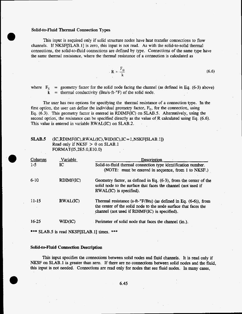
Solid-to-Fluid Thermal Connection Types
This input is required only if solid structure nodes have heat transfer connections to flow channels. If NKSF[SLAB.l] is zero, this input is not read. As with the solid-to-solid thermal connections, the solid-to-fluid connections are defined by type. Connections of the same type have the same thermal resistance, where the thermal resistance of a connection is calculated as
where F, = geometry factor for the solid node facing the channel (as defined in Eq. (6-3) above) k = thermal conductivity (Btu/s-ft-"F) of the solid node.
The user has two options for specifying the thermal resistance of a connection type. In the first option, the user can define the individual geometry factor, FG, for the connection, using Eq. (6.3). This geometry factor is entered in RDIMF(1C) on SLABS. Alternatively, using the second option, the resistance can be specified directly as the value of R calculated using Eq. (6.6). This value is entered in variable RWAL(1C) on SLAB.2.
SLABS (IC,RDIMF(IC),RWAL(IC),WID(IC),IC= 1 ,NSKF[SLAB. 11) Read only if NKSF > 0 on SLAB.l FORMAT(ISY2E5. O,E 10.0)
Columns Variable 1-5 IC
6-10
11-15
16-25
RDIMF(1C)
RWAL(1C)
WID(1C)
DescriD tion Solid-to-fluid thermal connection type identification number.
(NOTE: must be entered in sequence, from 1 to NKSF.)
Geometry factor, as defined in Eq. (6-3), from the center of the solid node to the surface that faces the channel (not used if RWAL(1C) is specified).
Thermal resistance (s-ft-"F/Btu) (as defined in Eq. (6-6)), from the center of the solid node to the node surface that faces the channel (not used if RDIMF(IC) is specified).
Perimeter of solid node that faces the channel (in.).
*** SLAB.5 is read NKSF[SLAB.l] times. ***
Solid-to-Fhid Connection Description
This input specifies the connections between solid nodes and fluid channels. It is read only if NKSF on SLAB.l is greater than zero. If there are no connections between solid nodes and the fluid, this input is not needed. Connections are read only for nodes that see fluid nodes. In many cases,
6.45

the number of nodes with fluid connections will be less than NWK, the total number of solid nodes. To signal the end of this input, zero must be entered for KW on SLAB.6, after all nodes with fluid connections have been identified.
SLAB.6 (KW ,NCHN,(IASSM(L,KW),IKW(L,KW),ICF(L,N),L= 1 ,NCHN)) Read only if NSKF > 0 on SLAB. 1 FORMAT(215,4(315))
Columns Variable 1-5 KW
6-10 NCHN
11-15, IASSM(L,KW
etc. 26-30,
16-20, IKW(L,KW)
etc. 31-35
21-25, ICF(L,KW) 36-40 etc.
Descriution Identification number of solid node with thermal connection(s) to channel(s).
NOTE: enter zero for KW to terminate this input when all solid-to-fluid connections have been identified.
Number of thermal connections to adjacent channels for node KW.
Index number of assembly containing the Lth channel with thermal connection to node KW.
Identification number of Lth channel with thermal connection to node KW.
Identification number of solid-to-fluid thermal connection type for the connection between node KW and channel IKW(L,KW).
(NOTE: This must correspond to a thermal connection type specified on SLABS.)
A maximum of four sets of values of IASSM, IKW, and ICF may be specified on SLAB.6. If NCHN is greater than four, continue the connection input on SLAB.7 to define all connections to node KW before going on to the input for the next node with connections to the fluid.)
SLAB.7 (IASSM(L,KW),IKW(L,KW),ICF(L,N),L=S,NCHN)) Read only if NCHN > 4 on SLABS FORMAT( 15X,4(315))
Columns Variable 1-10
Description BLANK
11-15, IASSM(L,KW) Index number of assembly containing the Lth 26-30, channel with thermal connection to node KW etc.
16-20, IKW(L,KW) Identification number of Lth channel with thermal 31-35 connection to node KW. etc.
6.46

21-25, ICF(L,KW) Identification number of solid-to-fluid thermal 36-40 etc . and channel IKW(L,KW).
(NOTE: This must correspond to a thermal connection type specified on SLAB.5.)
connection type for the connection between node KW
*** SLAB.7 is read with 4 sets of (IASSM, IKW, ICF) entries per line. *** *** SLAB.6 (with SLAB.7, if needed), is read as many times as necessary *** *** to define the connections between solid nodes and the fluid nodes. ***
The input on SLAB.6 is terminated by entering a line with zero entered for KW, after all nodes with connections to flow channels have been identified.
Axial Variation of Slab Material
This option allows the user to specify different material properties in a slab node at different axial locations. The material type flag MATTYP(KN) on SLAB.3 is set to the profile index number for any nodes that are to use the axially varying profile. The input on SLAB.8 and SLAB.9 is used to define the profiles, by specifying which material properties (defined by input in group PROP) will be used at which axial locations for each profile. The user must specify NMAT profiles.
SLAB.8 MAT,NSET Read only if NMAT > 0 on SLAB.l FORMAT (215)
Columns Variable DescriDtion 1-5 MAT Axially varying material type profile identification number. (Used
. in SLAB.3 to identify axially varying material type profile for specific nodes. Must be greater than NSPROP on PROP.l.)
6-10 NSET Number of regions with different material properties in this profile.
SLAB.9 (Kl,K2,MATJ,N=l,NSET[SLAB.61) Read only if NMAT > 0 on SLAB.l FORMAT (4(315))
Columns Variable DescriDtion 1-5, K1 16-20,
Node number at the beginning of the Nth region of axially varying material profile MAT.
(NOTE: the 31-35,first entry for K1 must be node 2.) 46-50
6-10, K2 21-25, MAT.
36-40,
Number of axial nodes in the Nth region of profile
(NOTE: The total number of nodes for all NSET regions in profile MAT must sum to the total number 51-55 of axial nodes, NDX[CHAN. 13.)
6.47

11-15 26-30,
41-45, 56-60
MATJ Identification number of material type for the Nth region of profile MAT.
(NOTE: This must correspond to a material type specified in PROP.3.)
Four sets of entries (Kl,U,MATJ) are read on each line of SLAB.9. This line is repeated until all NSET regions are read for profile MAT.
***SLAB.8 and SLAB.9 are read NMATESLAB.11 times.***
6.2.7 Group RADG--Radiative Heat Transfer Exchange Factors
This group describes the exchange factors for radiative heat transfer within assemblies. Exchange factors are dimensionless geometry parameters that define how well a given surface can “see” another surface for radiative heat transfer. The radiative heat transfer exchange factor groups are specified by type, where a type is defined by the geometry and emissivities of the surfaces in the assembly. A radiative heat transfer exchange factor group type consists of an array of gray body view factors for every surface in the assembly as it exchanges thermal energy by radiation with every other surface in the assembly. The emissivities of the surfaces are also included in the definition of the group type.
There are two ways the user can define radiative heat transfer exchange factor group types for a given case. The gray body view factors and emissivities for some or all groups can be read from a separate input file, on logical unit 10 (opened with the file name tapelo). This file is generated by the auxiliary program RADX-1 or RADGEN, and must be consistent with the geometry input speci- fied in groups RODS and CHAN for the problem (see Section 6.3 for a discussion of the Cycle 2 version of the RADGEN code, and its input instructions).
The user also has the option of specifying black body view factors for assemblies that do not have grey body view factors supplied on tapel0. The code will automatically calculate the corres- ponding gray body exchange factors from the black body view factors. Both options can be used within the same problem, but in different assemblies. Typically, a tape10 file generated by the RADGEN code will be used to obtain the view factors for the assemblies containing rods, and the option for user-specified black body view factors will be used for assemblies modeling open regions of the system, such as the basket region, which do not contain rods.
When view factors generated by RADX-1 or RADGEN are used for square assemblies con- taining unconsolidated rods on a square pitch, the walls of the assembly must be modeled with eight slab nodes, two on each face of the assembly enclosure. For assemblies with consolidated rods on a triangular pitch, the walls of the assembly must be modeled with four slab nodes, one for each face of the enclosure. For assemblies where black body view factors are specified by the user, however, the walls can be modeled with any number of nodes. Only one radiative heat transfer group type can be specified within a given assembly, but a given solid structure node may belong to more than one group, if it has surfaces facing more than one assembly.
e
6.48

RADG.l AGROUP,NASSR,NT 10, NRADG FORMAT(A4,l X ,315)
Columns 1-4
6-10
11-15
16-20
Variable AGROUP
NASSR
NTlO
DescriDtion Enter RADG.
Number of assemblies for which radiative heat transfer groups are to be specified.
Number of radiative heat transfer groups to be read from logical unit 10 (maximum of 6; these radiative heat transfer exchange fac- tor groups are calculated using a program such as RADGEN; see Section 6.3.)
NRADG Number of radiative heat transfer exchange factor group types for which the gray body view factors will be calculated from input of black body view factors and emissivities.
Black Body Radiative Exchange Factor Types
This input is optional and is read only if NRADG on RADG.l is greater than zero. It is used to define radiative heat transfer view factors for enclosures that cannot be defined using program RADGEN; see Section 6.3.
RADG.2 NRAD,NSURF Read only if NRADG > 0 on RADG.l FORMAT(215)
Columns 1-5
6-10
Variable NRAD
NSURF
p DescriDtion
Radiative heat transfer exchange factor group type identification number.
(NOTE: groups must be numbered sequentially, from 1 to NRADG.)
Number of surfaces in radiative heat transfer exchange factor group type NRAD.
Black Body Radiative Exchange Factors
For each radiative exchange factor group type NRAD specified on RADG.2, the user must describe the geometry of the enclosure, and the black body view factors for all surfaces. These factors are area-weighted and can be calculated using the Hottel crossed-string correlation method (Cox 1977), such that
6.49

where &,A,,, = area of surfaces n and m, respectively F,, F,,
= gray body view factor from surface n to m = gray body view factor from surface m to n.
Refer to Section 6.3 for a iscussion of the black body view factors, and the auxiliary code, RADGEN, used to calculate grey body view factors for rod arrays.
RADG.3 IS ,AREAS( NR,IS) ,EMX(IS),(ISX ,FVW(NR,IS ,ISX),ISX = 1,6) ,NFACES Read only if NRADG > 0 on RADG. 1 . FORMAT(15,2F5.0,6(15 ,F5.0) ,I5)
Columns 1-5
6-10
11-15
Variable Description IS Identification number for a surface in radiative heat transfer group
type NRAD. (NOTE: Surfaces of the group type must be numbered sequentially from 1 to NSURF for this input; the number is a generic placeholder for nodes with surfaces in assemblies that use radiative heat transfer group type NRAD; IS does not refer to a specific slab node number. Slab nodes of assemblies of group type NRAD are assigned to specific surfaces of the group type by the input on RODS.11.)
AREAS(NR,IS) Perimeter (in.) of surface IS in group NRAD.
EMX(1S)
16-20, ISX 26-30, etc.
21-25, 31-35, etc.
76-80
Emissivity of surface IS in group NRAD.
Index number of a surface that can exchange thermal radiation with IS in group NRAD.
FVW(NR,IS,ISX) Black body view factor from surface IS to surface ISX.
NFACES Total number of surfaces that can exchange energy by thermal radiation with surface IS.
Up to six pairs of values for ISX,FVW(NR,IS,ISX) can be entered on RADG.3; if NFACES is greater than six, the remaining input for surface is read on RADG.4 before going on to the input for the next surface.
6.50

RADG.4
Columns 1-15
1 6-20, 26-30, etc.
21-25, 31-35, etc.
(ISX , FVW( NR,IS ,ISX) ,ISX = 7,NSURF[RADG.2]) Read only if NSURF > 6 on RADG.2. FORMAT( 15X,6(15 ,F5 .O))
Variable
ISX
Description blank
Index number of a surface that can exchange thermal radiation with IS in group NRAD.
FVW(NR,IS,ISX) Black body view factor from surface IS to surface ISX .
Up to six pairs of values for ISX,FVW(NR,IS,ISX) may be entered on RADG.4. RADG.4 is read as many times as necessary to define all view factors to all surfaces seen by surface IS in group NRAD.
*** RADG.2 and RADG.3, (with RADG.4, if required), are read *** *** sequentially, NRADGWDG. 13 times. ***
Input lines RADG.5 through RADG.9 are read from logical unit 10, which can be generated using the auxiliary program RADGEN. The input lines are listed here for information only. They are not supplied in the normal input stream.
RADG.5 NROWS,PDR,EMW,EMR Read from I/O unit 10, only if NTlO > 0 on RADG.l. FORMAT(I5,3ES .0,15)
Columns 1-5
6-10
11-15
16-20
Variable NROWS
PDR
EMW
EMR
Description Number of rows of rods in the rod bundles modeled by this radiative heat transfer group.
Nominal pitch to diameter ratio for the rod bundle modeled by this radiative heat transfer group.
Emissivity of the slab nodes modeling the walls of the assembly for this radiative heat transfer group.
Emissivity of the rods for this radiative heat transfer group.
6.51

RADG.6
Columns 1-5
6-10
11-15
16-20
RADG.7
Columns 1-15, 16-30, 21-45, etc.
RADG.8
Columns 1-15, 16-30, 31-45, etc.
MMl,MM2,MM3,MM4 Read from I/O unit 10, only if NTlO > 0 on RADG.l. F 0 RM A T (4 I5 )
Variable Descriu tion MM1 Total number of surfaces in radiative heat transfer group MM2.
MM2 Identification number for this radiative heat transfer group. (NOTE: 1 I MM2 5 6)
MM3 Flag for number of surfaces on a rod (NOTE: must correspond to the value for NTHETA entered on RODS. 1).
MM4 Number of wall surfaces in this radiative heat transfer group (must be 8 for unconsolidated rod bundle, and 4 for consolidated rod bundle with triangular pitch in a square enclosure).
(EMV(MM2,N),N= 1,MM4) Read from I/O unit 10, only if NTlO > 0 on RADG.l. FORMAT(8E15.0)
Variable DescriDtion EMV(MM2,N) Emissivity of the Nth slab node enclosing an
assembly with radiative heat transfer group MM2. (NOTE: Default is EMW[RADG.S] for all wall nodes; if wall emissivities are uniform, this input can be entered as a blank line.)
(RRATIO(MM2,N),N = 1,MM4) Read from I/O unit 10, only if NTlO > 0 on RADG.l. FORMAT(8E15.0)
Variable DescriDtion RRATIO(MM2,N) Ratio of the perimeter of the Nth node of the
assembly wall to the rod perimeter, for radiative heat transfer group MM2.
6.52

RADG.9 (FVn(N,M),M=l,MMl),N= 1,MMl) Read from 110 unit 10 only if NTlO > 0 on RADG.l. FORMAT(8E15.5)
Columns 1-15, 16-30, 31-45, etc.
Variable FVn(N,M)
Descriution Gray body exchange factor from surface N to surface M for radiative heat transfer group MM2.
*** RADG.9 is read for MM1 sets of exchange factors. ***
RADG.6 through RADG.9 are read sequentially NTlO times from logical unit 10.
This is the end of the input read from logical unit 10.
Assembly Radiative Heat Transfer Group Information
This input line assigns the appropriate radiative heat transfer group type to each assembly that has radiative heat transfer.
RADG.10 IASS,ITYPR(IASS),MSID(IASS),(KSIDE(IASS,L),L= 1,12) FORMAT(315,12(15))
Columns 1-5
6-10
11-15
16-20, 21-25, etc.
Variable Descriution IASS Identification number of an assembly with radiative heat transfer.
ITYPR(1ASS)
MSID(1ASS)
Radiative heat transfer group type:
- for a radiative group type read from logical unit 10, enter a positive number (must correspond to a group type identified on RADG.6).
- for a radiative group calculated from user specified black body view factors, enter the negative of the group identification number (must correspond to a group type identified on RADG.2).
Number of slab nodes with surfaces in radiative exchange factor group ITYPR(1ASS). (NOTE: must be the same as NSURF on RODS.2 for group type ABS[ITYPR(IASS)] .)
KSIDE(IASS,L) Identification number of the slab node corresponding to the Lth surface of radiative exchange factor group ABS[ITYPR(IASS)] .
6.53

Up to 12 values for KSIDE can be entered on RADG.lO; if MSID(1ASS) is greater than 12, the remaining input for assembly IASS is read on RADG. 11 before going on to the input for the next assembly.
RADG.ll (KSIDE(IASS,L),L= 13 ,MSID(IASS)) Read only if MSID(1ASS)mDG. 101 > 12 FORMAT( 15X, 12(15))
Columns Variable Description 1-15 BLANK
16-20, KSIDE(IASS,L) Identification number of the slab node 21-25, etc. heat transfer group ITYPR(1ASS).
corresponding to the Lth surface of radiative
*** RADG.10 (with RADG.ll if MSID(1ASS) > 12) is read NASSRMDG.11 times. *?*
6.2.8 Group HEAT--Heat Transfer Correlations
This group defines the heat transfer coefficient correlations for convection and conduction heat exchange between the fuel rods and the fluid only. Heat transfer between the fluid and the structures represented by slab nodes is modeled using thermal connections, as defined in group SLAB (see Section 6.2.6. The correlations are identified by type number, which must correspond to the values specified for NFLMC(NASS) on CHAN.6. The option for the single-phase turbulent mixing model in COBRA-SFS can also be selected by input in this group.
HEAT.1
Columns 1-4
6-10
11-15
where
AGROUP,NHEAT ,NSCBC ,NFCON ,NTHEAT ,NFHEAT FORMAT(A4,lX,515)
Variable DescriDtion AGROUP Enter HEAT.
NHEAT
NSCBC
Number of heat transfer correlation sets to be read in on HEAT.2.
Flag for single-phase turbulent mixing model:
= 0; no turbulent mixing (default)
= 2; Wk = AMIX * (Re ** BMIX) * (SG) = 3; W; = AMIX *(Re ** BMIX) * m) = 4; W, = AMIX * (Re ** BMIX) * (&ifK) (bG)
= 1; WT = AMIx * (&e)
WT = turbulent crossflow. Re = Reynolds number (based on axial velocity) e SK = lateral gap width
= average axial mass flux of the two channels connected by lateral flow connection k
6.54

16-20
21-25
26-30
b
P,
= average hydraulic diameter of the two channels connected by lateral flow connection
= transverse momentum control volume length for flow connection k AMIX, BMIX = user-defined constants; see HEAT.3.
NFCON Flag for radial conduction in the fluid:
= 0; no conduction in the fluid.
= 1; fluid conduction between channels through the gap connections.
NTHEAT Number of lateral convection heat transfer correlation sets to be read in on HEAT.6.
NFHEAT Number of axial free convection heat transfer correlations to be read in on HEAT.6.
Axial Flow Forced Convection Heat Transfer Correlations
Forced convection heat transfer correlations are specified in the code using the standard formula,
k H = (a, Re" ha' .t ad) - De
where a,, a,, a,, 4 = empirical coefficients Re = Reynolds number Pr = Prandtl number
De = channel hydraulic diameter k = thermal conductivity of the fluid
The convention in the code is to enter heat transfer correlations in pairs, with one set of coefficients for laminar flow and one set for turbulent flow, such that Eq. (6.8) becomes
(6.9)
The local heat transfer coefficient for a node is evaluated as the maximum value obtained with the turbulent and laminar equations for the local Reynolds number and Prandtl number,
H,, = max(%nImlr,H&daJ
6.55

The heat transfer correlations are numbered sequentially in the code, from 1 to NHEAT, in the order they are read in on HEAT.2. These sequence numbers must be used when specifying the values entered for variable NFLMC(NASS) on CHAN.6, when identifying the heat transfer corre- lation used by each assembly type.
HEAT.2 (AHl(I),AH2(I),AH3(I),AH4(I),AHL1(I),AHL2(I),AHL3(I),AH~(I), I= 1,NHEAT) Read only if NHEAT > 0 on HEAT.l FORMAT( 12F5.0)
Columns Variable Description 1-5 AHl(1) Reynolds number multiplier coefficient of Ith axial heat transfer
correlation for turbulent flow (i.e., atl in Eq. [6.9]).
6-10 AH2(I) Reynolds number exponent of Ith axial heat transfer correlation for turbulent flow (Le., a, in Eq. r6.91).
11-15 AH3(I) Prandtl number exponent of Ith axial heat transfer correlation for turbulent flow (Le., a, in Eq. r6.91).
16-20 AH4(I) Additive coefficient of Ith axial heat transfer correlation for turbulent flow (i.e., a, in Eq. [6.9]).
Reynolds number multiplier coefficient of Ith axial heat transfer correlation for laminar flow, (Le., a,, in Eq. r6.91).
Reynolds number exponent of Ith axial heat transfer correlation for laminar flow (Le., af2 in Eq. [6.9]).
Prandtl number exponent of Ith axial heat transfer correlation for laminar flow(i.e., af3 in Eq. r6.91)
Additive coefficient of Ith axial heat transfer correlation for laminar flow (Le., at4 in Eq. [6.9]).
21-25 AHLl(I)
26-30 AHL2(I)
31-35 ML3(I)
36-40 AHLA(1)
HEAT3 (AMIX(N),BMIX(N),N = 1 ,MAXTYP) Read only if NSCBC > 0 on HEAT. 1 FORMAT(2ES .O)
Columns Variable DescriDtion 1-5 M W N ) Multiplicative coefficient for turbulent mixing correlation, of form
specified by value of NSCBC on HEAT. 1, $0 be applied to all assemblies of type N.
6-10 B M w N ) Reynolds number exponent for turbulent mixing correlation of form specified by value of NSCBC on HEAT.1, to be applied to all assemblies of type N. (NOTE: BMIX(N) is not used if NSCBC = 1.)
MAXTYP is the total number of assembly types (Le., the number of unique values specified for ITYPA on CHAN .5).
*** HEAT.3 is read MAXTYP times, once for each assembly type, *** *** if NSCBC > 0 on HEAT.l. ***
6.56

Radial Fluid Conduction
If NFCON = 1, radial heat conduction in the fluid will be calculated for the problem. Heat conduction through the fluid is treated as occurring between adjacent channels through the gap con- nections. The conduction path is defined by the centroid length of the lateral control volume, which is specified by user input in variable DIST(K) on CHAN.7. The input on HEAT.4 can be used to modify the conduction length for the lateral connections in a given assembly, to account for variations in the connection lengths not considered in the value entered for DIST.
HEAT.4 (GK(N),N= 1,MAXTYP) Read only if NFCON = 1 on HEAT.l. FORMAT( 16E5.0)
Columns Variable Descriution 1-5, GK(N) Multiplier on the lateral control volume length for 6-10, thermal conduction between channels in assemblies 11-15, of type N: etc.
- if GK(N) is specified as 1.0, the length specified in DIST on CHAN.7 for a particular gap connection on is used for the conduction length.
- if GK(N) is specified as 0.0, fluid conduction is zero in assemblies of type N.
MAXTYP is defined for this input as for HEAT.3; it is the number of unique assembly types.
Up to 16 values can be read on a line for HEAT.4. If there are more than 16 assembly types, this line is repeated as many times as necessary to specify a GK(N) value for each of MAXTYP assembly types.
Lateral Flow Forced Convection Heat Transfer Correlations
Heat transfer correlations for forced convection due to lateral flow follow the same convention as the correlations for axial flow. Coefficients are read in for a turbulent and a laminar formulation,
(6.10)
where q,, %, a,, a, = empirical coefficients for turbulent correlation a,, , a,,, +3, +4 = empirical coefficients for laminar correlation
Re, = Reynolds number, based on rod diameter Pr = Prandtl number
6.57

k = thermal conductivity of the fluid D, = rod nominal diameter.
The local heat transfer coefficient is evaluated as the maximum of the two;
These heat transfer correlations are numbered sequentially in the code, from 1 to NTHEAT, in the order they are read in on HEAT .5. The heat transfer correlation to be used in a particular lateral flow connection is determined by the value specified for NFLMC(1ASS) on CHAN.6 for the assembly containing the lateral flow connection. The input for NFLMC(1ASS) on CHAN.6 is thus made to do double duty, since it also specifies the heat transfer correlation for axial flow in the channels of the assembly, by identifying the index of a correlation defined by input on HEAT.2). The user must make certain that the index number entered on CHAN.6 in variable NFLMC(1ASS) for an assembly type corresponds to the correct axial heat transfer correlation (from HEAT.2) for the channels and to the correct lateral heat transfer correlation (from HEAT.5) for the lateral connections between channels in the assembly.
HEATS (AHTl(I),AHT2(I),AHT3(I),AHT4(I),AHTLl~),AHTL2(I),~TL3~), AHTU(I),I= 1,NTHEATmEAT. 11) Read only if NTHEAT > 0 FORMAT(8F5 .O)
Columns Variable DescriDtion 1-5 AHTl(1) Reynolds number multiplier coefficient of Ith lateral heat transfer
correlation for turbulent flow (i.e., ql in Eq. r6.101).
6-10 AHT2(I) Reynolds number exponent of Ith lateral heat transfer correlation for turbulent flow (Le., a, in Eq. r6.101).
11-15 M T 3 0 Prandtl number exponent of Ith lateral heat transfer correlation for turbulent flow (i.e., a, in Eq. [6.10]).
Additive coefficient of Ith lateral heat transfer correlation for turbulent flow (i.e., a, in Eq. [6. lo]).
16-20 AHT4(1)
2 1-25 AHTLl(1) Reynolds number multiplier coefficient of Ith lateral heat transfer correlation for laminar flow (i.e., ai, in Eq. r6.101).
Reynolds number exponent of Ith lateral heat transfer correlation for laminar flow (Le., all in Eq. [6.10]).
26-30 AHTL2(I)
31-35 AHTL3(I) Prandtl number exponent of Ith lateral heat transfer correlation for laminar flow (Le., a, in Eq. [6.10]).
36-40 AHTWO Additive coefficient of Ith lateral heat transfer correlation for laminar flow (Le., a, in Eq. [6.10]).
*** HEATS is read NTHEATWEAT.11 times. ***
6.58 a

Axial Flow Free Convection Heat Transfer Correlations
Heat transfer correlations for free convection due to buoyancy-driven recirculating axial flows are specified in the form,
k Hf = - (afi Raan) Dr
(6.11)
where q,, a, = empirical coefficients Ra
k
= local Rayleigh number of the flow, (defined as the Grashof number times the
= thermal conductivity of the fluid Prandtl number)
Dr = rod diameter.
These heat transfer correlations are numbered sequentially in the code, from 1 to NFHEAT, in the order they are read in on HEAT.6. The heat transfer correlation to be used for free convection in a given assembly is determined by the value specified for NFLMC(1ASS) on CHAN.6. The input for NFLMC(1ASS) on CHAN.6 is thus made to do triple duty, since it also specifies the heat transfer correlations for axial and lateral forced convection in the assembly. The user must make certain that the index number entered on CHAN.6 in variable NFLMC(1ASS) for an assembly type corresponds to the correct axial heat transfer correlation (from HEAT.2) for the channels, and to the correct lateral heat transfer correlation (from HEAT.5) for the lateral connections between channels in the assembly, and to the correct free convection heat transfer correlation (from HEAT.6).
HEAT.6 (AHFl(I),AHF2(1),1= 1,NFHEATwEAT.lI) Read only if NFHEAT > 0 FORMAT (2F5.0)
Columns 1 -5
6-10
Variable AHFl(1)
DescriDtion Rayleigh number multiplier coefficient of Ith axial heat transfer correlation for free convection (Le., a, in Eq. [6.11]).
Rayleigh number exponent of Ith axial heat transfer correlation for free convection (Le., a, in Eq. [6.11]).
' *** HEAT.6 is read NFHEATBEAT.11 times ***
6.2.9 Group DRAG--Friction Factors and Loss Coefficients
This group describes the axial pressure losses due to wall friction and local obstructions in the flow field. The optional network model can also be specified, by setting the flag NETWK on DRAG. 1 (refer to Section 5.1.2.2 for a discussion of the network model).
6.59

DRAG. 1 AGROUP, NFRICT, NOLC , NRAMP,NLCFF ,NLCFP, NETWK, NOGRP, NBLOCK,NVISCW,NFTRAN FORMAT(A4, l X , 1015)
Description Enter DRAG.
Variable AGROUP
Columns 1-4
6-10 NFRICT Number of friction factor correlation sets to be read in (default is 1).
11-15 NOLC Number of assembly types for which loss coefficients are to be specified.
16-20 NRAMP Number of iterations over which the loss terms are to be ramped into the solution (default is 1).
21-25 NLCFF Number of loss coefficient versus Reynolds number forcing functions.
26-30 NLCFP Number of points in the loss coefficient versus Reynolds number forcing functions.
31-35 NETWK Flag for optional pressure drop network model:
= 0; not used.
= 1; pressure drop will be calculated for user- specified assembly network.
NOGRP 36-40 Number of assembly groups for the network model (used only if N E W > 0).
41-45
46-50
NBLOCK
NVISCW
Number of axial locations where axial flow blockages occur.
Flag for hot wall correction to viscosity in friction factor correlation:
= 0; no hot wall correction.
= 1; apply hot wall correction to channels with heated surfaces.
Number of lateral flow fraction loss correlation sets to be read in on DRAG. 13.
51-55 ' NFTRAN
6.60

Friction Factor Correlations
Wall friction losses are described using the Darcy friction factor correlation form. This is defined in terms of the pressure drop such that the axial frictional pressure gradient is given by
dP - flmlm dX 2gcD,pA - -
The friction factor, f, is determined from the Blasius relation,
(6.12)
f = a R e b + c (6.13)
Each correlation consists of a formulation with a set of turbulent and a set of laminar coefficients, of the form
fT = a R e b + c R e d + e (6.14)
fL = a,Re bL + cL (6.15)
The code evaluates the friction factor as the qaximum of the turbulent and laminar values, 9
f = max(f,,fd
A total of NFRICT[DRAG.l] correlations are specified by input on DRAG.2. These corre- lations are numbered sequentially in the order they are read in on DRAG.2. These identification numbers are used when specifying the values for N on CHAN.7, in the geometry description for each channel of an assembly type. The default for N is type 1, and in most cases, this will be sufficient for all channels. However, the user can specify as many friction factor correlations as needed to model the various wall resistances in a given problem.
Alternatively, instead of specifying N for each channel on CHAN.7, a friction factor corre- lation can be specified for the assembly type, in the value for MDFLT on CHAN.6. The value for N can then be entered as zero, and all channels in assemblies of that type will be assigned the friction factor correlation identified in .MDFLT on CHAN.6.
a 6.61

DR4G.2 (AA(I),BB(I),CC(I),DD(I),EE(I),AAL(I),BBL(I),CCL(I),I=1,NFRICT[DRAG.1]) Read only if NFRICT > 0 on DRAG.l. FORMAT(8FS .O)
Columns 1-5
6-10
11-15
16-20
21-25
26-30
3 1-35
3 1-35
AAL(1)
BBL(1)
CCL(1)
Descriution First multiplicative coefficient on the Reynolds number for turbulent flow friction factor correlation (a in Eq. [6.14]).
First Reynolds number exponent for turbulent flow friction factor correlation 0, in Eq. [6.14]).
Second multiplicative coefficient on the Reynolds number for turbulent flow friction factor correlation (c in Eq. [6.14]).
Second Reynolds number exponent for turbulent flow friction factor correlation (d in Eq. [6.14]).
Additive coefficient for turbulent flow friction factor correlation (e in Eq. [6.14]).
Multiplicative coefficient on the Reynolds number for laminar flow friction factor correlation (aL in Eq. [6.15]).
Reynolds number exponent for laminar flow friction factor correlation (bL in Eq. [6.15]).
Additive coefficient for laminar flow friction factor Correlation (cL in Eq. [6.15]).
*** DRAG.2 is read NFRICT[DRAG.l] times. ***
Axial Form Loss Coefficients
The pressure loss due to form drag on local obstructions in the flow field such as grid spacers and orifice plates is given by
where C, = loss coefficient m = upstream mass flow rate (lbds).
Axial form loss coefficients can be specified for any channel or group of channels, at any axial location in the problem. Local loss coefficients are specified by assembly type. Assemblies of the same type see the same form losses. In each assembly type having local losses, the user must define
6.62

the axial levels and channels where the losses occur, and specify the loss coefficient to be applied at each location. This input is specified on DRAG.3 and DRAG.4. These two input records are read in sequence NOLC[DRAG. 11 times.
DRAG.3 LCASST(I),NBl(I),LCFF(I) Read only if NOLC > 0 on DRAG.l. FORMAT( 3 15)
Columns 1-5
6-10
11-15
Variable LCASST(1)
NBl(1)
Description Identification number of an assembly type with loss coefficients.
Number of sets of channels in assembly type LCASST(1) that have loss coefficients.
(NOTE: A channel set is defined as a group of sequentially numbered channels that have the same loss coefficients at the same axial locations.)
LCFF(1) Identification number of loss coefficient forcing function to be applied to loss coefficients in assembly type LCASST(1) (optional input; must correspond to a forcing function entered on DRAG.6).
DRAG.4 (with DRAGS, if needed) is read for L= l,NBl(I) sets of channels with local losses in assemblies of type LCASST(1).
DRAG.4 (NLEVEL(I,L),ILCS(I,L),ILCE(I,L),(FACTOR(I,L,J),XCD(I,L,J),J = 1,6) Read only if NOLC > 0 on DRAG.l. FORMAT(315,12F5.0)
Columns Variable DescriDtion 1-5 NLEVEL(1,L) Number of axial locations in the Lth location set for assembly type
LCASST(1). (NOTE: L=l,NBl(I))
6-10
11-15
16-20, 26-30, etc.
21-25, 31-35, etc.
ILCS(1,L)
ILCE(1,L)
Identification number of starting channel in the Lth location set of assembly type LCASST(1).
Identification number of ending channel in the Lth location set of assembly type LCASST(1).
(NOTE: all channels from ILCS(I,L) to ILCE(I,L) will be assigned the same losses at the same locations, as specified by the values for the FACTOR and ZCD arrays.)
FACTOR(I,L,J) Relative height (x/L) of the Jth axial location for the Lth channel set in assembly type LCASST(1).
XCD(I,L, J) Loss coefficient to be applied in channels ILCS(I,L) through ILCE(I,L) at axial location FACTOR(I,L,J).
6.63

Up to six pairs of (FACTOR, XCD) values can be entered on DRAG.4. If NLEVEL(1,L) is greater than six, the remaining pairs of (FACTOR,XCD) are read on DRAGS for the current location set before going on to the next location set.
DRAGS (FACTOR(I,L,J),XCD(I,L,J),J=7,NLEVEL(I,L)) Read only if NLEVEL(1,L) > 6 on DRAG.4. FORMAT( 15X, 12F5.0)
Columns 1-15
1 6-20, 26-30, etc.
21-25, 31-35, etc.
Variable DescriDtion blank
FACTOR(I,L,J) Relative height (x/L) of the Jth axial location for the Lth channel set in assembly type LCASST(1).
XCD(1 ,L, J) Loss coefficient to be applied in channels ILCS(1,L) through ILCE(1,L) at axial location FACTOR(I,L,J).
DRAG.3 and DRAG.4 (with DRAG.5, if needed) are read in sequence NOLCPRAG.11 times, with DRAG.4 (and DRAG.5) read NBl(1) times for each time DRAG.3 is read.
Losses for Network Model
This input is required only if the network model has been specified by NETWK= 1 on DRAG.l. The assembly grouping for the network is defined by reading DRAG.6 for each assembly. Each assembly is assigned a group number, inlet loss parameters, and optional loss coefficient forcing functions. A loss coefficient for the total flow in all assemblies is specified on DRAG.7. Loss parameters for individual groups of assemblies are specified on DRAG.8 for NOGRPDRAG. 11 groups of assemblies.
DRAG.6 (NETGRP(N),NINFF(N),NOUTFF(N),RAIN(N),PWIN(N),HAIN(N),RAOUT(N), PWOUT(N),HAOUT(N),N = 1 ,NASSEM[CHAN. 11) Read only if NETWK = 1 on CHAN.l FORMATOIS ,6F10.0)
Columns 1-5
Variable 0 NETGRP
6-10 NINFF(N
DescriDtion Assembly grouping number to be used with assembly N, corresponding to the assembly groups described in DRAG.9 (default is 1).
Identification number of loss coefficient forcing function versus Reynolds number, (defined on DRAGS and DRAG.6), to be used with assembly inlet loss, M ( N ) (default is 0 for no forcing function).
6.64

11-15 NOUTFF( N)
16-25 RAIN(N)
26-35 PWIN(N)
36-45 HAIN(N)
46-55 RAOUT(N)
56-55 PWOUT(N)
66-75 HAOUT(N)
Identification number of loss coefficient forcing function versus Reynolds number, to be used with assembly outlet loss RAOUT(N) (default is 0 for no forcing function).
Inlet loss parameter (ft-1bm)-' to be applied at inlet of assembly N.
Wetted perimeter (in.) associated with inlet loss RAIN (used only in Reynolds number calculation when NINFF(N) > 0; default is 1 .O).
Gravitational head length (in.) associated with the assembly inlet loss.
Outlet loss parameter (ft-lbm)-' to be applied at outlet of assembly N.
Wetted perimeter (in.) associated with outlet loss RAOUT(N). (Used only in Reynolds number calculation when NOUTFF(N) > 0; default is 1.0).
Gravitational head length (in.) associated with the assembly outlet loss.
*** DRAG.6 is read NASSEM[CHAN.l] times. *** DRAG.7 RTIN Read only if NETWK > 0 on DRAG.l
FORMAT(F 10.5)
Columns Variable DescriDtion 1-10 RTIN Loss parameter (ft-lbm)-' to be applied to the total flow rate (sum
of all assembly flow rates; Reynolds-number independent).
DRAG.8 (RGIN(L),HGIN(L),RGOUT(L),HGOUT(L),L= 1 ,NOGRP) Read only if NOGRP > 0 on DRAG.1 FORMAT(4F 1 0.5)
Columns Variable DescriDtion 1-10 RGIN(L) Loss parameter (ft-lbm)-' to be applied at assembly grouping inlet
(Reynolds number independent).
Gravitational head length (in.) associated with the inlet pressure loss for group L.
Loss parameter (ft-lbm)-' to be applied at assembly grouping outlet (Reynolds number independent).
11-20 HGIN(L)
21-30 RGOUT(L)
31-40 HGOUT( L) Gravitational head length (in.) associated with the outlet pressure loss for group L.
*** DRAG.8 is read NOGRP[DRAG.l] times. ***
6.65

Loss Coefficient Forcing Functions
This input is read only if NLCFP > 0 on DRAG.l. Loss coefficients are specified as con- stants (in XCD(I,L,J) on DRAG.4 and DRAG.5), but the user has the option of varying loss coeffi- cients as a function of the Reynolds number. The forcing functions are numbered sequentially in the order they are defined on DRAG.7.
The variations in loss coefficients are specified as a function of Reynolds number. The same table of Reynolds number values applies to all forcing functions. The variations in loss coefficient with Reynolds number are expressed as multiplicative factors normalized to the value of XCD(I,L,J) entered on DRAG.4.
DRAG.9 (RECL(I),I= l,NLCFP[DRAG. 11) Read only if NCLFP > 0 on DRAG.l FORMAT( 12E5.0)
Columns Variable Descriution 1-5, 6-10, coefficient forcing function profiles. etc.
RECL(1) Reynolds number for the Ith point in the loss
NOTE: the table of Reynolds number values must be monotonically increasing.
DRAG.10 ((FFLC(J,L),J= 1 ,NLCFP[DRAG.l]),L= 1 ,NLCFF[DRAG. 11 Read only if NCLFF > 0 and NCLFP > 0 on DRAG.l. FORMAT( 12E5.0)
Columns Variable Descrimion 1-5, FFLC(J,L) The loss coefficient factor for Reynolds number 6-10, etc.
RECL(1) in the Lth forcing function profile.
*** DRAG.10 is read NLCFFpRAG.11 times. ***
Local Blockages
This input allows the user to specify flow blockages at some axial locations in some channels. The axial flow at the blocked level is set to zero in the affected channels. Note that this input is specified by axial level number; if the axial noding is changed in a problem, this input must be adjusted to reflect the new locations of the blocked axial levels, or the blockages may turn up in the wrong places. This is optional and is read only if NBLOCK is greater than zero on DRAG. 1.
6.66

DF2AG.11 NBLOKA,NBLOKC Read only if NBLOCK > 0 on DRAG. 1 . FORMAT(215)
Columns 1-5
6-10
DRAG. 12
Columns 1-5, 11-15, etc.
6-10, 1 6-20, etc.
Variable DescriDtion NBLOKA Axial level where the blockage is located.
NBLOKC Number of channels blocked at axial level NBLOKA.
(IBLOKA(I),IBLOKC(I),I=l,NBLOKC[DRAG.lO]) Read only if NBLOCK > 0 on DRAG. 1 FORMAT( 1615)
Variable DescriDtion IBLOKA(1) Identification number of assembly containing
blocked channel IBLOKC(1).
IBLOKC(1) Identification number of the Ith blocked channel.
DRAG. 11 and DRAG. 12 are read in sequence NBLOCK times to define all blocked channels.
Lateral Friction Loss Correlations
The default approach in COBRA-SFS is to treat lateral friction and form losses with a constant value for all gaps. This is specified by input as the gap resistance IUJ(l), defined in group CHAN on CHAN.8. This input provides an alternative, in which the lateral friction loss can be expressed as a Blasius-type friction factor correlation.
The lateral pressure loss due to flow through a gap can be expressed in the form
where f = friction loss coefficient for flow through a single gap.
The friction loss coefficient is expressed in terms of the transverse Reynolds number, which is defined with the rod diameter as the characteristic length, such that
6.67
(6.16)
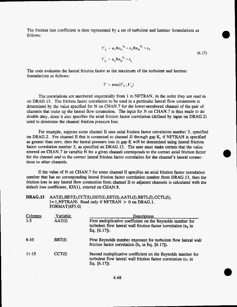
The friction loss coefficient is then represented by a set of turbulent and laminar formulations as follows:
f‘, = aTReDbT + cTReD dT + eT (6.17)
flL = a,ReD bl. + cL
The code evaluates the lateral friction factor as the maximum of the turbulent and laminar formulations as follows:
f’ = max(f’, , PL)
The correlations are numbered sequentially from 1 to NFTRAN, in the order they are read in on DRAG.13. The friction factor correlation to be used in a particular lateral flow connection is determined by the value specified for N on CHAN.7 for the lower-numbered channel of the pair of channels that make up the lateral flow connection. The input for N on CHAN.7 is thus made to do double duty, since it also specifies the axial friction factor correlation (defined by input on DRAG.2) used to determine the channel friction pressure loss.
For example, suppose some channel I1 uses axial friction factor correlation number 3, specified on DRAG.2. For channel I1 that is connected to channel JJ through gap K, if NFTRAN is specified as greater than zero, then the lateral pressure loss in gap K will be determined using lateral friction factor correlation number 3, as specified on DRAG.13. The user must make certain that the value entered on CHAN.7 in variable N for a given channel corresponds to the correct axial friction factor for the channel and to the correct lateral friction factor correlation for the channel’s lateral connec- tions to other channels.
If the value of N on CHAN.7 for some channel I1 specifies an axial friction factor correlation number that has no corresponding lateral friction factor correlation number from DRAG.13, then the friction loss in any lateral flow connection from channel I1 to adjacent channels is calculated with the default loss coefficient, KIJ(l), entered on CHAN.8.
DRAG.13 AAT(I),BBT(I),CCT(I),DDT(I),EET(I),AATL(I),BBTL(I),CCTL(I), I = 1 ,NlTRAN) Read only if NFTRAN > 0 on DRAG. 1. FORMAT(8FS.O)
Columns Variable Description 1-5 AAT(I) First multiplicative coefficient on the Reynolds number for
turbulent flow lateral wall friction factor Correlation (aT in Eq. [6.171).
6-10 BBT(I) First Reynolds number exponent for turbulent flow lateral wall friction factor correlation (bT. in Eq. [6.17).
11-15 CCT(1) Second multiplicative coefficient on the Reynolds number for turbulent flow lateral wall friction factor correlation (G in Eq. [6.17]).
6.68

16-20
2 1-25
26-30
3 1-35
36-40
DDT(1)
EET(1)
AATL(1)
BBTL(1)
CCTL(1)
Second Reynolds number exponent for turbulent flow lateral wall friction factor correlation (i.e., d, in Eq. 16.171).
Additive coefficient for turbulent flow lateral wall friction factor correlation (% in Eq.{(6.17]).
Multiplicative coefficient on the Reynolds number for laminar flow lateral wall friction factor correlation (aL in Eq. [6.17]).
Reynolds number exponent for laminar flow lateral wall friction factor correlation (bL in Eq. [6.17]).
Additive coefficient for laminar flow lateral wall friction factor correlation (cL in Eq. 16.171).
*** DRAG.13 is read in NFTRANrDRAG.11 times. ***
6.2.10 Group BDRY-Thermal Boundary Conditions
The input for this group defines the heat transfer boundary conditions for the calculation. In most instances, this will be the interface between the system being modeled and the environment, but the user has a great deal of flexibility in specifying the heat transfer boundary conditions for a problem.
The default in COBRA-SFS is to assume that the side boundaries of a system are adiabatic. If there is heat transfer to the environment in the radial direction, boundary conditions must be defmed explicitly for the sides of the system. In COBRA-SFS, heat is transferred out the boundaries through a series of user-defined boundary regions, each of which can use a different boundary connection type. A boundary connection type is defined as a semi-empirical correlation for the boundary surface heat flux qb, and has the form
where C, = user-defmed constants IT
ei, ei+] Ti,Ti+l
= Stefan-Boltzmann constant, 0.1714( 10') Btu/h-fP-"R4 = surface emissivity of boundary nodes i and i+ 1 = temperature of nodes i and i+ 1.
(6.18)
The total number of boundary types, NBTYP, is defined for a given problem by the user on BDRY. 1. These boundary connection types are defined by input on BDRY .2, with coefficients for correlations of the form shown in Eq. (6.18). The total number of slab nodes that use these boundary connection types is specified in NWSID on BDRY. 1.
6.69

The temperature of the environment seen by the boundary node is defined using axial profiles of boundary temperatures, read on BDRY.3. The number of axial boundary temperature profiles to be read in is defined by the user, as NBTEMP on BDRY. 1 The user can read in as many axial profiles as needed to characterize a given problem. The boundary condition types seen by specific slab nodes are defined by input on BDRY.5 through BDRY.?. This input also includes the option to define axially varying boundary connection types.
If the plenum model is not used, the boundaries at the top and bottom of the system are assumed adiabatic for heat transfer, and the flow boundary conditions are defined by the input in group OPER. In this case, the inlet flow boundary condition treats the entering fluid as coming from an essentially infinite reservoir at the fluid boundary temperature and pressure defined in OPER. At the exit, the fluid vanishes into another essentially infinite reservoir at the specified boundary pres- sure. If flow should reverse at the exit, the properties of the incoming fluid are defined at the boundary pressure and some user-specified temperature.
The group BDRY input includes the alternative option of defining inlet and outlet plena to model a closed flow system, with heat transfer connections to the external environment. When the optional plenum model is used, the boundary conditions specified in group OPER are used as the initial values for inlet flow rate, temperature, and pressure. Conditions in the inlet plenum are calcu- lated for each iteration by summing the flows from all channels having negative inlet flow. This temperature and pressure are used to define the conditions for flow into all channels with positive inlet flow. In the upper plenum, the conditions are calculated by summing the flow from channels with positive flow at the exit. These conditions define the temperature and pressure of flow into channels with negative flow at the exit.
The fluid conditions in the inlet plenum and the exit plenum are treated as one-diiensional. It is assumed that the flow mixes instantaneously in these regions, and no radial gradients are main- tained in the fluid. Thermal boundary conditions on the upper and lower plena can vary radially, however. In addition, different plenum boundary regions can connect axially to different slab nodes. It is also possible to specify separate top and side boundary conditions on the plenum regions. The plenum input is specified on lines BDRY.8 through BDRY.14.
BDRY. 1 AGROUP ,NBTYP ,NBTEMP ,NWSID , NPR FORMAT(A4,1X,415)
Columns 1-4
6-10
11-15
16-20
Variable AGROUP
NBTYP
NBTEMP
NWSID
DescriDtion Enter BDRY.
Number of t h e m 1 boundary connection types.
Number of axial boundary temperature profiles.
Number of solid structure nodes connected to the side thermal boundary.
6.70
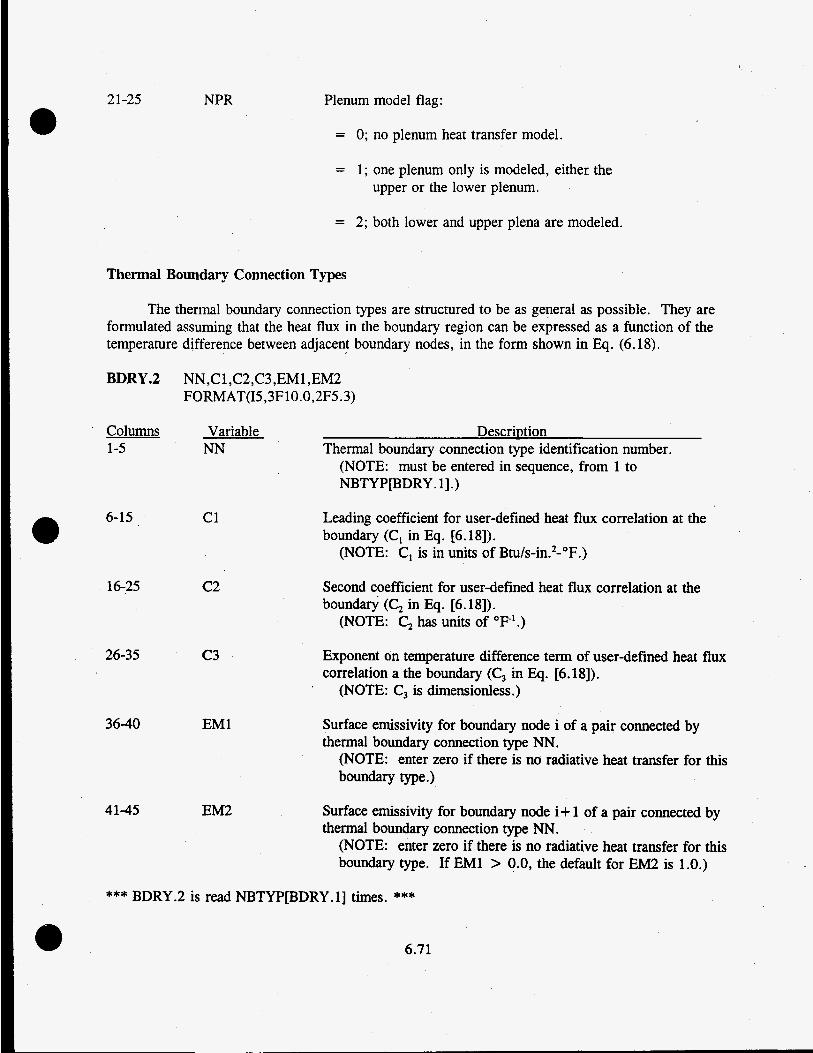
2 1-25 NPR Plenum model flag:
= 0; no plenum heat transfer model.
= 1; one plenum only is modeled, either the upper or the lower plenum.
= 2; both lower and upper plena are modeled.
Thermal Boundary Connection Types
The thermal boundary connection types are structured to be as general as possible. They are formulated assuming that the heat flux in the boundary region can be expressed as a function of the temperature difference between adjacent boundary nodes, in the form shown in Eq. (6.18).
BDRY .2 NN,C 1 ,C2 ,C3 ,EM 1 ,EM2 FORMAT(I5,3F10.0,2F5.3)
Columns Variable 1-5 NN
6-15
16-25
26-35
36-40
41-45
c 1
c 2
c 3
EM1
EM2
DescriDtion Thermal boundary connection type identification number.
(NOTE: must be entered in sequence, from 1 to NBTYPPDRY. 11 .)
Leading coefficient for userdefined heat flux correlation at the boundary (C, in Eq. [6.18]).
(NOTE: C, is in units of Btu/s-in.*-OF.)
Second coefficient for userdefined heat flux correlation at the boundary (C, in Eq. [6.18]).
(NOTE: C, has units of OF-'.)
Exponent on temperature difference term of userdefined heat flux correlation a the boundary (C, in Eq. [6.18]).
(NOTE: C, is dimensionless.)
Surface emissivity for boundary node i of a pair connected by thermal boundary connection type NN.
(NOTE: enter zero if there is no radiative heat transfer for this boundary type.)
Surface emissivity for boundary node i+ 1 of a pair connected by thermal boundary connection type NN.
(NOTE: enter zero if there is no radiative heat transfer for this boundary type. If EM1 > 0.0, the default for EM2 is 1.0.)
*** BDRY.2 is read NBTYPPDRY.11 times. ***
6.71

Boundary Axial Temperature Profiles
This input defines the temperature of the environment seen by the system. A boundary temper- ature can be specified as uniform by entering a two-point table, with the same temperature at relative axial locations 0.0 and 1.0. A total of NBTEMPPDRY.11 boundary temperature profiles must be entered.
BDRY .3
Columns 1-5
6-10
11-15, 21-25, 31-35, etc.
16-20, 26-30, 36-40, etc.
(N ,NZONET(N),(ZENDT(I,N) ,BT(I,N) ,I = 1,6) Read only if NBTEMP > 0 on BDRY. 1 . FORMAT(21S16(2F5. 0))
Variable N
Description Side boundary temperature profile identification number.
(NOTE: must be entered in sequence, from 1 to NBTEMP.)
NZONET(N) Number of pairs of entries in the Nth table of boundary tempera- ture versus axial position.
(NOTE: each table must include at least two points; for relative axial locations 0.0 and 1.0.)
ZENDT(1, N) Relative axial location (x/L) of the Ith element of boundary temperature profile N. (ZENDT must begin with 0.0 and increase monotonically to 1 .O)
Boundary temperature at location ZENDT (1,N).
Up to six pairs of values for (ZENDT&N],BT[I,Nl) can be entered on BDRY.3. If NZONET(N) > six, the remaining pairs of points are read on BDRY.4, with 6 pairs of points per line. All points for the Nth profile are entered before going on to the input for the next profile.
BDRY .4 (ZENDT(I,N),BT(I,N),I =7,NZONET(I)) Read only if NZONET(N) > 6. FORMAT( 1OX ,6(2F5 .O))
Columns 1-10
11-15, 21-25, 31-35, etc.
16-20, 26-30, etc.
Variable
ZENDT(1,N)
Description blank
Relative axial location (x/L) of the Ith element of boundary temperature profile N. (ZENDT must begin with 0.0 and increase monotonically to 1.0.)
Boundary temperature at location ZENDT(I,N).
*** BDRY.3 (with BDRY.4, if needed) is read NBTEMPpDRY.11 times ***
6.72

Side Thermal Boundary Connections
Heat transfer connections to the boundary must be defined for NWSIDPDRY. 11 slab nodes. The heat transfer connections linking a given slab node to the boundary are defined as occurring through a series of sequentially connected regions, each of which can use a different boundary connection type to define the heat transfer through that region. In’most cases, one region is sufficient to define the heat transfer connection from the slab node constituting the edge of the system to the environment, (e.g., from the outer surface of the cask to the ambient). In some cases, however, there may be additional material between the boundary slab node and the environment that is not modeled explicitly with slab nodes using the input in group SLAB. The effect of this material can be included by using appropriately defined boundary regions, connected by user-defined boundary connection types. The connection types specified between the boundary regions must define the heat flux through the regions using the relation in Eq. (6.18).
The total number of regions connecting a given slab node to the environment is defined by the user, in variable NHSID(1) on BDRY.5 for each of the NWSID nodes with connections to the boundary. The first region connects to the slab node on one side, and to the next region out on the other side. The remaining regions, 2 through NHSID(I), are connected in series, each to the adjacent region by an appropriate boundary type. The NHSID(1)th region connects to the specified boundary temperature. (If NHSID(1) is 1, the slab node is connected directly to the boundary temperature, using the specified boundary connection type, with no intermediate regions.)
The user can also specify a heat source term in the outermost radial region of a thermal boundary connection. This allows the user to model heat loading on the cask due to external conditions, such as fire or solar radiation.
For the IWSID(N) solid structure node identified on BDRY.5, the user must define the radial boundary region associated with that node. BDRY.6 is read NHSID(N) times to define all radial boundary regions connecting node IWSID(N) to the boundary temperature.
BDRY.5 (IWSID(N),NHSID(N),AWSID(N),NBTTYP(N),QBSRC(N),N = 1 ,NWSID[BDRY. 11) Read only if NWSID > 0 on BDRY. 1. FORMAT(215,E5.3,I5,E5.3)
Columns Variable 1-5 IWSID(N)
6-10 NHSID(N)
11-15 AWSID(N)
16-20 NBTTYP(N)
21-25 QBSRC(N)
DescriDtion Index number of Nth solid structure node connected to a side thermal boundary temperature.
Number of radial boundary regions connecting node IWSID(N) to the boundary temperature.
Perimeter (in.) of node IWSID(N) facing the boundary.
Identification number of boundary temperature profile seen by node IWSID(N) on the far side of region NHSID(N).
(NOTE: must correspond to the index of a profile entered on BDRY.3.)
Optional boundary heat flux (Btu/h-ft2); to be applied to the NHSID(N)th radial region (default is 0.0).
6.73

BDRY. 6
Columns 1-5
6-10
11-15
16-20, 26-30, etc.
21-25, 31-35, etc.
BDRY.7
Columns 1-15
16-20, 26-30, etc.
((I,SPER(I,N),NZONEB(I,N),(ZENDB(I,N,K),NBCTYP(I,N,K),I=l,NHSID(N)), K=1,6) Read only if NHSID(N) > 0 on BDRY.5. FORMAT(I5 ,F5.0,15,6(F5.0,15))
Variable I
SPER(1, N)
NZONEB(1, N)
ZENDB(I,N,K)
NBCTYP(I,N,K)
Descrimion Index of a radial boundary region associated with node IWSID(N).
(NOTE: Boundary regions must be numbered sequentially from 1 to NHSID(N).)
Perimeter of Ith boundary region of node IWSID(N), normalized to AWSID(N) (dimensionless).
Number of axial zones to be read for a table of boundary connection type versus axial position for region I. (Default is 1, for an axially uniform boundary connection.)
Relative axial location (x/L} of the end of the Kth boundary connection type zone in region I.
(NOTE: if NZONEB(1,N) is 1, the boundary is axially uniform, and ZENDB(I,N,l) must be entered as 1.0.)
Boundary thermal connection type for the Kth axial segment of region I. (This index must correspond to a boundary connection type defined on BDRY .2).
NOTE: the first six pairs of (ZENDB,NBCTYP) for any radial boundary region I of the NWSID(N)th boundary node are read on BDRY.6. If NZONEB(1,N) > 6, the remainder are read on BDRY.7, with six entries on a line, before going on to the input for the next region.
(ZENDB(I,N,K),NBCTYP(I,N,K),K = 7,NZONEB(I,J)) Read only if NZONEB(1,N) > 6 on BDRY.6. FORMAT( 15X,6(F5.0,15))
Variable DescriDtion Blank
ZENDB(I,N,K) Relative axial location (x/L) of the end of the Kth boundary connection type zone in region I.
(NOTE: if NZONEB(1,N) is 1, the boundary is axially uniform, and ZENDB(I,N, 1) must be entered as 1 .O.)
6.74 a

21-25, 31-35, etc.
NBCTYP(I,N,K) Boundary thermal connection type for the Kth axial segment of region I (this index must correspond to a boundary connection type defined on BDRY.2).
BDRY.6 (with BDRY.7, if needed) is read NHSID(N)[BDRY.S] times for node IWSID(N), which is connected to a thermal boundary.
*** BDRY.5 and BDRY.6 are read as a set NWSIDPDRY.11 times. ***
Plenum Boundary Connections
This input group defines the flow and heat transfer connections to the upper and lower plena. This input is optional; if NPRVDRY. 13 is zero, the upper and lower heat transfer boundaries are assumed adiabatic, and the flow boundary is determined by the input in group OPER. When this option is used, the model may include the lower plenum only, the upper plenum only, or both the lower and upper plenum.
The upper and lower plena are basically specialized heat transfer boundary models, but also include a lumped parameter fluid node. Flow from all channels connected to a plenum is assumed to be instantaneously and completely mixed at a single temperature and pressure. The flow channels of all assemblies are assumed to connect to the plena, unless an assembly is explicitly specified as not connected, using the input on BDRY. 13 and BDRY. 14. The lower plenum provides an inlet fluid temperature for positive flow entering the channels at the inlet, and the upper plenum provides the fluid temperature for negative flow entering the channels at the exit. Natural recirculation is calcu- lated in the momentum solution.
Heat transfer paths can be specified through the plena, connecting the slab nodes with the appropriate boundary temperatures by means of detailed connections between the plenum regions and the top or bottom of the slab nodes. The plena are defined with nominal heat transfer areas in the axial and radial directions. These areas model surfaces through which heat can move through the sides and top (or bottom) of the plenum. The heat transfer paths through the plenum to the boundary are defined using a series of plenum boundary regions, in the same manner as the boundary regions for the side boundary nodes. These regions connect radially or axially from the plenum to the bound- ary, and the connections between regions are specified by thermal boundary connection type, as defined on BDRY.2. The ambient temperature of the environment beyond the upper or lower plenum is specified in TAMBP(1,N) for the radial regions, and in TAMBP(2,N) for the axial regions, both on BDRY. 8. The user may also specify heat sources in the outermost region of the plenum.
The input for each plenum is read on BDRY .8 through BDRY. 12. If NPRPDRY. 11 is 1, only one plenum is specified. It may be either the upper plenum or the lower plenum, as specified by the flag N on BDRY .8. If NPRPDRY. 11 is specified as 2, both the lower plenum and upper plenum must be defined. In this case, the lower plenum is defined in the first set of inputs for BDRY.8 through BDRY. 12, and the upper plenum is defined in the second set of inputs.
6.75

BDRY .8
Columns 1-5
6-10
11-15
16-20
2 1-25
26-30
3 1-35
36-40
41-45
BDRY .9
Columns 1-5
6-10
N, AWPS(N), AWPAX(N), NPSID(N) ,NPAX(N) ,TAMBP( 1 ,N) ,TAMBP(2 ,N), QPSRC( 1 ,N),QPSRC(2,N) Read only if NPR > 0 on BDRY. 1 FORMAT(I5,2F5.3,215,4F5.3)
Variable N
AWPS(N)
A WPAX( N)
NPSID(N)
NPAX(N)
TAMBP( 1 ,N)
TAMBP(2 ,N)
QPSRC( 1 ,N)
QPSRC(2 ,N)
Description Flag for plenum region under consideration:
= 1; lower plenum.
= 2; upper plenum.
Nominal plenum radial heat transfer area (in.*).
Nominal plenum axial heat transfer area (in.').
Number of radial plenum boundary regions.
Number of axial plenum boundary regions.
Plenum radial boundary temperature (F) .
Plenum axial boundary temperature (F).
Optional plenum radial boundary heat flux (Btu/h-ft2).
(NOTE: this is applied to the outermost plenum radial region only .>
Optional plenum axial boundary heat flux (Btuh-fP). (NOTE: this is applied to the outermost plenum axial region only.)
(I,SPERP(K,l,N),NPTYP(K,l,N),NPWN, (IPINTP(l,NPW),MATYPP(Nl?W), AREiACP(NPW),DXPLEN(NPW),J= 1,3) Read only if NPSID(N) > 0 on BDRY.8 FORMAT05 ,F5.0,215,3(215,2F5.0))
Variable DescriDtion I Plenum radial region number.
(NOTE: Regions must be numbered in sequence from 1 to NPSID(N) .)
SPERP(K,l,N) Plenum radial region heat transfer area multiplier, normalized to AWPS(N) on BDRY .8 (dimensionless).
6.76

11-15 NPTYP(K, 1 ,N) Thermal connection type number for connections between slab nodes and plenum radial region I.
(NOTE: This must correspond to a boundary connection type defined on BDRY.2.)
16-20 NPWN Number of slab nodes connected to plenum radial region I.
21-25, IPINTP(1,NPW) Identification number of the Jth slab node 41-45, 6 1-65
connected to plenum radial region I. (NOTE: must correspond to a node entered on SLAB.3.)
26-30, MATYPP(NPW) Identification number of the material type for the 46-50, 66-70 axial region I.
connection between node IPINTP( 1 ,NPW) and plenum
31-35, AREACP(NPW) Heat transfer area (in.*) for connection between 51-55, node IPINTP( 1 ,NPW) and plenum region I. (Default 7 1-75 is node IPINTP( 1 ,NPW) cross-sectional area for axial conduction,
WALLXC, specified on SLAB.3.)
36-40, DXPLEN(NPW) Length (in.) for heat transfer from node 56-60 76-80 region I.
IPINTP(1,NPW) to the center of plenum radial
e NOTE: u p to three sets of values for ( IpIwp, W T w P , AREACP, DXPLEN) may be read on BDRY.9. If NPWN[BDRY.9] is greater than three, then the remaining sets of values are read on BDRY.40, with 3 sets of values per line, before going on to the input for the next plenum region.
BDRY .10 (IPINTP( 1, NPW) ,MATYPP(NPW), AREACP(NPW) ,DXPLEN(NPW), J = 4,NPWN) Read only if NPWN > 3 on BDRY.9 FORMAT(20X,3(215,2F5 .O))
Columns Variable Description 1-20 BLANK
21-25,
61-65 41-45,
26-30,
66-70 46-50,
31-35, 51-55, 7 1-75
IPINTP(1,NPW) Identification number of the Jth slab node connected to plenum radial region I. (NOTE: must correspond to a n@e entered on SLAB.3.)
MATYPP(NPW) Identification n-ber of the material type for the connection between node IPINTP(1,NPW) and plenum axial region I.
AREACP(NPW) Heat transfer area (in.’) for connection between node IPINTP(1,NPW) and plenum region I. (Default is node IPINTPE 1 ,NPw] cross-sectional area for axial conduction; WALLXC, specified on SLAB.3.)
6.77

36-40, 56-60
76-80
DXPLEN(NPW) Length (in.) for heat transfer from node IPINTP( 1 ,NPW) to the center of plenum radial region I.
*** BDRY.9 (with BDRY.lO, if needed), is read K=l,NPSID(N)[BDRY.8] times. ***
BDRY .ll (I,SPERP(K,2 ,N) ,NPTYP(I ,2,N) ,NPWN , (IPINTP( 1 ,NPW) ,MATYPP(NPW) , AREACP(NPW),DXPLEN(NPW),J = 1,3)
Read only if NPAX(N) > 0 on BDRY.8 FORMAT(I5 ,F5.0,215,3(215,2P5 .O))
Columns Variable 1-5 I
6-10
11-15
16-20
21-25, 41-45, 6 1-65
26-30, 46-50, 66-70
31-35, 51-55, 7 1-75
36-40, 56-60,
SPERP(K,2,N)
NPTYP(K,2 ,N)
NPWN
IPINTP( 1 ,NPW)
M ATY PP(NPW)
AREACP( NPW)
DXPLEN(1,J)
DescriDtion Plenum axial region number.
(NOTE: Regions must be numbered sequentially from 1 to NPAX(N).)
Plenum axial region heat transfer area multiplier, normalized to AWPAX(N) on BDRY.8.
Thermal connection type for connections between slab nodes and plenum axial region I.
(NOTE: This must correspond to a boundary connection type defined on BDRY .2.)
Number of solid nodes connected to plenum axial region I.
Identification number of the Jth solid node connected to plenum axial region I.
(NOTE: must correspond to a node entered on SLAB.3.)
Identification number of the solid material type for the connection between IPINTP( 1 ,NPW) and plenum axial region I.
Heat transfer area (in.’) for connection from slab node IPINTP( 1 ,NPW) and plenum axial region I (default is IPINTP(1,NPW) area for axial conduction, WALLXC, specified on SLAB.4).
Length (in.) for heat transfer from node IPINTP(1,NPW) to center of plenum axial region I. 76-80
NOTE: Up to three sets of values for (IPINTP, MATYPP, AREACP, DXPLEN) may be read on BDRY. 11. If NPWNPDRY. 1 I] is greater than three, then the remaining sets are read on BDRY. 12, with three sets of values per line, before going on to the next plenum region.
6.78
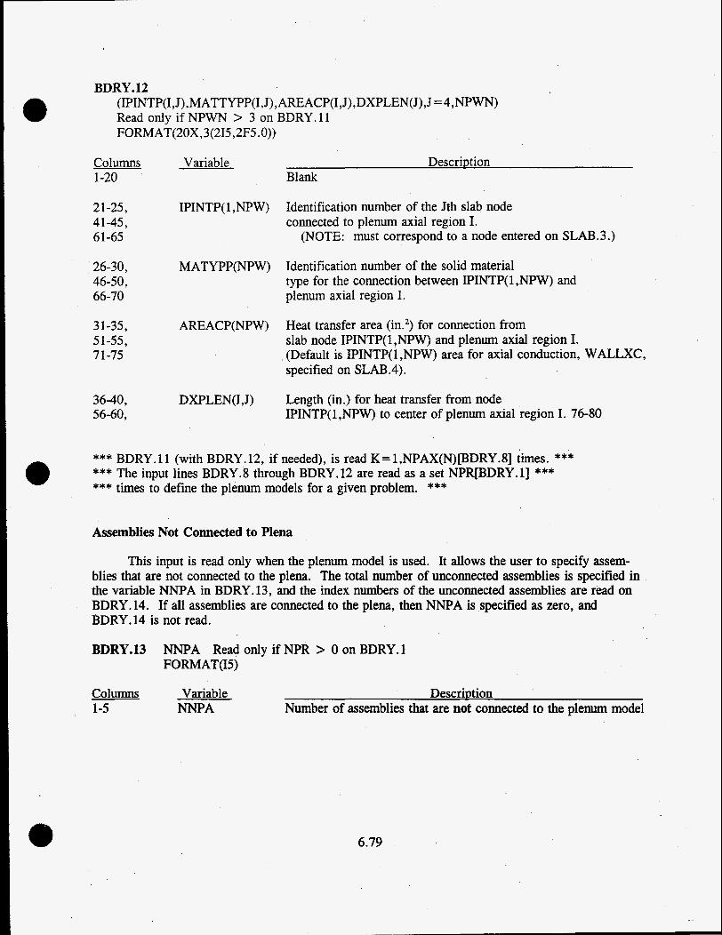
BDRY. 12 (IPINTP(I,J),MATTYPP(I,J),AREACP(I,J),DXPLEN(J),J=4,NPWN) Read only if NPWN > 3 on BDRY. 11 FORMAT(2OX,3(215,2F5 .O))
Columns 1-20
Variable Description Blank
21-25, 41-45, 6 1-65
IPINTP( 1, NPW) Identification number of the Jth slab node connected to plenum axial region I.
(NOTE: must correspond to a node entered on SLAB.3.)
26-30, 46-50, 66-70
MATYPP(NPW) Identification number of the solid material type for the connection between IPINTP(1,NPW) and plenum axial region I.
31-35, 51-55, 71-75
AREACP(NPW) Heat transfer area (in.*) for connection from slab node IPINTP(1,NPW) and plenum axial region I. (Default is IPINTP( 1 ,NPW) area for axial conduction, WALLXC, specified on SLAB.4).
36-40, 56-60.
DXPLEN(1,J) Length (in.) for heat transfer from node IPINTP(1,NPW) to center of plenum axial region I. 76-80
*** BDRY.ll (with BDRY.12, if needed), is read K=l,NPAX(N)[BDRY.8] times. *** *** The input lines BDRY.8 through BDRY. 12 are read as a set NPRpDRY.11 *** *** times to define the plenum models for a given problem. ***
Assemblies Not Connected to Plena
This input is read only when the plenum model is used. It allows the user to specify assem- blies that are not connected to the plena. The total number of unconnected assemblies is specified in the variable NNPA in BDRY. 13, and the index numbers of the unconnected assemblies are read on BDRY. 14. If all assemblies are connected to the plena, then NNPA is specified as zero, and BDRY. 14 is not read.
BDRY.13 NNPA Read only if NPR > 0 on BDRY.1 FORMAT(I5)
Columns 1-5
Variable NNPA
DescriDtion Number of assemblies that are not connected to the plenum model
6.79

BDRY.14 IUNCA(I), I=l,NNPA Read only if NNPA > 0 on BDRY.13 FORMAT( 1215)
Columns Variable Description 1-5, 6-10,
IUNCA(1) Index number of the Ith assembly that is not connected to the plenum model
11-15, 16-20,
56-60
*** BDRY.14 is read as many times as necessary to supply NNPA entries, *** *** with up to 12 entries on a record. ***
6.2.1 1 Group OPER-Operating Conditions
The input for this group defines the flow boundary conditions for the system, and the heat generation rate for the rods. When the plenum model in group BDRY is not used, group OPER is used to specify the flow boundary conditions at the inlet and outlet of the system. The user specifies the temperature and flow rate for fluid entering the system at the inlet to the channels and the channel exit pressure. This constitutes a complete set of flow boundary conditions for normal upflow condi- tions. If the flow could be negative at a channel exit, the user must also specify an enthalpy for fluid carried into the system by this reverse flow.
If the lower plenum model is specified in group BDRY, the inlet conditions are calculated as part of the overall solution, based on fluid conditions in the plenum. In such a case, the boundary conditions specified in group OPER are uses as the first guess in the iterative solution. If the upper plenum model is used, the properties of the fluid transported into the channels if flow reverses at the exit are determined from the solution of the fluid conditions in the upper plenum.
This group can also be used to define forcing functions for transient calculations. The transient capability has not been validated, however, and should be used with due caution. Axial and radial distributions of the heating rates are also specified in this group.
OPER. 1 AGROUP,IHH,IG,ITDP,NRPF,NP,NH,NG,NGPRFL,NHX,NQ,NQPRFL, NDPA,NRAMPH , NAXP FORMAT( A4,l X, 14I5)
Columns Variable DescriDtion 1 4 AGROUP Enter OPER.
6-10 IHH flag for units of enthalpy or temperature on inlet (or initial) fluid conditions:
= 0; uniform inlet (or initial) enthalpy (Btuflbm) in all channels.
6.80

11-15 IG
16-20 ITDP
= 1; uniform inlet (or initial) temperature (OF) in all channels.
= 2; define inlet enthalpy (Btu/lbm) for each channel on OPER.3.
= 3; define inlet temperature (OF) for each channel on OPER.3.
(NOTE: options 2 or 3 should not be used with the plenum model if all assemblies are connected to the lower plenum. However, IHH = 2 or 3 can be used to specify non-uniform inlet enthalpies or temperatures in the channels of any assemblies that are not connected to the lower plenum.)
Flag for option to specify inlet (or initial) flow distribution:
= 0; average inlet mass flux (Mlbdh-ft’).
= 2; average inlet mass flux (Mlbm/h-ft’), but assembly inlet flows will be determined by user-supplied flow fractions on OPER.4. Channel mass flux will be uniform within each assembly.
= 3; average inlet mass flux (Mlbm/h-ft’), but channel flows in each assembly will be determined by user-supplied flow fractions on OPER.7.
= 4; average inlet mass flux (Mlbmh-ft’), but flows will be determined by both assembly flow fractions on OPER.4 and channel flow fractions on OPER.6.
(NOTE: when the lower plenum is modeled, IG=O is the logical option for this input, unless it is necessary to specify inlet flow conditions for assemblies that are not connected to the plenum.)
Flag for flow or pressure drop boundary condition to be applied to all assemblies:
=-1; boundary condition flag set for each assembly by using ITDPA(NASS) on CHAN.6.
= 0; specified flow boundary condition.
6.81

= 1 ; uniform pressure drop (specified in DPS on OPER. 2).
2 1-25 NRPF
= 2; uniform inlet mass flux (required pressure drop calculated as part of the solution).
= 3; uniform pressure drop calculated for zero net inlet mass flow rate (FTOTAL on OPER.2. This is valid only for FTOTAL = 0.0).
= 4; zero flow at both top and bottom boundaries.
(NOTE: ITDP=4 can be used only when the plenum model is not used.)
(NOTE: If the plenum model is used, the logical choice for ITDP is 3. If any assemblies are not connected to the plenum, the individual boundary condition flag, ITDPA(NASS) rCHAN.61, should be specified as 3 for each assembly connected to the plena. In such a case, ITDP must be -1.
Flag for assembly heating rate specification:
= 0; all assemblies have the same average heat generation rate (PDN on OPER.2).
= 1; average heating rate is specified in PDN on OPER.2, and relative heat generation factors normalized to PDN are specified for each assembly on OPER.8.
= 2; heat generation rate is read for each assembly, on OPER.8 (PDN on OPER.2 is not used).
26-30 NP Number of pairs of values in table for transient forcing function on system pressure, to be read on OPER.9.
31-35 NH Number of pairs of values in transient forcing function table on inlet enthalpy or temperature, to be read on OPER.10.
(NOTE: If the lower plenum model is specified in group BDRY, this option can be used to define forcing functions only for channels in assemblies not connected to the lower plenum. Forcing functions cannot be applied to the inlet flow of channels in assemblies connected to the lower plenum.)
6.82

36-40 NG Number of pairs of values in transient forcing function table on the flow boundary, to be read on OPER. 11 and OPER. 12:
- if ITDP = 0 or 2, the forcing function is on the inlet flow rate.
- if ITDP = 1 or 3, the forcing function is on the pressure drop boundary condition.
- if ITDP = 4, this option cannot be used.
(NOTE: If the lower plenum model is specified in group BDRY, this option can be used to define forcing functions only for channels in assemblies not connected to the lower plenum. Forcing functions cannot be applied to the flow boundary condition on channels in assemblies connected to the lower plenum.)
41-45 NGPRFL Number of transient forcing functions for inlet mass flux or pressure drop profiles to be read on OPER.12. (Used only if NG > 0.)
46-50 NHX
5 1-55 NQ
Number of pairs of values in transient forcing function table on exit enthalpy or temperature, to be read on OPER.15.
(NOTE: If the upper plenum model is specified in group BDRY, this option can be used to define a forcing function only for channels in assemblies not connected to the upper plenum. A forcing function cannot be applied to the exit enthalpy boundary condition on channels in assemblies connected to the upper plenum .)
Number of entries in table@) of transient forcing function(s) on average heat generation rate. The table of time-values to be used by all forcing functions on heat generation rate is read on OPER. 13.
(NOTE: all tables of heat generation rate forcing functions must use the same set of time values.)
56-60 NQPRFL Number of heat generation rate transient forcing function tables to be read on OPER.14 (used only if NQ > 0).
6165 NDPA Flag for option to specify different pressure drop boundary conditions for each assembly when using the network model.
= 1 ; assembly pressure drops to be specified on OPER. 1 8.
6.83

66-70
71-75
NRAMPH
NAXP
= 0; uniform pressure drop or flow boundary condition.
(NOTE: The network model is specified by NETWK > 0 on DRAG. 1. If NETWK is specified as zero, the input for NDPA is not used. See the input instructions for group DRAG.)
(WARNING: The plenum model specified in group BDRY cannot be used with the network option. If the network option is used, ITDP must be specified as 1 or 2, and all assemblies must use the same boundary condition option.)
Number of iterations over which the heat generation is to be ramped into the solution (default is 1).
Number of axial heat generation profiles to be entered on OPER.16 and OPER.17 (default is zero, for uniform axial heat generation distribution for all rods).
Operating Conditions
This input defines the nominal operating conditions for the system. When the plenum model is not used, the input on OPER.2 defines the steady-state system pressure, inlet flow enthalpy or tem- perature, average heat generation rate, and flow or pressure drop boundary condition on the system. When the plenum model is used, this input defines the initial state of the system at the beginning of the steady-state iterative solution.
OPER.2 PEXIT,HIN( 1) ,GIN,PDN ,HOUT,DPS ,€TOTAL FORMAT(7FlO .O)
Columns Variable DescriDtion 1-10 PEXIT System pressure (psia). Used to calculate the boiling temperature
limit, based on the PLIQ[pROP.2] array (not used when coolant is gas>.
11-20 HIN If IHH = 0 or 2 on OPER. 1, average inlet (or initial) enthalpy (Btu/lbm) .
If IHH = 1 or 3, average inlet temperature (OF).
(NOTE: When there are 2 fluid types deked in input group PROP and IHH = 0 [or 11, it is assumed that both fluids have the same inlet enthalpy [or temperature]. If IHH > 1, the inlet enthalpy or temperature is defined for each channel individually, on input line OPER. 3 .)
6.84

21-30 GIN Average inlet mass flux (Mlbm/h-ft*).
3 1-40 PDN Average heat generation rate (MBtuh-ft3):
- When the fuel model is used (NC>4 on RODS. l), PDN is based on the volume of the fuel (defined using fuel diameter, DRODU], specified on RODS.4).
- When the fuel model is not used (NC=O or NC= 1 on RODS.l), PDN is based on volume of the rod, (defined using rod diameter, DIA[I], specified on RODS.3).
41-50 HOUT If IHH = 0 or 2 on OPER. 1, exit enthalpy (BtuAbm).
If IHH = 1 or 3, exit temperature ( O F )
(NOTE: HOUT is used to define fluid conditions for reverse flow at the exit of any channel. If the upper plenum model is used, however, HOUT is applied only to reverse exit flow in channels of assemblies that are not connected to the plenum. Default is HOUT = HIN.)
51-60 DPS Total system pressure drop (psia) (used only when ITDP = 1 or 2 on OPER. 1, or if ITDPA [NASS] = 1 or 2 on CHAN.6 for one or more assemblies.)
6 1-70 FTOTAL Total inlet flow rate (lbds) (used only when ITDP = 3 on OPER. 1).
Nonuniform Operating Parameter Distributions
This input is read only if option flags IHH or IG on OPER.l have been defined with vaIues that require detailed channel-by-channel specification of inlet flow conditions. The input on lines OPER.3 through OPER.8 is used to specify nonuniform inlet conditions for channel flow and enthalpy (or temperature), nonuniform assembly pressure drops, and to define a nonuniform radial distribution of heat generation rate.
Inlet Enthalpy/Temperature Distribution
This input is optional; it is read only if IHH is specified as 2 or 3 on OPER.1.
OPER.3 (HINLET(I),I= 1,NCHANL) Read only if IHH > 1 on OPER.1 FORMAT( 12E5.0)
Columns Variable Descriution 1-5, 6-10, channel I. 11-15, etc. channel I.
HINLET(1) If IHH = 2 on OPER. 1, inlet enthalpy (BtuAbm) for
If IHH = 3 on OPER. 1, inlet temperature (OF) for
6.85

Inlet Flow Distribution by Assembly
This input is optional; it is read only if IG is specified as 2 or 4 on OPER.l.
OPER.4 (ZDUM(I),I= 1 ,NASSEM[CHAN. 11) Read only if IG = 2 or 4 on OPER. 1 FORMAT( 12E5.0)
Colums 1-5, 6-10, 11-15, etc.
Variable ZDUM(1)
DescriDtion Inlet flow fraction for assembly I, normalized to the average mass flux, GIN on OPER.2.
Within assembly I, the inlet flow for each channel I1 is calculated as
F(I1,l) = ZDUM(I)*[GIN*( 10)6/3600.]*A(I, 1)
Inlet Flow Distribution by Channel
This input is optional; it is read only if IG is specified as 3 or 4 on OPER. 1. The total number of assemblies that have specified inlet flow distributions is specified as NASSIN on OPER.5. Then OPER.6 and OPER.7 are read in sequence NASSIN[OPER.S] times to define the specified inlet flow for the channels in the individual assemblies.
OPER.5 NASSIN Read only if IG = 3 or 4 on OPER.l FORMAT( 15)
Columns 1-5
Variable NASSIN
DescriDtion Number of assemblies for which channel inlet flow distribution is to be specified using the input on OPER.6 and OPER.7.
OPER.6 NASS Read only if NASSIN > 0 on OPER.5 FORMAT(I5)
Columns 1-5
Variable NASS
DescriDtion Identification number of an assembly with specified channel inlet flow distribution.
6.86

OPER.7 TERMl(II), II=NCHANl,NCHAN2) Read only if NASS > 0 on OPER.6 FORMAT( 12E5.0)
Columns Variable Description 1-5, 6-10, 11-15, on OPER.2. The mass flow fraction is used to etc.
TERMl(I1) Inlet mass flow fraction for channel I1 of assembly NASS[OPER.6]; this value must be normalized to GIN
define the channel inlet flow as
F(I1,l) = TERh41(II)*[GIN*106/3600.]*A(II,1)
*** OPER.6 and OPER.7 are read in sequence NASSIN[OPER.5] times. ***
Assembly Heat Generation Distribution
This input is optional; it is read only if NRPF is specified as greater than zero on OPER.l.
OPER.8 (PDNA(N),N= l,NASSEM[CHAN.l]) Read only if NRPF > 0 on OPER. 1 FORMAT( 12E5 .O)
Columns Variable Descriution 1-5, PDNA(N) Heating rate for assembly N: 6-10, 11-15, on OPER.2. etc .
if NRPF = 1, PDNA(N) is normalized to PDN
if NRPF = 2, PDNA(N) is assembly heating rate in units of M13tu/h-ft3 (PDN on OPER.2 is not used).
Transient Forcing Function Tables
The input on lines OPER.9 through OPER.15 can be used to specify forcing functions on the system pressure, inlet enthalpy or temperature, inlet flow rate or pressure drop, and the heat genera- tion rate. However, the transient capability has not been validated in the Cycle 2 release of the code, and should be used with caution. Forcing functions on the inlet flow conditions are ignored for assemblies connected to a lower plenum model. They are also ineffective when using the zero-flow boundary condition option, specified with ITDP = 4 on OPER. 1.
System Pressure Transient Forcing Function
This input is optional; it is read only if NP is specified as greater than zero on OPER. 1,
6.87

OPER.9 (YP(I],FP(I),I=l,NP) Read only if NP > 0 on OPER.l FORMAT( 12E5.0)
Columns 1-5, 11-15, etc.
6-10, 16-20, etc.
Variable W I )
Description Transient time (sec) for the Ith element of system pressure forcing function table.
(NOTE: This array must be entered as monotonically increasing from time zero.)
Fraction of steady-state system pressure at time YP(I), normalized to PEXIT on OPER.2.
Inlet Enthalpy or Temperature Transient Forcing Function
This input is optional; it is read only if NH is specified as greater than zero on OPER. 1.
OPER.10 (YH(I),FH(I),I= 1,NH) Read only if NH > 0 on OPER. 1 FORMAT( 12E5 .O)
Columns 1-5, 11-15, etc.
6-10, 16-20, etc .
DescriDtion Transient time (sec) for the Ith element of enthalpy (or temperature) forcing function table.
(NOTE: This array must be entered as monotonically increasing from time zero.)
If MH = 0 or 2, the fraction of inlet enthalpy at time YH(I), normalized to HIN entered on OPER.2. If IHH = 1 or 3, the fraction of inlet temperature at time YH(I), normalized to HIN entered on OPER.2.
Inlet Flow or Pressure Drop Transient Forcing Functions
This input is optional. OPER.11 and OPER.12 are read only if NG is specified as greater than zero on OPER. 1. OPER. 11 is read only once to define the time array to be used with all NGPRFL[OPER. 11 forcing functions. OPER. 12 is read NGPRFL[OPER. 11 times to define each of the inlet flow or pressure drop forcing functions. The tables are numbered sequentially in the code, in the order in which they are read in on OPER.12. These sequence numbers are assigned to specific assemblies by the values entered for NPFWT(NASS) on CHAN.6.
6.88

OPER.ll (YG(J),J = 1 ,NG) Read only if NG > 0 on OPER. 1 FORMAT( 12E5 .O)
Columns 1-5, 6-10, etc.
Variable YG(J)
Descriution Transient time (sec) for the Jth element of inlet flow or pressure drop forcing function tables.
(NOTE: must be entered as monotonically increasing from time zero.)
OPER.12 ((FG(J,L),J= l,NG),L= 1,NGPRFL) Read only if NG > 0 and NGPRFL > 0 on 0PER.I FORMAT( 12E5 .O)
Columns 1-5, 6-10, 11-15, etc .
Descriution If ITDP = 0 or 2 on OPER. 1 , the inlet flow fraction at time YG(J) for the Lth table, normalized to GIN entered on OPER.2.
(NOTE: If ITDP = -1, the inlet flow forcing function[s] can be applied only to assemblies with ITDPAPASS] defined as 0 or 2 on CHAN.6.)
If ITDP = 1 on OPER.l, the pressure drop multiplier at time YG(J) for the Lth table, normalized to DPS entered on OPER.2.
'(NOTE: If ITDP = -1, the pressure drop forcing function[s] can be applied only to channels in assemblies with ITDPAflASS] defined as 1 on CHAN.6.)
*** OPER.12 is read NGPRFL[OPER.l] times. ***
Heat Generation Rate Transient Forcing Functions
This input is optional. OPER. 13 and OPER. 14 are read only if NQ is specified as greater than zero on OPER. 1. OPER. 13 is read only once to define the time array to be used with all NQPRFL[OPER. 11 forcing functions. OPER. 14 is read NQPRFL[OPER. 1 J times to define the heat generation rate forcing functions. The tables are numbered sequentially in the code, in the order in which they are read in on OPER.14. These sequence numbers are assigned to specific assemblies by the values entered in NHFVT(NASS) on CHAN.6.
OPER.13 (YQ(J),J=l,NQ) Read only if NQ > 0 on OPER.l FORMAT( 12E5.0)
Columns 1-5, 6-10, etc.
Variable YQ(J)
Descrimion Transient time (sec) for the Jth element of heat generation rate forcing function tables. (NOTE: must be entered as monotonically increasing from time zero.)
6.89

OPER. 14 ((FQ(J ,L) , J = 1 ,NQ), L = 1 ,NQPRFL) Read only if NQ > 0 and NQPRFL > 0 on OPER.l FORMAT( 12E5.0)
Columns Variable Descrimion 1-5, FQ(J,L) The heat generation rate multiplier, normalized 6-10, etc. Lth table.
to PDN on OPERl2, at transient time YQ(J), for the
*** OPER.14 is read NQPRFL[OPER.l] times. ***
Exit Enthalpy Transient Forcing Function
This input is optional; it is read only if NHX is specified as greater than zero on OPER. 1.
OPER.15 (YHX(I),FHX(I),I= 1,NHX) Read only if NHX > 0 on OPER.l FORMAT( 12E5.0)
Columns Variable DescriDtion 1-5, YHX(1) 11-15, etc. (NOTE: must be entered as monotonically increasing from
Transient time (sec) for the Ith element of exit flow conditions forcing function table.
time zero.)
6-10, FHX(1) 16-20, etc.
If IHH = 0 or 2, the fraction of exit enthalpy entered in HOUT on OPER.2. If IHH = 1 or 3, the fraction of exit temperature entered in HOUT on OPER.2.
Axial Heat Generation Profiles
Unless specified otherwise, the axial heat generation profile is assumed to be a uniform distri- bution along the total axial length Z, specified in group CHAN on CHAN.3. This default option is obtained simply by entering NAXP as zero on OPER. 1. In most applications, however, the axial heat generation rate will not be axially uniform. Nonuniform axial heat generation profiles can be speci- fied as tables of relative axial power factors versus axial distance. This option is specified by setting NAXP on OPER. 1 to the number of axial heat generation rate profiles needed for the problem. Tables describing the axial heat generation rate distributions are then entered using the input on OPER.16 and OPER.17.
The axial heat generation rate profiles are numbered sequentially from 1 to NAXP, in the order they are entered on OPER.16 and OPER.17. If the option for the default uniform profile is used, this profile is automatically numbered heat generation profile 1. The particular profile to be used in an assembly is specified by input on CHAN.5, by the value specified for NAFLX(NASS).
6.90

OPER.16 NAX(1) Read only if NAXP > 0 on OPER.l FORMAT(I5)
Columns 1-5
Variable NAX(1)
Description Number of pairs of entries in the Ith axial heat generation rate profile table.
OPER.17 (Y(L,I),AXIAL(L,I),L= l,NAX(I)) Read only if NAXP > 0 on OPER.l FORMAT( 12F5.0)
Columns 1-5, 11-15, 21-25, etc.
6-10, 16-20, 26-30, etc.
AXIAL(L,I)
Description Relative location (X/L) of the Lth element of axial heat generation rate profile I.
(NOTE: Must be entered monotonically increasing from 0.0 to 1 .O.)
Relative heat generation rate at Y(I,L), normalized to average heat generation rate, in PDN on OPER.2.
*** OPER.16 and OPER.17 are read in sequence NAXP[OPER.l] times. ***
Non-Uniform Pressure Drop Boundary Condition
This input it optional, It is read only if NDPA is greater than zero on OPER.l. It is used to specify a separate pressure drop boundary condition for each assembly. This option can be used only with ITDP = 1 on OPER.l, or if some assemblies have ITDPA(NASS) = 1 specified on CHAN.5. When this option is used, the pressure drop entered in DPA on OPER.2 is ignored.
OPER.18 (DPA(I),I= 1,NASSEMrCHAN. 11) Read only if NDPA > 0 on OPER. 1 FORMAT( 12E5.0)
Columns 1-5, 6-10, etc.
Variable DPA(1)
DescriDtion Pressure drop @si) for assembly I.
used with the network model, flagged by NETWK > 0 on DRAG. 1 .)
(NOTE: Supersedes DPS on OPER.2. This option cannot be
6.2.12 Group CALC--Calculational Parameters
This group defines the calculational parameters needed to specify the manner in which the problem will be solved. The input specifies the various convergence limits, damping factors, acceleration factors, and iteration limits required for the steady state solution. The simulation time and time step size for transients is also defined by this input.
6.91

CALC.l AGROUP,ISCHEME,ITSTEP,NODUMP FORMAT(A4,lX ,15,5X,215)
Columns Variable DescriDtion 1-4 AGROUP Enter CALC.
6-10 ISCHEME Lateral momentum solution flag:
= 0; lateral momentum equation solved'for crossflows (default).
11-15
16-20 ITSTEP
21-25
= 1; lateral flows set to zero (no solution of lateral momentum equation).
Blank
Number of entries in variable time step table. (NOTE: this input is used only for transient calculations. Default is zero, for uniform time step size throughout the transient .)
NODUMP Flag for option to write a binary restart file on logical unit 8:
= 0; create a restart file (default).
= 1; do not create a restart file.
Solution Damping and Acceleration Factors
.Damping and acceleration factors used in the solution are entered on CALC.2. All factors are applied as
x = n + (1 -c l )xn- l
where X = calculational variable a n = current iteration number.
= damping or acceleration factor
Convergence limits are defined in nondirnensional form so that the relative magnitude of the affected variable does not affect the rate of convergence.
6.92

CALC.2
Columns 1-5
6-10
11-15
16-20
21-25
26-30
31-35
36-40
4 1-45
46-50
51-55
56-60
61-65
TTIME, WERRY ,FERROR,HERROR,QERROR,DAMPNG,ACCELY ,ACCELF, ACCRHO,ACCELW,ACCROD,ACCAX,SLDAMP FORMAT( 13E5 .O)
Variable -
TTIME
WERRY
FERROR
HERROR
QERROR
DAMPNG
ACCELY
ACCELF
ACCRHO
ACCELW
ACCROD
ACCAX
SLDAMP
Descriution Total transient time (sec) (default is a steady state calculation, with TTIME = 0.0).
Inner loop convergence criterion for the recirculation solution scheme (default is 0.001).
External axial flow convergence criterion, defined for the implicit axial momentum equation as the maximum allowable error for iterative axial flows. If the error is greater than FERROR, another iterative sweep of the entire bundle is made (default is 0.01).
Convergence criterion for fluid enthalpy (default is 0.001).
Convergence criterion for total energy balance (default is 0.001).
No longer used; leave blank.
Acceleration factor for the iterative Gauss-Seidel solution of the momentum equations (default is 1.0).
Damping factor for iterative axial flow (default is 0.7).
Damping factor for change in fluid density (default is 1 .O).
Acceleration factor for the solid structure energy equation solution (default is 1.2).
Damping factor for the rod energy solution (default is 0.5).
Damping factor for axial energy rebalancing (default is 0.0, no axial energy rebalancing).
Damping factor in the energy solution for slab conduction (default is 0.0).
6.93

Time Step and Iteration Control
This input specifies the number of time steps for a transient, and the time step size, if the variable time step option is used. For steady state calculations, the number of time steps must be specified as zero. The number of iterations for the steady state solution is specified with NTRIES on CALC.3. This value is used for all time steps in a transient, as well.
CALC.3 NDT,NTRIES FORMAT(215)
Columns Variable DescriDtion 1-5 NDT Total number of time steps.
(NOTE: enter zero for steady-state calculations.)
6-10 NTRIES Maximum number of external iterations allowed for any time step, including the steady state at time zero(defau1t is 20).
The default in the code is a uniform time step size for the transient, calculated from NDT on CALC.3 and TTIME on CALC.2 as DT = TTIME/NDT. Nonuniform time step sizes are specified by setting ITSTEP > 0 on CALC. 1, and entering a table of time step size versus time on CALC.4.
CALC.4
Columns 1-5, 11-15, 21-25, etc .
6-10, 16-20, 26-30, etc .
(YT(I),FT(I),I=l,ITSTEP) Read only if ITSTEP > 0 on CALC.l. FORMAT( 12E5 .O)
Variable Descriution Transient time (s) when the first time step that is FT(1) seconds long begins.
W I ) Time step size (sec) from time YT(1).
When this option is used, the time step size for any give time step is calculated by linear interpolation in the table entered on CALC.4.
6.94

Damping For Heat Transfer Solution of Slab Nodes
This input is optional, and is read only when SLDAMP is greater than zero on €ALC.2. It allows the user to specify a damping factor on the heat transfer solution of specific slab nodes in a problem. This is a particularly useful capability for cases where certain nodes are not well-coupled with the fluid energy solution.
CALC.5 NSLGRP Read only if SLDAMP > 0.0 on CALC.2. FORMAT(I5)
Columns 1-5,
Variable NSLGRP
Descrbtion Number of groups of slabs for which the conduction solution will be damped.
(NOTE: for this input, a group is defined as a set of slabs with sequential identification numbers .)
CALC.6 (BSLGRP(I),ESLGW(I),I= 1,NSPGRP) Read only if NSLGW > 0 on CALC.5. FORMAT( 1215)
Columns 1-5, 11-15, 21-25, etc.
6-10, 16-20, 26-30, etc.
Variable BSLGRP(1)
ESLGRP(1)
DesscriDtion The index number of the first slab in the Ith group of slabs with the conduction solution damped.
The index number of the last slab in the Ith group of slabs with the conduction solution damped.
6.2.13 Group OUTP--Output Options
This group allows the user to select the information to be written to the output file. The default is to print everything (Le., all channels, rods, lateral flow connections, and solid structure nodes at every axial level for the steady state solution and for every time step in a transient). For large problems, or long-running transients, this can result in enormous output files. The user might want to limit the output, either by restricting the number of channels, rods, lateral flow connections, or solid structure nodes for which output will be produced, or by limiting the frequency of output generated during a transient. This input allows considerable flexibility in specifying the output, so that the user can print only what is actually needed in the way of calculational results.
6.95

OUTP. 1 AGROUP,NCOUT, NROUT ,NGOUT , NWOUT,NALL,NSKIPX,NSKIPT, NPCHAN, NPROD ,NPNODE ,NPGAP, NPAVG,NPWALL,IPREB ,IOTEMP FORMAT(A4,1X,511,1015)
Columns 1-4
6
7
8
9
10
11-15
16-20
Variable AGROUP
NCOUT
NROUT
NGOUT
NWOUT
NALL
NSKIPX
NSKIPT
DescriDtion Enter OUTP.
Flag for channel output:
= 0; no channel printout.
= 1 ; channel printout controlled by NPCHAN
Flag for rod output:
= 0; no rod printout.
= 1; rod printout controlled by NPROD.
Flag for lateral flow connection output:
= 0; no lateral flow connection printout.
= 1 ; lateral flow connection printout controlled by NPGAP.
Flag for solid node output:
= 0; no solid node printout.
= 1; solid node printout controlled by NPWALL.
Flag for output of all information:
= 0; output is governed by NCOUT, etc. flags.
= 1; everybng is printed, regardless of values assigned to other flags.
Number of axial nodes to skip when printing results (default is 1, which results in every axial node being printed).
Number of time steps to skip between printed results (default is 1, which results in every time step being printed).
6.96

2 1-25
26-30
3 1-35
36-40
41-45
NPCHAN
NPROD
NPNODE
NPGAP
NPAVG
Flag for number of channels to be printed if NCOUT = 1:
= 0; print all channels (default).
> 0; print NPCHAN channels (see OUTP.2).
Flag for number of rods to be printed if NROUT = 1:
= 0; print all rods (default).
> 0; print NPROD rods (see OUTP.3).
Flag for fuel temperature node printout, if NROUT = 1:
= 0; print only fuel centerline temperature, fuel surface temperature, and cladding surface temperature (default).
> 0; print cladding surface temperature and all internal node1 temperatures (used only with the conduction model; NC > 4 on RODS. 1).
Flag for number of lateral flow connections to be printed if NGOUT = 1:
= 0; print all lateral flow connections (default).
> 0; print NPGAP lateral flow connections (see OUTP.4.)
Flag for assembly average and channel exit values to be printed:
= 0; no additional output (default).
= 1; channel exit values only.
= 2; assembly-average values only.
= 3; channel exit and assembly-average values.
6.97

46-50 NPWALL Flag for solid node printout if NWOUT = 1:
= 0; print all solid nodes (default).
> 0; print NPWALL solid nodes (see OUTP.5).
5 1-55 IPREB Flag for solution description output;
= 0; normal iteration summary only (default).
> 0; axial rebalancing summary and detailed iteration summary.
56-60 IOTEMP Flag for output units on temperature:
= 0; output in Fahrenheit
= 1; output in Celsius.
User-Defmed Output Options
The following input lines, OUTP.2 through OUTP.5, are optional. They are needed only if the corresponding options to limit the output to user-defined items have been specified by setting NPCHAN, NPROD, NPGAP, NPWALL or NSKIPT to non-zero values on OUTP. 1. The default in the code is to print all information about all modeled structures.
Channels to be Printed
This input is optional; it is read only if NCOUT is 1 and NPCHAN is greater than zero on OUTP. 1. A total of NPCHAN pairs of assembly index number and channel index number must be specified on OUTP.2.
OUTP.2 (PRINTA(I),PRINTC(I),I = 1 ,NPCHAN) Read only if NCOUT = 1 and NPCHAN > 0 on OUTP.l FORMAT( 1615)
Columns Variable DescriDtion 1-5, PRINTA(1) Identification number of assembly containing 11-15, channel PFUNTC(1). etc,
6-10, PRINTC(1) Index number of the Ith channel in assembly 16-20, PRINTA(I) for which output will be printed. etc.
6.98

JT is 1 an( NP
Rods to be Printed
This input is optional; it is read only if NR OD is greater than zero on OUTP. 1. A total of NPROD pairs of assembly index number and rod index number must be specified on OUTP.3.
OUTP.3 (PRINTA(I),PRINTR(I), 1 = 1 ,NPROD) Read only if NROUT = 1 and NPROD > 0 on OUTP.l FORMAT( 1615)
Columns Variable Description 1-5, PRINTA(1) Index number of assembly containing rod PRINTR(1).
etc. 11-15,
6-10, 16-20, etc.
PRINTR(1) Index number of the Ith rod in assembly PRINTA(1) for which output will be printed.
Lateral Flow Connections to be Printed
This input is optional; it is read only if NGOUT is 1 and NPGAP is greater than zero on OUTP. 1. A total of NPGAP pairs of assembly index number and gap index number must be specified on OUTP.4.
OUTP.4 (PRINTA(I),PRINTG(I),I= 1 ,NPGAP) Read only if NGOUT = 1 and NPGAP > 0 on OUTP.1 FORMAT( 1615)
Columns Variable DescriDtion 1-5, PRINTAU) Index number of assembly containing lateral flow 11-15, connection PFUNTG(1). etc.
6-10, PRINTG(I) Index number of the Ith lateral flow connection 16-20, etc. printed.
in assembly PRINTA(I) for which output will be
Solid Nodes to be Printed
This input is optional; it is read only if NWOUT is 1 and NPWALL is greater than zero on OUTP. 1. A total of NPWALL slab node index numbers must be specified on OUTP.5.
6.99

OUTP.5 (PRINTW(I),I = 1 ,NPWALL) Read only if NWOUT = 1 and NPWALL > 0 on OUTP.l FORMAT( 1215)
Columns Variable 1-5, PRINTW(1) 6-10, 11-15, etc.
Description Index number of Ith slab node for which temperatures are to be printed.
Transient Output Interval
This input is optional; it is read only if NSKIPT is greater than zero on OUTP. 1. To define the output interval using only NSKIPT, enter zero for TRANT. Otherwise, output will be produced every NSKIPT time steps, or every TRANT seconds, whichever comes first.
OUTP.6 TRANT Read only if NSKIPT > 1 on OUTP.l FORMAT(F5.3)
Columns 1-5
Variable TRANT
Description Time interval (sec) between successive output time steps in a transient calculation (default is 0.0, which means that the output interval will be controlled by the value of NSIUPT alone).
6.2.14 Termination of Input File
Once all groups have been entered, the end of the input stream is indicated by entering an end- flag for the group input name.
SETIN. 1 :
Columns 1-4
AGROUP FORMAT( A4)
Variable AGROUP
DescriDtion Enter ENDD, to signal end of input stream for this case.
6.3 View Factor Input Generation: RADGEN Code
The RADGEN code is an auxiliary code which can be used to generate the grey body view factors for radiative heat transfer within an enclosure modeled as an assembly in COBRA-SFS. RADGEN is documented in detail elsewhere (Rector 1987). It is not the purpose of this section to give a complete description of this auxiliary code. However, it is virtually impossible to run any significant fuel storage analysis problem with COBRA-SFS without using view factors of the sort generated with the RADGEN code. The user must therefore be able to use the RADGEN code to obtain view factors that are appropriate for the problem being modeled in COBRA-SFS. This section
6.100

6.101
presents a general description of the RADGEN code in Section 6.3.1, including a description of the rod arrangements and enclosure geometries for which the code can determine the grey body view factors. Section 6.3.2 gives the input instructions for the RADGEN code for both interactive and batch mode execution. Examples are also presented for three common rod geometries.
6.3.1 Description of RADGEN Code
The RADGEN code calculates grey body view factors to be used in the calculation of radiative heat transfer between solid surfaces, as defined by Eq. (3.5) in Section 3.2.4. The method used in RADGEN is an extension of Cox’s cross-string correlation approach for square and triangular pitch rod arrays (Cox 1977). It can also be used to define the view factors for an arbitrary enclosure made up of user-defined surfaces, and containing no internal structures to block or reflect radiation exchange among the surfaces.
The black body view factor expressions for a given surface A,, to another surface 4, are determined using Hottel’s cross-string method for two-dimensional geometries. In this approach, a “view” from surface n to surface m is approximated by the concept of anchoring two strings at each end of surface n and tying one to the nearer end of surface m and the other to the farther end of surface m. This is illustrated in Figure 6.6. The endpoints of surface n are labeled a and b, and the endpoints of surface m are labeled c and d, so the strings from a to c and from b to d are the “crossed” strings. and the strings from a to d and from b to c are the ’uncrossed’ strings. Note that the strings wrap around any other surfaces lying along the ’line of sight’ between the endpoints of surface n and m. This wrapping is taken into account in computing the length of a given string.
In Hottel’s method, the black body view factor between surface n and surface m is calculated as a function of the difference between the sums of the lengths of the crossed and uncrossed strings. The view factor from surface n to m is given by the following relation:
The S terms refer to the lengths of the strings between the endpoints designated by the subscript pair, and L, is the length of surface n. Note that the strings wrap around obstructions in the path from one surface endpoint to another.
In the RADGEN code, an enclosure for radiative heat transfer is treated as a set of discrete surfaces, each of which acts independently in emitting, absorbing, and reflecting radiant energy. The basic assumptions for this radiative heat transfer model are as follows:
1. Each rod and wall surface is isothermal. 2. Surfaces are grey, with uniform emissivity for all rods. 3. Reflected radiation is diffusely distributed. 4. Emitted radiation is diffusely distributed. 5 . Radiosity is uniform over each surface segment. 6. Energy not transferred to rod surfaces must go to a wall surface. 7. Wall surfaces correspond to slab nodes in the COBRA-SFS model.

d
S9503052.16
Figure 6.6. Hottel’s Crossed String Correlation for Black Body View Factors
In an enclosure containing rods on a square pitch, the rods are divided into quarter segments, so that each rod consists of four surfaces. The enclosure is assumed to be rectangular, and the walls must be modeled with two surfaces each, for a total of eight wall surfaces. In an enclosure contain- ing rods on a triangular pitch, the rods are divided into one-sixth segments. The walls of the enclo- sure are modeled with a single surface each, for a total of four wall surfaces for a rectangular enclo- sure, or a total of six for a hexagonal enclosure. The RADGEN code calculates the black body view factors for each rod surface that sees other rods, for each rod surface that sees other rods and the walls, and the walls that see rod surfaces or other wall surfaces.
An example of adjacent quarter-segment surfaces for radiative heat transfer between two rods in a square array is shown in Figure 6-7. For these two surfaces, the view factor expression using Hottel’s method is
2(bc + ce) - (bf + de) 2bd F,, =
The string lengths can be expressed in terms of the geometry of the rod array, using the rod radius R, and the ratio of the array pitch to the rod diameter, Dd (where the array pitch is the distance between the centers of adjacent rods, p). For this example, the uncrossed strings are the lengths ed and fb; the crossed strings are the lengths fd and eb. Note that the crossed string lengths
6.102

S9509026.1
Figure 6.7. Example of Cross-String Method for Calculating View Factors Between Rod Quarter- Segment Surfaces in the RADGEN Code
wrap some portion of one surface. The length of the wrapped portion of the string is determined by the pitch of the array and the rod diameter. The relevant lengths can be expressed in terms of the array geometry, as follows:
ab = ac = ad = R
P b f = 2 R - Dmd
de = 2 ( R x -R) Dmd
6.103

, = 4(2R&-R) i - R 2
The length of the portion of string eb that is wrapped around surface 2 (Le., the segment cb) can be calculated from plane geometry. First, the angle w must be determined, as
x ce o = - - arctan- 2 ac
Substituting the length definitions given above yields,
The length of the arc bc, therefore, is
The expression for the view factor from surface 1 to surface 2, therefore, can be expressed as
Similar calculations are made in RADGEN for all surfaces seen by a given surface. For rods on a square pitch, a given rod quarter-segment can see up to 15 other rod quarter-segment surfaces, as illustrated in Figure 6.8. For rods on a triangular pitch, a given rod sixth-segment can see up to 17 other rod sixth-segment surfaces, as illustrated in Figure 6.9. The black body view factors are calculated for each of these connections, taking into account rod shadowing due to pitch and diameter.
View factors between the wall surfaces are calculated by arbitrarily dividing the walls into segments of uniform length based on the rod pitch. For rods on a square pitch, a wall segment can potentially see eleven quarter-segment rod surfaces, as shown in Figure 6.10. For rods on a
6.104

n
Figure 6.8. Quarter-Section Surfaces on Adjacent Rods With Black Body View Factors to Surface S in a Square Array Rod Bundle
-18
Figure 6.9. One-Sixth Section Surfaces on Adjacent Rods With Black Body VIGW I a.u.s to Surface S in a Triangular Array Rod Bundle
6.105

l- X I
s9503052.19
Figure 6.10. Black Body View Factors From Wall Surface S to Quarter-Section Surfaces on Rods in a Square Array
6.106

~
l triangular pitch.
triangular pitch, a wall segment can see up to eight sixth-segment rod surfaces, as shown in Figure 6.11. This applies to both rectangular canisters and hexagonal canisters for rods on a
Some adjustments must be made for the corner effects, and view factors between wall segments have to be calculated, as well. The grey body exchange factors for these surfaces are determined by solving Eq. (3.6), as shown in Section 2.4.2. This forms a set of N2 equations, where N is the total number of surfaces in the enclosure, which is solved numerically in RADGEN using successive over- relaxation. The grey body view factors for each rod and wall (four for each rod and two for each wall in the square array case, and six for each rod and one for each wall in the triangular array case) are summed to obtain the view factor input expected by COBRA-SFS for a rod assembly.
The arrays of view factors are written to an output file named TAPElO by the RADGEN code, and this file can be used for input to the COBRA-SFS model of the assembly. If the COBRA-SFS model consists of a lumped rod and channel model of the assembly, rather than a detailed model in which every rod and subchannel is represented explicitly, RADGEN can be used to combine the rod view factors to match the lumping used in the COBRA-SFS input. In that case, the TAPElO output
S
59503052.20
Figure 6.11. Black Body View Factors From Wall Surface S to One-Sixth Section Surfaces on Rods in a Triangular Array
6.107

containing the view factors for the complete assembly is not used as input to COBRA-SFS. It is instead renamed TAPE11 and used as input to RADGEN for a new calculation to generate the lumped TAPEIO.
When this option is used in RADGEN, the greybody view factors are not calculated again, but are read from the previously created TAPE10, renamed TAPE1 1. The user supplies a description of the rod lumping appropriate to the problem, and RADGEN combines the view factors to make a new TAPE10 output file. This second TAPE10 is used as input to COBRA-SFS for the radiation modeling. The lumping calculation can be done in the same step as the TAPE10 generation for the full assembly. In that case, the view factors for the lumped geometry are added to the TAPE10 file, as a second group of view factors after the view factors for the full assembly. This means that the full assembly view factors will be identified in TAPE10 as radiation group 1, and the lumped geometry view factors will be group 2.
6.3.2 RADGEN Input Instructions
The RADGEN code is designed to accept input in interactive mode. However, it also has the option to read input from an external file. This option can be used in the interactive mode, but the code can also be run in batch mode. The decision as to which mode to use must be made when the code is compiled, by setting the variable flag “ibatch” at the top of program RADGEN. If ibatch=O, input will be interpreted in interactive mode. If ibatch= 1 , all input will be read from logical unit 9, a file named input. The input required by the RADGEN code is essentially the same in both cases, but is organized slightly differently. Therefore, the input instructions for the two options are presented separately below. In the interactive mode, the input is entered format-free, with entries separated by commas if more than one variable is called for on a given line. In the batch mode, however, the input file must be in the format given in the input instructions.
The major portion of the input to RADGEN is concerned with describing the geometry of the surfaces for which the view factors are to be calculated. For rod arrays, the code needs to know the number of rod rows and columns. In a square array rod bundle, the numbers of rows and columns are usually the same (Le., a 15 x 15 bundle has 15 rows and 15 columns). In a triangular array within a square canister, the matter is slightly less straightforward. Depending on the angle one chooses to view the array, one might define different numbers of rows and columns, and in any case, not all rows (or columns) are of the same length. The convention used in RADGEN for the orientation of the triangular array within a square canister is as illustrated in Figure 6.12.
In this example, there are 22 rod rows in the array. The number of columns in a triangular array within a square canister is defined as the number of rods in the longer rows; in this case, 19 rods.
For a triangular array of rods in a hexagonal canister, there is no meaningful distinction between rows and columns. Because of the regularity of the triangular array within a hexagonal bundle, defining the number of rod rows automatically defines the number of columns, so the input requires only that the user define the number of rows.
In the RADGEN code it is assumed that the rods in the array have been numbered according to the pattern illustrated in Figure 6.12. Starting in the upper left-hand comer of the top row, the rods
6.108

Figure 6.12. Triangular Array of Rods within a Square Canister
are numbered from left to right, row by row. The wall nodes are assigned numbers starting with nrod+ 1, where nrod is the number of rods. For a square canister containing a square array of rods, the walls are assumed to have two nodes per face, as shown in Figure 6.13(a). For a square canister containing a triangular array of rods, the walls are assumed to have only one node per face, as shown in Figure 6.13@). For a triangular array of rods in a hexagonal canister, the walls are assumed to consist of one node per face, as illustrated in Figure 6.13(c).
It is important for the user to observe this numbering convention in defining the rod geometry with the COBRA-SFS input in group RODS, so that the view factors generated with RADGEN will apply to the correct rods within the array. The COBRA-SFS code checks the view factors for each rod array to determine that the factors sum to unity within an assembly. Error messages from COBRA-SFS relating to improper view. factors will in most cases be due to inconsistencies in the numbering convention between the input for RADGEN and that for COBRA-SFS.
In many applications, the COBRA-SFS model includes rod arrays that are not complete bundles, either because a bundle is a section of symmetry, or because the rod geometry has been lumped into a number of average rods in order to reduce the number of nodes required for a given model. For such cases, RADGEN can be used to generate view factors for the section of symmetry or the lumped assembly model, but the first step in all cases is the calculation of view factors for the full array. The user must take care to adhere to the rod numbering convention illustrated above in the process of generating view factors for lumped assemblies or sections of symmetry, or the resultant
6.109

Figure 6.13. Examples of Rod Numbering Convention Assumed in RADGEN
view factors will not conform to the model geometry, and probably will not conserve energy in radiative heat transfer. Illustrative examples are presented below for the two cases of modeling a section of symmetry and modeling an array with lumped rods. The procedure is not complicated, but it can be confusing if not followed through step by step.
6.110

' 6 , The rod-and-subchannel model of a half-section of the 15 x 15 rod array illustrated in Fig-
ure 6.4 is used here to illustrate the procedure for obtaining view factors for a section of symmetry. The first step in obtaining the view factors for this model is to run RADGEN to generate a tape10 with the view factors for the full bundle, assuming the rod numbering for the full array shown in Figure 6.14. This tape10 is then renamed tape1 1 and is used as an input file to a second RADGEN run for the purpose of summing the view factors for the lumped array. For the case of half symmetry on the diagonal, RADGEN has the capability of automatically calculating the correspondences between the original full bundle rods and the rods in the section of symmetry. The code can also automatically calculate the lumping for an eighth section of symmetry for a square array of rods in a rectangular canister, and a sixth section of symmetry for a triangular array in a hexagonal canister.
For the half bundle illustrated in Figure 6.4, rod No. 1 in the COBRA-SFS model corresponds to rod No. 1 of the full bundle; rod No. 2 corresponds to rod No. 16 of the full bundle; rod No. 3
Slab No. 1 Slab No.2
Slal No.
Slat No.
Control Rod Simulator (D = 0.50 in.)
@ Unheated Rod
Slab vo. 3
Slab uo. 4
Figure 6.14. Example of Rod Numbering Convention Assumed in RADGEN for Full Rod Array
6.111

corresponds to rod No. 17 of the full bundle; rod No. 4 corresponds to rod No. 31 of the full bundle, and so on. The numbering of the rods in the COBRA-SFS model must bear this relationship to the full bundle in order for the automatic view factor lumping feature to work properly in RADGEN. A similar pattern must be adhered to for the eighth section and sixth section of symmetry.
The lumped rod model for the full bundle illustrated in Figure 6.5 is used here as an example of how view factors are combined for lumped rod geometries. As with the above illustration for a section of symmetry, the first step is to obtain a set of view factors for the full bundle. The tape10 generated using RADGEN is then renamed tapell, and is used as an input file to a second RADGEN run. In this case, however, the code cannot automatically determine the proper view factor summa- tions, since the lumping is purely at the user’s discretion. The user must specify by input to RADGEN exactly which rods of the original array correspond to the lumped rods in the COBRA-SFS model.
This is done by defining each lumped rod as a “group,” and specifying by rod number the rods in the original array that make up that “group.” For the lumped rod model in Figure 6.5, there are a total of 105 groups, which corresponds to the number of lumped rods in the model. Note that even the rods that are not lumped with other rods in this model are also each counted as a separate “group” of lumped rods. Each of these “lumped” rods consists of only one rod, but it is still necessary to identify which rod it corresponds to in the numbering scheme assumed for the original full bundle array. In general, the rod number in the original array will not correspond to the rod number in the COBRA-SFS model.
In this example, rod No. 1 in the COBRA-SFS lumped model corresponds to group 1, and consists of rods 2, 3, 4, 5, 6, and 7 in the full bundle. RADGEN will combine the view factors for these six rods to make the view factors for rod No. 1 in the lumped model. Similarly, rod No. 49 in the COBRA-SFS lumped model corresponds to group 49, and consists of rod 1 in the full bundle. The following is a partial listing of the grouping input required by RADGEN for this case.
Total number of groups: 422: 105
input for group 1 (Le., rod 1 in the COBRA-SFS lumped model): 423: 6 424: 2,3,4,5,6,7 425: 0
input for group 2 (Le., rod 2 in the COBRA-SFS lumped model): 423: 6 424: 9,10,11,12,13,14 425: 0
input for group 3 (i.e., rod 3 in the COBRA-SFS lumped model): 423: 6 424: 30,45,60,75,90,105 425: 0
6.112

input for group 4 (Le., rod 4 in the COBRA-SFS lumped model): 423: 6 424: 135,150,165,180,195,210 Q25: 0
input for group 5 @e., rod 5 in the COBRA-SFS lumped model): Q23: 6 424: 219,220,221,222,223,224 425: 0
input for group 6 (i.e., rod 6 in the COBRA-SFS lumped model): 423: 6 424 : 2 12,2 1 3,2 14,2 15,2 16,2 1 7 425: 0
input for group 7 (i.e., rod 7 in the COBRA-SFS lumped model): 423: 6 424: 121,136,151,166,181,196 425: 0
input for group 8 (Le., rod 8 in the COBRA-SFS lumped model): 423: 6 424: 16,31,46,61,76,91 '
425: 0
input for group 9 (Le., rod in the COBRA-SFS lumped model): 423: 5 424: 18,19,20,2 1,22 425: 0
input for group 34 (Le., rod 34 in the COBRA-SFS lumped model): 423: 2 424: 69,70 425: 0
input for group 35 (i.e., rod 35 in the COBRA-SFS lumped model): 423: 2 424: 86,101 425: 0
6.113

input for group 94 (i.e., rod 94 in the COBRA-SFS lumped model): 423: 1 424: 143 Q25: 0
input for group 105 (i.e., rod 105 in the COBRA-SFS lumped model): 423: 1 424: 113 425: 0
The RADGEN code uses the input describing the correspondence between the full array and the lumped rod model to combine the view factors. The example given here is for lumping that includes only whole rods in a given group. If the rod lumping pattern selected for the COBRA-SFS model includes parts of rods in some lumped rods, that too can be accommodated in the view factor summation process, by using the input for Q25 and 426.
When RADGEN is used to generate the view factors for an enclosure that does not contain rods, the input is greatly simplified, compared to that required for enclosures containing rod arrays. In such a case, the user only has to describe the geometry of the enclosure, by specifying the number of wall surfaces, and defining their emissivities, and their geometric relationship to each other. The enclosure can be of virtually any shape; the only restriction is that all wall surfaces (which must correspond to slab nodes in the COBRA-SFS input) must be flat or concave. That is, a wall surface cannot shadow itself or other surfaces from the line-of-sight view of any other surface.
The specification of the number of wall surfaces and their emissivities is relatively straight- forward, but defining the geometry may require a moment’s thought. The user must supply the x- and y-coordinates of the endpoints of each wall surface on a Cartesian grid. The grid is essentially arbitrary, since the x- and y-coordinates are meaningful only in relation to each other in this appli- cation. The simplest approach is to place the left endpoint of wall surface 1 at the origin, and specify all other locations relative to that endpoint.
The orientation of the enclosure geometry on the Cartesian grid is up to the user, but in most cases it will be most convenient to orient it with as many surfaces as possible perpendicular or parallel to the x- or y-axis. Figure 6.15 shows an example of a typical case, with an enclosure consisting of both straight and curved surfaces. For convenience, the straight surfaces are laid on the x-y axes. The endpoints of the wall surface nodes making up the curved surface can be determined by inspection, or by application of simple plane geometry relations.
number of wall surfaces (WALL): Q12: 8
x- and y-coordinates for first endpoint of wall surface 1: Q13: O.O,O.O,l.O
6.114

Y
(1.8,0.8)
(151.4)
I w x 8 7
I I 1
S9506018.10
Figure 6-15. Example of Orientation of Enclosure on a Cartesian Grid
x- and y-coordinates for first endpoint of wall surface 2: 413: 0.0,1.0,1 .O
x- and y-coordinates for first endpoint of wall surface 3: 413: 0.0,2.0,1.15
x- and y-coordinates for first endpoint of wall surface 4: 413: 0.8,2.0,0.95
x- and y-coordinates for first endpoint of wall surface 5: 413: 1.5,1.4,0.8
x- and y-coordinates for first endpoint of wall surface 6: 413: 1.8,0.8,0.8
x- and y-coordinates for first endpoint of wall surface 7: 413: 2.0,0.0,1.0
x- and y-coordinates for first endpoint of wall surface 8: 413: 1.0,0.0,1 .O
6.115

The code assumes that the second endpoint of node N coincides with the first endpoint of node N + 1, with the single exception that the second endpoint of the last node (WALL) coincides with the first endpoint of node 1. Therefore, it is only necessary to specify the first endpoint for each wall node.
7
8
9
10
For a surface N that lies on a straight line on the Cartesian grid, the length PElUM(N) can be entered as zero, and the correct length with be calculated in the code from the specified endpoints of surfaces N and N+ 1 . For curved surfaces, such as surfaces 3, 4, 5, and 6 in the example in Figure 6.14, the user must supply the correct length. This allows the user to model a surface of any curvature with a relatively few number of wall nodes.
output
tape8
input
tape10
tape1 1
The RADGEN code reads from and writes to a number of files, providing informative output for the user, as well as the view factors needed for COBRA-SFS input. given in Table 6.3.
A summary of these files is
6.3.2.1 Input Instructions for Interactive Mode
The RADGEN code queries the user for the appropriate input, giving the name of the variables required, and their definition. These instructions list each RADGEN query, note the interdependence of selected input options, and define the variables requested. Interactive input is entered format free, with individual variable entries on a line separated by commas. Note that it is possible to use the "batch mode" input file (lun 9, named "input"), in the interactive mode, simply by answering Q1 with an "n." The input supplied on lun 9 must be formatted, however, following the input instruc- tions in Section 6.3.2.3.
Table 6.3. Input and Output Files in RADGEN
Logical unit number I File name I Description
11
summary of results
detailed results
input file for batch mode execution
view factors for COBRA-SFS input
former tapelo, to be combined in new view factors for lumped model
6.116 . e

Q1: INTERACTIVE INPUT? IF NOT, READ FROM TAPE9. (code variable READIN) (Y/YES,RET/NO)
Variable READIN
Description Flag for input mode;
y -- yes, input is interactive. n -- no, read input from file 'input',(lun 9).
If READIN # y, all further input is read from logical unit 9, as in batch mode. See input instructions in Section 6.3.2.3.
4 2 : SPECIFY MODE OF OPERATION (code variable IMODE)
Variable IMODE
Description Flag for mode of operation;
= 0 -- generate view factors for new geometry. = 1 -- read existing view factors from unit 11
and combine according to specified input.
. . . . . . . . . . . . . . . . . . . . . . . . . . . . . . . . . . . . . . . . . . . . . . . . . . . . . . . . . . . . . . . . . . . . . . . . ********** NOTE: If IMODE = 1, processing skips immediately ************ ********** to 420; input lines 4 3 through Q19 are not read. ************ . . . . . . . . . . . . . . . . . . . . . . . . . . . . . . . . . . . . . . . . . . . . . . . . . . . . . . . . . . . . . . . . . . . . . . . .
43: ENTER TITLE FOR PROBLEM (UP TO 64 CHARACTERS) (code variable TEXT)
Variable TEXT
DescriDtion Title for case identification.
Q4: TYPE OF GEOMETRY DESIRED (code variable IGEOM)
Variable IGEOM
DescriDtion Geometry type flag;
= 0 -- rods on square pitch in a rectangular canister = 1 -- rods on triangular pitch in a rectangular canister = 2 -- rods on triangular pitch in a hexagonal canister = 3 -- enclosure without rods, (Le., open channel)
. . . . . . . . . . . . . . . . . . . . . . . . . . . . . . . . . . . . . . . . . . . . . . . . . . . . . . . . . . . . . . . . . . . . . . . . . . . . NOTE: If IGEOM = 3, processing skips to 412; the input for Q5 through Q l l is required only for enclosures with square or triangular pitch rod arrays. . . . . . . . . . . . . . . . . . . . . . . . . . . . . . . . . . . . . . . . . . . . . . . . . . . . . . . . . . . . . . . . . . . . . . . . . . . . .
Q5: ROD PITCH-TO-DIAMETER RATIO (code variable PDR)
Variable PDR
Description Rod pitch-to-diameter ratio (dimensionless).
6.117

Q6: NUMBER OF ROWS OF RODS (code variable NROWS)
Variable NROWS
Description Number of rod rows in the assembly matrix.
Q7: NUMBER OF RODS IN EACH ROW (code variable NCOL)
Variable NCOL
Description For square pitch bundle (IGEOM=O), number of rod columns.
For triangular pitch bundle in a square canister (IGEOM= l), number of rods in the longer rows.
For triangular pitch bundle in a hexagonal canister (IGEOM=2), this input is not needed; enter zero
For nonuniform arrays (IGEOM < 3), enter zero; number of rods in each row will be specified in response to Q S .
NOTE: Q8 is processed only if IGEOM < 2 in response to 44 and NCOL = 0 in response to 47.
Q8: USER SPECIFIED GEOMETRY: FOR EACH ROW, ENTER THE BEGINNING LOCATION AND NUMBER OF RODS
Variable JBEG(1)
NLINE(1)
DescriDtion Index number of first rod in the Ith row.
Number of rods in the Ith row.
Input for QS is specified for NROWS pairs of entries.
NOTE: Q9 is processed only if IGEOM = 1 (Le., for triangular pitch rod array in a rectangular canister).
Q9: RODS IN A SQUARE CANISTER ARE ASSUMED TO BE ARRANGED IN ALTERNATING LONG AND SHORT ROWS. INDICATE WHETHER THE TOP ROW IS LONG OR SHORT (code variable IFIRST)
Variable IFIRST
DescriDtion Flag for triangular array geometry in a square canister;
= 1 -- top row is a long row. = -1 -- top row is a short row.
6.118

Q10: ROD OUTSIDE DIAMETER (IN.) (code variable DIA)
Variable DIA
Description Rod outside diameter (in.).
NOTE: The value for DIA is the nominal diameter of the fuel rods; it is assumed that all rods in the bundle are the same diameter. The effect of different rod diameters (such as the control rod thimbles) is ignored.
Q l l : DISTANCE BETWEEN THE EDGE OF THE RODS AND THE CANISTER WALL (IN.)
If IGEOM = 2, it is assumed that all wall gaps are uniform, and only one value is read, in XR(1).
Descriution Clearance distance (in.) between the rods and the walls on all six sides of the hexagonal canister.
If IGEOM = 0 or 1, the wall gap must be specified at the top, right side, bottom, and left side, entered for XR(l), XR(2), XR(3), and XR(4), as shown below.
AT THE TOP (code variable XR[l])
Variable Descriution W 1 ) Clearance distance (in.) between the top row of rods and
the canister wall.
ON THE RIGHT SIDE (code variable XR[2])
DescriDtion Clearance distance (in.) between the right column of rods and the canister wall.
(NOTE: for triangular arrays, this is the distance between the wall and the end rod of a long row.)
AT THE BOTTOM (code variable XR[3])
Variable XW3)
DescriDtion Clearance distance (in.) between the bottom row of rods and the canister wall.
ON THE LEFT SIDE (code variable XR[4])
Variable W 4 )
Description Clearance distance (in.) between the left column of rods and the canister wall.
6.119

(NOTE: for triangular arrays, this is the distance between the wall and the end rod of a long row.)
NOTE: Input for 412 and 413 is required only for an enclosure without rods. If IGEOM <3, processing skips 412 and 413, and continues with 414. 412 and 413 are processed only if IGEOM = 3.
412: NUMBER OF RADIATION SURFACES SURROUNDING THE CHANNEL (code variable W A L L )
Variable W A L L
Descriution Number of wall surfaces in the enclosure.
413: FOR EACH SURFACE, ENTER THE X AND Y COORDINATES FOR THE FIRST ENDPOINT, AND THE SURFACE LENGTH, (IN.) (ENTER ZERO FOR A STRAIGHT LINE.)
Variable XU)
Descriution X-coordinate for first endpoint coordinate for the Ith surface.
Y-coordinate for first endpoint coordinate for the Ith surface.
PERIM(1) Perimeter of Ith surface (in.). (NOTE: if the surface is not curved, enter zero, and the code will automatically calculate the length as the distance to the first endpoint of the next node .)
Input for 413 is required for W A L L surfaces.
414: ROD EMISSIVITY (code variable EMROD)
Variable EMROD
Descriution emissivity of rod surfaces. (NOTE: all rods are assumed to have the same emissivity.)
Q15: WALL EMISSIVITY (ENTER ZERO IF VALUES ARE TO BE READ FOR EACH WALL) (code variable EMWALL)
Variable EMWALL
Descriution Emissivity of wall surfaces, if all walls have the same emissivity.
NOTE: 416 is processed only if W A L L has not already been defined. That is, if IGEOM < 3, and the assembly contains rods on a square or triangular pitch.
6.120
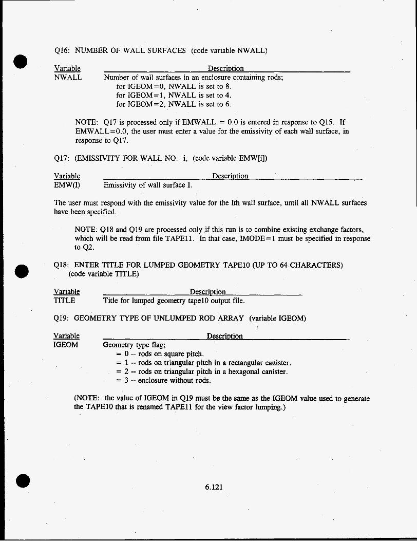
416: NUMBER OF WALL SURFACES (code variable NWALL)
Variable Descriution NWALL Number of wall surfaces in an enclosure containing rods;
for IGEOM=O, NWALL is set to 8. for IGEOM= 1, NWALL is set to 4. for IGEOM=2, W A L L is set to 6.
NOTE: 417 is processed only if EMWALL = 0.0 is entered in response to Q15. If EMWALL=O.O, the user must enter a value for the emissivity of each wall surface, in response to Q17.
417: (EMISSIVITY FOR WALL NO. i, (code variable EMW[i])
Variable Descriution E M W ) Emissivity of wall surface I.
The user must respond with the emissivity value for the Ith wall surface, until all NWALL surfaces have been specified.
NOTE: 418 and Q19 are processed only if this run is to combine existing exchange factors, which will be read from file TAPE1 1. In that case, IMODE= 1 must be specified in response to 42.
418: ENTER TITLE FOR LUMPED GEOMETRY TAPElO (UP TO 64 CHARACTERS) (code variable TITLE)
Variable Descriution TITLE Title for lumped geometry tape10 output file.
Q19: GEOMETRY TYPE OF UNLUMPED ROD ARRAY (variable IGEOM)
Variable Descriution IGEOM Geometry type flag;
= 0 -- rods on square pitch. = 1 - rods on triangular pitch in a rectangular canister. = 2 -- rods on triangular pitch in a hexagonal canister. = 3 - enclosure without rods.
(NOTE: the value of IGEOM in Q19 must be the same as the IGEOM value used to generate the TAPElO that is renamed TAPE11 for the view factor lumping.)
6.121

420: INDICATE AUTOMATIC EXCHANGE FACTOR LUMPING OPTIONS (code variable ILUMP)
Variable Description ILUMP Flag for view factor lumping;
= -1 -- no view factor lumping. = 0 -- user-specified lumping. = 1 -- automatic lumping for half symmetry on diagonal
= 2 -- automatic lumping for eighth symmetry (square pitch). = 3 -- automatic lumping for sixth symmetry
(square pitch).
(triangular pitch).
421: NUMBER OF WALL SURFACES IN LUMPED MODEL (code variable LNWALL)
Variable Description LNWALL Number of wall surfaces in the radiation group.
422: NUMBER OF GROUPS FOR USER SPECIFIED LUMPING (code variable NGRP)
Variable DescriDtion NGRP Number of groups for user specified lumping.
Enter zero if no lumping groups are to be specified.
Note that all three queries, 420, 421, and 422, must be answered, even if no lumping options are desired. If the lumping options are not used, the input value for each of the three queries is zero.
If 420 and 421 are processed with nonzero values for ILUMP or NGRP when IMODE = 0, the view factors will be calculated for the detailed rod array, but the output to TAPE10 will be the lumped view factors. The view factors for the detailed rod array will be lost.
NOTE: 423 through 426 are processed only if NGRP > 0 in response to 421. If NGRP is greater than zero, the input lines 423 through 426 are processed as a group NGRP times.
423: NUMBER OF WHOLE SURFACES IN GROUP i (code variable NWHOLE)
Variable DescriDtion NWHOLE Number of whole surfaces in the Ith group.
424: LIST THE WHOLE SURFACE NUMBERS (code variable LLOC(j))
Variable DescriDtion LLOC(J) Index number of Jth whole surface in the Ith group.
(NOTE: NWHOLE entries are expected.)
6.122 a

425: NUMBER OF PARTIAL SURFACES IN GROUP i (code variable NPART)
@ Variable Description NPART Number of partial surfaces in the Ith group
426: LIST THE SURFACE NUMBERS AND FRACTION OF SURFACE FOR EACH b
Variable Description LLOC(J+N,) Index number of Jth partial surface in the Ith group.
AX(J+N,) Fraction of the Jth surface that is in the Ith group.
(NOTE: NPART pairs of entries are expected. N, = NWHOLE.)
***** THIS IS THE END OF THE INPUT REQUIRED IN THE INTERACTIVE MODE *****
6.3.2.2 Sample Problems for RADGEN
The following sample problems illustrate the interactive input for the RADGEN code. The problems are for the rod geometries shown in Figure 6.13. Test case 1 is a 3 x 3 square array of rods in a square canister (Figure 6.13[a]). Test case 2 is a triangular array of rods in a square canister (Figure 6.13@]). Test case 3 is for a triangular array of rods in a hexagonal canister (Figure 6.13[c]).
In all three cases, the rod diameter is 0.422 in., and the pitch-to-diameter ratio is 1.2891 for cases 1 and 3. Case 2 models consolidated rods, and the pitch-to-diameter ratio is 1.0. The rod emissivity is assumed to be 0.8, and the wall emissivity is 0.2 in all three cases. For case 1, the gap between the walls and the rods is 0.1 in.; for case 2, the gap is 0.1565 in. at the top and bottom, and 0.1 in. at the left and right sides.
INTERACTIVE PROCESS FOR RADGEN TEST CASE 1:
INTERACTIVE INPUT? IF NOT, READ FROM INPUT Oun 9) (code variable READIN)
Y SPECIFY MODE OF OPERATION (code variable MODE)
(Y/YES,RET/NO)
0 - GENERATE NEW EXCHANGE FACTORS 1 - LUMP EXISTING EXCHANGE FACTORS (TO BE READ FROM TAPE11)
0 ENTER TITLE FOR PROBLEM (UP TO 64 CHARACTERS) (code variable TEXT) RADGEN test case 1 (3x3 square array in a square canister) TYPE OF GEOMETRY DESIRED (code variable IGEOM)
0 - RODS ON SQUARE PITCH IN A RECTANGULAR CAN 1 - RODS ON TRIANGULAR PITCH IN RECTANGULAR CAN OR ANY OTHER NON-HEXAGONAL ENCLOSURE
2 - RODS ON TRIANGULAR PITCH IN A HEXAGONAL CAN 3 - ARBITRARY UNOBSTRUCTED ENCLOSURE; NO RODS
0
6.123

ROD PITCH-TO-DIAMETER RATIO (code variable PDR) 1.2891 NUMBER OF ROWS OF RODS (code variable NROWS) 3 NUMBER OF RODS IN EACH ROW (code variable NCOL) 3 ROD OUTSIDE DIAMETER (IN.) (code variable DIA) A22 DISTANCE BETWEEN THE EDGE OF THE RODS AND THE CANISTER WALL (IN.)
.2
.2
.2
.2 ROD EMISSIVITY (code variable EMROD) 0.8 WALL EMISSIVITY (ENTER ZERO IF VALUES ARE TO BE READ FOR EACH WALL)
0.2 NUMBER OF WALL SURFACES (code variable NWALL) 8 INDICATE AUTOMATIC EXCHANGE FACTOR LUMPING OPTIONS (code variable LUMP)
AT THE TOP (code variable XR(1))
ON THE RIGHT SIDE (code variable XR(2))
AT THE BOTTOM (code variable XR(3))
ON THE LEFT SIDE (code variable XR(4))
(code variable EMWALL)
-1 - NO VIEW FACTOR LUMPING 0 - USER SPECIFIED LUMPING 1 - AUTOMATIC LUMPING FOR HALF SYMMETRY ALONG DIAGONAL (SQUARE PITCH) 2 - AUTOMATIC LUMPING FOR EIGHTH SYMMETRY (SQUARE PITCH) 3 - AUTOMATIC LUMPING FOR SIXTH SYMMETRY (TRIANGULAR PITCH)
-1
. . . . . . . . . . . . . . . . . . . . . . . . . . . . . . . . . . . . . . . . . . . . . . . . . . . . . . . . . . . . . . . . . . . . . . . . . . . . . . . . . . . . . . INTERACTIVE PROCESS FOR RADGEN TEST CASE 2:
INTERACTIVE INPUT? IF NOT, READ FROM INPUT (lun 9) (code variable READIN)
Y SPECIFY MODE OF OPERATION (code variable MODE)
(Y/YES,RETINO)
0 - GENERATE NEW EXCHANGE FACTORS 1 - LUMP EXISTING EXCHANGE FACTORS (TO BE READ FROM TAPEl1)
0 ENTER TITLE FOR PROBLEM (UP TO 64 CHARACTERS) (code variable TEXT) RADGEN test case 2 (triangular array in a square canister) TYPE OF GEOMETRY DESIRED (code variable IGEOM)
0 - RODS ON SQUARE PITCH IN A RECTANGULAR CAN 1 - RODS ON TRIANGULAR PITCH IN RECTANGULAR CAN
OR ANY OTHER NON-HEXAGONAL ENCLOSURE 2 - RODS ON TRIANGULAR PITCH IN A HEXAGONAL, CAN 3 - ARBITRARY UNOBSTRUCTED ENCLOSURE; NO RODS
1 ROD PITCH-TO-DIAMETER RATIO (code variable PDR) 1 .o NUMBER OF ROWS OF RODS (code variable NROWS) 3
6.124

NUMBER OF RODS IN EACH ROW (code variable NCOL) (FOR TRIANGULAR ARRAY IN A RECTANGULAR CANISTER, ENTER THE NUMBER OF RODS IN THE LONGER ROW)
(FOR IRREGULAR TRIANGULAR ARRAY IN A
OF RODS MUST BE SPECIFIED FOR EACH ROW; ENTER ZERO FOR ncol)
NON-HEXAGONAL CANISTER, THE NUMBER
3 RODS IN A RECTANGULAR CANISTER ARE ASSUMED TO BE ARRANGED IN ALTERNATING
INDICATE WHETHER THE TOP ROW IS LONG OR SHORT (code variable IFIRST) LONG AND SHORT ROWS
1 - LONG ROW -1 - SHORT ROW
1 ROD OUTSIDE DIAMETER (IN.) (code variable DIA) 0.422 DISTANCE BETWEEN THE EDGE OF THE RODS AND THE CANISTER WALL (IN.)
0.1565
0.1
0.1565
0.1 ROD EMISSIVITY (code variable EMROD) 0.8 WALL EMISSIVITY (ENTER ZERO IF VALUES ARE TO BE READ FOR EACH WALL)
0.2 NUMBER OF WALL SURFACES (code variable NWALL) 4 INDICATE AUTOMATIC EXCHANGE FACTOR LUMPING OPTIONS (code variable ILUMP)
AT THE TOP (code variable XR(1))
ON THE RIGHT SIDE (code variable XR(2))
AT THE BOTTOM (code variable XR(3))
ON THE LEFT SIDE (code variable XR(4))
(code variable EMWALL)
-1 - NO VIEW FACTOR LUMPING 0 - USER SPECIFIED LUMPING 1 - AUTOMATIC LUMPING FOR HALF SYMMETRY ALONG DIAGONAL (SQUARE PITCH) 2 - AUTOMATIC LUMPING FOR EIGHTH SYMMETRY (SQUARE PITCH) 3 - AUTOMATIC LUMPING FOR SIXTH SYMMETRY (TRIANGULAR PITCH)
t
-1
. . . . . . . . . . . . . . . . . . . . . . . . . . . . . . . . . . . . . . . . . . . . . . . . . . . . . . . . . . . . . . . . . . . . . . . . . . . . . . . . . . . . . .
INTERACTIVE PROCESS FOR RADGEN TEST CASE 3:
INTERACTIVE INPUT? IF NOT, READ FROM INPUT Oun 9) (code variable WADIN)
Y SPECIFY MODE OF OPERATION (code variable IMODE)
(YIYES,RET/NO)
0 - GENERATE NEW EXCHANGE FACTORS 1 - LUMP EXISTING EXCHANGE FACTORS (TO BE READ FROM TAPEll)
0 ENTER TITLE FOR PROBLEM (UP TO 64 CHARACTERS) (code variable TEXT) RADGEN test case 3 (hexagonal array in hexagonal canister) TYPE OF GEOMETRY DESIRED (code variable IGEOM)
6.125

0 - RODS ON SQUARE PITCH IN A RECTANGULAR CAN 1 - RODS ON TRIANGULAR PITCH IN RECTANGULAR CAN
OR ANY OTHER NON-HEXAGONAL ENCLOSURE 2 - RODS ON TRIANGULAR PITCH IN A HEXAGONAL CAN 3 - ARBITWRY UNOBSTRUCTED ENCLOSURE; NO RODS
2 ROD PITCH-TO-DIAMETER RATIO (code variable PDR) 1.2891 NUMBER OF ROWS OF RODS (code variable NROWS) 5 ROD OUTSIDE DIAMETER (IN.) (code variable DIA) 0.422 DISTANCE BETWEEN THE EDGE OF THE RODS AND THE CANISTER WALL (IN.) 0.1 ROD EMISSIVITY (code variable EMROD) 0.8 WALL EMISSIVITY (ENTER ZERO IF VALUES ARE TO BE READ FOR EACH WALL)
0.2 NUMBER OF WALL SURFACES (code variable NWALL) 6 12 wall nodes, (2 per face), are assumed for triangular array hexagonal bundles. nwall will be set to 12 INDICATE AUTOMATIC EXCHANGE FACTOR LUMPING OPTIONS (code variable LUMP)
(code variable EMWALL)
-1 - NO VIEW FACTOR LUMPING 0 - USER SPECIFIED LUMPING 1 - AUTOMATIC LUMPING FOR HALF SYMMETRY ALONG DIAGONAL (SQUARE PITCH) 2 - AUTOMATIC LUMPING FOR EIGHTH SYMMETRY (SQUARE PITCH) 3 - AUTOMATIC LUMPING FOR SIXTH SYMMETRY (TRIANGULAR PITCH)
-1
6.126

The view factors produced in these three test cases are as follows:
31.2890.2000 17 1 1
0.2000000 7.20346E-01 1.9 1532E-0 1 9.93075E-04 6.671028-02 1.55108E-01 1.29645802 7.85580E-03 2.18470E-02 2.18470E-02
1.55108E-01 1.04329503
1.2964%-02 3.80426E-02 7.51515E-02 7.51515E-02 3.9813 1 E-03 1.29645E-02
5.44135E-04
2.18470E-02
1.55108E-01
2.18470E-02
8.45465E-03 1.29645E-02 1.55108E-01 2.78989E-04 9.93075E-04 1.91532E-01 3.36853E-05 9.26086602 4.67626E-05 9.52826E-03 1.17369E-02 1.44831E-03
1.44831 E-03 1.17369E-02 1.05301E-05 4.67626E-05 9.26086E-02 1.62914E-06 4.67626E-05 9.26086E-02 2.30217E-06 1 AI83 1 E-03 1.17369E-02 9.17294E-05 1.17369E-02 1.44831 E-03 1.15187E-03 9.26086E-02 4.67626E-05 1.28946E-02
9.17294E-05
,800 R.4 8
0.2000000 7.20346E-03 1.55108E-01 6.671 02E-02
.DGEN test case 1 (3x3 square at
0.2000000 7.20346E-0 1 1 .55 108E-01 1.04329E-03
'ray in a quare
0.2000000 7.20346E-03 7.5 15 15E-02 3.36853E-05
1.0682OE-01 2.78989E-04
canister)
0.2000000 7.20346803 2.18470E-02 1.04329E-03
1.29645E-02 5.44135E-04
0.2000000 7.20346E-0 1 1.29645E-02 8.45465E-03
5.56963E-03 2.78989E-04
1.29645E-02 3.36853E-05
7.55036E-02 3.80426802
I .06820E-01 3.98 13 1 E-03
7.55036E-02 5.44135E-04
1.55108E-01 6.67103E-02
1.07015E-01 7.85580E-03
1.55108E-01 1.04329E-03
7.55380E-04 9.17294E-05
7.55380E-04 2.30217E-06
3 A7299E-04 1.62914E-06
I .09056E-02 1.05301E-05
5.281 16E-02 9.17294E-05
5.28116E-02 9.52825E-03
I .Q9056E-02 1.28946E-02
3.87299E-04 1.15 187E-03
0.2000000 7.20346E-01 2.18470E-02 8.45465E-03
0.2000000 7.20346E-01 1.29645E-02 3.36853E-05
7.55036E-02 5.441358-04
1.07015E-01 3.80426E-02
1.55108E-01 3.80426E-02
7.55036E-02 7.85580E-03
1.55108E-01 8.454658-03
1.91532E-01 6.67 IO2E-02
1.29645E-02 6.67 1 02E-02
7.51515E-02 8.45465E-03
1.55108E-01 1.04329E-03
9.93075E-04 3.36853 E-05
7.55036E-02 7.85580803
1.06820B01 3.98 13 1 E-03
7,550368-02 2.78989E-04
1.29645E-02 1.04329E-03
5.56963E-03 5.441 35E-04
I .29645E-02 3.36853E-05
5.281 16E-02 1.28946E-02
5.28116E-02 1.15 187E-03
1.09056E-02 9.17294E-05
3.87299E-04 2.30217E-06
7.55380E-04 1.62914E-06
1.29645E-02 2.78989E-04
1.07015E-01 5.44 135E-04
1.06820E-01 5.44135E-04
5.56963E-03 2.78989804
1.55108E-01 7.85580E-03
7.51515E-02 3.98 13 1 E-03
1.55108E-01 7.85580E-03
9.93075E-04 3.36853E-05
1.29645E-02 5.44135E-04
2.18470E-02 1.043298-03
1.17369E-02 1. I5 187E-03
9.26086E-02 1.28946E-02
9.26086E-02 9.52825E-03
1.17369E-02 9. I7294E-05
1.44831 E-03 1.05301E-05
4.67626E-05 1.62914E-06
1.0682OE-01 3.98 13 1 E-03
4.02624E-02 3.98 13 1 E-03
1.06820E-01 3.981 3 1E-03
7.51515E-02 3.9813 1 E-03
5.56963E-03 3.8Q426E-02
1.06820E-03 3 A0426802
1.07015E-01 7.8558OE-03
1.29645802 2.78989E-04
1.55108E-01 3.36853E-05
7.55036E-02 2.78989E-04
1.29645E-M 8.45465E-03
1.09056E-02 9.17294E-05
3.87299- 9.52825E-03
7.55380E-W 1.28946E-02
7.55380E-W 1.15 187E-03
3.87299E-04 9.17294E-05
1.09056E-02 2.30217E-06
7.51515E-02 1.04329E-03
1.06820E-01 7.85580803
7.5 15 15E-02 6.67 102E42
5 S2694E-03 2.30217E-06
5 S2694E-03 9.17294E-05
5.52694E-03 1.15187E-03
5.52694E-03 1.28946E-02
5.52694E-03 9.52826E-03
5.52694E-03 9.17294E-05
5.52694E-03 I .05301E-O5
,532694E-03 1.62914E-06
1.29645E-02 8.45465E-03
7.550363-02 3.804268-02
1.55108E-01 6.67102E-02
3.87299- 1.62914E-06
1.09056E-02 1.05301E-05
5.28116E-02 9.17294E-05
5.28116E-02 9.52826E-03
1.09056E-02 1.28946E-02
3.87299- 1.15187E-03
7.55380- 9.17294E-05
7.55380E-04 2.30217E-06
1.91532E-01 6.67 102E-02
1.55108E-01 3.80426E-02
2.18470802 8.45465E-03
1.44831E-03 1.05301E-05
4.67626E-05 1.62914E-06
4.67626E-05 2.30217E-06
1.4483 1E-03 9.17294E-05
1.17369E-02 1.1S187E-03
9.26086E-02 1.28946E-02
9.26086E-02 9.5282SE-03
1.17369502 9.17294E-05
7.55380E-04 1.05301 E M
3.872998-04 9.17294E-05
4.67626E-05 2.30217E-06
5.28116E-02 1.62914E-06
1.09056E-02 9.52825E-03
1 .44831E-O3 9.17294E-05
5.28116E-02 1.05301E-05
31.oooO.2000.800 1 2 1 1 4
0.2000000 0.2000000 0.2000000 0.2ooMxx) 1.19102E+00 1.02050E+00 1.19102E+00 1.02050E+00
RADGEN test case 2 (triangular array in a square canister)
2.50649E-01 1.72135E-01 1.36512E-03 3.58459E-01 2.32095E-07 7.08450E-02 1.28059E-05 4.88526E-07 7.10516E-02 8.14953E-06 1.83325E-04 7.52908E-02
6.127

1.72135E-01 6.18761 E-02 1.36512E-03 7.105 16E-02 1.58459E-01 1.73825E-04 2.32095E-07 1.73825E-04 7.08450E-02 1.83325E-04 1.28059E-05 4.92025E-08 4.88526607 1.83325E-04
1.77814E-02 7.98585E-06 6.0422 1 E-03
5.98530E-07
5.96560E-02
1.53922E-04
7.37786E-02 6.04221E-03
1.50555E-01 4.121 86E-04 1.72135E-01 7.529088-02 1.21224E-01
1.21224E-01 2.99 145E-02
2.8 1068E-09
1.280598-05 8.14953E-06 3.39451E-09 4.121 86E-04 1.28059E-05 7.52908E-02
5.1771 1 E-03 5.19521E-02
4.03907E-04 1.02209E-02 4.13 1 12E-08 5.1771 1 E-03 4.03908E-04 9.654278-08
1.72135E-01 4.92025E-08 2.50649E-01 1.83325E-04 2.32095E-07 1.73825844 1.584598-01 1.73825E-04 4.88526E-07 7.1 05 1 6E-02 1.28059E-05 6.18760E-02 7.08450E-02 7.1051 6E-02 5.96560E-02 5.98530E-07 7.37786E-02 6.04221 E-03 1.53922E-04 1.77814E-02
6.04221 E-03 7.98585E-06
1.21224E-01 4.12 1 86E-04 2.320958-07
8.915848-02 2.993458-02
2.81068E-09
8.149538-06
1.2 12 12E-01
1.58459E-01 7.52908E-02 1.212246-01
2.32095807
1.45946E-04 5.1771 1E-03
9.65426E-08
5.1771 1 E-03 2.93 1378-02 1.02209E-02
4.121 86604
8.14953E-06
2.75422E-09
1.45946E-04
1.21224E-0 1
1.58459E-0 1
1.21212E-01
8.91584E-02
2.32095E-07
1.21224E-01
1.58459E-01
1.45946E-04
2.93 137E-02
1.45946804
2.75422E-09
1.28059E-05
4.88526E-07
1.58459E-01
2.32095E-07
2.50649E-01
1.72135E-01
1.36512E-03
1 S3922E-04
7.98585E-06
5.96560E-02
7.37786802
3.39451 E-09
1.280598-05
1.21224E-01
1.21224E-01
1.72 135E-01
1.50555E-01
1.72135E-01
4.13112E-08
4.03907E-04
5.19521E-02
4.039088-04
1.28059E-05
7.08450E-02
2.320958-07
1.58459E-01
1.36512E-03
1.72135803
2.50649E-0 1
1 S3922E-04
7.37186802
5.96560E-02
7.98585E-06
. . . . . . . . . . . . . . . . . . . . . . . . . . . . . . . . . . . . . . . . . . . . . . . . . . . . . . . . . . . . . . . . . . . . . . . . . . . . . . . . . . . . . . . . . . . . . . . . . . . . . . . . . . . . . . . . . . . . . . .
5 1.2890.2oOO 31 1 1 0.2000000 0.2000000
5.45770E-01 5.457708-01 2.21805E-01 2.47041 €42 1.42236E-06 9.03226E-09
1.34532E-03
5.53067E-08 1.60206E-03 7.79126E-05 3.002 19E-07 1.7 1 136E-07 1.45195E-01 1.08786E-01 8.06696E-05 7.07592E-09 1.17256E-01 1.ooO11E-01 7.79126E-05 4.25203E-07 2.47041 E-02 2.43659E-02 3.33967E-05 5.36124M 8.06696E-05 7.09899E-05 1.4201 1E-06 7.78644E-06 1.60206E-03
1.60206E-03 7.83008E-09 2.47041 E-02 4.83 164E-02 2.47041E-02
1.45195E-01
3.42011E-06
1.17256E-01
.800 MI
0.2000000 0.2000000
5.45770E-01 5.4577OE-01
12
1.45195E-01 1.36967E-03 1.4201 1 E-06 9.03226E-09 1.42112E-01 2.44175E-02 1.39557E-06 7.07593E-09 1.45195E-01 1.36967E-03 1.420llE-06 7.83008E-09 2.48748E-02 2.44175E-02 3.35802E-05 5.53067E-08 1.08786E-01 9.98788E-02 7.09899E-05 4.25203E-07 1.08786E-01 9.98789E-02 7.09899E-05 3.82840E-07 2.48748E-02 2.44175E-02 3.35802E-05 4.84310E-07 8.066%E-05 1.36967E-03 8.06696E-05 1.71136E-07 1.34532E-03 9.98788E-02 1.34532E-03
IGEN test case 3 (hexagonal ari
0.2000000 0.2000000
5.45770E-0 1 5.45770E-01 1 AO206E-03 7.791 26E-05
7.83008E-09 3.00219E-07
1.451958-03 1.34532803 1.4201 1E-06 7.07592E-09 2.21805E-01 2.47041E-02 1.42236E-06 9.03226E-09 8.06696E-05 7.09899E-05 1.42011E-06 4.843 10E-07 2.47041 E-02 2.43659EoL 3.33967E-05 3.82840E-07 1.17256E-01 1.OOO11E-01 7.79 126E-05 4.25203E-07 1.45195E-01 1.08786E-01 8.06696E-05 5.53067E-08 1.42236E-06 3.33967E-05 1.42236E-06 7.91442E-06 7.79126E-05 1.30504E-03 7.79126E-05
0.2000000 0.2000000
5.45770E-01 5.45770E-0 1 1.45195E-01 1.42236E-06 5.74811E-02 1.71136E-07 2.48748E-02 8.06696E-05 3.58026E-02 5.53067E-08 8.06696E-05 1.60206E-03 6.15541E-04 9.03226E-09 1.421 12E-01 1.42011E-06 5.35734E-04 7.78644E-06 1.08786E-01 7.79126E-05 6.85591E-03 5.36124E-06 1.34532E-03 2.47041 €42 3.55958E-04 4.25203E-07 3.35802E-05 1.45195E-01 7.78644E-06 7.07592E49 1.45195E-01 3.00218E-07 7.91442E-06 6.15541 E-04 1.08786E-01 3.33967E-05 2.56835E-05
ray in hexagonal
0.2000000
5:45770E-01
1.17256E-01
6.15541E-04 7.91442E-06 1.08786E-01 3.35802E-05 3.58026E-02 4.84310E-07 2.47041 E-02 1.4201 1E-06 5.74811E-02 7.83008E-09 I .08786E-01 2.48748E-02 7.78644E-06 5.35734E-04 4.83164E-02 1.34532E-03 3.55958W 2.56835E-05 1 .OOOllE-01 7.09899E-05 6.85591 E43 3.8284OE-07 1.34532E-03 1.39557E-06 5.35734E-04 7.07592m 2.47041M12 1.45195E-01 1.71136E-07 5.7481 1 E-02 1.OOOllE-01 1.08786E-01 5.36124E-06
8.06696E-05
canister)
0.2000000
5.45770E-01
2.47041E-02 7.79 126E-05
6.15541E-04 1.08786E-01 7 ,09899E-05 5.35734E-04 7.78644E-06 1.17256E-01 3.33967E-05 5.748 12E-02 1.71 136E-07 1.34532E-03 1.34532E-03 4.84310E-07 3 S8026E-02 1.OOO11E-01 2.43659E-02 2.56835E-05 3.55958W 4.83164E-02 1.30504E-03 6.85591E-03 5.361 24E-06 1.08786E-01 7.09899E-05 3.58026m 5.53067E-08 7.19126E-05 2.47041E-02 7.83008E-09 5.748 12E-02 2.43 659E-02 1.OOO11E-01 3.82840E-07
7.9 1442E-06
0.2000000
5.45770E-01
8.06696E-05 3.33967E-05 1.71 136E-07 5.74811E-02 2.48748E-02 7.09899E-05 7.78644E-06 5.35734E-04
7.79126E-05 6.15541 E-04 7.91442E-06 3.35802E-05 7.09899E-05 5.53067E-08 3.58026EM 1.34532E-03 1.30504E-03 5.36124E-06 6.85591 E-03 1.08786E-01 2.43659E-02 3.55958E-04 2.56835E-05 1.42112E-01 1.34532E-03 3.58026E-02 4.84310E-07 1.4201 1E-06 7.791 26E-05 9.03226E-09 6.15541E-04 7.09899E-05 2.43659E-02 4.25203E-07
1.45195E-01
0.2000000
5.45770E-0 1
1 hO206E-03 1.42011E-06 7.83008E-09
8.06696E-05 3.35802E-05 4.84310E-07
1.42236E-06 8.066%€-05 7.91442E-06
1.45 195E-01 1.39557E-06 7.07592E-09
2,47041 E-02 7.09899E-05 3.82840E-07
7.79126E-05 1.34532E-03 2.56835E-05
1.42011E-06 2.48748E-02 5.35734E-04
2.21805E-01 1.4201 1E-06 9.03225E-09
1.17256E-01 7.09899E-05 4.25203E-07
6.128

3.82840E-07 1.36967E-03 9.98788E-02 1.369678-03 2.342 10E-05 7.79126E-05 1.30504E-03 7.79126E-05 3.55958E-04 1.42236E-06
e
3.33967E-05 1.42236846 6.15541844 8.066968-05 1.08786E-01 1.45 195E-01
7.791 26E-05 1.OOOllE-01 1.17256E-01 2.56835805 3.33967E-05 2.436598-02
6.85591E-03 1.4201 1E06 7.09899E-05
3.58026E-02 1.42236E-06 2.47041E-02 2.21 805E-01 7.9 1442E-06 1.42011E-06 1.34532E-03 1.45195E-01 5.35734E-04 3.0021 9E-07 7.791 26E-OS
5.7481 1 E-02 1.05321E-01 4.70592E-05 1.43468E-08 5.02807E-10 1.12784E-03 9.82325E-06 1 AS496E-08 1.25056E-09 1.45014E-05 7.01467E-07 1.65496E-08 2.55064E-08 3.13569E-07 7.79089E-07 1.43468E-08 4.04328E-06 1.43468E-08
4.843 1OE-07
2.47041 E-02
8.06696E-03-05
1.60206E-03
5.36124E-06 2.44 1758-02 4.57227E-02 2.441 75E-02 2.342 1OE-05 1.34532E-03 9.987898-02 1.34532E-03 2.568358-05 8.06696E-05 1.36967E-03 8.06696E-05 7.91442E-06 3.35802E-05 2.44175E-02 2.48748802 7.78644806 7.09899E-05 9.98788E-02 1.08786E-01 3.55958E-04
9.98788E-02 7.09899805
1.08786E-01 6.85591 E-03 3.35802E-05 2.44175E-02 2.48748E-02 5.35734E-04 1.4201 1E-06 1.36967E-03
6.15541E-04 1.39557E-06 2.44175E-02 1.421 12E-01 3.58026E-02 1.4201 1E-06 1.36967E-03 1.45195E-01 5.748 12E-02 6.56001M2 4.29136E-05
1.451 95E-01
1.29650E-08 6.66516E-I 1 6.56001 E-02 4.29136E-05 1.29650E-08 8.86007B11 9.81611E-04 4.29136E-05 1.01337E-07 1.25056E-09 1.42669E-05 4.29136E-05 8.87387E-07 4.86355E-08 8.87387E-07
2.56835E-05 1.36967E-03 9.98788E-02 1.369676-03 2.34210E-05 2.47041 E-02 4.83 164E-02 2.47041 E-02 5.36124E-06 1.60206E-03 1.17256E-01 1.60206E-03 1.71136E-07 1.42011E-06 7.09899E-05 8.06696E-45 5.35734E-04 3.33967E-05
2.47041 E-02 2.43659E-02
6.85591E-03 7.79126E-05 1 .OOOllE-01
3.55958E-04 1.17256E-01
8.06696E-05 1.08786E-01 1.45195E-01 7.78644E-06 3.00219E-07 7.79126E-05 1.602068-03 5.748 1 1 E-02 1.42011E-06 1.34532M3 1.45195E-01 3.58026E-02 1.42236E-06 2.47041 E-02
6.15541E-04 I . 12784E-03 9.82325E-06 1.65496E-08 8.86007E-11 1.05321E-01 4.70592E-05 1.43468E-08
1.05321E-01 6.52213E-04 3.13569E-07
1.12784E-03 1 .25619E-O2 1.45014E-05 1.25056E-09 1.45014E-05
2.21 805E-0 1
6.66516E-11
5.028ME- 10
3.559588-04 2.44175E-02 1.36967E-03 2.34210E-05 2.3421OE-05 7.09899E-05 1.17256E-01 5.36 1248-06 3.82840E-07 1.42011E-06 2.2 1 805E-01 1.71136E-07 7.83008E-09 2.487488-02 1.4201 1E-06 4.843108-07 3.58026802 1.34532E-03 7.79126E-05 3.82840E-07 6.85591 E-03 7.09899E-05 2.47041 E-02 4.25203E-07 2.568358-05 1.39557E-06 1.45 195E-01 5.53067E-08 4.843 1 OEM 8.06696E-05 1.42236E-06 7.830088-09 5.74812E-02
8.06696E-05 7.07592E-09 5.35734E-04 1.42011E-06 1.60206E-03 9.03226W 7.91442E-06 9.81611E-04
9.44086E-03 1.25056E-09 1.42669E-05 1.45014E-05 7.31206E-M 5.02807E-10 8.87387E-07 1.12784E-03 4.04328E-06 6.66S16E-11 1.01337E-07 1.05321E-01 2.55064E-08 8.86007E-11 1.29650E-08
3.35802E-05
3.13569E-07
6.85591 E-03 9.98788E-02 2.44 175 E-02 2.342 1 OE-OS 2.342 1 OE-05 2.43659E-02 7.09899E-05 2.56835E-05 4.252038-07 7.79126805
7.91442E-06 9.03226E-09 1.34532E-03 1.42112E-01
1.4201 1E-06
5 S3067E-08 3 S8026E-02 2.43659E-02
4.25203E-07 3.55958E-04 1.30504E-03 1.34532E-03
1.08786E-01
3.82840E-07 5.36124E-06 7.09899E-05
4.843 1OE-07
7.791 26E-05 1.45 195E-01 9.03226E-09 6.15541 E-04 7.09899E-05 2.48748E-02 7.07592E-09 7.78644E-06 3 :33967E-05 8.06696E-05 7.83008E-09 1.71 136E-07 1.25619E-W 8.87387E-07 7.31206E-M 4.86355E-08 6.52213E-04 1.01337E-07 9.44086E-03 I .25056E-09 4.70592E-05 1.29650E-08 3.44362E-03
9.82325E-06 1.2965OE-08 4.04328E-06
7.01467Eo7
3.35802E-05
5.53067E-08
8.86007E-11
6.66516E-11
6.85591 E-03
9.98788E-02 2.342 1 OE-05
9.98788E-02
2.34210E-05 1 .OOOllE-Ol 2.43659E-02 3.55958E-04 4.25203E-07 2.47041E-02 7.791 26E-05
9.03226E-09 7.098998-05 1.08786801 7.07592E-09
1.30504E-03
6.1.55418-04
5.35734E-04
4.83164E-02 4.25203807 2.568358-05 2.43659E-02 1.00011E-01 5.36124E-06 3.8284OE-07 1.34532E-03 1.34532E-03 7,78644806
3.339678-05 3.17256E-01 9.03225E-09 7.91442M 7.09899E-05 1.08786E-01 5.53067E-08 4.84310E-07 7.79126E-05 2.47041E-02 1.71136E-07 7.83008E-09 6.52213E-04 7.01 467E-07 4.04328E-06 4.04328- 1.25619E-02 7.79089E-07 3.44362E-03 2.55064E-08 1.25619EM 7.79089E-07 9.44086E-03 1.25056E-09 6.522 13- 7.01467E-07 7.3 1 206E-04 5.02807E-10 4.70592E-05
7.07592E-09
3.559588-04 2.44175802 9.98788E-02 2.342 1 OE-05 2.34210E-05 1.08786E-01
6.855918-03
3.45195E-01 2.47041 E-02
7.83008E-09 1.39557E-06 1.34532E-03 7.07592E-09
7 .09899E-05 1.OOOllE-01
1.00011E-01
3.82840E-07
5.7481 1E-02
7.78644E-06
3.82840E-07 5.361 24E-06 1.34532M3 4.83164E-02 2.56835E-05
2.48748E-02 1.08786E-01 5.35734E-04 7.07592E-09 1.42011E-06 2.47041 E-02 7.83008E-09 1.71 136E-07 3.35802E-05 1.08786E-01 4.843 10E-07 5.53067E-08 8.06696E-05 1 .17256E-01 7.9 1442s-06 9.03225E-09 1.42669E-05 7.79089E-07 2.55064E-08 3 A4362E-03 9.81611E-04 7.01467W 4.04328E-06 4.04328- 6.56001E-W 9.82325E-06 7.31206- 4.86355E-08 6.56001E-02 4.70592E-05 9.44086E-03 1.25056E-09 9.8161 1M)Q
4.25203E-07
1.36967803 2.441758-02 2.342108-05
3.33967E-05 1.08786E-01 6.8559 1 E-03
3.00219E-07 1.45195E-01 5.748 1 1 E-02
1.45195E-01
5.53067808 3.35802E-05
2.47041 E M 1.34532E-03 5.36124E-06
7.79126E-05 1.08786E-01 3.55958E-04
1.4201 1E-06 1.42112E-01 3 S8026E-02
1.60206E-03 8.06696E-05 1.71 136E-07
8.06696E-05 2.48748E-02 7.78644E-06
I ,42236E-06 1.45195E-01 6.15541E-04
1.45014E-05 1 .01337W 1.25056E-09
3.13569E-07 8.87387E-07 4.86355E-08
1.43468E-08 1.42669E-05 4.04328E-06
1.65496E-08 9.81611E-04 3.44362E-03
1.65496E-08 7.79089E-07 4.29136E-05 1.25619E-02 1.05321E-01 1.01337E-07 9.82325E-06 6.52213E-M 6.56001Mn 3.13569E-07 1.42669M5 1.12784E-03 1.25056E-09 4.86355E-08 4.04328E-06 3.44362E-03 9.44086E-03 7.3 1206E-04 1.65496E-08 7.01467E-07 1.45014E-05 9.44086E-03 1.65496E-08 9.82325E-06 1.12784E-03
4.04328- 1.01337E-W 4.29136E-05 9.81611E-M 3.443628-03
4.29136E-05 6.56001E-02
1.2965OE-08
2.55064E-08 3.13569E-07 6.52213E-04 1.05321E-01 4.04328E-06 1.43468E-08 4.70592E-05 1.05321E-01
1.25056E-09 1.29650E-08 1.12784E-03
4.86355E-08 1.01337E-07 1.45014E-05 6.66516E-11
5.02807E-10
5.02807E-10 7.79089E-07 8.87387E-07 1.25056E-09 1.25056E-09 7.79089E-07 1.42669E-05 8.86007E-11
6.66516E-11 9.82325- 4.70592E-05 2.55064E-08 8.86007E-11 7.01467E.47 6.5221 3E-M 1.25056E-09
8.86007E-11 1.42669E-05 1.43468E-08 1.25619E-M 6.56001E-M 4.04328E-06 7.31206- 6.66516E-11 8.87388E-07 3.13569E-07 1.25619E-02 9.81611E-04 4.86355E-08 4.04328-
0 6.129

3.443628-03 1.434688-08 4.70592E-05 1.05321E-01 4.04328806 3,13569807 6.52213E-04 1.0532lE-01
1.45014E-05 1.25619E-02 1.12784E-03
1.12784E-03 1.25619E-02
4.86355E-08
1.25056E-09
1.45014E-05 8.86007E-11 1.053218-01
3.135698-07 6.52213E-04
6.66516E-11
9.44086E-03 1.29650E-08 4.291 36E-05 6.56001 E-02 7.3 1206E-04 1.01337s-07 4.29136E-05 9.81611E-04 4.04328E-06 8.87387E-07 4.291368-05 1.42669s-05 2.55064E-08 1.42669E-05 4.29136E-05 8.87387E-07 1.25056E-09 9.81611E-04 4.29136E-05 1.013378-07 5.02807E- 10
7.31 206E-04 1.654968-08 9.82325846 1.12784E-03 9.44086E-03 1.65496808 7.0 1467E-07 1.45014E-05
1.434688-08 3.44362E-03
7.79089E-07 3,13569E-07 4.04328E-06 3.13569E-07 7.79089E-07 1.43468E-08 4.86355E-08 1.45014E-05
1.65496E-08 1.25056E-09
7.01 467807
4.043288-06 8.87387807 3.335698-07 8.86007E-11 3.44362E-03 1.42669E-05 1.434688-08 1.25056809 9.44086E-03 9.81611E-04 1.65496E-08
7.3 1206E-04 4.86355E-08
6.56001E-02 1.65496E-08 4.04328E-06 4.04328E-06 6.56001E-02 1.43468E-08 3.44362803 2.550648-08
2.55064808 7.01 467E-07 9.8 1 61 1 E-04 6.66516E-11 4.043288-06 9.82325E-06 6.56001E-02 5.02807E-10 7.3 1206E-04 4.70592E-05 6.56001 E-02 1.25056s-09 9.44086E-03 6.522 1 3 E-04 9.81611E-04 2.55064808 3.44362E-03 1.256198-02 1.42669E-05 4.04328E-06 4.04328E-06
1.25056E-09
1.25619E-02
4.863558-08 7.79089807 1.256 1 9E-02
7.79089E-07
5.02807E- 10
6.66516E-11 4.04328E-06 7.01 467807 6.52213E-04
3.44362E-03 9.82325E-06 4.70592E-05 1.25056E-09 9.44086E-03 4.70592E-05
8.86007E-11
9.82325E-06 4.86355E-08 7.31206E-04
5.02807E-10 1.013378-07 6.522 13 E-04 1.25056E-09 1.25056E-09 1.29650E-08 4.70592E-05 8.860078-11 2.55064E-08 1.29650E-08 9.82325E-06
4.04328E-06 1.01337E-07
5.02807B10 7.31206E-W 8.87387E-07
1.25056E-09
6.66516E-11
7.01 4678-07
7.790898-07
9.44086E-03
1.450148-05 1.42669E-05 2.55064E-08
1.12784E-03 8.873878-07 1.25056809
1.0532 1 E-01 1.01337E-07 5.02807s- 10
1.05321 E-01 1.2965OE-08 6.66516E-11
I . 127848-03 1.29650E-08 8.860078-1 I
6.3.2.3 Input instructions for Batch Mode
The RADGEN input is read from logical unit 9, file name “input,” when the code is executed in batch mode, or when the option READIN=n is selected in the interactive mode: The input requirements are the same as for the interactive mode, but must be supplied in the formatted input lines described here.
RADGEN.l IMODE Format(I5)
Columns Variable DescriDtion 1-5 IMODE Flag for mode of operation;
= 0 -- generate view factors for new geometry.
= 1 -- read existing view factors from unit 11 and process according to user input.
. . . . . . . . . . . . . . . . . . . . . . . . . . . . . . . . . . . . . . . . . . . . . . . . . . . . . . . . . . . . . . . . . . . . . . . . . . . **** IF MODE = 1, input lines RADGEN.2 through RADGEN.9 are not read **** **** . . . . . . . . . . . . . . . . . . . . . . . . . . . . . . . . . . . . . . . . . . . . . . . . . . . . . . . . . . . . . . . . . . . . . . . . . . . Input processing skips to line RADGEN.10 if IMODE = 1 ****
RADGEN.2 TEXT Format( 16A4)
Columns Variable Description 1-64 TEXT Title for case identification.
6.130

RADGEN.3
Columns 1-5
6-10
11-15
16-20
21-25
IGEOM, PDR, NROWS, NCOL, IFIRST Format(IS,f5.3,3i5)
Variable IGEOM
PDR
NROWS
NCOL
IFIRST
DescriDtion Geometry type flag; = 0 -- rods on squaTe pitch. = 1 -- rods on triang.ular pitch in a
in a rectangular canister. = 2 -- rods on a triangular pitch in a
hexagonal canister. = 3 -- enclosure without rods.
Rod pitch-to-diameter ratio
number of rod rows.
For square pitch array, number of rod columns.
For triangular pitch array in rectangular canister, number of rods in the longer rows.
For triangular pitch array in hexagonal canister, enter zero.
For nonuniform square pitch or triangular pitch arrays, enter zero (number of rods in each row will be specified on RADGEN.8.)
Flag for triangular array in rectangular canister; = 1 -- top row is a long row. = -1 -- top row is a short row. = 0 -- not a triangular array in a rectangular
canister
RADGEN.4 DIA, (XR(I),I=1,4) Read only if (IGEOM C 2 and NCOL > 0) orIGEOM = 2.
Format(5FS.O)
Columns 1-5
6- 10
Variable DIA
DescriDtion Rod outside diameter (in.).
Clearance distance (in.) between the top row of rods and canister wall NOTE: for IGEOM = 2, this value is used for all six wall gaps for a triangular array of rods in a hexagonal canister.)
6.131

11-15 X W ) Clearance distance (in.) between the right column of rods and the canister wall.
(NOTE: for triangular arrays in a rectangular canister, this is the distance between the wall and the end rod of a long row.)
16-20 XW3) Clearance distance (in.) between the bottom row of rods and the canister wall.
2 1-25 XN4) Clearance distance (in.) between the left column of rods and the canister wall. ' (NOTE: for triangular arrays in a rectangular canister, this is the
distance between the wall and the end rod of a long row.)
RADGEN.5 JBEG(I), NLINE(I), I=l,NROWS Read only if NCOL = 0 Format( 1615)
Columns Variable DescriDtion
1 -5 JBEG(1) Index number of first rod in the Ith row.
6-10 NLINE(1) Number of rods in the Ith row.
Input line RADGEN.5 is read with eight pairs of (JBEG,NLINE) entries per line, until NROWS pairs have been specified. The last line may have fewer than eight pairs, if NROWS is not an even multiple of eight.
RADGEN.6 W A L L Read only if IGEOM = 3 Format(I5)
Columns Variable DescriDtion 1-5 NWALL Number of wall surfaces in the enclosure.
RADGEN.7 X(I), Y(I), PERIM(I), I= 1,NWALL Read only if IGEOh Format(3FS .O)
Columns Variable Description
1-5 X(I) left endpoint coordinate for the Ith surface
=3
6-10 Y(I) right endpoint coordinate for the Ith surface
11-15 PERIMQ perimeter.of Ith surface, (inches)
Input line RADGEN.7 is read NWALL times.
6.132

R4DGEN.8 EMROD, EMWALL Format(2F5 .O)
Colurnns Variable 1-5 EMROD
6-10 EMWALL
Description Emissivity of rod surfaces
(NOTE: all rod surfaces are assumed to have the same emissivity).
Emissivity of wall surfaces, if all walls have the same emissivity.
RADGEN.9 EMW(I), I = l , W A L L Read only if EMWALL = 0.0 Format( 12F5 .O)
Columns 1-5
Variable Description EMW(1) emissivity of wall surface I
, Input line RADGEN.9 is read with 12 entries per line until W A L L values have been specified. The last line may have fewer than 12 entries, if W A L L is not an even multiple of 12.
RADGEN.10 TITLE Read only if IMODE = 1 Format( 16A4)
Columns 1-64
Variable TITLE a RADGEN.ll ILUMP Format (15)
e
Columns Variable 1-5 ILUMP
Description Title for identification of lumped view factor set.
Description Flag for view factor lumping; = -1 -- no lumping of view factors = 0 -- user specified lumping. = 1 - automatic lumping for half symmetry on
diagonal (square pitch). = 2 - automatic lumping for eighth symmetry
(square pitch). = 3 - automatic lumping for sixth symmetry
(triangular pitch).
RADGEN.12 NGRP, LNWALL Read only if ILUMP > -1 Format(215)
Columns 1-5
6-10
Variable Description NGRP Number of groups for user-specified lumping.
LNWALL Number of wall surfaces in lumped view factor set.
6.133

RADGEN.13 IDUMY, NTOT Read only if NGRP > 0 Form at(215)
Columns 1-5
6-10
Variable IDUMY
NTOT
Descriution Index number of Ith group. (NOTE: groups must be numbered from 1 to NGRP.)
Total number of surfaces in this group.
RADGEN.14 LLOC(J), AX(J), J=l,NTOT Read only if NGRP > 0 Format(6(15 ,F5.3))
Columns
1-5
6-10
Variable Descriution
LLOC(J) Index number of Jth surface in the Ith group
Fraction of the Jth surface that is contained in the Ith group.
Input line FtADGEN.14 is read with six pairs of (LLOC,AX) entries per line, until all NTOT pairs of entries have been specified. The last line may have fewer than six pairs, if NTOT is not an even multiple of six.
Input lines RADGEN.13 and FtADGEN.14 are read as a set NGRP times, to define all the lumping of all surfaces in the enclosure.
6.134

7.0 Validation for Cycle 2
This section presents the results of the validation of the code changes comprising the Cycle 2 release of COBRA-SFS. The size and complexity of the code make it virtually impossible to exercise every feature and all possible combinations of modeling options, but a concerted effort has been macle to test out the features in a manner consistent with the expected usage of the code. The new capabili- ties added in Cycle 2 were explicitly tested by one case or another, and existing models from earlier cycles were also tested to make certain that code improvements have not compromised performance in any way.
The first test case is a benchmark test case, comparing the performance of the Cycle 2 version of the code with the previous release, Cycle 1. The purpose is to compare the results obtained using Cycle 2 with those of Cycle 1 for a case that both versions can solve. These results are presented in Section 7.1, in a code-to-code comparison. For the remainder of the test cases, the comparison is between Cycle 2 code calculations and experimental data. Section 7.2 gives the results for three single-assembly cases, and Section 7.3 presents results for two multiple-assembly storage casks.
The test cases presented in Sections 7.1 through 7.3 were all run on a SUN SPARCstation 2. Additional testing was performed on various alternative platforms, including workstations and a mainframe computer system. In addition to the SUN SPARCstation, the code has been run on IBM’s RS6000, an INTEL Pentium workstation, the DEC workstation, the HP9000, and the Apple- Macintosh workstation. Cycle 2 of the code has also been run on a CRAY mainframe, under the uniCOS operating system. Essentially the same version of the code was run on all platforms; the only conversion changes were the time and date routines, and the Zuc function for clearing common blocks and writing the restart dump file. 0
Three representative test cases were run on the alternative platforms. These were the Mitsubishi single-assembly case, the TN24 unconsolidated cask in vertical orientation, and the PSN VSC-17 ventilated concrete cask model. Section 7.4 compares the results obtained on the various platforms for these three cases.
7.1 Benchmark Test: Cycle 1 to Cycle 2
The purpose of the benchmark test is to verify that Cycle 2 of COBRA-SFS produces essen- tially the same answers as Cycle 1 when presented with the same input. The COBRA-SFS model of the Mitsubishi electrically heated assembly was selected for this illustration, mainly because it is a relatively small problem that uses many code capabilities which might be called into play in a typical cask analysis. It is, therefore, a good test case to verify that improvements in Cycle 2 have not degraded the overall performance of the code for its primary application.
This section is concerned with the comparison of results between Cycle 2 and Cycle 1 for the test case. For this purpose, it is necessary only to know that the assembly is an electrically heated model of a 15 x 15 PWR fuel rod array enclosed in a square canister with nitrogen back-fill. The test
7.1

assembly was oriented horizontally, and sealed at both ends (the Mitsubishi assembly is described in detail in Section 7.2.1, in which the Cycle 2 calculational results are compared to the data).
The COBRA-SFS model consisted of a single assembly with the geometry represented by 225 rods, 256 subchannels, and 8 wall nodes. The boundary conditions were defined by specifying a uniform temperature on the outside of the wall nodes, and specifying a zero flow at the top and bottom of the assembly (with ITDP = 4 on OPER. 1; see Section 6.2.11).
The same input file was used when executing both the Cycle 1 and the Cycle 2 versions of the code. Only the case title was changed between the two cases, for easier identification in examining the output. In both cases the calculation was run for 20 iterations, and produced a predicted peak clad temperature of 734.8"F. After 20 iterations, both code versions displayed convergence errors of 0.0000 for flow, fluid energy, and rod energy. The total energy error was 1.0000, which in this context means that exactly the same amount of energy was removed at the wall boundary as was added to the system by the heat generating rods.
In the output of fluid conditions, the enthalpies, temperatures, densities, and flow rates in the fluid nodes comprising the subchannels were identical between the two cases. The pressure was slightly different on some subchannels; Cycle 1 predicted 0.0000008 psi, while Cycle 2 predicted 0.0000000 psi. All rod temperatures were identical between the two cases, except for two instances. In one case, a rod was predicted to be at 616.8"F in one node with Cycle 1, while Cycle 2 predicted 616.9"F at that location. In the other case, Cycle 1 predicted 628,3"F, while Cycle 2 predicted 628.4"F for that particular node.
The individual subchannel flow rates were identical between the two cases, to the seven deci- mal places displayed on the COBRA-SFS output. The total flow rate (Le., the sum of the inlet flow rates for all subchannels) was predicted in the Cycle 1 calculation to be -0.490(10-'3) lbdsec; Cycle 2 predicted 0.212(10-") lbm/sec. Both values are well within the convergence criteria for the boundary condition of zero flow. This difference is not in any sense significant.
This comparison gives some confidence that the Cycle 2 changes have not introduced signifi- cant errors into the solution. However, it is advisable for users of Cycle 1 to perform their own benchmark validation on Cycle 2 of models developed for Cycle 1 , as part of installation and check- out of the new version. The results obtained with Cycle 2 should not differ substantially from the results with Cycle 1 . The cause of any significant differences should be resolved before attempting to use the new features and models included in Cycle 2.
7.2 Single-Assembly Test Cases
Three single-assembly test cases were selected as part of the validation of the Cycle 2 changes to COBRA-SFS. These cases provide relatively simple problems for analysis that nevertheless contain many of the same elements as large multi-assembly cask models. All three assemblies were electri- cally heated models of PWR fuel in a square canister. Section 7.2.1 describes the validation test for Pacific Northwest Laboratory's (PNL's) Single-Assembly Heat Transfer Test (SAHTT) bundle;
7.2

Section 7.2.2 describes the validation of Cycle 2 with the Mitsubishi bundle, and Section 7.2.3 discusses the results obtained for a test assembly built by British Nuclear Fuels, Ltd. (BNFL). In each case, input models of the assemblies were run with Cycle 2 of the code, and the results compared with experimental data.
7.2.1 SAHTT 15 x 15 PWR Test Assembly
The SAHTT was developed as part of work at the PNL to investigate heat transfer characteristics of spent light water reactor fuel under dry storage conditions (Bates 1986). The test section, illustrated in Figure 7.1, was an electrically heated model of a 15 x 15 PWR spent fuel assembly, with simulated fuel rods 0.42 in. (1.07 cm) in diameter on a nominal pitch of 0.562 in. (1.4275 cm). Control rod thimbles were modeled with nine unheated rods that had an outer diameter of 0.5 in. (1.27 cm).
The axial heated length was 144 in. (3.658 m). The bundle was oriented horizontally, and back-filled with air or helium. Instrumentation included 98 thermocouples, to measure cladding temperatures and canister surface temperatures. The power generation rate was axially uniform, with total power of 0.5 kW or 1.0 kW, depending on the test.
The COBRA-SFS input consisted of a detailed subchannel model, with 256 subchannels, 225 rods, and 8 slab nodes modeling the canister wall. A cross-section of the model is shown in Figure 7.2. The locations of the rods modeling control rod thimbles are noted on the diagram. Four other rods that modeled fuel rods (identified as 61,92, 104, and 151 in the diagram) had zero power, due to heater malfunction during testing. These were included in the COBRA-SFS model geometry input as zero-power rods. a -
To reduce problem size and save computation time, the bundle was modeled axially by taking a slice three nodes wide through the center of the bundle. The axially uniform power distribution in the test resulted in an essentially uniform temperature distribution for the full length of the bundle, and the ends were sufficiently well insulated for losses to be minimal. As a result, the axial temperature profile was essentially flat, with only a slight dip on the profile near the ends.
The most important Cycle 2 feature included in this model is lateral momentum coupling for the cross-flows. This allows the code to calculate the effect of natural convection in the lateral direc- tion, due to the horizontal orientation of the bundle. In Cycle 1, natural convection in the lateral direction could not be modeled, due to the assumption of no crossflow coupling for momentum.
Boundary conditions on the calculations were taken from measured temperatures on the top, bottom, and sides of the test section. At the top, the boundary temperature was 215.9"C (420°F); at the bottom, it was 208.9"C (408°F); on the sides, 209.9"C (410°F). Radiative heat transfer was modeled using rod-to-rod and rod-to-wall exchange factors, assuming a surface emissivity of 0.2 for the walls and.0.6 for the rods. The grey body view factors were calculated using the auxiliary code RADGEN, (Rector 1987; see Section 6.3 for a description of this code).
The heat transfer coefficient correlations used in this input model are based on data obtained for flow through tube bundles or arrays of heated rods. The internal matrix subchannels modeling the test section falls within this data base, but the applicability of the correlations to the subchannels that
7.3

S9505005.1
Upper Closure Lid
1 Cask Outer Wall
\ Cask Inner Wall
\ Fuel Tube
Model PWR Fuel Bundle
Transition Piece
Fuel Bundle Flange
Figure 7.1. Diagram of SAHTT Assembly
7.4

Slab No. 1 Slab No.2
Slab No. 8
Slab No. 7
U Slab N0.5 Slab No. 6
Control Rod Simulator (D = 0.50 in.)
@ Unheated Rod
-2
Figure 7.2. COBRA-SFS subchannel model of SAHTT Assembly
Slab No. 3
Slab No. 4
see the canister wall is not well validated. For simplicity, it was assumed that the subchannel correla- tions could be used with the wall channels, but this is an area where it might be profitable to do further work.
In the laminar flow regime, the heat transfer correlation was defined as
1
In the turbulent flow regime, the heat transfer correlation is
k H,-nar = -(0.83Re033 De
k - -( 0.33 Reo.6 Pp.3) De
Yurbutent -
7.5

In both correlations, k is the thermal conductivity of the fluid, De is the subchannel hydraulic diameter, which is also the characteristic dimension for the Reynolds number. As explained in Section 6.2.8, the code calculates the local heat transfer coefficient in a node as the maximum of the laminar and turbulent correlation values.
With a zero flow boundary condition resulting in zero axial flow in the subchannels, the axial friction factor is not an important item in the input, but it is necessary to provide a reasonable value to be used in the solution of the axial momentum equation. The axial friction factor, f, was specified at a value typical for PWR rods in square array, as
The lateral friction factor, f', however, is quite important in this case, since this is the direction for natural circulation occurring in the horizontal assembly. The friction factor correlation for laminar flow in the lateral direction is as follows:
For turbulent flow in the lateral direction, the friction factor correlation is given by
f' = 0.47Re4."
For lateral flow, the characteristic dimension for the Reynolds number is the width of the gap for crossflow between adjacent channels.
The results obtained with the COBRA-SFS code using this model for Test Run No. 12 of the SAHTT series are presented in Figure 7.3. The graph in Figure 7.3(a) is a profile of the peak rod temperatures on a diagonal across the assembly cross-section (refer to Figure 7.2 for the indices of the rods lying on the diagonal). The graph in Figure 7.3(b) shows a profile from top to bottom of the assembly cross-section. In both plots, the COBRA-SFS results show excellent agreement with the measured temperatures. The code predictions are in general slightly above the measured temperatures, as shown in Table 7.1,
The measurement uncertainty is based on the reported total uncertainty of 53°C (f37"F) in the rod temperature measurements in the tests. The, reported total uncertainty in the boundary temperature measurement is f5"C (f41 OF). Given these measurement uncertainties, the COBRA- SFS results show that the code is correctly modeling the heat transfer phenomena within the bundle, taking into account both natural convection in the lateral direction, and radiative heat transfer from rod-to-rod and rod-to-wall.
7.6

I
t 400
Rod No. vs sfs and data
13
I
e
I
0 50 100 150 200 250 Rod Number
Figure 7.3(a). Comparison of COBRA-SFS Results with SAHTT Data: Rod Temperature Profiles on the Diagonal
Rod No. vs sfs and data
560 T I
520 l
B t
a f
440
0
0
0
0
o data (F)
0 sfs (F)
7.7

Table 7.1. Comparison of COBRA-SFS Predictions to Measured Temperatures for SAHTT Test No. 12
Rod number
1
49
129
COBRA-SFS Measurement predicted Measured Percent uncertainty
temperature ("C) temperature ("C) difference (%I 240.7 241.0 -0.12 k 1.25
272.6 268.0 1.71 k1.12
280.4 278.0 0.86 k 1.08 ~ ~
177
8
~ ~ ~~ ~~~
261.1 258.0 1.20 - +1.16
261.9 259.0 1.12 f1.16
7.2.2 Mitsubishi 15 x 15 PWR Test Assembly
128
218
An electrically heated test assembly modeling PWR spent fuel was developed by Mitsubishi Heavy Industries (Irino et al. 1986). This assembly had essentially the same geometry as the PNL SAHTT assembly described in Section 7.2.1, except that the Mitsubishi cask was only 78.74 in. (2 m) long, rather than 144 in. (3.658 m). Also, all 21 rods in positions corresponding to the loca- tions of control rod thimbles in a 15 x 15 fuel bundle were unheated. The unheated rods were of the same diameter (0.42 in. E1.07 cm]) as the heated rods. A diagram of the assembly geometry model is shown in Figure 7.4.
280.9 278.0 1.04 f 1.08
246.3 251.0 -1.87 k1.20
The Mitsubishi assembly was operated at powers up to about 2.5 kW, with a constant tempera- ture of 200°C (392°F) on all boundaries. The test selected for comparison with COBRA-SFS calcu- lations had nitrogen back-fill and total power input of 1.26 kW.
The Mitsubishi assembly was modeled for the COBRA-SFS calculations by making a few modifications to the input model developed for the SAHTT assembly. The full axial length was modeled in four axial nodes, rather than the center slice used for the SAHTT assembly. In addition, the subchannel geometry was modified slightly to correct for the difference in control rod diameter (0.5 in. r1.270 cm] in the SAHTT assembly and 0.42 in. r1.067 cm] in the Mitsubishi assembly). The total power input was specified as 1.26 kW in the Mitsubishi assembly model.
Even though the SAHTT and Mitsubishi assemblies had essentially the same geometry, the grey body view factors for radiative heat transfer were different, due to different rod diameters and the surface emissivities. The rest of the input, however, including the friction factor and heat transfer correlations, remained the same. The grey body view factors were calculated with RADGEN, using an estimated surface emissivity of 0.2 for both the rods and the walls. A constant temperature of 200°C (392°F) was specified on all boundary surfaces for the Mitsubishi assembly.
7.8

Slab No. 1 Slab No.2
Slab No.
Slab. No. .
Slab No. 6 shb N0.5
Control Rod Simulator (D = 0.42 in.)
Slab No. 3
Slab No. 4
Figure 7.4. COBRA-SFS Subchannel Model of Mitsubishi Test Assembly
The results obtained with COBRA-SFS for the Mitsubishi assembly test case are difficult to assess against the measured rod temperatures, since the published reference (Irino et al. 1986) does not include this information directly. The paper presents, instead, a comparison with the results of calculations using the computer code SICOH3D, using a contour map of temperatures. This is reproduced in Figure 7.5(a), along with a similar contour map of the COBRA-SFS results for a i s case in Figure 7.5(b). The two mappings are very similar, and both show the expected shifting of the peak temperature to slightly above the center of the bundle, due to the effect of natural circulation in the lateral direction.
The closest estimate of the peak rod surface temperature that can be determined from the data presented in the reference is a value somewhere between 346°C (655°F) and 366°C (691 OF). The peak rod temperature obtained with Cycle 2 of COBRA-SFS is 365"C, (689°F). The peak rod temperature obtained with Cycle 1 of COBRA-SFS (which cannot take into account the effects of natural convection in the lateral direction), was 390°C (735°F) for this case. The difference of 25°C (77°F) between the two results indicates how important natural convection can be in a problem of this type.
The ability to model natural circulation in the axial direction has been a feature of COBRA-SFS from the beginning. The new version, Cycle 2, adds the capability of modeling natural circulation in the lateral direction as well, for application to analysis of horizontal assemblies and casks.
7.9
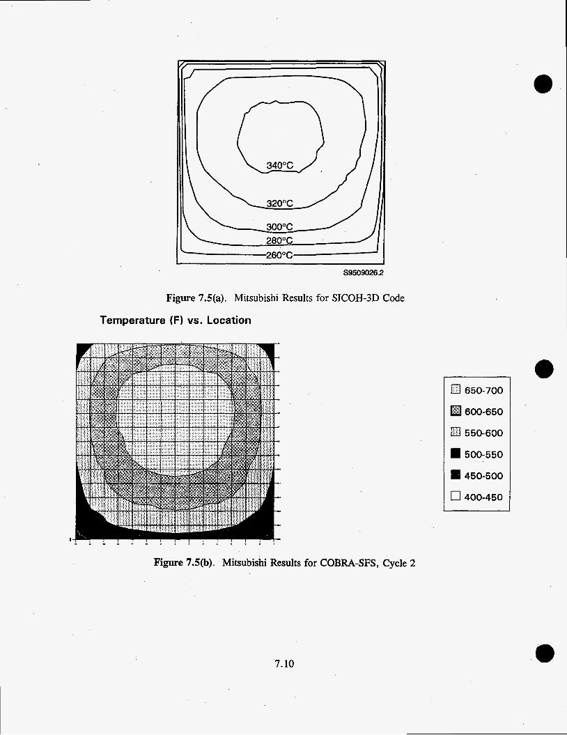
~~
S9509026.2
Figure 7.5(a). Mitsubishi Results for SICOH3D Code
Temperature (F) vs. Location
0 650-700
600-650
fzJ 550-600
500-550
8 450-500
0 400-450
Figure 7.5(b). Mitsubishi Results for COBRA-SFS, Cycle 2
7.10

7.2.3 BNFL 16 x 16 PWR Test Assembly
0 The test assembly built by BNFL consisted of a 16 x 16 array of zircaloy-4 tubes bound by nine spacer grids within a square aluminum canister (Fry et al. 1983). The tubes modeled typical PWR fuel, having an outer diameter of 0.42 in. (1.067 cm), and an axial heated length of 144 in. (365.8 cm). Heating elements were inserted inside the tubes in the assembly, except for the 20 tubes in the locations normally occupied by unheated control rod thimbles in a fuel assembly. The assembly was held in place within the aluminum canister by means of guide rails, two per side, between the canister wall and the support grid frames.
The heating elements were designed to give an extremely flat axial power profile representative of spent fuel. The radial power distribution was also uniform across the assembly cross-section. Temperature measurements were obtained at these 224 locations: at eight axial locations on 26 rods, and at four axial locations on the four sides of the canister.
The total hemispherical emissivity of the inside wall of the aluminum canister was measured at the start and end of the test program. The average measured value at the completion of the tests was 0.38, with a range of 0.36 to 0.40. However, results of measurements of the emissivities of the heater rod surfaces were more equivocal. Measured values varied from 0.42 to 0.93, indicating a large range in surface emissivities for the rods, which may also have been varying in time during the test.
The COBRA-SFS model represented the BNFL assembly using subchannel geometry similar to the models of the SAHTT and Mitsubishi assemblies. A diagram of the model is shown in Figure 7.6. The COBRA-SFS input model consisted of 289 subchannels, 256 rods, and 8 slab nodes modeling the walls of the canister. The rods and subchannels were numbered in the same pattern as illustrated for the SAHTT and Mitsubishi assemblies in Figures 7.2 and 7.4, respectively. In the BNFL test assembly, the rods in positions corresponding to control rod locations had zero power input, but were the same diameter as the rods modeling the fuel rods &e., d,,,,, = 0.42 in. [ 1.067 cm]).
The same friction factor correlations that were used in the SAHTT and Mitsubishi models were also used in the model of the BNFL assembly. The heat transfer correlations were also the same, except that the leading coefficient on the Reynolds number in the correlation for the laminar flow range was 1.39 instead of 0.83. A zero-flow boundary condition was used in the calculation, with constant boundary temperature on the top, bottom and sides of the assembly. An adiabatic boundary was assumed at the inlet and outlet ends of the horizontal assembly. Based on the measured data, the boundary temperature on the top surface (slab nodes 1 and 2; refer to Figure 7.6), was 254°C (489°F). On the bottom surface (slab nodes 5 and 6), the boundary temperature was 244°C (471°F). On the upper half of the vertical sides, (slab nodes 3 and 8), the boundary temperature was 255°C (491 OF), and on the lower half of the vertical sides (slab nodes 4 and 7), it was 250°C (482°F).
The grey body view factors for radiative heat transfer were calculated for the assembly using the RADGEN code. Surface emissivities were assumed to be 0.38 for the walls and 0.7 for the rods, The value of 0.38 is a good estimate of the wall emissivity, as obtained by post-test measurement. The value of 0.7 for the rods, however, is simply a rough average of the high and low measured values for the surface emissivities of the rods. The wide range of values obtained in post-test
7.11

I
Slab Jode 8
Slab rlode 7
Slab god6 3
Slab Uodt
4
1
s9505005.: @ Thermocouple Location
@ controt RW Simulator
Figure 7.6. Cross-Section of BNFL Test Assembly
measurements indicate that the local emissivities differed substantially from the average.
I
This is perhaps the greatest source of uncertainty in the model for this calculation, since radiative heat transfer was very significant in this test.
Results obtained with the COBRA-SFS model for BNFL test No. 007 are presented in Figure 7.7. In general, the code results predict temperature profiles across the assembly that are in good agreement with the measured data. The shape of the predicted and measured temperature distri- butions follow the same trends, and reach very nearly the same peak value. The code results are from 9°F (5°C) to 45°F (25°C) hotter than the measured values, but even the largest discrepancy is only about 5 % of the total temperature difference between the peak rod temperature and the boundary.
Since radiative heat transfer is the dominant mode for this case, a large part of the difference between the predicted and measured temperatures can be attributed to the unknown variation in local rod surface emissivities. This result underscores the importance of accurate and reliable input data for COBRA-SFS calculations. The predicted temperatures obtained with the code cannot be more accurate than the data on which the calculation is based.
7.12

BNFL: air, high power case
1000 950 900
& 850 Q) 800
750 700 650 600
c 550 500 450 400
- c
BNFL Test
0 COBRA-SFS
0 50 100 150 200 250
Rod Number Figure 7.7(a). Comparison of COBRA-SFS, Cycle 2 Results with BNFL Data: Rod
Temperature Profile on the Diagonal
BNFL: air, high power case ~
0 0
W a a a
a m a
7.3 Multiple-Assembly ShippingKtorage Cask Test Cases
BNFLTest
COBRA-SFS
1000 950 900 850
750 0
0
- 800 Q c 2 700 Q 650 f 600
550 c
500 450
Q)
4 0 0 i ; ; . : : ; : ; : : ; ' ; ' ~ ' ; ~ ; ~ ; ; ~ ; ' 0 50 100 150 200 250
Rod Number Figure 7.7(b). Comparison of COBRA-SFS Results with BNFL Data: Rod Temperature
Profiles; Top Face to Bottom Face
The real utility of COBRA-SFS lies in its ability to model large complex spent fuel storage systems using subchannel analysis, so that convective, conductive, and radiative heat transfer modes can be accounted for in appropriate detail. Comparison with single assembly tests is a useful and necessary step in the process of validating the code, but the acid test is the code's ability to predict the temperature field within a multi-assembly shipping or storage cask.
7.13
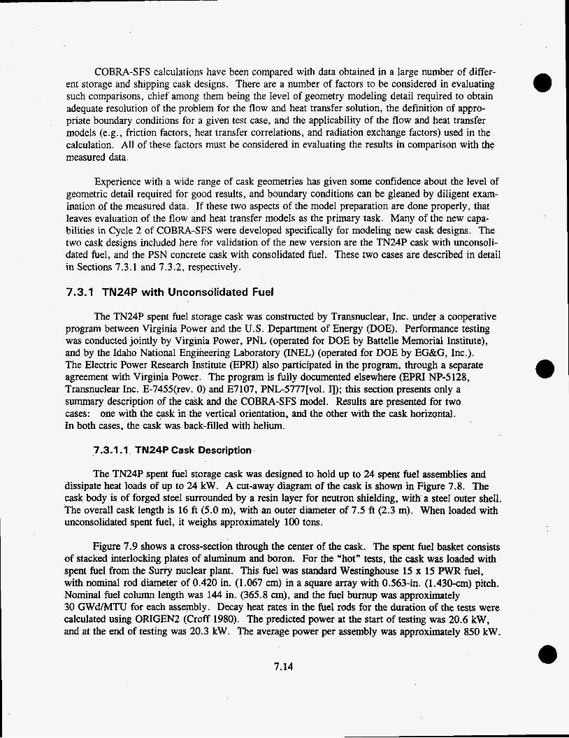
COBRA-SFS calculations have been compared with data obtained in a large number of differ- ent storage and shipping cask designs. There are a number of factors to be considered in evaluating such comparisons, chief among them being the level of geometry modeling detail required to obtain adequate resolution of the problem for the flow and heat transfer solution, the definition of appro- priate boundary conditions for a given test case, and the applicability of the flow and heat transfer models (e.g. , friction factors, heat transfer correlations, and radiation exchange factors) used in the calculation. All of these factors must be considered in evaluating the results in comparison with the measured data.
Experience with a wide range of cask geometries has given some confidence about the level of geometric detail required for good results, and boundary conditions can be gleaned by diligent exam- ination of the measured data. If these two aspects of the model preparation are done properly, that leaves evaluation of the flow and heat transfer models as the primary task. Many of the new capa- bilities in Cycle 2 of COBRA-SFS were developed specifically for modeling new cask designs. The two cask designs included here for validation of the new version are the TN24P cask with unconsoli- dated fuel, and the PSN concrete cask with consolidated fuel. These two cases are described in detail in Sections 7.3.1 and 7.3.2, respectively.
7.3.1 TN24P with Unconsolidated Fuel
The TN24P spent fuel storage cask was constructed by Transnuclear, Inc. under a cooperative program between Virginia Power and the U S . Department of Energy (DOE). Performance testing was conducted jointly by Virginia Power, PNL (operated for DOE by Battelle Memorial Institute), and by the Idaho National Engineering Laboratory (INEL) (operated for DOE by EG&G, Inc.). The Electric Power Research Institute (EPRI) also participated in the program, through a separate agreement with Virginia Power. The program is fully documented elsewhere (EPRI NP-5128, Transnuclear Inc. E-7455(rev. 0) and E7107, PNG5777[vol. I]); this section presents only a summary description of the cask and the COBRA-SFS model. Results are presented for two cases: one with the cask in the vertical orientation, and the other with the cask horizontal. In both cases, the cask was back-filled with helium.
7.3.1 .I. TN24P Cask Description
The TN24P spent fuel storage cask was designed to hold up to 24 spent fuel assemblies and dissipate heat loads of up to 24 kW. A cut-away diagram of the cask is shown in Figure 7.8. The cask body is of forged steel surrounded by a resin layer for neutron shielding, with a steel outer shell. The overall cask length is 16 ft (5.0 m), with an outer diameter of 7.5 ft (2.3 m). When loaded with unconsolidated spent fuel, it weighs approximately 100 tons.
Figure 7.9 shows a cross-section through the center of the cask. The spent fuel basket consists of stacked interlocking plates of aluminum and boron. For the “hot” tests, the cask was loaded with spent fuel from the Surry nuclear plant. This fuel was standard Westinghouse 15 x 15 PWR fuel, with nominal rod diameter of 0.420 in. (1.067 cm) in a square array with 0.563-in. (1.430-cm) pitch. Nominal fuel column length was 144 in. (365.8 cm), and the fuel burnup was approximately 30 GWd/MTU for each assembly. Decay heat rates in the fuel rods for the duration of the tests were calculated using ORIGEN2 (Croff 1980). The predicted power at the start of testing was 20.6 kW, and at the end of testing was 20.3 kW. The average power per assembly was approximately 850 kW.
7.14

a
s9505005.4
Figure 7.8. TN24P PWR Spent Fuel Storage Cask
Trunnion
. Neutron Shield
Six tests were run to assess the performance of the TN24P cask: three with the cask oriented vertically and three with the cask horizontal. In each orientation, tests were run with these three different back-fills: nitrogen, helium, and vacuum. A summary of the test matrix is given in Table 7.2.
7.15

s9505005.5
Figure 7.9. TN24P PWR Spent Fuel Storage Cask Cross-Section
The system was massively instrumented with thermocouples to obtain performance and boundary condition data during operation. These included 14 thermocouples attached to the inner wall and basket of the cask, 54 thermocouples in the fuel assemblies and basket, and 35 thermo- couples on the cask exterior.
The thermocouple locations were selected for measurement redundancy, to provide measures of expected temperature symmetries within the cask, and to define axial, radial and temperature profiles
7.16

Table 7.2. TN24P Cask Test Matrix and Peak Temperatures
Cask heat Ambient Estimated peak clad Run number Orientation Back-fill load (kW) temperature temperature
1 vertical helium 20.6 18°C (64°F) 221 "C (430°F) ~ ~~~
, 2 vertical nitrogen 20.6 20°C (68°F) 241°C (466°F)
3 vertical vacuum 20.6 20°C (68°F) 290°C (554°F)
4 horizontal helium 20.5 18°C (64°F) 215°C (419°F)
5 horizontal nitrogen 20.4 21°C (70°F) 256°C (493°F)
6 horizontal vacuum 20.3 19°C (66°F) 280°C (536°F)
for both the vertical and horizontal orientations. The peak clad temperature for each test was esti- mated using a cubic fit to the data from the thermocouples in the fuel assembly(a) and assuming a parabolic temperature distribution across the assembly.
COBRA-SFS calculations were performed for all six tests, but only two have been selected to present as part of the validation of Cycle 2. These are runs Nos. 1 and 4; the vertical and horizontal cases with helium back-fill. The COBRA-SFS models for these calculations are presented in the following subsection.
7.3.1.2 COBRA-SFS Model of the TN24P Cask
Two geometry models were needed to model the TN24P cask for COBRA-SFS. For the vertical tests, the cask could be represented with a one-eighth section of symmetry. With the cask in the horizontal position, however, the weight of the fuel assembly basket caused it to shift until it was in contact with the cask wall on the lower side. As a result, the only remaining plane of symmetry was the vertical one through the cask center. It was therefore necessary to model at least one half of the cask for the horizontal tests,
In both cases, however, the axial geometry modeling was the same, and consisted of 18 uni- form axial nodes, as shown in Figure 7.10. Flow and heat transfer connections to the cask at the top and bottom were modeled using the optional plenum model in the code, to provide connections for natural recirculation within the cask and conductive heat transfer through the cask ends (refer to Section 6.2.10 input group BDRY).
Figure 7.11 shows a cross-section of the model of a one-eighth section of symmetry of the cask. For simplicity, this diagram does not include the subchannel modeling of the individual fuel assemblies within the basket. The cask is represented with 51 slab nodes: 27 modeling the spent fuel
(a) Thermocouples in the fuel assemblies were inserted in the guide tube thimbles. There were no thermocouples on the fuel rods, so a direct measure of peak clad temperature was not obtained.
7.17

Upper Plenum Region
Subchannel+ Model
15 -
14 -
13 -
12 -
11 -
10 -
9 -
8 -
7 -
6 -
5 -
4 -
3 -
2 -
1 - -
Lower Plenum / Region
-1-
s9505005.6
Figure 7.10. Axial Noding for COBRA-SFS Model of TN24P Cask
basket, 12 for the cask body, 4 for the neutron shield, and 8 for the cask outer shell. The outermost nodes of the cask shell are zero-thickness boundary nodes to represent the cask surface temperature, and are used to calculate the appropriate contribution of radiative and convective heat transfer to the environment.
7.18

Steel Body
Neutron Shield
Shell
S9505005.7
Figure 7.11. COBRA-SFS Model of One-Eighth Section of Symmetry of TN24P Cask
Within the spent fuel basket, the fuel assemblies were modeled using subchannel analysis. In the one-eighth section of symmetry, there are two types of fuel assemblies; half-symmetry assemblies and whole assemblies. The half-symmetry assemblies were modeled with a subchannel array, as illustrated in Figure 7.12. In the assemblies of this type, the model includes 136 subchannels and 120 rods. Figure 7.13 shows the lumped rod-and-channel arrangement used to model the whole assemblies. Modeling studies (Rector et al. 1986a) have shown that this type of modeling gives adequate resolution of temperature gradients within an unconsolidated spent fuel assembly. This model requires only 57 channels and 105 rods to represent the assembly.
A cross-section of the model for a one-half section of symmetry of the cask is shown in Figure 7.14. In this model, the geometry takes into account both the shifting of the spent fuel basket to contact the inner cask surface on the bottom, and the shifting of the fuel assemblies within the basket. The cask is represented with these 191 slab nodes: 95 for the spent fuel basket, 48 for the cask body, 16 for the neutron shield, and 32 for the cask outer shell. In this model, all of the fuel assemblies were whole assemblies, and were represented with the same lumped channel model as was used for the whole assemblies in the one-eighth section-of-symmetry model (refer to Figure 7.13). In the model for the vertical orientation, it was assumed that the fuel assemblies were centered within their respective basket cells. In this half-symmetry case, however, the flow areas of the channels between the rod array and the assembly canister walls were adjusted to account for the shifting of the fuel assembly within the basket due to the horizontal orientation.
.7.19

@J TC Lance Location
s9503oy.14
Figure 7.12. Subchannel Model of One-Half Section of Fuel Assembly
COBRA-SFS predictions of the flow and temperature field within the TN24P cask require solving for conductive, convective, and radiative heat transfer. Conduction heat transfer within and between the slab nodes was modeled using thermal resistances based on the material properties of the walls and internals of the cask. The flow field within the cask was determined by imposing boundary conditions of uniform pressure drop in all channels, and zero net flow for the system. The friction factor for the momentum solution was specified at a value typical for square array rods, as
100 f =. - Re
Convective heat transfer within the cask was modeled with a heat transfer coefficient deter- mined for a Nusselt number of 3.66. This value comes from an analytical solution (Kays and Crawford 1980) of the energy equation for fully developed temperature and velocity profiles in a circular tube. Previous work (Wiles et al. 1986) has shown that this model gives the best overall results for nitrogen and helium back-fill at temperatures typical of spent fuel assemblies.
Radiative heat transfer within the cask was modeled using grey body exchange factors. The RADGEN code was used to calculate these view factors for the enclosures containing spent fuel rods. The option in RADGEN to sum view factors of lumped rods was used for the enclosures containing
7.20

Figure 7.13. Lumped Channel and Rod Model of Fuel Assembly
whole assemblies modeled as lumped channels and rods (see Section 6.3). For enclosures within the cask that did not contain rods, black body view factors calculated using the Hottel (Hottel and Sarofin 1967) crossed-string correlation method were specified by input along with the surface emissivities for the slab nodes comprising the open assembly walls. The grey body view factors were calculated automatically in COBRA-SFS .
Thermal boundary conditions on the exterior of the cask were specified by means of heat transfer coefficients on the sides, top and bottom. The outside of the cask was a smooth painted surface that was free to exchange heat with the environment by natural convection and radiative heat transfer. Separate heat transfer coefficients were defined for each region. Radiative heat transfer was calculated at all boundary surface nodes using the formula
o ( T , ~ - T24 I f
1 1 q r a d = - + - - I
This is identical to the expression for radiative heat transfer between two parallel plates. The ambient air was assumed to be a black body at 18.25"C (65°F).
7.21

0"
180" S9505005.8
Figure 7.14. COBRA-SFS Model of One-Half Section of Symmetry of TN24P Cask
7.22

The cask was placed upright on the bed of a rail car for the vertical tests, and natural convec- tion with the ambient air occurred on the top and sides of the cask. The heat transfer coefficient for the side surface was specified using a Nusselt number for a natural convection from a vertical cylinder in air at 1 atm (Lindeburge 19Sl), as
Nu = 0.l3(GrPr)lB
There was no natural convection directly on the bottom surface, but the rail car bed acted something like a cooling fin that exchanged heat with the ambient air by natural convection. The heat transfer coefficient was therefore formulated using the Nusselt number for free convection from a fin.
Heat transfer from the cask lid to ambient was modeled using an expression for the natural convection Nusselt number for a horizontal plate in air at 1 atm (Lindeburge 1981), as
Nu = 0.20(GrPr)"3
With the cask in the horizontal position, the Nusselt number for a vertical cylinder in air was used to approximate the heat transfer coefficient on both the ends and the sides.
7.3.1.3 COBRA-SFS Results with TN24P Cask Model
The results obtained with COBRA-SFS for the six tests in the TN24P cask are fully docu- mented elsewhere (EPRI-NP-5 128/PNL-6054). Sample results are presented here, to illustrate the performance of Cycle 2 in this analysis. Table 7.3 shows the peak clad temperatures predicted for the two tests selected for Cycle 2 validation. Note that the input files used for this testing were the pre-test models, so the Cycle 2 results compare most favorably with the reported pre-test predictions.
Sample data comparisons are shown in Figure 7.15 for the vertically oriented TN24P cask with helium back-fill (Run No. 1 in Table 73). The data in the graph of Figure 7.15(a) is from the thermocouple lance (DataD1-6) in the center assembly of the one-eighth section of symmetry. The calculated temperatures plotted on this graph are for rod No. 28 of the center assembly in the COBRA-SFS model. The data in Figure 7.15(b) are from the thermocouple lance (Data5-6) in the outer assembly
Table 7.3. Peak Temperature Predictions for TN24P-Cask Tests
COBRA-SFS predictions '
Peak clad temperature RUn Orientation/
number Backfill Pre-Test Post-Test Cycle 2
1 vertical, He 225C0(437"F) 220°C (428°F) 224°C (435°F)
4 horizontal, He 218Co(424"F) 222°C (431 OF) 220°C (428°F)
Estimated peak clad
temperature
21 1 "C (41 1 OF)
206°C (403°F)
'7.23

4.5 - 4
3.5
--
-- - E 3
5 2
-- 1
8 2.5 --
-- c1 v) 5 1.5 --
I 0.5
--
- -
D 1-5 Data vs COBRA-SFS Calculations
0 50 100 150 200 250 Temperature (C)
DataDl -5
--e--- CalcD 1 -5
Figure 7.15(a). Comparison of COBRA-SFS Calculations with Measured Temperatures in the Center Assembly of the TN24P Cask (vertical orientation, helium back-fill)
4
3.5
- 3 E
2.5
8 2
1.5 i5
- S
Q)
1
0.5
0
D5-6 Data vs COBRA-SFS Calculations
4.5
100 150 200 0 50 Temperature (C)
Data5-6 - Calc5-6
7.24
Figure 7.15(b). Comparison of COBRA-SFS Calculations with Measured Temperatures in the Outer Assembly of the TN24P Cask (vertical orientation, helium back-fill)

with one corner of the basket touching the inner surface of the cask shell. The calculated tempera- tures for the graph in Figure 7.15(b) are for rod No. 88 of the outer assembly.
In both comparisons, the COBRA-SFS calculations predict a slightly higher peak temperature than the data shows. However, these results are well within the uncertainty in the measurements, and the code results show the appropriate trends for the overall heat transfer solution.
Figure 7.16 shows a plot of the radial peak temperature profile through the centerline of the cross-section of the horizontal cask. The calculated temperatures are from the lower edge of the cask outer wall (location 0.0 on the graph) to the temperature at the upper edge of the cask outer wall (location 2.2835 m on the graph, corresponding to the cask outside diameter). The solid line on the graph represents the slab node temperatures through the thickness of the cask wall at the top and bottom, and the rod temperatures from the center row of rods in assemblies which lie on the vertical centerline of the cask cross-section (Figure 7.14).
The temperature data on the plot represent the thermocouple lance temperatures measured in the rod bundles corresponding to assembly Nos. 22, 1, 2, and 4 in the COBRA-SFS model. Note that these measured temperatures are not peak temperatures. The thermocouple lances were located within a guide tube thimble four rod rows from the bundle centerline. The agreement between the measured temperatures and the calculated values shown in Figure 7.16 is very good.
tn24h data vs COBRA-SFS Calc
0 0 50 100 150 200 250
Temperature (C)
tn24h Data
COBRA-SFS
Figure 7.16. COBRA-SFS Calculation of Top-to-Bottom Peak Temperature Profile Through the Centerline of the Cross-Section of the Horizontal TN24P Cask, Compared with Measured Temperatures
7.25

7.3.2 PSN Concrete Cask
The PSN spent fuel storage cask was constructed by Pacific Sierra Nuclear Associates'') for long-term storage of consolidated spent fuel from pressurized water reactors. Performance testing was conducted for DOE and PSN by PNL, and INEL. EPRI also participated in the program, as part of a cooperative program involving EPRI, DOE, PSN, and Wisconsin Electric Power Company, to evaluate horizontal modular storage systems for spent fuel.
Testing was conducted at INEL's Test Area North (TAN) cask testing facility. The pretest preparations, performance testing, and post-test activities are fully documented elsewhere (EPRI TR-100305). Only summary descriptions of the cask and COBRA-SFS model are presented here, along with results obtained with the test cases selected for validation of Cycle 2. These are the two cases with vents fully open, one with helium back-fill, and the other with nitrogen back-fill.
7.3.2.1 PSN Concrete Cask Description
The VSC-17 spent fuel storage system designed by PSN is a passive container for storing up to 17 assemblies or canisters of irradiated nuclear fuel. The system consists of a Ventilated Concrete Cask (VCC), and a Multi-Assembly Sealed Basket (MSB). Diagrams of the cask structure are shown in Figure 7.17, with vertical and horizontal cross-sections. The concrete shell is a one-piece cylinder 20-in. (50-cm) thick, with a steel inner liner. The shell provides structural support, radiation shield- ing, and an annular path for natural convection cooling of the basket assembly. The cask weighs approximately 80 tons empty, and 110 tons when fully loaded with consolidated fuel.
The concrete of the cask bottom is an integral part of the cask shell, as shown in Figure 7.17, not a separate piece fastened to the concrete annulus forming the body of the cask. The cask bottom consists of a concrete slab 22-in. (56-cm) thick, with a steel plate on the inner surface that forms the bottom of the internal cavity. The cask lid consists of a steel weather cover capping the concrete annulus. The steel plate is bolted to the top of the steel liner over a sheet rubber seal. The lower side of the cask lid is formed by the lid of the basket assembly, which consists of two steel plates with neutron shielding material sandwiched between them.
The basket assembly is of pressure vessel grade steel, and consists of an outer shell, the shield lid, and the fuel guide sleeve assembly, as shown in Figure 7.18. There is sufficient clearance between the outer shell of the basket and the storage sleeve assembly to ensure that differential ther- mal expansion during operation will not result in load transfer between the two structures. Interior structural support for the basket is provided by three steel shells wrapped around the framework of the fuel guide sleeves at the top, bottom, and middle of the assembly, as shown in Figure 7.18. These basket support structures are welded to the outer edges of the framework of the fuel guide sleeves and to the inner surface of the basket outer shell.
(a) Pacific Sierra Nuclear Associates became Sierra Nuclear Corporation; in some of the docu- mentation of the cask design and testing, SNC is used interchangeably with PSN in reference to the cask manufacturer.
7.26

/ Lifting Lug
LMSB Lug
90
Figure 7.17. Diagram of PSNNSC-17 Cask Structure
The basket lid is sealed with two O-rings, one of steel and one of elastomer, to provide a gas- tight seal to hold a back-fill of helium, nitrogen, or vacuum. The depth of the cask cavity is suffi- cient to accommodate BWR fuel; therefore, an MSB support assembly is required when the cask is loaded with PWR fuel, as illustrated in Figures 7.17 and 7.18. This support assembly allows free circulation of air from the vented annulus along the underside of the basket assembly within the cask cavity.
Decay heat generated in the spent fuel is transmitted through the basket wall to the air in the annulus between the basket and the concrete shell. Natural circulation brings cooling air in through the bottom vents and exhausts it to the environment through the top vents. The'inlet and outlet vents are steel-lined penetrations arranged in a cruciform pattern, with the flow path constrained by a stepped structure to minimize radiation streaming, as illustrated in the cross-sectional diagrams in Figure 7.17.
The cask was instrumented with pressure transducers in the cask cavity, and a total of 98 ther- mocouples to measure thermal performance. Ten thermocouples were attached to the outer surface of the cask, five to the MSB lid, and two to the weather cover. Ten were embedded in the concrete,
7.27

- Shield Lid
7) : e- RX-277 (Neutron Shield)
Fuel Guide Sleeve Basket Support Structure
Ventilating Holes
MS8 Support Assembly
5950601 8.5
Figure 7.18. PSNNSC-17 Cask Multi-Assembly Sealed Basket
nine were attached to the outside surface of the basket shell, nine to the steel inner liner of the concrete shell, and one was installed in the center of each air inlet and outlet vent. The basket internals were instrumented with seven thermocouple lances containing a total of 42 thermocouples, which were inserted into selected guide tubes within six of the fuel canisters. The axial and radial locations of the thermocouple lances were selected to allow evaluation of temperature symmetry and axial and radial temperature profiles in the cask.
The cask was loaded with Westinghouse 15 x 15 PWR spent fuel from the Surry 2 and Turkey Point plants. The fuel had been removed from the normal 15 x 15 rod array and consolidated with the rods from two fuel assemblies in each canister. The canisters were of stainless steel, and con- sisted of a base and top locking cover, as. shown in Figure 7.19. Each canister was loaded with 408 fuel rods, stacked on a triangular pitch. The top and bottom plates of the canister did not provide a gas-tight seal, but nevertheless severely limited the gas flow rate into or out of the canister.
Decay heat rates for the fuel were calculated from measured properties of the fuel using the OTUGEN2 computer code. Decay heat from the individual canisters ranged from 700 to 1050 watts, with an average of about 877 W per canister. The canister placement was selected to produce a
7.28

Canister Cover
Spent Fuel Rods
TC Lance Guide Tube
' Canister Base Plate S9506018.4
Figure 7.19. Cross-section of Consolidated Fuel Assembly
one-eighth symmetry in heat generation within the basket, and to produce the maximum fuel temperature in the center of the MSB. The OIUGEN2 code was also used to predict the axial decay heat profiles, which are required for the COBRA-SFS model of the system.
Performance testing of the VSC-17 cask consisted of six test runs with three internal environ- ments and four cask venting configurations, ranging from vents fully open to vents closed. In all tests, the cask was oriented vertically. Table 7.4 summarizes the test conditions.
COBRA-SFS calculations were performed for all six tests, both pre- and post-test, and are fully documented elsewhere. For purposes of validating Cycle 2, only two test cases are summarized here. Both are with vents fully open, one with helium backfill, the second with nitrogen (Nos. 1 and 5 from Table 7.4). Essentially the same model was used for both cases, the only significant differences being in the fluid properties, the boundary conditions, and the constraints on the flow paths into the air annulus between the basket assembly and the concrete cask shell. The COBRA-SFS input model for the PSNNSC-17 cask is described in the following subsection. ,
7.3.2.2 COBRA-SFS Model of PSN Cask
Geometric and power distribution symmetries allowed modeling of the VSC-17 cask with a one-half section of symmetry. The axial geometry of the cask is modeled with 12 axial nodes, plus a lower plenum region and an upper plenum region which are modeled using the optional plenum model
7.29

number
1
2
3
4
5
6
Cask heat load Back-fill (kW)
helium 14.9
helium 14.9
helium 14.9
helium 14.9
nitrogen 14.9
vacuum 14.9
Table 7.4. PSN/VSC-17 Cask Test Matrix and Peak Temperatures
Ambient Estimated peak temperature clad temperature
21°C (70°F) 321°C (610°F)
23°C (73°F) 334°C (633°F)
23°C (73°F) 378°C (712°F)
22°C (72°F) 381°C (718°F)
24°C (75°F) 376°C (709°F)
24°C (75°F) 397°C (747°F)
vent configuration
all open
2 inlet vents blocked
all inlet vents blocked
all inlet and outlet vents blocked
all open
all open
in the code. A diagram of the axial noding is shown in Figure 7.20. All channels, rods, and slabs see the same axial noding, but flow and heat transfer connections to the plena are determined by user input for specific channels and slab nodes.
The physical structure of the cask is modeled with 280 slab nodes representing the concrete shell, steel liner, basket shell and assembly, and the fuel canisters. Figure 7.21 shows a cross- sectional diagram of the COBRA-SFS model, with 10 slab nodes for the MSB outer shell, 30 for the steel liner, and 50 slab nodes modeling the cask concrete shell. The outermost ten of these nodes are zero-thickness surface nodes, for accurately calculating the contribution of radiative and convective 'heat transfer to the environment. Figure 7.22 shows a more detailed cross-sectional diagram of the COBRA-SFS model of the structures within the multi-assembly basket. The basket itself is modeled with 122 slab nodes, and the fuel canisters within the basket are modeled with 68 slab nodes.
Because of the close packing of the rods and the consequent flatness of the radial temperature gradient across the fuel array, the rods within each canister were modeled by lumping rings of rods into average rods with total power generation equal to the sum of all the rods each average rod represents. Figure 7.23 illustrates the rod lumping pattern for one assembly. All assemblies used this pattern, including those cut by the line of symmetry.
The flow subchannels within the fuel canisters were also lumped into average channels, con- sisting of all the subchannels enclosed between two radial rings of rods combined in the lumped rod model. The gap between the outermost rods and the canister wall was modeled with a single average channel on each wall, on the assumption that the close-packed triangular array of rods would remain centered within the canister. This assumption is somewhat unphysical, given the actual geometry of the canister, as illustrated in Figure 7.19, but it is conservative in that it presents the greatest possible thermal resistance for heat transfer between the rods and the wall of the canister. It also avoids the
7.30

Upper Plenum
Region \ Axial Level
subc Mc
- 12
11
nnel 6 41
Lower Plenum Region
S9506018.3
Figure 7.20. Axial Noding for COBRA-SFS Model of PSNNSC-17 Cask
problem of having to determine the actual orientation of the fuel rods within the canister, and having to obtain estimates of appropriate values for contact resistance between the rods and the wall.
The axial decay heat power profile determined from ORIGEN2 calculations was applied to all fuel, and the radial power distribution was also determined from ORIGEN2 calculations that were based on gamma scans of spent fuel from the Turkey Point plant. This fuel was similar to the fuel actually loaded into the cask.
As with the TN24P cask, the COBRA-SFS predictions for the flow and temperature fields within the PSNNSC-17 cask required solving for conductive, convective, and radiative heat transfer. Conduction heat transfer in the nodes modeling the solid structure of the cake was modeled using
7.31
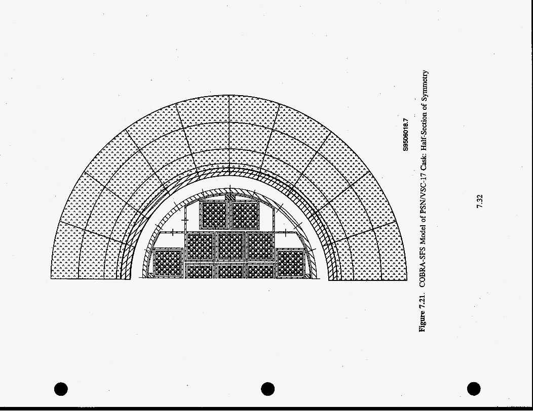
U

5950601 8.8
Figure 7.22. COBRA-SFS Model of Structures Within the MSB in the PSN Cask
7.33

5950601 82 Figure 7.23. COBRA-SFS Model of Consolidated Fuel Assemblies in PSN Cask
thermal resistances based on the material properties of the cask body and internals. The flow field within the MSB was modeled by imposing an unspecified uniform pressure drop on all assemblies within the basket, and a zero net flow boundary condition. The flow boundary conditions on the assembly representing the annulus between the MSB and the concrete shell, which was open to the atmosphere through the cask vents, were modeled with a specified pressure drop corresponding to the gravity head of a column of air (at ambient temperature and pressure equal to the height of the distance between the cask inlet and outlet vents). For ambient conditions of 0.1014 Mpa (14.7 psia) and 25°C (77"F), the pressure drop is 48.5 Pa (0.00703 psi).
Axial friction losses in the assemblies containing fuel rods were specified at a value typical for close-packed rods, as
40.0 f = - Re
7.34

In the open assemblies within the basket, and in the annulus between the basket and the steel- lined concrete shell, the friction factor was specified at a value typical for low-speed flow in a duct, as
f = max(f, ,f,)
where < = 0.0850 Re-'.*'
f, = 96.0 Re-'.'
For the narrow gap between the fuel canisters and the supporting basket structure, it is assumed that the flow will always be laminar, and the laminar flow correlation given above for the vented annulus is used in those assemblies as well.
Form drag losses due to the structure of the end closures on the fuel canisters were modeled using a very large loss coefficient of 9.0 x (10s) at the top and bottom of each assembly with fuel rods. For the open assemblies within the basket, the inlet and outlet losses were modeled with a more modest loss coefficient of 1.5. Inlet and outlet losses for the annular assemblies, which included the annuli between the fuel canisters and the basket cells, and the annulus that was vented to the atmosphere, were specified with a loss coefficient of 6.0. The channels comprising this annular assembly also included area variations to simulate the effects of the flow paths through the inlet and outlet ports.
Because of the extremely low flow rates in the channels formed by the close-packed rods within the assemblies, heat transfer between the rods and the fluid is modeled with a Nusselt number of 1.0, on the assumption that the dominant mode would be conduction. In the open assemblies within the basket, however, convection can play a more significant role in the heat transfer. For channels in these assemblies, the Nusselt number is defined using the relation
@
Nu = max(Nu,,Nu,)
where NU, = 0.102 Reo.914Pro.4
NU^ = 4.80
For the natural recirculation of air through the assembly modeling the annulus vented to the atmosphere, the Dittus-Boelter heat transfer coefficient was used for turbulent flow, with a constant value for laminar flow. For these channels, the Nusselt number defined as
Nu = max(Nu,,Nu,)
where Nu, = 0.023 Reo-8
Nu, = 7.54
7.35

Radiative heat transfer within the cask was modeled using grey body exchange factors calcu- lated with the RADGEN code for the assemblies containing fuel rods. For the open assemblies within the basket, and for the annulus surrounding the basket, the black body view factors were specified in the COBRA-SFS input, and the code automatically calculated the grey body view factors for these enclosures. For radiative heat exchange with the environment from the cask exterior, the same models as those employed in the TN24P calculations were used.
Measured
316°C (601°F)
366°C (691°F)
7.3.2.3 COBRA-SFS Results for PSN Cask Model
~
COBRA-SFS COBRA-SFS predict ion Measured prediction
317°C (602°F) 69°C (157°F) 72°C (162°F)
376°C (708°F) 72°C (161°F) 83°C (182°F)
The results obtained with COBRA-SFS for the tests performed in the PSNNSC-17 cask are documented elsewhere. Sample results are presented here, to illustrate the performance of Cycle 2. Table 7.5 shows the peak clad temperatures in the fuel and in the concrete shell of the cask for the two validation tests.
For the helium case, the peak clad temperature predicted with COBRA-SFS is within 1°C of the measured value, and the peak temperature in the concrete is within 3°C of the measured value. This is a difference of less than 0.5% for the peak clad temperature, and a difference of about 4% for the peak temperature in the concrete. These results are well within the uncertainty in the measured values, and show that COBRA-SFS does an excellent job of predicting the heat transfer for conditions where conduction is dominant.
For the nitrogen case, the code overpredicts the peak clad temperature by 1O"C, and also overpredicts the peak temperature in the concrete by 11 "C. The predicted values are in reasonable agreement with the data, but the larger differences reflect the greater sensitivity of the results to modeling uncertainties when convective heat transfer is more important.
Figures 7.24 and 7.25 show calculated and measured axial temperature profiles in the PSNNSC cask for the helium and nitrogen back-fill cases, respectively. The measured temperature profile from the thermocouple lance in the center assembly is compared to the calculated peak rod temperature. Measured temperatures from the multi-assembly basket are compared with the calcu- lated temperatures in slab node 94, the slab node corresponding most closely with the thermocouple locations on the MSB. The measured temperatures on the cask surface within the vented annulus are compared to the calculated temperatures in slab node 83, modeling one segment of the cask shell.
Table 7.5. Peak Temperature Predictions for PSNNSC-17 Cask Tests
Run 1 Vent config./ number Back-fill
5 I all opednitrogen
Peak Clad Temperature I Peak Concrete Temperature 11
7.36

Data vs COBRA-SFS Calculations (Helium)
1.5
1
0.5
o *
4.5
4
3.5
- 3 E g 2.5
8 2
1.5
1
0.5
0
- C
v)
I I
I I
-- --
0: A I I I
-- Q : A I '
I
~~
PSN cask
* MSBshell
0 TC lance
CalcPSN
CalcTC lance
0 50 100 150 200 250 300 350 Temperature (C)
Figure 7.24. Comparison of COBRA-SFS Calculations with Measured Temperatures in the PSNNSC- 17 Cask; vertical orientation, vents open, helium back-fill
Data vs COBRA-SFS Calculations (Nitrogen)
3 t I
I P I A
I 2-5 1 p 1 I
2
0 100 200 300 400 Temperature IC)
CalcPSN cask CalcMSB Calc TC lance -
Figure 7.25. Comparison of COBRA-SFS Calculations with Measured Temperatures in the PSNNSC-17 Cask; vertical orientation, vents open, nitrogen back-fill
7.37

For both the helium back-fill case (Figure 7.24) and the nitrogen back-fill case (Figure 7.25), the COBRA-SFS calculations are in good agreement with the measured temperatures. These results are well within the experimental and modeling uncertainties inherent in the comparison.
Sun RS6000 Intel
818.09 176.21 249.64
4599.66 988.69 641.26
3494.54 714.33 482.17
7.4 Validation on Alternative Platforms
In transferring the COBRA-SFS code to a new computing platform, the first concern is to determine that the code gives the same results as before. Also of interest, however, is how well the code runs on the new platform. In general, the main motivation for moving to a different platform is usually to gain some improvement in performance. For this code, improved performance means faster number-crunching .
DEC HP9000 Macintosh
107.80 217.00 366.00
641.26 1334.00 4131.00
482.17 980.32 1594.00
The code was originally developed to run on large mainframe computers, such as the CDC and Cray machines. With the advent of powerful desktop workstations, however, the code has shown itself easily adaptable to the new computing environment (see Section 8.4). Versions of the code have been developed for the Sun SPARCstation, the IBM RS6000, an IBM clone with a Pentium proc- essor, the SUN4 and DEC workstations, Hewlett-Packard’s HP9000 workstation, and the Macintosh workstation.
Validation test cases have been run on these platforms to verify that the code gives the same results for the various versions. The run times for the validation cases on the various platforms are summarized in Table 7.6. The three test cases consist of models of one small test assembly and two relatively large multi-assembly casks.
The Mitsubishi test case is a model of a single-assembly test section, consisting of 256 sub- channels, 225 rods, and 8 slab nodes (see Section 7.2.2). The TN24P test case is the one-eighth section of symmetry model of the vertical cask with helium back-fill. This model contains 7 assem- blies, with a total of 389 channels, 450 rods, and 51 slab nodes (see Section 7.3.1.2). The PSN test case is the half-section of symmetry model of the PSNNSC-17 cask with nitrogen back-fill, vents fully open. This model contains 22 assemblies, with a total of 214 channels, 130 rods, and 249 slab nodes (see Section 7.3.2.2).
Table 7.6. Run Time on Alteinative Platforms (cpu seconds)
Test case
Mitsubishi
TN24P
PSN cask
Platforms
CRAY (UniCOS)
80.10
2189.18
546.61
7.38

The only significant differences observed in these test case results are in the run times on the different platforms. As might be expected, the newer platforms are significantly faster than the older ones. It should be noted that the run times for all of the workstations compare quite favorably to the run times on the Cray mainframe.
0
e 7.39

8.0 Code Structure and Installation
This section describes COBRA-SFS from the programmer’s standpoint. Section 8.1 describes the functional hierarchy in the code, and Section 8.2 presents a brief description of each subroutine. The dimension parameters used to define the sizes of the various arrays in the code are described in Section 8.3. This section also includes the dimension parameters for the RADGEN code. Platform- dependent coding is described in Section 8.4. Installation instructions and a description of the files that make up the code package are included in Section 8.5.
8.1 Functional Hierarchy of COBRA-SFS
The COBRA-SFS code is derived from COBRA-WC (George et al. 1980) and retains essentially the same structure. The main program COBRA, calls various routines to process the input and set up the problem, to perform the solution, and to process the output. At the beginning of a case, subroutine CLEAR is called to zero all common blocks. After the input has been processed, the boundary conditions are set (or updated for the new time step values in transient cases), and the solution is performed. After the solution is complete, the output routines are called to write information to the output files, and to save a restart file.
8.1.1 input Routines
In program COBRA, subroutine ECHO is called to write the input file verbatim to the output file, providing an exact record of the input for future reference in archived output files. The input is then processed, by execution of the driver routine for the input processing, subroutine SETUP. Subroutine SETUP calls subroutine SETIN, which reads the input group by group, from logical unit 2. The one exception is geometry input, group CHAN. Subroutine SETIN calls subroutine GROUP4 to process the input for group CHAN. After the input is read, subroutine SETUP calls subroutine SETOUT to process the input, fill the various arrays required for the problem description, and initialize the flow and energy field variables.
On a restarted case, the restart file is read from logical unit 9, in subroutine RESTRT. (This file would have been created in a previous run, in which the common arrays are written to logical unit 8 for each time step.) On a restart, additional input may also be read from the input file on logical unit 2, to define such things as changed boundary conditions, new forcing functions, or different models and correlations. This new input is processed through SETUP, as described in Section 6.0.
\
8.1.2 Solution Routines
After the input is processed, control renuns to the main program COBRA, and the calculation enters the time step loop. Arrays are filled with the specified boundary conditions, various control parameters are set, and the solution is initiated by calling subroutine RECIRC. Subroutine RECIRC is the driver routine for the solution, and also performs the solution of the mass continuity equation for each cell of the system, and the axial rebalancing.
8.1

Each external iteration of the solution procedure begins with an axial sweep of the system from the bottom to the top axial level. In this sweep, subroutine ENERGY is called to solve the fluid and wall node energy equations. If the plenum model is specified by user input, heat transfer to or from the upper and lower plena is calculated by calling subroutine EXPROP. Subroutine REHEAT is called to calculate the heat flux terms for heat transfer connections between rod, slab and fluid nodes, and subroutine HOTROD is called to solve for the temperature of the rod surface. This will include internal rod material temperatures, if the appropriate options have been specified and fuel material properties defined by the input. Subroutines MOMENT and DIFFER are called to solve the axial and lateral momentum equations for the fluid nodes. After the fluid energy equation has been solved, subroutine PROP is called to calculate new values for the fluid and material properties.
The continuity equation is then solved, with optional axial rebalancing, in a level-by-level and channel-by-channel internal iteration. The rebalancing is performed in subroutine ONED, and the pressure matrix is solved by calling a banded matrix solver in subroutine SOLVER. When the internal iteration on the continuity solution is completed, new pressures are calculated and the maximum energy, momentum, and continuity errors are evaluated. If these errors meet the convergence tests, the solution is complete. If not, the solution continues on to the next external iteration, but first checks for negative axial flows in the system. If any are found, subroutine ENERGY is called for a reverse sweep of the system, from the top axial level to the bottom.
At the completion of each external iteration, a summary line containing the current value of the peak clad temperature, its location, and all convergence errors is written to the output file. The solution continues iterating until all convergence criteria have been satisfied, or the maximum number of iterations is exceeded. Subroutine RECIRC then returns control to the main program, for processing of the output. If the problem is a transient, the solution is repeated for the next time step.
8.1.3 Output Routines
Main program COBRA calls subroutine RESULT to write the output data to logical unit 3. This output consists of fluid conditions (pressure drop, enthalpy, temperature, density, flow rate, mass flux, and velocity) for each node in all channels, flow conditions (mass flux and velocity) in each node of all gaps for crossflow between channels, temperatures for all rod nodes, slab nodes, and boundary nodes, and plenum fluid and solid node temperatures. The default is to print all information about all solid and fluid nodes, but the level of detail can be regulated by user-input, to specify output only for certain channels, rods, gaps, and walls.
In addition to the printer output file, COBRA also calls subroutine DUMPIT to save a restart file for the case, on logical unit 8. If the option has been specified by input, subroutine POST is also called from COBRA to write information to a file on logical unit 1 for post-solution plotting.
8.2

call list arguments: areafijx) j - axial level index jx - axial level index
8.2 Subroutine Descriptions
The COBRA-SFS code consists of the main program COBRA and 32 subroutines. This subsection describes each subroutine in the code. The call list is given, with the definition of each variable in the list, along with a brief explanation of the routine’s function. The first routine described is the main program COBRA; the subroutines are listed in alphabetical order.
Main Program COBRA
This is the driver routine for the COBRA-SFS code. It calls the input routines to set up the problem, and contains the time step loop to drive the solution in both steady state and transient calculations. When the solution is complete, it calls the output routines to report the results of the calculation.
Program COBRA calls subroutines DATTIM, CLEAR, ECHO, RESTRT, RESULT, SETUP, CURVE, PROP, PREFIX, RECIRC, POST,and DUMPIT.
Subroutine AREA
This subroutine fills the channel geometry arrays, based on the input provided in groups CHAN and VARY. It fills the axial cross-sectional area array for each node of each channel, and calculates the local hydraulic diameter using the input values for area and wetted perimeter. It also fills the gap width array with the input values, and calculates all area and gap-width variations specified by input in group VARY.
Subroutine AREA calls CURVE, and is called by RECIRC and SETIN.
subroutine CLEAR
This subroutine sets all elements of the common blocks to zero. It uses the function LOCA to find the beginning and ending addresses of a common block, and sets to zero all addresses in between those endpoints. This subroutine is called at the beginning of each case.
call list arguments: none
Subroutine CLEAR calls function LOCA. Subroutine CLEAR is called by main program COBRA.
8.3

Subroutine COLOC
This subroutine sets up the geometric locations of the boundaries of the fuel collocation nodes, to be used in the calculation of the fuel internal temperatures when the fuel collocation model is specified by input.
call list arguments: coloc(ia,isym,kft,kk,rmin,rmax,rcl,tcl) ia - flag for noding geometry:
= 1; planar geometry = 2; cylindrical geometry
= 2; solid fuel = 1; anhular or plate fuel
kft - fuel type index kk - absolute value of fuel type flag rmin - inner fuel radius (inches) rmax - outer fuel radius (inches) rcl - cladding radius (inches) tcl - cladding thickness (inches)
isym - flag for fuel geometry:
Subroutine COLOC is called by SETIN.
Subroutine CURVE
This subroutine performs linear interpolation in tabular arrays. It is called to determine axial geometry variations, fluid and material properties, and boundary condition values.
call list arguments: curve(fx,x,f,y,n,j,isave) fk X f y n j - error flag;
isave - flag to use the same interpolation ratio as calculated
- dependent variable for interpolation - independent variable for interpolation - dummy array for the dependent variable - dummy array for the independent variable - number of elements in the interpolation table
= 10; indicates subroutine CURVE for output message
in last call to subroutine CURVE
Subroutine CURVE is called by main program COBRA, and subroutines AREA, DIFFER, ENERGY, EXPROP, NETWORK, POST, PROP, REHEAT, RESULT, and SETIN.
Subroutine DA'ITIM
This subroutine calls various system routines to determine the time and date of a calculation, and the cpu time used during execution. It contains platform dependent coding.
8.4

call list arguments: dattim(iopt,alph,xivar) iopt - flag for target calculation;
= 1; find elapsed cpu time = 2; find clock time = 3; find current date
alph - alphanumeric array containing formatting information for time
xivar - current clock time and date printout
Subroutine DATTIM calls system routines that provide date and time functions. It is called by main program COBRA, and subroutines ENERGY, MOMENT, POST, RECIRC, REHEAT, RESULT, and SETUP.
Subroutine DIFFER
This routine is used to calculate the coefficients for the momentum solution and radial conduction in the fluid. It consists of four parts, which are called from different portions of the momentum and energy solution. Part 1 calculates the terms for the fluid energy equation. Part 2 calculates the crossflow resistance term and turbulent cross-flow mixing for the momentum solution. Parts 3 and 4 calculate the local loss coefficients in each node due to grids and other obstructions in the flow field. The Reynolds number dependencies for the momentum equations are also calculated for each node, based on local fluid conditions.
call list arguments: differ(ipart,j,jx) ipart - flag for different parts of the subroutine j - axial level index jx - axial level index
a Subroutine DIFFER calls CURVE, and is called by MOMENT and RECIRC.
Subroutine DUMPIT
This subroutine writes out the solution arrays and calculated results to a binary file on logical unit 8, for use in a future restart. All information needed to obtain a complete output of the calculation is saved, along with all arrays needed to continue the solution for more iterations or more time steps.
call list arguments: dumpit(ntsave) ntsave - index number of the time step being written to the
dump N e on lun 8.
Subroutine DUMPIT calls Function LOCA, and is called by main program COBRA.
8.5

Subroutine ECHO
This subroutine writes a line-for-line listing of the input file to the output file.
call list arguments: none
Subroutine ECHO is called from main program COBRA.
Subroutine ENERGY
This subroutine sets up and solves the combined rod and fluid energy equations at each axial level using the method of over-relaxation. New values of the fluid enthalpy are determined for each node at each axial level, and new slab node temperatures are also calculated. When the plenum model is used, the subroutine EXPROP is called to determine the upper and lower plenum temperatures.
call list arguments: energyQ,jpl,jml,ipart) j - axial level index jpl - index of next axial level jml - index of previous axial level ipart - flag for direction of solution sweep;
= 1; from bottom to top = 2; from top to bottom
Subroutine ENERGY calls subroutines DATTIM, CURVE, and EXPROP. Subroutine ENERGY is called by RECIRC.
Subroutine EXPROP
This subroutine sums the exit flows and enthalpies at the top and bottom of the channels when the plenum model is used, and calculates the average mixed fluid temperature for the upper and lower plenum. The regional temperatures for the plena are also calculated, based on heat transfer from the fluid, and conduction from slab nodes in contact with the plenum regions.
call list arguments: exprop(jjx,ll) j - axial level index jx - axial level index 11 - plenum flag;
= 1; lower plenum = 2; upper plenum
Subroutine EXPROP calls CURVE to determine local fluid properties, and is called by ENERGY.
Subroutine FORCE
This subroutine calculates the forced diversion crossflow due to form losses seen by the axial flow in the channels.
8.6

call list arguments: forceujx) j - axial level index jx - axial level index
Subroutine FORCE is called by RECIRC.
Subroutine GROUP4
This subroutine reads the input for group CHAN in the processing of the input stream. It is called by subroutine SETIN, and calls subroutine LIMITS to check dimension parameters against the problem input.
call list arguments: group4(ierror) ierror - error flag
Subroutine GROUP4 calls subroutine LIMITS.
GROUP4 is called by SETIN.
Subroutine HOTROD
This subroutine solves for the temperature distribution in each fuel rod, using the fluid temperature and a boundary condition.
call list arguments: hotrod(j,jx) j - axial level index jx - axial level index
Subroutine HOTROD is called by RECIRC.
Subroutine LIMITS
Subroutine LIMITS is called during the processing of the input to check the problem input against the dimensions specified in the parameter statements in the compiled version of the code. If the input exceeds the allowed dimensions, an error message is written to the output file and execution terminates.
call list arguments: limits(num,minval,maxval,avar,apar,agroup,card,error) - value specified by input - minimum value permitted for num - maximum value permitted for num - alphanumeric identifier for variable num - alphanumeric identifier of parameter num is to be
- alphanumeric identifier of current input group
num minVal maxval avar aPar
agrOUP checked against
8.7

card error
- input line number - alphanumeric error flag;
= no ; num is within permitted limits = yes ; num is outside permitted limits
Subroutine LIMITS is called by GROUP4 and SETIN.
Subroutine LOAD
Subroutine LOAD is a generalized input processor that reads information from the input file for selected input lines that specify data in tabular form.
call list arguments : load(x, y ,z,min,max,limit ,step,image,card,lu) X - first dummy input array Y - second dummy input array Z - third dummy input array min - number of elements in the input table max - maximum number of entries permitted in the input table limit - maximum number of table entries on a single line of input step - number of elements in a set for a table entry image - alphanumeric variable carrying format description; 12e5 .O card - input line counter lu - input file logical unit number
Subroutine LOAD is called by SETIN.
Function LOCA
This function uses a system routine to determine the address of a specific variable. The system routine is platform dependent. The variables correspond to the endpoints of the common blocks, and are used in subroutine CLEAR to find the beginning and end of memory locations to set to zero before initiating a new COBRA-SFS calculation.
call list arguments: loca(ae,ab) ae ab
- ending variable of a common block - beginning variable of a common block
Function LOCA is called by subroutines CLEAR, DUMPIT, and RESTRT. Function LOCA calls a system routine such as %loc, locf, or loc, depending on the platform version.
Subroutine MIX
This subroutine calculates the turbulent cross-flow mixing parameter for the momentum equation, using a user-specified correlation.
8.8

call list arguments: mix@ j - axial level index
Subroutine MIX is called by subroutines MOMENT and RECIRC.
Subroutine MOMENT
This subroutine solves the linearized momentum equations for the axial and lateral directions. The flow in all channels is solved at each axial level by direct elimination, using the matrix solver in subroutine SOLVER. MOMENT is called twice from the solution driver routine, RECIRC. In the first call, the flow and flow derivatives are initialized for the first axial level only. In the second call, the flow and flow derivatives are calculated for the current axial level. The optional models for fluid- fluid shear are also included, when specified by user input.
call list arguments: moment(i,jx,jml j p l ,ipart) j - axial level index jx - axial level index jml - previous axial level jpl - next axial level ipart - flag for subroutine section;
= 1; section for axial level 1 = 2; section for axial levels j > 1
Subroutine MOMENT calls subroutines DATTIM, DIFFER, MIX, and SOLVER.
Subroutine MOMENT is called by RECIRC.
Subroutine NETWORK
This subroutine implements the network model, providing a specialized version of the pressure drop boundary condition. It provides initial flow and pressure values for all channels and assemblies, to satisfy the uniform pressure drop boundary conditions for the orifice losses specified by input.
call list arguments: network(iter) iter - solution section flag
Subroutine NETWORK calls CURVE, and is called by RECIRC and RESULT.
Subroutine ONED
This subroutine solves a onedimensional formulation of the continuity equations for each assembly, providing an approximate solution for the pressure and axial flows. This approximate solution is used as a rebalancing correction to the overall continuity solution in each fluid node.
8.9

call list arguments: oned(nass) nass - assembly index
Subroutine ONED is called by RECIRC.
Subroutine POST
This subroutine writes data to an external file on logical unit 17. This data is organized for plotting COBRA-SFS output results, and consists of geometry data describing the system model, rod temperatures, slab temperatures, fluid temperatures, and local pressures. The information is written ' to the file for every time step, including the initial steady state.
call list arguments: post(nt,text) nt - time step number text - alphanumeric array containing case title
Subroutine POST calls DATTIM and CURVE. POST is called by main program COBRA.
Subroutine PREFIX
This subroutine sets up the arrays governing the interaction terms used in the coefficient matrix for the combined rod and fluid energy equation.
call list arguments: none
Subroutine PREFIX is called by main program COBRA.
Subroutine PROP
This subroutine sets up the properties tables for the fluid and solid material nodes. It also computes the local fluid density as a function of pressure and enthalpy or temperature, and calculates the local values of the heat transfer coefficient for convection and friction factors for flow losses and form drag.
call list arguments: prop(ipartjjxjmljp1) ipart - flag for section of subroutine
= 1; fill the fluid properties arrays from the input tables = 2; compute local fluid properties and parameters
j - axial level index jx - axial level index jml - previous axial level jpl - next axial level
Subroutine PROP calls CURVE to interpolate in the properties tables. Subroutine PROP is called by main program COBRA and subroutines RECIRC and SETIN.
8.10

Subroutine RECIRC
This subroutine is the driver for the numerical solution. It calls MOMENT and ENERGY to solve the momentum and energy conservation equations. It solves the continuity equation for new pressures and flows, and tests for convergence on the energy, momentum, and continuity errors.
call list arguments: none
Subroutine RECIRC calls subroutines DATIIM, AREA, PROP, FORCE, MOMENT, MIX, DIFFER, REHEAT, ENERGY, HOTROD, NETWORK, ONED, and SOLVER. RECIRC is called by main program COBRA.
Subroutine REHEAT
This subroutine computes the heat flux dependent terms for the rod energy equation. It also calculates the coefficients for heat transfer from the rods to the fluid, using the finite difference solution of the solid material energy equation.
call list arguments: reheat(j,jx,ipart) j - axial level index jx - axial level index ipart - flag for direction of solution sweep;
= 1; solving from bottom to top = 2; solving from top to bottom
Subroutine REHEAT cdls DA'ITIM, CURVE, and VARPRP. Subroutine REHEAT is called by RECIRC.
Subroutine RESTRT
This routine reads a restart file created in a previous code run in order to continue the calculation. This file was written to logical unit 8 by subroutine DUMPlT in an earlier run. Subroutine RESTRT reads this file from logical unit 9. The user has the option of simply printing the output for the original case, or may specify additional iterations or time steps in the solution. Some changes can be made in the input to modify such things as the problem boundary conditions, heat transfer connections, material properties, power distributions, or forcing functions. However, changes in the rod or channel geometry are not permitted on a restart.
call list arguments: restrt(ntstrt,istart) ntstrt - time step number of restart istart - iteration number to begin restarted calculation
Subroutine RESTRT calls Function LOCA, and is called from main program COBRA.
8.11

Subroutine RESULT
This subroutine writes the calculation results to the output file for printing. Fluid conditions of pressure, temperature, flow rate, enthalpy, velocity, and mass flux are printed for every node of each channel and gap of each assembly. Temperatures are printed for each rod node and each slab node. Temperatures are printed for each region of the lower and upper plenum, and for all boundary nodes. The user may limit the amount of output by input specifications in group OUTP, but the default is to print all information for all fluid and solid material nodes and boundaries.
call list arguments: result(nt,text) nt - time step number text - alphanumeric array containing the case title specified by input
Subroutine RESULT calls subroutines DA'ITIM, NETWORK, and CURVE. RESULT is called by main program COBRA.
Subroutine SETIN
This subroutine reads and processes the input data from all groups except group CHAN. It performs error checks on the input arrays against the dimension parameters, and provides diagnostic error messages if any parameter is too small for the particular case.
call list arguments : setin(igperr,error ,tpost,ntpost) igperr - flag for input processing;
= 0; print only new input data = 1; print all input (including previously
= 2; print only input data from group OPER describing
= 10; print all input data, then stop execution
= yes ; input error encountered, halt execution = no ; no input errors detected
defined input on a restart)
the operating conditions for the case
- flag for input error;
tpost ntpost
- time interval for post-processing plot dumps - time step interval for post-processing plot clumps
error
Subroutine SETIN calls subroutine LOAD to read tabular input arrays, and subroutine LIMITS to check input values against array dimensions. It calls subroutine GROUP4 to process the input for group CHAN. It calls subroutines PROP, AREA, and COLOC to initialize property, geometry, and temperature arrays. It calls CURVE to interpolate in various tables. Subroutine SETIN is called by SETUP.
8.12

Subroutine SETOUT
This subroutine processes the input data and writes it to the output file in an organized manner for each input group. It performs some additional dimension parameter checks, on array sizes not directly specified by input, but calculated from input parameters. It also writes to the output file a summary of the dimension parameters required for a given case, along with the value defined for the given parameter in the parameter statement.
call list arguments: none
Subroutine SETOUT is called by subroutine SETUP.
Subroutine SETUP
This subroutine is the driver routine for input processing. It computes miscellaneous input- dependent parameters and sets up the array for form loss coefficient as a function of axial position. It also fills the temperature boundary node arrays, and checks the grey body view factors in tape10 for conservation of energy.
call list arguments: setup (text,tpost,ntpost) text tpost ntpost
- alphanumeric array containing the case title - time interval for post-processing plot dumps - time step interval for post-processing plot dumps
Subroutine SETUP calls subroutines DATTIM, SETIN, and SETOUT. SETUP is called by main program COBRA.
Subroutine SOLVER
This subroutine solves a banded matrix by direct inversion. The matrix may be either symmetric or nonsymmetric, and must be of the form
The matrix [A] is the banded coefficient matrix, [XI is the solution vector, and [B] is the resultant matrix. '
For the symmetric case, the coefficient matrix is passed in an array dimensioned A(nrow[ibwl -t 1 + ibwr]), where
nrow = number of rows in the matrix ibwl = number of nonzero columns to the left of the diagonal ibwr = number of nonzero columns to the right of the diagonal
The matrix diagonal appears in the A(nrow,ibwl+ 1) location in the array.
8.13

For the nonsymmetric case, the coefficient matrix is passed in an array dimensioned A(nrow,[l+ibwr]). The matrix diagonal appears in the A(nrow,l) location of the array.
call list arguments: none
Subroutine SOLVER is called by subroutines MOMENT and RECIRC.
Subroutine VARPRP
This subroutine calculates the variation of thermal properties for ldel rod nodes as a function of temperature, when the option for material properties that vary with temperature is specified by user input. The properties are calculated as a thermal storage term (density times the specific heat divided by the time derivative), and a conduction term (thermal conductivity divided by the node thickness). Values are calculated for each fuel rod node, and the density, specific heat, and thermal conductivity are a function of temperature.
call list arguments: varprp(rc,k,tz,ntjx) rc
k
tz nt - fuel type index jx - axial level index
- thermal storage term (density times specific heat divided
- conduction term (thermal conductivity divided by the node
- local fuel rod node temperature
by the time derivative) for the current temperature
thickness) for the current temperature
Subroutine VARPW is called by subroutine REHEAT.
8.3 Dimension Parameters
Most of the variable arrays used in COBRA-SFS are stored in common blocks that are stored in COMDECKS. The COMDECKS are features of the WITNESS utility that work much like 'include' statements, allowing a single location for coding that can be inserted into many different subroutines when the compilable file is created. Appendix A contains a listing of the COBRA-SFS COMDECKS, and includes a brief definition of each variable. Array sizes in the COBRA-SFS common blocks are specified by means of parameter statements. This allows the user to tailor the storage requirements of the executable file to the size needed for a particular application. The dimension parameters are listed in Table 8.1, along with a description of the purpose each one serves, and the model input that is checked against it.
8.14

Table 8.1. Dimension Parameters for COBRA-SFS Code
ie
ih
lir
lif
lit
iu
liw
lix
ma
mc
mg
mi
Definition
width of energy and momentum coefficient matrix; ie 2 2*ibwl + 1, where ibwl is the maximum value of the difference between the index numbers of channels connected by lateral flow through a gap
maximum number of second order connections to any channel (six for square arrays; nine for hexagonal arrays)
maximum number of rods interacting with a given channel
maximum number of thermal boundary connection types; limit for nbtyp on BDRY.1
maximum number of assembly types
maximum number of assemblies; limit for nassem on CHAN. 1
maximum number of loss coefficient forcing function profiles, and maximum number of friction factor and heat transfer correlations;
limit for: nflmc(nass) on CHAN.6 nhfvt(nass) on CHAN.6 npfvt(nass) on CHAN.6 mdflt on CHAN.6 nheat on HEAT. 1 nfrict on DRAG. 1 nlcff on DRAG. 1 ngprfl on OPER.l nqprfl on OPER.l
maximum number of flow separated regions within a single assembly
maximum number of channels with area variations; limit for nafact on VARY.l
maximum number of channels; limit for nchanl (sum of all values of nchana specified on cHAN.5)
maximum number of la ted flow connections between channels; limit for nk (sum of all gaps all assemblies, as defined by input on line CHAN.7)
~~
maximum number of connections to a channel (thermal plus flow) ~
maximum number of assembly groupings in network model; limit for nogrp on DRAG.1
maximum number of local axial flow blockages; limit for: nblock on DRAG.l
nblokc on DRAG. 10
maximum number of axial locations for gap and area variations; limit for: naxl on VARY.l
ngxl on VARY .1
8.15

Table 8.1. Cont’d
Parameter
Imm
Illll
mo
mPP
mr
ms
mt
mv
mw
mx
id
fiP
maximum number of points in any input profile table; loss coefficient vs. Reynolds no. (nlcfp on DRAG.l) flow or pressure drop vs. time (ng on OPER. 1) heat flux vs. time (nq on OPER.l) system pressure vs. time (np on OPER. 1) inlet and exit enthalpies vs. time (nh and nhx on OPER.1)
maximum number of fuel nodes in a rod; limit for nc + 1 (nc defined on RODS.l)
maximum number of gaps coupled to any one gap for lateral momentum transport, plus one; (seven for square arrays, five for triangular arrays)
maximum number of entries in each table of fluid properties, axial heat flux profile, and variable time step size;
limit for: nprop on PROP.l nfprop (j) on PROP.2 nlcfp on DRAG.1 naxi(i) on OPER.16 itstep on CALC.l
total number of values permitted in interpolated property tables in 10°F increments; default is 4O00, which allows 200 entries of 5 properties (specific heat, thermal conductivity, specific volume, viscosity and coefficient of thermal expansion) at each temperature in eack of two tables.
maximum number of fuel rods; limit for nrod (summation of all values specified for norods on RODS.2)
~ ~ ~~ ~ ~ ~~ ~ ~ ~ ~
maximum number of gaps that can have gap spacing variations; limit for ngaps on VARY.]
maximum number of fuel types; limit for: nfuelt on RODS1
nrodtp on RODS. 1
maximum number of axial heat flux profiles; limit for: naflx(nass) on CHAN.6
naxp on OPER.l
maximum number of slab nodes; limit for nwk on SLAB.1
maximum number of axial nodes, plus one; limit for ndx + 1 (ndx is defined on CHAN.1)
maximum number of axial fuel type divisions; limit for knz on rods.7
maximum number of solid material propetty types; limit for: nsprop on PROP.l
mat on SLAB.6
maximum number of radial boundary regions; limit for nhsid(n) on BDRY.4
8.16

Table 8.1. Cont’d
Parameter Definition
iq maximum number of circumferential boundary nodes; limit for nwsid on BDRY. 1
mh
/mq , nd
no
maximum number of slab-to-slab and slab-to-fluid thermal connection types; limit for: n k s s on SLAB.l
nksf on SLAB.l
maximum number of slab-to-slab thermal connections for a solid structure node; limit for: nslab on SLAB.3
maximum number of channels with local axial losses in any one assembly; limit for: nbl (i) on DRAG.3
maximum number of fluid channels connected to a slab node
maximum number of boundary temperature types; limit for: nbtemp on BDRY. 1
II nv maximum number of userdefined radiation groups (fvw array); limit for: nradg on RADG.l
Inz
la
lb
maximum number of surfaces in any user-defined radiation group;
msid(iass) on RADG.9 limit for: nsurf on RADG.2
number of surfaces for radiation group 1 on tape10
number of surfaces for &ation group 2 on tape10
ll llc I number of surfaces for radiation group 3 on tape10
Id
le
If
number of surfaces for radiation group 4 on tape10
number of surfaces for radiation group 5 on tape10
number of surfaces for radiation EIOUD 6 on taoelO
Parametem to run Cycle 2 test cases - parameter(ma= 13,mc = 70O,mx=21 ,mg = 1400,mpp =4OOO) parameter(mi=12,rnj=l,mk=8,ml=2O,lmm=lO) parameter(mn = 9,mp = 20,mq=57,mr= 1300) parameter(ms= 15,mt=2,mv= l,mw=3OO,mh= 11) parameter(my =2,nd = 16,110 =5,nv =5) parameter(lnz=80,id=6,ie=40,lif=20) parameter(lip=9,iq=2O,lir= 10,lit =7,iu =22) parameter(liw =6,lix=22,liz=4O,ih=6) parameter(la=264,lb=113,11c= l,ld=l,le= l,lf= 1)
8.17

The auxiliary program RADGEN, used to generate the grey body view factors for radiative heat transfer in rod arrays, also contains variable arrays dimensioned by means of parameter statements. RADGEN requires fewer parameters than COBRA-SFS, since it is concerned only with input related to the rod arrays. Table 8.2 lists the parameters and their definitions.
nP
nw
Table 8.2. Dimension Parameters for RADGEN Code
c) for triangular arrays, nr must be greater than or equal to the number of rows, since the array does not form well-defined columns
maximum number of rods in an enclosure
maximum number of number computational wall surface segments making up an enclosure;
Parameter I Definition
nd
nl
nr maximum number of rows or columns of rods;
number of computational surface segments on each rod; nd=4 for square pitch nd=6 for triangular pitch
maximum number of lumped surfaces
a)
b)
for square arrays, the number or rows and columns is the same
for rectangular arrays (rods on a square pitch, but with N rows and M columns, where N + M), nr must be greater than or equal to max(N,M)
nx
nf
maximum number of surfaces each surface sees; must be at least 18 for rod arrays (either square or triangular pitch) for enclosures without rods, nx must be equal to or greater than nw
maximum number of lumped surfaces that a given surface from the original view factor set can belong to
b) for an enclosure without rods, the number of surfaces is specified by user input (on input line RADGEN.6 for batch mode, or 412 for interactive mode).
The default values of the dimension parameters in Cycle 2 of RADGEN are
parameter(nr = 50,np =9OO,nw = 500,nd =6,nl=220,nx =500,nf = 1)
These values define arrays large enough to create the view factors for the problems in the COBRA- SFS Cycle 2 test case set, and therefore represent a rather large dimension set. The user should select values for the parameters that are consistent with the dimensions of the problem to be solved.
8.18

,There are numerous dimension checks in Cycle 2 of the RADGEN code. If the input results in any of these dimensions being exceeded, an error message is written to the output file and execution is terminated.
8.4 Platf orm-Dependent Coding
The COBRA-SFS code is written in standard Fortran-77, and conforms to ASCII standards. It should be possible to successfully compile the code on any Fortran-77 compiler. However, the code has the feature of writing the time and date to the output file during execution, and this information is available only through system calls. Also, the cpu time is presented in the output, to provide the user with information on the execution speed of the code. Like the clock time and date, the cpu time is usually available only through a system call. Therefore, the date, clock time, and cpu time features are, by definition, platform-dependent. In addition, the procedure used in subroutines CLEAR, RESTRT, and DUMPIT to locate the addresses of the variables at the start and end of each common block uses a system routine usually called the “loc” function.
The COBRA-SFS code was originally developed on CDC and CRAY mainframe computers, using COS and uniCOS operating systems. Since the advent of powerful desktop UNIX workstations, it has been installed on the Sun SPARCstation, HP9000 workstation, the IBM RS6000 (risc) workstation, and the DEC workstation. It has also been installed on a number of DOS workstations; including the IBM ps2 workstation, and workstations with INTEL 486 and Pentium processors. It has also been installed on the APPLE MAC-WMPW workstation.
To prevent a confusing multiplication of code versions, all platform versions are maintained in a single source. Platform-specific lines of coding are flagged with appropriate identifiers, and commented in or commented out of the compilable source at the user’s discretion. Subroutine DATITM and Function LOCA contain the platform dependent coding for all platforms in the Cycle 2 source coding. The following is a source listing of DATTIM and LOCA, showing the flagged program lines. The coding for a given platform is activated by removing the comment lines from the appropriate lines.
The platform flags used to identify the different sets of platform-specific coding are defined as follows:
Platform Identification Code
IBM/pd INTELx86, (x > 2) IBM/unix SUN SPARCstation SUN4 and DEC stations CRAY with uniCOS system HP-9000 workstation APPLE MAC-II/MPW with AbSoft Compiler
8.19
PS2 INT a i X Sun DEC u c s HP9 MAC

An example of a platform-specific line for IBMhnix (aix) workstations is:
caix integer ibuf(4) aix 12345678901234567890123456789012345678901234567890123456789012345678901234567890
When the line is not active, column 1 contains a "c" and columns 2-4 contain the platform identification code. Columns 5-76 contain the Fortran coding for the line, and columns 77-79 repeat the platform identification code. To activate a line for a given platform, the first four columns are deleted.
For the above example, the line would appear in the aix version of the code as
integer ibuf(4) aix 1234567890 1234567890 1234567890 12345 67890 1234567890 1234567890 1234567890 1234567890
The master source of the COBRA-SFS code is maintained under a configuration management utility call WITNESS. WITNESS is similar to the UPDATE and HISTORIAN utilities on CDC and IBM mainframes. The above example is from the WITNESS source of COBRA-SFS. The WITNESS source is a noncompilable source that is used to create the program library for configuration management. The program library is used to create the compilable source. In the process, any information beyond column 72 on a line of coding is lost in the compile file, so the user must rely on the source listing to identify all lines of platform dependent coding.
The following is a listing of the subroutine DATTIM. Note that this listing is for the Sun SPARCstation version of the code, and all platform dependent coding for other versions is commented out. The coding for all platforms appears in the source file.
subroutine dattim(iopt,alph,xivar) C . . . . . . . . . . . . . . . . . . . . . . . . . . . . . . . . . C c iopt = 1 - find elapsed cpu time c iopt = 2 - find clock time c iopt = 3 - fmd current date
. . . . . . . . . . . . . . . . . . . . . . . . . . . . . . . . . C
C c this subroutine calls various system routines to determine c the time and date, of the run, and the cpu time used during c code execution.
. . . . . . . . . . . . . . . . . . . . . . . . . . . . . . . . . . . . . . . . . . . . . . . . . . . . . . . . . . . . . . . . . . . . . . . . . . . . caixc the next eight lines are for the IBM UNIX (aix) workstations aix caixc aix caix implicit double precision (a-h,o-z) aix caix integer ibuf(4) aix caix dimension idays(l2) aix CaixC aix caix character*8 alph aix caix real tarray(2),xivar aix caix character*4 chx3 aix
C
8.20

caix integer iarray(3),iopt caixc caix caixc caixc . . . . . . . . . . . . . . . . . . . . . . . . . . . . . . . . . . . . . . . . . . . . . . . . . . . . . . . . . . . . . . . . . . . . . . cps2c . . . . . . . . . . . . . . . . . . . . . . . . . . . . . . . . . . . . . . . . . . . . . . . . . . . . . . . . . . . . . . . . . . . . . . cps2c the next eight lines are for the IBM ps2 operating system cps2c cps2 charactefl8 alph cps2 real tarray(2),xivar cps2 characteF4 chx3 cps2 integer iarray(3),iopt
cps2 intege92 ihr,imin,isec,ilOOth cps2 integee2 iyr,iday,imon cps2 charactefl4 hour,minute,second cps2 charactefl4 year,day,month
data idays/3 1,28,3 1,30,3 1,30,3 1,3 1,30,3 1,30,3 1/
cps2c
cps2c cps2c********************************************************************** cINTc********************************************************************** cINTc the next six lines are for INTELx86 platforms (x > 2) cINTc NOTE: this coding has been tested only on a Pentium processor cINTc cINT charactex% alph cINT real tarray(2),xivar cINT characW4 chx3 cINT integer iarray(3),iopt cINTc cINT cINT integer*2 iyr, iday, imon cINTc
integer*2 ihr, imin, isec, ilOOth
cINTc********************************************************************** ~Hpgc********************************************************************** cHP9c the next three lines are for the HP9000 workstation cHP9c cHP9 character% alph cHP9 realxivar cHP9 integeriopt cHP9c
C**************************************************************************
c the next four lines are for the SUN SPARCstation I1
. . . . . . . . . . . . . . . . . . . . . . . . . . . . . . . . . . . . . . . . . . . . . . . . . . . . . . . . . . . . . . . . . . . . . . . . . . .
C
charactee8 alph
characte144 c h d integer iarray(3),iopt
real tmay(2),xivar
C C**************************************************************************
cDECc the next four lines are for the DEC workstation cDECc cDEC charactee8 alph cDEC real tarray(2),xivar cDEC charactefl4 c h d
cDECc**********************************************$**********************
aix aix aix aix aix PS2 PS2 PS2 PS2 PS2 PS2 PS2 PS2 PS2 PS2 PS2 PS2 PS2 PS2 INT INT INT INT INT INT INT INT INT INT INT INT INT HP9 HP9 HP9 HP9 HP9 HP9 HP9 HP9 Sun Sun Sun Sun Sun Sun Sun Sun Sun DEC DEC DEC DEC DEC DEC
8.21

cDEC integer iarray(3),iopt cDECc
cucsc********************************************************************** CUCSC the next four lines are for the CRAY with uniCOS operating system cucsc cuCS character*8 alph cuCS real tarray(2),xivar cuCS character*4 c h d CUCS integer iarray(3),iopt cucsc cucsc********************************************************************** ccosc********************************************************************* cCOSc the next four lines are for the CRAY with COS operating system
cCOS charactefl8 alph cCOS real tarray(2),xivar cCOS character*4 c h d cCOS integer iamay(3),iopt c c o s c ccosc********************************************************************* C***********************************************~**************************
c start of date/time logic for the SUN SPARCstation I1
cDECc*********************************************************************
ccosc ,
if(iopt .eq. 1) then
endif xivar = etime(tarray)
if(iopt.eq.2) then call itime(iamay) write (alph(l:2),’(i2)’) iarray(1) write (alph(4:5),’(i2)’) iarray(2) write (chx3,’(i4)’) iarray(3) alph(7:l) = chx3(3:4) alph(3:3) = ’:’ alph(6:6) = ’:’
endif
if(iopt.eq.3) then call idate(iamay) write (alph(4:5),’(i2)’) iarray(1) write (dph(l:2),’(i2)’) iarray(2) write (chx3,’(i4)’) iarmy(3) alph(7:8) = chx3(3:4) alph(3:3) = ’I’ alph(6:6) = ’/’
endif
return
c end of date/time logic for the SUN SPARCstation I1 c************************************************************************** caixc*********************************************************************** caixc start of dateltime logic for the IBM UNIX (aix) workstation caixC
DEC DEC DEC ucs ucs u c s u c s ucs u c s u c s u c s u c s cos cos cos cos cos cos cos cos cos Sun Sun Sun Sun Sun Sun Sun Sun Sun Sun Sun Sun Sun Sun Sun Sun Sun Sun Sun Sun Sun Sun Sun Sun Sun SUn Sun Sun Sun Sun Sun aix aix aix
8.22
caixc CaiXC
caixc caixc caixc caixc caixc caixc caijlc caixc caixc Caix Caix caix Caix Caix caixc Caix C a i x
caixc Caix C a i X CaiX
CaiX Caix caixc Caix caix CaiX
C a i X C a i x C a i X
caix caixC caix C a i x CaiXC
C a i X C a i X
caix caix CaiX
caix caix caix caixC caix caix caix caix caix CaiXC
caix C a i x caix
ibm aix: aix returns the number of seconds since 1-jan-1970 gmt (gmt is greenwich mean time; it is 8 hours ahead of pacific
standard time, and 9 hours ahead of pacific daylight time.)
if(iopt .eq. 1) then istat =. times(ibu0 user = ibuf(l)/lOO.O system = ibuf(2)llOO.O cpu = user + system
xivar = cpu endif
if(iopt .eq. 2) then istat = time(iwall) ikone = 8 iwall = iwall - itzone*3600 wall =iwall
nday = wdU86400.0 wall = wall - 86400.0*nday nyear = nday1365.25 nleap = 1 + nyearl4 wall = iwall - 86400*(nyear*365 + nleap) nyear = nyear+1970 if(mod(nyear,4).eq.O) idays(2) = 29
nday = waly86400.0 wall = wall - 86400.0*nday
nhour = wdU3600.0
nmin = wdU60.0
nsec = wall write (alph’4) nhour,nmin,nsec
wall = wall - 3600.0*nh0~r
wall = wall - 60.0*Nnin
4 format (ii,’:’,i2,’:’,i2) endif
if(i0pt .eq. 3) then istat = time(iwall) itzone = 8
wall =iwall = i w d - itzone*3600
nday = waly86400.0 wall = wall - 86400.0*nday “year = ndayl365.25
aix aix aix aix aix aix aix aix aix aix aix aix aix aix aix aix aix aix aix aix aix aix aix aix aix aix aix aix aix aix aix aix aix aix aix aix aix aix aix aix aix aix aix aix aix aix aix aix aix aix aix aix aix aix aix
8.23

Caix CaiX Caix Caix caixc Caix Caix CaiX Caix Caix Caix Caix C a i x l caix 2 Caix caix caix 3
nleap = 1 + nyearl4 wall = i w d - 86400*(nyear*365 + nleap) nyear = nyear+70 if(mod(nyear,4).eq.O) idays(2) = 29
nday = waW86400.0 wall = wall - 86400.0*nday nday = nday + 1 do 1 m=1,12
imon = m nday = nday - idays(imon) if(nday.lt.0) go to 2
continue continue nday = nday + idays(imon) + 1 write (alph,3) imon,nday,nyear format (i2,’/’’2,’/’,i2)
caix endif caixc caix return caixc caixc caixc end of &@/time logic for the IBM UNIX (aix) workstation caixc*********************************************************************** cPs2c********************************************************************** cps2c start of date/time logic for the IBM ps2 operating system
if(i0pt .eq. 1) then call gettim(ihr,imin,isec,ilOOth) xivar = 3600% + 6O*imin + isec + O.Ol*ilOOth
endif
if(i0pt .eq. 2) then call getlim(ihr,imin,isec,i1oOth) ihr4 =ihr *4 = jmin isec4 = isec call intoch(ihr4,hour,lenstr) call intoch(imin4,minute,lenstr) call intoch(isec4,second,lenstr) if (minutl=.eq.’ alph = hour(3:4)//’:’//minute(3:4)//’:’//second(3:4)
’) minute(3:4) = ’00’
endif
if(i0pt .eq. 3) then
. iyr4 =iyr call getdat(iyr,imon,iday)
iday4 = iday imon4 = imon call intoch(iyr4,year,lenstr) call intoch(iday4,day,lenstr) call intoch(imon4,rnonth,lenstr) alph = day(3:4)/l’-’l/month(3:4)//’-’//year(3:4)
endif
8.24
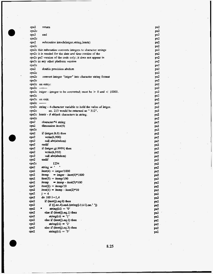
cps2 return
cps2 end
cps2 subroutine intoch(intger,string,lenstr)
cps2c this subroutine converts integers to character strings cps2c it is needed for the date and time routine of the cps2c ps2 version of the code only; it does not appear in cps2c in any other platform version cps2c cps2 double precision abtdum cps2c q s 2 c cps2c cps2c on entry: cps2c - cps2c intger - integer to be converted; must be > 0 and < 10000. cps2c cps2c on exit: cps2c - cps2c string - 4-character variable to hold the value of intger. cps2c cps2c lenstr - # nblank characters in string.
cps2c
cps2c
cps2c
convert integer “intger” into character string format
ex. 213 would be returned as ” 312”.
characteF4 string dimension itest(4)
if (intger.lt.0) then write(6,900) call abt(abtdum)
endif if (intger.gt.9999) then
call abt(abtdum)
1234
itest(4) = intger/lOOO itemp = intger - itest(4)*1000 iteSy3) = itemp/loO itemp = itemp - iteSy3)*100 itesy2) = itempllo itest(1) = itemp - itest(2)*10 j = 4 do 100 I=1,4
write(6’9 10)
endif
string=’ ’
if (itesyi).eq.O) then
* string(i5) = ’0’
string(i:i) = ’1’
string(i:i) = ’2’
string(i:i) = ’3’
if ((j.ne.4).and.(string(i-1:i-l).ne.’ ’))
else if (itest(i).eq.f) then
else if (itest(j).eq.2) then
else if (itest(j).eq.3) then
8.25

cps2 else if (itest(j).eq.4) then cps2 string(i:i) = ’4’ cps2 else if (itest(j).eq.S) then cps2 string(i:i) = ’5’ cps2 else if (itest(j).eq.6) then cPs2 string(i:i) = ’6’ cps2 else if (itest(j).eq.7) then cps2 string(i:i) = ’7’ cps2 else if (itest(j).eq.S) then cps2 string(i:i) = ’8’ cps2 else if (itest(j).eq.9) then cps2 string(i:i) = ’9’ v s 2 endif
cps2 100 continue cps2 do 110 1=1,4 cps2 cps2 110 continue cps2 120 continue cps2 lenstr = 5-i
cps2 900 format(lx,’error ...integ er value less than zero in routine ’, cps2 *’intoch’) cps2 910 format(lx,’error ...integ er value greater than 999 in intoch’) cps2c cps2 return cps2c cps2c end of date/time logic for the IBM ps2 operating system cps2c**********************************************************************
cps2 j = j-1
if (string(i:i).ne.’ ’) go to 120
cps2c
cINTc********************************************************************** cINTc start of dateltime logic for INTELx86 platform (x 7 2) cINTc NOTE: this coding has been tested only on a Pentium processor cINTc cINT if(i0pt .eq. 1) then cINT call gettim(ihr,imin,isec,ilOOth) cINT cINT endif cINTc cINT if(iopt .eq. 2) then cINT call g&(ihr,imin,isec,ilOOth)
cINT Unite (alph(4:5),’(2.2)’) imin cINT write (dph(7:8),’(2.2)’) isec cINT dph(3:3) = ’:’ cINT dph(6:6) = ’:’ cINT endif cINTc cINT if(i0pt .eq. 3) then cINT call getdat(iyr,imon,iday) cINT write (dph(l:2),’(2.2)’) imon cINT write (aIph(4:5),’(2.2)’) iday cINT write (~hfl~’(i4.4)’) iyr cINT alph(7:8) = chx3(3:4) CINT alph(3:3) = ’/’ cINT alph(6:6) = ’I’
xivar = 3600*ihr + 60*imin + isec + O.Ol*ilOOth
dNT write (alph(l:2),’(i2.2)’) ihr
8.26

cINT endif cINTc cINT return cINTc cINTc end of date/time logic for INTELx86 platforms (x > 2) c]NTc************************************************************************ cDECc********************************************************************* cDECc start of date/time logic for the SUN4 and DEC workstations cDECc cDEC if(i0pt .eq. 1) then cDEC calI etime(tarray) cDEC xivar = tarray(1) cDEC endif cDECc cDEC if(iopt .eq. 2) then cDEC call itime(iarray) cDEC write (alph(1:2),’(2)’) iarray(1) cDEC write (alph(4:5),’(i2)’) iarray(2) cDEC write (chx3,’(i4)’) iarray(3) cDEC alph(7:8) = chx3(3:4) cDEC alph(3:3) = ’:’ cDEC alph(6:6) = ’:’ cDEC endif cDECC cDEC if(i0pt .eq. 3) then cDEC call idate(iarray) cDEC write (alph(4:5),’(2)’) iarray(1) cDEC write (alph(l:2),’(2)’) iarray(2) cDEC write (chx3,’(i4)’) iarray(3) cDEC alph(7:8) = chx3(3:4) cDEC alph(3:3) = ’I’ cDEC alph(6:6) = ’/’ cDEC endif cDECC cDEC return cDECc cDECc end of date/time logic for the SUN4 and DEC workstations
ccosc********************************************************************* cCOSc start of date/time logic for the CRAY-COS operating system ccosc cCOS if(i0pt .eq. 1) then c c o s call second(xivar) c c o s endif c c o s c cCOS if(i0pt .eq. 2) then ccos call time(alph) cCOS endif c c o s c &OS if(iopt .eq. 3) then
cCOS endif ccosc cCOS return c c o s c
cDECc*********************************************************************
ccos call date(*)
INT INT INT INT INT INT DEC DEC DEC DEC DEC DEC DEC DEC DEC DEC DEC DEC DEC DEC DEC DEC DEC DEC DEC DEC DEC DEC DEC DEC DEC DEC DEC DEC DEC DEC DEC DEC cos cos cos cos cos cos cos cos cos COS cos cos cos COS cos cos cos
8.27
cCOSc end of date/time logic for the CRAY-COS operating system ccosc********************************************************************* cucsc********************************************************************** cuCSc start of dateltime logic for the CRAY-uniCOS operating system cucsc CUCS if(iopt .eq. 1) then CUCS call second(xivar) cuCS endif cucsc cuCS if(iopt .eq. 2) then CUCS call clock(alph) cuCS endif cucsc cuCS if(iopt .eq. 3) then CUCS call date(alph) cuCS endif cucsc cuCS return cucsc CUCSC end of dateltime logic for the CRAY-uniCOS operating system cucsc********************************************************************** CHpgc*********************************************************************** cHP9c start of datehime logic for the HP-9000 operating system cHP9c cHP9 if(iopt .eq. 1) then cHP9 call second(xivar) cHP9 endif cHP9c cHP9 if(iopt .e+ 2) then cHP9 call time(alph) cHP9 endif cHP9c cHP9 if(iopt .eq. 3) then cHP9 call idate(mon,iday,iyr) cHP9 write(alph,2) mon,iday,iyr cHP9 2 format(i2,’/’,i2,’/’,G!) cHP9 endif cHP9c cHF9 return cHP9c cHp9c end of dateltime logic for the HP-9000 operating system CHP~C************L******************************************************** cMACc***********L********************************************************** cMACC start of date/time logic for the Apple/Macintosh Operating system cMACC** cMACC** cMACC** Quadra and PPC compatible cMACC** cMACC** cMACC define a datetime record, structure and comments taken cMACC from Inside Macintosh, Vol2, page 378 cMACC cMAC IMPLICIT NONE cMAC INCLUDE “0SUtils.inc” cMAC character *4tempvar
APPLE MAC-II/MPW with AbSoft Compiler
Note: MPW include fde 0SUtils.inc required
cos cos u c s u c s u c s u c s u c s u c s u c s u c s u c s u c s u c s u c s u c s u c s u c s u c s u c s u c s u c s HP9 HP9 HP9 HP9 HP9 HP9 HP9 HP9 HP9 HP9 HP9 HP9 HP9 HP9 HP9 HP9 HP9 HP9 HP9 HP9 HP9 MAC MAC MAC MAC MAC MAC MAC MAC MAC MAC MAC MAC MAC
8 -28

cMAC character *8 alph cMAC integer *4iopt cMAC real *4xivar cMAC RECORD /DateTimeRec/ DateTime cMAC cMAC cMAC xivar = 0.0 cMAC alph(1:S) = ’12345678’ cMAC tempvar = ’ ’ cMAC cMAC go to (100,200,300),iopt cMAC 300 continue cMAC CALL GetTime@ateTime) cMAC write(alph(l:2), 1000) DateTime.month cMAC write(alph(4:5), 1000) DateTime.day cMAC write(tempvar, 1002) DateTime.year cMAC alph(7:S) = tempvar(3:4) cMAC alph(3:3) = ’1’ cMAC alph(6:6) = ’I’ cMAC cMAC go to 999 cMAC 200 continue cMAC CALL GetTime@ateTime) cMAC write(alph( 1:2), 1000) DateTime.hour cMAC write(alph(4:5), 1000) DateTime.minute cMAC write(alph(7:8), lO00) DateTime.second cMAC cMAC cMAC alph(3:3) = ’:’ cMAC alph(6:6) = ’:’ cMAC go to 999 cMAC 100continue cMAC CALL GetTime@ateTime) cMAC cMAC cMAC cMAC got0 999 cMAC lo00 format(i2) cMAC 1002 format(i4) cMACC** cMACC**
cMAC 999retum
cMACC**
cMACc end of date/time logic for the ApplelMacintosh operating system
if (alph(4:4).eq.’ ’) alph(4:4) = ’0’
if (alph(4:4).eq.’ ’) alph(4:4) = ’0’ if (alph(7:7).eq.’ ’) alph(7:7) = ’0’
xivar = 3600.0 * DateTime-hour xivar = xivar + (60.0 * DateTime.minute) xivar = xivar + DateTime.second
cMACC**+*****************************************************************
cMACc****************+***************************************************** End of MPW Absofi Compiler Timing call
cMACC***************************t******************************************
cMACc******************************************************************** end
MAC MAC MAC MAC MAC MAC MAC MAC MAC MAC MAC MAC MAC MAC MAC MAC MAC MAC MAC MAC MAC MAC MAC MAC MAC MAC MAC MAC MAC MAC MAC MAC MAC MAC MAC MAC MAC MAC MAC MAC MAC MAC MAC MAC MAC MAC MAC MAC
8.29

The following is a listing of the function LOCA, showing all platform dependent coding for the Zoc function used in determining the locations of the beginning and ending variables in the common blocks for subroutines CLEAR, DUMPIT, and RESTRT. This listing is from the Sun SPARCstation version, with the coding for all other platforms commented out.
function loca(ae, ab)
save C
C
C c * * * * * * * * * * * * * * * * * * * * * * * * * * * * * * * * * * *
c this function returns the number of c "words" between ae and ab.
c this is needed by subroutines clear and c dumpit. C
c arguments- c ae ending variable in common c ab beginning variable in common
c loca is called by clear and dumpit
c loca calls system functions %1oc, locf or loc
c * * * * * * * * * * * * * * * * * * * * * * * * * * * * * * * * * * *
c dimension fl(2)
c vax (i.e.; 32-bit machine) c
c ibm c loca=( loc(ae)- loc(ab))/(loo(fl(2))-loc(fl(l)))
c cdc c loca=(loc(ae) - loc(ab))
C
C
C
C
C
C
C
loca=(%loc(ae) - %loc(ab)) / 4 C
C
C
C c************************************************************************** Sun
Sun Sun Sun Sun Sun DEC DEC DEC DEC DEC DEC HP9 HP9
8.30

cHP9c cHP9 cHP9c cHPgc*********************************************************************
cMACc loca function for Apple-Macintosh workstation cMACc cMAC loca=(loc(ae) - loc(ab)) / 4 + 1 cMACc
loca=(loc(ae) - loc(ab)) / 4 + 1
cMACc********************************************************************
cMACc******************************************************************** cINTc********************************************************************* cINTc loca function for INTELx86 platforms (x > 2) cINTc cINT dimension fl(2) cINTc cINT cINTc
loca = (loc(ae) - loc(ab)) / (loc(fl(2)) - Ioc(fl(1)))
cINTc****************U****************************************************** cps2c********************************************************************** cps2c loca function for IBMlps2 workstation cps2c cps2 cps2c cps2c********************************************************************** caixc*********************************************************************** caixc loca function for IBM/unix workstation caixc caix dimension fl(2) caixc caix caixc caixC*********************************************************************** ccosc********************************************************************* cCOSc loca function for CRAY with COS operating system c c o s c cCOS loca=(loc(ae) - loc(ab)) c c o s c ccosc********************************************************************* CUCSC********************************************~******************~****
CUCSC loca function for CRAY with uniCOS operating sysww cucsc CUCS loca=(loc(ae) - loc(ab)) cucsc cucsc**********************************************************************
loca=(loc(ae) - loc(ab)) / (loc(fl(2)) - loc(fl(1)))
loca=(loc(ae) - loc(ab)) / (loc(fl(2)) - loc(fl(1)))
C return end
H B HP9 HP9 HP9 MAC MAC MAC MAC MAC MAC INT INT INT INT INT INT INT INT PS2 PS2 PS2 PS2 PS2 PS2 aix aix aix aix aix aix aix aix cos cos cos cos cos cos u c s u c s u c s u c s u c s ucs
8.31

8.5 Installation Guide
Versions of COBRA-SFS, Cycle 2, have been developed or validated on eight different platforms, including the following seven workstations: the SUN SPARCstation 2; the IBM RS6000; the Hewlett-Packard HP9000; the DEC workstation; pc’s with INTEL-386, -486, and Pentium processors; IBM/ps2, and the APPLE MAC-II/MPW. All eight versions of the code are essentially identical. The only differences are in the logic for the date, clock time, and cpu time subroutine DATTIM, and the LOCA function, which is used to find the beginning and ending addresses in memory for the common blocks (see Section 8.4 for a complete listing of platform dependent coding). The code transmittal package for COBRA-SFS, Cycle 2, as described in Section 8.5.1 and Section 8.4.2, gives step-by-step installation instructions.
8.5.1 Code Transmittal Package
The master version of the COBRA-SFS code is maintained under a configuration management utility called WITNESS. WITNESS is similar to the UPDATE and HISTORIAN utilities on CDC and IBM mainframes, and the master source files for both COBRA-SFS and RADGEN are ASCII text files in WITNESSIUPDATE format. These files are not compilable. The WITNESS source file is used to create a WITNESS program library, which assigns line numbers and identifiers to each line of coding. This program library cannot be edited, but it can be used to create (with or without modifications) compilable files, new source files, and list files, by running the WITNESS program with appropriate input.
The WITNESS source files for both COBRA-SFS and RADGEN are included in the code transmittal package. This is done mainly to give the user a source that can be converted fairly easily to an alternative configuration management utility. For users who do not have such a utility, or do not choose to use one for this code, the transmittal package also includes compilable files for each platform.
These compilable files contain the appropriate platform-specific coding, and each has been tested on the workstation for which it is designed. In most cases, a version should compile on its particular platform without errors. However, differences in operating systems and fortran compiler versions may necessitate some minor changes in a particular installation.
There is only one compilable source for RADGEN. Since it has no platform dependent coding, it can be expected to compile successfully on any platform that has adequate memory and a Fortran-77 compiler.
Input files for two test cases are included in the transmittal package, for reference in verifying code installation on any platform. The Mitsubishi test case is a single-assembly model (refer to Section 7.2.2 for a complete description), and the TN24 test case (see Section 7.3.1) is a full cask model, including both upper and lower plena.
8.32

0
a
The output files for the mitsubishi and TN24 test cases are from the Sun SPARCstation version. All other platforms gave essentially the same results in the validation testing of Cycle 2. Any significant differences between the results obtained on another platform and the Sun output files should be investigated carefully and corrected before using the code in any of the applications.
Three test cases are included for verification of the installation of RADGEN. These are the same cases as the sample problems presented in Section 6.3. As with the COBRA-SFS output files, the output files for the RADGEN test cases are from the Sun SPARCstation 11. All other platforms should give the same results. Table 8.3 lists the COBRA-SFS code package files along with each of their descriptions.
Table 8.3. COBRA-SFS Code Package
~-~ - FileName . Description
sfs2-Sun.src UPDATE/WITNESS source of COBRA-SFS, cycle 2 (Sun version)
sfs2-xxx. f I compilable sources for all 8 platforms; XXX stands for platform identifier code
sec0nd.c
mitsubishi-cycle2.inp
subroutine in C programming language for time calculation on the HP9000 version; object must be linked at compile time (see Section 8.5.2)
~~~ ~~ ~
input file for single-assembly Mitsubishi test case
mitsubishi.tapel0 I tape10 file created using RADGEN for Mitsubishi test case
mitsubishi-cycle2.out
tn24-vertical.inp
tn24v. tape10
output file for single-assembly Mitsubishi test case (Sun version)
input file for multi-assembly TN24P cask test case
tape10 file created using RADGEN for TN24P vertical cask model ~p ~~~~~~~ ~- ~ ~
tn24-vertical.outp 1 output file for multi-assembly TN24P cask test case
radgen-cycle2. src
radgen-cycle2 . f testcasel.inp
testcasel .out
testcase2.inp
testcase2.out
UPDATE/WITNESS source of RADGEN, cycle 2
compiiable source (suitable for all platforms)
input for RADGEN test case 1: 3 x 3 square array in a square canister
output for RADGEN test case 1: 3 x 3 square array in a square canister
input for RADGEN test case 2: triangular array in a square canister
output for RADGEN test case 2: triangular array in a square canister
testcase.3 .inp I input for RADGEN test case 3: hexagonal array in a hexagonal canister
testcase3 .out I input for RADGEN test case 3: hexagonal array in a hexagonal canister
8.33

8.5.2 Installation Instructions
The first step in the installation of COBRA-SFS should be to convert a copy of the WITNESS source files of COBRA-SFS and RADGEN to a form acceptable to the code configuration management (CCM) utility on the user's computer. The second step would then be to create a compilable file for each code using the CCM utility, with the appropriate platform coding activated and all coding for other platforms deactivated. However, if the user's platform does not have a CCM utility, or there is some reason for not bringing COBRA- SFS under its aegis, then the first step in the installation of the code is to copy the appropriate compilable version from the transmittal package, and run it through the Fortran-77 compiler.
The transmittal package includes compilable files for eight different platforms, identified as follows: .
Platform Compilable file name IBM/ps2 sfs2qs2.f INTELx86, (x > 2) sfs2-INT. f '
IBM/RS6000 (aix) sfs2-aix. f SUN SPARCstation sfs2Sun. f
CRAY with uniCOS system sfs2-uniC0S.f SUN4 and DEC stations sfs2-DEC. f
HP-9000 workstation sfs2-HP9.f APPLE MAC-LI/MPW with AbSoft Compiler sfs2-MAC. f
The compilable file for the RADGEN code is radgen-~ycle2.f~ and is suitable for all platforms with standard Fortran-77 compilers.
Compilation of the code can be accomplished on most platforms with the single command:
f77 sfs2-xxx.f -0 sfs2-XXX.x
Note that XXX corresponds to the platform identifier mnemonic shown in the file name list above. Similarly, the command to compile the RADGEN code is
f77 radgen-cycle2.f -o radgen-cycle2.x
Mainly for convenience of transmittal, the entire code is contained in a single compilable file. It is also possible to split the compilable file into separate files for each subroutine, using the 'fsplit' utility available on most Unix workstations. With the code split into separate subroutines, a script file can be used to compile the subroutines individually, then create an object library and executable. An example of such a script file for the Sun SPARCstation is as follows:
# # The following makefde is to generate the following files: # # 1) cobrasfs2.a a library containing all *.o files # # 2) cobrasfs2.x the master version of the executable # # This makefde assumes that "witness" has already # created the *.f files #
8.34

# NOTE: If a new routine is added the list of routines # # # This maketile is for use on the master directory only # # Author: Annette Koontz # # # SUFFIXES: .o .f # OBJS = cobra.0 \
under OBJS must be modified accordingly
(plagarized by J. M. Cuta, 7/12/89)
area.0 c1ear.o c01oc.o curve.0 dattim.0 differ.0 \ dumpit.0 echo.0 energy.0 exprop.0 force.0 group4.0 \ hotrod.0 1imits.o 1oad.o 1oca.o mix.0 moment.0 \ network.0 oned.0 post.0 prefix.0 prop.0 recirc.0 \ reheat.0 restrt.0 result.0 setin.0 setout.0 setup.0 \ so1ver.o varprp.0
# cobrasfs2.x: cobrasfs2.a # # load step #
ar x cobrasfs2.a cobra.0 f77 cobra.0 cobrasfs2.a -0 cobrasfs2.x
# cobrasfs2.a: $(OBJS) # # build the library #
rm -f cobrasfs2.a ar rv cobrasfs2.a $(OBJS) ranlib cobrasfs2.a
.f.o: # # Compile #
# f77 -e $*.f
For the validation assessments for Cycle 2, the'codes was compiled without optimization, as indicated in the sample command lines given above. Optimization can significantly decrease execution time, however, and might be advisable for users who expect to run a large number of cases, or very large problems. Some care must be exercised, however, to make certain that code optimization does not affect code results. Output from the optimized version should be verified against the output from an unoptimized executable. If the optimized version does not give the same results as the unoptimized version, it is probably not a good idea to optimize the code with that particular compiler.
8.35

Platform-specific coding for the HP9000 version calls a subroutine named “second” to obtain the cpu time. This subroutine is in the C programming language, and so cannot easily be included in the COBRA-SFS Fortran source file. This subroutine is included in the transmittal package as the file “second.c.” It is a very simple routine, consisting of the following lines:
#include < sys/times.h > second (s) float *s;
struct tms tbuf; times (&tbuf); *s = 0.01 * (tbuf.tms-utime + tbuf.tms-stime); return; 1
{
Compilation of the HP9000 version of COBRA-SFS requires compiling. “second.c” with the C compiler, then linking the resulting object file, “second.o”, in the compilation and load step for the COBRA-SFS compile file. This can be done with the following command lines:
cc +03 -c sec0nd.c f77 +e sfs2-HP9.f second.0 -0 sfs2-HP9.x
The final step in the installation of the code is to run the test cases for COBRA-SFS and RADGEN. The input files for two COBRA-SFS and three RADGEN test cases are included in the transmittal package. Note that the input files are the same for all platforms; there are no platform- specific changes to the code input stream.
To verify the installation, the executable version of COBRA-SFS created in the compilation step above (sfs2 XXX.x) is run with the test case input file (mitsubishi cycle2.inp or tn24 vertical.inp) copied to a file named “input”. The view factor input for each case (mitshbishi.tapel0 or tn24v.tapelO), must be copied to the file named “tapelO.” The code wilI produce an output file of the results, in the local file “output.” The transmittal tape includes output files produced on the SUN SPARCstation (mitsubishi-cycle2-Sun.out and tn24-vertical-Sun.out). The results obtained with the users installation of COBRA-SFS should be compared with these output files from the transmittal tape. There should be no significant differences.
Similarly, the executable version of RADGEN (radgen-cycle2.x) should be run with the input file (testcasel.inp, testcaseZ.inp, or testcase3.inp) assigned to the local file name “input.” If RADGEN has been compiled for interactive mode (Le., ibatch = 0 in the main program), the test cases are run by responding to Q1 with “n,” to decline interactive input (see Section 6.3.2.1). The RADGEN results are written to file “tapelo,” and should be compared with the appropriate output file in the transmittal package (testcasel .tapelo, testcase2.tapel0, ot testcase3.tapelO). There should be no significant differences between these files and the results obtained on the new platform.
8.36

8.5.3 Redimensioning COBRA-SFS and RADGEN
The dimensions of arrays in both COBRA-SFS and RADGEN are defined using parameter statements, as described in Section 8.3. The values specified for the dimension parameters in the master version of the code are large enough to run all the validation test cases reported in Section 7.0. These parameters will probably be sufficient for most applications of the code. However, if the user needs a larger version, it will be necessary to change the parameter statements in the code.
This will be much easier if the code is under some sort of configuration management utility. In the WITNESS source file, the dimension parameters are included in a COMDECK called SPECS that appears in nearly every subroutine in the code. It is possible to change the parameter statements by editing the compilable file (sfs2-XXX.f), but the changes must be propagated without error through every occurrence of the parameter statements in the code. A CCM utility will generally make this simple. If it has to be done by editing the compilable file, however, the chance for error can approach certainty.
With the RADGEN code, the problem is somewhat less onerous since there are only five subroutines in the code, in addition to the main program. However, the same caveat regarding the necessity for consistent changes applies. A parameter statement changed in one subroutine must be altered in exactly the same manner in all other subroutines.
Once a new compilable file has been created, either by invoking a CCM utility or by editing a copy of the original compilable file, the code can be compiled as described above to create a new executable. This executable will have the redimensioned arrays, and will be able to run the new cases.
8.37

9.0 References
Bates, J. M. 1986. Single PWR Spent Fuel Assembly Heat Transfer Data for Computer Code Evaluations. PNL-5571, Pacific Northwest Laboratory, Richland, Washington.
Cox, R. L. 1977. Radiation Heat Transfer in Arrays of Parallel Qlinders. ORNL-5239, Oak Ridge National Laboratory, Oak Ridge, Tennessee.
Creer, J. M., T. E. Michener, M. A. McKinnon, J. E. Tanner, E. R. Gilbert, and R. L. Goodman. 1987. The 7iV-24P PWR Spent-Fuel Storage Cask: Testing and Analyses. EPRI-NP-5 128/PNL-6054, Electric Power Research Institute, Palo Alto, California.
Croff, A. G. 1980. ORIGEN-2 -- A Revised and Updated Version of the Oak Ridge Isotope Generation and Depletion Code. ORNL-5621, Oak Ridge National Laboratory, Oak Ridge, Tennessee.
Cuta, J. M., D. R. Rector, and J. M. Creer. 1984. Comparisons of COBRA-SFS Calculations with Data from Simulated Sections of Unconsolidated and Consolidated BWR Spent Fuel. EPRI-NP-3764, Electric Power Research Institute, Palo Alto, California.
Cuta, J. M., and J. M. Creer. 1986. Comparisons of COBRA-SFS Calculations to Datafrom Electrically Heated Test Sections Simulating Unconsolidated and Consolidated BWR Spent Fuel. EPRI-NP-4593, Electric Power Research Institute, Palo Alto, California.
Fry, C. J., E. Livesey, and G. T. Spiller. 1983. “Heat Transfer in a Dry, Horizontal LWR Spent Fuel Assembly. ” In Proceedings of Seventh Znternational Symposium, New Orleans, Louisiana. Oak Ridge National Laboratory, Oak Ridge, Tennessee. From Packaging and Transportation of Radioactive Materials (PATRAM’83) Symposium.
George, T. L., K. L. Basehore, C. L. Wheeler, W. A. Prather, and R. E. Masterson. 1980. COBRA- WC: A version of COBRA for Single-phase Multi-assembly Thermul-Hydraulic Transient Analysis. PNL-3259, Pacific Northwest Laboratory, Richland, Washington.
Gosman, A. D., R. Herbert, S. V. Patankor, R. Potter, and D. B. Spalding. 1973. “The SABRE Code for Prediction of Coolant Flows and Temperatures in Pin Assemblies Containing Blockages.” Presented at International Meeting on Reactor Heat Transfer, Karlsruhe, Germany. HTS/73/47, Imperial College of Science and Technology.
Hirt, C. W., and J. L. Cook. 1972. “Calculating Three-Dimensional Flows Around Structures and Over Rough Terrain. ’’ J o u m l of Computational Physics, 10:324-340.
Hottel, H. C., and A. F. Sarofin. 1967. Radiative Heat Transfer. McGraw-Hill, Inc., New York.
9.1
Ingesson, L. and S . Hedberg. 1970. “Heat Transfer Between Subchannels in a Rod Assembly.” Paper No. FC7.11. Presented at the Fourth International Heat Transfer Conference, Versailles, France.
Irino, M., M. Oohashi, T. Irie, and T. Nishikawa. 1986. Study on Surface Temperatures of Fuel Pins in Spent Fuel Dry Shipping/Storage Casks. IAEA-SM-286/139P9 pp. 585-598.
Kays, E. U., and M. E. Crawford. 1980. Convective Heat and Mass Transfer, McGraw-Hill, Inc., New York.
Khan, E. U., W. A. Prather, T.L. George, and J.M. Bates. 1981. A Validation Study of the COBRA-WC Computer Program for M F B R mermal-Hydraulic Analysis, PNL-4 128, Pacific Northwest Laboratory, Richland, Washington.
Lindeburge, M. R. 1981 Mechanical Engineering Review Manual, 6th ed. The Professional Engineering Program, San Carlos, California.
Lombardo, N. J., T. E. Michener, C. L. Wheeler, and D. R. Rector. 1986. COBRA-SFS Predictions of Single-Assembly Spent Fuel Heat Transfer Data. PNL-578 1, Pacific Northwest Laboratory, Richland, Washington.
Lombardo, N. J . , J . M. Cuta, T. E. Michener, D. R. Rector, and C. L. Wheeler. 1986a. COBRA- SFS: A Thermal-Hydraulic Analysis Computer Code; Volume 111: Validation Assessments. PNL-6049, Vol. 3, Pacific Northwest Laboratory, Richland, Washington.
McKinnon, M. A., J. M. Creer, T. E. Michener, J . E. Tanner, E. R. Gilbert, and R. L. Goodman. 1986. TN-24P PW2Z Spent Fuel Storage Cask Performance Testing and Analysis. EPRI-5128, Electric Power Research Institute, Palo Alto, California.
McKinnon, M. A., R. E. Dodge, R. C. Schmitt, L. E. Eslinger, and G. Dineen. 1992. Performunce Testing and Analyses of the VSC-I 7 Ventilated Concrete Cask. EPRI-TR-100305/ PNL-7839, Electric Power Research Institute, Palo Alto, California.
Rector, D. R., C. L. Wheeler, and N. J . Lombardo. 1986. COBRA-SFS: A Thennul-Hydraulic Analysis Computer Code, Volume I : Mathematical Models and Solution Method. PNL-6049, Vol. 1, Pacific Northwest Laboratory, Richland, Washington.
Rector, D. R., R. A. McCann, U. P. Jenquin, C. M. Heeb, J. M. Creer, and C. L. Wheeler. 1986b. CASTOR-IC Spent Fuel Storage Cask Decay Heat, Heat Transfer, and Shielding Analyses. PNL-5974, Pacific Northwest Laboratory, Richland, Washington.
Rector, D. R., J. M. Cub, and N. J . Lombardo. 1986c. COBRA-SFS Thennal-Hydraulic Analyses of the CASTOR-I C and REA 2023 BWR Storage casks Containing Consolidated Spent Fuel. PNL-5802, Pacific Northwest Laboratory, Richland, Washington.
9.2

Rector, D. R. 1987. RADGEN: A Radiation Exchange Factor Generator for Rod Bundles. PNL-6342, Pacific Northwest Laboratory, Richland, Washington.
Rector, D. R., and T. E. Michener. 1989. COBRA-SFS Modifications and Cask Model Optimization. PNL-6706, Pacific Northwest Laboratory, Richland, Washington.
Rogers, J. T., and N. E. Todreas. 1968. “Coolant Mixing in Reactor Fuel Rod Assemblies--Single Phase Coolants.” In Heat Transfer in Rod Assemblies, ASME, pp. 1-56.
Rogers, J. T., and R. G. Rosehart. 1972. Mixing by Turbulent Interchange in Fuel Assemblies: Correlations and Inferences, ASME Paper No. 72-HT-53. .
Rowe, D. S . 1973, COBRA-IIIC: A Digital Computer Program for Steady-State and Transient Thermal-Hydraulic Analysis of Rod Bundle Nuclear Fuel Elements. BNWL-1695, Battelle Northwest Laboratory, Richland, Washington.
Slattery, J. C., 1972, Momentum, Energy, and Mass Transfer in Continua, McGraw-Hill, Inc., New York.
Stewart, C. W., C. L. Wheeler, R. J . Cena, C. A. McMonagle, J. M. Cuta, and D. S. Trent. 1977. COBRA-IV: The Model and the Method. BNWL-2214, Battelle Northwest Laboratory, Richland, Washington.
Tong, L. S. 1968. “Pressure Drop Performance of a Rod Assembly.” In Heat Transfer in Rod Assemblies, ASME, pp. 57-69.
Wheeler, C. L., R. A. McCann, N. J. Lombardo, D. R. Rector, and T. E. Michener. 1986. “HYDRA and COBRA-SFS Temperature Calculations for CASTOR-IC , REA-2023, CASTOR- VI2 1, and TN-24P Casks. ” In Proceedings, Third International Spent Fuel Storage Technology Symposium and Workshop, Vol. 1, S77-S98, CONF-960417, National Technical Information Service, Springfield, Virginia.
Wiles, L. E., N. J. Lombardo, C. M. Heeb, U. P. Jenquin, T. E. Michener, C. L. Wheeler, J. M. Creer, and R. A. McCann. 1986. BWR Spent Fuel Storage Cask Pe~ormunce Test, Volume I . : Pre- and Post-Test Decay Heat, Heat Transfer, and Shielding Analyses. PNL-5777, Vol. 2, Pacific Northwest Laboratory, Richland, Washington.
9.3

Appendix A
Common Block Variables

Listing of Common Blocks in COBRA-SFS, Cycle 2
C common /flags/ 1 2 3 4
C common /const/
common /barea/ C
1 2
C
gbeg2(l),ierrorfjl,iterat,nrc,nwk, naah , naahpl , nspec ( 2 0 ) , nangl t , isolve,iass,nfcon,nscbc,nramph, ischeme,ibwl,ibwr,ic,iwide,iclose,iclosa(iu), isym,nrow,i3post,endg2
pi,dtgc,gc,idtgc,dti,sb
C
C
common /field2/ fbeg2 (1) ,hah(ie,mc) rsaver(mc) r flow(mc) ,qprim(mc) ,ichan(ln6,mc) ,const (lib) , hf ilm (mc) I t m h (mc) , ftemp (mc) fsp (mc) I tinlet (mc) , finlet (mc) , hinlet (mc) , fmomf (mc) , dpk (mc) , dpdx (mc) relxi (mc) r dhdx (mc) , dfdx (iu) , v (mc) , cons (mx) nach (mc) , itypin (lit , 3) , f irstt , endf2
1 2 2 3 4 5
common /bundle/ fbeg3(1) ,ipoint(iu,8) ,ngapl,ngap2, 1 nchanl,nchan2,nassemfnchanl, 2 3 maxtyp,ndxpl,ndx,endf3
mm, it, ip, ia, iw, iz,ix, ir, if ,nz,nk,
C common /fields3/ conk (mg) , dpbar (lip*iq) common /f ieldb/ term1 (mc) , wpp (mg)
C
C C level 2, /fieldl/ C level 2,' /field2/ C C *comdeck props
A. 1
C
C
C
C
C
2 3 4
common /prop2/ pbeg2 (1) ,pref, lamnh(1iw) ,nheat,nflmc (iu) ,ah1 (liw) 1 2 3 4 5 istar(mg) ,ntheat,nfheat,endp2
1 2 ntype(mc) ,amix(lit) ,bmix(lit), 3 endp3
common /matprp/ pbeg4 (1) ,uwcp(nd,mw) ,uwall (nd,mw) , 1 areacp(mw2),matypp(mw2) ,tpsave(mw2) , 2 3 4 4 imat (id) ,pdna(iu) ,pdn,nsprop,end~4
ah2 (liw) ,ah3 (liw) ,ah4 (liw) ,ah11 (liw) ,ah12 (liw) , ah13 (liw) , ah14 (liw) , ahtl (liw) , aht2 (liw) , aht3 (liw) , aht4 (liw) , ahtll (liw) , ahtl2 (liw) , ahtl3 (liw) , ahtl4 (liw) , ahfl (liw) , ahf2 (liw) ,
common /prop3/ pbeg3 (1) ,visc(mc,3) ,viscw(mc) ,con(mc) cp(mc) ,vp(mc) ,t(mc) ,vscm(mc) ,beta(mc),
npwcon, con0 (id) , con1 (id) , con2 (id) , con3 (id) , cpsol (id) rhosol (id) , rdima (liz) , rdimb (liz) , nqvt (id) ,conw(mw) ,mat] (id,mx) ,mattyp(mw) I
common /alpha/ aname (id) , alph character*8 aname, alph
logical lamnh C
C C level 2, /prop3/ *corndeck drags C
common /drag/ 1 2 3 4 5
C CI 1 2 3 4 5 6 7 8 9 1 2
C
dbegl(1) , dpa (iu) , kij (mg) , cij (mg) itran, aa (liw) , bb (liw) , cc (liw) , dd (liw) , ee (liw) , aal (liw) , bbl (liw) , ccl (liw) , lamnf (liw) , aat (liw) , bbt (liw) , cct (liw) , ddt (liw) , eet (liw) , aatl (liw) , bbtl (liw) , cctl (liw) , nfrict, ishear,nshear,kn(mg,2) , ck(mg,4) ,enddl
Dmmon /bgrid/ dbeg2 (1) ,factor(lit,mq,mx) ,ilce(lit,mq) , lcass (iu) , lcff (mk) , lcasst (mk) , ifact (mq,mx) I nlevel (lit,mq) ,cd(lit,mq,mx) ,xcd(lit,mq,mx), ifb(mc) ,nblock,flo(iu) ,allf,nbl(lit) flog (mj , pwin (iu) , pwout (iu) , rain (iu) , raout (iu) , rgin (mj 1 , rgout (mj ) , netgrp (iu) , noutf f (iu) , dpt (iu) , rmuinlt , nogrp , pdrop netwk,fpri(iu) ,dppri(iu) ,lblok(mkf2) I
iblokt , rtin, hgin (mj , hgout (mj 1 , hain (iu) , ghead (mc) , dpcor (mc) , walls (iu) , ilcs (lit , mq) , nramp, ninff (iu) ,phead, haout (iu) , ibloka (mc) , iblokc (mc) , endd2
real ki j logical lcass logical lamnf
C level 2, /bgrid/ *corndeck time C
common /timez/ tbegl(l),dt,iprnte,iprnta,ttime, 1 etime,clock(8) ,maxt,ndt,ndtpl,itstep,endtl
A. 2

C common /outout/ tbeg2 (1) ,output (12) ,print (14) ,tdumy(lO) , 1 tprint,trant,naxp,nout,npchanfnpgap,i2,i3, 1 ipost,jhot,jpres,jrods,jslab, 2 npnode,nprod,printn(lO) ,nskipt,nskipx,nq,ng,ig, 3 4 5
6
nh,ihh,np,im(ms), jm(ms) ,imp(lO), jmp(l0) ti81
* kase, printc (mc) , printg (mg) , printr (mr) ipreb, ncout,nrout,ngout,nwout,npwall,printw(mw) postr(mr) ,postw(mw) ,posth(mc) ,postp(mc), conv(2),iotemprendt2
C
C common /chrvar/ hl, h2, h3 , h4, h5, h6 , h7 , h8
character*l hl, h2, h3, h6, h7 character*4 h4, h5 character * 2 h8
C
C
C
C
m c C
common /bound/ tbeq4(l),hout,njump,ntries,hin(2),~in,tin,dpsf 1 2
- - itdp, itdpa(iu) ,ngprfl,nqprfl,npfvt~iu) , exith, exitrnu,exitt,negf(iu),negflo,ftotalfendt4
common /index/ tbeg5 (1) ,nhigh(mc) ,nlow(mc) ,ncount (mr) , ihigh,
common /convrg/ tbeg6(1) ,qoh,accely,werry,accelf,ferror,qerror
integer printc,printg,printn,printr,printw logical print
1 ilow,ilowpl,npoint,ihalt~endt5
1 ,dampng,accelh,accrho~accelw,herror,qor,endt6
*comdeck fuels C
comon /fuel/ flbegl(1) ,kfuel (mt) ,kclad(mt) , rfuel (mt) , rclad(mt1 , cfuel(mt1 ,cclad(mt) ,tclad(mt) ,hgap(mt) ,Powr(ij) I
bx(2,mn,mr) , zx(mn,mr) ,qtotal, scladmx, . scldmxo,cladmx,acladmx(2) , rcladmx(2) , zcladmx(2) , lr ( m r , 6) , dfuel (mt) ,phi (mr, 6) , radial (mr) ,d (mr) , idfuel (mr) , nhfvt (id, sparev(20) ,qvoid (mr) , idtyp(mt1 ,nzone(mt) ,iztyp(mt,my) ,Zend(mt,mY) I nclad (mr , 6 1 , nwall (mr, 10) , n r r (mr) , nrw (mr) , rcon, rrdim, conr (mr) , endf 11
1 2 ntheta,nrdthta,nqax,nc,nrod~nrodtp,nfuelt,recall, 3 4 5 6 7 8 9 wcon,wrdim,delrad(mt) ,dodr(mn,mt) ,dsqr(m,mt) I 9
C common /repeat/ flbeg2 (1) ,drod(mt) ,geomf (mt) ,dfueli (mt) , 1 2 3
rcfuel (mt) , rcclad (mt) , r2kf (mt) , phitot (mr) , ring (mr) , rang (mr) , rung (mr) , hgapl (mt) , lri (lir,mc), trold(m7,mr,mx) I rtr-,endfl2
C , real kfue1,kclad
integer acladmx, rcladmx, zcladmx C level 2, /fuel/ C level 2, /repeat/ *corndeck walls C
common /walls/ wbegl(1) ,ksideCiu,mll) ,uwal(mhl,mwl) ,qwal(mw) ,
A. 3

1 2 3 4
C
kwal (mh,mw) , icf (nd,mw) , twsave (mw) , rdimf (liz) , icon (mh,mw) , rwal (liz) ,wid (liz) , nsidf (mw) , nsidw (mw) , relxk (mw) , nkss, nksf , wallxc (mw) , nrpf , qslab (mw) ,naxk (mw) endwl
C
C
common /radi8/ wbega(1) ,rser(liz) ,rpar(liz) ,ema(liz) ,emb(liz) , 1 arad(1i.z) ,radsav(2,mw) ,sumsav(iu,mll) ,t4(m6) , 2 radgap (liz) , emx (lnz) ,brad (lnz, m8) , areas (nv, 1nz) , 3 fvl(la,la) ,fv2(lb,lb) ,fv3(llc,llc) ,fv4(ld,ld), 4 fv5 (le, le) , fv6 (If, If) , rratio(6, lnz) , irad,msid(iu) , 5 itypr (iu) , fvw (nv, lnz , lnz , sumr (mr) , emv (6 , lnz 1 , 6 emrsav(6) , radc(mr) ,sumrg(lnz,nv) ,endw2
C C C
common /plena/ wbeg4 (1) ,npr, iplenr (21, awps (lip) , awpax(1iP) I 1 npsid(2) ,npax(2) ,tambp(2,2) ,nPtyp(liPt2,2) 2 3 5 6 hplen,endw4
sperp (lip, 2 , 2 , ttop (lip , 2,2 1 , qtop (2 1 I pexitf if~ln, npw(2,2) ,cpsav(2) ,hsave(2) ,exittod(2) ,iunca(iu) , dxwall, dxplen (mw2 1 , ipw (mw) , ipintp (2 mw2)
common /redstf/ wbeg5 (1) ,sldamp,nslgrp,bslgrp(6) ,eslgrp(6) ,endw5 integer bslgrp, eslgrp
C
C C level 2 , /walls/ C level 2, /radi8/ C level 2, /walbnd/ C level 2, /plena/ *corndeck rebal C
common /rebal/ rbegl(1) , qcoef (iu) , coefh (mc) , coefw (iu, lnz) , caxld (mx2 , 3 1 , qres (mx2 1 , dtax ( ~ 2 1 , 1
2 qcon (iu) , endrl level 2, /reball
A. 4

COBRA-SFS, Cycle 2 Common Block Variable Definitions
COMDECK GEOM a
iloc (1x18)
common /geom/
gbegl ( 1
ik (mg)
jk(mg)
length (mg)
gangle (mg)
ikw (nd,mw)
z
ftm
theta
atotal
gelev
angle (5)
elev
sl
ibandw (iu)
an (mc)
array storing the number of gap connections seen by a given channel
variable defining beginning address for common block georn
index of lower-numbered channel of the pair connected by a given gap k
index of higher-numbered channel of the pair connected by a given gap k
centroid length of a given gap k, units: ft
angle of cross-flow velocity vector in a given gap, with respect to the vertical; converted to radians from input value in degrees
array storing index numbers of channels with thermal connections to a given slab node
total axial length of channels, units: ft
user-defined turbulent mixing parameter ( dimens i on1 e ss 1
channel orientation angle with respect to the vertical. units: degrees
sum of inlet axial cross-sectional area at all channels in an assembly. units: ft2
angle of lateral control volume length with respect to the vertical; units: degrees
array used to read orientation angle for lateral flow velocity vectors; units: input as degrees from the vertical
channel orientation with respect to the vertical; units : degrees
nominal ratio of gap width to centroid length (dimensionless)
axial node length array, units: ft
multiplier on lateral control volume length for thermal conduction in the fluid
solution matrix bandwidth for a given assembly
nominal channel area, as specified by input; converted to units of ft2
A. 5
. .

dhydn (mc )
ilocs (lnl, mc)
perim (mc)
per (mc)
hperim (mc)
nominal channel hydraulic diameter, units: ft
array containing indices of all higher-numbered channels connected through gaps to a given channel
nominal channel wetted perimeter, as specified by input; converted to units of ft
summation of perimeters of all slab nodes connected to a given channel; units: ft
nominal channel heated perimeter, as specified by input; converted to units of ft
dduct (iu, lix) array storing index number of the last channel in a given assembly that sees other channels through crossflow connections
abar (mc )
endgl
common /flags/
gbeg2 ( 1)
ierror
11
iterat
nrc
nwk
naah
naahpl
nspec ( 2 0 )
nanglt
isolve
iass
nf con
nscbc
fluid density in the node above the channel exit; units : lbm/ft3
variable defining ending a.ddress for common block geom
variable defining beginning address for common block f l a g s
flag for table interpolation error
flag for control of processing of output of input data; defined by user input
counter for external solution iterations
maximum number of rods interacting with a channel
total number of slab nodes specified by user input
maximum number of thermal plus flow connections to a channel, plus 1
maximum number of thermal plus flow connections to a channel, plus 2
array to store required values of spec parameters for a given input
number of pairs of channel orientation angles to be specified by user input
flag to solve the energy equation by a semi-implicit method if not using the fuel conduction solution, or if there are no rods in the problem
index number of current assembly
flag for radial conduction in fluid
flag for single-phase turbulent mixing model
A. 6

nramph
ischeme
ibwl
ibwr
ic
iwide
iclose
iclosa (iu)
isym
nrow
i3post
endg2
common /const/
Pi
dtgc
gc
idtgc
number of iterations over which heat generation is to be ramped into the solution
flag for lateral momentum solution; specified by user input
maximum difference between indices o f channels connected by a gap; defines number of columns to the left of the diagonal for the banded matrix solution in subroutine SOLVER
maximum difference between indices of channels connected by a gap; defines number of columns to the right of the diagonal for the banded matrix solution in subroutine SOLVER
maximum difference between indices of channels connected by a gap, plus 1; diagonal locator for banded matrix solver in subroutine SOLVER:
- - for symmetrical matrix, index number of the array column that contains the diagonal element of the banded matrix;
- - for non-symmetrical matrix, the position ‘of the diagonal in the nrow x ibw matrix array
maximum width of solution matrix; defined by parameter ie
flag set to indicate zero flow boundary condition for all assemblies
flag for zero flow boundary condition on a given assembly
flag for symmetrical or nonsymmetrical matrix for banded matrix solution in subroutine SOLVER
number of rows in the banded matrix for the solver in subroutine SOLVER
logical unit number for post-processor output file ”post ”
variable defining ending address for common block f l a g s
geometric constant A , defined as 355.0/113.0
time step (sec) times the gravitational acceleration constant; units: ft/sec
gravitational acceleration constant, 32.2 ft/sec2
inverse of the time step times gc; units: sec/ft
A. 7

dti
sb
common /barea/
gbeg3 ( 1)
afact (m1,ma)
gf act (ml , ms
ax1 (ml)
x ( m x )
gapxl (ml 1
naramp
nafact
naxl
ngxl
ngap (ms 1
idakea (mc)
idgap (mg)
gapn (mg)
endg3
COMDECK FIELDS
coRlRlon /fieldl/
fbegl(1)
inverse of the time step; units: sec-l
Stefan-Boltzmann constant, 4.7611(10)-’3 Btu/sec-ft2-R4
variable defining beginning address for common block barea
channel axial area variation input array; (dimensionless)
gap width variation table input array; (dimensionless)
input array for axial locations of axial area variation input tables; (dimensionless)
array of axial level locations; units: ft
input array for axial locations of gap width variation input tables; (dimensionless)
number of iterations over which to insert geometry variations into solution
number of channels with axial area variation
number of axial locations in axial area variation tables -specified by user input
number of axial locations in gap width variation tables specified by user input
number of gaps with gap width variations
temporary storage array for index numbers of channels with area variations
temporary storage array for index numbers of gaps with gap width variations
array storing index number of area variation table used by a given channel i
array storing index number of gap width variation table used by a given gap k
nominal gap width for gap k, converted from input value; units: ft
variable defining ending address for common block barea
variable defining beginning address for common block field1
A. 0

wtemp (mg)
p (mc, mx)
. f (mc, mx)
fold (mc , m x )
h (mc, mx)
hold (mc , mx)
rho (mc, mx)
rhoold (mc , mx)
rhobar (mc, m x )
tentative cross-flow array, in level-by-level solution of axial momentum equation, units: lbm/sec-ft
fluid pressure in each channel at each axial level; expresses as differential pressure relative to boundary exit pressure; units: lbf/ft2
fluid flow rate in each channel at each axial level; units: lbm/sec
flow field from previous time step; units: lbm/sec
fluid enthalpy in each channel in each axial node; units: Btu/lbm
enthalpy field from previous time step; units: Btu/lbm
fluid density in each channel in each axial node; units: lbm/ft’
density field from previous time step; units: lbm/ft3
average density in channel i between axial levels j and j + l , for transport quantities in lateral momentum equation solukion; units: lbm/ft3
cross-flow in each gap k at each axial level; units: lbm/sec-ft
wold (mg , m x ) cross-flow field from previous time step
dfdp (mc, mx) derivative of flow with respect to pressure in each channel at each axial level; units:
dwdp (mg, m x )
twall (mw, m x )
twold (mw,mx)
ftyp (mr , mx)
flux (mr, mx)
hsurf (mr,mx)
derivative of crossflow with respect to pressure for each gap at each axial level; units:
temperature in each slab node at each axial level; units: OF
slab temperature field from previous time step; units: OF
real array storing integer values of array of material type indices in different axial fuel zones of a given axially varying fuel type table
surface heat flux for each rod in each axial node; units: Btu/sec-ft2
surface heat transfer coefficient for each rod in each axial node; units: Btu/sec-ft-OF
trod (mn, mr, mx) rod temperature array, for each node of each rod in each axial node; units: OF
a (mc , mx)
dhyd (mc , mx)
axial flow area of each channel at each axial level; units: ft2
hydraulic diameter of each channel at each axial level; units: ft
A. 9

dfdpd ( m x )
df dpo ( m x )
dtii (mg)
dtj j (mg)
end.f 1
common /f ield2 /
f beg2 ( 1 )
hah (ie, mc)
saver (mc)
flow (mc)
qprim (mc 1
ichan (1116 , mc )
cons t (lib)
hf ilm (mc)
tmh (mc)
f temp (mc)
gap width for each gap at each axial level; units: ft
axial flow area, averaged over level j , j -1 , and j + l , for each channel at each axial level j; units: ft2
turbulent cross-flow for momentum exchange, in each gap k for the current level in the level-by-level solution of the axial momentum equation; units: lbm/sec-ft
'summation of dfdp arrays for all channels at all levels, in the one-dimensional solution in subroutine ONED
difference of dfddp arrays for all channels at level j, in the one-dimensional solution in subroutine ONED
turbulent momentum transport term for gap k when the donor channel is channel ii
turbulent momentum transport term for gap k when the donor channel is channel j j
variable defining ending address for common block field1
variable defining beginning address for common block field2
storage array for coefficient matrix in energy and momentum solution
array to return the residual from the matrix solution of the axial momentum equation
array to store summation of all cross-flows into or out of a given channel, for the energy solution
local heat deposited in channel if calculated in each node; units: Btu/sec-ft
array storing index numbers of rods seen by a given channel
array storing the source term vector in the matrix formulation for the solution of the momentum equations
array storing the local value of the heat transfer coefficient for a given channel; units: Btu/s-ft2-OF
array storing the local fluid temperature error for the calculation of the spatial derivative of enthalpy for the energy equation
array storing the previous iteration values of the flow rate in each channel at a level, for the momentum and energy equation solutions
A. 10

f sp (mc 1
tinlet (mc)
f inlet (mc)
hjnlet (mc)
f momf ( mc )
dpk (mc)
dpdx (mc 1
relxi (mc)
dhdx (mc)
dfdx (iu)
cons (mx)
nach (mc)
friction loss in channel i, calculated in each axial node; (dimensionless)
input array for specifying channel inlet temperature for each channel; units: OF
input array for specifying channel inlet flow rate for each channel; units: lbm/sec or dimensionless, depending on user specified input options
input array for specifying channel inlet enthalpy for each channel; units: Btu/lbm
array storing tentative axial flows solved for in the momentum solution at each channel at an axial level
array storing the term for local pressure loss due to friction and form drag, in the momentum equation solution; units : (lbm/ft3)
array storing derivative of pressure with respect to axial length in each channel at a given axial level
array storing the value of the relaxation term for each channel at a given axial level in the solution of the fluid energy equation
derivative of enthalpy with respect to axial length '
for each channel at a given axial location
derivative of axial flow rate with respect to axial length for each channel at a given axial level
array storing local value of fluid specific volume for each channel at a given axial level; units: ft3/lbm
array storing the total axial continuity error at a given axial level in the one-dimensional rebalancing solution; also, array storing the continuity error at a given axial level for a given channel in the channel-by-channel solution of the continuity equation
array storing the index number of the assembly that a given channel resides in
itypin(lit,3) array storing identifying information for a given assembly type; i.e., type index number, number of channels, and number of gaps
f irstt
endf 2
comon /bundle/
fbeg3 (1)
time returned for first call to cpu timing routine at the beginning of a calculation
variable defining ending address for common block f i el d2
variable defining beginning address for common block bund1 e
A. 11
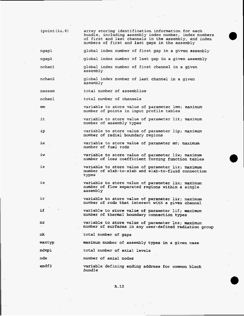
ipoint ( iu, 8 ) array storing identification information for each bundle, including assembly index number, index numbers of first and last channels in the assembly, and index
ngapl
ngap2
nchanl
nchan2
nassem
nchanl
mm
it
iP
ia
iw
iZ
ix
ir
if
nz
nk
=tYP
n-1
ndx
endf 3
numbers of first and last gaps in the ass;?mbly
global index number of first gap in a given assembly
global index number of last gap in a given assembly
global index number of first channel in a given assembly
global index number of last channel in a given assembly
total number of assemblies
total number of channels
variable to store value of parameter lmm; maximum number of points in input profile tables
variable to store value of parameter lit; maximum number of assembly types
variable to store value of parameter lip; maximum number of radial boundary regions
variable to store value of parameter mr; maximum number of fuel rods
variable to store value of parameter liw; maximum number of loss coefficient forcing function tables
variable to store value of parameter liz; maximum number of slab-to-slab and slab-to-fluid connection types
variable to store value of parameter lix; maximum number of flow separated regions within a single assembly
variable to store value of parameter lir; maximum number of rods that interact with a given channel
variable to store value of parameter lif; maximum number of thermal boundary connection types
variable to store value of parameter lnz; maximum number of surfaces in any user-defined radiation group
total number of gaps
maximum number of assembly types in a given case
total number of axial levels
number of axial nodes
variable defining ending address for common block bundl e
A. 12

common /fields3/
conk (mg)
dpbar (lip*iq)
common /fieldb/
term1 (mc)
COMDECK PROPS
common /propl/
pbegl(1)
pl i q ( mp ,2 1
temliq (mp, 2
hliq(mp,2)
conliq (mp, 2
cpliq(mp,2)
visliq (mp, 2)
vliq(mp,2)
bliq (mp, 2 1
tvary (mp)
varyk (mp)
varycp (mp)
varyr (mp
array storing local value of fluid thermal conduction in the lateral direction f o r a given gap at an axial level
array storing plenum node temperatures written to the output file for the plenum temperature summary
array storing input values for inlet mass flow fraction for each channel in an assembly
array storing the sum of the turbulent cross-flow term and the fluid conduction term for the lateral momentum equation solution in each gap at a give axial level
variable defining beginning address for common block Prop1
input array for fluid property tables; pressure (psia)
input array for fluid property tables; temperature (OF)
input array for fluid property tables; enthalpy (Btu/lbm)
input array for fluid property tables; thermal conductivity (Btu/h-ft-OF)
input array for fluid property tables; specific heat ( B tu/ lbm- F )
input array for fluid property tables; viscosity ( lbm/ f t - h) input array for fluid property tables; specific volume ( f t3/lbm)
input array for fluid property tables; coefficient of thermal expansion, (l/OF)
input array for temperature-varying material properties tables; temperature (OF)
input array for temperature-varying material properties tables; thermal conductivity (Btu/h-ft-OF)
input array for temperature-varying material properties tables; specific heat (Btu/lbm-OF)
input array for temperature-varying material properties tables; density (lbm/ft3)
A. 13

ntnode
nsett
nf prop ( 2 1
nviscw
data (mpp)
tmelt (2)
tboil(2 1
nfass (iu)
endpl
common /prop2/
pbeg2 ( 1)
pref
lamnh (liw)
nheat
nf lmc (iu)
ah1 (liw)
ah2 (liw)
ah3 (liw)
ah4 (liw)
ah11 (liw)
number of entries in the temperature dependent material properties table for fuel type 1
total number of fluid properties tables; (maximum is 2)
number of entries in each input fluid property table
flag €or hot wall correction to fluid viscosity calculation
data array for interpolated table(s1 of fluid properties, created in 10°F increments from input properties table ( s )
starting-temperature for each fluid property table interpolated in 10°F increments from the input table values; defined as 10°F below the first entry in the user-specified input table
ending temperature for each interpolated fluid property table; defined at the last entry in the user- specified input table
index number of fluid properties table to be used in a given assembly
variable defining beginning address for common block Prop1
variable defining beginning address for common block Prop2
system pressure; units: psia
logical variable; set to .true. if laminar coefficients are defined by user input as non-zero for a given heat transfer correlation
number of heat transfer coefficient correlation specified by input in group HEAT
index of heat transfer correlation to be used in a given assembly
Reynolds number multiplier coefficient for heat transfer correlation(s) for turbulent axial flow
Reynolds number exponent for heat transfer correlation(s) for turbulent axial flow
Prandtl number exponent for heat transfer correlation(s) for turbulent axial flow
additive coefficient for heat transfer correlation(s) for turbulent axial flow
Reynolds number multiplier coefficient for heat transfer correlation(s) for laminar axial flow
A. 14

ah12 (liw)
ah13 ( l i w )
ah14 (liw)
aht 1 ( 1 iw)
aht2 (liw)
aht3 (liw)
aht4 (liw)
ahtll (liw)
ahtl2 (liw)
ahtl3 (liw)
ahtl4 (liw)
ahf 1 (liw)
ahf2 (liw)
istar (mg).
ntheat
nfheat
endp2
common /prop3/
pbeg3 (1 1
visc (mc, 3)
viscw (mc)
Reynolds number exponent for heat transfer correlation(s) for laminar axial flow
Prandtl number exponent for heat transfer correlation(s) for laminar axial flow
additive coefficient for heat transfer correlation(s) for laminar axial flow
Reynolds number multiplier coefficient for heat transfer correlation(s) for turbulent lateral flow
Reynolds number exponent for heat transfer correlation(s) for turbulent lateral flow
Prandtl number exponent for heat transfer correlation(s) for turbulent lateral flow
additive coefficient for heat transfer correlation(s1 for turbulent lateral flow
Reynolds number multiplier coefficient for heat transfer correlation(s) for laminar lateral flow
Reynolds number exponent for heat transfer correlation(s) for laminar lateral flow
Prandtl number exponent for heat transfer correlation(s) for laminar lateral flow
additive coefficient for heat transfer correlation(s) for laminar lateral flow
Rayleigh number multiplier coefficient for heat transfer correlation(s) for free convection axial flow
Rayleigh number exponent for heat transfer correlation(s1 for free convection axial flow
in-line function to define donor channel for cross- flow in a given gap
number of forced convection heat transfer correlations specified by user input
number of free convection heat transfer correlations specified by user input
variable defining beginning address for common block Prop2
variable defining ending address for common block prop3
viscosity of a fluid node; -units: lbm/ft-s
viscosity in a node at a heated wall; units: lbm/ft-s
A. 15

con (mc)
cp (mc)
beta (mc)
ntype (mc)
amix (lit)
bmix (lit)
endp3
common /matprp/
pbeg4 (1)
uwcp (nd, mw)
uwall (nd, mw)
areacp (mw2 )
matypp (mw2 1
tpsave (mw2 1
npwcon
con0 (id)
thermal conductivity in a fluid node; units: Btu/s-ft-OF)
specific heat of the fluid in a node; units: Btu/lbm- OF)
specific volume of a fluid node; units: ft3/lbm
temperature in a fluid node; units: O F
local value of the heat flux profile for a given axial level; units: Btu/s-ft2
array storing the local coefficient of thermal expansion in a fluid node at a given axial level
array storing index number of axial friction factor correlation for a given channel
multiplicative coefficient for lateral turbulent mixing correlation ( s )
Reynolds number exponent for turbulent mixing correlation (s)
variable defining beginning address for common block prop3
variable defining beginning address for common block ma t P r p
sum of the thermal conductances for heat transfer between a fluid node and a wall node divided by the specific heat of the fluid node, at a given axial level
sum of the thermal conductances for heat transfer between a fluid node and a wall node, at a given axial level
heat transfer area for axial connections between a given slab node and a plenum axial region; units: input in in?
array storing index numbers of material type €or connections between a given slab node and a plenum axial region
array to save the previous iteration value of the plenum fluid temperatures, in the energy equation solution
total number of slab nodes with thermal connections to the plena
leading additive coefficient for correlation(s) for temperature-dependent solid material thermal conductivity
A. 16

con1 (id)
con2 (id)
con3 (id)
cpsol (id)
rhosol (id)
rdima (liz)
rdimb (liz)
nqvt (id)
conw Imw)
matj (id,mx)
mattyp (mw)
imat (id)
pdna (iu)
P h
nsprop
endp4
common /alpha/
aname (id)
alph
multiplicative coefficient on temperature for temperature-dependent solid material thermal conductivity
multiplicative coefficient on temperature-squared term for temperature-dependant solid material thermal conductivity
multiplicative coefficient on temperature-cubed term of temperature-dependant solid material thermal conductivity
solid material properties table input array; specific heat (Btu/lbm- OF)
solid material properties table input array; density ( lbm/ f t 1
geometry factor for the lower-numbered node of any pair of nodes connected by a given thermal connection tme
geometry factor f o r the higher-numbered node of any pair of nodes connected by a given thermal connection type
index number of transient heat rate forcing function to be used for user specified solid material properties
array storing current value of boundary heat flux correlation for each boundary slab node at a given axial level
array storing index numbers of fuel material types for profiles of axially varying fuel material type
array storing index of material type for each slab node
solid material type index number
array storing heat generation rate for each assembly
average heat generation rate; units: input as Mbtu/h- f t2
number of solid material properties tables specified by input
variable defining ending address for common block ma tPrp
alphanumeric identifier for solid material properties table
alphanumeric variable used to store date and time information for printout to output file (s)
A. 17

COMDECK DRAGS
common /drag/
dbegl(1)
dpa (iu)
kij (mg)
cij (mgl
itran
aa (liw)
bb (liw)
cc (liw)
dd (liw)
ee (liw)
aal (liw)
bbl (liw)
ccl (liw)
lamnf (liw)
aat (liw)
bbt (liw)
cct (liw)
ddt (liw)
variable defining beginning address for common block drag
array storing pressure drop boundary condition for each assembly; units: input in psi
loss coefficient for lateral flow in gap connections
array storing the combined form drag and friction loss term for the lateral momentum equation in each gap at a given axial level
flag for lateral convection heat transfer correlations
first multiplicative coefficient on the Reynolds number for turbulent flow friction factor correlation (SI
first Reynolds number exponent for turbulent flow friction factor correlation(s)
second multiplicative coefficient on the Reynolds number for turbulent flow friction factor correlation ( s )
second Reynolds number exponent for turbulent flow friction factor correlation(s)
additive coefficient for turbulent flow friction factor correlation ( s )
multiplicative coefficient on the Reynolds number for laminar flow friction factor correlation(s1
Reynolds number exponent for laminar flow friction factor correlation (s)
additive coefficient for laminar flow friction factor correlation ( s )
logical variable; set to .true. if laminar coefficients are defined as non-zero for a given friction factor correlation
first multiplicative coefficient on the Reynolds number for lateral wall friction factor correlation(s)
first Reynolds number exponent for lateral wall friction factor correlation(s1
second multiplicative coefficient on the Reynolds number for lateral wall friction factor correlation(s)
second Reynolds number exponent for lateral wall friction factor correlation(s)
A. 18

eet (liw)
aatl (liw) 1
bbtl (liw,)
cctl (liw)
nf rict
ishear
nshear
kn (mg , 2 )
ck (mg, 4 )
enddl
common /bgrid/
dbeg2 ( 1)
additive coefficient for lateral wall friction factor correlation ( s )
multiplicative coefficient on the Reynolds number for laminar flow lateral wall friction factor correlation ( s )
Reynolds number exponent for laminar flow lateral wall friction factor correlation(s)
additive coefficient for laminar flow lateral wall friction factor correlation(s)
number of axial friction factor correlations specified by user input
user specified input flag for fluid shear stress model
number of pairs of gaps that are connected by fluid- fluid shear in the lateral direction
array storing index numbers of gaps connected to a given gap for fluid-fluid shear
array storing shear stress terms in each gap at a given axial level for fluid-fluid shear in the lateral momentum equation
variable defining ending address for common block drag
variable defining beginning address for common block bgri d
factor(lit,mq,mx) array storing relative axial locations for loss coefficients to be applied to a specified set of channels in a given assembly
ilce (lit , mq)
lcass (iu)
lcff (mk)
lcasst (mk)
array storing identification number of ending channel in a location set of loss coefficients in a given assembly
logical variable; set to .true. if an assembly has form drag loss coefficients defined by user input
array storing index numbers of loss coefficient forcing functions to be applied to loss coefficients in channels of a given assembly
array storing index numbers of assembly types with loss coefficients
ifact (mq, mx)
nlevel(lit,mq) number of axial locations in a given location set of
array storing axial level locations of axial form drag loss coefficients for a given channel
loss coefficients for a given assembly
A. 19

cd (lit, mq, m x )
xcd (lit, mq, mx)
ifb (mc)
nblock
f lo (iu)
allf
nbl (lit)
flog (mj 1
pwin (iu)
pwout (iu)
rain (iu)
raout (iu)
rgin (m j
rgout (mj)
netgrp (iu)
noutff (iu)
dpt (iu)
rmuinlt
array storing axial form drag loss coefficients at a given axial level in a given channel of a given assembly type
array storing loss coefficients to be applied in a specified set of channels in a given assembly at a specified axial location
array used to flag a blocked axial level in a channel at a given axial level
number of axial locations where flow blockages are specified by user input
array storing total assembly flow when the network model is used
summation of all assembly flows is used
number of sets of channels in a loss coefficients
array storing total flow in all group for the network model
when the network model
given assembly having
assemblies of a given
wetted perimeter associated with the inlet loss in a given assembly when using the network model
wetted perimeter associated with the outlet loss in a given assembly when using the network model
inlet loss parameter to be applied to a given assembly when using the network model; units: (ft-lbm1-l
outlet loss parameter to be applied to a given assembly when using the network model; units: (ft- lbm) -I
inlet loss parameter to be applied to a given assembly group when using the network model; units: (ft-lbml-’
outlet loss parameter to be applied to a given assembly group when using the network model; units: ( f t - lbm) -’ assembly grouping number in the network model for a given assembly
array storing identification number of loss coefficient forcing function versus Reynolds number to be used at the assembly outlet in the network model
array storing pressure drop in each assembly; units: lbf /ft2
fluid viscosity at the inlet enthalpy of channel number 1; used to calculate the Reynolds number of the inlet flow in the network model
number of assembly groups in the network model
A. 2 0

netwk
fpri (iu)
dppri (iu)
lblok (mk, 2)
iblokt
rtin
hgin (mj 1
hgout (mj )
hain (iu)
ghead (mc 1
dpcor (mc)
walls (iu)
ilcs (lit,mq)
nramp
ninf f (iu)
phead
haout ( iu )
ibloka (mc)
variable storing pressure drop boundary condition for network model; units: lbf/ft2
flag for optional network pressure drop model
array storing the previous iteration value of *the total pressure drop in each assembly; units: lbf/ft2
array storing the previous iteration value of the friction pressure gradient in each assembly, for use in the network model
array storing index numbers of axial levels of blockages, and channels that have blockages
total number of local blockages
loss parameter on the total flow rate summed over all assemblies, for the network model; units: (ft-1bmI-l
gravitational head length associated with inlet loss in a given assembly group inlet in the network model; units: input in in.
gravitational head length associated with outlet loss in a given assembly group inlet in the network model; units: input in in.
gravitational head length associated with the assembly inlet loss in a given group in the network model; units: input in in.
pressure drop due to gravity head in a given channel, for network model calculations
array storing the total momentum pressure drop in each channel at a given axial level
array storing the current iteration value of the friction pressure gradient in each assembly, for use in the network model
array storing the index of the starting channel in a location set of loss coefficients in a given assembly
number of iterations over which loss coefficients are to be ramped into the solution
array storing identification number of loss coefficient forcing function versus Reynolds number to be used for the.inlet loss of a given assembly for the network model
assembly average pressure drop, to be used in calculations for the network model
gravitational head length associated with the assembly outlet loss in a given group in the network model; units: input in inches
array storing index numbers of assemblies containing specified blocked channels
A. 21

iblokc (mc)
endd2
COMDECK TIME
common /timez/
tbegl(1)
dt
iprnte
iprnta
t t ime
etime
clock ( 8 1
maxt
ndt
ndtpl
itstep
endtl
common /outout/
tbeg2 (1)
output (12
print (14
tdumy(l0)
tprint
array storing index numbers of blocked channels in a given assembly
variable defining ending address for common block bgri d
variable defining beginning address for common block t i m e z
time step; units: seconds
flag to activate option for output of assembly average and channel exit values
flag to activate option for output of channel exit values
total transient time specified by user input; units: seconds
elapsed simulation time; units: seconds
array storing cpu time intervals spent in different parts of the solution during code execution; units: seconds
maximum cpu time allowed for code execution; units: seconds
number of time steps
number of specified time steps, plus 1
number of entries in variable time step table
variable defining ending address for common block timez
variable defining beginning address for common block outout
array for storing calculated output variables
logical variable; set to .true. if input options specify that processed input is to be written to the output file
array to store rod values in degrees Celsius for output
printout interval for determining the time steps written to the output file in a transient.calculation; units: seconds
A. 22

trant
naxp
nout
npchan
nP9aP
i2
i3
ipost
j hot
jpres
j rods
j slab
npnode
nprod
time interval between successive output time steps is a transient calculation
number of axial heat generation profile tables
flag for all printout, or selected printout controlled by flags ncout, nrout, ngout, and nwout
number of channels to be printed
number of gaps to be printed
variable defining logical unit number for reading input
variable defining logical unit number for output file
logical unit number for output to the post processing file written in subroutine POST
axial level treated as the bottom of the channel region; level 1 for pressure boundary condition or if the lower plenum model is used, level 2 for flow boundary condition
option for input group GRAF; (NOTE: developmental feature; not validated, and not documented in Cycle 2 )
option for input group GRAF; (NOTE: developmental feature; not validated in Cycle 2 )
option for input group GRAF; (NOTE; developmental feature; not validated in Cycle 2 )
flag for fuel temperature node printout
number of rods to be printed
printn (10) array storing index numbers of fuel rod nodes for which temperatures will be printed in the output file
nskipt
nskipx
ihh
interval to skip in time step printout; default is 1, and means no skipped time steps
interval to skip in axial node printout; default is 1, and means no skipped nodes
number of time values in each transient forcing function table on average heat generation rate
number of pairs of values in transient forcing function on inlet flow
flag for inlet flow distribution option
number of pairs of values in transient forcing function on inlet enthalpy or temperature
flag for units of enthalpy or temperature on channel inlet conditions
A. 23

number of pairs of values in transient forcing function on system pressure
im (ms)
jm(ms)
imp (10)
i8
kase
printc (mc)
printg (mg)
printr (mr)
ipreb
.ncout
nrout
ngout
nwout
npwall
printw (mw)
postr (mr)
postw (mw)
posth (mc)
postp (mc)
conv’( 2
array to store ii indices of gaps for output of input data describing channel gap connections
array to store jj indices of gaps for output of input data describing channel gap connections
array to store ii indices of gaps for a line of output of crossflow results
array to store ii indices of gaps for a line of output of crossflow results
variable storing logical unit number for restart file (tape8)
index number of a given case
array storing index numbers of channels to be printed
array storing index numbers of gaps to be printed
array storing index numbers of rods to be printed
flag to print rebalancing summary with solution iteration summary
flag for restricted channel output
flag for restricted rod output
flag for restricted gap output
flag for restricted slab node output
flag for slab node printout
array storing index numbers of slab nodes to be printed
array for post-processing logic; (NOTE: developmental feature; not validated in Cycle 2 )
array for post-processing logic; (NOTE: developmental feature; not validated in Cycle 2 )
array for post-processing logic; (NOTE: developmental feature; not validated in Cycle 2)
array for post-processing logic; (NOTE; developmental feature; not validated in Cycle 2 )
array storing factors to convert units on temperature from Fahrenheit to Celsius in the output
A. 24

iotemp
endt2
common /chrvar/
hl
h2
h3
h4
h5
h6
h7
h8
common /tables/
tbeg3 (1)
yp (lmm)
fp (lmm)
yg (lmm)
fg (lmm, liw)
fh(1mm) 1
fq(lmm, liw)
yh (lmm)
flag for option for OF or OC units on output temperatures
variable defining ending address for common block ou t o u t
character variable;
character variable;
character variable;
character variable;
character variable;
character variable;
character variable;
character variable;
left parenthesis, ( I
period, ' . ' right parenthesis,
w ( 1
' ) w P ( '
' W'
' X'
I t ( '
variable defining beginning address of common block tab1 es
array storing transient time in the system pressure forcing function table; units: seconds
array storing time-dependent forcing factor normalized to initial value for the system pressure forcing function table
array storing transient time in the inlet flow or pressure drop forcing function tables; units: seconds
array storing time-dependent forcing factors normalized to initial value for the inlet flow or pressure drop forcing function tables
array storing time-dependent forcing factor normalized to initial value for the inlet enthalpy or temperature forcing function table
array storing transient time in the heat generation rate forcing function tables; units: seconds
array storing time-dependent forcing factor normalized to initial value for the heat generation rate forcing function tables
array storing transient time in the time-step size table for variable time-step size; units: seconds
array storing transient time in the inlet enthalpy or temperature forcing function table; units: seconds
A. 25

ft (mp)
y (mp, mv)
axial (mp, mv)
naf lx (iu)
tmncvl( iu 1
recl (lmm)
fflc (lmm, liw)
nax (mv)
nlcfp
nolc
nlcf f
nhx
endt3
array storing time-dependent forcing factor normalized to initial value for the exit enthalpy forcing function table
array storing transient time in the exit enthalpy forcing function table; units: seconds
array storing variable time step sizes for table of variable time step size
array storing relative axial location of elements in axial heat generation rate profile tables
array storing relative heat generation rate profiles, normalized to the average heat generation rate
index number of axial heat flux profile table used in a given assembly
array storing input value of factor to adjust lateral momentum control volume length for the calculation of turbulent crossflow exchange in all gaps of a given assembly
array storing the Reynolds numbers for the loss coefficient forcing function profiles
array storing the loss coefficient factors for the loss coefficient versus Reynolds number forcing function profiles
number of pairs of entries in a given axial heat generation rate profile table
maximum number of points in input tables of loss coefficient versus Reynolds number, flow or pressure drop versus time, heat flux versus time, system pressure versus time, and inlet or exit enthalpy versus time
number of assembly types for which loss coefficients are to be specified by user input
number of forcing functions of loss coefficient versus Reynolds number
number of pairs of values in transient forcing function on exit enthalpy or temperature
variable defining ending address of common block tables
conanon /bound/
tbeg4 ( 1) variable defining beginning address for common block
hout exit enthalpy (Btu/lbm) or temperature (OF)
n j ump input flag for restart calculation
bound
A. 26

ntries
hin (2)
gin
tin
dPS
itdp
itdpa (iu)
ngprf 1
nqprf 1
npfvt (iu)
exith
exitmu
exitt
negf (iu)
negf lo
ftotal
endt4
cormmon /index/
tbeg5 ( 1)
nhigh (mc 1
maximum number of outer iterations in solution of conservation equations
average inlet enthalpy or temperature for channels with each specified fluid; units: Btu/lbm or OF
average inlet mass flux; units: input as Mlbm/h-ft2
average inlet temperature; units: OF
pressure drop; defined by input for uniform specified pressure drop boundary condition option
flag for flow or pressure drop boundary condition option to be applied to all assemblies
flag for flow or pressure drop boundary condition option in a given assembly
number of transient forcing functions for inlet mass flux or pressure drop tables
number of heat generation rate transient forcing function tables
index number of pressure drop of flow forcing function used by a given assembly
enthalpy at the channel exit, for transport terms for reverse flow at the exit; units: Btu/lbm
viscosity of the fluid in the plenum node, when the plenum model is used; units: lbm/ft-s
temperature of the fluid in the plenum node, when the plenum model is used; units: OF
array storing flag indicating the presence of negative axial flow in some channel(s) of a given assembly
flag set when negative flow is encountered in a channel
total inlet flow rate; units: (lbm/sec)
variable defining ending address for common block bound
variable defining beginning address for common block index
array storing index numbers of channels that interact with a given channel for the higher order interaction terms in the solution of the fluid and rod energy equations solution
A. 27

nlow (mc) array storing index numbers of channels that interact with a given channel for the lower order interaction terms in the solution of the fluid and rod energy equations
ncount (mr 1 array storing the number of channels that interact with each rod for the interaction terms in the solution of the fluid and rod energy equations
ihigh
ilow
current value of nhigh(i1 for a given channel i, in the solution of the fluid and rod energy equations
current value of nlow(i) for a given channel i, in the solution of the fluid and rod energy equations
ilowpl current value of ilow, plus 1
npoint current value of ihigh
ihalt
endt5
common /convrg/
tbeg6 ( 1)
qoh
accely
werry
accelf
f error
qerror
dampng
accelh
accrho
accelw
maximum number of iterations in the solution of the fluid and rod energy equations by the method of successive over-relaxation; defined as 100 in subroutine SETIN
variable defining ending address for common block index
variable defining beginning address for common block convrg
maximum error in the fluid energy equation
acceleration factor €or iterative Gauss-Siedel solution of momentum equations
convergence criterion for continuity solution in inner loop of main interaction loop
damping factor for iterative axial flow solution
axial flow convergence criterion for axial momentum equation
convergence criterion for total energy conservation
not used
acceleration factor for successive over-relaxation solution of the rod and fluid energy equations; set equal to accelw, which is specified by input
damping factor on change in fluid density
acceleration factor for the solid node energy equation solution
herror convergence criterion for fluid energy equation

qor
endt 6
maximum error in the solution of the rod energy e quat ion
variable defining ending address for common block convrg
GOMDECK FUELS
common /fuel/
f lbegl(1) variable defining beginning address for common block f u e l
kfuel (mt)
kclad (mt)
rfuel (mt)
rclad (mt
cfuel (mt)
cclad (mt 1
tclad (mt)
hgap (mt 1
powr (ij)
ntheta
nrdthta
nqax
nc
nrod
nrodtp
nfuelt
thermal conductivity of fuel for a given fuel geometry type; units: input in Btu/h-ft-OF, converted to Btu/s-ft-F
thermal conductivity of cladding for a given fuel geometry type; units: input in Btu/h-ft-OF, converted to Btu/s-ft-OF
density of fuel for a given fuel geometry type; units: lbm/ft’
density of cladding for a given fuel geometry type; units : lbm/ft3
specific heat of fuel for a given fuel geometry type; units: Btu/lbm-OF
specific heat of cladding for a given fuel geometry type; units: Btu/lbm-OF
cladding thickness for a given fuel geometry type; units: input in in., converted to ft
gap conductance coefficient of the fuel-cladding gap for a given fuel geometry type; units: Btu/h-ft2-OF
array storing current value of forcing function multiplicative factor for each power profile table
number of circumferential nodes in fuel rods
total number of rod nodes; nrodxntheta
flag for temperature dependent fuel material properties
flag for fuel model option; if nc>4, number of finite difference nodes in the fuel rod, including one node in the cladding
number of rods
number of tables of axial fuel type variation
number of fuel types
A. 29

recall
bx ( 2 , mn, mr)
zx (mn,mr)
qtotal
scladmx
scldmxo
cladmx
acladmx
rcladmx
zcladmx
lr (mr, 6 )
dfuel (mt)
phi (mr, 6 )
radial (mr)
d (mr)
idfuel (mr)
nhf vt (iu)
sparev (2 0 )
void (mr)
flag to indicate iterative solution is finished, either because converged, or specified cpu time has been exceeded
array storing the nonzero elements of the triangular matrix in the solution of the rod energy equation
array used in the matrix algebra for the solution of the rod energy equation
total heat generation; units: Btu/sec
maximum clad surface temperature; units: O F
previous iteration value of maximum clad surface temperature; units: O F
maximum cladding surface temperature on a given rod; units: O F
index number of assembly containing rod with maximum cladding surface temperature
index number of rod with maximum cladding surface temperature
axial level location of maximum rod cladding surface temperature
array containing index numbers of up to six channels seen by a given rod
fuel pellet diameter for a given fuel geometry type; units: input in in., converted to ft
fraction of rod surface that sees a given channel
rod radial power factor, normalized to average rod power; (dimensionless)
fuel rod diameter; units: ft
array storing fuel geometry type index for each rod
index number of heat generation rate forcing function used by a given assembly
spare variable array; used to store information needed temporarily between subroutines
heat generation rate in the central void of an annular fuel rod of a given fuel geometry type; units: Btu/s- et3
array storing index numbers of fuel geometry types
array storing index number of fuel type in different zones of rods with axially varying fuel type
index of fuel material type table to be used in a given axial zone
A.30

zend (mt, my)
nclad (mr , 6 )
nwall (mr, 10)
nrr (mr)
nrw (mr )
rcon
rrdim
wcon
wrdim
delrad (mt)
dodr (mn
dsqr (mn
conr (mr
endf 11
mt)
mt)
common /repeat/
f lbeg2 ( 1)
drod ( mt )
geomf (mt)
dfueli (mt)
refuel (mt 1
rcclad (mt)
e
relative axial location of the end of a fuel zone for an axially varying fuel type table; (dimensionless)
array storing index numbers of up to six rods in contact with a given rod for conduction heat transfer
array storing index numbers of up to ten rods that are in contact with a given wall node
array storing index numbers of rods in contact with adjacent rods for conduction heat transfer
array storing index numbers of wall nodes in contact with rods for conduction heat transfer
contact conductance between rods; units: h-ft-OF/Btu
geometry factor for thermal connections for rod-to-rod contact; (dimensionless)
contact conductance between rods and wall surfaces; units: h-ft-OF/Btu
geometry factor for thermal connections for rod-to- wall contact; (dimensionless)
array storing node thickness of each node for the conduction heat transfer solution in the fuel pellet; units: ft
array storing the node outside diameter divided by the node thickness for each fuel node of a given fuel type
array storing the node outside diameter squared, minus the inside diameter squared for each fuel node of a given fuel type
array storing average fluid conductivity in the channels seen by each rod at a given axial level; units: Btu/sec-ft-OF
variable defining ending address for common block fuel’
variable defining beginning address for common block repeat
rod outside diameter for a given fuel geometry type; units: input in inches, converted to ft
rod geometry flag for a given fuel geometry type
inside diameter of annular fuel rod of a given fuel geometry type; units: input in inches, converted to ft
array storing the time derivative term for the fuel material, &/At, for each fuel type
array storing the time derivative term for the cladding material, &,/At, for each fuel type
A. 31

r2kf (mt 1
phitot (mr 1
ring (mr)
rang (mr 1
rung (mr 1
hgapl (mt 1
lri (lir,mc)
array storing the coefficient term, fuel diameter squared divided by four times the fuel thermal conductivity, for each fuel type
summation of all phi(n,6) terms for a given rod
array storing constant terms for matrix algebra in solution of rod energy equation
array storing constant terms for matrix algebra in solution of rod energy equation
array storing constant terms for matrix algebra in solution of rod energy equation
array storing the total thermal conductance of the gap and cladding for each fuel type
array storing the index numbers of all rods that see a given channel
trold(m7,mr,mx) rod temperature at each node, in each rod, at each axial level; units: OF
rtran
endf 12
COMDECK WALLS
common /walls/
kside (iu,mll)
uwal (mhl , mwl)
pal (mw)
kwal (mh, mw)
icf (nd, mw)
twsave (mw)
local variable storing current value of transient time derivative in rod energy equation
variable defining ending address for common block repeat
variable defining beginning address for common block w a l l s
array storing index numbers of slab nodes corresponding to the surfaces in a given radiative heat transfer group
array storing total conductance between adjacent slab nodes
array storing summation of all energy entering or leaving each slab node
array storing index numbers of solid nodes adjacent to a given slab node for solid-to-solid thermal connections
array storing index numbers of solid-to-fluid thermal connection type for a given slab node that is connected to a channel
array storing previous iteration value of temperatures of all slab nodes connected to a given slab node, at a given axial level
A. 32
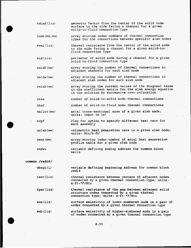
rdimf (liz 1
icon (mh,mw)
rwal (liz)
wid(1i.z)
ns idf (mw)
nsidw (mw)
relxk (mw)
nkss
nksf
wallxc (mw)
nrpf
qslab (mw)
naxk (mw)
endwl
colllMln /raCiiS/
wbeg2 ( 1)
rser (liz)
rpar (liz)
ema (liz)
emb (Liz)
geometry factor from the center of the solid node surface to the side facing a channel for a given solid-to-fluid connection type
array storing index numbers of thermal connection types for the connections between specific slab nodes
thermal resistance from the center of the solid node to the side facing a channel for a given solid-to- fluid connection type
perimeter of solid node facing a channel for a given solid-to-fluid connection type
array storing the number of thermal connections to adjacent channels for each slab node
array storing the number of thermal connections to adjacent slab nodes for each slab node
array storing the current values of the diagonal terms in the coefficient matrix for the slab energy equation in the solution by successive over-relaxation
number of solid-to-solid node thermal connections
number of solid-to-fluid node thermal connections
axial cross-sectional area of a given slab node; units: input in in?
flag for option to specify different heat rate for each assembly
volumetric heat generation rate in a given slab node; units: Btu/h-ft3
array storing index number of axial heat generation profile table for a given slab node
variable defining ending address for common block w a l l s
variable defining beginning address for common block rad i8
thermal resistance between centers of adjacent nodes connected by a given thermal connection type; units:
thermal resistance of the gap between adjacent solid structure nodes connected by a given thermal connection type; units: s-ft-OF/Btu
surface emissivity of lower-numbered node in a pair of nodes connected by a given thermal connection type
surface emissivity of higher-numbered node in a pair of nodes connected by a given thermal connection type
s-ft-OF/Btu
t A. 33

arad (liz) length of node on the face looking at the gap between adjacent nodes connected by a given thermal connection type; units: input in in.
radsav ( 2 , mw ) array storing radiation source term and matrix coefficient in the slab energy equation
sumsav (iu, mll ) array storing summation of the radiation view factor terms times the fourth power of the surface temperature for all surfaces in a given assembly
t4 (m6)
radgap (1 iz )
e m (lnz)
brad (lnz , m8 )
areas (nv, lnz)
fvl (la, la)
fv2 (lb, lb)
fv3 (llc, llc)
fv4 (Id, ld)
fv5 (le, le)
fv6 (If, If)
rratio (6, Inz)
irad
msid (iu)
itypr (iu)
array storing the fourth power of the surface temperature for all rod and slab surfaces
radiation portion of contact conductance for a given slab-to-slab thermal connection type
emissivity of a given surface in a user-defined radiation group
array used in calculation of grey body view factors from black body view factor input, using gaussian elimination in subroutine SETIN
perimeter of a given surface in a user-defined radiation group; units: input in in?
array storing grey body view factors for radiation group 1, read from tape10
array storing grey body view factors for radiation group 2 , read from tape10
array storing grey body view factors for radiation group 3, read from tape10
array storing grey body view factors for radiation group 4 , read from tape10
array storing grey body view factors for radiation group 5, read from tape10
array storing grey body view factors for radiation group 6, read from tape10
array storing ratio of wall node perimeters to rod perimeter, in a radiation group read from tape10
flag for radiation heat transfer in energy solution
array storing the number of slab nodes with surfaces in a given radiative heat transfer group
array storing radiative heat transfer group type for a given assembly
fvw(nv,lnz,lnz) array storing input values of black body view factors between surfaces in a given user-specified radiation group; (maximum of six)
sumr (mr 1 sum of all radiation view factors for a given rod
A. 34

emv ( 6, lnz 1
emrsav(6)
radc (mr)
sumrg (lnz , nv)
endw2
common /walbnd/
wbeg3 (1 1
csl (lif 1
cs2 (lif 1
ems (lif 1
array storing emissivity values for wall nodes in a radiation group read from tape10
array storing.the rod emissivity value f o r each user- defined radiation group
array storing radiation term, emissivity times temperature cubed, for each rod at a given level
array storing summation of all radiation view factors for each surface, in each radiation group read from tape10
variable defining ending address for common block r a d i 8
variable defining beginning address for common block walbnd
first coefficient for user-defined boundary heat flux correlation
first coefficient for user-defined boundary heat flux correlation
combined surface emissivities of boundary nodes for user-defined boundary heat flux correlation
ts (iq, lip, mx)
nzoneb(lip,iq)
temperature array for side axial and radial boundary nodes
array storing number of axial zones in a table of boundary connection types versus axial distance for a given boundary node
nbctyp(lip,iq,mx) array storing the thermal boundary connection types for an axial boundary variation table for a given boundary node
zendb(lip,iq,mx) array storing relative axial locations of entries in an axial boundary variation table for a given boundary node
array storing number of pairs of entries in a given side boundary temperature profile table
nzone t (no )
zendt ( m x , no) array storing relative axial location of a given element in a given side boundary temperature profile table
bt (mx, no)
nbttyp (iq)
nbtemp
array storing boundary temperatures in a given side boundary temperature profile table
array storing identification number of boundary temperature profile seen by a given boundary node
number of axial boundary temperature profiles
A.35

qbsrc (iq)
qpsrc(2,2)
tamb (iq,mx)
sper (lip, iq)
qside (mx)
nhsid (iq)
nwsid
iwsid (iq)
awsid (iq)
endw3
c o m n /plena/
wbeg4 (1)
nPr
iplenr (2 1
awps (lip)
awpax (lip)
npsid (2)
npax (2 1
tambp (2,2)
boundary heat flux applied to a given radial region; units: input as Btu/h-ft2
plenum radial and axial boundary heat flux; units: input as Btu/h-ft2
array storing boundary temperature seen by each boundary node at each axial level
perimeter of a given boundary region of a boundary node, normalized awsid(iq); dimensionless
array storing total heat loss from side boundary nodes at each axial level
array storing number of radial boundary regions connecting a given node to a boundary temperature
number of solid structure nodes connected to the side boundary
array storing index numbers of solid structures nodes connected to side thermal boundary temperatures
perimeter of the side facing the boundary for a given solid structure node temperature
connected to a side boundary
number of thermal boundary connection types
variable defining ending address for common block walbnd
variable defining beginning address for common block plena
plenum model flag
array storing plenum type flag
nominal plenum radial heat transfer area; units: input in inz
nominal plenum axial heat transfer area; units: input in in2
number of radial plenum boundary regions
number of axial plenum boundary regions
plenum radial and axial boundary temperatures; units: OF
array storing thermal connection type number for axial connections between slab nodes and plenum
plenum radial region heat transfer area multiplier; normalized to awps(lip):(dimensionless)
A. 36

ttop (lip, 2,2
qtop (2)
pexit
ifpln
npw (2 2
cpsav ( 2
hsave (2
exittod (2)
iunca ( iu)
dxwall
dxplen (mw2 )
ipw (mw)
ipintp (2 mw2 )
hplen
endw4
conrmon /redstf/
wbeg5 ( 1)
sldamp
nsigrp
bslgrp (6 1
array storing fluid and radial boundary node temperatures in plena
total energy lost through the plena
system pressure; units: psia
flag for fluid properties table to use in plena
array storing starting and ending slab node numbers for thermal connections to plena
average specific heat of fluid in the plena
average enthalpy in the plena
previous iteration value of average fluid temperature in the plena
array storing index numbers of assemblies not connected to the plenum model
half-node length for axial fluid connection between channels and the plena in the energy equation solution
length for heat transfer from a given slab node to the center of a plenum radial region; units: input in inches
array storing number of solid-to-solid thermal connections for each slab node
array storing index numbers of slab nodes connected to a given plenum radial region
average fluid enthalpy for energy transport due to reverse flow at the channel exit or inlet when the plenum model is used
variable defining ending address for common block plena
variable defining beginning address for common block redstf
damping factor for slab conduction equation in the energy solution
number of groups of slab nodes for which the conduction solution is damped
index number of the first node in a set of sequentially numbered nodes for which the conduction solution is damped
index number of the last node in a set of sequentially numbered nodes for which the conduction solution is damped
A. 37

endw5
COMDECK REBAL
common /rebal/
rbegl(1)
qcoef (iu)
coefh (mc)
coefw (iu, lnz)
caxld (mx2,3)
qres (mx2)
dtax (mx2)
qcon (iu)
endr 1
variable defining ending address for common block redstf
variable defining beginning address for common block rebal
array storing rod dependent terms for each assembly in solution of the fluid and rod energy equations
array storing radiation terms for each channel in an assembly, in the solution of the fluid and rod energy equations
array storing radiation contribution to source term for each surface in each assembly, in the fluid and rod energy equation solution
array storing terms in the coefficient matrix for the fluid energy equation solution in subroutine ENERGY, and also for the one-dimensional energy rebalancing in subroutine RECIRC
array storing net energy in all nodes at each axial level
array used in one-dimensional energy rebalancing for average temperature at each level
array storing summation of radiation terms in all channels of each assembly, for the solution of the fluid and rod energy equations
variable defining ending address for common block rebal
A.38

PNL-10782 UC-800
Distribution
No. of Copies
OFFSITE
Battelle Memorial Institute Technical Library Office of Nuclear Waste Isolation 505 King Avenue Columbus, Ohio 43201
A. Brownstein U.S. Department of Energy 1000 Independence Avenue Washington, D.C. 20585
2 Electric Power Research Institute P.O. Box 10412 Palo Alto, CA 94303
Attn: R. W. Lambert R. L. Yang
2
FLUOR Engineers Advanced Technology Division 333 Michelson Drive Irvine, CA 92730
J. V. Massey Sierra Nuclear Corporation 5619 Scotts Valley Drive, #240 Scotts Valley, CA 95066
Office of Civilian Radioactive Waste Management
U.S. Department of Energy Washington, D.C. 20585
Attn: W. J. Danker, RW-33 L. Stewart, RW-421 J. R. Williams, RW-421
J. Richardson WESTON Technical Support Team 955 L’Enfant Plaza SW washington, D.C. 20024
No. of CoDies
T. L. Sanders Sandia National Laboratory P.O. Box 5800 Albuquerque, NM 87 185
M. L. Smith Virginia Power Company 5000 Dominion Blvd. Glen Allen, VA 23060
2 US . Nuclear Regulatory Commission Office of Nuclear Materials Safety
Mail Stop 6-H-3 Washington, D.C. 20555
and Safeguards
Attn: F. C. Sturz M. B. Raddatz
ONSITE
3 DOE Richland Operations Office
D. C. Langstaff D. E. Trader J. W. Wiley
1 Westinghouse Hanford Company
D. tI. Nyman
29 Pacific Northwest Laboratory
J. M. Creer J. M. Cuta C. W. Enderlin M. A. McKinnon T. E. Michener (14) D. R. Reactor (2) K. P. Recknagle Z. I. Zntoniak Information Release Office (7)
K8-50 K8-50 K8-50
B5-24
K8-50 K7-15 K7- 15 K8-34 K7- 15 K7- 15 K7-15 K7-15 K1-06
Distr. 1