Modelling of strata movement with a special reference to caving mechanism in thick seam coal mining
Upload
independentCategory
view
11download
0
ES-1
Global Energy Decisions
Coal Advisory Service Reference Case
Coal Fall 2007
© Copyright 2007, Global Energy Decisions, LLC All rights reserved. No part of this report may be reproduced or transmitted in any form or means, electronic or mechanical, including photocopying, recording, or by any information storage or retrieval system without the permission of Global Energy Decisions, LLC. This report constitutes and contains valuable trade secret information of Global Energy Decisions. Disclosure of any information contained in this report by you and your Company to anyone other than the employees of your Company ("Unauthorized Persons") is prohibited unless authorized in writing by Global Energy Decisions. You will take all necessary precautions to prevent this report from being available to Unauthorized Persons, as defined above, and will instruct and make arrangements with employees of your Company to prevent any unauthorized use of this report. You will not lend, sell, or otherwise transfer this reports (or information contained therein or parts thereof) to any Unauthorized Person without Global Energy Decisions prior written approval. PROPRIETARY AND CONFIDENTIAL Global Energy Advisors 2379 Gateway Oaks Drive, Suite 200 | Sacramento, CA 95833 tel 916-569-0985 | fax 916-569-0999 Global Energy Decisions

The opinions expressed in this report are based on Global Energy Decisions’ judgment and analysis of key factors
expected to affect the outcomes of future power markets. However, the actual operation and results of power markets
may differ from those projected herein. Global Energy Decisions makes no warranties, expressed or implied, including
without limitation, any warranties of merchantability or fitness for a particular purpose, as to this report or other
deliverables or associated services. Specifically, but without limitation, Global Energy Decisions makes no warranty or
guarantee regarding the accuracy of any forecasts, estimates, or analyses, or that such work products will be accepted
by any legal, financial, or regulatory body.

Executive Summary
Coal Reference Case, Fall 2007 ES-1
The purpose of the Coal Reference Case Fall 2007 is to provide a large scope analysis of the U.S. electric-steam coal industry’s historic and current status and Global Energy’s predictions for the industry’s direction over the next 25 years. As mining costs rise, coal seams and reserves deplete, emission regulations change and increase, and some fuels become more competitive over the next 25 years, the allocation of coal in the electric generation industry is certain to see substantial changes.
Recent History And Current Status Of The Coal Industry Historically, the electric power sector has always consumed more coal than any other sector. It has shown significant demand growth and increased its coal demand share from 73 percent in 1975 to 93 percent of total U.S. coal consumption in 2006, a year in which total electric power coal consumption was 1.06 billion short tons. The industrial and coking plant sectors combined for the last 7 percent or approximately 100 million tons of demand in 2006. This steady increase in use over the years in a volatile industry shows coal’s reliability as a fuel source despite any competitive disadvantages it may have. Coal Production
In order to meet increasing demand, mainly from the electricity generation sector, total U.S. coal production has increased by approximately 52 million tons in the past 10 years to 1.16 billion tons. The Powder River Basin has been responsible for nearly all of the increase while most other major producing basins have seen production declines. The Powder River Basin has increased production by 55 percent to 472 million tons in 2006 from 1997 levels. In the same time frame Central Appalachia has seen production decline by 18.6 percent to 236 million tons in 2006. Higher sulfur Illinois Basin coal production has declined 13.4 percent to 96 million tons in response to the Clean Air Act amendments while Northern Appalachia coal production has declined 12.5 percent to 136 million tons since 1997 for the same reason. The only basin to see an increase in production since 1997 was the Rocky Mountain Basin, showing a modest increase of 1.3 percent in the last 10 years with 112 million tons of total production in 2006. While not considered production, coal imports have steadily increased from 15 million tons in 2000 to 36 million tons in 2006, a 142 percent increase. Coal Mine Productivity
All major coal producing basins have seen declines in basin-level productivity since 2001 due to a lack of new mining technology and deteriorating reserve quality. Though accounting for all U.S. gains in coal mine production over the past decade, the Powder River Basin has seen its overall basin-level productivity decline by 16.7 percent to 34.98 tons per miner hour since 2001. In the same time frame Central Appalachia has seen productivity decline by 25 percent to 2.82 tons per miner-hour in 2006. Illinois Basin and Rocky Mountain productivity have also seen very significant declines of 11.26 and 20.34 percent, respectively. Northern Appalachia productivity saw a decrease of only 1.23 percent, the smallest productivity decline of all the major basins since 2001. Decreasing productivity and increasing production indicate more numerous yet smaller coal mines than in the past.

Executive Summary
ES-2
Coal Prices
All major U.S. coal producing basins have experienced tremendous growth in the FOB (free on board) mine prices they receive for their coal over the past decade. In constant dollars weighted average FOB mine prices (includes spot and contract pricing) have increased 32 percent in the United States from 1998 to 2006. Central Appalachia has seen the most significant increase in FOB prices from $25 to $46/ton over this time period, an increase of 84 percent. The Illinois Basin and Northern Appalachia have both seen a 36 percent increase in FOB mine prices, with 2006 prices of $29.92 and $37.39/ton, respectively. Rocky Mountain coal has realized one of the smallest increases on a dollar per ton basis of approximately five dollars/ton, though this does equate to a significant 27 percent increase. The Powder River Basin’s increases in FOB mine prices have been the most modest from $7.83 to $9.11/ton, or 16 percent. Electricity Generation
In 2006, coal-fired power plants generated 50 percent of U.S. electricity. A decade ago the picture was very different. Coal’s share of electricity generation was near 60 percent in 1997, but has since fallen to 50 percent due to a massive build out of cheap (approximately $600/kW) natural gas plants driven by very low natural gas prices in the early portion of this decade. With low gas prices apparently a thing of the past, coal now holds the title of lowest cost fossil fuel for electricity generation. This is reflected in plant utilization rates, which are much higher for coal than for gas. In 2006 the utilization rate, or capacity factor, of coal plants was 71 percent compared to 25 percent for gas plants. Despite the fact that coal’s generation share is smaller than it was 10 years ago, coal production and consumption increased during that time frame as demand for coal as a source for power generation has continued to increase to meet increasing demand for electricity in the United States. Transportation
In the coal industry, transportation costs factor strongly in the ultimate delivered price at the plant. For instance, 60 percent of the delivered price of coal produced in the PRB is attributable to transportation costs on average. Rail is the transportation method most heavily relied upon in the coal industry due to the vast geographic area that rail infrastructure covers and its ability to move large amounts of coal long distances through varied terrain. Almost 72 percent of coal deliveries utilize rail transportation for at least a portion of their journey. The Powder River Basin, where the average haul distance is 1,200 miles to the plant and 2,400 miles roundtrip—almost exclusively by rail—is of particular note due to rail transportation capacity issues. The owners of the Joint Line are investing in capacity expansion but this may only be prolonging the inevitable—construction of another railroad to the PRB. Another route for coal out of the PRB is necessary, and the market may provide it with the proposed Tongue River Railroad and/or the Dakota, Minnesota and Eastern Railroad (DM&E). River barges are one of the most economical ways to move coal large distances on a cost per ton-mile basis. The obvious constraint to moving coal via barge is geographic location of coal mines and plants in relation to navigable waterways. In 2006, 161 million tons of

Executive Summary
Coal Reference Case, Fall 2007 ES-3
coal had terminating transportation on river barges. Lake vessels are more constrained by geographic location of plants than river barges and were responsible for only 25 million tons of delivered coal in 2006. Fifty percent of the Illinois Basin’s and Central Appalachia’s deliveries, amounting to nearly 130 million tons, utilized trucks as their first and in some cases only form of transportation in 2006. Ocean vessels account at least in some part for nearly all of the 81 million tons of combined U.S. imports and exports. Contracts
Historically, coal contracts were made for longer terms than they are today. The tendency in the industry has been to shorten contract length as other potentially more reliable means of managing risk (e.g., over-the-counter coal trading) have become more widely available and accepted. The reality is that over 85 percent of coal is delivered under contracts with lengths of one year ore more; a dynamic that is unlikely to change anytime soon because of the risk management tool it provides to both producers and consumers. Mining Costs
Deeper and thinner seams, growing underground mine safety costs, and diminishing opportunities to consolidate reserves will cause production to decrease in Central Appalachia. Some of these same issues will add upward cost pressures in all of the other basins. Trends in Central Appalachia over the last 10 year’s coal production are towards surface mining and away from underground mining. With mountaintop mining under attack from environmentalists in the courts there is an added degree of uncertainty about the future of some operations. This situation affords opportunity for consolidation even with the merger and acquisition activity in the coal industry over the last several years. Opportunities for companies to capitalize on potential synergies and the pressure from low prices and rising costs with some producers particularly exposed provide lots of room for ongoing and potentially big consolidation moves—especially in Central Appalachia. Coal-Fired Generation
Today, 93 percent of coal produced in the United States is used for generating electric power. The forecast for future coal use derives from our current understanding of the coal supply and electric generating markets. In addition to cost pressures, coal faces challenges on the demand side in the form of environmental regulation of power plants and competition from other sources of electric power. Coal plants currently provide the U.S. with the half of its electric supply even though coal’s share of U.S. electricity supply has been reduced to 50 percent from about 59 percent over the past decade. Coal remains far cheaper than natural gas on a delivered basis, even with current environmental costs factored in. Alternatives to coal-fired power each come with a set of advantages and disadvantages: • There are 66 operating nuclear power plants in the U.S. today, which account for 21
percent of U.S. electric power generation. Utilization is at 90 percent so up-rates are not likely to account for much further capacity expansion. Fuel is currently cheap, waste disposal is an ongoing and long-term expense, and adding capacity with new

Executive Summary
ES-4
plants faces long lead-times and public opposition but there are a few in the planning stages.
• Gas capacity is the highest of any other fuel with increasing government and public scrutiny regarding emissions in recent years. Gas has become more desirable due to its low emissions and relatively low construction costs, increasing its contribution to total electricity output to 20 percent of total generation. High fuel costs and volatility are likely to keep utilization levels low, but 60,000 MW are on the drawing board nonetheless.
• Hydropower’s percentage of electrical output has dropped from 11 percent to 7 percent over the past 10 years, much of which is likely attributable to increased awareness on the sometimes overlooked harmful environmental effects hydropower can have. Several regions are in the midst of droughts which are lowering output and new, large scale capacity additions are virtually out of the question.
• Renewable energy’s contribution to electricity output is barely 2 percent and remains relatively insignificant. Wind’s contribution will grow as long as subsidies last, but output intermittency and transmission remain as sizeable obstacles. Renewable portfolio standards and carbon regulation will lend support for greater deployment.
Since 1990, net SO2 and NOX emissions at coal burning plants have fallen by 31.3 percent and 33.1 percent, respectively, while the amount of coal burned has increased from 783 million tons/year to 1,015 million tons/year. Nonetheless, utilities continue to face close scrutiny to reduce their emission exposure, which has helped contribute to coal’s decreasing role in the U.S. electricity supply—displaced primarily by gas. Investments in emissions control have resulted in 121 GW of coal-fired capacity that currently has SO2 controls and 306 GW with some form of NOX controls. New emissions limits under the Clean Air Interstate Rule (CAIR) and Clean Air Mercury Rule (CAMR) have spurred a further boom in emissions control equipment installations.
Forecast For The Coal Industry Coal markets are subject to boom and bust cycles with supply and demand constantly in flux and production, contracts, transportation, and stockpiles all playing a role in adding to the uncertainty. In order to address this uncertainty, the Coal Quality Market Model (CQMM) is used by Global Energy to forecast future U.S. consumption, allocation, and price of coal from every mine to every boiler over the 25-year study period. The CQMM relies on data from Global Energy and uses a highly sophisticated network linear program to find the optimal minimum cost solution for the given model input and constraints. Much of the data supplied by Global Energy is extracted from the Velocity Suite, the industry’s leading coal and energy market database. Along with the help of numerous government, public, and private data sources Global Energy has created the most thorough, accurate, and highly representative database achievable. The results from this model represent Global Energy’s forecast and are detailed in the section below.

Executive Summary
Coal Reference Case, Fall 2007 ES-5
Coal Demand Forecast
Coal will remain the single largest contributor to overall U.S. electric supply over the course of this forecast as demonstrated in Figure ES-1. Our forecast shows coal generation will increase almost 28 percent through 2031 though coal’s relative share of the market will decline 4 percent. Gas-fired capacity increases its market share of generation by 10 percent while posting a 227 percent increase; this is the second largest growth in generation in this forecast. The largest relative growth in generation comes from renewables which will experience a 341 percent increase, but still remains only 5 percent of the total U.S. generation. Figure ES-1 Historical and Forecasted Electricity Generation by Fuel
0
1,000,000
2,000,000
3,000,000
4,000,000
5,000,000
6,000,000
7,000,000
1997
1999
2001
2003
2005
2007
2009
2011
2013
2015
2017
2019
2021
2026
2031
Year
Gen
erat
ion
(GW
h)
Coal Nuc Gas Water Petro Renew
Historical Forecast
SOURCE: Global Energy.
Since U.S. coal demand differs between different regions of the country, Global Energy has partitioned the results into smaller, well-defined demand regions.1 The U.S. regional coal demand forecast can be found in Figure ES-2. Coal demand will differ by region due to several key factors: • Growth in overall electricity demand; • Status of the existing coal fleet, the age of the units, and their utilization rate; • Difficulty in permitting new plants; and • Delivered cost of coal and competing fuels. The Northeast region has the lowest current coal demand and the slightest increase in coal demand of all the regions over the forecast period. With an average growth of 0.5 percent a year, its total demand will increase 13 percent over the 25-year time span. The West region is also relatively flat, increasing 16 percent over 25 years. The Southeast region is expected to increase 24 percent, which equates to over 160,000 GW-hours of
1 Please refer to Section 3 to view a map of the five U.S. demand regions.

Executive Summary
ES-6
coal generation. The Midwest shows growth every year resulting in the highest absolute increase (248,300 GWh or 34 percent since 2007) in coal power demand by 2031. The South Central region, while small, shows the greatest average yearly increase (1.5 percent) and overall increase (44 percent) in coal-fired electricity generation. Figure ES-2 Coal Generation Demand by Region
0
200
400
600
800
1,000
1,200
2007 2009 2011 2013 2015 2017 2019 2021 2023 2025 2027 2029 2031
Coa
l Dem
and
(000
's G
W-h
r)
Northeast West South Central Southeast Midwest
SOURCE: Global Energy.
Coal Supply Forecast
Total deliveries of coal within the U.S. are expected to increase from 1.05 billion tons in 2007 to 1.3 billion tons in 2031, an annual average increase of 1.98 percent. Demand for coal is expected to increase for all basins except for Central and Southern Appalachia, which should see demand decrease by 45 percent and 28 percent, respectively. The largest percentage increase in demand is expected to come from Colombian coal at 178 percent—a 36 million ton increase over the 25-year study period. Demand for PRB coal is forecasted to rise by 50 percent (annual growth of 9.4 million tons/year) and the Illinois Basin should see a 37 percent growth in demand (annual growth of 1.28 million tons/year). Rocky Mountain coal is expected to command a 27 percent increase in demand (annual growth of 1.1 million tons/year). Lignite demand should remain relatively flat. Figure ES-3 details our 25-year forecast for basin-level coal deliveries.

Executive Summary
Coal Reference Case, Fall 2007 ES-7
Figure ES-3 United States Delivered Coal Quantities
-
200
400
600
800
1,000
1,200
1,400
2007 2010 2013 2016 2019 2022 2025 2028 2031
MM
tons
Import / Other Local Lignite Rocky Mountain Illinois Basin
Northern App Central / Southern App PRB
SOURCE: Global Energy.
Mine Fully Allocated Costs
Fully allocated mine costs, which include full production costs including return on capital, are expected to increase over the forecasted period. Although taxes and royalties are expected to decline over the midterm, the cash cost of coal for all U.S. coal basins is expected to rise for a number of reasons: • Decreasing productivity due to thinner and deeper seams; • Limits on the economies of scale ; • Rising prices for fuel, equipment, tires, and explosives; • Competition for skilled labor across the energy sector; and • An aging workforce that is nearing retirement in the East. U.S. coal mine fully allocated costs are expected to decrease over the next five years by about 4 percent, as shown in Figure ES-4. This is a result of increases in production of Powder River Basin coal and decreases in production of Central Appalachian coal. Numerous industry sources have indicated that the MINER Act will add up to $8 per ton of coal extracted from underground mines.

Executive Summary
ES-8
Figure ES-4 U.S. Fully Allocated Mine Costs; 2007-2031 (Constant 2007 Dollars)
20
22
24
26
28
30
32
2007
2009
2011
2013
2015
2017
2019
2021
2023
2025
2027
2029
2031
FAC
$/to
n
U.S Fully Allocated Costs
SOURCE: Global Energy.
Global Energy expects fully allocated costs for Appalachian coal mines to increase over the mid term. A significant amount of the Appalachian fully allocated cost increase is due to increased cash costs of complying with the provisions in the MINER Act of 2006, which affects Appalachian mines more than any other region in the United States. Compliance with the new safety regulations will place a heavy burden on all underground mine operators, but the heaviest burden will be on the smaller operators who will be unable to distribute compliance costs over a broad production base. Unless there is significant consolidation of reserves and operations in the East, longwall mining will not be as economical to install. As a result, less efficient, higher cost underground operations will continue in the Appalachian region. Western coal basins (including the Powder River and Rocky Mountain) fully allocated costs are expected to increase by approximately 5-6 percent over the next five years. Increasing coal ratios; seam splitting and washouts; higher input costs for fuel, labor, explosives, tires, and equipment; and increasing tax and royalty costs will all contribute. These cost increases are not expected to be offset by productivity-increasing technological improvements. Productivity is the single largest factor that contributes to a mine’s overall production costs. U.S. coal mines’ aggregate productivity is likely to fluctuate through the mid term. The variability in productivity is mainly due to large volumes of higher cost, lower productivity mines being shut-in and some larger western mines ramping up production as market conditions and prices fluctuate. For example, in 2007 over 43 million tons of production capacity with productivity less than 19.6 tons per miner-hour will go off line. With reserve blocks becoming increasingly difficult to mine we do not expect to see major increases in productivity in the future unless new technologies for extracting coal are developed.
Executive Summary
Coal Reference Case, Fall 2007 ES-9
Eastern U.S. productivity (Appalachia and Illinois Basin) primarily depends on the mine type (surface vs. underground) and technology (e.g., continuous miner vs. longwall). Surface mines typically have higher productivity than underground mines due to accessibility and economies of scale that allow for easier and more cost effective production. On average, eastern surface mines have almost twice the productivity as underground mines. Central Appalachian productivity is expected to steadily decline 6 percent over the next five years as producers continue to move into thinner and more geologically challenging seams. Northern Appalachian productivity will not decline as rapidly as Central Appalachia, with only a 2.5 percent drop over the next five years. While some underground seams in this region are becoming smaller, the extensive use of longwall miners in Northern Appalachia helps support positive productivity. Even though Illinois Basin production capacity will grow over the mid-term, productivity is expected to decline through 2010. Productivity in the Powder River Basin is expected to flatten over the next three years, but remain the highest of all the U.S. coal basins. FOB Mine Prices
FOB mine prices (Figure ES-5) will also escalate over the forecasted period due to increasing production costs coupled with growing demand. Unparalleled mining conditions allow the Powder River Basin to have much lower FOB mine prices than other areas with smaller, less productive mines. Increased short-term FOB prices for South American imports will be due to increased U.S. and European demand for the coal while expanded supply with weakened European demand will dampen import coal prices through the long term. Northern Appalachian FOB prices should experience the strongest growth over the mid term due to robust demand. FOB coal price inflation will be tempered by escalating competition among the basins for customers that have the ability to switch to a primarily Btu-centric rather than sulfur-centric coal product. Figure ES-5 FOB Mine Price Forecast by Basin; 2007-2031 (Constant 2007 Dollars)
$0.00
$10.00
$20.00
$30.00
$40.00
$50.00
$60.00
$70.00
2007 2010 2013 2016 2019 2022 2025 2028 2031
FOB
$/to
n
Central App Colombia Illinois Basin Northern AppPRB Rocky Southern App
SOURCE: Global Energy.

Executive Summary
ES-10
Coal Transportation
Of all the transportation issues facing the U.S. coal markets, the development and expansion of rail in the Powder River Basin will have the biggest impact on U.S. coal consumption patterns. In addition to plans by UP and BNSF to expand the existing lines, there are two major plans to add more transportation capacity out of the PRB: the Dakota, Minnesota & Eastern Railroad and development of the Tongue River Railroad. Increased competition for tonnage from the PRB could be the only check on the two major rail carriers’ stranglehold on western rail pricing, which Global Energy is forecasting to show the greatest increases over the forecast period. Our forecasted 25-year coal transport price inflation assumptions can be found below in Table ES-1. Table ES-1 Global Energy Forecasted 25-Year Coal Transport Price Inflation
Barge Lake Vessel Ocean Vessel Eastern Rail Western Rail
102.8% 106.4% 103.5% 115.3% 127.7%
SOURCE: Global Energy.
Besides western rail pricing and bottlenecks, forecasted coal transportation will be dependent upon a wide variety of factors: • Barge pricing will remain flat but increased river flooding, drought, dam and lock
repair work, and dredging will all factor into barge availability; • Lake vessels will also show little pricing inflation though environmental concerns coupled
with climate change related freezing/thawing patterns could add uncertainty; and • Ocean vessels’ current extremely high pricing should settle down with increased
availability and port expansions on the way. Delivered Price Forecast by Region Increased FOB mine and transportation prices will translate into continued pressure on the delivered price of coal. While the Powder River Basin has extremely low FOB mine prices, the coal produced here has to be transported great distances and in great quantities because of its low heat content. For this reason the eastern regions (Southeast and Northeast) have high delivered coal costs because of higher eastern mining costs or very high transportation rates for cheaper western coal. Colombian imports also keep eastern prices high due to the extremely high transportation costs. For western coal consumers the low price and short hauls equate to retaining the lowest burner-tip price of coal even with considerable inflation over the forecast period. Figure ES-6 below details the changes in regional delivered prices over the course of this forecast.

Executive Summary
Coal Reference Case, Fall 2007 ES-11
Figure ES-6 U.S. Regional Delivered Price of Coal (Constant 2007 $/MMBtu)
1.2
1.4
1.6
1.8
2
2.2
2.4
2.6
2007
2009
2011
2013
2015
2017
2019
2021
2023
2025
2027
2029
2031
Del
iver
ed $
/MM
Btu
West Midwest South Central Southeast Northeast SOURCE: Global Energy.
Battlegrounds
Battlegrounds are supply areas in which different basins can deliver coal for the same price on a dollar per MMBtu basis. Map ES-1 shows the areas in 2007 where delivered prices are $2.00/MMBtu or less. The Powder River Basin is able to deliver to a very large geographic area, penetrating nearly all of the areas served by the Illinois Basin and Central Appalachia at this price. While the PRB is able to penetrate central Indiana and Ohio at this price level, this is a rail market that has a higher price than surrounding areas such as the Ohio River and the Great Lakes which can be accessed more cheaply by barge or lake vessel. This is shown clearly below with the “horseshoe” shape the PRB’s $2.00/MMBtu area takes in this region. Competition is currently heaviest in Illinois and the river markets directly surrounding it, as well as into the Ohio River Valley as far east as West Virginia. The main competition will continue to be on the river markets through the mid term, particularly the Ohio River. This remains the only area where all three basins are able to deliver coal under $2.00/MMBtu. The greatest shift in the market occurs through the longer term as Central Appalachia’s production declines and costs continue to increase. The market that is reachable at a delivered price of $2.00/MMBtu shrinks dramatically to contain only a small part of the Ohio River Valley. Meanwhile, increased demand for Illinois Basin coal inflates delivered prices around the basin and into the southeast, leaving the Illinois Basin area and the western half of the Ohio River Valley the only major battleground left at this price range. Competition among these basins will certainly occur elsewhere in the country with the southeast being the likeliest alternate battleground.

Executive Summary
ES-12
Map ES 1 2007 Coal Battleground Areas
SOURCE: Global Energy.

Table of Contents
Coal Reference Case, Fall 2007 i
Executive Summary ES-1 1 Introduction 1-1
Purpose Of Study........................................................................................ 1-1 Organization Of The Report ........................................................................ 1-4
2 Forecast Methodology and Assumptions 2-1
Forecast Methodology ................................................................................ 2-1
• Global Energy’s Approach to Modeling Demand for Electric Power ....................2-1
• Global Energy’s Approach to Modeling Natural Gas Prices.............................2-6
• Global Energy’s Approach to Modeling Emissions Prices ...............................2-8
• Coal Price Volume and Model .........................................................................2-10
• Global Energy’s Coal Cost Model ...................................................................2-14
• Global Energy’s Approach to Modeling Productivity and Production ............2-17
Forecast Assumptions ...............................................................................2-20
• Electricity Demand...........................................................................................2-20
• Natural Gas and Oil Pricing .............................................................................2-22
• Generating Capacity ........................................................................................2-24
• Key Assumptions Applied to the MARKETSYM™ Model................................2-25
• Environmental Issues.......................................................................................2-31
• Transportation Assumptions............................................................................2-38
3 Historic and Current Market Conditions 3-1
Demand For Electricity Generation............................................................. 3-1 • Historic and Current Electricity Generation by Fuel ..........................................3-1
• Historic and Current Electricity Capacity by Fuel ..............................................3-2
Supply Of Coal...........................................................................................3-12 • Historic and Current Coal Consumption by Sector.........................................3-12
• Basin Production and Quality ..........................................................................3-14
• Basin Reserves ................................................................................................3-17
• Basin Costs......................................................................................................3-22
• Non-Utility Coal Consumption .........................................................................3-25
Coal Transportation....................................................................................3-28 • Railroad Transportation ...................................................................................3-28
• River Barge.......................................................................................................3-37
• Truck ................................................................................................................3-39
• Lake Vessel ......................................................................................................3-39
• Ocean Vessel ...................................................................................................3-40
• Slurry Pipeline ..................................................................................................3-42

Table of Contents
ii
Coal Supply Contracts ...............................................................................3-42 Regulatory Issues.......................................................................................3-48
• Clearn Air Act ...................................................................................................3-49
• Clean Air Mercury Rule ....................................................................................3-54
• Clean Air Interstate Rule ..................................................................................3-56
• Carbon Emissions Regulations .......................................................................3-56
• Mountain Top Removal Mining........................................................................3-62
• The Surface Mine Control and Reclamation Act .............................................3-64
• The Mine Safety and Health Administration ....................................................3-65
Other Issues...............................................................................................3-66
• Industry Consolidation Through Merger and Acquisition (M&A) ....................3-66
• OTC Markets ....................................................................................................3-70
• Foreign Markets ...............................................................................................3-72
4 Coal Demand Outlook 4-1
Demand Region Outlook ............................................................................ 4-1 • Overall U.S. Demand .........................................................................................4-1
Midwest ....................................................................................................... 4-4 Northeast..................................................................................................... 4-9 South Centtral ............................................................................................4-13 Southeast ...................................................................................................4-17
West ...........................................................................................................4-21 Non-Utility Future Coal Consumption ........................................................4-25
• Coking Coal .....................................................................................................4-25
• Industrial, Commercial, and Residential Coal Use..........................................4-26
• Coal-to-Liquids and Coal-to-Gas ..................................................................... 426
• 25-Year Projections..........................................................................................4-28
5 Coal Supply Outlook 5-1
Forecasted Coal Costs ............................................................................... 5-1
• U.S. Fully Allocated Costs .................................................................................5-1
• Basin Fully Allocated Costs ...............................................................................5-2
• Basin Productivity ..............................................................................................5-5
• Avaialble Spot Curves by Basin.......................................................................5-10
FOB And Delivered Prices By Supply Basin And Region ..........................5-14
• Central Appalachia ..........................................................................................5-15
• Norhtern Appalachia........................................................................................5-19
• Illinois Basin .....................................................................................................5-21
• Powder River Basin..........................................................................................5-25

Table of Contents
Coal Reference Case, Fall 2007 iii
• Rocky Mountain Region...................................................................................5-30
• All Other Basins ...............................................................................................5-35
Coal Basin Battleground ............................................................................5-39 Forecasted Coal Production ......................................................................5-42
• Central Appalachia ..........................................................................................5-43
• Northern Appalachia........................................................................................5-43
• Illinois Basin ...................................................................................................... 545
• Rocky Mountain ...............................................................................................5-46
• Powder River Basin..........................................................................................5-49
Future Coal Transportation ........................................................................5-52
• Railroad Transportation ...................................................................................5-53
• Barge Transportation .......................................................................................5-60
• Ocean Vessel Transportation ..........................................................................5-61
Appendix A Demand Region Prices
Appendix B Demand Region Volumes
Appendix C Basin Volumes & Prices

iv
List of Tables
Coal Reference Case, Fall 2007 v
ES-1 Global Energy Forecasted 25-Year Coal Transport Price Inflation..................... ES-10
2-1 Reference Case Gas Price Forecasting Phases......................................................2-6
2-2 Emissions Costs .....................................................................................................2-10
2-3 Historic and Forecasted Economic and Population Growth .................................2-20
2-4 Forecasted Electricity Growth - GWh .....................................................................2-21
2-5 Key Statistics for Future Fuel Mix; 2007-2031........................................................2-22
2-6 Average Market Clearing Price Forecast................................................................2-22
2-7 Natural Gas and Oil Price Forecast; 2007 S/MMBtu .............................................2-24
2-8 Current and Forecasted Capacity (MW) ...............................................................2-24
2-9 Key Statistics for Future Coal Technology; 2007-2031..........................................2-25
2-10 Generic Unit Costs and Operating Characteristics................................................2-27
2-11 Regional Multipliers ................................................................................................2-28
2-12 Capital Structure Characteristics............................................................................2-29
2-13 Cost Assumptions for Emissions Control Equipment............................................2-32
2-14 Effectiveness of Emissions Control Equipment .....................................................2-32
2-15 Reference Case SO2 Allowance Price Forecast .....................................................2-33
2-16 National and CAIR NOX Emissions Prices..............................................................2-36
2-17 Escalation by Transportation Mode .......................................................................2-39
3-1 Electric Power Plants and Average Capacity ...........................................................3-4
3-2 Appalachia Recoverable Resources by Coal Bed.................................................3-18
3-3 Remaining Coal in the Illinois Basin by Coal Bed ..................................................3-19
3-4 Powder River Basin Coal Reserves by Coalfield....................................................3-20
3-5 Historical Total Delivered Coal by Purchase Type.................................................3-45
3-6 Top Ten Contract Holders in 2007 .........................................................................3-46
3-7 National Ambient Air Quality Standards.................................................................3-50
3-8 State Mercury Emissions Rules..............................................................................3-55
3-9 Major Federal GHG Emission Reduction Proposals .............................................3-60
3-10 World Steam Coal Trade 2005-2006......................................................................3-73
4-1 Yearly Coal Generation Demand by Region ............................................................4-2
4-2 Approximate Ton Makeup of Coal Source Categories Seen in Figures..................4-3
4-3 Projected Coking Coal Exports by Country; 2007-2032........................................4-25
4-4 Coal-to-Liquids Plants under Development ...........................................................4-27
5-1 Central Appalachia Quality Ranges .......................................................................5-15

List of Tables
vi
5-2 North Appalachia Northeast Quality Ranges .........................................................5-19
5-3 North Appalachia Ohio Quality Ranges .................................................................5-20
5-4 Illinois Basin Quality Ranges ..................................................................................5-21
5-5 Northern Powder River Basin Quality Ranges .......................................................5-25
5-6 Southern Powder River Basin FOB Mine Prices ....................................................5-26
5-7 Rocky Mountain Colorado North Quality Ranges..................................................5-31
5-8 Rocky Mountain Colorado West Quality Ranges...................................................5-32
5-9 Rocky Mountain Four Corners Quality Ranges......................................................5-33
5-10 Rocky Mountain Wyoming Quality Ranges............................................................5-34
5-11 Rocky Mountain Utah Quality Ranges ...................................................................5-35
5-12 Central Interior Quality Ranges...............................................................................5-35
5-13 Northern Lignite Quality Ranges ............................................................................5-36
5-14 Gulf Lignite Quality Ranges....................................................................................5-37
5-15 Import Coal Quality Ranges ...................................................................................5-38
5-16 Southern Appalachia Quality Ranges ....................................................................5-39
5-17 Mill Rates by Transportation Mode.........................................................................5-52
5-18 Potential DM&E PRB Coal Tonnage by Termination .............................................5-56
5-19 Rail Access to Notable Coal Docks .......................................................................5-57
5-20 Import Handling Facility Capacities .......................................................................5-61
List of Figures
Coal Reference Case, Fall 2007 vii
ES-1 Historical and Forecasted Electricity Generation by Fuel..................................... ES-5
ES-2 Coal Generation Demand by Region .................................................................... ES-6
ES-3 United States Delivered Coal Quantities ............................................................... ES-7
ES-4 U.S. Fully Allocated Mine Costs; 2007-2031 (Constant 2007 Dollars) ................. ES-8
ES-5 FOB Mine Price Forecast by Basin; 2007-2031 (Constant 2007 Dollars) ............ ES-9
ES-6 U.S. Regional Delivered Price of Coal (Constant 2007 $/MMBtu)...................... ES-11
1-1 Forecasted Coal Demand ........................................................................................1-1
2-1 Global Energy’s Fuels Analysis Uses an Integrated Cross Commodity Approach 2-1
2-2 Gas Price Seasonal Variation ...................................................................................2-7
2-3 CQMM Logic Flowchart..........................................................................................2-13
2-4 How the CQMM Handles Sulfur Allowances..........................................................2-14
2-5 Historic GDP and Electricity Generation Growth ...................................................2-21
2-6 Historical and Forecasted Electricity Generation by Fuel......................................2-21
2-7 Gulf of Mexico Monthly Natural Gas Production and Wellhead Price ...................2-23
2-8 Gulf of Mexico Crude Oil Production, NY Harbor Oil Prices, and Average Wellhead Natural Gas Prices..................................................................................2-23
2-9 Historical and Forecasted Electricity Generation by Coal Plant Technology ........2-25
2-10 Forecasted Scrubbed and Un-Scrubbed U.S. Coal Capacity...............................2-33
2-11 National and CAIR NOx Emissions.........................................................................2-35
2-12 SCR Installations by MW Capacity .........................................................................2-35
3-1 Electricity Generation by Region ..............................................................................3-2
3-2 Percentage of Electricity Generation by Fuel ...........................................................3-2
3-3 U.S. Generating Capacity by Fuel Type; 2007.........................................................3-3
3-4 U.S. Capacity Installation Timeline ...........................................................................3-3
3-5 Historic and Current Capacities by Fuel Type .........................................................3-4
3-6 Historic and Current Capacity Factors by Fuel Type...............................................3-5
3-7 Average Delivered Fuel Price to Electric Utilities .....................................................3-8
3-8 Coal Consumption by Sector 1975 and 2006........................................................3-13
3-9 Production of Major Coal Basins (1997-2006).......................................................3-13
3-10 U.S. Coal Resources ..............................................................................................3-18
3-11 Coal Mine Productivity by Basin; 1995-2007 .........................................................3-23
3-12 Historical Non-Utility Coal Consumption; 1973-2006 ............................................3-26
3-13 Average Coking Coal Prices in the U.S.; 2001-2007 .............................................3-27
3-14 Rail Cost Adjustment Factor...................................................................................3-35

List of Figures
viii
3-15 Terminating Transportation of Coal Imports ..........................................................3-42
3-16 Coal Quantities under Existing Contracts by Basin ...............................................3-44
3-17 Historical Delivered Contract Coal Quantity by Basin............................................3-45
3-18 Historical Average FOB Contract Prices by Basin .................................................3-47
3-19 Historic FOB Contract & Spot Prices for Select Basins .........................................3-48
3-20 Production and Productivity at Surface and Underground Mines in
Central Appalachia; 1990-2007..............................................................................3-63
3-21 Market Concentration for U.S. Coal Producers by Basin; 1990-2007 ...................3-69
3-22 Example of Hedging in the Coal Markets ..............................................................3-71
4-1 United States Coal Demand by Basin......................................................................4-1
4-2 Coal Generation Demand by Region .......................................................................4-3
4-3 Midwest Delivered Coal Quantities ..........................................................................4-5
4-4 Midwest FOB Mine Price ..........................................................................................4-6
4-5 Midwest Transportation Cost by Basin ....................................................................4-7
4-6 Midwest Delivered Price ...........................................................................................4-7
4-7 Midwest Coal under Contract...................................................................................4-8
4-8 Northeast Delivered Coal Quantities ......................................................................4-10
4-9 Northeast FOB Mine Price......................................................................................4-11
4-10 Northeast Transportation Price...............................................................................4-12
4-11 Northeast Delivered Price.......................................................................................4-12
4-12 Northeast Coal under Contract ..............................................................................4-13
4-13 South Central Delivered Coal Quantities................................................................4-14
4-14 South Central FOB Mine Price................................................................................4-15
4-15 South Central Transportation Price ........................................................................4-15
4-16 South Central Delivered Price.................................................................................4-16
4-17 South Central Coal under Contract ........................................................................4-16
4-18 Southeast Delivered Coal Quantities .....................................................................4-18
4-19 Southeast FOB Mine Price .....................................................................................4-18
4-20 Southeast Transportation .......................................................................................4-19
4-21 Southeast Delivered Price ......................................................................................4-20
4-22 Southeast Current Coal under Contract.................................................................4-20
4-23 West Delivered Coal Quantities..............................................................................4-22
4-24 West FOB Mine Price..............................................................................................4-23
4-25 West Transportation Cost .......................................................................................4-23
4-26 West Delivered Price...............................................................................................4-24

List of Figures
Coal Reference Case, Fall 2007 ix
4-27 West Current Coal Under Contract ........................................................................4-24 4-28 Projected Non-Utility Coal Consumption; 2004-2031............................................4-29
5-1 U.S. Fully Allocated Mine Costs ...............................................................................5-1
5-2 Projected Appalachian Fully Allocated Costs ..........................................................5-3
5-3 Projected Illinois Basin Fully Allocated Costs ..........................................................5-4
5-4 Projected PRB Fully Allocated Costs .......................................................................5-4
5-5 Projected Rocky Mountain Fully Allocated Costs ....................................................5-5
5-6 Weighted Average U.S. Productivity ........................................................................5-6
5-7 Weighted Average Central Appalachian Productivity ..............................................5-6
5-8 Weighted Average Northern Appalachian Productivity............................................5-7
5-9 Weighted Average Illinois Basin Productivity ...........................................................5-7
5-10 Stratigraphic Cross Section of Future Mining Conditions at Buckskin Mine...........5-8
5-11 Weighted Average PRB Productivity ........................................................................5-9
5-12 Weighted Average Rocky Mountain Productivity .....................................................5-9
5-13 Central Appalachia Available Spot Curves ............................................................5-11
5-14 Southern Appalachia Available Spot Curves .........................................................5-11
5-15 Northern Appalachia Available Spot Curves..........................................................5-12
5-16 Illinois Basin Available Spot Curves .......................................................................5-12
5-17 Rocky Mountain Available Spot Curves .................................................................5-13
5-18 Powder River Basin Available Spot Curves............................................................5-13
5-19 Central Appalachia FOB Mine Price Forecast .......................................................5-16
5-20 North Appalachia Northeast FOB Mine Price Forecas ..........................................5-20
5-21 Northern Appalachia Ohio FOB Mine Price Forecast ............................................5-21
5-22 Illinois Basin FOB Mine Price Forecast ..................................................................5-22
5-23 Northern Powder River Basin FOB Mine Price Forecast .......................................5-26
5-24 Southern Powder River Basin FOB Mine Price Forecast .......................................5-27
5-25 Rocky Mountain Colorado North FOB Mine Price Forecast ..................................5-31
5-26 Rocky Mountain Colorado West FOB Mine Price Forecast...................................5-32
5-27 Rocky Mountain Four Corner FOB Mine Price Forecast........................................5-33
5-28 Rocky Mountain Wyoming FOB Mine Price Forecast............................................5-34
5-29 Rocky Mountain Utah FOB Mine Price Forecast ...................................................5-35
5-30 Central Interior FOB Mine Price Forecast...............................................................5-36
5-31 Northern Lignite FOB Mine Price Forecast ............................................................5-37
5-32 Gulf Lignite FOB Mine Price Forecast ....................................................................5-37
5-33 Import FOB Mine Price Forecast............................................................................5-38
List of Figures
x
5-34 Southern Appalachia FOB Mine Price Forecast ....................................................5-39
5-35 U.S. Coal Production ..............................................................................................5-42
5-36 Projected Central Appalachian Production............................................................5-43
5-37 Projected Northern Appalachian Production .........................................................5-44
5-38 Projected Northern Appalachian - North East Production.....................................5-44
5-39 Projected Northern Appalachian - Ohio Production ..............................................5-45
5-40 Projected Illinois Basin Production.........................................................................5-46
5-41 Projected Rocky Mountain Production...................................................................5-46
5-42 Projected Rocky Mountain - Colorado Production ................................................5-47
5-43 Projected Rocky Mountain - Wyoming Production ................................................5-48
5-44 Projected Rocky Mountain - Four Corners Production ..........................................5-48
5-45 Projected Rocky Mountain - Utah Production........................................................5-49
5-46 Projected Powder River Basin Production .............................................................5-50
5-47 Projected Southern Powder River Basin Production..............................................5-51
5-48 Projected Northern Powder River Basin Production ..............................................5-52
List of Maps
Coal Reference Case, Fall 2007 xi
ES-1 2007 Coal Battleground Areas ............................................................................ ES-12
1-1 Coal Consumption by Source Region......................................................................1-2
2-1 Natural Gas Liquid Market Centers ..........................................................................2-8
3-1 The Five U.S. Coal Demand Regions.......................................................................3-1
3-2 U.S. Nuclear Power Plants .......................................................................................3-5
3-3 U.S. Gas-Fired Power Plants....................................................................................3-7
3-4 U.S. Hydropower Plants ...........................................................................................3-9
3-5 U.S. Renewable Energy Sites.................................................................................3-10
3-6 U.S. Coal-Fired Power Plants .................................................................................3-11
3-7 U.S. Coal Supply Regions ......................................................................................3-15
3-8 Rail Transportation in Appalachia ..........................................................................3-29
3-9 Illinois Basin Rail Infrastructure and Coal Docks ...................................................3-30
3-10 Rail Transportation in the Powder River Basin .......................................................3-31
3-11 Powder River Basin.................................................................................................3-34
3-12 River Transportation in the Eastern United States. ................................................3-37
3-13 Coal Handling Facilities..........................................................................................3-40
3-14 Major Import Facilities and Planned Import Capacity Increases...........................3-41
3-15 Coal Plant Mercury Emissions in 1999...................................................................3-55
3-16 GHG Reduction Initiatives in North America ..........................................................3-58
4-1 The Five U.S. Coal Demand Regions.......................................................................4-2
4-2 Midwest Demand Region - Current..........................................................................4-4
4-3 Northeast Demand Region - Current .......................................................................4-9
4-4 South Central Demand Region - Current ...............................................................4-13
4-5 Southeast Demand Region - Current.....................................................................4-17
4-6 West Demand Region - Current .............................................................................4-21
5-1 U.S. Coal Supply Regions ......................................................................................5-14
5-2 Central Appalachia 2007 Delivered Prices.............................................................5-17
5-3 Central Appalachia 2015 Delivered Prices.............................................................. 518
5-4 Central Appalachia 2031 Delivered Prices.............................................................5-19
5-5 Illinois Basin 2007 Delivered Prices........................................................................5-23
5-6 Illinois Basin 2015 Delivered Prices........................................................................5-24
5-7 Illinois Basin 2031 Delivered Prices........................................................................5-25
5-8 Powder River Basin 2007 Delivered Prices ............................................................5-28

List of Maps
xii
5-9 Powder River Basin 2015 Delivered Prices ............................................................5-29
5-10 Powder River Basin 2031 Delivered Prices ............................................................5-30
5-11 2007 Battleground Areas .......................................................................................5-40
5-12 2015 Battleground Areas........................................................................................5-41
5-13 2031 Battleground Areas........................................................................................5-42
5-14 Canadian Pacific and DM&E Rail and Potential Coal Plant Market.......................5-55
5-15 Rail Routes in the Powder River Basin ...................................................................5-59

Section 1 Introduction


Introduction
Coal Reference Case, Fall 2007 1-1
Purpose Of Study The consumption of coal in the United States has grown dramatically over the past five decades principally in response to growing demand for electricity generation. The consistent historic increase in utilization of existing steam-electric coal plants combined with the proposed construction of over 77,000 MW of new coal-fired power plants promises to create a significant increase in future coal demand. Alternative and novel uses for coal such as steel production, liquefaction, gasification, ethanol production, and hydrogen production will create even greater demand for coal. In addition to Global Energy’s forecast of future coal consumption, the Energy Information Agency’s (EIA) Annual Energy Outlook (AEO) and the National Coal Council (NCC) also predict that consumption of coal will significantly rise over the next several decades as shown in Figure 1-1. The AEO reference growth scenario reveals that U.S. coal supply must increase by 465 million tons to meet demand by 2025. Even the AEO low growth scenario adds 323 million tons by 2025. More aggressively, the NCC recommends that U.S. coal supply must increase by 1.3 billion tons by 2025 to meet expected demand for electricity, liquefaction, gasification, and other uses. Figure 1-1 Forecasted Coal Demand
SOURCE: Annual Energy Outlook.
The Global Energy mine capacity study, Can Coal Deliver?, provided an in-depth view of current and future production costs, annual production and productivity associated with every mine in the United States. While Can Coal Deliver? provided detailed analyses of mining issues based on geology, resources, costs, and productivity from 2007 through 2012, the purpose of this study is to provide a large scope analysis of the U.S. coal markets. Specifically, this study provides a highly detailed forecast of coal production and consumption patterns and prices in the U.S. over the next 25 years. Using a state-of-the-art coal price and allocation model, Global Energy has created a forecast of mine price,
Introduction
1-2
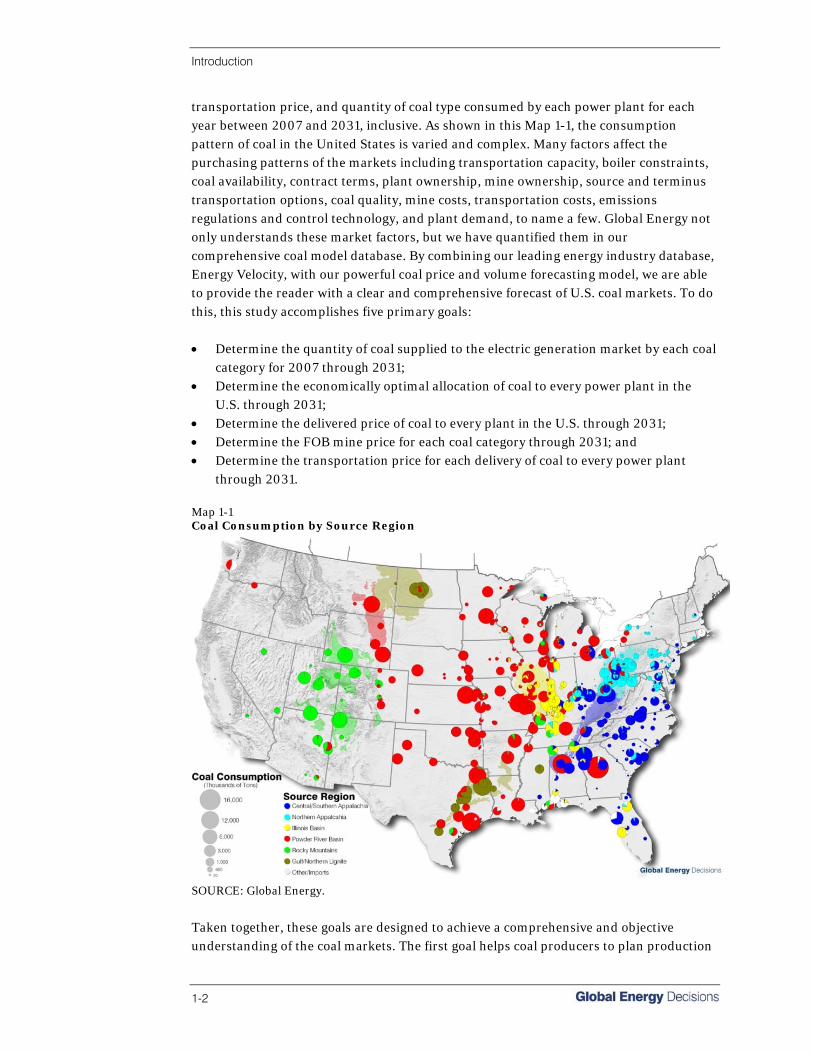
transportation price, and quantity of coal type consumed by each power plant for each year between 2007 and 2031, inclusive. As shown in this Map 1-1, the consumption pattern of coal in the United States is varied and complex. Many factors affect the purchasing patterns of the markets including transportation capacity, boiler constraints, coal availability, contract terms, plant ownership, mine ownership, source and terminus transportation options, coal quality, mine costs, transportation costs, emissions regulations and control technology, and plant demand, to name a few. Global Energy not only understands these market factors, but we have quantified them in our comprehensive coal model database. By combining our leading energy industry database, Energy Velocity, with our powerful coal price and volume forecasting model, we are able to provide the reader with a clear and comprehensive forecast of U.S. coal markets. To do this, this study accomplishes five primary goals: • Determine the quantity of coal supplied to the electric generation market by each coal
category for 2007 through 2031; • Determine the economically optimal allocation of coal to every power plant in the
U.S. through 2031; • Determine the delivered price of coal to every plant in the U.S. through 2031; • Determine the FOB mine price for each coal category through 2031; and • Determine the transportation price for each delivery of coal to every power plant
through 2031. Map 1-1 Coal Consumption by Source Region
SOURCE: Global Energy.
Taken together, these goals are designed to achieve a comprehensive and objective understanding of the coal markets. The first goal helps coal producers to plan production

Introduction
Northeast Regional Outlook, Spring 2007 1-3
and manage reserve assets effectively by providing information on coal types that are likely to be in high demand. It also provides utilities with planning tools by determining which coals are likely to be in high demand and thus likely to be more costly. The second goal logically follows, providing producers information about their likely markets and consumers with likely available least cost sources of fuel. A forecast for the delivered price of coal at the plant level gives coal consumers a planning tool for generation asset management. The FOB mine price forecast provides a planning tool for coal producers’ potential revenue streams. And finally, the transportation price forecast provides a planning tool for producers, consumers, and coal transporters. These goals form the core of the study, but understanding the reasoning and logic that underlie forecast results is also essential to a useful forecast. In order to provide context for the forecast, substantiate the findings, and provide the reader with the necessary background, a comprehensive review of the current and historical coal market is necessary. This study also assesses two broad but essential aspects of the coal market: • Alternative electricity generation sources, their current and historic costs and
utilization rates relative to coal as generation sources, and associated financial and environmental risks for each generation type; and
• The coal industry’s place in the current electric generation market based on historic production, productivity, reserves, and costs as well as transportation issues, environmental constraints, changing historical patterns of supply and demand, and coal transaction contracts.
On the surface, this study is intended to make broad brush strokes to describe the fundamentals of coal supply and demand. Its foundation, however, is much more detailed and inclusive and builds a forecast from the most basic data on what is essentially the most granular level possible. This study is driven by the desire to add plant level coal price input to complete Global Energy’s interconnected power market model and to provide a mine level forecast for coal production. This study has given us a better understanding of the complex market dynamics that underlie the coal industry and has enabled us to answer questions such as, “How much Powder River Basin coal will penetrate the eastern coal markets given our understanding of the historic, current, and likely future production, mine costs, transportation rates, plant fuel limitations, environmental regulations, and competition from other basins?” This is a complicated question which demands a comprehensive understanding of all aspects of a fascinating industry. Global Energy, in partnership with RBAC, has developed the Coal Quality Market Model (CQMM) and comprehensive input dataset to forecast the likely consumption patterns of coal at the boiler level over the next 25 years. In other words, we would like to know which boilers will receive coal from which mines. This model essentially acts as a coal router, matching coal supply from individual mines to coal demand at individual boilers. It seeks to find the lowest cost solution for the entire system. The model is designed to

Introduction
1-4
meet the goal of determining the most likely allocation of coal given the cost of producing it at each mine, the possible transportation options and prices, and the demand and limitations of each boiler. When we aggregate the model results we can answer questions like the one posed above with a great deal of precision or adjust the parameters of the model to more accurately reflect our understanding of and expectation for the coal industry. In Global Energy’s MARKETSYM™ model the prices of oil, natural gas, coal, and emissions allowances are inputs utilized to produce outputs of future demand of coal, natural gas, oil, and their contributions to U.S. power generation over the next 25 years. The Global Energy Reference Case Model is a dynamic tool allowing users to create forecasts based on industry factor assumptions made by Global Energy as well as create unique forecasts based on variations of factor assumptions.
Organization Of The Report The report detailing the Fall 2007 Coal Reference Case is divided into six main sections: • The Executive Summary briefly describes the purpose and results of the study; • The Introduction outlines the purpose of the study and describes the organization
of the report; • The Forecast Methodology and Assumptions section outlines how Global
Energy integrates oil, gas, coal, emissions, and power models to produce outputs; describes our CQMM and its scenario and sensitivity capabilities; gives insight into our cost modeling methodology for coal; and analyzes electricity demand and related supply as well as related constraints such as emissions;
• The Historic and Current Market Conditions section outlines demand for electricity, possible generation options and their advantages and disadvantages; paints a picture of coal supply for electricity generation and other uses; addresses issues concerning transportation, emissions, and safety regulations and their possible effect on coal supply and demand; and outlines important contract volumes and expiration dates;
• The Coal Demand Outlook section examines forecasted demand for coal used for electricity by region and coal type as well as outlining historic and future consumption of coal in the coking, industrial, commercial, and residential sectors;
• The Coal Supply Outlook section provides forecasts on costs, productivity, and production; as well as forecasts on prices of steam coal and consumption of steam, industrial, commercial, and residential coal by region; and outlines import price and volume forecasts.
Section 2 Forecast Methodology and Assumptions


Forecast Methodology and Assumptions
Coal Reference Case, Fall 2007 2-1
Forecast Methodology Global Energy’s approach to market forecasting integrates model inputs and outputs from our power, emissions, and fuels forecasting models. Figure 2-1 shows how the models in our suite of forecast products are interrelated. The coal model takes the demand for electric power at each coal generating station from the Reference Case forecast, which is tied directly to the gas, oil, coal, and emissions models. Prices for emissions (NOx, SO2, and Hg) allowances at a national and regional level are used as inputs for the Emissions Price forecast. Prices for gas, oil, and coal are taken from the gas, oil, and coal models, respectively, and input to the Power Reference Case, which in turn feeds the fuels and emissions models. Each of the inputs into the coal market model is itself the result of sophisticated modeling techniques as described below. Figure 2-1 Global Energy’s Fuels Analysis Uses an Integrated Cross Commodity Approach
SOURCE: Global Energy.
Global Energy’s Approach to Modeling Demand for Electric Power The MARKETSYM™ Model Global Energy uses a fundamentals-based methodology to forecast power prices in each region of North America. Based on its proprietary MARKETSYM™ system—MARKETSYM™ is a sophisticated, relational database that operates with a state-of-the-art, multi-area, chronological production simulation model—Global Energy simulates the operation of each region of North America. For each region, MARKETSYM™ considers:
Demand
EmissionPrice
Forecast
Price
Oil Model
Coal Model
GasModel
ReferenceCase
ForecastPrice Price
Price
Price
Demand Demand
PricePrice
Demand
EmissionPrice
Forecast
Price
Oil Model
Coal Model
GasModel
ReferenceCase
ForecastPrice Price
Price
Price
Demand Demand
PricePrice

Forecast Methodology and Assumptions
2-2
• Individual power plant characteristics including heat rates, start-up costs, ramp rates, and other technical characteristics of plants;
• Transmission line interconnections, ratings, losses, and wheeling rates; • Forecasts of resource additions and fuel costs over time; • Forecasts of loads for each utility or load serving entity in the region; and • The cost and availability of fuels that supply the plants.
MARKETSYM™ simulates the operation of individual generators, utilities, and control areas to meet fluctuating loads within the region with hourly detail. The model is based on a zonal approach where market areas (zones) are delineated by critical transmission constraints. The simulation is based on a mathematical objective function that minimizes the cost of serving load within the modeled electric system subject to meeting load, a number of operational constraints, as well as the assumed strategic behavior (bidding) of market participants. Monte Carlo analysis is employed to incorporate individual unit forced outages. The result is a long-term price forecast that allows existing and new generators to recover all short- and long-term costs (including financing costs) from the market. To understand how uncertainty regarding power prices, fuel prices, and hydro conditions influence the forecast, Global Energy also prepares a sample stochastic analysis of power prices and generator profitability that explicitly models key stochastic variables and their correlation. As such, Global Energy simulates the price formation in competitive markets using a least cost approach with an explicitly defined scarcity bidding behavior. Three fundamental principles guide the forecast development: • Maintain sufficient reliability in all market areas; • In the short term, benchmark the model against observed historical market prices
and market heat rates; and • In the long term, allow new capacity to recover all costs, including fixed and financing
costs from the energy market.
Long-Term Forecasting and Boom/Bust Cycles Electricity markets are subject to significant boom and bust cycles. U.S. markets have gone from capacity shortage in the late 1990s to a significant overbuild in many market areas. The timing of boom and bust cycles can have a significant impact on the net present value of new capacity investments; attempting to forecast the timing of such events is very difficult at best, and there is not yet sufficient data to predict the duration of a “typical” boom/bust cycle. Therefore, Global Energy employs an approach in which we start at current market conditions and then gradually—depending on load growth and capacity under construction—arrive at long-term market equilibrium where new capacity is added to meet forecast load growth while achieving long-term revenue requirements. In an overbuilt market, this means holding off on new capacity additions until supported by market prices and then continuously adding new resources throughout the remainder of

Forecast Methodology and Assumptions
Coal Reference Case, Fall 2007 2-3
the forecast, thus maintaining an equilibrium price level where new capacity just meets long-term revenue requirements. Market Equilibrium Concepts Global Energy’s modeling approach is well suited to an interconnected regional grid. The model simulates prices, output, and investment that occur over time to keep the market in equilibrium. Market equilibrium has two key elements: • First, it must be technically feasible. Generation, transmission, etc., must not be
stressed beyond their engineered limits. • Second, the equilibrium must be consistent with behavior of market participants
(good utility practice and/or centrally dispatched systems). Developers invest in additional generating capacity when new investment is profitable.
In its power market simulations, Global Energy ensures consistency between these equilibrium concepts by a continuous examination of the long-term economic opportunities for adding new plants, while ensuring that physical plant and transmission constraints—as well as reliability constraints—are observed in any given time period. Bidding Strategy Forecast power prices are formed each hour based on the simulated bids submitted by individual generators. The marginal unit determines the market clearing price in each hour simulated. A station’s bid includes variable costs such as fuel, variable O&M, and no-load costs, as well as an additional amount that serves to cover the generators’ fixed and financing costs. Global Energy uses sophisticated bidding strategies that group generators into different strategies depending on their costs, technology, and expected load-serving characteristics. In practice, generators employ a wide variety of strategies that are consistent with the cost and load serving characteristics of their generating portfolio. These entities forecast how tight the supply/demand situation is to assess the pricing opportunities in the market, and will price their output in a manner that reflects not only the costs of individual units, but also the cost of operating the entire portfolio, including the most expensive units needed to meet load. Scarcity Rents and Quasi-Rents During high load hours, there may be barely enough generation to meet loads.1 At this point, a generator can, in theory, price electricity at very high levels and is limited only by the load’s willingness to voluntarily curtail to avoid those high prices. In most markets, retail prices do not follow wholesale prices and customers therefore have little incentive to curtail demand when supplies are tight and spot prices are high. During these times, the scarcity premium collected by individual generators increases with the scarcity present in the market and over time can contribute significantly to the coverage of financing and other fixed costs. Generators with peaking units need to capture these high
1 This can be due to short-term unit commitment or de-commitment decisions, as well as to longer-term plant investment or retirement decisions.

Forecast Methodology and Assumptions
2-4
scarcity premiums when conditions allow them to do so because their assets will be sitting idle during most hours in a given year. Simulating Rents and Cost Recovery: Bid Markups In modeling the regional power markets, Global Energy has devised bid markup strategies that are consistent with revenue recovery in both the short and long term. In the short term, Global Energy has set bid markups to allow generators to recover start-up and minimum-run costs. Long-term equilibrium requires that generator revenues be sufficient to allow developers to invest in additional capacity. In determining the level of the bid markups, guidance is provided by: • Industry Knowledge. Utilizing Global Energy’s extensive experience of power market
analytics and utility operations to ensure that the simulated bidding behavior is consistent with how power plants are operated in reality;
• Historical prices. Bid markups are validated against observed historical prices in order to capture market pricing characteristics; and
• Rational Bidding. Global Energy carefully examines and groups all existing assets in the modeled region according to their operating costs and load serving characteristics. A shadow pricing methodology is then applied to ensure that the bidding of individual generators is consistent with the behavior of other comparable assets. Furthermore, the bidding is controlled such that generators never price themselves out of profitable generation opportunities.
Facilities under Development The starting point for Global Energy’s simulations is the current plant expansion plans of the utilities, independent power producers, and others in each region. For the year 2007 and earlier years, information from Global Energy’s EnerPrise Online New Entrants™ database is used with modifications consistent with Global Energy’s consulting knowledge. Economic Entry The long-run equilibrium involves simulated plant expansion when such expansions would be profitable in the sense of meeting reasonable financial performance targets. This is the economists’ sense of zero economic profit but does not mean that investors add plants without expecting a reasonable return. Rather, Global Energy models expansion so that investors exhaust all opportunities to earn a reasonable return. Global Energy focuses on a balanced entry of base loaded and peaking generation to maintain system reliability while allowing profitable entry of new capacity. Base loaded capacity determines the pace of construction and, generally, prices in the market. Peaking capacity is entered to ensure sufficient reliability. Profitability of this peaking capacity is determined by not only the simulated deterministic prices but also by volatility and the likelihood of failure of other generation and transmission facilities, and is treated somewhat differently.

Forecast Methodology and Assumptions
Coal Reference Case, Fall 2007 2-5
Base Load Capacity The simulation for a given year is an iterative procedure. A simplified explanation of the process is as follows. First, initial expansion cases are identified for the next few years using regional reserve margin criteria and guidelines. This includes new generation technology based on the vintage of the unit. Construction costs are identified, taking into account regional variations in such costs. A target rate of return for new generation is identified (technological assumptions and costs are discussed in the following section on key assumptions). Peaking Capacity Global Energy’s first-cut approach to modeling peaking facilities involves the addition of new units to maintain sufficient capacity reserve margin. Reserve margin targets are set for each region, typically in the range of 12 to 20 percent. If reserve margins drop too low, then contingent events (such as failure of generating or transmission equipment) may result in a substantial likelihood of a loss of load and/or electricity price spikes. Whether traditional reliability-based planning techniques or a market-driven merchant investment approach is used, capacity to maintain reliability is necessary. This typically involves adding peaking facilities that provide a balance between operational flexibility, operating costs, and capital costs. Reserve margin analysis offers a useful set of rules to estimate the appropriate level of capacity needed for reliability. This approach is consistent both with past and present industry practices including power-flow contingency models. Ancillary Services A key issue in the restructuring of the electric power industry has been the unbundling of the various components of electricity service, particularly on the wholesale side. FERC had originally specified several elements under its standard market design (SMD) principles to be transacted separately including energy, transmission, and several ancillary services (AS) that are necessary for reliable operations of the power grid. Volatility Analysis Global Energy’s Reference Case forecast of power prices is based on a deterministic approach that includes generator-forced outages as its only stochastic variable. In its stochastic market analysis Global Energy models principle drivers of uncertainty including fuel prices, hydroelectric supplies, equipment-forced outages, and load. Volatility, as well as correlation among these variables, is estimated from historical data. For example, low hydroelectric supplies in the West can drive up the prices for gas in the region. Global Energy captures such effects by conducting a stochastic simulation in which all of these uncertainties are considered simultaneously using Monte Carlo techniques. From this analysis, Global Energy builds a distribution of prices that drive the profitability of individual units. This approach allows for an assessment of a station’s real option value as well as to quantify the fundamental drivers of uncertainty and is a powerful tool for understanding market volatility and asset values in the context of physical constraints that characterize the electric power industry.

Forecast Methodology and Assumptions
2-6
Locational Marginal Prices While the forecast prices presented in this report are based on a zonal modeling approach, Global Energy also frequently prepares nodal market analysis where power prices are determined at the bus bar. LMP forecasting can be important for generators since nodal-determined prices often vary significantly from zonal expected prices. The higher level of detail drives this discrepancy in a nodal approach; the LMP model accounts for physical power flows, more detailed transmission representation (and possibilities for congestion), and allocates load and resources on a nodal basis rather than aggregating within a zone. This information was developed using Global Energy’s MARKETSYM™ LMP software platform. Global Energy’s Approach to Modeling Natural Gas Prices
To forecast natural gas prices, Global Energy uses three forecasting phases. These are outlined in Table 2-1. Table 2-1 Reference Case Gas Price Forecasting Phases
Forecast Phase Period Length Data Source Forecast Technique
Futures Driven First 24 Months NYMEX Henry Hub futures and market differentials
Calculated Henry Hub and liquid market center differentials
Mean Reversion Next 24 Months Global Energy Linear process to gradually equate near-term to long-term trend
Long-term Trend Remaining forecast period (to 2030)
Various Global Energy data sources
Fundamental supply and demand analysis modeling
SOURCE: Global Energy.
To derive the burner-tip forecasts used, Global Energy first examined regional prices and basis swaps at a number of trading hubs. Using this historical data, for the first 24 months of the forecast, Global Energy developed a differential price between the appropriate market center nearest to the power plant and the Henry Hub. Gas prices used for the first 24 months were driven by Henry Hub futures market prices plus a basis differential (if any). Applying this approach permitted Global Energy’s forecast to include recent shifts in natural gas prices. During the following 24 months of the forecast period, Global Energy imposed a linear mean reversion process on the forecast. This process aligns natural gas prices during the first 24 months back to their long-term, fundamental levels. To forecast future burner-tip gas prices beyond the initial 48-month period, Global Energy has incorporated the RBAC’s Gas Price Cost Model (GPCM) into our modeling methodology for medium- to long-term analysis. The model is a general equilibrium model of gas supply and demand in a competitive environment for the North American natural gas industry. Another important component in Global Energy’s gas forecast is the seasonal or monthly variation in price. In general, gas prices have been traditionally higher during winter

Forecast Methodology and Assumptions
Coal Reference Case, Fall 2007 2-7
months due to greatly increased core heating demand. To determine the seasonal variation in gas prices, data at individual pricing points are utilized. The appropriate observed seasonal pattern is applied to annual gas price forecasts to derive monthly price forecasts that are used in Global Energy’s market simulations. These seasonal factors represent typical or normalized variation in monthly spot gas prices within a region. The estimated seasonal variation in gas prices is shown in Figure 2-2. This indicates the deviation among monthly gas prices as recorded at the Henry Hub. A polynomial curve was then fitted to the monthly average. The figure indicates that prices are highest during periods of increased core heating demand, while they decline during the spring and early summer months. On average, prices tend to begin rising starting in June due to electricity demand increase coupled with the beginning of the traditional gas storage-filling season. A similar estimation technique is used to forecast monthly fuel oil prices. Figure 2-2 Gas Price Seasonal Variation
0%
20%
40%
60%
80%
100%
120%
Jan Feb Mar Apr May Jun Jul Aug Sep Oct Nov Dec SOURCE: Global Energy.
For electric generators, Global Energy models natural gas burner-tip prices as the sum of commodity prices (the cost of gas at a particular liquid market center, which may be a gas-producing basin, a recognized hub—for example, the Henry Hub—or a citygate) and all relevant transportation charges involved in transporting natural gas from the market center to the generation plant. An active aftermarket consisting of a “capacity release” market exists on most interstate pipeline systems. This capacity allows a gas shipper to offer its own reserved capacity, in excess of current needs, to others for a negotiated price. Capacity release transportation often trades at rates well below firm transportation rates, although this varies depending on prevailing market conditions. Generators within a particular region can generally receive gas from a number of supply basins or hubs. The number of sources is dependent on the geography of where the plant is located relative to the interstate pipeline system. Global Energy assumes that
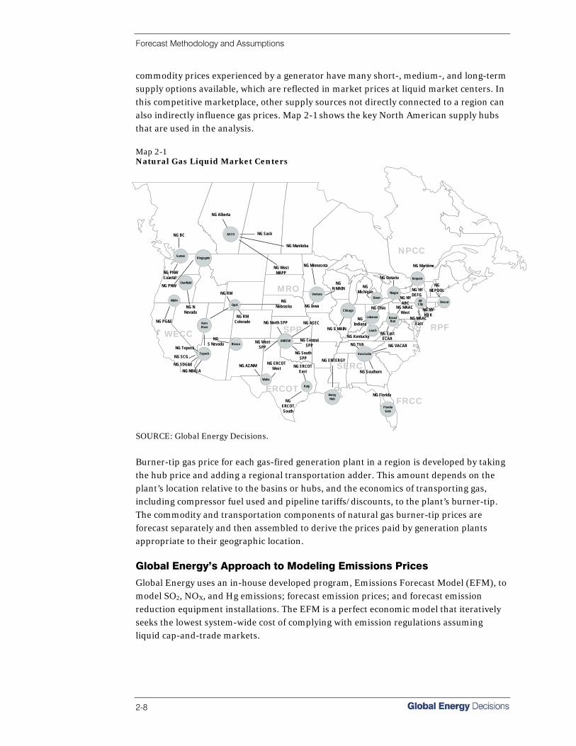
Forecast Methodology and Assumptions
2-8
commodity prices experienced by a generator have many short-, medium-, and long-term supply options available, which are reflected in market prices at liquid market centers. In this competitive marketplace, other supply sources not directly connected to a region can also indirectly influence gas prices. Map 2-1 shows the key North American supply hubs that are used in the analysis. Map 2-1 Natural Gas Liquid Market Centers
WECC
MAPP
SPP
ERCOT
SERC
FRCC
MAINECAR
NPCC
RPFNG PG&E
NGNEPOOL
NG NNevada
NG SCG
NG SDG&E
NGS Nevada
NG AZ/NM
NG BC
NG PNWCoastal
NG PNW
NG Sask
NG Manitoba
NG Minnesota
NG Ontario
NG Maritime
NGNebraska
NG RM
NG RMColorado NG North SPP
NG CentralSPP
NG WestSPP
NG ASEC
NG Iowa
NGN MAIN
NG Florida
NG Southern
NG VACARNG TVA
NG ENTERGY
NG Kentucky NG EastECAR
NGIndiana
NG Ohio
NG NYABC
NG SouthSPP
NG NBAJA
NG WestMAPP
NG Alberta
NG S MAIN
NGMichigan
Lebanon
NG NYHIJK
DracutDawn
Chicago
Ventura
Opal
Sumas Kingsgate
Stanfield
Malin
Topock
FloridaGate
Waha
ANRSW
NYCity
Katy
NG MAAC East
Iroquois
NG NYDEFG
AECO
Blanco
Leach
BroadRun
Kosciusko
NG ERCOTWest
NGERCOTSouth
NG ERCOTEast
ERCOT
NG MAAC West
NG Topock
Niagra
HenryHub
KernRiver
MRO
SPP
NPCC
WECC
SERC
SOURCE: Global Energy Decisions.
Burner-tip gas price for each gas-fired generation plant in a region is developed by taking the hub price and adding a regional transportation adder. This amount depends on the plant’s location relative to the basins or hubs, and the economics of transporting gas, including compressor fuel used and pipeline tariffs/discounts, to the plant’s burner-tip. The commodity and transportation components of natural gas burner-tip prices are forecast separately and then assembled to derive the prices paid by generation plants appropriate to their geographic location. Global Energy’s Approach to Modeling Emissions Prices
Global Energy uses an in-house developed program, Emissions Forecast Model (EFM), to model SO2, NOX, and Hg emissions; forecast emission prices; and forecast emission reduction equipment installations. The EFM is a perfect economic model that iteratively seeks the lowest system-wide cost of complying with emission regulations assuming liquid cap-and-trade markets.
Forecast Methodology and Assumptions
Coal Reference Case, Fall 2007 2-9
EFM Inputs • Individual generator characteristics, forecast emissions, and forecast generation; • Type of generator based on five generator classifications: small or large coal, small or
large gas, or oil; • Known emissions control equipment installations, both existing and announced; • Emissions caps by year and/or season as applicable; • Emissions control equipment costs and efficiency defined for each generator
classification; and • Input adjustments to compensate for real-world actions that deviate from the “perfect
economic” assumptions. For example, regulated utilities largely roll the capital investment costs of emission reduction equipment into their rate base and do not need a return on this investment from the emissions markets. As such, GED models approximately 12 percent of installations with zero capital cost.
EFM Outputs • Emission costs by year ($/ton or $/lb as appropriate); • Forecast emissions (tons/year, lbs/year) and resulting banked allowances; and, • Forecast installations (FGD, SCR, ACI).
Localized Markets Markets such as Southern California’s NOX RECLAIM and Texas’ NOX MECT are not modeled. Emission price forecasts for these are based on futures/forward curves, historical data, expected market changes, and other market intelligence. Estimated Emission Costs Affecting the Forecast Table 2-2 shows the forecast emission costs for generators in the United States. The only direct input to the Coal Quality Market Model (CQMM) in Table 2-2 is the SO2 allowance forecast under the National Acid Rain Program. Note that only a few of the listed emission costs apply to a given regional power forecast. As discussed in the introduction to this section, direct inputs to the regional power forecasts are indirectly related to the coal forecast since the power forecasts provide the demand input to the coal model. For SO2, this should not be interpreted as an “Allowance Price” forecast due to the declining allowance value discussed in Section 2 Forecast Assumptions and Section 3 Regulatory Issues. The number of Title IV SO2 allocations remains constant under CAIR but they decline in value based on the issued year (vintage). Prior to 2010, they will be worth 1 ton, those issued 2010-14 will be worth 0.5 tons, and from 2015 forward will be worth 0.35 tons. To calculate an estimated CAIR SO2 allowance price, simply multiply the forecast cost ($/ton) by the vintage allowance value in tons (e.g., for a 2012 vintage allowance, multiply the forecast control costs of $460/ton × 0.5 tons/allowance to arrive at $230/allowance). Also, remember that all Title IV (non-CAIR states) SO2 allowances will be worth 1 ton regardless of issuance year and may be traded in the CAIR SO2 trading program at their full value.

Forecast Methodology and Assumptions
2-10
Table 2-2 Emission Costs (in $ per ton removed, except Hg which is in $/lb)
Pollutant NOx NOx NOx NOx NOx SO2 SO2 SO2 Mercury CO2
Program RECLAIM CAIR - Seasonal
CAIR - Annual
Eastern SIP Call HGB
Acid Rain
Program New York CAIR CAMR GHG
Geographic Scope
South Coast Air Quality
Management District
(SCAQMD)
25 Eastern States +
D.C.
25 Eastern States +
D.C.
Eastern SIP Call States
Houston/ Galveston (ERCOT)
National New York
25 Eastern States +
D.C. National North
American
Year (2007 $/ton) (2007 $/ton)
(2007 $/ton)
(2007 $/ton)
(2007 $/ton)
(2007 $/ton)
(2007 $/ton)
(2007 $/ton)
(2007 $/lb)
(2007 $/ton)
2007 4,949 950 3,000 460 329
2008 7,953 1,097 4,500 460 373
2009 12,497 1,097 368 4,500 460 417
2010 11,924 1,170 368 4,500 460 460 460 6,253
2011 9,225 1,244 368 4,500 460 460 460 6,253
2012 9,032 1,244 368 4,500 460 460 460 6,253 2
2013 9,000 1,244 368 4,500 442 442 442 6,253 3
2014 9,000 1,244 368 4,500 433 433 433 6,253 4
2015 9,000 1,196 357 4,500 416 416 416 6,253 5
2016 9,000 1,172 352 4,500 400 400 400 6,253 6
2017 9,000 1,127 342 4,500 384 384 384 6,253 7
2018 9,000 1,084 332 4,500 369 369 369 6,253 8
2019 9,000 1,033 322 4,500 355 355 355 6,253 9
2020 9,000 915 313 4,500 342 342 342 6,253 10
2021 9,000 803 304 4,500 329 329 329 6,253 11
2022 9,000 709 295 4,500 316 316 316 6,253 12
2023 9,000 623 286 4,500 304 304 304 6,253 13
2024 9,000 535 278 4,500 293 293 293 6,253 14
2025 9,000 490 270 4,500 282 282 282 6,253 15
2026 9,000 469 262 4,500 271 271 271 6,253 15
2027 9,000 416 254 4,500 215 215 215 6,253 15
2028 9,000 352 247 4,500 171 171 171 6,253 15
2029 9,000 313 240 4,500 104 104 104 6,253 15
2030 9,000 263 233 4,500 101 101 101 6,253 15
2031 9,000 251 226 4,500 98 98 98 6,253 15
Note:
Superseded by Seasonal CAIR
SOURCE: Evolutionmarkets.com, Cantor, South Coast Air Quality Management District, EPA, Global Energy.
Coal Price and Volume Model
The CQMM is used by Global Energy to forecast future U.S. consumption, allocation, and delivered price of coal from every mine to every boiler over the 25-year study period. Developed in partnership with RBAC Inc., developers of the Gas Price Cost Model (GPCM), the CQMM relies on data from Global Energy and is operated by Global Energy modelers. The model uses a highly sophisticated network linear program to find the optimal minimum cost solution for the given model input and constraints.
Forecast Methodology and Assumptions
Coal Reference Case, Fall 2007 2-11
A sophisticated model, however, is only as good as the data feeding it. The adage “garbage in, garbage out” applies to all models and the CQMM is no exception. To produce accurate and sophisticated forecasts, one must use an exhaustive and comprehensive dataset that accurately depicts current and expected market conditions. Using the Velocity Suite, the industry’s leading coal and energy market database, and numerous other data sources described in this report, Global Energy has created the most thorough, highly representative database achievable. The model input dataset falls into one of three primary areas: supply, demand, and transportation. Supply data are provided at the mine level and include the current and future fully allocated costs for every current and existing mine in the United States as described in Global Energy’s Coal Capacity Study. Mine opening and retirement dates are obtained by researching press releases, annual reports, and coal publications. Coal quality specifications are obtained from the Velocity Suite database and are used to categorize forecasted coal prices. Each of the roughly 1,900 mines in the dataset are assigned to a coal type. Coal from Illinois Basin with a low Btu and high sulfur content is assigned the ILLBLoHi category. Overall, there are 70 different coal types assigned in the model. Demand data are at the boiler level and are derived primarily from the MARKETSYM™ power model output. Each boiler is assigned a range of acceptable Btu, ash, and sulfur concentrations to prevent the model from inadvertently assigning an inappropriate coal to the boiler. If a below-standard coal is available to a boiler at an acceptable economic cost, the model will penalize the coal (add cost) to make it less desirable. As long as the penalized coal is less than the delivered price of alternative coal sources, the substandard coal will be used. In virtually all cases, substandard coal is not assigned to a boiler by the model. The model also sets absolute minimum and maximum levels for acceptable Btu and ash, respectively; coal outside of these ranges cannot be assigned to a plant regardless of the delivered price advantage. Transportation routes and costs are assigned between mines and the plants that may possibly consume the coal during the 25-year study period. A coal plant in Georgia, for example, may currently consume CAPP coal, but in the future it may burn CAPP, ILLB, PRB, or imported coal. By allowing the model to choose coal from virtually any reasonable coal basin, the model is better able to mimic real world economic conditions. Plants that are unlikely to consume coal from a particular basin (e.g., a Virginia plant consuming Gulf lignite coal) are not assigned a transportation link from that group of mines. To ensure that the total quantity of coal from a basin or coal producing region does not exceed the transportation capacity of the area, the model has a feature that allows transportation to be constrained. The transportation capacity constraint may be applied at the national level, at the mine level, at an individual transloader level, or any other point in the coal supply chain. To speed the model’s processing time, redundant data has been aggregated within the dataset. For example, transportation routes are grouped from similar mines based on coal quality and geographic region to each plant. Currently the model dataset has over 185,000 routes and costs between groups of mines and individual plants. If the
Forecast Methodology and Assumptions
2-12
transportation dataset were not aggregated, there would be millions of potential routes and costs between individual mines and plants, significantly slowing the processing speed of the model. Inputs into the CQMM and the primary source of the data are listed below: • Electricity demand for each boiler (from MARKETSYM™ power model); • Coal plant retirements and new plant construction (from MARKETSYM™ power
model); • Long-term coal contracts (from numerous sources, but primarily from Velocity
Suite); • Boiler specification requirements - ash, Btu, sulfur (from Velocity Suite); • Annual production of coal from each mine (from Global Energy Coal Capacity Study); • Coal quality specifications - ash, Btu, sulfur (from Velocity Suite); • Total reserves available from each mine (from Global Energy Coal Capacity Study); • Fully allocated costs of extracting coal from each mine (from Global Energy Coal
Capacity Study); • Available transportation mode and capacity (from industry research); • Transportation costs from each mine to each plant (from Velocity Suite, waybill data,
U.S. Rail Desktop and PC Miler); • Current and forecasted SO2 emissions removal efficiency (from Global Energy
Emissions model); • SO2 emissions prices (from Global Energy Emissions model); and • SO2 allowance inventory for each plant (from EPA). For each coal-fired power boiler, the model finds the optimal coal or blend of coals to be consumed for each year of the study period. Before assigning spot coal, the model enforces contracts so that contract coal is consumed up to the limit of the contract or the plant demand, whichever comes first for the given year. If there is still boiler level demand that is not satisfied by existing contracts, the model finds the optimal spot coal or blend of spot coals to be consumed at the plant for the given year. The lowest delivered prices for spot coals to each plant are calculated by the model by taking into account: • Total GWH demand; • Minimum average Btu (and/or threshold Btu level); • Maximum average Ash (and/or threshold Ash level); • Maximum allowable sulfur threshold; • SIP constraints (where applicable); • Production capacity at each mine; • Remaining reserves at each mine; • SO2 removal efficiency; • SO2 scrubber installation date; • Assigned SO2 annual allowances and total inventory; • SO2 allowance price; • Transportation costs; • Transportation capacity; and • Plant stockpiles.

Forecast Methodology and Assumptions
Coal Reference Case, Fall 2007 2-13
The logic used by CQMM is depicted in Figure 2-3. This schematic representation of the logic flowchart shows how a mine may be linked to multiple seams with different reserves, costs, and annual production. The coal from the mine has some of its supply siphoned off by non-electricity generation demand (e.g., metallurgical, industrial, residential, commercial coal) and the remainder is available for coal plants. Coal under contract is first removed from the mine’s annual production and any remaining production is available to the spot market. Spot market coal is assigned to a boiler based on the numerous factors described in the bulleted points above. Figure 2-3 CQMM Logic Flowchart
Supply
Contract Coal Transported
Spot Coal Transported
Spot
Spot
Other Mines – this Origin Region
Mine
Non-ElecGen
Demand ElecDemand
Supplemental Elec Supply
Spot Coal Used
Contract Coal Used
Contract Coal
Stockpiled
Initial Stockpile
Final Stockpile
Stockpile Used
Other Origin Regions
Origin Region
Boiler
Plant
Seam
Seam
Seam
SOURCE: RBAC and Global Energy.
The Coal Quality Market Model uses Global Energy’s SO2 allowance price forecast as a direct input. Figure 2-4 graphically demonstrates how an individual modeled boiler in CQMM treats SO2 allowances. Each boiler has an initial allowance inventory in the initial period (in this case 2007) it is granted allowances in accord with the CAA cap-and-trade program. Each boiler also has information on its scrubber efficiency for each period of the model included with its other boiler specifications. If a boiler does not yet have sulfur emissions equipment installed but will in the future, an estimated removal efficiency is assigned for the periods following the installation date. CQMM allocates the coal based on the lowest-cost basis, including the allowance model. Thus, depending on total initial allowance inventory plus allowance grants for each boiler the model will make decisions about the lowest cost solution for each boiler and sell or buy allowances for each boiler accordingly. Unused allowances are banked until the next period.
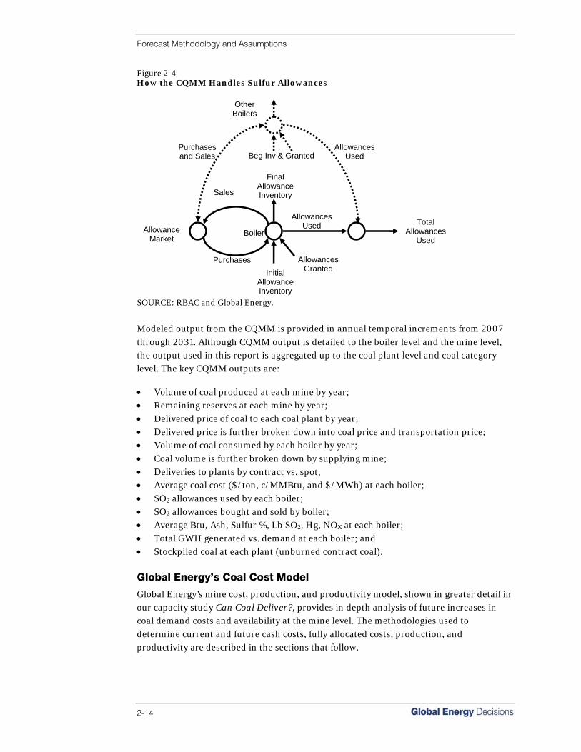
Forecast Methodology and Assumptions
2-14
Figure 2-4 How the CQMM Handles Sulfur Allowances
Purchases
Allowance Market
Boiler Total
Allowances Used
Allowances Used
Sales
Allowances Granted Initial
Allowance Inventory
Final Allowance Inventory
Other Boilers
Allowances Used
Purchases and Sales Beg Inv & Granted
SOURCE: RBAC and Global Energy.
Modeled output from the CQMM is provided in annual temporal increments from 2007 through 2031. Although CQMM output is detailed to the boiler level and the mine level, the output used in this report is aggregated up to the coal plant level and coal category level. The key CQMM outputs are: • Volume of coal produced at each mine by year; • Remaining reserves at each mine by year; • Delivered price of coal to each coal plant by year; • Delivered price is further broken down into coal price and transportation price; • Volume of coal consumed by each boiler by year; • Coal volume is further broken down by supplying mine; • Deliveries to plants by contract vs. spot; • Average coal cost ($/ton, c/MMBtu, and $/MWh) at each boiler; • SO2 allowances used by each boiler; • SO2 allowances bought and sold by boiler; • Average Btu, Ash, Sulfur %, Lb SO2, Hg, NOX at each boiler; • Total GWH generated vs. demand at each boiler; and • Stockpiled coal at each plant (unburned contract coal).
Global Energy’s Coal Cost Model
Global Energy’s mine cost, production, and productivity model, shown in greater detail in our capacity study Can Coal Deliver?, provides in depth analysis of future increases in coal demand costs and availability at the mine level. The methodologies used to determine current and future cash costs, fully allocated costs, production, and productivity are described in the sections that follow.
Forecast Methodology and Assumptions
Coal Reference Case, Fall 2007 2-15
Global Energy’s Approach to Assessing Mine Cash Costs Cash costs, when used in the context of coal mining operations, can be defined as those costs that are directly attributable to the daily operations of the mine. Mine cash costs are the summation of: • Operating costs; • Replacement of capital costs; and • Taxes and royalties.
The operating cost of a mine includes equipment, fuel, labor, and all other direct costs associated with the daily operations of the mine less the administration costs. Global Energy used public and private data sources to determine the direct operating mine costs associated with hard rock mines. Using our proprietary database of mine cost information that we have assembled over the years coupled with information obtained from the Western Mine Engineering Mine Cost Service, Global Energy estimated costs associated with labor, materials, explosives, fuel, etc. We estimated operating costs by developing cost algorithms that incorporated mine technology, production levels, basin geography and geology, mining operations (i.e., surface or underground), and productivity (or ratio information, where available). Replacement of capital costs are the amount of money put into the upkeep of equipment each year to keep it operating. For example, it is the cash outlay to replace the teeth on a continuous miner each year. To calculate the replacement cost of capital, a set percentage of the operating cost was used based on industry standards. The replacement cost of capital as a percent of operating costs ranged from 5 percent for a Central Appalachian surface mine producing less than 500,000 tons per year to 8 percent for a Rocky mountain mine using a continuous miner with drift access. Overall, U.S. mines were assigned operating cost percentages based on 16 unique categories. For example, if a mine has an operating cost of $20/ton and the replacement cost of capital as a percent is 5 percent, then the replacement cost of capital is $1/ton. To calculate taxes and royalties, Global Energy used all applicable state and federally mandated taxes and royalty payments imposed on coalmine operators. Property taxes were determined for each state using the average of the actual reported mill levies for all “coal” counties. Based on the average levy, Global Energy determined the tax burden on a typical mine in the state.2 From this burden, Global Energy determined the rate and then determined what that represented as a percent of the FOB mine price. This new “effective tax rate” was used for all mines in a particular state. Additional components of the taxes and royalties are listed below: • Royalties: In the West, the federal rates of 8 percent and 12.5 percent were used for
all mines, whether on state, federal, Indian, or private land.
2 Colorado does not assess severance taxes on the first 300,000 tons of coal production each quarter. To determine the “effective” severance tax rate, the severance tax rate was applied to all tons > 1.2 million each year (300,00 * 4 quarters) and then that figure is allocated across all production.
Forecast Methodology and Assumptions
2-16
• For other states, industry experts provided royalty rates based on industry experience;
• Severance Taxes: Researched on a state-by-state basis. Colorado does not assess severance taxes on the first 300,000 tons of coal production each quarter. To determine the “effective” severance tax rate, the severance tax rate was applied to all tons > 1.2 million each year (300,000 * 4 quarters) and then that figure is allocated across all production;
• Black Lung: 4.4 percent of the FOB mine price, up to a max of $1.10 per ton for deep mines and $0.55/ton for surface mines; and
• OSM: $0.35/ton surface and $0.15/ton deep mines through September 30, 2007, $0.315/ton surface and $0.135/ton deep mines from October 1, 2007 through 2012; and $0.28/ton surface and $0.12/ton from 2013 through 2021 when the reclamation fee program is set to expire.
Results from the cash cost model were vetted by our industry contacts from six publicly traded, major coal suppliers as well as by our individual contacts ranging from consultants and coal buyers to a former president of a coal company. After the model results were vetted by our industry contacts, Global Energy researched the latest SEC filings to determine the reported mine cash costs at the following companies: • Arch Coal; • Foundation Coal; • Massey Energy; • CONSOL; • Alliance Resource Partners; • Peabody; • ICG; and • Alpha Natural Resources.
Global Energy’s Approach to Assessing Mine Fully Allocated Costs Fully allocated costs, when used in the context of coal mining operations, can be defined as those costs that a mine will need to recover to operate profitably over the long term. Fully allocated costs are the summation of: • Cash costs (defined above); • Capital recovery; and • Return on capital.
Capital recovery costs are the same as depreciation. It is a sunk cost, not a cash cost. It is defined as the non-cash expense that reduces the value of an asset due to wear and tear, age, or obsolescence. Most assets lose their value and must be replaced once their useful life is over. Depreciation lowers the company’s reported earnings while increasing free cash flow. For example, a $100 million longwall miner with a useful life of 20 years will be depreciated at $5 million per year. The life of the equipment used in the Global Energy model ranged from 15 to 20 years, depending on the historical longevity data associated with each type of equipment.

Forecast Methodology and Assumptions
Coal Reference Case, Fall 2007 2-17
Return on capital is the measure of how effectively a company uses the money that is invested in its operations. The money that is invested by the company may either be borrowed or owned by the company. Global Energy assumed between a 10 and 20 percent return on capital based on the presumed risk associated with the mine. While this range of return on capital has been vetted by industry contacts, the number may go up or down depending on the state of the coal markets. Results from the fully allocated cost model were vetted by our industry contacts from six publicly traded, major coal suppliers as well as by our individual contacts, ranging from consultants and coal buyers to a former president of a coal company. After the model results were reviewed by our industry contacts, Global Energy researched the latest SEC filings to determine the reported fully allocated costs at the following companies: • Arch Coal; • Foundation Coal; • Massey Energy; • CONSOL; • Alliance Resource Partners; • Peabody; • ICG; and • Alpha Natural Resources.
Global Energy’s Approach to Modeling Productivity and Production Global Energy’s Approach to Forecasting Mine Productivity Mine productivity is a measurement of how efficiently coal is extracted from a mine; it is typically measured in tons of coal extracted per miner hour. Because labor costs are such a large part of the overall direct cash costs of coal suppliers, any increase in productivity results in increased returns on capital for investors. In tight coal markets, where margins are very thin, every percent increase in productivity over competitors can be the difference between a profitable mine and a money-losing operation. The productivity of a mine is dependent on many technical, geological, environmental, political, and even cultural factors, but there are three factors that have the most influence on productivity: • The ratio of overburden to seam thickness; • The mining operation (surface or underground); and • The type of equipment used to extract the coal (e.g., continuous vs. longwall, truck
and shovel vs. dragline).
These three factors are used in this study to estimate future growth or decline in productivity. Mines located within similar geographic and geologic regions often, though not always, share similar operating conditions as they are usually mining the same or similar seams of coal with similar ratios. A surface mine will have higher productivity than an equivalent underground mine as the main obstacle to extraction is the overburden. For underground mines, the seams tend to be thinner, more difficult to

Forecast Methodology and Assumptions
2-18
extract and include many additional obstacles and safety issues that surface mines do not have to face. Coal bed methane gas build-up, roof collapse, drainage issues, equipment scalability, and the moving of equipment all tend to hamper underground mining operations. Improvements in technology and economies of scale continue to improve productivity, although there are limitations to how big one can make trucks, tires, and shovels that are easily and readily maintained. Global Energy combined the above three factors to form 20 mine categories for the non-PRB mines. The historical productivity, as calculated from MSHA form 7000-2, was compiled for each of these 20 categories and projections were made for each of these groupings based on historic trend analysis For both existing and new mines, Global Energy researched corporate annual reports and press releases to supplement our data on future mine productivity. For example, if a mine has announced that it will add or retire a longwall operation in 2009, then the productivity data is adjusted accordingly. Global Energy’s Approach to Assessing Coal Production Capacity Coal production capacity is the maximum amount of coal a mine can produce under optimal conditions. It is used to show how readily the coal supply industry can respond to a sudden surge in demand. Global Energy uses three methods for determining annual coal production capacity: • Annual EIA maximum production data; • EIA Maximum state weekly data multiplied by 52; and • Global Energy Decisions’ “proved-in-place” capacity calculations.
Coal production capacity statistics are collected by the EIA on Form EIA-7A which requires reporting “…the maximum amount of coal that your mining operation could have produced during the year with existing mining equipment in place, assuming that the labor and materials sufficient to utilize the equipment were available, and that the market existed for the maximum coal production.” Statistics reported to the EIA are summarized in the Quarterly Coal Report, the Monthly Energy Review, and the Annual Energy Review. However, they are only collected once per year, and the lag time is significant; coal production capacity data reported for 2006 will be available in late 2007. Further, the data are published at the regional and state level, but do little good for industry analysts maintaining a timely measurement of the pulse of productive capacity on anything but an anecdotal basis. It is not possible to use the data to do mine level analysis, and without mine level aggregation capability, it is impossible to conduct timely measurements of coal production capacity by quality category, rail origin, productivity range, mine type, or any other of a number of categorizations. Because of the annual temporal resolution of the EIA data and the time lag in publication, the data provide no insights into capacity changes throughout the year as new mines open and close. They are excellent sources of

Forecast Methodology and Assumptions
Coal Reference Case, Fall 2007 2-19
“after the fact” statistics to confirm the accuracy of other techniques for estimating capacity, and undoubtedly will have great value for the assignment of blame by political and legal officials, and senior management should catastrophic capacity failures occur. A second approach used by Global Energy is based upon more timely statistics, but is more appropriately aggregated. The EIA weekly coal production report provides weekly estimates for U.S. coal production by state based upon railroad car loading data. The report for the previous week is published on the EIA web site six days after the end of the subject week. The release schedule provides for ongoing, short-term evaluation of capacity. For each state, Global Energy selects the highest weekly production for the past 52 weeks and multiplies it by 52 to get a capacity estimate by state. State estimates can then be aggregated to estimate regional (e.g., Central Appalachia, Northern Appalachia, etc.) capacity. This method is called the state or regional “Max Week x 52” approach by Global Energy. The approach typically yields a capacity that is lower than the EIA reported capacity. Because of limitations with the EIA capacity statistics mentioned above, Global Energy has developed an alternative approach to estimate coal production capacity, called the “proved-in-place” capacity method. To calculate capacity using this approach, quarterly production statistics reported on MSHA Form 7000-2 are used. These data are collected quarterly and published with a lag time of 60 to 90 days. Thus, they can be used for analysis of changes throughout the year and are available (in a preliminary form) much sooner than EIA capacity statistics. For surface mines, Global Energy examined production reported for the previous 12 quarters at the mine level. The maximum two-quarter moving average of production is multiplied by two to estimate the maximum proved-in-place capacity. If the mine is not identified as a “new mine” and did not produce in the last two quarters of the year being analyzed, then it was assumed to have closed and the proved-in-place capacity was set to zero. Proved-in-place capacity calculations for underground mines differ from surface mine calculations because a surface mine can more easily reproduce the production from a stellar quarter. Underground mines are typically not able to sustain high quarterly production over an entire year. Longwall operations have to be moved, underground seams split and don’t “cooperate” with machinery, methane gas build-up, and numerous other issues prevent an underground mine from being able to replicate one stellar quarter. To account for these factors, Global Energy used an alternate proved-in-place capacity estimate for underground mines. As with the approach to surface mines, MSHA Form 7000-2 data were used, but unlike the surface mine capacity calculation, a “maximum rolling average” methodology was used to calculate the proved-in-place capacity for underground mines. The last 12 quarters of production for each mine were compiled and the greatest “annual” production over four continuous quarters was identified. An unlikely spike or outlier in any one quarter will be smoothed by using a rolling average. To account for newer mines that are

Forecast Methodology and Assumptions
2-20
ramping up production or older mines that are returning to higher productive capacity, Global Energy constructed an algorithm to identify mines that will have production levels greater than their historic “maximum rolling average.” The production capacity estimates have been confirmed by discussions with coal producers and by industry experience. Although the proved-in-place capacity is often slightly greater than the annual maximum production estimates published by the EIA, this is likely because most producers are able to “coax” extra production out of their operations by mining in the best areas, pushing equipment to its maximum operating parameters, adding short-term labor, and using other techniques when profitable sales opportunities occur. Further, capacity upgrades occurring throughout the year are better reflected by this approach, and new capacity additions (less closures) show up in a more timely fashion. A comparison of the proved-in-place methodology to the EIA reported capacity confirms that the capacity estimates of each approach track very closely and move in the same direction each year.
Forecast Assumptions Electricity Demand Electricity Growth Forecast To understand Global Energy’s electricity growth forecast, it is important to compare forecasts related to both economic growth and population growth. Economic growth is an indicator of electricity demand on a business level while population growth is an indicator of electricity demand on a personal level. The EIA expects real GDP to increase by 2.9 percent on an annual basis between 2005 and 2030. Population is expected to increase by 0.9 percent on an annual basis. Historic and forecasted population and GDP are shown in Table 2-3. Table 2-3 Historic and Forecasted Economic and Population Growth
2005 2006 2007 2008 2009 2010 2015 2020 2025 2030
Real GDP (Billion 2000 chain weighted dollars)
11,049 11,415 11,696 12,052 12,419 12,790 14,698 17,077 19,666 22,494
Population Aged 16 and Over (Millions)
229 232 234 237 240 242 253 261 265 277
SOURCE: EIA Annual Energy Outlook.
The trend of increasing electricity generation with increased economic development can be seen in recent history as illustrated in Figure 2-5.

Forecast Methodology and Assumptions
Coal Reference Case, Fall 2007 2-21
Figure 2-5 Historic GDP and Electricity Generation Growth
2,500,000
2,700,000
2,900,000
3,100,000
3,300,000
3,500,000
3,700,000
3,900,000
4,100,000
1997 1998 1999 2000 2001 2002 2003 2004 2005 2006
Gen
erat
ion
(GW
h)
8,000
8,500
9,000
9,500
10,000
10,500
11,000
11,500
12,000
Bill
ion
Cha
ined
200
0 D
olla
rs
Electricity Generation GDP
SOURCE: EIA and Global Energy.
With an increasing population as well as economic and industrial development, demand for electricity is expected to increase. It should therefore be no surprise that Global Energy expects total electricity output to increase year by year just as it has in the past with a 40 percent increase in 2031 from 2007 levels as shown in Table 2-4. Table 2-4 Forecasted Electricity Growth - GWh
2007 2008 2009 2010 2015 2020 2026 2031
4,047,972 4,135,144 4,201,330 4,268,632 4,666,679 4,994,471 5,429,135 5,827,877
SOURCE: Global Energy.
Figure 2-6 Historical and Forecasted Electricity Generation by Fuel
0
1,000,000
2,000,000
3,000,000
4,000,000
5,000,000
6,000,000
7,000,000
1997
1999
2001
2003
2005
2007
2009
2011
2013
2015
2017
2019
2021
2026
2031
Year
Gen
erat
ion
(GW
h)
Coal Nuc Gas Water Petro Renew
Historical Forecast
SOURCE: EIA and Global Energy Power Reference Case.

Forecast Methodology and Assumptions
2-22
Table 2-5 provides summary statistics about the data shown in the previous graphic. Table 2-5 Key Statistics for Future Fuel Mix; 2007-2031
Coal Nuclear Gas Water Petro Renew
Change in GWh 587,652 21,170 940,158 31,089 -19,071 218,905
Change in Share -6% -5% 11% -2% -1% 3%
Average Yearly Growth 2% 0% 5% 2% -4% 8%
SOURCE: Global Energy.
After electricity prices deflate from currently high prices, we forecast steady increases in price until 2031 due to increasing demand as well as some increasing costs for utilities such as installing emissions control technologies and higher fuel costs. Electricity rates are currently highest in the Northeast, a region where relatively little coal is burned. Lowest electricity rates are in the Midwest, where significant amounts of coal are burned. Table 2-6 Average Market Clearing Price Forecast; 2007 $/MWh*
Year WECC Northeast Midwest ERCOT Southeast
2008 54.86 62.46 50.36 61.09 54.16
2009 49.56 58.16 49.39 57.99 52.75
2010 41.68 52.19 45.57 51.27 48.54
2015 48.69 57.12 53.17 57.76 56.33
2020 55.50 59.03 57.79 61.12 60.83
2026 66.34 64.12 62.17 65.57 65.31
2031 69.86 65.27 63.04 66.58 66.31
*Includes Canada SOURCE: Global Energy.
Natural Gas and Oil Pricing
Natural gas and oil prices have remained extremely volatile by most historic standards over the last five years. The horrific 2005 hurricane damage in the Gulf of Mexico added further stress to domestic natural gas and oil supply infrastructure that is not yet back to “normal.” For example, U.S. crude oil production in 2006 is estimated to have averaged 5.1 million bbl/day, down slightly from 2005 levels as a result of the hurricanes; and offshore gas production averaged 7.8 Bcf/day, down approximately 10 percent from 2005 levels (some of which is undoubtedly due to gas reserve/deliverability depletion). The long-term decline in deliverability in the Gulf is readily apparent, with 2006 gas production roughly 25-35 percent below the 2001-2003 production levels, as shown in Figure 2-7.
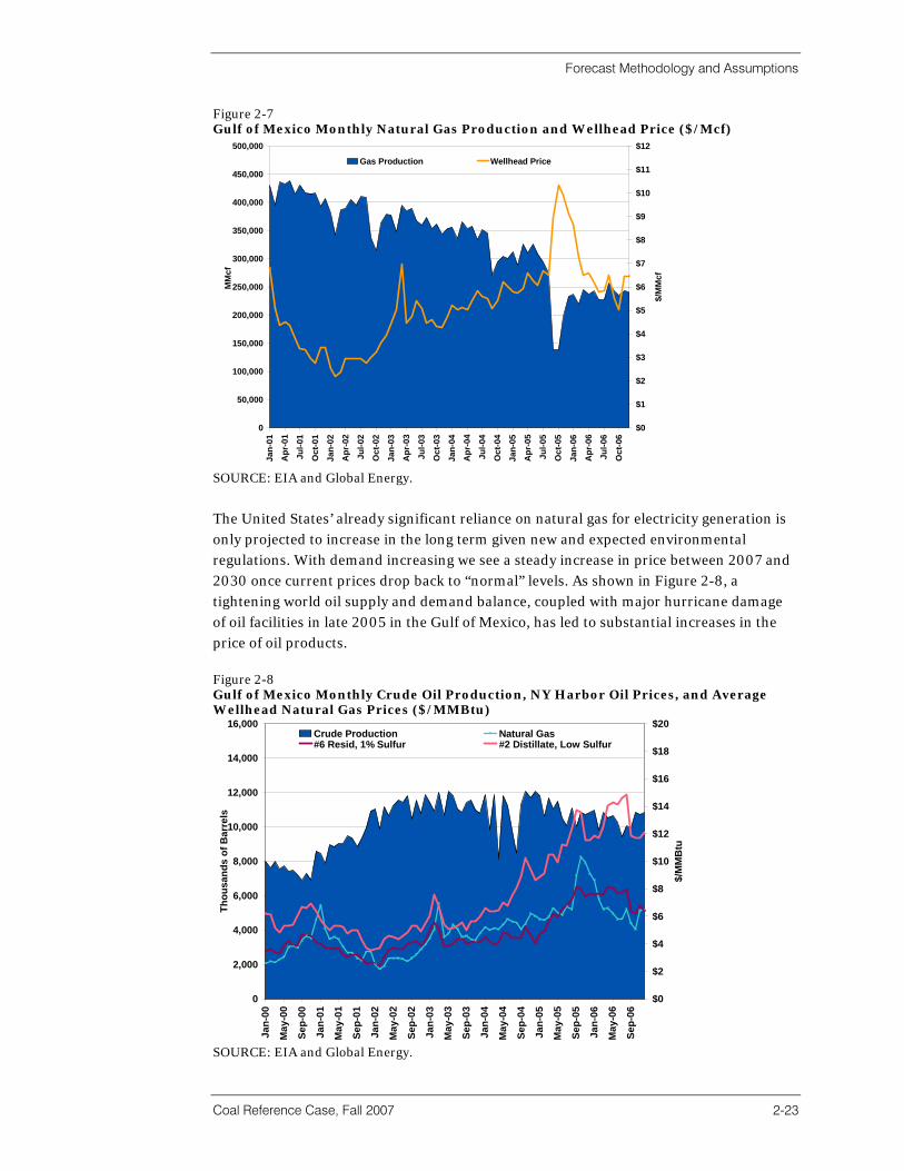
Forecast Methodology and Assumptions
Coal Reference Case, Fall 2007 2-23
Figure 2-7 Gulf of Mexico Monthly Natural Gas Production and Wellhead Price ($/Mcf)
0
50,000
100,000
150,000
200,000
250,000
300,000
350,000
400,000
450,000
500,000
Jan-
01
Apr
-01
Jul-0
1
Oct
-01
Jan-
02
Apr
-02
Jul-0
2
Oct
-02
Jan-
03
Apr
-03
Jul-0
3
Oct
-03
Jan-
04
Apr
-04
Jul-0
4
Oct
-04
Jan-
05
Apr
-05
Jul-0
5
Oct
-05
Jan-
06
Apr
-06
Jul-0
6
Oct
-06
MM
cf
$0
$1
$2
$3
$4
$5
$6
$7
$8
$9
$10
$11
$12
$/M
Mcf
Gas Production Wellhead Price
SOURCE: EIA and Global Energy.
The United States’ already significant reliance on natural gas for electricity generation is only projected to increase in the long term given new and expected environmental regulations. With demand increasing we see a steady increase in price between 2007 and 2030 once current prices drop back to “normal” levels. As shown in Figure 2-8, a tightening world oil supply and demand balance, coupled with major hurricane damage of oil facilities in late 2005 in the Gulf of Mexico, has led to substantial increases in the price of oil products. Figure 2-8 Gulf of Mexico Monthly Crude Oil Production, NY Harbor Oil Prices, and Average Wellhead Natural Gas Prices ($/MMBtu)
0
2,000
4,000
6,000
8,000
10,000
12,000
14,000
16,000
Jan-
00
May
-00
Sep-
00
Jan-
01
May
-01
Sep-
01
Jan-
02
May
-02
Sep-
02
Jan-
03
May
-03
Sep-
03
Jan-
04
May
-04
Sep-
04
Jan-
05
May
-05
Sep-
05
Jan-
06
May
-06
Sep-
06
Thou
sand
s of
Bar
rels
$0
$2
$4
$6
$8
$10
$12
$14
$16
$18
$20
$/M
MB
tu
Crude Production Natural Gas#6 Resid, 1% Sulfur #2 Distillate, Low Sulfur
SOURCE: EIA and Global Energy.

Forecast Methodology and Assumptions
2-24
Global Energy expects the high price of oil to continue through the end of the decade, where it will begin to decline before another slight rise. Price levels in 2030 are forecasted to be very similar to 2010 prices on a constant dollar basis. Table 2-7 Natural Gas and Oil Price Forecast - 2007 $/MMBtu
2007 2008 2009 2010 2015 2020 2025 2030
Oil - No. 6, 3% Sulfur 8.60 8.47 7.97 7.02 6.21 6.20 6.54 7.08
Gas - Henry Hub 7.67 7.96 7.36 6.36 6.37 6.55 7.38 7.89
SOURCE: Global Energy Decisions.
Generating Capacity
Table 2-8 shows the forecasted capacity for the major electricity generating sources: coal, hydro, gas, nuclear, and renewables. Oil and pump storage account for 67,000 MW, but are not included in the table. Table 2-8 Current and Forecasted Capacity (MW)
Fuel Source 2007 2008 2009 2010 2015 2020 2026 2031
Coal 308,287 307,585 308,728 314,348 328,711 341,043 364,896 383,876
Hydro 71,870 72,001 72,024 72,104 72,572 72,693 72,693 72,693
Natural Gas 374,225 377,999 389,223 397,345 445,871 490,649 562,055 650,852
Nuclear 100,799 101,784 101,796 102,017 102,157 108,657 108,657 103,330
Renewables 21,496 27,897 30,427 33,967 54,196 71,693 84,272 93,354
SOURCE: Global Energy.
Coal’s significance as a heat source for power generation will remain high. In the study time frame, coal-fired power generation capacity is expected to increase by approximately 75,000 MW. In the short-tern, capacity will remain flat and perhaps even decrease slightly before ramping up more steadily in 2010 and beyond. New coal units will be brought on line between 2007 and 2010. This additional capacity will be offset by retiring units such as the Leland and Olds Plant, which is planning to retire the larger of its two coal-fired units (447 MW) in May 2009. Xcel Energy plans to retire four units at its High Bridge and Riverside Plants in Minnesota between May 2008 and May 2009, which have a combined capacity of 649 MW. Increased utilization will account for the increase in coal-fired generation over the next few years while capacity levels off temporarily. The 25-year power forecast modeled by Global Energy and applied to the CQMM model is completed at the boiler level. That is, Global Energy forecasts the expected demand of each boiler in the U.S. and uses that as input to the coal model. On an aggregated basis, Figure 2-9 shows power generation by coal technology for the past 10 years and for the next 25. The technologies that are used today and likely to be used in the future are steam turbine (a traditional coal-fired plant), atmospheric fluidized bed (a more advanced steam turbine) and integrated gasification combined cycle turbine (IGCC).

Forecast Methodology and Assumptions
Coal Reference Case, Fall 2007 2-25
Traditional steam turbines have been and will account for the bulk of coal-fired electricity generation. Actual fluidized bed and IGCC units are in the process of being permitted and built and some will undoubtedly come on line in the future. Beyond these, however, Global Energy’s Power Reference Case model does not anticipate much generation from advanced technologies. Figure 2-9 Historical and Forecasted Electricity Generation by Coal Plant Technology
0
500,000
1,000,000
1,500,000
2,000,000
2,500,000
3,000,000
1997
1999
2001
2003
2005
2007
2009
2011
2013
2015
2017
2019
2021
2026
2031
Year
Gen
erat
ion
(GW
h)
Steam Turbine Atmospheric Fluidized Bed IGCC
Historical Forecast
SOURCE: EIA and Global Energy Power Reference Case.
Table 2-9 provides summary statistics about the data shown in the above graphic. Table 2-9 Key Statistics for Future Coal Technology; 2007-2031
Steam Turbine Atmospheric Fluidized Bed IGCC
Change in GWh 667,342 20,360 24,822
Change in Share of Generation -1.3% 0.4% 0.9%
Past Average Yearly Growth 1% 65% 9%
Future Average Yearly Growth 2% 4% 24%
SOURCE: Global Energy.
Key Assumptions Applied to the MARKETSYM™ Model
This section provides an overview of the forecast, modeling, and market assumptions that support the 2007 Market Advisory Report and forecast prices. Constant Dollar Forecast The analysis assumptions and results are presented in constant 2007 dollars. Inflation General inflation drives a number of cost elements that underlie power market prices, including O&M costs and the cost of new resource additions. General inflation is
Forecast Methodology and Assumptions
2-26
combined with expectations of real price escalation in order to forecast future fuel prices. Market simulations utilized constant dollar cost inputs; that is, general inflation equal to zero percent per year. While Global Energy’s analyses are performed in constant dollars, many Global Energy clients conduct their studies in current (or “nominal”) dollars, which include an assumption for underlying inflation. Global Energy recommends that this report’s constant dollar price forecasts be converted to current dollars using the inflation forecast consistent with a client’s other corporate planning guidelines. This is typically an inflation rate of around 2.5 percent per year. Forecast Horizon The power forecast horizon covers a 25-year period, through the end of 2031, with market simulations performed for all years from 2007 to 2021. Thereafter market simulations were performed for every fifth year. Prices between the five-year intervals are based on interpolation. Non-Fuel Operations and Maintenance Costs Power plant-specific, non-fuel O&M costs are reported annually to FERC. Global Energy uses a historical five-year average of those costs—adjusted for inflation—to develop average starting O&M costs. The amounts in these various accounts are then allocated between fixed and variable O&M. To estimate this split, 60 percent of the costs shown in two FERC accounts, Maintenance of Boiler Plant (FERC Account 512), and Maintenance of Electric Plant (FERC Account 513), are assumed as non-labor costs and associated with variable O&M costs. The amount associated with variable production costs is divided by the average energy production of each respective station. This value is used to represent the station’s variable O&M costs. To derive a unit’s fixed O&M cost, the total O&M costs are decreased by the variable O&M cost component. For stations not subject to FERC reporting requirements, Global Energy applies average fixed and variable O&M cost estimates consistent with each unit’s age and generating technology. Market Entry and Exit This study assumes that new generating capacity will enter the marketplace in two phases. In the first phase—called Initial Entry—all capacity that is currently under construction is assumed completed and brought on line. In the second phase, units are brought on line when reasonable profit opportunities are available. Global Energy also adds renewable energy sources reflecting the increase in expected renewable capacity entry due to state-set renewable portfolio standards. To meet future needs for new generating capacity, Global Energy adds four types of resources during the 25-year forecast period. New resources are added in response to forecast electric demand and as such the added capacity is economically viable while

Forecast Methodology and Assumptions
Coal Reference Case, Fall 2007 2-27
maintaining reserve margins that are either in accordance with regional requirements or sufficient to ensure reliability. Global Energy’s five resource types are gas-fired combined cycle (CC) and combustion turbine (CT) units, new pulverized coal-fired capacity, new IGCC coal-fired capacity, and wind generation. The capacity additions are modeled to enter in response to economic conditions such that the level of new entry represents results in a long-term equilibrium state for new entrants in response to expected profit opportunities. The “balanced” market that results is characterized by constant long-term reserve margins, relatively flat annual prices, and an annual profit level for new capacity that is sufficient to cover operational as well as fixed and financing costs. As shown in Table 2-10, with the exception of heat rate levels, operating costs are assumed to remain constant for combined cycle technology throughout the study period. However, in 2007 and again in 2010, Global Energy assumes that new combined cycle technology will be available, improving heat rate levels for new combined cycle units. Under that assumption, the full-load heat rate for generic combined cycle units decreases from the current value of 7,100 Btu/kWh to 6,800 Btu/kWh for units built between 2007 and 2009, and to 6,500 for units built in or after 2010. Table 2-10 Generic Unit Cost and Operating Characteristics
Unit Characteristics Units Aeroderivative CT- LMS100
Combustion Turbine (CT)
Combined Cycle (CC)
Pulverized Coal* IGCC* Wind
Installation Years 2007-2031 2007-2031 2007-2031 2007-2013
2022-2031
2010-2031 2007-2031
Summer Capacity MW 90 160 450 500 500 500 100
Winter Capacity MW 100 180 490 500 500 500 100
Full Load Heat Rate Average Degradation
HHV, Btu/kWh 9,000 10,500 (2007) 6,800
(2010) 6,500 8,600 8,600 8,300 N/A
Fixed O&M 2007 $/kW-yr $10.33 $11.88 $12.25 $25.42 $25.42 $44.63 $29.71
Variable O&M 2007 $/MWh $3.11 $3.50 $2.02 $3.74 $3.74 $4.35 $0.00 Forced Outage Rate
(Applies To All Hours) % 3.60% 3.60% 5.50% 6.00% 6.00% 6.00% 3.60%
Maintenance Outage Rate (MOR) % 4.10% 4.10% 4.10% 6.50% 6.50% 6.50% NA
Overnight Construction Cost 2007 $/kW $743 $483 $714 $2,022 $1,482 $2,000-
2,500 $1,462
Note: Between 2013 and 2021 overnight construction costs for pulverized coal-fired facilities decline with a mean reversion to a long-term equilibrium level of $1,479/kw-yr. *Overnight Construction Cost for IGCCs excludes Carbon Sequestration. In addition, IGCC entry in Global Energy's Reference Case forecast is not balanced economically. The range of overnight construction cost is provided based on announcements made by IGCC developers. SOURCE: Global Energy primary research, EIA Annual Energy Outlook of 2006, MIT and CECA Report on “The Future of Nuclear Energy,” CPUC, Basin Electric Cooperative and GE Power.
The costs in Table 2-10 are a result of Global Energy’s research and information obtained from the Annual Energy Outlook 2006 published by the Energy Information Administration (EIA) of the U.S. Department of Energy (DOE), MIT, and CECA Report on “The Future of Nuclear Energy,” the CPUC, Basin Electric Cooperative, and GE Power. The cost of a gas-fired generation facility can be significantly impacted by a number of factors, including:

Forecast Methodology and Assumptions
2-28
• Cost of electrical interconnection including distance to grid; • Identified need to enforce the transmission grid in the vicinity of the plant; • Cost of gas interconnection including distance of interconnection; • Need to enhance pressure on the gas system to accommodate the plant; • Cost to obtain air permits including cost of purchasing offsets; and • Equipment for water or air-cooling of plant and related costs.
Based on Global Energy’s research there are also significant costs associated with future capital additions and plant upgrades as well as costs for major maintenance and G&A costs. We estimate these costs to be approximately $11/kW-yr for a CCs and CTs and about $21/kW-yr for a new coal plant. The main driver behind the difference between coal- and gas-fired plants is the higher need for capital additions and upgrades in a coal facility. The $714/kW construction cost included above appears to be reasonable for a combined cycle generation unit that is sited in an area that needs little interconnection costs (either gas or electric), little infrastructure reinforcement, minimal air permit costs, and that is water cooled with minimal water infrastructure costs. This would be an ideal site and Global Energy believes that sites with these characteristics can still be found. However, there may be reasons that other, less economic sites would be pursued. Table 2-11 Regional Multipliers
Region CC CT
Boston 1.041 1.035
New England- Rest of Pool 0.955 0.950
Maine 0.993 0.988
NYK (Long Island) 1.472 1.812
NYC (New York City) 1.663 2.048
NY_W (West) 0.955 0.950
NY_E (East) 1.022 1.024
PJM 0.996 0.996
Southeast 0.960 0.960
Midwest 1.004 1.004
SPP 0.997 0.997
Rockies 1.003 1.003
Northwest 1.026 1.026
FRCC 0.961 0.961
California/Nevada 1.058 1.058
ERCOT 0.986 0.986
SOURCE: EIA.
As a point of reference, we note that SMUD (Sacramento Municipal Utility District) reports that its 1,000 MW Cosumnes combined cycle power plant, which currently has 500 MW in commercial operation and the other 500 MW under construction, will have a capital cost of $595 million or about $600/kW.

Forecast Methodology and Assumptions
Coal Reference Case, Fall 2007 2-29
The specifications for the generic wind plant listed in Table 2-12 are based on a review of several sources and publications as of the spring of 2007. The overnight construction cost for a new turbine and tower has increased significantly over the past three years because of high demand and skyrocketing steel prices. The assumed siting of new resources can impact the overall market forecast. Global Energy’s approach is to assume that new generation resources are added in those areas that optimize economics. The simulated siting takes into account differences in construction costs, estimated by applying construction labor cost multipliers shown in Table 2-12. This data is taken from the EIA’s Annual Energy Outlook. Table 2-12 Capital Structure Characteristics
Financial Assumption Capital Structure and Costs
Debt/Equity Ratio 60/40 50/50 40/60
Cost of Equity (after tax) 16% 14.5% 13.25%
Thermal Plants Wind*
Cost of Debt (%) 8.5% 8.5%
Book Life (years) 30 20
Debt Life (years) 20 5
Property Tax (%) 1.7 0
Insurance (%) 0.4 0.4
Income Taxes (%) 39.55 39.55
Inflation (%) 2.5 2.5
*New renewable capacity is exempt from property taxes in most cases and federal legislation allows renewable energy projects to be written off in five years. SOURCE: Global Energy and EIA’s Annual Energy Outlook.
Global Energy enters new capacity into the market on a merchant basis, and does not account for any additional revenues that might be realized through power purchase agreements (PPAs), etc. New CC resources are installed in response to expected profit opportunities in regional energy markets. In determining appropriate amounts of new entry, Global Energy completed several iterations around target reserve margin levels until new combined cycle units achieved equilibrium profit levels. Equilibrium is defined as the point where all new CC entrants are able to recover most of their investment costs from the market. However, to acknowledge the fact that a portion of a new CC’s revenues will likely stem from the realization of stochastic real options (that are not modeled in this forecast), revenues for new market capacity are calibrated to fall slightly short of the costs listed in Table 2-10. A comparison between a deterministic and stochastic analysis of plant value would suggest that the full real option value of a new CC is approximately $56/kW-yr, the full value of which is difficult to capture in the market due to limited market liquidity and transaction costs. Our calibration of new market entry is therefore based on the assumption that about 50 percent of the plant’s real option value can realistically be captured.

Forecast Methodology and Assumptions
2-30
The net operating revenue expectation for the new CC entrants is based on the financing assumptions presented in Table 2-12. As indicated in this table, the annual cost of capital is approximately equal for 60 percent debt leverage with 16 percent after tax cost of equity, 50 percent debt leverage with 14.5 percent after tax cost of equity, and 40 percent debt leverage with 13.25 percent after tax cost of equity. Renewable Energy This study incorporates the impact of state laws designed to encourage the addition of new renewable generating resources and state mandates that include Renewable Portfolio Standards (RPS). Global Energy has reviewed and analyzed data on renewable energy requirements compiled by expert sources and governmental and academic publications. These include the EIA’s Annual Energy Outlook 2006 and data on RPS included in the Internet Database of State Incentives for Renewable Energy (DSIRE), sponsored by DOE and maintained by North Carolina State University; the California Energy Commission Renewable Resources Development Report, November 2003 (CEC-RRD); and personal communications with staff of EIA. In Global Energy’s market study, in addition to projects under construction, 5,400 MW of renewable nameplate capacity is assumed to be brought on line between the years 2007 and 2010. These renewable additions have been added in an effort to reach toward RPS goals. Capacity Retirements In general, existing resources are assumed to continue operating through the forecast horizon, except for those resources that have specific published retirement dates, or those that reach their retirement age. Existing resources are retired in the forecast based on published retirement schedules or the age of the plant. Plants are generally retired based on the following schedule: • 55 years for thermal stations; • 75 years for large coal stations; and • No retirement for hydro and wind stations.
Nuclear plants normally receive a 40-year operating license, and many are now extending their licenses to 50 years. During the forecast period, 50,000 MW—roughly 50 percent of operating nuclear units—of nuclear capacity throughout the United States reaches the end of the original operating licenses. The forecast assumes that all nuclear units successfully re-license for 20 years, achieving total operating lives of 60 years. This leads to no nuclear retirements during the study period.

Forecast Methodology and Assumptions
Coal Reference Case, Fall 2007 2-31
Technical Assumptions The power forecast has been produced using the software and database programs listed below:
MARKETSYMTM Market Simulation V5.3.8 11/01/03
NERC Database Plant and Load Database V7.8 03/01/07
New EntrantsTM New Generation Tracking 09/01/06
Planning & RiskTM Stochastic Analysis V EnerPrise 2.1 11/01/03
PROSYM Simulation Engine V5.4.04 1/01/07
Environmental Issues
In 2006, Global Energy developed a proprietary Emission Forecast Model (EFM) to simulate emission control decisions and results simultaneously in the three cap-and-trade markets (SO2 NOX, Hg). This economic model acts as a central system planner to minimize system-wide total cost of environmental compliance across the entire forecast period. Unit characteristics, simulated operations, emission control costs, control efficiencies, announced installations, and CAIR/CAMR emission caps provide the input data. Based on these inputs, the EFM forecasts emission prices, installation dates, and resulting system-wide emissions. In addition to the input data, the EFM relies on the following assumptions: • Fully liquid cap-and-trade markets with all affected states participating; • After known announcements, cap-and-trade economics determine equipment
installation timing; • The installation of additional control equipment does not significantly change the
plant dispatch (or merit order); • SCR, Wet FGD, and ACI will be used for NOX, SO2, and Hg control, respectively. Also,
the model assumes Hg receives some removal as a c0-benefit of FGD installations; • Approximately 12 percent of environmental control investments will be rolled into
utilities’ rate base and not contribute to allowance price; • Remaining environmental control investments will be reflected in allowance prices;3 • Limits on forecast installations per year; • Compliance with the CAIR annual NOX cap is considered the constraining regulation
rather than the seasonal cap; • EPA’s 200,000 ton Compliance Supplement Pool (CSP) for the annual NOX program
is modeled as banked allowances; and • Cost and efficiency values listed in Tables 2-13 and 2-14. Forecasting the use of emission control devices on power plants gives insight into the future of allowance prices and the demand of certain coal types. A source of current emission control information is the United States EPA Continuous Emissions Monitoring (CEMS) program. Under CEMS, power plants use real-time software and measuring devices to track emissions of certain pollutants and report any measures they take to 3 A 12 percent discount rate is assumed in the analysis.

Forecast Methodology and Assumptions
2-32
clean their emissions. Other sources for emission control are reports from other U.S. EPA Clean Air Markets programs and Global Energy Intelligence research. SO2 Allowance Market Today, 64 percent of U.S. coal-fired capacity is unscrubbed. By 2023, Global Energy projects that only 21 percent of U.S. coal-fired capacity will remain unscrubbed. It is assumed that all future units will be built with some form of sulfur removal technology. Of the unscrubbed units today, Global Energy expects 174,846 MW will be retrofitted with scrubbers and 110,865 MW will be new capacity during the study period. The amount of future scrubbed capacity indicates that the sulfur content of coal and the price paid for SO2 allowances will gradually become less important. However, as the demand of SO2 allowances decreases, so will the supply. The cap-and-trade system was designed to reduce allowances in the same period that plants could upgrade to SO2 removal. Ideally, the demand will step down with the supply and the coal industry will not be adversely affected by the tightening environmental controls. Almost all plants will choose to upgrade or add sulfur control technology while small or inefficient plants will retire and other plants will control emission by fuel management. Table 2-13 Cost Assumptions for Emissions Control Equipment
SCR Wet FGD Dry FGD ACI
LC VOM LC VOM LC VOM LC VOM
($/kW-yr) ($/MWh) ($/kW-yr) ($/MWh) ($/kW-yr) ($/MWh) ($/kW-yr) ($/MWh)
Coal Plant <= 700 MW 14.58 0.61 46.61 1.34 NA NA 1.44 0.21
Coal Plant > 700 MW 11.61 0.55 30.67 1.85 25.37 1.96 1.44 0.21
Oil 6.60 0.10 NA NA NA NA NA NA
NG <= 100 MW 6.60 0.10 NA NA NA NA NA NA
NG > 100 MW 3.76 0.10 NA NA NA NA NA NA
Notes: LC = Levelized Cost in $/kW-yr (20-yr life); VOM = Variable Operation & Maintenance Costs in $/MWh; SCR = Selective Catalytic Reduction; FGD = Flue Gas Desulphurization; and ACI = Activated Carbon (or other Sorbant) Injection.
SOURCE: EPA 2004 Base Case and Global Energy.
It is interesting to note that, based on the assumptions in Table 2-13, there was very little difference in final SO2 cost/ton between wet FGDs and dry FGDs used for large coal plants. However, as the dominant choice in the current market, the emissions forecast model assumes that wet limestone scrubbers (FGD) will be used to control SO2 emissions. Table 2-14 Effectiveness of Emissions Control Equipment Equipment Plant Type Reduction
FGD All Plants 97%
SCR Coal Plants 90%
SCR Oil & NG Plants 80%
SOURCE: Global Energy.

Forecast Methodology and Assumptions
Coal Reference Case, Fall 2007 2-33
Global Energy’s proprietary emissions model has identified the most likely coal boilers to install a scrubber over the study period. The CQMM input dataset incorporates the scrubber installation date and removal efficiency at the boiler level for all coal plants. All new boilers (on line after 2007) are assumed by the model to have an SO2 removal efficiency of 97 percent unless otherwise specified. Figure 2-10 shows the total nameplate capacity of all coal-fired units broken out by scrubbed or un-scrubbed status. Current and future scrubber additions, along with current emissions regulations and expected demand, are used to generate Global Energy’s price forecast for sulfur dioxide emissions allowances, which is a direct input to the CQMM. The price affects a plant’s operating cost and the fuel price it will pay for certain coal types. Figure 2-10 Forecasted Scrubbed and Un-Scrubbed U.S. Coal Capacity
0
50,000
100,000
150,000
200,000
250,000
300,000
350,000
400,000
450,000
500,000
2007 2010 2013 2016 2019 2022 2025 2028 2031
Cap
acity
(MW
)
Un-Scrubbed Scrubbed
SOURCE: Global Energy.
Table 2-15 Reference Case SO2 Allowance Price Forecast
Program Acid Rain Program New York CAIR
Geographic Scope National New York 25 Eastern States + D.C.
Year (2007 $/ton) (2007 $/ton) (2007 $/ton)
2007 460 329 2008 460 373 2009 460 417 2010 460 460 460 2011 460 460 460 2012 460 460 460 2013 442 442 442 2014 433 433 433 2015 416 416 416 2016 400 400 400 2017 384 384 384
Table continued on next page.

Forecast Methodology and Assumptions
2-34
Program Acid Rain Program New York CAIR
Geographic Scope National New York 25 Eastern States + D.C.
Year (2007 $/ton) (2007 $/ton) (2007 $/ton)
2018 369 369 369 2019 355 355 355 2020 342 342 342 2021 329 329 329 2022 316 316 316 2023 304 304 304 2024 293 293 293 2025 282 282 282 2026 271 271 271 2027 215 215 215 2028 171 171 171 2029 104 104 104 2030 101 101 101 2031 98 98 98
SOURCE: Global Energy.
NOx Allowance Market In previous emissions forecasts, Global Energy used a modeling assumption that the CAIR seasonal NOX cap would be the constraining factor. However, emerging market activity, recent industry announcements, and additional analysis indicates that the annual cap will be the system constraint. A combination of technical issues and uncertainty are likely to drive substantial volatility in the first few years of annual compliance NOX trading. The industry is faced with limited resources in the push to install equipment. This is evident in expected delays that have been announced by electric generators over the past six months. In the Spring 2007 forecast, industry announcements indicated that 11.3 GW of capacity would receive Selective Catalytic Reduction (SCR) retrofits in 2007. That number drops to 8.1 GW in the Fall 2007 forecast. Consequently, although the total SCR retrofits between 2007 and 2009 cover approximately 44 GW for both the Spring and Fall forecasts, the timing may prove to be challenging. In addition to fines that vary by state, units failing to comply with their NOX limits (combined allocations and purchased allowances) must cover their excess emissions with future allowances at a 3:1 ratio. Therefore, it is not unreasonable to expect early trades for annual NOX to exceed triple the forecast cost of control. Indeed, this is what we are seeing with early 2009 compliance trading in the $5,000/ton range and climbing compared to the forecast of $1,377/ton. Until some of these uncertainties are resolved, we expect limited liquidity in annual NOX trading markets leading to high volatility. Seasonal NOX compliance for CAIR in 2009 does not have any of these issues and prices have continued their sharp decline of recent years. As resources pursue annual compliance in favor of seasonal, our forecast shows seasonal compliance costs converging with annual costs in 2012. Figure 2-11 shows National and CAIR NOx results with the market nearly in compliance with Phase II by 2018. In addition, Figure 2-12 illustrates

Forecast Methodology and Assumptions
Coal Reference Case, Fall 2007 2-35
both announced and forecasted equipment installations. Table 2-16 shows forecasted NOX emissions prices from the EFM. Figure 2-11 National and CAIR NOx Emissions
-
500
1,000
1,500
2,000
2,500
3,000
3,500
4,000
2007
2008
2009
2010
2011
2012
2013
2014
2015
2016
2017
2018
2019
2020
2021
2022
2023
2024
2025
2026
2027
2028
2029
2030
2031
2032
Tons
(000
) per
Yea
r
National NOx Emissions CAIR NOx Emissions NOx Banking CAIR Annual NOx Cap
CAIR Phase II ComplianceAchieved in 2018
CAIR Phase II ComplianceAchieved in 2010
SOURCE: Global Energy.
Figure 2-12 SCR Installations by MW Capacity
0
5000
10000
15000
20000
25000
2007 2008 2009 2010 2011 2012 2013 2014 2015 2016 2017 2018 2019 2020
MW
Cap
acity
by
Yea
r
Announced SCR Forecast SCR
SOURCE: Global Energy.

Forecast Methodology and Assumptions
2-36
Table 2-16 National and CAIR NOx Emissions Prices
Program RECLAIM CAIR - Seasonal
CAIR - Annual
Eastern SIP Call* HGB
Geographic Scope
South Coast Air Quality Management District (SCAQMD)
25 Eastern States + D.C.
25 Eastern States + D.C.
Eastern SIP Call States
Houston/ Galveston (ERCOT)
Year (2007 $/ton) (2007 $/ton) (2007 $/ton) (2007 $/ton) (2007 $/ton)
2007 4,949 950 3,000
2008 7,953 1,097 4,500
2009 12,497 1,097 368 4,500
2010 11,924 1,170 368 4,500
2011 9,225 1,244 368 4,500
2012 9,032 1,244 368 4,500
2013 9,000 1,244 368 4,500
2014 9,000 1,244 368 4,500
2015 9,000 1,196 357 4,500
2016 9,000 1,172 352 4,500
2017 9,000 1,127 342 4,500
2018 9,000 1,084 332 4,500
2019 9,000 1,033 322 4,500
2020 9,000 915 313 4,500
2021 9,000 803 304 4,500
2022 9,000 709 295 4,500
2023 9,000 623 286 4,500
2024 9,000 535 278 4,500
2025 9,000 490 270 4,500
2026 9,000 469 262 4,500
2027 9,000 416 254 4,500
2028 9,000 352 247 4,500
2029 9,000 313 240 4,500
2030 9,000 263 233 4,500
2031 9,000 251 226 4,500
*Note: Superseded by Seasonal CAIR. SOURCE: Global Energy.
Mercury Allowance Market As part of CAMR, electric generators are required to cut Hg emissions dramatically over the next 15 years—by 2010 emissions are to be reduced from the present ~48 tons to 38 tons per year. By 2018, Hg emissions are capped at 15 tons per year. The timing of emission caps under CAMR was designed to achieve most if not the entire 2010 cap as a co-benefit when implementing the SO2 and NOX caps under CAIR. After analyzing the results of the EPA’s 1999 Information Collection Request (ICR) for control and emission of mercury, and combining them with Global Energy’ s analysis of emissions for 2010, this appears to be the case. The ICR results include an estimated mercury removal co-benefit as related to various combinations of coal type, burner technology, and emission controls. In general, wet FGD

Forecast Methodology and Assumptions
Coal Reference Case, Fall 2007 2-37
along with fabric filters provides good co-benefit mercury removal, hot-side ESPs perform better than cold-side, and bituminous coal receives more co-benefit than subbituminous. However, recent studies have shown that blending as little as 5 percent bituminous with subbituminous can yield co-benefit results similar to pure bituminous consumption. Lignite burning plants appear to receive the least mercury removal co-benefit. SCRs have mixed results, though subbituminous plants often show some benefit. There are, however, some significant unknowns and limitations in the ICR analysis. A primary concern is that mercury emission rates were often below measurement thresholds. In addition, post-combustion carbon data (which may act as a sorbent, improving mercury collection in PM controls) was not collected for the ICR. Despite these concerns, the EPA’s 1999 ICR (and associated analysis) is the most extensive and detailed available. By combining the simulated plant operations underlying Global Energy’s Power Reference Case with the co-benefit mercury reduction for both existing and forecast upgrades to SO2 and NOx emission controls, Global Energy estimates Hg emissions in 2010 to be just about 38 tons per year. It gradually drops to 27 tons per year by 2018. After applying additional analysis to the EFM Hg results, Global Energy is confident that early Hg allowance banking will delay final compliance until the early to mid 2020s. Even with the continuing installation of SO2 and NOX controls beyond 2018, the 15-ton Hg cap cannot be reached by co-benefit alone. Currently, the only proven Hg-specific reduction technology is activated carbon injection (ACI) also known as powered activated carbon (PAC). This is a technology that has been effectively used to control Hg emissions in municipal waste incinerators, but it is expensive to scale up to coal burning power plants. The high end cost estimates of $35,000/lb Hg removed led the EPA to propose a safety valve price cap of that amount in the initial CAMR draft. However, the EPA recognized that competition and innovation in the marketplace would yield more cost-effective solutions. In the end, they excluded the safety valve from the final CAMR. Indeed, several technologies look promising and suggest that the 15-ton annual mercury cap can be achieved at reasonable costs. Among the more popular suggestions are combustion modification and fuel blending to oxidize more of the mercury (making it easier to capture), alternate sorbent injection (at lower cost to the proven ACI), and the addition of fabric filters to existing emission controls (e.g., COPAC). Because many of these are still in bench scale demonstration and only a few have undergone full commercial demonstration, accurate cost estimates are problematic. Further complicating Hg removal cost estimates are the emerging multi-pollutant control technologies. Specifically, when a generator uses a single investment to simultaneously control SO2, NOX, and Hg how are individual emission control costs allocated? Global Energy will actively monitor this promising market segment, especially the successful commercial demonstration of PowerSpan’s Electro Catalytic Oxidation (ECO). Even though these new technologies do not have accurate cost estimates, they are indicative of the market innovation that will drive down costs. Therefore, Global Energy used EPA’s low-end estimates for ACI in a simplified cost model. As previously discussed in this section, a number of states are opting out of the CAMR trading program. This and

Forecast Methodology and Assumptions
2-38
other uncertainties in Hg control may contribute to significant volatility in the early years of trading. Because the coal heavy Midwest and Southeast markets are in the CAMR trading program, Global Energy did not make any major changes to its Hg cost forecast assumptions. As we approach the first CAMR target year, Global Energy will continue to monitor the increasing state-specific regulations, the new Hg control technologies, and how they could impact electric generators. Although coal-fired generators will face significant investments for emission controls in the next 15 years, the impact on power prices is relatively modest averaging only about 5 percent over what prices would have been had these costs not been introduced. However, the costs for individual plants vary significantly and, especially in the CAMR opt-out states, smaller coal-fired units may be forced out of service. It remains to be seen how widespread this could be and what impact it will have on local prices and reliability. Global Energy’s forecast for national CAMR Mercury emissions price starts at 6,253 $/lb in 2010 (2007 dollars) and remains flat through 2031. Transportation Assumptions
Transportation is used in the CQMM to link coal supply origins with demand destinations. The transportation table links origin regions with plants via transportation modes where origin regions are county-state combinations. Structured this way the model is able to decide which mines within that county-state will meet demand based on each coal’s quality, mine price, and transportation links, ultimately meeting the boiler specifications in the most economically efficient manner. The Global Energy Velocity Suite database is the primary source for transportation data used in the CQMM and this reference case. Coal origins and plant destinations are assigned through reported EIA and FERC 423 data. When unknown sources or aggregate non-mine sources (loading docks, tipples etc) are reported, Velocity Suite analysts route the coal back to known mine origins that are linked via the Velocity Suite transportation model to these unknown or aggregate non-mine sources. Once the transportation links are established the pricing component of the transportation record still needs to be calculated. Velocity Suite analysts use multiple sources to derive the transportation cost from mine source to plant destination: waybill data, BEA statistics, PC Miler and U.S. Rail desktop software, reported transportation costs via industry publications and SEC filings, and the Association of American Railroads (AAR) Rail Cost Adjustment Factor (RCAF - used to escalate known contract or spot transportation rates). When all transportation links and prices are established these completed records populate the transportation table in the CQMM. In total, over 185,000 transportation links between mines and the possible plants that they can supply were created for the CQMM dataset. Escalating the transportation records according to each transportation mode is the final step used to populate the transportation linkages table. The escalation rates used for the transportation model can be found in Table 2-17.

Forecast Methodology and Assumptions
Coal Reference Case, Fall 2007 2-39
Table 2-17 Escalation by Transportation Mode
Year Barge Belt Lake Vessel
Ocean Vessel RR East RR West Truck
2007 0.75% 0.25% 0.25% 0.50% 1.50% 2.50% 0.35%
2008 0.75% 0.25% 0.25% 0.25% 1.00% 2.00% 0.79%
2009 0.75% 0.25% 0.25% -0.75% 1.00% 2.00% -1.11%
2010 0.75% 0.25% 0.25% -0.75% 0.39% 1.00% -4.27%
2011 0.75% 0.25% 0.25% -0.75% 0.39% 0.81% -6.09%
2012 0.75% 0.25% 0.25% -0.75% 0.39% 0.81% -1.95%
2013 0.75% 0.25% 0.25% -0.75% 0.39% 0.81% 0.42%
2014 0.75% 0.25% 0.25% -0.75% 0.39% 0.81% 2.11%
2015 0.75% 0.25% 0.25% -0.75% 0.39% 0.81% 0.83%
2016 -0.25% 0.25% 0.25% 0.50% 0.39% 0.81% -0.62%
2017 -0.25% 0.25% 0.25% 0.50% 0.54% 0.81% -0.84%
2018 -0.25% 0.25% 0.25% 0.50% 0.54% 0.81% 0.32%
2019 -0.25% 0.25% 0.25% 0.50% 0.54% 0.81% 0.83%
2020 -0.25% 0.25% 0.25% 0.50% 0.54% 0.81% 0.24%
2021 -0.25% 0.25% 0.25% 0.50% 0.54% 0.81% 0.38%
2022 -0.25% 0.25% 0.25% 0.50% 0.54% 0.81% 0.15%
2023 -0.25% 0.25% 0.25% 0.50% 0.54% 0.81% 0.34%
2024 -0.25% 0.25% 0.25% 0.50% 0.54% 0.81% 0.64%
2025 -0.25% 0.25% 0.25% 0.50% 0.54% 0.81% 0.64%
2026 -0.25% 0.25% 0.25% 0.50% 0.54% 0.81% 0.64%
2027 -0.25% 0.25% 0.25% 0.50% 0.54% 0.81% 0.64%
2028 -0.25% 0.25% 0.25% 0.50% 0.54% 0.81% 0.64%
2029 -0.25% 0.25% 0.25% 0.50% 0.54% 0.81% 0.64%
2030 -0.25% 0.25% 0.25% 0.50% 0.54% 0.81% 0.64%
2031 -0.25% 0.25% 0.25% 0.50% 0.54% 0.81% 0.46% SOURCE: Global Energy.


Section 3 Historic and Current Market Conditions


Historic and Current Market Conditions
Coal Reference Case, Fall 2007 3-1
Demand For Electricity Generation Historic and Current Electricity Generation by Fuel
In the last 10 years, electricity generation in the United States has increased from 3 million GWh to over 3.8 million GWh. For the purpose of this report in particular and for the Reference Case in general, Global Energy devised five distinct U.S. demand regions which aid the analysis of electric demand, coal supply, pricing, and coal use. The regions are shown in Map 3-1. While all regions have seen a fairly steady increase in generation over this time period the West and Midwest regions have seen the smallest growth since 1997 with only 20 and 20.8 percent, respectively. The South Central, East, and Southeast regions have seen the largest increases in generation, increasing 39.4, 34.2, and 22.4 percent, respectively, over the same time period. The overall national increase in electricity generation has been 27 percent for the years 1997-2006. Figure 3-1 illustrates the different regions’ increases in electricity generation over the last 10 years. Map 3-1 The Five U.S. Coal Demand Regions
SOURCE: Global Energy.

Historic and Current Market Conditions
3-2
Figure 3-1 Electricity Generation by Region
0
200
400
600
800
1000
1200
1997 1998 1999 2000 2001 2002 2003 2004 2005 2006
Mill
ion
GW
hrs
EastMidwestSouth CentralSoutheastWest
SOURCE: Global Energy.
Figure 3-2 illustrates the percentage of electricity generated in 1997 and 2006 by the five major fuel sources: coal, gas, water (hydro), nuclear, and renewables such as wind, biomass, geothermal, and solar. In 1997, coal accounted for 59 percent of electricity generation, slightly up from 56 percent in 1990. Gas, on the other hand, accounted for only 9-10 percent of electricity generation during those same years, with nuclear, hydro, and renewables also remaining mostly flat. Undoubtedly the most striking difference between these figures is that natural gas increased it’s percentage of national generation by 11 percent, with coal being the main loser with its percentage of electricity generation dropping 9 percent. Figure 3-2 Percentage of Electricity Generation by Fuel
1997
Coal59%
Renew0%
Gas9%
Nuc21%
Water11%
2006
Coal50%
Gas20%
Nuc21%
Renew2%
Water7%
SOURCE: Global Energy.
Historic and Current Electricity Capacity by Fuel The market dynamics of the United States electric supply and generating fuel mix is becoming increasingly complex. Heightened concerns over fuel supply availability and price volatility, grid reliability, energy independence, and environmental compliance are forcing the industry to favor a more diversified fuel mix that promotes renewable energy

Historic and Current Market Conditions
Coal Reference Case, Fall 2007 3-3
while maintaining base load resources. During the 1960s through the 1980s, electric capacity additions were primarily fueled by coal, which led to a 150 percent rise in coal-fired capacity and coal’s large contribution to current U.S. electricity generation. This was followed by a building boom in nuclear generation during the 1970s and 1980s, when American energy independence was the top priority and nuclear energy was supposed to make metering “a thing of the past.” During the recent gas-fired building boom, coal conceded some of its share to natural gas as utilities sought to capitalize on what was then considered the cheapest, cleanest fuel source around. As shown in Figure 3-3, natural gas currently comprises about 40 percent of the U.S. generating capacity while coal-fired and nuclear capacity represent about 32 and 10 percent, respectively. Figure 3-3 U.S. Generating Capacity by Fuel Type; 2007
Other3% Hydro
9%
Coal32%
Nuclear10%
Oil6%
Natural Gas40%
SOURCE: Global Energy.
As shown in Figure 3-4, current new entrant capacity additions would bring about a more diversified fuel mix than in recent history with an increased contribution of nuclear, coal, and renewable (mostly wind) generators at the expense of natural gas. Figure 3-4 U.S. Capacity Installation Timeline
0
10,000
20,000
30,000
40,000
50,000
60,000
70,000
80,000
1950 1960 1970 1980 1990 2000 2010 2021
Nam
epla
te C
apac
ity (M
W)
Renew & OtherWaterPetroNucGasCoal
SOURCE: Global Energy.

Historic and Current Market Conditions
3-4
In 2006, there were 997 gas plants in the United States that produced electricity with an average capacity of roughly 370 MW. This information for all fuel types is shown in Table 3-1. Table 3-1 Electric Power Plants and Average Capacity
Coal Gas Hydro Nuclear Renewables
2006 Number of Plants 511 997 400 66 313
2006 Average Capacity Per Plant 607 371 216 1,527 62
SOURCE: Global Energy.
Although there are fewer coal plants, average capacity at these 511 plants was about 600 MW. Sixty-six nuclear power plants (operating with 104 reactors) are present in the U.S. with an average capacity of 1,527 MW. Aside from a few very large hydro power plants in the West, in general hydro plants have low capacity. Renewable plants also tend to have very low capacity, though this trend has recently shifted to large scale wind farms. Figure 3-5 shows historic and current capacity for the five major fuel types. The gas-fired building boom that began in 1998 can clearly be seen here overtaking “king coal” in installed capacity in 2004. Figure 3-5 Historic and Current Capacities by Fuel Type
0
50,000
100,000
150,000
200,000
250,000
300,000
350,000
400,000
1997 1998 1999 2000 2001 2002 2003 2004 2005 2006
Cap
acity
MW
Coal Gas Nuc Water Renew
SOURCE: Global Energy.
Despite the fact that the gas building boom vaulted gas beyond coal in terms of capacity, coal remains the overwhelming fuel of choice when it comes to actual electricity generation. In 2006, coal-fired plants generated slightly over 50 percent of U.S. electricity. Coal-fired power plants are more highly utilized than gas-fired power plants. Figure 3-6 shows the utilization rate or capacity factors aggregated by fuel source for the past 10 years. Capacity factor is defined as the ratio of electrical energy produced by a generating plant over a period of time relative to the electrical energy that could have been produced at continuous full power operation during the same period.

Historic and Current Market Conditions
Coal Reference Case, Fall 2007 3-5
Figure 3-6 Historic and Current Capacity Factors by Fuel Type
0%10%20%30%40%50%60%70%80%90%
100%
1997 1998 1999 2000 2001 2002 2003 2004 2005 2006
Cap
acity
Fac
tor
Coal Gas Nuc Water Renew
c
SOURCE: Global Energy.
Nuclear Power In total, 104 nuclear reactors are present in 66 operating nuclear power plants in the U.S. today and account for 20 percent of U.S. electric power production. At the current utilization rate of over 90 percent, it is unlikely that nuclear power will see much of an increase in the percentage of electricity generated from the existing fleet of plants. Most of the plants were built in the 1960s through 1980s and many are nearing the end of their planned operational life. It is likely that the NRC will allow the plants to continue operating beyond their originally scheduled lifespan. However, given the long lead-time to build new nuclear plants, it will likely take many years before nuclear power accounts for more than 20 percent of electricity generation. Assuming electric power growth between 1 and 2 percent per year would still require that an additional one or two new nuclear plants be added to the fleet each year, in addition to replacing retiring plants. Map 3-2 shows current nuclear power plants operating within the United States. Map 3-2 U.S. Nuclear Power Plants
SOURCE: Global Energy.

Historic and Current Market Conditions
3-6
The last nuclear plant built in the U.S. was the Tennessee Valley Authority’s (TVA) Watts Bar plant in 1996. Construction on Units 1 and 2 of the Watts Bar project, however, began in 1973 and it took over 23 years to complete Unit 1. Unit 2 was abandoned in 1988, but on August 1, 2007, the TVA board approved completion of the unit. Construction is expected to resume this year and the reactor is scheduled to begin operating in 2013. Nuclear energy is the cheapest way of producing energy and increases America’s energy independence. Desire for nuclear energy also lies in its lack of air pollution and emission of greenhouse gases, of which there are none. The average construction time for nuclear plants built during the last nuclear buildup in the 70s and 80s was a little over five years. It is uncertain how long it will take to build the new generation of nuclear plants, but unless the permitting and engineering processes are streamlined and a standardized, modular design is approved it is likely that nuclear plant construction will take a significant time. The permitting process can result in plants that take more than a decade to become approved, constructed, and fully operational. Safe operation of nuclear power plants is certainly a concern due to past events such as the disaster at the fourth reactor of the Chernobyl Nuclear Power Plant in Ukraine in 1986 and the partial core meltdown that occurred in Unit 2 at Three Mile Island in Pennsylvania in 1979. The Chernobyl disaster released radioactive contamination and more than 2 million people were exposed. The accident at Three Mile Island resulted in no identifiable injuries due to radiation. However, the clean up process was slow and expensive and the public outcry against nuclear power gained momentum. Perhaps the largest concern for nuclear power is storage of the spent fuel. A large nuclear reactor produces approximately 30 tons of spent fuel each year. The spent fuel is highly radioactive and needs to be stored in basins of water to shield the environment from the radioactivity. Nuclear reprocessing may reuse up to 95 percent of the waste, however, in the U.S. reprocessing is not allowed, in part due to the U.S. non-proliferation policy. There are currently no long-term storage facilities for spent nuclear fuel in the United States. As a result, spent fuel is stored in “temporary” storage facilities located on site at the nuclear plant. The only major long-term storage site in the approval process is Yucca Mountain in Nevada. It has limited space of 77,000 tons, which would likely be filled soon after its planned opening in 2017 due to 50,000 tons of current waste ready for disposal. This amount is estimated to grow around 2,000 tons per year. Once the long-term storage site is completed, there will likely be many legal issues raised by communities that do not want to have radioactive waste transported from the plant to the disposal site through their community. On the positive side, nuclear power emits virtually no greenhouse gases and in a world that is showing greater affinity for carbon constraint, it is a sizeable advantage. Nuclear power is also reliable with over 90 percent utilization at existing plants. Furthermore, nuclear power is not very susceptible to fuel price changes. The typical rule of thumb is

Historic and Current Market Conditions
Coal Reference Case, Fall 2007 3-7
that doubling the price of uranium results in a roughly 10 percent increase in the price of electricity. As a comparison, when natural gas prices double, electricity prices from gas generation go up roughly 70 percent. Gas Power Generating capacity of gas, the highest of any other fuel, speaks for its popularity as a current and possibly increasing future fuel source for the generation of electricity. With increasing government and public scrutiny regarding emissions in recent years, gas has become more desirable due to its low emissions of greenhouse gases, increasing its contribution to total electricity output by 11 percent of total generation in the last 10 years. Map 3-3 shows all natural gas plants that produced electricity in 2006. Map 3-3 U.S. Gas-Fired Power Plants
SOURCE: Global Energy.
There are currently 997 natural gas plants operating within the U.S. with a total capacity of approximately 370,000 MW accounting for 20 percent of electricity generation. As shown above, a gas plant building boom occurred in the early part of this decade increasing capacity nearly 75 percent from 2000 to 2006. Efficiency of natural gas plants can be as high as 60 percent, but capacity is currently underutilized at less than 30 percent. Even with underutilization of current plants, 321 new gas-fired units with nearly 60,000 MW of capacity are in some stage of the planning process with estimated on line dates between the present and December 31, 2030. Fifty-one units with a capacity of approximately 5,600 MW are planned to retire during the same period. The cost of construction for these projects (those that have reported estimates) ranges from $50 million to $700 million. On average the cost of constructing a gas-fired power plant is approximately $650/kW, the lowest price of construction between gas, coal, and nuclear, which in the last generation of builds could cost up to $5,000/kW. Nuclear advocates indicate that construction of new nuclear plants could be as little as

Historic and Current Market Conditions
3-8
$1,400/kW, though as discussed above there are a large number of factors to consider in regards to nuclear energy other than direct cost. In addition to low construction costs, gas-fired plants have an advantage similar to that of nuclear plants in that they emit only a fraction of harmful gases that are released through the burning of coal. Natural gas emits virtually no sulfur dioxide, 80 percent less nitrogen oxides, and 45 percent less carbon than coal on a per-kilowatt basis. Low amounts of byproducts and thus environmental friendliness makes the permitting process for new gas plants much easier than for coal or nuclear plants where waste disposal can be a major issue whether it be ash from a coal-fired plant or storage of spent fuel for nuclear plants as mentioned above. Unfortunately, for natural gas advocates, natural gas production in the U.S. does not have much room for expansion. The EIA projects an increase in production of only 3 percent from 19.12 trillion cubic feet in 2007 in the next 10 years indicating a need for an increase in natural gas imports if gas is to be increasingly utilized in the generation of electricity. Even with current gas supply coming from predominantly domestic sources, the price of gas is much more volatile than other fuel sources and is very sensitive to the unstable price of oil that stems partly from heavy dependence on foreign oil supplies. An increase in dependence of foreign natural gas could result in even more volatile gas prices in the future due to supply issues that could arise for various reasons. Increased price volatility could send already high natural gas prices soaring even higher in the future, a major disadvantage with coal consistently being priced below $2.00/MMBtu on a delivered basis since 2000 as Figure 3-7 shows. Figure 3-7 Average Delivered Fuel Price to Electric Utilities
0.00
2.00
4.00
6.00
8.00
10.00
12.00
2000-01 2001-03 2002-05 2003-07 2004-09 2005-11 2007-01Year-Month
$ / M
MBt
u
Coal Gas Petro
SOURCE: Global Energy Fossil Fuel Price Index.
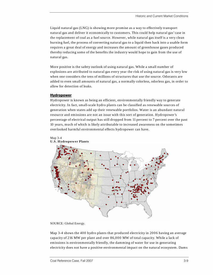
Historic and Current Market Conditions
Coal Reference Case, Fall 2007 3-9
Liquid natural gas (LNG) is showing more promise as a way to effectively transport natural gas and deliver it economically to customers. This could help natural gas’ case in the replacement of coal as a fuel source. However, while natural gas itself is a very clean burning fuel, the process of converting natural gas to a liquid then back into a usable form requires a great deal of energy and increases the amount of greenhouse gases produced thereby reducing some of the benefits the industry would hope to gain from the use of natural gas. More positive is the safety outlook of using natural gas. While a small number of explosions are attributed to natural gas every year the risk of using natural gas is very low when one considers the tens of millions of structures that use the source. Odorants are added to even small amounts of natural gas, a normally colorless, odorless gas, in order to allow for detection of leaks. Hydropower Hydropower is known as being an efficient, environmentally friendly way to generate electricity. In fact, small-scale hydro plants can be classified as renewable sources of generation when states add up their renewable portfolios. Water is an abundant natural resource and emissions are not an issue with this sort of generation. Hydropower’s percentage of electrical output has still dropped from 11 percent to 7 percent over the past 10 years, much of which is likely attributable to increased awareness on the sometimes overlooked harmful environmental effects hydropower can have. Map 3-4 U.S. Hydropower Plants
SOURCE: Global Energy.
Map 3-4 shows the 400 hydro plants that produced electricity in 2006 having an average capacity of 216 MW per plant and over 86,000 MW of total capacity. While a lack of emissions is environmentally friendly, the damming of water for use in generating electricity does not have a positive environmental impact on the natural ecosystem. Dams
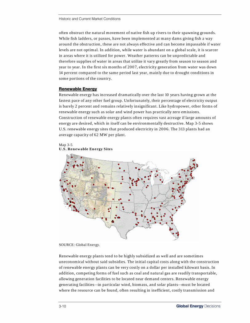
Historic and Current Market Conditions
3-10
often obstruct the natural movement of native fish up rivers to their spawning grounds. While fish ladders, or passes, have been implemented at many dams giving fish a way around the obstruction, these are not always effective and can become impassable if water levels are not optimal. In addition, while water is abundant on a global scale, it is scarcer in areas where it is utilized for power. Weather patterns can be unpredictable and therefore supplies of water in areas that utilize it vary greatly from season to season and year to year. In the first six months of 2007, electricity generation from water was down 14 percent compared to the same period last year, mainly due to drought conditions in some portions of the country. Renewable Energy Renewable energy has increased dramatically over the last 10 years having grown at the fastest pace of any other fuel group. Unfortunately, their percentage of electricity output is barely 2 percent and remains relatively insignificant. Like hydropower, other forms of renewable energy such as solar and wind power has practically zero emissions. Construction of renewable energy plants often requires vast acreage if large amounts of energy are desired, which in itself can be environmentally destructive. Map 3-5 shows U.S. renewable energy sites that produced electricity in 2006. The 313 plants had an average capacity of 62 MW per plant. Map 3-5 U.S. Renewable Energy Sites
SOURCE: Global Energy.
Renewable energy plants tend to be highly subsidized as well and are sometimes uneconomical without said subsidies. The initial capital costs along with the construction of renewable energy plants can be very costly on a dollar per installed kilowatt basis. In addition, competing forms of fuel such as coal and natural gas are readily transportable, allowing generation facilities to be located near demand centers. Renewable energy generating facilities—in particular wind, biomass, and solar plants—must be located where the resource can be found, often resulting in inefficient, costly transmission and

Historic and Current Market Conditions
Coal Reference Case, Fall 2007 3-11
increasing the ultimate costs of wheeling the power to demand centers. Like hydropower, the largest source of renewable energy, wind power, is dependant on unpredictable natural climate patterns. Coal-Fired Generation Coal plants currently provide the U.S. with half of its electric supply even though coal’s share of U.S. electricity supply has been reduced from 59 to 50 percent over the past decade. Advances in mining technology have led to increased productivity on the supply side keeping the delivered cost of coal relatively low, which remains far cheaper than natural gas on a delivered basis as was illustrated above. Map 3-6 U.S. Coal-Fired Power Plants
SOURCE: Global Energy.
The United States experienced its largest increase in coal-fired plant capacity between 1960 and the late 1980s. Since then there has been a dearth of new coal-fired units. The U.S. currently utilizes over 500 coal-fired power plants, each having an average capacity of over 600 MW. Nearly 70,000 MW of new capacity are at some stage of the planning process and projected to come on line sometime before December 31, 2030. It is highly unlikely that most of this estimated new capacity will be built, though it is certain that some of it will. In fact, there is already 15,000 MW of coal-fired capacity currently under some form of construction or development and is expected to be on line within five years. Forty-three coal-fired units with a total capacity of approximately 10,000 MW have proposed retirement dates in the same time period as mentioned above. Coal’s natural domestic abundance and the U.S.’s increasing desire to reduce dependence on foreign natural resources give coal advantages over other fuel sources. Over the last three decades, huge advances in coal extraction technology coupled with the development of the Powder River Basin has led to unprecedented increases in the productivity of coal mining ultimately making it more economical. Additionally, the ability to reliably and

Historic and Current Market Conditions
3-12
inexpensively transport coal to demand centers makes coal a very desirable fuel source. This most certainly has an impact on the amount of coal capacity on the drawing board for the future. Coal’s major drawback is the environmental effects of extraction coupled with having the highest levels of emissions of all fuel sources. Sulfur dioxide (SO2), nitrogen oxides (NOX), mercury (Hg), and carbon dioxide (CO2) are all byproducts of burning coal. Utilities are under close scrutiny to reduce their emission exposure, which has helped contribute to coal’s decreasing role in the U.S. electricity supply—displaced primarily by gas. Coal’s positive attributes such as domestic abundance, economical extraction, transportation, and delivery are important enough that the electric industry over the last decade has undertaken massive investments in emission control technology to minimize the environmental effects. Increased legislation such as CAIR and CAMR was a catalyst for this investment and has set strict standards that must be met in preset time frames. Currently, 115,000 MW of operating and standby coal capacity have SO2 controls and SO2 controls are planned for another 146,000 MW prior to December 31, 2018. Nitrogen oxides controls are even more prominent now, with over 290,000 MW currently equipped, roughly 88 percent of capacity. Beyond the issues relating to the consumption of coal are the safety and environmental issues associated with the production of coal. The year 2006 began with the explosion of the Sago Mine in Upshur County, West Virginia, on January 2, sparking a media frenzy that closely criticized coal mining safety practices due to the 47 deaths that occurred that year. The 2007 Crandall Mine disaster has not helped coal mining’s public image with the Sago disaster still fresh in its memory. Adding to coal industry woes are increased costs and difficulty in permitting mountain top mining. If mine-related accidents have not hurt the image of coal enough, images of mountain top removal certainly work to pour salt in the wound. Even with coal’s greater environmental impact and additional dangers associated with extraction than other fuel sources, the positive economic attributes have led the electricity industry to find creative ways of overcoming these shortfalls and maintain the ability to use coal as a fuel source for power generation. This creative problem solving shows how important coal is to the current and future U.S. electric industry.
Supply Of Coal Historic and Current Coal Consumption by Sector
Coal is primarily used to generate electricity, and has less demand from the residential, industrial, commercial, and steel sectors. Figure 3-8 shows coal’s past and current consumption by different sectors. In 1975, only 72 percent of coal was consumed by the electric power generation sector, whereas in 2006, the amount jumped to 93 percent.
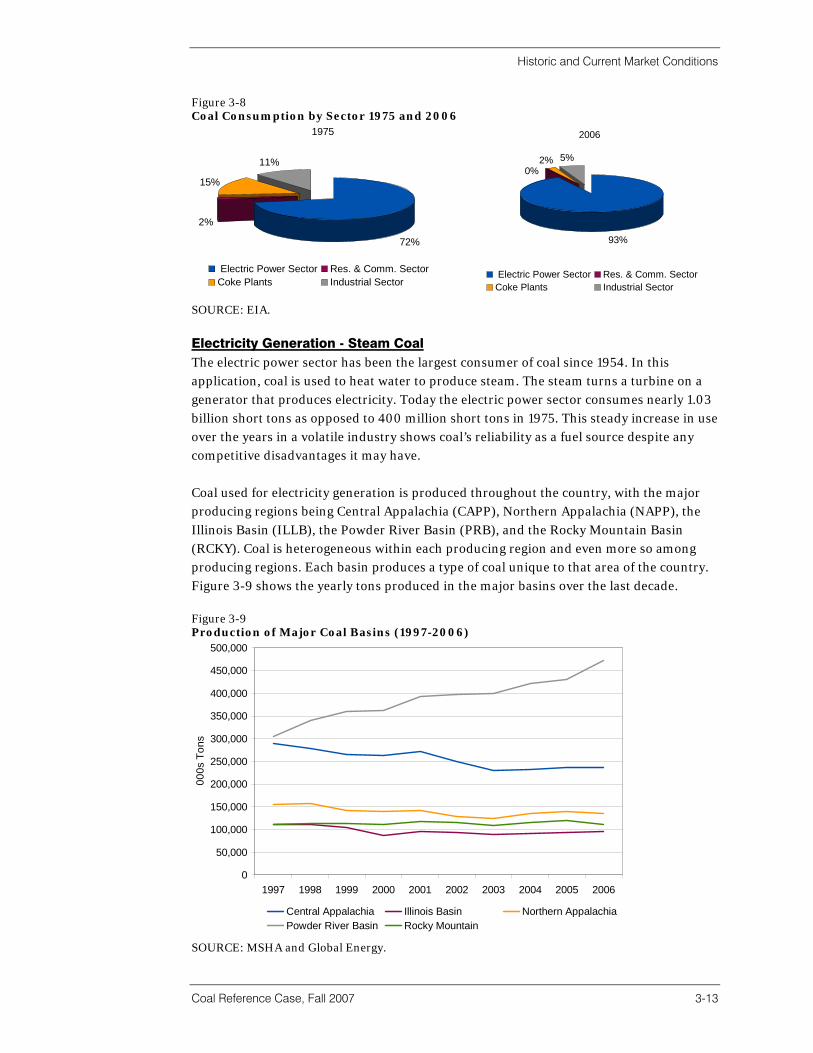
Historic and Current Market Conditions
Coal Reference Case, Fall 2007 3-13
Figure 3-8 Coal Consumption by Sector 1975 and 2006
93%
5%2%0%
Electric Power Sector Res. & Comm. SectorCoke Plants Industrial Sector
2006
72%
2%
15%
11%
Electric Power Sector Res. & Comm. SectorCoke Plants Industrial Sector
1975
SOURCE: EIA.
Electricity Generation - Steam Coal The electric power sector has been the largest consumer of coal since 1954. In this application, coal is used to heat water to produce steam. The steam turns a turbine on a generator that produces electricity. Today the electric power sector consumes nearly 1.03 billion short tons as opposed to 400 million short tons in 1975. This steady increase in use over the years in a volatile industry shows coal’s reliability as a fuel source despite any competitive disadvantages it may have. Coal used for electricity generation is produced throughout the country, with the major producing regions being Central Appalachia (CAPP), Northern Appalachia (NAPP), the Illinois Basin (ILLB), the Powder River Basin (PRB), and the Rocky Mountain Basin (RCKY). Coal is heterogeneous within each producing region and even more so among producing regions. Each basin produces a type of coal unique to that area of the country. Figure 3-9 shows the yearly tons produced in the major basins over the last decade. Figure 3-9 Production of Major Coal Basins (1997-2006)
0
50,000
100,000
150,000
200,000
250,000
300,000
350,000
400,000
450,000
500,000
1997 1998 1999 2000 2001 2002 2003 2004 2005 2006
000s
Ton
s
Central Appalachia Illinois Basin Northern AppalachiaPowder River Basin Rocky Mountain
SOURCE: MSHA and Global Energy.

Historic and Current Market Conditions
3-14
Basin Production and Quality Central Appalachia Central Appalachia is known for producing the highest quality coal in the country. High in heat value (Btus) and generally low in sulfur, CAPP coal is ideal for use in the generation of steam whether on its own or blended with other coal that might have lesser heat or higher sulfur content. CAPP coal normally has a heat value between 10,000 and 13,500 Btu with SO2 ranging from compliance with less than 1.2 lbs/MMBtu to around 4.5 lbs/MMBtu. Central Appalachia has seen a large amount of mining in its history due to the quality of its reserves. This has led to reserve degradation and producers are being forced to move into smaller, thinner, more geologically complex seams that are both more difficult and more costly to mine. This is the primary reason that production in CAPP has declined over the past 10 years and is expected to decline further in upcoming years while costs continue to increase. Illinois Basin With the implementation of more SO2 control technologies annually, the Illinois Basin becomes a logical place to see increased production. This coal has fair heat value, between 10,000 and 12,500 Btu, with SO2 content as high as 7.5 lbs/MMBtu. High sulfur content has kept the number of plants that can burn Illinois Basin coal at a minimum over the years due to compliance with the Clean Air Act Amendments. Declining production in CAPP and a desire by utilities to keep purchasing options open has led to many scrubber additions and therefore more plants with the ability to burn higher sulfur coal. While Illinois Basin production has remained fairly steady over the past 10 years, expect an increase in upcoming years. Northern Appalachia Northern Appalachia produces a high Btu, mid to high sulfur coal. Heat content normally ranges from 10,500 to 13,500 Btu/lb with SO2 ranging from 3.0 to 6.0 lbs/MMBtu. Like the Illinois Basin, this coal will have increasing market opportunities in the upcoming years with the addition of more scrubbers. Coal production in NAPP has remained fairly constant over the past 10 years. Most current Northern Appalachian coal penetrates the northern Ohio River market and the northeast, which has been the case for many years. Powder River Basin The PRB has seen a 55 percent increase in production over the past 10 years, from 300 to 470 million tons per year. Massive seam thickness (up to 200 feet) and highly favorable mining ratios have given this region the ability for such large expansion. This increase has only been possible due to increased demand of course, which has in part come with the increased regulations on SO2 emissions. PRB coal ranges in Btu from 8,000 to 10,500 Btu/lb, though 8,000 to 8,900 Btu/lb is considered more of a “normal” range for the southern part of the region in Wyoming. The northern PRB, located primarily in Montana, has higher Btu, similar sulfur, but often higher chlorine content. High chlorine content can lead to fouling and slagging in boilers if not consumed properly. The SO2 content of PRB coal is low, ranging from 0.4 to 2.0 lbs/MMBtu. A large number of plants

Historic and Current Market Conditions
Coal Reference Case, Fall 2007 3-15
in the Midwest, north Midwest, and even the southeast are now considering PRB coal their coal of choice. Rocky Mountain The Rocky Mountain Basin is the only non-continuous coal basin in the United States. Hence, it produces a wide variety of coal. Between the Green River, Uinta, and Four Corners sub regions Btu ranges from 8,750 to 12,500 Btu/lb and SO2 ranges from 0.5 to 2.5 lbs/MMBtu. Production in this region has remained fairly steady over the past 10 years just as NAPP and the Illinois Basin. The majority of the coal produced in the region stays in the western states though some does make its way across the Mississippi River to select plants such as those owned by the Tennessee Valley Authority. Map 3-7 shows the different U.S. coal basins and their coal characteristics. Map 3-7 U.S. Coal Supply Regions
SOURCE: Global Energy.
Australia Australia produced about 305 million tons of saleable coal in 2006. During that time, it exported about 122 million tons of steam coal and 138 million tons of coking coal making it by far the largest exporter of coal in the world and accounting for about 68 percent of global seaborne coking coal trade. The Australian coal industry produces a wide range of coals and has the flexibility to tailor products to suit customer requirements. Although coal is a natural product, many producers can vary product specifications by selective mining, blending, or by changing parameters at preparation plants. Coal quality varies significantly throughout Australia’s large reserves; typical specifications for the standardized over-the-counter steam coal contract at the largest export terminal, Newcastle, are 6,000 kcal/kg (10,792 Btu/lb) to 5,850 kcal/kg (10,522 Btu/lb) minimum with less than 1 percent sulfur.

Historic and Current Market Conditions
3-16
Australia has a sound investment environment for increasing supply and many new projects and expansions are in the pipeline. It also has a very large export terminal capacity and although it has been a bottleneck of late, extensive expansions are planned for the next two to three years. At that point, the remaining supply chain bottleneck is likely to be the rail infrastructure, which may prove more difficult to expand than shipping terminals. Canada Canada’s coal production in 2006 was 62 million tons and the production in 2005 was 67 million tons. Canada is a major exporter of coking coal, a distant second to Australia. Canadian production is concentrated in western Canada in Alberta, British Columbia, and Saskatchewan. In eastern Canada, New Brunswick has one operation and Nova Scotia has several small-scale operations without significant production. Canada is known for its metallurgical coal in the Peace River coalfield. Bearing low ash and sulfur content, medium volatility, as well as high heat, the products can be used for metallurgy and pulverized coal injection (PCI). Colombia Colombia produced 64 million tons in 2006 and in the first third of 2007 produced over 16 million tons. The coal from Colombia is considered one of the top quality coals in South America with high heat content ranging between 10,000 and 14,700 Btu/lb but is typically around 11,300 Btu/lb. Colombian over-the-counter standard contracts require a maximum of 0.85 percent sulfur and in general Columbia’s coal resources are near or below. Major coal operations in Colombia include Cerrejon, owned jointly by Anglo America, BHP Biliton, and Xstrata and Drummond’s Mina Pribbenow. Nine states in Colombia produce coal but Cesar and Guajira together account for about 92 percent of current production. The highest quality Colombian coal is found in the states of Santander and Norte de Santander, where production is currently limited by access and availability of capital equipment. Indonesia In 2006, production of coal in Indonesia was 193 million tons and 162 million tons were exported. The types of coal in Indonesia are ranked as follows: lignite (59 percent), sub-bituminous (27 percent), and bituminous (14 percent). Anthracite accounts for less than 0.5 percent of Indonesia’s coal deposits. Indonesian coal has heat values ranging between 9,000 and 12,500 Btu/lb, typically 11,150 Btu/lb. Sulfur content is typically 0.8 percent with a maximum of 1.0 percent on the standard over-the-counter contract. Indonesia adopted a new coal policy in January 2004, which seeks to promote the development of the country’s coal resources to meet domestic requirements and to increase coal exports in the long-run. However, a recent report from the U.S. Embassy in Jakarta suggests that the growth in coal production in Indonesia has been export-oriented, owing to the higher international price fetched by coal producers. A large portion of Indonesian coal that makes it to market goes unreported due to local corruption, putting the more realistic 2006 export figure at around 170 million tons or 15 percent more than the officially reported numbers.

Historic and Current Market Conditions
Coal Reference Case, Fall 2007 3-17
Russia Russia’s production of coal in 2005 was 296 million tons and in 2006, the production was greater than 300 million tons. In 2006, Russia exported 71 million tons of coal, up 15 percent over 2005. Russia exported its coal to 45 countries in 2006. About 37 percent of coal exports went to Western Europe, 10 percent to Eastern Europe, 12 percent to former Soviet republics, 24 percent to the Middle East, and 17 percent to the Asia-Pacific. The quality of the coal is high quality steam, coking, and anthracite with high calorific value and low sulfur content. The location of coal resources in Russia will play an important role in the future of its coal and gas export strategy. There are six major producing regions in Russia: Donbass (Donetsk), Kansko-Achinsk, Kuzbass (Kuznetsk), Pechora, Moscow, and Yakutia coal basins. The Kuzbass in western Siberia is the most important coal mining region in production and quality, and represents 45 percent of all Russian’s coal production. Its location creates a situation of very high transportation costs to export terminals, often 35-40 percent of the free on board (FOB) price. Much of Russia’s electricity is produced from gas. The Kansko-Achinsk coal basin produces about 25 percent of all Russian steam coal and is one of the largest lignite deposits in the world. Today, only 5 percent of these reserves are under commercial development. The lignite produced is characterized by low sulfur content of less than 1 percent, ash between 8-12 percent, heat content of 3,700 kcal/kg (6,660 Btu/lb), and production cost lower than $3 per ton. South Africa South Africa produced 242.8 million metric tons of saleable coal in 2006. Of the total production in South Africa 28 percent or 74 million tons (2006) is exported through Richards Bay Coal Terminal, making South Africa the fourth largest coal exporting country in the world. Most raw South African coal is low quality and requires beneficiation, which generates large amounts of coal waste. Venezuela Venezuela produced more than 7 million tons in 2006. The heat content of Venezuelan coal ranges from 8,000 to 13,500 Btu/lb, with most being low sulfur. Sulfur content from Mina Paso del Diablo, for example, is 0.70 percent. Imports from Colombian mines just across the border are blended with Venezuelan coal to improve heat content in some cases. Basin Reserves
Coal’s abundance and position as the most economical fuel for electric power generation are both indicators that it will be heavily relied upon for electricity generation in the future. According to the USGS, the United States has the largest coal reserves in the world with approximately 275 billion tons of economically recoverable coal at existing and new mines and an additional 3.7 trillion tons of coal from implied and assumed sources (see Figure 3-10). At the current 1.1 billion tons per year consumption rate of coal in the U.S., the EIA estimates that there is enough coal at new and existing mines to last

Historic and Current Market Conditions
3-18
approximately 250 years with an additional 3,300 years worth of coal available from all known and implied sources in the U.S. Figure 3-10 U.S. Coal Resources
SOURCE: EIA Coal Reserve Database.
Appalachia The overall remaining coal available by Appalachian coalfield is shown in Table 3-2. Of the 92.5 billion tons of coal that were originally available, only 14.4 billion tons are considered economically recoverable. Please note, however, that this figure does not represent all the coal in Appalachia; it is only a summary of the major coalfields for which there are available data. Table 3-2 Appalachia Recoverable Resources by Coal Bed (millions of short tons)1
Coal Bed Original Remaining Recoverable (statistical estimate)
Economically Recoverable (statistical estimate)
Northern Region
Pittsburgh 34,000 16,000 11,900 7,820
Upper Freeport 34,000 <31,000 15,640 3,740
Central Region
Fire Clay 6,300 5,100 2,457 630
Pond Creek 11,000 8,700 3,630 990
Pocahontas #3 7,200 5,100 2,088 1,224
Grand Total 92,500 65,900 35,715 14,404
SOURCE: USGS.
1 The recoverable and economically recoverable figures are estimates based on very small statistical sampling done by the USGS. These estimates may or may not reflect the true amount of coal recoverable.

Historic and Current Market Conditions
Coal Reference Case, Fall 2007 3-19
Other factors to consider are: • Deeper coal, thinner seams, growing underground mine safety costs, and diminishing
opportunities to consolidate reserves will cause production to decrease in Central Appalachia. Northern Appalachia is better positioned, but problems remain.
• Central Appalachian production continues to decline and is expected to lose additional capacity into the mid-term.
• Northern Appalachia has seen production flatten and there is not much growth expected over the next five years.
• Dams and locks are in need of maintenance and upgrades and additional dredging is needed in many of the waterways that serve Appalachian coal. Rail is limited to two carriers and additional routes out of the interior of Appalachia are unlikely. Trucking remains viable but with increased diesel prices comes increased transportation costs to the delivered price of Appalachian coal.
• Increased competition from imports would place additional pressure on Appalachian producers to lower costs.
Illinois Basin The overall remaining coal available by coalfield is shown in Table 3-3. Of the 189.9 billion tons of coal that were originally available, only 24.5 billion tons are considered economically recoverable. Please note, however, that this figure does not represent all the coal in Illinois Basin; it is only a summary of the major coalfields for which there are available data. Table 3-3 Remaining Coal in the Illinois Basin by Coal Bed (millions of short tons) 2
Coal Bed Remaining Economically Recoverable
(statistical sample)
Springfield 80,800 10,068 Herrin 81,500 11,150
Danville & Baker 27,600 3,241 Grand Total 189,900 24,459
SOURCE: USGS and Global Energy.
Other factors to consider include: • The proposed construction of sulfur emissions control equipment for nearly 100 GW
of coal-fired generation before 2011 means higher sulfur Illinois Basin coal stands to recapture a portion of the market it lost to lower sulfur western coal.
• Large, untapped Illinois Basin coal reserves remain, many with fairly low ratios, strategically located near rail and rivers in the heartland of the U.S.
2 The recoverable and economically recoverable figures are estimates based on very small statistical sampling done by the USGS. These estimates may or may not reflect the true amount of coal that is economically recoverable.
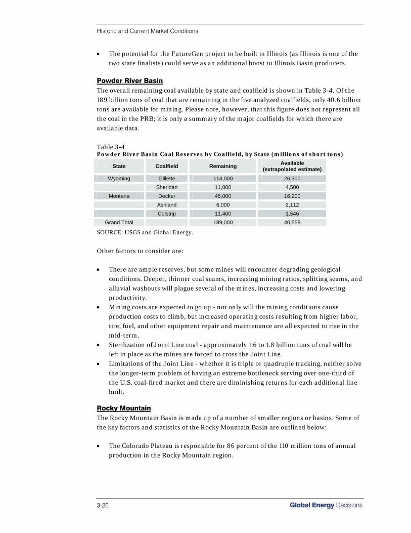
Historic and Current Market Conditions
3-20
• The potential for the FutureGen project to be built in Illinois (as Illinois is one of the two state finalists) could serve as an additional boost to Illinois Basin producers.
Powder River Basin The overall remaining coal available by state and coalfield is shown in Table 3-4. Of the 189 billion tons of coal that are remaining in the five analyzed coalfields, only 40.6 billion tons are available for mining. Please note, however, that this figure does not represent all the coal in the PRB; it is only a summary of the major coalfields for which there are available data. Table 3-4 Powder River Basin Coal Reserves by Coalfield, by State (millions of short tons)
State Coalfield Remaining Available (extrapolated estimate)
Wyoming Gillette 114,000 26,300 Sheridan 11,000 4,500
Montana Decker 45,000 16,200 Ashland 6,000 2,112 Colstrip 11,400 1,546
Grand Total 189,000 40,558
SOURCE: USGS and Global Energy.
Other factors to consider are: • There are ample reserves, but some mines will encounter degrading geological
conditions. Deeper, thinner coal seams, increasing mining ratios, splitting seams, and alluvial washouts will plague several of the mines, increasing costs and lowering productivity.
• Mining costs are expected to go up - not only will the mining conditions cause production costs to climb, but increased operating costs resulting from higher labor, tire, fuel, and other equipment repair and maintenance are all expected to rise in the mid-term.
• Sterilization of Joint Line coal - approximately 1.6 to 1.8 billion tons of coal will be left in place as the mines are forced to cross the Joint Line.
• Limitations of the Joint Line - whether it is triple or quadruple tracking, neither solve the longer-term problem of having an extreme bottleneck serving over one-third of the U.S. coal-fired market and there are diminishing returns for each additional line built.
Rocky Mountain The Rocky Mountain Basin is made up of a number of smaller regions or basins. Some of the key factors and statistics of the Rocky Mountain Basin are outlined below: • The Colorado Plateau is responsible for 86 percent of the 110 million tons of annual
production in the Rocky Mountain region.

Historic and Current Market Conditions
Coal Reference Case, Fall 2007 3-21
• Of the 535 billion tons of coal measured in the Colorado Plateau, 57 percent is available after environmental and technical restrictions are taken into account, 42 percent is recoverable and only 21 percent is economically recoverable.
• Similar recoverability percentages are applied to the other coalfields that make up the Rocky Mountain region.
• Traditional consumers of Colorado-origin and Utah-origin coals have experienced some sustained shortages as these regions experienced short-term mine outages and were also tapped to replace constrained PRB coal supply.
Australia Australia has more than 39 billion tons of recoverable bituminous and anthracite coal reserves. Of the total identified bituminous and anthracite resources, just under half is accessible through surface mining with the remainder accessible by underground mining. Australian coal deposits also include over 37 billion tons of brown coal (lignite), which ranks it first in lignite reserves. Canada Canada has proven reserves of about 7.3 billion short tons (equivalent to about a 90-year supply at current production rates), located primarily in the provinces of Alberta, Saskatchewan, and British Columbia. The composition of recoverable reserves is 3.4 billion tons of anthracite and bituminous coal and 3.8 billion tons of lignite sub-bituminous coal. Colombia Colombia has 6.9 billion tons total recoverable reserves of anthracite and bituminous coal and 420 million short tons of lignite sub-bituminous coal. Colombia’s coal resources are primarily (75 percent) situated in the Caribbean region of Colombia and 25 percent in the interior. Indonesia The tested reserves of coal in Indonesia are about 5.5 billion tons. Indonesian coal reserves represent only 3.1 percent of the total reserves of coal in the world. The total recoverable reserves of anthracite and bituminous coal in Indonesia are 816 million short tons and 4.66 billion tons of recoverable reserves of lignite and sub-bituminous coal. Russia Russia has recoverable coal reserves of 173 billion short tons the world’s second largest. The majority of the Russian coal is located east of the Ural Mountains in Siberia. The total recoverable reserves of anthracite and bituminous coal in Russia are 54 billion short tons and 119 recoverable reserves of lignite and sub-bituminous coal. South Africa South Africa has huge coal reserves that consist of a relatively high ash and low sulfur bituminous coal. Recoverable reserves are estimated in about 53.74 billion short tons. South Africa’s coal reserves represent 5.4 percent of the world's total coal reserves.

Historic and Current Market Conditions
3-22
Venezuela Venezuela exports almost all of its coal production and has recoverable coal reserves of approximately 530 million tons. Basin Costs
Fuel costs, labor costs, and productivity influence current and future mining costs. Fuel costs have been on the rise for many years now. In July 1997, the price of a barrel of crude oil was $17.00 compared to a price of over $80.00 in September 2007, an increase of 370 percent in a little over 10 years. The price of gasoline increased 250 percent in the same period from $1.20/gallon to $2.98/gallon. These statistics indicate rising fuel costs for coal operations, though on an inflation-adjusted basis fuel prices are comparable to 1981 fuel crises prices. Labor costs have also remained fairly flat for a number of years. While many union contracts had inflation clauses giving workers raises on an annual basis, the inflation-adjusted increase was not significant. One advantage was had by non-union mines, mainly in CAPP, where they were able to keep labor costs significantly lower than other operations. However, the recent coal boom and lack of workers put pressure on labor costs, increasing them across the industry and erasing advantages non-union operations once had. Productivity is the next variable used to analyze basin costs. Economics would indicate that companies would mine the cheapest reserves first in order to maximize profits in present value terms. Assuming this is true, costs in all basins should have been increasing due to reserve degradation since mining commenced. This makes sense, but with the exception of a brief dip in productivity in the mid-1970s due to tightening safety standards and mine reclamation costs, mine productivity has consistently increased due to tremendous advancements in mining technology over the last 50 years up until the start of this decade. Unless another technological breakthrough is seen, reserve degradation, which is seen in all basins on some level, will continue to bring down productivity and increase costs as it has in the past decade. Some cases where reserve degradation has influenced recent productivity in particular basins are: Appalachia: • Approaching higher ratios seams; and • Inability to further consolidate reserves due to geology, previous mining operations,
and current ownership.
Illinois Basin: • Highly productive surface mine reserves are being replaced with less productive
underground mines.

Historic and Current Market Conditions
Coal Reference Case, Fall 2007 3-23
Gulf and Northern Lignite: • Maturing mines; and • Increasing distance to mine mouth plants from mines.
Other West: • Less productive underground mines are replacing highly productive surface mines.
Powder River Basin: • Approaching higher ratio seams, sand channels, and seam splitting; and • Limits to economies of scale (larger trucks and draglines are not being produced).
In summary, fuel and labor costs have remained fairly steady in history on an inflation-adjusted basis. Due to reserve degradation, cost control was obtained through increases in productivity. This trend continued until the early part of the current decade, where it seems technology is not advancing as rapidly as in the past. Compounded by reserve degradation, this has caused productivity to level and in most basins decrease over the last five years as seen in Figure 3-11. As a result of our growing dependence on foreign energy sources, it is likely that greater emphasis will be placed on obtaining energy from secure, domestic supplies. Domestic production of coal not only ensures a secure, reliable energy source, but it also has benefits that ripple throughout the economy, thus creating a strong political base for coal. Figure 3-11 Coal Mine Productivity by Basin 1995-2007 (2007 based on Q1 data)
2
3
4
5
6
7
8
9
1995 1996 1997 1998 1999 2000 2001 2002 2003 2004 2005 2006 2007
Tons
/Man
-Hou
r
0
5
10
15
20
25
30
35
40
45PR
B To
ns/M
an-H
our
CAPP ILLB NAPP Rky Mtn PRB SOURCE: Global Energy.

Historic and Current Market Conditions
3-24
Australia Most (76 percent) of Australia’s coal was mined by surface methods in 2005. Labor productivity in the Australian coal-mining sector increased substantially from 1990 to 2001 but has since fallen. This decline is largely a result of increasing stripping ratios (the ratio of overburden thickness to coal thickness) which grew from 6.7 in 2000 to 7.9 in 2005 as average depth at surface mines increased. In addition, the skilled labor pool has diminished. These factors, along with the cost pressures that other mining operations around the globe face (i.e., high costs for steel and tires) will lead to higher costs in the long run. During the first half of 2007 the average price for standard Newcastle product was about $55.00 per ton. Colombia The cost of coal production in Colombia varies by region and is subject to transportation, machinery, labor, and location. The highest cost mines are in the zones of Valle del Cauca and Cesar. In the Cesar area limited transportation capacity in the Jagua de Ibirico district is negatively affecting prices. The highest mining costs are encountered in the Valle del Cauca that belongs to the Jamundi district. As a result of large investments made by international corporations operating in the states of Guajira and Cesar, the price per ton of coal is lower than in other states. Of Cerrejon’s production in the first half of 2007, 64 percent went to Europe while 20 percent was exported to the United States because of significantly higher prices it commands on the east side of the Atlantic. Low sulfur, 11,300 Btu/lb standardized OTC coal averaged about $52.00/ton for the first half of 2007. Venezuela The estimated production cost of coal in Venezuela fluctuates between $18.00 and $27.00 per ton. Hugo Chavez’s Venezuelan government has restricted much of the data regarding Venezuelan coal production and costs. Canada Canadian coal mining faces many of the same challenges faced by U.S. operators. A Coal Association of Canada survey of select coal mine operations in Canada revealed that high taxes and royalties and complex permitting and regulation were issues of prime concern. Canada exports only a very small amount of steam coal with metallurgical coal making up the vast majority of exports. Indonesia Indonesia is able to produce coal very cheaply in comparison to other coal exporters by most accounts. However, taxes and royalties take a much bigger bite out of revenues of operators in Indonesia than in other coal exporting countries, so much so that in 2003-2004 most of the foreign investment in Indonesia’s coal industry fled. The situation seems to have improved marginally since then but corruption is still widespread.
Historic and Current Market Conditions
Coal Reference Case, Fall 2007 3-25
South Africa Many South African deposits were originally exploited at extremely low costs and, as a result, a large coal-mining industry has developed. However, South Africa’s coal industry has been fueling the economy for a long time. Coal-to-liquids plants were built to compensate for the economic sanctions that came in response to apartheid. Furthermore, coal fuels 93 percent of the electricity production in South Africa. As a result, coal production in South Africa is mature which will lead to higher mining costs as reserve quality degrades in the near future. Labor costs face upward pressure from the epidemic of HIV/AIDS. The coal industry will not escape escalating health care costs and productivity problems caused by this human tragedy. The average FOB price at Richard’s Bay coal terminal for the first half of 2007 was $52.82/ton for standard 10,800 Btu/lb OTC coal. Russia The average price of Russian coal sold in the Pacific market (from Vostochny) was $68.31/ton, reflecting the long transportation route to the coast from the Siberian interior mines. The average first half 2007 price at the Russian Baltic ports was about $62.00/ton. Non-Utility Coal Consumption
Consumption of coal in applications other than for electricity generation has been declining since the mid-1970s almost entirely as a result of reduced demand for coking coal. The shift away from blast furnace steel manufacturing to electric arc furnaces and pulverized coal injection combined with a general slowing of U.S. steel manufacturing, accounts for this decline. Annual primary production of pig iron in the U.S. declined 54 percent between 1973 and 2004 while U.S. finished steel production declined 30 percent during the same period. Falling steel and iron production accounts for some of the 75 percent decline in coking coal consumption, while efficiency improvements and conversion to newer steel production technology account for the much of the rest of the decline. Commercial and Residential Commercial coal use consists primarily of small combined heat and power applications with some district heating applications. Residential coal use is confined to heating. Residential and commercial coal consumption has declined over the last 30 years or so. This should not come as a surprise when the cost of transporting small volumes of coal and availability of natural gas in many areas makes coal less economical for small applications.

Historic and Current Market Conditions
3-26
Figure 3-12 Historical Non-Utility Coal Consumption; 1973-2006
0
20
40
60
80
100
120
140
160
1973 1976 1979 1982 1985 1988 1991 1994 1997 2000 2003 2006
Con
sum
ptio
n (M
illio
ns o
f Ton
s)
Residential Commercial Industrial Coke Plants Other Industrial
SOURCE: EIA and Global Energy.
Coking Coal An important use for higher quality coal is in the coking portion of the steel manufacturing process. Coking coal or metallurgical (met) coal is generally highest in carbon content of all coal and is generally required to be very low in sulfur and other impurities. Met coal is categorized very specifically and valued by consumers for an array of quality specifications making it much more difficult to price as a standardized product. This is in contrast to steam coal, which is priced almost exclusively based on heating value and sulfur content. These requirements, combined with its relative scarcity typically create a substantial premium for met coal over steam coal. The coking process begins by turning met coal into coke by heating it to between 1,000 and 1,100 degrees Centigrade in the absence of air. This removes gases and other elemental constituents from the coal, leaving a hard porous from of nearly pure carbon behind called coke. The crushed coke is combined in a blast furnace with limestone and iron ore to produce first iron and then steel. Though most steel manufacturing uses this two-step process, first producing coke, then using coke in the blast furnace, electric arc furnaces for steel manufacturing are replacing blast furnaces in the United States where scrap steel is readily available. This ultimately diminishes the demand for coking coal since electric arc furnaces do not use coke (although the electricity generated to power them is often generated from coal). About 64 percent of steel production worldwide is dependent on coking coal. While the U.S. steel industry once consumed over 83 million tons of coal, this amount has decreased significantly over the last 30 years. Lower steel production costs overseas created a strong U.S. import market for steel during this time period forcing domestic

Historic and Current Market Conditions
Coal Reference Case, Fall 2007 3-27
producers like US Steel to diversify their operations internationally thus decreasing the domestic demand for coking coal. Coal used in the production of coke and steel must meet certain quality standards. As mentioned earlier it is among the highest in carbon content of all coal, normally over 12,400 Btu/lb, and is required to be very low in sulfur and ash content. Due to these restrictions, met coal is produced mainly in two places: Southern and Central Appalachia. Massey Energy, based in Central Appalachia, is the largest supplier of coking coal in the United States with approximately 20 million tons of met coal sold in 2006. Coking coal prices increased dramatically between 2003 and 2006 from around $50/ton to $95/ton, as shown in Figure 3-13. This price run up has made it more profitable for mines that can “switch hit,” that is sell their coal into either the met or steam markets. This deceases available supply from the Appalachian steam markets for as long as the price differential lasts and Appalachian coking coal producers can get their coal to market. Figure 3-13 Average Coking Coal Prices in the U.S.; 2001-2007
$0.00
$20.00
$40.00
$60.00
$80.00
$100.00
$120.00
Jan-01
Sep-01
May-02
Jan-03
Sep-03
May-04
Jan-05
Sep-05
May-06
Jan-07
Sep-07
Declared Monthly Export Value ($/ton) Quarterly Coke Plant Receipts ($/ton)
SOURCE: EIA.
Industrial Coal Coal is useful in a variety of industrial applications including chemical and fertilizer industries, alumina refineries, and paper manufacturing, but its primary industrial use is as an energy input in the production of cement. About 80 percent of the coal used by industry in the U.S. goes to produce cement and clinker. Cement production requires large amounts of energy to heat the kilns which produce clinker. Clinker is made from calcium carbonate in the form of limestone, silica iron oxide, and alumina. These ingredients are heated in a kiln to produce the clinker which is then combined with gypsum and ground to a fine powder to produce cement. The ratio of coal required to produce cement is about 1:2, or one ton of coal in for two tons of cement out. United States cement production was approximately 100 million tons in 2006 representing

Historic and Current Market Conditions
3-28
about 50 million tons of coal consumption. This leaves an annual production shortfall of about 37.5 million tons of cement that is covered by imports. Cement production in the U.S. is at about 91.5 percent of capacity which combined with high demand has spurred investment in clinker and cement production. United States capacity is expected to expand from about 110 million tons per year in 2005 to 131 million tons per year in 2010.3 This expansion would add about 11 million tons of new coal demand from the industrial sector.
Coal Transportation Coal is moved to market directly by rail, water (river barges, lake, and ocean vessels), truck, conveyor belt, slurry pipeline, or a combination of methods depending on the location of the mine and the location of the end customer. Due to the vast geographic area that rail infrastructure covers and its ability to move large amounts of coal long distance through many types of terrain, the majority of coal is delivered for at least part of its journey from mine to plant by rail. In fact, almost 72 percent of all coal delivered to end-users in 2006 was transported in part by rail. The four Class I railroads in the United States—CSX, Norfolk Southern, Union Pacific, and Burlington Northern Santa Fe railroads—account for the majority of rail movements. Most western rail coal is originated on the Union Pacific railroad (UP) or the Burlington Northern Santa Fe railroad (BNSF). Most eastern rail coal is originated on the Norfolk Southern Railroad (NS) or the CSX railroad. Midwest coal is originated by one of the railroads named above or other regional carriers. Railroad Transportation Appalachia Two Class I railroads serve the Northern and Central Appalachian coalfields. They are the CSX and Norfolk Southern. Some mines, such as Foundation’s Cumberland mine, have a dedicated railroad that transports coal to the Monongahela River for loading onto barges. The CSX and NS railroads share trackage rights to a Joint Line referred to as the MGA corridor, which originates in Marion County, West Virginia, and follows the Monongahela River north to terminate to the west of Pittsburgh, Pennsylvania. By using this transportation corridor, coal from these mines is transported to coal docks located on the Monongahela River for loading onto barges, or continues by rail to networks operated by the two individual railroads. Some of the large mines served by this rail network include Consol’s Bailey/Enlow Fork complex, Blacksville #2, Loveridge #2, and Peabody’s Federal #2 mine. Map 3-8 shows the rail network in and around the Appalachian coalfields. Because of the difficult terrain in Northern Appalachia, coal that travels by rail is routed to the north or east to make its way out of NAPP. Railroads traveling south on the coastal plains from Northern Appalachia are congested areas. These factors could play a role in limiting NAPP coals penetration into the southeastern U.S. markets even though
3 Portland Cement Association.

Historic and Current Market Conditions
Coal Reference Case, Fall 2007 3-29
scrubbing equipment is being installed that can burn this high sulfur coal. Other factors also include train cycle times, grades/inclines, and speed restrictions. In 2006, 82 percent of coal produced in Central Appalachia was transported by rail. Close to half of these deliveries were carried solely by rail while the rest consists mostly of trucks and barges transporting coal from mine mouth to river docks for transportation on barges to the Ohio River market. A large portion of the coal transported only by rail makes its way into the southeast states of Virginia, North Carolina, South Carolina, Georgia, and Florida. In fact, over 50 percent of CAPP deliveries are made to these states. Map 3-8 Rail Transportation in Appalachia
SOURCE: Global Energy.
The Illinois Basin
Approximately 45 percent of the 86 million tons of coal delivered from the Illinois Basin in 2006 originated on rail with the remainder mainly on trucks or barges. Of coal originating on rail, 25 percent will end its journey aboard another form of transportation, more than likely barge, with a large portion of the remaining 75 percent being delivered within the Illinois Basin itself or to surrounding states such as Indiana, Iowa, Missouri, and Wisconsin, which have an extensive railway system. The Illinois Basin’s rail infrastructure is shown below in Map 3-9.
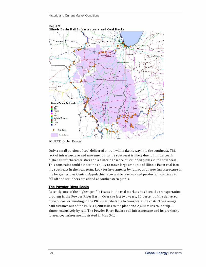
Historic and Current Market Conditions
3-30
Map 3-9 Illinois Basin Rail Infrastructure and Coal Docks
SOURCE: Global Energy.
Only a small portion of coal delivered on rail will make its way into the southeast. This lack of infrastructure and movement into the southeast is likely due to Illinois coal’s higher sulfur characteristics and a historic absence of scrubbed plants in the southeast. This constraint could hinder the ability to move large amounts of Illinois Basin coal into the southeast in the near term. Look for investments by railroads on new infrastructure in the longer term as Central Appalachia recoverable reserves and production continue to fall off and scrubbers are added at southeastern plants. The Powder River Basin
Recently, one of the highest profile issues in the coal markets has been the transportation problem in the Powder River Basin. Over the last two years, 60 percent of the delivered price of coal originating in the PRB is attributable to transportation costs. The average haul distance out of the PRB is 1,200 miles to the plant and 2,400 miles roundtrip—almost exclusively by rail. The Powder River Basin’s rail infrastructure and its proximity to area coal mines are illustrated in Map 3-10.

Historic and Current Market Conditions
Coal Reference Case, Fall 2007 3-31
Map 3-10 Rail Transportation in the Powder River Basin
SOURCE: Global Energy.
Wyoming The highest profile topic in the western—and perhaps U.S.—coal sector is the rail transportation problem in the Wyoming PRB. Initial service from the Wyoming PRB began in 1978 as coal was shipped from the Sheridan and Gillette coalfields. Burlington Northern Railroad (later to become the BNSF) was the sole provider of rail service from the PRB until 1982. Then a jointly owned venture of the Union Pacific and the Chicago and North Western (C&NW) railroads, (the Western Rail Properties, Inc or WRPI) acquired half interest in the Burlington Northern coal line from Shawnee Junction to Coal Creek Junction, Wyoming, and began construction of new rail from Shawnee Junction, Wyoming, to Joyce, Nebraska. The first shipments of coal on the new line began in August 1984. In 1986, WRPI purchased half interest in 11 miles more of BN line from Coal Creek Junction to Caballo Junction, Wyoming. Union Pacific Railroad acquired ownership of the entire C&NW in April 1995. Today the Joint Line consists of a 103-mile line jointly owned by the BNSF and the UP running from Caballo Junction to Shawnee Junction, Wyoming.

Historic and Current Market Conditions
3-32
The Joint Line connects to eight mines that produced about 75 percent of PRB coal in 2006. In addition, a BNSF line extends northwestward from Campbell, Wyoming, to access the north Gillette area where the Buckskin, Dry Fork, Eagle Butte, Fort Union, Rawhide, and Wyodak mines are located. Coal from the Joint Line routed on the BNSF can exit north at Donkey Creek, Wyoming, and be routed to Alliance, Nebraska, for further switching to main coal corridors that run through Nebraska, Iowa, and Illinois to the east; through Nebraska, Missouri, and Arkansas to Memphis; and to the southeast and through Colorado, New Mexico, and Texas to the south. BNSF coal originating on the Joint Line can also exit to the south through Bill, Wyoming, but intermixing BNSF trains with UP trains that exit south exacerbates congestion problems. Coal originating in the north Gillette area can exit the spur at Campbell, Wyoming, for initial routing to Alliance, Nebraska. Significantly, coal originating in the north Gillette area avoids the Joint Line
congestion, which raises transit speeds and reduces train cycle time. Most Joint Line coal originating on the UP is routed southward through Shawnee Junction, Wyoming, and east to Northport, Nebraska, for routing through Nebraska and Kansas to Kansas City, Missouri, where coal can be routed south to Missouri, Arkansas, Oklahoma, Louisiana, and Texas. Coal can also be routed south through Wyoming and Colorado to west Texas. BNSF controls dispatch from the Joint Line, and has latitude to route coal through either the north or south ends as the situation warrants. Wyoming PRB Rail Congestion Although congestion is endemic throughout the Joint Line area, more problems occur at the southern exit and in western Nebraska. Periodic derailments, steep grades, and problems with coal dust infiltration into the track ballast have resulted in a marginal situation deteriorating into a near catastrophic situation in the past 36 months. The railroads have responded to chronic capacity problems (most recently since 2004) with repeated “mea culpas,” well-tuned publicity campaigns touting their awareness, and announcements of hundreds of millions of dollars of investment in capacity enhancements. The most popular and visible enhancements are the multiple tracking of sections of the line where congestion is worse, and expansions of marshalling yards in Nebraska and Wyoming to hold loaded and empty unit trains. What the railroads are doing, in effect, is making northeastern Wyoming and western Nebraska a train parking lot, while trying to figure out how to get even more trains into the area. Super highway designers are familiar with the problem—eventually capacity expansion becomes part of the problem as higher and higher levels of investment only make the problem grow worse. Numerous metropolitan areas—wrestling with gridlock—have come to realize that building wider, multi-lane corridors and higher efficiency interchanges is not a solution to congestion. In economics jargon, this is a sign of diminishing returns that leads to diseconomies of scale. Diseconomies of scale describe a situation where average costs keep rising as output rises. When the diseconomies are sustained even in the face of massive investment, it is considered a signal that a new approach may be needed.
Historic and Current Market Conditions
Coal Reference Case, Fall 2007 3-33
The railroads, the coal suppliers, and perhaps the coal consumers have chosen to ignore the experience of many highway expansion programs—and continue to promote the myth that the Joint Line can provide all the low cost sub bituminous coal that the United States needs. If the Gillette coalfield is “the heart” of the U.S. steam coal sector, then its circulatory system is suffering from a severe case of arterial sclerosis. To date, it has been solved by use of bypass surgery and the insertion of stents. Currently, a triple bypass is being performed on the Bill to Caballo Junction, Wyoming, portion of the artery, and a stent is being placed at Logan Hill. Quadruple bypass surgery has been proposed to avoid the next bout of “heart failure.” Researching the history of Wyoming PRB rail transportation is a “déjà vu” experience. One encounters numerous articles describing sclerotic performance, followed by railroad promises to invest in more tracking. In the 1993 to 1994 period, poor rail performance resulted in the expenditure of nearly $200 million in 1994-1995 on double tracking and other upgrades in the Joint Line area and in Nebraska. The objective was to raise the capacity from 185 to 328 million annual tons. In 1994, 166 million tons was produced by the Joint Line mines. By 2004, it is generally acknowledged that the Joint Line mines shipped only 90 percent to 95 percent of the total demand for their product, and production exceeded 322 million tons. Thus, a capacity increase of 137 million annual tons was achieved by the initial investment—not 143 million. The investment missed the mark—significantly if the 5 percent to 10 percent 2004 demand shortfall is included. But the investment did enable shipments to rise from about 48 to 57 train loadings per day. Current plans are to invest another $200 to $300 million to raise capacity to 400 million annual tons in the 2007 to 2009 period. Thus, the investment is projected to add another 78 million annual tons to capacity. Global Energy projects that demand for Joint Line origin coal will exceed 400 million annual tons by 2009—if the railroads can get the coal to market. Another notable point is that in 1994, the 48 trains per day figure equates to trains of about 9,500 tons. Currently, UP and BNSF protocols encourage much larger trains—15,000 is the standard now. It is generally recognized that physical constraints on the rail lines will prevent much growth in average train size—thus there is no longer a 55 percent to 60 percent equipment size improvement built into railroad capacity growth estimates. None of these factors portend a bright future for a coal producer or consumer relying on Joint Line coal supply. A logical approach for coal industry forecaster would be to look at this situation of yet another capacity shortfall at the end of the decade, and just program in a capacity related market disruption in the next three to five years. One issue, however, is whether to simulate a slow painful degradation (like the early 1990s), or a sharp, catastrophic stab like the 2005 disruption. Coal forecasters are not often rewarded, before the fact, for projecting disruption—but this situation warrants some type of early warning to our clients.

Historic and Current Market Conditions
3-34
Montana Currently, the producing mines in the Montana PRB are served by one railroad—the Burlington Northern and Santa Fe. The BNSF main line running across southeastern Montana from Billings to Glendive provides direct service for coal from Absaloka and Rosebud mines at Finch, Montana, and Nichols, Montana, respectively. Further, coal originating at Decker and Spring Creek mines in the Decker coalfield is routed northwest to Jones Junction, Montana, and then east to major eastern Montana coal markets, and west through Huntley, Montana, to western coal markets. Because of shorter haul distances, Montana coal has managed to hold on to critical market niches in Michigan, Minnesota, North Dakota, Oregon, South Dakota, Washington, and Wisconsin despite somewhat higher mining costs and coal quality penalties related to sulfur and sodium content. Indeed, growth in this “northern tier” market has resulted in supply moving to the Wyoming PRB as the Montana coal mining sector declined in the 1990s and 2000s. Increased consumption at existing plants and new plant construction will strongly increase this market in the next 15 years. Map 3-11 Powder River Basin
SOURCE: Global Energy.
Despite improving market prospects, Montana coal production is projected to increase modestly due to the lack of accessible coal reserves. A major expansion at Spring Creek Mine and a small boost at Westmoreland’s Absaloka Mine will just barely offset an expected decline at the Decker Mine. Stronger Montana coal expansion likely will require opening the Tongue River corridor by construction of a railroad to access coal reserves in the Ashland coalfield. Map 3-11 shows the proposed Tongue River Railroad as well as the DM&E’s proposed extension of its current line into the Wyoming Powder River Basin. Transportation constraints on the BNSF mainline are not a problem for Montana coal producers. The line is operating below capacity at this time. The major transportation related constraint in Montana is lack of rail access to attractive reserve blocks in the Ashland coalfield.

Historic and Current Market Conditions
Coal Reference Case, Fall 2007 3-35
Rail Pricing Legislation in the 1970s and 1980s gave railroads some freedom to price their services at market conditions in response to worsening carrier financial conditions. Unit costs and rail rates declined steadily in the 1990s. However, in response to declining profits, railroads in both the East and the West have matched bulk carrying capacity—including coal—much more carefully to current and near-term future capacity expectations. High productivity growth in the 1990s resulted in de facto “over building” which placed strong downward pressure on rail rates and depressed the price of railroad stocks. The new capacity-demand paradigm followed by the railroads has resulted in a shortage of rail equipment and capacity in peak demand periods—especially when coal demand is stimulated by high substitute fuel prices, low inventory levels, or extreme weather. While the details and causes are not precisely the same, similar forces have also depressed capacity growth in the domestic barge, ocean vessel, and trucking sectors. While productivity increases outpaced increases in costs in the 1990s and therefore put downward pressure on rates, the opposite is occurring now. Since 2002, productivity has not been able to outpace increases in costs resulting in a rising rail cost adjustment factor (RCAF). The rail cost adjustment factor measures the rate of inflation in railroad inputs such as labor and fuel and drives the pricing in long-term contracts. The unadjusted RCAF represents the All-Inclusive Price Index, composed of seven component indices, plus a forecasted error adjustment accounting for the two prior quarters that are forecasted. The adjusted RCAF is the unadjusted RCAF divided by the productivity adjustment factor, a factor used to convert the RCAF from an index to a productivity-adjusted cost adjustment factor. The increasing adjusted RCAF combined with railroads’ attempts to increase their return on capital means rail rates throughout the country are going up. Figure 3-14 shows adjusted and unadjusted rail cost adjustment factors for years 2001 through Q1 2007. Figure 3-14 Rail Cost Adjustment Factor
0
50
100
150
200
250
300
350
400
450
00-1
00-3
01-1
01-3
02-1
02-3
03-1
03-3
04-1
04-3
05-1
05-3
06-1
06-3
07-1
RC
AF
Unadjusted Adjusted
SOURCE: Global Energy.

Historic and Current Market Conditions
3-36
Railroad shipping rates vary greatly based on geographic location. Western rail rates are usually less expensive on a cost per ton-mile basis because the western rail infrastructure is newer and better employs economies of scale than the eastern railroads. Despite relatively lower unit costs, western-origin coal more often travels great distances to market. This contributes to a higher transportation cost component of western delivered coal prices. More rugged terrain and smaller scale equipment and facilities contribute to eastern cost per ton-mile coal rail rates that are frequently twice the rate of western coal carriers, but often for shorter total distances to market. While western rates tend to be less on a cost per ton-mile basis compared to the east, many consumers are not satisfied with current pricing. Rail costs and rates, driven by sharp rises in input prices like fuel, steel, labor and other commodities have risen strongly since 2003. Cost-push inflation has been further exacerbated by diminished productivity growth related to factors such as the end of expansion of train scale mentioned above. While consumers have accepted, with much grumbling, the necessity for railroads to pass on their increased costs, dramatic rate increases since 2003 have fueled a firestorm of consumer resentment. Western railroads—particularly the BNSF and the UP—have increased rates anywhere from 50 percent to 200 plus percent when contracts expired or new business is quoted. The railroads have justified these increases by pointing to the capital requirements for capacity expansion. They also point to low return on capital ratios, and insist that they need to be raised to preserve shareholders’ value. Nevertheless, consumers experiencing diminished stocks, longer cycle times, missed deliveries and a necessity to buy replacement power and/or expensive substitute fuels have moved from grumbling towards fiercely anti-railroad tirades. Perhaps more ominous for coal producers investing in Wyoming PRB operations, is a suspicion that the railroads are pricing coal—on a delivered cost basis—to capture the increment of value between coal generation costs and a ceiling set by combined cycle gas generation costs. Power analysts have noted that this pattern is becoming widespread, and that Wyoming PRB delivered coal costs exceeding $3.00/MMBtu leave coal units highly exposed to displacement by gas if gas price drop significantly. Further, it opens the door for “coal-on-coal” competition in regions where coal from other regions (and transportation origins) competes with Wyoming PRB coal on the transmission grid. Many have noted the irony, that the UP/BNSF rail oligopoly—which virtually created the Wyoming PRB coal boom in the later part of the last century—may be inaugurating its decline with their rail capacity and rail rate policies. Coal transportation groups and the legal community that advises them have dusted off old regulation concepts, and started talking about captive shipper protection, revision of the STB regulatory protocols, and the introduction of more competition in the system. Critics insist that the STB is far more interested in railroad financial health than shippers’ equity. Further, they suspect that the western railroads are using the capacity problems of their inelastic coal customers to justify recapitalization of the railroad main lines—so that they can capture more inter modal cargo volume from their competitors in the trucking industry. This suspicion stretches to include a feeling that longer cycle times, lack of

Historic and Current Market Conditions
Coal Reference Case, Fall 2007 3-37
locomotive availability, rail yard delays, and other delivery problems are directly related to a desire to improve conditions for other cargo at the cost of the coal chain. While these allegations are yet to be fully reviewed, litigated, and negotiated, a sense of general unease may stimulate some changes in the configuration of Wyoming PRB rail transportation dynamics for the first time in more than 20 years. River Barge
River barges are perhaps the most economical way to move coal large distances on a cost per ton-mile basis. The obvious constraint to moving coal via barge is geographic location of coal mines and plants in relation to navigable waterways. Some mines are located near enough to waterways that their coal is loaded directly on to barges. More often, however, coal is either trucked or moved by rail to river docks then transloaded onto barges. Even with added transloader costs, barge transportation can be much more economical than moving coal an equal distance by rail. Map 3-12 River Transportation in the Eastern United States
SOURCE: Global Energy.
The geographic location of the Illinois Basin provides most mines there with easy access to waterways and barges. The Mississippi, Illinois, and Ohio Rivers are all utilized for coal transportation from the Illinois Basin. Thirty-two percent of 2006 deliveries were moved by barge; nearly 100 percent of this coal was moved to the river via railroad or truck. With

Historic and Current Market Conditions
3-38
over thirty coal docks within Illinois’ borders and access to many others in bordering states, it is not surprising that many plants in the Ohio River Valley market have scrubbers and are large consumers of Illinois Basin coal. Large deliveries of Illinois Basin coal are also shipped down the Mississippi, Cumberland, and Tennessee Rivers to access southern plants such as Cumberland, Johnsonville, Colbert, and Widows Creek. Barge transportation is critical to the Northern and Central Appalachian mining industry. The Allegheny, Monongahela, and Ohio Rivers serve Northern Appalachian coalfields very efficiently providing easy access to plants in eastern Pennsylvania, West Virginia, eastern Kentucky, and Ohio. Close to 40 million tons, or 30 percent, of NAPP deliveries were transported on river barges. Coal transported by barge from the Pittsburgh No 8 seam has moved as far as Cincinnati, Ohio, to power plants operated by utilities such as Dayton Power & Light and Duke Energy (former Cinergy plants). These utilities purchase NAPP coal to blend with CAPP coal because of its high Btu, high sulfur content, and relative low cost as compared to CAPP coals. This trend should continue in the future as more utilities are installing scrubbers, which enables them to continue blending and burning NAPP coals. While the remainder of the Ohio River Valley is also accessible, that market is in closer proximity to the Illinois Basin making it more difficult for Northern Appalachian coals to compete. Some of the large mines that feed the barge market are Consol’s McElroy mine, Murray Energies’ Century and Powhatan #6 mines, and Foundation’s Cumberland & Emerald mines. It is worth noting that Consol Shoemaker mine producing approximately 3.5 million tons/year has been idled until 2009 for upgrading of its underground haulage system after Consol secured a long-term coal contract with AEP. When Shoemaker comes back on line in three years, it is expected to increase production to nearly 6 millions tons. Consol has commented in industry publications that Shoemaker could be brought back into production sooner if the high sulfur market picks up in 2007 or 2008 period. Twenty percent of 2006 CAPP deliveries had terminating transportation on river barges. Central Appalachia is served by the Big Sandy River and the Kanawha River where large coal terminals are present. These rivers allow a geographical area with mountainous terrain to be accessed by a method of transportation other than railroads and trucks. In this region coal is trucked, moved by rail, or sometimes simply belted short distances from mine mouth to coal terminal. The Big Sandy and Kanawha Rivers give CAPP coal access to the Ohio River market. As mentioned above many plants in this region blend the low sulfur CAPP coal with high sulfur NAPP coal. Frasure Creek Mining’s No 6 mine, Magnum Coal’s Hobet 21 and American Eagle Mines, and Massey Energy’s Black Castle Mine are large participants in the barge market in Central Appalachia contributing over 8 million tons in 2006. While barging coal may have a price advantage over rail and other types of transportation this is not necessarily indicative of total transportation costs. In some cases travel distances via river barge would far exceed those of rail transportation from a given mine to a given plant, in which case the cost of barging coal can be more expensive than using rail transportation. Coal inventory level is another issue in which some plants might take

Historic and Current Market Conditions
Coal Reference Case, Fall 2007 3-39
higher priced transportation rather than use barges. Due to changes in water level conditions and therefore delivery size and timing variability utilities taking barge coal must often carry larger inventories. In northern states this is compounded by the fact that navigable waterways may not be open year round, forcing utilities to carry larger inventories than desired into cold winter months to ensure an adequate supply. Truck
Trucking is one of the lesser utilized forms of transportation in the coal industry, though it certainly has its niche. Economics demand that large amounts of coal traveling long distances be moved using some sort of mass transportation system whether it be by rail, river barge, ocean, or lake vessels. In many cases trucks are meant to provide the “middlemen” between the mine mouth and the mass transportation system, accounting for short hauls to river terminals, rail loadouts or in some cases power plants themselves. Trucks are commonly utilized in areas such as the Illinois Basin where a number of mines are in close proximity to the Ohio and Mississippi Rivers, as well as Appalachia where in addition to close river proximity rough terrain prohibits the direct access of railroads to mining operations located in remote areas. Fifty percent of Illinois Basin’s and CAPP’s deliveries, amounting to nearly 130 million tons, utilized trucks as their first form of transportation in 2006. Trucking may also be used for imports, where plants lying inland do not have direct access to the ocean ports. In addition to providing intermediate transportation, trucks are sometimes utilized as the only form of transportation in moving coal from mine to plant. This is more often the case in areas with extremely large reserve blocks, such as the Illinois Basin, where plants are strategically located to be provided with a long lasting, reliable supply of coal. One example would be Duke Energy’s Gibson Station plant located in Gibson County, Illinois, where in 2006 9.4 million of 10.7 million delivered tons were transported directly from mine to plant using trucks. Pricing for delivery of coal via trucks has a wide range. Years ago, many formulas were used to estimate such costs, such as $1/ton for loading into trucks then $.08/ton-mile for delivery. With volatile oil prices and recent short availability of drivers, trucking costs have become much more complicated and difficult to estimate. Lake Vessel
Transport by lake vessel through the Great Lakes region is perhaps not as well known as other forms of transportation within the coal industry. Impressive ships, similar to barges but of massive size with the ability to carry up to 80,000 tons of material are used to move coal within the Great Lakes system . These vessels are so large that many are restricted to only certain areas of the Great Lakes because they cannot be transferred through the locks connecting the five Great Lakes. In 2006, deliveries of coal made by lake vessels amounted to 25 million tons. Spread over 24 power plants lining the coasts of the Great Lakes these deliveries were a product of

Historic and Current Market Conditions
3-40
every major producing basin. Approximately 20 million tons of Powder River Basin coal was delivered via lake vessel accounting for the overwhelming majority of these deliveries. This is likely due to favorable transportation routes from the Powder River Basin where the Burlington Northern Santa Fe Railroad has access to major coal ports on the western tip of Lake Superior. Other large ports are located in Chicago on the southern tip of Lake Michigan as well as the southern coasts of Lake Huron and Lake Erie. Map 3-13 Coal Handling Facilities
SOURCE: Global Energy.
Ocean Vessel
Ocean vessels are responsible for transporting the majority of all imports and exports. Historically the United States has exported more coal than it has imported. Port facilities currently have sufficient export capacity and limited import capacity. In 2006, the U.S. exported over 46 million tons of coal and imported 36 million tons, mainly from Colombia, utilizing 38 port facilities throughout the nation. Pier No. 6 in Norfolk and the Detroit port both represented nearly 30 percent of exports. The McDuffie Terminal in Mobile, Alabama, was the largest importer of coal responsible for 33 percent of imports. Major import terminals can be seen in Map 3-14. With imports expected to increase in upcoming years, construction of new import terminals is a possibility, but more likely is increased capacity at existing terminals. Recent announcements in industry publications indicate proposed expansion plans at the major port facilities to increase import capacity by 2010. The major port facilities capable
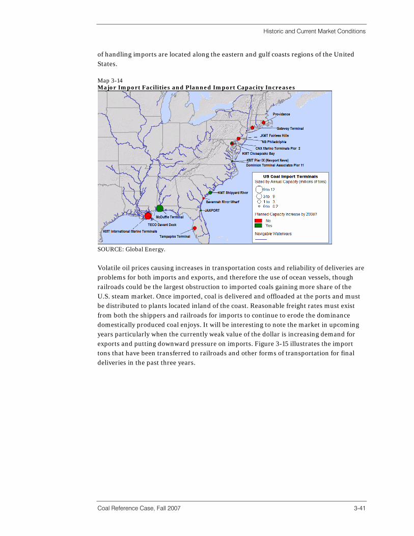
Historic and Current Market Conditions
Coal Reference Case, Fall 2007 3-41
of handling imports are located along the eastern and gulf coasts regions of the United States. Map 3-14 Major Import Facilities and Planned Import Capacity Increases
SOURCE: Global Energy.
Volatile oil prices causing increases in transportation costs and reliability of deliveries are problems for both imports and exports, and therefore the use of ocean vessels, though railroads could be the largest obstruction to imported coals gaining more share of the U.S. steam market. Once imported, coal is delivered and offloaded at the ports and must be distributed to plants located inland of the coast. Reasonable freight rates must exist from both the shippers and railroads for imports to continue to erode the dominance domestically produced coal enjoys. It will be interesting to note the market in upcoming years particularly when the currently weak value of the dollar is increasing demand for exports and putting downward pressure on imports. Figure 3-15 illustrates the import tons that have been transferred to railroads and other forms of transportation for final deliveries in the past three years.
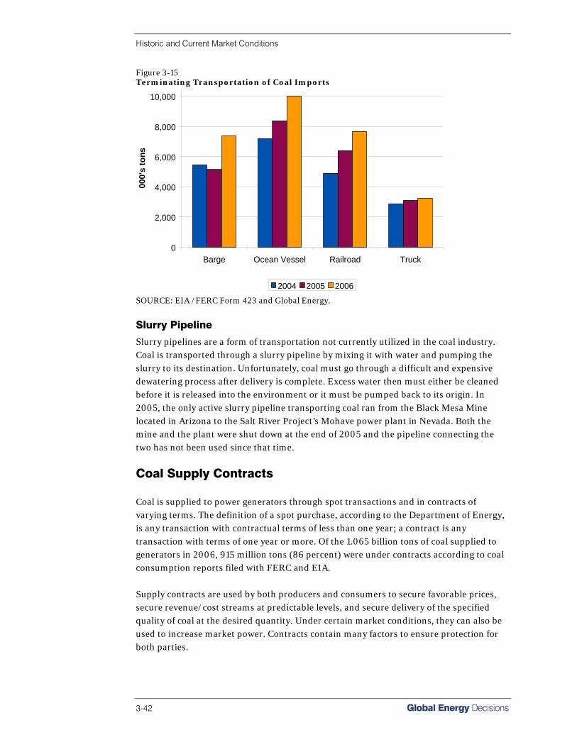
Historic and Current Market Conditions
3-42
Figure 3-15 Terminating Transportation of Coal Imports
0
2,000
4,000
6,000
8,000
10,000
Barge Ocean Vessel Railroad Truck
000'
s to
ns
2004 2005 2006 SOURCE: EIA /FERC Form 423 and Global Energy.
Slurry Pipeline
Slurry pipelines are a form of transportation not currently utilized in the coal industry. Coal is transported through a slurry pipeline by mixing it with water and pumping the slurry to its destination. Unfortunately, coal must go through a difficult and expensive dewatering process after delivery is complete. Excess water then must either be cleaned before it is released into the environment or it must be pumped back to its origin. In 2005, the only active slurry pipeline transporting coal ran from the Black Mesa Mine located in Arizona to the Salt River Project’s Mohave power plant in Nevada. Both the mine and the plant were shut down at the end of 2005 and the pipeline connecting the two has not been used since that time.
Coal Supply Contracts Coal is supplied to power generators through spot transactions and in contracts of varying terms. The definition of a spot purchase, according to the Department of Energy, is any transaction with contractual terms of less than one year; a contract is any transaction with terms of one year or more. Of the 1.065 billion tons of coal supplied to generators in 2006, 915 million tons (86 percent) were under contracts according to coal consumption reports filed with FERC and EIA. Supply contracts are used by both producers and consumers to secure favorable prices, secure revenue/cost streams at predictable levels, and secure delivery of the specified quality of coal at the desired quantity. Under certain market conditions, they can also be used to increase market power. Contracts contain many factors to ensure protection for both parties.

Historic and Current Market Conditions
Coal Reference Case, Fall 2007 3-43
A term limit specifies the amount of time over which the coal deliveries will take place. In the past, contracts have had longer time frames. Today, most contracts range from three to five years but occasionally are signed for much longer, depending on the motivations of both the buyer and seller. In addition to shorter periods, most current contracts have openings for price adjustments every one to three years. At price re-openings, new prices are negotiated based on the current market but the parties may also choose to end the contract if an agreement cannot be reached. Price adjustments can be based on many things such as a coal price index or operating costs. Most contracts specify the tons to be delivered per year. A contract can typically range from as little as 30,000 tons/year to as much as 10 million tons/year depending on the plant’s need. Usually, slight adjustments are allowed if the plant’s needs fluctuate. Mines may also push back the delivery dates if production problems arise. Payment is usually due 15 to 30 days after shipping. A contract gives the consumer power to specify coal quality and ensures consistent coal quality. It is usually specified by an average, while individual shipments are allowed to vary within set limits. The contract specifies where the coal quality is sampled, at the mine load-out or at the plant. Price adjustments may be made in accordance with a single shipment’s specifications. If the coal varies slightly from the agreed upon average, the paid price will be adjusted accordingly. The most common specifications are heat, ash, and sulfur content. Sulfur price adjustments vary with SO2 allowance trading prices in the case of many contracts. The contract may specify the specific mine and coal seam or it may be broadly set to accept any coal that meets the quality specifications. Most contracts have specified mines with ability to switch if problems arise. Over the counter contracts only specify a barge or rail loading terminal in the coal region. Transportation arrangements and costs are usually found in a separate but concurrent contract between the coal consumer and a transportation provider. Two other clauses commonly seen in contracts are “government imposition” price adjustments and force majeure delivery adjustments. Government impositions can come in the form of regulations that cause a much higher costs for the coal producer or consumer. Force majeure adjustments occur when there is unexpected weather or equipment failure that can delay shipping/receiving. Many other clauses may be found for adjusting prices and deliveries within contracts. The coal market and the way its contracts are written and handled are constantly evolving. Contracts of today are much more sophisticated than in decades past. Most of the norms that are mentioned here are a result of trial-and-error on all sides of a changing market. Figure 3-16 shows Global Energy’s current aggregated data for coal contracts broken out by their quantity and coal origin basin. Only known contracts are shown and obviously many more will be signed and/or reported throughout 2007 and into the future. The drop
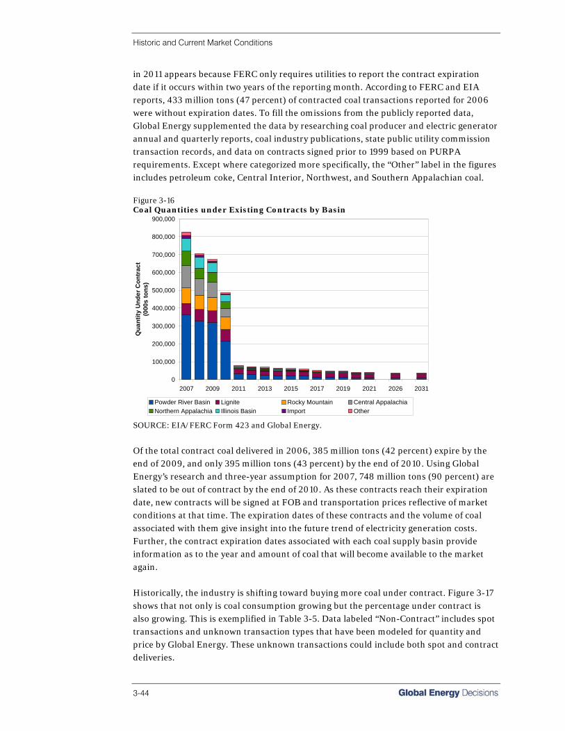
Historic and Current Market Conditions
3-44
in 2011 appears because FERC only requires utilities to report the contract expiration date if it occurs within two years of the reporting month. According to FERC and EIA reports, 433 million tons (47 percent) of contracted coal transactions reported for 2006 were without expiration dates. To fill the omissions from the publicly reported data, Global Energy supplemented the data by researching coal producer and electric generator annual and quarterly reports, coal industry publications, state public utility commission transaction records, and data on contracts signed prior to 1999 based on PURPA requirements. Except where categorized more specifically, the “Other” label in the figures includes petroleum coke, Central Interior, Northwest, and Southern Appalachian coal. Figure 3-16 Coal Quantities under Existing Contracts by Basin
0
100,000
200,000
300,000
400,000
500,000
600,000
700,000
800,000
900,000
2007 2009 2011 2013 2015 2017 2019 2021 2026 2031
Qua
ntity
Und
er C
ontr
act
(000
s to
ns)
Powder River Basin Lignite Rocky Mountain Central AppalachiaNorthern Appalachia Illinois Basin Import Other
SOURCE: EIA/FERC Form 423 and Global Energy.
Of the total contract coal delivered in 2006, 385 million tons (42 percent) expire by the end of 2009, and only 395 million tons (43 percent) by the end of 2010. Using Global Energy’s research and three-year assumption for 2007, 748 million tons (90 percent) are slated to be out of contract by the end of 2010. As these contracts reach their expiration date, new contracts will be signed at FOB and transportation prices reflective of market conditions at that time. The expiration dates of these contracts and the volume of coal associated with them give insight into the future trend of electricity generation costs. Further, the contract expiration dates associated with each coal supply basin provide information as to the year and amount of coal that will become available to the market again. Historically, the industry is shifting toward buying more coal under contract. Figure 3-17 shows that not only is coal consumption growing but the percentage under contract is also growing. This is exemplified in Table 3-5. Data labeled “Non-Contract” includes spot transactions and unknown transaction types that have been modeled for quantity and price by Global Energy. These unknown transactions could include both spot and contract deliveries.
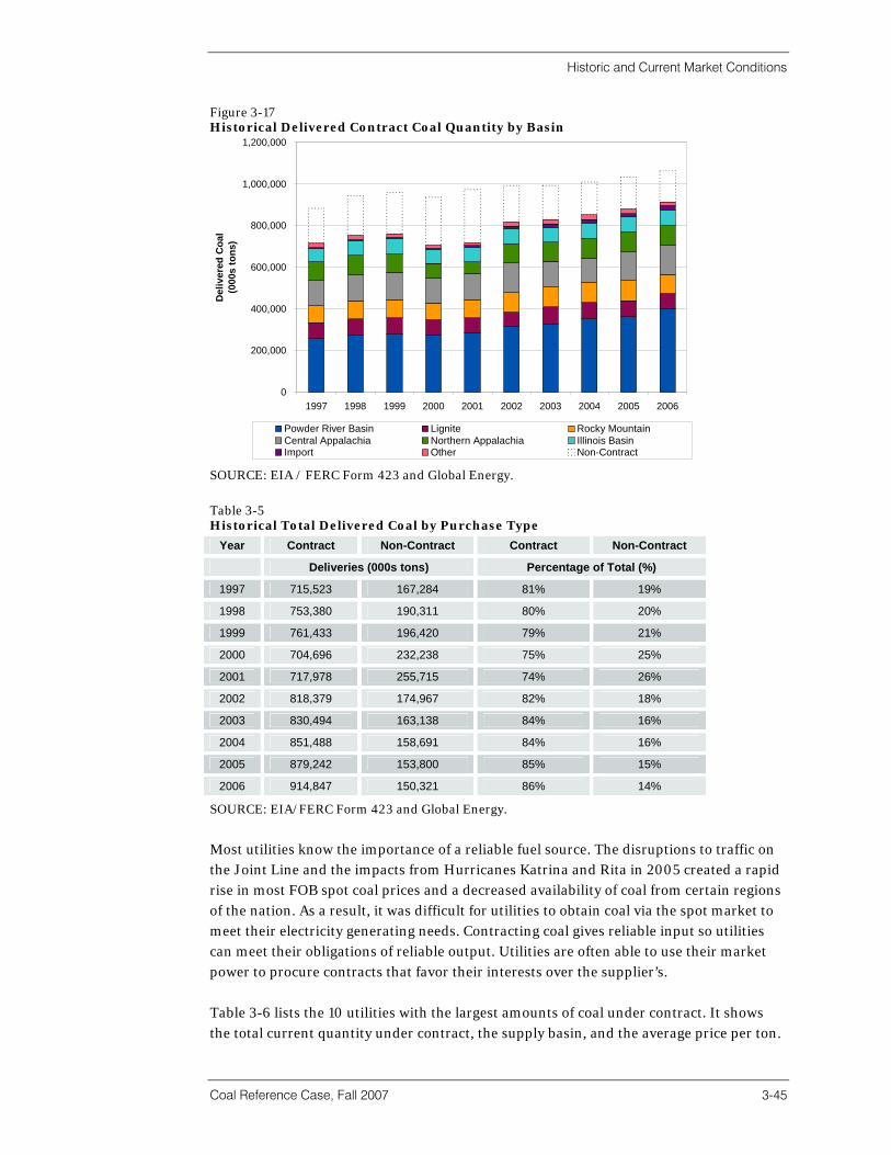
Historic and Current Market Conditions
Coal Reference Case, Fall 2007 3-45
Figure 3-17 Historical Delivered Contract Coal Quantity by Basin
0
200,000
400,000
600,000
800,000
1,000,000
1,200,000
1997 1998 1999 2000 2001 2002 2003 2004 2005 2006
Del
iver
ed C
oal
(000
s to
ns)
Powder River Basin Lignite Rocky MountainCentral Appalachia Northern Appalachia Illinois BasinImport Other Non-Contract
SOURCE: EIA / FERC Form 423 and Global Energy.
Table 3-5 Historical Total Delivered Coal by Purchase Type
Year Contract Non-Contract Contract Non-Contract
Deliveries (000s tons) Percentage of Total (%)
1997 715,523 167,284 81% 19%
1998 753,380 190,311 80% 20%
1999 761,433 196,420 79% 21%
2000 704,696 232,238 75% 25%
2001 717,978 255,715 74% 26%
2002 818,379 174,967 82% 18%
2003 830,494 163,138 84% 16%
2004 851,488 158,691 84% 16%
2005 879,242 153,800 85% 15%
2006 914,847 150,321 86% 14%
SOURCE: EIA/FERC Form 423 and Global Energy.
Most utilities know the importance of a reliable fuel source. The disruptions to traffic on the Joint Line and the impacts from Hurricanes Katrina and Rita in 2005 created a rapid rise in most FOB spot coal prices and a decreased availability of coal from certain regions of the nation. As a result, it was difficult for utilities to obtain coal via the spot market to meet their electricity generating needs. Contracting coal gives reliable input so utilities can meet their obligations of reliable output. Utilities are often able to use their market power to procure contracts that favor their interests over the supplier’s. Table 3-6 lists the 10 utilities with the largest amounts of coal under contract. It shows the total current quantity under contract, the supply basin, and the average price per ton.
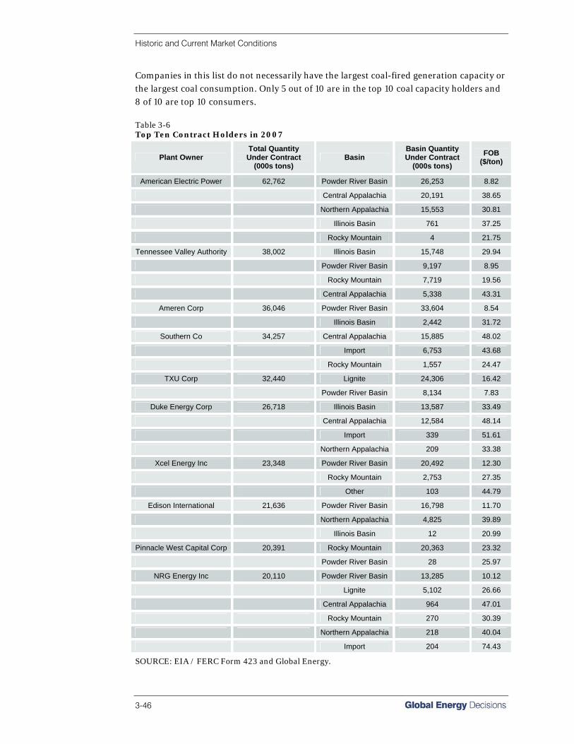
Historic and Current Market Conditions
3-46
Companies in this list do not necessarily have the largest coal-fired generation capacity or the largest coal consumption. Only 5 out of 10 are in the top 10 coal capacity holders and 8 of 10 are top 10 consumers. Table 3-6 Top Ten Contract Holders in 2007
Plant Owner Total Quantity
Under Contract (000s tons)
Basin Basin Quantity Under Contract
(000s tons)
FOB ($/ton)
American Electric Power 62,762 Powder River Basin 26,253 8.82
Central Appalachia 20,191 38.65
Northern Appalachia 15,553 30.81
Illinois Basin 761 37.25
Rocky Mountain 4 21.75
Tennessee Valley Authority 38,002 Illinois Basin 15,748 29.94
Powder River Basin 9,197 8.95
Rocky Mountain 7,719 19.56
Central Appalachia 5,338 43.31
Ameren Corp 36,046 Powder River Basin 33,604 8.54
Illinois Basin 2,442 31.72
Southern Co 34,257 Central Appalachia 15,885 48.02
Import 6,753 43.68
Rocky Mountain 1,557 24.47
TXU Corp 32,440 Lignite 24,306 16.42
Powder River Basin 8,134 7.83
Duke Energy Corp 26,718 Illinois Basin 13,587 33.49
Central Appalachia 12,584 48.14
Import 339 51.61
Northern Appalachia 209 33.38
Xcel Energy Inc 23,348 Powder River Basin 20,492 12.30
Rocky Mountain 2,753 27.35
Other 103 44.79
Edison International 21,636 Powder River Basin 16,798 11.70
Northern Appalachia 4,825 39.89
Illinois Basin 12 20.99
Pinnacle West Capital Corp 20,391 Rocky Mountain 20,363 23.32
Powder River Basin 28 25.97
NRG Energy Inc 20,110 Powder River Basin 13,285 10.12
Lignite 5,102 26.66
Central Appalachia 964 47.01
Rocky Mountain 270 30.39
Northern Appalachia 218 40.04
Import 204 74.43
SOURCE: EIA / FERC Form 423 and Global Energy.
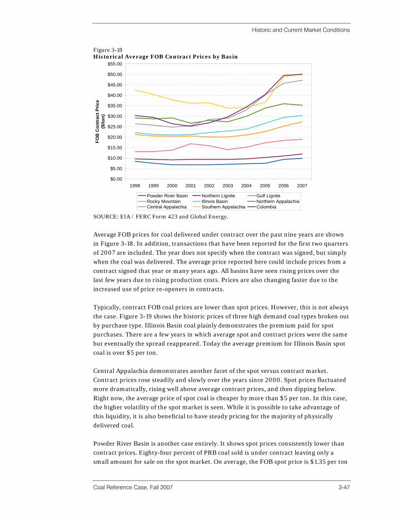
Historic and Current Market Conditions
Coal Reference Case, Fall 2007 3-47
Figure 3-18 Historical Average FOB Contract Prices by Basin
$0.00
$5.00
$10.00
$15.00
$20.00
$25.00
$30.00
$35.00
$40.00
$45.00
$50.00
$55.00
1998 1999 2000 2001 2002 2003 2004 2005 2006 2007
FOB
Con
trac
t Pric
e ($
/ton)
Powder River Basin Northern Lignite Gulf LigniteRocky Mountain Illinois Basin Northern AppalachiaCentral Appalachia Southern Appalachia Colombia
SOURCE: EIA / FERC Form 423 and Global Energy.
Average FOB prices for coal delivered under contract over the past nine years are shown in Figure 3-18. In addition, transactions that have been reported for the first two quarters of 2007 are included. The year does not specify when the contract was signed, but simply when the coal was delivered. The average price reported here could include prices from a contract signed that year or many years ago. All basins have seen rising prices over the last few years due to rising production costs. Prices are also changing faster due to the increased use of price re-openers in contracts. Typically, contract FOB coal prices are lower than spot prices. However, this is not always the case. Figure 3-19 shows the historic prices of three high demand coal types broken out by purchase type. Illinois Basin coal plainly demonstrates the premium paid for spot purchases. There are a few years in which average spot and contract prices were the same but eventually the spread reappeared. Today the average premium for Illinois Basin spot coal is over $5 per ton. Central Appalachia demonstrates another facet of the spot versus contract market. Contract prices rose steadily and slowly over the years since 2000. Spot prices fluctuated more dramatically, rising well above average contract prices, and then dipping below. Right now, the average price of spot coal is cheaper by more than $5 per ton. In this case, the higher volatility of the spot market is seen. While it is possible to take advantage of this liquidity, it is also beneficial to have steady pricing for the majority of physically delivered coal. Powder River Basin is another case entirely. It shows spot prices consistently lower than contract prices. Eighty-four percent of PRB coal sold is under contract leaving only a small amount for sale on the spot market. On average, the FOB spot price is $1.35 per ton
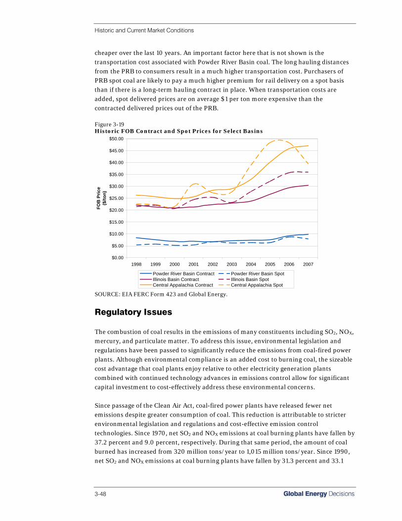
Historic and Current Market Conditions
3-48
cheaper over the last 10 years. An important factor here that is not shown is the transportation cost associated with Powder River Basin coal. The long hauling distances from the PRB to consumers result in a much higher transportation cost. Purchasers of PRB spot coal are likely to pay a much higher premium for rail delivery on a spot basis than if there is a long-term hauling contract in place. When transportation costs are added, spot delivered prices are on average $1 per ton more expensive than the contracted delivered prices out of the PRB. Figure 3-19 Historic FOB Contract and Spot Prices for Select Basins
$0.00
$5.00
$10.00
$15.00
$20.00
$25.00
$30.00
$35.00
$40.00
$45.00
$50.00
1998 1999 2000 2001 2002 2003 2004 2005 2006 2007
FOB
Pric
e($
/ton)
Powder River Basin Contract Powder River Basin SpotIllinois Basin Contract Illinois Basin SpotCentral Appalachia Contract Central Appalachia Spot
SOURCE: EIA FERC Form 423 and Global Energy.
Regulatory Issues The combustion of coal results in the emissions of many constituents including SO2, NOX, mercury, and particulate matter. To address this issue, environmental legislation and regulations have been passed to significantly reduce the emissions from coal-fired power plants. Although environmental compliance is an added cost to burning coal, the sizeable cost advantage that coal plants enjoy relative to other electricity generation plants combined with continued technology advances in emissions control allow for significant capital investment to cost-effectively address these environmental concerns. Since passage of the Clean Air Act, coal-fired power plants have released fewer net emissions despite greater consumption of coal. This reduction is attributable to stricter environmental legislation and regulations and cost-effective emission control technologies. Since 1970, net SO2 and NOX emissions at coal burning plants have fallen by 37.2 percent and 9.0 percent, respectively. During that same period, the amount of coal burned has increased from 320 million tons/year to 1,015 million tons/year. Since 1990, net SO2 and NOX emissions at coal burning plants have fallen by 31.3 percent and 33.1

Historic and Current Market Conditions
Coal Reference Case, Fall 2007 3-49
percent, respectively, while the amount of coal burned has increased from 783 million tons/year to 1,015 million tons/year. The major air emissions regulations that affect coal-fired generation include the Clean Air Act (CAA) in 1963 and the updated amendments in 1966, 1970, 1977, 1990, and 1997 and the 2005 Clean Air Mercury Rule and Clean Air Interstate Rule. The implementation of each successive set of regulations has resulted in tighter pollution control requirements for coal plants. Clean Air Act 1970 The Clean Air Act (CAA) is the comprehensive federal law that regulates air emissions from stationary and mobile sources. The Clean Air Act of 1970 was an extension of the Clean Air Act of 1963 and the subsequent amendment in 1966. It was written to protect the general public from exposure to airborne contaminants that are known to be hazardous to human health. Under the CAA, the EPA sets limits on how much of a pollutant can be in the air anywhere in the United States, ensuring that all Americans have the same basic health and environmental protections. The law allows individual states to have stricter pollution controls, but states are not allowed to have weaker pollution controls than those set for the whole country. Under Sections 111 and 112 of the CAA, the EPA established the New Source Performance Standards (NSPS) and National Ambient Air Quality Standards (NAAQS). The NAAQS are shown in Table 3-7. Implementation of the NSPS set SO2, NOX, and particulate matter emissions standards for fossil fuel-fired steam generators constructed after August 17, 1971. Coal-fired steam generators constructed prior to this date were “grandfathered” and exempted from these standards. Under the NSPS emissions standard, new generators were not allowed to emit more than 1.2 pounds of SO2 for every million Btu of coal consumed; coal that contains 1.20 lbSO2/MMBtu or less is called “compliance coal.” The goal of the CAA was to set and achieve National Ambient Air Quality Standards in every state by 1975. The NAAQS are national outdoor air pollution standards established by the EPA. The Clean Air Act establishes primary and secondary categories of air quality. Primary standards are set to protect public health from harmful concentrations of NAAQS pollutants. Secondary standards are limits to protect against public welfare effects, such as damage to vegetation or farm crops. Under NAAQS, the EPA is required to set standards for six criteria pollutants: • Carbon Monoxide; • Lead; • Nitrogen Oxide; • Particulate matter; • PM10 (2.5 to 10 micrometers in size); • PM2.5 (2.5 micrometers in size or less); • Ozone; and • Sulfur Dioxide.

Historic and Current Market Conditions
3-50
Table 3-7 National Ambient Air Quality Standards
Pollutant Primary Standards Averaging Times Secondary Standards
9 ppm (10 mg/m3) 8 Hour None Carbon Monoxide
35 ppm (40 mg/m3) 1 Hour None
Lead 1.5 µg/m3 Quarterly Average Same as Primary
Nitrogen Oxide 0.053 ppm (100 µg/m3) Annual (Arithmetic Mean) Same as Primary
50 µg/m3 Annual (Arithmetic Mean) Same as Primary Particulate Matter (PM10)
150 ug/m3 24 Hour
15.0 µg/m3 Annual (Arithmetic Mean) Same as Primary Particulate Matter (PM2.5)
65 ug/m3 24 Hour
Ozone 0.08 ppm 8 Hour Same as Primary
0.03 ppm Annual (Arithmetic Mean) -
0.14 ppm 24 Hour - Sulfur Oxides
- 3 Hour 0.5 ppm (1300 ug/m3)
SOURCE: Environmental Protection Agency.
The EPA also implemented National Emissions Standards for Hazardous Air Pollutants (NESHAP) regulations to establish emissions standards for air pollutants not covered by NAAQS. Nearly 200 pollutants were identified and regulated under NESHAP guidelines. Under the regulations, no coal-fired electric generating plant greater than 25 MW is allowed to emit more than 10 tons of any listed pollutant or more than 25 tons of any combination of listed pollutants per year. The standards for a particular source category require emissions to be reduced using the Maximum Achievable Control Technology (MACT). Although the federal government gives the EPA the authority to enforce the CAA in 49 states (California is excluded), the EPA has granted the individual states the authority to regulate and enforce provisions of the CAA within their border in exchange for federal funding. The CAA recognizes that states are better at taking the lead in carrying out the Clean Air Act than the federal government because states have a better understanding of the geological, geographical, cultural, residential, and industrial characteristics of their own region and will be able to come up with a more appropriate plan for achieving compliance with the CAA provisions. States that elect to take on this responsibility must develop a state implementation plan (SIP) for those non-attainment regions within their borders that do not comply with the CAA standards. A SIP is a detailed description of the programs that a state will use to clean up polluted areas and it must be approved by the EPA. The states must involve the public, through hearings and opportunities to comment, when developing a SIP. The EPA must approve each SIP and if it is not acceptable, the EPA can take over enforcing the CAA in the state.

Historic and Current Market Conditions
Coal Reference Case, Fall 2007 3-51
The CAA also included specific provisions for citizens to bring suit against violators or government agencies to enforce environmental laws. Today most environmental laws have provisions for citizen suits and they have become a major means of ensuring compliance with environmental laws. 1977 Because many states failed to meet mandated targets set under the 1970 Clean Air Act extension, the CAA was amended in 1977. One of the most effective provisions of the 1977 CAA amendments is the New Source Review (NSR), which addresses older facilities that had been grandfathered by the original law. When the CAA extension was passed in 1970, Congress had assumed that older industrial facilities, such as power plants and refineries, would be phased out of production, so they were exempted from the legislation. However, these older plants continued to operate and emit pollution at much higher levels than new facilities that were built with modern pollution-control equipment. The resulting New Source Review requires grandfathered industrial facilities that want to make a major modification or upgrade to their facility to undergo an EPA review of their emissions and install pollution control technologies if their planned expansion will produce significantly more emissions. Older facilities that fall under the NSR can opt to offset their increased emissions by lowering them in other units they own. Under this scenario, older plants will not impinge on the lower emissions that are produced by plants that are more modern. The program has been accused by some of creating a disincentive for the replacement of grandfathered plants since its requirements impose regulatory costs only on new plants or on plants that undergo significant modifications or upgrades. Much of the controversy lies in what constitutes a significant modification or upgrade. For example, if a grandfathered plant replaces 5 percent of its grandfathered equipment every year for 20 years, it will have completely replaced its plant yet it will not be required to comply with NSR or CAA regulations. 1990 The 1990 Amendments to the Clean Air Act were intended in large part to address unresolved or poorly resolved air pollution problems such as acid rain, ground level ozone, stratospheric ozone depletion, and air toxics. Additional amendments to the Clean Air Act as it relates to coal plants include acid rain control. Regarded as an innovative approach toward curbing sulfur dioxides (SO2) and nitrogen oxides (NOX), the two main sources of acid rain, the new provisions offered companies an array of choices to meet emissions standards as economically as possible. Acid rain is formed when the sulfur in coal combines with oxygen during combustion and becomes sulfur dioxide; nitrogen that is present in the atmosphere combines with oxygen during combustion and becomes nitrogen oxide. The SO2 and NOX emissions are transformed in the atmosphere and return to the earth in rain, fog, or snow. Although acid rain components come from many sources including automobiles, trucks, and factories, coal-burning activities account for roughly 70 percent of SO2 and a little over 20

Historic and Current Market Conditions
3-52
percent of NOX released in the U.S. each year. Approximately 20 million tons of SO2 are emitted annually in the United States, mostly from the burning of fossil fuels by electric utilities. Rain from an unpolluted atmosphere has a pH close to 6.0, which is due to the dilute carbonic acid that is formed when water vapor reacts to atmospheric carbon dioxide. Acid rain has a pH of 5.6, which is mainly due to the reaction of water vapor with SO2 and NOX. A pH of 7.0 is considered neutral; less than 7.0 is acidic and above 7.0 is basic. Acid rain damages lakes, harms forests and buildings, contributes to reduced visibility, and is suspected of damaging health. Acid rain can leach aluminum from soil into groundwater, lakes, and rivers poisoning fish and aquatic life. At low concentrations, acid rain can slow the production of chlorophyll in plants and at high concentrations it forms sulfuric acid that kills the plant. Buildings and marble statues are damaged by the calcium carbonate in acid rain. The 1990 CAA resulted in a permanent 10 million ton reduction in SO2 emissions from 1980 levels, despite a 78 percent increase in coal consumption over that same period. In 1980, U.S. utilities consumed 569 million tons of coal; in 2006, U.S. utilities consumed 1.03 billion tons. To achieve this reduction, the EPA allocated emissions allowances in two phases. The first phase took effect in 1995 and required 110 power plants to reduce their SO2 emissions to 2.5 lbSO2/MMBtu times their average fuel use in 1985 through 1987. Plants that met their reduction requirements by using certain control technologies were given a two-year compliance extension. The law also gave a special allocation of 200,000 annual allowances for the first five years of Phase I to power plants in Illinois, Indiana, and Ohio. The second phase became effective in 2000 and required virtually all fossil-fuel electric power producers to reduce their SO2 emissions to the equivalent of 1.2 lbSO2/MMBtu times their average annual fuel use in 1985 through 1987. For both phases, affected plants were required to install continuous emissions monitoring systems (CEMS) to assure their compliance. The 1990 Clean Air Act uses a market-based approach to clean up air pollution as efficiently and inexpensively as possible, letting businesses make decisions on the best way to reach pollution cleanup goals. This approach gives utilities flexibility in how they can most efficiently, economically, and effectively meet their emissions requirements created under Phase I and Phase II of the CAA. The CAA gave utilities the choice of using any one or combination of the following ways to meet the standard annual emissions allowance limit: • Fuel switching or blending - using a cleaner fuel or choosing lower sulfur coal to
replace higher sulfur coal; • Obtaining additional emissions allowances; • Installing flue gas desulfurization equipment; and • Retiring units.

Historic and Current Market Conditions
Coal Reference Case, Fall 2007 3-53
Perhaps the most successful and innovative part of the CAA of 1990 is that it allows for SO2 emissions allowance trading. The EPA issues allowances to power plants covered by the acid rain program; each allowance is worth one ton of sulfur dioxide emitted to the atmosphere. Each source must have sufficient allowances to cover its annual emissions. If not, the source is penalized with a $2,000/ton excess emissions fee and a requirement to offset the excess emissions the following year. If a plant expects to emit more SO2 than it has allowances, it must get additional allowances, perhaps by buying them from another power plant that has reduced its SO2 releases below its number of allowances and therefore has allowances to sell or trade. Under the law, utilities are allowed to trade allowances within their utility and/or buy or sell allowances to and from other affected sources. Allowances can also be bought and sold by brokers, or by anyone who wants to take part in the allowances market. Allowances can also be banked for use in later years. Allowances can be traded and sold nationwide and currently trade at around $500/ton SO2 (September 2007). The acid rain program provides bonus allowances to power plants for (among other things) using renewable energy sources, increasing their utilization in the last five years, and installing qualifying clean coal technology that reduces sulfur dioxide releases or encourages energy conservation by customers so that less power needs to be produced. Nationwide, plants that emit SO2 at a rate below 1.2 lbs/MMBtu are able to increase emissions by 20 percent between a baseline year and 2000. Additional allowances are distributed to accommodate growth by units in states with a statewide emissions average below 0.8 lbs/MMBtu. The new law also includes specific requirements for reducing emissions of nitrogen oxides, based on EPA regulations issued in mid-1992 for certain boilers and 1997 for all remaining boilers. Air pollution often travels from its source in one state to another state. In many urban areas, people live in one state and work or shop in another; air pollution from cars and trucks may spread throughout the interstate area. Besides controlling emissions at the state level, the CAA provides for interstate commissions on air pollution control, which are charged with developing regional strategies for cleaning up air pollution. Another major breakthrough created by the 1990 Clean Air Act is a permit program for large sources (including coal-fired power plants) that release pollutants into the air. Air pollution is managed by a national permit system in which permits are issued by states or, when a state fails to implement the Clean Air Act satisfactorily, by the EPA. The permit includes information on which pollutants are being released, how much may be released, and what kinds of steps the source’s owner or operator is taking to reduce pollution, including plans to monitor the pollution. The permit system is especially useful for situations where a business is covered by more than one part of the law, since information about all of a source’s air pollution are now in one place.

Historic and Current Market Conditions
3-54
1997 Changes to the Clean Air Act Emissions standards for ground-level ozone (i.e., smog) and particulate matter were tightened further when the Clean Air Act was amended in 1997. Although the 1997 amendments were minor compared to previous amendments and extensions to the CAA, the legislation highlighted the fact that Congress and the EPA continue to ratchet air emissions from mobile and stationary sources downward. Clean Air Mercury Rule
Currently, about two-thirds—or 48 tons—of the 75 tons of mercury entering coal-fired generators is emitted to the atmosphere. The 27-ton reduction is the co-beneficial result of existing air pollution control devices such as scrubbers, selective catalytic reduction (SCR) systems, and particulate matter capture devices. Although mercury capture is not the purpose of these devices, mercury is reduced as a co-benefit. The Clean Air Mercury Rule impacts new and existing coal-fired electric generating plants through a market-based cap-and-trade program similar to the EPA’s highly successful Acid Rain Program. The first phase of the program will be implemented in 2010 when mercury emissions are reduced to 38 tons. This 10-ton reduction is expected to be achieved at no additional cost to utilities through the co-benefit from planned air pollution control devices. The second phase goes into action in 2018 with a final mercury emissions cap of 15 tons. Mercury emissions at this level will likely require some combination of mercury-specific control devices and consumption of coal that emits less mercury. Map 3-15 shows total mercury emissions from U.S. power plants in 1999, the latest year in which mercury data are available. Under CAMR, states are able to develop their own rules if they will result in greater statewide emissions reductions than the national plan. Table 3-8 shows which states have adopted requirements that go beyond CAMR. California, the District of Columbia, Idaho, Rhode Island, and Vermont do not have point source emitters that necessitate mercury emission controls. The remaining states that do not appear in Table 3-8 have approved the nationwide mercury rules. In Table 3-8, the values in the column for “Implementation Year(s)” indicate the year that the corresponding requirement in the “Mercury Reduction Requirement” column begins.

Historic and Current Market Conditions
Coal Reference Case, Fall 2007 3-55
Map 3-15 Coal Plant Mercury Emissions in 1999
SOURCE: EPA and Global Energy.
Table 3-8 State Mercury Emissions Rules
State Status of State Mercury Plan
Implementation Year(s) Mercury Reduction Requirement
Arizona State Plan Approved 2013 90% or 0.0083lb/GWh
Connecticut State Plan Approved 2008 90% or 0.6lb/1,000 Btu
Delaware State Plan Approved 2009/2013 80% or 1.0 lb/TBtu / 90% or 0.6 lb/TBtu
Florida State Plan In Development
Georgia State Plan Approved 2010/2012-2015 80-85%/90%
Illinois State Plan Approved 2009/2015 75%/90%
Indiana State Plan Approved 2008 90%
Maryland State Plan Approved 2010/2013 80%/90%
Massachusetts State Plan Approved 2008/2012 85%/95%
Michigan State Plan Approved 2015 90%
Minnesota State Plan Approved 2010 90% Plants >500MW
Montana State Plan Approved 2010
New Hampshire State Plan Approved 2013 80%
New Jersey State Plan Approved 2007 90%
New York State Plan Approved 2010/2015 50%/90%
North Carolina State Plan Approved 2013 64%
Oregon State Plan Approved 2012 90%
Pennsylvania State Plan Approved 2010/2015 80%/90%
Virginia State Plan Approved
Washington State Plan In Development
Wisconsin State Plan Approved 2010/2015/2018 40%/75%/80%
SOURCE: EPA and Global Energy.
Historic and Current Market Conditions
3-56
Clean Air Interstate Rule
The Clean Air Interstate Rule affects 28 eastern states and the District of Columbia. This region accounts for more than 90 percent of the SO2 and 77 percent of the NOX emissions from electric plants nationwide. Phase I for NOX begins in 2009 and 2010 for SO2. When full compliance is reached in 2015 for both plans, SO2 emissions will have dropped by more than 83 percent and NOX by nearly 81 percent since the Acid Rain Program was created under Title IV of the 1990 Clean Air Act Amendments. The EPA regulations originally required the CAIR-affected states to develop a compliance strategy by September 2006. To comply with the CAIR rules, generating companies needed to carefully weigh the costs and benefits of adding emissions controls, expanding their renewable generating portfolio, building new clean coal generating plants, switching to lower sulfur coal, or securing and banking enough emission credits to comply with the stringent EPA caps. The cost of complying with CAIR has been estimated by industry experts at between $50 and $60 billion during the next 15 years. Several heavily impacted companies are currently adding scrubbers and NOX controls or have announced their intentions to invest heavily in emissions technologies. To put the impacts of CAIR into perspective consider Ohio, the state with the largest electric plant emissions. To comply with 2015 CAIR standards, 49 of Ohio’s largest non-scrubbed units (16 GW) would need to be retrofitted with emission controls—the cost alone will range from $4 to $6 billion. Since 33 of these 49 generating units were built more than 35 years ago, decisions to retrofit will need to be carefully weighed with investment in new generation and other compliance strategies. Carbon Emissions Regulations
Two events stand out as harbingers for future carbon emissions regulation at the federal level: • In April 2007, the Supreme Court in a 5-4 ruling rebuked the Bush administration for
its relative inaction on global warming, declaring that CO2 and other greenhouse gases qualify as air pollutants under the Clear Air Act and thus can be regulated by the EPA.
• On May 14, 2007, President Bush responded by ordering federal agencies to find a way to begin regulating vehicle emission during his expiring term.
Carbon Dioxide (CO2), Methane (CH4), and Other Greenhouse Gases (GHG) Momentum continues to build towards federal regulation of GHG emissions. There is a growing (though not universal) acceptance of scientific evidence linking global warming and climate change to the increase in post-industrial GHG atmospheric concentrations. And as a result, it seems that not a day goes by that a mayor, governor, or industrial
Historic and Current Market Conditions
Coal Reference Case, Fall 2007 3-57
leader makes a headline-winning announcement about their plans to reduce GHG emissions. Many of these entities participate in the Chicago Climate Exchange (CCX). The all-voluntary membership spans most sectors of the economy from industrial to municipal. Phase 1 members committed to a 4 percent CO2 (or equivalent) reduction from baseline 1998-2001 emissions by 2006 and Phase II members have committed to an additional 2 percent reduction by 2010. The CCX began trading CO2 for compliance with these voluntary emission cuts in 2003 and cumulative CO2 trading volume reached 1 million metric tons in June of 2004. Currently, trading volume surpasses that amount monthly and hit a record 3.71 million metric tons in February of 2007. The National Center for Policy Analysis (NCPA) recently cited some compelling United Nations data supporting the relative success of these voluntary efforts. They reported that “The U.S. is doing a far better job reining in its emissions than Europe…” and cited data from 2000 to 2004, where the EU-15 emissions grew at nearly double the U.S. rate. On that same topic, some argue that the European Union Emission Trading Scheme’s (EU ETS) recent collapse indicates that mandatory cap-and-trade regulation is less effective than voluntary reduction programs such as the CCX. The EU ETS was established on January 1, 2005 and was reporting trades as high as €30 per metric ton in April 2006. By the end of February 2007, the market had dropped to €0.80-0.90. However, most agree that a number of the EU-15 countries bowed to industrial interests and did not require strict enough GHG reductions by way of issuing too many emission credits. These surplus credits far exceeded demand and effectively killed the Phase 1 market. The EU is working towards a more successful Phase II. Although this initial attempt at large scale GHG cap-and-trade regulation failed, there is growing belief that such regulation in the United States is inevitable. Simply look at the growing number of utilities including CO2 costs in their resource plans. Further, in February 2007, the Wall Street Journal reported that JPMorgan Chase will soon be announcing the “Environmental Index-Carbon Beta,” a new high-grade corporate bond index. This index is intended to offer a relative measure of energy companies’ exposure to GHG emissions regulation. It will be interesting to see if there is any market response to “carbon risk.” In addition to state-level regulations discussed below, there are at least five major GHG cap-and-trade proposals with potential impact to the electricity sector currently in Congress. Although they vary widely in scope and execution, there is significant industry support (Calpine, Entergy, Exelon, FPL, PG&E, and PSEG) for Senator Diane Feinstein’s Electric Utility Cap-and-Trade Act in particular. This support is partially due to the Act’s regulatory simplicity and transparency. Also, it strikes a good balance between the Regional Greenhouse Gas Initiative (RGGI) goals and the rather aggressive target California has set.

Historic and Current Market Conditions
3-58
Map 3-16 GHG Reduction Initiatives in North America
SOURCE: Global Energy.
Regional Greenhouse Gas Initiative (RGGI) Started in 2003, the Northeast and Mid-Atlantic RGGI expanded their membership to include 10 states (Connecticut, Delaware, Maine, Maryland, Massachusetts, New Hampshire, New Jersey, New York, Rhode Island, and Vermont) and released their revised draft model rules for a carbon cap-and-trade market in January of 2007. Although “leakage” issues have yet to be solved, the primary elements of RGGI’s model rule are: • CO2 cap-and-trade with the cap initially set at projected 2009 emissions; • Cap stays flat from 2009 to 2014 then declines by 2.5 percent per year for 2015 to
2018; • Early compliance banking has already begun; • At least 25 percent of permits (allowances) will be auctioned by each state with
proceeds going to “consumer benefits or strategic energy purposes” such as efficiency programs, consumer rebates, or other related public benefit; and
• The use of offsets (e.g., methane capture, sulfur hexafluoride capture (an extremely potent greenhouse gas used as a dielectric in the electric industry and used in the semiconductor and Magnesium industries), tree planting, and end use NG/Oil efficiency) in lieu of actual CO2 reductions.
RGGI’s model rule also includes some price trigger safety valves to mitigate emission prices and volatility. If CO2 prices are below $7/ton, participants are encouraged to support local offset markets and offsets acquired outside the RGGI states are worth only half their CO2 value (e.g., 10 tons of CO2e (CO2 equivalent) from a Texas agricultural

Historic and Current Market Conditions
Coal Reference Case, Fall 2007 3-59
methane capture project would count towards 5 tons of CO2 emission reductions). With prices between $7 and $10/ton, national offsets would be worth full value. And if prices remain above $10/ton for “an extended period of time,” generators can purchase offsets in the international market. These price triggers also allow generators to cover an increasing percentage of emission reductions with the use of offsets. California AB32, Western Area Governors It began with the passage of CA AB32 (Global Warming Solutions Act of 2006). Although currently lacking in mechanistic detail, AB32 sets a cap on California’s GHG emissions to 1990 levels by the year 2020. Then in February 2007, the Western Area Governors (Arizona, California, New Mexico, Oregon, and Washington) signed the Western Regional Climate Action Initiative, a Memorandum of Understanding agreeing to develop a regional target of lower greenhouse gases and create a market-based approach to achieve that target. Although this group is a few years behind RGGI, they are on a very similar path. It is possible that the group could learn from the eastern states action and develop an RGGI-like plan in fairly short order. If there is not a federal GHG plan by around 2012, it is likely that a western version of RGGI’s cap-and-trade will be in effect. Further, it is quite possible that these two markets would converge into a single cap-and-trade market as the respective market participants have already discussed the possibility. Other States In addition to progressive action by RGGI and the West, other states are developing GHG and climate action initiatives. For example: • North Carolina formed the Climate Action Plan Advisory Group (CAPAG) in 2005 for
dealing with global climate change issues; • Illinois created the Illinois Climate Change Advisory Group in November 2006 to
“provide recommendations to the Office of the Governor regarding climate change policy.”
• Minnesota Governor Pawlenty announced his Next Generation Energy Initiative, which will result in more renewable energy, more energy conservation, and less carbon emissions for Minnesota. His plan may be one of the first to explicitly list load reduction (“reduce their retail sales by 1.5 percent annually”) as part of the plan;
• Utah has established the Governor’s Blue Ribbon Advisory Council on Climate Change;
• Colorado has established the Rocky Mountain Climate Organization; and • Montana has established the Climate Change Advisory Committee. Current Federal Activity Pressure is mounting on countries that have not ratified Kyoto. Most recently, in February 2007, Jacques Chirac of France demanded that the U.S. sign both the Kyoto Protocol and a future agreement that will take effect when Kyoto runs out in 2012 or else face a carbon import tax by the EU, the largest export market for American goods. The new Senate and House political landscape that took shape in January 2007 increase the odds for a cap-and-trade CO2 legislation, if not an outright ratification Kyoto, paving
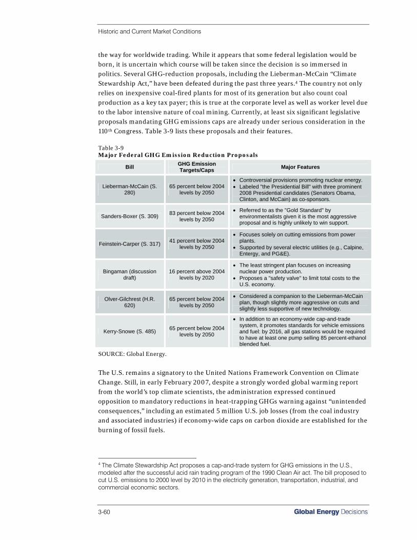
Historic and Current Market Conditions
3-60
the way for worldwide trading. While it appears that some federal legislation would be born, it is uncertain which course will be taken since the decision is so immersed in politics. Several GHG-reduction proposals, including the Lieberman-McCain “Climate Stewardship Act,” have been defeated during the past three years.4 The country not only relies on inexpensive coal-fired plants for most of its generation but also count coal production as a key tax payer; this is true at the corporate level as well as worker level due to the labor intensive nature of coal mining. Currently, at least six significant legislative proposals mandating GHG emissions caps are already under serious consideration in the 110th Congress. Table 3-9 lists these proposals and their features. Table 3-9 Major Federal GHG Emission Reduction Proposals
Bill GHG Emission Targets/Caps Major Features
Lieberman-McCain (S. 280)
65 percent below 2004 levels by 2050
• Controversial provisions promoting nuclear energy. • Labeled "the Presidential Bill" with three prominent
2008 Presidential candidates (Senators Obama, Clinton, and McCain) as co-sponsors.
Sanders-Boxer (S. 309) 83 percent below 2004 levels by 2050
• Referred to as the "Gold Standard" by environmentalists given it is the most aggressive proposal and is highly unlikely to win support.
Feinstein-Carper (S. 317) 41 percent below 2004 levels by 2050
• Focuses solely on cutting emissions from power plants.
• Supported by several electric utilities (e.g., Calpine, Entergy, and PG&E).
Bingaman (discussion draft)
16 percent above 2004 levels by 2020
• The least stringent plan focuses on increasing nuclear power production.
• Proposes a "safety valve" to limit total costs to the U.S. economy.
Olver-Gilchrest (H.R. 620)
65 percent below 2004 levels by 2050
• Considered a companion to the Lieberman-McCain plan, though slightly more aggressive on cuts and slightly less supportive of new technology.
Kerry-Snowe (S. 485) 65 percent below 2004 levels by 2050
• In addition to an economy-wide cap-and-trade system, it promotes standards for vehicle emissions and fuel: by 2016, all gas stations would be required to have at least one pump selling 85 percent-ethanol blended fuel.
SOURCE: Global Energy.
The U.S. remains a signatory to the United Nations Framework Convention on Climate Change. Still, in early February 2007, despite a strongly worded global warming report from the world’s top climate scientists, the administration expressed continued opposition to mandatory reductions in heat-trapping GHGs warning against “unintended consequences,” including an estimated 5 million U.S. job losses (from the coal industry and associated industries) if economy-wide caps on carbon dioxide are established for the burning of fossil fuels.
4 The Climate Stewardship Act proposes a cap-and-trade system for GHG emissions in the U.S., modeled after the successful acid rain trading program of the 1990 Clean Air act. The bill proposed to cut U.S. emissions to 2000 level by 2010 in the electricity generation, transportation, industrial, and commercial economic sectors.

Historic and Current Market Conditions
Coal Reference Case, Fall 2007 3-61
The Anticipated National Greenhouse Gas Cap-and-Trade Clearly, national GHG regulation has a great potential to reshape the electricity generating fuel mix as well as electricity and fuel prices. Therefore, while the eventual form and timing of such regulation remains highly uncertain, Global Energy has included a national CO2 cost beginning with its Spring 2007 Reference Case forecast for the North American markets. We assume that CO2 costs will take effect in 2012. Our assumption is that the cap-and-trade of RGGI’s model rule, the western states’ emerging cap-and-trade, as well as the existing SO2 and NOX trading programs will provide a framework for a national GHG cap-and-trade program. Conceptually, we expect this to include: • Cap-and-trade beginning in 2012; • Banking for early compliance; • Transparent regulations, with a clearly defined future; • The inclusion of all six major GHG gases (CO2, CH4, NOX, HFCs, PFCs and SF6); • Flexible use of offsets to mitigate allowance price and volatility, likely similar to
RGGI’s offsets and price triggers; • Mechanisms to encourage renewable energy and efficiency; • An initial cap based on a recent or near future year’s emissions (e.g., 2009 for RGGI,
2006 for Feinstein’s Cap-and-Trade Act); • A gradually declining cap in the medium term (10 to 20 years); and • A likely more aggressive long-term goals (e.g., 80 percent reduction by 2050), that
will not be modeled. Because GHG emission regulation is such new territory, Global Energy does not have enough known economic inputs to adequately model a forecast of CO2 emissions pricing. Instead, we have taken a more qualitative approach to developing this forecast. Our emissions team focused primarily on research conducted by the RGGI states (both before and after the formation of RGGI), the EPA, and the DOE NETL as well as numerous industry and academic studies. Global Energy expects the combination of a fairly easy initial target (e.g., RGGI’s 2009 base year), early compliance banking, and “low-hanging fruit” such as methane capture to contribute to a CO2 price of $2/ton in 2012 which will escalate by $1/year. Note that this is in 2007 dollars and measured in tons, not metric tons. Beyond 2012, we expect a declining cap and price trigger mechanism to contribute to a medium-term price cap of $15/ton, reached in 2025 and held at that level thereafter. To be clear, this is research-influenced, but subject to much uncertainty. We believe this is a reasonable approach to balancing public concern and the real markets being developed on both the East and West Coasts with the high degree of uncertainty present. Also uncertain is Canada’s pursuit of GHG emission regulations. However, they are a Kyoto ratifying country with a strong public willingness to make sacrifices for the environment. We expect that Canada will not accept being “out-greened” by the United States and will likely join forces or form a similar program. As such, Global Energy is applying our CO2 emissions pricing to all North American generators.

Historic and Current Market Conditions
3-62
This expected GHG regulation has influenced some assumptions in Global Energy’s 2007 electricity price forecast. In summary, we expect increased interest in nuclear development, IGCC development with other coal development using super-critical designs, and load growth beyond 2015 to be ~20 percent below the 2012-2015 growth rates. The allocation of the cost of CO2 emissions regulation among the power generator, the utility, the consumer, and the coal producer (as a lower FOB mine price) is uncertain, but will likely be considered in negotiations of long-term power supply and coal supply agreements. Regulators will be concerned if a disproportionate share of these costs is passed on to consumers. The cost allocation will depend upon the type of combustion technology involved, as certain types of coal provide better combustion and operational efficiencies for certain clean-coal technologies than do other coal types. While rules governing the burning of coal dominate the headlines, there are also rules that govern the production of coal, including the “Mountain Top Removal” ruling and the Surface Mine Control and Reclamation Act of 1977. Mountain Top Removal Mining
Underground mining has historically dominated as the favored mining method in Central Appalachia. This situation has changed over the last few decades as fewer and fewer remaining reserves are economically recoverable by underground mining. Figure 3-20 shows historic production and productivity at Central Appalachian mines on an annual basis by the operation type (either surface or underground) as reported on MSHA form 7000-2. This chart has several important attributes: • The trend in underground production is declining; • The trend in surface production is increasing, though not at a rate sufficient to
prevent the overall decline in basin production; and • Since 2004, the productivity decline in surface operations has stabilized while the
productivity decline in underground operations has continued unabated. These data taken together indicate that it is likely that within the next few years the dominant method of coal production in Central Appalachia will be surface mining barring a significant impediment to it.

Historic and Current Market Conditions
Coal Reference Case, Fall 2007 3-63
Figure 3-20 Production and Productivity at Surface & Underground Mines in Central Appalachia; 1990-20075
80,000
100,000
120,000
140,000
160,000
180,000
200,000
1990 1992 1994 1996 1998 2000 2002 2004 2006
Year
Prod
uctio
n(00
0's
tons
)
0
1
2
3
4
5
6
Prod
uctiv
ity (t
ons/
min
er h
our)
Surface Production Underground Production Surface Productivity Underground Productivity
SOURCE: MSHA and Global Energy.
Surface mining in Appalachia is generally referred to as mountain top mining (MTM) with mountain top removal mining (MTR) being the most contested and controversial method, along with often being the most efficient. The differentiating factor is that with MTR the overburden from the entire mountain top or ridgeline is moved so that the entire coal seam can be removed. Other MTM operations may only mine a portion of a seam requiring that only some fraction of the mountain top overburden is removed. Highwall or auger mining uses large drilling and conveying equipment, similar to a continuous miner, to extract coal from seams which have been exposed by previous surface mining. Mountain top removal has caused controversy and litigation since the late 1990s, continuing up to the present. Mountain top removal is reportedly involved in a third of West Virginia’s coal production (USA Today, April 14) which would put the total at more than half of all surface mining in the state. Ongoing Litigation On March 23, 2007, Judge Robert C. Chambers of the U.S. District Court for the Southern District of West Virginia blocked four mining permits for “valley fills” issued by the U.S. Army Corps of Engineers.6 A valley fills is created by mountain top removal mining when the overburden is placed in valleys or hollows adjoining the mining operation. The case was dismissed on the grounds of “alarming cumulative stream loss” and other environmental features protected under the Clean Water Act. The plaintiffs in the case claim that the U.S. Army Corps of engineers is breaking the law by issuing permits for the valley fills which accompany mountain top removal mining.
5 2007 production and productivity estimated from 2007 Q1 data. 6 Ohio Valley Environmental Coalition, et al. v. U.S. Army Corps of Engineers, et al., Civil Action No. 3:05-0784, U.S. District Court for the Southern District of West Virginia, Huntington Division.
Historic and Current Market Conditions
3-64
This is the fourth instance in which a lower court decision has challenged Mountain Top Removal. However, in the previous three cases, such rulings have been overturned by the 4th U.S. Circuit Court of Appeals in Richmond, Virginia. • In 1998, the lower court ruled that the Corps of Engineers could not allow mining
debris to be placed in streams. The 4th Circuit Court of Appeals ruled that the lawsuit should have been filed in state court;
• In 2001, the court ruled that the type of debris from coal mining was not allowed under the definition of “fill” allowed in the waterways. The Bush administration adjusted the fill regulations to cover mining debris. Environmental groups claim that this action can only be performed legally by Congress;
• In 2004, the court ruled against general (streamlined) permits and required stricter specific permits, but the Court of Appeals sent the case back to trial court; and
• In 2007, in addition to the above mentioned block age of permits by the District Court, on June 19th the plaintiffs were granted leave to challenge four more permits within the context of this ongoing case.
The most recent action involves a proposed rule change by the Office of Surface Mining (OSM) involving the 100-foot Stream Buffer Zone Rule. The OSM released a draft environmental impact statement on August 24, 2007. The OSM has said that the proposed rule change is intended to clarify existing rules on the disposal of excess spoil form coal mines by requiring mine operators to protect the environment “to the extent possible” using the “best technology currently available.” The operator must demonstrate how the standard will be met before a permit is issued and continue to demonstrate compliance throughout a project’s life. Environmentalists have reacted negatively to the primary proposal, vowing legal action if it is approved as is. Several alternative rule changes are included in the draft environmental statement. The issue of “burying streams” is not going away anytime in the foreseeable future, and can be expected to be pursued aggressively by both sides of the issue. Though past rulings have been overturned, they may have the effect of curtailing mountain top coal mining as a result of uncertainty about future litigation against valley fill practices. To date, the U.S. Supreme Court has refused to hear an appeal. Central Appalachia is in the midst of an overall decline in productivity but surface mining has been less affected by the decline since 2004 as evidenced by the increasing ratio of surface productivity to underground productivity. This is the opposite of what we would expect to find if this litigation was having a large impact on surface mining productivity in Central Appalachia. However, the effects of the most recent decisions by the District Court for the Southern District of West Virginia have yet to be reflected in the data. The Surface Mine Control and Reclamation Act
The Surface Mine Control and Reclamation Act of 1977 (SMCRA) established a program for regulating surface coal mining and reclamation activities on state and federal lands, including a requirement that adverse impacts on fish, wildlife, and related environmental values be minimized. The Act creates an Abandoned Mine Reclamation Fund for use in reclaiming and restoring land and water resources adversely affected by coal mining

Historic and Current Market Conditions
Coal Reference Case, Fall 2007 3-65
practices. To fund abandoned mine reclamation activity, the legislation originally authorized a tax of 35¢ per ton on surface mined coal, 15¢ per ton on underground mined coal, and 10¢ per ton on lignite. The fee had been reauthorized for short periods several times. In 2006, the SMCRA Amendments Act was signed that extended the collection of fees to 2021. The following fee reduction structure was included in this legislation. For the period from September 30, 2007 through FY 2012 A 10 percent reduction: • Surface mine fee - 31.5¢/ton; • Underground mine fee - 13.5¢/ton; and • Lignite mine fee - 9¢/ton For the period from FY 2013 through FY 2021 a 20 percent cumulative reduction: • Surface mine fee - 28¢/ton; • Underground mine fee - 12¢/ton; and • Lignite mine fee - 8¢/ton. This fee structure is represented in the CQMM input dataset. The Mine Safety and Health Administration History of Mine Safety Regulation Regulation of coal mine safety has been evolving—along with regulation in many other parts of the economy—since the late nineteenth century. The first 60 years of coal mine safety regulation was generally weak since it was not until the Federal Coal Mine Safety Act of 1952 that any underground mines were subject to inspection. At this time, the Bureau of Mines (under the Department of the Interior) was charged with both mine industry development and regulation and had only limited powers of enforcement. This is the first point at which inspections could lead to any kind of sanction against violators. The Federal Coal Mine Health and Safety Act of 1969 extended the regulatory program to include most of the fundamental components that exist in today’s Mine Safety and Health Administration (MSHA). These components include regular inspections of all mines, surface and underground, monetary penalties for all violations, criminal penalties for willful violations, stronger safety standards, and health standards were introduced for the first time. This legislation provided compensation for miners who were permanently disabled by “black lung” disease. The Coal Act of 1969 was a substantial step forward for mine safety and health standardization but since regulation was still under the auspices of the Bureau of Mines a fairly good potential existed for problems with conflicts of interest. In 1973, the Secretary of the Interior created the Mining Enforcement and Safety Administration as a separate entity from the Bureau of Mines to address any potential or perceived conflicts of interest. The Mine Safety and Health Act of 1977 The current regulatory incarnation for mine safety is the Mine Safety and Health Administration (MSHA) which was created by the Federal Mine Safety and Health Act of
Historic and Current Market Conditions
3-66
1977 (Mine Act). The Mine Act moved mine regulatory responsibility to the Department of Labor. It further expanded and strengthened the rights of miners and enhanced protection for miners from retaliatory actions by their employers. Safety standards regulated by MSHA include nearly every aspect of mining operations from roof support and ventilation to fire protection and communications. The Act also created the Federal Mine Safety and Health Review Commission so that MSHA’s enforcement actions could be reviewed in an independent fashion. MINER Act of 2006 Following the deadliest year in the coal mining industry in over a decade, including the Sago mine explosion which killed 12 miners, Congress passed the Mine Improvement and New Emergency Response Act of 2006 (MINER). This measure was designed as “the most sweeping overhaul of federal mine safety law in nearly three decades” (White House Press Release, 6/15/06), subsequent to the Mine Safety and Health Act of 1977. The MINER Act has the following provisions which will affect the delivered cost of coal: • Each underground coal mine to develop and continuously update a written
emergency response plan which covers: communications, a system for locating trapped miners, provision of self-contained self rescue breathing devices, fire resistant lifelines, training and local coordination between operators, rescue teams, and local emergency response personnel;
• Each underground coal mine to make available two experienced rescue teams capable of a one-hour response time, mines can share rescue teams, but the requirements for training and availability are extensive;
• Wireless two-way communications and electronic tracking systems within three years;
• The pre MINER Act requirement for mine seal pressure rating was 20 psi; the MINER Act requires that seals with inert atmosphere behind them must withstand 50 psi, seals with non-inert atmosphere behind them must withstand 120 psi;
• Increased penalties for willful violations, increased minimum fines for all violations, and gives MSHA the authority to seek injunctions to close mines whose operators failed to pay fines and penalties; and
• Establishes the Office of Mine Safety and Health within the Occupational Safety and Health Administration.
The MINER Act affects underground mining almost exclusively. Global Energy estimates that these recent new safety regulations for underground mines will add up to $8 per ton to coal mining costs for the most adversely impacted mines.
Other Issues Industry Consolidation through Merger and Acquisition (M&A)
Consolidation through mergers and acquisitions is a common trend across industries and the coal industry is no stranger to this phenomenon. The coal industry has seen steady consolidation since the 1950s. In most industries, mergers and acquisitions are intended
Historic and Current Market Conditions
Coal Reference Case, Fall 2007 3-67
to improve investment returns by increasing economies of scale, cutting costs, organizational improvements, and improving productivity through better access to financial capital. Opportunities for pursuing these kinds of improvements are arising in the coal industry as some smaller producers find it increasingly difficult to turn a profit in today’s climate of depressed prices and increasing mining costs. While the definition of a small-scale producer might have changed over the years to include a few more tons produced and fully integrated production, processing and sales companies, generally we find only a select few small and successful operators in any given operating region. It may not be wise to think of consolidation as more of an issue now than it was prior to the price escalation we saw in 2004-2005. Often the perception is that with rising prices and high margins, a great deal of new companies and producers entered the marketplace increasing the likelihood of further consolidation down the road. There was a great deal of new money that entered the coal industry, but in many cases in the form of private equity or similar sources. Rarely was this money invested in startup coal projects, but rather was invested on large and small scales to consolidate current coal operations. These consolidations did not drastically change coal production patterns in the U.S. but provided producers with the latest way of financing their coal operations. Many of the consolidations seen in recent years had original dreams of maturing into public companies; some of these dreams were realized but many were not. Those companies that did not grow as planned could be on larger companies’ lists of possible acquisitions. Large companies do not make new acquisitions hastily, and will look at both reserve body quality of the operation(s) to be acquired as well as their fit with the already existing organization. If these characteristics are not appealing, companies will invest their capital elsewhere. This is assuming egos are not a factor, which is sometimes the case. While more consolidation in the coal industry is likely to occur soon, timing of such actions is uncertain. Companies may choose to take action in good markets while others may wait for financial stress to impact less sound companies and perhaps provide a bargain price. This possible financial strain could be a result of normal market conditions or an outside force such as labor agreements or new mine safety regulations. The required implementation of certain mine safety mechanisms such as available rescue teams with one-hour response, two-way communications and electronic tracking systems for miners, and higher seal pressure requirements will certainly boost costs. New regulations will have a more significant impact on small operators and it is likely that some small producers may have incentive to sell at attractive prices for companies looking for opportunities. Several factors influence decisions on either side (buyer or seller) of the merger and acquisition transaction. These factors are listed here and detailed below: • Union affiliation and other corporate culture compatibility issues; • Reduction of exposure and liabilities, diversification of assets; • Investment strategies of private equity;
Historic and Current Market Conditions
3-68
• Specialization of mining technology; and • Market concentration and antitrust concerns. While it is likely that a union company would purchase non-union assets, non-union companies are nearly guaranteed not to purchase operations with union affiliations. Several CEOs have recently commented that while there are opportunities for solid M&A deals, especially in Central Appalachia, there has been a distinct lack of fit between potentially acquiring CEOs and acquisition target companies. Since the coal business has been traditionally a family affair in some areas, the lack of a relative to take on responsibility for company operations might create some buying opportunities. These are likely to be cases where chemistry between executives and the acquired company’s workforce culture is a critical element in deal consummation as well as future company operations. Legacy pension and healthcare programs probably make up the biggest portion of liabilities for coal producers. Merger or acquisition of a company with smaller legacy obligations might be part of an M&A strategy. Some companies may see a need to diversify in order to reduce the impact of unforeseeable events such as adverse geologic conditions to force majeure declarations by railroads, barge operators, etc. Bigger companies are seen as having greater ability to absorb the impact of these kinds of events, if they are strategically structured. “Private equity,” one of the financial world’s recent favorite buzzwords, seems to have been eclipsed of late only by “sub-prime lending.” The coal industry has not escaped the interest and influence of private equity. Several Central Appalachian organizations have been consolidated under the direction of private equity firms including Arclight Capital Partners with Magnum Coal, Sowood Capital Management with Frasure Creek Mining, and Wexford Capital with Rhino Resource Partners. The end of the three- to six-year investment timeline between the purchase and sale of assets employed by private equity companies is approaching for many of the firms that entered the coal industry earlier this decade. Industry executives expect that this will create some buying opportunities over the next one to two years. A company that specialized in production of a certain type of coal (like low-sulfur) or utilizing a specific mining technique (e.g., CONSOL and longwall mining) might want to expand by purchasing other companies using similar techniques to match skill sets. It is also possible that an underground-heavy or -exclusive company might try to lower costs by purchasing surface operations. The size of future mergers and acquisitions could be of greater magnitude as well. As stated above the already heavily consolidated industry has left few small-scale producers on the map. This indicates the industry might see an increase in mergers of large companies. If this is the case, it will be interesting to note the reaction of the Federal Trade Commission, an organization that has not had extensive experience in the coal industry until lately. Arch Coal’s motivations were highly questioned in the West with their desire to purchase the Rochelle Mine a few years ago, though the FTC decided the

Historic and Current Market Conditions
Coal Reference Case, Fall 2007 3-69
purchase would not be a threat to healthy competition in the market. The U.S. coal markets are generally competitive when taken as a whole; however, market concentration levels within the individual coal producing basins are such that many mergers would be highly scrutinized by U.S. antitrust authorities. One market concentration metric that is widely accepted and commonly used in antirust proceedings is the Herfindahl-Hirschman Index or HHI. It is calculated by establishing the market shares of each company in a relevant market, then summing the squares of all of the market shares in that market. The result is a number between 0 and 10,000. (i.e., if a company has 100 percent of the market, the HHI will be 1002 =10,000 or a market where five companies have 20 percent each would have a HHI of 202 × 5 = 2,000). When a horizontal merger is analyzed by one of the antitrust authorities a post-merger HHI of 1,000 or more can trigger red flags and warrant further investigation. Markets are considered to have medium levels of concentration when HHI ranges from 1,000 to 1,800; over 1,800 HHI is considered highly concentrated. Mergers that would cause the HHI to exceed one of these thresholds in a relevant market would likely be fought by the antitrust authorities. Figure 3-21 Market Concentration for U.S. Coal Producers by Basin; 1990-2007
0
500
1,000
1,500
2,000
2,500
3,000
1990 1992 1994 1996 1998 2000 2002 2004 2006
Year
HH
I
All U.S. Powder River Basin Central AppalachiaIllinois Basin Northern Appalachia Rocky Mountain
SOURCE: MSHA and Global Energy.
Figure 3-21 shows Global Energy’s estimated market concentration for the U.S. as a whole and for each basin using the HHI. The merger guidelines in the relevant antitrust statute law call for market concentration to be measured in the “smallest relevant market.” Defining this market is usually the central argument in an antitrust case. The choice of delineating markets by coal basin is likely to be too small in many cases. For instance, Powder River Basin coal competes with coal from all of the other basins in one region or another, thus Powder River Basin producers would likely argue that the “smallest relevant market” from a competition standpoint would not be limited strictly to the

Historic and Current Market Conditions
3-70
Powder River Basin. Even though dividing the U.S. coal markets into producing basins might not be a completely accurate market definition, it serves to show where markets are likely to be considered concentrated by antitrust authorities and how trends in market concentration have developed since 1990. Market share in Figure 3-21 is determined based on share of total production which assumes that coal is a homogeneous product which it most certainly is not, but for the purposes of this analysis, this assumption provides a sufficient level of detail. Figure 3-21 shows that the level of market concentration in all of the coal producing basins is medium to high with the exception of Central Appalachia. Antitrust authorities are likely to closely examine mergers between major operators and junior operators within the same basin except in the case of Central Appalachia. Proposed mergers or acquisitions between Central Appalachian coal operations would likely be lightly scrutinized by antitrust authorities with the exception of a Massey Energy acquisition. Because of Massey Energy’s market dominance in Central Appalachia, authorities will likely examine any acquisition closely. The coal industry as a whole is a competitive market with low levels of concentration, as Figure 3-21 shows. This indicates that consolidation of companies across basins is quite possible and would not be likely to draw uncomfortably close examination from antitrust authorities. The last point to note is that the general trend in market concentration since the late 1990s has been down, especially in Central Appalachia. This lends some quantitative support to the notion expressed by many industry executives that Central Appalachia is ripe for consolidation. Another way to look at market concentration in Central Appalachia is to examine how the larger players’ market shares have changed since 1999, when the peak occurred. On average, those producers with more than 1 percent of total Central Appalachian production lost 12 percent of their market share. In fact, all of the five major producers (those with over 5 percent of the market) lost market share with the exception of Alpha Natural Resources, whose share grew from a low of 6.8 percent in 1999 to 7.1 percent in 2006. There remains plenty of opportunity for consolidation even with the merger and acquisition activity in the coal industry over the last several years. Opportunities for companies to capitalize on potential synergies and the pressure from low prices and rising costs, with some producers particularly exposed, provide lots of room for ongoing and potentially big consolidation moves, especially in Central Appalachia. Corporate strategies will dictate the time frame in which the coal industry will see consolidation. As the industry becomes more consolidated, expect smaller deals to become scarce and an increase in large-scale mergers and acquisitions relative to historic transactions. OTC Markets
Over-the-counter (OTC) coal trading got its start in the U.S. during the early 1990s but its growth has remained sluggish. The notion of using OTC markets as a risk management tool seems to have generated much more interest outside the U.S. coal marketplace, even though the global OTC markets got a later start. Understanding many significant differences between the global and U.S. OTC coal markets can help in understanding
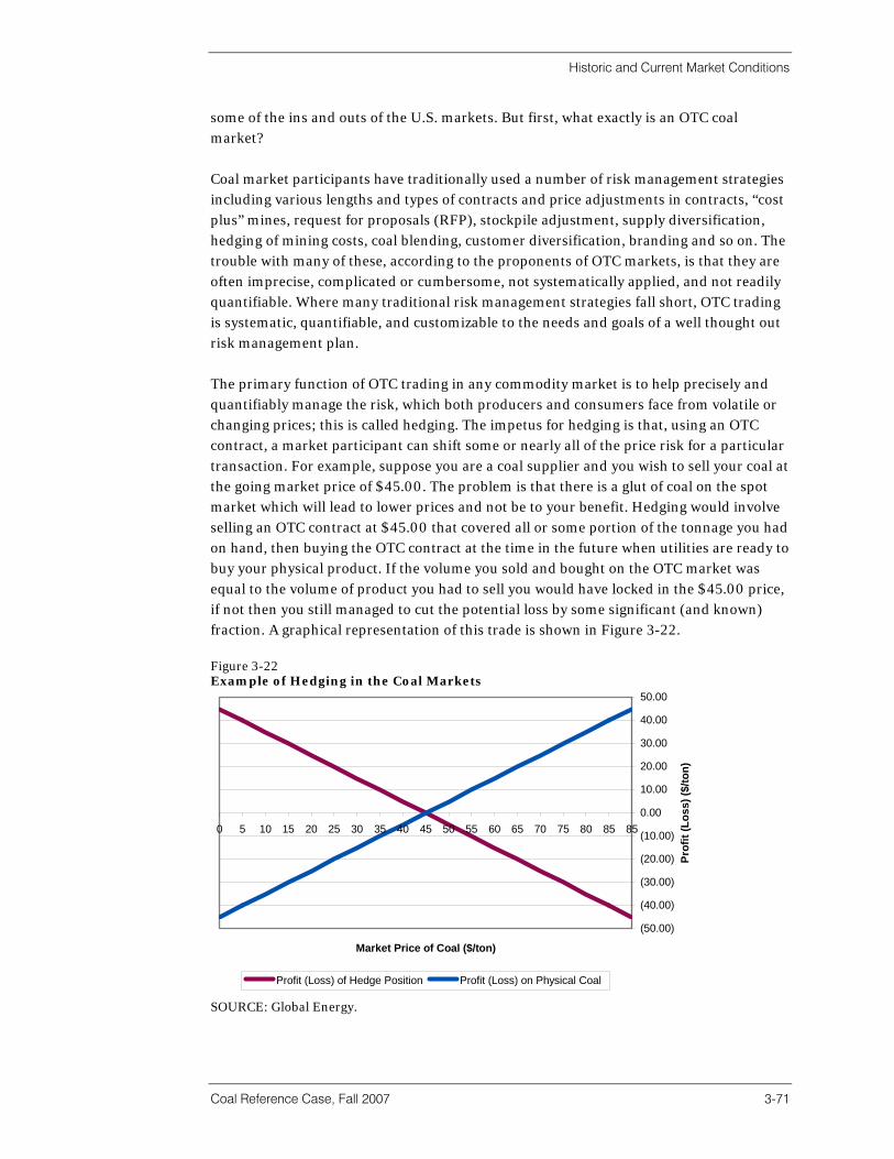
Historic and Current Market Conditions
Coal Reference Case, Fall 2007 3-71
some of the ins and outs of the U.S. markets. But first, what exactly is an OTC coal market? Coal market participants have traditionally used a number of risk management strategies including various lengths and types of contracts and price adjustments in contracts, “cost plus” mines, request for proposals (RFP), stockpile adjustment, supply diversification, hedging of mining costs, coal blending, customer diversification, branding and so on. The trouble with many of these, according to the proponents of OTC markets, is that they are often imprecise, complicated or cumbersome, not systematically applied, and not readily quantifiable. Where many traditional risk management strategies fall short, OTC trading is systematic, quantifiable, and customizable to the needs and goals of a well thought out risk management plan. The primary function of OTC trading in any commodity market is to help precisely and quantifiably manage the risk, which both producers and consumers face from volatile or changing prices; this is called hedging. The impetus for hedging is that, using an OTC contract, a market participant can shift some or nearly all of the price risk for a particular transaction. For example, suppose you are a coal supplier and you wish to sell your coal at the going market price of $45.00. The problem is that there is a glut of coal on the spot market which will lead to lower prices and not be to your benefit. Hedging would involve selling an OTC contract at $45.00 that covered all or some portion of the tonnage you had on hand, then buying the OTC contract at the time in the future when utilities are ready to buy your physical product. If the volume you sold and bought on the OTC market was equal to the volume of product you had to sell you would have locked in the $45.00 price, if not then you still managed to cut the potential loss by some significant (and known) fraction. A graphical representation of this trade is shown in Figure 3-22. Figure 3-22 Example of Hedging in the Coal Markets
(50.00)
(40.00)
(30.00)
(20.00)
(10.00)
0.00
10.00
20.00
30.00
40.00
50.00
0 5 10 15 20 25 30 35 40 45 50 55 60 65 70 75 80 85 85
Market Price of Coal ($/ton)
Prof
it (L
oss)
($/to
n)
Profit (Loss) of Hedge Position Profit (Loss) on Physical Coal
SOURCE: Global Energy.
Historic and Current Market Conditions
3-72
There are much more sophisticated approaches but the preceding example demonstrates the possibility of completely offsetting a price change with an OTC trade of equal coal volume. In other words, there is a dollar for dollar offset for price changes in either direction—less administrative and brokerage fees. This is generally referred to as a perfect hedge but there are many other types of hedging that can be accomplished in a well functioning OTC market. These strategies can be customized to meet many different risk management profiles. Two essential components of an effective OTC market are liquidity and the existence of a basis contract. Liquidity is essentially tied to the trading volume on a day to day basis. If a market participant can easily get into the market but not easily get out of the market, it is said to be an illiquid market. This situation will not attract speculators who are an essential element in a commodity market since they are the ones who assume the risk, allowing hedgers to quantifiably transfer a portion of their risk to the speculator. The speculator, in turn, gains the potential of generating a profit from the market by taking the other side of some portion of transactions. It is virtually impossible for a liquid market to develop without a standard contract that can be entered and exited quickly and easily. A contract of this nature will usually develop around a natural hub. In Europe, this hub is called the ARA (for Amsterdam, Rotterdam, Antwerp). These three ports in northwestern Europe see the majority of coal shipped into northern and central Europe, forming a natural hub between them. A standardized OTC trading contract has developed with specific quality, quantity, and mode of delivery to serve the needs of coal market participants. Foreign Markets Global Coal Markets Overview In response to decreasing production in some regions and skyrocketing demand in others the global coal trade is brisk and on the rise. Global steam coal trading volume is up from 579 million tons in 2005 to 622 million tons in 2006, an annual growth rate of 7.4 percent. While we do not expect this growth rate to continue over the long-term, global coal supply is in the midst of a large expansion to meet actual and expected rising demand, and supply will continue to increase until prices come down significantly from their current historical highs. The global steam coal market naturally divides into an Atlantic and Pacific section because there has been little historical supply competition between the two. The major steam coal exporters and their 2005 and 2006 volumes are shown in Table 3-10. This separation between the two markets is likely to diminish somewhat as demand growth driven by China and India draws some supply from South Africa, which has historically sold 90 percent or more of its coal into the Atlantic market. In addition, as shipping rates return to levels that are more normal from their current historical highs, Australian and Indonesian steam coal will have greater opportunity for market penetration into Europe.

Historic and Current Market Conditions
Coal Reference Case, Fall 2007 3-73
Table 3-10 World Steam Coal Trade; 2005-2006 (millions of tons)
2005 2006 % Change 2005 2006 % Change
Steam coal 579 622 7.4%
Coking coal 207 203 -2.1%
Total 786 825 4.9%
Pacific Market Official Figures Unofficial Estimates
Australia 118 122 3.7%
China 74 65 -11.9%
Indonesia 129 162 25.6% 142 187 31.8%
Russia 12 13 9.1%
Vietnam 18 23 31.3% 20 31 55.6%
Total 351 386 10.1% 366 419
Atlantic Market Official Figures Unofficial Estimates
Colombia 60 64 7.4%
Poland 11 8 -30.0%
Russia 57 65 13.5%
South Africa 77 74 -2.9%
Venezuela 9 9 0.0%
Others 14 15 7.7%
Total 228 236 3.4%
SOURCE: European Association for Coal and Lignite and Global Energy.
Coal exporters are increasing their investments in production and terminal capacity in response to both generally increasing fuel prices and coal prices that are at historic highs. Prominent market commentators suggest, however, that new supply chain investment comes most often only in response to actual demand growth rather than in anticipation of higher demand, much to the chagrin of coal consumers who must pay the resulting higher prices. This is reflected in current transportation bottlenecks, which are putting a snag in the supply chains of some exporting countries, particularly Australia and South Africa. Suppliers have in many cases expanded production over the last several years to take advantage of an apparently structural shift in prices in 2003-2004. However, export terminals and the transport networks that feed them have sometimes been slow to respond with corresponding capital investment. South Africa is a particularly good example of this. Overseas shipping prices for dry bulk goods are at their highest level in many years; coal makes up about 20 percent of this market. Average annual prices increased over 17 percent per year from 2000 to 2006 with the underlying theme being volatility with prices ranging between $10 and $30 per ton over the course of less than one year for Capesize (140,000 ton cargo) coal from Richard’s Bay South Africa delivered to Northwest Europe (Amsterdam, Rotterdam, or Antwerp). Upward pressure on shipping prices over the short term will continue as a result of worldwide supply shortages in shipping vessels, mostly as a result of China’s insatiable appetite for bulk commodities—especially iron ore to feed its steel production, and congestion at Australian and Indonesian ports. Some relief from this congestion should come over the next few years

Historic and Current Market Conditions
3-74
as Australian and South African ports are upgraded to improve capacity by 55 million tons in the long run with a 20 million ton improvement expected by 2010. Asia Demand growth for coal in Asia will largely be driven by India and China, especially over the next 5 to 10 years. The EIA International Energy Outlook reference case forecast for 2006 slates the Asian market for 5.8 percent growth in annual coal consumption from 2003 to 2010. The low and high economic growth cases call for 5.2 percent and 6.3 percent, respectively, for the same period. Growth of coal use is slated to slow with weakening economic growth after 2010 to 3.2 percent annually through 2015 and then fall off to less than 3 percent thereafter. The largest suppliers of steam coal to the Asian region are Australia and Indonesia with estimated 2006 exports of 162 and 122 million short tons of steam coal exports, respectively. In 2006, 81 percent of Australia’s exports and 89 percent of Indonesia’s exports ended up in Asian markets. As China’s demand for coal has exploded over the past few years, it has decreased its exports becoming a net importer of coal for the first time earlier this year. This trend will continue as China’s ability and incentive to use its own coal increases. Europe European coal prices have increased by 9.4 percent per year since 1999 as part of a structural shift to higher prices for all fuels. Coal production in Europe is in decline and is unlikely to recover barring major shifts in policy and production technology. The EU-27 experienced a 3.0 percent annual decline in production from 1994 to 2005. Demand for coal in Europe is expected to decline over the next 25 years with a slight increase between 2007 and the 2010. Demand for coal for power generation in Europe has been nearly flat over the last 10 years. Electricity generated at coal-fired plants in 20 major European states grew about 1 percent per year from 1994 to 2005 while total electricity generation for those states grew about 2 percent per year over the same time period. The preference for other fuels over coal in Europe is demonstrated by the falling share of coal in total generation; from 1994 to 2005, the share of coal generation decreased steadily from 38.6 percent to 34.4 percent. Coal’s share of generation also fell in all of the five largest consumers of coal in Europe: Germany, the United Kingdom, Poland, Spain, and the Czech Republic. The EIA International Energy Outlook 2007 projects that demand for coal-fired electricity generation in OECD Europe is expected to fall by over 21 percent from 2004 levels by 2030 or about 0.6 percent annually. World supply is expanding to meet the needs of rapidly growing demand from developing countries. Delivery of coal from exporters to importers, primarily by ocean vessel, is expensive and is expected to remain so over the near term, but soften in the mid term. These factors combine to form a picture of European coal prices which are likely to remain near recent high levels through the end of this decade then gradually decline through 2015 in synch with expected lower natural gas prices, softening prices for dry bulk shipping and increased availability of coal on the global market. After 2015, prices

Historic and Current Market Conditions
Coal Reference Case, Fall 2007 3-75
increase steadily with continued growing world demand for energy, increasing competing fuel prices, and correction of oversupply conditions. Consequences for the U.S. Marketplace Increasing demand from China, India and the rest of the developing world, fluctuating currency exchange rates, and the projected production declines in a European electricity sector already heavily dependant on imports are resulting in higher prices for coal around the globe. Europe’s main suppliers outside of Europe and Asia are South Africa and South America. With increasing South African supply going east into the Asian markets, Europe will have to rely more heavily on other sources of overseas supplies, namely South America and the United States. Delivered prices for South American coal in Europe are currently higher than what South American coal fetches in the United States. As long as this dynamic persists, coal that is not under contract is more likely to flow from Colombia across the Atlantic than to the United States.


Section 4 Coal Demand Outlook


Coal Demand Outlook
Coal Reference Case, Fall 2007 4-1
Demand Region Outlook Overall U.S. Demand
Total deliveries of coal to the United States are expected to increase from 1.05 billion tons in 2007 to 1.3 billion tons in 2031, an annual average increase of 1.98 percent. Demand for coal is expected to increase for all basins except for Central and Southern Appalachia, which should see demand decrease by 45 percent and 28 percent, respectively. The largest percentage increase in demand is expected to come from Colombian coal at 178 percent—a 36 million ton increase over the 25-year study period. Demand for PRB coal is forecasted to rise by 50 percent (annual growth of 9.4 million tons/year) and the Illinois Basin should see a 37 percent growth in demand (annual growth of 1.28 million tons/year). Rocky Mountain coal is expected to command a 27 percent increase in demand (annual growth of 1.1 million tons/year). Lignite demand should remain relatively flat. Figure 4-1 United States Coal Demand by Basin
0
200,000
400,000
600,000
800,000
1,000,000
1,200,000
1,400,000
2007 2009 2011 2013 2015 2017 2019 2021 2023 2025 2027 2029 2031
000s
tons
Import / Other Local Lignite Rocky MountainIllinois Basin Northern App Central / Southern AppPRB
SOURCE: Global Energy.
This report organizes the U.S. into five distinct U.S. demand regions, based on geographical location, electricity demand, coal supply, coal use, pricing, and transportation options. These regions are: • Northeast (MD, DE, PA, NJ, NY, CT, RI, MA, VT, NH, ME); • Southeast (FL, MS, AL, GA, TN, SC, NC, KY, WV, VA); • Midwest (KS, MO, IL, IN, OH, NE, IA, MI, SD, ND, MN, WI); • South Central (TX, OK, AK, LA); and • West (CA, AZ, NM, NV, UT, CO, OR, ID, WY, WA, MT).

Coal Demand Outlook
4-2
Map 4-1 The Five U.S. Coal Demand Regions
SOURCE: Global Energy.
The Northeast region has the lowest current demand and the slightest increase in coal demand of all the regions. With an average growth of 0.5 percent a year, its total demand will increase 13 percent over the 25-year time span. The West region is also relatively flat, increasing 16 percent over 25 years. The Southeast region is expected to increase 24 percent, which equates to over 160,000 GWh of coal generation. The Midwest shows growth every year resulting in the highest absolute increase (248,300 GWh or 34 percent since 2007) in coal power demand by 2031. The South Central region, while small, shows the greatest average yearly increase (1.5 percent) and overall increase (44 percent) in coal-fired electricity generation. Table 4-1 Yearly Coal Generation Demand by Region (GWh)
Year Northeast Southeast Midwest South Central West Grand Total
2007 219,284 654,651 731,731 233,920 227,362 2,066,948
2008 218,165 661,451 734,657 234,031 228,750 2,077,053
2009 218,764 670,371 734,714 234,429 231,075 2,089,353
2010 217,675 671,057 735,045 241,692 237,673 2,103,142
2011 225,621 673,994 749,586 244,656 241,129 2,134,986
2012 226,451 688,513 763,866 253,384 241,351 2,173,565
2013 226,923 697,226 767,915 262,516 241,235 2,195,814
2014 223,028 696,650 779,228 265,566 240,619 2,205,092
2015 222,542 701,325 793,472 267,405 244,038 2,228,781
2020 222,596 714,623 832,242 290,356 249,068 2,308,885
2025 241,004 747,399 895,167 310,247 256,338 2,450,154
2031 247,275 814,895 980,047 336,984 263,981 2,643,182
SOURCE: Global Energy.

Coal Demand Outlook
Coal Reference Case, Fall 2007 4-3
Figure 4-2 Coal Generation Demand by Region
-
200,000
400,000
600,000
800,000
1,000,000
1,200,000
2007 2009 2011 2013 2015 2017 2019 2021 2023 2025 2027 2029 2031
Gen
erat
ion
Dem
and
(GW
-hr)
Northeast Southeast Midwest South Central West
SOURCE: Global Energy.
There are seven primary coal supply basins used in this report. Details of the basins and their more detailed regions are listed in the following table. The “percent total” represents the tons of coal delivered from that region divided by the tons delivered for that basin during the time frame of the model. The exact tons of each region by source can be seen in Appendix B. Table 4-2 Approximate Ton Makeup of Coal Source Categories Seen in Figures
Category Source Percent Total
Colombia Import 76%
Petroleum Coke 13%
Venezuela Import 8%
Indonesia Import 2%
Import / Other
Central Interior 1%
Gulf Lignite 66% Local Lignite
Northern Lignite 34%
Colorado 40%
Four Corners 29%
Utah 20% Rocky Mountain
Wyoming 11%
North East 85% Northern App
Ohio 15%
Central 94% Central / Southern App
Southern 6%
Southern PRB 90% Powder River Basin
Northern PRB 10%
Illinois Basin Illinois Basin 100%
SOURCE: Global Energy.
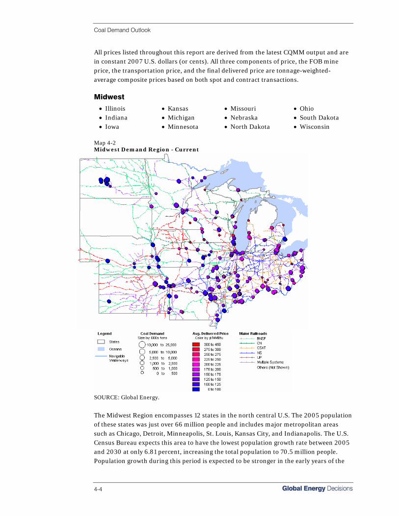
Coal Demand Outlook
4-4
All prices listed throughout this report are derived from the latest CQMM output and are in constant 2007 U.S. dollars (or cents). All three components of price, the FOB mine price, the transportation price, and the final delivered price are tonnage-weighted-average composite prices based on both spot and contract transactions. Midwest
• Illinois • Kansas • Missouri • Ohio • Indiana • Michigan • Nebraska • South Dakota • Iowa • Minnesota • North Dakota • Wisconsin
Map 4-2 Midwest Demand Region - Current
SOURCE: Global Energy.
The Midwest Region encompasses 12 states in the north central U.S. The 2005 population of these states was just over 66 million people and includes major metropolitan areas such as Chicago, Detroit, Minneapolis, St. Louis, Kansas City, and Indianapolis. The U.S. Census Bureau expects this area to have the lowest population growth rate between 2005 and 2030 at only 6.81 percent, increasing the total population to 70.5 million people. Population growth during this period is expected to be stronger in the early years of the
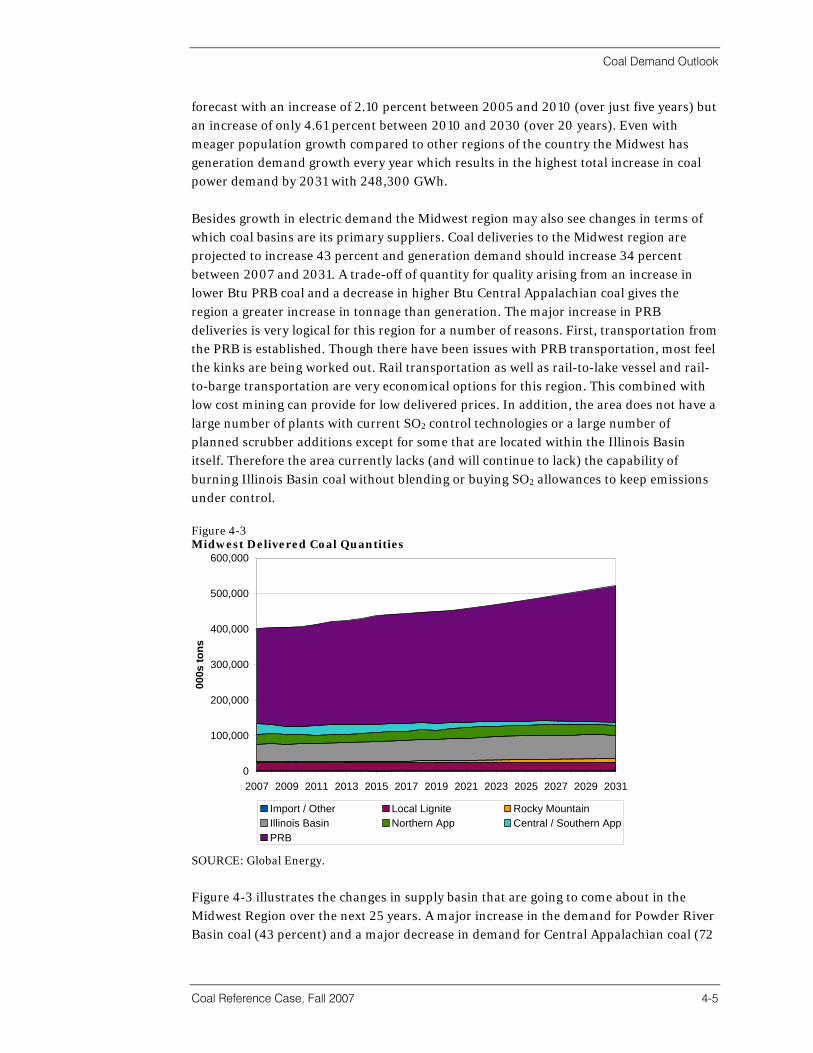
Coal Demand Outlook
Coal Reference Case, Fall 2007 4-5
forecast with an increase of 2.10 percent between 2005 and 2010 (over just five years) but an increase of only 4.61 percent between 2010 and 2030 (over 20 years). Even with meager population growth compared to other regions of the country the Midwest has generation demand growth every year which results in the highest total increase in coal power demand by 2031 with 248,300 GWh. Besides growth in electric demand the Midwest region may also see changes in terms of which coal basins are its primary suppliers. Coal deliveries to the Midwest region are projected to increase 43 percent and generation demand should increase 34 percent between 2007 and 2031. A trade-off of quantity for quality arising from an increase in lower Btu PRB coal and a decrease in higher Btu Central Appalachian coal gives the region a greater increase in tonnage than generation. The major increase in PRB deliveries is very logical for this region for a number of reasons. First, transportation from the PRB is established. Though there have been issues with PRB transportation, most feel the kinks are being worked out. Rail transportation as well as rail-to-lake vessel and rail-to-barge transportation are very economical options for this region. This combined with low cost mining can provide for low delivered prices. In addition, the area does not have a large number of plants with current SO2 control technologies or a large number of planned scrubber additions except for some that are located within the Illinois Basin itself. Therefore the area currently lacks (and will continue to lack) the capability of burning Illinois Basin coal without blending or buying SO2 allowances to keep emissions under control. Figure 4-3 Midwest Delivered Coal Quantities
0
100,000
200,000
300,000
400,000
500,000
600,000
2007 2009 2011 2013 2015 2017 2019 2021 2023 2025 2027 2029 2031
000s
tons
Import / Other Local Lignite Rocky MountainIllinois Basin Northern App Central / Southern AppPRB
SOURCE: Global Energy.
Figure 4-3 illustrates the changes in supply basin that are going to come about in the Midwest Region over the next 25 years. A major increase in the demand for Powder River Basin coal (43 percent) and a major decrease in demand for Central Appalachian coal (72

Coal Demand Outlook
4-6
percent) are evident from the modeled output. The net effect will be an increase in the number of Btu’s in order to keep pace with demand for electricity in this region. Figure 4-4 illustrates the weighted average FOB mine price for the coal basins supplying the Midwest. As expected, the Powder River Basin has the lowest prices while Central Appalachia has the highest with other basins falling somewhere in between. Low FOB mine prices contribute to the competitive advantage PRB coal enjoys in the Midwest region. Figure 4-4 Midwest FOB Mine Price
0
50
100
150
200
250
300
2007 2009 2011 2013 2015 2017 2019 2021 2023 2025 2027 2029 2031
¢/M
MB
tu
Import / Other Local Lignite Rocky MountainIllinois Basin Northern App Central / Southern AppPRB Average
SOURCE: Global Energy.
Due to the long distances PRB coal typically travels, transportation rates on a dollar per ton basis from this supply basin are normally higher than other basins. This is shown below in Figure 4-5 where PRB transportation costs range from just over $11 to nearly $14 in 2031 compared to other basins, such as Northern Appalachia, which has much lower transportation costs to this region hovering at approximately $5 per ton for the duration of the forecasted period. Even with high transportation costs, the benefits of low FOB mine prices and low sulfur coal to save expenses on emissions controls or allowances makes the PRB the economical choice for the region. Rocky Mountain transportation rates are high due to navigation of the Rocky Mountains and the Continental Divide which requires extra engines, fuel, and expenses. The fact that the majority of the Illinois Basin resides within the Midwest region means transportation costs are low, though much of this high sulfur coal is delivered to plants in very close proximity to the basin itself, which is where the concentration of SO2 controls are located. High sulfur coal that moves beyond this concentration of scrubbed plants needs to be supplemented with low sulfur coal of some type, whether it is PRB as we see in the future or Central Appalachian coal as we have seen in the past.

Coal Demand Outlook
Coal Reference Case, Fall 2007 4-7
Figure 4-5 Midwest Transportation Cost by Basin
$0.00
$5.00
$10.00
$15.00
$20.00
$25.00
2007 2009 2011 2013 2015 2017 2019 2021 2023 2025 2027 2029 2031
$/to
n
Import / Other Local Lignite Rocky MountainIllinois Basin Northern App Central / Southern AppPRB Average
SOURCE: Global Energy.
The Powder River Basin’s ability to move coal cheaply into this region means that competing basins will need to achieve low prices if they wish to have market share in these areas. With opportunities for higher prices in the other U.S. demand regions, there is little incentive for other supply basins to gain market share in the Midwest. Combined with Central Appalachia’s increasing costs and therefore FOB mine prices increasing and the need for the Midwest to continually have a low sulfur producer, the PRB’s low sulfur coal and the economics of transportation make it the only real plausible choice for the foreseeable future. Figure 4-6 Midwest Delivered Price
0
50
100
150
200
250
300
2007 2009 2011 2013 2015 2017 2019 2021 2023 2025 2027 2029 2031
¢/M
MB
tu
Import / Other Local Lignite Rocky MountainIllinois Basin Northern App Central / Southern AppPRB Average
SOURCE: Global Energy.
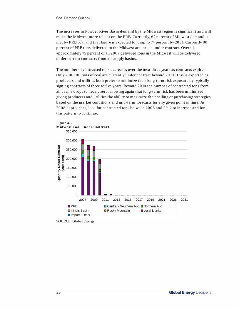
Coal Demand Outlook
4-8
The increases in Powder River Basin demand by the Midwest region is significant and will make the Midwest more reliant on the PRB. Currently, 67 percent of Midwest demand is met by PRB coal and that figure is expected to jump to 74 percent by 2031. Currently 80 percent of PRB tons delivered to the Midwest are locked under contract. Overall, approximately 75 percent of all 2007 delivered tons in the Midwest will be delivered under current contracts from all supply basins. The number of contracted tons decreases over the next three years as contracts expire. Only 200,000 tons of coal are currently under contract beyond 2010. This is expected as producers and utilities both prefer to minimize their long-term risk exposure by typically signing contracts of three to five years. Beyond 2010 the number of contracted tons from all basins drops to nearly zero, showing again that long-term risk has been minimized giving producers and utilities the ability to maximize their selling or purchasing strategies based on the market conditions and mid-term forecasts for any given point in time. As 2008 approaches, look for contracted tons between 2008 and 2012 to increase and for this pattern to continue. Figure 4-7 Midwest Coal under Contract
0
50,000
100,000
150,000
200,000
250,000
300,000
350,000
2007 2009 2011 2013 2015 2017 2019 2021 2026 2031
Qua
ntity
Und
er C
ontr
act
(000
s to
ns)
PRB Central / Southern App Northern AppIllinois Basin Rocky Mountain Local LigniteImport / Other
SOURCE: Global Energy.

Coal Demand Outlook
Coal Reference Case, Fall 2007 4-9
Northeast • Connecticut • Maine • New Hampshire • Pennsylvania • Delaware • Maryland • New Jersey • Rhode Island • District of Columbia • Massachusetts • New York • Vermont
Map 4-3 Northeast Demand Region - Current
SOURCE: Global Energy.
The Northeast region includes all of New England, New York to the north, Maryland and the District of Colombia to the south, and all three states in between (New Jersey, Pennsylvania, and Delaware). It includes major metropolitan areas such as Pittsburgh, New York City, Philadelphia, Baltimore, and Boston. Similar to the Midwest region, Northeast population growth is expected to be only 7 percent between 2005 and 2030 increasing from 62 million people in 2005 to just over 66 million in 2030. The Northeast region is forecasted to have the lowest increase in total coal powered demand in the next 25 years with an increase of only 28,000 GWh or 13 percent for three major reasons: low population growth, majority of economic growth in the region is in non-energy intensive growth areas such as financial and service oriented industries, and 7 of the 11 states within the region are part of the Regional Greenhouse Gas Initiative (RGGI).

Coal Demand Outlook
4-10
The RGGI is a cooperative effort by eight northeastern states to reduce carbon dioxide emissions, one of the major gases emitted during the burning of coal.1 With eight northeastern states as part of the RGGI with hopes of reducing carbon emissions, coal plants will have a very difficult time being permitted in the Northeast. Therefore the region will likely rely on upgrades of nuclear plants to meet growing demand for total electricity generation. In addition, this region has the highest relative capacity of natural gas burners allowing for fuel switching when gas prices are low, which creates a fluctuation of coal consumption from year to year. Increases that do come in the form of coal powered demand will be a result of upgrades on existing coal-fired units rather than the construction of new units. New York does have one coal plant in Popes Creek with an application pending. The plant would be an integrated gasification combined cycle (IGCC) plant, with fewer emissions than a standard coal-fired plant. The size of the project is minimal with a capacity of only 40 MW. The supply basins providing the Northeast region with coal will change slightly over the next 25 years. With declining production and increasing costs in Central Appalachia the Northeast region is forecasted to replace 11 million Central Appalachia tons with higher sulfur Northern Appalachia coal. Higher sulfur content does not present a major problem for the region because many coal plants either currently have SO2 control technologies or are planning to implement them. Import coal is mostly flat through 2010 but then increases substantially over the next 20 years, increasing its total supply to the region by 3.5 million tons, or a 42 percent increase over 2007 levels. The small amount of Rocky Mountain coal currently delivered to the Northeast region is eliminated after 2011. Figure 4-8 Northeast Delivered Coal Quantities
0
10,000
20,000
30,000
40,000
50,000
60,000
70,000
80,000
90,000
100,000
2007 2009 2011 2013 2015 2017 2019 2021 2023 2025 2027 2029 2031
000s
tons
Import / Other Rocky Mountain Illinois BasinNorthern App Central / Southern App PRB
SOURCE: Global Energy.
1 The RGGI is discussed in greater detail in Section 3 Regulatory Issues

Coal Demand Outlook
Coal Reference Case, Fall 2007 4-11
FOB mine prices for deliveries made to the Northeast region are typical of what we would expect. PRB has the lowest FOB prices though not a great deal of this coal will make its way into the region (discussed in greater detail below). Central Appalachia and Northern Appalachia have similar FOB prices, with NAPP’s being slightly lower in early years. While continued reserve degradation will contribute to rising costs and FOB prices in CAPP, the basin’s FOB prices will drop below the level of those in NAPP because only those few remaining efficient mines in CAPP will be able to overcome the higher transportation rates compared to NAPP and still make deliveries to the Northeast at economical prices. Figure 4-9 Northeast FOB Mine Price
0
50
100
150
200
250
300
2007 2009 2011 2013 2015 2017 2019 2021 2023 2025 2027 2029 2031
¢/M
MB
tu
Import / Other Rocky Mountain Illinois BasinNorthern App Central / Southern App PRBAverage
SOURCE: Global Energy.
Figure 4-10 outlines transportation rates on a dollar per ton basis for deliveries made to the Northeast region over the next 25 years. The Powder River Basin has the highest costs solely because of the distance that coal from the PRB must travel if its destination is in the Northeast region. More important to note from this graphic is the much higher transportation costs out of Central Appalachia that were noted above. Navigation of coal through the heart of the Appalachian Mountains can be very costly as the figure indicates. The transportation cost of imports from South America is half that of Central Appalachia in the majority of the forecasted years.
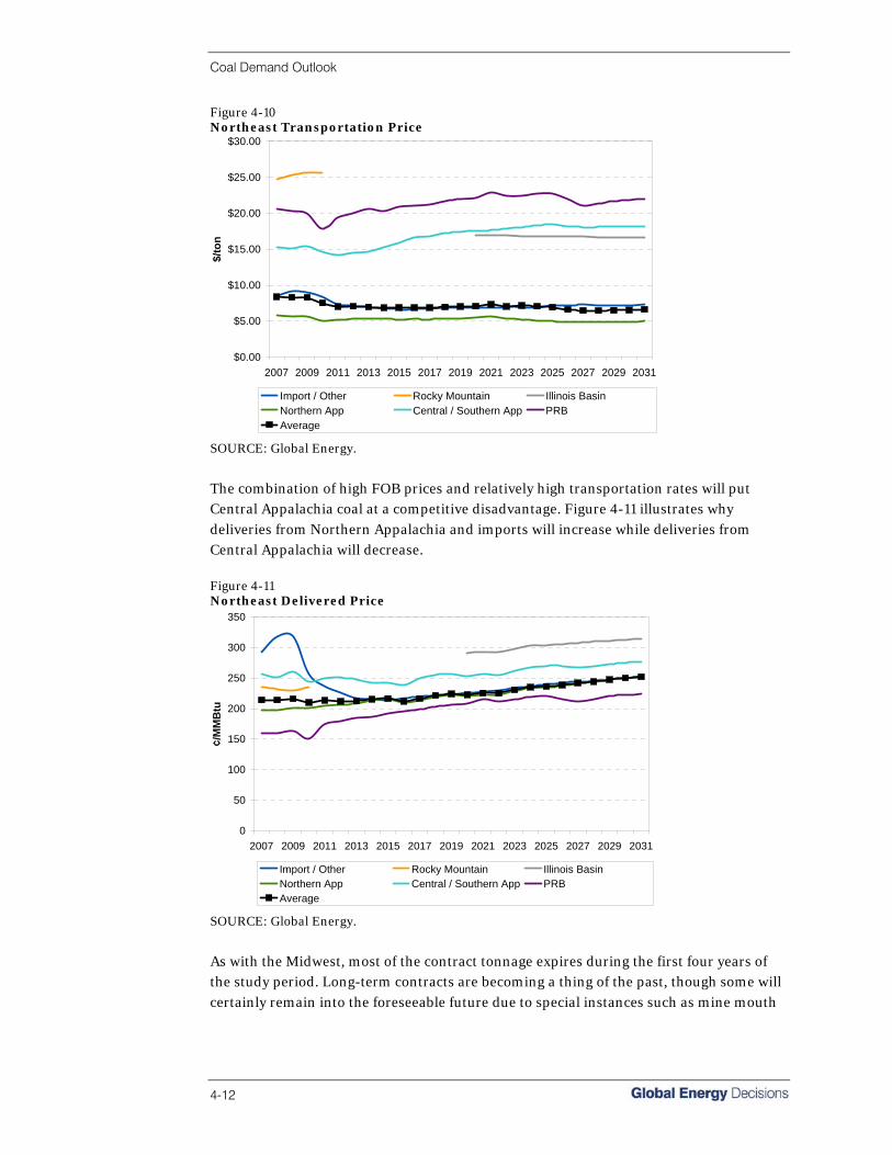
Coal Demand Outlook
4-12
Figure 4-10 Northeast Transportation Price
$0.00
$5.00
$10.00
$15.00
$20.00
$25.00
$30.00
2007 2009 2011 2013 2015 2017 2019 2021 2023 2025 2027 2029 2031
$/to
n
Import / Other Rocky Mountain Illinois BasinNorthern App Central / Southern App PRBAverage
SOURCE: Global Energy.
The combination of high FOB prices and relatively high transportation rates will put Central Appalachia coal at a competitive disadvantage. Figure 4-11 illustrates why deliveries from Northern Appalachia and imports will increase while deliveries from Central Appalachia will decrease. Figure 4-11 Northeast Delivered Price
0
50
100
150
200
250
300
350
2007 2009 2011 2013 2015 2017 2019 2021 2023 2025 2027 2029 2031
¢/M
MB
tu
Import / Other Rocky Mountain Illinois BasinNorthern App Central / Southern App PRBAverage
SOURCE: Global Energy.
As with the Midwest, most of the contract tonnage expires during the first four years of the study period. Long-term contracts are becoming a thing of the past, though some will certainly remain into the foreseeable future due to special instances such as mine mouth
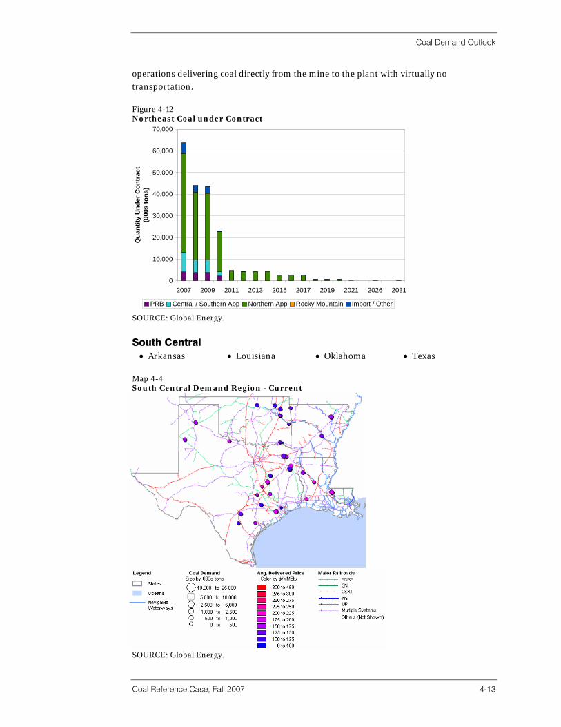
Coal Demand Outlook
Coal Reference Case, Fall 2007 4-13
operations delivering coal directly from the mine to the plant with virtually no transportation. Figure 4-12 Northeast Coal under Contract
0
10,000
20,000
30,000
40,000
50,000
60,000
70,000
2007 2009 2011 2013 2015 2017 2019 2021 2026 2031
Qua
ntity
Und
er C
ontr
act
(000
s to
ns)
PRB Central / Southern App Northern App Rocky Mountain Import / Other SOURCE: Global Energy.
South Central • Arkansas • Louisiana • Oklahoma • Texas
Map 4-4 South Central Demand Region - Current
SOURCE: Global Energy.

Coal Demand Outlook
4-14
Although the South Central region has by far the lowest population of the five regions in this study, with only 33 million people in 2005, it has the third highest coal power demand. In 2007, demand from coal-fired plants was 233,920 GWh. Compared to the Northeast and West, the South Central region burns twice as much coal per capita. The South Central region is forecasted to have the largest percentage increase in coal power demand over the forecast period. There will be substantial economic development in this region in upcoming years mainly as increased oil refining capacity will need to keep pace with future U.S. oil consumption. Refineries are mainly gas powered and will not have a direct effect on coal power demand, but they will have an indirect effect on population growth that will occur in response to increased economic development. Between 2005 and 2030, the U.S. Census Bureau expects the South Central region to grow by 35 percent. As both the population and economy grow, coal demand to meet generation needs will increase significantly. The majority of coal deliveries to the South Central region come from the Powder River Basin, with remaining tons coming primarily from Gulf Lignite which has a dramatic transportation advantage over competitors due to its location. It is forecasted that the bulk of increased coal demand will be supplied by the Powder River Basin. Despite transportation advantages lignite may have, with low heat content and high sulfur as well as a limited supply, it cannot compete for new capacity but will remain important to existing plants currently using it in their mine mouth operations. Figure 4-13 shows forecasted coal demand supply regions to 2031. Figure 4-13 South Central Delivered Coal Quantities
0
50,000
100,000
150,000
200,000
250,000
2007 2009 2011 2013 2015 2017 2019 2021 2023 2025 2027 2029 2031
000s
tons
Import / Other Local Lignite Rocky Mountain PRB
SOURCE: Global Energy.
Although the FOB mine price in Figure 4-14 shows that the South Central Region uses coal from the Rocky Mountain Basin as well as Imports/Other, the volumes are insignificant. Figure 4-14 shows FOB mine prices out of the PRB compared to other
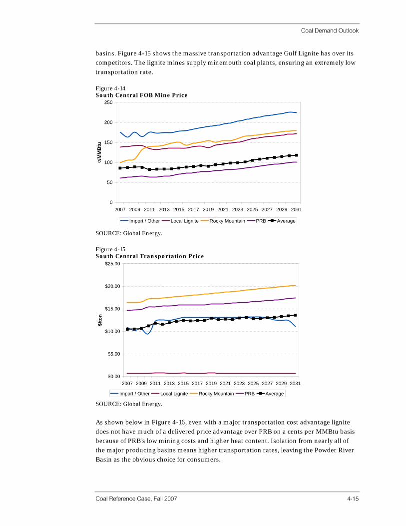
Coal Demand Outlook
Coal Reference Case, Fall 2007 4-15
basins. Figure 4-15 shows the massive transportation advantage Gulf Lignite has over its competitors. The lignite mines supply minemouth coal plants, ensuring an extremely low transportation rate. Figure 4-14 South Central FOB Mine Price
0
50
100
150
200
250
2007 2009 2011 2013 2015 2017 2019 2021 2023 2025 2027 2029 2031
¢/M
MB
tu
Import / Other Local Lignite Rocky Mountain PRB Average
SOURCE: Global Energy.
Figure 4-15 South Central Transportation Price
$0.00
$5.00
$10.00
$15.00
$20.00
$25.00
2007 2009 2011 2013 2015 2017 2019 2021 2023 2025 2027 2029 2031
$/to
n
Import / Other Local Lignite Rocky Mountain PRB Average
SOURCE: Global Energy.
As shown below in Figure 4-16, even with a major transportation cost advantage lignite does not have much of a delivered price advantage over PRB on a cents per MMBtu basis because of PRB’s low mining costs and higher heat content. Isolation from nearly all of the major producing basins means higher transportation rates, leaving the Powder River Basin as the obvious choice for consumers.

Coal Demand Outlook
4-16
Figure 4-16 South Central Delivered Price
0
50
100
150
200
250
300
2007 2009 2011 2013 2015 2017 2019 2021 2023 2025 2027 2029 2031
¢/M
MB
tu
Import / Other Local Lignite Rocky Mountain PRB Average
SOURCE: Global Energy.
As with other U.S. demand regions, most of the tons under contract expire in the next four years. Lignite mines are the exception to this observation as these mine mouth operations are locked into long-term contracts with the nearby plant. While contracted tons from the PRB drop significantly from 2010 to 2011, the contracted lignite tons do not drop as dramatically and remain steady until the end of the forecast period. The long-term lignite contracts have benefits for both supplier and consumer, especially when it comes to transportation issues that could arise from relying on coal deliveries from other portions of the country. Figure 4-17 South Central Coal under Contract
0
20,000
40,000
60,000
80,000
100,000
120,000
140,000
2007 2009 2011 2013 2015 2017 2019 2021 2026 2031
Qua
ntity
Und
er C
ontr
act
(000
s to
ns)
PRB Rocky Mountain Local Lignite Import / Other
SOURCE: Global Energy.

Coal Demand Outlook
Coal Reference Case, Fall 2007 4-17
Southeast • Alabama • Kentucky • South Carolina • West Virginia • Florida • Mississippi • Tennessee • Georgia • North Carolina • Virginia
Map 4-5 Southeast Demand Region - Current
SOURCE: Global Energy.
The Southeast region has the largest population of the five U.S. Demand Regions and it is expected to remain in that position until 2020 according to the U.S. Census Bureau. It is projected to have 35 percent growth between 2005 and 2030. The region has several large metropolitan areas such as Charlotte, Atlanta, Raleigh-Durham, Richmond, and Jacksonville that are expected to grow. The coastal states are popular retirement areas and with many baby-boomers nearing retirement age, this could have a major effect on population and residential electricity demand growth. There will be some development in energy intensive industries, but most economic growth will be in financial, software, and services.

Coal Demand Outlook
4-18
Colombian coal sales into the Southeast are forecasted to grow by 242 percent over the next 25 years. PRB coal runs second with a projected increase of 151 percent, though on an absolute tonnage basis PRB deliveries increase considerably more than imports. Rocky Mountain use doubles and Illinois Basin increases by over 30 percent. Central Appalachia loses 1.9 million tons a year on average, resulting in a 36 percent decline and 3 million tons/year of Southern Appalachia coal are also lost over the forecasted period. Figure 4-18 shows basin supply for the Southeast region and Central Appalachia’s failure to meet current supply levels. Figure 4-18 Southeast Delivered Coal Quantities
0
50,000
100,000
150,000
200,000
250,000
300,000
350,000
400,000
2007 2009 2011 2013 2015 2017 2019 2021 2023 2025 2027 2029 2031
000s
tons
Import / Other Local Lignite Rocky MountainIllinois Basin Northern App Central / Southern AppPRB
SOURCE: Global Energy.
A wide variety of coal basins supply coal to the Southeast. FOB mine prices are bounded by PRB on the low end and CAPP on the high end. The Illinois Basin’s large reserve blocks and affinity for new longwall mines keeps FOB prices approximately even with that of Northern Appalachia. Figure 4-19 Southeast FOB Mine Price
0
50
100
150
200
250
300
350
400
2007 2009 2011 2013 2015 2017 2019 2021 2023 2025 2027 2029 2031
¢/M
MB
tu
Import / Other Local Lignite Rocky MountainIllinois Basin Northern App Central / Southern AppPRB Average
SOURCE: Global Energy.

Coal Demand Outlook
Coal Reference Case, Fall 2007 4-19
Rocky Mountain and PRB transportation rates are the highest of any basin delivering coal to the Southeast region because of the distance the coal must travel. Illinois Basin transportation costs are relatively low due to the basin’s proximity to barge access on the river market which is a very economical way to transport coal. The Illinois Basin transports coal via rail as well. Central Appalachia uses barge transportation to move coal up and down the Ohio River but delivers more coal via rail to North Carolina, South Carolina, and Georgia. This mixing provides the Southeast with an average transportation rate around $10 to $12/ton The fact that West Virginia is included in the region accounts for these low Northern Appalachian transportation rates. Most coal delivered from NAPP into this region will be delivered with minimal transportation to plants located within the bounds of Northern Appalachia, largely on the Monongahela River that runs north from West Virginia to Pittsburgh where the Allegheny and Monongahela rivers combine to form the Ohio. The reality is that moving coal from Northern Appalachia into the southeastern states located on the eastern seaboard and Gulf Coast is difficult and very expensive due to the full capacity of railroads that run the coastal plains. This is one reason why deliveries of Northern Appalachian coal do not increase more dramatically. The same scenario can also be used to describe deliveries from the Illinois Basin. In this case coal is moving short distances to the river where it is barged to relatively nearby plants. Or in the case of western Kentucky even trucked directly to the plant resulting in low transportation costs shown below, which would be significantly higher if a significant amount of tons were being moved via rail into the very southeast states mentioned above. Figure 4-20 Southeast Transportation
$0.00
$5.00
$10.00
$15.00
$20.00
$25.00
$30.00
2007 2009 2011 2013 2015 2017 2019 2021 2023 2025 2027 2029 2031
$/to
n
Import / Other Local Lignite Rocky MountainIllinois Basin Northern App Central / Southern AppPRB Average
SOURCE: Global Energy.
The average delivered price of Illinois Basin and Northern Appalachia competes vigorously with the delivered prices of PRB. Coal delivered via rail to the southeastern
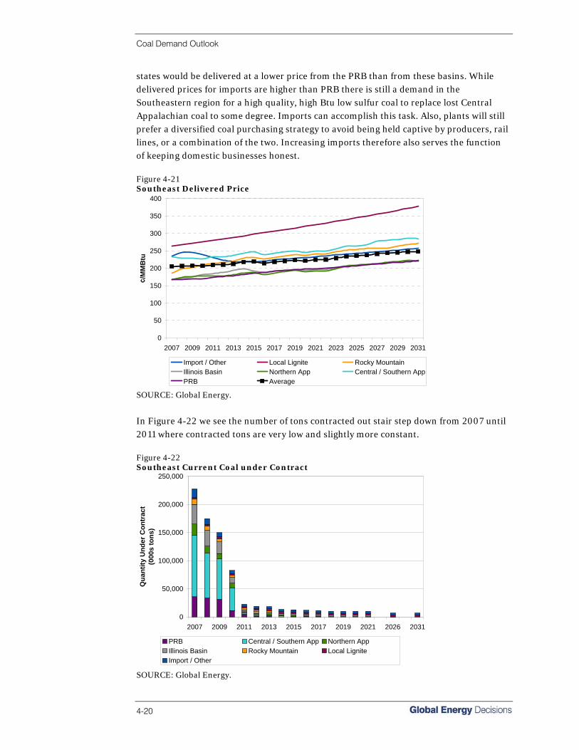
Coal Demand Outlook
4-20
states would be delivered at a lower price from the PRB than from these basins. While delivered prices for imports are higher than PRB there is still a demand in the Southeastern region for a high quality, high Btu low sulfur coal to replace lost Central Appalachian coal to some degree. Imports can accomplish this task. Also, plants will still prefer a diversified coal purchasing strategy to avoid being held captive by producers, rail lines, or a combination of the two. Increasing imports therefore also serves the function of keeping domestic businesses honest. Figure 4-21 Southeast Delivered Price
0
50
100
150
200
250
300
350
400
2007 2009 2011 2013 2015 2017 2019 2021 2023 2025 2027 2029 2031
¢/M
MB
tu
Import / Other Local Lignite Rocky MountainIllinois Basin Northern App Central / Southern AppPRB Average
SOURCE: Global Energy.
In Figure 4-22 we see the number of tons contracted out stair step down from 2007 until 2011 where contracted tons are very low and slightly more constant. Figure 4-22 Southeast Current Coal under Contract
0
50,000
100,000
150,000
200,000
250,000
2007 2009 2011 2013 2015 2017 2019 2021 2026 2031
Qua
ntity
Und
er C
ontr
act
(000
s to
ns)
PRB Central / Southern App Northern AppIllinois Basin Rocky Mountain Local LigniteImport / Other
SOURCE: Global Energy.

Coal Demand Outlook
Coal Reference Case, Fall 2007 4-21
West • Arizona • Idaho • New Mexico • Washington • California • Montana • Oregon • Wyoming • Colorado • Nevada • Utah
Map 4-6 West Demand Region - Current
SOURCE: Global Energy.
The 10 states of the West are projected to have the highest percentage population growth rate (36 percent) and total population (89.8 million people) by 2030. Though the region covers 10 states, most of the population growth will occur in the coastal states of California, Oregon, and Washington where a large portion of the current population is already located. Though the region should experience considerable population growth, coal power demand is forecasted to increase by only 16 percent. This disconnect is due primarily to California, Oregon, and Washington’s minimal reliance on coal power, relying more on gas and hydro power for their electricity generation. Only 10 coal plants with 2,735 MW

Coal Demand Outlook
4-22
of capacity have been proposed between 2007 and 2015 with only two currently permitted. Meanwhile 30 gas plants with a combined capacity of 13,000 MW and 22 hydro plants with a total capacity of 3,413 MW have been proposed with estimated on line dates prior to 2015. Deliveries of coal to the West region do not increase nearly as dramatically as the other regions reviewed in this study. Consumption from the two major supply basins—the Powder River Basin and the Rocky Mountain basin—will grow but at a very slow pace. Rocky Mountain consumption should increase 8 million tons or 10 percent and Powder River Basin should increase 8.5 million tons or 18 percent over the 25-year period. Figure 4-23 below shows the modest increase in coal deliveries to the region. Figure 4-23 West Delivered Coal Quantities
0
20,000
40,000
60,000
80,000
100,000
120,000
140,000
160,000
2007 2009 2011 2013 2015 2017 2019 2021 2023 2025 2027 2029 2031
000s
tons
Import / Other Local Lignite Rocky Mountain PRB
SOURCE: Global Energy.
Low cost surface mining in the PRB results in much lower FOB mine prices than the less productive underground and surface mining in the Rocky Mountain basin.
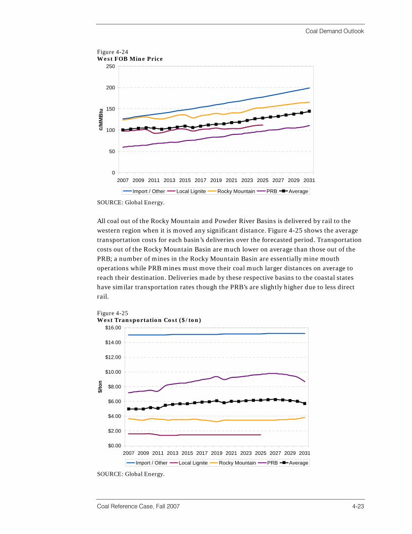
Coal Demand Outlook
Coal Reference Case, Fall 2007 4-23
Figure 4-24 West FOB Mine Price
0
50
100
150
200
250
2007 2009 2011 2013 2015 2017 2019 2021 2023 2025 2027 2029 2031
¢/M
MB
tu
Import / Other Local Lignite Rocky Mountain PRB Average
SOURCE: Global Energy.
All coal out of the Rocky Mountain and Powder River Basins is delivered by rail to the western region when it is moved any significant distance. Figure 4-25 shows the average transportation costs for each basin’s deliveries over the forecasted period. Transportation costs out of the Rocky Mountain Basin are much lower on average than those out of the PRB; a number of mines in the Rocky Mountain Basin are essentially mine mouth operations while PRB mines must move their coal much larger distances on average to reach their destination. Deliveries made by these respective basins to the coastal states have similar transportation rates though the PRB’s are slightly higher due to less direct rail. Figure 4-25 West Transportation Cost ($/ton)
$0.00
$2.00
$4.00
$6.00
$8.00
$10.00
$12.00
$14.00
$16.00
2007 2009 2011 2013 2015 2017 2019 2021 2023 2025 2027 2029 2031
$/to
n
Import / Other Local Lignite Rocky Mountain PRB Average
SOURCE: Global Energy.
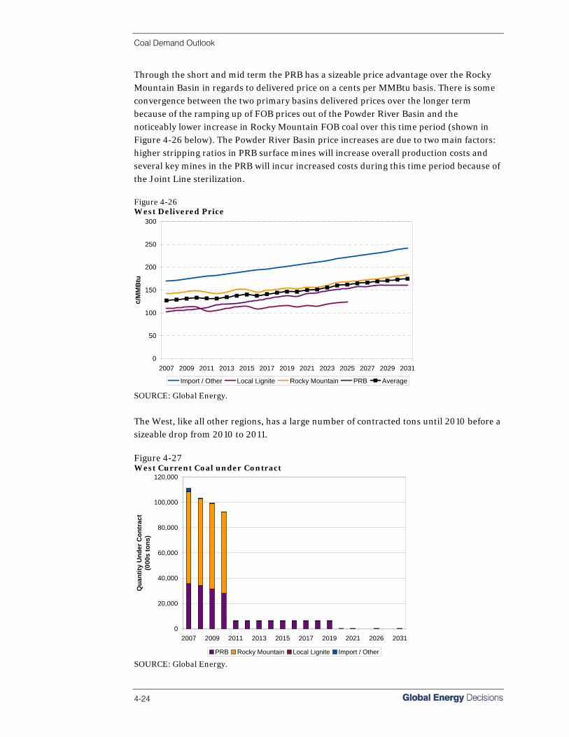
Coal Demand Outlook
4-24
Through the short and mid term the PRB has a sizeable price advantage over the Rocky Mountain Basin in regards to delivered price on a cents per MMBtu basis. There is some convergence between the two primary basins delivered prices over the longer term because of the ramping up of FOB prices out of the Powder River Basin and the noticeably lower increase in Rocky Mountain FOB coal over this time period (shown in Figure 4-26 below). The Powder River Basin price increases are due to two main factors: higher stripping ratios in PRB surface mines will increase overall production costs and several key mines in the PRB will incur increased costs during this time period because of the Joint Line sterilization. Figure 4-26 West Delivered Price
0
50
100
150
200
250
300
2007 2009 2011 2013 2015 2017 2019 2021 2023 2025 2027 2029 2031
¢/M
MB
tu
Import / Other Local Lignite Rocky Mountain PRB Average
SOURCE: Global Energy.
The West, like all other regions, has a large number of contracted tons until 2010 before a sizeable drop from 2010 to 2011. Figure 4-27 West Current Coal under Contract
0
20,000
40,000
60,000
80,000
100,000
120,000
2007 2009 2011 2013 2015 2017 2019 2021 2026 2031
Qua
ntity
Und
er C
ontr
act
(000
s to
ns)
PRB Rocky Mountain Local Lignite Import / Other SOURCE: Global Energy.
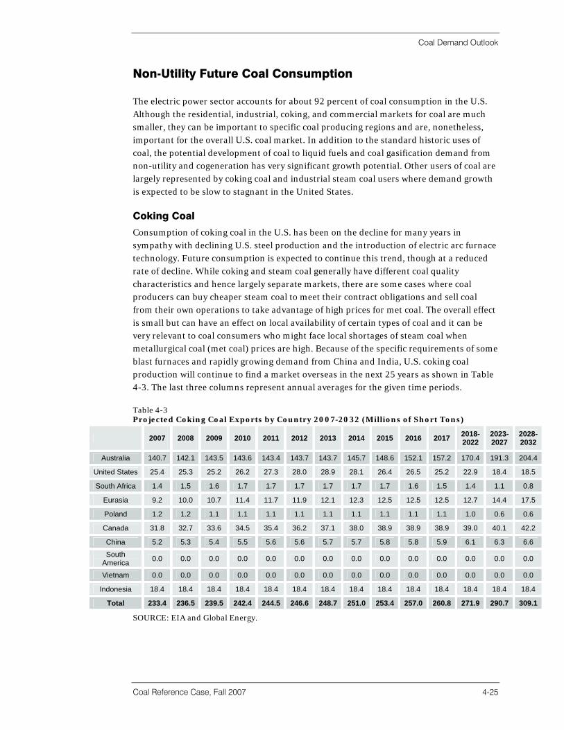
Coal Demand Outlook
Coal Reference Case, Fall 2007 4-25
Non-Utility Future Coal Consumption The electric power sector accounts for about 92 percent of coal consumption in the U.S. Although the residential, industrial, coking, and commercial markets for coal are much smaller, they can be important to specific coal producing regions and are, nonetheless, important for the overall U.S. coal market. In addition to the standard historic uses of coal, the potential development of coal to liquid fuels and coal gasification demand from non-utility and cogeneration has very significant growth potential. Other users of coal are largely represented by coking coal and industrial steam coal users where demand growth is expected to be slow to stagnant in the United States. Coking Coal
Consumption of coking coal in the U.S. has been on the decline for many years in sympathy with declining U.S. steel production and the introduction of electric arc furnace technology. Future consumption is expected to continue this trend, though at a reduced rate of decline. While coking and steam coal generally have different coal quality characteristics and hence largely separate markets, there are some cases where coal producers can buy cheaper steam coal to meet their contract obligations and sell coal from their own operations to take advantage of high prices for met coal. The overall effect is small but can have an effect on local availability of certain types of coal and it can be very relevant to coal consumers who might face local shortages of steam coal when metallurgical coal (met coal) prices are high. Because of the specific requirements of some blast furnaces and rapidly growing demand from China and India, U.S. coking coal production will continue to find a market overseas in the next 25 years as shown in Table 4-3. The last three columns represent annual averages for the given time periods. Table 4-3 Projected Coking Coal Exports by Country 2007-2032 (Millions of Short Tons)
2007 2008 2009 2010 2011 2012 2013 2014 2015 2016 2017 2018- 2022
2023- 2027
2028-2032
Australia 140.7 142.1 143.5 143.6 143.4 143.7 143.7 145.7 148.6 152.1 157.2 170.4 191.3 204.4
United States 25.4 25.3 25.2 26.2 27.3 28.0 28.9 28.1 26.4 26.5 25.2 22.9 18.4 18.5
South Africa 1.4 1.5 1.6 1.7 1.7 1.7 1.7 1.7 1.7 1.6 1.5 1.4 1.1 0.8
Eurasia 9.2 10.0 10.7 11.4 11.7 11.9 12.1 12.3 12.5 12.5 12.5 12.7 14.4 17.5
Poland 1.2 1.2 1.1 1.1 1.1 1.1 1.1 1.1 1.1 1.1 1.1 1.0 0.6 0.6
Canada 31.8 32.7 33.6 34.5 35.4 36.2 37.1 38.0 38.9 38.9 38.9 39.0 40.1 42.2
China 5.2 5.3 5.4 5.5 5.6 5.6 5.7 5.7 5.8 5.8 5.9 6.1 6.3 6.6
South America 0.0 0.0 0.0 0.0 0.0 0.0 0.0 0.0 0.0 0.0 0.0 0.0 0.0 0.0
Vietnam 0.0 0.0 0.0 0.0 0.0 0.0 0.0 0.0 0.0 0.0 0.0 0.0 0.0 0.0
Indonesia 18.4 18.4 18.4 18.4 18.4 18.4 18.4 18.4 18.4 18.4 18.4 18.4 18.4 18.4
Total 233.4 236.5 239.5 242.4 244.5 246.6 248.7 251.0 253.4 257.0 260.8 271.9 290.7 309.1
SOURCE: EIA and Global Energy.
Coal Demand Outlook
4-26
Industrial, Commercial, and Residential Coal Use
One potential new source of industrial demand for coal is in the ethanol industry as recent high gas prices have shifted some process heat fuel use in this emerging industry from gas to coal. The difficulty in permitting new coal-fired ethanol plants is an impediment to large expansion of coal use but the price differential between coal and gas is encouraging some project developers to go with coal as the fuel source. By many accounts, however, U.S. ethanol production from corn is very inefficient, which should leave the long-term viability of ethanol production in question but for the extensive history of poorly devised U.S. subsidy programs (e.g., the synfuel tax credit). The residential and commercial sectors account for a very small portion (0.4 percent) of overall coal consumption in the United States. Forecasts from the EIA indicate that residential coal consumption will continue to fall while commercial use will remain largely flat over the next 25 years (please refer to Figure 4-28 at the end of this section). Coal-to-Liquids and Coal-to-Gas
Producing liquid fuels from coal is touted by supporters as a path to energy security and an environmentally friendly way to use coal, if carbon capture and sequestration becomes economically and legally viable. The goal of coal-to-liquid (CTL) fuel conversion, using either direct or indirect liquefaction, is to break coal down into its smaller constituent molecules then add hydrogen which creates more stable molecules, similar to the ones which result from the petroleum cracking process. The important resulting products are gasoline, diesel fuel, and electric power, but fuels suitable for end use by the consumer may require additional off site refining, depending on plant design. Estimated production efficiencies vary but seem to fall in at just over two barrels of liquid product from one ton of coal, plus net electricity production. Plant designs which incorporate CTL alongside an integrated gasification combined cycle (IGCC) power plant have better estimated coal use, in the range of just less than three barrels of liquid products per ton of coal. To date no CTL plants have been constructed in the United States. Several efforts have been made toward proposals but most CTL supporters argue that significant subsidies will be necessary to get the industry off the ground. The prospects for CTL are clouded by three major impediments in the form of uncertainties about the costs and performance of CTL plants, possible costs from greenhouse gas regulation, and future oil prices. There is not yet a clear picture of how or if these uncertainties will be addressed making forecasts of CTL’s potential effect on coal demand hazy at best. The EIA projects that coal utilization by CTL plants will grow from 4 million tons per year in 2011 to 46 million tons per year in 2030. The 2030 coal consumption would represent about 440,000 barrels of liquid product per day, a very small contribution to the supply of petroleum-derived fuels. There are 14 or more CTL projects in development. Only one major project is currently as far along as the permitting stage. The 13,000 bbl/day plant in Medicine Bow, Wyoming, is scheduled for groundbreaking in 2008 with operations commencing in 2011 according

Coal Demand Outlook
Coal Reference Case, Fall 2007 4-27
to DKRW, the owner of the project. It will be constructed in conjunction with a coal mine which is to be operated by Arch, which will provide about 3 million tons per year. The remaining CTL projects currently under development are in the feasibility study stage but could add 50-75 million tons of new demand if all of them are completed. The National Coal Council has proposed expansion of CTL production to 2.6 million barrels per day or about 475 million tons of coal production. This would obviously require a tremendous investment in new coal extraction at a time when underinvestment in coal production seems to be the rule. Table 4-4 shows the list of possible CTL projects in the United States. Table 4-4 Coal-to-Liquids Plants under Development
Project Lead Project Partners Location Feedstock Status Capacity Cost
American Clean Coal Fuels None cited Oakland, IL Bituminous Feasibility 25,000 bpd N/A
Synfuels Inc. GE, Haldor-Topsoe, NACC, ExxonMobil
Ascension Parish, LA Lignite Feasibility N/A $5 billion
DKRW Advanced Fuels
Rentech, GE, Arch Coal
Medicine Bow, WY Bituminous Permitting
(2011) 13,000 bpd $1.4 billion
DKRW Advanced Fuels
Rentech, GE, Bull Mountain Land
Company Roundup, MT
Sub-bituminous/
Lignite Feasibility 22,000 bpd $1-1.5 billion
AIDEA ANRTL, CPC Cook Inlet, AK Sub-bituminous Feasibility 80,000 bpd $5-8 billion
Mingo County Rentech WV Bituminous Feasibility 20,000 bpd $2 billion
WMPI Sasol, Shell, DOE Gilberton, PA Anthracite Design 5,000 bpd $612 million
Rentech/Peabody N/A MT Sub-
bituminous/ lignite
Feasibility 10,000 to 30,000 bpd N/A
Rentech/Peabody N/A Southern IL,
Southwest IN, Western KY
Bituminous Feasibility 10,000 to 30,000 bpd N/A
Rentech* Kiewit Energy
Company, WorleyParsons
East Dubuque, IL Bituminous Construction
(2009) 1,800 bpd $800 million
Rentech Adams County Natchez, MS Coal/Petcoke Feasibility 10,000 bpd $650-750 mil
Rentech Baard Energy Wellsville, OH Sub-bituminous Feasibility 35,000 bpd $4 billion
Headwaters Hopi Tribe AZ Bituminous Feasibility 10,000 to 50,000 bpd N/A
Headwaters NACC, GRE, Falkirk ND Lignite Feasibility 40,000 bpd $3.6 billion
SOURCE: U.S. Department of Energy and Global Energy.
Efforts are under way on several fronts in coal gasification. These R&D programs are aimed at producing either synthetic natural gas (SNG), a substitute for natural gas, or hydrogen from coal gasification derived syngas. Hydrogen or SNG (after it has been reformed to remove carbon and leave only hydrogen) can be used to produce electricity from fuel cells with near zero emissions. Syngas production technology is well established but remains expensive compared to conventional coal conversion technology as evidenced by the existence of just two integrated gasification combined cycle (IGCC)

Coal Demand Outlook
4-28
power plants and one coal gasification plant in the United States. The Dakota Gasification plant in Beulah, North Dakota, profitably produces pipeline quality SNG and a number of byproducts, including CO2, 16 percent of which is sold for enhanced oil recovery in Canada essentially sequestering it permanently. The project operates under a revenue sharing agreement between the U.S. Department of Energy (DOE) and the plant owners, Basin Electric Power Cooperative. All of these technologies produce CO2 as a byproduct of the gasification process. Each one of them would require a viable technological solution to this problem in the presence of greenhouse gas regulation. Gasification has an advantage over conventional coal burning technology in that the separation of CO2 is more easily accomplished. The question of storage remains; however, and significant advances are needed to make widespread use of CTL and coal-to-SNG viable options in a carbon constrained world. 25-Year Projections
Figure 4-28 shows our forecast for non-utility coal consumption. Coal-to-liquids heat and power and expanding cement production are the only significant contributors to non-electric demand growth. Since designs for most CTL plants include some net generation capability which is sold onto the grid, this implies that some coal consumption from CTL plants could be counted toward electric generation but the forecast categories are not segregated in this way. CTL development is expected to heat up in 2015 and approach its potential by 2025 with demand from CTL plants expected to grow over 600 percent during that decade. Demand from cement production is expected to grow at an average annual rate of 3.2 percent through 2010 with an expansion of 20 million tons of cement production capacity over that period, and then stabilize at about 71 million tons per year. Demand for coking or met coal in the U.S. is expected to continue its decline through 2010 then stabilize to a slower decline through 2020. Overall, coking coal consumption is expected to decline 8.5 percent over the 25-year forecast period. Residential coal consumption is expected to continue to fall while the commercial sector increases consumption by 7.5 percent or about 0.6 percent annually. Carbon constraints have not been factored into this forecast but a cap-and-trade system would likely curb expanded use of coal in the commercial sector and would be a serious cost increase for CTL and gasification plants unable to sequester their CO2 emissions.

Coal Demand Outlook
Coal Reference Case, Fall 2007 4-29
Figure 4-28 Projected Non-Utility Coal Consumption; 2004-2031
0
20
40
60
80
100
120
140
2007
2009
2011
2013
2015
2017
2019
2021
2023
2025
2027
2029
2031
Con
sum
ptio
n(M
illio
ns o
f Ton
s)
Residential Commercial Industrial Coke PlantsOther Industrial CTL Heat and Power Net Coke Imports
SOURCE: EIA and Global Energy.


Section 5 Coal Supply Outlook


Coal Supply Outlook
Coal Reference Case, Fall 2007 5-1
Forecasted Coal Costs All cost projections are weighted by mine production. Detailed tables corresponding to figures in this section can be found in Appendix C. U.S. Fully Allocated Costs
As discussed in Section 2, fully allocated costs are the summation of cash costs, capital recovery costs, and return on capital costs. Fully allocated costs represent what a mine will need to recover to profitably operate over the long term. It is important to note that the sale price of coal is often less than the fully allocated cost of coal; not every mine is able to fully realize its returns on capital and investment. However, by setting the costs of all mines to their fully allocated costs, Global Energy is able to compare mine costs on a consistent basis. Using the mine cost database developed as part of Global Energy’s Coal Capacity Study, we were able to assemble the likely mine costs associated with every new and existing mine in the United States. While it is useful to examine fully allocated costs on a basin level to gain better understanding of current and upcoming geological challenges or other factors specific to a given area, it is also helpful to look at the national forecast and trend for costs as these provide a solid overview of where the industry as a whole is headed. Figure 5-1 shows Global Energy’s forecasted U.S. fully allocated costs from 2007 to 2031 in constant 2007 dollars. Figure 5-1 U.S. Fully Allocated Mine Costs; 2007-2031 (Constant 2007 Dollars)
20
21
22
23
24
25
26
27
28
29
30
2007
2009
2011
2013
2015
2017
2019
2021
2023
2025
2027
2029
2031
FAC
$/to
n
U.S. Fully AllocatedC t
SOURCE: Global Energy.
U.S. coal mine fully allocated costs are expected to decrease over the next five years by about 4 percent, as shown in Figure 5-1. This is a result of increases in production of Powder River Basin coal and decreases in production of Central Appalachian coal. Without weighting the information we would see increasing fully allocated costs

Coal Supply Outlook
5-2
throughout the forecast period. The cash cost of coal is expected to rise for the following reasons: • Passage of the MINER Act of 2006 and its resulting compliance cost pressures; • Thinner, deeper seams; • Decreases in productivity; • Limits on economies of scale; • Rising prices for fuel, equipment, tires, and explosives; • Competition for skilled labor across the energy sector; and • An aging workforce that is nearing retirement in the East. The Mine Improvement and New Emergency Response (MINER) Act of 2006 is the first mine safety law amendment passed by Congress and signed by the president since 1977. Provisions in the Act include: • Maximum and minimum penalty increases for all mine safety violations; • New requirements for rescue and recovery plans, rescue teams, underground oxygen
supplies, lifelines, wireless communication, and mantags; • Notification requirements within 15 minutes to Mine Safety and Health
Administration (MSHA) for any accident that is fatal or is likely to be fatal; • Additional mine safety and engineering research from the National Institute for
Occupational Safety Health (NIOSH); and • Mine safety research and scholarship funding. Numerous industry sources have indicated that the MINER Act will add up to $8 per ton of coal extracted from underground mines. In addition to the MINER Act provisions listed above, added costs will result from ancillary compliance with the law such as miner safety training, executive media training, and investment in mobile telecommunications vehicles to coordinate governmental and media communications, etc. The law requires mines to install two-way wireless communications and mantag tracking location systems in three years. In West Virginia the deadline is less than one year. Productivity decreases caused by thinner, deeper seams; limits on the economies of scale; rising prices for fuel, equipment, tires, and explosives; competition for skilled labor across the energy sector; and an aging workforce that is nearing retirement in the East are not expected to be offset by productivity-increasing technological improvements. Historic data indicates that productivity has flattened or declined across most coal basins since the beginning of this decade. Increases in economies of scale have plateaued at the large PRB surface mines and the conditions of available coal reserves are typically less desirable than the depleted coal reserves they are replacing. The above considerations (and many others) were included in the mine cost model developed by Global Energy. Basin Fully Allocated Costs Appalachia Global Energy expects fully allocated costs for Appalachian coal mines to increase over the mid-term. A significant amount of the Appalachian fully allocated cost increase is due

Coal Supply Outlook
Coal Reference Case, Fall 2007 5-3
to increased cash costs of complying with the provisions in the MINER Act of 2006, which affects Appalachian mines more than any other region in the United States. Compliance with the new safety regulations will place a heavy burden on all underground mine operators, but the heaviest burden will be on the smaller operators who will be unable to distribute compliance costs over a broad production base. Other operating costs, particularly labor, but also fuel and equipment, will contribute to the increase in Appalachian cash and fully allocated costs. Unless there is significant consolidation of reserves and operations in the East, longwall mining will not be as economical to install. As a result, less efficient, higher cost underground operations will continue in the Appalachian region. Figure 5-2 Projected Appalachian Fully Allocated Costs (Constant 2007 Dollars)
30
35
40
45
50
55
60
65
2007
2009
2011
2013
2015
2017
2019
2021
2023
2025
2027
2029
2031
FAC
$/to
n
CAPP NAPP
SOURCE: Global Energy.
Illinois Basin Global Energy projects Illinois Basin fully allocated costs to increase over the mid-term. Operating costs will not increase as much as they will in Appalachia. Illinois Basin producers face some conditions similar to those faced by Appalachian producers—increased labor, fuel and input costs, and increased safety compliance costs. Illinois Basin fully allocated costs are expected to rise one percent over the next three years, rising more from 2010 to 2015 as mines absorb safety-related costs. Thereafter fully allocated costs should drop off before leveling off in 2019 and then increasing steadily in later years.

Coal Supply Outlook
5-4
Figure 5-3 Projected Illinois Basin Fully Allocated Costs (Constant 2007 Dollars)
25
27
29
31
33
35
37
39
41
2007
2009
2011
2013
2015
2017
2019
2021
2023
2025
2027
2029
2031
FAC
$/to
n
Illinois Basin
SOURCE: Global Energy.
Powder River Basin Powder River Basin fully allocated costs are expected to increase by approximately 5-6 percent over the next five years. Increasing coal ratios; seam splitting and coal washouts; higher input costs for fuel, labor, explosives, tires, and equipment; and increasing tax and royalty costs will all contribute. Labor is a major factor. Competition for skilled labor in the PRB is not limited to other PRB-area coal mines; employers as far away as Fort McMurray are luring PRB employees to work on the tar sand projects in Canada. In Global Energy’s price forecast, we project PRB prices to steadily climb over the mid-term, resulting in higher tax and royalty payments and thus higher cash costs. In as little as 10 years, PRB costs may rise even higher as Black Thunder, North Antelope Rochelle, and Antelope mines move operations to the east side of the Joint Line. The costs associated with building new loadouts on the west side of the Joint Line will add significant costs to those mines. Figure 5-4 Projected PRB Fully Allocated Costs (2007 Constant Dollars)
7
9
11
13
15
17
19
21
23
2007
2009
2011
2013
2015
2017
2019
2021
2023
2025
2027
2029
2031
FAC
$/to
n
NPRB SPRB
SOURCE: Global Energy.

Coal Supply Outlook
Coal Reference Case, Fall 2007 5-5
Rocky Mountain The Rocky Mountain region is not expected to see sizeable jumps in fully allocated costs over the next five years primarily as a result of increasing efficiency due to resolution of equipment and other issues. Cash costs are expected to stay steady or possibly decrease slightly. There are too many mine-specific incidents to be fully covered in this report, but longwall system issues at Foidel Creek, gas build-up in West Elk, and the shuttering of the Black Mesa mine are but a few examples of increased pressure on mines’ costs throughout this region. Fully allocated costs are expected to steadily increase over the mid term with larger increases in the long term. Figure 5-5 Projected Rocky Mountain Fully Allocated Costs (2007 Constant Dollars)
22
24
26
28
30
32
34
36
2007
2009
2011
2013
2015
2017
2019
2021
2023
2025
2027
2029
2031
FAC
$/to
n
Rocky Mountain
SOURCE: Global Energy.
Basin Productivity
Mine productivity is a measurement of how efficiently coal is extracted from a mine; it is typically measured in tons of coal extracted per miner hour. Because labor costs are such a large part of the overall direct cash costs of coal suppliers, any increase in productivity results in increased returns on capital for investors. In tight coal markets, where margins are very thin, every percent increase in productivity over competitors can be the difference between a profitable mine and a money-losing operation. U.S. Productivity
Aggregated productivity of U.S. coal mines is likely to fluctuate over the next five years as shown in Figure 5-6. The variability in productivity is mainly due to large volumes of higher cost, lower productivity mines being shut-in and some larger western mines ramping up production as market conditions and prices fluctuate. For example, in 2007 over 43 million tons of production capacity with productivity less than 19.6 tons per miner-hour will go off line. The increase in overall U.S. productivity is expected to be 1.0 percent over the next five years. With reserve blocks becoming increasingly difficult to mine we do not expect to see major increases in productivity in the future unless new technologies for extracting coal are developed.
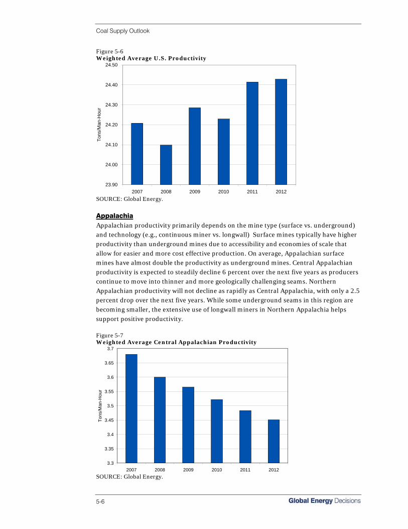
Coal Supply Outlook
5-6
Figure 5-6 Weighted Average U.S. Productivity
23.90
24.00
24.10
24.20
24.30
24.40
24.50
2007 2008 2009 2010 2011 2012
Tons
/Man
-Hou
r
SOURCE: Global Energy.
Appalachia
Appalachian productivity primarily depends on the mine type (surface vs. underground) and technology (e.g., continuous miner vs. longwall) Surface mines typically have higher productivity than underground mines due to accessibility and economies of scale that allow for easier and more cost effective production. On average, Appalachian surface mines have almost double the productivity as underground mines. Central Appalachian productivity is expected to steadily decline 6 percent over the next five years as producers continue to move into thinner and more geologically challenging seams. Northern Appalachian productivity will not decline as rapidly as Central Appalachia, with only a 2.5 percent drop over the next five years. While some underground seams in this region are becoming smaller, the extensive use of longwall miners in Northern Appalachia helps support positive productivity. Figure 5-7 Weighted Average Central Appalachian Productivity
3.3
3.35
3.4
3.45
3.5
3.55
3.6
3.65
3.7
2007 2008 2009 2010 2011 2012
Tons
/Man
-Hou
r
SOURCE: Global Energy.

Coal Supply Outlook
Coal Reference Case, Fall 2007 5-7
Figure 5-8 Weighted Average Northern Appalachian Productivity
4.8
4.82
4.84
4.86
4.88
4.9
4.92
4.94
4.96
4.98
5
5.02
2007 2008 2009 2010 2011 2012
Tons
/Man
-Hou
r
SOURCE: Global Energy.
Illinois Basin Even though Illinois Basin production capacity will grow over the mid-term, productivity is expected to decline through 2010. Productivity has been slowly eroding in Illinois Basin since 2001 and Global Energy estimates that productivity will continue to decline, although at a very low rate. Estimated productivity in 2007 is 4.73 tons per miner hour and will decline 1.3 percent by 2009. Productivity should rebound 0.8 percent by 2011 to 4.71 tons per miner hour due to flattening productivity at most Illinois mines coupled with the ramping up of the North Canton mine in 2011. Figure 5-9 Weighted Average Illinois Basin Productivity
4.62
4.64
4.66
4.68
4.7
4.72
4.74
2007 2008 2009 2010 2011 2012
Tons
/Man
-Hou
r
SOURCE: Global Energy.

Coal Supply Outlook
5-8
Powder River Basin Productivity in the Powder River Basin is expected to flatten over the next three years, but remain the highest of all the U.S. producing basins at over 39 tons per miner hour. A relatively dramatic decline in productivity will take place in 2010 when some PRB mines will encounter split seams, sand channel washouts, harder overburden, and increasing coal ratios. The stratigraphic cross section shown in Figure 5-10 is typical of some of the future mining conditions that will be encountered. Mining operations at the Buckskin mine are currently near the A-A mark in the diagram below and are moving from east to west. In several years, the mine will encounter a sandstone washout that will have replaced roughly half of the coal seam. Mine costs will go up as productivity declines until operations resume to the west of the washout. Figure 5-11 charts the change in the projected annual productivity in the Powder River Basin. Figure 5-10 Stratigraphic Cross Section Depicting Future Mining Conditions at Buckskin Mine
SOURCE: USGS.
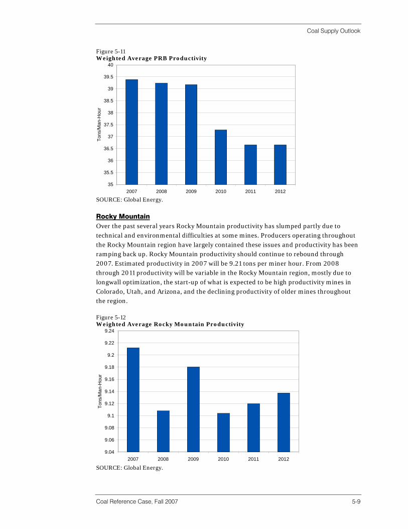
Coal Supply Outlook
Coal Reference Case, Fall 2007 5-9
Figure 5-11 Weighted Average PRB Productivity
35
35.5
36
36.5
37
37.5
38
38.5
39
39.5
40
2007 2008 2009 2010 2011 2012
Tons
/Man
-Hou
r
SOURCE: Global Energy.
Rocky Mountain Over the past several years Rocky Mountain productivity has slumped partly due to technical and environmental difficulties at some mines. Producers operating throughout the Rocky Mountain region have largely contained these issues and productivity has been ramping back up. Rocky Mountain productivity should continue to rebound through 2007. Estimated productivity in 2007 will be 9.21 tons per miner hour. From 2008 through 2011 productivity will be variable in the Rocky Mountain region, mostly due to longwall optimization, the start-up of what is expected to be high productivity mines in Colorado, Utah, and Arizona, and the declining productivity of older mines throughout the region. Figure 5-12 Weighted Average Rocky Mountain Productivity
9.04
9.06
9.08
9.1
9.12
9.14
9.16
9.18
9.2
9.22
9.24
2007 2008 2009 2010 2011 2012
Tons
/Man
-Hou
r
SOURCE: Global Energy.
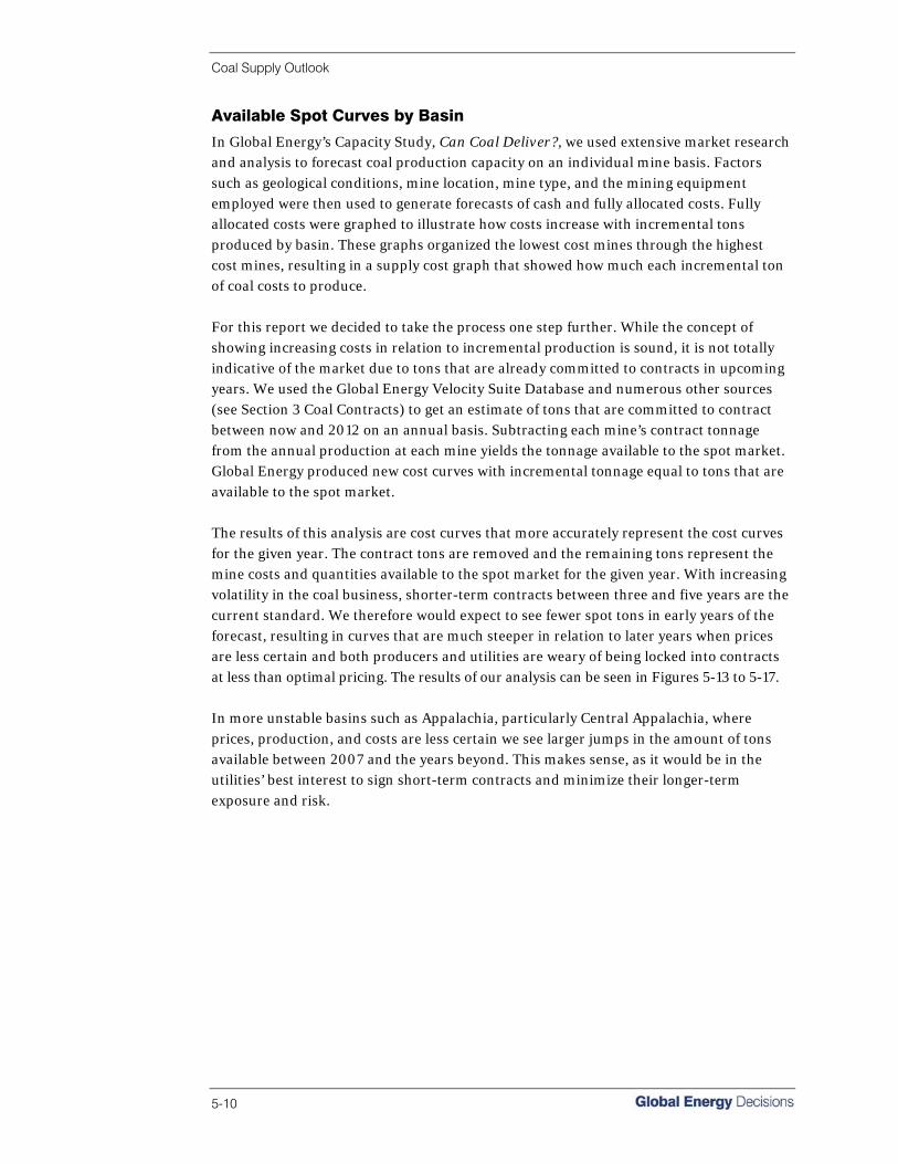
Coal Supply Outlook
5-10
Available Spot Curves by Basin
In Global Energy’s Capacity Study, Can Coal Deliver?, we used extensive market research and analysis to forecast coal production capacity on an individual mine basis. Factors such as geological conditions, mine location, mine type, and the mining equipment employed were then used to generate forecasts of cash and fully allocated costs. Fully allocated costs were graphed to illustrate how costs increase with incremental tons produced by basin. These graphs organized the lowest cost mines through the highest cost mines, resulting in a supply cost graph that showed how much each incremental ton of coal costs to produce. For this report we decided to take the process one step further. While the concept of showing increasing costs in relation to incremental production is sound, it is not totally indicative of the market due to tons that are already committed to contracts in upcoming years. We used the Global Energy Velocity Suite Database and numerous other sources (see Section 3 Coal Contracts) to get an estimate of tons that are committed to contract between now and 2012 on an annual basis. Subtracting each mine’s contract tonnage from the annual production at each mine yields the tonnage available to the spot market. Global Energy produced new cost curves with incremental tonnage equal to tons that are available to the spot market. The results of this analysis are cost curves that more accurately represent the cost curves for the given year. The contract tons are removed and the remaining tons represent the mine costs and quantities available to the spot market for the given year. With increasing volatility in the coal business, shorter-term contracts between three and five years are the current standard. We therefore would expect to see fewer spot tons in early years of the forecast, resulting in curves that are much steeper in relation to later years when prices are less certain and both producers and utilities are weary of being locked into contracts at less than optimal pricing. The results of our analysis can be seen in Figures 5-13 to 5-17. In more unstable basins such as Appalachia, particularly Central Appalachia, where prices, production, and costs are less certain we see larger jumps in the amount of tons available between 2007 and the years beyond. This makes sense, as it would be in the utilities’ best interest to sign short-term contracts and minimize their longer-term exposure and risk.
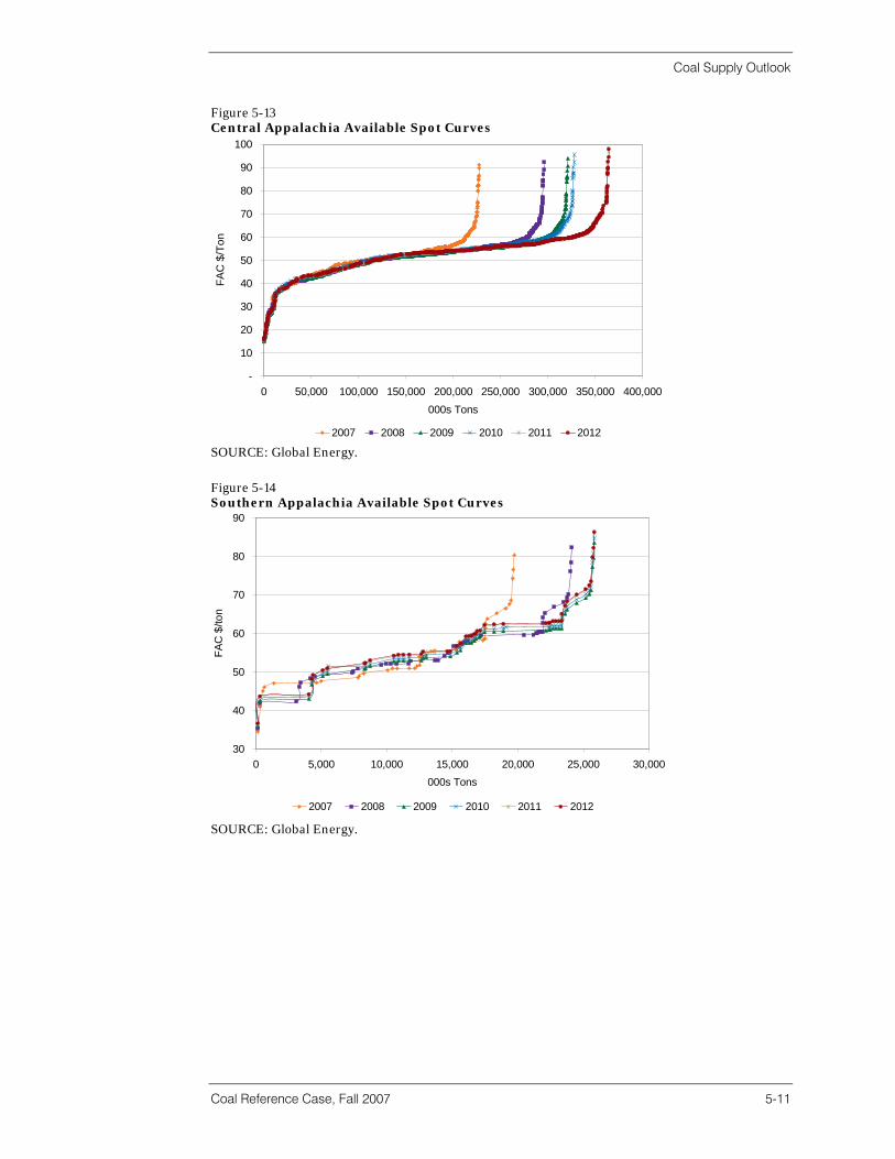
Coal Supply Outlook
Coal Reference Case, Fall 2007 5-11
Figure 5-13 Central Appalachia Available Spot Curves
-
10
20
30
40
50
60
70
80
90
100
0 50,000 100,000 150,000 200,000 250,000 300,000 350,000 400,000000s Tons
FAC
$/T
on
2007 2008 2009 2010 2011 2012 SOURCE: Global Energy.
Figure 5-14 Southern Appalachia Available Spot Curves
30
40
50
60
70
80
90
0 5,000 10,000 15,000 20,000 25,000 30,000000s Tons
FAC
$/to
n
2007 2008 2009 2010 2011 2012
SOURCE: Global Energy.

Coal Supply Outlook
5-12
Figure 5-15 Northern Appalachia Available Spot Curves
-
10
20
30
40
50
60
70
80
90
0 50,000 100,000 150,000 200,000000s Tons
FAC
$/to
n
2007 2008 2009 2010 2011 2012 SOURCE: Global Energy.
Other trends may be seen in basin cost curves as well. Looking at the Illinois Basin we see curves that are somewhat evenly spaced for the next few years, indicating that while conditions in that particular marketplace are not completely stabilized consumers do not expect to see radical changes coming to the spot markets in the short term. This gives producers and utilities the comfort of having contracts in place while having the knowledge that if radical changes do take place they will have an opportunity to improve their position in the short term. This same trend can be seen in the cost curve of the Rocky Mountains. Figure 5-16 Illinois Basin Available Spot Curves
10
20
30
40
50
60
70
0 20,000 40,000 60,000 80,000 100,000 120,000 140,000
000s Tons
FAC
$/to
n
2007 2008 2009 2010 2011 2012 SOURCE: Global Energy.

Coal Supply Outlook
Coal Reference Case, Fall 2007 5-13
Figure 5-17 Rocky Mountain Available Spot Curves
10
15
20
25
30
35
40
45
0 25,000 50,000 75,000 100,000 125,000 150,000 175,000000s Tons
FAC
$/to
n
2007 2008 2009 2010 2011 2012 SOURCE: Global Energy.
The Powder River Basin is thought of as a stable basin as far as production is concerned despite the fact that it is likely to remain flat in 2007. Based on the cost curves seen in Figure 5-18 one can see that there are 98.3 and 71.8 million tons of contracted coal that become available at the end of 2007 and 2008, respectively. The one major concern of the basin currently is transportation issues and the ability of the UP and BNSF to make deliveries on time. Ideas on how to solve these problems are in the works, and utilities may be holding off the signing of some contracts beyond 2008 until it becomes more apparent how these transportation issues will be handled—whether through the construction of a new Class I railroad into the PRB, upgrades to existing railroads, or a combination of the two. Figure 5-18 Powder River Basin Available Spot Curves
8.50
9.00
9.50
10.00
10.50
11.00
11.50
12.00
0 100,000 200,000 300,000 400,000 500,000 600,000Free Cumulative Tons (000s)
FAC
$/to
n
2007 2008 2009 2010 2011 2012 SOURCE: Global Energy.

Coal Supply Outlook
5-14
FOB And Delivered Prices By Supply Basin And Region Coal’s heterogeneous nature and the distinct pricing and demand characteristics of each coal supply region inspired Global Energy to categorize coal supply into regions which are subsets of commonly known coal basins. This section will cover the forecasted spot Free on Board (FOB) mine price listed by coal supply region. Each distinct coal supply region in this section can be identified by several key factors: the location (basin and state), the heat content (Btu/lb), and the sulfur (lbs SO2/MMBtu) content. As an example, pricing for coal originating from the Northern Powder River Basin (NPRB) will be different than coal from the Southern Powder River Basin (SPRB). Not only will each basin have multiple coal qualities, but each basin is located in a unique geographic region, with specific geologic conditions and transportation options. For example, “SPRBHiLo” represents coal form the SPRB with heat content greater than 8,600 Btu/lb and sulfur content less than 1.2 lbs SO2/MMBtu. One can reasonably expect SPRBHiLo to be priced higher than SPRBLoLo. Map 5-1 U.S. Coal Supply Regions
SOURCE: Global Energy.
Spot FOB mine prices are defined as the price a coal consumer should expect to pay for coal at the coal source before transportation and handling fees. The primary source for Global Energy’s reference case FOB pricing data is the Velocity Suite database, and ultimately the FERC Form 423. While the FOB mine prices are not reported to FERC,
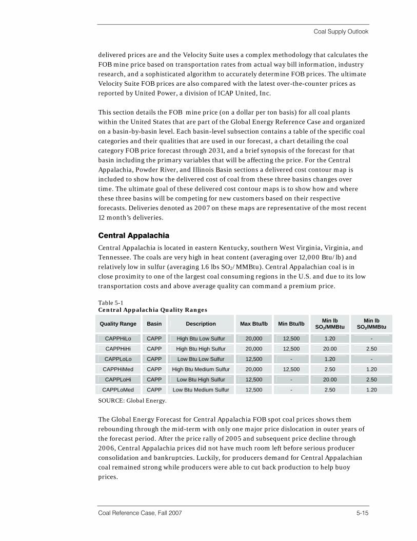
Coal Supply Outlook
Coal Reference Case, Fall 2007 5-15
delivered prices are and the Velocity Suite uses a complex methodology that calculates the FOB mine price based on transportation rates from actual way bill information, industry research, and a sophisticated algorithm to accurately determine FOB prices. The ultimate Velocity Suite FOB prices are also compared with the latest over-the-counter prices as reported by United Power, a division of ICAP United, Inc. This section details the FOB mine price (on a dollar per ton basis) for all coal plants within the United States that are part of the Global Energy Reference Case and organized on a basin-by-basin level. Each basin-level subsection contains a table of the specific coal categories and their qualities that are used in our forecast, a chart detailing the coal category FOB price forecast through 2031, and a brief synopsis of the forecast for that basin including the primary variables that will be affecting the price. For the Central Appalachia, Powder River, and Illinois Basin sections a delivered cost contour map is included to show how the delivered cost of coal from these three basins changes over time. The ultimate goal of these delivered cost contour maps is to show how and where these three basins will be competing for new customers based on their respective forecasts. Deliveries denoted as 2007 on these maps are representative of the most recent 12 month’s deliveries. Central Appalachia
Central Appalachia is located in eastern Kentucky, southern West Virginia, Virginia, and Tennessee. The coals are very high in heat content (averaging over 12,000 Btu/lb) and relatively low in sulfur (averaging 1.6 lbs SO2/MMBtu). Central Appalachian coal is in close proximity to one of the largest coal consuming regions in the U.S. and due to its low transportation costs and above average quality can command a premium price. Table 5-1 Central Appalachia Quality Ranges
Quality Range Basin Description Max Btu/lb Min Btu/lb Min lb SO2/MMBtu
Min lb SO2/MMBtu
CAPPHiLo CAPP High Btu Low Sulfur 20,000 12,500 1.20 -
CAPPHiHi CAPP High Btu High Sulfur 20,000 12,500 20.00 2.50
CAPPLoLo CAPP Low Btu Low Sulfur 12,500 - 1.20 -
CAPPHiMed CAPP High Btu Medium Sulfur 20,000 12,500 2.50 1.20
CAPPLoHi CAPP Low Btu High Sulfur 12,500 - 20.00 2.50
CAPPLoMed CAPP Low Btu Medium Sulfur 12,500 - 2.50 1.20
SOURCE: Global Energy.
The Global Energy Forecast for Central Appalachia FOB spot coal prices shows them rebounding through the mid-term with only one major price dislocation in outer years of the forecast period. After the price rally of 2005 and subsequent price decline through 2006, Central Appalachia prices did not have much room left before serious producer consolidation and bankruptcies. Luckily, for producers demand for Central Appalachian coal remained strong while producers were able to cut back production to help buoy prices.
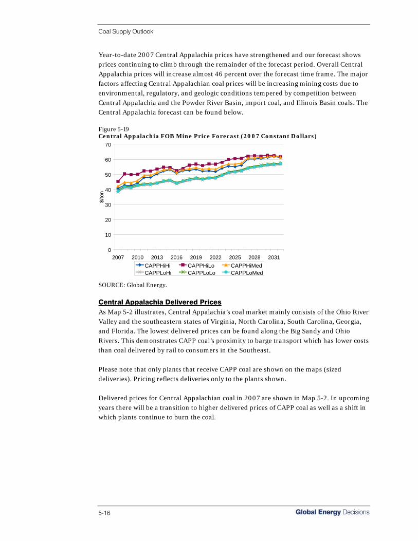
Coal Supply Outlook
5-16
Year-to-date 2007 Central Appalachia prices have strengthened and our forecast shows prices continuing to climb through the remainder of the forecast period. Overall Central Appalachia prices will increase almost 46 percent over the forecast time frame. The major factors affecting Central Appalachian coal prices will be increasing mining costs due to environmental, regulatory, and geologic conditions tempered by competition between Central Appalachia and the Powder River Basin, import coal, and Illinois Basin coals. The Central Appalachia forecast can be found below. Figure 5-19 Central Appalachia FOB Mine Price Forecast (2007 Constant Dollars)
0
10
20
30
40
50
60
70
2007 2010 2013 2016 2019 2022 2025 2028 2031
$/to
n
CAPPHiHi CAPPHiLo CAPPHiMedCAPPLoHi CAPPLoLo CAPPLoMed
SOURCE: Global Energy.
Central Appalachia Delivered Prices As Map 5-2 illustrates, Central Appalachia’s coal market mainly consists of the Ohio River Valley and the southeastern states of Virginia, North Carolina, South Carolina, Georgia, and Florida. The lowest delivered prices can be found along the Big Sandy and Ohio Rivers. This demonstrates CAPP coal’s proximity to barge transport which has lower costs than coal delivered by rail to consumers in the Southeast. Please note that only plants that receive CAPP coal are shown on the maps (sized deliveries). Pricing reflects deliveries only to the plants shown. Delivered prices for Central Appalachian coal in 2007 are shown in Map 5-2. In upcoming years there will be a transition to higher delivered prices of CAPP coal as well as a shift in which plants continue to burn the coal.

Coal Supply Outlook
Coal Reference Case, Fall 2007 5-17
Map 5-2 Central Appalachia 2007 Delivered Prices
SOURCE: Global Energy.
In 2015, the area of low cost delivered prices between $1.50/MMBtu and $2.00/MMBtu has slightly decreased in size. Delivered prices to other areas of the country have not varied a great deal remaining somewhere between $2.00 and $3.00/MMBtu for the majority of plants. What is most noticeable is a decrease in the number of plants burning Central Appalachian coal from 141 plants in 2007 to 115 plants in 2015. This change is due to decreasing supply of CAPP coal as well as scrubber installations and the ability of plants to burn high sulfur coal while still meeting emissions requirements. Central Appalachian 2015 delivered prices can be seen in Map 5-3.

Coal Supply Outlook
5-18
Map 5-3 Central Appalachia 2015 Delivered Prices
SOURCE: Global Energy.
The change in delivered prices is more noticeable from the years 2015 to 2031, where it is apparent that delivered prices have increased in all areas of the country, particularly the Ohio River market. The increases in delivered prices are mainly due to increases in production costs associated with degrading reserves, higher input costs (labor, fuel, explosives, etc.), and stricter mining regulations. There are 73 plants burning CAPP coal in 2031, an even more dramatic decrease than the decline from 2007 to 2015. The reduction in the number of plants is due to a combination of a large decrease in CAPP production and therefore less available coal, higher pricing mentioned above, and increased scrubber installations and technologies to deal with the emissions of higher sulfur coals that make higher sulfur coals from competing basins more appealing.
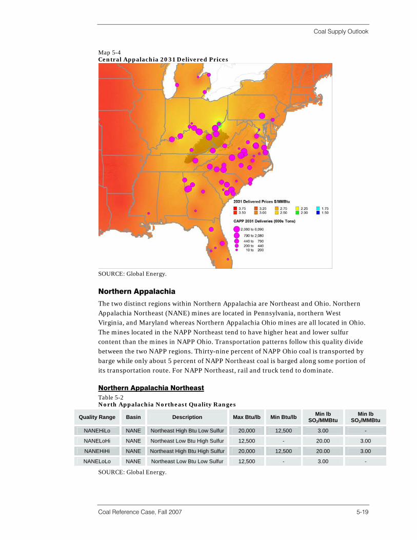
Coal Supply Outlook
Coal Reference Case, Fall 2007 5-19
Map 5-4 Central Appalachia 2031 Delivered Prices
SOURCE: Global Energy.
Northern Appalachia
The two distinct regions within Northern Appalachia are Northeast and Ohio. Northern Appalachia Northeast (NANE) mines are located in Pennsylvania, northern West Virginia, and Maryland whereas Northern Appalachia Ohio mines are all located in Ohio. The mines located in the NAPP Northeast tend to have higher heat and lower sulfur content than the mines in NAPP Ohio. Transportation patterns follow this quality divide between the two NAPP regions. Thirty-nine percent of NAPP Ohio coal is transported by barge while only about 5 percent of NAPP Northeast coal is barged along some portion of its transportation route. For NAPP Northeast, rail and truck tend to dominate. Northern Appalachia Northeast Table 5-2 North Appalachia Northeast Quality Ranges
Quality Range Basin Description Max Btu/lb Min Btu/lb Min lb SO2/MMBtu
Min lb SO2/MMBtu
NANEHiLo NANE Northeast High Btu Low Sulfur 20,000 12,500 3.00 -
NANELoHi NANE Northeast Low Btu High Sulfur 12,500 - 20.00 3.00
NANEHiHi NANE Northeast High Btu High Sulfur 20,000 12,500 20.00 3.00
NANELoLo NANE Northeast Low Btu Low Sulfur 12,500 - 3.00 -
SOURCE: Global Energy.

Coal Supply Outlook
5-20
The forecast for Northern Appalachia Northeast coal shows flat prices through the mid term with minimal gains into the longer-term range of this forecast. Over the course of this forecast we expect Northern Appalachia Northeast coal prices to escalate by 29 percent. Over the short term, North Appalachia Northeast prices will be held in check by increased competition from both the PRB and Illinois Basin, but in the longer run NAPP Northeast should expect to see increased demand for their product and more robust pricing as more plants are scrubbed and CAPP production declines. The Northern Appalachia Northeast forecast can be found below. Figure 5-20 North Appalachia Northeast FOB Mine Price Forecast (2007 Constant Dollars)
0
10
20
30
40
50
60
70
2007 2010 2013 2016 2019 2022 2025 2028 2031
$/to
n
NANEHiHi NANEHiLo NANELoHi NANELoLo
SOURCE: Global Energy.
Northern Appalachia Ohio Table 5-3 North Appalachia Ohio Quality Ranges
Quality Range Basin Description Max Btu/lb
Min Btu/lb
Min lb SO2/MMBtu
Min lb SO2/MMBtu
NAOHLoLo NAOH Northwest Low Btu Low Sulfur 12,000 - 5.00 -
NAOHHiLo NAOH Northwest High Btu Low Sulfur 20,000 12,000 5.00 -
NAOHLoHi NAOH Northwest Low Btu High Sulfur 12,000 - 20.00 5.00
NAOHHiHi NAOH Northwest High Btu High Sulfur 20,000 12,000 20.00 5.00
SOURCE: Global Energy.
The forecast for Northern Appalachia Ohio coal shows flat prices through the mid term with stronger gains than NAPP Northeast into the longer-term range of this forecast. Northern Appalachia Ohio coal prices are forecast to escalate by almost 26 percent. This is due to the lower level of expected growth in demand for these coals and the fact that these mines will compete against lower cost Illinois Basin coals once the scrubber build-out occurs. The Northern Appalachia Ohio forecast can be found below in Figure 5-21.

Coal Supply Outlook
Coal Reference Case, Fall 2007 5-21
Figure 5-21 Northern Appalachia Ohio FOB Mine Price Forecast (2007 Constant Dollars)
0
10
20
30
40
50
60
70
2007 2010 2013 2016 2019 2022 2025 2028 2031
$/to
n
NAOHHiHi NAOHHiLo NAOHLoHi NAOHLoLo SOURCE: Global Energy.
Illinois Basin Illinois Basin mines are located in Indiana, Illinois, and the western panhandle of Kentucky. Virtually all of the coal from the Illinois Basin is non-compliance (> 1.2 lbs/MMBtu) high sulfur coal, though it is considerably higher in heat content than western sub bituminous coal. In fact, over 50 percent of 2006 delivered Illinois Basin coal had sulfur content greater than 5 lbs SO2/MMbtu. Illinois Basin FOB Mine Prices Table 5-4 Illinois Basin Quality Ranges
Quality Range Basin Description Max Btu/lb Min Btu/lb Min lb SO2/MMBtu
Min lb SO2/MMBtu
ILLBHiLo ILLB High Btu Low Sulfur 20,000 11,300 3.00 -
ILLBLoHi ILLB Low Btu High Sulfur 11,300 - 20.00 3.00
ILLBLoMed ILLB Low Btu Medium Sulfur 11,300 - 3.00 1.20
ILLBHiHi ILLB High Btu High Sulfur 20,000 11,300 20.00 3.00
ILLBLoLo ILLB Low Btu Low Sulfur 11,300 - 1.20 -
SOURCE: Global Energy.
Producers, consumers, and analysts are all watching the Illinois Basin market closely. They are waiting to see what happens as the market grows for higher sulfur coal due to the scrubber build-out. The question on everyone’s mind is whether Illinois Basin producers will recapture a significant portion of the market they lost due to the Clean Air Act Amendments. Illinois Basin mine prices will stay relatively flat over the mid term, even with significant growth in production and a corresponding increase in demand for Illinois Basin coal. Global Energy’s forecast for the Illinois Basin does show strengthening prices (almost 24 percent gain) over the duration of the forecast but prices are kept in

Coal Supply Outlook
5-22
check due to the increased competitive interplay between Illinois Basin, Central Appalachia, and the Powder River Basin all vying for the same consumers. The Illinois FOB price forecast is detailed in Figure 5-22. Figure 5-22 Illinois Basin FOB Mine Price Forecast (2007 Constant Dollars)
0
10
20
30
40
50
60
2007 2010 2013 2016 2019 2022 2025 2028 2031
$/to
n
ILLBHiHi ILLBHiLo ILLBLoHi ILLBLoLo ILLBLoMed
SOURCE: Global Energy.
Illinois Basin Delivered Prices Historically the Illinois Basin’s coal has not moved far from its source on a regular basis, mostly due to the coal’s high sulfur characteristics and a concentration of plants with the ability to burn this coal in close proximity to the basin. As Map 5-5 shows, a large portion of deliveries that travel beyond the confines of the Illinois Basin are delivered by barge up the Ohio River or south to plants such as the Tennessee Valley Authority’s Cumberland, Johnsonville, Colbert, and Widows Creek plants. Please note that only plants that receive Illinois Basin coal are shown on the maps (sized by deliveries). Pricing reflects deliveries only to the plants shown.

Coal Supply Outlook
Coal Reference Case, Fall 2007 5-23
Map 5-5 Illinois Basin 2007 Delivered Prices
SOURCE: Global Energy.
Global Energy expects the Illinois Basin and its current market to see fairly significant changes in delivered prices between 2007 and 2015. While the geographic area that can be reached at delivered prices of less than $2.00/MMBtu will decrease only slightly, delivered prices in the Illinois Basin itself will increase substantially. Forecasted delivered prices for 2015 can be seen in Map 5-6.

Coal Supply Outlook
5-24
Map 5-6 Illinois Basin 2015 Delivered Prices
SOURCE: Global Energy.
As with Central Appalachia, a more significant change in delivered prices is noticeable between 2015 and 2031 particularly for the majority of those plants in close proximity to the basin. With Central Appalachia’s decreasing production over the next 25 years it is expected that demand for Illinois Basin coal will increase and along with it delivered prices as can be seen in Map 5-7. Railroads’ desires to increase profits may also play a role in increasing delivered costs as they try to capitalize on new demand for Illinois Basin coal.

Coal Supply Outlook
Coal Reference Case, Fall 2007 5-25
Map 5-7 Illinois Basin 2031 Delivered Prices
SOURCE: Global Energy.
Powder River Basin
The Powder River Basin can be divided into two distinct regions: the Northern and Southern Powder River Basin. The Northern Powder River Basin (NPRB) mines are located in Montana with the exception of the proposed Young’s Creek Mine, whereas all Southern Powder River Basin (SPRB) mines are located in Wyoming. North PRB mines have a higher heat, similar sulfur, and higher chlorine content than the SPRB mines. Additionally, though NPRB mines are captive to BNSF rail (SPRB mines have both UP and BNSF rail lines to haul coal), there is ample spare capacity to haul the coal on the northern BNSF track whereas the SPRB Joint Line is running at near capacity. Northern Powder River Basin FOB Mine Prices Table 5-5 Northern Powder River Basin Quality Ranges
Quality Range Basin Description Max Btu/lb Min Btu/lb Min lb SO2/MMBtu
Min lb SO2/MMBtu
NPRBLoLo NPRB Low Btu Low Sulfur 9,000 - 1.20 -
NPRBHiHi NPRB High Btu High Sulfur 20,000 9,000 20.00 1.20
NPRBHiLo NPRB High Btu Low Sulfur 20,000 9,000 1.20 -
NPRBLoHi NPRB Low Btu High Sulfur 9,000 - 20.00 1.20
SOURCE: Global Energy.

Coal Supply Outlook
5-26
Global Energy’s forecast for Northern Powder River Basin coal shows that after short-term price swings over the next few years we expect prices to continue to strengthen. Demand should stay strong and grow for this product and as long as available supply grows in step with demand we expect over 50 percent increase in price over the forecast time frame. There are many factors influencing the long-term pricing of Northern Powder River coal: Southern PRB competition, regulatory and tax related environment for Montana producers, and rail rates. This decrease in differential between NPRB coal types comes as no surprise since the sulfur content is relatively low and scrubber additions makes the sulfur content of coal less an issue. The Northern Powder River Basin spot FOB forecast can be found below. Figure 5-23 Northern Powder River Basin FOB Mine Price Forecast (2007 Constant Dollars)
0
5
10
15
20
25
2007 2010 2013 2016 2019 2022 2025 2028 2031
$/to
n
NPRBHiLo NPRBHiHi NPRBLoHi NPRBLoLo SOURCE: Global Energy.
Southern Powder River Basin FOB Mine Prices Table 5-6 Southern Powder River Basin FOB Mine Prices
Quality Range Basin Description Max Btu/lb
Min Btu/lb
Min lb SO2/MMBtu
Min lb SO2/MMBtu
SPRBLoHi SPRB Low Btu High Sulfur 8,600 - 20.00 1.20
SPRBLoLo SPRB Low Btu Low Sulfur 8,600 - 1.20 0.80
SPRBHiHi SPRB High Btu High Sulfur 20,000 8,600 20.00 1.20
SPRBLoUltraLo SPRB Low Btu Ultra Low Sulfur 8,600 - 0.80 -
SPRBHiLo SPRB High Btu Low Sulfur 20,000 8,600 1.20 0.80
SPRBHiUltraLo SPRB High Btu Ultra Low Sulfur 20,000 8,600 0.80 -
SOURCE: Global Energy.
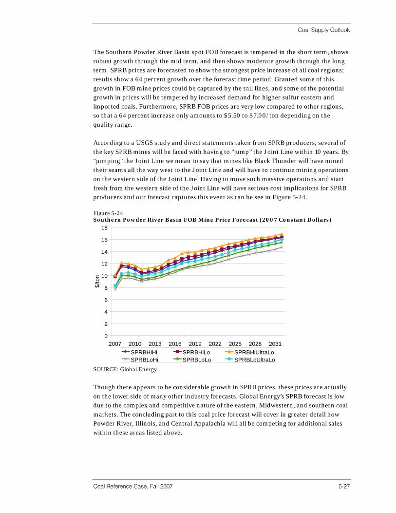
Coal Supply Outlook
Coal Reference Case, Fall 2007 5-27
The Southern Powder River Basin spot FOB forecast is tempered in the short term, shows robust growth through the mid term, and then shows moderate growth through the long term. SPRB prices are forecasted to show the strongest price increase of all coal regions; results show a 64 percent growth over the forecast time period. Granted some of this growth in FOB mine prices could be captured by the rail lines, and some of the potential growth in prices will be tempered by increased demand for higher sulfur eastern and imported coals. Furthermore, SPRB FOB prices are very low compared to other regions, so that a 64 percent increase only amounts to $5.50 to $7.00/ton depending on the quality range. According to a USGS study and direct statements taken from SPRB producers, several of the key SPRB mines will be faced with having to “jump” the Joint Line within 10 years. By “jumping” the Joint Line we mean to say that mines like Black Thunder will have mined their seams all the way west to the Joint Line and will have to continue mining operations on the western side of the Joint Line. Having to move such massive operations and start fresh from the western side of the Joint Line will have serious cost implications for SPRB producers and our forecast captures this event as can be see in Figure 5-24. Figure 5-24 Southern Powder River Basin FOB Mine Price Forecast (2007 Constant Dollars)
0
2
4
6
8
10
12
14
16
18
2007 2010 2013 2016 2019 2022 2025 2028 2031
$/to
n
SPRBHiHi SPRBHiLo SPRBHiUltraLoSPRBLoHi SPRBLoLo SPRBLoUltraLo
SOURCE: Global Energy.
Though there appears to be considerable growth in SPRB prices, these prices are actually on the lower side of many other industry forecasts. Global Energy’s SPRB forecast is low due to the complex and competitive nature of the eastern, Midwestern, and southern coal markets. The concluding part to this coal price forecast will cover in greater detail how Powder River, Illinois, and Central Appalachia will all be competing for additional sales within these areas listed above.
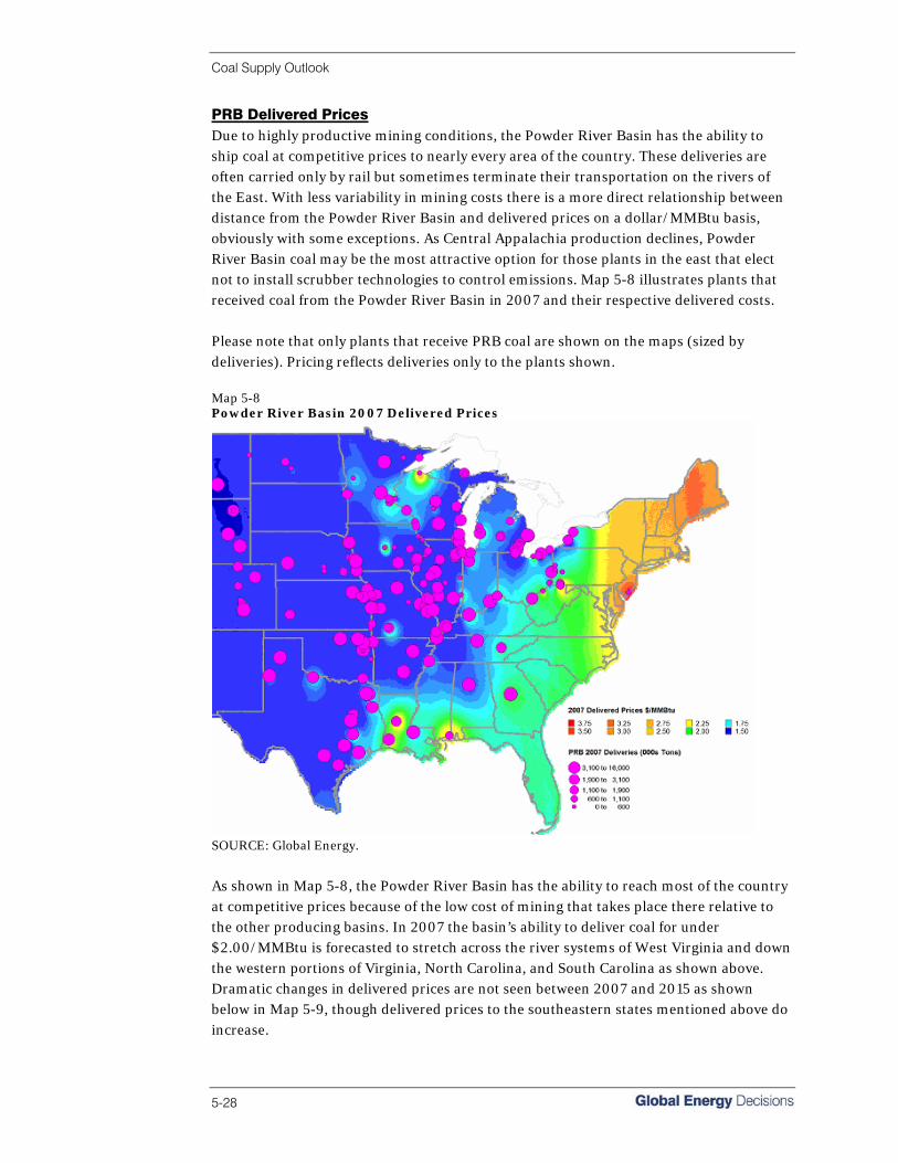
Coal Supply Outlook
5-28
PRB Delivered Prices Due to highly productive mining conditions, the Powder River Basin has the ability to ship coal at competitive prices to nearly every area of the country. These deliveries are often carried only by rail but sometimes terminate their transportation on the rivers of the East. With less variability in mining costs there is a more direct relationship between distance from the Powder River Basin and delivered prices on a dollar/MMBtu basis, obviously with some exceptions. As Central Appalachia production declines, Powder River Basin coal may be the most attractive option for those plants in the east that elect not to install scrubber technologies to control emissions. Map 5-8 illustrates plants that received coal from the Powder River Basin in 2007 and their respective delivered costs. Please note that only plants that receive PRB coal are shown on the maps (sized by deliveries). Pricing reflects deliveries only to the plants shown. Map 5-8 Powder River Basin 2007 Delivered Prices
SOURCE: Global Energy.
As shown in Map 5-8, the Powder River Basin has the ability to reach most of the country at competitive prices because of the low cost of mining that takes place there relative to the other producing basins. In 2007 the basin’s ability to deliver coal for under $2.00/MMBtu is forecasted to stretch across the river systems of West Virginia and down the western portions of Virginia, North Carolina, and South Carolina as shown above. Dramatic changes in delivered prices are not seen between 2007 and 2015 as shown below in Map 5-9, though delivered prices to the southeastern states mentioned above do increase.
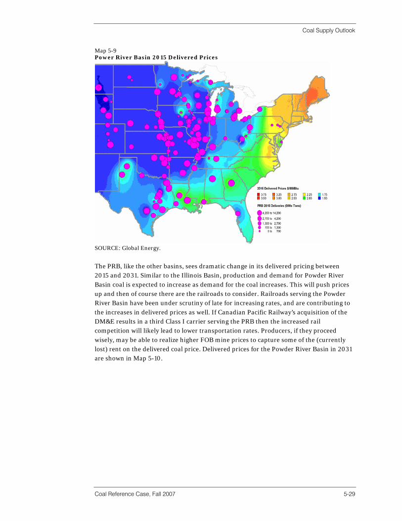
Coal Supply Outlook
Coal Reference Case, Fall 2007 5-29
Map 5-9 Power River Basin 2015 Delivered Prices
SOURCE: Global Energy.
The PRB, like the other basins, sees dramatic change in its delivered pricing between 2015 and 2031. Similar to the Illinois Basin, production and demand for Powder River Basin coal is expected to increase as demand for the coal increases. This will push prices up and then of course there are the railroads to consider. Railroads serving the Powder River Basin have been under scrutiny of late for increasing rates, and are contributing to the increases in delivered prices as well. If Canadian Pacific Railway’s acquisition of the DM&E results in a third Class I carrier serving the PRB then the increased rail competition will likely lead to lower transportation rates. Producers, if they proceed wisely, may be able to realize higher FOB mine prices to capture some of the (currently lost) rent on the delivered coal price. Delivered prices for the Powder River Basin in 2031 are shown in Map 5-10.
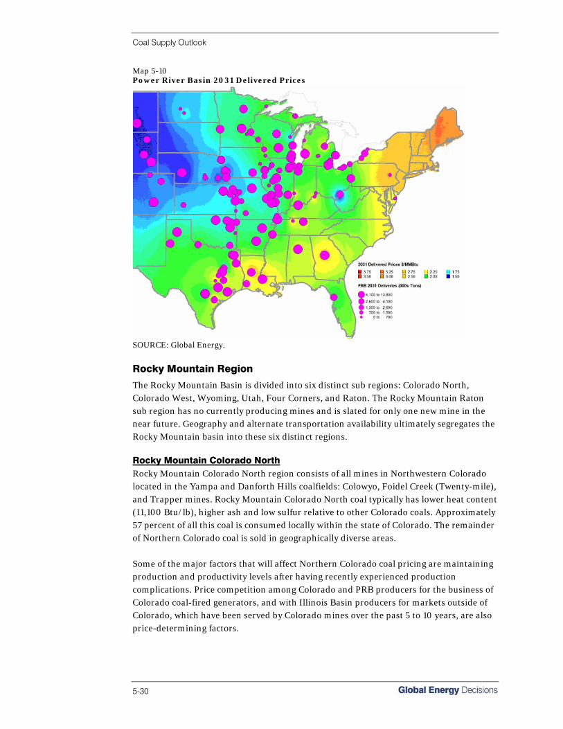
Coal Supply Outlook
5-30
Map 5-10 Power River Basin 2031 Delivered Prices
SOURCE: Global Energy.
Rocky Mountain Region
The Rocky Mountain Basin is divided into six distinct sub regions: Colorado North, Colorado West, Wyoming, Utah, Four Corners, and Raton. The Rocky Mountain Raton sub region has no currently producing mines and is slated for only one new mine in the near future. Geography and alternate transportation availability ultimately segregates the Rocky Mountain basin into these six distinct regions. Rocky Mountain Colorado North Rocky Mountain Colorado North region consists of all mines in Northwestern Colorado located in the Yampa and Danforth Hills coalfields: Colowyo, Foidel Creek (Twenty-mile), and Trapper mines. Rocky Mountain Colorado North coal typically has lower heat content (11,100 Btu/lb), higher ash and low sulfur relative to other Colorado coals. Approximately 57 percent of all this coal is consumed locally within the state of Colorado. The remainder of Northern Colorado coal is sold in geographically diverse areas. Some of the major factors that will affect Northern Colorado coal pricing are maintaining production and productivity levels after having recently experienced production complications. Price competition among Colorado and PRB producers for the business of Colorado coal-fired generators, and with Illinois Basin producers for markets outside of Colorado, which have been served by Colorado mines over the past 5 to 10 years, are also price-determining factors.

Coal Supply Outlook
Coal Reference Case, Fall 2007 5-31
Over the long-term Global Energy expects Northern Colorado FOB coal prices to substantially increase—43 percent over the forecast period. Results from our long-term model for Northern Colorado coal can be viewed in Figure 5-25. Table 5-7 Rocky Mountain Colorado North Quality Ranges
Quality Range Basin Description Max
Btu/lb Min
Btu/lb Min lb
SO2/MMBtu Min lb
SO2/MMBtu
RMCONLoHi RMCO North Low Btu High Sulfur 10,000 - 20.00 1.20
RMCONHiLo RMCO North High Btu Low Sulfur 20,000 10,000 1.20 -
RMCONLoLo RMCO North Low Btu Low Sulfur 10,000 - 1.20 -
RMCONHiHi RMCO North High Btu High Sulfur 20,000 10,000 20.00 1.20
SOURCE: Global Energy.
Figure 5-25 Rocky Mountain Colorado North FOB Mine Price Forecast (2007 Constant Dollars)
0
5
10
15
20
25
30
35
40
2007 2010 2013 2016 2019 2022 2025 2028 2031
$/to
n
RMCONHiHi RMCONHiLo RMCONLoHi RMCONLoLo
SOURCE: Global Energy.
Rocky Mountain Colorado West Rocky Mountain Colorado West region consists of all mines in central and south western Colorado: West Elk, Elk Creek, and Bowie are located in the North Fork area within the Grand Mesa and Somerset coal fields, while Deserado and McClane Canyon are in the Grand Mesa/Bookcliffs area. Approximately 7 percent of this coal is consumed within Colorado while the Tennessee Valley Authority accounts for almost 57 percent of consumption. The remainder of Western Colorado coal is sold in fairly geographically diverse areas. Some of the major factors affecting the forecast for Western Colorado coal pricing are the introduction of the Redcliff mine, TVA’s demand for this low sulfur product as additional scrubbers are added to their coal-fired fleet, very favorable long-term rates negotiated by TVA, and the competitive pricing structure against the PRB and the Illinois Basin.
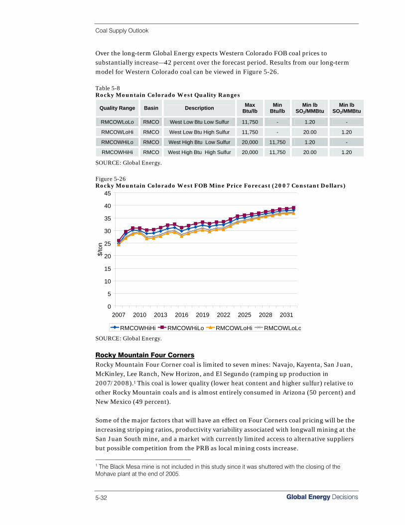
Coal Supply Outlook
5-32
Over the long-term Global Energy expects Western Colorado FOB coal prices to substantially increase—42 percent over the forecast period. Results from our long-term model for Western Colorado coal can be viewed in Figure 5-26. Table 5-8 Rocky Mountain Colorado West Quality Ranges
Quality Range Basin Description Max Btu/lb
Min Btu/lb
Min lb SO2/MMBtu
Min lb SO2/MMBtu
RMCOWLoLo RMCO West Low Btu Low Sulfur 11,750 - 1.20 -
RMCOWLoHi RMCO West Low Btu High Sulfur 11,750 - 20.00 1.20
RMCOWHiLo RMCO West High Btu Low Sulfur 20,000 11,750 1.20 -
RMCOWHiHi RMCO West High Btu High Sulfur 20,000 11,750 20.00 1.20
SOURCE: Global Energy.
Figure 5-26 Rocky Mountain Colorado West FOB Mine Price Forecast (2007 Constant Dollars)
0
5
10
15
20
25
30
35
40
45
2007 2010 2013 2016 2019 2022 2025 2028 2031
$/to
n
RMCOWHiHi RMCOWHiLo RMCOWLoHi RMCOWLoLo SOURCE: Global Energy.
Rocky Mountain Four Corners Rocky Mountain Four Corner coal is limited to seven mines: Navajo, Kayenta, San Juan, McKinley, Lee Ranch, New Horizon, and El Segundo (ramping up production in 2007/2008).1 This coal is lower quality (lower heat content and higher sulfur) relative to other Rocky Mountain coals and is almost entirely consumed in Arizona (50 percent) and New Mexico (49 percent). Some of the major factors that will have an effect on Four Corners coal pricing will be the increasing stripping ratios, productivity variability associated with longwall mining at the San Juan South mine, and a market with currently limited access to alternative suppliers but possible competition from the PRB as local mining costs increase.
1 The Black Mesa mine is not included in this study since it was shuttered with the closing of the Mohave plant at the end of 2005.

Coal Supply Outlook
Coal Reference Case, Fall 2007 5-33
Global Energy’s long-term forecast shows Four Corner FOB mine prices to escalate just over 34 percent over the course of this study time frame. This increase is higher than other Rocky Mountain coals as demand for this coal will be high throughout Arizona and New Mexico through the long-term. The forecast for Four Corner coal can be found in Figure 5-27. Table 5-9 Rocky Mountain Four Corners Quality Ranges
Quality Range Basin Description Max Btu/lb Min Btu/lb Min lb SO2/MMBtu
Min lb SO2/MMBtu
RMFCHiHi RMFC High Btu High Sulfur 20,000 10,000 20.00 1.20
RMFCLoLo RMFC Low Btu Low Sulfur 10,000 - 1.20 -
RMFCHiLo RMFC High Btu Low Sulfur 20,000 10,000 1.20 -
RMFCLoHi RMFC Low Btu High Sulfur 10,000 - 20.00 1.20
SOURCE: Global Energy.
Figure 5-27 Rocky Mountain Four Corner FOB Mine Price Forecast (2007 Constant Dollars)
0
5
10
15
20
25
30
35
40
45
2007 2010 2013 2016 2019 2022 2025 2028 2031
$/to
n
RMFCHiHi RMFCHiLo RMFCLoHi RMFCLoLo
SOURCE: Global Energy.
Rocky Mountain Wyoming Rocky Mountain Wyoming coal is really only produced by four mines—Kemmerer, Black Butte, Leucite Hills, and Bridger. Since the most of the coal is consumed locally in southwestern Wyoming (over 92 percent) and is under long-term supply agreements there is not much upward pressure on prices. Some of the major factors that will have an effect on Rocky Mountain Wyoming coal pricing will be increased stripping ratios and mining costs along with competitive pricing against Powder River and Utah producers. Over the course of the forecast Wyoming mines will have a moderate increase in price, escalating 27 percent over this time frame. Our long-term FOB price forecast is shown in Figure 5-28.
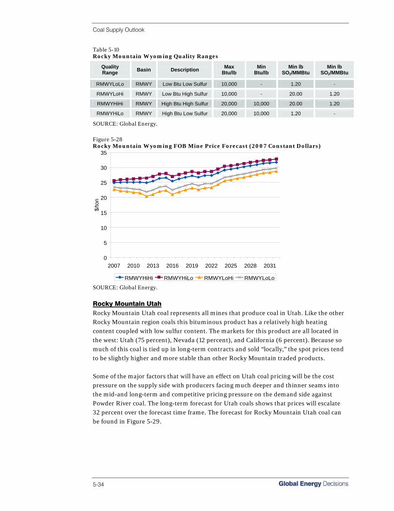
Coal Supply Outlook
5-34
Table 5-10 Rocky Mountain Wyoming Quality Ranges
Quality Range Basin Description Max
Btu/lb Min
Btu/lb Min lb
SO2/MMBtu Min lb
SO2/MMBtu
RMWYLoLo RMWY Low Btu Low Sulfur 10,000 - 1.20 -
RMWYLoHi RMWY Low Btu High Sulfur 10,000 - 20.00 1.20
RMWYHiHi RMWY High Btu High Sulfur 20,000 10,000 20.00 1.20
RMWYHiLo RMWY High Btu Low Sulfur 20,000 10,000 1.20 -
SOURCE: Global Energy.
Figure 5-28 Rocky Mountain Wyoming FOB Mine Price Forecast (2007 Constant Dollars)
0
5
10
15
20
25
30
35
2007 2010 2013 2016 2019 2022 2025 2028 2031
$/to
n
RMWYHiHi RMWYHiLo RMWYLoHi RMWYLoLo SOURCE: Global Energy.
Rocky Mountain Utah Rocky Mountain Utah coal represents all mines that produce coal in Utah. Like the other Rocky Mountain region coals this bituminous product has a relatively high heating content coupled with low sulfur content. The markets for this product are all located in the west: Utah (75 percent), Nevada (12 percent), and California (6 percent). Because so much of this coal is tied up in long-term contracts and sold “locally,” the spot prices tend to be slightly higher and more stable than other Rocky Mountain traded products. Some of the major factors that will have an effect on Utah coal pricing will be the cost pressure on the supply side with producers facing much deeper and thinner seams into the mid-and long-term and competitive pricing pressure on the demand side against Powder River coal. The long-term forecast for Utah coals shows that prices will escalate 32 percent over the forecast time frame. The forecast for Rocky Mountain Utah coal can be found in Figure 5-29.
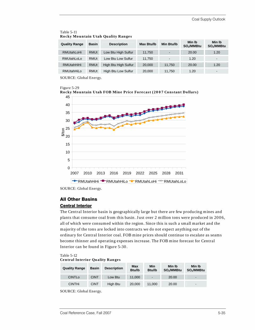
Coal Supply Outlook
Coal Reference Case, Fall 2007 5-35
Table 5-11 Rocky Mountain Utah Quality Ranges
Quality Range Basin Description Max Btu/lb Min Btu/lb Min lb SO2/MMBtu
Min lb SO2/MMBtu
RMUtahLoHi RMUt Low Btu High Sulfur 11,750 - 20.00 1.20
RMUtahLoLo RMUt Low Btu Low Sulfur 11,750 - 1.20 -
RMUtahHiHi RMUt High Btu High Sulfur 20,000 11,750 20.00 1.20
RMUtahHiLo RMUt High Btu Low Sulfur 20,000 11,750 1.20 -
SOURCE: Global Energy.
Figure 5-29 Rocky Mountain Utah FOB Mine Price Forecast (2007 Constant Dollars)
0
5
10
15
20
25
30
35
40
45
2007 2010 2013 2016 2019 2022 2025 2028 2031
$/to
n
RMUtahHiHi RMUtahHiLo RMUtahLoHi RMUtahLoLo
SOURCE: Global Energy.
All Other Basins Central Interior The Central Interior basin is geographically large but there are few producing mines and plants that consume coal from this basin. Just over 2 million tons were produced in 2006, all of which were consumed within the region. Since this is such a small market and the majority of the tons are locked into contracts we do not expect anything out of the ordinary for Central Interior coal. FOB mine prices should continue to escalate as seams become thinner and operating expenses increase. The FOB mine forecast for Central Interior can be found in Figure 5-30. Table 5-12 Central Interior Quality Ranges
Quality Range Basin Description Max Btu/lb
Min Btu/lb
Min lb SO2/MMBtu
Min lb SO2/MMBtu
CINTLo CINT Low Btu 11,000 - 20.00 -
CINTHi CINT High Btu 20,000 11,000 20.00 -
SOURCE: Global Energy.

Coal Supply Outlook
5-36
Figure 5-30 Central Interior FOB Mine Price Forecast (2007 Constant Dollars)
0
5
10
15
20
25
30
35
40
45
50
2007 2010 2013 2016 2019 2022 2025 2028 2031
$/to
n
CINTHi CINTLo
SOURCE: Global Energy.
Gulf and Northern Lignite Since lignite has such a low heat content it is not economical to transport it very long distances. In fact, most lignite is consumed at the mine mouth. This creates a unique situation where virtually all coal produced at a lignite mine is consumed at the mine mouth plant. Long-term contracts ensure a stable supply and it is in both the producers’ and consumers’ best interests to keep each other happy in their coal supply agreements. The only issue that arises is one of thinning seams and increased production costs as the mines migrate away from the plant. This is indeed the case for the limestone plant that has just broken agreement with Westmoreland for supplying Gulf Lignite—it was no longer economic to continue to mine the Jewett mine at the prices that were agreed to in the long-term supply contract. Our forecast shows a modest 34 percent increase in Gulf Lignite FOB mine prices for the term of this study. This is higher than the 28 percent increase in Northern Lignite prices due to the fact that Gulf Lignite seams are thinner, smaller, and more expensive to mine. Yet both of these increases reflect the increased costs and thinning seams throughout the existing Gulf and Northern Lignite basins. The FOB mine forecast for Northern and Gulf Lignite can be found in Figures 5-31 and 5-32. Northern Lignite Table 5-13 Northern Lignite Quality Ranges
Quality Range Basin Description Max Btu/lb
Min Btu/lb
Min lb SO2/MMBtu
Min lb SO2/MMBtu
NLIGHi NLIG High Sulfur 20,000 - 20.00 2.30
NLIGLo NLIG Low Sulfur 20,000 - 2.30 -
SOURCE: Global Energy.
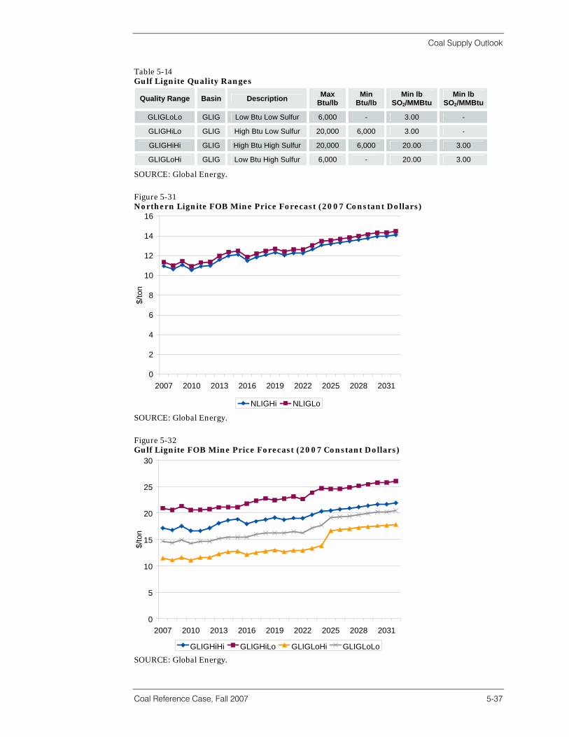
Coal Supply Outlook
Coal Reference Case, Fall 2007 5-37
Table 5-14 Gulf Lignite Quality Ranges
Quality Range Basin Description Max Btu/lb
Min Btu/lb
Min lb SO2/MMBtu
Min lb SO2/MMBtu
GLIGLoLo GLIG Low Btu Low Sulfur 6,000 - 3.00 -
GLIGHiLo GLIG High Btu Low Sulfur 20,000 6,000 3.00 -
GLIGHiHi GLIG High Btu High Sulfur 20,000 6,000 20.00 3.00
GLIGLoHi GLIG Low Btu High Sulfur 6,000 - 20.00 3.00
SOURCE: Global Energy.
Figure 5-31 Northern Lignite FOB Mine Price Forecast (2007 Constant Dollars)
0
2
4
6
8
10
12
14
16
2007 2010 2013 2016 2019 2022 2025 2028 2031
$/to
n
NLIGHi NLIGLo SOURCE: Global Energy.
Figure 5-32 Gulf Lignite FOB Mine Price Forecast (2007 Constant Dollars)
0
5
10
15
20
25
30
2007 2010 2013 2016 2019 2022 2025 2028 2031
$/to
n
GLIGHiHi GLIGHiLo GLIGLoHi GLIGLoLo
SOURCE: Global Energy.
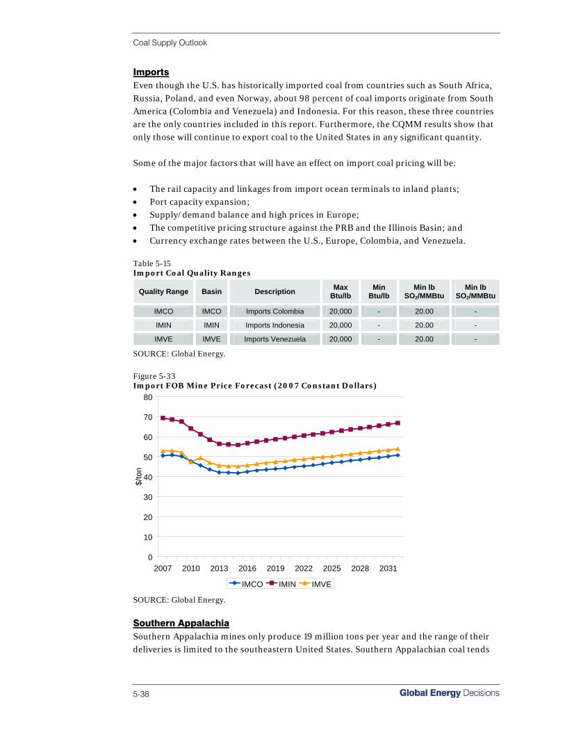
Coal Supply Outlook
5-38
Imports Even though the U.S. has historically imported coal from countries such as South Africa, Russia, Poland, and even Norway, about 98 percent of coal imports originate from South America (Colombia and Venezuela) and Indonesia. For this reason, these three countries are the only countries included in this report. Furthermore, the CQMM results show that only those will continue to export coal to the United States in any significant quantity. Some of the major factors that will have an effect on import coal pricing will be: • The rail capacity and linkages from import ocean terminals to inland plants; • Port capacity expansion; • Supply/demand balance and high prices in Europe; • The competitive pricing structure against the PRB and the Illinois Basin; and • Currency exchange rates between the U.S., Europe, Colombia, and Venezuela. Table 5-15 Import Coal Quality Ranges
Quality Range Basin Description Max Btu/lb
Min Btu/lb
Min lb SO2/MMBtu
Min lb SO2/MMBtu
IMCO IMCO Imports Colombia 20,000 - 20.00 -
IMIN IMIN Imports Indonesia 20,000 - 20.00 -
IMVE IMVE Imports Venezuela 20,000 - 20.00 -
SOURCE: Global Energy.
Figure 5-33 Import FOB Mine Price Forecast (2007 Constant Dollars)
0
10
20
30
40
50
60
70
80
2007 2010 2013 2016 2019 2022 2025 2028 2031
$/to
n
IMCO IMIN IMVE
SOURCE: Global Energy.
Southern Appalachia Southern Appalachia mines only produce 19 million tons per year and the range of their deliveries is limited to the southeastern United States. Southern Appalachian coal tends

Coal Supply Outlook
Coal Reference Case, Fall 2007 5-39
to have high heat content and moderate levels of sulfur. Since the coal from this basin is delivered to such a limited region and extraction costs are relatively high with increasing stripping ratios and thinning seams we do not expect demand for Southern Appalachian coal to change over the long term. In fact the price forecast for Southern Appalachia shows minimal growth with a 13 percent increase over the forecast period. The long-term forecast for Southern Appalachia basin can be found below. Table 5-16 Southern Appalachia Quality Ranges
Quality Range Basin Description Max Btu/lb
Min Btu/lb
Min lb SO2/MMBtu
Min lb SO2/MMBtu
SAPPLoHi SAPP Low Btu High Sulfur 12,200 - 20.00 1.20
SAPPHiHi SAPP High Btu High Sulfur 20,000 12,200 20.00 1.20
SAPPLoLo SAPP Low Btu Low Sulfur 12,200 - 1.20 -
SAPPHiLo SAPP High Btu Low Sulfur 20,000 12,200 1.20 -
SOURCE: Global Energy.
Figure 5-34 Southern Appalachia FOB Mine Price Forecast (2007 Constant Dollars)
0
10
20
30
40
50
60
70
2007 2010 2013 2016 2019 2022 2025 2028 2031
$/to
n
SAPPHiHi SAPPHiLo SAPPLoHi SAPPLoLo
SOURCE: Global Energy.
Coal Basin Battleground Delivered prices from three major U.S. coal basins—the Powder River Basin, Central Appalachia, and the Illinois Basin—make for an interesting competitive dynamic within the marketplace, particularly with the Powder River Basin’s ability to deliver coal cheaply over long distances. Certain geographic areas may be accessed by two or more of these basins in the same delivered price range giving utilities flexibility with the type of coal they burn at more reasonable prices. These areas are what we refer to as battlegrounds, where multiple basins will be fighting to increase their market share. However, it is important to keep in

Coal Supply Outlook
5-40
mind that not all plants are able to burn certain coal types. Even though the delivered coal may be competitively priced from a given supply basin, it still must meet minimum standards for heat content, sulfur, ash, ash fusion temperature, chlorine, etc. Typically, older plants are less flexible with the range of coal specifications that can be burned without deleterious effects. Going forward we expect most new plants to be designed with flexible fuel capability. Thus, battleground markets are geographic areas that over the long run will experience direct price competition between basins at many of the plants within those areas. Map 5-11 shows the current battleground areas for delivered prices of $2.00/MMBtu or less. The PRB is able to deliver at this price in a very large geographical area and encompasses nearly all of the areas served by the Illinois Basin and Central Appalachia at this price. The maps introduced above in the Powder River Basin section indicate that the PRB is able to penetrate central Indiana and Ohio at the magic $2.00/MMBtu price level. However, there are no plants that currently receive PRB coal in that area at $2.00/MMBtu because Central Indiana and Ohio are rail served markets. At $2.00/MMBtu PRB coal delivered to that part of the country arrives at plants located either on or near the Ohio River or Great Lakes, not in the interior part of the state. It is evident that the higher cost for rail transport in this congested area precludes PRB market penetration. This is shown clearly below with the “horseshoe” shape the PRB’s $2.00/MMBtu area takes in this region. Competition is currently heaviest in Illinois and the river markets directly surrounding it, as well as into the Ohio River Valley as far east as Ohio. Map 5-11 2007 Battleground Areas
SOURCE: Global Energy.

Coal Supply Outlook
Coal Reference Case, Fall 2007 5-41
In 2015 the situation is not likely to change a great deal. While the area of the country where the PRB and Illinois Basin compete heavily will likely shrink in size to some degree, the main competition will continue to be on the river markets, particularly the Ohio River. This remains the only area where all three basins are able to deliver at under $2.00/MMBtu. Map 5-12 shows the battlegrounds for 2015. Map 5-12 2015 Battleground Areas
SOURCE: Global Energy.
Map 5-13 shows the 2031 battleground area for $2.00/MMBtu coal. As Central Appalachia’s production declines and costs increase the market that is reachable at a delivered price of $2.00/MMBtu shrinks dramatically to only a small part of the Ohio River Valley. Meanwhile the demand price forecast for Illinois Basin coal increases around the basin and into the southeast, leaving the Illinois Basin area and the western half of the Ohio River Valley the only major battleground left at this price range. PRB should still be able to deliver coal to parts of the Ohio River and on the Mississippi River after transloading at St. Louis. Competition among basins is certainly possible elsewhere in the country with a possible concentration in the southeast.
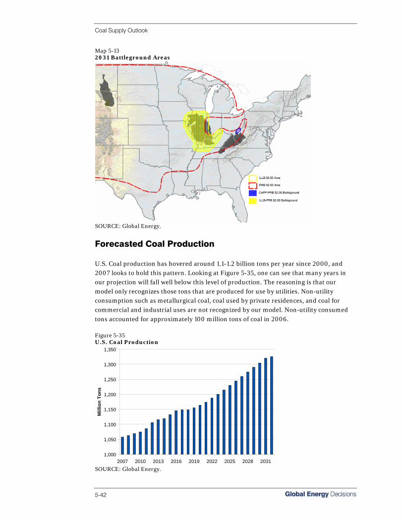
Coal Supply Outlook
5-42
Map 5-13 2031 Battleground Areas
SOURCE: Global Energy.
Forecasted Coal Production U.S. Coal production has hovered around 1.1-1.2 billion tons per year since 2000, and 2007 looks to hold this pattern. Looking at Figure 5-35, one can see that many years in our projection will fall well below this level of production. The reasoning is that our model only recognizes those tons that are produced for use by utilities. Non-utility consumption such as metallurgical coal, coal used by private residences, and coal for commercial and industrial uses are not recognized by our model. Non-utility consumed tons accounted for approximately 100 million tons of coal in 2006. Figure 5-35 U.S. Coal Production
1,000
1,050
1,100
1,150
1,200
1,250
1,300
1,350
2007 2010 2013 2016 2019 2022 2025 2028 2031
Mill
ion
Tons
SOURCE: Global Energy.
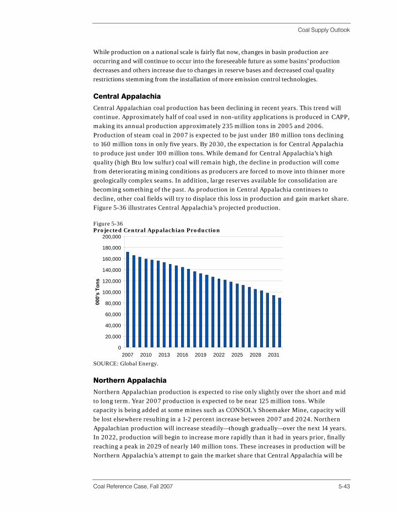
Coal Supply Outlook
Coal Reference Case, Fall 2007 5-43
While production on a national scale is fairly flat now, changes in basin production are occurring and will continue to occur into the foreseeable future as some basins’ production decreases and others increase due to changes in reserve bases and decreased coal quality restrictions stemming from the installation of more emission control technologies. Central Appalachia
Central Appalachian coal production has been declining in recent years. This trend will continue. Approximately half of coal used in non-utility applications is produced in CAPP, making its annual production approximately 235 million tons in 2005 and 2006. Production of steam coal in 2007 is expected to be just under 180 million tons declining to 160 million tons in only five years. By 2030, the expectation is for Central Appalachia to produce just under 100 million tons. While demand for Central Appalachia’s high quality (high Btu low sulfur) coal will remain high, the decline in production will come from deteriorating mining conditions as producers are forced to move into thinner more geologically complex seams. In addition, large reserves available for consolidation are becoming something of the past. As production in Central Appalachia continues to decline, other coal fields will try to displace this loss in production and gain market share. Figure 5-36 illustrates Central Appalachia’s projected production. Figure 5-36 Projected Central Appalachian Production
0
20,000
40,000
60,000
80,000
100,000
120,000
140,000
160,000
180,000
200,000
2007 2010 2013 2016 2019 2022 2025 2028 2031
000'
s To
ns
SOURCE: Global Energy.
Northern Appalachia
Northern Appalachian production is expected to rise only slightly over the short and mid to long term. Year 2007 production is expected to be near 125 million tons. While capacity is being added at some mines such as CONSOL’s Shoemaker Mine, capacity will be lost elsewhere resulting in a 1-2 percent increase between 2007 and 2024. Northern Appalachian production will increase steadily—though gradually—over the next 14 years. In 2022, production will begin to increase more rapidly than it had in years prior, finally reaching a peak in 2029 of nearly 140 million tons. These increases in production will be Northern Appalachia’s attempt to gain the market share that Central Appalachia will be
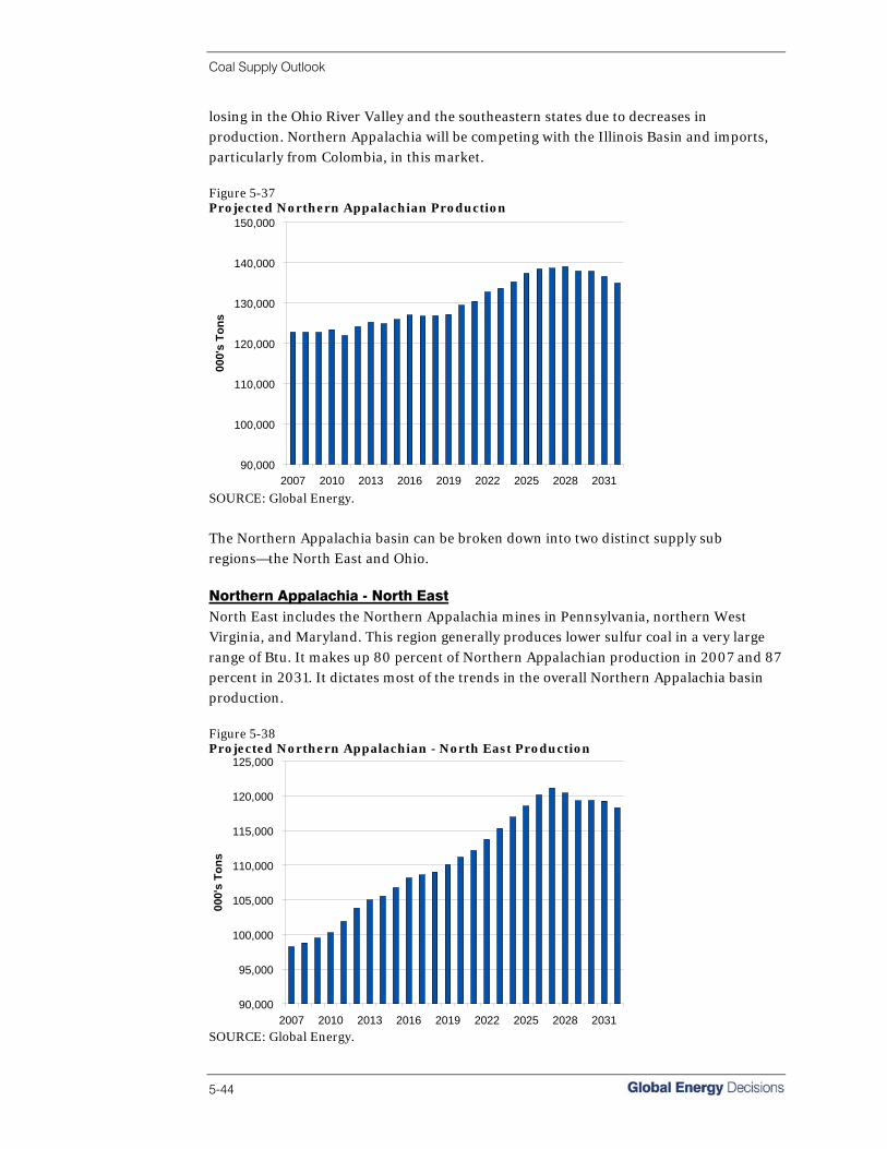
Coal Supply Outlook
5-44
losing in the Ohio River Valley and the southeastern states due to decreases in production. Northern Appalachia will be competing with the Illinois Basin and imports, particularly from Colombia, in this market. Figure 5-37 Projected Northern Appalachian Production
90,000
100,000
110,000
120,000
130,000
140,000
150,000
2007 2010 2013 2016 2019 2022 2025 2028 2031
000'
s To
ns
SOURCE: Global Energy.
The Northern Appalachia basin can be broken down into two distinct supply sub regions—the North East and Ohio. Northern Appalachia - North East North East includes the Northern Appalachia mines in Pennsylvania, northern West Virginia, and Maryland. This region generally produces lower sulfur coal in a very large range of Btu. It makes up 80 percent of Northern Appalachian production in 2007 and 87 percent in 2031. It dictates most of the trends in the overall Northern Appalachia basin production. Figure 5-38 Projected Northern Appalachian - North East Production
90,000
95,000
100,000
105,000
110,000
115,000
120,000
125,000
2007 2010 2013 2016 2019 2022 2025 2028 2031
000'
s To
ns
SOURCE: Global Energy.

Coal Supply Outlook
Coal Reference Case, Fall 2007 5-45
Northern Appalachia - Ohio The Northern Appalachian mines in Ohio are characterized by slightly higher sulfur and a more consistent Btu coal. In 2007, Ohio is responsible for only 20 percent of Northern Appalachian production. By 2019, it decreases to 13 percent and tonnage remains flat while the rest of the basin increases production. Figure 5-39 Projected Northern Appalachian - Ohio Production
-
5,000
10,000
15,000
20,000
25,000
30,000
2007 2010 2013 2016 2019 2022 2025 2028 2031
000'
s To
ns
SOURCE: Global Energy.
Illinois Basin
With the additions of SO2 controls at a large number of power plants throughout the country, more power plants than ever will have the ability to burn the Illinois Basin’s higher sulfur coal. These scrubber additions are in no small part related to the projected decline in Central Appalachian production in upcoming years and the desire for utilities to harness the capability to keep their purchasing strategies diversified. This has sparked large scale development in the basin and production is expected to increase for the foreseeable future. The majority of this increase is expected to occur in the next 15 years, with production flattening thereafter. While surface mines in the basin are diminishing, many new mines are utilizing longwall technology to keep productivity as high as possible. Current production levels of approximately 90 million tons per year are expected to increase to 120 million tons per year by 2022, a 38 percent increase mostly due to new mine additions rather than increased production at existing mine sites. Thereafter production will increase more gradually until flattening and declining slightly in later years.

Coal Supply Outlook
5-46
Figure 5-40 Projected Illinois Basin Production
80,000
85,000
90,000
95,000
100,000
105,000
110,000
115,000
120,000
125,000
130,000
2007 2010 2013 2016 2019 2022 2025 2028 2031
000'
s To
ns
SOURCE: Global Energy.
Rocky Mountain
Rocky Mountain production is expected to increase over the short-term, reaching a peak around 2011. This represents a time when some Rocky Mountain mines are scheduled to close after current contracts expire, resulting in decreases in production. In 2014, the West Elk Mine is planned to stop production when Arch’s contract with the Tennessee Valley Authority ends, particularly the deliveries to the Shawnee Plant, which plans to switch to south Powder River Basin coal. In addition, some mines such as Bowie #2 are expected to take production hits in 2015 with the final implementation of CAIR. This is responsible for fairly flat production in the years between 2015 and 2020, with the basin rebounding from these negative effects from 2021 and beyond. Figure 5-41 Projected Rocky Mountain Production
80,000
85,000
90,000
95,000
100,000
105,000
110,000
115,000
120,000
125,000
130,000
2007 2010 2013 2016 2019 2022 2025 2028 2031
000'
Ton
s
SOURCE: Global Energy.
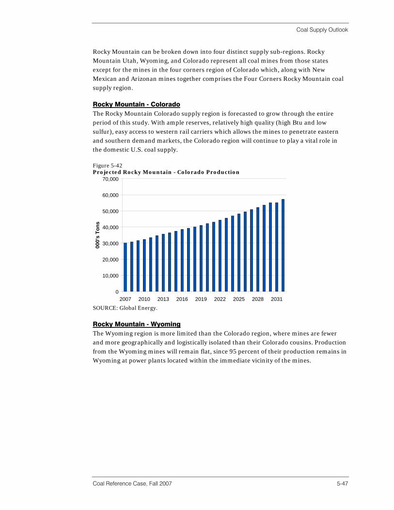
Coal Supply Outlook
Coal Reference Case, Fall 2007 5-47
Rocky Mountain can be broken down into four distinct supply sub-regions. Rocky Mountain Utah, Wyoming, and Colorado represent all coal mines from those states except for the mines in the four corners region of Colorado which, along with New Mexican and Arizonan mines together comprises the Four Corners Rocky Mountain coal supply region. Rocky Mountain - Colorado The Rocky Mountain Colorado supply region is forecasted to grow through the entire period of this study. With ample reserves, relatively high quality (high Btu and low sulfur), easy access to western rail carriers which allows the mines to penetrate eastern and southern demand markets, the Colorado region will continue to play a vital role in the domestic U.S. coal supply. Figure 5-42 Projected Rocky Mountain - Colorado Production
0
10,000
20,000
30,000
40,000
50,000
60,000
70,000
2007 2010 2013 2016 2019 2022 2025 2028 2031
000'
s To
ns
SOURCE: Global Energy.
Rocky Mountain - Wyoming The Wyoming region is more limited than the Colorado region, where mines are fewer and more geographically and logistically isolated than their Colorado cousins. Production from the Wyoming mines will remain flat, since 95 percent of their production remains in Wyoming at power plants located within the immediate vicinity of the mines.

Coal Supply Outlook
5-48
Figure 5-43 Projected Rocky Mountain - Wyoming Production
0
2,000
4,000
6,000
8,000
10,000
12,000
14,000
2007 2010 2013 2016 2019 2022 2025 2028 2031
000'
s To
ns
SOURCE: Global Energy.
Rocky Mountain - Four Corners Production from the Four Corners region is distributed to a larger geographic area than the Wyoming mines and Four Corners’ mines will have to compete with Powder River suppliers for futures supply contracts. Our forecast shows that Four Corners mines production will eventually be displaced with coal from Powder River suppliers through the mid term, but as more and more plants compete for PRB coal, the Four Corners region production should ramp back up to meet expected increase in western demand for their coal. Figure 5-44 Projected Rocky Mountain - Four Corners Production
0
5,000
10,000
15,000
20,000
25,000
30,000
35,000
40,000
2007 2010 2013 2016 2019 2022 2025 2028 2031
000'
s To
ns
SOURCE: Global Energy.

Coal Supply Outlook
Coal Reference Case, Fall 2007 5-49
Rocky Mountain - Utah Though Utah coal mines have been increasing their production over the past few years to try to meet their 1996 all time record annual production, problems remain and it is questionable whether they will be able to sustain the current level of output. Not only will Utah mines face increasing costs and lower productivity due to thinning seams and having already picked the low hanging fruit, the mines will also face increasing competition from Colorado and Powder River producers looking to increase their sales into newly established markets. The Utah forecast proves that after some mid-term variability in production, Utah mines will lose some market share to other western producers, only to gain back some of their lost sales further into the future. Figure 5-45 Projected Rocky Mountain - Utah Production
0
5,000
10,000
15,000
20,000
25,000
2007 2010 2013 2016 2019 2022 2025 2028 2031
000'
s To
ns
SOURCE: Global Energy.
Powder River Basin
The major increases in production over the next 25 years are expected to come from the Powder River Basin. This makes sense given the massive coal seams this region mines making large production increases a more realistic option than other mining regions. Global Energy expects PRB coal demand to remain firm in the near term as utility stockpiles are replenished. In response to the real and anticipated increase in demand, producers are eager to expand production. For example: • Peabody Coal increased its PRB production 10 percent or 12.7 million tons in 2006
from 2005 levels, though it appears production may drop up to 6 percent in 2007. Plans to construct a new School Creek mine opening in 2008 with annual capacity of 35 million tons by 2010 have been postponed at least one year but the mine is still on the drawing board assuming market conditions permit.
• Arch Coal’s Coal Creek facility is back in production and on pace to produce over 9 million tons in 2007. This facility was idled in mid-2000 after producing close to 4.2 million tons in response to market conditions. Arch views this facility as one of the most strategic expansion opportunities in the entire U.S. coal industry. They are

Coal Supply Outlook
5-50
targeting an annual production of 15 million short tons, with the capability of adding another 3 to 5 million tons if market conditions prove favorable. Arch has also secured the necessary permit to expand the mine’s annual output to 25 million tons, should market conditions warrant.
• Foundation Coal has long-term plans to expand its production to the limit of its air quality permits, about 27 million tons.
• Rio Tinto North America has boosted its production at the Antelope mine by 13 percent from 2005 to 2006, producing 33.9 million tons in 2006. The mine looks on pace to match this production through the first two quarters of 2007. The Jacobs Ranch and Cordero Rojo Mines saw smaller increases of 5 and 7 percent, respectively, between 2005 and 2006. While the Cordero Rojo mine looks to keep this pace in 2007 it appears as though production from Jacobs Ranch may not match 2006 levels.
• Hungry, smaller producers like Wyodak, Dry Fork, and Buckskin are actively pursuing new customers.
Additional capacity in the long term will come from more mine expansions as well as the introduction of new mines. New mines may utilize currently accessible reserves or newly accessible reserves. Of note is the possible construction of the Tongue River Railroad, which will connect Miles City and Ashland, Montana, opening up 2 billion tons of recoverable reserves at a minimum. The low cost Btus of the Powder River Basin will continue to be in demand for years to come. Low sulfur characteristics will make the coal desirable for those plants that do not install scrubbers and for those that wish to blend lower Btu PRB coal with higher Btu eastern coals. While the cost of producing high quality coal in the east continues to rise, more utilities will look for cheap Btus to meet increasing demand for electricity. Global Energy expects production in the Powder River Basin to increase 50 percent to 700 million tons over the forecast period. Figure 5-46 Projected Powder River Basin Production
400,000
450,000
500,000
550,000
600,000
650,000
700,000
750,000
2007 2010 2013 2016 2019 2022 2025 2028 2031
000'
s To
ns
SOURCE: Global Energy.

Coal Supply Outlook
Coal Reference Case, Fall 2007 5-51
The Powder River Basin can be broken down into two distinct supply sub regions: the Southern Powder River Basin (SPRB) and the Northern Powder River Basin (NPRB). The SPRB mines are all located within the Powder River Basin within the state of Wyoming while the NPRB mines are all located in Montana. SPRB mines tend to have lower Btu and lower sulfur whereas the NPRB mines are higher Btu and higher sulfur. Powder River Basin - Southern Providing that transportation capacity out of the Southern Powder River Basin (primarily the Joint Line) is able to keep up with expected demand for and production of SPRB coal, Global Energy is forecasting SPRB production to increase by over 50 percent between 2007 and 2032. Output from the SPRB will slow down between 2016 and 2018 due to production delays as a result of several of the mines having to “jump” the Joint Line to continue mining on the west side of the rail lines. Production will soon recover and bounce back in 2019 and then steadily continue to increase through the remainder of the study period. Figure 5-47 Projected Southern Powder River Basin Production
400,000
450,000
500,000
550,000
600,000
650,000
2007 2010 2013 2016 2019 2022 2025 2028 2031
000'
s To
ns
SOURCE: Global Energy.
Powder River Basin - Northern The Northern Powder River Basin is not as heavily dependent upon rail capacity since there is currently spare capacity to haul coal out of the NRPB and we will see continued growth through the short and mid term. In 2027, NPRB production output will flatten as the SPRB continues to out price many of the other basins, including the NPRB on a delivered dollar per Btu basis.

Coal Supply Outlook
5-52
Figure 5-48 Projected Northern Powder River Basin Production
30,000
35,000
40,000
45,000
50,000
55,000
60,000
65,000
70,000
2007 2010 2013 2016 2019 2022 2025 2028 2031
000'
s To
ns
SOURCE: Global Energy.
Future Coal Transportation Table 5-17 Mill Rates by Transportation Mode
2007 2015 2031
Rail East 0-200 20.02 22.45 28.43
200-400 10.01 11.23 14.22
400-600 6.84 7.67 9.71
600-800 1.73 1.94 2.46
800-1000 1.70 1.91 2.42
1000-1200 0.26 0.29 0.36
1200-1400 0.25 0.28 0.35
1400-1600 0.01 0.01 0.01
Rail West 0-200 5.15 5.77 7.31
200-400 2.55 2.86 3.62
400-600 1.69 1.89 2.40
600-800 1.26 1.41 1.79
800-1000 1.01 1.13 1.43
1000-1200 0.84 0.94 1.19
1200-1400 0.71 0.80 1.01
1400-1600 0.62 0.70 0.89
1600-1800 0.55 0.62 0.79
1800-2000 0.50 0.56 0.71
>2000 0.33 0.37 0.47
River Barge 22.82 24.94 28.19
Ocean Vessel 3.02 3.31 3.74
Lake Vessel 15.30 16.74 18.91
SOURCE: Global Energy.

Coal Supply Outlook
Coal Reference Case, Fall 2007 5-53
Railroad Transportation Appalachia Northern and Central Appalachia are served by two Class I railroads—CSX and Norfolk Southern. While production in NAPP is expected to remain strong, decreasing production in CAPP will decrease rail shipments from the area whether the coal is hauled continuously by rail or transported to the Kanawha or Big Sandy Rivers. It is difficult at this point to determine precisely where tons will be going off line and therefore which railroad may be affected more heavily. It is certain that both CSX and Norfolk Southern will try to increase deliveries from other basins to replace tons they will lose in CAPP in upcoming years. Where these new deliveries originate is a function of basin production and the market being penetrated; the majority of CAPP coal is delivered into the southeast. While NAPP has strong reserves in place this is an area with an extensive history of mining and therefore a fairly defined market. NAPP coal is moved with relative ease into the Northeast via rail. While increased infrastructure to the east could provide routing into the southeast the likelihood of this infrastructure is uncertain as it seems the alternatives of the Illinois Basin, the Powder River Basin, and imports may be better suited for the task. Illinois Basin The Illinois Basin is more of an emerging market than Northern Appalachia particularly when it relates to shipments of coal well beyond the perimeters of the basin. The railroad system within the basin is extensive with multiple major railroads including the Canadian National, Kansas City Southern, Burlington Northern Santa Fe, Union Pacific, CSX, and Norfolk Southern. With a large portion of Illinois Basin production either moving near the basin by rail or via barge, railroad infrastructure to move coal into other areas is sufficient for the time being but may fall short of what is needed if production in the basin increases as much as expected over the next 10 to 15 years. Expect companies to expend capital to improve rail transportation from the Illinois Basin to other areas where an increasing number of scrubbers are being installed annually allowing a greater number of plants to burn the high sulfur Illinois Basin coal. Powder River Basin Of all the transportation issues facing the U.S. coal markets, the development and expansion of rail in the Powder River Basin will have the biggest impact on U.S. coal consumption patterns. As a result, this report devotes considerable attention to transportation issues of the PRB. The Powder River Basin is served by the Union Pacific and the Burlington Northern Santa Fe. Transportation from the basin has seen its share of issues in the recent past, particularly in the Spring of 2005 when derailments on the Joint Line caused capacity constraints and many deliveries were missed. Current capacity is barely sufficient and with the basin’s production expected to increase over the short and long term a number of improvements to rail infrastructure related to the Powder River Basin have been proposed. In addition to plans by UP and BNSF to expand the existing lines, there are two

Coal Supply Outlook
5-54
major plans to add more transportation capacity out of the PRB: the Dakota, Minnesota & Eastern Railroad and development of the Tongue River Railroad. The DM&E Railroad The Dakota, Minnesota & Eastern Railroad Corporation (DM&E) was formed in 1986 by acquisition of rail infrastructure, trackage rights, and equipment from the Chicago and North Western railroad. In 2002, the Iowa, Chicago & Eastern Railroad (ICE) was joined to the DM&E through Cedar American Rail Holding, Inc. The combined railroads serve eight states (Iowa, Illinois, Minnesota, Montana, Nebraska, South Dakota, Wisconsin, and Wyoming). Together, the railroads operate 2,500 miles of track, making them the largest Class II railroad in the country. The company operates 150 locomotives and 8,000 freight cars with additions of up to 600 new covered hopper cars reported for 2005. The railroad handles nearly 250,000 carloads of freight yearly, with bulk commodities comprising most of the traffic. Grain is the largest cargo at about 37 percent with coal coming in second at 17 percent of the total. In February 1998, the DM&E applied to the Surface Transportation Board (STB) to construct a 262-mile extension from Wall through Edgemont, South Dakota, into the Wyoming Powder River Basin. Although not finalized, the current route would take the extension into the Gillette Coalfield near the Campbell-Converse counties’ border to connect with the UP-BNSF Joint Line near where Peabody’s North Antelope-Rochelle and Arch Coal’s Black Thunder mines meet. Since the application filing, the proposed PRB extension has crept towards regulatory approval and financing. In January 2002, the STB granted final approval of the PRB project, and in 2006 approved the use of a subsidiary—Wyoming, Dakota Railroad Properties, Inc. (WDRPI)—as a financing conduit for the project. On February 26, 2007, the Federal Railroad Administration denied a $2.3 billion Railroad Rehabilitation and Improvement Financing loan application from the DM&E, citing unacceptably high risk to federal tax payers. On September 4, 2007, Canadian Pacific Railway announced that it had reached an agreement to acquire the DM&E and its subsidiaries for $1.48 billion, with additional contingent payments totaling up to $1 billion. Total project costs to develop the DM&E into the PRB range between $6.0 and $7.5 billion as mentioned in the press. The project includes construction of 260 miles of new track and rehabilitation of more than 600 miles of existing track. Part of the project involves replacing old tracks with new, continuous welded rail that can handle 15,000 ton coal unit trains. While no detailed financial analysis has been published, the “magic” number often quoted for successful performance is to reach an annual volume of 100 million tons of coal. Initial reaction to the proposed project among major players in the coal chain was, at best, lukewarm. The DM&E was derisively branded “the railroad to nowhere” by more vocal doubters, and awareness in the coal industry chain has risen gradually. Although the city of Rochester, Minnesota, and the Mayo Clinic (based in Rochester) have mounted aggressive, high profile opposition to the project, support has been conspicuously

Coal Supply Outlook
Coal Reference Case, Fall 2007 5-55
“restrained” until recently, when the two railroads serving the PRB began aggressively raising rates. Map 5-14 Canadian Pacific and DM&E Rail and Potential Coal Plant Market
SOURCE: Global Energy.
Potential PRB Rail Traffic At a high level, Global Energy’s analysis of PRB rail transportation indicates that coal-fired plants where access cannot be blocked by the UP or BNSF burned in excess of 200 million tons of PRB-origin coal in 2006. However, these data must be examined more thoroughly to determine where DM&E /CP-origin PRB coal would be competitive. There are many problems routing DM&E -origin coal on the existing rail infrastructure—especially if one assumes that the UP and BNSF will not be cooperative. Some of the results of the analysis are summarized in the Table 5-18.

Coal Supply Outlook
5-56
Table 5-18 Potential DM&E PRB Coal Tonnage by Termination
2006 2010 2015
Million Tons
Lake Vessel1 37.8 38.6 39.5
DM&E/ Ohio River2 20.0 20.9 21.1
DM&E/ Miss. River3 16.4 19.6 20.3
DM&E/ Illinois River4 4.5 4.6 4.8
Subtotal, Water 78.6 83.7 85.7
DM&E only5 7.8 8.3 9.1
DM&E /CP6 13.9 14.3 15.1
DM&E /CN7 24.5 25.7 26.2
DM&E /NS 24.4 25.7 26.8
DM&E /CSX 22.8 23.4 23.6
DM&E /KCS 20.0 20.6 21.2
DM&E /MNARK 8.1 8.6 9.1
DM&E /CRIC 0.6 0.6 0.7
DM&E /IANR 0.0 0.0 1.8
DM&E /IAIS/ILMID 13.9 14.9 15.7
Subtotal, Rail 128.2 133.8 140.2
Grand Total 206.8 217.5 225.9
(1) Terminating on the CP at Thunder Bay Terminal, ON; assumes continued operation of Ontario Power Generation coal-fired units through forecast period at 10 MMtpy
(2) Terminating on the CN at Metropolis, IL (3) Terminating on the DM&E/ICE system at Camanche/Dubuque, IA (4) Terminating on the IM; IAIS bridge carrier; at Havana, IL (5) Contains tons terminating on DM&E and ICE (6) Contains tons terminating on DM&E and CP. Does not include ‘Lake Vessel’ volume which moves to
Thunder Bay Terminal on the CP (7) Contains tons terminating on DMIR and MISS where CN is the ‘bridge’ carrier
SOURCE: Global Energy.
Waterway Volume A large component of the subject coal is capable of terminating at plants served by lake vessels and barges. In 2006, 37.8 and 40.9 million tons terminated at sites primarily served by lake vessels and barges, respectively. Thus, nearly 37 percent of the accessible 2006 market is linked to routes enabling origination on the Great Lakes and inland river system. There is no direct DM&E /CP access to the Great lakes via the Superior Midwest Energy Terminal (SMET). To gain access the DM&E would have to hand the coal trains off to the UP or BNSF to enter the SMET in Superior, Wisconsin. It can be reasonably assumed that these railroads will not cooperate, thus the alternative is to access the Thunder Bay Terminal in Thunder Bay, Ontario, via CP track. The DM&E /CP system has direct access to the Great Lakes at Thunder Bay, Ontario, on the northern shore of Lake Superior. The routing on the CP through South Dakota, North Dakota, Minnesota, Manitoba, and Ontario may be competitive, but is still 24 percent

Coal Supply Outlook
Coal Reference Case, Fall 2007 5-57
longer than moves to SMET on UP and BNSF. Thus, much longer joint moves, with associated switching, and other logistics-related costs, will have to compete with moves on the existing UP and BNSF infrastructure.
The DM&E /ICE system has rail to river transfer capability at one location each in Minnesota and Illinois, and eight locations in Iowa. Of the ten docks, only two—located at Camanche and Dubuque in Iowa—are configured to handle significant volumes of coal. As much as 5.4 million tons of coal could move through these directly accessible river terminals in 2006 to power plants on the Upper Mississippi River above Muscatine, Iowa. Although coal currently moves through both sites, the Upper Mississippi River is closed to barge navigation during the winter, and is located remotely from major river markets on the Illinois, Lower Mississippi, and Ohio rivers. If, however, the railroad and barge operators are able to offset the long haul distances with lower unit rates, another 11.0 million tons of coal could move through the DM&E accessible docks to terminate on the Mississippi River, bringing the 2006 volume to 16.4 million tons. To penetrate markets on the Illinois and Ohio rivers, DM&E/CP-origin coal would need to transit docks located in central and southern Illinois that require multi-line hauls with concomitant switching and logistical charges. In 2006, 4.5 and 20.0 million tons of coal could have moved through Illinois and Ohio River terminals respectively. The only portion of the river coal over which the DM&E /CP appears to have near full control of the delivered cost is the 5.4 million tons moving to the markets on the Upper Mississippi River above Muscatine, Iowa. Thus, less than 10 percent of the 2006 barge accessible market appears to be securely available, while the remainder will require substantial cooperation from other major and short line railroads, and barge operators to become viable. The proposed merger with the CP will create additional access to waterways as noted in Table 5-19 Canadian Pacific has access to notable coal docks on the Mississippi River in Minnesota and Iowa, the Black River in Wisconsin and Milwaukee Outer Harbor in Wisconsin. Table 5-19 Rail Access to Notable Coal Docks
Name Town State Waterway Railway Connection
Port of Milwaukee South Pier No. 2, General Cargo Term #3 Milwaukee WI Milwaukee Outer Harbor C&NWR, CP
La Crosse Municipal Terminal La Crosse WI Black River CP
F.J. Roberts Co. Dock La Crosse WI Black River CP
River Services, Minneapolis North Dock Minneapolis MN Mississippi River CP
River Services, Minneapolis South Dock Minneapolis MN Mississippi River CP
Dakota Bulk Terminal, Wharf South St. Paul MN Mississippi River CP
Interstate Power & Light Co., Lansing Plant Coal Dock Lansing IA Mississippi River CP
Determann Industries Dock Camanche IA Mississippi River BNSF, UP, IC&E
Blackhawk Fleet Terminal Wharf Davenport IA Mississippi River IC&E
Lafarge North America, Davenport Plant Wharf Buffalo IA Mississippi River IC&E
River Terminal Corp. / CK Processing Co. Wharf Muscatine IA Mississippi River IC&E
SOURCE: U.S. Army Corps of Engineers.

Coal Supply Outlook
5-58
Rail-Only Volume Rail only terminations are also summarized in Table 5-18. It should be noted that a significant volume of the lake vessel and river coal has the DM&E, CP, CN and the combined Iowa Interstate Railroad/Illinois & Midland (IAIS/IM) as its “bridge” carriers. For example, when the DM&E/CP and the DM&E/Mississippi River coal are summed, the total 2006 market volume reaches 30.3 million tons. When the Ohio River and Illinois River coal are added, the total estimated 2006 volume reaches 54.8 million tons. Lake vessel coal could potentially add another 37.8 million tons, bringing the total to 92.6 million tons. Global Energy estimates that there are approximately 136.0 million tons of coal that can potentially be delivered by rail alone. Certainly not all of that market potential will be realized because of competitive pressures from other market entrants, namely UP and BNSF. Further, potential DM&E/CP markets will be reliant on multi-line hauls for roughly 89.8 million tons per year. Only 13.9 million tons of coal can be moved solely on DM&E/CP rail to coal plants. The DM&E/KCS combination has the potential to serve 20.0 million tons of coal. The DM&E/NS combination can serve up to 24.4 million tons. Finally, the IAIS/IM short line combination reaches a market potential of 13.9 million tons. With the exception of the DM&E controlled river coal, the haul distances to the respective river and Great Lakes ports places DM&E origin coal at a steep disadvantage unless the DM&E and/or the bridge carriers are willing and able to absorb significant unit cost concessions. Conclusion Detailed analysis of routing and costs that are necessary to link the DM&E with the prospective rail terminations is beyond the scope of this study, but it is important to note that the distances and costs are generally higher than those of current UP and BNSF origins. Further, interchanges and other infrastructure will undoubtedly need significant upgrades in many locations to increase traffic of coal unit trains. These costs are not included in the DM&E upgrade proposal. At this juncture, significant capital and commitment need to materialize and strengthen before the means to create another PRB rail transportation link occurs—with all of the necessary extensions, upgrades, trackage rights, and mergers. The link will not become a reality without substantial political, regulatory, and consumer backing. While the stars may be aligning at this time, it is directly related to the sclerotic performance of the UP and BNSF over the last several years, followed by an aggressive campaign of rate hikes and continued constrained performance from the Joint Line area. If, as the UP and BNSF seem to be hoping, high natural gas prices continue to support high rail rates, forces may continue to coalesce supporting the DM&E project. Declining gas prices and shrinking coal demand will likely undermine the DM&E effort and slow or terminate its progress. The Tongue River Railroad An application to build and operate an 89-mile railroad between Miles City and Ashland, Montana, was submitted to the Interstate Commerce Commission (ICC) in 1983. The

Coal Supply Outlook
Coal Reference Case, Fall 2007 5-59
decision approving the 89-mile extension was approved by the ICC in May 1986. Subsequently, the Tongue River Railroad (TRR) submitted an application in 1992 for an extension of the line from Ashland to Decker, Montana. The 41-mile extension was approved by the Surface Transportation Board (STB)—the successor to the ICC—in November 1996. The railroad approved by the federal government enables transit of trains originating on the BNSF main line at Dutch, Wyoming, northward through Decker Junction, Montana, to Miles City to connect with the BNSF main line running between Billings and Glendive, Montana. The initial plan for the TRR was to open up access to coal reserves in the Ashland coalfield and provide additional access to reserves in the Colstrip coalfield. Subsequent engineering work indicated that the proposed extension to Colstrip was not viable; however, viable access to reserves to the south and east of Ashland, Montana, was confirmed. Further extension of the line to Decker, Montana, provides shorter haul distances from the Decker coalfield to coal markets located east of Miles City, Montana, and further, opens shorter access for PRB mines originating on the BNSF in the Gillette coalfield. Map 5-15 Rail Routes in the Powder River Basin
SOURCE: Global Energy.
In April 1998, the TRR submitted an application to the STB to realign 17.3 miles of the 41-mile extension from Ashland to Decker, Montana, to improve train operating and safety performance and reduce construction costs. The STB issued a revised Environmental Impact Statement in the Fall of 2006. Current plans call for construction to begin in Miles City, Montana, with full costs currently estimated in the $500 to $600 million range. Construction of the first 89 miles will take approximately three years, with full construction requiring four years. The construction of the TRR will have a two-fold affect on PRB supply dynamics. First, it will provide large scale rail transportation to the Ashland coalfield, opening up
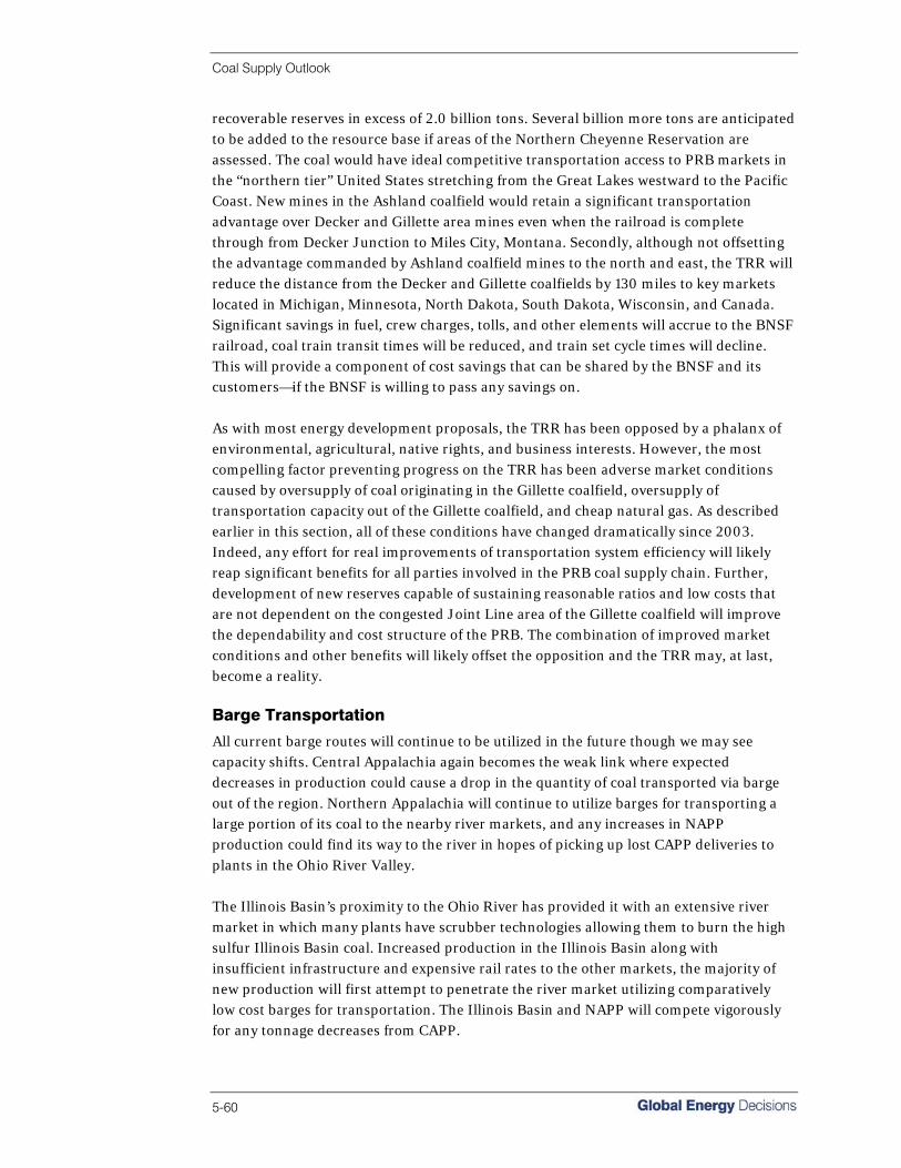
Coal Supply Outlook
5-60
recoverable reserves in excess of 2.0 billion tons. Several billion more tons are anticipated to be added to the resource base if areas of the Northern Cheyenne Reservation are assessed. The coal would have ideal competitive transportation access to PRB markets in the “northern tier” United States stretching from the Great Lakes westward to the Pacific Coast. New mines in the Ashland coalfield would retain a significant transportation advantage over Decker and Gillette area mines even when the railroad is complete through from Decker Junction to Miles City, Montana. Secondly, although not offsetting the advantage commanded by Ashland coalfield mines to the north and east, the TRR will reduce the distance from the Decker and Gillette coalfields by 130 miles to key markets located in Michigan, Minnesota, North Dakota, South Dakota, Wisconsin, and Canada. Significant savings in fuel, crew charges, tolls, and other elements will accrue to the BNSF railroad, coal train transit times will be reduced, and train set cycle times will decline. This will provide a component of cost savings that can be shared by the BNSF and its customers—if the BNSF is willing to pass any savings on. As with most energy development proposals, the TRR has been opposed by a phalanx of environmental, agricultural, native rights, and business interests. However, the most compelling factor preventing progress on the TRR has been adverse market conditions caused by oversupply of coal originating in the Gillette coalfield, oversupply of transportation capacity out of the Gillette coalfield, and cheap natural gas. As described earlier in this section, all of these conditions have changed dramatically since 2003. Indeed, any effort for real improvements of transportation system efficiency will likely reap significant benefits for all parties involved in the PRB coal supply chain. Further, development of new reserves capable of sustaining reasonable ratios and low costs that are not dependent on the congested Joint Line area of the Gillette coalfield will improve the dependability and cost structure of the PRB. The combination of improved market conditions and other benefits will likely offset the opposition and the TRR may, at last, become a reality. Barge Transportation
All current barge routes will continue to be utilized in the future though we may see capacity shifts. Central Appalachia again becomes the weak link where expected decreases in production could cause a drop in the quantity of coal transported via barge out of the region. Northern Appalachia will continue to utilize barges for transporting a large portion of its coal to the nearby river markets, and any increases in NAPP production could find its way to the river in hopes of picking up lost CAPP deliveries to plants in the Ohio River Valley. The Illinois Basin’s proximity to the Ohio River has provided it with an extensive river market in which many plants have scrubber technologies allowing them to burn the high sulfur Illinois Basin coal. Increased production in the Illinois Basin along with insufficient infrastructure and expensive rail rates to the other markets, the majority of new production will first attempt to penetrate the river market utilizing comparatively low cost barges for transportation. The Illinois Basin and NAPP will compete vigorously for any tonnage decreases from CAPP.

Coal Supply Outlook
Coal Reference Case, Fall 2007 5-61
The western coals will also continue to utilize barges as a form of terminating transportation. In 2005 and 2006 approximately 9 percent of coal delivered from the Rocky Mountain and Powder River Basins was transferred to barges, where the Ohio, Tennessee, Cumberland, Illinois, Monongahela, and Allegheny rivers provided routes for western coal to 40 different plants located in numerous states. Ocean Vessel Transportation
While the U.S. is a net exporter of coal, importing only 35 million tons in 2006 as opposed to 46 million tons exported, the current value of the dollar is having an impact. With the dollar weak some coal companies have seen an increase in demand for exports and a decrease in demand for imports. This trend could continue if the dollar remains weak in the international currency exchange market though in the long term a large effect is not anticipated. U.S. coal imports are expected to increase in future years with the majority of new imports coming from Colombia. If this occurs the amount of coal transported via ocean vessel would without question increase. U.S. capacity to handle exports is sufficient for current and predicted future levels, though importing capacity will need to be increased if imports are expected to increase. In anticipation of higher import volumes many import terminals have released plans for increasing their on site capacity. Another variable facing ocean vessel transportation is increased costs mainly due to high fuel prices. In regards to imports, a weak dollar only makes the transporting of coal increasingly expensive; the opposite would be true for countries importing U.S. coal. Fuel prices seem to have stabilized with prices in the summer months of 2007 failing to reach the highs that were anticipated. Though current prices are still considered high, a flattening of current prices and a forecasted drop in future oil prices would imply U.S. coal imports would become less expensive than they currently are and demand for imports would increase as would the need for additional capacity at import terminals. Table 5-20 Import Handling Facility Capacities
Terminal Name State 2005 2008 Change
McDuffie Terminal AL 12.0 24.0 12.0
TECO Davant Dock LA 9.0 9.0 -
KMT International Marine Terminals LA 3.0 3.0 -
KMT Shipyard River SC 2.5 6.0 3.5
Tampaplex Terminal FL 2.5 2.5 -
KMT Fairless Hills PA 1.0 2.0 1.0
KMT Chesapeake Bay MD 1.0 1.0 -
NS Philadelphia PA 1.0 1.0 -
Gateway Terminal CT 1.0 1.0 -
Providence RI 1.0 1.0 -
Savannah River Wharf GA 0.1 0.1 -
Table continued on next page.
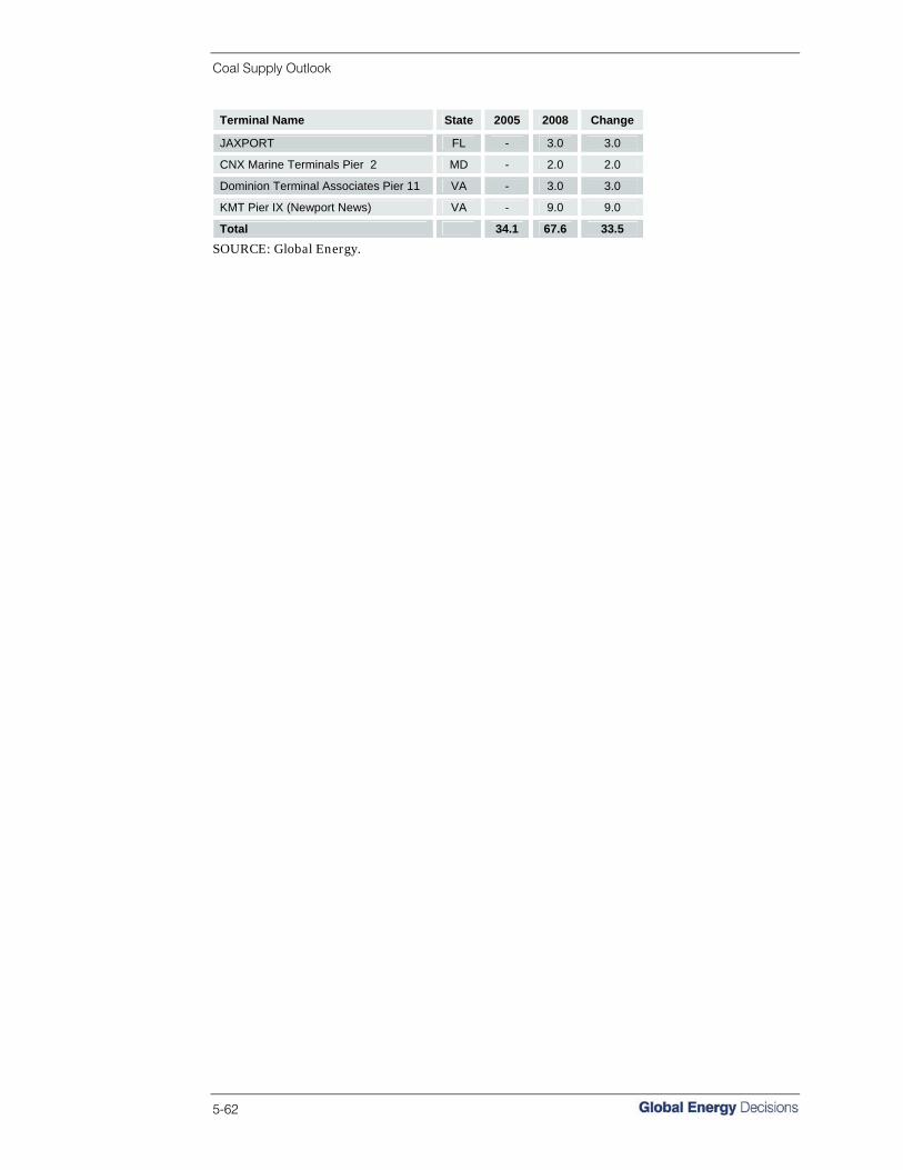
Coal Supply Outlook
5-62
Terminal Name State 2005 2008 Change
JAXPORT FL - 3.0 3.0
CNX Marine Terminals Pier 2 MD - 2.0 2.0
Dominion Terminal Associates Pier 11 VA - 3.0 3.0
KMT Pier IX (Newport News) VA - 9.0 9.0
Total 34.1 67.6 33.5 SOURCE: Global Energy.

Appendices

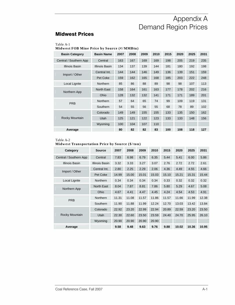
Appendix A Demand Region Prices
Coal Reference Case, Fall 2007 A-1
Midwest Prices Table A-1 Midwest FOB Mine Price by Source (¢/MMBtu)
Basin Category Basin Name 2007 2008 2009 2010 2015 2020 2025 2031
Central / Southern App Central 163 167 169 169 198 205 219 235
Illinois Basin Illinois Basin 134 137 139 144 181 180 192 198
Central Int. 144 144 146 149 136 139 151 159 Import / Other
Pet Coke 159 162 165 168 185 203 222 248
Local Lignite Northern 85 86 88 89 98 98 107 113
North East 158 164 161 163 177 178 202 216 Northern App
Ohio 128 132 132 141 171 171 189 201
Northern 57 64 65 74 99 109 119 131 PRB
Southern 54 55 56 55 68 78 89 102
Colorado 149 149 155 155 133 135 150 162
Utah 125 121 122 123 133 133 148 156 Rocky Mountain
Wyoming 100 104 107 110
Average 80 82 82 83 100 108 118 127
Table A-2 Midwest Transportation Price by Source ($/ton)
Category Source 2007 2008 2009 2010 2015 2020 2025 2031
Central / Southern App Central 7.83 6.98 6.79 6.35 5.44 5.41 6.00 5.86
Illinois Basin Illinois Basin 3.32 3.33 3.27 3.07 2.76 2.72 2.72 2.61
Central Int. 2.80 2.25 2.29 2.06 4.36 4.49 4.55 4.66 Import / Other
Pet Coke 14.99 15.00 15.01 15.03 15.10 15.21 15.31 15.44
Local Lignite Northern 0.34 0.34 0.34 0.34 0.33 0.32 0.32 0.32
North East 8.04 7.87 8.81 7.86 5.80 5.29 4.67 5.08 Northern App
Ohio 4.67 4.41 4.47 4.45 4.24 4.54 4.53 4.91
Northern 11.31 11.08 11.57 11.86 11.57 11.66 11.99 12.38 PRB
Southern 11.90 11.88 11.99 12.24 12.70 13.03 13.42 13.84
Colorado 22.92 23.20 22.99 22.94 20.89 22.59 23.20 23.50
Utah 22.30 22.60 23.50 23.59 24.40 24.70 25.95 26.10 Rocky Mountain
Wyoming 20.90 20.90 20.90 20.90
Average 9.58 9.48 9.63 9.76 9.88 10.02 10.36 10.95

Appendix A
A-2
Table A-3 Midwest Delivered Price by Source (¢/MMBtu)
Category Source 2007 2008 2009 2010 2015 2020 2025 2031
Central Int. 156 154 156 159 157 160 172 181 Import / Other
Pet Coke 212 215 218 221 238 256 277 303
Local Lignite Northern 87 88 90 91 101 100 109 116
Colorado 250 251 256 255 222 231 248 261
Utah 216 214 219 219 234 235 254 262 Rocky Mountain
Wyoming 221 225 228 232
Illinois Basin Illinois Basin 149 151 153 157 194 192 205 210
North East 189 194 195 194 199 199 221 235 Northern App
Ohio 147 150 150 159 188 190 207 221
Central / South App Central 194 196 196 195 220 228 244 259
Northern 119 124 127 138 162 174 186 200 PRB
Southern 122 124 125 126 141 153 167 183
Average 133 134 135 137 155 164 176 189
Northeast Prices Table A-4 Northeast FOB Mine Price by Source (¢/MMBtu)
Category Basin Name 2007 2008 2009 2010 2015 2020 2025 2031
Central / Southern App Central 196 190 198 184 179 183 197 204
Illinois Basin Illinois Basin 208 222 233
Colombia 253 275 274 208 179 191 203 214
Indonesia 242 318 313 297 259 275 289 306
Pet Coke 168 171 175 178 193 207 226 248 Import / Other
Venezuela 264 266 268 191 175 183 196 213
North East 174 175 178 180 194 199 215 232 Northern App
Ohio 122 149 146 146 162 163 238
Northern 60 96 104 113 123 PRB
Southern 43 45 50 50 72 80 89 98
Rocky Mountain Colorado 132 127 124 127
Average 179 179 181 179 188 193 207 224

Appendix A
Coal Reference Case, Fall 2007 A-3
Table A-5 Northeast Transportation Price by Source ($/ton)
Category Source 2007 2008 2009 2010 2015 2020 2025 2031
Central / Southern App Central 15.19 15.17 15.46 14.67 15.91 17.58 18.42 18.14
Illinois Basin Illinois Basin 16.95 16.78 16.58
Colombia 7.00 7.19 7.15 7.24 5.64 5.80 5.91 6.09
Indonesia 13.45 13.70 13.59 13.48 12.95 13.28 13.61 14.02
Pet Coke 15.00 15.00 15.00 15.00 14.77 14.71 14.64 14.62 Import / Other
Venezuela 8.52 8.96 8.91 6.77 6.79 7.08 8.24 7.82
North East 5.83 5.59 5.73 5.11 5.25 5.53 4.99 5.01 Northern App
Ohio 3.16 2.23 2.22 2.14 1.99 1.98 2.84
Northern 20.98 26.84 27.77 28.75 29.98 PRB
Southern 20.51 20.27 20.01 17.91 20.40 21.12 21.21 21.58
Rocky Mountain Colorado 24.71 25.29 25.66 25.70
Average 8.36 8.32 8.29 7.52 6.90 7.08 6.93 6.64
Table A-6 Northeast Delivered Price by Source (¢/MMBtu)
Category Source 2007 2008 2009 2010 2015 2020 2025 2031
Colombia 283 306 305 239 204 216 229 240
Indonesia 315 381 376 359 319 336 352 371
Pet Coke 224 227 231 234 247 261 280 301 Import / Other
Venezuela 298 302 303 217 202 211 229 244
Rocky Mountain Colorado 235 232 230 234
Illinois Basin Illinois Basin 290 304 313
North East 197 198 201 201 215 220 234 252 Northern App
Ohio 135 158 155 155 171 172 249
Central / South App Central 256 251 260 243 243 253 270 276
Northern 172 240 254 268 285 PRB
Southern 159 160 163 151 188 200 209 220
Average 214 214 216 210 216 223 236 252

Appendix A
A-4
South Central Prices Table A-7 South Central FOB Mine Price by Source (¢/MMBtu)
Category Basin Name 2007 2008 2009 2010 2015 2020 2025 2031
Central Int. 119 140 146 147 167 166 182 193
Colombia 224 322 248 207 180 191 201 213 Import / Other
Pet Coke 154 157 160 163 180 196 216 240
Local Lignite Gulf 138 140 142 142 136 143 159 172
PRB Southern 61 63 64 65 71 79 88 101
Rocky Mountain Colorado 100 106 108 132 150 151 167 180
Average 86 87 89 88 86 94 105 118
Table A-8 South Central Transportation Price by Source ($/ton)
Category Source 2007 2008 2009 2010 2015 2020 2025 2031
Central Int. 1.62 1.95 1.94 1.90 1.81 1.81 1.85 1.91
Colombia 12.23 9.95 11.83 12.45 12.14 12.43 12.75 13.11 Import / Other
Pet Coke 14.97 14.96 14.99 15.03 15.01 15.07 15.13 15.19
Local Lignite Gulf 0.70 0.70 0.70 0.72 0.74 0.72 0.71 0.73
PRB Southern 14.68 14.78 14.89 15.36 15.86 16.02 16.59 17.40
Rocky Mountain Colorado 16.37 16.45 16.54 17.14 17.84 18.56 19.32 20.23
Average 10.46 10.52 10.64 11.21 12.45 12.59 12.83 13.60
Table A-9 South Central Delivered Price by Source (¢/MMBtu)
Category Source 2007 2008 2009 2010 2015 2020 2025 2031
Central Int. 127 149 154 156 175 174 190 201
Colombia 277 362 298 260 232 245 256 270 Import / Other
Pet Coke 206 209 212 215 231 248 268 292
Local Lignite Gulf 144 145 147 147 142 149 165 178
Rocky Mountain Colorado 178 185 188 215 236 240 260 277
PRB Southern 146 149 151 154 162 171 183 202
Average 146 148 151 153 158 167 179 197

Appendix A
Coal Reference Case, Fall 2007 A-5
Southeast Prices Table A-10 Southeast FOB Mine Price by Source (¢/MMBtu)
Basin Category Basin Name 2007 2008 2009 2010 2015 2020 2025 2031
Central 180 183 185 188 214 214 232 254 Central / Southern App
Southern 205 185 185 185 190 191 207 225
Illinois Basin Illinois Basin 134 138 143 152 166 168 183 194
Colombia 201 219 219 208 180 191 202 217
Pet Coke 158 161 164 167 183 199 218 238 Import / Other
Venezuela 209 212 214 199 193 205 198 179
Local Lignite Gulf 240 244 248 252 274 297 321 354
North East 144 153 156 160 174 175 192 205 Northern App
Ohio 122 143 144 151 162 178 193 214
Northern 125 129 132 96 PRB
Southern 55 58 59 60 72 82 91 104
Colorado 96 101 111 117 135 137 150 160 Rocky Mountain
Utah 118 142 121 122
Average 151 155 157 160 174 175 186 188
Table A-11 Southeast Transportation Price by Source ($/ton)
Category Source 2007 2008 2009 2010 2015 2020 2025 2031
Central 12.63 11.67 11.46 9.96 8.63 8.37 8.40 8.48 Central / Southern App
Southern 7.37 6.51 6.08 4.88 5.04 5.18 5.01 5.29
Illinois Basin Illinois Basin 7.79 7.70 7.44 6.93 6.20 5.87 6.07 6.28
Colombia 9.02 8.15 8.11 8.03 8.09 8.28 8.57 8.83
Pet Coke 14.87 14.85 14.85 14.90 14.86 14.88 14.91 14.78 Import / Other
Venezuela 8.37 8.48 8.45 11.54 12.08 9.55 9.10 8.27
Local Lignite Gulf 2.42 2.42 2.42 2.42 2.42 2.42 2.42 2.42
North East 6.76 5.64 5.60 5.07 4.16 4.25 4.50 4.18 Northern App
Ohio 6.59 5.97 5.88 5.26 1.48 1.45 2.05 2.41
Northern 19.08 19.08 19.08 21.23 PRB
Southern 19.42 19.27 19.38 19.04 19.85 20.27 20.38 20.57
Colorado 21.28 21.37 21.86 22.39 23.07 24.06 24.97 26.51 Rocky Mountain
Utah 18.47 22.96 19.14 19.23
Average 12.09 11.52 11.34 10.49 9.96 10.18 10.70 12.26

Appendix A
A-6
Table A-12 Southeast Delivered Price by Source (¢/MMBtu)
Category Source 2007 2008 2009 2010 2015 2020 2025 2031
Colombia 241 255 254 243 215 227 239 255
Pet Coke 210 213 217 220 236 252 271 290 Import / Other
Venezuela 241 245 247 245 241 243 233 212
Local Lignite Gulf 264 268 272 276 297 320 345 377
Colorado 186 190 202 210 232 237 254 271 Rocky Mountain
Utah 196 239 202 203
Illinois Basin Illinois Basin 167 171 175 182 193 193 209 221
North East 171 175 178 180 190 191 210 221 Northern App
Ohio 150 168 168 173 168 184 201 224
Central 231 230 231 228 249 248 267 289 Central / South App
Southern 235 212 210 205 210 212 228 246
Northern 221 224 228 210 PRB
Southern 166 168 170 168 185 197 207 222
Average 205 206 207 207 219 222 235 248
West Prices Table A-13 West FOB Mine Price by Source (¢/MMBtu)
Basin Category Basin Name 2007 2008 2009 2010 2015 2020 2025 2031
Import / Other Pet Coke 127 129 132 134 148 163 178 199
Local Lignite Northern 98 99 100 101 103 103 112
Northern 82 83 84 87 95 108 122 131 PRB
Southern 47 50 51 53 66 74 88 101
Colorado 120 124 129 129 137 138 153 163
Four Corners 133 135 137 139 146 147 164 178
Utah 113 114 118 119 130 133 147 157 Rocky Mountain
Wyoming 123 125 126 128 118 119 136 149
Average 101 103 105 106 110 115 129 145

Appendix A
Coal Reference Case, Fall 2007 A-7
Table A-14 West Transportation Price by Source ($/ton)
Category Source 2007 2008 2009 2010 2015 2020 2025 2031
Import / Other Pet Coke 15.00 15.01 15.02 15.03 15.08 15.13 15.18 15.23
Local Lignite Northern 1.63 1.63 1.63 1.62 1.47 1.46 1.50
Northern 5.03 5.14 5.31 5.37 5.41 5.66 5.88 6.07 PRB
Southern 8.52 8.64 8.67 8.76 9.96 10.41 11.20 9.86
Colorado 5.88 5.56 5.00 6.01 6.40 6.16 5.93 6.27
Four Corners 2.85 2.85 3.13 3.08 2.58 2.73 2.51 3.40
Utah 5.27 5.01 4.68 4.77 4.17 4.22 4.39 4.22 Rocky Mountain
Wyoming 1.14 1.14 1.14 0.82 0.29 0.29 0.29 0.29
Average 4.99 4.98 4.98 5.17 5.70 5.83 6.18 5.72
Table A-15 West Delivered Price by Source (¢/MMBtu)
Category Source 2007 2008 2009 2010 2015 2020 2025 2031
Import / Other Pet Coke 169 172 174 177 191 205 221 242
Local Lignite Northern 110 111 113 113 114 114 123
Colorado 147 149 151 156 165 165 179 191
Four Corners 147 150 153 155 159 161 176 195
Utah 135 136 138 140 148 151 165 175 Rocky Mountain
Wyoming 129 131 132 132 119 121 138 151
Northern 110 112 114 118 126 140 156 165 PRB
Southern 97 100 102 104 124 135 153 159
Average 127 129 131 133 140 146 162 175


Appendix B Demand Region Volumes
Coal Reference Case, Fall 2007 B-1
Delivered Coal Quantities Table B-1 Overall U.S. Delivered Coal Quantities by Source (000s tons)
Category Source 2007 2008 2009 2010 2015 2020 2025 2031
Central Int. 1,535 1,505 1,350 1,336 296 284 381 625
Colombia 19,821 18,673 17,692 19,549 31,655 37,615 45,034 55,206
Indonesia 1,517 1,306 1,284 1,259 1,116 1,090 1,070 1,068
Venezuela 3,352 3,190 3,165 2,430 3,968 3,968 3,968 3,968
Import / Other
Pet Coke 5,708 5,834 5,903 5,709 6,212 6,335 6,474 7,646
Gulf 49,333 49,810 49,309 47,285 41,381 43,467 48,544 49,965 Local Lignite
Northern 22,855 22,970 23,823 23,811 23,817 23,549 23,055 22,808
Colorado 30,024 30,761 31,539 32,346 37,453 42,086 48,151 55,052
Four Corners 34,701 34,683 36,119 36,126 28,256 29,126 28,783 36,220
Utah 20,347 22,400 20,726 21,779 18,573 21,122 21,125 21,122 Rocky
Mountain
Wyoming 12,048 12,046 12,048 11,430 11,319 11,314 11,300 11,287
Illinois Basin Illinois Basin 87,068 89,210 91,463 93,804 107,448 116,246 123,968 119,585
North East 98,214 98,793 99,477 100,234 106,751 111,135 118,516 119,259 Northern App
Ohio 24,520 23,910 23,193 23,131 19,088 18,251 18,799 17,266
Central 171,971 165,710 162,469 159,057 147,156 130,316 114,368 93,733 Central / Southern App Southern 11,008 11,280 11,564 9,693 7,476 7,575 7,791 7,951
Northern 42,964 43,900 44,884 45,906 52,374 58,244 65,925 66,000 PRB
Southern 420,146 426,263 432,867 439,824 487,632 501,811 542,516 631,419
Grand Total 1,057,132 1,062,243 1,068,876 1,074,711 1,131,971 1,163,534 1,229,768 1,320,180
Table B-2 Midwest Delivered Coal Quantities by Source (000s tons)
Category Source 2007 2008 2009 2010 2015 2020 2025 2031
Central Int. 1,024 1,024 865 625 149 137 234 233 Import / Other
Pet Coke 684 689 694 666 675 610 605 583
Local Lignite Northern 22,488 22,596 23,442 23,431 23,458 23,213 22,990 22,808
Colorado 2,120 2,046 1,905 2,112 1,801 4,469 7,619 10,537
Utah 1,795 1,733 1,425 1,333 628 555 364 876 Rocky Mountain
Wyoming 46 46 46 46 - - - -
Illinois Basin Illinois Basin 46,664 49,354 47,973 48,930 56,593 62,906 67,137 65,488
North East 10,107 9,771 8,003 8,724 10,477 14,460 15,539 14,622 Northern App
Ohio 18,436 17,798 17,222 15,931 14,311 13,630 13,909 14,080
Central / South App Central 30,091 26,100 25,012 23,589 23,258 17,935 12,422 8,550
Northern 24,847 25,891 26,740 27,825 34,150 40,226 47,362 48,390 PRB
Southern 243,603 246,990 252,415 253,122 271,712 274,232 293,490 335,147
Grand Total 401,904 404,037 405,742 406,333 437,212 452,372 481,672 521,314

Appendix B
B-2
Table B-3 Northeast Delivered Coal Quantities by Source (000s tons)
Category Source 2007 2008 2009 2010 2015 2020 2025 2031
Colombia 4,962 3,173 3,336 2,762 8,244 7,937 8,672 7,632
Indonesia 1,517 1,306 1,284 1,259 1,116 1,090 1,070 1,068
Venezuela 2,115 2,174 2,149 2,035 3,698 3,240 2,803 3,470 Import / Other
Pet Coke 54 54 54 54 67 72 78 85
Rocky Mountain Colorado 295 1,618 1,854 2,023 - - - -
Illinois Basin - - - - - 276 267 258
North East 61,366 62,638 64,881 64,816 64,584 65,541 70,818 73,720Northern App
Ohio 889 339 291 291 281 281 - 169
Central / South App Central 15,164 13,889 10,988 12,432 7,625 5,354 4,706 4,239
Northern 186 - - - 252 459 1,000 215 PRB
Southern 3,884 3,797 4,462 2,569 2,782 2,653 3,939 3,737
Grand Total 90,432 88,988 89,299 88,241 88,650 86,903 93,354 94,593
Table B-4 South Central Delivered Coal Quantities by Source (000s tons)
Category Source 2007 2008 2009 2010 2015 2020 2025 2031
Central Int. 511 481 485 711 147 147 146 392
Colombia 986 101 363 285 57 63 67 66 Import / Other
Pet Coke 819 835 824 804 863 859 858 860
Local Lignite Gulf 46,451 46,928 46,427 44,403 38,500 40,586 45,662 47,083
Rocky Mountain Colorado 855 1,007 1,000 169 152 144 146 181
PRB Southern 106,110 106,946 107,146 112,886 131,573 140,230 146,941 159,711
Grand Total 155,733 156,298 156,245 159,259 171,291 182,029 193,820 208,293
Table B-5 Southeast Delivered Coal Quantities by Source (000s tons)
Category Source 2007 2008 2009 2010 2015 2020 2025 2031
Colombia 13,873 15,400 13,993 16,502 23,353 29,614 36,296 47,508
Venezuela 1,237 1,016 1,015 395 270 728 1,165 498 Import / Other
Pet Coke 3,974 4,080 4,156 4,008 4,432 4,618 4,757 5,943
Local Lignite Gulf 2,882 2,882 2,882 2,882 2,882 2,882 2,882 2,882
Colorado 12,650 12,058 13,607 13,853 17,492 21,023 22,737 24,687 Rocky Mountain
Utah 43 2,134 751 1,110 - - - -
Illinois Basin 40,405 39,856 43,490 44,874 50,856 53,065 56,564 53,839
North East 26,742 26,384 26,593 26,694 31,690 31,134 32,159 30,916 Northern App
Ohio 5,195 5,772 5,679 6,909 4,496 4,340 4,890 3,017
Central 126,716 125,721 126,470 123,036 116,273 107,027 97,240 80,944 Central / South App
Southern 11,008 11,280 11,564 9,693 7,476 7,575 7,791 7,951
Northern 59 59 59 - 287 - - - PRB
Southern 37,684 38,905 38,493 38,726 41,855 44,528 54,686 94,984
Grand Total 282,468 285,544 288,752 288,682 301,361 306,533 321,165 353,169
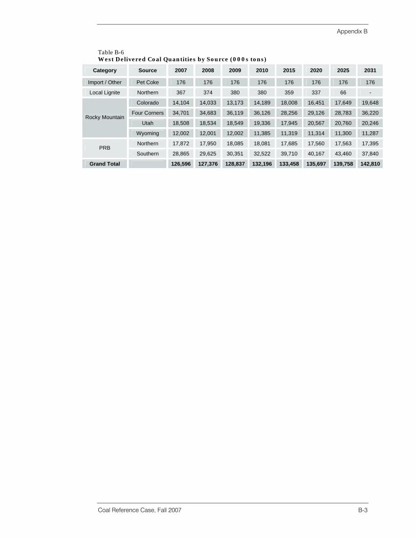
Appendix B
Coal Reference Case, Fall 2007 B-3
Table B-6 West Delivered Coal Quantities by Source (000s tons)
Category Source 2007 2008 2009 2010 2015 2020 2025 2031
Import / Other Pet Coke 176 176 176 176 176 176 176 176
Local Lignite Northern 367 374 380 380 359 337 66 -
Colorado 14,104 14,033 13,173 14,189 18,008 16,451 17,649 19,648
Four Corners 34,701 34,683 36,119 36,126 28,256 29,126 28,783 36,220
Utah 18,508 18,534 18,549 19,336 17,945 20,567 20,760 20,246 Rocky Mountain
Wyoming 12,002 12,001 12,002 11,385 11,319 11,314 11,300 11,287
Northern 17,872 17,950 18,085 18,081 17,685 17,560 17,563 17,395 PRB
Southern 28,865 29,625 30,351 32,522 39,710 40,167 43,460 37,840
Grand Total 126,596 127,376 128,837 132,196 133,458 135,697 139,758 142,810


Appendix C Basin Volumes & Prices
Coal Reference Case, Fall 2007 C-1
Fully Allocated Costs Table C-1 Fully Allocated Mine Costs by Basin ($/ton)
Basin 2007 2008 2009 2010 2011 2015 2020 2025 2031
Northern App 33.54 34.63 35.12 35.44 37.03 39.72 40.27 44.85 48.73
Central App 38.02 40.26 41.26 42.57 44.75 48.18 48.48 52.88 57.93
Southern App 42.92 45.05 45.35 45.14 43.93 46.63 46.96 50.76 54.89
Illinois Basin 29.84 30.30 30.79 31.14 32.10 33.37 32.95 35.95 37.87
North PRB 12.57 13.00 12.71 12.97 12.92 14.45 16.27 18.24 20.27
South PRB 9.57 9.69 9.75 9.90 10.13 11.45 13.15 14.96 17.23
Rocky Mtn. 25.59 26.15 26.34 26.51 26.43 28.37 28.71 31.91 34.41
Central Int. 32.52 32.10 32.45 32.78 30.41 33.77 34.68 36.13 40.98
North Lignite 11.43 11.07 11.64 11.10 11.73 12.95 12.88 14.06 14.90
Gulf Lignite 19.06 18.54 18.68 17.37 17.56 16.49 17.39 19.17 20.43
Overall 20.80 21.98 22.25 22.55 23.60 24.70 25.42 27.59 29.15
FOB Mine Prices Table C-2 Northern App North East FOB Mine Price by Quality Category ($/ton)
2007 2008 2009 2010 2011 2015 2020 2025 2031
NANEHiHi 38.87 41.29 41.32 42.28 44.61 47.15 47.30 51.75 55.19
NANEHiLo 46.45 48.91 48.72 49.62 49.38 51.75 52.42 57.23 61.66
NANELoHi 34.18 35.35 35.03 35.41 36.87 39.42 40.29 44.92 48.03
NANELoLo 41.53 44.61 43.48 42.03 47.10 49.19 50.50 55.48 60.87
Table C-3 Northern App Ohio FOB Mine Price by Quality Category ($/ton)
2007 2008 2009 2010 2011 2015 2020 2025 2031
NAOHHiHi 33.99 40.10 38.77 38.65 40.24 42.80 43.23 47.13 49.31
NAOHHiLo 38.39 46.10 44.71 44.66 44.01 47.03 48.79 53.80 59.70
NAOHLoHi 31.33 36.99 35.75 35.77 31.91 35.37 35.58 39.16 45.88
NAOHLoLo 37.46 43.37 40.83 40.75 35.97 38.21 38.44 42.40 45.44
Table C-4 Central App FOB Mine Price by Quality Category ($/ton)
2007 2008 2009 2010 2011 2015 2020 2025 2031
CAPPHiHi 40.78 42.82 42.49 44.22 48.01 52.95 52.18 55.00 61.99
CAPPHiLo 45.31 50.38 49.86 50.10 52.33 54.69 55.88 60.50 62.54
CAPPHiMed 42.29 44.78 44.40 45.75 49.13 53.53 53.41 56.83 62.17
CAPPLoHi 38.26 41.16 40.64 42.22 42.80 45.56 46.21 51.25 56.12
CAPPLoLo 39.27 42.21 41.65 43.23 43.80 46.56 47.21 52.25 57.12
CAPPLoMed 38.77 41.68 41.15 42.72 43.30 46.06 46.71 51.75 56.62

Appendix C
C-2
Table C-5 Southern App FOB Mine Price by Quality Category ($/ton)
2007 2008 2009 2010 2011 2015 2020 2025 2031
SAPPHiHi 51.26 46.24 46.78 45.95 46.77 49.28 49.61 53.41 57.54
SAPPHiLo 59.20 53.00 54.02 54.76 55.31 57.22 57.55 61.35 65.48
SAPPLoHi 48.61 43.99 44.36 43.01 43.92 46.63 46.96 50.76 54.89
SAPPLoLo 56.55 50.75 51.61 51.82 52.46 54.57 54.90 58.70 62.83
Table C-6 Illinois Basin FOB Mine Price by Quality Category ($/ton)
2007 2008 2009 2010 2011 2015 2020 2025 2031
ILLBHiHi 33.93 36.26 35.43 34.82 33.90 34.89 35.54 38.26 40.61
ILLBHiLo 43.18 46.15 45.09 44.31 43.14 44.40 45.23 48.69 51.68
ILLBLoHi 30.84 32.96 32.21 31.65 30.81 31.71 32.31 34.78 36.91
ILLBLoLo 39.07 41.75 40.79 40.09 39.03 40.17 40.92 44.05 46.76
ILLBLoMed 35.99 38.46 37.57 36.93 35.95 37.00 37.69 40.58 43.07
Table C-7 Northern PRB FOB Mine Price by Quality Category ($/ton)
2007 2008 2009 2010 2011 2015 2020 2025 2031
NPRBHiHi 15.50 16.10 15.28 15.83 16.38 17.83 19.46 20.85 22.31
NPRBHiLo 16.00 16.75 15.75 16.17 16.79 18.16 19.63 21.00 22.52
NPRBLoHi 14.00 14.13 13.88 14.81 15.14 16.83 18.93 20.41 21.67
NPRBLoLo 14.50 14.79 14.35 15.15 15.55 17.16 19.11 20.56 21.88
Table C-8 Southern PRB FOB Mine Price by Quality Category ($/ton)
2007 2008 2009 2010 2011 2015 2020 2025 2031
SPRBHiHi 9.73 11.49 11.28 10.92 10.26 11.52 13.18 14.66 16.14
SPRBHiLo 9.84 11.68 11.50 11.16 10.51 11.87 13.51 14.90 16.31
SPRBHiUltraLo 10.06 12.06 11.94 11.65 11.02 12.56 14.18 15.39 16.65
SPRBLoHi 7.62 9.43 9.57 9.36 9.04 10.19 11.60 13.01 14.38
SPRBLoLo 8.12 9.94 10.01 9.74 9.36 10.43 11.99 13.66 15.24
SPRBLoUltraLo 8.31 10.30 10.45 10.22 9.87 11.13 12.66 14.21 15.70
Table C-9 Rocky Mountain Colorado North FOB Mine Price by Quality Category ($/ton)
2007 2008 2009 2010 2011 2015 2020 2025 2031
RMCONHiHi 22.62 25.18 26.28 26.22 26.22 28.44 28.63 31.89 34.36
RMCONHiLo 23.64 26.10 27.20 27.15 27.58 29.70 29.88 32.87 35.10
RMCONLoHi 22.01 23.54 24.77 25.15 24.17 26.55 26.76 30.41 33.25
RMCONLoLo 22.55 23.99 25.23 25.62 24.85 27.18 27.38 30.90 33.62

Appendix C
Coal Reference Case, Fall 2007 C-3
Table C-10 Rocky Mountain Colorado West FOB Mine Price by Quality Category ($/ton)
2007 2008 2009 2010 2011 2015 2020 2025 2031
RMCOWHiHi 24.90 28.64 30.13 30.05 28.85 31.19 31.49 35.08 37.89
RMCOWHiLo 25.92 29.56 31.05 30.98 30.21 32.45 32.74 36.06 38.63
RMCOWLoHi 24.40 26.96 28.61 29.03 26.80 29.30 29.62 33.60 36.78
RMCOWLoLo 24.93 27.41 29.07 29.50 27.48 29.93 30.24 34.09 37.15
Table C-11 Rocky Mountain Four Corners FOB Mine Price by Quality Category ($/ton)
2007 2008 2009 2010 2011 2015 2020 2025 2031
RMFCHiHi 28.85 29.30 29.48 29.62 29.87 32.57 32.82 36.40 39.04
RMFCHiLo 29.81 30.28 30.48 30.53 30.73 33.03 33.25 36.93 39.79
RMFCLoHi 25.85 26.16 26.06 26.18 25.79 27.77 27.96 31.11 33.81
RMFCLoLo 27.83 28.22 28.27 28.36 28.26 30.40 30.61 34.02 36.80
Table C-12 Rocky Mountain Utah FOB Mine Price by Quality Category ($/ton)
2007 2008 2009 2010 2011 2015 2020 2025 2031
RMUtahHiHi 27.91 28.92 30.68 30.55 30.20 32.34 32.53 35.92 38.53
RMUtahHiLo 28.48 30.34 31.29 31.48 30.70 33.12 33.56 36.92 39.44
RMUtahLoHi 24.37 25.25 27.44 28.60 25.43 25.26 27.34 30.06 32.16
RMUtahLoLo 25.55 26.47 28.52 29.25 27.02 27.62 29.07 32.01 34.28
Table C-13 Rocky Mountain Wyoming FOB Mine Price by Quality Category ($/ton)
2007 2008 2009 2010 2011 2015 2020 2025 2031
RMWYHiHi 24.85 25.01 25.08 25.03 25.13 26.60 26.76 29.41 31.46
RMWYHiLo 25.58 25.94 26.08 26.16 26.35 28.00 28.15 30.60 32.49
RMWYLoHi 22.66 22.22 22.06 21.65 21.47 22.38 22.57 25.83 28.35
RMWYLoLo 23.39 23.15 23.07 22.78 22.69 23.79 23.97 27.02 29.39
Table C-14 Gulf Lignite FOB Mine Price by Quality Category ($/ton)
2007 2008 2009 2010 2011 2015 2020 2025 2031
GLIGHiHi 22.38 21.67 21.89 20.45 20.59 18.81 18.70 20.45 21.66
GLIGHiLo 20.91 20.56 21.30 20.54 20.61 21.07 22.72 24.54 25.77
GLIGLoHi 11.46 11.10 11.57 11.04 11.56 12.76 12.69 16.65 17.64
GLIGLoLo 14.69 14.33 14.94 14.29 14.59 15.42 16.21 19.10 20.21
Table C-15 Northern Lignite FOB Mine Price by Quality Category ($/ton)
2007 2008 2009 2010 2011 2015 2020 2025 2031
NLIGHi 10.96 10.63 11.07 10.54 10.93 12.11 12.04 13.17 13.97
NLIGLo 11.34 10.99 11.44 10.91 11.30 12.48 12.41 13.54 14.34

Appendix C
C-4
Table C-17 Central Interior FOB Mine Price by Quality Category ($/ton)
2007 2008 2009 2010 2011 2015 2020 2025 2031
CINTHi 33.92 33.24 34.44 35.71 35.57 39.27 39.05 42.70 45.23
CINTLo 27.23 26.36 25.72 24.53 25.70 28.37 30.01 32.02 33.83
Table C-18 Import / Pet Coke FOB Mine Price by Quality Category ($/ton)
2007 2008 2009 2010 2011 2015 2020 2025 2031
IMCO (Colombia) 50.53 50.88 50.17 47.66 45.63 41.75 44.29 46.86 50.09
IMIN (Indonesia) 69.30 68.56 67.54 64.07 61.13 55.82 59.25 62.27 66.11
IMVE (Venezuela) 52.74 52.95 52.02 47.48 49.35 45.06 47.83 50.27 53.36
Pet Coke 45.20 45.68 46.24 46.74 46.97 50.28 51.19 57.19 61.97
Delivered Coal Quantities Table C-1 Continental U.S. Coal Deliveries to Electricity Generators by Basin (000s tons)
Coal Source 2007 2008 2009 2010 2011 2015 2020 2025 2031
Northern App 122,734 122,702 122,670 123,365 121,870 125,839 129,386 137,315 136,525
North East 98,214 98,793 99,477 100,234 101,853 106,751 111,135 118,516 119,259
Ohio 24,520 23,910 23,193 23,131 20,018 19,088 18,251 18,799 17,266
Central App 171,971 165,710 162,469 159,057 157,368 147,156 130,316 114,368 93,733
Southern App 11,008 11,280 11,564 9,693 7,478 7,476 7,575 7,791 7,951
Illinois Basin 87,068 89,210 91,463 93,804 96,988 107,448 116,246 123,968 119,585
PRB 463,110 470,163 477,751 485,731 497,877 540,007 560,055 608,441 697,419
South 420,146 426,263 432,867 439,824 450,580 487,632 501,811 542,516 631,419
North 42,964 43,900 44,884 45,906 47,297 52,374 58,244 65,925 66,000
Rocky Mountain 97,120 99,891 100,433 101,682 99,338 95,601 103,648 109,359 123,680
Colorado 30,024 30,761 31,539 32,346 33,444 37,453 42,086 48,151 55,052
Four Corners 34,701 34,683 36,119 36,126 34,694 28,256 29,126 28,783 36,220
Utah 20,347 22,400 20,726 21,779 19,880 18,573 21,122 21,125 21,122
Wyoming 12,048 12,046 12,048 11,430 11,320 11,319 11,314 11,300 11,287
Central Int. 1,535 1,505 1,350 1,336 448 296 284 381 625
Northern Lignite 22,855 22,970 23,823 23,811 23,912 23,817 23,549 23,055 22,808
Gulf Lignite 49,333 49,810 49,309 47,285 42,122 41,381 43,467 48,544 49,965
Import 24,690 23,169 22,141 23,238 31,940 36,738 42,673 50,072 60,242
Colombia 19,821 18,673 17,692 19,549 26,755 31,655 37,615 45,034 55,206
Venezuela 3,352 3,190 3,165 2,430 3,968 3,968 3,968 3,968 3,968
Indonesia 1,517 1,306 1,284 1,259 1,217 1,116 1,090 1,070 1,068
Pet Coke 5,708 5,834 5,903 5,709 5,957 6,212 6,335 6,474 7,646
Total (× 1,000) 1,027 1,033 1,041 1,046 1,047 1,089 1,115 1,173 1,252

Appendix C
Coal Reference Case, Fall 2007 C-5
Delivered Coal Qualities Table C-19 Weighted Averages of Coal Qualities by Source
Basin Quality Category
Average Btu/lb
AverageSO2/lb
Average Tons/Year
NANEHiLo 12,933 2.84 38,152
NANELoHi 11,931 5.36 25,255
NANEHiHi 12,896 3.82 36,184 NANE
NANELoLo 11,471 2.29 11,209
NAOHLoLo 11,531 4.90 806
NAOHHiLo 12,494 4.20 1,584
NAOHLoHi 11,667 5.33 2,352 NAOH
NAOHHiHi 12,346 6.10 14,544
CAPPHiLo 12,645 1.38 11,869
CAPPHiHi 12,853 2.28 706
CAPPLoLo 12,248 1.18 26,178
CAPPHiMed 12,604 1.68 21,557
CAPPLoHi 11,882 3.65 3,934
CAPP
CAPPLoMed 12,149 1.57 69,891
SAPPLoHi 12,233 2.16 7,790
SAPPHiHi 12,293 1.89 786
SAPPLoLo n/a n/a - SAPP
SAPPHiLo 12,425 1.22 892
ILLBHiLo 12,032 2.33 8,184
ILLBLoHi 11,039 4.84 35,178
ILLBLoMed 10,803 2.08 14,496
ILLBHiHi 11,687 5.00 42,713
ILLB
ILLBLoLo 10,259 1.41 8,563
NPRBLoLo n/a n/a -
NPRBHiHi n/a n/a -
NPRBHiLo 9,291 0.75 22,246 NPRB
NPRBLoHi 8,612 1.54 34,759
SPRBLoHi 8,026 1.37 14,111
SPRBLoLo 8,464 0.82 110,511
SPRBHiHi n/a n/a -
SPRBLoUltraLo 8,466 0.74 112,201
SPRBHiLo 8,585 0.91 60,785
SPRB
SPRBHiUltraLo 8,817 0.59 218,323
Continued on next page.

Appendix C
C-6
Table C-19 continued from previous page. Weighted Averages of Coal Qualities by Source
Basin Quality Category
Average Btu/lb
Average SO2/lb
Average Tons/Year
RMCONLoHi n/a n/a -
RMCONHiLo 10,901 0.84 10,145
RMCONLoLo 9,680 0.92 2,144
RMCONHiHi n/a n/a -
RMCOWLoLo 11,140 0.97 115
RMCOWLoHi n/a n/a -
RMCOWHiLo 11,969 0.86 28,765
RMCO
RMCOWHiHi n/a n/a -
RMFCHiHi 10,633 1.62 392
RMFCLoLo 9,803 0.92 4,763
RMFCHiLo 10,895 0.96 8,413 RMFC
RMFCLoHi 9,588 1.52 21,152
RMWYLoLo 9,381 1.02 2,937
RMWYLoHi 9,464 1.39 10,946
RMWYHiHi n/a n/a - RMWY
RMWYHiLo 10,256 0.76 1,420
RMUtahLoHi 10,217 1.42 3,514
RMUtahLoLo 11,263 0.73 9,171
RMUtahHiHi 12,364 1.70 2,762 RMUt
RMUtahHiLo 11,791 1.06 8,045
CINTLo 10,580 5.73 225 CINT
CINTHi 11,689 6.33 308
NLIGHi 6,820 2.69 7,767 NLIG
NLIGLo 6,451 1.97 15,616
GLIGLoLo 5,106 1.86 2,882
GLIGHiLo 6,623 2.20 19,492
GLIGHiHi 6,684 4.19 19,163 GLIG
GLIGLoHi 5,268 8.66 4,687
IMCO (Colombia) 11,585 1.01 37,291
IMIN (Indonesia) 10,731 0.26 1,139 IM
IMVE (Venezuela) 12,779 1.03 3,824
PETC PETCOKE 14,133 7.23 6,445
Copyright © 2022 FDOKUMEN