CNN-Annals
59
Annals of Physics 339 (2013) 22–80 Contents lists available at ScienceDirect Annals of Physics journal homepage: www.elsevier.com/locate/aop Spinful fermionic ladders at incommensurate filling: Phase diagram, local perturbations, and ionic potentials Sam T. Carr a,b,c,∗ , Boris N. Narozhny b,c , Alexander A. Nersesyan d a School of Physical Sciences, University of Kent, Canterbury CT2 7NH, UK b Institut für Theorie der Kondensierten Materie, Karlsruher Institut für Technologie, 76128 Karlsruhe, Germany c DFG Center for Functional Nanostructures, Karlsruher Institut für Technologie, 76128 Karlsruhe, Germany d The Abdus Salam International Centre for Theoretical Physics, 34100, Trieste, Italy highlights • We study low temperature electronic properties of a two leg ladder. • We find a wide variety of phase transitions as a function of model parameters. • We study the effect of impurities on these models. • Conductance may be very sensitive to the structure of these impurities. article info Article history: Received 15 June 2013 Accepted 5 August 2013 Available online 11 August 2013 Keywords: Luttinger liquid Spin gap Ladder materials Charge transport abstract We study the effect of external potential on transport properties of the fermionic two-leg ladder model. The response of the system to a local perturbation is strongly dependent on the ground state properties of the system and especially on the dominant correla- tions. We categorize all phases and transitions in the model (for in- commensurate filling) and introduce ‘‘hopping-driven transitions’’ that the system undergoes as the inter-chain hopping is increased from zero. We also describe the response of the system to an ionic potential. The physics of this effect is similar to that of the single impurity, except that the ionic potential can affect the bulk prop- erties of the system and in particular induce true long range order. © 2013 Elsevier Inc. All rights reserved. ∗ Corresponding author at: School of Physical Sciences, University of Kent, Canterbury CT2 7NH, UK. Tel.: +44 1227 82 3509. E-mail address: [email protected] (S.T. Carr). 0003-4916/$ – see front matter © 2013 Elsevier Inc. All rights reserved. http://dx.doi.org/10.1016/j.aop.2013.08.007
Transcript of CNN-Annals
Annals of Physics 339 (2013) 22–80
Contents lists available at ScienceDirect
Annals of Physics
journal homepage: www.elsevier.com/locate/aop
Spinful fermionic ladders at incommensuratefilling: Phase diagram, local perturbations, andionic potentialsSam T. Carr a,b,c,∗, Boris N. Narozhny b,c,Alexander A. Nersesyan d
a School of Physical Sciences, University of Kent, Canterbury CT2 7NH, UKb Institut für Theorie der Kondensierten Materie, Karlsruher Institut für Technologie, 76128 Karlsruhe,Germanyc DFG Center for Functional Nanostructures, Karlsruher Institut für Technologie, 76128 Karlsruhe, Germanyd The Abdus Salam International Centre for Theoretical Physics, 34100, Trieste, Italy
h i g h l i g h t s
• We study low temperature electronic properties of a two leg ladder.• We find a wide variety of phase transitions as a function of model parameters.• We study the effect of impurities on these models.• Conductance may be very sensitive to the structure of these impurities.
a r t i c l e i n f o
Article history:Received 15 June 2013Accepted 5 August 2013Available online 11 August 2013
Keywords:Luttinger liquidSpin gapLadder materialsCharge transport
a b s t r a c t
We study the effect of external potential on transport propertiesof the fermionic two-leg ladder model. The response of the systemto a local perturbation is strongly dependent on the ground stateproperties of the system and especially on the dominant correla-tions. We categorize all phases and transitions in themodel (for in-commensurate filling) and introduce ‘‘hopping-driven transitions’’that the system undergoes as the inter-chain hopping is increasedfrom zero. We also describe the response of the system to an ionicpotential. The physics of this effect is similar to that of the singleimpurity, except that the ionic potential can affect the bulk prop-erties of the system and in particular induce true long range order.
© 2013 Elsevier Inc. All rights reserved.
∗ Corresponding author at: School of Physical Sciences, University of Kent, Canterbury CT2 7NH, UK. Tel.: +44 1227 82 3509.E-mail address: [email protected] (S.T. Carr).
0003-4916/$ – see front matter© 2013 Elsevier Inc. All rights reserved.http://dx.doi.org/10.1016/j.aop.2013.08.007
S.T. Carr et al. / Annals of Physics 339 (2013) 22–80 23
1. Introduction
The wonderful world of electrons confined to move in one dimension has fascinated physicists formore than fifty years. Since the pioneering work of Tomonaga [1] and Luttinger [2], powerful theoret-ical methods have been devised to treat interacting one-dimensional (1D) systems [3–6], culminatingin establishing the concept of the Tomonaga–Luttinger (TL) liquid [6,7] (see for a review [8,9]). Thedistinctive feature of the TL liquid is that the elementary excitations have nothing to do with freeelectrons, but rather consist of plasmon-like collective modes. Moreover, various perturbations, suchas backscattering or Umklapp processes, can lead to the development of a strong-coupling regimewhere spectral gaps are dynamically generated [10–12] without spontaneous breakdown of any con-tinuous symmetry [13].
For a long time, beautiful one-dimensional models mainly remained in the theoretical domain.However, due to recent technological advances, quantum wires have become experimentally realiz-able [14,15], and one-dimensional physics is undergoing a renaissance. TL-liquid effects have beenobserved in carbon nanotubes [16–19], and cleaved edge [20,21] and V-groove [22] semiconductorquantum wires.
Though much experimental effort goes into making quantum wires as clean as possible, any realsystem inevitably contains some degree of disorder. The traditional approach to disorder in solidsbuilds on the approximation of nearly free electrons. At a certain concentration of impurities the sys-tem undergoes an Anderson localization transition [23,24]. This one-particle description of disorderhas been realized in all possible dimensions— in particular, it was established that in one-dimensionaldisordered systems electrons are always localized [25].
Going beyond the free electron limit onemust study the interplay of disorder and electron–electroninteractions — one of central topics in modern condensed matter physics. If disorder strength isinsufficient to reach the Anderson transition, the electrons remain mobile and one finds interactioncorrections to physical observables [26]. On the other hand, when free electrons are localized bydisorder, then the electron–electron interaction is not expected to change the insulating nature ofthe ground state [27]. This cannot be the whole story in 1D systems, however; here interactions maydramatically change the nature of the ground state and therefore should never be considered as asmall perturbation.
In a seminal paper [28], Kane and Fisher have shown that, due to strong correlation effects, trans-port properties of the TL liquid can dramatically change even in the presence of a single impurity.While a clean TL liquid is an ideal conductor, a single impurity, no matter how weak, completelyreflects the charge carriers driving the zero-temperature conductance to zero in the physical caseof repulsive bulk interactions. This may also be understood [29] as an extreme limit of the Alt-shuler–Aronov corrections [26]; the reduced dimensionality enhances the effect such that it may nolonger be considered a correction.
The result of Kane and Fisher is specific to purely 1D models where a strongly renormalizedimpurity potential effectively splits the chain into two disconnected pieces. Conversely, if a singleimpurity is added to a two- or three-dimensional system, then, no matter how strong, suchperturbation will have no effect whatsoever on global observable properties. Exactly how one caninterpolate between one- and two-dimensional (2D) behavior (i.e. between the TL and Fermi liquids)is still an open question, despite considerable theoretical effort [30–32]. Instead, one can consider asimpler situation where only a small number of 1D systems are coupled to form a ladder-like lattice.
The simplest ladder model is that of a two-leg ladder. The extensive research in this field [33–56]is motivated in part by purely theoretical reasons (e.g. the crossover between the 1D and 2D), but alsoby a plethora of experimental realizations. Many solids are structurally made up of weakly coupledladders [57], which leaves a wide temperature range within which the properties are dominated byone-dimensional physics. Of particular relevance are the metallic ladder compounds which includethe ‘‘telephone number’’ compound Sr14−xCaxCu24O41 [58,59] and PrBa2Cu4O8 [60] as well as mem-bers of the cuprate family Srn−1Cun+1O2n after hole doping [61]; for a review of such compounds seeRef. [62]. It was also suggested that such physics may be seen in the (fluctuating) stripe ordered phasein certain cuprate high-temperature superconductors [63]. More recently, the development of nan-otechnology has reached the point where systems manufactured in the laboratory can be ‘‘tailored’’
24 S.T. Carr et al. / Annals of Physics 339 (2013) 22–80
to resemble microscopic models of interest. Double-chain nanostructures can be manufactured [20]while multi-sub-band quantumwires [64,65] have a theoretical low-energy description equivalent tothat of ladders [66]. Similarly, metallic single wall carbon nanotubes [67] have a low energy descrip-tion equivalent to that of a two-leg ladder [68–70], the two channels (legs) originating from the valleydegeneracy of graphene. The ladder geometry can also be created in optical lattices in cold atomsexperiments [71–73].
Taking the viewpoint that ladder models may serve as an intermediate step between purely 1Dand 2D systems, we ask a natural question: does the dramatic response of interacting 1D systems toa local potential extend onto the ladder structures as well? In a recent publication [74], we addressedthis question in the context of the spinless ladder (e.g. in themodelwhere the particles hopping on theladder are spin polarized electrons). We found that in the case where the bulk interaction is repulsive,the effect of a generic local potential is described by the Kane–Fisher scenario leading to vanishingconductance, G→ 0 at T → 0. Physically, this result follows from the fact that the external potentialcouples to the local density-wave order parameter which determines leading dynamical correlationsin the ground state of the system.
While this result might have been expected, it has a rather surprising corollary: if the impuritypotential is tuned to the form that does not couple to the dominant order parameter, then the densitywave does not get pinned by the impurity and the ladder exhibits ideal conductance (at T = 0). Thus,contrary to a naive expectation, a potential applied symmetrically at the two opposite sites of a givenrung of the ladder remains transparent [74].
In this paper we extend our analysis to the more realistic case where the charge carriers in thesystem are real electrons. Our strategy remains the same as above: to describe transport properties ofthe system, we need to (i) identify the nature of the ground state of the model, (ii) determine whichlocal operator acquires a non-zero expectation value in a given ground state, and, finally, (iii) establishwhether the external perturbation couples to the dominant order parameter. Throughout the paperwe consider a generic, incommensurate filling.
The problemof a single impurity is essentially that of 2kF backscattering at a single point in the one-dimensional structure. One can extend this to the case where such a backscattering occurs uniformlythroughout the entire ladder, a perturbation known as an ionic potential. The theoretical attractionof this problem is apparent: the structure of the gaps and correlations in the ground state of theunperturbed ladder and the ionic crystal are not necessarily the same — and therefore the path fromone to the other may show rich physics with one or more quantum phase transition as happens in theinterplay between the Mott insulator and band insulator in single chains [75]. Beyond the theoreticalinterest, there are also a number of natural experimental realizations of such an ionic potential. Thetelephone number compound [58,59] consists of both ladders and chainswith incommensurate latticespacings. Hence the chains provide an ionic potential for the ladders within the same system. Byvarying the doping, the periodicity of this potentialmay be tuned to the Fermi level. Similarly, orderedmonolayers of atoms adsorbed onto the surface of carbon nanotubes [76] act as an ionic potential onthe electrons within the nanotube. Furthermore, such ionic potentials may be seen as intermediatebetween single impurities and true disordered systems [77]. In fact, within cold-atom systems inan optical lattice, the addition of a second incommensurate optical lattice is often used to mimicdisorder [78,79], the combined bichromatic lattice having only quasi-periodicity.
The first step in the above program, i.e. finding the ground state correlations of the laddermodel, iswell studied [33–56], with all possible ground states [49] and transitions between them [53] discussedin the literature. However, the scattered nature and sheer number of relevant publications in thefield presents a certain challenge when one wants to find the answer to a seemingly straightforwardquestion: given a set of values of themicroscopic parameters of themodel Hamiltonian, what is the groundstate of the system and what is the nature of dominant correlations? Having been unable to identify asingle source, where this question could be answered for arbitrary values of themodel parameters, wedecided that this paper would be incomplete without an overview of the phase diagram of the laddermodel in the absence of the perturbation. In particular, previous works have mostly concentrated onthe limitswhen inter-chain hopping is either large or small; to our knowledge, how one of these limitsevolves into the other has not yet been studied.We therefore spend some time on this question beforestudying the effects of the perturbations.
S.T. Carr et al. / Annals of Physics 339 (2013) 22–80 25
The structure of the paper is as follows: in Section 2 we introduce the model, review previousliterature and summarize our main results. The main body of the paper then provides the formalismfrom which these results are obtained. In Section 3 we present the phase diagram for the model oftwo capacitively coupled chains, followed by the discussion in Section 4 of the phase diagram of thetwo-leg ladder, where the inter-chain hopping is sufficiently strong. Comparing the phase diagramsin Sections 3 and 4, we notice significant differences between the two. Therefore, in Section 5 weintroduce a concept of a ‘‘hopping-driven phase transition’’ and describe the evolution of the groundstate of the model as the inter-chain hopping parameter t⊥ is increased from zero.
Having identified the necessary properties of the model in the absence of external perturbations,we turn to the central issue of this paper, namely the effect of a local perturbation, which we discussin Section 6. In Section 7 we argue that the analysis of Section 6 can be extended to the case of theionic potential. We conclude the paper with a summary and outlook. Technical details are relegatedto Appendices.
2. The model and summary of results
In this section, we define the ladder model and external perturbations that we will consider in thispaper. We then present a historic summary of what is already known about the ladder model beforesummarizing the results that will be derived in the remainder of this paper.
2.1. The Hamiltonian of the ladder model
We consider a model Hamiltonian consisting of the single-particle part H0 and the interactionterms Hint
H = H0 +Hint. (1a)
The single-particle part of the Hamiltonian H0 represents a nearest-neighbor tight-binding model
H0 = −t∥2
imσ
cĎi,m,σ ci+1,m,σ − t⊥iσ
cĎi,1,σ ci,2,σ + H.c, (1b)
while Hint contains an on-site Hubbard term as well as in-chain and inter-chain nearest-neighbordensity–density interactions1:
Hint = Ui,m
ni,m,↑ni,m,↓ + V∥
i,m,σ ,σ ′
ni,m,σni+1,m,σ ′ + V⊥i,σ ,σ ′
ni,1,σni,2,σ ′ . (1c)
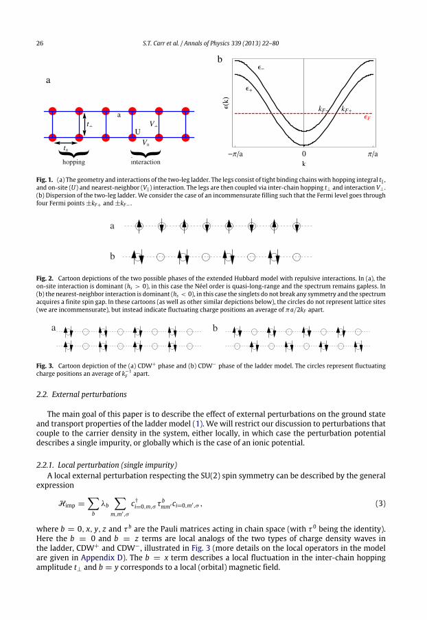
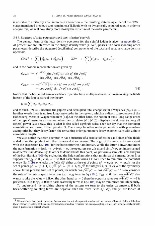
In above formulas ci,m,σ is the annihilation operator of an electron with the spin projection σ =↑ (↓)localized at the site i of the chain m = 1, 2, (hereafter this set of fermionic operators will be referredto as the chain basis), nimσ = cĎi,m,σ ci,m,σ are the occupation number operators, and t∥ and t⊥ are theintra- and inter-chain hopping amplitudes, respectively. This Hamiltonian is illustrated schematicallyin Fig. 1(a).
The kinetic part of the Hamiltonian has a spectrum consisting of two cosine bands
ϵ±(k) = −t∥ cos(ka)∓ t⊥ (2)
where a is the longitudinal lattice spacing. In this paper, we analyze main features of this modelat incommensurate filling factors such that the Fermi level goes through four Fermi points, asillustrated in Fig. 1(b). Consequently Umklapp processes play no role in our analysis and thereforethe unperturbed model always remains in the metallic regime: while certain collective modes mayacquire a gap, the total charge mode always remains gapless.
1 While it is possible (see e.g. Ref. [49]) to include also an inter-chain exchange interaction J⊥
i Si,1 Si,2 (where Si,m =cĎi,m,σ σσσ ′ ci,m,σ ′ and σ is the vector of Pauli matrices), the model (1c) is quite representative: it is general enough to encompassall possible ground states of the two-leg ladder with short range interactions respecting the SU (2) spin symmetry. Moreover,the inter-chain exchange interaction is dynamically generated, see Section 3.5.
26 S.T. Carr et al. / Annals of Physics 339 (2013) 22–80
Fig. 1. (a) The geometry and interactions of the two-leg ladder. The legs consist of tight binding chainswith hopping integral t∥ ,and on-site (U) and nearest-neighbor (V∥) interaction. The legs are then coupled via inter-chain hopping t⊥ and interaction V⊥ .(b) Dispersion of the two-leg ladder. We consider the case of an incommensurate filling such that the Fermi level goes throughfour Fermi points±kF+ and±kF− .
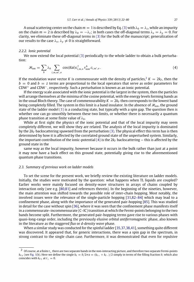
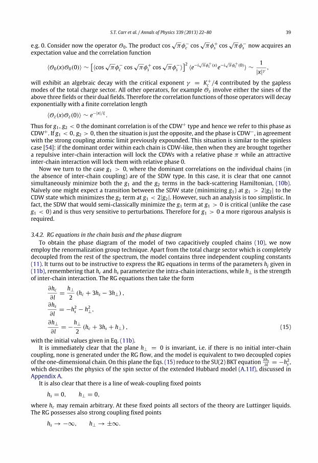
Fig. 2. Cartoon depictions of the two possible phases of the extended Hubbard model with repulsive interactions. In (a), theon-site interaction is dominant (hs > 0), in this case the Néel order is quasi-long-range and the spectrum remains gapless. In(b) the nearest-neighbor interaction is dominant (hs < 0), in this case the singlets do not break any symmetry and the spectrumacquires a finite spin gap. In these cartoons (as well as other similar depictions below), the circles do not represent lattice sites(we are incommensurate), but instead indicate fluctuating charge positions an average of πa/2kF apart.
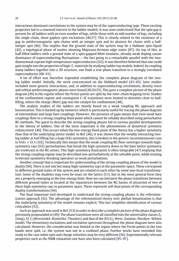
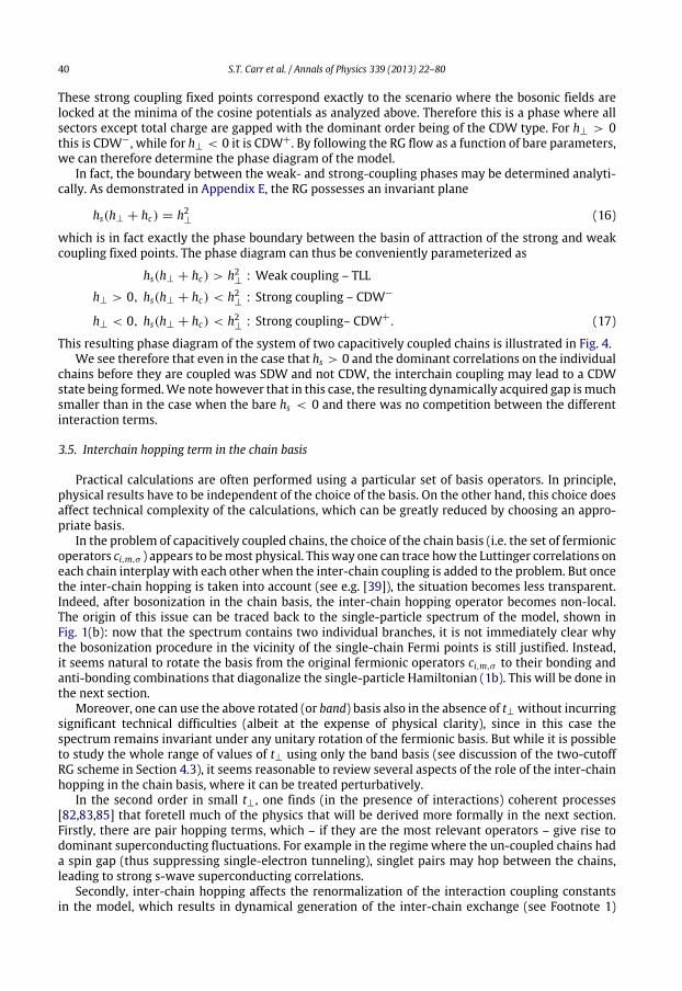
Fig. 3. Cartoon depiction of the (a) CDW+ phase and (b) CDW− phase of the ladder model. The circles represent fluctuatingcharge positions an average of k−1F apart.
2.2. External perturbations
The main goal of this paper is to describe the effect of external perturbations on the ground stateand transport properties of the ladder model (1). We will restrict our discussion to perturbations thatcouple to the carrier density in the system, either locally, in which case the perturbation potentialdescribes a single impurity, or globally which is the case of an ionic potential.
2.2.1. Local perturbation (single impurity)A local external perturbation respecting the SU(2) spin symmetry can be described by the general
expression
Himp =b
λb
m,m′,σ
cĎi=0,m,σ τ bmm′ci=0,m′,σ , (3)
where b = 0, x, y, z and τ b are the Pauli matrices acting in chain space (with τ 0 being the identity).Here the b = 0 and b = z terms are local analogs of the two types of charge density waves inthe ladder, CDW+ and CDW−, illustrated in Fig. 3 (more details on the local operators in the modelare given in Appendix D). The b = x term describes a local fluctuation in the inter-chain hoppingamplitude t⊥ and b = y corresponds to a local (orbital) magnetic field.
S.T. Carr et al. / Annals of Physics 339 (2013) 22–80 27
Ausual scattering center on the chainm = 1 is described by Eq. (3)withλ0 = λz , while an impurityon the chain m = 2 is described by λ0 = −λz ; in both cases the off-diagonal terms λx = λy = 0. Forclarity, we eliminate these off-diagonal terms in (3) for the bulk of the manuscript; generalization ofour results to the case λx, λy = 0 is straightforward.
2.2.2. Ionic potentialWe now extend the local potential (3) periodically to the whole ladder to obtain a bulk perturba-
tion:
Hion =b
λb
i,m,m′,σ
cos(Kai)cĎi,m,σ τ bmm′ci,m′,σ . (4)
If the modulation wave vector K is commensurate with the density of particles,2 K = 2kF , then theb = 0 and b = z terms are proportional to the local operators that serve as order parameters forCDW+ and CDW−, respectively. Such a perturbation is known as an ionic potential.
If the energy scale associatedwith the ionic potential is the largest in the system, then the particleswill arrange themselves at theminima of the cosine potential, with the energy levels forming bands asin the usual Bloch theory. The case of commensurability K = 2kF then corresponds to the lowest bandbeing completely filled. The system in this limit is a band insulator. In the absence of Hion, the groundstate of the ladder model (1) is a conducting state, but typically with a spin gap. The question then iswhether one can go smoothly between these two limits, or whether there is necessarily a quantumphase transition at some finite value of λb.
While at first sight the physics of the ionic potential and that of the local impurity may seemcompletely different, we will show they are related. The analysis of the local impurity is dominatedby the 2kF backscattering spawned from the perturbation (3). The physical effect this term has is thendetermined by how it is affected by the correlated ground state of the unperturbed system. Similarly,the important contribution of the ionic-potential (4) is the 2kF backscattering — this is affected by theground state in the
same way as the local impurity, however because it occurs in the bulk rather than just at a pointit may now have a back effect on this ground state, potentially giving rise to the aforementionedquantum phase transitions.
2.3. Summary of previous work on ladder models
To set the scene for the present work, we briefly review the existing literature on ladder models.Initially, the studies were motivated by the question: what happens when TL liquids are coupled?Earlier works were mainly focused on density-wave structures in arrays of chains coupled byinteraction only (see e.g. [80,81] and references therein). In the beginning of the nineties, however,the main attention was shifted towards the possible role of inter-chain hopping. Most notably, theinvolved issues were the relevance of the single-particle hopping [31,82–84] which may lead to aconfinement phase, along with the importance of the generated pair-hopping [85]. This was studiedin detail for the case without spin [36], where it was seen that the confinement phase manifests itselfin a commensurate–incommensurate (C–IC) transition atwhich the Fermi-points belonging to the twobands become split. Furthermore, the generated pair-hopping terms gave rise to various phases withquasi-long-range order, including the previously elusive orbital antiferromagnetic phase, also knownin the literature as the staggered flux or d-density wave phase.
When a similar studywas conducted for the spinful ladder [35,37,38,41], something quite differentwas discovered. It appeared that, for generic interactions, there was a spin gap in the spectrum, instrong contrast to the single chain case. Furthermore, it was demonstrated that even for repulsive
2 Of course, at a finite t⊥ there are two separate bands in the non-interacting picture, and therefore two separate Fermi-pointskF± (see Fig. 1(b). Here we define the single kF = n/2πa = (kF+ + kF−)/2 simply in terms of the filling fraction n; which alsocoincides with kF± at t⊥ = 0.
28 S.T. Carr et al. / Annals of Physics 339 (2013) 22–80
interactions dominant correlations in the systemmay be of the superconducting type. These excitingproperties led to a renewed interest in the ladder models. It was soon understood that the spin gap ispresent for all ladders with an even number of legs, while those with an odd number of legs, includingthe single chain, show gapless spin excitations [40,57]. This is closely related to the existence of agap in antiferromagnetic spin chains with an integer spin and its absence for chains with a half-integer spin [86]. This implies that the ground state of the system may be a Haldane spin-liquid[42], a topological phase of matter showing Majorana-fermion edge states [87]. On top of this, inhalf-filled ladders with a ground state of a spin-gapped Mott insulator, already weak doping causesdominance of superconducting fluctuations — the fact going in a remarkable parallel with the two-dimensional cuprate high-temperature superconductors [62]. It was therefore believed that one couldgain insight into the properties of high-Tc materials by studying ladder toymodels. Indeed, by couplingmany ladders together into a 3D structure, one finds a true phase transition to a strongly correlatedsuperconductor [88–91].
A lot of effort was therefore expended establishing the complete phase diagram of the two-leg ladder model. Initially, the work concentrated on the Hubbard model [43–45]; later studiesincluded more generic interactions, and, in addition to superconducting correlations, density waveand orbital antiferromagnetic phaseswere found [49,50,55]. This gave a complete picture of the phasediagram [49] in the regime where the Fermi-points are split by the inter-chain hopping term. Studiesof the confinement regime and consequent C–IC transitions were limited to densities close to half-filling, where the charge (Mott) gap was the catalyst for confinement [48].
The analytic studies of the ladders are mostly based on a weak coupling RG approach andbosonization. This is backed up by numerics which is particularly useful for tracing the phase diagramat intermediate and large bare couplings. However, the presence of gaps means that even weak barecouplings flow to a strong coupling fixed point which cannot be reliably described using perturbativeRG methods. The quest to describe the strong-coupling phases led to various parallel developmentsin the theory of ladders. One of the most important is the phenomenon of dynamical symmetryenhancement [46]. This occurs when the low-energy fixed point of the theory has a higher symmetrythan that of the underlying lattice model. In Ref. [46], it was shown that the weakly interacting two-leg ladder at half filling has a huge O(8) symmetry, this is broken in the generic incommensurate caseto O(6)×U(1) [92]. Technically this means that the weak-coupling RG flow converges towards high-symmetry rays [93] (perturbations that break the high symmetry down to the bare lattice symmetryare irrelevant in the RG sense). This high-symmetry fixed point is often integrable [47] implying thatthe strong-coupling regimemay be described non-perturbatively at the solvable point, while treatingirrelevant symmetry-breaking operators as weak perturbations.
Another concept that is important for understanding of the strong-coupling phases of the model isduality [94]. There is not one but many high-symmetry rays in the parameter space. These correspondto different ground states of the system and are related to each other by some non-local transforma-tion. Some of the dualities may even be exact on the lattice [51], but in the most general form theyare a property emerging in the low-energy limit. Nowwe can interpret the phase transitions betweendifferent ground states as located at the separatrices between the RG basins of attraction of two ofthese high-symmetry rays in parameter space. These represent self-dual points of the correspondingduality transformations [94].
The final important tool developed to understand the strong-coupling phases is the refermion-ization approach [42]. The advantage of the refermionized theory over abelian bosonization is thatthe underlying symmetry of the model remains explicit. This fact simplifies identification of variouscriticalities [52].
Such an approachwas used in Ref. [53] in order to describe a complete picture of the phase diagrampreviously propounded in [49]. The phase transitionswere all classified into the universality classes Z2(Ising), U(1) (Berezinskii–Kosterlitz–Thouless) and that of the SU(2)2 Wess–Zumino–Novikov–Wittenmodel. The elementary excitations and excitation spectrum throughout the phase diagram were alsocalculated. However, the consideration was limited to the region where the Fermi points in the twobands were split, i.e. the system was not in a confined phase. Further works have extended thisstudy to the case when spin and charge velocities may be very different [56]. Experimentally relevantproperties such as the NMR relaxation rate have also been calculated [95–97].
S.T. Carr et al. / Annals of Physics 339 (2013) 22–80 29
Important further developments address the role of disorder [98–100]. One of themain conclusionsreached is that for any repulsive interactions (or weak attractive ones), the disorder is always relevantdriving the system to a localized phase. Some otherworksworthy of note are Ref. [66], where disorderand some transport properties of a two-subband quantum wire were also studied; Ref. [101] whereweak localization in the two-leg ladder was studied; and the recent publication [102] which looks atsome aspects of the two-leg ladder in an ionic potential.
2.4. Summary of present results
For the benefit of the reader not interested in technical details, we summarize our results here. Ourprincipal results are three-fold. Firstly, we introduce the notion of hopping-driven phase transitions,in-particular those relating to confinement. Secondly, we establish the effect of the single impurity onthe ground state and transport properties of the system. Finally, we extend our results on the single-impurity problem to the effect of the ionic potential.
These results rely on the precise knowledge of the phase diagramof themodel including the natureof the phase transitions. Although all of the phases of the ladder model are already known, we haveincluded a detailed discussion of the phase diagram in order to make the paper self-contained.
2.4.1. Hopping-driven phase transitionsMicroscopic Hamiltonians describing electronic systems, including strongly correlated ones, often
contain separate single-particle (e.g. tight-binding or kinetic) and interaction terms (our Hamiltonian(1) is no exception). In a typical experiment, one may vary the carrier density (e.g. by applyingexternal electro-static potentials), temperature, pressure, etc., and try tomodify the effective strengthof electron–electron interaction. At the same time, the parameters describing the bare single-particlespectrum are determined by the crystal properties of thematerial and are assumed to remain constantin the course of the measurements (a notable exception is the case of pressure-induced structuralphase transitions [103]).
Recently there has been renewed interest in the Hubbard-type models due to the rapid advancesin the experimental techniques related to optically trapped cold atoms [104]. In such measurements,almost any parameter of the optical lattice can be controlled by tuning the laser fields that create theoptical traps. Thus it is conceivable to study the evolution of the observable properties of the systemwith the change in tunneling amplitudes, and in particular, the interchain hopping parameter t⊥.
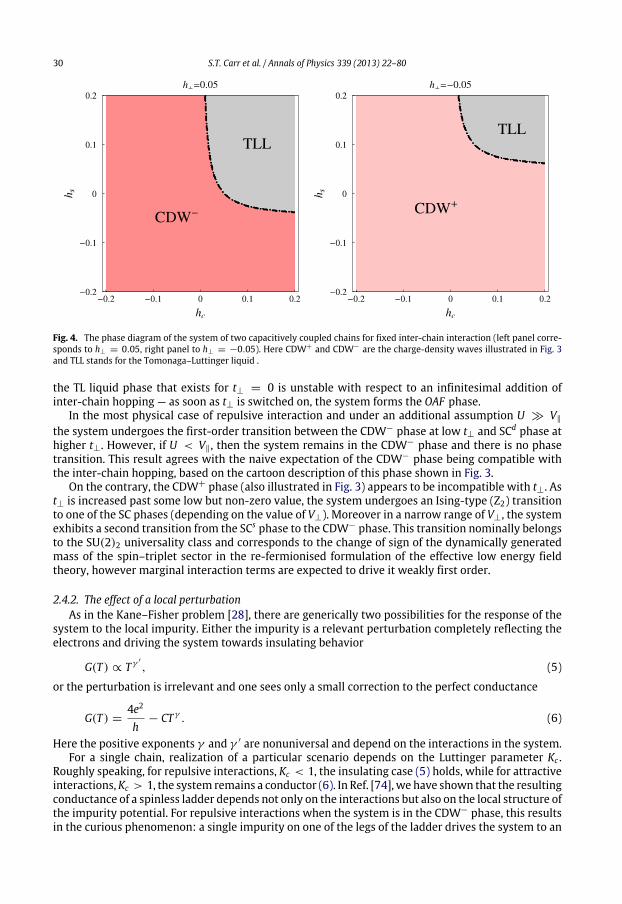
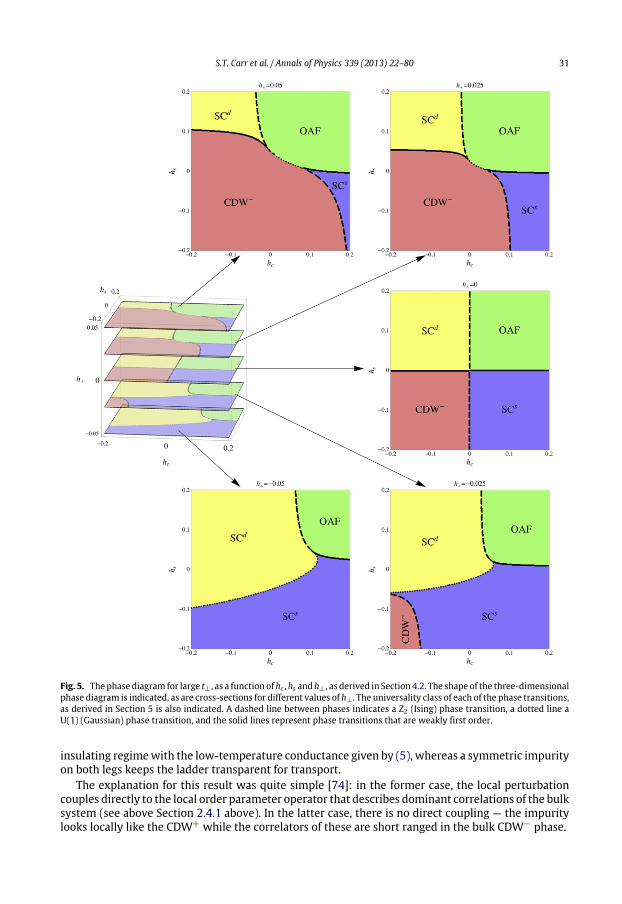
The fact that such evolution should go through critical regions associated with quantum phasetransitions can be seen by comparing the phase diagrams of the ladder model (1) in the two cases ofvanishing and sufficiently large inter-chain hopping shown in Figs. 4 and 5, respectively. The mostobvious differences between the two is the absence of the CDW+ and TL liquid phases in Fig. 5. At thesame time, the superconducting (SC) phases and the orbital anti-ferromagnet (OAF) can only appearin the presence of t⊥.
Our primary technical tool is the perturbative (‘‘one-loop’’) renormalization group (RG). The RGequations are formulated on the basis of the effective low-energy field theory, which in turn reliesupon the details of the single-particle spectrum [8,9]. The latter undergoes significant changes as theinter-chain hopping is introduced. Consequently, the RG equations for t⊥ = 0 and large t⊥ (given byEqs. (15) and (26), respectively) are rather different. However in the representation used in Eq. (26),known as the band-basis, the inter-chain hopping parameter t⊥ itself is not part of the RG equations,as it couples to a topological current of the theory. As soon as t⊥ is changed, the RG flow has to bere-calculated. Thus, in order to describe the evolution of the system as t⊥ increases from zero, weuse a two-cut-off scaling procedure, explained in Section 4.2. One may use an alternative approachand derive the RG equations in the chain basis. Then the operator that couples to t⊥ is a vertexoperator with a nonzero conformal spin and subject to renormalization. We outline how this looksin Section 3.5, but do not develop this further, since this alternative procedure does not allow us tofollow the phase diagram to the large t⊥ limit.
Numerical integration of the RG equations within the two-cut-off scaling procedure results in thet⊥ − V⊥ phase diagram (see Fig. 6), that illustrates the hopping-driven phase transitions. Note, that
30 S.T. Carr et al. / Annals of Physics 339 (2013) 22–80
Fig. 4. The phase diagram of the system of two capacitively coupled chains for fixed inter-chain interaction (left panel corre-sponds to h⊥ = 0.05, right panel to h⊥ = −0.05). Here CDW+ and CDW− are the charge-density waves illustrated in Fig. 3and TLL stands for the Tomonaga–Luttinger liquid .
the TL liquid phase that exists for t⊥ = 0 is unstable with respect to an infinitesimal addition ofinter-chain hopping — as soon as t⊥ is switched on, the system forms the OAF phase.
In the most physical case of repulsive interaction and under an additional assumption U ≫ V∥the system undergoes the first-order transition between the CDW− phase at low t⊥ and SCd phase athigher t⊥. However, if U < V∥, then the system remains in the CDW− phase and there is no phasetransition. This result agrees with the naive expectation of the CDW− phase being compatible withthe inter-chain hopping, based on the cartoon description of this phase shown in Fig. 3.
On the contrary, the CDW+ phase (also illustrated in Fig. 3) appears to be incompatible with t⊥. Ast⊥ is increased past some low but non-zero value, the system undergoes an Ising-type (Z2) transitionto one of the SC phases (depending on the value of V⊥). Moreover in a narrow range of V⊥, the systemexhibits a second transition from the SCs phase to the CDW− phase. This transition nominally belongsto the SU(2)2 universality class and corresponds to the change of sign of the dynamically generatedmass of the spin–triplet sector in the re-fermionised formulation of the effective low energy fieldtheory, however marginal interaction terms are expected to drive it weakly first order.
2.4.2. The effect of a local perturbationAs in the Kane–Fisher problem [28], there are generically two possibilities for the response of the
system to the local impurity. Either the impurity is a relevant perturbation completely reflecting theelectrons and driving the system towards insulating behavior
G(T ) ∝ T γ ′ , (5)
or the perturbation is irrelevant and one sees only a small correction to the perfect conductance
G(T ) =4e2
h− CT γ . (6)
Here the positive exponents γ and γ ′ are nonuniversal and depend on the interactions in the system.For a single chain, realization of a particular scenario depends on the Luttinger parameter Kc .
Roughly speaking, for repulsive interactions, Kc < 1, the insulating case (5) holds, while for attractiveinteractions,Kc > 1, the system remains a conductor (6). In Ref. [74], we have shown that the resultingconductance of a spinless ladder depends not only on the interactions but also on the local structure ofthe impurity potential. For repulsive interactions when the system is in the CDW− phase, this resultsin the curious phenomenon: a single impurity on one of the legs of the ladder drives the system to an
S.T. Carr et al. / Annals of Physics 339 (2013) 22–80 31
Fig. 5. Thephase diagram for large t⊥ , as a function of hc , hs and h⊥ , as derived in Section 4.2. The shape of the three-dimensionalphase diagram is indicated, as are cross-sections for different values of h⊥ . The universality class of each of the phase transitions,as derived in Section 5 is also indicated. A dashed line between phases indicates a Z2 (Ising) phase transition, a dotted line aU(1) (Gaussian) phase transition, and the solid lines represent phase transitions that are weakly first order.
insulating regimewith the low-temperature conductance given by (5), whereas a symmetric impurityon both legs keeps the ladder transparent for transport.
The explanation for this result was quite simple [74]: in the former case, the local perturbationcouples directly to the local order parameter operator that describes dominant correlations of the bulksystem (see above Section 2.4.1 above). In the latter case, there is no direct coupling — the impuritylooks locally like the CDW+ while the correlators of these are short ranged in the bulk CDW− phase.
32 S.T. Carr et al. / Annals of Physics 339 (2013) 22–80
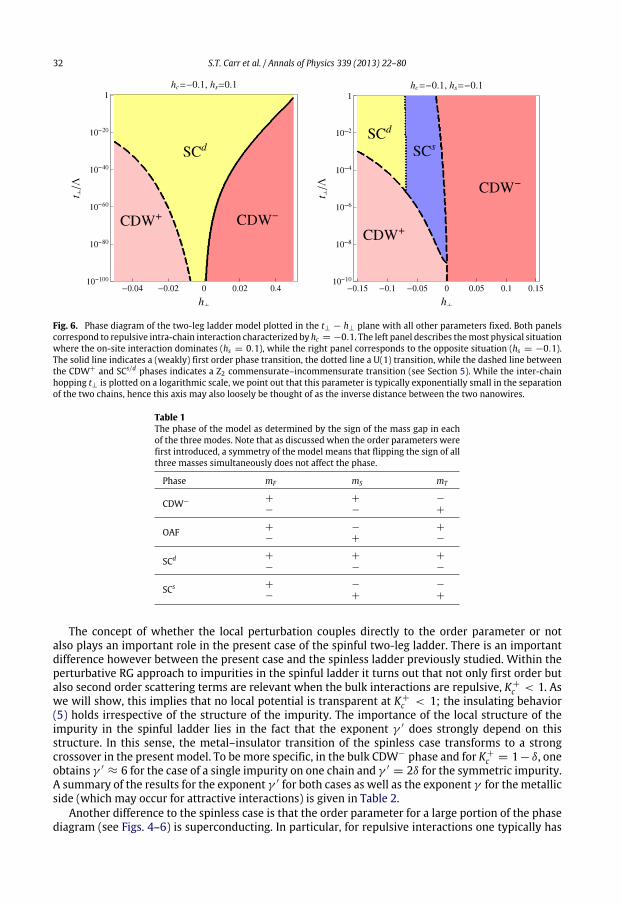
Fig. 6. Phase diagram of the two-leg ladder model plotted in the t⊥ − h⊥ plane with all other parameters fixed. Both panelscorrespond to repulsive intra-chain interaction characterized by hc = −0.1. The left panel describes themost physical situationwhere the on-site interaction dominates (hs = 0.1), while the right panel corresponds to the opposite situation (hs = −0.1).The solid line indicates a (weakly) first order phase transition, the dotted line a U(1) transition, while the dashed line betweenthe CDW+ and SCs/d phases indicates a Z2 commensurate–incommensurate transition (see Section 5). While the inter-chainhopping t⊥ is plotted on a logarithmic scale, we point out that this parameter is typically exponentially small in the separationof the two chains, hence this axis may also loosely be thought of as the inverse distance between the two nanowires.
Table 1The phase of the model as determined by the sign of the mass gap in eachof the three modes. Note that as discussed when the order parameters werefirst introduced, a symmetry of the model means that flipping the sign of allthree masses simultaneously does not affect the phase.
Phase mF mS mT
CDW− + + −
− − +
OAF + − +
− + −
SCd + + +
− − −
SCs + − −
− + +
The concept of whether the local perturbation couples directly to the order parameter or notalso plays an important role in the present case of the spinful two-leg ladder. There is an importantdifference however between the present case and the spinless ladder previously studied. Within theperturbative RG approach to impurities in the spinful ladder it turns out that not only first order butalso second order scattering terms are relevant when the bulk interactions are repulsive, K+c < 1. Aswe will show, this implies that no local potential is transparent at K+c < 1; the insulating behavior(5) holds irrespective of the structure of the impurity. The importance of the local structure of theimpurity in the spinful ladder lies in the fact that the exponent γ ′ does strongly depend on thisstructure. In this sense, the metal–insulator transition of the spinless case transforms to a strongcrossover in the present model. To be more specific, in the bulk CDW− phase and for K+c = 1− δ, oneobtains γ ′ ≈ 6 for the case of a single impurity on one chain and γ ′ = 2δ for the symmetric impurity.A summary of the results for the exponent γ ′ for both cases as well as the exponent γ for the metallicside (which may occur for attractive interactions) is given in Table 2.
Another difference to the spinless case is that the order parameter for a large portion of the phasediagram (see Figs. 4–6) is superconducting. In particular, for repulsive interactions one typically has
S.T. Carr et al. / Annals of Physics 339 (2013) 22–80 33
Table 2Summary of the different power laws seen as a response to different impurity structuresand in different phases of the bulk system. In each case, one finds insulating behavior forK+c < K ∗ defined as G ∝ [Max(T , V )]γ
′
; or conducting behavior for K+c > K ∗ defined asG = 4e2/h − const. × [Max(T , V )]γ . The perturbations are divided into two types: those thatcouple directly to the order parameter of the system (such as a single impurity on one of thelegs in the CDW− phase of the system, see [74]); and those that do not (for example, any localdensity perturbation in one of the superconducting phases of the bulk).
Perturbation γ ′ γ K ∗
First order coupling 8/K+c − 2 K+c /2− 2 4Second order only 2/K+c − 2 2K+c − 2 1
Table 3Summary of the impurity effects in the vicinity of phase transition lines in the case where the impuritycouples directly to bulk correlations. The notation for the exponents γ ′ near the insulating fixed point and γ
near the conducting fixed point is the same as in Table 2. If there is no direct coupling between the impurityand the bulk order parameters, then the results are identical to those in Table 2. For each transition line,there is a range of values of K+c for which both conducting and insulating fixed points are stable — these areseparated by an intermediate unstable fixed point which is beyond the scope of the present work.
SU(2)2 γ = K+c /2− 5/4 K+c > 5/2Conducting U(1) γ = K+c /2− 3/2 K+c > 3
Z2 γ = K+c /2− 7/4 K+c > 7/2
Insulating All γ ′ = 2/K+c K+c < 3γ ′ = 8/K+c − 2 3 < K+c < 4
either the CDW− phase or the SCd phase, depending on whether the interchain interaction or theinterchain hopping is dominant. In the latter case, no local density perturbation couples directly tothe order parameter and so the structure of the perturbation becomes unimportant. On the otherhand, this strongly correlated (quasi-long-range order) superconducting state nevertheless becomesinsulating (for K+c < 1) when any impurity is added.
All above considerations apply to energies (temperatures) less than the dynamically generatedgaps in the system, the results being technically obtained by integrating out the high-energy gappeddegrees of freedom leaving an effective single-channel model for the current-carrying gapless mode.Close to any of the phase transition lines (discussed in Section 2.4.1 above) however, one observes thesoftening of further modes, leaving a wide temperature range between these new close-to-criticalmodes and the remaining gapped ones. The properties of the system then depends crucially on whichphase transition we are talking about, and therefore there is a rich variety of possibilities. Thustransport at or near one of the quantum critical lines is governed by modified power laws; whichare summarized in Table 3. For K+c < 1, we see that the behavior is again that of an insulator, givenby (5). Finally, even if the temperature is bigger than all of the gaps, the system is still an insulator forK+c < 1; in this case, the general result is given by (56).
2.4.3. Ionic potentialAs with the local perturbation, we may express an ionic potential commensurate with the carrier
density in terms of the same operators used to describe the dominant correlations of the unperturbedsystem. When the energy scale of the added ionic potential is much larger than the dynamicallygenerated gaps, the dominant correlations in the system are clearly going to be of the same type as thepotential we have explicitly added. If the unperturbed ground state of the system showed differentcorrelations, then the systemmust evolve from one sort of correlation to the other as a function of theapplied perturbation λb in Hamiltonian (4).
This evolution may happen in one of two ways — it may be smooth; or it may undergo certainquantum-phase transitions en route. Examples of such phase transitions are known in similarsituations in the literature — for example, the SU(2)1 transition in dimerized spin ladders [105,106]or zig–zag carbon-nanotubes [107]; or the two transitions between the Mott insulator and the bandinsulator in a half-filled single chain in an ionic potential [75].
34 S.T. Carr et al. / Annals of Physics 339 (2013) 22–80
Table 4Summary of the phase transitions in the ladder model subjected to the external ionic potential. Where more thanone transition is indicated, the behavior of the system depends on the relative magnitudes of the dynamicallygenerated gaps. Empty entries indicate the absence of any phase transitions in the caseswhere the system acquiresa gap in the total charge sector as soon as the ionic potential is applied and then remains in the ordered stateindependent of the strength of the effective coupling constants. The relative charge sector is denoted as ‘‘flavor’’.
Ground state CDW+ ionic potential CDW− ionic potential
CDW− Z2 (flavor) / Z2 (spin) /SU(2)2 (spin) —CDW+ — Z2 (flavor) / Z2 (spin) /SU(2)2 (spin)OAF Z2 (flavor) / Z2 (spin) / SU(2)2 (spin) Z2 (flavor)SCd(s) — —
Our aim in this work is to categorize the transitions that may or may not take place when an ionicpotential is added to the doped (incommensurate) two-leg ladder. Clearly, this depends on both theground state of the unperturbed system, as well as the type of ionic potential added. To be specific,we consider ionic potentials coupling to the local density (of either CDW+ or CDW− types) added toa system with any of the five possible ground states discussed in this work. To avoid too many cases,we also limit ourselves to the situation when K+c < 2.
In all cases we consider, we find that the first effect of adding the ionic potential, λb = 0, is thatthe previously critical total charge mode φ+c becomes gapped. In other words, the system immedi-ately exhibits true long range order and becomes an insulator. This does not contradict the Hohen-berg–Mermin–Wagner theorem [13] for there is no spontaneous symmetry breaking — the externalionic potential explicitly breaks the translational symmetry.
We then proceed to identify any quantum phase transitions that may take place as λb becomeslarger, see Table 4. As expected, we find that if the ionic potential has the same structure as the alreadyexisting correlations, then there is no possibility of a transition. We also find that if the ground stateis in one of the superconducting phases, the evolution is smooth. In all other cases however, we findthere is some critical λ∗b at which the system becomes critical; the universality class for each case islisted in Table 4.
3. Capacitively coupled chains
Consider a situation where two individual quantum wires are placed close enough to each othersuch that the Coulomb interaction between electrons in different wires is strong enough and, at thesame time, there is no direct contact between the wires preventing the electrons from tunneling fromonewire into another. This systemcan be described by the ladderHamiltonian (1b), (1c) in the absenceof inter-chain hopping
t⊥ = 0,
andwas first studied in Ref. [33]. In this case, the Fermimomenta for all four channels remain the same,and the single-particle Hamiltonian (1b) is diagonal at the outset. Therefore it is natural to discussthe case of t⊥ = 0 using the original chain basis. We first briefly review the case of two completelydecoupled chains, before adding the inter-chain interaction V⊥ and analyzing the effect such a termhas on the ground state of the system.
3.1. Two independent chains
In the absence of interchain hopping the two chains are connected only by the interaction V⊥. If onesets V⊥ = 0, then the model reduces to two copies of the 1D extended Hubbard model. Its bosonizedform is well-known [8] (see Appendix A for details and notations). Themost prominent feature of thismodel is spin–charge separation. In particular, the effective low-energy theory (A.11) contains twodecoupled sectors describing collective charge and spin degrees of freedom.
The case of two independent chains is rather trivial — we now have two copies of charge and spinfields (A.10), whichwe denote asφm,c andφm,s (m = 1, 2 is the chain index). Thus for V⊥ = t⊥ = 0 the
S.T. Carr et al. / Annals of Physics 339 (2013) 22–80 35
model Hamiltonian can be written in the form (A.11a) where the charge sector contains two copies ofthe Gaussian model
Hc =vF
2
m
Πm,c(x)2 +
1−
hc
πvF
∂xφm,c(x)
2, (7a)
and the spin sector — two copies of the sine–Gordon model
Hs =vF
2
m
Πm,s(x)2 +
1−
hs
πvF
∂xφm,s(x)
2+
hs
2(πα)2
m
cos√8πφm,s(x). (7b)
As the chains are identical, the interaction parameters are independent of the chain indexm. In termsof the original lattice coupling constants they are given by
hc = −aU − 2aV∥ [2− cos(2kFa)] ,
hs = aU + 2aV∥ cos(2kFa). (8)
Notice that the same constant hs appears in two different terms in Eq. (7b). This is a consequence ofSU(2) symmetry. In fact, (7) is more general than the original lattice model, and one may consider thedecoupled legs of the ladder parameterized via hc and hs rather than U and V∥.
At hs > 0 the perturbation is marginally irrelevant, the model flows to weak coupling, andthe spectrum remains gapless. At hs < 0 the perturbation is relevant, the model flows to strongcoupling, and the spin sector acquires a spectral gap. Note that for fillings between 1/4 < n < 1/2,cos(2kFa) < 0, so both cases can occur even for purely repulsive bare interactions (in fact the upperlimit of fillings is 3/4 but for the sake of concreteness, we will always deal with the case of less thanhalf filling), depending on whether U or V is dominant. These two different phases are schematicallyillustrated in Fig. 2.
It is easy to understand within a strong-coupling picture (see e.g. Fig. 2) why the interactions Uand V are in competition with each other for fillings between 1/4 and 1/2. The on-site interaction Umakes double occupancy energetically unfavorable — which for this range of fillings means particlesmust be placed in nearest neighbor positions. Such neighboring particles feel an exchange interaction;whichmeans that in this phase the dominant correlations are those of the spin-densitywave type. Theinteraction V favors opposite configurations, where particles do not sit in neighboring positions; andtherefore there must be some double occupancy. In this case, the dominant correlations are of thecharge-density wave type, while the doubly occupied singlets lead to the presence of a spin-gap. Thetransition at the point U = −2V cos(2kFa) (i.e. hs = 0) is exactly of the BKT type.
3.2. Inter-chain interaction
Consider now the interchain interaction V⊥ described by the last term in Eq. (1c). Its bosonizedversion can be obtained using representation (A.4) for the fermion density (with all bosonic fieldssupplied with the additional chain index). The result is a sum of two terms
σσ ′
ni,1,σni,2,σ ′ → Sfs + Sbs.
The first term is the interchain forward scattering
Sfs =1π
∂xφ1,c∂xφ2,c .
The second term is the interchain backscattering similar to Eq. (A.8d):
Sbs = cos√2πφ1,c − φ2,c
cos√2πφ1,s + φ2,s
+ cos
√2πφ1,c − φ2,c
cos√2πφ1,s − φ2,s
.
36 S.T. Carr et al. / Annals of Physics 339 (2013) 22–80
Now we rearrange the bosonic fields into four linear combinations that correspond to the total andrelative charge, as well as total and relative spin:
φ±c(s) =φ1,c(s) ± φ2,c(s)
√2
. (9)
This transformation simplifies the interchain backscattering terms and at the same time diagonalizesthe quadratic part of the Hamiltonian, which now contains four copies of the Gaussian model:
H0 =vF
2
µ=c,sν=±
Πν
µ(x)2 +1−
gνµ
πvF
∂xφ
νµ(x)
2. (10a)
The remaining part of the bosonized Hamiltonian contains the inter- and intra-chain backscatteringterms
Hbs =g1
(πα)2cos√4πφ+s cos
√4πφ−s
+g2
(πα)2cos√4πφ−c
cos√4πφ+s + cos
√4πφ−s
. (10b)
Backscattering terms (10b) couple the relative chargemode (φ−c ) to the total (φ+s ) and relative (φ−s )spin modes. The corresponding coupling constants in the Hamiltonian (10) may be parameterized as
g−c = hc + h⊥, g±s = g1 = hs, g2 = h⊥, (11a)
where
h⊥ = aV⊥ (11b)
while hc and hs are defined in Eqs. (8). The first two parameters in Eq. (11b) coincide with Eq. (8)reflecting the fact, that for V⊥ = 0 the Hamiltonian (10) describes two uncoupled chains [c.f. Eqs. (7)].In fact, this parameterization is valid for any two spinful TL-liquids coupled via a density–densityinteraction, where hc and hs parameterize the chains, and h⊥ the interchain coupling. We willtherefore retain this trio hc, hs, h⊥ throughout the paper as a convenient way to parameterize thephase diagram of the model.
The total charge mode (φ+c ) is decoupled from the rest of the spectrum and hence describes a TLliquid with the Luttinger parameter
K+c ≈ 1+g+c
2πvF. (12)
As this algebraic relation only holds for weak interactions |gc | ≪ 1, while the TL liquid concept ismuch more general, it is therefore appropriate to think of the Luttinger parameter K+c as the fourthindependent parameter of the ladder.3 There is another reason to consider K+c independently.Much ofour analysis of theHamiltonian (10)will be based on the renormalization group,where the parametersh will be allowed to flow. Clearly however, no renormalization occurs in the decoupled φ+c sectorwhich is described by the Gaussian model.
3.3. Refermionized form of the spin sector and symmetries of the model
While the bosonized representation (10) is extremely convenient for a renormalization groupanalysis, the representation in terms of four scalar bosonic fields obscures the symmetries of themodel, particularly in the spin sector where we would expect at least that the SU(2) symmetry is
3 For the latticemodel (1) the Luttinger parameter can be related to the h’s in Eq. (11) bymeans of the equality g+c = hc−h⊥ .However, this equality is not general and may be changed by adding further interactions; for example in carbon-nanotubeswhere the Coulomb interaction is poorly screened, g+c may become strongly modified by the long range tail of the interaction,while the coupling constants in the other sectors of the theory remain largely unaffected [68].
S.T. Carr et al. / Annals of Physics 339 (2013) 22–80 37
still present, which is not at all apparent in (10). For this reason, we give another representation of theHamiltonian here, in which the spin sector is re-fermionized. The physical idea behind this techniqueultimately goes back to the seminal works by S. Coleman [108] and Itzykson and Zuber [109] in whichthe equivalence between the sine–Gordon model at the decoupling point (β2
= 4π ), a free massiveDirac fermion, and a pair of noncritical two-dimensional Ising models was established. Accordingto this correspondence the spin sector of the ladder model (1) is equivalent to four weakly coupledquantum Ising chains [109]. The latter can be represented in terms of Majorana fermions [8,42,110].While ultimately, this is just another way of writing the same Hamiltonian, we will see that in theMajorana representation the symmetries of the Hamiltonian are made explicit.
We now introduce four Majorana fermion fields ξ iR(L) to replace the two bosonic spin fields φ±s
according to the re-fermionization rules in (B.2). The Hamiltonian is split up into a kinetic (Gaussian)part and interaction (non-linear) terms,
H = Hk +Hint, (13a)
which are grouped slightly differently as compared to the fully bosonized case. The kinetic partstill includes two Gaussian models for the bosonized charge modes φ±c with the forward scatteringamplitudes g±c explicitly included (see Eq. (10a)), and fourmasslessMajorana fields for the spinmodes
Hk = H0φ+c+H0
φ−c+
ivs
2
a=1,2,3,0
ξ aL ∂xξ
aL − ξ a
R∂xξaR
. (13b)
Marginal interaction in the spin sector, parameterized by g1,2, is included in Hint:
Hint = −g1
3
a=0
ξ aR ξ
aL
2
+ig2πα
cos√4πφ−c
3a=0
ξ aR ξ
aL . (13c)
There are four independent coupling constants: two of them describe forward scattering in thecharge sectors (g+c and g−c ), and two more describe the spin sectors (g1 and g2), the bare values beinggiven by Eq. (11) as before. In the absence of the interchain hopping the spin symmetry of the laddermodel is that of two decoupled chains: SU(2) × SU(2) ≈ O(4); this is unbroken by an interchaindensity–density interaction. This is why the Hamiltonian contains only O(4) invariants: (
3a=0 ξ a
R ξaL )
2
which originates from the intra-chain interaction, as well as the mixed term cos√4πφ−c
3a=0 ξ a
R ξaL .
When interchain hopping processes are allowed, we will see that they generate interchain exchangeterms which reduce the spin symmetry from SU(2) × SU(2) to a single SU(2). As we will see inSection 3.5, the O(4) symmetry present in the four Majorana fields will split into a spin–triplet modedescribed by ξ i with i = 1, 2, 3 and a spin–singlet degree of freedomdescribed by the remaining i = 0fermion.
3.4. Phase diagram
We now proceed to construct the phase diagram of the model of capacitively coupled chainsdescribed by Hamiltonian (1) with t⊥ = 0. We will do this carefully using renormalization groupmethods in the following, but to begin with let us consider a simple strong coupling picture in theatomic limit. If the interchain interaction is weak, then a good reference point is the state of eachindividual chain. The single-chain model is described in detail in Appendix A and illustrated in Fig. 2.
Let us first suppose that V∥ > U (or more precisely, hs < 0). Then each chain exhibits quasi-long-range order of the CDW type as illustrated in Fig. 2(b). When such chains are coupled by interchaininteraction V⊥, it is clear that all potential energy terms may be minimized by forming density waveson both changes with a relative phase of 0 for attractive interchain interaction and π for the repulsivecase. Such states are known as CDW+ and CDW− respectively, and are illustrated in Fig. 3.
In the opposite case when V∥ < U (hs > 0) and the dominant correlations in the uncoupled chainsare SDW rather than CDW, the situation is less obvious as there is now competition between thedifferent interaction terms. In fact, the SDW state in the single chain is quite delicate — as the SU(2)symmetry prevents the appearance of a spin-gap in this state. It will therefore turn out that the SDW
38 S.T. Carr et al. / Annals of Physics 339 (2013) 22–80
is unstable to arbitrarily small interchain interaction — the resulting state being either of the CDW±states mentioned previously, or remaining a TL liquid with no dynamically acquired gaps. In order toanalyze this, we will now study more closely the structure of the order parameters.
3.4.1. Structure of order parameters and semi-classical analysisThe general form of the local density operators for the spinful ladder is given in Appendix D.
At present, we are interested in the charge density wave (CDW±) phases. The corresponding orderparameters describe the staggered (oscillating) components of the total and relative charge densityoperators
CDW+ ←
σ
cĎ1σ c1σ + cĎ2σ c2σ
, CDW− ←
σ
cĎ1σ c1σ − cĎ2σ c2σ
,
and in the bosonic representation are given by
OCDW+ ∼ e−i√
πφ+csin√
πφ−c sin√
πφ+s sin√
πφ−s− i cos
√πφ−c cos
√πφ+s cos
√πφ−s
,
OCDW− ∼ −e−i√
πφ+csin√
πφ−c cos√
πφ+s cos√
πφ−s− i cos
√πφ−c sin
√πφ+s sin
√πφ−s
. (14)
Notice that the bosonized formof each local operator has amultiplicative structure involving the fieldsin each of the four sectors of the theory
O =
Oc+Oc−Os+Os− ,
and as such, ⟨O⟩ = 0 because the gapless and decoupled total charge sector always has ⟨Oc+⟩ = 0.In other words there is no true long-range order in the system, which is a direct consequence of theHohenberg–Mermin–Wagner theorem [13]. On the other hand, the notion of quasi-long-range orderof the type O assumes a situation when the correlator ⟨O(r)O(0)⟩ displays the slowest (among allothers) power-law decay. This is what is also called algebraic order. Then we say that the dominantcorrelations are those of the operator O. There may be other order parameters with power-lowasymptotics but they decay faster; the remaining order parameters decay exponentially with a finitecorrelation length.
We also notice that each operator O has a structure of a product of cosines and sines of the fieldsadded to another productwith the cosines and sines reversed. The origin of this construct is consistentwith the expression Eq. (10b) for the backscattering Hamiltonian. While the latter is invariant underthe transformation
√4πφa →
√4πφa + π , the operators cos
√πφa and sin
√πφa get interchanged
in all sectors simultaneously. In order to demonstrate this point, we perform a semi-classical analysisof the Hamiltonian (10b) by evaluating the field configurations that minimize the energy. Let us firstsuppose that g1 < 0 (i.e. hs < 0 so that each chain forms a CDW). Then to minimize the potentialenergy Eq. (10b), one locks the fields φ±s either at the set of points φ+s = n
√π , φ−s = m
√π ; or the
set of points φ+s = (n + 1/2)√
π , φ+s = (m + 1/2)√
π for integers n,m. In view of the symmetryabove, let us pick the first set of points, for which cos
√4πφ+s = cos
√4πφ−s = 1.4 Now consider
the role of the inter-layer interaction, i.e. the g2 term in Eq. (10b). If g2 < 0, then cos√4πφ−c also
wants to take the value+1. If, on the other hand, g2 > 0 then the opposite value cos√4πφ−c = −1 is
preferred. Thus for g1 < 0 both back-scattering terms in Eq. (10b) may be minimized simultaneously.To understand the resulting phases of the system we turn to the order parameters. If both
back-scattering coupling terms are negative, then the three fields φ−c , φ+s , and φ−s are locked at
4 We note here that, due to quantum fluctuations, the actual expectation values of the cosines of bosonic fields will be lessthan 1. However, as long as the cosine term is relevant andwe remain in the strong coupling regime, such semiclassical estimategives a qualitatively correct answer.
S.T. Carr et al. / Annals of Physics 339 (2013) 22–80 39
e.g. 0. Consider now the operator O0. The product cos√
πφ−c cos√
πφ+s cos√
πφ−s now acquires anexpectation value and the correlation function
⟨O0(x)O0(0)⟩ ∼⟨cos√
πφ−c cos√
πφ+s cos√
πφ−s ⟩2⟨e−i√
πφ+c (x)e−i√
πφ+c (0)⟩ ∼
1|x|γ
,
will exhibit an algebraic decay with the critical exponent γ = K+c /4 contributed by the gaplessmodes of the total charge sector. All other operators, for example Oz involve either the sines of theabove three fields or their dual fields. Therefore the correlation functions of those operators will decayexponentially with a finite correlation length
⟨Oz(x)Oz(0)⟩ ∼ e−|x|/ξ .
Thus for g1, g2 < 0 the dominant correlation is of the CDW+ type and hence we refer to this phase asCDW+. If g1 < 0, g2 > 0, then the situation is just the opposite, and the phase is CDW−, in agreementwith the strong coupling atomic limit previously expounded. This situation is similar to the spinlesscase [54]: if the dominant order within each chain is CDW-like, then when they are brought togethera repulsive inter-chain interaction will lock the CDWs with a relative phase π while an attractiveinter-chain interaction will lock them with relative phase 0.
Now we turn to the case g1 > 0, where the dominant correlations on the individual chains (inthe absence of inter-chain coupling) are of the SDW type. In this case, it is clear that one cannotsimultaneously minimize both the g1 and the g2 terms in the back-scattering Hamiltonian, (10b).Naïvely one might expect a transition between the SDW state (minimizing g1) at g1 > 2|g2| to theCDW state which minimizes the g2 term at g1 < 2|g2|. However, such an analysis is too simplistic. Infact, the SDW that would semi-classically minimize the g1 term at g1 > 0 is critical (unlike the caseg1 < 0) and is thus very sensitive to perturbations. Therefore for g1 > 0 a more rigorous analysis isrequired.
3.4.2. RG equations in the chain basis and the phase diagramTo obtain the phase diagram of the model of two capacitively coupled chains (10), we now
employ the renormalization group technique. Apart from the total charge sector which is completelydecoupled from the rest of the spectrum, the model contains three independent coupling constants(11). It turns out to be instructive to express the RG equations in terms of the parameters hj given in(11b), remembering that hc and hs parameterize the intra-chain interactions, while h⊥ is the strengthof inter-chain interaction. The RG equations then take the form
∂hc
∂ l=
h⊥2
(hc + 3hs − 3h⊥) ,
∂hs
∂ l= −h2
s − h2⊥,
∂h⊥∂ l= −
h⊥2
(hc + 3hs + h⊥) , (15)
with the initial values given in Eq. (11b).It is immediately clear that the plane h⊥ = 0 is invariant, i.e. if there is no initial inter-chain
coupling, none is generated under the RG flow, and the model is equivalent to two decoupled copiesof the one-dimensional chain. On this plane the Eqs. (15) reduce to the SU(2) BKT equation ∂hs
∂ l = −h2s ,
which describes the physics of the spin sector of the extended Hubbard model (A.11f), discussed inAppendix A.
It is also clear that there is a line of weak-coupling fixed points
hs = 0, h⊥ = 0,
where hc may remain arbitrary. At these fixed points all sectors of the theory are Luttinger liquids.The RG possesses also strong coupling fixed points
hs →−∞, h⊥ →±∞.
40 S.T. Carr et al. / Annals of Physics 339 (2013) 22–80
These strong coupling fixed points correspond exactly to the scenario where the bosonic fields arelocked at the minima of the cosine potentials as analyzed above. Therefore this is a phase where allsectors except total charge are gapped with the dominant order being of the CDW type. For h⊥ > 0this is CDW−, while for h⊥ < 0 it is CDW+. By following the RG flow as a function of bare parameters,we can therefore determine the phase diagram of the model.
In fact, the boundary between the weak- and strong-coupling phases may be determined analyti-cally. As demonstrated in Appendix E, the RG possesses an invariant plane
hs(h⊥ + hc) = h2⊥
(16)
which is in fact exactly the phase boundary between the basin of attraction of the strong and weakcoupling fixed points. The phase diagram can thus be conveniently parameterized as
hs(h⊥ + hc) > h2⊥: Weak coupling – TLL
h⊥ > 0, hs(h⊥ + hc) < h2⊥: Strong coupling – CDW−
h⊥ < 0, hs(h⊥ + hc) < h2⊥: Strong coupling– CDW+. (17)
This resulting phase diagram of the system of two capacitively coupled chains is illustrated in Fig. 4.We see therefore that even in the case that hs > 0 and the dominant correlations on the individual
chains before they are coupled was SDW and not CDW, the interchain coupling may lead to a CDWstate being formed.We note however that in this case, the resulting dynamically acquired gap ismuchsmaller than in the case when the bare hs < 0 and there was no competition between the differentinteraction terms.
3.5. Interchain hopping term in the chain basis
Practical calculations are often performed using a particular set of basis operators. In principle,physical results have to be independent of the choice of the basis. On the other hand, this choice doesaffect technical complexity of the calculations, which can be greatly reduced by choosing an appro-priate basis.
In the problem of capacitively coupled chains, the choice of the chain basis (i.e. the set of fermionicoperators ci,m,σ ) appears to bemost physical. This way one can trace how the Luttinger correlations oneach chain interplay with each other when the inter-chain coupling is added to the problem. But oncethe inter-chain hopping is taken into account (see e.g. [39]), the situation becomes less transparent.Indeed, after bosonization in the chain basis, the inter-chain hopping operator becomes non-local.The origin of this issue can be traced back to the single-particle spectrum of the model, shown inFig. 1(b): now that the spectrum contains two individual branches, it is not immediately clear whythe bosonization procedure in the vicinity of the single-chain Fermi points is still justified. Instead,it seems natural to rotate the basis from the original fermionic operators ci,m,σ to their bonding andanti-bonding combinations that diagonalize the single-particle Hamiltonian (1b). This will be done inthe next section.
Moreover, one can use the above rotated (or band) basis also in the absence of t⊥ without incurringsignificant technical difficulties (albeit at the expense of physical clarity), since in this case thespectrum remains invariant under any unitary rotation of the fermionic basis. But while it is possibleto study the whole range of values of t⊥ using only the band basis (see discussion of the two-cutoffRG scheme in Section 4.3), it seems reasonable to review several aspects of the role of the inter-chainhopping in the chain basis, where it can be treated perturbatively.
In the second order in small t⊥, one finds (in the presence of interactions) coherent processes[82,83,85] that foretell much of the physics that will be derived more formally in the next section.Firstly, there are pair hopping terms, which – if they are the most relevant operators – give rise todominant superconducting fluctuations. For example in the regime where the un-coupled chains hada spin gap (thus suppressing single-electron tunneling), singlet pairs may hop between the chains,leading to strong s-wave superconducting correlations.
Secondly, inter-chain hopping affects the renormalization of the interaction coupling constantsin the model, which results in dynamical generation of the inter-chain exchange (see Footnote 1)
S.T. Carr et al. / Annals of Physics 339 (2013) 22–80 41
Without going into details, the main result of such a term on the low energy effective Hamiltonianis best seen in the refermionized form, where the marginal interaction in the spin-sector previouslywritten in (13c) is modified to become
Hint = −g1,t
3
a=1
ξ aR ξ
aL
2
− g1,sξ 0R ξ 0
L
3a=1
ξ aR ξ
aL
+i
παcos√4πφ−c
g2,sξ 0
R ξ 0L + g2,t
3a=0
ξ aR ξ
aL
. (18)
The interchain exchange splits the previously seen O(4) symmetry down to O(3)× Z2, correspondingto a spin singlet mode (labeled by a = 0), and a spin–triplet mode (labeled by a = 1, 2, 3). Physically,the most important part of Hint to focus on is the g2 terms, which – if relevant – roughly speakingprovide the Majorana Fermions with mass (see Section 5.1 for details of the mechanism of Majoranamass generation). The single parameter g2 has now split into two parts g2,s ∼ a(V⊥ + J⊥) andg2,t ∼ a(V⊥ − J⊥). If g2,s and g2,t are the same sign, then the singlet and triplet modes are split,but other than this the CDW correlations are fundamentally no different than in the case J⊥ = 0.On the other hand, if the (dynamically generated) inter-chain exchange J⊥ is larger than the inter-chain interaction V⊥, then g1,s and g1,t will have opposite signs. In this case, the CDW correlationswill decay exponentially, and the systemwill be in a fundamentally different phase. In the case of halffilling when the system is a Mott insulator, this would be a topological (Haldane) phase [42]; in thedoped (incommensurate) case this will be either an orbital antiferromagnetic or a superconductingphase, as we will see in the next section.
4. Low-energy effective theory for the two-leg ladder
The full laddermodel (1) differs from themodel of two capacitively coupled chains by the presenceof the inter-chain hopping term
−t⊥iσ
cĎi,1,σ ci,2,σ + cĎi,2,σ ci,1,σ
.
Now, in the original chain basis used in the previous section, the single-particle problem is no longerdiagonal. A commonapproach to the problem is to performaunitary transformation (or basis rotation)that diagonalizes H0.
If no external magnetic field affecting orbital motion of the electrons in the ladder is present, thenthe single-particle problem is diagonalized by the transformation
cα(β),i,σ =ci,1,σ ± ci,2,σ√2
, (19)
where the new operators cα(β) refer to particles belonging to the two bands (hereafter this set ofoperators will be referred to as the band basis). The single-particle energies of the two bands are splitby t⊥:
ϵα(β)(k) = −t∥ cos(ka)∓ t⊥. (20)
In contrast to the case of the capacitively coupled chains, now there are four distinct Fermi points,provided that both bands are partially filled. The spectrum may be linearized around the four Fermipoints and the resulting chiral fields may be bosonized.
At the same time, if the inter-chain tunneling is weak, t⊥ ≪ t∥, an alternative approach is possible.One can start from the limit t⊥ = 0 and then bosonize the capacitively coupled chains in the rotatedbasis. The backscattering part of the interaction becomes more complicated because the interchaininteraction conserves the particle number in each chain but not in each band. In otherwords, there are
42 S.T. Carr et al. / Annals of Physics 339 (2013) 22–80
processes that describe interband transitions of pairs of fermions.5 However, the inter-chain hoppingterm acquires a simple diagonal form of the topological charge density:
−t⊥√
π∂xφ−
c . (21)
When t⊥ is sufficiently large (but still smaller than the ‘‘ultraviolet’’ cutoff ∼ t∥), the effect of thegradient term (21) is basically the same as that caused by band splitting (20). This follows from thefact that the emergence of four Fermi points in the single-particle spectrum leads to the suppressionof backscattering processes that involve the field φ−c and no longer conserve momentum. However,the convenience of the representation (21) is that it also allows one to study the small-t⊥ limit (whereinteraction effects may lead to suppression of the Fermi-point splitting in the excitation spectrum ofthe fully interacting problem [84]), as well as the nonperturbative regime of a C–IC transition takingplace on increasing t⊥, specifically at t⊥ comparable with the mass gap in the relative charge sector.The existence of such transition follows from the comparison of the phase diagrams of the model att⊥ = 0 and in the limit of large t⊥. The resulting phase diagram for arbitrary t⊥ will be presented inSection 5.
4.1. Interaction Hamiltonian in the band basis
Similarly to Eq. (10), we represent the bosonized Hamiltonian in the band basis as a sum of theGaussian and backscattering parts. The Gaussian part is formally identical to Eq. (10a), where thebosonic fields now refer to the band basis, see Eq. (F.9). The backscattering part of the Hamiltonianin the band basis has been derived in many previous works (see e.g. [35,37–40,43,45,46]). Forcompleteness, we give a derivation in Appendix F in terms of symmetries alone,wherewe also presentthe transformation in the bosonized language between the chain and the band bases, which to ourknowledge has never appeared in literature.
Consider first the band basis in the absence of the inter-chain hopping (i.e. at t⊥ = 0). Then theprocesses that involve the field φ−c conserve momentum and as a result we find the most generalback-scattering Hamiltonian respecting the SU(2) spin symmetry in the form
Hbs =1
2(πα)2
cos√4πφ−c
gT cos
√4πφ+s +
gT − gS2
cos√4πφ−s +
gT + gS2
cos√4πθ−s
+ cos
√4πθ−c
gT cos
√4πφ+s +
gT − gS2
cos√4πφ−s +
gT + gS2
cos√4πθ−s
+ cos
√4πφ+s
g+s + g−s
2cos√4πφ−s +
g+s − g−s2
cos√4πθ−s
. (22a)
Similarly to Section 3.3, we can make the SU(2) symmetry explicit by refermionizing the spin sectorof the model. Again, the kinetic (Gaussian) part of the Hamiltonian has the same form as Eq. (13b),while the interaction part of the refermionized Hamiltonian in the band basis is given by
Hint =i
2παcos√4πφ−c
gT
3i=1
ξ iRξ
iL − gSξ 0
R ξ 0L
+i
2παcos√4πθ−c
gT
3i=1
ξ iRξ
iL − gSξ 0
R ξ 0L
− g−s ξ 0R ξ 0
L
3i=1
ξ iRξ
iL − g+s
3
i=1
ξ iRξ
iL
2
. (22b)
5 One must be very careful, however, not to immediately associate such terms with superconducting fluctuations. Thephysical interpretation of terms in this rotated basis is not particularly transparent, and onemust instead refer to the definitionsof the local operators in the rotated basis.
S.T. Carr et al. / Annals of Physics 339 (2013) 22–80 43
The Majorana fermions representing the spin degrees of freedom clearly split into a triplet mode ξ i
with i = 1, 2, 3 and a singlet ξ 0.We now consider what happens to the above Hamiltonianwhen the inter-chain hopping term (21)
is added. By making the change of variables
φ−c (x)→ φ−c (x)−K 2c−t⊥√
πvFx,
where Kc− = 1 + g−c /(4πvF ), we see that the term (21) is absorbed into the kinetic part of theHamiltonian, while the cosine term is transformed as follows:
cos√4πφ−c → cos
√4πφ−c +
4K 2c−t⊥vF
x
.
The condition of sufficiently large t⊥ is then equivalent to averaging the cosine over many oscillationswhich yields zero. More accurately, when at t⊥ = 0 a spectral gap M is dynamically generated in therelative charge sector, the large-t⊥ condition actually means that
t⊥ξ/vF ∼ t⊥/|M| ≫ 1, (23)
where ξ = vF/|M| is the correlation length. Then this cosine drops out from the interaction, andeffectively this is equivalent to setting gT = gS = 0 in (22). Same conclusion can be reached by notingthat for large enough t⊥ there are four Fermi points in the single-particle spectrum and therefore theprocesses involving φ−c do not conserve momentum and should be dropped from the Hamiltonian. Atthe same time, the cosine of the dual field remains unchanged by the above transformation.
The initial (bare) values of the coupling constants can still be expressed in terms of the fourcombinations (11) and (12) of the parameters of the microscopic Hamiltonian (1). In fact, as shown inAppendix F, the Luttinger liquid parameters for the total charge and total spin are the same in bothchain and band bases because the change-of-basis transformation only involves relative degrees offreedom. The total charge sector remains decoupled [see the footnote after Eq. (12)], while
g+s = hs. (24a)
The remaining coupling constants can be expressed in terms of hi as
g−c = g−s = h⊥, gT =h⊥ − hs
2, gS = −
hc
2. (24b)
The fact that the initial values of five coupling constants g−c , g±s , gT , and gS can be parameterized bythree quantities hi reflects the higher symmetry of the baremicroscopic interaction Hamiltonian (1c),namely that a density–density interaction always conserves individually the particle number on eachchain. However, under renormalization, further interactionswill be generatedwhen t⊥ is present thatdo not respect this symmetry. These generated interactions manifest themselves in the RG equationsas independent flow of these five parameters.
4.2. Phase diagram for large t⊥
The strategy here is the same as for the case t⊥ = 0. We will perform the semi-classical analysis ofthe backscattering Hamiltonian equation (22a) (with the first line removed). Defining the bosonizedform of the order parameters in the band representation, we then associate each of the semi-classicalsolutions with one of the phases of the model. We then derive the RG equations for the above model,identify the strong-coupling fixed points of the RG flow, relate them to the semi-classical solutions,and thus construct the phase diagram of the model. As each of these steps is analogous to thoseperformed in Section 3, we will not present full details here and resort only to an outline and theresults.
In addition to the two CDW operators previously discussed, we will find an operator describing anorbital antiferromagnetic phase, which is characterized by the staggered part of the local current (see
44 S.T. Carr et al. / Annals of Physics 339 (2013) 22–80
Appendix D.2 for details)
OAF ← icĎ1σ c2σ − cĎ2σ c1σ
, (25a)
as well as two superconducting operators
OSCs =c1↑c1↓ − c1↓c1↑
+c2↑c2↓ − c2↓c2↑
,
OSCd = 2c1↑c2↓ − c1↓c2↑
.
(25b)
The bosonized and refermionized forms of these operators are given in Appendix D.2.As indicated previously, in the large-t⊥ regime, the RG flow is parameterized by five independent
coupling constants (see Appendix F.4):
∂gT∂ l=
12
g−c − 2g+s
gT + g−s gS
,
∂gS∂ l=
12
g−c gS + 3g−s gT
,
∂g−c∂ l=
12
3g2
T + g2S
,
∂g+s∂ l= −
12
2g2
T +g+s2+g−s2
,
∂g−s∂ l= gTgS − g+s g−s . (26)
The only weak-coupling fixed point of these equations is gi = 0 for all i, which is the case of anoninteracting system. This is a repulsive fixed point. On the other hand, the Eqs. (26) allow for thefollowing four strong coupling fixed points:
g−s →+∞, gT →+∞, gS →+∞⇒ CDW−,
g−s →+∞, gT →−∞, gS →−∞⇒ OAF ,
g−s →−∞, gT →+∞, gS →−∞⇒ SC s,
g−s →−∞, gT →−∞, gS →+∞⇒ SCd. (27)
The flow of the two remaining parameters in Eq. (26) is the same in all of the above cases:
g−c →∞, g+s →−∞. (28)
The identification of the strong-coupling phases follows along the lines of the analysis of Sec-tion 3.4.1. For example, when g−s , gT , gS → +∞ then the three terms in the back-scattering Hamil-tonian (22) that do not involve the relative spin field φ−s flow to strong coupling, such that the fieldsθ−c , θ−s , and φ+s get ‘‘locked’’ at some minima of the cosine potentials. The choice of the minima isdegenerate (see the previous discussion on the structure of order parameters), but for gT → ∞ letus choose the minima such that cos
√4πθ−c → 1, while cos
√4πφ+s → −1. Then from the condi-
tions gT + gS → ∞, g+s − g−s → −∞ it immediately follows that the third field should be lockedsuch that cos
√4πθ−s →−1. Comparing this result with the structure of the order parameters (D.3),
we conclude that in this case the correlations of the operator OCDW− are dominant, i.e. decaying as apower law (in contrast to all other correlation functions which decay exponentially), similarly to thediscussion in Section 3.4.1.
The analysis of the remaining three strong-coupling phases is similar. It is worth stressing, thatboth the relative charge density wave (CDW−) and the orbital antiferromagnet (OAF) correspond tothe locking of the θ−s field, while in the ‘‘superconducting’’ phases the field φ−s is locked. These twopossibilities are distinguished by the relative sign of the two coupling constants gT and gS . Let us stressit again (see Section 3.4.1) that in any of the phases discussed here the total charge sector remainsgapless and thus there is never a long-range order in the system.
S.T. Carr et al. / Annals of Physics 339 (2013) 22–80 45
The phase diagram is now determined as the basin of attraction of each of the strong-couplingfixed points as a function of the bare parameters of the theory, (24). Certain regions may bedetermined analytically (see Appendix G), including the existence and attraction of certain rays inphase space with an enhanced O(6) symmetry. Ultimately however, the phase diagram is determinedby numerically integrating the flow (26), the results are shown in Fig. 5. As before, the phase diagramis plotted as a function of the three parameters: hc and hs parameterizing the correlations on theindividual chains before coupling, and h⊥ which is the strength of the inter-chain interaction.
The middle panel in Fig. 5 – i.e. the phase diagram in the case h⊥ = 0 – is well known (see e.g. [9]).In particular, themost important feature of this phase diagram is that in the region of purely repulsive(intra-chain) interactions, hc < 0, there is a phase SCd in which the dominant correlations are super-conducting. Cross-sections for non-zero h⊥ show how repulsive inter-chain interaction enlarges theregion of the CDW− phase at the expense of the superconducting ones; while attractive inter-chaininteraction has the opposite effect. Curiously, the OAF phase is only weakly affected by the inter-chaininteraction.
Fig. 5 also indicates the universality class of each of the phase transitions, which is something thatcannot be determined from the RG alone, and will be derived in Section 5 where an effective strongcoupling theory is developed in each of the phases. Before we look at this however, we first turn ourattention to the case when t⊥ is present, but not necessarily large — in other words, to interpolationbetween the phase diagram shown in Fig. 4 for t⊥ = 0, and that of Fig. 5 for large t⊥.
4.3. Phase diagram at intermediate values of t⊥
Comparison of the t⊥ = 0 and large-t⊥ limits, Figs. 4 and 5, reveals a number of features causedby inter-chain tunneling. First we note that the TL liquid phase present at t⊥ = 0 transforms to anOAF phase when hopping is present (a similar situation occurs in the spinless chain [36]). As the TLLis critical, we would expect this to happen for arbitrarily weak inter-chain hopping. The situationis different if one starts from one of the gapped phases at t⊥ = 0. Let us consider first the case ofrepulsive inter-chain interaction, h⊥ > 0. Then we see that depending on the other parameters, theCDW− phase at t⊥ = 0may become a superconducting phase as t⊥ is gradually increased. But becauseof the finite gap already present at t⊥ = 0, wewould naturally expect such a phase transition to occurat a small but non-zero value of t⊥.
For attractive inter-chain interaction (h⊥ < 0), evenmore scenarios are possible. In fact, the CDW+phasewhich is the ground state at t⊥ = 0 does not exist at large t⊥. The reason for this may be seen byreturning to the cartoon depiction of the state in Fig. 3—where it is clear that the CDW+ state preventsthe electrons from lowering their energy by delocalizing between the chains, as would be expectedat sufficiently large t⊥. A similar effect is seen in spinless chains [36] where this phase becomes a TLliquid phase at large t⊥ via a C–IC transition. In the present (spinful) case, we see that, depending oninitial parameters, the CDW+ phase at small t⊥ becomes at larger t⊥ either a superconducting phaseor even a CDW− phase. As we will show in Section 5, this occurs again via a C–IC like transition, butin contrast to the spinless case, this occurs between two gapped phases. The precise meaning of thenomenclature C–IC in this context will be explained in Section 5.2.1.
Before getting to a description of the phase transitions let us first ask ourselves: how can we treatthe system at small but non-zero t⊥? The RG equations (26) were derived under the assumption thatt⊥ is sufficiently large [see the condition (23)], such that the backscattering processes involving therelative charge field φ−c can be neglected as violating momentum conservation. On the contrary, inthe absence of the interchain hopping, one must retain the gT and gS terms in Eq. (22). As shownin Appendix F.4, when the RG equations for this full system (which now involves eight couplingconstants) are derived, it is found that the initial values Eq. (F.21) which are written in terms ofthree independent parameters actually flow on a three-dimensional invariant hyper-surface, withthe equations as given in Eq. (15). This is not an accident — while the backscattering Hamiltonian inthe band basis (22) in the absence of t⊥ may look substantially different from that in the chain basis(10b), they ultimate are two different representations of the same physical model, and thereforemusthave the same physical properties.
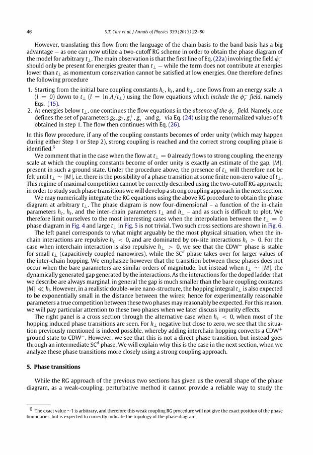
46 S.T. Carr et al. / Annals of Physics 339 (2013) 22–80
However, translating this flow from the language of the chain basis to the band basis has a bigadvantage — as one can now utilize a two-cutoff RG scheme in order to obtain the phase diagram ofthemodel for arbitrary t⊥. Themain observation is that the first line of Eq. (22a) involving the field φ−cshould only be present for energies greater than t⊥ — while the term does not contribute at energieslower than t⊥ as momentum conservation cannot be satisfied at low energies. One therefore definesthe following procedure
1. Starting from the initial bare coupling constants hc , hs, and h⊥, one flows from an energy scale Λ
(l = 0) down to t⊥ (l = lnΛ/t⊥) using the flow equations which include the φ−c field, namelyEqs. (15).
2. At energies below t⊥, one continues the flow equations in the absence of the φ−c field. Namely, onedefines the set of parameters gS , gT , g+s , g−s and g−c via Eq. (24) using the renormalized values of hobtained in step 1. The flow then continues with Eq. (26).
In this flow procedure, if any of the coupling constants becomes of order unity (which may happenduring either Step 1 or Step 2), strong coupling is reached and the correct strong coupling phase isidentified.6
We comment that in the case when the flow at t⊥ = 0 already flows to strong coupling, the energyscale at which the coupling constants become of order unity is exactly an estimate of the gap, |M|,present in such a ground state. Under the procedure above, the presence of t⊥ will therefore not befelt until t⊥ ∼ |M|, i.e. there is the possibility of a phase transition at some finite non-zero value of t⊥.This regime of maximal competition cannot be correctly described using the two-cutoff RG approach;in order to study suchphase transitionswewill develop a strong coupling approach in the next section.
Wemay numerically integrate the RG equations using the above RG procedure to obtain the phasediagram at arbitrary t⊥. The phase diagram is now four-dimensional – a function of the in-chainparameters hc , hs, and the inter-chain parameters t⊥ and h⊥ – and as such is difficult to plot. Wetherefore limit ourselves to the most interesting cases when the interpolation between the t⊥ = 0phase diagram in Fig. 4 and large t⊥ in Fig. 5 is not trivial. Two such cross sections are shown in Fig. 6.
The left panel corresponds to what might arguably be the most physical situation, when the in-chain interactions are repulsive hc < 0, and are dominated by on-site interactions hs > 0. For thecase when interchain interaction is also repulsive h⊥ > 0, we see that the CDW− phase is stablefor small t⊥ (capacitively coupled nanowires), while the SCd phase takes over for larger values ofthe inter-chain hopping. We emphasize however that the transition between these phases does notoccur when the bare parameters are similar orders of magnitude, but instead when t⊥ ∼ |M|, thedynamically generated gap generated by the interactions. As the interactions for the doped ladder thatwe describe are always marginal, in general the gap is much smaller than the bare coupling constants|M| ≪ hi. However, in a realistic double-wire nano-structure, the hopping integral t⊥ is also expectedto be exponentially small in the distance between the wires; hence for experimentally reasonableparameters a true competition between these twophasesmay reasonably be expected. For this reason,we will pay particular attention to these two phases when we later discuss impurity effects.
The right panel is a cross section through the alternative case when hs < 0, when most of thehopping induced phase transitions are seen. For h⊥ negative but close to zero, we see that the situa-tion previously mentioned is indeed possible, whereby adding interchain hopping converts a CDW+ground state to CDW−. However, we see that this is not a direct phase transition, but instead goesthrough an intermediate SCd phase. We will explain why this is the case in the next section, when weanalyze these phase transitions more closely using a strong coupling approach.
5. Phase transitions
While the RG approach of the previous two sections has given us the overall shape of the phasediagram, as a weak-coupling, perturbative method it cannot provide a reliable way to study the
6 The exact value∼1 is arbitrary, and therefore this weak coupling RG procedure will not give the exact position of the phaseboundaries, but is expected to correctly indicate the topology of the phase diagram.
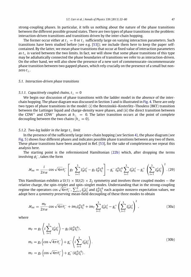
S.T. Carr et al. / Annals of Physics 339 (2013) 22–80 47
strong-coupling phases. In particular, it tells us nothing about the nature of the phase transitionsbetween the different possible ground states. There are two types of phase transitions in the problem:interaction-driven transitions and transitions driven by the inter-chain hopping.
The former occur either at t⊥ = 0 or t⊥ sufficiently large on varying interaction parameters. Suchtransitions have been studied before (see e.g. [53]); we include them here to keep the paper self-contained. By the latter, wemean phase transitions that occur at fixed value of interaction parametersas t⊥ is varied between the two limits. In fact, we will show that some phase transitions of this typemay be adiabatically connected the phase boundaries of transitions we refer to as interaction-driven.On the other hand, we will also show the presence of a new sort of commensurate–incommensuratephase transition between two gapped phases, which rely crucially on the presence of a small but non-zero t⊥.
5.1. Interaction-driven phase transitions
5.1.1. Capacitively coupled chains, t⊥ = 0We begin our discussion of phase transitions with the ladder model in the absence of the inter-
chain hopping. The phase diagramwas discussed in Section 3 and is illustrated in Fig. 4. There are onlytwo types of phase transitions in the model: (i) the Berezinskii–Kosterlitz–Thouless (BKT) transitionbetween the Luttinger liquid and charge-density wave phases, and (ii) the direct transition betweenthe CDW+ and CDW− phases at h⊥ = 0. The latter transition occurs at the point of completedecoupling between the two chains (h⊥ = 0).
5.1.2. Two-leg ladder in the large t⊥ limitIn the presence of the sufficiently large inter-chain hopping (see Section 4), the phase diagram (see
Fig. 5) shows four different phases and indicates possible phase transitions between any two of them.These phase transitions have been analyzed in Ref. [53], for the sake of completeness we repeat thisanalysis here.
The starting point is the refermionized Hamiltonian (22b) which, after dropping the termsinvolving φ−c , takes the form
Hint =i
2παcos√4πθ−c
gT
3i=1
ξ iRξ
iL − gS ξ 0
R ξ 0L
− g−s ξ 0
R ξ 0L
3i=1
ξ iRξ
iL − g+s
3
i=1
ξ iRξ
iL
2
. (29)
This Hamiltonian exhibits a U(1) × SU(2) × Z2 symmetry and involves three coupled modes — therelative charge, the spin–triplet and spin–singlet modes. Understanding that in the strong-couplingregime the operators cos
√4πθ−c ,
3i=1 ξ i
RξiL and ξ 0
R ξ 0L each acquire nonzero expectation values, we
adopt here a symmetry preserving mean-field decoupling of these three modes to obtain
Hint =mF
2παcos√4πθ−c + imSξ
0R ξ 0
L + imT
3i=1
ξ iRξ
iL − g+s
3
i=1
ξ iRξ
iL
2
, (30a)
where
mF = gT
i
3i=1
ξ iRξ
iL
− gS⟨iξ 0
R ξ 0L ⟩,
mS = gScos√4πθ−c
+ g−s
i
3i=1
ξ iRξ
iL
.
mT = gTcos√4πθ−c
+ g−s ⟨iξ
0R ξ 0
L ⟩.
(30b)
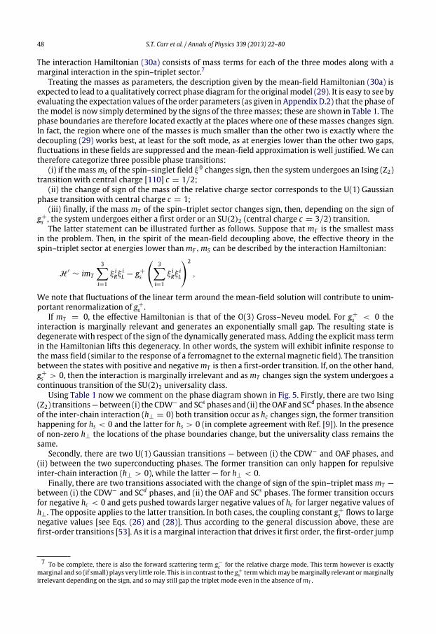
48 S.T. Carr et al. / Annals of Physics 339 (2013) 22–80
The interaction Hamiltonian (30a) consists of mass terms for each of the three modes along with amarginal interaction in the spin–triplet sector.7
Treating the masses as parameters, the description given by the mean-field Hamiltonian (30a) isexpected to lead to a qualitatively correct phase diagram for the originalmodel (29). It is easy to see byevaluating the expectation values of the order parameters (as given in Appendix D.2) that the phase ofthemodel is now simply determined by the signs of the threemasses; these are shown in Table 1. Thephase boundaries are therefore located exactly at the places where one of these masses changes sign.In fact, the region where one of the masses is much smaller than the other two is exactly where thedecoupling (29) works best, at least for the soft mode, as at energies lower than the other two gaps,fluctuations in these fields are suppressed and the mean-field approximation is well justified. We cantherefore categorize three possible phase transitions:
(i) if the massmS of the spin–singlet field ξ 0 changes sign, then the system undergoes an Ising (Z2)transition with central charge [110] c = 1/2;
(ii) the change of sign of the mass of the relative charge sector corresponds to the U(1) Gaussianphase transition with central charge c = 1;
(iii) finally, if the mass mT of the spin–triplet sector changes sign, then, depending on the sign ofg+s , the system undergoes either a first order or an SU(2)2 (central charge c = 3/2) transition.
The latter statement can be illustrated further as follows. Suppose that mT is the smallest massin the problem. Then, in the spirit of the mean-field decoupling above, the effective theory in thespin–triplet sector at energies lower thanmF ,mS can be described by the interaction Hamiltonian:
H ′ ∼ imT
3i=1
ξ iRξ
iL − g+s
3
i=1
ξ iRξ
iL
2
,
We note that fluctuations of the linear term around the mean-field solution will contribute to unim-portant renormalization of g+s .
If mT = 0, the effective Hamiltonian is that of the O(3) Gross–Neveu model. For g+s < 0 theinteraction is marginally relevant and generates an exponentially small gap. The resulting state isdegenerate with respect of the sign of the dynamically generatedmass. Adding the explicit mass termin the Hamiltonian lifts this degeneracy. In other words, the system will exhibit infinite response tothe mass field (similar to the response of a ferromagnet to the external magnetic field). The transitionbetween the states with positive and negativemT is then a first-order transition. If, on the other hand,g+s > 0, then the interaction is marginally irrelevant and as mT changes sign the system undergoes acontinuous transition of the SU(2)2 universality class.
Using Table 1 now we comment on the phase diagram shown in Fig. 5. Firstly, there are two Ising(Z2) transitions—between (i) the CDW− and SCs phases and (ii) theOAF and SCd phases. In the absenceof the inter-chain interaction (h⊥ = 0) both transition occur as hc changes sign, the former transitionhappening for hs < 0 and the latter for hs > 0 (in complete agreement with Ref. [9]). In the presenceof non-zero h⊥ the locations of the phase boundaries change, but the universality class remains thesame.
Secondly, there are two U(1) Gaussian transitions — between (i) the CDW− and OAF phases, and(ii) between the two superconducting phases. The former transition can only happen for repulsiveinter-chain interaction (h⊥ > 0), while the latter — for h⊥ < 0.
Finally, there are two transitions associated with the change of sign of the spin–triplet massmT —between (i) the CDW− and SCd phases, and (ii) the OAF and SCs phases. The former transition occursfor negative hc < 0 and gets pushed towards larger negative values of hc for larger negative values ofh⊥. The opposite applies to the latter transition. In both cases, the coupling constant g+s flows to largenegative values [see Eqs. (26) and (28)]. Thus according to the general discussion above, these arefirst-order transitions [53]. As it is a marginal interaction that drives it first order, the first-order jump
7 To be complete, there is also the forward scattering term g−c for the relative charge mode. This term however is exactlymarginal and so (if small) plays very little role. This is in contrast to the g+s termwhichmay bemarginally relevant ormarginallyirrelevant depending on the sign, and so may still gap the triplet mode even in the absence ofmT .
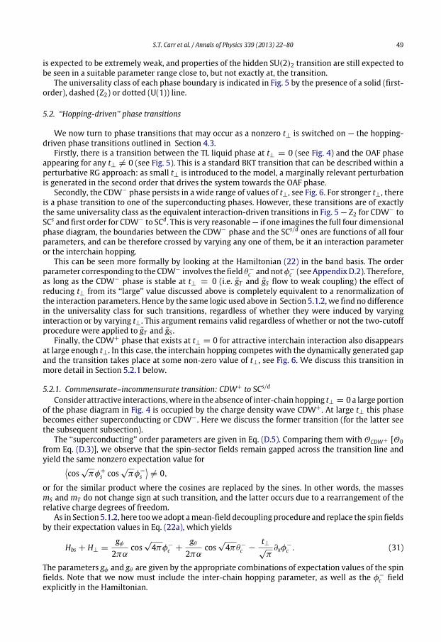
S.T. Carr et al. / Annals of Physics 339 (2013) 22–80 49
is expected to be extremely weak, and properties of the hidden SU(2)2 transition are still expected tobe seen in a suitable parameter range close to, but not exactly at, the transition.
The universality class of each phase boundary is indicated in Fig. 5 by the presence of a solid (first-order), dashed (Z2) or dotted (U(1)) line.
5.2. ‘‘Hopping-driven’’ phase transitions
We now turn to phase transitions that may occur as a nonzero t⊥ is switched on — the hopping-driven phase transitions outlined in Section 4.3.
Firstly, there is a transition between the TL liquid phase at t⊥ = 0 (see Fig. 4) and the OAF phaseappearing for any t⊥ = 0 (see Fig. 5). This is a standard BKT transition that can be described within aperturbative RG approach: as small t⊥ is introduced to the model, a marginally relevant perturbationis generated in the second order that drives the system towards the OAF phase.
Secondly, the CDW− phase persists in a wide range of values of t⊥, see Fig. 6. For stronger t⊥, thereis a phase transition to one of the superconducting phases. However, these transitions are of exactlythe same universality class as the equivalent interaction-driven transitions in Fig. 5 — Z2 for CDW− toSCs and first order for CDW− to SCd. This is very reasonable — if one imagines the full four dimensionalphase diagram, the boundaries between the CDW− phase and the SCs/d ones are functions of all fourparameters, and can be therefore crossed by varying any one of them, be it an interaction parameteror the interchain hopping.
This can be seen more formally by looking at the Hamiltonian (22) in the band basis. The orderparameter corresponding to the CDW− involves the field θ−c and notφ−c (see AppendixD.2). Therefore,as long as the CDW− phase is stable at t⊥ = 0 (i.e. gT and gS flow to weak coupling) the effect ofreducing t⊥ from its ‘‘large’’ value discussed above is completely equivalent to a renormalization ofthe interaction parameters. Hence by the same logic used above in Section 5.1.2, we find no differencein the universality class for such transitions, regardless of whether they were induced by varyinginteraction or by varying t⊥. This argument remains valid regardless of whether or not the two-cutoffprocedure were applied to gT and gS .
Finally, the CDW+ phase that exists at t⊥ = 0 for attractive interchain interaction also disappearsat large enough t⊥. In this case, the interchain hopping competes with the dynamically generated gapand the transition takes place at some non-zero value of t⊥, see Fig. 6. We discuss this transition inmore detail in Section 5.2.1 below.
5.2.1. Commensurate–incommensurate transition: CDW+ to SCs/d
Consider attractive interactions,where in the absence of inter-chain hopping t⊥ = 0 a large portionof the phase diagram in Fig. 4 is occupied by the charge density wave CDW+. At large t⊥ this phasebecomes either superconducting or CDW−. Here we discuss the former transition (for the latter seethe subsequent subsection).
The ‘‘superconducting’’ order parameters are given in Eq. (D.5). Comparing them with OCDW+ [O0from Eq. (D.3)], we observe that the spin-sector fields remain gapped across the transition line andyield the same nonzero expectation value for
cos√
πφ+s cos√
πφ−s= 0,
or for the similar product where the cosines are replaced by the sines. In other words, the massesmS and mT do not change sign at such transition, and the latter occurs due to a rearrangement of therelative charge degrees of freedom.
As in Section 5.1.2, here toowe adopt amean-field decoupling procedure and replace the spin fieldsby their expectation values in Eq. (22a), which yields
Hbs + H⊥ =gφ
2παcos√4πφ−c +
gθ
2παcos√4πθ−c −
t⊥√
π∂xφ−
c . (31)
The parameters gφ and gθ are given by the appropriate combinations of expectation values of the spinfields. Note that we now must include the inter-chain hopping parameter, as well as the φ−c fieldexplicitly in the Hamiltonian.
50 S.T. Carr et al. / Annals of Physics 339 (2013) 22–80
Looking at this Hamiltonian, we can now understand the meaning of commensurate–incommen-surate transition in this context. Starting from the case gθ = t⊥ = 0, we see that the gφ term locks thefield φ−c at one of the classical minima of the potential, meaning that ⟨ei
√πφ−c ⟩ = 0, and we are in the
CDW+ phase. The inter-chain hopping t⊥ then acts as a chemical potential for this field. This situationis maintained as long as the particle number is conserved (i.e. there are no terms with the dual fieldin the Hamiltonian). Otherwise t⊥ affects the spectrumwhich is generically massive. The existence ofthe transition follows from the qualitative difference between the massive phases in the two limitingcases.
Now suppose that t⊥ becomes larger than the gap, meaning that φ−c is no longer locked, and⟨ei√
πφ−c ⟩ = 0. In the absence of gθ , one then sees CDW+ at two different wavenumbers correspondingto the splitting of the Fermi points that would be expected in the non-interacting model. Thisis the traditional commensurate–incommensurate transition, which occurs in the spinless two-legladders [36]. The current case is slightly different however, when one restores the gθ term present in(31). In this case, as soon as the t⊥ termpreventsφ−c frombeing locked, the gθ termwould lock the dualfield instead θ−c , meaning that ⟨ei
√πθ−c ⟩ = 0. This means that correlation functions involving ei
√πφ−c
(for example, the CDW+ one) decay exponentially with a finite correlation length. Nevertheless, suchcorrelation functions would show the interchain incommensurability, coming from an underlyingtheory where t⊥ has split the Fermi points. This is the meaning of the C–IC transition in this context.
To study this transition, we now refermionize the relative charge sector of the model (31). Usingthe conventions in (B.4), this gives8
H =iv2
a=α,β
ξ aL ∂xξ
aL − ξ a
R∂xξaR
− iµ
ξαR ξ
β
R + ξαL ξ
β
L
− i
a=α,β
maξaR ξ
aL . (32)
Here the ‘‘chemical potential’’ of the Majorana fermions µ ∝ t⊥, while the masses are given bymα(β) = (gφ ± gθ )/2. In momentum representation the Hamiltonian (32) may be expressed as a4× 4 matrix acting on the 4-component field Ψ = (ξα
R , ξβ
R , ξαL , ξ
β
L )T :
H =k>0
Ψ Tk HkΨk, Hk = µσ2 + vkτ3 +
m+ +m−σ3
τ2, (33)
where
m± =mα ±mβ
2,
and σi and τj are the Pauli matrices operating in the two 2× 2 sectors: (1, 2) and (R, L), respectively.The spectrum of this model is given by
ϵ2k = µ2
+ v2k2 +m2++m2
−± 2
m2+m2− + µ2v2k2 + µ2m2
+.
The spectral gap is defined as
ϵ20 =
m+ ±
µ2 +m2
−
2
.
Thus, there exists an Ising transition occurring at
µ = µc =|mαmβ |.
The sign of the masses in the above relation distinguishes between transitions to the SCd and SCs
phases.We note that an analogous transition has recently been discussed in the context of the
superconductor–insulator transition in superconducting quantum wires [112,113].
8 The sameMajoranamodel appears in Ref. [111] in the theory of the S = 1 biquadratic spin chain in amagnetic field parallelto the anisotropy axis.

S.T. Carr et al. / Annals of Physics 339 (2013) 22–80 51
5.2.2. Absence of direct CDW+ to CDW− transitionFinally, we turn to the last remaining potential phase transition in this model. Comparing the two
phase diagrams, Fig. 4 and 5 for zero and large t⊥, respectively, we see that in a relatively narrow rangeof interaction parameters, the addition of interchain hopping may drive the system from a CDW+phase to a CDW− one. As seen from numerical integration of the two-cutoff RG procedure in the righthand panel of Fig. 6 however, this transition appears not to be direct, and instead goes through anintermediate SCs phase. We now give an explanation of this phenomena.
Comparing the order parameters for CDW+ and CDW− in the band basis (O0 and Ox respectivelyin Eq. (D.3)), we see that in addition to the change in locking from the φ−c to the θ−c field as before, themass of one of the spin degrees of freedom must also change sign. While at finely tuned parameters,both of these things could happen simultaneously, we will show that this is not the generic situation.Consequently, the path from CDW+ to CDW− in general involves two phase transitions, and thereforean intermediate phase.
The important part of the Hamiltonian (22) to see this is
H ′ ∼ i cos√4πθ−c
gT
3i=1
ξ iRξ
iL − gSξ 0
R ξ 0L
+ i cos√4πφ−c
gT
3i=1
ξ iRξ
iL − gSξ 0
R ξ 0L
+ t⊥∂xφ−c .
The CDW− phase at large t⊥ corresponds to the strong-coupling fixed point of the RG equations (26)where gT , gS →∞, while the CDW+ phase at t⊥ = 0 corresponds to the strong-coupling fixed pointwith gT →−∞, gS →∞.
The numerical results depicted in Fig. 6 can nowbe interpreted as follows. Increasing t⊥ suppressesthe field φ−c and allows the dual field θ−c to lock. This changes the nature of the order parameter — thenon-zero expectation value of cos
√πφ−c is replaced by a non-zero expectation value of cos
√πθ−c
via the Z2 transition described above. However, the expectation values of the terms appearing in theHamiltonian ⟨cos
√4πφ−c ⟩ and ⟨cos
√4πθ−c ⟩ are continuous as one passes through the transition. As a
result, the spin degrees of freedom are not affected by this first transition, and therefore the transitionis to an intermediate SCs phase.
One can now focus on the spin degrees of freedom via our usual mean-field decoupling, where inparticular, the spin–triplet massmT is given by
mT ∼ gTcos√4πθ−c
+ gT
cos√4πφ−c
.
From the previous analysis of the charge degree of freedom, the expectation values ⟨cos√4πθ−c ⟩ and
⟨cos√4πφ−c ⟩ change with the increase of t⊥: the former value increases while the latter decreases.
Given that gT > 0 and gT < 0 the mass crosses zero when
gTcos√4πθ−c
= |gT |
cos√4πφ−c
.
This is the second transition, to the CDW− phase; due to the presence of the marginal term discussedin Section 5.1.2, this transition becomes weakly first order; as is indicated in Fig. 6.
6. Effect of a local perturbation
In the preceding sectionwehave identified the phase diagramof the laddermodel (1). In particular,for themost physical case of predominantly repulsive interaction, the system is either in the CDW− orSCd phase, depending on the relative strength of the on-site (U) and nearest-neighbor (V∥) interactions(see Fig. 5).
Now we turn to the central issue of this paper, i.e. the effect of a local perturbation. Previously(see Ref. [74]), we have studied the impurity problem in the context of the spinless ladder model.Focusing on external probes coupled to the local charge density, we expressed the impurity potential in
52 S.T. Carr et al. / Annals of Physics 339 (2013) 22–80
terms of the same operators that we used as order parameters that define the structure of the groundstate of the system. The response to the impurity, i.e. the conductance G, is then fully determinedby whether the impurity couples to the dominant order parameter or not: in the former case theimpurity pins the incoherent density wave related to the order parameter leading to the insulatingbehavior (G(T = 0) = 0, as in the single-channel Kane–Fisher problem [28]), while in the latter casethe impurity has a minimal effect on the system which remains an ideal conductor (at T = 0). As aresult [74], one can ‘‘switch’’ between metallic and insulating behavior by tuning the parameters ofthe impurity potential to the point where it is decoupled from the dominant order parameter in thesystem.
In the spinful ladder that is the subject of the present paper the situation is more complex. Incontrast to the spinless case, we typically have not one but three gapped modes. It turns out thatin this situation, it is not possible to achieve the fully metallic behavior for any reasonable choiceof impurity (as well as the interaction in the bulk). However, as we show below, there can be alarge difference in the scaling dimension of the impurity, depending on whether or not the localperturbation couples directly to the order parameter. This leads to a sizeable crossover effect in thetemperature dependence of the conductance G(T ). We also consider the situationwhere temperatureis lower than most of the gaps in the system, but greater than the gap in one of the collective modes,as can happen near one of the phase transition lines.
6.1. Local perturbation coupled to the dominant order parameter
Suppose the impurity potential contains the operator describing one of the massive bulk modesin the problem. As a physical example, consider the CDW− phase characterized by the non-zeroexpectation value
µ1µ2µ3σ0 sin√
πθ−c= 0. (34)
Now consider a local perturbation of the form
Himp = λOCDW−(0). (35)
Given the multiplicative form of the operator OCDW− (see Appendix D), we can replace the massivefields in Eq. (35) by their expectation value (34). Technically, this is equivalent to ‘‘integrating out’’these massive degrees of freedom. Then the effective Hamiltonian for the total charge takes the form
Heff = H0[φ+
c ] + λ cos√
πφ+c (0), (36)
where
λ = λµ1µ2µ3σ0 sin
√πθ−c
. (37)
The effective Hamiltonian (36) describes a boundary sine–Gordon model (which is equivalent to thesingle-channel Kane–Fisher problem) with a local perturbation having scaling dimension d = K+c /4.Hence for K+c > 4 the operator is irrelevant and one obtains a power-law correction to perfectconductance [28]
G =4e2
h− const.× [Max(T , V )]γ , γ = 2(d− 1) = K+c /2− 2 > 0. (38)
For K+c < 4 the perturbation is relevant and flows to strong coupling.9The strong-coupling physics is determined solely by the total charge sector. Mathematically, the
resulting behavior is similar to that in the Kane–Fisher problem. There is, however, an importantdifference. In the Kane–Fisher problem [28], the strong-coupling regime is equivalent to tunneling
9 In this paper we assume the base impurity potential to be weak enough, allowing us to consider its RG flow in the presenceof the dynamically generated bulk masses. It is worth noting that for a stronger bare impurity, the RG flows of bulk interactionsand the impurity may be entangled. This issue lies outside of the scope of the present paper and will be discussed elsewhere.

S.T. Carr et al. / Annals of Physics 339 (2013) 22–80 53
across the weak link connecting two semi-infinite chains. In our case, such analogy is also useful,however, it is confined to the total charge sector only, while the three massive sectors of the modelremain largely unaffected by the impurity. Thus, the resulting strong-coupling picture is by no meansrelated to the problem of tunneling between two semi-infinite ladders. In other words, while in thesingle-chain case [28] the impurity effectively cuts the chain into two semi-infinite parts, the ladderremains intact, with only one (out of four) sectors of the effective low-energy theory being affectedby the impurity. Within the total charge sector, the weak-link analogy can still be used, but withthe caveat that single-electron processes are now forbidden (by the gaps) and so ‘‘tunneling acrossthe weak link’’ refers to four-fermion processes that do not change any quantum numbers relatedto the gapped degrees of freedom. Such a process is represented by the operator cos
√16πθ+c , with
the scaling dimension d = 4/K+c . Alternatively [114], one may realize that this operator generates asoliton in the φ+c field between successive minima of the cos
√πφ+c potential; hence purely on field-
theoretic grounds it may be considered as the leading (irrelevant) operator involved in generating acurrent in the strong coupling regime. An RG analysis as studied by Kane and Fisher [28] then leadsimmediately to the result that the conductance at temperature T and bias voltage V is given by apower law
G ∝ [Max(T , V )]γ′
, γ ′ = 8/K+c − 2 > 0. (39)
While we have arrived at Eq. (39) specifically for the case of the CDW− phase, such a behavior alwaysoccurs if some component of the local impurity couples to the bulk ‘‘order parameter’’ of the systemso long as temperature and bias voltage remain lower than the bulk gaps.
6.2. Local perturbation not directly coupled to the dominant order parameter
Now, let us suppose that no component of the local perturbation is identical to the bulk orderparameter — for concreteness we again consider the case of being in the CDW− phase, but now witha symmetric impurity [74]
Himp = λOCDW+(0). (40)
To obtain the effective theory of the total charge sector for energies small compared to the dynamicallygenerated gaps,we again integrate out the gapped degrees of freedom. In contrast to the previous case,the impurity potential (40) does not contribute in the first order, as becomes clear by comparing thenon-zero expectation value (34) to the multiplicative structure of the order parameter [see Eq. (D.3)]
λcos√
πφ+c sin√
πφ−c σ1σ2σ3σ0 + sin√
πφ+c cos√
πφ−c µ1µ2µ3µ0.
Focusing on the first term, we find that the second-order contribution of the impurity to the effectiveaction for φ+c has the form
λ2
2
dτ1dτ2C(τ1, τ2) cos
√πφ+c (τ1) cos
√πφ+c (τ2), (41)
where τi are the imaginary times, all quantities are taken at the impurity site (xi = 0), the effectivecoupling constant is λ = λ⟨σ1σ2σ3⟩ and C(τ1, τ2) is the short-hand notation for the correlationfunction
C(τ1, 0; τ2, 0) =sin√
πφ−c (τ1, 0) sin√
πφ−c (τ2, 0)⟨σ0(τ1, 0)σ0(τ2, 0)⟩ . (42)
The correlation function (42) is short-ranged due to the presence of dynamically generated gaps:
C(τ1, τ2) ∼ e−|τ1−τ2|∆, (43)
where ∆ ∼ mS + mF (up to numerical factors; mS and mF are gaps in the spin–singlet and relativecharge sectors, respectively). Then we can neglect the difference between τ1 and τ2 in the operatorsin Eq. (41), which leads to the effective model of the total charge sector
Heff = H0[φ+
c ] + λ′ cos√4πφ+c (0). (44)
54 S.T. Carr et al. / Annals of Physics 339 (2013) 22–80
Unlike the spinless case [74], the impurity potential in Eq. (44), which has scaling dimension d = K+c ,is still relevant for overall bulk repulsive interactions K+c < 1, although significantly less relevantthan the similar term in Eq. (36). The strong coupling arguments used in the previous subsection maystill be applied, but now the soliton in the fields φ+c is generated by the operator cos
√4πθ+c , which
physically corresponds to pair-hopping through the strong impurity. As a result, the conductance isdescribed by the weaker power law
G ∝ [Max(T , V )]γ′
, γ ′ = 2/K+c − 2 > 0. (45)
The metallic behavior found in the case of the spinless ladder [74] can appear in the spinful ladderonly if the bulk interactions are attractive K+c > 1. The impurity potential in Eq. (44) is now irrelevant(in the RG sense) and the conductance remains close to its maximal value
G =4e2
h− const.× [Max(T , V )]γ , γ = 2K+c − 2 > 0. (46)
The qualitative results obtained so far, can be summarized as follows:
1. For the system in the bulk CDW− state, the response of the system to a local impurity indeeddepends on the nature of the impurity, as in the spinless model [74]. However, in contrast to thespinless model, changing the local structure of the impurity in the case of repulsive interactions,K+c < 1, does not lead to a metal–insulator transition, but rather to a strong crossover at any non-zero temperature (T 6−8δ behavior as compared to T 2δ behavior for K+c = 1 − δ). The potential-sensing applications detailed in [74] are still therefore realistic in the spinful case.
2. The critical K+c separating metallic and insulating behavior is different for the first- and second-order terms. For certain attractive interactions with 1 < K+c < 4, one may therefore still seea metal–insulator transition as the component of the local impurity that couples to the orderparameter is tuned to zero.
3. If the system is in one of the bulk superconducting states (as is most realistic for ladders withstrong interchain hopping), the response to the local impurity is independent of the structure ofthe impurity.
The results for the different power laws are summarized in Table 2.Finally, we mention that the qualitative picture of the strong coupling (insulating) phase of the
impurity, i.e. whether four electrons are required to tunnel (forming a singlet of all the gapped sectors)or whether pair tunneling is possiblemay be extended to SU(N) ladders with all modes gapped excepttotal charge [115].
6.3. Transport near one of the phase transition lines
Throughoutmost of the phase diagram, the three gapped collectivemodes all have gaps of the sameorder ofmagnitude. However,when the system is sufficiently close to one of the phase transition lines,the situation is different. Here, one of the gaps becomes very small (vanishing at the transition line),allowing for a sizeable regime where voltage and/or temperature are much larger than the smallestgap, but still much smaller than the remaining two. The extra soft degree of freedom leads tomodifiedexponents in the power laws, but, as it turns out, only if the impurity couples directly to the orderparameter. For second order processes, this extra soft degree of freedom does not affect the resultingbehavior. In this subsection, we showhow this happens, discussing in detail the situation for transportnear a U(1) transition line, then outlining the differences for the other cases.
6.3.1. Transport near the U(1) transitionAs discussed in Section 5.1.2, U(1) phase transitions (to be concrete, we will consider the CDW−
to OAF transition) in the two-leg ladder are associated with the change of sign of the mass mF in therelative charge sector. In the vicinity of the U(1) transition line, mF is small compared to the gaps inthe spin sector and we may consider an intermediate temperature regime where
mF ≪ T ≪ mT ,mS .
S.T. Carr et al. / Annals of Physics 339 (2013) 22–80 55
In this case the relative charge sector should be considered on equal footing with the gapless totalcharge sector, while the gapped spin modes may be integrated out.
Consider now an impurity (35), which couples to the CDW− order parameter. In this case the spinpart of the impurity potential has a non-zero expectation value across the transition line.10 Integratingout the spin degrees of freedom, we find the effective impurity potential for the charge sector in thefollowing form
λ sin√
πφ+c (0) cos√
πθ−c (0), λ = λ⟨µ1µ2µ3σ0⟩. (47)
Up to certain duality transformations and rescaling, the problem appears to be similar to that of thesingle impurity in a two-channel (i.e. spinful) Luttinger liquid [28]. Our analysis of the present casewill then be guided by this equivalence. The scaling dimension of the operator (47) is
d = K+c /4+ 1/4K−c . (48)
ForK−c ≈ 1, the operator (47) is relevant ifK+c < 3. As before,we analyze the strong-coupling phase byidentifying leading irrelevant operators that generate current flow. Due to themultiplicative structureof the potential (47), there are two such operators: (i) cos
√16πθ+c , and (ii) cos
√4πθ+c cos
√4πφ−c .
The former operator (with the scaling dimension d = 4/K+c ) creates a full soliton in the φ+c channel,while the latter (with the scaling dimension 1/K+c +K−c ) creates a half-soliton in both the φ+c and theφ−c channels.
The conductance is then dominated by the least irrelevant operator, which gives
G ∝ [Max(T , V )]γ′
, γ ′ =
2/K+c > 0, K+c < 3,8/K+c − 2, 3 < K+c < 4. (49)
We should point out that for values of 3 < K+c < 4, both the conducting and insulating fixed pointsare stable, implying that there must be an unstable intermediate fixed point. This is typical in two-channel Kane–Fisher like problems; in this case however, it occurs far away in phase space from themost realistic repulsive interactions K+c < 1 in which we are most interested, so we will say no moreabout this in the present work.
As before, we may also consider an impurity potential where the spin part has no expectationvalue in the ground state of the system. For the CDW− to OAF transition, an example of such apotential is given by the symmetric impurity on both legs, Eq. (40). In both the CDW− and OAF phases,⟨σ1σ2σ3σ0⟩ = 0. Similar to the discussion in Section 6.2, the leading contribution of the impurity tothe effective theory in the charge sector therefore comes from the second order term, which may beexpressed as
Himp ∼
C1 + cos
√4πφ+c (0)
C2 + cos
√4πθ−c (0)
. (50)
The constants C1 and C2 appear due to the structure of the operator product expansion (OPE) [8]:
cosβφ cosβφ ∼ I+ cos 2βφ, (51)
which was used to obtain (50).Now, the only term of relevance is cos
√4πφ+c (with scaling dimension d = K+c ). The problem is
thus identical to Eq. (44) that arises deep in the ordered phases. Furthermore, we notice that such aterm will always appear in second order due to the presence of the identity in the OPE (51) above. Inwhat follows we therefore focus only on the cases where the impurity contributes in the first order,where the presence of the extra gapless mode modifies the observable properties of the system.
10 This is true in general for any impurity which couples to the ground state of the system to first order on either side of thetransition. For example, one gets the same scenario if the impurity is a local flux, coupling to the OAF order parameter.
56 S.T. Carr et al. / Annals of Physics 339 (2013) 22–80
6.3.2. Transport near the Z2 and SU(2)2 transitionsWe now apply the theory developed in the previous subsection to the other transition lines. As we
have already shown that the presence of the transition line does notmake a difference in the situationwhen the impurity does not couple directly to the order parameter of the bulk system,we present onlythe calculations for the first-order case.
Consider now the situation in the vicinity of the Z2 transition (for example, between the CWD− andSCs phases), and focus on the impurity potential (35). Similarly to the U(1) case, within the interval
mS ≪ T ≪ mT ,mF ,
we integrate out the two gapped degrees of freedom and find the effective potential contributing inthe first order
Himp ∼ cos√
πφ+c (0)σ0(0). (52)
The scaling dimension of this operator is
d = K+c /4+ 1/8. (53)
For K+c < 7/2 the impurity potential (52) is relevant and again we find two operators that generatea current flow: (i) cos
√16πθ+c , and (ii) iξ 0
R ξ 0L cos√4πθ+c . As before, the first operator creates a full
soliton in the φ+c channel, while the second creates a half-soliton in the φ+c channel and at the sametime changes the sign of the Ising order parameter in the spin–singlet sector.
This can be clarified as follows. Consider the bosonic form of the impurity operator (35) [given byEq. (D.3)]
e−i√
πφ+c sin√
πθ−c cos√
πφ+s cos√
πθ−s ∼ e−i√
πφ+c sin√
πθ−c µ1µ2µ3σ0.
The Ising operator σ0 is ‘‘contained’’ in the relative spin sector cos√
πθ−s . A half-soliton of this fieldcan be created by the operator cos
√4πφ−s , which under the re-fermionization rules (B.2) corresponds
to iξ 3R ξ 3
L + iξ 0R ξ 0
L . The triplet sector is gapped. Therefore, given the additive structure of the Gaussianpart of the Hamiltonian, the contribution of the triplet component may be disregarded here, leadingto the above form (ii) of the current generating operator.
The scaling dimensions of the operators (i) and (ii) are d = 4/K+c and d = 1/K+c + 1 respectively.These are identical to those in the U(1) case, and thus lead to the same conductance behavior (49).
Finally, going through the same logic in the vicinity of one of the SU(2)2 transitions when
mT ≪ T ≪ mS,mF ,
one finds after integrating out the gapped degrees of freedom the operator
Himp ∼ cos√
πφ+c (0)σ1(0)σ2(0)σ2(0), (54)
so long as the impurity couples to first order. This operator has scaling dimension d = K+c /4 + 3/8and is therefore relevant for K+c < 5/2. Again, there are two soliton-creating operators in the problemwith the scaling dimensions that are the same as in the previous two cases. The resulting conductanceis still given by Eq. (49).
A summary of transport near one of the transition lines is given in Table 3. Ultimately for the caseof repulsive interactions K+c < 1 [see the upper case of Eq. (49)], the impurity couples directly to thebulk correlations. For the cases when the impurity does not have a direct coupling on either side ofthe transition, the transition line is irrelevant.
6.4. High-temperature transport properties
Having discussed the conductance of the system at low (i.e. lower than all the dynamically gener-ated gaps) and intermediate temperatures, we now turn to the discussion of high-temperature trans-port, where the temperature is highest energy scale in the effective theory, in other words
T ≫ mS,mT , ∆−c .
S.T. Carr et al. / Annals of Physics 339 (2013) 22–80 57
In this case the dynamically generated gaps are not important and one may consider all four modesas critical. Now, the precise form of the impurity potential is no longer important. To be concretehowever, below we consider the CDW− potential (35) as a representative example.
The bosonic form of the operatorOCDW− is given in Eq. (D.3). The scaling dimension of this operatoris
d ≈ K+c /4+ 3/4,
where we assume that all Luttinger liquid parameters except for K+c are of order unity. Thus theoperator (35) is relevant for K+c < 1, which is the case for overall bulk repulsive interaction. Asbefore, we now need to identify operators, that can generate the current flow. There are now threepossibilities: (i) the operator cos
√16πθ+ (with the scaling dimension d = 4/K+c ), creating a soliton
in the total charge sector; (ii) operators creating half-solitons in the total charge and simultaneously inone other sector (d = 1/K+c + 1); and (iii) an operator creating ‘‘quarter-solitons’’ in all four sectors.This is possible due to the double degeneracy of all local operators in Eq. (D.3). A ‘‘quarter-soliton’’corresponds to the one-quarter period shift of bosonic fields, that ‘‘switches’’ between the two additiveterms in the bosonic form of the local operators. In the case of OCDW− , such an object can be createdby the operator11
cos√
πθ+c sin√
πφ−c cos√
πθ+s cos√
πφ−s ∼ cos√
πθ+c sin√
πφ−c µ1σ2σ3σ0,
with the scaling dimension
d = 1/(4K+c )+ 3/4. (55)
Putting this all together gives us the expression for conductance
G ∝ [Max(T , V )]γ′
, γ ′ = 1/(2K+c )− 1/2 > 0, K+c < 1
G =4e2
h− const.× [Max(T , V )]γ , γ = K+c /2− 1/2 > 0, K+c > 1. (56)
Finally, the case when the temperature is bigger than all but one of the gaps (as may happen in theregions of the phase diagram when two phase boundaries meet), the situation is very similar to thishigh-temperature phase; particularly in that here the structure of the local impurity is not important.Aside from some slight changes in scaling dimensions from the single ‘‘locked’’ degree of freedom,and the absence of the quarter-soliton in all sectors, the analysis of this case is identical to the presentsection. We will however not delve further into details of this final uncommon case.
7. The effect of an ionic potential
We now consider the situation where the ladder is subject to a periodic external potentialcommensurate with the carrier density in the system, i.e. the potential is characterized by the wave-vector 2kF . As discussed in the introduction, this potential may be there naturally in certainmaterials [58,59] or artificially added in other setups [76,78,79]. Such a potential is similar to thecharge-density wave order parameters CDW± and couples directly to the particle density in a similarmanner to the local perturbations considered in the previous section. We therefore express theexternal potential in terms of the same local operators (D.3) that we have used as order parametersto describe the bulk phases of the system, as well as to describe the impurity potentials (35) and (40).In the presence of such a perturbation, the Hamiltonian of the system is
H = Hbulk + [λiOCDW± + H.c.] , (57)
where Hbulk is the Hamiltonian (1). Without loss of generality, we may allow λi to be real.
11 Naively the operator creating ‘‘quarter-solitons’’ appears to break the SU(2) symmetry. This, however, is not so, sincethe duality transformation used to derive this operator involves a particle–hole transformation that changes the SU(2)representation. Keeping this in mind it is not difficult to see that the operator is in fact SU(2)-invariant.
58 S.T. Carr et al. / Annals of Physics 339 (2013) 22–80
Let us reiterate, that in contrast to the local impurity potential, we now subject the system to abulk perturbation. The perturbation therefore will affect the bulk state of the system. Indeed, whenthe characteristic energy of the perturbation is the largest energy scale in the problem, the dominantcorrelations in the systemwill be determined by said perturbation, and not by the interactions whichmay favor a different phase. There is therefore a possibility of exhibiting a quantum phase transitionas λi is increased from zero. In the equivalent situation in a half-filled single chain, there may occurtwo quantum phase transitions [75] on the path from Mott Insulator to band insulator. Adding adimerizing potential to the spin ladder may lead to an SU(2)1 transition [105,106], a possibility whichalso naturally occurs in half-filled zig–zag carbon nanotubes [107]. The present case of adding such apotential to a doped ladder has been recently discussed [102] in the context of unusual ground states,such as pair-density waves.
As discussed in Section 4 and illustrated in Fig. 5, in a typical ground state of the system in theabsence of the external potential the relative charge sector and the two spin sectors of the theory aregapped. In such a state, one of the order parameters (D.3) is characterized by power-law correlations,while all other operators are short-ranged. Therefore we expect two typical scenarios: (i) the ionicpotential may couple to the dominant order parameter in the system; we expect that in this case theionic potential will stabilize the existing correlations and lead to the appearance of the true long-range order; or (ii) the ionic potential may couple to one of the short-ranged density operators. In thiscase the competition between the ionic potential and the pre-existing dominant correlationsmay leadto phase transitions at some critical values of the strength of the potential. Below we describe bothsituations. The resulting phase transitions are summarized in Table 4.
7.1. Ionic potential coupled to the dominant order parameter
In this sectionwe consider the situationwhere the ionic potential couples directly to the dominantorder parameter in the system. This happens if either the CDW− potential is applied to the system inthe CDW− phase, or the CDW+ potential is applied to the CDW+ phase.
7.1.1. CDW− ground stateWe start by considering the ladder with repulsive interaction, such that the system is in the CDW−
phase (see Fig. 5). This phase is characterized by the non-zero expectation value (34), whichwe repeatfor convenience:
µ1µ2µ3σ0 sin√
πθ−c= 0. (58)
Suppose that the external potential is also of the CDW− type. Integrating out all gapped degrees offreedom, we find the effective perturbation in the total charge sector
δHeff = λiµ1µ2µ3σ0 sin
√πθ−c
cos√
πφ+c . (59)
This is a relevant perturbation which effectively pins the incoherent charge-density wave and opensa gap in the total charge sector, turning the system into an insulator. In other words, the quasi-long-range order CDW− phase exhibits true long-range order as soon as the external potential is non-zero.This does not violate the Hohenberg–Mermin–Wagner theorem [13] because there is no spontaneoussymmetry breaking — the symmetry is explicitly broken by the external potential.
7.1.2. CDW+ ground stateAn equivalent situation occurs in the case of attractive inter-layer interaction and very weak (or
vanishing) inter-chain hopping, where the ground state of the system is CDW+ and the system ischaracterized by the expectation value
σ1σ2σ3σ0 sin√
πφ−c= 0. (60)
In full analogy to the previous case of repulsive interaction, we integrate out the gapped degrees offreedom and find the same effective perturbation (59), although with a different effective coupling
S.T. Carr et al. / Annals of Physics 339 (2013) 22–80 59
constant
δHeff = λiσ1σ2σ3σ0 sin
√πφ−c
cos√
πφ+c ,
which has the same effect of opening the gap in the total charge sector and forming a state with truelong-range order.
7.2. Ionic potential coupled to short-ranged correlations
Nowwe turn to the case where the ionic potential couples not to the dominant order parameter inthe system, but instead to one of the short-ranged operators. Since we consider ionic potentials of theCDW type (57), here we discuss the situation, where the CDW+ perturbation is applied to the CDW−phase of the ladder (and vice versa), as well as the effect of such potentials on either the SCd(s) or OAFground states.
In what follows, we concentrate only on the case where K+c < 2 (thus includes the physical caseof repulsive interactions K+c < 1). For K+c > 2, the situation is quite different from that presentedhere, as the second-order terms are not relevant in this case. However, as values of K+c greater thantwo correspond to unphysically large attractive interactions, we do not discuss this case further in thepresent work.
7.2.1. Ground states with superconducting correlationsConsider now ground states with superconducting correlations. For the case of repulsive interac-
tion, this is the state with SCd correlations, characterized by the expectation value (again, without lossof generality, we may choose one of the two possibilities)
cos√
πθ−c µ1µ2µ3µ0= 0. (61)
Suppose, that the ionic potential is of the CDW+ type. This operator has the same structure of thespin degrees of freedom as the expectation value (61). The perturbation will therefore not affect thespin sector, and we may integrate out the spin degrees of freedom and focus on the effective theoryof the charge sector
Heff = H0φ+c+H0
φ−c− gθ cos
√4πθ−c + δHeff, (62a)
δHeff = λi ⟨µ1µ2µ3µ0⟩ sin√
πφ+c cos√
πφ−c . (62b)
We now argue, that the effective perturbation (62b) leads to a gap opening in the total charge sector.As in the local impurity case, the perturbation δHeff does not couple to first order to the correlationsof the bare system. However, in the second order, a term cos
√4πφ−c is generated. This is generally
relevant (for K+c < 2), and so will lead to a gap opening in the φ+c mode, i.e. to a non-zero expectationvalue ⟨sin
√πφ+c ⟩ = 0. Hence, we may integrate out the total charge and focus on the relative charge
sector, which is now described by the effective Hamiltonian
Heff = H0φ−c− gθ cos
√4πθ−c + λi cos
√πφ−c , (63)
where
λi = λisin√
πφ+c⟨µ1µ2µ3µ0⟩ .
Naively, Eq. (63) is the Hamiltonian of the double sine–Gordon model. However, the appearance ofboth the field φ−c and its dual field θ−c means that additional analysis is necessary. Refermionizing therelative charge sector using the convention in Eqs. (B.4) and (B.5) gives
Heff =j=α,β
iv2
ξjL∂xξ
jL − ξ
jR∂xξ
jR
+ igθ
ξ
β
R ξβ
L − ξαR ξα
L
+ λiµαµβ . (64)
The mass term, gθ , therefore gives the spontaneously broken symmetries ⟨µα⟩ = 0 and ⟨σβ⟩ = 0,while the field term explicitly gives a non-zero expectation value to ⟨µαµβ⟩. We therefore find that
60 S.T. Carr et al. / Annals of Physics 339 (2013) 22–80
as soon as the coupling constants in Eq. (63) are non-zero gθ = 0 and λi = 0, there are two non-zeroexpectation values
cos√
πθ−c= 0,
cos√
πφ−c= 0, (65)
however there is no phase transition — the physics is essentially that of a disordered Ising model inan external field.12
Thus we conclude, that the ionic potential immediately drives the system into a state where theCDW+ correlations are fully locked. The resulting state is characterized by a non-zero expectationvalue of both the CDW+ order parameter, and the operator
⟨sin√
πφ+c cos√
πθ−c µ1µ2µ3µ0⟩ = 0, (66)
which corresponds to a spin-liquid type order.If the ground state is of the SCs type, the effect is the same, with the only difference that all
occurrences of cos√
πθ−c should be replaced with sin√
πθ−c .Now, if the external potential is of the CDW− type and the ground state is SCd, then applying the
same line of argument as above, we find that one must focus on the triplet sector, and the effectiveperturbation (having integrated out the spin–singlet and relative-charge degrees of freedom) is
sin√
πφ+c ⟨cos√
πθ−c ⟩σ1σ2σ3⟨µ0⟩. (67)
As above, treating this operator in the second order, we find that the total charge sector acquires agap as soon as the ionic potential is applied. The remaining question is the physics in the spin–tripletsector, where the effective Hamiltonian is
Heff ∼ H0 [ξi]+ imT
3i=1
ξ iRξ
iL + λiσ1σ2σ3. (68)
The sign of mT is such that ⟨µ1µ2µ3⟩ = 0 in the absence of the λi term. However, this term doesnot induce a phase transition and similarly to above we find a state with both ⟨µ1µ2µ3⟩ = 0and ⟨σ1σ2σ3⟩ = 0. Again, one understands the former expectation value as corresponding to aspontaneously broken (although non-local) symmetry that was present in the ground state of theunperturbed chain, while the second expectation value does not involve symmetry breaking as it is aterm appearing explicitly in the Hamiltonian when the ionic potential is added (in the Ising language,an external field).
Finally, consider the case where the external potential is of the CDW− type and the ground stateis SCs. As already mentioned above for the case of the CDW+ perturbation, the analysis remains thesame, butwe need to replace cos
√πθ−c with sin
√πθ−c . In particular, instead of the expectation value
(61) we now have
⟨sin√
πθ−c µ1µ2µ3µ0⟩ = 0 (69)
in the ground state, so that the effective perturbation is
cos√
πφ+c ⟨sin√
πθ−c ⟩⟨µ1µ2µ3⟩σ0. (70)
The subsequent analysis is the same as for the SCd state, but with the triplet sector replaced by thesinglet one.
In summary, applying an ionic potential to one of the superconducting states leads to states withunconventional correlations, but does not cause any quantum phase transitions.
12 This becomes more apparent if one alters the notation via a duality transformation interchanging µβ and σβ .

S.T. Carr et al. / Annals of Physics 339 (2013) 22–80 61
7.2.2. CDW+ perturbation in the CDW− phaseConsider again the case of repulsive interaction, where the ladder is in the CDW− phase. Suppose
now that we apply the ionic potential of the CDW+ type. This is perhaps the most interesting case,where the dominant CDW− correlations compete with the external potential that tries to force thesystem to form the CDW+ state.
The CDW− phase of the ladder model is characterized by the non-zero expectation value (58).Within the mean-field decoupling procedure, we find that now the effective perturbation has theform
δHeff = λisin√
πφ+c cos√
πφ−c ⟨µ1µ2µ3⟩µ0 + cos√
πφ+c sin√
πφ−c σ1σ2σ3⟨σ0⟩.
As before, at energies less than the gaps, the operator (71) contributes to the effective action in thesecond order yielding the relevant term
λi cos√4πφ+c . (71)
Thus the total charge field acquires a gap and true long-range order is formed in the system.However, in contrast to the case of superconducting ground states above, the nature of the resulting
state depends on the sign of the effective coupling constant λi which is given by
λi ∼ −λ2i
⟨µ1µ2µ3⟩
2
dxcos√
πφ−c (x) cos√
πφ−c (0)⟨µ0(x)µ0(0)⟩
− ⟨σ0⟩2
dxsin√
πφ−c (x) sin√
πφ−c (0)⟨σ1(x)σ1(0)⟩3
. (72)
Note, that the sign of λi is not fixed, and depends on the relative magnitudes of |mF |, |mS |, |mT |.Suppose for the sake of argument that λi < 0 such that ⟨cos
√πφ+c ⟩ = 0. Then the signs of the
mass terms in the total charge and spin–singlet sectors is fixed and we may integrate them out. As aresult we find the effective model for the relative charge and spin–singlet sectors13
Heff ∼ H0φ−c+H0 [ξi]+ imT
3i=1
ξ iRξ
iL − A cos
√4πθ−c + λi sin
√πφ−c σ1σ2σ3. (73)
The sign of the triplet mass termmT is such that it alone would generate a state with ⟨µ1µ2µ3⟩ = 0.Now there are two limiting cases in the problem: |mT | ≫ |mF | and |mT | ≪ |mF |. Focusing on the
former case, we integrate out the spin–triplet fields. The last term in Eq. (73) contributes in secondorder and we find
Heff ∼ H0φ−c− A cos
√4πθ−c + B cos
√4πφ−c . (74)
As B is increased relative to A, there occurs a Z2 transition in the relative charge field. As soon as thishappens, the perturbation starts to contribute to the spin–triplet sector in first order. At this point wefind a state with two order parameters present, similar to the situation with the ground states withsuperconducting correlations considered above.
In the opposite limit one applies the same procedure, but integrating out the relative charge field.We are then left with the effective theory in the spin–triplet sector — in the second order, we find acontribution similar to the mass term, but with the opposite sign. Thus the resulting effective mass inthe spin–triplet channel may change sign and the system undergoes an SU(2)2 transition (similar tothe transition described in Section 5.1.2).
Finally, in the casewhen λi > 0 one finds the similar behavior, but nowwith the spin–singlet sectorinstead of the triplet. The only difference with the above is that the spin–singlet sector undergoes theIsing (Z2) transition.
13 As the gapped fields are integrated out, we also generate a term proportional to
ξ iRξ
iL cos√4πθ−c . This term is less
relevant than the terms already written, and therefore can be disregarded.
62 S.T. Carr et al. / Annals of Physics 339 (2013) 22–80
We therefore see that adding a non-zero ionic potential λi, the system immediately becomes fullygapped (and insulating); however the CDW− correlations of the λi = 0 system persist until somecritical λ∗i ; whereby one sees a single quantum phase transition of either the Z2 or SU(2)2 universalityclass, depending on the relative magnitudes of the gaps in the system.
7.2.3. CDW− perturbation in the CDW+ phaseLet us now briefly outline the calculation in the converse case where the CDW− ionic potential is
applied to the ladder in the CDW+ phase, where the system possesses the non-zero expectation value(60). The effective perturbation is qualitatively similar to Eq. (71)
δHeff = λisin√
πφ+c cos√
πθ−c ⟨σ1σ2σ3⟩µ0 + cos√
πφ+c sin√
πθ−c µ1µ2µ3⟨σ0⟩.
Thus the subsequent arguments are practically identical to the those in the previous case. Treatingthe perturbation in the second order, we generate the relevant operator± cos
√4πφ+c and find true
long-range order. The sign depends on the relative magnitude of the mass gaps in the spin sector.If |mS | ≪ |mT |, then ⟨sin
√πφ+c ⟩ = 0. Integrating out the total charge and spin–singlet degrees of
freedom we arrive at the effective Hamiltonian
Heff ∼ H0φ−c+H0 [ξi]+ imT
i
ξ iRξ
iL − A cos
√4πφ−c + λi sin
√πθ−c σ1σ2σ3, (75)
which is almost identical to Eq. (73). The conclusions are also the same: depending on the relationbetween |mT | and |mF | one finds either a Z2 transition in the relative charge sector, or the SU(2)2spin–triplet transition.
7.2.4. OAF ground stateLast, but not least, let us consider the effect of the ionic potential in the casewhen the laddermodel
is in the OAF phase. The only difference between the OAF order parameter and that of CDW− is thesubstitution
cos√
πθ−c ↔ sin√
πθ−c .
Therefore, if the CDW+ ionic potential is applied, the behavior is the same as in the case when theCDW+ ionic potential is applied to the CDW− ground state.
If on the other hand the CDW− ionic potential is applied, then a slightly different situation arises.Indeed, instead of the expectation value (58) we now have
µ1µ2µ3σ0 cos√
πθ−c= 0, (76)
so that the effective perturbation is different from (59)
δHeff ∼ λisin√
πφ+ccos√
πθ−cσ1σ2σ3µ0 + cos
√πφ+c sin
√πθ−c ⟨µ1µ2µ3σ0⟩
. (77)
Which term is dominant depends on the relative magnitude of the gaps in the relative charge andspin sectors. Let us suppose that the spin gaps are larger, which allows us to focus on the second term.Integrating out the gapped degrees of freedomwe generate a relevant term in the total charge sector,such that ⟨cos
√πφ+c ⟩ = 0. Thus we arrive at the effective model for the relative charge
Heff = H0θ−c− gθ cos
√4πθ−c − λi cos
√πθ−c . (78)
This is the classic double sine–Gordon model which undergoes an Ising (Z2) transition as the strengthof the ionic potential is increased.
To summarize the results of this section, we see that the addition of an ionic potential (of either theCDW+ or CDW− type) to the incommensurate two-leg ladder will immediately lead to a fully gapped,insulating, state. However in some situations, onemay also find a critical strength of ionic potential λ∗iat which the system undergoes a further phase transition at which correlations of the original orderparameter of the system becomes short range. The possible transitions are summarized in Table 4.
S.T. Carr et al. / Annals of Physics 339 (2013) 22–80 63
8. Conclusions and outlook
In this work, we have considered interacting spin-1/2 fermions on a two-leg ladder, as describedby Hamiltonian (1), focusing on the case where the lattice is at an incommensurate filling. The groundstate of such a model is typically characterized as having a gapless charge-carrying mode and threegapped collectivemodes, conventionally knownas flavor or relative charge, spin singlet and spin triplet.The critical chargemodemeans there is no long-range order in the system; however certain operatorsshow power law correlations, which may be considered as the order parameters for quasi-long-rangeorder.
Our main goal was to study the response of the system to one of two perturbations: either alocal impurity (3), or an ionic potential (4). Such analysis requires the complete knowledge of thephase diagram of the system in the absence of the impurity. Although the ground states of the ladderhave been extensively studied in previous literature, we have described all possible phases and phasetransitions to make the paper self-contained. The contents of this work may thus be summarized asfollows:
1. We reviewed the phase diagram of the clean system for both zero (see Fig. 4) and large (see Fig. 5interchain hopping t⊥. We also reviewed (see Section 5.1) the classification of the transitionsbetween these phases. In doing so, we also presented Appendix F a comprehensive descriptionof the relationship between the chain and band bases used to study these two limits.
2. We extended the known phase diagram to arbitrary t⊥, shown in Fig. 6, highlighting transitionsthat may occur as a function of t⊥ in Section 5.2. In particular, we identified a new sort of Z2commensurate–incommensurate transitions between the CDW+ phase and a superconductingphase. This is a transition between two gapped phases; however, on one side of the transition,there are no (interchain) incommensurate correlations, while on the other side certain operators(characterized by exponentially decaying correlation functions) do show such incommensuratecorrelations.
3. We showed in Section 6 that the response of the system to a local impurity may depend on thedetailed structure of the applied potential. For repulsive interactions K+c < 1, this manifests itselfin strong crossover behavior (and not themetal–insulator transition seen in the spinless case [74]).We also analyzed transport properties at the critical lines, where the conductance is still charac-terized by the power-law temperature dependence, but with a different set of exponents.
4. Finally, we showed in Section 7 that the addition of an ionic potential to such a systemwill alwayslead to a gap opening in the total charge sector, and therefore turn the system into an insulator.However, in certain circumstances, further phase transitionsmay be seenwhichwe have classifiedin Table 4.
While we have made every effort to be as comprehensive as possible in this work, let us finishby mentioning a few important points that have not been discussed. We have limited ourselves toweak impurities. This means not only that the bare impurity is weak, but also that the renormalizedimpurity at the energy scale of the bulk gaps is also weak. As the impurity in the high-temperaturephase is in general a relevant perturbation (see Eq. (55)), an alternative hierarchy of energy scalesmaybe realized, even forweak bare impurities. In this case, the impuritywould indeed split the ladder intotwo semi-infinite parts, and onemust study tunneling between themwithout first projecting onto thegapless total charge sector. Certain aspects of this have been discussed in Ref. [66]; however to ourknowledge the crossover between this behavior and that presented by us has never been discussed.One can also envisage a situationwhen the component of the impurity coupled to the dominant orderof the system is small but non-zero, which would lead to a crossover energy or temperature scaleseparating the different exponents. While it is more or less clear how such crossovers would be, webelieve a more serious study of these effects to be necessary in order to have a complete picture oftransport in the ladder systems.
Studying the local impurity, it was crucial whether the impurity coupled directly to the dominantbulk order parameter in the system. This could only happen if the system was in one of thedensity wave ground states — in the superconducting states, the structure of the local impurity wasunimportant. However, one could study the dual problem of tunneling into the ladder. In this case,
64 S.T. Carr et al. / Annals of Physics 339 (2013) 22–80
such ‘‘matches’’ would occur in the superconducting states andnot the densitywave ones, again givingrise to strong changes in power-law exponents. Results for this setup will be presented elsewhere[116].
Finally, we mention the possibility of extending the work to ladders with a larger number of legs.For example, could the ZN parafermion criticality discussed recently in the context of N-leg bosonicladders [117,118] also be seen in fermionic ladders? And if so, what would be the transport propertiesof such a system and the response to local impurities? We expect, that systems with a gapless chargemode but gapped spin excitations are conductors, however as strongly correlated states they mayexhibit unusual responses to disorder. This is therefore an extremely fertile ground for investigation,which is becoming technologically more andmore important as well, as quantumwires shrink in sizeand such correlations may become important to model their behavior.
Acknowledgments
The authors would like to thank the Abdus Salam International Center for Theoretical Physics forits hospitality during part of this work. They also thank P. Azaria, T. Giamarchi, E. König, S. Ngo Dinh,M. Schütt and E. Shimshoni, for useful discussions. A.A.N. is supported by Grant IZ73Z0-128058/1.
Appendix A. Extended Hubbard model
The most representative model of spinful fermions on a single chain with short-range interactionand unbroken SU(2) spin symmetry is the extended Hubbard model [8,9]. The Hamiltonian of thismodel includes the single-particle hopping
H0 = −t∥2
i,σ
cĎi,σ ci+1,σ + H.c., (A.1)
and the interaction term consisting of an on-site interaction U and nearest-neighbor interaction V :
Hint = U
i
ni,↑ni,↓ + Vi,σ ,σ ′
ni,σni+1,σ ′ . (A.2)
Bosonization of this model proceeds by linearizing the spectrum around the Fermi-points. In thecontinuum limit the lattice fermionic operators undergo chiral decomposition:
ci,σ →√aeikF xRσ (x)+ e−ikF xLσ (x)
. (A.3)
Here x = ai, a being the lattice spacing, kF is the Fermi wavevector, and Rσ (x) and Lσ (x) are slowlyvarying fields defined in the vicinity of the right and left Fermi points. The local density operator canthen be written as the sum of a smooth part and a rapidly oscillating staggered part
niσ = aRĎσRσ + LĎσ Lσ + e−2ikF xRĎσ Lσ + e2ikF xLĎσRσ
. (A.4)
For the case of incommensurate filling (i.e. 2kF = π/a) one neglects all rapidly oscillating terms thatwould appear after substituting the density (A.4) into the interaction Hamiltonian (A.2). It is thenstraightforward to express the Hamiltonian in terms of the chiral fields Rσ and Lσ . Yet, as a smallsubtlety, one should be careful not to break Galilean invariance when dealing with the equal-spinnearest-neighbor term ni,σni+1,σ . This is a well known and unimportant problem of the regularizationappearing in models with the infinite linear spectrum. The standard approach for the extendedHubbard model is to replace the product ni,σni+1,σ by the term
ni,σni+1,σ ∼ a2 (1− cos(2kFa))RĎσRσ + LĎσ Lσ
RĎσRσ + LĎσ Lσ
,
which is Galilean-invariant and reproduces correct answers for small V . For larger values of V theparameters appearing in the bosonized theory must be considered phenomenological anyway, withno simple relationship to the bare parameters of the lattice model. No such problem exists whenσ = σ ′.
S.T. Carr et al. / Annals of Physics 339 (2013) 22–80 65
We now apply the standard bosonization procedure (see e.g. Refs. [8,9]), with the followingconventions
Rσ =κσ√2πα
ei√4πφR
σ , Lσ =κσ√2πα
e−i√4πφL
σ ,
φR
σ , φLσ ′
=
i4δσσ ′ , {κσ , κσ ′} = 2δσσ ′ ,
φσ = φRσ + φL
σ , θσ = φLσ − φR
σ , (A.5)
where α is the bosonic ultraviolet cut-off. The Klein factors κσ are introduced to ensure anti-commutation between operators with different spins. They are not dynamic variables, so we are freeto choose a particular representation:
κ↑κ↓ = −κ↓κ↑ = i, κ2σ = 1. (A.6)
Note that the correct anti-commutation between the two different chiral branches are fixed by thenon-local commutation relations between φR and φL.
Using the above definitions we find that
RĎσ Lσ = −i
2παe−i√4πφσ ,
RĎσRσ + LĎσ Lσ =
1π
∂xφσ . (A.7)
In terms of the bosonic fields (A.5) the Hamiltonian of the extended Hubbardmodel can be writtenas a sum of three parts
H = H0 +Hf +Hb. (A.8a)
The kinetic part of the Hamiltonian is
H0 =vF
2
σ
Πσ (x)2 + [∂xφσ (x)]2
, (A.8b)
where Πσ (x) = ∂xθσ (x) is the momentum conjugate to φσ (x)
[Πσ (x), φσ ′(y)] = −iδ(x− y)δσσ ′ .
The interaction consists of the forward-scattering terms
Hf =
σ
f2π
[∂xφσ (x)]2 +f ′22π
∂xφσ (x)∂xφ−σ (x)
, (A.8c)
and the back-scattering
Hb =f1
2(πα)2cos
√4πφ↑(x)− φ↓(x)
. (A.8d)
The parameters appearing in Eq. (A.8) can (for weak coupling) be related to the ‘‘lattice’’ interactionconstants U and V as follows
f2 = aV (1− cos(2kFa)) ,
f ′2 = aU + 2aV ,
f1 = aU + 2aV cos(2kFa). (A.9)
Notice that as a consequence of the SU(2) symmetry these parameters are not independent but satisfythe relation
f1 = f ′2 − 2f2.
66 S.T. Carr et al. / Annals of Physics 339 (2013) 22–80
This notation is slightly different from the common g-ology [8] insofar that here we keep the Galileaninvariance explicit by not splitting the g2 and g4 terms.
A simple rotation of the bosonic basis
φc =φ↑ + φ↓√2
, φs =φ↑ − φ↓√2
, (A.10)
leads to the well-known charge–spin separated [8] structure of the Hamiltonian (A.8):
H = Hc +Hs, [Hc, Hs] = 0. (A.11a)
The charge sector is described by a Gaussian model
Hc =vF
2
Π2
c (x)+1−
gcπvF
[∂xφc(x)]2
=
vc
2
KcΠ
2c (x)+ K−1c (∂xφc(x))2
(A.11b)
where vc is the group velocity of the gapless collective charge excitations, whereas Kc is the Luttinger-liquid coupling constant. The twoparameters satisfy the condition following fromGalilean invariance:
vcKc = vF , (A.11c)
the parameters being given by
Kc ≈ 1+gc
2πvF+ O(g2
c ), (A.11d)
where in terms of the original lattice parameters
gc = −f ′2 − 2f2 = −aU − 2aV (2− cos(2kFa)) . (A.11e)
For repulsive interactions U, V > 0, we find that Kc < 1.The spin sector is represented by a sine–Gordon model
Hs =vF
2
Πs(x)2 +
1−
gsπvF
[∂xφs(x)]2
+
gs2(πα)2
cos√8πφs(x). (A.11f)
where
gs = f ′2 − 2f2 = f1 = aU + 2aV cos(2kFa). (A.11g)
Due to the SU(2) symmetry, manifesting in the fact that there is only one parameter in Eq. (A.11f), theRG flow of this model lies on one of the two separatrices of the Kosterlitz–Thouless phase diagram,and is given by
∂gs∂ l= −g2
s . (A.12)
Consequently it can be seen that if the bare gs > 0, the flow is to a weak coupling fixed point wherethe spin-sector is described by a Luttinger liquid, while if gs < 0 then the flow is to a strong couplingfixed point characterized by a spin gap.
Appendix B. Refermionization conventions
The principle of refermionization comes from the equivalence of the sine–Gordon model and themassive Thirring model [108]. This equivalence is based on the correspondence between bosonicvertex operators with scaling dimension 1 and fermionic bilinears:
ei√4πΦ↔ − 2π iαLĎR, ei
√4πΘ↔ 2π iαLĎRĎ.
S.T. Carr et al. / Annals of Physics 339 (2013) 22–80 67
If the sine–Gordon Hamiltonian is defined as
HSG = H0 +mπα
cos√4πΦ, (B.1)
then using the above correspondence between the bosonic and fermionic operators (such thatcos√4πΦ → iπα
RĎL− h.c.
one finds the refermionized perturbation to have the form of the
fermion mass term:
+im(RĎL− h.c.).
This becomes particularly useful if one replaces a Dirac fermion by a pair of twoMajorana fermions(for details, see e.g. [8])
RĎ =ξ 1R + iξ 2
R√2
, LĎ =ξ 1L + iξ 2
L√2
, (ξ aR,L)
Ď= ξ a
R,L.
In terms of the Majorana fields the cosine perturbation becomes
+imξ 1R ξ 1
L + ξ 2R ξ 2
L
.
So, the original β2= 4π sine–Gordon model now consists of two massive Majorana modes,14 each
of which is formally equivalent to the off-critical transverse-field (or quantum) Ising model after aJordan–Wigner transformation [109]:
HSG →j=1,2
H(j)M =
j=1,2
iv2
ξjL∂xξ
jL − ξ
jR∂xξ
jR
+ imξ
jRξ
jL
.
This allows potential order parameters, such as cos√
πφ or sin√
πφ, to be rewritten in terms of theorder (σ ) and disorder (µ) parameters of the corresponding quantum Ising chains.
With the sign convention adopted in Eq. (B.1), the case m > 0 describes the ordered phase of thequantum Ising model with ⟨σ ⟩ = 0, ⟨µ⟩ = 0, while the case m < 0 corresponds to the disorderedphase with ⟨σ ⟩ = 0, ⟨µ⟩ = 0. The case m = 0 corresponds to a critical Ising model, and hence a Z2quantum criticality.
B.1. Spin modes
For the two-leg ladder, it is convenient to refermionize the two bosonic modes corresponding tothe spin degrees of freedom of the original model [42]. There are therefore four Majorana fermionsξ iR(L), which are related to the bosonic fields according to the following convention:
cos√4πφ+s → iπα
ξ 1R ξ 1
L + ξ 2R ξ 2
L
, ∂xφ
+
s → i√
πξ 1R ξ 2
R + ξ 1L ξ 2
L
,
cos√4πθ+s → iπα
ξ 1R ξ 1
L − ξ 2R ξ 2
L
,
cos√4πφ−s → iπα
ξ 3R ξ 3
L + ξ 0R ξ 0
L
, ∂xφ
−
s → i√
πξ 3R ξ 0
R + ξ 3L ξ 0
L
,
cos√4πθ−s → iπα
ξ 3R ξ 3
L − ξ 0R ξ 0
L
.
(B.2)
Re-fermionizing the order parametersmakes use the Ising order and disorder operators [8] as follows:
cos√
πφ+s → µ1µ2, sin√
πφ+s → σ1σ2,
cos√
πθ+s → µ1σ2, sin√
πθ+s → σ1µ2,
cos√
πφ−s → µ3µ0, sin√
πφ−s → σ3σ0,
cos√
πθ−s → µ3σ0, sin√
πθ−s → σ3µ0. (B.3)
14 The refermionized Hamiltonian in general also has marginal four Majorana mode interactions, which appear as a result ofrefermionizing the forward-scattering g2 terms.
68 S.T. Carr et al. / Annals of Physics 339 (2013) 22–80
B.2. Relative charge mode
In the study of the hopping-driven phase transitions, we also bosonize the relative charge sector.Here, the following convention is used
cos√4πφ−c → iπα
ξαR ξα
L + ξβ
R ξβ
L
, ∂xφ
−
c → i√
πξαR ξ
β
R + ξαL ξ
β
L
,
cos√4πθ−c → iπα
ξαR ξα
L − ξβ
R ξβ
L
(B.4)
and therefore the order parameters are
cos√
πφ−c → µαµβ , sin√
πφ−c → σασβ ,
cos√
πθ−c → µασβ , sin√
πθ−c → σαµβ . (B.5)
Appendix C. Klein factors in the 4-channel case
Bosonization of the 4-channel model proceeds similar to the 2-channel case (A.5):
Rµσ =κµσ√2πα
ei√4πφR
µσ , Lµσ =κµσ√2πα
e−i√4πφL
µσ ,φR
µσ , φLµ′σ ′
=
i4δµµ′δσσ ′ ,
κµσ , κµ′σ ′
= 2δµµ′δσσ ′ ,
φµσ = φRµσ + φL
µσ , θµσ = φLµσ − φR
µσ . (C.1)
However, the situation with the Klein factors κµσ , which ensure anti-commutation between fermionoperators corresponding to different channels,15 is now more involved.
The anti-commutation relations of the Klein factors (C.1) imply
κ2µσ = 1.
Aside from the identity, the only other term that may appear in our Hamiltonian (in the Klein factorsubspace) is
Γ = κ1↑κ1↓κ2↑κ2↓. (C.2)
It is easy to see that Γ is a Hermitian operator, and satisfies Γ 2= 1. As Γ is not a dynamic variable
in this model, we can choose the sector Γ = 1.For local operators, we will also need the bi-linear combinations
hσ = κ2σ κ1σ , h′µ = κµ↑κµ↓. (C.3)
These combinations are anti-Hermitian and satisfy
h2σ = h′µ
2= −1.
All of these bi-linears commute with Γ , but they do not commute with each other and thus cannot bediagonalized simultaneously. Strictly speaking, this means that one ought to keep the Klein factors inall operators (or order parameters) which are combinations of products of two fermionic operators.However, in this paper we always discuss various order parameters ‘‘one at a time’’, i.e. we never fusedifferent order parameters. Even in the case of the ionic potential where wemay need to consider thesecond order in the ionic perturbation, we would fuse two identical order parameters and thus wouldneed only the squared bi-linears h.
15 Anti-commutation between left and right movers in the same channel are ensured by our convention of bosoniccommutation relations.

S.T. Carr et al. / Annals of Physics 339 (2013) 22–80 69
In other words, Klein factors only matter for the resulting structure of the effective Hamiltonian.Once the vacua for a given strong-coupling phase are identified, the fate of the ordering does notdepend on what specific Klein prefactor stands in the definition of that order parameter. Only itsbosonic structure is important.
As a result, in all expressions for the local operators (see Appendix D) we will replace the Klein-factor bi-linears by c-numbers as follows (here the actual values are chosen to represent a consistentrepresentation of the Clifford algebra)
Γ = 1, hσ = i, h′µ = i(−1)µ, (C.4)
or explicitly
κ1↑κ1↓κ2↑κ2↓ = 1,κ2↑κ1↑ = i, κ1↑κ2↑ = −i,κ2↓κ1↓ = i, κ1↓κ2↓ = −i,κ1↑κ1↓ = −i, κ1↓κ1↑ = i,
κ2↑κ2↓ = i, κ2↓κ2↑ = −i. (C.5)
Appendix D. Bosonized and refermionized form of local operators
The general form of the of a local density operator for the spinful ladder is given by
Oαa =
m,m′;σ ,σ ′
cĎm,σ τ aµµ′σ
ασσ ′cm′,σ ′ , (D.1)
where τ a and σ α are Pauli matrices in the space of chains and spin respectively (including the identityoperators, τ 0
= I and σ 0= I).
Using the chiral decomposition (A.3), we can split any operator (D.1) into smooth and oscillating(staggered) components:
Oαa =
Oα
a
smooth +
Oα
a
stag ,
where the smooth part of the operator Oαa is given by
Oαa
smooth =
m,m′;σ ,σ ′
RĎm,σ τ a
µµ′σασσ ′Rm′,σ ′ + LĎm,σ τ a
µµ′σασσ ′Lm′,σ ′
,
and the staggered part isOα
a
stag = e−2ikF xOα
a + e2ikF xOα
a
Ď, Oα
a =
m,m′;σ ,σ ′
RĎm,σ τ aµµ′σ
ασσ ′Lm′,σ ′ . (D.2)
The oscillating parts – the density waves – are the most interesting, as these act as local orderparameters to distinguish the different phases of the model.16 Therefore in this paper we concentrateon the Oα
a component of the density operators.For our purposes, we need only the operatorswithα = 0, as the operators coupling to spin-density
can never act as local order parameters (for their bosonized form, see e.g. [49]). With our conventionfor Klein factors, their bosonized and refermionized form is
O0 ∼ e−i√
πφ+csin√
πφ−c sin√
πφ+s sin√
πφ−s − i cos√
πφ−c cos√
πφ+s cos√
πφ−s
∼ e−i√
πφ+csin√
πφ−c σ1σ2σ3σ0 − i cos√
πφ−c µ1µ2µ3µ0,
16 While 4kF density waves are also possible, they only become dominant at very strong interaction K+c < 1/2, which we donot discuss here.
70 S.T. Carr et al. / Annals of Physics 339 (2013) 22–80
Ox ∼ −e−i√
πφ+csin√
πθ−c cos√
πφ+s cos√
πθ−s − i cos√
πθ−c sin√
πφ+s sin√
πθ−s
∼ −e−i√
πφ+csin√
πθ−c µ1µ2µ3σ0 − i cos√
πθ−c σ1σ2σ3µ0,
Oy ∼ −e−i√
πφ+ccos√
πθ−c cos√
πφ+s cos√
πθ−s + i sin√
πθ−c sin√
πφ+s sin√
πθ−s
− e−i√
πφ+ccos√
πθ−c µ1µ2µ3σ0 + i sin√
πθ−c σ1σ2σ3µ0,
Oz ∼ −e−i√
πφ+csin√
πφ−c cos√
πφ+s cos√
πφ−s − i cos√
πφ−c sin√
πφ+s sin√
πφ−s
∼ −e−i√
πφ+csin√
πφ−c µ1µ2µ3µ0 − i cos√
πφ−c σ1σ2σ3σ0. (D.3)
D.1. Chain basis
In the chain basis, the association of the operators (D.3) abovewith their physicalmeaning is trivial,as (D.1) is naturally written in the chain basis. The operators with a = 0 and a = z correspondto charge density waves (CDWs) with a relative phase of 0 (CDW+) and π (CDW−), respectively (asdepicted in Fig. 2). The operator with a = x is a bond density wave (BDW), while the operator witha = y corresponds to the orbital anti-ferromagnet (OAF) [36]; which is also known in the literatureas the staggered-flux phase or d-density wave.
The BDW order parameter turns out to be not terribly important in the physics of the two legladder, unless a magnetic field affecting the orbital motion of the electrons is added [54]; a situationthat we do not consider in the present work.
D.2. Band basis
As (D.3) is a complete set of local density operators, the rotation to the band basis does not modifythe set, but merely changes the physical association of each operator. Ultimately, the rotation to theband basis is a rotation of π/2 around the y axis (in chain/band space); hence the only difference withthe chain-basis is the interchanging of the roles of Ox and Oy. For reference the association is now:
a = 0 : CDW+, a = x : CDW−, a = y : OAF, a = z : BDW.
It turns out that in addition to the local density operators, there are two further superconductingoperators that are important for the two-leg ladder [35,37,38]. These are known as s-wave and d-wavesuperconductivity (SCs and SCd) as they are truncations of the order parameters of these symmetrieson the two-dimensional lattice, and are defined as (as usual 1, 2 refers to the chains, while α, β refersto the bands)
OSCs =c1↑c1↓ − c1↓c1↑
+c2↑c2↓ − c2↓c2↑
=cα↑cα↓ − cα↓cα↑
+cβ↑cβ↓ − cβ↓cβ↑
,
OSCd = 2c1↑c2↓ − c1↓c2↑
=cα↑cα↓ − cα↓cα↑
−cβ↑cβ↓ − cβ↓cβ↑
. (D.4)
We give the bosonized and refermionized forms of these operators only in the band representation:
OSCs = expi√
πθ+c
sin√
πθ−c cos√
πφ+s cos√
πφ−s − i cos√
πθ−c sin√
πφ+s sin√
πφ−s
= exp
i√
πθ+c
sin√
πθ−c µ1µ2µ3µ0 − i cos√
πθ−c σ1σ2σ3σ0
.
OSCd = expi√
πθ+c
cos√
πθ−c cos√
πφ+s cos√
πφ−s − i sin√
πθ−c sin√
πφ+s sin√
πφ−s
= exp
i√
πθ+c
cos√
πθ−c µ1µ2µ3µ0 − i sin√
πθ−c σ1σ2σ3σ0
. (D.5)
S.T. Carr et al. / Annals of Physics 339 (2013) 22–80 71
Appendix E. Analysis of RG equations for capacitively coupled chains
The phase diagram (see Fig. 4) of the system consisting of two capacitively coupled chains wasobtainedby solving theRG flowequations (15). These RGequations allow for analytical analysis,whichcan be simplified by re-writing the Eqs. (15) bymeans of simple linear transformations of the couplingconstants.
Firstly, we can formulate the RG equations in terms of the coupling constants gj appearing in theHamiltonian (10), rather than in terms of the parameters hj as in Eqs. (15):
∂g1∂ l= −g2
1 − g22 ,
∂g2∂ l= −
g22
g−c + 3g1
,
∂g−c∂ l= −2g2
2 , (E.1)
with the initial values of gi are still given by Eqs. (11).The RG flow (E.1) possesses a higher-symmetry line. Indeed, the model (10) becomes O(6)-
symmetric if
g1 = ±g2 = g−c = g, (hs = ±h⊥ = hc + h⊥ = g)
with the corresponding RG equation being
∂g∂ l= −2g2.
Clearly, this model flows to strong coupling if the bare g < 0, and to weak coupling otherwise.Secondly, consider a linear combination of the three fields (11b)
hw = hc + 3hs + h⊥.
Using this new field hw in place of hc , the RG equations (15) may be re-written as
∂hs
∂ l= −h2
s − h2⊥,
∂h⊥∂ l= −
h⊥hw
2,
∂hw
∂ l= −3h2
s − 5h2⊥. (E.2)
These equations are invariant under the sign change h⊥ → −h⊥. Thus we will only analyze the casewhere the bare h⊥ > 0, the opposite case follows from this symmetry.
There is a line of weak-coupling fixed points
hs = 0, h⊥ = 0,
and a strong coupling fixed point
hs →−∞, h⊥ →∞, hw →−∞.
To determine the boundary between the basins of attraction of the weak and strong coupling fixedpoints, let us combine the flow equations (E.2) as follows
∂
∂ l
hshw − 3h2
s − h2⊥
= −hs
hshw − 3h2
s − h2⊥
. (E.3)
72 S.T. Carr et al. / Annals of Physics 339 (2013) 22–80
It is now clear that the RG possesses an invariant plane
hshw = 3h2s + h2
⊥⇒ hs(h⊥ + hc) = h2
⊥. (E.4)
Moreover, the combination hs(h⊥ + hc)− h2⊥can never change sign. In particular, if the initial values
of the interaction parameters are such that hs(h⊥ + hc) > h2⊥with hs > 0, then both parameters hs
and hw can never become negative. The RG then flows to weak coupling.On the other hand, if the initial values of hs and h⊥+ hc are negative, then they will always remain
negative under the RG and flow to strong coupling. Same result will be achieved for any initial valuessuch that hs(h⊥+hc) < h2
⊥. In that case nothing prevents either of hs and h⊥+hc to become negative
followed by the flow to−∞. Thus we conclude that the surface (E.4) with positive hs and hw definesthe phase boundary in the model (10), as discussed and plotted in Section 3.4.2 of the main text.
Appendix F. Relationship between the chain and band bases
The unitary transformation equation (19) diagonalizes the single-particle Hamiltonian (1b). Forlarge values of t⊥ the eigen-basis of H0 is the band basis. However, for t⊥ = 0 the single-particle Hamiltonian is diagonal already in the chain basis. In this case, the two bases are completelyequivalent. At the same time, the precise formof the interactionHamiltonian (1c) in terms of the chiralfermionic fields aswell as their bosonic counterparts strongly depends on the choice of the basis. Herewe discuss the connection between the two and derive the most general form of Hint in the bosonicrepresentation.
F.1. Rotation of chiral fields between the chain and band bases
Consider the unitary transformation (19) between the chain and the band bases in the case wheret⊥ = 0. Then the Fermi momenta are the same in both bases and a similar transformation relates thechiral fields as well
Rα(β),σ =R1,σ ± R2,σ√2
,
Lα(β),σ =L1,σ ± L2,σ√2
. (F.1)
Now we apply this transformation to all the terms in the interaction Hamiltonian and observe howthe coupling constants in the two bases are related to each other. In order to do this, we writedown all possible two-particle interaction terms disregarding all constraints due to symmetries andconservation laws (these will be enforced later by requiring certain relations between the couplingconstants). All such terms can be arranged into three distinct categories: (here µ = ± denotes thetwo fermionic flavors; these should be understood as ‘‘chains’’ – that we usually denote by m = 1, 2– in the chain basis and ‘‘bands’’ – usually denoted as ν = α(β) in the band basis).(A) interactions between particles of the same spin
⋆ f A1µσ
Rϵ,σRµ,σ + Lϵ,σ Lµ,σ
Rϵ,σRµ,σ + Lϵ,σ Lµ,σ
,
⋆ f A2µσ
Rϵ,σRµ,σ + Lϵ,σ Lµ,σ
RĎ−µ,σR−µ,σ + LĎ−µ,σ L−µ,σ
,
⋆ f A3µσ
Rϵ,σ Lµ,σ L
Ď−µ,σR−µ,σ + Lϵ,σRµ,σR
Ď−µ,σ L−µ,σ
,
f A4µσ
Rϵ,σ L
ϵ,σ L−µ,σR−µ,σ + Lϵ,σR
ϵ,σR−µ,σ L−µ,σ
;
(F.2a)
S.T. Carr et al. / Annals of Physics 339 (2013) 22–80 73
(B) interaction between particles of opposite spin, but without spin transfer between left and rightFermi points
⋆ f B1µσ
Rϵ,σRµ,σ + Lϵ,σ Lµ,σ
Rϵ,−σRµ,−σ + Lϵ,−σ Lµ,−σ
⋆ f B2
µσ
Rϵ,σRµ,σ + Lϵ,σ Lµ,σ
RĎ−µ,−σR−µ,−σ + LĎ−µ,−σ L−µ,−σ
f B3µσ
Rϵ,σR−µ,σ + Lϵ,σ L−µ,σ
Rϵ,−σR−µ,−σ + Lϵ,−σ L−µ,−σ
f B4µσ
Rϵ,σR−µ,σ + Lϵ,σ L−µ,σ
RĎ−µ,−σRµ,−σ + LĎ−µ,−σ Lµ,−σ
(F.2b)
(C) backscattering with respect to spin degrees of freedom:
⋆ f C1µσ
Rϵ,σ Lµ,σ L
ϵ,−σRµ,−σ + Lϵ,σRµ,σR
ϵ,−σ Lµ,−σ
⋆ f C2
µσ
Rϵ,σ L
ϵ,σ L−µ,−σR−µ,−σ + Lϵ,σR
ϵ,σR−µ,−σ L−µ,−σ
f C3µσ
Rϵ,σ L−µ,σ L
ϵ,−σR−µ,−σ + LĎ−µ,σRµ,σR
Ď−µ,−σ Lµ,−σ
f C4µσ
Rϵ,σ L
Ď−µ,σ L−µ,−σRµ,−σ + LĎ−µ,σR
ϵ,σRµ,−σ L−µ,−σ
.
(F.2c)
Terms, that respect the particle-number conservation on each individual chain are marked with astar (these are the terms that are present in the chain basis). A technical reason to arrange theinteraction terms (F.2) into the three categories is that these categories remain ‘‘invariant’’ under thebasis rotation (F.1). The coupling constants corresponding to these interaction terms transformwithintheir categories. The transformation rules are:
f A1f A2f A3f A4
= 12
1 1 −1 11 1 1 −1−1 1 1 11 −1 1 1
f A1f A2f A3f A4
(F.3a)
f B1f B2f B3f B4
= 12
1 1 1 11 1 −1 −11 −1 1 −11 −1 −1 1
f B1f B2f B3f B4
(F.3b)
f C1f C2f C3f C4
= 12
1 1 1 11 1 −1 −11 −1 1 −11 −1 −1 1
f C1f C2f C3f C4 .
(F.3c)
The transformation matrices satisfyR2= 1 as they must.
F.2. Interaction Hamiltonian in the fermionic representation
Unlike Eqs. (F.2) which simply list all possible interaction terms, the interaction Hamiltonian of aphysical model is restricted by symmetries and conservation laws.
74 S.T. Carr et al. / Annals of Physics 339 (2013) 22–80
F.2.1. Chain basisConsider first the ladder model (1) in the chain basis. Then the interaction Hamiltonian (1c)
respects the conservation of the number of particles on each individual chain. As a result f A4 = f B3 =f B4 = f C3 = f C4 = 0. The remaining seven terms are marked in Eqs. (F.2) with a star. These terms arefurther restricted by the SU(2) symmetry, as discussed in Section 3. The ensuing condition
f A1 + f C1 = f B1 , f A2 = f B2 , f A3 = f C2 , (F.4)
reduces the number of free parameters to 4: three that enter the RG equations (15), and the Luttinger-liquid parameter in the total charge sector. The parameters in Eqs. (F.2) are related to those in Eqs. (15)by
f A(B)1 = −
g+c + hc + h2 ± 2h1
4, f A3 = f C2 = h2,
f A(B)2 = −
g+c − hc − h2
4, f C1 = h1. (F.5)
F.2.2. Band basisThe band basis looks very similar to the chain basis, with the exception of one important difference:
there is no particle-number conservation for each individual band. In fact, if t⊥ = 0, one still has torequire particle-number conservation for each of the chains, since this is a physical conservation lawindependent of the choice of the basis. This constrains the coupling constants f ai as
f B1 = f B2 , f C1 = f C2 , f B3 = f B4 , f C3 = f C4 . (F.6)
Furthermore, one has to respect the global SU(2) symmetry. This yields the following additionalrestrictions
f A1 + f C1 = f B1 , f C3 = f B3 − f A4
f A2 = f B2 − f C4 , f A3 = f C2 − f B4 . (F.7)
The SU(2) conditions (F.7) are valid also in the chain basis, but there they are combinedwith vanishingof the five coupling constants due to the particle-number conservation leading to Eq. (F.4). In the bandbasis we need to use both relations (F.6) and (F.7) to reduce the number of independent parameters.Since the total charge sector (described by g+c ) always decouples we are left with 7 parametersdescribing the remaining sectors of the theory.
F.3. Interaction Hamiltonian in the bosonic representation
As usual, the low-energy effective Hamiltonian corresponding to the twelve interaction terms (F.2)can be represented as a sum of forward and backscattering terms.
F.3.1. Forward scatteringFour out of the twelve interaction terms, f A1 , f A2 , f B1 and f B2 are regular current–current forward
scattering terms. They can be bosonized to a quadratic form
12π
µσ
f A1 ∂xφµσ ∂xφµσ + f A2 φµσ ∂xφ−µ,σ + f B1 ∂xφµσ ∂xφµ,−σ + f B2 φµσ ∂xφ−µ,−σ
. (F.8)
Introducing the usual total and relative charge and spin
φ±c =φ1↑ + φ1↓ ± (φ1↑ + φ2↓)
2,
φ±s =φ1↑ − φ1↓ ± (φ1↑ − φ2↓)
2, (F.9)
S.T. Carr et al. / Annals of Physics 339 (2013) 22–80 75
we find that each mode is the Luttinger liquid with the corresponding Luttinger parameter K νµ =
1+ γ νµ/4πvF , where the effective coupling constants are
γ+c = −f A1 + f A2 + f B1 + f B2
,
γ−c = −f A1 − f A2 + f B1 − f B2
,
γ+s = −f A1 + f A2 − f B1 − f B2
,
γ−s = −f A1 − f A2 − f B1 + f B2
. (F.10)
Note that when combined with the transformation (F.3), we see that γ+c and γ+s are invariant, as theymust be.
F.3.2. BackscatteringThe eight remaining interaction terms in Eq. (F.2) yield the backscattering part of the effective
Hamiltonian. The bosonization of these terms is straightforward (please note our choice of the Kleinfactors, described in Appendix C). As a result we find eight regular backscattering terms (there are alsotwo extra terms with non-zero conformal spin; such terms do not contribute to the one-loop RG andtherefore we disregard them here)
HBS =1
2(πα)2
cos√4πφ−c
γ1 cos
√4πφ+s + γ2 cos
√4πφ−s + γ3 cos
√4πθ−s
+ cos
√4πθ−c
γ4 cos
√4πφ+s + γ5 cos
√4πφ−s + γ6 cos
√4πθ−s
+ cos
√4πφ+s
γ7 cos
√4πφ−s + γ8 cos
√4πθ−s
. (F.11)
Here we have re-labeled the coupling constants as follows:γ1 = f C2 , γ2 = f A3 , γ3 = f B4 ,
γ4 = −f C3 , γ5 = −f B3 , γ6 = f A4
γ7 = f C1 , γ8 = f C4 . (F.12)
F.3.3. Refermionized representation and SU(2) spin symmetryBy applying the refermionization rules in Appendix B, we obtain an alternative representation
(terms involving the decoupled φ+c field are dropped for convenience)
HFS +HBS =i
2παcos√4πφ−c
γ1(ξ
1R ξ 1
L + ξ 2R ξ 2
L )+ γ2(ξ3R ξ 3
L + ξ 0R ξ 0
L )+ γ3(ξ3R ξ 3
L − ξ 0R ξ 0
L )
+i
2παcos√4πθ−c
γ4(ξ
1R ξ 1
L + ξ 2R ξ 2
L )+ γ5(ξ3R ξ 3
L + ξ 0R ξ 0
L )+ γ6(ξ3R ξ 3
L − ξ 0R ξ 0
L )
+γ7
2(ξ 1
R ξ 1L + ξ 2
R ξ 2L )(ξ 3
R ξ 3L + ξ 0
R ξ 0L )+
γ8
2(ξ 1
R ξ 1L + ξ 2
R ξ 2L )(ξ 3
R ξ 3L − ξ 0
R ξ 0L )
+γ+s
2ξ 1R ξ 1
L ξ 2R ξ 2
L +γ−s
2ξ 3R ξ 3
L ξ 0R ξ 0
L −γ−c
π(∂xφ
−
c )2. (F.13)
By the rules governing the addition of two spin-half objects, we know that there should be one tripletspin-mode (here represented by ξ i with i = 1, 2, 3) and one singlet mode (ξ 0). We therefore see thatthe SU(2) spin symmetry is satisfied so long as the following relations between the parameters hold
γ1 = γ2 + γ3, γ+s = γ7 + γ8,
γ4 = γ5 + γ6, γ−s = γ7 − γ8. (F.14)The above set of conditions reduce by four the number of free parameters in the most generalinteraction Hamiltonian written above; and is furthermore preserved by the rotation between chainand band basis, Eq. (F.3a), as it must be. Before analyzing further symmetries of themodel in the chainand bandbasis however, it is convenient to derive the renormalization group flow for the abovemodel.
76 S.T. Carr et al. / Annals of Physics 339 (2013) 22–80
F.4. RG equations
The easiest way to derive the RG flow equations for the most general form of the coupledsine–Gorden model, Eq. (F.12) along with the relevant forwards scattering terms, Eq. (F.8), is usingthe operator product expansion method, as described in e.g. Ref. [119]. This gives to second order theset of equations
∂γ1
∂ l= −γ1
γ−c + γ+s
2
− γ2γ7 − γ3γ g8,
∂γ7
∂ l= −γ7
γ+s + γ−s
2
− γ1γ2 − γ4γ5,
∂γ2
∂ l= −γ2
γ−c + γ−s
2
− γ1γ7,
∂γ8
∂ l= −γ8
γ+s − γ−s
2
− γ1γ3 − γ4γ6,
∂γ3
∂ l= −γ3
γ−c − γ−s
2
− γ1γ8,
∂γ4
∂ l= −γ4
−γ−c + γ+s
2
− γ5γ7 − γ6γ8,
∂γ−c
∂ l= −γ 2
1 − γ 22 − γ 2
3 + γ 24 + γ 2
5 + γ 26 ,
∂γ5
∂ l= −γ5
−γ−c + γ−s
2
− γ4γ7,
∂γ+s
∂ l= −γ 2
1 − γ 24 − γ 2
7 − γ 28 ,
∂γ6
∂ l= −γ6
−γ−c − γ−s
2
− γ4γ8,
∂γ−s
∂ l= −γ 2
2 − γ 25 − γ 2
7 + γ 23 + γ 2
6 + γ 28 .
(F.15)
It is easy to check that the hyperplane described by conditions (F.14) is invariant under the RG flow.We now reduce these general equations to the specific cases of the chain and the band bases.
F.4.1. Chain basisIn the chain basis only three terms in Eq. (F.11) respect the particle-number conservation so that
in the chain basis
γ3 = γ4 = γ5 = γ6 = γ8 = 0. (F.16)
Adding the SU(2) symmetry, which leads to the condition
γ1 = γ2, g+s = g−s = γ7 (F.17)
we see that the backscattering Hamiltonian takes the form (10b), reparameterized as
γ7 = g1, γ1 = γ2 = g2, γ−c = g−c . (F.18)
By parameterizing the RG flow in the sameway, the general RG equations above (F.15) reduce to thosegiven previously, Eq. (E.1).
F.4.2. Band basisThe backscattering interaction, Eq. (22) presented in the main text may be obtained from (F.11) by
a reparameterization of the SU(2) conditions, (F.14), specifically
γ+s = g+s , γ−s = g−s , γ7 =g+s + g−s
2, γ8 =
g+s − g−s2
,
γ1 = gT , γ2 =gT − gS
2, γ3 =
gT + gS2
,
γ4 = gT , γ5 =gT − gS
2, γ6 =
gT + gS2
. (F.19)
The bare values of these parameters are conveniently obtained from applying the transformations(F.3a) to the values parameterizing the chain basis. The rotation of the condition (F.16) into the bandbasis gives
γ−c = γ−s , γ1 = γ7, γ3 = −γ5, γ4 = −γ8. (F.20)

S.T. Carr et al. / Annals of Physics 339 (2013) 22–80 77
Combining this with the SU(2) symmetry gives eight conditions on the eleven parameters of Hamil-tonian (F.11) which again leads to a parameterization in terms of three free parameters:
γ−c = γ−s = g2, γ+s = g1,
γ1 = γ7 =12g1 + g2 γ2 =
14(g1 + 2g2 + g−c ),
γ3 = −γ5 =14(g1 − g−c ), γ6 =
14(2g2 − g1 − g−c ),
γ4 = −γ8 =12(g2 − g1).
(F.21)
The equivalent parameterization in terms of the set of hi (Luttinger liquid parameters for the decou-pled chains) is given in the main text in (24).
Substituting this parameterization (F.21) into the RG flow (F.15), one finds that it is indeed aninvariant hyperplane of the flow, and furthermore leads to the same RG equations (E.1) for g1, g2, andg−c as found in the chain basis. This is not surprising — the change-of-basis in which the Hamiltonianis written should not change any physical observable.
At energy scales less than t⊥ however, the flow is altered, as processes involving cos√4πφ−c should
be dropped due to the rapid oscillations of this term which average out to zero. In other words, onesets γ4 = γ5 = γ6 = 0 in the above flow and sees what happens. In this case, although the initialvalues of γi may be parameterized as in (F.21) above, the RG flowwill now leave this three parameterhyperplane. Physically, the renormalization in the presence of t⊥ generates interaction terms thatdo not conserve particle number individually on each chain. The SU(2) symmetry remains unbrokenthough, so out of the initially eleven parameters, one drops three of them relating to φ−c and SU(2)symmetry fixes another three of them, leaving five free parameters. Substituting these conditionsinto the general RG flow (F.15) above gives the set of five RG equations (26) in the main text.
Appendix G. Analysis of RG equations in the large t⊥ limit
Here, we summarize a few important properties of the RG flow equations for themodel in the larget⊥ limit, given by Eq. (26).
G.1. Duality and O(6) symmetry
First, we point out that there are two transformations between the parameters that leave the RGflow invariant:
(i) gT →−gT and g−s →−g−s simultaneously; and
(ii) gS →−gS and g−s →−g−s simultaneously.
These are manifestations of duality transformations, discussed in detail in Ref. [94], that effectivelymap the flow to one of the ordered phases to one of the others.
This duality becomes particularly useful when combined with another property of the equations— namely, the existence of high-symmetry rays. Explicitly, we see that if one sets
gT = gS = g+s = −g−
s = −g−
c = g (G.1)
then the flow remains along this single-parameter line
∂g∂ l= −2g2, (G.2)
and furthermore, the Hamiltonian on this ray in phase space has an explicit O(6) symmetry. By alsoapplying the transformations above, we see that in fact there are a total of four high-symmetry rays,related by duality transformations.
The existence of such high-symmetry rays was first discussed in [46] for the half-filled case, wherethe enhanced symmetry turns out to be SO(8). The importance of this is the theory of two-leg ladders
78 S.T. Carr et al. / Annals of Physics 339 (2013) 22–80
stems from two important facts — firstly, these high-symmetry rays are attractive (in the RG sense), aphenomena known as dynamical symmetry enhancement. In other words, small deviations from thishigh symmetry flow are irrelevant, meaning that the analysis of such rays is more general than thefine-tuned parameters (G.1) may suggest. Secondly, the high-symmetry strong-coupling fixed pointturns out to be described by an integrablemodel – in this case the Gross–Neveumodel –meaning thatnon-perturbative properties may be calculated.
A full analysis of the consequences of this for the doped case with which we are currently dealingwas performed in Ref. [53]. Indeed, with the following modification in notation,
g+s =gσ+
2, g−s = −
gσ−
2, g−c = −
gρ−
2, gT (S) =
gc,st(ss)2
, (G.3)
our RG equations (26) become equivalent to those in Eq. 5 of [53]. In particular, the stability of theserays against small perturbations breaking theO(6) symmetrywas explicitly shown in this paper; alongwith an analysis of the correlation functions and elementary excitations in the strong coupling phases.
G.2. Qualitative analysis of the RG flow
Unlike the flow equations (15) for the case t⊥ = 0, we were unable to analytically determine thephase boundaries from the RG equations (26) for large t⊥. However, we can still make a few obser-vations about the equations which allow us to determine the phase for a wide variety of parameters,and aids the numerical determination of the fixed point of the flow for other initial parameters.
Consider the flow of the product of the two coupling constants gT and gS . By combining theequations in Eq. (26), we see that
∂(gTgS)∂ l
=g−c − g+s
gTgS +
g−s2
3g2
T + g2S
, (G.4)
and at the same time
∂(g−s gTgS)∂ l
=g−c − 2g+s
gTgSg−s +
12
3g2
T
g−s2+ g2
S
g−s2+ 2g2
T g2S
. (G.5)
From these combinations, we can therefore state the following:
(i) The second term in (G.5) is always positive. Therefore if the product g−s gTgS > 0 is positive, thenit can never change sign. As a consequence, when combined with (G.4),
(ii) if at any point during the RG flow both g−s > 0 and gTgS > 0 then the field θ−s gets locked and theRGequations flow to either the CDW− orOAF fixedpoint, depending on the sign of gT [as indicatedin Eq. (27)]. This situation is realized for repulsive interactions if the intra-chain nearest-neighborcoupling dominates over the on-cite Hubbard interaction (see Fig. 2). Then hc < 0, hs < 0, andh⊥ > 0. The bare values of all three coupling constants gT , gS , and g−s are positive and thereforethe system flows to the CDW− phase.
(iii) alternatively, if at any point during the RG flow both g−s < 0 and gTgS < 0, then the resultingphase is superconducting. This situation is realized in the particular case, where each chain isdescribed by a Hubbard model, i.e. for V⊥ = V∥ = 0, the bare values of the coupling constantsare [according to Eqs. (24) and (11b)]:
g+s = 2gS = aU, gT = −aU/2, g−c = g−s = 0, (G.6)
and the system flows to the superconducting state in full agreement with known results (seee.g. Ref. [9]).
In the case when g−s gTgS < 0, such that g−s and gTgS have opposite signs, no general statementsimilar to (i) above can be made and one needs to integrate the RG equations (26) numerically.However, the above analysis allows one to stop the numerical integration and determine the l→∞fixed point when any of the previous conditions is met. This enables a fast and efficient numericaldetermination of the phase diagram, as given by the RG equations (26).
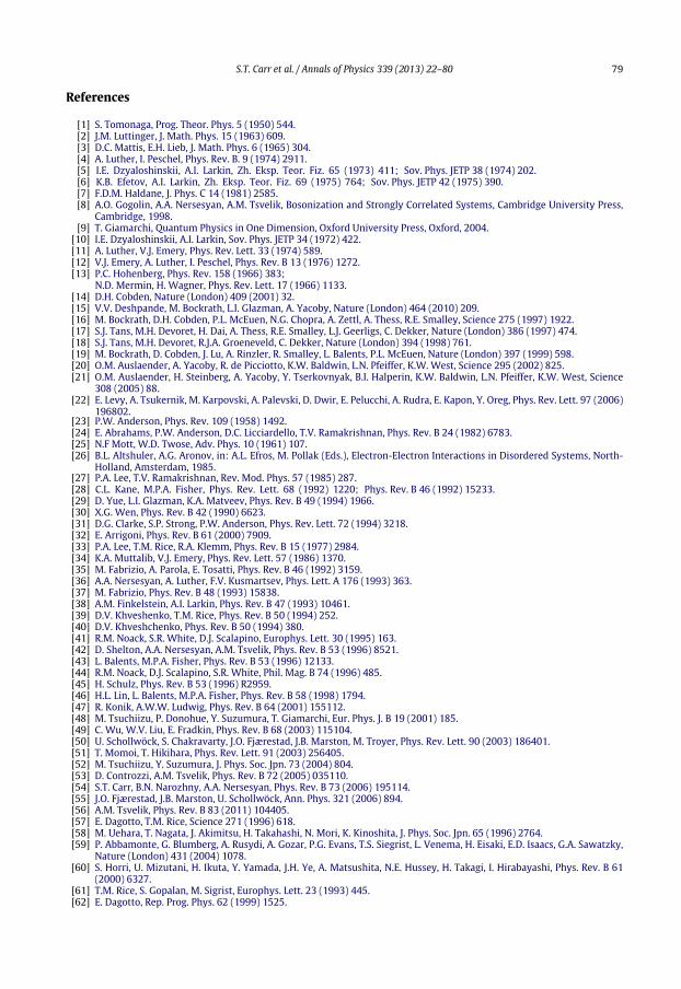
S.T. Carr et al. / Annals of Physics 339 (2013) 22–80 79
References
[1] S. Tomonaga, Prog. Theor. Phys. 5 (1950) 544.[2] J.M. Luttinger, J. Math. Phys. 15 (1963) 609.[3] D.C. Mattis, E.H. Lieb, J. Math. Phys. 6 (1965) 304.[4] A. Luther, I. Peschel, Phys. Rev. B. 9 (1974) 2911.[5] I.E. Dzyaloshinskii, A.I. Larkin, Zh. Eksp. Teor. Fiz. 65 (1973) 411; Sov. Phys. JETP 38 (1974) 202.[6] K.B. Efetov, A.I. Larkin, Zh. Eksp. Teor. Fiz. 69 (1975) 764; Sov. Phys. JETP 42 (1975) 390.[7] F.D.M. Haldane, J. Phys. C 14 (1981) 2585.[8] A.O. Gogolin, A.A. Nersesyan, A.M. Tsvelik, Bosonization and Strongly Correlated Systems, Cambridge University Press,
Cambridge, 1998.[9] T. Giamarchi, Quantum Physics in One Dimension, Oxford University Press, Oxford, 2004.
[10] I.E. Dzyaloshinskii, A.I. Larkin, Sov. Phys. JETP 34 (1972) 422.[11] A. Luther, V.J. Emery, Phys. Rev. Lett. 33 (1974) 589.[12] V.J. Emery, A. Luther, I. Peschel, Phys. Rev. B 13 (1976) 1272.[13] P.C. Hohenberg, Phys. Rev. 158 (1966) 383;
N.D. Mermin, H. Wagner, Phys. Rev. Lett. 17 (1966) 1133.[14] D.H. Cobden, Nature (London) 409 (2001) 32.[15] V.V. Deshpande, M. Bockrath, L.I. Glazman, A. Yacoby, Nature (London) 464 (2010) 209.[16] M. Bockrath, D.H. Cobden, P.L. McEuen, N.G. Chopra, A. Zettl, A. Thess, R.E. Smalley, Science 275 (1997) 1922.[17] S.J. Tans, M.H. Devoret, H. Dai, A. Thess, R.E. Smalley, L.J. Geerligs, C. Dekker, Nature (London) 386 (1997) 474.[18] S.J. Tans, M.H. Devoret, R.J.A. Groeneveld, C. Dekker, Nature (London) 394 (1998) 761.[19] M. Bockrath, D. Cobden, J. Lu, A. Rinzler, R. Smalley, L. Balents, P.L. McEuen, Nature (London) 397 (1999) 598.[20] O.M. Auslaender, A. Yacoby, R. de Picciotto, K.W. Baldwin, L.N. Pfeiffer, K.W. West, Science 295 (2002) 825.[21] O.M. Auslaender, H. Steinberg, A. Yacoby, Y. Tserkovnyak, B.I. Halperin, K.W. Baldwin, L.N. Pfeiffer, K.W. West, Science
308 (2005) 88.[22] E. Levy, A. Tsukernik, M. Karpovski, A. Palevski, D. Dwir, E. Pelucchi, A. Rudra, E. Kapon, Y. Oreg, Phys. Rev. Lett. 97 (2006)
196802.[23] P.W. Anderson, Phys. Rev. 109 (1958) 1492.[24] E. Abrahams, P.W. Anderson, D.C. Licciardello, T.V. Ramakrishnan, Phys. Rev. B 24 (1982) 6783.[25] N.F Mott, W.D. Twose, Adv. Phys. 10 (1961) 107.[26] B.L. Altshuler, A.G. Aronov, in: A.L. Efros, M. Pollak (Eds.), Electron-Electron Interactions in Disordered Systems, North-
Holland, Amsterdam, 1985.[27] P.A. Lee, T.V. Ramakrishnan, Rev. Mod. Phys. 57 (1985) 287.[28] C.L. Kane, M.P.A. Fisher, Phys. Rev. Lett. 68 (1992) 1220; Phys. Rev. B 46 (1992) 15233.[29] D. Yue, L.I. Glazman, K.A. Matveev, Phys. Rev. B 49 (1994) 1966.[30] X.G. Wen, Phys. Rev. B 42 (1990) 6623.[31] D.G. Clarke, S.P. Strong, P.W. Anderson, Phys. Rev. Lett. 72 (1994) 3218.[32] E. Arrigoni, Phys. Rev. B 61 (2000) 7909.[33] P.A. Lee, T.M. Rice, R.A. Klemm, Phys. Rev. B 15 (1977) 2984.[34] K.A. Muttalib, V.J. Emery, Phys. Rev. Lett. 57 (1986) 1370.[35] M. Fabrizio, A. Parola, E. Tosatti, Phys. Rev. B 46 (1992) 3159.[36] A.A. Nersesyan, A. Luther, F.V. Kusmartsev, Phys. Lett. A 176 (1993) 363.[37] M. Fabrizio, Phys. Rev. B 48 (1993) 15838.[38] A.M. Finkelstein, A.I. Larkin, Phys. Rev. B 47 (1993) 10461.[39] D.V. Khveshenko, T.M. Rice, Phys. Rev. B 50 (1994) 252.[40] D.V. Khveshchenko, Phys. Rev. B 50 (1994) 380.[41] R.M. Noack, S.R. White, D.J. Scalapino, Europhys. Lett. 30 (1995) 163.[42] D. Shelton, A.A. Nersesyan, A.M. Tsvelik, Phys. Rev. B 53 (1996) 8521.[43] L. Balents, M.P.A. Fisher, Phys. Rev. B 53 (1996) 12133.[44] R.M. Noack, D.J. Scalapino, S.R. White, Phil. Mag. B 74 (1996) 485.[45] H. Schulz, Phys. Rev. B 53 (1996) R2959.[46] H.L. Lin, L. Balents, M.P.A. Fisher, Phys. Rev. B 58 (1998) 1794.[47] R. Konik, A.W.W. Ludwig, Phys. Rev. B 64 (2001) 155112.[48] M. Tsuchiizu, P. Donohue, Y. Suzumura, T. Giamarchi, Eur. Phys. J. B 19 (2001) 185.[49] C. Wu, W.V. Liu, E. Fradkin, Phys. Rev. B 68 (2003) 115104.[50] U. Schollwöck, S. Chakravarty, J.O. Fjærestad, J.B. Marston, M. Troyer, Phys. Rev. Lett. 90 (2003) 186401.[51] T. Momoi, T. Hikihara, Phys. Rev. Lett. 91 (2003) 256405.[52] M. Tsuchiizu, Y. Suzumura, J. Phys. Soc. Jpn. 73 (2004) 804.[53] D. Controzzi, A.M. Tsvelik, Phys. Rev. B 72 (2005) 035110.[54] S.T. Carr, B.N. Narozhny, A.A. Nersesyan, Phys. Rev. B 73 (2006) 195114.[55] J.O. Fjærestad, J.B. Marston, U. Schollwöck, Ann. Phys. 321 (2006) 894.[56] A.M. Tsvelik, Phys. Rev. B 83 (2011) 104405.[57] E. Dagotto, T.M. Rice, Science 271 (1996) 618.[58] M. Uehara, T. Nagata, J. Akimitsu, H. Takahashi, N. Mori, K. Kinoshita, J. Phys. Soc. Jpn. 65 (1996) 2764.[59] P. Abbamonte, G. Blumberg, A. Rusydi, A. Gozar, P.G. Evans, T.S. Siegrist, L. Venema, H. Eisaki, E.D. Isaacs, G.A. Sawatzky,
Nature (London) 431 (2004) 1078.[60] S. Horri, U. Mizutani, H. Ikuta, Y. Yamada, J.H. Ye, A. Matsushita, N.E. Hussey, H. Takagi, I. Hirabayashi, Phys. Rev. B 61
(2000) 6327.[61] T.M. Rice, S. Gopalan, M. Sigrist, Europhys. Lett. 23 (1993) 445.[62] E. Dagotto, Rep. Prog. Phys. 62 (1999) 1525.
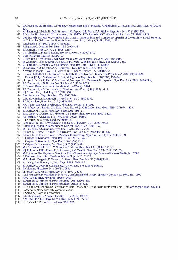
80 S.T. Carr et al. / Annals of Physics 339 (2013) 22–80
[63] S.A. Kivelson, I.P. Bindloss, E. Fradkin, V. Oganesyan, J.M. Tranquada, A. Kapitulnik, C. Howald, Rev. Mod. Phys. 75 (2003)1201.
[64] K.J. Thomas, J.T. Nicholls, M.Y. Simmons, M. Pepper, D.R. Mace, D.A. Ritchie, Phys. Rev. Lett. 77 (1996) 135.[65] A. Yacoby, H.L. Stormer, N.S. Wingreen, L.N. Pfeiffer, K.W. Baldwin, K.W. West, Phys. Rev. Lett. 77 (1996) 4612.[66] O.A. Starykh, D.L. Maslov,W. Häusler, L.I. Glazman, Interactions and Transport Properties of Lower Dimensional Systems,
in: T. Brandes (Ed.), Lecture Notes in Physics, vol. 544, Springer, Berlin, 2000, p. 37.[67] T. Ebbesen, Phys. Today 49 (6) (1996) 26.[68] R. Egger, A.O. Gogolin, Eur. Phys. J. B 3 (1998) 281.[69] S.T. Carr, Int. J. Mod. Phys. 22 (2008) 5235.[70] J.-C. Charlier, X. Blase, S. Roche, Rev. Mod. Phys. 79 (2007) 677.[71] I. Bloch, Nature Physics 1 (2005) 23.[72] I. Danshita, J.E. Williams, C.A.R. Sá de Melo, C.W. Clark, Phys. Rev. A 76 (2007) 043606.[73] M. Anderlini, J. Sebby-Strabley, J. Kruse, J.V. Porto, W.D. Phillips, J. Phys. B 39 (2006) S199.[74] S.T. Carr, B.N. Narozhny, A.A. Nersesyan, Phys. Rev. Lett. 106 (2011) 126805.[75] M. Fabrizio, A.O. Gogolin, A.A. Nersesyan, Phys. Rev. Lett. 83 (1999) 2014.[76] Z. Wang, P. Morse, J. Wei, O.E. Vilches, D.H. Cobden, Science 327 (2010) 552.[77] G. Roux, T. Barthel, I.P. McCulloch, C. Kollath, U. Schollwöck, T. Giamarchi, Phys. Rev. A 78 (2008) 023628.[78] L. Fallani, J.E. Lye, V. Guarrera, C. Fort, M. Inguscio, Phys. Rev. Lett. 98 (2007) 130404.[79] J.E. Lye, L. Fallani, C. Fort, V. Guarrera, M. Modugno, D.S. Wiersma, M. Inguscio, Phys. Rev. A 75 (2007) 061603(R).[80] S.A. Brazovskii, N.N. Kirova, Sov. Sci. Rev. A 5 (1984) 0099.[81] G. Gruner, Density Waves in Solids, Addison Wesley, 1994.[82] S.A. Brazovskii, V.M. Yakovenko, J. Physique Lett. (France) 46 (1985) L-111.[83] H.J. Schulz, Int. J. Mod. Phys. B 5 (1991) 57.[84] P.W. Anderson, Phys. Rev. Lett. 67 (1991) 3844.[85] C. Bourbonnais, L.G. Caron, Int. J. Mod. Phys. B 5 (1991) 1033.[86] F.D.M. Haldane, Phys. Lett. 93A (1983) 464.[87] A.A. Nersesyan, A.M. Tsvelik, Eur. Phys. Lett. 96 (2011) 17002.[88] K.B. Efetov, A.I. Larkin, Zh. Eksp. Teor. Fiz. 66 (1974) 2290; Sov. Phys.—JETP 39 (1974) 1129.[89] S.T. Carr, A.M. Tsvelik, Phys. Rev. B 65 (2002) 195121.[90] E.W. Carlson, D. Orgad, S.A. Kivelson, V.J. Emery, Phys. Rev. B 62 (2000) 3422.[91] A.V. Rozkhov, A.J. Millis, Phys. Rev. B 66 (2002) 134509.[92] H.J. Schulz, 1998. arXiv:cond-mat/9808167.[93] R. Konik, F. Lesage, A.W.W. Ludwig, H. Saleur, Phys. Rev. B 61 (2000) 4983.[94] E. Boulat, P. Azaria, P. Lecheminant, Nuclear Phys. B 822 (2009) 367.[95] M. Tsuchiizu, Y. Suzumura, Phys. Rev. B 72 (2005) 075121.[96] B. Dóra, M. Gulásci, F. Simon, H. Kuzmany, Phys. Rev. Lett. 99 (2007) 166402.[97] B. Dóra, M. Gulásci, F. Simon, P. Wzietek, H. Kuzmany, Phys. Stat. Sol. (B) 245 (2008) 2159.[98] E. Orignac, T. Giamarchi, Phys. Rev. B 53 (1996) R10453.[99] E. Orignac, T. Giamarchi, Phys. Rev. B 56 (1997) 7167.
[100] E. Orignac, Y. Suzumura, Eur. Phys. J. B 23 (2001) 57.[101] M.P. Schneider, S.T. Carr, I.V. Gornyi, A.D. Mirlin, Phys. Rev. B 86 (2012) 155141.[102] N.J. Robinson, F.H.L. Essler, E. Jeckelmann, A.M. Tsvelik, Phys. Rev. B 85 (2012) 195103.[103] M. Fujimoto, The Physics of Structural Phase Transitions, Springer Science+Business Media, Inc, 2005.[104] T. Esslinger, Annu. Rev. Condens. Matter Phys. 1 (2010) 129.[105] M.A. Martin-Delgado, R. Shankar, G. Sierra, Phys. Rev. Lett. 77 (1996) 3443.[106] Y.J. Wang, A.A. Nersesyan, Nucl. Phys. B 583 (2000) 671.[107] S.T. Carr, A.O. Gogolin, A.A. Nersesyan, Phys. Rev. B 76 (2007) 245121.[108] S. Coleman, Phys. Rev. D 11 (1975) 2088.[109] J.B. Zuber, C. Itzykson, Phys. Rev. D 15 (1977) 2875.[110] P. Di Francesco, P. Mathieu, D. Senechal, Conformal Field Theory, Springer-Verlag New York, Inc, 1997.[111] A.M. Tsvelik, Phys. Rev. B 42 (1990) 10499.[112] Y. Atzmon, E. Shimshoni, Phys. Rev. B 83 (2011) 220518(R.[113] Y. Atzmon, E. Shimshoni, Phys. Rev. B 85 (2012) 134523.[114] H. Saleur, Lectures on Non Perturbative Field Theory and Quantum Impurity Problems, 1998, arXiv:cond-mat/9812110.[115] P. Azaria, E. Altman, Private communication.[116] T. Sproll, S.T. Carr, in preparation.[117] P. Lecheminant, H. Nonne, Phys. Rev. B 85 (2012) 195121.[118] A.M. Tsvelik, A.B. Kuklov, New. J. Phys. 14 (2012) 115033.[119] D. Sénéchal, 1999. arXiv:cond-mat/9908262.