Clustering method for estimating principal diffusion directions

Clustering method for estimating principal diffusion directions

Mohammad-Reza Nazem-Zadeha,b,*, Kourosh Jafari-Khouzanic, Esmaeil Davoodi-Bojda,Quan Jiangb, and Hamid Soltanian-Zadeha,c

aControl and Intelligent Processing Center of Excellence, School of Electrical and ComputerEngineering, University of Tehran, Tehran 14395-515, IranbDepartment of Neurology, Henry Ford Hospital, Detroit, MI 48202, USAcImage Analysis Laboratory, Department of Diagnostic Radiology, Henry Ford Hospital, Detroit,MI, 48202, USA

AbstractDiffusion tensor magnetic resonance imaging (DTMRI) is a non-invasive tool for the investigationof white matter structure within the brain. However, the traditional tensor model is unable tocharacterize anisotropies of orders higher than two in heterogeneous areas containing more thanone fiber population. To resolve this issue, high angular resolution diffusion imaging (HARDI)with a large number of diffusion encoding gradients is used along with reconstruction methodssuch as Q-ball. Using HARDI data, the fiber orientation distribution function (ODF) on the unitsphere is calculated and used to extract the principal diffusion directions (PDDs). Fast andaccurate estimation of PDDs is a prerequisite for tracking algorithms that deal with fiber crossings.In this paper, the PDDs are defined as the directions around which the ODF data is concentrated.Estimates of the PDDs based on this definition are less sensitive to noise in comparison with theprevious approaches. A clustering approach to estimate the PDDs is proposed which is anextension of fuzzy c-means clustering developed for orientation of points on a sphere. MDL(Minimum description length) principle is proposed to estimate the number of PDDs. Using bothsimulated and real diffusion data, the proposed method has been evaluated and compared withsome previous protocols. Experimental results show that the proposed clustering algorithm is moreaccurate, more resistant to noise, and faster than some of techniques currently being utilized.

KeywordsPrincipal diffusion directions; Fuzzy c-means; Minimum description length; Fiber orientationdistribution function

IntroductionDiffusion of water molecules is conventionally investigated using diffusion tensor magneticresonance imaging (DTMRI) that uses a symmetric positive definite matrix (tensor) tomodel the diffusion behavior. Under Gaussian diffusion condition, this model characterizesthe diffusion behavior very well (Basser et al., 1994a, 1994b); however, it fails to modelanisotropies of orders higher than two in the heterogeneous tissues containing more than onefiber population. Diffusion behavior can be evaluated more accurately if the probabilitydensity function (PDF) of the molecular displacement over diffusion time is determined

© 2011 Elsevier Inc. All rights reserved.*Corresponding author at: Department of Radiation Oncology, University of Michigan Health System, 1500 E, Medical Center Drive,Ann Arbor, MI, USA, 48109. Fax: +1 734 936 2261.

NIH Public AccessAuthor ManuscriptNeuroimage. Author manuscript; available in PMC 2012 July 06.

Published in final edited form as:Neuroimage. 2011 August 1; 57(3): 825–838. doi:10.1016/j.neuroimage.2011.05.056.

NIH

-PA Author Manuscript

NIH


NIH


from which desirable diffusion indices such as mean diffusivity, second order tensor (andrelated anisotropies), fourth order kurtosis, and even higher order statistics can be extracted.Estimation of the diffusion PDF conventionally involves diffusion spectrum imaging (DSI),a modified q-space imaging method that resolves intra-voxel diffusion heterogeneity bymeasuring diffusion spectra (Wedeen et al., 2000). This method is clinically impracticalbecause it takes a long time to acquire the required data.

To address the time complexity, high angular resolution diffusion imaging (HARDI) andorientation distribution function (ODF) have been introduced as alternatives to DSI anddiffusion PDF, respectively (Tuch et al., 2002). The ODF requires taking more than 50measurements of HARDI, each corresponding to a specific gradient direction. The ODFmaintains information about the orientation of the diffusivity by integrating over the radialcomponent of the PDF in the spherical domain. The ODF may be estimated using the Funk–Radon transform, closely approaching the true ODF under certain conditions (Tuch, 2004).Descoteaux et al. estimated the ODF by a linear combination of the spherical harmoniccoefficients that describe the diffusion signal within a voxel (Descoteaux et al., 2007).

In previous work (Jansons and Alexander, 2003; Tournier et al., 2004; Bloy and Verma,2008; Ghosh et al., 2008), principal diffusion directions (PDDs) are defined as the directionsof the ODF local maxima. Several methods have been proposed to find the PDDs from ODFbased on this definition. Jansons and Alexander assumed a symmetry on the ODF withrespect to the position vector x (Jansons and Alexander, 2003). That means the ODF peaksappear in equal and opposite pairs. In their method, for each spherical point s on the sphereS, the set M is defined as follows:

(1)

(2)

where ρ is a constant. The set M contains the candidate PDDs. Starting at each member ofM, the estimates are refined by searching for local maxima using the Powell's method, ageneral method for estimation of the local minima without taking derivatives (Press et al.,2007). Finally, tiny ODF peaks smaller than the ODF mean are discarded. In Tournier et al.(2004) and Sakaie and Lowe (2007), the same strategies are adopted, except for the Powell'smethod which is replaced by spherical Newton's method and sequential quadraticprogramming (constraint spherical Newton's method) (Cottle et al., 2009), respectively. Theproblem of all these methods is the likelihood of getting trapped in small local maxima. InDescoteaux (2008), assuming that the PDDs are the local maxima of the normalized ODFprojected on a tessellated sphere with a fine mesh, the finite difference method is applied tothe sphere in order to obtain the PDDs. In this method, if the ODF value for a point is aboveall of its neighbors and above 0.5, the point will be reserved as a local maximum.Thresholding is required in order to diminish minor peaks. The method, subsequently, isdependent on the threshold value. Plus, this method is very sensitive to the mesh grid size.Frey et al. (2008) take derivative of the ODF smoothed by a Gaussian kernel to get the localmaxima. Applying such kernel, which is used to diminish noise, may degrade the angularresolution of the PDDs. In Bloy and Verma (2008), the ODF is represented by a symmetrictensor constrained to the sphere resulting in a homogeneous polynomial representation. Theidea takes advantage of such representation to take analytic derivatives and find thestationary points of the ODF instead of the maxima. These stationary points are thenclassified into primary maxima (PDDs), secondary maxima, minima and saddle points. InGhosh et al. (2008), the stationary points are found by using Lagrange multipliers andapplying the combination of subdivision methods and generalized normal form algorithms to

Nazem-Zadeh et al.

Neuroimage. Author manuscript; available in PMC 2012 July 06.

NIH


NIH


NIH


the resulting polynomial system. The stationary points are then sorted and thresholded toextract the PDDs. In this paper, we refer to this technique Poly-Tensor method. One of themain problems of the Bloy's and Ghosh's methods is that classifying stationary points inorder to get the PDDs may become erroneous in noisy data condition. In our previous work,we determined the first principal direction as the gradient direction in which the ODF ismaximum and sorted the other gradient directions based on their angular distances from thisprincipal direction (Nazem-Zadeh et al., 2011). We then estimated the envelope of theresulting 1D profile using a moving maximum filter whose output peaks are the remainingprincipal diffusion directions. This method is sensitive to noise. We refer to this technique asAngular-Distance method. Using finite difference method, Camino software package (Cooket al., 2006) locates local maxima by ascertaining all points at which the function is largerthan all other points within a fixed search radius. It then removes duplicates and tiny peakswith function values smaller than a pre-specified threshold (Descoteaux et al., 2007). Thisprocedure is both inaccurate and time-consuming. In addition, the number of PDDs isrestricted to three for estimation and two for visualization. For DTI data with dimensions128 × 128 × 56, it takes almost a week to find up to three PDDs for each voxel, using acommonly used personal computer (Core 2Due CPU, E8400@ 3.00 GHz, 3.00 GHz, and 8GB RAM).

All of the above methods define the PDDs as the directions in which the ODF data is locallymaximal. The PDDs, based on this definition, are sensitive to noise. In addition, some of themethods post-process the results by discarding tiny ODF detected peaks. Depending on thekernel width, this may lead to discarding important diffusivity information. In this paper, thePDDs are defined as the directions around which the ODF data is concentrated (clustered).Estimates of the PDDs based on this definition are less sensitive to noise in comparison withthe previous approaches. They may be related to clustering principles whereby a set of datapoints is considered as potential PDDs and examined to determine whether they properlyrepresent the ODF data. In other words, they are examined to determine whether theyminimize the overall distance of the data points from the cluster centers. Unfortunately, thisapproach involves an exhaustive search which is very time-consuming when there are morethan two PDDs. To reduce the computational complexity, we propose an iterative algorithmbased on fuzzy c-means clustering (Dunn, 1973; Bezdek, 1981) in which the cluster centersand memberships are iteratively updated. Our proposed algorithm benefits from goodfeatures of the fuzzy c-means algorithm and is sufficiently accurate for practical purposes. Ittransforms the original 3D cluster data into a 2D format and thus simplifies computation.The 2D data points contain co-latitudes and co-longitudes of the spherical angles.

The ODF can be considered as a convolution of complex fiber structure, denoted by fODF(fiber ODF), and the ODF response to a single fiber (ODF kernel). Therefore, fODF can becalculated by deconvolution of the ODF with the ODF kernel (Descoteaux et al., 2007;Tournier et al., 2004). The fODF has more distinct lobes and thus is more appropriate forlocating the PDDs. Hence, we apply our algorithm to the fODF.

Starting with two cluster centers and using the spherical law of cosines, the proposedapproach calculates the arc (geodesic) distances between points on the sphere and the clustercenters. The membership values and centers of the clusters are updated iteratively untilconvergence is achieved. To automatically determine the number of clusters, this number isincreased by two and the resulting data representation is evaluated based on the minimumdescription length (MDL) criterion (Rissanen, 1989). Applications of the proposed methodto simulated and clinical data show that our algorithm is more accurate, and easier toimplement than current methods in the literature, especially when the signal-to-noise ratio(SNR) is low.

Nazem-Zadeh et al.


NIH


NIH


NIH


Materials and methodsSpherical deconvolution

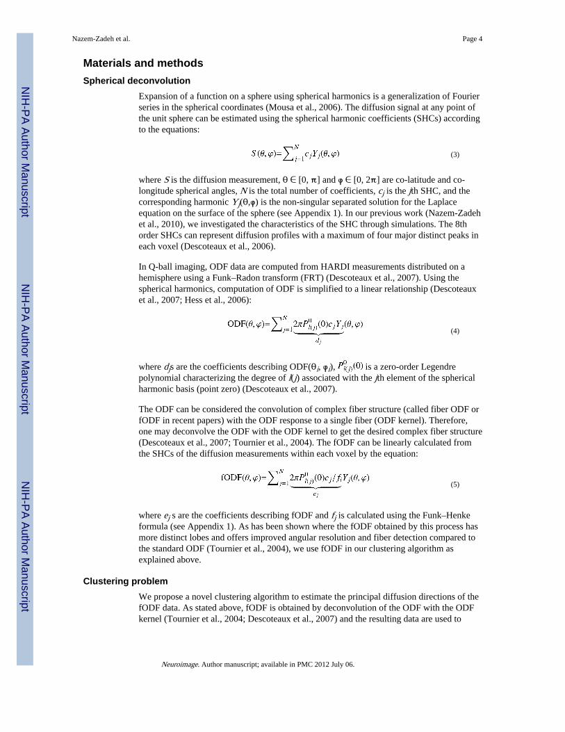
Expansion of a function on a sphere using spherical harmonics is a generalization of Fourierseries in the spherical coordinates (Mousa et al., 2006). The diffusion signal at any point ofthe unit sphere can be estimated using the spherical harmonic coefficients (SHCs) accordingto the equations:

(3)

where S is the diffusion measurement, θ ∈ [0, π] and φ ∈ [0, 2π] are co-latitude and co-longitude spherical angles, N is the total number of coefficients, cj is the jth SHC, and thecorresponding harmonic Yj(θ,φ) is the non-singular separated solution for the Laplaceequation on the surface of the sphere (see Appendix 1). In our previous work (Nazem-Zadehet al., 2010), we investigated the characteristics of the SHC through simulations. The 8thorder SHCs can represent diffusion profiles with a maximum of four major distinct peaks ineach voxel (Descoteaux et al., 2006).

In Q-ball imaging, ODF data are computed from HARDI measurements distributed on ahemisphere using a Funk–Radon transform (FRT) (Descoteaux et al., 2007). Using thespherical harmonics, computation of ODF is simplified to a linear relationship (Descoteauxet al., 2007; Hess et al., 2006):

(4)

where djs are the coefficients describing ODF(θi, φi), is a zero-order Legendrepolynomial characterizing the degree of l(j) associated with the jth element of the sphericalharmonic basis (point zero) (Descoteaux et al., 2007).

The ODF can be considered the convolution of complex fiber structure (called fiber ODF orfODF in recent papers) with the ODF response to a single fiber (ODF kernel). Therefore,one may deconvolve the ODF with the ODF kernel to get the desired complex fiber structure(Descoteaux et al., 2007; Tournier et al., 2004). The fODF can be linearly calculated fromthe SHCs of the diffusion measurements within each voxel by the equation:

(5)

where ej s are the coefficients describing fODF and fj is calculated using the Funk–Henkeformula (see Appendix 1). As has been shown where the fODF obtained by this process hasmore distinct lobes and offers improved angular resolution and fiber detection compared tothe standard ODF (Tournier et al., 2004), we use fODF in our clustering algorithm asexplained above.

Clustering problemWe propose a novel clustering algorithm to estimate the principal diffusion directions of thefODF data. As stated above, fODF is obtained by deconvolution of the ODF with the ODFkernel (Tournier et al., 2004; Descoteaux et al., 2007) and the resulting data are used to

Nazem-Zadeh et al.


NIH


NIH


NIH


estimate the PDDs. By PDDs we do not mean the directions that generate the highest ODFvalues, but rather the directions around which most of the ODF points are concentrated.

For illustrating the problem, consider a three-cluster profile of fODF data points distributedin 3D space with cluster directions S1, S2 and S3 (Fig. 1). The Euclidean distance between adata point Pi and a cluster center (direction) Sj (distance between a point and a line) iscalculated as:

(6)

We define the distance of Pi to the profile of all data points (the set of all data points) as theminimum of distances to the cluster directions. For example, in Fig. 1A, since Pi is closer toS3, it is classified to the cluster whose main direction is S3 and hence, its distance to theprofile of whole data points is its distance to S3.

The overall distance is defined by the summation of the distances of all points to the profileof all data points. At certain specific orientations (Sj*, Sk*, …), the overall distance of thedata points is minimal. In the three-cluster case:

(7)

These directions may be considered as PDDs which have low sensitivity to noise. One mayconsider each possible combination of data points as a set of PDD candidates and evaluatetheir representation of the fODF data in terms of minimizing overall distance. We refer tothis as the “Search-All” method, however, increasing the number of clusters renders thesearch very time consuming. Here, we introduce an iterative algorithm in the sphericaldomain based on the fuzzy c-means clustering algorithm (Dunn, 1973; Bezdek, 1981),called, hereafter, Sph-FCM. The fuzzy c-means algorithm has been proven more accuratethan K-means algorithm in clustering, as it takes into account the membership of each pointto each cluster. As all measurements are made on a sphere, we perform the clusteringalgorithm in the spherical domain concentrating on orientation of fODF.

For visualization of fODF data, the unit radius of the spherical coordinate of each point maybe replaced by its fODF value as shown in Fig. 1A. In this representation, we deal withpoints in 3D space. Fig. 1B, alternatively, shows the use of hot colors in visualizing thefODF value on the sphere. We are interested in a clustering method which simply exploitsthe points on the sphere and their fODF values and returns the PDDs. Therefore, the searchdomain is the space of co-latitude and co-longitude spherical angles of the points.

We introduce an on-sphere version of fuzzy c-means clustering in which cluster centers areupdated based on formulas derived in the spherical domain. The proposed clusteringtechnique has worked very well for this application and is data-driven. Moreover, thetechnique favors rounded clusters, which is mostly the case in practice. Note that using thefuzzy c-means clustering in the 3D spatial domain does not generate an analytic solution forthe derivatives in updating cluster centers (directions) with the definition of distance in Eq.(6). Using the spherical law of cosines, the geodesic distance between each point xi on thesphere and the cluster center μj is calculated as:

(8)

Nazem-Zadeh et al.


NIH


NIH


NIH


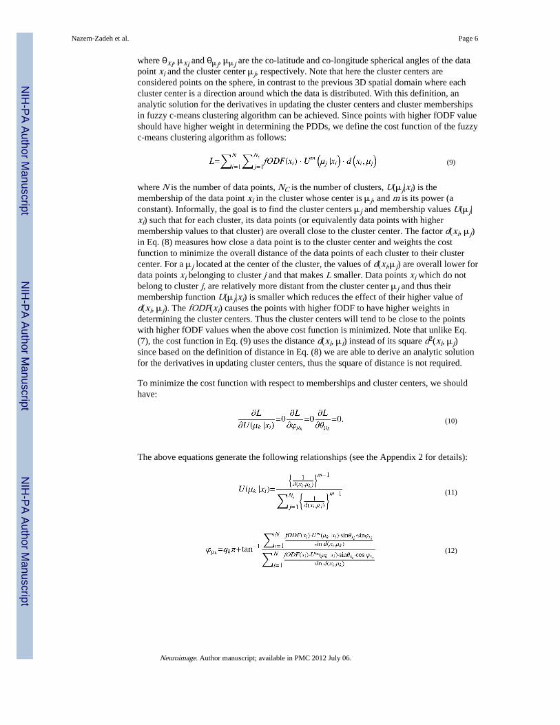
where θxi, μxi and θμj, μμj are the co-latitude and co-longitude spherical angles of the datapoint xi and the cluster center μj, respectively. Note that here the cluster centers areconsidered points on the sphere, in contrast to the previous 3D spatial domain where eachcluster center is a direction around which the data is distributed. With this definition, ananalytic solution for the derivatives in updating the cluster centers and cluster membershipsin fuzzy c-means clustering algorithm can be achieved. Since points with higher fODF valueshould have higher weight in determining the PDDs, we define the cost function of the fuzzyc-means clustering algorithm as follows:

(9)

where N is the number of data points, NC is the number of clusters, U(μj|xi) is themembership of the data point xi in the cluster whose center is μj, and m is its power (aconstant). Informally, the goal is to find the cluster centers μj and membership values U(μj|xi) such that for each cluster, its data points (or equivalently data points with highermembership values to that cluster) are overall close to the cluster center. The factor d(xi, μj)in Eq. (8) measures how close a data point is to the cluster center and weights the costfunction to minimize the overall distance of the data points of each cluster to their clustercenter. For a μj located at the center of the cluster, the values of d(xi,μj) are overall lower fordata points xi belonging to cluster j and that makes L smaller. Data points xi which do notbelong to cluster j, are relatively more distant from the cluster center μj and thus theirmembership function U(μj|xi) is smaller which reduces the effect of their higher value ofd(xi, μj). The fODF(xi) causes the points with higher fODF to have higher weights indetermining the cluster centers. Thus the cluster centers will tend to be close to the pointswith higher fODF values when the above cost function is minimized. Note that unlike Eq.(7), the cost function in Eq. (9) uses the distance d(xi, μi) instead of its square d2(xi, μj)since based on the definition of distance in Eq. (8) we are able to derive an analytic solutionfor the derivatives in updating cluster centers, thus the square of distance is not required.

To minimize the cost function with respect to memberships and cluster centers, we shouldhave:

(10)

The above equations generate the following relationships (see the Appendix 2 for details):

(11)

(12)

Nazem-Zadeh et al.


NIH


NIH


NIH


(13)

where qk, q′k are integers. Depending on the choice of qk and q′k, the resulting φμk and θμkmay maximize or minimize the cost function. For each cluster center, we choose appropriatevalues of qk and q′k that minimize L.

Minimum description lengthChoosing the right number of clusters is crucial for any algorithm; choosing a wrongnumber will result in a poor outcome as demonstrated in Fig. 2, in which selection of two orfour clusters rather than three; the final extracted PDDs (red lines) deviates from the actualdirections (blue lines) around which the diffusion signal is simulated. Alexander et al.proposed a method for selecting the number of clusters that estimates the order of non-Gaussian diffusion (Alexander et al., 2002) by determining the truncation level of the SHCcoefficients used in the diffusion signal logarithm by means of ANOVA (Armitage, 1971).They use incomplete beta probability statistics in Camino (Voxelclassify function) instead ofthe F-test proposed originally (Cook et al., 2006). In our comparative experiments, we haveimplemented Alexander's original method as well as the method used in Camino. A problemwith these methods is that their statistical thresholds are not sufficient to obtain a goodclassification of the diffusion orders as we show in the Results section.

We estimate the optimal number of clusters from the data distribution based on theminimum description length (MDL) criterion (Rissanen, 1989). This criterion has beenpreviously used in vector quantization as the minimization of the length of the descriptionfor the data S is transferred to a receiver without error (Bischof et al., 1999). A set ofreference vector A is specified around which the data points are distributed. The data S isdivided into inliers I, i.e., data points clustered around the reference vectors A, and outliersO. Thus, S = I + O. The inliers I are coded by the reference vectors and transferred. Theoutliers O are identified and not coded by the reference vectors. Using the reference vectorsA, the length of encoding S is then given by:

(14)

where L(A) is the length of encoding the reference vectors A, L(I(A)) is the length ofencoding the index of A to which the vectors in I are assigned, L(∈IA) is the length ofencoding the residual errors, and L(O) is the length of encoding the outliers. Therefore, ourgoal is to minimize the cost of encoding S using A to determine outliers and the number ofclusters (Bischof et al., 1999).

Considering the ODF is antipodally symmetric and each pair of diffusion lobes repeatsreciprocally, we consider two centers for each pair. We start with two cluster centers andraise the number of clusters by two until increasing the clusters no longer lowers the transfercost. The PDD estimation algorithm is updated based on the number of clusters we obtainusing the MDL.

Proposed algorithmThe proposed algorithm is summarized in Fig. 3. Starting with two cluster centers, the arcdistance between each point and the cluster centers are calculated and the cluster centers andmemberships updated accordingly. The procedure is repeated until the difference betweentwo consecutive cluster centers is negligible. The final cluster centers are considered the

Nazem-Zadeh et al.


NIH


NIH


NIH


principal diffusion directions. Next, we increase the number of clusters by two and evaluateits effect on the data representation using MDL. If it is beneficial, the algorithm continueswith the new number of clusters; otherwise, it stops and the previous number of clusters istaken as final.

As mentioned before, the 8th order SHC can represent diffusion profiles that have amaximum of four major distinct peaks (Descoteaux et al., 2006). However for real MRIdata, practically, it is preferred to restrict the number of PDDs to three.

Experimental results and discussionSimulated data

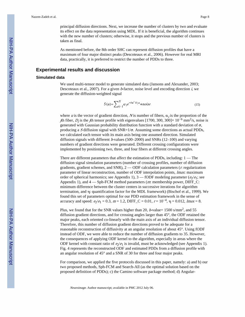
We used multi-tensor model to generate simulated data (Jansons and Alexander, 2003;Descoteaux et al., 2007). For a given b-factor, noise level and encoding direction i, wegenerate the diffusion-weighted signal

(15)

where u is the vector of gradient direction, N is number of fibers, αj is the proportion of thejth fiber, Dj is the jth tensor profile with eigenvalues [1700, 300, 300]× 10−6 mm2/s, noise isgenerated with Gaussian probability distribution function with a standard deviation of σ,producing a S diffusion signal with SNR=1/σ. Assuming some directions as actual PDDs,we calculated each tensor with its main axis being one assumed direction. Simulateddiffusion signals with different b-values (500–2000) and SNRs (12–100) and varyingnumbers of gradient directions were generated. Different crossing configurations wereimplemented by positioning two, three, and four fibers at different crossing angles.

There are different parameters that affect the estimation of PDDs, including: 1 — Thediffusion signal simulation parameters (number of crossing profiles, number of diffusiongradients, gradient schemes, and SNR), 2 — ODF calculation parameters (r: regularizationparameter of linear reconstruction, number of ODF interpolation points, lmax: maximumorder of spherical harmonics; see Appendix 1), 3 — fODF modeling parameter (e2/e1; seeAppendix 1), and 4 — Sph-FCM method parameters (m: membership power, DIFF_C:minimum difference between the cluster centers in successive iterations for algorithmtermination, and η: quantification factor for the MDL framework) (Bischof et al., 1999). Wefound this set of parameters optimal for our PDD estimation framework in the sense ofaccuracy and speed: e2/e1 = 0.3, m = 1.2, DIFF_C = 0.01, r = 10−4, η = 0.012, lmax = 8.

Plus, we found that for the SNR values higher than 20, b-value= 1500 s/mm2, and 55diffusion gradient directions, and for crossing angles larger than 45°, the ODF retained themajor peaks, each oriented co-linearly with the main axis of an individual diffusion tensor.Therefore, this number of diffusion gradient directions proved to be adequate for areasonable reconstruction of diffusivity at an angular resolution of about 45°. Using fODFinstead of ODF, we were able to reduce the number of diffusion gradients to 35. However,the consequences of applying ODF kernel to the algorithm, especially in areas where theODF kernel with constant ratio of e2/e1 is invalid, must be acknowledged (see Appendix 1).Fig. 4 represents the reconstructed ODF and estimated PDDs from a diffusion profile withan angular resolution of 45° and a SNR of 30 for three and four major peaks.

For comparison, we applied the five protocols discussed in this paper, namely: a) and b) ourtwo proposed methods, Sph-FCM and Search-All (as the optimal solution based on theproposed definition of PDDs); c) the Camino software package method; d) Angular-

Nazem-Zadeh et al.


NIH


NIH


NIH


Distance technique (Nazem-Zadeh et al., 2011), and e) Poly-Tensor method (Ghosh et al.,2008). By averaging over 50 repetitions, we calculated the similarity between the actualPDDs (the main axes of the tensors used in diffusion signal simulation in Eq. (15)) and thoseextracted using each method over a wide range of SNRs (12, 16, 20, 24, 28, 32, 36, 40, 44,50, 60, 70, 80, 100) and using diffusion profiles with three and four major peaks. We definethe following similarity measure which incorporates both the accuracy of each estimatedPDD as well as the estimated number of PDDs:

(16)

where PDDa(i) is ith actual PDD and PDDe(i) is the closest estimated PDD to PDDa(i). Na isthe number of actual PDDs and Ne is the estimated number of PDDs by a given method.Since the estimated PDDs and the number of PDDs may be different in different trials (withdifferent added noise), we repeated the algorithm 50 times for each SNR value and averagedthem.

As shown in Fig. 5 as expected, the Search-All method was superior among all methods,whereas Camino was inferior in terms of similarity between actual and extracted PDDs aswell as the estimated number of PDDs. The Search-All method is more robust to noise andworks slightly better than Sph-FCM at low SNRs. With close performance to the Search-Allmethod, our proposed Sph-FCM method is significantly more accurate than the Poly-Tensor,Angular-Distance and Camino methods in low SNRs, while in high SNRs both Sph-FCMand Poly-Tensor methods perform similarly and result in high similarity as defined by Eq.(16). The inferiority of Poly-Tensor method compared to Sph-FCM is due to the fact thatfitting high order tensor to a noisy measurement leads to inaccuracy in the PDDs detection.Note that the total error in the simulations combines the estimation error (due to ODFapproximation by the SHCs) and detection error (i.e., deviation from the PDDs based ondefinition).

Based on the MDL criterion, our proposed methods (Sph-FCM, Search-All) correctlyestimate the number of PDDs for almost all SNRs especially for the SNRs higher than 28.Among the other methods, the Poly-Tensor shows good performance especially for theSNRs higher than 50.

Real dataHARDI data for a normal subject was acquired using a GE Signa Excite 3 T MRI scanner atHenry Ford Hospital (Detroit, MI, USA) with 55 diffusion gradient directions with b-value=1500 s/mm2 and six B0 references. The imaging in-plane pixel and matrix size were0.975 × 0.975 mm2 and 256 × 256, respectively, with a slice thickness of 2.5 mm. Thesevalues were originally 1.95 × 1.95 mm2 and 128 × 128 but were automatically interpolatedto 256 × 256 #x000D7; 6 by the E console.

To evaluate Camino in the estimation of number of clusters, we implemented and appliedthe method described in Alexander et al. (2002) and the method implemented by Camino.The problem with both methods is that their statistical thresholding is not appropriate toobtain a good classification of non-Gaussian diffusion order. For instance, in most crossingsbetween the corona radiata, superior longitudinal fasciculus (SLF) and corpus callosum,diffusion with an order of four or more is expected, whereas within the corpus callosum,prolate diffusion of order two should predominate. However, by changing the F-teststatistical thresholds in order to assign an order of four to the crossing, an order of four isassigned to the corpus callosum as well.

Nazem-Zadeh et al.


NIH


NIH


NIH


To improve inter-plane resolution, we further interpolated diffusion data to a voxel size of0.975 × 0.975 × 0.98 mm3 and matrix size of 256 × 256 × 144. The proposed method takesabout 24 h to find up to three PDDs for each voxel using a PC with Intel Core 2Due CPU(E8400@ 3.00 GHz, 3.00 GHz) and 8 GB RAM and using a MATLAB Executable-MEXfile that is dynamically linked to the function produced from visual C++ 2008 source code inWindows Vista 64 bit. However, when we restored the data to their original size (128 × 128× 56), the computation time was decreased to less than three hours which can be consideredfeasible in the clinical settings, especially compared to the Camino method which takesabout one week to find up to three PDDs for each voxel using the same machine.

Fig. 6 shows color-coded fractional anisotropy (FA) in the coronal plane at the intersectionof the corpus callosum, superior corona radiata (internal capsule of cortico-spinal tract), andSLF with PDDs extracted by Camino in the crossing area (Fig. 6B).

Figs. 7 and 8 represent the same crossing area in Fig. 6A with PDDs estimated by the Poly-Tensor and the proposed Sph-FCM method, respectively. Note that Camino did not resolvethe crossings between these fiber tracts, while the Poly-Tensor (partly) and the proposedSph-FCM methods were successful in resolving the fibers in the crossing areas. Asillustrated in these figures, the Poly-Tensor method underestimates the number of clusters.

Fig. 9 illustrates the intersection of the SLF and arcuate fasciculi. Note that Camino, as aHARDI-based method, again was unable to resolve the crossings between these fiber tracts,whereas the proposed Sph-FCM method was able to resolve this crossing in this intersectionin Fig. 10. Although the SLF crosses the arcuate fasciculi, one can zoom in on the image andtrack one of the PDDs parallel to the main axis of the SLF from the occipital to the frontallobe. In addition, note the smooth transition from the main PDD of the SLF to the inferiorlongitudinal fasciculus (ILF), rarely detectable by other methods.

Fig. 11 shows a tractography reconstruction of the corpus callosum and the cortico-spinaltract up to the corona radiata, cingulum and SLF using up to three PDDs as estimated by ourproposed method in sagittal, axial, and coronal views, respectively. The FACT algorithm(Mori and van Zijl, 2002) has been modified to deal with more than one PDD and used toreconstruct the fiber tracts with an FA threshold of 0.01 and a maximum 25° angle ofsuccessive trajectories. When the trajectory reaches a voxel with more than one PDD, itadopts the most co-linear direction. Then, by removing the most co-linear and maintainingthe other directions, we consider the current voxel as a new ROI (region of interest) point.Thus, the modified FACT algorithm is capable of dealing with the branching fibers. As inthe crossing between these fiber tracts, our tracking algorithm is capable of resolving eachtract using the PDDs extracted by the proposed method.

DiscussionIn this paper, for estimating the fiber ODF, we used spherical deconvolution method as it isstill being used in the literature (Leergaard et al., 2010). Although different ODFreconstruction methods have been proposed in the literature, there is no specific onepreferred in general over others. Tristan-Vega et al. (2009) proposed a probabilistic methodfor computing the orientation probability density function, and demonstrated improvedresults in better resolving fiber crossings over Q-ball reconstruction using sphericalharmonics. Compared to Q-ball method that does not assume any kind of underlying model,they assume slow variation of the apparent distribution function, which would be arestriction especially for very noisy images with low SNR. Plus, they may suffer from somecomputational imperfections which need a post-processing on the results. In Aganj et al.(2010), a new technique is proposed for correcting the definition of the ODF resulting in a

Nazem-Zadeh et al.


NIH


NIH


NIH


dimensionless and normalized expression. They showed an improvement in performance oftheir proposed ODF on simulated as well as HARDI data. However, in addition to thecalculation complexity, they made some approximations, simplifications and assumptionswhich may not be valid in every diffusivity condition. In another theoretical work, Barnett(2009) showed that the interpretation of the approximated ODF described by Tuch (2004) isnot valid. Instead, he derived another ODF expression from Q-ball imaging and claimed thatit is more accurate. However, he demonstrated that for large b values, the ODF derived fromtheir proposed method and the ODF described by Tuch's approach to same values andtherefore reveal same representation of diffusion profiles. Therefore, using b-value=1500 s/mm2 in our data acquisition makes the ODF estimation error very small.

We chose 755 reconstruction points for ODF which have been recommended in Tuch(2004). This number of ODF points is large enough to achieve a high level of accuracy. Wefound out that further increase of this number does not improve the PDD estimationaccuracy. However, this is not a rigid choice and we could have chosen a smaller number.Also since we are interested in estimating up to three PDDs in the crossing areas, we couldset lmax=6. However, setting lmax=8 along with small regularization parameter (r = 10−4)would generate sharper ODF/fODF profile making it easier to estimate PDDs using theproposed clustering method.

We used fuzzy c-means algorithm to extract the PDDs. Although this is an old technique, ithas worked very well for this application. There are other techniques that could be used butsome of them with better convergence, such as Expectation Maximization, are based on aspecific model of the clusters which may not be an appropriate assumption in this particularapplication.

ConclusionsIn this paper, we have proposed an iterative clustering algorithm in the spherical domain forestimation of the PPDs. The proposed algorithm is based on fuzzy c-means clustering andbenefits from the stability of the fuzzy c-means algorithm (Dunn, 1973; Bezdek, 1981). Inthis framework, the clustering process in 3D Cartesian space is transformed into 2D inspherical space, simplifying computation. Since fODF has more distinct lobes than ODF andthus is more appropriate for locating PDDs, we applied the proposed algorithm to the fODF.Also, we used the MDL criterion to estimate the number of clusters, which we found to besuperior to some other methods proposed in the literature. By applying our method to thesimulated data, we showed that it is both more accurate than the traditional methods,especially at low SNRs. Furthermore, we showed that the proposed method is applicable totracking the fibers in the crossing regions of the human brain. We were able to resolvecrossing in the corpus callosum, cortico-spinal tract extending to the corona radiata,cingulum, and SLF using our algorithm.

AcknowledgmentsThis work was supported in part by Iran National Science Foundation (INSF).

Appendix 1. Spherical deconvolutionExpansion of a function on a sphere using spherical harmonics is a generalization of Fourierseries in the spherical coordinates (Mousa et al., 2006). The diffusion signal at any point ofthe unit sphere can be estimated using the spherical harmonic coefficients (SHCs) accordingto the equations:

Nazem-Zadeh et al.


NIH


NIH


NIH


(A1 – 1)

(A1 – 2)

(A1 – 3)

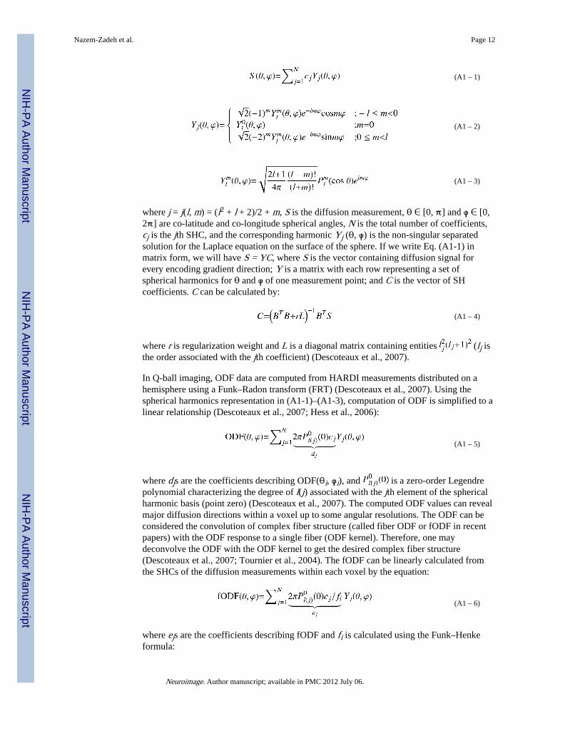
where j = j(l, m) = (l2 + l + 2)/2 + m, S is the diffusion measurement, θ ∈ [0, π] and φ ∈ [0,2π] are co-latitude and co-longitude spherical angles, N is the total number of coefficients,cj is the jth SHC, and the corresponding harmonic Yj (θ, φ) is the non-singular separatedsolution for the Laplace equation on the surface of the sphere. If we write Eq. (A1-1) inmatrix form, we will have S = YC, where S is the vector containing diffusion signal forevery encoding gradient direction; Y is a matrix with each row representing a set ofspherical harmonics for θ and φ of one measurement point; and C is the vector of SHcoefficients. C can be calculated by:

(A1 – 4)

where r is regularization weight and L is a diagonal matrix containing entities (lj isthe order associated with the jth coefficient) (Descoteaux et al., 2007).

In Q-ball imaging, ODF data are computed from HARDI measurements distributed on ahemisphere using a Funk–Radon transform (FRT) (Descoteaux et al., 2007). Using thespherical harmonics representation in (A1-1)–(A1-3), computation of ODF is simplified to alinear relationship (Descoteaux et al., 2007; Hess et al., 2006):

(A1 – 5)

where djs are the coefficients describing ODF(θi, φi), and is a zero-order Legendrepolynomial characterizing the degree of l(j) associated with the jth element of the sphericalharmonic basis (point zero) (Descoteaux et al., 2007). The computed ODF values can revealmajor diffusion directions within a voxel up to some angular resolutions. The ODF can beconsidered the convolution of complex fiber structure (called fiber ODF or fODF in recentpapers) with the ODF response to a single fiber (ODF kernel). Therefore, one maydeconvolve the ODF with the ODF kernel to get the desired complex fiber structure(Descoteaux et al., 2007; Tournier et al., 2004). The fODF can be linearly calculated fromthe SHCs of the diffusion measurements within each voxel by the equation:

(A1 – 6)

where ejs are the coefficients describing fODF and fi is calculated using the Funk–Henkeformula:

Nazem-Zadeh et al.


NIH


NIH


NIH


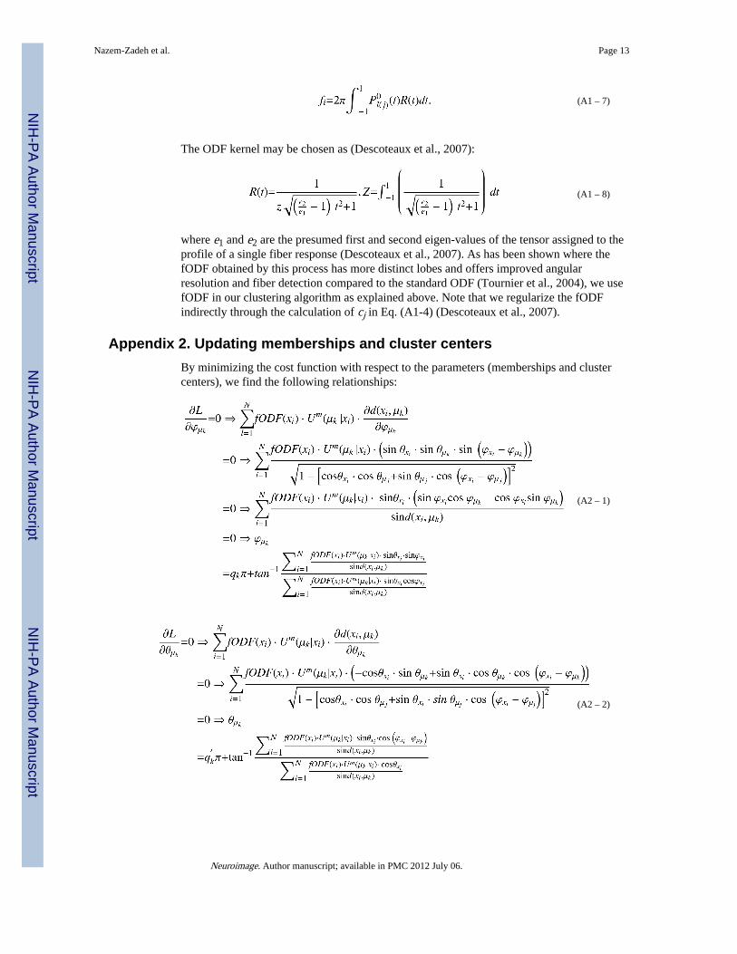
(A1 – 7)

The ODF kernel may be chosen as (Descoteaux et al., 2007):

(A1 – 8)

where e1 and e2 are the presumed first and second eigen-values of the tensor assigned to theprofile of a single fiber response (Descoteaux et al., 2007). As has been shown where thefODF obtained by this process has more distinct lobes and offers improved angularresolution and fiber detection compared to the standard ODF (Tournier et al., 2004), we usefODF in our clustering algorithm as explained above. Note that we regularize the fODFindirectly through the calculation of cj in Eq. (A1-4) (Descoteaux et al., 2007).

Appendix 2. Updating memberships and cluster centersBy minimizing the cost function with respect to the parameters (memberships and clustercenters), we find the following relationships:

(A2 – 1)

(A2 – 2)

Nazem-Zadeh et al.


NIH


NIH


NIH


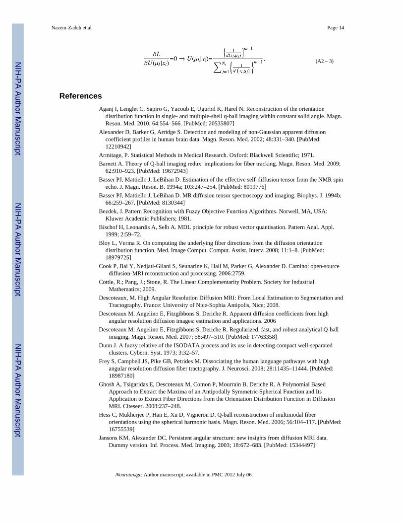
(A2 – 3)

ReferencesAganj I, Lenglet C, Sapiro G, Yacoub E, Ugurbil K, Harel N. Reconstruction of the orientation

distribution function in single- and multiple-shell q-ball imaging within constant solid angle. Magn.Reson. Med. 2010; 64:554–566. [PubMed: 20535807]

Alexander D, Barker G, Arridge S. Detection and modeling of non-Gaussian apparent diffusioncoefficient profiles in human brain data. Magn. Reson. Med. 2002; 48:331–340. [PubMed:12210942]

Armitage, P. Statistical Methods in Medical Research. Oxford: Blackwell Scientific; 1971.

Barnett A. Theory of Q-ball imaging redux: implications for fiber tracking. Magn. Reson. Med. 2009;62:910–923. [PubMed: 19672943]

Basser PJ, Mattiello J, LeBihan D. Estimation of the effective self-diffusion tensor from the NMR spinecho. J. Magn. Reson. B. 1994a; 103:247–254. [PubMed: 8019776]

Basser PJ, Mattiello J, LeBihan D. MR diffusion tensor spectroscopy and imaging. Biophys. J. 1994b;66:259–267. [PubMed: 8130344]

Bezdek, J. Pattern Recognition with Fuzzy Objective Function Algorithms. Norwell, MA, USA:Kluwer Academic Publishers; 1981.

Bischof H, Leonardis A, Selb A. MDL principle for robust vector quantisation. Pattern Anal. Appl.1999; 2:59–72.

Bloy L, Verma R. On computing the underlying fiber directions from the diffusion orientationdistribution function. Med. Image Comput. Comput. Assist. Interv. 2008; 11:1–8. [PubMed:18979725]

Cook P, Bai Y, Nedjati-Gilani S, Seunarine K, Hall M, Parker G, Alexander D. Camino: open-sourcediffusion-MRI reconstruction and processing. 2006:2759.

Cottle, R.; Pang, J.; Stone, R. The Linear Complementarity Problem. Society for IndustrialMathematics; 2009.

Descoteaux, M. High Angular Resolution Diffusion MRI: From Local Estimation to Segmentation andTractography. France: University of Nice-Sophia Antipolis, Nice; 2008.

Descoteaux M, Angelino E, Fitzgibbons S, Deriche R. Apparent diffusion coefficients from highangular resolution diffusion images: estimation and applications. 2006

Descoteaux M, Angelino E, Fitzgibbons S, Deriche R. Regularized, fast, and robust analytical Q-ballimaging. Magn. Reson. Med. 2007; 58:497–510. [PubMed: 17763358]

Dunn J. A fuzzy relative of the ISODATA process and its use in detecting compact well-separatedclusters. Cybern. Syst. 1973; 3:32–57.

Frey S, Campbell JS, Pike GB, Petrides M. Dissociating the human language pathways with highangular resolution diffusion fiber tractography. J. Neurosci. 2008; 28:11435–11444. [PubMed:18987180]

Ghosh A, Tsigaridas E, Descoteaux M, Comon P, Mourrain B, Deriche R. A Polynomial BasedApproach to Extract the Maxima of an Antipodally Symmetric Spherical Function and ItsApplication to Extract Fiber Directions from the Orientation Distribution Function in DiffusionMRI. Citeseer. 2008:237–248.

Hess C, Mukherjee P, Han E, Xu D, Vigneron D. Q-ball reconstruction of multimodal fiberorientations using the spherical harmonic basis. Magn. Reson. Med. 2006; 56:104–117. [PubMed:16755539]

Jansons KM, Alexander DC. Persistent angular structure: new insights from diffusion MRI data.Dummy version. Inf. Process. Med. Imaging. 2003; 18:672–683. [PubMed: 15344497]

Nazem-Zadeh et al.


NIH


NIH


NIH


Leergaard TB, White NS, de Crespigny A, Bolstad I, D'Arceuil H, Bjaalie JG, Dale AM. Quantitativehistological validation of diffusion MRI fiber orientation distributions in the rat brain. PLoS One.2010; 5:e8595. [PubMed: 20062822]

Mori S, van Zijl PC. Fiber tracking: principles and strategies — a technical review. NMR Biomed.2002; 15:468–480. [PubMed: 12489096]

Mousa M, Chaine R, Akkouche S. Frequency-based Representation of 3D Models Using SphericalHarmonics. Citeseer. 2006:193–200.

Nazem-Zadeh M, Davoodi-Bojd E, Soltanian-Zadeh H. Level set fiber bundle segmentation usingspherical harmonic coefficients. Comput. Med. Imaging Graph. 2010; 34:192–202. [PubMed:19846274]

Nazem-Zadeh M, Davoodi-Bojd E, Soltanian-Zadeh H. Automatic atlas-based fiber bundlesegmentation using principal diffusion directions and spherical harmonic coefficients.NeuroImage. 2011; 54:S146–S164. [PubMed: 20869453]

Press, W.; Flannery, B.; Teukolsky, S.; Vetterling, W. Numerical Recipes. Cambridge: CambridgeUniversity Press; 2007.

Rissanen, J. Stochastic complexity in Statistical Inquiry Theory. River Edge, NJ, USA: WorldScientific Publishing Co., Inc.; 1989.

Sakaie KE, Lowe MJ. An objective method for regularization of fiber orientation distributions derivedfrom diffusion-weighted MRI. NeuroImage. 2007; 34:169–176. [PubMed: 17030125]

Tournier J, Calamante F, Gadian D, Connelly A. Direct estimation of the fiber orientation densityfunction from diffusion-weighted MRI data using spherical deconvolution. NeuroImage. 2004;23:1176–1185. [PubMed: 15528117]

Tristan-Vega A, Westin CF, Aja-Fernandez S. Estimation of fiber orientation probability densityfunctions in high angular resolution diffusion imaging. NeuroImage. 2009; 47:638–650. [PubMed:19393321]

Tuch DS. Q-ball imaging. Magn. Reson. Med. 2004; 52:1358–1372. [PubMed: 15562495]

Tuch DS, Reese TG, Wiegell MR, Makris N, Belliveau JW, Wedeen VJ. High angular resolutiondiffusion imaging reveals intravoxel white matter fiber heterogeneity. Magn. Reson. Med. 2002;48:577–582. [PubMed: 12353272]

Wedeen V, Reese T, Tuch D, Weigel M, Dou J, Weiskoff R, Chessler D. Mapping fiber orientationspectra in cerebral white matter with Fourier-transform diffusion MRIp. 2000:82.

Nazem-Zadeh et al.


NIH


NIH


NIH


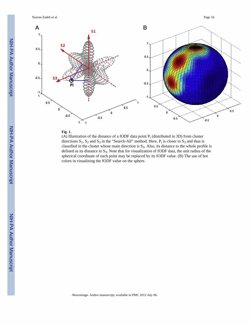
Fig. 1.(A) Illustration of the distance of a fODF data point Pi (distributed in 3D) from clusterdirections S1, S2 and S3 in the “Search-All” method. Here, Pi is closer to S3 and thus isclassified in the cluster whose main direction is S3. Also, its distance to the whole profile isdefined as its distance to S3. Note that for visualization of fODF data, the unit radius of thespherical coordinate of each point may be replaced by its fODF value. (B) The use of hotcolors in visualizing the fODF value on the sphere.

Nazem-Zadeh et al.


NIH


NIH


NIH


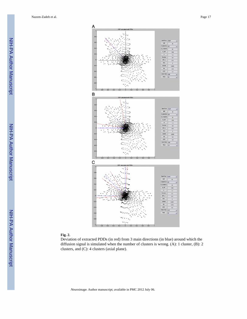
Fig. 2.Deviation of extracted PDDs (in red) from 3 main directions (in blue) around which thediffusion signal is simulated when the number of clusters is wrong. (A): 1 cluster, (B): 2clusters, and (C): 4 clusters (axial plane).

Nazem-Zadeh et al.


NIH


NIH


NIH


Fig. 3.The proposed algorithm for clustering fODF data points.

Nazem-Zadeh et al.


NIH


NIH


NIH


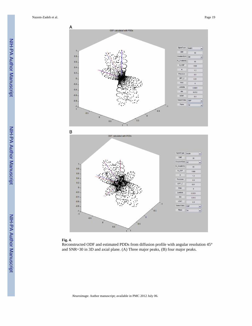
Fig. 4.Reconstructed ODF and estimated PDDs from diffusion profile with angular resolution 45°and SNR=30 in 3D and axial plane. (A) Three major peaks, (B) four major peaks.

Nazem-Zadeh et al.


NIH


NIH


NIH


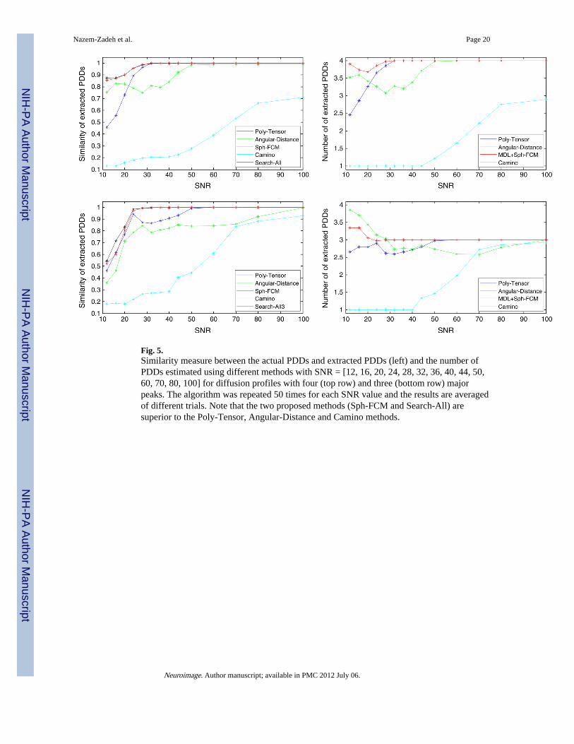
Fig. 5.Similarity measure between the actual PDDs and extracted PDDs (left) and the number ofPDDs estimated using different methods with SNR = [12, 16, 20, 24, 28, 32, 36, 40, 44, 50,60, 70, 80, 100] for diffusion profiles with four (top row) and three (bottom row) majorpeaks. The algorithm was repeated 50 times for each SNR value and the results are averagedof different trials. Note that the two proposed methods (Sph-FCM and Search-All) aresuperior to the Poly-Tensor, Angular-Distance and Camino methods.

Nazem-Zadeh et al.


NIH


NIH


NIH


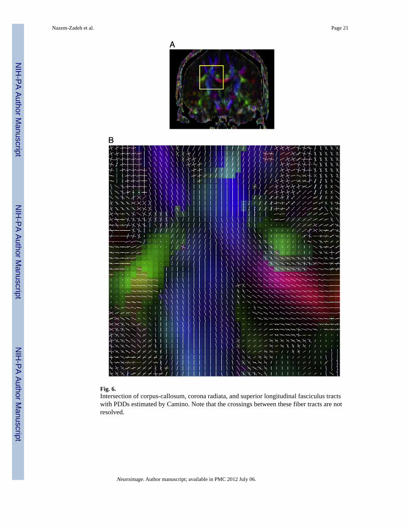
Fig. 6.Intersection of corpus-callosum, corona radiata, and superior longitudinal fasciculus tractswith PDDs estimated by Camino. Note that the crossings between these fiber tracts are notresolved.

Nazem-Zadeh et al.


NIH


NIH


NIH


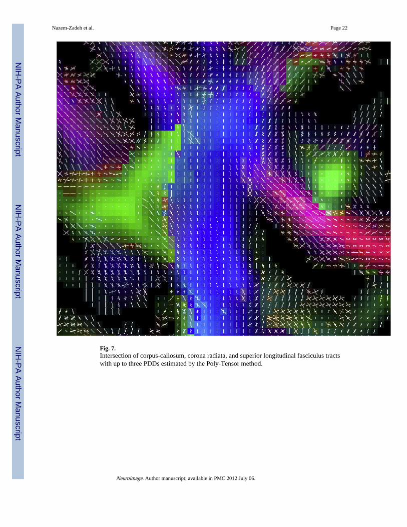
Fig. 7.Intersection of corpus-callosum, corona radiata, and superior longitudinal fasciculus tractswith up to three PDDs estimated by the Poly-Tensor method.

Nazem-Zadeh et al.


NIH


NIH


NIH


Fig. 8.Intersection of corpus-callosum, corona radiata, and superior longitudinal fasciculus tractswith up to three PDDs estimated by the proposed method.

Nazem-Zadeh et al.


NIH


NIH


NIH


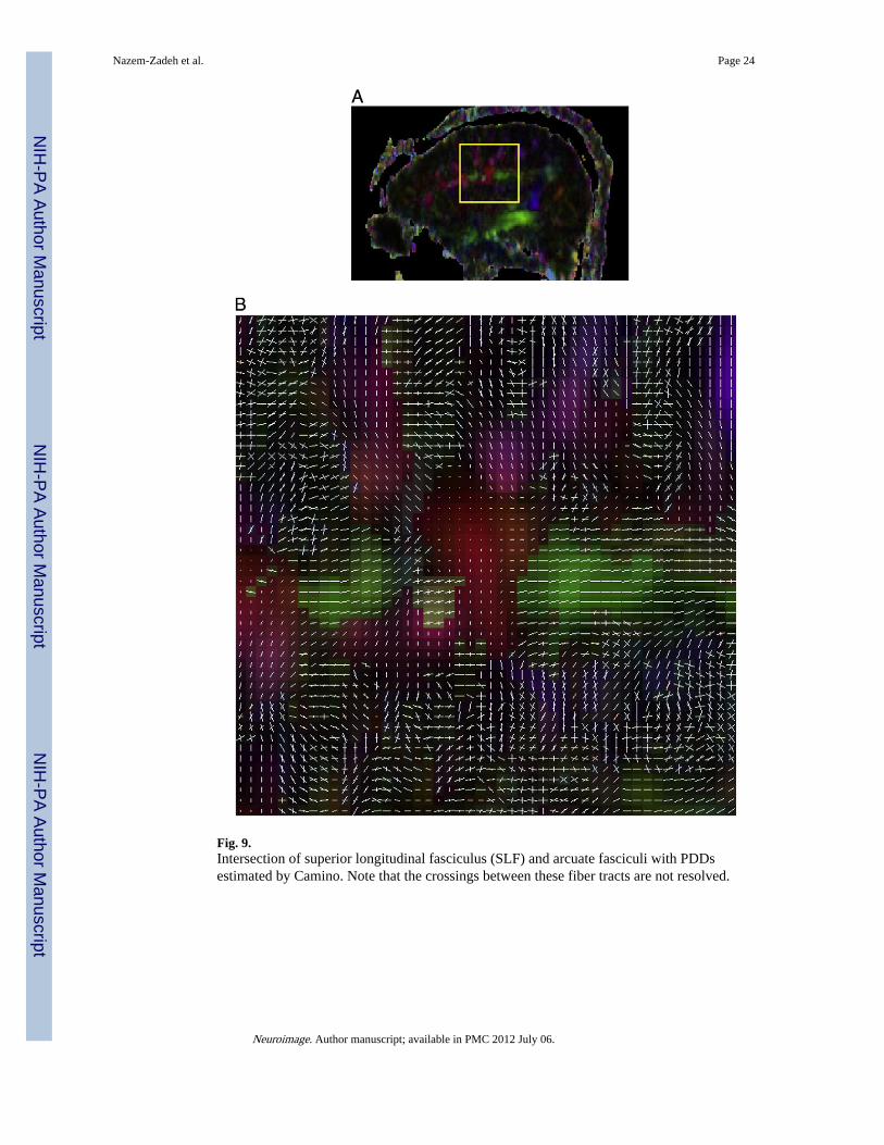
Fig. 9.Intersection of superior longitudinal fasciculus (SLF) and arcuate fasciculi with PDDsestimated by Camino. Note that the crossings between these fiber tracts are not resolved.

Nazem-Zadeh et al.


NIH


NIH


NIH


Fig. 10.Intersection of superior longitudinal fasciculus (SLF) and arcuate fasciculi with up to threePDDs estimated by the proposed method. Although crossing with arcuate fasciculus, onecan zoom on the image and track one of PDDs parallel to the main axis of SLF formoccipital to frontal lobes, which cannot be resolved by tensor-based PDDs findingalgorithms and non-accurate HARDI-based algorithms like Camino. In addition, note thesmooth transition of this main PDD of SLF to the inferior longitudinal fasciculus (ILF)which is rarely detectable in other methods.

Nazem-Zadeh et al.


NIH


NIH


NIH


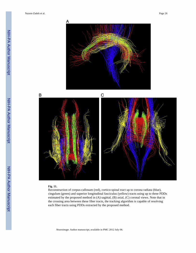
Fig. 11.Reconstruction of corpus-callosum (red), cortico-spinal tract up to corona radiata (blue),cingulum (green) and superior longitudinal fasciculus (yellow) tracts using up to three PDDsestimated by the proposed method in (A) sagittal, (B) axial, (C) coronal views. Note that inthe crossing area between these fiber tracts, the tracking algorithm is capable of resolvingeach fiber tracts using PDDs extracted by the proposed method.

Nazem-Zadeh et al.


NIH


NIH


NIH


Clustering method for estimating principal diffusion directions

Documents

Transcript of Clustering method for estimating principal diffusion directions