
Cluster-Preserving Dimension Reduction Methods for Document Classification
254
Michael W. Berry and Malu Castellanos, Editors Survey of Text Mining: Clustering, Classification, and Retrieval, Second Edition September 30, 2007 Springer
Transcript of Cluster-Preserving Dimension Reduction Methods for Document Classification

Michael W. Berry and Malu Castellanos, Editors
Survey of Text Mining:Clustering, Classification, andRetrieval, Second Edition
September 30, 2007
Springer

Preface
As we enter the third decade of the World Wide Web (WWW), the textual revolutionhas seen a tremendous change in the availability of online information. Finding infor-mation for just about any need has never been more automatic — just a keystroke ormouseclick away. While the digitalization and creation of textual materials continuesat light speed, the ability to navigate, mine, or casually browse through documentstoo numerous to read (or print) lags far behind.
What approaches to text mining are available to efficiently organize, classify,label, and extract relevant information for today’s information-centric users? Whatalgorithms and software should be used to detect emerging trends from both textstreams and archives? These are just a few of the important questions addressed at theText Mining Workshop held on April 28, 2007, in Minneapolis, MN. This workshop,the fifth in a series of annual workshops on text mining, was held on the final day ofthe Seventh SIAM International Conference on Data Mining (April 26–28, 2007).
With close to 60 applied mathematicians and computer scientists representinguniversities, industrial corporations, and government laboratories, the workshop fea-tured both invited and contributed talks on important topics such as the application oftechniques of machine learning in conjunction with natural language processing, in-formation extraction and algebraic/mathematical approaches to computational infor-mation retrieval. The workshop’s program also included an Anomaly Detection/TextMining competition. NASA Ames Research Center of Moffett Field, CA, and SASInstitute Inc. of Cary, NC, sponsored the workshop.
Most of the invited and contributed papers presented at the 2007 Text MiningWorkshop have been compiled and expanded for this volume. Several others arerevised papers from the first edition of the book. Collectively, they span several majortopic areas in text mining:
I. Clustering,II. Document retrieval and representation,
III. Email surveillance and filtering, andIV. Anomaly detection.

vi Preface
In Part I (Clustering), Howland and Park update their work on cluster-preservingdimension reduction methods for efficient text classification. Likewise, Senellart andBlondel revisit thesaurus construction using similarity measures between verticesin graphs. Both of these chapter were part of the first edition of this book (basedon a SIAM text mining workshop held in April 2002). The next three chapters arecompletely new contributions. Zeimpekis and Gallopoulos implement and evaluateseveral clustering schemes that combine partitioning and hierarchical algorithms.Kogan, Nicholas, and Wiacek look at the hybrid clustering of large, high-dimensionaldata. AlSumait and Domeniconi round out this topic area with an examination oflocal semantic kernels for the clustering of text documents.
In Part II (Document Retrieval and Representation), Kobayashi and Aono re-vise their first edition chapter on the importance of detecting and interpreting minordocument clusters using a vector space model based on principal component anal-ysis (PCA) rather than the popular latent semantic indexing (LSI) method. This isfollowed by Xia, Xing, Qi, and Li’s chapter on applications of semidefinite program-ming in XML document classification.
In Part III (Email Surveillance and Filtering), Bader, Berry, and Browne takeadvantage of the Enron email dataset to look at topic detection over time usingPARAFAC and multilinear algebra. Gansterer, Janacek, and Neumayer examine theuse of latent semantic indexing to combat email spam.
In Part IV (Anomaly Detection), researchers from the NASA Ames ResearchCenter share approaches to anomaly detection. These techniques were actually en-tries in a competition. held as part of the workshop. The top three finishers in thecompetition were: Cyril Goutte of NRC Canada, Edward G. Allan, Michael R. Hor-vath, Christopher V. Kopek, Brian T. Lamb, and Thomas S. Whaples of Wake ForestUniversity (Michael W. Berry of the University of Tennessee was their advisor), andan international group from the Middle East led by Mostafa Keikha. Each chapterprovides an explanation of its approach to the contest.
This volume details the state-of-the-art algorithms and software for text min-ing from both the academic and industrial perspectives. Familiarity or coursework(undergraduate-level) in vector calculus and linear algebra is needed for several ofthe chapters. While many open research questions still remain, this collection servesas an important benchmark in the development of both current and future approachesto mining textual information.
Acknowledgments
The editors would like to thank Murray Browne of the University of Tennessee andCatherine Brett of Springer UK in coordinating the management of manuscriptsamong the authors, editors, and the publisher.
Michael W. Berry and Malu CastellanosKnoxville, TN and Palo Alto, CA
August 2007

Contents
Preface . . . . . . . . . . . . . . . . . . . . . . . . . . . . . . . . . . . . . . . . . . . . . . . . . . . . . . . . . . . . v
Contributors . . . . . . . . . . . . . . . . . . . . . . . . . . . . . . . . . . . . . . . . . . . . . . . . . . . . . . . viii
Part I Clustering
1 Cluster-Preserving Dimension Reduction Methods for DocumentClassificationPeg Howland, Haesun Park . . . . . . . . . . . . . . . . . . . . . . . . . . . . . . . . . . . . . . . . . 3
2 Automatic Discovery of Similar WordsPierre Senellart, Vincent D. Blondel . . . . . . . . . . . . . . . . . . . . . . . . . . . . . . . . . . . 25
3 Principal Direction Divisive Partitioning with Kernels and k-MeansSteeringDimitrios Zeimpekis, Efstratios Gallopoulos . . . . . . . . . . . . . . . . . . . . . . . . . . . . 45
4 Hybrid Clustering with DivergencesJacob Kogan, Charles Nicholas, Mike Wiacek . . . . . . . . . . . . . . . . . . . . . . . . . . . 65
5 Text Clustering with Local Semantic KernelsLoulwah AlSumait, Carlotta Domeniconi . . . . . . . . . . . . . . . . . . . . . . . . . . . . . . . 87
Part II Document Retrieval and Representation
6 Vector Space Models for Search and Cluster MiningMei Kobayashi, Masaki Aono . . . . . . . . . . . . . . . . . . . . . . . . . . . . . . . . . . . . . . . . 109
7 Applications of Semidefinite Programming in XML DocumentClassificationZhonghang Xia, Guangming Xing, Houduo Qi, Qi Li . . . . . . . . . . . . . . . . . . . . . 129

viii Contents
Part III Email Surveillance and Filtering
8 Discussion Tracking in Enron Email Using PARAFACBrett W. Bader, Michael W. Berry, Murray Browne . . . . . . . . . . . . . . . . . . . . . . . 147
9 Spam Filtering Based on Latent Semantic IndexingWilfried N. Gansterer, Andreas G.K. Janecek, Robert Neumayer . . . . . . . . . . . . 165
Part IV Anomaly Detection
10 A Probabilistic Model for Fast and Confident Categorization ofTextual DocumentsCyril Goutte . . . . . . . . . . . . . . . . . . . . . . . . . . . . . . . . . . . . . . . . . . . . . . . . . . . . . 187
11 Anomaly Detection Using Nonnegative Matrix FactorizationEdward G. Allan, Michael R. Horvath, Christopher V. Kopek, Brian T. Lamb,Thomas S. Whaples, Michael W. Berry . . . . . . . . . . . . . . . . . . . . . . . . . . . . . . . . . 203
12 Document Representation and Quality of Text: An AnalysisMostafa Keikha, Narjes Sharif Razavian, Farhad Oroumchian,Hassan Seyed Razi . . . . . . . . . . . . . . . . . . . . . . . . . . . . . . . . . . . . . . . . . . . . . . . . 219
Appendix: SIAM Text Mining Competition 2007 . . . . . . . . . . . . . . . . . . . . . . . 233
Index . . . . . . . . . . . . . . . . . . . . . . . . . . . . . . . . . . . . . . . . . . . . . . . . . . . . . . . . . . . . . 237

Contributors
Edward G. AllanDepartment of Computer ScienceWake Forest UniversityP.O. Box 7311Winston-Salem, NC 27109Email: [email protected]
Loulwah AlsumaitDepartment of Computer ScienceGeorge Mason University4400 University Drive MSN 4A4Fairfax, VA 22030Email: [email protected]
Masaki AonoDepartment of Information and Computer Sciences, C-511Toyohashi University of Technology1-1 Hibarigaoka, Tempaku-choToyohashi-shi, Aichi 441-8580JapanEmail: [email protected]
Brett W. BaderSandia National LaboratoriesApplied Computational Methods DepartmentP.O. Box 5800Albuquerque, NM 87185-1318Email: [email protected]: http://www.cs.sandia.gov/˜bwbader
Michael W. BerryDepartment of Electrical Engineering and Computer ScienceUniversity of Tennessee203 Claxton ComplexKnoxville, TN 37996-3450Email: [email protected]: http://www.cs.utk.edu/˜berry

x Contributors
Vincent D. BlondelDivision of Applied MathematicsUniversite de Louvain4, Avenue Georges LemaıtreB-1348 Louvain-la-neuveBelgiumEmail: [email protected]: http://www.inma.ucl.ac.be/˜blondel
Murray BrowneDepartment of Electrical Engineering and Computer ScienceUniversity of Tennessee203 Claxton ComplexKnoxville, TN 37996-3450Email: [email protected]
Malu CastellanosIETL DepartmentHewlett-Packard Laboratories1501 Page Mill Road MS-1148Palo Alto, CA 94304Email: [email protected]
Pat CastleIntelligent Systems DivisionNASA Ames Research CenterMoffett Field, CA 94035Email: [email protected]
Santanu DasIntelligent Systems DivisionNASA Ames Research CenterMoffett Field, CA 94035Email: [email protected]
Carlotta DomeniconiDepartment of Computer ScienceGeorge Mason University4400 University Drive MSN 4A4Fairfax, VA 22030Email: [email protected]: http://www.ise.gmu.edu/˜carlotta

Contributors xi
Efstratios GallopoulosDepartment of Computer Engineering and InformaticsUniversity of Patras26500 PatrasGreeceEmail: [email protected]: http://scgroup.hpclab.ceid.upatras.gr/faculty/stratis/stratise.html
Wilfried N. GanstererResearch Lab for Computational Technologies and ApplicationsUniversity of ViennaLenaugasse 2/8A - 1080 ViennaAustriaEmail: [email protected]
Cyril GoutteInteractive Language TechnologiesNRC Institute for Information Technology283 Boulevard Alexandre TacheGatineau, QC J8X 3X7CanadaEmail: [email protected]: http://iit-iti.nrc-cnrc.gc.ca/personnel/goutte cyril f.html
Michael R. HorvathDepartment of Computer ScienceWake Forest UniversityP.O. Box 7311Winston-Salem, NC 27109Email: [email protected]
Peg HowlandDepartment of Mathematics and StatisticsUtah State University3900 Old Main HillLogan, UT 84322-3900Email: [email protected]: http://www.math.usu.edu/˜howland

xii Contributors
Andreas G. K. JanecekResearch Lab for Computational Technologies and ApplicationsUniversity of ViennaLenaugasse 2/8A - 1080 ViennaAustriaEmail: [email protected]
Mostafa KeikhaDepartment of Electrical and Computer EngineeringUniversity of TehranP.O. Box 14395-515, TehranIranEmail: [email protected]
Mei KobayashiIBM Research, Tokyo Research Laboratory1623-14 Shimotsuruma, Yamato-shiKanagawa-ken 242-8502JapanEmail: [email protected]: http://www.trl.ibm.com/people/meik
Jacob KoganDepartment of Mathematics and StatisticsUniversity of Maryland, Baltimore County1000 Hilltop CircleBaltimore, MD 21250Email: [email protected]: http://www.math.umbc.edu/˜kogan
Christopher V. KopekDepartment of Computer ScienceWake Forest UniversityP.O. Box 7311Winston-Salem, NC 27109Email: [email protected]
Brian T. LambDepartment of Computer ScienceWake Forest UniversityP.O. Box 7311Winston-Salem, NC 27109Email: [email protected]

Contributors xiii
Qi LiDepartment of Computer ScienceWestern Kentucky University1906 College Heights Boulevard #11076Bowling Green, KY 42101-1076Email: [email protected]: http://www.wku.edu/˜qi.li
Robert NeumayerInstitute of Software Technology and Interactive SystemsVienna University of TechnologyFavoritenstraße 9-11/188/2A - 1040 ViennaAustriaEmail: [email protected]
Charles NicholasDepartment of Computer Science and Electrical EngineeringUniversity of Maryland, Baltimore County1000 Hilltop CircleBaltimore, MD 21250Email: [email protected]: http://www.cs.umbc.edu/˜nicholas
Farhad OroumchianCollege of Information TechnologyUniversity of Wollongong in DubaiP.O. Box 20183, DubaiU.A.E.Email: [email protected]
Matthew E. OteyIntelligent Systems DivisionNASA Ames Research CenterMoffett Field, CA 94035Email: [email protected]
Haesun ParkDivision of Computational Science and EngineeringCollege of ComputingGeorgia Institute of Technology266 Ferst DriveAtlanta, GA 30332-0280Email: [email protected]: http://www.cc.gatech.edu/˜hpark

xiv Contributors
Houduo QiDepartment of MathematicsUniversity of Southampton, HighfieldSouthampton SO17 1BJ, UKEmail: [email protected]: http://www.personal.soton.ac.uk/hdqi
Narjes Sharif RazavianDepartment of Electrical and Computer EngineeringUniversity of TehranP.O. Box 14395-515, TehranIranEmail: [email protected]
Hassan Seyed RaziDepartment of Electrical and Computer EngineeringUniversity of TehranP.O. Box 14395-515, TehranIranEmail: [email protected]
Pierre SenellartINRIA Futurs & Universite Paris-Sud4 rue Jacques Monod91893 Orsay CedexFranceEmail: [email protected]: http://pierre.senellart.com/
Ashok N. SrivastavaIntelligent Systems DivisionNASA Ames Research CenterMoffett Field, CA 94035Email: [email protected]
Thomas S. WhaplesDepartment of Computer ScienceWake Forest UniversityP.O. Box 7311Winston-Salem, NC 27109Email: [email protected]
Mike WiacekGoogle, Inc.1600 Amphitheatre ParkwayMountain View, CA 94043Email: [email protected]

Contributors xv
Zhonghang XiaDepartment of Computer ScienceWestern Kentucky University1906 College Heights Boulevard #11076Bowling Green, KY 42101-1076Email: [email protected]: http://www.wku.edu/˜zhonghang.xia
Guangming XingDepartment of Computer ScienceWestern Kentucky University1906 College Heights Boulevard #11076Bowling Green, KY 42101-1076Email: [email protected]: http://www.wku.edu/˜guangming.xing
Dimitrios ZeimpekisDepartment of Computer Engineering and InformaticsUniversity of Patras26500 PatrasGreeceEmail: [email protected]


Part I
Clustering


1
Cluster-Preserving Dimension Reduction Methods forDocument Classification
Peg Howland and Haesun Park
Overview
In today’s vector space information retrieval systems, dimension reduction is im-perative for efficiently manipulating the massive quantity of data. To be useful, thislower dimensional representation must be a good approximation of the original doc-ument set given in its full space. Toward that end, we present mathematical models,based on optimization and a general matrix rank reduction formula, which incor-porate a priori knowledge of the existing structure. From these models, we developnew methods for dimension reduction that can be applied regardless of the rela-tive dimensions of the term-document matrix. We illustrate the effectiveness of eachmethod with document classification results from the reduced representation. Afterestablishing relationships among the solutions obtained by the various methods, weconclude with a discussion of their relative accuracy and complexity.
1.1 Introduction
The vector space information retrieval system, originated by Gerard Salton [Sal71,SM83], represents documents as vectors in a vector space. The document set com-prises anm×n term-document matrix, in which each column represents a document,and the (i, j)th entry represents a weighted frequency of term i in document j. Sincethe data dimensionmmay be huge, a lower dimensional representation is imperativefor efficient manipulation.
Dimension reduction is commonly based on rank reduction by the truncated sin-gular value decomposition (SVD). For any matrix A ∈ Rm×n, its SVD can be de-fined as
A = UΣV T , (1.1)
where U ∈ Rm×m and V ∈ Rn×n are orthogonal, Σ = diag(σ1 · · ·σp) ∈ Rm×nwith p = min(m,n), and the singular values are ordered as σ1 ≥ σ2 ≥ · · ·σp ≥ 0[GV96, Bjo96]. Denoting the columns of U , or left singular vectors, by ui, and thecolumns of V , or right singular vectors, by vi, and the rank of A by q, we write

4 P. Howland, H. Park
A =q∑i=1
σiuivTi . (1.2)
For l < q, the truncated SVD
A ≈l∑i=1
σiuivTi
provides the rank-l approximation that is closest to the data matrix in L2 norm orFrobenius norm[GV96]. This is the main tool in principal component analysis (PCA)[DHS01], as well as in latent semantic indexing (LSI) [DDF+90, BDO95] of docu-ments.
If the data form clusters in the full dimension, the goal may change from find-ing the best lower dimensional representation to finding the lower dimensional rep-resentation that best preserves this cluster structure. That is, even after dimensionreduction, a new document vector should be classified with the appropriate cluster.Assuming that the columns of A are grouped into clusters, rather than treating eachcolumn equally regardless of its membership in a specific cluster, as is done withthe SVD, the dimension reduction methods we will discuss attempt to preserve thisinformation. This is important in information retrieval, since the reduced representa-tion itself will be used extensively in further processing of data.
In applied statistics/psychometrics [Har67, Hor65], techniques have been devel-oped to factor an attribute-entity matrix in an analogous way. As argued in [HMH00],the components of the factorization are important, and “not just as a mechanism forsolving another problem.” This is one reason why they are well suited for the prob-lem of finding a lower dimensional representation of text data. Another reason istheir simplicity—having been developed at a time when additions and subtractionswere significantly cheaper computations than multiplications and divisions—theircreators used sign and binary vectors extensively. With the advent of modern com-puters, such methods have become overshadowed by more accurate and costly al-gorithms in factor analysis [Fuk90]. Ironically, modern applications often have tohandle very high-dimensional data, so the accuracy of the factors can sometimes becompromised in favor of algorithmic simplicity.
In this chapter, we present dimension reduction methods derived from two per-spectives. The first, a general matrix rank reduction formula, is introduced in Sec-tion 1.2. The second, linear discriminant analysis (LDA), is formulated as trace op-timization, and extended in Section 1.3 using the generalized singular value decom-position (GSVD). To reduce the cost of the LDA/GSVD algorithm, we incorporateit as the second stage after PCA or LSI. We establish mathematical equivalence inSection 1.4 by expressing both PCA and LSI in terms of trace optimization. Finally,Section 1.5 combines the two perspectives by making a factor analysis approxima-tion in the first stage.

1 Cluster-Preserving Dimension Reduction Methods 5
1.2 Dimension Reduction in the Vector Space Model (VSM)
Given a term-document matrix
A = [a1 a2 · · · an] ∈ Rm×n,
we want to find a transformation that maps each document vector aj in the m-dimensional space to a vector yj in the l-dimensional space for some l� m:
aj ∈ Rm×1 → yj ∈ Rl×1, 1 ≤ i ≤ n.
The approach we discuss in Section 1.3 computes the transformation directly fromA.Rather than looking for the mapping that achieves this explicitly, another approachrephrases dimension reduction as an approximation problem where the given matrixA is decomposed into two matrices B and Y as
A ≈ BY (1.3)
where bothB ∈ Rm×l with rank(B) = l and Y ∈ Rl×n with rank(Y ) = l are to befound. This lower rank approximation is not unique since for any nonsingular matrixZ ∈ Rl×l,
A ≈ BY = (BZ)(Z−1Y ),
where rank(BZ) = l and rank(Z−1Y ) = l.The mathematical framework for obtaining such matrix factorizations is the Wed-
derburn rank reduction formula [Wed34]: If x ∈ Rn and y ∈ Rm are such thatω = yTAx 6= 0, then
E = A− ω−1(Ax)(yTA) (1.4)
has rank(E) = rank(A)− 1. This formula has been studied extensively in both thenumerical linear algebra (NLA) [CF79, CFG95] and applied statistics/psychometrics(AS/P) [Gut57, HMH00] communities. In a 1995 SIAM Review paper [CFG95], Chu,Funderlic, and Golub show that for x = v1 and y = u1 from the SVD in Eq. (1.2),
E = A− (uT1 Av1)−1(Av1)(uT1 A) = A− σ1u1v
T1 .
If repeated q = rank(A) times using the leading q singular vectors, this formulagenerates the SVD of A.
In general, starting with A1 = A, and choosing xk and yk such that ωk =yTk Akxk 6= 0, the Wedderburn formula generates the sequence
Ak+1 = Ak − ω−1k (Akxk)(yTk Ak).
Adding up all the rank one updates, factoring into matrix outer product form, andtruncating gives an approximation A ≈ BY . The question becomes: what are goodchoices for xk and yk?
One answer was provided by Thurstone [Thu35] in the 1930s, when he appliedthe centroid method to psychometric data. To obtain an approximation of A as BY ,

6 P. Howland, H. Park
the method uses the rank one reduction formula to solve for one column of B andone row of Y at a time. It approximates the SVD while restricting the pre- and post-factors in the rank reduction formula to sign vectors. In Section 1.5, we incorporatethis SVD approximation into a two-stage process so that knowledge of the clustersfrom the full dimension is reflected in the dimension reduction.
1.3 Linear Discriminant Analysis and Its Extension for Text Data
The goal of linear discriminant analysis (LDA) is to combine features of the orig-inal data in a way that most effectively discriminates between classes. With an ap-propriate extension, it can be applied to the goal of reducing the dimension of aterm-document matrix in a way that most effectively preserves its cluster structure.That is, we want to find a linear transformation G whose transpose maps each doc-ument vector a in the m-dimensional space to a vector y in the l-dimensional space(l� m):
GT : a ∈ Rm×1 → y ∈ Rl×1.
Assuming that the given data are already clustered, we seek a transformation thatoptimally preserves this cluster structure in the reduced dimensional space.
For simplicity of discussion, we will assume that data vectors a1, . . . , an formcolumns of a matrix A ∈ Rm×n, and are grouped into k clusters as
A = [A1, A2, · · · , Ak], Ai ∈ Rm×ni ,
k∑i=1
ni = n. (1.5)
Let Ni denote the set of column indices that belong to cluster i. The centroid c(i) iscomputed by taking the average of the columns in cluster i; i.e.,
c(i) =1ni
∑j∈Ni
aj
and the global centroid c is defined as
c =1n
n∑j=1
aj .
Then the within-cluster, between-cluster, and mixture scatter matrices are defined[Fuk90, TK99] as

1 Cluster-Preserving Dimension Reduction Methods 7
Sw =k∑i=1
∑j∈Ni
(aj − c(i))(aj − c(i))T ,
Sb =k∑i=1
∑j∈Ni
(c(i) − c)(c(i) − c)T
=k∑i=1
ni(c(i) − c)(c(i) − c)T , and
Sm =n∑j=1
(aj − c)(aj − c)T ,
respectively. The scatter matrices have the relationship [JD88]
Sm = Sw + Sb. (1.6)
Applying GT to the matrix A transforms the scatter matrices Sw, Sb, and Sm to thel × l matrices
GTSwG, GTSbG, and GTSmG,
respectively.There are several measures of cluster quality that involve the three scatter matri-
ces [Fuk90, TK99]. When cluster quality is high, each cluster is tightly grouped, butwell separated from the other clusters. Since
trace(Sw) =k∑i=1
∑j∈Ni
(aj − c(i))T (aj − c(i))
=k∑i=1
∑j∈Ni
‖aj − c(i)‖22
measures the closeness of the columns within the clusters, and
trace(Sb) =k∑i=1
∑j∈Ni
(c(i) − c)T (c(i) − c)
=k∑i=1
∑j∈Ni
‖c(i) − c‖22
measures the separation between clusters, an optimal transformation that preservesthe given cluster structure would be
maxG
trace(GTSbG) and minG
trace(GTSwG). (1.7)
Assuming the matrix Sw is nonsingular, classical LDA approximates this simul-taneous trace optimization by finding a transformation G that maximizes

8 P. Howland, H. Park
J1(G) = trace((GTSwG)−1GTSbG). (1.8)
It is well-known that the J1 criterion in Eq. (1.8) is maximized when the columns ofG are the l eigenvectors of S−1
w Sb corresponding to the l largest eigenvalues [Fuk90].In other words, LDA solves
S−1w Sbxi = λixi (1.9)
for the xi’s corresponding to the largest λi’s. For these l eigenvectors, the maximumachieved is J1(G) = λ1 + · · ·+ λl. Since rank(Sb) of the eigenvalues of S−1
w Sb aregreater than zero, if l ≥ rank(Sb), this optimal G preserves trace(S−1
w Sb) exactlyupon dimension reduction.
For the case when Sw is singular, [HJP03] assumes the cluster structure given inEq. (1.5), and defines the m× n matrices
Hw = [A1 − c(1)e(1)T
, A2 − c(2)e(2)T
, . . . , Ak − c(k)e(k)T
] (1.10)
Hb = [(c(1) − c)e(1)T
, (c(2) − c)e(2)T
, . . . , (c(k) − c)e(k)T
]
Hm = [a1 − c, . . . , an − c] = A− ceT , (1.11)
where e(i) = (1, . . . , 1)T ∈ Rni×1 and e = (1, · · · , 1)T ∈ Rn×1. Then the scattermatrices can be expressed as
Sw = HwHTw , Sb = HbH
Tb , and Sm = HmH
Tm. (1.12)
Another way to define Hb that satisfies Eq. (1.12) is
Hb = [√n1(c(1) − c),
√n2(c(2) − c), . . . ,
√nk(c(k) − c)] (1.13)
and using this m×k form reduces the storage requirements and computational com-plexity of the LDA/GSVD algorithm.
As the product of an m × n matrix and an n ×m matrix, Sw is singular whenm > n [Ort87]. This means that J1 cannot be applied when the number of availabledata points is smaller than the dimension of the data. In other words, classical LDAfails when the number of terms in the document collection is larger than the totalnumber of documents (i.e., m > n in the term-document matrix A). To circumventthis restriction, we express λi as α2
i /β2i , and the eigenvalue problem in Eq. (1.9)
becomesβ2iHbH
Tb xi = α2
iHwHTwxi. (1.14)
This has the form of a problem that can be solved using the GSVD of the matrix pair(HT
b ,HTw ), as described in Section 1.3.1.
1.3.1 Generalized Singular Value Decomposition
After the GSVD was originally defined by Van Loan [Loa76], Paige and Saunders[PS81] defined the GSVD for any two matrices with the same number of columns,which we restate as follows.

1 Cluster-Preserving Dimension Reduction Methods 9
Theorem 1.3.1 Suppose two matrices HTb ∈ Rk×m and HT
w ∈ Rn×m are given.Then for
K =(HTb
HTw
)and t = rank(K),
there exist orthogonal matrices U ∈ Rk×k, V ∈ Rn×n,W ∈ Rt×t, andQ ∈ Rm×msuch that
UTHTb Q = Σb(WTR︸ ︷︷ ︸
t
, 0︸︷︷︸m−t
)
andV THT
wQ = Σw(WTR︸ ︷︷ ︸t
, 0︸︷︷︸m−t
),
where
Σbk×t
=
IbDb
Ob
, Σwn×t
=
OwDw
Iw
,
and R ∈ Rt×t is nonsingular with its singular values equal to the nonzero singularvalues of K. The matrices
Ib ∈ Rr×r and Iw ∈ R(t−r−s)×(t−r−s)
are identity matrices, where
r = t− rank(HTw ) and s = rank(HT
b ) + rank(HTw )− t,
Ob ∈ R(k−r−s)×(t−r−s) and Ow ∈ R(n−t+r)×r
are zero matrices with possibly no rows or no columns, and
Db = diag(αr+1, . . . , αr+s)
andDw = diag(βr+1, . . . , βr+s)
satisfy
1 > αr+1 ≥ · · · ≥ αr+s > 0, 0 < βr+1 ≤ · · · ≤ βr+s < 1, (1.15)
and α2i + β2
i = 1 for i = r + 1, . . . , r + s.
This form of GSVD is related to that of Van Loan [Loa76] as
UTHTb X = (Σb, 0) and V THT
wX = (Σw, 0), (1.16)
where
Xm×m
= Q
(R−1W 00 Im−t
).
This implies that

10 P. Howland, H. Park
XTHbHTb X =
(ΣTb Σb 0
0 0
)and
XTHwHTwX =
(ΣTwΣw 0
0 0
).
Letting xi represent the ith column of X , and defining
αi = 1, βi = 0 for i = 1, . . . , r
andαi = 0, βi = 1 for i = r + s+ 1, . . . , t,
we see that Eq. (1.14) is satisfied for 1 ≤ i ≤ t. Since
HbHTb xi = 0 and HwH
Twxi = 0
for the remainingm−t columns ofX , Eq. (1.14) is satisfied for arbitrary values of αiand βi when t+ 1 ≤ i ≤ m. The columns of X are the generalized singular vectorsfor the matrix pair (HT
b ,HTw ). They correspond to the generalized singular values,
or the αi/βi quotients, as follows. The first r columns correspond to infinite values,and the next s columns correspond to finite and nonzero values. The following t −r − s columns correspond to zero values, and the last m− t columns correspond tothe arbitrary values. This correspondence between generalized singular vectors andvalues is illustrated in Figure 1.1(a).
(a) Applied to A (b) After PCA→ rank(Hm)
Fig. 1.1. Generalized singular vectors and their corresponding generalized singular values.

1 Cluster-Preserving Dimension Reduction Methods 11
1.3.2 Application of the GSVD to Dimension Reduction
A question that remains is which columns of X to include in the solution G. If Swis nonsingular, both r = 0 and m − t = 0, so s = rank(HT
b ) generalized singularvalues are finite and nonzero, and the rest are zero. The generalized singular vectorsare eigenvectors of S−1
w Sb, so we choose the xi’s that correspond to the largest λi’s,where λi = α2
i /β2i . When the GSVD construction orders the singular value pairs
as in Eq. (1.15), the generalized singular values, or the αi/βi quotients, are in non-increasing order. Therefore, the first s columns of X are all we need.
When m > n, the scatter matrix Sw is singular. Hence, the eigenvectors ofS−1w Sb are undefined, and classical discriminant analysis fails. [HJP03] argues in
terms of the simultaneous optimization Eq. (1.7) that criterion J1 is approximating.Letting gj represent a column of G, we write
trace(GTSbG) =∑
gTj Sbgj
andtrace(GTSwG) =
∑gTj Swgj .
If xi is one of the leftmost r vectors, then xi ∈ null(Sw) − null(Sb). BecausexTi Sbxi > 0 and xTi Swxi = 0, including this vector in G increases the trace wewant to maximize while leaving the trace we want to minimize unchanged. On theother hand, for the rightmost m − t vectors, xi ∈ null(Sw) ∩ null(Sb). Adding thecolumn xi to G has no effect on these traces, since xTi Swxi = 0 and xTi Sbxi = 0,and therefore does not contribute to either maximization or minimization in Eq. (1.7).We conclude that, whether Sw is singular or nonsingular, G should be comprised ofthe leftmost r + s = rank(HT
b ) columns of X , which are shaded in Figure 1.1(a).As a practical matter, the LDA/GSVD algorithm includes the first k− 1 columns
ofX inG. This is due to the fact that rank(Hb) ≤ k−1, which is clear from the def-inition ofHb given in Eq. (1.13). If rank(Hb) < k−1, including extra columns inG(some of which correspond to the t−r−s zero generalized singular values and, possi-bly, some of which correspond to the arbitrary generalized singular values) will haveapproximately no effect on cluster preservation. As summarized in Algorithm 1.3.1,we first compute the matrices Hb and Hw from the data matrix A. We then solve fora very limited portion of the GSVD of the matrix pair (HT
b ,HTw ). This solution is ac-
complished by following the construction in the proof of Theorem 1.3.1 [PS81]. Themajor steps are limited to the complete orthogonal decomposition [GV96, LH95] of
K =(HTb
HTw
),
which produces orthogonal matrices P and Q and a nonsingular matrix R, followedby the singular value decomposition of a leading principal submatrix of P , whosesize is much smaller than that of the data matrix. (This k × t submatrix is specifiedin Algorithm 1.3.1 using the colon notation of MATLAB1.) Finally, we assign theleftmost k − 1 generalized singular vectors to G.1 http://www.mathworks.com

12 P. Howland, H. Park
Algorithm 1.3.1 LDA/GSVDGiven a data matrix A ∈ Rm×n with k clusters and an input vector a ∈ Rm×1, compute thematrix G ∈ Rm×(k−1) that preserves the cluster structure in the reduced dimensional space,using
J1(G) = trace((GT SwG)−1GT SbG).
Also compute the k − 1 dimensional representation y of a.
1. Compute Hb and Hw from A according to
Hb = (√
n1(c(1) − c),
√n2(c
(2) − c), . . . ,√
nk(c(k) − c))
and Eq. (1.10), respectively. (Using this equivalent but m × k form of Hb reduces com-plexity.)
2. Compute the complete orthogonal decomposition
P T KQ =
„R 00 0
«, where K =
„HT
b
HTw
«∈ R(k+n)×m
3. Let t = rank(K).4. Compute W from the SVD of P (1 : k, 1 : t), which is
UT P (1 : k, 1 : t)W = ΣA.
5. Compute the first k − 1 columns of X = Q
„R−1W 00 I
«, and assign them to G.
6. y = GT a
1.4 Equivalent Two-Stage Methods
Another way to apply LDA to the data matrixA ∈ Rm×n withm > n (and hence Swsingular) is to perform dimension reduction in two stages. The LDA stage is precededby a stage in which the cluster structure is ignored. A common approach [Tor01,SW96, BHK97] for the first part of this process is rank reduction by the truncatedsingular value decomposition (SVD). A drawback of these two-stage approachesis that experimentation has been needed to determine which intermediate reduceddimension produces optimal results after the second stage.
Moreover, since either PCA or LSI ignores the cluster structure in the first stage,theoretical justification for such two-stage approaches is needed. Yang and Yang[YY03] supply theoretical justification for PCA plus LDA, for a single discriminantvector. In this section, we justify the two-stage approach that uses either LSI or PCA,followed by LDA. We do this by establishing the equivalence of the single-stageLDA/GSVD to the two-stage method, provided that the intermediate dimension af-ter the first stage falls within a specific range. In this range Sw remains singular, andhence LDA/GSVD is required for the second stage. We also present a computation-ally simpler choice for the first stage, which uses QR decomposition (QRD) ratherthan the SVD.

1 Cluster-Preserving Dimension Reduction Methods 13
1.4.1 Rank Reduction Based on the Truncated SVD
PCA and LSI differ only in that PCA centers the data by subtracting the global cen-troid from each column of A. In this section, we express both methods in terms ofthe maximization of J2(G) = trace(GTSmG).
If we let G ∈ Rm×l be any matrix with full column rank, then essentially J2(G)has no upper bound and maximization is meaningless. Now, let us restrict the solu-tion to the case whenG has orthonormal columns. Then there existsG′ ∈ Rm×(m−l)
such that(G, G′
)is an orthogonal matrix. In addition, since Sm is positive semidef-
inite, we have
trace(GTSmG) ≤ trace(GTSmG) + trace((G′)TSmG′)= trace(Sm).
Reserving the notation in Eq. (1.1) for the SVD of A, let the SVD of Hm begiven by
Hm = A− ceT = UΣV T . (1.17)
ThenSm = HmH
Tm = UΣΣT UT .
Hence the columns of U form an orthonormal set of eigenvectors of Sm corre-sponding to the non-increasing eigenvalues on the diagonal of Λ = ΣΣT =diag(σ2
1 , . . . , σ2n, 0, . . . , 0). For p = rank(Hm), if we denote the first p columns
of U by Up, and let Λp = diag(σ21 , . . . , σ
2p), we have
J2(Up) = trace(UTp SmUp)
= trace(UTp UpΛp)
= σ21 + · · ·+ σ2
p
= trace(Sm). (1.18)
This means that we preserve trace(Sm) if we take Up as G. Clearly, the same is truefor Ul with l ≥ p, so PCA to a dimension of at least rank(Hm) preserves trace(Sm).
Now we show that LSI also preserves trace(Sm). Suppose x is an eigenvector ofSm corresponding to the eigenvalue λ 6= 0. Then
Smx =n∑j=1
(aj − c)(aj − c)Tx = λx.
This means x ∈ span{aj − c|1 ≤ j ≤ n}, and hence x ∈ span{aj |1 ≤ j ≤ n}.Accordingly,
range(Up) ⊆ range(A).
From Eq. (1.1), we write
A = UqΣqVTq for q = rank(A), (1.19)

14 P. Howland, H. Park
where Uq and Vq denote the first q columns of U and V , respectively, and Σq =Σ(1 : q, 1 : q). Then range(A) = range(Uq), which implies that
range(Up) ⊆ range(Uq).
HenceUp = UqW
for some matrix W ∈ Rq×p with orthonormal columns. This yields
J2(Up) = J2(UqW )= trace(WTUTq SmUqW )
≤ trace(UTq SmUq)= J2(Uq).
Since J2(Up) = trace(Sm) from Eq. (1.18), we preserve trace(Sm) if we take Uqas G. The same argument holds for Ul with l ≥ q, so LSI to any dimension greaterthan or equal to rank(A) also preserves trace(Sm).
Finally, in the range of reduced dimensions for which PCA and LSI preservetrace(Sm), they preserve trace(Sw) and trace(Sb) as well. This follows from thescatter matrix relationship in Eq. (1.6) and the inequalities
trace(GTSwG) ≤ trace(Sw)trace(GTSbG) ≤ trace(Sb),
which are satisfied for anyGwith orthonormal columns, since Sw and Sb are positivesemidefinite. In summary, the individual traces of Sm, Sw, and Sb are preserved byusing PCA to reduce to a dimension of at least rank(Hm), or by using LSI to reduceto a dimension of at least rank(A).
1.4.2 LSI Plus LDA
In this section, we establish the equivalence of the LDA/GSVD method to a two-stage approach composed of LSI followed by LDA, and denoted by LSI + LDA.Using the notation of Eq. (1.19), the q-dimensional representation of A after the LSIstage is
B = UTq A,
and the second stage applies LDA to B. Letting the superscript B denote matricesafter the LSI stage, we have
HBb = UTq Hb and HB
w = UTq Hw.
HenceSBb = UTq HbH
Tb Uq and SBw = UTq HwH
TwUq.
Suppose

1 Cluster-Preserving Dimension Reduction Methods 15
SBb x = λSBwx;
i.e., x and λ are an eigenvector-eigenvalue pair of the generalized eigenvalue problemthat LDA solves in the second stage. Then, for λ = α2/β2,
β2UTq HbHTb Uqx = α2UTq HwH
TwUqx.
Suppose the matrix(Uq, U
′q
)is orthogonal. Then (U ′q)
TA = (U ′q)TUqΣqV
Tq =
0, and accordingly, (U ′q)THb = 0 and (U ′q)
THw = 0, since the columns of both Hb
and Hw are linear combinations of the columns of A. Hence
β2
(UTq
(U ′q)T
)HbH
Tb Uqx =
(β2UTq HbH
Tb Uqx
0
)=(α2UTq HwH
TwUqx
0
)= α2
(UTq
(U ′q)T
)HwH
TwUqx,
which impliesβ2HbH
Tb (Uqx) = α2HwH
Tw (Uqx).
That is, Uqx and α/β are a generalized singular vector and value of the gen-eralized singular value problem that LDA solves when applied to A. To showthat these Uqx vectors include all the LDA solution vectors for A, we show thatrank(SBm) = rank(Sm). From the definition in Eq. (1.11), we have
Hm = A− ceT = A(I − 1neeT ) = UqΣqV
Tq (I − 1
neeT )
andHBm = UTq Hm,
and henceHm = UqH
Bm.
Since Hm and HBm have the same null space, their ranks are the same. This means
that the number of non-arbitrary generalized singular value pairs is the same forLDA/GSVD applied to B, which produces t = rank(SBm) pairs, and LDA/GSVDapplied to A, which produces t = rank(Sm) pairs.
We have shown the following.
Theorem 1.4.1 If G is an optimal LDA transformation for B, the q-dimensionalrepresentation of the matrix A via LSI, then UqG is an optimal LDA transformationfor A.
In other words, LDA applied to A produces
Y = (UqG)TA = GTUTq A = GTB,
which is the same result as applying LSI to reduce the dimension to q, followed byLDA. Finally, we note that if the dimension after the LSI stage is at least rank(A),that is B = UTl A for l ≥ q, the equivalency argument remains unchanged.

16 P. Howland, H. Park
1.4.3 PCA Plus LDA
As in the previous section for LSI, it can be shown that a two-stage approach inwhich PCA is followed by LDA is equivalent to LDA applied directly to A. FromEq. (1.17), we write
Hm = UpΣpVTp for p = rank(Hm), (1.20)
where Up and Vp denote the first p columns of U and V , respectively, and Σp =Σ(1 : p, 1 : p). Then the p-dimensional representation of A after the PCA stage is
B = UTp A,
and the second stage applies LDA/GSVD to B. Letting the superscript B denotematrices after the PCA stage, we have
SBm = UTp SmUp = Σ2p , (1.21)
which implies LDA/GSVD applied to B produces rank(SBm) = p non-arbitrarygeneralized singular value pairs. That is the same number of non-arbitrary pairs asLDA/GSVD applied to A.
We have the following, which is proven in [HP04].
Theorem 1.4.2 If G is an optimal LDA transformation for B, the p-dimensionalrepresentation of the matrixA via PCA, then UpG is an optimal LDA transformationfor A.
In other words, LDA applied to A produces
Y = (UpG)TA = GT UTp A = GTB,
which is the same result as applying PCA to reduce the dimension to p, followed byLDA. Note that if the dimension after the PCA stage is at least rank(Hm), that isB = UTl A for l ≥ p, the equivalency argument remains unchanged.
An additional consequence of Eq. (1.21) is that
null(SBm) = {0}.
Due to the relationship in Eq. (1.6) and the fact that Sw and Sb are positive semidef-inite,
null(SBm) = null(SBw ) ∩ null(SBb ).
Thus the PCA stage eliminates only the joint null space, as illustrated in Fig-ure 1.1(b), which is why we don’t lose any discriminatory information before ap-plying LDA.

1 Cluster-Preserving Dimension Reduction Methods 17
1.4.4 QRD Plus LDA
To simplify the computation in the first stage, we use the reduced QR decomposition[GV96]
A = QR,
where Q ∈ Rm×n and R ∈ Rn×n, and let Q play the role that Uq or Up played be-fore. Then the n-dimensional representation ofA after the QR decomposition (QRD)stage is
B = QTA,
and the second stage applies LDA to B. An argument similar to that for LSI [HP04]yields Theorem 1.4.3.
Theorem 1.4.3 IfG is an optimal LDA transformation forB, the n-dimensional rep-resentation of the matrix A after QRD, then QG is an optimal LDA transformationfor A.
In other words, LDA applied to A produces
Y = (QG)TA = GTQTA = GTB,
which is the same result as applying QRD to reduce the dimension to n, followed byLDA.
1.5 Factor Analysis Approximations
In this section, we investigate the use of the centroid method as the first step of atwo-step process. By using a low-cost SVD approximation, we can avoid truncationand reduce no further than the theoretically optimal intermediate reduced dimension.That is, the centroid approximation may be both inexpensive and accurate enough tooutperform an expensive SVD approximation that loses discriminatory informationby truncation.
Thurstone [Thu35] gives a complete description of the centroid method, in whichhe applies the Wedderburn rank reduction process in Eq. (1.4) to the correlation ma-trixR = AAT . To approximate the SVD, a sign vector (for which each component is1 or −1) x is chosen so that triple product xTRx is maximized. This is analogous tofinding a general unit vector in which the triple product is maximized. At the kth step,a single factor loading vector is solved for at a time, starting with xk = (1 · · · 1)T .The algorithm changes the sign of the element in xk that increases xTkRkxk the most,and repeats until any sign change would decrease xTkRkxk.
The rank-one reduction formula is
Rk+1 = Rk −(Rkxk√lk
)(Rkxk√lk
)Twhere lk = xTkRkxk is the triple product. If rank(R) = r, then a recursion yields

18 P. Howland, H. Park
R = [R1v1 · · ·Rrvr]
1l1
. . .1lr
vT1 R1
...vTr Rr
=[R1v1√l1· · · Rrvr√
lr
]vT1 R1√l1...
vTr Rr√lr
.
In factor analysis, Rkxk√lk
is called the kth factor loading vector.In [Hor65], the centroid method is described for the data matrix itself. That is, to
approximate the SVD of A, sign vectors y and x are chosen so that the bilinear formyTAx is maximized. At the kth step, the method starts with xk = yk = (1 · · · 1)T .It alternates between changing the sign of the element in yk that increases yTk Akxkmost, and changing the sign of element in xk that increases it most. After repeatinguntil any sign change would decrease yTk Akxk, this process yields
A =∑
(Akxk)(yTk Akxk)−1(yTk Ak),
where (yTk Akxk)−1 is split so that yTk Ak is normalized.
Chu and Funderlic [CF02] give an algorithm for factoring the correlation matrixAAT without explicitly forming a cross product. That is, they approximate SVD ofAAT by maximizing xTAATx over sign vectors x. Their algorithm uses pre-factorxk and post-factor ATk xk as follows:
Ak+1 = Ak − (Ak(ATk xk))(xTkAk(A
Tk xk))
−1(xTkAk).
This yields
A =∑
(AkATk xk‖ATk xk‖
)(xTkAk‖ATk xk‖
)
They also claim that if truncated, the approximation loses statistical meaning unlessthe rows of A are centered at 0. Finally, they show that the cost of computing lterms of the centroid decomposition involves O(lm2n) complexity for an m × ndata matrix A.
Our goal is to determine how effectively the centroid method approximates theSVD when used as a first stage before applying LDA/GSVD. Toward that end, wehave initially implemented the centroid method as applied to the data matrix. Tofurther reduce the computational complexity of the first stage approximation, wewill also implement the implicit algorithm of Chu and Funderlic.
1.6 Document Classification Experiments
The first set of experiments were performed on five categories of abstracts fromthe MEDLINE2 database. Each category has 500 documents. The dataset was di-2 http://www.ncbi.nlm.nih.gov/PubMed

1 Cluster-Preserving Dimension Reduction Methods 19
Table 1.1. MEDLINE training data set
Class Category No. of documents1 heart attack 2502 colon cancer 2503 diabetes 2504 oral cancer 2505 tooth decay 250
dimension 22095× 1250
Table 1.2. Classification accuracy (%) on MEDLINE test data
Dimension reduction methodsClassification Full LSI→ 1246 LSI→ 5 LDA/GSVDmethods 22095×1250 1246×1250 5×1250 4×1250Centroid (L2) 85.2 85.2 71.6 88.7Centroid (cosine) 88.3 88.3 78.5 83.95NN (L2) 79.0 79.0 77.8 81.515NN (L2) 83.4 83.4 77.5 88.730NN (L2) 83.8 83.8 77.5 88.75NN (cosine) 77.8 77.8 77.8 83.815NN (cosine) 82.5 82.5 80.2 83.830NN (cosine) 83.8 83.8 79.8 83.8
vided into 1250 training documents and 1250 test documents (see Table 1.1). Afterstemming and removal of stop words [Kow97], the training set contains 22,095 dis-tinct terms. Since the dimension (22,095) exceeds the number of training documents(1250), Sw is singular and classical discriminant analysis breaks down. However,LDA/GSVD circumvents this singularity problem.
Table 1.2 reports classification accuracy for the test documents in the full space aswell as those in the reduced spaces obtained by LSI and LDA/GSVD methods. Herewe use a centroid-based classification method [PJR03], which assigns a documentto the cluster to whose centroid it is closest, and K nearest neighbor classification[TK99] for three different values ofK. Closeness is determined by both the L2 normand cosine similarity measures.
Since the training set has the nearly full rank of 1246, we use LSI to reduce tothat. As expected, we observe that the classification accuracies match those fromthe full space. To illustrate the effectiveness of the GSVD extension, whose opti-mal reduced dimension is four, LSI reduction to dimension five is included here.With the exception of centroid-based classification using the cosine similarity mea-sure, LDA/GSVD results also compare favorably to those in the original full space,while achieving a significant reduction in time and space complexity. For details, see[KHP05].
To confirm our theoretical results regarding equivalent two-stage methods, weuse a MEDLINE dataset of five categories of abstracts with 40 documents in each.

20 P. Howland, H. Park
Table 1.3. Traces and classification accuracy (%) on 200 MEDLINE documents
Traces & Dimension reduction methodsclassification Full LSI PCA QRDmethods 7519× 200 198× 200 197× 200 200× 200
Trace(Sw) 73048 73048 73048 73048Trace(Sb) 6229 6229 6229 6229Centroid (L2) 95% 95% 95% 95%1NN (L2) 60% 60% 60% 59%3NN (L2) 49% 48% 49% 48%
Table 1.4. Traces and classification accuracy (%) on 200 MEDLINE documents
Two-stage methodsLSI→ 198 PCA→ 197 QRD→ 200 Centroid→ 198
Traces & + + + +classification LDA/GSVD LDA/GSVD LDA/GSVD LDA/GSVD LDA/GSVDmethods 4× 200 4× 200 4× 200 4× 200 4× 200
Trace(Sw) 0.05 0.05 0.05 0.05 0.05Trace(Sb) 3.95 3.95 3.95 3.95 3.95Centroid (L2) 99% 99% 99% 99% 99%1NN (L2) 99% 99% 99% 99% 99%3NN (L2) 98.5% 98.5% 98.5% 99% 98.5%
There are 7519 terms after preprocessing with stemming and removal of stop words[Kow97]. Since 7519 exceeds the number of documents (200), Sw is singular, andclassical discriminant analysis breaks down. However, LDA/GSVD and the equiva-lent two-stage methods circumvent this singularity problem.
Table 1.3 confirms the preservation of the traces of individual scatter matricesupon dimension reduction by the methods we use in the first stage. Specifically,since rank(A) = 198, using LSI to reduce the dimension to 198 preserves the val-ues of trace(Sw) and trace(Sb) from the full space. Likewise, PCA reduction torank(Hm) = 197 and QRD reduction to n = 200 preserve the individual traces.The effect of these first stages is further illustrated by the lack of significant differ-ences in classification accuracies resulting from each method, as compared to the fullspace. Closeness is determined by L2 norm or Euclidean distance.
To confirm the equivalence of the two-stage methods to single-stage LDA/GSVD,we report trace values and classification accuracies for these in Table 1.4. Since Swis singular, we cannot compute trace(S−1
w Sb) of the J1 criterion. However, we ob-serve that trace(Sw) and trace(Sb) are identical for LDA/GSVD and each two-stagemethod, and they sum to the final reduced dimension of k − 1 = 4. Classificationresults after dimension reduction by each method do not differ significantly, whetherobtained by centroid-based or KNN classification.
Finally, the last column in Table 1.4 illustrates how effectively the centroidmethod approximates the SVD when used as a first stage before LDA/GSVD.

1 Cluster-Preserving Dimension Reduction Methods 21
1.7 Conclusion
Our experimental results verify that maximizing the J1 criterion in Eq. (1.8) ef-fectively optimizes document classification in the reduced-dimensional space, whileLDA/GSVD extends its applicability to text data for which Sw is singular. In addi-tion, the LDA/GSVD algorithm avoids the numerical problems inherent in explicitlyforming the scatter matrices.
In terms of computational complexity, the most expensive part of AlgorithmLDA/GSVD is step 2, where a complete orthogonal decomposition is needed. As-suming k ≤ n, t ≤ m, and t = O(n), the complete orthogonal decomposition of Kcosts O(nmt) when m ≤ n, and O(m2t) when m > n. Therefore, a fast algorithmneeds to be developed for step 2.
Since K ∈ R(k+n)×m, one way to lower the computational cost of LDA/GSVDis to first use another method to reduce the dimension of a document vector fromm to n, so that the data matrix becomes a roughly square matrix. For this reason,it is significant that the single-stage LDA/GSVD is equivalent to two-stage methodsthat use either LSI or PCA as a first stage. Either of these maximizes J2(G) =trace(GTSmG) over all G with GTG = I , preserving trace(Sw) and trace(Sb).The same can be accomplished with the computationally simpler QRD. Thus weprovide both theoretical and experimental justification for the increasingly commonapproach of either LSI + LDA or PCA + LDA, although most studies have reducedthe intermediate dimension below that required for equivalence.
Regardless of which approach is taken in the first stage, LDA/GSVD providesboth a method for circumventing the singularity that occurs in the second stage anda mathematical framework for understanding the singular case. When applied to thereduced representation in the second stage, the solution vectors correspond one-to-one with those obtained using the single-stage LDA/GSVD. Hence the second stageis a straightforward application of LDA/GSVD to a smaller representation of theoriginal data matrix. Given the relative expense of LDA/GSVD and the two-stagemethods, we observe that, in general, QRD is a significantly cheaper first stage forLDA/GSVD than either LSI or PCA. However, if rank(A)� n, LSI may be cheaperthan the reduced QR decomposition, and will avoid the centering of the data requiredin PCA. Therefore, the appropriate two-stage method provides a faster algorithm forLDA/GSVD.
We have also proposed a two-stage approach that combines the theoretical ad-vantages of linear discriminant analysis with the computational advantages of factoranalysis methods. Here we use the centroid method from factor analysis in the firststage. The motivation stems from its ability to approximate the SVD while simplify-ing the computational steps. Factor analysis approximations also have the potentialto preserve sparsity of the data matrix by restricting the domain of vectors to considerin rank reduction to sign or binary vectors. Our experiments show that the centroidmethod may provide a sufficiently accurate SVD approximation for the purposes ofdimension reduction.
Finally, it bears repeating that dimension reduction is only a preprocessing stage.Since classification and document retrieval will be the dominating parts computation-

22 P. Howland, H. Park
ally, the expense of dimension reduction should be weighed against its effectivenessin reducing the cost involved in those processes.
Acknowledgment
This work was supported in part by a New Faculty Research Grant from the VicePresident for Research, Utah State University.
References
[BDO95] M.W. Berry, S.T. Dumais, and G.W. O’Brien. Using linear algebra for intelligentinformation retrieval. SIAM Review, 37(4):573–595, 1995.
[BHK97] P.N. Belhumeur, J.P. Hespanha, and D.J. Kriegman. Eigenfaces vs. fisherfaces:recognition using class specific linear projection. IEEE Transactions on PatternAnalysis and Machine Intelligence, 19(7):711–720, 1997.
[Bjo96] A. Bjorck, Numerical Methods for Least Squares Problems. SIAM, 1996.[CF79] R.E. Cline and R.E. Funderlic. The rank of a difference of matrices and associated
generalized inverses. Linear Algebra Appl., 24:185–215, 1979.[CF02] M.T. Chu and R.E. Funderlic. The centroid decomposition: relationships between
discrete variational decompositions and svd. SIAM J. Matrix Anal. Appl., 23:1025–1044, 2002.
[CFG95] M.T. Chu, R.E. Funderlic, and G.H. Golub. A rank-one reduction formula and itsapplications to matrix factorizations. SIAM Review, 37(4):512–530, 1995.
[DDF+90] S. Deerwester, S. Dumais, G. Furnas, T. Landauer, and R. Harshman. Indexing bylatent semantic analysis. Journal of the American Society for Information Science,41(6):391–407, 1990.
[DHS01] R. Duda, P. Hart, and D. Stork. Pattern Classification. John Wiley & Sons, Inc.,New York, second edition, 2001.
[Fuk90] K. Fukunaga. Introduction to Statistical Pattern Recognition. Academic Press,Boston, second edition, 1990.
[Gut57] L. Guttman. A necessary and sufficient formula for matric factoring. Psychome-trika, 22(1):79–81, 1957.
[GV96] G. Golub and C. Van Loan. Matrix Computations. John Hopkins University Press,Baltimore, MD, third edition, 1996.
[Har67] H.H. Harman. Modern Factor Analysis. University of Chicago Press, second edi-tion, 1967.
[HJP03] P. Howland, M. Jeon, and H. Park. Structure preserving dimension reduction forclustered text data based on the generalized singular value decomposition. SIAMJ. Matrix Anal. Appl., 25(1):165–179, 2003.
[HMH00] L. Hubert, J. Meulman, and W. Heiser. Two purposes for matrix factorization: ahistorical appraisal. SIAM Review, 42(1):68–82, 2000.
[Hor65] P. Horst. Factor Analysis of Data Matrices. Holt, Rinehart and Winston, Inc.,1965.
[HP04] P. Howland and H. Park. Equivalence of several two-stage methods for lineardiscriminant analysis. In Proceedings of Fourth SIAM International Conferenceon Data Mining, 2004.

1 Cluster-Preserving Dimension Reduction Methods 23
[JD88] A.K. Jain and R.C. Dubes. Algorithms for Clustering Data. Prentice Hall, Engle-wood Cliffs, NJ, 1988.
[KHP05] H. Kim, P. Howland, and H. Park. Dimension reduction in text classification withsupport vector machines. Journal of Machine Learning Research, 6:37–53, 2005.
[Kow97] G. Kowalski. Information Retrieval Systems : Theory and Implementation. KluwerAcademic Publishers, Boston, 1997.
[LH95] C.L. Lawson and R.J. Hanson. Solving Least Squares Problems. SIAM, 1995.[Loa76] C.F. Van Loan. Generalizing the singular value decomposition. SIAM J. Numer.
Anal., 13(1):76–83, 1976.[Ort87] J. Ortega. Matrix Theory: A Second Course. Plenum Press, New York, 1987.[PJR03] H. Park, M. Jeon, and J.B. Rosen. Lower dimensional representation of text data
based on centroids and least squares. BIT Numer. Math., 42(2):1–22, 2003.[PS81] C.C. Paige and M.A. Saunders. Towards a generalized singular value decomposi-
tion. SIAM J. Numer. Anal., 18(3):398–405, 1981.[Sal71] G. Salton. The SMART Retrieval System. Prentice-Hall, Englewood Cliffs, NJ,
1971.[SM83] G. Salton and M.J. McGill. Introduction to Modern Information Retrieval.
McGraw-Hill, New York, 1983.[SW96] D.L. Swets and J. Weng. Using discriminant eigenfeatures for image retrieval.
IEEE Transactions on Pattern Analysis and Machine Intelligence, 18(8):831–836,1996.
[Thu35] L.L. Thurstone. The Vectors of Mind: Multiple Factor Analysis for the Isolation ofPrimary Traits. University of Chicago Press, Chicago, 1935.
[TK99] S. Theodoridis and K. Koutroumbas. Pattern Recognition. Academic Press, 1999.[Tor01] K. Torkkola. Linear discriminant analysis in document classification. In IEEE
ICDM Workshop on Text Mining, San Diego, 2001.[Wed34] J.H.M. Wedderburn. Lectures on Matrices, Colloquium Publications, volume 17.
American Mathematical Society, New York, 1934.[YY03] J. Yang and J.Y. Yang. Why can LDA be performed in PCA transformed space?
Pattern Recognition, 36(2):563–566, 2003.


2
Automatic Discovery of Similar Words
Pierre Senellart and Vincent D. Blondel
Overview
The purpose of this chapter is to review some methods used for automatic extractionof similar words from different kinds of sources: large corpora of documents, theWorld Wide Web, and monolingual dictionaries. The underlying goal of these meth-ods is in general the automatic discovery of synonyms. This goal, however, is mostof the time too difficult to achieve since it is often hard to distinguish in an automaticway among synonyms, antonyms, and, more generally, words that are semanticallyclose to each others. Most methods provide words that are “similar” to each other,with some vague notion of semantic similarity. We mainly describe two kinds ofmethods: techniques that, upon input of a word, automatically compile a list of goodsynonyms or near-synonyms, and techniques that generate a thesaurus (from somesource, they build a complete lexicon of related words). They differ because in thelatter case, a complete thesaurus is generated at the same time while there may notbe an entry in the thesaurus for each word in the source. Nevertheless, the purposesof both sorts of techniques are very similar and we shall therefore not distinguishmuch between them.
2.1 Introduction
There are many applications of methods for extracting similar words. For example, innatural language processing and information retrieval, they can be used to broadenand rewrite natural language queries. They can also be used as a support for thecompilation of synonym dictionaries, which is a tremendous task. In this chapter wefocus on the search of similar words rather than on applications of these techniques.
Many approaches for the automatic construction of thesauri from large corporahave been proposed. Some of them are presented in Section 2.2. The interest ofsuch domain-specific thesauri, as opposed to general-purpose human-written syn-onym dictionaries, will be stressed. The question of how to combine the result ofdifferent techniques will also be broached. We then look at the particular case of the
26 P. Senellart, V.D. Blondel
World Wide Web, whose large size and other specific features do not allow it to bedealt with in the same way as more classical corpora. In Section 2.3, we proposean original approach, which is based on a monolingual dictionary and uses an algo-rithm that generalizes an algorithm initially proposed by Kleinberg for searching theWeb. Two other methods working from a monolingual dictionary are also presented.Finally, in light of this example technique, we discuss the more fundamental rela-tions that exist between text mining and graph mining techniques for the discoveryof similar words.
2.2 Discovery of Similar Words from a Large Corpus
Much research has been carried out about the search for similar words in textualcorpora, mostly for applications in information retrieval tasks. The basic assumptionof most of these approaches is that words are similar if they are used in the samecontexts. The methods differ in the way the contexts are defined (the document, atextual window, or more or less elaborate grammatical contexts) and the way thesimilarity function is computed.
Depending on the type of corpus, we may obtain different emphasis in the re-sulting lists of synonyms. The thesaurus built from a corpus is domain-specific tothis corpus and is thus more adapted to a particular application in this domain thana general human-written dictionary. There are several other advantages to the use ofcomputer-written thesauri. In particular, they may be rebuilt easily to mirror a changein the collection of documents (and thus in the corresponding field), and they are notbiased by the lexicon writer (but are of course biased by the corpus in use). Obvi-ously, however, human-written synonym dictionaries are bound to be more liable,with fewer gross mistakes. In terms of the two classical measures of information re-trieval, we expect computer-written thesauri to have a better recall (or coverage) anda lower precision (except for words whose meaning is highly biased by the applica-tion domain) than general-purpose human-written synonym dictionaries.
We describe below three methods that may be used to discover similar words. Wedo not pretend to be exhaustive, but have rather chosen to present some of the mainapproaches, selected for the variety of techniques used and specific intents. Variantsand related methods are briefly discussed where appropriate. In Section 2.2.1, wepresent a straightforward method, involving a document vector space model and thecosine similarity measure. This method is used by Chen and Lynch to extract infor-mation from a corpus on East-bloc computing [CL92] and we briefly report theirresults. We then look at an approach proposed by Crouch [Cro90] for the automaticconstruction of a thesaurus. The method is based on a term vector space model andterm discrimination values [SYY75], and is specifically adapted for words that arenot too frequent. In Section 2.2.3, we focus on Grefenstette’s SEXTANT system[Gre94], which uses a partial syntactical analysis. We might need a way to combinethe result of various different techniques for building thesauri: this is the object ofSection 2.2.4, which describes the ensemble method. Finally, we consider the par-

2 Automatic Discovery of Similar Words 27
ticular case of the World Wide Web as a corpus, and discuss the problem of findingsynonyms in a very large collection of documents.
2.2.1 A Document Vector Space Model
The first obvious definition of similarity with respect to a context is, given a collec-tion of documents, to say that terms are similar if they tend to occur in the same doc-uments. This can be represented in a multidimensional space, where each documentis a dimension and each term is a vector in the document space with boolean entriesindicating whether the term appears in the corresponding document. It is commonin text mining to use this type of vector space model. In the dual model, terms arecoordinates and documents are vectors in term space; we see an application of thisdual model in the next section.
Thus, two terms are similar if their corresponding vectors are close to each other.The similarity between the vector i and the vector j is computed using a similaritymeasure, such as cosine:
cos(i, j) =i · j√
i · i× j · jwhere i · j is the inner product of i and j. With this definition we have |cos(i, j)| ≤ 1,defining an angle θ with cos θ = cos(i, j) as the angle between i and j. Similar termstend to occur in the same documents and the angle between them is small (they tendto be collinear). Thus, the cosine similarity measure is close to ±1. On the contrary,terms with little in common do not occur in the same documents, the angle betweenthem is close to π/2 (they tend to be orthogonal), and the cosine similarity measureis close to zero.
Cosine is a commonly used similarity measure. However, one must not forgetthat the mathematical justification of its use is based on the assumption that the axesare orthogonal, which is seldom the case in practice since documents in the collectionare bound to have something in common and not be completely independent.
Chen and Lynch compare in [CL92] the cosine measure with another measure,referred to as the cluster measure. The cluster measure is asymmetrical, thus givingasymmetrical similarity relationships between terms. It is defined by:
cluster(i, j) =i · j‖i‖1
where ‖i‖1 is the sum of the magnitudes of i’s coordinates (i.e., the l1-norm of i).For both these similarity measures the algorithm is then straightforward: Once
a similarity measure has been selected, its value is computed between every pair ofterms, and the best similar terms are kept for each term.
The corpus Chen and Lynch worked on was a 200-MB collection of various textdocuments on computing in the former East-bloc countries. They did not run thealgorithms on the raw text. The whole database was manually annotated so that ev-ery document was assigned a list of appropriate keywords, countries, organization

28 P. Senellart, V.D. Blondel
names, journal names, person names, and folders. Around 60, 000 terms were ob-tained in this way and the similarity measures were computed on them.
For instance, the best similar keywords (with the cosine measure) for the keywordtechnology transfer were: export controls, trade, covert, export, import, micro-electronics, software, microcomputer, and microprocessor. These are indeed related(in the context of the corpus) and words like trade, import, and export are likely tobe some of the best near-synonyms in this context.
The two similarity measures were compared on randomly chosen terms withlists of words given by human experts in the field. Chen and Lynch report that thecluster algorithm presents a better recall (that is, the proportion of relevant termsthat are selected) than cosine and human experts. Both similarity measures exhibitsimilar precisions (that is, the proportion of selected terms that are relevant), whichare inferior to that of human experts, as expected. The asymmetry of the clustermeasure here seems to be a real advantage.
2.2.2 A Thesaurus of Infrequent Words
Crouch presents in [Cro90] a method for the automatic construction of a thesaurus,consisting of classes of similar words, with only words appearing seldom in the cor-pus. Her purpose is to use this thesaurus to rewrite queries asked to an informationretrieval system. She uses a term vector space model, which is the dual of the spaceused in previous section: Words are dimensions and documents are vectors. The pro-jection of a vector along an axis is the weight of the corresponding word in the doc-ument. Different weighting schemes might be used; one that is effective and widelyused is the “term frequency inverse document frequency” (tf-idf), that is, the numberof times the word appears in the document multiplied by a (monotonous) function ofthe inverse of the number of documents the word appears in. Terms that appear oftenin a document and do not appear in many documents have therefore an importantweight.
As we saw earlier, we can use a similarity measure such as cosine to characterizethe similarity between two vectors (that is, two documents). The algorithm proposedby Crouch, presented in more detail below, is to cluster the set of documents, accord-ing to this similarity, and then to select indifferent discriminators from the resultingclusters to build thesaurus classes.
Salton, Yang, and Yu introduce in [SYY75] the notion of term discriminationvalue. It is a measure of the effect of the addition of a term (as a dimension) tothe vector space on the similarities between documents. A good discriminator is aterm that tends to raise the distances between documents; a poor discriminator tendsto lower the distances between documents; finally, an indifferent discriminator doesnot change much the distances between documents. Exact or even approximate com-putation of all term discrimination values is an expensive task. To avoid this problem,the authors propose to use the term document frequency (i.e., the number of docu-ments the term appears in) instead of the discrimination value, since experimentsshow they are strongly related. Terms appearing in less than about 1% of the doc-uments are mostly indifferent discriminators; terms appearing in more than 1% and
2 Automatic Discovery of Similar Words 29
less than 10% of the documents are good discriminators; very frequent terms arepoor discriminators. Neither good discriminators (which tend to be specific to sub-parts of the original corpus) nor poor discriminators (which tend to be stop words orother universally apparent words) are used here.
Crouch suggests using low-frequency terms to form thesaurus classes (theseclasses should thus be made of indifferent discriminators). The first idea to buildthe thesaurus would be to cluster together these low-frequency terms with an ade-quate clustering algorithm. This is not very interesting, however, since, by defini-tion, one has not much information about low-frequency terms. But the documentsthemselves may be clustered in a meaningful way. The complete link clustering al-gorithm, presented next and which produces small and tight clusters, is adapted tothe problem. Each document is first considered as a cluster by itself, and, iteratively,the two closest clusters—the similarity between clusters is defined as the minimumof all similarities (computed by the cosine measure) between pairs of documents inthe two clusters—are merged together, until the distance between clusters becomeshigher than a user-supplied threshold.
When this clustering step is performed, low-frequency words are extracted fromeach cluster, thus forming corresponding thesaurus classes. Crouch does not describethese classes but has used them directly for broadening information retrieval queries,and has observed substantial improvements in both recall and precision, on two clas-sical test corpora. It is therefore legitimate to assume that words in the thesaurusclasses are related to each other. This method only works on low-frequency words,but the other methods presented here do not generally deal well with such words forwhich we have little information.
2.2.3 Syntactical Contexts
Perhaps the most successful methods for extracting similar words from text are basedon a light syntactical analysis, and the notion of syntactical context: For instance, twonouns are similar if they occur as the subject or the direct object of the same verbs.We present here in detail an approach by Grefenstette [Gre94], namely SEXTANT(Semantic EXtraction from Text via Analyzed Networks of Terms); other similarworks are discussed next.
Lexical Analysis
Words in the corpus are separated using a simple lexical analysis. A proper nameanalyzer is also applied. Then, each word is looked up in a human-written lexiconand is assigned a part of speech. If a word has several possible parts of speech, adisambiguator is used to choose the most probable one.
Noun and Verb Phrase Bracketing
Noun and verb phrases are then detected in the sentences of the corpus, using starting,ending, and continuation rules. For instance, a determiner can start a noun phrase, a

30 P. Senellart, V.D. Blondel
noun can follow a determiner in a noun phrase, an adjective cannot neither start, end,or follow any kind of word in a verb phrase, and so on.
Parsing
Several syntactic relations (or contexts) are then extracted from the bracketed sen-tences, requiring five successive passes over the text. Table 2.1, taken from [Gre94],shows the list of extracted relations.
Table 2.1. Syntactical relations extracted by SEXTANT
ADJ an adjective modifies a noun (e.g., civil unrest)NN a noun modifies a noun (e.g., animal rights)
NNPREP a noun that is the object of a proposi-tion modifies a preceding noun
(e.g., measurements along the crest)
SUBJ a noun is the subject of a verb (e.g., the table shook)DOBJ a noun is the direct object of a verb (e.g., he ate an apple)IOBJ a noun in a prepositional phrase mod-
ifying a verb(e.g., the book was placed on the table)
The relations generated are thus not perfect (on a sample of 60 sentences Grefen-stette found a correctness ratio of 75%) and could be better if a more elaborate parserwas used, but it would be more expensive too. Five passes over the text are enoughto extract these relations, and since the corpus used may be very large, backtracking,recursion or other time-consuming techniques used by elaborate parsers would beinappropriate.
Similarity
Grefenstette focuses on the similarity between nouns; other parts of speech are notdealt with. After the parsing step, a noun has a number of attributes: all the wordsthat modify it, along with the kind of syntactical relation (ADJ for an adjective, NNor NNPREP for a noun and SUBJ, DOBJ or IOBJ for a verb). For instance, thenoun cause, which appears 83 times in a corpus of medical abstracts, has 67 uniqueattributes in this corpus. These attributes constitute the context of the noun, on whichsimilarity computations are made. Each attribute is assigned a weight by:
weight(att) = 1 +∑
noun i
patt,i log(patt,i)log(total number of relations)
wherepatt,i =
number of times att appears with itotal number of attributes of i
The similarity measure used by Grefenstette is a weighted Jaccard similaritymeasure defined as follows:

2 Automatic Discovery of Similar Words 31
jac(i, j) =
∑att attribute of both i and j weight(att)∑att attribute of either i or j weight(att)
Results
Table 2.2. SEXTANT similar words for case, from different corpora
1. CRAN (Aeronautics abstract)case: characteristic, analysis, field, distribution, flaw, number, layer, problem
2. JFK (Articles on JFK assassination conspiracy theories)case: film, evidence, investigation, photograph, picture, conspiracy, murder
3. MED (Medical abstracts)case: change, study, patient, result, treatment, child, defect, type, disease, lesion
Grefenstette used SEXTANT on various corpora and many examples of the re-sults returned are available in [Gre94]. Table 2.2 shows the most similar words ofcase in three completely different corpora. It is interesting to note that the corpushas a great impact on the meaning of the word according to which similar words areselected. This is a good illustration of the interest of working on a domain-specificcorpus.
Table 2.3. SEXTANT similar words for words with most contexts in Grolier’s Encyclopediaanimal articles
species bird, fish, family, group, form, animal, insect, range, snakefish animal, species, bird, form, snake, insect, group, waterbird species, fish, animal, snake, insect, form, mammal, duckwater sea, area, region, coast, forest, ocean, part, fish, form, lakeegg nest, female, male, larva, insect, day, form, adult
Table 2.3 shows other examples, in a corpus on animals. Most words are closelyrelated to the initial word and some of them are indeed very good (sea, ocean, lakefor water; family, group for species. . . ) There remain completely unrelated wordsthough, such as day for egg.
Other Techniques Based on a Light Syntactical Analysis
A number of works deal with the extraction of similar words from corpora with thehelp of a light syntactical analysis. They rely on grammatical contexts, which can beseen as 3-tuples (w, r, w′), where w and w′ are two words and r characterizes therelation between w and w′. In particular, [Lin98] and [CM02] propose systems quitesimilar to SEXTANT, and apply them to much larger corpora. Another interesting

32 P. Senellart, V.D. Blondel
feature of these works is that the authors try to compare numerous similarity mea-sures; [CM02] especially presents an extensive comparison of the results obtainedwith different similarity and weight measures.
Another interesting approach is presented in [PTL93]. The relative entropy be-tween distributions of grammatical contexts for each word is used as a similaritymeasure between these two words, and this similarity measure is used in turn for ahierarchical clustering of the set of words. This clustering provides a rich thesaurusof similar words. Only the DOBJ relation is considered in [PTL93], but others canbe used in the same manner.
2.2.4 Combining the Output of Multiple Techniques
The techniques presented above may use different similarity measures, differentparsers, or may have different inherent biases. In some contexts, using a combinationof various techniques may be useful to increase the overall quality of lists of similarwords. A general solution to this problem in the general context of machine learn-ing is the use of ensemble methods [Die00]; these methods may be fairly elaborate,but a simple one (Bayesian voting) amounts to performing some renormalizationof the similarity scores and averaging them together. Curran uses such a techniquein [Cur02] to aggregate the results of different techniques based on a light parsing;each of these uses the same similarity measure, making the renormalization step use-less. Another use of the combination of different techniques is to be able to benefitfrom different kinds of sources: Wu and Zhou [WZ03] extend Curran’s approach toderive a thesaurus of similar words from very different sources: a monolingual dictio-nary (using a method similar to the distance method of Section 2.3.3), a monolingualcorpus (using grammatical contexts), and the combination of a bilingual dictionaryand a bilingual corpus with an original algorithm.
2.2.5 How to Deal with the Web
The World Wide Web is a very particular corpus: Its size simply cannot be comparedwith the largest corpora traditionally used for synonym extraction, its access timesare high, and it is also richer and more lively than any other corpus. Moreover, alarge part of it is conveniently indexed by search engines. One could imagine that itshyperlinked structure could be of some use too (see the discussion in Section 2.3.7).And of course it is not a domain-specific source, though domain-specific parts ofthe Web could be extracted by restricting ourselves to pages matching appropriatekeyword queries. Is it possible to use the Web for the discovery of similar words?Obviously, because of the size of the Web, none of the above techniques can apply.
Turney partially deals with the issue in [Tur01]. He does not try to obtain a list ofsynonyms of a word i but, given a word i, he proposes a way to assign a synonymyscore to any word j. His method was validated against synonym recognition ques-tions extracted from two English tests: the Test Of English as a Foreign Language(TOEFL) and the English as a Second Language test (ESL). Four different synonymy

2 Automatic Discovery of Similar Words 33
scores are compared, and each of these use the advanced search capabilities of theAltavista search engine (http://www.altavista.com/).
score1(j) =hits(i AND j)
hits(j)
score2(j) =hits(i NEAR j)
hits(j)
score3(j) =hits ((i NEAR j) AND NOT ((iOR j) NEAR not))
hits (j AND NOT(j NEAR not))
score4(j) =hits ((i NEAR j) AND context AND NOT ((iOR j) NEAR not))
hits (j AND context AND NOT(j NEAR not))
In these expressions, hits(·) represents the number of pages returned by Altavistafor the corresponding query, AND, OR, and NOT are the classical boolean opera-tors, NEAR imposes that the two words are not separated by more than ten words,and context is a context word (a context was given along with the question in ESL,the context word may be automatically derived from it). The difference betweenscore2 and score3 was introduced in order not to assign a good score to antonyms.
The four scores are presented in increasing order of quality of the correspondingresults: score3 gives the right synonym for 73.75% of the questions from TOEFL(score4 was not applicable since no context was given) and score4 gives the rightsynonym in 74% of the questions from ESL. These results are arguably good, since,as reported by Turney, the average score of TOEFL by a large sample of students is64.5%.
This algorithm cannot be used to obtain a global synonym dictionary, as it is tooexpensive to run for each candidate word in a dictionary because of network accesstimes, but it may be used, for instance, to refine a list of synonyms given by anothermethod.
2.3 Discovery of Similar Words in a Dictionary
2.3.1 Introduction
We propose now a method for automatic synonym extraction in a monolingual dic-tionary [Sen01]. Our method uses a graph constructed from the dictionary and isbased on the assumption that synonyms have many words in common in their defi-nitions and are used in the definition of many common words. Our method is basedon an algorithm that generalizes the HITS algorithm initially proposed by Kleinbergfor searching the Web [Kle99].
Starting from a dictionary, we first construct the associated dictionary graph G;each word of the dictionary is a vertex of the graph and there is an edge from u tov if v appears in the definition of u. Then, associated to a given query word w, weconstruct a neighborhood graph Gw that is the subgraph of G whose vertices arethose pointed to by w or pointing to w. Finally, we look in the graph Gw for verticesthat are similar to the vertex 2 in the structure graph

34 P. Senellart, V.D. Blondel
1 −→ 2 −→ 3
and choose these as synonyms. For this last step we use a similarity measure betweenvertices in graphs that was introduced in [BGH+04].
The problem of searching synonyms is similar to that of searching similar pageson the Web, a problem that is dealt with in [Kle99] and [DH99]. In these references,similar pages are found by searching authoritative pages in a subgraph focused on theoriginal page. Authoritative pages are pages that are similar to the vertex “authority”in the structure graph
hub −→ authority.
We ran the same method on the dictionary graph and obtained lists of good hubsand good authorities of the neighborhood graph. There were duplicates in these listsbut not all good synonyms were duplicated. Neither authorities nor hubs appear tobe the right concept for discovering synonyms.
In the next section, we describe our method in some detail. In Section 2.3.3, webriefly survey two other methods that are used for comparison. We then describein Section 2.3.4 how we have constructed a dictionary graph from 1913 Webster’sdictionary. We compare next the three methods on a sample of words chosen fortheir variety. Finally, we generalize the approach presented here by discussing therelations existing between the fields of text mining and graph mining, in the contextof synonym discovery.
2.3.2 A Generalization of Kleinberg’s Method
In [Kle99], Jon Kleinberg proposes the HITS method for identifying Web pages thatare good hubs or good authorities for a given query. For example, for the query“automobile makers,” the home pages of Ford, Toyota and other car makers are goodauthorities, whereas Web pages that list these home pages are good hubs. To identifyhubs and authorities, Kleinberg’s method exploits the natural graph structure of theWeb in which each Web page is a vertex and there is an edge from vertex a to vertexb if page a points to page b. Associated to any given query word w, the method firstconstructs a “focused subgraph” Gw analogous to our neighborhood graph and thencomputes hub and authority scores for all vertices of Gw. These scores are obtainedas the result of a converging iterative process. Initial hub and authority weights are allset to one, x1 = 1 and x2 = 1. These initial weights are then updated simultaneouslyaccording to a mutually reinforcing rule: The hub score of the vertex i, x1
i , is setequal to the sum of the authority scores of all vertices pointed by i and, similarly,the authority scores of the vertex j, x2
j , is set equal to the sum of the hub scores ofall vertices pointing to j. Let Mw be the adjacency matrix associated to Gw. Theupdating equations can be written as(
x1
x2
)t+1
=(
0 Mw
MTw 0
)(x1
x2
)t
t = 0, 1, . . .

2 Automatic Discovery of Similar Words 35
It can be shown that under weak conditions the normalized vector x1 (respec-tively, x2) converges to the normalized principal eigenvector of MwM
Tw (respec-
tively, MTwMw).
The authority score of a vertex v in a graphG can be seen as a similarity measurebetween v in G and vertex 2 in the graph
1 −→ 2.
Similarly, the hub score of v can be seen as a measure of similarity between v in Gand vertex 1 in the same structure graph. As presented in [BGH+04], this measureof similarity can be generalized to graphs that are different from the authority-hubstructure graph. We describe below an extension of the method to a structure graphwith three vertices and illustrate an application of this extension to synonym extrac-tion.
Let G be a dictionary graph. The neighborhood graph of a word w is constructedwith the words that appear in the definition of w and those that use w in their defi-nition. Because of this, the word w in Gw is similar to the vertex 2 in the structuregraph (denoted P3)
1 −→ 2 −→ 3.
For instance, Figure 2.1 shows a part of the neighborhood graph of likely. Thewords probable and likely in the neighborhood graph are similar to the vertex 2 inP3. The words truthy and belief are similar to, respectively, vertices 1 and 3. We saythat a vertex is similar to the vertex 2 of the preceding graph if it points to verticesthat are similar to the vertex 3 and if it is pointed to by vertices that are similar to thevertex 1. This mutually reinforcing definition is analogous to Kleinberg’s definitionsof hubs and authorities.
invidious
truthy
verisimilar
likely
probable
adapted
giving
belief
probably
Fig. 2.1. Subgraph of the neighborhood graph of likely.
The similarity between vertices in graphs can be computed as follows. To everyvertex i of Gw we associate three scores (as many scores as there are vertices in thestructure graph) x1
i , x2i , and x3
i and initially set them equal to one. We then iterativelyupdate the scores according to the following mutually reinforcing rule: The score x1
i
is set equal to the sum of the scores x2j of all vertices j pointed by i; the score x2
i

36 P. Senellart, V.D. Blondel
is set equal to the sum of the scores x3j of vertices pointed by i and the scores x1
j ofvertices pointing to i; finally, the score x3
i is set equal to the sum of the scores x2j
of vertices pointing to i. At each step, the scores are updated simultaneously and aresubsequently normalized:
xk ← xk
‖xk‖(k = 1, 2, 3).
It can be shown that when this process converges, the normalized vector score x2
converges to the normalized principal eigenvector of the matrix MwMTw +MT
wMw.Thus, our list of synonyms can be obtained by ranking in decreasing order the entriesof the principal eigenvector of MwM
Tw +MT
wMw.
2.3.3 Other Methods
In this section, we briefly describe two synonym extraction methods that will becompared to ours on a selection of four words.
The Distance Method
One possible way of defining a synonym distance is to declare that two words areclose to being synonyms if they appear in the definition of many common words andhave many common words in their definition. A way of formalizing this is to definea distance between two words by counting the number of words that appear in oneof the definitions but not in both, and add to this the number of words that use oneof the words but not both in their definition. Let A be the adjacency matrix of thedictionary graph, and i and j be the vertices associated to two words. The distancebetween i and j can be expressed as
d(i, j) = ‖(Ai,· −Aj,·)‖1 + ‖(A·,i −A·,j)T ‖1
where ‖ · ‖1 is the l1-norm. For a given word i we may compute d(i, j) for all j andsort the words according to increasing distance.
Unlike the other methods presented here, we can apply this algorithm directlyto the entire dictionary graph rather than on the neighborhood graph. However, thisgives very bad results: The first two synonyms of sugar in the dictionary graphconstructed from Webster’s Dictionary are pigwidgeon and ivoride. We shall see inSection 2.3.5 that much better results are achieved if we use the neighborhood graph.
ArcRank
ArcRank is a method introduced by Jannink and Wiederhold for building a thesaurus[JW99]; their intent was not to find synonyms but related words. The method is basedon the PageRank algorithm, used by the Web search engine Google and describedin [BP98]. PageRank assigns a ranking to each vertex of the dictionary graph in the

2 Automatic Discovery of Similar Words 37
following way. All vertices start with identical initial ranking and then iterativelydistribute it to the vertices they point to, while receiving the sum of the ranks fromvertices they are pointed to by. Under conditions that are often satisfied in practice,the normalized ranking converges to a stationary distribution corresponding to theprincipal eigenvector of the adjacency matrix of the graph. This algorithm is actuallyslightly modified so that sources (nodes with no incoming edges, that is words notused in any definition) and sinks (nodes with no outgoing edges, that is words notdefined) are not assigned extreme rankings.
ArcRank assigns a ranking to each edge according to the ranking of its vertices.If |as| is the number of outgoing edges from vertex s and pt is the page rank of vertext, then the edge relevance of (s, t) is defined by
rs,t =ps/|as|pt
Edge relevances are then converted into rankings. Those rankings are computedonly once. When looking for words related to some word w, one selects the edgesstarting from or arriving to w that have the best rankings and extract the correspond-ing incident vertices.
2.3.4 Dictionary Graph
Before proceeding to the description of our experiments, we describe how we con-structed the dictionary graph. We used the Online Plain Text English Dictionary[OPT], which is based on the “Project Gutenberg Etext of Webster’s UnabridgedDictionary,” which is in turn based on the 1913 U.S. Webster’s Unabridged Dic-tionary. The dictionary consists of 27 HTML files (one for each letter of the al-phabet, and one for several additions). These files are available from the Web-site http://www.gutenberg.net/. To obtain the dictionary graph, severalchoices had to be made.
• Some words defined in Webster’s dictionary are multi-words (e.g., All Saints,Surinam toad). We did not include these words in the graph since there is nosimple way to decide, when the words are found side-by-side, whether or notthey should be interpreted as single words or as a multi-word (for instance, atone is defined but the two words at and one appear several times side-by-side inthe dictionary in their usual meanings).
• Some head words of definitions were prefixes or suffixes (e.g., un-, -ous), thesewere excluded from the graph.
• Many words have several meanings and are head words of multiple definitions.For, once more, it is not possible to determine which meaning of a word is em-ployed in a definition, we gathered the definitions of a word into a single one.
• The recognition of inflected forms of a word in a definition is also a problem. Wedealt with the cases of regular and semiregular plurals (e.g., daisies, albatrosses)and regular verbs, assuming that irregular forms of nouns or verbs (e.g., oxen,sought) had entries in the dictionary. Note that a classical stemming here would

38 P. Senellart, V.D. Blondel
not be of use, since we do not want to merge the dictionary entries of lexicallyclose words, such as connect and connection).
The resulting graph has 112,169 vertices and 1,398,424 edges, and can be down-loaded at http://pierre.senellart.com/stage maitrise/graphe/.We analyzed several features of the graph: connectivity and strong connectivity, num-ber of connected components, distribution of connected components, degree distri-butions, graph diameter, etc. Our findings are reported in [Sen01].
We also decided to exclude stop words in the construction of neighborhoodgraphs, that is words that appear in more than L definitions (best results were ob-tained for L ≈ 1, 000).
2.3.5 Results
To be able to compare the different methods presented above (Distance, ArcRank,and our method based on graph similarity) and to evaluate their relevance, we ex-amine the first ten results given by each of them for four words, chosen for theirvariety.
disappear a word with various synonyms such as vanish.parallelogram a very specific word with no true synonyms but with some similar
words: quadrilateral, square, rectangle, rhomb. . .sugar a common word with different meanings (in chemistry, cooking, di-
etetics. . . ). One can expect glucose as a candidate.science a common and vague word. It is hard to say what to expect as syn-
onym. Perhaps knowledge is the best option.
Words of the English language belong to different parts of speech: nouns, verbs,adjectives, adverbs, prepositions, etc. It is natural, when looking for a synonym of aword, to get only words of the same kind. Websters’s Dictionary provides for eachword its part of speech. But this presentation has not been standardized and wecounted no less than 305 different categories. We have chosen to select five types:nouns, adjectives, adverbs, verbs, others (including articles, conjunctions, and inter-jections), and have transformed the 305 categories into combinations of these types.A word may of course belong to different types. Thus, when looking for synonyms,we have excluded from the list all words that do not have a common part of speechwith our word. This technique may be applied with all synonym extraction methodsbut since we did not implement ArcRank, we did not use it for ArcRank. In fact,the gain is not huge, because many words in English have several grammatical na-tures. For instance, adagio or tete-a-tete are at the same time nouns, adjectives, andadverbs.
We have also included lists of synonyms coming from WordNet [Wor], which ishuman-written. The order of appearance of the words for this last source is arbitrary,whereas it is well defined for the distance method and for our method. The resultsgiven by the Web interface implementing ArcRank are two rankings, one for wordspointed by and one for words pointed to. We have interleaved them into one ranking.

2 Automatic Discovery of Similar Words 39
We have not kept the query word in the list of synonyms, since this has not muchsense except for our method, where it is interesting to note that in every example wehave experimented with, the original word appeared as the first word of the list (apoint that tends to give credit to the method).
To have an objective evaluation of the different methods, we asked a sample of21 persons to give a mark (from 0 to 10, 10 being the best one) to the lists of syn-onyms, according to their relevance to synonymy. The lists were of course presentedin random order for each word. Tables 2.4, 2.5, 2.6, and 2.7 give the results.
Table 2.4. Proposed synonyms for disappear
Distance Our method ArcRank WordNet1 vanish vanish epidemic vanish2 wear pass disappearing go away3 die die port end4 sail wear dissipate finish5 faint faint cease terminate6 light fade eat cease7 port sail gradually8 absorb light instrumental9 appear dissipate darkness10 cease cease efface
Mark 3.6 6.3 1.2 7.5Std dev. 1.8 1.7 1.2 1.4
Concerning disappear, the distance method (restricted to the neighborhoodgraph) and our method do pretty well. vanish, cease, fade, die, pass, dissipate,faint are very relevant (one must not forget that verbs necessarily appear without theirpostposition). dissipate or faint are relevant too. However, some words like lightor port are completely irrelevant, but they appear only in 6th, 7th, or 8th position. Ifwe compare these two methods, we observe that our method is better: An importantsynonym like pass takes a good ranking, whereas port or appear go out of the topten words. It is hard to explain this phenomenon, but we can say that the mutuallyreinforcing aspect of our method is apparently a positive point. On the contrary, Arc-Rank gives rather poor results with words such as eat, instrumental, or epidemicthat are out of the point.
Because the neighborhood graph of parallelogram is rather small (30 vertices),the first two algorithms give similar results, which are not absurd: square, rhomb,quadrilateral, rectangle, and figure are rather interesting. Other words are less rel-evant but still are in the semantic domain of parallelogram. ArcRank, which alsoworks on the same subgraph, does not give as interesting words, although gnomonmakes its appearance, since consequently and popular are irrelevant. It is interest-ing to note that WordNet here is less rich because it focuses on a particular aspect(quadrilateral).

40 P. Senellart, V.D. Blondel
Table 2.5. Proposed synonyms for parallelogram
Distance Our method ArcRank WordNet1 square square quadrilateral quadrilateral2 parallel rhomb gnomon quadrangle3 rhomb parallel right-lined tetragon4 prism figure rectangle5 figure prism consequently6 equal equal parallelepiped7 quadrilateral opposite parallel8 opposite angles cylinder9 altitude quadrilateral popular10 parallelepiped rectangle prism
Mark 4.6 4.8 3.3 6.3Std dev. 2.7 2.5 2.2 2.5
Table 2.6. Proposed synonyms for sugar
Distance Our method ArcRank WordNet1 juice cane granulation sweetening2 starch starch shrub sweetener2 cane sucrose sucrose carbohydrate4 milk milk preserve saccharide5 molasses sweet honeyed organic compound6 sucrose dextrose property saccarify7 wax molasses sorghum sweeten8 root juice grocer dulcify9 crystalline glucose acetate edulcorate10 confection lactose saccharine dulcorate
Mark 3.9 6.3 4.3 6.2Std dev. 2.0 2.4 2.3 2.9
Once more, the results given by ArcRank for sugar are mainly irrelevant (prop-erty, grocer. . . ) Our method is again better than the distance method: starch, su-crose, sweet, dextrose, glucose, and lactose are highly relevant words, even if thefirst given near-synonym (cane) is not as good. Its given mark is even better than forWordNet.
The results for science are perhaps the most difficult to analyze. The distancemethod and ours are comparable. ArcRank gives perhaps better results than for otherwords but is still poorer than the two other methods.
As a conclusion, the first two algorithms give interesting and relevant words,whereas it is clear that ArcRank is not adapted to the search for synonyms. The vari-ation of Kleinberg’s algorithm and its mutually reinforcing relationship demonstratesits superiority on the basic distance method, even if the difference is not obvious forall words. The quality of the results obtained with these different methods is stillquite different from that of human-written dictionaries such as WordNet. Still, theseautomatic techniques show their interest, since they present more complete aspects

2 Automatic Discovery of Similar Words 41
Table 2.7. Proposed synonyms for science
Distance Our method ArcRank WordNet1 art art formulate knowledge domain2 branch branch arithmetic knowledge base3 nature law systematize discipline4 law study scientific subject5 knowledge practice knowledge subject area6 principle natural geometry subject field7 life knowledge philosophical field8 natural learning learning field of study9 electricity theory expertness ability10 biology principle mathematics power
Mark 3.6 4.4 3.2 7.1Std dev. 2.0 2.5 2.9 2.6
of a word than human-written dictionaries. They can profitably be used to broaden atopic (see the example of parallelogram) and to help with the compilation of syn-onym dictionaries.
2.3.6 Perspectives
A first immediate improvement of our method would be to work on a larger subgraphthan the neighborhood subgraph. The neighborhood graph we have introduced maybe rather small, and therefore may not include important near-synonyms. A good ex-ample is ox, of which cow seems to be a good synonym. Unfortunately, ox does notappear in the definition of cow, neither does the latter appear in the definition of theformer. Thus, the methods described above cannot find this word. Larger neighbor-hood graphs could be obtained either as Kleinberg does in [Kle99] for searching sim-ilar pages on the Web, or as Dean and Henzinger do in [DH99] for the same purpose.However, such subgraphs are not any longer focused on the original word. That im-plies that our variation of Kleinberg’s algorithm “forgets” the original word and mayproduce irrelevant results. When we use the vicinity graph of Dean and Henzinger,we obtain a few interesting results with specific words: For example, trapezoid ap-pears as a near-synonym of parallelogram or cow as a near-synonym of ox. Yetthere are also many degradations of performance for more general words. Perhaps achoice of neighborhood graph that depends on the word itself would be appropriate.For instance, the extended vicinity graph may be used either for words whose neigh-borhood graph has less than a fixed number of vertices, or for words whose incomingdegree is small, or for words who do not belong to the largest connected componentof the dictionary graph.
One may wonder whether the results obtained are specific to Webster’s dictio-nary or whether the same methods could work on other dictionaries (using domain-specific dictionaries could for instance generate domain-specific thesauri, whose in-terest was mentioned in Section 2.2), in English or in other languages. Although thelatter is most likely since our techniques were not designed for the particular graph

42 P. Senellart, V.D. Blondel
we worked on, there are undoubtedly differences with other languages. For example,in French, postpositions do not exist and thus verbs do not have as many differentmeanings as in English. Besides, it is much rarer in French to have the same word forthe noun and for the verb than in English. Furthermore, the way words are definedvary from language to language. Despite these differences, preliminary studies on amonolingual French dictionary seem to show equally good results.
2.3.7 Text Mining and Graph Mining
All three methods described for synonym extraction from a dictionary use classi-cal techniques from text mining: stemming (in our case, in the form of a simplelemmatization), stop-word removal, a vector space model for representing dictio-nary entries. . . But a specificity of monolingual dictionaries makes this vector spacevery peculiar: Both the dimensions of the vector space and the vectors stand for thesame kind of objects—words. In other words, rows and columns of the correspond-ing matrix are indexed by the same set. This peculiarity makes it possible to see thedictionary, and this vector space model, as a (possibly weighted) directed graph. Thisallows us to see the whole synonym extraction problem as a problem of informationretrieval on graphs, for which a number of different approaches have been elaborated,especially in the case of the World Wide Web [BP98, DH99, Kle99]. Thus, classicaltechniques from both text mining (distance between vectors, cosine similarity, tf-idfweighting. . . ) and graph mining (cocitation count, PageRank, HITS, graph similaritymeasures. . . ) can be used in this context. A study [OS07] on the Wikipedia on-lineencyclopedia [Wik], which is similar to a monolingual dictionary, compares somemethods from both worlds, along with an original approach for defining similarity ingraphs based on Green measures of Markov chains.
A further step would be to consider any text mining problem as a graph min-ing problem, by considering any finite set of vectors (in a finite-dimensional vectorspace) as a directed, weighted, bipartite graph, the two partitions representing respec-tively the vectors and the dimensions. Benefits of this view are somewhat lower, be-cause of the very particular nature of a bipartite graph, but some notions from graphtheory (for instance, matchings, vertex covers, or bipartite random walks), may stillbe of interest.
2.4 Conclusion
A number of different methods exist for the automatic discovery of similar words.Most of these methods are based on various text corpora, and three of these aredescribed in this chapter. Each of them may be more or less adapted to a specificproblem (for instance, Crouch’s techniques are more adapted to infrequent wordsthan SEXTANT). We have also described the use of a more structured source—amonolingual dictionary—for the discovery of similar words. None of these methodsis perfect and in fact none of them favorably competes with human-written dictionar-ies in terms of liability. Computer-written thesauri, however, have other advantages
2 Automatic Discovery of Similar Words 43
such as their ease to build and maintain. We also discussed how different methods,with their own pros and cons, might be integrated.
Another problem of the methods presented is the vagueness of the notion of“similar word” that they use. Depending on the context, this notion may or maynot include the notion of synonyms, near-synonyms, antonyms, hyponyms, etc. Thedistinction between these very different notions by automatic means is a challengingproblem that should be addressed to make it possible to build thesauri in a completelyautomatic way.
Acknowledgment
We would like to thank Yann Ollivier for his feedback on this work.
References
[BGH+04] V.D. Blondel, A. Gajardo, M. Heymans, P. Senellart, and P. Van Dooren. A mea-sure of similarity between graph vertices: applications to synonym extraction andWeb searching. SIAM Review, 46(4):647–666, 2004.
[BP98] S. Brin and L. Page. The anatomy of a large-scale hypertextual Web search engine.Computer Networks and ISDN Systems, 30(1-7):107–117, 1998.
[CL92] H. Chen and K.J. Lynch. Automatic construction of networks of concepts charac-terizing document databases. IEEE Transactions on Systems, Man and Cybernet-ics, 22(5):885–902, 1992.
[CM02] J.R. Curran and M. Moens. Improvements in automatic thesaurus extraction. InProc. ACL SIGLEX, Philadelphia, July 2002.
[Cro90] C.J. Crouch. An approach to the automatic construction of global thesauri. Infor-mation Processing and Management, 26(5):629–640, 1990.
[Cur02] J.R. Curran. Ensemble methods for automatic thesaurus extraction. In Proc. Con-ference on Empirical Methods in Natural Language Processing, Philadelphia, July2002.
[DH99] J. Dean and M.R. Henzinger. Finding related pages in the world wide web. InProc. WWW, Toronto, Canada, May 1999.
[Die00] T.G. Dietterich. Ensemble methods in machine learning. In Proc. MCS, Cagliari,Italy, June 2000.
[Gre94] G. Grefenstette. Explorations in Automatic Thesaurus Discovery. Kluwer Aca-demic Press, Boston, MA, 1994.
[JW99] J. Jannink and G Wiederhold. Thesaurus entry extraction from an on-line dictio-nary. In Proc. FUSION, Sunnyvale, CA, July 1999.
[Kle99] J.M. Kleinberg. Authoritative sources in a hyperlinked environment. Journal ofthe ACM, 46(5):604–632, 1999.
[Lin98] D. Lin. Automatic retrieval and clustering of similar words. In Proc. COLING,Montreal, Canada, August 1998.
[OPT] The online plain text English dictionary. http://msowww.anu.edu.au/∼ralph/OPTED/.
[OS07] Y. Ollivier and P. Senellart. Finding related pages using Green measures: An illus-tration with Wikipedia. In Proc. AAAI, Vancouver, Canada, July 2007.

44 P. Senellart, V.D. Blondel
[PTL93] F. Pereira, N. Tishby, and L. Lee. Distributional clustering of english words. InProc. ACL, Columbus, OH, June 1993.
[Sen01] P. Senellart. Extraction of information in large graphs. Automatic search for syn-onyms. Technical Report 90, Universite catholique de Louvain, Louvain-la-neuve,Belgium, 2001.
[SYY75] G. Salton, C.S. Yang, and C.T. Yu. A theory of term importance in automatic textanalysis. Journal of the American Society for Information Science, 26(1):33–44,1975.
[Tur01] P.D. Turney. Mining the Web for Synonyms: PMI-IR versus LSA on TOEFL. InProc. ECML, Freiburg, Germany, September 2001.
[Wik] Wikipedia. The free encyclopedia. http://en.wikipedia.org/.[Wor] WordNet 1.6. http://wordnet.princeton.edu/.[WZ03] H. Wu and M. Zhou. Optimizing synonym extraction using monolingual and bilin-
gual resources. In Proc. International Workshop on Paraphrasing, Sapporo, Japan,July 2003.

3
Principal Direction Divisive Partitioning with Kernelsand k-Means Steering
Dimitrios Zeimpekis and Efstratios Gallopoulos
Overview
Clustering is a fundamental task in data mining. We propose, implement, and eval-uate several schemes that combine partitioning and hierarchical algorithms, specifi-cally k-means and principal direction divisive partitioning (PDDP). Using availabletheory regarding the solution of the clustering indicator vector problem, we use 2-means to induce partitionings around fixed or varying cut-points. 2-means is appliedeither on the data or over its projection on a one-dimensional subspace. These tech-niques are also extended to the case of PDDP(l), a multiway clustering algorithmgeneralizing PDDP. To handle data that do not lend themselves to linear separabil-ity, the algebraic framework is established for a kernel variant, KPDDP. Extensiveexperiments demonstrate the performance of the above methods and suggest that itis advantageous to steer PDDP using k-means. It is also shown that KPDDP canprovide results of superior quality than kernel k-means.
3.1 Introduction
Clustering is a major operation in text mining and in a myriad of other applications.We consider algorithms that assume the vector space representation for data objects[SB88], modeled as feature-object matrices (term-document matrices in text mining,hereafter abbreviated as tdms). Data collections are represented as m × n matricesA, where aij measures the importance of term i in document j. Two broad cate-gories of clustering algorithms are partitional (the best known being k-means) andhierarchical, the latter being very desirable for Web-type applications[Ber06].
The k-means algorithm models clusters by means of their centroids. Startingfrom some initial guess for the k centroids, say {ci}ki=1, representing the clus-ters, it iterates by first reclustering data depending on their distance from the cur-rent set of centroids, and then updating the centroids based on the new assign-ments. The progress of the algorithm can be evaluated using the objective function

46 D. Zeimpekis, E. Gallopoulos∑ki=1
∑aj∈cluster(i) d(ci, aj), where d is some distance metric, e.g., quadratic Eu-
clidean distance [Kog07]. This minimization problem for the general case is NP-hard. Two well-known disadvantages of the algorithm are that the generated clustersdepend on the specific selection of initial centroids (e.g., random, in the absence ofany data or application related information) and that the algorithm can be trappedat local minima of the objective function. Therefore, one run of k-means can easilylead to clusters that are not satisfactory and users are forced to initialize and run thealgorithm multiple times.
On the other hand, a highly desirable feature, especially for Web-based applica-tions, is the clustering structure imposed by hierarchical clustering algorithms (di-visive or agglomerative), such as Single Link [SKK00]. Bisecting k-means is a di-visive hierarchical variant of k-means that constructs binary hierarchies of clusters.The algorithm starts from a single cluster containing all data points, and at each stepselects a cluster and partitions it into two subclusters using the classical k-means forthe special case of k = 2. Unfortunately, the weaknesses of k-means (cluster qualitydependent upon initialization and trappings at local minima) remain.
One particularly powerful class of clustering algorithms, with origins in graphpartitioning ([DH73]), utilizes spectral information from the underlying tdm.1 Thesealgorithms provide the opportunity for the deployment of computational technolo-gies from numerical linear algebra, an area that has seen enormous expansion inrecent decades. In this paper we focus on principal direction divisive partitioning(PDDP), a clustering algorithm from this class that can be interpreted using princi-pal component analysis (PCA). The algorithm first proposed by D. Boley [Bol98]is the primary source. PDDP can be quite effective when clustering text collectionsas it exploits sparse matrix technology and iterative algorithms for very large eigen-value problems. See [Bol01, LB06, SBBG02, ZG03] as well as the recent monograph[Kog07] and references therein that present several variants of PDDP. At each iter-ation, PDDP selects one of the current clusters and partitions it into two subclustersusing information from the PCA of the corresponding tdm. In fact, the basic PDDPalgorithm can be viewed as a special case of a more general algorithm, PDDP(l), thatconstructs 2l-ary cluster trees. PDDP is known to be an effective clustering methodfor text mining, where tdms are very large and extremely sparse. The algorithm re-quires the repeated extraction of leading singular vector information from the tdm2
and submatrices thereof via the singular value decomposition (SVD). Even though,in general, the SVD is an expensive computation, it has long been known that signif-icant savings can result when seeking only selected singular triplets from very sparsetdms [Ber92]. PDDP, however, is typically more expensive than k-means. Further-more, the partitioning performed at each step of PDDP is duly determined by theoutcome of the partial SVD of the cluster tdm (Section 3.2). Despite the convenient1 See Chris Ding’s collection of tutorials and references at https://crd.lbl.gov/∼cding/Spectral.
2 More precisely, from the matrix resulting from the tdm after centering it by subtractingfrom each column its centroid.

3 k-Means Steering of Spectral Divisive Clustering Algorithms 47
deterministic nature of this step, it is easy to construct examples where PDDP pro-duces inferior partitionings than k-means.
For some time now, we have been studying the characteristics of PDDP and havebeen considering ways to improve its performance. An early contribution in thisdirection was PDDP(l) ([ZG03]), a generalization along the lines of early work inmultiway spectral graph partitioning [AKY99, AY95, HL95]. Our first original con-tribution here is to show how to leverage the power of k-means and some interestingrecent theory ([DH04, ZHD+01]) in order to better steer the partitioning decisionat each iteration of PDDP. Our results confirm that such an approach leads to betterperformance compared to standard PDDP, in which the decision criteria are readilyavailable from the spectral characteristics of the tdm.
Our second contribution is that we combine PDDP with kernel techniques, mak-ing the algorithm suitable for datasets not easily linearly separable. Specifically, weestablish the necessary algebraic framework and propose KPDDP, a kernel versionof PDDP as well as variants that we analyze and demonstrate that they return resultsof high quality compared to kernel k-means, albeit at higher cost.
The chapter is organized as follows. Section 3.2 describes algorithms that gen-eralize PDDP and introduces the concept of k-means steering. Section 3.3 reviewskernel PCA, and Section 3.4 discusses the kernel versions of the above algorithms.Finally, Section 3.5 contains extensive experimental results.
As is frequently done, we will be using capital letters to denote matrices, lower-case letters for (column) vectors, and lower-case Greek letters for scalars. Whenreferring to specific matrix elements (scalars), we will use the lower case Greekletter corresponding to the Latin capital letter. When referring to vectors (rows orcolumns) of a matrix, we will use the corresponding lower case Latin letter. We alsouse diag(·) to denote the diagonal of its argument.
3.2 PDDP Multipartitioning and Steering
It has long been known that the effectiveness of clustering algorithms depends on theapplication and data at hand. We focus on PDDP as an example of a spectral cluster-ing algorithm that has been reported to be quite effective for high dimensional data,such as text, where standard density-based algorithms, such as DBSCAN, are notas effective because of their high computational cost and difficulty to achieve effec-tive discrimination [BGRS99, SEKX98]. PDDP, on the other hand, extracts spectralinformation from the data and uses it to construct clusterings that can be of betterquality than those provided by k-means. PDDP can be quite efficient in comparisonto other agglomerative hierarchical algorithms and can be used either as an indepen-dent clustering tool or as a “preconditioning tool” for the initialization of k-means.
We next highlight some features of PDDP that motivate the proposals and vari-ants of our chapter. At each step of PDDP, a cluster is selected and then partitioned intwo subclusters using information from the PCA of the matrix corresponding to thedata points belonging to the cluster. In this manner, the algorithm constructs a binary

48 D. Zeimpekis, E. Gallopoulos
tree of clusters. More precisely, let p indicate the cluster node selected for parti-tioning at step ip, A(p) the corresponding matrix (i.e., a submatrix of A with n(p)
columns), c(p) its column centroid, and C(p) = (A(p) − c(p)e>)(A(p) − c(p)e>)>
the corresponding covariance matrix. During the split process, ordinary PDDP usesthe first principal component of A(p). Equivalently, if [u(pi), σ(pi), v(pi)] is the ithsingular triplet of the centered matrix B(p) = (A(p) − c(p)e>), the two subclustersare determined by the sign of the projection coefficients of each centered data pointinto the first principal component, (u(p1))>(a(pj)− c(p)) = σ(p1)v(p1j), i.e., the signof the corresponding element of v(p1), since σ(p1) > 0.
Geometrically, the points (u(p1))>(z − c(p)) = 0 define a hyperplane pass-ing through the origin and perpendicular to u(p1). Each data element is classifiedto one of two hyperplane-defined half-spaces. This can be extended to an 2l-waypartitioning strategy, based on information readily available from l ≥ 1 singularvectors [ZG03]. This method, named PDDP(l), classifies data points to one of 2l or-thants, based on the specific sign combination of the vector (U (p)
l )>(a(pj)− c(p)) =Σ
(p)l (V (p)
l (j, :))>, where U (p)l Σ
(p)l (V pl )> is the l-factor truncated SVD of B(p).
Each one of (u(pi))>(z − c(p)) = 0 defines a hyperplane passing through the originorthogonal to u(pi). In the sequel it would be useful to note that PDDP(l) reduces tothe original PDDP algorithm when l = 1. Moreover, l is the dimension of the spacein which lie the projection coefficients used to decide upon the splitting at each stepof the algorithm. Finally, since PDDP(l) immediately classifies data into 2l clusters,it can be used to partition k = 2l clusters in one single step.
Note that throughout our discussion, the cluster selected for partitioning willbe the one with maximum scatter value, defined as sp = ‖A(p) − c(p)e>‖2F . Thisquantity is a measure of coherence, and it is the same as the one used by k-means[KMN+02, Llo82]. For convenience, we tabulate PDDP(l) in Algorithm 3.2.1.
Algorithm 3.2.1 Algorithm PDDP(l).Input: Feature×object matrix A (tdm), desired number
of clusters k, number of principal components lOutput: Structure of pddp tree, withl
k−12l−1
m(2l − 1) + 1 leaves
Initialize pddp tree(A);
for i = 1 :l
k−12l−1
mSelect a cluster node p to split with n(p) elements;Let A(p) be the tdm of cluster node p, c(p) the corresponding centroid;Compute the leading l singular triplets [u(pj), s(pj), v(pj)],
j = 1, ..., l of (A(p) − c(p)e>);Assign each column a(pj) of A(p) to node 2 + (i− 2)2l + j,
j = 0 : 2l − 1 according to the signs of row j of [v(p1), ..., v(pl)];Update pddp tree;
end

3 k-Means Steering of Spectral Divisive Clustering Algorithms 49
We have seen that with some work, PDDP classifies data from the cluster underconsideration (possibly the entire dataset) into 2l subclusters at the end of the firstiteration. As outlined above, data are classified based on their orthant address, ob-tained from the corresponding sign combination of the l right singular vectors of thetdm. As we will see, there are cases where the sign combination is not a good clusterpredictor and alternative classification techniques must be sought.
k-Means Steered PDDP
We next show how k-means can provide an effective steering mechanism for thepartitioning at each step of PDDP(l). As we will see there are several alternatives;we first describe them in the context of the simplest version of PDDP. There, clustermembership of each datapoint is based on the sign of the corresponding elementof the leading (l = 1) right singular vector of the centered tdm. Restating slightly,membership is decided based on whether the aforementioned element of the singularvector is smaller or larger than some “cut-point,” which in this case is selected to bezero.
We call the “cluster indicator vector problem” the computation of an indicatorvector d with elements δi ∈ {±1}, whose values could imply a specific clusterassignment, for example, assigning data element i to cluster C1 (resp. C2) if δi = 1(resp. “-1”). We make use of the following result:
Theorem 1 ([DH04]). Let A ∈ Rm×n be the tdm. For k-means clustering wherek = 2, the continuous solution of the cluster indicator vector problem is the leadingprincipal component, r = [ρ1, ..., ρn]>, of A, that is, data will be assigned to eachof the two clusters according to the following index partitioning: C1 = {i|ρi ≤0}, C2 = {i|ρi > 0}, where i = 1, ..., n.
The above theorem suggests that if we relax the condition that δi ∈ {±1} andallow the elements of the indicator vector to take any real value, the resulting vectorwould be r. Therefore, one partitioning technique could be to classify every dataelement in the cluster that is a candidate for splitting based on the position of thecorresponding element of r relative to 0. Theorem 1 suggests that splitting the datavectors according to r could be a good initialization for bisecting k-means. Thistechnique can also be viewed as a refinement of the basic PDDP, in which 2-meansis applied to ameliorate the initial splitting. We refer to this approach as PDDP-2MEANS.
Initial centroids of 2-means are given by the ordering of r, that is,
c1 = (1/n1)∑i:ρi≤0
ai and c2 = (1/n2)∑i:ρi>0
ai,
where n1, n2 denote respectively the numbers of negative or zero and positive ele-ments of r. Therefore, the nondeterminism in (bisecting) k-means is eliminated.
We next note that even though r gives the solution of the relaxed problem, zeromight not be the best cut-point. Indeed, Theorem 1 provides only an ordering for

50 D. Zeimpekis, E. Gallopoulos
the data vectors, but not necessarily the best solution for the relaxed problem. Inparticular, another cut-point could lead to a smaller value for the k-means objectivefunction. Specifically, we can check all possible splittings using the ordering impliedby r, and select the one that optimizes the k-means objective function.
Lemma 1. Let A ∈ Rm×n and let (j1, j2, . . . , jn) be an ordering of its columns.Then the optimal cut-point for 2-means can be obtained at cost O(mn).
Proof. Let {aj1aj2 . . . ajn} the ordering of A’s columns and C1 = {aj1 . . . ajl},C2 = {ajl+1 . . . ajn} a partition. The objective function value of C1, C2 is
s1 =jl∑i=j1
‖ai − c1‖2 =jl∑i=j1
‖ai‖2 − l‖c1‖2
s2 =jn∑
i=jl+1
‖ai − c2‖2 =jn∑
i=jl+1
‖ai‖2 − (n− l)‖c2‖2
while the objective function value for the clustering is given by s = s1+s2. Considernow the partition C1 = {aj1 . . . ajlajl+1}, C2 = {ajl+2 . . . ajn}. The new centroidvectors are given by
c1 =lc1 + ajl+1
l + 1, c2 =
lc2 − ajl+1
n− l − 1
while
s =jn∑i=j1
‖ai‖2 − (l + 1)c1 − (n− l − 1)c2.
Clearly, the update of the centroid vectors requires O(m) operations as well as thecomputation of the new value of the objective function. This operation is appliedn− 1 times and the proof follows.
Based on the above proof, we can construct an algorithm to determine the optimalcut-point corresponding to the elements of the leading principal component ofA. Theresulting splitting can be used directly in PDDP; alternatively, it provides a startingpoint for the application of 2-means. We refer to the algorithms corresponding tothese two options as PDDP-OC and PDDP-OC-2MEANS respectively. The abovetechniques can be extended to the case of PDDP(l).
We next note that in the course of their 2-means phase, all the above enhance-ments of PDDP (PDDP-2MEANS, PDDP-OC, PDDP-OC-2MEANS) necessitatefurther operations between m-dimensional data vectors. Despite the savings im-plied by Lemma 1, costs can quickly become prohibitive for datasets of very high-dimensionality. On the other extreme, costs would be minimal for datasets consistingof only one feature. We can thus consider constructing algorithms in which we ap-ply the above enhancements, not on the original dataset but on some compressed

3 k-Means Steering of Spectral Divisive Clustering Algorithms 51
representation. We know, for example, that in terms of the Euclidean norm, the op-timal unit rank approximation of the centered tdm can be written as σ1u1v
>1 , where
{σ1, u1, v1} is its largest singular triplet. Vector v1 contains the coefficients of theprojection of the centered tdm on the space spanned by u1 and can be used as a one-dimensional encoding of the dataset. We further refine the usual PDDP policy, whichutilizes zero as the cut-point, that is, employs a sign-based splitting induced by thisvector. In this manner, however, the magnitude of the corresponding elements playsno role in the decision process.
−0.4 −0.3 −0.2 −0.1 0 0.1 0.2 0.3 0.40
5
10
15
20
25
30
35
40
45
Fig. 3.1. Histogram of the projection coefficients employed by PDDP.
To see that this could lead to an inferior partitioning, we depict in Fig. 3.1 a his-togram of the elements of v1 corresponding to part of the Reuters-21578 collection.Many elements cluster around the origin; however, a value near −0.1 appears to bea more reasonable choice for cut-point than 0. Our next proposal is an algorithmthat addresses this issue in the spirit of the previous enhancements of PDDP. Specif-ically, we propose the application of the 2-means algorithm on the elements of v1. Akey feature of this proposal is the fact that 2-means is applied on a one-dimensionaldataset. We can thus evade NP-hardness, in fact we can compute the optimal cut-point so that the centroids of the two subsets of data points on either side of thispoint maximize the objective function of 2-means. To accomplish this, it is sufficientto sort the elements of v1 and examine all possible partitions. Since the objectivefunction for each attained partitioning can be computed in constant time and thereare only n − 1 possible partitions, the entire process can be completed at a cost ofonly O(n) operations. Note that this is a direct extension of Lemma 1 for the case ofone-dimensional datasets.
We can apply the same principle to PDDP(l), where l > 1, by identifying theoptimal cut-point along each one of the l leading principal components (equivalently,the leading right singular vectors). If z := [ζ1 . . . ζl]> consists of the l cut-pointsthat are optimal for each dimension, we can apply the basic PDDP(l) procedure by

52 D. Zeimpekis, E. Gallopoulos
first shifting the origin by z. We denote by PDDP-OCPC the implied technique.Note that all the above policies eliminate the random start from 2-means and make itdeterministic.
It is fair to mention here that the potential for alternative partitioning strategieswas already mentioned in the original PDDP paper.3 Two related approaches are[Dhi01] and [KDN04]. The former paper proposes the use of k-means to best assignscalar data into k clusters, the case k = 2 being the most prominent. In the lat-ter, an algorithm called spherical PDDP (sPDDP for short) is proposed, employingl = 2 principal components during the split procedure and computing the optimalseparation line into the circle defined by the normalized vectors of the projectioncoefficients.
We finally note that PDDP could be deployed as a preconditioner, to determinethe k initial clusters necessary to start the iterations of k-means. This idea was de-scribed in [XZ04] and also resolves the indeterminacy in k-means but is fundamen-tally different from our proposed k-means steered PDDP variants.
3.3 Kernel PCA
The key idea in kernel learning methods is the mapping of a set of data points intoa more informative high-dimensional feature space through a nonlinear mapping.Using Mercer kernels, any algorithm that can be expressed solely in terms of innerproducts, can be applied without computing explicitly the mapping. Kernel meth-ods have been used widely in support vector machine (SVM) research [CST00].In the context of clustering, Finley and Joachims in [FJ05] and Ben-Hur et al. in[BHHSV01] propose some SVM based clustering algorithms. Scholkopf et al. in[SSM98] and Camastra and Verri in [CV05] propose the kernel k-means algorithm,while Zhang and Chen in [ZC03] propose a kernel fuzzy c-means variant. Dhillonet al. in [DGK04] provide a useful connection between kernel k-means and spectralclustering.
PCA is an important statistical tool used in a wide range of applications wherethere is a need for dimensionality reduction. Kernel PCA (KPCA) is an extension ofPCA that is applied to a vector space defined by a nonlinear mapping and has beenused with success in a wide range of applications (e.g., [KS05, MMR+01, SM97,SSM98, YAK00]). In particular, let φ be a general mapping, φ : X → F , mappinginput vectors x ∈ X to vectors φ(x) ∈ F . We assume that X is a subset of Rm.KPCA amounts to the application of standard PCA to a new vector space, calledfeature space. Let 〈·, ·〉 denote the Euclidean inner product. Inner products in F canbe computed via the “kernel trick,” that is, by defining an appropriate symmetrickernel function, k(x, y) over X×X , which satisfies Mercer’s theorem ([CST00]) sothat3 As stated in [Bol98], “... the values of the singular vector are used to determine the splitting
... in the simplest version of the algorithm we split the documents strictly according to thesign ...”

3 k-Means Steering of Spectral Divisive Clustering Algorithms 53
k(x(i), x(j)) := 〈φ(x(i)), φ(x(j))〉 (3.1)
for x(i), x(j) ∈ X . There are various kernel functions, with the polynomial, k(x, y) =(x>y + 1)d, and Gaussian, k(x, y) = exp(−‖x − y‖2/σ2), being two of the mostcommon. It then becomes possible to express algorithms over F that use only innerproducts via kernels, specifically without ever computing the φ(x(i))’s.
Assume for now that the φ(x(i))’s are already centered. The covariance matrixof A = [φ(x(1)) . . . φ(x(n))] is
C =n∑i=1
φ(x(i))φ(x(i))> = AA>.
The principal components of A are the eigenvectors of C, that is, the solutionsof Cv = λv. Each v can be expressed as a linear combination of the columnsof A, i.e., v =
∑ni=1 ψiφ(x(i)). The latter can be rewritten as v = Ay, where
y = [ψ1, ..., ψn]>; therefore, projecting the eigenvalue problem into each columnof A, it turns out that the PCA of A amounts to an eigenvalue problem for the Grammatrix, namely solutions of Ky = λy where (K)i,j := κij = 〈φ(x(i)), φ(x(j))〉.This can be solved using Eq. (3.1) without forming the φ(x(i))’s, assuming that theGram matrix K is available. The last step is the normalization of the eigenvectorsy(j), j = 1, . . . , n. This is necessary since 〈v(j), v(j)〉 = 1 must hold:
1 = 〈v(j), v(j)〉 = 〈n∑i=1
ψ(j)i φ(x(i)),
n∑r=1
ψ(j)r φ(x(r))〉
=n∑
i,r=1
y(j)i ψ(j)
r 〈φ(x(i)), φ(x(r))〉
= 〈y(j),Ky(j)〉 = λj〈y(j), y(j)〉 = λj‖y(j)‖22.
So, the final step is the normalization of y(j) according to
‖y(j)‖2 =1√λj. (3.2)
The coefficients of the projection of a column φ(x(r)) of A into an eigenvector v(j)
of C are given by
〈v(j), φ(x(r))〉 =n∑i=1
y(j)i 〈φ(x(i)), φ(x(r))〉 = (y(j))>K:,r
where K:,r denotes the rth column of the Gram matrix.Setting Yk to be the matrix formed by the k leading eigenvectors of K, Y >k K
contains a k-dimensional representation for each vector φ(x(j)). If the φ(x(i))’s arenot centered, it was shown in [SSM98] that the principal components of C are givenby the eigenvectors of

54 D. Zeimpekis, E. Gallopoulos
K = K − 1nee>K − 1
nKee> +
1n2ee>Kee>. (3.3)
After some algebraic manipulation, K can be expressed as (I−P )K(I−P ), whereP := ee>/n is an orthogonal projector. In this case the projection coefficients of thedata points into the first k principal components are Y >k K, where Yk consists of theleading k eigenvectors of K.
3.4 Kernel Clustering
Our proposal is to use KPCA in place of PCA during the splitting step of PDDP.Assuming that, based on scatter, p is the cluster node selected for partitioning atstep ip, we accomplish this using information from the KPCA of the correspondingmatrix A(p), i.e., from the linear PCA of B(p) = Φ(B(p)) = Φ(A(p) − c(p)e>),where Φ(·) denotes the matrix Φ(X)(j) = φ(x(j)) and φ(·) a nonlinear mapping(e.g., polynomial kernel).
As indicated in Eq. (3.3), the principal components of B(p) are given by theeigenvectors of
K(p) = K(p) −MK(p) −K(p)M +MK(p)M (3.4)
where M = 1n(p) ee
> and [K(p)ij ] = [〈φ(a(pi) − c(p)), φ(a(pj) − c(p))〉], the Gram
matrix corresponding to cluster p. The projection coefficients of B(p) into the top leigenvectors of the covariance matrix (B(p))(B(p))> are given by
(V (p)l )>B(p) ∈ Rl×n
(p)(3.5)
where V (p)l are the l leading eigenvectors of [K(p)
ij ]. Note that the normalization con-dition for the eigenvectors of K(p) also causes the normalization of V (p)’s columnsaccording to Eq. (3.2).

3 k-Means Steering of Spectral Divisive Clustering Algorithms 55
Algorithm 3.4.1 Algorithm KPDDP(l).Input: Feature×object matrix A (tdm), desired number
of clusters k, number of principal components lOutput: Structure of pddp tree, withl
k−12l−1
m(2l − 1) + 1 leaves
Initialize pddp tree(A);
for i = 1 :l
k−12l−1
mSelect a cluster node p to split according to (3.6); Let A(p) be the tdm
of cluster p, c(p) the corresponding centroid;Form the Gram matrix K(p);Compute the leading l eigenvectors and eigenvalues of K(p);Normalize the eigenvectors V (pi), i = 1, . . . , l of K(p) according to (3.2);Assign each column a(pj) of A(p) to cluster node 2 + (i− 2)2l + j,
j = 0 : 2l − 1 according to the signs of row j of (V(p)
l )>B(p);Update pddp tree;
end
Regarding the cluster selection step, note that
spφ= ‖Φ(A(p))− c(p)(e(p))>‖2F
=n(p)∑j=1
‖a(pj) − c(p)‖2F =n(p)∑j=1
‖a(pj) − c(p)‖22
where c(p) the centroid of Φ(A(p)) into the feature space defined by φ(·). Since‖x − y‖22 = 〈x, x〉2 + 〈y, y〉2 − 2〈x, y〉, it follows that the scatter value can becomputed from
spφ=
n(p)∑j=1
‖φ(a(pj))‖22 +n(p)∑j=1
‖c(p)‖22 − 2n(p)∑j=1
〈φ(a(pj)), c(p)〉
=n(p)∑j=1
〈φ(a(pj)), φ(a(pj))〉+ n(p)〈Φ(A(p))en(p)
,Φ(A(p))en(p)
〉
−2∑〈φ(a(pj)), Φ(A(p))e(p)〉
=n(p)∑j=1
〈φ(a(pj)), φ(a(pj))〉+ ‖K(p)e‖1n(p)
− 2‖K(p)e‖1n(p)
where K(p)ij = 〈φ(a(pi)), φ(a(pj))〉 denotes the Gram matrix of A(p). Therefore,
spφ= trace(K(p))− 2
‖K(p)e‖1n(p)
. (3.6)

56 D. Zeimpekis, E. Gallopoulos
We call the proposed algorithm KPDDP(l) (Kernel PDDP(l)). The algorithm istabulated in Algorithm 3.4.1. As in the basic algorithm, at each step the cluster nodep with the largest scatter value [Eq. (3.6)] is selected and partitioned into 2l subclus-ters. Each member of the selected node is classified into the subcluster defined by thecombination of its projection coefficients [Eq. (3.5)] into the l principal componentsof B(p). In our implementation, we experimented with polynomial and Gaussiankernels. Our formulation, however, is general and can be applied for any kernel. Theleading eigenpairs of the covariance matrix were computed from the SVD of thecentered tdm using PROPACK [Lar]. This consists of a very efficient MATLAB im-plementation that applies Lanczos bidiagonalization with partial reorthogonalizationto compute selected singular triplets. The algorithm requires access to a routine toform matrix-vector productsK(p)x, but does not necessitate the explicit constructionof the Gram matrix K(p).
Kernel k-Means
Kernel learning has already been applied in k-means clustering; e.g., [CV05, SSM98]outline efficient implementations. As in the linear case, each cluster is represented byits centroid into the new feature space, c(p) = 1
np(φ(ap1) + . . .+ φ(apn)); however,
there is no need to compute c(p)’s. In particular, the algorithm operates iteratively ask-means by assigning each data point to the nearest cluster and updates centroidsusing the last assignment. The norm of the Euclidean distance of x, y equals to‖x − y‖22 = 〈x, x〉 + 〈y, y〉 − 2〈x, y〉. Denoting by K the Gram matrix of A andusing MATLAB notation, the distance of a single data point aj from a centroid c(p)
is 〈aj , aj〉+diag(K)p1 ... pn− 2Kj,(p1 ... pn). 〈aj , aj〉’s can be computed initially,
and then during each iteration the cluster membership indication matrix can be com-puted as P = ex> + ye> − 2Z, where x contains the norms of A’s columns, y thenorms of centroids computed from a partial sum of K’s elements once in each itera-tion, and Z the k × n matrix with elements ζi,k = 〈c(i), aj〉. The algorithm assignseach element j to cluster ij = arg{mini P (i, j)}.
k-means can be extended as in the linear case in order to get a hierarchical cluster-ing solution (kernel bisecting k-means). Furthermore, using the same reasoning, wecan combine the kernel versions of PDDP and k-means in order to derive more effec-tive clustering solutions. In particular, we propose the use of the kernel 2-means al-gorithm during the splitting process of KPDDP (we refer to it as KPDDP-2MEANS).Finally, we can extend the PDDP-OCPC variant in the kernel learning framework.4
3.5 Experimental Results
We next conduct extensive experiments in order to evaluate the impact of the pro-posed techniques. For this purpose, we use the well known Reuters-21578, Ohsumed4 We note that methods PDDP-OC and PDDP-OC-2MEANS can also be extended in kernel
variants (see Theorem 3.5 in [DH04]); however, we observed that this results in a highcomputational overhead that makes these approaches prohibitive.

3 k-Means Steering of Spectral Divisive Clustering Algorithms 57
(part of the TREC filtering track), and CLASSIC3 (a merge of MEDLINE, CRAN-FIELD, and CISI) collections. For the linear case, we use the ModApte split ofthe Reuters-21578 collection as well as part of the Ohsumed collection composedof those documents that belong to a single cluster. Furthermore, we use CLAS-SIC3 for a toy example. For the nonlinear case, we use four datasets, named REUTj(j = 1, ..., 4), constructed from the ModApte split with varying number of clustersand cluster sizes.5 Table 3.1 depicts the characteristics of those collections. TMG[ZG06] has been used for the construction of the tdms. Based on [ZG06], we usedlogarithmic local term and IDF global weightings with normalization, stemming,and stopword removal, removing also terms that appeared only once in the collec-tion. Our experiments were conducted on a Pentium IV PC with 1-GB RAM usingMATLAB.
Table 3.1. Dataset statistics
Feature MODAPTE OHSUMED CLASSIC3 REUT1 REUT2 REUT3 REUT4Documents 9,052 3,672 3,891 840 1,000 1,200 3,034terms 10,123 6,646 7,823 2,955 3,334 3,470 5,843Terms/document 60 81 77 76 75 60 78tdm nonzeros (%) 0.37 0.76 0.64 1.60 1.43 0.37 84Number of clusters 52 63 3 21 10 6 25
In the following discussion, we denote by k the sought number of clusters. Foreach dataset we ran all algorithms for a range of k. In particular, denoting by r thetrue number of clusters for a dataset, we ran all algorithms for k = 4 : 3 : kmax
and k = 8 : 7 : kmax for some kmax > r in order to record the results of PDDP(l)and related variants for l = 1, 2, 3. For all k-means variants we have conducted 10experiments with random initialization of centroids and recorded the minimum, max-imum, and mean values of attained accuracy and run time. Although we present onlymean-value results, minimum and maximum values are important to the discussionthat follows. For the SVD and eigendecomposition we used the MATLAB interfaceof the PROPACK software package [Lar]. For the algorithms’ evaluation, we use theobjective function of k-means (and PDDP), the entopy and run-time measures.
Fig. 3.2 depicts the objective function, entropy values, and run time for all vari-ants, for the linear case and datasets MODAPTE and OHSUMED. Although k-meansappears to give the best results between all variants and all measures, we note thatthese plots report mean values attained by k-means and related variants. In practice,a single run of k-means may lead to poor results. As a result, a “good” partitioningmay require several executions of the algorithm. Compared to the basic algorithm, itshierarchical counterpart (bisecting k-means) appears to degrade the quality of clus-tering and suffers from the same problems as k-means. On the other hand, PDDPappears to give results inferior to k-means. Regarding the proposed variants, we notethat all techniques always improve PDDP and bisecting k-means in most cases, while5 We will call the ModApte and Ohsumed datasets as MODAPTE, OHSUMED.

58 D. Zeimpekis, E. Gallopoulos
0 10 20 30 40 50 60 707500
7600
7700
7800
7900
8000
8100
8200
8300
8400
8500
Number of clusters
Obj
ectiv
e fu
nctio
n
Objective function versus number of clusters for MODAPTE (mean values for k−means)
K−MEANSBISECTING K−MEANSPDDP(1)PDDP_2−MEANSPDDP_OCPDDP_OC_2−MEANSPDDP_OCPC
0 10 20 30 40 50 60 70 803050
3100
3150
3200
3250
3300
3350
3400
3450
3500
3550Objective function versus number of clusters for OHSUMED (mean values for k−means)
Number of clusters
Obj
ectiv
e fu
nctio
n
K−MEANSBISECTING K−MEANSPDDP(1)PDDP_2−MEANSPDDP_OCPDDP_OC_2−MEANSPDDP_OCPC
0 10 20 30 40 50 60 7010
−1
100
101
102
103
Number of clusters
Run
tim
e (s
ec)
Run time versus number of clusters for MODAPTE (mean values for k−means)
K−MEANSBISECTING K−MEANSPDDP(1)PDDP_2−MEANSPDDP_OCPDDP_OC_2−MEANSPDDP_OCPC
0 10 20 30 40 50 60 70 8010
−1
100
101
102
Run time versus number of clusters for OHSUMED (mean values for k−means)
Number of clusters
Run
tim
e (s
ec)
K−MEANSBISECTING K−MEANSPDDP(1)PDDP_2−MEANSPDDP_OCPDDP_OC_2−MEANSPDDP_OCPC
0 10 20 30 40 50 60 700.8
1
1.2
1.4
1.6
1.8
2
2.2
2.4
2.6
Number of clusters
Ent
ropy
Entropy versus number of clusters for MODAPTE (mean values for k−means)
K−MEANSBISECTING K−MEANSPDDP(1)PDDP_2−MEANSPDDP_OCPDDP_OC_2−MEANSPDDP_OCPC
0 10 20 30 40 50 60 70 801
1.5
2
2.5
3
3.5
4
4.5
5Entropy versus number of clusters for OHSUMED (mean values for k−means)
Number of clusters
Ent
ropy
K−MEANSBISECTING K−MEANSPDDP(1)PDDP_2−MEANSPDDP_OCPDDP_OC_2−MEANSPDDP_OCPC
Fig. 3.2. Objective function, entropy values, and run time for k-means, PDDP, and variants.
approaching the clustering quality of k-means. PDDP-OC-2MEANS and PDDP-OCappear to give the best results; however, their high run times make them relativelyexpensive solutions. On the other hand, PDDP-2MEANS and PDDP-OCPC provideresults similar to k-means without impacting significantly the overall efficiency ofPDDP.
Fig. 3.3 (upper) depicts the quality of clustering of PDDP-OCPC vs. PDDP(l) forl = 1, 2, 3. PDDP-OCPC appears to improve significantly the efficiency of PDDP(l)

3 k-Means Steering of Spectral Divisive Clustering Algorithms 59
0 10 20 30 40 50 60 700.8
1
1.2
1.4
1.6
1.8
2
2.2
2.4
2.6Entropy of PDDP(l) versus number of clusters for MODAPTE
Number of clusters
Ent
ropy
PDDP(1)PDDP_OPC(1)PDDP(2)PDDP_OPC(2)PDDP(3)PDDP_OPC(3)
0 10 20 30 40 50 60 70 801.5
2
2.5
3
3.5
4
4.5
5
5.5Entropy of PDDP(l) versus number of clusters for OHSUMED
Number of clusters
Ent
ropy
PDDP(1)PDDP_OPC(1)PDDP(2)PDDP_OPC(2)PDDP(3)PDDP_OPC(3)
0 5 10 15 20 25 301
1.5
2
2.5
3
3.5
4Entropy of KPDDP(l) (polynomial) versus number of clusters for REUT−1
Number of clusters
Ent
ropy
KPDDP(1)KPDDP_OPC(1)KPDDP(2)KPDDP_OPC(2)KPDDP(3)KPDDP_OPC(3)
0 5 10 15 20 25 300.8
1
1.2
1.4
1.6
1.8
2
2.2
2.4
2.6
2.8Entropy of KPDDP(l) (gaussian) versus number of clusters for REUT−2
Number of clusters
Ent
ropy
KPDDP(1)KPDDP_OPC(1)KPDDP(2)KPDDP_OPC(2)KPDDP(3)KPDDP_OPC(3)
Fig. 3.3. Objective function and entropy values for PDDP and PDDP-OCPC and l = 1, 2, 3,linear (upper) and nonlinear (lower) case.
Table 3.2. Confusion matrices for CLASSIC3 for PDDP (upper left quadrant for k = 3 andright for k = 4) and PDDP-OCPC (lower left quadrant for k = 3 and right for k = 4)
Cluster 1 2 3 1 2 3 4Class 1 12 6 1,015 12 1,015 4 2Class 2 1,364 14 20 1,364 20 8 6Class 3 2 1,392 66 2 66 788 604Class 1 0 9 1,024 0 1,024 7 2Class 2 1,253 29 116 1,253 116 23 6Class 3 0 1,431 29 0 29 917 514
for equal values of parameter l. A simple example that demonstrates the success ofPDDP-OCPC is given in Table 3.2, where we give the confusion matrices for PDDPand PDDP-OCPC for CLASSIC3 and k = 3, 4. PDDP-OCPC appears to approximatebetter the cluster structure of the collection by producing “cleaner” clusters.
In Figs. 3.4, 3.5 (polynomial and gaussian kernels, respectively) we give the re-sults for the kernel versions of the algorithms for datasets REUT1-REUT4. As in thelinear case, kernel k-means appears to give better results than kernel PDDP. However,

60 D. Zeimpekis, E. Gallopoulos
0 5 10 15 20 25 302150
2200
2250
2300
2350
2400
2450Objective function (polynomial) versus number of clusters for REUT−1
Number of clusters
Obj
ectiv
e fu
nctio
n
K_K−MEANSK_BISECTING K−MEANSKPDDPKPDDP_OCPCKPDDP_2−MEANS
0 5 10 15 20 25 303050
3100
3150
3200
3250
3300
3350
3400
3450Objective function (polynomial) versus number of clusters for REUT−3
Number of clusters
Obj
ectiv
e fu
nctio
n
K_K−MEANSK_BISECTING K−MEANSKPDDPKPDDP_OCPCKPDDP_2−MEANS
0 5 10 15 20 25 300
0.5
1
1.5
2
2.5Run time (polynomial) versus number of clusters for REUT−1
Number of clusters
Run
tim
e (s
ec)
K_K−MEANSK_BISECTING K−MEANSKPDDPKPDDP_OCPCKPDDP_2−MEANS
0 5 10 15 20 25 300.5
1
1.5
2
2.5
3
3.5
4
4.5
5
5.5Run time (polynomial) versus number of clusters for REUT−3
Number of clusters
Run
tim
e (s
ec)
K_K−MEANSK_BISECTING K−MEANSKPDDPKPDDP_OCPCKPDDP_2−MEANS
0 5 10 15 20 25 301
1.5
2
2.5
3
3.5
4Entropy (polynomial) versus number of clusters for REUT−1
Number of clusters
Ent
ropy
K_K−MEANSK_BISECTING K−MEANSKPDDPKPDDP_OCPCKPDDP_2−MEANS
0 5 10 15 20 25 300.4
0.6
0.8
1
1.2
1.4
1.6
1.8
2
2.2
2.4Entropy (polynomial) versus number of clusters for REUT−3
Number of clusters
Ent
ropy
K_K−MEANSK_BISECTING K−MEANSKPDDPKPDDP_OCPCKPDDP_2−MEANS
Fig. 3.4. Objective function, entropy values and runtime for kernel versions of k-means, PDDPand variants (polynomial kernels).
our hybrid schemes appear to improve even the k-means algorithm at low additionalrun time. Fig. 3.3 (lower) depicts the quality of clustering of the kernel versionsPDDP-OCPC vs. PDDP(l) for l = 1, 2, 3. As in the linear case, PDDP-OCPC ap-pears to provide significant improvements over PDDP. It is worth noting that in ourexperiments, results with the linear versions appeared to be uniformly better thanresults with the kernel implementations. This does not cause concern since our goal

3 k-Means Steering of Spectral Divisive Clustering Algorithms 61
0 5 10 15 20 25 30600
610
620
630
640
650
660
670Objective function (gaussian) versus number of clusters for REUT−2
Number of clusters
Obj
ectiv
e fu
nctio
n
K_K−MEANSK_BISECTING K−MEANSKPDDPKPDDP_OCPCKPDDP_2−MEANS
0 5 10 15 20 25 301900
1950
2000
2050Objective function (gaussian) versus number of clusters for REUT−4
Number of clusters
Obj
ectiv
e fu
nctio
n
K_K−MEANSK_BISECTING K−MEANSKPDDPKPDDP_OCPCKPDDP_2−MEANS
0 5 10 15 20 25 300.5
1
1.5
2
2.5
3
3.5
4
4.5
5Run time (gaussian) versus number of clusters for REUT−2
Number of clusters
Run
tim
e (s
ec)
K_K−MEANSK_BISECTING K−MEANSKPDDPKPDDP_OCPCKPDDP_2−MEANS
0 5 10 15 20 25 300
10
20
30
40
50
60Run time (gaussian) versus number of clusters for REUT−4
Number of clusters
Run
tim
e (s
ec)
K_K−MEANSK_BISECTING K−MEANSKPDDPKPDDP_OCPCKPDDP_2−MEANS
0 5 10 15 20 25 300.5
1
1.5
2
2.5
3Entropy (gaussian) versus number of clusters for REUT−2
Number of clusters
Ent
ropy
K_K−MEANSK_BISECTING K−MEANSKPDDPKPDDP_OCPCKPDDP_2−MEANS
0 5 10 15 20 25 301
1.5
2
2.5
3
3.5
4Entropy (gaussian) versus number of clusters for REUT−4
Number of clusters
Ent
ropy
K_K−MEANSK_BISECTING K−MEANSKPDDPKPDDP_OCPCKPDDP_2−MEANS
Fig. 3.5. Objective function, entropy values and runtime for kernel versions of k-means, PDDPand variants (gaussian kernel).
was to improve kernel k-means algorithm along deterministic approaches that areexpected to give better results in case there are strong nonlinearities in the data athand.
The above results indicate that our hybrid clustering methods that combine k-means and PDDP can be quite successful in addressing the nondeterminism in k-means, while achieving at least its “average-case” effectiveness. The selection of a

62 D. Zeimpekis, E. Gallopoulos
specific technique can be dictated by the quality or run-time constraints imposed bythe problem. Furthermore, we proposed a kernel version of the PDDP algorithm,along some variants that appear to improve kernel version of both PDDP and k-means. The implications on memory caused by the use of the tdm Gramian in kernelmethods are currently under investigation.
Acknowledgments
An earlier version of this paper was presented at and included in the proceedings ofthe Text Mining Workshop held during the 2007 SIAM International Conference onData Mining. The workshop was organized by Michael Berry and Malu Castellanos.We thank them and Murray Browne for inviting us to contribute to the current vol-ume. We also thank Dan Boley and Jacob Kogan for discussions on topics relatedto the subject of this paper. Part of this work was conducted when the authors weresupported by a University of Patras K. Karatheodori grant (no. B120).
References
[AKY99] C.J. Alpert, A.B. Kahng, and S.-Z. Yao. Spectral partitioning with multiple eigen-vectors. Discrete Applied Mathematics, 90:3–26, 1999.
[AY95] C.J. Alpert and S.-Z. Yao. Spectral partitioning: the more eigenvectors, the better.In Proc. 32nd ACM/IEEE Design Automation Conf., pages 195–200. ACM Press,1995. Available from World Wide Web: http://doi.acm.org/10.1145/217474.217529.
[Ber92] M.W. Berry. Large scale singular value decomposition. Int’l. J. Supercomp.Appl., 6:13–49, 1992.
[Ber06] P. Berkhin. A survey of clustering data mining techniques. In J. Kogan,C. Nicholas, and M. Teboulle, editors, Grouping Multidimensional Data: RecentAdvances in Clustering, pages 25–72. Springer, Berlin, 2006.
[BGRS99] K. Beyer, J. Goldstein, R. Ramakrishnan, and U. Shaft. When is “nearest neigh-bor” meaningful? In Lecture Notes in Computer Science, volume 1540, pages217–235. Sprnger, London, 1999.
[BHHSV01] A. Ben-Hur, D. Horn, H.T. Siegelmann, and V. Vapnik. Support vector cluster-ing. Machine Learning Research, 2:125–137, 2001.
[Bol98] D. Boley. Principal direction divisive partitioning. Data Mining and KnowledgeDiscovery, 2(4):325–344, 1998.
[Bol01] D. Boley. A scalable hierarchical algorithm for unsupervised clustering. InR. Grossman, C. Kamath, P. Kegelmeyer, V. Kumar, and R. Namburu, editors,Data Mining for Scientific and Engineering Applications. Kluwer Academic Pub-lishers, Norwell, MA, 2001.
[CST00] N. Cristianini and J. Shawe-Taylor. An Introduction to Support Vector Machinesand Other Kernel-Base Learning Methods. Cambridge University Press, Cam-bridge, UK, 2000.
[CV05] F. Camastra and A. Verri. A novel kernel method for clustering. IEEE Transac-tions on Pattern Analysis and Machine Intelligence, 27(5):801–804, 2005.

3 k-Means Steering of Spectral Divisive Clustering Algorithms 63
[DGK04] I.S. Dhillon, Y. Guan, and B. Kulis. Kernel k-means: spectral clustering andnormalized cuts. In Proc. 10th ACM SIGKDD, pages 551–556, ACM Press, NewYork, 2004.
[DH73] W.E. Donath and A.J. Hoffman. Lower bounds for the partitioning of graphs.IBM J. Res. Develop., 17:420–425, 1973.
[DH04] C. Ding and X. He. Cluster structure of k-means clustering via principal com-ponent analysis. In PAKDD, pages 414–418, 2004. Available from World WideWeb: http://springerlink.metapress.com/openurl.asp?genre=article&issn=0302-9743&volume=3056&spage=414.
[Dhi01] I.S. Dhillon. Co-clustering documents and words using bipartite spectral graphpartitioning. In Proc. 7th ACM SIGKDD, pages 269–274, ACM Press, New York,2001.
[FJ05] T. Finley and T. Joachims. Supervised clustering with support vector machines.In ICML ’05: Proceedings of the 22nd international conference on Machinelearning, pages 217–224, New York, 2005.
[HL95] B. Hendrickson and R. Leland. An improved spectral graph partitioning algo-rithm for mapping parallel computations. SIAM J. Sci. Comput., 16(2):452–469, 1995. Available from World Wide Web: citeseer.nj.nec.com/hendrickson95improved.html.
[KDN04] J. Kogan, I.S. Dhillon, and C. Nicholas. Feature selection and document cluster-ing. In M. Berry, editor, A Comprehensive Survey of Text Mining. Springer, NewYork, 2004.
[KMN+02] T. Kanungo, D.M. Mount, N.S. Netanyahu, D. Platko, and A.Y. Wu. An efficientk-means clustering algorithm: analysis and implementation. IEEE Trans. PAMI,24(7):881–892, 2002.
[Kog07] J. Kogan. Introduction to Clustering Large and High-Dimensional Data. Cam-bridge University Press, New York, 2007.
[KS05] E. Kokiopoulou and Y. Saad. PCA and kernel PCA using polynomial filtering: acase study on face recognition. In SIAM Conf. on Data Mining, 2005.
[Lar] R.M. Larsen. Propack: a software package for the symmetric eigenvalue prob-lem and singular value problems on Lanczos and Lanczos bidiagonalizationwith partial reorthogonalization. Available from World Wide Web: http://sun.stanford.edu/∼rmunk/PROPACK/. Stanford University.
[LB06] D. Littau and D. Boley. Clustering very large datasets with PDDP. In J. Kogan,C. Nicholas, and M. Teboulle, editors, Grouping Multidimensional Data: RecentAdvances in Clustering, pages 99–126. Springer, New York, 2006.
[Llo82] S.P. Lloyd. Least squares quantization in PCM. IEEE Trans. Information Theory,28:129–137, 1982.
[MMR+01] K.R. Muller, S. Mika, G. Ratsch, K. Tsuda, and B. Scholkopf. An introductionto kernel-based learning algorithms. IEEE Transactions on Neural Networks,12(2):181–202, 2001.
[SB88] G. Salton and C. Buckley. Term weighting approaches in automatic text retrieval.Information Processing and Management, 24(5):513–523, 1988.
[SBBG02] S. Savaresi, D. Boley, S. Bittanti, and G. Gazzaniga. Choosing the cluster tosplit in bisecting divisive clustering algorithms. In Second SIAM InternationalConference on Data Mining (SDM’2002), 2002.
[SEKX98] J. Sander, M. Ester, H.-P. Kriegel, and X. Xu. Density-based clustering in spa-tial databases: the algorithm GDBSCAN and its applications. Data Mining andKnowledge Discovery, 2(2):169–194, 1998.

64 D. Zeimpekis, E. Gallopoulos
[SKK00] M. Steinbach, G. Karypis, and V. Kumar. A comparison of document cluster-ing techniques. In 6th ACM SIGKDD, World Text Mining Conference, Boston,MA, 2000. Available from World Wide Web: citeseer.nj.nec.com/steinbach00comparison.html.
[SM97] A.J. Scholkopf, B. Smola and K.R. Muller. Kernel principal component analysis.In Proc. International Conference on Artificial Neural Networks, pages 583–588,1997.
[SSM98] B. Scholkopf, A.J. Smola, and K.R. Muller. Nonlinear component analysis as akernel eigenvalue problem. Neural Computation, 10(5):1299–1319, 1998.
[XZ04] S. Xu and J. Zhang. A parallel hybrid Web document clustering algorithm andits performance study. J. Supercomputing, 30(2):117–131, 2004.
[YAK00] M.H. Yang, N. Ahuja, and D.J. Kriegman. Face recognition using kernel eigen-faces. In Proc. International Conference on Image Processing, 2000.
[ZC03] D.Q. Zhang and S.C. Chen. Clustering incomplete data using kernel-based fuzzyc-means algorithm. Neural Processing Letters, 18(3):155–162, 2003.
[ZG03] D. Zeimpekis and E. Gallopoulos. PDDP(l): towards a flexible principal directiondivisive partitioning clustering algorithm. In D. Boley, I. Dhillon, J. Ghosh, andJ. Kogan, editors, Proc. Workshop on Clustering Large Data Sets (held in con-junction with the Third IEEE Int’l. Conf. Data Min.), pages 26–35, Melbourne,FL, November 2003.
[ZG06] D. Zeimpekis and E. Gallopoulos. TMG: A MATLAB toolbox for generat-ing term-document matrices from text collections. In J. Kogan, C. Nicholas,and M. Teboulle, editors, Grouping Multidimensional Data: Recent Advances inClustering, pages 187–210. Springer, New York, 2006.
[ZHD+01] H. Zha, X. He, C. Ding, M. Gu, and H. Simon. Spectral relaxation for k-means clustering. In NIPS, pages 1057–1064, 2001. Available from WorldWide Web: http://www-2.cs.cmu.edu/Groups/NIPS/NIPS2001/papers/psgz/AA41.ps.gz.

4
Hybrid Clustering with Divergences
Jacob Kogan, Charles Nicholas, and Mike Wiacek
Overview
Clustering algorithms often require that the entire dataset be kept in the computermemory. When the dataset is large and does not fit into available memory, one has tocompress the dataset to make the application of clustering algorithms possible. Thebalanced iterative reducing and clustering algorithm (BIRCH) is designed to operateunder the assumption that “the amount of memory available is limited, whereas thedataset can be arbitrarily large” [ZRL97]. The algorithm generates a compact datasetsummary minimizing the I/O cost involved. The summaries contain enough informa-tion to apply the well-known k-means clustering algorithm to the set of summariesand to generate partitions of the original dataset. (See [BFR98] for an application ofquadratic batch k-means, and [KT06] for an application of k-means with Bregmandistances to summaries.) An application of k-means requires an initial partition tobe supplied as an input. To generate a “good” initial partition of the summaries, thischapter suggests a clustering algorithm, PDsDP, motivated by PDDP [Bol98]. We re-port preliminary numerical experiments involving sequential applications of BIRCH,PDsDP, and k-means/deterministic annealing to the Enron email dataset.
4.1 Introduction
Clustering very large datasets is a contemporary data mining challenge. A numberof algorithms capable of handling large datasets that do not fit into memory havebeen reported in the literature (see [Ber06]). A sequence of algorithms such that theoutput of algorithm i is the input to algorithm i+1 may be useful in this context (see[KNV03]). For example, a sequential application of clustering procedures that firstcompress dataA, then cluster the compressed data B, and finally recover a partition-ing of the original dataset A from the partitioning of the compressed dataset B hasbeen reported, for example, in [BFR98, LB06, KNW07].
BIRCH [ZRL97] is one of the first clustering algorithms that computes sum-maries (or sufficient statistics), and uses summaries instead of the original dataset

66 J. Kogan, C. Nicholas, M. Wiacek
for clustering. An application of the classical batch k-means to summaries is reportedin [BFR98]. The proposed algorithm clusters summaries, and, through association,partitions the original dataset without access to its elements.
The choice of a “good” initial partition for k-means is an additional clusteringchallenge. The principal direction divisive partitioning (PDDP) introduced by D. Bo-ley [Bol98] can be used to address this task. PDDP substitutes for the original datasetA the one-dimensional “approximation” A′, bisects A′ into two clusters, and recov-ers the induced two-cluster partition of A. The algorithm is then applied to each ofthese two clusters recursively. The subdivision is stopped when, for example, thedesired number of clusters is generated for the dataset A.
When applying PDDP to the summaries, B one should keep in mind that eachsummary represents a vector set, hence the approximation B′ should reflect the size,the “quality,” and the “geometry” of the vector set. In this chapter we present theprincipal directions divisive partitioning (PDsDP), a computationally efficient pro-cedure to build the approximation set B′. The algorithm applies the building blockof PDDP to each summary separately.
The chapter is organized as follows. Section 4.2 introduces centroids and twospecific families of distance-like functions. In Section 4.3 we briefly review thewell-known clustering algorithms BIRCH, k-means, and DA. The principal direc-tions divisive partitioning algorithm (which is the main contribution of the chapter)is introduced in detail. Section 4.4 reports on numerical experiments with the Enronemail datasets. The particular distance-like function d(x,y) we use for numericalexperiments is a combination of weighted squared Euclidean distance and Kullback–Leibler divergence. Section 4.5 indicates how the clustering strategy can be modifiedto reduce its computational complexity and better fit the data, and concludes thechapter.
4.2 Distance-Like Functions and Centroids
We start with some preliminary notations. For a finite vector set π ⊂ Rn and adistance-like function d(x,y), we define the centroid c(π) as a solution of the mini-mization problem:
c (π) = arg min
{∑a∈π
d(x,a), x ∈ C
}, (4.1)
where C is a specified subset of Rn (as, for example, Rn+, or an n − 1 dimensional
sphere S = {x : ‖x‖ = 1}). The quality of π is defined by
Q (π) =∑a∈π
d (c (π) ,a) . (4.2)
For a datasetA = {a1, . . . ,am} ⊂ Rn the quality of partitionΠ = {π1, . . . , πk},πi ∩ πj = ∅ if i 6= j, π1 ∪ · · · ∪ πk = A is given by

4 Hybrid Clustering with Divergences 67
Q (Π) =k∑i=1
Q (πi) . (4.3)
The degree of difficulty involved in solving (4.1) depends on the function d(·, ·),and the set C. In this chapter we shall be concerned with two specific families ofdistance-like functions: the Bregman and Csiszar divergences.
4.2.1 Bregman Divergence
Let ψ : Rn → (−∞,+∞] be a closed proper convex function. Suppose that ψis continuously differentiable on int(dom ψ) 6= ∅. The Bregman divergence Dψ :dom ψ × int(dom ψ)→ R+ is defined by
Dψ(x,y) = ψ(x)− ψ(y)−∇ψ(y)(x− y) (4.4)
where ∇ψ is the gradient of ψ. This function measures the convexity of ψ, that is,
−1 0 1 2 3−1
0
1
2
3
4
5
Convex function and tangent
y
ψ(y)
x
ψ(x)
−1 0 1 2 3−1
0
1
2
3
4
5
Bregman distance
y
ψ(y)
x
ψ(x)
Dψ(x,y)
Fig. 4.1. Bregman divergence.
Dψ(x,y) ≥ 0 if and only if the gradient inequality for ψ holds, that is, if and onlyif ψ is convex. With ψ strictly convex one has Dψ(x,y) ≥ 0 and Dψ(x,y) = 0 iffx = y (see Figure 4.1).
Note thatDψ(x,y) is not a distance (it is, in general, not symmetric and does notsatisfy the triangle inequality). The well-known examples of Bregman divergencesare:
1. The squared Euclidean distance Dψ(x,y) = ‖x − y‖2 (with ψ(x) = ‖x‖2),and
2. The Kullback–Leibler divergence
Dψ(x,y) =n∑j=1
x[j] logx[j]y[j]
+ y[j]− x[j]

68 J. Kogan, C. Nicholas, M. Wiacek
(with ψ(x) =n∑j=1
x[j] log x[j]− x[j]).
For additional interesting examples we refer the reader to [BMDG04], [TBD+06].Bregman divergences are convex with respect to the first argument, hence centroids(solutions for minimization problem (4.1)) can be computed efficiently. Since thefunction Dψ(x,y) is not symmetric, by reversing the order of variables in Dψ , thatis,
←−Dψ(x,y) = Dψ(y,x) = ψ(y)− ψ(x)−∇ψ(x)(y − x), (4.5)
one obtains a different distance-like function (compare with (4.4)). For example,using the kernel
ψ(x) =n∑j=1
x[j] log x[j]− x[j], (4.6)
we obtain
←−Dψ(x,y) = Dψ(y,x) =
n∑j=1
[y[j] log
y[j]x[j]
+ x[j]− y[j]], (4.7)
a distance-like function popular in clustering research.
While in general distances←−Dψ(x,y) given by (4.5) fail to be convex with re-
spect to the first variable, the following surprising result was recently reported in[BMDG04].
Theorem 1. If d(x,y) is given by (4.5), π = {a1, . . . ,am} ⊂ dom ψ, anda1 + · · ·+ am
m∈ int(dom ψ)
⋂C, then the solution for (4.1) is
c (π) = c (π) =a1 + · · ·+ am
m=
1|π|∑a∈π
a, (4.8)
where |π| is the size of π.
Switching the variables has the potential to change the result. Indeed, for d(x,y) =←−Dψ(x,y) = Dψ(y,x) =
n∑j=1
[y[j] log
y[j]x[j]
+ x[j]− y[j]]
, the centroid is given by
the arithmetic mean. On the other hand, if d(x,y) = Dψ(x,y) =n∑j=1
x[j] logx[j]y[j]
+
y[j]− x[j], then the centroid is given by the geometric mean (see [TBD+06]).
4.2.2 Csiszar Divergence
Let Φ = {ϕ : R→ (−∞,+∞]} be the class of functions satisfying (1)–(4) below.We assume that for each ϕ ∈ Φ one has dom ϕ ⊆ [0,+∞), ϕ(t) = +∞ when t < 0and ϕ satisfies the following:

4 Hybrid Clustering with Divergences 69
1. ϕ is twice continuously differentiable on int(dom ϕ) = (0,+∞).2. ϕ is strictly convex on its domain.3. lim
t→0+ϕ′(t) = −∞.
4. ϕ(1) = ϕ′(1) = 0 and ϕ′′(1) > 0.
Given ϕ ∈ Φ, for x,y ∈ Rn we define dϕ(x,y) by
dϕ(x,y) =n∑j=1
y[j]ϕ(
x[j]y[j]
). (4.9)
The function dϕ(x,y) is convex with respect to x and with respect to y.1 Recall thatcentroid computations require us to solve a minimization problem (4.1) involvingdϕ. Assumptions (1) and (2) above ensure existence of global minimizers, and as-sumption (3) enforces the minimizer to stay in the positive octant. Condition (4) isa normalization that allows for the handling of vectors in Rn
+ (rather than probabili-ties).
The functional dϕ enjoys basic properties of a distance-like function, namely∀(x,y) ∈ Rn ×Rn. One has:
dϕ(x,y) ≥ 0 and dϕ(x,y) = 0 iff x = y.
Indeed, the strict convexity of ϕ and Assumption 4 above imply
ϕ(t) ≥ 0, and ϕ(t) = 0 iff t = 1.
The choice ϕ(t) = − log t+ t− 1, with domϕ = (0,+∞) leads to
dϕ(x,y) ≡ KL(y,x) =n∑j=1
[y[j] log
y[j]x[j]
+ x[j]− y[j]]. (4.10)
The above examples show that the functions
d(x,y) = ‖x− y‖2, and d(x,y) =n∑j=1
[y[j] log
y[j]x[j]
+ x[j]− y[j]]
are Bregman divergences convex with respect to both variables. In the numericalexperiments section we work with the Bregman divergence
d(x,y) =ν
2‖x− y‖2 + µ
n∑j=1
[y[j] log
y[j]x[j]
+ x[j]− y[j]], ν ≥ 0, µ ≥ 0.
(4.11)In the next section we review briefly two well known clustering algorithms, and
introduce the PDsDP algorithm that mimics PDDP [Bol98].1 In [Ros98] and [WS03] the function d(x,y) is required to be convex with respect to x.
Csiszar divergences are natural candidates for distance-like functions satisfying this re-quirement.

70 J. Kogan, C. Nicholas, M. Wiacek
4.3 Clustering Algorithms
We start with a brief review of the BIRCH algorithm.
4.3.1 BIRCH
Let Π = {π1, . . . , πM} be a partition of A = {a1, . . . ,am}. For i = 1, . . . ,M wedenote by
1. bi the centroid c(πi) of πi,2. mi or m(bi) the size of πi,3. qi the quality Q(πi) of the cluster πi.
For proof of the next result, consult [TBD+06]:
Q (Π) =k∑i=1
Q (πi) +k∑i=1
mid(c,bi) =k∑i=1
Q (πi) +k∑i=1
mi [ψ(bi)− ψ (c)]
(4.12)where
c = c (A) =m1
mb1 + · · ·+ mk
mbk, and m = m1 + · · ·+mk.
Formula (4.12) paves the way to approach the clustering of A along the two lines:
• Given a positive real constant R (which controls the “spread” of a cluster), aninteger L (which controls the size of a cluster), p already available clustersπ1, . . . πp (i.e., p summaries (mi, qi,bi)), and a vector a ∈ Rn, one can computeQ (πi ∪ {a}), i = 1, . . . , p using a and summaries only. If for some index i
Q (πi ∪ {a}) = qi + d(
a+mibi
1+mi,a)
+mid(
a+mibi
1+mi,bi)< R
andmi + 1 ≤ L
(4.13)
then a is assigned to πi, and the triplet (mi, qi,bi) is updated. Otherwise {a}becomes a new cluster πp+1 (this is the basic BIRCH construction).An alternative “greedy” and computationally more expensive strategy is to as-sign a to the cluster π that satisfies (4.13) and minimizes “average quality”Q (πi ∪ {a})mi + 1
over all clusters πi satisfying (4.13). In the numerical experiments
presented in Section 4.4 we follow the “greedy” approach.• Once a partitionΠ = {π1, . . . , πM} ofA is available, one can cluster the setB ={b1, . . . ,bM}. Note that the M cluster partition {π1, . . . , πM} of A associateseach subset πB ⊆ B with a subset πA ⊆ A through
πA =⋃
bj∈πBπj .

4 Hybrid Clustering with Divergences 71
Hence a k cluster partition ΠB = {πB1 , . . . , πBk } of the set B is associated with ak cluster partition ΠA = {πA1 , . . . , πAk } of the set A through
πAi =⋃
bj∈πBi
πj , i = 1, . . . , k. (4.14)
One can, therefore, apply k-means to the smaller dataset B to generate a parti-tion of the dataset A (this approach is suggested in [BFR98] for batch k-meansequipped with d(x,y) = ‖x− y‖2).
Consider a k cluster partition ΠB = {πB1 , . . . , πBk } of the set B and the associatedk cluster partition ΠA = {πA1 , . . . , πAk } of the set A. Consider, for example, πB1 ={b1, . . . ,bp} with c
(πB1)
and the corresponding cluster πA1 = π1 ∪ · · · ∪ πp. Dueto (4.12) one has
Q(πA1)
=p∑j=1
Q(πj) +∑
b∈πB1
m(b)d(c(πB1),b).
Repetition of this argument for other clusters πBi and summing the correspondingexpressions leads to
k∑i=1
Q(πAi)
=M∑l=1
Q(πl) +k∑i=1
∑b∈πBi
m(b)d(c(πBi),b). (4.15)
We set QB (ΠB) =k∑i=1
∑b∈πBi
m(b)d(c(πBi),b), note that
M∑l=1
Q(πl) = Q(Π) is a
constant, and arrive at the following formula
Q (ΠA) = Q(Π) +QB (ΠB) . (4.16)
We next describe PDsDP–a deterministic algorithm that generates partitions of theset B (these partitions will be fed to a k-means–type algorithm at the next step of theclustering procedure).
4.3.2 PDsDP
The PDDP algorithm approximates the dataset A by the projection of the set on theline l that provides the best least squares approximation forA (see [Bol98]). The lineis defined by the arithmetic mean c of A, and the principal eigenvector of the matrix
M =∑a∈A
(ai − c) (ai − c)T . (4.17)
An application of BIRCH to the original datasetA generates a partition {π1, . . . , πM}and only the sufficient statistics (|πi|, Q(πi),bi), i = 1, . . . , k are available (see Fig-ure 4.2). To apply PDDP to the set {b1, . . . ,bM}, one has to take onto account each

72 J. Kogan, C. Nicholas, M. Wiacek
−2 −1 0 1 2 3 4 5
−4
−3
−2
−1
0
1
2
BIRCH partition of dataset A
a1
a2
a3
a4
a5
a6
a7
−2 −1 0 1 2 3 4 5
−4
−3
−2
−1
0
1
2
Dataset B
b1
b2
Fig. 4.2. BIRCH 2 cluster partition of dataset A, and the summaries B.
cluster size |πi| as well as the spatial distribution of the cluster’s elements. Figure 4.3shows that the triplets (|πi|, Q(πi),bi) alone do not capture the information requiredto generate the best least squares approximation line l for the set A.
Indeed, consider the following two different datasets:
A1 ={[
10
],
[−1
0
],
[20
]}, and A2 =
{[1√2
1√2
],
[− 1√
2
− 1√2
],
[20
]}.
While the corresponding best least squares approximation lines l are different (seeFigure 4.3), the sufficient statistics (|πi|, Q(πi),bi), i = 1, 2 for the BIRCH-generated partitions Π1 =
{π1
1 , π12
}and Π2 =
{π2
1 , π22
}(see Table 4.1) are identi-
Table 4.1. Different datasets with identical sufficient statistics
π11 π1
2 π21 π2
2»10
–,
»−1
0
–ff »20
–ff ("1√2
1√2
#,
"− 1√
2
− 1√2
#) »20
–ff
cal. They are (2, 2,
[00
])and
(1, 0,
[20
]).
Reconstruction of the best least squares approximation lines l based on triplets(|πi|, Q(πi),bi) alone is therefore not possible.

4 Hybrid Clustering with Divergences 73
To build the principal direction, most of the iterative algorithms compute theproduct Mx. Formula (4.17) indicates that access to the entire datasetA = {a1, . . . ,am}
−2 −1 0 1 2 3 4−2
−1.5
−1
−0.5
0
0.5
1
1.5
2Two Clusters
a1
a2
a3
l
−2 −1 0 1 2 3 4−2
−1.5
−1
−0.5
0
0.5
1
1.5
2Two Clusters
a1
a2
a3
l
Fig. 4.3. Two BIRCH-generated clusters with identical sufficient statistics and different linesl.
is needed to determine the projection line l. When the dataset A does not fit intomemory, we propose to approximateA by the datasetA′ = {a′1, . . . ,a′m} and to usethe covariance matrix
M′ =m∑i=1
(a′i − c′) (a′i − c′)T . (4.18)
While the size of A′ is identical to the size of A, to compute the product M′x, inaddition to the triplets (|πi|, Q(πi), c (πi)), one needs to know only M additionalvectors x1i and scalars λ1i (see Theorem 2).
The suggested approximations is motivated by PDDP. For each i = 1, . . . ,M ,we propose to identify the principal eigenvector x1i and the corresponding largesteigenvalue λ1i of the covariance matrix corresponding to the cluster πi:
Mi =|πi|∑a∈πi
(a− bi) (a− bi)T (4.19)
(see Figure 4.4, top left). For a ∈ π the vector a′ is defined as the orthogonal projec-tion of a on the line li = {bi + x1it, −∞ < t <∞} defined by the mean bi andthe cluster’s principal direction vector x1i (see Figure 4.4, bottom center).
Theorem 2. The matrix vector product M′x =
[ ∑a′∈A′
(a′ − c) (a′ − c)T]x is
given by

74 J. Kogan, C. Nicholas, M. Wiacek
−2 −1 0 1 2 3 4 5
−4
−3
−2
−1
0
1
2
Line approximation of BIRCH partition of A
a1
a2
a3
a4
a5
a6
a7
−2 −1 0 1 2 3 4 5
−4
−3
−2
−1
0
1
2
Cluster projection onto one−dimensional line
a1
*a1‘
a2
*a
2‘
a3
*a3‘
a4
*a
4‘
a5
*a5‘
a6
*a
6‘
a7
*a7‘
−2 −1 0 1 2 3 4 5
−4
−3
−2
−1
0
1
2
Dataset A‘
*a1‘
*a
2‘
*a3‘
*a
4‘
*a5‘ *
a6‘
*a7‘
Fig. 4.4. Principal directions (top left), projections (top right), and “linear” approximation A′(bottom center).
M′x =M∑i=1
bimi
(bTi x
)+
M∑i=1
x1iλ1i
(xT1ix
)−mc
(cTx
).
Hence, in addition to sufficient statistics (|πi|, Q(πi),bi), i = 1, . . . ,M required byBIRCH, computation of M′x requires the eigenvectors x1i along with the eigenval-ues λ1i, i = 1, . . . ,M .
Proof. For a ∈ πi the vector a′ is the projection of a on the line defined by a unitnorm vector xi and the centroid bi of the cluster πi, that is,

4 Hybrid Clustering with Divergences 75
a′ = bi + xit(a), t(a) = xTi (a− bi)
with∑a∈πi
t(a) = 0, and∑a∈πi
t2(a) = λi
(4.20)
(when πi contains mi identical copies of bi we set xi = 0, and λi = 0). A straight-forward substitution completes the proof.
We note that in information retrieval (IR) applications with data vectors a ∈ Rn+,
the vector xi is as sparse as bi. Hence when high-quality BIRCH-generated clusterscontaining documents with many words in common are available, the centroids bias well as principal direction vectors x1i are sparse.
Let λ1i, λ2i, . . . , λNi and x1i,x2i, . . . ,xNi be the N largest eigenvalues of thecluster πi covariance matrix along with the corresponding eigenvectors. Let a′ bean orthogonal projection of a ∈ πi on the affine subspace passing through bi andspanned by the N eigenvectors x1i,x2i, . . . ,xNi. A straightforward computationimmediately leads to the following generalization of Theorem 2.
Theorem 3. The matrix vector product M′x =
[ ∑a′∈A′
(a′ − c) (a′ − c)T]x is
given by
M′x =M∑i=1
bimi
(bTi x
)+
N∑j=1
[M∑i=1
xjiλji(xTjix
)]−mc
(cTx
).
As N increases the quality of the approximation a′ improves. Additional memoryis needed to accommodate N eigenvectors and N eigenvalues for each BIRCH-generated cluster πi, i = 1, . . . ,M . Provided the centroids bi are sparse, and Nis not too large, this memory requirement may be negligible.
While this chapter focuses on high-dimensional IR applications, when the vectorspace dimension n is relatively small, Theorem 3 opens the way to computation ofthe dataset A principal direction when only summaries (|πi|, Q(πi),bi) along withn eigenvectors and eigenvalues are available for each BIRCH-generated cluster πi.
To indicate the number of eigenvectorsN used to generate the approximations a′,we shall refer to the algorithm as PDsNDP. Numerical results reported in Section 4.4are generated by PDs1DP and PDs2DP.
4.3.3 k-Means
First we briefly recall batch and incremental k-means (see [DHS01]).The batch k–means algorithm is an iterative two-step procedure. An iteration of
the algorithm transforms a partition Π into a partition Π ′ so that Q(Π) ≥ Q(Π ′) ≥0. The iterations run as long as Q(Π)−Q(Π ′) exceeds a user specified tol ≥ 0.
The two-step procedure that buildsΠ ′ fromΠ = {π1, . . . , πk} is briefly outlinednext.

76 J. Kogan, C. Nicholas, M. Wiacek
1. Use (4.1) to compute centroids c (πi), i = 1, . . . , k.2. For a set of k “centroids” {c1, . . . , ck}, build the updated partition Π ′ ={π′1, . . . , π′k}:
π′i = {a : a ∈ A d (ci,a) ≤ d (cl,a) for each l = 1, . . . , k} (4.21)
(we break ties arbitrarily). Note that, in general, c (πi) 6= ci (π′i).
This popular clustering algorithm was outlined already in the 1956 work of Steinhaus[Ste56]. While fast and simple to implement, this two-step procedure ignores thedifference between the “old” and “new” centroids, and often “misses” better qualitypartitions (for a discussion see [TBD+06]).
An iteration of incremental k-means examines partitions Π ′ generated from Πby removing a single vector a from cluster πi and assigning it to cluster πj . If thereassignment leads to a better partition, then the obtained partition becomes the itera-tion outcome. Otherwise a different reassignment is examined. The stopping criterionfor this algorithm is the same as for the batch k–means algorithm.
While each iteration of incremental k-means changes the cluster affiliation ofa single vector only, the iteration is based on the exact computation of Q(Π) andQ(Π ′). An application of a sequence of batch k-means iterations followed by a sin-gle incremental k-means iteration combines the speed of the former and the accuracyof the later. The computational cost of the additional incremental step depends onthe specific distance-like function and may come virtually for free (see [DKN03],[TBD+06]). We shall refer to the merger of the batch and incremental k-means asjust the k-means clustering algorithm. The “merger” algorithm was recently sug-gested in [ZKH99], [HN01], and [Kog01]. Since the number of different partitionsof a finite set A is finite, one can safely run k-means with tol = 0 (and we selecttol = 0 for numerical experiments described in Section 4.4).
An application of quadratic batch k-means to summaries generated by BIRCH isreported in [BFR98], and k-means equipped with Bregman divergences and appliedto summaries is reported in [KT06].
A different approach to clustering transforms k-means into a finite dimensionaloptimization problem, and opens the way to application of available optimizationalgorithms.
4.3.4 smoka
Rather than focusing on partitions, one can search for the set of k “centroids”{x1, . . . ,xk} ⊂ Rn, or the vector x = (x1, . . . ,xk) ∈ Rnk = RN . Since the“contribution” of the data vector ai to the partition cost is min
1≤l≤kd (xl,ai), we con-
sider the objective function F (x) =m∑i=1
min1≤l≤k
d (xl,ai). The clustering problem is
now reduced to a continuous optimization problem in a finite dimensional Euclideanspace RN :
minx∈RN
F (x). (4.22)

4 Hybrid Clustering with Divergences 77
This is a nonconvex and nonsmooth optimization problem. Approximation of F bya family of smooth functions Fs as a way to handle (4.22) was suggested recentlyin [TK05] specifically for d(x,a) = ‖x− a‖2, and in [Teb07] for general distance-like functions (mathematical techniques dealing with smooth approximations can betraced to the classic manuscript [HLP34]). The particular choice of the family Fs(x)given by
Fs(x) =m∑i=1
−s log
(k∑l=1
e−d(xl,ai)
s
)(4.23)
leads to a special case of a simple iterative algorithm smoothed k−means algorithm(smoka) that generates a sequence of centroids x(t) with
Fs(x(t)) ≥ Fs(x(t+ 1)) ≥ −sm log k.
The iterations run until Fs(x(t)) − Fs(x(t + 1)) ≥ tol, where tol > 0 is userspecified [TK05].
Due to the lack of convexity, smoka convergence to a global minimum is notguaranteed (in general smoka converges to a critical point only). The computationaleffort of one iteration of smoka does not exceed that of k-means [Teb07] (hence inSection 4.4 we report and compare the number of iterations).
In 1990 Rose, Gurewitz, and Fox [RGF90] introduced a remarkable clusteringalgorithm called deterministic annealing (DA). The algorithm focuses on centroidsrather than on partitions. The algorithm is inspired by principles of statistical me-chanics. DA is used in order to avoid local minima of the given nonconvex objectivefunction (see [RGF90]). Simulated annealing (SA, see [KGV83]) is a well-knownmethod for solving nonconvex optimization problems. This stochastic method is mo-tivated by its analogy to statistical physics and is based on the Metropolis algorithm[MRR+53]. Unlike simulated annealing, the DA algorithm replaces the stochasticsearch by a deterministic search, whereby the annealing is performed by minimizinga cost function (the free energy) directly, rather than via stochastic simulations of thesystem dynamics. Building on this procedure, global minima is obtained by mini-mizing the cost function (the free energy) while gradually reducing a parameter thatplays the role of “temperature” (smoothing parameter s of smoka). The “right” rateof temperature change should lead to the global minimum of the objective function.
Among other things DA offers “the ability to avoid many poor local optima” (see[Ros98], p. 2210). More recently [Ros98], the DA has been restated within a purelyprobabilistic framework within basic information theory principles. The annealingprocess consists of keeping a system at equilibrium given by the minimum of the freeenergy while gradually reducing the temperature, so that the ground state is achievedat the limit of a low temperature. Many reports in the literature have indicated that theDA algorithm outperforms the standard k-means clustering algorithm, and it can bealso used in the context of other important applications (see [Ros98] and referencestherein). The “right” rate of temperature decrease still remains an open problem.
The clustering algorithm smoka equipped with the quadratic Euclidean distancecoincides with the deterministic annealing with fixed temperature. The numerical

78 J. Kogan, C. Nicholas, M. Wiacek
results collected in Section 4.4 provide insight into the performance of smoka vs.k-means. Several additional contributions consider k-means as a finite dimensionaloptimization problem (see [NK95], [ZHD99], [Kar99], [Yu05]).
Note that while clustering summaries B = {b1, . . . ,bM}, one has to modifyF (x) and Fs(x) as follows:
F (x) =M∑i=1
mi minld (xl,bi) , Fs(x) = −s
M∑i=1
mi log
(k∑l=1
e−d(xl,bi)
s
). (4.24)
Implementation of an algorithm minimizing the modified Fs(x) is identical tosmoka.
4.4 Numerical Experiments
In this section we report on numerical experiments with the Enron email dataset.2
The dataset contains 517,431 email messages located in 3501 subdirectories. Thereare 14 large (over 300 kb) files that apparently contain attachments.3 We removethese large files from the collection, and process the remaining 517417 files.
In all the experiments 5000 “best” terms are selected (see [TBD+06] for theterm selection procedure) to represent the documents in the vector space model (see[BB99]), and the tfn is applied to normalize the vectors (see [CK99]). In whatfollows we refer to a clustering algorithm equipped with the distance-like function(4.11) as “(ν, µ) clustering algorithm.”
The three-step clustering procedure includes:
1. (ν, µ) BIRCH (to generate a set of summaries),2. PDs1DP or PDs2DP (to generate an initial partition for k-means/smoka),3. (ν, µ) k-means/smoka (to partition the summaries B and, by association, the
original dataset A).
In experiments reported below, k-means, applied to a finite set of partitions, runswith tol = 0, while smoka, minimizing functions of a vector variable, runs withtol = 0.0001, and s = 0.0001. The choice of s is motivated by the bound
0 ≤ F (x)− Fs(x) ≤ sm log k
where m is the dataset size, and k is the desired number of clusters [Teb07]. Werun the experiments with two extreme weights (2, 0), (0, 1), and the mixed weight(50, 1) (this weight is selected to equate contributions of quadratic and logarithmicparts of Q(A)).
Since each email message contains a time stamp, in an attempt to simulate a datastream and to improve BIRCH clustering, we sort the messages with respect to timeand feed them in this order to BIRCH.2 Available at http://www.cs.cmu.edu/˜enron/3 For example \maildir\dorland-c\deleted−items\20

4 Hybrid Clustering with Divergences 79
The upper bound for BIRCH generated cluster size is L = 100, and the upper
bound for cluster average qualityQ(π)|π|
as a fraction ofQ(A)|A|
, the maximal cluster
average quality, is reported in Table 4.2 for the three choices of parameters (ν, µ)along with additional characteristics of the collections A and B.
Table 4.2. Collection: Enron email dataset; size, upper bound for cluster average quality, av-erage cluster size, and sparsity for the original dataset A, and (ν, µ) BIRCH generated vectorsets B
Dataset/(ν, µ) A B/(2, 0) B/(0, 1) B/(50, 1)
Size 517,417 6073 6185 5322Max clus. av. quality na 0.9 0.8 0.9Av. clus. size na 85.19 83.65 97.22Sparsity 1.5% 25% 25% 28%
We compute sparsity of a vectors set {a1, . . . ,ap} ∈ Rn as1
n · p
p∑i=1
n(ai),
where n(a) is the number of nonzero entries of a vector a.In these experiments PDsNDP, N = 1, 2 generate 10 clusters. Results of se-
quential applications of (2, 0) BIRCH, PDs1DP/PDs2DP, and (2, 0) k-means/smokaare reported in Table 4.3. The results collected in Table 4.3 show that two dimen-
Table 4.3. Collection: Enron email dataset; number of iterations and quality Q of 517, 417vector datasetA partition generated by (2,0) BIRCH, PDs1DP/PDs2DP, (2,0) k-means, and(2,0) smoka; the size of the dataset B is 6073, the vector space dimension is 5000, total of 10clusters
Algorithm PDs1DP (2, 0) batch k-means (2, 0) k-means (2, 0) smoka# of iterations na 7 1389 28Quality 499,485 498,432 497,467 497,466Algorithm PDs2DP (2, 0) batch k-means (2, 0) k-means (2, 0) smoka# of iterations na 11 1519 36Quality 499,044 498,092 497,334 497,385
sional approximations provided by PDs2DP generate better partitions than thoseprovided by PDs1DP. The results also indicate that smoka generates clustering re-sults of quality comparable with those generated by k-means.
The number of iterations performed by smoka is a fraction of the number ofiterations performed by k-means. Note that distance computations are the most nu-merically expensive operation performed by k-means. In addition to computing thedistances between high-dimensional vectors and centroids performed by k-means,

80 J. Kogan, C. Nicholas, M. Wiacek
each iteration of smoka also computes exponents of the distances. This additionalcomputational effort is negligible as compared to that required to compute the dis-tances. Moreover, for distance-like functions other than the quadratic Euclidean dis-tance the incremental step may require as much computation as the batch step. Incontrast smoka does not perform incremental iterations. In this case the compu-tational cost of a single smoka iteration requires about 50% of the computationaleffort required by one iteration of the k-means algorithm.
In all experiments reported in this chapter smoka converges roughly as fastas batch k-means, and generates superior results. Convergence for (2, 0) k-means,(2, 0) batch k-means, and (2, 0) smoka applied to the initial partition generated byPDs1DP is shown in Figure 4.5. While smoka stops after 28 iterations, already af-
−5 0 5 10 15 20 25 305
5.05
5.1
5.15
5.2
5.25x 10
4 Smoka vs k−means
Iteration
Obj
ectiv
e fu
nctio
n va
lue
Fig. 4.5. Collection: Enron email dataset; quality QB of partitions generated by the first 28iterations of (2, 0) k-means (batch iterations are marked by “*”, incremental iterations aremarked by “o”), and (2, 0) smoka (marked by “x”).
ter the first eight iterations the smoka corresponding lower branch of the graph isalmost flat.
Table 4.4 reports results for the purely logarithmic distance-like function
d(x,y) =n∑j=1
[y[j] log
y[j]x[j]
+ x[j]− y[j]].
In contrast to the quadratic case (reported in Table 4.3) PDs1DP outperformsPDs2DP. Nonetheless, the final partition generated by BIRCH, PDs2DP, and k-means/smoka is of about the same quality as that generated by BIRCH, PDs1DP,and k-means/smoka.
Finally Table 4.5 displays results for the logarithmic function augmented withthe quadratic weight:

4 Hybrid Clustering with Divergences 81
Table 4.4. Collection: Enron email dataset; number of iterations and quality Q of 517, 417vector dataset A partitions generated by (0,1) BIRCH, PDs1DP/PDs2DP, (0,1) k-means,and (0,1) smoka; the size of the dataset B is 6185, the vector space dimension is 5000, totalof 10 clusters
Algorithm PDs1DP (0, 1) batch k-means (0, 1) k-means (0, 1) smoka# of iterations na 34 2661 29Quality 1.3723e+07 1.36203e+07 1.34821e+07 1.35365e+07Algorithm PDs2DP (0, 1) batch k-means (0, 1) k-means (0, 1) smoka# of iterations na 41 2717 33Quality 1.37277e+07 1.36271e+07 1.34821e+07 1.35316e+07
d(x,y) =502‖x− y‖2 +
n∑j=1
[y[j] log
y[j]x[j]
+ x[j]− y[j]].
Table 4.5. Collection: Enron email dataset; number of iterations and quality Q of517, 417 vector dataset A 10 cluster partition partitions generated by (50,1) BIRCH,PDs1DP/PDs2DP, (50,1) k-means, and (50,1) smoka; the size of the dataset B is 5322,the vector space dimension is 5000, total of 10 clusters
Algorithm PDs1DP (50, 1) batch k-means (50, 1) k-means (50, 1) smoka# of iterations na 2 4388 26Quality 2.65837e+07 2.65796e+07 2.6329e+07 2.63877e+07Algorithm PDs2DP (50, 1) batch k-means (50, 1) k-means (50, 1) smoka# of iterations na 2 4371 27Quality 2.6599e+07 2.659449e+07 2.63247e+07 2.63903e+07
In this case initial partitions generated through PDs1DP are superior to thosegenerated through PDs2DP.
4.5 Conclusion
The chapter presented a three-step clustering procedure based on BIRCH, PDsDP,and k-means or smoka algorithms running with divergences. Our numerical exper-
iments show that the fractionλj1 + λj2
Λjvaries from 0.95 to 0.1 (here Λj is the total
sum of the eigenvalues of cluster πj , so that Λj = Q(πj) when d(x,y) = ‖x−y‖2).This observation suggests that N , the dimension of cluster πj approximation gener-ated by PDsNDP, should be cluster dependent. This has the potential to improve thequality of final partition and, at the same time, to bring additional memory savings.

82 J. Kogan, C. Nicholas, M. Wiacek
The trade-off between the computational cost of high-dimensional approximationsand the quality of the final partitions will be investigated.
Good-quality BIRCH-generated clusters are paramount for consequent PDsNDPand k-means type clustering. A theoretical foundation for applications of BIRCHwith Csiszar divergences is already available. The k-means algorithm with Csiszardivergence tends to build clusters with many words in common (see [KTN03],[TBD+06]). Application of BIRCH equipped with Csiszar divergence may lead toclusters with sparse centroids, and this approach will be examined.
In an attempt to speed up BIRCH clustering, one may consider selecting only afraction of the existing clusters for an assignment of a “new” vector. A number ofselection techniques have been reported recently in [Wia07].
The numerical experiments conducted by these authors indicate that smoka gen-erates clustering results of quality comparable with those generated by k-means. Atthe same time the number of iterations performed by smoka is a fraction of the num-ber of iterations performed by k-means. Moreover, the experiments show a sharp
decrease in# of smoka iterations
# of k-means iterationswith the growing size of the dataset. Table 4.6
shows the ratio for some of the results reported in this section as well as for resultsreported in [TK05],[Kog07].
Table 4.6. Examples of iteration ratio per dataset size and distance-like function
Dataset Number (2,0) smoka
(2,0) k−means(0,1) smoka
(0,1) k−means(20,1) smoka
(20,1) k−means(50,1) smoka
(50,1) k−means
of iteration iteration iteration iterationsize clusters ratio ratio ratio ratio3891 3 0.08 0.04 0.025322 10 0.00596101 10 0.0336185 10 0.019469 20 0.01519997 20 0.0087 0.0029 0.0025
Acknowledgment
Kogan’s work was supported in part by the United States–Israel Binational ScienceFoundation (BSF).

4 Hybrid Clustering with Divergences 83
References
[BB99] M.W. Berry and M. Browne. Understanding Search Engines: Mathematical Mod-eling and Text Retrieval. SIAM, Philadelphia, 1999.
[Ber06] P. Berkhin. A survey of clustering data mining techniques. In J. Kogan,C. Nicholas, and M. Teboulle, editors, Grouping Multidimensional Data: RecentAdvances in Clustering, pages 25–72. Springer, Berlin, 2006.
[BFR98] P.S. Bradley, U.M. Fayyad, and C. Reina. Scaling clustering algorithms to largedatabases. In Proceedings of the Fourth International Conference on KnowledgeDiscovery and Data Mining, pages 9–15, AAAI Press, Menlo Park, CA, 1998.
[BMDG04] A. Banerjee, S. Merugu, I. S. Dhillon, and J. Ghosh. Clustering with Bregmandivergences. In Proceedings of the 2004 SIAM International Conference on DataMining, pages 234–245. SIAM, Philadelphia, 2004.
[Bol98] D. Boley. Principal direction divisive partitioning. Data Mining and KnowledgeDiscovery, 2(4):325–344, 1998.
[CK99] E. Chisholm and T. Kolda. New term weighting formulas for the vector spacemethod in information retrieval, 1999. Report ORNL/TM-13756, Computer Sci-ence and Mathematics Division, Oak Ridge National Laboratory.
[DHS01] R. Duda, P. Hart, and D. Stork. Pattern Classification. John Wiley & Sons, Inc.,New York, second edition, 2001.
[DKN03] I. S. Dhillon, J. Kogan, and C. Nicholas. Feature selection and document cluster-ing. In M.W. Berry, editor, Survey of Text Mining, pages 73–100. Springer, NewYork, 2003.
[HLP34] G. Hardy, J.E. Littlewood, and G. Polya. Inequalities. Cambridge UniversityPress, Cambridge, 1934.
[HN01] P. Hansen and N. Mladenovic. J-Means: a new local search heuristic for minimumsum of squares clustering. Pattern Recognition, 34:405–413, 2001.
[Kar99] N.B. Karayiannis. An axiomatic approach to soft learning vector quantization andclustering. IEEE Transactions on Neural Networks, 10(5):1153–1165, 1999.
[KGV83] S. Kirkpatrick, C.D. Gelatt, and M.P. Vecchi. Optimization by simulated anneal-ing. Science, 220:671–680, 1983.
[KNV03] J. Kogan, C. Nicholas, and V. Volkovich. Text mining with hybrid clusteringschemes. In M.W.Berry and W.M. Pottenger, editors, Proceedings of the Work-shop on Text Mining (held in conjunction with the Third SIAM International Con-ference on Data Mining), pages 5–16, 2003.
[KNW07] J. Kogan, C. Nicholas, and M. Wiacek. Hybrid clustering of large high dimen-sional data. In M. Castellanos and M.W. Berry, editors, In Proceedings of theWorkshop on Text Mining (held in conjunction with the SIAM International Con-ference on Data Mining). SIAM, 2007.
[Kog01] J. Kogan. Means clustering for text data. In M.W.Berry, editor, Proceedings ofthe Workshop on Text Mining at the First SIAM International Conference on DataMining, pages 47–54, 2001.
[Kog07] J. Kogan. Introduction to Clustering Large and High-Dimensional Data. Cam-bridge University Press, New York, 2007.
[KT06] J. Kogan and M. Teboulle. Scaling clustering algorithms with Bregman distances.In M.W. Berry and M. Castellanos, editors, Proceedings of the Workshop on TextMining at the Sixth SIAM International Conference on Data Mining, 2006.
[KTN03] J. Kogan, M. Teboulle, and C. Nicholas. The entropic geometric means algorithm:an approach for building small clusters for large text datasets. In D. Boley et al,

84 J. Kogan, C. Nicholas, M. Wiacek
editor, Proceedings of the Workshop on Clustering Large Data Sets (held in con-junction with the Third IEEE International Conference on Data Mining), pages63–71, 2003.
[LB06] D. Littau and D. Boley. Clustering very large datasets with PDDP. In J. Kogan,C. Nicholas, and M. Teboulle, editors, Grouping Multidimensional Data: RecentAdvances in Clustering, pages 99–126. Springer, New York, 2006.
[MRR+53] N. Metropolis, A.W. Rosenbluth, M.N. Rosenbluth, A.H. Teller, and E. Teller.Equations of state calculations by fast computing machines. Journal of. ChemicalPhysics, 21(6):1087–1091, 1953.
[NK95] O. Nasraoui and R. Krishnapuram. Crisp interpretations of fuzzy and possibilisticclustering algorithms. In Proceedings of 3rd European Congress on IntelligentTechniques and Soft Computing, pages 1312–1318, ELITE Foundation, Aachen,Germany, April 1995.
[RGF90] K. Rose, E. Gurewitz, and G. Fox. A deterministic annealing approach to cluster-ing. Pattern Recognition Letters, 11(11):589–594, 1990.
[Ros98] K. Rose. Deterministic annealing for clustering, compression, classification,regression, and related optimization problems. Proceedings of the IEEE,86(11):2210–2239, 1998.
[Ste56] H. Steinhaus. Sur la division des corps materiels en parties. BulletinDe L’Academie Polonaise Des Sciences Classe III Mathematique, Astronomie,Physique, Chimie, Geologie, et Geographie, 4(12):801–804, 1956.
[TBD+06] M. Teboulle, P. Berkhin, I. Dhillon, Y. Guan, and J. Kogan. Clustering withentropy-like k-means algorithms. In J. Kogan, C. Nicholas, and M. Teboulle,editors, Grouping Multidimensional Data: Recent Advances in Clustering, pages127–160. Springer, Berlin, 2006.
[Teb07] M. Teboulle. A unified continuous optimization framework for center-based clus-tering methods. Journal of Machine Learning Research, 8:65–102, 2007.
[TK05] M. Teboulle and J. Kogan. Deterministic annealing and a k-means type smoothingoptimization algorithm for data clustering. In I. Dhillon, J. Ghosh, and J. Kogan,editors, Proceedings of the Workshop on Clustering High Dimensional Data andits Applications (held in conjunction with the Fifth SIAM International Conferenceon Data Mining), pages 13–22, SIAM, Philadelphia 2005.
[Wia07] M. Wiacek. An implementation and evaluation of the balanced iterative reduc-ing and clustering algorithm (BIRCH). Technical Report TR-CS-07-02, CSEEDepartment, UMBC, Baltimore, MD, March 2007.
[WS03] S. Wang and D. Schuurmans. Learning continuous latent variable modelswith Bregman divergences. In Lecture Notes in Artificial Intelligence, vol-ume 2842, pages 190–204, 2003. Available from World Wide Web: http://www.cs.ualberta.ca/∼dale/papers.html,http://www.cs.ualberta.ca/%7Eswang/publication/publication.html.
[Yu05] J. Yu. General C-Means Clustering Model. IEEE Transactions on Pattern Analysisand Machine Intelligence, 27(8):1197–1211, 2005.
[ZHD99] B. Zhang, M. Hsu, and U. Dayal. K-harmonic means — a data clustering algo-rithm. Technical Report HPL-1999-124 991029, HP Labs, Palo Alto, CA, 1999.
[ZKH99] B. Zhang, G. Kleyner, and M. Hsu. A local search approach to K-clustering.HP Labs Technical Report HPL-1999-119, HP Labs, Palo Alto, CA, 1999.Available from World Wide Web: citeseer.ist.psu.edu/article/zhang99local.html.

4 Hybrid Clustering with Divergences 85
[ZRL97] T. Zhang, R. Ramakrishnan, and M. Livny. BIRCH: A new data clustering al-gorithm and its applications. Journal of Data Mining and Knowledge Discovery,1(2):141–182, 1997.

5
Text Clustering with Local Semantic Kernels
Loulwah AlSumait and Carlotta Domeniconi
Overview
Document clustering is a fundamental task of text mining, by which efficient or-ganization, navigation, summarization, and retrieval of documents can be achieved.The clustering of documents presents difficult challenges due to the sparsity and thehigh dimensionality of text data, and to the complex semantics of natural language.Subspace clustering is an extension of traditional clustering that is designed to cap-ture local feature relevance, and to group documents with respect to the features (orwords) that matter the most.
This chapter presents a subspace clustering technique based on a locally adap-tive clustering (LAC) algorithm. To improve the subspace clustering of documentsand the identification of keywords achieved by LAC, kernel methods and semanticdistances are deployed. The basic idea is to define a local kernel for each cluster bywhich semantic distances between pairs of words are computed to derive the clus-tering and local term weightings. The proposed approach, called semantic LAC, isevaluated using benchmark datasets. Our experiments show that semantic LAC iscapable of improving the clustering quality.
5.1 Introduction
With the astonishing expansion of the internet, intranets, and digital libraries, bil-lions of electronic text documents are made available. Extracting implicit, nontrivial,and useful knowledge from these huge corpora is essential for applications such asknowledge management in large business enterprises, semantic web, and automaticprocessing of messages, emails, surveys, and news.
Document clustering is a fundamental task of text mining by which efficient or-ganization, navigation, summarization, and retrieval of documents can be achieved.Document clustering seeks to automatically partition unlabeled documents intogroups. Ideally, such groups correspond to genuine themes, topics, or categories ofthe corpus [TSK06].

88 L. AlSumait, C. Domeniconi
The classical document representation is a word-based vector, known as the vec-tor space model (VSM) [STC04]. According to the VSM, each dimension is associ-ated with one term from the dictionary of all the words that appear in the corpus. TheVSM, although simple and commonly used, suffers from a number of deficiencies.Inherent shortages of the VSM include breaking multi-word expressions, like ma-chine learning, into independent features, mapping synonymous words into differentcomponents, and treating polysemous as one single component. Although traditionalpreprocessing of documents, such as eliminating stop words, pruning rare words,stemming, and normalization, can improve the representation, it is still essential toembed semantic information and conceptual patterns in order to enhance the predic-tion capabilities of clustering algorithms.
Moreover, the VSM representation of text data can easily result in hundreds ofthousands of features. As a consequence, any clustering algorithm would suffer fromthe curse of dimensionality. In such sparse and high-dimensional space, any distancemeasure that assumes all features to have equal importance is likely to be ineffective.This is because points within the same cluster would at least have a few dimensionson which they are far apart from each other. As a result, the farthest point is expectedto be almost as close as the nearest one. Since feature relevance is local in nature(e.g., a single word may have a different importance across different categories),global feature selection approaches are not effective, and may cause a loss of crucialinformation. To capture local feature relevance, local operations that embed differentdistance measures in different regions are required. Subspace clustering is an exten-sion of traditional clustering that is designed to group data points, i.e. documents,with respect to the features (or words) that matter the most.
In this chapter, a subspace clustering technique based on the locally adaptiveclustering (LAC) algorithm [DGM+07] is used. To improve the subspace clusteringof documents and the identification of keywords achieved by LAC, kernel methodsand semantic distances are deployed. The idea is to define a local kernel for eachcluster, by which semantic distances between pairs of words are computed to derivethe clustering and local term weightings.
The chapter is organized as follows. Some background on kernel methods for textis provided in Section 5.2. The LAC algorithm is briefly described in Section 5.3. InSections 5.4 and 5.5, we present our approach, the experimental design, and results.A review of recent work on the application of semantic information in kernel-basedlearning methods is provided in Section 5.6. Our final conclusions and suggestionsfor future work are discussed in Section 5.7.
5.2 Kernel Methods for Text
Kernel methods are a promising approach to pattern analysis. Formally, the VSMcan be defined as the following mapping:
φ : d 7→ φ(d) = (tf(t1, d), tf(t2, d), . . . , tf(tD, d)) ∈ RD

5 Text Clustering with Local Semantic Kernels 89
where tf(ti, d) is the frequency of term ti in document d, and D is the size of thedictionary.
To represent the whole corpus of N documents, the document-term matrix , D,is introduced. D is a N × D matrix whose rows are indexed by the documents andwhose columns are indexed by the terms [STC04].
The basic idea of kernel methods is to embed the data in a suitable feature space,such that solving the problem in the new space is easier (e.g., linear). A kernel rep-resents the similarity between two objects (e.g., documents or terms), defined asdot-product in this new vector space. The kernel trick allows keeping the mappingimplicit. In other words, it is only required to know the inner products between theimages of the data items in the original space. Therefore, defining a suitable kernelmeans finding a good representation of the data objects.
In text mining, semantically similar documents should be mapped to nearby po-sitions in feature space. To address the omission of semantic content of the words inthe VSM, a transformation of the document vector of the type φ(d) = φ(d)Sem isrequired, where Sem is a semantic matrix. Different choices of the matrix Sem leadto different variants of the VSM. Using this transformation, the corresponding vectorspace kernel takes the form
k(d1, d2) = φ(d1)SemSem>φ(d2)> (5.1)= φ(d1)φ(d2)>
Thus, the inner product between two documents d1 and d2 in feature space can becomputed efficiently directly from the original data items using a kernel function.The semantic matrix Sem can be created as a composition of successive embeddings,which add additional refinements to the semantics of the representation. Therefore,Sem can be defined as:
Sem = RP
where R is a diagonal matrix containing the term weightings or relevances, while Pis a proximity matrix defining the semantic similarities between the different termsof the corpus. One simple way of defining the term-weighting matrix R is to usethe inverse document frequency (idf ) . In this chapter, a new weighting measure,dynamically learned by means of the LAC algorithm, is used to construct R.
P has nonzero off-diagonal entries, Pij > 0, when the term i is semanticallyrelated to the term j. Embedding P in the vector space kernel corresponds to rep-resenting a document as a less sparse vector, φ(d)P , which has nonzero entries forall terms that are semantically similar to those present in document d. There aredifferent methods for obtaining P . A semantic network, like WordNet, which en-codes relationships between words of a dictionary in a hierarchical fashion, is onesource of term similarity information. An alternative, the proximity matrix, can becomputed using latent semantic indexing (LSI). The singular value decomposition(SVD) of the matrix D> is calculated to extract the semantic information, and toproject the documents onto the space spanned by the first k eigenvectors of theD>Dmatrix. The corresponding kernel is called latent semantic kernel (LSK). The sim-plest method to compute P , and used in this chapter, is the generalized vector space

90 L. AlSumait, C. Domeniconi
model (GVSM) [WZW85]. This technique aims at capturing correlations of termsby investigating their co-occurrences across the corpus. Two terms are consideredsemantically related if they frequently co-occur in the same documents. Thus, a doc-ument is represented by the embedding
φ(d) = φ(d)D>
and the corresponding kernel is
k(d1, d2) = φ(d1)D>Dφ(d2)> (5.2)
where the (i, j)th entry of the matrix D>D is given by
(D>D)ij =∑d
tf(ti, d)tf(tj , d)
The matrix DTD has a nonzero entry (DTD)ij if there is a document d in which thecorresponding terms ti and tj co-occur, and the strength of the relationship is givenby the frequency and the number of their co-occurrences.
5.3 Locally Adaptive Clustering (LAC)
As mentioned earlier, clustering suffers from the curse of dimensionality problem inhigh-dimensional spaces. Furthermore, several clusters may exist in different sub-spaces, comprised of different combinations of features. In many real-world prob-lems, in fact, some points are correlated with respect to a given set of dimensions,and others are correlated with respect to different dimensions. Each dimension couldbe relevant to at least one of the clusters.
To capture the local correlations of data, a proper feature selection procedureshould operate locally in the input space. Local feature selection allows one to em-bed different distance measures in different regions of the input space; such distancemetrics reflect local correlations of data. LAC [DGM+07] (a preliminary versionappeared in [DPGM04]) is a soft feature selection procedure that assigns (local)weights to features. Dimensions along which data are loosely correlated receive asmall weight, which has the effect of elongating distances along that dimension.Features along which data are strongly correlated receive a large weight, which hasthe effect of constricting distances along that dimension. Figure 5.1 gives a simpleexample. The upper plot depicts two clusters of data elongated along the x and ydimensions. The lower plot shows the same clusters, where within-cluster distancesbetween points are computed using the respective local weights generated by our al-gorithm. The weight values reflect local correlations of data, and reshape each clusteras a dense spherical cloud. This directional local reshaping of distances better sepa-rates clusters, and allows for the discovery of different patterns in different subspacesof the original input space.
Thus, LAC discovers weighted clusters. A weighted cluster is a subset of datapoints, together with a weight vector w, such that the points are closely clustered

5 Text Clustering with Local Semantic Kernels 91
-10-9-8-7-6-5-4-3-2-10123456789
10
-3 -2 -1 0 1 2 3 4 5 6 7 8 9 10 11 12 13 14 15 16 17 18 19 20
y
x
Cluster0 in original input spaceCluster1 in original input space
-10-9-8-7-6-5-4-3-2-10123456789
10
-3 -2 -1 0 1 2 3 4 5 6 7 8 9 10 11 12 13 14 15 16 17 18 19 20
y
x
Cluster0 transformed by local weightsCluster1 transformed by local weights
Fig. 5.1. (Top) Clusters in original input space. (Bottom) Clusters transformed by localweights.
according to the corresponding weighted Euclidean distance. The wj measures thedegree of participation of feature j to the cluster. The objective of LAC is to findcluster centroids and weight vectors.
The partition induced by discovering weighted clusters is formally defined asfollows. Given a set S ofN points x ∈ RD, a set of k centers {c1, ..., ck}, cj ∈ RD,j = 1, ..., k, coupled with a set of corresponding weight vectors {w1, ...,wk},wj ∈RD, j = 1, ..., k, partition S into k sets:
Sj = {x|(D∑i=1
wji(xi − cji)2)12 < (
D∑i=1
wqi(xi − cqi)2)12 ,∀q 6= j}
where wji and cji represent the ith components of vectors wj and cj , respectively.The set of centers and weights is optimal with respect to the Euclidean norm, if
they minimize the error measure:
E1(C,W ) =k∑j=1
D∑i=1
(wji1|Sj |
∑x∈Sj
(cji − xi)2)

92 L. AlSumait, C. Domeniconi
subject to the constraints ∀j∑i wji = 1. C and W are (D × k) matrices whose
columns are cj and wj , respectively, that is, C = [c1...ck] and W = [w1...wk], and|Sj | is the cardinality of set Sj . The solution
(C∗,W ∗) = arg minC,W
E1(C,W )
will discover one-dimensional clusters: it will put maximal (unit) weight on the fea-ture with smallest dispersion 1
|Sj |∑
x∈Sj(cji − xi)2, within each cluster j, and zero
weight on all other features. To find weighted multidimensional clusters, where theunit weight gets distributed among all features according to the respective dispersionof data within each cluster, LAC adds the regularization term
∑Di=1 wji logwji. This
term represents the negative entropy of the weight distribution for each cluster. It pe-nalizes solutions with maximal weight on the single feature with smallest dispersionwithin each cluster. The resulting error function is
E(C,W ) =k∑j=1
D∑i=1
(wji1|Sj |
∑x∈Sj
(cji − xi)2 + hwji logwji)
subject to the constraints ∀j∑i wji = 1. The coefficient h ≥ 0 is a parameter of the
procedure; it controls the strength of the incentive for clustering on more features.Increasing its value will encourage clusters on more features, and vice versa. Byintroducing the Lagrange multipliers, the solution of this constrained optimizationproblem is
w∗ji =
exp
(− 1|Sj |
∑x∈Sj
(cji − xi)2/h
)D∑i=1
exp
(− 1|Sj |
∑x∈Sj
(cji − xi)2/h
) (5.3)
c∗ji =1|Sj |
∑x∈Sj
xi (5.4)
To find a partition that identifies the clustering solution, a search strategy that pro-gressively improves the quality of initial centroids and weights is proposed. Thesearch starts with well-scattered points in S as the k centroids, and weights equallyset to 1/D. Then, for each centroid cj , the corresponding sets Sj are computed aspreviously defined. Next, the average distance of the points in Sj to the centroid cj ,along each dimension, is computed. The smaller the average, the stronger the degreeof participation of feature i to cluster j. To credit weights to features (and to clus-ters), the average distances are used, as given above. Consequently, the computedweights are used to update the sets Sj , and therefore the centroids’ coordinates. Theprocedure is iterated until convergence is reached.

5 Text Clustering with Local Semantic Kernels 93
5.4 Semantic LAC
The local weights provided by LAC are exploited to identify the keywords specificto each topic (cluster). To improve the subspace clustering of documents and thecomputation of local term weights, the learning paradigm of kernel methods is used.The idea is to use a semantic distance between pairs of words by defining a localkernel for each cluster, derived from Equation (5.1), as follows:
Kj(d1, d2) = φ(d1)SemjSem>j φ(d2)>, (5.5)
where Semj = RjP . Rj is a local term-weighting diagonal matrix correspondingto cluster j, and P is the proximity matrix between the terms. The weight vector thatLAC learns is used to construct the weight matrix R for each cluster. Formally, Rjis a diagonal matrix where rii = wji, that is, the weight of term i for cluster j, fori = 1, . . . , D, and can be expressed as follows:
Rj =
wj1 0 ... 00 wj2 . . . 0...
......
...0 0 . . . wjD
To compute P , the GVSM is used. Since P holds a similarity figure between wordsin the form of co-occurrence information, it is necessary to transform it to a distancemeasure before utilizing it. To this end, the values of P are recomputed as follows:
P disij = 1− (Pij/max(P )),
where max(P ) is the maximum entry value in the proximity matrix.Consequently, a semantic dissimilarity matrix for cluster j is a D × D matrix
given bySemj = RjP
dis
which represents semantic dissimilarities between the terms with respect to the localterm weightings. Thus, by means of local kernels driven by dissimilarity matrices,the new representation of documents highlights terms or dimensions that have higherdegree of relevance for the corresponding cluster, as well as terms that are semanti-cally similar.
Such transformation enables the kernels to be plugged-in directly in the dynamicof LAC. This results in our proposed semantic LAC algorithm.
5.4.1 Semantic LAC Algorithm
Similarly to the LAC algorithm described earlier in Section 5.3, semantic LAC startswith k initial centroids and equal weights. It partitions the data points, recomputes theweights and data partitions accordingly, and then recomputes the new centroids. Thealgorithm iterates until convergence, or a maximum number of iterations is exceeded.

94 L. AlSumait, C. Domeniconi
Semantic LAC uses a semantic distance. A point x is assigned to the cluster j thatminimizes the semantic distance of the point from its centroid. The semantic distanceis derived from the kernel in Eq. (5.5) as follows:
Lw(cj ,x) = (x− cj)SemjSem>j (x− cj)>.
Thus, every time the algorithm computes Sj’s, the semantic matrix must be com-puted by means of the new weights. The resulting algorithm, called semantic LAC,is summarized in Algorithm 5.4.1.
Algorithm 5.4.1 Semantic LACInput: N points x ∈ RD , k, and h1. Initialize k centroids c1, c2, . . . , ck
2. Initialize weights: wji = 1D
, for each centroid cj , j = 1, . . . , k,and for each feature i = 1, . . . , D
3. Compute P ; then compute P dis
4. Compute Sem for each cluster j: Semj = RjPdis
5. For each centroid cj , and for each point x, set:Sj = {x|j = arg minl Lw(cl,x)},where Lw(cl,x) = (x− cl)SemlSem
>l (x− cl)
>
6. Compute new weights:for each centroid cj , and for each feature i:
w∗ji =
exp
− 1
|Sj |
Xx∈Sj
(cji − xi)2.
h
!DX
i=1
exp
− 1
|Sj |Xx∈Sj
(cji − xi)2.
h
! ;
7. For each centroid cj :Recompute Semj matrix using new weights;
8. For each point x:Recompute Sj = {x|j = arg minl Lw(cl,x)}
9. Compute new centroids:
cj =
Px x1Sj
(x)Px 1Sj
(x)for each j = 1, . . . , k,
where 1s(.) is the indicator function of set S10. Iterate 5–9 until convergence, or
maximum number of iterations is exceeded
The running time of one iteration of LAC is O(kND), where k is the number ofclusters, N is the number of data, and D is the number of dimensions. For semanticLAC, local kernels are computed for each cluster, based on semantic distances be-tween pairs of terms. Thus, the running time of one iteration becomes O(kND2).However, we perform feature selection in our experiments, and reduce D to the hun-dreds. In addition, as discussed later, semantic LAC reaches better solutions in feweriterations than LAC in general. Thus, by stopping the execution of semantic LAC

5 Text Clustering with Local Semantic Kernels 95
when a maximum number of iterations is reached, we are able to limit the computa-tional burden without affecting accuracy.
5.5 Experimental Results
5.5.1 Datasets
The datasets used in our experiments (see Table 5.1) were preprocessed according tothe following steps: removal of stop words, stemming of words to their root source,and removal of rare words that appeared in less than four documents. A global featureselection algorithm, called DocMine, which is based on frequent itemset mining, wasalso performed [BDK04]. Briefly, DocMine mines the documents to find the frequentitemsets, which are sets of words that co-occur frequently in the corpus, accordingto a given support level (SL). In principle, the support level is driven by the targetdimensionality of the data. The union of such frequent items is used to represent eachdocument as a bag of frequent itemsets. The weight of the new entry is the frequencyof the corresponding word in the document [KDB05, BDK04]. In the following, weprovide a short description of the datasets.
Email-1431. The original Email-1431 corpus consists of texts from 1431 emailsmanually classified into three categories: conference (370), job (272), and spam(789). The total dictionary size is 38713 words. In this chapter, we consider a two-class classification problem by combining the conference and job emails into oneclass (NS = Non Spam). In addition, the set with 285 features, that corresponds to10% support level, is used.
Ling-Spam. This dataset is a mixture of spam messages (453) and messages (561)sent via the linguist list, a moderated list concerning the profession and science oflinguistics. The original size of the dictionary is 24627. In our experiments, the setswith 350, 287, 227, and 185 features were used, corresponding to 7%, 8%, 9%, and10% support level, respectively.
20NewsGroup. This dataset is a collection of 20,000 messages collected from20 different net-news newsgroups. In this chapter, two-class classification problemsare considered using the following two categories: auto (990 documents) and space(987 documents); electronics (981 documents) and medical (990 documents). Thedimension of the former set is 166, which correspond to 5% support level, while thelatter set has 134 features with 5% support level.
Classic3. This dataset is a collection of abstracts from three categories: MED-LINE (1033 abstracts from medical journals), CISI (1460 abstracts from IR papers),and CRANFIELD (1399 abstracts from aerodynamics papers). We consider fourproblems constructed from the Classic3 set, which consist of 584 (SL = 2%), 395(SL = 3%), 277 (SL = 4%), and 219 (SL = 5%) features, respectively.
5.5.2 Results
We ran LAC six times on all the datasets for 1/h = 1, . . . , 6. Table 5.2 lists aver-age error rates, standard deviations, and minimum error rates obtained by running

96 L. AlSumait, C. Domeniconi
Table 5.1. Characteristics of the datasets
Dataset k SL D N points/classEmail1431 2 10 285 1431 S(789), NS(642)Ling-Spam(10%) 2 10 185 1014 S(453), NS(561)Ling-Spam(9%) 2 9 227 1014 S(453), NS(561)Ling-Spam(8%) 2 8 287 1014 S(453), NS(561)Ling-Spam(7%) 2 7 350 1014 S(453), NS(561)Auto-Space 2 5 166 1977 A(990), S(987)Medical-Elect. 2 5 134 1971 M(990), E(981)Classic3(5%) 3 5 219 3892 Med(1033), Cran(1399), Cisi(1460)Classic3(4%) 3 4 277 3892 Med(1033), Cran(1399), Cisi(1460)Classic3(3%) 3 3 395 3892 Med(1033), Cran(1399), Cisi(1460)Classic3(2%) 3 2 584 3892 Med(1033), Cran(1399), Cisi(1460)
Table 5.2. Experimental results of semantic LAC, LAC, and k-means
LAC Sem LAC k-meansclustering clustering clustering
Ave Std Min Ave Std Min Ave Std MinDataset error dev error error dev error error dev errorEmail1431 2.12 0.45 1.54 1.7 0.21 1.50 42.85 3.95 40.01Ling-Spam 10% 6.33 0.28 5.96 4.67 0.26 4.24 20.07 19.16 6.31Ling-Spam 9% 10.8 12.7 5.3 3.63 0.08 3.55 23.47 19.78 8.97Ling-Spam 8% 5.5 0.9 4.0 3.18 0.18 3.06 20.15 18.74 7.40Ling-Spam 7% 12.2 12.1 5.2 3.1 3.06 5.4 31.69 19.09 6.71Auto-Space 28.7 6.35 24.7 27.6 2.02 25.0 42.85 3.95 40.01Medical-Elect. 27.47 4.37 24.7 25.67 2.61 24.35 44.83 2.96 42.89Classic3 5% 24.54 10.97 12.25 10.79 0.32 10.38 27.22 11.44 12.79Classic3 4% 10.18 0.81 9.0 9.36 0.33 8.99 29.05 9.24 10.63Classic3 3% 18.28 8.49 7.24 8.46 0.45 8.04 28.44 9.59 9.27Classic3 2% 11.8 7.3 5.9 7.15 0.5 6.45 23.03 16.13 8.58
semantic LAC on all the datasets, along with the corresponding results of the LACalgorithm, and k-means as baseline comparison. Figures 5.2 and 5.3 illustrate theerror rates of semantic LAC and LAC as a function of the h parameter values forthe Classic3 (3%) and NewsGroup/Medical-Electronic, respectively. Error rates arecomputed according to the confusion matrices using the ground truth labels.
LAC and semantic LAC provided superior partitionings of the data with respectto k-means for all the datasets. As a further enhancement, semantic LAC providederror rates lower than LAC for all the datasets, many of which, as in Ling-Spam andClassic3, are with major improvements. Although, in some cases, LAC found so-lutions with lowest minimum error rates, for example, Newsgroup/Auto-Space andClassic3 2% and 3%, semantic LAC, on average, performed better. In addition, thestandard deviations of the error rates for semantic LAC were significantly smallerthan those of LAC, which demonstrates the stability of our subspace clustering ap-

5 Text Clustering with Local Semantic Kernels 97
proach when semantic information is embedded. The robustness of semantic LACwith respect to the parameter h is clearly depicted in Figures 5.2 and 5.3. This is arelevant result since the setting of the h parameter is an open problem, as no domainknowledge for its tuning is likely to be available in practice. Furthermore, parame-ter tuning is a difficult problem for clustering in general. Thus, the achievement ofrobust clustering is a highly desirable result.
1 2 3 4 5 6
6
11
16
21
26
1/h
Err
orSemantic LACLAC
Fig. 5.2. Error rate vs. parameter h for semantic LAC and LAC on Classic3 3%.
1 2 3 4 5 6
26
31
36
1/h
Err
or
Semantic LACLAC
Fig. 5.3. Error rate vs. parameter h for semantic LAC and LAC on NewsGroup20/Medical-Electronics.

98 L. AlSumait, C. Domeniconi
We further investigated the behavior of semantic LAC using different supportlevels. Figures 5.4 and 5.5 illustrate the error rate vs. h values for different supportlevels on the Classic3 data, using semantic LAC and LAC, respectively. For increas-ing support values, that is, decreasing number of selected features, semantic LACprovided higher error rates. At the same time, no clear trend can be observed for LAC(see Figure 5.5). As expected, as more features are used to represent the documents,better clustering results are obtained with semantic LAC, and embedding semanticinformation within distance metrics further enhanced the clustering quality.
1 2 3 4 56
7
8
9
10
11
12
1/h
Err
or
Classic 2%Classic 3%Classic 4%Classic 5%
Fig. 5.4. Error rate vs. parameter h for different support levels on Classic3 using semanticLAC.
Moreover, lower error rates were achieved for higher h, that is, lower 1/h (Figure5.4), which favors multidimensional clusters. Nonetheless, the trend is slightly dif-ferent for the Ling-Spam dataset (Figure 5.6). The error rate has the same increasingtrend with respect to the support level but, in general, lower error rates resulted fromlower h, that is, higher 1/h. In general, it is expected that the optimal dimensionalitydepends on the nature of the dataset. The non-spam emails in the Ling-Spam datacome from one narrow area of linguistics, so fewer words are required to correctlyidentify the class. On the other hand, Classic3, although collected from three dif-ferent areas, is basically a collection of scientific journal abstracts. Therefore, manywords may be shared across classes, and the algorithm requires more features tocorrectly identify the classes.
In addition, the performance of LAC and semantic LAC was evaluated usingthe F1 measure to further investigate the quality of solutions provided by both ap-proaches in terms of the harmonic mean of their recall and precision. The recall fora given class is the fraction of documents of the class that was correctly clustered inone group, over the total number of documents in the class. On the other hand, theprecision for a given class is the fraction of documents of the class that was correctly

5 Text Clustering with Local Semantic Kernels 99
1 2 3 4 55
10
15
20
25
30
35
40
1/h
Err
or
Classic 2%Classic 3%Classic 4%Classic 5%
Fig. 5.5. Error rate vs. parameter h for different support levels on Classic3 using LAC.
clustered in one group, over the total number of documents assigned to that group.Figure 5.7 shows the F1 measure, averaged over the six runs corresponding to differ-ent h values, for semantic LAC and LAC on the four sets of the Ling-Spam data. Theexact F1 measures for different h values for the Ling-Spam 9% data set is shown inFigure 5.8. It can be seen that the recall and precision of semantic LAC are higherthan those of LAC.
1 2 3 4 5 6
3
4
5
1/h
Err
or
LingSpam 7%LingSpam 8%LingSpam 9%LingSpam 10%
Fig. 5.6. Error rate vs. parameter h for different support levels on Ling-Spam data using se-mantic LAC.
Finally, we compared the convergence behavior of semantic LAC and LAC. Re-sults are shown in Figures 5.9, 5.10, and 5.11. To partially eliminate the randomness

100 L. AlSumait, C. Domeniconi
7% 8% 9% 10%0
0.2
0.4
0.6
0.8
1
1.2
1.4
1.6
1.8
2
F1
SL
LACSemantic LAC
Fig. 5.7. Average F1 measure for LAC and semantic LAC run on Ling-Spam sets.
1 2 3 4 5 60
0.2
0.4
0.6
0.8
1
1.2
1.4
1.6
1.8
2
F1
1/h
LACSemantic LAC
Fig. 5.8. F1 measure for different h values for LAC and semantic LAC run on Ling-Spam 9%.

5 Text Clustering with Local Semantic Kernels 101
of the initial centroids, the figures plot the error rate starting at iteration three for bothLAC and semantic LAC. Figure 5.9 shows the error rate at every iteration of a singlerun for the Classic3 5% set. Figures 5.10 and 5.11 illustrate the error rate at eachiteration averaged over six runs for the Ling-Spam 10% and the Medical-Electronicdatasets, respectively. Although one iteration of semantic LAC requires more com-putations, semantic LAC does converge to a stable error value in fewer iterations. Infact, on average, semantic LAC reaches better error rates in less than six iterations. Inparticular, the results reported in Table 5.2 are executed with the maximum thresholdfor the number of iterations set to five. This demonstrates the potential of using localkernels that embed semantic relations as a similarity measure.
3 4 5 6 7 8 9 10 11 12 13 1410
11
12
13
14
15
16
Iteration
Err
or
LACSemantic LAC
Fig. 5.9. Error rate vs. number of iterations for LAC and semantic LAC on Classic3 5%.
5.6 Related Work
There are a number of subspace clustering algorithms in the literature of datamining. Examples of such algorithms include the CLIQUE algorithm [AGGR98],density-based optimal projective clustering (DOC) [PJAM02], and projected clus-tering (PROCLUS) [AWY+99]. A comparative survey of subspace clustering tech-niques can be found in [PHL04].
The problem of embedding semantic information within the document represen-tation and/or distance metrics has recently attracted a lot of attention. Most of thiswork focuses on text classification [BCM06, CSTL02, LY05]. In particular, Cris-tianini et al. [CSTL02] introduced and developed Latent Semantic Kernels (LSK),as described earlier, and applied their novel approach on multiclass text classifica-tion problems. LSKs were tested using Reuters21578, and some improvement was

102 L. AlSumait, C. Domeniconi
3 4 5 6 74
5
6
7
8
9
10
11
12
13
14
Err
or
Iteration
LACSemantic LAC
Fig. 5.10. Average error rate vs. number of iterations for LAC and semantic LAC on Ling-Spam 10%.
3 4 5 6 7 825
26
27
28
29
30
31
32
33
34
Err
or
Iteration
LACSemantic LAC
Fig. 5.11. Average error rate vs. number of iterations for LAC and semantic LAC on Medical-Electronics.
reported. The authors in [SdB00] have combined a semantic kernel with SVMs to de-fine a new similarity measure for text classification. To identify semantic proximitiesbetween words, WordNet was utilized: the length of the path linking each possiblepair of words in the taxonomy was used to measure the similarity. By incorporat-ing the proximities within the VSM, documents were represented by new less sparsevectors and, hence, a new distance metric was induced and integrated into K-NN andSVMs. While the work in [SdB00] reported improvement in terms of accuracy whenthe semantic kernel was deployed, the task involves supervised learning.

5 Text Clustering with Local Semantic Kernels 103
Hotho et al. [HSS03] integrated conceptual account of terms found in WordNetto investigate its effects when deployed for unsupervised document clustering. Theyintroduced different strategies for disambiguation, and applied bi-section k-means,a variant of k-means clustering [SKK00], with the cosine similarity measure on theReuters21578 corpus. Similarly, [WH06] deployed WordNet to define a sense disam-biguation method based on the semantic relatedness among the senses that was usedin basic document clustering algorithms, for example, k-means, bisecting k-means,and HAC. They found that the use of senses of words can improve the clusteringperformance, but the improvement was statistically insignificant.
Recently [JZNH06], a subspace clustering approach that uses an ontology-basedsemantic distance has been proposed. In this approach, an ontology-based VSM isconstructed from the original term-based VSM by means of a principal-component-analysis–like factorization of a term mutual information matrix. This approach cap-tures the semantic relationship between each pair of terms based on the WordNetontology. Similarly to LAC, the work in [JZNH06] applied the new representationto a subspace clustering algorithm, extended from the standard k-means. It identifiesclusters by assigning large weights to the features that form the subspaces in whichthe clusters exist. The work in [JZNH06] generates fixed term weights prior to theclustering process. On the other hand, our semantic distance measure is driven bythe local term weighting within each cluster, and the clusters together with the localweights are derived and enhanced by the embedded semantic, iteratively during theclustering process.
5.7 Conclusions and Future Work
In this chapter, the effect of embedding semantic information within subspace clus-tering of text documents was investigated. In particular, a semantic distance basedon a GVSM kernel approach is embedded in a locally adaptive clustering algorithmto enhance the subspace clustering of documents, and the identification of relevantterms. Results have shown improvements over the original LAC algorithm in termsof error rates for all datasets tested. In addition, the semantic distances resulted inmore robust and stable subspace clusterings.
The proposed approach can be explored further. In particular, in our future workwe plan to perform more experiments using different datasets and various feature se-lection approaches. In addition, other kernel methods, for example, semantic smooth-ing of the VSM, LSK, and diffusion kernels, may provide more sophisticated seman-tic representations. Furthermore, an analysis of the distribution of the terms’ weightsproduced by semantic LAC may identify the keywords that best represent the seman-tic topics discussed in the documents.
Acknowledgment
This work was supported in part by National Science Foundation (NSF) CAREERAward IIS-0447814.

104 L. AlSumait, C. Domeniconi
References
[AGGR98] R. Agrawal, J. Gehrke, D. Gunopulos, and P. Raghavan. Automatic subspaceclustering of high dimensional data for data mining applications. In Proceedingsof the ACM SIGMOD International Conference on Management of Data, pages94–105, ACM Press, New York, 1998.
[AWY+99] C.C. Aggarwal, J.L. Wolf, P.S. Yu, C. Procopiuc, and J.S. Park. Fast algorithmsfor projected clustering. In Proceedings of the ACM SIGMOD International Con-ference on Management of Data, pages 61–72, ACM Press, New York, 1999.
[BCM06] R. Basili, M. Cammisa, and A. Moschitti. A semantic kernel to classify texts withvery few training examples. Informatica, 30:163–172, 2006.
[BDK04] D. Barbara, C. Domeniconi, and N. Kang. Classifying documents without labels.In Proceedings of the Fourth SIAM International Conference on Data Mining,pages 502–506, SIAM, Philadelphia, 2004.
[CSTL02] N. Cristianini, J. Shawe-Taylor, and H. Lodhi. Latent semantic kernels. Journalof Intelligent Information Systems, 18(2-3):127–152, 2002.
[DGM+07] C. Domeniconi, D. Gunopulos, S. Ma, B. Yan, M. Al-Razgan, and D. Papadopou-los. Locally adaptive metrics for clustering high dimensional data. Data Miningand Knowledge Discovery Journal, 14(1):63–97, 2007.
[DPGM04] C. Domeniconi, D. Papadopoulos, D. Gunopulos, and S. Ma. Subspace cluster-ing of high dimensional data. In Proceedings of the Fourth SIAM InternationalConference on Data Mining, pages 517–521, SIAM, Philadelphia, 2004.
[HSS03] A. Hotho, S. Staab, and G. Stumme. Wordnet improves text document clustering.In Proceedings of the Workshop on Semantic Web, SIGIR-2003, Toronto, Canada,2003.
[JZNH06] L. Jing, L. Zhou, M.K. Ng, and J. Zhexue Huang. Ontology-based distance mea-sure for text clustering. In Proceedings of the Text Mining Workshop, SIAM Inter-national Conference on Data Mining, SIAM, Philadelphia, 2006.
[KDB05] N. Kang, C. Domeniconi, and D. Barbara. Categorization and keyword identifica-tion of unlabeled documents. In Proceedings of the Fifth International Conferenceon Data Mining, pages 677–680, IEEE, Los Alamitos, CA, 2005.
[LY05] C.-H. Lee and H.-C. Yang. A classifier-based text mining approach for evaluat-ing semantic relatedness using support vector machines. In Proceedings of theIEEE International Conference on Information Technology: Coding and Comput-ing (ITCC’05), pages 128–133, IEEE, Los Alamitos, CA, 2005.
[PHL04] L. Parsons, E. Haque, and H. Liu. Evaluating subspace clustering algorithms. InProceedings of the Fourth SIAM International Conference on Data Mining, pages48–56, SIAM, Philadelphia, 2004.
[PJAM02] C.M. Procopiuc, M. Jones, P.K. Agarwal, and T.M. Murali. A monte carlo algo-rithm for fast projective clustering. In Proceedings of the ACM SIGMOD Inter-national Conference on Management of Data, pages 418–427, ACM Press, NewYork, 2002.
[SdB00] G. Siolas and F. d’Alche Buc. Support vector machines based on a semantic kernelfor text categorization. In Proceedings of the International Joint Conference onNeural Networks (IJCNN’00), pages 205–209, IEEE, Los Alamitos, CA, 2000.
[SKK00] M. Steinbach, G. Karypis, and V. Kumar. A comparison of document clusteringtechniques. In Proceedings of the Sixth ACM SIGKDD World Text Mining Con-ference, Boston, MA, 2000. Available from World Wide Web: citeseer.nj.nec.com/steinbach00comparison.html.

5 Text Clustering with Local Semantic Kernels 105
[STC04] J. Shawe-Taylor and N. Cristianini. Kernel Methods for Pattern Analysis. Cam-bridge University Press, Cambridge, UK, 2004.
[TSK06] P.-N. Tan, M. Steinbach, and V. Kumar. Introduction to Data Mining. PearsonAddison Wesley, Boston, 2006.
[WH06] Y. Wang and J. Hodges. Document clustering with semantic analysis. In Pro-ceedings of the Hawaii International Conference on System Sciences (HICSS’06),IEEE, Los Alamitos, CA, 2006.
[WZW85] S.K. Michael Wong, W. Ziarko, and P.C.N. Wong. Generalized vector space modelin information retrieval. In Proceedings of the ACM SIGIR Conference on Re-search and Development in Information Retrieval, pages 18–25, ACM Press, NewYork, 1985.


Part II
Document Retrieval and Representation


6
Vector Space Models for Search and Cluster Mining
Mei Kobayashi and Masaki Aono
Overview
This chapter reviews some search and cluster mining algorithms based on vectorspace modeling (VSM). The first part of the review considers two methods to ad-dress polysemy and synonomy problems in very large data sets: latent semantic in-dexing (LSI) and principal component analysis (PCA). The second part focuses onmethods for finding minor clusters. Until recently, the study of minor clusters hasbeen relatively neglected, even though they may represent rare but significant typesof events or special types of customers. A novel new algorithm for finding minorclusters is introduced. It addresses some difficult issues in database analysis, suchas accommodation of cluster overlap, automatic labeling of clusters based on theirdocument contents, and user-controlled trade-off between speed of computation andquality of results. Implementation studies with new articles from Reuters and LosAngeles Times TREC datasets show the effectiveness of the algorithm compared toprevious methods.
6.1 Introduction
Public and private institutions are being overwhelmed with processing informationin massive databases [WF99]. Since the documents are generated by different peopleor by machines, they are of heterogeneous format and may contain different types ofmultimedia data (audio, image, video, HTML) and text in many different languages.A number of successful methods for retrieving nuggets of information have been de-veloped by researchers in the data mining community.1 This chapter examines vectorspace modeling (VSM), an effective tool for information retrieval (IR) [BYRN99] in-troduced by Salton [Sal71] over three decades ago. It reviews methods for enhancingthe scalability of VSM to enable mining information from large databases on theorder of magnitude greater than originally envisioned by Salton. Several features ofVSM make an attractive method:1 www.kdnuggets.com

110 M. Kobayashi, M. Aono
• It can handle documents of heterogeneous format.• It can handle different types of multimedia data.• It can facilitate processing of documents in many different languages.• Query, search, retrieval, and ranking can be fully automated.• Most of the computational workload is carried out during the preprocessing
stage, so query and retrieval are relatively fast.
The second part of this chapter examines methods based on VSM for findingboth major and minor clusters.2 In real-world applications, topics in major clus-ters are often known to practitioners in the field, for example, through interactionswith customers and observations of market trends. In contrast, information in minorclusters cannot be discerned from daily experience, and until recently, demand formethods to facilitate their discovery and analysis has been relatively weak. Althoughsuccessful techniques have been developed for identifying major clusters, few tech-niques have been developed for understanding smaller, minor clusters. However, thelandscape is changing.
Recently, corporate, government, and military planners are recognizing that min-ing even a portion of the information in minor clusters can be extremely valuable[SY02]. For example:
• Corporations may want to mine customer data to find minor reasons for customerdissatisfaction (in addition to the major reasons), since minor clusters may rep-resent emerging trends or long-term, small dissatisfactions that may lead users toswitch to another product.
• Credit card and insurance firms may want to better understand customer data toset interest and insurance rates.
• Security agencies may want to use mining technologies for profile analysis.• Scientists may want to mine weather and geographical data to refine their fore-
casts and predictions of natural disasters.
This chapter is organized as follows. Section 6.2 reviews basic terminology andmathematical tools used in VSM, then introduces some methods for increasing thescalability of IR systems based on VSM. Section 6.3 reviews clustering, another ap-proach for addressing the scalability problem associated with VSMs. In particular,it examines nonpartitioning approaches for mining clusters. Section 6.4 introducesan algorithm for mining major and minor clusters, and then examines variations thatcan significantly reduce computational and memory requirements, with only a slightdecrease in the number of retrieved clusters. Users may select the best variation fortheir application based on their own cost-benefit analyses. Results from implemen-tation studies with the algorithm and its variations are presented in Section 6.5. Thischapter concludes with a discussion of open problems and possible directions forfuture research.2 Major and minor clusters are are relatively large and relatively small clusters with respect
to a database under consideration.

6 Vector Space Models for Search and Cluster Mining 111
6.2 Vector Space Modeling (VSM)
6.2.1 The Basic VSM Model for IR
VSM has become a standard tool in IR systems since its introduction over threedecades ago [BDJ99, BDO95, Sal71]. One of the advantages of the method is itssupport of relevance ranking of documents of heterogeneous format with respect toqueries. The attributes must be well-defined characteristics of the documents, suchas keywords, key phrases, names, and time stamps.
In Boolean vector models, each coordinate of a document vector is naught (whenthe corresponding attribute is absent) or unity (when the corresponding attributeis present). Term weighting is a common refinement of Boolean models that takesinto account the frequency of appearance of attributes (such as keywords and keyphrases), the total frequency of appearance of each attribute in the document set, andthe location of appearance (for example, in the title, section header, abstract, or text).
A fairly common type of term weighting is term frequency inverse documentfrequency weighting (tf-idf), in which the weight of the ith term in the jth document,denoted by weight(i, j), is defined by
weight(i, j) ={
(1 + tfi,j) log2(N/dfi), if tfi,j ≥ 1 ,0 , if tfi,j = 0 ,
where tfi,j is the number of occurrences of the ith term within the jth document dj ,and dfi is the number of documents in which the term appears [MS00]. There aremany variations of the tf-idf formula. All are based on the idea that term weightingreflects the importance of a term within a given document and within the entire doc-ument collection. Tf-idf models assume that the importance of a term in a documentis reflected by its frequency of appearance in documents.3
In IR systems, queries are modeled as vectors using the same attribute space asthe documents. The relevancy ranking of a document with respect to a query dependson its similarity distance to the query vector. Many systems use the cosine of theangle defined by the query and document vectors to “measure” the similarity, becauseit is relatively simple to compute,4 and implementation experiments have indicatedthat it tends to lead to better IR results than the Euclidean distance (Figure 6.1).Numerous other distances have been proposed for various applications and databasesizes [Har99].3 Some researchers believe that this fundamental assumption of correlation between term
frequency and its importance is not valid. For example, when a document is about a single,main subject, it does not need to be explicitly mentioned in every sentence since it is tacitlyunderstood. Consequently, its term frequency may be quite low relative to its importance.However, if a document is about multiple subjects, each time the subject (person or object)changes, it must be explicitly mentioned to avoid ambiguity, so the term frequencies of allsubjects will be very high [Kat96].
4 The cosine of the angle defined by two normalized vectors is their inner product. Sincedocument vectors are very sparse (usually less than 2% nonzero), the computation is fastand simple.

112 M. Kobayashi, M. Aono
θ1 θ
2
q
d 2
d 1
Fig. 6.1. Similarity ranking of documents d1 and d2 with respect to query q. The first documentd1 is ”closer” to the query q when the distance is defined as the cosine of the angle madebetween the corresponding vectors. The second document d2 is ”closer” to the query q in theEuclidean norm. That is, cos θ1 < cos θ2, while ‖d1 − q‖2 > ‖d2 − q‖2.
Many databases are so massive that the inner product-based ranking method re-quires too many computations and comparisons for real-time response. Scalability ofrelevancy ranking methods is a serious concern as users consistently select the mostimportant feature of IR engines to be a fast, real-time response to their queries.5 Oneapproach toward solving this problem is to reduce the dimension of mathematicalmodels by projection into a subspace of sufficiently small dimension to enable fastresponse times, but large enough to retain characteristics for distinguishing contentsof individual documents. This section reviews and compares two algorithms for car-rying out dimensional reduction: latent semantic indexing (LSI) and a variation ofprincipal component analysis (PCA). Some other approaches for reducing the di-mension of VSM-based IR are centroid and least squares analysis [PJR01] and aKrylov subspace method [BR01].
6.2.2 Latent Semantic Indexing (LSI)
Given a database with M documents and N distinguishing attributes for relevancyranking, let A denote the corresponding M -by-N document-attribute matrix modelwith entries a(i, j) that represent the importance of the ith term in the jth document.The fundamental idea in LSI is to reduce the dimension of the IR problem to k,where k � M,N , by projecting the problem into the space spanned by the rowsof the closest rank-k matrix to A in the Frobenius norm [DDF+90]. Projection isperformed by computing the singular value decomposition (SVD) of A [GV96], andthen constructing a modified matrix Ak, from the k largest singular values σi ; i =1, 2, . . . , k, and their corresponding vectors:
Ak = Uk Σk VTk .
Σk is a diagonal matrix with monotonically decreasing diagonal elements σi. Thecolumns of matrices Uk and Vk are the left and right singular vectors of the k largestsingular values of A.5 Graphics, Visualization, and Usability Center of Georgia Institute of Technology (GVU)
Web users’ survey: www.gvu.gaetch.edu/user surveys

6 Vector Space Models for Search and Cluster Mining 113
Processing the query takes place in two steps: projection, followed by matching.In the projection step, input queries are mapped to pseudo-documents in the reducedquery-document space by the matrix Uk, then weighted by the corresponding singu-lar values σi from the reduced rank, singular matrix Σk:
q −→ q = qT Uk Σ−1k ,
where q represents the original query vector, q the pseudo-document, qT the trans-pose of q, and (·)−1 the inverse operator. In the second step, similarities betweenthe pseudo-document q and documents in the reduced term document space V Tk arecomputed using a similarity measure, such as angle defined by a document and queryvector.
keyword i:
keyword j:
kth coordinate {(N-k) zeros
0 0 . . . 0 . . . 0 0 0 . . . 0 * 0 . . . 0 0 . . . 0 * *
0 0 . . . 0 . . . 0 0 0 . . . 0 * 0 . . . 0 0 . . . 0 * *
nonzeros *
Fig. 6.2. LSI handles synonymy. Keywords i and j are synonyms that were inadvertentlyselected as distinct attributes during vector space modeling. When the dimension is reducedfrom N to k in LSI, the ith and jth keyword vectors are mapped to similar vectors, becausethe synonyms appear in similar contexts.
The inventors of LSI claim that the dimensional reduction process reduces un-wanted information or noise in the database, and aids in overcoming the synonymyand polysemy problems. Synonymy refers to the existence of equivalent or similarterms that can be used to express an idea or object in most languages, while polysemyrefers to the fact that some words have multiple, unrelated meanings [DDF+90]. Forexample, LSI correctly processes the synonyms car and automobile that appear in theReuters news article set by exploiting the concept of co-occurrence of terms. Syn-onyms tend to appear in documents with many of the same terms (i.e., text documentattributes), because the documents will tend to discuss similar or related concepts.During the dimensional reduction process, co-occurring terms are projected onto thesame dimension (Figure 6.2). Failure to account for synonymy will lead to manysmall, disjoint clusters, some of which should be clustered together, while failure toaccount for polysemy can lead to clustering unrelated documents together.
Conversely, a word with multiple, unrelated meanings has many contexts inwhich it appears. The word will be mapped to a different region for each separatemeaning and context because the existence of co-occurring terms is unlikely for doc-uments that cover different meanings of a word (Figure 6.3). An example of poly-semy is the word book, which may be synonymous with novel, biography, or text.

114 M. Kobayashi, M. Aono
meaning 1:
kth coordinate {(N-k) zeros
0 0 . . . 0 . . . 0 0 0 . . . 0 * . . . 0 0 . . . 0 * *
nonzeros *
keyword h: 0 0 . . . 0 0 . . . 0 0 0 . . . 0 * * * * 0 . . . 0 0 . . . 0 * *
0 0 . . . 0 . . . 0 0 0 . . . 0 * * * 0 . . . meaning 2:
Fig. 6.3. LSI handles polysemy. Words with multiple meanings are mapped to distinct areasin the LSI subspace for each meaning.
An alternate meaning is synonymous with making a reservation, as in “book a flight”[DDF+90].
A major bottleneck in applying LSI to massive databases is efficient and accuratecomputation of the largest few hundred singular values and singular vectors of adocument-attribute matrix. Even though matrices that appear in IR tend to be verysparse (typically less than 2% nonzero), computation of the top 200 to 300 singulartriplets of the matrix using a powerful desktop PC becomes impossible when thenumber of documents exceeds several hundred thousand. An algorithm presentedin the next section, overcomes some scalability issues associated with LSI, whilehandling synonymy and polysemy in an analogous manner.
6.2.3 Principal Component Analysis (PCA)
The scalability issue can be resolved while effectively handling synonymy and pol-ysemy by applying a dimensional reduction method known as principal componentanalysis (PCA) [Jol02]. Invented first by Pearson [Pea01] in 1901 and independentlyreinvented by Hotelling [Hot33] in 1933, PCA has several different names such as theKahrhunen-Loeve procedure, eigenvector analysis, and empirical orthogonal func-tions, depending on the context in which one is being used. Until recently it has beenused primarily in statistical data analysis and image processing.
We review a PCA-based algorithm for text and data mining that focuses on co-variance matrix analysis (COV). In the COV algorithm, document and query vec-tors are projected onto the subspace spanned by the k eigenvectors for the largest keigenvalues of the covariance matrix of the document vectors C, that is, the IR prob-lem is mapped to a subspace spanned by top k principal components. Stated morerigorously, given a very large database modeled by a set of M document vectors{dTi | i = 1, 2, . . . , M} with N attributes, the associated document covariancematrix is
C ≡ 1M
M∑i=1
didTi − d dT ,

6 Vector Space Models for Search and Cluster Mining 115
where di represents the ith document vector and d is the component-wise averageover the set of all document vectors [MKB79]. Since the covariance matrix is sym-metric, positive semidefinite, it can be decomposed into the product
C = V Σ V T .
Here V is an orthogonal matrix that diagonalizes C so that the diagonal entries ofΣ are in monotone decreasing order going from top to bottom, that is, diag(Σ) =(λ1, λ2, . . . , λN ), where λi ≥ λi+1 for i = 1, 2, . . . , N − 1 [Par97].
To reduce the dimension of the IR problem to k � M,N , project all docu-ment vectors and the query vector into the subspace spanned by the k eigenvectors{v1, v2, . . . , vk} corresponding to the largest k eigenvalues {λ1, λ2, . . . , λk} ofthe covariance matrix C. Relevancy ranking with respect to the modified query anddocument vectors is performed in a manner analogous to the LSI algorithm, that is,projection of the query vector into the k dimensional subspace followed by measure-ment of the similarity.
6.2.4 Comparison of LSI and COV
Implementation studies for IR show that LSI and COV are similar. Both project ahigh-dimensional problem into a subspace to reduce the computational cost of rank-ing documents with respect to a query, but large enough to retain distinguishingcharacteristics of documents to enable accurate retrieval [KAST02].
However, the algorithms differ in several ways. For instance, they use differentcriteria to determine a subspace: LSI finds the space spanned by the rows of theclosest rank-k matrix to A in the Frobenius norm [EY39], while COV finds the k-dimensional subspace that best represents the full data with respect to the minimumsquare error. COV shifts the origin of the coordinate system to the “center” of thesubspace to spread apart documents to better distinguish them from one another.
A second advantage of the COV algorithm is scalability. The primary bottleneckof COV is the computation of the largest few hundred eigenvalues and correspond-ing eigenvectors of a square, symmetric, positive semidefinite matrix with height andwidth less than or equal to the dimension of the attribute space. Because the dimen-sion of a covariance matrix is independent of the number of documents, COV canbe used for real-time IR and data mining as long as the attribute space is relativelysmall. Usually the dimension of the attribute space is less than 20,000, so computa-tions can be performed in the main memory of a standard PC. When the dimensionof the attribute space is so large that the covariance matrix cannot fit into the mainmemory, the eigenvalues of the covariance matrix can be computed using an im-plicit construction of the covariance matrix [MKS00]. Since paging will occur, thisalgorithm is much slower, especially for databases with hundreds of thousands ofdocuments.
An alternative method suitable for limited applications is neural networks forestimation of the eigenvalues and eigenvectors of the covariance matrix [Hay99]. Theadvantage of the neural network approach is a reduction in computational expense.

116 M. Kobayashi, M. Aono
However, the disadvantages make the method unattractive for IR. For example, it isnot clear when convergence to an eigenvector has occurred (although convergencecan be tested, to some extent, by multiplying the vector to the matrix and examiningthe difference in the angle made by the input and output vectors). Also, it is not clearwhich eigenvector has been found, that is, whether it is the ith or (i+1)st eigenvalue.And sometimes the neural network is not converging toward anything at all. In short,neural network approaches are not suitable for IR and clustering applications sincethere is no guaranteed means by which the eigenvectors corresponding to the largestk eigenvalues can be computed.
A third attractive feature of COV is an algorithm for mining information fromdatasets that are distributed across multiple locations [QOSG02]. The main idea ofthe algorithm is to compute local principal components for dimensional reductionfor each location. Information about local principal components is subsequently sentto a centralized location, and used to compute estimates for the global principal com-ponents. The advantage of this method over a centralized (nondistributed) approachand parallel processing approach is the savings in data transmission rates. Data trans-mission costs often exceed computational costs for large datasets [Dem97]. Morespecifically, transmission rates will be of order O(sp) instead of O(np), where n isthe number of all documents over all locations, p is the number of attributes, ands is the number of locations. According to the authors, when the dominant princi-pal components provide a good representation of the datasets, the algorithm can beas equally accurate as its centralized (nondistributed) counterpart in implementationexperiments. However, if the dominant components do not provide a good represen-tation, up to 33% more components need to be computed to attain a level of accuracycomparable to its centralized counterpart, and then the subspace into which the IRproblem will be mapped will be significantly larger.
6.3 Clustering Methods
Cluster analysis can also be used to understand topics addressed by documents inmassive databases [Ham03]. It is important to note that unlike an arithmetic computa-tion, there is no “correct solution” to the clustering problem for very large databases.Depending on the perspective, two documents may or may not be similar. Studieshave shown that manual clustering and human evaluation of clustering results areriddled with inconsistencies [MBDH98]. The work provides insight into the diffi-culty of automating this task. Nevertheless, studies have also shown that despite im-perfections associated with automated and human clustering methods, they may stillprovide valuable insights into the contents of databases.
This section focuses on clustering methods and how they handle cluster overlaps,that is, whether or not documents are allowed to belong to more than one cluster.From this perspective, there are at least four categories of methods:
• Hard clustering methods that require each document to belong to exactly onecluster;

6 Vector Space Models for Search and Cluster Mining 117
• Hard clustering methods that permit each document to belong to at most onecluster (documents can be classified as an outlier or noise, in which case they donot belong to any cluster);
• Soft clustering methods that accommodate overlapping clusters, although they donot actively target the discovery of overlapping clusters; and
• Soft clustering methods that actively support mining of overlapping clusters andoverlap information.
Many well-known, classic clustering algorithms are partition-based, hard cluster-ing methods. Examples include k-means, k-medoid, k-modes, and k-prototypes algo-rithms; agglomerative and divisive algorithms; and gravitational methods [HK00].Variations of these hard clustering methods have been developed in which appropri-ate documents can be classified as noise rather than be forced to be associated witha cluster.
Soft clustering methods have been less publicized. However, they are equally im-portant. Some classic methods that are not scalable to larger databases are reviewedin [ELL01]. Methods that use fractional assignment of documents to more than onecluster tend to emphasize the computation of the assignments rather than understand-ing the contents of the database through mining information about relationships be-tween the overlapping clusters.
More recent works on soft clustering are designed to process document collec-tions that are many orders larger. Overlapping cluster analysis and good visualiza-tion help users understand situations in which many categories are associated witha set of documents: “A one-document/one-category assumption can be insufficientfor guiding a user through hundreds or thousands of articles” [Hea99]. Works fromcomputer science [KG99], machine learning [Bez81, PM01], and Web page min-ing [LK01, ZE98] perspectives also advocate membership in multiple clusters withdifferent degrees of association.
Houle [Hou03] proposed a soft clustering method that recognizes the importanceof mining clusters overlaps, and actively looks for and accommodates their presence.His method is based on use of a new and efficient type of data structure for fast,approximate nearest-neighbor search. It may be implemented using VSM.
Kobayashi and Aono [KA06] proposed a soft clustering algorithm that differsfrom those listed above in several respects. It appears to be the only soft clusteringalgorithm for massive (non-Web) document databases that handles the synonymy andpolysemy problems to some extent and reduces the dimensionality of the problemthrough projections, random sampling, and a user-specified trade-off between thespeed and accuracy of the results.
6.3.1 Minor Cluster Mining – Related Work
Implementation studies show that LSI and COV can successfully find major docu-ment clusters [KA02]. However, they are not as successful at finding smaller, minorclusters, because major clusters dominate the process. During dimensional reductionin LSI and COV, documents in minor clusters are often mistaken for noise or placedarbitrarily into any cluster.

118 M. Kobayashi, M. Aono
Ando [And00] proposed iterative rescaling, an algorithm for clustering smallcollections of documents (such as personal email archives) and conducted imple-mentation studies with a set of 683 articles from TREC.6 The main idea of the al-gorithm is to prevent major themes from dominating the selection of basis vectorsin the subspace into which the clustering and IR problem will be mapped. A fixed,unfavorable bias is introduced to documents that belong to clusters that are well rep-resented by basis vectors that have already been selected. The weight for unfavorablebiasing is based on the magnitude (length in the Euclidean norm) of the residual ofeach document vector.7
The algorithm is somewhat successful in detecting clusters; however, the follow-ing problems can occur when the number of documents is large (greater than a fewthousand): fixed weighting can obscure the associations of documents that belong tomore than one cluster after one of the clusters to which it belongs is identified; allminor clusters may not be identified; the procedure for finding eigenvectors may be-come unstable when the scaling factor q is large; the basis vectors bi are not alwaysorthogonal; and if the number of documents in the database is very large, the eigen-vector cannot be computed on an ordinary PC, because the residual matrix becomesdense after only a few iterations, leading to a memory overflow.
Recently, Kobayashi and Aono [KA02] proposed two algorithms for identifying(possibly overlapping) multiple major and minor document clusters that overcomesome of the difficulties associated with the iterative rescaling algorithm. Their pri-mary new contribution, called LSI with rescaling (LSI-RS), is the introduction ofdynamic control of the weighting to reduce loss of information about minor clus-ters. A second modification replaces the computation of eigenvectors in the iterativerescaling algorithm with the computation of the SVD for robustness. A third modi-fication is the introduction of modified Gram-Schmidt orthogonalization of the basisvectors [GV96].
A second algorithm proposed in [KA02] for minor cluster identification, calledCOV-rescale (COV-RS), is a modification of COV, analogous to LSI-RS and LSI. TheCOV-RS algorithm computes the residual of the covariance matrix. Our implementa-tion studies indicate that COV-RS is better than LSI, COV, and LSI-RS at identifyinglarge and multiple minor clusters.
Both LSI-RS and COV-RS are computationally expensive, because they requirerescaling of all document vectors before computation of each additional basis vectorfor subspace projection. For even moderately large databases, after a few iterationsthe document attribute matrix becomes dense so that main memory constraints be-come a bottleneck. Details on a comparison study of LSI-RS, COV-RS, and iterativerescaling algorithms are available in [KA02]. In the next section we propose tech-niques for enhancing the LSI-RS algorithm to overcome the scalability issue for verylarge databases.6 Text REtrieval Competition (TREC) sponsored by the United States National Institute of
Standards and Technology (NIST): http://trec.nist.gov7 The residual of a document vector is the proportion of the vector that cannot be represented
by the basis vectors that have been selected thus far.

6 Vector Space Models for Search and Cluster Mining 119
6.4 Selective Scaling, Sampling, and Sparsity Preservation
The basic COV algorithm is recommended for mining major clusters. This section in-troduces COV with selective scaling (COV-SS) [KA06], a more efficient minor clus-ter mining algorithm than COV-RS [KA02]. Like COV-RS, COV-SS allows usersto skip over iterations that find repeats of major clusters and jump to iterations tofind minor clusters. In addition, COV-SS reduces computational, storage, and mem-ory costs by quickly testing whether rescaling is necessary. Although the savingsper iteration is modest, the total savings is large because sparsity is preserved overseveral or more subsequent iterations. When random sampling is incorporated intothe COV-SS algorithm, it will increase minor cluster mining capabilities to databasesthat are several orders of magnitude higher. To further increase the speed and scala-bility of the algorithm, modifications to COV-SS may be introduced to preserve thesparsity of the document vectors, at the expense of a slight degradation in the miningresults. Empirical observations by the authors indicate that there may be at most, afew rare cases in which introduction of the perturbations may lead to poor results.No cases have been reported in practice [KA06]. Since the computational reductionis so significant, the sparsity preserving versions of the algorithm seem preferableand advantageous for most commercial applications.
The input parameters for algorithm COV-SS are denoted as follows. A is an M -by-N document attribute matrix for a dataset under consideration. k is the dimensionto which the VSM will be reduced (k � M,N ). ρ is a threshold parameter. And µis the scaling offset. Initially, the residual matrix R is set to be A. Matrix R doesnot need to be kept in the main memory. It suffices to keep just the N -dimensionalresidual vector ri during each of the M loops. The output is the set of basis vectors{bi : i = 1, 2, . . . , k} for the k-dimensional subspace. M is either the total numberof documents in the database or the number of randomly sampled documents from avery large database.
Here P and Q are M -dimensional vectors; R is the residual matrix (which existsin theory, but is not allocated in practice); ri is the ith document vector of R (anN -dimensional vector); r is the component-wise average of the set of all residualvectors r, that is, r = (1/M)
∑Mi=1 r; C is the N -by-N square covariance matrix; w
and t are double-precision floating point numbers; and first is a Boolean expressioninitially set equivalent to true.
COV-SS selectively scales document residual vectors based on the similaritymeasure P[i] of the dot product of the most recently computed basis vector and thedocument vector. The user-specified threshold ρ and offset parameter µ control thenumber of minor clusters that will be associated with each basis vector. A smallthreshold and large offset value tend to lead to basis vectors associated with a largenumber of minor clusters. Conversely, a large threshold and a small offset value tendto lead to basis vectors with few minor clusters.
The computational work associated with the COV-based rescaling algorithms(COV-RS and COV-SS) is significantly greater than the basic COV algorithm. Re-scaling is computationally expensive for large databases. COV has no rescaling costs,but it uses a moderately expensive eigenvalue-eigenvector solver for large, symmet-

120 M. Kobayashi, M. Aono
Algorithm 6.4.1 COV-SS: (A, k, ρ, µ, b)for (int h = 1, h ≤ k, h + +) {
if (! first) for (int i = 1, i ≤ M , i + +) {t = |ri|; (length of document vector)if (‖ P[i] ‖ > ρ ) { (dot product greater than threshold)
w = (1− ‖P[i] ‖)(t+µ) ; (compute scaling factor)ri = riw ; (selective scaling)continue;}
}C = (1/M)
PMi=1 ri rT
i − r rT ; (compute covariance matrix)bh = PowerMethod(C) ; (compute λmax and its eigenvector)bh = MGS(bh) ; (Modified Gram-Schmidt)for (int i = 1, i ≤ M , i + +) {
Q[i] = ri · bh ; P[i] = ‖ri‖2 ;P[i] = Q[i] /
√P[i] ; (store dot product = similarity measure)
}for (int i = 1, i ≤ M , i + +) ; ri = ri - Q[i] bh ; (residual)if (first) first = false ;}
ric positive semidefinite matrices. COV-RS and COV-SS use the accurate and inex-pensive power method [GV96] to find the largest eigenvalue and its correspondingeigenvector after each round of (possible) rescaling of residual vectors. A selectivescaling algorithm for LSI, which will be denoted by LSI-SS, can be constructed inan analogous manner. It suffers from the same difficulties associated with sparsitypreservation as COV-SS.
Mining minor clusters using the selective scaling algorithm for COV becomesprohibitively expensive if the database under consideration is large. One way to over-come the problem is to introduce random sampling of documents. COV-SS is appliedto the covariance matrix constructed from a set of randomly selected document vec-tors in the database. Since different results can be expected for different samples,this process of sampling followed by selective scaling should be repeated as manytimes as the stopping criterion permits. The stopping criterion may determined bya number of factors, such as computational, memory and storage resources or thenumber of new clusters found during each sampling. In setting the sample sizes, theuser needs to recognize the computational trade-off between sample sizes and thenumber of times sampling must be performed to find most minor clusters. Largersamples increase the cost of selective scaling. However, smaller samples are likelyto lead to identification of fewer clusters.
The major bottleneck in selective scaling is the conversion of sparse vectors intodense vectors. However, many of the nonzero coordinates are very small relative tothe original nonzero coordinates. To further increase the speed and scalability of thealgorithm, additional methods for preserving the sparsity of the document vectorsmay be employed. One idea is to select a threshold ε such that all nonzeros in the

6 Vector Space Models for Search and Cluster Mining 121
residual matrix smaller than εwill be reset to zero after rescaling. A larger ε thresholdwill lead to greater preservation of sparsity, and hence more reduction in computa-tion and data access times, but it will also introduce larger numerical error duringcomputation. Another method is to consider the very small nonzero coordinates ofa newly computed basis vector. Before rescaling the residual matrix, set the smallvalues in the basis vector to zero to reduce the computational cost of rescaling andthe introduction of errors. The first ε method was tested in implementation studiesthat are described in the next section.
6.5 Implementation Studies
This section describes implementation studies with the LSI- and COV-based algo-rithms described in previous sections.
6.5.1 Studies with TREC Benchmark Data Sets
Numerical experiments were carried out with LSI, COV, COV-RS, and COV-SS withand without sampling using the Reuters and Los Angeles Times news databases fromTREC (with 21,578 and 127,742 articles, respectively) [KA06]. Results from boththe LSI- and COV-based search engines were good. In experiments with the Reutersand Los Angeles Times articles, the LSI and COV algorithms could be used to findmajor clusters, but they usually failed to find all minor clusters. The algorithms lostinformation in some minor clusters, because major clusters and their large subclus-ters dominate the subjects that will be preserved during dimensional reduction.
Table 6.1 summarizes the strengths and limitations of various cluster identifi-cation algorithms based on theoretical considerations and results from implementa-tion studies. For medium-size databases, major clusters should be mined using basicCOV and minor clusters using COV with selective scaling. Major cluster identifica-tion results from LSI and COV are usually identical. However, COV usually requires20% to 30% fewer iterations to find major clusters because it can detect clusters inboth the negative and positive directions along each basis vector, since the origin isshifted during the dimensional reduction phase in pre-computations. LSI can onlydetect clusters either in the positive direction or in the negative direction of eachbasis vector, but not both.
For massive databases, major clusters should be mined using basic COV (sinceLSI is not scalable to massive databases), and COV with selective scaling and sam-pling should be used to find minor clusters. Selective scaling is preferable to com-plete rescaling since the results from both should be similar, but selective scaling ismore computationally efficient.
Figure 6.4 shows results from cluster identification experiments with basic COVand its variations for the Los Angeles Times dataset. It displays the number of majorand minor clusters retrieved using COV, COV with rescaling and sampling, and COVwith selective scaling and sampling with and without replacement of small nonzeroentries by zero. The computational complexity of computing 20 basis vectors from

122 M. Kobayashi, M. Aono
Table 6.1. LSI- and COV-based cluster analysis algorithms
Algorithm Scalability Clusters foundVariations DB size Speed Major Minor
LSI basic ++ ++ ++++ +iterative RS + + ++ ++RS + + ++++ +++SS + ++ ++++ +++sampling +++ +++ + +++RS + sampling ++ ++ + +++SS + sampling ++ +++ + +++
COV basic +++ ++ ++++ +RS + + ++++ +++SS + + ++++ +++sampling +++ ++ + +++RS + sampling +++ ++ + +++SS + sampling +++ +++ + +++SS + sampling w/sparsity ++++ ++++ + ++++
DB size: ++++ = very large, +++ = large, ++ = medium, + = small.Speed: ++++ = fast, +++ = moderate, ++ = slow, + = prohibitive.No. of clusters found: ++++ = most , +++ = many , ++ = some , + = few.
this dataset is summarized in Table 6.2. Several conclusions can be drawn from theseresults:
• COV with selective scaling and sampling finds the largest number of clusters.Straightforward COV and COV with rescaling and sampling find approximatelythe same number of clusters.
• Straightforward COV finds the largest number of major clusters, and its ratio ofmajor to minor clusters is the largest among the three methods.
• COV with rescaling and sampling and COV with selective scaling and samplingfind approximately the same number of major clusters. However, COV with se-lective scaling and sampling finds many more minor clusters (see Figure 6.5.)
• Overlaps between document clusters appear to be more common than isolatedclusters. Our algorithms preserve overlaps that naturally occur in databases. Fig-ure 6.6 shows overlapping clusters in a three-dimensional slice of documentspace. In some three-dimensional projected views, clusters overlap to a greateror lesser extent, or more than one pair may overlap.
6.6 Directions for Future Work
This chapter concludes by mentioning a number of interesting questions and openproblems in information retrieval and clustering:

6 Vector Space Models for Search and Cluster Mining 123
0
20
40
60
80
100
LSI COV LSI-IR COV-SR1 COV-SR2 0% 65% 60% 100% 100%
Fig. 6.4. Clusters (major and minor combined) retrieved using COV, COV with rescaling andsampling, and COV with selective scaling and sampling. Sampled data are averaged over threeruns.
Table 6.2. Computation time and storage for determining 20 basis vectors of an artificialdataset (Figure 6.4)
LSI COV LSI-IR COV-SS+samp COV-SS+samp+sparseTime (sec) 0.56 1.8 104.5 1488.9 49.1
Memory (MB) 3 3 70 65 11
• How can users determine the optimal dimension k to which the attribute spaceshould be reduced? Clearly, the answer will depend on the computational hard-ware resources, the dimension of the original attribute space, the number of pol-ysemy and synonymy problems associated with the selection of the original at-tributes, and other factors. Some ideas for resolving this problem have been pro-posed recently by Dupret [Dup03] and Hundley and Kirby [HK03].
• How can one determine whether a massive database is suitable for random sam-pling? That is, are there simple tests to determine whether or not there is anabundance of witnesses or whether the database consists entirely of noise or doc-uments on completely unrelated topics?
• How can one devise a reliable means for estimating the optimal sampling sizefor a given database? Factors to be considered are the cluster structure of thedatabase (the number and sizes of the clusters and the amount of noise) and thetrade-off between sample sizes and the number of samples. And are there anyadvantages to be gained from dynamically changing the sample sizes based oncluster that have already been identified?
• What is a good stopping criterion for sampling? That is, when is it appropriatefor a user to decide that it is likely that most of the major or minor clusters havebeen found?
• How can the GUI effectively map identified clusters and their interrelation-ships (subclusters of larger clusters, cluster overlap, etc.)? Some successful ap-

124 M. Kobayashi, M. Aono
0
50
300
LSI COV COV-SR1 COV-SR2
100
150
200
250
107,126 108,124 82,181 83,172 (# major, # minor)
Fig. 6.5. Major clusters (light gray bar, bottom) and minor clusters (black bar, top) retrievedfrom the first 64 basis vectors computed for the Los Angeles Times news dataset using COV,COV with rescaling and sampling, and COV with selective scaling and sampling. Sampleddata are averaged over three runs.
proaches for commercial applications have been reported by Ishii [Ish04] andStrehl [Str02].8
The study of methods for evaluating the effectiveness of a clustering algorithm orcluster validation is fast becoming an important area of research. Some techniquesand validity indices are surveyed and proposed in [HBV01, NJT04, ZFLW02].
Acknowledgments
The authors thank Eric Brown of the IBM T.J. Watson Lab for helping us obtainaccess to TREC datasets, Michael E. Houle for technical discussions, Koichi Takedaof IBM Japan for his thoughtful management, and anonymous referees of journalsand SIAM conferences for helpful suggestions. This work was conducted while bothauthors were members of the knowledge management team at IBM Tokyo ResearchLaboratory.
8 Also see KDnuggets Software Visualization:http://www.kdnuggets.com/software/visualization.html

6 Vector Space Models for Search and Cluster Mining 125
Fig. 6.6. Two overlapping document clusters on { school council, tax, valley, California } and{ school, art, music, film, child } from the Los Angeles Times database. The clusters consistof 3,433 and 630 documents, respectively, and have 414 documents in common, with overlapratios of 12.0% and 65.7%, respectively.
References
[And00] R. Ando. Latent semantic space. In Proceedings of ACM SIGIR, pages 213–232.ACM Press, New York, 2000.
[BDJ99] M.W. Berry, Z. Drmac, and E.R. Jessup. Matrices, vector spaces, and informationretrieval. SIAM Review, 41(2):335–362, 1999.
[BDO95] M.W. Berry, S.T. Dumais, and G.W. O’Brien. Using linear algebra for intelligentinformation retrieval. SIAM Review, 37(4):573–595, 1995.
[Bez81] J. Bezdek. Pattern Recognition with Fuzzy Objective Function Algorithms.Plenum Press, New York, 1981.
[BR01] K. Blom and A. Ruhe. Information retrieval using very short Krylov sequences. InProceedings of Computational Information Retrieval Workshop, North CarolinaState University, pages 3–24. SIAM, Philadelphia, 2001.
[BYRN99] R. Baeza-Yates and B. Ribeiro-Neto. Modern Information Retrieval. ACM Press,New York, 1999.
[DDF+90] S. Deerwester, S. Dumais, G. Furnas, T. Landauer, and R. Harshman. Indexing bylatent semantic analysis. Journal of the American Society for Information Science,41(6):391–407, 1990.
[Dem97] J. Demmel. Applied Numerical Linear Algebra. SIAM, Philadelphia, 1997.[Dup03] G. Dupret. Latent concepts and the number of orthogonal factors in latent semantic
analysis. In Proceedings of ACM SIGIR, pages 221–226. ACM Press, New York,2003.
[ELL01] B. Everitt, S. Landau, and N. Leese. Cluster Analysis. Arnold, London, UK,fourth edition, 2001.

126 M. Kobayashi, M. Aono
[EY39] C. Eckart and G. Young. A principal axis transformation for non-Hermitian ma-trices. Bulletin of the American Mathematics Society, 45:118–121, 1939.
[GV96] G. Golub and C. Van Loan. Matrix Computations. John Hopkins University Press,Baltimore, MD, third edition, 1996.
[Ham03] G. Hamerly. Learning Structure and Concepts in Data Through Data Clustering.PhD thesis, University of California at San Diego, CA, 2003.
[Har99] D. Harman. Ranking algorithms. In R. Baeza-Yates and B. Ribeiro-Neto (eds.),Information Retrieval, pages 363–392, ACM Press, New York, 1999.
[Hay99] S. Haykin. Neural Networks: A Comprehensive Foundation. Prentice-Hall, UpperSaddle River, NJ, second edition, 1999.
[HBV01] M. Halkidi, Y. Batistakis, and M. Vazirgiannis. On cluster validation techniques.Journal of Intelligent Infoormation Systems, 17(2-3):107,145, 2001.
[Hea99] M. Hearst. The use of categories and clusters for organizing retrieval results. InT. Strzalkowski, editor, Natural Language Information Retrieval, pages 333–374.Kluwer Academic, Dordrecht, The Netherlands, 1999.
[HK00] J. Han and M. Kamber. Data Mining: Concepts & Techniques. Morgan Kaufmann,San Francisco, 2000.
[HK03] D. Hundley and M. Kirby. Estimation of topological dimension. In Proceed-ings of SIAM International Conference on Data Mining, pages 194–202. SIAM,Philadelphia, 2003.
[Hot33] H. Hotelling. Analysis of a complex of statistical variables into principal compo-nents. Journal of Educational Psychology, 24:417–441, 1933.
[Hou03] M. Houle. Navigating massive sets via local clustering. In Proceedings of ACMKDD, pages 547–552. ACM Press, New York, 2003.
[Ish04] Y. Ishii. Analysis of customer data for targeted marketing: case studies usingairline industry data (in Japanese). In Proceedings of ACM SIGMOD of JapanConference, pages 37–49, 2004.
[Jol02] I. Jolliffe. Principal Component Analysis. Springer, New York, second edition,2002.
[KA02] M. Kobayashi and M. Aono. Major and outlier cluster analysis using dynamic re-scaling of document vectors. In Proceedings of the SIAM Text Mining Workshop,Arlington, VA, pages 103–113, SIAM, Philadelphia, 2002.
[KA06] M. Kobayashi and M. Aono. Exploring overlapping clusters using dynamic re-scaling and sampling. Knowledge & Information Systems, 10(3):295–313, 2006.
[KAST02] M. Kobayashi, M. Aono, H. Samukawa, and H. Takeuchi. Matrix computationsfor information retrieval and major and outlier cluster detection. Journal of Com-putational and Applied Mathematics, 149(1):119–129, 2002.
[Kat96] S. Katz. Distribution of context words and phrases in text and language modeling.Natural Language Engineering, 2(1):15–59, 1996.
[KG99] S. Kumar and J. Ghosh. GAMLS: a generalized framework for associative mod-ular learning systems. Proceedings of Applications & Science of ComputationalIntelligence II, pages 24–34, 1999.
[LK01] K.-I. Lin and R. Kondadadi. A similarity-based soft clustering algorithm for doc-uments. In Proceedings of the International Conference on Database Systems forAdvanced Applications, pages 40–47. IEEE Computer Society, Los Alamitos, CA,2001.
[MBDH98] S. Macskassy, A. Banerjee, B. Davison, and H. Hirsh. Human performance onclustering Web pages. In Proceedings of KDD, pages 264–268. AAAI Press,Menlo Park, CA, 1998.

6 Vector Space Models for Search and Cluster Mining 127
[MKB79] K. Mardia, J. Kent, and J. Bibby. Multivariate Analysis. Academic Press, NewYork, 1979.
[MKS00] L. Malassis, M. Kobayashi, and H. Samukawa. Statistical methods for searchengines. Technical Report RT-5181, IBM Tokyo Research Laboratory, 2000.
[MS00] C. Manning and H. Schutze. Foundations of Statistical Natural Language Pro-cessing. MIT Press, Cambridge, MA, 2000.
[NJT04] Z.-Y. Niu, D.-H. Ji, and C.-L. Tan. Document clustering based on cluster vali-dation. In Proceedings of ACM CIKM, pages 501–506. ACM Press, New York,2004.
[Par97] B. Parlett. The Symmetric Eigenvalue Problem. SIAM, Philadelphia, 1997.[Pea01] K. Pearson. On lines and planes of closest fit to systems of points in space. The
London, Edinburgh and Dublin Philosophical Magazine and Journal of Science,Sixth Series, 2:559–572, 1901.
[PJR01] H. Park, M. Jeon, and J. Rosen. Lower dimensional representation of text datain vector space based information retrieval. In M. Berry (ed.), Proceedings of theComputational Information Retrieval Conference held at North Carolina StateUniversity, Raleigh, Oct. 22, 2000, pages 3–24, SIAM, Philadelphia, 2001.
[PM01] D. Pelleg and A. Moore. Mixtures of rectangles: interpretable soft clustering. InProceedings of ICML, pages 401–408. Morgan Kaufmann, San Francisco, 2001.
[QOSG02] Y. Qu, G. Ostrouchov, N. Samatova, and A. Geist. Principal component analysisfor dimension reduction in massive distributed datasets. In S. Parthasarathy, H.Kargupta, V. Kumar, D. Skillicorn, and M. Zaki (eds.), SIAM Workshop on HighPerformance Data Mining, pages 7–18, Arlington, VA, 2002.
[Sal71] G. Salton. The SMART Retrieval System. Prentice-Hall, Englewood Cliffs, NJ,1971.
[Str02] A. Strehl. Relationship-based clustering and cluster ensembles for high-dimensional data mining. PhD thesis, University of Texas at Austin, 2002.
[SY02] H. Sakano and K. Yamada. Horror story: the curse of dimensionality). InformationProcessing Society of Japan (IPSJ) Magazine, 43(5):562–567, 2002.
[WF99] I. Witten and E. Frank. Data Mining: Practical Machine Learning Tools andTechniques with Java Implementations. Morgan Kaufmann, San Francisco, 1999.
[ZE98] O. Zamir and O. Etzioni. Web document clustering: a feasibility demonstration.In Proceedings of ACM SIGIR, pages 46–54. ACM Press, New York, 1998.
[ZFLW02] O. Zaine, A. Foss, C.-H. Lee, and W. Wang. On data clustering analysis: scal-ability, constraints and validation. In Proceedings of PAKDD, Lecture Notes inArtificial Intelligence, No. 2336, pages 28–39. Springer, New York, 2002.


7
Applications of Semidefinite Programming in XMLDocument Classification
Zhonghang Xia, Guangming Xing, Houduo Qi, and Qi Li
Overview
Extensible Markup Language (XML) has been used as a standard format for datarepresentation over the Internet. An XML document is usually organized by a set oftextual data according to a predefined logical structure. It has been shown that storingdocuments having similar structures together can reduce the fragmentation problemand improve query efficiency. Unlike the flat text document, the XML document hasno vectorial representation, which is required in most existing classification algo-rithms.
The kernel method and multidimensional scaling are two general methods torepresent complex data in relatively simple manners. While the kernel method repre-sents a group of XML documents by a set of pairwise similarities, the classical mul-tidimensional scaling embeds data points into the Euclidean space. In both cases,the similarity matrix constructed by the data points should be semidefinite. Thesemidefniteness condition, however, may not hold due to the inference techniqueused in practice, which may lead to poor classification performance.
We will find a semidefinite matrix that is the closest to the distance matrix inthe Euclidean space. Based on recent developments on strongly semismooth matrixvalued functions, we solve the nearest semidefinite matrix problem with a Newton-type method.
7.1 Introduction
Along with dramatic growth of XML documents on the internet, it becomes more andmore challenging for users to retrieve their desirable information. The demand of ef-ficient search tools has led to extensive research in the area of information retrieval.XML documents are semistructured, including the logical structure and the textualdata. Structural information plays an important role in information retrieval. A wordmay have different meanings depending on positions in a document. The semistruc-tured data extracted from XML pages are usually maintained by relational database

130 Z. Xia, G. Xing, H. Qi, Q. Li
technologies [LCMY04], with which XML documents are decomposed and storedin corresponding tables. Studies [LCMY04] show that categorizing documents andstoring their components according to their structures can reduce table fragmenta-tion, and, thus, improve query performance.
Machine learning, building an automatic text classifier through learning pre-labeled documents, has become a standard paradigm in this field. Among many ap-proaches [Seb02], support vector machines (SVMs) have achieved appealing perfor-mance in a variety of applications [Bur98, Joa98, ZI02, LCB+04]. Like other ma-chine learning techniques, classical SVM algorithms are only applicable to vectorialdata and not suitable for XML data containing structural information. A straight-forward solution to vectorize a Web document involves the pairwise comparison ofvector elements in which each element represents the similarity between a givendocument and another document. The number of dimensions of a vector, however,becomes huge, a so-called dimensional explosion problem when one uses this solu-tion over a large set of documents.
Two possible solutions are the kernel method and multidimensional scaling(MDS). The kernel method [STV04] is a potential solution to cope with data hav-ing complex structures, for example, trees and graphs. Without vectorial formats oftraining data, a kernel-based learning algorithm requires only pairwise similaritiesamong a set of data. These similarities are usually specified by a positive semidef-inite matrix, called the kernel matrix. Along another direction, the MDS approach[CC01] embeds data points into a low-dimensional Euclidean space while preserv-ing the original metric on the input data points if such a metric exists. A problem,however, arises when this method is applied to a set of XML documents without doc-ument type definitions (DTDs). When the DTDs of a set of XML documents are notprovided, a common practice is to use some inference techniques (see [GGR+00]) toinfer a schema from these sample documents. However, the edit distance estimatedby inference techniques may not be Euclidean, resulting in deviation of the kernelmatrix and MDS embedding.
In this work, we propose a novel method to compute a positive semidefinite ma-trix nearest to the estimated similarity matrix. The problem of searching a properkernel matrix and a MDS embedding is formulated as semidefinite programming(SDP). Based on recent developments on strongly semismooth matrix valued func-tions, a Newton-type method is investigated to solve the SDP. We also report a newresult characterizing the rank-deficient nearest semidefinite matrix, which is a prop-erty often desired in problems requiring a low-rank approximation. We test the pro-posed method on document sets selected from [DG] to justify this kernel method.Since existing inferred techniques can hardly work on large-size datasets, we mod-ify the Xtract scheme to make it more efficient. Experimental studies show that ourapproach outperforms the algorithm with original similarity matrix in terms of theclassification accuracy.
In the next section, we review some related work on XML document representa-tion and classification. Section 7.3 introduces the background knowledge of the SVMclassifier, the kernel method, MDS, and the measure of similarities among XML doc-uments. In Section 7.4, we formulate the problem of finding a kernel matrix as SDP.

7 SDP in XML Document Classification 131
The Newton-type method is presented in Section 7.5. Experimental studies are pre-sented in Section 7.6. Section 7.7 states the conclusion of this chapter.
7.2 Related Work
A vectorial representation method for an XML document has been proposed in[GJK+06] by using a vector of similarities between the document and a set of se-lected samples. Since an XML document can be represented by an ordered, labeledtree, tree edit distance is a common metric to measure the similarity/dissimilarity be-tween two documents. Various algorithms have been proposed to compute the tree-edit distance between trees [SZ97, Che01, NJ02, CX05].
A structural rule-based classifier for XML documents is presented in [ZA03].In the training phase, the classifier finds the structures that are most closely relatedto the class variable. In the test phase, the constructed rules are used to performthe structural classification. The proposed system is significantly more effective thanan association-based classifier due to its ability of mining discriminatory structuresin the data. [SZC+04] presented a method to optimize composite kernels for XMLdocument classification. The paper showed that the problem of optimizing the lin-ear combination of kernels is equivalent to a generalized eigenvalue problem, whichleads to an efficient algorithm to construct the optimal composite kernel. Note thatformulating an XML page as a linear combination of various media components(such as text, images) simplifies the construction of kernels since the kernel asso-ciated with each specific component is a positive semidefinite, and so is the linearcombination. But this formulation ignores structural information of the XML data. ABayesian network model is considered in [DG04] for semistructured document clas-sification. The Bayesian model adopts the discriminant features via the method ofFisher kernel. Similar to [SZC+04], [DG04] also formulates an XML document as alinear combination of various media components, and does not fully utilize structuralinformation of the XML data.
7.3 XML Document Representation and Classification
7.3.1 SVM Classifier
A binary setting of the classification problem can be described as follows. Given a setof training data {x1, x2, . . . , xl} in some space Rp and their labels {y1, y2, . . . , yl},where yi ∈ {−1,+1}, estimate a prediction function f such that it can classify anunseen datapoint x.
The SVM learning algorithm aims to find a linear function of the form f(x) =wTx+ b, with w ∈ Rp and b ∈ R such that data point x is assigned to a label +1 iff(x) > 0, and a label −1 otherwise.
Let ξi ≥ 0, 1 ≤ i ≤ l be slack variables. Then, the linear SVM classifier can beobtained by solving the following optimization problem:

132 Z. Xia, G. Xing, H. Qi, Q. Li
minw,b,ξ
12 (||w||)2 + C
l∑i=1
ξi
s. t. yi(wTxi + b) ≥ 1− ξi, 1 ≤ i ≤ l,ξi ≥ 0, 1 ≤ i ≤ l,
where C is a predefined constant to control the trade-off between the gap of twoclasses and errors of classification.
7.3.2 Kernel Method
The kernel method represents data objects through a set of pairwise comparisons[STV04]. In the example of n XML documents given above, the dataset χ is rep-resented by a n × n matrix, where the ijth element is a pairwise comparisonkij = k(xi, xj). Formally, a function k : χ × χ −→ R is called a positive def-inite kernel if and only if it is symmetric, that is, k(x, x′) = k(x′, x) for any twoobjects x, x′ ∈ χ, and positive definite, that is,
n∑i=1
n∑j=1
cicjk(xi, xj) ≥ 0
for any n > 0, any choice of n objects x1, x2, . . . , xn ∈ χ, and any choice of realnumbers c1, . . . , cn ∈ R.
It is well known that for any kernel function k on a space χ, there exists a Hilbertspace F (also called the feature space) and a mapping φ : χ −→ F such that
k(x, x′) =< φ(x), φ(x′) >, for any x, x′ ∈ χ.
Hence, the similarity between x and x′ is actually measured by the inner product oftheir images in the feature space F . The kernel function k allows us to calculate thesimilarity without explicitly knowing the mapping φ. There are some well-knownkernels, such as linear kernel, Gaussian RBF kernel, and sigmoid kernel. However,these kernels may not specifically adapt to XML documents.
7.3.3 MDS Method
Generally, for n data points xi, i = 1, . . . , n with dissimilarities δij , classic MDSattempts to find their coordinates in p dimensional space such that δ2ij = (xi −xj)T (xi − xj). These vectors can be written as a matrix X = [x1, x2, . . . , xn]T .One first constructs a matrix A = [aij ] such that aij = − 1
2δ2ij . Then, matrix A is
multiplied by centering matrix H = In − 1nLL
T where L = [1, 1, . . . , 1]T , a vectorof n ones. Let B = HAH . The following theorem [Bur05] states whether thereexists a matrix X satisfying B = XXT .
Theorem 1. Consider the class of symmetric matrices A such that aij > 0, andaii = 0, for any i, j. Then B is positive semidefinite if and only if A is a distancematrix.

7 SDP in XML Document Classification 133
Hence, if B is symmetric, positive semidefinite, one has a diagonal matrix Λ andmatrix V whose columns are the eigenvectors of B such that B = V ΛV T . If p < n,the rank of B is p and B has p nonnegative eigenvalues and n− p zero eigenvalues.Let Λp = diag(λ1, . . . , λp) and Vp be the corresponding eigenvector matrix. One
has X = VpΛ12p .
7.3.4 XML Documents and Their Similarities
An XML document can be represented as an ordered, labeled tree. Each node in thetree represents an XML element in the document and is labeled with the elementtag name. Each edge in the tree represents the element nesting relationship in thedocument. Fig. 7.1. shows an example of a segment of an XML document and itscorresponding tree.
</SigmodRecord> 47
SigmodRecord
issue
volume number articles
article11 12
title initPage authorendPage
45XML Someone
<initPage> 45 </initPage> <endPage> 47 </endPage> <authors> <author> Someone </author> </author>
<title> XML </title>
<SigmodRecord> <issue> <volume> 11 </volume> <number> 12 </number> <articles> <article>
</article> </articles> </issue>
Fig. 7.1. SigmodRecord data and tree representation.
For the purpose of classification, a proper similarity/dissimilarity metric shouldbe provided. Tree edit distance, which is a natural extension of string edit distance,can be used to measure the structural difference between two documents. Shasha andZhang [SZ97] proposed three types of elementary editing operations for ordered,labeled forests: (1) insert, (2) delete, and (3) replace. Given two trees T1 and T2,the tree edit distance, denoted by δ(T1, T2), is defined as the minimum number oftree-edit operations to transform one tree to another.
However, using the tree edit distance between two documents directly may not bea good way of measuring the dissimilarity. Consider two SigmodRecord documentsthat contain 10 and 100 articles, respectively. To transform one tree to another, 90insertions (or deletions) are required. Although they have similar structures, the treeedit distance can be very large.

134 Z. Xia, G. Xing, H. Qi, Q. Li
<!ELEMENT author (#PCDATA)>
<!ELEMENT issue (volume,number,articles) ><!ELEMENT volume (#PCDATA)><!ELEMENT number (#PCDATA)><!ELEMENT articles (article)* ><!ELEMENT article (title,initPage,endPage,authors) ><!ELEMENT title (#PCDATA)><!ELEMENT initPage (#PCDATA)><!ELEMENT endPage (#PCDATA)><!ELEMENT authors (author)* >
<!ELEMENT SigmodRecord (issue)* >
Fig. 7.2. An example of DTD for a SigmodRecord document.
Note that these documents may conform to the same DTD, meaning that theycan be generated by the DTD. As an example, a SigmodRecord DTD is given inFig. 7.2. DTD has been widely used to specify the schema of an XML documentsince it provides a simple way to specify the structure of an XML document. Hence,a potential solution to measure the dissimilarity between two documents is to usethe cost that a document conforms to the schema and generates the other document.This cost is actually the edit distance between the document and DTD. Specifically,given two documents xi and xj and the corresponding schemas s(xi) and s(xj),respectively, according to [CX05], the cost that xi confirms to s(xj) is δ(xi, s(xj)).Since this cost depends on the sizes of xi and s(xj), we normalize it as
δ(xi, s(xj)) =δ(xi, s(xj))|xi|+ |s(xj)|
.
Obviously, one has 0 ≤ δ(xi, s(xj)) ≤ 1. Similarly, we have normalized distanceδ(xj , s(xi)). Now, let’s define the dissimilarity between xi and xj by
δij =12δ(xi, s(xj)) +
12δ(xj , s(xi))
and similarity bysij = 1− δij . (7.1)
However, not all XML documents provide DTDs in practice. In this case, tomeasure the similarity among documents, the inference technique [GGR+00] hasto be used to infer DTD schemas from a set of sample documents. That is, given acollection of XML documents, find a schema s, such that these document instancescan be generated by schema s.
A schema can be represented by a tree in which edges are labeled with the cardi-nality of the elements. As a DTD may be recursive, some nodes may lead to a infi-nite path. A normalized regular hedge grammar [Mur00] became a common practicerather than DTD itself. Note that the definition of an element in a schema is in-dependent of the definitions of other elements and it restricts only the sequence ofsubelements (the attributes are omitted in this work) nested within the element. Ex-tracting a schema can be simplified by inferring a regular expression R (right lineargrammar or nondeterministic finite automata) from a collection of input sequences

7 SDP in XML Document Classification 135
I satisfying (1) R is concise, that is, the inferred expression is simple and small insize; (2) R is general enough to accept sequences that are similar to those in I and(3) R is precise enough to exclude sequences not similar to those in I .
Inferring regular expressions from a set of strings has been studied in the Xtractscheme [GGR+00], which introduces minimum length description (MLD) to rankcandidate expressions. In general, the MLD principle states that the best grammar(schema) to infer from a set of data is the one that minimizes the sum of the lengthof the grammar Lg and the length of the data Ld when encoded with the grammar.The overall goal is to minimize L = Lg + Ld.
According to our experimental studies, the Xtract scheme is not efficient for thelarge set of documents. To solve this problem, we modify the Xtract scheme, andthe details will be introduced in the experimental studies when a similarity matrix isconstructed.
7.3.5 Representation of XML Documents
To classify XML documents with SVM classifiers, the first thing to be addressedis how to represent the XML document as a standard input to SVM classifier. Ageneral solution to represent XML documents can be described as follows. Define amapping φ(x) : χ −→ F = Rp, where F is a Hilbert space, also called a featurespace, and p is the dimension of the feature space. This means, for each documentx ∈ χ, its representation can be a vector of reals in Rp. One can choose a finiteset of documents x1, x2, . . . , xp ∈ χ [STV04]. Then, any document x ∈ χ can berepresented by a vector in the feature space:
x ∈ χ 7−→ φ(x) = (s(x, x1), s(x, x2), . . . , s(x, xp))T ∈ Rp,
where s(x, y) is the similarity/dissimilarity between document x and y. The ques-tion is whether this vectorization is Euclidean. In other words, does the Euclideandistance between point xi and xj , denoted by dij , match the original dissimilarityδij?
Since the schema is obtained by using an inference technique, a document maynot exactly conform to its inferred schema. Note that a metric space is a pair (X, ρ),where X is a set and ρ : X × X → [0,∞) is a metric if it satisfies the followingthree axioms:
1. ρ(u, v) = 0 if and only if u = v,2. ρ(u, v) = ρ(v, u),3. ρ(u, v) + ρ(v, w) ≥ ρ(u,w).
Unfortunately, the dissimilarity δ may not satisfy the third condition (i.e., the triangleinequality).

136 Z. Xia, G. Xing, H. Qi, Q. Li
7.4 SDP Problem Formulation
We solve the problem by finding a positive semidefinite matrix nearest to the es-timated distance matrix. Formally, given a symmetric matrix G, find a positivesemidefinite matrix K such that the following norm is minimized:
minK�0
||G−K||2
:= minK�0
∑i,j
(dij − kij)2, (7.2)
whereK � 0 means thatK is a positive semidefinite symmetric matrix and the normis the Frobenius norm.
It is considered effective to normalize K so that all the diagonal elements are 1.Note that there is no close-form solution to problem (7.2) if G has negative eigen-values. An easy normalization may work as follows. Since G is symmetric, it can bewritten in terms of its spectral decomposition
G = V ΛV T ,
where Λ = diag(λ1, λ2, . . . , λn) is the diagonal matrix of eigenvalues of G, andV = [v1, . . . , vn] is the matrix of corresponding eigenvectors. Then K ′ = V ΛV T ,where Λ = diag(max(λ1, 0),. . . ,max(λn, 0)), is the solution to problem (7.2). Let
kij =k′ij√k′iik
′jj
,
and we have kii = 1. A potential problem with this method is that kii may be closeto 0 for some i in practice.
In summary, we formulate the nearest positive semidefinite matrix (NPSDM)problem as follows.
min ‖G−K‖2subject to K � 0
Kii = 1.(7.3)
It is widely known that this problem can be reformulated as a semidefinite program-ming problem by introducing new variables:min tsubject to K 0 0
0 In2 vec(G)− vec(K)0 (vec(G)− vec(K))T t
� 0,
Kii = 1
where the vec operator stacks the columns of a matrix into one long vector. Ascounted in [Hig02], in total there are n4/2 + 3n2/2 + n + 1 constraints in thisSDP formulation, where n is the number of training documents in our case. [Hig02]

7 SDP in XML Document Classification 137
further commented on this reformulation that “unfortunately, this number of con-straints makes it impractical to apply a general semidefinite programming solver —merely specifying the constraints (taking full advantage of their sparsity) requiresprohibitive amount of memory.” Numerical experiments with the SeDuMi package[Stu99] against problems of n ≥ 50 confirm this conclusion.
With a semidefinite matrix K, we can apply the kernel method and MDS onXML document representation.
7.5 Newton-Type Method
In this section, we will show how a Newton-type method in [QS06] can be appliedto the problem (7.3). Actually, problem (7.3) is another version of the low-rank ap-proximation problem which is nonconvex and extremely hard to solve.
Given a symmetric matrix G, computing its nearest correlation matrix is recentlystudied by using the projection method in [Hig02]. The projection method is knownto be linearly convergent. When the underlying problem is big, the projection methodis quite slow, requiring many iterations to terminate. To introduce the semismoothtechniques in our Newton’s method, we rewrite problem (7.3) as
min ‖G−K ‖2s.t. Kii = 1, i = 1, . . . , n
K ∈ S+ ,(7.4)
where S+ is the cone of positive semidefinite matrices in S, the set of n × n sym-metric matrices.
The Newton method for (7.4) is based on its dual problem rather than on itself.According to Rockafellar [Roc74], the dual problem is the following unconstrainedand differentiable problem:
minz∈<n
θ(z) :=12‖ (G+A∗z)+ ‖2 − bT z, (7.5)
where A : S 7→ <n is the diagonal operator defined by A(K) = diag(K) and A∗is its adjoint operator, b = e the vector of all ones, and for a matrix K ∈ S, K+
denotes its orthogonal projection to S+. We note that θ(·) is only once continuouslydifferentiable. Hence, quasi-Newton methods are suitable to find a solution of (7.5),see [Mal05, BX05]. However, the convergence rate of these methods appears to beonly linear at best. A fast convergent method is more desirable in order to save com-putation given that the variables are of matrices with positive semidefinite constraintsto satisfy.
The optimality condition of the dual problem (7.5) is
A (G+A∗z)+ = b, z ∈ <n. (7.6)
Once a solution z∗ of (7.6) is found, we can construct the optimal solution of (7.4)by

138 Z. Xia, G. Xing, H. Qi, Q. Li
K∗ = (G+A∗z∗)+ . (7.7)
A very important question on K∗ is when it is of full rank (i.e., rank(K∗) =n). Equivalently, one may ask when K∗ is rank-deficient (i.e., rank(K∗) < n). Aninteresting interpretation of the rank of K∗ is that the number rank(K∗) representsthe defining factors from all n factors. These defining factors usually characterizethe fundamental structure of the space that consists of all n factors. It remains to seehow the low rank approximation K∗ can be interpreted for the problem (7.3).
To present a result characterizing the rank of K∗, we need some notations. Let
U := {Y ∈ S : Yii = 1, i = 1, . . . , n} .
Then K is a positive semidefinite matrix if and only if K ∈ S+ ∩ U . For K,Y ∈ S,the inner product of K and Y is defined by
〈K,Y 〉 = Trace(KY ).
The normal cone of the convex sets S+ and U at a point K ∈ S are given asfollows [Hig02, Lemmas 2.1 and 2.2]:
∂S+(K) = {Y ∈ S : 〈Y,K〉 = 0, Y � 0}∂U(K) = {diag(ηi) : ηi arbitrary} .
The following result characterizes when K∗ is of full rank.
Proposition 1. Let G ∈ S be given and K∗ denotes its nearest positive semidefinitematrix. Let C++ denote the set of all positive definite matrices and D denote the setof all diagonal matrices. Then rank(K∗) = n if and only if
G ∈ D + C++.
Proof. It follows from [Hig02, Theorem 2.4] that a positive semidefinite matrixK∗ solves (7.4) if and only if
K∗ = G+ (V DV T + diag(τi)),
where V ∈ <n×n has orthonormal columns spanning the null space of K∗, D =diag(di) ≥ 0, and the τi are arbitrary.
Suppose now that rank(K∗) = n (i.e., K∗ ∈ C++), then V = 0, which yields
K∗ = G+ diag(τi).
Equivalently,G = K∗ − diag(τi) ∈ C++ +D.
This completes the necessary part of the proof.Now suppose we have G ∈ C++ +D. Then there exists a diagonal matrix D and
a positive definite matrix Y ∈ C++ such that

7 SDP in XML Document Classification 139
G = D + Y. (7.8)
It follows from the characterization of K∗ [Hig02, Eq. 2.4] that
G−K∗ ∈ ∂S+(K∗) + ∂U(K∗).
Hence there exists a matrix Z satisfying Z � 0 and 〈Z,K∗〉 = 0, and a diagonalmatrix D′ ∈ ∂U(K∗), such that
G−K∗ = −Z +D′.
Noting (7.8), we haveD −D′ = K∗ − Y − Z,
which givesK∗ = D −D′ + Y + Z.
Because both K∗ and Y are positive semidefinite matrices, their diagonal elementsare all equal to 1. Hence,
D −D′ = −diag(Z),
where diag(Z) is the diagonal matrix whose diagonal elements are that of Z.By using the relation that 〈K∗, Z〉 = 0 and relations above, we have
0 = 〈Z,K∗〉= 〈Z,D −D′〉+ 〈Z, Y 〉+ ‖Z‖2
= −〈Z, diag(Z)〉+ 〈Z, Y 〉+ ‖Z‖2
≥ 〈Z, Y 〉.
The inequality uses the fact that ‖Z‖2 − 〈Z, diag(Z)〉 ≥ 0. Since Y is positivedefinite and Z is positive semidefinite, the fact that 〈Z, Y 〉 ≤ 0 means that Z = 0,which in turn implies D −D′ = 0. Hence
K∗ = D −D′ + Y + Z = Y
and rank(K∗) = rank(Y ) = n, completing the sufficient part of the proof.Proposition 1 provides an interesting justification on a heuristic method to find
a positive semidefinite matrix from a given matrix G. Specifically, we replace eachof the diagonal elements of G with 1, denoted by G, and conduct a spectral decom-position of G. If G is a positive semidefinite matrix, then it is all done. Otherwisewe will project G to the semidefinite matrix cone S+ and get a new matrix, denotedby G+. Replace all the diagonal elements of G+ by one and test it if it is a positivesemidefinite matrix. The procedure carries on until a positive semidefinite matrix isfound.
The method tries to solve the optimality Eq. (7.6). For notation convenience, let
F (z) := A(G+A∗z)+.

140 Z. Xia, G. Xing, H. Qi, Q. Li
Then Eq. (7.6) becomesF (z) = b. (7.9)
Since F is not differentiable due to the projection operator (·)+, the classic Newtonmethod is not suitable. However, we may use the generalized Newton method tosolve it.
zk+1 = zk − V −1k (F (zk)− b), (7.10)
Vk ∈ ∂F (zk), k = 0, 1, 2, . . .
where ∂F (z) denotes the generalized Jacobian of F , see [Cla83].As analyzed in [QS06], the generalized Newton method has the following prop-
erties. First, the function F is strongly semismooth everywhere, a crucial propertyfor the method to be convergent. Due to this reason, the method (7.10) is often re-ferred to as the semismooth Newton method. Second, every element in ∂F (z∗) isnonsingular, where z∗ is a solution of (7.9). This nonsingularity property justifieswhy we can calculate the inverse of Vk when zk is near z∗. The consequence ofthese properties is Theorem 2.
Theorem 2. [QS06] The semismooth Newton method (7.10) is locally quadraticallyconvergent.
7.6 Experimental Studies
In this section, we examine the effectiveness of the kernel-based approaches on theclassification of structured data. The goal is to evaluate the classification accuracyof the kernel-based approaches and compare the nearest semidefinite matrix methodwith the method using the original similarity matrix without correction.
The dataset used in our experiments is obtained from the MovieDB corpus, whichwas created by using the IMDB [DG] database. The dataset contains 9643 XMLdocuments. MovieDB is designed for both the structure only, and structure and con-tent tasks. Since our algorithm exploits only structural information, all labels of thedocuments come from 11 possible structure categories, which correspond to trans-formations of the original data structure. There are four classification tasks, createdwith different levels of noise on the structure. Training and test sets are generated byrandomly selecting samples from six of 11 categories. At two different noise levels,we generated five training sets and five test sets, using 5, 10, 20, 30, and 40 samplesrespectively in each selected categories.
To construct kernel matrices over the five sets of samples, we first infer theirschema and then compute similarities among these documents according to Eq. (7.1).Similar to the Xtract scheme, we extract candidate regular expressions based on thefrequencies of the repeat patterns appearing in the input sequences. The candidateregular expressions are ranked by using the MLD principle. To make the Xtractscheme usable on large-size document sets, we modify it as follows:
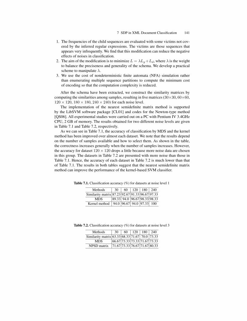
7 SDP in XML Document Classification 141
1. The frequencies of the child sequences are evaluated with some victims not cov-ered by the inferred regular expressions. The victims are those sequences thatappears very infrequently. We find that this modification can reduce the negativeeffects of noises in classification.
2. The aim of the modification is to minimize L = λLg+Ld, where λ is the weightto balance the preciseness and generality of the schema. We develop a practicalscheme to manipulate λ.
3. We use the cost of nondeterministic finite automata (NFA) simulation ratherthan enumerating multiple sequence partitions to compute the minimum costof encoding so that the computation complexity is reduced.
After the schema have been extracted, we construct the similarity matrices bycomputing the similarities among samples, resulting in five matrices (30×30, 60×60,120× 120, 180× 180, 240× 240) for each noise level.
The implementation of the nearest semidefinite matrix method is supportedby the LibSVM software package [CL01] and codes for the Newton-type method[QS06]. All experimental studies were carried out on a PC with Pentium IV 3.4GHzCPU, 2 GB of memory. The results obtained for two different noise levels are givenin Table 7.1 and Table 7.2, respectively.
As we can see in Table 7.1, the accuracy of classification by MDS and the kernelmethod has been improved over almost each dataset. We note that the results dependon the number of samples available and how to select them. As shown in the table,the correctness increases generally when the number of samples increases. However,the accuracy for dataset 120× 120 drops a little because more noise data are chosenin this group. The datasets in Table 7.2 are presented with more noise than those inTable 7.1. Hence, the accuracy of each dataset in Table 7.2 is much lower than thatof Table 7.1. The results in both tables suggest that the nearest semidefinite matrixmethod can improve the performance of the kernel-based SVM classifier.
Table 7.1. Classification accuracy (%) for datasets at noise level 1
Methods 30 60 120 180 240Similarity matrix 87.23 92.67 91.33 96.67 97.33
MDS 89.33 94.0 96.67 98.33 98.33Kernel method 94.0 96.67 94.0 97.33 100
Table 7.2. Classification accuracy (%) for datasets at noise level 3
Methods 30 60 120 180 240Similarity matrix 63.33 68.33 71.67 70.0 73.33
MDS 66.67 73.33 73.33 71.67 73.33NPSD matrix 71.67 73.33 76.67 71.67 80.33

142 Z. Xia, G. Xing, H. Qi, Q. Li
7.7 Conclusion and Discussion
In this chapter, we have studied two data representation methods for classifying XMLdocuments based on their structures. Based on the fact that many XML documentsare without schema, we first infer the document schema given a set of documents andthen estimate the similarities among the documents. Since the estimated similaritymatrix is usually not a distance matrix, it is not a well-defined kernel matrix. Weformulate the problem as a nearest semidefinite matrix problem and present a novelNewton-type method, named NPSDM, to determine the similarity matrix for the setof XML documents. The NPSDM is quadratically convergent and usually takes nomore than 10 iterations to converge. Using the Newton-type method, it has beenreported recently [QS06] that problems with n up to 2000 have been successfullysolved. To make use of the Newton method, we have to address how to select anelement Vk in ∂F (zk). One of the choices can be found in [QS06]. Another issueis to globalize the method in Eq. (7.10), which in its current form is only locallyconvergent as indicated in the above theorem. One globalized version can also befound in [QS06, Algorithm 5.1].
Acknowledgment
This work was supported in part by the Kentucky Experimental Program to StimulateCompetitive Research (EPSCoR) under grant No. 4800000786 .
References
[Bur98] C.J.C. Burges. A tutorial on support vector machines for pattern recognition. DataMin. Knowl. Discov., 2(2):121–167, 1998.
[Bur05] C.J.C. Burges. Geometric methods for feature extraction and dimensional reduc-tion — a guided tour. In The Data Mining and Knowledge Discovery Handbook,pages 59–92. Springer, New York, 2005.
[BX05] S. Boyd and L. Xiao. Least-squares covariance matrix adjustment. SIAM Journalon Matrix Analysis and Applications, 27(2):532–546, 2005. Available from WorldWide Web: http://link.aip.org/link/?SML/27/532/1.
[CC01] T.F. Cox and M.A.A. Cox. Multidimensional Scaling. Monographs on Statisticsand Applied Probability. Chapman & Hall/CRC, Boca Raton, 2nd edition, 2001.
[Che01] W. Chen. New algorithm for ordered tree-to-tree correction problem. J. Algo-rithms, 40(2):135–158, 2001.
[CL01] C.-C. Chang and C.-J. Lin. LIBSVM: a library for support vector machines,2001. Software available at http://www.csie.ntu.edu.tw/∼cjlin/libsvm.
[Cla83] F.H. Clark. Optimization and Nonsmooth Analysis. John Wiley and Sons, NewYork, 1983.
[CX05] E.R. Canfield and G. Xing. Approximate xml document matching. In SAC ’05:Proceedings of the 2005 ACM Symposium on Applied Computing, pages 787–788.ACM Press, New Work, 2005.

7 SDP in XML Document Classification 143
[DG] L. Denoyer and P. Gallinari. XML Document Mining Challenge. Database avail-able at http://xmlmining.lip6.fr/.
[DG04] L. Denoyer and P. Gallinari. Bayesian network model for semistructured documentclassification. Inf. Process. Manage., 40(5):807–827, 2004.
[GGR+00] M. Garofalakis, A. Gionis, R. Rastogi, S. Seshadri, and K. Shim. Xtract: a systemfor extracting document type descriptors from xml documents. In SIGMOD ’00:Proceedings of the 2000 ACM SIGMOD International Conference on Managementof Data, pages 165–176. ACM Press, New York, 2000.
[GJK+06] S. Guha, H.V. Jagadish, N. Koudas, D. Srivastava, and T. Yu. Integrating xmldata sources using approximate joins. ACM Trans. Database Syst., 31(1):161–207,2006.
[Hig02] N.J. Higham. Computing the nearest correlation matrix — a problem from finance.IMA Journal of Numerical Analysis, 22(3):329–343, 2002.
[Joa98] T. Joachims. Text categorization with suport vector machines: learning withmany relevant features. In Claire Nedellec and Celine Rouveirol, editors, Pro-ceedings of ECML-98, 10th European Conference on Machine Learning, vol-ume 1398 of Lecture Notes in Computer Science, pages 137–142. Springer, NewYork, 1998. Available from World Wide Web: citeseer.ist.psu.edu/joachims97text.html.
[LCB+04] G.R.G. Lanckriet, N. Cristianini, P. Bartlett, L. El Ghaoui, and M.I. Jordan. Learn-ing the kernel matrix with semidefinite programming. J. Mach. Learn. Res., 5:27–72, 2004.
[LCMY04] W. Lian, D.W. Cheung, N. Mamoulis, and S.-M. Yiu. An efficient and scal-able algorithm for clustering xml documents by structure. IEEE Transactions onKnowledge and Data Engineering, 16(1):82–96, 2004.
[Mal05] J. Malick. A dual approach to semidefinite least-squares problems. SIAM J. MatrixAnal. Appl., 26(1):272–284, 2005.
[Mur00] M. Murata. Hedge automata: a formal model for XML schemata. Webpage, 2000. Available from World Wide Web: citeseer.ist.psu.edu/article/murata99hedge.html.
[NJ02] A. Nierman and H.V. Jagadish. Evaluating structural similarity in xml documents.In WebDB, pages 61–66, 2002.
[QS06] H. Qi and D. Sun. A quadratically convergent newton method for computing thenearest correlation matrix. SIAM J. Matrix Anal. Appl., 28(2):360–385, 2006.
[Roc74] R.T. Rockafellar. Conjugate duality and optimization. Society for Industrial andApplied Mathematics, Philadelphia, 1974.
[Seb02] F. Sebastiani. Machine learning in automated text categorization. ACM Comput.Surv., 34(1):1–47, 2002.
[Stu99] J.F. Sturm. Using SeDuMi 1.02, a MATLAB toolbox for optimization over sym-metric cones. Optimization Methods and Software, 11-12:625–653, 1999. Avail-able from World Wide Web: citeseer.ist.psu.edu/sturm99using.html. Special issue on Interior Point Methods (CD supplement with software).
[STV04] B. Scholkopf, K. Tsuda, and J.P. Vert. Kernel Methods in Computational Biology.MIT Press, Cambridge, MA, 2004.
[SZ97] D. Shasha and K. Zhang. Approximate tree pattern matching. In Pat-tern Matching Algorithms, pages 341–371. Oxford University Press, NewYork, 1997. Available from World Wide Web: citeseer.ist.psu.edu/shasha95approximate.html.

144 Z. Xia, G. Xing, H. Qi, Q. Li
[SZC+04] J.-T. Sun, B.-Y. Zhang, Z. Chen, Y.-C. Lu, C.-Y. Shi, and W.-Y. Ma. Ge-cko:A method to optimize composite kernels for web page classification. In WI ’04:Proceedings of the 2004 IEEE/WIC/ACM International Conference on Web Intel-ligence, pages 299–305, 2004.
[ZA03] M.J. Zaki and C.C. Aggarwal. Xrules: an effective structural classifier for xml data.In KDD ’03: Proceedings of the Ninth ACM SIGKDD International Conference onKnowledge Discovery and Data Mining, pages 316–325. ACM Press, New York,2003.
[ZI02] T. Zhang and V.S. Iyengar. Recommender systems using linear classifiers. J. Mach.Learn. Res., 2:313–334, 2002.

Part III
Email Surveillance and Filtering


8
Discussion Tracking in Enron Email Using PARAFAC
Brett W. Bader, Michael W. Berry, and Murray Browne
Overview
In this chapter, we apply a nonnegative tensor factorization algorithm to extract anddetect meaningful discussions from electronic mail messages for a period of oneyear. For the publicly released Enron electronic mail collection, we encode a sparseterm-author-month array for subsequent three-way factorization using the PARAl-lel FACtors (or PARAFAC) three-way decomposition first proposed by Harshman.Using nonnegative tensors, we preserve natural data nonnegativity and avoid sub-tractive basis vector and encoding interactions present in techniques such as princi-pal component analysis. Results in thread detection and interpretation are discussedin the context of published Enron business practices and activities, and benchmarksaddressing the computational complexity of our approach are provided. The result-ing tensor factorizations can be used to produce Gantt-like charts that can be usedto assess the duration, order, and dependencies of focused discussions against theprogression of time.
8.1 Introduction
When Enron closed its doors on December 2, 2001, and filed for Chapter 11bankruptcy, it began a turn of events that released an unprecedented amount of infor-mation (over 1.5 million electronic mail messages, phone tapes, internal documents)into the public domain. This information was the cornerstone of the Federal EnergyRegulatory Commission’s (FERC) investigation into the global energy corporation.The original set of emails was posted on FERC’s Web site [Gri03], but it suffereddocument integrity problems, and attempts were made to improve the quality of thedata and remove sensitive and irrelevant private information. Dr. William Cohenof Carnegie-Mellon University oversaw the distribution of this improved corpus—known as the Enron email sets. The latest version of the Enron email sets1 (dated1 http://www-2.cs.cmu.edu/∼enron

148 B.W. Bader, M.W. Berry, M. Browne
March 2, 2004) contains 517, 431 email messages of 150 Enron employees cover-ing a period from December 1979 through February 2004, with the majority of themessages spanning the three years of 1999, 2000, and 2001.
For the most part, the emails reflect the day-to-day activities of America’s sev-enth largest company, but certain distinct topics of discussion are linked to Enron.One involved Enron’s development of the Dabhol Power Company (DPC) in the In-dian state of Maharashtra, an endeavor awash in years of logistical and political prob-lems. Another topic was the deregulation of the California energy market, which ledto rolling blackouts during the summer of 2000—a situation that Enron (and otherenergy companies) took advantage of financially. Eventually a combination of greed,overspeculation, and deceptive accounting practices snowballed into an abrupt col-lapse in the fourth quarter of 2001, which again is reflected in the emails. The Enronemail sets provide a unique opportunity not only to study the mechanics of a sizableemail network, but it also offers a glimpse of the machinations of how huge globalcorporations operate on a day-to-day basis.
In this research, we seek to extract meaningful threads of discussion from a sub-set of the Enron email set. The idea underlying our thread extraction is as follows.Suppose we have a collection of q emails from n authors over a period of p months(or similar unit of time). In aggregate, there are a collection of m terms parsed fromthe q emails. From these data, we create an m × n × p term-author-month array2
X. We then decompose X using PARAFAC or a nonnegative tensor factorization totrack discussions over time.
In the next section we provide background information on tensor decompositionsand related work. Section 8.3 provides a formal discussion of the notations used todefine these decompositions and algorithms that are given in Section 8.4. Detailsof the specific Enron subset used in this study are provided in Section 8.5, and ourobservations and results in applying PARAFAC to this subset of emails follow inSection 8.6. Finally, a brief summary of future work in the use of nonnegative tensorfactorization for discussion tracking is given in Section 8.7.
8.2 Related Work
Tensor decompositions date back 40 years [Tuc66, Har70, CC70], and they havebeen used extensively in a variety of domains, from chemometrics [SBG04] to signalprocessing [SGB00]. PARAFAC is a three-way decomposition that was proposed byHarshman [Har70] using the name PARAllel FACtors or PARAFAC. At the sametime, Carroll and Chang [CC70] published the same mathematical model, whichthey call canonical decomposition (CANDECOMP).
The use of multidimensional models is relatively new in the context of text anal-ysis. Acar et al. [ACKY05] use various tensor decompositions of (user × key word× time) data to separate different streams of conversation in chatroom data. Several2 Note that the array X is generally sparse due to the word distribution used by each author
over time.

8 Discussion Tracking 149
Web search applications involving tensors relied on query terms or anchor text toprovide a third dimension. Sun et al. [SZL+05] apply a three-way Tucker decom-position [Tuc66] to the analysis of (user × query term × Web page) data in orderto personalize Web searches. Kolda et al. [KBK05] and Kolda and Bader [KB06]use PARAFAC on a (Web page × Web page × anchor text) sparse, three-way ten-sor representing the Web graph with anchor-text-labeled edges to get hub/authorityrankings of pages related to an identified topic.
8.3 Notation
Multidimensional arrays and tensors are denoted by boldface Euler script letters, forexample, X. Element (i, j, k) of a third-order tensor X is denoted by xijk.
The symbol ◦ denotes the tensor outer product,
A1 ◦B1 =
A11B11 · · · A11Bm1
.... . .
...Am1B11 · · · Am1Bm1
.
The symbol ∗ denotes the Hadamard (i.e., elementwise) matrix product,
A ∗B =
A11B11 · · · A1nB1n
.... . .
...Am1Bm1 · · · AmnBmn
.
The symbol ⊗ denotes the Kronecker product,
A⊗B =
A11B · · · A1nB...
. . ....
Am1B · · · AmnB
.
The symbol � denotes the Khatri-Rao product (columnwise Kronecker) [SBG04],
A�B =(A1 ⊗B1 · · · An ⊗Bn
).
The concept of matricizing or unfolding is simply a rearrangement of the entriesof X into a matrix. Although different notations exist, we are following the notationused in [SBG04]. For a three-dimensional array X of size m × n × p, the notationX(m×np) represents a matrix of sizem×np in which the n-index runs the fastest overthe columns and p the slowest. Other permutations, such as X(p×nm), are possibleby changing the row index and the fast/slow column indices.
The norm of a tensor, ‖X ‖, is the same as the Frobenius norm of the matricizedarray, that is, the square root of the sum of squares of all its elements.

150 B.W. Bader, M.W. Berry, M. Browne
= ...+ +
Fig. 8.1. PARAFAC provides a three-way decomposition with some similarity to the singularvalue decomposition.
8.4 Tensor Decompositions and Algorithms
Suppose we are given a tensor X of size m × n × p and a desired approximationrank r. The goal is to decompose X as a sum of vector outer products as shown inFigure 8.1. It is convenient to group all r vectors together in factor matrices A,B,Ceach having r columns. The following mathematical expressions of this model usedifferent notations but are equivalent:
xijk ≈r∑l=1
AilBjlCkl,
X ≈r∑l=1
Al ◦Bl ◦ Cl, (8.1)
X(m×np) ≈ A(C �B)T .
PARAFAC may apply to general N -way data, but because our application pertainsonly to three-way data, we are considering only the specific three-way problem atthis time.
Without loss of generality, we typically normalize all columns of the factor ma-trices to have unit length and store the accumulated weight (i.e., like a singular value)in a vector λ:
X ≈r∑l=1
λl(Al ◦Bl ◦ Cl)
Moreover, we typically reorder the final solution so that λ1 ≥ λ2 ≥ · · · ≥ λr. Inthe following subsections, we describe general algorithms for the model without λbecause this normalization can be performed in a postprocessing step.
Our goal is to find the best-fitting matrices A,B, and C in the minimizationproblem:
minA,B,C
∥∥∥∥∥X−r∑l=1
Al ◦Bl ◦ Cl
∥∥∥∥∥2
. (8.2)
It is important to note that the factor matrices are not required to be orthogonal.Under mild conditions, PARAFAC provides a unique solution that is invariant tofactor rotation [Har70]. Hence, the factors are plausibly a valid description of thedata with greater reason to believe that they have more explanatory meaning than a“nice” rotated two-way solution.

8 Discussion Tracking 151
Given a value r > 0 (loosely corresponding to the number of distinct topics orconversations in our data), the tensor decomposition algorithms find matrices A ∈Rm×r, B ∈ Rn×r, and C ∈ Rp×r, to yield Equation (8.1). Each triad {Aj , Bj , Cj},for j = 1, . . . , r, defines scores for a set of terms, authors, and time for a particularconversation in our email collection; the value λr after normalization defines theweight of the conversation. (Without loss of generality, we assume the columns ofour matrices are normalized to have unit length.) The scales in C indicate the activityof each conversation topic over time.
8.4.1 PARAFAC-ALS
A common approach to solving Equation (8.2) is an alternating least squares (ALS)algorithm [Har70, FBH03, TB05], due to its simplicity and ability to handle con-straints. At each inner iteration, we compute an entire factor matrix while holding allthe others fixed.
Starting with random initializations for A,B, and C, we update these quantitiesin an alternating fashion using the method of normal equations. The minimizationproblem involving A in Equation (8.2) can be rewritten in matrix form as a leastsquares problem [FBH03]:
minA
∥∥∥X(m×np) −AZ∥∥∥2
, (8.3)
where Z = (C �B)T .The least squares solution for Equation (8.3) involves the pseudo-inverse of Z:
A = X(m×np)Z†.
Conveniently, the pseudo-inverse of Z may be computed in a special way that avoidscomputing ZTZ with an explict Z [SBG04], so the solution to Equation (8.3) isgiven by
A = X(m×np)(C �B)(BTB ∗ CTC)−1.
Furthermore, the product X(m×np)(C � B) may be computed efficiently if X issparse [KB06] by not forming the Khatri-Rao product C � B. Thus, computing Aessentially reduces to several matrix inner products, sparse tensor-matrix multiplica-tion of B and C into X, and inverting an R×R matrix.
Analogous least-squares steps may be used to update B and C.
8.4.2 Nonnegative Tensor Factorization
We also considered a PARAFAC model with nonnegativity constraints on the fac-tor matrices. Because we are dealing with nonnegative data in X, it often helps toexamine decompositions that retain the nonnegative characteristics of the originaldata. Modifications to the ALS algorithm are needed, and we use the multiplica-tive update introduced in [LS99] and adapted for tensor decompositions by Mørup

152 B.W. Bader, M.W. Berry, M. Browne
[Mør05, MHA06]. We also incorporate the addition of ε for stability as was done in[BB05a]. Overall, the approach is similar to PARAFAC-ALS except that the factormatrices are updated differently.
First, we note that residual norm of the various formulations of the PARAFACmodel are equal:
||X(m×np) −A(C �B)T ||F =||X(n×mp) −B(C �A)T ||F =||X(p×mn) − C(B �A)T ||F .
Each of these matrix systems is treated as a nonnegative matrix factorization (NMF)problem and solved in an alternating fashion. That is, we solve for A using the mul-tiplicative update rule holding B and C fixed, and so on:
Aiρ ← Aiρ(X(m×np)Z)iρ(AZTZ)iρ + ε
, Z = (C �B)
Bjρ ← Bjρ(X(n×mp)Z)jρ(BZTZ)jρ + ε
, Z = (C �A)
Ckρ ← Ckρ(X(p×mn)Z)kρ(CZTZ)kρ + ε
, Z = (B �A)
Here ε is a small number like 10−9 that adds stability to the calculation and guardsagainst introducing a negative number from numerical underflow.
As was mentioned previously, X is sparse, which facilitates a simpler compu-tation in the procedure above. Each matricized version of X (which has the samenonzeros but reshaped) is a sparse matrix. The matrix Z from each step should notbe formed explicitly because it would be a large, dense matrix. Instead, the prod-uct of a matricized X with Z should be computed specially, exploiting the inherentKronecker product structure in Z so that only the required elements in Z need to becomputed and multiplied with the nonzero elements of X. See [KB06] for details.
8.5 Enron Subset
For a relevant application, we consider the email corpus of the Enron corporationthat was made public during the federal investigation. The whole collection is avail-able online [Coh] and contains 517,431 emails stored in the mail directories of 150users. We use a smaller graph of the Enron email corpus prepared by Priebe etal. [PCMP06] that consists of messages among 184 Enron email addresses plus 13more that have been identified in [BB05a] as interesting. We considered messagesonly in 2001, which resulted in a total of 53,733 messages over 12 months (mes-sages were sent on a total of 357 days).
An obvious difficulty in dealing with the Enron corpus is the lack of informationregarding the former employees. Without access to a corporate directory or orga-nizational chart of Enron at the time of these emails, it is difficult to ascertain the

8 Discussion Tracking 153
validity of our results and assess the performance of the PARAFAC model. Otherresearchers using the Enron corpus have had this same problem, and information onthe participants has been collected slowly and made available.
The Priebe dataset [PCMP06] provided partial information on the 184 employ-ees of the small Enron network, which appears to be based largely on informationcollected by Shetty and Adibi [SA05]. It provides most employees’ position andbusiness unit. To facilitate a better analysis of the PARAFAC results, we collectedextra information on the participants from the email messages themselves and foundsome relevant information posted on the FERC Web site [Fed]. To help assess ourresults, we searched for corroborating information of the preexisting data or for newidentification information, such as title, business unit, or manager. Table 8.1 lists 11of the most notable authors (and their titles) whose emails were tracked in this study.
Table 8.1. Eleven of the 197 email authors represented in the term-author-time array X
Email accountName (@enron.com) TitleRichard Sanders b..sanders VP Enron Wholesale ServicesGreg Whalley greg.whalley PresidentJeff Dasovich jeff.dasovich Employee Government Relationship
ExecutiveJeffery Skilling jeff.skilling CEOSteven Kean j..kean VP and Chief of StaffJohn Lavorato john.lavorato CEO Enron AmericaKenneth Lay kenneth.lay CEOLouise Kitchen louise.kitchen President Enron OnlineMark Haedicke mark.haedicke Managing Director Legal DepartmentRichard Shapiro richard.shapiro VP Regulatory AffairsVince Kaminski vince.kaminski Manager Risk Management Head,
Enron Energy Services
Of the 197 authors whose emails were tracked (in the year 2001), there were afew cases of aliasing. That is, different email accounts of the form
employee [email protected] used by the same employee. A few sample aliases from the 11 notable authorsin Table 8.1 are David Delaney (david.delainey, w..delainey) and VinceKaminski (j.kaminski, j..kaminski, vince.kaminski).
8.5.1 Term Weighting
We considered two datasets: monthly and daily time periods. The monthly data cor-respond to a sparse adjacency array X of size 69157 × 197 × 12 with 1,042,202nonzeros, and the daily data correspond to a sparse adjacency array Y of size69157×197×357 with 1,770,233 nonzeros. The 69,157 terms were parsed from the53,733 messages using a master dictionary of 121,393 terms created by the General

154 B.W. Bader, M.W. Berry, M. Browne
Text Parser (GTP) software environment (in C++) maintained at the University ofTennessee [GWB03]. This larger set of terms was previously obtained when GTPwas used to parse 289,695 of the 517,431 emails defining the Cohen distribution atCarnegie-Mellon (see Section 8.1). To be accepted into the dictionary, a term had tooccur in more than one email and more than 10 times among the 289,695 emails.
Unique to previous parsings of Enron subsets by GTP (see [BBL+07, SBPP06,BB05b]), a much larger stoplist of unimportant words was used to filter out thecontent-rich 69,157 terms for the X and Y arrays. This stoplist of 47,154 words washuman-generated by careful screening of the master (GTP-generated) dictionary forwords with no specific reference to an Enron-related person or activity.
We scaled the nonzero entries of X and Y according to a weighted frequency:xijk = lijkgiaj ,
yijk = lijkgiaj ,
where lijk is the local weight for term i written by author j in month/day k, gi is theglobal weight for term i, and aj is an author normalization factor.
Let fijk be the number of times term i is written by author j in month/day k, anddefine hij =
Pk fijkPjk fijk
. The specific components of each nonzero are listed below:
Log local weight lijk = log(1 + fijk)
Entropy global weight gi = 1 +n∑j=1
hij log hijlog n
Author normalization aj = 1vuuut∑i,k
(lijkgi)
These weights are adapted from the well-known log-entropy weighting scheme[BB05c] used on term-by-document matrices. The log local weight scales the rawterm frequencies to diminish the importance of high-frequency terms. The entropyglobal weight attempts to emulate an entropy calculation of the terms over all mes-sages in the collection to help discriminate important terms from common terms.The author normalization helps to correct imbalances in the number of messagessent from each author. Without some type of normalization, discussions involvingprolific authors would tend to dominate the results.
8.6 Observations and Results
In this section we summarize our findings of applying PARAFAC and nonnega-tive tensor factorization (NNTF) on the Enron email collection. Our algorithmswere written in MATLAB, using sparse extensions of the Tensor Toolbox [BK06a,BK06b]. All tests were performed on a dual 3-GHz Pentium Xeon desktop computerwith 2 GB of RAM.

8 Discussion Tracking 155
8.6.1 PARAFAC
We computed a 25-component (r = 25) decomposition of the term-author-montharray X using PARAFAC. One ALS iteration of PARAFAC took about 22.5 seconds,requiring an average of 27 iterations to satisfy a tolerance of 10−4 in the change offit. We chose the smallest minimizer from among ten runs starting from randominitializations. The relative norm of the difference was 0.8904.
We also computed a 25-component (r = 25) decomposition of the term-author-day array Y using PARAFAC. For this larger dataset, one ALS iteration of PARAFACtook 26 seconds, requiring an average of 13 iterations to satisfy a tolerance of 10−4
in the change of fit. We chose the smallest minimizer from among ten runs startingfrom random initializations. The relative norm of the difference was 0.9562.
8.6.2 Nonnegative Tensor Decomposition
We computed a 25-component (r = 25) nonnegative decomposition of the term-author-month array X. One iteration took about 22 seconds, and most runs requiredless than 50 iterations to satisfy a tolerance of 10−4 in the relative change of fit. Wechose the smallest minimizer from among ten runs from random starting points, andthe relative norm of the difference was 0.8931.
We also computed a 25-component (r = 25) nonnegative decomposition of thelarger term-author-day array Y. One iteration took about 26 seconds, and the averagerun required about 17 iterations to satisfy a tolerance of 10−4 in the relative changeof fit. We chose the smallest minimizer from among ten runs from random startingpoints, and the relative norm of the difference was 0.9561.
8.6.3 Analysis of Results
PARAFAC is able to identify and track discussions over time in each triad {Aj , Bj , Cj},for j = 1, . . . , r. A discussion is associated with the topic and primary participantsidentified in the columns of A and B, respectively, and the corresponding columnof C provides a profile over time, showing the relative activity of that discussionover 12 months or over 357 days. Figures 8.2 and 8.3 present a histogram (or Ganttchart) of the monthly activity for each discussion identified by the classical and non-negative PARAFAC models, respectively. Similarly, Figures 8.4 and 8.5 present linecharts of the daily activity for each discussion identified by the classical and nonneg-ative PARAFAC models, respectively. We first discuss the monthly results, and thendescribe the finer grained details uncovered in the daily results.

156 B.W. Bader, M.W. Berry, M. Browne
Group Jan Feb Mar Apr May June July Aug Sept Oct Nov Dec
College Football
India
College Football
Key
# Bars[.01,0.1) [0.1, 0.3)Interval [-1.0,.01) [0.3, 0.5) [0.5, 0.7) [0.7,1.0)
(Gray = unclassified topic)
24
25
Downfall
18
15
16
17
23
12
13
22
Education (Kaminski)
11
14
19
20
21
9
10
5
6
7
8
California
1
2
3
4
Fig. 8.2. Six distinguishable discussions among the 25 extracted by classic PARAFAC. Diag-onal shading of cells is used to indicate negative components in the tensor groups.

8 Discussion Tracking 157
Group Jan Feb Mar Apr May June July Aug Sept Oct Nov Dec
Key
Interval# Bars
[.01,0.1) [0.1, 0.3) [0.3, 0.5) [0.5, 0.7) [0.7,1.0)
(Gray = unclassified topic)
24
25
Downfall Newsfeeds
California Energy
College Football
Fastow Companies
18
15
16
17
23
12
13
14
19
20
21
22
India
Education (Kaminski)
11
5
6
7
8
9
10
Downfall
India
1
2
3
4
Fig. 8.3. Eight distinguishable discussions among the 25 extracted by nonnegative PARAFAC.

158 B.W. Bader, M.W. Berry, M. Browne
Qualitatively, the results of the nonnegative decomposition are the same as thestandard three-way PARAFAC results. The difference between the two models was inthe ability to interpret the results. In the 25 discussion groups depicted in Figure 8.2,only six of the groups have any discernible meaning based on our knowledge ofthe events surrounding Enron [ME03]. In comparison, the nonnegative PARAFACmodel revealed eight group discussions that could be interpreted.
The topics generated by the nonnegative PARAFAC model do reflect the eventsof the year 2001, a tumultuous one for the global energy corporation, to say the least.In the first quarter of the year, the company was still dealing with the fallout of the2000 California energy crisis. Discussions about the federal and California state gov-ernments’ investigation of the California situation showed up in emails during thistime frame. Another ongoing and ever-present topic was Enron’s attempted devel-opment of the Dabhol Power Company (DPC) in the Indian State of Maharashtra.The company’s efforts in India had been ongoing for several years, and the emailsof the early half of 2001 reflect some of the day-to-day dealings with the less-than-profitable situation in India.
By October 2001, Enron was in serious financial trouble, and when a merger withthe Dynegy energy company fell through, Enron was forced to file for Chapter 11bankruptcy. Many of the emails of this time frame (more specifically in October andNovember) were newsfeeds from various news organizations that were being passedaround Enron. Because it was learned at this time that Chief Financial Officer AndyFastow was heavily involved with the deceptive accounting practices (by setting upsham companies to boost Enron’s bottom line), it is not surprising a thread on thistopic (Fastow companies) emerged. Predictably, the College Football topic emergesin late fall as well. One of the surprise topics uncovered was the Education topic,which reflects the interests and responsibilities of Vince Kaminski, head of research.Kaminski taught a class at nearby Rice University in Houston in the spring of 2001,and was the focal point of emails about internships, class assignments, and resumeevaluation.
The fact that at most eight of the 25 topics had any discernible meaning reflectsthe nature of topic detection. A significant amount of noise or undefined contentmay permeate the term-author-month arrays. Sometimes, as shown by the height ofthe gray bars in Figures 8.2 and 8.3, there are indicators of a possible thread of somekind (not necessarily directly related to Enron), but further inspection of those emailsreveals no identifiable topic of discussion.
The daily results provided a similar interpretation as the monthly results but at afiner resolution. In general, there were four types of profiles over time: (1) discus-sions centered largely on one or a few days, resulting in a single spike (see, e.g.,Figures 8.4 and 8.5); (2) continual activity, represented as multiple weekly spikesthroughout the year; (3) continual activity with lulls, where a period of calm sepa-rates bursts of discussion; and (4) a series of weekly spikes usually spanning three ormore months.
Of the 25 groups found with the PARAFAC model, roughly half were singlespikes. We have identified three of these groups of particular significance in Fig-ure 8.4. The first identifies a flood of emails about the possible Dynegy/Enron merger

8 Discussion Tracking 159
(November 11 and 12), which was something new. This merger topic was found in[BB05a], but this topic did not show up previously in our monthly results. The secondis a topic on January 7 that the Enron employees (Kean, Hughes, and Ambler) werediscussing India based on an article published by Reuters and another media reportthat required some attention by the Enron executives. The third group also matcheswhat happened on August 27, when discussion was centered on the U.S. Court ofAppeals ruling on section 126 of an Environmental Protection Agency code. Thisspecific topic concerning compliance of emission limitations had not yet surfacedanywhere before in our analysis.
Jan Feb Mar Apr May Jun Jul Aug Sep Oct Nov Dec0
0.5
1
Month
Act
ivity
Lev
el Aug. 27 (U.S. Court of Appeals/Sec 126)
Jan Feb Mar Apr May Jun Jul Aug Sep Oct Nov Dec0
0.5
1
Month
Act
ivity
Lev
el Jan. 07 (India/Reuters article)
Jan Feb Mar Apr May Jun Jul Aug Sep Oct Nov Dec0
0.5
1
Month
Act
ivity
Lev
el Nov. 11 (Dynegy/Enron merger)
Fig. 8.4. Three daily discussions among the 25 extracted by PARAFAC.
The nonnegative PARAFAC model identified the same temporal patterns asPARAFAC, with a majority being a series of weekly spikes spanning three or moremonths. Roughly one third are single-spike patterns, and just two discussions are ofthe bimodal type with a lull. We mention three of the more interesting groups fromsingle-spike discussions, shown in Figure 8.5. The first group of the nonnegativemodel is interesting because it either reveals a potentially new topic or a specificoccurrence of a general topic. On August 22, there was a flurry of emails and re-sponses to an Email called California Campaign Closeout. Richard Shapiro praisedthe employees working in California and many responded to his acknowledgment. Asecond group is a very strong cluster pointing to college football with terms like Ne-braska, Sooners, bowl, Cougars, and Tennessee. These were sent by Matthew Motley

160 B.W. Bader, M.W. Berry, M. Browne
on November 20. Finally, a third group was influenced heavily by Enron’s final im-plosion in and around October 25 and 26. There were many news wire stories aboutthe plight of Enron during this time. PARAFAC had found this topic but had identi-fied the time period 2 days earlier. We believe this difference is a result of the randominitialization that both were provided.
Jan Feb Mar Apr May Jun Jul Aug Sep Oct Nov Dec
0.20.40.60.8
Month
Act
ivity
Lev
el Aug. 22 (California Campaign Closeout)
Jan Feb Mar Apr May Jun Jul Aug Sep Oct Nov Dec
0.20.40.60.8
Month
Act
ivity
Lev
el Nov. 19 (College Football/Nebraska/Sooners)
Jan Feb Mar Apr May Jun Jul Aug Sep Oct Nov Dec
0.20.40.60.8
Month
Act
ivity
Lev
el Oct. 25 (Enron implodes/news wires)
Fig. 8.5. Three daily discussions among the 25 extracted by nonnegative PARAFAC.
8.7 Future Work
As demonstrated by this study, nonnegative tensor factorization (implemented byPARAFAC) can be used to extract meaningful discussions from email communica-tions. The ability to assess term-to-author (or term-to-email) associations both se-mantically and temporally via three-way decompositions is an important advance-ment in email surveillance research. Previously reported clusters of Enron emails us-ing nonnegative matrix factorization (i.e., two-way decompositions) [BB05b, BBL+07,SBPP06] were unable to extract discussions such as the Education thread mentionedin Section 8.6.2 or sequence the discussion of the company’s downfall by source(news feeds versus employee-generated). The optimal segmentation of time as thethird dimension for email clustering may be problematic. Grouping emails by monthmay not be sufficient for some applications, and so more research in the cost-benefit

8 Discussion Tracking 161
trade-offs of finer time segmentation (e.g., grouping by weeks, days, or even minutes)is needed. Determining the optimal tensor rank r for models such as PARAFAC iscertainly another important research topic. Term weighting in three-way arrays isalso an area that greatly influences the quality of results but is not yet well under-stood.
Acknowledgments
This research was sponsored by the United States Department of Energy and by San-dia National Laboratory, a multiprogram laboratory operated by Sandia Corporation,a Lockheed Martin Company, for the United States Department of Energy undercontract DE–AC04–94AL85000.
References
[ACKY05] E. Acar, S.A. Camtepe, M.S. Krishnamoorthy, and B. Yener. Modeling and mul-tiway analysis of chatroom tensors. In ISI 2005: IEEE International Conference onIntelligence and Security Informatics, volume 3495 of Lecture Notes in ComputerScience, pages 256–268. Springer, New York, 2005.
[BB05a] M.W. Berry and M. Browne. Email surveillance using non-negative matrix factor-ization. In Workshop on Link Analysis, Counterterrorism and Security, SIAM Conf.on Data Mining, Newport Beach, CA, 2005.
[BB05b] M.W. Berry and M. Browne. Email surveillance using nonnegative matrix factor-ization. Computational & Mathematical Organization Theory, 11:249–264, 2005.
[BB05c] M.W. Berry and M. Browne. Understanding Search Engines: Mathematical Mod-eling and Text Retrieval. SIAM, Philadelphia, second edition, 2005.
[BBL+07] M.W. Berry, M. Browne, A.N. Langville, V.P. Pauca, and R.J. Plemmons. Algo-rithms and applications for approximate nonnegative matrix factorization. Compu-tational Statistics & Data Analysis, 52(1):155–173, 2007.
[BK06a] B.W. Bader and T.G. Kolda. Efficient MATLAB computations with sparse and fac-tored tensors. Technical Report SAND2006-7592, Sandia National Laboratories,Albuquerque, New Mexico and Livermore, California, December 2006. Avail-able from World Wide Web: http://csmr.ca.sandia.gov/∼tgkolda/pubs.html#SAND2006-7592.
[BK06b] B.W. Bader and T.G. Kolda. Matlab tensor toolbox, version 2.1. http://csmr.ca.sandia.gov/∼tgkolda/TensorToolbox/, December 2006.
[CC70] J.D. Carroll and J.J. Chang. Analysis of individual differences in multidimensionalscaling via an N-way generalization of ‘Eckart-Young’ decomposition. Psychome-trika, 35:283–319, 1970.
[Coh] W.W. Cohen. Enron email dataset. Web page. http://www.cs.cmu.edu/∼enron/.
[FBH03] N.M. Faber, R. Bro, and P.K. Hopke. Recent developments in CANDE-COMP/PARAFAC algorithms: a critical review. Chemometr. Intell. Lab.,65(1):119–137, January 2003.

162 B.W. Bader, M.W. Berry, M. Browne
[Fed] Federal Energy Regulatory Commission. FERC: Information released in En-ron investigation. http://www.ferc.gov/industries/electric/indus-act/wec/enron/info-release.asp.
[Gri03] T. Grieve. The decline and fall of the Enron empire. Slate, October 14 2003. Avail-able from World Wide Web: http://www.salon.com/news/feature/2003/10/14/enron/index\ np.html.
[GWB03] J.T. Giles, L. Wo, and M.W. Berry. GTP (General Text Parser) Software for TextMining. In H. Bozdogan, editor, Software for Text Mining, in Statistical DataMining and Knowledge Discovery, pages 455–471. CRC Press, Boca Raton, FL,2003.
[Har70] R.A. Harshman. Foundations of the PARAFAC procedure: models and con-ditions for an “explanatory” multi-modal factor analysis. UCLA Working Pa-pers in Phonetics, 16:1–84, 1970. Available at http://publish.uwo.ca/∼harshman/wpppfac0.pdf.
[KB06] T.G. Kolda and B.W. Bader. The TOPHITS model for higher-order weblink analysis. In Workshop on Link Analysis, Counterterrorism and Security,2006. Available from World Wide Web: http://www.cs.rit.edu/∼amt/linkanalysis06/accepted/21.pdf.
[KBK05] T.G. Kolda, B.W. Bader, and J.P. Kenny. Higher-order web link analysis usingmultilinear algebra. In ICDM 2005: Proceedings of the 5th IEEE InternationalConference on Data Mining, pages 242–249. IEEE Computer Society, Los Alami-tos, CA, 2005.
[LS99] D. Lee and H. Seung. Learning the parts of objects by non-negative matrix factor-ization. Nature, 401:788–791, 1999.
[ME03] B. Mclean and P. Elkind. The Smartest Guys in the Room: The Amazing Rise andScandalous Fall of Enron. Portfolio, New York, 2003.
[MHA06] M. Mørup, L. K. Hansen, and S. M. Arnfred. Sparse higher order non-negativematrix factorization. Neural Computation, 2006. Submitted.
[Mør05] M. Mørup. Decomposing event related eeg using parallel factor (parafac). Presen-tation, August 29 2005. Workshop on Tensor Decompositions and Applications,CIRM, Luminy, Marseille, France.
[PCMP06] C.E. Priebe, J.M. Conroy, D.J. Marchette, and Y. Park. Enron dataset. Web page,February 2006. http://cis.jhu.edu/∼parky/Enron/enron.html.
[SA05] J. Shetty and J. Adibi. Ex employee status report. Online, 2005. http:www.isi.edu/∼adibi/Enron/Enron Employee Status.xls.
[SBG04] A. Smilde, R. Bro, and P. Geladi. Multi-Way Analysis: Applications in theChemical Sciences. Wiley, West Sussex, England, 2004. Available fromWorld Wide Web: http://www.wiley.com/WileyCDA/WileyTitle/productCd-0471986917.html.
[SBPP06] F. Shahnaz, M.W. Berry, V.P. Pauca, and R.J. Plemmons. Document clusteringusing non-negative matrix factorization. Information Processing & Management,42(2):373–386, 2006.
[SGB00] N.D. Sidiropoulos, G.B. Giannakis, and R. Bro. Blind PARAFAC receivers forDS-CDMA systems. IEEE Transactions on Signal Processing, 48(3):810–823,2000.
[SZL+05] J.-T. Sun, H.-J. Zeng, H. Liu, Y. Lu, and Z. Chen. CubeSVD: a novel approach topersonalized Web search. In WWW 2005: Proceedings of the 14th InternationalConference on World Wide Web, pages 382–390. ACM Press, New York, 2005.
[TB05] G. Tomasi and R. Bro. PARAFAC and missing values. Chemometr. Intell. Lab.,75(2):163–180, February 2005.

8 Discussion Tracking 163
[Tuc66] L.R. Tucker. Some mathematical notes on three-mode factor analysis. Psychome-trika, 31:279–311, 1966.


9
Spam Filtering Based on Latent Semantic Indexing
Wilfried N. Gansterer, Andreas G.K. Janecek, and Robert Neumayer
Overview
In this chapter, the classification performance of latent semantic indexing (LSI) ap-plied to the task of detecting and filtering unsolicited bulk or commercial email(UBE, UCE, commonly called “spam”) is studied. Comparisons to the simple vectorspace model (VSM) and to the extremely widespread, de-facto standard for spamfiltering, the SpamAssassin system, are summarized. It is shown that VSM and LSIachieve significantly better classification results than SpamAssassin.
Obviously, the classification performance achieved in this special applicationcontext strongly depends on the feature sets used. Consequently, the various clas-sification methods are also compared using two different feature sets: (1) a set ofpurely textual features of email messages that are based on standard word- and token-extraction techniques, and (2) a set of application-specific “meta features” of emailmessages as extracted by the SpamAssassin system. It is illustrated that the lattertends to achieve consistently better classification results.
A third central aspect discussed in this chapter is the issue of problem reductionin order to reduce the computational effort for classification, which is of particularimportance in the context of time-critical on-line spam filtering. In particular, theeffects of truncation of the SVD in LSI and of a reduction of the underlying featureset are investigated and compared. It is shown that a surprisingly large amount ofproblem reduction is often possible in the context of spam filtering without heavyloss in classification performance.
9.1 Introduction
Unsolicited bulk or commercial email (UBE, UCE, “spam”) has been a severe prob-lem on the Internet in the last several years. Although many strategies for addressingthis problem have been proposed, we are still far away from a satisfactory and fun-damental solution. In part, this is due to the fact that many of the methods proposed

166 W.N. Gansterer, A.G.K. Janecek, R. Neumayer
and developed into concepts usable in practice have an ad-hoc nature and lack a last-ing effect. Those individuals who make a profit based on the spam phenomenon (the“spammers”) can easily find ways to circumvent the proposed methods.
The problem of filtering spam is a binary classification problem in the sense thatevery incoming email has to be classified as “spam” or “not spam.” The investiga-tions summarized here were motivated by the general assumption that spam emailmessages tend to have several semantic elements in common, which are usuallynot present in regular email (commonly called “ham”). This assumption is plausi-ble due to the economic aspects underlying the spam phenomenon (see, for example,[ISGP06] for a discussion). However, the common semantic elements are hard to pin-point comprehensively, because they are not fully known, not always explicit, or maychange dynamically. In other words, they are in some sense implicit or latent. Someapproaches that were developed have tried to concentrate on some specific propertiesof (current) spam and to design anti-spam methods based thereon. However, due tothe difficulties in identifying a comprehensive set of properties that unambiguouslycharacterize spam, these approaches have not led to fundamental and persistent anti-spam strategies.
9.1.1 Approaches Investigated
In this chapter, the classification performance of a vector space model (VSM) andlatent semantic indexing (LSI) applied to the task of spam filtering are studied. Basedon a feature set used in the extremely widespread, de-facto standard spam filteringsystem known as SpamAssassin and also on subsets selected from this feature set,a vector space model and latent semantic indexing are applied for classifying emailmessages as spam or not spam. The test datasets used are partly from the officialTREC 2005 dataset and partly self-collected.
The investigation of LSI for spam filtering summarized here evaluates the re-lationship between two central aspects: (i) the truncation of the SVD in LSI, and() the resulting classification performance in this specific application context. It isshown that a surprisingly large amount of truncation is often possible without heavyloss in classification performance. This forms the basis for good and extremely fastapproximate (pre-) classification strategies, which are very useful in practice. Theapproaches investigated in this chapter are shown to compare favorably to two im-portant alternatives, in that they achieve better classification results than SpamAssas-sin, and (2) they are better and more robust than a related LSI-based approach usingtextual features, which has been proposed earlier.
The low-rank approximation of the feature-document matrix within LSI is onepossibility to reduce the potentially huge size of the classification problem. As analternative, we investigate strategies for reducing the feature set before the classi-fication process. Compared to the LSI truncation process on a full feature set, thisapproach can potentially reduce the computing time as the matrices in the time-consuming SVD computation become smaller. The classification performances ofthese two approaches to problem size reduction are investigated and compared.
9 Spam Filtering Based on Latent Semantic Indexing 167
9.1.2 Background and Related Work
Existing anti-spam methods can be categorized according to their point of action inthe email transfer process. Consequently, three classes of approaches can be distin-guished (for details, see [GIL+05]). Pre-send methods act before the email is trans-ported over the network, whereas post-send methods act after the email has beentransferred to the receiver. A third class of approaches comprises new protocols,which are based on modifying the transfer process itself. Pre-send methods (see,for example, [Bac02] or [GHI+05]) are very important because of their potentialto avoid the wasting of resources (network traffic, etc.) caused by spam. However,the efficiency of pre-send methods and of new protocols heavily depends on theirwidespread deployment. It is unrealistic to expect global acceptance and widespreaduse of these new methods in the near future, and thus the third group of methods,post-send spam filtering methods, will continue to be the “workhorse” in spam de-fense.
Many of the spam filtering concepts currently used in practice are mostly static innature, such as black- and whitelisting or rule-based filters. A de-facto standard of arule-based spam filtering system is SpamAssassin [Apa06]. SpamAssassin extracts amultitude of features from incoming email messages, comprising pieces of informa-tion from header, body, and the full text of the message. One of the tests integratedinto SpamAssassin is a Bayesian classifier, a statistical approach exclusively basedon textual features. An example of its application to the scenario of spam filtering isgiven in [AKCS00]. The underlying idea is to compute a conditional probability foran email being spam based on the words (tokens) it contains. From the point of viewof the individual user, these and similar filtering methods may achieve reasonablysatisfactory results provided they are trained, tuned, and maintained permanently.The user effort required for sustaining satisfactory performance is one of the disad-vantages of almost all existing filtering methods.
The application of state-of-the-art information retrieval and text-mining tech-niques to the tasks of spam filtering and email classification is a topic of currentresearch. An approach closely related to the methods investigated in this chapter hasbeen proposed by Gee [Gee03], where an LSI-based classifier is used for spam filter-ing. However, in contrast to the investigations summarized here, Gee’s approach isexclusively based on textual features of the email messages. One of the main motiva-tions for our work was to investigate the influence of the choice of different featuresets on the performance of VSM- and LSI-based spam filtering. In particular, ourobjective was to extend Gee’s approach (LSI on text-based features), to evaluate theclassification performance achieved with LSI on a set of “meta features,” such asthose used in SpamAssassin, and to quantify the influence of feature set reductionson the classification results.
9.1.3 Synopsis
In Section 9.2, the basic principle of LSI is reviewed briefly, and in Section 9.3 itsadaptation to the context of spam filtering is discussed. Section 9.4 describes our

168 W.N. Gansterer, A.G.K. Janecek, R. Neumayer
implementation of this concept and summarizes a set of experiments performed withtwo email test sets. In Section 9.5, conclusions are drawn and future work in thiscontext is outlined.
9.2 Classification Methodology
In this section, the standard VSM and LSI methods—as, for example, used in Websearch engines [LM04]—are reviewed briefly. Their adaptation and application tothe task of spam filtering is discussed in Section 9.3.
9.2.1 The Basic Vector Space Model
In information retrieval, a vector space model (VSM) is widely used for represent-ing information. Documents and queries are represented as vectors in a potentiallyvery high dimensional metric vector space. The distance between a query vector andthe document vectors is the basis for the information retrieval process, which wesummarize here very briefly in its standard form (for more details see, for example,[Lan05]).
Generally speaking, a vector space model for n documents is based on a certainset F of f features, F = {F1, F2, . . . , Ff}. A feature extraction component has to beavailable to extract the values vij for each of these features Fi from each documentj. The f -dimensional (column) vector Vj with the components vij , i = 1, 2, . . . , f ,then represents document j in the VSM. The f × n feature-document matrix M (inother contexts called the term-document matrix) is composed using all the vectors Vjas columns.
Given a query vector q of length f , the distances of q to all documents representedin M can then be measured (for example) in terms of the cosines of the angles be-tween q and the columns of M . The column with the smallest angle (largest cosinevalue) represents the closest match between the document collection and the queryvector.
9.2.2 LSI
Latent semantic indexing (LSI) or latent semantic analysis (LSA) is a variant ofthe basic vector space model. Instead of the original feature-document matrix M itoperates on a low-rank approximation toM . More specifically, based on the singularvalue decomposition of M , a low-rank approximation Mk is constructed:
M = UΣV > ≈ UkΣkV >k =: Mk, (9.1)
whereΣk contains the k largest singular values ofM and k < f . Technically, this ap-proximation replaces the original matrix M by another matrix whose column spaceis a subspace of the column space of M .

9 Spam Filtering Based on Latent Semantic Indexing 169
LSI Truncation
We call the approximation process (9.1) LSI truncation and denote the amount oftruncation as a percentage value: If Σk contains only those k singular values of Mthat are greater than p percent of the maximum singular value ofM , then the approx-imation is called “LSI p%” truncation. If, for example, the maximum singular valueof M is 100, then for “LSI 2.5%” all k singular values that are greater than 2.5 areused in the approximation of M . Note that as the truncation parameter p increases,the rank of the approximation matrix decreases.
One of the main drawbacks of LSI is the rather large (sometimes even pro-hibitive) computational cost required for computing the singular value decomposi-tion. On the other hand, it has advantages in terms of storage requirements and com-putational cost for determining the distances between the query vector q and the doc-uments. These and other considerations are discussed in greater detail in [BDJ99].
9.3 VSM and LSI for Spam Filtering
The main focus of this section is the application of VSM and LSI to the task of spamfiltering. In this context, each document is an email message that is represented by avector in the vector space model.
To construct this vector space model, each email message has to be representedby a set of feature values determined by a feature extraction component. This leads totwo central questions arising in the context of spam filtering methodology: (1) Whichfeatures of email data are (most) relevant for the classification into spam and ham(textual features, header information, etc.) ? (2) Based on a certain set of features,what is the best method for categorizing email messages into spam and ham? Inthe remainder of this section, we will mainly focus on the former question. Theevaluation of VSM and LSI summarized in Section 9.4 is an attempt to contribute toanswering the latter question.
9.3.1 Feature Sets
In this study, we consider and compare two types of features that are very importantand widely used in the context of spam filtering. On the one hand, we use the featuresextracted by the state-of-the-art spam filtering system SpamAssassin. This featureset is denoted by “F SA” in the following. On the other hand, we use a comparablenumber of purely text-based features. This feature set is denoted by “F TB” in thefollowing. First, these two types of feature sets and their extraction are discussed.Then, we discuss feature/attribute selection methods for investigating a controlledreduction of the number of features in each set.
SpamAssassin Features
For our first feature set we use the SpamAssassin system [Apa06] to extract theirvalues from each message. SpamAssassin applies many tests and rules (795 in the

170 W.N. Gansterer, A.G.K. Janecek, R. Neumayer
version used) to extract these features from each email message. Different parts ofeach email message are tested, comprising the message body (56% of all tests) andthe message header (36% of the tests). Moreover, there are URI checks (5% of thetests) as well as rawbody tests (multimedia email (MIME) checks, 2% of the tests)and blacklist tests (1% of the tests). Tests acting on the message body compriseBayesian classifiers, language-specific tests, tests searching for obfuscated words,html tests, and many others (for a complete list, see http://spamassassin.apache.org/tests\ 3\ 1\ x.html).
Each test is assigned a certain value. This value is a positive real number if thetest points to a spam message, and a negative real number if the test points to a hammessage. The specific values have been derived by the SpamAssassin team using aneural network trained with error back propagation. In the SpamAssassin system,the overall rating of a message is computed by summing up all values assigned tothe tests. If this sum exceeds a user-defined threshold (the default threshold is set to5), a message is classified as spam. Increasing the threshold will decrease the spamdetection rate but will also reduce the false-positive rate, whereas decreasing it willincrease the spam detection rate but also the false-positive rate.
Although the number of features extracted from each email message by theSpamAssassin system is very large, experimental analysis shows that only a rela-tively small subset of these features provides widely applicable useful information.More specifically, for our datasets (see Section 9.4.1) only about half of all Spam-Assassin tests triggered at least once, and only about 4% of the tests triggered formore than 10% of the messages. Besides the Bayesian classifier (which returnsa value for every message) the SpamAssassin tests triggering most often for ourdatasets are the “all trusted” test, which checks whether a message has only passedthrough trusted SMTP relays (this test points to ham), as well as the “razor2” real-time blacklist test (this test points to spam). A more detailed list of the tests triggeringmost often for the datasets used in this work can be found in [GIJ+06].
It should be mentioned that the SpamAssassin feature set is “unbalanced” in thesense that about 96% of all tests check for a feature that points to spam and onlyabout 4% of the tests point to ham. Another potential problem is that some of theSpamAssassin tests tend to trigger incorrectly. For our test data, 11 tests triggeredwrongly for more than 2% of the messages, and seven of them triggered wronglymore often than correctly (see [GIJ+06]). Obviously, this tends to have a negativeimpact on the classification performance achieved. However, most of these problem-atic tests are assigned only a low default score, and therefore their impact on theoverall classification result is not too strong in practice.
In the work summarized here, we selected those 377 and 299 SpamAssassin fea-tures, respectively, which triggered at least once for both of the datasets used (seeSection 9.4.1) as a first starting point. We used the features in binary form and alsothe original values assigned by SpamAssassin. In some cases, using binary features,turned out to yield only slightly better classification results than using the original,weighted values. The experimental results shown in Section 9.4 are based on binaryfeature values. The shortcomings of the SpamAssassin feature set mentioned above

9 Spam Filtering Based on Latent Semantic Indexing 171
motivated our investigation of improved feature selection and extraction strategiessummarized later in this section.
Text-Based Features
The classic alternative, which is used widely, not only in text mining but also in thearea of spam filtering, is a purely text-based feature set. Consequently, we considera second feature set, which consists of words extracted from the email messages.Document frequency thresholding is used for reducing the potentially prohibitivedimensionality.
Dimensionality Reduction
When tokenizing text documents, one often faces very high dimensional data. Tensof thousands of features are not easy to handle; therefore, feature selection plays asignificant role. Document frequency thresholding achieves reductions in dimension-ality by excluding terms having very high or very low document frequencies. Terms(words, tokens) that occur in almost all documents in a collection do not provideany discriminating information. A good overview of various term selection methodsexplaining their advantages and disadvantages is given in [YP97].
It is usually possible to scale down the dimensionality to about 300 features.Document frequency thresholding is often used as a first step to reduce the dimen-sionality. Furthermore, techniques such as information gain can be used to select themost important features from that “pre-selection” in order to further reduce compu-tational cost.
Document Frequency Thresholding
Document frequency thresholding is even feasible for unsupervised data. The basicassumption is that very frequent terms are less discriminative when trying to dis-tinguish between classes (a term occurring in every single spam and ham messagewould not contribute to differentiate between them). The majority of tokens (words),however, tends to occur only in a very small number of documents. The biggest ad-vantage of document frequency thresholding is that class information is not needed.It is therefore mainly used for clustering applications where the data consists onlyof one class or where no class information is available at all. Besides, document fre-quency thresholding is relatively inexpensive in terms of computational cost. In thecontext considered here it can be used for dimensionality reduction, for clustering,and to compare the classification results obtained by more sophisticated approaches.Document frequency thresholding proceeds as follows:
• First, the upper threshold is fixed to 0.5, hence all terms that occur in more thanhalf of the documents are omitted.
• Then, the lower threshold is dynamically adapted in order to achieve a predefineddesired number of features.

172 W.N. Gansterer, A.G.K. Janecek, R. Neumayer
Information Gain
Information gain (IG) is a technique originally used to compute splitting criteria fordecision trees. The basic idea behind IG is to find out how well each single featureseparates the given dataset.
The overall entropy I for a given dataset S is computed according to the follow-ing equation:
I = −C∑i=1
pi log2 pi, (9.2)
where C denotes the total number of classes and pi the portion of instances thatbelong to class i. Now, the reduction in entropy or gain in information is computedfor each attribute A or token according to
IG(S,A) = I(S)−∑vεA
|Sv||S|
I(Sv), (9.3)
where v is a value of A and Sv is the number of instances where A has that value v(i.e., the number of instances A occurs in).
According to Eq. (9.3), an information gain value can be computed for eachtoken extracted from a given document collection. Documents are then representedby a given number of tokens having the highest information gain values.
Feature/Attribute Selection Methods Used
We used various feature/attribute selection methods to reduce the number of featureswithin both feature sets introduced before. On that basis, we create different featuresubsets comprising only the top discriminating features for both feature sets. Thisfeature reduction reduces the computational effort in the classification process foreach message and therefore saves computing time.
The features within the text-based feature set are already ranked based on infor-mation gain. We applied information gain attribute selection to the SpamAssassinfeature set as well. The computation of the information gain for each SpamAssassinfeature can be performed similarly to the computation of the information gain foreach token for the text-based features (cf. Eq. (9.2) and (9.3)). Based on the resultingranking of features, two subsets containing the top 50 and the top 10 features, respec-tively, were selected for both feature sets, text-based and SpamAssassin features.
For the SpamAssassin feature set, we used two more feature selection strate-gies for comparison purposes—χ2 attribute selection and an intuitive strategy: (1)The χ2 attribute selection evaluates the significance of an attribute by computing thevalue of the χ2 statistic with respect to the class. (2) As an intuitive strategy, weextract two feature subsets containing only the top 50 and the top 10 triggering fea-tures, respectively (i.e., those SpamAssassin tests that have triggered most often forall email messages within our training data).
For the computation of the information gain and χ2 attribute selection we usedthe publicly available machine learning software WEKA [WEK06]. Applying the

9 Spam Filtering Based on Latent Semantic Indexing 173
χ2 attribute selection to the text-based features (which have already been rankedby information gain did) not change the order of the features. When comparingthe three feature selection methods for the SpamAssassin feature set, eight Spa-mAssassin features occur in all three top 10 subsets extracted. These compriseBayesian classifiers (“bayes 00” and “bayes 99”), special black- and whitelist tests(“razor2 cf range 51 100” and “razor2 check”), tests that check whether the mes-sage body contains an URL listed in a special URL blacklist (“uribl ws surbl” and“uribl ob surbl”), a test that checks whether all headers in the message were insertedby trusted SMTP relays (“all trusted”), and a test that checks whether the messagecontains html tags (“html message”).
9.3.2 Training and Classification
The application of VSM and LSI to spam filtering investigated here involves twophases: a training phase and the actual classification phase. The training phase com-prises the indexing of two known datasets (one consisting of spams and one consist-ing of hams) and, in the case of LSI, the computation of the singular value decom-position of the feature- or term-document matrix. The classification phase comprisesthe query indexing and the retrieval of the closest message from the training sets. Anewly arriving message can be classified by indexing it based on the feature set usedand comparing the resulting query vector to the vectors in the training matrices. If theclosest message is contained in the spam training set, then the query message is clas-sified as spam, otherwise it is classified as ham. The distance measurement is basedon the angles between the query vector and the training vectors and is computedanalogously to standard VSM (see [Lan05]).
9.3.3 Performance Metrics
In the context of spam filtering, a “positive” denotes an email message that is clas-sified as spam and a “negative” denotes an email message that is classified as ham.Consequently, a “true positive” is a spam message that was (correctly) classified asspam, and a “false positive” is a ham message that was (wrongly) classified as spam.
The main objective is to maximize the rate of “true positives” and to minimizerate of “false positives” simultaneously (in order not to lose ham messages). Some-times, these two metrics are aggregated into a single one, for example, by computingthe overall percentage of correctly classified messages (correctly classified spamsplus correctly classified hams) in all messages classified (see Figures 9.3 and 9.6).
9.4 Experimental Evaluation
The concepts and methods discussed before have been implemented and evaluatedexperimentally in the context of spam filtering. The results achieved are summarizedin this section.

174 W.N. Gansterer, A.G.K. Janecek, R. Neumayer
9.4.1 Data Sets
For the experiments we used two different datasets, one consisting of a part (25%)of the TREC 2005 spam and ham corpus. This dataset is denoted as “S1” in the fol-lowing and is publicly available [CL05]. The other dataset consists of self-collectedemail messages and is denoted as “S2” in the following. The messages in S2 havebeen collected recently over a period of several months from several sources in orderto achieve as much diversity as possible. Spam was mostly collected from variousspam traps, and ham came from volunteers (mainly private email). S1 contains 9,751ham messages and 13,179 spam messages. S2 contains 5,502 ham messages and5,502 spam messages.
9.4.2 Experimental Setup
We performed two different cross-validations for our datasets, a threefold cross-validation for the larger sample S1 and a tenfold cross-validation for the smallersample S2. For an n-fold cross-validation, we split each of our samples randomlyinto n parts of roughly equal size and used alternately n−1 of these parts for trainingand one of them for testing. The true/false-positive rates and the true/false-negativerates were measured and the aggregated classification results were computed fromthese results. The cross-validations were performed for six different LSI truncationsusing the feature sets F SA and F TB as defined in Section 9.3.
The experiments involved processing a large amount of data and a variety ofdifferent parameter settings. We used six different machines for the test runs, rangingfrom a Sun Sparc 64-bit multiprocessor running SunOS v5.10 to standard desktopPCs running Windows XP or Linux Ubuntu 4.0.3.
9.4.3 Analysis of Data Matrices
The average ranks k of the truncated SVD matrices for both datasets and both featuresets are listed in Tables 9.1 and 9.2.
Table 9.1. Rank k of the truncated SVD matrices for different cut-off values in the singularvalues for S1
Truncation: 0.0% 2.5% 5.0% 10.0% 25.0% 50.0%Features F SA
kHam: 377 24 12 5 1 1kSpam: 377 94 47 23 6 1
Features F TBkHam: 377 83 37 14 4 3kSpam: 377 86 50 19 7 2

9 Spam Filtering Based on Latent Semantic Indexing 175
Table 9.2. Rank k of the truncated SVD matrices for different cut-off values in the singularvalues for S2
Truncation: 0.0% 2.5% 5.0% 10.0% 25.0% 50.0%Features F SA
kHam: 299 31 15 7 3 1kSpam: 299 79 42 17 5 2
Features F TBkHam: 299 53 26 14 4 2kSpam: 299 55 27 11 4 2
50 100 150 200 250 300 350
-14
-12
-10
-8
-6
-4
-2
0
2
number of singular value
log1
0 of
sin
gula
r val
ue
HamSpam
Fig. 9.1. Singular values in vector space models for sample S1 using feature set F SA.
50 100 150 200 250 300 350
-14
-12
-10
-8
-6
-4
-2
0
2
4
number of singular value
log1
0 of
sin
gula
r val
ue
HamSpam
Fig. 9.2. Singular values in vector space models for sample S1 using feature set F TB.

176 W.N. Gansterer, A.G.K. Janecek, R. Neumayer
The distribution of the singular values in the vector space models for sample S1 isillustrated in Figures 9.1 and 9.2. The sharp decline in the magnitude of the singularvalues for both classes (ham and spam) is very interesting.
Comparing Figures 9.1 and 9.2, it can be observed that the singular values forfeature set F TB tend to be significantly larger than the singular values for featureset F SA. Until the sharp decline at about singular value number 250 (for both hamand spam features), all singular values for the feature set F TB are larger than 5,whereas the majority of the singular values for feature set F SA is much smaller than5 (93% for the ham sample and 66% for the spam sample, respectively). Moreover,the largest singular values for the feature set F TB are about 8 to 10 times largerthan the largest singular values for the feature set F SA. Looking at Figure 9.1, it isclearly visible that the singular values for the ham messages are significantly smallerthan those for the spam messages.
This analysis of the data matrices forms the basis for understanding and explain-ing the observations summarized in the following sections: when using feature setF SA, very low-rank approximations of the feature-document matrix (even k = 1)still achieve a very good classification quality—partly even better than standardSpamAssassin (see Figure 9.3 and Tables 9.1 and 9.2 for feature set F SA and LSI50%).
9.4.4 Aggregated Classification Results
Figure 9.3 depicts the aggregated classification results for both datasets used. Sixdifferent LSI truncations are shown for the two feature sets F SA and F TB. Asmentioned in Section 9.3.1, SpamAssassin assigns positive values to features point-ing to spam and negative values to features pointing to ham. Classification is thenperformed based on a threshold value, the standard (and rather conservative) defaultvalue being 5. To compare our results to a standard approach the classification re-sults of SpamAssassin (version 3.1) using this default threshold are also shown inFigure 9.3 (“SA th=5”). The bar for the configuration [sample S1/LSI 50.0%/featureset F TB] is not visible, as in this case the aggregated classification result is below80%. It has to be pointed out that in Figure 9.3 even for low LSI truncations mostresults are better than the aggregated classification results achieved by standardSpamAssassin.
When we compare the feature sets F SA and F TB, we observe that for all LSItruncations the classification results for F SA are significantly better than the cor-responding results for F TB. For the LSI classification, the aggregated results forsample S2 are better than those achieved for S1. When using SpamAssassin withthe default threshold 5 we observe the opposite—here, the results achieved for S1exceed the results achieved for S2. Using feature set F SA, the aggregated resultsfor LSI 2.5% and LSI 5.0% are even slightly better than the results for LSI 0.0%(standard VSM), where all features are used for the classification. In contrast, forfeature set F TB almost every increase of the LSI truncation (decrease in the rankof the truncated SVD) causes a decrease in the classification result (being the case[sample S2/LSI 50.0%]).

9 Spam Filtering Based on Latent Semantic Indexing 177
80%
85%
90%
95%
100%
S1 - F_SA S1 - F_TB S2 - F_SA S2 - F_TB
% o
f cor
rect
ly c
lass
ified
mes
sage
s
VSM LSI 2.5% LSI 5.0% LSI 10.0% LSI 25.0% LSI 50.0% SA th=5
Fig. 9.3. Aggregated classification results for S1 and S2.
9.4.5 True/False-Positive Rates
In contrast to Figure 9.3, Figures 9.4 and 9.5 show true- and false-positive ratesseparately. The SpamAssassin threshold was again set to 5. Using a more aggres-sive threshold for SpamAssassin would increase both the false-positive rate and thetrue-positive rate (e. g., for sample S1 a SpamAssassin threshold of 3 achieved atrue/false-positive rate of 93.89% and 1.94%, respectively).
SA - true pos.
SA - false pos.
80%
85%
90%
95%
100%
SA (th=5
)VSM
LSI 2.5%
LSI 5.0%
LSI 10.0
%
LSI 25.0
%
LSI 50.0
%
true
pos
itive
rate
0%
5%
10%
15%
20%
fals
e po
sitiv
e ra
te
F_SA - true positive rate F_TB - true positive rateF_SA - false positive rate F_TB - false positive rate
Fig. 9.4. True- and false-positive rates for sample S1.
Both figures show a similar behavior of the true/false-positive rates for F SAand F TB and indicate a significantly higher false-positive rate when using fea-ture set F TB. In particular, for sample S1 the false-positive rate of F TB is quite

178 W.N. Gansterer, A.G.K. Janecek, R. Neumayer
SA - true pos.
SA - false pos.
80%
85%
90%
95%
100%
SA (th=5
)VSM
LSI 2.5%
LSI 5.0%
LSI 10.0
%
LSI 25.0
%
LSI 50.0
%
true
pos
itive
rate
0%
5%
10%
15%
20%
fals
e po
sitiv
e ra
te
F_SA - true positive rate F_TB - true positive rateF_SA - false positive rate F_TB - false positive rate
Fig. 9.5. True- and false-positive rates for sample S2.
high (4.91% using VSM), although the aggregated classification result reaches arespectable 96.80% (see Figure 9.3, F TB using VSM). The false-positive rate forsample S2 using feature set F TB is slightly lower but still consistently higher thanwhen feature set F SA is used. The false-positive rates tend to remain almost constantexcept for high LSI truncations where they increase significantly.
9.4.6 Feature Reduction
The low-rank approximation of the feature-document matrix M within LSI is oneway to reduce the problem size. Alternatively, one could try to reduce the numberof features before the classification process using one of the feature selection meth-ods mentioned in Section 9.3.1. Compared to the LSI truncation process on the fullfeature sets, this approach can significantly reduce the computing time as the time-consuming SVD computation within LSI is done for smaller matrices.
To compare these two basic approaches, we evaluated the classification resultsfor various selected subsets of the feature sets F SA and F TB. These subsets wereextracted using the feature/attribute selection methods mentioned in Section 9.3.1.
Feature Reduction—Aggregated Results
Figure 9.6 shows the aggregated classification results using only top discriminatingsubsets of features from F SA and F TB, respectively, based on a ranking of featuresusing information gain (see Section 9.3.1). The subsets selected contained the top 50and the top 10 discriminating features, respectively. For classification, VSM and LSI25% were used.
It can be observed that classification results based on a reduced number of fea-tures are slightly worse than the results achieved with the original feature sets (ex-cept for the top 50 F TB features for sample S1, where the classification results are

9 Spam Filtering Based on Latent Semantic Indexing 179
80%
85%
90%
95%
100%
S1 - F_SA S1 - F_TB S2 - F_SA S2 - F_TB
% o
f cor
rect
ly c
lass
ified
mes
sage
s
VSM (all feat.) VSM (50 f.) LSI 25.0% (on 50 f.) VSM (10 f.) LSI 25.0% (on 10 f.)
Fig. 9.6. Aggregated results. VSM and LSI classification on reduced feature sets using infor-mation gain.
nearly equal). When applying LSI to reduced feature sets, only the results for featureset F SA remain acceptable. Thus, feature set F SA turns out to be more robust interms of feature reduction than feature set F TB. It is also very interesting to notethat the LSI 25% classification based on 10 selected features outperforms the VSMclassification based on the same ten features for both samples and both feature sets.
Feature Reduction—True/False-Positive Rates
Figures 9.7 and 9.8 show the true/false-positive rates for samples S1 and S2, respec-tively, using different subsets of feature set F SA. Three different attribute selectionmethods have been applied to extract these subsets (see Section 9.3.1).
While the classification results for the subsets selected by information gain andχ2 attribute selection are almost equal (except for the true-positive rate for sampleS1 in Figure 9.7), the results for the subsets containing the top triggering tests (TT)differ slightly. All curves (except the TT true-positive rate for Figure 9.8) showa similar behavior: When LSI 25% is applied (on the top 50 and top 10 featuresubsets, respectively) the true-positive and the false-positive rates tend to increase incomparison to the basic VSM. Focusing on the classification results for VSM basedon the top 50 and the top 10 features, respectively, it can be observed that for allsubsets the false-positive rates are nearly equal, whereas the true-positive rates tendto decrease when the number of features is reduced. Contrary to that, the resultsfor LSI 25% based on 10 features are almost equal to the results of the same LSItruncation based on 50 features. Only for sample S1 the false-positive rate for allthree feature selection methods increases slightly when LSI 25% is based on only 10features.

180 W.N. Gansterer, A.G.K. Janecek, R. Neumayer
Page 1
80%
85%
90%
95%
100%
VSM50 LSI25% (50 f.) VSM10 LSI25% (10 f.)
true
pos
itive
rate
0%
5%
10%
fals
e po
sitiv
e ra
te
TT true positive rate IG true positive rate Χ² true positive rate TT false positive rate IG false positive rate Χ² false positive rate
Fig. 9.7. Feature selection results for sample S1 using feature set F SA.
Page 1
80%
85%
90%
95%
100%
VSM50 LSI25% (50 f.) VSM10 LSI25% (10 f.)
true
pos
itive
rate
0%
5%
10%
fals
e po
sitiv
e ra
teTT true positive rate IG true positive rate Χ² true positive rate TT false positive rate IG false positive rate Χ² false positive rate
Fig. 9.8. Feature selection results for sample S2 using feature set F SA.
9.5 Conclusions
In this chapter, the application of latent semantic indexing (LSI) to the task of spamfiltering has been investigated. The underlying vector space models are based on twodifferent feature sets: Purely text-based features resulting from word/token extrac-tion (similar to the approach investigated by [Gee03]) were compared with a featureset based on the widespread SpamAssassin system for spam filtering. Moreover, sev-eral feature selection methods for extracting subsets of features containing the topdiscriminating features from each of the feature sets have been investigated as analternative way of reducing the problem size. Experimental evaluations on two largedatasets showed several interesting results:

9 Spam Filtering Based on Latent Semantic Indexing 181
1. For both feature sets (F SA and F TB), VSM and LSI achieve significantly betterclassification results than the extremely widespread de-facto standard for spamfiltering, SpamAssassin.
2. The classification results achieved with both VSM and LSI based on the featureset of SpamAssassin (F SA) are consistently better than the results achieved withpurely textual features (F FB).
3. For both feature sets, VSM achieves better classification results than LSI at manytruncation levels. However, when using LSI based on the SpamAssassin featureset, the classification results are surprisingly robust to LSI truncations with verylow rank. This indicates that LSI can provide ways for computing good (approx-imate) “preclassifications” extremely fast, which is very useful in practice.
4. Distinguishing true- and false-positive rates, we observed that for all truncationlevels of LSI the false positive rate, which is a very important performance metricin spam filtering, based on feature set F SA is much lower than the one basedon feature set F TB. Standard SpamAssassin also achieves a good false-positiverate; however, its true-positive rate is rather poor compared to VSM and LSI.
5. Among the approaches for reducing the problem size and thus the computationaleffort for the classification problem, LSI truncation based on the original featuresets turned out to be more stable than VSM classification using only subsets ofthe feature sets. Especially for feature set F TB, the classification results usingonly the top 10 discriminating features were poor compared to the LSI 10%classification using low-rank approximations of the original feature-documentmatrix (between k = 11 and k = 19; see Tables 9.1 and 9.2).
6. The classification performance of LSI based on SpamAssassin features is alsoquite robust if the number of features used is reduced significantly and stillachieves remarkably good aggregated classification results, which is not the casefor LSI based on purely textual features.
Overall, the experiments indicate that VSM and LSI are very well suited for spamfiltering if the feature set is properly chosen. In particular, we showed that the Spam-Assassin feature set achieves better results than the commonly used purely textualfeature sets based on word- and token-extraction. Both VSM and LSI based on prop-erly chosen small subsets of the SpamAssassin feature set are very well suited asapproximate but highly efficient preclassification strategies, which can assign a bigpart of a live-stream of email messages to a given category very fast (for example,in the context of a recently developed component-based architecture for spam filter-ing [GJL07]).
Our current work focuses on more analysis of various feature selection and fea-ture extraction strategies in order to further improve upon the currently used Spam-Assassin feature set and on comparisons with other well-established classificationmethods (see, for example, [CS02]) in the context of spam filtering. Moreover, an-other important topic in our ongoing work is the utilization of special sparsity struc-tures for classification. Applying various types of sparse matrix techniques will makeVSM highly competitive, in particular in terms of computational cost.

182 W.N. Gansterer, A.G.K. Janecek, R. Neumayer
Acknowledgments
We would like to express our gratitude to Internet Privatstiftung Austria, mobilkomaustria, and UPC Telekabel for supporting this research. We also thank the anony-mous referees for their valuable comments, which helped us improve our work.
References
[AKCS00] I. Androutsopoulos, J. Koutsias, K. Chandrinos, and C.D. Spyropoulos. Anexperimental comparison of naive bayesian and keyword-based anti-spam filteringwith personal e-mail messages. In SIGIR ’00: Proceedings of the 23rd AnnualInternational ACM SIGIR Conference on Research and Development in Informa-tion Retrieval, pages 160–167, 2000. Available from World Wide Web: http://doi.acm.org/10.1145/345508.345569.
[Apa06] Apache Software Foundation. SpamAssassin open-source spam filter, 2006. Avail-able from World Wide Web: http://spamassassin.apache.org/.
[Bac02] A. Back. Hashcash—a denial of service counter-measure, 2002. Available fromWorld Wide Web: http://www.hashcash.org/papers/hashcash.pdf.
[BDJ99] M.W. Berry, Z. Drmac, and E.R. Jessup. Matrices, vector spaces, and informationretrieval. SIAM Review, 41(2):335–362, 1999.
[CL05] G.V. Cormack and T.R. Lynam. TREC 2005 spam public corpora, 2005. Availablefrom World Wide Web: http://plg.uwaterloo.ca/cgi-bin/cgiwrap/gvcormac/foo.
[CS02] N. Cristiani and B. Scholkopf. Support vector machines and kernel methods: the newgeneration of learning machines. AI Magazine, 23:31–41, 2002.
[Gee03] K.R. Gee. Using latent semantic indexing to filter spam. In ACM Symposium onApplied Computing, Data Mining Track, pages 460–464, 2003. Available from WorldWide Web: http://ranger.uta.edu/∼cook/pubs/sac03.ps.
[GHI+05] W.N. Gansterer, H. Hlavacs, M. Ilger, P. Lechner, and J. Strauß. Token buckets foroutgoing spam prevention. In M.H. Hamza, editor, Proceedings of the IASTED Inter-national Conference on Communication, Network, and Information Security (CNIS2005). ACTA Press, Anaheim, CA, November 2005.
[GIJ+06] W.N. Gansterer, M. Ilger, A. Janecek, P. Lechner, and J. Strauß. Final report project’Spamabwehr II’. Technical Report FA384018-5, Institute of Distributed and Multi-media Systems, Faculty of Computer Science, University of Vienna, 05/2006.
[GIL+05] W.N. Gansterer, M. Ilger, P. Lechner, R. Neumayer, and J. Strauß. Anti-spammethods—state of the art. Technical Report FA384018-1, Institute of Distributedand Multimedia Systems, Faculty of Computer Science, University of Vienna, March2005.
[GJL07] W.N. Gansterer, A.G.K. Janecek, and P. Lechner. A reliable component-based ar-chitecture for e-mail filtering. In Proceedings of the Second International Conferenceon Availability, Reliability and Security (ARES 2007), pages 43–50. IEEE ComputerSociety Press, Los Alamitos, CA, 2007.
[ISGP06] M. Ilger, J. Strauß, W.N. Gansterer, and C. Proschinger. The economy of spam.Technical Report FA384018-6, Institute of Distributed and Multimedia Systems, Fac-ulty of Computer Science, University of Vienna, September 2006.

9 Spam Filtering Based on Latent Semantic Indexing 183
[Lan05] A.N. Langville. The linear algebra behind search engines. In Journal of OnlineMathematics and Its Applications (JOMA), 2005, Online Module, 2005. Avail-able from World Wide Web: http://mathdl.maa.org/mathDL/4/?pa=content&sa=viewDocument&nodeId=636.
[LM04] A.N. Langville and C.D. Meyer. The use of linear algebra by web search engines.IMAGE Newsletter, 33:2-6, 2004.
[WEK06] WEKA, 2006. Available from World Wide Web: http://www.cs.waikato.ac.nz/ml/weka/. Data Mining Software in Java.
[YP97] Y. Yang and J.O. Pedersen. A comparative study on feature selection in text cat-egorization. In Douglas H. Fisher, editor, Proceedings of ICML-97, 14th Inter-national Conference on Machine Learning, pages 412–420, Nashville, TN, 1997.Morgan Kaufmann Publishers, San Francisco. Available from World Wide Web:citeseer.ist.psu.edu/yang97comparative.html.


Part IV
Anomaly Detection


10
A Probabilistic Model for Fast and ConfidentCategorization of Textual Documents
Cyril Goutte
Overview
We describe the National Research Council’s (NRC) entry in the Anomaly Detec-tion/Text Mining competition organized at the Text Mining 2007 Workshop1 (seeAppendix). This entry relies on a straightforward implementation of a probabilisticcategorizer described earlier [GGPC02]. This categorizer is adapted to handle multi-ple labeling and a piecewise-linear confidence estimation layer is added to provide anestimate of the labeling confidence. This technique achieves a score of 1.689 on thetest data. This model has potentially useful features and extensions such as the use ofa category-specific decision layer or the extraction of descriptive category keywordsfrom the probabilistic profile.
10.1 Introduction
We relied on the implementation of a previously described probabilistic categorizer[GGPC02]. One of its desirable features is that the training phase is extremely fast,requiring only a single pass over the data to compute the summary statistics used toestimate the parameters of the model. Prediction requires the use of an iterative max-imum likelihood technique (expectation maximization (EM) [DLR77]) to computethe posterior probability that each document belongs to each category.
Another attractive feature of the model is that the probabilistic profiles associatedwith each class may be used to describe the content of the categories. Indeed, eventhough, by definition, class labels are known in a categorization task, those labelsmay not be descriptive. This was the case for the contest data, for which only thecategory number was given. It is also the case, for example, with some patent classi-fication systems (e.g., a patent on text categorization may end up classified as “G06F15/30” in the international patent classification, or “707/4” in the U.S.).1 http://www.cs.utk.edu/tmw07

188 C. Goutte
In the following section, we describe the probabilistic model, the training phase,and the prediction phase. We also address the problem of providing multiple labelsper documents, as opposed to assigning each document to a single category. We alsodiscuss the issue of providing a confidence measure for the predictions and describethe additional layer we used to do that. Section 10.3 describes the experimental re-sults obtained on the competition data. We provide a brief overview of the data andwe present results obtained both on the training data (estimating the generalizationerror) and on the test data (the actual prediction error). We also explore the use ofcategory-specific decisions, as opposed to a global decision layer, as used for thecompetition. We also show the keywords extracted for each category and comparethose to the official class description provided after the contest.
10.2 The Probabilistic Model
Let us first formalize the text categorization problem, such as proposed in theAnomaly Detection/Text Mining competition. We are provided with a set of M doc-uments {di}i=1...M and associated labels ` ∈ {1, . . . C}, where C is the number ofcategories. These form the training setD = {(di, `i)}i=1...M . Note that, for now, wewill assume that there is only one label per document. We will address the multi-labelsituation later in Section 10.2.3. The text categorization task is the following: given anew document d 6∈ D, find the most appropriate label ˜. There are mainly two typesof inference for solving this problem [Vap98]. Inductive inference will estimate amodel f using the training data D, then assign d to category f(d). Transductiveinference will estimate the label ˜directly without estimating a general model.
We will see that our probabilistic model shares similarities with both. We esti-mate some model parameters, as described in Section 10.2.1, but we do not use themodel directly to provide the label of new documents. Rather, prediction is done byestimating the labeling probabilities by maximizing the likelihood on the new docu-ment using an EM-type algorithm, cf. Section 10.2.2.
Let us now assume that each document d is composed of a number of wordsw from a vocabulary V . We use the bag-of-words assumption. This means that theactual order of words is discarded and we use only the frequency n(w, d) of eachword w in each document d. The categorizer presented in [GGPC02] is a model ofthe co-occurrences (w, d). The probability of a co-occurrence, P (w, d), is a mixtureof C multinomial components, assuming one component per category:
P (w, d) =C∑c=1
P (c)P (d|c)P (w|c) (10.1)
= P (d)C∑c=1
P (c|d)P (w|c) .
This is in fact the model used in probabilistic latent semantic analysis (PLSA)(cf. [Hof99]), but used in a supervised learning setting. The key modeling aspect is
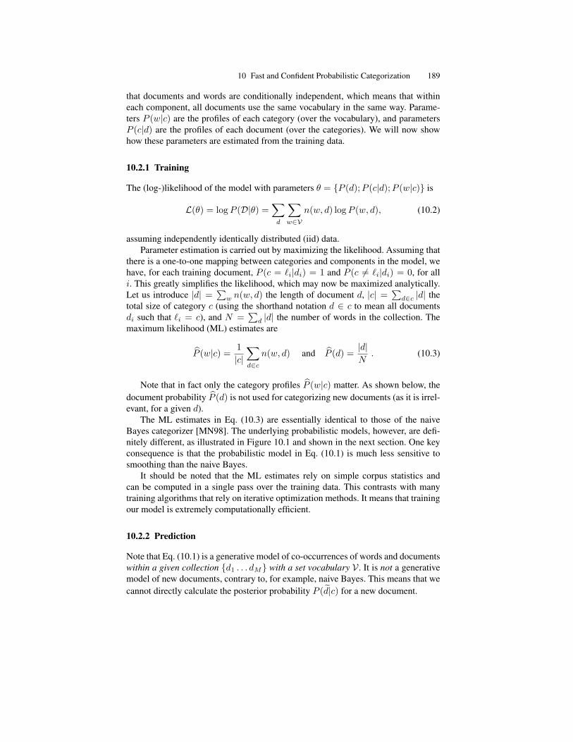
10 Fast and Confident Probabilistic Categorization 189
that documents and words are conditionally independent, which means that withineach component, all documents use the same vocabulary in the same way. Parame-ters P (w|c) are the profiles of each category (over the vocabulary), and parametersP (c|d) are the profiles of each document (over the categories). We will now showhow these parameters are estimated from the training data.
10.2.1 Training
The (log-)likelihood of the model with parameters θ = {P (d);P (c|d);P (w|c)} is
L(θ) = logP (D|θ) =∑d
∑w∈V
n(w, d) logP (w, d), (10.2)
assuming independently identically distributed (iid) data.Parameter estimation is carried out by maximizing the likelihood. Assuming that
there is a one-to-one mapping between categories and components in the model, wehave, for each training document, P (c = `i|di) = 1 and P (c 6= `i|di) = 0, for alli. This greatly simplifies the likelihood, which may now be maximized analytically.Let us introduce |d| =
∑w n(w, d) the length of document d, |c| =
∑d∈c |d| the
total size of category c (using the shorthand notation d ∈ c to mean all documentsdi such that `i = c), and N =
∑d |d| the number of words in the collection. The
maximum likelihood (ML) estimates are
P (w|c) =1|c|∑d∈c
n(w, d) and P (d) =|d|N
. (10.3)
Note that in fact only the category profiles P (w|c) matter. As shown below, thedocument probability P (d) is not used for categorizing new documents (as it is irrel-evant, for a given d).
The ML estimates in Eq. (10.3) are essentially identical to those of the naiveBayes categorizer [MN98]. The underlying probabilistic models, however, are defi-nitely different, as illustrated in Figure 10.1 and shown in the next section. One keyconsequence is that the probabilistic model in Eq. (10.1) is much less sensitive tosmoothing than the naive Bayes.
It should be noted that the ML estimates rely on simple corpus statistics andcan be computed in a single pass over the training data. This contrasts with manytraining algorithms that rely on iterative optimization methods. It means that trainingour model is extremely computationally efficient.
10.2.2 Prediction
Note that Eq. (10.1) is a generative model of co-occurrences of words and documentswithin a given collection {d1 . . . dM} with a set vocabulary V . It is not a generativemodel of new documents, contrary to, for example, naive Bayes. This means that wecannot directly calculate the posterior probability P (d|c) for a new document.

190 C. Goutte
d
c
wdocument document
w
c
d
Our modelNaive Bayes
collection collection
Fig. 10.1. Graphical models for naive Bayes (left) and for the probabilistic model used here(right).
We obtain predictions by folding in the new document in the collection. As doc-ument d is folded in, the following parameters are added to the model: P (d) andP (c|d),∀c. The latter are precisely the probabilities we are interested in for predict-ing the category labels. As before, we use a maximum likelihood (ML) approach,maximizing the likelihood for the new document:
L =∑w
n(w, d) logP (d)∑c
P (c|d)P (w|c) (10.4)
with respect to the unknown parameters P (c|d).The likelihood may be maximized using a variant of the expectation maximiza-
tion (EM) (cf. [DLR77]) algorithm. It is similar to the EM used for estimating thePLSA model (see [Hof99, GGPC02]), with the constraint that the category profilesP (w|c) are kept fixed. The iterative update is given by
P (c|d)← P (c|d)∑w
n(w, d)
|d|P (w|c)∑
c P (c|d)P (w|c). (10.5)
The likelihood (Eq. (10.4)) is guaranteed to be strictly increasing with every EMstep, therefore Eq. (10.5) converges to a (local) minimum. In the general case ofunsupervised learning, the use of deterministic annealing [RGF90] during parameterestimation helps reduce sensitivity to initial conditions and improves convergence(cf. [Hof99, GGPC02]). Note, however, that as we only need to optimize over asmall set of parameters, such annealing schemes are typically not necessary at theprediction stage. Upon convergence, the posterior probability estimate for P (c|d)may be used as a basis for assigning the final category label(s) to document d.
Readers familiar with nonnegative matrix factorization (NMF) (cf. [LS99]) willhave noticed that Eq. (10.5) is very similar to one of the update rules used for estimat-ing the NMF that minimizes a KL-type divergence between the data and the model.

10 Fast and Confident Probabilistic Categorization 191
Indeed, the unsupervised counterpart to our model, PLSA, is essentially equivalentto NMF in this context [GG05a]. Therefore, another way of looking at the catego-rization model described in this chapter is in fact to view it as a constrained NMFproblem, with the category labels providing the constraint on one of the factors (theloading).
The way the prediction is obtained also sheds some light on the difference be-tween our method and a naive Bayes categorizer. In naive Bayes, a category is as-sociated with a whole document, and all words from this document must then begenerated from this category. The occurrence of a word with a low probability inthe category profile will therefore impose an overwhelming penalty to the categoryposterior P (c|d). By contrast, the model we use here assigns a category c to eachco-occurrence (w, d), which means that each word may be sampled from a differ-ent category profile. This difference manifests itself in the re-estimation formula forP (c|d), Eq. (10.5), which combines the various word probabilities as a sum. As aconsequence, a very low probability word will have little influence on the poste-rior category probability and, more importantly, will not impose an overwhelmingpenalty. This key difference also makes our model much less sensitive to probabilitysmoothing than naive Bayes. This means that we do not need to set extra parametersfor the smoothing process. In fact, up to that point, we do not need to set any extrahyperparameter in either the training or the prediction phases.
As an aside, it is interesting to relate our method to the two paradigms of induc-tive and transductive learning [Vap98]. The training phase seems typically inductive:we optimize a cost function (the likelihood) to obtain one optimal model. Note, how-ever, that this is mostly a model of the training data, and it does not provide directlabeling for any document outside the training set. At the prediction stage, we per-form another optimization, this time over the labeling of the test document. This is infact quite similar to transductive learning. As such, it appears that our probabilisticmodel shares similarities with both learning paradigms.
We will now address two important issues of the Anomaly Detection/Text Miningcompetition that require some extensions to the basic model that we have presented.Multilabel categorization is addressed in Section 10.2.3 and the estimation of a pre-diction confidence is covered in Section 10.2.4.
10.2.3 Multiclass, Multilabel Categorization
So far, the model we have presented is strictly a multiclass, single-label categoriza-tion model. It can handle more than two classes (C > 2), but the random variable cindexing the categories takes a single value in a discrete set of C possible categories.
The Anomaly Detection/Text Mining competition is a multiclass, multilabel cat-egorization problem; that is, each document may belong to multiple categories. Infact, although most documents have only one or two labels, one document, number4898, has 10 labels (out of 22), and five documents have exactly nine labels.
One principled way to extend our model to handle multiple labels per documentis to consider all observed combinations of categories and use these combinationsas single “labels,” as described in [McC99]. On the competition data, however, there

192 C. Goutte
are 1151 different label combinations with at least one associated document. Thismakes this approach hardly practical. An additional issue is that considering labelcombinations independently, one may miss some dependencies between single cate-gories. That is, one can expect that combinations (C4, C5, C10) and (C4, C5, C11)may be somewhat dependent as they share two out of three category labels. This isnot modeled by the basic “all model combinations” approach. Although dependen-cies may be introduced as described, for example, in [GG06], this adds another layerof complexity to the system. In our case, the number of dependencies to considerbetween the 1151 observed label combinations is overwhelming.
Another approach is to reduce the multiple labeling problem to a number of bi-nary categorization problems. With 22 possible labels, we would therefore train 22binary categorizers and use them to make 22 independent labeling decisions. This isan appealing and usually successful approach, especially with powerful binary cat-egorizers such as support vector machines [Joa98]. However, it still mostly ignoresdependencies between the individual labels (for example, the fact that labels C4 andC5 are often observed together), and it multiplies the training effort by the numberof labels (22 in our case).
Our approach is actually somewhat less principled than the alternatives men-tioned above, but a lot more straightforward. We rely on a simple threshold a ∈ [0; 1]and assign any new document d to all categories c such that P (c|d) ≥ a. In addition,as all documents in the training set have at least one label, we make sure that d alwaysgets assigned the label with the highest P (c|d), even if this maximum is below thethreshold. This threshold is combined with the calculation of the confidence level, asexplained in the next section.
10.2.4 Confidence Estimation
A second important issue in the Anomaly Detection/Text Mining competition is thatlabeling has to be provided with an associated confidence level.
The task of estimating the proper probability of correctness for the output ofa categorizer is sometimes called calibration [ZE01]. The confidence level is thenthe probability that a given labeling will indeed be correct, that is, labels with aconfidence of 0.8 will be correct 80% of the time. Unfortunately, there does not seemto be any guarantee that the cost function used for the competition will be optimizedby a “well-calibrated” confidence (cf. Section 10.3.2 below). In fact, there is alwaysa natural tension between calibration and performance. Some perfectly calibratedcategorizers can show poor performance; conversely, some excellent categorizers(for example, support vector machines) may be poorly or not calibrated.
Accordingly, instead of seeking to calibrate the categorizer, we use the providedscore function, Checker.jar, to optimize a function that outputs the confidence level,given the probability output by the categorizer. In fields like speech recognition, andmore generally in natural language processing, confidence estimation is often doneby adding an additional machine learning layer to the model [GIY97, GFL06], usingthe output of the model and possibly additional external features measuring the levelof difficulty of the task. We adopt a similar approach, but use a much simpler model.

10 Fast and Confident Probabilistic Categorization 193
Confidence vs. posterior probability
P(c|d)
Con
fiden
ce0 a 1
0b
1
label=1label=−1
Fig. 10.2. The piecewise linear function used to transform the posterior probability into aconfidence level.
The confidence layer transforms the conditional probability output by the model,P (c|d), into a proper confidence measure by using a piecewise linear function withtwo parameters (Figure 10.2). One parameter is the probability threshold a, whichdetermines whether a label is assigned or not; the second is a baseline confidencelevel b, which determines what confidence we give a document that is around thethreshold. The motivation for the piecewise-linear shape is that it seems reasonablethat the confidence is a monotonic function of the probability; that is, if two docu-ments d1 and d2 are such that a < P (c|d1) < P (c|d2), then it makes sense to give d2
a higher confidence to have label c than d1. Using linear segments is a parsimoniousway to implement this assumption.
Let us note that the entire model, including the confidence layer, relies on onlytwo learning parameters, a and b. These parameters may be optimized by maximizingthe score obtained on a prediction set or a cross-validation estimator, as explainedbelow.
10.2.5 Category Description
The model relies on probabilistic profiles P (w|c) that represent the probability ofeach word of the vocabulary to be observed in documents of category c. These pro-files allow us to identify which words are more typical of each category, and thereforemay provide a way to interpret the data by providing descriptive keywords for eachcategory.
Notice that the simplest way of doing this, by focusing on words w with thehighest probabilities P (w|c), is not very efficient. First of all, the probability profileis linked to the frequency of words in the training corpus (Eq. (10.3)), and high-frequency words tend to be grammatical (“empty”) words with no descriptive con-tent. Even when grammatical words have been filtered out, words typical of the gen-

194 C. Goutte
eral topic of the collection (e.g., related to planes and aviation in the contest corpus,see below) will tend to have high frequency in many categories.
To identify words that are typical of a class c, we need to identify words that arerelatively more frequent in c than in the rest of the categories. One way of doing thatis to contrast the profile of the category P (w|c) and the “profile” for the rest of thedata, that is, P (w|¬c) ∝
∑γ 6=c P (w|γ). We express the difference between the two
distributions by the symmetrized Kullback-Leibler divergence:
KL(c,¬c) =∑w
(P (w|c)− P (w|¬c)) logP (w|c)P (w|¬c)︸ ︷︷ ︸
kw
. (10.6)
Notice that the divergence is an additive sum of word-specific contributions kw.Words with a large value of kw contribute the most to the overall divergence, andhence to the difference between category c and the rest. As a consequence, we pro-pose as keywords the words w for which P (w|c) > P (w|¬c) and kw is the largest.2
In the following section, we will see how this strategy allows us to extract keywordsthat are related to the actual description of the categories.
10.3 Experimental Results
We will now describe some of our experiments in more details and give some resultsobtained both for the estimated prediction performance, using only the training dataprovided for the competition, and on the test set using the labels provided after thecompetition.
10.3.1 Data
The available training data consists of 21,519 reports categorized in up to 22 cate-gories. Some limited preprocessing was performed by the organizers, such as tok-enization, stemming, acronym expansion, and removal of places and numbers. Thispreprocessing makes it nontrivial for participants to leverage their own in-house lin-guistic preprocessing. On the other hand, it places contestants on a level playingfield, which puts the emphasis on differences in the actual categorization method, asopposed to differences in preprocessing.3
The only additional preprocessing we performed on the data was stop-word re-moval, using a list of 319 common words. Similar lists are available many places onthe Internet. After stop-word removal, documents were indexed in a bag-of-wordsformat by recording the frequency of each word in each document.
To obtain an estimator of the prediction error, we organized the data in a 10-fold cross-validation manner. We randomly reordered the data and formed 10 splits:
2 Alternatively, we can rank words according to kw = kwsign(P (w|c)− P (w|¬c)).3 In our experience, differences in preprocessing typically yield larger performance gaps than
differences in categorization method.

10 Fast and Confident Probabilistic Categorization 195
nine containing 2152 documents, and one with 2151 documents. We then trained acategorizer using each subset of nine splits as training material, as described in Sec-tion 10.2.1, and produced predictions on the remaining split, as described in Section10.2.2. As a result, we obtain 21,519 predictions on which we optimized parametersa and b.
Note that the 7077 test data on which we obtained the final results reported be-low were never used during the estimation of either model parameters or additionaldecision parameters (thresholds and confidence levels).
10.3.2 Results
The competition was judged using a specific cost function combining prediction per-formance and confidence reliability. For each category c, we compute the area underthe ROC curve,Ac, for the categorizer.Ac lies between 0 and 1, and is usually above0.5. In addition, for each category c, denote tic ∈ {−1,+1} the target label fordocument di, yic ∈ {−1,+1} the predicted label and qic ∈ [0; 1] the associatedconfidence. The final cost function is
Q =1C
C∑c=1
(2Ac − 1) +1M
M∑i=1
qicticyic . (10.7)
Given predicted labels and associated confidence, the reference script Checker.jarprovided by the organizers computes this final score. A perfect prediction with 100%confidence yields a final score of 2, while a random assignment would give a finalscore of around 0.
Using the script Checker.jar on the cross-validated predictions, we optimizeda and b using alternating optimizations along both parameters. The optimal valuesused for our submission to the competition are a = 0.24 and b = 0.93, indicatingthat documents are labeled with all categories that have a posterior probability higherthan 0.24, and the minimum confidence is 0.93. This seems like an unusually highbaseline confidence (i.e., we label with at least 93% confidence). However, this isnot surprising if one considers the expression of the cost function (Eq. (10.7)) moreclosely. The first part is the area under the curve, which depends only on the ordering.Although the ordering is based on the confidence levels, it only depends on the rela-tive, not the absolute, values. For example, with our confidence layer, the ordering ispreserved regardless of the value of b, up to numerical precision.
On the other hand, the second part of the cost function (Eq. (10.7)) directly in-volves the confidence estimates qic. The value of this part will increase if we canreliably assign high confidence (qic ≈ 1) to correctly labeled documents (tic = yic)and low confidence (qic ≈ 0) to incorrectly labeled documents (tic 6= yic). However,if we could reliably detect such situations, we would arguably be better off swappingthe label rather than downplay its influence by assigning it low confidence. So as-suming we cannot reliably do so, that is, qic and ticyic are independent, the secondpart of the cost becomes approximately equal to q(2×MCE−1), with q the averageconfidence and MCE the misclassification error, MCE = 1/M
∑i(tic 6= yic). So

196 C. Goutte
a
b
0.1 0.2 0.3 0.40.
60.
70.
80.
9 Max. scoreCV
Fig. 10.3. Score for various combinations of a and b. The best (maximum) test score is indi-cated as a cross, the optimum estimated by cross-validation (CV) is a = 0.24 and b = 0.93,indicated by a circle.
the optimal strategy under this assumption is to make q as high as possible by settingqic as close to 1 as possible, while keeping the ordering intact. This explains why arelatively high value of b turned out to be optimal. In fact, using a higher precisionin our confidence levels, setting b to 0.99 or higher yields even better results.4
Using the setting a = 0.24 and b = 0.93, the cross-validated cost is about 1.691.With the same settings, the final cost on the 7077 test documents is 1.689, showing anexcellent agreement with the cross-validation estimate. To illustrate the sensitivity ofthe performance to the setting of the two hyperparameters a and b, we plot the finalcost obtained for various combinations of a and b, as shown in Figure 10.3. Theoptimal setting (cross) is in fact quite close to the cross-validation estimate (circle).In addition, it seems that the performance of the system is not very sensitive to theprecise values of a and b. Over the range plotted in Figure 10.3, the maximal score(cross) is 1.6894, less than 0.05% above the CV-optimized value, and the lowestscore (bottom left) is 1.645, 2.5% below. This means that any setting of a and b inthat range would have been within 2.5% of the optimum.
We also measured the performance using some more common and intuitive met-rics. For example, the overall mislabeling error rate is 7.22%, and the micro-averagedF -score is a relatively modest 50.05%.
Note, however, that we have used a single confidence layer, and in particular asingle labeling threshold a, for all categories. Closer inspection of the performanceon each category shows quite a disparity in performance, and in particular in pre-4 Note, however, that setting b to higher value only yields marginal benefits in terms of final
cost.

10 Fast and Confident Probabilistic Categorization 197
Table 10.1. Performance of the probabilistic model: precision, recall, and F -score for eachof the 22 categories. Low (< 50%) scores are in italics and high (> 75%) scores are in bold.Column “# docs” contains the number of test documents with the corresponding label.
Category #docs p (%) r (%) F (%)C1 435 64.99 83.22 72.98C2 3297 46.72 99.57 63.60C3 222 74.06 79.73 76.79C4 182 52.15 59.89 55.75C5 853 80.07 75.38 77.66C6 1598 51.33 80.98 62.83C7 546 36.38 77.29 49.47C8 631 55.32 67.51 60.81C9 168 59.30 60.71 60.00
C10 349 37.21 58.74 45.56C11 161 77.44 63.98 70.06
Category #docs p (%) r (%) F (%)C12 918 72.02 79.08 75.39C13 687 51.21 55.46 53.25C14 393 68.73 70.48 69.60C15 183 30.61 24.59 27.27C16 314 32.93 60.83 42.73C17 162 45.22 43.83 44.51C18 351 57.30 58.12 57.71C19 1767 61.54 80.42 69.73C20 229 72.40 69.87 71.11C21 137 78.79 56.93 66.10C22 233 88.66 73.81 80.56
cision and recall, across the categories.5 This suggests that the common value ofthe threshold a may be too high for some categories (hence low recall) and too lowfor others (hence low precision). Using the cross-validated prediction, we thereforeoptimized some category-specific thresholds using various metrics:
• Maximum F -score• Break-even point (i.e., point at which precision equals recall)• Minimum error rate
For example, for maximum F -score, we optimized 22 thresholds, one per category,by maximizing the F -score for each category on the cross-validated predictions.
Table 10.1 shows the performance obtained on the test data for all 22 categories,using category-specific, maximum F -score optimized thresholds. Performance is ex-pressed in terms of the standard metrics of precision, recall, and F-score. The per-formance varies a lot depending on the category. However, there does not seem tobe any systematic relation between the performance and the size of the categories.The worst, but also the best performance are observed on small categories (less that250 positive test documents). This suggests that the variation in performance maybe simply due to varying intrinsic difficulty of modeling the categories. The best F-scores are observed on categories C3, C5, C12 and C22, while categories C15, C16,C17, C10 and C7 get sub-50% performance.
The average performance is presented in Table 10.2 for our submission to thecompetition, as well as for three different strategies for optimizing a category-per-category threshold. One weakness of the original submission was the low recall,due to the fact that a single threshold was used for all 22 categories. This producesa relatively low average F -score of 50.05%. By optimizing the threshold for each5 Precision estimates the probability that a label provided by the model is correct, while
recall estimates the probability that a reference label is indeed returned by the model[GG05b]. F-score is the harmonic average of precision and recall.

198 C. Goutte
Table 10.2. Micro-averaged performance for our contest submission, and three threshold opti-mization strategy. Highest is best for precision (p), recall (r), F -score (F ), and final cost (Eq.(10.7)), and lowest is best for misclassification error (MCE).
p (%) r (%) F (%) MCE (%) Final costOur submission 64.87 40.74 50.05 7.22 1.689Maximum F-score 53.30 78.55 63.51 8.01 1.678Break-even point 58.88 67.35 62.83 7.07 1.697Minimum error 61.53 62.37 61.95 6.80 1.702
category over various performance measures, we largely improve over that. Not sur-prisingly, optimizing the thresholds for F -scores yields the best F -score of 63.51%,although both the misclassification error and the final cost degrade using this strat-egy. Optimizing the threshold for reducing the misclassification error reduces the testmisclassification error6 to 6.80% and improves the final cost slightly, to 1.702. Note,however, that despite a large impact on F -score and MCE, using category-specificdecision thresholds optimized over various thresholds seems to have little impact onthe final cost, which stays within about 0.8% of the score of our submission.
10.3.3 Category Description
The only information provided by the organizers at the time of the contest was thelabeling for each document, as a number between 1 and 22. These data, therefore,seemed like a good test bed for applying the category description technique describedabove, and to see whether the extracted keywords brought any information on thecontent of the categories.
Table 10.3 shows the results we obtained on about half the categories by extract-ing the top five keywords. For comparison, we also extracted the five words withhighest probability (first column), and we also give the official category descriptionfrom the Distributed National Aviation Safety Action Program Archive (DNAA),which was released after the competition.
Based on only five keywords, the relevance of the keywords provided by eitherhighest probability or largest divergence and their mapping to the official categorydescriptions are certainly open to interpretation. The most obvious problem with thechoice of the highest probability words, however, is that the same handful of key-words seem to appear in almost all categories. The words “aircraft” is among thetop-five probability in 19 out of 22 categories! Although it is obviously a very rele-vant and common word for describing issues dealing with aviation, it is clearly notvery useful to discriminate the content of one category versus the others. The otherfrequent members of the top-five highest probability are: runway (14 times), air-port (11), approach (11), feet (9), and land (9). These tend to “pollute” the keywordextraction. For example, in category C8 (course deviation), three out of the five high-est probability keywords are among these frequent keywords and bring no relevant6 For 7077 test documents with 22 possible labels, reducing the MCE by 0.1% corresponds
to correcting 156 labeling decisions.

10 Fast and Confident Probabilistic Categorization 199
Table 10.3. Keywords extracted for 12 of the contest categories using either the highest prob-ability words or the largest contributions to the KL divergence; for comparison, the officialdescription from the DNAA, released after the competition, is provided.
Category Highestprobability
Largestdivergence
Official DNAA category description
C1 aircraftmaintainminimumequip-mentlistcheck flight
minimumequip-mentlistmaintaininstall deferinspect
Airworthiness/documentation event: An eventinvolving a incorrect or incomplete airworthi-ness or documentation requirement
C2 aircraftrunwayairportfeetapproach
securityflightboardagentairspace
Operation in noncompliance—FARs, pol-icy/procedures: An event involving a viola-tion, deviation, or noncompliance by the crewwhich involved a policy, procedure, or FAR
C3 runway takeoffaircraft cleartower
takeoff abortrunway rejectroll
Rejected takeoff: An event involving a re-jected takeoff
C4 runwayaircraft landtaxiway left
brake taxiwayrunwaydamage grass
Excursion: An event involving the loss of con-trol or inadvertent control of an aircraft fromthe designated airport surface
C5 runwayaircrafttaxiwaytaxi hold
runwaytaxiwaytaxi holdshort
Incursion: An event involving a vehicle, per-son, object or other aircraft that creates a col-lision hazard or results in loss of separationwith an aircraft
C8 runway turnairport degreeapproach
degree turnhead radialcourse
Course deviation: An event involving a devia-tion from an assigned or planned course
C9 feet knotaircraftapproachspeed
knot speedslow knotsindi-catedairspeedairspeed
Speed deviation: An event involving a devia-tion from a planned or assigned air speed
C10 aircraftrunwayapproachland feet
brake knotwind autopilotdamage
Uncommanded/unintended state or loss ofcontrol: An event involving an uncommanded,unintended state or loss of control of the air-craft
C11 approach feetairport runwaydescend
approachgroundproximi-tywarningsys-tem terrain feetglideslope
Terrain proximity event: An event involvingthe aircraft operating in close proximity to ter-rain
C13 airport feetapproachaircraftrunway
weatherturbulent cloudencounter icethunderstorm
Weather issue/ weather proximity event: Anevent involving a weather issue or aircraft op-erating in proximity to weather
descriptive information. The remaining two keywords, “turn” and “degree,” on theother hand, seem like reasonable keywords to describe course deviation problems.

200 C. Goutte
By contrast, the five words contributing to the largest divergence, “degree,” “turn,”“head,” “radial,” and “course,” appear as keywords only for this category, and theyall seem topically related to the corresponding problem. For the largest divergencemetric, kw, the word selected most often in the top-five is “runway,” which describessix categories containing problems related to takeoff or landing (e.g., C3, C4, C5,and C6). Other top-five keywords appear in at most four categories. This suggeststhat using kw instead of P (w|c) yields more diverse and more descriptive keywords.
This is also supported by the fact that only 32 distinct words are used in the top-five highest probability keywords over the 22 categories, while the top-five largestkw selects 83 distinct words over the 22 categories. This further reinforces the factthat kw will select more specific keywords, and discard the words that are commonto all categories in the corpus.
This is well illustrated on category C13 (Weather Issue). The top-five probabilitywords are all among the high probability words mentioned above. By contrast, thetop-5 kw are all clearly related to the content of category C13, such as “weather,”“cloud,” “ice,” and “thunderstorm.”
Overall, we think that this example illustrates the shortcomings of the choice ofthe highest probability words to describe a category. It supports our proposition touse instead words that contribute most to the divergence between one category andthe rest. These provide a larger array of keywords and seem more closely related tothe specificities of the categories they describe.
10.4 Summary
We have presented the probabilistic model that we used in NRC’s submission to theAnomaly Detection/Text Mining competition at the Text Mining Workshop 2007.This probabilistic model may be estimated from preprocessed, indexed, and labeleddocuments with no additional learning parameters, and in a single pass over the data.This makes it extremely fast to train. On the competition data, in particular, the train-ing phase takes only a few seconds on a current laptop. Obtaining predictions for newtest documents requires a bit more calculations but is still quite fast. One particularlyattractive feature of this model is that the probabilistic category profiles can be usedto provide descriptive keywords for the categories. This is useful in the common sit-uation where labels are known only as codes and the actual content of the categoriesmay not be known to the practitioner.
The only training parameters we used are required for tuning the decision layer,which selects the multiple labels associated to each document, and estimates theconfidence in the labeling. In the method that we implemented for the competition,these parameters are the labeling threshold and the confidence baseline. They areestimated by maximizing the cross-validated cost function.
Performance on the test set yields a final score of 1.689, which is very close to thecross-validation estimate. This suggests that despite its apparent simplicity, the prob-abilistic model provides a very efficient categorization. This is actually corroboratedby extensive evidence on multiple real-life use cases.

10 Fast and Confident Probabilistic Categorization 201
The simplicity of the implemented method, and in particular the somewhat rudi-mentary confidence layer, suggests that there may be ample room for improving theperformance. One obvious issue is that the ad-hoc layer used for labeling and esti-mating the confidence may be greatly improved by using a more principled approach.One possibility would be to train multiple categorizers, both binary and multicate-gory. Then use the output of these categorizers as input to a more complex modelcombining this information into a proper decision associated with a better confi-dence level. This may be done, for example, using a simple logistic regression. Notethat one issue here is that the final score used for the competition, Eq. (10.7), com-bines a performance-oriented measure (area under the ROC curve) and a confidence-oriented measure. As a consequence, and as discussed above, there is no guaranteethat a well-calibrated classifier will in fact optimize this score. Also, this suggeststhat there may be a way to invoke multiobjective optimization in order to furtherimprove the performance.
Among other interesting topics, let us mention the sensitivity of the method tovarious experimental conditions. In particular, although we have argued that ourprobabilistic model is not very sensitive to smoothing, it may very well be that aproperly chosen smoothing, or similarly, a smart feature selection process, may fur-ther improve the performance. In the context of multilabel categorization, let us alsomention the possibility to exploit dependencies between the classes, for example,using an extension of the method described in [RGG+06].
References
[DLR77] A.P. Dempster, N.M. Laird, and D.B. Rubin. Maximum likelihood from incom-plete data via the EM algorithm. Journal of the Royal Statistical Society, Series B,39(1):1–38, 1977.
[GFL06] S. Gandrabur, G. Foster, and G. Lapalme. Confidence estimation for NLP applica-tions. ACM Transactions on Speech and Language Processing,, 3(3):1–29, 2006.
[GG05a] E. Gaussier and C. Goutte. Relation between PLSA and NMF and implications.In Proceedings of the 28th Annual International ACM SIGIR Conference, pages601–602, ACM Press, New York, 2005.
[GG05b] C. Goutte and E. Gaussier. A probabilistic interpretation of precision, recall and F-score, with implication for evaluation. In Advances in Information Retrieval, 27thEuropean Conference on IR Research (ECIR 2005), pages 345–359. Springer, NewYork, 2005.
[GG06] C. Goutte and E. Gaussier. Method for multi-class, multi-label categorization usingprobabilistic hierarchical modeling. US Patent 7,139,754, granted November 21,2006.
[GGPC02] E. Gaussier, C. Goutte, K. Popat, and F. Chen. A hierarchical model for clusteringand categorising documents. In Advances in Information Retrieval, Lecture Notesin Computer Science, pages 229–247. Springer, New York, 2002.
[GIY97] L. Gillick, Y. Ito, and J. Young. A probabilistic approach to confidence estimationand evaluation. In ICASSP ’97: Proceedings of the 1997 IEEE International Con-ference on Acoustics, Speech, and Signal Processing, volume 2, pages 879–882,IEEE, Los Alamitos, CA, 1997.

202 C. Goutte
[Hof99] T. Hofmann. Probabilistic latent semantic analysis. In K.B. Laskey and H. Prade,editors, UAI ’99: Proceedings of the Fifteenth Conference on Uncertainty in Arti-ficial Intelligence, pages 289–296. Morgan Kaufmann, San Francisco, 1999.
[Joa98] T. Joachims. Text categorization with suport vector machines: learning withmany relevant features. In Claire Nedellec and Celine Rouveirol, editors, Pro-ceedings of ECML-98, 10th European Conference on Machine Learning, vol-ume 1398 of Lecture Notes in Computer Science, pages 137–142. Springer, NewYork, 1998. Available from World Wide Web: citeseer.ist.psu.edu/joachims97text.html.
[LS99] D. Lee and H. Seung. Learning the parts of objects by non-negative matrix factor-ization. Nature, 401:788–791, 1999.
[McC99] A. McCallum. Multi-label text classification with a mixture model trained by EM.In AAAI’99 Workshop on Text Learning, 1999.
[MN98] A. McCallum and K. Nigam. A comparison of event models for naive Bayes textclassification. In AAAI/ICML-98 Workshop on Learning for Text Categorization,pages 41–48, AAAI Press, Menlo Park, CA, 1998.
[RGF90] K. Rose, E. Gurewitz, and G. Fox. A deterministic annealing approach to cluster-ing. Pattern Recognition Letters, 11(11):589–594, 1990.
[RGG+06] J.-M. Renders, E. Gaussier, C. Goutte, F. Pacull, and G. Csurka. Categorization inmultiple category systems. In Machine Learning, Proceedings of the Twenty-ThirdInternational Conference (ICML 2006), pages 745–752, ACM Press, New York,2006.
[Vap98] V.N. Vapnik. Statistical Learning Theory. Wiley, New York, 1998.[ZE01] B. Zadrozny and C. Elkan. Obtaining calibrated probability estimates from deci-
sion trees and naive bayesian classifiers. In Proceedings of the Eighteenth Inter-national Conference on Machine Learning (ICML 2001), pages 609–616, MorganKaufmann, San Francisco, 2001.

11
Anomaly Detection Using Nonnegative MatrixFactorization
Edward G. Allan, Michael R. Horvath, Christopher V. Kopek, Brian T. Lamb,Thomas S. Whaples, and Michael W. Berry
Overview
For the Text Mining 2007 Workshop contest (see Appendix), we use the nonnega-tive matrix factorization (NMF) to generate feature vectors that can be used to clusterAviation Safety Reporting System (ASRS) documents. By preserving non-negativity,the NMF facilitates a sum-of-parts representation of the underlying term usage pat-terns in the ASRS document collection. Both the training and test sets of ASRSdocuments are parsed and then factored by the NMF to produce a reduced-rank rep-resentation of the entire document space. The resulting feature and coefficient matrixfactors are used to cluster ASRS documents so that the (known) anomalies of train-ing documents are directly mapped to the feature vectors. Dominant features of testdocuments are then used to generate anomaly relevance scores for those documents.The General Text Parser (GTP) software environment is used to generate term-by-document matrices for the NMF model.
11.1 Introduction
Nonnegative matrix factorization (NMF) has been widely used to approximate high-dimensional data comprised of nonnegative components. Lee and Seung [LS99] pro-posed the idea of using NMF techniques to generate basis functions for image datathat could facilitate the identification and classification of objects. They also demon-strated the use of NMF to extract concepts/topics from unstructured text documents.This is the context that we exploit the so-called sum-of-parts representation offeredby the NMF for the Aviation Safety Reporting System (ASRS) document collection.
Several manuscripts have cited [LS99], but as pointed out in [BBL+07] thereare several (earlier) papers by P. Paatero [Paa97, Paa99, PT94] that documented thehistorical development of the NMF. Simply stated, the problem defining the NMF isas follows:
Given a nonnegative matrix A ∈ Rm×n and a positive integer k < min{m,n},find nonnegative matrices W ∈ Rm×k and H ∈ Rk×n to minimize the functional

204 E.G. Allan, M.R. Horvath, C.V. Kopek, B.T. Lamb et al.
f(W,H) =12‖A−WH‖2F. (11.1)
The product WH is called a nonnegative matrix factorization of A, althoughA is not necessarily equal to the product WH. Although the product WH is anapproximate factorization of rank at most k, we will drop the word approximate inour NMF discussions below. The best choice for the rank k is certainly problemdependent, and in most cases it is usually chosen such that k � min(m,n). Hence,the product WH can be considered a compressed form of the data in A.
Another key characteristic of NMF is the ability of numerical methods that mini-mize Eq. (11.1) to extract underlying features as basis vectors in W, which can thenbe subsequently used for identification and classification. By not allowing negativeentries in W and H, NMF enables a non-subtractive combination of parts to forma whole [LS99]. Features may be parts of faces in image data, topics or clusters intextual data, or specific absorption characteristics in hyperspectral data. In this chap-ter, we discuss the enhancement of NMF algorithms for the primary goal of featureextraction and identification in text and spectral data mining.
Important challenges affecting the numerical minimization of Eq. (11.1) includethe existence of local minima due to the nonconvexity of f(W,H) in both W andH. The nonuniqueness of its solution is easily realized by noting that WDD−1Hfor any nonnegative invertible matrix D whose inverse, D−1, is also nonnegative.Fortunately, the NMF is still quite useful for text/data mining in practice since evenlocal minima can provide desirable data compression and feature extraction as willbe demonstrated in this contest entry.
Alternative formulations of the NMF problem certainly arise in the literature. Assurveyed in [BBL+07], an information theoretic formulation in [LS01] is based onthe Kullback–Leibler divergence of A from WH, and the cost functions proposed in[CZA06] are based on Csiszar’s ϕ-divergence. A formulation in [WJHT04] enforcesconstraints based on the Fisher linear discriminant analysis, and [GBV01] suggestsusing a diagonal weight matrix Q in the factorization model, AQ ≈ WHQ, asan attempt to compensate for feature redundancy1 in the columns of W. For otherapproaches using alternative cost functions, see [HB06] and [DS05].
To speed up convergence of Lee and Seung’s (standard) NMF iteration, variousalternative minimization strategies for Eq. (11.1) have been suggested. For example,[Lin05b] proposes the use of a projected gradient bound-constrained optimizationmethod that presumably has better convergence properties than the standard mul-tiplicative update rule approach. However, the use of certain auxiliary constraintsin Eq. (11.1) may break down the bound-constrained optimization assumption andthereby limit the use of projected gradient methods. Accelerating the standard ap-proach via an interior-point gradient method has been suggested in [GZ05], and aquasi-Newton optimization approach for updating W and H, where negative valuesare replaced with small positive ε parameter to enforce nonnegativity, is discussed in1 Such redundancy can also be alleviated by using column stochastic constraints on H
[PPA07].

11 Nonnegative Matrix Factorization 205
[ZC06]. For a more complete overview of enhancements to improve the convergenceof the (standard) NMF algorithm, see [BBL+07].
Typically, W and H are initialized with random nonnegative values to start thestandard NMF algorithm. Another area of NMF-related research has focused on al-ternate approaches for initializing or seeding the algorithm. The goal, of course, is tospeed up convergence. In [WCD03] spherical k-means clustering is used to initializeW and in [BG05] singular vectors of A are used for initialization and subsequentcost function reduction. Optimal initialization, however, remains an open researchproblem.
11.2 NMF Algorithm
As surveyed in [BBL+07], there are three general classes of NMF algorithms:multiplicative update algorithms, gradient descent algorithms, and alternating leastsquares algorithms. For this study, we deployed the most basic multiplicative updatemethod (initially described in [LS01]). This approach, based on a mean squared errorobjective function, is illustrated below using MATLAB R©array operator notation:
Algorithm 11.2.1 Multiplicative Update Algorithm for NMFW = rand(m,k); % W initially randomH = rand(k,n); % H initially randomfor i = 1 : maxiter
H = H .* (WTA) ./ (WTWH + ε);W = W .* (AHT) ./ (WHHT + ε);
end
The parameter ε = 10−9 is added to avoid division by zero. As explained in[BBL+07], if this multiplicative update NMF algorithm converges to a stationarypoint, there is no guarantee that the stationary point is a local minimum for the ob-jective function. Additionally, if the limit point to which the algorithm has convergedlies on the boundary of the feasible region, we cannot conclude that it is, in fact, a sta-tionary point. A modification of the Lee and Seung multiplicative update scheme thatresolves some of the convergence issues and guarantees convergence to a stationarypoint is provided in [Lin05a].
11.3 Document Parsing and Term Weighting
The General Text Parsing (GTP) software environment [GWB03] (written in C++)was used to parse all the ASRS training and test documents for this contest. LetA = [R|T] = [aij] define an m × n term-by-document matrix, where the subma-trices R and T represent training and test documents, respectively. Each element or

206 E.G. Allan, M.R. Horvath, C.V. Kopek, B.T. Lamb et al.
component aij of the matrix A defines a weighted frequency at which term i occursin document j. We can define aij = lijgidj , where lij is the local weight for term ioccurring in document j, gi is the global weight for term i in the subcollection, anddj is a document normalization factor that specifies whether or not the columns of A(i.e., the documents) are normalized (i.e., have unit length). Let fij be the number oftimes (frequency) that term i appears in document j, and define pij = fij/
∑j fij ,
that is, the empirical probability of term i appearing in document j. Using GTP, wedeploy a log-entropy term-weighting scheme whereby
lij = log(1 + fij) and gi = 1 + (∑j
pij log(pij))/ log n) .
No document normalization was used in parsing ASRS documents, that is, dj = 1for all aij . By default, GTP requires that the global frequency of any term, that is,∑nj=1 fij , be greater than 1 and that a term’s document frequency (or number of
documents containing that term) be greater than 1 as well. No adjustments to thesethresholds were made in parsing the ASRS documents. A stoplist of 493 words2 wasused by GTP to filter out unimportant terms. The minimum and maximum length (incharacters) of any accepted term was 2 and 200, respectively. For the initial trainingset of ASRS documents, GTP extracted m = 15,722 terms from the n = 21,519documents. The elapsed GTP parsing time was 21.335 CPU seconds on a 3.2-GHzIntel Xeon having a 1024-KB cache and 4.1-GB RAM.
11.4 NMF Classifier
The classification of ASRS documents using NMF is outlined in Tables 11.1 and 11.2.Let Hi denote the ith column of matrix H. Some of the constants used include
α, the threshold on the relevance score or (target value) tij for documenti and anomaly/label j;
δ, the threshold on the column elements of H, which will filter out theassociation of features with both the training (R) and test (T) documents;
σ, the percentage of documents used to define the training set (or number ofcolumns of R).
11.4.1 Preliminary Testing
The rank or number of columns of the feature matrix factor W used to test our NMFmodel (prior to contest submission) was k = 40. Hence, the W and H matrix factorswere 15,722×40 and 40×21,519, respectively. The percentage of ASRS documentsused for training (subset R) in our testing was 70% (i.e., σ = .70). Hence, 15,0632 See SMART’s English stoplist at ftp://ftp.cs.cornell.edu/pub/smart/english.stop.

11 Nonnegative Matrix Factorization 207
documents were used as the initial training set (R) and 6,456 documents were usedfor testing (T) our NMF classifier. In step 1 of Table 11.1 we chose δ = .30 forthe columnwise pruning of the elements in the coefficient matrix H. This parametereffectively determines the number of features (among the k = 40 possible) thatany document (training or test) can be associated with. As δ increases, so does thesparsity of H.
The α parameter specified in step 8 of Tables 11.1 and 11.2 was defined to be .40.This is the prediction control parameter that ultimately determines whether or notdocument i will be given label (anomaly) j, that is, whether pij = +1 or pij = −1for the contest cost function
Q =1C
C∑j=1
Qj , (11.2)
Qj = (2Aj − 1) +1D
D∑i=1
qijtijpij , (11.3)
where C is the number of labels (anomalies) and D is the number of test documents.As mentioned above,D = 6,456 for our preliminary evaluation of the NMF classifierand C = 22 (as specified by the TRAINCATEGORYMATRIX.CSV file). The costQ given by Eq. 11.2 for our preliminary NMF testing was always in the interval[1.28, 1.30]. To measure the quality of (anomaly) predictions across all C = 22categories, a figure of merit (FOM) score defined by
FOM =1C
C∑j=1
F − FjF
Qj , F =C∑j=1
Fj , (11.4)
where Fj denotes the frequency of documents having label (anomaly) j, and wasgenerated for each experiment. By definition, the FOM score will assign lowerweights to the higher frequency labels or categories. The best FOM score for σ = .70was 1.267 to three significant decimal digits. Keep in mind that the initial matrix fac-tors W and H are randomly generated and will produce slightly different features(columns of W) and coefficients (columns of H) per NMF iteration.3
11.4.2 Contest Results
For the text mining contest (sponsored by NASA Ames Research Center) at the Sev-enth SIAM International Conference on Data Mining in Minneapolis, MN (April26–28, 2007), all contestants were provided an additional 7,077 ASRS unclassifieddocuments. For the NMF classifier, we treat these new documents as the test subsetT and define the training subset R as all the previously available (classified) docu-ments (21,519 of them). Since all of the previously classified ASRS documents wereused in the term-by-document matrix A for the contest entry, the σ parameter was3 Only five iterations were used in our preliminary study.

208 E.G. Allan, M.R. Horvath, C.V. Kopek, B.T. Lamb et al.
Table11.1.N
MF-based
classifierforASR
Sdocum
entsw
ithcorresponding
MA
TL
AB
R©functions:steps
1–6
StepD
escriptionM
ATL
AB
R©function
call
1Filterelem
entsof
Hgiven
A≈
WH
;hThresh=asrsThreshold(H,DELTA);
fori=
1,...,n
,determine
ηi=
max(H
i )and
zerooutallvalues
inH
i lessthan
ηi ×
(1−
δ).
2N
ormalize
the(new
)filteredm
atrixH
sohNorm=asrsNorm(hThresh,K);
thatallcolumn
sums
arenow
1.
3G
iventhe
releasedsetofA
SRS
documents,generate
[trainBinarySet,testBinarySet]=
asetofindices
(integers)thatwillpartition
theasrsGenerateSet(N,SIGMA);
documents
intothe
training(R
)andtest(T
)subsets.
4G
eneratethe
correspondingsubm
atricesofthe
[hTrainhTestanTrainanTest]=
normalized
Hm
atrixthatcorrespond
toR
(hTrain)
asrsMapSets(hNorm,AN,
andT
(hTest);generate
submatrices
forthetrainBinarySet);
anomaly
matrix
(csvfile)so
thatanTrain
andanTest
arearrays
forthedocum
entsubsetsR
andT
,respectively.
5C
lusterthecolum
nsof
Hcorresponding
todocum
entshClus=asrsClus(hTrain,K);
inthe
trainingset
Rby
known
anomalies
(labels).
6Sum
thenum
berofdocuments
associatedw
itheach
hClusAnom=
anomaly
perNM
Ffeature
(kofthem
);the(i,j)entry
asrsAnomClus(hClus,anTrain,K);
oftheoutputarray
hClusAnom
specifiesthe
number
ofanomaly/label
jdocum
entsrepresented
byfeature
i.

11 Nonnegative Matrix Factorization 209
Tabl
e11
.2.N
MF-
base
dcl
assi
fierf
orA
SRS
docu
men
tsw
ithco
rres
pond
ing
MA
TL
AB
R ©fu
nctio
ns:s
teps
7–10
Step
Des
crip
tion
MAT
LA
BR ©
func
tion
call
7Fo
reac
hdo
cum
enti
nsu
bset
T,p
rodu
cea
scor
ehResults=asrsTesting(hTest,hClus,
(orp
roba
bilit
y)th
atth
edo
cum
enti
sre
leva
ntto
each
hClusAnom,K);
anom
aly;
loop
over
the
num
bero
fNM
Ffe
atur
es(k
ofth
em)u
sing
the
colu
mns
ofth
ehTest
andhClus
arra
ysan
dus
een
trie
sofhTest
asw
eigh
tson
the
rela
tive
freq
uenc
yof
any
anom
aly
foun
din
the
curr
entf
eatu
re.
8U
sing
α,p
rodu
ceth
ere
leva
nce/
targ
etsc
ore
t ij
[prediction,confidence]=
for(
docu
men
ti,a
nom
aly
j)pa
irs
usin
gth
ear
ray
asrsComputePC(hResults,ALPHA);
hResults
;the
scor
ew
illyi
eld
apo
sitiv
epr
edic
tion
ift i
j>
ρi×
(1−
α),
whe
reρ
i=
max(H
T i),
i.e.,
the
max
imum
elem
ento
fthe
row
ofhResults
corr
espo
ndin
gto
docu
men
ti;e
ntri
esof
the
outp
utar
ray
prediction
are
eith
er+
1or−
1to
refle
ctpo
sitiv
eor
nega
tive
pred
ictio
ns,r
espe
ctiv
ely;
theconfidence
arra
yco
ntai
nsth
eas
soci
ated
targ
etva
lues
t ij.
9Pr
oduc
ea
com
pone
nt-w
ise
mat
rix
ofpr
edic
tions
(pij
)[answers,testResults,
times
confi
denc
es(t
ij)i
nth
eou
tput
arra
yanswers
wrongAnswers]=asrsComputeAnR(
that
can
bevi
sual
ized
;cre
ate
outp
utar
rays
ofprediction,confidence,anTest);
corr
ect(testResults
)and
inco
rrec
t(wrongAnswers
)an
swer
sw
here
byro
ws
corr
espo
ndto
docu
men
tsan
dco
lum
nsco
rres
pond
toan
omal
ies
(orl
abel
s).
10G
ener
ate
RO
Ccu
rves
(and
area
sun
dern
eath
)per
fori=1:N
anom
aly
and
eval
uate
the
cont
estc
ostf
unct
ion,
and
[tp,fp]=roc(anTest(:,i),
figur
eof
mer
itsc
ore
hResults(:,i));
rocarea(i)=auroc(tp,fp);
end;
[cost,fom]=asrsCost(anTest,
prediction,confidence,rocarea’);

210 E.G. Allan, M.R. Horvath, C.V. Kopek, B.T. Lamb et al.
set to 1.0. The other two parameters for the NMF classifier were not changed, thatis, α = 0.40 and δ = 0.30 (see Section 11.4.1). Using five iterations and k = 40features for the multiplicative update algorithm mentioned in Section 11.2, a cost ofQ = 1.27 (see Eq. 11.2) was reported by contest officials for the NMF classifierin mapping each of the 7,077 test documents to any of the 22 anomaly categorieswas 1.27 (a second place finish). Had a tie occurred among any of the cost functionvalues generated by contest entries, the FOM score would have been used to breakit. For the NMF classifier, the average contest FOM score was 1.22 (slightly lowerthan what was observed in the preliminary testing phase).
11.4.3 ROC Curves
Figures 11.1 through 11.5 contain the receiver operating characteristic (ROC) curvesfor the NMF classifier, when applied to selected training documents in the prelimi-nary testing phase and to the unclassified test documents in the text mining compe-tition (see Section 11.4.2). A comparison of graphs for the preliminary testing andthe contest entry show similar performance for a majority of the 22 anomaly classes.Some of the best curves of the true-positive rate (TPR) versus the false-positive rate(FPR) were obtained for the following anomalies: 4, 5, 7, 11, 14, 12, 21, and 22. Theworst predictions were obviously for anomalies 2, 10, and 13. In the cases of anoma-lies 7, 11, 15, and 18, the performance obtained in the contest entry (as measured bythe area under the respective ROC curves) was slightly better than that obtained inthe preliminary testing.
Thirteen (of the 22) event types (or anomaly descriptions) listed in Table 11.3were obtained from the Distributed National ASAP Archive (DNAA) maintained bythe University of Texas Human Factors Research Project.4 The generality of topicsdescribed in the ASRS reports of the Noncompliance (anomaly 2), Uncommanded(loss of control) (anomaly 10), and Weather Issue (anomaly 13) categories greatlycontributed to the poorer performance of the NMF classifier. Additional experimentswith a larger numbers of features (k > 40) may produce an NMF model that wouldbetter capture the diversity of contexts described by those events.
11.5 Summary and Future Work
Nonnegative matrix factorization (NMF) is a viable alternative for automated doc-ument classification problems. As the volume and heterogeneity of documentationcontinues to grow, the ability to discern common themes and contexts can be prob-lematic. This study demonstrated how NMF can be used to both learn and assign(anomaly) labels for documents from the ASRS. As this study was done as part of atext mining competition and a project in a data mining course taught at Wake ForestUniversity, there is room for improvement in both the performance and interpretabil-ity of the NMF. In particular, the summarization of anomalies (document classes)4 See http://homepage.psy.utexas.edu/HomePage/Group/HelmreichLAB.

11 Nonnegative Matrix Factorization 211
0 0.1 0.2 0.3 0.4 0.5 0.6 0.7 0.8 0.9 10
0.1
0.2
0.3
0.4
0.5
0.6
0.7
0.8
0.9
1
FPR
TP
R
12345
(a) Preliminary training
0 0.1 0.2 0.3 0.4 0.5 0.6 0.7 0.8 0.9 10
0.1
0.2
0.3
0.4
0.5
0.6
0.7
0.8
0.9
1
FPR
TP
R
12345
(b) Contest performance
Fig. 11.1. ROC curves for the NSF classifier applied to anomalies (labels) 1 through 5.

212 E.G. Allan, M.R. Horvath, C.V. Kopek, B.T. Lamb et al.
0 0.1 0.2 0.3 0.4 0.5 0.6 0.7 0.8 0.9 10
0.1
0.2
0.3
0.4
0.5
0.6
0.7
0.8
0.9
1
FPR
TP
R
678910
(a) Preliminary training
0 0.1 0.2 0.3 0.4 0.5 0.6 0.7 0.8 0.9 10
0.1
0.2
0.3
0.4
0.5
0.6
0.7
0.8
0.9
1
FPR
TP
R
678910
(b) Contest performance
Fig. 11.2. ROC curves for the NSF classifier applied to anomalies (labels) 6 through 10.

11 Nonnegative Matrix Factorization 213
0 0.1 0.2 0.3 0.4 0.5 0.6 0.7 0.8 0.9 10
0.1
0.2
0.3
0.4
0.5
0.6
0.7
0.8
0.9
1
FPR
TP
R
1112131415
(a) Preliminary training
0 0.1 0.2 0.3 0.4 0.5 0.6 0.7 0.8 0.9 10
0.1
0.2
0.3
0.4
0.5
0.6
0.7
0.8
0.9
1
FPR
TP
R
1112131415
(b) Contest performance
Fig. 11.3. ROC curves for the NSF classifier applied to anomalies (labels) 11 through 15.

214 E.G. Allan, M.R. Horvath, C.V. Kopek, B.T. Lamb et al.
0 0.1 0.2 0.3 0.4 0.5 0.6 0.7 0.8 0.9 10
0.1
0.2
0.3
0.4
0.5
0.6
0.7
0.8
0.9
1
FPR
TP
R
1617181920
(a) Preliminary training
0 0.1 0.2 0.3 0.4 0.5 0.6 0.7 0.8 0.9 10
0.1
0.2
0.3
0.4
0.5
0.6
0.7
0.8
0.9
1
FPR
TP
R
1617181920
(b) Contest performance
Fig. 11.4. ROC curves for the NSF classifier applied to anomalies (labels) 16 through 20.

11 Nonnegative Matrix Factorization 215
0 0.1 0.2 0.3 0.4 0.5 0.6 0.7 0.8 0.9 10
0.1
0.2
0.3
0.4
0.5
0.6
0.7
0.8
0.9
1
FPR
TP
R
21
22
(a) Preliminary training
0 0.1 0.2 0.3 0.4 0.5 0.6 0.7 0.8 0.9 10
0.1
0.2
0.3
0.4
0.5
0.6
0.7
0.8
0.9
1
FPR
TP
R
21
22
(b) Contest performance
Fig. 11.5. ROC curves for the NSF classifier applied to anomalies (labels) 21 and 22 in theTRAINCATEGORYMATRIX.CSV file).

216 E.G. Allan, M.R. Horvath, C.V. Kopek, B.T. Lamb et al.
Table 11.3. ROC areas versus DNAA event types for selected anomalies
ROC areaAnomaly DNAA event type Training Contest
22 Security concern/threat .9040 .89255 Incursion (collision hazard) .8977 .87164 Excursion (loss of control) .8296 .7159
21 Illness/injury event .8201 .817212 Traffic proximity event .7954 .77517 Altitude deviation .7931 .8085
15 Approach/arrival problems .7515 .672418 Aircraft damage/encounter .7250 .726111 Terrain proximity event .7234 .75759 Speed deviation .7060 .6893
10 Uncommanded (loss of control) .6784 .650413 Weather issue .6287 .60182 Noncompliance (policy/proc.) .6009 .5551
using k NMF features needs further work. Alternatives to the filtering of elements ofthe coefficient matrix H (based on the parameter δ) could be the use of sparsity orsmoothing constraints (see [BBL+07]) on either (or both) factors W and H.
Acknowledgment
This research was sponsored by the National Aeronautics and Space Administration(NASA) Ames Research Center under contract No. 07024004.
References
[BBL+07] M.W. Berry, M. Browne, A.N. Langville, V.P. Pauca, and R.J. Plemmons. Algo-rithms and applications for approximate nonnegative matrix factorization. Compu-tational Statistics & Data Analysis, 52(1):155–173, 2007.
[BG05] C. Boutsidis and E. Gallopoulos. On SVD-based initialization for nonnegative ma-trix factorization. Technical Report HPCLAB-SCG-6/08-05, University of Patras,Patras, Greece, 2005.
[CZA06] A. Cichocki, R. Zdunek, and S. Amari. Csiszar’s divergences for non-negative ma-trix factorization: family of new algorithms. In Proc. 6th International Conferenceon Independent Component Analysis and Blind Signal Separation, Springer, NewYork, 2006.
[DS05] I.S. Dhillon and S. Sra. Generalized nonnegative matrix approximations with Breg-man divergences. In Proceeding of the Neural Information Processing Systems(NIPS) Conference, Vancouver, B.C., 2005.
[GBV01] D. Guillamet, M. Bressan, and J. Vitria. A weighted non-negative matrix factoriza-tion for local representations. In Proc. 2001 IEEE Computer Society Conference on

11 Nonnegative Matrix Factorization 217
Computer Vision and Pattern Recognition, volume 1, pages 942–947, IEEE, LosAlamitos, CA, 2001.
[GWB03] J.T. Giles, L. Wo, and M.W. Berry. GTP (General Text Parser) software for textmining. In H. Bozdogan, editor, Software for Text Mining, in Statistical Data Min-ing and Knowledge Discovery, pages 455–471. CRC Press, Boca Raton, FL, 2003.
[GZ05] E.F. Gonzalez and Y. Zhang. Accelerating the Lee-Seung Algorithm for Nonneg-ative Matrix Factorization. Technical Report TR-05-02, Rice University, March2005.
[HB06] A. B. Hamza and D. Brady. Reconstruction of reflectance spectra using ro-bust non-negative matrix factorization. IEEE Transactions on Signal Processing,54(9):3637–3642, 2006.
[Lin05a] C.-J. Lin. On the Convergence of Multiplicative Update Algorithms for Non-negative Matrix Factorization. Technical Report Information and Support ServicesTechnical Report, Department of Computer Science, National Taiwan University,2005.
[Lin05b] C.-J. Lin. Projected gradient methods for non-negative matrix factorization. Tech-nical Report Information and Support Services Technical Report ISSTECH-95-013, Department of Computer Science, National Taiwan University, 2005.
[LS99] D. Lee and H. Seung. Learning the parts of objects by non-negative matrix factor-ization. Nature, 401:788–791, 1999.
[LS01] D. Lee and H. Seung. Algorithms for non-negative matrix factorization. Advancesin Neural Information Processing Systems, 13:556–562, 2001.
[Paa97] P. Paatero. Least squares formulation of robust non-negative factor analysis.Chemometrics and Intelligent Laboratory Systems, 37:23–35, 1997.
[Paa99] P. Paatero. The multilinear engine—a table-driven least squares program for solv-ing multilinear problems, including the n-way parallel factor analysis model. Jour-nal of Computational and Graphical Statistics, 8(4):1–35, 1999.
[PPA07] V.P. Pauca, R.J. Plemmons, and K. Abercromby. Nonnegative Matrix FactorizationMethods with Physical Constraints for Spectral Unmixing, 2007. In preparation.
[PT94] P. Paatero and U. Tapper. Positive matrix factorization: a non-negative factor modelwith optimal utilization of error estimates of data values. Environmetrics, 5:111–126, 1994.
[WCD03] S. Wild, J. Curry, and A. Dougherty. Motivating non-negative matrix fac-torizations. In Proceedings of the Eighth SIAM Conference on Applied Lin-ear Algebra, SIAM, Philadelphia, 2003. Available from World Wide Web:http://www.siam.org/meetings/la03/proceedings.
[WJHT04] Y. Wang, Y. Jiar, C. Hu, and M. Turk. Fisher non-negative matrix factorization forlearning local features. In Asian Conference on Computer Vision, Korea, January27–30, 2004.
[ZC06] R. Zdunek and A. Cichocki. Non-negative matrix factorization with quasi-newtonoptimization. In Proc. Eighth International Conference on Artificial Intelligenceand Soft Computing, ICAISC, Zakopane, Poland, June 25–29, 2006.


12
Document Representation and Quality of Text: AnAnalysis
Mostafa Keikha, Narjes Sharif Razavian, Farhad Oroumchian, andHassan Seyed Razi
Overview
There are three factors involved in text classification: the classification model, thesimilarity measure, and the document representation. In this chapter, we will focuson document representation and demonstrate that the choice of document representa-tion has a profound impact on the quality of the classification. We will also show thatthe text quality affects the choice of document representation. In our experiments wehave used the centroid-based classification, which is a simple and robust text classi-fication scheme. We will compare four different types of document representation:N-grams, single terms, phrases, and a logic-based document representation calledRDR. The N-gram representation is a string-based representation with no linguis-tic processing. The single-term approach is based on words with minimum linguisticprocessing. The phrase approach is based on linguistically formed phrases and singlewords. The RDR is based on linguistic processing and representing documents as aset of logical predicates. Our experiments on many text collections yielded similar re-sults. Here, we base our arguments on experiments conducted on Reuters-21578 andcontest (ASRS) collection (see Appendix). We show that RDR, the more complexrepresentation, produces more effective classification on Reuters-21578, followed bythe phrase approach. However, on the ASRS collection, which contains many syntac-tic errors (noise), the 5-gram approach outperforms all other methods by 13%. Thatis because the 5-gram approach is a robust method in presence of noise. The morecomplex models produce better classification results, but since they are dependenton natural language processing (NLP) techniques, they are vulnerable to noise.
12.1 Introduction
Text classification is the task of assigning one or more classes to a passage froma predefined set of classes, and it can be done in different ways. The distributionof the class members among the training and test dataset is an important factor indetermining the success of the classification algorithm.

220 M. Keikha, N. Sharif Razavian, F. Oroumchian, H. Seyed Razi
Most of the classification algorithms work based on a defined distance betweentwo documents, and this distance can also be computed based on different features.The choice of the feature set has a profound effect on the quality of the classification.Different document representation methods create different types of features.
There are many different document representations. The simplest is the N -gramwhere words are represented as strings of length N . The most popular and effec-tive representation is single words, where documents are represented by their words.Most often the stem of the words is used instead of the words themselves. Stem-ming the words increases the possibility of matches between the documents and thequeries or other documents. A little more sophisticated approach involves extractingstatistical or linguistic phrases and representing documents with their stemmed sin-gle words and phrases. All the above approaches assume term independence, that is,the relevance of one term does not provide any clues for relevance of other terms.
There are document representation models that do not assume term independenceand are able to represent term relationships. One such approach is logical imaging[CvR95]. Other systems such as DRLINK have complex document representationwhere documents are represented by several features that were extracted and repre-sented independent of each other. For example, one of many features of the DRLINKsystem [LPY94] is called subject field coder (SFC). The SFCs were codes assignedto topics. The documents were processed using NLP techniques, and then severalSFC codes were assigned to each document. SFCs also were matched against SFCsin other documents and queries and the result was combined with the results of otherdocument features to produce the final similarity weight. Some systems use logic torepresent the relationships among the words in the text. One such system is PLIR[OO96]. PLIR uses NLP-based methods to discover the relationship among differ-ent words or phrases in the collection. Then it uses a logical form to represent adocument. This logical representation is called rich document representation (RDR).In this chapter we want to show that in the context of document classification, thequality of the representation is of utmost importance. Also we want to demonstratethat degrading the quality of text affects the finer grain representations more than thesimple and crude representations.
In Section 12.2 we will describe the vector space model with more detail. Sec-tion 12.3 describes our classification approach, and in Section 12.4 the documentrepresentation approaches will be discussed along with the distance and similaritymeasures. Section 12.5 describes the experimental results, and Section 12.6 presentsthe conclusion of the obtained results.
12.2 Vector Space Model
The vector space is one of the most common models for representing documents. Inthis model, each document is represented as a vector of terms. The terms are the fea-tures that best characterizes the document and can be anything from a string of lengthN , single words, phrases, or any set of concepts or logical predicates. The VSM doesnot keep any information regarding the order in which the terms occur. Often, before

12 Document Representation and Quality of Text: An Analysis 221
processing the terms, stop-words, terms with little discriminatory power, are elimi-nated. Also it is common to use the stems of the words instead of the actual wordsthemselves.
All the terms in the dataset define a “space” in which each term represents one“dimension.” For distinguishing a document from the other documents, numeric val-ues are assigned to terms in order to show the importance of that term for that docu-ment.
The base weighting schema in vector space model uses two main factors: thefrequency of a term in the document or term frequency (tf), and the inverse of thenumber of documents containing that term or inverse document frequency (idf). Thetf factor indicates the importance of a term in the document and is a document-specific statistic. This parameter is usually normalized. The idf factor is a globalstatistic and measures how widely a term is distributed over the collection. There aremany functions for calculating tf and idf factors described in [SB88].
Another element in weighting schema is the normalization factor, which usu-ally tries to diminish the effect of the length of the document in weighting. We willexplain our normalization factor in the weighting subsection [Gre00].
12.3 Text Classification
There is a wide range of classification methods available for the task of text classi-fication. The support vector machines (SVM) method [YL99] is based on a learningapproach to solve the two-class pattern recognition problems. The method is definedover a vector space where the problem is to find a decision surface that best sepa-rates the documents into two classes. The k-nearest neighbor (kNN) method, on theother hand, classifies documents according to the voting of its k nearest neighbordocuments, which can be discovered using a distance measure between documents[YL99]. The neural network has also been used in classification tasks. However, Hanand Karypis showed that the two methods of SVM and kNN significantly outperformthe neural network approach when the number of the positive training instances percategory is small [HK00]. Another method is the centroid-based text classification[HK00], which is a very simple yet powerful method that outperforms other methodson a wide range of datasets. In this method, given a new document, D, which is to belabeled, the system computes the similarity of D to the centroid of each of the exist-ing classes. The centroid of a class is defined as the average of the document vectorsof that class. The following formula shows how the centroid of a class is calculated:
Ck =
∑Di∈Classk
−→Di
|Classk|(12.1)
where Ck is the kth centroid, Di is the vector representation of the ith document,and Classk is the collection of documents that are members of the kth class. Anydocument that is to be classified is compared with all of the centroids of the clusters,and receives a similarity value for each of the centroids:

222 M. Keikha, N. Sharif Razavian, F. Oroumchian, H. Seyed Razi
Sim(−−−→Dnew,
−→Ci) =
−−−→Dnew.
−→Ci (12.2)
After comparing with all of the centroids, the system computes a score of mem-bership for that document in each one of the classes. These scores form the categoryvector for that document
A threshold could then be used in calculation of the final categories. It is notice-able that working with category vectors enables the method to deal with multiplecategories for a document.
12.4 Document Representation Approaches
Document representation is the method of representing documents in a system. Thereare many models for representing documents, which differ on the assumptions theymake about the words and documents. The two common assumptions are term inde-pendence and document independence.
Term independence states that from the relevance of a term we cannot make anystatement about the relevance of other terms. Term independence assumes that termsin documents of a collection have no relationship with each other. Document inde-pendence states that the relevance of a document has no effect on the relevance ofthe other documents. The validity of these assumptions or lack of it has nothing todo with their usefulness. The simpler document representation models, by acceptingboth of the above assumptions, treat documents as a bag of terms or a set of indepen-dent features. The more complex models may accept only one or none of the aboveassumptions. For example, systems that use a thesaurus accept only limited termindependence where the only accepted relationships between terms are thesaurus re-lations such as similarity or dissimilarity. IR systems that use clustering in groupingtheir output do not subscribe to document independence; therefore, they try to groupthe like documents in to one group. Logic-based systems such as GRANT [KC88] donot subscribe to neither of the assumptions. The GRANT system follows a semanticnetwork approach where all the terms and documents are connected to each otherthrough a variety of relationships.
In this chapter we investigate two questions. First, is there a relationship betweenthe complexity of the representation and the quality of the classification? Second, isthere a relationship between the quality of text and the performance of the documentrepresentations? To answer these questions we will look at four different documentrepresentations with different levels of complexity.
However, the way a system uses its document representation is also an issue. Thatis, two systems with identical document representations but with different matchingtechniques will perform differently. For example, RDR is a logical representationthat does not subscribe to either of the independence assumptions. The PLIR sys-tem utilizes RDR as a document representation model. PLIR uses reasoning in orderto estimate the similarity of queries to documents or documents to each other. Thepower of PLIR, which normally outperforms the best vector space models in experi-mental conditions, comes from both its document representation and its inferences.

12 Document Representation and Quality of Text: An Analysis 223
To isolate the effect of document representation, we will apply the same weight-ing and matching techniques to different document representation models. For thispurpose we have selected the VSM because of its simplicity. We will demonstratethe performance of four document representation models—N -grams, single words,single words plus phrases, and RDR—in the presence and absence of noise to showhow noise affects quality and what can be done.
12.4.1 N -Grams
In the N -gram representation approach, the text is broken down into strings of nconsecutive characters with or without regard to word length or word boundaries[Gre00].
Zamora uses trigram analysis for spelling error detection [ZPZ81]. Damashekuses N -grams of length 5 and 6 for clustering of text by language and topic. He usesN = 5 for English and N = 6 for Japanese [Dam95]. Some authors [Sue79] drawN -grams from all the words in a document but use only N -grams wholly within asingle word. Others [Dam95] use N -grams that cross word boundaries; that is, anN -gram string could start within one word and end in another word, and include thespace characters that separate consecutive words.
A pure N -gram analysis does not use language-specific or semantic information.Stemming, stop-word removal, syntactically based phrase detection, thesaurus ex-pansion, etc., are ignored by this method. So, theoretically, the performance of thisapproach should be lower than methods that make effective use of the language-specific clues. However, it is a very simple and fast method, and can be a very ef-fective in situations where the language of the document is not previously known, orwhen the dataset contains textual errors. In some languages such as Persian, N -grammethods have comparable performance to that of unstemmed single words [AHO07].Authors of [Dam95] and [PN96] show that the performance of an N -gram systemis remarkably resistant to textual errors, for example, spelling errors, typos, errorsassociated with optical character recognition, etc. In our experiments, we used 3, 4,and 5 as N and didn’t cross the word boundaries in the creation of the N -grams.We used words without stemming and did not remove stop words. When the n inthe N -gram method increases, the method slowly loses its N -gram characteristic,and gains more of the characteristics of the single word representation method. Fora special dataset such as the SIAM text mining competition dataset, we noticed thatthe 5-gram approach results in the best performance as explained below.
12.4.2 Single-word representation
Single words are the most common way by which to represent documents. In thismethod, each document is represented as a vector of weights of its distinct words.
This method, while quite simple, is very powerful for indexing documents[Lee94]. However, some characteristics of the documents may affect the perfor-mance of this method. Spelling errors, for instance, cause the incorrect weights tobe assigned to words. The vector space model and the TFIDF weighting are very

224 M. Keikha, N. Sharif Razavian, F. Oroumchian, H. Seyed Razi
sensitive to weights. In these situations, errors will result in false weights [BDO94].Preprocessing algorithms like error detection and correction can be helpful in thesesituations.
12.4.3 Stemmed Single-Word Representation
Stemming is a method to improve the quality of single-word indexing by groupingwords that have the same stem. The most common stemming algorithm for Englishlanguage is the Porter algorithm [Por80]. This algorithm removes the common post-fixes in different steps, and its simplicity and high effectiveness have caused it tobe used in many applications requiring stemming. In our experiments we used thisalgorithm for stemming.
12.4.4 Phrases
Many systems index phrases along with single words. There are two ways to formphrases. First is statistical, where co-occurrence information is used in some way togroup together words that co-occur more than usual. Second, is syntactical, wherelinguistic information is used to form the phrases. For example, an adjective and anoun together form a phrase. Normally the length of statistical phrases is two. But insystems that use linguistic phrases the length of the phrases is one the system param-eters. It could be two, three, or more. There is little value in using statistical phrases.However, syntactical phrases are more widely used in conjunction with stemmedwords in order to improve the precision of the system.
12.4.5 Rich Document Representation (RDR)
Another approach in document indexing is rich document representation. In thismethod, the document is represented by a set of logical terms and statements. Theselogical terms and statements describe the relationships that have been found in thetext with a logical notation close to the multivalued logic of Michalski. In [JO04] ithas been reported that this kind of document indexing has improved the quality ofthe document clustering.
The process of producing these logical forms is as follows: First, the text is taggedby a part-of-speech (POS) tagger. Then a rule-based extraction process is applied tothe output of the part of speech tagger. Matched rules indicate the existence of aspecial relation in the text. For example, a proposition such as “for” in the sentencefragment such as “. . .operating systems for personal computers. . .” suggests a rela-tionship between two noun phrases “operating systems” and “personal computers”[RKOR06]. Then, these relations are represented with a format similar to that ofmultivalued logic as used in the theory of human plausible reasoning; that is, op-erating system(personal computers) [CM89]. In a similar way, a logical statementsuch as operating system (personal computers) = Windows XP can be formed froma sentence fragment such as “. . .Windows XP is a new operating system for personalcomputers. . ..”

12 Document Representation and Quality of Text: An Analysis 225
Rich document representation represents documents by their stemmed singleterms, stemmed phrases, logical terms, and logical statements. This method pro-vides more semantic representation for a document. PLIR system uses the RDR andcombines all the documents’ representations into a single semantic network. By do-ing this, the information contained in documents complements other information andcreates a semantic space. PLIR applies its inferences in this semantic space to inferrelevance or closeness of documents to concepts or other documents [OO96]. Theperformance of this method depends on the power of the rules and the characteristicsof the dataset. Noisy text usually misleads the part of speech tagger and the patternmatching rules, and thus reduces the performance of the method. Also, the ambigu-ities of the natural language text, for example, the existence of anaphora, make thismethod susceptible to missing some of the relations. A higher level of text prepro-cessing in the discourse or pragmatic level can lead to a better performance of thisrepresentation model.
12.5 Experiments
Two set of experiments have been performed. In the first set, we used the Reuters-21578 test collection and demonstrated that RDR has better results than N -grams,single words, and single words plus phrases. In the second set of experiments, weused the contest text collection (ASRS documents), and ran our tests with 3-gram,4-gram, and 5-gram, and single word, stemmed single word, and RDR documentrepresentations, and found out that among these experiments 5-gram was better thanthe other representation methods. The main difference between the first and secondset of experiments is the presence of noise in the SIAM collection. In all experimentswe used centroid-based text classification as our classification method.
12.5.1 Experiment 1: Reuters-21578 Collection
In the first part of the experiments we used the Reuters-21578 collection. To dividethe collection into training and test sets, we used the ModLewis split. This leads to atraining set consisting of 13,625 stories and a test set consisting of 6188 stories and135 different categories.
We created four different representations for each document including 5-gram,single term, and phrase and logical representation. Using these representations, fourdifferent similarities for each document and category were computed. Here we spec-ified one category for each document, so the category with the highest similarity willbe assigned as the category of that document.
All of the experiments in this part have been done on stemmed words, based onthe Porter stemming algorithm. Stop words were also removed using Van Rijsber-gen’s list for removing stop words [Rij79]. In the weighting step, we used the sameweighting schema for both training and test documents, namely Ltu.Ltu weight-ing schema [Gre00], which means we used the following formulas for tf, idf , andnormalization factor (nf ):
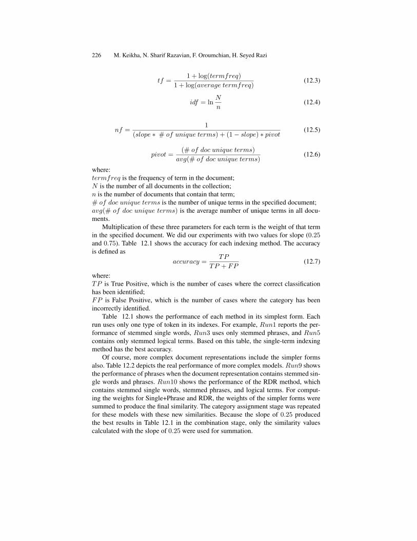
226 M. Keikha, N. Sharif Razavian, F. Oroumchian, H. Seyed Razi
tf =1 + log(termfreq)
1 + log(average termfreq)(12.3)
idf = lnN
n(12.4)
nf =1
(slope ∗ # of unique terms) + (1− slope) ∗ pivot(12.5)
pivot =(# of doc unique terms)
avg(# of doc unique terms)(12.6)
where:termfreq is the frequency of term in the document;N is the number of all documents in the collection;n is the number of documents that contain that term;# of doc unique terms is the number of unique terms in the specified document;avg(# of doc unique terms) is the average number of unique terms in all docu-ments.
Multiplication of these three parameters for each term is the weight of that termin the specified document. We did our experiments with two values for slope (0.25and 0.75). Table 12.1 shows the accuracy for each indexing method. The accuracyis defined as
accuracy =TP
TP + FP(12.7)
where:TP is True Positive, which is the number of cases where the correct classificationhas been identified;FP is False Positive, which is the number of cases where the category has beenincorrectly identified.
Table 12.1 shows the performance of each method in its simplest form. Eachrun uses only one type of token in its indexes. For example, Run1 reports the per-formance of stemmed single words, Run3 uses only stemmed phrases, and Run5contains only stemmed logical terms. Based on this table, the single-term indexingmethod has the best accuracy.
Of course, more complex document representations include the simpler formsalso. Table 12.2 depicts the real performance of more complex models. Run9 showsthe performance of phrases when the document representation contains stemmed sin-gle words and phrases. Run10 shows the performance of the RDR method, whichcontains stemmed single words, stemmed phrases, and logical terms. For comput-ing the weights for Single+Phrase and RDR, the weights of the simpler forms weresummed to produce the final similarity. The category assignment stage was repeatedfor these models with these new similarities. Because the slope of 0.25 producedthe best results in Table 12.1 in the combination stage, only the similarity valuescalculated with the slope of 0.25 were used for summation.

12 Document Representation and Quality of Text: An Analysis 227
Table 12.1. Accuracy of three different indexing methods
Run.ID Indexing method Slope Accuracy1 Single 0.25 56.32 Single 0.75 56.03 Phrase 0.25 53.94 Phrase 0.75 53.95 Logic 0.25 30.96 Logic 0.75 30.97 5-Gram 0.25 47.88 5-Gram 0.75 47.8
Table 12.2. Accuracy of combined methods
Run.ID Combined methods Combined run.IDs Accuracy9 Single+Phrase (1),(2) 59.910 RDR (1),(2),(3) 63.2
Table 12.1 demonstrates that the accuracy of the RDR method is 6.9% better thanthe accuracy of the single-term indexing and 15.4% better than 5-gram and about3.3% better than phrases. It should be noted that when more complex combinatoricformulas are used for combining the simple similarity values, the difference betweenthe Single+Phrase model and RDR could be as high as 7% or 9%.
This experiment demonstrates that the more complex a document representation,the better the performance of the categorization. In this experiment, single words out-performs 5-grams, Single+Phrase outperforms single words, and the RDR is betterthan phrases.
12.5.2 Experiment 2: SIAM Text Mining Contest Collection
In this part of the experiment we used the contest (ASRS) test collection. We in-dexed the first 20,000 documents of training file with six different indexing schemesdiscussed in Section 12.3; 3-gram, 4-gram, and 5-gram, and single-word, stemmed-single-word, and RDR.
For indexing each document, the frequency of each term in that documentwas counted as the term frequency, or termfreq of that term, and the average oftermfreq for all document terms was calculated. The final weight of a term in adocument was then calculated as
1 + log(termfreq)1 + log(average termfreq)
(12.8)
After indexing all the documents, we also calculated the inverse document frequency(idf ) in a separate table for each of the terms. Using idf can compensate for the lackof stop-word removal, because stop-words receive a very low idf automatically. We
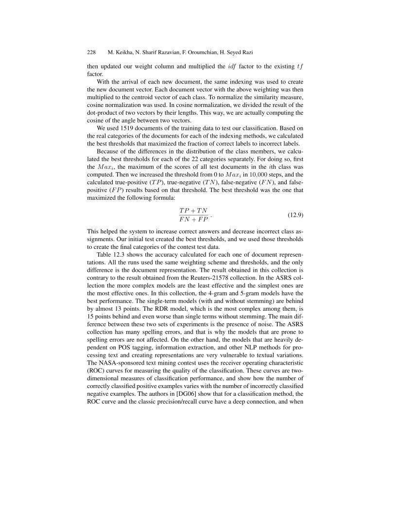
228 M. Keikha, N. Sharif Razavian, F. Oroumchian, H. Seyed Razi
then updated our weight column and multiplied the idf factor to the existing tffactor.
With the arrival of each new document, the same indexing was used to createthe new document vector. Each document vector with the above weighting was thenmultiplied to the centroid vector of each class. To normalize the similarity measure,cosine normalization was used. In cosine normalization, we divided the result of thedot-product of two vectors by their lengths. This way, we are actually computing thecosine of the angle between two vectors.
We used 1519 documents of the training data to test our classification. Based onthe real categories of the documents for each of the indexing methods, we calculatedthe best thresholds that maximized the fraction of correct labels to incorrect labels.
Because of the differences in the distribution of the class members, we calcu-lated the best thresholds for each of the 22 categories separately. For doing so, firstthe Maxi, the maximum of the scores of all test documents in the ith class wascomputed. Then we increased the threshold from 0 to Maxi in 10,000 steps, and thecalculated true-positive (TP ), true-negative (TN ), false-negative (FN ), and false-positive (FP ) results based on that threshold. The best threshold was the one thatmaximized the following formula:
TP + TN
FN + FP. (12.9)
This helped the system to increase correct answers and decrease incorrect class as-signments. Our initial test created the best thresholds, and we used those thresholdsto create the final categories of the contest test data.
Table 12.3 shows the accuracy calculated for each one of document represen-tations. All the runs used the same weighting scheme and thresholds, and the onlydifference is the document representation. The result obtained in this collection iscontrary to the result obtained from the Reuters-21578 collection. In the ASRS col-lection the more complex models are the least effective and the simplest ones arethe most effective ones. In this collection, the 4-gram and 5-gram models have thebest performance. The single-term models (with and without stemming) are behindby almost 13 points. The RDR model, which is the most complex among them, is15 points behind and even worse than single terms without stemming. The main dif-ference between these two sets of experiments is the presence of noise. The ASRScollection has many spelling errors, and that is why the models that are prone tospelling errors are not affected. On the other hand, the models that are heavily de-pendent on POS tagging, information extraction, and other NLP methods for pro-cessing text and creating representations are very vulnerable to textual variations.The NASA-sponsored text mining contest uses the receiver operating characteristic(ROC) curves for measuring the quality of the classification. These curves are two-dimensional measures of classification performance, and show how the number ofcorrectly classified positive examples varies with the number of incorrectly classifiednegative examples. The authors in [DG06] show that for a classification method, theROC curve and the classic precision/recall curve have a deep connection, and when

12 Document Representation and Quality of Text: An Analysis 229
Table 12.3. Accuracy of each method for best threshold value
Run.ID Indexing method Accuracy11 Single 52.312 Stemmed Single 53.913 Single+Phrase 53.314 RDR 51.415 5-Gram 66.716 4-Gram 65.617 3-Gram 59.5
a classifier dominates in the ROC curve, it will dominate in the precision/recall curvetoo, and vice versa.
In ROC space, one plots the false-positive rate (FPR) on the x-axis and the true-positive rate (TPR) on the y-axis. The FPR measures the fraction of the negativeexamples that are misclassified as positive. The TPR measures the fraction of positiveexamples that are correctly labeled. Based on this observation, we compared ourcategorization results against the real values, and drew the ROC curve for all ofthem, which can be seen in Figures 12.1 and 12.2.
Here also it is evident that the 5-gram model is the one that dominates the ROCcurve. The area under the ROC curve is a standard measure of performance for clas-sifier algorithms [DG06], and that means that the 5-gram model is the best documentrepresentation method for this noisy dataset.
12.6 Conclusion
There are three factors in text categorization: categorization model, similarity mea-sure, and document representation. There are many alternatives for each one of thesefactors. In this chapter we focused on the document representation model and ex-amined four different document representation techniques with different levels ofcomplexity. The simplest of all is the N -gram model where the words are brokendown into overlapping strings of length N . The most popular model is the single-term approach where each word is treated as a term independent of any other term.It is common to use word stems instead of their original surface form in order to in-crease recall. A little more complicated model uses phrases (mostly syntactic) alongwith single terms. There are many more complex approaches to document represen-tation. Here we used a logical approach called rich document representation (RDR),which extracts the relationships between terms and represents them as predicates.We have demonstrated that in the context of the classification, the better documentrepresentation produces better classification. This is not completely the same as ad-hoc information retrieval. Over the years it has been observed that many differentsystems with different document representations exhibit similar performances in thecontext of TREC conferences.

230 M. Keikha, N. Sharif Razavian, F. Oroumchian, H. Seyed Razi
Fig. 12.1. ROC curve for 5-gram, single-word, stemmed single-word, and RDR indexing
Fig. 12.2. Close-up of ROC curve of Figure 12.1

12 Document Representation and Quality of Text: An Analysis 231
We have also demonstrated that the noise, the textual variations, has a graveeffect on more complex document representations. We showed that on the SIAMdataset, which contains many spelling errors, the best models are the simplest andmore robust ones.
In that context, the 5-gram approach dominated the other methods. The worstapproach was the RDR model, which is dependent on NLP techniques to extract andrepresent the relationships. In the text mining contest (ASRS) dataset, our centroidclassification method with 5-gram document representation model shows significantimprovement over the Schapire’s and Singer’s BoosTexter approach as standard ap-proaches.
In the context of document classification, the choice of document representationshould be taken seriously. It should be decided based on two factors: first, the amountof the noise or syntactic variations in the text collection; second, the amount of timeand resources available. The simpler models require less processing, while the morecomplicated models such as RDR require POS tagging and other NLP text processingtechniques. The NLP methods and tagging are time-consuming and heavy users ofresources.
Acknowledgments
This work is partially supported by the Iranian Communication Research Center(ITRC) under contract number 500/12204.
References
[AHO07] A. AleAhmad, P. Hakimian, and F. Oroumchian. N-gram and local context analysisfor persian text retrieval. International Symposium on Signal Processing and itsApplications (ISSPA2007), 2007.
[BDO94] M.W. Berry, S.T. Dumais, and G.W. O’Brien. Using linear algebra for intelli-gent information retrieval. Technical Report UT-CS-94-270, University of Ten-nessee, 1994. Available from World Wide Web: citeseer.ist.psu.edu/berry95using.html.
[CM89] A. Collins and R. Michalski. The logic of plausible reasoning: a core the-ory. Cognitive Science, 13(1):1–49, 1989. Available from World Wide Web:citeseer.ist.psu.edu/collins89logic.html.
[CvR95] F. Crestani and C.J. van Rijsbergen. Probability kinematics in information re-trieval. In Proceedings of the Eighteenth Annual International ACM SIGIR Con-ference on Research and Development in Information Retrieval, pages 291–299,ACM Press, New York, 1995.
[Dam95] M. Damashek. Gauging similarity with n-grams: language-independent catego-rization of text. Science, 267(5199):843, 1995.
[DG06] J. Davis and M. Goadrich. The relationship between Precision-Recall and ROCcurves. Proceedings of the 23rd International Conference on Machine Learning,pages 233–240, ACM Press, New York, 2006.

232 M. Keikha, N. Sharif Razavian, F. Oroumchian, H. Seyed Razi
[Gre00] E. Greengrass. Information Retrieval: A Survey. IR Report, 120600, 2000.Available from World Wide Web: http://www.csee.umbc.edu/cadip/readings/IR.report.120600.book.pdf.
[HK00] E.H. Han and G. Karypis. Centroid-based Document Classification: Analysis andExperimental Results. Springer, New York, 2000.
[JO04] A. Jalali and F. Oroumchian. Rich document representation for document clus-tering. In Coupling Approaches, Coupling Media and Coupling Languages forInformation Retrieval Avignon (Vaucluse), pages 800–808, RIAO, Paris, France,2004.
[KC88] R. Kjeldsen and P.R. Cohen. The evolution and performance of the GRANT sys-tem. IEEE Expert, pages 73–79, 1988.
[Lee94] J.H. Lee. Properties of extended Boolean models in information retrieval. Proceed-ings of the 17th Annual International ACM SIGIR Conference on Research andDevelopment in Information Retrieval, pages 182–190, ACM Press, New York,1994.
[LPY94] E.D. Liddy, W. Paik, and E.S. Yu. Text categorization for multiple users basedon semantic features from a machine-readable dictionary. ACM Transactions onInformation Systems (TOIS), 12(3):278–295, 1994.
[OO96] F. Oroumchian and R.N. Oddy. An application of plausible reasoning to informa-tion retrieval. In Proceedings of the Nineteenth Annual International ACM SIGIRConference on Research and Developement in Information Retrieval, pages 244–252, ACM Press, New York, 1996.
[PN96] C. Pearce and C. Nicholas. TELLTALE: Experiments in a dynamic hypertext en-vironment for degraded and multilingual data. Journal of the American Society forInformation Science, 47(4):263–275, 1996.
[Por80] M.F. Porter. An algorithm for suffix stripping. Information Systems, 40(3):211–218, 1980.
[Rij79] C.J. Van Rijsbergen. Information Retrieval. Butterworth-Heinemann, Newton,MA, 1979.
[RKOR06] F. Raja, M. Keikha, F. Oroumchian, and M. Rahgozar. Using Rich Document Rep-resentation in XML Information Retrieval. Proceedings of the Fifth InternationalWorkshop of the Initiative for the Evaluation of XML Retrieval (INEX), Springer,New York, 2006.
[SB88] G. Salton and C. Buckley. Term weighting approaches in automatic text retrieval.Information Processing and Management, 24(5):513–523, 1988.
[Sue79] C.Y. Suen. N-gram statistics for natural language understanding and text process-ing. IEEE Transactions on Pattern Analysis and Machine Intelligence, 1(2):164–172, 1979.
[YL99] Y. Yang and X. Liu. A re-examination of text categorization methods. Proceedingsof the 22nd Annual International ACM SIGIR Conference on Research and Devel-opment in Information Retrieval, pages 42–49, ACM Press, New York, 1999.
[ZPZ81] E.M. Zamora, J.J. Pollock, and A. Zamora. The use of trigram analysis for spellingerror detection. Information Processing and Management, 17(6):305–316, 1981.

A
Appendix: SIAM Text Mining Competition 2007
Overview
The 2007 Text Mining Workshop held in conjunction with the Seventh SIAM Inter-national Conference on Data Mining was the first to feature a text mining competi-tion. Members of the Intelligent Data Understanding group at NASA Ames ResearchCenter in Moffett Field, California, organized and judged the competition. Being thefirst such competition held as a part of the workshop, we did not expect the largenumber of contestants that more established competitions such as KDDCUP1 have,but we did receive five submissions, though one person later withdrew.
Matthew E. Otey, Ashok N. SrivastavaSantanu Das, and Pat Castle
A.1 Classification Task
The contest focused on developing text mining algorithms for document classifi-cation. The documents making up the corpus used in the competition are aviationsafety reports documenting one or more problems that occurred on certain flights.These documents come from the Aviation Safety Reporting System (ASRS), andthey are publicly available in their raw form at http://asrs.arc.nasa.gov. Since each ofthese documents can describe one or more anomalies that occurred during a givenflight, they can be tagged with one or more labels describing a class of anomalies.The goal is to label the documents according to the classes to which they belong,while maximizing both precision and recall, as well as the classifier’s confidence inits labeling. This second criterion concerning confidence is useful for presenting re-sults to end-users, as an end-user may be more forgiving of a misclassification if heor she knew that the classifier had little confidence in its labeling.1 See http://www.kdnuggets.com/datasets/kddcup.html.

234 A Appendix: SIAM Text Mining Competition 2007
The competition entries were scored using the following cost function that ac-counts for both the accuracy and confidence of the classifier. When describing thecost function, we will use the following notation. Let D be the number of documentsin the corpus, and let L be the number of labels. Let Fj be the fraction of documentshaving label j. Let tij ∈ {−1,+1} be the target (true) value for label j of docu-ment i. Let pij ∈ {−1,+1} be the predicted value for label j of document i, andlet qij ∈ [0, 1] be the classifier’s confidence of the value pij. Finally, let Aj be thearea under the ROC curve for the classifier’s predictions for label j. We define theintermediate cost function Qj for label j as
Qj = (2Aj − 1) +1D
D∑i=1
qijtijpij . (A.1)
This function has a maximum value of 2. The final cost function Q is the average Qjfor all labels:
Q =1C
C∑j=1
Qj . (A.2)
In case of ties, we also formulated a figure of merit (FOM), defined as
FOM =1C
C∑j=1
(F − Fj)F
Qj (A.3)
where
F =C∑j=1
Fj . (A.4)
This figure of merit measures the quality of predictions across all anomaly cate-gories, giving a lower weighting to those categories making up a larger fraction ofthe dataset. Hence, better FOM are achieved by obtaining higher accuracies andconfidences on rarer classes.
We wrote a small Java program implementing these functions to use during ourjudging of the submissions. Before the contest deadline, we made this program andits source code available to the contestants so that they could validate its correctness,and so that they could use our implementation to tune their algorithms.
A.2 Judging the Submissions
A training dataset was provided over a month in advance of the deadline, giving thecontestants time to develop their approaches. Two days before the deadline we re-leased the test dataset. Both of these datasets had been run through PLADS, a systemthat performs basic text processing operations such as stemming and acronym expan-sion. The contestants submitted their labeling of the test dataset, their confidences inthe labeling, and the source code implementing their approach. The scores of the

A.3 Contest Results 235
submissions were calculated using the score function described above. In addition toscoring the submissions, we ran each contestant’s code to ensure that it worked andproduced the same output that was submitted, and we inspected the source code toensure that the contestants properly followed the rules of the contest.
A.3 Contest Results
The submissions of the contestants all successfully ran and passed our inspection,and we announced our three winners. First place was awarded to Cyril Goutte at theNRC Institute for Information Technology, Canada, with a score of 1.69. A teamconsisting of Edward G. Allan, Michael R. Horvath, Christopher V. Kopek, Brian T.Lamb, and Thomas S. Whaples of Wake Forest University, and their advisor, MichaelW. Berry of the University of Tennessee, Knoxville, came in second with a score of1.27. The third place team of Mostafa Keikha and Narjes Sharif Razavian of theUniversity of Tehran in Iran, and their advisor, Farhad Oroumchian of the Universityof Wollongong, Dubai, United Arab Emirates, scored a 0.97. At NASA, we evalu-ated Schapire’s and Singer’s BoosTexter approach, and achieved a maximum scoreof 0.82 on the test data, showing that the contestants made some significant improve-ments over standard approaches.


Index
N -gram, 218, 221k-means, 45, 58, 76, 96, 103
batch, 75bisecting, 49, 58incremental, 75kernel, 52, 55, 60smoothed (smoka), 76, 77
Allan, Edward, 200, 233AlSumait, Loulwah, 85Alternating Least Squares (ALS), 151annealing
deterministic, 65, 77, 188simulated, 77
anti-spam methods, 165Aono, Masaki, 109ArcRank, 36–41attribute selection, 170
χ2, 170authority, 34, 35Aviation Safety Reporting System (ASRS),
201, 203, 217, 231
Bader, Brett, 147bag-of-words, 186balanced iterative reducing and clustering
(BIRCH), 65, 70Berry, Michael W., 147, 200, 233Blondel, Vincent, 23BoosTexter, 233break-even point, 195Browne, Murray, 147
calibration, 190
CANDECOMP, 148Castle, Pat, 231categorization
multiclass, multilabel, 189category description, 191centroid, 6, 66, 219
method, 17, 219cluster
indicator vector problem, 49measure, 27, 28quality, 7
clustering, 28, 29, 31, 65, 87algorithm, 45, 65hierarchical, 45partitional, 45spherical k-means, 203
co-occurrence model, 186, 187confidence estimation, 185, 190corpus, 25–29, 31, 32, 42
bilingual, 32cosine, 26–29, 42COV with selective scaling (COV-SS), 119covariance matrix analysis (COV), 114cross-validation, 192curse of dimensionality, 88, 90
Das, Santanu, 231descriptive keywords, 191dictionary
bilingual, 32monolingual, 25, 26, 32, 33, 42synonym, 25, 26, 33, 41
dictionary graph, 33, 34, 36, 37, 41

238 Index
dimensionality reduction, 4, 169, 176discriminant analysis, 6distance, 32, 36, 39–42
semantic, 88, 93, 94Distributed National ASAP Archive
(DNAA), 208divergence
Bregman, 67Csiszar, 67, 68, 202Kullback–Leibler, 67
documentfrequency thresholding, 169representation, 218
document type definition (DTD), 130document vector space, 26–28Domeniconi, Carlotta, 85
eigenvalue, 53, 54, 73eigenvector, 71, 73
principal, 34, 36email classification, 165Enron, 147Enron email corpus, 65, 78, 147, 152ensemble, 26, 32entropy, 170
relative, 31expectation maximization (EM), 185, 188
F1 measure, 98, 100factor analysis, 17false-positive rate (FPR), 175, 226feature
reduction, 176selection, 95, 170
figure of merit (FOM), 205, 232Fisher linear discriminant analysis, 202folding in, 188frequent itemset mining, 95function
closed, proper, convex, 67distance-like, 69
Gallopoulos, Efstratios, 44Gansterer, Wilfried, 162General Text Parser (GTP), 153, 203generalized singular value decomposition
(GSVD), 8generalized vector space model (GVSM),
89, 93
Goutte, Cyril, 185, 233Gram matrix, 53grammatical context, see syntactical contextgraph mining, 26, 34, 42Green measure, 42
Hadamard product, 149hierarchical clustering
agglomerative, 46divisive, 46
HITS, 33, 34, 42Horvath, Michael, 200, 233Howland, Peg, 3hub, 34, 35human plausible reasoning, 222
indifferent discriminator, 28, 29inductive inference, 186, 189information gain, 170information retrieval, 25, 26, 28, 29, 42, 75,
165inverse document frequency, 219
Jaccard measure, 30Janecek, Andreas, 162
Keikha, Mostafa, 215, 233kernel
clustering, 54local, 88, 93method, 88, 93, 130, 132, 137
kernel PCA (KPCA), 52Gaussian kernels, 52, 61kernel trick, 52Mercer’s Theorem, 52polynomial kernels, 52, 60
keywordshighest probability, 196largest divergence, 192, 196
Khatri-Rao product, 149, 151Kobayashi, Mei, 109Kogan, Jacob, 64Kopek, Christopher, 200, 233Kronecker product, 149, 152Kullback–Leibler divergence, 202
Lamb, Brian, 200, 233latent semantic indexing (LSI), 12, 89, 112,
163, 164, 166, 174

Index 239
truncation, 167, 174latent semantic kernels (LSK), 89, 101LDA/GSVD algorithm, 11lexical analysis, 29local
feature relevance, 88feature selection, 90
locally adaptive clustering (LAC) algorithm,88, 90
logicalstatement, 222terms, 222
MATLAB Tensor Toolbox, 154matricizing, 149matrix
covariance, 53feature-document, 166proximity, 89, 93scatter, 6semantic, 89semantic dissimilarity, 93term-document, 45, 57, 89
maximum F -score threshold, 195maximum likelihood (ML), 187, 188mean
arithmetic, 68geometric, 68
MEDLINE, 18Metropolis algorithm, 77minimum error rate threshold, 195mixture of multinomial, 186multidimensional scaling (MDS), 130
naive Bayes, 187, 189natural language processing (NLP), 218, 226neighborhood graph, 33–36, 38, 39, 41Neumayer, Robert, 162Newton-type method, 130, 137Nicholas, Charles, 64nonconvexity, 202nonnegative matrix factorization (NMF),
152, 188, 201constrained, 189multiplicative update, 152, 203
nonnegative tensor factorization (NNTF),151, 155, 158
normalization factor, 219
Ohsumed collection, 56optimization
bound-constrained, 202quasi-Newton, 202
Oroumchian, Farhad, 215, 233orthogonal projection, 73Otey, Matthew, 231
PageRank, 36, 37, 42PARAFAC, 148
model, 150nonnegative factors, 151uniqueness, 150
Park, Haesun, 3part of speech, 29, 30, 38
tags, 222partition
ΠA, ΠB, 71quality of, 66
phrase, 218, 222PLIR, 218, 220, 222precision, 26, 28, 29, 98principal component analysis (PCA), 12, 46,
52, 109, 114principal direction divisive partitioning
(PDDP), 45, 46, 58, 59, 66, 71k-means steering, 49geometric interpretation, 48KPDDP-2MEANS, 56KPDDP-OCPC, 56KPDDP: Kernel PDDP, 47, 54, 55, 60PDDP(l), 48, 58PDDP-2MEANS, 49, 58PDDP-OC, 50, 58PDDP-OC-2MEANS, 50, 58PDDP-OCPC, 52, 58, 59
principal directions divisive partitioning(PDsDP), 66, 69, 71
probabilisticcategorizer, 185model, 186profiles, 185, 191
probabilistic latent semantic analysis(PLSA), 186, 188
PROPACK, 55
Qi, Houduo, 127
recall, 26, 28, 29, 98

240 Index
receiver operating characteristic (ROC), 208,226
related words, see similar wordsReuters-21578 collection, 56, 223
Modapte split, 56rich document representation (RDR), 217,
218, 222, 225
Salton, Gerard, 3, 109SDP, see semidefinite programmingsearch engine, 32semantic LAC algorithm, 93semantic network, 89
WordNet, 89, 101–103semidefinite programming (SDP), 130Senellart, Pierre, 23SEXTANT, 26, 29–31, 42Seyed Razi, Hassan, 215Sharif Razavian, Narjes, 215, 233similar words, 25–43similarity, 25–35, 42singular value decomposition (SVD), 3, 46,
163, 164, 166, 174, 176spam filtering, 164, 167SpamAssassin, 163, 164, 167sparsity, 79Srivastava, Ashok, 231stemming, 37, 42, 218, 222stop word, 28, 38, 223
stoplist, 154, 204stop-word, 42subspace clustering, 88, 93, 101, 103supervised learning, 186support vector machine (SVM), 52, 130synonym, 25, 26, 32–34, 36, 38, 39, 41, 43syntactical analysis, 26, 29–32syntactical context, 26, 29, 31
tensordecomposition, 148norm, 149
outer product, 149term
discrimination value, 26, 28frequency, 219vector space model, 26, 28
term vector space, 27, 28term weighting
log-entropy, 154term-weighting, 89, 93
inverse document frequency (idf ), 89log-entropy, 204
textcategorization, 186classification, 217
text to matrix generator (TMG), 56tf-idf, 28, 42thesaurus, 25, 26, 28, 29, 31, 32, 36, 42, 43trace optimization, 7transductive inference, 186, 189tree edit distance, 131true-positive rate (TPR), 175, 226
unfolding, 149unsolicited bulk email (UBE), 163unsolicited commercial email (UCE), 163
vector space model (VSM), 4, 45, 88, 111,163, 164, 166, 174, 218
Wedderburn rank reduction, 5weighted Euclidean distance, 90weighting schema, 219Whaples, Thomas, 200, 233Wiacek, Mike, 64WordNet, 38–41World Wide Web, 25, 26, 32–34, 41, 42
Xia, Zhonghang, 127Xing, Guangming, 127
Zeimpekis, Dimitrios, 44

Index 241