Climate change trend in China, with improved accuracy

Tian-Xiang Yue & Na Zhao & R. Douglas Ramsey &

Chen-Liang Wang & Ze-Meng Fan & Chuan-Fa Chen &

Yi-Min Lu & Bai-Lian Li

Received: 26 September 2011 /Accepted: 6 May 2013 /Published online: 24 May 2013# Springer Science+Business Media Dordrecht 2013

Abstract We have found that a spatial interpolation of mean annual temperature (MAT) inChina can be accomplished using a global ordinary least squares regression model since therelationship between temperature and its environmental determinants is constant. Therefore theestimation of MAT does not very across space and thus exhibits spatial stationarity. Theinterpolation of mean annual precipitation (MAP), however, is more complex and changesspatially as a function of topographic variation. Therefore, MAP shows spatial non-stationarityand must be estimated with a geographically weighted regression. A statistical transfer function(STF) of MATwas formulated using minimized residuals output from a high accuracy and highspeed method for surface modeling (HASM) with an ordinary least squares (OLS) linearequation that uses latitude and elevation as independent variables, abbreviated as HASM-OLS. The STF of MAP under a BOX-COX transformation is derived as a combination ofminimized residuals output by HASM with a geographically weighted regression (GWR) usinglatitude, longitude, elevation, impact coefficient of aspect and sky view factor as independentvariables, abbreviated as HASM-GWR-BC. In terms of HASM-OLS and HASM-GWR-BC,

Climatic Change (2013) 120:137–151DOI 10.1007/s10584-013-0785-5

Electronic supplementary material The online version of this article (doi:10.1007/s10584-013-0785-5)contains supplementary material, which is available to authorized users.

T.<X. Yue (*) : N. Zhao : C.<L. Wang : Z.<M. FanState Key Laboratory of Resources and Environment Information System, Institute of GeograpicalScience and Natural Resources Research, Chinese Academy of Sciences, 11A, Datun Road, Anwai,100101 Beijing, Chinae-mail: yue@lreis.ac.cn

C.<F. ChenGeomatics College, Shandong University of Science and Technology266510 Qingdao, Shandong Province, China

R. D. RamseyDepartment of Wildland Resources, Utah State University, Logan, UT 84322-5230, USA

Y.<M. LuKey Lab of Spatial Data Mining and Information Sharing, Fuzhou UniversityNo. 523, Gongye Road, 350002 Fuzhou, China

T.<X. Yue : B.<L. LiEcological Complexity and Modeling Laboratory, University of CaliforniaRiverside, CA 92521, USA

MAT had an increasing trend since the 1960s in China, with an especially accelerated increasingtrend since 1980. Overall, our data show thatMAT has increased by 1.44 °C since the 1960s. Thewarming rates increase from the south to north in China, except in the Qinghai-Xizang plateau.Specifically, the 2,100 °C·d contour line of annual accumulated temperature (AAT) of ≥10 °Cshifted northwestward 255 km in the Heilongjiang province since the 1960s. MAP in Qinghai-Xizang plateau and in arid region had a continuously increasing trend. In the other 7 regions ofChina, MAP shows both increasing and decreasing trends. On average, China became wetterfrom the 1960s to the 1990s, but drier from the 1990s to 2000s. The Qinghai-Xizang Plateau andNorthern China experienced more climatic extremes than Southern China since the 1960s.

1 Introduction

Meteorological stations are primary sources for climatic data. However, sparsely distributedmeteorological stations are often unable to satisfy the data requirements of most ecosystemchange studies. One major problem is how to estimate values for locations where primarydata is not available (Akinyemi and Adejuwon 2008).

GIS-based techniques have been widely used for interpolating observed point-basedclimatic data (Agnew and Palutikof 2000; Yue 2011). For instance, Ordinary kriging (OK)was used to interpolate the daily and monthly rainfall of Australia using ground-basedobservational data (Jeffrey et al. 2001). Lloyd (2005) compared the performance of differentinterpolation methods, including a moving window regression (MWR), inverse distanceweighting (IDW) and Kriging, demonstrating that methods using elevation as secondarydata performed better than others because of the relationships between climate factors, suchas temperature, precipitation and evaporation, to elevation. Hancock and Hutchinson (2006)used thin plate smoothing splines (Spline) to interpolate mean annual temperature of theAustralian and African continents.

Thiessen polygons (TP), IDW, Spline and OK were used to interpolate thirteen widelyscattered rainfall stations and their daily time series into gridded rainfall surfaces over the1950–1992 period in a West African catchment; assessment of the interpolation methodsusing reference point data indicated that interpolations using the IDW and OK were moreefficient than TP and, to a lesser extent, Spline (Ruelland et al. 2008). Different interpolationmodels in a GIS environment were used to generate precipitation surfaces for the north-western Himalayan Mountains and upper Indus plains of Pakistan at a spatial resolution of250×250 m2 for a baseline period (1960–1990). This precipitation simulation using aregional climate model (PRECIS) showed that OK, using elevation as secondary data,provided the best results especially for the monsoon months (Ashiq et al. 2010). Threeinterpolation approaches, IDW, Spline and Co-kriging, were used to interpolate monthlymean temperature, seasonal mean temperature, and annual mean temperature in the easternpart of India; it was found that Spline was preferred to Kriging and IDW because it wasfaster and easier to use (Samanta et al. 2012).

Many scholars are working to improve the interpolation of climate surfaces by using datafrom meteorological stations in China. For instance, Shang et al. (2001) employed IDW tointerpolate mean annual precipitation from 1951 to 1980, including a digital elevation model(DEM) as secondary data; the interpolation had a mean absolute error of 102.23 mm. Lin etal. (2002) applied different interpolation techniques, OK and IDW, to estimate 10-day meanair temperature from 1951 to 1990; the results indicated that the mean absolute errors for OKand IDW were 2.15 °C and 1.9 °C respectively. Pan et al. (2004) interpolated mean annualtemperature using 726 meteorological station observations in China from 1961 to 2000

138 Climatic Change (2013) 120:137–151

using IDW with a mean absolute error of 1.51 °C. Hong et al. (2005) used climate data from1971 to 2000 from meteorological stations in China to develop thin-plate smoothing splinesurfaces for monthly mean temperature and precipitation for January, April, July andOctober. Their results showed interpolation errors for monthly temperatures varying from0.42 to 0.83 °C and 8–13 % for monthly precipitation.

A combination of interpolation methods applied through statistical transfer func-tions (STFs) is an efficient approach to improve the estimation error of climaticvariables for locations where primary data is not available. It has been determinedthat the statistical relationship between mean annual temperature (MAT) and itsenvironmental determinants is the same no matter where the measurement takes place(Yue 2011). But a simple ‘global’ model cannot explain the relationship betweenmean annual precipitation (MAP) and its environmental variables. The MAP relation-ship changes across space as a function of topographic structure across the landscape.In other words, MAT exhibits spatial stationarity and its statistical transfer functioncan be expressed by an Ordinary Least Squares regression (OLS), while MAP exhibitsspatial non-stationarity and therefore its statistical transfer functions have to beformulated through Geographically Weighted Regression (GWR). In this paper, OLSfor MAT and GWR for MAP are combined with a high accuracy and high speedmethod for surface modeling (HASM) to produce surfaces of climatic change for thepast 50 years in China at a spatial resolution of 1 km×1 km. HASM, OLS and GWRare described in detail by the online supplements 1 and 2.

2 Methods

A STF of MATwas formulated using minimized residuals output from HASM with an OLSlinear equation that used latitude and elevation as independent variables. This MAT transferfunction is abbreviated as HASM-OLS (Supplement 2). The simulated MAT from 1961 to2010 at every grid cell i, in which i=1, 2,…, 19606916, can be formulated as,

Tsi tð Þ ¼ θols⋅xT þ HASM Tk tð Þ−θols⋅xT� � ð1Þ

where x=(1, Lat, Ele), θols=(38.552, 0.705, 0.003), Tk (t) is the MATobserved in the year oft at the meteorological station k.

The STF of MAP under a BOX-COX transformation was derived as a combination ofminimized residuals output by HASM with a GWR using latitude, longitude, elevation,impact coefficient of aspect and sky view factor as independent variables. The MAP transferfunction is abbreviated as HASM-GWR-BC (Supplement 2). Let x=(Lon, Lat, Ele, ICA,SVF), in which Lat represents latitude, Lon refers to longitude, Ele is elevation, ICA theimpact coefficient of aspect on precipitation, and SVF the sky view factor. Then the STF ofMAP under a BOX-COX transformation can be formulated as,

Psi tð Þ ¼ θgwr⋅xT þ HASM Ψ0:475 Pk tð Þð Þ−θgwr⋅xT� � ð2Þ

where θgwr=(x ⋅W ⋅xT)−1 ⋅x ⋅W ⋅<0.475(Pk(t));W is the geographical weight matrix; Psi is thesimulated MAP at the grid cell i(i=1, 2,…,19606916);<0.475(Pk(t))=(Pk

0.475(t)−1)/0.475 is aBOX-COX transformation of annual mean precipitation Pk (t) at observation station k in theyear t.

Results of the HASM-OLS of MAT and HASM-GWR-BC of MAP were cross-validatedusing observational data from meteorological stations across China for the same period, for

Climatic Change (2013) 120:137–151 139

which mean absolute error (MAE) and mean relative error (MRE) of climate variables arecalculated. They are respectively formulated as,

MAE ¼ 1

n

Xni

oi−sij j ð3Þ

MRE ¼ MAE

1

n

Xni¼1

oij j� 100% ð4Þ

where oi represents the observed value such as MAT or MAP at the ith meteorologicalstation; si the simulated value at the ith meteorological station; n is the total number ofmeteorological stations for validation.

We used a consistent cross-validation methodology to test OK, IDW, Spline, and HASMresults. Validation results of HASM-OLS for MAT during the 1961 to 2010 period werecompared to the OK-OLS, IDW-OLS and Spline-OLS results. OK-OLS, IDW-OLS andSpline-OLS respectively refer to the combination of OK, IDW and Spline with the OLS.GWR-BC means that the result of a BOX-COX transformation of MAP during the 1961 to2010 period at every meteorological station were used to operate the geographicallyweighted regression. HASM-GWR-BC, OK-GWR-BC, IDW-GWR-BC and Spline-GWR-BC respectively describe the interpolation processes of MAP by combining HASM, OK,IDW and Spline with GWR-BC.

2.1 Cross-validation in space

Cross-validation in space was comprised of four steps: i) 5 % of the meteorologicalstations were removed for validation prior to model creation; ii) MAT and MAP from1961 to 2010 were simulated at a spatial resolution of 1km×1km using the remaining95 % of meteorological stations, iii) MAE and MRE were calculated using the 5 %validation set, and iv) the 5 % validation set is returned to the pool of availablestation for the next iteration. This process is repeated until MAT and MAP at allmeteorological stations have been simulated and the simulation error statistics for eachstation can be calculated.

Cross validation in space indicates that MAEs of MAT during the 1961 to 2010 periodcreated by HASM-OLS, OK-OLS,IDW-OLS and Spline-OLS were 0.73 °C, 0.81 °C,0.82 °C and 1.18 °C respectively. MAT accuracy of HASM-OLS was 11 %, 12 % and62 % higher than OK-OLS, IDW-OLS and Spline-OLS respectively. MAEs of MAP duringthe 1961 to 2010 period produced by HASM-GWR-BC, OK-GWR-BC, IDW-GWR-BC andSpline-GWR-BC are 48.78 mm, 65.29 mm, 65.10 mm and 124.14 mm respectively(Table 1). MAP accuracy of HASM-GWR-BC was 34 %, 34 % and 155 % greaterthan the accuracies of OK-GWR-BC, IDW-GWR-BC and Spline-GWR-BC respective-ly. HASM was the best performer when compared to the more widely used classicalmethods.

Results from Pan et al. (2004) and Shang et al. (2001) indicated that the interpolationresults of MAT and MAP had MREs of 13 % and 14 % using IDW (Table 1). In other words,the accuracies of MAT and MAP interpolation were respectively increased by 6 % and 3 %because of the introduction of the STFs.

140 Climatic Change (2013) 120:137–151

2.2 Cross-validation in time

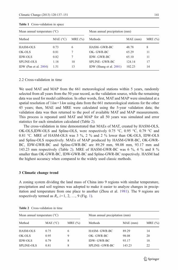
We used MAT and MAP from the 661 meteorological stations within 5 years, randomlyselected from all years from the 50 year record, as the validation source, while the remainingdata was used for model calibration. In other words, first, MATand MAP were simulated at aspatial resolution of 1km×1km using data from the 661 meteorological stations for the other45 years; then, MAE and MRE were calculated using the 5-year validation data; thevalidation data was then returned to the pool of available MAT and MAP measurements.This process is repeated until MAT and MAP for all 50 years was simulated and errorstatistics for each simulation calculated (Table 2).

The cross-validation in time demonstrated that MAEs of MAT, created by HASM-OLS,OK-OLS,IDW-OLS and Spline-OLS, were respectively 0.75 °C, 0.95 °C, 0.79 °C and0.81 °C. MRE of HASM-OLS was 3 %, 2 % and 2 % lower than OK-OLS, IDW-OLSand Spline-OLS respectively. MAEs of MAP produced by HASM-GWR-BC, OK-GWR-BC, IDW-GWR-BC and Spline-GWR-BC are 89.29 mm, 98.08 mm, 93.17 mm and143.23 mm respectively (Table 2). MRE of HASM-GWR-BC was 6 %, 4 % and 8 %smaller than OK-GWR-BC, IDW-GWR-BC and Spline-GWR-BC respectively. HASM hadthe highest accuracy when compared to the widely used classic methods.

3 Climatic change trend

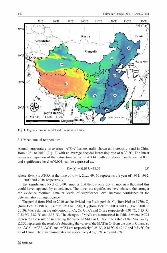
A zoning system dividing the land mass of China into 9 regions with similar temperature,precipitation and soil regimes was adopted to make it easier to analyze changes in precip-itation and temperature from one place to another (Zhou et al. 1981). The 9 regions arerespectively termed as Ri, i=1, 2, …, 9 (Fig. 1).

Table 1 Cross-validation in space

Mean annual temperature (°C) Mean annual precipitation (mm)

Method MAE (°C) MRE (%) Methods MAE (mm) MRE (%)

HASM-OLS 0.73 6 HASM- GWR-BC 48.78 8

OK-OLS 0.81 7 OK- GWR-BC 65.29 11

IDW-OLS 0.82 7 IDW- GWR-BC 65.10 11

SPLINE-OLS 1.18 10 SPLINE- GWR-BC 124.14 17

IDW (Pan et al. 2004) 1.51 13 IDW (Shang et al. 2001) 102.23 14

Table 2 Cross-validation in time

Mean annual temperature (°C) Mean annual precipitation (mm)

Method MAE (°C) MRE (%) Methods MAE (mm) MRE (%)

HASM-OLS 0.75 6 HASM- GWR-BC 89.29 14

OK-OLS 0.95 9 OK- GWR-BC 98.08 20

IDW-OLS 0.79 8 IDW- GWR-BC 93.17 18

SPLINE-OLS 0.81 8 SPLINE- GWR-BC 143.23 22

Climatic Change (2013) 120:137–151 141

3.1 Mean annual temperature

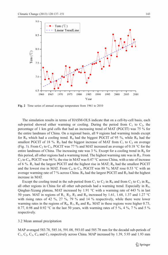
Annual temperature on average (ATOA) has generally shown an increasing trend in Chinafrom 1961 to 2010 (Fig. 2) with an average decadal increasing rate of 0.33 °C. The linearregression equation of the entire time series of ATOA, with correlation coefficient of 0.85and significance level of 0.001, can be expressed as,

Tem tð Þ ¼ 0:033t−58:33 ð5Þwhere Tem(t) is ATOA at the time of t; t=1, 2,…, 49, 50 represents the year of 1961, 1962,…, 2009 and 2010 respectively.

The significance level of 0.001 implies that there’s only one chance in a thousand thiscould have happened by coincidence. The lower the significance level chosen, the strongerthe evidence required. Smaller levels of significance level increase confidence in thedetermination of significance.

The period from 1961 to 2010 can be divided into 5 sub-periods: C1 (from1961 to 1970), C2

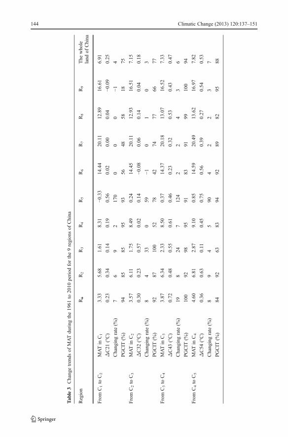
(from 1971 to 1980), C3 (from 1981 to 1990), C4 (from 1991 to 2000) and C5 (from 2001 to2010). MATs during the sub-periods of C1, C2, C3, C4 and C5 are respectively 6.91 °C, 7.15 °C,7.33 °C, 7.82 °C and 8.35 °C. The changes of MATs are summarized in Table 3 where ΔC21represents the result of subtracting the value of MAT in C1 from the value of the MAT in C2,ΔC32 represents the result of subtracting the value of the MAT in C2 from the one in C3, and soon.ΔC21,ΔC32,ΔC43 andΔC54 are respectively 0.25 °C, 0.18 °C, 0.47 °C and 0.53 °C forall of China. Their increasing rates are respectively 4 %, 3 %, 6 % and 7 %.

Fig. 1 Digital elevation model and 9 regions of China

142 Climatic Change (2013) 120:137–151

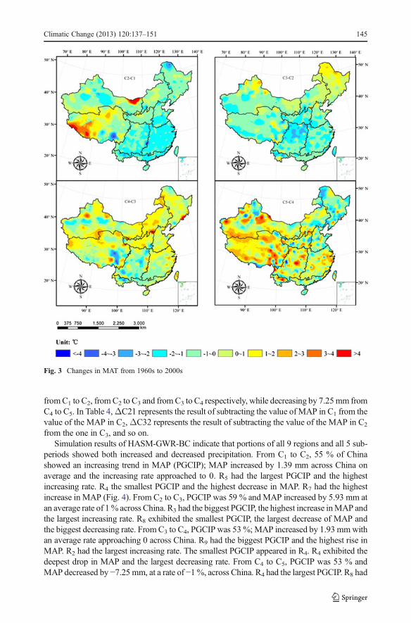
The simulation results in terms of HASM-OLS indicate that on a cell-by-cell basis, eachsub-period showed either warming or cooling. During the period from C1 to C2, thepercentage of 1 km grid cells that had an increasing trend of MAT (PGCIT) was 75 % forthe entire landmass of China. On a regional basis, all 9 regions had warming trends exceptfor R9 which had a cooling trend. R4 had the biggest PGCIT of 95 %, while R9 had thesmallest PGCIT of 18 %. R5 had the biggest increase of MAT from C1 to C2 on average(Fig. 3). From C2 to C3, PGCIT was 77 % and MAT increased an average of 0.18 °C for theentire landmass of China. The increasing rate was 3 %. Except for a cooling trend in R6 forthis period, all other regions had a warming trend. The highest warming rate was in R3. FromC3 to C4, PGCITwas 94 %; the rise in MATwas 0.47 °C across China, with a rate of increaseof 6 %. R1 had the largest PGCIT and the highest rise in MAT; R6 had the smallest PGCITand the lowest rise in MAT. From C4 to C5, PGCIT was 88 %; MAT rose 0.53 °C with anaverage warming rate of 7 % across China. R9 had the largest PGCIT and R5 had the highestincrease in MAT.

Except the cooling trend in the sub-period from C1 to C2 in R9 and from C2 to C3 in R6,all other regions in China for all other sub-periods had a warming trend. Especially in R5,Qinghai-Xizang plateau, MAT increased by 1.91 °C with a warming rate of 443 % in last50 years. MAT in regions of R1, R2, R3 and R4 increased by 1.61, 1.68, 1.37 and 1.27 °Cwith rising rates of 42 %, 27 %, 79 % and 14 % respectively, while there were lowerwarming rates in the regions of R6, R7, R8 and R9. MAT in these regions were higher 0.73,0.77, 0.98 and 0.92 °C in the last 50 years, with warming rates of 5 %, 4 %, 7 % and 5 %respectively.

3.2 Mean annual precipitation

MAP averaged 583.78, 585.16, 591.08, 593.03 and 585.78 mm for the decadal sub-periods ofC1, C2, C3, C4 and C5 respectively across China. MAP increased by 1.39, 5.93 and 1.93 mm

Fig. 2 Time series of annual average temperature from 1961 to 2010

Climatic Change (2013) 120:137–151 143

Tab

le3

Changetrends

ofMATdu

ring

the19

61to

2010

period

forthe9region

sof

China

Region

R1

R2

R3

R4

R5

R6

R7

R8

R9

The

who

leland

ofChina

From

C1to

C2

MATin

C1

3.33

5.68

1.61

8.31

−0.33

14.44

20.11

12.89

16.61

6.91

ΔC21

(°C)

0.23

0.34

0.14

0.19

0.56

0.02

0.00

0.04

−0.09

0.25

Changingrate

(%)

76

92

170

00

0−1

4

PGCIT

(%)

9485

8595

9356

4858

1875

From

C2to

C3

MATin

C2

3.57

6.11

1.75

8.49

0.24

14.45

20.11

12.93

16.51

7.15

ΔC32

(°C)

0.30

0.23

0.57

0.02

0.14

−0.08

0.06

0.14

0.04

0.18

Changingrate

(%)

84

330

59−1

01

03

PGCIT

(%)

9287

100

5278

4274

7766

77

From

C3to

C4

MATin

C3

3.87

6.34

2.33

8.50

0.37

14.37

20.18

13.07

16.52

7.33

ΔC43

(°C)

0.72

0.48

0.55

0.61

0.46

0.23

0.32

0.53

0.43

0.47

Changingrate

(%)

198

247

124

22

43

6

PGCIT

(%)

100

9298

9591

8391

9910

094

From

C4to

C5

MATin

C4

4.60

6.81

2.87

9.10

0.85

14.59

20.49

13.62

16.97

7.82

ΔC54

(°C)

0.36

0.63

0.11

0.45

0.75

0.56

0.39

0.27

0.54

0.53

Changingrate

(%)

89

45

904

22

37

PGCIT

(%)

8492

6383

9492

8982

9588

144 Climatic Change (2013) 120:137–151

fromC1 to C2, fromC2 to C3 and fromC3 to C4 respectively, while decreasing by 7.25mm fromC4 to C5. In Table 4,ΔC21 represents the result of subtracting the value of MAP in C1 from thevalue of the MAP in C2,ΔC32 represents the result of subtracting the value of the MAP in C2

from the one in C3, and so on.Simulation results of HASM-GWR-BC indicate that portions of all 9 regions and all 5 sub-

periods showed both increased and decreased precipitation. From C1 to C2, 55 % of Chinashowed an increasing trend in MAP (PGCIP); MAP increased by 1.39 mm across China onaverage and the increasing rate approached to 0. R5 had the largest PGCIP and the highestincreasing rate. R4 the smallest PGCIP and the highest decrease in MAP. R7 had the highestincrease in MAP (Fig. 4). From C2 to C3, PGCIP was 59 % and MAP increased by 5.93 mm atan average rate of 1% across China. R3 had the biggest PGCIP, the highest increase inMAP andthe largest increasing rate. R8 exhibited the smallest PGCIP, the largest decrease of MAP andthe biggest decreasing rate. From C3 to C4, PGCIP was 53 %; MAP increased by 1.93 mmwithan average rate approaching 0 across China. R9 had the biggest PGCIP and the highest rise inMAP. R2 had the largest increasing rate. The smallest PGCIP appeared in R4. R4 exhibited thedeepest drop in MAP and the largest decreasing rate. From C4 to C5, PGCIP was 53 % andMAP decreased by −7.25 mm, at a rate of −1%, across China. R4 had the largest PGCIP. R8 had

Fig. 3 Changes in MAT from 1960s to 2000s

Climatic Change (2013) 120:137–151 145

Tab

le4

Changetrends

ofMAPdu

ring

the19

61to

2010

period

forthe9region

sof

China

Region

R1

R2

R3

R4

R5

R6

R7

R8

R9

The

who

leland

ofChina

From

C1to

C2

MAP(m

m)in

C1

324.60

117.44

547.12

529.77

371.80

1037

.60

1465.40

734.78

1414.95

583.78

ΔC21

(mm)

−3.34

3.15

−25.08

−43.45

19.60

−22.95

47.34

−18.74

15.3

1.39

Chang

ingrate

(%)

−13

−5−8

5−2

3−3

10

PGCIP

(%)

5571

155

8618

6411

5855

From

C2to

C3

MAP(m

m)in

C2

321.26

120.58

522.03

486.31

391.39

1014

.60

1512.71

716.03

1430.30

585.16

ΔC32

(mm)

6.32

3.71

91.80

15.19

5.27

−4.96

−13.56

−46.62

3.44

5.93

Chang

ingrate

(%)

23

183

1−1

−1−7

01

PGCIP

(%)

4561

9868

5957

4414

5859

From

C3to

C4

MAP(m

m)in

C3

327.57

124.28

613.82

501.49

396.65

1009

.64

1499.14

669.45

1433.75

591.08

ΔC43

(mm)

3.57

8.58

−29.92

−54.11

2.75

−39.48

16.87

6.53

71.49

1.93

Chang

ingrate

(%)

17

−5−1

11

−41

15

0

PGCIP

(%)

5776

74

4537

7258

8353

From

C4to

C5

MAP(m

m)in

C4

331.15

132.85

549.36

447.40

399.43

970.21

1516.06

675.97

1505.18

593.03

ΔC54

(mm)

−48.33

5.42

−32.30

24.23

24.93

5.34

−24.82

38.15

−89.62

−7.25

Chang

ingrate

(%)

−14

4−6

56

1−2

6−6

−1PGCIP

(%)

860

1588

8762

2779

1153

146 Climatic Change (2013) 120:137–151

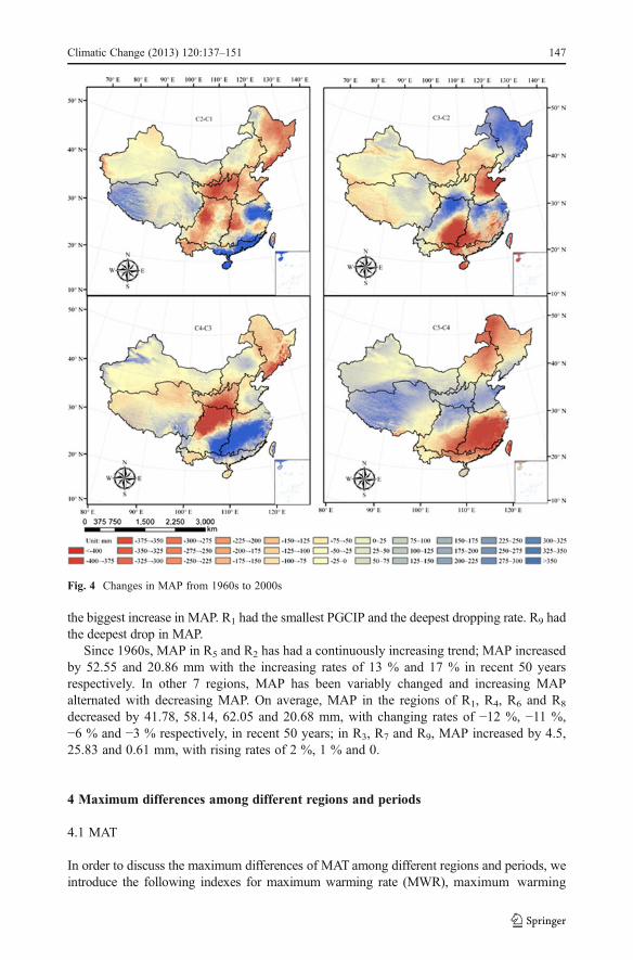
the biggest increase in MAP. R1 had the smallest PGCIP and the deepest dropping rate. R9 hadthe deepest drop in MAP.

Since 1960s, MAP in R5 and R2 has had a continuously increasing trend; MAP increasedby 52.55 and 20.86 mm with the increasing rates of 13 % and 17 % in recent 50 yearsrespectively. In other 7 regions, MAP has been variably changed and increasing MAPalternated with decreasing MAP. On average, MAP in the regions of R1, R4, R6 and R8

decreased by 41.78, 58.14, 62.05 and 20.68 mm, with changing rates of −12 %, −11 %,−6 % and −3 % respectively, in recent 50 years; in R3, R7 and R9, MAP increased by 4.5,25.83 and 0.61 mm, with rising rates of 2 %, 1 % and 0.

4 Maximum differences among different regions and periods

4.1 MAT

In order to discuss the maximum differences of MAT among different regions and periods, weintroduce the following indexes for maximum warming rate (MWR), maximum warming

Fig. 4 Changes in MAP from 1960s to 2000s

Climatic Change (2013) 120:137–151 147

amplitude (MWA), maximum cooling rate (MCR) and maximum cooling amplitude(MCA) as follows,

MWR Ri;Ctð Þ ¼ maxj;kð Þ∈Ri

MAT j;k Ri;Ctþ1ð Þ−MAT j;k Ri;Ctð ÞMAT j;k Ri;Ctð Þ � 100%

� �ð6Þ

MWA Ri;Ctð Þ ¼ maxj;kð Þ∈Ri

MAT j;k Ri;Ctþ1ð Þ−MAT j;k Ri;Ctð Þ� � ð7Þ

MCR Ri;Ctð Þ ¼ maxj;kð Þ∈Ri

MAT j;k Ri;Ctð Þ−MAT j;k Ri;Ctþ1ð ÞMAT j;k Ri;Ctð Þ � 100%

� �ð8Þ

MCA Ri;Ctð Þ ¼ maxj;kð Þ∈Ri

MAT j;k Ri;Ctð Þ−MAT j;k Ri;Ctþ1ð Þ� � ð9Þ

where (j, k)∈ Ri means that (j, k) is any grid cell in the region of Ri, i=1,2,…,9; MATj,k (Ri,Ct) represents the mean annual temperature at grid cell (j, k) in the sub-period Ct, t=1,2,3,4.

In light of changing rates (Table 5), from C1 to C2, the MWRs greater than 300 %appeared in northeastern R2 and western R5, respectively with MWRs of 447 % and 337 %as well as MWAs of 5.01 °C and 3.64 °C; the biggest MCR, 66 %, happened in northern R3,with a MCA of 1.22 °C. From C2 to C3, the biggest MWR was 136 %, appearing insoutheastern R3 with a MWA of 1.74 °C; the biggest MCR of 223 %, with a MCA of1.58 °C, was in the eastern R5. From C3 to C4, the biggest MWR was 340 % in western R2,

Table 5 Maximum differences of MAT among different regions and periods

Region R1 R2 R3 R4 R5 R6 R7 R8 R9

From C1 to C2 MWA (°C) 0.88 5.01 0.67 0.77 3.64 0.7 0.46 1.21 0.38

MWR (%) 19 447 46 10 337 12 4 15 3

MCA (°C) 0.66 0.63 1.22 0.67 3.33 2.03 0.78 0.85 1.86

MCR (%) 8 5 66 8 50 13 3 11 13

From C2 to C3 MWA (°C) 1.44 1.28 1.74 1.46 1.77 1.02 1.47 1.18 0.84

MWR (%) 66 66 136 25 25 8 8 14 6

MCA (°C) 0.6 0.46 0.18 0.62 1.58 0.94 1.32 0.47 0.36

MCR (%) 8 4 5 8 223 6 11 3 3

From C3 to C4 MWA (°C) 3.09 2.45 4.5 3.09 2.31 1.93 2.53 2.11 2.27

MWR (%) 140 340 276 46 120 13 20 26 15

MCA (°C) 0.04 0.51 0.66 0.95 1.59 1.02 1.52 0.45 0.28

MCR (%) 1 6 10 7 20 7 7 3 2

From C4 to C5 MWA (°C) 1.79 3.5 4.7 1.76 3.81 4.98 3.76 1.49 2.22

MWR (%) 30 37 101 14 57 30 16 11 15

MCA (°C) 0.92 2.47 1.58 2.43 1.67 2.54 1.74 2.58 1.46

MCR (%) 103 229 27 38 43 22 9 24 8

148 Climatic Change (2013) 120:137–151

with a MWA of 2.45 °C, and the largest MCAwas 1.59 °C, with the biggest MCR of 20 % insoutheastern R5. From C4 to C5, the biggest MWR, 101 %, was found in southeastern R3,with a MWA of 4.7 °C; the largest MCR, 229 %, happened in western R2 and the MCAwas2.47 °C.

In terms of changing amplitudes of MAT, the biggest MWAs were 5.01 °C innortheastern R2, 1.77 °C in southeastern R5, 4.5 °C in southeastern R3, and 4.98 °Cin southeastern R6 respectively in the sub-periods from C1 to C2, from C2 to C3, fromC3 to C4 and from C4 to C5. The highest MCAs were 3.33 °C in southeastern R5,1.58 °C in eastern R5, 1.59 °C in southeastern R5, and 2.58 °C in the middle of R8 inthe same sub-periods.

4.2 MAP

Indexes of maximum wetter rate (MWER), maximum wetter amplitude (MWEA), maximumdrier rate (MDR) and maximum drier amplitude (MDA) are formulated as follows,

MWER Ri;Ctð Þ ¼ maxj;kð Þ∈Ri

MAP j;k Ri;Ctþ1ð Þ−MAPj;k Ri;Ctð ÞMAPj;k Ri;Ctð Þ � 100%

� �ð10Þ

MWEA Ri;Ctð Þ ¼ maxj;kð Þ∈Ri

MAP j;k Ri;Ctþ1ð Þ−MAPj;k Ri;Ctð Þ� � ð11Þ

MDR Ri;Ctð Þ ¼ maxj;kð Þ∈Ri

MAP j;k Ri;Ctð Þ−MAT j;k Ri;Ctþ1ð ÞMAPj;k Ri;Ctð Þ � 100%

� �ð12Þ

MDA Ri;Ctð Þ ¼ maxj;kð Þ∈Ri

MAP j;k Ri;Ctð Þ−MAPj;k Ri;Ctþ1ð Þ� � ð13Þ

where (j, k)∈Ri means that (j, k) is any grid cell in the region of Ri, i=1,2,…,9;MAPj,k (Ri, Ct)represents the mean annual precipitation at grid cell (j, k) in the sub-period Ct, t=1,2,3,4.

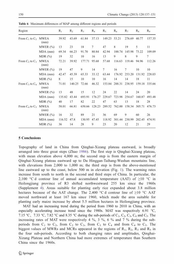
The biggest value of MWER was 47 % in the sub-period from C1 to C2 and happened insouthwestern R5, 47 % from C2 to C3 in southern R2, 48 % from C3 to C4 in southwesternR2, and 89 % from C4 to C5 in southwestern R3. From C1 to C2, the largest MDR was 32 %,which was found in western R2; from C2 to C3, it was 18 % in southwestern R8; from C3 toC4, it was 82 % in southwestern R3; from C4 to C5, the highest MDR appeared in the middleof R1 (Table 6).

The biggest WMEAs were 276.69 mm in the sub-period from C1 to C2 appearingin southern Hainan province of R7, 177.71 mm from C2 to C3 in southeastern R3;335.66 mm from C3 to C4 in southeastern R9, and 762.00 mm from C3 to C4 in themiddle of R6. The highest MDAwas 145.98 mm in the southeastern Hainan province of R7,253.20 mm in southwestern R7, 723.98 mm in southwestern R6 and 474.91 mm in southeasternR9 in the sub-periods from C1 to C2, from C2 to C3, from C3 to C4 and from C4 to C5

respectively.

Climatic Change (2013) 120:137–151 149

5 Conclusions

Topography of land in China from Qinghai-Xizang plateau eastward, is broadlyarranged into three great steps (Zhao 1986). The first step is Qinghai-Xizang plateau,with mean elevation above 4,000 m; the second step is from the eastern margin ofQinghai-Xizang plateau eastward up to Da Hinggan-Taihang-Wushan mountains line,with elevations from 2,000 to 1,000 m; the third step is from the above-mentionedline eastward up to the coast, below 500 m in elevation (Fig. 1). The warming ratesincrease from south to north in the second and third steps of China. In particular, the2,100 °C d contour line of annual accumulated temperature (AAT) of ≥10 °C inHeilongjiang province of R3 shifted northwestward 255 km since the 1960s(Supplement 4). Areas suitable for planting early rice expanded about 3.8 millionhectares because of the AAT change. The 2,400 °C d contour line of ≥10 °C AATmoved northward at least 167 km since 1960, which made the area suitable forplanting early maize increase by about 5.5 million hectares in Heilongjiang province.

MAT had an increasing trend during the period from 1960 to 2010 in China, with anespecially accelerating increase trend since the 1980s. MAT was respectively 6.91 °C,7.15 °C、7.33 °C, 7.82 °C and 8.35 °C during the sub-periods of C1, C2, C3, C4 and C5. Theincreasing rates of MAT were respectively 4 %, 3 %, 6 % and 7 % during the sub-periods from C1 to C2, from C2 to C3, from C3 to C4 and from C4 to C5. Thebiggest values of MWRs and MCRs appeared in the regions of R1, R2, R3 and R5 inthe four sub-periods. According to both changing rates and amplitudes, Qinghai-Xizang Plateau and Northern China had more extremes of temperature than SouthernChina since the 1960s.

Table 6 Maximum differences of MAP among different regions and periods

Region R1 R2 R3 R4 R5 R6 R7 R8 R9

From C1 to C2 MWEA(mm)

39.92 43.69 61.84 37.13 149.23 53.21 276.69 40.77 157.35

MWER (%) 13 23 18 7 47 8 19 5 11

MDA (mm) 69.34 66.23 91.70 80.84 42.94 100.74 145.98 73.22 109.09

MDR (%) 19 32 10 16 13 9 8 9 7

From C2 to C3 MWEA(mm)

72.21 39.92 177.71 95.68 57.68 116.63 119.46 94.96 112.26

MWER (%) 19 47 9 14 7 16 7 10 10

MDA (mm) 42.47 45.39 65.33 33.12 63.44 176.92 253.20 131.92 228.03

MDR (%) 8 15 10 10 16 14 14 18 11

From C3 to C4 MWEA(mm)

71.01 140.25 72.66 46.32 153.84 288.31 238.95 159.18 335.66

MWER (%) 13 48 15 12 24 22 14 24 20

MDA (mm) 135.82 43.44 693.91 176.27 229.67 723.98 254.67 160.87 493.48

MDR (%) 40 17 82 22 47 63 13 18 28

From C4 to C5 MWEA(mm)

58.01 66.81 650.66 128.23 289.52 762.00 158.34 305.71 476.73

MWER (%) 16 32 89 21 36 69 9 60 26

MDA (mm) 116.52 47.8 130.95 47.45 118.92 301.44 230.99 202.45 474.91

MDR (%) 36 14 28 9 23 20 12 21 29

150 Climatic Change (2013) 120:137–151

MAP was 583.78 mm in C1, 585.16 mm in C2, 591.08 mm in C3, 593.03 mm in C4 and585.78 mm in C5. MAP increased by 1.39 mm from C1 to C2, by 5.93 mm from C2 to C3, andby 1.93 mm from C3 to C4, while MAP decreased by 7.254 mm from C4 to C5. On average,China became wetter during the period from 1960s to 1990s, but much drier from 1990s to2000s. Since the 1960s, MAP in Qinghai-Xizang plateau and in arid region has had acontinuously increasing trend, with the increasing rates of 13 % and 17 % in recent 50 yearsrespectively. In other regions, increasing MAP alternated with decreasing MAP decade bydecade.

In terms of changing rates, north China and Qinghai-Xizang plateau had more extremesof precipitation in the last five decades. According to changing amplitudes, South China andSichuan basin had more extremes of precipitation.

Acknowledgments This work is supported by National Basic Research Priorities Program (2010CB950904)of Ministry of Science and Technology of the People’s Republic of China, by National High-tech R&DProgram of the Ministry of Science and Technology of the People’s Republic of China(2013AA122003), and by the Key Program of National Natural Science of China (41023010). Wewould like to acknowledge the two anonymous reviewers and Dr. L. D. Danny Harvey for theirvaluable comments and suggestions.

References

Agnew MD, Palutikof JP (2000) GIS-based construction of baseline climatologiesfor the Mediterranean usingterrain variables. Clim Res 14:115–127

Akinyemi FO, Adejuwon JO (2008) A GIS-based procedure for downscaling climate data for west Africa.Trans GIS 12(5):613–631

Ashiq MW, Zhao CY, Ni J, Akhtar M (2010) GIS-based high-resolution spatial interpolation of precipitationin mountain–plain areas of Upper Pakistan for regional climate change impact studies. Theor ApplClimatol 99:239–253

Hancock PA, Hutchinson MF (2006) Spatial interpolation of large climate data sets using bivariatethin platesmoothing splines. Environ Model Softw 21:1684–1694

Hong Y, Nix HA, Hutchinson MF, Booth TH (2005) Spatial interpolation of monthly mean climate data forChina. Int J Climatol 25:1369–1379

Jeffrey SJ, Carter JO, Moodie KB, Beswick AR (2001) Using spatial interpolation to construct a comprehen-sive archive of Australian climate data. Environ Model Softw 16:309–330

Lin ZH, Muo XG, Li HX, Li HB (2002) Comparison of three spatial interpolation methods for climatevariables in China. Acta Geograph Sin 57:47–56 (in Chinese)

Lloyd CD (2005) Assessing the effect of integrating elevation data into the estimation of monthly precipitationin Great Britain. J Hydrol 308:128–150

Pan YZ, Gong DY, Deng L, Li J, Gao J (2004) Smart distance searching based and DEM informedinterpolation of surface air temperature in China. Acta Geograph Sin 59:366–374 (in Chinese)

Ruelland D, Ardoin-Bardin S, Billen G, Servat E (2008) Sensitivity of a lumped and semi-distributedhydrological model to several methods of rainfall interpolation on a large basin in West Africa. JHydrol 361:96–117

Samanta S, Pal DK, Lohar D, Pal B (2012) Interpolation of climate variables and temperature modeling. TheorAppl Climatol 107:35–45

Shang ZB, Guo Q, Yang DA (2001) Spatial pattern analysis of annual precipitation with climate informationsystem of China. Acta Ecol Sin 21:689–694 (in Chinese)

Yue TX (2011) Surface Modelling: High Accuracy and High Speed Methods. CRC Press, New YorkZhao SQ (1986) Physical Geography of China. John Wiley & Sons, New YorkZhou LS, Sun H, Shen YQ, Deng JZ, Shi YL (1981) Comprehensive Agricultural Planning of China. China

Agricultural Press, Beijing (in Chinese)

Climatic Change (2013) 120:137–151 151