Submitted to Galaxies. Pages 1 - 19.OPEN ACCESS

galaxiesISSN 2075-4434

www.mdpi.com/journal/galaxies

Article

Classical and relativistic evolution of an extra-galactic jet withback-reactionLorenzo Zaninetti 1,

1 Department of Physics, University of Turin, via P.Giuria 1,I-10125 Turin,Italy

Version December 13, 2018 submitted to Galaxies. Typeset by LATEX using class file mdpi.cls

Abstract: We consider a turbulent jet which is moving in a Lane–Emden (n = 5) medium.1

The conserved quantity is the energy flux, which allows finding, to first order, an analytical2

expression for the velocity and an approximate trajectory. The conservation of the relativistic3

flux for the energy allows deriving, to first order, an analytical expression for the velocity,4

and numerically determining the trajectory. The back-reaction due to the radiative losses for5

the trajectory is evaluated both in the classical and the relativistic case.6

Keywords: Radio galaxies; Jets and bursts; galactic winds and fountains Radio sources7

PACS classifications: 98.54.Gr 98.62.Nx 98.70.Dk8

1. Introduction9

The study of extra-galactic jets started with the observations of NGC 4486 (M87), where ‘a curiousstraight ray lies in a sharp gap in the nebulosity . . . ’, see [1] and Figure 1. At the moment of writing,the extra-galactic radio sources are classified on the basis of the position of the brightest radio emittingregions with respect to the channel, see [2,3] for details. FR-I, after Fanaroff & Riley, have hot spots thatare more distant from the nucleus (a typical example is Cygnus A) and luminosity, L, at 178 Mhz of

L ≤ h100 2 1025 W

Hz strFR-I , (1)

where h100 = H0/100 and H0 is the Hubble constant. FR-II radio galaxies have emission uniformly10

distributed along the channel (typical example 3C449) and luminosities greater than the above value or,11

in other words, the more powerful radio galaxies are classified as FR-II. A list of the properties, length in12

arX

iv:1

812.

0497

2v1

[as

tro-

ph.H

E]

12

Dec

201

8

Version December 13, 2018 submitted to Galaxies 2 of 19

Figure 1. The super-giant elliptical galaxy M87 and the optical jet; the credit is due toInstituto de Astrofísica de Canarias.

kpc and power in Watt, of extra-galactic radio jets can be found in [4,5]. In the following we will study13

jets with small openings, such as that of M87.14

The problem of the velocity of extra-galactic radio jets has been analysed in two ways:15

1. The velocity of the jet is constant over many kpc and takes the value v. Due to the fact that is16

thought that this velocity is nearly relativistic, it is parametrized as β = vc, where c is the velocity17

of light. As an example, [6] analysed some wide-angle tail radio galaxies and found a terminal18

velocity of β = 0.3.19

2. The velocity of the jet decreases with an imposed law, see [7], or is evaluated by a numerical code,20

see [8,9]. In this case, the relativistic parameter β decreases along the trajectory.21

Recently the problem of the decrease of the velocity along a turbulent jet has been solved, imposing the22

conservation of the flux of momentum, see [10], or imposing the conservation of the energy flux, see23

[11]. The approach using the conservation of the flux of energy is attractive because it has the same24

dimension of the luminosity. Further on, the jets are radiating away in the various observational bands,25

such as radio, optical, infrared, etc., and we briefly recall that the extra-galactic radio source covers a26

range in observed luminosity from 1019 WHz

to 1028 WHz

, see [12].27

Therefore the flux of energy available at the beginning of the jet will progressively decrease due to28

the radiative losses. This paper, in Section 2, introduces the Lane–Emden (n = 5) density profile and29

consequently derives an approximate trajectory to first order as well as a numerical trajectory to second30

order in the presence of losses. In Section 3 we present a series solution for the relativistic trajectory to31

first order and a numerical solution to second order. Section 4 models the intensity of the radio-jet in32

3C31.33

2. Conservation of the flux of energy34

A turbulent jet is defined as a jet which has the same density as the surrounding intergalactic medium35

(IGM), see the next subsection for details. The conservation of the flux of energy in a turbulent jet has36

been explored in [11] for three types of IGM, with the following radial dependences: constant density37

Version December 13, 2018 submitted to Galaxies 3 of 19

Figure 2. Coaxial liquid-air jet; the credit is due to Mixing Enhancement via SecondaryParallel Injection (MESPI).

profile, hyperbolic and inverse power law density profiles. Here we analyse the case of a Lane–Emden38

(n=5) density profile, to which a subsection will be dedicated.39

2.1. The turbulent jet40

Turbulent jets are a subject of laboratory experiments, as an example, see Figure 2. The theory of41

turbulent jets emerging from a circular hole can be found in different books with different theories, see42

[13], [14], and [15]. The basic assumptions common to the three already cited approaches are43

1. The rate of momentum flow, J , represented by

J = constant× ρb2jv2x,max , (2)

is constant; here x is the distance from the initial circular hole, bj(x) is the jet’s diameter at distancex, vx,max is the maximum velocity along the the centreline, constant is

constant = 2π

∫ ∞0

f 2ξdξ , (3)

wheref(ξ) =

vxvx,max

with ξ =x

b1/2, (4)

and ρ is the density of the surrounding medium, see equation (5.6-3) in [13].44

2. The jet’s density ρ is constant over the expansion and equal to that of the surrounding medium.45

The pressure is absent in this theory.46

Omitting the details of the computation, an expression can be found for the average velocity vx, seeequation (5.6-21) in [13],

vx =ν(t)

x

2C23[

1 + 14(C3

rx)2]2 , (5)

where ν(t) is the kinematical eddy viscosity and C3 is as follows, see equation (5.6-23) in [13],

C3 =

√3

16π

√J

ρ

1

ν(t). (6)

Version December 13, 2018 submitted to Galaxies 4 of 19

An important quantity is the radial position, r = b1/2, corresponding to an axial velocity one-half of thecentreline value, see equation (5.6-24) in [13],

vx(b1/2, x)

vx,max(x)=

1

2=

1[1 + 1

4(C3

b1/2x)2]2 . (7)

The experiments in the range of Reynolds number, Re, 104 ≤ Re ≤ 3106 (see [16], [17] and [18])indicate that

b1/2 = 0.0848x , (8)

and as a consequenceC3 = 15.17 , (9)

and thereforevx(r)

vx,max(r)=

1[1 + 0.414( r

b1/2)2]2 . (10)

The average velocity, vx, is ≈ 1/100 of the centreline value when r/b1/2 = 4.6 and this allows seeingthat the diameter of the jet is

bj = 2× 4.6b1/2 . (11)

On introducing the opening angle α, the following new relation is found:

α

2= arctan

4.6b1/2x

. (12)

The generally accepted relation between the opening angle and Mach number, see equation (A33) in[19], is

α

2=csvj

=1

M, (13)

where cs is the velocity of sound, vj the jet’s velocity, and M the Mach number. The new relation (12)replaces the traditional relation (13). The parameter b1/2 can therefore be connected with the jet’sgeometry:

b1/2 =1

4.6tan(

α

2)x . (14)

If this approximate theory is accepted, equation (8) gives α = 42.61◦: this is the theoretical value thatyields the so called Reichardt profiles. The value of b1/2 fixes the value of C3 and therefore the eddyviscosity is

ν(t) =

√3

16π

√J

ρ

1

C3

=

√3

16π

√constant bvx,max

1

C3

. (15)

In order to continue, the integral that appears in constant should be evaluated, see equation (3).Numerical integration gives ∫ ∞

0

f 2ξdξ = 0.402 , (16)

and thereforeconstant = 2.528 . (17)

Version December 13, 2018 submitted to Galaxies 5 of 19

On introducing typical parameters of jets like α=5◦, vx,max=v100 = v[km/sec]/100, bj = b1, where b1 isthe momentary diameter in pc, it is possible to deduce an astrophysical formula for the kinematical eddyviscosity:

ν(t) = 2.92 10−9 b1v100pc2

yearwhen C3 = 135.61 . (18)

This paragraph concludes by underlining the fact that in extra-galactic sources it is possible to observe47

both a small opening angle, ≈ 5◦ and great opening angles, i.e. ≈ 34◦ in the outer regions of 3C3148

[20].49

2.2. The Lane–Emden profile50

The self gravitating sphere of a polytropic gas is governed by the Lane–Emden differential equationof the second order

d2

dx2Y (x) + 2

ddxY (x)

x+ (Y (x))n = 0 ,

where n is an integer, see [21–25]. The solution Y (x)n has the density profile

ρ = ρcY (x)nn ,

where ρc is the density at x = 0. The pressure P and temperature T scale as

P = Kρ1+1n , (19)

T = K ′Y (x) , (20)

where K and K′ are two constants. For more details, see [26].51

Analytical solutions exist for n = 0, 1, and 5. The analytical solution for n=5 is

Y (x) =1

(1 + x2

3)1/2

,

and the density for n=5 is

ρ(x) = ρc1

(1 + x2

3)5/2

. (21)

The variable x is non-dimensional and we now introduce the new variable x = r/b

ρ(r; b) = ρc1

(1 + r2

3b2)5/2

. (22)

2.3. Preliminaries52

The chosen physical units are pc for length and yr for time; with these units, the initial velocityv0 is expressed in pc yr−1. When the initial velocity is expressed in km s−1, the multiplicative factor1.02×10−6 should be applied in order to have the velocity expressed in pc yr−1. In these units, the speedof light is c = 0.306 pc yr−1. The goodness of the approximation of a solution is evaluated through thepercentage error, δ, which is

δ =

∣∣x− xapp|x

× 100 , (23)

where x is the analytical or numerical solution and xapp the approximate solution, see [27].53

Version December 13, 2018 submitted to Galaxies 6 of 19

2.4. Classical solution to first order54

The conservation of the energy flux in a straight turbulent jet the concept of the perpendicular sectionsection to the motion along the Cartesian x-axis, A

A(r) = π r2 (24)

where r is the radius of the jet. The section A at position x0 is

A(x0) = π(x0 tan(α

2))2 (25)

where α is the opening angle and x0 is the initial position on the x-axis. At position x we have

A(x) = π(x tan(α

2))2 . (26)

The conservation of energy flux states that

1

2ρ(x0)v

30A(x0) =

1

2ρ(x)v(x)3A(x) (27)

where v(x) is the velocity at position x and v0(x0) is the velocity at position x0, see Formula A28 in55

[19]. We now assume that a Lane–Emden (n = 5) density profile is valid, see equation (22). Then the56

above conservation law becomes57

1

2ρ0v(x)

3π x2(tan(α2

))2(1 +

1

3

x2

b2

)−5/2=

1

2ρ0v0(x0)

3π x02(tan(α2

))2(1 +

1

3

x02

b2

)−5/2, (28)

where v(x) is the velocity at position x, v0(x0) is the velocity at position x0 and α is the opening angleof the jet. The above equation is a cubic equation which has one real root plus two non-real complexconjugate roots. Here and in the following we take into account only the real root. The real analyticalsolution for the velocity without losses is

v(x; b, x0, v0) =v0 (3 b

2 + x2)56 x0

23

(3 b2 + x02)56 x

23

. (29)

The asymptotic expansion of above velocity, va, with respect to the variable x, which means x→∞, is

va(x; b, x0, v0) =v0x0

23 (5 b2 + 2x2)

2 (3 b2 + x02)5/6 x

. (30)

The trajectory can be found by the indefinite integral of the inverse of the velocity as given by equation(29):

F (x) =

∫1

v(x; b, x0, v0)dx =

6√3 (3 b2 + x0

2)56 x

53 2F1(

56, 56; 11

6; − x2

3 b2)

5 v0 (b2)5/6 x02/3

, (31)

Version December 13, 2018 submitted to Galaxies 7 of 19

Figure 3. Numerical solution as given by equation (32) (full line) and asymptotic solutionas given by equation (35) (dashed line), with parameters as in Table 1.

where 2F1(a, b; c; v) is a regularized hypergeometric function, see [27–30]. The trajectory expressed interms of t as a function of x is

F (x)− F (x0) = t . (32)

The above equation can not be inverted in the usual form, which is x as a function of t. The asymptotictrajectory can be found by the indefinite integral of the inverse of the asymptotic velocity as given byequation (30)

Fa(x) =

∫1

va(x; b, x0, v0)dx =

(3 b2 + x02)

56 ln (5 b2 + 2x2)

2 v0x02/3. (33)

The equation of the asymptotic trajectory is

Fa(x)− Fa(x0) = t , (34)

and the solution for x of the above equation, the asymptotic trajectory, is

x(t; b, x0, v0) =1

2

√−10 b2 + 2 e

(3 b2+x02)5/6 ln(5 b2+2 x0

2)+2 tv0x02/3

(3 b2+x02)5/6 . (35)

Figure 3 shows a typical example of the above asymptotic expansion.58

Table 1. Parameters for a classical extra-galactic jet.

parameter valuex0 (pc) 100v0 (km

s) 10000

b (pc) 10000

Version December 13, 2018 submitted to Galaxies 8 of 19

2.5. Solution to second order59

Let us suppose that the radiative losses are proportional to the flux of energy

− ερ0v

3π x2(tan(α2

))22(1 + 1

3x2

b2

)5/2 . (36)

Inserting in the above equation the velocity to first order as given by equation (29) the radiative losses,Q(x;x0, v0, b, ε), are

Q(x;x0, v0, b, ε) = −ερ0v

3π x2(tan(α2

))22(1 + 1

3x2

b2

)5/2 , (37)

where ε is a constant which fixes the conversion of the flux of energy to other kinds of energies, in thiscase, the radiative losses. The sum of the radiative losses between x0 and x is given by the followingintegral, L,

L(x;x0, v0, b, ε) =

∫ x

x0

Q(x;x0, v0, b, ε)dx =−9 ε ρ0

√3b5v0

3x02π (tan (α/2))2 (x− x0)

2 (3 b2 + x02)5/2

. (38)

The conservation of the flux of energy in the presence of the back-reaction due to the radiative losses is60

9√3ρ0

(b5v0

3x02ε(

3 b2+x2

b2

)5/2x− b5v03x03ε

(3 b2+x2

b2

)5/2+ v3x2 (3 b2 + x0

2)5/2

)2(3 b2+x2

b2

)5/2(3 b2 + x02)

5/2

= 9 ρ0√3v0

3x022

(3 b2 + x0

2

b2

)5/2

. (39)

The analytical solution for the velocity to second order, vc(x; b, x0, v0), is

vc(x; b, x0, v0) =v0

3√

1 + ε (−x+ x0) (3 b2 + x2)

56 x0

23

(3 b2 + x02)56 x

23

, (40)

and Figure 4 shows an example.61

There are no analytical results for the trajectory corrected for radiative losses, and a numerical62

example is shown in Figure 5.63

The inclusion of back-reaction allows the evaluation of the jet’s length, which can be derived fromthe minimum in the corrected velocity to second order as a function of x,

∂vc(x; b, x0, v0)

∂x= 0 , (41)

which is64

−v0ε3

(3 b2 + x2

) 56 x0

23 (1 + ε (−x+ x0))

− 23(3 b2 + x0

2)− 5

6 x−23

+5 v03

3√

1 + ε (−x+ x0)x023 3√x(3 b2 + x0

2)− 5

61

6√3 b2 + x2

−2 v03

3√

1 + ε (−x+ x0)(3 b2 + x2

) 56 x0

23

(3 b2 + x0

2)− 5

6 x−53 = 0 . (42)

Version December 13, 2018 submitted to Galaxies 9 of 19

Figure 4. Velocity corrected for radiative losses, i.e. velocity to second order, equation (40),as a function of the distance, with parameters as in Table 1: ε = 0 full line, ε = 1.0 10−4

dashed line, ε = 2.0 10−4 dot-dash-dot-dash line and ε = 3.0 10−4 dotted line.

Figure 5. Numerical trajectory corrected for radiative losses as a function of time, withparameters as in Table 1: ε = 0 full line and ε = 8.0 10−5 dashed line.

Version December 13, 2018 submitted to Galaxies 10 of 19

Figure 6. Length of the jet, xj , in pc as a function of ε, with b as in Table 1.

The solution for x of the above minimum determines the jet’s length, xj ,

xj =4 b2ε2 + ε2x0

2 + 3√D2ε x0 +D2

23 + 2 ε x0 +

3√D2 + 1

4 ε 3√D2

, (43)

where65

D1 = −16 b4ε4 + 429 b2ε4x02 − 24 ε4x0

4 + 858 b2ε3x0

−96 ε3x03 + 429 b2ε2 − 144 ε2x02 − 96 ε x0 − 24 , (44)

andD2 = −42 b2ε3x0 + ε3x0

3 − 42 b2ε2 + 3 ε2x02 + 2 b

√D1 ε+ 3 ε x0 + 1 . (45)

Figure 6 shows xj numerically.66

3. Conservation of relativistic flux of energy67

The corrections in special relativity (SR) for stable atomic clocks in satellites of the Global Positioning68

System (GPS) are applied to satellites which are moving at a velocity of ≈ 3.87kms

, see [31,32].69

In astrophysics we deal with velocities near that of light and therefore we should introduce relativisticconservation laws. The conservation of the relativistic flux of energy in SR in the presence of a velocityv along one direction states that

A(x)1

1− v2

c2

(e0 + p0)v = cost (46)

where A(x) is the considered area in the direction perpendicular to the motion, c is the speed of light,70

e0 = c2ρ is the energy density in the rest frame of the moving fluid, and p0 is the pressure in the rest71

frame of the moving fluid, see formula A31 in [19] and [11]. In accordance with the current models of72

classical turbulent jets, we insert p0 = 0. Then the conservation law for the relativistic flux of energy is73

Version December 13, 2018 submitted to Galaxies 11 of 19

ρc2v1

1− v2

c2

A(x) = cost . (47)

In the presence of a Lane–Emden (n = 5) density profile, as given by equation (22) andA(x) as givenby equation (26), the conservation of relativistic flux of energy for a straight jet takes the form

ρ0c3β π x2 (tan (α/2))2(

1 + 13x2

b2

)5/2(1− β2)

=ρ0c

3β0π x02 (tan (α/2))2(

1 + 13x02

b2

)5/2 (1− β02

) , (48)

where v is the velocity at x, v0 is the velocity at x0, β = vc

and β0 = v0c

. The solution for β to first orderis

β(x;x0, b, β0) =N(

1 + 13x02

b2

)5/2 (β02 − 1

) , (49)

where74

N = 9√3 b2 + x02x

2b4β02 + 6

√3 b2 + x02x

2b2x02β0

2 +√

3 b2 + x02x2x0

4β02

−9√

3 b2 + x02x2b4 − 6

√3 b2 + x02x

2b2x02 −

√3 b2 + x02x

2x04

+

(243x4(b2 +

1

3x0

2)5β04 + (−2x4x010 − 30 b2x4x0

8 − 180 b4x4x06

+(972 b10 + 1620 b8x2 + 540 b6x4 + 360 b4x6 + 60 b2x8 + 4x10)x04

−810 b8x4x02 − 486 b10x4)β02 + 243x4(b2 +

1

3x0

2)5

)1/2

. (50)

The equation for the relativistic trajectory is∫ x

x0

1

β(x;x0, b, β0) cdx = t . (51)

The integral in the above equation does not have an analytical solution and should be integratednumerically. In order to have analytical results, two approximation are now introduced. The firstapproximation computes a truncated series expansion for the integrand of the integral in equation (51),which transforms the relativistic equation of motion into

F (x)− F (x0) = t , (52)

withF (x) =

NF

162x02β0b10c, (53)

where75

NF =(b2)5/2

x(9√3√

3 b2 + x02b4β0

2x2 + 6√3√

3 b2 + x02b2β0

2x2x02

+√3√

3 b2 + x02β02x2x0

4 − 9√3√

3 b2 + x02b4x2

−6√3√

3 b2 + x02b2x2x0

2 −√3√3 b2 + x02x

2x04 − 162

√b10x04β0

2)

. (54)

In the above analytical result we have the time as a function of the distance, see Figure 7 where the76

percentage error at x = 15 kpc is δ = 15.91%.77

Version December 13, 2018 submitted to Galaxies 12 of 19

Figure 7. Numerical relativistic solution as given by equation (51) (full line) and truncatedseries expansion as given by equation (7) (dashed line), with parameters as in Table 2.

Table 2. Parameters for a relativistic extra-galactic jet.

parameter valuex0 (pc) 100β0 0.9

b (pc) 10000

The second approximation computes a Padé approximant of order [2/1], see [33–35], for the integrandof the integral in equation (51)

P (x)− P (x0) = t , (55)

withP (x)

NP

162 b10x04β02c

, (56)

where78

NP (x) = −x(b2)5/2

x02β0

(9√3√

3 b2 + x02b4β0

2x2

+6√3√

3 b2 + x02b2β0

2x2x02 +√3√

3 b2 + x02β02x2x0

4

−9√3√

3 b2 + x02b4x2 − 6

√3√

3 b2 + x02b2x2x0

2 −√3√

3 b2 + x02x2x0

4

−162√b10x04β0

2)

. (57)

The above equation can be inverted, but the analytical expression for x = G(t;x0, β0, b) as a function oftime is complicated and is omitted here. As an example, with the parameters of Table 2, we have

G(t) =NG

DG, (58)

with79

NG = −2.9237× 10−17(−1.7397× 1054 t− 5.8851× 1056

+2.9816× 1020√1.9201× 1073 + 2.3032× 1070 t

+3.4042× 1067 t2)2/3

+ 3.2399× 1021 , (59)

Version December 13, 2018 submitted to Galaxies 13 of 19

Figure 8. Numerical relativistic solution as given by equation (51) (full line) and Padéapproximant as given by equation (8) (dashed line), with parameters as in Table 2.

and80

DG =

(− 1.7397× 1054 t− 5.8851× 1056

+2.9816× 1020√1.9201× 1073 + 2.3032× 1070 t+ 3.4042× 1067 t2

) 13

. (60)

An example is shown in Figure 8, where the percentage error at x = 15 kpc is δ = 4.81%.81

3.1. Relativistic solution to second order82

We now suppose that the radiative losses are proportional to the relativistic flux of energy. The integralof the losses, Lr, between x0 and x is

Lr(x;x0, β0, b, c) = −ε9 (x− x0) ρ0 c3β0x02π (tan (α/2))2 b5

√3

(3 b2 + x02)5/2 (1− β02) . (61)

The conservation of the relativistic flux of energy in the presence of the back-reaction due to the radiative83

losses is84

NR

(3 b2 + x2)5/2 (3 b2 + x02)5/2 (β2 − 1)

(β0

2 − 1) =

9 ρ0√3c3β0x0

2b5

(3 b2 + x02)5/2 (β02 − 1

) , (62)

where85

NR = 81 ρ0 b5√3

((b2 +

1

3x2)2ε (β + 1)β0(β − 1)(x− x0)x02

√3 b2 + x2

+(b2 +1

3x0

2)2β x2(β0 + 1)(β0 − 1)√

3 b2 + x02

)c3 . (63)

Version December 13, 2018 submitted to Galaxies 14 of 19

Figure 9. Numerical relativistic solution as given by equation (51) (full line) and solutionwith back-reaction, i.e. to second order, (dashed line), with parameters as in Table 2 andε = 2.0 10−5.

The solution of the above equation, to second order, for β is

β =NB

2 (3 b2 + x2)5/2 (ε x− ε x0 − 1) (3 b2 + x02)x02β0, (64)

where86

NB = −√

3 b2 + x02

(√3 b2 + x02 ×(

x4(β0 − 1)2(β0 + 1)2x010 + 15 b2x4(β0 − 1)2(β0 + 1)2x0

8

+(972 (b2 +1

3x2)5β0

2ε2 + 90 b4x4(β0 − 1)2(β0 + 1)2)x06

−1944 ε (b2 + 1

3x2)5β0

2(ε x− 1)x05 + (972 (b2 +

1

3x2)5β0

2x2ε2

−1944 (b2 + 1

3x2)5β0

2xε+ 4x10β02 + 60 b2x8β0

2 + 360 b4x6β02

+270 b6(β02 + 1)2x4 + 1620 b8x2β0

2 + 972 b10β02)x0

4

+405 b8x4(β0 − 1)2(β0 + 1)2x02 + 243 b10x4(β0 − 1)2(β0 + 1)2

)1/2+27 (b2 +

1

3x0

2)3(β0 + 1)x2(β0 − 1)

). (65)

The relativistic equation of motion with back-reaction can be solved by numerically integrating the87

relation in equation (51). Figure 9 gives an example.88

4. Astrophysical applications89

We now analyse two models for the synchrotron emission along the jet.90

4.1. Direct conversion91

Version December 13, 2018 submitted to Galaxies 15 of 19

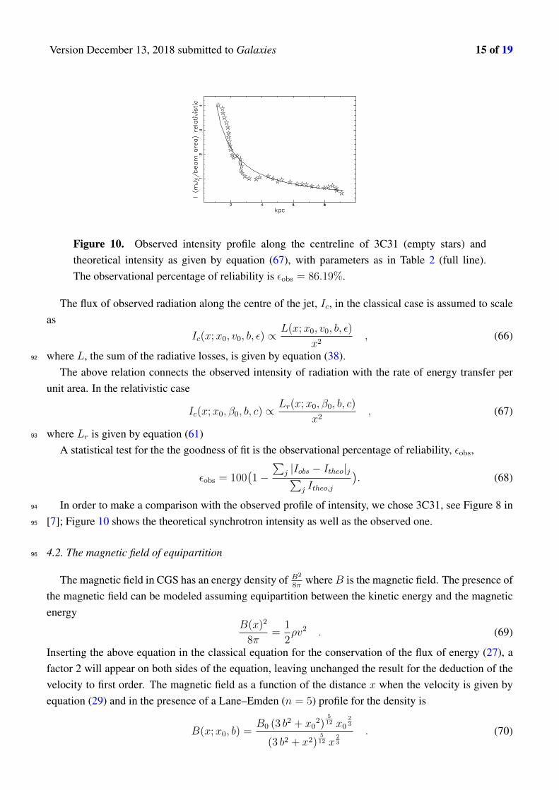
Figure 10. Observed intensity profile along the centreline of 3C31 (empty stars) andtheoretical intensity as given by equation (67), with parameters as in Table 2 (full line).The observational percentage of reliability is εobs = 86.19%.

The flux of observed radiation along the centre of the jet, Ic, in the classical case is assumed to scaleas

Ic(x;x0, v0, b, ε) ∝L(x;x0, v0, b, ε)

x2, (66)

where L, the sum of the radiative losses, is given by equation (38).92

The above relation connects the observed intensity of radiation with the rate of energy transfer perunit area. In the relativistic case

Ic(x;x0, β0, b, c) ∝Lr(x;x0, β0, b, c)

x2, (67)

where Lr is given by equation (61)93

A statistical test for the the goodness of fit is the observational percentage of reliability, εobs,

εobs = 100(1−

∑j |Iobs − Itheo|j∑

j Itheo,j

). (68)

In order to make a comparison with the observed profile of intensity, we chose 3C31, see Figure 8 in94

[7]; Figure 10 shows the theoretical synchrotron intensity as well as the observed one.95

4.2. The magnetic field of equipartition96

The magnetic field in CGS has an energy density of B2

8πwhereB is the magnetic field. The presence of

the magnetic field can be modeled assuming equipartition between the kinetic energy and the magneticenergy

B(x)2

8π=

1

2ρv2 . (69)

Inserting the above equation in the classical equation for the conservation of the flux of energy (27), afactor 2 will appear on both sides of the equation, leaving unchanged the result for the deduction of thevelocity to first order. The magnetic field as a function of the distance x when the velocity is given byequation (29) and in the presence of a Lane–Emden (n = 5) profile for the density is

B(x;x0, b) =B0 (3 b

2 + x02)

512 x0

23

(3 b2 + x2)512 x

23

. (70)

Version December 13, 2018 submitted to Galaxies 16 of 19

where B0 is the magnetic field at x = x0. We assume an inverse power law spectrum for theultrarelativistic electrons, of the type

N(E)dE = KE−pdE (71)

where K is a constant and p the exponent of the inverse power law. The intensity of the synchrotron97

radiation has a standard expression, as given by formula (1.175) in [36],98

I(ν) ≈ 0.933× 10−23αp(p)KlH(p+1)/2⊥

(6.26× 1018

ν

)(p−1)/2 (72)

erg sec−1cm−2Hz−1rad−2

where ν is the frequency, H⊥ is the magnetic field perpendicular to the electron’s velocity, l is thedimension of the radiating region along the line of sight, and αp(p) is a slowly varying function of pwhich is of the order of unity. We now analyse the intensity along the centreline of the jet, which meansthat the radiating length is

l(x;α) = x tan(α

2) . (73)

The intensity, assuming a constant p, scales as

I(x;x0, p) =I0B

p2+ 1

2x

B0

p2+ 1

2 x0, (74)

where I0 is the intensity at x = x0 and B0 the magnetic field at x = x0. We insert Eq. (70) in order tohave an analytical expression for the centreline intensity

I(x;x0, p, b) =(3 b2 + x0

2) 5 p

24+ 5

24 i0x− p

3+ 2

3x0p3− 2

3

(3 b2 + x2

)− 5 p24− 5

24 . (75)

The above equation for the intensity is relative to the unit area; in order to have the intensity on thecentreline, Ic, we should make a further division by the area of interest, which scales ∝ x2

Ic(x;x0, p, b) =I(x;x0, p, b)

x2. (76)

Figure 11 shows the theoretical synchrotron intensity with the variable magnetic field as well as the99

observed one for 3C31.100

5. Conclusions101

Classical case The approximate trajectory of a turbulent jet in the presence of a Lane–Emden (n =102

5) medium has been evaluated to first order, see equation (35). The solution for the velocity to first103

order allows the insertion of the back-reaction, i.e. the radiative losses, in the equation for the flux of104

energy conservation, see equation (39), and as a consequence the velocity corrected to second order, see105

equation (40). The trajectory, calculated numerically to second order, is shown in Figure 5. The radiative106

losses allow evaluating the length at which the advancing velocity of the jet is zero. This length has a107

complicated analytical expression and was presented numerically, see Figure 6.108

Relativistic case In the relativistic case it is possible to derive an analytical expression for β to first109

order, see equation (49), and to second order (taking into account radiative losses), see equation (64).110

Version December 13, 2018 submitted to Galaxies 17 of 19

Figure 11. Observed intensity profile along the centreline, Ic, of 3C31 (empty stars)and theoretical intensity as given by equation (76), with parameters as in Table 1. Theobservational percentage of reliability is εobs = 73.79%.

The relativistic trajectory to first order has been evaluated through a series, see equation (52) or a Padé111

approximant of order [2/1], see equation (58). The relativistic equation of motion to second order112

(back-reaction) has been evaluated numerically, see Figure 9. In other words, with the introduction113

of the radiative losses, the length of the classical or relativistic jet becomes finite rather than infinite.114

An astrophysical application The radiative losses are represented by equation (37) in the classical case115

and by (61) in the relativistic case. A division of the two above quantities by the area of interest allows116

deriving the theoretical rate of energy transfer per unit area, which can be compared with the intensity117

of radiation along the jet, for example, 3C31, see Figure 10. The spatial behaviour of the magnetic118

field is introduced under the hypothesis of equipartition between the kinetic and magnetic energy, see119

equation (70), and this allows closing the standard equation for the synchrotron emissivity, see equation120

(73).121

References122

1. Curtis, H.D. Descriptions of 762 Nebulae and Clusters Photographed with the Crossley Reflector.123

Publications of Lick Observatory 1918, 13, 9–42.124

2. Fanaroff, B.L.; Riley, J.M. The morphology of extragalactic radio sources of high and low125

luminosity. MNRAS 1974, 167, 31P–36P.126

3. Kembhavi, A.K.; Narlikar, J.V. Quasars and active galactic nuclei : an introduction; Cambridge127

University Press: Cambridge, 1999.128

4. Bridle, A.H.; Perley, R.A. Extragalactic Radio Jets. ARA&A 1984, 22, 319–358.129

5. Liu, F.K.; Zhang, Y.H. A new list of extra-galactic radio jets. A&A 2002, 381, 757–760,130

[astro-ph/0212477].131

6. Hardcastle, M.J.; Sakelliou, I. Jet termination in wide-angle tail radio sources. MNRAS 2004,132

349, 560–575.133

7. Laing, R.A.; Bridle, A.H. Relativistic models and the jet velocity field in the radio galaxy 3C 31.134

MNRAS 2002, 336, 328–352.135

Version December 13, 2018 submitted to Galaxies 18 of 19

8. Nawaz, M.A.; Wagner, A.Y.; Bicknell, G.V.; Sutherland, R.S.; McNamara, B.R. Jet-intracluster136

medium interaction in Hydra A - I. Estimates of jet velocity from inner knots. MNRAS 2014,137

444, 1600–1614, [1408.4512].138

9. Nawaz, M.A.; Bicknell, G.V.; Wagner, A.Y.; Sutherland, R.S.; McNamara, B.R. Jet-intracluster139

medium interaction in Hydra A - II. The effect of jet precession. MNRAS 2016, 458, 802–815,140

[1602.02969].141

10. Zaninetti, L. Classical and relativistic conservation of momentum flux in radio-galaxies . Applied142

Physics Research 2015, 7, 43–62.143

11. Zaninetti, L. Classical and Relativistic Flux of Energy Conservation in Astrophysical Jets.144

Journal of High Energy Physics, Gravitation and Cosmology 2016, 1, 41–56.145

12. Kellermann, K.I.; Richards, E.A. Radio Observations of the Hubble Deep Field. The Hubble146

Deep Field; Livio, M.; Fall, S.M.; Madau, P., Eds.; Cambridge University Press: Cambridge,147

1998; p. 60.148

13. Bird, R.; Stewart, W.; Lightfoot, E. Transport Phenomena ; second Edition; John Wiley and149

Sons: New York, 2002.150

14. Landau, L. Fluid Mechanics 2nd edition; Pergamon Press: London, 1987.151

15. Goldstein, S. Modern Developments in Fluid Dynamics; Dover: New York, 1965.152

16. Reichardt, V. Gesetzmabigkeiten der freien Turbulenz. VDI-Forschungsheft 1942, 414, 141.153

17. Reichardt, V. Vollstandige Darstellung der turbulenten Geschwindigkeitsverteilung in glatten154

Leitungen. Zeitschrift fur Angewandte Mathematik und Mechanik 1951, 31, 208–219.155

18. Schlichting, H. Boundary Layer Theory; McGraw-Hill: New York, 1979.156

19. De Young, D.S. The physics of extragalactic radio sources; University of Chicago Press:157

Chicago, 2002.158

20. Laing, R.A.; Bridle, A.H. Adiabatic relativistic models for the jets in the radio galaxy 3C 31.159

MNRAS 2004, 348, 1459–1472, [astro-ph/0311499].160

21. Lane, H.J. On the Theoretical Temperature of the Sun, under the Hypothesis of a gaseous Mass161

maintaining its Volume by its internal Heat, and depending on the laws of gases as known to162

terrestrial Experiment. American Journal of Science 1870, 148, 57–74.163

22. Emden, R. Gaskugeln: anwendungen der mechanischen warmetheorie auf kosmologische und164

meteorologische probleme; B. Teubner.: Berlin, 1907.165

23. Chandrasekhar, S. An introduction to the study of stellar structure; Dover: New York, 1967.166

24. Binney, J.; Tremaine, S. Galactic dynamics, Second Edition; Princeton University Press:167

Princeton, NJ, 2011.168

25. Zwillinger, D. Handbook of differential equations; Academic Press: New York, 1989.169

26. Hansen, C.J.; Kawaler, S.D. Stellar Interiors. Physical Principles, Structure, and Evolution.;170

Springer-Verlag: Berlin, 1994.171

27. Abramowitz, M.; Stegun, I.A. Handbook of Mathematical Functions with Formulas, Graphs,172

and Mathematical Tables; Dover: New York, 1965.173

28. von Seggern, D. CRC Standard Curves and Surfaces; CRC: New York, 1992.174

29. Thompson, W.J. Atlas for computing mathematical functions; Wiley-Interscience: New York,175

1997.176

Version December 13, 2018 submitted to Galaxies 19 of 19

30. Olver, F.W.J.e.; Lozier, D.W.e.; Boisvert, R.F.e.; Clark, C.W.e. NIST handbook of mathematical177

functions.; Cambridge University Press. : Cambridge, 2010.178

31. Ashby, N. Relativity in the Global Positioning System. Living Reviews in Relativity 2003, 6, 1.179

32. Ashby, N.; Nelson, R.A. GPS, Relativity, and Extraterrestrial Navigation. IAU Symposium180

#261, American Astronomical Society, 2009, Vol. 261, p. 889.181

33. Adachi, M.; Kasai, M. An Analytical Approximation of the Luminosity Distance in182

Flat Cosmologies with a Cosmological Constant. Progress of Theoretical Physics 2012,183

127, 145–152, [arXiv:astro-ph.CO/1111.6396].184

34. Aviles, A.; Bravetti, A.; Capozziello, S.; Luongo, O. Precision cosmology with Padé rational185

approximations: Theoretical predictions versus observational limits. Phys. Rev. D 2014,186

90, 043531, [arXiv:gr-qc/1405.6935].187

35. Wei, H.; Yan, X.P.; Zhou, Y.N. Cosmological applications of Pade approximant. Journal of188

Cosmology and Astroparticle Physic 2014, 1, 45, [arXiv:astro-ph.CO/1312.1117].189

36. Lang, K.R. Astrophysical formulae. (Second Edition); Springer: New York, 1980.190

c© December 13, 2018 by the author; submitted to Galaxies for possible open access191

publication under the terms and conditions of the Creative Commons Attribution license192

http://creativecommons.org/licenses/by/4.0/.193