![Acer [Course Title] [Teacher's Name](https://static.fdokumen.com/doc/165x107/6320a62900d668140c0d1f09/acer-course-title-teachers-name.jpg)
CIT755 COURSE TITLE: Wireless Communication I - National ...
224
NATIONAL OPEN UNIVERSITY OF NIGERIA SCHOOL OF SCIENCE AND TECHNOLOGY COURSE CODE: CIT755 COURSE TITLE: Wireless Communication I
-
Upload
khangminh22 -
Category
Documents
-
view
1 -
download
0
Transcript of CIT755 COURSE TITLE: Wireless Communication I - National ...
NATIONAL OPEN UNIVERSITY OF NIGERIA
SCHOOL OF SCIENCE AND TECHNOLOGY
COURSE CODE: CIT755
COURSE TITLE: Wireless Communication I

CIT755 COURSE GUIDE
ii
COURSE GUIDE
CIT755 WIRELESS COMMUNICATION I
Course Team A. J. Ikuomola (Developer/Writer) - AUOA Prof. H.O.D Longe (Editor) - UNILAG Prof. Obidairo (Programme Leader) - NOUN A.A. Afolorunso (Coordinator) - NOUN
NATIONAL OPEN UNIVERSITY OF NIGERIA

CIT755 COURSE GUIDE
National Open University of Nigeria Headquarters 14/16 Ahmadu Bello Way Victoria Island Lagos
Abuja Office No. 5 Dar es Salaam Street Off Aminu Kano Crescent Wuse II, Abuja Nigeria
e-mail: [email protected] URL: www.nou.edu.ng
Published By: National Open University of Nigeria
First Printed 2011
ISBN: 978-058-537-0 All Rights Reserved
iii

CIT755 COURSE GUIDE
iv
CONTENTS PAGE
Introduction ……………………………………………….………. 1 What You Will Learn in this Course…………………………….…. 1 Course Aims…………………………………………………….….. 2 Course Objectives……………………………………………….…. 2 Working through this Course…………………………………….… 2 The Course Material……………………………………………..…. 3 Study Units………………………………………………………..... 3 Presentation Schedule………………….……………………….….. 5 Assessment…………………………………………………….…… 5 Tutor-Marked Assignment………………………………………..… 5 Final Examination and Grading…………………………………..… 6 Course Marking Scheme……………………………………….…... 6 Facilitators/Tutors and Tutorials…………………………………… 6 Summary……………………………………………………….…… 7

CIT755 WIRELESS COMMUNICATION I
v
Introduction
Introduction to Wireless Communication 1 is a 3-unit post graduate course in Information Technology.
Wireless communication is the transfer of information over a distance without the use of electrical conductors or “wires”. The distances involved may be short (a few meters as in television remote control) or long (thousands or millions of kilometers for radio communications). When the context is clear, the term is often shortened to “wireless”.
Wireless communication is generally considered to be a branch of telecommunications.
It encompasses various types of fixed, mobile, and portable two-way radios, cellular telephones, personal digital assistants (PDAs), and wireless networking. Other examples of wireless technology include GPS units, garage door openers, wireless computer mice, keyboards and headsets, satellite television and cordless telephones
This course introduces you to the most important new technology in wireless communication system. To provide wireless communications to the whole world was a dream before the development of cellular concept. With the development of highly reliable, miniature, solid-state radio frequency hardware, the wireless communication era came into existence. The recent exponential growth in cellular radio and personal communication systems throughout the world has been possible because of the new technologies developed. Further, the future growth of consumer-based mobile and portable communication system will be coupled closely to the allocations of radio spectrum which support new technologies advancement in signal process.
What You Will Learn in this Course This Course Guide is the starting point for this course. It tells you briefly what the course is about, what course materials you will be using and how you can work your way through these materials. It also gives you guidance on your tutor-marked assignments as well as describes what you need to do in order to pass this course. There will be regular tutorial classes that are related to the course. It is advisable for you to attend these tutorial sessions. The course will prepare you for the challenges you will meet in the field of wireless communication.
CIT755 WIRELESS COMMUNICATION I
2
Course Aims
The aim of this course is to provide you with an understanding of wireless communication, its use, application and the technology behind it; it also aims to provide you with solutions to problems in wireless/cellular communication system. This will be achieved by:
introducing you to what the wireless communication is and what it consists of explaining to you the basic technology underlying the wireless communication explaining to you the cellular design concept helping you to understand the various modulation, diversity and multiple access techniques.
Course Objectives
To achieve the aims set out above, the course has a set of objectives.
Each unit has specific objectives which are included at the beginning of each unit. You should read these objectives before you study the unit. You may wish to refer to them during the study to check on your progress. On successful completion of this course, you should be able to:
explain the concept and evolution of wireless communication identify the various cellular system generations and the mechanism for capacity increase in a cellular system discuss the three basic radio propagation mechanism explain the concept of radio wave propagation: Large scale path loss model, small scale fading and shadowing describe various modulation techniques discuss on the types of diversity techniques categorise the multiple access techniques and state their application areas solve practical problems in wireless communication.
Working through this Course
To complete this course you are required to read each study unit, the textbooks, related materials you find on the internet and other materials which may be provided by the National Open University of Nigeria.
Each unit contains self-assessment exercises, and at a point in the course, you are required to submit assignments for assessment purposes.

CIT755 WIRELESS COMMUNICATION I
3
At the end of this course there is a final examination. The course will take about 18 weeks to complete. Below, you will find listed all the components of the course, what you have to do and how you should allocate your time to each unit in order to complete the course successfully on time.
Course Materials The main components of the course are:
1. The Course Guide 2. Study Units 3. Presentation Schedule 4. Assignment 5. References/Further Reading
Study Units There are 21 study units in this course. Each unit should take you 2-3 hours to work through. The 21 units are divided into four modules.
Three modules contain 5 units each while the last module contains 6 units. This is arranged as follows: The study units in this course are as follows:
Module 1 Introduction Unit 1 Overview and History of Wireless Communication Unit 2 Modern Wireless Communication System Unit 3 Wireless Data Network Unit 4 The Cellular Concept Unit 5 Improving Capacity in Cellular System
Module 2 Mobile Radio Propagation Unit 1 Wireless Channel Model Unit 2 Large-Scale Propagation Model Unit 3 Radio Propagation Mechanisms Unit 4 Path Loss Model Unit 5 Shadowing
Module 3 Mobile Radio Propagation Unit 1 Small Scale Fading and Multipath Unit 2 Types of Small Scale Fading Unit 3 Small Scale Fading: Racian, Rayleigh and Nakagami

CIT755 WIRELESS COMMUNICATION I
4
Unit 4 Small Scale Fading: Threshold Crossing Rate, Fade Duration and Scatter Function
Unit 5 Channel Classification
Module 4 Modulation and Diversity Techniques
Unit 1 Introduction to Modulation Unit 2 Analog Modulation Techniques Unit 3 Digital (Bandpass) Modulation Techniques Unit 4 Digital Baseband and Pulse Shaping Modulation
Techniques Unit 5 Diversity Techniques for Fading channel Unit 6 Multiple Access Techniques
In Module 1: The first unit focuses on the meaning, concept, differences between wired and wireless, application, brief history of wireless communication, mobile radio communication and evolution, radio and the electromagnetic spectrum, how radio signals are created, radio- wavelength, frequency and antennas, radio signal and energy. The second unit deals with the meaning of cellular system, basic cellular system and wireless communication standards generations. The third unit concentrates on various wireless data network. Unit 4 deals with the meaning of cellular communication, cell fundamentals, cell size, cellular frequency reuse, cell planning, mobile phone network, concept of cell cluster and geometry of hexagonal cells. Unit 5 discusses the advantages of cellular system, interference and system capacity, channel assignment strategies and mechanisms for capacity increase in cellular system.
In Module 2: The first five units concentrate on meaning of channel model, statistical propagation models, basic concept of path loss, causes and propagation prediction, free space propagation model, relating power to electric field, radio propagation mechanisms, empirical path loss model, practical link budget design using path loss model, and the concept of shadowing.
In Module 3: The first five units focus on the meaning and factor affecting small scale multipath propagation, multipath fading channel models, concept of doppler, types of small scale fading, mitigation, fading models: racian, rayleigh and nakagami fading, threshold crossing rate, fade duration, average fade duration, scatter function, and channel classification.
In Module 4: The first four units discuss definition, choice of modulation, how to modulate a sound wave and types of modulation techniques, Unit 5 deals with diversity techniques for fading channel and its application. Unit 6 concentrates on meaning of multiple access,

CIT755 WIRELESS COMMUNICATION I
5
multiple access in a radio cell, category, comparison and application of multiple access techniques.
Presentation Schedule Your course materials have important dates for the early and timely completion and submission of your TMAs and attending tutorials are necessary. You should remember that you are required to submit all your assignments by the stipulated time and date. You should guard against falling behind in your work. The assignment file will be made available to you in due course. In this file, you will find all the details of the work you must submit to your tutor for marking. The marks you obtain for these assignments will count in computing the final mark you obtain for this course.
Assessment There are three aspects to the assessment of the course: the self- assessment exercises, the tutor-marked assignments and the written examination/end of course examination.
You are advised to do the exercises. In tackling the assignments, you are expected to apply information, knowledge and techniques you gathered during the course. The assignments must be submitted to your facilitator for formal assessment in accordance with the deadlines stated in the presentation schedule and the assignment file. The work you submit to your tutor for assessment will count for 30% of your total course work.
At the end of the course you will need to sit for a final or end of course examination of about three hour duration. This examination will count for 70% of your total course mark.
Tutor-Marked Assignment (TMA) The TMA is a continuous assessment component of your course. It accounts for 30% of the total score. You will be given four (4) TMAs to answer. Three of these must be answered before you are allowed to sit for the end of course examination. The TMAs would be given by your facilitator and returned after you have done the assignment. Assignment questions for the units in this course are contained in the Assignment File. You will be able to complete your assignments from the information and materials contained in your reading and study units, references and the internet. When you complete each assignment, send it, together with the TMAs, to your tutor. Make sure that each assignment reaches your tutor/facilitator on or before the deadline given in the presentation schedule and assignment file.

CIT755 WIRELESS COMMUNICATION I
6
Final Examination and Grading
The end of course examination for Wireless Communication will be for about 3 hours and it has a value of 70% of the total course work. The final examination covers information from all parts of the course i.e. all areas of the course will be assessed. You might find it useful to review your Self-Assessment Exercises, Tutor-Marked Assignments and comments on them before the examination.
Course Marking Scheme
The following table lays out how the actual course marking is broken down.
Assignment Marks Assignment 1 – 4 Four assignments, best three marks
of the four count at 10% each – 30% of course marks
End of course examination 70% of overall course marks Total 100%
Facilitators/Tutors and Tutorials
There are 16 hours of tutorials provided in support of this course. You will be notified of the dates, times and location of these tutorials as well as the name and phone number of your facilitator, as soon as you are allocated a tutorial group.
Your facilitator will mark and comment on your assignments, keep a close watch on your progress and any difficulties you might face and provide assistance to you during the course. You are expected to mail your Tutor-Marked Assignment to your facilitator before the schedule date (at least two working days are required). They will be marked by your tutor and returned to you as soon as possible.
Do not delay to contact your facilitator by telephone or e-mail if you need assistance. The following might be circumstances in which you would find assistance necessary, hence you would have to contact your facilitator if:
You do not understand any part of the study or the assigned readings You have difficulty with the self-tests or exercises You have a question or problem with an assignment or with the grading of an assignment.

CIT755 WIRELESS COMMUNICATION I
7
You should try to attend the tutorials. This is the only chance to have face to face contact with your course facilitator and to ask questions which are answered instantly. You can raise any problem encountered in the course of your study.
Summary Introduction to wireless Communication I is a course that describes communications in which electromagnetic waves or RF (rather than some form of wire) carry a signal over part or the entire communication path. Upon completing this course, you will be equipped with the basic knowledge of Wireless communication. In addition, you will be able to answer the questions.
What does wireless communication I is mean? What are the applications areas of wireless technology? Identify four generations of wireless communication Explain the cell concept Explain the three propagation mechanisms Describe large scale path loss, small scale fading and shadowing State the advantages of FM over Am List six types of diversity techniques Define the term Multiple Access.
Of course, the list of questions that you can answer is not limited to the above list. We wish you success in the course and hope that you will find it both interesting and useful and wishing you every success in your future endeavours.


CIT755 COURSE GUIDE
Course Code CIT755 Course Title Wireless Communication I
Course Team A. J. Ikuomola (Developer/Writer) - AUOA Prof. H.O.D Longe (Editor) - UNILAG Prof. Obidairo (Programme Leader) - NOUN A.A. Afolorunso (Coordinator) - NOUN
NATIONAL OPEN UNIVERSITY OF NIGERIA
CIT755 WIRELESS COMMUNICATION I
ii
National Open University of Nigeria Headquarters 14/16 Ahmadu Bello Way Victoria Island Lagos
Abuja Office No. 5 Dar es Salaam Street Off Aminu Kano Crescent Wuse II, Abuja Nigeria
e-mail: [email protected] URL: www.nou.edu.ng
Published By: National Open University of Nigeria
First Printed 2011
ISBN: 978-058-537-0
All Rights Reserved

CIT755 WIRELESS COMMUNICATION I
iii
CONTENTS PAGE
Module 1 Introduction………………………………..…….…… 1 Unit 1 Overview and History of Wireless Communication….. 1 Unit 2 Modern Wireless Communication System ………….. 13 Unit 3 Wireless Data Network……………………………….. 18 Unit 4 The Cellular Concept…………………………………. 24 Unit 5 Improving Capacity in Cellular System………………. 37
Module 2 Mobile Radio Propagation…………………….……. 48 Unit 1 Wireless Channel Model……………………………… 48 Unit 2 Large-Scale Propagation Model………........................ 56 Unit 3 Radio Propagation Mechanisms………........................ 65 Unit 4 Path Loss Model………………………........................ 77 Unit 5 Shadowing…………………………………………….. 90
Module 3 Mobile Radio Propagation……………………………94 Unit 1 Small Scale Fading and Multipath……………………. 94 Unit 2 Types of Small Scale Fading………………………….102 Unit 3 Small Scale Fading: Racian, Rayleigh and Nakagami 109 Unit 4 Small Scale Fading: Threshold Crossing Rate, Fade
Duration and Scatter Function………………………. 118 Unit 5 Channel Classification………………………………. 129
Module 4 Modulation and Diversity Techniques…………….. 136 Unit 1 Introduction to Modulation………………………….. 136 Unit 2 Analog Modulation Techniques……………………… 141 Unit 3 Digital (Bandpass) Modulation Techniques ………… 159 Unit 4 Digital Baseband and Pulse Shaping Modulation
Techniques..................................................................... 174 Unit 5 Diversity Techniques for Fading Channel …………… 180 Unit 6 Multiple Access Techniques…………………………. 186


CIT755 WIRELESS COMMUNICATION I
1
MODULE 1 INTRODUCTION
Unit 1 Overview and Evolution of Wireless Communication Unit 2 Modern Wireless Communication System Unit 3 Wireless Data Network Unit 4 The Cellular Concept Unit 5 Improving Capacity in Cellular System
UNIT 1 OVERVIEW AND EVOLUTION OF WIRELESS COMMUNICATION
CONTENTS
1.0 Introduction 2.0 Objectives 3.0 Main Content
3.1 Concept of Wireless Communication 3.1.1 Wireless Equipment 3.1.2 Examples of Wireless Communication and Control 3.1.3 Uses of Wireless Technology 3.1.4 Classification of Wireless 3.1.5 Applications of Wireless Technology
3.2 Brief History of Wireless Communications 3.3 Mobile Radio Communication
3.3.1 Evolution of Mobile Radio Communication 3.3.2 Radio and the Electromagnetic Spectrum 3.3.3 How Radio Signals Are Created 3.3.4 Radio – Wavelengths, Frequencies and Antennas 3.3.5 Radio Signals and Energy
3.4 Differences between Wired and Wireless 4.0 Conclusion 5.0 Summary 6.0 Tutor-Marked Assignment 7.0 References/Further Reading
1.0 INTRODUCTION Wireless communication is experiencing its fastest growth period in history. This has been possible because of enabling technologies that permit widespread deployment.
Wireless communication is the transfer of information over a distance without the use of electrical conductors or “wires”. The distances involved may be short (a few meters as in television remote control) or long (thousands or millions of kilometers for radio communications).

CIT755 WIRELESS COMMUNICATION I
2
Wireless communication is generally considered to be a branch of telecommunications.
It encompasses various types of fixed, mobile, and portable two-way radios, cellular telephones, personal digital assistants (PDAs), and wireless networking. Other examples of wireless technology include GPS units, garage door openers, wireless computer mice, keyboards and headsets, satellite television and cordless telephones.
Wireless communication can be via:
radio frequency communication microwave communication, for example long-range line-of-sight via highly directional antennas, or short-range communication or infrared (IR) short-range communication, for example from remote controls or via Infrared Data Association (IrDA).
2.0 OBJECTIVES
At the end of this unit, you should be able to:
define wireless communication mention examples of wireless communication equipment state the application area of wireless communication explain the history of radio communication identify the use of wireless technology state the classes of wireless.
3.0 MAIN CONTENT
3.1 Concept of Wireless Communication
Wireless is a term used to describe telecommunications in which electromagnetic waves (rather than some form of wire) carry the signal over part or the entire communication path.
3.1.1 Wireless Equipment
Common examples of wireless equipment in use today include:
Cellular phones and pagers: These provide connectivity for portable and mobile applications, both personal and business Global Positioning System (GPS): Allows drivers of cars and trucks, captains of boats and ships, and pilots of aircraft to ascertain their location anywhere on earth
CIT755 WIRELESS COMMUNICATION I
3
Cordless computer peripherals: The cordless mouse is a common example; keyboards and printers can also be linked to a computer via wireless Cordless telephone sets: These are limited-range devices, not to be confused with cell phones Home-entertainment-system control boxes: The VCR control and the TV channel control are the most common examples; some hi-fi sound systems and FM broadcast receivers also use this technology Remote garage-door openers: One of the oldest wireless devices commonly use by consumers which are usually operated at radio frequencies Two-way radios: These include amateur and citizens radio service, as well as business, marine, and military communications Baby monitors: These devices are simplified radio transmitter/receiver units with limited range Satellite television: Allows viewers in almost any location to select from hundreds of channels Wireless LANs or Local Area Networks: Provide flexibility and reliability for business computer users.
3.1.2 Examples of Wireless Communication and Control More specialised and exotic examples of wireless communications and control include:
Global System for Mobile Communication (GSM): A digital mobile telephone system General Packet Radio Service (GPRS): A packet-based wireless communication service that provides continuous connection to the Internet for mobile phone and computer users. Enhanced Data GSM Environment (EDGE): A faster version of the Global System for Mobile (GSM) wireless service. Universal Mobile Telecommunications System (UMTS): A broadband, packet-based system offering a consistent set of services to mobile computer and phone users no matter where they are located in the world. Wireless Application Protocol (WAP): A set of communication protocols to standardise the way that wireless devices, such as cellular telephones and radio transceivers, can be used for internet access. i-Mode: The world’s first “smart phone” for Web browsing, first introduced in Japan; provides colour and video over telephone sets.

CIT755 WIRELESS COMMUNICATION I
4
3.1.3 Uses of Wireless Technology
Wireless technology is rapidly evolving, and is playing an increasing role in the lives of people throughout the world. In addition, increasing numbers of people are relying on the technology directly or indirectly.
The following situations justify the use of wireless technology:
to span a distance beyond the capabilities of typical cabling to avoid obstacles such as physical structures to provide a backup communications link in case of normal network failure to link portable or temporary workstations to overcome situations where normal cabling is difficult or financially impractical, or to remotely connect mobile users or networks.
3.1.4 Classification of Wireless
Wireless can be divided into the following classes:
Fixed wireless: The operation of wireless devices or systems in homes and offices, and in particular, equipment connected to the Internet via specialised modems Mobile wireless: The use of wireless devices or systems aboard motorised, moving vehicles; examples include the automotive cell phone and PCS (personal communications services) Portable wireless: The operation of autonomous, battery- powered wireless devices or systems outside the office, home, or vehicle; examples include handheld cell phones and PCS units IR wireless: The use of devices that convey data via IR (infrared) radiation; employed in certain limited-range communications and control systems
3.1.5 Applications of Wireless Technology
Security systems: Wireless technology may supplement or replace hard wired implementations in security systems for homes or office buildings. Television remote control: Modern televisions use wireless (generally infrared) remote control units but now radio waves are also used. Cellular telephony (phones and modems): These instruments use radio waves to enable the operator to make phone calls from many locations world-wide. They can be used anywhere there is

CIT755 WIRELESS COMMUNICATION I
5
a cellular telephone site to house the equipment that is required to transmit and receive the signal that is used to transfer both voice and data to and from these instruments. WiFi: Wi-Fi (for wireless fidelity) is a wireless LAN technology that enables laptop PC’s, PDA’s, and other devices to connect easily to the internet. Wi-Fi is less expensive and nearing the speeds of standard Ethernet and other common wire-based LAN technologies. Wireless energy transfer: Wireless energy transfer is a process whereby electrical energy is transmitted from a power source to an electrical load that does not have a built-in power source, without the use of interconnecting wires. Computer interface devices: Answering the call of customers frustrated with cord clutter, many manufactures of computer peripherals turned to wireless technology to satisfy their consumer base. Originally these units used bulky, highly limited transceivers to mediate between a computer and a keyboard and mouse, however more recent generations have used small, high quality devices, some even incorporating Bluetooth
3.2 Brief History of Wireless Communications
Before the “Birth of Radio” 1867-1896
1867 - Maxwell predicts existence of electromagnetic (EM) waves 1887 - Hertz proves existence of EM waves; first spark transmitter generates a spark in a receiver several meters away 1890 - Branly develops coherer for detecting radio waves 1896 - Guglielmo Marconi demonstrates wireless telegraph to English telegraph office
“The Birth of Radio”
1897 – “The Birth of Radio” - Marconi awarded patent for wireless telegraph 1897 - First “Marconi station” established on Needles Island to communicate with English coast 1898 - Marconi awarded English patent no. 7777 for tuned communication 1898 - Wireless telegraphic connection between England and France established

CIT755 WIRELESS COMMUNICATION I
6
Transoceanic Communication
1901 - Marconi successfully transmits radio signal across Atlantic Ocean from Cornwall to Newfoundland 1902 - First bidirectional communication across Atlantic 1909 - Marconi awarded Nobel Prize for physics
Voice over Radio
1914 - First voice over radio transmission 1920s - Mobile receivers installed in Police cars in Detroit 1930s - Mobile transmitters developed; radio equipment occupied most of Police car trunk 1935 - Frequency modulation (FM) demonstrated by Armstrong 1940s - Majority of Police systems converted to FM
Birth of Mobile Telephony
1946 - First interconnection of mobile users to public switched telephone network (PSTN) 1949 – Federal Communication Commission (FCC) recognises mobile radio as new class of service 1940s - Number of mobile users > 50,000 1950s - Number of mobile users > 500,000 1960s - Number of mobile users > 1,400,000 1960s - Improved Mobile Telephone Service (IMTS) introduced; supports full-duplex, auto dial, auto trunking 1976 - Bell Mobile Phone has 543 pay customers using 12 channels in the New York City area; waiting list is 3700 people; service is poor due to blocking
Cellular Mobile Telephony
1979 – NTT Communications Corporation Japan deploys first cellular communication system 1983 - Advanced Mobile Phone System (AMPS) deployed in US in 900 MHz band: supports 666 duplex channels 1989 - Groupe Spècial Mobile defines European digital cellular standard, GSM 1991 - US Digital Cellular phone system introduced 1993 - IS-95 code-division multiple-access (CDMA) spread- spectrum digital cellular system deployed in US 1994 - GSM system deployed in US, labelled “Global System for Mobile Communications”

CIT755 WIRELESS COMMUNICATION I
7
PCS and Beyond
1995 - Federal Communication Commission (FCC) auctions off frequencies in Personal Communications System (PCS) band at 1.8 GHz for mobile telephony 1997 - Number of cellular telephone users in U.S. > 50,000,000 2000 - Third generation cellular system standards. Bluetooth standards.
3.3 Mobile Radio Communication Radio is the technology and practice that enables the transmission and reception of information carried by long-wave electromagnetic radiation. Radio makes it possible to establish wireless two-way communication between individual pairs of transmitter and receiver, and it is used for one-way broadcasts to many receivers. Radio signals can carry speech, music, telemetry, or digitally-encoded entertainment.
Radio is used by the general public, within legal guidelines, or it is used by private business or governmental agencies. Cordless telephones are possible because they use low-power radio transmitters to connect without wires. Cellular telephones use a network of computer-controlled low power radio transmitters to enable users to place telephone calls away from phone lines.
Radio receivers recover modulation information in a process called demodulation or detection. The radio carrier is discarded after it is no longer needed. The radio carrier's cargo of information is converted to sound using a loudspeaker or headphones.
3.3.1 Evolution of Mobile Radio Communication In the 19th Century, in Scotland, James Clerk Maxwell described the theoretical basis for radio transmissions with a set of four equations known ever since as Maxwell’s Field Equations. Maxwell was the first scientist to use mechanical analogies and powerful mathematical modelling to create a successful description of the physical basis of the electromagnetic spectrum. His analysis provided the first insight into the phenomena that would eventually become radio.
Not long after Maxwell’s remarkable revelation about electromagnetic radiation, Heinrich Hertz demonstrated the existence of radio waves by transmitting and receiving a microwave radio signal over a considerable distance. Hertz’s apparatus was crude by modern standards but it was important because it provided experimental evidence in support of Maxwell’s theory.

CIT755 WIRELESS COMMUNICATION I
8
Guglielmo Marconi developed a wireless telegraphy which was able to send a long-wave radio signal across the Atlantic Ocean.
The first radio transmitters to send messages, Marconi's equipment included, used high-voltage spark discharges to produce the charge acceleration needed to generate powerful radio signals. Spark transmitters could not carry speech or music information. They could only send coded messages by turning the signal on and off using a telegraphy code similar to the landline Morse code.
Spark transmitters were limited to the generation of radio signals with very-long wavelengths, much longer than those used for the present AM-broadcast band in the United States. The signals produced by a spark transmitter were very broad with each signal spread across a large share of the usable radio spectrum. Only a few radio stations could operate at the same time without interfering with each other. Mechanical generators operating at a higher frequency than those used to produce electrical power were used in an attempt to improve on the signals developed by spark transmitters.
A technological innovation enabling the generation of cleaner, narrower signals was needed. Electron tubes provided that breakthrough, making it possible to generate stable radio frequency signals that could carry speech and music. Broadcast radio quickly became established as source of news and entertainment.
Continual improvements to radio transmitting and receiving equipment opened up the use of successively higher and higher radio frequencies.
Short waves, as signals with wavelengths less than 200m were found to be able to reach distant continents. International broadcasting on shortwave frequencies followed, allowing listeners to hear programming from around the world.
The newer frequency-modulation system, FM, was inaugurated in the late 1930s and for more than 25 years struggled for acceptance until it eventually became the most important mode of domestic broadcast radio. FM offers many technical advantages over AM, including an almost complete immunity to the lightning-caused static that plagues AM broadcasts. The FM system improved the sound quality of broadcasts tremendously, far exceeding the fidelity of the AM radio stations of the time. The FM system was the creation of E. H. Armstrong, perhaps the most prolific inventor of all those who made radio possible.

CIT755 WIRELESS COMMUNICATION I
9
In the late 1950s, stereo capabilities were added to FM broadcasts along with the ability to transmit additional programmes on each station that could not be heard without a special receiver. A very high percentage of FM broadcast stations today carry these hidden programmes that serve special audiences or markets. This extra programme capability, called SCA for Subsidiary Communications Authorisation, can be used for stock market data, pager services, or background music for stores and restaurants.
3.3.2 Radio and the Electromagnetic Spectrum Radio utilises a small part of the electromagnetic spectrum, the set of related wave-based phenomena that includes radio along with infrared light, visible light, ultraviolet light, x rays, and gamma rays. Radio waves travel at the velocity of electromagnetic radiation. A radio signal moves fast enough to complete a trip around the earth in about 1/7 second.
3.3.3 How Radio Signals Are Created If you jiggle a collection of electrons up and down one million times a second, then a 1-MegaHertz radio signal will be created. Change the vibration frequency and the frequency of the radio signal will change. Radio transmitters are alternating voltage generators. The constantly changing voltage from the transmitter creates a changing electric field within the antenna. This alternating field pushes and pulls on the conduction electrons in the wire that are free to move. The resulting charge acceleration produces the radio signal that moves away from the antenna. The radio signal causes smaller sympathetic radio frequency currents in any distant electrical conductor that can act as a receiving antenna.
3.3.4 Radio – Wavelengths, Frequencies and Antennas Each radio signal has a characteristic wavelength just as it is in sound wave. The higher the frequency of the signal, the shorter will be the wavelength. Antennas for low-frequency radio signals are long. Antennas for higher frequencies are shorter; to match the length of the waves they will send or receive.
It is a characteristic of all waves, not just radio signals, that there is greater interaction between waves and objects when the length of the wave is comparable to the object's size. Just as only selected sound wavelengths fit easily into the air column inside a bugle, only chosen frequencies will be accepted by a given antenna length. Antennas, particularly transmitting antennas, function poorly unless they have a
CIT755 WIRELESS COMMUNICATION I
10
size that matches the wavelength of the signal presented to them. The radio signal must be able to fit on the antenna as a standing wave. This condition of compatibility is called resonance. If a transmitter is able to “feed” energy into an antenna, the antenna must be resonant or it will not “take power” from the transmitter. A receiver antenna is less critical, since inefficiency can be compensated by signal amplification in the receiver, but there is improvement in reception when receiving antennas are tuned to resonance.
If an antenna’s physical length is inappropriate, capacitors or inductors may be used to make it appear electrically shorter or longer to achieve resonance.
3.3.5 Radio Signals and Energy
Energy is required to create a radio signal. Radio signals use the energy from the transmitter that accelerates electric charge in the transmitting antenna. A radio signal carries this energy from the transmitting antenna to the receiving antenna. Only a small fraction of the transmitter's power is normally intercepted by any one receiving antenna, but even a vanishingly-small received signal can be amplified electronically millions of times as required.
3.4 Differences between Wired and Wireless
The main difference between wired and wireless data communication infrastructure is the existence of physical cabling. A wired network uses wires (cables) to connect devices whereas a wireless network uses radio waves. Wired networks are easy to set up and troubleshoot whereas wireless networks are comparatively difficult to set up, maintain and troubleshoot. Wired networks make you immobile while wireless ones provide you with convenience of movement. Wired network proves expensive when covering a large area because of the wiring and cabling while wireless network do not involve this cost. Wired networks have better transmission speeds than wireless ones. In wired networks, a user does not have to share space with other users and thus gets dedicated speed while in wireless networks the same connection may be shared by multiple users.

CIT755 WIRELESS COMMUNICATION I
11
4.0 CONCLUSION
This unit has introduced you to the concept, applications and origination of wireless communication. You have also been informed on how radio signals are created.
5.0 SUMMARY The main points in this unit include the following:
Wireless communication is the transfer of information over a distance without the use of electrical conductors or “wires” It encompasses various types of fixed, mobile, and portable two- way radios, cellular telephones, personal digital assistants (PDAs), wireless networking, etc. Radio is the technology and practice that enables the transmission and reception of information carried by long-wave electromagnetic radiation Marconi successfully transmits radio signal across Atlantic Ocean from Cornwall to Newfoundland The main difference between wired and wireless data communication infrastructure is the existence of physical cabling.
SELF ASSESSMENT EXERCISE 1. What is wireless communication? 2. Why are antennas on cell phones smaller than antenna on your
radio?
6.0 TUTOR-MARKED ASSIGNMENT 1. Discuss the evolution of radio communication 2. Why are car antennas about the same size as TV antenna? 3. Mention five examples of wireless communication equipment. 4. List five uses of wireless technology 5. Briefly explain the application area of wireless communication 6. Outline the four classes of wireless

CIT755 WIRELESS COMMUNICATION I
12
7.0 REFERENCES/FURTHER READING
Goldsmith, A. (2005). Wireless Communications. Cambridge University Press.
Lior, Baruch (2008). Mobile Computing: Definition-Wireless.
O’Brien, J. & Marakas, G. M. (2008). Management Information Systems. New York: McGraw-Hill Irwin.
Shea J. (2000). Brief History of Wireless Communication.
CIT755 WIRELESS COMMUNICATION I
13
UNIT 2 MODERN WIRELESS COMMUNICATION
SYSTEM CONTENTS
1.0 Introduction 2.0 Objectives 3.0 Main Content
3.1 Introduction to Cellular System 3.1.1 Basic Cellular System
3.2 Wireless Communications Standards/Generations 3.2.1 First Generation Cellular Systems 3.2.2 Second Generation Cellular Systems 3.2.3 Third Generation Cellular Systems 3.2.4 Fourth Generation Cellular Systems
4.0 Conclusion 5.0 Summary 6.0 Tutor-Marked Assignment 7.0 References/Further Reading
1.0 INTRODUCTION As you have learnt in the previous unit, the field of mobile communications has experienced various advanced developments. In fact, it can be said that mobile radio communications industry has grown up during the last ten years. There are various factors which are responsible for speedy developments in mobile or wireless communications. These factors are digital and RF fabrication improvements, new large scale circuit integration and other miniaturisation technologies.
2.0 OBJECTIVES At the end of this unit, you should be able to:
explain a cellular system state the basic components of cellular system discuss the wireless communication generations.
3.0 MAIN CONTENT
3.1 Introduction to Cellular System
A cellular system is a radio network made up of a number of radio cell (or just cells) each served by at least one fixed-location transceiver known as a cell site or base station. These cells cover different land

CIT755 WIRELESS COMMUNICATION I
14
areas to provide radio coverage over a wider area than the area of one cell, so that a variable number of portable transceivers can be used in any one cell and moved through more than one cell during transmission.
Cellular systems offer a number of advantages including but not limited to the following over alternative solutions:
Increased capacity Reduced power usage Larger coverage area Reduced interference from other signals
3.1.1 Basic Cellular System
A basic cellular system is made up of three parts:
i. A mobile unit ii. A cell site iii. Mobile Telephone Switching Office (MTSO) and with
connections to link the three subsystems:
Mobile Unit: A mobile telephone unit contains a control unit, a transceiver and an antenna system Cell Site: The cell site provides interface between the MTSO and the mobile unit. It has control unit, radio cabinets, antennas, a power plant and data terminals. MTSO: The switching office, the central coordinating element for all cell sites, contains the cellular processor and cellular switch. It interfaces with telephone company zone offices; controls call processing and handle billing activities. Connections: As a matter of fact, the radio and high speed data links connect the three subsystems. Each mobile unit can only use one channel at a time for its communication link.
However, the channel is not fixed i.e. it can be any one in the entire band assigned by the serving area, with each site having multi-channel capabilities that can connect simultaneously to many mobile units.
In addition to the above:
The MTSO is the heart of the cellular mobile system. Its processor provides central coordination and cellular administration. The cellular switch, which can be either analog or digital, switches calls to connect mobile subscribers to other mobile

CIT755 WIRELESS COMMUNICATION I
15
subscribers and to the nationwide telephone network. It uses voice trucks similar to telephone company interoffice voice trucks. It also contains data links providing supervision links between the processor and the switch and between the cell sites and the processor. The radio link carries the voice and signal between the mobile unit and the cell site. The high-speed data links cannot be transmitted over the standard telephone trucks and therefore must use either microwave links or T-carriers (wire lines). Microwave radio links or T-carriers carry both voice and data between the cell site and the MTSO.
3.2 Wireless Communications Standards/Generations 3.2.1 First Generation Cellular Systems
The first generation (1G) wireless communications stems use frequency division multiple access (FDMA) as the multiple access technology.
FDMA is an analog transmission technique that is inherently narrowband. As a matter of fact, the first generation cellular systems make use of analog FM scheme for speech transmission. The individual calls use different frequencies and share the available spectrum through a particular multiple access technique known as frequency-division multiplexing access (FDMA).
3.2.2 Second Generation Cellular Systems The second generation (2G) wireless systems use digital transmission. The multiple access technology is both time division multiple access (TDMA) and code division multiple access (CDMA). Although, the second generation wireless systems offer higher transmission rates with greater flexibility than the first generation systems, they are nevertheless narrowband systems. The service offered by both 1G and 2G system is predominantly voice. The digital technology allows greater sharing of the radio hardware in the base station among the multiple users, and provides a larger capacity to support more users per base station per Megahertz (Mhz) of spectrum as compared to analog system. As a matter of fact, digital systems offer a number of advantages over analog system.
Digital systems provide:
flexibility for supporting multimedia services flexibility for capacity expansion

CIT755 WIRELESS COMMUNICATION I
16
reduction in Radio Frequency (RF) transmit power encryption for communication privacy reduction in system complexity.
3.2.3 Third Generation Cellular Systems
The third generation (3G) standard is based on CDMA as the multiple access technology. With a transmission rate of up to 2 megabits per second (Mbps), 3G systems are wideband, and are expected to support multimedia services. It is likely that the third generation cellular systems will be equipped with the infrastructure to support Personal Communications Systems (PCS). The network infrastructure support will likely include the following:
public land mobile networks (PLMNs) mobile Internet Protocol (Mobile IP) wireless asynchronous transfer mode (WATM) networks, and low earth orbit (LEO) satellite network
3.2.4 Fourth Generation Cellular Systems
During the last 20 years, wireless networks have evolved from an analog, single medium (voice), and low data rate (a few kilobits per second) system to the digital, multimedia, and high data rate (ten to hundreds of megabits per second) system of today. Future systems will be based on user’s demands as the fourth-generation (4G) cellular system applications which need high speed data rates to achieve them.
In July 2003, the International Telecommunications Union (ITU) made requirements for 4G system which are:
i. at a standstill condition, the transmission data rate should be 1
Gbps. ii. at a moving condition, the transmission data rate should be 100
Mbps.
Any proposed system that can meet these requirements with less bandwidth and higher mobile speed will be considered. A potential 4G system could be used in the family of OFDM (Orthogononal Frequency Division Multiplexing), because the Wireless Metropolitan Area Network (WMAN) using OFDM can have a transmission data rate of 54-70 Mbps, which is much higher than what the Code Division Multiple Access (CDMA) system can provide.
4.0 CONCLUSION
CIT755 WIRELESS COMMUNICATION I
17
In this unit, you have learnt the concepts of a cellular system and the generations/standard of wireless communications.
5.0 SUMMARY The main points in this unit are:
A cellular system is a radio network made up of a number of radio cell (or just cells) each served by at least one fixed-location transceiver known as a cell site or base station. A basic cellular system is made up of three parts: a mobile unit, cell site, and mobile Telephone Switching Office (MTSO) and with connections to link the three subsystems Wireless communications systems that have been in deployment for sometime are those of the first generation and second generation. Third generation systems are also currently under deployment, but continue to evolve.
SELF ASSESSMENT EXERCISE Write on the Fourth Generation (4G) Systems
6.0 TUTOR-MARKED ASSIGNMENT 1. Discuss on the first, second and third generation wireless
communication networks 2. What do you understand about a basic cellular system?
7.0 REFERENCE/FURTHER READING Sharma S. (2006). Wireless & Cellular Communications. New Delhi: S.
K. Kataria & Sons.
UNIT 3 WIRELESS DATA NETWORK

CIT755 WIRELESS COMMUNICATION I
18
CONTENTS
1.0 Introduction 2.0 Objectives 3.0 Main Content
3.1 Wireless Data Networks 3.1.1 Personal Area Network (PAN) 3.1.2 Local Area Network (LAN) 3.1.3 Metropolitan Area Network (MAN) 3.1.4 Wide Area Network (WAN)
4.0 Conclusion 5.0 Summary 6.0 Tutor-Marked Assignment 7.0 References/Further Reading
1.0 INTRODUCTION
In this unit, in brief, we are going to discuss various issues related to wireless data networks.
2.0 OBJECTIVES
At the end of this unit, you should be able to:
discuss the wireless data network differentiate between PAN, LAN, MAN and WAN illustrate with diagram wireless data network.
3.0 MAIN CONTENT
3.1 Wireless Data Networks
The wireless data network can be classified according to their coverage areas as: Personal Area Network (PAN), Local Area Network (LAN), Metropolitan Area Network (MAN) and Wide Area Network (WAN).
3.1.1 Personal Area Network (PAN)
Personal Area Network (PAN) is a computer network organised around an individual person. It is a computer network used for communication among computer devices (including telephones and personal digital assistants) close to one’s person. Personal area network typically involve a mobile computer, a cell phone and/or a handheld computing device such as a PDA. You can use these networks to transfer files including email and calendar appointments, digital photos and music. The smallest

CIT755 WIRELESS COMMUNICATION I
19
coverage area, where the network is called wireless personal area network (PAN), is limited to an office. A cell of such a small size would enable connection of computers or electronic input devices. A wireless PAN network can use Bluetooth. Personal area networks generally cover a range of less than 10 meters (about 30 feet).
The channel bandwidth is 200 kHz using Quadrature Amplitude Modulation (QAM). The data rate can be 1 Mbps. It is a short wire replacement for wireless. Today, most of cell phones are equipped with Bluetooth.
Fig. 3.1: Personal Area Network
3.1.2 Local Area Network (LAN) Local Area Network (LAN) is a computer network covering a small physical area, like a home, office, or small group of buildings, such as a school, or an airport. Wireless local area network (LAN) connects users on a particular floor of a building. For example, two computers linked together at home are the simplest form of a LAN while several hundred computers cabled together across several buildings at school form a more complex LAN. In 1990s, wireless LANs was divided into the radio-frequency (RF) systems and infrared (IR) systems specified by the Federal Communication Commission (FCC). The RF systems are divided into the licensed non-spread-spectrum (NSS) and the unlicensed spread spectrum (SS). In the unlicensed SS, it requires a minimum of 50 and 75 hopping frequency at 910MHz and 2.5GHz, respectively, or achieved by a spread-spectrum modulation exceeding a spreading factor of 10m in direct sequence systems. LANs are usually connected with coaxial or CAT5 cable.
CIT755 WIRELESS COMMUNICATION I
20
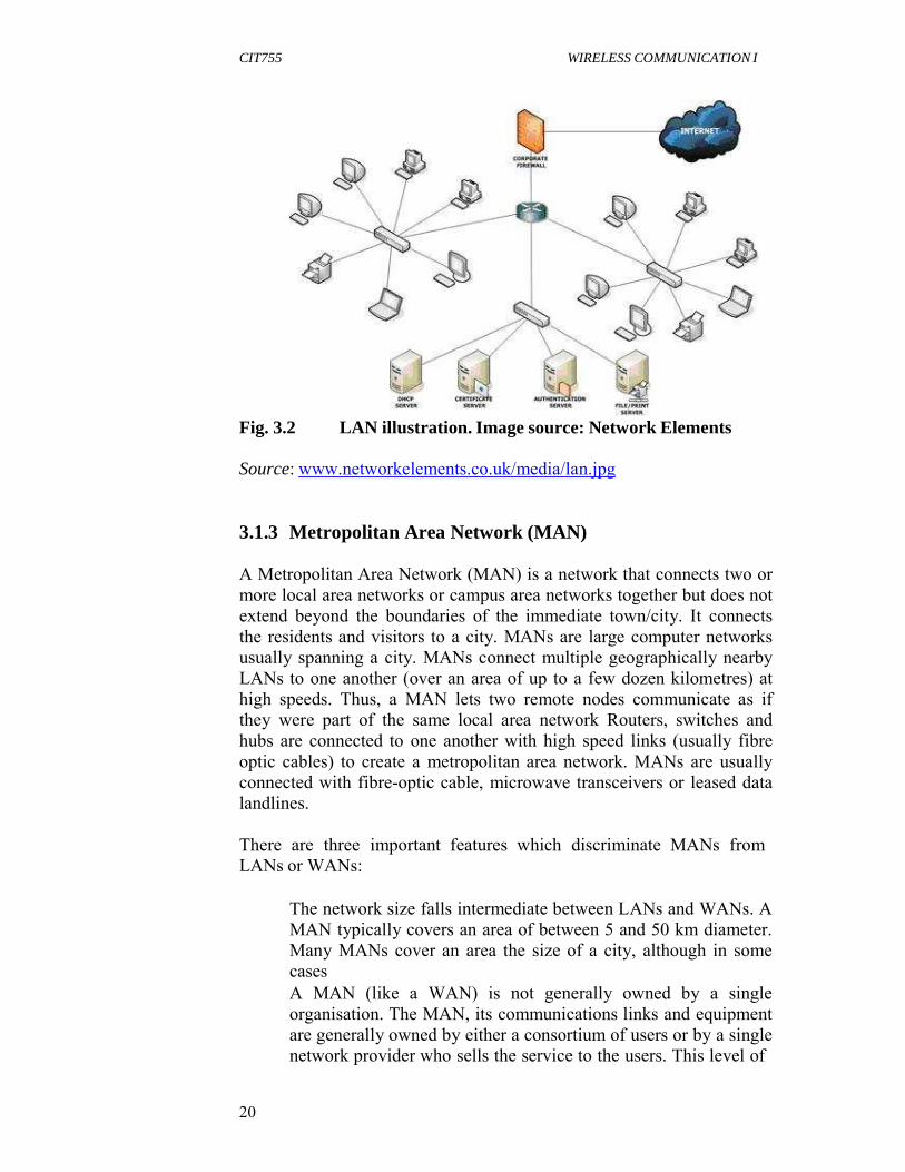
Fig. 3.2 LAN illustration. Image source: Network Elements
Source: www.networkelements.co.uk/media/lan.jpg
3.1.3 Metropolitan Area Network (MAN)
A Metropolitan Area Network (MAN) is a network that connects two or more local area networks or campus area networks together but does not extend beyond the boundaries of the immediate town/city. It connects the residents and visitors to a city. MANs are large computer networks usually spanning a city. MANs connect multiple geographically nearby LANs to one another (over an area of up to a few dozen kilometres) at high speeds. Thus, a MAN lets two remote nodes communicate as if they were part of the same local area network Routers, switches and hubs are connected to one another with high speed links (usually fibre optic cables) to create a metropolitan area network. MANs are usually connected with fibre-optic cable, microwave transceivers or leased data landlines.
There are three important features which discriminate MANs from LANs or WANs:
The network size falls intermediate between LANs and WANs. A MAN typically covers an area of between 5 and 50 km diameter. Many MANs cover an area the size of a city, although in some cases A MAN (like a WAN) is not generally owned by a single organisation. The MAN, its communications links and equipment are generally owned by either a consortium of users or by a single network provider who sells the service to the users. This level of

CIT755 WIRELESS COMMUNICATION I
21
service provided to each user must therefore be negotiated with the MAN operator, and some performance guarantees are normally specified. A MAN often acts as a high speed network to allow sharing of regional resources (similar to a large LAN). It is also frequently used to provide a shared connection to other networks using a link to a WAN.
Fig. 3.3 Metropolitan Area Network
Source rkcablenet.tradeindia.com/Exporters_Suppliers
3.1.4 Wide Area Network (WAN) Wide Area Network (WAN) is a computer network that covers a broad area (i.e., any network whose communications links cross metropolitan, regional, or national boundaries). WAN is a data communications network that covers a relatively broad geographic area (i.e. one city to another and one country to another country) and that often uses transmission facilities provided by common carriers, such as telephone companies. The largest and most well-known example of a WAN is the Internet. WANs are used to connect LANs and other types of networks together, so that users and computers in one location can communicate with users and computers in other locations. Typically, a WAN consists of two or more Local Area networks (LANs) connected by a communication sub-system, which is usually comprised of Autonomous System (AS) routers. For example, a national banking organisation may use a WAN to connect all of its branches across the country. WANs are usually connected using the Internet, ISDN landlines or satellite.

CIT755 WIRELESS COMMUNICATION I
22
(a) Source: www.air-stream.org.au/wan
(b) Source: www.computernetworks.com/WAN.cfm
Fig. 3.4 (a & b): Wide Area Network (WAN)
4.0 CONCLUSION
The wireless data network can be classified according to their coverage areas as:

CIT755 WIRELESS COMMUNICATION I
23
Personal Area Network (PAN) Local Area Network (LAN) Metropolitan Area Network (MAN) Wide Area Network (WAN)
5.0 SUMMARY
In this unit, you have learnt that:
Personal area network (PAN) is a computer network used for communication among computer devices (including telephones and personal digital assistants) close to one's person LAN means Local Area Network, and is generally restricted to a single building Local area network (LAN) is a computer network covering a small physical area, like a home, office, or small group of buildings, such as a school, or an airport MAN means Metropolitan Area Network, and usually encompasses multiple sites in the same city. It connects the residents and visitors to a city WAN means Wide Area Network and can cover any area. It connects the entire country.
SELF ASSESSMENT EXERCISE Mention four classifications of wireless data network
6.0 TUTOR-MARKED ASSIGNMENT 1. Discuss the wireless LAN. 2. Differentiate between MAN and WAN. 3. Illustrate with diagram a Local Area Network.
7.0 REFERENCES/FURTHER READING Sharma, S. (2006). Wireless and Cellular Communications. New Delhi:
S. K. Kataria & Sons. Tse, D. & Viswanath P. (2005). Fundamentals of Wireless
Communication. Cambridge University Press. UNIT 4 THE CELLULAR CONCEPT
CONTENTS

CIT755 WIRELESS COMMUNICATION I
24
1.0 Introduction 2.0 Objectives 3.0 Main Content
3.1 Concept of Cellular Communications 3.1.1 Cell Fundamentals 3.1.2 Cell Size 3.1.3 Cellular Frequency Reuse 3.1.4 Cell Planning 3.1.5 Mobile Phone Networks 3.1.6 Concept of Cell Cluster 3.1.7 Geometry of Hexagonal Cells
4.0 Conclusion 5.0 Summary 6.0 Tutor-Marked Assignment 7.0 References/Further Reading
1.0 INTRODUCTION
Cellular systems are widely used today and cellular technology needs to offer very efficient use of the available frequency spectrum. With billions of mobile phones in use around the globe today, it is necessary to refuse the available frequencies many times over without mutual interference of one cell phone to another. It is this concept of frequency reuse that is at the heart of cellular technology.
2.0 OBJECTIVES
At the end of this unit, you should be able to:
explain the cell concept discuss the use of frequency reuse concept mention different types of cell state the importance of hexagonal cell shape over other shapes.
3.0 MAIN CONTENT
3.1 Concept of Cellular Communications
The limitation in spectral width and the maximum number of user (i.e. system capacity) that can be supported in a wireless mobile system is an important performance measure. If a single transmitter were used to cover a large geographical area (a single small area called a cell that is served by a single base station, or a cluster of cells), a very high power transmitter and very high antenna would be required. With a single high power transmitter, all users will share the same set of frequencies, or radio channels. If the same set of radio resources were assigned to serve
CIT755 WIRELESS COMMUNICATION I
25
a smaller geographical area and then reused to serve another small geographical area, it would be possible to expand the system capacity (i.e. the number of users).The geographical regions that use the same set of radio frequencies must be physically separated from each other so that the power level of the signal that spills out from one region to a neighbouring region does not produce unacceptable interference. This way of replicating identically structured and operated geographical regions gives rise to the concept of cellular communications.
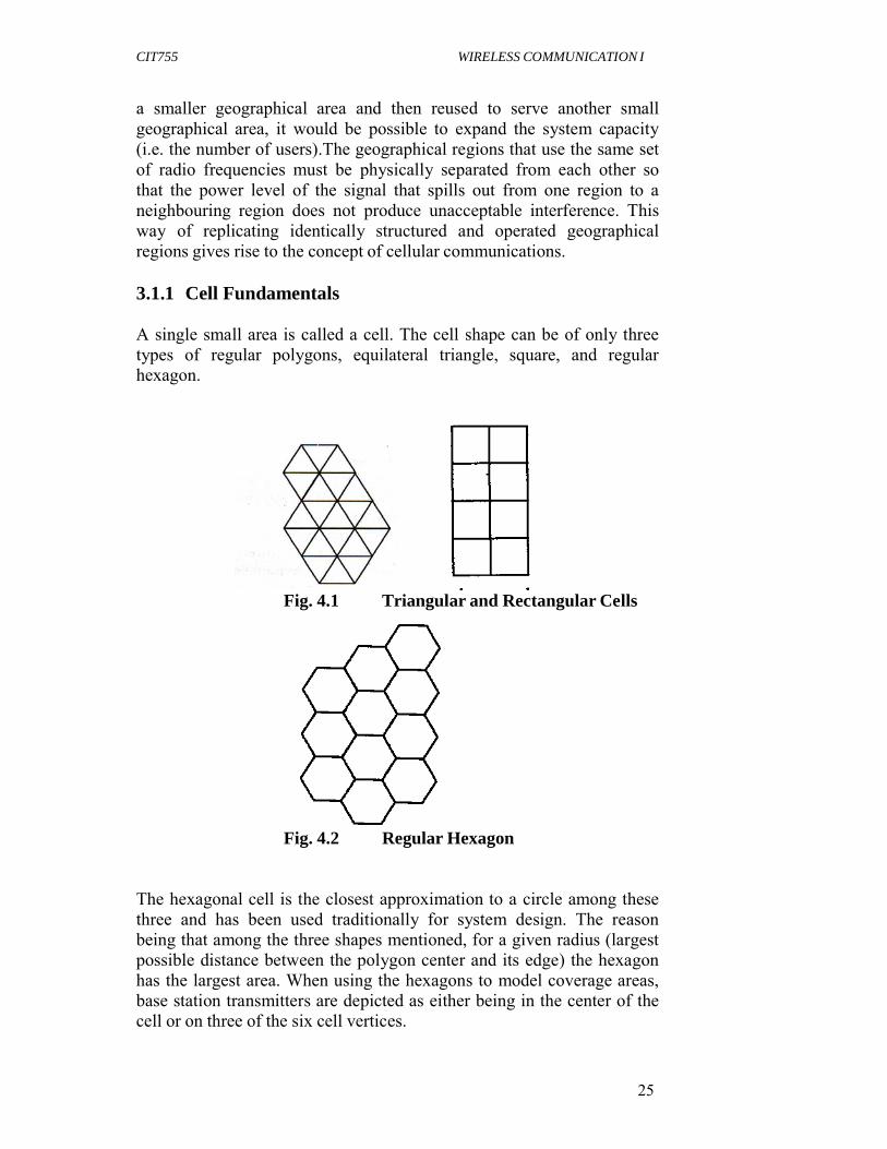
3.1.1 Cell Fundamentals A single small area is called a cell. The cell shape can be of only three types of regular polygons, equilateral triangle, square, and regular hexagon.
Fig. 4.1 Triangular and Rectangular Cells
Fig. 4.2 Regular Hexagon
The hexagonal cell is the closest approximation to a circle among these three and has been used traditionally for system design. The reason being that among the three shapes mentioned, for a given radius (largest possible distance between the polygon center and its edge) the hexagon has the largest area. When using the hexagons to model coverage areas, base station transmitters are depicted as either being in the center of the cell or on three of the six cell vertices.
CIT755 WIRELESS COMMUNICATION I
26
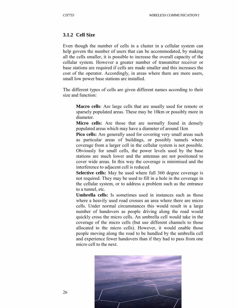
3.1.2 Cell Size
Even though the number of cells in a cluster in a cellular system can help govern the number of users that can be accommodated, by making all the cells smaller, it is possible to increase the overall capacity of the cellular system. However a greater number of transmitter receiver or base stations are required if cells are made smaller and this increases the cost of the operator. Accordingly, in areas where there are more users, small low power base stations are installed.
The different types of cells are given different names according to their size and function:
Macro cells: Are large cells that are usually used for remote or sparsely populated areas. These may be 10km or possibly more in diameter. Micro cells: Are those that are normally found in densely populated areas which may have a diameter of around 1km Pico cells: Are generally used for covering very small areas such as particular areas of buildings, or possibly tunnels where coverage from a larger cell in the cellular system is not possible. Obviously for small cells, the power levels used by the base stations are much lower and the antennas are not positioned to cover wide areas. In this way the coverage is minimised and the interference to adjacent cell is reduced. Selective cells: May be used where full 360 degree coverage is not required. They may be used to fill in a hole in the coverage in the cellular system, or to address a problem such as the entrance to a tunnel, etc. Umbrella cells: Is sometimes used in instances such as those where a heavily used road crosses an area where there are micro cells. Under normal circumstances this would result in a large number of handovers as people driving along the road would quickly cross the micro cells. An umbrella cell would take in the coverage of the micro cells (but use different channels to those allocated to the micro cells). However, it would enable those people moving along the road to be handled by the umbrella cell and experience fewer handovers than if they had to pass from one micro cell to the next.

CIT755 WIRELESS COMMUNICATION I
27
Fig. 4.3 Cell Size
Decreasing cell size gives
Increased user capacity Increased number of handovers per call Increased complexity in locating the subscriber Lower power consumption in mobile terminal: so it gives longer talk time, safer operation
3.1.3 Cellular Frequency Reuse Frequency reuse is a technique of reusing frequencies and channels within a communications system to improve capacity and spectral efficiency. Frequency reuse is one of the fundamental concepts in which commercial wireless systems are based that involves the partitioning of an RF radiating area (cell) into segments of a cell. One segment of the cell uses a frequency that is far enough away from the frequency in the bordering segment that does not provide interference problems.
In the cellular concept, frequency allocated to the service are reused in a regular pattern of areas, called ‘cells’, each covered by one base station.
Every cellular base station is assigned a group of radio channels which are used within a small geographical area called a cell. The base station antennas are designed to achieve the desired coverage within a particular cell. In mobile-telephone system these cells are usually hexagonal. To ensure that the mutual interference between users remains below harmful level, adjacent cells use different frequencies. In fact, a set of C different frequencies (f1…fc) are used for each cluster of C adjacent cells. Cluster patterns and the corresponding frequencies are re-used in a regular pattern over the entire service area.
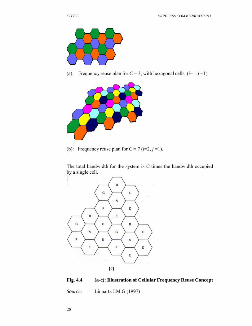
CIT755 WIRELESS COMMUNICATION I
28
(a): Frequency reuse plan for C = 3, with hexagonal cells. (i=1, j =1)
(b): Frequency reuse plan for C = 7 (i=2, j =1).
The total bandwidth for the system is C times the bandwidth occupied by a single cell.
(c)
Fig. 4.4 (a-c): Illustration of Cellular Frequency Reuse Concept
Source: Linnartz J.M.G (1997)

CIT755 WIRELESS COMMUNICATION I
29
3.1.4 Cell Planning
In the practice of cell planning, cells are not hexagonal as considered in the theoretical studies. However, propagation over irregular terrain leads to quite different cell shapes and cell sizes. Computer methods are being used for optimised planning of base station locations and cell frequencies. Path loss and link budgets are computed from the terrain features and antenna data. This determines the coverage of each base station and interference to other cells.
In the initial phases of operating a cellular network, the planners typically aim at maximum coverage. Subscribers should be able to reach a base station anywhere. The map of the service coverage should not contain dark spots where the service is not available. Base stations are located such that they reach as many locations as possible, e.g. typically on hill tops.
Later on, when the number of subscribers increases, there is a need to optimise the capacity. Cell size should be as small as possible to accommodate as many different cell areas as possible. The effect that hills can shield on signals and avoid propagation into other valleys can be used as advantage. It allows that frequencies are reused in nearby valleys, particularly if base station are not located at the hill tops but in the valleys.
Effect of Traffic Density An important aspect is the distribution of traffic. Cell sizes need to be smaller in areas with more traffic. The erlang theory addresses the amount of traffic that can be carried over a given number of channels, at a given blocking rate. If a GSM operator faces blocking rates that are too large in a certain area, he could for instance
Split the cell into two cells with disjoint coverage areas, for instance by using two sectors from the same mast, or by using two separate base station locations. Install equipment for a second GSM carrier, for 8 telephone channels. The old and new carriers have the same coverage and together provide 16 voice channels.
The first option is more efficient from a frequency scarcity point of view. In both cells, the 8 channels can carry 3.13 erlang at a blocking rate of 1%. In the second case, the 16 channels can carry 8.8 erlang at 1% blocking rate. Note that this is significantly more than 2 times 3.13 erlang.
CIT755 WIRELESS COMMUNICATION I
30
3.1.5 Mobile Phone Networks
The most common example of a cellular network is a mobile phone (cell phone) network. A mobile phone is a portable telephone which receives or makes calls through a cell site (base station), or transmitting tower. Radio waves are used to transfer signals to and from the cell phone.
Large geographic areas (representing the coverage range of a service provider) may be split into smaller cells to avoid line-of-sight signal loss and the large number of active phones in an area. In cities, each cell site has a range of up to approximately ½ mile, while in rural areas; the range is approximately 5 miles. Many times in clear open areas, a user may receive signals from a cell site 25 miles away. All of the cell sites are connected to cellular telephone exchanges “switches”, which connect to a public telephone network or to another switch of the cellular company.
As the phone user moves from one cell area to another cell, the switch automatically commands the handset and a cell site with a stronger signal (reported by each handset) to switch to a new radio channel (frequency). When the handset responds through the new cell site, the exchange switches the connection to the new cell site.
With CDMA, multiple CDMA handsets share a specific radio channel. The signals are separated by using a pseudonoise code (PN code) specific to each phone. As the user moves from one cell to another, the handset sets up radio links with multiple cell sites (or sectors of the same site) simultaneously. This is known as “soft handoff” because, unlike with traditional cellular technology, there is no one defined point where the phone switches to the new cell.
Modern mobile phone networks use cells because radio frequencies are limited and shared resource. Cell-sites and handsets change frequency under computer control and use low power transmitters so that a limited number of radio frequencies can be simultaneously used by many callers with less interference.
Since almost all mobile phones use cellular technology, including GSM, CDMA, and AMPS (analog), the term “cell phone” is used interchangeably with “mobile phone”. However, satellite phones are mobile phones that do not communicate directly with a ground-based cellular tower, but may do so indirectly by way of a satellite.
There are a number of different digital cellular technologies, including: Global System for Mobile Communications (GSM), General Packet Radio Service (GPRS), Code Division Multiple Access (CDMA),

CIT755 WIRELESS COMMUNICATION I
31
Evolution-Data Optimized (EV-DO), Enhanced Data Rates for GSM Evolution (EDGE), 3GSM, Digital Enhanced Cordless Telecommunications (DECT), Digital AMPS (IS-136/TDMA), and Integrated Digital Enhanced Network (iDEN).
3.1.6 Concept of Cell Cluster When devising the infrastructure technology of a cellular system, the interference between adjacent channels is reduced by allocating different frequency bands or channels to adjacent cells so that their coverage can overlap slightly without causing interference. In this way cells can be grouped together in what is termed a cluster. A group of cells that use different set of frequencies in each cell is called a Cell Cluster. Let N be the cluster size in terms of the number of cells within it and K be the total number of available channels without frequency reuse. The N cells in the cluster would then utilise all K available channels. In this way, each cell in the cluster contains one-Nth of the total number of available channels. In this sense, N is also referred to as the frequency reuse factor of the cellular system.
Seven is a convenient number of cells that can be in a cluster, but there are number of conflicting requirements that need to be balanced when choosing the number of cells in a cluster for a cellular system:
Limiting interference levels Number of channels that can be allocated to each cell site
It is necessary to limit the interference between cells having the same frequency. The topology of the cell configuration has a large impact on this. The larger the number of cells in the cluster, the greater the distance between cells sharing the same frequencies. In the ideal world it might be good to choose a large number of cells to be in each cluster. Unfortunately there are only a limited number of channels available.
This means that the larger the number of cells in a cluster, the smaller the number available to each cell, and this reduces the capacity. This means that there is a balance that needs to be made between the number of cells in a cluster, and the interference levels and the capacity that is required.
(a) Capacity Increase by Frequency Reuse Concept Let us consider that each is allocated J channels (J≤K). If the K channels are divided among the N cells into unique and disjoint channel groups, each with J channels, then we have

CIT755 WIRELESS COMMUNICATION I
32
K = J N
N cells in a cluster use the complete set of available frequencies while K is the total number of available channel. By decreasing the cluster size N, it is possible to increase the capacity per cell. The cluster can be replicated many times to form the entire cellular communication system.
Let M be the number of times the cluster is replicated and C be the total number of channels used in the entire cellular system with frequency reuse. C is then the system capacity and is given by
C = M J N
If M is increased, the system capacity C will increase.
EXERCISE 4
Given a cellular system which has a total of 1001 radio channels available for handling traffic and given the area of a cell is 6 km2 and the area of the entire system is 2100 km2.
i. Calculate the system capacity if the cluster size is 7. ii. How many times would the cluster of size 4 have to be replicated
in order to approximately cover the entire cellular area? iii. Calculate the system capacity if the cluster size is 4. iv. Does decreasing the cluster size increase the system capacity?
Explain
Solution: Given that
The total number of available channels K = 1001. Cluster size N = 7. Area of cell Acell = 6 km2 Area of cellular system Asys = 2100 km2
(i) The number of channels per cell is given by J K
N
Then we have J 1001
7
143 channels / cell
Also, we know that the coverage area of a cluster is given by Acluster N Acell 7 6 42km 2
The number of times that the cluster has to be replicated to cover
the entire system will be M Asys
Acluster
or M 2100
50 42

CIT755 WIRELESS COMMUNICATION I
33
Hence, the system capacity C will be C = M J N = 50 x 143 x 7 = 50,050 channels.
(ii) For N = 4, Acluster = 4 x 6 = 24 km2
Hence M Asys
Acluster
2100
24
87.5
87.
(iii) With N = 4, J 1001
4
250 channels / cell.
The system capacity is then
C = 87 x 250 x 4 = 87,000 channels. From (i) and (iii), it is obvious that a decrease in N from 7 to 4 is accompanied by an increase in M from 50 to 87, and the system capacity is increased from 50,050 channels to 87,000 channels.
Hence, decreasing the cluster size does increase the system capacity.
(iv) Cellular Layout for Frequency Reuse Rule to Determine the Nearest Co-channel Neighbours
The following two-step rule can be used to determine the location of the nearest co-channel cell:
Step 1: Move i cells along any chain of hexagons; Step 2: Turn 60 degrees counter clockwise and move j cells. Figure 4.5 shows the method of locating co-channel cells in a cellular system using the preceding rule for i = 3 and j= 2, where the co-channel cells are the shaded cells.
Fig. 4.5 Locating Co-Channel Cells in a Cellular System Figure 4.6 illustrates the cluster concept and frequency reuse in a cellular network where cells with the same number use the same set of

CIT755 WIRELESS COMMUNICATION I
34
frequencies. These are co-channel cells that must be separated by a distance such that the co-channel interference is below a prescribed threshold. The parameters i and j measure the number of nearest neighbours between co-channel cells; the cluster size, N, is related to i and j by the following expression:
N = i2 + ij + j2
For example, if i = 1 and j = 2, then, N = 7. With a cluster size N = 7, the frequency reuse factor is seven since each cell contains one-seventh of the total number of available channels.
Fig. 4.6 Illustrations of Cell Clusters
3.1.7 Geometry of Hexagonal Cells
Figure 4.7 shows the geometry of an array of hexagonal cell where R is the radius of the hexagonal cell (from the center to a vertex). A hexagonal has exactly six equidistant neighbours. In the cellular array the line joining the centers of cell and each of its neighbours are separated by multiples of 600. It may be noted that angle 600 is bounded by the vertical line and the 300 line, which join centers of hexagonal

CIT755 WIRELESS COMMUNICATION I
35
cells. The distance between the centers of two adjacent hexagonal cells is 3R .
Fig. 4.7 Distance between Nearest Co-Channel Cells
The actual distance between the center of the candidate cell (the cell under consideration) and the other nearest co-channel cell is expressed as
D Dnorm 3R or
D 3R For hexagonal cells, there are six nearest co-channel neighbours to each cell. Co-channel cells are located in tiers. In general, a candidate cell is surrounded by 6k cells in tier k. For cells with the same size, the co- channel cells in each tier lie on the boundary of the hexagon that chains all the co-channel cell in that tier.
4.0 CONCLUSION Any cellular radio system mainly depends upon an intelligent assignment and reuse of channel (i.e. frequency) throughout a coverage region. Every cellular base station is assigned a group of radio channels which are used within a small geographical area called a cell.
5.0 SUMMARY In this unit, you have learnt that:
Cell is a single small area. Cell shape can be of only three types of regular polygons equilateral triangle, square, and regular hexagon. Computer methods are being used for optimised planning of base station locations and cell frequencies. A group of cells that use different set of frequencies in each cell is called a Cell Cluster. Frequency reuse is a technique of reusing frequencies and channels within a communications system to improve capacity and spectral efficiency.

CIT755 WIRELESS COMMUNICATION I
36
The increase in system capacity comes from the use of smaller cells, reuse of frequencies and antenna sectoring. The actual distance between the center of the candidate cell (the cell under consideration) and the other nearest co-channel cell is expressed as:
D Dnorm 3R or
D 3R
SELF ASSESSMENT EXERCISE
What do you understand by hexagonal cell concept?
6.0 TUTOR-MARKED ASSIGNMENT
1. What do you understand by cell 2. Mention the different types of cell 3. In the radio cell layout, in addition to the hexagonal topology, a
square or an equilateral triangle topology can also be used. Given the same distance between the cell center and its farthest perimeter points, compare the cell coverage areas among the three regular polygons (hexagon, square and triangle).
4. Discuss the advantages of using the hexagonal cell shape over the square and triangle cell shape
7.0 REFERENCES/FURTHER READING
Linanartz J. M. G. (1997). Wireless Communication. (Online) Available at: http://wireless.per.nl/reference/about.htm
Sharma, S. (2006). Wireless and Cellular Communications. New Delhi:
S.K. Kataria & Sons.
Walke, B. H. (2002). Mobile Radio Networks: Networking, Protocols and Traffic Performance. London: John Wiley and Sons.

CIT755 WIRELESS COMMUNICATION I
37
UNIT 5 IMPROVING CAPACITY IN CELLULAR
SYSTEM CONTENTS
1.0 Introduction 2.0 Objectives 3.0 Main Content
3.1 Advantages of Cellular Systems 3.2 Interference and System Capacity
3.2.1 Co-Channel Interference 3.2.2 Adjacent Channel Interference (ACI)
3.3 Channel Assignment Strategies 3.3.1 Fixed Channel Assignment (FCA) 3.3.2 Dynamic Channel Assignment (DCA)
3.4 Mechanisms for Capacity Increase in Cellular System 4.0 Conclusion 5.0 Summary 6.0 Tutor-Marked Assignment 7.0 References/Further Reading
1.0 INTRODUCTION In this unit, you will be exposed to the concept of cell cluster and the advantage of cellular system.
2.0 OBJECTIVES At the end of this unit, you should be able to:
enumerate the advantages of cellular system discuss the mechanism for increasing the capacity of a cellular system compute the size and number of cells cluster in a service area compute the maximum number of user in service.
3.0 MAIN CONTENT
3.1 Advantages of Cellular Systems
The advantages of operating in a cellular arrangement are listed below:
the use of low power transmitter, and an allowance for frequency reuse

CIT755 WIRELESS COMMUNICATION I
38
Frequency reuse needs to be structured so that co-channel interference is kept at an acceptable level. As the distance between co-channel cells increases co-channel interference will decrease. If the cell size is fixed, the average signal-to-co-channel interference ratio will be independent of the transmitted power of each cell. The distance between any two co- channel cells can be examined by making use of the geometry of hexagonal cells.
Exercise 5.1
Given a cellular system with a total bandwidth of 30 MHz which uses two 25 kHz simplex channels to provide full duplex voice and control channels. Assuming that the system uses a nine-cell reuse pattern and 1 MHz of the total bandwidth is allocated for control channels. (i) calculate the total available channels (ii) determine the number of control channels (iii) determine the number of voice channels per cell, and (iv) determine an equitable distribution of control and voice channels in each cell.
Solution: Given that
Total bandwidth = 30 MH
Channel bandwidth = 25 kHz x 2 = 50 kHz/duplex channel
i. The total number of available channels = 1000
30000
50 20
600
ii. The number of control channels = 50
iii. The number of voice channels per cell = 600 20
9
64.
iv. Since, only a maximum of 20 channels can be used as control channels, for N = 9, one way is to allocate 7 cells with 2 control channels and 64 voice channels each, and 2 cells with 3 control channels and 66 voice channels each. It may be noted that the allocation performed in part (iv) is not unique.
3.2 Interference and System Capacity
Interference is the major limiting factor in the performance of the cellular radio systems. Sources of the interference include the following cases:
Another mobile in the same cell A call in progress in the neighbouring cell
CIT755 WIRELESS COMMUNICATION I
39
Other base stations operating in the same frequency band Any non-cellular system which inadvertently leaks energy into cellular frequency band.
Interference on the voice channels causes crosstalk, where the subscriber hears interference in the background due to an undesired transmission. On control channels, interference leads to missed and blocked call due to errors in the digital signaling. Interference is more severe in urban areas due to the greater radio frequency (RF) noise floor and the large number of base stations and the mobiles. Interference has been recognised as a major bottleneck in increasing capacity.
The two major types of system generated cellular interference are:
Co-channel interference Adjacent channel interference
3.2.1 Co-Channel Interference Frequency reuse implies that in a given coverage areas there are several cells that use the same set of frequencies. These cells are called co- channel cells and the interference between the signals from these cells is called co-channel interference. Co-channel interference or CCI is crosstalk from two different radio transmitters using the same frequency.
Co-channel radio interference is caused by the following:
Adverse weather conditions: During periods of abnormally high-pressure weather, VHF signals which would normally exit through the atmosphere can instead be reflected by the troposphere. This troposphere ducting will cause the signal to travel much further than intended; often causing interference to local transmitters in the areas affected by the increased range of the distant transmitter. Poor frequency planning: Poor planning of frequencies by broadcasters can cause CCI, although this is rare. A very localised example is Listowel in the south-west of Ireland. The RTÉNL UHF television transmitter systems in Listowel and Knockmoyle (near Tralee) are on the same frequencies but with opposite polarization. However in some outskirts of Listowel town, both transmitters can be picked up causing heavy CCI. This problem forces residents in these areas to use alternative transmitters to receive RTÉ programming. Overly-crowded radio spectrum: In many populated areas, there is no much room in the radio spectrum. Stations are jam-
CIT755 WIRELESS COMMUNICATION I
40
packed, sometimes to the point that one can hear loud and clear two, three, or more stations on the same frequency, at once.
Co-channel interference cannot be combated by simply increasing the carrier power of transmitter. This is because an increase in carrier transmitter power increases the interference to neighbouring co-channel cells. To reduce co-channel interference co-channel cells must be physically separated by a minimum distance to provide sufficient isolation due to propagation.
When the size of the cell is approximately the same and the base station transmit the same power the co-channel interference ratio is independent of the transmitted power and becomes a function of radius of cell and the distance between the centers of the nearest co-channel cells. By increasing the ratio of D/R the spatial separation between co-channel cells relative to the coverage distance of the cell is increased. Thus the interference is reduced from the improved isolation of the RF energy from the co-channel cell. The parameter Q called the co-channel reuse ratio is related to the cluster size. For a hexagonal geometry
Q D
3N R
A small value of Q provides larger capacity since the cluster size N is small, whereas a larger value of Q improves the transmission quality due to the smaller capacity.
Exercise 5.2
The acceptable signal-to-co-channel interference ratio in a certain
cellular communications situation is S
I
20 dB or 100. Also, from
measurements, it is determined that k = 4. What will be the minimum cluster size?
Solution:
The frequency reuse ratio can be calculated as q
q 2
(6 100) 1 / 4 4.9494
The cluster size is given by N 8.165 9 3
In this case, a 9-reuse pattern is required for an S/I ratio of at least 20
dB. Since
q D
or D qR R
CIT755 WIRELESS COMMUNICATION I
41
D can be determined, given the cell radius R, and vice versa. It may be noted that if N is less than 9, the S/I value would be below the acceptable level of 20 dB.
3.2.2 Adjacent Channel Interference (ACI) Interference resulting from signals which are adjacent in frequency to the desired signal is called adjacent channel interference. Adjacent channel interference results from the imperfect receiver filters which allow nearby frequency to leak into the passband.
Let us consider the uplink transmission from two mobile users using adjacent channels, one very close to the base station and the other very close to the cell boundary. Without proper transmission power control, the received power from the mobile close to the base station is much larger than that from the other mobile far away. This near-far effect can significantly increase the ACI from the strong received signal to the weak received signal. Adjacent channel interference can be minimised by:
using modulation schemes which have low out-of-band radiation (e.g., MSK is better than QPSK and GMSK is better than MSK) carefully designing the bandpass filter at the receiver front end using proper channel interleaving by assigning adjacent channels to different cells avoiding using adjacent channels in adjacent cells to further reduce ACI if cell cluster size is large enough and separate the uplink and downlink properly by Time Division Duplex (TDD) or Frequency Division Duplex (FDD)
3.3 Channel Assignment Strategies In Time Division Multiple Access (TDMA) and Frequency Division Multiple Access (FDMA) based cellular radio systems and wireless networks, channel allocation schemes are required to allocate channels to base stations and access points and to avoid co-channel interference among nearby cells. Different approaches have been tried to assign bandwidth to users in an efficient manner while minimising interference to other users.
The two approaches to channel assignment are: (i) fixed channel assignment, and (ii) dynamic channel assignment.
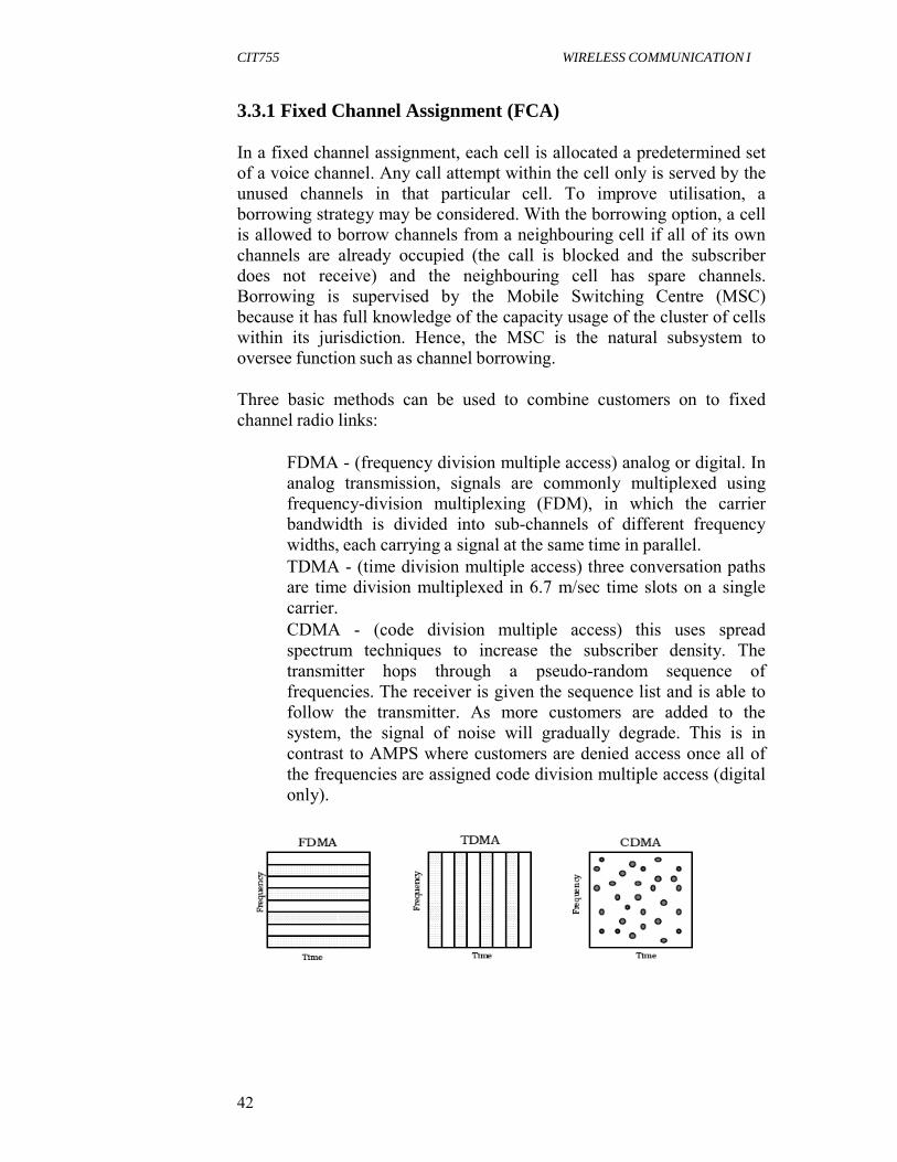
CIT755 WIRELESS COMMUNICATION I
42
3.3.1 Fixed Channel Assignment (FCA)
In a fixed channel assignment, each cell is allocated a predetermined set of a voice channel. Any call attempt within the cell only is served by the unused channels in that particular cell. To improve utilisation, a borrowing strategy may be considered. With the borrowing option, a cell is allowed to borrow channels from a neighbouring cell if all of its own channels are already occupied (the call is blocked and the subscriber does not receive) and the neighbouring cell has spare channels. Borrowing is supervised by the Mobile Switching Centre (MSC) because it has full knowledge of the capacity usage of the cluster of cells within its jurisdiction. Hence, the MSC is the natural subsystem to oversee function such as channel borrowing.
Three basic methods can be used to combine customers on to fixed channel radio links:
FDMA - (frequency division multiple access) analog or digital. In analog transmission, signals are commonly multiplexed using frequency-division multiplexing (FDM), in which the carrier bandwidth is divided into sub-channels of different frequency widths, each carrying a signal at the same time in parallel. TDMA - (time division multiple access) three conversation paths are time division multiplexed in 6.7 m/sec time slots on a single carrier. CDMA - (code division multiple access) this uses spread spectrum techniques to increase the subscriber density. The transmitter hops through a pseudo-random sequence of frequencies. The receiver is given the sequence list and is able to follow the transmitter. As more customers are added to the system, the signal of noise will gradually degrade. This is in contrast to AMPS where customers are denied access once all of the frequencies are assigned code division multiple access (digital only).

CIT755 WIRELESS COMMUNICATION I
43
Drawback of TDMA and FDMA Systems with FCA
Fixed Channel Allocation or Fixed Channel Assignment (FCA) requires manual frequency planning, which is an arduous task in TDMA and FDMA based systems, since such systems are highly sensitive to co-channel interference from nearby cells that are reusing the same channel. Another drawback with TDMA and FDMA systems with FCA is that the number of channels in the cell remains constant irrespective of the number of customers in that cell. This result in traffic congestion and some calls being lost when traffic gets heavy in some cells, and idle capacity in other cells.
3.3.2 Dynamic Channel Assignment (DCA) The more efficient way of channel allocation would be Dynamic Channel Allocation or Dynamic Channel Assignment (DCA). In DCA, voice channels are not allocated to different cells on a permanent basis.
Each time a call request is made, the serving base station requests a channel from MSC. The MSC determine (dynamically) the availability of a channel and executes its allocation procedure accordingly. The MSC only allocates a given frequency (radio channel) if that frequency (radio channel) is not presently in use in the cell, or any other cell which falls within the minimum restricted distance of frequency reuse to avoid co-channel interference.
Dynamic channel assignment reduces the likelihood of call blocking, which increases the trucking capacity of the system, since all available channels under the control of the MSC are accessible to all of the cells.
Dynamic channel assignment strategies require the MSC to collect real- time data on channel occupancy, traffic distribution and radio signal quality of all channels on a continuous basis.
Merit
Dynamic Channel Assignment (DCA) and Dynamic Frequency Selection (DFS) eliminate the tedious manual frequency planning work. DCA also handles busty cell traffic and utilises the cellular radio resources more efficiently. DCA allows the number of channels in a cell to vary with the traffic load, hence increasing channel capacity with little costs.

CIT755 WIRELESS COMMUNICATION I
44
3.4 Mechanisms for Capacity Increase in Cellular System
The capacity of a cellular system can be enlarged through frequency and it can also be improved based on cellular layout and antenna design. Basically, the following are the three popular mechanisms for increasing the capacity of a cellular system:
Cell Splitting
One way to perform cell splitting is to subdivide a congested cell into smaller cells, each with its own base station and corresponding reduction in antenna height and transmission power. With more cells, there will be more clusters in the same coverage area. Hence cell splitting increases the capacity of a cellular system since it increases the number of times that channels are reused. In figure 5.1, the central area is assumed to be saturated with traffic. The original large cell with radius R in the center is split into the medium cells with radius R/2 and the medium cell in the center is further split into the small cells with radius R/4. The cell splitting reduces the call blocking probability in the area, and increases the frequency with which mobiles hand off from cell to cell.
Fig. 5.1 Illustration of Cell Splitting from Radius R to R/2 and
to R/4
Directional Antennas (Sectoring)
One way to increase the subscriber capacity of a cellular network is replace the omni-directional antenna at each base station by three (or six) sector antennas of 120 (or 60) degrees opening. Each sector can be considered as a new cell, with its own (set of) frequency channel(s).

CIT755 WIRELESS COMMUNICATION I
45
The base station can either be located at:
the centre of the original (large) cell, or the corners of the original (large) cell.
The use of directional sector antennas substantially reduces the interference among co-channel cells. This allows denser frequency reuse. Sectoring is less expensive than cell-splitting, as it does not require the acquisition of new base station sites.
(c) Fig. 5.2 (a,b,c): Antenna Sectorization
Microcell Zone The microcell concept is based on the seven cell reuse, in which three or more zone sites are connected to a single base station and share the same radio equipment. As mobile travels within the cell, it is served by the zone with the strongest signal. As a mobile travels from one zone to another within the cell, it retains the same channel. The base station simply switches the channel to different zone site. In this way, a given channel is active only in the particular zone in which the mobile is

CIT755 WIRELESS COMMUNICATION I
46
traveling and hence the base station radiation is localised and interference is reduced.
4.0 CONCLUSION
If different cells in the entire cellular system were to use different set of frequencies, inter cell interference would be kept at minimum. However, the system capacity would be limited. In fact deployment of frequency reuse is necessary to enlarge the system capacity.
5.0 SUMMARY
In this unit, you have learnt that:
Interference is the major limiting factor in the performance of the cellular radio systems. The two major types of system generated cellular interference are: Co-channel interference and adjacent channel interference. Co-channel interference or CCI is crosstalk from two different radio transmitters using the same frequency. Interference resulting from signals which are adjacent in frequency to the desired signal is called adjacent channel interference. Channel allocation schemes are required to allocate channels to base stations and access points and to avoid co-channel interference among nearby cells. The two approaches to channel assignment are: fixed channel assignment, and dynamic channel assignment. In a fixed channel assignment, each cell is allocated a predetermined set of a voice channel. In DCA, voice channels are not allocated to different cells on a permanent basis The three popular mechanisms for increasing the capacity of a cellular system are: cell splitting, directional antennas and microcell zone.
SELF ASSESSMENT EXERCISE
1. How can you increase the capacity of cellular system with the help of frequency reuse concept?
2. What are the advantages of cellular systems?

CIT755 WIRELESS COMMUNICATION I
47
6.0 TUTOR-MARKED ASSIGNMENT
A cellular system has a total of 500 duplex voice channels (without frequency reuse). The service area is divided into 150 cells. The required signal-t-co-channel interference ratio is 1dB. Consider the path loss exponent k equal to 3, 4 and 5 respectively. Determine:
i. the cell cluster size ii. the number of cell clusters in the service area and iii. the maximum number of users in service at any instant. Discuss
effects of the path loss exponent on the frequency reuse and on the transmit power (when the cell size is fixed).
7.0 REFERENCES/FURTHER READING Linanartz J. M. G. (1997). Wireless Communication. (Online) Available
at: http://wireless.per.nl/reference/about.htm Sharma, S. (2006). Wireless & Cellular Communications. New Delhi: S.
K. Kataria & Sons.

CIT755 WIRELESS COMMUNICATION I
48
MODULE 2 MOBILE RADIO PROPAGATION
Unit 1 Wireless Channel Model Unit 2 Large Scale Propagation Model Unit 3 Radio Propagation Mechanisms Unit 4 Path Loss Model Unit 5 Shadowing
UNIT 1 WIRELESS CHANNEL MODEL
CONTENTS
1.0 Introduction 2.0 Objectives 3.0 Main Content
3.1 Channel Model 3.1.1 Statistical Propagation Models 3.1.2 Basic Concept of Path Loss
3.1.2.1Causes 3.1.2.2Propagation Prediction 3.1.2.3Received Signal Power and Attenuation
4.0 Conclusion 5.0 Summary 6.0 Tutor-Marked Assignment 7.0 References/Further Reading
1.0 INTRODUCTION
Mobile communication is burdened with particular propagation complications, making reliable wireless communication more difficult than fixed communication between carefully positioned antennas. The antenna height at a mobile terminal is usually very small, typically less than a few meters. Hence, the antenna is expected to have very little 'clearance', so obstacles and reflecting surfaces in the vicinity of the antenna have a substantial influence on the characteristics of the propagation path. Moreover, the propagation characteristics change from place to place and, if the terminal moves, from time to time.
2.0 OBJECTIVES
At the end of this unit, you should be able to:
explain the term channel model mention the two types of communication channels discuss the statistical propagation models
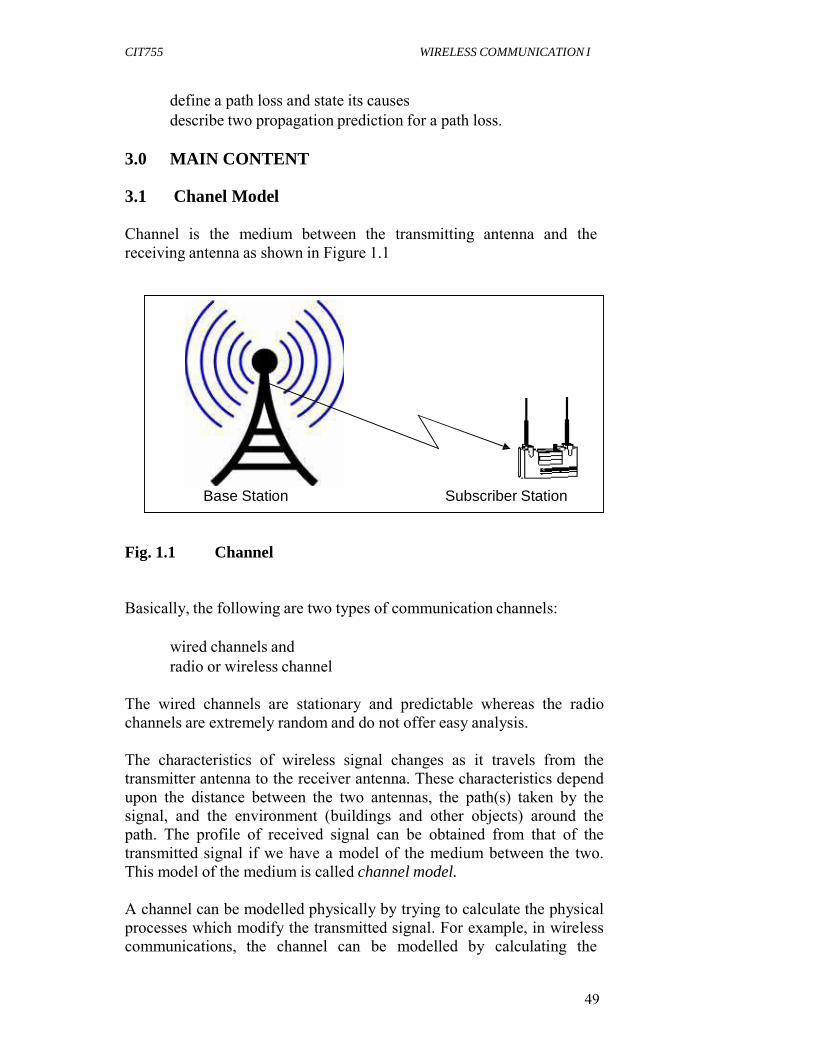
CIT755 WIRELESS COMMUNICATION I
49
Channel
define a path loss and state its causes describe two propagation prediction for a path loss.
3.0 MAIN CONTENT 3.1 Chanel Model
Channel is the medium between the transmitting antenna and the receiving antenna as shown in Figure 1.1
Base Station Subscriber Station
Fig. 1.1 Channel
Basically, the following are two types of communication channels:
wired channels and radio or wireless channel
The wired channels are stationary and predictable whereas the radio channels are extremely random and do not offer easy analysis.
The characteristics of wireless signal changes as it travels from the transmitter antenna to the receiver antenna. These characteristics depend upon the distance between the two antennas, the path(s) taken by the signal, and the environment (buildings and other objects) around the path. The profile of received signal can be obtained from that of the transmitted signal if we have a model of the medium between the two. This model of the medium is called channel model.
A channel can be modelled physically by trying to calculate the physical processes which modify the transmitted signal. For example, in wireless communications, the channel can be modelled by calculating the

CIT755 WIRELESS COMMUNICATION I
50
reflection of every object in the environment. A sequence of random numbers might also be added in to simulate external interference and/or electronic noise in the receiver.
Statistically a communication channel is usually modeled as a triple consisting of an input alphabet, an output alphabet, and for each pair (i, o) of input and output elements a transition probability p (i, o). Semantically, the transition probability is the probability that the symbol o is received given that i was transmitted over the channel.
Statistical and physical modeling can be combined. For example in wireless communications the channel is often modeled by a random attenuation (known as fading) of the transmitted signal, followed by additive noise. The attenuation term is a simplification of the underlying physical processes and captures the change in signal power over the course of the transmission. The noise in the model captures external interference and/or electronic noise in the receiver. If the attenuation term is complex it also describes the relative time a signal takes to get through the channel. The statistics of the random attenuation are decided by previous measurements or physical simulations.
Channel models may be continuous channel models in that there is no limit to how precisely their values may be defined.
A channel model may include:
Noise model, for example, Additive White Gaussian Noise (AWGN). Distortion model, for example non-linear channel causing intermodulation distortion (IMD). Interference model, for example cross-talk (co-channel interference) and intersymbol interference (ISI) . Modeling of underlying physical layer transmission techniques, for example an equivalent baseband model of modulation and frequency response. Radio frequency propagation model. Fading model, for example Rayleigh fading, Ricean fading, log- normal shadow fading and frequency selective (dispersive) fading. Doppler shift model, which combined with fading results in a time-invariant system Mobility models, which also causes a time-invariant system.

CIT755 WIRELESS COMMUNICATION I
51
3.1.1 Statistical Propagation Models
In generic system studies, the mobile radio channel is usually evaluated from 'statistical' propagation models: no specific terrain data is considered, and channel parameters are modelled as stochastic variables.
Three mutually independent, multiplicative propagation phenomena can usually be distinguished: 'large-scale' path loss, shadowing and multipath fading.
Path-loss The 'large-scale' effect causes the received power to vary gradually due to signal attenuation determined by the geometry of the path profile in its entirety. This is in contrast to the local propagation mechanisms, which are determined by terrain features in the immediate vicinity of the antennas.
Shadowing This is a 'medium-scale' effect: field strength variations occur if the antenna is displaced over distances larger than a few tens or hundreds of metres.
Multipath-Propagation Fading leads to rapid fluctuations of the phase and amplitude of the signal if the vehicle moves over a distance in the order of a wave length or more. Multipath fading thus has a 'small-scale' effect.
3.1.2 Basic Concept of Path Loss Path Loss (or path attenuation) is the reduction in power density (attenuation) of an electromagnetic wave as it propagates through space. Path loss may be due to many effects, such as free space loss, refraction, diffraction, reflection, aperture-medium coupling loss, and absorption.
Path loss is also influenced by terrain contours, environment (urban or rural, vegetation and foliage), propagation medium (dry or moist air), the distance between the transmitter and the receiver, and the height and location of antennas.
Path loss model describes the signal attenuation between transmitting and receiving antennas as a function of the propagation distance and other parameters. The simplest channel is the free space line of sight channel with no objects between the receiver and the transmitter or

CIT755 WIRELESS COMMUNICATION I
52
around the path between them. In this simple case, the transmitted signal attenuates since the energy is spread spherically around the transmitting antenna.
3.1.2.1 Causes
Path loss normally includes propagation losses caused by the natural expansion of the radio wave front in free space (which usually takes the shape of an ever-increasing sphere), absorption losses (sometimes called penetration losses), when the signal passes through media not transparent to electromagnetic waves, diffraction losses when part of the radio wave front is obstructed by an opaque obstacle, and losses caused by other phenomena.
3.1.2.2 Propagation Prediction
Calculation of the path loss is usually called prediction. Exact prediction is possible only for simpler cases, such as the above-mentioned free space propagation or the flat-earth model. For practical cases the path loss is calculated using a variety of approximations.
Statistical methods (also called stochastic or empirical) are based on measured and averaged losses along typical classes of radio links. Among the most commonly used methods are Okumura-Hata, the cost Hata model, W.C.Y. Lee, etc. These are also known as radio wave propagation models and are typically used in the design of cellular network. For wireless communication in the VHF and UHF frequency band (the bands used Walkie-talkies, police, taxis and cellular phones), one of the most commonly used methods is that of Okumura-Hata as refined by the COST 231 project. Other well-known models are those of Walfisch-Ikegami, W.C.Y. Lee, and Erceg . For FM radio and TV broadcasting, the ITU model is commonly used in predicting the path loss.
Deterministic methods based on the physical laws of wave propagation are also used; ray tracing is one of such methods. These methods are expected to produce more accurate and reliable predictions of the path loss than the empirical methods; however, they are significantly more expensive in computational effort and depend on the detailed and accurate description of all objects in the propagation space, such as buildings, roofs, windows, doors, and walls. For these reasons they are used predominantly for short propagation paths. Among the most commonly used methods in the design of radio equipment such as antennas and feeds is the finite-difference time-domain method.

CIT755 WIRELESS COMMUNICATION I
53
The path loss in other frequency bands such as MW, SW, and Microwave are predicted with similar methods, though the concrete algorithms and formulas may be very different from those for VHF/UHF. Reliable prediction of the path loss in the SW/HF band is particularly difficult, and its accuracy is comparable to weather predictions.
(a)
(b) Fig. 1.2 (a) & (b): Illustration of Path Loss
In the above path profile in Figure 1.2 (a and b), the most appropriate path loss model depends on the location of the receiving antenna:
At location 1, free space loss is likely to give an accurate estimate of path loss At location 2 and 3, a strong line-of-sight is present, but ground reflections can significantly influence path loss. The plane earth loss model appears appropriate At location 4, free space loss needs to be corrected for significant diffraction losses, caused by trees cutting into the direct line of sight Path loss prediction at location 5, 6 and 7 is more difficult than at the other locations. Ground reflection and diffraction mechanisms interact.
3.1.2.3 Received Signal Power and Attenuation Path loss is one of the mechanisms causing attenuation between the transmitter power amplifier and receiver front end. Some other effects

CIT755 WIRELESS COMMUNICATION I
54
are listed below, with an indication of the order of magnitude in a GSM- like system.
Losses in the antenna feeder (0 .. 4 dB) Losses in transmit filters, particularly if the antenna radiates signal of multiple transmitters (0 .. 3 dB) Antenna directionality gain (0 .. 12 dB) Losses in duplex filter Fade margins to anticipate for multipath (9 .. 19 dB) and shadow losses (5 dB) Penetration losses if the receiver is indoors, typically about 10 dB for 900 MHz signals.
4.0 CONCLUSION
Channel model is the medium between the transmitting antenna and the receiving antenna. The three mutually independent, multiplicative propagation phenomena are ‘large-scale’ path loss, shadowing and multipath fading.
5.0 SUMMARY
In this unit, you have learnt that:
Channel models may be continuous channel models in that there is no limit to how precisely their values may be defined The three mutually independent, multiplicative propagation phenomena are: 'large-scale' path loss, shadowing and multipath fading Path Loss (or path attenuation) is the reduction in power density (attenuation) of an electromagnetic wave as it propagates through space Path loss includes propagation losses caused by the natural expansion of the radio wave front in free space, absorption losses, diffraction losses, etc Path loss is calculated using a variety of approximations such as statistical and deterministic methods.
SELF ASSESSMENT EXERCISE
1. What is meant by path loss? 2. What are the causes of a path loss?
CIT755 WIRELESS COMMUNICATION I
55
6.0 TUTOR-MARKED ASSIGNMENT
1. What do you understand by channel model? 2. Mention two types of communication channels 3. Describe two propagation predictions for a path loss 4. Discuss on the statistical method of propagation prediction
7.0 REFERENCES/FURTHER READING Linnartzs, J.M.G. (1996). Wireless Communication. Baitzer Science
Publishers.
Molisch, A. F. (2005). Wireless Communications. Wiley & Associates.
Rappaport, T. S. (2005). Wireless Communication: Principles and Practice. (2nd ed.). India: Prentice Hall.

CIT755 WIRELESS COMMUNICATION I
56
UNIT 2 LARGE SCALE PROPAGATION MODEL
CONTENTS
1.0 Introduction 2.0 Objectives 3.0 Main Content
3.1 Free Space Propagation Model for Mobile Communication 3.1.1 Relating Power to Electric Field
4.0 Conclusion 5.0 Summary 6.0 Tutor-Marked Assignment 7.0 References/Further Reading
1.0 INTRODUCTION
Mobile radio channel puts various limitations on the performance of wireless or mobile communication systems. The two fundamental blocks of any communication system are transmitter and the receiver. In wireless communications, the transmission path between the transmitter and receiver can vary from simple line-of-sight to one that is severely obstructed by buildings, mountains and foliage.
2.0 OBJECTIVES
At the end of this unit, you should be able to:
define an effective isotropic radiated power describe free space propagation model compute the power and the magnitude of the E-field at the receiver antenna.
3.0 MAIN CONTENT
3.1 Free Space Propagation Model for Mobile Communication
The free space propagation model is a model which is used to predict received signal strength at a particular location when the transmitter and receiver have a clear, unobstructed line-of-sight path between them. For example, satellite communication systems and microwave line-of-sight radio links, typically, undergo free space propagation. Like other large- scale radio-wave propagation models, the free space-radio propagation model predicts that the received power decays as a function of the transmitter-receiver separation distance raised to some power (i.e. a

CIT755 WIRELESS COMMUNICATION I
57
power law function). It states that power falls off proportional to distance (d).
Fig. 2.1 Line-of-sight
In a radio communication system, the propagation of the modulated signal is accomplished by means of a transmitting antenna, the function of which is twofold:
To convert the electrical modulated signal into an electromagnetic field. In this capacity, the transmitting antenna acts as an “impedance-transforming” transducer, matching the impedance of the antenna to that of the free space. To radiate the electromagnetic energy in desired directions.
At the receiver, we have a receiving antenna whose function is the opposite of that of the transmitting antenna. It converts the electromagnetic field into an electrical signal from which the modulated signal is extracted. In addition, the receiving antenna may be required to suppress radiation originating from directions where it is not wanted.
Typically, the receiver is located in the far-field of the transmitting antenna, in which case, for all practical purposes, we may view the transmitting antenna as a fictitious volumeless emitter or point source.
Let us consider an isotropic source radiating a total power denoted by Pt , measured in watts. The radiating power passes uniformly through a sphere of surface area 4 d 2 , where d is the distance (in meters) from the source. Therefore, the power density, denoted by P(d), at any point on the surface of the sphere is given by
P d Pt
4 d 2
watts / m 2
Free space (Line-of-sight) LOS without obstacles, satellite communications, microwave line-of-sight radio link. Friis Free Space Equation: The far-field or Fraunhoher region, of a transmitting antenna may be defined as the region beyond the far field distance df, which is related to the largest linear

CIT755 WIRELESS COMMUNICATION I
58
2
G
2
dimension of the transmitter antenna aperture and the carrier wavelength. The Fraunhofer distance can be expressed as
2D 2
d f , D: the largest physical linear dimension of the
antenna
Additionally, to be in the far field region, df must satisfy df >> D and df
>>λ
The received signal power is expressed as:
Pr d Pt Gt Gr
2 2
4 d L where Pt = total power radiated by an isotropic source
Gt = transmitting antenna gain Gr = receiving antenna gain d = distance between transmitting and receiving antenna λ = wavelength of the carrier signal = c/f c = 3 x 10⁸ m/s, velocity of light f = carrier frequency PtGt = EIRP L: system loss factor not related to propagation (L ≥ 1)
Due to transmission line attenuation, filter loss, antenna losses
4 Ae
2
, Ae
: antenna’s effective aperture physical size of
the antenna, c 2 c
, f : carrier frequency[rad/s], c: speed of light [3 x f wc
108 m/s]
Received power in Free Space
d 0 Pr d Pr d 0 d
, d d 0 d f
Pr (d 0 ) d 0 Pr (d )[dBm] 10 log 0.001 20 log , d d 0 d f
W d where Pr (d0 ) is in units of watts
Maximum radiated power:

CIT755 WIRELESS COMMUNICATION I
59
22
The effective isotropic radiated power (EIRP) is defined as the product of the transmitted power, Pt, and the power gain of the transmitting antenna, Gt i.e.
The effective isotropic radiated power (EIRP) = PtGt watts
In fact, EIRP represents the maximum radiated power available from a transmitter in the direction of maximum antenna gain, as compared to an isotropic radiator.
In dB, EIRP is equal to sum of the antenna gain, Gt (in dBi) plus the power, Pt (in dBm) into that antenna. For example, a 12 dBi gain antenna fed directly with 15
dBm
of power has an Effective Isotropic Radiated Power (EIRP) of:
12 dBi+ 15dBm = 27 dBm(500 mW). ERP: Effective radiated power as compared to a half-wave dipole antenna ERP = EIRP – 2.15dB Effective Aperture (Ae) of an antenna is defined as the ratio of the power available at the antenna terminal to the power per unit area of the appropriately polarized incident electromagnetic wave.
Path loss
2
Ae G 4
Path loss (PL) for the free space model when antenna gains are included can be expressed as
Pt Gt Gr
4 d PL dB 10 log
Pr
10 log 4
2 2 d 10 log10 Gt Gr 10 log10
when antenna gains are excluded,
P 2 t
PL dB 10 log Pr
10 log 4
2 2 d
Note: Measuring in Decibels: dB, dBm, dBi
dB (Decibel) = 10 log 10 (Pr/Pt)
Log-ratio of two signal levels. Named after Alexander Graham Bell. For example, a cable has 6 dB loss or an amplifier has 15 dB of gain. System gains and losses can be added/subtracted, especially when changes are in several orders of magnitude.

CIT755 WIRELESS COMMUNICATION I
60
dBm (dB milliWatt)
Relative to 1mW, i.e. 0 dBm is 1 mW (milliWatt). Small signals are negative (e.g.-83dBm). Typical 802.11b WLAN cards have +15 dBm (32mW) of output power. They also specified -83 dBm RX sensitivity (minimum RX signal level required for 11Mbps reception).
For example, 125mW is 21dBm and 250mW is 24dBm. (Commonly used numbers)
dBi (dB isotropic) for EIRP (Effective Isotropic Radiated Power)
The gain a given antenna has over a theoretical isotropic (point source) antenna. The gain of microwave antennas (above1 GHz) is generally given in dBi.
dBd (dB dipole)
The gain an antenna has over a dipole antenna at the same frequency. A dipole antenna is the smallest, least gain practical antenna that can be made. A dipole antenna has 2.14 dB gain over a 0 dBi isotropic antenna.
Thus, a simple dipole antenna has a gain of 2.14 dBi or 0 dBd and is used as a standard for calibration.
The term dBd (or sometimes just called dB) generally is used to describe antenna gain for antennas that operate less than 1GHz (1000Mhz).
3.1.1 Relating Power to Electric Field
Fig. 2.2 Relating Power to Electric Field

CIT755 WIRELESS COMMUNICATION I
61
V
er
0 c
2
V 2
E I 0 L cos 1 c j ct
kd , E
I 0 L sin j c c c2 e j
ct kd
2 0 c d 2
j c d
4 c 2
d
d 2 j d 3
H I 0 L sin
4 c
j c
d
c e j
d 2
ct kd , E
H r H 0
As d , only E , H be considered!
Power flux density EIRP P G
E 2 E 2 E 2
P W t t , d m 2 4 d 2 4 d 2 R fs 0 377
Rfs: intrinsic impendence of free space,
0
0
376.7 120
E : electric field at the receiver
P d W P A E A
Pt Gt Gr d d e 120 e
4 2 d 2
Circuit Model for antenna system
Fig.2.3 Circuit Model for Antenna System
2
Pr (d ) W R
Vant 2 R
2 ant
4R ant ant ant
Exercise 2.1
Compute the far field distance for an antenna with maximum dimension of 1m and operating frequency of 900MHz
Solution: Given: largest dimension of antenna, D =1m
Operating frequency f = 900MHz, 8
c 3 10 m / s m
0.33 f 900 106 Hz

CIT755 WIRELESS COMMUNICATION I
62
2
r
we know that the far-field distance is expressed as 2D 2
d f
2 1 2
d f 6m 0.33
Exercise 2.2
If a transmitter produces 50W of power, express the transmit power in units of (a) dBm, and (b) dBW. If 50 W is applied to a unity gain antenna with a 900MHz carrier frequency, determine the received power in dBm at a free space distance of 100m from the antenna. What is Pr
(10km)? Assume unity gain for the receiver antenna.
Solution: Given that Transmitter power,
Pt 50W
Carrier frequency, fc = 900MHz 8
c 3 10 m / s m
1
0.33 f 900 106 Hz 3
a. We know that the transmitter power is given by
P (dBm) 10 log Pt (mW)
10 log 50
103 47.0dBm
t 1mW b. Transmitter power in dBW will be given by
P (dBW )
Pt (W ) 10 log 50
17.0dBW t 1W
We know that the received power can be determined using the following expression:
P d Pt Gt Gr 50(1)(1)(1 / 3) 2
(3.5
10 6 )W 3.5
10 3 mW 4 2 d 2 L (4 ) 2 (100) 2 (1)
Now, the received power in (dBm) will be given by Pr (dBm) = 10 log Pr (mW)
= 10 log (3.5 x 10⁻³ mW) = -24.5 dBm
Further, the received power at 10km may be expressed in terms of dBm, where d0 = 100m and d = 10km, as under:
Pr (10km)
Pr (100) 20 log
100
24.5 dBm
40 dB
64.5 dBm
10000

CIT755 WIRELESS COMMUNICATION I
63
4 d 4
2
EG
Exercise 2.3
Assume a receiver is located 10km from a 50W transmitter. The carrier frequency is 900MHz, free space propagation is assumed, Gt = 1, and Gr
=2, determine (a) the power at the receiver, (b) the magnitude of the E- field at the receiver antenna, (c) the rms voltage applied to the receiver input assuming that the receiver antenna has a purely real impedance of 50Ω and is matched to the receiver.
Solution: Given that
Transmitter power, Pt = 50W Carrier frequency, fc = 900MHz Transmitter antenna gain, Gt = 1 Receiver antenna gain, Gr = 2 Receiver antenna resistance = 50 Ω
a. We know that the power received at distance d = 10km is given
by PG G 2 50 1 2 (1 32
P d 10log t t r 10log 91.5dBW 61.5dBm r 2 2
2100002
b. Again, we know that the magnitude of the received E-field is expressed as
E Pr
4
d 120
Ae
A E Since G e
2
10
and Pr d Ae
120 10
7 10 2
r
120
4
7 10
2 0.332
120
4
0.0039 V / m
c Also the applied rms voltage at the receiver input (50Ω) is given by
Vant Pr d 4Rant 7 10 10 4 50 0.374mV
4.0 CONCLUSION In this unit, we have discussed the free space propagation model and the relating power to electric field.

CIT755 WIRELESS COMMUNICATION I
64
2
7.0 SUMMARY
In this unit, you have learnt that:
The free space propagation model is a model which is used to predict received signal strength at a particular location when the transmitter and receiver have a clear, unobstructed line-of-sight path between them. For example, satellite communication systems and microwave line-of-sight radio links, typically, undergo free space propagation. The free space power received by a receiver antenna situated at a particular location which is separated from a radiating transmitter antenna, by a distance d, is given by the following free space expression
Pr d Pt Gt Gr
2 2
4 d L
SELF ASSESSMENT EXERCISE
1. What are the two basic types of communication channels? 2. Define Effective Isotropic Radiated Power (EIRP)
8.0 TUTOR-MARKED ASSIGNMENT
1. Assume a receiver is located 15m from a 55W transmitter. The carrier frequency is 900MHz, free space propagation is assumed Gt = 1, and Gr =2, find (a) the power at the receiver and (b) the magnitude of the E-field at the receiver antenna.
2. Describe free space propagation model for mobile radio wave propagation.
7.0 REFERENCES/FURTHER READING
Linnartz J. M. G. (1996). Wireless Communication. Baitzer Science Publishers.
Molisch, A. F. (2005). Wireless Communications. Wiley and Associates.
Rappaport, T. S. (2005). Wireless Communication: Principle and Practice. (2nd ed.), India: Prentice Hall.
Sharma, S. (2007). Wireless and Cellular Communication. New Delhi:
S. K. Kataria & sons.

CIT755 WIRELESS COMMUNICATION I
65
UNIT 3 RADIO PROPAGATION MECHANISMS
CONTENTS 1.0 Introduction 2.0 Objectives 3.0 Main Content
3.1 The Three Basic Propagation Mechanisms 3.1.1 Reflection 3.1.2 Diffraction Loss 3.1.3 Scattering
3.2 Total Path Loss 4.0 Conclusion 5.0 Summary 6.0 Tutor-Marked Assignment 7.0 References/Further Reading
1.0 INTRODUCTION Singular information is transmitted with the help of electromagnetic wave. Electromagnetic wave consists of electric and magnetic fields.
As a matter of fact, the mechanisms responsible for electromagnetic wave propagation are:
reflection, diffraction and scattering
In case of mobile communications, operating conditions are quite severe. The reason is that most cellular radio systems operate in urban areas. In urban areas there is no direct line-of-sight path available between the transmitter and the receiver, and also, the presence of high- rise buildings creates severe diffraction loss.
Further, because of multiple reflections from various objects, the electromagnetic waves travel along different paths having variable lengths. Now, these waves interact with each other and this interaction creates the so-called multipath fading at a particular point location. As a result of this, the strengths of the waves reduce with the increase in distance between the transmitter and receiver.
CIT755 WIRELESS COMMUNICATION I
66
2.0 OBJECTIVES
At the end of this unit, you should be able to:
explain the three propagation mechanisms describe Ground Reflection Model.
3.0 MAIN CONTENT
3.1 The Three Basic Propagation Mechanisms
In order to describe radio propagation, three basic mechanisms are generally considered. These mechanisms are:
Reflection: Occurs when a propagating electromagnetic wave impinges upon an object which is very large in dimensions when compared to the wavelength of the propagation wave e.g. the surface of the earth, buildings, walls, etc. These mechanisms often dominate radio propagation in indoor applications. In outdoor urban areas, this mechanism often loses its importance because it involves multiple transmissions that reduce the strength of the signal to negligible values. Diffraction: Occurs when the radio path between the Transmitter (Tx) and Receiver (Rx) are obstructed by a surface that has irregularities (edges). The secondary waves resulting from the obstructing surface are present throughout the space and even behind the obstacle, giving rise to a bending of waves around the obstacle, even when a line-of-sight path does not exist between transmitter and receiver. At high frequencies, diffraction, like reflection, depends on the geometry of the object, as well as the amplitude, phase, and polarization of the incident wave at the point of diffraction. Scattering: Occurs when the medium through which the wave travels consists of objects with dimensions that are small compared to the wavelength, and where the number of obstacles per unit volume is large. Scattered waves are produced by rough surfaces, small objects, or by other irregularities in the channel. In practice, foliage, street signs, and lamp posts induce scattering in a mobile communications system.
3.1.1 Reflection

CIT755 WIRELESS COMMUNICATION I
67
Reflection = f(Fresnel reflection coefficient) = f(material property, wave polarisation, angle of incident, frequency)
Perfect Perfect dieletric conductor
Fig. 3.1 Reflection
Ground Reflection (2-Ray) Model
Free space propagation model is inaccurate when used alone. 2-ray ground reflection model has been found to be reasonable and accurate for predicting the large-scale signal strength model over distances of several kilometers for mobile radio systems that use tall towers (height which exceed 50m) as well as for line-of- sight (LOS) microcell channels in urban environments.
a. b. Fig. 3.2 (a & b) The Method of Images is used to find the Path
Difference between the Line-of-Sight and the Ground Reflected Paths
The free space propagation E-field:

CIT755 WIRELESS COMMUNICATION I
68
c
2
From figure 3.2(b), ht is the height of the transmitter and hr is the height of the receiver. If E0 is the free space E-field (in units of V/m) at a reference distance d0 from the transmitter, then for d > d0, the free space propagating E-field is expressed
E(d , t) E0 d 0
d cos
c t d
(d d 0 )
here E(d , t )
E0 d 0
d
denotes the envelope of the E-field at d
meters from the transmitter. Two propagating waves arrive at the receiver: the direct wave which travels a distance d’, and the reflected wave which travels a distance d”. The E-field because of the line-of- sight component at the receiver will be given by
E LOS (d ' , t) E0 d 0 '
cos
c t
d ' d c
and the E-field for the group reflected wave, which has a propagation distance of d”, will be given by
E g (d " , t) E0 d 0
"
cos
c t
d "
d c
According to laws of reflection in dielectrics, we have i 0 and E g Ei , Et (1 )Ei where is the reflection coefficient for
ground. For small values of i E g Ei perfect ground reflection 1, Et 0
ETOT (d , t ) E0 d 0 '
cos
c t
d ' ( 1)
E0 d 0 "
cos
c t
d "
d c d c
Path difference between the LOS and the ground reflected paths will be given by
d "
if d
d ' ht hr
(ht
, ht
hr ) hr (1
d 2
x 2 )1 / 2
(ht
1
hr ) d
1 x 2
2
If d is very large:

CIT755 WIRELESS COMMUNICATION I
69
' "
2
d
c
r e
4d
d " d ' 2ht hr
d 2 c , and
c d
c 2 f c
It must be noted that as d becomes large, the difference between the distances d’ and d” become very small, and the amplitudes of ELOS and Eg are virtually identical and differ only in phase i.e.
E0 d 0
d
E0 d 0
d '
E0 d 0
d "
If the received E-field is evaluated at some time, say at t = d”/c
d E d
d
d ' E d
ETOT
(d , t ") 0 0 cos
"
(
1) 0 0 cos(00 ) c d
E0 d 0 cos d '
c E0 d 0
d "
E0 d 0
d '
d
cos 1
if d>>hthr and 1, cos 1
E d E0 d 0 E0 d 0 2 2ht hr
1 E0 d 0 4 ht hr k
V m
TOT ( ) cos d
d
E 2
d d 2
16 2 h 2 h 2 d 2
/ d 2
E A P (d ) TOT A tt rr 00 0 e
120 2 d 4 120
16 2 h 2 h 2 d 2 P G G 2 h 2 h 2 t r 0 t t r P G G t r
2 4 2 2 0
t t r d 4
Power falls off proportional to distance rose to the fourth powers.
Exercise 3.1
It is given that a mobile is located 5km away from a base station and makes use of a vertical λ/4 monopole with a gain of 2.55dB to receive cellular radio signal. The E-field at the transmitter is measured to be 10-
3V/m. The carrier frequency used for this system is 900MHz.
a. Find the length and the effective aperture of the receiving Rx
antenna. b. Compute the receiver power at the mobile using the 2-ray ground
reflection model assuming the height of the transmitting antenna is 50m and the receiving antenna is 1.5m above ground.
Solution:

CIT755 WIRELESS COMMUNICATION I
70
2
E
Given that T-R separation distance = 5km, E-field at a distance of 1km = 10-3 V/m Frequency of operation, f = 900MHz
8
Now, c 3
f 900
10
106
0.333m
(a) Antenna length: L = λ/4 = 0.333/4 = 0.833m = 8.33cm Also, effective aperture of /4 monopole antenna can be obtained as under:
Gain : G 4 A
2.55dB
1.8
2 0.3332
A G
1.8
0.0158 m 2
e 4 4 3.1428
b. Now, since d ht hr , the electric field will be given by
ER (d ) 2E0 d 0
d 3
2 ht hr
d 3
k
V / m d 2
2 10 r
1 10 3
2 (50)(1.5) 3
113.1
10 6
V / m 5 10 0.333(5 10 )
Further, we know that the received power at a distance d can be obtained as below
Pr (d ) (113.1 10 6 ) 2 1.8(0.333) 2
Pr (d
5km)
5.4
377 4 10 13 W
122.68 dBW 92.68 dBm
3.1.2 Diffraction-Loss
If the direct line-of-sight is obstructed by a single object (of height hm), such as a mountain or building, the attenuation caused by diffraction over such an object can be estimated by treating the obstruction as a diffracting knife-edge.
Allow radio signals to propagate around the curved surface of the earth Huygen’s principle

CIT755 WIRELESS COMMUNICATION I
71
1
Fig. 3.3 Knife-Edge Geometry
Excess path length ( )= diffraction path length-direct path length
h 2 (d d 2 ) Phase difference
2 2 h 2 (d1 d 2 )
2d1 d 2
h 2
2(d1
d
2
d 2 ) d
if ht hr
2 d1 d 2
Fresnel Zones:
1 2
Illustrate how shadowing is sensitive to the frequency as well as the location of obstructions with relation to the Tx or Rx.
Fig. 3.4 (a) Fresnel Zones
If an obstruction does not block the volume contained within the first Fresnel zone, then the diffraction loss will be minimal, and diffraction effect may be neglected. For design of LOS microwave links, as long as 55% of the 1st
Fresnel zone is kept clear, then further Fresnel zone clearance does not significantly alter the diffraction loss.
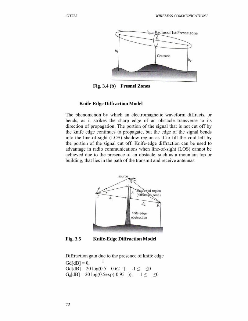
CIT755 WIRELESS COMMUNICATION I
72
Fig. 3.4 (b) Fresnel Zones
Knife-Edge Diffraction Model
The phenomenon by which an electromagnetic waveform diffracts, or bends, as it strikes the sharp edge of an obstacle transverse to its direction of propagation. The portion of the signal that is not cut off by the knife edge continues to propagate, but the edge of the signal bends into the line-of-sight (LOS) shadow region as if to fill the void left by the portion of the signal cut off. Knife-edge diffraction can be used to advantage in radio communications when line-of-sight (LOS) cannot be achieved due to the presence of an obstacle, such as a mountain top or building, that lies in the path of the transmit and receive antennas.
Fig. 3.5 Knife-Edge Diffraction Model
Diffraction gain due to the presence of knife edge
Gd[dB] = 0, 1 Gd[dB] = 20 log(0.5 – 0.62 ), -1 ≤ ≤0 Gd[dB] = 20 log(0.5exp(-0.95 )), -1 ≤ ≤0

CIT755 WIRELESS COMMUNICATION I
73
2
G d [dB] = 20 log(0.4 - 0.1184 - (0.38 - 0.1 ) 2 , 1 2.4
G [dB] = 20 log 0.225
,
2.4 d
h 2(d1
d 2 ) :
Fresnel
Kirchoff
diffraction parameter
d1 d 2
Exercise 3.2
Find diffraction loss λ = 1/3m, d1 = 1km, d2 = 1km.
a. h = 25m
h 2(d1
d 2 ) 25 2(1000 1000) 2.74
d1 d 2 (1/ 3) 1000 1000
Gd dB 20 log 0.225
,
2.4
G [dB] 20 log
0.225
21.7
d 2.74
h (d1 d2 ) 252 1000 1000 1,250,000
0.625m 2d1d2 2 1000 1000 2000,000
n n
2 2
2 0.625
0.333
3.75
The tip of the obstruction completely blocks the first three Fresnel zones b. h = 0
h 2 ( d 1 d 2 ) 0 2 (1000 1000 )
0 d 1 d 2 (1 / 3 ) 1000 1000
Gd dB 20 log 0 . 5 0 . 62 , when 1 0
G d [ dB ]
0
20 log 0 . 5 0 . 62 0 20 log 0 . 5 6
n 0
The tip of the obstruction lies in the middle of the first Fresnel zone
c. h = -25m
h 2(d1
d2 ) 25 2(1000 1000)
2.74 Gd [dB] 0
n 3.75
d1d2 (1/ 3) 1000 1000
The diffraction losses are negligible

CIT755 WIRELESS COMMUNICATION I
74
Multiple Knife-Edge Diffraction

CIT755 WIRELESS COMMUNICATION I
75
2 2
Fig. 3.6 Multiple Knife-Edge Diffraction
3.1.3 Scattering
Objects such as lamp posts and trees tend to scatter energy in all directions, thereby providing additional radio energy at a receiver. Roughness test: Rayleigh criterion
Critical height : h c , 8sin i
i :angle of incidence
Smooth surface: Max to min protuberance h < hc
Reflection coefficient for rough surface
rough
ps , ps
exp 8 h sin i
I 0 8 h sin i ,
σh : standard deviation of the surface height above the mean surface height.
Radar Cross Section (RCS) Model For rough surface
RCS[m2] powerdensityof thesignalscatteredin thedirectionof receiver
powerdensityof theradiowaveincidenton thescatteringobject
Received power due to scattering: the propagation of wave traveling in free space impinges on a distant scattering object, and is then reradiated in the direction of the receiver
Assumption: scattering object is in the far field (Fraunhofer region)
PR [dBm] P [dBm] G [dBi] 20 log d R

CIT755 WIRELESS COMMUNICATION I
76
dT(dR): the distance from the scattering object to the Tx(Rx) dBi: dB gain with respect to an isotropic source
RCS for medium and large size building located 5-10km away: 14.1dB.m2 ~ 55.7dB.m2
3.2 Total Path Loss The previously presented methods for ground reflection loss and diffraction losses suggest a “Mondriaan” interpretation of the path profile: Obstacles occur at straight vertical lines while horizontal planes cause reflections. That is, the propagation path is seen as a collection of horizontal and vertical elements.
Total loss=Free space loss + Ground reflection loss + Multiple knife- edge diffraction loss
4.0 CONCLUSION The three basic propagation mechanisms are reflection, diffraction, and scattering.
7.0 SUMMARY In this unit, you have learnt that:
Electromagnetic wave consists of electric and magnetic fields. Reflection occurs when a propagating electromagnetic wave impinges upon an object which is very large in dimensions when compared to the wavelength of the propagation wave. Diffraction occurs when the radio path between the Transmitter (Tx) and Receiver (Rx) are obstructed by a surface that has irregularities (edges). Scattering occurs when the medium through which the wave travels consists of objects with dimensions that are small compared to the wavelength, and where the number of obstacles per unit volume is large.
SELF ASSESSMENT EXERCISE 1. What are the mechanisms responsible for electromagnetic wave
propagation? 2. Discuss the effect of path loss on the performance of a cellular
radio network

CIT755 WIRELESS COMMUNICATION I
77
6.0 TUTOR-MARKED ASSIGNMENT
Describe Ground Reflection (Two-Ray) Model for mobile radio wave propagation
7.0 REFERENCES/FURTHER READING
Goldsmith, A. (2005). Wireless Communications. Cambridge University Press.
Linnartz J. M. G. (1996). Wireless Communication. Baitzer Science
Publishers.
Molisch, A. F. (2005). Wireless Communications. Wiley & Associates.
Rappaport, T. S. (2005). Wireless Communication: Principles and Practice. (2nd ed.), India: Prentice Hall.
Sharma, S. (2007). Wireless and Cellular Communication. New Delhi:
S. K. Kataria & Sons.

CIT755 WIRELESS COMMUNICATION I
78
UNIT 4 PATH LOSS MODEL
CONTENTS 1.0 Introduction 2.0 Objectives 3.0 Main Content
3.1 Empirical Path Loss Model 3.1.1 Practical Link Budget Design Using Path Loss
Model 3.1.1.1Log-Distance Path Loss Model 3.1.1.2 Log-Normal Shadowing 3.1.1.3Determination of Percentage of Coverage
Area 3.1.2 Empirical Model for Outdoor Propagation Models 3.1.3 Indoor Propagation Models
4.0 Conclusion 5.0 Summary 6.0 Tutor-Marked Assignment 7.0 References/Further Reading
8.0 INTRODUCTION In this unit, you are going to learn the various path loss models for predicting radio coverage area when designing a wireless communication system.
9.0 OBJECTIVES At the end of this unit, you should be able to:
describe log-distance path model list outdoor propagation models mention two indoor propagation models.
10.0 MAIN CONTENT 3.1 Empirical Path Loss Model
The primary use of an empirical model such as log-normal shadowing is to predict radio coverage when designing a wireless communication system.
The actual environments are too complex to model accurately. In practice, most simulation studies use empirical models that have been developed based on measurements taken in various real environments.

CIT755 WIRELESS COMMUNICATION I
79
The commonly used empirical models are: Hata model, Cost 231 Extension to Hata model, COST 231-Walfish-Ikegami Model, Erceg Model etc.
3.1.1 Practical Link Budget Design Using Path Loss Model
What Is Link Budget Calculation?
A link budget is a rough calculation of all known elements of the link to determine if the signal will have the proper strength when it reaches the other end of the link. To make this calculation, various details are required like total length of transmission cable and loss per unit length at the specified frequency as there will always be some loss of signal strength through the cables.
3.1.1.1 Log-Distance Path Loss Model
The log-distance path loss model is a radio propagation model that predicts the path loss a signal encounters inside a building or densely populated areas over distance. In the log-distance path loss model, the path loss is automatically calculated based on the distance between the transmitter and the receiver in the emulator world.
Average large-scale path loss for an arbitrary T_R separation:
PL(d)
(d/d
n PL d
PL d
d n log
d
0 d0: the close – in reference distance in the far field of the antenna
Environment Path Loss exponent, n
Free space 2 Urban area cellular radio 2.7 ~ 3.5 Shadowed urban cellularradio
3 ~ 5
In building line-of –sight 1.6 ~ 1.8 Obstructed in building 4 ~ 6 Obstructed in factories 2 ~ 3
Uses the idea that both theoretical and empirical evidence suggests that average received signal strength decreases logarithmically with distance. Measure received signal strength near to transmitter and approximate to different distances based on above “reference” observation

CIT755 WIRELESS COMMUNICATION I
80
2
z
b
3.1.1.2 Log-Normal Shadowing
The path loss PL(d) at a particular location: log-normal distribution
d PL(d)[dB] PL(d) X PL(d0 ) 10nlog X ; Normadl istribuotin
Pr (d)[dB]
Pt [dBm]
PL(d)[dB]
d0
X ~ N(0, 2 ) : zero meanGaussiandistributder.v withs tandarddeviation [dB]
duetoenvironmetanl surroundgin
: 4 ~12dB,dependinogntheseverityof theshadowiing
Log
normalrv:
eX , X ~ N(m, 2 )
The probability that the received signal level will exceed a certain value
P (d) P[P (d) ][dB] Q r
r
1 x2 1
z
2 x
t 2
Q(z) exp2
dx 2
1 erf
, erf (x) 2
0 e dt
3.1.1.3 Determination of Percentage of Coverage Area
U(γ) : Percentage of useful service area – Percentage of area with a received signal that is equal or greater than γ
U( )
0.51 - erf(a)
exp 1 - 2ab
1
erf 1 - ab
2 b
R : the radius of a circular cov erage area
a Pt
PL(d 0 )
10n log(R / d 0 ) , b 2
(10n log e)
2
: s tan dard deviation
Exercise 4.1
A pass loss model: PL(d)[dB] PL(d) X PL d n log d d X d m
Distance from Tx Received Power [dBm] 100m / 200m / 1 km /2 km 0 / -20 / -35 / -70
a. Find the minimum mean square error (MMSE) estimate for the
path loss exponent n b. Find the standard deviation c. Estimate the received power at d = 2km


CIT755 WIRELESS COMMUNICATION I
80
r
d. Predict the likelihood that the received signal level at 2km will be greater than -60dBm.
e. Predict the percentage of area within a 2km radius cell that received signals greater than -60dBm.
Solution:
(a) Since PL(d)[dB] PL(d 0 ) 10n log(d/d 0 ) PL(d 0 ) - 10n log(d i /100m)
Pr (100m)
Pr (200m)
Pr (1km)
Pr(3km)
Pr (100m) - 0 0,
- 3n,
- 10,
- 14.77n
J(n)
(0 - 0) 2
(-20 - (-3n))2
(-35 - (-10n)) 2
(-70 - (-14.77n))2
6525 - 2887.8n
327.153n 2
dJ(n)
dn
654.306n
2887.8
0 n
4.4
(b) standard deviation
σ2 = J(n) / 4 = 152.36 / 4 = 38.09 → σ = 6.17dB
(c) Pr(2km) = 0 – 10 log(2000/100) = -57.24dBm
(d) P[P (d)
- 60dBm] Q
- P (d) 60 Q
57.24 67.4%
r
(e) 92%
6.17
3.1.2 Empirical Model for Outdoor Propagation Models
More sophisticated models take into account factors such as terrain. urban clutter, antenna heights, and diffraction e.g. Longley-Rice, Durkin, Okumura, Hata, COST-231, Walfisch & Bertoni etc.
(a) Longley-Rice Model [1967, 1978]
Applicable to point-to-point communication systems in frequency range from 40MHz ~ 100GHz over different kinds of terrains. Not considering the effects of buildings and foliage, and the multipath
(b) Durkin’s Model [1969]
Adopted by the Joint Radio Committee (JRC) in the U.K for the estimation of effective mobile radio coverage areas

CIT755 WIRELESS COMMUNICATION I
81
Modeled LOS and diffraction from obstacles Excludes reflections from other surrounding objects and local scatters
(c) Okumura Model
Most widely used models for signal prediction in urban areas 150 ~ 1920 MHz Distance: 1km ~ 100km Base station antenna height: 30m ~ 100m Wholly based on measured data and does not provide any analytic explanation The simplest and best in terms of accuracy in path loss prediction for mature cellular and land mobile radio systems in clustered environment The model is fairly good in urban and suburban areas, but not as good in rural areas A standard for system planning in modern land mobile radio system in Japan Common standard derivations between predicted and measured path loss: 10dB ~ 14dB L50[dB] = LF + Amu(f,d) – G(hte) – G(hre) – GAREA L50 : the 50th percentile (i.e. median) value of propagation path loss LF: free space propagation loss
Amu : median attenuation relative to free space
G(hte) :base station antenna height gain factor G(hre) : mobile antenna height gain factor
GAREA : the gain due to the type of environment
G(h ) h
20 log te , 1000m h
30m, te
G(h )
200
h 10 log re , h
te 3m,
re
3 re
h re G(h re ) 20 log , 3
10m h te 3m,

CIT755 WIRELESS COMMUNICATION I
82
Exercise 4.2
Find the median path loss and Pr(d) using Okumura’s model. d = 50km, hte = 100m, hre = 10m (suburban environment). Base station’s EIRP: 1kW@900MHz, Gr = 0dB.
Solution:
L50[dB] = LF + Amu(f,d) – G(hte) – G(hre) - GAREA
Free space loss
LF 10 log (4
2
) 2 d 2
125.5dB
A mu (900MHz, 50km) 43dB, G AREA 9dB from the Okumura curves
G(h ) h
20 log te 6dB
te
G(h )
200
h 20 log re
10.46dB
re
3 L50 [dB] LF Amu ( f , d ) G(hte ) G(hre ) G AREA
125.5dB 43dB ( 6)dB 10.46dB 9dB 155.04dB
The medium received power:
Pr(d) = EIRP(dBm) - L50[dB] + Gr(dB) = 60dBm – 155.04dB + 0dB = -95.04dBm
(d) Hata Model [1990]
Empirical formulation of the graphical path loss data provided by Okumura The model is designed for 150MHz ~ 1500MHz and are applicable to the first generation cellular system Median path loss in urban areas
L50(urban)[dB] = 69.55 + 26.16logƒc – 13.82log hte -a(hre) + (44.9 –6.55log hte)log d d[km] : Tx – Rx distance ƒc = carrier frequency hte = height of the transmitting (base station) antenna hre = height of the receiving (mobile) antenna a(hre) : correction factor for effective mobile antenna height
a(hre)= (1.1 logƒc–0.7)hre-(1.56 logƒc-0.8)dB: for a small to medium sized city a(hre)= 8.29(log1.54hre)
2 – 1.1dB : for a large city, ƒc ≤ 300Hz
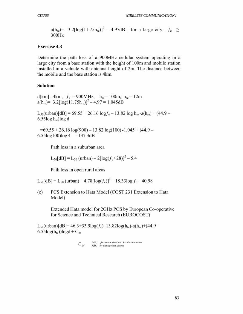
CIT755 WIRELESS COMMUNICATION I
83
C
a(hre)= 3.2[log(11.75hre)]2 – 4.97dB : for a large city , ƒc ≥
300Hz
Exercise 4.3 Determine the path loss of a 900MHz cellular system operating in a large city from a base station with the height of 100m and mobile station installed in a vehicle with antenna height of 2m. The distance between the mobile and the base station is 4km.
Solution d[km] : 4km, ƒc = 900MHz, hte = 100m, hre = 12m a(hre)= 3.2[log(11.75hre)]
2 – 4.97 = 1.045dB L50(urban)[dB] = 69.55 + 26.16 logƒc – 13.82 log hte -a(hre) + (44.9 – 6.55log hte)log d
=69.55 + 26.16 log(900) – 13.82 log(100) -1.045 + (44.9 –
6.55log100)log 4 =137.3dB
Path loss in a suburban area
L50[dB] = L50 (urban) – 2[log(ƒc / 28)]2 – 5.4
Path loss in open rural areas L50[dB] = L50 (urban) – 4.78[log(ƒc)]
2 – 18.33log ƒc – 40.98 (e) PCS Extension to Hata Model (COST 231 Extension to Hata
Model)
Extended Hata model for 2GHz PCS by European Co-operative for Science and Technical Research (EUROCOST)
L50(urban)[dB]= 46.3+33.9log(ƒc)–13.82log(hte)-a(hre)+(44.9– 6.55log(hte))logd + CM
0 dB ,
M 3dB, for meium sized city & suburban areas
for metropolit an centers
CIT755 WIRELESS COMMUNICATION I
84
This model is restricted to the following parameters:
Carrier frequency 1.5GHz to 2GHz Base Antenna Height 30m to 300m Mobile Antenna Height
1m to 10m
Distance d 1km to 20km
This model is designed for large and small macro-cells, i.e., base station antenna heights above rooftop levels adjacent to base station.
(f) CCIR Model
An empirical formula for the combined effects of free-space path loss and terrain-induced path loss was published by the CCIR (Comité Consultatif International des Radio-Communication, now ITU-R) and is given by
LCCIRdB 69.55 26.16log10 fMHz 13.82log10h1 a h2 44.9 6.55log10h1 log10dkm B
where h1 and h2 are base station and mobile antenna heights in meters, respectively, dkm is the link distance in kilometers, fMHz is the center frequency in megahertz, and
a h2 1.1log10 f MHz 0.7 h2 1.56 log10 f MHz 0.8
B 30 25 log10 % of area cov ered by buildings
This formula is the Hata model for medium–small city propagation conditions, supplemented with a correction factor, B.
The term B is such that the correction B = 0 is applied for an urban area, one that is about 15% covered by buildings; for example, if 20% of the area is covered by buildings, then
B 30 25 log10 20 25dB
(g) The Hata-Davidson Model
The Telecommunications Industry Association (TIA) recommends in their publication TSB-88A the following modification to the Hata model to cover a broader range of input parameters. The modification consists of the addition of correction terms to the Hata model:

CIT755 WIRELESS COMMUNICATION I
85
LHD LHata A h1 , d km S1 d km S3 f MHz S 4 f MHz , d km
in which A and S1 are distance correction factors extending the range to 300 km, S2 is a base station antenna height correction factor extending the range of h1 values to 2500 and S4 are frequency correction factors extending frequency to 1500MHz:
Distance A(h1, dkm) S1(dkm) dkm <20 0 0 20 ≤ dkm< 64.38
0.62137(dkm– 20)[0.5+0.15log10(h1/121.92]
0
64.38 ≤dkm< 300
0.62137(dkm– 20)[0.5+0.15log10(h1/121.92]
0.174(dkm – 64.38)
S 2 h1 , d km 0.00784 log10 9.98 / d km h1 300 for h1 300
S3 f MHz f MHz / 250 log10 1500 / f MHz
S 4 f MHz , d km [0.112 log10 1500 / f MHz ] d km 64.38 for d km 64.38
3.1.3 Indoor Propagation Models There are several causes of signal corruption in an indoor wireless channel. The primary causes are signal attenuation due to distance, penetration losses through walls and floors and multipath propagation.
The indoor signal propagation differs from an outdoor case particularly in distances and in variability of the environment, so these models are site specific and they have to take account of partition losses and surrounding objects which cause multipath propagation.
Difference from the mobile radio channel
The distances covered are much smaller. The variability of the environment is very high even for small T- R separations e.g. doors closed vs. opens, ceiling vs. desk mounted antennas walls, floors, furniture, people moving around.
Physical Effects:
Signal decays much faster Coverage contained by walls, etc. Walls, floors, furniture attenuate/ scatter radio signals

CIT755 WIRELESS COMMUNICATION I
86
Path loss formula:
Path Loss = Unit Loss + 10 n log(d) = k F + l W where:
Unit loss = power loss (dB) at 1m distance (30 dB) n = power-delay index d = distance between transmitter and receiver k = number of floors the signal traverses F = loss per floor I = number of walls the signal traverses W = loss per wall
Building Freq (MHz)
n dB
Retail StoresGrocery Stores Office, Hard Partitions Office, Soft Partitions Office, Soft Partitions
Factory LOS Textile/Chemical Textile/Chemical Paper/Cereals Metalworking
Suburban home Indoor to street Factory OBS Textile/Chemical Metalworking
914914 1500 900 1900
1300 4000 1300 1300
900
4000 1300
2.2 1.8 3.0 2.4 2.6
2.0 2.1 1.8 1.6
3.0
2.1 3.3
8.7 5.2 7.0 9.6 14.1
3.0 7.0 6.0 5.8
7.0
9.7 6.8
Table 4.1: Measure of accuracy of simple model; the larger the σ, the
less accurate the model
Source: Prof. Randy H. Katz (Radio Propagation Lecture)
Other Effecting Factors
People moving around: Additional multipath induced attenuation of 10 dB. Buildings with few metal and hard partitions: RMS delay spread of 30 to 60 ns (several mbps w/o equalization).
CIT755 WIRELESS COMMUNICATION I
87
Buildings with metal/open aisles: RMS delay spread of up to 300 ns (100s kbps w/o equalisation)
Between floors: Concrete/steel flooring yields less attenuation than steel plate
flooring Metallic tinted windows yield greater attenuation 15 dB for first floor separation, 6 - 10 dB for next four floors, 1 -
2 dB for each additional floor of separation Received signal strength depends on open plan offices, construction materials, density of personnel, furniture, etc.
Path loss exponents:
Narrowband (max delay spread < bit period) Vary between 2 and 6, 2.5 to 4 most common
Wall losses: 10 dB to 15 dB Floor losses: 12 dB to 27 dB
Wideband (max delay spread > bit period) Delay spread varies between 15 ns and 100 ns
Can vary up to 250 ns Requires sophisticated equalisation techniques to achieve
acceptable bit error rates.
Example 1: Indoor RF propagation at 2.4GHz (U.C. Berkeley). RF propagation obstacles can be termed hard partitions if they are part of the physical / structural components of a building. On the other hand, obstacles formed by the office furniture and fixed or movable / portable structures that do not extend to a buildings ceiling are considered soft partitions. Radio signals effectively penetrate both kinds of obstacles or partitions in ways that are very hard to predict.
Example 2: Indoor RF propagation at 60GHz. The 60 GHz band can be a good candidate for indoor wireless office communication, once RF components and modules become more widely available. Indoor rms delay spreads presumably are on the order of 15 to 50 nsec.
Typical delay profiles show
a dominant line-of-sight a collection of early reflections with a constant delay profile between 0 and some instant t.- an exponential decay beyond t.

CIT755 WIRELESS COMMUNICATION I
88
For 60 GHz in-office propagation, t is about 50 nanoseconds. Oxygen attenuation is not noticeable for such short-range transmission. With highly directional antennas, the delay spread can be reduced to 5 to 8 nanoseconds. Severe attenuation occurs when signals have to penetrate through glass or wood. This helps to confine cell areas. Double-glazed windows: 3 - 7 dB, concrete wall: 20-30 dB.
11.0 CONCLUSION
In this unit, you have learned the empirical path loss, practical link budget design using path loss models, the outdoor and indoor propagation models.
12.0 SUMMARY
The main points in this unit include the following:
The primary use of an empirical model such as log-normal shadowing is to predict radio coverage when designing a wireless communication system. A link budget is a rough calculation of all known elements of the link to determine if the signal will have the proper strength when it reaches the other end of the link. The log-distance path loss model is a radio propagation model that predicts the path loss as a signal encounters inside a building or densely populated areas over distance. The actual environments are too complex to model accurately, so most simulation studies use empirical models such as Hata model, Cost 231 Extension to Hata model, COST 231-Walfish- Ikegami Model, Erceg Model etc. The primary causes of indoor wireless channels are signal attenuation due to distance, penetration losses through walls and floors and multipath propagation.
SELF ASSESSMENT EXERCISE
List three outdoor propagation models
13.0 TUTOR-MARKED ASSIGNMENT
1. Describe log-distance path model. 2. What are the causes of signal corruption in an indoor wireless
channel?
CIT755 WIRELESS COMMUNICATION I
89
14.0 REFERENCES/FURTHER READING
Garg, V. K. & Wilkes J. E. (1996). Wireless and Personal
Communications Systems. Prentice Hall. Goldsmith, A. (2005). Wireless Communications. Cambridge University
Press. Linnartz, J. M. G. (1996). Wireless Communication. Baitzer Science
Publishers. Molisch, A. F. (2005). Wireless Communications. Wiley & Associates
Rappaport, T. S. (2005). Wireless Communication: Principles and
Practice. (2nd ed.), India: Prentice Hall. Saunders, S.R. (1999). Antennas and Propagation for Wireless
Communication Systems. Wiley & Associates. Sharma, S. (2007). Wireless and Cellular Communication. New Delhi:
S. K. Kataria & Sons.
CIT755 WIRELESS COMMUNICATION I
90
UNIT 5 SHADOWING
CONTENTS
1.0 Introduction 2.0 Objectives 3.0 Main Content
3.1 Shadowing Concept 3.1.1 Depth of Shadowing 3.1.2 Implications for Cell Planning
4.0 Conclusion 5.0 Summary 6.0 Tutor-Marked Assignment 7.0 References/Further Reading
8.0 INTRODUCTION
Shadowing is the effect that the received signal power fluctuates due to objects obstructing the propagation path between transmitter and receiver. These fluctuations are experienced on a local-means power, which is short term averages to remove fluctuations due to multipath fading.
9.0 OBJECTIVES
At the end of this unit, you should be able to:
define a shadowing model illustrate with a diagram a shadowing model.
10.0 MAIN CONTENT
3.1 Shadowing Concept
If there are any objects (such buildings or trees) along the path of the signal, some part of the transmitted signal is lost through absorption, reflection, scattering, and diffraction. This effect is called shadowing. As shown below, if the base antenna were a light source, the middle building would cast a shadow on the subscriber antenna; hence the name, shadowing.

CIT755 WIRELESS COMMUNICATION I
91
22
2P
Fig. 5.1 Shadowing
Experiments reported by Egli in 1957 showed that, for paths longer than a few hundred meters, the received (local-mean) power fluctuates with a ‘log-normal’ distribution about the area- mean power.
“Log-normal” means that the local-mean power expressed in
P logarithmic values i.e, P log ln dB or neper has a normal i.e.,
Gaussian distribution.
P
local means is the average over about 40l, to remove multipath fading denoted by a single overline area means is the average over tens or hundreds of meters, to remove multipath fading and shadowing denoted by a double overbar.
The probability density function (pdf) of the local-mean power is thus of the form
f p log
P log
1 exp
2 s
1 2 log
2 s
where Ωs is the logarithmic standard deviation of the shadowing, expressed in natural units. The standard deviation in dB is found from s = 4.34 s. For instance s = 6 dB shadowing is equivalent to s = 1.36. If we convert 'nepers' to 'watts', the log-normal distribution of received (local-mean) power is found
1 1 P
f p log
P log exp2 2
ln
s s P
CIT755 WIRELESS COMMUNICATION I
92
Here the factor “1/local-mean power” occurs due to the conversion of the pdf of PLog to local-mean power.
3.1.1 Depth of Shadowing
For average terrain, Egli reported a logarithmic standard deviation of about 8.3 dB and 12 dB for VHF and UHF frequencies, respectively. Such large fluctuations are caused not only by local shadow attenuation by obstacles in the vicinity of the antenna, but also by large-scale effects leading to a coarse estimate of the area-mean power.
3.1.2 Implications for Cell Planning
Shadowing makes practical cell planning complicated. To fully predict local shadow attenuation, up-to-date and highly detailed terrain data bases are needed. If one extends the distinction between large-area and small-area shadowing, the definition of shadowing covers any statistical fluctuation of the received local-mean power about a certain area-mean power, with the latter determined by (predictable) large-scale mechanisms. Multipath propagation is separated from shadow fluctuations by considering the local-mean powers. That is, the standard deviation of the shadowing will depend on the geographical resolution of the estimate of the area-mean power. A propagation model which ignores specific terrain data produces about 12 dB of shadowing. On the other hand, prediction methods using topographical data bases with unlimited resolution can, at least in theory, achieve a standard deviation of 0 dB. Thus, the standard deviation is a measure of the impreciseness of the terrain description. If, for generic system studies, the (large-scale) path loss is taking a simple form depending only on distance but not on details of the path profile, the standard deviation will necessarily be large. On the other hand, for the planning of a practical network in a certain (known) environment, the accuracy of the large-scale propagation model may be refined. This may allow a spectrally more efficient planning if the cellular layout is optimized for the propagation environment.
11.0 CONCLUSION
Shadowing is attenuation from natural and man-made object (fast). Signals are blocked by obstructing structures.
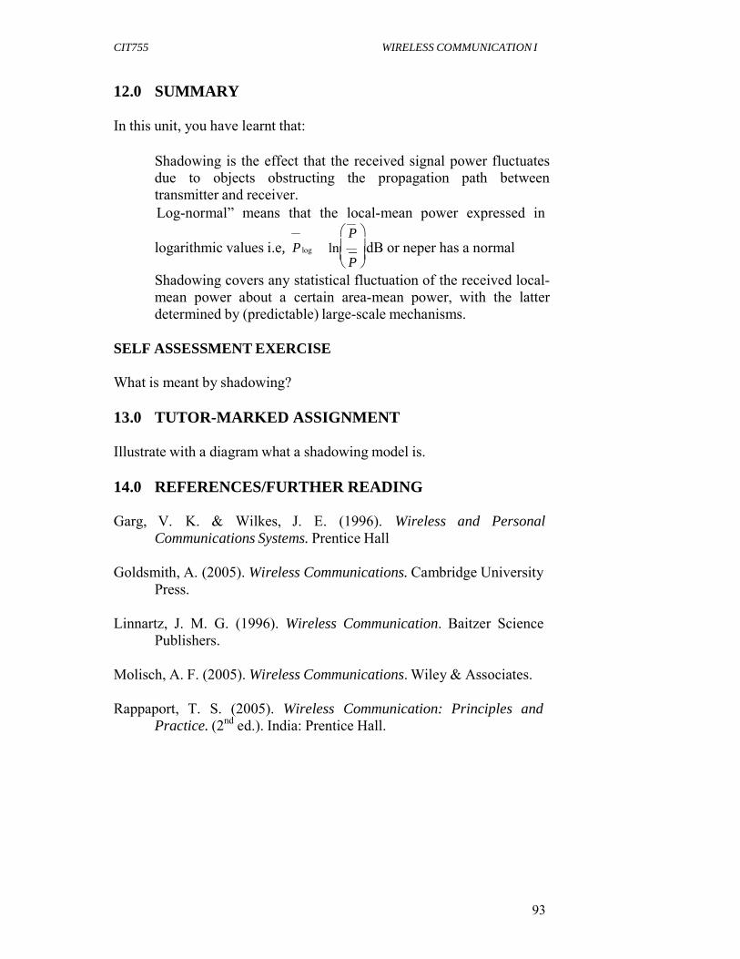
CIT755 WIRELESS COMMUNICATION I
93
12.0 SUMMARY
In this unit, you have learnt that:
Shadowing is the effect that the received signal power fluctuates due to objects obstructing the propagation path between transmitter and receiver. Log-normal” means that the local-mean power expressed in
P logarithmic values i.e, P log ln dB or neper has a normal P
Shadowing covers any statistical fluctuation of the received local- mean power about a certain area-mean power, with the latter determined by (predictable) large-scale mechanisms.
SELF ASSESSMENT EXERCISE What is meant by shadowing?
13.0 TUTOR-MARKED ASSIGNMENT Illustrate with a diagram what a shadowing model is.
14.0 REFERENCES/FURTHER READING Garg, V. K. & Wilkes, J. E. (1996). Wireless and Personal
Communications Systems. Prentice Hall Goldsmith, A. (2005). Wireless Communications. Cambridge University
Press. Linnartz, J. M. G. (1996). Wireless Communication. Baitzer Science
Publishers.
Molisch, A. F. (2005). Wireless Communications. Wiley & Associates.
Rappaport, T. S. (2005). Wireless Communication: Principles and Practice. (2nd ed.). India: Prentice Hall.

CIT755 WIRELESS COMMUNICATION I
94
MODULE 3 MOBILE RADIO PROPAGATION
Unit 1 Small Scale Fading and Multipath Unit 2 Types of Small Scale Fading Unit 3 Small Scale Fading - Rician, Rayleigh and Nakagami Unit 4 Small-Scale Fading-Threshold Crossing, Fade Duration
and Scatter Function Unit 5 Channel Classification
UNIT 1 SMALL SCALE FADING AND MULTI-PATH
CONTENTS
1.0 Introduction 2.0 Objectives 3.0 Main Content
3.1 Small-Scale Multi-Path Propagation 3.1.1 Factors Affecting Small Scale Fading 3.1.2 Multi-Path Fading Channel Models 3.1.3 Concept of Doppler
4.0 Conclusion 5.0 Summary 6.0 Tutor-Marked Assignment 7.0 References/Further Reading
1.0 INTRODUCTION
Small scale fading or in simple word fading is used to describe the rapid fluctuations in amplitudes, phases, or muti-path delays of a radio signal over a small period of time or travel distance, so that large scale path loss effects may be ignored. In wireless communications, fading is deviation or the attenuation that a carrier-modulated telecommunication signal experiences over certain propagation media. The fading may vary with time, geographical position and/or radio frequency, and is often modelled as a random process. A fading channel is a communication channel that experiences fading. In wireless systems, fading may be due to multipath propagation, referred to as multipath induced fading, or due to shadowing from obstacles affecting the wave propagation, sometimes referred to as shadow fading.
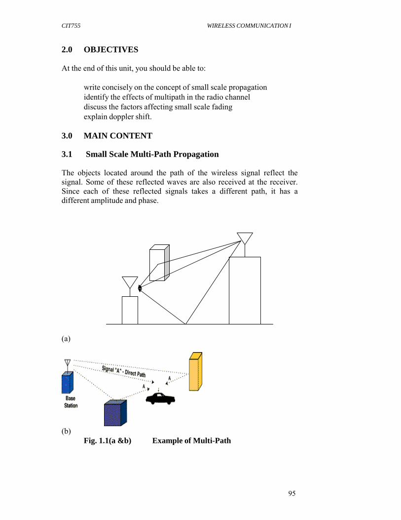
CIT755 WIRELESS COMMUNICATION I
95
2.0 OBJECTIVES
At the end of this unit, you should be able to:
write concisely on the concept of small scale propagation identify the effects of multipath in the radio channel discuss the factors affecting small scale fading explain doppler shift.
3.0 MAIN CONTENT 3.1 Small Scale Multi-Path Propagation
The objects located around the path of the wireless signal reflect the signal. Some of these reflected waves are also received at the receiver. Since each of these reflected signals takes a different path, it has a different amplitude and phase.
(a)
(b)
Fig. 1.1(a &b) Example of Multi-Path

CIT755 WIRELESS COMMUNICATION I
96
As a matter of fact, multi-path in the radio channel produces small-scale fading effects. The three important effects are:
i. Rapid changes in signal strength over a small travel distance or time interval
ii. Random frequency modulation due to varying Doppler shifts on different multipath signals
iii. Time dispersion (echoes) caused by multi-path propagation delays.
Fig. 1.2 Phase Difference between Original and Reflected Wave
In built-up urban areas, fading occurs since the height of the mobile antennas are well below the height of surrounding structures, hence there is no single line-of-sight path to the base station. Even when a line- of-sight exists, multipath still occurs due to reflections from the ground and surrounding structures. The incoming radio waves arrive from different directions with different propagation delays. The signal received by the mobile at any point in space may consist of a large number of plane waves having randomly distributed amplitudes, phases and angles of arrival. These multipath components combine in a vectorial manner at the receiver antenna and can cause the signal received by the mobile to distort or fade. Even when a mobile receiver is stationary, the received signal may fade because of movement of surrounding objects in the radio channel. If objects are static in the radio channel, and motion is considered to be due to mobile, then fading is purely a spatial phenomenon.
3.1.1 Factors Affecting Small Scale Fading
The physical factors in the radio propagation channel influencing small scale fading are:
i. Multi-Path Propagation: The presence of reflecting objects and
scattering in the channel creates a constantly changing

CIT755 WIRELESS COMMUNICATION I
97
environment that dissipates the signal energy in amplitude, phase and time. The random phase and amplitudes of different multipath components cause fluctuations in signal strength, thereby inducing small scale fading, signal distortion or both. Multipath propagation often lengthens the time required for the baseband portion of the signal to reach the receiver which can cause signal smearing due to inter-symbol interference.
ii. Speed of the Mobile: The relative motion between the base station and the mobile results in random frequency modulation due to different Doppler shifts on each of the multipath component. Doppler shift will be positive or negative depending on whether the mobile receiver is moving toward or away from the base station.
Fig. 1.3 The Doppler Effect for a Moving Sound
Source: Spring 07- CS 527 – Lecture 3
iii. Speed of Surrounding Objects: If objects in the radio channel are in motion, they induce a time varying Doppler shift on multipath components. If the surrounding object moves at a greater rate than the mobile, then this effect dominates the small scale fading. Otherwise, motion of surrounding objects may be ignored, and only the speed of the mobile need be considered.
iv. The Transmission Bandwidth of the Signal: If the transmitted radio signal bandwidth is greater than the “bandwidth” of the multipath channel, the received signal will be distorted, but the received signal strength will not fade much over a local area (i.e. the small scale fading will not be significant). If the transmitted signal has a narrow bandwidth as compared with the channel, the amplitude of the signal will change rapidly, but the signal will not be distorted in time. Thus, the statistics of small-scale signal strength and the likelihood of signal smearing over small-scale
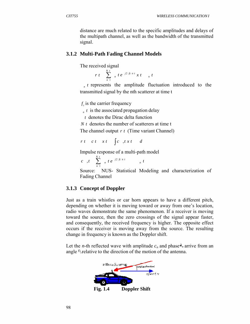
CIT755 WIRELESS COMMUNICATION I
98
n
t
distance are much related to the specific amplitudes and delays of the multipath channel, as well as the bandwidth of the transmitted signal.
3.1.2 Multi-Path Fading Channel Models
The received signal N t
r t n t e j 2 fc n t x t t
n 1
n t represents the amplitude fluctuation introduced to the transmitted signal by the nth scatterer at time t
f c is the carrier frequency
n t is the associated propagation delay t denotes the Dirac delta function
N t denotes the number of scatterers at time t
The channel output r t (Time variant Channel)
r t c t x t c , t x t d
Impulse response of a multi-path model N t
c , t n t e j 2 fc n t
n n 1
Source: NUS- Statistical Modeling and characterization of Fading Channel
3.1.3 Concept of Doppler
Just as a train whistles or car horn appears to have a different pitch, depending on whether it is moving toward or away from one’s location, radio waves demonstrate the same phenomenon. If a receiver is moving toward the source, then the zero crossings of the signal appear faster, and consequently, the received frequency is higher. The opposite effect occurs if the receiver is moving away from the source. The resulting change in frequency is known as the Doppler shift.
Let the n-th reflected wave with amplitude cn and phase arrive from an angle relative to the direction of the motion of the antenna.
Fig. 1.4 Doppler Shift

CIT755 WIRELESS COMMUNICATION I
99
6
The Doppler shift of this wave is
f f D n
f 0 v cos c
where f0 is the carrier transmission frequency, v is the speed of the antenna
Exercise 1.1 An aircraft is headed toward an airport control tower with a speed of 500km/h at an elevation of 200. Safety communications between the aircraft tower and the plane occur at frequency of approximately 128MHz. What is the expected Doppler shift of the received signal?
Solution: The velocity of the aircraft in the direction away from the tower is
v = -500km/hr x cos 200 = -130m/s Speed of light = 3 x 10⁸
The corresponding Doppler shift is
f f 0 v cos
D c
128
3
106
108
130
55Hz
If the plane banks suddenly and heads in the other direction, the Doppler shift will change from 55Hz to -55Hz. This rapid change in frequency, dfD /dt, is sometimes referred to as frequency slewing. A good mobile receiver must be capable of tracking the frequency slew rates that can be generated by the receiving motion.
Exercise 1.2 Given a transmitter which radiates a sinusoidal carrier frequency of 1850 MHz. For a vehicle moving at 60mph, calculate the received carrier frequency if the mobile is moving (i) directly toward the transmitter, (ii) directly away from the transmitter, and (iii) in a direction which is perpendicular to the direction of arrival of the transmitted signal.
Solution: Given that Carrier frequency fc = 1850MHz
8
Hence,
wavelength c 3 10 f c 1850 10
0.162m
Vehicle speed v =60mph = 26.82m/s

CIT755 WIRELESS COMMUNICATION I
100
i. The vehicle is moving directly towards the transmitter. The Doppler shift in this case will be positive and the received frequency will be given by
f f c
f d 1850
106
3
1850
108
106
f 1850.00016MHz
ii. The vehicle is moving directly away from the transmitter. The Doppler shift in this case will be negative and therefore, the received frequency will be given by
f f c
f d 1850
106
3
1850
108
106
f 1849.999834MHz
iii. The vehicle is moving perpendicular to the angle of arrival of the transmitted signal. In this case, 900 , cos = 0, and hence, there is no Doppler shift. Thus, in this case, the received signal frequency will remain same as the transmitted frequency of 1850MHz.
4.0 CONCLUSION
In wireless communications, fading is deviation or the attenuation that a carrier-modulated telecommunication signal experiences over certain propagation media. The fading may vary with time, geographical position and/or radio frequency, and is often modeled as a random process. Fading may be due to multipath propagation, referred to as multipath induced fading, or due to shadowing from obstacles affecting the wave propagation, sometimes referred to as shadow fading.
5.0 SUMMARY
The main points in this unit are:
Multipath in the radio channel produces three important fading effects which are:
(i) Rapid changes in signal strength over a small travel distance or time interva (ii) Random frequency modulation due to varying Doppler shifts on different multipath signals (iii) Time dispersion (echoes) caused by multipath propagation delays. Even when mobile is stationary, the received signals may fade due to movement of surrounding objects.
CIT755 WIRELESS COMMUNICATION I
101
The physical factors in the radio propagation channel influencing small-scale fading are: Multipath propagation, speed of the mobile, speed of surrounding objects, the transmission bandwidth of the signal. The Doppler shift can be expressed as
f f D n
f 0 v cos c
where f0 is the carrier transmission frequency, v is the speed of the antenna.
SELF ASSESSMENT EXERCISE Explain four factors affecting small-scale fading
6.0 TUTOR-MARKED ASSIGNMENT 1. What is Doppler effect? Explain 2. What do you understand by small scale fading 3. Identify the three important effects of multipath in the radio
channel
7.0 REFERENCES/FURTHER READING Linnartz, J. M. G. (1996). Wireless Communication. Baitzer Science
Publishers.
Molisch, A. F. (2005): Wireless Communications. Wiley & Associates.
Rappaport, T. S. (2005). Wireless Communication: Principles and Practice. (2nd ed.). India: Prentice Hall.
Sharma, S. (2007). Wireless and Cellular Communication. New Delhi: S. K. Kataria & Sons.

CIT755 WIRELESS COMMUNICATION I
102
UNIT 2 TYPES OF SMALL SCALE FADING
CONTENTS
1.0 Introduction 2.0 Objectives 3.0 Main Content
3.1 Types of Small Scale Fading 3.1.1 Fading Effects Due to Multi-Path Time Delay
Spread 3.1.2 Fading Effects Due to Doppler Spread
3.2 Mitigation 4.0 Conclusion 5.0 Summary 6.0 Tutor-Marked Assignment 7.0 References/Further Reading
1.0 INTRODUCTION
The presence of reflectors in the environment surrounding a transmitter and receiver create multiple paths that a transmitted signal can traverse.
As a result, the receiver sees the superposition of multiple copies of the transmitted signal, each traversing a different path. Each signal copy will experience differences in attenuation, delay and phase shift while traveling from the source to the receiver. This can result in either constructive or destructive interference, amplifying or attenuating the signal power seen at the receiver. Strong destructive interference is frequently referred to as a deep fade and may result in temporary failure of communication due to a severe drop in the channel signal-to-noise ratio.
A common example of multipath fading is the experience of stopping at a traffic light and hearing an FM broadcast degenerate into static, while the signal is re-acquired if the vehicle moves only a fraction of a meter.
The loss of the broadcast is caused by the vehicle stopping at a point where the signal experienced severe destructive interference. Cellular phones can also exhibit similar momentary fades.
Fading channel models are often used to model the effects of electromagnetic transmission of information over the air in cellular networks and broadcast communication. Fading channel models are also used in underwater acoustic communications to model the distortion caused by the water. Mathematically, fading is usually modeled as a

CIT755 WIRELESS COMMUNICATION I
103
time-varying random change in the amplitude and phase of the transmitted signal.
2.0 OBJECTIVES At the end of this unit, you should be able to:
mention two types of small scale fading explain fading effects due to Doppler spread discuss fading effect due to multipath time delay spread.
3.0 MAIN CONTENT 3.1 Types of Small Scale Fading
The type of fading experienced by signal propagating through a mobile radio channel depends upon the nature of the transmitted signal with respect to the characteristics of the channel. Depending on the relation between the signal parameters and the channel parameters, different transmitted signals will undergo different types of fading.
Fading Effects due to Multipath Time Delay Spread Fading Effects due to Doppler Spread
Fig. 2.1 Illustration of Types of Small Scale Fading

CIT755 WIRELESS COMMUNICATION I
104
3.1.1 Fading Effects Due to Multi-Path Time Delay Spread
As the carrier frequency of a signal is varied, the magnitude of the change in amplitude will vary. The coherence bandwidth measures the separation in frequency after which two signals will experience uncorrelated fading. Because of time dispersion, multipath caused the transmitted signal to experience either flat or frequency selective fading
i. Flat Fading
In flat fading, the coherence bandwidth of the channel is larger than the bandwidth of the signal. Therefore, all frequency components of the signal will experience the same magnitude of fading. That is if the mobile radio channel exhibits a constant gain and linear phase response over a bandwidth which is greater than the bandwidth of the transmitted signal, then the received signal will experience flat fading. In flat fading, the multipath structure of the channel is such that the spectral characteristics of the transmitted signal are preserved at the receiver. However, the strength of the signal changes with time, because of fluctuations in the gain of the channel created by multipath. Flat fading channels are also referred to as amplitude varying channel or narrowband channel.
ii. Frequency Selective Fading
In frequency-selective fading, the coherence bandwidth of the channel is smaller than the bandwidth of the signal. Different frequency components of the signal therefore experience decorrelated fading. That is if the channel possesses a constant-gain and linear phase response over a bandwidth that is smaller than the bandwidth of transmitted signal, then the channel creates frequency selective fading on the received signal. Under such conditions, the channel impulse response has a multipath delay spread which is greater than the reciprocal bandwidth of the transmitted message waveform. When this occurs, the received signal includes multiple versions of the transmitted waveform which are attenuated (faded) and delayed in time, and hence the received signal is distorted. Frequency selective fading is due to time dispersion of the transmitted symbols within the channel.
Since different frequency components of the signal are affected independently, it is highly unlikely that all parts of the signal will be simultaneously affected by a deep fade. Certain modulation schemes such as OFDM and CDMA are well-suited to employing frequency diversity to provide robustness to fading. OFDM divides the wideband signal into many slowly modulated narrowband subcarriers, each exposed to flat fading rather than frequency selective fading. This can be

CIT755 WIRELESS COMMUNICATION I
105
combated by means of error coding, simple equalization or adaptive bit loading. Inter-symbol interference is avoided by introducing a guard interval between the symbols. CDMA uses the Rake receiver to deal with each echo separately.
Frequency-selective fading channels are also dispersive, in that the signal energy associated with each symbol is spread out in time. This causes transmitted symbols that are adjacent in time to interfere with each other. Equalisers are often deployed in such channels to compensate for the effects of the intersymbol interference.
The echoes may also be exposed to Doppler shift, resulting in a time varying channel model.
3.1.2 Fading Effects Due to Doppler Spread Depending on how rapidly the transmitted baseband signal changes as compared to the rate of change of the channel, a channel may be classified either as a fast fading or slow fading channel. The terms slow and fast fading refer to the rate at which the magnitude and phase change imposed by the channel on the signal changes. The coherence time is a measure of the minimum time required for the magnitude change of the channel to become decorrelated from its previous value.
Slow Fading: In Slow fading channel, the impulse response changes at a rate much slower than the transmitted baseband signal. In this case, the channel may be assumed to be static over one or several reciprocal bandwidth interval. In frequency domain, this implies that the Doppler spread of the channel is much less than the bandwidth of the baseband signals.
Slow fading arises when the coherence time of the channel is large relative to the delay constraint of the channel. In this regime, the amplitude and phase change imposed by the channel can be considered roughly constant over the period of use. Slow fading can be caused by events such as shadowing, where a large obstruction such as a hill or large building obscures the main signal path between the transmitter and the receiver. The amplitude change caused by shadowing is often modeled using a log-normal distribution with a standard deviation according to the log-distance path loss model.
Fast Fading: In fast fading channel, the channel response changes rapidly within the symbol duration. That is the coherence time of the channel is smaller than the symbol period of the transmitted signal. This causes frequency dispersion (also called time selective fading) due to Doppler spreading, which leads to

CIT755 WIRELESS COMMUNICATION I
106
D
signal distortion. When viewed in the frequency domain, signal distortion due to fast fading increases with increasing Doppler spread relative to the bandwidth of transmitted signal.
In a fast-fading channel, the transmitter may take advantage of the variations in the channel conditions using time diversity to help increase robustness of the communication to a temporary deep fade. Although a deep fade may temporarily erase some of the information transmitted, use of an error-correcting code coupled with successfully transmitted bits during other time instances (interleaving) can allow for the erased bits to be recovered. In a slow-fading channel, it is not possible to use time diversity because the transmitter sees only a single realisation of the channel within its delay constraint. A deep fade therefore lasts the entire duration of transmission and cannot be mitigated using coding.
The coherence time of the channel is related to a quantity known as the Doppler spread of the channel. When a user (or reflectors in its environment) is moving, the user's velocity causes a shift in the frequency of the signal transmitted along each signal path. This phenomenon is known as the Doppler shift. Signals traveling along different paths can have different Doppler shifts, corresponding to different rates of change in phase. The difference in Doppler shifts between different signal components contributing to a single fading channel tap is known as the Doppler spread. Channels with a large Doppler spread have signal components that are each changing independently in phase over time. Since fading depends on whether signal components add constructively or destructively, such channels have a very short coherence time.
In general, coherence time is inversely related to Doppler spread, typically expressed as:
T k
c s
where Tc is the coherence time, Ds is the Doppler spread, and k is a constant taking on values in the range of 0.25 to 0.5.
3.2 Mitigation
Fading can cause poor performance in a communication system because it can result in a loss of signal power without reducing the power of the noise. This signal loss can be over some or all of the signal bandwidth.

CIT755 WIRELESS COMMUNICATION I
107
Fading can also be a problem as it changes over time: communication systems are often designed to adapt to such impairments, but the fading can change faster than when adaptations are made. In such cases, the probability of experiencing a fade (and associated bit errors as the signal-to-noise ratio drops) on the channel becomes the limiting factor in the link's performance.
RF multipath problems can be mitigated in a number of ways:
(i) Radio system design: redundant paths for each receiver, if at all
possible. (ii) Antenna system design: dual diversity antennas used at each
receiver, as a minimum. (iii) Signal/waveform design: spread spectrum radio design with the
highest feasible chip rate. iv) Building/environment design: not much can be done in this area,
unless new “RF Friendly” buildings are constructed. The effects of fading can be combated by using diversity to transmit the signal over multiple channels that experience independent fading and coherently combining them at the receiver. The probability of experiencing a fade in this composite channel is then proportional to the probability that all the component channels simultaneously experience a fade, a much more unlikely event.
Diversity can be achieved in time, frequency, or space. Common techniques used to overcome signal fading include:
Diversity reception and transmission OFDM (orthogonal frequency division multiplexing) Rake receivers Space–time codes MIMO (multiple-input multiple-output)
4.0 CONCLUSION In this unit we have discussed the two types of small scale fading which are fading effects due to multipath time delay spread and fading effects due to Doppler spread.

CIT755 WIRELESS COMMUNICATION I
108
9.0 SUMMARY
In this unit, you have learnt that:
Fading channel models are often used to model the effects of electromagnetic transmission of information over the air in cellular networks and broadcast communication. The two types of small scale fading are fading effect due to multipath time delay spread and fading effect due to Doppler spread Fading effect due to multipath time delay spread causes the signal to experience either flat or frequency selective fading In flat fading, the coherence bandwidth of the channel is larger than the bandwidth of the signal. In frequency-selective fading, the coherence bandwidth of the channel is smaller than the bandwidth of the signal. Fading effect due to Doppler spread may be classified either as a fast fading or slow fading channel In Slow fading channel, the impulse response changes at a rate much slower than the transmitted baseband signal. In fast fading channel, the channel response changes rapidly within the symbol duration.
SELF ASSESSMENT EXERCISE
Mention two types of small scale fading
10.0 TUTOR-MARKED ASSIGNMENT
1. Explain briefly slow and fast fading 2. Write short note on fading effects due to multipath time delay
spread.
7.0 REFERENCES/FURTHER READING
Molisch, A. F. (2005). Wireless Communications. Wiley & Associates.
Rappaport, T. S. (2005). Wireless Communication :Principles and Practice. (2nd ed.). India: Prentice Hall.
Sharma, S. (2007). Wireless and Cellular Communication. New Delhi: S. K. Kataria & Sons.
CIT755 WIRELESS COMMUNICATION I
109
UNIT 3 SMALL SCALE FADING: RICIAN, RAYLEIGH
AND NAKAGAMI CONTENTS
1.0 Introduction 2.0 Objectives 3.0 Main Content
3.1 Fading Models/Local Propagation Effects with Mobile Radio 3.1.1 Rician Fading 3.1.2 Rayleigh Fading
3.1.2.1 Rayleigh Fading Simulator 3.1.2.2 Jakes’ Simulator 3.1.2.3 Frequency Domain Simulator
3.1.3 Nakagami Fading 4.0 Conclusion 5.0 Summary 6.0 Tutor-Marked Assignment 7.0 References/Further Reading
1.0 INTRODUCTION Small Scale fading results from the fact that the propagation channel consists of several obstacles and reflectors.
2.0 OBJECTIVES At the end of this unit, you should be able to:
discuss on the small scale fading models list examples of fading models differentiate between the fading models.
3.0 MAIN CONTENT
3.1 Fading Models/Local Propagation Effects with Mobile
Radio Most mobile communication systems are used in and around centers of population. The major difficulties are caused by the fact that the mobile antenna is well below the surrounding buildings. Thus, most communication is via scattering of electromagnetic waves from surfaces or diffraction over and around buildings. These multiple propagation paths or multipaths have both slow and fast aspects:

CIT755 WIRELESS COMMUNICATION I
110
i. Slow-fading arises from the fact that most of the large reflectors and diffracting objects along the transmission path are distant from the terminal. The motion of the terminal relative to these distant objects is small. Consequently, the corresponding propagation changes are slow. These factors contribute to the median path losses between a fixed transmitter and a fixed receiver. The slow fading also referred to as shadowing or log- normal fading.
ii. Fast fading is the rapid variation of signal levels when the user terminal moves short distances. Fast fading is due to reflection of local objects and the motion of terminal relative to those objects. That is, the received signal is the sum of a number of signals reflected from local surfaces, and these signals sum in a signals constructive and destructive manner depending on their relative phase relationships.
Examples of fading models for the distribution of the attenuation are:
Rician fading Rayleigh fading Nakagami fading Log-normal shadow fading Weibull fading: is a simple statistical model of fading used in wireless communications and based on the Weibull distribution. It is an effective model in both indoor and outdoor environments Dispersive fading models, with several echoes, each exposed to different delay, gain and phase shift, often constant. This results in frequency selective fading and inter-symbol interference. The gains may be Rayleigh or Rician distributed. The echoes may also be exposed to Doppler shift, resulting in a time varying channel model.
3.1.1 Rician Fading
Rician fading is a stochastic model for radio propagation anomaly caused by partial cancellation of a radio signal by itself , the signal arrives at the receiver by two different paths and at least one of the paths is changing (lengthening or shortening). Rician fading occurs when one of the paths, typically a line of sight signal, is much stronger than the others. In Rician fading, the amplitude gain is characterized by a Rician distribution.
The model behind Rician fading is similar to that of Rayleigh fading, except that in Rician fading a strong dominant component is present.

CIT755 WIRELESS COMMUNICATION I
111
This dominant component can for instance be the line-of-sight wave. Refined Rician models also consider that:
the dominant wave can be a phasor sum of two or more dominant signals, e.g. the line-of-sight, plus a ground reflection. This combined signal is then mostly treated as a deterministic (fully predictable) process, and that the dominant wave can also be subject to shadow attenuation. This is a popular assumption in the modeling of satellite channels.
Besides the dominant component, the mobile antenna receives a large number of reflected and scattered waves.
Fig. 3.1 Phasor Diagram of Rician Fading
Rician fading happens when
there is a dominant signal component such as LOS. random components arriving at different angles are superimposed on a stationary signal i.e. a component is essentially added to the multipath.
Signal Model A narrowband propagation channel can be model by considering a sinusoidal transmitted carrier: s(t) = cos wct
This signal received over a Rician multipath channel can be expressed
N
as v t C cos wt t S n 1 rn cos wc t f n
where C is the amplitude of the line-of-sight component rn is the amplitude of the n-th reflected wave fn is the phase of the n-th reflected wave n = 1 .. N identify the reflected, scattered waves.

CIT755 WIRELESS COMMUNICATION I
112
Rayleigh fading is recovered for C= 0 The Rician K-factor is defined as the ratio of signal power in dominant component over the (local-mean) scattered power.
C 2 / 2
K direct power 2 scattered power
In the expression for the received signal, the power in the line-of-sight equals C2/2. In indoor channels with an unobstructed line-of-sight between transmitting and receiving antennas the K-factor is between, say, 4 and 12 dB. Rayleigh fading is recovered for K = 0 (-infinity dB).
Rician Channels
Examples of Rician fading are found in
Microcellular channels Vehicle to Vehicle communication, e.g., for AVCS Indoor propagation Satellite channels
3.1.2 Rayleigh Fading
Rayleigh fading is a statistical model for the effect of a propagation environment on a radio signal. It is a specialised model for stochastic fading when there is no line of sight signal, and is sometimes considered as a special case of the more generalised concept of Rician fading. In Rayleigh fading, the amplitude gain is characterised by a Rayleigh distribution. Rayleigh fading models assume that the magnitude of a signal that passed through a communications channel will vary randomly, or fade, according to a Rayleigh distribution (i.e. the radial component of the sum of two uncorrelated Gaussian random variables).
Rayleigh fading is most applicable when there is no dominant propagation along a line of sight between the transmitter and receiver. If there is a dominant line of sight, Rician fading may be more applicable.
Rayleigh fading is caused by multipath reception. The mobile antenna receives a large number, say N, reflected and scattered waves. As a result of wave cancellation effects, the instantaneous received power seen by a moving antenna becomes a random variable, dependent on the location of the antenna.

CIT755 WIRELESS COMMUNICATION I
113
Fig. 3.2 A Sample of a Rayleigh Fading Signal
Signal amplitude (in dB) versus time for an antenna moving at constant velocity.
Deep fades occur occasionally but it have the tendency to occur approximately every half a wavelength of motion. Also, if the antenna speed is set to zero, channel fluctuations will no longer occur. Fading is due to motion of the antenna but an exception occurs if reflecting objects move. In a vehicular cellular phone system, the user is likely to move out of a fade, but in a Wireless LAN, a terminal may by accident be placed permanently in a fade where no reliable coverage is available.
Rayleigh fading happens when:
flat fading or narrowband mobile radio channel bandwidth of applied signal is narrow compared to channel bandwidth. either transmitter or receiver is immersed in cluttered surrounding so that there is no LOS component.
The Model Rayleigh fading is a reasonable model when there are many objects in the environment that scatter the radio signal before it arrives at the receiver. The central limit theorem holds that, if there is sufficiently much scatter, the channel impulse response will be well-modeled as a Gaussian process irrespective of the distribution of the individual components. If there is no dominant component to the scatter, then such a process will have zero mean and phase evenly distributed between 0 and 2π radians. The envelope of the channel response will therefore be Rayleigh distributed.
It is called random variable R; it will have a probability density function:
PR r 2r
e
r 2 / , r 0
where Ω = E(R2).

CIT755 WIRELESS COMMUNICATION I
114
3.1.2.1 Rayleigh Fading Simulator
Narrowband Rayleigh fading is modeled often as a random process that multiplies the radio signal by a complex-valued Gaussian random function. The spectrum of this random function is determined by the Doppler spread of the channel. Thus one can generate two appropriately filtered Gaussian noise signals and use these to modulate the signal and a 90 degree phase shifted version of the signal.
Fig. 3.4 Block Diagram of a Narrowband Rayleigh Fading Simulator (in baseband)
Source: Linnartz J. (2009)
3.1.2.2 Jakes’ Simulator
It is common practice to generate two filtered noise components by adding a set of six or more sinusoidal signals. Their frequencies are chosen as to approximate the typical U-shaped Doppler spectrum.
Fig. 3.5 Crude Approximation (Orange) of the Theoretical Doppler Spectr1m (Black) Used in Animation Taking Only 4 Components (N=3)
Source: Linnartz J. (2009)
CIT755 WIRELESS COMMUNICATION I
115
N frequency components are taken as
2 f i f m cos
2 2N 1 with i 1,2,..., N
This specific set of frequencies is chosen to approximate the U-shaped Doppler spectrum. All amplitudes are taken equal to unity. One component at the maximum Doppler shift is also added, but at amplitude of 1 2 ,i.e., at about 0.707 . Jakes suggests using 8 sinusoidal signals.
3.1.2.3 Frequency Domain Simulator Many channel simulation models follow the narrowband model. Wideband channels are often simulated by extending the model assuming multiple time-delayed resolvable paths. This allows the simulation of the channel impulse response, including its stochastic behavior. To determine the performance of a multicarrier, OFDM or MC-CDMA system, another approach can be to model a set of fading subchannels. Considering a single subcarrier, the channel may be modeled as a narrowband fading channel, for instance with Rician or Rayleigh amplitude distributions. The collection of multiple subcarriers can be modeled as a set of mutually dependent fading channels.
3.1.3 Nakagami Fading Besides Rayleigh and Rician fading, refined models for the probability density function (pdf) of signal amplitude exposed to mobile fading is Nakagami fading.
Nakagami Math The distribution of the amplitude and signal power can be used to find probabilities on signal outages.
If the envelope is Nakagami distributed, the corresponding instantaneous power is gamma distributed. The parameter m is called the 'shape factor' of the Nakagami or the gamma distribution. In the special case m = 1, Rayleigh fading is recovered, with an exponentially distributed instantaneous power For m > 1, the fluctuations of the signal strength reduce compared to Rayleigh fading.
The Nakagami fading model was initially proposed because it matched empirical results for short wave ionospheric propagation. In current

CIT755 WIRELESS COMMUNICATION I
116
wireless communication, the main role of the Nakagami model can be summarised as follows
When does Nakagami Fading occur?
It describes the amplitude of received signal after maximum ratio diversity combining. After k-branch maximum ratio combining (MRC) with Rayleigh-fading signals, the resulting signal is Nakagami with m = k. MRC combining of m-Nakagami fading signals in k branches gives a Nakagami signal with shape factor mk. The sum of multiple independent and identically distributed (i.i.d.) Rayleigh-fading signals have a Nakagami distributed signal amplitude. This is particularly relevant to model interference from multiple sources in a cellular system. The Nakagami distribution matches some empirical data better than other models Nakagami fading occurs for multipath scattering with relatively large delay-time spreads, with different clusters of reflected waves. The Rician and the Nakagami model behave approximately equivalently near their mean value.
4.0 CONCLUSION
In this unit, we have discussed on the Rician fading, Rayleigh fading and Nakagami fading.
8.0 SUMMARY
In this unit, you have learnt that:
Rician fading occurs when one of the paths, typically a line of sight signal, is much stronger than the others The model behind Rician fading is similar to that of Rayleigh fading, except that in Rician fading a strong dominant component is present. This dominant component can for instance be the line - of-sight wave. Rayleigh fading is caused by multipath reception. Rayleigh fading is most applicable when there is no dominant propagation along a line of sight between the transmitter and receiver Nakagami fading occurs for multipath scattering with relatively large delay-time spreads, with different clusters of reflected waves.
CIT755 WIRELESS COMMUNICATION I
117
SELF ASSESSMENT EXERCISE
Discuss briefly Rician and Rayleigh fadings
9.0 TUTOR-MARKED ASSIGNMENT 1. Mention five examples of fading models. 2. Differentiate between Rician and Nakagami fading. 3. When does Rician fading occur?
7.0 REFERENCES/FURTHER READING Awad, M., Wong, K. T. & Li, Z. (2008). An Integrative Overview of the
Open Literature's Empirical Data on the Indoor Radiowave Channel's Temporal Properties, IEEE Transactions on Antennas & Propagation, 56, 5,1451-1468.
Linnartz, J. M. G. (1996). Wireless Communication, Baitzer Science
Publishers.
Rappaport, T. S., Wireless Communications: Principles and Practice. (2nd ed.). Prentice Hall.
Tse, D. & Viswanath, P. (2005). Fundamentals of Wireless
Communication. Cambridge University Press.

CIT755 WIRELESS COMMUNICATION I
118
UNIT 4 SMALL SCALE FADING: THRESHOLD CROSSING FADE DURATION AND SCATTER FUNCTION
CONTENTS
1.0 Introduction 2.0 Objectives 3.0 Main Content
3.1 Fading 3.1.1 Threshold Crossing Rate 3.1.2 Fade Duration
3.1.2.1 Average Fade Duration 3.1.3 Scatter Function
4.0 Conclusion 5.0 Summary 6.0 Tutor-Marked Assignment 7.0 Reference/Further Reading
15.0 INTRODUCTION
In this unit, you will learn what threshold crossing rate, fade duration, average fade duration and scatter function are.
16.0 OBJECTIVES
At the end of this unit, you should be able to:
explain the concept threshold crossing rate discuss briefly on average fade duration write concisely on scatter function.
17.0 MAIN CONTENT
3.1 Fading
3.1.1 Threshold Crossing Rate
The average number of times per second that a fading signal crosses a certain threshold is called the threshold crossing rate. Let’s enlarge the following (orange) signal path, at the (yellow) instant when it crosses the (purple) threshold.

CIT755 WIRELESS COMMUNICATION I
119
Fig. 4.1 Threshold Crossing: Threshold R is Crossed with
Derivative dr/dt.
The above crossing of the threshold R with width dr lasts for dt seconds. The derivative of the signal amplitude, with respect to time, is dr/dt.
If the signal always crosses the threshold with the same derivative, then:
Average number of crossings per second * dt = Probability that the amplitude is in the interval [R, R + dr].
The probability that the signal amplitude is within the window [R, R + dr] is known from the probability density of the signal amplitude, which can for instance be Rayleigh, Rician or Nakagami. Moreover, the joint pdf of signal amplitude and its derivative can be found. For a Rayleigh- fading signal.
The amplitude is Rayleigh, with mean equal to the local-mean power The derivative is zero-mean Gaussian with variance var = 2 * ( )2 * (Doppler spread)2 * local-mean power
The expected number of crossings per second is found by integrating over all possible derivatives.
TRC 2 f D exp
M
1 / M

CIT755 WIRELESS COMMUNICATION I
120
Fig. 4.2 Threshold Crossing Rate in Rayleigh Fading Channel versus Fade Duration for n = 1, 2, and 6 Rayleigh Fading Interfering Signals and for a Constant Noise Floor. Normalized to the Doppler Spread
Source Linnartz, J. (1996)
The TCR curve has a maximum if the local-mean-power is about as large as the threshold noise or interference power. If the signal is on average much stronger than the threshold, the number of threshold crossings (i.e., deep fades) is relatively small. Also, if the signal is much weaker than the threshold, the number of crossings is small because signals “up-fades” are unlikely.
3.1.2 Fade Duration
The mobile Rayleigh or Rician radio channel is characterized by rapidly changing channel characteristics. As the amplitude of a signal received over such a channel also fluctuates, the receiver will experience periods during which the signal cannot be recovered reliably. If a certain minimum (threshold) signal level is needed for acceptable communication performance, the received signal will experience periods of
sufficient signal strength or “non-fade intervals”", during which the receiver can work reliably and at low bit error rate insufficient signal strength or “"fades”, during which the bit error rate inevitably is close to one half (randomly guessing ones and zeros) and the receiver may even fall out of lock.
This two-state simplification of the wireless channel behavior is called a Gilbert-Elliot model.

CIT755 WIRELESS COMMUNICATION I
121
Fig. 4.3 Fade and Non-Fade Periods for a Sample of a Fading Signal
It is of critical importance to the performance of digital mobile networks that the block length or packet duration is chosen taking into account the expected duration of fades and non-fade intervals. One of two approaches can make:
the block length at least an order of magnitude longer than the average fade / non-fade period, and rely on error correction to cope with burst errors. This approach can be used for mobile reception of digital broadcast signals (e.g. DAB), particularly if the effect of fading is mitigated through using a wide transmission bandwidth and appropriate signal processing. This approach would be impractical in indoor office communication (wireless LANs) with high bit rates and extremely small Doppler spreads, i.e., with very long fade / non-fade periods. the block length shorter than the average fade / non-fade period and retransmit lost data. This approach works best in full duplex mobile data systems and random access data systems. The effective throughput depends on two aspects: (1) the probability that a block runs into a fade and (2) the overhead bits required in block headers.
If the data block length is larger than the average non-fade period, almost all blocks will experience a signal fade and a corresponding burst of bit errors. This may result in an excessive packet dropping rate, unless powerful error correction codes are used. If the system supports a feedback signal with acknowledgments of received blocks, it is mostly advantageous to use only limited error correction coding, but to rely on retransmission of lost blocks. To minimise the number of retransmissions, one should choose the block length shorter than the average fade and non-fade period.

CIT755 WIRELESS COMMUNICATION I
122
3.1.2.1 Average Fade Duration
The average fade duration quantifies how long the signal spends below the threshold.
Outage Probability = Average number of fades per second * Average fade duration where the average number of fades per second is called the threshold crossing rate.
Expressions for Average Non- Fade Duration
In a Rayleigh fading channel with fade margin M, the average non-fade duration (ANFD) is
ANFD M
2 f D
where fD is the Doppler spread, M is the ratio of the local-mean signal power and the minimum (threshold) power needed for reliable communication.
Fig. 4.4 Average Non-Fade Duration in Rayleigh Fading Channel versus Fade Margin for n = 1, 2, 3, 4, 5 and 6 Rayleigh Fading Interfering Signals. Normalized by Dividing by the Doppler Spread
Source Linnartz, J. (1996)
The curve for n = 6 closely resembles the curve of ANFD in an interference-free but noise-limited channel.
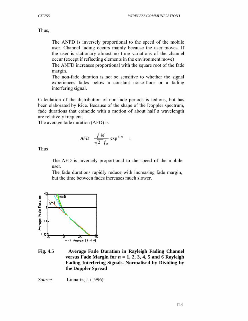
CIT755 WIRELESS COMMUNICATION I
123
Thus,
The ANFD is inversely proportional to the speed of the mobile user. Channel fading occurs mainly because the user moves. If the user is stationary almost no time variations of the channel occur (except if reflecting elements in the environment move) The ANFD increases proportional with the square root of the fade margin. The non-fade duration is not so sensitive to whether the signal experiences fades below a constant noise-floor or a fading interfering signal.
Calculation of the distribution of non-fade periods is tedious, but has been elaborated by Rice. Because of the shape of the Doppler spectrum, fade durations that coincide with a motion of about half a wavelength are relatively frequent. The average fade duration (AFD) is
Thus
AFD
M
2 f D
exp 1 / M 1
The AFD is inversely proportional to the speed of the mobile user. The fade durations rapidly reduce with increasing fade margin, but the time between fades increases much slower.
Fig. 4.5 Average Fade Duration in Rayleigh Fading Channel versus Fade Margin for n = 1, 2, 3, 4, 5 and 6 Rayleigh Fading Interfering Signals. Normalised by Dividing by the Doppler Spread
Source Linnartz, J. (1996)
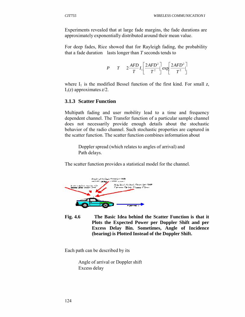
CIT755 WIRELESS COMMUNICATION I
124
Experiments revealed that at large fade margins, the fade durations are approximately exponentially distributed around their mean value.
For deep fades, Rice showed that for Rayleigh fading, the probability that a fade duration lasts longer than T seconds tends to
AFD 2 AFD 2 2 AFD 2
P T 2 T
I1 T 2 exp T 2
where I1 is the modified Bessel function of the first kind. For small z, I1(z) approximates z/2.
3.1.3 Scatter Function
Multipath fading and user mobility lead to a time and frequency dependent channel. The Transfer function of a particular sample channel does not necessarily provide enough details about the stochastic behavior of the radio channel. Such stochastic properties are captured in the scatter function. The scatter function combines information about
Doppler spread (which relates to angles of arrival) and Path delays.
The scatter function provides a statistical model for the channel.
Fig. 4.6 The Basic Idea behind the Scatter Function is that it Plots the Expected Power per Doppler Shift and per Excess Delay Bin. Sometimes, Angle of Incidence (bearing) is Plotted Instead of the Doppler Shift.
Each path can be described by its
Angle of arrival or Doppler shift Excess delay

CIT755 WIRELESS COMMUNICATION I
125
1f
A Practical Example
Fig. 4.7 Measured Scatter Plot for DCS 1800 MHz System
Doppler spread = 60.3 Hz; Coherence time = 5.9 msec. Delay Spread = 1.2 msec; coherence BW = 1.3 MHz
Source Research group of Prof. Paul Walter Baier, U. of
Kaiserslautern, Germany.
Theoretical Example Let’s consider a
U-shaped Doppler spectrum, as it occurs with uniformly distributed angles of arrival of reflected waves. The maximum shift is fm. an exponential delay spread with mean Trms
Moreover, we assume that the delay spread and Doppler spread are separable. Then the amount of scatter power per frequency and time bin can be expressed as
P f , t Plocal
4
mean f m
1
f f c
2 m
1 2 Trms
exp
t Trms
The integral over p(f,t) gives total received local mean power Plocal-mean.

CIT755 WIRELESS COMMUNICATION I
126
Fig. 4.8(a) Scatter Function. Received Power per Unit of Frequency Shift and per Unit of Excess Time Delay. Frequency Shift Normalized to the Maximum Doppler Shift. Delay Time Normalized to the Delay Spread
Fig. 4.8(b) Scatter Function Projected to Frequency Axis. This Gives the Doppler Spread. Received Power per Unit of Frequency Shift. Frequency Shift Normalised to the Maximum Doppler Shift
CIT755 WIRELESS COMMUNICATION I
127
Fig. 4.8(c) Scatter Function Project to Delay Time Axis:
This Gives the Delay Profile. Received Power per Unit of Excess Time Delay. Delay Time Normalised to the Delay Spread.
Source Channel simulations based on this theoretical model have
been contributed by Ralph Haas (2009).
18.0 CONCLUSION Here you learnt the concept of threshold crossing rate, average fade duration and scatter function.
19.0 SUMMARY In this unit, you have learnt that:
Threshold crossing rate is average number of times per second that a fading signal crosses a certain threshold. The expected number of crossings per second is found by integrating over all possible derivatives
TRC
2 f D exp M
1/ M
The average fade duration quantifies how long the signal spends below the threshold. The average fade duration is inversely proportional to the speed of the mobile user. The average fade duration (AFD) is
AFD
M
2 f D
exp 1 / M 1
The average nonfade duration (ANFD) can be expressed as
ANFD M
2 f D
where fD is the Doppler spread, M is the ratio of the local-mean signal power and the minimum (threshold) power needed for reliable communication The scatter function combines information about the Doppler spread (which relates to angles of arrival) and Path delays.
SELF ASSESSMENT EXERCISE Write short note on threshold crossing rate

CIT755 WIRELESS COMMUNICATION I
128
20.0 TUTOR-MARKED ASSIGNMENT
What is meant by Average fade duration and scatter function.
21.0 REFERENCE/FURTHER READING
Linnartz, J. M. G. (1996). Wireless Communication. Baitzer Science Publishers

CIT755 WIRELESS COMMUNICATION I
129
UNIT 5 CHANNEL CLASSIFICATION
CONTENTS 1.0 Introduction 2.0 Objectives 3.0 Main Content
3.1 Channel Classification 3.1.1 Time Selective Channels 3.1.2 Frequency Selective Channels 3.1.3 General Channels 3.1.4 WSSUS Channels 3.1.5 Coherence Time 3.1.6 Power Delay Profile 3.1.7 Coherence Bandwidth 3.1.8 Stationary and Non-Stationary Channels
4.0 Conclusion 5.0 Summary 6.0 Tutor-Marked Assignment 7.0 Reference/Further Reading
15.0 INTRODUCTION In previous units, we investigated the effect that various propagation phenomena have on the received electric field. From observations we can categorised these as large scale propagation effects and small scale propagation effects.
Large scale effects are due to the general terrain and the density and height of buildings and vegetation. Large-scale effects are important for predicting the coverage and availability of a particular service.
Small scale effects are due to the local environment, nearby trees, buildings etc. and the movement of the radio terminal through that environment. Small-scale effects are important for the design of the modulation format and for general transmitter and receiver design.
16.0 OBJECTIVES At the end of this unit, you should be able to:
define a channel explain different classifications of channel.

CIT755 WIRELESS COMMUNICATION I
130
17.0 MAIN CONTENT
3.1 Channel Classification
Channel, in communications (sometimes called communications channel), refers to the medium used to convey information from a sender (or transmitter) to a receiver. Channel can be classified as follows: time-selective channels, frequency selective channels, general channels, WSSUS channels, coherence time channels, power-delay profile channels, coherence bandwidth channels, stationary and non- stationary channels.
3.1.1 Time Selective Channels
A channel is said to be Time selective, if the channel is better at selected times than at other times.
Time variations of the channel due to a relative motion between transmitter and receiver lead to a broadening of the signal spectrum.
This frequency dispersion can be characterized by the U-shaped power spectrum of isotropic scattering.
The spectral line of a pure sine wave will have a power spectrum as shown in figure 5.1 after transmission over the channel. The frequency range, where the power spectrum is nonzero defines the Doppler spread BD. The reciprocal of BD approximates the coherence time Tc of the channel. If we represent the channel influence as an attenuation of the signal amplitude, Tc denotes the minimum time interval between two decorrelated attenuation factors.

CIT755 WIRELESS COMMUNICATION I
131
s
l
L
tl l
t,L
~
Fig. 5.1 Power Density Spectrum of a Sine Wave Suffering from a Doppler Spread
3.1.2 Frequency Selective Channels With large-scale effects, the signal may arrive at the reeceiver via paths with different path lengths. As a result, in complex phasor notation, a model for this large-scale effect is
~x t ~ ~ i 1
where relative delay associated with the lth
~ path and, for the moment,
the complex gains l are assumed constant (due to the transmitter and receiver being physically stationary). With this channel impulse response can be represented as
~ h l l
i 1
This channel is time-invariant but it does show a frequency-dependent response.
The multipath delay spread Tm represents the time interval for which the impulse response of the channel is considerably greater than zero.

CIT755 WIRELESS COMMUNICATION I
132
Fig. 5.2 Delay Profile Expected Received Power as a Function of Excess Delay Time
The coherence bandwidth Bc of the channel is proportional to the reciprocal of Tm. Bc denotes the maximum frequency separation of two sinusoidal signals, for which the channel affects these waves still in a highly correlated manner. This implies that a signal with a bandwidth larger than Bc will suffer from intersymbol interference. If its bandwidth is considerably smaller than Bc the channel can be considered as frequency-nonselective or "flat" fading.
3.1.3 General Channels
In a situation where the channel is neither time varying nor frequency varying such a channel is referred to as flat-flat, since the response is flat in both the time and frequency domains
3.1.4 WSSUS Channels
The mobile channel introduces delay spread into the received signal.
That is, the received signal has a longer duration than that of the transmitted signal, due to the different delays of the signal paths. This is referred to as Time Dispersion.
The mobile channel introduces Doppler spread into the received signal.
That is, the received signal has a larger bandwidth than that of the transmitted signal, due to the different Doppler shifts introduced by the components of the multipath. This is referred to as Frequency Dispersion.

CIT755 WIRELESS COMMUNICATION I
133
Both time dispersion and frequency dispersion introduce distortion into the received signal. The amount of degradation caused by this distortion depends on how the signal is designed. Doppler spreading or frequency dispersion causes variations of the received signal in the time domain.
Of interest for the design of data transmission systems is the maximum duration for which the channel can be assumed to be approximately constant. A transmitted data symbol that has duration less than this time should suffer little distortion from the effects of frequency dispersion.
However, it will still suffer the effects of reduced signal levels.
Just as fading does in the time domain, time dispersion causes slow variations in the received signal in the frequency domain. Of interest in the design of digital transmissions systems is the maximum transmission bandwidth over which there is little variation. A signal contained within that bandwidth should suffer little distortion from the effects of time dispersion.
A random process is wide-sense stationary if it has a mean that is time independent and a correlation function. It is also assumed that, in multipath channels, the gain and phase shift at one delay are uncorrelated with the gain and phase shift at another delay. This type of behaviour is referred to as uncorrelated scattering (US). The combination of a wide-sense stationary signal and uncorrelated scattering is referred to as a wide-sense stationary uncorrelated scattering (WSSUS) channel. The wide sense stationary uncorrelated scattering (WSSUS) model is commonly used for multipath fading channels. WSSUS channel assumes that the channel correlation function is invariant over time, and that the scattering with different path delays are uncorrelated
3.1.5 Coherence Time The coherence time is defined as the period over which there is a strong correlation of the channel time response. It is a measure of the length of time for which the channel can be assumed to be approximately constant in the time domain. Coherence time is the time over which a propagating wave may be considered coherent. In other words, it is the time interval within which its phase is, on average, predictable. In long-distance transmission systems, the coherence time may be reduced by propagation factors such as dispersion, scattering, and diffraction.
Coherence Time can be expressed as Tcoherence 1
2 f D

CIT755 WIRELESS COMMUNICATION I
134
TBW
That is, coherence time of the channel is approximately the inverse of the Doppler spread of the channel
3.1.6 Power Delay Profile
The power delay profile (PDP) gives the intensity of a signal received through a multipath channel as a function of time delay. The time delay is the difference in travel time between multipath arrivals. The abscissa is in units of time and the ordinate is usually in decibels. It is easily measured empirically and can be used to extract certain channel's parameters such as the delay spread.
3.1.7 Coherence Bandwidth
Coherence bandwidth is a statistical measurement of the range of frequencies over which the channel can be considered “flat”, or in other words the approximate maximum bandwidth or frequency interval over which two frequencies of a signal are likely to experience comparable or correlated amplitude fading. Coherence bandwidth is a measure of the approximate bandwidth within which the channel can be assumed to be nearly constant. Coherence bandwidth of a channel is related to the autocorrelation function of the time-varying frequency response. As a result of the inverse relationship between the time and frequency domains, we have the relationship
1
coh M
That is, the coherence bandwidth is inversely proportional to the multipath spread of the channel. The coherence bandwidth of the channel is the bandwidth over which the frequency response is strongly correlated, that is, relatively flat. If the coherence bandwidth is small with respect to the bandwidth of the transmitted signal, then the channel is said to be frequency selective. When the coherence bandwidth is large with respect to the bandwidth of the transmitted signal, then the channel is said to be frequency non selective or frequency-flat.
3.1.8 Stationary and Non-Stationary Channels
The key feature of wide-sense stationary uncorrelated-scattering (WSSUS) channel is that correlation of the channel response depends only on the time difference and not on the absolute time. These stationary models for channel characteristics are convenient for analysis, but often, except for short time intervals, they are not an accurate description of reality. For example, terrestrial mobile channels are usually highly non-stationary, for the following reasons, among others:

CIT755 WIRELESS COMMUNICATION I
135
i. The propagation “often consists of several discontinuities, such as buildings, that can cause significant changes in the propagation characteristics.
ii. The environment itself is physically non-stationary. There may be moving trucks, moving people, or other elements of the environment that can significantly affect propagation.
iii. The interference caused by other users sharing the same frequency channel will vary dynamically as these other users come onto and leave the system. All of these factors contribute to the non-stationary of the link
18.0 CONCLUSION In this unit, you have learned about channel and classifications of wireless channel. A channel is said to be time selective, if the channel is better at selected times than at other times. The coherence time is defined as the period over which there is a strong correlation of the channel time response.
19.0 SUMMARY In this unit, you have learnt that:
Channel refers to the medium used to convey information from a sender (or transmitter) to a receiver. Channels are classified on the basic of the properties of the time- varying impulse response. The effects of noise are not considered in classifying channels. Channel can be classified as follows: time-selective channels, frequency selective channels, general channels, WSSUS channels, coherence time channels, power-delay profile channels, coherence bandwidth channels, stationary and non-stationary channels.
SELF ASSESSMENT EXERCISE What is meant by a channel?
20.0 TUTOR-MARKED ASSIGNMENT Briefly explain any five classes of channels.
21.0 REFERENCE/FURTHER READING Sharma, S. (2006). Wireless and Cellular Communication. New Delhi:
S. K. Kataria & Sons.

CIT755 WIRELESS COMMUNICATION I
136
MODULE 4 MODULATION, DIVERSITY AND MULTIPLE ACCESS TECHNIQUES
Unit 1 Introduction to Modulation Unit 2 Analog Modulation Techniques Unit 3 Digital (Bandpass) Modulation Techniques Unit 4 Digital Baseband and Pulse Shaping Modulation
Techniques Unit 5 Diversity Techniques for Fading Channel Unit 6 Multiple Access Techniques
UNIT 1 INTRODUCTION TO MODULATION
CONTENTS
1.0 Introduction 2.0 Objectives 3.0 Main Content
3.1 Definition of Modulation 3.1.1 Why Modulate? 3.1.2 Modulation Choices 3.1.3 Modulating a Sound Wave 3.1.4 Types of Modulation Techniques
4.0 Conclusion 5.0 Summary 6.0 Tutor-Marked Assignment 7.0 References/Further Reading
1.0 INTRODUCTION
The simple transmission scheme outlined in the previous units cannot be used for commercial broadcasting. If a dozen of stations all transmitted sounds by the mechanism described in the previous units, a receiving station would pick up a garbled combination of all transmissions. To prevent interference from a number of transmitting stations, all broadcast radio waves are first modulated.
2.0 OBJECTIVES
At the end of this unit, you should be able to:
define a modulation state the reason for modulation explain how a sound wave is modulated list clearly the four types of modulation techniques.

CIT755 WIRELESS COMMUNICATION I
137
3.0 MAIN CONTENT
3.1 Definition of Modulation
Modulation is the process of encoding information from a message source into manner suitable for transmission. It generally involves translating a baseband message signal (called the source) to a bandpass signal at frequencies that are very high when compared to the baseband frequency. The bandpass signal is called the modulated signal and the baseband signal is called the modulating signal. Modulation may be done by varying the amplitude, phase or frequency of a high frequency carrier in accordance with the amplitude of the message signal.
Modulation may be defined as a process by which some characteristic of a signal known as carrier is varied according to the instantaneous value of another signal known as modulating signal. The signals containing intelligence or information to be transmitted are called modulating signals. These modulating signals containing information are also called baseband signals. Also the carrier frequency is greater than the modulating frequencies and the signal which results from the process of modulation is known as modulated signal.
Demodulation is the process of extracting the baseband message from the carrier so that it may be processed and interpreted by the intended receiver (also called sink). It is the process of extracting a modulating or baseband signal from the modulated signal. In other word, demodulation is the process by which the message is recovered from the modulated signal at the receiver.
A device that performs modulation is known as a modulator and a device that performs the inverse operation of modulation is known as a demodulator (sometimes detector or demod). A device that can do both operations is a modem (short for “Modulator-Demodulator”).
3.1.1 Why Modulate?
For allowing multiple signals to share a single physical channel by Frequency Division Multiplexing Necessary for wireless communication where the antenna diameter must be at least equal to the wavelength of the carrier signal. This means, for a 3000 Hz signal through space, the antenna diameter must be at least 60 miles

CIT755 WIRELESS COMMUNICATION I
138
3.1.2 Modulation Choices
The simplest modulation method is also the first used to transmit messages. The signal is turned on and off to transmit the characters of an agreed code. Text messages can be carried by the signal modulated in this way. Unique patterns stand for letters of the alphabet, numerals, and punctuation marks. Amplitude modulation is the least complicated modulation method capable of transmitting speech or music by varying the carrier signal's instantaneous power. It means that the amplitude (or size) of the wave of the original sound wave has been changed by adding it to the carrier wave. Sound waves can be modulated in such a way that their frequency is altered. For example, a sound wave can be added to a carrier signal to produce a signal with the same amplitude, but a different frequency. The sound wave has, in this case, undergone frequency modulation (FM). Sound can be converted to digital data, transmitted, then used to reconstruct the original waveform in the receiver. This sound wave is a form of digital modulation.
3.1.3 Modulating a Sound Wave
After the sound wave has been modulated at the transmitting station, both AM and FM signals must be decoded at the receiving station. In either case, the carrier wave is electronically subtracted from the radio wave that is picked up by the receiving antenna. What remains after this process is the original sound wave, encoded, of course, as an electrical signal.
All broadcasting stations are assigned characteristic carrier frequencies by the Federal Communications Commission (FCC). This system allows a number of stations to operate in the same area without overlapping.
Thus, two stations a few kilometers apart could both be sending out exactly the same program, but they would sound different (and have different electric signals) because each had been overlaid on a different carrier signal.
Receiving stations can detect the difference between these two transmissions because they can tune their equipment to pick up only one or the other carrier frequency. When you turn the tuning knob on your own radio, for example, you are adjusting the receiver to pick up carrier waves from station A, station B, or some other station. Your radio then decodes the signal it has received by subtracting the carrier wave and converting the remaining electric signal to a sound wave.

CIT755 WIRELESS COMMUNICATION I
139
The identifying characteristics by which you recognise a radio station reflect its two important transmitting features. The frequency, such as 101.5 megahertz (or simply “101.5 on your dial”) identifies the carrier wave frequency, as described above. The power rating (“operating with 50,000 watts of power”) describes the power available to transmit its signal. The higher the power of the station, the greater the distance at which its signal can be picked up.
3.1.4 Types of Modulation Techniques
Analog modulation: The aim of analog modulation is to transfer an analog baseband (or lowpass) signal, for example an audio signal or TV signal, over an analog passband channel, for example a limited radio frequency band or a cable TV network channel. BandPass digital modulation: The aim of digital modulation is to transfer a digital bit stream over an analog passband channel, for example over the public switched telephone network (where a bandpass filter limits the frequency range to between 300 and 3400 Hz), or over a limited radio frequency band. Digital baseband modulation or line coding modulation: The aim of digital baseband modulation methods, also known as line coding, is to transfer a digital bit stream over a baseband channel, typically a non-filtered copper wire such as a serial bus or a wired local area network. Pulse shaping modulation: The aim of pulse modulation methods is to transfer a narrowband analog signal, for example a phone call over a wideband baseband channel or, in some of the schemes, as a bit stream over another digital transmission system.
4.0 CONCLUSION In this unit, the term “modulation”, the reason for modulation, the choices of modulation, how a sound wave is being modulated and the four modulation techniques were discussed.
5.0 SUMMARY In this unit, you have learnt that:
Modulation is a fundamental requirement of a communication system. Modulation may be done by varying the amplitude, phase or frequency of a high frequency carrier in accordance with the amplitude of the message signal

CIT755 WIRELESS COMMUNICATION I
140
The four types of modulation techniques are analog modulation, digital bandpass modulation, digital baseband modulation and pulse shaping modulation.
SELF ASSESSMENT EXERCISE
What do you understand by the term modulation?
6.0 TUTOR-MARKED ASSIGNMENT
1. Briefly describe how sound wave can be modulated? 2. Mention four types of modulation techniques. 3. State two major reasons for modulation.
7.0 REFERENCES/FURTHER READING
Bloomfield, L. A. (2000). How Things Work: The Physics of Everyday Life. (2nd ed.). New York: John Wiley & Sons.
Davidovits, P. (1972). Communication. New York: Holt Rinehart & Winston Inc.
Sharma, S. (2006). Wireless and Cellular Communications. New Delhi: S. K. Kataria & Sons.

CIT755 WIRELESS COMMUNICATION I
141
UNIT 2 ANALOG MODULATION TECHNIQUES
CONTENTS 1.0 Introduction 2.0 Objectives 3.0 Main Content
3.1 Concept of Analog Modulation Techniques 3.1.1 Amplitude Modulation (AM)
3.1.1.1Types of Amplitude Modulation Techniques 3.1.2 Angle Modulation
3.1.2.1 Types of Angle Modulation 3.1.2.1.1 Frequency Modulation (FM) 3.1.2.1.2 Phase Modulation (PM)
3.1.3 Comparison of Angle Modulated Wave and Amplitude Modulated Wave 3.1.4 Comparison of Frequency Modulation and
Amplitude Modulation 4.0 Conclusion 5.0 Summary 6.0 Tutor-Marked Assignment 7.0 References/Further Reading
1.0 INTRODUCTION In analog modulation the carrier waveform is continuous in nature. The two families of continuous wave modulation systems are amplitude modulation and angle modulation.
2.0 OBJECTIVES At the end of this unit, you should be able to:
differentiate between the two types of analog modulation explain the meaning of angle modulation state the types of angle modulation mention the merit and demerit of FM compute the modulation index, frequency, deviation, carrier frequency and power of a signal.

CIT755 WIRELESS COMMUNICATION I
142
3.0 MAIN CONTENT
3.1 Concept of Analog Modulation Techniques
In analog modulation, the modulation is applied continuously in response to the analog information signal. The aim of analog modulation is to transfer an analog baseband (or lowpass) signal, for example an audio signal or TV signal, over an analog passband channel, for example a limited radio frequency band or a cable TV network channel.
Figure 2.1 Low-Frequency Message Signal (top) May Be Carried by an AM or FM Radio Wave
Common analog modulation techniques are:
Amplitude Modulation and Angle Modulation
3.1.1 Amplitude Modulation (AM)
AM may be defined as a system in which the maximum amplitude of the carrier wave is made proportional to the instantaneous value (amplitude) of the modulating or baseband signal. AM is a technique used in electronic communication, most commonly for transmitting information via a radio carrier wave. AM works by varying the strength of the transmitted signal in relation to the information being sent. For example, changes in the signal strength can be used to reflect the sounds to be reproduced by a speaker, or to specify the light intensity of television pixels.

CIT755 WIRELESS COMMUNICATION I
143
Figure 2.2 Illustration of Amplitude Modulation Source: Sharma, S. (2006). Wireless and Cellular Communication.
Conventional AM This is how a typical AM system transmitter works:
Figure 2.3 Conventional Amplitude Modulation
The information signal is mixed with the carrier signal and produces the full AM signal to be transmitted.
Transmission Efficiency of Amplitude Modulated Signal The total modulated power of an AM signal is expressed as
Pt Pc Ps 1
A2
2
x 2 t

CIT755 WIRELESS COMMUNICATION I
144
Out of this total power Pt, the useful message or baseband power is the power carried by the sidebands, i.e. Ps. The large carrier power Pc is a waste from the transmission point of view because it does not carry any information or message. This large carrier power Pc is transmitted along with the sideband power only for the convenient and cheap detection. Hence, Ps is the only useful message power present in the AM wave. In AM wave, the amount of useful message power Ps may be expressed by a term known as transmission efficiency .
Hence, transmission efficiency of AM wave may be defined as the percentage of total power contributed by the sidebands.
Mathematically,
Transmission Efficiency,
P
s 100 or Pt
1 2
x t 2 100 100 x 2 t 1
A2
2
x 2 t A2 x 2 t
The maximum transmission efficiency of the AM is only 33.33%. This implies that only one-third of the total power is carried by the sidebands and the rest two-third is wasted.
3.1.1.1 Types of Amplitude Modulation Techniques
(a) Single-Sideband Modulation (SSB, or SSB-AM): Is a refinement of amplitude modulation that uses electrical power and bandwidth. It is closely related to vestigial sideband modulation (VSB). Amplitude modulation produces a modulated output signal that has twice the bandwidth of the original baseband signal. Single-sideband modulation avoids this bandwidth doubling, and the power wasted on a carrier, at the cost of somewhat increased device complexity. The SSB Schemes are:
SSB with carrier (SSB-WC) SSB suppressed carrier modulation (SSB-SC): is a modulation which provides a single sideband with suppressed carrier. In SSB-SC the carrier power level is suppressed to the point where it is insufficient to demodulate the signal. The information represented by the modulating signal is contained in both the upper and the lower sidebands. Since each modulating frequency fc produces corresponding upper and lower side-frequencies
fc + fi and fc − fi

CIT755 WIRELESS COMMUNICATION I
145
it is not necessary to transmit both side-bands. Either one can be suppressed at the transmitter without any loss of information.
Advantages of SSB-WC
Less transmitter power. Less bandwidth, one-half that of Double-Sideband (DSB). Less noise at the receiver. Size, weight and peak antenna voltage of a single-sideband (SSB) transmitters is significantly less than that of a standard AM transmitter
The single side-band (SSB) is very simple: if you do not need two side- bands, you can get rid of one of the band. To do this, you add a band pass filter component to your system that removes the extra side-band.
This is how the SSB transmitter looks like:
Figure 2.4 SSB Transmitter
Note that the band pass filter has removed the lower side-band (LSB) and the carrier from the spectrum. The remainder is transmitted.
The receiver cannot output the signal as it is, it must first restore the signal to what it should be before demodulation. The receiver in a SSB system has its own carrier signal (from a local oscillator) that is puts back in. The receiver looks like the diagram in figure 2.5 below:
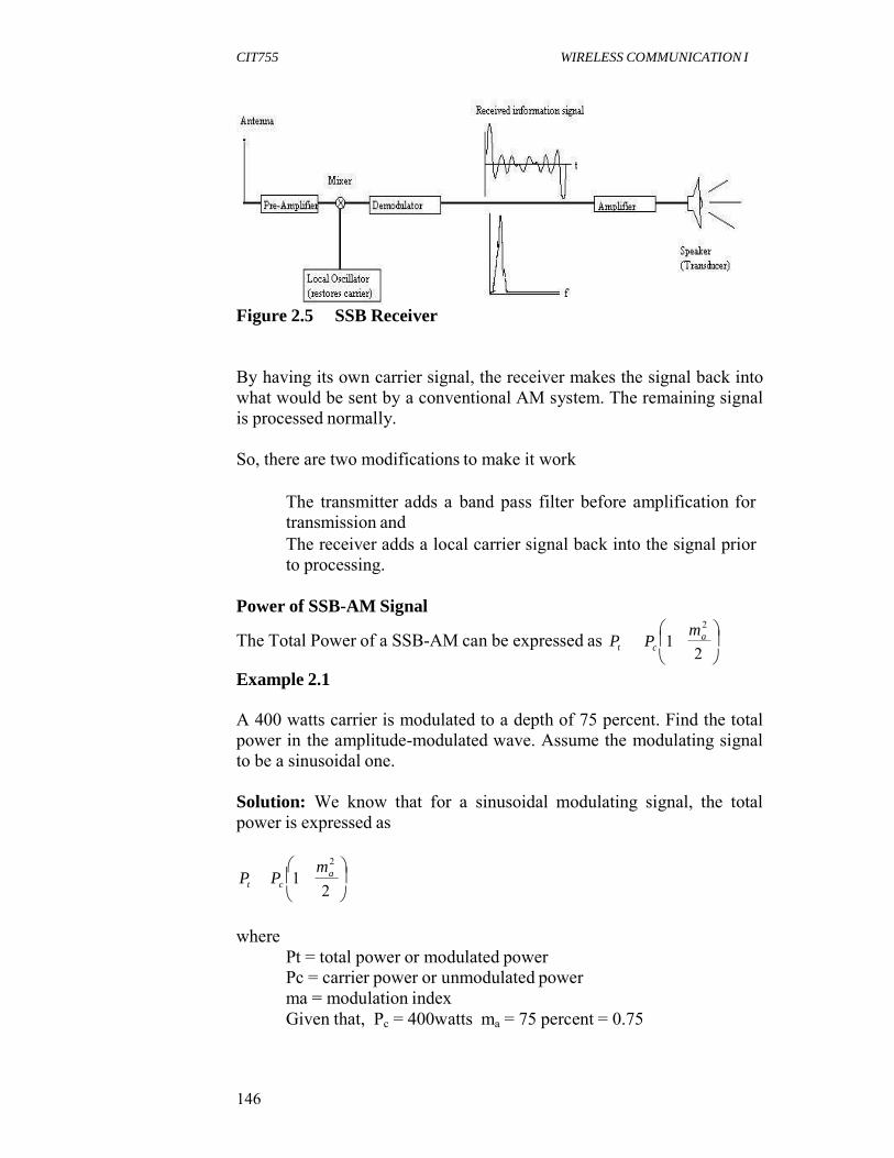
CIT755 WIRELESS COMMUNICATION I
146
Figure 2.5 SSB Receiver
By having its own carrier signal, the receiver makes the signal back into what would be sent by a conventional AM system. The remaining signal is processed normally.
So, there are two modifications to make it work
The transmitter adds a band pass filter before amplification for transmission and The receiver adds a local carrier signal back into the signal prior to processing.
Power of SSB-AM Signal
The Total Power of a SSB-AM can be expressed as Pt
Pc 1
m 2 a
Example 2.1
2
A 400 watts carrier is modulated to a depth of 75 percent. Find the total power in the amplitude-modulated wave. Assume the modulating signal to be a sinusoidal one.
Solution: We know that for a sinusoidal modulating signal, the total power is expressed as
Pt Pc
1 m 2 a 2
where
Pt = total power or modulated power Pc = carrier power or unmodulated power ma = modulation index Given that, Pc = 400watts ma = 75 percent = 0.75

CIT755 WIRELESS COMMUNICATION I
147
Therefore, Pt
Pc 1 m 2 a =
4001 0.752
512.5watts
2 2 Example 2.2
An AM broadcast radio transfer radiates 10K watts of power, if modulation percentage is 60. Calculate how much of this the carrier power is.
Solution: We known that the total power is expressed as
Pt Pc
1 m 2 a 2
where Pt = total power or modulated power Pc = carrier power or unmodulated power ma = modulation index Given that, Pt = 10 K watts ma =60 percent = 0.6
Pt 10
Therefore Pc 2 2
or Pc
1 ma
2 10
1 8.47 KW
0.6
2
1.18 Current Calculation for SSB AM
In AM, it is generally more convenient to measure the AM transmitter current than the power. In this case, the modulation index may be calculated from the values of unmodulated and modulated currents in the AM transmitter. Let Ic be the r.m.s value of the carrier or unmodulated current and It be the r.m.s value of the total or modulated current of an AM transmitter. Let R be the antenna resistance through which these currents flow.
We know that for an SSB AM the power relation is expressed as
Pt Pc
1 m 2 a 2
where Pt = total power or modulated power Pc = carrier power or unmodulated power ma = modulation index From the above equation, we may write
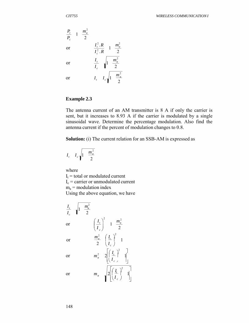
CIT755 WIRELESS COMMUNICATION I
148
m
t
c
m
m
m
m
I
2
2
2
2
2
c
Pt 1 a
Pc 2
or
or
I 2 . R 2
1 a
I 2 . R 2
I t 1 a
I c 2
m 2
or I t I c 1 a
2
Example 2.3
The antenna current of an AM transmitter is 8 A if only the carrier is sent, but it increases to 8.93 A if the carrier is modulated by a single sinusoidal wave. Determine the percentage modulation. Also find the antenna current if the percent of modulation changes to 0.8.
Solution: (i) The current relation for an SSB-AM is expressed as
I t I c 1 2
a
2
where It = total or modulated current Ic = carrier or unmodulated current ma = modulation index Using the above equation, we have
It 1 a
Ic 2
2
I t or c
1 ma
2
m 2 I
or a
2 t 1 I c I
2 or m 2 2 t 1a
I
I 2
or m 2 t 1a I
c

CIT755 WIRELESS COMMUNICATION I
149
m
2
Putting all the given values, we have
8.93 2
ma 2 12 1.116 2 1
8
ma 2(1.246 1) 0.492 0.701 70.1%
(ii) Since I t I c 1
2 a
2 Here, Ic = 8A and ma = 0.8
Therefore, I t 8 1 0.8
2 8 1
0.64 2
or I t 8 1.32 8 1.149 9.19 A
(b) Double-Sideband Modulation (DSB)
Double-sideband modulation with unsuppressed carrier (DSB- WC): is used on the AM radio broadcasting band. Double-sideband suppressed-carrier transmission (DSB-SC): is a modulated signal, which contains no carrier but two sidebands. It is a transmission in which (a) frequencies produced by amplitude modulation are symmetrically spaced above and below the carrier frequency and (b) the carrier level is reduced to the lowest practical level, ideally completely suppressed. In the double- sideband suppressed-carrier transmission (DSB-SC) modulation, unlike AM, the wave carrier is not transmitted; thus, a great percentage of power that is dedicated to it is distributed between the sidebands, which imply an increase of the cover in DSB-SC, compared to AM, for the same power used. DSB-SC transmission is a special case of Double-sideband reduced carrier transmission. This is used for RDS (Radio Data System) because it is difficult to decouple. Double-sideband reduced carrier transmission (DSB-RC): transmission in which (a) the frequencies produced by amplitude modulation are symmetrically spaced above and below the carrier and (b) the carrier level is reduced for transmission at a fixed level below that which is provided to the modulator. In DSB-RC transmission, the carrier is usually transmitted at a level suitable for use as a reference by the receiver, except for the case in which

CIT755 WIRELESS COMMUNICATION I
150
it is reduced to the minimum practical level, i.e. the carrier is suppressed.
(c) Vestigial Sideband Modulation (VSB, or VSB-AM) is a
sideband that has been only partly cut off or suppressed. In VSB modulation instead of rejecting one sideband completely as in SSB modulation scheme, a gradual cut-off of one sideband is allowed. This gradual cut is compensated by a vestige or portion of the other sideband. Television broadcasts (in analog video formats) use this method if the video is transmitted in AM, due to the large bandwidth used. It may also be used in digital transmission, such as the ATSC standardized 8-VSB.
(d) Quadrature Amplitude Modulation (QAM) is also called Quadrature Carrier Multiplexing. This modulation scheme enables two DSC-SC modulated signals to occupy the same transmission bandwidth and therefore it allows for the separation of the two message signals at the receiver output. It is, therefore, known as a bandwidth-conservation scheme.
Problems with Conventional AM
Conventional AM transmission has several problems:
Bandwidth is wasted by having two identical side-bands on either side of the carrier The efficiency is limited to 33% to prevent distortion in the receiver when demodulating. The carrier signal is present even if nothing is being transmitted.
3.1.2 Angle Modulation
Angle Modulation is a class of analog modulation. Angle modulation may be defined as the process in which the total phase angle of a carrier wave is varied in accordance with the instantaneous value of the modulating or message signal while keeping the amplitude of the carrier constant. These techniques are based on altering the angle (or phase) of a sinusoidal carrier wave to transmit data, as opposed to varying the amplitude, such as in AM transmission. The two main types of angle modulation are: (i) Frequency modulation (FM) and (ii)Phase modulation (PM), with its digital correspondence phase-shift keying (PSK).

CIT755 WIRELESS COMMUNICATION I
151
3.1.2.1 Types of Angle Modulation
3.1.2.1.1 Frequency Modulation (FM)
Frequency modulation conveys information over a carrier wave by varying its frequency. Here the frequency of the modulated signal is varied. The two types of frequency modulation are Single Tone frequency modulation and Multiple Frequency Modulation.
(a) Single Tone Frequency Modulation is a type of frequency
modulation (FM) in which the modulating or baseband signal contains a single frequency.
The total variation in frequency from the lowest to the highest point is called carrier swing. Obviously,
the Carrier Swing 2 x frequency deviation 2 x
For FM, the modulation index is defined as the ratio of frequency deviation to the modulating frequency.
Mathematically,
Modulation index, m
Frequency deviation
or m f
f Modulaion m
frequency
This modulation index may be greater than unity.
The term “percentage modulation” as it is used in reference to FM refers to the ratio of actual frequency deviation to the maximum allowable frequency deviation. Thus 100% modulation corresponds to 75 kHz for the commercial FM broadcast band and 25 kHz for television.
Percent modulation M f actual
f max
The expression for single-tone FM wave is s(t ) A cos i A cos c t m f sin m t

CIT755 WIRELESS COMMUNICATION I
152
V
c f
mf
Example 2.4
A single-tone FM is represented by the voltage equation as:
v(t) = 12 cos(6 x 10⁸ t + 5 sin1250 t)
Determine the following:
i. carrier frequency
ii. modulating frequency iii. the modulation index iv. maximum deviation v. what power will this FM wave dissipate in 10 resistor
Solution: We know that the standard expression for a single-tone FM wave is given as v(t) = A cos ct m f sin mt ……………………….(i)
The given expression is v(t) = 12 cos(6 x 10⁸ t + 5 sin1250 t) …….(ii)
Comparing equation (i) and (ii), we get
i. Carrier frequency 8
6 108 rad/sec or 6 10
c 2
95.5MHz
ii. modulating frequency
1250
iii.
m 1250 rad / sec or f m
2 m f 5
199Hz
iv. maximum frequency deviation is given as
f f
m m
or f m f f m 5 199 995
v. the power dissipated is 2
P rms
R
2
12 / 2 10
72 7.2watts
10
Example 2.5
What is the modulation index of an FM signal having a carrier swing of 100 kHz when the modulating signal has a frequency of 8 kHz?

CIT755 WIRELESS COMMUNICATION I
153
Solution: Given that carrier swing = 100 kHz modulating frequency fm = 8 kHz modulating index is given as
m Frequency deviation f
…………(i) f Modulaion frequency f m
but we know that
carrier swing = 2 f
carrier swing 100
kHz
f 50 2 2
using equation (i) we get
m 50
f 8
6.25
Example 2.6
An FM transmission has a frequency deviation of 20 kHz.
i. Determine the percent modulation of this signal if it is
broadcasted in the 88 – 08 MHz band ii. Calculate the percent modulation if this signal is broadcasted as
the audio portion of a television broadcast. Solution: Given that
f 20 kHz
i. Percent modulation for an FM wave is defined as
f M actual
f max
100
f actual is given as 20 kHz The maximum frequency deviation
f max permitted in the FM broadcast band is 75 kHz. Thus,
M
20 103
100
26.67%
75 103

CIT755 WIRELESS COMMUNICATION I
154
(ii) M factual
fmax
100
f 20 kHz
The maximum frequency deviation of a TV broadcast is 25 kHz.
fmax permitted for FM audio portion
Thus, M 20 103
100
80%
25 103
Types of Frequency Modulation (FM)
Depending on the value of frequency sensitivity k f , FM may be divided
as:
(i) Narrowband FM: In this case,
bandwidth of FM is narrow.
k f is small and hence the
(ii) Wideband FM: In this case, k f
has a wide bandwidth.
Application of FM
is large and hence the FM signal
Broadcasting: FM is commonly used at VHF radio frequencies for high-fidelity broadcasts of music and speech and also for broadcasting Normal (analog) TV sound. A narrow band form is used for voice communications in commercial and amateur radio settings. The type of FM used in broadcast is generally called wide-FM, or W-FM. In two- way radio, narrowband narrow-fm (N-FM) is used to conserve bandwidth and also to send signals into space.
Sound: FM is used at audio frequencies to synthesise sound. This technique, known as FM synthesis, was popularised by early digital synthesizers and became a standard feature for several generations of personal computer sound cards
Hardware: FM is used at intermediate frequencies by all analog VCR systems, including VHS, to record both the luminance (black and white) and the chrominance portions of the video signal. FM is the only feasible method of recording video to and retrieving video from magnetic tape without extreme distortion, as video signals have a very large range of frequency components - from a few hertz to several megahertz, too wide for equalizers to work with due to electronic noise below -60 dB. FM also keeps the tape at saturation level, and therefore acts as a form of noise reduction, and a simple limiter can mask
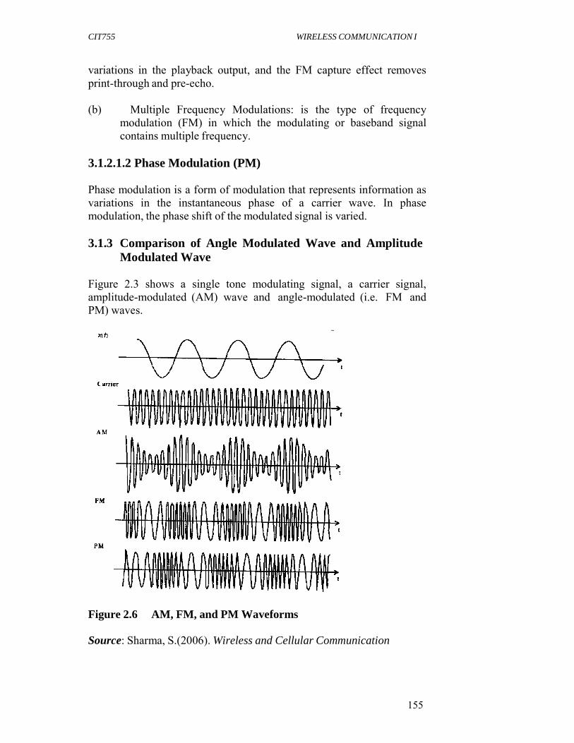
CIT755 WIRELESS COMMUNICATION I
155
variations in the playback output, and the FM capture effect removes print-through and pre-echo.
(b) Multiple Frequency Modulations: is the type of frequency
modulation (FM) in which the modulating or baseband signal contains multiple frequency.
3.1.2.1.2 Phase Modulation (PM) Phase modulation is a form of modulation that represents information as variations in the instantaneous phase of a carrier wave. In phase modulation, the phase shift of the modulated signal is varied.
3.1.3 Comparison of Angle Modulated Wave and Amplitude Modulated Wave
Figure 2.3 shows a single tone modulating signal, a carrier signal, amplitude-modulated (AM) wave and angle-modulated (i.e. FM and PM) waves.
Figure 2.6 AM, FM, and PM Waveforms Source: Sharma, S.(2006). Wireless and Cellular Communication

CIT755 WIRELESS COMMUNICATION I
156
On comparison, the following differences between the two techniques are:
The envelope of FM wave or PM wave is constant and is equal to the unmodulated carrier amplitude. On the other hand, the envelope of AM wave is dependent on the modulating signal x(t). The zero crossings (i.e. the instants of time at which the waveform changes from negative to a positive value or vice- versa) of a FM wave or a PM wave no longer exhibit a perfect regularity in their spacing like AM wave. Thus this makes the instantaneous frequency of the angle modulated wave depend upon time.
3.1.4 Comparison of Frequency Modulation and Amplitude Modulation
(a) Advantages of FM over AM
FM receivers may be fitted with amplitude limiters to remove the amplitude variations caused by noise. This makes FM reception a good deal more immune to noise than AM reception. It is possible to reduce noise still further by increasing the frequency-deviation. This is a feature which AM does not have because it is not possible to exceed 100 percent modulation without causing severe distortion. Standard Frequency Allocations provide a guard band between commercial FM stations. Due to this, there is less adjacent- channel interference than in AM. FM broadcast operates in the upper VHF and UHF frequency ranges at which there happens to be less noise than in the MF and HF ranges occupied by AM broadcasts. The amplitude of the FM wave is constant. It is thus independent of the modulation depth, whereas in AM, modulation depth governs the transmitted power.
(b) Disadvantages of FM over AM
A much wider channel typically 200 KHz is required in FM as against only 10 KHz in AM broadcast. This forms serious limitation of FM. FM transmitting and receiving equipment particularly used for modulation and demodulation tend to be more complex and hence more costly.
CIT755 WIRELESS COMMUNICATION I
157
4.0 CONCLUSION
You have been taken through the analog modulation concepts and its various techniques, the comparison between angle modulated wave and amplitude modulated wave as well as the comparison between FM and AM.
11.0 SUMMARY In this unit, you have learnt that:
In analog modulation, the modulation is applied continuously in response to the analog information signal. The aim of analog modulation is to transfer an analog baseband signal over an analog passband channel. The two types of analog techniques are amplitude modulation and angle modulation. Amplitude modulation is a system in which the maximum amplitude of the carrier wave is made proportional to the instantaneous value (amplitude) of the modulating or baseband signal. The amplitude modulation schemes are single sideband modulation (SSB), double-side band modulation (DSB), vestigial sideband modulation (VSB), and quadrature amplitude modulation (QAM) Angle modulation is based on altering the angle (or phase) of a sinusoidal carrier wave to transmit data, as opposed to varying the amplitude, such as in AM transmission. Angle modulation schemes are frequency modulation and phase modulation.
SELF ASSESSMENT EXERCISE 1. What is angle modulation? 2. What are the types of angle modulation?
12.0 TUTOR-MARKED ASSIGNMENT 1. Differentiate between the two types of analog modulation. 2. Mention the application areas of Frequency Modulation 3. A single-tone FM signal is given by
v(t ) 10 sin 16 106 t 20 sin 2 103t volts . Determine the
modulation index, modulating frequency, frequency deviation, carrier frequency and the power of the FM signal
4. What are the principal merits and limitations of FM?

CIT755 WIRELESS COMMUNICATION I
158
7.0 REFERENCES/FURTHER READING
Carlson, B. (1981). Communication Systems. (2nd ed.). McGraw-Hill Inc.
David, N. & Rick, K. (2004). “Mixers, Modulators and Demodulators”.
In: D. G. Reed (Ed.). The ARRL Handbook for Radio Communications (81st ed.), Newington: ARRL.
Leon, W. C. (2001). Digital and Analog Communication Systems, (6th
ed.). Prentice-Hall Inc.
Sharma, S. (2006). Wireless and Cellular Communications. New Delhi: S. K. Kataria & Sons.

CIT755 WIRELESS COMMUNICATION I
159
UNIT 3 DIGITAL (BANDPASS) MODULATION
TECHNIQUES CONTENTS
1.0 Introduction 2.0 Objectives 3.0 Main Content
3.1 An Overview of Digital Modulation Techniques 3.2 Factors that Influence the Choice of Digital Modulation 3.3 List of Common Digital Modulation Techniques
3.3.1 Phase-Shift Keying (PSK) 3.3.1.1Binary Phase Shift Keying (BPSK), Using
M=2 symbols 3.3.12 Quadrature Phase Shift Keying (QPSK),
Using M=4 symbols 3.3.1.3Differential Phase Shift Keying (DPSK)
3.3.2 Frequency-Shift Keying (FSK) 3.3.2.1Audio Frequency-Shift Keying (AFSK) 3.3.2.2Continuous-Phase Frequency-Shift
Keying (CPFSK) 3.3.2.3Multi-Frequency Shift Keying (M-ary
FSK or MFSK) 3.3.2.4Dual-Tone Multi-Frequency (DTMF)
3.3.3 Amplitude-Shift Keying (ASK) 3.3.4 On-Off Keying (OOK) 3.3.5 Quadrature Amplitude Modulation (QAM) 3.3.6 Continuous Phase Modulation (CPM) Method 3.3.7 Orthogonal Frequency Division Multiplexing
(OFDM) Modulation 3.3.8 Wavelet Modulation 3.3.9 Trellis Coded Modulation (TCM) 3.3.10 Spread-Spectrum Techniques
3.4 Modulator and Detector Principles of Operation 4.0 Conclusion 5.0 Summary 6.0 Tutor-Marked Assignment 7.0 References/Further Reading
1.0 INTRODUCTION Modern mobile communication systems use digital modulation techniques. Advancements in very large-scale integration (VLSI) and digital signal processing (DSP) technology have made digital modulation more cost effective than analog transmission systems.
CIT755 WIRELESS COMMUNICATION I
160
2.0 OBJECTIVES
At the end of this unit, you should be able to:
state the factors that govern the choice of digital modulation explain the digital modulation techniques.
3.0 MAIN CONTENT
3.1 An Overview of Digital Modulation Techniques
In digital modulation, an analog carrier signal is modulated by a digital bit stream. Digital modulation methods can be considered as digital-to- analog conversion, and the corresponding demodulation or detection as analog-to-digital conversion. The changes in the carrier signal are chosen from a finite number of M alternative symbols (the modulation alphabet).
The aim of digital modulation is to transfer a digital bit stream over an analog passband channel, for example over the public switched telephone network (where a bandpass filter limits the frequency range to between 300 and 3400 Hz), or over a limited radio frequency band.
For example, a telephone line is designed for transferring audible sounds, for example tones, and not digital bits (zeros and ones).
Computers may however communicate over a telephone line by means of modems, which are representing the digital bits by tones, called symbols. If there are four alternative symbols (corresponding to a musical instrument that can generate four different tones, one at a time), the first symbol may represent the bit sequence 00, the second 01, the third 10 and the fourth 11. If the modem plays a melody consisting of 1000 tones per second, the symbol rate is 1000 symbols/second, or baud.
Since each tone represents a message consisting of two digital bits in this example, the bit rate is twice the symbol rate, i.e. 2000 bit per second.
3.2 Factors that Influence the Choice of Digital Modulation
The performance of a modulation scheme is often measured in terms of its power efficiency and bandwidth efficiency.
Power efficiency describes the ability of a modulation technique to preserve the fidelity of the digital message at low power levels. In a digital communication system, in order to increase noise

CIT755 WIRELESS COMMUNICATION I
161
2 B
immunity, it is necessary to increase the signal power. However, the amount by which the signal power should be increased to obtain a certain level of fidelity (i.e., an acceptable bit error probability) depends on the particular type of modulation employed. Bandwidth efficiency describes the ability of a modulation scheme to accommodate data within a limited bandwidth. In general, increasing the data rate implies decreasing the pulse width of a digital symbol, which increases the bandwidth of the signal. If R is the data rate in bits per second, and B is the bandwidth occupied by the modulated RF signal, then bandwidth efficiency B is expressed as
R
pss / Hz B B
Shannon’s channel coding theorem states that for an arbitrarily small probability error, the maximum possible bandwidth efficiency is limited by the noise in the channel, and is given by the channel capacity formula. Note that Shannon’s bound applies for AWGN non-fading channels.
C log
1
S B N
where C is the channel capacity (in bps), B is the RF bandwidth and
S
is the signal-to-noise ratio. N
Exercise 3.1
If the SNR of a wireless communication link is 20 dB and the RF bandwidth is 30 kHz. Calculate the maximum theoretical data rate which may be transmitted. Compare this rate to the US Digital Cellular Standard.
Solution
Given that
S
= 20 dB = 100 N
RF Bandwidth B = 30000 Hz Making use of Shannon’s channel capacity expression the maximum possible data rate will be given by

CIT755 WIRELESS COMMUNICATION I
162
C B log S
2 1 N
30000 log 2 1
100
199.75 kbps
The USDC data rate is 48.6 kbps, which is only about the one-fourth the theoretical limit under 20 dB SNR conditions.
Exercise 3.2
What is the theoretical maximum data rate which can be supported in a 200 kHz channel for SNR = 10 dB, 30 dB. How can this be compared with the GSM standard.
Solution
For SNR = 10 dB = 10, B = 200 kHz.
Making use of Shannon’s channel capacity theorem, the maximum possible data rate, will be given by
S C B log 2 1
N
200000 log 2 1 10
691.886 kbps
The GSM data rate is 270.833 kbps, which is only about 40% of the theoretical limit for 10 dB SNR conditions.
For SNR = 30 dB = 1000,B = 200 kHz The maximum possible data rate will be
C B log S
2 1 N
200000 log 2 1
1000
1.99Mbps
3.3 List of Common Digital Modulation Techniques
Any digital modulation scheme uses a finite number of distinct signals to represent digital data. The most common digital modulation techniques are:
Phase Shift Keying Frequency shift Keying Amplitude Shift Keying On-Off Keying Quadrature Amplitude Modulation Continuous Phase Modulation Spread-Spectrum Techniques

CIT755 WIRELESS COMMUNICATION I
163
3.3.1 Phase-Shift Keying (PSK)
PSK is a digital modulation scheme that conveys data by changing, or modulating, the phase of a reference signal (the carrier wave). PSK uses a finite number of phases; each assigned a unique pattern of binary bits.
3.3.1.1 Binary Phase Shift Keying (BPSK), Using M=2 Symbols
In Binary phase shift keying, the binary symbols ‘1’ and ‘0’modulate the phase of the carrier. With Binary Phase Shift Keying (BPSK), the binary digits 1 and 0 may be represented by the analog levels and respectively. The system model is as shown in the Figure below.
Figure 3.1 Simplified Block Diagram with BPSK Transmitter- Receiver
The Bandwidth of BPSK signal will be, BW = Highest frequency – Lowest frequency
BW = or
f c f b
BW 2 f b
f c f b
Hence the minimum bandwidth of BPSK signal is equal to twice of the highest frequency contained in baseband signal.
Probability of Bit Error Rate (BER) for BPSK modulation
The received signal, y s1 n when bit 1 is transmitted and y s0 n when bit 0 is transmitted.
The conditional probability distribution function (PDF) of for the two cases are:

CIT755 WIRELESS COMMUNICATION I
164
2
0
2
y1
N N N
Figure 3.2 Conditional Probability Density Function with BPSK
Modulation
Source Krishna Sankar (2007)
Probability of error given s1 was transmitted
With this threshold, the probability of error given that transmitted is (the area in blue region):
s1 was
p e | s1
1 e
2 y Eb
N0 dy
1 e
z 2
dz
1 erfc
E b , N N 0
where,
2 2
N Eb
N 0 0
erfc x e x dx x
is the complementary error function.
Probability of error given s0 was transmitted
Similarly the probability of error given that
area in green region): s0 was transmitted is (the
2
0 Eb 1 2 1
E N 0 z
b
p e | s0 e dy 0
e dz Eb
N0
erfc 0
Total probability of bit error
P e p s1 p e | s1 p s0 p e | s0
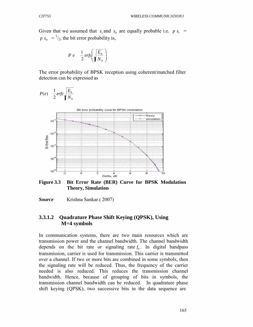
CIT755 WIRELESS COMMUNICATION I
165
N
Given that we assumed that
1
s1 and s0 are equally probable i.e. p s1 =
p s0 = /2, the bit error probability is,
1 E P e erfc
2 b
0
The error probability of BPSK reception using coherent/matched filter detection can be expressed as
P(e) 1
erfc Eb
2 N 0
Figure 3.3 Bit Error Rate (BER) Curve for BPSK Modulation
Theory, Simulation Source Krishna Sankar.( 2007)
3.3.1.2 Quadrature Phase Shift Keying (QPSK), Using M=4 symbols
In communication systems, there are two main resources which are transmission power and the channel bandwidth. The channel bandwidth depends on the bit rate or signaling rate fb . In digital bandpass transmission, carrier is used for transmission. This carrier is transmitted over a channel. If two or more bits are combined in some symbols, then the signaling rate will be reduced. Thus, the frequency of the carrier needed is also reduced. This reduces the transmission channel bandwidth. Hence, because of grouping of bits in symbols, the transmission channel bandwidth can be reduced. In quadrature phase shift keying (QPSK), two successive bits in the data sequence are

CIT755 WIRELESS COMMUNICATION I
166
1 2
b
grouped together. This reduces the bits rate or signaling rate (i.e. fb ) and thus reduces the bandwidth of the channel.
The bandwidth of QPSK signal will be BW
probability of error is
2 1
2Tb
f b and the
P ' (e)
P ' (e) 1
erfc 2
2Eb
2N 0
1 erfc
Eb
2 N 0
Thus, bit error probability of QPSK and BPSK are the same.
3.3.1.3 Differential Phase Shift Keying (DPSK)
DPSK does not need a synchronous (coherent) carrier at the demodulator. The input sequence of binary bits is modified such that the next bit depends upon the previous bit.
The Bandwidth is expressed as BW
2 1 f
T Tb
and the average probability of error or bit error rate (BER) of DPSK can
be expressed as
P(e) 1
e Eb / N0
2
3.3.2 Frequency-Shift Keying (FSK)
FSK is a frequency modulation scheme in which digital information is transmitted through discrete frequency changes of a carrier wave. The simplest FSK is binary FSK (BFSK). BFSK literally implies using a couple of discrete frequencies to transmit binary (0s and 1s) information.
In BFSK, the frequency of the carrier is shifted according to the binary symbol. However, the phase of the carrier is unaffected. This means that we have two different frequency signals according to binary symbols.
With this scheme, the “1” is called the mark frequency and the “0” is called the space frequency. In the case of FSK, a finite number of frequencies are used.
The bandwidth of BFSK 2 f b 2 f b
or BW = 4 f b

CIT755 WIRELESS COMMUNICATION I
167
Now, if we compare this bandwidth with that of BPSK, we note that BW (BFSK) = 2 x BW(BPSK)
The probability of error, of BFSK signal can be expressed as
1 2E 1 E P e erfc b
or P e erfc b
2 2 N 0 2 2N 0
This equation shows that error probability of BFSK is higher compared to that of BPSK
The various frequency-shift keying scheme are
3.3.2.1 Audio Frequency-Shift Keying (AFSK) AFSK is a modulation technique by which digital data is represented by changes in the frequency (pitch) of an audio tone, yielding an encoded signal suitable for transmission via radio or telephone. Normally, the transmitted audio alternates between two tones: one, the “mark”, represents a binary one; the other, the “space”, represents a binary zero.
AFSK differs from regular frequency-shift keying in performing the modulation at baseband frequencies. In radio applications, the AFSK- modulated signal normally is being used to modulate an RF carrier (using a conventional technique, such as AM or FM) for transmission.
AFSK is not always used for high-speed data communications, since it is far less efficient in both power and bandwidth than the other modulation modes. In addition to its simplicity, however, AFSK has the advantage that encoded signals will pass through AC-coupled links, including most equipment originally designed to carry music or speech.
3.3.2.2 Continuous-Phase Frequency-Shift Keying (CPFSK)
CPFSK is a commonly-used variation of frequency-shift keying (FSK), which is itself a special case of analog frequency modulation. FSK is a method of modulating digital data onto a sinusoidal carrier wave, encoding the information present in the data to variations in the carrier's instantaneous frequency between one of two frequencies (referred to as the space frequency and mark frequency). In general, a standard FSK signal does not have continuous phase, as the modulated waveform switches instantaneously between two sinusoids with different frequencies.

CIT755 WIRELESS COMMUNICATION I
168
As the name suggests, the phase of a CPFSK is in fact continuous; this attribute is desirable for signals that are to be transmitted over a band limited channel, as discontinuities in a signal introduce wideband frequency components. In addition, some classes of amplifiers exhibit nonlinear behavior when driven with nearly-discontinuous signals; this could have undesired effects on the shape of the transmitted signal.
3.3.2.3 Multi-Frequency Shift Keying (M-ary FSK or MFSK)
MFSK is a variation of frequency-shift keying (FSK) that uses more than two frequencies. MFSK is a form of M-ary orthogonal modulation, where each symbol consists of one element from an alphabet of orthogonal waveforms. M, the size of the alphabet, is usually a power of two so that each symbol represents log2M bits. M is usually between 2 and 64
3.3.2.4 Dual-Tone Multi-Frequency (DTMF)
DTMF signaling is used for telecommunication signaling over analog telephone lines in the voice-frequency band between telephone handsets and other communications devices and the switching center. As a method of in-band signaling, DTMF tones were also used by cable television broadcasters to indicate the start and stop times of local commercial insertion points during station breaks for the benefit of cable companies.
3.3.3 Amplitude-Shift Keying (ASK)
ASK is a form of modulation that represents digital data as variations in the amplitude of a carrier wave. The amplitude of an analog carrier signal varies in accordance with the bit stream (modulating signal), keeping frequency and phase constant. In the case of ASK, a finite number of amplitudes are used.
3.3.4 On-Off Keying (OOK)
OOK is the simplest form of amplitude-shift keying (ASK) modulation that represents digital data as the presence or absence of a carrier wave. In its simplest form, the presence of a carrier for a specific duration represents a binary one, while its absence for the same duration represents a binary zero. Some more sophisticated schemes vary these durations to convey additional information. It is analogous to unipolar encoding line code.

CIT755 WIRELESS COMMUNICATION I
169
M-ary vestigial sideband modulation, for example 8VSB: A vestigial sideband (in radio communication) is a sideband that has been only partly cut off or suppressed.
3.3.5 Quadrature Amplitude Modulation (QAM) QAM is a combination of PSK and ASK. QAM is both an analog and a digital modulation scheme. It conveys two analog message signals, or two digital bit streams, by changing (modulating) the amplitudes of two carrier waves, using the amplitude-shift keying (ASK) digital modulation scheme or amplitude modulation (AM) analog modulation scheme. These two waves, usually sinusoids, are out of phase with each other by 90° and are thus called quadrature carriers or quadrature components — hence the name of the scheme. The modulated waves are summed, and the resulting waveform is a combination of both phase- shift keying (PSK) and amplitude-shift keying, or in the analog case of phase modulation (PM) and amplitude modulation. In the digital QAM case, a finite number of at least two phases and at least two amplitudes are used.
Polar modulation like QAM is a combination of PSK and ASK: It makes use of polar coordinates, r (amplitude) and Θ (phase).
3.3.6 Continuous Phase Modulation (CPM) Method CPM is a method for modulation of data commonly used in wireless modems. In contrast to other coherent digital phase modulation techniques where the carrier phase abruptly resets to zero at the start of every symbol (e.g. M-PSK), with CPM the carrier phase is modulated in a continuous manner.
(i) Minimum-Shift Keying (MSK): In MSK, the output waveform
is continuous in phase hence there are no abrupt changes in amplitude. The sidelobes of MSK are very small hence bandpass filtering is not required to avoid interchannel interference. The Bandwidth of MSK is BW = 1.5 f b
(ii) Gaussian Minimum-Shift Keying (GMSK): It is similar to standard minimum-shift keying (MSK); however the digital data stream is first shaped with a Gaussian filter before being applied to a frequency modulator. This has the advantage of reducing sideband power, which in turn reduces out-of-band interference between signal carriers in adjacent frequency channels. However, the Gaussian filter increases the modulation memory in the system and causes intersymbol interference, making it more difficult to discriminate between different transmitted data values and requiring more complex channel equalization algorithms

CIT755 WIRELESS COMMUNICATION I
170
such as an adaptive equalizer at the receiver. GMSK is most notably used in the Global System for Mobile Communications (GSM).
3.3.7 Orthogonal Frequency Division Multiplexing (OFDM) Modulation
OFDM is essentially identical to Coded OFDM (COFDM) and Discrete Multi-Tone modulation (DMT). It is a frequency-division multiplexing (FDM) scheme utilised as a digital multi-carrier modulation method. A large number of closely-spaced orthogonal sub-carriers are used to carry data. The data is divided into several parallel data streams or channels, one for each sub-carrier. Each sub-carrier is modulated with a conventional modulation scheme (such as quadrature amplitude modulation or phase shift keying) at a low symbol rate, maintaining total data rates similar to conventional single-carrier modulation schemes in the same bandwidth. The primary advantage of OFDM over single- carrier schemes is its ability to cope with severe channel conditions — for example, attenuation of high frequencies in a long copper wire, narrowband interference and frequency-selective fading due to multipath — without complex equalization filters.
3.3.8 Wavelet Modulation
Wavelet modulation also known as fractal modulation is a modulation technique that makes use of wavelet transformations to represent the data being transmitted. One of the objectives of this type of modulation is to send data at multiple rates over a channel that is unknown. If the channel is not clear for one specific bit rate, meaning that the signal will not be received, the signal can be sent at a different bit where the signal to noise ratio is higher.
3.3.9 Trellis Coded Modulation (TCM)
Trellis coded modulation also known as trellis modulation is a modulation scheme which allows highly efficient transmission of information over band-limited channels such as telephone lines.
3.3.10 Spread-Spectrum Techniques
Spread-spectrum techniques are methods by which electromagnetic energy generated in a particular bandwidth is deliberately spread in the frequency domain, resulting in a signal with a wider bandwidth. These techniques are used for a variety of reasons, including the establishment of secure communications, increasing resistance to natural interference

CIT755 WIRELESS COMMUNICATION I
171
and jamming, to prevent detection, and to limit the power flux density on satellite downlinks.
i. Direct-sequence spread spectrum (DSSS): As with other spread
spectrum technologies, the transmitted signal takes up more bandwidth than the information signal that is being modulated. The name 'spread spectrum' comes from the fact that the carrier signals occur over the full bandwidth (spectrum) of a device's transmitting frequency.
ii. Chirp spread spectrum (CSS): uses pseudo-stochastic coding. It is a spread spectrum technique that uses wideband linear frequency modulated chirp pulses to encode information. A chirp is a sinusoidal signal whose frequency increases or decreases over a certain amount of time.
iii. Frequency-hopping spread spectrum (FHSS) applies a special scheme for channel release. It is a method of transmitting radio signals by rapidly switching a carrier among many frequency channels, using a pseudorandom sequence known to both transmitter and receiver. It is utilized as a multiple access method in the frequency-hopping code division multiple access (FH- CDMA) scheme.
3.4 Modulator and Detector Principles of Operation PSK and ASK, and sometimes also FSK, are often generated and detected using the principle of QAM. The I and Q signals can be combined into a complex-valued signal I+jQ (where j is the imaginary unit). The resulting so called equivalent lowpass signal or equivalent baseband signal is a complex-valued representation of the real-valued modulated physical signal (the so called passband signal or RF signal).
These are the general steps used by the modulator to transmit data:
i. Group the incoming data bits into codewords, one for each
symbol that will be transmitted. ii. Map the codewords to attributes, for example amplitudes of the I
and Q signals (the equivalent low pass signal), or frequency or phase values.
iii. Adapt pulse shaping or some other filtering to limit the bandwidth and form the spectrum of the equivalent low pass signal, typically using digital signal processing.
iv. Perform digital-to-analog conversion (DAC) of the I and Q signals (since today all of the above is normally achieved using digital signal processing, DSP).
v. Generate a high-frequency sine wave carrier waveform, and perhaps also a cosine quadrature component. Carry out the

CIT755 WIRELESS COMMUNICATION I
172
modulation, for example by multiplying the sine and cosine wave form with the I and Q signals, resulting in that the equivalent low pass signal is frequency shifted into a modulated passband signal or RF signal. Sometimes this is achieved using DSP technology, for example direct digital synthesis using a waveform table, instead of analog signal processing. In that case the above DAC step should be done after this step.
vi. Amplification and analog bandpass filtering to avoid harmonic distortion and periodic spectrum.
At the receiver side, the demodulator typically performs:
i. Bandpass filtering. ii. Automatic gain control, AGC (to compensate for attenuation, for
example fading). iii. Frequency shifting of the RF signal to the equivalent baseband I
and Q signals, or to an intermediate frequency (IF) signal, by multiplying the RF signal with a local oscillator sinewave and cosine wave frequency (see the superheterodyne receiver principle).
iv. Sampling and analog-to-digital conversion (ADC) (Sometimes before or instead of the above point, for example by means of undersampling).
v. Equalization filtering, for example a matched filter, compensation for multipath propagation, time spreading, phase distortion and frequency selective fading, to avoid intersymbol interference and symbol distortion.
vi. Detection of the amplitudes of the I and Q signals, or the frequency or phase of the IF signal.
vii. Quantization of the amplitudes, frequencies or phases to the nearest allowed symbol values.
viii. Mapping of the quantized amplitudes, frequencies or phases to codewords (bit groups).
ix. Parallel-to-serial conversion of the codewords into a bit stream. x. Pass the resultant bit stream on for further processing such as
removal of any error-correcting codes.
As it is common to all digital communication systems, the design of both the modulator and demodulator must be done simultaneously.
Digital modulation schemes are possible because the transmitter- receiver pair have prior knowledge of how data is encoded and represented in the communications system. In all digital communication systems, both the modulator at the transmitter and the demodulator at the receiver are structured so that they perform inverse operations.

CIT755 WIRELESS COMMUNICATION I
173
Non-coherent modulation methods do not require a receiver reference clock signal that is phase synchronized with the sender carrier wave. In this case, modulation symbols (rather than bits, characters, or data packets) are asynchronously transferred. The opposite is coherent modulation.
4.0 CONCLUSION In this unit, the concept of digital bandpass modulation and its various techniques as well as the factors that govern the choice of digital modulation were discussed.
10.0 SUMMARY In this unit, you have learnt that:
The aim of digital modulation is to transfer a digital bit stream over an analog passband channel. In digital modulations, instead of transmitting one bit at a time, two or more bits are transmitted simultaneously. The factors that influence the choice of digital (bandpass) modulation are power efficiency and bandwidth efficiency. Power efficiency describes the ability of a modulation technique to preserve the fidelity of the digital message at low power levels Bandwidth efficiency describes the ability of a modulation scheme to accommodate data within a limited bandwidth. The common digital modulation techniques are PSK, FSK, ASK, OOK,QAM,CPM,OFDM, Wavelet modulation, TCM and spread-spectrum techniques. The most fundamental digital modulation techniques are PSK, FSK, ASK and QAM.
SELF ASSESSMENT EXERCISE
What factors govern the choice of digital modulation?
6.0 TUTOR-MARKED ASSIGNMENT
Explain briefly four major digital modulation techniques.
7.0 REFERENCES/FURTHER READING Leon, W. C. (2001). Digital and Analog Communication Systems, (6th
ed.). Prentice-Hall. Inc.
Sharma, S. (2006). Wireless and Cellular Communications. New Delhi: S. K. Kataria & Sons.

CIT755 WIRELESS COMMUNICATION I
174
UNIT 4 DIGITAL BASEBAND AND PULSE SHAPING MODULATION TECHNIQUES
CONTENTS
1.0 Introduction 2.0 Objectives 3.0 Main Content
3.1 Digital Baseband and Pulse Shaping Modulation 3.1.1 Digital Baseband Modulation or Line Coding
Techniques 3.1.2 Pulse Shaping Modulation Techniques
3.1.2.1 Analog-Over-Analog Methods 3.1.2.2 Analog-Over-Digital Methods
4.0 Conclusion 5.0 Summary 6.0 Tutor-Marked Assignment 7.0 References/Further Reading
22.0 INTRODUCTION
In this unit, you will learn baseband and pulse shaping modulation techniques. Baseband modulation aims at transferring a digital bit stream over a baseband channel, as an alternative to carrier-modulated approaches. The term digital baseband modulation (or digital baseband transmission) is synonymous to line codes. Line codes are codes chosen for use within a communications system for baseband transmission purposes.
23.0 OBJECTIVES
At the end of this unit, you should be able to:
discuss digital baseband modulation write concisely on pulse modulation explain briefly the types of pulse modulation.
CIT755 WIRELESS COMMUNICATION I
175
24.0 MAIN CONTENT
3.1 Digital Baseband and Pulse Shaping Modulation
3.1.1 Digital Baseband Modulation or Line Coding
Techniques Line coding is a method which transfer a digital bit stream over an analog baseband channel (lowpass channel) using a pulse train, i.e. a discrete number of signal levels, by directly modulating the voltage or current on a cable such as fiber optical cables and short-range copper cables, for example serial cables and LAN networks.
Baseband signal is used to modulate a higher frequency carrier wave so that it may be transmitted via radio. Shifting the signal to higher frequencies (radio frequencies, or RF) than it originally spanned result in modulation. The key consequence of the usual double-sideband amplitude modulation (AM) is that, the range of frequencies of the signal span (its spectral bandwidth) is doubled. Thus, the RF bandwidth of a signal (measured from the lowest frequency as opposed to 0 Hz) is usually twice its baseband bandwidth. Steps may be taken to reduce this effect, such as single-sideband modulation; the highest frequency of such signals greatly exceeds the baseband bandwidth.
Some signals can be treated as baseband or not, depending on the situation. For example, a switched analog connection in the telephone network has energy below 300 Hz and above 3400 Hz removed by bandpass filtering; since the signal has no energy very close to zero frequency, it may not be considered a baseband signal, but in the telephone systems frequency-division multiplexing hierarchy, it is usually treated as a baseband signal, by comparison with the modulated signals used for long-distance transmission. The 300 Hz lower band edge in this case is treated as “near zero”, being a small fraction of the upper band edge.
Figure 4.1 below depicts what happens with AM modulation:
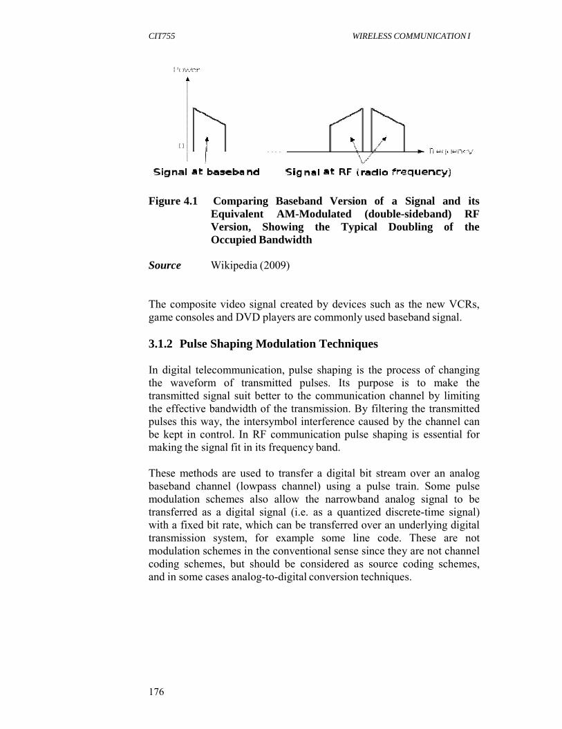
CIT755 WIRELESS COMMUNICATION I
176
Figure 4.1 Comparing Baseband Version of a Signal and its Equivalent AM-Modulated (double-sideband) RF Version, Showing the Typical Doubling of the Occupied Bandwidth
Source Wikipedia (2009)
The composite video signal created by devices such as the new VCRs, game consoles and DVD players are commonly used baseband signal.
3.1.2 Pulse Shaping Modulation Techniques
In digital telecommunication, pulse shaping is the process of changing the waveform of transmitted pulses. Its purpose is to make the transmitted signal suit better to the communication channel by limiting the effective bandwidth of the transmission. By filtering the transmitted pulses this way, the intersymbol interference caused by the channel can be kept in control. In RF communication pulse shaping is essential for making the signal fit in its frequency band.
These methods are used to transfer a digital bit stream over an analog baseband channel (lowpass channel) using a pulse train. Some pulse modulation schemes also allow the narrowband analog signal to be transferred as a digital signal (i.e. as a quantized discrete-time signal) with a fixed bit rate, which can be transferred over an underlying digital transmission system, for example some line code. These are not modulation schemes in the conventional sense since they are not channel coding schemes, but should be considered as source coding schemes, and in some cases analog-to-digital conversion techniques.

CIT755 WIRELESS COMMUNICATION I
177
3.1.2.1 Analog-Over-Analog Methods
(i) Pulse-Amplitude Modulation (PAM) is a form of signal
modulation where the message information is encoded in the amplitude of a series of signal pulses. For example, a two bit modulator (PAM-4) will take two bits at a time and will map the signal amplitude to one of four possible levels, for example −3 volts, −1 volt, 1 volt, and 3 volts.
(ii) Pulse-Width Modulation (PWM) is a very efficient way of providing intermediate amounts of electrical power between fully on and fully off. A simple power switch with a typical power source provides full power only, when switched on. PWM is a comparatively-recent technique, made practical by modern electronic power switches.
(iii) Pulse-Position Modulation (PPM) is a form of signal modulation in which M message bits are encoded by transmitting a single pulse in one of 2M possible time-shifts. This is repeated every T seconds, such that the transmitted bit rate is M/T bits per second. It is primarily useful for optical communications systems, where there tends to be little or no multipath interference.
3.1.2.2 Analog-Over-Digital Methods (i) Pulse-Code Modulation (PCM) is a digital representation of an
analog signal where the magnitude of the signal is sampled regularly at uniform intervals, then quantized to a series of symbols in a numeric (usually binary) code. PCM has been used in digital telephone systems, 1980s-era electronic musical keyboards, digital audio in computers, digital video and the compact disc “red book” format.
Differential pulse-code modulation (DPCM) is a signal encoder that uses the baseline of PCM but adds some functionality based on the prediction of the samples of the signal. The input can be an analog signal or a digital signal. If the input is a continuous-time analog signal, it needs to be sampled first so that a discrete-time signal is the input to the DPCM encoder. Adaptive DPCM (ADPCM) is a variant of DPCM (differential pulse-code modulation) that varies the size of the quantization step, to allow further reduction of the required bandwidth for a given signal-to-noise ratio.
(ii) Delta modulation (DM or ∆-modulation) is an analog-to-digital
and digital-to-analog signal conversion technique used for transmission of voice information where quality is not of primary importance. DM is the simplest form of differential pulse-code

CIT755 WIRELESS COMMUNICATION I
178
modulation (DPCM) where the difference between successive samples is encoded into n-bit data streams. In delta modulation, the transmitted data is reduced to a 1-bit data stream.
Its main features are:
the analog signal is approximated with a series of segments. each segment of the approximated signal is compared to the original analog wave to determine the increase or decrease in relative amplitude. the decision process for establishing the state of successive bits is determined by this comparison. only the change of information is sent, that is, only an increase or decrease of the signal amplitude from the previous sample is sent whereas a no-change condition causes the modulated signal to remain at the same 0 or 1 state of the previous sample.
(iii) Delta-Sigma (∆Σ) or sigma-delta (Σ∆) modulation is a method
for encoding high resolution signals into lower resolution signals using pulse-density modulation. This technique has found increasing use in a range of modern electronic components, such as analog-to-digital and digital-to-analog converters, frequency synthesizers, switched-mode power supplies and motor controls. One of the earliest and most widespread uses of delta-sigma modulation is in data conversion.
(iv) Continuously variable slope delta modulation (CVSDM) also called Adaptive-delta modulation (ADM) is a voice coding method. It is a delta modulation with variable step size (i.e. special case of adaptive delta modulation).CVSD encodes at 1 bit per sample, so that audio sampled at 16 kHz is encoded at 16 kbit/s.
(v) Pulse-density modulation (PDM) is a form of modulation used to represent an analog signal in the digital domain. In a PDM signal, specific amplitude values are not encoded into pulses as they would be in PCM. Instead, it is the relative density of the pulses that corresponds to the analog signal's amplitude. Pulse- width modulation (PWM) is the special case of PDM where all the pulses corresponding to one sample are contiguous in the digital signal.
25.0 CONCLUSION
Digital baseband modulations and pulse modulation were discussed in this unit.

CIT755 WIRELESS COMMUNICATION I
179
26.0 SUMMARY
In this unit, you have learnt that:
Baseband modulation aims at transferring a digital bit stream over a baseband channel, as an alternative to carrier-modulated approaches. Pulse shaping is the process of changing the waveform of transmitted pulses. Some pulse shaping modulation schemes also allow the narrowband analog signal to be transferred as a digital signal (i.e. as a quantized discrete-time signal) with a fixed bit rate, which can be transferred over an underlying digital transmission system.
SELF ASSESSMENT EXERCISE What is digital baseband modulation?
27.0 TUTOR-MARKED ASSIGNMENT Explain briefly two types of pulse modulation
28.0 REFERENCES/FURTHER READING Jayant, N. S. & Noll, P. (1984). Digital Coding of Waveforms:
Principles and Applications to Speech and Video. Englewood Cliffs: Prentice-Hall.
Schreier, R. & Temes, G. (2005). Understanding Delta-Sigma Data
Converters.

CIT755 WIRELESS COMMUNICATION I
180
1.0 Introduction
2.0 Objectives 3.0 Main Content
3.1 Concept of Diversity 3.1.1 Diversity Techniques
3.2 Space/Antenna Diversity Scheme 3.2.1 Applications of Space/Antenna
Diversity
4.0
Conclusion
5.0 Summary 6.0 Tutor-Marked Assignment 7.0 References/Further Reading
22.0
INTRODUCTION
UNIT 5 DIVERSITY TECHNIQUES FOR FADING CHANNEL
CONTENTS
Techniques
Diversity is a powerful communication receiver technique that provides wireless link improvement at relatively low cost. Diversity exploits the random nature of radio propagation by finding independent or at least highly uncorrected signal paths for communication.
23.0 OBJECTIVES
At the end of this unit, you should be able to:
explain diversity concept discuss the types of diversity techniques outline space diversity scheme state the application of space diversity technique.
24.0 MAIN CONTENT
3.1 Concept of Diversity
A signal transmitted at a particular carrier frequency and at a particular instant of time may be received in a multipath null. Diversity reception reduces the probability of occurrence of communication failures (outages) caused by fades by combining several copies of the same message received over different channels.
CIT755 WIRELESS COMMUNICATION I
181
In telecommunications, diversity scheme is referred to as a method for improving the reliability of a message signal by using two or more communication channels with different characteristics. Diversity plays an important role in combating fading and co-channel interference and avoiding error bursts. It is based on the fact that individual channels experience different levels of fading and interference. Multiple versions of the same signal may be transmitted and/or received and combined in the receiver. Alternatively, a redundant forward error correction code may be added and different parts of the message transmitted over different channels. Diversity techniques may exploit the multipath propagation, resulting in a diversity gain, often measured in decibels. In general, the efficiency of the diversity techniques reduces if the signal fading is correlated at different branches.
Diversity is a commonly used technique in wireless systems to combat channel fading, due to the following facts:
(i) The degradation of transmission quality due to channel fading
cannot be simply overcome by increasing the transmitted signal power. This is because, even with high transmitted power, when the channel is in deep fading, the instantaneously received SNR can still be very low, resulting in a high probability of transmission error during the deep fading period.
(ii) In wireless communications, the power available on the reverse link is severely limited by the battery capacity in hand-held subscriber units. With diversity, the required transmitted power can be greatly reduced.
(iii) Cellular communications systems are mostly limited by interference. Also, mitigation of channel fading by diversity reception can translate into improved interference tolerance which, in turn, means greater ability to support additional users and therefore higher system capacity.
3.1.1 Diversity Techniques The following classes of diversity schemes can be identified:
(a) Time diversity: Multiple versions of the same signal are
transmitted at different time instants. Alternatively, a redundant forward error correction code is added and the message is spread in time by means of bit-interleaving before it is transmitted. Thus, error bursts are avoided, which simplifies the error correction. In time diversity, the time difference between two transmissions should be large compared to the time it takes the mobile antenna to move half a wavelength. In systems with stationary antennas, such as indoor wireless communication, time diversity will be

CIT755 WIRELESS COMMUNICATION I
182
less effective as the channel characteristics do not change very much with time. However, time diversity may be helpful if uncorrected interference signals are experienced during successive attempts.
(b) Frequency diversity: In frequency diversity, the same message is transmitted more than once, respectively at different carrier frequencies. The difference in carrier frequency should be more than the coherence bandwidth to achieve effective diversity. Digital cellular system can use slow frequency hopping (SFH) for diversity reason: each block of bits is transmitted at a different carrier.
(c) Angle diversity: The desired message is received simultaneously by several directed antennas pointing in widely different directions. The received signal consists of scattering wave coming from all directions. It has been observed that the scattered signals associated with the different (non-overlapping) directions are uncorrelated. Angle diversity can be viewed as a special case of space diversity since it also requires multiple antennas.
(d) Multiuser diversity: Multiuser diversity is obtained by opportunistic user scheduling at either the transmitter or the receiver. Opportunistic user scheduling is as follows: the transmitter selects the best user among candidate receivers according to the qualities of each channel between the transmitter and each receiver. In Frequency Division Duplex (FDD) systems, a receiver must feedback the channel quality information to the transmitter with the limited level of resolution.
(e) Co-operative diversity: Is a co-operative multiple antenna techniques which exploit user diversity by decoding the combined signal of the relayed signal and the direct signal in wireless multihop networks. A conventional single hop system uses direct transmission where a receiver decodes the information only based on the direct signal while regarding the relayed signal as interference, whereas the cooperative diversity considers the other signal as contribution. That is, cooperative diversity decodes the information from the combination of two signals. Hence, it can be seen that cooperative diversity is an antenna diversity that uses distributed antennas belonging to each node in a wireless network. Note that user co-operation is another definition of co-operative diversity. User co-operation considers an additional fact that each user relays the other user's signal while co-operative diversity can also be achieved by multi-hop relay networking systems.
Co-operative diversity achieves antenna diversity gain by using the cooperation of distributed antennas belonging to each node.

CIT755 WIRELESS COMMUNICATION I
183
Co-operative diversity decodes information from the combination of two signals.
(f) Space diversity, also known as Antenna diversity, is any one of several wireless diversity schemes that use two or more antennas to improve the quality and reliability of a wireless link. Often, especially in urban and indoor environments, there is no clear line-of-sight (LOS) between transmitter and receiver. Instead the signal is reflected along multiple paths before finally being received. Each of these bounces can introduce phase shifts, time delays, attenuations, and even distortions that can destructively interfere with one another at the aperture of the receiving antenna. Antenna diversity is especially effective at mitigating these multipath situations.
The desired message is transmitted by using multiple transmitting antennas (transmit diversity) and/or receiving antennas (reception diversity). This is because multiple antennas afford a receiver several observations of the same signal. The space separation between adjacent antennas should be large enough to ensure that the signals from different antennas are independently faded; each of the antennas will experience a different interference environment. Thus, if one antenna is experiencing a deep fade, it is likely that another has a sufficient signal. Collectively such a system can provide a robust link.
3.2 Space/Antenna Diversity Scheme Antenna diversity can be realized in several ways. Depending on the environment and the expected interference, designers can employ one or more of these methods to improve signal quality. In fact multiple methods are frequently used to further increase reliability.
Spatial Diversity – Spatial diversity employs multiple antennas, usually with the same characteristics, that are physically separated from one another. Depending upon the expected incidence of the incoming signal, sometimes a space on the order of a wavelength is sufficient. Other times much larger distances are needed. Cellularization or sectorization, for example, is a spatial diversity scheme that can have antennas or base stations miles apart. This is especially beneficial for the mobile communications industry since it allows multiple users to share a limited communication spectrum and avoid co-channel interference. Pattern Diversity – Pattern diversity consists of two or more co- located antennas with different radiation patterns. This type of diversity makes use of directive antennas that are usually physically separated by some (often short) distance. Collectively
CIT755 WIRELESS COMMUNICATION I
184
they are capable of discriminating a large portion of angle space and can provide a higher gain versus a single omnidirectional radiator. Polarisation Diversity – Polarisation diversity combines pairs of antennas with orthogonal polarisations (i.e. horizontal/vertical, ± slant 45°, Left-hand/Right-hand CP etc). Reflected signals can undergo polarization changes depending on the media. By pairing two complementary polarisations, this scheme can immunise a system from polarisation mismatches that would otherwise cause signal fade. Additionally, such diversity has proven valuable at radio and mobile communication base stations since it is less susceptible to the near random orientations of transmitting antennas. Transmitter/Receiver Diversity–Transmitter/Receiver diversity uses two separate, collocated antennas for transmitting and receiving functions. Such a configuration eliminates the need for a duplexer and can protect sensitive receiver components from the high power used in transmission. Adaptive Arrays – Adaptive arrays can be a single antenna with active elements or an array of similar antennas with ability to change their combined radiation pattern as different conditions persist. Active electronically scanned arrays (AESAs) manipulate phase shifters and attenuators at the face of each radiating site to provide a near instantaneous scan ability as well as pattern and polarization control. This is especially beneficial for radar applications since it affords a signal antenna the ability to switch among several different modes such as searching, tracking, mapping and jamming countermeasures.
3.2.1 Applications of Space/Antenna diversity Techniques
A well-known practical application of diversity reception is in wireless microphones, and in similar electronic devices such as wireless guitar systems. A wireless microphone with a non- diversity receiver (a receiver having only one antenna) is prone to random drop-outs, fades, noise, or other interference, especially if the transmitter (the wireless microphone) is in motion. A wireless microphone or sound system using diversity reception will switch to the other antenna within microseconds if one antenna experiences noise, providing an improved quality signal with fewer drop-outs and noise. Ideally, no drop-outs or noise will occur in the received signal. Another common usage is in Wi-Fi networking gear and cordless telephones to compensate for multipath interference. The base station will switch reception to one of two antennas depending on which is currently receiving a stronger signal. For best results, the

CIT755 WIRELESS COMMUNICATION I
185
antennas are usually placed one wavelength apart. For microwave bands, where the wavelengths are under 100 cm, this can often be done with two antennas attached to the same hardware. For lower frequencies and longer wavelengths, the antennas must be multiple meters apart, making it much less reasonable. Mobile phone towers also often take advantage of diversity - each face of a tower will often have three antennas; one is transmitting, while the other two perform diversity reception. The uses of multiple antennas at both transmitter and receiver results in a multiple-input multiple-output (MIMO) system. The use of diversity techniques at both ends of the link is termed space–time coding.
25.0 CONCLUSION In this unit the concept of diversity and different types of diversity techniques were discussed. It was revealed that diversity improves transmission performance by making use of more than one independently faded version of the transmitted signal. If several replicas of the signal, carrying the same information, are received over multiple channels that exhibit independent fading with comparable strengths, the chances that all the independently faded signal components experience deep fading simultaneously are greatly reduced.
26.0 SUMMARY
Diversity is a powerful communication receiver technique that provides wireless link improvement at relatively low cost. Diversity reception reduces the probability of occurrence of communication failures (outages) caused by fades by combining several copies of the same message received over different channels. Diversity scheme is refers to as a method for improving the reliability of a message signal by using two or more communication channels with different characteristics. The classes of diversity schemes are time diversity, frequency diversity, space diversity, angle diversity, multiple diversity and cooperative diversity techniques
SELF ASSESSMENT EXERCISE What is meant by diversity?

CIT755 WIRELESS COMMUNICATION I
186
27.0 TUTOR-MARKED ASSIGNMENT
1. Write short note on any four diversity techniques. 2. State the application areas of space diversity techniques. 3. Mention the types of space diversity schemes.
28.0 REFERENCES/FURTHER READING
Dietrich, C. (2000). Adaptive Arrays and Diversity Antenna Configurations for Handheld Wireless Communication Terminals.
Laneman, J. N.; Tse, D. N. C. & Wornell, G. W. (2004). “Cooperative
Diversity in Wireless Networks: Efficient Protocols and Outage Behavior,” IEEE Trans. Inform. Theory, 50 (12), 3062-3080.
Moon, J. & Kim, Y. (2003). “Antenna Diversity Strengthens Wireless
LANs.” Communication Systems Design.
Sendonaris, A.; Erkip E, & Aazhang, B. (2003). “User Cooperation Diversity Part I and Part II,” IEEE Trans. Communication, 51(11), 1927–48.
Sharma, S. (2006). Wireless and Cellular Communications. New Delhi:
S.K. Kataria & Sons.
CIT755 WIRELESS COMMUNICATION I
187
UNIT 6 MULTIPLE ACCESS TECHNIQUES
CONTENTS 1.0 Introduction 2.0 Objectives 3.0 Main Content
3.1 Multiple Access in a Radio Cell 3.1.1 Multiple Access Techniques
3.1.1.1Circuit Mode and Channelization Methods 3.1.1.3Packet Mode Methods 3.1.1.3 Duplex Methods
3.1.2 Comparison of Multiple Access Techniques 3.1.3 Application Areas of Multiple Access
4.0 Conclusion 5.0 Summary 6.0 Tutor-Marked Assignment 29.0 References/Further Reading
1.0 INTRODUCTION Multiple Access is a signal transmission situation in which two or more users wish to simultaneously communicate with each other using the same propagation channel. This is precisely the uplink transmission situation in a wireless communication. In the uplink or reverse channel, multiple users will want to transmit information simultaneously.
Without proper coordination among the transmitting users, collisions will occur when two or more users transmit simultaneously. Access methods that incur collision are referred to as random access and variants of random access.
Multiple access method allows several terminals connected to the same multi-point transmission medium to transmit over it and to share its capacity.
2.0 OBJECTIVES At the end of this unit, you should be able to:
explain Multiple Access Concept discuss the types of Multiple Access Techniques define Carrier Sense Multiple Access state the types of Carrier Sense Multiple Access describe the attribute of Carrier Sense Multiple Access mention the application areas of Multiple Access.

CIT755 WIRELESS COMMUNICATION I
188
3.0 MAIN CONTENT
3.1 Multiple Access in a Radio Cell
In each radio cell, the transmission from the base station in the downlink can be heard by each and every mobile user in the cell. For this reason, this mode of transmission is referred to as broadcasting. On the other hand, a transmission from the mobile user in the uplink to the base station is many-to-one, and is referred to as multiple access.
Transmission in the uplink mode has the following properties:
Multiple mobile users want to access the common resource (base station) simultaneously; If the transmission from two or more users arrive at the base station at the same time, there will be destructive interference, umless the multiple arriving signals are mutually orthogonal; Orthogonality between two signals xi (t) and xj (t), t [0,T], means that their inner product over the signaling interval vanishes. Mathematically, this means that
T
0 xi t x j t dt 0. for i j
The key element in multiple access is to make the transmitted signals from the different users orthogonal to each other.
3.1.1 Multiple Access Techniques
Multiple Access method allows several terminals connected to the same multi-point transmission medium to transmit over it and to share its capacity. Examples of shared physical media are wireless networks, bus networks, ring networks, hub networks and half-duplex point-to-point links. Multiple Access technique is based on a multiplex method that allows several data streams or signals to share the same communication channel or physical media.
Multiple Access methods address the problem of how many users can share the same spectrum resources in an efficient manner. We distinguish between:
Multiple access within one cell, i.e., a fixed assignment of resources in time or bandwidth to specific users Random access, i.e., a dynamic assignment of spectrum resources in time or bandwidth to users, according to their needs

CIT755 WIRELESS COMMUNICATION I
189
Frequency reuse, i.e., assignment of spectrum resources considering the location of users and the attenuation of radio signals that travel over sufficiently large distances.
Multiple access is a signal transmission situation in which two or more users wish to simultaneously communicate with each other using the same propagation channel. Multiple access methods/techniques can be categorized under circuit mode and channelization methods, packet mode methods and duplex methods.
3.1.1.1 Circuit Mode and Channelization Methods (a) Frequency Division Multiple Access (FDMA)
FDMA is based on frequency-division multiplex (FDM). It gives users an individual allocation of one or several frequency bands, or Channels.
FDMA provides different frequency bands to different users or nodes. In FDMA, the total bandwidth is divided into non-overlapping frequency subband. Each user is allocated a unique frequency subband for the duration of the connection, whether the connection is an active or idle state. Othogonality among transmitted signals from different mobile users is achieved by bandpass filtering in the frequency domain. This type of multiple access support is narrowband, and is not suitable for multimedia communications with various transmission rates. In addition, it incurs a waste of bandwidth when the user is in a dormant state.
An example of FDMA systems were the first-generation (1G) cell-phone systems. A related technique is wave-length division multiple access (WDMA), based on Wavelength division multiplex (WDM), where different users get different colors in fiber-optical communication.
Wavelength division multiple access (WDMA): is a technology which transmit multiple radio carrier signals on a single channel by using different frequency to carry different signals. Orthogonal Frequency Division Multiple Access (OFDMA), based on Orthogonal frequency-division multiplexing (OFDM). Multiple access is achieved in OFDMA by assigning subsets of subcarriers to individual users. Single-carrier FDMA (SC-FDMA) can be viewed as linearly- preceded OFDMA (LP-OFDMA), based on single-carrier frequency-domain-equalization (SC-FDE).

CIT755 WIRELESS COMMUNICATION I
190
(b) Time-Division Multiple Access (TDMA)
TDMA is based on time-division multiplex (TDM). It allows several users to share the same frequency channel by dividing the signal into different time slots. The users transmit in rapid succession, one after the other, each using his own time slot. This allows multiple stations to share the same transmission medium (e.g. radio frequency channel) while using only a part of its channel capacity.
TDMA provides different time-slots to different transmitters in a cyclically repetitive frame structure. In a TDMA, the channel time is partitioned into frames. The length of a frame is long enough so that every user in service has an opportunity to transmit once per frame. To achieve this, a TDMA frame is further partitioned into time slots. Users have to transmit in their assigned slots from frame to frame. For example, user 1 may use time slot 1, user 2 time slot 2, etc until the last user. Then it starts all over again. TDMA is used in the digital 2G cellular systems such as Global System for Mobile Communications (GSM), IS-136, Personal Digital Cellular (PDC) and in the Digital Enhanced Cordless Telecommunications (DECT) standard for portable phones. It is also used extensively in satellite systems, and combat-net radio systems. Multi-Frequency Time Division Multiple Access (MF- TDMA) is one of the types of TDMA.
(c) Code Division Multiple Access (CDMA), or Spread Spectrum
Multiple Access (SSMA)
CDMA is a spread spectrum multiple access method. The principle of spread spectrum communications is that the bandwidth of the baseband information-carrying signals from the different users is spread by different signals with a bandwidth much larger than that of the baseband signals. Ideally, the spreading signals used for different users are orthogonal to each other. Thus, at the receiver, the same spreading signal is used as the dispreading signals to coherently extract the baseband signal from the target user, while suppressing the transmissions from any other users. An example of CDMA is the 3G cell phone system.
In Spread Spectrum communication, the bandwidth occupancy of a single transmitted signal is much higher than in systems using conventional modulation methods. This band-spreading is achieved by selecting appropriate transmission waveforms with a wide bandwidth. A very popular method is to multiply the user data signal with a fast code sequence, which mostly is independent of the transmitted data message.
CIT755 WIRELESS COMMUNICATION I
191
With Code Division Multiple Access (CDMA) multiple users can share the same portion of the radio spectrum but use different codes to distinguish their transmissions.
CDMA Schemes Various spread-spectrum techniques are:
Direct-Sequence CDMA (DS-CDMA), based on Direct-sequence spread spectrum (DSSS): DS-CDMA is a method which shares spectrum among multiple simultaneous users. Moreover, it can exploit frequency diversity, using a RAKE receiver. However, in a dispersive multipath channel, DS-CDMA with a spread factor N can accommodate N simultaneous users only if highly complex interference cancellation techniques are used. In practice this is difficult to implement. MC-CDMA can handle N simultaneous users with good bit error rate (BER), using standard receiver techniques. Frequency-Hopping CDMA (FH-CDMA), based on Frequency- hopping spread spectrum (FHSS) is a method of transmitting radio signals by rapidly switching a carrier among many frequency channels, using a pseudorandom sequence known to both transmitter and receiver. Orthogonal frequency-hopping multiple access (OFHMA). Multi-Carrier Code Division Multiple Access (MC-CDMA): is a multiple access scheme used in OFDM-based telecommunication systems, allowing the system to support multiple users at the same time. Its development aimed at improved performance over multipath links. Ultra Wide Band (UWB) techniques using very steep pulses at well defined instants. This is sometimes called “Time Hopping”. Time hopping technique is a spread spectrum technique in which the carrier is turned on and off by the pseudorandom code sequence. It is usually used in combination with other methods, in which the transmitted pulse occurs in a manner determined by a pseudorandom code which places the pulse in one of several possible positions per frame.
Attributes of CDMA in Cellular Systems There are many attributes of CDMA which are of great benefit to the cellular system
Soft-handoff: Since every cell uses the same radio frequency band, the only difference between user channels is the spreading code sequences. Therefore, there is no jump from one frequency

CIT755 WIRELESS COMMUNICATION I
192
to another frequency when a user moves between cells. The mobile terminal receives the same signal in one cell as it does in the next, and thus there is no harsh transition from one receiving mode to another. Two or more neighboring base stations can receive the signal of a particular user, because they all use the same channel. Moreover, two base stations can simultaneously transmit to the same user terminals. The mobile (rake) receiver can resolve the two signals separately and combine them. This feature is called soft handoff. Soft capacity or graceful degradation: In FDMA and TDMA, N channels can be used virtually without interference from other users in the same cell but potential users N+1, N+2, ..., are blocked until a channel is released. The capacity of FDMA and TDMA is therefore fixed at N users and the link quality is determined by the frequency reuse pattern. In theory, it does not matter whether the spectrum is divided into frequencies, time slots, or codes, the capacity provided from these three multiple access schemes is the same. However, in CDMA, all the users in all cells share one radio channel and are separated by codes. Therefore, an additional user may be added by sacrificing somewhat the link quality, with the effect that voice quality is just slightly degraded compared to that of the normal N-channel cell. Thus, degradation of performance with an increasing number of simultaneous users is “graceful” in CDMA systems, versus the hard limits placed on FDMA and TDMA systems. Multipath-tolerance: Spread spectrum techniques are effective in combating the frequency selective fading that takes place in multipath channels. The underlying principle is that when a signal is spread over a wide bandwidth, a frequency selective fade will corrupt only a small portion of the signal's power spectrum, while passing the remaining spectrum unblemished. As a result, upon dispreading there is a better probability that the signal can be recovered correctly. For an unspread signal whose spectral density happens to be misplaced in a deep fade, an unrecoverable signal at the receiver is virtually assured. To optimally combine signals received over various delayed paths, a rake receiver can be used. No channel equalization needed: When the transmission rate is much higher than 10 kbps in both FDMA and TDMA, an equalizer is needed for reducing the intersymbol interference caused by time delay spread. This is because when the bit period becomes smaller than about ten times the time delay spread, intersymbol interference becomes significant. However, in CDMA a correlation is needed at minimum. To achieve good performance a rake receiver is needed to combat delay spread.
CIT755 WIRELESS COMMUNICATION I
193
Privacy: An important requirement of spreading signals is that they are “noise-like”, or pseudorandom. Dispreading the signal requires knowledge of the user's code, and for a binary code with spreading factor N there exist 2N possible random sequences. In military systems these codes are kept secret, so it is very difficult for an unauthorised attacker to tap into or transmit on another users channel. Often it is even difficult to detect the presence of a spread-spectrum signal because it is below the noise that is present in the transmit bandwidth.
Note that in cellular systems, the codes are fully described in publicly available standards. In digital systems, security against eavesdropping (confidentiality) is obtained through encryption. This is a highly desirable alternative to the analog FDMA cellular phone system in wide use today, where with an inexpensive scanner one can tune in to the private conversations of unwary neighbours.
Disadvantages of CDMA There are, of course, a number of disadvantages associated with CDMA; two of the most severe are the problem of “self-interference,” and the related problem of the “near-far” effect.
Self-interference arises from the presence of delayed replicas of signal due to multipath. The delays cause the spreading sequences of the different users to lose their orthogonality, as by design they are orthogonal only at zero phase offset. Hence in dispreading a given user's waveform, nonzero contributions to that user's signal arise from the transmissions of the other users in the network. This is distinct from both TDMA and FDMA, wherein for reasonable time or frequency guardbands, respectively, orthogonality of the received signals can be preserved. The near-far problem arises from the fact that signals closer to the receiver are received with smaller attenuation than signals located further away. Therefore the strong signal from the nearby transmitter will mask the weak signal from the remote transmitter. In TDMA and FDMA, this is not a problem since mutual interference can be filtered. In CDMA, however, the near- far effect combined with imperfect orthogonality between codes (e.g. due to different time sifts), leads to substantial interference. Accurate and fast power control appears essential to ensure reliable operation of multi-user DS-CDMA systems.
CIT755 WIRELESS COMMUNICATION I
194
Applications of spread spectrum are in:
Military System: This is the oldest known application. It is popular for security reasons. Positioning Systems: High bandwidth signals allow accurate measurements of propagation delays. This is used to estimate the distance of a transmitter. Cellular radio: It is mainly used to combat dispersion and to provide multiple access. Wireless LANs: If conventional modulation would be used, frequency management for many coexisting links can be very difficult. Moreover, narrowband transmission could be impaired by deep local fades.
(a) Space Division Multiple Access (SDMA)
SDMA enables creating parallel spatial pipes next to higher capacity pipes through spatial multiplexing and/or diversity, by which it is able to offer superior performance in radio multiple access communication systems. In traditional mobile cellular network systems, the base station has no information on the position of the mobile units within the cell and radiates the signal in all directions within the cell in order to provide radio coverage. These results in wasting power on transmissions when there are no mobile units to reach, in addition to causing interference for adjacent cells using the same frequency, so called co-channel cells.
Likewise, in reception, the antenna receives signals coming from all directions including noise and interference signals. By using smart antenna technology and by leveraging the spatial location of mobile units within the cell, space-division multiple access techniques offer attractive performance enhancements. The radiation pattern of the base station, both in transmission and reception is adapted to each user to obtain highest gain in the direction of that user. This is often done using phased array techniques.
3.1.1.2 Packet Mode Methods
Packet mode methods are typically also based on time-domain multiplexing, but not in a cyclically repetitive frame structure, and therefore it is not considered as TDM (Time Division Multiplexing) or TDMA (Time Division Multiple Access). Due to its random character it can be categorized as statistical multiplexing methods, making it possible to provide dynamic bandwidth allocation.
(a) Contention based random multiple access methods

CIT755 WIRELESS COMMUNICATION I
195
In packet mode communication networks, contention is a media access method that is used to share a broadcast medium.
i. Aloha: Any terminal is allowed to transmit without considering
whether channel is idle or busy. If packet is received correctly, the base station transmits an acknowledgement. If no acknowledgement is received by the mobile, it retransmits the packet after waiting a random time. The mode of random access in which users can transmit at anytime is called pure aloha. In pure aloha system, where the packet length is a fixed constant, the vulnerability period (i.e. the maximum interval over which two packets can overlap and destroy each other) is two slot times i.e. the time interval required to transmit two packets.
ii. Slotted Aloha: A version in which users are restricted to transmit only from the instant corresponding to the slot boundary. Any slot is available for utilization without regards to prior usage
iii. Multiple Access with Collision Avoidance (MACA) is a slotted media access control protocol used in wireless LAN data transmission to avoid collisions caused by the hidden station problem and to simplify exposed station problem. The basic idea of MACA is that, a wireless network node makes an announcement before it sends the data frame to inform other nodes to keep silent. When a node wants to transmit, it sends a signal called Request-To-Send (RTS) with the length of the data frame to send. If the receiver allows the transmission, it replies the sender with a signal called Clear-To-Send (CTS) with the length of the frame it is about to receive. Meanwhile, a node that hears RTS should remain silent to avoid conflict. with CTS; a node that hears CTS should keep silent until the data transmission is complete.
iv. Multiple Access with Collision Avoidance for Wireless (MACAW): If WLAN data transmission collisions occur after data transmission completion in MACA, then the MACA for Wireless (MACAW) is introduced to extend the function of MACA. It requires nodes sending acknowledgements after each successful frame transmission, as well as the additional function of Carrier sense.
v. Carrier Sense Multiple Access (CSMA) is a probabilistic Media Access Control (MAC) protocol in which a node verifies the absence of other traffic before transmitting on a shared transmission medium, such as an electrical bus, or a band of the electromagnetic spectrum. In Carrier Sense Multiple Access (CSMA), users listen before transmission and the listening is referred to as sensing the channel. A station wishing to transmit has to first listen to the channel for a predetermined amount of
CIT755 WIRELESS COMMUNICATION I
196
time so as to check for any activity on the channel. If the channel is sensed “idle” then the station is permitted to transmit. If the channel is sensed as “busy” the station has to defer its transmission.
Types of CSMA
1-persistent CSMA: When the sender (station) is ready to transmit data, it checks if the physical medium is busy. If so, it senses the medium continually until it becomes idle, and then it transmits a piece of data (a frame). In case of a collision, the sender waits for a random period of time and attempts to transmit again. P-persistent CSMA: This protocol is a generalisation of 1- persistent CSMA. When the sender is ready to send data, it checks continually if the medium is busy. If the medium becomes idle, the sender transmits a frame with a probability p. In case the transmission did not happen (the probability of this event is 1-p) the sender waits until the next available time slot and transmits again with the same probability p. This process repeats until the frame is sent or some other sender starts transmitting. In the latter case the sender waits a random period of time, checks the channel, and if it is idle, transmits with a probability p, and so on. Non-persistent CSMA: When the sender is ready to send data, it checks if the medium is busy. If so, it waits for a random amount of time and checks again. When the medium becomes idle, the sender starts transmitting. If collision occurs, the sender waits for a random amount of time, and checks the medium, repeating the process. Carrier Sense Multiple Access with Collision Detection (CSMA/CD) - suitable for wired networks. CSMA/CD is a modification of pure Carrier Sense Multiple Access (CSMA). Collision detection is used to improve CSMA performance by terminating transmission as soon as a collision is detected, and reducing the probability of a second collision on retry. Carrier Sense Multiple Access with Collision Avoidance (CSMA/CA) - suitable for wireless networks. In CSMA/CA (Local Talk), once the channel is clear, a station sends a signal telling all other stations not to transmit, and then sends its packet. In Ethernet 802.3, the station continues to wait for a time, and checks to see if the channel is still free. If it is free, the station transmits, and waits for an acknowledgment signal that the packet was received. Distributed Coordination Function (DCF): requires a station wishing to transmit to listen for the channel status for a DCF Interframe Space (DIFS) interval. If the channel is found busy

CIT755 WIRELESS COMMUNICATION I
197
during the DIFS interval, the station defers its transmission. In a network where a number of stations contend for the multi-access channel, if multiple stations sense the channel busy and defer their access, they will also virtually simultaneously find that the channel is released and then try to seize the channel. As a result, collisions may occur. In order to avoid such collisions, DCF also specifies random backoff, which forces a station to defer its access to the channel for an extra period. DCF also has an optional virtual carrier sense mechanism that exchanges short Request-to-send (RTS) and Clear-to-send (CTS) frames between source and destination stations during the intervals between the data frame transmissions. DCF includes a positive acknowledgement scheme, which means that if a frame is successfully received by the destination it is addressed to, the destination needs to send an ACK frame to notify the source of the successful reception. Point Coordination Function (PCF): is a Media Access Control (MAC) technique used in wireless networks which relies on a central node, often an Access Point (AP), to communicate with a node listening to see if the airwaves are free (i.e., all other nodes are not communicating). Since most APs have logical bus topologies (they are shared circuits) only one message can be processed at one time (it is a contention based system), and thus a media access control technique is required. Carrier Sense Multiple Access with Collision Avoidance and Resolution Using Priorities (CSMA/CARP): Instead of detecting network collisions, CSMA/CARP attempts to avoid collisions by using a system of transmission priorities. When a station wants to transmit on a CSMA/CARP network it first listens for network traffic and if the medium is clear instead of immediately transmitting as a station would in CSMA/CD, it waits a predefined amount of time. This waiting period is called the interframe spacing (IFS) and it varies by the type of data being transmitted. High priority data will transmit almost immediately whereas lower priority data such as polling will have a longer IFS. This system allows CSMA/CARP to avoid many collisions that would occur if it was not used. In addition to having different IFS per priority, a station in a CSMA/CARP network will add a "random backoff" to its waiting period, to reduce the collision probability between stations that have to transmit packets in the same priority. Carrier Sense Multiple Access/Bitwise Arbitration (CSMA/BA) Based on constructive interference (Controller Area Network - bus) .When two nodes on CAN attempt to transmit at the same time, a non-destructive arbitration technique guarantees the messages are sent in order of priority.

CIT755 WIRELESS COMMUNICATION I
198
a. Token passing: Is where a signal called a token is passed around between nodes that authorize the node to communicate. Token passing schemes are technique in which only the system which has the token can communicate. The token is a control mechanism which gives authority to the system to communicate or use the resources of that network. Once the communication is over, the token is passed to the next candidate in a sequential manner. The most well-known examples are token ring and token bus.
b. Token ring: Token ring local area network (LAN) technology is a local area network protocol which resides at the data link layer (DLL) of the OSI model. It uses a special three-byte frame called a token that travels around the ring. Token ring frames travel completely around the loop.
c. Token bus: Is a network implementing the token ring protocol over a "virtual ring" on a coaxial cable. A token is passed around the network nodes and only the node possessing the token may transmit. If a node doesn't have anything to send, the token is passed on to the next node on the virtual ring. Each node must know the address of its neighbour in the ring, so a special protocol is needed to notify the other nodes of connections to, and disconnections from, the ring.
d. Polling: Refers to actively sampling the status of an external device by a client program as a synchronous activity. Polling also refers to the situation where a device is repeatedly checked for readiness, and if it is not the computer returns to a different task.
e. Resource Reservation (scheduled) Packet-Mode Protocols: Is a transport layer protocol designed to reserve resources across a network for an integrated internet services.
i. Dynamic Time Division Multiple Access (Dynamic TDMA): is
a scheduling algorithm which dynamically reserves a variable number of time slots in each frame to variable bit-rate data streams, based on the traffic demand of each data stream. Dynamic TDMA is used in HIPERLAN/2 broadband radio access network, IEEE 802.16a WiMax , Bluetooth , etc.
ii. Packet Reservation Multiple Access (PRMA) is a packet-based TDMA concept where the users contend for the time slots. In situations where the system is not near capacity, a user can reserve a time slot for future uses.
iii. Reservation ALOHA (R-ALOHA) is a multiple access method for wireless transmission which allows uncoordinated users to share a common transmission resource. Reservation ALOHA (and its parent scheme, Slotted ALOHA) is a schema or rule set for the division of transmission resources over fixed time increments also known as slots. If this rule set or schema is

CIT755 WIRELESS COMMUNICATION I
199
properly followed, the bandwidth users are allowed to cooperatively utilize a shared transmission resource (i.e. the allocation of transmission time).
3.1.1.3 Duplex Methods A duplex communication system is a system composed of two connected parties or devices that can communicate with one another in both directions. Duplex systems are employed in many communications networks, either to allow for “two-way street" communication between two connected parties or to provide a "reverse path" for the monitoring and remote adjustment of equipment in the field. Where these methods are used for dividing forward and reverse communication channels, they are known as duplex methods. Examples are:
(i) Time division duplex (TDD) is the application of time-division
multiplexing to separate outward and return signals. It emulates full-duplex communication over a half-duplex communication link. Time-division duplex has a strong advantage in the case where there is asymmetry of the uplink and downlink data rates. As the amount of uplink data increases, more communication capacity can be dynamically allocated, and as the traffic load becomes lighter, capacity can be taken away. The same applies in the downlink direction.
(ii) Frequency division duplex (FDD) means that the transmitter and receiver operate at different carrier frequencies. The term is frequently used in ham radio operation, where an operator is attempting to contact a repeater station. The station must be able to send and receive a transmission at the same time, and does so by slightly altering the frequency at which it sends and receives. This mode of operation is referred to as duplex mode or offset mode.
Uplink and downlink sub-bands are said to be separated by the frequency offset. Frequency- division duplex can be efficient in the case of symmetric traffic. Frequency-division duplex makes radio planning easier and more efficient, since base stations do not "hear" each other (as they transmit and receive in different sub-bands) and therefore will normally not interfere with each other.
3.1.2 Comparison of Multiple Access Techniques (i) Modulation: TDMA and FDMA depend on the choice of a
modulation scheme to maximize spectral efficiency. To achieve a higher throughput in the same bandwidth, a higher order

CIT755 WIRELESS COMMUNICATION I
200
modulation scheme must be used. With CDMA, the simple method of BPSK modulation is required, although, for practical symmetry considerations, QPSK is often used. In fact, the choice of modulation strategy and the use of SDMA are independent.
(ii) Forward Error-Correction (FEC) Coding: All multiple-access techniques are affected by the distortions offered by the wireless channel. With FDMA and TDMA, if the same basic throughput is to be maintained, a higher transmission rate and a greater bandwidth is required as a result of the redundancy introduced by FEC coding. This is the classic trade-off between bandwidth and power efficiency. With CDMA, FEC coding can be added without increasing the system bandwidth or harming the processing gain. The inclusion of FEC is transparent to SDMA. If transmit diversity is implemented, then there can be increased bandwidth with SDMA.
(iii) Source Coding: The use of source coding improves the bandwidth efficiency of all multiple-access techniques. However, CDMA is in a position to take greater advantage of voice activation than other techniques, since its bandwidth efficiency is determined by average interference.
(iv) Diversity: Multiple transmitters or receivers or both are required to obtain diversity with FDMA, which is an added hardware expense. The same is applied to TDMA, except when it is used as part of a TDMA/FDMA hybrid. In that case, frequency-hopped TDMA can provide some diversity advantage. The large bandwidth of CDMA naturally provides some frequency diversity, and this can be used advantageously with a rake receiver (A rake receiver is a radio receiver designed to counter the effects of multipath fading). The implementation cost of a rake receiver is less than the dual-receiver cost of an FDMA system with frequency diversity.
(v) User Terminal Complexity: With the progression from FDMA through TDMA to CDMA comes an evolution of terminal complexity. SDM systems introduce a different and additional form of complexity that is related to the antennas which is not present in any of the other systems.
(vi) Handover: With their single-receiver terminals, both FDMA and TDMA are somehow handicapped when they must switch between base stations at a cell boundary. With CDMA, since the frequencies are used in adjacent cells, it is easier to implement a “dual receiver” and provide a soft handover capability.
(vii) System Complexity: With an FDMA system, users can operate quite independently. With TDMA, the level of cooperation among users must increase to share slots. With CDMA, the system must delegate spreading codes, power control information, and synchronization information.

CIT755 WIRELESS COMMUNICATION I
201
(viii) Multiple-Access Interference (MAI): Because FDMA and TDMA tend to be limited by worst-case interference, interference is often limited in the system planning stage by the fixed assignment of frequency groups to specific cells. With CDMA, the same bandwidth is used everywhere, and performance is limited by average interference levels. However, CDMA relies heavily on accurate power control to eliminate the near-far problem.
(ix) Fading-Channel Sensitivity: FDMA systems are typically narrowband and therefore suffer from flat fading. If the fading is not severe, then simple channel estimation and forward error correction can often compensate for its effects. TDMA systems are typically medium-bandwidth solutions. As a result of this, they observe some frequency selectivity. This requires the implementation of an equalizer. In fact, the implementation of a robust tracking equalizer in wireless channels is of utmost importance. CDMA systems face frequency-selective channels because of their large bandwidth, but take advantage of this natural diversity with a RAKE receiver.
(x) Bandwidth Efficiency: For single-cell systems, FDMA and TDMA systems are generally more bandwidth efficient than CDMA systems, because they do not have to cope with multiple- access interference (MAI). However, once their frequency plan is made and the modulation selected, the maximum throughput is fixed. CDMA holds an advantage because it can reuse frequencies everywhere, while FDMA and TDMA have much lower frequency reuse rates because they are limited by peak interference levels. CDMA can often add a user at the expense of a small degradation of existing users.
(xi) Synchronization: Wireless system using FDMA, TDMA and CDMA show a progression in synchronization resolution and a corresponding progression in complexity. The main concern of FDMA is symbol timing. In fact, TDMA terminals must contend with chip timing.
(xii) Flexibility: FDMA is the least flexible of the techniques. Once the service is designed, any change requires a redesign. With TDMA, higher data rates can be provided by assigning more slots per user, usually with very little change to the hardware. With CDMA, different data rates can be provided by trading off the spreading rate (processing gain), making it very flexible. Out of these techniques Space Division Multiple Access (SDMA) is transparent.
(xiii) Voice and Data Integration: The comments regarding flexibility also apply to the integration of voice and data over the same terminal. With TDMA, it is possible as well to make use of periods of voice inactivity to transmit data, thus making the
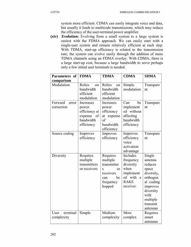
CIT755 WIRELESS COMMUNICATION I
202
system more efficient. CDMA can easily integrate voice and data, but usually it leads to multicode transmissions, which may reduce the efficiency of the user-terminal power amplifier.
(xiv) Evolution: Evolving from a small system to a large system is easiest with the FDMA approach. We can easily start with a single-user system and remain relatively efficient at each step. With TDMA, start-up efficiency is related to the transmission rate; the system can evolve easily through the addition of more TDMA channels using an FDMA overlay. With CDMA, there is a large start-up cost, because a large bandwidth to serve perhaps only a few initial user terminals is needed.
Parameters of comparison
FDMA TDMA CDMA SDMA
Modulation Relies onbandwidth efficient modulation
Relies onbandwidth efficient modulation
Simple modulation
Transparent
Forward error correction
Increasespower efficiency at expense of bandwidth efficiency
Increasespower efficiency at expense of bandwidth efficiency
Can be implement ed without affecting bandwidth efficiency
Transparent
Source coding Improvesefficiency
Improvesefficiency
Improves efficiency voice activation advantage
Transparent
Diversity Requiresmultiple transmitters or receivers
Requiresmultiple transmitter s or receivers can be frequency hopped
Includes frequency diversity when implement ed with a RAKE receiver.
Singleantenna reduces space diversity, orthogon al coding improves diversity with multiple transmit antennas
User terminal complexity
Simple Medium complexity
More complex
Requires smart antennas

CIT755 WIRELESS COMMUNICATION I
203
Handover Hard Hard Soft Potentiall y soft
System complexity
Large number of simple components
Reducednumber of channel unit
Largenumber of complex interacting component s
Additiona l complexit y related to antennas
Multiple-access interference
Limited bysystem planning
Limited bysystem planning
Dynamicpower control
Limited by resolution of antennas
Fading Flat-fading no diversity simple to track
May needfrequency- selective and equalizer
Frequency-selective diversity via RAKEreceiver
Reduced multipath
Bandwidth efficiency
Hard limitsbased on modulation and channel spacing
Hard limitsbased on modulation and channel spacing
Soft limits Depends on antenna resolution
Synchronizatio n
Low resolution
Mid-resolution
Highresolution
Requires terminal location
Flexibility Fixed data rate
Data rate variable in discrete steps
Can provide a variety ofdata rates without affecting signal in space
Transpare nt
Voice and data integration
Possible, but may require revisions to system
Straightforward using multiple slots
Multicodetransmissio n, which may decrease efficiency of mobile terminal
Transpare nt
Evolution Bandwidth to fit application
Requiresmedium initial
Requireslarge initial bandwidth
Flexible, can be added as

CIT755 WIRELESS COMMUNICATION I
204
bandwidth far as itdoes not affect mobile
Table 6.1 Comparison of Different Multiple Access Strategies
Source Sharma S. (2006)
3.1.3 Application Areas of Multiple Access
Local and metropolitan area networks : In local area networks (LANs) and metropolitan area networks (MANs), multiple access methods enable bus networks, ring networks, hubbed networks, wireless networks and half duplex point-to-point communication, but are not required in full duplex point-to-point serial lines between network switches and routers, or in switched networks (logical star topology). The most common multiple access method is CSMA/CD, which is used in Ethernet. Although today’s Ethernet installations typically are switched, CSMA/CD is utilised to achieve compatibility with hubs. Satellite communications: In satellite communications, multiple access is the capability of a communications satellite to function as a portion of a communications link between more than one pair of satellite terminals concurrently. Three types of multiple access presently used with communications satellites are code- division, frequency-division, and time-division multiple access. Switching centers: In telecommunication switching centers, multiple access is the connection of a user to two or more switching centers by separate access lines using a single message routing indicator or telephone number.
4.0 CONCLUSION
In this unit, different multiple access techniques were discussed under circuit and packet mode, channelization and duplex methods. Also areas where multiple access can be applied and the comparison of multiple access techniques were discussed.
5.0 SUMMARY
In this unit, you have learnt that:
Multiple Access is a signal transmission situation in which two or more users wish to simultaneously communicate with each other using the same propagation channel. Multiple Access can be categorized under:
CIT755 WIRELESS COMMUNICATION I
205
- Circuit mode and channelization methods: FDMA, TDMA,
CDMA, SDMA. - Packet mode - Duplex Method
The basic multiple access techniques are FDMA, TDMA, CDMA, SDMA, and PMMA FDMA is based on frequency division multiplex. It gives users an individual allocation of one or several frequency bands, or Channels. Each user is allocated a unique frequency subband for the duration of the connection, whether the connection is an active or idle state. TDMA is based on time-division multiplex (TDM). It allows several users to share the same frequency channel by dividing the signal into different time slots. The users transmit in rapid succession, one after the other, each using his own time slot. CDMA is a spread spectrum multiple access method. The principle of spread spectrum communications is that the bandwidth of the baseband information-carrying signals from the different users is spread by different signals with a bandwidth much larger than that of the baseband signals. SDMA enables creating parallel spatial pipes next to higher capacity pipes through spatial multiplexing and/or diversity, by which it is able to offer superior performance in radio multiple access communication systems.
SELF ASSESSMENT EXERCISE 1. What is multiple access? 2. Define CSMA. 3. Discuss the types of CSMA.
6.0 TUTOR-MARKED ASSIGNMENT 1. Discuss on any three types of multiple access techniques. 2. Write short note on the following: OFDMA, Dynamic TDMA
and Aloha. 3. Discuss the concept of CDMA techniques. 4. Define and explain TDMA systems.

CIT755 WIRELESS COMMUNICATION I
206
7.0 REFERENCES/FURTHER READING
Linnartz, J. P. G (2001). “Performance Analysis of Sychronous MC- CDMA in Mobile Rayleigh Channels with Both Delay and Doppler Spreads”, IEEE, 50(6), 1375-1387.
Linnartz, J. P. G. (1995). Cellular Telephone Network. (Online)
Available at http://wireless.per.nl/reference/about.htm
Sharma, S. (2006). Wireless and Cellular Communications. New Delhi: S.K. Kataria & Sons.
Yee, N. & Linnartz J. P.G (1994). “Wiener Filtering for Multi-Carrier
CDMA”, IEEE/ICCC Conference on Personal Indoor Mobile Radio Propagation Communications (PIMRC) and Wireless Computer Networks (WCN), 4, 1344-1347
Yee, N., Linnartz, J. P.G & Fettweis, G. (1993). “Multi-Carrier CDMA
in Indoor Wireless Radio Network”, IEEE Personal Indoor and Mobile Radio Communications (PIMRC) International Conference, Yokohama, Japan, 109-113