CIT 852: DATA COMMUNICATION AND NETWORK - National ...

1

CIT 852:

DATA COMMUNICATION AND NETWORK

NATIONAL OPEN UNIVERSITY OF NIGERIA

FACULTY OF SCIENCE

COURSE CODE: CIT 852

COURSE TITLE:


3

CIT 852


Course Adapter

Afolorunso, A. A.

National Open University of

Nigeria

Course Coordinator Afolorunso, A. A.

National Open University of Nigeria

Course Reviewer Prof. A.A. Obiniyi

Department of Computer

Science

Ahmadu Bello University

Zaria, Kaduna State.

Nigeria

COURSE

GUIDE

CREDIT UNIT: 3 CU



Headquarters

14/16 Ahmadu Bello Way

Victoria Island

Lagos

Abuja Office

5, Dar Es Salaam Street

Off Aminu Kano Crescent Wuse II, Abuja Nigeria.

e-mail: [email protected]

URL: www.nou.edu.ng

Published by


Printed 2008

ISBN: 978-058-378-5

All Rights Reserved

TABLE OF CONTENT

TABLE OF CONTENTS CIT 852 ................................................................................................................. 3

DATA COMMUNICATION AND NETWORK ................................................. 3

5

NATIONAL OPEN UNIVERSITY OF NIGERIA .............................................. 4

TABLE OF CONTENT ........................................................................................ 4

LIST OF FIGURES ............................................................................................ 14

Introduction ............................................................................................................. 19

What You Will Learn in this course ....................................................................... 20

Course Aims ............................................................................................................ 20

Course Objectives ............................................................................................... 20

Working through this Course .................................................................................. 21

Course Materials ................................................................................................. 21

Study Units .......................................................................................................... 21

Textbooks and References .................................................................................. 22

Assignments File ................................................................................................. 22

Presentation Schedule ......................................................................................... 23

Assessment .......................................................................................................... 23

Tutor Marked Assignment .................................................................................. 23

Final Examination and Grading .......................................................................... 24

Course Marking Scheme ..................................................................................... 25

Course Overview .................................................................................................... 25

How to Get the Best from this Course .................................................................... 26

Facilitators/Tutors and Tutorials ......................................................................... 27

Summary ............................................................................................................. 28

NATIONAL OPEN UNIVERSITY OF NIGERIA ............................................ 29

NETWORK CONCEPTS ..................................................................................... 2

1.0 INTRODUCTION ...................................................................................... 3

2.0 OBJECTIVES ............................................................................................. 3

3.0 MAIN CONTENT ...................................................................................... 3

3.2 Network Goals and Motivations ................................................................. 5

3.3 Classification of Networks .......................................................................... 6

3.3.1 Broadcast Networks ................................................................................. 6

3.3.2 Point-to-Point or Switched Networks ...................................................... 8

SELF ASSESSMENT EXERCISE 1 .................................................................. 10

3.4 Network Topology .................................................................................... 10

3.4.1 Bus Topology ......................................................................................... 10

3.4.2 Star Topology ............................................................................................. 12

3.4.3 Ring Topology ....................................................................................... 12

3.4.4 Tree Topology ............................................................................................ 13

3.4.5 Mesh Topology ...................................................................................... 14

3.4.6 Cellular Topology ...................................................................................... 15

SELF ASSESSMENT EXERCISE 2.................................................................. 15

3.5 Applications of Network ........................................................................... 16

3.6 Networking Model .................................................................................... 17

3.6.1 OSI References Model ........................................................................... 18

3.6.2 TCP/IP Reference Model ....................................................................... 25

SELF ASSESSMENT EXERCISE 3.................................................................. 31

3.7 Network Architecture ............................................................................... 31

1.8.1 Client/Server Architecture ..................................................................... 31

3.7.2 Peer-to-Peer Architecture ....................................................................... 33

3.8 Example Networks .................................................................................... 33

3.8.1 Novell Netware ...................................................................................... 33

3.8.2 Arpanet ................................................................................................... 35

3.8.3 Internet ................................................................................................... 36

3.8.4 ATM Network ........................................................................................ 39

3.9 Types of Computer Networks ................................................................... 40

1.9.1 Metropolitan Area Network (MAN) .......................................................... 40

3.9.2 Wide Area Network (WAN) .................................................................. 41

3.9.3 Comparison between LAN, MAN, WAN and GAN ............................. 42

3.10 Advantages of Networks ........................................................................... 42

4.0 CONCLUSION ......................................................................................... 43

5.0 SUMMARY .............................................................................................. 44

6.0 TUTOR MARKED ASSIGNMENT 1 .................................................... 44

7.0 REFERENCE/FURTHER READINGS .................................................. 44

8.0 ANSWERS TO SELF-ASSESSMENT EXERCISES 1 ............................... 44

ANSWERS TO SELF-ASSESSMENT EXERCISES 2..................................... 46

ANSWERS TO SELF-ASSESSMENT EXERCISES 3..................................... 48

9.0 ANSWERS TO TUTOR MARKED ASSIGNMENT 1 .......................... 49

UNIT 2 DATA TRANSMISSION ................................................................. 51

1.0 INTRODUCTION.................................................................................... 51

2.0 OBJECTIVES ........................................................................................... 52

3.1 Data Communication Terminology .......................................................... 52

3.1.1 Channel .................................................................................................. 52

3.1.2 Baud ....................................................................................................... 53

3.1.3 Bandwidth .............................................................................................. 53

3.1.4 Frequency ............................................................................................... 53

3.2 Modes of Data Transmission .................................................................... 53

3.2.1 Serial and Parallel Communication ....................................................... 54

3.2.2 Asynchronous, Synchronous and Isochronous Communication ........... 55

7

3.2.3 Simplex, Half Duplex and Full Duplex Communication ....................... 57

3.3 Analogue and Digital Data Transmission ................................................. 60

3.4 Transmission Impairments ........................................................................ 61

3.4.1 Attenuation ............................................................................................. 62

3.4.2 Delay Distortion ..................................................................................... 62

3.4.3 Noise ...................................................................................................... 62

3.4.3 Concept of Delays .................................................................................. 62

3.5 Transmission Media and its Characteristics.............................................. 63

3.5.1 Magnetic Media ..................................................................................... 63

3.5.2 Twisted Pair ........................................................................................... 64

3.5.3 Baseband Coaxial Cable ........................................................................ 65

3.5.4 Broadband Coaxial Cable ...................................................................... 65

3.5.5 Optical Fibre .......................................................................................... 66

3.5.6 Comparison between Optical Fibre and Copper Wire ............................... 67

3.6 Wireless Transmission ............................................................................. 68

3.6.1 Microwave Transmission ....................................................................... 69

3.6.2 Radio Transmission ............................................................................... 72

3.6.3 Infrared and Millimetre Waves .............................................................. 72

3.7 Wireless LAN ........................................................................................... 74

4.0 CONCLUSION ......................................................................................... 74

5.0 SUMMARY .............................................................................................. 74

6.0 TUTOR MARKED ASSIGNMENT 2 ..................................................... 75

7.0 REFERENCES/FURTHER READINGS ................................................. 75

8.0 ANSWERS TO SELF-ASSESSMENT EXERCISES 4 .......................... 75

9.0 ANSWERS TO SELF-ASSESSMENT EXERCISES 5 ............................... 77

9.0 ANSWER TO TUTOR MARKED ASSIGNMENT 2 ............................. 78

UNIT 3 DATA ENCODING AND COMMUNICATION TECHNIQUE .... 81

1.0 INTRODUCTION .................................................................................... 81

2.0 OBJECTIVES ........................................................................................... 81

3.1 Encoding ................................................................................................... 82

3.2 Analogue- To-Analogue Modulation ........................................................ 82

3.3 Analogue to Digital Modulation ............................................................... 86

3.4 Digital to Analogue Modulation ............................................................... 88

3.5 Digital to Digital Encoding ....................................................................... 93

4.0 CONCLUSION ......................................................................................... 97

5.0 SUMMARY .............................................................................................. 97

6.0 TUTOR MARKED ASSIGNMENT 3 ..................................................... 97

7.0 REFERENCES/FURTHER READINGS ................................................ 98

8.0 ANSWERS TO SELF-ASSESSMENT 6 ................................................ 98

9.0 ANSWERS TO TUTOR MARKED ASSIGNMENT 3 ........................ 100

UNIT 4 MULTIPLEXING AND SWITCHING ........................................ 105

1.0 INTRODUCTION .................................................................................. 105

106

2.0 OBJECTIVES ......................................................................................... 106

3.1 Multiplexing ............................................................................................ 106

3.1.1 Frequency Division Multiplexing ........................................................ 107

3.1.2 Time Division Multiplexing .................................................................... 109

3.2 Digital Subscriber Lines ......................................................................... 112

3.3 ADSL vs. Cable ...................................................................................... 113

3.4 Switching ................................................................................................ 114

3.4.1 Circuit Switching ................................................................................. 114

3.4.2 Packet Switching .................................................................................. 118

4.0 CONCLUSION ....................................................................................... 120

5.0 SUMMARY ............................................................................................ 120

6.0 TUTOR MARKED ASSIGNMENT 4 .................................................... 120

7.0 REFERENCES/FURTHER READINGS .............................................. 121

MODULE 2: MEDIA ACCESS CONTROL AND DATA LINK LAYER ..... 125

UNIT 1 DATA LINK LAYER FUNDAMENTALS ................................. 125

1.0 INTRODUCTION .................................................................................. 125

2.0 OBJECTIVES ......................................................................................... 126

3.1 Framing ................................................................................................... 126

3.1.3 Bit Patterns ...................................................................................... 128

3.2 Basics of Error Detection ........................................................................ 130

3.2.1 Types of Error ...................................................................................... 130

Lost Message (Frame) ................................................................................... 131

3.2.2 Error Detection ..................................................................................... 131

00000010 01010000 10101101 .................................................................. 134

3.3 Forward Error Correction ....................................................................... 134

3.4 Cyclic Redundancy Check Codes for Error Detection ........................... 136

3.5 Flow Control ........................................................................................... 139

3.5.1 Slop and Wait .................................................................................. 140

3.5.2 Sliding Window Protocol ................................................................ 141

4.0 CONCLUSION ....................................................................................... 145

5.0 SUMMARY ............................................................................................ 145

6.0 TUTOR MARKED ASSIGNMENT 5 ................................................... 145


9

8.0 ANSWERS TO TUTOR MARKED ASSIGNMENTS 5 ...................... 146

UNIT 2 RETRANSMISSION STRATEGIES ........................................... 150

1.0 INTRODUCTION .................................................................................. 150

151

2.0 OBJECTIVES ......................................................................................... 151

3.1 Stop & Wait ARQ ................................................................................... 151

3.1.1 Normal Operation ........................................................................... 152

3.1.1 When ACK is lost ........................................................................... 152

3.1.3 When Frame is lost ......................................................................... 153

3.1.4 When ACK time out occurs ............................................................ 153

3.2 Go-Back-N ARQ .................................................................................... 155

3.3 Selective Repeat ARQ ............................................................................ 155

3.4 Pipelining ................................................................................................ 156

3.5 Piggybacking ........................................................................................... 157

4.0 CONCLUSION ....................................................................................... 158

5.0 SUMMARY ............................................................................................ 158


7.0 REFERENCES/FURTHER READINGS ............................................... 159


UNIT 3 CONTENTION-BASED MEDIA ACCESS PROTOCOLS .......... 161

1.0 INTRODUCTION .................................................................................. 161

2.0 OBJECTIVES ......................................................................................... 162

3.1 Advantages of Multiple Access Sharing of Channel Resources ............. 162

3.2 Pure ALOHA .......................................................................................... 163

3.3 Slotted ALOHA ...................................................................................... 165

3.4 Carrier Sense Multiple Access (CSMA) ................................................. 166

3.5 CSMA with Collision Detection (CSMA/CD) ....................................... 167

3.6 Ethernet Frame Format (IEEE 802.3) ..................................................... 169

4.0 CONCLUSION ....................................................................................... 171

5.0 SUMMARY ............................................................................................ 171




UNIT 4 WIRELESS LAN AND DATA LINK LAYER SWITCHING ...... 174

CONTENTS .................................................................................................. 174

1.0 INTRODUCTION .................................................................................. 174

2.0 OBJECTIVES ........................................................................................ 175

3.1 Introduction to Wireless LAN................................................................. 175

3.2 Wireless LAN Architecture (IEEE 802.11) ............................................ 175

3.3 Hidden Station and Exposed Station Problems ...................................... 176

3.4 WIRELESS LAN PROTOCOLS: Multiple Access with Collision

Avoidance (MACA) AND Media Access protocol for Wireless LANs

(MACAW) ........................................................................................................ 177

3.5 IEEE 802.11 Protocol Stack ................................................................... 179

3.5.1 The 802.11 Physical Layer .................................................................. 179

3.5.2 The 802.11 MAC Sub-layer Protocol .................................................. 181

3.6 Switching at Data Link Layer ................................................................. 184

3.6.1 Operation of Bridges in Different LAN Environment ......................... 185

3.6.1 Transparent Bridges ............................................................................. 187

3.6.2 Spanning Tree Bridges ......................................................................... 188

3.6.3 Source Routing Bridges ....................................................................... 188

4.0 CONCLUSION ....................................................................................... 189

5.0 SUMMARY ............................................................................................ 189



8.0 ANSWERS TO TUTOR MARKED ASSIGNMENT 8 ......................... 190

MODULE 3 NETWORK LAYER ............................................................... 191

UNIT 1 INTRODUCTION TO LAYER FUNCTIONALITY AND DESIGN

ISSUES 191

1.0 INTRODUCTION .................................................................................. 192

2.0 OBJECTIVES ......................................................................................... 192

3.1 Connection Oriented vs. Connectionless Services .................................. 193

3.1.1 Connection-Oriented Services ............................................................. 193

3.1.2 Connection-less Services ..................................................................... 194

3.2 Implementation of the Network Layer Services ..................................... 195

3.2.1 Packet Switching .................................................................................. 195

3.2.2 Implementation of Connection-oriented Services ............................... 196

3.2.3 Implementation of Connection-less Services ....................................... 197

3.3 Comparison between Virtual Circuit and Datagram Subnet ................... 199

SELF-ASSESSMENT EXERCISE 7 ............................................................... 200

3.4 Addressing .............................................................................................. 200

3.4.1 Hierarchical vs. Flat Address ............................................................... 201

3.4.2 Static vs. Dynamic Address ................................................................. 202

3.4.3 IP Address ............................................................................................ 202

3.5 Concept of Congestion ............................................................................ 203

3.6 Routing Concept ..................................................................................... 205

11

3.6.1 Main Issues in Routing ........................................................................ 205

1.7.2 Classification of Routing Algorithm .................................................... 207

4.0 CONCLUSION ....................................................................................... 207

5.0 SUMMARY ........................................................................................... 208

6.0 SELF ASSESSMENT EXERCISE 6 ..................................................... 208


7.0 REFERENCES/FURTHER READINGS ................................................... 208

8.0 ANSWERS TO SELF ASSESSMENT EXERCISE 6 .......................... 209


UNIT 2 ROUTING ALGORITHMS .......................................................... 212

1.0 INTRODUCTION .................................................................................. 212

2.0 OBJECTIVES ......................................................................................... 212

3.1 Flooding .................................................................................................. 213

SELF ASSESSMENT EXERCISE 7 ................................................................ 214

3.2 Shortest Path Routing Algorithm ............................................................ 214

3.2.1: Dijkstra Algorithm .................................................................................. 214

3.3 Distance Vector Routing ......................................................................... 216

3.3.1 Comparison .......................................................................................... 218

3.3.2 The Count-to-Infinity Problem ............................................................ 219

3.4 Link State Routing .................................................................................. 220

3.5 Hierarchical Routing ............................................................................... 223

3.6 Broadcast Routing ................................................................................... 225

3.7 Multicast Routing ................................................................................... 227

4.0 CONCLUSION ....................................................................................... 229

5.0 SUMMARY ........................................................................................... 229

6.0 TUTOR MARKED ASSIGNMENT 10 ................................................ 230


8.0 ANSWERS TO TUTOR MARKED ASSIGNMENT 10 ....................... 230

9.0 ANSWERS TO SELF-ASSESSMENT 7 .............................................. 232

UNIT 3 CONGESTION CONTROL IN PUBLIC SWITCHED NETWORK

232

1.0 INTRODUCTION .................................................................................. 233

233

2.0 OBJECTIVES ........................................................................................ 233

3.1 Reasons for Congestion in the Network ................................................. 233

3.2 Congestion Control Vs Flow Control .................................................... 234

3.3 Congestion Prevention Mechanism ....................................................... 235

3.4 General Principles of Congestion Control .............................................. 235

3.5 Open Loop Control ................................................................................. 237

3.5.1 Admission Control ............................................................................... 237

3.5.2 Traffic Policing and its Implementation .............................................. 237

3.5.3 Traffic Shaping and its Implementation .............................................. 238

3.5.4 Difference between Leaky Bucket Traffic Shaper and Token Bucket

Traffic Shaper ............................................................................................... 240

3.6 Congestion Control in Packet-Switched Networks ................................. 240

4.0 CONCLUSION ...................................................................................... 241

5.0 SUMMARY ................................................................................................ 241

6.0 TUTOR MARKED ASSIGNMENT 11 ................................................. 241


8.0 ANSWER TO TUTOR MARKED ASSIGNMENT 11 ......................... 242

UNIT 4 INTERNETWORKING ................................................................ 244

1.0 INTRODUCTION .................................................................................. 245

2.0 OBJECTIVES ......................................................................................... 245

3.1 Internetworking ....................................................................................... 245

3.1.2 Networks Connecting Mechanisms ..................................................... 246

3.1.3 Tunnelling and Encapsulation .............................................................. 248

3.2 Network Layer Protocols ........................................................................ 248

3.2.1 IP Datagram Formats ........................................................................... 249

3.2.2 Internet Control Message Protocol (ICMP) ......................................... 259

3.2.3 OSPF: The Interior Gateway Routing Protocol ................................... 260

3.2.4 BGP: The Exterior Gateway Routing Protocol .................................... 261

Internet Protocol Version 6 (IPv6) .................................................................... 263

4.0 CONCLUSION ....................................................................................... 270

5.0 SUMMARY ............................................................................................ 270



8.0 ANSWERS TO TUTOR MARKED ASSIGNMENT 12 ...................... 271

MODULE 4 TRANSPORT LAYER AND APPLICATION LAYER

SERVICES 273

UNIT 1 TRANSPORT SERVICES AND MECHANISM ......................... 273

1.0 INTRODUCTION .................................................................................. 273

2.0 OBJECTIVES ......................................................................................... 274

3.1 Transport Services .................................................................................. 274

3.1.1 Types of Services ................................................................................. 275

3.1.2 Quality of Service ........................................................................... 276

3.1.3 Data Transfer ....................................................................................... 277

13

3.1.4 Connection Management ..................................................................... 278

3.1.5 Expedited Delivery .............................................................................. 278

3.2 Elements of Transport Layer protocols ................................................... 278

3.2.1 Addressing ........................................................................................... 278

3.2.2 Multiplexing ......................................................................................... 280

3.2.3 Flow Control and Buffering ................................................................. 281

3.2.4 Connection Establishment ................................................................... 284

3.1.5 Crash Recovery .................................................................................... 285

4.0 CONCLUSION ....................................................................................... 285

5.0 SUMMARY ........................................................................................... 285




UNIT 2 TCP/UDP ....................................................................................... 288

1.0 INTRODUCTION .................................................................................. 288

288

2.0 OBJECTIVES ......................................................................................... 288

3.1 Services Provided by Internet Transport Protocols ................................ 289

3.1.1 TCP Services ............................................................................................ 289

3.1.2 UDP Services ....................................................................................... 290

3.2 Introduction to UDP ................................................................................ 290

3.3 Introduction to TCP ............................................................................... 293

3.4 TCP Segment Header .............................................................................. 293

3.5 TCP Connection Establishment .............................................................. 295

3.6 TCP Connection Termination ................................................................. 297

3.7 TCP Flow Control ................................................................................... 298

3.8 TCP Congestion Control ......................................................................... 301

3.9 Remote Procedure Call ........................................................................... 304

4.0 CONCLUSION ....................................................................................... 306

5.0 SUMMARY ............................................................................................ 306




1.0 INTRODUCTION .................................................................................. 309

2.0 OBJECTIVES ......................................................................................... 310

3.1 Cryptography .......................................................................................... 310

3.2 Symmetric Key Cryptography ................................................................ 311

SELF ASSESSMENT EXERCISE 8 ................................................................ 328

3.3 Public Key Cryptography ....................................................................... 329

3.3.1 RSA Public Key Algorithm (Rivest-Shamir-Adelman Algorithm) ..... 333

3.3.2 Diffie-Hellman ..................................................................................... 335

3.3.3 Elliptic Curve Public Key Cryptosystems ...................................... 336

3.3.4 DSA ...................................................................................................... 338

3.4 Mathematical Background ...................................................................... 341

3.4.1 Exclusive OR (XOR) .......................................................................... 341

3.4.2 The Modulo Function .......................................................................... 342

4.0 CONCLUSION ....................................................................................... 343

5.0 SUMMARY ............................................................................................ 343




8.0 ANSWERS TO SELF-ASSESSMENT EXERCISE 8 .......................... 345

UNIT 4 NETWORK SECURITY-II .......................................................... 346

1.0 INTRODUCTION .................................................................................. 346

2.0 OBJECTIVES ......................................................................................... 347

3.1 Digital Signatures .................................................................................... 347

Figure 11: Issuing of a digital certificate by the certifying authority Uses of

Digital Signature ........................................................................................... 352

SELF ASSESSMENT EXERCISE 9................................................................ 353

3.3 Management of Public Keys ................................................................... 353

3.3 Communication Security ........................................................................ 358

3.4 Web Security ........................................................................................... 368

4.0 CONCLUSION ....................................................................................... 371

5.0 SUMMARY ............................................................................................ 371


7.0 REFERENCES/FURTHER READINGS ................................................... 372

8.0 ANSWERS TO SELF ASSESSMENT EXERCISE 9 .......................... 372

9.0 ANSWERS TO TUTOR-MARKED ASSIGNMENT 16...................... 373

LIST OF FIGURES

Figure 1.1: A computer-networked environment ...................................................... 4

15

Figure 1.2: Bus topology ......................................................................................... 11

Figure 1.3: Star topology ........................................................................................ 12

Figure 1.4: Ring Topology ...................................................................................... 12

Figure 1.5: Tree Topology ...................................................................................... 13

Figure 1.6: Mesh Topology ..................................................................................... 14

Figure 1.7: Cellular Topology ................................................................................. 15

Figure 1.8: Layered network architecture ............................................................... 18

Figure 1.9: Layers or OSI Reference Model ........................................................... 19

Figure 1.10: Data package names in the OSI reference model ............................... 23

Figure 1.11: Working of OSI Reference Model ..................................................... 24

Figure 1.12: Layers of TCP/IP reference model ..................................................... 25

Figure 1.13: Comparison between OSI and TCP/IP reference model .................... 29

Figure 1.14: Difference between OSI and TCP/IP reference model....................... 30

Figure 1.15: Client/Server Architecture .................................................................. 31

Figure 1.16: Peer-to-peer architecture .................................................................... 33

Figure 1.17: The Novell NetWare reference model ................................................ 35

Figure 1.18: Working of internet ............................................................................ 38

Figure 1.19: Metropolitan Area network ................................................................ 40

Figure 1.20: Wide area network .............................................................................. 41

Figure 1.21: Comparison between different types of networks. ............................. 42

Figure 1.22: Serial Communication ........................................................................ 54

Figure 1.23: Parallel Data Transmission ................................................................. 54

Figure 1.24: Simplex connection ............................................................................ 58

Figure 1.25: Half duplex connection ...................................................................... 58

Figure 1.26: Full duplex connection ....................................................................... 59

Figure 1.27: Analogue signal .................................................................................. 60

Figure 1.28: Digital Data Transmission .................................................................. 61

Figure 1.29: Twisted pair cable .............................................................................. 64

Figure 1.30: Coaxial cable ...................................................................................... 65

Figure 1.31: Optical fibre ........................................................................................ 66

Figure 1.32: Frequency spectrum for Wireless Transmission ................................ 68

Figure 1.33: Microwave transmission station ......................................................... 69

Figure 1.34: Encoding/Conversion Techniques ...................................................... 81

Figure 1.35: Amplitude modulation ........................................................................ 84

Figure 1.36: Frequency modulation ....................................................................... 85

Figure 1.37: Phase Modulation ............................................................................... 86

Figure 1.38 : Pulse Code Modulation ..................................................................... 88

Figure 1.39; digital to analogue modulation techniques ......................................... 89

Figure 1.40: Amplitude Shift Keying. .................................................................... 90

Figure 1.41: Frequency Shift Keying ..................................................................... 91

Figure 1.42: 8 PSK .................................................................................................. 91

Figure 1.43: 8 PSK .................................................................................................. 92

Figure 1.44: 8-QAM and 8-QAM constellations .................................................... 92

Figure 1.45: Unipolar encoding .............................................................................. 93

Figure 1.46: NRZ -L and NRZ-I encoding ............................................................. 95

Figure 1.47: RZ encoding ...................................................................................... 95

Figure 1.48: Manchester and differential Manchester encoding............................. 96

Figure 1.49: Bipola Encoding ................................................................................. 96

Figure 1.50: Frequency division multiplexing ...................................................... 108

Figure 1.51: Analogue hierarchy .......................................................................... 109

Figure 1.52: Time division multiplexing ............................................................. 109

Figure 1.53: Circuit Switching .............................................................................. 115

Figure 1.54: Multistage Switch ............................................................................. 116

Figure 1.55: Picket switching ............................................................................... 118

Figure 2.1: Data link layer providing services to network layer ........................... 126

Figure 2.2: Frame format ...................................................................................... 127

Figure 2.3: Character count ................................................................................... 127

Figure 2. 4: Problem in character count ................................................................ 127

Figure 2. 5: Character patterns (Character stuffing) ............................................. 128

Figure 2.6a: Before stuffing .................................................................................. 128

Figure 2.7 (a): Original‘ data ready to be sent ...................................................... 129

Figure 2.8: 1bit error ............................................................................................. 130

Figure 2.9: Burst error ........................................................................................... 130

Figure 2.10 : Error Detection ................................................................................ 131

Figure 2.11: Forward Error Correction ................................................................. 135

Figure 2.12: Error Correction ............................................................................... 136

Figure 2.13: Cyclic redundancy check ................................................................. 138

Figure 2.14: Cyclic redundancy check the receiver side ...................................... 139

Figure 2.15: Stop and Wait ................................................................................... 140

Figure 2.16: Normal now diagram of sliding ....................................................... 142

Figure 2.17: Sending Window in I Sliding Window ............................................ 143

Figure 2.18: Receiving window in 1 sliding window ........................................... 143

Figure 2.19: Function of a sliding window machine ............................................ 144

Figure 2.20: Stop and wait protocol ...................................................................... 152

Figure 2.21: Loss of ACK ..................................................................................... 153

Figure 2.22: Loss of a frame ................................................................................. 153

Figure 2. 23: ACK lime out .................................................................................. 154

Figure 2. 24: Piggybacking 1 ................................................................................ 154

Figure 2. 25: Go-Back-N ...................................................................................... 155

Figure 2.26: Selective Repeat .............................................................................. 156

Figure 2. 27: Pipelining in Go-Bank-N ................................................................. 157

Figure 2.28: Pipelining in selective repeat ............................................................ 157

Figure 2.29: Piggybacking .................................................................................... 158

Figure 2. 30: Shared media ................................................................................... 161

Figure 2. 31: Channel allocation technique .......................................................... 162

Figure 2.32: ALOHA ............................................................................................ 163

Figure 2.33: Vulnerable period ............................................................................. 164

Figure 2.34: Throughput vs. load graph of pure ALOHA .................................... 165

Figure 2.35: Throughput vs. load graph of slotted ALOHA ................................. 166

Figure 2.36: Collision detection ............................................................................ 168

Figure 2.37: Transmission states .......................................................................... 168

Figure 2.38: Characteristics of Ethernet Cable ..................................................... 169

Figure 2.39: Ethernet Frame Format .................................................................... 170

Figure 2.40: Wireless LAN architecture ............................................................... 176

Figure 2.41: Hidden and exposed station problem .............................................. 177

Figure 2.42: MACA Protocol ............................................................................... 178

Figure 2.43: The MACAW protocol ..................................................................... 178

Figure 2.44: Part of the 802.11 protocol tack ....................................................... 179

Figure 2.45: (a) The hidden station problem ........................................................ 181

Figure 2.46: The use of virtua1 channel sensing using CSMA/CA ...................... 182

Figure 2.47: A fragment burst ............................................................................... 183

17

Figure 2.48: Multiple LANs connected by backbone to handle a total load higher

than the capacity of single LAN ........................................................................... 185

Figure 2.49: Three LANS and two bridges ........................................................... 188

Figure 3.1: A Packet switched network ................................................................ 195

Figure 3.2: Routing in a virtual subnet ................................................................. 197

Figure 3.3: Routing table for VC subnet ............................................................... 197

Figure 3.4: Routing in a datagram subnet ............................................................. 198

Table 3.5: Comparison between Virtual Circuit and Datagram Subnets (Source:

Ref. [1]) ................................................................................................................. 200

Figure 3.6: MAC addresses, data-link addresses, and the IEEE Sub-layer, of the

data link layer are all related ................................................................................. 201

Figure 3.7: Hierarchical and flat address spaces differ in comparison operations 202

Figure 3.8: IP address ........................................................................................... 203

Figure 3.9: Congestion .......................................................................................... 203

Figure 3.10: interaction of routing and now control ............................................. 206

Figure 3.11: Throughput vs. delay graph .............................................................. 206

Figure 3.12: Example a sub network .................................................................... 207

Figure 3.13: Broadcasting (Source: Ref [2J) ........................................................ 214

Figure 3.14(a) Dijkstra Algorithm A .................................................................... 215

Figure 3.15: Public Switched Network ................................................................. 218

Figure 3.16: Link Cost (Ref. Source [3]) .............................................................. 218

Figure 3.17(a): five node subnets .......................................................................... 219

Figure 3.18: Link State Packet (LSP) ................................................................... 221

Figure 3.19: A subnet for link state routing .......................................................... 222

Figure 3.20: The link state packets (LSPs) for the subnet in figure ..................... 222

Figure 3.21: typical graph and routing table ......................................................... 224

Figure 3.22: Network graph .................................................................................. 224

Figure 3.23: A's Routing table for Hierarchical! Routing ..................................... 224

Figure 3.24: Hierarchical routing .......................................................................... 225

Figure 3.25: Network containing two groups i.e., 1 and 2 .................................... 227

Figure 3.26: Spanning tree for the leftmost router ................................................ 228

Figure 3.27: A pruned spanning multicast tree for group 1 .................................. 228

Figure 3.28: A pruned spanning multicast tree for group 2 .................................. 229

Figure 3.29: Congestion in Network ..................................................................... 233

Figure 3.30: Congestion Control vs. Flow Control ............................................... 234

Table 3.31: Mechanism Affecting Congestion .................................................... 235

Figure 3.32: Possible traffic patterns at the average rate of 30 Kbps ................... 238

Figure 3.33: A leaky bucket traffic shaper ............................................................ 239

Figure 3.34: Token bucket traffic shaper .............................................................. 240

Figure 3.35: Leaky Bucket Traffic Shaper and Token Bucket Traffic Shaper ..... 240

Figure 3.36: Different type of Networks ............................................................... 246

Figure 3.37: Network layer protocols ................................................................... 249

Figure 3.38 (a): IP datagram ................................................................................. 249

Figure 3.39: IP address classes in dotted decimal formal with their range. .......... 253

Figure 3.40: Private Addresses Provided in RFC 1918 ........................................ 257

Figure 3.41: Fragmentation Table ......................................................................... 259

Figure 3.42: Working domain of OSPF ................................................................ 261

Figure 3.43: Solution to Count to infinity problems in BGP ................................ 262

Figure 4.1: Transport entity environment ............................................................. 274

Figure 4.2: Transport connections between a client and a server ......................... 279

Figure 4.3: Multiplexing ....................................................................................... 280

Figure 4.4: Flow control and buffering ................................................................. 284

Figure 4.5: UDP segment structure ....................................................................... 292

Figure 4.6: TCP header format ............................................................................. 294

Figure 4.7: Three-way handshake mechanism ...................................................... 297

Figure 4.8: Dynamics of TCP congestion window ............................................... 303

Figure 4.9: Concept of local procedure call .......................................................... 305

Figure 4.10: Concept of remote procedure call .................................................... 305

Figure 4.11: Secret Key Cryptography ................................................................. 311

Figure 4.12: Block cipher ..................................................................................... 312

Figure 4.13: Stream cipher linear feedback shift register (LFSR) ........................ 312

Figure 4.14: Substitution ....................................................................................... 313

Figure 4.15: Transition .......................................................................................... 313

Figure 4.16: Feistel‘ Cipher .................................................................................. 314

Figure 4.17: Cipher block chaining ...................................................................... 315

Figure 4.18: Cipher feedback model ..................................................................... 316

Figure 4.19: Output feedback block ...................................................................... 316

Figure 4.20: DEI; algorithm .................................................................................. 318

Figure 4.21: Algorithm ......................................................................................... 323

Figure 4.22: Transmission Rounds (NV) in Rijadael ........................................... 324

Table 4.23: Supported Variables ........................................................................... 324

Figure 4.24: Shiftrows Transformation ................................................................. 325

Figure 4.25: 192-bit Cipher key ............................................................................ 327

Figure 4.26: Digital Signature ............................................................................... 330

Figure 4.27: Digital signature verification process ............................................... 330

Figure 4.28: Encryption and decryption process .................................................. 333

Figure 4.29: Elliptic Curve Cryptography ............................................................ 337

Figure 4.30: Relationship between ECC and RSA ............................................... 338

Figure 4.31: Digital signature ............................................................................... 347

Figure 4.32: Encryption and signing using public key cryptography ................... 348

Figure 4.33: Explanation using an example .......................................................... 348

Figure 4.34: Ram‘s co-workers ............................................................................. 348

Figure 4.35: Encryption of a message using public key of Ram .......................... 349

Figure 4.36: Hashing and Manage Digest ............................................................. 349

Figure 4.37: Encryption of message digest using prey ......................................... 350

Figure 4.38: Append the digital signature to the document .................................. 350

Figure 4.39: The decryption using public key ...................................................... 350

Figure 4.40: Creation of a digital certificate ......................................................... 351

Figure 4.41: Digital Certificate ............................................................................. 352

Figure 4.42: Hierarchical model being followed in India ..................................... 354

Figure 4.43: The CCITT-ITU/ISO X.509 certificate format ................................ 355

Figure 4.44: CRL format (version 2) .................................................................... 356

Figure 4.45: Kerberos ........................................................................................... 359

Figure 4.46: Services of PGP ................................................................................ 360

Figure 4.47: Functionality inspects traffic, and encapsulates and encrypt traffic

Secure Sockets Layer (SSL) ................................................................................. 362

Figure 4.48: Secure socket layer (SSL). ............................................................... 362

Figure 4.49: Protocol redirector ............................................................................ 365

19

Introduction

CIT 852 -Data Communication and Networks is a three [3] credit unit course of

16 units. The main objective of the course is to deal with fundamental issues in

Computer Networks. It starts with the philosophy of data communication covering

different modulation and multiplexing techniques. Then, it proceeds to cover

MAC layer protocols, several routing techniques protocols, congestion techniques

and several network layer protocol. The final module of the course takes up issues

related to the transport layer mechanism, such as, addressing, connection,

establishment, flow control and multiplexing issues. It also covers the transport

layer protocol in details. The module ends with the security issue, which is an

important topic today.

This Course Guide gives you a brief overview of the course content, course

duration, and course materials.

What You Will Learn in this course

The main purpose of this course is to deal with fundamental issues in Computer

Networks. It makes available the steps and tools that will enable you to make

proper and accurate decision about data transmission and computer

systems connectivity whenever the need arises. This, we intend to achieve

through the following:

Course Aims

i. Introduce the concepts data communication and computer

networks;

ii. Provide in-depth knowledge of Data Link Layer fundamental such as,

error detection, correction, and flow techniques; as well as introduce data

link layer switching concepts;

iii. Discuss the concept of routing and congestion as well as highlight the

different routing and congestion control algorithms; and

iv. Introduce internetworking concepts and protocols;

v. Discuss topics like network security which include symmetric key

algorithm, public key algorithm, digital signature, etc. as well as topics

like addressing, multiplexing, connection establishment, crash recovery

and TCPIUDP Protocols.

Course Objectives

Certain objectives have been set out to ensure that the course achieves its aims.

Apart from the course objectives, every unit of this course has set objectives. In

the course of the study, you will need to confirm, at the end of each unit, if you

have met the objectives set at the beginning of each unit. By the end of this

course you should be able to:

i. describe the various components and data communication and computer

networking;

ii. differentiate between different types of computer networks; iii.

compare the different network topologies;

iv. describe the mechanism and techniques of encoding;

v. describe a wireless LAN and Data Link Layer switching, and operations

of bridges;

21

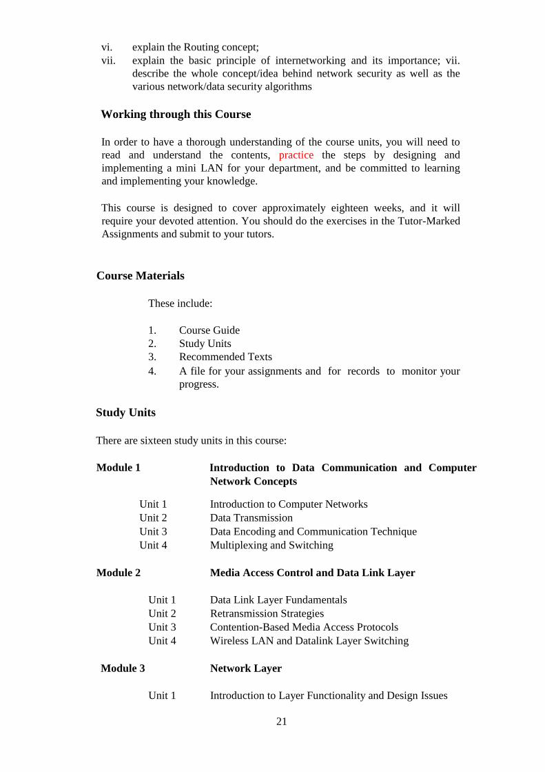
vi. explain the Routing concept;

vii. explain the basic principle of internetworking and its importance; vii.

describe the whole concept/idea behind network security as well as the

various network/data security algorithms

Working through this Course

In order to have a thorough understanding of the course units, you will need to

read and understand the contents, practice the steps by designing and

implementing a mini LAN for your department, and be committed to learning

and implementing your knowledge.

This course is designed to cover approximately eighteen weeks, and it will

require your devoted attention. You should do the exercises in the Tutor-Marked

Assignments and submit to your tutors.

Course Materials

These include:

1. Course Guide

2. Study Units

3. Recommended Texts

4. A file for your assignments and for records to monitor your

progress.

Study Units

There are sixteen study units in this course:

Module 1

Introduction to Data Communication and Computer

Network Concepts

Unit 1 Introduction to Computer Networks

Unit 2 Data Transmission

Unit 3 Data Encoding and Communication Technique

Unit 4 Multiplexing and Switching

Module 2

Media Access Control and Data Link Layer

Unit 1 Data Link Layer Fundamentals

Unit 2 Retransmission Strategies

Unit 3 Contention-Based Media Access Protocols

Unit 4

Wireless LAN and Datalink Layer Switching

Module 3

Network Layer

Unit 1 Introduction to Layer Functionality and Design Issues

Unit 2 Routing Algorithms

Unit 3 Congestion Control in Public Switched Network

Unit 4

Internetworking

Module 4

Transport Layer and Application Layer Services

Unit 1 Transport Services and Mechanism

Unit 2 TCPIUDP

Unit 3 Network Security I

Unit 4 Network Security II

Make use of the course materials, do the exercises to enhance your learning.

Textbooks and References

Computer Networks, Andrew S. Tenenbaum, PHI, New Delhi.

Data and Computer Communication, William Stalling, PHI, New Delhi.

Computer Communications and Networking Technologies, by Michael A. Gallo

and William M. Hancock, Thomson Asia, Second

Reprint, 2002.

Introduction to Data Communications and Networking, by Behrouz Forouzan,

Tata McGraw-Hill, 1999.

Networks, Tirothy S. Ramteke, Second Edition, Pearson Education, New Delhi.

Communications Networks, Leon Garcia, and Widjaja, Tata McGraw- Hill, 1999.

Computer Networking, J. F. Kurose & K. W. Ross, A Top Down

Approach Featuring the Internet, Pearson Edition, 2003.

Computer Networks, Andrew S. Tanenbaum 4th Edition Prentice Hall of India,

New Delhi. 2003.

Communication Networks, Fundamental Concepts and Key

Architectures, Leon and Widjaja, 3rd Edition, Tata McGraw-Hill.

Data Network, Dmitri Berteskas and Robert Galleger, Second Edition, Prentice

Hall of India, 1997, New Delhi.

Network Security Essential -Application and Standard, William Stallings,

Pearson Education, New Delhi.

Assignments File

23

These are of two types: the self-assessment exercises and the Tutor- Marked

Assignments. The self-assessment exercises will enable you monitor your

performance by yourself, while the Tutor-Marked Assignment is a supervised

assignment. The assignments take a certain percentage of your total score in this

course. The Tutor-Marked Assignments will be assessed by your tutor within a

specified period. The examination at the end of this course will aim at

determining the level of mastery of the subject matter. This course includes

twelve Tutor-Marked Assignments and each must be done and submitted

accordingly. Your best scores however, will be recorded for you. Be sure to send

these assignments to your tutor before the deadline to avoid loss of marks.

Presentation Schedule

The Presentation Schedule included in your course materials gives you the

important dates for the completion of tutor marked assignments and attending

tutorials. Remember, you are required to submit all your assignments by the due

date. You should guard against lagging behind in your work.

Assessment

There are two aspects to the assessment of the course. First are the tutor marked

assignments; second, is a written examination.

In tackling the assignments, you are expected to apply information and knowledge

acquired during this course. The assignments must be submitted to your tutor for

formal assessment in accordance with the deadlines stated in the Assignment File.

The work you submit to your tutor for assessment will count for 30% of your total

course mark.

At the end of the course, you will need to sit for a final three-hour examination.

This will also count for 70% of your total course mark.

Tutor Marked Assignment

There are sixteen tutor marked assignments in this course. You need to submit all

the assignments. The total marks for the best four (4) assignments will be 30% of

your total course mark.

Assignment questions for the units in this course are contained in the Assignment

File. You should be able to complete your assignments from the information and

materials contained in your set textbooks, reading and study units. However, you

may wish to use other references to broaden your viewpoint and provide a deeper

understanding of the subject.

When you have completed each assignment, send it together with form to your

tutor. Make sure that each assignment reaches your tutor on or before the deadline

given. If, however, you cannot complete your work on time, contact your tutor

before the assignment is due to discuss the possibility of an extension.

Final Examination and Grading

The final examination for the course will carry 70% percentage of the total marks

available for this course. The examination will cover every aspect of the course,

so you are advised to revise all your corrected assignments before the

examination.

This course endows you with the status of a teacher and that of a learner. This

means that you teach yourself and that you learn, as your learning capabilities

would allow. It also means that you are in a better position to determine and to

ascertain the what, the how, and the when of your language learning. No teacher

imposes any method of learning on you.

The course units are similarly designed with the introduction following the table

of contents, then a set of objectives and then the dialogue and so on.

The objectives guide you as you go through the units to ascertain your knowledge

of the required terms and expressions.

25

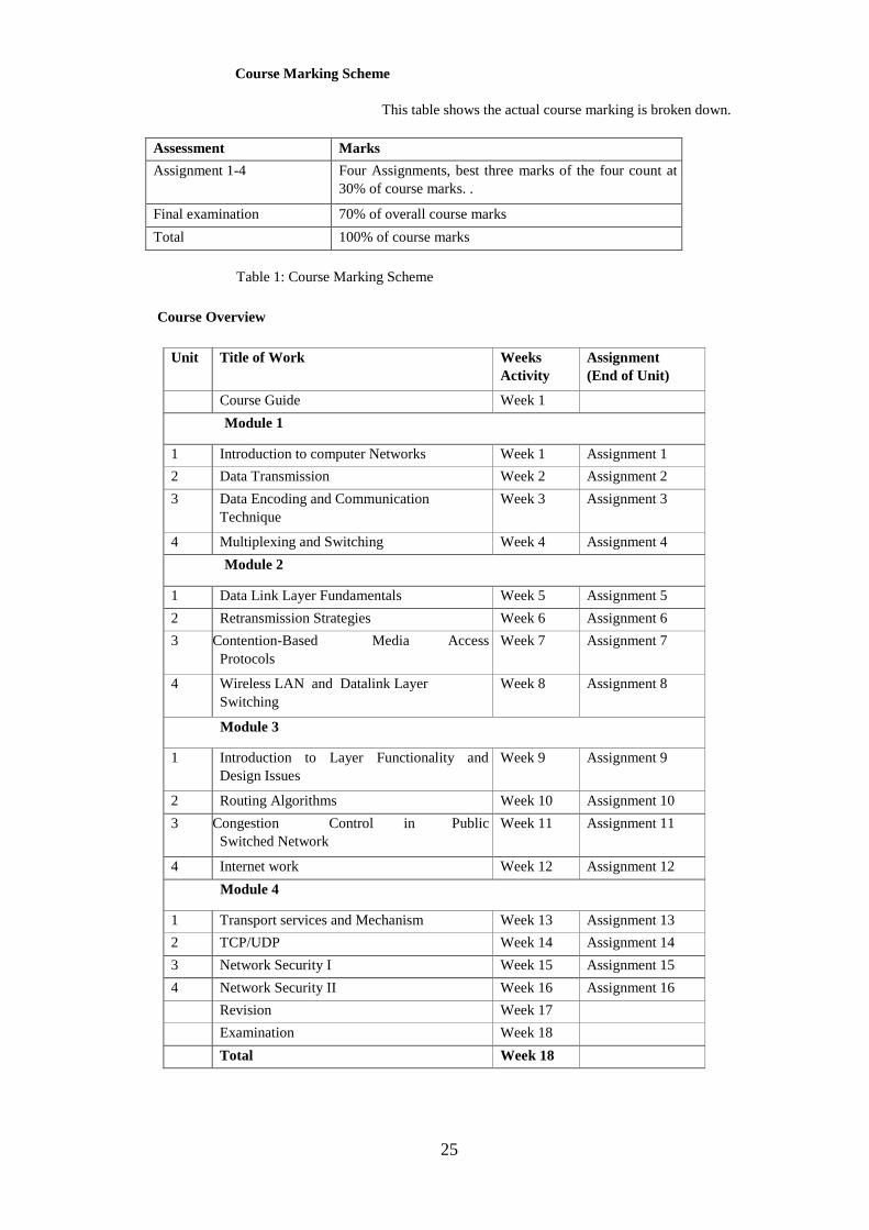
Course Marking Scheme

This table shows the actual course marking is broken down.

Assessment Marks

Assignment 1-4 Four Assignments, best three marks of the four count at

30% of course marks. .

Final examination 70% of overall course marks

Total 100% of course marks

Table 1: Course Marking Scheme

Course Overview

Unit Title of Work Weeks

Activity

Assignment

(End of Unit)

Course Guide Week 1

Module 1

1 Introduction to computer Networks Week 1 Assignment 1

2 Data Transmission Week 2 Assignment 2

3 Data Encoding and Communication

Technique

Week 3 Assignment 3

4 Multiplexing and Switching Week 4 Assignment 4

Module 2

1 Data Link Layer Fundamentals Week 5 Assignment 5

2 Retransmission Strategies Week 6 Assignment 6

3 Contention-Based Media Access

Protocols

Week 7 Assignment 7

4 Wireless LAN and Datalink Layer

Switching

Week 8 Assignment 8

Module 3

1 Introduction to Layer Functionality and

Design Issues

Week 9 Assignment 9

2 Routing Algorithms Week 10 Assignment 10

3 Congestion Control in Public

Switched Network

Week 11 Assignment 11

4 Internet work Week 12 Assignment 12

Module 4

1 Transport services and Mechanism Week 13 Assignment 13

2 TCP/UDP Week 14 Assignment 14

3 Network Security I Week 15 Assignment 15

4 Network Security II Week 16 Assignment 16

Revision Week 17

Examination Week 18

Total Week 18

How to Get the Best from this Course

In distance learning the study units replace the university lecturer. This is one of

the great advantages of distance learning; you can read and work through

specially designed study materials at your own pace, and at a time and place that

suit you best. Think of it as reading the lecture instead of listening to a lecturer. In

the same way that a lecturer might set you some reading to do, the study units tell

you when to read your set books or other material. Just as a lecturer might give

you an in-class exercise, your study units provide exercises for you to do at

appropriate points.

Each of the study units follows a common format. The first item is an introduction

to the subject matter of the unit and how a particular unit is integrated with the

other units and the course as a whole. Next is a set of learning objectives. These

objectives enable you know what you should be able to do by the time you have

completed the unit. You should use these objectives to guide your study. When

you have finished the units you must go back and check whether you have

achieved the objectives. If you make a habit of doing this you will significantly

improve your chances of passing the course.

Remember that your tutor's job is to assist you. When you need help, don't

hesitate to call and ask your tutor to provide it.

1. Read this Course Guide thoroughly.

2. Organize a study schedule. Refer to the 'Course Overview' for more

details. Note the time you are expected to spend on each unit and

how the assignments relate to the units. Whatever method you

chose to use, you should decide on it and write in your own dates for

working on each unit.

3. Once you have created your own study schedule, do everything you

can to stick to it. The major reason that students fail is that they lag

behind in their course work.

4. Turn to Unit 1 and read the introduction and the objectives for the

unit.

5. Assemble the study materials. Information about what you need for a

unit is given in the 'Overview' at the beginning of each unit. You will

almost always need both the study unit you are working on and one

of your set of books on your desk at the same time.

6. Work through the unit. The content of the unit itself has been

arranged to provide a sequence for you to follow. As you work

through the unit you will be instructed to read sections from your set

books or other articles. Use the unit to guide your reading.

7. Review the objectives for each study unit to confirm that you have

achieved them. If you feel unsure about any of the objectives,

review the study material or consult your tutor.

27

8. When you are confident that you have achieved a unit's

objectives, you can then start on the next unit. Proceed unit by unit

through the course and try to pace your study so that you keep

yourself on schedule.

9. When you have submitted an assignment to your tutor for

marking, do not wait for its return before starting on the next unit.

Keep to your schedule. When the assignment is returned, pay

particular attention to your tutor's comments, both on the tutor-

marked assignment form and also written on the assignment. Consult

your tutor as soon as possible if you have any questions or problems.

10. After completing the last unit, review the course and prepare

yourself for the final examination. Check that you have achieved the

unit objectives (listed at the beginning of each unit) and the course

objectives (listed in this Course Guide).

Facilitators/Tutors and Tutorials

There are 15 hours of tutorials provided in support of this course. You will be

notified of the dates, times and location of these tutorials, together with the

name and phone number of your tutor, as soon as you are allocated a tutorial

group.

Your tutor will mark and comment on your assignments, keep a close watch on

your progress and on any difficulties, you might encounter and provide

assistance to you during the course. You must mail or submit your tutor-marked

assignments to your tutor well before the due date (at least two working days are

required). They will be marked by your tutor and returned to you as soon as

possible.

Do not hesitate to contact your tutor by telephone, or e-mail if you need help.

The following might be circumstances in which you would find help necessary.

Contact your tutor if:

you do not understand any part of the study units or the assigned readings, you

have difficulty with the self-tests or exercises, you have a question or problem

with an assignment, with your tutor's comments on an assignment or with the

grading of an assignment.

You should try your best to attend the tutorials. This is the only chance to have

face to face contact with your tutor and to ask questions which are answered

instantly. You can raise any problem encountered in the course of your study.

To gain the maximum benefit from course tutorials, prepare a question list

before attending them. You will learn a lot from participating in discussions

actively.

Summary

This is course, Data communication and Networks exposes you to basic know

ledge and skills about data communication and computer networking you need to

acquire as an information technology professional. The content of the course

material was planned and written to build upon whatever knows you have

acquired at undergraduate or post graduate diploma level and to ensure that you

acquire the proper knowledge and skills for the appropriate situations. Real-life

situations have been created to enable you identify with and create some of your

own. The essence is to get you to acquire the necessary knowledge and

competence, and by equipping you with the necessary tools, we hope to have

achieved that.

I wish you success with the course and hope that you will find it both interesting

and useful.

Course Code

CIT 852

Course Title

Data Communication and Network

Course Adapter

Afolorunso, A. A.


Course Coordinator Afolorunso, A. A.


Course Reviewer Prof. A.A. Obiniyi

Department of Computer Science

Ahmadu Bello University

Zaria, Kaduna State.

Nigeria

29



Headquarters

14/16 Ahmadu Bello Way

Victoria Island

Lagos

Abuja Office

5, Dar Es Salaam Street

Off Aminu Kano Crescent Wuse II, Abuja Nigeria.

e-mail: [email protected] URL: www.nou.edu.ng

Published by


Printed 2008

Second Print 2020

ISBN: 978-058-378-5

All Rights Reserved

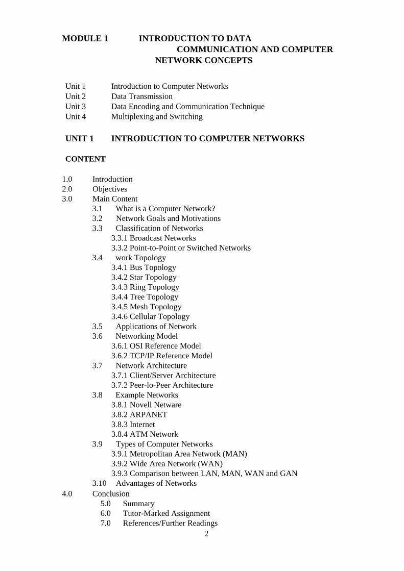
2

MODULE 1 INTRODUCTION TO DATA

COMMUNICATION AND COMPUTER

NETWORK CONCEPTS

Unit 1 Introduction to Computer Networks

Unit 2 Data Transmission

Unit 3 Data Encoding and Communication Technique

Unit 4

Multiplexing and Switching

UNIT 1 INTRODUCTION TO COMPUTER NETWORKS

CONTENT

1.0 Introduction

2.0 Objectives

3.0 Main Content

3.1 What is a Computer Network?

3.2 Network Goals and Motivations

3.3 Classification of Networks

3.3.1 Broadcast Networks

3.3.2 Point-to-Point or Switched Networks

3.4 work Topology

3.4.1 Bus Topology

3.4.2 Star Topology

3.4.3 Ring Topology

3.4.4 Tree Topology

3.4.5 Mesh Topology

3.4.6 Cellular Topology

3.5 Applications of Network

3.6 Networking Model

3.6.1 OSI Reference Model

3.6.2 TCP/IP Reference Model

3.7 Network Architecture

3.7.1 Client/Server Architecture

3.7.2 Peer-lo-Peer Architecture

3.8 Example Networks

3.8.1 Novell Netware

3.8.2 ARPANET

3.8.3 Internet

3.8.4 ATM Network

3.9 Types of Computer Networks

3.9.1 Metropolitan Area Network (MAN)

3.9.2 Wide Area Network (WAN)

3.9.3 Comparison between LAN, MAN, WAN and GAN

3.10 Advantages of Networks

4.0 Conclusion

5.0 Summary

6.0 Tutor-Marked Assignment

7.0 References/Further Readings

3

1.0 INTRODUCTION

These days, practically every business, no matter how small uses

computers to handle various transactions and as business grows, they often need

several people to input and process data simultaneously and in order to achieve this,

the earlier model of a single computer serving all the organisations computational

needs has been replaced by a model in which a number of separate but interconnected

computers do the job and this model is known as a Computer Network. By linking

individual computers over a network their productivity has been increased

enormously.

A most distinguishing characteristic of a general computer network is that data can

enter or leave at any point and can be processed at any workstation. For example: A

printer can be controlled from any word processor at any computer on the network.

This is an introductory unit where, you will be learning about the basic concepts

regarding Computer Networks. Here, you will learn about Networks, different types of

Networks, their applications, Network topology, Network protocols, OSI Reference

Model, TCP/IP Reference Model. We shall also examine some of the popular

computer networks like Novell network, ARPANET, Internet, and ATM networks.

Towards the end of this unit, the concept of Delays in computer networks is also

discussed.

2.0 OBJECTIVES

After going through this unit, you should be able to:

1. understand the concept of computer networks

2. differentiate between different types of computer networks

3. understand the different application of networks

4. compare the different network topologies

5. signify the importance of network protocols

6. know the importance of using networked system

7. understand the layered organisation and structuring of computer networks

using OSI and TCPIIP reference model

8. have a broad idea about some of the popular networks like Novell network,

ARPANET, INTERNET, ATM etc., and

9. understand the concept of delays.

3.0 MAIN CONTENT

3.1 What is a computer network?

4

Figure 1.1: A computer-networked environment

A Computer network consists of two or more autonomous computers that are linked

(connected) together in order to:

1. Share resources (files, printers, modems, fax machines).

2. Share Application software like MS Office.

3. Allow Electronic communication.

4. Increase productivity (makes it easier to share data amongst users).

Figure 1 shows people working in a networked environment. The Computers on a

network may be linked through Cables, telephones lines, radio waves, satellites etc.

A Computer network includes, the network operating system in the client and server

machines, the cables, which connect different computers and all supporting

hardware such as bridges, routers and switches. In wireless systems, antennas and

towers are also part of the network.

Computer networks are generally classified according to their structure and the area

they are localized in as:

1. Local Area Network (LAN): The network that spans a relatively small area

that is, in the single building or campus is known as LAN. It usually functions

at 300m with to 100GPS data rate but can be upscaled to a few kms by

employing Optical Fibre as a channel of sending signals. LAN is sometimes

refers to as Ethernet. It is in most cases made use of networking in homes,

offices, schools or school laboratories, network between two or few computers

and WIFI in wireless LAN. Local Area Network (LAN): can be further divided

into:

a. Personal Area Network (PAN)

b. Storage Area Network (SAN)

c. Enterprise Private Network (EPN)

d. Virtual Private Network (VPN)

Personal Area Network

This can be wired or wireless depending on the devices that are used for the

connection but centred on an individual person. It covers an area between 10 to 100m

5

in most cases at a few kbps to few Mbps data rates. Bluetooth, ZigBee, USB,

firewire, WIFI-direct, near share (in windows 10) and part of IEEE802.15x standard

are examples of PAN.

Storage Area Network (SAN)

SAN as the name of the acronym implies is a local storage on different devices which

works on disk blocks. Its pave way for a group of block-level storage. Most of the

time, SAN path way to connect storage devices such as disk arrays and tape library

from servers to enable machines manifest to the operating system as direct-attached

storage. There is no direct access between SAN and LAN, however, SAN can be

accessed by LAN through shared-disk file system constructed on top of SAN.

Enterprise Private Network (EPN)

This is a network solely managed by one organization but may have diverse locations

for example, production sites, shops and offices.

Virtual Private Network (VPN)

This may be an extension of EPN across public network so that communication can

be undertaken as if it is within a private network. It has the advantages of private

network such as security and administration of the private network. Other types of

LAN are peer-to-peer network and server-based network.

2. Metropolitan Area Network (MAN): The type of computer network that is,

designed for a city or town is known as MAN.

3. Wide Area Network (WAN): A network that covers a large geographical

area and covers different cities, states and sometimes even countries, is

known as WAN. All these networks can either be wired or wireless.

The additional characteristics that are also used to categorise different

types of networks are:

1. Topology: Topology is the graphical arrangement of

computer systems in a network. Common topologies

include a bus, star, ring, and mesh.

2. Protocol: The protocol defines a common set of rules which

are used by computers on the network that communicate

between hardware and software entities. One of the most

popular protocols for LANs is the Ethernet. Another

popular LAN protocol for PCs is the token-ring network.

3. Architecture: Networks can be broadly classified as using

either a peer-to-peer or client/server architecture.

3.2 Network Goals and Motivations

6

Before designing a computer network we should see that the designed network fulfils

the basic goals. We have seen that a computer network should satisfy a broad range

of purposes and should meet various requirements. One of the main goals of a

computer network is to enable its users to share resources, to provide low cost

facilities and easy addition of new processing services. The computer network thus,

creates a global environment for its users and computers.

Some of the basic goals that a Computer network should satisfy are:

1.Cost reduction by sharing hardware and software resources.

2.Provide high reliability by having multiple sources of supply.

3.Provide an efficient means of transport for large volumes of data among

various locations (High throughput).

4.Provide inter-process communication among users and processors.

5.Increase productivity by making it easier to share data amongst users.

6.Repairs, upgrades, expansions, and changes to the network should be

performed with minimal impact on the majority of network users.

7.Standards and protocols should be supported to allow many types of

equipment from different vendors to share the network (interoperability).

8.Provide centralised/distributed management and allocation of network

resources like host processors, transmission facilities etc.

3.3 Classification of Networks

Depending on the transmission technology i.e., whether the network contains

switching elements or not, we have two types of networks:

1. Broadcast networks.

2. Point-to-point or Switched networks.

3.3.1 Broadcast Networks

Broadcast networks have a single communication channel that is shared by all the

machines on the network. In this type of network, short messages sent by any

machine are received by all the machines on the network. The packet contains an

address field, which specifies for whom the packet is intended. All the machines,

upon receiving a packet check for the address field, if the packet is intended for itself,

it processes it and if not, the packet is just ignored.

Using Broadcast networks, we can generally address a packet to all destinations

(machines) by using a special code in the address field. Such packets are received

and processed by all machines on the network. This mode of operation is known as

―Broadcasting‖. Some Broadcast networks also support transmission to a subset of

machines and this is known as ―Multicasting‖. One possible way to achieve

7

Multicasting is to reserve one bit to indicate multicasting and the remaining (n-l)

address bits contain group number. Each machine can subscribe to any or all of the

groups.

Broadcast networks are easily configured for geographically localised networks.

Broadcast networks may be Static or dynamic, depending on how the channel is

allocated.

In Static allocation, time is divided into discrete intervals and using round robin

method, each machine is allowed to broadcast only when its time slot comes up. This

method is inefficient because the channel capacity is wasted when a machine has

nothing to broadcast during its allocated slot.

Dynamic allocation may be centralised or decentralised. In centralised allocation

method, there is a single entity, for example, a bus arbitration unit which determines

who goes next and this is achieved by using some internal algorithm. In

Decentralised channel allocation method, there is no central entity, here, each

machine decides for itself whether or not to transmit.

The different types of Broadcast networks are:

1. Packet Radio Networks.

2. Satellite Networks.

3. Local Area Networks.

Packet Radio Networks

These are diverse access mechanism networks in which it is not possible for all nodes

to hear the transmission of the other nodes. The broadcasting differs from satellite

networks broadcasting in several ways. In particular stations have limited range

introducing the need for radio repeaters, which in turn affects the routing, and

acknowledges schemes. Also, the propagation delay is much less than for satellite

broadcasting.

Satellite Networks

These are made up of unified hubs/switches and thousands of remote devices which

sends and receives data, voice and information with the hubs/switches through

satellites. In other words, it communicates with satellite dishes on earth by sending

and receiving data, voice and information from the orbiting geostationary satellite

thousands of kilometres above the equator. Satellite Networks made available cheap,

resizable and lofty suitable relay of services that cover large area geographically.

LAN (Local Area Network)

Local Area Network is a computer network that spans over a relatively small area.

Most LANs are confined to a single building or group of buildings within a campus.

However, one LAN can be connected to other LANs over any distance via telephone

8

lines and radio waves. A system of LANs connected in this way is called a wide-area

network (WAN).

Most LANs connect workstations and personal computers. Each node (individual

computer) in a LAN has its own CPU with which it executes programs, but it is also

able to access data and devices anywhere on the LAN. This means that many users

can share data as well as expensive devices, such as laser printers, fax machines etc.

Users can also use the LAN to communicate with each other, by sending e-mail or

engaging in chat sessions. There are many different types of LANs, Ethernets being

the most common for PCs.

The following characteristics differentiate one LAN from another:

1. Topology

The geometric arrangement of devices on the network. For example, devices can be

arranged in a ring or in a straight line.

2. Protocols

The rules and encoding specifications for sending data. The protocols also determine

whether the network uses peer-to-peer or client/server architecture.

3. Media

Devices can be connected by twisted-pair wire, coaxial cables, or fibre optic cables.

Some networks communicate via radio waves hence, do not use any connecting

media.

LANs are capable of transmitting data at very fast rates, much faster than data can be

transmitted over a telephone line; but the distances are limited, and there is also a

limit on the number of computers that can be attached to a single LAN.

The typical characteristics of a LAN are:

1. Confined to small areas i.e., it connects several devices over a distance

of5to 10km.

2. High speed.

3. Most inexpensive equipment.

4. Low error rates.

5. Data and hardware sharing between users owned by the user.

6. Operates at speeds ranging from 10Mbps to 100Mbps. Nowadays 1000

Mbps are available.

3.3.2 Point-to-Point or Switched Networks

Point-to-point or switched, networks are those in which there are many connections

between individual pairs of machines. In these networks, when a packet travels from

source to destination it may have to first visit one or more intermediate machines.

9

Routing algorithms play an important role in Point-to-point or Switched networks

because often multiple routes of different lengths are available.

An example of switched network is the international dial-up telephone system.

The different types of Point- to-point or Switched networks are:

1. Circuit Switched Networks.

2. Packet Switched Networks.

In Switched network, the temporary connection is established from one point to

another for either the duration of the session (circuit switching) or for the

transmission of one or more packets of data (packet switching).

Circuit Switched Networks

Circuit Switched networks use a networking technology that provides a temporary,

but dedicated connection between two stations no matter how many switching

devices are used in the data transfer route. Circuit switching was originally developed

for the analogue based telephone system in order to guarantee steady and consistent

service for two people engaged in a phone conversation. Analogue circuit switching

has given way to digital circuit switching, and the digital counterpart still maintains

the connection until broken (one side hangs up). This means bandwidth is

continuously reserved and ―silence is transmitted‖ just the same as digital audio in

voice conversation.

Packet Switched Networks

Packet switched Networks use a networking technology that breaks up a message into

smaller packets for transmission and switches them to their required destination.

Unlike circuit switching, which requires a constant point-to-point circuit to be

established, each packet in a packet- switched network contains a destination address.

Thus, all packets in a single message do not have to travel the same path. They can be

dynamically routed over the network as lines become available or unavailable. The

destination computer reassembles the packets back into their proper sequence.

Packet switching efficiently handles messages of different lengths and priorities. By

accounting for packets sent, a public network can charge customers for only the data

they transmit. Packet switching has been widely used for data, but not for real-time

voice and video. However, this is beginning to change. IP and Asynchronous

Transfer Mode (ATM) technologies are expected to enable packet switching to be

used for everything.

The first international standard for wide area packet switching networks was X.25,

which was defined when all circuits were digited and susceptible to noise.

Subsequent technologies, such as frame relay and Switch Multimegabit Data Service

(SMDS) were designed for today‘s almost-error-free digital lines.

ATM uses a cell-switching technology that provides the bandwidth sharing efficiency

of packet switching with the guaranteed bandwidth of circuit switching.

10

Higher-level protocols, such as TCPIP, IPX/SPX and NetBIOS, are also packet based

and are designed to ride over packet-switched topologies.

Public packet switching networks may provide value added services, such as protocol

conversion and electronic mail.

SELF ASSESSMENT EXERCISE 1

1. Explain the difference between Client/Server and Peer-to-peer architecture?

2. List the important aspects that should be kept in mind while designing a

network?

3. Write briefly about the areas where networks are used?

4. Differentiate between Broadcast and point-to-point networks.

3.4 Network Topology

Topology refers to the shape of a network, or the network‘s layout. How different

nodes in a network are connected to each other and how they communicate with each

other is determined by the network‘s topology. Topologies are either physical or

logical. In other words, it is the physical and logical arrangement of network, that is,

the physical and logical mapping of a network.

Some of the most common network topologies are:

1. Bus topology

2. Ring topology

3. Star topology

4. Mesh topology

5. Tree topology and

6. Cellular topology

The parameters that are to be considered while selecting a physical topology are:

1. Ease of installation.

2. Ease of reconfiguration.

3. Ease of troubleshooting.

3.4.1 Bus Topology

11

Figure 1.2: Bus topology

In Bus topology, all devices are connected to a central cable, called the bus or

backbone. The bus topology connects workstations using a single cable. Each

workstation is connected to the next workstation in a point- to-point fashion. All

workstations connect to the same cable. Figure 1.2 shows computers connected using

Bus Topology.

In this type of topology, if one workstation goes faulty all workstations may be

affected as all workstations share the same cable for the sending and receiving of

information. The cabling cost of bus systems is the least of all the different

topologies. Each end of the cable is terminated using a special terminator.

The common implementation of this topology is Ethernet. Here, message transmitted

by one workstation is heard by all the other workstations.

Advantages of Bus Topology

1. Installation is easy and cheap when compared to other topologies

2. Connections are simple and this topology is easy to use.

3. Less cabling is required.

4. The breakdown of one computer in the network does not affect the other

computer

Disadvantages of Bus Topology

1. Used only in comparatively small networks.

2. The breakdown of the backbone cable can cause the breakdown of the whole

system

3. As all computers share the same bus, the performance of the network deteriorates

when we increase the number of computers beyond a certain limit.

4. Fault identification is difficult.

5. Improper termination of the backbone can cause the system not to function well.

6. A single fault in the cable stops all transmission.

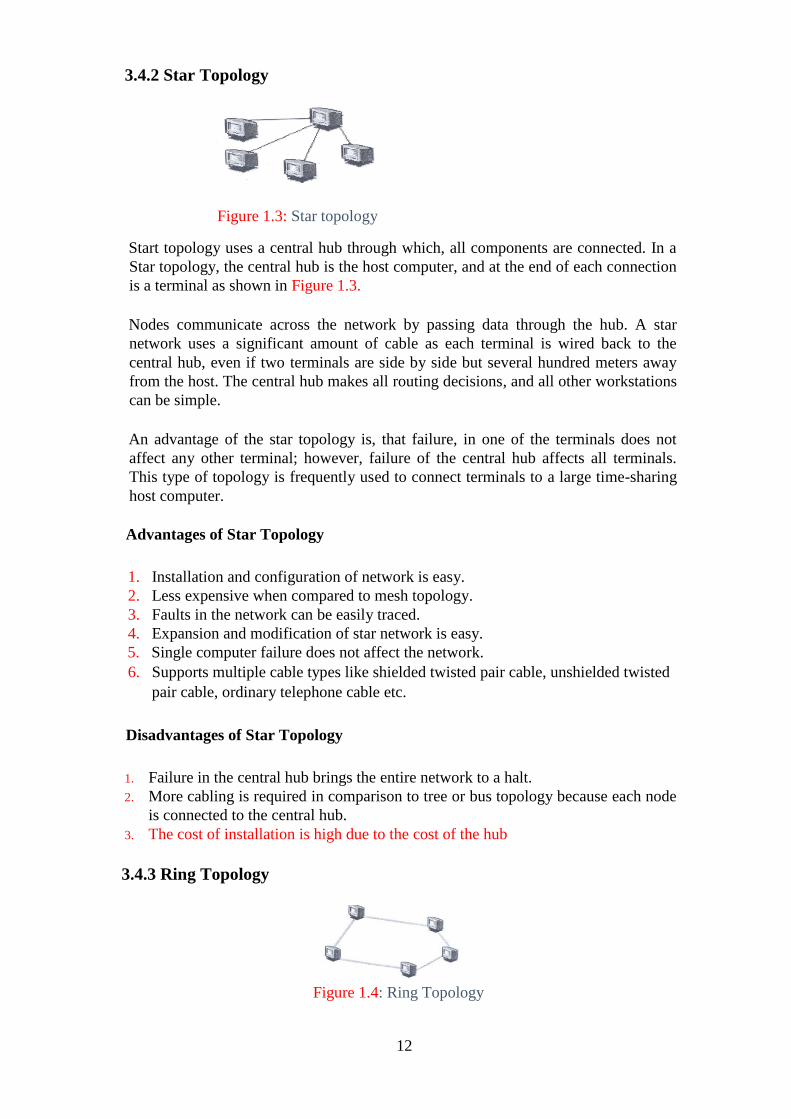
12

3.4.2 Star Topology

Figure 1.3: Star topology

Start topology uses a central hub through which, all components are connected. In a

Star topology, the central hub is the host computer, and at the end of each connection

is a terminal as shown in Figure 1.3.

Nodes communicate across the network by passing data through the hub. A star

network uses a significant amount of cable as each terminal is wired back to the

central hub, even if two terminals are side by side but several hundred meters away

from the host. The central hub makes all routing decisions, and all other workstations

can be simple.

An advantage of the star topology is, that failure, in one of the terminals does not

affect any other terminal; however, failure of the central hub affects all terminals.

This type of topology is frequently used to connect terminals to a large time-sharing

host computer.

Advantages of Star Topology

1. Installation and configuration of network is easy.

2. Less expensive when compared to mesh topology.

3. Faults in the network can be easily traced.

4. Expansion and modification of star network is easy.

5. Single computer failure does not affect the network.

6. Supports multiple cable types like shielded twisted pair cable, unshielded twisted

pair cable, ordinary telephone cable etc.

Disadvantages of Star Topology

1. Failure in the central hub brings the entire network to a halt.

2. More cabling is required in comparison to tree or bus topology because each node

is connected to the central hub.

3. The cost of installation is high due to the cost of the hub

3.4.3 Ring Topology

Figure 1.4: Ring Topology

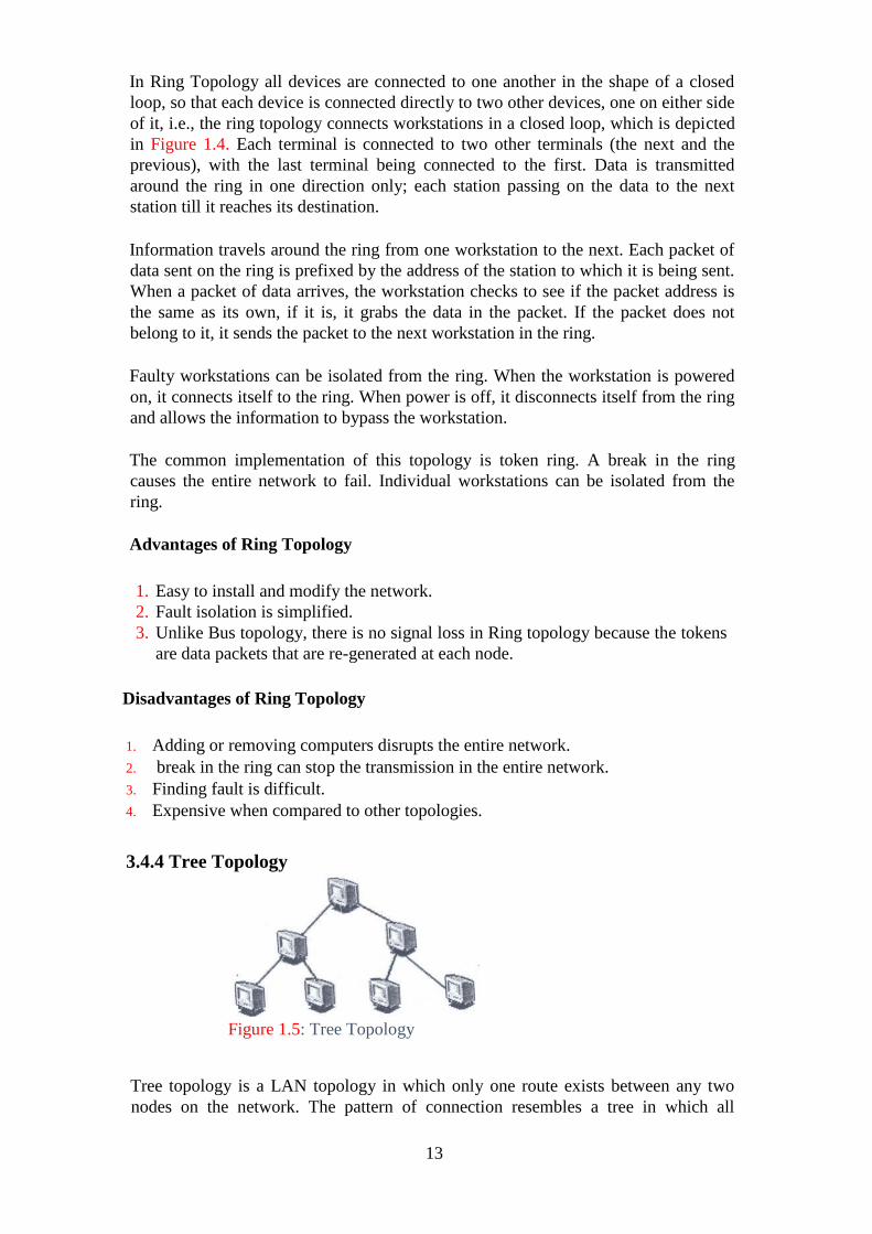
13

In Ring Topology all devices are connected to one another in the shape of a closed

loop, so that each device is connected directly to two other devices, one on either side

of it, i.e., the ring topology connects workstations in a closed loop, which is depicted

in Figure 1.4. Each terminal is connected to two other terminals (the next and the

previous), with the last terminal being connected to the first. Data is transmitted

around the ring in one direction only; each station passing on the data to the next

station till it reaches its destination.

Information travels around the ring from one workstation to the next. Each packet of

data sent on the ring is prefixed by the address of the station to which it is being sent.

When a packet of data arrives, the workstation checks to see if the packet address is

the same as its own, if it is, it grabs the data in the packet. If the packet does not

belong to it, it sends the packet to the next workstation in the ring.

Faulty workstations can be isolated from the ring. When the workstation is powered

on, it connects itself to the ring. When power is off, it disconnects itself from the ring

and allows the information to bypass the workstation.

The common implementation of this topology is token ring. A break in the ring

causes the entire network to fail. Individual workstations can be isolated from the

ring.

Advantages of Ring Topology

1. Easy to install and modify the network.

2. Fault isolation is simplified.

3. Unlike Bus topology, there is no signal loss in Ring topology because the tokens

are data packets that are re-generated at each node.

Disadvantages of Ring Topology

1. Adding or removing computers disrupts the entire network.

2. break in the ring can stop the transmission in the entire network.

3. Finding fault is difficult.

4. Expensive when compared to other topologies.

3.4.4 Tree Topology

Figure 1.5: Tree Topology

Tree topology is a LAN topology in which only one route exists between any two

nodes on the network. The pattern of connection resembles a tree in which all

14

branches spring from one root. Figure 1.5 shows computers connected using Tree

Topology. This type of topology is also called hierarchical topology.

Tree topology is a hybrid topology, it is similar to the star topology but the nodes are

connected to the secondary hub or switch, which in turn is connected to the central

hub or switch. In this topology groups of star-configured networks are connected to a

linear bus backbone.

Advantages of Tree Topology

1. Installation and configuration of network is easy.

2. Less expensive when compared to mesh topology.

3. Faults in the network can be detected traced.

4. The addition of the secondary hub allows more devices to be attached to the

central hub.

5. Supports multiple cable types like shielded twisted pair cable, unshielded twisted

pair cable, ordinary telephone cable etc.

Disadvantages of Tree Topology

1. Failure in the central hub brings the entire network to a halt.

2. More cabling is required when compared to bus topology because each node is

connected to the central hub.

3.4.5 Mesh Topology

Figure 1.6: Mesh Topology

Devices are connected with many redundant interconnections between network nodes.

In a well-connected topology, every node has a connection to every other node in the

network. The cable requirements are high, but there are redundant paths built in.

Failure in one of the computers does not cause the network to break down, as they

have alternative paths to other computers.

Mesh topologies are used in critical connection of host computers (typically telephone

exchanges). Alternate paths allow each computer to balance the load to other computer

systems in the network by using more than one of the connection paths available. A

fully connected mesh topology with n devices has n(n-1) simplex links and n(n-1)/2

duplex links. The total number of inputs/outputs in n devices is (n-1).

15

Advantages of Mesh Topology

1. Use of dedicated links eliminates traffic problems.

2. Failure in one of the computers does not affect the entire network.

3. Point-to-point link makes fault isolation easy.

4. It is robust.

5. Privacy between computers is maintained as messages travel along dedicated

path.

Disadvantages of Mesh Topology

1. The amount of cabling required is high.

2. A large number of I/O (input/output) ports are required.

3.4.6 Cellular Topology

Figure 1.7: Cellular Topology

Cellular topology, divides the area being serviced into cells. In wireless media each

point transmits in a certain geographical area called a cell, each cell represents a

portion of the total network area. Figure 1.7 shows computers using Cellular

Topology. Devices that are present within the cell, communicate through a central

hub/switches. Hubs/switches in different cells are interconnected and hubs/switches

are responsible for routing data across the network. They provide a complete network

infrastructure. Cellular topology is applicable only in case of wireless media that

does not require cable connection.

Advantages of Cellular Topology

1. If the hubs maintain a point-to-point link with devices, trouble shooting is easy.

2. Hub-to-hub fault tracking is more complicated, but allows simple fault isolation.

Disadvantages of Cellular Topology

When a hub/switch fails, all devices serviced by the hub/switch lose service (are

affected).


1. List the importance of using computer networks in Airline and Railway

reservation systems?

16

2. What are the various types of networks??

3. Compare Tree topology with Star topology.

4. Suppose we have~ to add new nodes to the network, then which is the best suited

topology and why?

3.5 Applications of Network

Computer networks are used as a highly reliable medium for exchange of

information. Using a computer network, we can do virtually everything that a

Mainframe or a Minicomputer can do, but at a much lower cost.

There are numerous applications of computer networks, some of them are:

1. Share resources and information.

2. Access to remote information.

3. Person-to-person communication.

4. Interactive entertainment.

3.5.1 Share Resources and Information

Using a Computer network, we can share expensive resources such as laser printers,

CD-ROM Drives, Fax machines etc. We can share information and many persons can

work together on projects and tasks that require co-ordination and communication,

even though these users may not be physically close.

3.5.2 Access to Remote Information

Access to remote information involves interaction between a person and a remote

database. Financial Institutions allow access to their information so that

people can pay their bills, handle their investments and manage their bank accounts

electronically. Online shopping also allows people, access to product information

before purchasing the product.

These days, many newspapers and digital libraries are available online and allow

users to access news and information which is of interest to them. Another

application is the World Wide Web, which contains information about a wide variety

of subjects like health, sports, science, recreation, history, government etc.

Person-to-person Communication

Person-to-person communication is mostly carried out using e-mail (Electronic mail)

Electronic mail is a simple, yet potent facility. E-mail is more valuable and useful

than the telephone because by using e-mail we can convey information that is

difficult or impossible to read over the telephone, like reports, tables, charts, images

etc. Using a computer network, it is also possible to organise virtual meeting among

people who are far away from each other and this is called video conferencing.

17

Virtual meetings have other applications such as in Distance education, getting

medical opinions from distant specialists (remote diagnosis) etc. Multimedia

communication can also be used for tele training. COVID-19 has made virtual reality

(such as video conferencing, teleconferencing and telepresence) a new normal for

almost all activities of men.

Interactive Entertainment

Computer Networks such as Internet offer a wide variety of entertainment, there are

many companies online, which offer video-on- demand. A large variety of multi-

person real-time simulation games, like hide-and seek in a virtual dungeon and flight

simulators with the players in one team trying to shoot down the players in the

opposite team and many such games are available on-line.

3.6 Networking Model

Most of the networks today are organised as a series of stacked layers with each layer

stacked over another layer below it. This is done in order to divide the workload and

to simplify the systems design. The architecture is considered scalable if it is able to

accommodate a number of layers in either large or small scales. For example, a

computer that runs an Internet application may require all of the layers that were

defined for the architectural model. Similarly, a computer that acts as a router may

not need all these layers. Systems design is furthermore simplified because with a

layered architecture, the design has to only concern the layer in question and not

worry about the architecture in a macro sense.

The depth and functionality of this stack differs from network to network. However,

regardless of the differences among all networks, the purpose of each layer is to

provide certain services (job responsibilities) to the layer above it, shielding the upper

layers from the intricate details of how the services offered are implemented.

Every computer in a network possesses within it a generic stack. A logical

communication may exist between any two computers through the layers of the same

―level‖. Layer-n on one computer may converse with layer-n on another computer as

shown in Figure 1.8. There are rules and conventions used in the communication at

any given layers, which are known collectively as the layer-n protocol for the nth

layer.

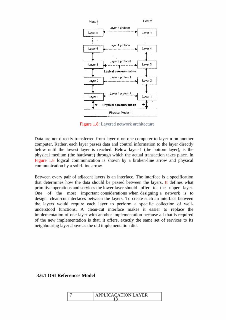
18

Figure 1.8: Layered network architecture

Data are not directly transferred from layer-n on one computer to layer-n on another

computer. Rather, each layer passes data and control information to the layer directly

below until the lowest layer is reached. Below layer-1 (the bottom layer), is the

physical medium (the hardware) through which the actual transaction takes place. In

Figure 1.8 logical communication is shown by a broken-line arrow and physical

communication by a solid-line arrow.

Between every pair of adjacent layers is an interface. The interface is a specification

that determines how the data should be passed between the layers. It defines what

primitive operations and services the lower layer should offer to the upper layer.

One of the most important considerations when designing a network is to

design clean-cut interfaces between the layers. To create such an interface between

the layers would require each layer to perform a specific collection of well-

understood functions. A clean-cut interface makes it easier to replace the

implementation of one layer with another implementation because all that is required

of the new implementation is that, it offers, exactly the same set of services to its

neighbouring layer above as the old implementation did.

3.6.1 OSI References Model

7 APPLICACATION LAYER

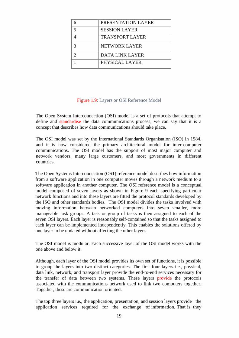
19

Figure 1.9: Layers or OSI Reference Model

The Open System Interconnection (OSI) model is a set of protocols that attempt to

define and standardise the data communications process; we can say that it is a

concept that describes how data communications should take place.

The OSI model was set by the International Standards Organisation (ISO) in 1984,

and it is now considered the primary architectural model for inter-computer

communications. The OSI model has the support of most major computer and

network vendors, many large customers, and most governments in different

countries.

The Open Systems Interconnection (OS1) reference model describes how information

from a software application in one computer moves through a network medium to a

software application in another computer. The OSI reference model is a conceptual

model composed of seven layers as shown in Figure 9 each specifying particular

network functions and into these layers are fitted the protocol standards developed by

the ISO and other standards bodies. The OSI model divides the tasks involved with

moving information between networked computers into seven smaller, more

manageable task groups. A task or group of tasks is then assigned to each of the

seven OSI layers. Each layer is reasonably self-contained so that the tasks assigned to

each layer can be implemented independently. This enables the solutions offered by

one layer to be updated without affecting the other layers.

The OSI model is modular. Each successive layer of the OSI model works with the

one above and below it.

Although, each layer of the OSI model provides its own set of functions, it is possible

to group the layers into two distinct categories. The first four layers i.e., physical,

data link, network, and transport layer provide the end-to-end services necessary for

the transfer of data between two systems. These layers provide the protocols

associated with the communications network used to link two computers together.

Together, these are communication oriented.

The top three layers i.e., the application, presentation, and session layers provide the

application services required for the exchange of information. That is, they

6 PRESENTATION LAYER

5 SESSION LAYER

4 TRANSPORT LAYER

3 NETWORK LAYER

2 DATA LINK LAYER

1 PHYSICAL LAYER

20

allow two applications, each running on a different node of the network to interact

with each other through the services provided by their respective operating systems.

Together, these are data processing oriented.

The following are the seven layers of the Open System Interconnection (OSI)

reference model:

Layer 7 -Application layer

Layer 6 -Presentation layer

Layer 5 -Session layer

Layer 4 -Transport layer

Layer 3 -Network layer

Layer 2 -Data Link layer

Layer I -Physical layer

Application Layer (Layer 7)

The Application layer is probably the most easily misunderstood layer of the model.

This top layer defines the language and syntax that programs use to communicate with

other programs. The application layer represents the purpose of communicating in the

first place. For example, a program in a client workstation uses commands to request

data from a program in the server. Common functions at this layer are opening,

closing, reading and writing files, transferring files and e-mail messages, executing

remote jobs and obtaining directory information about network resources etc.

Presentation Layer (Layer 6)

The Presentation layer performs code conversion and data reformatting (syntax

translation). It is the translator of the network; it makes sure the data is in the correct

form for the receiving application.

When data are transmitted between different types of computer systems, the

presentation layer negotiates and manages the way data are represented and encoded.

For example, it provides a common denominator between ASCII and EBCDIC

machines as well as between different floating point and binary formats. Sun‘s XDR

and OSI‘s ASN. 1 are two protocols used for this purpose. This layer is also used for

encryption and decryption. It also provides security features through encryption and

decryption.

Session Layer (Layer 5)

21

The Session layer decides when to turn communication on and off between two

computers. It provides the mechanism that controls the data-exchange process and

coordinates the interaction (communication) between them in an orderly manner.

It sets up and clears communication channels between two communicating

components. It determines one-way or two-way communications and manages the

dialogue between both parties; for example, making sure that the previous request has

been fulfilled before the next one is sent. It also marks significant parts of the

transmitted data with checkpoints to allow for fast recovery in the event of a

connection failure.

Transport Layer (Layer 4)

The transport layer is responsible for overall end-to-end validity and integrity of the

transmission i.e., it ensures that data is successfully sent and received between two

computers. The lower data link layer (layer 2) is only responsible for delivering

packets from one node to another.

Thus, if a packet gets lost in a router somewhere in the enterprise Internet, the

transport layer will detect that. It ensures that if a 12MB file is sent, the full 12MB is

received.

If data is sent incorrectly, this layer has the responsibility of asking for retransmission

of the data. Specifically, it provides a network- independent, reliable message-

independent, reliable message- interchange service to the top three application-

oriented layers. This layer acts as an interface between the bottom and top three layers.

By providing the session layer (layer 5) with a reliable message transfer service, it

hides the detailed operation of the underlying network from the session layer.

Network Layer (Layer 3)

The network layer establishes the route between the sending and receiving stations.

The unit of data at the network layer is called a packet. It provides network routing

and flow and congestion functions across computer-network interface.

It makes a decision as to where to route the packet based on information and

calculations from other routers, or according to static entries in the routing table. It

examines network addresses in the data instead of physical addresses seen in the Data

Link layer.

The Network layer establishes, maintains, and terminates logical and/or physical

connections.

The network layer is responsible for translating logical addresses, or names, into

physical addresses.

The main device found at the Network layer is a router.

Data link Layer (Layer 2)

22

The data link layer groups the bits that we see on the Physical layer into Frames. It is

primarily responsible for error-free delivery of data on a hop. The Data link layer is

split into two sub-layers i.e., the Logical Link Control (LLC) and Media Access

Control (MAC).

The Data-Link layer handles the physical transfer, framing (the assembly of data into

a single unit or block), flow control and error- Control functions (and retransmission

in the event of an error) over a single transmission link; it is responsible for getting

the data packaged and onto the network cable. The data link layer provides the

network layer (layer 3) reliable information-transfer capabilities.

The main network device found at the Datalink layer is a bridge. This device works

at a higher layer than the repeater and therefore is a more complex device. It has

some understanding of the data it receives and can make a decision based on the

frames it receives as to whether it needs to let the information pass, or can remove

the information from the network. This means that the amount of traffic on the

medium can be reduced and therefore, the usable bandwidth can be increased.

Physical Layer (Layer 1)

The data units on this layer are called bits. This layer defines the mechanical and

electrical definition of the network medium (cable) and network hardware. This

includes how data is impressed onto the cable and retrieved from it.

The physical layer is responsible for passing bits onto and receiving them from the

connecting medium. This layer gives the data-link layer (layer 2) its ability to

transport a stream of serial data bits between two communicating systems; it conveys

the bits that moves along the cable. It is responsible for ensuring that the raw bits get

from one place to another, no matter what shape they are in, and deals with the

mechanical and electrical characteristics of the cable.

This layer has no understanding of the meaning of the bits, but deals with the

electrical and mechanical characteristics of the signals and signalling methods.

The main network device found in the Physical layer is a repeater. The purpose of a

repeater (as the name suggests) is simply to receive the digital signal, reform it, and

retransmit the signal. This has the effect of increasing the maximum length of a

network, which would not be possible due to signal deterioration if, a repeater were

not available. The repeater, simply regenerates cleaner digital signal so it doesn‘t

have to understand anything about the information it is transmitting, and processing

on the repeater.

An example of the Physical layer is RS-232.

Each layer, with the exception of the physical layer, adds information to the data as it

travels from the Application layer down to the physical layer. This extra information

is called a header. The physical layer does not append a header to information

because it is concerned with sending and receiving information on the individual bit

level.

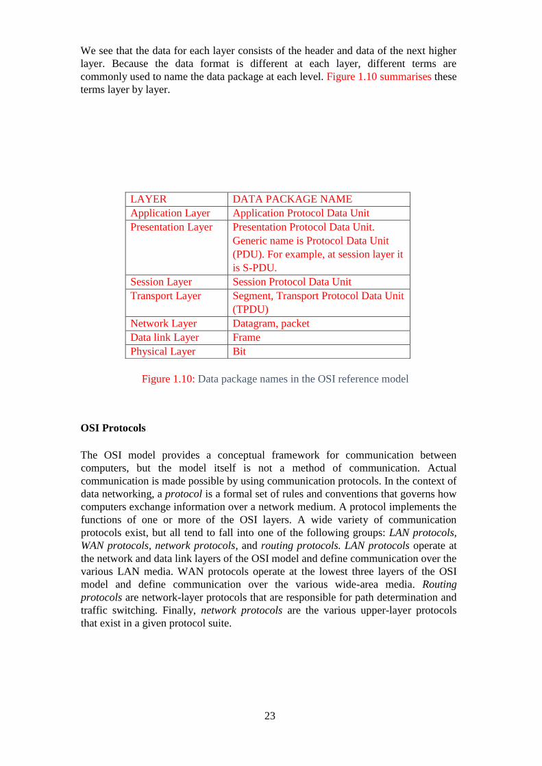
23

We see that the data for each layer consists of the header and data of the next higher

layer. Because the data format is different at each layer, different terms are

commonly used to name the data package at each level. Figure 1.10 summarises these

terms layer by layer.

Figure 1.10: Data package names in the OSI reference model

OSI Protocols

The OSI model provides a conceptual framework for communication between

computers, but the model itself is not a method of communication. Actual

communication is made possible by using communication protocols. In the context of

data networking, a protocol is a formal set of rules and conventions that governs how

computers exchange information over a network medium. A protocol implements the

functions of one or more of the OSI layers. A wide variety of communication

protocols exist, but all tend to fall into one of the following groups: LAN protocols,

WAN protocols, network protocols, and routing protocols. LAN protocols operate at

the network and data link layers of the OSI model and define communication over the

various LAN media. WAN protocols operate at the lowest three layers of the OSI

model and define communication over the various wide-area media. Routing

protocols are network-layer protocols that are responsible for path determination and

traffic switching. Finally, network protocols are the various upper-layer protocols

that exist in a given protocol suite.

LAYER DATA PACKAGE NAME

Application Layer Application Protocol Data Unit

Presentation Layer Presentation Protocol Data Unit.

Generic name is Protocol Data Unit

(PDU). For example, at session layer it

is S-PDU.

Session Layer Session Protocol Data Unit

Transport Layer Segment, Transport Protocol Data Unit

(TPDU)

Network Layer Datagram, packet

Data link Layer Frame

Physical Layer Bit

24

Figure 1.11: Working of OSI Reference Model

Information being transferred from a software application in one computer system to

software application in another must pass through each of the OSI layers. Each layer

communicates with three other OSI layers i.e., the layer directly above it, the layer

directly below it, and its peer layer ill other networked systems. If, for example, in

Figure 1.11, a software application in System A has information to transmit to a

software application in System B, the application program in System A will pass its

information to the application layer (Layer 7) of System A. The application layer

then passes the information to the presentation layer (Layer 6); the presentation layer

reformats the data if required such that B can understand it. The formatted data is

passed to the session layer (Layer 5), which in turn requests for connection

establishment between session layers of A and B, it then passes the data to the

transport layer. The transport layer breaks the data into smaller units called segments

and sends them to the Network layer. The Network layer selects the route for

transmission and if, required breaks the data packets further. These data packets are

then sent to the Data link layer that is responsible for encapsulating the data packets

into data frames. The Data link layer also adds source and destination addresses with

error checks to each frame, for the hop.

The data frames are finally transmitted to the physical layer. In the physical layer, the

data is in the fond of a stream of bits and this is placed on the physical network

medium and is sent across the medium to System B.

B receives the bits at its physical layer and passes them on to the Data link layer,

which verifies that no error has occurred. The Network layer ensures that the route

selected for transmission is reliable, and passes the data to the Transport layer. The

function of the Transport layer is to reassemble the data packets into the file being

transferred and then, pass it on to the session layer. The session layer confirms that

the transfer is complete, and if so, the session is terminated.

The data is then passed to the Presentation layer, which may or may not reformat it to

suit the environment of B and sends it to the Application layer. Finally, the

Application layer of System B passes the information to the recipient Application

program to complete the communication process.

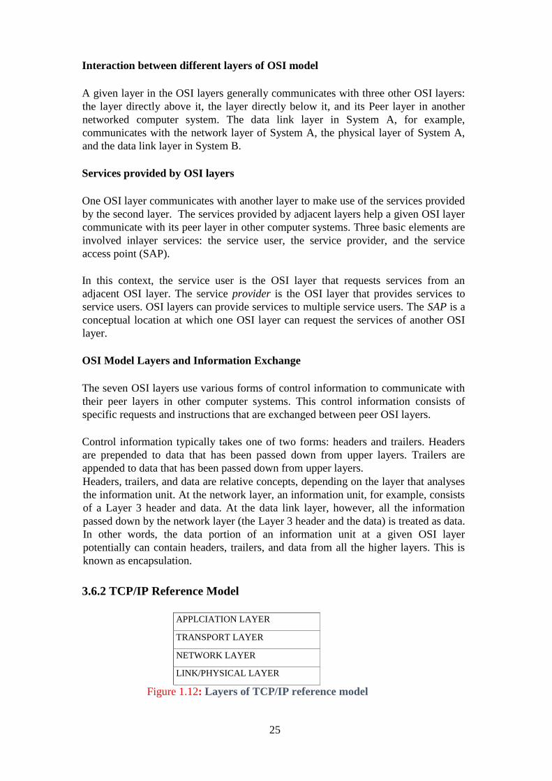
25

Interaction between different layers of OSI model

A given layer in the OSI layers generally communicates with three other OSI layers:

the layer directly above it, the layer directly below it, and its Peer layer in another

networked computer system. The data link layer in System A, for example,

communicates with the network layer of System A, the physical layer of System A,

and the data link layer in System B.

Services provided by OSI layers

One OSI layer communicates with another layer to make use of the services provided

by the second layer. The services provided by adjacent layers help a given OSI layer

communicate with its peer layer in other computer systems. Three basic elements are

involved inlayer services: the service user, the service provider, and the service

access point (SAP).

In this context, the service user is the OSI layer that requests services from an

adjacent OSI layer. The service provider is the OSI layer that provides services to

service users. OSI layers can provide services to multiple service users. The SAP is a

conceptual location at which one OSI layer can request the services of another OSI

layer.

OSI Model Layers and Information Exchange

The seven OSI layers use various forms of control information to communicate with

their peer layers in other computer systems. This control information consists of

specific requests and instructions that are exchanged between peer OSI layers.

Control information typically takes one of two forms: headers and trailers. Headers

are prepended to data that has been passed down from upper layers. Trailers are

appended to data that has been passed down from upper layers.

Headers, trailers, and data are relative concepts, depending on the layer that analyses

the information unit. At the network layer, an information unit, for example, consists

of a Layer 3 header and data. At the data link layer, however, all the information

passed down by the network layer (the Layer 3 header and the data) is treated as data.

In other words, the data portion of an information unit at a given OSI layer

potentially can contain headers, trailers, and data from all the higher layers. This is

known as encapsulation.

3.6.2 TCP/IP Reference Model

APPLCIATION LAYER

TRANSPORT LAYER

NETWORK LAYER

LINK/PHYSICAL LAYER

Figure 1.12: Layers of TCP/IP reference model

26

TCP/IP stands for Transmission Control Protocol/Internet Protocol. It is a protocol

suite used by most communications‘ software. TCP/IP is a robust and proven

technology that was first tested in the early I 980s on ARPA Net, the U.S. military‘s

Advanced Research Projects Agency network, and the world‘s first packet-switched

network. TCP/IP was designed as an open protocol that would enable all types of

computers to transmit data to each other via a common communications language.

TCP/IP is a layered protocol similar to the ones used in all the other major

networking architectures, including IBM‘s SNA, Windows‘ NetBIOS, Apple‘s

AppleTalk, Novell‘s NetWare and Digital‘s DECnet. The different layers of the

TCP/IP reference model are shown in Figure 1.12. Layering means that after an

application initiates the communications, the message (data) to be transmitted is

passed through a number of stages or layers until it actually moves out onto the wire.

The data are packaged with a different header at each layer. At the receiving end, the

corresponding programs at each protocol layer unpack the data, moving it ―back up

the stack‖ to the receiving application.

TCP/IP is composed of two major parts: TCP (Transmission Control Protocol) at the

transport layer and IP (Internet Protocol) at the network layer. TCP is a connection-

oriented protocol that passes its data to IP, which is a connectionless one. TCP sets

up a connection at both ends and guarantees reliable delivery of the full message sent.

TCP tests for errors and requests retransmission if necessary, because IP does not.

An alternative protocol to TCP within the TCP/IP suite is UDP (User Datagram

Protocol), which does not guarantee delivery. Like IP, it is also connectionless, but

very useful for real-time voice and video, where it doesn‘t matter if a few packets get

lost.

Layers of TCP/IP reference model

Application Layer (Layer 4)

The top layer of the protocol stack is the application layer. It refers to the programs

that initiate communication in the first place. TCP/IP includes several application

layer protocols for mail, file transfer, remote access, authentication and name

resolution.

These protocols are embodied in programs that operate at the top layer just as any

custom- made or packaged client/server application would.

There are many Application Layer protocols and new protocols are always being

developed.

The most widely known Application Layer protocols are those used for the exchange

of user information, some of them are:

The Hypertext Transfer Protocol (HTTP) is used to transfer files that

make up the Web pages of the World Wide Web.

The File Transfer Protocol (FTP) is used for interactive file transfer.

27

The Simple Mail Transfer Protocol (SMTP) is used for the transfer of

mail messages and attachments.

The post office protocol 3 (POP3) is used to retrieve email from remote

email server to local server to a local email client through port 110.

SMTP is the protocol used in sending the email to the POP3.

Telnet, is a terminal emulation protocol, and, is used for remote login to

network hosts.

Other Application Layer protocols that help in the management of TCP/IP networks

are:

The Domain Name System (DNS), which, is used to resolve a host name

to an IP address.

The Simple Network Management Protocol (SNMP) which is used

between network management consoles and network devices (routers,

bridges, and intelligent hubs/switches) to collect and exchange network

management information.

Examples of Application Layer interfaces for TCP/IP applications are Windows

Sockets and NetBIOS. Windows Sockets provides a standard application-

programming interface (API) under the Microsoft Windows operating system.

NetBIOS is an industry standard interface for accessing protocol services such as

sessions, datagrams, and name resolution.

Transport Layer (Layer 3)

The Transport Layer (also known as the Host-to-Host Transport Layer) is responsible

for providing the Application Layer with session and datagram communication

services.

TCP/IP does not contain Presentation and Session layers, the services are performed

if required, but they are not part of the formal TCP/IP stack. For example, Layer 6

(Presentation Layer) is where data conversion (ASCII to EBCDIC, floating point to

binary, etc,) and encryption/decryption is performed, Layer 5 is the Session Layer,

which is performed in layer 4 in TCP/IP, Thus, we jump from layer 7 of OS I down

to layer 4 of TCP/IP.

From Application to Transport Layer, the application delivers its data to the

communications system by passing a Stream of data bytes to the transport layer along

with the socket of the destination machine.

The core protocols of the Transport Layer are TCP and the User Datagram Protocol

(UDP).

TCP: TCP provides a one-to-one, connection-oriented, reliable

communications service. TCP is responsible for the establishment of a TCP

28

connection, the sequencing and acknowledgment of packets sent, and the

recovery of packets lost during transmission.

UDP: UDP provides a one-to-one or one-to-many, connectionless, unreliable

communications service. UDP is used when the amount of data to be

transferred is small (such as the data that would fit into a single packet), when

the overhead of establishing a TCP connection is not desired, or when the

applications or upper layer protocols provide reliable delivery.

The transport Layer encompasses the responsibilities of the OSI Transport Layer and

some of the responsibilities of the OSI Session Layer.

Internet Layer (Layer 2)

The internet layer handles the transfer of information across multiple networks

through the use of gateways and routers. The internet layer corresponds to the part of

the OSI network layer that is concerned with the transfer of packets between

machines that are connected to different networks. It deals with the routing of packets

across these networks as well as with the control of congestion. A key aspect of the

internet layer is the definition of globally unique addresses for machines that are

attached to the Internet.

The Internet layer provides a single service namely, best-effort connectionless packet

transfer. IP packets are exchanged between routers without a connection setup; the

packets are ‗touted independently and so they may traverse different paths. For this

reason, IP packets are also called datagrams. The connectionless approach makes the

system robust; that is, if failures occur in the network, the packets are routed around

the points of failure; hence, there is no need to set up connections. The gateways that

interconnect the intermediate networks may discard packets when congestion occurs.

The responsibility for recovery from these losses is based on to the Transport Layer.

The core protocols of the Internet Layer are IP. ARP, ICMP, and IGMP.

The Internet Protocol (IP) is a routable protocol responsible for

IP addressing and the fragmentation and reassembly of packets.

The Address Resolution Protocol (ARP) is responsible for the resolution of

the Internet Layer address to the Network Interface Layer address, such as a

hardware address.

The Internet Control Message Protocol (ICMP) is responsible for providing

diagnostic functions and reporting errors or conditions regarding the delivery

of IP packets.

The Internet Group Management Protocol (IGMP) is responsible for the

management of IP multicast groups.

The Internet Layer is analogueous to the Network layer of the OSI model.

Link/Physical Layer (Layer I)

29

The Link/Physical Layer (also called the Network Access Layer) is responsible for

placing TCP/IP packets on the network medium and receiving TCP/IP packets of the

network medium. TCP/IP was designed to be independent of the network access

method, frame format, and medium. In this way, TCP/IP can be used to connect

differing network types. This includes LAN technologies such as Ethernet or Token

Ring and WAN technologies such as X.25 or Frame Relay. Independence from any

specific network technology gives TCP/IP the ability to be adapted to new

technologies such as Asynchronous Transfer Mode (ATM).

The Network Interface Layer encompasses the Data Link and Physical layers of the

OSI Model. Note, that the Internet Layer does not take advantage of sequencing and

acknowledgement services that may be present in the Data Link Layer. An unreliable

Network Interface Layer is assumed, and reliable communications through session

establishment and the sequencing and acknowledgement of packets is the

responsibility of the Transport Layer.

Comparison between OSI and TCP/IP reference model

Figure 1.13: Comparison between OSI and TCP/IP reference model

Both OSI and TCP/IP reference models are based on the concept of a stack of

protocols. The functionality of the layers is almost similar. In both models, the layers

are there to provide an end-to-end network- independent transport service to processes

wishing to communicate with each other.

The Two models have many differences. An obvious difference between the two

models is the number of layers: the OSI model has seven layers and the TCP/IP has

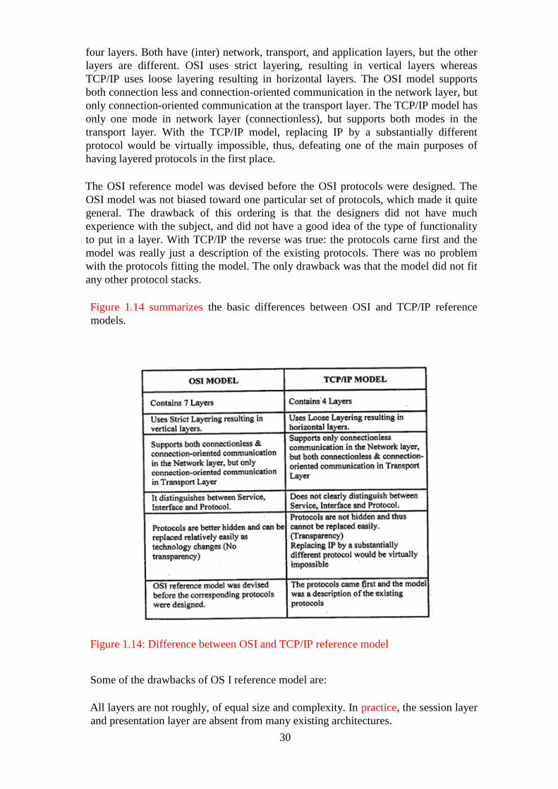
30

four layers. Both have (inter) network, transport, and application layers, but the other

layers are different. OSI uses strict layering, resulting in vertical layers whereas

TCP/IP uses loose layering resulting in horizontal layers. The OSI model supports

both connection less and connection-oriented communication in the network layer, but

only connection-oriented communication at the transport layer. The TCP/IP model has

only one mode in network layer (connectionless), but supports both modes in the

transport layer. With the TCP/IP model, replacing IP by a substantially different

protocol would be virtually impossible, thus, defeating one of the main purposes of

having layered protocols in the first place.

The OSI reference model was devised before the OSI protocols were designed. The

OSI model was not biased toward one particular set of protocols, which made it quite

general. The drawback of this ordering is that the designers did not have much

experience with the subject, and did not have a good idea of the type of functionality

to put in a layer. With TCP/IP the reverse was true: the protocols carne first and the

model was really just a description of the existing protocols. There was no problem

with the protocols fitting the model. The only drawback was that the model did not fit

any other protocol stacks.

Figure 1.14 summarizes the basic differences between OSI and TCP/IP reference

models.

Figure 1.14: Difference between OSI and TCP/IP reference model

Some of the drawbacks of OS I reference model are:

All layers are not roughly, of equal size and complexity. In practice, the session layer

and presentation layer are absent from many existing architectures.

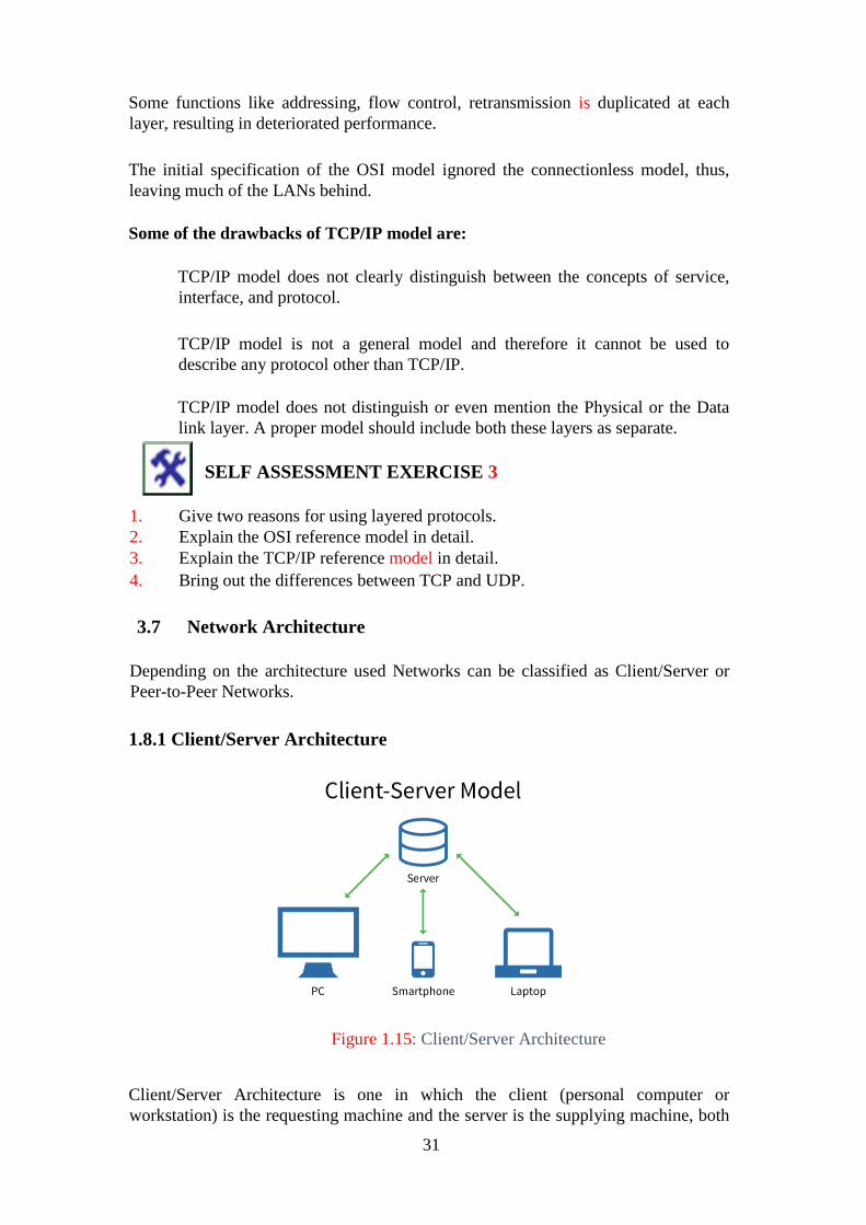
31

Some functions like addressing, flow control, retransmission is duplicated at each

layer, resulting in deteriorated performance.

The initial specification of the OSI model ignored the connectionless model, thus,

leaving much of the LANs behind.

Some of the drawbacks of TCP/IP model are:

TCP/IP model does not clearly distinguish between the concepts of service,

interface, and protocol.

TCP/IP model is not a general model and therefore it cannot be used to

describe any protocol other than TCP/IP.

TCP/IP model does not distinguish or even mention the Physical or the Data

link layer. A proper model should include both these layers as separate.


1. Give two reasons for using layered protocols.

2. Explain the OSI reference model in detail.

3. Explain the TCP/IP reference model in detail.

4. Bring out the differences between TCP and UDP.

3.7 Network Architecture

Depending on the architecture used Networks can be classified as Client/Server or

Peer-to-Peer Networks.

1.8.1 Client/Server Architecture

Figure 1.15: Client/Server Architecture

Client/Server Architecture is one in which the client (personal computer or

workstation) is the requesting machine and the server is the supplying machine, both

32

of which are connected via a local area network (LAN) or wide area network (WAN).

Since the early 1990s, client/server has been the buzzword for building applications

on LANs in contrast to centralised minis and mainframes with dedicated terminals. A

client/server network is called Centralised or Server based network. Figure 1.15

shows the arrangement of computers in the client/server environment.

The client contains the user interface and may perform some or all of the application

processing. Servers can be high-speed microcomputers, minicomputers or even

mainframes. A database server maintains the databases and processes requests from

the client to extract data from or update the database. An application server provides

additional business processing for the clients.

The term client/server is sometimes used to contrast a peer-to-peer network, in which

any client can also act as a server. In that case, a client/server entails having a

dedicated server.

However, client/server architecture means more than dedicated servers. Simply

downloading files from or sharing programs and databases on a server is not true

client/server either. True client/server implies that the application was originally

designed to run on a network and that the network infrastructure provides the same

quality of service as traditional mini and mainframe information systems. Figure 1.15

shows the arrangement of computers in the Client/Server system.

The network operating system (NOS) together with the database management system

(DBMS) and transaction monitor (TP monitor) are responsible for integrity and

security of these types of networks. Some of these products have gone through many

client/server versions by now and have finally reached industrial strength.

Non-client/server

In non-client/server architecture, the server is nothing more than a remote disk drive.

The user‘s machine does all the processing. If, many users routinely perform lengthy

searches, this can bog down the network, because each client has to pass the entire

database over the net. At 1,000 bytes per record, a 10,000 record database requires

10MB of data be transmitted.

Two-tier client/server

Two-tier client/server is really the foundation of client/server. The database

processing is done in the server. An SQL request is generated in the client and

transmitted to the server. The DBMS searches locally and returns only matching

records. If 50 records met the criteria only 50K would be transmitted. This reduces

traffic in the LAN.

Three-tier client/server

Many applications lend themselves to centralised processing. If, they contain

proprietary algorithms, security is improved. Upgrading is also simpler. Sometimes,

programs are just too demanding to be placed into every client PC. In three-tier

client/server, application processing is performed in one or more servers.

33

3.7.2 Peer-to-Peer Architecture

Figure 1.16: Peer-to-peer architecture

A type of network in which each workstation as equal capabilities and

responsibilities is called peer-to-peer network. Figure 1.16 shows the arrangement of

computers in a peer-to-peer environment. Here each workstation acts as both a client

and a server. There is no central repository for information and there is no central

server to maintain. Data and resources are distributed throughout the network, and

each user is responsible for sharing data and resources connected to their system.

This differs from client/server architectures, in which some computers are dedicated

to serving the others. Peer-to-peer networks are generally simpler and less expensive,

but they usually do not offer the same performance under heavy loads. A peer-to-peer

network is also known as a Distributed network.

3.8 Example Networks

Nowadays, as computers are extensively used in almost every field, we have many

different types of networks. Some of them are public networks, research networks,

and co-operative networks, commercial or corporate networks. We can distinguish

between different networks on the basis of their history, administration, facilities

offered, technical design and the people who use them/user communities). Here we

shall discuss some of the popular networks, such as, Novell NetWare, ARPANET,

Internet, ATM network etc.

3.8.1 Novell Netware

Novell NetWare is the most popular network system in the PC world. Novell

NetWare contains the protocols that are necessary to allow communication between

different types of PC‘s and devices. There are several versions of NetWare. The

earlier versions NetWare 286 version 2.X was written to run on 286 machines.

NetWare 386 versions 3.X were written to run on 386 and 486 machines. The most

recent version NetWare 4.X can probably run on almost any type of machine.

34

Novell Networks are based on the client/server model in which at least one computer

functions as a network file server, which runs all of the NetWare protocols and

maintains the networks shared data on one or more disk drives. File servers generally

allow users on other PC‘s to access application software or data files i.e., it provides

services to other network computers called clients.

There are two types of file servers:

1. Dedicated file servers.

2. Non-dedicated file servers.

Dedicated File Servers

Dedicated file server runs only NetWare and do not run any other software, such as

Windows application. Dedicated file servers are mostly used in large networks,

because, in large networks, one extra client is less significant and a dedicated server

can handle a larger number of requests more efficiently. In large networks, security is

one of the major concerns as providing a clear distinction between client and server

hardware provides greater security.

Non-dedicated File Server

Non-dedicated file server can run both applications and NetWare. It is useful in small

networks because it allows the server to also act as a client and thus, increase the

number of clients in the network by one.

There are many other servers within a Novell NetWare such as, Print server, Message

server, and Database server.

Print server

Most of the applications that uses NCP or IPX are legacy packages. However,

Microsoft and Novell assist IPX/SPX to communicate as intranet via a firewall

through proxy server/industrial standard architecture (ISA) server and boarder

manager correspondingly. This gives room for devices using client to have passage to

the Internet without installation of TCP/IP locally.

The job of the Print server is to allow users to access shared printers. A Print server

manages both requests and printers.

Message server: The job of the Message server is to transfer email messages between

a client‘s PC and a user‘s mailbox.

Database server: A database server manages database files i.e., it adds, deletes and

modifies records in the database; queries the database and generates the result

required by the client; and transmits the results back to the client.

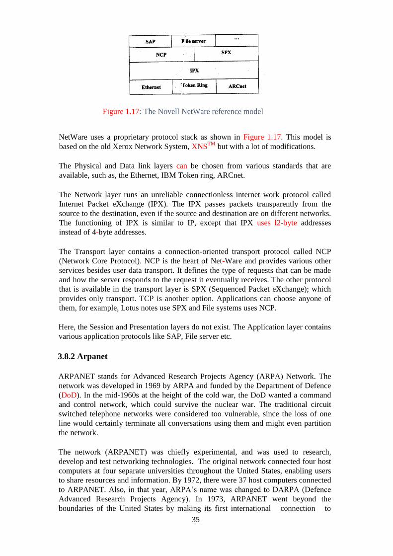
35

Figure 1.17: The Novell NetWare reference model

NetWare uses a proprietary protocol stack as shown in Figure 1.17. This model is

based on the old Xerox Network System, XNSTM

but with a lot of modifications.

The Physical and Data link layers can be chosen from various standards that are

available, such as, the Ethernet, IBM Token ring, ARCnet.

The Network layer runs an unreliable connectionless internet work protocol called

Internet Packet eXchange (IPX). The IPX passes packets transparently from the

source to the destination, even if the source and destination are on different networks.

The functioning of IPX is similar to IP, except that IPX uses l2-byte addresses

instead of 4-byte addresses.

The Transport layer contains a connection-oriented transport protocol called NCP

(Network Core Protocol). NCP is the heart of Net-Ware and provides various other

services besides user data transport. It defines the type of requests that can be made

and how the server responds to the request it eventually receives. The other protocol

that is available in the transport layer is SPX (Sequenced Packet eXchange); which

provides only transport. TCP is another option. Applications can choose anyone of

them, for example, Lotus notes use SPX and File systems uses NCP.

Here, the Session and Presentation layers do not exist. The Application layer contains

various application protocols like SAP, File server etc.

3.8.2 Arpanet

ARPANET stands for Advanced Research Projects Agency (ARPA) Network. The

network was developed in 1969 by ARPA and funded by the Department of Defence

(DoD). In the mid-1960s at the height of the cold war, the DoD wanted a command

and control network, which could survive the nuclear war. The traditional circuit

switched telephone networks were considered too vulnerable, since the loss of one

line would certainly terminate all conversations using them and might even partition

the network.

The network (ARPANET) was chiefly experimental, and was used to research,

develop and test networking technologies. The original network connected four host

computers at four separate universities throughout the United States, enabling users

to share resources and information. By 1972, there were 37 host computers connected

to ARPANET. Also, in that year, ARPA‘s name was changed to DARPA (Defence

Advanced Research Projects Agency). In 1973, ARPANET went beyond the

boundaries of the United States by making its first international connection to

36

England and Norway. One goal of ARPANET was to devise a network that

would still be operational, even if, part of the network failed. The research in this area

resulted in a set of networking rules or protocols, called TCP/IP (Transmission

Control Protocol/Internet Protocol).

TCP/IP is a set of protocols that govern how data is transmitted across networks. It

also enables different types of computer operating systems such as DOS and UNIX to

share data across a network.

ARPANET functioned as a ―backbone‖ network allowing smaller local networks to

connect to the backbone.

Once these smaller networks were connected to the backbone, they were in effect

connected to each other.

In 1983, DARPA decided that TCP/IP would be the standard set of protocols used by

computers connecting to ARPANET. This meant that any smaller networks (for

example, a university network) that wanted to connect to ARPANET also had to use

TCP/IP. TCP/IP was available for free and was increasingly used by networks. The

spread of TCP/IP helped create the Internet, as we know it today, which is the

network of networks that either use the TCP/IP protocols, or can interact with TCP/IP

networks.

ARPANET continued to grow, encompassing many networks from universities and

government institutions. To help manage this rapidly growing ―network of

networks‖, ARPANET was split into two networks in 1983:

ARPANET continued to be a research and development network.

MILNET an unclassified network reserved only for military sites. MILNET

continues to serve this function.

In 1986, a faster backbone network called the NSFNET (National Science

Foundation Network) was created. By 1989, there were over 10,000 host computers

connected to the Internet.

Because of the success of the NSFNET, plans were made to phase out ARPANET.

Many of the sites connected to ARPANET were absorbed by the NSFNET and in

1990 ARPANET was officially dissolved.

3.8.3 Internet

When ARPANET and NSFNET were interconnected the number of networks,

machines and users grew exponentially, many regional networks joined up and

connections were made across many countries.

The Internet is said to have been ―officially‖ born around 1982 when the different

networks (Because It‘s Time Network(BITNET), European Academic and Research

Network(EARN), etc.) agreed on using the TCP/IP protocol as a standard for their

interconnections making it a network of networks and overcoming some of the

previous cacophony of standards, protocols and increasing its coverage.

37

The word Internet was coined from the word‘s ―interconnection‖ and ―network‖,

Now Internet is the world‘s largest computer network. It is considered to be the

network of networks, and is scattered all over the world. The computers connected to

the Internet may communicate with each other using fibre optic cables, telephone

lines, satellite links and other media.

The development of Internet is coordinated by a non-profit organisation called the

Internet Society (ISOC). Its aim is to spread the use of Internet, keep statistics of its

use, helpless developed countries in building their infrastructure and Internet-

technology. The Internet Architecture Board (lAB), plans long term trends and keeps

a record of the RFC (Request for Comments) documents on various technical

solutions and protocols used in Internet. The development is also steered by the IETF

(Internet Engineering Task Force), which has several subgroups for handling

various problems and planning new standards etc.

The rapid growth of Internet may also be due to several important factors:

1. Easy-to-use software -graphical browsers

2. Improved telecommunications connections

3. Rapid spread of automatic data processing, including electronic mail, bank

transfers, etc.

4. The Information Superhighway projects.

The Internet Society maintains a list of Internet service providers providing

connections all over the world. There is one ―universal‖ aspect of all computers

connect to the Internet i.e., they all run the TCP/IP family of protocols.

The Internet Protocol (IP) gives the physical 32-bit address, which uniquely identifies

an individual computer connected to the Internet, while Transmission Control

Protocol (TCP) is a connection-oriented protocol, which takes care of the delivery

and order of the packages. TCP also provides the port numbers for individual

services within a computer.

The major information services provided by the Internet are (with the protocol in

parentheses): electronic mail (SMTP), remote file copying (FTP), remote login,

terminal connections (TELNET), menu-based file access (GOPHER), Wide Area

Information Servers (WAIS, Z39.50), the World Wide Web (HlTP), and the Packet

Internet Groper (PING).

There are three major ways to connect your computer to the Internet:

1. dial up modem access to a computer connected to Internet,

2. dial-up networking, and

3. leased lines (usually from a local telephone company).

Switched Dial-Up Lines

The most common circuit provided by public communication carriers are dial-up

telephone circuits. Subscribers send routing information i.e., the dialled number to

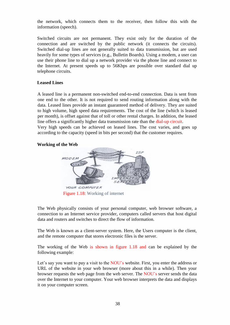
38

the network, which connects them to the receiver, then follow this with the

information (speech).

Switched circuits are not permanent. They exist only for the duration of the

connection and are switched by the public network (it connects the circuits).

Switched dial-up lines are not generally suited to data transmission, but are used

heavily for some types of services (e.g., Bulletin Boards). Using a modem, a user can

use their phone line to dial up a network provider via the phone line and connect to

the Internet. At present speeds up to 56Kbps are possible over standard dial up

telephone circuits.

Leased Lines

A leased line is a permanent non-switched end-to-end connection. Data is sent from

one end to the other. It is not required to send routing information along with the

data. Leased lines provide an instant guaranteed method of delivery. They are suited

to high volume, high speed data requirements. The cost of the line (which is leased

per month), is offset against that of toll or other rental charges. In addition, the leased

line offers a significantly higher data transmission rate than the dial-up circuit.

Very high speeds can be achieved on leased lines. The cost varies, and goes up

according to the capacity (speed in bits per second) that the customer requires.

Working of the Web

Figure 1.18: Working of internet

The Web physically consists of your personal computer, web browser software, a

connection to an Internet service provider, computers called servers that host digital

data and routers and switches to direct the flow of information.

The Web is known as a client-server system. Here, the Users computer is the client,

and the remote computer that stores electronic files is the server.

The working of the Web is shown in figure 1.18 and can be explained by the

following example:

Let‘s say you want to pay a visit to the NOU‘s website. First, you enter the address or

URL of the website in your web browser (more about this in a while). Then your

browser requests the web page from the web server. The NOU‘s server sends the data

over the Internet to your computer. Your web browser interprets the data and displays

it on your computer screen.

39

The glue that holds the Web together is called hypertext and hyperlinks. This feature

allows electronic files on the Web to be linked so that you can easily jump between

them. On the Web you can navigate through pages of information based on what

interests you at that particular moment. This is commonly known as browsing or

surfing the Net.

To access the Web you need software such as Netscape Navigator, Google Chrome,

Mozilla Firefox, Opera or Microsoft Internet Explorer. These are known as web

browsers. Web pages are written in a computer language called HTML, which stands

for Hypertext Markup Language.

3.8.4 ATM Network

Asynchronous Transfer Mode (ATM) is a network technology adopted by the

telecommunication sector. It is a high-performance, cell-oriented switching and

multiplexing technology that utilises fixed-length packets to carry different types of

traffic. The data transfer takes place in the form of cells or packets of a fixed size (53

bytes). The cell used with ATM is relatively small compared to units used with older

technologies. The small constant cell size allows ATM equipment to transmit video,

audio, and computer data over the same network, and assures that no single type of

data hogs the line.

ATM technology is used for both local and wide area networks (LANs and WANs)

that support real-time voice and video as well as data. The topology uses switches

that establish a logical circuit from end to end, which guarantees quality of service

(QoS). However, unlike telephone switches that dedicate circuits end-to-end, unused

bandwidth in ATM‘s logical circuits can be utilised when needed. For example,

idle bandwidth in a video conference circuit can be used to transfer data.

ATM is widely used as a backbone technology in carrier networks and large

enterprises, but never became popular as a local network (LAN) topology. ATM is

highly scalable and supports transmission speeds of 1.5, 25, 100, 155, 622, 2488 and

9953 Mbps. ATM is also running as slow as 9.6 Kbps between ships at sea. An ATM

switch can be added into the middle of a switch fabric to enhance total capacity, and

the new switch is automatically updated using ATM‘s Private Network-to Network

interface (PNNI) routing protocol.

One of the important features of ATM is its ability to specify Quality of Service

(QoS), allowing video and voice to be transmitted smoothly. It provides the

following levels of service:

1. Constant Bit Rate (CBR) guarantees bandwidth for real-time voice and video.

2. Realtime variable Bit Rate (rt-VBR) supports interactive multimedia that

requires minimal delays.

3. Non-Realtime variable-bit-rate (nrt- VBR) is used for busty transaction

traffic.

4. Available Bit Rate (ABR) adjusts bandwidth according to congestion levels

for LAN traffic.

40

5. Unspecified Bit Rate (UBR) provides the best effort for non- critical data such

as file transfers.

Advantages of ATM

1. Flexible bandwidth allocation.

2. Simple routing due to connection-oriented technology.

3. High bandwidth utilisation due to statistical multiplexing.

4. Potential QoS (Quality of Service) guarantees.

Disadvantages of ATM

1. Overhead of cell header (5 bytes per cell).

2. Complex mechanisms for achieving Quality of Service.

3. Congestion may cause cell losses.

4. It is costly compared to IP.

3.9 Types of Computer Networks

Computer Networks are mostly classified on the basis of the geographical

area that the network covers, the topology used, the transmission media used and the

computing model used.

Based on the geographical area covered the networks may be LAN, MAN, WAN.

Local Area Network was discussed in unit 1.

1.9.1 Metropolitan Area Network (MAN)

Figure 1.19: Metropolitan Area network

MAN (Metropolitan Area Network)

Metropolitan Area Network is a Computer network designed for a town or city as

shown in Figure 1.19. In terms of geographic area MAN‘s are larger than local-area

networks (LANs), but smaller than wide-area networks (WANs). MAN‘s are usually

characterised by very high-speed connections using fibre optical cable or other digital

media.

The Typical Characteristics of a MAN are:

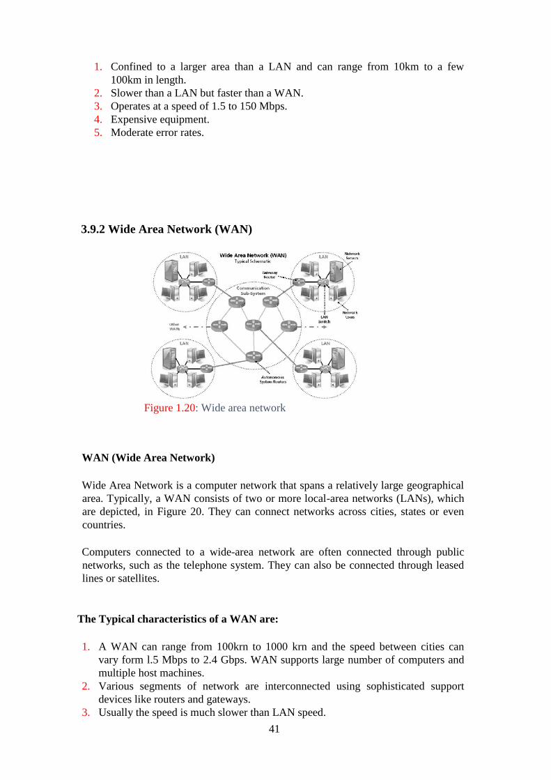
41

1. Confined to a larger area than a LAN and can range from 10km to a few

100km in length.

2. Slower than a LAN but faster than a WAN.

3. Operates at a speed of 1.5 to 150 Mbps.

4. Expensive equipment.

5. Moderate error rates.

3.9.2 Wide Area Network (WAN)

Figure 1.20: Wide area network

WAN (Wide Area Network)

Wide Area Network is a computer network that spans a relatively large geographical

area. Typically, a WAN consists of two or more local-area networks (LANs), which

are depicted, in Figure 20. They can connect networks across cities, states or even

countries.

Computers connected to a wide-area network are often connected through public

networks, such as the telephone system. They can also be connected through leased

lines or satellites.

The Typical characteristics of a WAN are:

1. A WAN can range from 100krn to 1000 krn and the speed between cities can

vary form l.5 Mbps to 2.4 Gbps. WAN supports large number of computers and

multiple host machines.

2. Various segments of network are interconnected using sophisticated support

devices like routers and gateways.

3. Usually the speed is much slower than LAN speed.

42

4. Highest possible error rate compared to LAN & MAN.

3.9.3 Comparison between LAN, MAN, WAN and GAN

Figure 1.21: Comparison between different types of networks.

3.10 Advantages of Networks

Computers in a networked environment provide numerous advantages when

compared to computers in a standalone environment. The immense benefits that the

computer networks provide are in the form of excellent sharing of computational

resources, computational load, increased level of reliability, economy and efficient

person-to-person communication.

Following are some of the major advantages of using computer networks.

1. Resource Sharing

The main aim of a computer network is to make all programs, equipment, and data

available to anyone on the network without regard to the physical location of the

resource and the user. Users need to share resources other than files, as well. A

NETWORK SIZE TRANSMISSION

MEDIA

MAXIMUM

DISTANCE

Local Area

Network

Confined

to building

or campus

Cable used Covers up to

10km

Metropolitan

Area Network

Network

confined

to

city or

town

Different

hardware &

transmission

media are used

Covers the area

of a city or town

Wide Area

Network

Larger than

MAN

Telephone lines,

radio waves,

leased lines or

satellites.

Covers a number

of cities or

countries

43

common example being printers. Printers are utilised only a small percentage of the

time; therefore, companies don‘t want to invest in a printer for each computer.

Networks can be used in this situation to allow all the users to have access to any of

the available printers.

2. High Reliability

Computer networks provide high reliability by having alternative sources of supply.

For example, all files could be replicated on two or three machines, so, if one of them

is unavailable (due to hardware failure), the other copies could be used. In addition,

the presence of multiple CPUs means that if one goes down, the others may be able

to take over its work, although at reduced performance. For military, banking, air

traffic control, nuclear reactor safety, and many other applications, the ability to

continue operating in the face of hardware problems is of utmost importance.

3. Saving Money

Small computers have a much better price/performance ratio than larger ones.

Mainframes are roughly a factor of ton faster than personal computers but they cost

much more. This imbalance has caused many systems designers to build systems

consisting of personal computers, one per user, with data kept on one or more shared

file server machines. In this model, the users are called clients, and the whole

arrangement is called the client-server model.

4. Scalability

The ability to increase the system performance gradually as the workload grows

just by adding more processors. With centralized mainframes, when a system is full,

it must be replaced by a larger one, usually at great expense and even greater

disruption to the users. With client-server model, new clients and new servers can be

added when needed.

5. Communication Medium

A computer network can provide a powerful communication medium among widely

separated users. Using a computer network it is easy for two or more people who are

working on the same project and who live far apart to write a report together. When

one worker, makes a change to an on-line document, the others can see the change

immediately, instead of waiting several days for a letter. Such a speedup makes

cooperation among far-flung groups of people easy whereas previously it was

impossible.

6. Increased Productivity

Networks increase productivity as several people can enter data at the same time, but

they can also evaluate and process the shared data. So, one person can handle

accounts receivable, and someone else processes the profit-and-loss statements.

4.0 CONCLUSION

44

In this introductory unit, you have learnt about the basic concepts of Computer

Networks. You have not only learnt about Networks, but also about the different

types of Networks, their applications, Network Topology, Network protocols, OSI

reference mode and the TCP/IP reference model which is the most commonly used

on the Internet today. Also, the importance of the network protocols and the

importance of using networked system have been extensively discussed.

5.0 SUMMARY

In this unit we have learnt about the basic concepts of Networking. Here we

discussed the different types of networks and the difference between them. Computer

networks are basically classified as LAN, MAN, WAN depending on the

geographical distance covered and depending on the various ways of interconnecting

computers in a network (network topology) like Star, Bus, Ring, Tree, Mesh and

cellular topologies.

We have seen the immense benefits that the computer networks provide in the form

of excellent sharing of computational resources, computational load, increased level

of reliability, economy and efficient person-to-person communication. Here we have

briefly explained some of the network protocols which define a common set of rules

and signals that computers on the network use to communicate with each other.

Standard network architecture is required for meaningful communication between

end systems. We have discussed the two most widely used reference models i.e., the

OSI reference model and the TCP/IP reference model. Nowadays, we come across

different types of networks like Public networks, Research networks, Co-operative

networks, Commercial networks etc. and we have learnt about some of the popular

networks such as Novell NetWare, ARPANET, Internet, ATM network. Towards the

end of this unit the concept of delays was also introduced.

6.0 TUTOR MARKED ASSIGNMENT 1

1. Briefly describe NCP and IPX of Novell NetWare reference model.

2. List the basic components (equipment) needed to connect a computer to

the Internet.

3. What are advantages of having small fixed size cells in ATM?

7.0 REFERENCE/FURTHER READINGS

Andrew S. Tenenbaum, Computer Networks, PHI, New Delhi.

William Stalling, Data and Computer Communication, PHI, New Delhi

8.0 ANSWERS TO SELF-ASSESSMENT EXERCISES 1

Question 1

45

Explain the difference between Client/ server and peer-to-peer architecture

Solution

The difference between client/server and peer-to-peer architecture are illustrated in the

table 1.1.

Table 1.1: The difference between client/server and peer-to-peer architecture

S/N Client/server architecture Peer-to-peer architecture

a. This involves dedicated server and specific

clients

Here, nodes act as servers

and at the same time act

as clients

b. Here, services are provided to the clients In this architecture, each

peer has the ability to

give services and receive

services.

c. Each age of information is more important here In this case, connection

between peers is more

vital

d. The storage of data is centralised Each peer stores its own

data

e. There are room for bottleneck since the server

is centralized

There are no room for

bottleneck since the

server is a distributed

system

f. This is more expensive to administer This is less scalable and

stable

Question 2

List the important aspect that should be kept in mind while designing a network

Solution

The important factors that should be noted while building a network are;

a. It is pertinent to have a thorough knowledge of what the network will be

used for to avoid confusion during the network installation

b. You should have a very good budget for an IT network, manage he budget

properly and reserve capital for IT essentials.

c. Giving of adequate installation in the form of training, providing good

safety system and making sure the network has the ability to respond to

future increase demand of the system is very important in the design of a

good network.

d. Having adequate plan to keep the IT system in good condition is very vital

to the sustainability of the network. In other words, there should be good

strategies for maintaining the system.

e. Create room for redundancy in the case of sudden breakthrough of the

network.

f. Write briefly about the areas where networks are used.

46

Question 3

Write briefly about the areas where networks are used.

Solution

A network is the linking of individuals and devices together. These networks are used

in virtually every aspect of lives, ranging from offices where you share printers, world

Wide Web (WWW) you exchange information, digital video share among friends

through social media and e-mail address and sharing of applications and storage

servers

Question 4

Differentiate between broadcast and point-to-point networks.

Solution

Broadcast is a method of sending message from individual person or devices to

multiple person or devices. In other words, it is a method of connection between one

node and many networking nodes.

While point-to-point is a method of sending message from one individual or devices to

another individual or devices. In other words, it is a method of having direct

connection between two entities or networking nodes.

ANSWERS TO SELF-ASSESSMENT EXERCISES 2

Question 1

List the importance of using computer networks in Airline and Railway reservation

systems.

Solution

The importance of using Computer networks in Airline and Railway Reservation

Systems:

a. Computer devices are used for booking and reservations

b. They are used for maintaining time-table

c. They are used for scheduling crews

d. They are used for managing the movement of Airline and control of Railways

reservation System, most especially, the underground railways.

Question 2

What are the various types of networks

Solution

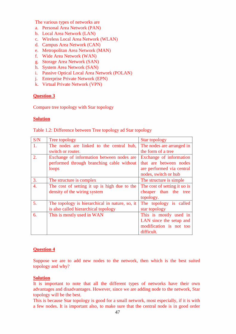
47

The various types of networks are

a. Personal Area Network (PAN)

b. Local Area Network (LAN)

c. Wireless Local Area Network (WLAN)

d. Campus Area Network (CAN)

e. Metropolitan Area Network (MAN)

f. Wide Area Network (WAN)

g. Storage Area Network (SAN)

h. System Area Network (SAN)

i. Passive Optical Local Area Network (POLAN)

j. Enterprise Private Network (EPN)

k. Virtual Private Network (VPN)

Question 3

Compare tree topology with Star topology

Solution

Table 1.2: Difference between Tree topology ad Star topology

S/N Tree topology Star topology

1. The nodes are linked to the central hub,

switch or router.

The nodes are arranged in

the form of a tree

2. Exchange of information between nodes are

performed through branching cable without

loops

Exchange of information

that are between nodes

are performed via central

nodes, switch or hub

3. The structure is complex The structure is simple

4. The cost of setting it up is high due to the

density of the wiring system

The cost of setting it uo is

cheaper than the tree

topology.

5. The topology is hierarchical in nature, so, it

is also called hierarchical topology

The topology is called

star topology

6. This is mostly used in WAN This is mostly used in

LAN since the setup and

modification is not too

difficult.

Question 4

Suppose we are to add new nodes to the network, then which is the best suited

topology and why?

Solution

It is important to note that all the different types of networks have their own

advantages and disadvantages. However, since we are adding node to the network, Star

topology will be the best.

This is because Star topology is good for a small network, most especially, if it is with

a few nodes. It is important also, to make sure that the central node is in good order

48

and always functioning. The switches, routers or hubs should be well secured since

they are the heart of the system.

ANSWERS TO SELF-ASSESSMENT EXERCISES 3

Question 1

Give two reasons for using layered protocols

Solution

Layered protocols are used to make:

1. Simple, the deign process, hence, give proper definition of the functions of each

layer and the interaction between them.

2. The network pliable so that it can be easy to modify and develop.

Question 2

Explain OSI reference model in detail.

Solution

The student is referred to section 3.6.1, pages 19-27

Question 3

Explain the TCP/IP reference model in detail

Solution

The student is refered to section 3.6.2, pages 27-31

Question 4

Bring out the difference between TCP and UDP

Table 1.3: difference between TCP and UDP

S/N TCP UDP

1. Connection oriented protocols i.e.,

link the sender and receiver before

sending data

Connection oriented protocol i.e,

does not link sender and receiver

before sending data

2. It is reliable. Data sent are sure to be

delivered to the receiver. If there is

failure along the way, it resends the

data. It also checks for error in the

packet so that it is not lost or

It is unreliable. There is no

assurance of delivering the

datagram packet. The datagram

packet may be lost or corrupted

along the way.

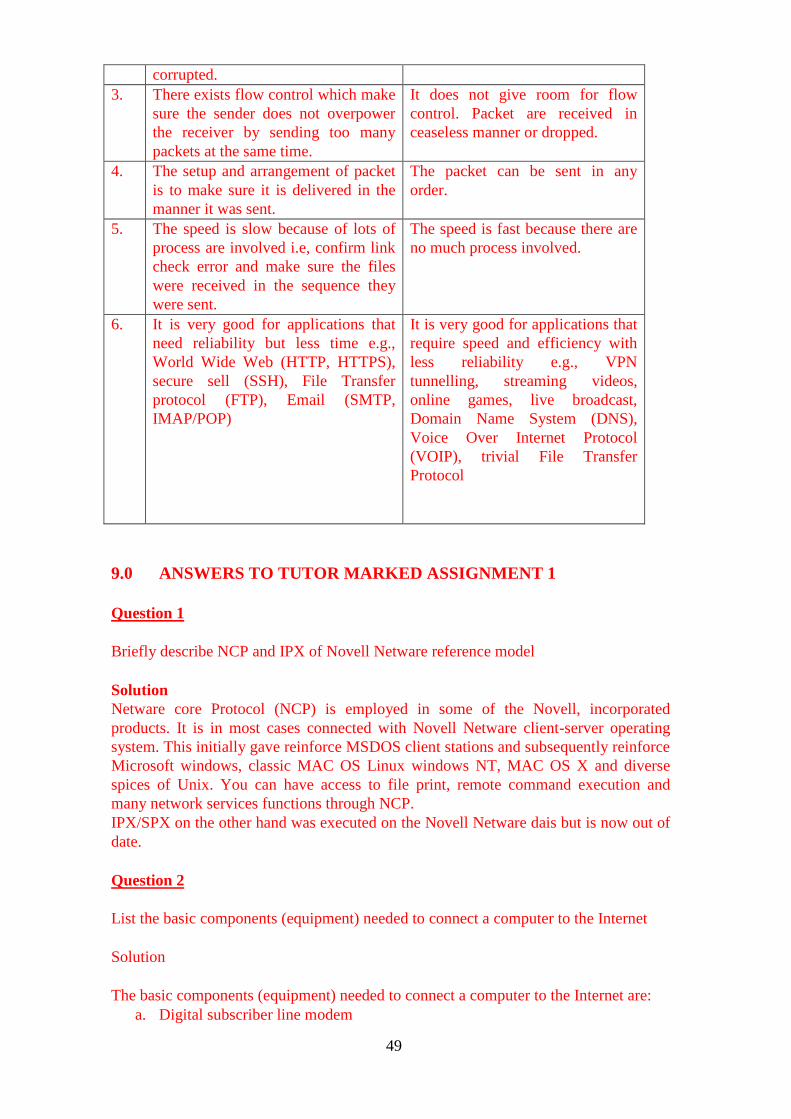
49

corrupted.

3. There exists flow control which make

sure the sender does not overpower

the receiver by sending too many

packets at the same time.

It does not give room for flow

control. Packet are received in

ceaseless manner or dropped.

4. The setup and arrangement of packet

is to make sure it is delivered in the

manner it was sent.

The packet can be sent in any

order.

5. The speed is slow because of lots of

process are involved i.e, confirm link

check error and make sure the files

were received in the sequence they

were sent.

The speed is fast because there are

no much process involved.

6. It is very good for applications that

need reliability but less time e.g.,

World Wide Web (HTTP, HTTPS),

secure sell (SSH), File Transfer

protocol (FTP), Email (SMTP,

IMAP/POP)

It is very good for applications that

require speed and efficiency with

less reliability e.g., VPN

tunnelling, streaming videos,

online games, live broadcast,

Domain Name System (DNS),

Voice Over Internet Protocol

(VOIP), trivial File Transfer

Protocol

9.0 ANSWERS TO TUTOR MARKED ASSIGNMENT 1

Question 1

Briefly describe NCP and IPX of Novell Netware reference model

Solution

Netware core Protocol (NCP) is employed in some of the Novell, incorporated

products. It is in most cases connected with Novell Netware client-server operating

system. This initially gave reinforce MSDOS client stations and subsequently reinforce

Microsoft windows, classic MAC OS Linux windows NT, MAC OS X and diverse

spices of Unix. You can have access to file print, remote command execution and

many network services functions through NCP.

IPX/SPX on the other hand was executed on the Novell Netware dais but is now out of

date.

Question 2

List the basic components (equipment) needed to connect a computer to the Internet

Solution

The basic components (equipment) needed to connect a computer to the Internet are:

a. Digital subscriber line modem

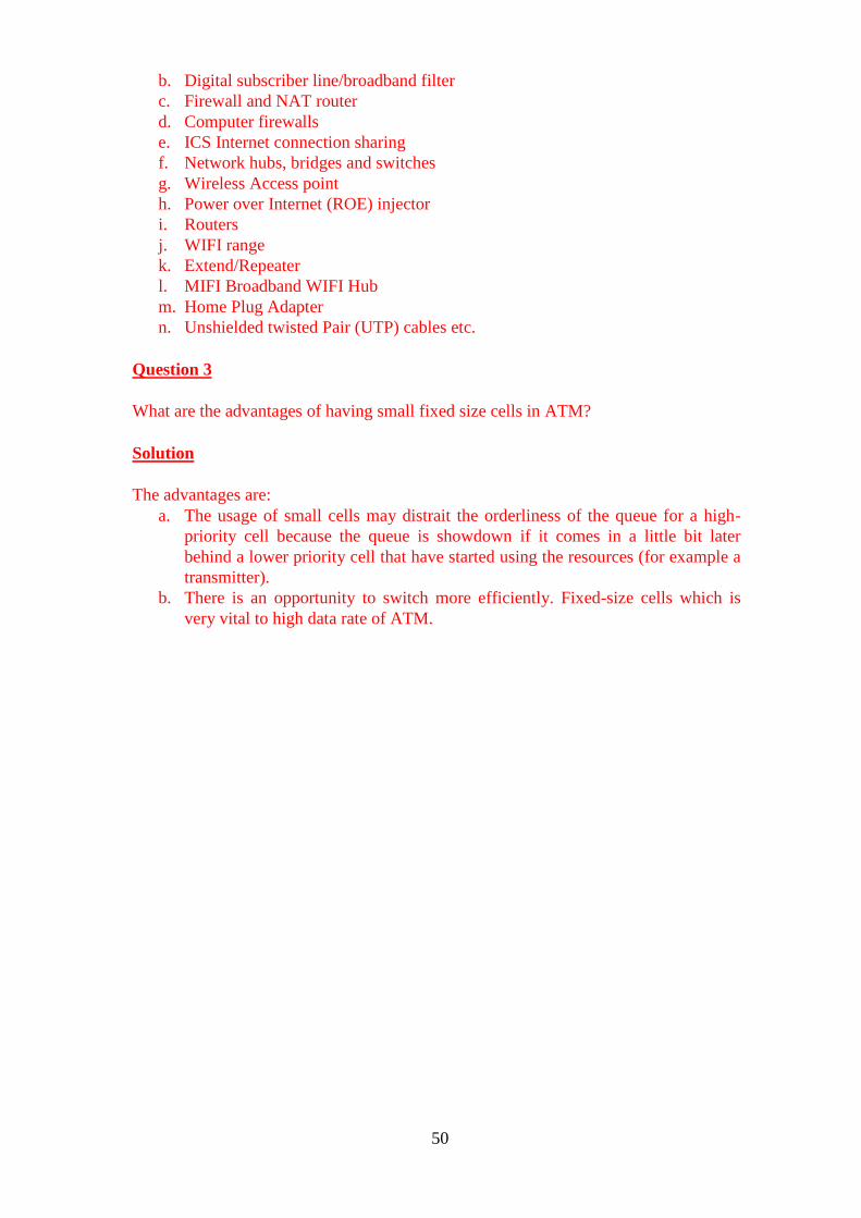
50

b. Digital subscriber line/broadband filter

c. Firewall and NAT router

d. Computer firewalls

e. ICS Internet connection sharing

f. Network hubs, bridges and switches

g. Wireless Access point

h. Power over Internet (ROE) injector

i. Routers

j. WIFI range

k. Extend/Repeater

l. MIFI Broadband WIFI Hub

m. Home Plug Adapter

n. Unshielded twisted Pair (UTP) cables etc.

Question 3

What are the advantages of having small fixed size cells in ATM?

Solution

The advantages are:

a. The usage of small cells may distrait the orderliness of the queue for a high-

priority cell because the queue is showdown if it comes in a little bit later

behind a lower priority cell that have started using the resources (for example a

transmitter).

b. There is an opportunity to switch more efficiently. Fixed-size cells which is

very vital to high data rate of ATM.

51

UNIT 2 DATA TRANSMISSION

CONTENTS

1.0 Introduction

2.0 Objectives

3.0 Main Content

3.1 Data Communication Terminology

3.1.1 Channel

3.1.2 Baud

3.1.3 Bandwidth

3.1.4 Frequency

3.2 Modes of Data Transmission

3.2.1 Serial and Parallel Communication

3.2.2 Synchronous, Asynchronous and Isochronous Communication

3.2.3 Simplex, Half Duplex and Full Duplex Communication

3.3 Analogue and Digital Data Transmission

3.4 Transmission Impairments

3.4.1 Attenuation

3.4.2 Delay Distortion

3.4.3 Noise

3.4.4 Concept of Delays

3.5 Transmission Media and its Characteristics

3.5.1 Magnetic media

3.5.2 Twisted Pair

3.5.3 Baseband Coaxial Cable

3.5.4 Broadband Coaxial Cable

3.5.5 Optical Fibre

3.5.6 Comparison between Optical Fibre and Copper wire

3.6 Wireless Transmission

3.6.2 Microwave Transmission

3.6.2 Radio Transmission

3.6.3 Infrared and Millimetre Waves

3.7 Wireless LAN

4.0 Conclusion

5.0 Summary



1.0 INTRODUCTION

Communication from a source to a destination, that is, from one computer to another

or from one device to another, involves the transfer of information from the sender to

52

the receiver. The transfer of data from one machine to another machine such that, the

sender and the receiver both interpret the data correctly is known as Data

Communication.

All communication between devices requires that the devices agree on the format of

the data. The set of rules defining a format is known as a protocol. At the very least, a

communications protocol must define the following:

1. Transmission media used.

2. Rate of transmission (in baud or bps).

3. Whether transmission is to be synchronous or asynchronous.

4. Whether data is to be transmitted in half-duplex or full-duplex mode.

In order to understand this, we need to learn about some of the basic concepts and

terminologies related to data transmission, which we will be explained in this unit.

2.0 OBJECTIVES


1. understand the concept of Transmission terminology

2. differentiate between Serial and Parallel communication

3. differentiate between Analogue and Digital Data Transmission

4. have a broad idea about the different Transmission Impairments

5. compare the different Transmission Media and their characteristics

6. understand Wireless Transmission and realise its importance.

3.0 MAIN CONTENT

3.1 Data Communication Terminology

The transfer of data from one machine to another machine such that, the sender and

the receiver both interpret the data correctly is known as Data Communication.

3.1.1 Channel

In communications, the term channel refers to a path of communications between two

computers or devices. A communication channel provides everything that is needed

for the transfer of electronic information from one location to another. It may refer to

the physical medium, such as coaxial cable, or to a specific carrier frequency (sub-

channel) within a larger channel or a wireless medium.

The channel capacity of a transmission system is the maximum rate at which

information can be transferred reliably over a given period of time. Two basic types

of channels that are used in voice and data communication are Analogue and Digital.

The Analogue type of channel transmits signals generally using sinusoidal waves as

shown in Figure 1.22. Non-sinusoidal waves can also be used for transmission. The

commercial radio station and Public telephone system are examples of this type. The

53

Digital type of channel transmits pulsed wave signals, such as, those shown in Figure

1.23.

3.1.2 Baud

Pronounced bawd, Baud is the number of signalling elements that occur each second.

The term is named after J.M.E. Baudot, the inventor of the Baudot telegraph code.

At slow speeds, only one bit of information (signalling element) is encoded in each

electrical change. The baud, therefore, indicates the number of bits per second that

are transmitted. For example, 300 baud means that 300 bits are transmitted each

second (abbreviated 300 bps). Assuming asynchronous communication, which

requires 10 bits per character, this translates in to 30 characters per second (cps). For

slow rates (below 1,200 baud), you can divide the baud by 10 to see how many

characters per second are sent.

At higher speeds, it is possible to encode more than one bit in each electrical change.

4,800 baud may allow 9,600 bits to be sent each second. At high data transfer speeds;

therefore, data transmission rates are usually expressed in bits per second (bps) rather

than baud. For example, a 9,600bps modem may operate at only 2,400 baud.

3.1.3 Bandwidth

The amount of data or signals that the transmission media can carry in a fixed

amount of time is called Bandwidth. The Bandwidth depends upon the length, media

and signalling technique used. A high bandwidth allows increased throughput and

better performance. A medium that has a high capacity has a high bandwidth. A

medium that has limited capacity has a low bandwidth. It is calculated using the

difference between the highest and the lowest frequencies that the medium can carry.

For digital devices, the bandwidth is usually expressed in bits per second (bps) or

bytes per second. For analogue devices, the bandwidth is expressed in cycles per

second, or Hertz (Hz).

Bandwidth is particularly important for 1/0 devices. For example, a fast disk drive

can be hampered by a bus with a low bandwidth.

3.1.4 Frequency

Frequency is the number of cycles or periods a signal completes within one second.

The unit of measuring frequency is called Hertz named after a German

mathematician Heinrich Hertz. One Hz is one cycle/second. We use one Kilohertz

or one kHz to mean 1000Hz and one Megahertz or one MHz to mean 1000 kHz or

1000000Hz.

3.2 Modes of Data Transmission

Data can be transmitted from Source to Destination in a number of ways. The

different modes of data transmission will be outlined as follows:

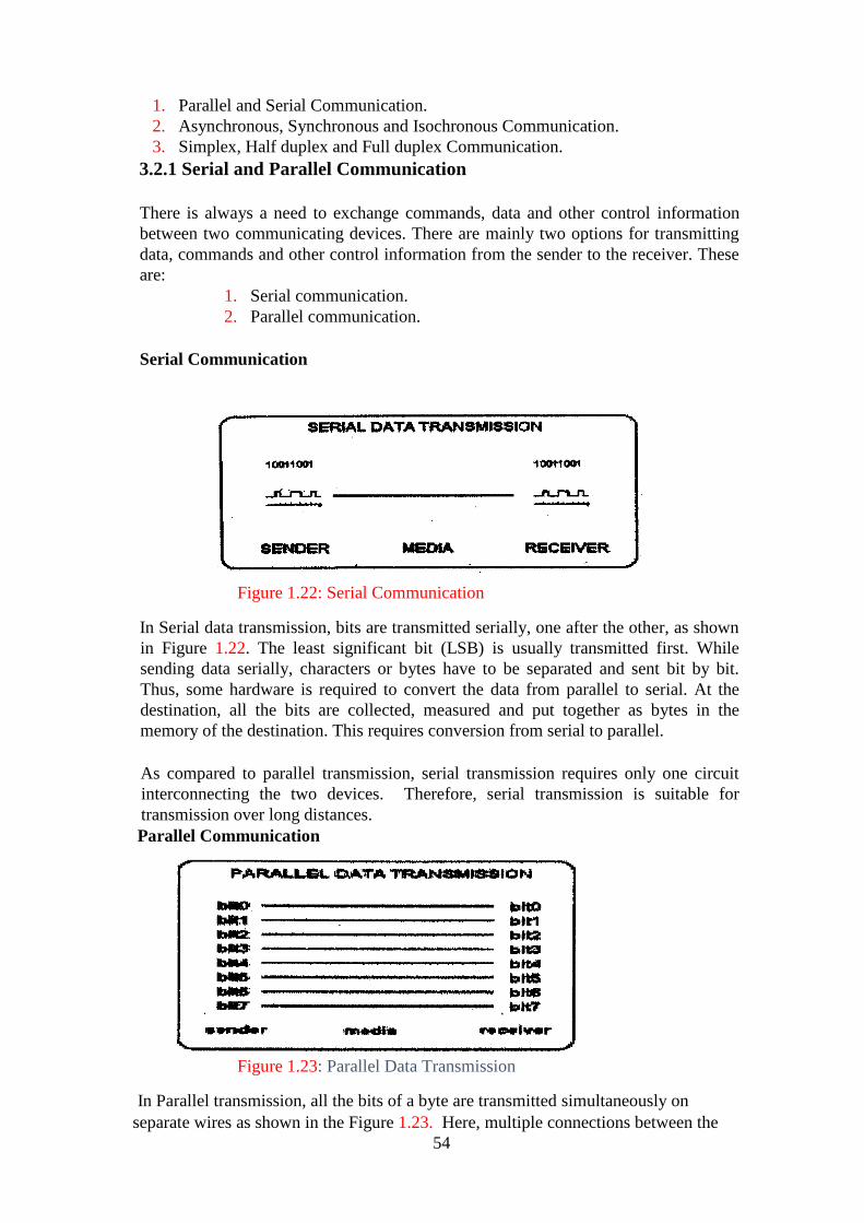
54

1. Parallel and Serial Communication.

2. Asynchronous, Synchronous and Isochronous Communication.

3. Simplex, Half duplex and Full duplex Communication.

3.2.1 Serial and Parallel Communication

There is always a need to exchange commands, data and other control information

between two communicating devices. There are mainly two options for transmitting

data, commands and other control information from the sender to the receiver. These

are:

1. Serial communication.

2. Parallel communication.

Serial Communication

Figure 1.22: Serial Communication

In Serial data transmission, bits are transmitted serially, one after the other, as shown

in Figure 1.22. The least significant bit (LSB) is usually transmitted first. While

sending data serially, characters or bytes have to be separated and sent bit by bit.

Thus, some hardware is required to convert the data from parallel to serial. At the

destination, all the bits are collected, measured and put together as bytes in the

memory of the destination. This requires conversion from serial to parallel.

As compared to parallel transmission, serial transmission requires only one circuit

interconnecting the two devices. Therefore, serial transmission is suitable for

transmission over long distances.

Parallel Communication

Figure 1.23: Parallel Data Transmission

In Parallel transmission, all the bits of a byte are transmitted simultaneously on

separate wires as shown in the Figure 1.23. Here, multiple connections between the

55

two devices are therefore, required. This is a very fast method of transmitting data

from one place to another.

The disadvantage of Parallel transmission is that it is very expensive, as it requires

several wires for both sending, as well as receiving equipment. Secondly, it demands

extraordinary accuracy that cannot be guaranteed over long distances.

3.2.2 Asynchronous, Synchronous and Isochronous Communication

One of the major difficulties in data transmission is that of synchronising

the receiver (destination) with the sender (source). This is the main problem with

serial communication. The receiver must be able to detect the beginning of each new

character in the bit stream, that is, being presented to it and if it is not able to achieve

this, it will not be able to interpret the incoming bit stream correctly.

The three mechanisms used for synchronisation are:

1. Asynchronous Communication

2. Synchronous Communication

3. Isochronous Communication

Asynchronous Communication

Asynchronous communication sends individual characters one at a time framed by a

start bit and I or 2 stop bits. Each frame begins with a start bit that enables the

receiving device to adjust to the timing of the transmitted signal. The message can

begin at any time. Here, messages are kept as short as possible because, the sending

and receiving devices should not draft out of synchronisation, when the message is

being transferred. Asynchronous communication is most frequently used to transmit

character data and is ideally suited for characters that are transmitted at irregular

intervals, such as, when users are typing in character data from the keyboard.

A typical frame used to transmit a character data has four components:

1. A start bit: Signals the starting a frame and enables the receiving device to

synchronise itself with the message.

2. Data Bits: Consists of 7 or 8 bits when character data is being transmitted.

3. Parity Bits: Optionally used as a crude method for detecting transmission

errors.

4. A stop bit or bits: Signals the end of the data frame.

Error detection in asynchronous transmission makes use of the parity bit Parity

techniques can detect errors that affect only one bit and if two or more bits are

affected by errors, the parity techniques may not be able to detect them.

Advantages of Asynchronous Communication

56

1. Asynchronous transmission is simple, inexpensive and is ideally suited for

transmitting small frames at irregular intervals (e.g., Data entry from a

keyboard).

2. As each individual character is complete in itself, if a character is corrupted

during transmission, its successor and predecessor will not be affected.

Disadvantages of Asynchronous Communication

1. As start, stop and parity bits must be added to each character that is to be

transmitted, this adds a high overhead to transmission. This wastes the

bandwidth; as a result, asynchronous transmission is undesirable for

transmitting large amounts of data.

2. Successful transmission inevitably depends on the recognition of the start bits,

hence, as these bits can be easily missed or occasionally spurious, as start bits

can be generated by line interference, the transmission may be unsuccessful.

3. Due to the effects of distortion the speed of asynchronous transmission is

limited.

Synchronous Communication

In synchronous communication the whole block of data bits is transferred at once,

instead of one character at a time. Here, transmission begins at a predetermined

regular time instant. A sync signal is used to tell the receiving station that a new

frame is arriving and to synchronise the receiving station.

Sync signals, generally utilise a bit pattern that cannot appear elsewhere in the

messages, ensuring that they will always be distinct and easy for the receiver to

recognise. As the transmitter and receiver remain in synchronisation for the duration

of the transmission, frames can be of longer length.

As frames are longer, the parity method of error detection is not suitable because, if

multiple bits are affected, then, the parity technique will not report error accurately.

Hence, the technique used with synchronous transmission is the Cyclic Redundancy

Check (CRC).

The transmitter uses an algorithm to calculate a CRC value that summarises the

entire value of data bits. This CRC value is appended to the data frame. The receiver

uses the same algorithm, recalculates the CRC and compares the CRC in the frame to

the value that it has calculated. If these values match then, it is sure that the frame

was transmitted without error.

An end bit pattern indicates the end of the frame. Like sync the bit pattern for end is

such that, it will not appear elsewhere in the messages, ensuring that they will always

be distinct and easy for the receiver to recognise at the end of the frame.

Serial synchronous transmission is used for high-speed communication between

computers. It is used when high volumes of data are to be transmitted.

57

Advantages of Synchronous Communication

1. Synchronous transmission is more efficient because, only 4 additional bytes

(for start and end frames) are required to transmit up to 64 k bits.

2. Synchronous transmission is not really prone to distortion, as a result, it can

be used at high-speeds.

Disadvantages of Synchronous Communication

1. Synchronous transmission is expensive as complex circuitry is required and it

is difficult to implement.

2. If an error occurs during transmission, rather than just a single character the

whole block of data is lost.

3. The sender cannot transmit characters simply, as they occur, but has to store

them until it has built up a block. Thus, this is not suitable where characters

are generated at irregular intervals.

Isochronous Communication

This method combines the approaches of asynchronous and synchronous

connumerations. As in the asynchronous method, each character has both the start

and stop bits. The idle period (where no transmission takes place) between the two

characters is not random but an exact multiple of one-character time interval. If, the

time to transmit a character (Including its parity, start, stop bits) is t, the time interval

between characters cannot be random as in the asynchronous method. It is also not 0

as in the synchronous method. It has to be t, 2t, 3t………. nt where n is any positive

integer. Here, the signal is expected to be received within certain delay bounds say

Tmin to Tmax.

Advantages of Isochronous Communication

1. Isochronous transmission guarantees transmission rates, and it is almost

deterministic.

2. It has low overheads.

3. It has high speed.

Disadvantages of Isochronous Communication

1. In isochronous transmission its necessary to ensure that the clocking device is

fault tolerant.

3.2.3 Simplex, Half Duplex and Full Duplex Communication

This classification of data transmission is based on the question of, communication

can send data and at what point of time.

The three basic ways in which this can be done are:

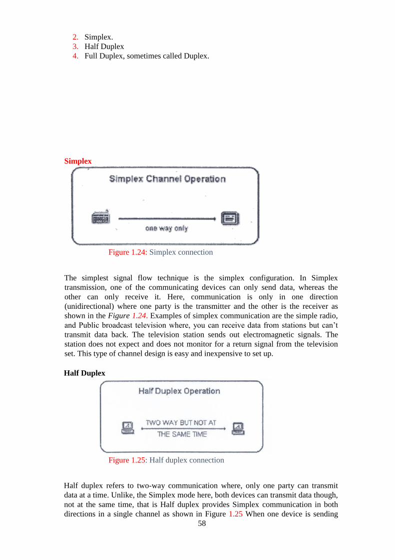
58

2. Simplex.

3. Half Duplex

4. Full Duplex, sometimes called Duplex.

Simplex

Figure 1.24: Simplex connection

The simplest signal flow technique is the simplex configuration. In Simplex

transmission, one of the communicating devices can only send data, whereas the

other can only receive it. Here, communication is only in one direction

(unidirectional) where one party is the transmitter and the other is the receiver as

shown in the Figure 1.24. Examples of simplex communication are the simple radio,

and Public broadcast television where, you can receive data from stations but can‘t

transmit data back. The television station sends out electromagnetic signals. The

station does not expect and does not monitor for a return signal from the television

set. This type of channel design is easy and inexpensive to set up.

Half Duplex

Figure 1.25: Half duplex connection

Half duplex refers to two-way communication where, only one party can transmit

data at a time. Unlike, the Simplex mode here, both devices can transmit data though,

not at the same time, that is Half duplex provides Simplex communication in both

directions in a single channel as shown in Figure 1.25 When one device is sending

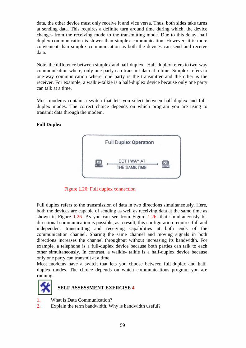
59

data, the other device must only receive it and vice versa. Thus, both sides take turns

at sending data. This requires a definite turn around time during which, the device

changes from the receiving mode to the transmitting mode. Due to this delay, half

duplex communication is slower than simplex communication. However, it is more

convenient than simplex communication as both the devices can send and receive

data.

Note, the difference between simplex and half-duplex. Half-duplex refers to two-way

communication where, only one party can transmit data at a time. Simplex refers to

one-way communication where, one party is the transmitter and the other is the

receiver. For example, a walkie-talkie is a half-duplex device because only one party

can talk at a time.

Most modems contain a switch that lets you select between half-duplex and full-

duplex modes. The correct choice depends on which program you are using to

transmit data through the modem.

Full Duplex

Figure 1.26: Full duplex connection

Full duplex refers to the transmission of data in two directions simultaneously. Here,

both the devices are capable of sending as well as receiving data at the same time as

shown in Figure 1.26. As you can see from Figure 1.26, that simultaneously bi-

directional communication is possible, as a result, this configuration requires full and

independent transmitting and receiving capabilities at both ends of the

communication channel. Sharing the same channel and moving signals in both

directions increases the channel throughput without increasing its bandwidth. For

example, a telephone is a full-duplex device because both parties can talk to each

other simultaneously. In contrast, a walkie- talkie is a half-duplex device because

only one party can transmit at a time.

Most modems have a switch that lets you choose between full-duplex and half-

duplex modes. The choice depends on which communications program you are

running.


1. What is Data Communication?

2. Explain the term bandwidth. Why is bandwidth useful?

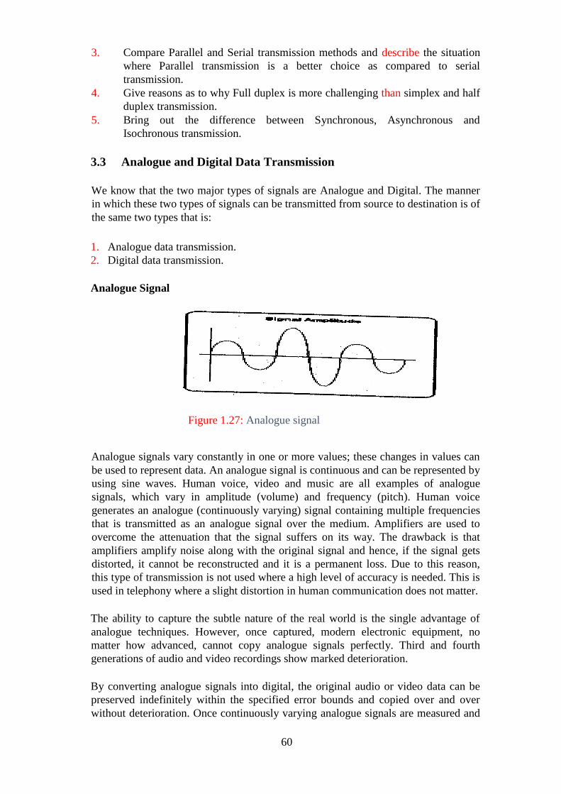
60

3. Compare Parallel and Serial transmission methods and describe the situation

where Parallel transmission is a better choice as compared to serial

transmission.

4. Give reasons as to why Full duplex is more challenging than simplex and half

duplex transmission.

5. Bring out the difference between Synchronous, Asynchronous and

Isochronous transmission.

3.3 Analogue and Digital Data Transmission

We know that the two major types of signals are Analogue and Digital. The manner

in which these two types of signals can be transmitted from source to destination is of

the same two types that is:

1. Analogue data transmission.

2. Digital data transmission.

Analogue Signal

Figure 1.27: Analogue signal

Analogue signals vary constantly in one or more values; these changes in values can

be used to represent data. An analogue signal is continuous and can be represented by

using sine waves. Human voice, video and music are all examples of analogue

signals, which vary in amplitude (volume) and frequency (pitch). Human voice

generates an analogue (continuously varying) signal containing multiple frequencies

that is transmitted as an analogue signal over the medium. Amplifiers are used to

overcome the attenuation that the signal suffers on its way. The drawback is that

amplifiers amplify noise along with the original signal and hence, if the signal gets

distorted, it cannot be reconstructed and it is a permanent loss. Due to this reason,

this type of transmission is not used where a high level of accuracy is needed. This is

used in telephony where a slight distortion in human communication does not matter.

The ability to capture the subtle nature of the real world is the single advantage of

analogue techniques. However, once captured, modern electronic equipment, no

matter how advanced, cannot copy analogue signals perfectly. Third and fourth

generations of audio and video recordings show marked deterioration.

By converting analogue signals into digital, the original audio or video data can be

preserved indefinitely within the specified error bounds and copied over and over

without deterioration. Once continuously varying analogue signals are measured and

61

converted into digital form, they can be stored and transmitted without loss of

integrity due to the accuracy of digital methods.

Digital Data Transmission

Figure 1.28: Digital Data Transmission

Digital data transmission describes any system based on discontinuous data or events.

Computers are digital machines because at their most basic level they can distinguish

between just two values, 0 and 1, or off and on. There is no simple way to represent all

the values in between, such as 0.25. All data that a computer processes must be

encoded digitally, as a series of zeroes and ones.

Information coming out of the computer is in the form of digital signals. The

bandwidth of a digital signal is infinite as compared to any medium, which has a

limited bandwidth. Therefore, as the signal is generated and enters the medium, at

that point of entry, only limited frequencies are permissible on the medium and this

depends upon the bandwidth. As the signal traverses over the medium it gets

distorted and beyond a certain distance, the signal becomes unrecognisable from the

original one. A hardware device called Repeater is used to regenerate the digital

signal.

The repeater measures the signal values at regular intervals to recognise the 0‘s and

l‘s in the signal and regenerates them. Hence, there is no loss of information. The

number of repeaters to be used depends on the distance between the source and the

destination. Any line with repeaters placed at appropriate distance is called a digital

line.

When information, music, voice and video are turned into binary digital form, they

can be electronically manipulated, preserved and regenerated perfectly at high speed.

The millionth copy of a computer file is exactly the same as the original. This is,

nevertheless, a major advantage of digital processing.

3.4 Transmission Impairments

When data is transmitted from a transmitter to receiver, there is scope for

transmission errors. If, transmission media were perfect, the receiver would receive

exactly the same signal that the transmitter sent. Unfortunately, media are not perfect,

so the received signal may sometimes not be the same as the transmitted signal.

Transmission lines suffer from three major problems:

1. Attenuation.

2. Delay distortion.

3. Noise.

62

3.4.1 Attenuation

Attenuation is the loss of energy as the signal propagates outwards. On guided media

(e.g., wires and optical fibres), the signal falls off logarithmically with the distance.

Attenuation is very small at short distances; therefore, the original signal can be

recognised without too much distortion. Attenuation increases with distance as, some

of the signal energy is absorbed by the medium. The loss is expressed in decibels per

kilometre (db/km). The amount of energy lost depends on the frequency. Attenuation

is also higher at higher frequencies.

If the attenuation is high, the receiver may not be able to detect the signal at all, or

the signal may fall below the noise level. In many cases, the attenuation properties of

a medium are known, so amplifiers can be put in place to try to compensate for

the frequency-dependent attenuation. This approach helps but can never restore the

signal exactly back to its original shape.

3.4.2 Delay Distortion

Delay distortion is caused by the fact that the signals of varying frequencies travel at

different speeds along the medium. Any complex signal can be decomposed into

different sinusoidal signals of different frequencies, resulting, in a frequency

bandwidth for every signal.

One property of signal propagation is that the speed of travel of the frequency is the

highest at the centre of this bandwidth, and lowest at both ends. Therefore, at the

receiving end, signals with different frequencies in a given bandwidth will arrive at

different times. If, the signals received are measured at a specific time, they will not

be exactly like the original signal resulting in its misinterpretation.

For digital data, fast components from one bit may catch up and overtake low

components from the bit ahead, mixing the two bits and increasing the probability of

incorrect reception.

3.4.3 Noise

Noise is unwanted energy from sources other than the transmitter. Thermal noise is

caused by the random motion of the electrons in a wire and is unavoidable. Cross talk

is caused by inductive coupling between two wires that are close to each other.

Sometimes when talking on the telephone, you can hear another conversation in the

background. That is crosstalk. Finally, there is impulse noise, caused by spikes on the

power line or other causes. For digital data, impulse noise can wipe out one or more

bits.

3.4.3 Concept of Delays

The average delay required to deliver a packet from source (origin) to destination has

a large impact on the performance of a data network. Delay considerations strongly

influence the choice and performance of network algorithms, such as routing and

flow control. Because of these reasons, it is very important to understand the nature

63

and mechanism of network delay, and the manner in which it depends on the

characteristics of the network.

A large delay is disastrous for data transfer. The total delay can be categorised into

two types. The first type is fixed delay. This is the total delay which is always present

due to buffering, link capacity etc. The second type is variable delay. This is the

delay component which is caused by packets queuing in the routers, congestions etc.

Among the different types of delays, here, we shall discuss Transmission delay and

Propagation delay.

Transmission delay

Transmission delay is the delay, which is present due to link capacities. When

resource reservation methods are supported in routers, transmission delays can

probably be kept low enough to satisfy the overall delay constraint of 200 ms.

When data is transmitted, there is always a minimal amount ‗of delay, due to the

capacity of the links along which the data travels. But the most significant part of the

delay of transmission is usually due to queuing of packets inside routers. This delay

is highly variable and depends both on the number of routers along the path and the

load of the routers.

Propagation delay

Satellite microwave systems can reach remote places on the earth and can also

communicate with mobile devices. As the signal travels a long distance (around

36,000 km), there is a delay of about 5 kms between, the transmission and the

reception of the signal. This delay is known as the propagation delay. Such delays

occur in all communication channels, however, small they may be.

Propagation delay is the time between the last bit transmitted at the head node of the

link and the time the last bit is received at the tail node. This is proportional to the

physical distance between the transmitter and the receiver; it can be relatively

substantial, particularly for a satellite link or a very high-speed link.

The propagation delay depends on the physical characteristics of the link and is

independent of the traffic carried by the link.

3.5 Transmission Media and its Characteristics

Various physical media can be used for the actual transmission of information from

one place to another. Each one has its own niche in terms of bandwidth, delay,

cost, ease of installation and maintenance. Transmission media are roughly

grouped into guided media, such as copper wire and fibre optics, and unguided

media, such as radio and lasers.

3.5.1 Magnetic Media

One of the most common ways to transport data from one computer to another is to

write them onto magnetic tape or floppy disks, physically transport the tape or disks

64

to the destination machine, and read them back in again. While, this method is not as

sophisticated as using a geosynchronous communication satellite, it is often much

more cost effective, especially for applications in which high bandwidth or cost per

bit transported is the key factor.

3.5.2 Twisted Pair

Figure 1.29: Twisted pair cable

Although, the bandwidth characteristics of magnetic tape are excellent, the delay

characteristics are poor. Transmission time is measured in minutes or hours, not

milliseconds. For many applications, an on-line connection is needed. The oldest and

still most common transmission medium is the twisted pair. A twisted pair as shown

in figure 1.29 consists of two insulated copper wires, typically about 1 mm thick. The

purpose of twisting the wires is to reduce electrical interference from similar pairs

that may be close by.

The most common application of the twisted pair is in the telephone system. Nearly

all telephones are connected to the telephone company office by a twisted pair.

Twisted pairs can run several kilometres without amplification, but for longer

distances, repeaters are needed. When many twisted pairs run in parallels for a

substantial distance, such as, all the wires coming from an apartment building to the

telephone company office, they are bundled together and encased in a protective

sheath. The pairs in these bundles would interfere with one another if, it were not

twisted.

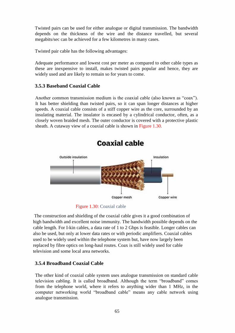
65

Twisted pairs can be used for either analogue or digital transmission. The bandwidth

depends on the thickness of the wire and the distance travelled, but several

megabits/sec can be achieved for a few kilometres in many cases.

Twisted pair cable has the following advantages:

Adequate performance and lowest cost per meter as compared to other cable types as

these are inexpensive to install, makes twisted pairs popular and hence, they are

widely used and are likely to remain so for years to come.

3.5.3 Baseband Coaxial Cable

Another common transmission medium is the coaxial cable (also known as ―coax‖).

It has better shielding than twisted pairs, so it can span longer distances at higher

speeds. A coaxial cable consists of a stiff copper wire as the core, surrounded by an

insulating material. The insulator is encased by a cylindrical conductor, often, as a

closely woven braided mesh. The outer conductor is covered with a protective plastic

sheath. A cutaway view of a coaxial cable is shown in Figure 1.30.

Figure 1.30: Coaxial cable

The construction and shielding of the coaxial cable gives it a good combination of

high bandwidth and excellent noise immunity. The bandwidth possible depends on the

cable length. For I-kin cables, a data rate of 1 to 2 Gbps is feasible. Longer cables can

also be used, but only at lower data rates or with periodic amplifiers. Coaxial cables

used to be widely used within the telephone system but, have now largely been

replaced by fibre optics on long-haul routes. Coax is still widely used for cable

television and some local area networks.

3.5.4 Broadband Coaxial Cable

The other kind of coaxial cable system uses analogue transmission on standard cable

television cabling. It is called broadband. Although the term ―broadband‖ comes

from the telephone world, where it refers to anything wider than 1 MHz, in the

computer networking world ―broadband cable‖ means any cable network using

analogue transmission.

66

Since, broadband networks use standard cable television technology, the cables can

be used up to 300 MHz (and often up to 450 MHz) and can run for nearly 100 kin

due to the analogue signalling, which is much less critical than digital signalling. To

transmit digital signals on an analogue network, each interface must contain

electronics to, convert the outgoing bit stream to an analogue signal, and the

incoming analogue signal to a bit stream. Depending on the type of electronics, 1

bps may occupy roughly, 1 Hz of bandwidth. At higher frequencies, many bits per

Hz are possible using advanced modulation techniques.

3.5.5 Optical Fibre

Figure 1.31: Optical fibre

Fibre optic cable as shown in Figure 1.31 is made of fine strands of silicon glass fibre

(thinner than a human hair), and is coated with a refractive surface. The signals are

converted to light pulses before being sent. When light (provided by a laser or LED)

is show into the strand, it travels along the fibre strand (the refractive layer prevents it

from escaping). Each fibre optic strand can support thousands of speech channels and

multiple TV channels simultaneously. It is used for long haul telecommunications

links, for providing high-speed data communications links for computers, and

information services to homes (e.g., PAY TV).

Advantages of Fibre optic cable are:

1. high capacity (laser bandwidth),

2. immune to interference (electromagnetic), and

3. can go long distances (low attenuation).

Its disadvantages are:

1. costly,

2. difficult to join, and

3. expensive to install and greater skill is required.

67

An Optical fibre transmission system has three components: the light source, the

transmission medium, and the detector. Conventionally, a pulse of light indicates a 1

bit and the absence of light indicates a zero bit. The transmission medium is an ultra-

thin fibre of glass. The detector is a photo-divider that generates an electrical pulse

when light falls on it. By attaching a light source to one end of an optical fibre and a

detector to the other, we have a unidirectional data transmission system that accepts

an electrical signal, converts and transmits it by light pulses, and then reconverts the

output to an electrical signal at the receiving end. Fibres can be connected in three

different ways. First, they can terminate in connectors and be plugged into fibre

sockets. Connectors lose about 10 to 20 percent of the light, but they make it easy to

reconfigure systems.

Second, they can be spliced mechanically. Mechanical splices just place the two

carefully cut ends next to each other in a special sleeve and clamp them together. The

alignment can be improved by passing light through the junction and then making

small adjustments to maximise the signal. Trained personnel can do mechanical

splicing in 5 minutes, and show result in a 10 percent light loss.

Third, two pieces of fibre can be fused (melted) to form a solid connection. A fusion

splice is almost as good as a single drawn fibre, but even here, a small amount of

attenuation occurs. For all three kinds of splices, reflections can occur at the point of

the splice, and the reflected energy can interfere with the signal.

3.5.6 Comparison between Optical Fibre and Copper Wire

Optical fibre has many advantages over copper wire. The advantages are:

1. Optical fibre can handle much higher bandwidths than copper wire. Due to the

low attenuation, repeaters are needed only about every 30 km on long lines,

whereas, copper wires require repeaters every 5 km, which, is substantial

sayings in cost. Optical fibre also has the advantage of not being affected by

power surges, electromagnetic interference, or power failures. Neither, is it

affected by corrosive chemicals in the air, making it ideal for harsh factory

environments.

2. Optical fibre is lighter than copper. One thousand twisted pairs 1 km long weigh

8000 kg. Two fibres have more capacity and weigh only 100 kg, which greatly

reduces the need for expensive mechanical support systems that must be

maintained. For new routes, the installation cost of optical fibre is much lower

than that for copper wire.

Finally, optical fibres do not leak light and are quite difficult to tap. This gives them

excellent security against potential wire trappers.

The reason that optical fibre is better than copper wire is inherent in underlying

physics. When electrons move in a wire, they affect one another and are themselves

affected by electrons outside the wire. Photons in a fibre do not affect one another

(they have no electric charge) and are not affected by stray photons outside the fibre.

The disadvantages of optical fibre are:

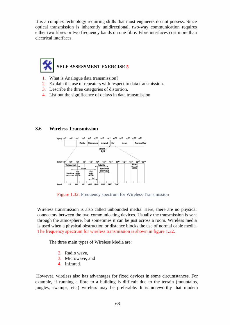
68

It is a complex technology requiring skills that most engineers do not possess. Since

optical transmission is inherently unidirectional, two-way communication requires

either two fibres or two frequency bands on one fibre. Fibre interfaces cost more than

electrical interfaces.


1. What is Analogue data transmission?

2. Explain the use of repeaters with respect to data transmission.

3. Describe the three categories of distortion.

4. List out the significance of delays in data transmission.

3.6 Wireless Transmission

Figure 1.32: Frequency spectrum for Wireless Transmission

Wireless transmission is also called unbounded media. Here, there are no physical

connectors between the two communicating devices. Usually the transmission is sent

through the atmosphere, but sometimes it can be just across a room. Wireless media

is used when a physical obstruction or distance blocks the use of normal cable media.

The frequency spectrum for wireless transmission is shown in figure 1.32.

The three main types of Wireless Media are:

2. Radio wave,

3. Microwave, and

4. Infrared.

However, wireless also has advantages for fixed devices in some circumstances. For

example, if running a fibre to a building is difficult due to the terrain (mountains,

jungles, swamps, etc.) wireless may be preferable. It is noteworthy that modem

69

wireless digital communication began in the Hawaiian Islands, where large chunks of

Pacific Ocean separated the users and the telephone system was inadequate.

3.6.1 Microwave Transmission

Figure 1.33: Microwave transmission station

Microwave is a radio system, which uses very high frequencies to send and receive

data. Because of the high frequencies involved, microwave stations are located about

30 kilometres apart and in line of sight (visible to each other). An example of

microwave transmission station is displayed in figure 1.33.

70

Microwave systems have sufficient bandwidth capacity to support a large number of

voice channels and one or two TV channels.

Above 100 MHz, the waves travel in straight lines and can therefore, be narrowly

focused upon. Concentrating all the energy into a small beam, using a parabolic

antenna (like the familiar satellite TV dish) gives a much higher signal to noise ratio,

but the transmitting and receiving antennas must be accurately aligned with each

other. In addition, this directionality allows, multiple transmitters lined up in a row to

communicate with multiple receivers in a row without interference. Before fibre

optics, microwaves formed the heart of long-distance telephone transmission system.

Since, microwaves travel in straight lines, if, the towers are too far apart, the earth

will get in the way. Consequently, repeaters are needed periodically. The higher the

towers are, the further apart they can be. The distance between repeaters increases

roughly, with the square root of the tower height. For 100-m high towers, repeaters

can be spaced 80 km apart.

Unlike, radio waves at lower frequencies, microwaves do not pass through buildings

wall. In addition, even though the beam may be well focused at the transmitter, there

is still some divergence in space. Some waves may be refracted off low-lying

atmospheric layers and may take slightly longer to arrive than, direct waves. The

delayed waves may arrive out of phase with the direct wave and thus cancel the

signal. This effect is called multipath fading and is often a serious problem. It is

weather and frequency dependent. Some operators keep 10 percent of their channels

idle as spares to switch on to when, multi path fading affects some frequency band

temporarily.

In summary, microwave communication is so widely used for long- distance

telephone communication, cellular telephones, television distribution, and other uses,

that a severe shortage of spectrum has developed.

Microwave systems have the advantage of:

1. medium capacity,

2. medium cost, and

3. can go long distances.

Its disadvantages are:

1. noise interference,

2. geographical problems due to line of sight requirements, and

3. becoming outdated.

Comparison between Microwave and Optical Fibre

The microwave has several significant advantages over optical fibre cable. The main

one is that no right of way is needed, and by buying a small plot of ground every 50

km and putting a microwave tower on it, one can bypass the telephone system and

communicate directly.

71

Microwave is also relatively inexpensive. Putting up two simple towers (may be just

big poles with four guy wires) and putting antennas on each one may be cheaper than

burying 50 km of fibre through a congested urban area or up over a mountain, and it

may also be cheaper than leasing optical fibre from a telephone company.

Terrestrial Microwave

Terrestrial Microwave employs Earth-based transmitters and receivers. The

frequencies used are in the low-gigahertz range, hence, limiting all communication to

line of sight.

Microwave transmissions are carried out using a parabolic antenna that produces an

―arrow, highly directional signal. At the receiving site a similar antenna, which is

sensitive to signals, only within a narrow focus, is placed. As both the transmitter and

receiver are highly focused, they must be carefully adjusted so that, the transmitted

signal is aligned with the receiver.

Microwave is frequently used as a means of transmitting signals where it would be

impractical to run cables.

Terrestrial microwave systems operate in the low-giga hertz range, typically at 2-

6GHz and 21-23GHz

Attenuation characteristics are determined by transmitter power, frequency and

antenna size. Properly designed systems are not affected by attenuation under normal

operational conditions. Rain and fog, however, can cause attenuation at higher

frequencies.

Microwave systems might be vulnerable to electronic eavesdropping and signals

transmitted through microwave are frequently encrypted.

Satellite Microwave

Satellite Microwave systems relay transmission through communication satellites that

operate in geosynchronous orbits (36,000 -40,000 km) above the Earth.

In order to communicate with satellites, the Earth stations use parabolic antennas.

Satellites can retransmit signals in broad or in narrow beams depending on the

locations that are to receive the signals. When the destination is on the opposite side of

the earth, the first satellite must relay the signal through another satellite, as it cannot

directly transmit to the receiver.

Satellite Microwave communication is possible with most remote sites and with

mobile devices as no cables are required. Ships at sea and motor vehicles also use

Satellite Microwave communication.

As all signals must travel 36,000 miles to the satellite and 36,000 miles when

returning to the receiver, the time required to transmit a signal is independent of the

distance. The time required for the signal to arrive at its destination is called

72

propagation delay. The delay encountered with satellite transmissions is about 0.5

seconds.

Satellite Microwave communication is extremely expensive, as a result of which,

organisations share the cost or they purchase services from a commercial provider.

Satellite links operate in the low-giga hertz range, typically at 4-6 GHz. Attenuation

depends on transmitter power, frequency and atmospheric conditions. Rain and

atmospheric conditions may cause attenuation at higher frequencies.

Signals transmitted through Satellite Microwave are usually encrypted.

3.6.2 Radio Transmission

The radio portion of the electromagnetic spectrum extends from 10KHz to 1GHz.

Within this range there are numerous bands or ranges of frequencies that are

designated for specific purposes. Some of the familiar frequency bands are:

Short wave, VHF (Very High Frequency) used for television and FM radio, and UHF

(Ultra High Frequency) used for television.

Radio waves are easy to generate, can travel long distances, and penetrate buildings

easily, so they are widely used for communication, both indoors and outdoors. Radio

waves also are omni directional, meaning that they travel in all directions from the

source, so that the transmitter and receiver do not have to be carefully aligned

physically and that the signal can be received by all the radios within the broadcast

area.

The properties of radio waves are frequency dependent. At low frequencies, radio

waves pass through obstacles well, but the power falls off sharply with distance from

the source, roughly as 1/r3 in air. At high frequencies, radio waves tend to travel in

straight lines and bounce off obstacles. They are also absorbed by rain. At all

frequencies, radio waves are subject to interference from motors and other electrical-

equipment.

3.6.3 Infrared and Millimetre Waves

Unguided infrared and millimetre waves are widely used for short-range

communication. The remote controls used on televisions, Video Cassette Recorder

(VCR‘s), and stereos all use infrared communication. The remote control transmits

pulses of infrared light that carry coded instructions to the receiver on the TV. They

are relatively directional, cheap, and easy to build, but they have a major drawback,

that is, they do not pass through solid objects (try standing between your remote

control and your television and see if it still works). In general, as we go from long-

wave radio toward visible light, the waves behave more and more like light and less

and less like radio.

Infrared waves do not pass through solid walls well, as a result of which, an Infrared

system in one room of a building, will not interfere with a similar system in adjacent

rooms, which is a great advantage. Due to this nature, security of infrared systems

against eavesdropping is better than that of radio systems. Because of these reasons,

73

no government license is needed to operate an infrared system, in contrast to radio

systems, which must be licensed.

These properties have made infrared suitable for indoor wireless LANS. For

example, the computers and offices in a building can be equipped with relatively

unfocused (i.e., somewhat omni directional), infrared transmitters and receivers. In

this way, portable computers with infrared capability can be on the local LAN

without having to physically connect to it. During a meeting where several people

use their portables, they can just sit down in the conference room and be fully

connected, without having to plug in. Infrared communication cannot be used

outdoors because the sun shines as brightly in the infrared as in the visible spectrum.

Two methods of infrared networking that are in use are:

1. Point-to-point and Broadcast Infrared

2. Point-to-point

The Point-to-point networks operate by relaying infrared signals from one device to

the next. Hence, transmissions are focused on a narrow beam, and the transmitter and

receiver must be aligned carefully. Point- to point infrared is not suitable for use with

devices that move frequently because, here, the devices must be carefully aligned and

setup.

High power laser transmitters can be used in order to transmit data for several

thousand yards when the line of sight communication is possible.

The cost of Point-to-point infrared equipment is higher than the cost for a comparable

cabled network. When systems use transmitters that are based on LED technology

and hardware cost is moderate, but, when long distance systems use high powered

laser transmitters then the cost is very high.

Infrared devices are insensitive to radio frequency interference, but, the reception can

be degraded by bright light. As the transmitters are tightly focused, they are fairly

immune to electronic eavesdropping.

Broadcast Infrared

Broadcast infrared disperses transmissions so that, they are visible to several

receivers. The two possible approaches to broadcast infrared networking are:

1. The active transmitter can be located at a high point so that, it can transmit to all

devices.

2. A reflective material can be placed on the ceiling. Devices transmit toward the

ceiling, from where, the light signals are dispersed to other devices in the room.

Installation is simple as device alignment is not critical. Hence, it is essential that

each device has clear transmission and reception pathways. As all devices are

sensitive to light interference, during installation, the control of ambient light is very

important.

74

3.7 Wireless LAN

Wireless LAN‘s are systems of portable computers that communicate using radio

transmission. Wireless LAN‘s make use of the omni directional wireless

communication.

The main objective of wireless LAN is to provide high-speed communication among

computers that are located in relatively close proximity.

Wireless LAN‘s are usually configured in an office building with the base stations

strategically placed around the building. Optical fibre cable can be used to cable all

base stations together. If the transmission power of the base stations and portables is

adjusted to a range of 3 or 4 meters, then, each room acts as a single cell, and the

entire building acts as a large cellular system. Here unlike the cellular telephone

system, each cell has only one channel that covers the entire bandwidth, which is

available. Typically, its bandwidth is 1 to 2 Mbps.

The disadvantages of using Radio transmitters are:

When the receiver is within the range of two active transmitters, the resulting signal

will usually be grab led and hence, useless.

In indoor wireless LAN‘s, the presence of walls between the stations have great

impact on the effective range of each station.

4.0 CONCLUSION

In this unit you have learn about the concept of transmission terminology as well as

the different types of data transmission. Also, you have learnt about the various types

of transmission media and their particular characteristics. It is believed that by how

you should be able to choose a suitable transmission media for your particular

network.

5.0 SUMMARY

In this unit, we have studied, the basic concepts of Data Transmission. To start with,

we discussed the basic terms that are frequently used in Data transmission like

Bandwidth, frequency, channel, baud etc. Bandwidth is the amount of data or signals

that a transmission media can carry in a fixed amount of time and its unit of

measurement is bits per second (bps) for digital signal and Hertz (Hz) for analogue

signals. Frequency is the number of cycles or periods that a signal completes within

one second and its unit of measurement is Hertz (Hz). Channel refers to the

communication path between the source and destination.

As it is essential to know how data can be transmitted from the source to the

destination, the different modes of data transmission were outlined as follows:

1. Parallel and Serial communication.

2. Asynchronous, Synchronous and Isochronous communication.

75

3. Simplex, Half duplex and Full duplex communication.

We also discussed the two major types of signals that is Analogue and Digital and,

the manner in which these two types of signals can be transmitted from the source to

the destination.

When, data is transmitted from the source to the destination, there is, always a scope

for transmission errors and the data may not reach in exactly the same form as it was

sent. We have seen that these transmission errors are classified into three main

categories that is Delay distortion, Attenuation and Noise. Delay distortion is caused

because, signals at different frequencies, travel at different speeds along the

transmission medium. As the signal travels along the transmission medium, its

strength decreases over distance, this is known as Attenuation. Usually, some

unwanted electromagnetic energy gets inserted during the course of transmission and

this is called Noise. The concept of Delays and how to reduce them were also

discussed.

We have seen that transmission media can be classified in to two categories, that are,

guided media and unguided media. The guided media uses physical cable for data

transmission. Twisted pair, co-axial cable and optical fibre are the three main types

of guided media; they differ in their physical characteristics as well as transmission

capacities. In case of unguided media, the transmission medium is air. Unguided

media can be Radio, Microwave or Infrared. Security is a major concern when using

unguided media for transmission.

Towards the end, Wifeless LAN‘s were also discussed. Here, we saw that Wireless

LAN‘s make use of Radio transmission and their main objective is to provide high

speed communication among computers that are located in relatively close proximity.

In the next unit, we will be studying, the different Data encoding and communication

techniques.


1. Discuss the twisted pair cable.

2. Describe co-axial cable and its uses.

3. Describe the structure of optical fibre and list its advantages and

disadvantages.

4. Explain how Radio communication differs from Satellite

communication.

5. Explain the working of Wireless LAN‘s.

7.0 REFERENCES/FURTHER READINGS

Andrew. S. Tannenbaum, Computer Networks, PHI, New Delhi.

William Stalling, Data and Computer Communication, PHI, New Delhi.


76

Question 1

What is data communication?

Solution

This is the processing of transferring of data from sender to receiver through

transmission media such as a cable irrespective of the geographical location.

Question 2

Explain the term bandwidth. Why is bandwidth useful?

Solution

Bandwidth is the highest rate of transfer of data through a channel. It is the difference

between the lower band and the upper band of a channel.

It is very useful to determine how quick a web page loads on a browser.

Question 3

Table 1.4: Compares of parallel and serial transmission method

S/N Serial Transmission Parallel Transmission

1. Data flows in both directions Data flows through many lines

2. It is cost effective It is not cost effective

3. One bit of data is sent at the rate of ne

per clock paulse

Eight bit of data are sent at the

rate of one per clock paulse

4. Shower than parallel transmission Faster than serial transmission

5. Used in most cases to transfer data over

a long distance

Used to transfer data over short

distance

6. Used simplex circuit to transmit data Used complex circuit to transmit

data

Question 4

Give reasons as to why full duplex is more challenging than simplex and half duplex

transmission

Solution

Full duplex is more challenging than simplex and half duplex transmission because it

allows two ways traffic simultaneously which gives it double utilization of the

bandwidth. This however, leads to better performance of the full duplex transmission.

Question 5

Bring out the difference between synchronous, Asynchronous and Isochronous

transmission.

77

Solution

Synchronous system transmits data continuously without start and stop bits between

the successive data items. Asynchronous system transmits data with some delay

emanating from the start and stop bit between any two successive data items. While

Isochronous system ensure transmission of data at a fast speed without the rigidity of

synchronous system with a stable gap in the midst of sending consecutive data items.


Question 1

What is analogue data transmission?

Solution

This is a method of sending information with the use of a continuous signal which

changes in amplitude, phase or other attributes in consonance to that information

Question 2

Explain the use of repeaters with respect to data transmission

Solution

A repeater is a device us to boosting signal in transmission to guide against

attenuation. The amplification of the signal with the help of repeater alters the signal

to travel a long distance without signal degradation.

Question 3

Describe the three categories of distortion

Solution

the three categories of distortion are:

1. Attenuation

2. Delay distortion

3. Noise

Attenuation is the loss of energy as the signal travel along a channel.

Amplifiers are used to boost the signal to come back to its original strength.

Delay is distortion is a process whereby signal of different frequencies travel with

diverse speed along the channel. This implies that all signals will get to the destination

at the same time. Thus, leading to distortion of the signal.

Question 4

78

List out the significance of the delay in data transmission

Solution

The significance of delay in data transmission are:

a. It has a list of impact in determining the selection and rendition of network

algorithms such as routing and flow control.

b. A substantial delay is catastrophic to data transfer.

9.0 ANSWER TO TUTOR MARKED ASSIGNMENT 2

Question 1

Discuss the twisted pair cable.

Solution

Twisted pair cable is a copper wire that links diverse nodes such as linking computers

in the home to those of the business offices. Twisted pair may be shielded (i.e

shielded twisted pair) with the acronym STP or not shielded (unshielded twisted pair)

with the acronym UTP. STP is common with the installation of the old telephone

networks to guide against crosstalk and reduce electromagnetic radiation. Twisted

pair are twisted to guide against signal interference. The bandwidth hinge on the

thickness of the wire and the distance it goes. They are less costly and easy to install.

Question 2

Describe co-axial cable and its uses.

Solution

Coaxial cable is made up of a tube of electronically conveying substances encircling

a central conductor clench in place by insulator. It is used for transmission of signal

such as telegraph, telephone, television and Internet signals.

Question 3

Describe the structure of optical fibre and list its advantages and disadvantages

Solution

Optical fibre is cable used to send data via fibres (threads) or plastic (glass). This

comprises pack of glass fibre which sends regulated messages over light waves. They

advantages are:

a. It has higher bandwidth than the copper cables

b. It gives room for transmission of data for a longer kilometre coverage at less loss.

c. The optical cable hinders electromagnetic blockages.

d. Fibre cable is better than copper wire 4.5 times in size.

e. Fibre cable fill less area when liken to copper wires and they are lighter and

thinner.

79

f. The installation is easy due to less weight.

g. The security is high when conveying data and are very difficult to tap since they

don‘t give raise to electromagnetic energy.

The disadvantages are:

a. It is difficult join optical fibre cables since the beam could be lost while

scattering.

b. Unique equipment are often needed for the installation

c. Fibre optic cable is delicate when fitting it since the cable are compact

d. Copper wires are not delicate as fibre optic cables

e. Expertise and unique devices are needed to maintain and check the transmission

of fibre cables.

Question 4

Explain how Radio communication differs from satellite communication

Solution

Satellite communication is the use of artificial satellite to connect varied places of the

earth for the purpose of communication. There are more than 2,000 analogues of

digital satellite moving along the earth orbit conveying voice, video and data from

one place to the other globally.

Radio communication on the other hand is the conveying of signal and connecting

one place to the other using radio waves. Radio wave consist of electromagnetic

waves which has frequency ranging from 30hertz (Hz) and 300gigahertz (GHz).

The differences between radio communication and satellite communication are that

the:

a. Frequency used by satellite is higher and more powerful than the radio wave. It

gives contraction of all obtainable power into a narrow beam. This reduces

bandwidth and gives more bandwidth for transmission.

b. Narrow beam are well focused and point t one direction. That is, it points at the

exact location of the antenna while radio station broadcast in all directions.

Question 5

Explain the working of wireless LAN

Solution.

Wireless LAN (WAN) is a mechanism that gives room for wireless communication.

WLAN links one place to the other via Wifi instead of Ethernet devices. It sends data

over the air with the assistance of one of the 802.11 protocols of IEEE while LAN

sends data over physical cables in a sequence of Ethernet packets.

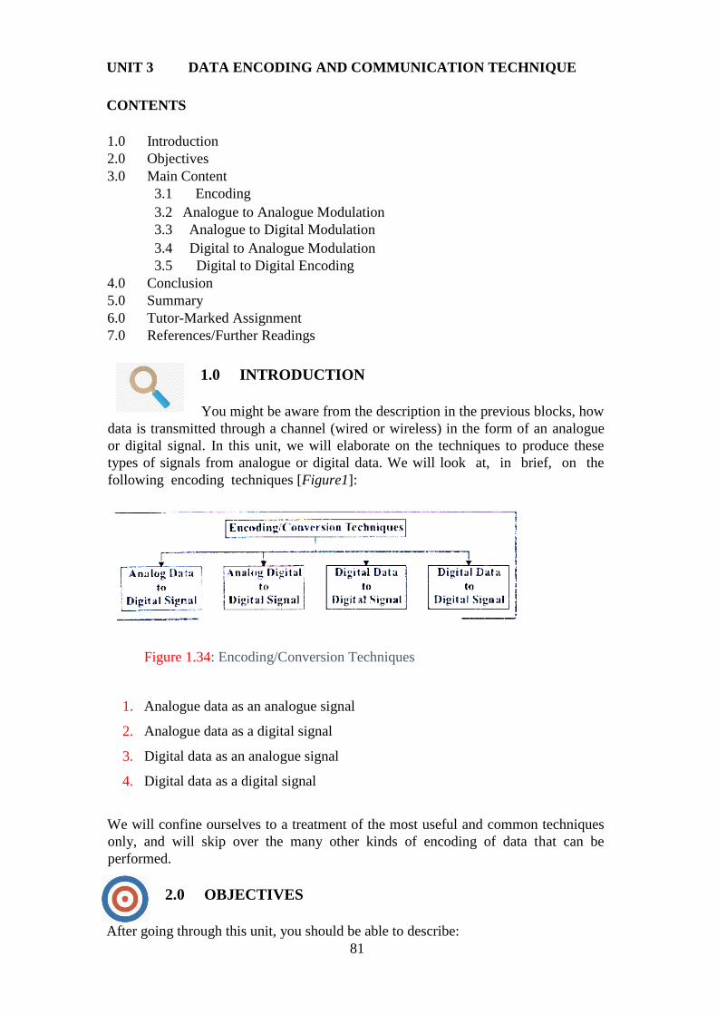
81

UNIT 3 DATA ENCODING AND COMMUNICATION TECHNIQUE

CONTENTS

1.0 Introduction

2.0 Objectives

3.0 Main Content

3.1 Encoding

3.2 Analogue to Analogue Modulation

3.3 Analogue to Digital Modulation

3.4 Digital to Analogue Modulation

3.5 Digital to Digital Encoding

4.0 Conclusion

5.0 Summary



1.0 INTRODUCTION

You might be aware from the description in the previous blocks, how

data is transmitted through a channel (wired or wireless) in the form of an analogue

or digital signal. In this unit, we will elaborate on the techniques to produce these

types of signals from analogue or digital data. We will look at, in brief, on the

following encoding techniques [Figure1]:

Figure 1.34: Encoding/Conversion Techniques

1. Analogue data as an analogue signal

2. Analogue data as a digital signal

3. Digital data as an analogue signal

4. Digital data as a digital signal

We will confine ourselves to a treatment of the most useful and common techniques

only, and will skip over the many other kinds of encoding of data that can be

performed.

2.0 OBJECTIVES

After going through this unit, you should be able to describe:

82

1. what encoding means

2. why encoding is needed

3. some different types of encoding

4. mechanisms and techniques used for encoding

5. when each type of encoding is used with examples.

There are several other types of encoding as well as encoding techniques that will not

be discussed in this unit.

3.0 MAIN CONTENT

3.1 Encoding

Sleekly, we cannot lend a signal containing information directly over a transmission

medium, at least not for long distances. For example, the sound of our voice can only

travel a few hundred meters. If we want to send our voice to the next city, we have to

be able to transform our voice, to, aft electrical signal that can then, be sent that long

distance. Then, we would also need to perform the reverse conversion at the other

end.

So, we see that, to send a signal over a physical medium, we need to encode or

transform the signal in some way so that the transmission medium can transmit it.

The sender and the receiver must agree on what kind of transformation has been done

so that it can be reversed at the other end and the actual signal or information can be

recovered. The information content in a signal is based upon having some changes in

it. For example, if we just send a pure sine wave, where the voltage varies with time

as a sine function, then, we cannot convey much information apart from the fact that

there is some entity at the other end that is doing the transmitting.

The information content of a signal is dependent on the variation in the signal. After

sending one cycle of a sine wave there is no point in sending another cycle because

we will not be able to convey anything more than what we have already done. What

is needed is to modify the sine wave in some way to carry the information we want to

convey. This is called modulation.

You know that there are two kinds of signals: analogue and digital. Likewise, there

are two types of information that we may want to transmit, again analogue and

digital. So, we get four basic combinations of encoding that we may need to perform,

depending on the signal type as well as the information type. We shall look at each of

these four types briefly in this unit and will also study the ways in which the actual

encoding can be done.

3.2 Analogue- To-Analogue Modulation

Let us first look at a situation where our signal and information are both of the

analogue type. The act of charging or encoding the information in the signal is

known as modulation. A good example of such encoding is radio broadcasting. Here

we primarily want to send sound in some form over the atmosphere to the receiving

radio gets. The sound is converted into an analogue electrical signal at the source and

83

is used to encode the signal which is the base frequency at which the transmission is

being done. The reverse process is performed at the radio set to recover the

information in electrical form, which is then converted back to sound so that, we hear

what was being said at the radio station.

Let us, formulate another definition of modulation. When a low frequency

information signal is encoded over a higher frequency signal, it is called modulation

[Ref.3]. The encoding can be done by varying amplitude (strength of a signal), period

(amount of time, in seconds, a signal needs to complete a cycle) and frequency

(number of cycles per second) and phase (position of waveform relative to zero).

Notice the simulations of the word modulation to the word modifying. For instance,

an audio signal (one that is audible to human ear) can be used to modify an RF

(Radio Frequency) carrier, when the amplitude of the RF is varied according to the

changes in the amplitude of the audio, it is called amplitude modulation (AM), and

when the frequency is varied, it is called FM (frequency modulation).

Although, it can be dangerous to use analogues as they can be carried too far, we can

understand this process with an example. Suppose we want to send a piece of paper

with something written on it to a person a hundred meters away. We will not be able

to throw the paper that far. So, we can wrap it around a small stone and then throw

the stone towards the person. He can then unwrap the paper and read the message.

Here, the stone is the signal and the piece of paper is the information that is used to

change the stone. Just as sending the stone alone would not have conveyed much to

our friend, similarly sending only the base signal (also called carrier signal) will not

convey much information to the recipient.

Therefore, there are three different ways in which this encoding of the analogue

signal with analogue information is performed. These methods are:

Amplitude modulation (AM), where the amplitude of the signal is changed

depending on the information to be sent (Figure 1.35)

Frequency modulation, where the frequency of the signal is changed

depending on the information to be sent (Figure 1.36)

Phase modulation, where it is the phase of the signal that is changed

according to the information to be sent (figure 1.37).

Amplitude Modulation

Now, let us go into the details. In this type of modulation, the frequency and phase of

the carrier or base signal are not altered. Only the amplitude changes and we can see

that the information is contained in the envelope of the carrier signal. It can be

proud/demonstrated that, the bandwidth of the composite signal is twice that of the

highest frequency in the information signal that modulates the carrier.

By international agreement, for radio transmission using AM, 9 KHz is allowed as

the bandwidth. So, if a radio station transmits at 618 KHz, the next station can only

transmit at 609 or at 627 KHz. It will be clear that the highest audio frequency that

can be carried over AM radio is thus 4.5 KHz, which is sufficient for most voice and

84

musical pieces. Actually, the modulating signal is centred around the carrier

frequency and extends the composite signal both ways in equal measure. Each of

these is called a sideband and therefore, AM radio transmission is dual sideband.

This is actually wasteful because the spectrum is unnecessarily used up, but the cost

and complexity associated with eliminating one sideband, and performing single

sideband AM modulation, have led to the technique not being used widely.

AM radio transmission has been assigned the frequency range of 530 to 1700 KHz.

The quality of AM transmission is not very good as noise in the channel (the

atmosphere, here) can easily creep into the signal and alter its amplitude. So, the

receiving end will likely find a fair amount of noise in the signal, particularly at

higher, short wave frequencies. That is why you often get a lot of static in short wave

or even medium wave broadcasts.

AM Bandwidth

Figure 1.35: Amplitude modulation

Frequency Modulation

In contrast to Amplitude Modulation, here it is the frequency of the base signal that is

altered depending on the information that is to be sent. The amplitude and phase of

the carrier signal are not changed at all. It can be shown that this results in a

bandwidth requirement of 10 times the modulating signal, centred on the carrier

frequency.

This method is the less susceptible to noise and gives the best performance of all data

encoding types as far as the quality of the transmitted signal is concerned. Although

digital encoding methods may give better performance over multiple hops (because

in their case, the original signal can be accurately reconstructed at each hop),

Frequency Modulation (PM) is the best as far as single hop transmission goes.

FM radio transmission has been allocated the spectrum range 88 MHz to 108MHz.

As a good stereo sound signal needs 15KHz of bandwidth, this means that PM

transmission has a bandwidth of 150KHz. To be safe from interference from

neighbouring stations, 200KHz is the minimum separation needed. As a further

safety measure, in any given area, only alternate stations are allowed and the

85

neighbouring frequencies are kept empty. This is practical because PM transmission

is line of sight (because of the carrier frequency) and so, beyond a range of about

100Km or so, the signal cannot be received directly (this distance depends on various

factors). We can therefore, have the most 50 FM stereo radio stations in a given

geographical area.

As in the case of AM transmission (having 2 sub-bands), PM also has multiple

sidebands maybe two or more, which is really wasteful but is tolerated in the interests

of simplicity and cost of the equipment.

In television transmission the bandwidth needed is 4.5 MHz in each sideband. The

video signal is sent using amplitude modulation. The audio signal goes at a frequency

that is 5.5 MHz over the video signal and is sent as a frequency modulated signal. To

reduce the bandwidth requirement, the video signal is sent using a method called

vestigial sideband that needs only 6 MHz, instead of the 9 MHz that would have been

needed for dual sideband transmission, though, it is more than the 4.5 MHz that a

pure single sideband transmission would have needed.

Figure 1.36: Frequency modulation

Phase Modulation

As you would have guessed by now, in Phase Modulation (PM) the modulating

signal leaves the frequency and amplitude of the carrier signal unchanged but alters

its phase. The characteristics of this encoding technique are similar to FM, but the

advantage is that of reduced complexity of equipment However, this method is not

used in commercial broadcasting.

86

Figure 1.37: Phase Modulation

SELF-ASSESSMENT EXERCISE 6

1. Why do we need modulation? Would it be right to simply send the

information as the signal itself?

2. A common FM broadband has a derivation of ±75kHz bandwidth and a

modulation frequency of 15kHz. Calculate the bandwidth of 98% of the power.

3. Why is AM the most susceptible to noise, of the three types of

modulation?

3.3 Analogue to Digital Modulation

Natural phenomena are analogue in nature and can take on any of the potentially

infinite number of values. For example, the actual frequencies contained in a

sound made by a human is an analogue signal, as is the amplitude or loudness of the

sound. One example of coding analogue data in digital form is when, we want to

record sound on digital media such as a Digital Video Disk (DVD) or in other forms

such as Moving Picture Expert Group Audio Layer-3 (MP3) or as a Waveform Audio

File Format ―.wav‖ file. Here, the analogue signal, that is, the musical composition or

the human voice is encoded in digital form. This is an example of analogue to digital

encoding.

While, in the case of analogue to analogue encoding, the motivation was to be able to

transmit the signal for long distances, here, the main reason is to be able to change

the information itself to digital form. That digital signal can then be transmitted, if

necessary, by any suitable method.

One method of encoding is what is called Pulse Code Modulation (PCM). This gives

very good quality and when used in conjunction with error correction techniques, can

be regenerated at every hop on the way to its final destination. This is the big

advantage of digital signals. At every hop, errors can be removed and the original

signal reconstructed almost exactly, barring the few errors that could not be

corrected.

The first step in PCM is, to convert the analogue signal into a series of pulses (Figure

1.32). This is called Pulse Amplitude Modulation (PAM). To do this the analogue

signal is sampled at fixed intervals and the amplitude at each sample decides the

amplitude of that pulse. You can see that at this step, the resulting signal is still

actually an analogue signal because the pulse can have any amplitude, equal to the

amplitude of the original signal at the time the sample was taken. In PAM, the

sampled value is held for a small time so that the pulse has a finite width. In the

original signal the value occurs only for the instant at which it was sampled.

One question that arises here is, how many samples do we have to take? We would

not want to take too many samples as that would be wasteful. At the same time, if,

we take too few samples, we may not be able to reconstruct the original signal

properly. The answer comes from Nyqist‘s theorem, which states that, to be able to

87

get back the original signal, we must sample at a rate, that is, at least twice that of

the highest frequency contained in the original signal.

Let us do some calculations to see what this means in practice. In the next unit, you

will see that a voice conversation over a telephone has a range of frequencies from

300 Hz to 3300 Hz. Because the highest frequency is 3300 Hz, we need at least 6600

samples a second to digitize the voice to be sent over a phone line. For safety we take

8000 samples per second, corresponding to a sampling interval of 125 microseconds.

The next stage in the digitization of the signal is quantization. In this process, the

analogue values of the sampled pulses are quantized, that is, converted into discrete

values. For example, if the original analogue signal had an amplitude ranging from

+5v to -5v, the result of PAM might be to produce pulses of the following amplitudes

(each sample is taken at say, intervals of 125 microseconds)

+4.32, +1.78, -3.19, -4.07, -2.56, +0.08 and so on.

In quantization, we may decide to give the amplitude 256 discrete values. So, they will

range from -127 to +128. The actual amplitude of +5v to -5v has to be represented in

this range, which means each value is of 39 mV nearly. By this token, the first value of

+4.32v lies between 110 and 111, and we can decide that such a value will be taken as

110. This is quantization. The analogue values now become the following quantized

values:

110, 45, -81, -104, -65, 2 and so on.

The above discrete value~ are now represented as 8 binary digits with, I bit giving the

sign while the other 7 bits represent the value of the sample.

In the final stage of the encoding, the binary digits are then transformed into a digital

signal using any of the digital to digital encoding mechanisms discussed later in this

unit. This digital signal is now the representation of the original analogue signal.

PCM is commonly used to transmit voice signals over a telephone line. It gives good

voice quality but, is a fairly complex method of encoding the signal. There is a

simpler method that can be used, but we have to pay the price in tends of the lower

quality of the encoded signal. This is called Delta modulation. Here, samples are

taken as described above, but instead of quantising them into 256 or more levels,

only the direction of change is retained. If the sample is larger in value than the

previous one, it is considered a 1 while otherwise it is considered a o bit. So the

sequence above would be encoded as:

1,0,0,0,1,1 and so on.

88

Figure 1.38 : Pulse Code Modulation

3.4 Digital to Analogue Modulation

So far, we have looked at the codification of analogue data, where the source

information could take up any value. We also have need for the reverse type of

encoding, where binary digital values have to be encoded into an analogue signal.

This may seem simple because after all, we only have to give two distinct values to

the analogue signal, but here you need to realise that, we have to be able to

distinguish between successive digital values that are the same, say three 1 ‗s in

succession or two 0‘s in succession. These should not get interpreted as a single I or a

single 0! This sort of problem did not exist in the case of analogue to analogue

encoding.

One example where such encoding is needed is, when we need to transmit between

computers over a telephone line. The computers generate digital data, but the

telephone system is analogue. So, this situation is a bit different from the

transmission of voice over the telephone, where the source signal is also analogue.

In this kind of encoding, one important factor of interest is the rate at which we can

transfer bits. Clearly, there will be some kind of limit to the amount of information

that we can send in a given time. This depends on the available bandwidth of the

carrier signal, that is, the variation that we can permit around the nominal frequency

as well as on the specific technique of encoding that we use.

Here it is important to understand two aspects of the rate of transfer of information.

The first is the bit rate that tells us the number of individual bits that are transmitted

per second. The second, and more important from the transmission angle, is the baud

rate. This is the number of signal transitions per second that are needed to represent

those bits. For a binary system, the two are equal. In general, the bit rate cannot be

lower than the baud rate, as there has to be at least one signal transition to represent a

bit.

89

We have seen in analogue to analogue encoding that, the source signal modulates the

base or carrier signal to convey the information that we want to transmit. A similar

principle is also used in digital to analogue encoding. The carrier signal has to be

modulated, but this time by the digital signal, to produce the composite signal that is

transmitted. However, while in the analogue case there were a potentially infinite

number of values that could have been transmitted, here we have only two values (a 0

or a 1) that will modulate the signal.

If, there is no modulation, the carrier signal will be a pure sine wave at the frequency

of transmission. You will realise that the baud rate that can be supported also depends

on the quality of the line and the amount of random noise that is present in the

medium. Like in analogue-to-analogue encoding, there are three properties of the sine

wave that we can alter to convey information. These are the amplitude, the frequency

and the phase. In addition, we can also use a combination of amplitude and phase

change to encode information more efficiently. Modulation is also referred to as shift

keying in this type of encoding technique.

There are three types of digital to analogue modulation (Figure 1.39)

Figure 1.39; digital to analogue modulation techniques

Now we will take up each one individually.

Amplitude Shift Keying (ASK)

In this kind of encoding, abbreviated as ASK, the amplitude of the analogue signal is

changed to represent the bits, while the phase and the frequency are kept the same.

The bigger the difference between the two values, the lower the possibility of noise

causing errors. There is no restriction, however, on what voltage should represent a 1

or a 0, and this is left to the designers. For the duration of a bit, the voltage should

remain constant.

One method could be to represent the high voltage as a 1 and the negative high

voltage as a 0, although the reverse convention could also be used. Sometimes, to

reduce the energy needed for transmission, we can choose to represent a 0 or a 1 by a

zero voltage, and the other bit by the high voltage. This scheme is called on-off-

keying (OOK).

Alternative, binary 1 can stand for a short pulse of light and binary 0 can stand for

light out. Again, low level light emitted by laser transmitter in most cases have a

fixed ―bias‖ which stands for 0. On the other hand, a higher amplitude light wave

stands for binary 1. Figure 3.5b displays an ASK.

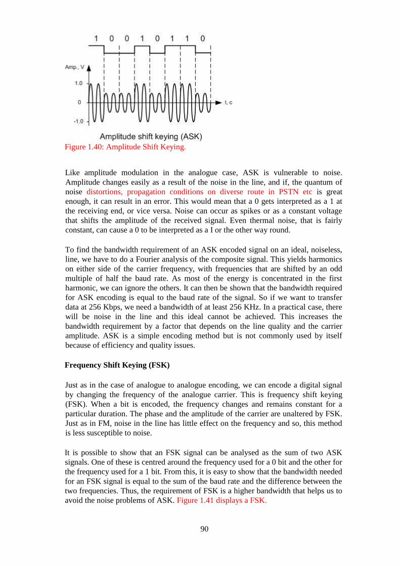
90

Figure 1.40: Amplitude Shift Keying.

Like amplitude modulation in the analogue case, ASK is vulnerable to noise.

Amplitude changes easily as a result of the noise in the line, and if, the quantum of

noise distortions, propagation conditions on diverse route in PSTN etc is great

enough, it can result in an error. This would mean that a 0 gets interpreted as a 1 at

the receiving end, or vice versa. Noise can occur as spikes or as a constant voltage

that shifts the amplitude of the received signal. Even thermal noise, that is fairly

constant, can cause a 0 to be interpreted as a I or the other way round.

To find the bandwidth requirement of an ASK encoded signal on an ideal, noiseless,

line, we have to do a Fourier analysis of the composite signal. This yields harmonics

on either side of the carrier frequency, with frequencies that are shifted by an odd

multiple of half the baud rate. As most of the energy is concentrated in the first

harmonic, we can ignore the others. It can then be shown that the bandwidth required

for ASK encoding is equal to the baud rate of the signal. So if we want to transfer

data at 256 Kbps, we need a bandwidth of at least 256 KHz. In a practical case, there

will be noise in the line and this ideal cannot be achieved. This increases the

bandwidth requirement by a factor that depends on the line quality and the carrier

amplitude. ASK is a simple encoding method but is not commonly used by itself

because of efficiency and quality issues.

Frequency Shift Keying (FSK)

Just as in the case of analogue to analogue encoding, we can encode a digital signal

by changing the frequency of the analogue carrier. This is frequency shift keying

(FSK). When a bit is encoded, the frequency changes and remains constant for a

particular duration. The phase and the amplitude of the carrier are unaltered by FSK.

Just as in FM, noise in the line has little effect on the frequency and so, this method

is less susceptible to noise.

It is possible to show that an FSK signal can be analysed as the sum of two ASK

signals. One of these is centred around the frequency used for a 0 bit and the other for

the frequency used for a 1 bit. From this, it is easy to show that the bandwidth needed

for an FSK signal is equal to the sum of the baud rate and the difference between the

two frequencies. Thus, the requirement of FSK is a higher bandwidth that helps us to

avoid the noise problems of ASK. Figure 1.41 displays a FSK.

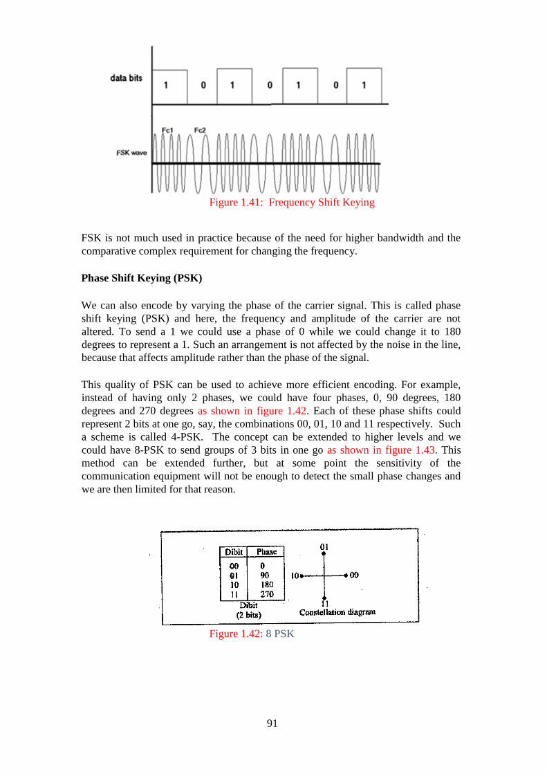
91

Figure 1.41: Frequency Shift Keying

FSK is not much used in practice because of the need for higher bandwidth and the

comparative complex requirement for changing the frequency.

Phase Shift Keying (PSK)

We can also encode by varying the phase of the carrier signal. This is called phase

shift keying (PSK) and here, the frequency and amplitude of the carrier are not

altered. To send a 1 we could use a phase of 0 while we could change it to 180

degrees to represent a 1. Such an arrangement is not affected by the noise in the line,

because that affects amplitude rather than the phase of the signal.

This quality of PSK can be used to achieve more efficient encoding. For example,

instead of having only 2 phases, we could have four phases, 0, 90 degrees, 180

degrees and 270 degrees as shown in figure 1.42. Each of these phase shifts could

represent 2 bits at one go, say, the combinations 00, 01, 10 and 11 respectively. Such

a scheme is called 4-PSK. The concept can be extended to higher levels and we

could have 8-PSK to send groups of 3 bits in one go as shown in figure 1.43. This

method can be extended further, but at some point the sensitivity of the

communication equipment will not be enough to detect the small phase changes and

we are then limited for that reason.

Figure 1.42: 8 PSK

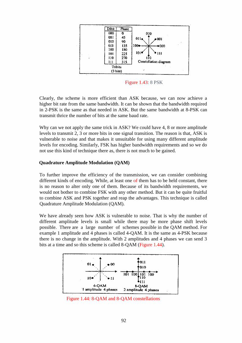
92

Figure 1.43: 8 PSK

Clearly, the scheme is more efficient than ASK because, we can now achieve a

higher bit rate from the same bandwidth. It can be shown that the bandwidth required

in 2-PSK is the same as that needed in ASK. But the same bandwidth at 8-PSK can

transmit thrice the number of bits at the same baud rate.

Why can we not apply the same trick in ASK? We could have 4, 8 or more amplitude

levels to transmit 2, 3 or more bits in one signal transition. The reason is that, ASK is

vulnerable to noise and that makes it unsuitable for using many different amplitude

levels for encoding. Similarly, FSK has higher bandwidth requirements and so we do

not use this kind of technique there as, there is not much to be gained.

Quadrature Amplitude Modulation (QAM)

To further improve the efficiency of the transmission, we can consider combining

different kinds of encoding. While, at least one of them has to be held constant, there

is no reason to alter only one of them. Because of its bandwidth requirements, we

would not bother to combine FSK with any other method. But it can be quite fruitful

to combine ASK and PSK together and reap the advantages. This technique is called

Quadrature Amplitude Modulation (QAM).

We have already seen how ASK is vulnerable to noise. That is why the number of

different amplitude levels is small while there may be more phase shift levels

possible. There are a large number of schemes possible in the QAM method. For

example 1 amplitude and 4 phases is called 4-QAM. It is the same as 4-PSK because

there is no change in the amplitude. With 2 amplitudes and 4 phases we can send 3

bits at a time and so this scheme is called 8-QAM (Figure 1.44).

Figure 1.44: 8-QAM and 8-QAM constellations

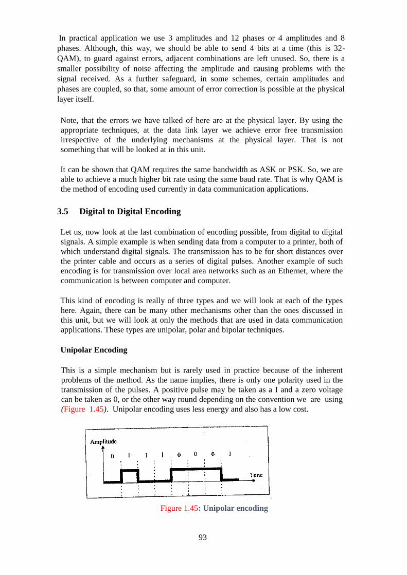
93

In practical application we use 3 amplitudes and 12 phases or 4 amplitudes and 8

phases. Although, this way, we should be able to send 4 bits at a time (this is 32-

QAM), to guard against errors, adjacent combinations are left unused. So, there is a

smaller possibility of noise affecting the amplitude and causing problems with the

signal received. As a further safeguard, in some schemes, certain amplitudes and

phases are coupled, so that, some amount of error correction is possible at the physical

layer itself.

Note, that the errors we have talked of here are at the physical layer. By using the

appropriate techniques, at the data link layer we achieve error free transmission

irrespective of the underlying mechanisms at the physical layer. That is not

something that will be looked at in this unit.

It can be shown that QAM requires the same bandwidth as ASK or PSK. So, we are

able to achieve a much higher bit rate using the same baud rate. That is why QAM is

the method of encoding used currently in data communication applications.

3.5 Digital to Digital Encoding

Let us, now look at the last combination of encoding possible, from digital to digital

signals. A simple example is when sending data from a computer to a printer, both of

which understand digital signals. The transmission has to be for short distances over

the printer cable and occurs as a series of digital pulses. Another example of such

encoding is for transmission over local area networks such as an Ethernet, where the

communication is between computer and computer.

This kind of encoding is really of three types and we will look at each of the types

here. Again, there can be many other mechanisms other than the ones discussed in

this unit, but we will look at only the methods that are used in data communication

applications. These types are unipolar, polar and bipolar techniques.

Unipolar Encoding

This is a simple mechanism but is rarely used in practice because of the inherent

problems of the method. As the name implies, there is only one polarity used in the

transmission of the pulses. A positive pulse may be taken as a I and a zero voltage

can be taken as 0, or the other way round depending on the convention we are using

(Figure 1.45). Unipolar encoding uses less energy and also has a low cost.

Figure 1.45: Unipolar encoding

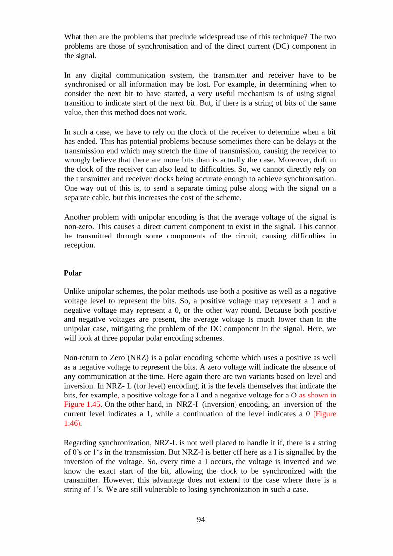
94

What then are the problems that preclude widespread use of this technique? The two

problems are those of synchronisation and of the direct current (DC) component in

the signal.

In any digital communication system, the transmitter and receiver have to be

synchronised or all information may be lost. For example, in determining when to

consider the next bit to have started, a very useful mechanism is of using signal

transition to indicate start of the next bit. But, if there is a string of bits of the same

value, then this method does not work.

In such a case, we have to rely on the clock of the receiver to determine when a bit

has ended. This has potential problems because sometimes there can be delays at the

transmission end which may stretch the time of transmission, causing the receiver to

wrongly believe that there are more bits than is actually the case. Moreover, drift in

the clock of the receiver can also lead to difficulties. So, we cannot directly rely on

the transmitter and receiver clocks being accurate enough to achieve synchronisation.

One way out of this is, to send a separate timing pulse along with the signal on a

separate cable, but this increases the cost of the scheme.

Another problem with unipolar encoding is that the average voltage of the signal is

non-zero. This causes a direct current component to exist in the signal. This cannot

be transmitted through some components of the circuit, causing difficulties in

reception.

Polar

Unlike unipolar schemes, the polar methods use both a positive as well as a negative

voltage level to represent the bits. So, a positive voltage may represent a 1 and a

negative voltage may represent a 0, or the other way round. Because both positive

and negative voltages are present, the average voltage is much lower than in the

unipolar case, mitigating the problem of the DC component in the signal. Here, we

will look at three popular polar encoding schemes.

Non-return to Zero (NRZ) is a polar encoding scheme which uses a positive as well

as a negative voltage to represent the bits. A zero voltage will indicate the absence of

any communication at the time. Here again there are two variants based on level and

inversion. In NRZ- L (for level) encoding, it is the levels themselves that indicate the

bits, for example, a positive voltage for a I and a negative voltage for a O as shown in

Figure 1.45. On the other hand, in NRZ-I (inversion) encoding, an inversion of the

current level indicates a 1, while a continuation of the level indicates a 0 (Figure

1.46).

Regarding synchronization, NRZ-L is not well placed to handle it if, there is a string

of 0‘s or 1‗s in the transmission. But NRZ-I is better off here as a I is signalled by the

inversion of the voltage. So, every time a I occurs, the voltage is inverted and we

know the exact start of the bit, allowing the clock to be synchronized with the

transmitter. However, this advantage does not extend to the case where there is a

string of 1‘s. We are still vulnerable to losing synchronization in such a case.

95

Figure 1.46: NRZ -L and NRZ-I encoding

Return to Zero (RZ) is a method that allows for synchronization after each bit as

shown in Figure 1.47. This is achieved by going to the zero-level midway through

each bit. So, a I bit could be represented by the positive to zero transition and a 0 bit

by a negative to zero transition. At each transition to zero, the clocks of the transmitter

and receiver can be synchronized. Of course, the price one has to pay for this is a

higher bandwidth requirement.

Figure 1.47: RZ encoding

A third polar method is biphase encoding. While in RZ, the signal goes to zero

midway through each bit, in biphase it goes to the opposite polarity midway through

each bit. These transitions help in synchronization, as you may have guessed. Again,

this has two flavours called Manchester encoding and Differential Manchester

encoding. The illustration is in Figure 1.40. In the former, there is a transition at the

middle of each bit that achieves synchronization. A 0 is represented by a negative to

positive transition while a 1 is represented by the opposite. In the Differential

Manchester method, the transition halfway through the bit is used for synchronization

as usual, but a further transition at the beginning of the bit represents the bit itself.

There is no transition for a 1 and there is a transition for a 0, so that a 0 is actually

represented by two transitions.

96

Figure 1.48: Manchester and differential Manchester encoding

Bipolar

This encoding method uses three levels, with a zero-voltage representing a 0 and a 1

being represented by positive and negative voltages respectively as shown in Figure

1.49. This way the DC component is done away with because, every I cancel the DC

component introduced by the previous 1. This kind of transmission also ensures that

every 1 bit is synchronized. This simplest bipolar method is called Alternate Mark

Inversion (AMI). The problem with Bipolar AMI is that synchronization can be lost

in a long string of 0‘s.

Figure 1.49: Bipola Encoding

One way of synchronizing O‘s is to use the High Density Bipolar 3 (HDB3) method.

This changes the pattern after every four consecutive 0‘s. The change is to represent

the 0 by a positive or negative signal instead of the zero voltage. How do we prevent

this from being wrongly interpreted as a I? It is done. by using the same voltage level

as was used for the previous 1. As in bipolar encoding, a real 1 bit is represented by

the opposite voltage level every time, there is no possibility of confusing the 0 with a

1. So we deliberately violate the convention to achieve synchronization, a scheme

which works because, the violation can be logically detected and interpreted for

synchronization.

HDB3 changes the pattern of four O‘s depending on the number of 1‘s since the last

such substitution and the polarity of the last 1. If the number of 1‘s since the last

substitution is odd, the pattern is violated at the fourth O. So, if the previous 1 was

positive, the 0 is also made positive to avoid confusion with a 1. If the number of 1‘s

since the last substitution is even, the first and fourth zeroes have a pattern violation.

97

Another method of achieving 0 synchronization is called 8-Zero Substitution (B8ZS).

Here, a string of 8 zeroes is encoded depending on the polarity of the previous actual

1 bit that occurred. If the previous 1 was sent as a negative voltage, the zeroes are

sent as three O‘s followed by a negative, positive, zero, positive, negative voltage

sequence. A similar but opposite pattern violation is performed for the case where the

last 1 was positive. This way a deliberate pattern violation is used to achieve

synchronization.

4.0 CONCLUSION

In this unit, you have learnt about data encoding and communication techniques. I

believe by now you should be able to discuss intelligently about encoding, what it

means, why it is read and the various types of encoding mechanisms and techniques.

5.0 SUMMARY

In this unit, you have seen the need for data encoding and seen that there are four

types of data encoding. These arise from the fact that there are 2 source signal types

and 2 transmission types. You have seen the different kind of techniques used for

each type of data encoding -analogue- to-analogue, analogue to digital, digital to

analogue and digital-to-digital. The bandwidth needed, noise tolerance,

synchronization methods and other features of each different technique of encoding

have been elaborated upon.


1. List three techniques of digital-to-digital conversion.

2. Distinguish between data rate and signal rate.

3. Define a DC component and its effect on digital transmission.

4. List five lines coding schemes discussed in this book.

5. Define scrambling and give its purpose.

6. What are the differences between parallel and serial transmission?

7. Calculate the value of the signal rate for each case in the figure below if

the data rate is 1 Mbps and c = 1/2.

8. Draw the graph of the NRZ-L scheme using each of the following data

streams, assuming that the last signa11evel has been positive. From the

graphs, guess the bandwidth for this scheme using the average number

of changes in the signal level. Compare your guess with the

corresponding entry in the table below

i. 00000000

ii. 11111111

iii. 01010101

iv. 00110011

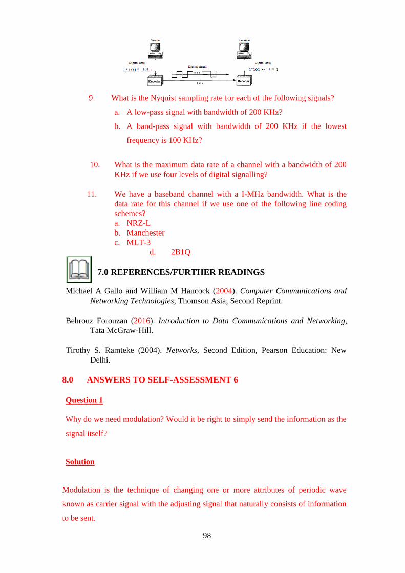
98

9. What is the Nyquist sampling rate for each of the following signals?

a. A low-pass signal with bandwidth of 200 KHz?

b. A band-pass signal with bandwidth of 200 KHz if the lowest

frequency is 100 KHz?

10. What is the maximum data rate of a channel with a bandwidth of 200

KHz if we use four levels of digital signalling?

11. We have a baseband channel with a I-MHz bandwidth. What is the

data rate for this channel if we use one of the following line coding

schemes?

a. NRZ-L

b. Manchester

c. MLT-3

d. 2B1Q


Michael A Gallo and William M Hancock (2004). Computer Communications and

Networking Technologies, Thomson Asia; Second Reprint.

Behrouz Forouzan (2016). Introduction to Data Communications and Networking,

Tata McGraw-Hill.

Tirothy S. Ramteke (2004). Networks, Second Edition, Pearson Education: New

Delhi.

8.0 ANSWERS TO SELF-ASSESSMENT 6

Question 1

Why do we need modulation? Would it be right to simply send the information as the

signal itself?

Solution

Modulation is the technique of changing one or more attributes of periodic wave

known as carrier signal with the adjusting signal that naturally consists of information

to be sent.

99

Why do we need modulation?

We need modulation because

a. Data signal wave is a low frequency signal wave. Example of such data signal

wave are conversation and music

Modulation enables data signal wave to become a higher signal wave since

lower frequency wave is more adaptable to blockage than higher frequency

wave.

b. Higher frequency wave carries more data since it has more bandwidth.

c. Much larger-size antenna is required at the destination by lower frequency

signals. However, the size of the antenna will be reduced with the increase of

the wave frequency by modulation.

d. It is pertinent to note that data signal is hidden inside carrier wave through

modulation, thereby, providing security.

Would it be right to simply send the information as the signal itself?

No, it will not be correct simply send the information as the signal itself because of the

many advantages of modulation. Students can explore more on this.

Question 2

A common fm broadband has a derivation of ±75kHz bandwidth and a modulation

frequency of 15kHz. Calculate the bandwidth of 98% of the power.

Solution

This calculation shall be done using Calson‘s rule which states that 98% of the power is

contained within a bandwidth equal to the deviation frequency, plus the modulation

frequency doubled. The formula states

that

BT = 2 (▲f + fm)

Where

▲f = deviation

BT = total bandwidth (for 98% power)

fm = frequency modulation

In this case, the common fm signal has a deviation of ±75kHz and 15kHz. Thus, the

bandwidth of 98% of the power approximate to

2(75+15) = 180kHz

100

It is pertinent to note that 200kHz is allowed for each station give room for acceptance

spaced channels.

Question 2

Why is AM the most susceptible to noise of the three types of modulation?

Solution

AM is the most susceptible to noise since noise is in the channel (i.e. atmosphere) which

easily creep into the signal and alter its amplitude.


Question 1

List three techniques of digital-to-digital conversion.

Solution

The three different techniques described in this chapter are line coding, block coding, and

scrambling.

Question 2

Distinguish between data rate and signal rate.

Solution

The data rate defines the number of data elements (bits) sent in 1s. The unit is bits per

second (bps). The signal rate is the number of signal elements sent in 1s. The unit is

the baud.

Question 3

Define a DC component and its effect on digital transmission

Solution

When the voltage level in a digital signal is constant for a while, the spectrum creates

very low frequencies, called DC components, that present problems for a system that

cannot pass low frequencies.

Question 4

List five lines coding schemes discussed in this section.

Solution

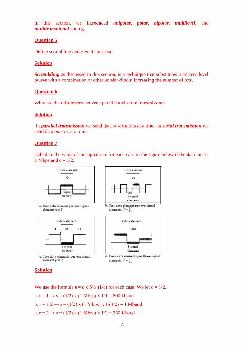
101

In this section, we introduced unipolar, polar, bipolar, multilevel, and

multitransitional coding.

Question 5

Define scrambling and give its purpose.

Solution

Scrambling, as discussed in this section, is a technique that substitutes long zero level

pulses with a combination of other levels without increasing the number of bits.

Question 6

What are the differences between parallel and serial transmission?

Solution

In parallel transmission we send data several bits at a time. In serial transmission we

send data one bit at a time.

Question 7

Calculate the value of the signal rate for each case in the figure below if the data rate is

1 Mbps and c = 1/2.

Solution

We use the formula s = c x N x (1/r) for each case. We let c = 1/2.

a. r = 1 → s = (1/2) x (1 Mbps) x 1/1 = 500 kbaud

b. r = 1/2 → s = (1/2) x (1 Mbps) x 1/(1/2) = 1 Mbaud

c. r = 2 → s = (1/2) x (1 Mbps) x 1/2 = 250 Kbaud

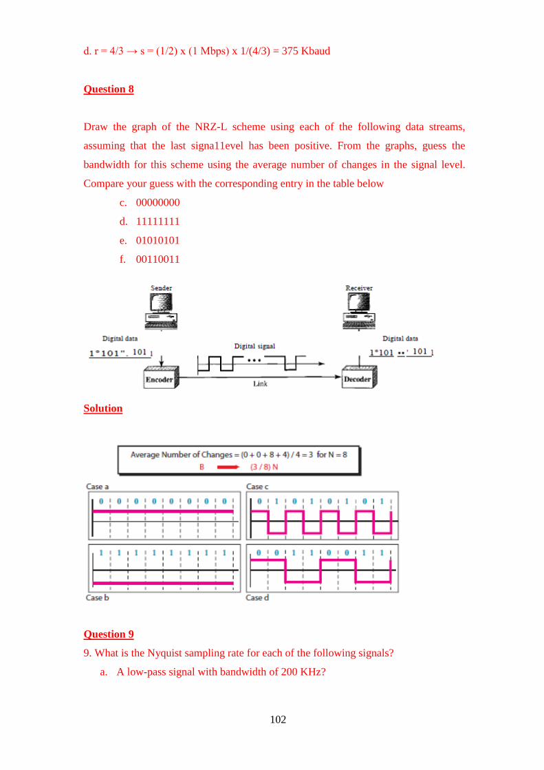
102

d. r = 4/3 → s = (1/2) x (1 Mbps) x 1/(4/3) = 375 Kbaud

Question 8

Draw the graph of the NRZ-L scheme using each of the following data streams,

assuming that the last signa11evel has been positive. From the graphs, guess the

bandwidth for this scheme using the average number of changes in the signal level.

Compare your guess with the corresponding entry in the table below

c. 00000000

d. 11111111

e. 01010101

f. 00110011

Solution

Question 9

9. What is the Nyquist sampling rate for each of the following signals?

a. A low-pass signal with bandwidth of 200 KHz?

103

b. A band-pass signal with bandwidth of 200 KHz if the lowest frequency is 100

KHz?

Solution

a. In a low-pass signal, the minimum frequency 0.

Therefore,

we have fmax = 0 + 200 = 200 KHz. → fs = 2 x 200,000 = 400,000 samples/s

b. In a bandpass signal, the maximum frequency is equal to the minimum

frequency plus the bandwidth. Therefore,

we have fmax = 100 + 200 = 300 KHz. → fs = 2 x 300,000 = 600,000

samples /s

Question 10

What is the maximum data rate of a channel with a bandwidth of 200 KHz if we

use four levels of digital signalling

Solution

The maximum data rate can be calculated as Nmax = 2 x B x nb = 2 x 200 KHz x

log24 = 800 kbps

Question 11

We have a baseband channel with a I-MHz bandwidth. What is the data rate for this

channel if we use one of the following line coding schemes?

a. NRZ-L

b. Manchester

c. MLT-3

d. 2B1Q

Solution

We can calculate the data rate for each scheme:

a. NRZ → N = 2 x B = 2 x 1 MHz = 2 Mbps

b. Manchester → N = 1 x B = 1 x 1 MHz = 1 Mbps

c. MLT-3 → N = 3 x B = 3 x 1 MHz = 3 Mbps

d. 2B1Q → N = 4 x B = 4 x 1 MHz = 4 Mbps

Question 12

104

Why is PAM necessary pre-requisite to PCM? Why can we not use PCM directly?

Solution

PAM is necessary prerequisite for PCM because it converts analogue signal into a

series of Pulses, then digitize the signal into what is called quantization. Hence, the

resulting binary digits is then transformed to digital signal using any of the digital to

digital encoding mechanization. This digital signal is the representation of the original

analogue signal.

Why can we not use PCM directly?

Solution

PCM cannot be used directly because the data in discuss are analogue data which

needs to be converted to digital before it can be used by PCM.

105

UNIT 4 MULTIPLEXING AND SWITCHING

CONTENTS

1.0 Introduction

2.0 Objectives

3.0 Main Content

3.1 Multiplexing

3.1.1 Frequency Division Multiplexing

3.1.2 Time Division Multiplexing

3.2 Digital Subscriber Lines

3.3 ADSL vs. Cable

3.4 Switching

3.4.1 Circuit Switching

3.4.2 Packet Switching

4.0 Conclusion

5.0 Summary



1.0 INTRODUCTION

The transmission of data over a network, whether wireless or not,

requires us to solve the problem of being able to send a large amount of data among

different groups of recipients at the same time without the message of one being

mixed up with those of the others. For example, think of the thousands of radio or

television channels that are being broadcast throughout the world simultaneously, or

of the millions of telephone conversations that are taking place every minute of the

day. This feat is achieved by multiplexing the transmissions in some way. In this unit,

we will look at the different methods of multiplexing that are commonly used,

frequency division multiplexing and time division multiplexing. Time division

multiplexing again can be synchronous or statistical.

There are some differences in the characteristics of voice and data communication.

Although, finally everything is really data, these differences dictate the design of the

telephone network as well as the techniques of switching. When one wants to transmit

data over a telephone line, we have to make some changes to be able to get sufficiently

high speeds. We will look at ADSL, a scheme for doing this at rates that can compete

on cost and quality with those offered by cable television service providers. We will

also look at the advantages and disadvantages of the two methods and of high-speed

data access.

When constructing networks of any size, a fundamental requirement is that any two

nodes of the network should be able to communicate with each other, for, if they

cannot do so, they are not on the same network. This brings up the issue of how to

switch the data stream, that is, to make sure it reaches its destination and not some

106

other random location on the network. This unit will, describe the different switching

techniques available to make this possible.

2.0 OBJECTIVES


1. state what multiplexing and switching mean

2. state how a telephone line can be used for transmitting data using ADSL

3. describe the differences between ADSL and cable television for data access;

4. describe the different kinds of multiplexing and switching

5. state the characteristics of Frequency Division Multiplexing

6. describe the features of Time Division Multiplexing, both synchronous and

statistical

7. differentiate between the different kinds of switching.

3.0 MAIN CONTENT

3.1 Multiplexing

If, one wanted to send data between a single source and a single destination, things

would be comparatively easy. All it would need is a single channel between the two

nodes, of a capacity sufficient to handle the rate of transmission based on Nyqist‘s

theorem and other practical considerations. Granted that there would be no other

claimants for the resources, there would be no need for sharing and no contention.

The transmission channel would be available to the sole users in the world at all

times, and any frequency which they chose could be theirs. In a broadcasting case,

we could have the single source transmitting at any time of its choosing and at any

agreed upon frequency.

However, things are not so straightforward in the real world. We have a large number

of nodes, each of which may be transmitting or receiving, from or to possibly

different nodes each time. These transmissions could be happening at the same

moment. So, when we need to transmit data on a large scale, we run into the problem

of how to do this simultaneously, because, there can be many different sources and

the intended recipients for each source are often different. The transmission resource,

that is the available frequencies, is scarce compared to the large number of users. So,

there will have to share the resource and consequently, the issue of preventing

interference between them will arise.

If, all possible pairs of nodes could be completely connected by channels(?!), we

would still not have a problem. But that is obviously out of the question, given the

very large number of possible source and destination nodes. There would be over a

billion telephones in the world today, for instance.

107

This problem is solved by performing what is called multiplexing. It can be done by

sharing the available frequency band or by dividing up the time between the

different transmissions. The former is called Frequency Division Multiplexing

(FDM) while the other scheme is Time Division Multiplexing (TDM).

Another reason for multiplexing is that it is more economical to transmit data at a

higher rate as the relative cost of the equipment is lower. But at the same time, most

applications do not require the high data rates that are technologically possible. This

is an added inducement to multiplex the data so that, the effective cost can be brought

down further by sharing across many different, independent transmissions.

In this context, a multiplexer is a device that can accept n different inputs and send

out I single output. This output can be transmitted over a link or medium to its

destination, where to be useful, the original inputs have to be recovered. This is done

by a demultiplexer. We need to realize that for this kind of scheme to work, the

creation of the composite signal by the multiplexer needs to be such that, the original

component signals can be separated at the receiving end -otherwise we would end up

with just a lot of noise!

When we transmit data over a cable, we are really setting up a different medium. We

can transmit data over different cables at the same frequency at the same time without

interference because the media or links are different even in radio transmission, where

the medium is space and hence is a single medium available to all transmissions,

geographical distance can in many cases give rise to different links. A low power

medium wave transmission happening in India can be done simultaneously with a

similar transmission in Europe without interference or the need for any special

precautions. However, throughout the rest of the unit, when we talk of multiplexing,

we are referring to the simultaneous transmission of data over the same medium or

link.

3.1.1 Frequency Division Multiplexing

Suppose, it is human voice that has to be transmitted, over a telephone. This has

frequencies that are mostly within the range of 300 Hz to 3400Hz. We can modulate

this on a bearer or carrier channel, such as one at 300 kHz. Another transmission that

has to be made can be modulated to a different frequency, such as, 304 kHz, and yet

another transmission could be made simultaneously at 308 kHz. We are thus, dividing

up the channel from 300 kHz up to 312 kHz into different frequencies for sending data.

This is Frequency Division Multiplexing (FDM) because all the different transmissions

are happening at the same time -it is only the frequencies that are divided up.

The composite signal to be transmitted over the medium of our choice is obtained by

summing up the different signals to be multiplexed (Figure 1.50). The transmission is

received at the other end, the destination and there, it has to be separated into

its original components, by demultiplexing. In practice, a scheme like this

could result in interference or cross talk between adjacent channels because the

bandpass filters that are used to constrain the original data between the agreed upon

frequencies (300 to 3400 kHz) are not sharp. To minimize this, there are guard bands,

or unused portions of the spectrum between every two channels.

108

Another possible cause of interference could arise because of the fact that the

equipment, such as amplifiers used to increase the strength of the signal, may not

behave linearly over the entire set of frequencies that we seek to transmit. Then, the

output can contain frequencies that are the sum or difference of the frequencies used

by the input. This produces what is called intermodulation noise.

In this kind of division, it should be realised that the actual modulation technique used

is not of consequence. So, one could use analogue modulation (AM) or Frequency

Modulation (FM). Also the composite signal that we have produced could again be

modulated over a different frequency altogether. For example, the three voice

channels, that have been modulated for commercial broadcast radio to produce a

spectrum from 300 kHz to 312 kHz could be modulated onto a 2 GHz satellite channel

for long distance transmission to the other side of the earth. This second modulation

could use a technique different from the first one. The only thing that needs to be take

care of is, that the recovery of the original signals have to be done in the reverse order,

complementing the method used for producing the composite signal.

Frequency (Hz) Frequency (Khz) (a) (b)

Figure 1.50: Frequency division multiplexing

[Source: Computer Network by A.S Tanenbaum]

The International Telecommunication Union (ITU) has standardised a hierarchy of

schemes that utilise FDM for the transmission of voice and video signals as shown in

Figure 1.43. To begin with, a cluster of 12 voice channels, each of 4 kHz is combined

to produce a signal of bandwidth 48 kHz that is then, modulated and transmitted over

the 60 to 108 kHz band. This is called a group.

The next level of the hierarchy is the supergroup, where 5 such groups are combined

to use 240 kHz of bandwidth, occupying from 312 to 552 kHz. The next level is the

master group that consists of 5 such supergroups. This uses 1232 kHz from 812 to

2044 kHz. Again, 3 such super groups form a super master group that contains 3.872

MHz from 8.516 to 12.388 MHz. The United States uses a similar hierarchy as

decided by AT&T (the telecommunications company) that is, not entirely identical to

the ITU standard.

109

Figure 1.51: Analogue hierarchy

We, thus, see that the original signal could find itself subjected to modulation

several times, each of which may be of different kinds, before it is finally

transmitted. This raises the possibility of interference and noise, but, with the very

good equipment available today, this need not be a matter of concern.

FDM has the disadvantage of not being entirely efficient if the transmissions that

are multiplexed together have periods of silence or no data. Since, a frequency band

is dedicated to each data source, any such periods are simply not utilised.

3.1.2 Time Division Multiplexing

Another multiplexing scheme is to use the entire bandwidth for each channel but to

divide it into different time slots, as shown in Figure 1.52.

Figure 1.52: Time division multiplexing

In this case, we have four different transmissions occurring with each being ¼ of the

time slice. The slice should be small enough so that the slicing is not apparent to the

application. So, for a voice transmission, a cycle of l00ms could be sufficient as we

110

would not be able to detect the fact that there are delays. In that case, each

transmission could be allotted a slice of 25ms.

At the receiving end, the transmission has to be reconstructed by dividing up the

cycle into the different slices, taking into account the transmission delays. This

synchronisation is essential, for if the transmission delay is, say 40ms, then the first

transmission would start reaching 40ms later, and would extend to 65ms. If, we

interpreted it to be from 0 to 25ms, there would be complete loss of the original

transmission. This interleaving of the signal could be at any level starting from that

of a bit or a byte or bigger.

Synchronous Time Division Multiplexing

In this kind of Time Division Multiplexing (TOM), the simpler situation is where the

time slots are reserved for each transmission, irrespective of whether it has any data

to transmit or not. Therefore, this method can be inefficient because many time slots

may have only silence. But it is a simpler method to implement because the act or

multiplexing and demultiplexing is easier. This kind of TDM is known as

Synchronous TDM.

Here, we usually transmit digital signals, although the actual transmission

may be digital or analogue. In the latter case, the composite signal has to be

converted into analogue data by passing it through a modem. Here, the data rate that

the link can support has to at least equal the sum of the data rates required for each

transmission. So, if one has to transmit four streams of data at 2400 bps each, we

would need a link that can support at least 9600 bps. For each data stream, we would

typically have a small, say I character buffer, that would take care of any data flow

issues from the source.

Although, the transmission has to be synchronous, that is not the reason the scheme is

called Synchronous TDM. It is because of the fact that each data source is given

fixed slots or time slices. We can also support data sources with differing data rates.

This could be done by assigning fewer slots to slower sources and more slots to the

faster ones. Here, a complete cycle of time slots is called a frame. At the receiving

end, the frame is decomposed into the constituent data streams by sending the data in

each time slot to the appropriate buffer. The sequence of time slots allotted to a single

data source makes up a transmission channel.

We have already seen that the transmission in TDM must be synchronous because

otherwise, all the data would be garbled and lost. How is this achieved? Because this

unit is concerned with the physical layer and not the data link layer, we will not

concern ourselves with the problem of flow control or error correction or control. But

even at the physical layer, we have to ensure that each frame is synchronised to

maintain the integrity of the transmission.

One scheme to attain this is to add an extra bit of data to each frame. In succeeding

frames, this extra bit forms a fixed pattern that is highly unlikely to occur naturally in

the data. The receiver can then use this fact to synchronise the frames. Suppose each

frame has n bits. Starting from anywhere, the receiver compares bit number 1, n+ 1,

2n+ 1 and so on. If the fixed data pattern is found, the frames are synchronised.

Otherwise, the receiver commences to check bit number 2, n+2, 2n+2, ...until it can

111

determine whether the frames are in synchronization or otherwise. This continues till,

it is able to synchronise the frames and can then start receiving the data from the

various channels.

Even after this, it is important to continue to monitor the fixed pattern to make sure

that the synchronisation remains intact. If it is lost, the routine of re-establishing it

needs to be repeated as before.

The second problem in synchronising the transmission is the fact that there can be

some variations between the different clock pulses from the different input streams.

To take care of this, we can use the technique of pulse stuffing. Here, the multiplexed

signal is of a rate that is a bit higher than that of the sum of the individual inputs. The

input data is stuffed with extra pulses as appropriate by the multiplexer at fixed

locations in the frame. This is needed so that the demultiplexer at the other, receiving,

end can identify and remove these extra pulses. All the input data streams are thus

synchronised with the single local, multiplexer clock.

Statistical Time Division Multiplexing

We have seen that synchronous TDM can be quite wasteful. For example, in a voice

transmission, much of the bandwidth can be wasted because there are typically many

periods of silence in a human conversation. Another example, could be, that of a

timesharing system where many terminals are connected to a computer through the

network. Here too, many of the time slots will not be used because there is no activity

at the terminal. In spite of being comparatively simpler, synchronous TDM is

therefore, often not an attractive option.

To take care of this problem, we can use statistical TDM. This is a method where

there are more devices than the number of time slots available. Each input data

stream has a buffer associated with it. The multiplexer looks at the buffer of each

device that provides the input data and checks to see if it has enough to fill a frame.

If, there are enough, the multiplexer sends the frame. Otherwise, it goes to the next

device in line and checks its input buffer. This cycle is continued indefinitely. At the

receiving end the demultiplexer decomposes the signal into the different data

streams and sends them to the corresponding output line.

The multiplexer data rate is not higher than that of the sum of all the input devices

connected to it. So statistical, TDM can make do with a lower transmission rate than

needed by synchronous TDM, at the cost of more complexity. The other way in

which this is of benefit is, by the ability to support higher throughput for the same

available data rate of the multiplexer. This capability is easily realised during the

normal, expected data transmission periods when the amount of data that the

different input devices have available for transmission is, in fact, lower than the

capacity of the multiplexing device. But the same attribute becomes a disadvantage

during peak loads, where all or many of the devices may have data to transmit for a

short time. In such a situation, the slack that was available to us for more efficient

transmission is no longer present. We will see later how to handle peak load

situations in statistical TDM.

In this kind of scheme, it is not known to us which input device will have data to

send at a given time. So, we cannot use a round robin positional scheme that was

112

possible in synchronous TDM. Each frame has to be accompanied by information

that will tell the demultiplexer which input device the frame belongs to, so that it can

be delivered to the appropriate destination. This is the overhead of statistical TDM,

besides increased complexity of equipment.

If, we are sending input data from only one source at a time, the structure of a frame

would need to have an address field for the source followed by the data for it. This is

really the statistical TDM data frame. It would form the data part of a larger,

enclosing High Level Data Link Control (HDLC) frame if we are using HDLC as the

transmission protocol. This frame would itself have various other fields that we will

not discuss here.

Such a scheme is also not as efficient as we can make it. This is because the quantum

of data available from the source, in that time slot, may not be enough to fill the

TDM sub frame. So, while it may be an adequate method if the load is not heavy, we

also need to think of a method that can utilise available resources better.

The way to do this would be, to have more than one input data source transmit in a

single TDM frame. We would then need to have a more complex structure for the

frame whereby, we would have to specify the different input devices in the frame

followed by the length of the data field. More sophisticated approaches could be

used, in order to optimise the number of bits, we need to encode all this addressing

and data information.

For peak loads, there is need for some kind of buffering mechanism, so that,

whenever there is excess input from the data sources that the multiplexer cannot

immediately handle, it is stored until it can be sent. The size of the buffer needed will

increase as the transmission capacity of the multiplexer decreases, as it will become

more likely that an input data stream will not be transmitted immediately. It will also

depend on the average data rate of the input devices taken together. No matter what

the buffer size we choose, there is always a non-zero probability that the buffer itself

will overflow, leading to loss of data. If, the average data rate of all devices is close

to the peak rate, then we are approaching a situation of synchronous TDM where we

are not able to take advantage of periods of silence that is the basis of statistical

TDM.

3.2 Digital Subscriber Lines

Digital Subscriber Lines are an example of multiplexing in action. They are really

telephone lines that can support much higher data rates than are possible with an

ordinary telephone connection. The concept came up in response to the high data

rates of more than 10 Mbps offered by cable television providers. Compared to those

rates, the 56Kbps possible over a telephone dial up connection was a miserable

offering.

The 56 Kbps rate is really an artificial barrier arising from the fact that voice

telephone line standards limited the bandwidth to about 3.1 KHz to take advantage of

the normal range of the human voice in conversation. Nyquist‘s theorem and the

limitations of line quality ensured that we ended up with that rate. Once the 3.1 KHz

limit is removed, the telephone line can support much higher data speeds.

113

Out of the several different technical solutions that came about, the ADSL

(Asymmetric DSL) technology has proved to be the most popular. Asymmetric

comes from the fact that the data rates in the two directions are different. The

approach is to divide the 1.1 MHz bandwidth available over the Cat-3 telephone

cables into 256 channels. Of these channels, 0 is used for normal voice

communication. The next 5 channels are not used to ensure separation and non-

interference between data and voice transmissions. The next 2 channels are used for

upstream and downstream control. The remaining 248 channels are available for data

transmission.

Like in voice circuits, it would have been possible to use half the channels for

communication in each direction. But, statistics show that most users download much

more data than they upload. So usually 32 channels are dedicated to uploading, that

is, transferring data from the users to the provider and the remaining 216 channels are

used for downloading data to the users. This typically translates into 512 Kbps to 1

Mbps download and 64 Kbps to 256 Kbps upload data rates. This then, is the

asymmetric aspect of the DSL line.

A problem with ADSL is that the physics of the local loop is such that, the speed at

which it can be driven depends heavily on the distance between the subscriber‘s

premises and the provider‘s nearest termination point. The speed falls sharply with

distance and so, distance can become a limiting factor in being able to offer

competitive speed compared to that of the cable television providers.

However, ADSL is comparatively simple for a service provider to offer, given an

existing telephone network, and does not require much change to its already available

equipment. It necessitates two modifications, one each, at the subscriber end and at

the end office. On the user‘s premises, a Network Interface Device has to be installed

that incorporates a filter. This is called a splitter and it sends the non-voice portion of

the signal to an ADSL modem. The signal from the computer has to be sent to the

ADSL modern at high speed, usually done these days by connecting them over a

USB port.

At the provider‘s end office, the signal from the users is recovered and converted into

packets that are then sent to the Internet Service Provider, which may be the

telephone company itself.

3.3 ADSL vs. Cable

At first glance, a comparison between ADSL and cable may seem like a no contest.

Cable television, sent over coaxial cables, has a bandwidth that is potentially

hundreds of times that of the twisted pair Cat-3 cable used for telephone connections.

But, as we go along, it turns out that there are considerations in favour of both sides.

First, there are specific assurances regarding bandwidth that we get from telephone

companies who provide ADSL connectivity. An ADSL link is a dedicated

connection that is always available to the user, unlike television cable that is shared

by scores or even hundreds of subscribers in the immediate neighbourhood. So the

114

kind of speeds that we can get over cable can vary from one moment to the next,

depending on the number of users that are working at the time.

There are security risks associated with the fact that cable is shared. Potentially other

users can always tap in and read (even change) what you are sending or receiving.

The problem does not exist on ADSL, because, each channel is separate and

dedicated to the specific user. Though, cable traffic is usually encrypted by the

provider, this situation is worse than ADSL where other users just do not get your

traffic at all. Also because the channel is dedicated to you, the total number of users

does not have any effect on your access speeds as there is no contention with other

users.

3.4 Switching

There are many potential sources of data in the world and likewise, many potential

recipients. Just think of the number of people who may like to reach one another over

the telephone. How can one ensure that every data source is able to connect to the

recipient? Clearly one cannot have a physical link between every pair of devices that

might want to communicate. Therefore, we need a mechanism, to be able to connect

together devices that, need to transfer data between them. This is the problem of

switching.

There are two basic approaches to switching. In circuit switching, we create a circuit

or link between devices, for the duration of time for which they wish to

communicate. This requires a mechanism for, the initiating device to choose the

device that it wants to send data to. All devices must also have an identifying, unique

address that can be used to set up the circuit. Then, the transmission occurs, and

when it is over, the circuit is dismantled so that the same physical resources can be

used for another transmission.

The packet switching approach can be used when we are using datagrams or packets

to transmit data over the channel. Each datagram is a self-contained unit that includes

within itself the needed addressing information. The datagrarns can arrive at the

destination by any route and may not come in sequence.

3.4.1 Circuit Switching

As discussed already, in circuit switching, we create a link or circuit between the

devices that need to communicate, for the duration of the transmission only. It entails

setting up the circuit, doing the actual transmission that can be simplex, half duplex

or full duplex, and then dismantling the circuit for use by another pair of devices. An

example is shown in the Figure 1.53 where there are 7 devices. These are divided into

two groups of 3 on the left and 4 on the right. To ensure complete connectivity

between them at all times, we would need 12 physical links. But, if connectivity is

not required at all times, we can achieve connectivity between any of the devices by

grouping them together and using switches to achieve temporary links.

115

Figure 1.53: Circuit Switching

For example, we can have 7 links that connect the devices A, Band C on the left to

the switch. The other devices D, E, F and G on the right are also connected to the

same switch. The switch can connect any two devices together using only these seven

links as desired.

The capacity of the switch is determined by the number of circuits that it can support

at any given time. In the Figure 1.53 example, we have seen a switch with 1 input

and 1 output. If devices C and E are communicating with each other, the others

cannot communicate at the same time, although, there are available links from them

to the switch. A circuit switch is really a device that has n inputs and m outputs (n

need not be equal to m).

There are two main approaches to circuit switching, called space division or time

division switches. Space division switches are so called because the possible circuit

paths are separated from one another in space. The old, and now obsolete, crossbar

telephone exchanges are an example of space division switching. The technique can

be used for both digital or analogue systems. There were other designs of such

switching but the only one that went into large scale use was the crossbar. Because of

the way it is constructed, such switching does not have any delays. Once the path is

established, transmission occurs continuously at the rate that the channel can support.

In essence, a crossbar connects p inputs to q outputs. Each such connection is

actually performed by connecting the input to the output using some switching

technology such as, a transistor based electronic switch or an electromechanical

relay. This requires a large number of possible connections, called cross points. For a

10,000line telephone exchange, it would mean that, each of the 10,000 possible

inputs be able to connect to any of the 10,000 possible outputs, requiring a total of

100,000,000 cross points. As this is clearly impractical, the pure crossbar design is

not usable on a commercial scale. Moreover, there are inherent inefficiencies in this

design as statistically, only a small fraction of these cross points are ever in use

simultaneously.

The way to get around this limitation is, to split the switch into different stages. If we

consider a 36 line exchange where each of36 inputs needs to be connected to 36

outputs, we can do so in, say, 3 stages. The first stage could have 3 switches, each

with 12 inputs and 2 outputs to the two second stage switches. These intermediate

B

A

C

D

E

F

G

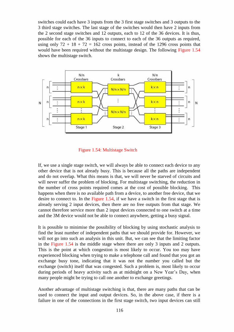
116

switches could each have 3 inputs from the 3 first stage switches and 3 outputs to the

3 third stage switches. The last stage of the switches would then have 2 inputs from

the 2 second stage switches and 12 outputs, each to 12 of the 36 devices. It is thus,

possible for each of the 36 inputs to connect to each of the 36 outputs as required,

using only 72 + 18 + 72 = 162 cross points, instead of the 1296 cross points that

would have been required without the multistage design. The following Figure 1.54

shows the multistage switch.

Figure 1.54: Multistage Switch

If, we use a single stage switch, we will always be able to connect each device to any

other device that is not already busy. This is because all the paths are independent

and do not overlap. What this means is that, we will never be starved of circuits and

will never suffer the problem of blocking. For multistage switching, the reduction in

the number of cross points required comes at the cost of possible blocking. This

happens when there is no available path from a device, to another free device, that we

desire to connect to. In the Figure 1.54, if we have a switch in the first stage that is

already serving 2 input devices, then there are no free outputs from that stage. We

cannot therefore service more than 2 input devices connected to one switch at a time

and the 3M device would not be able to connect anywhere, getting a busy signal.

It is possible to minimise the possibility of blocking by using stochastic analysis to

find the least number of independent paths that we should provide for. However, we

will not go into such an analysis in this unit. But, we can see that the limiting factor

in the Figure 1.54 is the middle stage where there are only 3 inputs and 2 outputs.

This is the point at which congestion is most likely to occur. You too may have

experienced blocking when trying to make a telephone call and found that you got an

exchange busy tone, indicating that it was not the number you called but the

exchange (switch) itself that was congested. Such a problem is, most likely to occur

during periods of heavy activity such as at midnight on a New Year‘s Day, when

many people might be trying to call one another to exchange greetings.

Another advantage of multistage switching is that, there are many paths that can be

used to connect the input and output devices. So, in the above case, if there is a

failure in one of the connections in the first stage switch, two input devices can still

117

connect to it. In the case of single stage switching, that would have meant that we

could not set up a circuit between those devices.

Let us, now look at another method of switching that uses time slots rather than spatial

separation. You have already seen how synchronous TDM involves transmission

between input and output devices using fixed time slots dedicated to each channel. But

that is not switching because the input-output device combinations are fixed. So, if we

have three devices A, B and C transmitting and three devices D, E and F that are

receiving the respective transmissions, there will be no way to change the circuit path

so that A can transmit to E or F.

To achieve switching, we use a device called a Time Slot Interchange (TSI). The

principle of such a device is simple. Based on the desired paths that we want to set up,

the TSI changes the input ordering in the data streams. So, if the demultiplexer is

sending the outputs to D, E and F in order, and if we want that A send data to E

instead of F, and that B send data to F rather than E, then the TSI will change the input

ordering of the time slots from A, B, C to C, A, B. The demultiplexer will not be

aware of this and will continue to send the output the same way as before. The result

will be, that our desired switching will be accomplished. However, unlike space

division switching, our output will be subject to delays because we might have to wait

for the input from the right device before it can be transmitted. This is unlike space

division switching where the data can be sent in a steady stream.

How does the TSI work? It consists of a control unit that does the actual reordering of

the input. For this, it has to first, buffer the input it gets, in the order it gets it. This

would be stored in some kind of volatile memory. The control unit then sends out the

data from the buffer in the order in which it is desired. Usually the size of each buffer

would be that of the data that the input generates in one time slice.

We do not have to confine ourselves to a single type of switch. There can be switches

that are based on a combination of both kinds of switching. For example, we could

have a multistage switch where, some of the stages are space division switches whiles

others are time division switches. With such an approach, we can try to optimise the

design by reducing the need for cross points while keeping the delays in the whole

system to a minimum. For example, we could have a TST three stage switch where the

first and last stages use time division switching while the middle stage uses cross

points.

Circuit switching is useful for voice-based communication because of the

characteristics of the data transfer. Although, a voice conversation tends to have

periods of silence in between, those periods are usually brief. The rest of the time there

is data available for transmission. Secondly, in such communication, we cannot

tolerate delays of more than about 100ms as that becomes perceptible to the human ear

and is quite annoying to the speaker and listener.

Again, because it is human beings that are present at both ends, the rate at which data

is generated at both ends is similar, even if one person talks a bit faster than the other!

Also, the other human can usually understand what is being said even if he cannot at

the same rate. And if really required, one can communicate to the other to speak

slower or louder. But, when we are dealing with data generating devices, there can

always be a mismatch between the rate at which one device generates data and at

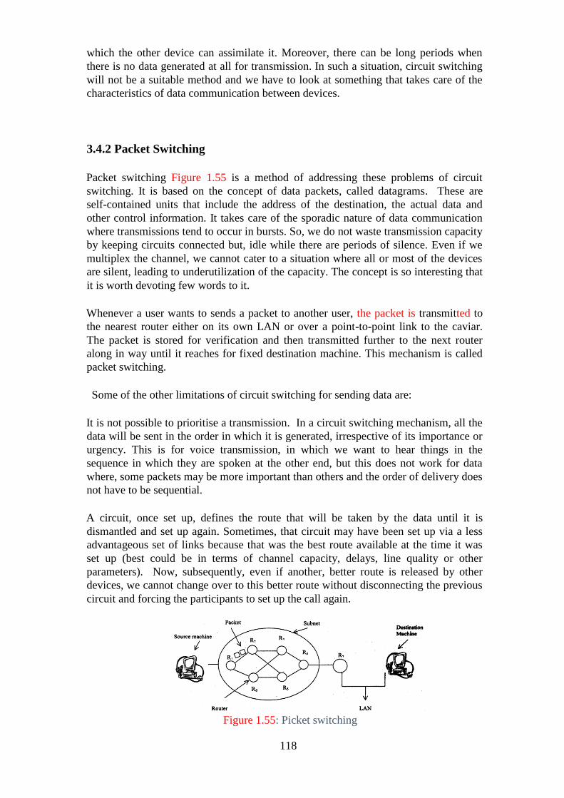
118

which the other device can assimilate it. Moreover, there can be long periods when

there is no data generated at all for transmission. In such a situation, circuit switching

will not be a suitable method and we have to look at something that takes care of the

characteristics of data communication between devices.


Packet switching Figure 1.55 is a method of addressing these problems of circuit

switching. It is based on the concept of data packets, called datagrams. These are

self-contained units that include the address of the destination, the actual data and

other control information. It takes care of the sporadic nature of data communication

where transmissions tend to occur in bursts. So, we do not waste transmission capacity

by keeping circuits connected but, idle while there are periods of silence. Even if we

multiplex the channel, we cannot cater to a situation where all or most of the devices

are silent, leading to underutilization of the capacity. The concept is so interesting that

it is worth devoting few words to it.

Whenever a user wants to sends a packet to another user, the packet is transmitted to

the nearest router either on its own LAN or over a point-to-point link to the caviar.

The packet is stored for verification and then transmitted further to the next router

along in way until it reaches for fixed destination machine. This mechanism is called

packet switching.

Some of the other limitations of circuit switching for sending data are:

It is not possible to prioritise a transmission. In a circuit switching mechanism, all the

data will be sent in the order in which it is generated, irrespective of its importance or

urgency. This is for voice transmission, in which we want to hear things in the

sequence in which they are spoken at the other end, but this does not work for data

where, some packets may be more important than others and the order of delivery does

not have to be sequential.

A circuit, once set up, defines the route that will be taken by the data until it is

dismantled and set up again. Sometimes, that circuit may have been set up via a less

advantageous set of links because that was the best route available at the time it was

set up (best could be in terms of channel capacity, delays, line quality or other

parameters). Now, subsequently, even if another, better route is released by other

devices, we cannot change over to this better route without disconnecting the previous

circuit and forcing the participants to set up the call again.

Figure 1.55: Picket switching

119

A datagram can contain different lengths of data. Besides, it would have control

information such as the address to which it needs to be sent, the address from which

it has originated, its type and priority and so on. From its source node it is sent to a

neighbouring node, depending on its final destination. The format of the datagram

depends on the protocol that is used and it is the responsibility of each node to route

the datagram onto the next node that would take it to its destination. There can be

several routes possible and each node would make the decision based on availability,

traffic conditions, channel quality and so on.

Although datagram length can vary, long messages would have to be split into more

than one datagram as the network protocol would have a limit on the maximum size

of a datagram. Because each datagram is routed independently, the different

datagrams that make up a message may arrive out of sequence at the destination, as

different routes may take different times to traverse. In communication protocols it is

the responsibility of the network layer to make sure that routing gets done, while it is

the transport layer that ensures that the message at the receiving end is in the proper

sequence.

Again, the physical link between two nodes can be of any type and is of no

consequence at the higher layers of the communication protocol in use. That link

itself may be multiplexed and may carry several transmissions simultaneously, for

the same or different pairs of source and destination nodes. Moreover, these

transmissions may be happening in different directions.

This was the datagram approach to packet switching. It is also possible to look at

packet switching in terms of a virtual circuit, which again has two different

approaches that are in current practice.

In a virtual circuit, when the first datagram is sent out, we decide on the route that

will be followed, and subsequent datagrams continue to follow that route. So, it is

like circuit switching to‘ a large extent. But, in circuit switching the link is dedicated

to the pair of nodes and there is no multiplexing that happens at the level of

individual switches. In virtual circuits there can be multiplexing at the switches as

well.

Permanent virtual circuits are dedicated channels set up for communication between

a pre-decided pair of nodes. It is thus, akin to a leased line where the routing is

decided once the virtual circuit is set up. There is no call set up required because, the

link is always available to the pair of nodes. On the other hand, we can also have

switched virtual circuit where the routing is decided every time a pair of nodes want

to communicate. This is like a dial-up connection where any two pairs of nodes can

communicate by setting up a call that is terminated when the conversation is over.

Another difference between circuit and virtual circuit switching has to do with

reliability and failure recovery. In circuit switching, if the link breaks because of a

failure in any portion, the call is terminated. It would have to be established again for

the conversation to continue. In virtual circuits, although the route is decided at the

beginning when the session is set up, in case of failure of any part of the route, an

alternate route will be agreed upon and set up.

120

Also, in circuit switching there is no possibility of failure due to congestion after the

link is set up. In virtual circuits, congestion can occur even later because of

multiplexing at the switches.

4.0 CONCLUSION

This unit has extensively described the basic concepts behind multiplexing and

switching. You have learnt how a telephone line can be used for transmitting data

using ADSL and also the differences between ADSL and cable television for data

access.

You have also learnt about the characteristics of frequency Division Multiplexing

and the features of Time Division Multiplexing both synchronous and statistical

different kinds of switching.

5.0 SUMMARY

Multiplexing is needed in communication networks because of the scarcity of

bandwidth compared to the large number of users. Frequency Division and Time

Division Multiplexing are the two ways of multiplexing, of which Time Division

Multiplexing can be synchronous or asynchronous. The asynchronous method is

more complex but more efficient for data transmission.

ADSL is a means of utilising the existing capacity of the local loop in the telephone

system for providing subscribers with high speed data access. Such access is also

provided by companies over the cable television network. ADSL is more secure and

predictable in terms of service quality, while cable does not have the limitations of

distance from the end office that ADSL has.

Switching is necessary to connect two nodes or devices over the network that intends

to communicate for a limited duration. Circuit switching is more suitable for voice

communication, and can be done using space division, time division or a combination

of both kinds of switches. Multistage switching is needed to optimise the number of

cross points needed. Packet switching is used for data transmission and allows for

prioritising of data packets, alternate routing as needed and is also more efficient for

the busty traffic pattern of data communication. Datagrams are self-contained packets

of data that are routed by the intermediate nodes of the network. Switched or

permanent virtual circuits can also be utilised, where the route is established at the

beginning of the session, but can be altered without disrupting the channel in case of

failure of any part of the route.


1. Describe the need for switching and define a switch.

2. List the three traditional switching methods. What are the most common today?

3. What are the two approaches to packet-switching?

121

4. Compare and contrast a circuit-switched network and a packet-switched

network.

5. What is the role of the address field in a packet traveling through a datagram

network?

6. What is the role of the address field in a packet traveling through a virtual

circuit network?

7. Compare space-division and time-division switches.

8. What is TSI and its role in a time-division switching?

9. Define blocking in a switched network.

10. List four major components of a packet switch and their functions.


Andrew.S. Tannenbaum, Computer Networks, PHI, New Delhi, 2011

William Stalling, Data and Computer Communication. PHI, New Delhi, 2003.

Behrouz Forouzan, (2016). Introduction to Data Communications and Networking

Tala McGraw-Hill, New Delhi.


Question 1

Describe the goals of multiplexing.

Solution

Multiplexing is the set of techniques that allows the simultaneous transmission of

multiple signals across a single data link.

Question 2

Distinguish between a link and a channel in multiplexing.

Solution

In multiplexing, the word link refers to the physical path. The word channel refers to

the portion of a link that carries a transmission between a given pair of lines. One link

can have many (n) channels.

Question 3

Which of the three multiplexing techniques is common for fibre optic links? Explain

the reason

122

Solution

Wavelength Division Multiplexing (WDM) is common of the three types of

multiplexing (Frequency Division Multiplexing (FDM), Wavelength

Division Multiplexing (WDM) and Time Division Multiplexing (TDM)) for

multiplexing optical signals because it allows the multiplexing of signals with a very

high frequency.

Question 4

Distinguish between synchronous and statistical TDM

Solution

In synchronous TDM, each input has a reserved slot in the output frame. This can be

inefficient if some input lines have no data to send. In statistical TDM, slots are

dynamically allocated to improve bandwidth efficiency. Only when an input line has a

slot‘s worth of data to send is it given a slot in the output frame.

Question 5

Assume that a voice channel occupies a bandwidth of 4 kHz. We need to multiplex 10

voice channels with guard bands of 500 Hz using FDM. Calculate the required

bandwidth.

Solution

To multiplex 10 voice channels, we need nine guard bands. The required bandwidth is

then B = (4 KHz) × 10 + (500 Hz) x 9 = 44.5 KHz

Question 6

Describe the need for switching and define a switch.

Solution

Switching provides a practical solution to the problem of connecting multiple devices

in a network. It is more practical than using a bus topology; it is more efficient than

using a star topology and a central hub. Switches are devices capable of creating

temporary connections between two or more devices linked to the switch.

Question 7

What are the two approaches to packet-switching?

Solution

There are two approaches to packet switching: datagram approach and virtual circuit

approach.

123

Question 8

What is the role of the address field in a packet traveling through a datagram network?

Solution

The address field defines the end-to-end (source to destination) addressing.

Question 9

Compare space-division and time-division switches.

Solution

In a space-division switch, the path from one device to another is spatially separate

from other paths. The inputs and the outputs are connected using a grid of electronic

microswitches. In a time-division switch, the inputs are divided in time using TDM. A

control unit sends the input to the correct output device.

Question 10

Define blocking in a switched network.

Solution

In multistage switching, blocking refers to times when one input cannot be connected

to an output because there is no path available between them—all the possible

intermediate switches are occupied. One solution to blocking is to increase the

number of intermediate switches based on the Clos criteria.

Question 11

A path in a digital circuit-switched network has a data rate of I Mbps. The exchange

of 1000 bits is required for the setup and teardown phases. The distance between two

parties is 5000km. Answer the following questions if the propagation speed is 2 X

108 m:

a. What is the total delay if 1000 bits of data are exchanged during the data

transfer phase?

b. What is the total delay if 100,000 bits of data are exchanged during the data

transfer phase?

c. What is the total delay if 1,000,000 bits of data are exchanged during the data

transfer phase?

d. Find the delay per 1000 bits of data for each of the above cases and compare

them. What can you infer?

Solution

We assume that the setup phase is a two-way communication and the teardown phase

is a one-way communication. These two phases are common for all three cases. The

delay for these two phases can be calculated as three propagation delays and three

124

transmission delays or 3 [(5000 km)/ (2 x108 m/s)] +3 [(1000 bits/1 Mbps)] = 75ms +

3ms = 78ms. We assume that the data transfer is in one direction; the total delay is

then delay for setup and teardown + propagation delay + transmission delay

a. 78 + 25 + 1 = 104ms

b. 78 + 25 + 100 = 203ms

c. 78 + 25 + 1000 = 1103ms

d. In case a, we have 104ms. In case b we have 203/100 = 2.03ms. In case c, we

have 1103/1000 = 1.101ms. The ratio for case c is the smallest because we use

one setup and teardown phase to send more data.

125

MODULE 2: MEDIA ACCESS CONTROL AND DATA LINK LAYER

Unit 1 Data Link Layer Fundamentals

Unit 2 Retransmission Strategies

Unit 3 Contention-Based Media Access Protocols

Unit 4 Wireless LAN and Datalink Layer Switching

UNIT 1 DATA LINK LAYER FUNDAMENTALS

CONTENTS

1.0 Introduction

2.0 Objectives

3.0 Main Content

3.1 Framing

3.2 Basics of Error Detection

3.3 Forward Error Correction

3.4 Cyclic Redundancy Check Codes for Error Detection

3.5 Flow Control

4.0 Conclusion

5.0 Summary



1.0 INTRODUCTION

Data Link Layer (DLL) is the second layer of the OSI model which

takes services from the Physical layer and provides services to the network layer.

DLL transfers the data from a host to a node or a node to another node.

The main task of the data link layer is to take a raw data from transmission facility and

transform it into a line that appears free of transmission errors to the network layer. Data

packets are encoded and decoded into bits. These are called frames. The Functions of the

Data Link Layer are Framing, Frame synchronisation, Error Handling Flow Regulation,

Addressing and Access Control. The data link layer is divided into two sublayers: The

Media Access Control (MAC) layer and the Logical Link Control (LLC) layer. The MAC

sublayer controls how a computer on the network gains access to the link resources and

grants permission to transmit it. The LLC layer controls frame synchronisation, flow

control and error checking.

Frame is a data structure used in transmissions at DLL consisting of a header and a trailer

bracketing a data frame. Packets are the fundamental unit of information transport in all

modem computer networks, and increasingly, in other communication networks as well

these are converted to frame at DLL. The destination host not receiving the data bits as

transmitted by the source host is termed as error in data. The error needs to be detected or

corrected, as the data on the network must be error free and reliable which is one of the

key features of the DLL. There are various methods used for detection and correction of

these errors viz.: FEC (Forward Error Correction) and CRC (Cyclic Redundancy Check).

To transmit data from a source to a destination node, a node in a network should be

uniquely identified. This identification is known as the address of the node. Access

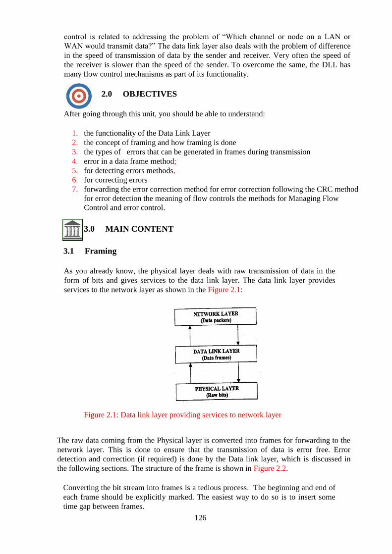
126

control is related to addressing the problem of ―Which channel or node on a LAN or

WAN would transmit data?‖ The data link layer also deals with the problem of difference

in the speed of transmission of data by the sender and receiver. Very often the speed of

the receiver is slower than the speed of the sender. To overcome the same, the DLL has

many flow control mechanisms as part of its functionality.

2.0 OBJECTIVES

After going through this unit, you should be able to understand:

1. the functionality of the Data Link Layer

2. the concept of framing and how framing is done

3. the types of errors that can be generated in frames during transmission

4. error in a data frame method;

5. for detecting errors methods,

6. for correcting errors

7. forwarding the error correction method for error correction following the CRC method

for error detection the meaning of flow controls the methods for Managing Flow

Control and error control.

3.0 MAIN CONTENT

3.1 Framing

As you already know, the physical layer deals with raw transmission of data in the

form of bits and gives services to the data link layer. The data link layer provides

services to the network layer as shown in the Figure 2.1:

Figure 2.1: Data link layer providing services to network layer

The raw data coming from the Physical layer is converted into frames for forwarding to the

network layer. This is done to ensure that the transmission of data is error free. Error

detection and correction (if required) is done by the Data link layer, which is discussed in

the following sections. The structure of the frame is shown in Figure 2.2.

Converting the bit stream into frames is a tedious process. The beginning and end of

each frame should be explicitly marked. The easiest way to do so is to insert some

time gap between frames.

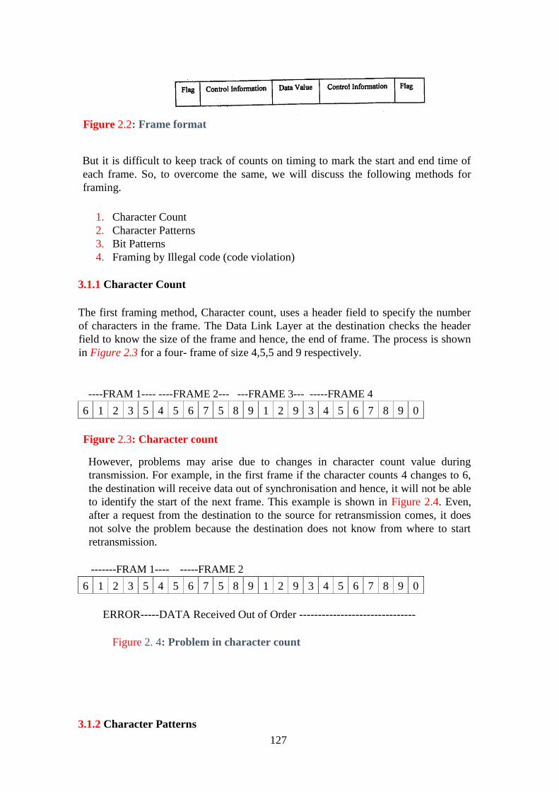
127

Figure 2.2: Frame format

But it is difficult to keep track of counts on timing to mark the start and end time of

each frame. So, to overcome the same, we will discuss the following methods for

framing.

1. Character Count

2. Character Patterns

3. Bit Patterns

4. Framing by Illegal code (code violation)

3.1.1 Character Count

The first framing method, Character count, uses a header field to specify the number

of characters in the frame. The Data Link Layer at the destination checks the header

field to know the size of the frame and hence, the end of frame. The process is shown

in Figure 2.3 for a four- frame of size 4,5,5 and 9 respectively.

----FRAM 1---- ----FRAME 2--- ---FRAME 3--- -----FRAME 4

6 1 2 3 5 4 5 6 7 5 8 9 1 2 9 3 4 5 6 7 8 9 0

Figure 2.3: Character count

However, problems may arise due to changes in character count value during

transmission. For example, in the first frame if the character counts 4 changes to 6,

the destination will receive data out of synchronisation and hence, it will not be able

to identify the start of the next frame. This example is shown in Figure 2.4. Even,

after a request from the destination to the source for retransmission comes, it does

not solve the problem because the destination does not know from where to start

retransmission.

-------FRAM 1---- -----FRAME 2

6 1 2 3 5 4 5 6 7 5 8 9 1 2 9 3 4 5 6 7 8 9 0

ERROR-----DATA Received Out of Order -------------------------------

Figure 2. 4: Problem in character count

3.1.2 Character Patterns

128

The second framing method, Character stuffing, solves the problem of out of

synchronisation. Here, each frame starts with special character set e.g., a special

ASCII character sequence.

The frame after adding the start sequence and the end sequence is shown in Figure 2.5.

Begin each frame with DLE STX. End each frame

with DLE ETX.

DLE stands for Data Link Escape

STX stands for Start of Text

ETX stands for End of Text

DLE STX ………………………….. DLE ETX

Figure 2. 5: Character patterns (Character stuffing)

If a OLE ETX occurs in the middle of the data and interferes with the data during

framing then, insert an ASCII OLE character just before DLE character in the data.

The Receiver interprets the single DLE as an escape indicating that the next character

is a control character.

If two OLE‘s appear in succession at the receiver‘s end, the first is discarded and the

second is regarded as data. Thus, framing OLE STX or OLE ETX is distinguished by

whether OLE is present once or twice.

Figure 2.6a: Before stuffing

Figure 2.6b: After stuffing

Figure 2.6c: After destuffing

A problem with character stuffing is that not all bit streams are character oriented

(e.g., Unicode is a 16-bit code). Hence, for arbitrary sized characters the process of

character stuffing becomes more complex. So next we will discuss a new method

known as the bit stuffing, which solves the problem of arbitrary sized character.

3.1.3 Bit Patterns

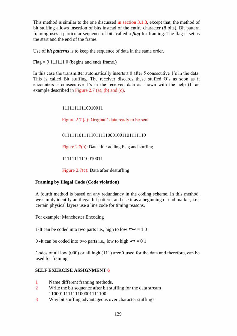
129

This method is similar to the one discussed in section 3.1.3, except that, the method of

bit stuffing allows insertion of bits instead of the entire character (8 bits). Bit pattern

framing uses a particular sequence of bits called a flag for framing. The flag is set as

the start and the end of the frame.

Use of bit patterns is to keep the sequence of data in the same order.

Flag = 0 111111 0 (begins and ends frame.)

In this case the transmitter automatically inserts a 0 after 5 consecutive 1‘s in the data.

This is called Bit stuffing. The receiver discards these stuffed O‘s as soon as it

encounters 5 consecutive 1‘s in the received data as shown with the help (If an

example described in Figure 2.7 (a), (b) and (c).

11111111110010011

Figure 2.7 (a): Original‘ data ready to be sent

01111110111110111110001001101111110

Figure 2.7(b): Data after adding Flag and stuffing

11111111110010011

Figure 2.7(c): Data after destuffing

Framing by Illegal Code (Code violation)

A fourth method is based on any redundancy in the coding scheme. In this method,

we simply identify an illegal bit pattern, and use it as a beginning or end marker, i.e.,

certain physical layers use a line code for timing reasons.

For example: Manchester Encoding

1-It can be coded into two parts i.e., high to low = 1 0

0 -It can be coded into two parts i.e., low to high = 0 1

Codes of all low (000) or all high (111) aren‘t used for the data and therefore, can be

used for framing.

SELF EXERCISE ASSIGNMENT 6

1 Name different framing methods.

2 Write the bit sequence after bit stuffing for the data stream

110001111111100001111100.

3 Why bit stuffing advantageous over character stuffing?

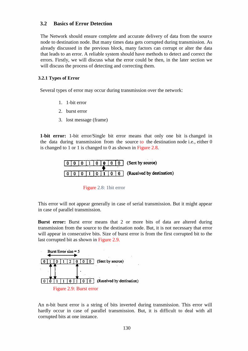
130

3.2 Basics of Error Detection

The Network should ensure complete and accurate delivery of data from the source

node to destination node. But many times data gets corrupted during transmission. As

already discussed in the previous block, many factors can corrupt or alter the data

that leads to an error. A reliable system should have methods to detect and correct the

errors. Firstly, we will discuss what the error could be then, in the later section we

will discuss the process of detecting and correcting them.

3.2.1 Types of Error

Several types of error may occur during transmission over the network:

1. 1-bit error

2. burst error

3. lost message (frame)

1-bit error: 1-bit error/Single bit error means that only one bit is changed in

the data during transmission from the source to the destination node i.e., either 0

is changed to 1 or 1 is changed to 0 as shown in Figure 2.8.

Figure 2.8: 1bit error

This error will not appear generally in case of serial transmission. But it might appear

in case of parallel transmission.

Burst error: Burst error means that 2 or more bits of data are altered during

transmission from the source to the destination node. But, it is not necessary that error

will appear in consecutive bits. Size of burst error is from the first corrupted bit to the

last corrupted bit as shown in Figure 2.9.

Figure 2.9: Burst error

An n-bit burst error is a string of bits inverted during transmission. This error will

hardly occur in case of parallel transmission. But, it is difficult to deal with all

corrupted bits at one instance.

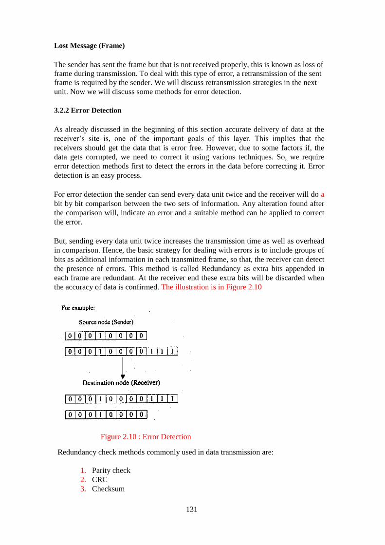
131

Lost Message (Frame)

The sender has sent the frame but that is not received properly, this is known as loss of

frame during transmission. To deal with this type of error, a retransmission of the sent

frame is required by the sender. We will discuss retransmission strategies in the next

unit. Now we will discuss some methods for error detection.

3.2.2 Error Detection

As already discussed in the beginning of this section accurate delivery of data at the

receiver‘s site is, one of the important goals of this layer. This implies that the

receivers should get the data that is error free. However, due to some factors if, the

data gets corrupted, we need to correct it using various techniques. So, we require

error detection methods first to detect the errors in the data before correcting it. Error

detection is an easy process.

For error detection the sender can send every data unit twice and the receiver will do a

bit by bit comparison between the two sets of information. Any alteration found after

the comparison will, indicate an error and a suitable method can be applied to correct

the error.

But, sending every data unit twice increases the transmission time as well as overhead

in comparison. Hence, the basic strategy for dealing with errors is to include groups of

bits as additional information in each transmitted frame, so that, the receiver can detect

the presence of errors. This method is called Redundancy as extra bits appended in

each frame are redundant. At the receiver end these extra bits will be discarded when

the accuracy of data is confirmed. The illustration is in Figure 2.10

Figure 2.10 : Error Detection

Redundancy check methods commonly used in data transmission are:

1. Parity check

2. CRC

3. Checksum

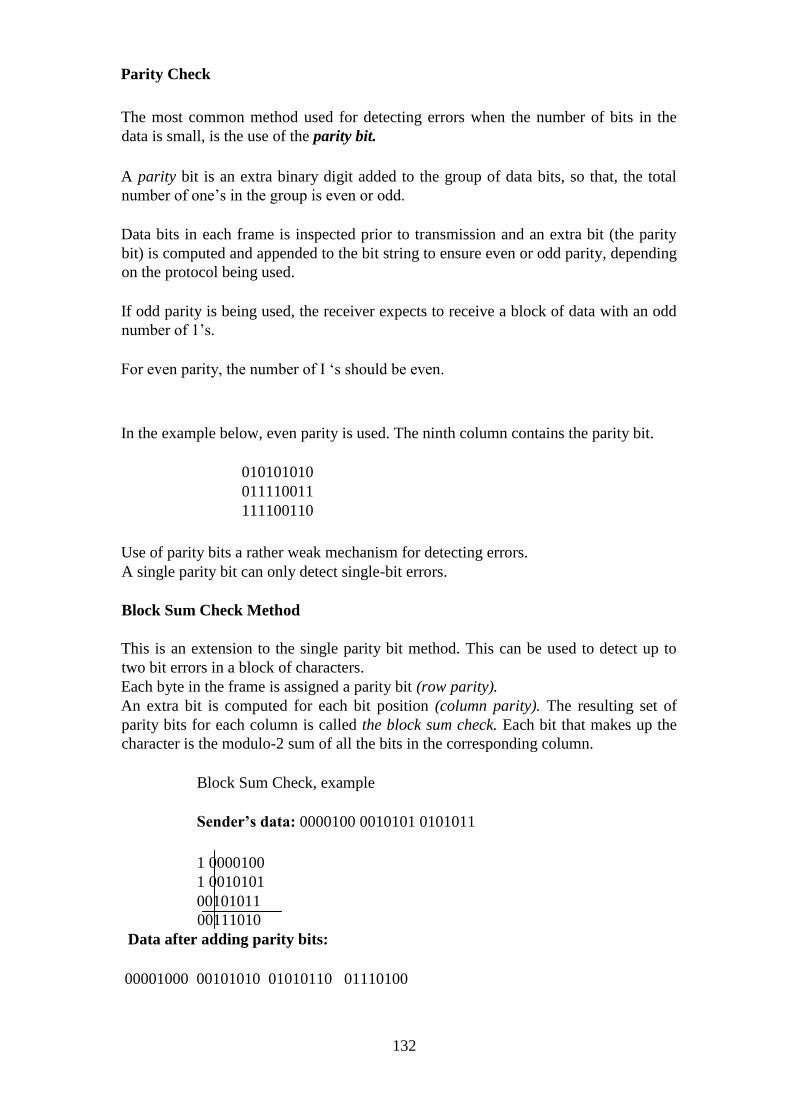
132

Parity Check

The most common method used for detecting errors when the number of bits in the

data is small, is the use of the parity bit.

A parity bit is an extra binary digit added to the group of data bits, so that, the total

number of one‘s in the group is even or odd.

Data bits in each frame is inspected prior to transmission and an extra bit (the parity

bit) is computed and appended to the bit string to ensure even or odd parity, depending

on the protocol being used.

If odd parity is being used, the receiver expects to receive a block of data with an odd

number of 1‘s.

For even parity, the number of I ‗s should be even.

In the example below, even parity is used. The ninth column contains the parity bit.

010101010

011110011

111100110

Use of parity bits a rather weak mechanism for detecting errors.

A single parity bit can only detect single-bit errors.

Block Sum Check Method

This is an extension to the single parity bit method. This can be used to detect up to

two bit errors in a block of characters.

Each byte in the frame is assigned a parity bit (row parity).

An extra bit is computed for each bit position (column parity). The resulting set of

parity bits for each column is called the block sum check. Each bit that makes up the

character is the modulo-2 sum of all the bits in the corresponding column.

Block Sum Check, example

Sender’s data: 0000100 0010101 0101011

1 0000100

1 0010101

00101011

00111010

Data after adding parity bits:

00001000 00101010 01010110 01110100

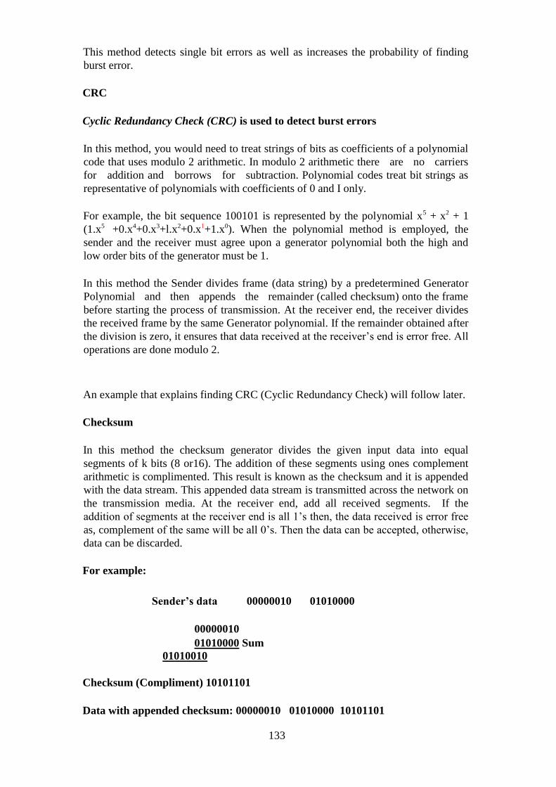
133

This method detects single bit errors as well as increases the probability of finding

burst error.

CRC

Cyclic Redundancy Check (CRC) is used to detect burst errors

In this method, you would need to treat strings of bits as coefficients of a polynomial

code that uses modulo 2 arithmetic. In modulo 2 arithmetic there are no carriers

for addition and borrows for subtraction. Polynomial codes treat bit strings as

representative of polynomials with coefficients of 0 and I only.

For example, the bit sequence 100101 is represented by the polynomial x5 + x2 + 1

(1.x5 +0.x4+0.x3+l.x2+0.x1+1.x0). When the polynomial method is employed, the

sender and the receiver must agree upon a generator polynomial both the high and

low order bits of the generator must be 1.

In this method the Sender divides frame (data string) by a predetermined Generator

Polynomial and then appends the remainder (called checksum) onto the frame

before starting the process of transmission. At the receiver end, the receiver divides

the received frame by the same Generator polynomial. If the remainder obtained after

the division is zero, it ensures that data received at the receiver‘s end is error free. All

operations are done modulo 2.

An example that explains finding CRC (Cyclic Redundancy Check) will follow later.

Checksum

In this method the checksum generator divides the given input data into equal

segments of k bits (8 or16). The addition of these segments using ones complement

arithmetic is complimented. This result is known as the checksum and it is appended

with the data stream. This appended data stream is transmitted across the network on

the transmission media. At the receiver end, add all received segments. If the

addition of segments at the receiver end is all 1‘s then, the data received is error free

as, complement of the same will be all 0‘s. Then the data can be accepted, otherwise,

data can be discarded.

For example:

Sender’s data 00000010 01010000

00000010

01010000 Sum

01010010

Checksum (Compliment) 10101101

Data with appended checksum: 00000010 01010000 10101101

134

Receiver’s accept the data as

00000010 01010000 10101101

At receiver’s end

00000010

01010000

10101101 sum

11111111

Complement 00000000

As complement is 0 it indicates that the data received at the receiver‘s end is error

free so, it will be accepted by the receiver.

The checksum method detects all errors as it retains all its carries.

Odd number of bits Most of

even number of bits.

3.3 Forward Error Correction

In the previous section we have discussed detection of error that appears after the

transmission of data over the network from sender to receiver. In this section, we will

study how to perform correction of errors. Forward Error Correction (FEC) is a type

of error correction method which improves on simple error detection schemes by

enabling the receiver to correct errors once they are detected. This reduces the need

for retransmissions of error frames.

Firstly we consider the simple case i.e., correcting single bit error. As we have

discussed earlier that a single bit error can be detected by adding one additional bit

(parity bit! redundant bit). This additional bit can detect error in any bit stream by

differentiating the two condition error or not error as a bit can have two states only

i.e., 0 and 1.

For correction of detected single bit error two states are not sufficient. As an error

occurs in bit stream indicates that one bit is altered from either 0 to 1 or 1 to 0. To

correct the same, conversion of altered bit is required. For performing this conversion

we must know the location of bit which is in error. Therefore, for error correction

identification of location of error bit is required. For example, for applying error

correction of single bit error in ASCII character we must find which of 7 bit is

altered. For doing this we could have eight different states i.e., no error, error in bit

position 1, error in bit position 2 up to error in bit position 7. For this we need many

redundant bits to represent all eight states.

Here, 3bit redundancy code can represent all possible eight states because 3 bits can

represent 8 states (000 to 111). But if an error occurs in redundancy bit then we need

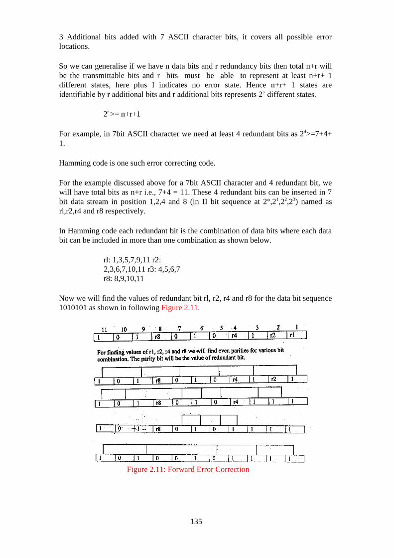
135

3 Additional bits added with 7 ASCII character bits, it covers all possible error

locations.

So we can generalise if we have n data bits and r redundancy bits then total n+r will

be the transmittable bits and r bits must be able to represent at least n+r+ 1

different states, here plus I indicates no error state. Hence n+r+ 1 states are

identifiable by r additional bits and r additional bits represents 2‘ different states.

2r >= n+r+1

For example, in 7bit ASCII character we need at least 4 redundant bits as 24>=7+4+

1.

Hamming code is one such error correcting code.

For the example discussed above for a 7bit ASCII character and 4 redundant bit, we

will have total bits as n+r i.e., 7+4 = 11. These 4 redundant bits can be inserted in 7

bit data stream in position 1,2,4 and 8 (in II bit sequence at 2°,21,22,23) named as

rl,r2,r4 and r8 respectively.

In Hamming code each redundant bit is the combination of data bits where each data

bit can be included in more than one combination as shown below.

rl: 1,3,5,7,9,11 r2:

2,3,6,7,10,11 r3: 4,5,6,7

r8: 8,9,10,11

Now we will find the values of redundant bit rl, r2, r4 and r8 for the data bit sequence

1010101 as shown in following Figure 2.11.

Figure 2.11: Forward Error Correction

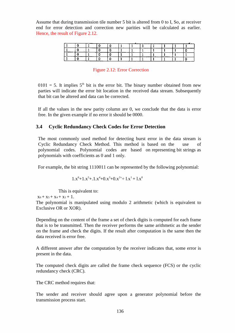
136

Assume that during transmission tile number 5 bit is altered from 0 to I, So, at receiver

end for error detection and correction new parities will be calculated as earlier.

Hence, the result of Figure 2.12.

Figure 2.12: Error Correction

0101 = 5. It implies 5th bit is the error bit. The binary number obtained from new

parties will indicate the error bit location in the received data stream. Subsequently

that bit can be altered and data can be corrected.

If all the values in the new parity column are 0, we conclude that the data is error

free. In the given example if no error it should be 0000.

3.4 Cyclic Redundancy Check Codes for Error Detection

The most commonly used method for detecting burst error in the data stream is

Cyclic Redundancy Check Method. This method is based on the use of

polynomial codes. Polynomial codes are based on representing bit strings as

polynomials with coefficients as 0 and 1 only.

For example, the bit string 1110011 can be represented by the following polynomial:

1.x6+1.x5+.1.x4+0.x3+0.x2‘+ l.x1 + l.x0

This is equivalent to:

x6 + x5 + x4 + x1 + 1.

The polynomial is manipulated using modulo 2 arithmetic (which is equivalent to

Exclusive OR or XOR).

Depending on the content of the frame a set of check digits is computed for each frame

that is to be transmitted. Then the receiver performs the same arithmetic as the sender

on the frame and check the digits. If the result after computation is the same then the

data received is error free.

A different answer after the computation by the receiver indicates that, some error is

present in the data.

The computed check digits are called the frame check sequence (FCS) or the cyclic

redundancy check (CRC).

The CRC method requires that:

The sender and receiver should agree upon a generator polynomial before the

transmission process start.

137

Both the high and low bits of the generator must be 1.

To compute the checksum for a frame with m bits, the size of the frame must be

longer than the generator polynomial.

Algorithm for Computing the Checksum is as follows as:

Let D(x) be the data and G(x) be the generating polynomial. Let r be the degree of

generator polynomial G(x).

Step 1: Multiply the data D(x)by x‘, giving r zeros in the low- order end of the frame.

Step 2: Divide the result obtained in step I by G(x), using modul0-2 division.

Step 3: Append the remainder from step 2 to D(x), thus, placing r tends in the r low-

order positions.

The type of generating polynomial is important for finding the types of error that are

detected.

A generator polynomial of R bits will detect:

1. all single-bit errors

2. all double-bit errors

3. all odd-number of bit errors

4. all burst errors < R

5. most burst errors >= R

Example:

Data 1011101

Generator Polynomial G(x): x4+x2+1 = 10101

Here the size of the generator polynomial is 5 bit long, so, we will place 5 -1 = 4 O‘sin

the low order data stream. So the data will be:

Data 10111010000

Now using modul02 division, (for getting data ready to be transmitted), we will divide

the data by the generator polynomial as shown in the Figure 2.13.

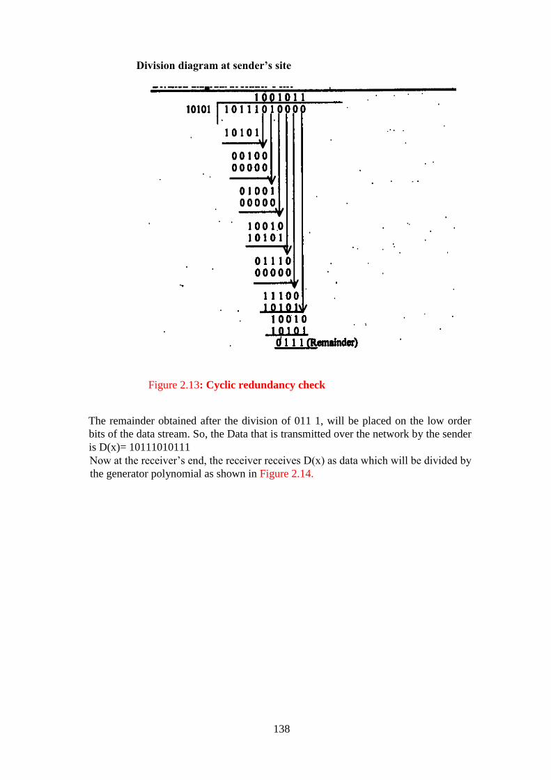
138

Division diagram at sender’s site

Figure 2.13: Cyclic redundancy check

The remainder obtained after the division of 011 1, will be placed on the low order

bits of the data stream. So, the Data that is transmitted over the network by the sender

is D(x)= 10111010111

Now at the receiver‘s end, the receiver receives D(x) as data which will be divided by

the generator polynomial as shown in Figure 2.14.

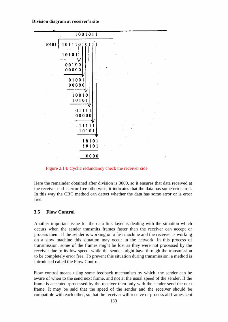
139

Division diagram at receiver’s site

Figure 2.14: Cyclic redundancy check the receiver side

Here the remainder obtained after division is 0000, so it ensures that data received at

the receiver end is error free otherwise, it indicates that the data has some error in it.

In this way the CRC method can detect whether the data has some error or is error

free.

3.5 Flow Control

Another important issue for the data link layer is dealing with the situation which

occurs when the sender transmits frames faster than the receiver can accept or

process them. If the sender is working on a fast machine and the receiver is working

on a slow machine this situation may occur in the network. In this process of

transmission, some of the frames might be lost as they were not processed by the

receiver due to its low speed, while the sender might have through the transmission

to be completely error free. To prevent this situation during transmission, a method is

introduced called the Flow Control.

Flow control means using some feedback mechanism by which, the sender can be

aware of when to the send next frame, and not at the usual speed of the sender. If the

frame is accepted /processed by the receiver then only with the sender send the next

frame. It may be said that the speed of the sender and the receiver should be

compatible with each other, so that the receiver will receive or process all frames sent

140

by the sender as every receiver has a limited block of memory called the buffer,

reserved for storing incoming frames.

There are several methods available for deciding when a sender should send one frame

or the next frame. Flow control ensures that the speed of sending the frame, by the

sender, and the speed of processing the received frame by the receiver are compatible.

There are two basic strategies for flow control:

1 Stop-and-wait

2 Sliding window.

We shall start with the assumption that the transmission is error free and that we have

an ideal channel.

3.5.1 Slop and Wait

Stop-and-Wait Flow Control (Figure 2.15) is the simplest form of flow control. In

this method, the receiver indicates its readiness to receive data for each frame, the

message is broken into multiple frames. The Sender waits for an ACK

(acknowledgement) after every frame for a specified time (called time out). It is sent

to ensure that the receiver has received the frame correctly. It will then send the next

frame only after the ACK has been received.

Operations:

1 Sender: Transmits a single frame at a time.

2 Receiver: Transmits acknowledgement (ACK) as it receives a frame.

3 Sender receives ACK within time out.

4 Go to step I.

Figure 2.15: Stop and Wait

If a frame or ACK is lost during transmission then it has to be transmitted

again by the sender. This retransmission process is known as ARQ (automatic repeat

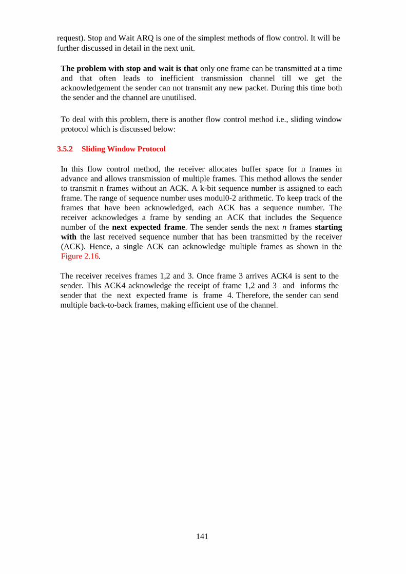
141

request). Stop and Wait ARQ is one of the simplest methods of flow control. It will be

further discussed in detail in the next unit.

The problem with stop and wait is that only one frame can be transmitted at a time

and that often leads to inefficient transmission channel till we get the

acknowledgement the sender can not transmit any new packet. During this time both

the sender and the channel are unutilised.

To deal with this problem, there is another flow control method i.e., sliding window

protocol which is discussed below:

3.5.2 Sliding Window Protocol

In this flow control method, the receiver allocates buffer space for n frames in

advance and allows transmission of multiple frames. This method allows the sender

to transmit n frames without an ACK. A k-bit sequence number is assigned to each

frame. The range of sequence number uses modul0-2 arithmetic. To keep track of the

frames that have been acknowledged, each ACK has a sequence number. The

receiver acknowledges a frame by sending an ACK that includes the Sequence

number of the next expected frame. The sender sends the next n frames starting

with the last received sequence number that has been transmitted by the receiver

(ACK). Hence, a single ACK can acknowledge multiple frames as shown in the

Figure 2.16.

The receiver receives frames 1,2 and 3. Once frame 3 arrives ACK4 is sent to the

sender. This ACK4 acknowledge the receipt of frame 1,2 and 3 and informs the

sender that the next expected frame is frame 4. Therefore, the sender can send

multiple back-to-back frames, making efficient use of the channel.

142

Normal Flow diagram of a sliding window

Figure 2.16: Normal now diagram of sliding

Sequence number is a field in the frame that is of finite size. If k bits are reserved for

the sequence number, then the values of sequence number ranges from 0 to 2k–1

(Modulo Arithmetic).

Operation of a Sliding Window

Sending Window

In this mechanism we maintain two types of windows (buffer) sending window and

receiving windows as shown in Figure 2.17 & 2.18.

At any instant, the sender is permitted to send frames with sequence numbers in a

certain range (3-bit sending window) as shown in Figure 2.17

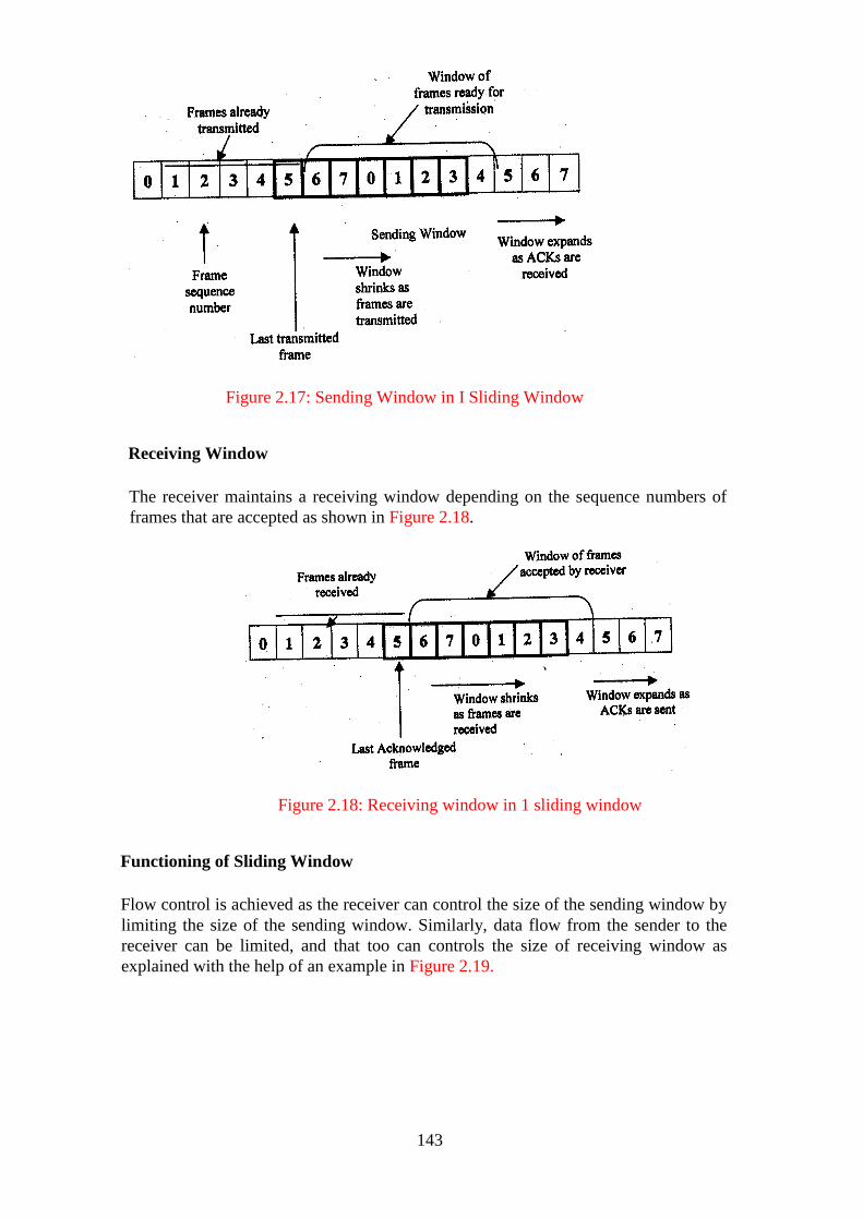
143

Figure 2.17: Sending Window in I Sliding Window

Receiving Window

The receiver maintains a receiving window depending on the sequence numbers of

frames that are accepted as shown in Figure 2.18.

Figure 2.18: Receiving window in 1 sliding window

Functioning of Sliding Window

Flow control is achieved as the receiver can control the size of the sending window by

limiting the size of the sending window. Similarly, data flow from the sender to the

receiver can be limited, and that too can controls the size of receiving window as

explained with the help of an example in Figure 2.19.

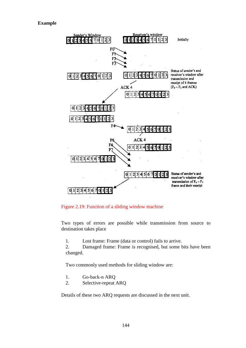
144

Example

Figure 2.19: Function of a sliding window machine

Two types of errors are possible while transmission from source to

destination takes place

1. Lost frame: Frame (data or control) fails to arrive.

2. Damaged frame: Frame is recognised, but some bits have been

changed.

Two commonly used methods for sliding window are:

1. Go-back-n ARQ

2. Selective-repeat ARQ

Details of these two ARQ requests are discussed in the next unit.

145

4.0 CONCLUSION

In this unit we have described the elementary issues of the Data Link Lagos such as

how to divide data streams into frames. You have learnt the different types of errors

that may occur. During the transmission of frames from the source mode to the

destination mode, also detecting and correcting these errors. You have also learnt

about flow control and the various methods for flow control.

5.0 SUMMARY

This unit introduced the basic fundamental issues related to the Data Link Layer. The

concept of framing and different methods of framing like Character Count, Character

Stuffing, Bit stuffing and Framing by Illegal code has been focused up on. In the

Data Link layer, data flow and error control are discussed. This error and flow

control is required in the system for reliable delivery of data in the network. For the

same, different types of error, different methods for error detection and correction are

discussed. Among various methods, Block sum check method detects burst of error

with high probability. CRC method is the one which detects the error with simplicity.

Forward Error Correction is the error correction method that uses the parity concept.

For flow control, stop and wait method tries to ensure that the speed of the sender

and the receivers are matching to an extent. To overcome this sliding Window

protocol is introduced. Sliding window protocol can send many frames at one

instance and that increases the efficiency of transmission channel. If some error

occurs in the data then retransmission of the error frame is required and it is known

as ARQ.


1. Define parity bit? Also define even and odd parity?

2. Name the method that can detect single bit error and burst error.

3. Define checksum.

4. Define Hamming distance.

5. Generate the Hamming code for the following input data 101111

6. Find the CRC for the data polynomial x3+X

2+X+ I where generator

polynomial is X3+1.

7. How does the sliding window protocol increase the utilisation of bandwidth?

8. Define ARQ. How does ARQ facilitate the error control process?


Andrew S. Tanenbaum, Computer Networks, 4th Edition, Prentice Hall of India, New

Delhi.

William Stalling, Data and Computer Communications, 5th Edition, Pearson

Education, New Delhi.

Behrouz A. Forouzan, Data Communications and Networking, 3rd Edition, Tata

McGraw Hill, New Delhi.

146

Leon Garcia and Widjaja, Communication Networks-Fundamental Concepts and Key

Architectures, 3rd Edition, Tata McGrew Hill, New Delhi.

8.0 ANSWERS TO TUTOR MARKED ASSIGNMENTS 5

Question 1

Define parity nit? Similarly define even and odd parity bit

Solution

A parity bit is the addition of a bit to a string of binary code which is used as the most

elementary form of error detecting code. Even and odd parity bits are two different

type of parity bits. The numbers of ones in a set of bits determine whether it is even or

odd. For instance, given a set of decimal coded number (BCD) 100001, this has two

―1s‖ which implies that is an even parity bit. Similarly, given 100101 which has three

―1s‖ implies that it is an odd parity bit.

Question 2

Name the method that can detect single bit error and burst error.

Solution

Single bit error correcting method is a technique of correcting single bit error while

burst error technique is the method of correcting multiple (burst) error.

Question 3

Define Checksum

Solution

A checksum is a small-sized datum derived from a block of digital data for the

purpose of detecting errors that may have been introduced during its transmission or

storage. By themselves, checksums are often used to verify data integrity but are not

relied upon to verify data authenticity

Question 4

Define Hamming Distance.

Solution

Hamming distance is the distance between two strings of equal length signifying the

position in which the two strings are different.

Question 5

Generate Hamming code for the following input data 101111

Solution

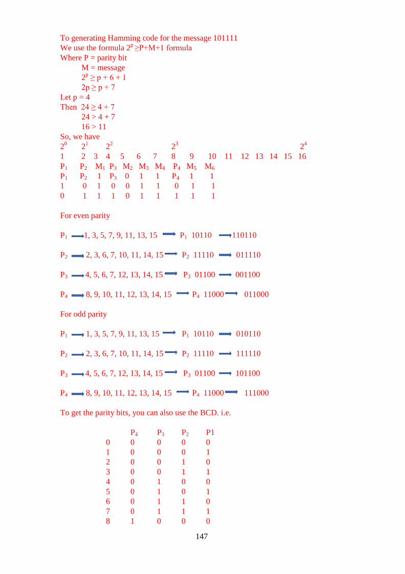
147

To generating Hamming code for the message 101111

We use the formula 2p

≥P+M+1 formula

Where P = parity bit

M = message

2p ≥ p + 6 + 1

2p ≥ p + 7

Let p = 4

Then 24 ≥ 4 + 7

24 > 4 + 7

16 > 11

So, we have

20 2

1 2

2 2

3 2

4

1 2 3 4 5 6 7 8 9 10 11 12 13 14 15 16

P1 P2 M1 P3 M2 M3 M4 P4 M5 M6

P1 P2 1 P3 0 1 1 P4 1 1

1 0 1 0 0 1 1 0 1 1

0 1 1 1 0 1 1 1 1 1

For even parity

P1 1, 3, 5, 7, 9, 11, 13, 15 P1 10110 110110

P2 2, 3, 6, 7, 10, 11, 14, 15 P2 11110 011110

P3 4, 5, 6, 7, 12, 13, 14, 15 P3 01100 001100

P4 8, 9, 10, 11, 12, 13, 14, 15 P4 11000 011000

For odd parity

P1 1, 3, 5, 7, 9, 11, 13, 15 P1 10110 010110

P2 2, 3, 6, 7, 10, 11, 14, 15 P2 11110 111110

P3 4, 5, 6, 7, 12, 13, 14, 15 P3 01100 101100

P4 8, 9, 10, 11, 12, 13, 14, 15 P4 11000 111000

To get the parity bits, you can also use the BCD. i.e.

P4 P3 P2 P1

0 0 0 0 0

1 0 0 0 1

2 0 0 1 0

3 0 0 1 1

4 0 1 0 0

5 0 1 0 1

6 0 1 1 0

7 0 1 1 1

8 1 0 0 0

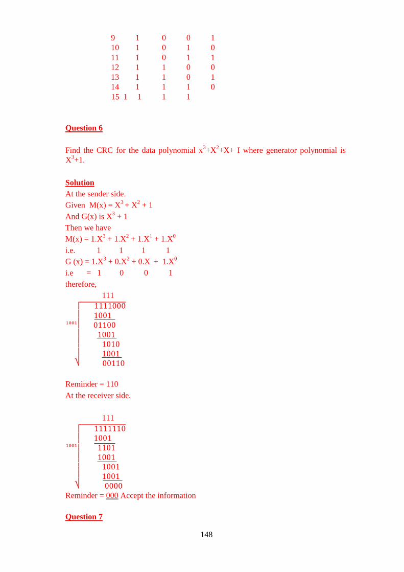
148

9 1 0 0 1

10 1 0 1 0

11 1 0 1 1

12 1 1 0 0

13 1 1 0 1

14 1 1 1 0

15 1 1 1 1

Question 6

Find the CRC for the data polynomial x3+X

2+X+ I where generator polynomial is

X3+1.

Solution

At the sender side.

Given M(x) = X3

+ X2 + 1

And G(x) is X3 + 1

Then we have

M(x) = 1.X3 + 1.X

2 + 1.X

1 + 1.X

0

i.e. 1 1 1 1

G (x) = 1.X3 + 0.X

2 + 0.X

+ 1.X

0

i.e = 1 0 0 1

therefore,

111

√

Reminder = 110

At the receiver side.

111

√

Reminder = 000 Accept the information

Question 7

149

How does the sliding window protocol increase the utilization of bandwidth?

Solution

Sliding window protocol increase the utilization of bandwidth by giving the receiver

the allowance to allocates buffer space for n frames in advance and allows

transmission of multiple frames.

Question 8

Define ARQ. How does ARQ facilitate the error control process?

Solution

Automatic repeat request, also known as automatic repeat query, is an error-control

method for data transmission that uses acknowledgements and timeouts to achieve

reliable data transmission over an unreliable communication channel.

ARQ facilitate the error control process by making sure packets are re-transmitted if

acknowledgement is not received within a specified time and re-transmissions are

repeated in a stipulated number of times

150

UNIT 2 RETRANSMISSION STRATEGIES

CONTENTS

1.0 Introduction

2.0 Objectives

3.0 Main Content

3.1 Stop & Wait ARQ

3.2 Go-Back-N ARQ

3.3 Selective Repeat ARQ

3.4 Pipelining

3.5 Piggybacking

4.0 Conclusion

5.0 Summary



1.0 INTRODUCTION

In the previous unit we discovered that, Data Link Layer is

responsible for ensuring that data is received at the receiver‘s end in line and error

free. For the same task it has two important functions to perform that is Flow control

and Error control. Flow and Error control are performed by the data link protocol.

Before starting discussion on methods for flow and error control, firstly, we will

define Flow control and Error control.

Flow control deals with when the sender should send the next frame and for how

long the sender should wait for an acknowledgement. Data link protocol takes care of

the amount of data that a sender can send and that a receiver can process as, the

receiver has its own limitation in terms of speed for processing the frames. It also

sees the compatibility of speed of both the sender and the receiver.

Error control deals with error detection and correction method that we have already

discussed in the previous unit. If, an error is found in the frame either due to loss of

frame or due to damage of frame, retransmission of the same is required by the

sender. Retransmission is required when a sender does not receive a positive

acknowledgement in time, due to a loss of frame or loss of acknowledgement or if,

the sender receives negative acknowledgment from the receiver due to frame not

been error free. This process of retransmission is called ARQ (Automatic

Repeat Request). The set of rules that will determine the operations for the sender

and the receiver are named the ARQ protocol. This ARQ protocol makes the network

reliable, and that is, one of the important requirements of a network system if, data

transmits from one node to another over the network and ensures that data received at

receiver‘s site is complete and accurate. Here, we will refer to ACK, for positive

acknowledgement (that is receiver has correct data) and NAK (REJect) to refer to

negative acknowledgement (that is frame is received with some error). In this unit,

you will study three commonly used methods for flow and error control that is Stop

& Wait ARQ, GoBack-n ARQ and Selective Repeat ARQ.

151

2.0 OBJECTIVES


1. define flow and error control

2. define IS ARQ

3. define functionality of data link protocol

4. define Stop & Wait ARQ method for error and flow control

5. define GoBack-n ARQ method for error and flow control

6. perform selective Repeat ARQ method for error and flow control

7. define pipelining.

3.0 MAIN CONTENT

3.1 Stop & Wait ARQ

This is the simplest method for flow and error control. This protocol is based on the

concept that, the sender will send a frame and wait for its acknowledgment. Until it

receives an acknowledgment, the sender cannot send the next frame to the receiver.

During transmission of frame over the network an error can appear.

Error can be due to a frame getting damaged/lost during transmission.

Then, the receiver discards that frame by using error detection method. The sender

will wait for acknowledgement of frame sent for a predetermined time (allotted time).

If timeout occurs in the system then, the same frame is required to be retransmitted.

Hence, the sender should maintain a duplicate copy of the last frame sent, as, in

future it can be required for retransmission. This will facilitate the sender in

retransmitting the lost/damaged frame.

At times the receiver receives the frame correctly, in time and sends the

acknowledgment also, but the acknowledgment gets lost/damaged during

transmission. For the sender it indicates time out and the demand for retransmission

of the same frame appears in the network. If, the sender sends the last frame again, at

the receiver‘s site, the frame would be duplicated. To overcome this problem it,

follows a number mechanism and discards the duplicate frame.

Another situation when an error can appear in the network system is when the

receiver receives the frame out of order, then it simply discards that frame and sends

no acknowledgement. If, the acknowledgement is not received by the sender in time

then, it assumes that the frame is lost during transmission, and retransmits it.

For distinguishing both data frame and acknowledgement frame, a number

mechanism is used. For example, A data frame 0 is acknowledged by

acknowledgement frame 1, to show that the receiver has received data frame 0 and is

expecting data frame l from the sender.

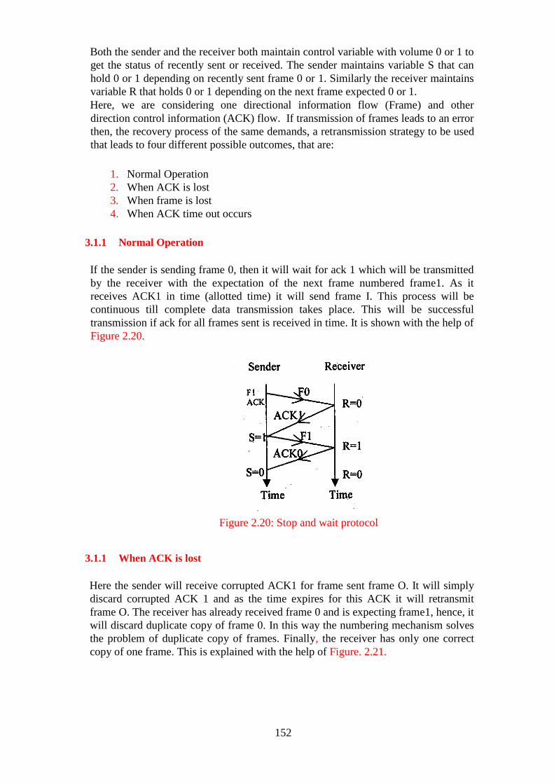
152

Both the sender and the receiver both maintain control variable with volume 0 or 1 to

get the status of recently sent or received. The sender maintains variable S that can

hold 0 or 1 depending on recently sent frame 0 or 1. Similarly the receiver maintains

variable R that holds 0 or 1 depending on the next frame expected 0 or 1. Here, we are considering one directional information flow (Frame) and other

direction control information (ACK) flow. If transmission of frames leads to an error

then, the recovery process of the same demands, a retransmission strategy to be used

that leads to four different possible outcomes, that are:

1. Normal Operation

2. When ACK is lost

3. When frame is lost

4. When ACK time out occurs

3.1.1 Normal Operation

If the sender is sending frame 0, then it will wait for ack 1 which will be transmitted

by the receiver with the expectation of the next frame numbered frame1. As it

receives ACK1 in time (allotted time) it will send frame I. This process will be

continuous till complete data transmission takes place. This will be successful

transmission if ack for all frames sent is received in time. It is shown with the help of

Figure 2.20.

Figure 2.20: Stop and wait protocol

3.1.1 When ACK is lost

Here the sender will receive corrupted ACK1 for frame sent frame O. It will simply

discard corrupted ACK 1 and as the time expires for this ACK it will retransmit

frame O. The receiver has already received frame 0 and is expecting frame1, hence, it

will discard duplicate copy of frame 0. In this way the numbering mechanism solves

the problem of duplicate copy of frames. Finally, the receiver has only one correct

copy of one frame. This is explained with the help of Figure. 2.21.

153

Figure 2.21: Loss of ACK

3.1.3 When Frame is lost

If the receiver receives corrupted/damaged frame1, it will simply discard it and

assumes that the frame was lost on the way. And correspondingly, the sender will not

get ACK0 as frame has not been received by the receiver. The sender will be in waiting

stage for ACK0 till its time out occurs in the system. As soon as time out occurs in the

system, the sender will retransmit the same frame i.e frame 1 (F1) and the receiver will

send ACKO in reply as shown in Figure 2.22.

Figure 2.22: Loss of a frame

3.1.4 When ACK time out occurs

In this operation, the receiver is not able to send ACK1 for received frame0 in time,

due to some problem at the receiver‘s end or network communication. The sender

retransmits frame0 as ACK1 is not received in time. Then, the sender retransmits

frame0 as ACK1 time expires. At the receiver end, the receiver discards this frameO

154

as the duplicate copy is expecting frame1 but sends the ACK1 once again

corresponding to the copy received for frame0. At the sender‘s site, the duplicate

copy of ACK1 is discarded as the sender has received ACK1 earlier as explained

with the help of Figure 2.23.

Figure 2. 23: ACK lime out

These operations indicate the importance of the numbering mechanism while,

transmitting frames over the network. The method in section 3.1 discussed, has low

efficiency due to improper use of the communication channel. So, now, we will

discuss the case, if flow of data is bidirectional. In Bidirectional transmission both the

sender and the receiver can send frames as well as acknowledgement. Hence, both will

maintain S and R variables. To have an efficient use of bandwidth the ACK can be

appended with the data frame during transmission. The process of combining ACK

with data is known as Piggybacking. The concept of piggybacking is explained in a

later section. This reduces transmission overhead and increases the overall efficiency

of data transmission.

The process is shown in Figure 2.24

Figure 2. 24: Piggybacking 1

The problem with stop and wait is that only one frame can be transmitted at a time

and this leads to inefficiency of transmission. To deal with this, we have another error

and flow control method that we will discuss in the next section.

155

3.2 Go-Back-N ARQ

In this section, we will try to overcome the inefficient transmission that occurs in

Stop & Wait ARQ. In this method, many frames can be transmitted during the

process without waiting for acknowledgement. In this, we cart send n frames without

making the sender wait for acknowledgements. At the same time, the sender will

maintain a copy of each sent frame till acknowledgement reaches it safely. As seen

earlier in the Stop & Wait ARQ where, we used number mechanism, here also, we

will use number method for transmission and receipt of frames. Each frame will have

k bit sequence number that will be added with the frame. If, the frame can have k bit

sequence number then the numbers will range between 0 to 2k-1. For example, if k is

2bit then numbers will be 0,1,2,3,0,1,2,3,0,

The sender can send 4 frames continuously without waiting for acknowledgment. But

the receiver will look forward to only one frame that must be in order. If, the frame

received is not in order, it will simply keep on discarding the frame till, it receives the

desired sequence number frame. The receiver is not bound to send an individual

acknowledgment for all frames received; it can send a cumulative acknowledgment

also. The receiver will send a positive acknowledgement if, the received frame is the

desired sequence number frame. Otherwise, it will keep on waiting if, the frame

received is corrupted or out of order. As soon as the timer expires for the frame sent

by the sender, the sender will GoBack and retransmit all frames including the frame

for which the timer expired, till, the last sent frame. Hence, it is named as Go-Back-N

ARQ. The process of retransmission for an error frame is shown in Figure 2.25. Go-

Back- N is used in HDLC protocol.

Figure 2. 25: Go-Back-N

If, the error rate is high, then, this leads to a lot of wastage of bandwidth as the sender

will retransmit all the frames from, the frame in which error appears till the last sent.

To increase the efficiency of transmission, when the error rate is high, another

protocol called Selective Repeat ARQ is used which is discussed in the next section.

3.3 Selective Repeat ARQ

.

This method increases the efficiency of the use of bandwidth. In this method, the

receiver has a window with the buffer that can hold multiple frames sent by the

sender. The sender will retransmit only that frame which has some error and not all

the frames as in Go-Back-N ARQ. Hence, it is named as selective repeat ARQ. Here,

the size of the sender and the receiver window will be same. The receiver will not

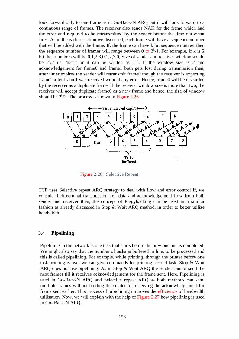
156

look forward only to one frame as in Go-Back-N ARQ but it will look forward to a

continuous range of frames. The receiver also sends NAK for the frame which had

the error and required to be retransmitted by the sender before the time out event

fires. As in the earlier section we discussed, each frame will have a sequence number

that will be added with the frame. If, the frame can have k bit sequence number then

the sequence number of frames will range between 0 to 2k-1. For example, if k is 2

bit then numbers will be 0,1,2,3,0,1,2,3,0, Size of sender and receiver window would

be 2k/2 i.e. 4/2=2 or it can be written as 2k-1. If the window size is 2 and

acknowledgement for frame0 and frame1 both gets lost during transmission then,

after timer expires the sender will retransmit frame0 though the receiver is expecting

frame2 after frame1 was received without any error. Hence, frame0 will be discarded

by the receiver as a duplicate frame. If the receiver window size is more than two, the

receiver will accept duplicate frame0 as a new frame and hence, the size of window

should be 2k/2. The process is shown in Figure 2.26.

Figure 2.26: Selective Repeat

TCP uses Selective repeat ARQ strategy to deal with flow and error control If, we

consider bidirectional transmission i.e., data and acknowledgement flow from both

sender and receiver then, the concept of Piggybacking can be used in a similar

fashion as already discussed in Stop & Wait ARQ method, in order to better utilize

bandwidth.

3.4 Pipelining

Pipelining in the network is one task that starts before the previous one is completed.

We might also say that the number of tasks is buffered in line, to be processed and

this is called pipelining. For example, while printing, through the printer before one

task printing is over we can give commands for printing second task. Stop & Wait

ARQ does not use pipelining. As in Stop & Wait ARQ the sender cannot send the

next frames till it receives acknowledgement for the frame sent. Here, Pipelining is

used in Go-Back-N ARQ and Selective repeat ARQ as both methods can send

multiple frames without holding the sender for receiving the acknowledgement for

frame sent earlier. This process of pipe lining improves the efficiency of bandwidth

utilisation. Now, we will explain with the help of Figure 2.27 how pipelining is used

in Go- Back-N ARQ.

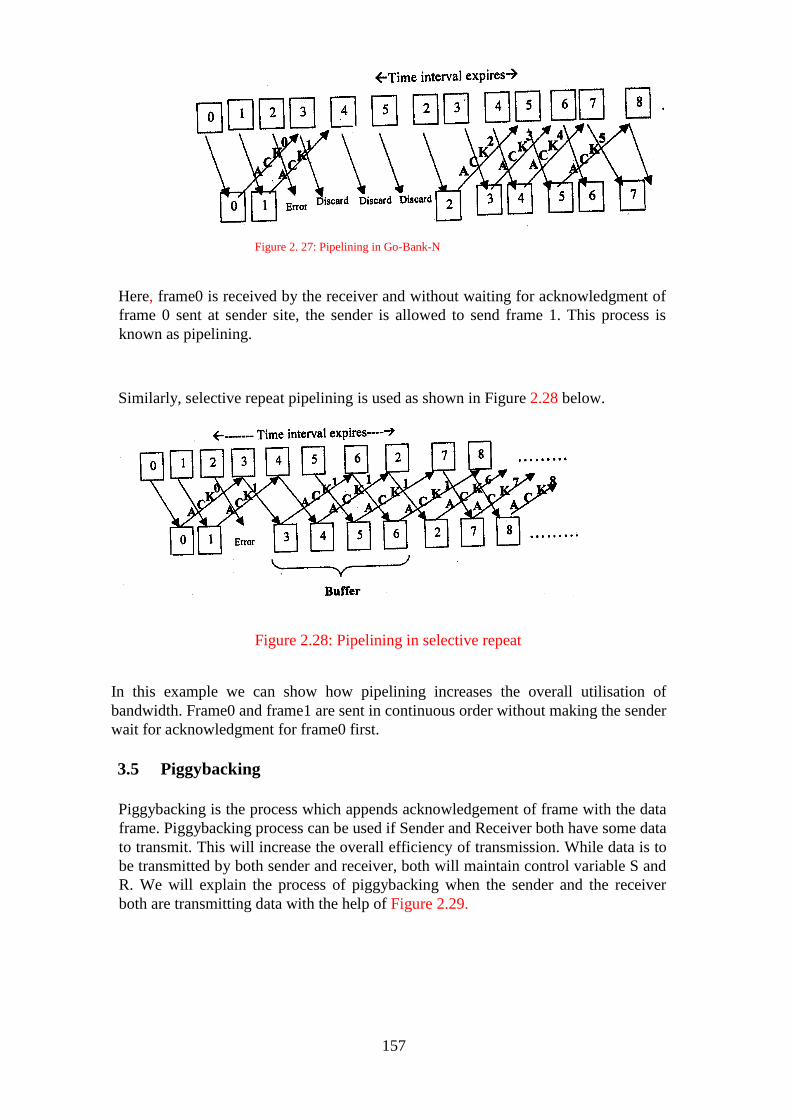
157

Figure 2. 27: Pipelining in Go-Bank-N

Here, frame0 is received by the receiver and without waiting for acknowledgment of

frame 0 sent at sender site, the sender is allowed to send frame 1. This process is

known as pipelining.

Similarly, selective repeat pipelining is used as shown in Figure 2.28 below.

Figure 2.28: Pipelining in selective repeat

In this example we can show how pipelining increases the overall utilisation of

bandwidth. Frame0 and frame1 are sent in continuous order without making the sender

wait for acknowledgment for frame0 first.

3.5 Piggybacking

Piggybacking is the process which appends acknowledgement of frame with the data

frame. Piggybacking process can be used if Sender and Receiver both have some data

to transmit. This will increase the overall efficiency of transmission. While data is to

be transmitted by both sender and receiver, both will maintain control variable S and

R. We will explain the process of piggybacking when the sender and the receiver

both are transmitting data with the help of Figure 2.29.

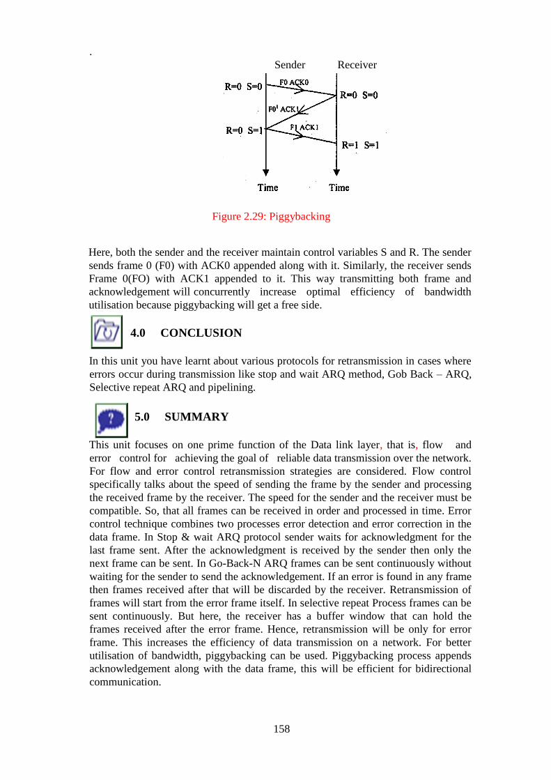
158

.

Sender Receiver

Figure 2.29: Piggybacking

Here, both the sender and the receiver maintain control variables S and R. The sender

sends frame 0 (F0) with ACK0 appended along with it. Similarly, the receiver sends

Frame 0(FO) with ACK1 appended to it. This way transmitting both frame and

acknowledgement will concurrently increase optimal efficiency of bandwidth

utilisation because piggybacking will get a free side.

4.0 CONCLUSION

In this unit you have learnt about various protocols for retransmission in cases where

errors occur during transmission like stop and wait ARQ method, Gob Back – ARQ,

Selective repeat ARQ and pipelining.

5.0 SUMMARY

This unit focuses on one prime function of the Data link layer, that is, flow and

error control for achieving the goal of reliable data transmission over the network.

For flow and error control retransmission strategies are considered. Flow control

specifically talks about the speed of sending the frame by the sender and processing

the received frame by the receiver. The speed for the sender and the receiver must be

compatible. So, that all frames can be received in order and processed in time. Error

control technique combines two processes error detection and error correction in the

data frame. In Stop & wait ARQ protocol sender waits for acknowledgment for the

last frame sent. After the acknowledgment is received by the sender then only the

next frame can be sent. In Go-Back-N ARQ frames can be sent continuously without

waiting for the sender to send the acknowledgement. If an error is found in any frame

then frames received after that will be discarded by the receiver. Retransmission of

frames will start from the error frame itself. In selective repeat Process frames can be

sent continuously. But here, the receiver has a buffer window that can hold the

frames received after the error frame. Hence, retransmission will be only for error

frame. This increases the efficiency of data transmission on a network. For better

utilisation of bandwidth, piggybacking can be used. Piggybacking process appends

acknowledgement along with the data frame, this will be efficient for bidirectional

communication.

159


1. Define flow and error control.

2. Explain why Go-Back-N ARQ and Selective repeat ARQ are better methods

for retransmission.

3. Give an example where pipelining can be applied.

4. What is the significance of control variables S and R?


Andrew S. Tanenbaum, Computer Networks. 4‖ Edition, Prentice Hall of India, New

Delhi, 2011.

William Stalling, Dala and Computer Communications. 5th Edition, Prentice Hall of

India, New Delhi, 2003

Behrouz A. Forouzan, Dala Communications and Networking. 3‖ Edition, Tata

McGraw Hill, New Delhi, 2016

Leon Garcia and Widjaja, Communication Network, Fundamental Concepts and Key

Architectures. 3‖ Edition, Tata McGraw Hill, New Delhi.


Question 1

Define flow and error control.

Solution

Flow control is the method of administration of data flow between two devices in

such a way that the sender does not overwhelm the receiver. While error control is the

method of detecting and correcting block of data during transmission.

Question 2

Explain Go-Back-N ARQ and Selective repeat ARQ are better methods for

retransmission.

Solution

Go-Back-N ARQ resends all frames that are received after the corrupted or lost frame

(i.e. if a frame is found corrupted or lost all the frames are resent) and wasted a lot of

bandwidth though message could be sent without waiting for acknowledgement.

While Selective repeat ARQ resends only the frame that is corrupted or lost and save

bandwidth, hence improved on Go-Back-N ARQ.

160

Question 3

Give an example where pipelining can be applied.

Solution

An example of where pipelining can be applied is the manufacturing of cares i.e. a

robotic arm manufactures a section of a car and pass it on the next section of the

production.

Question 4

What is the significance of control variables S and R?

The S and R variables refer to Sender and receiver variables. The significance is that

the two of them can send and acknowledge variables in a bidirectional transmission.

161

UNIT 3 CONTENTION-BASED MEDIA ACCESS PROTOCOLS

CONTENTS

1.0 Introduction

2.0 Objectives

3.0 Main Content

3.1 Advantages of Multiple Access Sharing of Channel Resources

3.2 Pure ALOHA

3.3 Slotted ALOHA

3.4 Carrier Sense Multiple Access (CSMA)

3.5 CSMA with Collision Detection (CSMA/CD)

3.6 Ethernet Frame Format (IEEE 802.3)

4.0 Conclusion

5.0 Summary



1.0 INTRODUCTION

As discussed in first unit of this module the Data Link Layer (DLL) is

divided into two sub layers i.e., the Media Access Control (MAC) layer and the

Logical Link Control (LLC)layer. In a network node are connected to or use a

common transmission media. Based on the connection of nodes, a network can be

divided into two categories, that is, point-to-point link and broadcast link. In this unit,

we will discuss, broadcast link and their protocols. If, we talk about broadcast network

then, a control process for solving the problem of accessing a multi access channel is

required. Many protocols are available for solving the problem of multi-access

channel. These protocols can control an access on shared link as in broadcast network.

It is an important issue to be taken into consideration that is, how to, who gets access

to the channel while, many nodes are in competition as shown in Figure 2.30.

Figure 2. 30: Shared media

The protocol which decides who will get access to the channel and who will go next

on the channel belongs to MAC sub-layer of DLL. Channel allocation is categorized

into two, based on the allocation of broadcast among competing users that is Static

channel allocation problem and Dynamic Channel allocation problem as shown in

Figure 2.31. In this unit, we will also discuss whether some access conflict or collision

comes in the network, and how to deal with these conflicts. This is an important issue

for LAN.

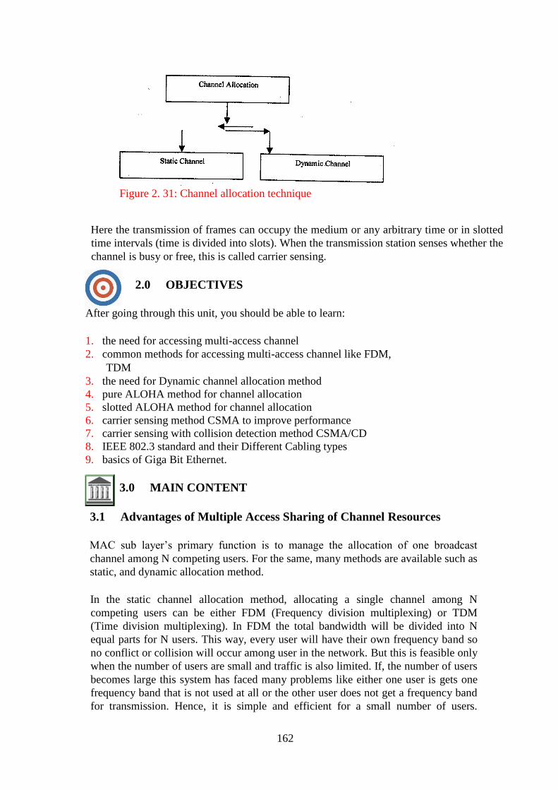
162

Figure 2. 31: Channel allocation technique

Here the transmission of frames can occupy the medium or any arbitrary time or in slotted

time intervals (time is divided into slots). When the transmission station senses whether the

channel is busy or free, this is called carrier sensing.

2.0 OBJECTIVES

After going through this unit, you should be able to learn:

1. the need for accessing multi-access channel

2. common methods for accessing multi-access channel like FDM,

TDM

3. the need for Dynamic channel allocation method

4. pure ALOHA method for channel allocation

5. slotted ALOHA method for channel allocation

6. carrier sensing method CSMA to improve performance

7. carrier sensing with collision detection method CSMA/CD

8. IEEE 802.3 standard and their Different Cabling types

9. basics of Giga Bit Ethernet.

3.0 MAIN CONTENT

3.1 Advantages of Multiple Access Sharing of Channel Resources

MAC sub layer‘s primary function is to manage the allocation of one broadcast

channel among N competing users. For the same, many methods are available such as

static, and dynamic allocation method.

In the static channel allocation method, allocating a single channel among N

competing users can be either FDM (Frequency division multiplexing) or TDM

(Time division multiplexing). In FDM the total bandwidth will be divided into N

equal parts for N users. This way, every user will have their own frequency band so

no conflict or collision will occur among user in the network. But this is feasible only

when the number of users are small and traffic is also limited. If, the number of users

becomes large this system has faced many problems like either one user is gets one

frequency band that is not used at all or the other user does not get a frequency band

for transmission. Hence, it is simple and efficient for a small number of users.

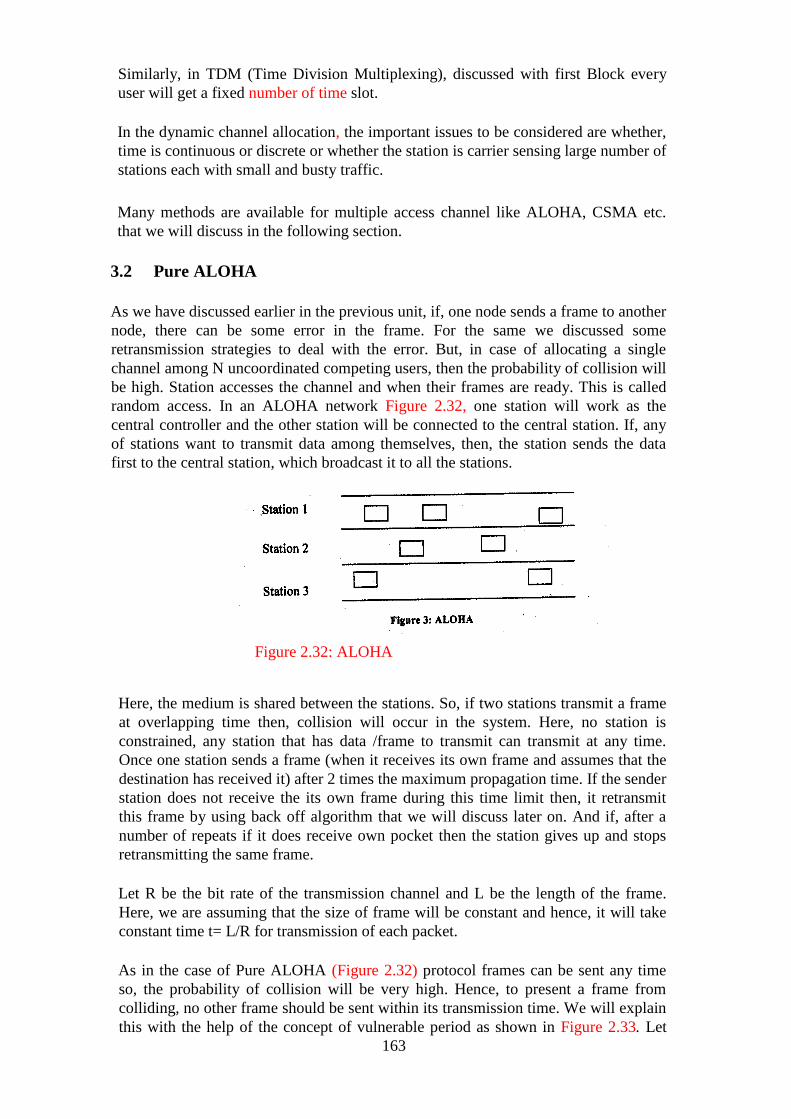
163

Similarly, in TDM (Time Division Multiplexing), discussed with first Block every

user will get a fixed number of time slot.

In the dynamic channel allocation, the important issues to be considered are whether,

time is continuous or discrete or whether the station is carrier sensing large number of

stations each with small and busty traffic.

Many methods are available for multiple access channel like ALOHA, CSMA etc.

that we will discuss in the following section.

3.2 Pure ALOHA

As we have discussed earlier in the previous unit, if, one node sends a frame to another

node, there can be some error in the frame. For the same we discussed some

retransmission strategies to deal with the error. But, in case of allocating a single

channel among N uncoordinated competing users, then the probability of collision will

be high. Station accesses the channel and when their frames are ready. This is called

random access. In an ALOHA network Figure 2.32, one station will work as the

central controller and the other station will be connected to the central station. If, any

of stations want to transmit data among themselves, then, the station sends the data

first to the central station, which broadcast it to all the stations.

Figure 2.32: ALOHA

Here, the medium is shared between the stations. So, if two stations transmit a frame

at overlapping time then, collision will occur in the system. Here, no station is

constrained, any station that has data /frame to transmit can transmit at any time.

Once one station sends a frame (when it receives its own frame and assumes that the

destination has received it) after 2 times the maximum propagation time. If the sender

station does not receive the its own frame during this time limit then, it retransmit

this frame by using back off algorithm that we will discuss later on. And if, after a

number of repeats if it does receive own pocket then the station gives up and stops

retransmitting the same frame.

Let R be the bit rate of the transmission channel and L be the length of the frame.

Here, we are assuming that the size of frame will be constant and hence, it will take

constant time t= L/R for transmission of each packet.

As in the case of Pure ALOHA (Figure 2.32) protocol frames can be sent any time

so, the probability of collision will be very high. Hence, to present a frame from

colliding, no other frame should be sent within its transmission time. We will explain

this with the help of the concept of vulnerable period as shown in Figure 2.33. Let

164

―a‖ be a frame that is transmitted at time t0 and t be the time required for its

transmission. If, any other station sends a frame between t0 and t0+t then the end of

the frame will collide with that earlier sent frame. Similarly, if any other station

transmits a frame between the time interval t0+t and t0+2t again, it will result in a

garbage frame due to collision with the reference frame. Hence, 2t is the vulnerable

interval for the frame. In case a frame meets with collision that frame is retransmitted

after a random delay.

Figure 2.33: Vulnerable period

Hence, for the probability of successful transmission, no additional frame should be

transmitted in the vulnerable interval 2t.

To find the probability of no collision with a reference a frame, we assume that a

number of users are generating new frames according to Poisons distribution. Let S be

the arrival rate of new frames per frame time. As we find probability of no collision, S

will represent the throughput of the system. Let 0 be the total arrival rate of frames

including retransmission frames (also called load of the system). For finding the

probability of transmission from the new and retransmitted frame. It is assumed that

frames arrival is Poisson distributed with an average number of arrivals of G

frames/frame time. The probability of k frames transmission in 2t seconds is given by

the Poisson distribution as follows:

The throughput of the system S is equal to total arrival rate 0 times the probability of

successful transmission with no collision

That is S = G * P

S = G * P (zero frame transmission in the vulnerable interval i.e.,

2t seconds) since

P [K frame in vulnerable interval 2t) = (2G)e-2G , K = 0, 1,2,3

K!

Thus

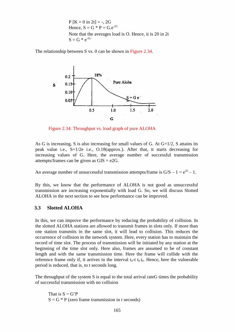
165

P [K = 0 in 2t] = -, 2G

Hence, S = G * P = G.e-2G

Note that the averages load is O. Hence, it is 20 in 2t

S = G * e-2G

The relationship between S vs. 0 can be shown in Figure 2.34.

Figure 2.34: Throughput vs. load graph of pure ALOHA

As G is increasing, S is also increasing for small values of G. At G=1/2, S attains its

peak value i.e., S=1/2e i.e., O.18(approx.). After that, it starts decreasing for

increasing values of G. Here, the average number of successful transmission

attempts/frames can be given as GIS = e2G.

An average number of unsuccessful transmission attempts/frame is G/S – 1 = e2G – 1.

By this, we know that the performance of ALOHA is not good as unsuccessful

transmission are increasing exponentially with load G. So, we will discuss Slotted

ALOHA in the next section to see how performance can be improved.

3.3 Slotted ALOHA

In this, we can improve the performance by reducing the probability of collision. In

the slotted ALOHA stations are allowed to transmit frames in slots only. If more than

one station transmits in the same slot, it will lead to collision. This reduces the

occurrence of collision in the network system. Here, every station has to maintain the

record of time slot. The process of transmission will be initiated by any station at the

beginning of the time slot only. Here also, frames are assumed to be of constant

length and with the same transmission time. Here the frame will collide with the

reference frame only if, it arrives in the interval t0-t t0 t0. Hence, here the vulnerable

period is reduced, that is, to t seconds long.

The throughput of the system S is equal to the total arrival rateG times the probability

of successful transmission with no collision

That is S = G‘P

S = G * P (zero frame transmission in t seconds)

166

The probability of k frames transmission in t seconds is given by the Poisson

distribution as follows:

P[k] = (G)k e-G/k! k = 0,1,2,3

Here average load in the vulnerable interval is G (one frame time) Hence, the

probability of zero frames in t seconds = e-G

S= Ge-G

The relationship between S vs G can be shown in Figure 2.35.

Figure 2.35: Throughput vs. load graph of slotted ALOHA

From the figure we can see that the system is exhibiting its performance, maximum

throughput that can be achieved with Slotted ALOHA S=1/e= 36 % (Approx.)

However, with this performance also we are not able to utilise the medium in an

efficient manner. Due to the high rate of collision systems the bandwidth is which

was designed to implement random access in LANs. So, we will discuss a new

protocol called CSMA in the next section.

3.4 Carrier Sense Multiple Access (CSMA)

As we have seen in previous section, the Slotted ALOHA maximum throughput that

can be achieved is i.e. only, though, the stations do not keep track of what the other

station is doing or what‘s going on in the medium. Then also, many frames meet and

collide. So in LANs we will observe the behaviour of other station as well and try to

reduce the number of collision to achieve better throughput of the network. To

achieve maximum throughput here, we will try to restrict transmission that will cause

collision by sensing whether the medium has some data or not. Protocols in which

station senses the channel before starting transmission are in the category of CSMA

protocols (also known as listen before talk protocols).

CSMA have many variants available that are to be adapted according to the

behaviour of the station that has frames to be transmitted when the channel is busy or

that some transmission is going on. The following are some versions of CSMA

protocols:

1. 1-Persistent CSMA

2. Non-Persistent CSMA

3. p-Persistent CSMA

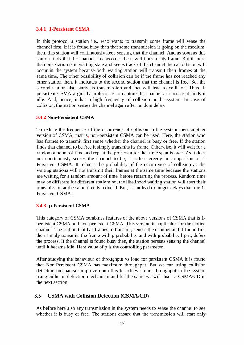
167

3.4.1 1-Persistent CSMA

In this protocol a station i.e., who wants to transmit some frame will sense the

channel first, if it is found busy than that some transmission is going on the medium,

then, this station will continuously keep sensing that the channel. And as soon as this

station finds that the channel has become idle it will transmit its frame. But if more

than one station is in waiting state and keeps track of the channel then a collision will

occur in the system because both waiting station will transmit their frames at the

same time. The other possibility of collision can be if the frame has not reached any

other station then, it indicates to the second station that the channel is free. So, the

second station also starts its transmission and that will lead to collision. Thus, I-

persistent CSMA a greedy protocol as to capture the channel as soon as it finds it

idle. And, hence, it has a high frequency of collision in the system. In case of

collision, the station senses the channel again after random delay.

3.4.2 Non-Persistent CSMA

To reduce the frequency of the occurrence of collision in the system then, another

version of CSMA, that is, non-persistent CSMA can be used. Here, the station who

has frames to transmit first sense whether the channel is busy or free. If the station

finds that channel to be free it simply transmits its frame. Otherwise, it will wait for a

random amount of time and repeat the process after that time span is over. As it does

not continuously senses the channel to be, it is less greedy in comparison of I-

Persistent CSMA. It reduces the probability of the occurrence of collision as the

waiting stations will not transmit their frames at the same time because the stations

are waiting for a random amount of time, before restarting the process. Random time

may be different for different stations so, the likelihood waiting station will start their

transmission at the same time is reduced. But, it can lead to longer delays than the 1-

Persistent CSMA.

3.4.3 p-Persistent CSMA

This category of CSMA combines features of the above versions of CSMA that is 1-

persistent CSMA and non-persistent CSMA. This version is applicable for the slotted

channel. The station that has frames to transmit, senses the channel and if found free

then simply transmits the frame with p probability and with probability l-p it, defers

the process. If the channel is found busy then, the station persists sensing the channel

until it became idle. Here value of p is the controlling parameter.

After studying the behaviour of throughput vs load for persistent CSMA it is found

that Non-Persistent CSMA has maximum throughput. But we can using collision

detection mechanism improve upon this to achieve more throughput in the system

using collision defection mechanism and for the same we will discuss CSMA/CD in

the next section.

3.5 CSMA with Collision Detection (CSMA/CD)

As before here also any transmission in the system needs to sense the channel to see

whether it is busy or free. The stations ensure that the transmission will start only

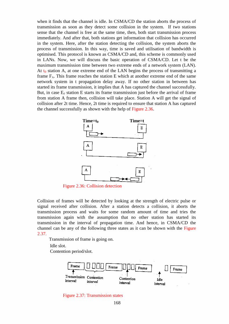
168

when it finds that the channel is idle. In CSMA/CD the station aborts the process of

transmission as soon as they detect some collision in the system. If two stations

sense that the channel is free at the same time, then, both start transmission process

immediately. And after that, both stations get information that collision has occurred

in the system. Here, after the station detecting the collision, the system aborts the

process of transmission. In this way, time is saved and utilisation of bandwidth is

optimised. This protocol is known as CSMA/CD and, this scheme is commonly used

in LANs. Now, we will discuss the basic operation of CSMA/CD. Let t be the

maximum transmission time between two extreme ends of a network system (LAN).

At t0 station A, at one extreme end of the LAN begins the process of transmitting a

frame FA. This frame reaches the station E which at another extreme end of the same

network system in t propagation delay away. If no other station in between has

started its frame transmission, it implies that A has captured the channel successfully.

But, in case EF station E starts its frame transmission just before the arrival of frame

from station A frame then, collision will take place. Station A will get the signal of

collision after 2t time. Hence, 2t time is required to ensure that station A has captured

the channel successfully as shown with the help of Figure 2.36.

Time=t0 Time=t

Figure 2.36: Collision detection

Collision of frames will be detected by looking at the strength of electric pulse or

signal received after collision. After a station detects a collision, it aborts the

transmission process and waits for some random amount of time and tries the

transmission again with the assumption that no other station has started its

transmission in the interval of propagation time. And hence, in CSMA/CD the

channel can be any of the following three states as it can be shown with the Figure

2.37.

Transmission of frame is going on.

Idle slot.

Contention period/slot.

Figure 2.37: Transmission states

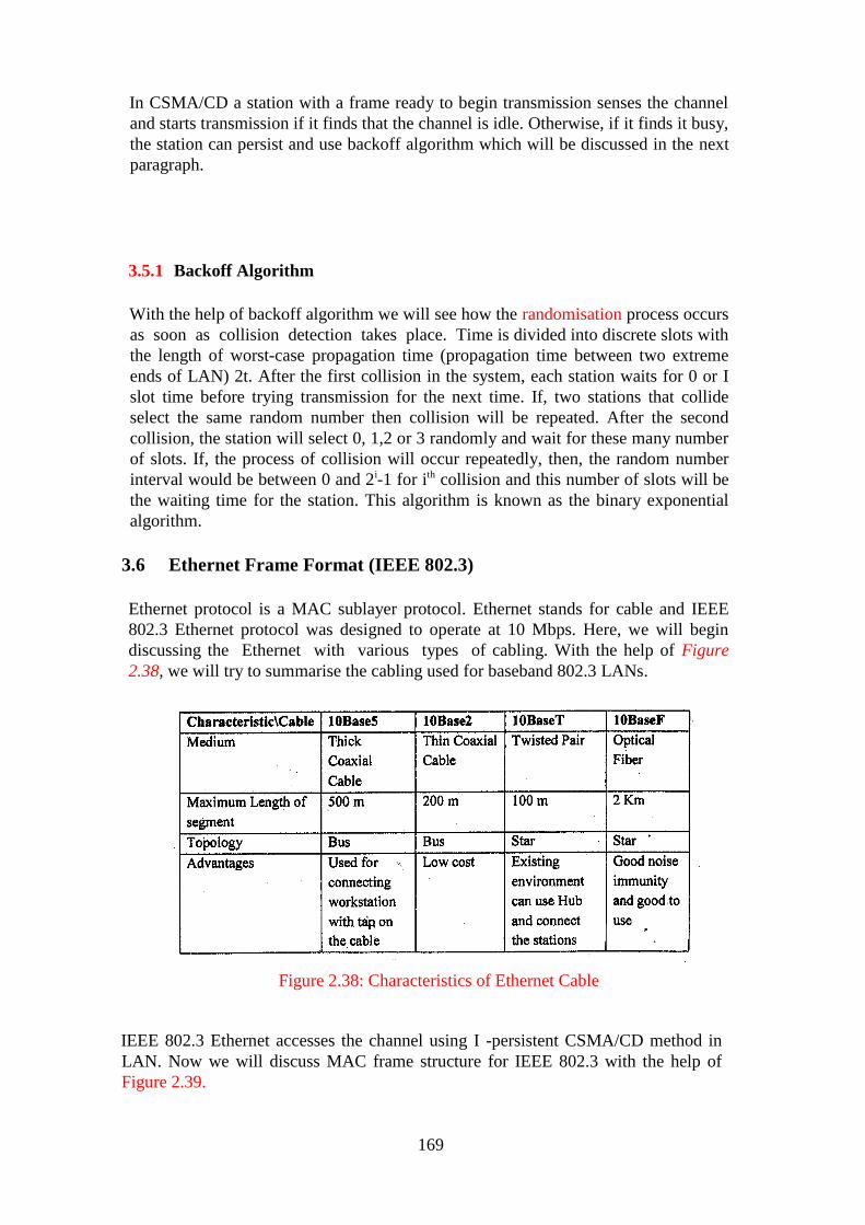
169

In CSMA/CD a station with a frame ready to begin transmission senses the channel

and starts transmission if it finds that the channel is idle. Otherwise, if it finds it busy,

the station can persist and use backoff algorithm which will be discussed in the next

paragraph.

3.5.1 Backoff Algorithm

With the help of backoff algorithm we will see how the randomisation process occurs

as soon as collision detection takes place. Time is divided into discrete slots with

the length of worst-case propagation time (propagation time between two extreme

ends of LAN) 2t. After the first collision in the system, each station waits for 0 or I

slot time before trying transmission for the next time. If, two stations that collide

select the same random number then collision will be repeated. After the second

collision, the station will select 0, 1,2 or 3 randomly and wait for these many number

of slots. If, the process of collision will occur repeatedly, then, the random number

interval would be between 0 and 2i-1 for ith collision and this number of slots will be

the waiting time for the station. This algorithm is known as the binary exponential

algorithm.

3.6 Ethernet Frame Format (IEEE 802.3)

Ethernet protocol is a MAC sublayer protocol. Ethernet stands for cable and IEEE

802.3 Ethernet protocol was designed to operate at 10 Mbps. Here, we will begin

discussing the Ethernet with various types of cabling. With the help of Figure

2.38, we will try to summarise the cabling used for baseband 802.3 LANs.

Figure 2.38: Characteristics of Ethernet Cable

IEEE 802.3 Ethernet accesses the channel using I -persistent CSMA/CD method in

LAN. Now we will discuss MAC frame structure for IEEE 802.3 with the help of

Figure 2.39.

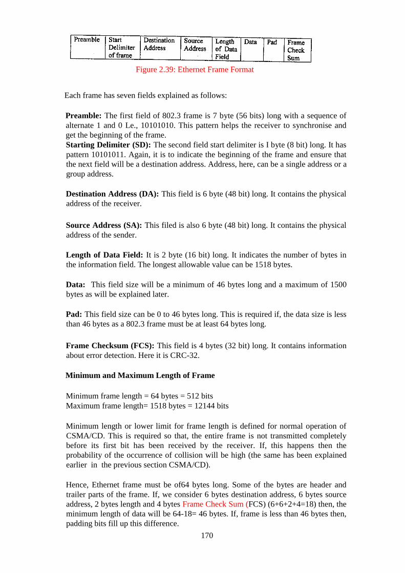
170

Figure 2.39: Ethernet Frame Format

Each frame has seven fields explained as follows:

Preamble: The first field of 802.3 frame is 7 byte (56 bits) long with a sequence of

alternate 1 and 0 Le., 10101010. This pattern helps the receiver to synchronise and

get the beginning of the frame.

Starting Delimiter (SD): The second field start delimiter is I byte (8 bit) long. It has

pattern 10101011. Again, it is to indicate the beginning of the frame and ensure that

the next field will be a destination address. Address, here, can be a single address or a

group address.

Destination Address (DA): This field is 6 byte (48 bit) long. It contains the physical

address of the receiver.

Source Address (SA): This filed is also 6 byte (48 bit) long. It contains the physical

address of the sender.

Length of Data Field: It is 2 byte (16 bit) long. It indicates the number of bytes in

the information field. The longest allowable value can be 1518 bytes.

Data: This field size will be a minimum of 46 bytes long and a maximum of 1500

bytes as will be explained later.

Pad: This field size can be 0 to 46 bytes long. This is required if, the data size is less

than 46 bytes as a 802.3 frame must be at least 64 bytes long.

Frame Checksum (FCS): This field is 4 bytes (32 bit) long. It contains information

about error detection. Here it is CRC-32.

Minimum and Maximum Length of Frame

Minimum frame length = 64 bytes = 512 bits

Maximum frame length= 1518 bytes = 12144 bits

Minimum length or lower limit for frame length is defined for normal operation of

CSMA/CD. This is required so that, the entire frame is not transmitted completely

before its first bit has been received by the receiver. If, this happens then the

probability of the occurrence of collision will be high (the same has been explained

earlier in the previous section CSMA/CD).

Hence, Ethernet frame must be of64 bytes long. Some of the bytes are header and

trailer parts of the frame. If, we consider 6 bytes destination address, 6 bytes source

address, 2 bytes length and 4 bytes Frame Check Sum (FCS) (6+6+2+4=18) then, the

minimum length of data will be 64-18= 46 bytes. If, frame is less than 46 bytes then,

padding bits fill up this difference.

171

As per 802.3 standard, the frames maximum length or upper limit of frame is = 1518

bytes (excluding preamble and SD). If we subtract 18 bytes of header and trailer then,

the maximum length will be 1500 bytes.

4.0 CONCLUSION

In this unit you have learnt about the various MAC sub-layer protocols like pure

ALOHA, slotted ALOHA, CSMA and CSMA/CD. The next unit will introduce you

to Wireless LAN and Data Link Layer Switching.

5.0 SUMMARY

In some networks, if a single channel and many users use that channel, then,

allocation strategy is required for the channel. We have discussed FDM and TDM

allocation method. They are the simplest methods for allocation. They work

efficiently for a small number of users. For a large number of users, the ALOHA

protocol is considered. There are two versions of ALOHA that is Pure ALOHA and

Slotted ALOHA. In Pure ALOHA no slotting was done but the efficiency was poor.

In Slotted ALOHA, slots have been made, so that every frame transmission starts at

the beginning of the slot and throughput is increased by a factor of2. For avoiding

collision and to increase efficiency in sensing the channel, CSMA is used. Many

versions of CSMA are persistent and non- persistent. In CSMA/CD collision

detection process is added so that process can be aborted just after a collision is

detected. Ethernet is a commonly used protocol for LAN. IEEE 802.3 Ethernet uses

1 persistent CSMA/CD access method.


1. Why is DLL divided into two sub layers? What are the key functions

of those sub layers?

2. How does Slotted ALOHA improve the performance of the system

over Pure ALOHA?

3. How has non-persistent reduced the probability of collision?

4. Explain Back off Algorithm and give one example of where it is used.


Andrew S. Tanenbaum, Computer Networks. 4th Edition, Prentice Hall of India, New

Delhi, 2011.

William Stalling, Data and Computer Communications. 5th Edition, Pearson

Education, New Delhi, 2003.

172

Behrouz A. Forouzan, Data Communications and Networking. 3‖ Edition, Tata

McGraw Hill, New Delhi, 2016.

Communication Networks- Fundamental Concepts and Key Architectures. Leon

Garcia and Widjaja 3rd

Edition, Tata McGraw Hill, New Delhi.


Question 1

Why is DLL divided into two sub layers? What are the key functions of those sub

layers?

Solution

The data link layer is divided into two sub layers (Logical Link Control (LLC) and

Media Access Control (MAC)) to allow for easy interoperability of different network

technologies.

LLC makes available the logics of the data link. Hence, manage the synchronization,

flow control and error checking activities of data link layer

MAC made available the management and assessment of the transmission medium. It

performs the function of transfer of data packets from one network interface card

(NIC) to another, throughout the shared communication channel. Here, physical

address and MAC address functions are handled.

Question 2

How does Slotted ALOHA improve the performance of the system over Pure

ALOHA?

Solution

Slotted Aloha gives room for transmission of data at the beginning of time slot and

reduces number of collisions to half thereby increases the efficiency to 36.8% from

18.4%.

Pure Aloha can transmit data at any time, continuous and not globally synchronized

Question 3

How has non-persistent reduced the probability of collision?

Solution

The non-persistent reduced the probability of collision by waiting a random number

of times after sensing the line before sensing again. It is not common for two ore more

173

station to wait the same number of times before sensing again and retry at the same

time.

Question 4

Explain Back off Algorithm and give one example of where it is used.

This is a method used in the transmission of data after collision between two stations.

If two stations transmit a frame at overlapping time then, collision will occur in the

system. Here, no station is constrained, any station that has data /frame to transmit can

transmit at any time. Once one station sends a frame (when it receives its own frame

and assumes that the destination has received it) after 2 times the maximum

propagation time. If the sender station does not receive the its own frame during this

time limit then, it retransmit this frame by using back off algorithm.

An example is the random-access MAC protocol (CSMA/CD), for instance, in

Ethernet to schedule re-transmissions after collisions.

174

UNIT 4 WIRELESS LAN AND DATA LINK LAYER SWITCHING

CONTENTS

1.0 Introduction

2.0 Objectives

3.0 Main Content

3.1 Introduction to Wireless LAN

3.2 Wireless LAN Architecture (IEEE 802.1 I)

3.3 Hidden Station and Exposed Station Problems

3.4 Wireless JAN Protocols: MACA and MACAW 49

3.5 IEEE 802.11 Protocol Stack

3.5.1 The 802.11 Physical Layer

3.5.2 The 802.11 MAC Sub-layer Protocol

3.6 Switching at Data Link Layer

3.6.1 Operation of Bridges in Different LAN Environment

3.6.2 Transparent Bridges

3.6.3 Spanning Tree Bridges

3.6.4 Source Routing Bridges

4.0 Conclusion

5.0 Summary



1.0 INTRODUCTION

The Previous discussion, we had in this block was related to wired

LANs but recently, wireless LANs are taking a dominant position due to coverage of

location difficult to wire, to satisfy the requirement of mobility and ad-hoc

networking. In a few years from now, we will notice a broader range of wireless

devices accessing the Internet, such as digital cameras, automobiles, security systems,

kitchen appliances. KUROSE and ROSS (2003) write that someday wireless devices

that communicate with the Internet may be present everywhere: on walls, in our cars,

in our bedrooms, in our pockets and in our bodies.

In this unit, we cover two broad topics: Wireless LAN, its protocols, its standard and

Data Link Layer Switching. In organisation we need an interconnection mechanism so

that all nodes can talk to each other. Bridges and switches are used for this purpose.

The spanning tree algorithms are used to build plugs and act as bridges.

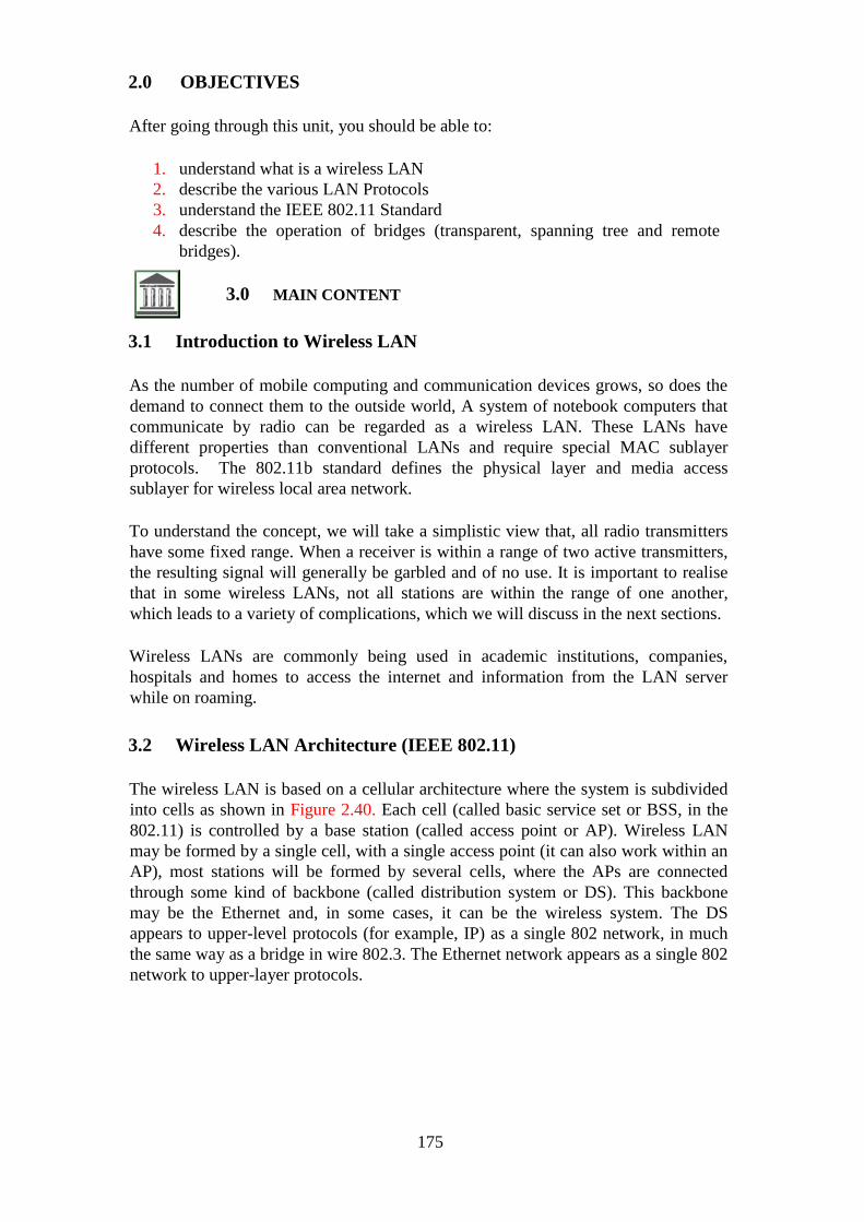
175

2.0 OBJECTIVES


1. understand what is a wireless LAN

2. describe the various LAN Protocols

3. understand the IEEE 802.11 Standard

4. describe the operation of bridges (transparent, spanning tree and remote

bridges).

3.0 MAIN CONTENT

3.1 Introduction to Wireless LAN

As the number of mobile computing and communication devices grows, so does the

demand to connect them to the outside world, A system of notebook computers that

communicate by radio can be regarded as a wireless LAN. These LANs have

different properties than conventional LANs and require special MAC sublayer

protocols. The 802.11b standard defines the physical layer and media access

sublayer for wireless local area network.

To understand the concept, we will take a simplistic view that, all radio transmitters

have some fixed range. When a receiver is within a range of two active transmitters,

the resulting signal will generally be garbled and of no use. It is important to realise

that in some wireless LANs, not all stations are within the range of one another,

which leads to a variety of complications, which we will discuss in the next sections.

Wireless LANs are commonly being used in academic institutions, companies,

hospitals and homes to access the internet and information from the LAN server

while on roaming.

3.2 Wireless LAN Architecture (IEEE 802.11)

The wireless LAN is based on a cellular architecture where the system is subdivided

into cells as shown in Figure 2.40. Each cell (called basic service set or BSS, in the

802.11) is controlled by a base station (called access point or AP). Wireless LAN

may be formed by a single cell, with a single access point (it can also work within an

AP), most stations will be formed by several cells, where the APs are connected

through some kind of backbone (called distribution system or DS). This backbone

may be the Ethernet and, in some cases, it can be the wireless system. The DS

appears to upper-level protocols (for example, IP) as a single 802 network, in much

the same way as a bridge in wire 802.3. The Ethernet network appears as a single 802

network to upper-layer protocols.

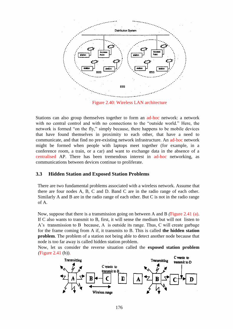
176

Figure 2.40: Wireless LAN architecture

Stations can also group themselves together to form an ad-hoc network: a network

with no central control and with no connections to the ―outside world.‖ Here, the

network is formed ―on the fly,‖ simply because, there happens to be mobile devices

that have found themselves in proximity to each other, that have a need to

communicate, and that find no pre-existing network infrastructure. An ad-hoc network

might be formed when people with laptops meet together (for example, in a

conference room, a train, or a car) and want to exchange data in the absence of a

centralised AP. There has been tremendous interest in ad-hoc networking, as

communications between devices continue to proliferate.

3.3 Hidden Station and Exposed Station Problems

There are two fundamental problems associated with a wireless network. Assume that

there are four nodes A, B, C and D. Band C are in the radio range of each other.

Similarly A and B are in the radio range of each other. But C is not in the radio range

of A.

Now, suppose that there is a transmission going on between A and B (Figure 2.41 (a).

If C also wants to transmit to B, first, it will sense the medium but will not listen to

A‘s transmission to B because, A is outside its range. Thus, C will create garbage

for the frame coming from A if, it transmits to B. This is called the hidden station

problem. The problem of a station not being able to detect another node because that

node is too far away is called hidden station problem.

Now, let us consider the reverse situation called the exposed station problem

(Figure 2.41 (b)).

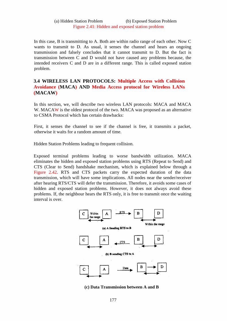
177

(a) Hidden Station Problem (b) Exposed Station Problem

Figure 2.41: Hidden and exposed station problem

In this case, B is transmitting to A. Both are within radio range of each other. Now C

wants to transmit to D. As usual, it senses the channel and hears an ongoing

transmission and falsely concludes that it cannot transmit to D. But the fact is

transmission between C and D would not have caused any problems because, the

intended receivers C and D are in a different range. This is called exposed station

problem.

3.4 WIRELESS LAN PROTOCOLS: Multiple Access with Collision

Avoidance (MACA) AND Media Access protocol for Wireless LANs

(MACAW)

In this section, we, will describe two wireless LAN protocols: MACA and MACA

W. MACAW is the oldest protocol of the two. MACA was proposed as an alternative

to CSMA Protocol which has certain drawbacks:

First, it senses the channel to see if the channel is free, it transmits a packet,

otherwise it waits for a random amount of time.

Hidden Station Problems leading to frequent collision.

Exposed terminal problems leading to worse bandwidth utilization. MACA

eliminates the hidden and exposed station problems using RTS (Repeat to Send) and

CTS (Clear to Send) handshake mechanism, which is explained below through a

Figure 2.42. RTS and CTS packets carry the expected duration of the data

transmission, which will have some implications. All nodes near the sender/receiver

after hearing RTS/CTS will defer the transmission. Therefore, it avoids some cases of

hidden and exposed station problems. However, it does not always avoid these

problems. If, the neighbour hears the RTS only, it is free to transmit once the waiting

interval is over.

(c) Data Transmission between A and B

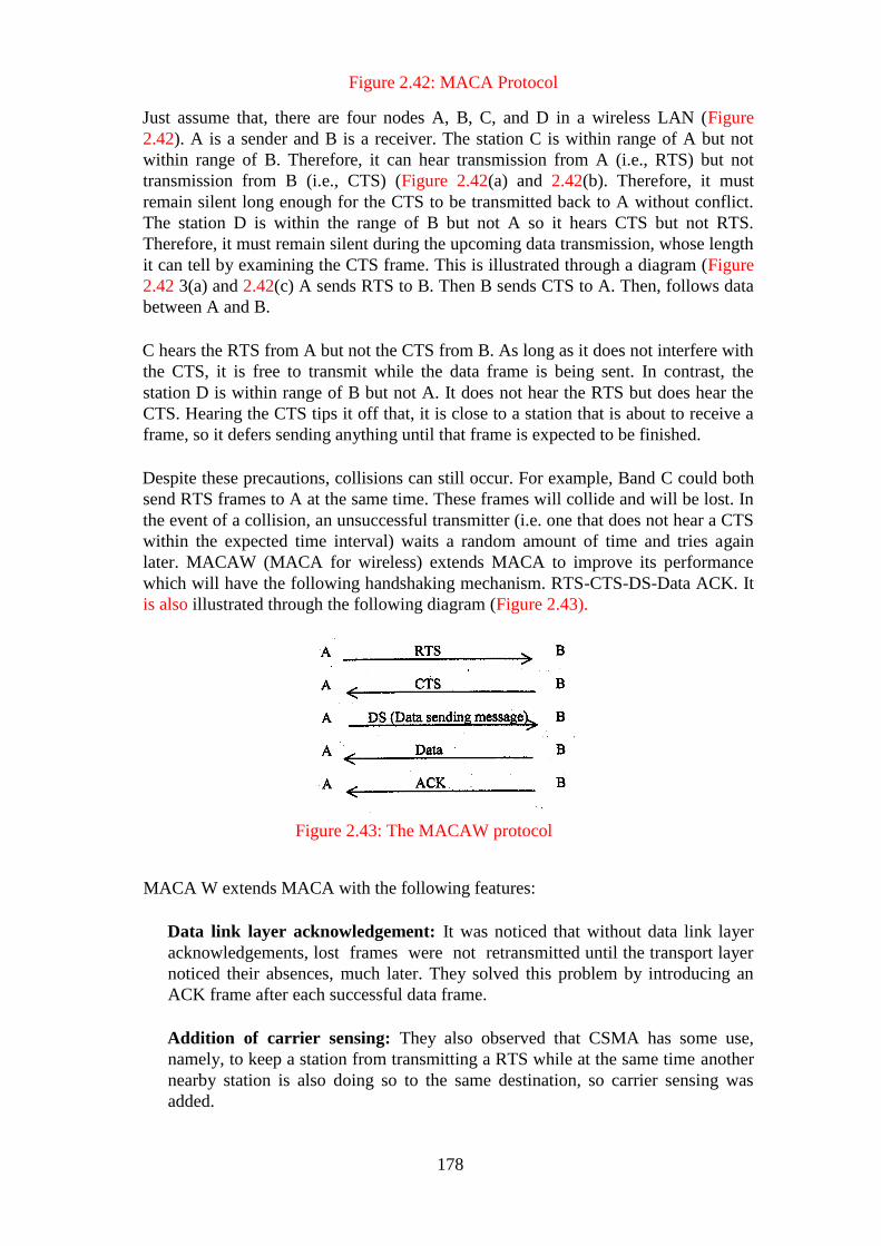
178

Figure 2.42: MACA Protocol

Just assume that, there are four nodes A, B, C, and D in a wireless LAN (Figure

2.42). A is a sender and B is a receiver. The station C is within range of A but not

within range of B. Therefore, it can hear transmission from A (i.e., RTS) but not

transmission from B (i.e., CTS) (Figure 2.42(a) and 2.42(b). Therefore, it must

remain silent long enough for the CTS to be transmitted back to A without conflict.

The station D is within the range of B but not A so it hears CTS but not RTS.

Therefore, it must remain silent during the upcoming data transmission, whose length

it can tell by examining the CTS frame. This is illustrated through a diagram (Figure

2.42 3(a) and 2.42(c) A sends RTS to B. Then B sends CTS to A. Then, follows data

between A and B.

C hears the RTS from A but not the CTS from B. As long as it does not interfere with

the CTS, it is free to transmit while the data frame is being sent. In contrast, the

station D is within range of B but not A. It does not hear the RTS but does hear the

CTS. Hearing the CTS tips it off that, it is close to a station that is about to receive a

frame, so it defers sending anything until that frame is expected to be finished.

Despite these precautions, collisions can still occur. For example, Band C could both

send RTS frames to A at the same time. These frames will collide and will be lost. In

the event of a collision, an unsuccessful transmitter (i.e. one that does not hear a CTS

within the expected time interval) waits a random amount of time and tries again

later. MACAW (MACA for wireless) extends MACA to improve its performance

which will have the following handshaking mechanism. RTS-CTS-DS-Data ACK. It

is also illustrated through the following diagram (Figure 2.43).

Figure 2.43: The MACAW protocol

MACA W extends MACA with the following features:

Data link layer acknowledgement: It was noticed that without data link layer

acknowledgements, lost frames were not retransmitted until the transport layer

noticed their absences, much later. They solved this problem by introducing an

ACK frame after each successful data frame.

Addition of carrier sensing: They also observed that CSMA has some use,

namely, to keep a station from transmitting a RTS while at the same time another

nearby station is also doing so to the same destination, so carrier sensing was

added.

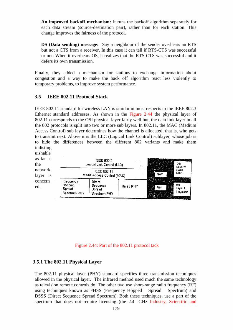
179

An improved backoff mechanism: It runs the backoff algorithm separately for

each data stream (source-destination pair), rather than for each station. This

change improves the fairness of the protocol.

DS (Data sending) message: Say a neighbour of the sender overhears an RTS

but not a CTS from a receiver. In this case it can tell if RTS-CTS was successful

or not. When it overhears OS, it realizes that the RTS-CTS was successful and it

defers its own transmission.

Finally, they added a mechanism for stations to exchange information about

congestion and a way to make the back off algorithm react less violently to

temporary problems, to improve system performance.

3.5 IEEE 802.11 Protocol Stack

IEEE 802.11 standard for wireless LAN is similar in most respects to the IEEE 802.3

Ethernet standard addresses. As shown in the Figure 2.44 the physical layer of

802.11 corresponds to the OSI physical layer fairly well but, the data link layer in all

the 802 protocols is split into two or more sub layers. In 802.11, the MAC (Medium

Access Control) sub layer determines how the channel is allocated, that is, who gets

to transmit next. Above it is the LLC (Logical Link Control) sublayer, whose job is

to hide the differences between the different 802 variants and make them

indisting

uishable

as far as

the

network

layer is

concern

ed.

Figure 2.44: Part of the 802.11 protocol tack

3.5.1 The 802.11 Physical Layer

The 802.11 physical layer (PHY) standard specifies three transmission techniques

allowed in the physical layer. The infrared method used much the same technology

as television remote controls do. The other two use short-range radio frequency (RF)

using techniques known as FHSS (Frequency Hopped Spread Spectrum) and

DSSS (Direct Sequence Spread Spectrum). Both these techniques, use a part of the

spectrum that does not require licensing (the 2.4 -GHz Industry, Scientific and

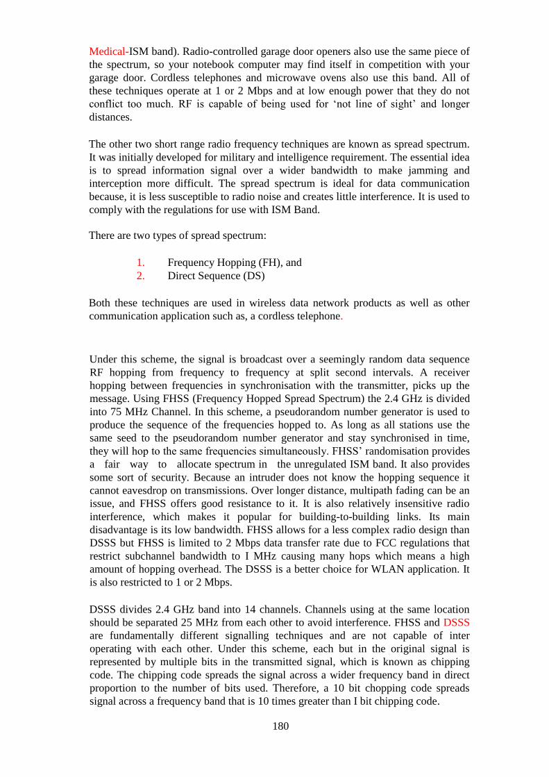
180

Medical-ISM band). Radio-controlled garage door openers also use the same piece of

the spectrum, so your notebook computer may find itself in competition with your

garage door. Cordless telephones and microwave ovens also use this band. All of

these techniques operate at 1 or 2 Mbps and at low enough power that they do not

conflict too much. RF is capable of being used for ‗not line of sight‘ and longer

distances.

The other two short range radio frequency techniques are known as spread spectrum.

It was initially developed for military and intelligence requirement. The essential idea

is to spread information signal over a wider bandwidth to make jamming and

interception more difficult. The spread spectrum is ideal for data communication

because, it is less susceptible to radio noise and creates little interference. It is used to

comply with the regulations for use with ISM Band.

There are two types of spread spectrum:

1. Frequency Hopping (FH), and

2. Direct Sequence (DS)

Both these techniques are used in wireless data network products as well as other

communication application such as, a cordless telephone.

Under this scheme, the signal is broadcast over a seemingly random data sequence

RF hopping from frequency to frequency at split second intervals. A receiver

hopping between frequencies in synchronisation with the transmitter, picks up the

message. Using FHSS (Frequency Hopped Spread Spectrum) the 2.4 GHz is divided

into 75 MHz Channel. In this scheme, a pseudorandom number generator is used to

produce the sequence of the frequencies hopped to. As long as all stations use the

same seed to the pseudorandom number generator and stay synchronised in time,

they will hop to the same frequencies simultaneously. FHSS‘ randomisation provides

a fair way to allocate spectrum in the unregulated ISM band. It also provides

some sort of security. Because an intruder does not know the hopping sequence it

cannot eavesdrop on transmissions. Over longer distance, multipath fading can be an

issue, and FHSS offers good resistance to it. It is also relatively insensitive radio

interference, which makes it popular for building-to-building links. Its main

disadvantage is its low bandwidth. FHSS allows for a less complex radio design than

DSSS but FHSS is limited to 2 Mbps data transfer rate due to FCC regulations that

restrict subchannel bandwidth to I MHz causing many hops which means a high

amount of hopping overhead. The DSSS is a better choice for WLAN application. It

is also restricted to 1 or 2 Mbps.

DSSS divides 2.4 GHz band into 14 channels. Channels using at the same location

should be separated 25 MHz from each other to avoid interference. FHSS and DSSS

are fundamentally different signalling techniques and are not capable of inter

operating with each other. Under this scheme, each but in the original signal is

represented by multiple bits in the transmitted signal, which is known as chipping

code. The chipping code spreads the signal across a wider frequency band in direct

proportion to the number of bits used. Therefore, a 10 bit chopping code spreads

signal across a frequency band that is 10 times greater than I bit chipping code.

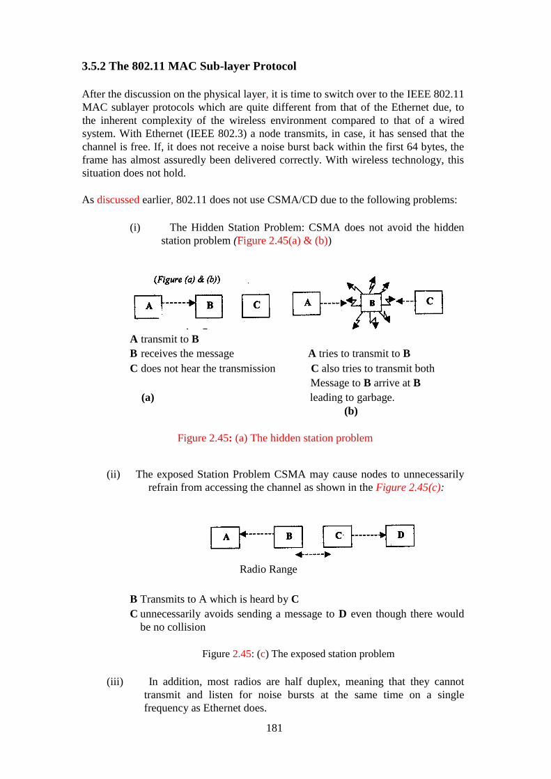
181

3.5.2 The 802.11 MAC Sub-layer Protocol

After the discussion on the physical layer, it is time to switch over to the IEEE 802.11

MAC sublayer protocols which are quite different from that of the Ethernet due, to

the inherent complexity of the wireless environment compared to that of a wired

system. With Ethernet (IEEE 802.3) a node transmits, in case, it has sensed that the

channel is free. If, it does not receive a noise burst back within the first 64 bytes, the

frame has almost assuredly been delivered correctly. With wireless technology, this

situation does not hold.

As discussed earlier, 802.11 does not use CSMA/CD due to the following problems:

(i) The Hidden Station Problem: CSMA does not avoid the hidden

station problem (Figure 2.45(a) & (b))

A transmit to B

B receives the message A tries to transmit to B

C does not hear the transmission C also tries to transmit both

Message to B arrive at B

(a) leading to garbage.

(b)

Figure 2.45: (a) The hidden station problem

(ii) The exposed Station Problem CSMA may cause nodes to unnecessarily

refrain from accessing the channel as shown in the Figure 2.45(c):

Radio Range

B Transmits to A which is heard by C

C unnecessarily avoids sending a message to D even though there would

be no collision

Figure 2.45: (c) The exposed station problem

(iii) In addition, most radios are half duplex, meaning that they cannot

transmit and listen for noise bursts at the same time on a single

frequency as Ethernet does.

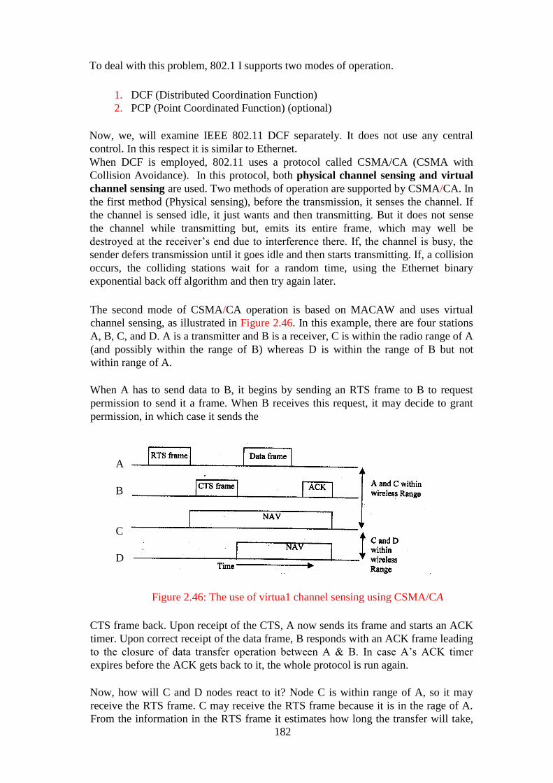
182

To deal with this problem, 802.1 I supports two modes of operation.

1. DCF (Distributed Coordination Function)

2. PCP (Point Coordinated Function) (optional)

Now, we, will examine IEEE 802.11 DCF separately. It does not use any central

control. In this respect it is similar to Ethernet.

When DCF is employed, 802.11 uses a protocol called CSMA/CA (CSMA with

Collision Avoidance). In this protocol, both physical channel sensing and virtual

channel sensing are used. Two methods of operation are supported by CSMA/CA. In

the first method (Physical sensing), before the transmission, it senses the channel. If

the channel is sensed idle, it just wants and then transmitting. But it does not sense

the channel while transmitting but, emits its entire frame, which may well be

destroyed at the receiver‘s end due to interference there. If, the channel is busy, the

sender defers transmission until it goes idle and then starts transmitting. If, a collision

occurs, the colliding stations wait for a random time, using the Ethernet binary

exponential back off algorithm and then try again later.

The second mode of CSMA/CA operation is based on MACAW and uses virtual

channel sensing, as illustrated in Figure 2.46. In this example, there are four stations

A, B, C, and D. A is a transmitter and B is a receiver, C is within the radio range of A

(and possibly within the range of B) whereas D is within the range of B but not

within range of A.

When A has to send data to B, it begins by sending an RTS frame to B to request

permission to send it a frame. When B receives this request, it may decide to grant

permission, in which case it sends the

Figure 2.46: The use of virtua1 channel sensing using CSMA/CA

CTS frame back. Upon receipt of the CTS, A now sends its frame and starts an ACK

timer. Upon correct receipt of the data frame, B responds with an ACK frame leading

to the closure of data transfer operation between A & B. In case A‘s ACK timer

expires before the ACK gets back to it, the whole protocol is run again.

Now, how will C and D nodes react to it? Node C is within range of A, so it may

receive the RTS frame. C may receive the RTS frame because it is in the rage of A.

From the information in the RTS frame it estimates how long the transfer will take,

A

B

C

D

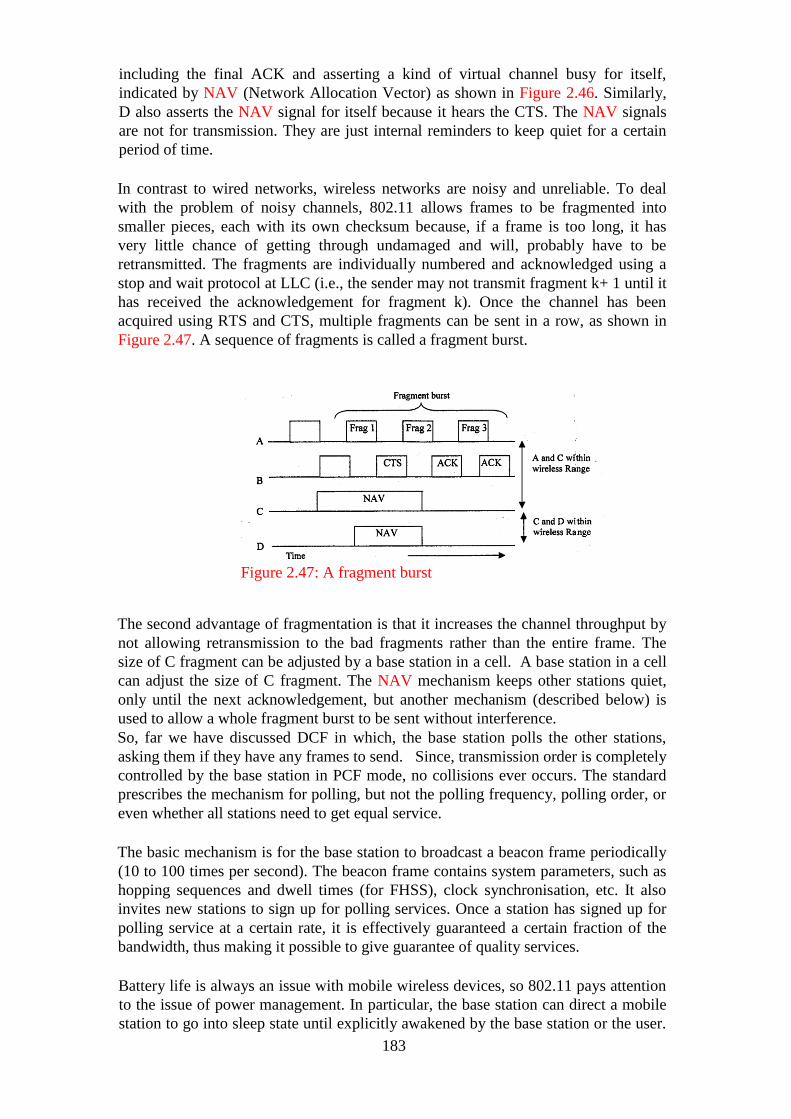
183

including the final ACK and asserting a kind of virtual channel busy for itself,

indicated by NAV (Network Allocation Vector) as shown in Figure 2.46. Similarly,

D also asserts the NAV signal for itself because it hears the CTS. The NAV signals

are not for transmission. They are just internal reminders to keep quiet for a certain

period of time.

In contrast to wired networks, wireless networks are noisy and unreliable. To deal

with the problem of noisy channels, 802.11 allows frames to be fragmented into

smaller pieces, each with its own checksum because, if a frame is too long, it has

very little chance of getting through undamaged and will, probably have to be

retransmitted. The fragments are individually numbered and acknowledged using a

stop and wait protocol at LLC (i.e., the sender may not transmit fragment k+ 1 until it

has received the acknowledgement for fragment k). Once the channel has been

acquired using RTS and CTS, multiple fragments can be sent in a row, as shown in

Figure 2.47. A sequence of fragments is called a fragment burst.

Figure 2.47: A fragment burst

The second advantage of fragmentation is that it increases the channel throughput by

not allowing retransmission to the bad fragments rather than the entire frame. The

size of C fragment can be adjusted by a base station in a cell. A base station in a cell

can adjust the size of C fragment. The NAV mechanism keeps other stations quiet,

only until the next acknowledgement, but another mechanism (described below) is

used to allow a whole fragment burst to be sent without interference.

So, far we have discussed DCF in which, the base station polls the other stations,

asking them if they have any frames to send. Since, transmission order is completely

controlled by the base station in PCF mode, no collisions ever occurs. The standard

prescribes the mechanism for polling, but not the polling frequency, polling order, or

even whether all stations need to get equal service.

The basic mechanism is for the base station to broadcast a beacon frame periodically

(10 to 100 times per second). The beacon frame contains system parameters, such as

hopping sequences and dwell times (for FHSS), clock synchronisation, etc. It also

invites new stations to sign up for polling services. Once a station has signed up for

polling service at a certain rate, it is effectively guaranteed a certain fraction of the

bandwidth, thus making it possible to give guarantee of quality services.

Battery life is always an issue with mobile wireless devices, so 802.11 pays attention

to the issue of power management. In particular, the base station can direct a mobile

station to go into sleep state until explicitly awakened by the base station or the user.

184

Having told a station to go to sleep, however, means that the base station has the

responsibility for buffering any frames directed at it while the mobile station is

asleep. These can be collected later.

PCF and DCF can coexist within one cell. At first it might seem impossible to have

central control and distributed control operating at the same time, but 802.11

provides a way to achieve this goal. It works by carefully defining the interframe

time interval. After a frame has been sent, a certain amount of dead time is required

before any station can send a frame.

3.6 Switching at Data Link Layer

Before discussing data ‗link layer switching devices, let us talk about repeaters which

are layer I devices. Repeaters provide both physical and electrical connections. Their

functions are to regenerating and propagate a signal in a channel. Repeaters are used

to extend the length of the LAN which depends upon the type of medium. For

example 10mbps 802.3 LAN that uses Unshielded Twisted pair (UTP) cable (10

BASE- T) has a maximum restriction of 100 meters. Many organisations have

multiple LANs and wish to connect them. LANs can be connected by devices called

bridges, which operate as the data link layer. Unlike repeaters, bridges connect

networks that have different physical layers. It can also connect networks using either

the same or different types of architecture at the MAC. (Token ring, Fibre Distributed

Data Interface (FDDl), Ethernet etc).

Bridges have some other characteristics:

1. Store and forward device.

2. Highly susceptible to broadcast storms.

Bridges are store and forward devices to provide error detection. They capture an entire

frame before deciding whether to filter or forward the frame, which provides a high level

of error detection because a frame‘s CRC checksum can be calculated by Tile Bridge.

Bridge is highly susceptible to broadcast storms. A broadcast storm occurs when several

broadcasts are transmitted at the same time. It can take up huge bandwidth.

Before looking at the technology of bridges, it is worthwhile taking a look at some

common situations in which bridges are used. Tanenbaum [Ref. I] has six reasons why a

single organisation may end up with multiple LANs.

1. Multiple LANs in organization

Many university and corporate departments have their own LANs, primarily to

connect their own personal computers, workstations, and servers. Since the goals of

the various departments differ, different departments choose different LANs. But

there is a need for interaction, so bridges are needed.

2. Geographical difference

The organisation may be geographically spread over several buildings separated by

considerable distances. It may be cheaper to have separate LANs in each building

185

and connect them with bridges and later link them to run a single cable over the

entire site as shown in figure 2.48.

Backbone LAN (For example -FDDI)

Figure 2.48: Multiple LANs connected by backbone to handle a total load

higher than the capacity of single LAN

3. Load distribution: It may be necessary to split what is logically a single LAN into

separate LANs to accommodate the load.

4. Long Round-Trip delay: In some situations, a single LAN would be adequate in

terms of the load, but the physical distance between the most distant machines can

be great (e.g. more than 2.5 km for Ethernet). Even if, laying the cable is easy to

do, the network would not work due to the excessively long round-trip delay. The

only solution is to partition the LAN and install bridges between the segments.

Using bridges, the total physical distance covered can be increased.

5. Reliability

By inserting bridges at critical points reliability can be enforced in the

network by isolating II defective node. Unlike a repeater, which just

copies whatever it sees, a bridge can be programmed to exercise some

discretion regarding what forwards and what it does not forward.

6. Security

Is a very important feature in bridges today, and can control the movement of

sensitive traffic by isolating the different parts of the network.

In an ideal sense, a bridge should have the following characters:

a Fully transparent

It means that it should allow the movement of a machine from one cable segment to

another cable segment without change of hardware and software or configuration

tools.

b Interpretability

It should allow a machine on one LAN segment to talk to another machine on

another LAN segment.

3.6.1 Operation of Bridges in Different LAN Environment

186

Having studied the features of bridges and why we require multiple LANs, let‘s learn

how they work. Assume that, there are two machines A and B. Both of them are

attached to a different LAN. Machine A is on a wireless LAN (Ethernet IEEE 802.3).

While B is on both LANs are connected to each other through a bridge. Now, A has a

packet to be sent to B. The flow of information at Host A is shown below:

1. The packet at machine A arrives at the LLC sublayer from the application

layer through the transport layer and network layer.

2. LLC Sub layer header get attached to the packet.

3. Then it moves to the MAC Sublayer. The packet gets MAC sublayer

header for attachment.

4. Since the node is part of a wireless LAN, the packet goes to the air using

Geographical Reference File-Names (GRF).

5. The packet is then picked up by the base station. It examines its destination

address and figures that it should be forwarded to the fixed LAN (it is

Ethernet in our case).

6. When the packet arrives at the bridge which connects the wireless LAN

and Ethernet LAN, it starts at the physical layer of the

bridge and moves to its LLC layer. At the MAC sublayer its 802.11 header

is removed.

7. The packet arrives at the LLC of a bridge without any 802.11 header.

8. Since the packet has to go to 802.3 LAN, the bridge prepares packets

accordingly.

Note that a bridge connecting k different LANs will have K different MAC sublayers

and k different physical layers. One for each type

So far, we have presented a very simplistic scenario in forwarding a packet from one LAN

to another through a bridge. In this section, we will point out some of the difficulties that

one encounters when trying to build a bridge between the various 802 LANs due to focus

on the following reasons:

1. Different frame Format

To start with, each of the LANs uses a different frame format. Unlike the

differences between Ethernet, token bus, and token ring, which were due to history

and big corporate egos, here the differences are to some extent legitimate. For

example, the Duration field in 802.11 is there, due to the MACAW protocol and

that makes no sense in Ethernet. As a result, any copying between different LANs

requires reformatting, which takes CPU time, requires a new checksum

calculation, and introduces the possibility of undetected errors due to bad bits in

the bridge‘s memory.

2. Different data rates

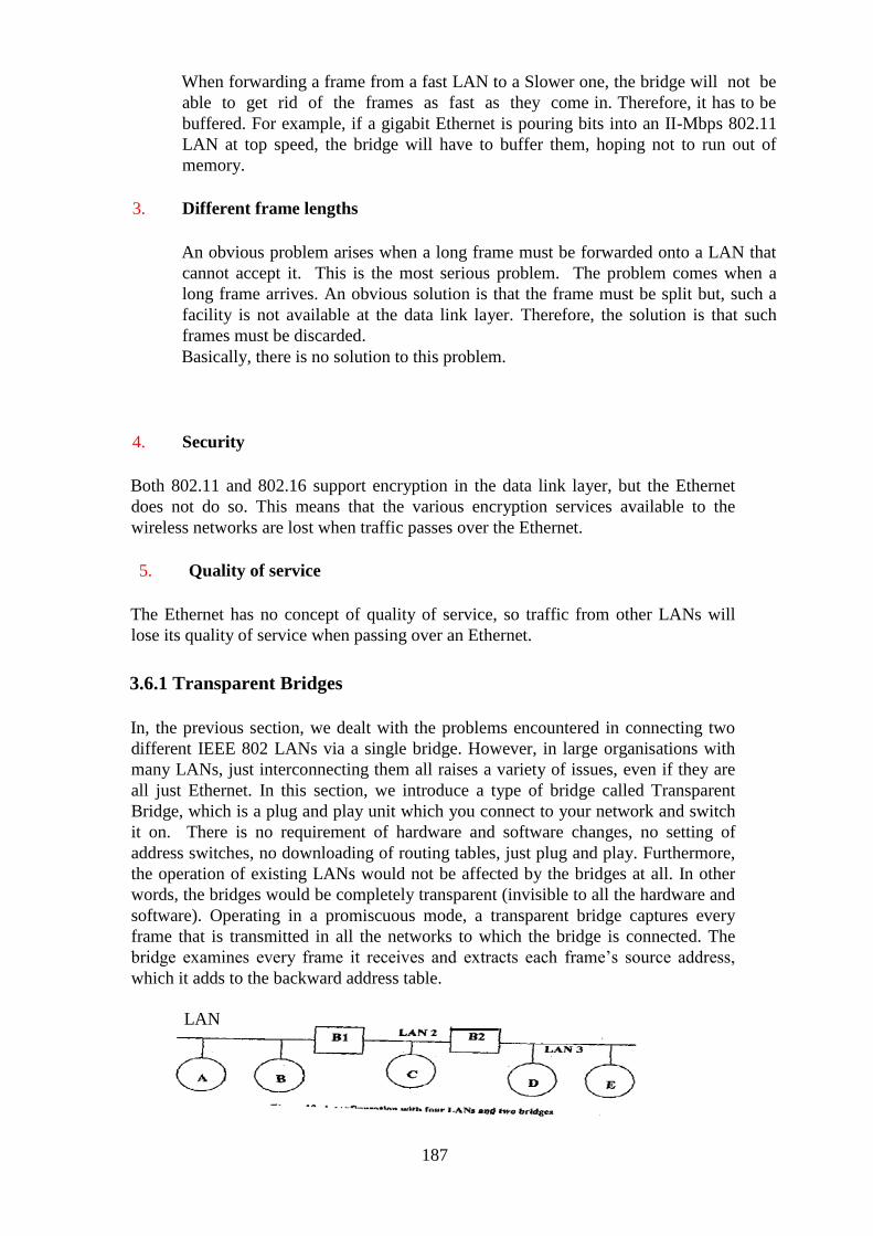
187

When forwarding a frame from a fast LAN to a Slower one, the bridge will not be

able to get rid of the frames as fast as they come in. Therefore, it has to be

buffered. For example, if a gigabit Ethernet is pouring bits into an II-Mbps 802.11

LAN at top speed, the bridge will have to buffer them, hoping not to run out of

memory.

3. Different frame lengths

An obvious problem arises when a long frame must be forwarded onto a LAN that

cannot accept it. This is the most serious problem. The problem comes when a

long frame arrives. An obvious solution is that the frame must be split but, such a

facility is not available at the data link layer. Therefore, the solution is that such

frames must be discarded.

Basically, there is no solution to this problem.

4. Security

Both 802.11 and 802.16 support encryption in the data link layer, but the Ethernet

does not do so. This means that the various encryption services available to the

wireless networks are lost when traffic passes over the Ethernet.

5. Quality of service

The Ethernet has no concept of quality of service, so traffic from other LANs will

lose its quality of service when passing over an Ethernet.

3.6.1 Transparent Bridges

In, the previous section, we dealt with the problems encountered in connecting two

different IEEE 802 LANs via a single bridge. However, in large organisations with

many LANs, just interconnecting them all raises a variety of issues, even if they are

all just Ethernet. In this section, we introduce a type of bridge called Transparent

Bridge, which is a plug and play unit which you connect to your network and switch

it on. There is no requirement of hardware and software changes, no setting of

address switches, no downloading of routing tables, just plug and play. Furthermore,

the operation of existing LANs would not be affected by the bridges at all. In other

words, the bridges would be completely transparent (invisible to all the hardware and

software). Operating in a promiscuous mode, a transparent bridge captures every

frame that is transmitted in all the networks to which the bridge is connected. The

bridge examines every frame it receives and extracts each frame‘s source address,

which it adds to the backward address table.

LAN

188

Figure 2.49: Three LANS and two bridges

As an example, take the following Confirmation (Figure 2.49). There are 3 LANs:

LAN1, LAN2 and LAN3 and two Bridges BI and B2. BI is connected to LAN1 and

LAN2 and bridges B2 is connected to LAN2 and LAN3. The routing procedure for

an incoming frame depends on the LAN it arrives on (the source LAN) and the LAN

its destination is on (the destination LAN), as follows:

1. If destination and source LANs are the same, discard the frame. (For

example, packet from A is going to B. Both are on the same LAN i.e.

LAN1).

2. If the destination and source LANs are different, forward the frame. (For

example, a packet from A on LAN I has to go to D on LAN 3)

3. If the destination LAN is unknown, use flooding.

When the bridges are first plugged in, all its hash tables are empty. None of the

bridges know where these destination nodes are exactly. Therefore, they use a

flooding algorithm: every incoming frame for an unknown destination is output on all

the LANs to which the bridge is connected, except to the one it arrived on. Gradually,

the bridges learn where destinations are. Once the destination is known there is no

more flooding and the packet is forwarded on the proper LAN.

The algorithm used by the transparent bridges is called backward learning.

As mentioned above, the bridges operate in promiscuous mode, so they

see every frame sent on any of their LANs. By looking at the source

address, they can tell which machine is accessible on which LAN. For

example, if bridge B2 in Figure 2.49 sees a frame on LAN 3 coming from

D, it knows that D must be reachable via LAN3, so it makes an entry in its

hash table noting that frames going to D should use LAN 3.

3.6.2 Spanning Tree Bridges

For reliability, some networks contain more than one bridge, which increases the

likelihood of networking loops. A networking loop occurs when frames are passed

from bridge to bridge in a circular manner, never reaching its destination. To prevent

networking loops when multiple bridges are used, the bridges communicate with each

other and establish a map of the network to derive what is called a spanning tree for all

the networks. A spanning tree consists of a single path between source and destination

nodes that does not include any loops. Thus, a spanning tree can be considered to be a

loop-free subset of a network‘s topology. The spanning tree algorithm, specified in

IEEE 802.ld, describes how bridges (and switches) can communicate to avoid network

loops.

3.6.3 Source Routing Bridges

IBM introduced source routing bridges for use in token ring networks. With source

routing, the sending machine is responsible for determining whether, a frame is

destined for a node on the same network or on a different network. If, the frame is

189

destined for a different network, then, the source machine designates this by setting

the high-order bit of the group address bit of the source address to 1. It also includes in

the frame‘s header the path the frame is to follow from source to destination.

Source routing bridges are based on the assumption that a sending machine will

provide routing information for messages destined for different networks. By making

the sending machine responsible for this task, a source routing bridge can ignore

frames that have not been ―marked‖ and forward only those frames with their

high-order destination bit set to 1.

4.0 CONCLUSION

In this conclusive unit of this module, you have bean take through the two broad

topics: Wireless LAN, its standard and Data Link Layer Switching through bridges

and Switches.

5.0 SUMMARY

In this unit we discussed two major topics wireless LANs and switching mechanism at

the data link layer with IEEE at the data link layer. With IEEE 802.11 standardisation,

wireless LANs are becoming common in most of the organisations but, they have

their own problems and solutions CSMA/CD does not work due to hidden station

problem. To make CSMA work better two new protocols, MACA and MACAW were

discussed. The physical layer of wireless LAN standard i.e. IEEE 802.11 allows five

different transmission modes, including infrared, various spread spectrum schemes

etc. As a part of inter LANs connecting mechanism we discussed different

types of bridges. Bluetooth was not taken up in this unit, although, it is a very

important topic today. It is a also a wireless network used for connecting handsets and

other peripherals to computers without wires.


1. What is Hidden Station Problem?

2. Why CSMA/CD cannot be used in wireless LAN environment? Discuss.

3. How is MACAW different from MACA?

4. What are the features of a transparent bridge?

5. What are the difficulties in building a bridge between the various 802 LANs?


Practice Hall of India, (2011). Computer Networks, A. S. Tanenbaum 4th Edition,

New Delhi.

J.F. Kurose & K. W. Ross, (2003). Computer Networking, A Top Down Approach

Featuring the Internet, Pearson Edition.

190

Behrouz Forouzan, (2016). Introduction to Data Communication & Networking,

Tata McGraw Hill.

Leon Garcia, and Widjaja, (2000). Communications Networks, Tata McGraw

Hill.

Willian Stallings, Data and Computer Communications, 6tb Edition, Pearson

Education, New Delhi,2003.


Question 1

What is Hidden Station Problem?

Solution

This is a situation in wireless LAN transmission where two or more stations who are

out of range of each other/one another communicate to the same recipient

Question 2

Why CSMA/CD cannot be used in wireless LAN environment? Discuss.

Solution

CSMA/CD cannot be use in wireless LAN environment because there is no way for

the source of information can sense collisions the same way CSMA/CD does on a

physical medium since the source is only able to communicate and obtain packets on

the channel but is not able to sense data crossing that channel.

Question 3

How is MACAW different from MACA?

Solution

Multiple Access with Collision Avoidance (MACA) enables nodes gives information

of sending data frame for others to remain silent in a wireless network. However,

collision can still exist in wireless LAN with MACA, hence the need for MACA for

Wireless (MACAW). In MACAW, nodes are requested to send acknowledgments

after every fruitful frame communication. This is mostly use in ad-hoc network and is

the foundation of numerous other MAC protocols that exist in wireless sensor

networks (WSN).

Question 4

What are the features of a transparent bridge?

Solution

Some of the features of transparent bridges are fast convergence time, low network

overhead, easier configuration and less CPU consumption.

Question 5

What are the difficulties in building a bridge between the various 802 LANs?

Solution

The difficulties in building a bridge between the various 802 LANs are:

The LANs uses a different frame format

The interconnected LANs do not necessarily run at the same data rate

The different 802 LANs have different maximum frame lengths

191

Both 802.11 and 802.16 support encryption in the data link layer but Ethernet does

not.

The issues of the quality of service is another point. Both 802.11 and 802.16 provide

it in various forms, the former using PCF mode and the latter using constant bit rate

connections

Note: Explain them

MODULE 3 NETWORK LAYER

Unit 1 Introduction to Layer Functionality and Design Issues

Unit 2 Routing Algorithms

Unit 3 Congestion Control in Public Switched Network Unit 4

Internetworking

UNIT 1 INTRODUCTION TO LAYER FUNCTIONALITY AND

DESIGN ISSUES

CONTENTS

1.0 Introduction

2.0 Objectives

3.0 Main Content

3.1 Connection Oriented vs. Connection-less Services

3.1.1 Connection-oriented Services

3.1.2 Connection-less Services

3.2 Implementation of the Network Layer Services


3.2.2 Implementation of Connection -oriented Services

3.2.3 Implementation of Connection-less Services

3.3 Comparison between Virtual Circuit and Datagram Subnet

3.4 Addressing

3.4.1 Hierarchical versus Flat Address

3.4.2 Static vs Dynamic Address

3.4.3 IP Address

3.5 Concept of Congestion

3.6 Routing Concept

3.6.1 Main Issues in Routing

3.6.2 Classification of Routing Algorithm

4.0 Conclusion

5.0 Summary


192


1.0 INTRODUCTION

In the previous blocks of this course, we have learned the basic

functions of physical layer and data link layer in networking. Now, in this chapter,

we will go through the functions of the network layer.

The network layer is at level three in OSI model. It responds to service requests from

the transport layer and issues service requests to the data link layer. It is responsible

for end-to-end (source to destination) packet delivery, whereas the data link layer is

responsible for node-to-node (hop-to-hop) packet delivery. Three important functions

of the network layers are:

1. Path Determination

It determines the route taken by the packets from the source to the

destination.

2. Forwarding

It forwards packets from the router's input to the appropriate router output.

3. Call Setup

Some network architectures require router call setup along the path before

the data flows. To perform these functions, the network layer must be

aware of the topology of the communication subnet (i.e., set of routers,

communication lines).

For end-to-end delivery, the network provides two type of services i.e.,

connection-oriented service and connectionless service to the transport

layer. The network layer services meet the following entries [ref.1].

a. Transport layer should not be aware of the topology of the, network

(subnet).

b. Services should be independent of the router technology.

In this unit, we will first go through the basic concepts of these services and will then

differentiate between these two. Then, we will introduce some other concepts like

routing and congestion.

2.0 OBJECTIVES


1. define basic functions of the network layer

2. differentiate between connection oriented and connection less services

3. define the concept of addressing in networking

193

4. define congestion in the network layer

5. explain the concept of routing

6. explain the concept of packet switching

7. define packet switching network.

3.0 MAIN CONTENT

3.1 Connection Oriented vs. Connectionless Services

In computer networks, delivery between source and destination can be accomplished

in either of the two ways:

1. Connection-oriented services

2. Connection-less services.

3.1.1 Connection-Oriented Services

Connection-oriented services define a way of transmitting data between a sender and

a receiver, in which an end-to-end connection is established before sending any data.

After establishing a connection, a sequence of packets, (from the source to

destination), can be sent one after another. All the packets belonging to a message are

sent from the same connection. When all packets of a message have been delivered,

the connection is terminated.

In connection-oriented services, the devices at both the endpoints use a

protocol to establish an end-to-end connection before sending any data.

Connection-oriented service usually has the following characteristics:

1. The network guarantees that all packets will be delivered in order without

loss or duplication of data.

2. Only a single path is established for the call. and all the data follows that

path.

3. The network guarantees. a minimal amount of bandwidth and this bandwidth

is reserved for the duration of the call.

4. If the network is over utilised, future call requests are refused.

Connection-oriented service is sometimes called a ―reliable‖ network service

because:

a. It guarantees that data will arrive in the proper sequence.

b. Single connection for entire message facilitates acknowledgement process

and retransmission of damaged and lost frames.

Connection-oriented transmission has three stages. These are:

1. Connection establishment

194

In connection-oriented services, before transmitting data, the sending

device must first determine the availability of the other to exchange data

and a connection must be established by which data can be sent.

Connection establishment requires three steps. These are:

a. First the sender computer requests the connection by sending a

connection request packet to the intended receiver.

b. Then the receiver computer returns a confirmation packet to the

requesting computer.

c. Finally, the sender computer returns a packet acknowledging the

confirmation.

2. Data transfer

After the connection gets established, the sender starts sending data packets to the

receiver.

3. Connection termination

After all the data gets transferred, the connection has to be terminated. Connection

termination also requires a three-way handshake i.e.:

a. First, the sender computer requests disconnection by sending a

disconnection request packet.

b. Then, the receiver computer confirms the disconnection request.

c. Finally, the sender computer returns a packet acknowledging the

confirmation.

Transmission Control Protocol (TCP) is a connection-oriented protocol.

3.1.2 Connection-less Services

Connection-less services define a way of communication between two network end

points in which, a message can be sent from one end point to another without prior

arrangement. The sender simply starts sending packets, addressed to the intended

recipient.

Connectionless service is a service that allows the transfer of information

among subscribers without the need for end-to-end connection establishment

procedures.

Connection-less service is sometimes known as ―unreliable‖ network service.

Connection-less protocols are usually described as stateless because the endpoints

have no protocol-defined way of remembering where they are in a ―conversation‖ of

message exchange.

The Internet Protocol (IP) and User Datagram Protocol (UDP) are connectionless

protocols, but TCP/IP (the most common use of IP) is connection-orientated.

195

3.2 Implementation of the Network Layer Services

In this section, we will examine how the network layer services are implemented. Two

different services are taken into consideration depending on the type of service being

offered. These two schemes are known as virtual circuit subnet (VC subnet) for

connection-oriented service and datagram subnet for connection-less services. A VC

subnet may be compared to the physical circuit required in a telephone setup. In a

connection-oriented service, a route from the source to the destination must be established.

In a datagram subnet, no advance set up is needed. In this case, packets are routed

independently. But, before we take up the implementation issues let us, revisit the packet

switching concepts once again. The services are implement through a packet switched

network.


In the fourth unit of Block I, we introduced the concept of packet switching. We

further elaborate in this section, in the context of the network layer. The network layer

operates in the packet switched network (or subnet) environment which comprises

several routers linked with transmission lines (leased or dial up) besides user's

machines as shown in Figure 3.1.

Figure 3.1: A Packet switched network

This subnet works in the following manner. Whenever user wants to send a packet to

another users, the packet is transmitted to the nearest router either on its own LAN or

over a point-to-point link to the carrier. The packet is stored for verification and then

transmitted further to the next router along the way until it reaches the final destination

machine. This mechanism is called packet switching.

But, why packet switching? Why not circuit switching? Now, let us discuss these

issues.

Circuit switching was not designed for packet transmission. It was primarily designed

for voice communication. It creates temporary (dialled) or permanent (leased)

dedicated links that are wel1 suited to this type of communication [Ref 2].

196

(i) Data transmission tends to be busty, which means that packets

arrive in spurts with gaps in between. In such cases, transmission

lines will be mostly idle leading to wastage of resources if we use

circuit switching for data transmission.

(ii) Single Data Rate: In circuit switching mechanism there is a single

data rate for the two end devices which limits flexibility and

usefulness of circuit switched connection for networks

interconnection of a variety of digital devices.

(iii) No priority to transmission: Circuit switching treats all

transmissions as equal. But often, with data transmission we may

be required to send a certain packet on a high priority basis, which

may not be implemented with the circuit switching approach.

3.2.2 Implementation of Connection-oriented Services

To implement connection-oriented services, we need to form a virtual- circuit subnet.

This idea behind the creation of a VC is so that, a new route for every packet sent. In

virtual circuits:

1. First, a connection needs to be established.

2. After establishing a connection, a route from the source machine to the

destination machine is chosen as part of the connection setup and stored in tables

inside the routers. This route is used for all traffic flowing over the connection.

3. After transmitting all the data packets, the connection is released. When the

connection is released, the virtual circuit is also terminated.

In a connection-oriented service, each packet carries an identifier that identifies the

virtual circuit it belongs to.

Now, let us take an example, consider the situation of a subnet in Figure 3.2. In this

figure, H1, H2 and H3 represent host machines and RI, R2, R3, R4, RS and R6

represent routers. Processes are running on different hosts.

Here, host HI has established connection 1 with host H2. It is remembered as the first

entry in each of the routing tables as shown in Table 3.1. The first line of RI 's table

says that, if a packet bearing connection identifier 1 comes in from HI, it is to be sent

to router R3, and given connection identifier 1. Similarly, the first entry at R3 routes

the packet to R5, also with connection identifier 1.

Now, let us consider a situation in which, H3 also wants to establish a connection with

H2. It chooses connection identifier I (because it is initiating the connection and this is

its only connection) and informs the subnet to setup the virtual circuit. This leads to

the second row in the table. Note, that we have a conflict here because although R1

can easily distinguish -connection I packets from HI and connection I packets from

H3, R3 cannot do this. For this reason, RI assigns a different connection identifier to

197

the outgoing traffic for the second connection (No.2). In order to avoiding conflicts of

this nature, it is important that routers have the ability to replace connection identifiers

in outgoing packets. In some contexts, this is called label switching.

Figure 3.2: Routing in a virtual subnet

Figure 3.3: Routing table for VC subnet

3.2.3 Implementation of Connection-less Services

In this section, we shall discuss the implementation of these services i.e., how

connection-less services are implemented in real networks. To implement connection-

less services, we need a datagram subnet.

In these services, packets are individually injected into the subnet and their routing

decisions are not dependent on each other (packets). Therefore, in connectionless

services, no advance setup is needed. In this context, the packets are frequently called

datagrams and the subnet is called a datagram subnet.

Now, let us take an example to learn how a datagram subnet works.

198

Consider the situation of Figure 3.4. In this Figure, HI and H2 represent host machines

and RI, R2, R3, R4, R5 and R6 represent routers. Suppose, that the process running at

host HI has a long message to be transmitted to a process running at H2 machine. To

do so, it transfers the message to the transport layer with appropriate instructions to

deliver it to the process running at H2. Where is the transfer layer process running,

can you figure out? Well, it may also be running on HI but within the operating

system. The transport layer process adds a transport header to the front of the message

and transfers the message (also called TPDU) to the network layer. The network layer

too, might be running as another procedure within the operating system.

Let us assume, that the message is five times longer than the maximum packet size,

therefore, the network layer has to break it into five packets, 1,2, 3, 4 and 5 and send

each of them in turn to router RI (because it is linked to RI) using some point-to-point

protocol. After this, the carrier (supported by ISP) takes over. Every router has an

internal table telling it where to send packets for each possible destination. Each table

entry is a pair consisting of a destination and the outgoing line to use for that

destination. Only directly-connected lines can be used. For example, in Figure 3.4, RI

has only two outgoing lines-to R2 and R3. So, every incoming packet must be sent to

one of these routers.

As the packets arrive at RI from HI, packets 1, 2, and 3 were stored briefly (to verify

their checksums). Then, each packet was forwarded to R3 according to Rl 's table

(table not shown here). Packet I was then forwarded to R5 and from R5 to R6. When it

got to R6, it was encapsulated in a data link layer frame and sent to H2. Packets 2 and

3 follow the same route.

However, something different happened to packet 4 and 5. When it got to RI it was

sent to router R2, even though it has the same destination. Due to some reason (for ex.

congestion), RI decided to send packet 4 and 5 via a different route than that of the

first three.

The algorithm that manages the tables and makes the routing decisions is known as the

routing algorithm. In next unit, we shall study routing algorithms. Students are

requested to refer to [Ref. I] for further study on the implementation of connection

oriented and connection less services. You should focus on connecting routing tables.

Figure 3.4: Routing in a datagram subnet

199

3.3 Comparison between Virtual Circuit and Datagram Subnet

Both virtual circuits and datagrams have their pros and cons. We shall compare

them on the basis of different parameters. These various parameters are:

1. Router memory space and bandwidth

Virtual circuits allow packets to contain circuit numbers instead of full destination

addresses. A full destination address lit every packet may represent a significant

amount of overhead, and hence waste bandwidth.

2. Setup time vs. address parsing time

Using virtual circuits requires a setup phase, which takes time and consumes

memory resources. However, figuring out what to do with a data packet in a

virtual-circuit subnet is easy: the router simply uses the circuit number to index

into a table to find out where the packet goes. In a datagram subnet, a more

complicated lookup procedure is required to locate the entry for the destination.

3. Amount of table space required in router memory

A datagram subnet needs to have an entry for every possible destination, whereas

a virtual-Circuit subnet just needs an entry for each virtual circuit.

4. Quality of service

Virtual circuits have some advantages in guaranteeing quality of service and avoiding

congestion within the subnet because resources (e.g., buffers, bandwidth, and CPU

cycles) can be reserved in advance, when the connection is established. Once the

packets start arriving, the necessary bandwidth and router capacity will be there.

With a datagram subnet, congestion avoidance is more difficult.

5. Vulnerability

Virtual circuits also have a vulnerability problem. If, a router crashes and loses its

memory, even if it comes back a second later, all the virtual circuits passing through

it will have to be aborted. In contrast, if a datagram router goes down, only those

users whose packets were queued in the router at the time will suffer, and maybe not

even all those, depending upon whether they have already been acknowledged. The

loss of a communication line is fatal to virtual circuits using it but can be easily

compensated for if datagrams are used.

6. Traffic balance

Datagrams also allow the routers to balance the traffic throughout the subnet, since

routes can be changed partway through a long sequence of packet transmissions. A

200

brief comparison between a virtual circuit subnet and a datagram subnet is given in

figure 3.5. Students should refer to Reference 1 for further discussion.

Table 3.5: Comparison between Virtual Circuit and Datagram Subnets (Source: Ref.

[1])

SELF-ASSESSMENT EXERCISE 7

Give right choice for the following:

1. Connection-oriented service is sometimes called a network service.

a Reliable

b Unreliable

2. ………………………….is a connection-oriented protocol.

a UDP

b TCP

c IP

3. Why are connection oriented services known as reliable services? Explain briefly.

3.4 Addressing

Network addresses identify devices separately or as members of a group. Addressing

is performed on various layers of the OSI model. Thus, schemes used for addressing

vary on the basis of the protocol used and the OSI layer. On this basis, internetwork

addresses can be categorised into three types. These are:

1 Data link layer addresses

2 Media Access Control (MAC) addresses

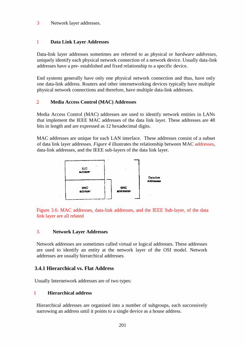
201

3 Network layer addresses.

1 Data Link Layer Addresses

Data-link layer addresses sometimes are referred to as physical or hardware addresses,

uniquely identify each physical network connection of a network device. Usually data-link

addresses have a pre- established and fixed relationship to a specific device.

End systems generally have only one physical network connection and thus, have only

one data-link address. Routers and other internetworking devices typically have multiple

physical network connections and therefore, have multiple data-link addresses.

2 Media Access Control (MAC) Addresses

Media Access Control (MAC) addresses are used to identify network entities in LANs

that implement the IEEE MAC addresses of the data link layer. These addresses are 48

bits in length and are expressed as 12 hexadecimal digits.

MAC addresses are unique for each LAN interface. These addresses consist of a subset

of data link layer addresses. Figure 4 illustrates the relationship between MAC addresses,

data-link addresses, and the IEEE sub-layers of the data link layer.

Figure 3.6: MAC addresses, data-link addresses, and the IEEE Sub-layer, of the data

link layer are all related

3. Network Layer Addresses

Network addresses are sometimes called virtual or logical addresses. These addresses

are used to identify an entity at the network layer of the OSI model. Network

addresses are usually hierarchical addresses.

3.4.1 Hierarchical vs. Flat Address

Usually Internetwork addresses are of two types:

1 Hierarchical address

Hierarchical addresses are organised into a number of subgroups, each successively

narrowing an address until it points to a single device as a house address.

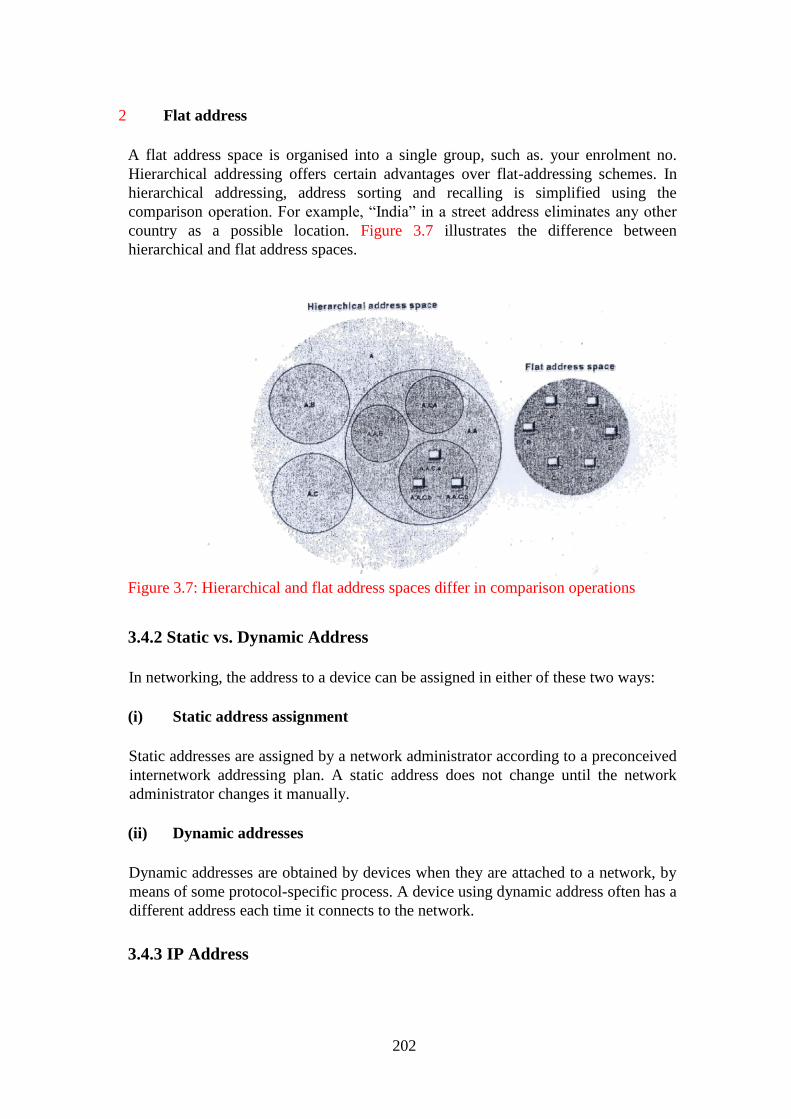
202

2 Flat address

A flat address space is organised into a single group, such as. your enrolment no.

Hierarchical addressing offers certain advantages over flat-addressing schemes. In

hierarchical addressing, address sorting and recalling is simplified using the

comparison operation. For example, ―India‖ in a street address eliminates any other

country as a possible location. Figure 3.7 illustrates the difference between

hierarchical and flat address spaces.

Figure 3.7: Hierarchical and flat address spaces differ in comparison operations

3.4.2 Static vs. Dynamic Address

In networking, the address to a device can be assigned in either of these two ways:

(i) Static address assignment

Static addresses are assigned by a network administrator according to a preconceived

internetwork addressing plan. A static address does not change until the network

administrator changes it manually.

(ii) Dynamic addresses

Dynamic addresses are obtained by devices when they are attached to a network, by

means of some protocol-specific process. A device using dynamic address often has a

different address each time it connects to the network.

3.4.3 IP Address

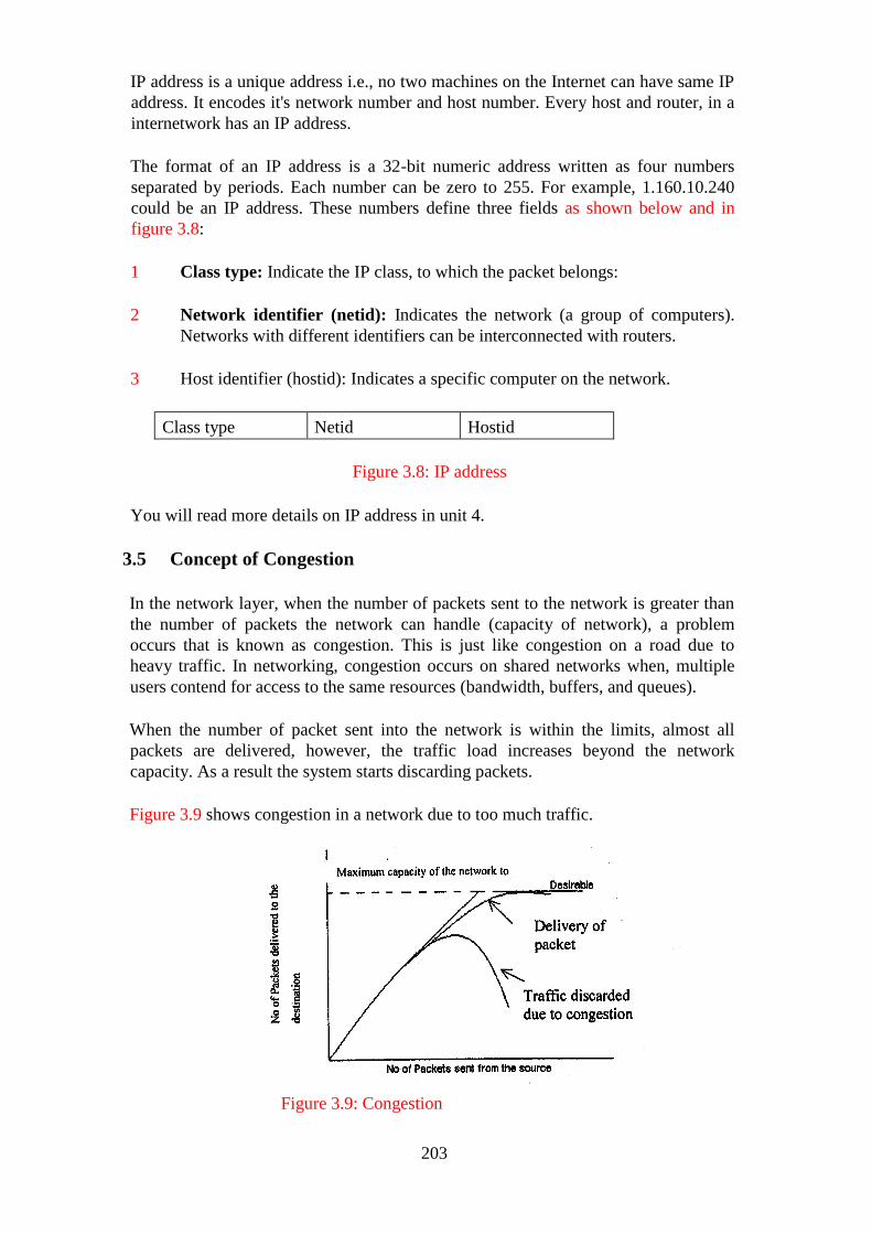
203

IP address is a unique address i.e., no two machines on the Internet can have same IP

address. It encodes it's network number and host number. Every host and router, in a

internetwork has an IP address.

The format of an IP address is a 32-bit numeric address written as four numbers

separated by periods. Each number can be zero to 255. For example, 1.160.10.240

could be an IP address. These numbers define three fields as shown below and in

figure 3.8:

1 Class type: Indicate the IP class, to which the packet belongs:

2 Network identifier (netid): Indicates the network (a group of computers).

Networks with different identifiers can be interconnected with routers.

3 Host identifier (hostid): Indicates a specific computer on the network.

Class type Netid Hostid

Figure 3.8: IP address

You will read more details on IP address in unit 4.

3.5 Concept of Congestion

In the network layer, when the number of packets sent to the network is greater than

the number of packets the network can handle (capacity of network), a problem

occurs that is known as congestion. This is just like congestion on a road due to

heavy traffic. In networking, congestion occurs on shared networks when, multiple

users contend for access to the same resources (bandwidth, buffers, and queues).

When the number of packet sent into the network is within the limits, almost all

packets are delivered, however, the traffic load increases beyond the network

capacity. As a result the system starts discarding packets.

Figure 3.9 shows congestion in a network due to too much traffic.

Figure 3.9: Congestion

204

Because routers receive packets faster than they can forward them, one of these two

things may happen in case of congestion:

a The subnet may prevent additional packets from entering the congested region

until those already present can be processed, or

b The congested routers can discard queued packets to make room for those that

are arriving currently.

Congestion Control

Congestion control refers to the network mechanism and techniques used to control

congestion and keep the load below the network‘s capacity.

Congestion handling can be divided into the following:

1. Congestion recovery: Restore the operating state of the network when demand

exceeds capacity.

2. Congestion avoidance: Anticipate congestion and avoid it so that congestion

never occurs.

By storing content closer to users i.e., caching can be the best congestion control

scheme. In this manner, majority of the traffic could be obtained locally rather than

being obtained from distant servers along routed paths that may experience

congestion.

Some basic techniques to manage congestion are:

1 End-system now control

This is not a congestion control scheme. It is a way of preventing the sender from

overrunning the buffers of the receiver.

2 Network congestion control

In this scheme, end systems throttle back in order to avoid congesting the network.

The mechanism is similar to end-to-end flow controls, but the intention is to reduce

congestion in the network, not at the receiver's end.

3 Network-based congestion avoidance

In this scheme, a router detects that congestion may occur and attempts to slow down

senders before queues become full.

4 Resource allocation

205

This technique involves scheduling the use of physical circuits or other resources,

perhaps for a specific period of time. A virtual circuit, built across a series of switches

with a guaranteed bandwidth is a form of resource allocation. This technique is

difficult, but can eliminate network congestion by blocking traffic that is in excess of

the network capacity.

3.6 Routing Concept

Suppose, you need to go from location (A) to another location (B) in your city and

more than one routes are available for going from location A to location B. In this

case, first you decide the best route for going from location A to B. This decision

may be based on a number of factors such as distance (route with minimum traffic

distance), time (route with minimum traffic jam), cost etc. After deciding the best

route, you start moving on that route. The same principle is at work here, in computer

networks also. While transferring data packets in a packet switched network the same

principle is applied, and this is known as routing. Now, we can say that routing is the

act of moving duck to packets in packet-switched network from a source to a

destination. Along the way, several intermediate nodes typically are encountered.

Routing occurs at Layer 3 (the network layer) in OSI reference model. It involves

two basic activities:

1 Determining optimal routing paths.

2 Forwarding packets through a subnet. In this section, we will look

at several issues related to routing.

3.6.1 Main Issues in Routing

Routing in a network typically involves a rather complex collection of algorithms that

work more or less independently mainly due to the environment in which it works

and yet support each other by exchanging services or information. The complex is

due to a number of reasons. First, routing requires coordination between all the nodes

of the subnet rather than just a pair of modules as, for example, in data link and

transport layer protocols. Second, the routing system must cope with transmission

link and router failures, requiring redirection of traffic resetting up of new VC and an

update of the routing tables databases maintained by the system. Third, to achieve

high performance, the routing algorithm may need to modify its routes when some

areas within the network become congested.

There are two main performance measures that are substantially affected by the

routing algorithm -throughput (quantity of service) and latency (average packet delay

when quality of service is required). The parameter throughput refers to the

number of packets delivered in the subnet. Routing interacts with flow control in

determining these performance measures by means of a feedback mechanism shown

in Figure 3.10. When the traffic load offered by the external resources to the subnet is

within the limits of the carrying capacity of the subnet, it will be fully accepted into

the network, that is, network throughput=offered packets.

206

Figure 3. 10: interaction of routing and now control

But, when the offered load exceeds the limit, the packet will be rejected by the

flow control algorithm and

Network Throughput = offered packets -rejected packets

The traffic accepted into the network will experience an average delay per packet that

will depend on the routes chosen by the routing algorithm.

However, throughput will also be greatly affected (if only indirectly) by the routing

algorithm because typical flow control schemes operate on the basis of striking a

balance between throughput and delay. Therefore, as the routing algorithm is more

successful in keeping delay low, the flow control algorithm allows more traffic into

the network, while the precise balance between delay and throughput will be

determined by flow control, the effect of good routing under high offered load

conditions is to realise a more favourable delay-throughput curve along which flow

control operates, as shown in Figure 3.11.

Throughput (Source Ref [2]) Figure 3.11: Throughput vs. delay graph

Let us take an example to understand the intimacy. In the network of Figure 3.12, all

links have a capacity of 10units. There is a single destination (R6) and two origins

(R1 and R2). The offered packets from each of Rl and R2 to R5 and R6 is 5 units.

Here, the offered load is light and can easily be accommodated with a short delay by

routing along the leftmost and rightmost paths, 1-3-6 and 2-5-6, respectively. If

instead, however, the routes 1-4-6 and 2-4-6 are used, the flow on link (4,6) with

equal capacity, resulting in very large delays.

207

(Source ref [2])

Figure 3.12: Example a sub network

Observe Figure 3.12 once again. All links have a capacity of 10 units. If, all traffic is

routed through the middle link (R4,R6), congestion occurs. If, instead, paths (RI -RJ-

R6) and (R2-R3-R6) are used, the average delay is shorter/lessees.

In conclusion, the effect of good routing is to increase throughput for the same value

of average delay per packet under high offered load conditions and decrease average

delay per packet under low and moderate offered load conditions. Furthermore, it is

evident as low as possible for any given level of offered load. While this is easier said

than done, analytically. Students are requested to refer to (Ref 2) for further

discussion. You are requested to further enhance your knowledge by reading [Ref 2].

1.7.2 Classification of Routing Algorithm

Routing can be classified into the following types:

1 Adaptive Routing

In adaptive routing; routing decisions are taken for each packet separately

i.e., for the packets belonging to the same destination, the router may

select a new route for each packet. In it, routing decisions are based on

condition or the topology of the network.

2 Non-adaptive Routing

In non-adaptive routing; routing decisions are not taken again and again i.e., once the

router decides a route for the destination, it sends all packets for that destination on

that same route. In it routing decisions are not based on condition or the topology of

the network.

4.0 CONCLUSION

In this unit, you have been introduced to concepts pertaining to the network layer

functionalities. You have also been introduced to the important services provided by

the network layer. It is therefore expected that by now after going through this unit

you will be able to differentiate between them and also describe how they are to be

implemented.

Origin 1

208

You have also learnt the concept of ranting and congestion as well as the interaction

between ranting and flow control.

5.0 SUMMARY

In this unit, we looked at the two types of end-to-end delivery services in computer

networks i.e., connection-oriented service and connection less service. Connection

oriented service is a reliable network service, while connection-less service is unreliable

network service. Then we studied the concept of addressing. A network address

identifies devices separately or as members of a group. Internetwork addresses can be

categorised into three types i.e., data link layer addresses, media access control (MAC)

addresses and network layer addresses. After this, we studied a problem that occurs at

the network layer level i.e., congestion. It is a problem that occurs due to overload on

the network. Then, we discussed routing. It is the act of moving data packets in packet-

switched network, from a source to a destination. We also examined the relationship

between routing and flow control through an example and diagrams.

6.0 SELF ASSESSMENT EXERCISE 6


1) Connection-oriented service is sometimes called a network service.

(a) Reliable

(b) Unreliable

2) ………………………….is a connection-oriented protocol.

(a) UDP

(b) TCP

(c) IP

3) Why are connection-oriented services known as reliable services?

Explain briefly


1. What are three types of internet work addresses? Explain in brief.

2. Differentiate between following:

a Hierarchical address and Flat address

b Static and Dynamic address.

3. What is congestion in the network? Explain in brief.

4. Explain various congestion control schemes.

5. What is routing? What are various activities performed by a router?

6. Differentiate between adaptive and non-adaptive routing.


209

A, S, Tanenbaum, (2002). Computer Network, 4th edition, Prentice Hall of India,

New Delhi, 2011.

Dmitri Berteskas and Robert Galleger, (1997). Data Network, Second edition,

Prentice Hall of India, New Delhi.

8.0 ANSWERS TO SELF ASSESSMENT EXERCISE 6


1) Connection-oriented service is sometimes called a network service.

(a) Reliable√

(b) Unreliable

2) ………………………….is a connection-oriented protocol.

(a) UDP

(b) TCP√

(c) IP

3) Why are connection-oriented services known as reliable services?

Explain briefly

Solution

connection-oriented services known as reliable services because it allows connection

to be established between the caller and the receiver before any transmission and it

makes sure data arrives in the same order it was sent.


Question 1

What are three types of internet work addresses? Explain in brief.

Solution

The three types of Internet work addresses are:

a. data-link layer addresses,

A data-link layer address distinctively finds each physical network linking of a

network device.

b. Media Access Control (MAC) addresses, and

Media Access Control (MAC) addresses comprise of a subgroup of data-link layer

addresses. MAC addresses find network entities in LANs that effect the IEEE MAC

addresses of the data-link layer

c. network-layer addresses

A network-layer address finds an entity at the network layer of the OSI layers.

Network addresses typically exist inside a classified address space and occasionally are

called virtual or logical addresses.

210

Question 2

Differentiate between following:

(i) Hierarchical address and Flat address

(ii) Static and Dynamic address.

Solution

Different between Hierarchical address and Flat address

Internetwork address space occasionally have one of two forms: hierarchical address

space or flat address space. A hierarchical address space is arranged into many

subdivisions, each consecutively thinning an address until it becomes a single device

just like street addresses. A flat address space is arranged into a single division just like

U.S. Social Security numbers.

A static address remains the same and does not change while a dynamic address

changes as the need arise.

Question 3

What is congestion in the network? Explain in brief.

Solution

Network congestion in data networking and queueing theory is the reduced quality of

service that occurs when a network node or link is carrying more data than it can

handle. Typical effects include queueing delay, packet loss or the blocking of new

connections.

Question 4

Explain various congestion control schemes.

Solution

Congestion control schemes can be divided into two:

a. Open Loop Congestion Control

b. Closed Loop Congestion Control

Open Loop Congestion Control

i. Retransmission Policy

ii. Window Policy

iii. Discarding Policy

iv. Acknowledgment Policy

v. Admission Policy

Closed Loop Congestion Control

i. Backpressure

ii. Choke Packet Technique

iii. Implicit signalling

iv. Explicit signalling

Forward signalling

211

Backward signalling

Explain them

Question 5

What is routing? What are various activities performed by a router?

Solution

Routing is the process of selecting a path for traffic in a network or between or across

multiple networks. Broadly, routing is performed in many types of networks, including

circuit-switched networks, such as the public switched telephone network, and

computer networks, such as the Internet.

The function of router is to direct traffic on the Internet and guide against signal

interference in the process.

Question 6

Differentiate between adaptive and non-adaptive routing.

Solution

Adaptive route made routing decision depending on the network traffic and layout

while nonadaptive routing does not make decision depending on the network traffic

and layout.

212

UNIT 2 ROUTING ALGORITHMS

CONTENTS

1.0 Introduction

2.0 Objectives

3.0 Main Content

3.1 Flooding

3.2 Shortest Path Routing Algorithm

3.3 Distance Vector Routing

3.3.1 Comparison

3.3.2 The Count-to-infinity Problem

3.4 Link State Routing

3.5 Hierarchical Routing

3.6 Broadcast Routing

3.7 Multicast Routing

4.0 Conclusion

5.0 Summary



1.0 INTRODUCTION

As you have studied earlier, the main function of the network layer is

to find the best route from a source to a destination. In routing, the route with the

minimum cost is considered to be the best route. For this purpose, a router plays an

important role. On the basis of cost of each link, a router tries to find the optimal

route with the help of a good routing algorithm. There are large number of routing

algorithms. These algorithms are part of the network layer and are responsible for

deciding on which output line an incoming packet should be transmitted. Some of

these routing algorithms are discussed in this unit.

2.0 OBJECTIVES

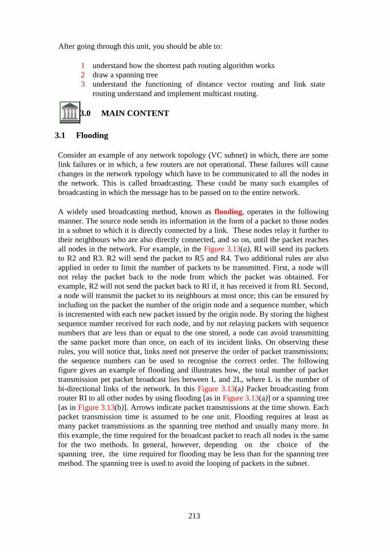
213


1 understand how the shortest path routing algorithm works

2 draw a spanning tree

3 understand the functioning of distance vector routing and link state

routing understand and implement multicast routing.

3.0 MAIN CONTENT

3.1 Flooding

Consider an example of any network topology (VC subnet) in which, there are some

link failures or in which, a few routers are not operational. These failures will cause

changes in the network typology which have to be communicated to all the nodes in

the network. This is called broadcasting. These could be many such examples of

broadcasting in which the message has to be passed on to the entire network.

A widely used broadcasting method, known as flooding, operates in the following

manner. The source node sends its information in the form of a packet to those nodes

in a subnet to which it is directly connected by a link. These nodes relay it further to

their neighbours who are also directly connected, and so on, until the packet reaches

all nodes in the network. For example, in the Figure 3.13(a), RI will send its packets

to R2 and R3. R2 will send the packet to R5 and R4. Two additional rules are also

applied in order to limit the number of packets to be transmitted. First, a node will

not relay the packet back to the node from which the packet was obtained. For

example, R2 will not send the packet back to Rl if, it has received it from RI. Second,

a node will transmit the packet to its neighbours at most once; this can be ensured by

including on the packet the number of the origin node and a sequence number, which

is incremented with each new packet issued by the origin node. By storing the highest

sequence number received for each node, and by not relaying packets with sequence

numbers that are less than or equal to the one stored, a node can avoid transmitting

the same packet more than once, on each of its incident links. On observing these

rules, you will notice that, links need not preserve the order of packet transmissions;

the sequence numbers can be used to recognise the correct order. The following

figure gives an example of flooding and illustrates how, the total number of packet

transmission pet packet broadcast lies between L and 2L, where L is the number of

bi-directional links of the network. In this Figure 3.13(a) Packet broadcasting from

router RI to all other nodes by using flooding [as in Figure 3.13(a)] or a spanning tree

[as in Figure 3.13(b)]. Arrows indicate packet transmissions at the time shown. Each

packet transmission time is assumed to be one unit. Flooding requires at least as

many packet transmissions as the spanning tree method and usually many more. In

this example, the time required for the broadcast packet to reach all nodes is the same

for the two methods. In general, however, depending on the choice of the

spanning tree, the time required for flooding may be less than for the spanning tree

method. The spanning tree is used to avoid the looping of packets in the subnet.

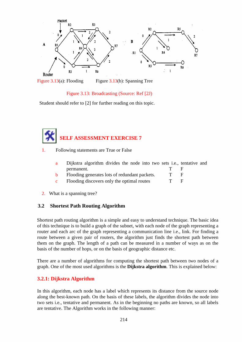
214

Figure 3.13(a): Flooding Figure 3.13(b): Spanning Tree

Figure 3.13: Broadcasting (Source: Ref [2J)

Student should refer to [2] for further reading on this topic.


1. Following statements are True or False

a Dijkstra algorithm divides the node into two sets i.e., tentative and

permanent. T F

b Flooding generates lots of redundant packets. T F

c Flooding discovers only the optimal routes T F

2. What is a spanning tree?

3.2

Shortest Path Routing Algorithm

Shortest path routing algorithm is a simple and easy to understand technique. The basic idea

of this technique is to build a graph of the subnet, with each node of the graph representing a

router and each arc of the graph representing a communication line i.e., link. For finding a

route between a given pair of routers, the algorithm just finds the shortest path between

them on the graph. The length of a path can be measured in a number of ways as on the

basis of the number of hops, or on the basis of geographic distance etc.

There are a number of algorithms for computing the shortest path between two nodes of a

graph. One of the most used algorithms is the Dijkstra algorithm. This is explained below:

3.2.1: Dijkstra Algorithm

In this algorithm, each node has a label which represents its distance from the source node

along the best-known path. On the basis of these labels, the algorithm divides the node into

two sets i.e., tentative and permanent. As in the beginning no paths are known, so all labels

are tentative. The Algorithm works in the following manner:

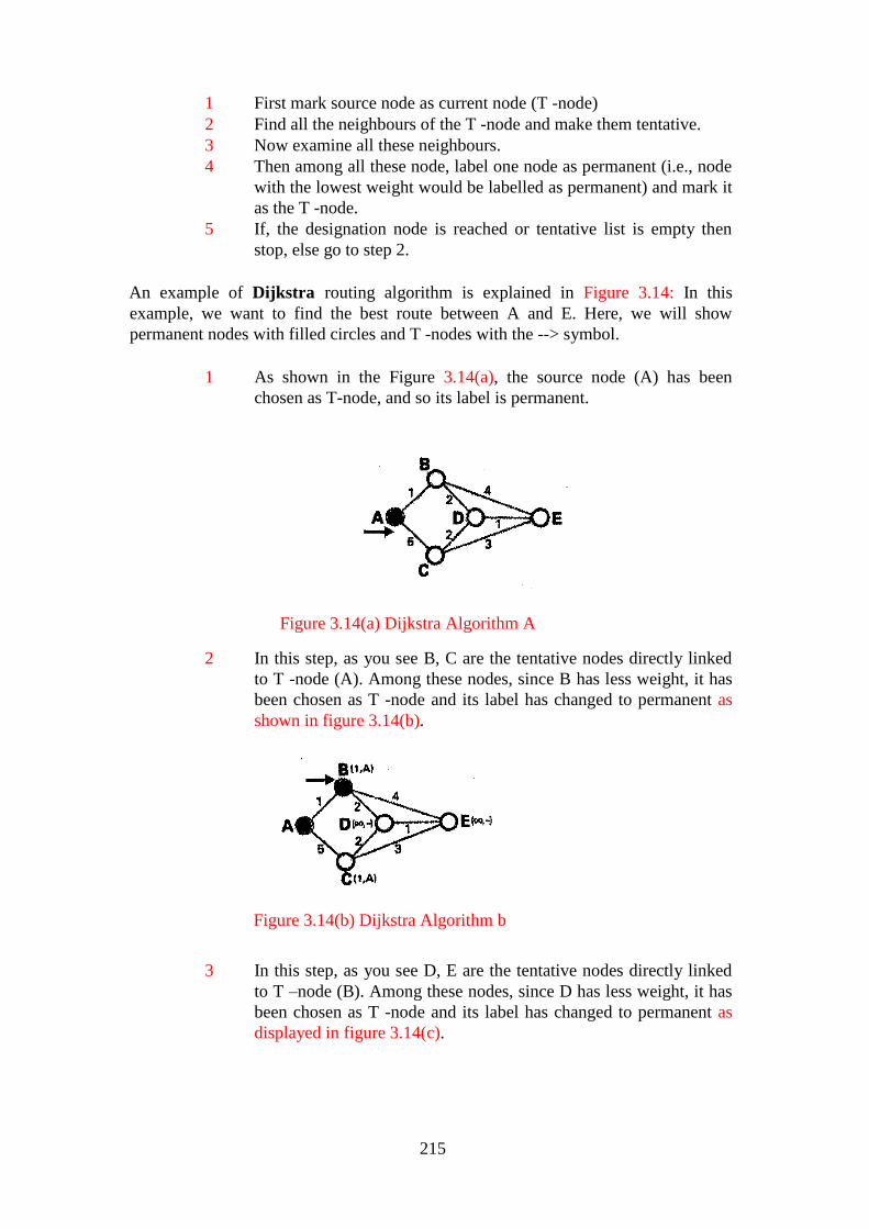
215

1 First mark source node as current node (T -node)

2 Find all the neighbours of the T -node and make them tentative.

3 Now examine all these neighbours.

4 Then among all these node, label one node as permanent (i.e., node

with the lowest weight would be labelled as permanent) and mark it

as the T -node.

5 If, the designation node is reached or tentative list is empty then

stop, else go to step 2.

An example of Dijkstra routing algorithm is explained in Figure 3.14: In this

example, we want to find the best route between A and E. Here, we will show

permanent nodes with filled circles and T -nodes with the --> symbol.

1 As shown in the Figure 3.14(a), the source node (A) has been

chosen as T-node, and so its label is permanent.

Figure 3.14(a) Dijkstra Algorithm A

2 In this step, as you see B, C are the tentative nodes directly linked

to T -node (A). Among these nodes, since B has less weight, it has

been chosen as T -node and its label has changed to permanent as

shown in figure 3.14(b).

Figure 3.14(b) Dijkstra Algorithm b

3 In this step, as you see D, E are the tentative nodes directly linked

to T –node (B). Among these nodes, since D has less weight, it has


displayed in figure 3.14(c).

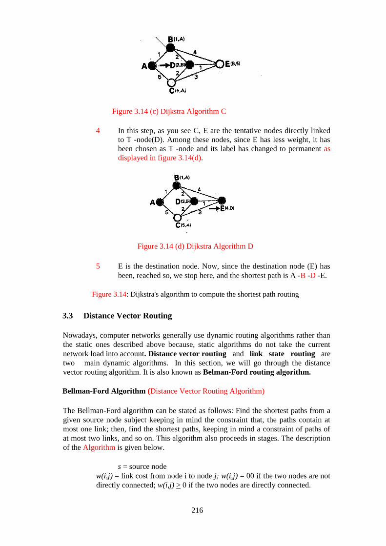
216

Figure 3.14 (c) Dijkstra Algorithm C

4 In this step, as you see C, E are the tentative nodes directly linked

to T -node(D). Among these nodes, since E has less weight, it has


displayed in figure 3.14(d).

Figure 3.14 (d) Dijkstra Algorithm D

5 E is the destination node. Now, since the destination node (E) has

been, reached so, we stop here, and the shortest path is A -B -D -E.

Figure 3.14: Dijkstra's algorithm to compute the shortest path routing

3.3 Distance Vector Routing

Nowadays, computer networks generally use dynamic routing algorithms rather than

the static ones described above because, static algorithms do not take the current

network load into account. Distance vector routing and link state routing are

two main dynamic algorithms. In this section, we will go through the distance

vector routing algorithm. It is also known as Belman-Ford routing algorithm.

Bellman-Ford Algorithm (Distance Vector Routing Algorithm)

The Bellman-Ford algorithm can be stated as follows: Find the shortest paths from a

given source node subject keeping in mind the constraint that, the paths contain at

most one link; then, find the shortest paths, keeping in mind a constraint of paths of

at most two links, and so on. This algorithm also proceeds in stages. The description

of the Algorithm is given below.

s = source node

w(i,j) = link cost from node i to node j; w(i,j) = 00 if the two nodes are not

directly connected; w(i,j) > 0 if the two nodes are directly connected.

217

h = maximum number of links in a path at the current stage of the

algorithm

Lh(n) = cost of the least-cost path from node s to node n under the

constraint of no more than h links

1. [Initialization]

L0(n) = ∞, for all n≠ s

Lh(S) = 0, for all h

2. [Update]

For each successive h > 0:

For each n ≠s, compute

min

Lh+1(n) = [Lh (j) = w(j,n)]

j

Connect n with the predecessor node j that achieves the minimum, and eliminate any

connection of n with a different predecessor node formed during an earlier iteration.

The path from s to n terminates with the link from j to n as shown in figure 3.15.

For the iteration of step 2 with h = K, and for each destination node n, the algorithm

compares potential paths from s to n of length K + 1 with the path that existed at the

end of the previous iteration. If the previous, shorter path has less cost, then that path

is retained. Otherwise a new path with length K + 1 is defined from s to n; this path

consists of a path of length K from s to some node j, plus a direct hop from node j to

node n. In this case, the path from s to j that is used is the K-hop path for j defined in

the previous iteration.

Figure 3.16 shows the result of applying this algorithm to a public switched network,

using s = 1. At each step, the least-cost paths with a maximum number of links equal

to h are found. After the final iteration, the least- cost path to each node and the cost

of that path has been developed. The same procedure can be used with node 2 as the

source node, and so on. Students should apply Dijkstra's algorithm to this subnet and

observe that the result will eventually be the same.

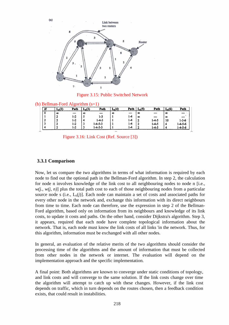
218

Figure 3.15: Public Switched Network

(b) Bellman-Ford Algorithm (s=1)

Figure 3.16: Link Cost (Ref. Source [3])

3.3.1 Comparison

Now, let us compare the two algorithms in terms of what information is required by each

node to find out the optional path in the Bellman-Ford algorithm. In step 2, the calculation

for node n involves knowledge of the link cost to all neighbouring nodes to node n [i.e.,

w(j., w(j, n)] plus the total path cost to each of those neighbouring nodes from a particular

source node s (i.e., Lh(j)]. Each node can maintain a set of costs and associated paths for

every other node in the network and, exchange this information with its direct neighbours

from time to time. Each node can therefore, use the expression in step 2 of the Bellman-

Ford algorithm, based only on information from its neighbours and knowledge of its link

costs, to update it costs and paths. On the other hand, consider Dijkstra's algorithm. Step 3,

it appears, required that each node have complete topological information about the

network. That is, each node must know the link costs of all links 'in the network. Thus, for

this algorithm, information must be exchanged with all other nodes.

In general, an evaluation of the relative merits of the two algorithms should consider the

processing time of the algorithms and the amount of information that must be collected

from other nodes in the network or internet. The evaluation will depend on the

implementation approach and the specific implementation.

A final point: Both algorithms are known to converge under static conditions of topology,

and link costs and will converge to the same solution. If the link costs change over time

the algorithm will attempt to catch up with these changes. However, if the link cost

depends on traffic, which in turn depends on the routes chosen, then a feedback condition

exists, that could result in instabilities.

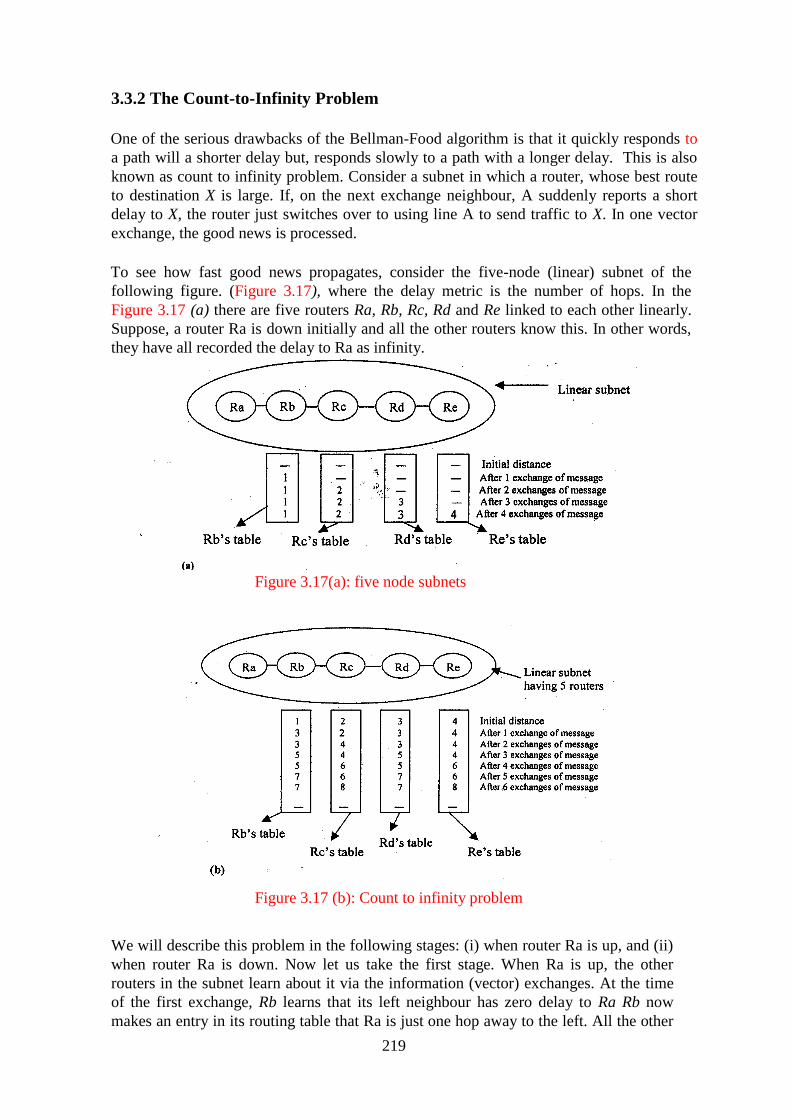
219

3.3.2 The Count-to-Infinity Problem

One of the serious drawbacks of the Bellman-Food algorithm is that it quickly responds to

a path will a shorter delay but, responds slowly to a path with a longer delay. This is also

known as count to infinity problem. Consider a subnet in which a router, whose best route

to destination X is large. If, on the next exchange neighbour, A suddenly reports a short

delay to X, the router just switches over to using line A to send traffic to X. In one vector

exchange, the good news is processed.

To see how fast good news propagates, consider the five-node (linear) subnet of the

following figure. (Figure 3.17), where the delay metric is the number of hops. In the

Figure 3.17 (a) there are five routers Ra, Rb, Rc, Rd and Re linked to each other linearly.

Suppose, a router Ra is down initially and all the other routers know this. In other words,

they have all recorded the delay to Ra as infinity.

Figure 3.17(a): five node subnets

Figure 3.17 (b): Count to infinity problem

We will describe this problem in the following stages: (i) when router Ra is up, and (ii)

when router Ra is down. Now let us take the first stage. When Ra is up, the other

routers in the subnet learn about it via the information (vector) exchanges. At the time

of the first exchange, Rb learns that its left neighbour has zero delay to Ra Rb now

makes an entry in its routing table that Ra is just one hop away to the left. All the other

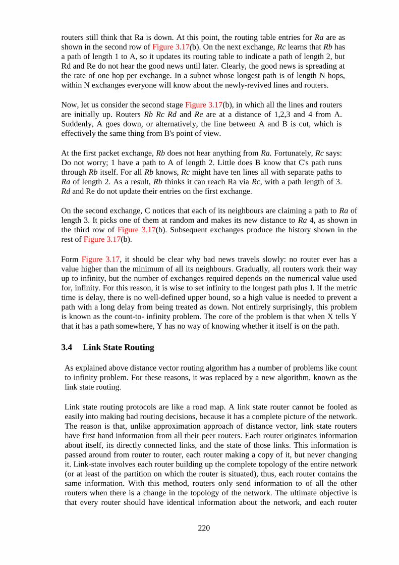
220

routers still think that Ra is down. At this point, the routing table entries for Ra are as

shown in the second row of Figure 3.17(b). On the next exchange, Rc learns that Rb has

a path of length 1 to A, so it updates its routing table to indicate a path of length 2, but

Rd and Re do not hear the good news until later. Clearly, the good news is spreading at

the rate of one hop per exchange. In a subnet whose longest path is of length N hops,

within N exchanges everyone will know about the newly-revived lines and routers.

Now, let us consider the second stage Figure 3.17(b), in which all the lines and routers

are initially up. Routers Rb Rc Rd and Re are at a distance of 1,2,3 and 4 from A.

Suddenly, A goes down, or alternatively, the line between A and B is cut, which is

effectively the same thing from B's point of view.

At the first packet exchange, Rb does not hear anything from Ra. Fortunately, Rc says:

Do not worry; 1 have a path to A of length 2. Little does B know that C's path runs

through Rb itself. For all Rb knows, Rc might have ten lines all with separate paths to

Ra of length 2. As a result, Rb thinks it can reach Ra via Rc, with a path length of 3.

Rd and Re do not update their entries on the first exchange.

On the second exchange, C notices that each of its neighbours are claiming a path to Ra of

length 3. It picks one of them at random and makes its new distance to Ra 4, as shown in

the third row of Figure 3.17(b). Subsequent exchanges produce the history shown in the

rest of Figure 3.17(b).

Form Figure 3.17, it should be clear why bad news travels slowly: no router ever has a

value higher than the minimum of all its neighbours. Gradually, all routers work their way

up to infinity, but the number of exchanges required depends on the numerical value used

for, infinity. For this reason, it is wise to set infinity to the longest path plus I. If the metric

time is delay, there is no well-defined upper bound, so a high value is needed to prevent a

path with a long delay from being treated as down. Not entirely surprisingly, this problem

is known as the count-to- infinity problem. The core of the problem is that when X tells Y

that it has a path somewhere, Y has no way of knowing whether it itself is on the path.

3.4 Link State Routing

As explained above distance vector routing algorithm has a number of problems like count

to infinity problem. For these reasons, it was replaced by a new algorithm, known as the

link state routing.

Link state routing protocols are like a road map. A link state router cannot be fooled as

easily into making bad routing decisions, because it has a complete picture of the network.

The reason is that, unlike approximation approach of distance vector, link state routers

have first hand information from all their peer routers. Each router originates information

about itself, its directly connected links, and the state of those links. This information is

passed around from router to router, each router making a copy of it, but never changing

it. Link-state involves each router building up the complete topology of the entire network

(or at least of the partition on which the router is situated), thus, each router contains the

same information. With this method, routers only send information to of all the other

routers when there is a change in the topology of the network. The ultimate objective is

that every router should have identical information about the network, and each router

221

should be able to calculate its own best path independently. Independently calculate its

own best paths.

In contrast to the distance-vector routing protocol, which works by sharing its knowledge

of the entire network with its neighbours, link- state routing works by having the routers

inform every router in the network about its nearest neighbours. The entire routing table is

not distributed any router but, the part of the table containing its neighbours is:

Link-state is also known as shortest path first.

Link State Packet

When a router floods the network with information about its neighbourhood, it is said to be

advertising. The basis of this advertising is a short packet called a link state packet (LSP).

An LSP usually contains four fields: the ID of the advertiser, the ID of the destination

network, the cost, and the ID of the neighbour router. The structure of a LSP is shown in

Figure 3.18.

Figure 3.18: Link State Packet (LSP)

How Link State Routing Operates

The idea behind link state routing is simple and can be stated in five parts as

suggested by Tanenbaum [Ref. I]. Each router must do the following:

1 Neighbour discovery

The Router has to discover its neighbours and learn their network addresses. As a

router is booted, its first task is to learn who its neighbours are.

The Router does this by sending a special HELLO packet on each point- to-point

line. The router on the other end is expected to send a reply disclosing its identity.

These names must be globally unique. If two or more routers are connected by a

LAN, the situation becomes slightly more complicated one way of modelling the

LAN is to consider it as a node itself. Please see reference [I] for further explanation

through a diagram.

2 Measure delay

Another job that a router needs to perform is to measure the delay or cost to each of

its neighbours. The most common way to determine this delay is to send over the line

a special ECHO packet that the other side is required to send back immediately. By

measuring the round-trip time and dividing it by two, the sending router can get a

reasonable estimate of the delay. For even better results, the test can be conducted

several times and the average used.

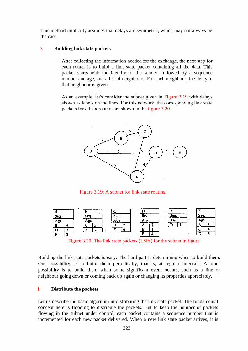
222

This method implicitly assumes that delays are symmetric, which may not always be

the case.

3 Building link state packets

After collecting the information needed for the exchange, the next step for

each router is to build a link state packet containing all the data. This

packet starts with the identity of the sender, followed by a sequence

number and age, and a list of neighbours. For each neighbour, the delay to

that neighbour is given.

As an example, let's consider the subnet given in Figure 3.19 with delays

shown as labels on the lines. For this network, the corresponding link state

packets for all six routers are shown in the figure 3.20.

Figure 3.19: A subnet for link state routing

Figure 3.20: The link state packets (LSPs) for the subnet in figure

Building the link state packets is easy. The hard part is determining when to build them.

One possibility, is to build them periodically, that is, at regular intervals. Another

possibility is to build them when some significant event occurs, such as a line or

neighbour going down or coming back up again or changing its properties appreciably.

1 Distribute the packets

Let us describe the basic algorithm in distributing the link state packet. The fundamental

concept here is flooding to distribute the packets. But to keep the number of packets

flowing in the subnet under control, each packet contains a sequence number that is

incremented for each new packet delivered. When a new link state packet arrives, it is

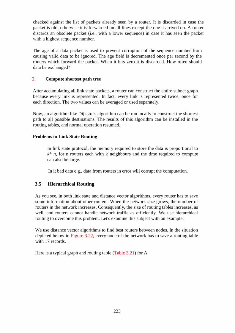
223

checked against the list of packets already seen by a router. It is discarded in case the

packet is old; otherwise it is forwarded on all lines except the one it arrived on. A router

discards an obsolete packet (i.e., with a lower sequence) in case it has seen the packet

with a highest sequence number.

The age of a data packet is used to prevent corruption of the sequence number from

causing valid data to be ignored. The age field is decremented once per second by the

routers which forward the packet. When it hits zero it is discarded. How often should

data be exchanged?

2 Compute shortest path tree

After accumulating all link state packets, a router can construct the entire subnet graph

because every link is represented. In fact, every link is represented twice, once for

each direction. The two values can be averaged or used separately.

Now, an algorithm like Dijkstra's algorithm can be run locally to construct the shortest

path to all possible destinations. The results of this algorithm can be installed in the

routing tables, and normal operation resumed.

Problems in Link State Routing

In link state protocol, the memory required to store the data is proportional to

k* n, for n routers each with k neighbours and the time required to compute

can also be large.

In it bad data e.g., data from routers in error will corrupt the computation.

3.5 Hierarchical Routing

As you see, in both link state and distance vector algorithms, every router has to save

some information about other routers. When the network size grows, the number of

routers in the network increases. Consequently, the size of routing tables increases, as

well, and routers cannot handle network traffic as efficiently. We use hierarchical

routing to overcome this problem. Let's examine this subject with an example:

We use distance vector algorithms to find best routers between nodes. In the situation

depicted below in Figure 3.22, every node of the network has to save a routing table

with 17 records.

Here is a typical graph and routing table (Table 3.21) for A:

224

Figure 3.21: typical graph and routing table

Figure 3.22: Network graph

In hierarchical routing, routers are classified in groups known as regions (Figure 3.23).

Each router has only the information about the routers in its own region and has no

information about routers in other regions. So, routers just save one record in their table

for every other region. In this example, we have classified our network into five regions

as shown Figure 3.24.

Figure 3.23: A's Routing table for Hierarchical! Routing

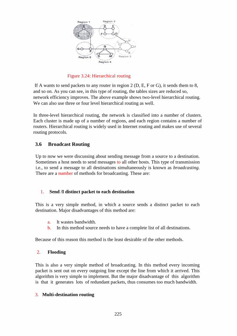
225

Figure 3.24: Hierarchical routing

If A wants to send packets to any router in region 2 (D, E, F or G), it sends them to 8,

and so on. As you can see, in this type of routing, the tables sizes are reduced so,

network efficiency improves. The above example shows two-level hierarchical routing.

We can also use three or four level hierarchical routing as well.

In three-level hierarchical routing, the network is classified into a number of clusters.

Each cluster is made up of a number of regions, and each region contains a number of

routers. Hierarchical routing is widely used in Internet routing and makes use of several

routing protocols.

3.6 Broadcast Routing

Up to now we were discussing about sending message from a source to a destination.

Sometimes a host needs to send messages to all other hosts. This type of transmission

i.e., to send a message to all destinations simultaneously is known as broadcasting.

There are a number of methods for broadcasting. These are:

1. Send /I distinct packet to each destination

This is a very simple method, in which a source sends a distinct packet to each

destination. Major disadvantages of this method are:

a. It wastes bandwidth.

b. In this method source needs to have a complete list of all destinations.

Because of this reason this method is the least desirable of the other methods.

2. Flooding

This is also a very simple method of broadcasting. In this method every incoming

packet is sent out on every outgoing line except the line from which it arrived. This

algorithm is very simple to implement. But the major disadvantage of this algorithm

is that it generates lots of redundant packets, thus consumes too much bandwidth.

3. Multi-destination routing

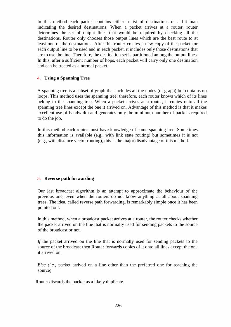
226

In this method each packet contains either a list of destinations or a bit map

indicating the desired destinations. When a packet arrives at a router, router

determines the set of output lines that would be required by checking all the

destinations. Router only chooses those output lines which are the best route to at

least one of the destinations. After this router creates a new copy of the packet for

each output line to be used and in each packet, it includes only those destinations that

are to use the line. Therefore, the destination set is partitioned among the output lines.

In this, after a sufficient number of hops, each packet will carry only one destination

and can be treated as a normal packet.

4. Using a Spanning Tree

A spanning tree is a subset of graph that includes all the nodes (of graph) but contains no

loops. This method uses the spanning tree; therefore, each router knows which of its lines

belong to the spanning tree. When a packet arrives at a router, it copies onto all the

spanning tree lines except the one it arrived on. Advantage of this method is that it makes

excellent use of bandwidth and generates only the minimum number of packets required

to do the job.

In this method each router must have knowledge of some spanning tree. Sometimes

this information is available (e.g., with link state routing) but sometimes it is not

(e.g., with distance vector routing), this is the major disadvantage of this method.

5. Reverse path forwarding

Our last broadcast algorithm is an attempt to approximate the behaviour of the

previous one, even when the routers do not know anything at all about spanning

trees. The idea, called reverse path forwarding, is remarkably simple once it has been

pointed out.

In this method, when a broadcast packet arrives at a router, the router checks whether

the packet arrived on the line that is normally used for sending packets to the source

of the broadcast or not.

If the packet arrived on the line that is normally used for sending packets to the

source of the broadcast then Router forwards copies of it onto all lines except the one

it arrived on.

Else (i.e., packet arrived on a line other than the preferred one for reaching the

source)

Router discards the packet as a likely duplicate.

227

3.7 Multicast Routing

In many cases, you need to send same data to multiple clients at the same time. In

this case, if, we use unicasting then the server will connect to each of its clients again

and again, but each time it will send an identical data stream to each client. This is a

waste of both server and network capacity. If, we use broadcasting in this case, it

would be inefficient because sometimes receivers are not interested in the message

but they receive it nonetheless, or sometimes they are interested but are not supposed

to see the message.

In such cases i.e., for sending a message to a group of users (clients), we use another

technique known as multicasting. The routing algorithm used for multicasting, is

called multicast routing.

Group management is the heart of multicasting. for group management, we require

some methods to create and destroy a group and to allow processes to join and leave

a group. When a router joins a group, it informs its host of this fact. For routing,

routers mainly want to know which of their hosts belong to which group. For this,

either the host must inform their router about changes in the group membership, or

routers must query their hosts periodically. On receiving this information, routers

tell their neighbours, so the information propagated through the subnet.

Now, we will learn the working of multicasting through an example. In our example

(as shown in Figure 3.25), we have taken a network containing two groups i.e.,

group 1 and 2. Here, some routers are attached to hosts that belong to only one of

these groups and some routers are attached to hosts that belong to both of these

groups.

Figure 3.25: Network containing two groups i.e., 1 and 2

To do multicast routing, first, each router computes a spanning tree covering all other

routers. For example, Figure 3.26 shows spanning tree for the leftmost router.

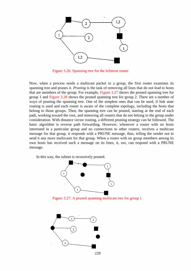
228

Figure 3.26: Spanning tree for the leftmost router

Now, when a process sends a multicast packet to a group, the first router examines its

spanning tree and prunes it. Pruning is the task of removing all lines that do not lead to hosts

that are members of the group. For example, Figure 3.27 shows the pruned spanning tree for

group 1 and Figure 3.28 shows the pruned spanning tree for group 2. There are a number of

ways of pruning the spanning tree. One of the simplest ones that can be used, if link state

routing is used and each router is aware of the complete topology, including the hosts that

belong to those groups. Then, the spanning tree can be pruned, starting at the end of each

path, working toward the root, and removing all routers that do not belong to the group under

consideration. With distance vector routing, a different pruning strategy can be followed. The

basic algorithm is reverse path forwarding. However, whenever a router with no hosts

interested in a particular group and no connections to other routers, receives a multicast

message for that group, it responds with a PRUNE message, thus, telling the sender not to

send it any more multicasts for that group. When a router with no group members among its

own hosts has received such a message on its lines, it, too, can respond with a PRUNE

message.

In this way, the subnet is recursively pruned.

Figure 3.27: A pruned spanning multicast tree for group 1

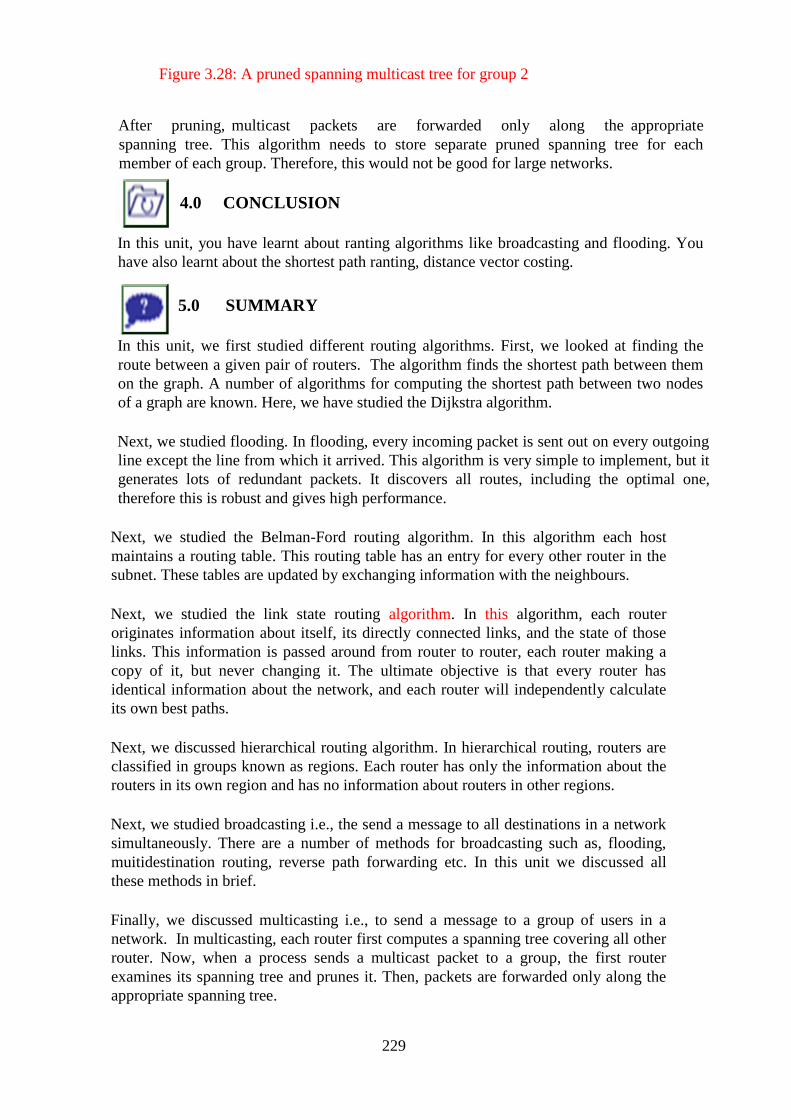
229

Figure 3.28: A pruned spanning multicast tree for group 2

After pruning, multicast packets are forwarded only along the appropriate

spanning tree. This algorithm needs to store separate pruned spanning tree for each

member of each group. Therefore, this would not be good for large networks.

4.0 CONCLUSION

In this unit, you have learnt about ranting algorithms like broadcasting and flooding. You

have also learnt about the shortest path ranting, distance vector costing.

5.0 SUMMARY

In this unit, we first studied different routing algorithms. First, we looked at finding the

route between a given pair of routers. The algorithm finds the shortest path between them

on the graph. A number of algorithms for computing the shortest path between two nodes

of a graph are known. Here, we have studied the Dijkstra algorithm.

Next, we studied flooding. In flooding, every incoming packet is sent out on every outgoing

line except the line from which it arrived. This algorithm is very simple to implement, but it

generates lots of redundant packets. It discovers all routes, including the optimal one,

therefore this is robust and gives high performance.

Next, we studied the Belman-Ford routing algorithm. In this algorithm each host

maintains a routing table. This routing table has an entry for every other router in the

subnet. These tables are updated by exchanging information with the neighbours.

Next, we studied the link state routing algorithm. In this algorithm, each router

originates information about itself, its directly connected links, and the state of those

links. This information is passed around from router to router, each router making a

copy of it, but never changing it. The ultimate objective is that every router has

identical information about the network, and each router will independently calculate

its own best paths.

Next, we discussed hierarchical routing algorithm. In hierarchical routing, routers are

classified in groups known as regions. Each router has only the information about the

routers in its own region and has no information about routers in other regions.

Next, we studied broadcasting i.e., the send a message to all destinations in a network

simultaneously. There are a number of methods for broadcasting such as, flooding,

muitidestination routing, reverse path forwarding etc. In this unit we discussed all

these methods in brief.

Finally, we discussed multicasting i.e., to send a message to a group of users in a

network. In multicasting, each router first computes a spanning tree covering all other

router. Now, when a process sends a multicast packet to a group, the first router

examines its spanning tree and prunes it. Then, packets are forwarded only along the

appropriate spanning tree.

230


1. Which of the following statements are True or False?

(i) Distance vector routing is a static routing algorithm. True or False

(ii) Dijkstra's algorithms can be run locally in link state routing to construct the

shortest path. True False.

2. Answer the following questions briefly.

(i) What are the problems with distance vector routing algorithm?

(ii) What is LSP?

3. Which of the following statements are True or False?

(i) In hierarchical routing, each router has no information about routers in other

regions. True or False

(ii) A spanning tree is a subset of a graph that includes some of the nodes of that

graph. True or False

(iii) Sending a message to a group of users in a network is known as broadcasting.

True or False

4. Answer the following questions in brief.

(i) Explain reverse path forwarding in brief.

(ii) What is Pruning?


S. Tanenbaum, (2011). Computer Network, 4‖' edition, Prentice Hall of India, New

Delhi.

Dmitri Berteskas and Robert Galleger, (1997). Data Network. Second edition,

Prentice Hall of India, New Delhi.

William Stalling, Data and Computer Communication. Pearson Education,

2bdEdition, Delhi, 2003.


Question 1

Which of the following statements are True or False?

(i) Distance vector routing is a static routing algorithm. T 0 F 0

False

231

(ii) Dijkstra's algorithms can he run locally in link state routing to

construct the shortest path. TO F 0

True

Question 2

Answer the following questions briefly.

(i) What are the problems with distance vector routing (DVR) algorithm?

The problem with DVR is routing loop which causes count to infinity. This takes

place when any interface goes down or two-routers send updates at the same time

(ii) What is LSP?

Link State Packet is a packet of information generated by a network router in a link

state routing protocol that lists the router's neighbours. Link state packet can also be

further defined as special datagrams that determine the names of and the cost or

distance to any neighbouring routers and associated networks.

Question 3

Which of the following statements are True or False?

(i) In hierarchical routing, each router has no information about routers in other

regions. TO FO

True

(ii) A spanning tree is a subset of a graph that includes some of the nodes of that

graph. TO FO

True

(iii) Sending a message to a group of users in a network is known as broadcasting. TO

F 0

False

Question 4

Answer the following questions in brief.

(i) Explain reverse path forwarding in brief.

Reverse path forwarding (RPF) is a technique in multicast routing that assists to guide

against IP address spoofing and other kinds of problems. This technique is known

as reverse path forwarding since in place of perceiving forward, the technique

managing packet path will view back to check the reverse path of the packet

(ii) What is Pruning?

The path pruning algorithm finds routing shortcuts by exploiting the channel

listening capability of wireless nodes, and is able to reduce a large number of hops

with the help of a little state information passively maintained by a subset of nodes on

the route.

232

9.0 ANSWERS TO SELF-ASSESSMENT 7

Question 1

Check whether the following statements are True or False

(i) Dijkstra algorithm divides the node into two sets i.e., tentative and permanent. T F

Answer: False

(ii) Flooding generates lots of redundant packets. T F

Answer: True

(iii) Flooding discovers only the optimal routes T F

Answer: False

Question 2

What is a spanning tree?

Solution

Taking for example, an extended LAN as being substituted by a graph that probably

has loops (cycles), then a spanning tree is a subgraph of this graph that covers (spans)

all the vertices but contains no cycles. That is, a spanning tree retains all of the

vertices of the original graph but throws out some of the edges.

UNIT 3 CONGESTION CONTROL IN PUBLIC SWITCHED

NETWORK

CONTENTS

1.0 Introduction

2.0 Objectives

3.0 Main Content

3.1 Reasons for Congestion in the network

3.2 Congestion Control vs. Flow Control

3.3 Congestion Prevention Mechanism

3.4 General Principles of Congestion Control

3.5 Open Loop Control

3.5.1 Admission Control

3.5.2 Traffic Policing and its Implementation

3.5.3 Traffic Shaping and its Implementation


Traffic Shaper

3.6 Congestion Control in Packet-switched Networks

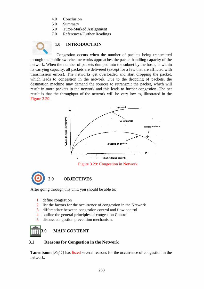
233

4.0 Conclusion

5.0 Summary



1.0 INTRODUCTION

Congestion occurs when the number of packets being transmitted

through the public switched networks approaches the packet handling capacity of the

network. When the number of packets dumped into the subnet by the hosts, is within

its carrying capacity, all packets are delivered (except for a few that are afflicted with

transmission errors). The networks get overloaded and start dropping the packet,

which leads to congestion in the network. Due to the dropping of packets, the

destination machine may demand the sources to retransmit the packet, which will

result in more packets in the network and this leads to further congestion. The net

result is that the throughput of the network will be very low as, illustrated in the

Figure 3.29.

Figure 3.29: Congestion in Network

2.0 OBJECTIVES


1 define congestion

2 list the factors for the occurrence of congestion in the Network

3 differentiate between congestion control and flow control

4 outline the general principles of congestion Control

5 discuss congestion prevention mechanism.

3.0 MAIN CONTENT

3.1 Reasons for Congestion in the Network

Tanenbaum [Ref 1] has listed several reasons for the occurrence of congestion in the

network:

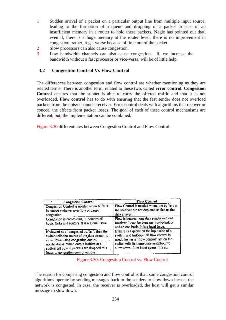
234

1 Sudden arrival of a packet on a particular output line from multiple input source,

leading to the formation of a queue and dropping of a packet in case of an

insufficient memory in a router to hold these packets. Nagle has pointed out that,

even if, there is a huge memory at the router level, there is no improvement in

congestion, rather, it get worse because of time out of the packet.

2 Slow processors can also cause congestion.

3 Low bandwidth channels can also cause congestion. If, we increase the

bandwidth without a fast processor or vice-versa, will be of little help.

3.2 Congestion Control Vs Flow Control

The differences between congestion and flow control are whether mentioning as they are

related terms. There is another term, related to these two, called error control. Congestion

Control ensures that the subnet is able to carry the offered traffic and that it is not

overloaded. Flow control has to do with ensuring that the fast sender does not overload

packets from the noisy channels receiver. Error control deals with algorithms that recover or

conceal the effects from packet losses. The goal of each of these control mechanisms are

different, but, the implementation can be combined.

Figure 3.30 differentiates between Congestion Control and Flow Control:

Figure 3.30: Congestion Control vs. Flow Control

The reason for comparing congestion and flow control is that, some congestion control

algorithms operate by sending messages back to the senders to slow down incase, the

network is congested. In case, the receiver is overloaded, the host will get a similar

message to slow down.

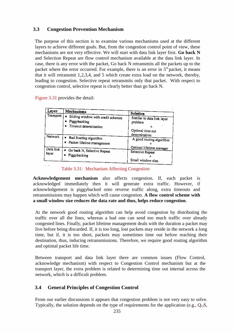
235

3.3 Congestion Prevention Mechanism

The purpose of this section is to examine various mechanisms used at the different

layers to achieve different goals. But, from the congestion control point of view, these

mechanisms are not very effective. We will start with data link layer first. Go back N

and Selection Repeat are flow control mechanism available at the data link layer. In

case, there is any error with the packet, Go back N retransmits all the packets up to the

packet where the error occurred. For example, there is an error in 5th packet, it means

that it will retransmit 1,2,3,4, and 5 which create extra load on the network, thereby,

leading to congestion. Selective repeat retransmits only that packet. With respect to

congestion control, selective repeat is clearly better than go back N.

Figure 3.31 provides the detail:

Table 3.31: Mechanism Affecting Congestion

Acknowledgement mechanism also affects congestion. If, each packet is

acknowledged immediately then it will generate extra traffic. However, if

acknowledgement is piggybacked onto reverse traffic along, extra timeouts and

retransmissions may happen which will cause congestion. A flow control scheme with

a small window size reduces the data rate and thus, helps reduce congestion.

At the network good routing algorithm can help avoid congestion by distributing the

traffic over all the lines, whereas a bad one can send too much traffic over already

congested lines. Finally, packet lifetime management deals with the duration a packet may

live before being discarded. If, it is too long, lost packets may reside in the network a long

time, but if, it is too short, packets may sometimes time out before reaching their

destination, thus, inducing retransmissions. Therefore, we require good routing algorithm

and optimal packet life time.

Between transport and data link layer there are common issues (Flow Control,

acknowledge mechanism) with respect to Congestion Control mechanism but at the

transport layer, the extra problem is related to determining time out internal across the

network, which is a difficult problem.

3.4 General Principles of Congestion Control

From our earlier discussions it appears that congestion problem is not very easy to solve.

Typically, the solution depends on the type of requirements for the application (e.g., QOS,

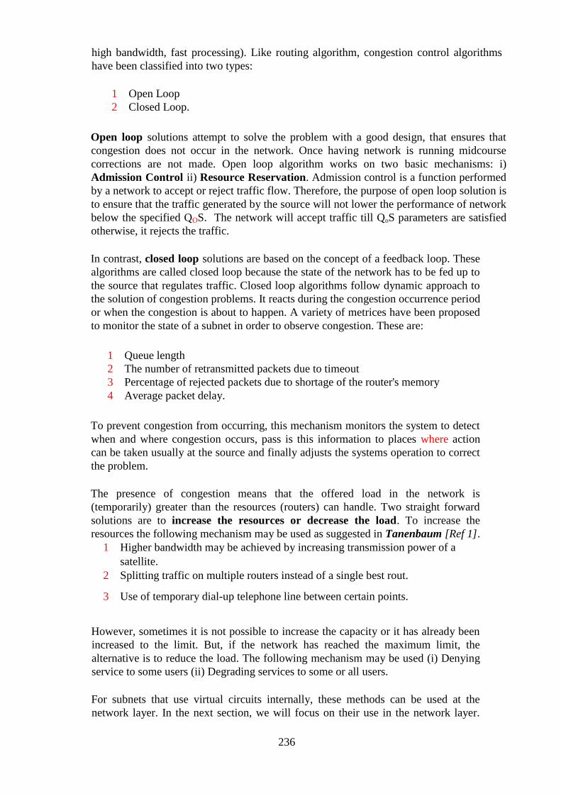
236

high bandwidth, fast processing). Like routing algorithm, congestion control algorithms

have been classified into two types:

1 Open Loop

2 Closed Loop.

Open loop solutions attempt to solve the problem with a good design, that ensures that

congestion does not occur in the network. Once having network is running midcourse

corrections are not made. Open loop algorithm works on two basic mechanisms: i)

Admission Control ii) Resource Reservation. Admission control is a function performed

by a network to accept or reject traffic flow. Therefore, the purpose of open loop solution is

to ensure that the traffic generated by the source will not lower the performance of network

below the specified QOS. The network will accept traffic till QoS parameters are satisfied

otherwise, it rejects the traffic.

In contrast, closed loop solutions are based on the concept of a feedback loop. These

algorithms are called closed loop because the state of the network has to be fed up to

the source that regulates traffic. Closed loop algorithms follow dynamic approach to

the solution of congestion problems. It reacts during the congestion occurrence period

or when the congestion is about to happen. A variety of metrices have been proposed

to monitor the state of a subnet in order to observe congestion. These are:

1 Queue length

2 The number of retransmitted packets due to timeout

3 Percentage of rejected packets due to shortage of the router's memory

4 Average packet delay.

To prevent congestion from occurring, this mechanism monitors the system to detect

when and where congestion occurs, pass is this information to places where action

can be taken usually at the source and finally adjusts the systems operation to correct

the problem.

The presence of congestion means that the offered load in the network is

(temporarily) greater than the resources (routers) can handle. Two straight forward

solutions are to increase the resources or decrease the load. To increase the

resources the following mechanism may be used as suggested in Tanenbaum [Ref 1].

1 Higher bandwidth may be achieved by increasing transmission power of a

satellite.

2 Splitting traffic on multiple routers instead of a single best rout.

3 Use of temporary dial-up telephone line between certain points.

However, sometimes it is not possible to increase the capacity or it has already been

increased to the limit. But, if the network has reached the maximum limit, the

alternative is to reduce the load. The following mechanism may be used (i) Denying

service to some users (ii) Degrading services to some or all users.

For subnets that use virtual circuits internally, these methods can be used at the

network layer. In the next section, we will focus on their use in the network layer.

237

We will also discuss the open loop control mechanism in detail. The closed loop

mechanism will be discussed in Block 4 Unit 2 as a part of TCP Protocol.

3.5 Open Loop Control

As discussed earlier, Open Loop Control algorithm prevent the occurrence of

Congestion occurrence rather than dealing with it after it has occurred. It does not

rely on feedback information to regulate the traffic. Thus, this technique is based on

the assumption that once the packets are accepted from a particular source, the

network will not get overloaded. In this section, we will examine several such

techniques and its implementation. Learners are requested to Leon Garcia's book

[Ref 2].

3.5.1 Admission Control

This is a widely used technique in virtual circuit network. The technique is very

simple and straight forward. Once congestion has occurred, no more virtual circuits

are to be set up. This is similar to a telephone system in which there is no dial tone in

case the source gets overloaded. When a source wants to establish a connection,

admission control mechanism examines QoS parameters of the connections initiated

by the source. If it is OK, the connection (YC) is established otherwise, it is rejected.

In order to initiate a connection setup, a source specifies its traffic flow indicating a

set of parameters called traffic descriptor, which includes peak rate, average rate,

and maximum traffic burst size. (Maximum length of time the traffic is generated at

the peak rate) and so on. Based on the characteristic of traffic flow, admission control

mechanism reserves the bandwidth (which usually lies between peak rate and

average rate).

3.5.2 Traffic Policing and its Implementation

Leon Garcia [Ref2] has defined traffic policing as tbe process of monitoring and

enforcing the traffic flow of packets during the connection period. The network may

drop or mark the packet as noncompliant and give low priority to traffic in case, it

does not obey the agreed upon parameters values during the initial connection setup

phase. Most implementations of traffic policing is done through the Leaky Bucket

algorithm. In this algorithm the bucket is considered as a network and traffic flow is

considered as water being poured into a bucket. The following assumptions are made:

1 The bucket has certain depth to hold water just like a network can accept a

certain number of packets.

2 The bucket leaks at a certain rate (if there is water is the bucket) no matter at

what rate water enters the bucket. In terms of computer networks, it should be

interpreted as follows: No matter at what rate the packets arrive at the input

lines of a routers, routers in a subnet passes to its outgoing link at a fixed rate.

3 If the bucket does not overflow when the water is poured into the bucket, then

the bucket of water is said to be conforming. In terms of network, if the traffic

is within the agreed norms, all packets will be transferred.

238

4 The bucket will spill over if, it is full and if, additional water is poured into it,

if it gets more packets than it can handle, it will lead to congestion and then the

network due to which the additional packets will be lost.

If, we expect the traffic flow to be very smooth, then the bucket has to be of a shallow

type. In case, the flow is busty in nature, the bucket should be deeper. In summary,

what we want to observe is whether the outflow of packets corresponds to the arrival

rate of packets or not? Implementation of a leaky bucket is similar to queue data

structure implementation. When a packet arrives, if there is space left in the queue, it

gets appended to the queue otherwise, it gets rejected.

3.5.3 Traffic Shaping and its Implementation

Leon Garcia [Ref2] defined traffic shaping as the process of altering traffic flow to

another flow. It is mainly used for smoothening the traffic. Consider an example,

where a host is generating data at 30 kbps, which, it can transmit to the network in

several ways (as shown in the following Figure 3.32).

It can transmit at the rate of 100 kbps for 0.3 Second

It can transmit at the rate of75 kbps for 0.4 Second

Figure 3.32: Possible traffic patterns at the average rate of 30 Kbps

You can make observation from the Figure 3.32 that the Figure 3.32(a) shows the

smoothened pattern will create less stress on the network but the destination machine

may not want to wait for 1 Second to retrieve 30 kbps data at each period. Now, we

will look at its implementation. There are two mechanisms:

1 Leaky bucket traffic Shaper

2 Token bucket traffic Shapero

Leaky Bucket Traffic Shaper

It is a very simple mechanism in which data stored at the senders buffer, is passed on

at a constant interval to smoothen traffic as shown in Figure 3.33. The buffer is used

to store busty traffic. This size defines the maximum burst that can be

accommodated.

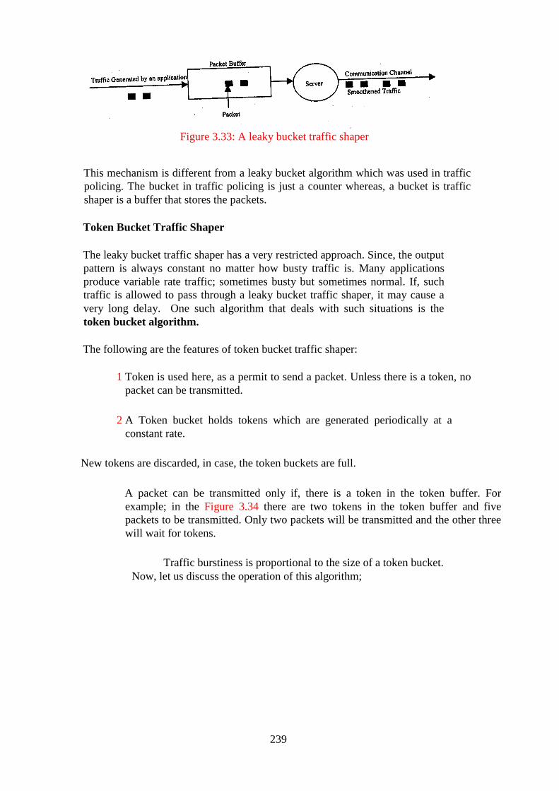
239

Figure 3.33: A leaky bucket traffic shaper

This mechanism is different from a leaky bucket algorithm which was used in traffic

policing. The bucket in traffic policing is just a counter whereas, a bucket is traffic

shaper is a buffer that stores the packets.

Token Bucket Traffic Shaper

The leaky bucket traffic shaper has a very restricted approach. Since, the output

pattern is always constant no matter how busty traffic is. Many applications

produce variable rate traffic; sometimes busty but sometimes normal. If, such

traffic is allowed to pass through a leaky bucket traffic shaper, it may cause a

very long delay. One such algorithm that deals with such situations is the

token bucket algorithm.

The following are the features of token bucket traffic shaper:

1 Token is used here, as a permit to send a packet. Unless there is a token, no

packet can be transmitted.

2 A Token bucket holds tokens which are generated periodically at a

constant rate.

New tokens are discarded, in case, the token buckets are full.

A packet can be transmitted only if, there is a token in the token buffer. For

example; in the Figure 3.34 there are two tokens in the token buffer and five

packets to be transmitted. Only two packets will be transmitted and the other three

will wait for tokens.

Traffic burstiness is proportional to the size of a token bucket.

Now, let us discuss the operation of this algorithm;

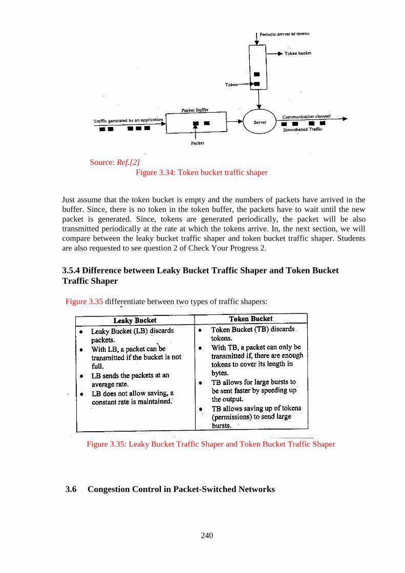
240

Source: Ref.[2]

Figure 3.34: Token bucket traffic shaper

Just assume that the token bucket is empty and the numbers of packets have arrived in the

buffer. Since, there is no token in the token buffer, the packets have to wait until the new

packet is generated. Since, tokens are generated periodically, the packet will be also

transmitted periodically at the rate at which the tokens arrive. In, the next section, we will

compare between the leaky bucket traffic shaper and token bucket traffic shaper. Students

are also requested to see question 2 of Check Your Progress 2.


Traffic Shaper

Figure 3.35 differentiate between two types of traffic shapers:

Figure 3.35: Leaky Bucket Traffic Shaper and Token Bucket Traffic Shaper

3.6 Congestion Control in Packet-Switched Networks

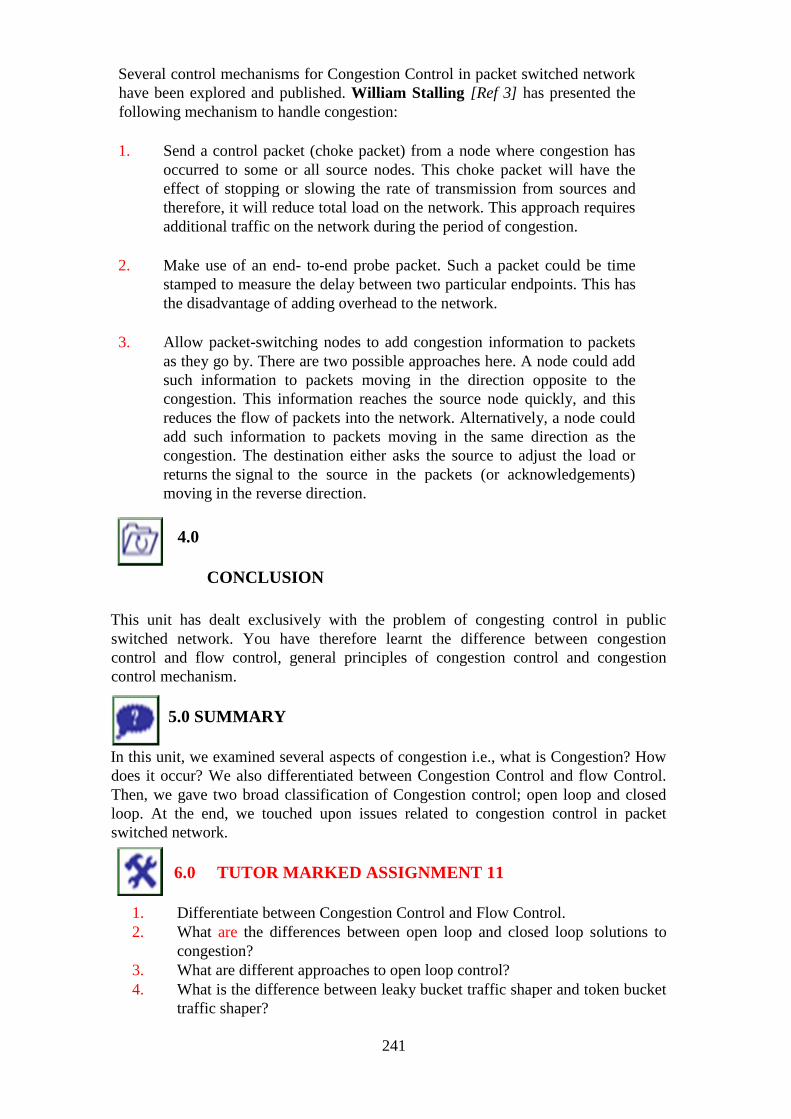
241

Several control mechanisms for Congestion Control in packet switched network

have been explored and published. William Stalling [Ref 3] has presented the

following mechanism to handle congestion:

1. Send a control packet (choke packet) from a node where congestion has

occurred to some or all source nodes. This choke packet will have the

effect of stopping or slowing the rate of transmission from sources and

therefore, it will reduce total load on the network. This approach requires

additional traffic on the network during the period of congestion.

2. Make use of an end- to-end probe packet. Such a packet could be time

stamped to measure the delay between two particular endpoints. This has

the disadvantage of adding overhead to the network.

3. Allow packet-switching nodes to add congestion information to packets

as they go by. There are two possible approaches here. A node could add

such information to packets moving in the direction opposite to the

congestion. This information reaches the source node quickly, and this

reduces the flow of packets into the network. Alternatively, a node could

add such information to packets moving in the same direction as the

congestion. The destination either asks the source to adjust the load or

returns the signal to the source in the packets (or acknowledgements)

moving in the reverse direction.

4.0

CONCLUSION

This unit has dealt exclusively with the problem of congesting control in public

switched network. You have therefore learnt the difference between congestion

control and flow control, general principles of congestion control and congestion

control mechanism.

5.0 SUMMARY

In this unit, we examined several aspects of congestion i.e., what is Congestion? How

does it occur? We also differentiated between Congestion Control and flow Control.

Then, we gave two broad classification of Congestion control; open loop and closed

loop. At the end, we touched upon issues related to congestion control in packet

switched network.


1. Differentiate between Congestion Control and Flow Control.

2. What are the differences between open loop and closed loop solutions to

congestion?

3. What are different approaches to open loop control?

4. What is the difference between leaky bucket traffic shaper and token bucket

traffic shaper?

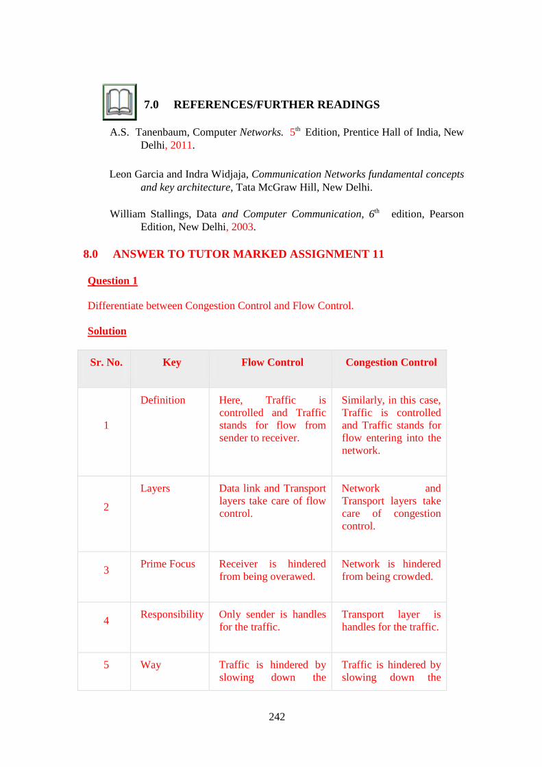
242


A.S. Tanenbaum, Computer Networks. 5th Edition, Prentice Hall of India, New

Delhi, 2011.

Leon Garcia and Indra Widjaja, Communication Networks fundamental concepts

and key architecture, Tata McGraw Hill, New Delhi.

William Stallings, Data and Computer Communication, 6th edition, Pearson

Edition, New Delhi, 2003.


Question 1

Differentiate between Congestion Control and Flow Control.

Solution

Sr. No. Key Flow Control Congestion Control

1

Definition Here, Traffic is

controlled and Traffic

stands for flow from

sender to receiver.

Similarly, in this case,

Traffic is controlled

and Traffic stands for

flow entering into the

network.

2

Layers Data link and Transport

layers take care of flow

control.

Network and

Transport layers take

care of congestion

control.

3 Prime Focus Receiver is hindered

from being overawed.

Network is hindered

from being crowded.

4 Responsibility Only sender is handles

for the traffic.

Transport layer is

handles for the traffic.

5 Way Traffic is hindered by

slowing down the

Traffic is hindered by

slowing down the

243

Sr. No. Key Flow Control Congestion Control

sender. transport layer.

Question 2

What are the differences between open loop and closed loop solutions to congestion?

Solution

Open-loop congestion control policies make effort to disallow congestion through

good design that ensures that congestion that congestion does not occur in the

network. Closed-loop congestion control policies make effort to ease the impact of

congestion through the concept of feedback loop

Question 3

What are different approaches to open loop control?

Solution

The different approaches to open loop control are:

a. Admission control

b. Traffic policing and its implementation

c. Traffic shaping and its implementation

Explain them

Question 4

What is the difference between leaky bucket traffic shaper and token bucket traffic

shaper?

Solution

The difference between leaky bucket traffic shaper and token bucket traffic shaper are

in the table below:

244

UNIT 4 INTERNETWORKING

CONTENTS

1.0 Introduction

2.0 Objectives

3.0 Main Content

3.1 Internetworking

3.1.1 How does a Network differ?

245

3.1.2 Networks Connecting Mechanisms

3.1.3 Tunnelling and Encapsulation

3.2 Network Layer Protocols

3.2.1 IP Datagram Formats

3.2.2 Internet Control Message Protocol (ICMP)

3.2.3 OSPF: The Interior Gateway Routing Protocol

3.2.4 BGP: The Exterior Gateway Routing Protocol

4.0 Conclusion

5.0 Summary



1.0 INTRODUCTION

There are many ways in which one network differs from another.

Some of the parameters in which a network differs from another network are packet

length, quality of services, error handling mechanisms, flow control mechanism,

congestion control mechanism, security issues and addressing mechanisms.

Therefore, problems are bound to occur when we require interconnection between

two different networks. Different mechanisms have been proposed to solve this

problem: Tunnelling is used when the source and destination are the same type of

network but, there is a different network in-between, Fragmentation may be used for

different maximum packet sizes of different networks. The network layer has a large

set of protocols besides IP. Some of these are (OSPF) Open shortest Path First and

(BGP) Boarder Gateway Protocol and (ICMP) Internet Control Message Protocol. In

this unit, we will discuss some of these protocols as well as some internetworking

mechanisms.

2.0 OBJECTIVES


1 list how are network differs from another

2 list the components of a network layer

3 define tunnelling and fragmentation concepts

4 discuss the field format of IP datagram, IP addressing

5 describe internet routing protocols, such OSPF and BGP

6 introduce Internet Control Message Protocol (ICMP).

7 Take a cursory look at IPV6

3.0 MAIN CONTENT

3.1 Internetworking

The Internet is comprised of several networks, each one with different protocols.

There are many reasons for having different networks (thus different protocols):

246

1 Many personal computers use TCP/IP,

2 Many larger business organisations still use IBM mainframes with SNA

Protocol.

3 Some PCs still run on Novell's NCP/IPX or Appletalk.

4 Wireless Network will have different protocols.

5 A large number of Telecommunication companies provide ATM facilities.

In this section, we will examine some issues that arise when two or more networks

are interconnected. The purpose of interconnecting that is to allow any node or any

network (e.g., Ethernet) to access data to any other node on any other network. (e, g.,

ATM). Users should not be aware of the existence of multiple networks

3.1.1 How does a Network differ?

Tanenbaum [Ref. 1] has defined several features (Kindly refer to Figure 3.36) that

distinguishes one network from another. These differences are resolved while

internetworking. All these features are defined at the network layer only, although,

the network differs at the other layers too. They might have different encoding

techniques at the physical layer, different frame formats at the data link layer, and

different QOS at the transport layer etc.

Figure 3.36: Different type of Networks

3.1.2 Networks Connecting Mechanisms

We have been addressing the problems of connecting network in the earlier blocks

also. Let us revisit these topics again. Networks can be connected by the following

devices:

Repeaters, Hubs, or switches can be used to connect networks at the physical layer.

The purpose of these devices is to move bits from one network to another network.

Hubs are mainly analogue devices and do not understand higher layer protocols.

However, switches are digital connecting network devices used to send data to its

destination. Switches are of different types. These are; LAN Switch, unmanaged

switch, stackable switch and power over Ethernet (POE) switch.

At data link layer, bridges and switches were introduced to connect multiple LANs.

They work at the frame level rather than bits level. They examine the MAC address

of frames and forward the frames to different LANs. They may do little translation

from one protocol (e.g., Token ring, Ethernet) to another MAC Layer Protocol.

247

Routers were used at the network layer, which also does translation, in case the

network uses different network layer protocols.

Finally, the transport layer and application layer gateways deal with conversion of

protocols at the transport and application layer respectively, in order to interconnect

networks.

The focus of this section is to introduce mechanism internetworking at the network

layer. Therefore, we have to understand the difference between the switching that

operates at the data link layer and routing that operate at the network layer.

The main difference between the two operations is that, with a switch, the entire

frame is forwarded to a different LAN on the basis of its MAC address. With a

router, the packet is extracted and encapsulated in a different kind of a frame and

forwarded to a remote router on the basis of the IP address in the packet. Switches

need not understand the network layer protocol to switch a packet, whereas, a router

requires to do so. Tanenbaum [Ref 1] has described two basic mechanisms of

internetworking: Concatenated virtual circuit and connectionless

internetworking. In the next sections we will talk about them.

Concatenated Virtual Circuit

This scheme is similar to the implementation of a connection-oriented service in

which, a connection from the source router to the destination router must be

established before any packet can be forwarded. This type of connection is called a

virtual circuit, keeping with the analogue of the physical circuits set up by the

telephone system and the subnet is called a Virtual Circuit Subnet. The idea behind a

Virtual Circuit is to avoid choosing a new route for every packet to be forwarded. A

route selected as a part of the connection setup is stored in tables inside the routers.

The essential feature of this mechanism is that a series of Virtual Circuits is setup

from the source machine on one network to the destination machine on another

network through one or more gateways. Just like a router, each gateway maintains

tables, indicating the virtual circuits that are to be used for packet forwarding. This

scheme works when all the networks follow the same QoS parameters. But, if only

some networks support reliable delivery service, then all the schemes will not work.

In summary, this scheme has the same advantage and disadvantage of a Virtual

Circuit within a subnet.

Datagram Model

Unlike the previous model, there is no concept of virtual circuits, therefore, there is no

guarantee of packet delivery. Each packet contains the full source and destination

address and are forwarded independently. This strategy uses multiple routes and

therefore, achieves higher bandwidth.

A major disadvantage of this approach is that, it can be used over subnets that do not

use Virtual Circuit inside. For example, many LAN and some mobile networks

support this approach.

248

In summary, approach to internetworking is the same as datagram subnets: Congestion

proves robustness in case of router failures.

3.1.3 Tunnelling and Encapsulation

It is used when the source and destination networks are the same but the network,

which lies in-between, is different. It uses a mechanism called encapsulation where, a

data transfer unit of one protocol is enclosed inside a different kind of protocol.

Tunnelling allows us to carry one kind of frame that uses a particular network but

uses, a different kind of frame.

Suppose two hosts located very far away from each other wants to communicate and

both have access to the Internet link. It means that both of them are running TCP/IP

based protocol. The carrier (WAN) which lies between the two hosts is based at

X.25. Its format is different from TCP/IP. Therefore, the IP datagram forwarded by

the host one will be encapsulated in X.25 network layer packet and will be

transported to the address of the router of the destination host, when it gets there. The

destination router removes the IP packet and sends it to host 2. WAN can be

considered as a big tunnel extending from one router to another. [Ref l]. The packet

from host J travels from one end of a X.25 based tunnel to another end of the tunnel

encapsulated properly. Sending and receiving hosts are not concerned about the

process. It is done by the concerned router at the other end.

3.2 Network Layer Protocols

In the network layer, the Internet can be viewed as a collection of subnetworks or

Autonomous systems that are interconnected. End systems are not usually directly

attached to each other via a single communication link. Instead, they are directly

connected to each other through intermediate switching devices known as routers. A

router takes a chunk of information arriving on, one of its incoming links and

forwards that chunk of information on one of its outgoing communication channels.

Routing and communication links are a part of Internet service providers. To allow

communication among Internet users and to allow users to access worldwide Internet

content, these lower tier ISPs are interconnected through national and international

upper tier ISPs. An upper tier ISP consists of high-speed routers interconnected with

high speed fibre-optic channels [Ref 5]. Each ISP network whether upper tier or

lower tier, is managed independently and runs the IP Protocol which holds the whole

Internet together and provides a best-efforts (not guaranteed) service to forward

information (datagrams) from source to destination without regards to where the

machines are located. In this section, we will introduce several network layers

protocols. Figure 3.37 shows the network layer with these major components [Ref 5]:

1 IP

2 ICMP

3 RIP, OSPF and BGP

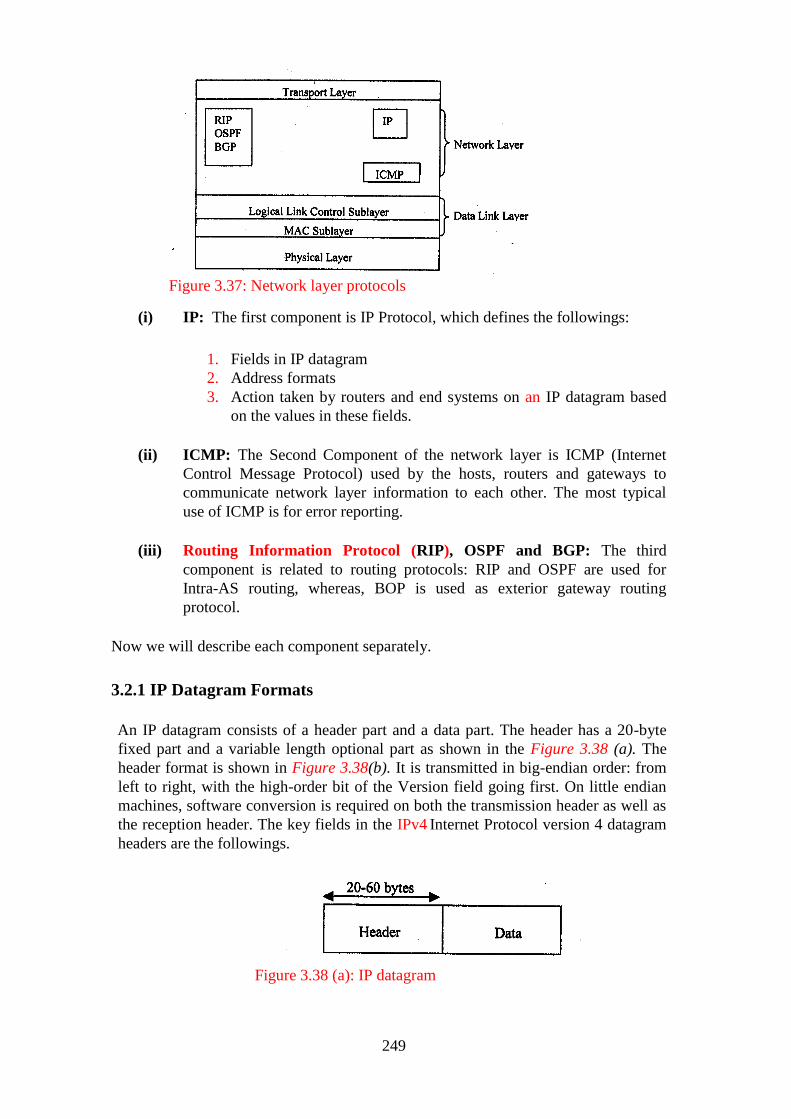
249

Figure 3.37: Network layer protocols

(i) IP: The first component is IP Protocol, which defines the followings:

1. Fields in IP datagram

2. Address formats

3. Action taken by routers and end systems on an IP datagram based

on the values in these fields.

(ii) ICMP: The Second Component of the network layer is ICMP (Internet

Control Message Protocol) used by the hosts, routers and gateways to

communicate network layer information to each other. The most typical

use of ICMP is for error reporting.

(iii) Routing Information Protocol (RIP), OSPF and BGP: The third

component is related to routing protocols: RIP and OSPF are used for

Intra-AS routing, whereas, BOP is used as exterior gateway routing

protocol.

Now we will describe each component separately.

3.2.1 IP Datagram Formats

An IP datagram consists of a header part and a data part. The header has a 20-byte

fixed part and a variable length optional part as shown in the Figure 3.38 (a). The

header format is shown in Figure 3.38(b). It is transmitted in big-endian order: from

left to right, with the high-order bit of the Version field going first. On little endian

machines, software conversion is required on both the transmission header as well as

the reception header. The key fields in the IPv4 Internet Protocol version 4 datagram

headers are the followings.

Figure 3.38 (a): IP datagram

250

Figure 3.38 (b): IP address formats

The Version field specifies the IP version of the protocol, the datagram belongs to. By

including the version in each datagram, the router can determine/interpret the reminder of

the IP datagram.

Header length (4 bits)

The field defines the length of the header in multiples of four bytes. The four bytes can

represent a number between 0 and 15, which when multiplied by 4, results in 60 bytes. A

typical IP datagram has 20-byte header only, because most IP datagram do not contain

options.

The Type of service (8 bits) defines how the datagram should be handled. It defines bits to

specify priority, reliability, delay, level of throughput to meet the different requirements.

For example, for digitised voice, fast delivery, beats accurate delivery. For file transfer,

error-free transmission is more important than fast transmission.

The Total length includes everything in the datagram both header and data. The

maximum length is 65,535 bytes. At present, this upper limit is tolerable, but with future

gigabit networks, larger datagrams may be needed.

The Identification filed is used in fragmentation. A datagram when passing through

different networks may be broken into several fragments to match the network

frame size. Once the fragmentation occurs, each fragment is identified with a sequence

number to this field.

Surprisingly, the IPv4. does not permit the fragmentation of the IP datagram at the

routers level.

Next, comes an unused bit and then two I-bit fields. DF stands for Don't Fragment.

It is an order to the router not to fragment the datagram because, the destination is

incapable of putting the pieces back together again.

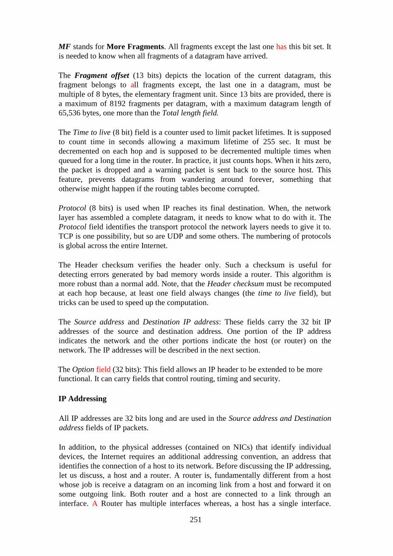
251

MF stands for More Fragments. All fragments except the last one has this bit set. It

is needed to know when all fragments of a datagram have arrived.

The Fragment offset (13 bits) depicts the location of the current datagram, this

fragment belongs to all fragments except, the last one in a datagram, must be

multiple of 8 bytes, the elementary fragment unit. Since 13 bits are provided, there is

a maximum of 8192 fragments per datagram, with a maximum datagram length of

65,536 bytes, one more than the Total length field.

The Time to live (8 bit) field is a counter used to limit packet lifetimes. It is supposed

to count time in seconds allowing a maximum lifetime of 255 sec. It must be

decremented on each hop and is supposed to be decremented multiple times when

queued for a long time in the router. In practice, it just counts hops. When it hits zero,

the packet is dropped and a warning packet is sent back to the source host. This

feature, prevents datagrams from wandering around forever, something that

otherwise might happen if the routing tables become corrupted.

Protocol (8 bits) is used when IP reaches its final destination. When, the network

layer has assembled a complete datagram, it needs to know what to do with it. The

Protocol field identifies the transport protocol the network layers needs to give it to.

TCP is one possibility, but so are UDP and some others. The numbering of protocols

is global across the entire Internet.

The Header checksum verifies the header only. Such a checksum is useful for

detecting errors generated by bad memory words inside a router. This algorithm is

more robust than a normal add. Note, that the Header checksum must be recomputed

at each hop because, at least one field always changes (the time to live field), but

tricks can be used to speed up the computation.

The Source address and Destination IP address: These fields carry the 32 bit IP

addresses of the source and destination address. One portion of the IP address

indicates the network and the other portions indicate the host (or router) on the

network. The IP addresses will be described in the next section.

The Option field (32 bits): This field allows an IP header to be extended to be more

functional. It can carry fields that control routing, timing and security.

IP Addressing

All IP addresses are 32 bits long and are used in the Source address and Destination

address fields of IP packets.

In addition, to the physical addresses (contained on NICs) that identify individual

devices, the Internet requires an additional addressing convention, an address that

identifies the connection of a host to its network. Before discussing the IP addressing,

let us discuss, a host and a router. A router is, fundamentally different from a host

whose job is receive a datagram on an incoming link from a host and forward it on

some outgoing link. Both router and a host are connected to a link through an

interface. A Router has multiple interfaces whereas, a host has a single interface.

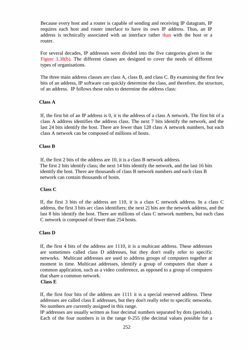
252

Because every host and a router is capable of sending and receiving IP datagram, IP

requires each host and router interface to have its own IP address. Thus, an IP

address is technically associated with an interface rather than with the host or a

router.

For several decades, IP addresses were divided into the five categories given in the

Figure 3.38(b). The different classes are designed to cover the needs of different

types of organisations.

The three main address classes are class A, class B, and class C. By examining the first few

bits of an address, IP software can quickly determine the class, and therefore, the structure,

of an address. IP follows these rules to determine the address class:

Class A

If, the first bit of an IP address is 0, it is the address of a class A network. The first bit of a

class A address identifies the address class. The next 7 bits identify the network, and the

last 24 bits identify the host. There are fewer than 128 class A network numbers, but each

class A network can be composed of millions of hosts.

Class B

If, the first 2 bits of the address are 10, it is a class B network address.

The first 2 bits identify class; the next 14 bits identify the network, and the last 16 bits

identify the host. There are thousands of class B network numbers and each class B

network can contain thousands of hosts.

Class C

If, the first 3 bits of the address are 110, it is a class C network address. In a class C

address, the first 3 bits arc class identifiers; the next 2] bits are the network address, and the

last 8 bits identify the host. There are millions of class C network numbers, but each class

C network is composed of fewer than 254 hosts.

Class D

If, the first 4 bits of the address are 1110, it is a multicast address. These addresses

are sometimes called class D addresses, but they don't really refer to specific

networks. Multicast addresses are used to address groups of computers together at

moment in time. Multicast addresses, identify a group of computers that share a

common application, such as a video conference, as opposed to a group of computers

that share a common network.

Class E

If, the first four bits of the address are 1111 it is a special reserved address. These

addresses are called class E addresses, but they don't really refer to specific networks.

No numbers are currently assigned in this range.

IP addresses are usually written as four decimal numbers separated by dots (periods).

Each of the four numbers is in the range 0-255 (the decimal values possible for a

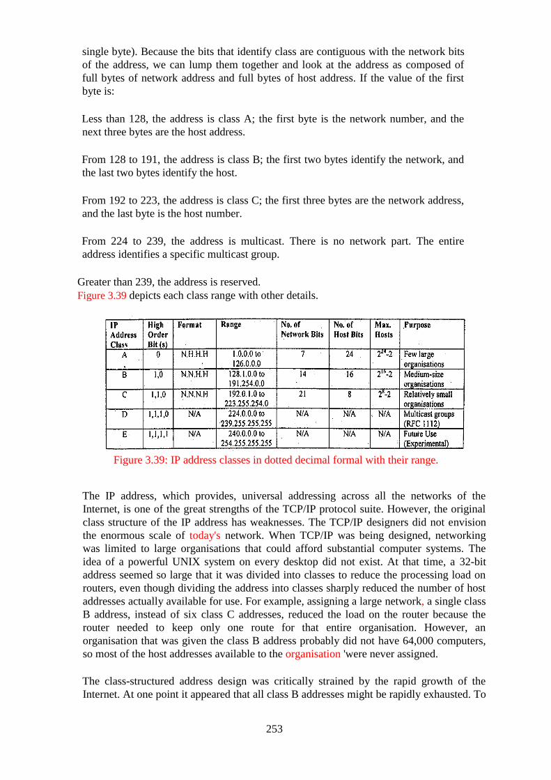
253

single byte). Because the bits that identify class are contiguous with the network bits

of the address, we can lump them together and look at the address as composed of

full bytes of network address and full bytes of host address. If the value of the first

byte is:

Less than 128, the address is class A; the first byte is the network number, and the

next three bytes are the host address.

From 128 to 191, the address is class B; the first two bytes identify the network, and

the last two bytes identify the host.

From 192 to 223, the address is class C; the first three bytes are the network address,

and the last byte is the host number.

From 224 to 239, the address is multicast. There is no network part. The entire

address identifies a specific multicast group.

Greater than 239, the address is reserved.

Figure 3.39 depicts each class range with other details.

Figure 3.39: IP address classes in dotted decimal formal with their range.

The IP address, which provides, universal addressing across all the networks of the

Internet, is one of the great strengths of the TCP/IP protocol suite. However, the original

class structure of the IP address has weaknesses. The TCP/IP designers did not envision

the enormous scale of today's network. When TCP/IP was being designed, networking

was limited to large organisations that could afford substantial computer systems. The

idea of a powerful UNIX system on every desktop did not exist. At that time, a 32-bit

address seemed so large that it was divided into classes to reduce the processing load on

routers, even though dividing the address into classes sharply reduced the number of host

addresses actually available for use. For example, assigning a large network, a single class

B address, instead of six class C addresses, reduced the load on the router because the

router needed to keep only one route for that entire organisation. However, an

organisation that was given the class B address probably did not have 64,000 computers,

so most of the host addresses available to the organisation 'were never assigned.

The class-structured address design was critically strained by the rapid growth of the

Internet. At one point it appeared that all class B addresses might be rapidly exhausted. To

254

prevent this, a new way of looking at IP addresses without a class structure was

developed.

Subnet Masks and CIDR Networks (Classless IP Addresses)

IP addresses are actually 32-bit binary numbers. Each 32-bit IP address consists of

two sub addresses, one identifying the network and the other identifying the host to

the network, with an imaginary boundary separating the two. The location of the

boundary between the network and host portions of an IP address is determined

through the use of a subnet mask. A subnet mask is another 32-bit binary number,

which acts like a filter when applied to the 32-bit IP address. By comparing a subnet

mask with an IP address system, can determine the portion of the IP address that

relates to the network, and the portion that relates to the host. Wherever, the subnet

mask has a bit set to ―I‖, the underlying bit in the IP address is part of the network

address. Wherever the subnet mask is set to ―0‖, the related bit in the IP address is

part of the host address. For example, assume that the IP address

11000000101010000000000100010100 has a subnet mask of

11111111111111111111111100000000. In this example, the first 24 bits of the

32-bit IP addresses are used to identify the network, while the last 8 bits are used to

identify the host address of that network.

The size of a network (i.e., the number of host addresses available for use on it) is a

function of the number of bits used to identify the host portion of the address. If, a

subnet mask shows that 8 bits are used for the host portion of the address block, a

maximum of 256 possible host addresses are available for that specific network.

Similarly, if a subnet mask shows that 16 bits are used for the host portion of the

address block, a maximum of 65,536 possible host addresses are available for use on

that network.

If a network administrator needs to split a single network into multiple virtual

networks, the bit-pattern in use with the subnet mask can be changed to allow as

many networks as necessary. For example, assume that we want to split the 24-bit

192.168.10.0 network (which allows for 8 bits of host addressing, or a maximum of

256 host addresses) into two smaller networks. All we have to do in this situation is,

change the subnet mask of the devices on the network so that they use 25 bits for the

network instead of 24 bits, resulting in two distinct networks with 128 possible host

addresses on each network. In this case, the first network would have a range

of network addresses between 192.168.111.0 -192.168.10.127, while the second

network would have a range of addresses between 192.168.10.128 -192.168.10.255.

Networks can also be enlarged through the use of a technique known as

―supernetting,‖ which works by extending the host portion of a subnet mask to the

left, into the network portion of the address. Using this technique, a pair of networks

with 24-bit subnet masks can be turned into a single large network with a 23-bit

subnet mask. However, this works only if you have two neighbouring 24-bit network

blocks, with the lower network having an even value (when the network portion of

the address is shrunk, the trailing bit from the original network portion of the subnet

mask should fall into the host portion of the new subnet mask, so the new network

mask will consume both networks). For example, it is possible to combine the 24-

bit 192.168.10.0 and . 192.168.1 1.0 networks together since the loss of the trailing

bit from each network (00001010 vs. 00001011) produces the same 23-bit subnet

255

mask (000001x), resulting in a consolidated 192.168.10.0 network. However, it is not

possible to combine the 24-bit 192.168.11.0 and 192.168.12.0 networks, since the

binary values in the seventh bit position (00001011 vs. 00001100) do not match

when the trailing bit is removed.

Classless Inter-Domain Routing

In the modem networking environment defined by RFC 1519 [Classless Inter-

Domain Routing (CIDR)], the subnet mask of a network is typically annotated in

written form as a ―slash prefix‖ that trails the network number. In the subnetting

example in the previous paragraph, the original 24-bit network would be written as

192.168.10.0/24, while the two new networks would be written as 192.168.10.0/25

and 192.168.10.128/25. Likewise, when the 192.168.10.0/24 and

192.168.11.0/24 networks were joined together as a single supernet, the resulting

network would be written as 192.168.10.0/23. Note, that the slash prefix annotation

is generally used for human benefit; infrastructure devices still use the 32-bit binary

subnet mask internally to identify networks and their routes. All networks must

reserve host addresses (made up entirely of either ones or zeros), to be used by the

networks themselves. This is so that, each subnet will have a network- specific

address (the all-zeroes address) and a broadcast address (the all- ones address). For

example, a /24 network allows for 8 bits of host addresses, but only 254 of the 256

possible addresses are available for use. Similarly, /25 networks have a maximum of

7 bits for host addresses, with 126 of the 128 possible addresses available (the all-

ones and all-zeroes addresses from each subnet must be set aside for the subnets

themselves). All the systems on the same subnet must use the same subnet mask in

order to communicate with each other directly. If, they use different subnet masks

they will think they are on different networks, and will not be able to communicate

with each other without going through a router first. Hosts on different networks can

use different subnet mask, although the routers will have to be aware of the subnet

masks in use on each of the segments.

Subnet masks are used only by systems that need to communicate with the network

directly. For example, external systems do not need to be aware of the subnet masks

in use on your internal networks, since those systems will route data to your network

by way of your parent network's address block. As such, remote routers need to know

only the provider's subnet mask. For example, if you have a small network that uses

only a / 28 prefix that is, a subset of your ISP's /20 network, remote routers need to

know only about your upstream provider's /20 network, while your upstream

provider needs to know your subnet mask in order to get the data to your local /28

network. The rapid depletion of the class B addresses showed that three primary

address classes were not enough: class A was much too large and class C was much

too small. Even a class B address was too large for many networks but was used

because it was better than the other alternatives.

The obvious solution to the class B address crisis was to force organisations to use

multiple class C addresses. There were millions of these addresses available and they

were in no immediate danger of depletion. As is often the case, the obvious solution

is not as simple as it may seem. Each class C address requires its own entry within

the routing table. Assigning thousands or millions of class C addresses would cause

the routing table to grow so rapidly that the routers would soon be overwhelmed. The

256

solution requires a new way of assigning addresses and a new way of looking at

addresses.

Originally network addresses were assigned in more or less sequential order as they

were requested. This worked fine when the network was small and centralised.

However, it did not take network topology into account. Thus, only random chance

would determine if the same intermediate routers would be used to reach network

195.4.12.0 and network 195.4.13.0, which makes it difficult to reduce the size of the

routing table. Addresses can only be aggregated if they are contiguous numbers and

are reachable through the same route. For example, if addresses are contiguous for

one service provider, a single route can be created for that aggregation because that

service provider will have a limited number of routes to the Internet. But if one

network address is in France and the next contiguous address is in Australia, creating

a consolidated route for these addresses will not work.

Today, large, contiguous blocks of addresses are assigned to large network service

providers in a manner that better reflects the topology of the network. The service

providers then allocate chunks of these address blocks to the organisations to which

they provide network services. This alleviates the short-term shortage of class B

addresses and, because the assignment of addressees reflects the topology of the

network, it permits route aggregation. Under this new scheme, we know that network

195.4.12.0 and network 195.4.13.0 are reachable through the same intermediate

routers. In fact, both these addresses are in the range of the addresses assigned

to Europe, 194.0.0.0 to 195.255.255.255. Assigning addresses that reflect the

topology of the network enables route aggregation, but does not implement it. As

long as network 195.4.12.0 and network 195.4.13.0 are interpreted as separate class

C addresses, they will require separate entries in the routing table. A new, flexible

way of defining addresses is therefore, needed.

Evaluating addresses according to the class rules discussed above limits the length of

network numbers to 8, 16, or 24 bits -1, 2, or 3 bytes. The IP address, however, is not

really byte-oriented. It is 32 contiguous bits. A more flexible way to interpret the

network and host portions of an address is with a bit mask. An address bit mask

works in this way: if a bit is on in the mask, that equivalent bit in the address is

interpreted as a network bit; if a bit in the mask is off, the bit belongs to the host part

of the address. For example, if address 195.4.12.0 is interpreted as a class C address,

the first 24 bits are the network numbers and the last 8 bits are the host addresses.

The network mask that represents this is 255.255.255.0, 24 bits on and 8 bits off. The

bit mask that is derived from the traditional class structure is called the default mask

or the natural mask.

However, with bit masks we are no longer limited by the address class structure. A

mask of 255.255.0.0 can be applied to network address 195.4.0.0. This mask

includes all addresses from 195.4.0.0 to 195.4.255.255 in a single network

number. In effect, it creates a network number as large as a class B network in the

class C address space. Using bit masks to create networks larger than the natural

mask is called supernetting, and the use of a mask instead of the address class to

determine the destination network is called Classless Inter-Domain Routing (CIDR).

Specifying both the address and the mask is cumbersome when writing out addresses.

A shorthand notation has been developed for writing CIDR addresses. Instead of

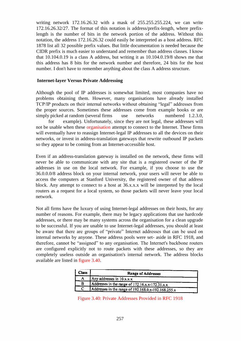
257

writing network 172.16.26.32 with a mask of 255.255.255.224, we can write

172.16.26.32/27. The format of this notation is address/prefix-length, where prefix-

length is the number of bits in the network portion of the address. Without this

notation, the address 172.16.26.32 could easily be interpreted as a host address. RFC

1878 list all 32 possible prefix values. But little documentation is needed because the

CIDR prefix is much easier to understand and remember than address classes. I know

that 10.104.0.19 is a class A address, but writing it as 10.104.0.19/8 shows me that

this address has 8 bits for the network number and therefore, 24 bits for the host

number. I don't have to remember anything about the class A address structure.

Internet-layer Versus Private Addressing

Although the pool of IP addresses is somewhat limited, most companies have no

problems obtaining them. However, many organisations have already installed

TCP/IP products on their internal networks without obtaining ―legal‖ addresses from

the proper sources. Sometimes these addresses come from example books or are

simply picked at random (several firms use networks numbered 1.2.3.0,

for example). Unfortunately, since they are not legal, these addresses will

not be usable when these organisation attempt to connect to the Internet. These firms

will eventually have to reassign Internet-legal IP addresses to all the devices on their

networks, or invest in address-translation gateways that rewrite outbound IP packets

so they appear to be coming from an Internet-accessible host.

Even if an address-translation gateway is installed on the network, these firms will

never be able to communicate with any site that is a registered owner of the IP

addresses in use on the local network. For example, if you choose to use the

36.0.0.0/8 address block on your internal network, your users will never be able to

access the computers at Stanford University, the registered owner of that address

block. Any attempt to connect to a host at 36.x.x.x will be interpreted by the local

routers as a request for a local system, so those packets will never leave your local

network.

Not all firms have the luxury of using Internet-legal addresses on their hosts, for any

number of reasons. For example, there may be legacy applications that use hardcode

addresses, or there may be many systems across the organisation for a clean upgrade

to be successful. If you are unable to use Internet-legal addresses, you should at least

be aware that there are groups of ―private‖ Internet addresses that can be used on

internal networks by anyone. These address pools were set- aside in RFC 1918, and

therefore, cannot be ―assigned‖ to any organisation. The Internet's backbone routers

are configured explicitly not to route packets with these addresses, so they are

completely useless outside an organisation's internal network. The address blocks

available are listed in figure 3.40.

Figure 3.40: Private Addresses Provided in RFC 1918

258

Since these addresses cannot be routed across the Internet, you must use an address-

translation gateway or a proxy server in conjunction with them. Otherwise, you will

not be able to communicate with any hosts on the Internet.

An important note here is that, since, nobody can use these addresses on the Internet,

it is safe to assume that anybody who is using these addresses is also utilising an

address-translation gateway of some sort. Therefore, while you will never see these

addresses used as destinations on the Internet, if your organisation establishes a

private connection to a partner organisation that is using the same block of addresses

that you are using, your firms will not be able to communicate on the Internet. The

packets destined for your partner's network will appear to be local to your network,

and will never be forwarded to the remote network.

There are many other problems that arise from using these addresses, making their

general usage difficult for normal operations. For example, many application-layer

protocols embed addressing information directly into the protocol stream, and in

order for these protocols to work properly, the address-translation gateway has to be

aware of their mechanics. In the preceding scenario, the gateway has to rewrite the

private addresses (which are stored as application data inside the application

protocol), rewrite the UDP/TCP and IP checksums, and possibly rewrite TCP

sequence numbers as well. This is difficult to do even with simple and open protocols

such as FTP, and extremely difficult with proprietary, encrypted, or dynamic

applications (these are problems for many database protocols, network games, and

voice-over- IP services, in particular). These gateways almost never work for all the

applications in use at a specific location.

It is always better to use formally-assigned, Internet-legal addresses whenever

possible: even if, the hosts on your network do not necessarily require direct Internet

access. In those cases, in which your hosts are going through a firewall or application

proxy of some sort, the use of Internet-legal addresses causes the least amount of

maintenance trouble over time. If, for some reason this is not possible, use one of the

private address pools described in Figure 3.40. Do not use random, self-assigned

addresses if you can possibly avoid it, as this will only cause connectivity

problems for you and your users.

Fragmentation

Fragmentation is process of breaking bigger IP datagrams into smal1er fragments.

Each network imposes some maximum size on its packets. Maximum payloads range

from 48 bytes (ATM cells) to 65,5 I 5 bytes (IP packets), although the payload size in

higher layers is often bigger.

What happens if the original host sends a source packet which is too large to be

handled by the destination network? The routing algorithm can hardly bypass the

destination.

Basically, the only solution to the problem is to allow routers to break up packets into

fragments.

259

The data in the IP datagram is broken among two or more smaller IP datagrams and

these smaller fragments are then sent over the outgoing link.

The real problems in the fragmentation process is reassembly of fragments into a single

IP datagram before sending it to the transport layer. If it is done at the network level, it

will decrease the performance of a router. Therefore, to keep the network layer simple.

IPv4. designer has left it to be done at the receiver level. When the destination host

receives a series of fragments from the same host, it examines the identification number

of a fragment, its flag number (the flag bit is set 100 for the last fragment whereas it is

a set to 1 for all the other fragments). This is required because one or more fragments

may never reach because IP provides best efforts service. Offset field is used to

determine where the fragment fits within the original IP datagram [Rej5]. When

all the packets have arrived, the destination host reassembles them and sends it to the

transport layer. The following table illustrates an example of 5000 bytes (20 bytes of IP

header plus 4980 bytes of IP Payload arrives at a router which must be forwarded to the

outgoing link 'with a maximum transfer unit of 1500 bytes (equivalent to Ethernet

frame size).

Figure 3.41: Fragmentation Table

This means that 4,980 data bytes in the original datagram must be allocated to four

separate segments (each of which are also IP datagram). The original datagram has

been stamped with an identification number 999. It is desirable to have a minimum

number of fragments because fragmentation and reassembling creates extra

overheads or a network system and a host. This is done by limiting the size of UDP

and TCP segments to small size.

3.2.2 Internet Control Message Protocol (ICMP)

It is a protocol used by hosts and routers to send notification of datagram

problems. The most typical use of ICMP is for error reporting. We have encountered

errors such as, ―Destination network unreachable‖ while running a telnet, FTP or

HTTP session. This type of error reporting is done by ICMP [Ref5]. As we are

aware, IP is an unreliable and connection less protocol, due to which, very often, a

datagram may not reach the destination because of a link failure, congestion etc.

ICMP does reporting of such cases to the sender.

ICMP is often considered part of IP but architecturally lies just above IP as ICMP

messages are carried inside IP packets. Similar TCP and UDP segments which are

carried as IP payloads, ICMP messages are also carried as IP payloads. Note, that, a

datagram carries only the addresses of the original sender and the final destination. It

260

does not know the addresses of the previous router (s) that passed a message. For this

reason, ICMP can send messages only to the source and not to an intermediate router.

Student are required to refer to Reference [1] & [5] for details of message types.

3.2.3 OSPF: The Interior Gateway Routing Protocol

Open Shortest Path First (OSPF) has become standard interior gateway routing

protocol. It supports many advanced features [Ref! and Ref5] to meet a long list of

requirements.

The protocol specification should be publicly available. O in OSPF stands for

open. It means that OSPF is not a proprietary protocol.

It is a dynamic algorithm one that adapts to changes in the topology

automatically and quickly.

Load distribution: When multiple paths to a destination have the same cost

OSPF allows multiple paths to be used.

Support for hierarchy within a single routing domain. By 1988, the Internet

had grown so large that no router was expected to know the entire topology.

OSPF was designed so that no router would have to do so.

Security: All exchanges between OSPF routers are authenticated and allows

only trusted routers 10 participate. OSPF supports three kinds of connections

and networks [Ref l]

1 Point-to-point lines between two routers only.

2 Multi-access networks with broadcasting (e.g., LANs).

3 Multi-access networks without broadcasting (e.g., Packet

Switched WANs).

OSPF identifies four types of routers:

(i) Internal routers (within one area).

(ii) Area border routers (connects two or more areas).

(iii) Backbone routers (performs routing within the backbone).

(iv) Autonomous Systems (AS) boundary routers (exchanges routing

information with routers in other ASes).

OSPF allows a longer AS to be divided into smaller areas. Topology and

details of one area is not visible to others. Every AS has a backbone area

(called Area 0) as shown in Figure 3.42.

261

Figure 3.42: Working domain of OSPF

All areas are connected to the backbone possibly by a tunnel, so it is possible to

move from one area to another area through a backbone. The primary role of the

backbone area is to route traffic between the other areas in the AS. Inter area routing

within the AS requires the follows movement of packets as shown below by arrows.

Host internal router of an area border router of a source area backbone area border

router of a destination area internal router of a destination area final destination

After having described all the components of OSPF, let us now conclude the topic by

describing its operation.

At its heart, however, OSPF is a link state protocol that uses flooding of link state

information and Dijkstra's Least-Cost path algorithm. Using flooding each router

informs all other routers in its area of its neighbours and costs. This information

allows each router to construct the graph for its area (s) and computers the shortest

path using Dijkstra's algorithm. This is done by backbone routers also. In addition,

backbone routers accept information from the area border routers in order to compute

the best route from each backbone router to every other router. This information is

propagated back to area border routers, which advertise it within their areas. In this

manner, the optimal route is selected.

3.2.4 BGP: The Exterior Gateway Routing Protocol

The purpose of Border Gateway Protocol is to enable two different ASes to exchange

routing information so that, IP traffic can flow across the AS border. A different

protocol is needed between the ASes because the objectives of an interior gateway

and exterior gateway routing protocol are different. Exterior gateway routing

protocol such as BGP is related to policy matters. BGP is fundamentally a distance

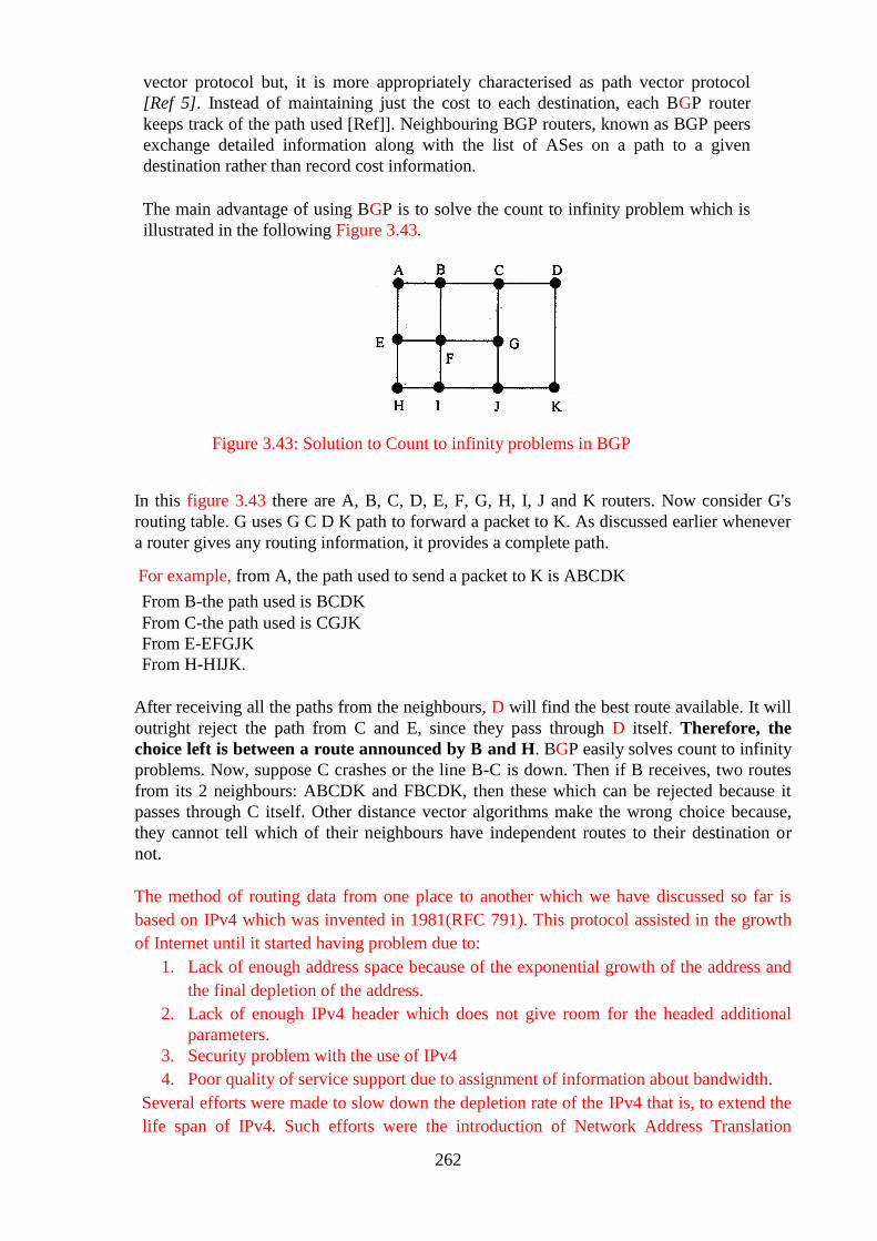
262

vector protocol but, it is more appropriately characterised as path vector protocol

[Ref 5]. Instead of maintaining just the cost to each destination, each BGP router

keeps track of the path used [Ref]]. Neighbouring BGP routers, known as BGP peers

exchange detailed information along with the list of ASes on a path to a given

destination rather than record cost information.

The main advantage of using BGP is to solve the count to infinity problem which is

illustrated in the following Figure 3.43.

Figure 3.43: Solution to Count to infinity problems in BGP

In this figure 3.43 there are A, B, C, D, E, F, G, H, I, J and K routers. Now consider G's

routing table. G uses G C D K path to forward a packet to K. As discussed earlier whenever

a router gives any routing information, it provides a complete path.

For example, from A, the path used to send a packet to K is ABCDK

From B-the path used is BCDK

From C-the path used is CGJK

From E-EFGJK

From H-HIJK.

After receiving all the paths from the neighbours, D will find the best route available. It will

outright reject the path from C and E, since they pass through D itself. Therefore, the

choice left is between a route announced by B and H. BGP easily solves count to infinity

problems. Now, suppose C crashes or the line B-C is down. Then if B receives, two routes

from its 2 neighbours: ABCDK and FBCDK, then these which can be rejected because it

passes through C itself. Other distance vector algorithms make the wrong choice because,

they cannot tell which of their neighbours have independent routes to their destination or

not.

The method of routing data from one place to another which we have discussed so far is

based on IPv4 which was invented in 1981(RFC 791). This protocol assisted in the growth

of Internet until it started having problem due to:

1. Lack of enough address space because of the exponential growth of the address and

the final depletion of the address.

2. Lack of enough IPv4 header which does not give room for the headed additional

parameters.

3. Security problem with the use of IPv4

4. Poor quality of service support due to assignment of information about bandwidth.

Several efforts were made to slow down the depletion rate of the IPv4 that is, to extend the

life span of IPv4. Such efforts were the introduction of Network Address Translation

263

(NAT), the use of subnetting and classless interdomain routing (CIDR). Finally, Internet

Protocol Version 6 (IPv6) was drafted by Internet Engineering Task Force (IETF) in 1998

(RFC 1883) which was obsoleted by RFC 2460 and became an Internet standard on 14th

July, 2017 (RF8200). Let us discuss IPv6.

Internet Protocol Version 6 (IPv6)

Internet Protocol Version 6 (IPv6) is an Internet Standard (RFC 8200) which is meant

to identify and create computer devices and other devices on interconnected systems

and transfers traffic through the Internet. It was developed to solve the problems of

IPv4. IPv6 has 128-bit address, that is, 2128

or 3.4 x1038

addresses. It solves IPv4

problems by;

1. Providing very large address space

2. Giving room for tree-like address system thereby providing route in aggregation

throughout the Internet, and restricting the enlargement of routing tables.

3. Enlarging and making easy employment of multicast addressing, thus, giving

room for providing services in the most effective way possible.

IPv6 address is represented as

2001:0db8:0000:0000: 0000:8a2e:370,7334

Which can also be written as

2001:0db8::8a2e: 0370:7334.

IPv4 to IPv6 transition assumes will take a long time. There are several methods of

transiting from IPv4 to IPv6. Some of the methods are;

1. Dual stock

This is system of running IPv4 and IPv6 on the same machine at the same time.

Many computer devices presently support IPv4 and IPv6.

2. Tunnelling

This is a method of conveying IPv6 traffic via IPv4 network. In this case, packets

are enclosed into a wrapper that allows the transfer from source to the destination

limpidly from where it can be retransmitted. There are several methods of

tunnelling. Such methods are manual IPv6 tunnels, Generic routing encapsulation

(GRE) IPv6 tunnels, 6 to 4 tunnels, IPv4 compatible tunnels and intra-site

automatic tunnel addressing protocol (ISATAP) tunnels.

3. Translation

This allows IPv6 to be transformed into IPv4 and vice-versa. In this case, the

traffic is charged (not encapsulated) to the destination type which can either be

IPv4 or IPv6. Translation methods are network address translation and NAT64.

Converting from IPv4 to IPv6

It is pertinent to note from our discussions that it is obvious to convert IPv4 to binary

using the four octets. Similarly, it is also easy to convert IPv6 to binary using the 16

8-bit octets.

264

Self-Study Exercise

1. Convert 172.16.254.1 from decimal to binary

Solution

To convert 172.16.254.1 to binary, it is easy to use a setup table of Binary Coded

Decimal (BCD) number such as:

27 2

6 2

5 2

4 2

3 2

2 2

1 2

0

128 64 32 16 8 4 2 1

1 0 1 0 1 1 0 0

Use this table and the steps below to convert for a start, 17210 to binary number.

Step 1

1

128 172

128

44

Step 2 0

64 44

64 cannot divide 44 so, write 0 down

Step 3

1

32 44

32

12

Step 4

16 12

16 cannot divide 12 so write 0 down

Step 5

1

8 12

8

4

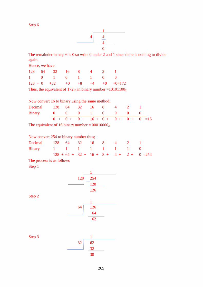
265

Step 6

1

4 4

4

0

The remainder in step 6 is 0 so write 0 under 2 and 1 since there is nothing to divide

again.

Hence, we have.

128 64 32 16 8 4 2 1

1 0 1 0 1 1 0 0

128 + 0 +32 +0 +8 +4 +0 +0=172

Thus, the equivalent of 17210 in binary number =101011002

Now convert 16 to binary using the same method.

Decimal 128 64 32 16 8 4 2 1

Binary 0 0 0 1 0 0 0 0

0 + 0 + 0 + 16 + 0 + 0 + 0 + 0 =16

The equivalent of 16 binary number = 000100002

Now convert 254 to binary number thus;

Decimal 128 64 32 16 8 4 2 1

Binary 1 1 1 1 1 1 1 0

128 + 64 + 32 + 16 + 8 + 4 + 2 + 0 =254

The process is as follows

Step 1

1

128 254

128

126

Step 2

1 64 126

64

62

Step 3 1

32 62

32

30

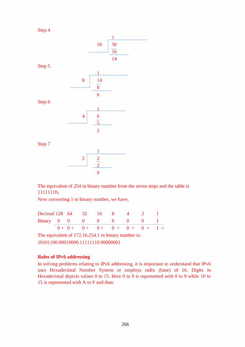
266

Step 4

1

16 30

16

14

Step 5

1

8 14

8

6

Step 6

1

4 6

5

2

Step 7

1

2 2

2

0

The equivalent of 254 in binary number from the seven steps and the table is

111111102

Now converting 1 to binary number, we have;

Decimal 128 64 32 16 8 4 2 1

Binary 0 0 0 0 0 0 0 1

0 + 0 + 0 + 0 + 0 + 0 + 0 + 1 =

The equivalent of 172.16.254.1 in binary number is:

10101100.00010000.11111110.00000001

Rules of IPv6 addressing

In solving problems relating to IPv6 addressing, it is important to understand that IPv6

uses Hexadecimal Number System or employs radix (base) of 16. Digits in

Hexadecimal depicts values 0 to 15. Here 0 to 9 is represented with 0 to 9 while 10 to

15 is represented with A to F and thus:

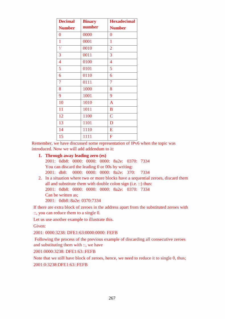
267

Decimal

Number

Binary

number

Hexadecimal

Number

0 0000 0

1 0001 1

⅟ 0010 2

3 0011 3

4 0100 4

5 0101 5

6 0110 6

7 0111 7

8 1000 8

9 1001 9

10 1010 A

11 1011 B

12 1100 C

13 1101 D

14 1110 E

15 1111 F

Remember, we have discussed some representation of IPv6 when the topic was

introduced. Now we will add addendum to it:

1. Through away leading zero (es)

2001: 0db8: 0000: 0000: 0000: 8a2e: 0370: 7334

You can discard the leading 0 or 00s by writing:

2001: db8: 0000: 0000: 0000: 8a2e: 370: 7334

2. In a situation where two or more blocks have a sequential zeroes, discard them

all and substitute them with double colon sign (i.e. ::) thus:

2001: 0db8: 0000: 0000: 0000: 8a2e: 0370: 7334

Can be written as;

2001: 0db8::8a2e: 0370:7334

If there are extra block of zeroes in the address apart from the substituted zeroes with

::, you can reduce them to a single 0.

Let us use another example to illustrate this.

Given:

2001: 0000:3238: DFE1:63:0000:0000: FEFB

Following the process of the previous example of discarding all consecutive zeroes

and substituting them with ::, we have

2001:0000:3238: DFE1:63::FEFB

Note that we still have block of zeroes, hence, we need to reduce it to single 0, thus;

2001:0:3238:DFE1:63::FEFB

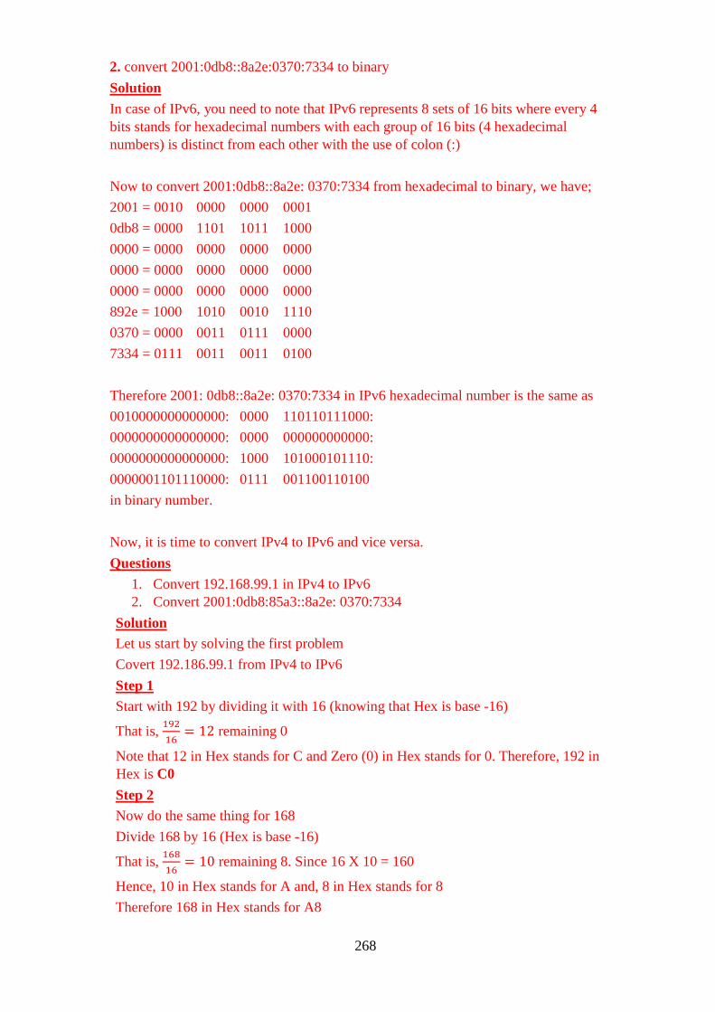
268

2. convert 2001:0db8::8a2e:0370:7334 to binary

Solution

In case of IPv6, you need to note that IPv6 represents 8 sets of 16 bits where every 4

bits stands for hexadecimal numbers with each group of 16 bits (4 hexadecimal

numbers) is distinct from each other with the use of colon (:)

Now to convert 2001:0db8::8a2e: 0370:7334 from hexadecimal to binary, we have;

2001 = 0010 0000 0000 0001

0db8 = 0000 1101 1011 1000

0000 = 0000 0000 0000 0000

0000 = 0000 0000 0000 0000

0000 = 0000 0000 0000 0000

892e = 1000 1010 0010 1110

0370 = 0000 0011 0111 0000

7334 = 0111 0011 0011 0100

Therefore 2001: 0db8::8a2e: 0370:7334 in IPv6 hexadecimal number is the same as

0010000000000000: 0000 110110111000:

0000000000000000: 0000 000000000000:

0000000000000000: 1000 101000101110:

0000001101110000: 0111 001100110100

in binary number.

Now, it is time to convert IPv4 to IPv6 and vice versa.

Questions

1. Convert 192.168.99.1 in IPv4 to IPv6

2. Convert 2001:0db8:85a3::8a2e: 0370:7334

Solution

Let us start by solving the first problem

Covert 192.186.99.1 from IPv4 to IPv6

Step 1

Start with 192 by dividing it with 16 (knowing that Hex is base -16)

That is,

remaining 0

Note that 12 in Hex stands for C and Zero (0) in Hex stands for 0. Therefore, 192 in

Hex is C0

Step 2

Now do the same thing for 168

Divide 168 by 16 (Hex is base -16)

That is,

remaining 8. Since 16 X 10 = 160

Hence, 10 in Hex stands for A and, 8 in Hex stands for 8

Therefore 168 in Hex stands for A8

269

Step 3

Next octet to convert using the same problem is 99.

Following the same process

remaining 3.

Since 6 X16 =96

Hence 6 in Hex stands for 6

And, 3 in Hex stands for 3

Therefore, 99 in Hex stands for 63

Step 4

Now converting the last Octet which is 1, we have,

remaining 1

Hence, 0 in Hex stands for 0

And 1 in Hex stands for 1

Therefore, 1 in Hex stands for 01

Thus, IPv4 address 192.168.99.1 depiction in IPv6 address segment would be

C0A8:6301.

This type of address conversion is classified as IPv6 6-to-4 tunnels which in most

cases join to form 2002: :/16 with the IPv4 Address infused.

The address format of the automatic 6-to-4 tunnels is as follows:

2002:<32 bit IPv4 site address in Hex>:<16 bit network number in Hex>::164. Hence,

for IPv4 address of 192.168.99.1, the wrap up of the IPv6 address would be

2002:C0A8:6301::1/64.

Now, let us convert the segment of C0A8:6301 to IPv4.

First, represent the address in the form of IPv4, that is, C0A8:6301 into two (2) tuple-

groupings (2 Hex characters) i.e. C0 AB 63 01

Note that any number raised to the power of 0 is 1 and any number raise to the power

of 1 is that number.

Step 1

Since IPv6 characters are in base-16, then for the case of C0: C will be multiplied by

16 and 0 multiplied by 1 to convert them to IPv4.

Hence, add the two values together to get the IPv4 decimal value. Thus (12x16) +

(0x1) since C is 12 and 0 is 0 in Hex. This implies 192 + 0 = 192

Step 2

Again, take A8 and follow theme process, we have

(10x16) +(8x1) since A =10 and 8=8 in Hex.

Thus, 160 + 8 = 168

Step 3

Take 63 and follow the same process, we have (6x16) + (3x1) since 6 is 6 and 3 is 3 in

Hex.

Thus, 96 + 3 = 99

270

Step 4

Take 01 and follow the same process, we have;

(0x16) + (1x1) since 0=0 and 1=1 in Hex.

Thus, 0 + 1 =1

Therefore, the IPv4 address is 192.168.99.1

4.0 CONCLUSION

In this concluding unit of this module you have learnt about internetworking

protocols. It has also taken you through tunnelling and encapsulation concepts.

5.0 SUMMARY

In this unit, we defined, a large number of concepts and protocols. Tunnelling is used

when the source and destination networks are identical but the network, which lies in

between, is different. A subnet allows a network to be split into several parts for

Internet use but still acts like a single network to the outside world. It makes

management of IP addresses simpler. Another reason for creating a subnet is to

establish security between different work groups. Internet is made of a large number

of autonomous regions controlled by a different organisation which can, use its own

routing algorithm inside. A routing algorithm within an autonomous region (such as

LAN, WAN) is called an interior gateway protocol, an algorithm for routing

between different autonomous regions are called exterior gateway routing protocols.


1 List the important features in which one network differs from another.

2 What are the mechanisms for interconnecting networks?

3 Where is tunnelling used?

4 What are the important categories of Network layer protocols?

5 List the important OSPF routes and their purposes.

6 How is BGP different from other distance vector routing protocols?


A.S. Tanenbaum, Computer Networks, 4‖ Edition, Prentice Hall of India, New

Delhi, 2011.

Leon Garcia and Indra Widjaja, Communication Networks fundamental concepts and

key architecture, Tata McGraw Hill, New Delhi.

Behrouz A. Forouzan, Data Communication and Networking, 2nd edition, Tata

McGraw Hill, New Delhi, 2016.

Timothy S Ramteke, Networks, 2nd Edition, Pearson edition, New Delhi.

271

James F. Kurose and Keith W. Ross. Computer Networking A Top down Approach

featuring the Internet, Pearson Edition, New Delhi.


Question 1

List the important features in which one network differs from another.

Solution

The reasons why one network differ from another are:

a. Many personal computers use TCP/IP,

b. Many larger business organizations still use IBM mainframes with SNA

Protocol.

c. Some PCs still run on Novell's NCP/IPX or Appletalk.

d. Wireless Network will have different protocols.

e. A large number of Telecommunication companies provide ATM facilities.

Question 2

What are the mechanisms for interconnecting networks?

The two basic mechanisms for interconnecting networks are concatenated virtual

circuit and connectionless interworking in addition to the use of repeaters, switches or

hubs and bridges

Explain them

Question 3

Where is tunnelling used?

Tunning is mostly used in virtual private network (VPN) and can be used to connect

two networks or use to bypass firewalls.

Question 4

What are the important categories of Network layer protocols?

Solution

The important categories of Network layer protocols are:

a. Physical layer

b. Data link layer

c. Network layer

d. Transport layer

Question 5

List the important OSPF routes and their purposes.

272

Solution

The important OSPF routes are:

a. Internal routers (within one area).

They receive traffic within the area or traffic coming from and to other areas.

b. Area border routers (connects two or more areas).

They are situated around the boarder and use for linkage between backbone

network and the OSPF areas.

c. Backbone routers (performs routing within the backbone).

They are used to combined and route traffic from many LAN segments and to

uphold routing data for thousands of machines

d. AS boundary routers (exchanges routing information with routers in other

ASes).

Read more about this

Question 6

How is BGP different from other distance vector routing protocols?

Solution

The main different is that it solves the count to infinity problem

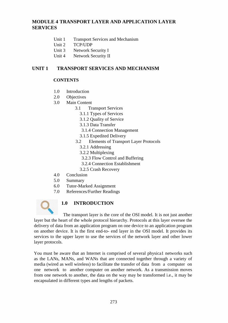
273

MODULE 4 TRANSPORT LAYER AND APPLICATION LAYER

SERVICES

Unit 1 Transport Services and Mechanism

Unit 2 TCP/UDP

Unit 3 Network Security I

Unit 4 Network Security II

UNIT 1 TRANSPORT SERVICES AND MECHANISM

CONTENTS

1.0 Introduction

2.0 Objectives

3.0 Main Content

3.1 Transport Services

3.1.1 Types of Services

3.1.2 Quality of Service

3.1.3 Data Transfer

3.1.4 Connection Management

3.1.5 Expedited Delivery

3.2 Elements of Transport Layer Protocols

3.2.1 Addressing

3.2.2 Multiplexing

3.2.3 Flow Control and Buffering

3.2.4 Connection Establishment

3.2.5 Crash Recovery

4.0 Conclusion

5.0 Summary



1.0 INTRODUCTION

The transport layer is the core of the OSI model. It is not just another

layer but the heart of the whole protocol hierarchy. Protocols at this layer oversee the

delivery of data from an application program on one device to an application program

on another device. It is the first end-to- end layer in the OSI model. It provides its

services to the upper layer to use the services of the network layer and other lower

layer protocols.

You must be aware that an Internet is comprised of several physica1 networks such

as the LANs, MANs, and WANs that are connected together through a variety of

media (wired as well wireless) to facilitate the transfer of data from a computer on

one network to another computer on another network. As a transmission moves

from one network to another, the data on the way may be transformed i.e., it may be

encapsulated in different types and lengths of packets.

274

The upper-layer protocols are unaware of the intricacy of the physical networks the

transport layer provides to the upper layers, the individual physical networks are a

simple homogeneous network that somehow takes data and delivers it to its

destination, reliably. For example, even if an Ethernet in the LAN part of internet is

replaced by a FDDI, the upper layers remain unaware of it. To them, the Internet is a

single and essentia1ly unchanging network. The transport layer provides this

transparency.

Examples of transport layer protocols are Transmission Control Protocol (TCP) and

User Datagram Protocol (UDP).

In this unit, we will first discuss types of services we might expect from a transport

layer. Next, we will examine several mechanisms to support these services.

2.0 OBJECTIVES

After going through this unit, you ‗should be able to:

1 list and describe transport services list and

2 describe transport mechanisms.

3.0 MAIN CONTENT

3.1 Transport Services

We begin by looking at the kinds of services that a transport protocol can or should

provide to upper layer protocols. Figure 4.1 outlines the environment for transport

services. There is a transport entity that provides services to the upper layer users,

which might be an application process such as http, telnet etc. This local transport

entity communicates with some remote-transport entity, based on the services

provided by the network layer.

Figure 4.1: Transport entity environment

275

As discussed earlier the general service provided by a transport protocol is the end-to-

end transport of data in a way that shields the upper layer user from the details of the

underlying networks infrastructure. The following categories of services are generally

used for describing the services provided by the transport layers.

1 Types of services

2 Quality of service

3 Data transfer

4 Connection management

5 Expedited delivery

3.1.1 Types of Services

There are generally two basic types of services: (i) Connection-oriented and (ii)

Connectionless, or datagram services provided by the Internet. A connection-oriented

service is the most common type of protocol service available. It provides the

establishment, maintenance, and termination of a logical connection between users.

This is also called handshaking procedures. The connection-oriented service

generally implies that the service is reliable which includes features such as flow

control, error control and sequence delivery. Flow control makes sure that neither

side of a connection overwhelms the other side by sending too many pockets too

quickly.

Connection-Oriented

The Internet connection-oriented service is accomplished using TCP (Transmission

Control Protocol). Reliable transport, flow control and congestion control are types

of services that are provided to an application by TCP. These services are

acknowledged. The TCP‘s congestion control mechanism is used to maintain

throughput.

Connectionless Service

There is no handshaking here before sending the packet. There are also no flow

control and congestion control mechanisms. Since there is no handshaking procedure,

data can be transferred faster. But there is no reliable data transfer either as these

services are acknowledged. The Internets connectionless service is called UDP

(User Datagram Protocol). Some of the applications of connectionless service are

internet telephony and video conferencing.

The connection-oriented transport service is similar to the connection-oriented

network service. So, the question is, why do we require two different layers to

provide the same type of service. The answer to this question is that the transport

code runs on the user‘s machine whereas the network layer runs mostly on the

routers, which are controlled by the carrier which provide poor service. Therefore,

the only possibility is to put another layer on top of the network layer, that improves

the quality of service.

It is due to the transport layer that application programmers can write programs

according to standard sets of library procedure calls and have these programs run on

276

networks without worrying about dealing with different subnet interfaces and

unreliable transmission.

Thus, there is a place at the transport level for both a connection- oriented and a

connection less type of service.

3.1.2 Quality of Service

The transport protocol entity should allow the upper layer protocol users to specify

the types of quality of transmission service to be provided. Based on these

specifications the transport entity attempts to optimise the use of the underlying link,

network, and other resources to the best of its ability, so as to provide the collective

requested services. But these services are limited to the Internet capabilities of the

network layer services.

Examples of services that might be requested are:

1 Expedited delivery of packet

2 Acceptable error and loss levels of packet

3 Desired average and maximum delay in transmission of a packet

4 Desired average and minimum throughout

5 Priority levels.

You are aware that IP is a standard protocol for the network layer. IP does provide a

quality-of-service parameter such as priority as well as a binary specification for

normal or low delay, normal or high throughput, and normal or high reliability. Thus,

the transport entity can make a request to the internetwork entity. The network may

alter flow control parameters and the amount of network resources allocated on a

virtual circuit to achieve desired throughput. The transport layer may also split one

transport connection among multiple virtual circuits to enhance throughput. This will

be explained in section 3.2.2.

You must be aware that different applications may require different quality of

services. For example:

1 A file transfer protocol might require high throughput. It may also require high

reliability to avoid retransmissions at the file transfer level.

2 A transaction protocol (e.g., web browser-web server) may require low

delay.

3 An electronic mail protocol may require multiple priority levels.

One approach to providing a variety of qualities of service is to include a quality-of-

service facility within the protocol; the transport protocols typically follow the same

approach. An alternative is to provide a different transport protocol for different

classes of traffic; this is to some extent the approach taken by the ISO-standard

family of transport protocols:

An application layer protocols need from the Transport layer [Ref.2]. These are:

1 Reliable data transfer

2 Bandwidth

277

3 Timing/delay.

1 Reliable data transfer

By reliable data transfer means that there is not a single bit of loss of data during

transmission. There are certain types of application, which does not tolerate any loss

of data, such as financial applications. In particular, a loss of file data, or data in a

financial transaction, can have devastating consequences (in the latter case, for either

the bank or the customer). Other applications in the category are transfer of web

documents, electronic mail, file transfer and remote host access. But there are some

applications which can tolerate some amount of data loss.

For example, multimedia applications such as real-time audio/video. In these

multimedia applications, lost data might result in a small glitch while playing the

audio/video, the effects of such ‗a loss on application quality and actual amount of

tolerable packet loss, will depend strongly on the application and the coding scheme

used.

2 Bandwidth

The concept of bandwidth has been explained in the first block. Just to recall, the

higher the bandwidth the more the channel capacity. There are certain applications,

which are bandwidth sensitive. For example, the Internet telephony, requires a

given amount of bandwidth. But there are some other types of application called

elastic application which can make use of as much or as little bandwidth as happens

to be available. Electronic mail, file transfer, and Web transfers are all elastic

application [Ref.2] of course; the more bandwidth, and the better would be transport

capacity.

3 Timing/delay

The final service requirement is that of timing. There are certain applications, which

require tight timing constraints on data delivery in order to be effective. For example,

interactive real-time applications, such as Internet telephony, virtual environments,

teleconferencing, and multiplayer games. Many of these applications require that

end-to end delays be on the order of a few hundred milliseconds or less. Long delays

in Internet telephony, and a long delay between taking an action and judging the

response from the environment in a multiplicity game tends to result in unnatural

pauses in the conversation.

3.1.3 Data Transfer

The whole purpose, of course, of a transport protocol is to transfer data between two

transport entities. Both user data and control data must be transferred from one end to

the other end either on the same channel or separate channels. Full-duplex service

must be provided. half-duplex and simplex modes may also be offered to support

peculiarities of particular transport users.

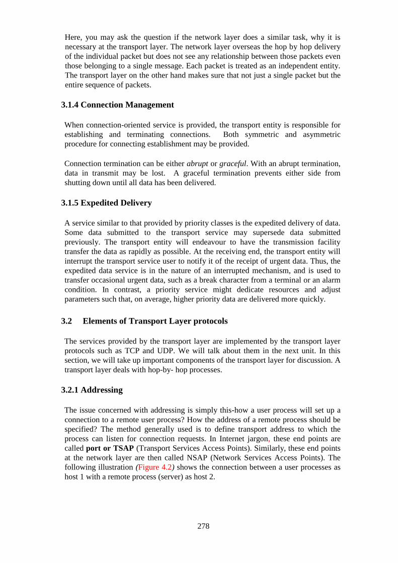
278

Here, you may ask the question if the network layer does a similar task, why it is

necessary at the transport layer. The network layer overseas the hop by hop delivery

of the individual packet but does not see any relationship between those packets even

those belonging to a single message. Each packet is treated as an independent entity.

The transport layer on the other hand makes sure that not just a single packet but the

entire sequence of packets.

3.1.4 Connection Management

When connection-oriented service is provided, the transport entity is responsible for

establishing and terminating connections. Both symmetric and asymmetric

procedure for connecting establishment may be provided.

Connection termination can be either abrupt or graceful. With an abrupt termination,

data in transmit may be lost. A graceful termination prevents either side from

shutting down until all data has been delivered.

3.1.5 Expedited Delivery

A service similar to that provided by priority classes is the expedited delivery of data.

Some data submitted to the transport service may supersede data submitted

previously. The transport entity will endeavour to have the transmission facility

transfer the data as rapidly as possible. At the receiving end, the transport entity will

interrupt the transport service user to notify it of the receipt of urgent data. Thus, the

expedited data service is in the nature of an interrupted mechanism, and is used to

transfer occasional urgent data, such as a break character from a terminal or an alarm

condition. In contrast, a priority service might dedicate resources and adjust

parameters such that, on average, higher priority data are delivered more quickly.

3.2 Elements of Transport Layer protocols

The services provided by the transport layer are implemented by the transport layer

protocols such as TCP and UDP. We will talk about them in the next unit. In this

section, we will take up important components of the transport layer for discussion. A

transport layer deals with hop-by- hop processes.

3.2.1 Addressing

The issue concerned with addressing is simply this-how a user process will set up a

connection to a remote user process? How the address of a remote process should be

specified? The method generally used is to define transport address to which the

process can listen for connection requests. In Internet jargon, these end points are

called port or TSAP (Transport Services Access Points). Similarly, these end points

at the network layer are then called NSAP (Network Services Access Points). The

following illustration (Figure 4.2) shows the connection between a user processes as

host 1 with a remote process (server) as host 2.

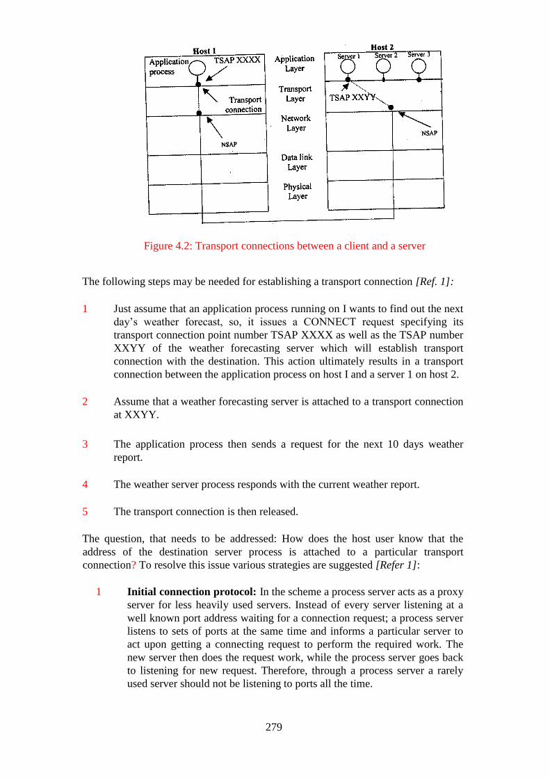
279

Figure 4.2: Transport connections between a client and a server

The following steps may be needed for establishing a transport connection [Ref. 1]:

1 Just assume that an application process running on I wants to find out the next

day‘s weather forecast, so, it issues a CONNECT request specifying its

transport connection point number TSAP XXXX as well as the TSAP number

XXYY of the weather forecasting server which will establish transport

connection with the destination. This action ultimately results in a transport

connection between the application process on host I and a server 1 on host 2.

2 Assume that a weather forecasting server is attached to a transport connection

at XXYY.

3 The application process then sends a request for the next 10 days weather

report.

4 The weather server process responds with the current weather report.

5 The transport connection is then released.

The question, that needs to be addressed: How does the host user know that the

address of the destination server process is attached to a particular transport

connection? To resolve this issue various strategies are suggested [Refer 1]:

1 Initial connection protocol: In the scheme a process server acts as a proxy

server for less heavily used servers. Instead of every server listening at a

well known port address waiting for a connection request; a process server

listens to sets of ports at the same time and informs a particular server to

act upon getting a connecting request to perform the required work. The

new server then does the request work, while the process server goes back

to listening for new request. Therefore, through a process server a rarely

used server should not be listening to ports all the time.

280

2 Some commonly used services are assigned ―well-known address‖

(for example, time sharing and word processing).

3 A name server or sometimes a directory server is provided. The Transport

Service user requests a service through some generic or global name. The

request is sent to the name server, which does a directory lookup and

returns an address. The transport entity then proceeds with the

connection. This service is useful for commonly used applications

that change location from time to time. It is also used for those stations in

which services do exist independently of a process server. For example, a

file server that needs 10 run on a special hardware (a machine with disk)

that cannot be created dynamically when someone want to talk to it [Ref.

1].

3.2.2 Multiplexing

The transport entity may also perform a multiplexing function with respect to the

network services that it uses. There are two types of multiplexing techniques that

define upward multiplexing as the multiplexing of multiple transport connections

on a single network connection, and downward multiplexing as the splitting of a

single transport connection among multiple lower-level connections. This is

illustrated in Figure 4.3

Transport Connections Transport Connections

Figure 4.3: Multiplexing

Consider, for example, a transport entity making use of an X.25 service. X.25 is a

network layer protocol like IP. Why should the transport entity employ upward

multiplexing? There are, after all, 4905 virtual circuits available. In the typical case,

this is a more than enough to handle all active Transport Service user. However, most

X.25 networks base part of their charge on virtual-circuit connect time, as each virtual

circuit consumes some node buffer resources. Thus, if a single virtual circuit provides

281

sufficient throughput for multiple TS users, upward multiplexing may be used [Figure

4.3].

On the other hand, downward multiplexing or splitting might be used to provide

more bandwidth than a single Virtual Circuit can manage. A way out is 10 open

multiple network connections and distribute traffic among them on a round-robin

basis, as indicated in Figure 4.3. This modus operandi is called downward

multiplexing. With network connections open, the effective bandwidth is increased

by a factor of k. A common example of downward multiplexing occurs with home

users who have an Integrated Service Digital Network (ISDN) line. This line

provides for two separate connections of 64 kbps each. Using both of them to call an

Internet provider and dividing the traffic over both lines makes it possible to achieve

an effective bandwidth of 128 kbps.

3.2.3 Flow Control and Buffering

There are similarities as well as differences between data link layer and transport

layer in order to support flow control mechanism. The similarity is in using the

sliding window protocol. The main difference is that a router usually has relatively

few lines, whereas a host may have numerous connections. Due to this reason it is

impractical to implement the data link buffering strategy in the transport layer.

Whereas flow control is a relatively simple mechanism at the data link layer, it is a

rather complex mechanism at the transport layer, for two main reasons:

1 Flow control at the transport level involves the interaction of three

components: TS users, transport entities, and the network service.

2 The transmission delay between transport entities is variable and generally

long compared to actual transmission time.

The following delay may arise during the interaction of the two transport entities A

and B:

1 Waiting time to get permission from its own transport entity (interface

flow control).

2 Waiting time by A to have permission to send the data to B.

3 Waiting time as network layer services.

In any case, once the transport entity has accepted the data, it sends out a segment.

Sometime later, it receives an acknowledgement that the data has been received at the

remote end. It then sends a confirmation to the sender.

Now let us come to the flow control problem.

First, we present two ways of coping with the flow control requirement [Ref.3] by

using a fixed sliding-window protocol and by using a credit scheme.

The first mechanism is already familiar to us from our discussions of data link layer

protocols. The key ingredients are:

282

1 The use of sequence numbers on data units.

2 The use of a window of fixed size.

3 The use of acknowledgements to advance the window.

This scheme really works well. For example, consider a protocol with a window size

of 3. Whenever the sender receives an acknowledgement from a particular segment,

it is automatically authorised to send the succeeding seven segments. (Of course,

some may already have been sent). Now, when the receiver‘s butter capacity comes

down to 7 segments, it can withhold acknowledgement of incoming segments to

avoid overflow. The sending transport entity can send, at most, seven additional

segments and then must stop. Because the underlying network service is reliable, the

sender will not time-out and retransmit. Thus, at some point, a sending transport

entity may have a number of segments outstanding, for which no acknowledgement

has been received. Because we are dealing with a reliable network, the sending

transport entity can assume that the segments will come through and that the lack of

acknowledgement is a flow control tactic. Such a strategy would not work well in an

unreliable network, as the sending transport entity would not know whether the lack

of acknowledgement is due to flow control or a lost segment.

The second alternative, a credit scheme, provides the receiver with a greater degree

of control over data flow.

The credit scheme decouples acknowledgement from flow control. In fixed sliding-

window protocols, used as the data Link layer, the two are synonymous. In a credit

scheme, a segment may be acknowledged without granting a new credit, and vice

versa. Figure 4.4 illustrates the protocol. For simplicity, we have depicted data flow

in one direction only. In this example, data segments are numbered sequentially

module 8 (e.g., SN 0 = segment with sequence number O). Initially, through the

connection-establishment process, the sending and receiving sequence numbers are

synchronised, and A is granted a credit allocation of 7. ―A‖ advances the trailing

edge of its window each time that it transmits, and advances the leading edge only

when it is granted a credit.

Figure 4.4 shows a view of this mechanism from the sending and receiving sides; of

course, both sides take both views because data may be exchanged in both directions.

From the receiving point of view, the concern is for received data and for the window

of credit that has been allocated. Note that the receiver is not required to immediately

acknowledge incoming segments, but may wait and issue a cumulative

acknowledgement for a number of segments; this is true for both TCP and the ISO

transport protocol.

In both the credit allocation scheme and the sliding window scheme, the receiver

needs to adopt some policy concerning the amount of data it permits the sender to

transmit. The conservative approach is only to allow new segments up to the limit of

available buffer space.

A conservative flow control scheme may limit the throughput of the transport

connection in long-delay situations. The receiver could potentially increase

283

throughput by optimistically granting credit for space it does not have. This is called

dynamic buffer allocation scheme. For example, if a receiver‘s buffer is full but it

anticipates that it can release space for two segments within a round-trip propagation

time, it could immediately send a credit of 2. If the receiver can keep up with the

sender, this scheme may increase throughput and can do no harm. If the sender is

faster than the receiver, however, some segments may be discarded, necessitating a

retransmission. Because retransmissions are not otherwise necessary with a reliable

network service, an optimistic flow control scheme will complicate the protocol.

® Status of sender's window alter transfer of 2 packets

Transport Entity A

0Status of sender's window after transfer of 3 more packets

@ Adjustment of each window with credit

Transport Entity A

0 1 2 3 4 5 6 7 0 1 2 3 4 5 6 7

284

(f) No remaining credits for A

Transport Entity B .

_,l.'l

c· -.t' >' --- c 0 1 2 3 4 5 6 7 0 1 2 3 4 5 6 7

@ Acknowledgment of S segments by rece1ver

Transport Entity A

lol!1213141sl6!7!o! ti213!4ISI617!

®.Sender receives a new credit

Figure 4.4: Flow control and buffering

The optimum trade-off between source buffering and destination buffering

depends on the type of traffic carried out by the connection. For low bandwidth busty

traffic, such as that produced by an interactive terminal. It is better not to dedicate any

buffer, but rather to acquire them dynamically at both ends. Since the sender cannot

be sure the receiver will be able to acquire a buffer, the sender must retain a copy of

the TPDU (Transport Protocol Data Unit) until it is acknowledged. On the other

hand, for file transfer and other high bandwidth traffic, it is better if the receiver

dedicates a full window of buffers, to allow the data to flow at maximum speed.

Thus, for low-bandwidth bursty traffic, it is better to buffer at the sender, and for

high-bandwidth smooth traffic, it is better to buffer at the receiver

.

As connections are opened and closed and as the traffic pattern changes, the sender

and receiver need to dynamically adjust their buffer allocations. Consequently, the

transport protocol should allow a sending host to request buffer space at the other

end. Buffers could be allocated per connection, or collectively, for all the connections

running between the two hosts. Alternatively, the receiver, knowing its buffer station

(but not knowing the offered traffic) could tell the sender ―I have reserved X buffers

for you‖. If the number of open connections should increase, it may be necessary for

an allocation to be reduced, so the protocol should provide for this possibility.

In summary, a reasonably general way to manage dynamic buffer allocation is to

decouple the buffering from the acknowledgements, in contrast to the sliding window

protocols of data link layer.

3.2.4 Connection Establishment

End-to-end delivery can be accomplished in either of two modes: connection-oriented

or connectionless. Of these two, the connection- oriented mode is the more

285

commonly used. A connection-oriented protocol establishes a virtual circuit or

pathway through the Internet between the sender and receiver. All of the packets

belonging to a message are then sent over this same path. Using a single pathway for

the entire message facilities, the acknowledgement process and retransmission of

damaged or lost frames. Connection-oriented services, therefore, are generally

considered reliable.

Connection-oriented transmission has three stages: connection establishment, data

transfer, and connection termination.

The network is generally unreliable and congested. Even with a reliable network

service, there is a need for connection establishment and termination -procedures to

support connection-oriented service.

Connection establishment serves three main purposes:

1. It allows each end to assure that the other exists.

2. It allows negotiation of optional parameters (e.g., minimum segment size,

maximum window size, quality of service).

3. It triggers allocation of transport entity resources (e.g., buffer space, entry in

connection table).

To solve the problems arising out of unreliable and congested networks 3-way

handshake procedure is used to establish transport connection, which is generally

comprised of three steps.

1. Connection initiation requirement

2. Connection confirmation

3. Acknowledgement of confirmation and data transfer.

3.1.5 Crash Recovery

Similar to the database this is an important issue in computer network. In a network a host

as well as a router can crash. Therefore, the issue is its recovery. In case of the loss of

Virtual Circuit (In case the network layer provides connection-oriented service) due to a

crash delivery, a new virtual circuit may be established then probing the transport entity to

ask which TPDU it has received and which one it has not received so that the latter can be

retransmitted. In case of datagram subnet, the frequency of the lost TPDU is high but the

network layer knows how to handle that. The real problem is the recovery from the host

crash. Students are requested to read Computer Network by Tanenbaum on this method

and also to relate to how a similar problem is resolved in the database (MCS-043).

4.0 CONCLUSION

In this unit you have learnt about transport services mechanism which comprise types of

transport services, quality of service data transfer mechanism, connection establishment,

multiplexing and finally flow control and buffering.

5.0 SUMMARY

286

In this unit, we have discussed two important components with respect to transport layer

namely, transport services and the elements of transport layer protocols. As a part of

transport services, we discussed type of services, quality of services, connection

mechanism. We also outlined three types of services provided by the transport layer

through the applications layer. We listed the various types of protocols (applications

layer) and the kind of services. We also differentiated between the data link layer and

transport layer with respect to flow control mechanism. Similarly, we also differentiated

between two types of multiplexing mechanism at the transport layer.


1. List the three types of services provided by Transport layer to

Applications layer.

2. Describe the presence of data loss and time sensitiveness for the

following applications:

a. File Transfer

b. E-mail

c. Web surfing

d. Real time audio/video.

3. List the important multiplexing mechanism at the Transport Layer and

also U explain how they are different from each other.


A. S. Tanenbaum, Computer Networks, 4th Edition. Prentice Hall of India, New Delhi,

2011.

James Kurose and Keith W. Ross, Computer Networking. A Top down approach

featuring the Internet, Pearson education, New Delhi.

William Stallings, Data and Computer communication. 6th

Edition, Pearson

Education, New Delhi, 2003.


Question 1

List the three types of services provided by Transport layer to Applications layer.

The services are:

a. Quality of service

b. Data transfer

c. Connection management

d. Expedited delivery

Question 2

Describe the presence of data loss and time sensitiveness for the following

applications:

287

a File Transfer

b E-mail

c Web surfing

d Stored audio/video.

Solution

a. File Transfer: File transfer is conscious of data loss and so it needs to be error

free. Hence, it is pertinent for the file to be error free in transmission rather than

been fast in transmission.

b. E-Mail: this is not delay sensitive. If the delays are uniform within a few

seconds, there will be no harm. Email does not need much bandwidth to

operate.

c. Web surfing: this is delay sensitive.

d. Real-time audio/video: here loss of data might result in small glitch while

playing the video, the effect of such loss on application quality and actual

amount of tolerable loss will depend strongly on the application and the coding

scheme used. Video and audio use a lot of bandwidth and are extremely

sensitive to jilter. For audio jilter of a few milliseconds is clearly audible.

Question 3

List the important multiplexing mechanism at the Transport Layer and also U

explain how they are different from each other.

Solution

The important multiplexing mechanism at the transport are:

a. Upward multiplexing

b. Downward multiplexing

Explain the difference between them.

288

UNIT 2 TCP/UDP

CONTENTS

1.0 Introduction

2.0 Objectives

3.0 Main Content

3.1 Services Provided by Internet Transport Protocols

3.1.1 TCP Services

3.1.2 UDP Services

3.2 Introduction to UDP

3.3 Introduction to TCP

3.4 TCP Segment Header

3.5 TCP Connection Establishment

3.6 TCP Connection Termination

3.7 TCP Flow Control

3.8 TCP Congestion Control

3.9 Remote Procedure Call

4.0 Conclusion

5.0 Summary



1.0 INTRODUCTION

In the previous unit, we discussed the fundamentals of the transport

layer which covered topics related to the quality of services, addressing,

multiplexing, flow control and buffering. The main protocols which are commonly

used such as TCP (Transmission Control Protocol and UDP (User Diagram Protocol)

were also discussed. TCP is the more sophisticated protocol of the two and is used

for applications that need connection establishment before actual data transmission.

Applications such as electronic mail, remote terminal access, web surfing and file

transfer are based on TCP.

UDP is a much simpler protocol than TCP because, it does not establish any

connection between the two nodes. Unlike TCP, UDP does not guarantee the delivery

of data to the destination. It is the responsibility of application layer protocols to

make UDP as reliable as possible.

In this unit, we will go into details on these two protocols.

2.0 OBJECTIVES

289


1 list and explain the various services provided by the Transport Layer

2 establish and release TCP connections

3 describe TCP and UDP header formats

4 describe TCP Flow Control mechanism and how it is different from data link

layer

5 discuss the Congestion mechanism in TCP.

3.0 MAIN CONTENT

3.1 Services Provided by Internet Transport Protocols

The Internet provides two service models: TCP and UDP. The selection of a

particular service model is left to the application developers. TCP is a connection

oriented and reliable data transfer service whereas UDP is connectionless and

provides unreliable data transfer service.

3.1.1 TCP Services

When an application invokes TCP for its transport protocol, the application receives

the following services from it:

1 Connection oriented service

2 Reliable transport service

3 Congestion-control mechanism.

Now let us describe these services in brief:

Connection-oriented service

As you are aware from your understanding of the previous unit that the connection-

oriented service is comprised of the handshake procedure which is a full duplex

connection in that, two processes can send messages to each other over the

connection at the same time. When the application has finished sending the message,

it must remove the connection. The service is referred to as a ―connection oriented‖

service. We are also aware from the discussion on the network layer that this service

is implemented through the virtual circuit mechanism.

Reliable Transport Service

Communicating processes can rely on TCP to deliver all the data that is sent, without

error and in the proper order. When one side of the application passes a stream of

bytes into a socket, it can count on TCP to deliver the same stream of data to the

receiving socket, with no missing or duplicate bytes. Reliability in the Internet is

achieved with the use of acknowledgement and retransmissions.

290

Congestion-control mechanism: TCP also includes a congestion-control mechanism

for the smooth functioning of Internet processes. When the packet load offered to the

network exceeds its handling capacity congestion builds up.

One point to be noted is that, although, the Internet connection-oriented service is

bundled with suitable data transfer, flow control and congestion control mechanisms,

they are not the essential components of the Connection oriented service [Ref. 2].

A connection-oriented service can be provided with bundling these services through

a different type of a network.

Now we will look at the services TCP does not provide? Some of these are:

1 It does not guarantee a minimum transmission rate,

2 It does not provide any delay guarantee. But it guarantees delivery of all data.

However, it provides no guarantee to the rate of data delivery.

3.1.2 UDP Services

Some of the important features of UDP are as follows:

1 UDP is connection less, so there is no hand shaking before the two

processes start communications.

2 It provides unreliable data transfer service therefore, there is no guarantee

that the message will reach. Due to this, the message may arrive as the

receiving process at a random time.

3 UDP does not provide a congestion-control service. Therefore, the sending

process can pump data into a UDP socket at any rate it pleases. Then, why

do we require such a protocol at the transport layer? There are certain types

of applications such as real time. Real-time applications are applications

that can tolerate some loss but require a minimum rate. Developers of real-

time applications often choose to run their applications over the UDP

because their applications cannot wait for acknowledgements for data input.

Now coming back to TCP, since it guarantees that all the packets will be

delivered to the host, many application protocols, layer protocols are used

for these services. For example, SMTP (E-mail), Telnet, HTTP, FTP

exclusively uses TCP whereas NFS and Streaming Multimedia may use

TCP or UDP. But Internet telephony uses UDP exclusively.

3.2 Introduction to UDP

So, you might have guessed from the previous section, that UDP is and unreliable

transport protocol. Apart from multiplexing/demultiplexing and some error correction

UDP adds little to the IP protocol. In this section, we take a look at UDP, at how it

works and at what it does.

In case, we select UDP instead of TCP for application development, then the

application is almost directly talking to the IP layer. UDP takes messages from the

291

application process, attaches the source and destination port number fields for the

multiplexing/demultiplexing service, adds two other small fields, and passes the

resulting segment to the network layer. Without establishing handshaking between

sending and receiving transport-layer entities, the network layer encapsulates the

segment into an IP datagram and then makes a best-effort attempt to deliver the

segment to the receiving host. If the segment arrives at the receiving host, UDP uses

the destination port number to deliver the segment‘s data to the desired application

process.

So, you might ask a question then why is UDP required? TCP should be the choice

for all types of application layer/protocol. DNS stands for domain name system. It

provides a directory service for the internet. It is commonly used by other application

protocols (HTTP, FTP etc.) to translate user given host names to IP address. But

before we answer your question let-us look at another application called the DNS,

which runs exclusively in UDP only but unlike other protocols DNS is not an

application with which users interact directly. Instead DNS is a core Internet function

that translates the host name to IP addresses. Also, unlike other protocols, DNS

typically uses UDP. When the DNS application in a host wants to make a query, it

constructs a DNS query message and passes the message to the UDP. Without

performing any handshaking with the UDP entity running on the destination end

system, UDP adds header fields to the message and passes the resulting segment to

the network layer. The network layer encapsulates the UDP segment into a datagram

and sends the datagram to a name server. The DNS application at the querying host

then waits for a reply to its query. If it doesn‘t receive a reply (possibly because the

underlying network lost the query or the reply), either it tries sending the query to

another name server, or it informs the invoking application that it can‘t get a reply.

Like DNS, there are many applications, which are better suited for UDP for the

following reasons [Ref2]:

No Connection Establishment

Since UDP does not cause any delay in establishing a connection, this is a probably

the principal reason why DNS runs over UDP rather than TCP-DNS which would be

much slower if it runs over TCP. HTTP uses TCP rather than UDP, since reliability

is critical for Web pages with text.

More Client Support

TCP maintains connection state in the end systems. This connection state includes

receiving and sending buffers, congestion-control parameters, and sequence and

acknowledgement number parameters. We will see in Section 3.5 that this state

information is needed to implement TCP‘s reliable data transfer service and

to provide congestion control. UDP, on the other hand, does not maintain

connection state and does not track any of these parameters. A server devoted to a

particular application can typically support many more active clients when the

application runs over UDP rather than TCP. Because UDP, (unlike TCP) does not

provide reliable data service and congestion control mechanism, therefore, it does not

need to maintain and track the receiving and sending of buffers (connection states),

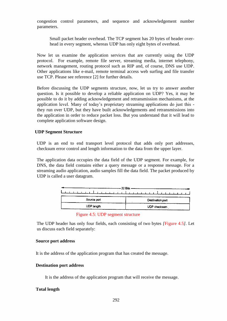
292

congestion control parameters, and sequence and acknowledgement number

parameters.

Small packet header overhead. The TCP segment has 20 bytes of header over-

head in every segment, whereas UDP has only eight bytes of overhead.

Now let us examine the application services that are currently using the UDP

protocol. For example, remote file server, streaming media, internet telephony,

network management, routing protocol such as RIP and, of course, DNS use UDP.

Other applications like e-mail, remote terminal access web surfing and file transfer

use TCP. Please see reference [2] for further details.

Before discussing the UDP segments structure, now, let us try to answer another

question. Is it possible to develop a reliable application on UDP? Yes, it may be

possible to do it by adding acknowledgement and retransmission mechanisms, at the

application level. Many of today‘s proprietary streaming applications do just this -

they run over UDP, but they have built acknowledgements and retransmissions into

the application in order to reduce packet loss. But you understand that it will lead to

complete application software design.

UDP Segment Structure

UDP is an end to end transport level protocol that adds only port addresses,

checksum error control and length information to the data from the upper layer.

The application data occupies the data field of the UDP segment. For example, for

DNS, the data field contains either a query message or a response message. For a

streaming audio application, audio samples fill the data field. The packet produced by

UDP is called a user datagram.

Figure 4.5: UDP segment structure

The UDP header has only four fields, each consisting of two bytes [Figure 4.5]. Let

us discuss each field separately:

Source port address

It is the address of the application program that has created the message.

Destination port address

It is the address of the application program that will receive the message.

Total length

293

It specifies the length of UDP segment including the header in bytes.

Checksum: The checksum is used by the receiving host to check whether errors have

been introduced into the segment. In truth, the checksum is also calculated over a few

of the fields in the IP header in addition to the UDP segment.

3.3 Introduction to TCP

TCP is designed to provide reliable communication between pairs of processes (TCP

users) across a variety of reliable and unreliable networks and Internets. TCP is

stream oriented (Connection Oriented). Stream means that every connection is treated

as stream of bytes. The user application does not need to package data in individual

datagram as it is done in UDP. In TCP a connection must be established between the

sender and the receiver. By creating this connection, TCP requires a VC at IP layers

that will be active for the entire duration of a transmission. The data is placed in

allocated buffers and transmitted by TCP in segments. In addition, TCP provides two

useful facilities for labelling data, push and urgent:

[When the PSH (data push) bit is set, this is an indication that the receiver should

pass the data to the upper layer immediately. The URG (Urgent) bit is used to

indicate that there is data in this segment that the sending side upper layer entity has

marked as urgent. The location of the last byte of this urgent data is indicated by the

16 bit urgent data pointer field 7).

Both IP and UDP treat multiple datagrams belongings to a single transmission as

entirely separate units, un-related to each other. TCP on the other hand is responsible

for the reliable delivery of entire segments. Every segment must be received and

acknowledged before the VC is terminated.

3.4 TCP Segment Header

TCP uses only a single type of protocol data unit, called a TCP segment. The header

is shown in Figure 4.6. Because one header must perform all protocol mechanisms, it

is rather large, with a minimum length of 20 octets. A segment beginning with 9

fixed format 20 byte headers may be followed by header option [Ref. I]. After the

options, if any, up to 65,535 -20 (IP header) -(TCP header) = 65,445 data bytes may

follow. A Segment with no data is used, for controlling messages and

acknowledgements.

294

Figure 4.6: TCP header format

The fields are:

Source port (16 bits)

Source service access points and identify local end points of connection.

Sequence number (32 bits)

Sequence number of the first data octet in this segment except when SYN is present. If

SYN is present, it is the initial sequence number (ISN), and the first data octet is

ISN+1.

Acknowledgement number (32 bits)

A piggybacked acknowledgement contains the sequence number of the next byte that

the TCP entity expects to receive and not for last byte correctly received. Separate

number field and acknowledgement number fields are used by the TCP sender and

the receiver has to implement a reliable data service.

Data offset (4 bits)

Number of 32-bit, words in the header.

Reserved (6 bits)

Reserved for future use.

Flags (6 bits):

URG: Used to indicate that there is data in this segment which sends the data at the

upper layer has marked urgent. The location of the last byte of this urgent data is

indicated by the 16 bit urgent data pointer field. ACK: Acknowledgement field

indicates that the value carried in the ACK field is valid.

295

PSH: Push function. The receiver is represented to deliver the data to the application

upon arrival, and not butter it until a full butter has been received.

RST: Reset the connection due to host crash or some other reason.

SYN: Synchronise the sequence numbers.

FIN: No more data from sender.

Receive Window (16 bits)

Used for credit based flow control scheme, in bytes. Contains the number of

data bytes beginning with the one indicated in the acknowledgement field that the

receiver is willing to accept.

Checksum (16 bits)

It provides extra reliability. It Checksums the header, the data and conceptual pseudo

header. The Checksum algorithm simply adds up all the 16bit words in one‘s

complement and then takes one‘s complement of the sum. As a consequence, when

the receiver performs calculations on the entire segment including the checksum

field, the result should be 0 [Ref. 1].

Urgent data pointer (16 bits)

Points to the octet following the urgent data; this allows the receiver to know how

much urgent data is coming.

Options (Variable)

At present, only one option is defined, which specifies the maximum segment size

that will be accepted.

Several of the fields in the TCP header warrant further elaboration. The source port

and destination port specify the sending and receiving users of TCP. As with IP,

there are a number of common users of TCP that have been assigned numbers; these

numbers should be reserved for that purpose in any implementation. Other port

numbers must be arranged by agreement between communicating parties.

3.5 TCP Connection Establishment

Before data transmission, a connection must be established. Connection

establishment must take into account the unreliability of a network service, which

leads to a loss of ACK, data as well as SYN. Therefore, the retransmission of these

packets have to be done. Recall that a connection establishment calls for the

exchange of SYNs.

Figure 4.7 illustrates typical three-way [Ref. 3] handshake operations.

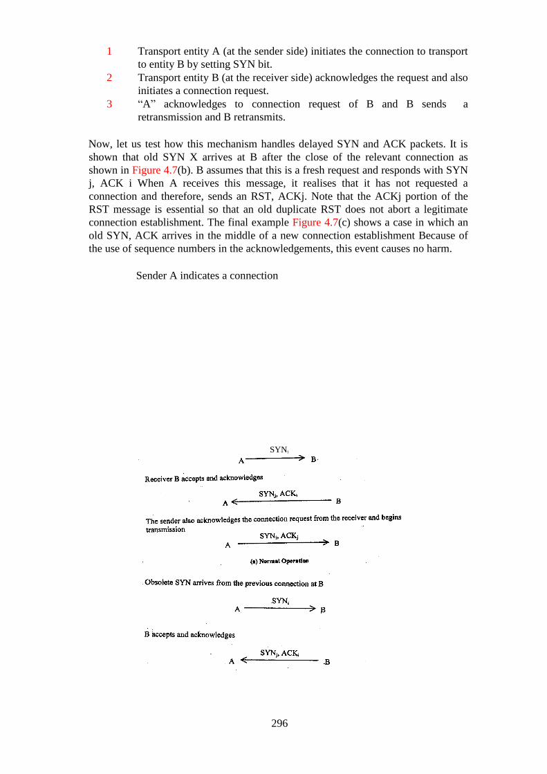
296

1 Transport entity A (at the sender side) initiates the connection to transport

to entity B by setting SYN bit.

2 Transport entity B (at the receiver side) acknowledges the request and also

initiates a connection request.

3 ―A‖ acknowledges to connection request of B and B sends a

retransmission and B retransmits.

Now, let us test how this mechanism handles delayed SYN and ACK packets. It is

shown that old SYN X arrives at B after the close of the relevant connection as

shown in Figure 4.7(b). B assumes that this is a fresh request and responds with SYN

j, ACK i When A receives this message, it realises that it has not requested a

connection and therefore, sends an RST, ACKj. Note that the ACKj portion of the

RST message is essential so that an old duplicate RST does not abort a legitimate

connection establishment. The final example Figure 4.7(c) shows a case in which an

old SYN, ACK arrives in the middle of a new connection establishment Because of

the use of sequence numbers in the acknowledgements, this event causes no harm.

Sender A indicates a connection

SYNi

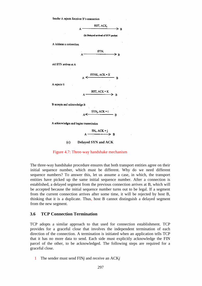
297

(c) Delayed SYN and ACK

Figure 4.7: Three-way handshake mechanism

The three-way handshake procedure ensures that both transport entities agree on their

initial sequence number, which must be different. Why do we need different

sequence numbers? To answer this, let us assume a case, in which, the transport

entities have picked up the same initial sequence number. After a connection is

established, a delayed segment from the previous connection arrives at B, which will

be accepted because the initial sequence number turns out to be legal. If a segment

from the current connection arrives after some time, it will be rejected by host B,

thinking that it is a duplicate. Thus, host B cannot distinguish a delayed segment

from the new segment.

3.6 TCP Connection Termination

TCP adopts a similar approach to that used for connection establishment. TCP

provides for a graceful close that involves the independent termination of each

direction of the connection. A termination is initiated when an application tells TCP

that it has no more data to send. Each side must explicitly acknowledge the FIN

parcel of the other, to be acknowledged. The following steps are required for a

graceful close.

1 The sender must send FINj and receive an ACKj

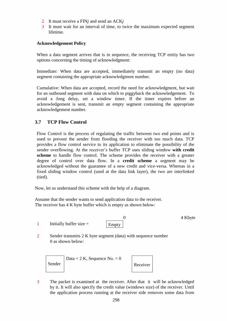
298

2 It must receive a FINj and send an ACKj

3 It must wait for an interval of time, to twice the maximum expected segment

lifetime.

Acknowledgement Policy

When a data segment arrives that is in sequence, the receiving TCP entity has two

options concerning the timing of acknowledgment:

Immediate: When data are accepted, immediately transmit an empty (no data)

segment containing the appropriate acknowledgment number.

Cumulative: When data are accepted, record the need for acknowledgment, but wait

for an outbound segment with data on which to piggyback the acknowledgement. To

avoid a Jong delay, set a window timer. If the timer expires before an

acknowledgement is sent, transmit an empty segment containing the appropriate

acknowledgement number.

3.7 TCP Flow Control

Flow Control is the process of regulating the traffic between two end points and is

used to prevent the sender from flooding the receiver with too much data. TCP

provides a flow control service to its application to eliminate the possibility of the

sender overflowing. At the receiver‘s buffer TCP uses sliding window with credit

scheme to handle flow control. The scheme provides the receiver with a greater

degree of control over data flow. In a credit scheme a segment may be

acknowledged without the guarantee of a new credit and vice-versa. Whereas in a

fixed sliding window control (used at the data link layer), the two are interlinked

(tied).

Now, let us understand this scheme with the help of a diagram.

Assume that the sender wants to send application data to the receiver.

The receiver has 4 K byte buffer which is empty as shown below:

0 4 Kbyte

1 Initially buffer size =

2 Sender transmits 2 K byte segment (data) with sequence number

0 as shown below:

Sender

Data = 2 K, Sequence No. = 0

Receiver

3 The packet is examined at the receiver. After that it will be acknowledged

by it. It will also specify the credit value (windows size) of the receiver. Until

the application process running at the receiver side removes some data from

Empty

299

buffer, its buffer size remains fixed at 2048. Therefore, credit value (window

size) is 2048 byte.

Receivers

Buffer =

ACK = 2048. Sequence No. = 2048 Credit = 2048

Sender Receiver

4 Now the sender transmits another 2048 bytes, which is

acknowledged, but the advertised window (credit) is 0.

Receivers

Buffer =

Data = 2048. Sequence No. = 2048

Sender Receiver

5 The sender must stop sending data until the application process on the

receiving host has removed some data from the buffer, at which time TCP can

advertise, a large window (credit value).

Receivers

Buffer =

ACK = 4096. Credit = 2048

Sender Receiver

When the credit size is zero, normally there is no transmission from the sender side

except in two situations:

1 Urgent data requires to be sent

2 Sender wants to know the credit size and the next byte expected by the

receiver.

Both senders and receivers can delay transmission from their side to resources. If a

sender knows that the buffer capacity of a receiver window is 8 K and currently it has

received just 2 K, then it may buffer it at the sender side till it gets more data from the

application process. Similarly, the receiver has to send some data to the sender it can

delay the acknowledgement till its data is ready for that the acknowledgement can be

piggybacked. Therefore, the basic reason of delaying the acknowledgement is to

reduce the bandwidth.

Let us consider an example of a log-in session, for example, Telnet Session in which

the user types one character at a time and the server (log-in server) reacts to every

keystroke. You will notice that one character requires four exchanges of IP packets

between the log-in session client and a Telnet server which is illustrated below:

[2 K data Empty

Full

Application

has read 2 K

byte data

2 K

300

Assume that TCP and IP header are 20 bytes each).

1st exchange (at the sender side)

- Whenever application data comes to TCP sender, it creates

20 bytes of a segment, which it gives to IP to create an IP

datagram.

Total no. of bytes sent = 20 bytes (TCP) + 20 bytes (IP) + I byte for

a character (a key stroke) = 41 byte.

2nd exchange (at the receiver side)

- The receiver (Telnet a log-in server) immediately sends an

acknowledgement to the sender.

Total no. of bytes sent by the server = 20 bytes (TCP) +20 byte (IP)

= 40 bytes No extra byte is required for an acknowledgement.

3rd exchange (From the log-in server)

- Window update-related message which moves to window

one byte right.

Total no of byte sent -20bytes (TCP) + 20byte (IP) = 40 bytes.

4th exchange (From the log-in server)

- Echos Character back to the client

Total no. bytes -20 bytes (TCP) + 20 byte (IP) + 1 byte (0 char) = 41 bytes.

Therefore, the total number of bytes exchanged = 41 + 40 + 40 + 41 = 162 bytes.

So what is the solution to reduce the wastage of bandwidth? The solution has been

proposed by Nagle and is known as Nagle’s algorithm.

The algorithm works as follows: When data comes the sender one byte at a time, just

send the first byte and buffer all the rest until the outstanding byte is acknowledged.

In the meantime, if the application generates some more characters before the

acknowledgement arrives, TCP will not transmit the character but buffer them

instead. After the acknowledgement arrives TCP transmits all the characters that have

been waiting in the buffer in a single segment.

Nagle’s algorithm is widely used for the TCP implementation). But in certain cases,

the algorithm might not be applicable. For example, in highly interactive applications

where every keystroke or a curser movement is required to be sent immediately.

301

Another problem that wastes network bandwidth is when the sender has a large

volume of data to transmit and the receiver can only process its receiver buffer a few

bytes at a time. Sooner or later the receiver buffer becomes full. When the receiving

application reads a few bytes from the receive buffer, the receiving TCP sends a

small advertisement window to the sender, which quickly transmits a small segment

and fills the receiver buffer again. This process goes on and on with many small

segments being transmitted by the sender for a single application message. This

problem is called the silly window syndrome. It can be avoided if the receiver does

not advertise the window until the window size is at least as large as half of the

receiver buffer size or the maximum segment size. The sender side can cooperate

by refraining from transmitting small segments.

To summarize, the silly window syndrome can be explained stepwise as:

Step I: Initially the receiver buffer is full

Step II: Application process reads one byte at the receiver side.

Step III:

The TCP running at the receiver sends a window update to

the sender.

Step IV: The TCP sender sends another byte.

Step V: The receiver buffer is filled up again.

Steps III, IV and V continue forever. Clark’s solution is to prevent the receiver from

sending a window update for I byte. In the solution, the receiver window is forced to

wait until it has a sufficient amount of space available and then only advertise.

Specifically, the receiver should not send a window update until it can handle the

maximum segment size it advertised when the connection was established, or its

buffer half empty, whichever is smaller.

Nagle‘s algorithm and Clark‘s solution to the silly window syndrome are

complementary. Both solutions are valid and can work together. The goal is for the

sender not to send small segments and the receiver not to ask for them. Nagle was

trying to solve the problem caused by the sending application delivering data to TCP

a byte at a time. Clark was trying to solve the problem of the receiving application.

3.8 TCP Congestion Control

As discussed in the previous section, TCP provides many services to the application

process. Congestion Control is one such service. TCP uses end-to-end Congestion

Control rather than the network supported Congestion Control, since the IP Protocol

does not provide Congestion released support to the end system. The basic idea of

TCP congestion control is to have each sender transmit just the right amount of data

to keep the network resources utilised but not overloaded. You are also aware that

TCP flow control mechanism uses a sliding-window protocol for end-to-end flow

control. This protocol is implemented by making the receiver advertise in its

acknowledgement the number of bytes it is willing to receive in the future, called the

advertised window to avoid the receiver‘s buffer from overflow. By looking at the

302

advertised window, the sender will resist transmitting data that exceeds the amount

that is specified in the advertised window. However, the advertised window does not

prevent the buffers in the intermediate routers from overflowing due to which routers

get overloaded. Because IP does not provide any mechanism to control congestion, it

is up to the higher layer to detect congestion and take proper action. It turns out that

TCP window mechanism can also be used to control congestion in the network.

The protocols designers have to see that the network should be utilised very

efficiently (i.e., no congestion and no underutilisation). If the senders are too

aggressive and send too many packets, the network will experience congestion. On

the other hand, if TCP senders are too conservative, the network will be

underutilised. The maximum number of bytes that a TCP sender can transmit without

congesting the network is specified by another window called the congestion

window. To avoid network congestion and receiver buffer overflow, the maximum

amount of data that the TCP sender can transmit at any time is the minimum of the

advertised window (receiver window) and the congestion window. Thus, the

effective window is the minimum of what the sender thinks is OK and what the

receiver thinks is OK. If the receiver advertises for 8K window but the sender sends

4K size of data if it thinks that 8 K will congest the network, then the effective

windows size is 4K.

The approach used in TCP is to have each sender limit the rate of data traffic into the

network as a function of perceived network congestion. If a TCP sender perceives

that there is small congestion along the path, then it increases its send rate otherwise

it reduces it.

The TCP congestion control algorithm dynamically adjusts the congestion window

according to the network state. The algorithm is called slow start. The operation of

the TCP congestion control algorithm may be divided into three phases: slow start,

congestion avoidance and congestion occurrence. The first phase is run when the

algorithm starts or restarts, assuming that the network is empty. The technique, slow

start, is accomplished by first setting the congestion window to one maximum-size

segment. Each time the sender receives an acknowledgement from the receiver, the

sender increases the congestion window by one segment. After sending the first

segment, if the sender receives an acknowledgement before a time-out, the sender

increases the congestion window to two segments. If these two segments are

acknowledged, the congestion window increases to four segments, and so on. As

shown in the Figure 4.8, the congestion window size grows exponentially during this

phase. The reason for the exponential increase is that slow start needs to fill an empty

pipe as quickly as possible. The name ―slow start‖ is perhaps a misnomer, since the

algorithm ramps up very quickly.

Slow start does not increase the congestion window exponentially forever, since the

network will be filled up eventually. Specifically, slow start stops when the

congestion window reaches a value specified as the congestion threshold, which is

initially set to 65,535 bytes. At this point a congestion avoidance (2nd phase) phase

takes over. This phase assumes that the network is running close to full utilisation. It

is wise for the algorithm to reduce the rate of increase so that it will not overshoot

excessively. Specifically, the algorithm increases the congestion window

linearly rather than exponentially when it tries to avoid congestion. This is realised

by increasing the congestion window by one segment for each round-trip time.

303

Obviously, the congestion window cannot be increased indefinitely. The congestion

window stops increasing when TCP detects that the network is congested. The

algorithm now enters the third phase.

Number of transmissions

Figure 4.8: Dynamics of TCP congestion window

At this point the congestion threshold is first set to one-half of the current window

size (the minimum of the congestion window and the advertised window, but at least

two segments). Next the congestion window is set to one maximum-sized segment.

Then the algorithm restarts, using the slow start technique.

How does TCP detect network congestion? There are two approaches:

1 Acknowledgement does not arrive before the timeout because of a segment

loss.

2 Duplicate acknowledgement is required.

The basic assumption the algorithm is making is that, a segment loss is due to

congestion rather than errors. This assumption is quite valid in a wired network

where the percentage of segment losses due to transmission errors is generally

low (less than 1 per cent). Duplicate ACK can be due to either segment reordering or

segment loss. In this case the TCP decreases the congestion threshold to one-half of

the current window size, as before. However, the congestion window is not reset to

one. If the congestion window is less than the new congestion threshold, then the

congestion window is increased as in slow start. Otherwise, the congestion window is

increased as in congestion avoidance. However, the assumption may not be valid in a

wireless network where transmission errors can be relatively high.

The Figure 4.8 illustrates the dynamics of the congestion window as time progresses.

Thus, assumes that maximum segment size is 1024, threshold to 32K and congestion

window to I K for the first transmission. The congestion window then grows

exponentially (slow start phase) until it hits the threshold (32 K). After that it grows

304

linearly (congestion avoidance phase I). Now, when congestion occurs, the threshold

is set to half the current window (20 K) and slow start initiated all over again. In case

there is no congestion, the congestion window will continue to grow.

In short, TCP‘s congestion control algorithm operates as follows:

1 When the Congestion Window is below the threshold, the sender uses for

slow start phase and congestion window grows exponentially.

2 When the congestion window is above the threshold the sender is in the

congestion avoidance phase and congestion window grows linearly.

You may wish to refer the references [1], [2] and [4] for further clarification on the

subject.

3.9 Remote Procedure Call

In this section we will look at two other files access mechanisms such as Network

File System and Remote Procedure Call used for accessing files from a server at the

client machine. These two mechanisms allow programs to call procedures located on

remote machines.

Network File System (NFS)

The network file system (NFS) is a file access protocol. FTP and TFTP transfer entire

files from a server to the client host. A file access service, on the other hand, makes

file systems on a remote machine visible, though they were on your own machine but

without actually transferring the files. NFS provides a number of features:

1 NFS allows you to edit a file on another machine exactly as you would if it

were on your own machine.

2 It even allows you to transfer files from the server to a third host not directly

connected to either of you.

Remote Procedure Call (RPC)

NFS works by invoking the services of a second protocol called remote procedure

call (RPC). Figure 4.9 shows a local procedure call (in this case, a C program calls

the open function to access a file stored on a disk).

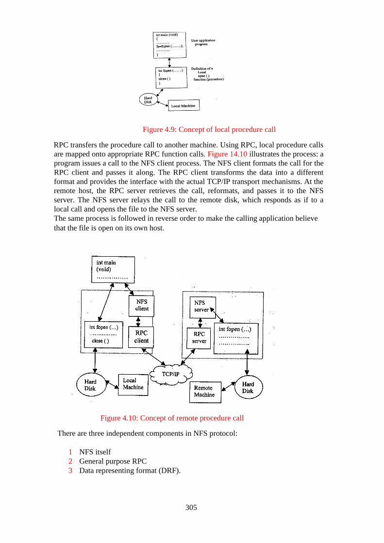
305

Figure 4.9: Concept of local procedure call

RPC transfers the procedure call to another machine. Using RPC, local procedure calls

are mapped onto appropriate RPC function calls. Figure 14.10 illustrates the process: a

program issues a call to the NFS client process. The NFS client formats the call for the

RPC client and passes it along. The RPC client transforms the data into a different

format and provides the interface with the actual TCP/IP transport mechanisms. At the

remote host, the RPC server retrieves the call, reformats, and passes it to the NFS

server. The NFS server relays the call to the remote disk, which responds as if to a

local call and opens the file to the NFS server.

The same process is followed in reverse order to make the calling application believe

that the file is open on its own host.

Figure 4.10: Concept of remote procedure call

There are three independent components in NFS protocol:

1 NFS itself

2 General purpose RPC

3 Data representing format (DRF).

306

In order to make the NFS computer independent what can be done is to use RPC and

DRF in other software, (including application), programme by dividing a program

into a client side and a server side that use RPC as the chief transport mechanism. On

the client side, the transfer procedures may be designated as remote, forcing the

compiler to incorporate RPC code into those procedures, On the server side, the

desired procedures are implemented by using other RPC facilities to declare them as

a part of a server. When the executing client program calls one of the remote

procedures, RPC automatically collects values for arguments, from a message, sends

the message to the remote server, awaits a response, and stores returned values in

the designated arguments. In essence, communication with the remote server occurs

automatically as a side-effect of a remote call. The RPC mechanism hides all the

details of protocols, making it possible for programmers who know little about the

underlying communication protocols but who can write distributed application

programs.

4.0 CONCLUSION

This unit has taken you through the various services provided by the Transport layer

as well as how to establish and release TCP connections. You have also learnt how

the TCP Flow Control mechanism and how it is different from data link layer as well

as congestion mechanism in TCP.

5.0 SUMMARY

In this unit, we discussed the two transport layer protocols (TCP & UDP) in detail.

The transport port can be light weight (very simple) which provide very little facility.

In such cases, the application directly talks to the IP. UDP is an example of a

transport protocol, which provides minimum facility, with no control, no connection

establishment, no acknowledgement and no congestion handling feature. Therefore, if

the application is to be designed around the UDP, then such features have to be

supported in the application itself. On the other hand, there is another protocol- TCP

which provides several feature such as reliability, flow control, connection

establishment to the various application services. Nevertheless, the services

that the transport layer can provide often constrain the network layer protocol.

We had a close look at the TCP connection establishment, TCP flow control, TCP

congestion handling mechanism and finally UDP and TCP header formats. With

respect to congestion control, we learned that congestion control is essential for the

well-being of the network. Without congestion control the network can be blocked.


1. Is it true that if IP is the network layer protocol, so TCP must be the

transport layer 1?

2. There are two protocols at the transport layer, which of the two is

better?

3. What is the difference between FTP and NFS?

4. What is a flow control problem? What is the basic mechanism at the

transport layer to handle flow control problem?

307


A.S Tanebaum, (2011). Computer Networks, 4th Edition, PHI, New Deihi.

J. F. Kurose & K. W. (2003). Computer Networking, A top down approach featuring

the Internet, Ross, Pearson Edition, New Delhi.

William Stallings, (2003). Data and Computer Communication, 6th Edition,

Pearson Education, New Delhi.

Leon Garcia, and Widjaja, (2000). Communications Networks, Tata McGraw

Hill.


Question 1

Is it true that if IP is the network layer protocol, so TCP must be the transport layer?

Solution

True

Question 2

There are two protocols at the transport layer, which of the two is better?

Solution

It depends, however, the two protocols in the Transport Layer are Transmission

Control Protocol (TCP) and User Datagram Protocol (UDP). TCP gives room for

dependable data conveyance service with end-to-end error detection and correction.

Question 4

What is the difference between FTP and NFS?

Solution

File Transfer Protocol (FTP) is employed for sending files from one place to another

place, normally using Internet. With FTP you can transfer large files. Network File

system (NFS) permits a user to acquire a file usually in a server.

Question 5

What is a flow control problem? What is the basic mechanism at the transport layer to

handle flow control problem?

308

Solution

Flow control is the method of data communication between two nodes in such a way

that the sender does not overwhelm the receiver i.e. the rate of sending the data is not

faster than the receiver can receive.

The basic mechanism at the transport layer to handle flow control problem is the

TCP/IP.TCP also disallows data loss due to a fast sender and slow receiver by

imposing some flow control strategies

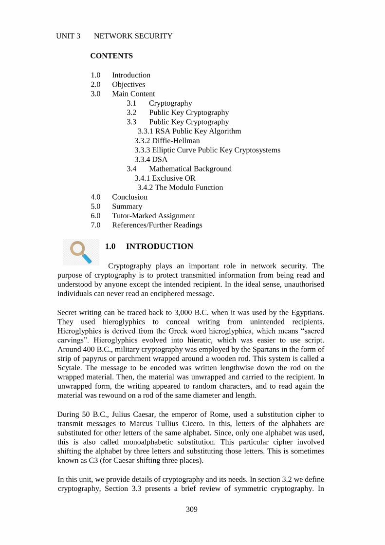
309

UNIT 3 NETWORK SECURITY

CONTENTS

1.0 Introduction

2.0 Objectives

3.0 Main Content

3.1 Cryptography

3.2 Public Key Cryptography


3.3.1 RSA Public Key Algorithm

3.3.2 Diffie-Hellman

3.3.3 Elliptic Curve Public Key Cryptosystems

3.3.4 DSA

3.4 Mathematical Background

3.4.1 Exclusive OR

3.4.2 The Modulo Function

4.0 Conclusion

5.0 Summary



1.0 INTRODUCTION

Cryptography plays an important role in network security. The

purpose of cryptography is to protect transmitted information from being read and

understood by anyone except the intended recipient. In the ideal sense, unauthorised

individuals can never read an enciphered message.

Secret writing can be traced back to 3,000 B.C. when it was used by the Egyptians.

They used hieroglyphics to conceal writing from unintended recipients.

Hieroglyphics is derived from the Greek word hieroglyphica, which means ―sacred

carvings‖. Hieroglyphics evolved into hieratic, which was easier to use script.

Around 400 B.C., military cryptography was employed by the Spartans in the form of

strip of papyrus or parchment wrapped around a wooden rod. This system is called a

Scytale. The message to be encoded was written lengthwise down the rod on the

wrapped material. Then, the material was unwrapped and carried to the recipient. In

unwrapped form, the writing appeared to random characters, and to read again the

material was rewound on a rod of the same diameter and length.

During 50 B.C., Julius Caesar, the emperor of Rome, used a substitution cipher to

transmit messages to Marcus Tullius Cicero. In this, letters of the alphabets are

substituted for other letters of the same alphabet. Since, only one alphabet was used,

this is also called monoalphabetic substitution. This particular cipher involved

shifting the alphabet by three letters and substituting those letters. This is sometimes

known as C3 (for Caesar shifting three places).

In this unit, we provide details of cryptography and its needs. In section 3.2 we define

cryptography, Section 3.3 presents a brief review of symmetric cryptography. In

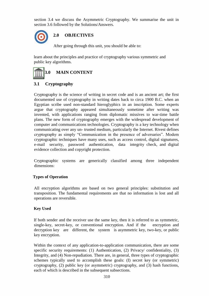
310

section 3.4 we discuss the Asymmetric Cryptography. We summarise the unit in

section 3.6 followed by the Solutions/Answers.

2.0 OBJECTIVES


learn about the principles and practice of cryptography various symmetric and

public key algorithms.

3.0 MAIN CONTENT

3.1 Cryptography

Cryptography is the science of writing in secret code and is an ancient art; the first

documented use of cryptography in writing dates back to circa 1900 B.C. when an

Egyptian scribe used non-standard hieroglyphics in an inscription. Some experts

argue that cryptography appeared simultaneously sometime after writing was

invented, with applications ranging from diplomatic missives to war-time battle

plans. The new form of cryptography emerges with the widespread development of

computer and communications technologies. Cryptography is a key technology when

communicating over any un- trusted medium, particularly the Internet. Rivest defines

cryptography as simply ―Communication in the presence of adversaries‖. Modem

cryptographic techniques have many uses, such as access control, digital signatures,

e-mail security, password authentication, data integrity check, and digital

evidence collection and copyright protection.

Cryptographic systems are generically classified among three independent

dimensions:

Types of Operation

All encryption algorithms are based on two general principles: substitution and

transposition. The fundamental requirements are that no information is lost and all

operations are reversible.

Key Used

If both sender and the receiver use the same key, then it is referred to as symmetric,

single-key, secret-key, or conventional encryption. And if the encryption and

decryption key are different, the system is asymmetric key, two-key, or public

key encryption.

Within the context of any application-to-application communication, there are some

specific security requirements: (1) Authentication, (2) Privacy/ confidentiality, (3)

Integrity, and (4) Non-repudiation. There are, in general, three types of cryptographic

schemes typically used to accomplish these goals: (I) secret key (or symmetric)

cryptography, (2) public key (or asymmetric) cryptography, and (3) hash functions,

each of which is described in the subsequent subsections.

311

3.2 Symmetric Key Cryptography

About twenty years ago, cryptography was the art of making and breaking codes. The

codes were used to transfer messages over an unsecured channel. The channel should

be protected from intruders who read, insert, delete or modify, messages, as depicted

in Figure 4.4. I. The transmission of a message is done using an encryption function

E that converts the message or plaintext using the key into a cipher text. The receiver

does the reverse of this operation, using the decryption function D and a decryption

key to recover the plaintext from the cipher text. The key is distributed in advance

over a secure channel, for example by courier.

Normally, the encryption and decryption function, but not the key, are considered

known to the adversary, so the protection of the information depends on the key only.

If the enemy knows the key, the whole system is useless until a new key is

distributed. In secret Key Cryptography, a single key is used for both encryption and

decryption, as shown in Figure 4.11. The main difficulty with this approach is the

distribution of the key.

Secret key cryptography schemes are generally categorised as being either stream

ciphers or block ciphers. Stream ciphers operate on a single byte (or computer word)

at a time, and implement some form of feedback mechanism so that the key is

constantly changing. Block cipher scheme encrypts one block of data at a time using

the same key on each block.

Figure 4.11: Secret Key Cryptography

The most common secret key cryptography scheme is Data Encryption Standard

(DES), designed by IBM in I 970s and adopted by the National Bureau of Standard

(NBS) of USA [now the National Institute for Standards and Technology (NIST)] in

1977 for commercial and unclassified government applications. DES is a block-cipher

employing a 56-bit key operating on 64-bit blocks of data. DES has a complex set of

rules and transformations designed basically for fast hardware implementation and

slow software implementation. The latter point is significant in today‘s context, as the

speed of CPU is several orders of magnitude faster than twenty years ago. IBM also

proposed a 112-bit key for DES in the 1990s, which was never implemented seriously.

In 1997, NIST initiated the task of developing a new secure cryptosystem

for U.S government applications. This effort has resulted in AES (Advanced

Encryption Standard). AES became the official successor to DES in December 2001.

AES is based on Rjndael Algorithm and employs a 128-, 192-, or 256-bit key.

The following terminology is often used when symmetric ciphers are examined:

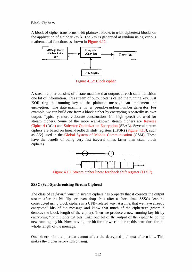
312

Block Ciphers

A block of cipher transforms n-bit plaintext blocks to n-bit ciphertext blocks on

the application of a cipher key k. The key is generated at random using various

mathematical functions as shown in Figure 4.12.

Figure 4.12: Block cipher

A stream cipher consists of a state machine that outputs at each state transition

one bit of information. This stream of output bits is called the running key. Just

XOR ring the running key to the plaintext message can implement the

encryption. The state machine is a pseudo-random number generator. For

example, we can build one from a block cipher by encrypting repeatedly its own

output. Typically, more elaborate constructions (for high speed) are used for

stream ciphers. Some of the more well-known stream ciphers are Reverse

Cipher 4 (RC4) and Software Optimization Encryption (SEAL). Several stream

ciphers are based on linear-feedback shift registers (LFSR) (Figure 4.13), such

as A5/] used in the Global System of Mobile Communication (GSM). These

have the benefit of being very fast (several times faster than usual block

ciphers).

Figure 4.13: Stream cipher linear feedback shift register (LFSR)

SSSC (Self-Synchronising Stream Ciphers)

The class of self-synchronising stream ciphers has property that it corrects the output

stream after the bit flips or even drops bits after a short time. SSSCs ‗can be

constructed using block ciphers in a CFB- related way. Assume, that we have already

encrypted‖ bits of the message and know that much of the ciphertext (where n

denotes the block length of the cipher). Then we produce a new running key bit by

encrypting ‗the n ciphertext bits. Take one bit of the output of the cipher to be the

new running key bit. Now moving one bit further we can iterate this procedure for the

whole length of the message.

One-bit error in a ciphertext cannot affect the decrypted plaintext after n bits. This

makes the cipher self-synchronising.

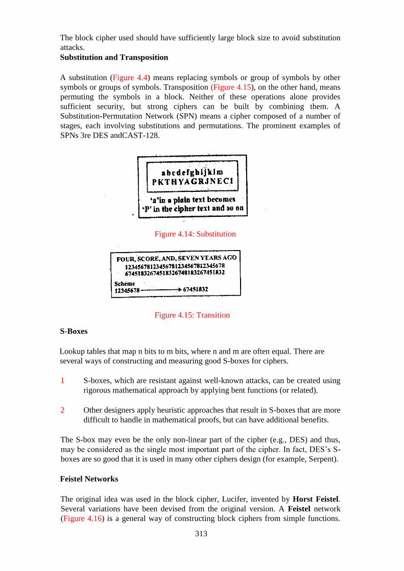
313

The block cipher used should have sufficiently large block size to avoid substitution

attacks.

Substitution and Transposition

A substitution (Figure 4.4) means replacing symbols or group of symbols by other

symbols or groups of symbols. Transposition (Figure 4.15), on the other hand, means

permuting the symbols in a block. Neither of these operations alone provides

sufficient security, but strong ciphers can be built by combining them. A

Substitution-Permutation Network (SPN) means a cipher composed of a number of

stages, each involving substitutions and permutations. The prominent examples of

SPNs 3re DES andCAST-128.

Figure 4.14: Substitution

Figure 4.15: Transition

S-Boxes

Lookup tables that map n bits to m bits, where n and m are often equal. There are

several ways of constructing and measuring good S-boxes for ciphers.

1 S-boxes, which are resistant against well-known attacks, can be created using

rigorous mathematical approach by applying bent functions (or related).

2 Other designers apply heuristic approaches that result in S-boxes that are more

difficult to handle in mathematical proofs, but can have additional benefits.

The S-box may even be the only non-linear part of the cipher (e.g., DES) and thus,

may be considered as the single most important part of the cipher. In fact, DES‘s S-

boxes are so good that it is used in many other ciphers design (for example, Serpent).

Feistel Networks

The original idea was used in the block cipher, Lucifer, invented by Horst Feistel.

Several variations have been devised from the original version. A Feistel network

(Figure 4.16) is a general way of constructing block ciphers from simple functions.

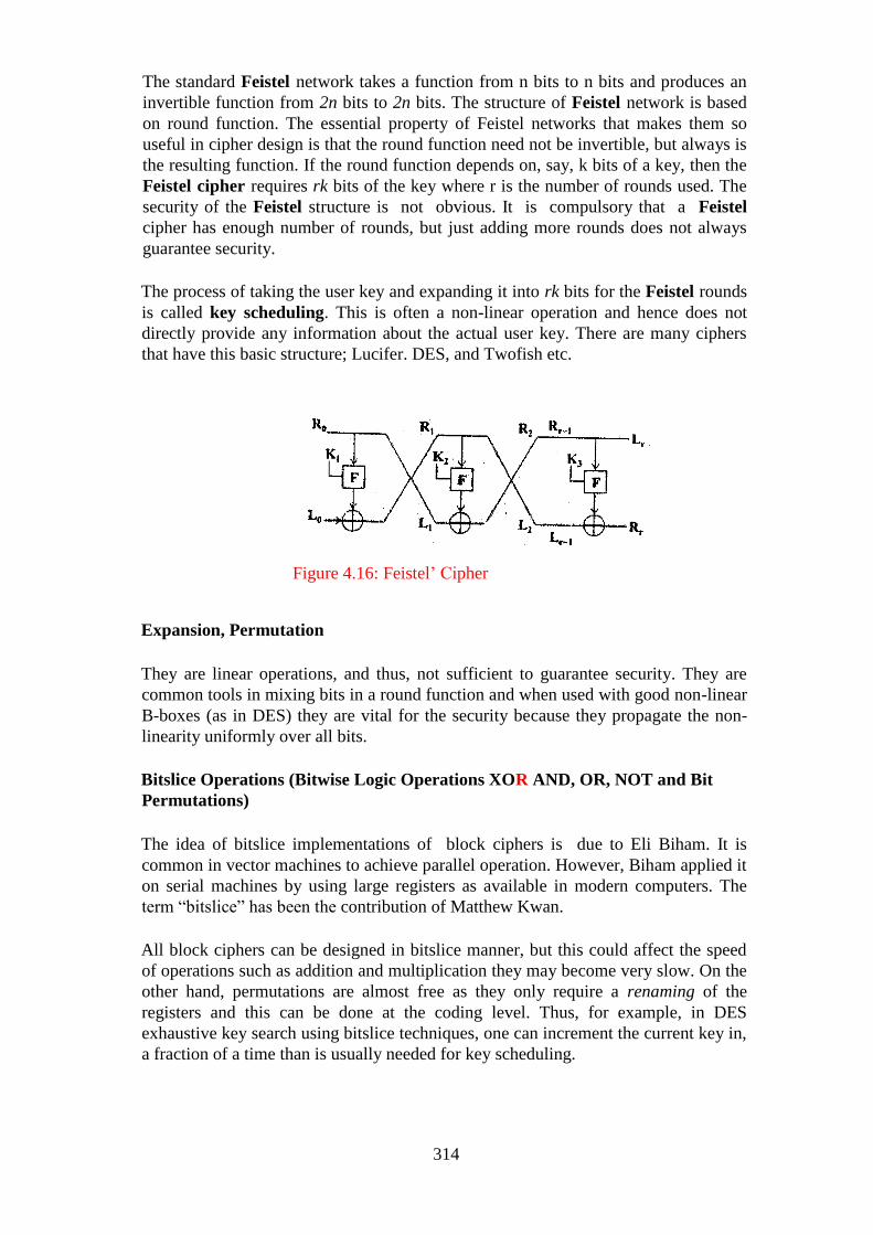
314

The standard Feistel network takes a function from n bits to n bits and produces an

invertible function from 2n bits to 2n bits. The structure of Feistel network is based

on round function. The essential property of Feistel networks that makes them so

useful in cipher design is that the round function need not be invertible, but always is

the resulting function. If the round function depends on, say, k bits of a key, then the

Feistel cipher requires rk bits of the key where r is the number of rounds used. The

security of the Feistel structure is not obvious. It is compulsory that a Feistel

cipher has enough number of rounds, but just adding more rounds does not always

guarantee security.

The process of taking the user key and expanding it into rk bits for the Feistel rounds

is called key scheduling. This is often a non-linear operation and hence does not

directly provide any information about the actual user key. There are many ciphers

that have this basic structure; Lucifer. DES, and Twofish etc.

Figure 4.16: Feistel‘ Cipher

Expansion, Permutation

They are linear operations, and thus, not sufficient to guarantee security. They are

common tools in mixing bits in a round function and when used with good non-linear

B-boxes (as in DES) they are vital for the security because they propagate the non-

linearity uniformly over all bits.

Bitslice Operations (Bitwise Logic Operations XOR AND, OR, NOT and Bit

Permutations)

The idea of bitslice implementations of block ciphers is due to Eli Biham. It is

common in vector machines to achieve parallel operation. However, Biham applied it

on serial machines by using large registers as available in modern computers. The

term ―bitslice‖ has been the contribution of Matthew Kwan.

All block ciphers can be designed in bitslice manner, but this could affect the speed

of operations such as addition and multiplication they may become very slow. On the

other hand, permutations are almost free as they only require a renaming of the

registers and this can be done at the coding level. Thus, for example, in DES

exhaustive key search using bitslice techniques, one can increment the current key in,

a fraction of a time than is usually needed for key scheduling.

315

The AES finalist Serpent is designed to be implemented using bitslice operations

only. This makes it particularly efficient on modern architectures with many

registers.

Modes of Operation

Block ciphers are the most commonly used cipher. Block ciphers transform a fixed-

size block of data (usually 64 bits) into another fixed- size block (possibly 64 bits

wide again) using a function selected by the key. If the key, input block and output

block have all n bits, a block cipher basically defines a one-to-one mapping from n-

bit integers to permutations of n-bit integers.

If the same block is encrypted twice with the same key. the resulting ciphertext

blocks are also the same (this mode of encryption is called electronic code book, or

ECB). This information could be useful for an attacker. For identical plaintext blocks

being encrypted to different ciphertext blocks, three standard modes are generally

used:

1 CBC (Cipher Block Chaining)

First XORing the plaintext block with the previous ciphertext block obtains a

ciphertext block, and then the resulting value needs to be encrypted. In this, leading

blocks influence all trailing blocks, which increases the number of plaintext bits one

ciphertext bit depends on, but this may also leads to synchronisation problems ifone

block is lost. The Process of Cipher Block Chaining shown in Figure 4.17. In this

Figure m1‖ m2‖ m3) are messages and C1, C2 and C3 are ciphertexts.

Figure 4.17: Cipher block chaining

2. CFB (Cipher Feedback)

In this the kth ciphertext block is obtained by encrypting the (k-l)th ciphertext block

and XORing the result onto the plaintext. The CFB mode possess self-synchrcnising

property: A CFB feedback loop can also be used as a pseudo-random number

generator (PRNG) if one simply feeds one block of true random data with trailing

blocks of zeroes into the encryption routine (although the expected period of this

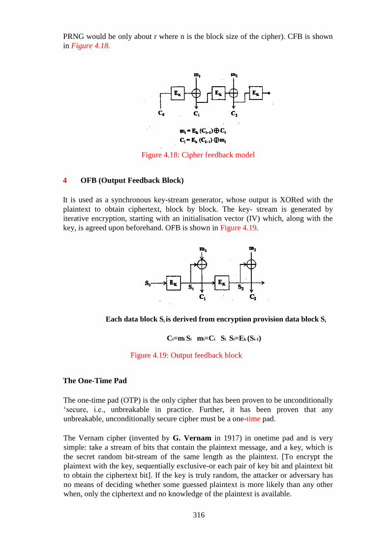
316

PRNG would be only about r where n is the block size of the cipher). CFB is shown

in Figure 4.18.

Figure 4.18: Cipher feedback model

4 OFB (Output Feedback Block)

It is used as a synchronous key-stream generator, whose output is XORed with the

plaintext to obtain ciphertext, block by block. The key- stream is generated by

iterative encryption, starting with an initialisation vector (IV) which, along with the

key, is agreed upon beforehand. OFB is shown in Figure 4.19.

Each data block Si is derived from encryption provision data block Si

Ci=mi Si mi=Ci Si Si=Ek (Si-1)

Figure 4.19: Output feedback block

The One-Time Pad

The one-time pad (OTP) is the only cipher that has been proven to be unconditionally

‗secure, i.e., unbreakable in practice. Further, it has been proven that any

unbreakable, unconditionally secure cipher must be a one-time pad.

The Vernam cipher (invented by G. Vernam in 1917) in onetime pad and is very

simple: take a stream of bits that contain the plaintext message, and a key, which is

the secret random bit-stream of the same length as the plaintext. [To encrypt the

plaintext with the key, sequentially exclusive-or each pair of key bit and plaintext bit

to obtain the ciphertext bit]. If the key is truly random, the attacker or adversary has

no means of deciding whether some guessed plaintext is more likely than any other

when, only the ciphertext and no knowledge of the plaintext is available.

317

The main practical problem is that the key does not have a small constant length, but

the same length as the message, and one part of a key should never be used twice (or

the cipher can be broken). However, this cipher has allegedly been in widespread use

since its invention, and even more since the security proof by C. Shannon in 1949.

Although, admittedly the security of this cipher had been conjectured earlier, it was

Shannon who actually found a formal proof for it.

DES

The Data Encryption Standard (DES) is an algorithm developed in the mid-l970s and

turned into a standard by the US National Institute of Standards and Technology

(NIST), and was also adopted by several other governments worldwide. It was and

still is widely used, especially in the financial industry.

DES is a block cipher with a 64-bit block size. It uses 56-bit keys. This makes it

suspectable to exhaustive key search with modem computing powers and special-

purpose hardware. DES is still strong enough to keep most. random hackers,

adversaries and individuals out, DES is easily breakable with special hardware by,

government, criminal organizations etc. DES is getting too weak, and should not be

used in new applications. NIST proposed in 2004 to withdraw the DES standard.

A variant of DES, Triple-DES (also 3DES) is based on using DES three times

(normally in an encrypt-decrypt-encrypt sequence with three different, unrelated

keys). The Triple-DES is arguably much stronger than (single) DES, however, it is

rather slow compared to some new block ciphers.

Although, at the time of DES‘s introduction, its design philosophy was held secret.

Some information has been published about its design, and one of the original

designers, Don Coppersmith, has said that they discovered ideas similar to

differential crypt analysis while designing DES in 1974. However, it was just a

matter of time that these fundamental ideas were re-discovered.

Although DES is no longer considered a practical solution, it is many a time used to

describe new crypt analytical methods. Even today, there are no crypt analytical

techniques that would completely break DES in a structural way; indeed, the only

real weakness known is the short key size (and perhaps the small block size).

DES uses the:

Data Encryption Algorithm (DEA),

A secret key block-cipher employing a 56-bit key operating on 64-bit blocks.

FIPS 81 describes four modes of DES operation: Electronic Codebook (ECB), Cipher

Block Chaining (CBC), Cipher Feedback (CFB), and Output Feedback (OFB).

Despite all these options, ECB is the most commonly deployed mode of operation.

DES uses a 56-bit key, which is divided into eight 7-bit blocks and an 8th odd parity

bit is added to each block (i.e., a ―0‖ or ―I‖ is added to the block so that there are an

odd number of I bit in each 8-bit block). By using the 8 parity bits for rudimentary

318

error detection, a DES key is actually 64 bits in length for computational purposes

(although it only has 56 bits worth of randomness, or entropy).

Figure 4.20: DEI; algorithm

DES process on 64-bit blocks of the plaintext, invoking 16 rounds of permutations,

swaps, and substitutes, as shown in Figure 4.20. The main DES steps are:

1 The 64.bit block undergoes an initial permutation (IP), where each bit is

moved to a new bit position; e.g., the 1st, 2nd, and 3rd bits are moved to the

58th, 50th, and 42nd position, respectively.

2 The permuted 64-bit input is divided into two 32-bit blocks, called left and

right, respectively. The initial values of the left and right blocks are denoted as

Lo and Ro.

3 There are then 16 rounds of operation on the L and R blocks.

During each iteration (where n ranges from I to 16), the following formula

is used:

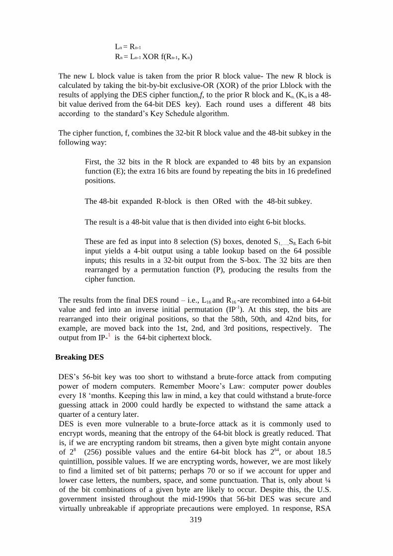
319

Ln = Rn-1

Rn = Ln-1 XOR f(Rn-1, Kn)

The new L block value is taken from the prior R block value- The new R block is

calculated by taking the bit-by-bit exclusive-OR (XOR) of the prior Lblock with the

results of applying the DES cipher function,f, to the prior R block and Kn. (Kn is a 48-

bit value derived from the 64-bit DES key). Each round uses a different 48 bits

according to the standard‘s Key Schedule algorithm.

The cipher function, f, combines the 32-bit R block value and the 48-bit subkey in the

following way:

First, the 32 bits in the R block are expanded to 48 bits by an expansion

function (E); the extra 16 bits are found by repeating the bits in 16 predefined

positions.

The 48-bit expanded R-block is then ORed with the 48-bit subkey.

The result is a 48-bit value that is then divided into eight 6-bit blocks.

These are fed as input into 8 selection (S) boxes, denoted S1,….,S8. Each 6-bit

input yields a 4-bit output using a table lookup based on the 64 possible

inputs; this results in a 32-bit output from the S-box. The 32 bits are then

rearranged by a permutation function (P), producing the results from the

cipher function.

The results from the final DES round – i.e., L16 and R16 -are recombined into a 64-bit

value and fed into an inverse initial permutation (IP-1). At this step, the bits are

rearranged into their original positions, so that the 58th, 50th, and 42nd bits, for

example, are moved back into the 1st, 2nd, and 3rd positions, respectively. The

output from IP-1 is the 64-bit ciphertext block.

Breaking DES

DES‘s 56-bit key was too short to withstand a brute-force attack from computing

power of modern computers. Remember Moore‘s Law: computer power doubles

every 18 ‗months. Keeping this law in mind, a key that could withstand a brute-force

guessing attack in 2000 could hardly be expected to withstand the same attack a

quarter of a century later. DES is even more vulnerable to a brute-force attack as it is commonly used to

encrypt words, meaning that the entropy of the 64-bit block is greatly reduced. That

is, if we are encrypting random bit streams, then a given byte might contain anyone

of 28 (256) possible values and the entire 64-bit block has 264, or about 18.5

quintillion, possible values. If we are encrypting words, however, we are most likely

to find a limited set of bit patterns; perhaps 70 or so if we account for upper and

lower case letters, the numbers, space, and some punctuation. That is, only about ¼

of the bit combinations of a given byte are likely to occur. Despite this, the U.S.

government insisted throughout the mid-1990s that 56-bit DES was secure and

virtually unbreakable if appropriate precautions were employed. 1n response, RSA

320

Laboratories sponsored a series of cryptographic challenges to prove that DES was

no longer secure and appropriate for use.

DES Challenge I was launched in March 1997. R. Verser completed it in 84 days in

a collaborative effort to break DES using thousands of computers on the Internet. The

first DES II challenge lasted 40 days during early 1998, This problem was solved

bydistributed.net, a worldwide distributed computing network using the spare CPU

cycles of computers around the Internet. The participants in distributed.net activities

load a client program that runs in the background, conceptually similar to the SETI

@Home ―Search for Extra-terrestrial Intelligence‖ project). By the end of the project,

distributed.net systems were checking 28 billion keys per second.

The second DES II challenge lasted just less than 3 days. On July 17, 1998,

the Electronic Frontier Foundation (EFF) announced the construction of a

hardware that could brute-force a DES key in an average of 4.5 days. The

device called Deep Crack, could check 90 billion keys per second and cost

only about $220,000 including design. As the design is scalable, this suggests

that an organization could develop a DES cracker that could break 56-bit keys

in an average of a day for as little as $1,000,000.

The DES III challenge, launched in January 1999, was broken in less than a

day by the coordinated efforts of Deep Crack and distributed.net.

The Deep Crack algorithm is to launch a brute-force attack by guessing every

possible key. A 56-bit key yields 256, or about 72 quadrillion, possible values. The

DES cracker team initially assumed that some recognisable plaintext would appear in

the decrypted string even though they didn‘t have a specific known plaintext block.

They then applied all 256 possible key values to the 64-bit block. The system checked

to find if the decrypted value of the block was ―interesting‖, which they defined as

bytes containing one of the alphanumeric characters, space, or some punctuation. As

the likelihood of a single byte being ―interesting‖ is about ¼, then the likelihood of

the entire 8-byte stream being ―interesting‖ is about ¼8, or 1/65536 (½16). This

dropped the number of possible keys that might yield positive results to about 240, or

about a trillion. After the assumption that an ―interesting‖ 8-byte block would be followed by another

―interesting‖ block. Therefore, if the first block of ciphertext decrypted to something

interesting, they decrypted the next block; otherwise, they abandoned this key. Only

if the second block was also ―interesting‖ did they examine the key closer. Looking

for 16 consecutive bytes that were ―interesting‖ meant that only 224, or 16 million,

keys required to be examined further. This further examination was primarily to see if

the text made any sense.

It is important to mention a couple of forms of crypt analysis that have been shown to

be effective against DES. Differential cryptanalysis, invented in 1990 by E. Biham

and A. Shamir (of RSA fame), is a chosen-plaintext attack. By selecting pairs of

plaintexts with particular differences, the crypt analyst examines the differences in

the resultant ciphertext pairs. Linear plaintext, invented by M. Matsui, uses a linear

approximation to analyse the actions of a block cipher (including DES). Both these

attacks one be more efficient than brute force.

321

DES Variants

After DES algorithm was ―officially‖ broken, several variants appeared. In the early

1990s, there was a proposal to increase the security of DES by effectively increasing

the key length by using multiple keys with multiple passes etc. But for this scheme to

work, it had to first be shown that, the DES function is not a group, as defined in

mathematics. If DES was a group, then we could show that for two DES keys, X1 and

X2, applied to some plaintext (P), we can get a single equivalent key, X3, that would

provide the same result; i.e.,

EX2(EX1(P)) = EX3(P)

where Ex(P) represents DES encryption of some plaintext P using DES key X. If

DES were a group, it wouldn‘t matter how many keys and passes we applied to some

plaintext; we could always find a single 56- bit key that would provide the same

result.

As DES was proven not to be a group, we apply additional keys and passes to

increase the effective key length. One choice, then, might be to use two keys and two

passes, yielding an effective key length of 112 bits. This can be called Double-DES.

The two keys, YI and Y2, might be applied as follows:

C = EY2(EY1(P))

P = DYl(DY2(C))

where EY(P) and DY(C) represent DES encryption and decryption, respectively, of

some plaintext P and ciphertext C, respectively, using DES key Y.

But an interesting attack can be launched against this ―Double-DES‖ scheme. The

applications of the formula above can be with the following individual steps (where

C‘ and P‘ are intermediate results):

C‘ = EY1(P) and C = EY2(C‘)

P‘ = DY2(C) and P = DY1(P‘)

Unfortunately, C‘=P‘, which leaves it vulnerable to a simple known plaintext attack

(or ―Meet-in-the-middle‖) where the attacker or adversary knows some plaintext (P)

and its matching ciphertext (C) To obtain C‘, the attacker or adversary needs to try all

256 possible values of Y1 applied to P; to obtain P‘, the attacker needs to try all 256

possible values ofY2 applied to C. Since C‘=P‘, the attacker knows when a match

has been achieved – after only 256 + 256 = 257 key searches, only twice the work of

brute-forcing DES.

Triple-DES (3DES) is based upon the Triple Data Encryption

322

Algorithm (mEA), as described in FIPS 46-3. 3DES, which is not susceptible to a

meet-in-the-middle attack, employs three DES passes and one, two, or three keys

called KI, K2, and K3. Generation of the ciphertext (C) from a block of plaintext (P)

is accomplished by:

C = EK3(DK2(EK1(P)) where EK(P) and DK(P) represent DES encryption and

decryption, respectively, of some plaintext P using DES key K. This is also

sometimes referred to as an encrypt-decrypt-encrypt mode operation.

Decryption of the ciphertext into plaintext is accomplished by:

P = DK1(EK2(DK3(C)))

The use of three, independent 56-bit keys provides 3DES with an effective

key length of 168 bits. The specification also defines use of two keys

where, in the operations above, K3 = K1; this provides an effective key

length of 112 bits. Finally, a third keying option is to use a single key, so

that K3 = K2 = K1 (in this case, the effective key length is 56 bits and

3DES applied to some plaintext, P, will yield the same ciphertext, C, as

normal DES would with that same key). With the relatively low cost of

key storage and the modest increase in processing due to the use of longer

keys, the best recommended practices are that 3DES are employed with

three keys.

Another variant of DES, called DESX, is the contribution of Ron Rivest. Developed

in 1996, DESX is a very simple algorithm that greatly increases DES‘s resistance to

brute-force attacks without increasing its computational complexity. In DESX, the

plaintext input is XORed with 64 additional key bits prior to encryption and the

output is likewise XORed with the 64 key bits. By adding just two XOR operations,

DESX has an effective keylength of 120 bits against an exhaustive key-search attack.

It is pertinent to note that DESX is not immune to other types of more sophisticated

attacks, such as differential or linear crypt analysis, but brute-force is the primary

attack vector on DES.

AES

In response to cryptographic attacks on DES, search for a replacement to DES started

in January 1997. In September 1997, a formal Call for Algorithms was initiated and

in August 1998 announced that 15 candidate algorithms were being considered

(Round 1). In April 1999, NIST announced that the 15 had been filtered down to five

finalists (Round 2): MARS (multiplication, addition, rotation and substitution) from

IBM; Ronald Rivest’s RC6; Rijndael from a Belgian team; Serpent, developed

jointly by a team from England, Israel, and Norway; and Twofish, developed by

Bruce Schneier. In October 2000, NI8.T announced their selection: Rijndael.

In October 2000, NIST published the Report on the Development of the Advanced

Encryption Standard (AES) that compared the five Round 2 algorithms in a number of

categories. The figure 4.21 below

summarises the relative scores of the five schemes (1=low,3=high):

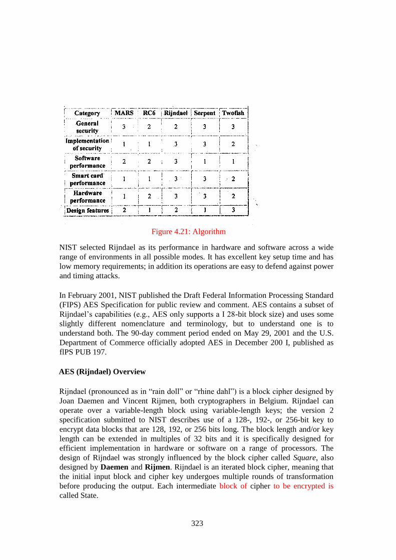
323

Figure 4.21: Algorithm

NIST selected Rijndael as its performance in hardware and software across a wide

range of environments in all possible modes. It has excellent key setup time and has

low memory requirements; in addition its operations are easy to defend against power

and timing attacks.

In February 2001, NIST published the Draft Federal Information Processing Standard

(FIPS) AES Specification for public review and comment. AES contains a subset of

Rijndael‘s capabilities (e.g., AES only supports a I 28-bit block size) and uses some

slightly different nomenclature and terminology, but to understand one is to

understand both. The 90-day comment period ended on May 29, 2001 and the U.S.

Department of Commerce officially adopted AES in December 200 I, published as

flPS PUB 197.

AES (Rijndael) Overview

Rijndael (pronounced as in ―rain doll‖ or ―rhine dahl‖) is a block cipher designed by

Joan Daemen and Vincent Rijmen, both cryptographers in Belgium. Rijndael can

operate over a variable-length block using variable-length keys; the version 2

specification submitted to NIST describes use of a 128-, 192-, or 256-bit key to

encrypt data blocks that are 128, 192, or 256 bits long. The block length and/or key

length can be extended in multiples of 32 bits and it is specifically designed for

efficient implementation in hardware or software on a range of processors. The

design of Rijndael was strongly influenced by the block cipher called Square, also

designed by Daemen and Rijmen. Rijndael is an iterated block cipher, meaning that

the initial input block and cipher key undergoes multiple rounds of transformation

before producing the output. Each intermediate block of cipher to be encrypted is

called State.

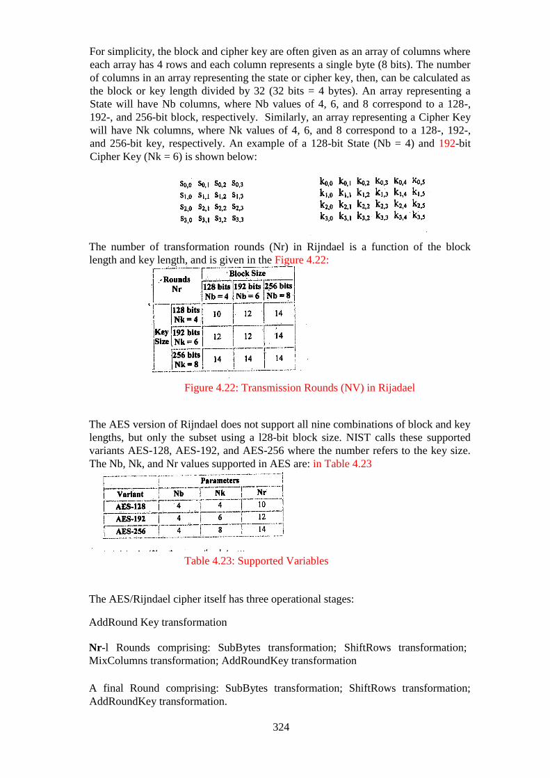
324

For simplicity, the block and cipher key are often given as an array of columns where

each array has 4 rows and each column represents a single byte (8 bits). The number

of columns in an array representing the state or cipher key, then, can be calculated as

the block or key length divided by 32 (32 bits = 4 bytes). An array representing a

State will have Nb columns, where Nb values of 4, 6, and 8 correspond to a 128-,

192-, and 256-bit block, respectively. Similarly, an array representing a Cipher Key

will have Nk columns, where Nk values of 4, 6, and 8 correspond to a 128-, 192-,

and 256-bit key, respectively. An example of a 128-bit State (Nb = 4) and 192-bit

Cipher Key (Nk = 6) is shown below:

The number of transformation rounds (Nr) in Rijndael is a function of the block

length and key length, and is given in the Figure 4.22:

Figure 4.22: Transmission Rounds (NV) in Rijadael

The AES version of Rijndael does not support all nine combinations of block and key

lengths, but only the subset using a l28-bit block size. NIST calls these supported

variants AES-128, AES-192, and AES-256 where the number refers to the key size.

The Nb, Nk, and Nr values supported in AES are: in Table 4.23

Table 4.23: Supported Variables

The AES/Rijndael cipher itself has three operational stages:

AddRound Key transformation

Nr-l Rounds comprising: SubBytes transformation; ShiftRows transformation;

MixColumns transformation; AddRoundKey transformation

A final Round comprising: SubBytes transformation; ShiftRows transformation;

AddRoundKey transformation.

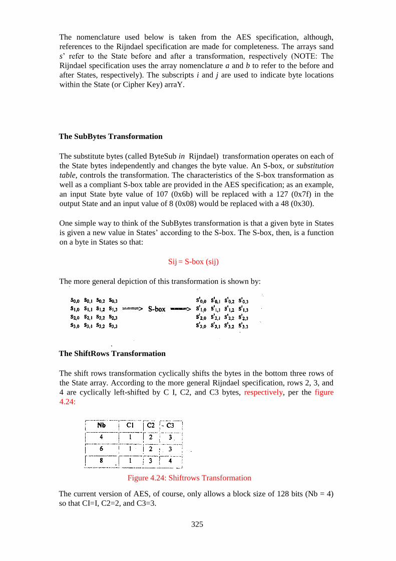
325

The nomenclature used below is taken from the AES specification, although,

references to the Rijndael specification are made for completeness. The arrays sand

s‘ refer to the State before and after a transformation, respectively (NOTE: The

Rijndael specification uses the array nomenclature a and b to refer to the before and

after States, respectively). The subscripts i and j are used to indicate byte locations

within the State (or Cipher Key) arraY.

The SubBytes Transformation

The substitute bytes (called ByteSub in Rijndael) transformation operates on each of

the State bytes independently and changes the byte value. An S-box, or substitution

table, controls the transformation. The characteristics of the S-box transformation as

well as a compliant S-box table are provided in the AES specification; as an example,

an input State byte value of 107 (0x6b) will be replaced with a 127 (0x7f) in the

output State and an input value of 8 (0x08) would be replaced with a 48 (0x30).

One simple way to think of the SubBytes transformation is that a given byte in States

is given a new value in States‘ according to the S-box. The S-box, then, is a function

on a byte in States so that:

Sij = S-box (sij)

The more general depiction of this transformation is shown by:

The ShiftRows Transformation

The shift rows transformation cyclically shifts the bytes in the bottom three rows of

the State array. According to the more general Rijndael specification, rows 2, 3, and

4 are cyclically left-shifted by C I, C2, and C3 bytes, respectively, per the figure

4.24:

Figure 4.24: Shiftrows Transformation

The current version of AES, of course, only allows a block size of 128 bits (Nb = 4)

so that CI=I, C2=2, and C3=3.

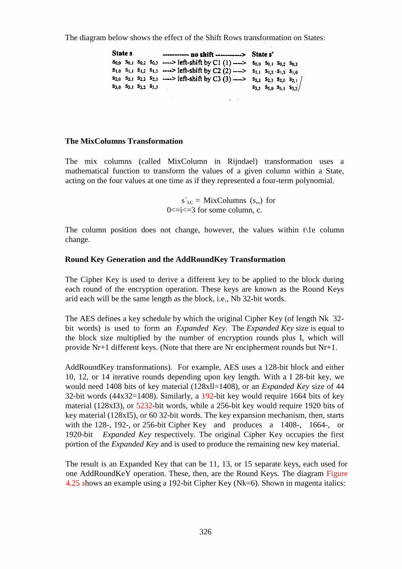
326

The diagram below shows the effect of the Shift Rows transformation on States:

The MixColumns Transformation

The mix columns (called MixColumn in Rijndael) transformation uses a

mathematical function to transform the values of a given column within a State,

acting on the four values at one time as if they represented a four-term polynomial.

s`I,C = MixColumns (s,,) for

0<=i<=3 for some column, c.

The column position does not change, however, the values within t\1e column

change.

Round Key Generation and the AddRoundKey Transformation

The Cipher Key is used to derive a different key to be applied to the block during

each round of the encryption operation. These keys are known as the Round Keys

arid each will be the same length as the block, i.e., Nb 32-bit words.

The AES defines a key schedule by which the original Cipher Key (of length Nk 32-

bit words) is used to form an Expanded Key. The Expanded Key size is equal to

the block size multiplied by the number of encryption rounds plus I, which will

provide Nr+1 different keys. (Note that there are Nr encipherment rounds but Nr+1.

AddRoundKey transformations). For example, AES uses a 128-bit block and either

10, 12, or 14 iterative rounds depending upon key length. With a I 28-bit key, we

would need 1408 bits of key material (128xll=1408), or an Expanded Key size of 44

32-bit words (44x32=1408). Similarly, a 192-bit key would require 1664 bits of key

material (128xI3), or 5232-bit words, while a 256-bit key would require 1920 bits of

key material (128xI5), or 60 32-bit words. The key expansion mechanism, then, starts

with the 128-, 192-, or 256-bit Cipher Key and produces a 1408-, 1664-, or

1920-bit Expanded Key respectively. The original Cipher Key occupies the first

portion of the Expanded Key and is used to produce the remaining new key material.

The result is an Expanded Key that can be 11, 13, or 15 separate keys, each used for

one AddRoundKeY operation. These, then, are the Round Keys. The diagram Figure

4.25 shows an example using a 192-bit Cipher Key (Nk=6). Shown in magenta italics:

327

Figure 4.25: 192-bit Cipher key

The AddRoundKey (called Round Key addition in Rijndael) transformation merely

applies each Round Key, in turn, to the State by a simple bit-wise exclusive OR

operation.

MARS: a candidate Cipher for AES, 1999 by Zunic et al (year)., IBM.

This new design uses a special type of a Feistel network, which depends heavily on

the instruction sets available on modern 32-bit processors. This has the benefit that on

these target machines it is efficient, but it may lead to implementation

problems/difficulties in cheaper architectures like smart cards.

RC6: Improved Analysis of some Simplified Variants of RC6 by Rivest,

Robshaw, and Yin, RSA Laboratories.

RC6.follows the ideas of RC5 with improvements. It attempts to avoid some of the

differential attacks against RC5‘s data dependent rotations. However, there are some

attacks that are not yet employed, and it is unclear whether RC6 is well enough

analysed yet.

Serpent: A new Block Cipher Proposal by Anderson, Biham, and Knudsen.

Serpent has a basically conservative but, in many ways innovative design. It may be

implemented by bitslice (or vector) gate logic throughout. This makes it rather

complicated to write and implement from scratch. The 32 rounds lead to probably the

highest security margin on all AES candidates, while it is still fast enough for all

practical purposes.

Twofish A 128-bit Block Cipher by Schneier et al., Counterpane Security, 1998

Twofish is a block cipher designed by Counterpane, whose founder and CTO is Bruce

Schneier. The design is highly delicate, supported with many alternative ways of

implementation. It is crypt analysed in much detail, by the very authoritative

―extended Twofish team‖. It is basically a Feistel cipher, but utilises many different

ideas. This cipher has key dependent S-boxes like Blowfish (another cipher by Bruce

Schneier).

Other Symmetric Ciphers

Blowfish

Bruce Schneier designed blowfish and it is a block cipher with a 64-bit block size

and variable length keys (which may vary up to 448 bits). It has gained of acceptance

in a number of applications, including Nautilus and PGPfone.

328

Blowfish utilises the idea of randomised S-boxes: while doing key scheduling, it

generates large pseudo-random lookup tables through several encryptions. These

tables depend on the user supplied key in a very complex manner. This makes

blowfish highly resistant against many attacks such as differential and linear crypt

analysis. But is not the algorithm of choice for environments where large memory

space (something like 4096 bytes) is not available. The known attacks against

Blowfish are based on its weak key classes.

CAST-128

CAST -128, Substitution-Permutation Network (SPN) cryptosystem, is similar to

DES, which have good resistance to differential, linear and related-key crypt analysis.

CAST-128 has Feistel structure and utilises eight fixed S-boxes. CAST -128 supports

variable key lengths between 40 and 128 bits (described in RFC2l4:4).

IDEA

IDEA (International Data Encryption Algorithm), was developed at Ern Zurich in

Switzerland by Xuejia Lai uses a l28-bit key, and is considered to be very secure.

The best attacks against IDEA uses the impossible differential idea of Biham,

Shamir and Biryukov. They can attack only 4.5 rounds of IDEA and this poses no

threat to the total of 8. 5 rounds used in IDEA. It is pertinent to note that IDEA is

patented in the United States and in most European countries.

Rabbit

Rabbit is a stream cipher, based on iterating a set of coupled nonlinear function. It is

characterised by a high performance in software.

RC4

RC4 is a stream cipher by Ron Rivest at RSA Data Security, Inc. It accepts keys of

arbitrary length. It used to be a trade secret, until someone posted source code for an

algorithm on the usenet, claiming it to be equivalent to RC4. The algorithm is very

fast. Its security is unknown, but breaking it does not seem trivial either. Because of

its speed, it may have uses in certain particular applications.

RC4 is essentially a pseudo random number generator, and the output of the

generator is exclusive-ored with the data stream. For this reason, it is very important

that the same RC4 key should not be used to encrypt two different data streams.


1. What is the result of the Exclusive OR operation 1 XOR 0

a 1

b 0

c Indeterminate

d 10

329

2. A block cipher:

a Is an asymmetric key algorithm

b Converts variable-length plaintext into fixed-length ciphertext (c)

Breaks a message into fixed length units for encryption (d)

Encrypts by operating on a continuous data stream.

3. What is the block length of the Rijndael Cipher?

a 64 bits

b 128 bits

c Variable

d 256 bits

4. What is the key length of the Rijndael Block Cipher?

a 56 or 64 bits

b 512 bits

c 128,192, or 256 bits

d 512 or 1024 bits

5. The NIST Advanced Encryption Standard uses the:

a 3 DES algorithm

b DES algorithm

c Rijndael algorithm

d IDEA algorithm

a. The modes of DES do not include:

a Electronic code book

b Variable block feedback

c Cipher block chaining

d Output feedback


Modern cryptography deals with communication between many different parties,

without using a secret key for every pair of parties. In 1976, Whitfield Diffie and

Martin Hellman published an invited paper in the IEEE Transactions on Information

Theory titled ―New Directions in Cryptography‖. This paper can be considered as the

beginning of modem cryptography. Their paper described a two -key crypto system

in which two parties can perform a secure communication over a non- secure channel

without having to share a secret key. PKC depends upon the existence of so-called

one-way function, or mathematical functions that are easy to calculate but the

calculation of the inverse function is relatively difficult.

Generic PKC uses two keys that are mathematically related and knowledge of one

key does not allow someone to easily determine the other key. One key is used to

encrypt and the other key is used to decrypt. It does not matter which key is applied

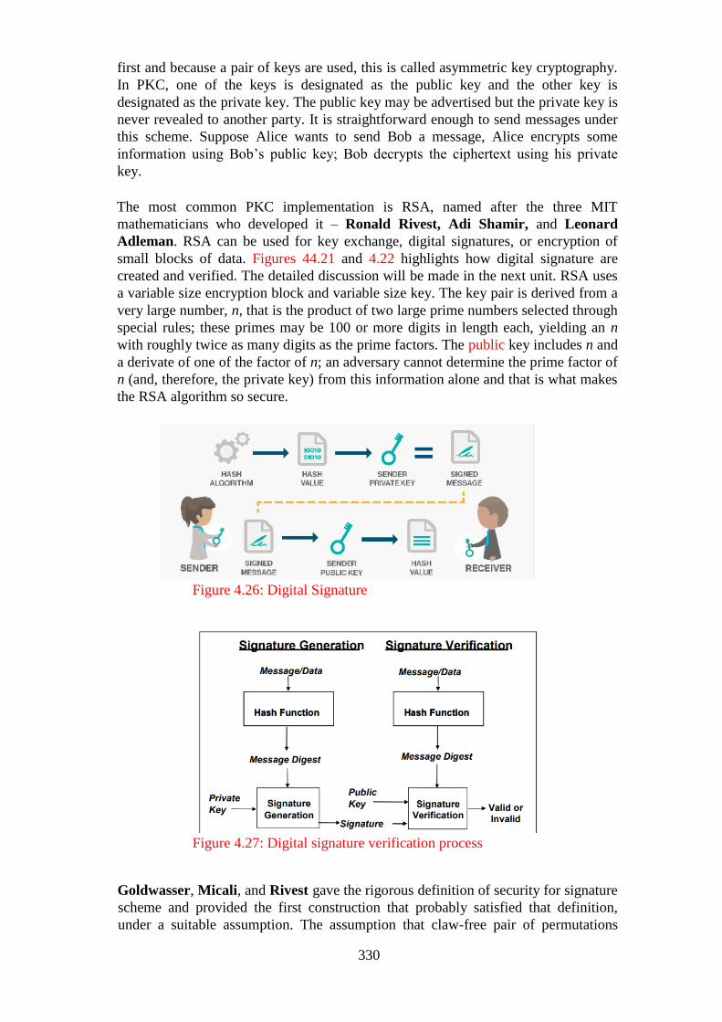
330

first and because a pair of keys are used, this is called asymmetric key cryptography.

In PKC, one of the keys is designated as the public key and the other key is

designated as the private key. The public key may be advertised but the private key is

never revealed to another party. It is straightforward enough to send messages under

this scheme. Suppose Alice wants to send Bob a message, Alice encrypts some

information using Bob‘s public key; Bob decrypts the ciphertext using his private

key.

The most common PKC implementation is RSA, named after the three MIT

mathematicians who developed it – Ronald Rivest, Adi Shamir, and Leonard

Adleman. RSA can be used for key exchange, digital signatures, or encryption of

small blocks of data. Figures 44.21 and 4.22 highlights how digital signature are

created and verified. The detailed discussion will be made in the next unit. RSA uses

a variable size encryption block and variable size key. The key pair is derived from a

very large number, n, that is the product of two large prime numbers selected through

special rules; these primes may be 100 or more digits in length each, yielding an n

with roughly twice as many digits as the prime factors. The public key includes n and

a derivate of one of the factor of n; an adversary cannot determine the prime factor of

n (and, therefore, the private key) from this information alone and that is what makes

the RSA algorithm so secure.

Figure 4.26: Digital Signature

Figure 4.27: Digital signature verification process

Goldwasser, Micali, and Rivest gave the rigorous definition of security for signature

scheme and provided the first construction that probably satisfied that definition,

under a suitable assumption. The assumption that claw-free pair of permutations

331

exist, is implied by the assumption that integer factorisation is hard. The earlier

signature scheme due to Merkle was also shown to satisfy this definition. Rompel,

Naor and Yung showed how to construct a digital signature scheme using anyone-

way function. The inefficiency of the above mentioned schemes, and due to the fact

that these schemes require the signer‘s secret key to change between invocations of

the signing algorithm make these solutions impractical.

Several other signature schemes have been shown to be secure in the so- called

random-oracle model. The random-oracle model is a model of computation in which

it is assumed that a given hash function behaves as an ideal random function. An

ideal random function is a function where the input domain is the set of binary

strings, such that each binary string is mapped to a random binary string of the same

length. Although this assumption is evidently false, as it formalises the notion that

the hash function is like a black box and its output cannot be determined until it is

evaluated. A proof of security in the random oracle model gives some evidence of

resilience to attack. The RSA signatures with special message formatting, the Fiat-

Shamir, and the Schnorr signature schemes have been analysed and proven secure in

the random oracle model. However, it is known that security in the random oracle

model does not imply security in the plain model.

Gennaro, Halevi, Rabin, Cramer Shoup proposed the first signature schemes

whose efficiency is suitable for practical use and whose security analysis does not

assume an ideal random function. These schemes are considered to be secure, under

RSA assumption.

PKC depends upon the existence of so-called one-way functions, or mathematical

functions that are easy to compute whereas their inverse function is relatively

difficult to compute. Let me give you two simple examples:

1 Multiplication vs. factorisation

2 Exponentiation vs. logarithms

The important Public-key cryptography algorithms are:

RSA

Diffie-Hellman: After the RSA algorithm was published, Diffie and Hellman came

up with their own algorithm. D-H is used for secret-key key exchange only, and

not for authentication or digital signatures.

Digital Signature Algorithm (DSA): The algorithm specified in

NIST‘s Digital Signature Standard (DSS), provides digital signature capability for the

authentication of messages.

ElGamal: Designed by Taher Elgamal, is a PKC system similar to Diffie-Hellman

and used for key exchange.

Elliptic Curve Cryptography (ECC): A PKC algorithm based upon elliptic curves.

ECC can offer levels of security with small keys comparable to RSA and other PKC

methods. It was designed for devices with limited compute power and/or memory,

such as smartcards and Personal Digital Assistance (PDAs).

332

Public-Key Cryptography Standards (PKCS): A set of interoperable standards and

guidelines for public-key cryptography, designed by RSA Data Security Inc. are:

1 PKCS #1: RSA Cryptography Standard (Also RFC 3447)

2 PKCS #2: Incorporated into PKCS #1.

3 PKCS #3: Diffie-Hellman Key-Agreement Standard

4 PKCS #4: Incorporated into PKCS #1.

5 PKCS #5: Password-Based Cryptography Standard (PKCS

#5 V2.0 is also RFC 2898)

6 PKCS #6: Extended-Cel1ificate Syntax Standard (being phased out in

favor ofX.509v3)

7 PKCS #7: Cryptographic Message Syntax Standard (Also RFC 2315)

8 PKCS #8: Private-Key Information Syntax Standard

9 PKCS #9: Selected Attribute Types (Also RFC 2985)

10 PKCS #10: Certification Request Syntax Standard (Also RFC 2986)

11 PKCS #11: Cryptographic Token Interface Standard

12 PKCS-#12: Personal Information Exchange Syntax Standard

13 PKCS #13: Elliptic Curve Cryptography Standard

14 PKCS #14: Pseudorandom Number Generation Standard is no longer

available

15 PKCS #15: Cryptographic Token Information Format Standard

Cramer-Shoup: A public-key cryptosystem proposed by R. Cramer and V. Shoup

of IBM in 1998.

Key Exchange Algorithm (KEA): A variation on Diffie- Hellman; proposed as the

key exchange method for Capstone.

LUC: A public-key cryptosystem designed by P.J. Smith and based on Lucas

sequences. Can be used for encryption and signatures, using integer factoring.

Public Key Infrastructure (PKI) in India

The Act provides the Controller of Certifying Authorities (CCA) to license and

regulate the working of Certifying Authorities (CAs) and also to ensure that CAs

does not violate any of the provisions of the Act. CCA has created the framework for

Public Key Infrastructure in India. It has prescribed technical standards for

cryptography and physical security based on international standards/best practices of

ITU, IETF, IEEE etc. CAs has to prove compliance with these standards through a

stringent audit procedure that has been put in place. CAs also needs to get their CPS

(Certification Practice Statement) approved by the CCA. India has seven Certifying

Authorities: (I) SafeScrypt-Certifying Authority; (2) National Informatics Centre-

Certifying Authority; (3) Tata Consl/ltancy- Services Certifying Authorities; (4)

Institute for Research and Development in Banking Technology-Certifying

Authority; (5) Customs and Central Excise-Certifying Authority; (6) Mahanagar

Telephone Nigam Limited- Certifying Authority; and (7) n(Code) Solutions CA

(GNFC).

333

The CCA also maintains the National Repository of Digital Certificates (NRDC), as

required under the IT Act 2000 that contains all the certificates issued by all the CAs

in India. The CCA operates its signing activity through the Root Certifying Authority

of India (RCAI), which is operational under stringent controls.

Public Key Cryptosystem Asymmetric key algorithms or Public key algorithm use a

different key for encryption and decryption (Figure 4.28), and the decryption key

cannot (practically) be derived from the encryption key. Public key methods are

important because they can be used to distribute encryption keys or other data

securely even when the parties have no opportunity to agree on a secret key in

private. All known public key methods are quite slow, and they are usually only used

to encrypt session keys, that are then used to encrypt the bulk of the data using a

symmetric encryption.

Figure 4.28: Encryption and decryption process

3.3.1 RSA Public Key Algorithm (Rivest-Shamir-Adelman Algorithm)

RSA Public Key Algorithm is the most commonly used public key algorithm and this

algorithm can be used both for encryption and for signing. It is generally considered

to be secure when sufficiently long keys are used (512 bits is insecure, 768 bits is

moderately secure, and 1024 bits is good). The security of RSA relies on the

difficulty of factoring large integers. The recent advances in factoring large integers

would make RSA vulnerable. It is patented in US and the Patent expired in year

2000.

RSA Algorithm

Key Generation Algorithm

1 Generate two large random primes, p and q, of approximately equal size such

that their product n = pq is of the required bit length, e.g., 1024 bits.

2 Compute n = pq and (φ) phi = (p -1)(q -1).

3 Choose an integer e, I < e < phi, such that gcd(e, phi) = 1.

4 Compute the secret exponent d, I < d < phi, such that ed = 1 (mod phi).

5 The public key is (n, e) and the private key is (n, d). The values of p, q, and

phi should also be kept secret.

334

where

n is known as the modulus.

1 e is known as the public exponent or encryption exponent. d is

known as the secret exponent or decryption exponent.

Encryption

Sender A does the following:

1 Obtains the recipient B‘s public key (n, e).

2 Represents the plaintext message as a positive integerm.

3 Computes the ciphertext c.= m^e mod n.

4 Sends the ciphertext c to B.

Decryption

Recipient B does the following:

1 Uses his private key (n, d) to compute m = c^d mod n.

2 Extracts the plaintext from the integer representative m.

Summary of RSA

n = pq where p and q are distinct

primes.

phi, φ = (p-1)(q-1) e < n

such that gcd (e,phi)=1 d =

e^-1 mod phi.

c = m^e mod n, 1<m<n. m

= c^d mod n.

Example RSA Algorithm

Let us select two prime numbers, p = 7 and q= 17. Keys are generated as follows:

1. Two prime numbers, p = 7 and q = 17

2. n=pq=7xI7= 119

3. P(n)=(p-I)(q-I)=(7-1)(17-1)=6x 16=96

4. Find e which is relatively prime to φ(n) = 96 and less than φ(n).

e = 5 for this case

5. Find d such that d.e = I mod 96 and d<96 d = 77

6. So, public key in=[5,119] and private key is= [77, 119]

335

Encryption and Decryption using RSA algorithm

Encryption: Let plain text input of M = 19

Cipher text C = Me(mod n)

= 195 (mod 19)= 2476099

119

= 20807 with remainder of 66

Cipher Tex t= 66

Decryption

M=cd(modn)

= 6677(mod 119)

= 19

3.3.2 Diffie-Hellman

Diffie-Hellman is a commonly used public-key algorithm for key exchange. It is

generally considered to be secure When sufficiently long keys and proper generators

are used. The security of Diffie-Hellman- relies on the difficulty of the discrete

logarithm problem (which is believed to be computationally equivalent to factoring

large integers). Diffie-Hellman is claimed to be patented in the United States, but the

patent expired on April 29, 1997. There are also strong rumours that the patent might

in fact be invalid (there is evidence of it having been published over an year before

the patent application was led). Diffie- Hellman is sensitive to the selection of the

strong prime, size of the secret exponent, and the generator.

The ―Diffie-Hellman Method For Key Agreement‖ allow two hosts to create and

share a secret key.

1 First, the hosts must get the ―Diffie-Hellman parameters‖.. A prime

number, ‗p‘ (larger than 2) and ―base‖, ‗g‘, an integer that is smaller than

‗p‘. They can either be hard coded or fetched from a server.

2 The hosts each secretly generate a private number called ‗x‘, which is less

than ―p-1‖.

3 The hosts next generate the public keys, ‗y‘. They are created with the

function:

y=g^x%p

4 The two host now exchange the public keys (‗y‘) and the exchanged

numbers are converted into a secret key, ‗z‖.

z=y^x%p

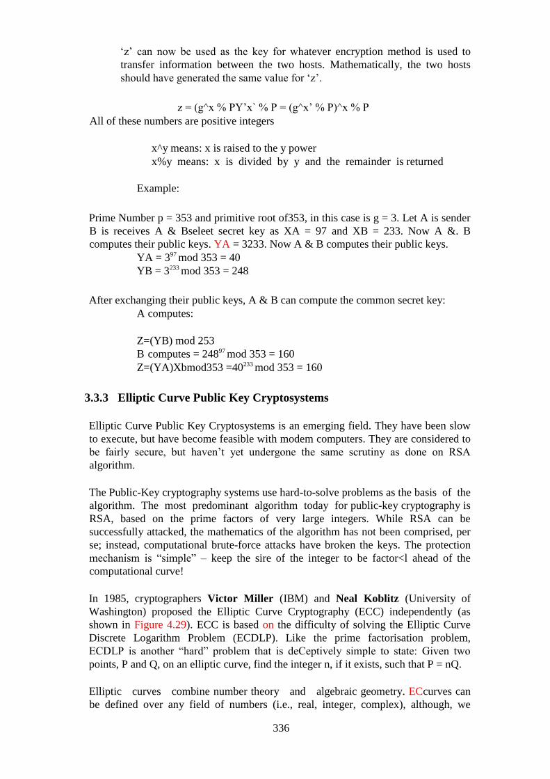
336

‗z‘ can now be used as the key for whatever encryption method is used to

transfer information between the two hosts. Mathematically, the two hosts

should have generated the same value for ‗z‘.

z = (g^x % PY‘x` % P = (g^x‘ % P)^x % P

All of these numbers are positive integers

x^y means: x is raised to the y power

x%y means: x is divided by y and the remainder is returned

Example:

Prime Number p = 353 and primitive root of353, in this case is g = 3. Let A is sender

B is receives A & Bseleet secret key as XA = 97 and XB = 233. Now A &. B

computes their public keys. YA = 3233. Now A & B computes their public keys.

YA = 397 mod 353 = 40

YB = 3233 mod 353 = 248

After exchanging their public keys, A & B can compute the common secret key:

A computes:

Z=(YB) mod 253

B computes = 24897 mod 353 = 160

Z=(YA)Xbmod353 =40233 mod 353 = 160

3.3.3 Elliptic Curve Public Key Cryptosystems

Elliptic Curve Public Key Cryptosystems is an emerging field. They have been slow

to execute, but have become feasible with modem computers. They are considered to

be fairly secure, but haven‘t yet undergone the same scrutiny as done on RSA

algorithm.

The Public-Key cryptography systems use hard-to-solve problems as the basis of the

algorithm. The most predominant algorithm today for public-key cryptography is

RSA, based on the prime factors of very large integers. While RSA can be

successfully attacked, the mathematics of the algorithm has not been comprised, per

se; instead, computational brute-force attacks have broken the keys. The protection

mechanism is ―simple‖ – keep the sire of the integer to be factor<l ahead of the

computational curve!

In 1985, cryptographers Victor Miller (IBM) and Neal Koblitz (University of

Washington) proposed the Elliptic Curve Cryptography (ECC) independently (as

shown in Figure 4.29). ECC is based on the difficulty of solving the Elliptic Curve

Discrete Logarithm Problem (ECDLP). Like the prime factorisation problem,

ECDLP is another ―hard‖ problem that is deCeptively simple to state: Given two

points, P and Q, on an elliptic curve, find the integer n, if it exists, such that P = nQ.

Elliptic curves combine number theory and algebraic geometry. ECcurves can

be defined over any field of numbers (i.e., real, integer, complex), although, we

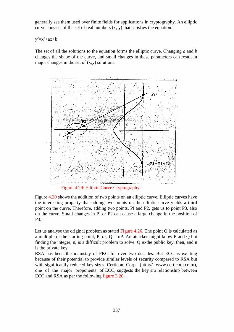
337

generally see them used over finite fields for applications in cryptography. An elliptic

curve consists of the set of real numbers (x, y) that satisfies the equation:

y2=x3+ax+b

The set of all the solutions to the equation forms the elliptic curve. Changing a and b

changes the shape of the curve, and small changes in these parameters can result in

major changes in the set of (x,y) solutions.

Figure 4.29: Elliptic Curve Cryptography

Figure 4.30 shows the addition of two points on an elliptic curve. Elliptic curves have

the interesting property that adding two points on the elliptic curve yields a third

point on the curve. Therefore, adding two points, PI and P2, gets us to point P3, also

on the curve. Small changes in PI or P2 can cause a large change in the position of

P3.

Let us analyse the original problem as stated Figure 4.26. The point Q is calculated as

a multiple of the starting point, P, or, Q = nP. An attacker might know P and Q but

finding the integer, n, is a difficult problem to solve. Q is-the public key, then, and n

is the private key.

RSA has been the mainstay of PKC for over two decades. But ECC is exciting

because of their potential to provide similar levels of security compared to RSA but

with significantly reduced key sizes. Certicom Corp. (httn:// www.certicom.com/),

one of the major proponents of ECC, suggests the key siu relationship between

ECC and RSA as per the following figure 3.20:

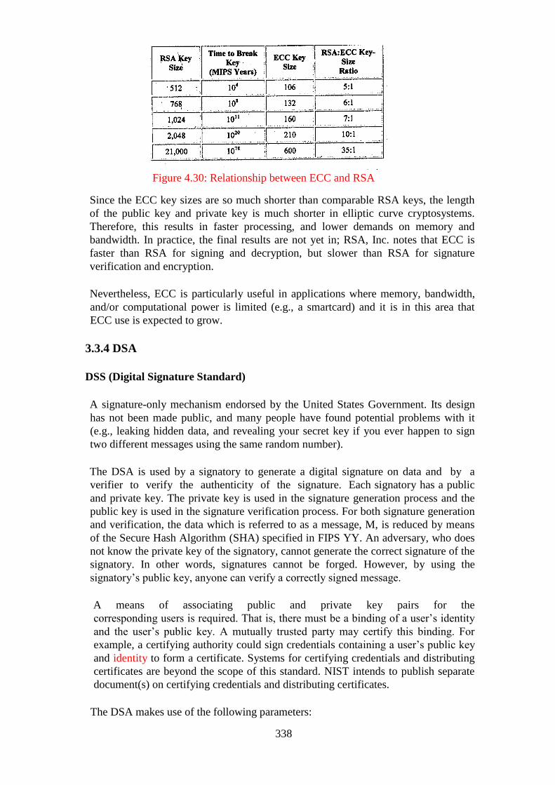
338

Figure 4.30: Relationship between ECC and RSA

Since the ECC key sizes are so much shorter than comparable RSA keys, the length

of the public key and private key is much shorter in elliptic curve cryptosystems.

Therefore, this results in faster processing, and lower demands on memory and

bandwidth. In practice, the final results are not yet in; RSA, Inc. notes that ECC is

faster than RSA for signing and decryption, but slower than RSA for signature

verification and encryption.

Nevertheless, ECC is particularly useful in applications where memory, bandwidth,

and/or computational power is limited (e.g., a smartcard) and it is in this area that

ECC use is expected to grow.

3.3.4 DSA

DSS (Digital Signature Standard)

A signature-only mechanism endorsed by the United States Government. Its design

has not been made public, and many people have found potential problems with it

(e.g., leaking hidden data, and revealing your secret key if you ever happen to sign

two different messages using the same random number).

The DSA is used by a signatory to generate a digital signature on data and by a

verifier to verify the authenticity of the signature. Each signatory has a public

and private key. The private key is used in the signature generation process and the

public key is used in the signature verification process. For both signature generation

and verification, the data which is referred to as a message, M, is reduced by means

of the Secure Hash Algorithm (SHA) specified in FIPS YY. An adversary, who does

not know the private key of the signatory, cannot generate the correct signature of the

signatory. In other words, signatures cannot be forged. However, by using the

signatory‘s public key, anyone can verify a correctly signed message.

A means of associating public and private key pairs for the

corresponding users is required. That is, there must be a binding of a user‘s identity

and the user‘s public key. A mutually trusted party may certify this binding. For

example, a certifying authority could sign credentials containing a user‘s public key

and identity to form a certificate. Systems for certifying credentials and distributing

certificates are beyond the scope of this standard. NIST intends to publish separate

document(s) on certifying credentials and distributing certificates.

The DSA makes use of the following parameters:

339

1 p = a prime modulus, where 2L-I < P < 2L for 512 = < L = <1024 and L a

multiple of 64

2 q=aprimedivisorofp-l,where2159<q<2160

3 g = h(P-1)/q mod p, where h is any integer with 1 < h < P - 1 such that h(P-1)/q mod

p> 1(g has order q mod p)

4 x = a randomly or pseudorandomly generated integer with 0 <x<q

5 y = gx mod p

6 k = a randomly or pseudorandomly generated integer with 0 <k<q

The integers p, q, and g can be public and can be common to a group of users. A

user‘s private and public keys are x and y, respectively. They are normally fixed for a

period of time. Parameters x and k are used for signature generation only, and must

be kept secret. Parameter k must be regenerated for each signature.

The signature of a message M is the pair of numbers r and s computed according to

the equations below:

r = (gk mod p) mod q and

s = (k-1(SHA(M) + xr)) mod q.

In the equation, k-1 is the multiplicative inverse of k, mod q; i.e., (k-1 k) mod q = 1

and 0 < k-1 < q. The value of SHA (M) is a 160-bit string output by the Secure Hash

Algorithm specified in FIPS 180. For use in computing s, this string must be

converted to an integer.

As an option, one may wish to check if r = 0 or s = 0. If either r = 0 or s = 0, a new

value of k should be generated and the signature should be recalculated (it is

extremely unlikely that r = 0 or s = 0 if signatures are generated properly).

The signature is transmitted along with the message to the verifier.

Prior to verifying the signature in a signed message, p, q and g plus the sender‘s

public key and identity are made available to the verifier after proper authentication.

Let M‘, r‘ and s‘ be the received versions of M, r, and s, respectively, and let y be the

public key of the signatory. To verify first check to see that 0 < r‘ < q and 0 < s‘ < q;

if either condition is violated, the signature shall be rejected. If these two conditions

are satisfied, the verifier computes:

w = (sri mod q)

ul = ((SHA(M‘)w) mod q u2

= ((r‘)w) mod q

v = (((g)ul (y)u2) mod p) mod q.

340

If v = r‘, then the signature is verified-and the verifier can have high confidence that

the received message was sent by the party holding the secret key x corresponding to

y. For a proof that v = r` when M` = M, r` = r, and s` = s, see Appendix 1 of [ref 2].

If v does not equal r`, then the message may have been modified, the message may

have been incorrectly signed by the signatory, or the message may have been signed

by an impostor. The message should be considered invalid.

EIGamal public key cryptosystem. Based on the discrete logarithm

problem.

ElGamal consists of three components: the key generator, the encryption

algorithm, and the decryption algorithm.

The key generator works as follows:

Alice generates an efficient description of a cyclic group G of order q with generator

g. See below for specific examples of how this can be done.

Alice chooses a random x from {0,...,q -1}.

Alice computes h = gx.

Alice publishes h, along with the description of G,q,g, as her public key, Alice retains

x as her secret key.

The encryption algorithm works as follows: to encrypt a message m to Alice under

her public key (G,q,g,h),

Bob converts m into an element of G.

Bob chooses a random k from {0,….,q - 1}, then calculates c1 = gk and c2 = m.hk

Bob sends the ciphertext (c1,c2) to Alice.

The decryption algorithm works as follows: to decrypt a ciphertext

(c1,c2) with her secret key x,

1

Alice computes c2 c1r as the plaintext message.

Note that the decryption algorithm does indeed produce the intended message since:

r 1 m.hk m.hrk

c c2 1 rk rk m (mod q) g g

If the space of possible messages is larger than the sire of G, then the message can be

split into several pieces and each piece can be encrypted independently. Typically,

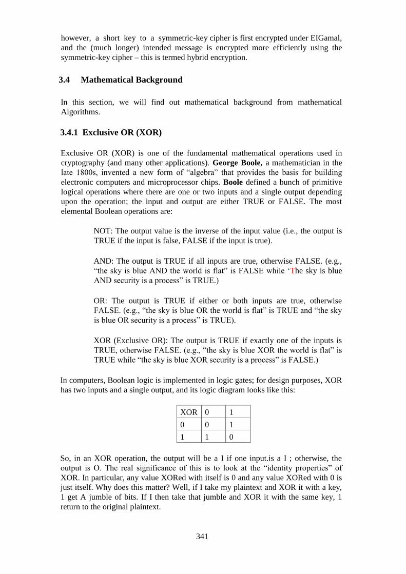
341

however, a short key to a symmetric-key cipher is first encrypted under EIGamal,

and the (much longer) intended message is encrypted more efficiently using the

symmetric-key cipher – this is termed hybrid encryption.

3.4 Mathematical Background

In this section, we will find out mathematical background from mathematical

Algorithms.

3.4.1 Exclusive OR (XOR)

Exclusive OR (XOR) is one of the fundamental mathematical operations used in

cryptography (and many other applications). George Boole, a mathematician in the

late 1800s, invented a new form of ―algebra‖ that provides the basis for building

electronic computers and microprocessor chips. Boole defined a bunch of primitive

logical operations where there are one or two inputs and a single output depending

upon the operation; the input and output are either TRUE or FALSE. The most

elemental Boolean operations are:

NOT: The output value is the inverse of the input value (i.e., the output is

TRUE if the input is false, FALSE if the input is true).

AND: The output is TRUE if all inputs are true, otherwise FALSE. (e.g.,

―the sky is blue AND the world is flat‖ is FALSE while ‗The sky is blue

AND security is a process‖ is TRUE.)

OR: The output is TRUE if either or both inputs are true, otherwise

FALSE. (e.g., ―the sky is blue OR the world is flat‖ is TRUE and ―the sky

is blue OR security is a process‖ is TRUE).

XOR (Exclusive OR): The output is TRUE if exactly one of the inputs is

TRUE, otherwise FALSE. (e.g., ―the sky is blue XOR the world is flat‖ is

TRUE while ―the sky is blue XOR security is a process‖ is FALSE.)

In computers, Boolean logic is implemented in logic gates; for design purposes, XOR

has two inputs and a single output, and its logic diagram looks like this:

XOR 0 1

0 0 1

1 1 0

So, in an XOR operation, the output will be a I if one input.is a I ; otherwise, the

output is O. The real significance of this is to look at the ―identity properties‖ of

XOR. In particular, any value XORed with itself is 0 and any value XORed with 0 is

just itself. Why does this matter? Well, if I take my plaintext and XOR it with a key,

1 get A jumble of bits. If I then take that jumble and XOR it with the same key, 1

return to the original plaintext.

342

3.4.2 The Modulo Function

The modulo function is, simply, the remainder function. It is commonly used in

programming and is critical to the operation of any mathematical function using

digital computers.

To calculate X modulo Y (usually written X mod Y), you merely determine the

remainder after removing all multiples of Y from X. Clearly, the value X mod Y will

be in the range from 0 to Y-1.

Some examples should clear up any remaining confusion:

mod 7 = I

25mod5=0 33

mod 12 = 9

203 mod 256 = 203

Modulo arithmetic is useful in crypto because it allows us to set the size of an

operation and be sure that we will never get numbers that are too large. This is an

important consideration when using digital computers.

1. Which of the following is an example of a symmetric key algorithm?

a RSA

b Diffie-Hellman

c Knapsack

2. Which of the following is a problem with symmetric key algorithms?

a It is slower than asymmetric key encryption

b Most algorithms are kept proprietry

c Work factor is not a function of the key siu.

d It provides secure distribution of the s=et key.

3. Which of the following is an example of an asymmetric key algorithms?

a ELLIPTIC CURVE

b IDEA

c 3 DES

d DES

4. In public key cryptography:

a Only the public key can encrypt, and only the private can decrypt

b Only the private key can encrypt, and only the public can decrypt

c The public key is used to encrypt and decrypt

d If the public key encrypts, and only the private can decrypt.

5. In a block cipher, diffusion:

343

a Conceals the connection between the ciphertext and plaintext

b Spread the influence of a plaintext character over many ciphertext

characters.

c Cannot be accomplished

d Is usually implemented by non-linear S-boxes.

6. State whether following statements are True or False. T 0 F 0

a Work factor of double DES is the same as for single DES

b Elliptic curse cryptosystem have a lower strength per bit than RSA.

c In digitally-signed message transmission using a hash function the

message digest is encrypted in the public key of the sender.

4.0 CONCLUSION

In this unit you have learnt about the fundamental problems in networking which is

network security. You have therefore been taken through the principles and practice

of cryptography and the various related algorithms.

5.0 SUMMARY

Information security can be defined as technological and managerial procedures

applied to computer systems to ensure the availability, integrity, and confidentiality

of the information managed by computer. Cryptography is a particularly interesting

field because of the amount of work that is, by necessity, done in secret. The

irony is that today, secrecy is not the key to the goodness of a cryptographic

algorithm. Regardless of the mathematical theory behind an algorithm, the best

algorithms are those that are well known and well documented because they are also

well tested and well studied! In fact, time is the only true test of good cryptography;

any cryptographic scheme that stays in use year after year is most likely to be a good

one. The strength of cryptography lies in the choice and management of the keys;

longer keys will resist attack better than shorter keys.

With the introduction of IT Act 2000, the electronic transactions and electronically

signed documents are valid under the court of law. Use of PKI in India is expected to

increase rapidly and for activation of global e-commerce and so also the use of digital

signatures within domestic and other Global PKI domains. This requires the

interoperability of PKI based applications.

Digitisation of information, networking, and WWW (World Wide Web), has changed

the economics of information. The Copyright Act 1957 as amended up to 1999 takes

care of the technological changes that still require major amendments in order to deal

with the challenges posed by the computer storage, Internet and the digital revolution.

With India being party to Trade Related Aspects of Intellectual Properties (TRIPs),

electronic transactions of IPRs and consultancy services related to them is expected

to be a new possibility in India. This may also promote our technology base to keep

344

pace with global trends. As India has already enacted IT Act 2000, this allows

transactions signed electronically for e- commerce primarily to be enforced in a court

of law. Several issues arise when we consider using digital documents and

exchanging them over the Internet, such as eavesdropping, tampering, impersonation

etc. All these can be remedied with the use of public key infrastructure (PKI).

However, the question of the time when a document was created may be answered by

using Digital Time stamping service, which is based on PKI. This information may

prove to be crucial for most e-commerce legally binding transactions, in particular for

supporting non-repudiation of digitally signed transactions.


1. What is cryptography?

2. List the various requirements of application-to-application communication.

3. List various types of cryptographic techniques.


Willam Stallings, Network Security Essential- Application and standard, Pearson

Education, New Delhi.

A.S. Tanenbaum, (2011). Computer Networks, 4th Edition, Practice Hall of India,

New Delhi.


Question 1

What is cryptography?

Solution

This the method of converting ordinary plaintext to an unintelligible text and vice

versa or is the science of writing secret codes.

Question 2

List the various requirements of application-to-application communication.

Solution

The various requirements of application-to-application communication are:

a. Authentication

b. Privacy/ confidentiality

c. Integrity

d. Non-repudiation.

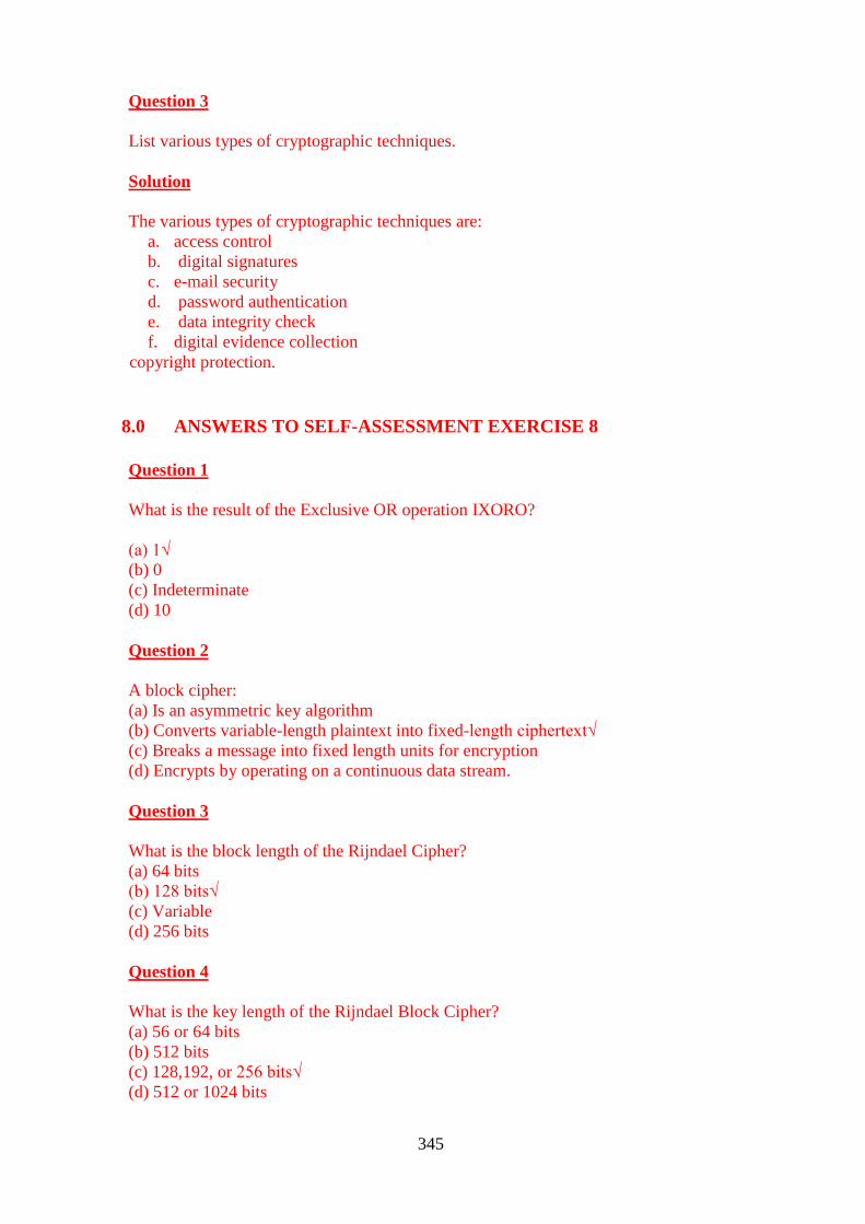
345

Question 3

List various types of cryptographic techniques.

Solution

The various types of cryptographic techniques are:

a. access control

b. digital signatures

c. e-mail security

d. password authentication

e. data integrity check

f. digital evidence collection

copyright protection.

8.0 ANSWERS TO SELF-ASSESSMENT EXERCISE 8

Question 1

What is the result of the Exclusive OR operation IXORO?

(a) 1√

(b) 0

(c) Indeterminate

(d) 10

Question 2

A block cipher:

(a) Is an asymmetric key algorithm

(b) Converts variable-length plaintext into fixed-length ciphertext√

(c) Breaks a message into fixed length units for encryption

(d) Encrypts by operating on a continuous data stream.

Question 3

What is the block length of the Rijndael Cipher?

(a) 64 bits

(b) 128 bits√

(c) Variable

(d) 256 bits

Question 4

What is the key length of the Rijndael Block Cipher?

(a) 56 or 64 bits

(b) 512 bits

(c) 128,192, or 256 bits√

(d) 512 or 1024 bits

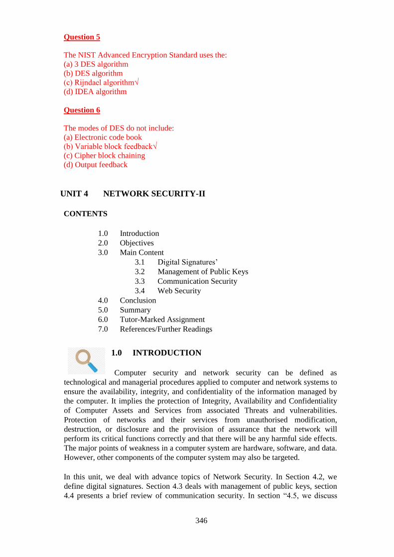
346

Question 5

The NIST Advanced Encryption Standard uses the:

(a) 3 DES algorithm

(b) DES algorithm

(c) Rijndael algorithm√

(d) IDEA algorithm

Question 6

The modes of DES do not include:

(a) Electronic code book

(b) Variable block feedback√

(c) Cipher block chaining

(d) Output feedback

UNIT 4 NETWORK SECURITY-II

CONTENTS

1.0 Introduction

2.0 Objectives

3.0 Main Content

3.1 Digital Signatures‘

3.2 Management of Public Keys

3.3 Communication Security

3.4 Web Security

4.0 Conclusion

5.0 Summary



1.0 INTRODUCTION

Computer security and network security can be defined as

technological and managerial procedures applied to computer and network systems to

ensure the availability, integrity, and confidentiality of the information managed by

the computer. It implies the protection of Integrity, Availability and Confidentiality

of Computer Assets and Services from associated Threats and vulnerabilities.

Protection of networks and their services from unauthorised modification,

destruction, or disclosure and the provision of assurance that the network will

perform its critical functions correctly and that there will be any harmful side effects.

The major points of weakness in a computer system are hardware, software, and data.

However, other components of the computer system may also be targeted.

In this unit, we deal with advance topics of Network Security. In Section 4.2, we

define digital signatures. Section 4.3 deals with management of public keys, section

4.4 presents a brief review of communication security. In section ―4.5, we discuss

347

web security. We summarise this unit in section 4.6 followed by Solutions and

Answers for ‗Check Your Progress‘.

2.0 OBJECTIVES

The objective of this unit is to provide a practical survey of both the principles and

practice of Digital Signature. After going through this unit you should be able to

understand:

digital Signature

public Key Infrastructure

management of Public Keys

communication and Web Security.

3.0 MAIN CONTENT

3.1 Digital Signatures

Digital signatures are based on public key cryptography. A private key is used to

create a digital signature and the public key is used to verify the digital signature. The

Hash value of a message when encrypted with the private key of a person is his

digital signature on that e-Document. The Digital Signature of a person therefore,

varies from document to document, thus, ensuring authenticity of each word in that

document. As the public key of the signer is known, anybody can verify the message

and the digital signature. The 4.31 shows the process of creating a digital signature.

The hash function is applied to the plain text which is further encrypted with the

private key of a sender for creating a digital signature.

Hash Function Encrypted by

Figure 4.31: Digital signature

The Figure 4.32 shows how one key is used for encryption and another key is used for

decryption. The Figure 4.33 shows that a person is having two keys in public key

cryptography.

Private key

Plain text Hash Value [H]

Digital Signature

348

Figure 4.32: Encryption and signing using public key cryptography

Figure 4.33: Explanation using an example

Ram has been given two keys. One of Ram’s Key is called the Public

key, and the other is a Private Key

Figure 4.34: Ram‘s co-workers

Ram‘s Public key is available to anyone who needs it (Figure 4.34), but he keeps his

Private Key to himself. Keys are used to encrypt information. Encrypting information

means ―scrambling it up‖, so that only the person with the appropriate key can make

it readable again. One of Ram‘s two keys can encrypt the data, while the other key

can decrypt that same data.

Ravi (Figure 4.35) can encrypt a message using Ram‘s Public Key. Ram uses his

Private Key to decrypt the message. Any of Ram‘s co-workers might have access to

the message Ravi encrypted, but without Ram‘s Private Key, the data is worthless.

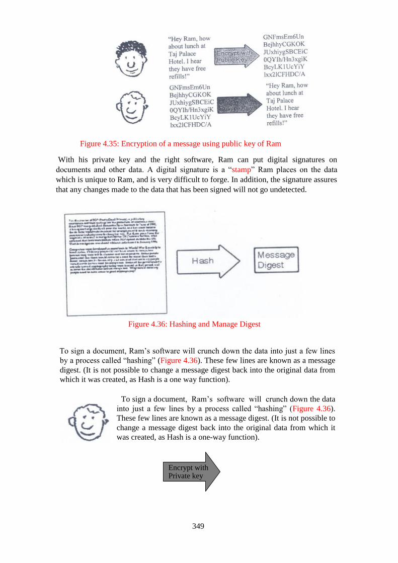
349

Figure 4.35: Encryption of a message using public key of Ram

With his private key and the right software, Ram can put digital signatures on

documents and other data. A digital signature is a ―stamp‖ Ram places on the data

which is unique to Ram, and is very difficult to forge. In addition, the signature assures

that any changes made to the data that has been signed will not go undetected.

Figure 4.36: Hashing and Manage Digest

To sign a document, Ram‘s software will crunch down the data into just a few lines

by a process called ―hashing‖ (Figure 4.36). These few lines are known as a message

digest. (It is not possible to change a message digest back into the original data from

which it was created, as Hash is a one way function).

To sign a document, Ram‘s software will crunch down the data

into just a few lines by a process called ―hashing‖ (Figure 4.36).

These few lines are known as a message digest. (It is not possible to

change a message digest back into the original data from which it

was created, as Hash is a one-way function).

Encrypt with Private key

350

Figure 4.37: Encryption of message digest using prey

Ram‘s software then encrypts (Figure 4.37) the message digests with his

private key. The result is the digital signature.

Figure 4.38: Append the digital signature to the document

Finally, Ram‘s software appends (Figure 4.38) the digital signature to the document.

All the data that was hashed has been signed (figure 4.38).

Figure 4.39: The decryption using public key

Shayam‘s software decrypts the signature in public changing it back into a Signature

message digest. If this work, then it proves that Ra m has signed the document,

because only Ram h this private key. Mohan‘s software then hashes as t document

data into a message digest. If the he message digest is the same as the message digest

created when the signature was decrypted, then Mohan knows that the signed data has

not been changed/tampered with.

Issues

Message

Digest Signature

Signature Append

Signature

Signature

Hash Message

Digest Ram now

passes the

document on

to Mohan.

Hash

351

Mohan (our disgruntled employee) wishes to deceive Shayam.

Mohan makes sure that Shayam receives a signed message and a

public key that appears to belong to Ram. Unknown to Shayam,

Mohan deceitfully sends a key pair he has created using Ram‘s

name. Short of receiving Ram‘s public key from him in person,

how can Shayam be sure that Ram‘s public key is authentic?

It so happens that Ravi works at the company‘s certificate

authority centre. Ravi can create a digital certificate for Ram by

using Ram‘s public key as well as some information (figure 4.39).

Figure 4.40: Creation of a digital certificate

Ram‘s co-workers can verify Ram‘s trusted certificate to make sure that his public key

truly belongs to him. In fact, no one at Ram‘s company accepts a signature for which

there does not exist a certificate generated by Ravi. This gives Ravi the power to

revoke signatures if private keys are compromised, or no longer needed. There are

even more widely accepted certificate authorities that certify Ravi.

If Ram sends a signed document to Shayam, to verify the signature on the document,

Shayam‘s software first uses Ravi‘s (the certificate authority‘s) public key to check

the signature on Ram‘s certificate. Successful de-encryption of the certificate proves

that Ravi created it. After the certificate is de-encrypted, Shayam‘s software can

check if Ram is in good standing with the certificate authority and that the certificate

information concerning Ram‘s identity has not been altered.

Shayam‘s software then takes Ram‘s public key from the certificate and uses it to

check Ram‘s signature. If Ram‘s public key de-encrypts the signature

successfully, then Shayam is assured that the signature was created using Ram‘s

private key, for Ravi has certified the matching public key. And of course, if the

signature is valid, then we know that Mohan didn‘t try to change the signed

content.

Digital Certificate

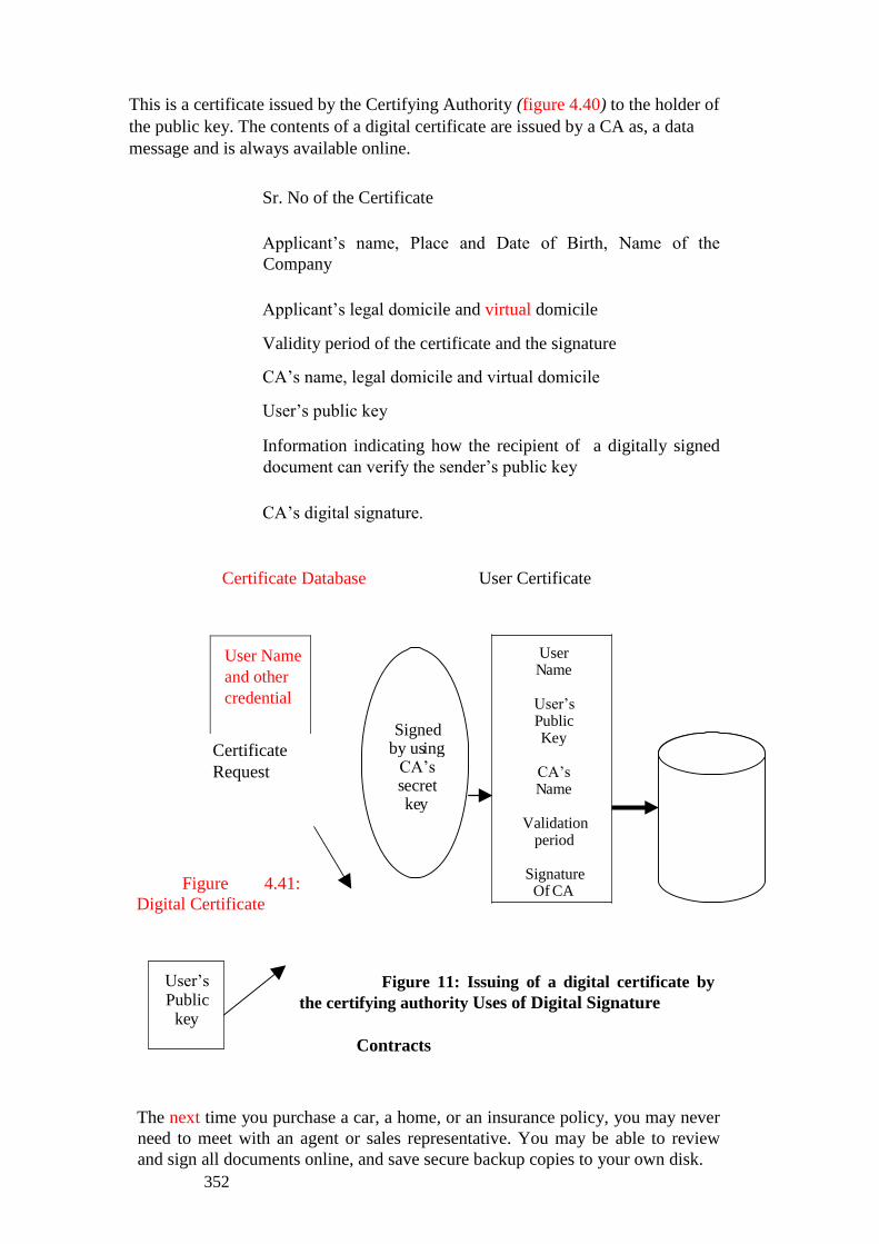
352

This is a certificate issued by the Certifying Authority (figure 4.40) to the holder of

the public key. The contents of a digital certificate are issued by a CA as, a data

message and is always available online.

Sr. No of the Certificate

Applicant‘s name, Place and Date of Birth, Name of the

Company

Applicant‘s legal domicile and virtual domicile

Validity period of the certificate and the signature

CA‘s name, legal domicile and virtual domicile

User‘s public key

Information indicating how the recipient of a digitally signed

document can verify the sender‘s public key

CA‘s digital signature.

Certificate Database User Certificate

Certificate

Request

Figure 4.41:

Digital Certificate

Figure 11: Issuing of a digital certificate by

the certifying authority Uses of Digital Signature

Contracts

The next time you purchase a car, a home, or an insurance policy, you may never

need to meet with an agent or sales representative. You may be able to review

and sign all documents online, and save secure backup copies to your own disk.

User Name

and other

credential

Signed by us ing

CA‘s s ecret ke y

User N ame

User‘s P ublic Key

CA‘s N ame

Validation

period

Signature Of CA

User‘s P ublic

ke y

353

Cheques and money orders

Buying online is now easy with a credit card, but digital Cheques or money

orders (authenticated by secure digital signatures) may be preferable for some

transactions, especially when you don‘t want to face a large credit card bill.

Letters and memos

Businesses already transmit many letters and memos online, especially those that

are only distributed internally. But when a letter or memo needs the weight of a

manager‘s signature, it must be printed, signed, duplicated, and distributed

manually or through the mail. Digital signatures will save companies the time and

expense of this manual process.

Approvals

Many kinds of documents are collaborative works, such as legal briefs, contracts,

reports, and others. Using digital signatures, people can collaborate on documents

online and approve final drafts, before/prior to releasing them for use.


1 What does the Electronic Signatures in Global and National Commerce

Act do?

2 What does a signature mean?

3 Why are handwritten signatures a drawback in some types of transactions?

4 What is a digital signature?

5 What are the benefits of using digital signatures?

3.3 Management of Public Keys

Public Key Infrastructure

The integration of Digital Signatures and Certificates and the other services

required for E-Commerce is known as Public Key Infrastructure (PKI). These

services provide integrity, access control, confidentiality, authentication, and non-

repudiation for electronic transactions and communications. The PKI includes the

followings: Digital certificates, Certificate authority (CA), Registration authority,

policies and procedures, Certificate revocation, Non-repudiation support, Time

stamping, Lightweight Directory Access Protoco1 (LDAP), and Security-enabled

applications.

The Digital certificate and management of the certificate are the main

components of PKI. The purpose of the digital certificate is to verify individual

public key. This certificate is accomplished by digital1y signing the individuals

public key and associated information using the Private Key. A CA (Certification

Authority) acts as the notary for verifying a person‘s identity and issuing a

certificate that vouches for the public key of the individual concerned. The CA

signs the certificate with its own private key. The certificate is then sent to a

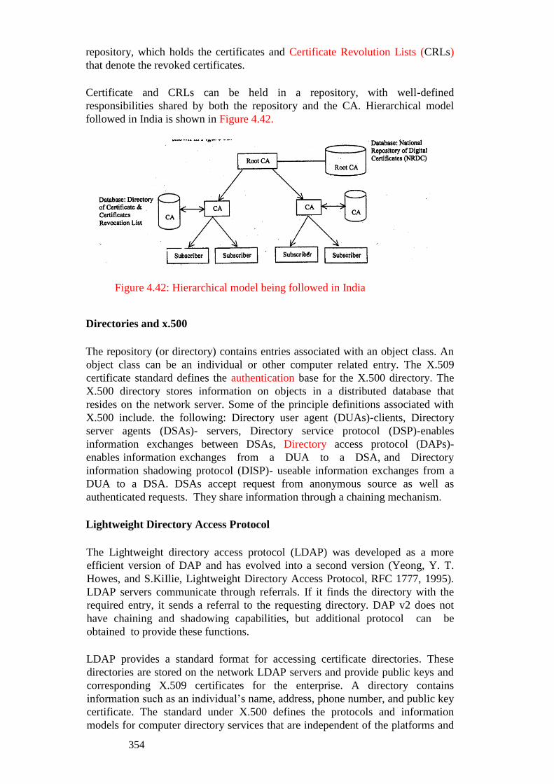
354

repository, which holds the certificates and Certificate Revolution Lists (CRLs)

that denote the revoked certificates.

Certificate and CRLs can be held in a repository, with well-defined

responsibilities shared by both the repository and the CA. Hierarchical model

followed in India is shown in Figure 4.42.

Figure 4.42: Hierarchical model being followed in India

Directories and x.500

The repository (or directory) contains entries associated with an object class. An

object class can be an individual or other computer related entry. The X.509

certificate standard defines the authentication base for the X.500 directory. The

X.500 directory stores information on objects in a distributed database that

resides on the network server. Some of the principle definitions associated with

X.500 include. the following: Directory user agent (DUAs)-clients, Directory

server agents (DSAs)- servers, Directory service protocol (DSP)-enables

information exchanges between DSAs, Directory access protocol (DAPs)-

enables information exchanges from a DUA to a DSA, and Directory

information shadowing protocol (DISP)- useable information exchanges from a

DUA to a DSA. DSAs accept request from anonymous source as well as

authenticated requests. They share information through a chaining mechanism.

Lightweight Directory Access Protocol

The Lightweight directory access protocol (LDAP) was developed as a more

efficient version of DAP and has evolved into a second version (Yeong, Y. T.

Howes, and S.KiIlie, Lightweight Directory Access Protocol, RFC 1777, 1995).

LDAP servers communicate through referrals. If it finds the directory with the

required entry, it sends a referral to the requesting directory. DAP v2 does not

have chaining and shadowing capabilities, but additional protocol can be

obtained to provide these functions.

LDAP provides a standard format for accessing certificate directories. These

directories are stored on the network LDAP servers and provide public keys and

corresponding X.509 certificates for the enterprise. A directory contains

information such as an individual‘s name, address, phone number, and public key

certificate. The standard under X.500 defines the protocols and information

models for computer directory services that are independent of the platforms and

355

other related entities. LDAP servers are subject to attacks that affect availability

and integrity. For example, Denial of Service attacks on an LDAP server could

prevent access to the CRLs and thus, permit the use of a revoked certificate. The

DAP protocol in X.500 was unwieldy and led to most client implementations

using LDAP. LDAP version 3 is under development; it will include extensions

that provide shadowing and chaining capabilities.

X.509 Certificates

The original X.509 certificate (CCITT, The Directory-Authentication Framework,

Recommendation X.509, 1988) was developed to provide authentication

foundation for the X.500 directory. Since then, a version 2, version 3, and

recently, a version 4 have been developed. Version 2 of the X.509 certificates

address the reuse of names, version 3 provides for certificate extensions to the

core certificate fields, and version 4 provides additional extensions. These

extensions can be used as needed by different users and different applications. A

version ofX.509 that takes into account the requirements of the internet was

published by the IETF (Housley, R. W. Ford, W.Polk, and D. Solo, Internet

X.509 public Key Infrastructure Certificate and CRL Profile, RFC 2459,1999).

The Consultation Committee, International Telephone and Telegraph,

International Telecommunications Union (CCITT -ITU)/International

Organization for standardization (ISO) has defined the basic format of an X.509

certificate. This structure is outlined in the Figure 4.43.

Figure 4.43: The CCITT-ITU/ISO X.509 certificate format

If version 3 certificates are used, the optional extensions field can be used. It is

before the signature field components in the certificate. Some typical extensions

are the entity‘s name and supporting identity information, the attributes of the

key, certificate policy information, and the type of subject. The digital signature

serves as a tamper-evident envelope.

Some of the different types of certificates that are issued include the following:

CA certificates

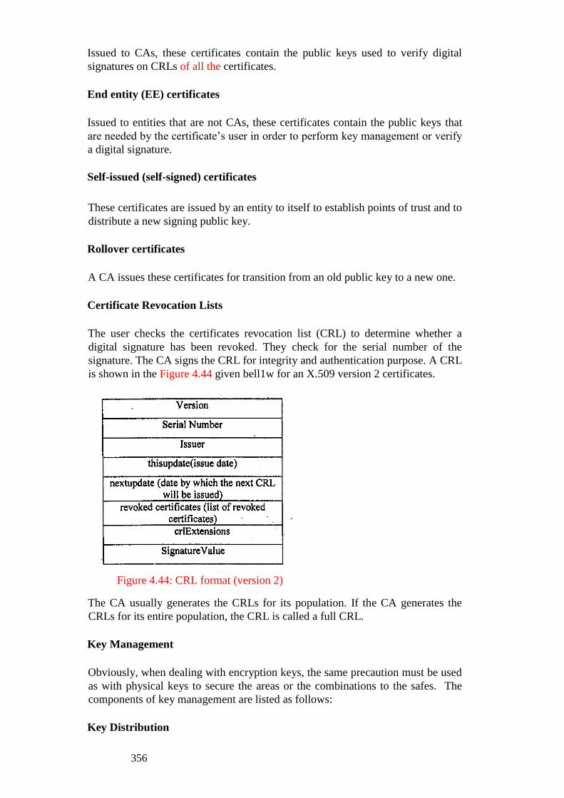
356

Issued to CAs, these certificates contain the public keys used to verify digital

signatures on CRLs of all the certificates.

End entity (EE) certificates

Issued to entities that are not CAs, these certificates contain the public keys that

are needed by the certificate‘s user in order to perform key management or verify

a digital signature.

Self-issued (self-signed) certificates

These certificates are issued by an entity to itself to establish points of trust and to

distribute a new signing public key.

Rollover certificates

A CA issues these certificates for transition from an old public key to a new one.

Certificate Revocation Lists

The user checks the certificates revocation list (CRL) to determine whether a

digital signature has been revoked. They check for the serial number of the

signature. The CA signs the CRL for integrity and authentication purpose. A CRL

is shown in the Figure 4.44 given bell1w for an X.509 version 2 certificates.

Figure 4.44: CRL format (version 2)

The CA usually generates the CRLs for its population. If the CA generates the

CRLs for its entire population, the CRL is called a full CRL.

Key Management

Obviously, when dealing with encryption keys, the same precaution must be used

as with physical keys to secure the areas or the combinations to the safes. The

components of key management are listed as follows:

Key Distribution

357

As noted earlier, distributing secret keys in symmetric key encryption poses a

problem. Secret keys can be distributed using asymmetric key cryptosystem.

Other means of distributing secret keys include face-to- face meeting to exchange

keys, sending the keys by a secure messenger, or some other secure alternate

channel. Another method is to encrypt the secret key with another key, called a

key encryption key, and send the encrypted key to the intended receiver. These

key encryption keys can be distributed manually, but they need not be distributed

often. The X9.l7 Standard (ANSI X9.l7 [Revised],‖ American National Standard

for Financial Institution Key Management [Wholesale],‖ American Bankers

Association, 1985) specifies key encryption keys as well as data keys for

encrypting the plaintext messages.

Splitting the keys into different parts and sending each part by a different

medium can also accomplish key distribution.

In large networks, key distribution can become a serious problem because in an

N-person network, the total number of key exchanges is N(N-I)/2. Using public

key cryptography or the creation and, exchange of session keys that are valid only

for a particular session and time are useful mechanism for managing the key

distribution problem. Keys can be updated by generating a new key from an old

key.

Key Revocation

A digital certificate contains a timestamp or period for which the certificate is

valid. Also if the key is compromised or must be made invalid because of

business-or personal-related issues, it must be revoked. The CA maintains a

CRL of all invalid certificates. The user should regularly examine this list.

Key Recovery

A system must be put in place to decrypt critical data if the encryption key is lost

or forgotten. One method is key escrow. In this system, the key is subdivided into

different parts, each of which is encrypted and then sent to a different trusted

individual in an organization. Keys can also be escrowed onto smart cards.

Key renewal

Obviously, the longer a secret key is used without changing it, the more it is

subject to compromise. The frequency with which you change the key is a direct

function of the value of the data being encrypted and transmitted. Also, if the

same secret key is used to encrypt valuable data over a relatively long period of

time, you risk compromising a larger volume of data when the key is broken.

Another important concern if the key is not changed frequently is that an attacker

can intercept and change messages and then send different messages to the

receiver. Key encryption keys, because they are not used as often as encryption

keys, provides some protection against attacks. Typically, private keys used for

digital signatures are not frequently changed and may be kept for years.

Key destruction

358

Keys that have been in use for long periods of time and are replaced by others

should be destroyed. If the keys are compromised, older messages sent with those

keys can be read.

Keys that are stored on disks or EEPROMS should be overwritten numerous

times. One can also destroy the disk by shredding and burning them. However, in

some cases, it is possible to recover data from disks that were put into fire. Any

hardware device storing the keys, such as an EEPROM, should also be physically

destroyed.

Older Keys stored by the operating system in various locations in the memory

must also be searched and destroyed.

Multiple Keys

Usually an individual has more than one public/private key pair. The keys may be

of different sires for different levels of security. A larger key sire may be used for

digitally signing documents and smaller key sire may be used for encryption. A

person may also have multiple roles or responsibilities wherein he/she may want

to sign messages with a different signature. One key pair may be used for

business matters, another for personal use, and another for some other activity,

such as being a school board member.

Distributed vs Centralized Key Management

A CA is a form of centralized key management. It is a central location that issues

certificates and maintains CRLs. An alternative is the distributed key

management, in which a ―chain of trust‖ or ―web of trust‖ is set up among users

who know each other. Because, they know each other, they can trust that each

one‘s public key is valid. Some of these users may know other users and thus,

verify their public key. The chain spreads outward from the original group. This

arrangement results in an informal verification procedure that is based on people

knowing and trusting each other.

3.3 Communication Security

This section describes authentication mechanism to support application- level

authentication and digital signatures. We will describe kerberos mechanism in the

following paragraphs.

Kerberos

Kerberos is a commonly used authentication scheme on the Internet. Developed

by MIT‘s Project Athena, Kerberos is named after the three- headed dog who,

according to Greek mythology, guards the entrance of Hades (rather than the exit,

for some reason!).

Kerberos (as shown in Figure 4.45) employs a client/server architecture and

provides user-to-server authentication rather than host-to-host authentication. In

this model, security and authentication will be based on a secret key technology

where every host on the network has its own secret key. It would clearly be

359

unmanageable if every host had to know the keys of all other hosts so, a secure,

trusted host somewhere on the network, known as a Key Distribution Centre

(KDC), knows the keys of all the hosts (or at least some of the hosts within a

portion of the network, called a realm). In this way, when a new node is brought

online, only the KDC and the new node need to be configured with the node‘s

key; keys can be distributed physically or by some other secure means.

Figure 4.45: Kerberos

The Kerberos Server/KDC has two main functions (Figure 4.45), known as the

Authentication Server (AS) and Ticket-Granting Server (TGS). The steps in

establishing an authenticated session between an application client and the

application server are:

The Kerberos client software establishes a connection with the Kerberos server‘s

AS function. The AS firstly authenticates that the client is who it purports to be.

The AS then provides the client with a secret key for this login session (the TGS

session key) and a ticket-granting ticket (TGT), which gives the client permission

to talk to the TGS. The ticket has a finite lifetime so that the authentication

process is repeated periodically.

The client now communicates with the TGS to obtain the Application Server‘s

key so that it (the client) can establish a connection with the service it wants. The

client supplies the TGS with the TGS session key and TGT; the TGS responds

with an application session key (ASK) and an encrypted form of the Application

Server‘s secret key; this secret key is never sent on the network in any other form.

The client has now authenticated itself and can prove its identity to the

Application Server by supplying the Kerberos ticket, application session key, and

encrypted Application Server secret key. The Application Server responds with

similarly encrypted information to authenticate itself to the client. At this point,

the client can initiate the intended service requests (e.g., Telnet, FTP, H1TP, or e-

commerce transaction session establishment).

Electronic Mail Security

360

Electronic mail is the most heavily used network-based application. It is also the

only distributed application that is widely used across all architectures and vendor

platforms. With the explosively growing reliance on electronic mail, there is a

concern for authentication and confidentiality of service. Two approaches, pretty

good privacy (PGP) and Secured Multipurpose Internet Mail Extension.

(S/MIME) are widely used for this purpose.

PGP

PGP is largely the effort of a single person, Phil Zimmermann, and provides a

confidentiality and authentication service that can be used for electronic mail and

file storage applications. Zimmermann has done the following:

Selected the best available cryptographic functions as building blocks, integrated

these functions into general purpose application that is independent of operating

system and processor,

Made the package and documentation, including source code, freely available via

the Internet, bulletin boards, and commercial networks, and

Also made the Commercial versions easily available.

The actual operation of PGP consists of five services: authentication,

confidentiality, compression, e-mail compatibility, and segmentation. A brief

summary of PGP services is described in the figure 4.46:

Figure 4.46: Services of PGP

S/MIME

S/MIME (Secure/Multipurpose Internet Mail Extension) is a security

enhancement to the MIME Internet e-mail format standard, based RSA data

security technology. Though both S/MlME and PGP are based on IETF standards,

361

S/MIME is industry standard for commercial and organizational use, and PGP is a

choice for personal e-mail security for many users.

MIME is an extension to the RFC 822 framework (traditional email format

standard) that is intended to address some of the problems and limitations of the

use of SMTP (simple mail transfer protocol) or some other mail transfer protocol

and RFC 822.

Virtual Private Network (VPN)

The VPN has become the de facto standard for secure remote access. It provides

business partners access to corporate network resources across un-trusted

networks. Typically, the untrusted network will be the Internet, but VPNs offer

excellent flexibility and can also be used across more traditional network

mediums such as frame relay or ATM networks. VPNs guarantee the

confidentiality and integrity of corporate data through the use of strong

encryption and authentication techniques. VPNs have become famous because of

excellent cost saving and performance improvements in comparison to more

traditional remote access methods. Types of VPN

VPNs are of two distinct categories: (I) Site to site VPNs, between two or more

offices or data centres; (2) Client to site VPNs, between a desktop client and a

central office or data centre.

IPSec

Most clients to site VPNs are based on IPSec (short for IP Security), which is a

suite of protocols developed by the IETF to support secure transmission of

packets at the IP layer. Typically, an IPSec tunnel connection will be created

from a Client software component to a VPN gateway (or firewall with VPN

functionality). Following the initialization of this tunnel, all packets destined for

the remote corporate network will be routed through this tunnel. The tunnel

provides the necessary security, by encrypting each packet (using one of a

selection of algorithms) before forwarding it to the remote gateway. When

packets reach the remote gateway, they are decrypted and then forwarded ‗in the

clear‘ to the final destination.

IPSec was initially devised for site to site VPN connections, so in order to add the

necessary functionality to IPSec to allow effective client to site connections and

management, each vendor has added vendor specific features to its IPSec

implementation. Good examples of this include Check Point hybrid mode (to

allow strong user authentication without certificates) and NAT traversal

techniques from the majority of vendors.

As shown in the Figure 4.47, IPSec clients work by adding extra functionality at

the bottom of the IP Layer. This functionality inspects traffic, and encapsulates

and encrypts traffic as necessary.

362

IPSec

Figure 4.47: Functionality inspects traffic, and encapsulates and encrypt traffic

Secure Sockets Layer (SSL)

Netscape originated SSL. Secure Sockets layer is a protocol, which is already

imbedded in most IP stacks and placed at the base of the application layer, as

shown in the Figure 4.48. SSL has been traditionally and widely deployed for

securing web-based applications in the form of HTTPS (or secure HTTP). Even

the most novice users are normally aware of the padlock symbol shown on secure

web sites, even if they are unaware of the fact that this symbol means that‖ the

site is protected by SSI.

Application Layer (OSI

Layers 5,6 & 7)

Transport Layer (OSI

Layer 4)

IP Layer (OSI Layer 3)

Network Access Layer

(OSI Layers 1 & 2)

Figure 4.48: Secure socket layer (SSL).

Some SSL VPNs claim 10 have clientless or near clientless operation. This means

access to the VPN can be created from any machine with a Web browser,

Application Layer (OSI

Layers 5,6 & 7)

Transport Layer (OSI

Layer 4)



(OSI Layers 1 & 2)

363

including machines in Internet cafe‘s and home machines. The main drivers for

SSL VPN are: Cost saving; independent platform and mobility.

Cost saving

Because SSL VPNs can be clientless, the cost of deploying clients is saved. For

large organizations this can be a large outlay.

Independent Platform & mobility

Access can be granted from many types of machine (Linux, Windows, PDAs) and

from many locations.

With these benefits, SSL VPNs also has many complications and disadvantages.

Benefits of SSL

Cost saving

Because SSL VPNs can be clientless, the cost of deploying clients is saved.

Platform independence/independent platform

Access can be granted from many types of machines with different operating

systems (Linux, Windows 2K/XP, Apple Mac, Palm OS, windows 7, windows 8,

windows 10, Symbian, Pocket PC).

Client type mobility

Although IPSec clients can grant access across most mediums (Leased line, DSL,

Dial, GPRS) they only offer access from the corporate desktop on which the

client is installed. SSL VPNs can be configured to allow access from corporate

built laptops, home desktops, customer or supplier desktops or any machine in an

Internet cafe. This extra choice allows a much wider audience (i.e., non-laptop

users) to improve productivity and work from anywhere (at home or while

traveling).

Client IP mobility

Although widespread deployment is yet to take hold, mobile IP network

deployment is growing steadily. A side effect of a mobile IP network is that the

client‘s source address can change as a client moves between cells and networks.

This has the effect of breaking an IPSec VPN connection, but because SSL VPNs

are not bound to the source IP address, connections can be maintained as clients

move. No NA Tissues-Traditionally Hide Network Address Translation Hide

NAT) has caused issues with IPSec VPNs. Vendors have generally overcome

these issues by developing vendor specific NAT traversal mechanisms based on

Payload encapsulation in UDP packets. Although these mechanisms normally

364

function well, they break and cause interoperability problems between vendors

deployments. SSL VPNs do not suffer such issues because they are not tied to the

IP layer.

Granular access control

Although IPSec VPNs also offer highly granular access control through machine

and the service it provides, SSL VPNs can offer a greater degree of granularity,

even as far as the URL. SSL VPNs also lend themselves to more granular access

control because each resource accessed must be explicitly defined. This differs

from IPSec VPN because the entire corporate network can be defined with a

single statement.

Restrictive firewall rules

Organizations with a reasonable security infrastructure employs a firewall rule set

with limits outbound access. SSL based VPNs communicate on the port used by

Secure HTTP (TCP port 443), which is one of the few ports allowed outbound

access from any machine in the corporate network in most environments. Even if

the proxy cache servers are deployed, since the HTTPS traffic is encrypted, as a

result, this encrypted traffic will pass un-inspected. This is not possible with

IPSec based VPN.

As stated above in the Figure 4.48 SSL VPNs make use of the existing SSL

functionality that are already present in most IP Stacks. Because SSL fits into the

stack between layers 4 and 5, each application must explicitly define its use.

Based on this fact, SSL VPNs fall into 3 distinct categories: (i) Application layer

proxies, (ii) Protocol redirectors, and (iii) Remote control enhancers. Commercial

SSL products are combination of the above-mentioned techniques.

These techniques are discussed below:

1 Application layer proxies

Application layer proxies are the simplest form of SSL VPNs because they rely

on the SSL functionality used by existing applications. Because of this,

application layer proxies have the least application support. Generally, they

only support Email and Web-based traffic. They function by using the SSL

setup in existing applications, for example, you would web browse to the

gateway which will then proxy web traffic internally (using a simple method to

display links to internal systems). To use the email, your administrators would

configure the SSL functionality in your email client and proxy all email traffic

via the gateway.

One of the advantages of application layer proxies are that they are truly

clientless. They operate with nearly all operating systems and web browsers.

2 Protocol redirectors

Protocol redirectors have more flexibility than application layer proxies, but they

are truly clientless in their operation. Protocol redirectors work by downloading a

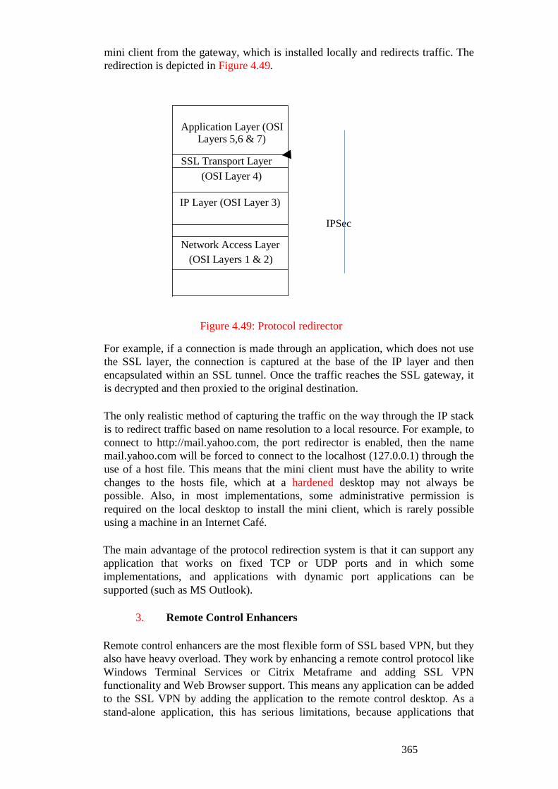
365

mini client from the gateway, which is installed locally and redirects traffic. The

redirection is depicted in Figure 4.49.

IPSec

Figure 4.49: Protocol redirector

For example, if a connection is made through an application, which does not use

the SSL layer, the connection is captured at the base of the IP layer and then

encapsulated within an SSL tunnel. Once the traffic reaches the SSL gateway, it

is decrypted and then proxied to the original destination.

The only realistic method of capturing the traffic on the way through the IP stack

is to redirect traffic based on name resolution to a local resource. For example, to

connect to http://mail.yahoo.com, the port redirector is enabled, then the name

mail.yahoo.com will be forced to connect to the localhost (127.0.0.1) through the

use of a host file. This means that the mini client must have the ability to write

changes to the hosts file, which at a hardened desktop may not always be

possible. Also, in most implementations, some administrative permission is

required on the local desktop to install the mini client, which is rarely possible

using a machine in an Internet Café.

The main advantage of the protocol redirection system is that it can support any

application that works on fixed TCP or UDP ports and in which some

implementations, and applications with dynamic port applications can be

supported (such as MS Outlook).

3. Remote Control Enhancers

Remote control enhancers are the most flexible form of SSL based VPN, but they

also have heavy overload. They work by enhancing a remote control protocol like

Windows Terminal Services or Citrix Metaframe and adding SSL VPN

functionality and Web Browser support. This means any application can be added

to the SSL VPN by adding the application to the remote control desktop. As a

stand-alone application, this has serious limitations, because applications that

Application Layer (OSI Layers 5,6 & 7)

SSL Transport Layer

( OSI Layer 4)



(OSI Layers 1 & 2)

366

reside on the local desktop cannot be used directly. This is why most remote

control enhancers are partnered with other SSL VPN technologies.

On the positive side though, they can offer features like the ability to read and

update a documents held centrally without ever having to download the entire

document. While travelling and using VPN over low speed connections, or when

connection quality is poor this could be a better option, because connections are

restarted without loosing any work.

Technical Issues

Other technical considerations include

Performance; high availability; and network performance.

Performance

SSL VPNs can support large number of concurrent users with adequate

performance.

High Availability

Most vendors (especially the ones with more mature products) are able to perform

some form of internal High Availability and fail over mechanisms.

Network Performance: Performance over a low speed link (GSM data or GPRS)

should be good to accept the mobility aspect of SSL VPNs. It has been noticed

that SSL VPNs can offer some performance advantages over IPSec VPNs.

Not considering the setup operations, which can be considered ―one time‖ for a

relatively short-lived connection, the overhead of IPSec on a packet is between 50

and 57 octets (including the new IP header, the ESP header and the trailers),

representing a 10% increase on an average packet (500 byte). In contrast to this,

SSL VPNs add only 5 octets of data to each packet, just a I % increase on the

average packet. However, setup operations cannot be ignored, but these are

roughly similar in size for IPSec and SSL connections. Also, because SSL VPNs

work at a much higher layer, they suffer far less from, the packet fragmentation

issues normally associated with IPSec VPNs. Finally, SSL has an in-built

compression mechanism.

Deployment Considerations and Disadvantages of SSL VPNs

Application Support

The main hurdle to deployment of SSL VPNs is likely to be application support.

As SSL works at the boundary of layers 4 and 5, each application must support its

use. Vendors add additional support through the use of protocol redirectors, but

these often require some user knowledge to operate. Based on this, the first

step to take when designing an SSL VPN solution is to look at the access that

will be required and assess how simple this will be to provide.

Internal Network Security Failings

367

With IPSec VPN, a large number of organisations allocate specific IP addresses

to remote clients‘ systems using the RIDIUS Protocol. This gives the ability to

file and control traffic based on the IP source, ensuring internal network security.

As all sessions from an SSL VPN are normally proxied from a single address, all

clients‘ sessions originate from this single IP. Due to this, a network

administrator is unable to allocate privileges using source IP addresses. In reality,

this level of control can be handled on the SSL VPN gateway, but if a network is

already configured to some IP source-based security, the overhead of altering it,

can be very high.

Audit and Activity Awareness

Any security appliance, hardware or software system should include a good level

of auditing. With SSL VPN this functionality is seen as the key, because of the

relatively simple systems needed to abuse an SSL VPN by a remote hacker (i.e.,

A web browser), should logon credentials become compromised. Further to this,

some form of real time alerting of unusual actions (such as trying to copy an

entire disk over the VPN) must be included. Some of this functionality is seen by

vendors, as fewer keys and, is still evolving.

Client Security

As SSL VPN offers a much greater choice of client platform with

‗clientless‘ or ‗near clientless‘ operation, the security of any client connecting to

the network must be scrutinised. For example, in no way would any organisation

consider a PC in an Internet cafe to be as trusted as a corporate issued laptop.

Due to this, vendors have developed several mechanisms to boost the trust

associated with an un-trusted client connection. Some of these are outlined

below:

1. Client Integrity Scanning

When a client connects to the VPN a small java applet is downloaded to the client

machine, which searches for good or bad files, process or ports listening. For

example, it can check for a running A V program with current definitions, the

presence of a personal firewall with a standard rule set or the presence of any

known Trojans. The disadvantage of this mechanism is it may place limitations

on the types of clients that can connect, but more importantly, it is only a onetime

snapshot of a system. Also with an understanding or the rule set, it seems feasible

that these checks may be fooled.

2. Sandbox

A sandbox is used to store any files downloaded from a corporate network over

the SSL VPN. Once the VPN session is terminated, the contents of the sandbox

are securely deleted. This avoids issues of email attachments and corporate data

being accidentally left on un-trusted machines. Sandboxes can also be used to

ensure Citrix Metaframe or other interactive session data is wiped from a machine

at logoff.

3. Secure logoff and credential wiping

368

This ensures that when users logoff the system all logon credentials are wiped

from the client machine. Of course, with enterprise strength VPN solution, a

strong authentication mechanism should also be used to protect credentials

further.

4. Timeouts and Re-authentication

To avoid systems being left connected to the network by users, sessions can be

terminated after periods of inactivity. Also, to ensure that the correct user is still

using the connection, periodic authentication during a session can be

implemented on client systems.

5. Virus, Malicious Code and Worm Activity

As the client is nearly un-trusted, most SSL VPNs can also filter traffic at the

application level (especially if an application level proxy is used, rather than a

protocol redirector), blocking worms and viruses at the gateway. SSL VPNs used

for remote access, no doubt, have significant advantages over the IPSec

alternatives. But the advantages they offer also add complexity, which must be

weighed against the advantages. Before considering an SSL VPN deployment

you should consider: security risks involved; added mobility and flexibility;

protocol support required.

3.4 Web Security

With the transformation of the Internet from a network used primarily by

universities and research laboratories to a world-wide communications medium,

attacks on the World Wide Web and Internet can be have very serious

consequences. In today‘s environment virtually all businesses, government

agencies, and many individuals now have their own web sites. But Internet and

Web are extremely vulnerable to compromises of various sorts. As a result

demand for secure web services grows. Thus, there is a need for protecting

nodes on the Internet and for providing for the confidentiality, integrity, and

availability of information utilising these networks.

Web Security Considerations

WWW is fundamentally a client/server application running over the Internet and

TCP/IP intranet. This presents new challenge:

The web is vulnerable to attacks on the Web server over the Internet.

Reputation can be damaged and money can be lost if the Web servers are

subverted, as it serves as a highly visible outlet for corporate and product

information.

The history of the web show that even upgraded, properly installed systems

are vulnerable to a variety of security attacks.

SSL/TLS

369

The Secure Sockets Layer (SSL) protocol was developed by Netscape in 1994 to

protect the confidentiality of information transmitted between two applications, to

verify the integrity of communication and to provide authentication means in

both directions. SSL implements these functions using public and private key

encryption and a message authentication code (MAC).

Microsoft has developed a newer version of SSL, Transport Layer security (TLS).

As with SSL, TLS includes confidentiality, integrity and authentication above the

transport layer and is application independent. Because SSL and TLS ride on the

transport layer protocol, they are independent of the application. Thus, SSL and

TLS can be used with application such as telnet, FTP, HTTP and email protocol.

Both SSL and TLS use certificates for public key verification that are based on

the X.509 standard. SSL 3.0

The design goals of SSL 3.0 were to provide:

1 Cryptographic Security: Protection of the confidentiality of

transmitted messages.

2 Interoperability: Application should be able to be developed using

SSL 3.0 by groups of individuals without knowledge of each other‘s

code.

3 Extensibility: The ability to incorporate different encryption algorithm

into SSL 3.0 without major changes to SSL 3.0.

4 Relative Efficiency: Efficient utilisation of computing and network

resources.

Session keys generated during SSL private key cryptography transaction are

either 40-bits or I 28-bits in length. Newer browsers support I 28-bit encryption.

The SSL protocol comprises two layers, the SSL Record Protocol and the SSL

Handshake Protocol. The SSL Record Protocol is layered above a transport

protocol, such as TCP. This record protocol is used for encapsulation of higher-

level-protocols, such as the SSL Handshake protocol. The latter protocol is used

for client/server mutual authentication, negotiation of a cryptographic algorithm,

and exchange of cryptographic keys.

Thus, through these mechanisms, SSL provides:

1 Mutual authentication using public key cryptography based on algorithms,

such as, the Digital Signature Standard (DSS) and RSA.

2 Encryption of messages using private key cryptography based on

algorithm, such as, IDEA, 3DES, and RC4.

3 Integrity verification of the message using a keyed message authentication

code (MAC) based on hash functions, such as, MO % and SHA.

TLS 1.0

Similar to SSL, the TLS protocol is comprised of the TLS Record and Handshake

Protocols. The TLS Record Protocol is layered on top of a transport protocol such

as TCP and provides privacy and reliability to the communications. The privacy

370

is implemented by encryption using symmetric key cryptography (DES or RC4).

Anew secret key is generated for each connection; but, the Record Protocol can

be used without encryption. Integrity is provided through the use of a MAC

(Message Authentication Code) using hash algorithms such as SHA or MOS.

The TLS Record Protocol is also used to encapsulate a higher-level protocol such

as the TLS Handshake Protocol. The server and client use this Handshake

Protocol to authenticate each other. The authentication can be accomplished using

asymmetric key cryptography (RSA or DSS). The Handshake Protocol also sets

up the encryption algorithm and cryptographic keys to enable the application

protocol to transmit and receive information.

Since TLS is based on SSL, they have similar functionality and goals; however,

SSL and TLS have enough differences that they cannot interoperate. In order to

address this situation, TLS through built-in mechanism becomes compatible with

SSL 3.0.

S-HTTP

Secure HTTP (S-HHTP) is a communication protocol for providing secure

messaging over HTTP. S-HTTP provides, equal and symmetric capabilities to

both client and server, but when an entity that is S-HTTP enabled communicates

with another entity that is not S-HTTP capable, the secure features will not work.

S-HTTP implements secure, end-to- end transactions. S-HTTP supports a

symmetric key encryption only mode, and therefore, does not require public key

encryption for key exchanges. It is flexible, but permits the clients and servers to

use different forms of transactions related to the signing of messages, encryption

of messages, algorithms used, and types of certificates. S- HTTP protocol

supports the following:

Option negotiations for defining the type of transactions

desired,

A variety of key management mechanisms,

Various trust models,

Multiple cryptographic algorithms,

Multiple operation modes, and

Different encapsulation formats.

Instant Messaging

Instant messaging supports the real time exchange of messages between two

parties using the Internet. To use this service, the user has to have instant

messaging client software on his or her computer system. The client software then

communicates with an instant messaging server. Some popular messaging utilities

are the freeware ICQ (for ―I seek you‖ at www. Icq.com), AIM (America

Online‘s Instant Messenger), Microsoft‘s instant messaging utility in MSN

Explorer, and Yahoo Instant Messenger.

One problem with instant messaging is lack of interoperability. A person with an

instant messaging utility from one source or vendor may not be able to

communicate with a person using a different instant messaging package. To solve

371

this problem, the Internet Engineering Task force (IETF) has developed a

standard protocol for instant messaging- the Instant Messaging Presence Protocol.

IM Vulnerabilities

Messages sent through the instant messaging protocol are not inherently secure and

safe. The instant messaging server is vulnerable because it contains both the

messages and the connection information of the user. Thus, instant messaging

servers should be secure servers located in protected and limited access areas. In

addition to that, some of the security features provided by some instant messaging

software utilities include:

encryption, integrity, and authentication services using SSL,

authentication against propriety databases, domains, or LDAP, secure

transfer of files, ability to use any TCP port,

web-based tools for administration of the instant messaging network on the instant

messaging server, including tools for user account administration, logging of

critical data, and analysis of log information.

Naming Conventions

New Technology File Systems (NTFS) has the capability to generate names in the

DOS 8.3 naming convention to service l6-bit application that access files that do

not conform to DOS 8.3 naming. Windows 2000, Windows NT, and Windows

NT Workstation support the NTFS file system. Windows 95/98 support, the

earlier FAT file system along with the FAT 32, new version. The NTFS

enhancement over FATIFAT32 includes optimisation of available disk space,

fault tolerance, and improved security features.

Web servers that respond to requests for files in their DOS 83 fields names are

vulnerable to attacks that can cause the server to reveal source code. A fix to this

problem is, to disable DOS 8.3 file name creation on the NTFS server, but this

may result in difficulties in using l6-bit applications.

4.0 CONCLUSION

In this concluding unit of this course you have been taken through digital

signature, public key infrastructure, management of public keys as well as web

security. It is our belief that with what you have learnt in this course you will be

able to show your own among dfgt professionals and build upon it.

5.0 SUMMARY

Computer and Network security relates to technological and Managerial

procedures applied to a computer, computer system, computer network to ensure

the availability, integrity and confidentiality of data. In this unit covered various

372

aspects of digital signatures, management of public keys, public key

infrastructures in Nigeria Communication and web security etc.


1. What is X.509 certificate?

2. List components of a X.509 Certificate and CRL certificate.

3. List all Certification Authorities Operating in India.

4. Which choice below most accurately describes SSL?

a It‘s a widely used standard of securing email at the Application level.

b It gives a user remote access to a command prompt across a secure,

encrypted session.

c It uses two protocols, the Authentication header and the

Encapsulating Security Payload.

d It allows an application to have authenticated, encrypted

communication across a network.

5. List differences between SSL and TLS.

6. What is S-HTfP?

7. What are instant messaging and its vulnerabilities?


William Stallings, Network Security Essential – Application and standard,

Pearson Education, New Delhi, 2003.

A.S. Tanenbaum, Computer Networks. 4. Edition, Practice Hall of India, New

Delhi, 2011.

8.0 ANSWERS TO SELF ASSESSMENT EXERCISE 9

Question 1

What does the Electronic Signatures in Global and National Commerce Act do?

Solution

The Electronic Signatures in Global and National Commerce Act (E-Sign Act), 1

signed into law on June 30, 2000, provides a general rule of validity for electronic

records and signatures for transactions in or affecting interstate or foreign

commerce. The E-Sign Act allows the use of electronic records to satisfy any

statute, regulation, or rule of law requiring that such information be provided in

writing, if the consumer has affirmatively consented to such use and has not

withdrawn such consent

(https://www.fdic.gov/regulations/compliance/manual/10/x-3.1.pdf).

Question 2

373

What does a signature mean?

Solution

This is an individual handwriting written in a unique form as a means of

identification in giving permission for a document or to end a written letter.

Question 3

Why are handwritten signatures a drawback in some types of transactions?

Solution

Handwritten signatures are a drawback in some types of transactions because;

a. It can be easily forged

b. It wastes to time before distributing electronically

c. It is costly to get the manual signature signed electronically

d. It is very cumbersome to be used for electronic transaction

Question 4

What is a digital signature?

Solution

A signature, or digital signature, is a protocol showing that a message is

authentic. From the hash of a given message, the signing process first generates a

digital signature linked to the signing entity, using the entity's private key

(https://developer.mozilla.org/en-

US/docs/Glossary/Signature/Security#:~:text=A%20signature%2C%20or%20digit

al%20signature,using%20the%20entity's%20private%20key.)

Question 5

What are the benefits of using digital signatures?

Solution

The benefits of using digital signatures are that:

1. They give rooms for more efficient and secure workplace

2. Assist organization save time

3. Assist organization save money and space giving room for

better security while increasing output and reducing paperwork.

9.0 ANSWERS TO TUTOR-MARKED ASSIGNMENT 16

Question 1

What is X.509 certificate?

https://developer.mozilla.org/en-US/docs/Glossary/Signature/Security#:~:text=A%20signature%2C%20or%20digital%20signature,using%20the%20entity's%20private%20key



374

Solution

This is a standard format for public key certificates which its original X.509

certificate (CCITT, The Directory-Authentication Framework, Recommendation

X.509, 1988) was developed to provide authentication foundation for the X.500

directory. Each X.509 certificate includes a public key, identifying information,

and a digital signature

Question 2

List components of a X.509 Certificate and CRL certificate.

Solution

The structure of an X.509 v3 digital certificate is as follows:

a. Certificate. Version Number.

b. Serial Number.

c. Signature Algorithm ID.

d. Issuer Name.

e. Validity period.

f. Not Before.

g. Not After.

h. Subject name.

i. Subject Public Key Info.

j. Public Key Algorithm.

k. Subject Public Key. ...

l. Certificate Signature Algorithm.

m. Certificate Signature.

Each entry in a Certificate Revocation List (CRL) include:

a. the serial number of the revoked certificate and

b. the revocation date.

The CRL file is signed by the Certificate Authority to prevent tampering

Question 3

Which choice below most accurately describes SSL?

(i) It‘s a widely used standard of securing email at the Application level.

Solution

True

(ii) It gives a user remote access to a command prompt across a secure, encrypted

session.

True

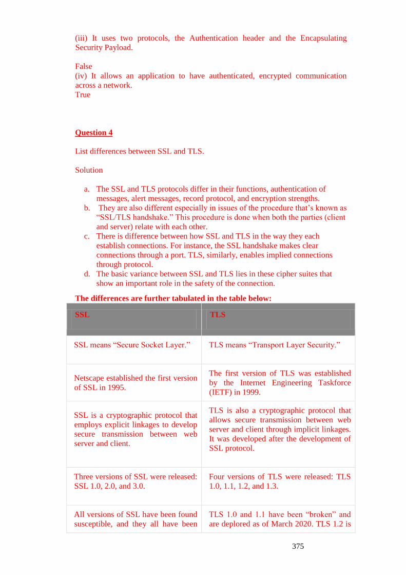
375

(iii) It uses two protocols, the Authentication header and the Encapsulating

Security Payload.

False

(iv) It allows an application to have authenticated, encrypted communication

across a network.

True

Question 4

List differences between SSL and TLS.

Solution

a. The SSL and TLS protocols differ in their functions, authentication of

messages, alert messages, record protocol, and encryption strengths.

b. They are also different especially in issues of the procedure that‘s known as

―SSL/TLS handshake.‖ This procedure is done when both the parties (client

and server) relate with each other.

c. There is difference between how SSL and TLS in the way they each

establish connections. For instance, the SSL handshake makes clear

connections through a port. TLS, similarly, enables implied connections

through protocol.

d. The basic variance between SSL and TLS lies in these cipher suites that

show an important role in the safety of the connection.

The differences are further tabulated in the table below:

SSL TLS

SSL means ―Secure Socket Layer.‖ TLS means ―Transport Layer Security.‖

Netscape established the first version

of SSL in 1995.

The first version of TLS was established

by the Internet Engineering Taskforce

(IETF) in 1999.

SSL is a cryptographic protocol that

employs explicit linkages to develop

secure transmission between web

server and client.

TLS is also a cryptographic protocol that

allows secure transmission between web

server and client through implicit linkages.

It was developed after the development of

SSL protocol.

Three versions of SSL were released:

SSL 1.0, 2.0, and 3.0.

Four versions of TLS were released: TLS

1.0, 1.1, 1.2, and 1.3.

All versions of SSL have been found

susceptible, and they all have been

TLS 1.0 and 1.1 have been ―broken‖ and

are deplored as of March 2020. TLS 1.2 is

376

deplored. the most widely uded protocol version.

Question 5

What is S-HTfP?

Solution

S-HTTP stands for Secure Hypertext Transfer Protocol

Question 6

What are instant messaging and its vulnerabilities?

Solution

Instant messaging is a method of sending messages to be received immediately.

The vulnerabilities are that they are used:

a. to transport Viruses and worms

b. to transport Identity theft/authentication spoofing

c. For Firewall tunnelling

Explain them

CIT 852: DATA COMMUNICATION AND NETWORK - National ...

Documents

Transcript of CIT 852: DATA COMMUNICATION AND NETWORK - National ...