Access to this work was provided by the University of Maryland, Baltimore County (UMBC) ScholarWorks@UMBC digital repository on the Maryland Shared Open Access (MD-SOAR) platform.

Please provide feedback

Please support the ScholarWorks@UMBC repository by emailing scholarworks-group@umbc.edu and telling us what having access to this work means to you and why it’s important to you. Thank you.

Linkages of Calcium Induced Calcium Release in aCardiomyocyte Simulated by a System of Seven Coupled

Partial Differential Equations

Gerson C. Kroiz, Carlos Barajas, Matthias K. Gobbert and Bradford E. Peercy(gkroiz1,barajasc,gobbert,bpeercy@umbc.edu)

Department of Mathematics and Statistics,University of Maryland, Baltimore County,1000 Hilltop Circle, Baltimore, MD 21250

Cardiac arrhythmias affect millions of adults in the U.S. each year. Thisirregularity in the beating of the heart is often caused by dysregulationof calcium in cardiomyocytes, the cardiac muscle cell. Cardiomyocytesfunction through the interplay between electrical excitation, calcium sig-naling, and mechanical contraction, an overall process known as calciuminduced calcium release (CICR). A system of seven coupled non-lineartime-dependent partial differential equations (PDEs), which model phys-iological variables in a cardiac cell, link the processes of cardiomyocytes.Through parameter studies for each component system at a time, we createa set of values for critical parameters that connect the calcium store in thesarcoplasmic reticulum, the effect of electrical excitation, and mechanicalcontraction in a physiologically reasonable manner. This paper shows thedesign process of this set of parameters and then shows the possibility tostudy the influence of a particular problem parameter using the overallmodel.

Keywords: Cardiac Arrhythmia, Calcium Induced Calcium Release, Re-action Diffusion Equations, Finite Volume Method, Parallel Computing

1. Introduction

The leading cause of death in the United States is currently heart disease [M+14].In order to continue searching for methods to combat heart disease, it is vital thatthe heart and its underlying processes are understood with greater depth. Theimportance of having a greater understanding of the heart provides the motivationfor this research.

The line of work of this project focuses on a single cardiac cell and uses a math-ematical model in order to represent the electrical excitation, calcium signaling,and mechanical contraction components of a cardiomyocyte. The original modelfor calcium induced calcium release (CICR) was introduced by Izu and co-workers[IMBW01, IWB01] with a three variable model and included only calcium signal-ing. This original model comprises the heart of the Calcium Signaling componentof the system indicated in Figure 1 (a). Figure 1 (b) sketches the domain of thesimulation. We use an hexahedron elongated in the z-direction for the shape ofa cell, since the focus of CICR research is on estimating reasonable physiologicalparameter values. A key of the model[IMBW01, IWB01] is to place the calciumrelease units (CRUs) on a regular lattice of size, for instance, 15× 15× 31 = 6,975throughout the cell; Figure 1 (b) shows three z-planes of 3 × 3 CRUs as example.At these many locations, calcium ions are released from the calcium store in thesarcoplasmic reticulum (SR) into the cytosol of the cell, and CRUs can open (‘fire’)and close repeatedly over time[IMBW01, IWB01].

1

2

(a) (b)

Figure 1. (a) The three components of the model and their linkslabeled 1© to 4©. (b) The CRU lattice with spacings ∆xs, ∆ys,∆zs throughout the three-dimensional cell.

The model was extended for the first time to include the Electrical Excitationcomponent in Figure 1 (a) [ADFI+15], which implemented a one-way interactionfrom electrical excitation to calcium signaling indicated by link 1© in Figure 1 (a).Studies with six variables in [ABM+16] extended the coupling to include a two-waycycle between electrical excitation and calcium signaling by incorporating bothlinks 1© and 2© in Figure 1 (a). The 2016 paper [ABM+16] also introduced theformulation of the complete eight variable model for all components in Figure 1 (a),but not all model variables were used in the simulations, and the studies did notincorporate the mechanical system.

The most recent work in [DFL+17a, DFL+17b] studies the introduction of theMechanical Contraction component in Figure 1 (a) by activating the links 3© and4© in Figure 1 (a). This is facilitated by adding a buffer species whose concentration

can be related to the contraction of the cell. Thus, this work uses a model withseven variables to represent the excitation-contraction coupling (ECC) occurringin the cardiomyocyte, in which CICR is the mechanism through which electricalexcitation is coupled with mechanical contraction through calcium signaling. Theinitial results for the newly extended model when studying model in its entiretymake simulations promising in their predictive capability.

From the previous work, the linkage of the mechanical contraction was existent,but not physiologically correct with the previous set of parameters. The resultingsimulations may not have provided realistic behaviors of a cardiac muscle cell. Assuch, it is important to create a set of parameters with physioligcally reasonable sim-ulations. To do this, we reduce the seven variable model to the three variable modelfrom [IMBW01, IWB01] by setting key parameters to zero. This removes severalCICR components: the calcium store in the SR, electrical excitation, and mechan-ical contraction. By this process, the additional CICR components are negated asthey all reduce to zero. From this base case, we reintroduce physiologically rea-sonable values for these parameters in successive order. First, the correspondingparameter for the calcium store was implemented, reconnecting this component tothe system. The selected parameters which negated electrical excitation are thenintroduced. To complete the system, the key variable connecting mechancial con-traction to the rest of the model is included. By creating this set of parametersthat included the CICR components, we are eventually able to study the model asa whole rather than individual components. This paper shows the design processof this set of parameters and then studies the influence of mechanical contraction

3

on the rest of the model for simulations to an extended final time. This showsthe possibility to study the influence of a particular problem parameter using theoverall model.

This paper is organized as follows: Section 2 details the seven variable modelused in this work. Section 3 specifies the numerical method used including itsparallelization and implementation. Section 4 is divided into several subsections.Subsections 4.1-4.4 show the step-by-step implementation of the CICR componentsof the seven variable model. With the complete construction of the set of parame-ters, Subsection 4.5 presents a sample application using the new set of parameters.Section 5 collects the conclusions of the work.

4

2. Dynamics of a Cardiac Cell

This section details the seven variable model used in this work. The sevenvariables of the model are calcium in the cytosol c(x, t), a florescent dye b

(c)1 (x, t),

a contractile protein (troponin) b(c)2 (x, t), a contractile force b

(c)3 (x, t), calcium in

the sarcoplasmic reticulum (SR) s(x, t), voltage V (x, t), and the potassium gatingfunction n(x, t). and are listed in Table 1 with their units and initial values. Theevolution of the system is modeled by the system of seven time-dependent, coupled,non-linear reaction diffusion equations

∂c

∂t= ∇ · (Dc∇c) +R

(c)b1

+R(c)b2

+(JCRU+Jleak−Jpump

)(1)

+ κJLCC +(Jmleak

−Jmpump

),

∂b(c)1

∂t= ∇ · (D

b(c)1∇b(c)1 ) +R

(c)b1, (2)

∂b(c)2

∂t= ∇ · (D

b(c)2∇b(c)2 ) +R

(c)b2, (3)

∂b(c)3

∂t= ∇ · (D

b(c)3∇b(c)3 ) +R

(c)b3, (4)

∂s

∂t= ∇ · (Ds∇s)− γ(JCRU + Jleak − Jpump), (5)

∂V

∂t= ∇ · (Dv∇V ) + τv

1

C

[Iapp − gL(V − VL)− gK n (V − VK) (6)

− 2FS τflux

JLCC − ω (Jmleak− Jmpump)

],

∂n

∂t= ∇ · (Dn∇n) + τv λn cosh

(V−V3

2V4

) (n∞(V )− n

). (7)

The domain in our model is a hexahedron

Ω = (−6.4, 6.4)× (−6.4, 6.4)× (−32.0, 32.0) (8)

with units of µm with isotropic CRU distribution as sketched in Figure 1 (b) witha sample of three z-planes of 3 × 3 CRUs. A typical cell has on the order of15 × 15 × 31 = 6,975 calcium release units (CRUs) throughout the cell. A cellis reasonably modeled by the hexahedral shape elongated in the z-direction, sincethe focus of CICR research is on estimating correct physiological parameter values.The following provides details on each of the components of the model, the calciumsignaling portion of the model, the electrical excitation that is connected to thecalcium signaling in both the feedforward and feedback directions represented bylink 1© and link 2© in Figure 1 (a), and the mechanical contraction component thatis also connected to the calcium signaling in both the feedback and feedforwarddirections represented by links 3© and 4© in Figure 1 (a).

Tables 2 and 3 contain the parameters in the PDEs of the calcium system withtheir values (if fixed) and units; some of the values are varied in the experiments inSection 4. The coefficients Dc, Db

(c)i

, and Ds are the diffusivity matrices for Ca2+

in the cytosol, buffer species i in the cytosol, and Ca2+ in the SR, respectively.The calcium signaling portion of the model consists of the equations (1)–(5). The

reaction terms R(c)bi

describe the reactions between calcium and the buffer species.

5

Variable Definition Initial value and unitsx spatial position variable (x, y, z) µmt time variable msc(x, t) calcium in the cytosol c0 = 0.1 µM

b(c)1 (x, t) free flourescent dye in the cytosol 45.918 µM

b(c)2 (x, t) free troponin in the cytosol 111.818 µM

b(c)3 (x, t) inactive actin-myosin cross-bridges [X] 145.20 µMs(x, t) calcium in the SR s0 = 10,000 µMV (x, t) membrane potential (voltage) −50 mVn(x, t) fraction of open potassium channels 0.1

Table 1. Independent and dependent variables of the seven vari-able model and their initial conditions. The concentration unit Mis shorthand for mol/L (moles per liter).

They are the connections between (1)–(4). More precisely, we have

R(c)b1

= − k+

b(c)1

c b(c)1 + k−

b(c)1

(b(c)1,total − b

(c)1

), (9)

for reaction between cytosol calcium and the flourescent dye.When troponin binds to Ca2+, the protein as a whole changes shape: this not

only allow actin-myosin cross-bridges to form, but also traps the calcium in its con-nection to the troponin so that the disassociation rate of troponin binding to Ca2+

decreases dramatically. To account for this, the shortening factor ε describes howthe separation of troponin and calcium has been physically, but not chemically, im-paired. When there are open CRUs that resultantly release calcium in the cytosol,this chain of changes of variables increases in severity. However, after t = 5 ms ofbeing open, the CRUs close and remain in a resting state for t = 100 ms. Duringthis period, the unbinding of troponin and calcium increase to the intial rate ofunbinding and myosin cross-bridges become inactive. This results in these termsreturning to their orignal states. This cycle is continuous triggered and reset by

the calcium waves produced by a cardiomyocyte. Note, again, that R(c)b2

remains a

function of cytosol calcium concentration c(x, t) by its equation

R(c)b2

= − k+

b(c)2

c b(c)2 +

k−b(c)2

ε

(b(c)2,total − b

(c)2

)(10)

with

ε = exp

(Fmax ks

(b(c)3,total − b

(c)3 − [XB]0

b(c)3,total − [XB]0

))(11)

and [XB]0 = b(c)3,total − b

(c)3 (x, 0). This shortening factor ε links 3© and 4© in Fig-

ure 1 (a). It is important to note that the disassociation rate of troponin bindingto Ca2+ is highest when the calcium concentration in the cytosol is lowest.

The shortening factor refers back to the concentration of b(c)3 (x, t), the actin-

myosin cross-bridges, and to the force that their linkage generates. It is scaledby the maximum possible contractile force Fmax, the actin stiffness ks, and the

6

Variable Definition Values/Units

Dc diffusivity matrix for c(x, t) diag(0.15,0.15,0.3) µm2/ms

Db(c)1

diffusivity matrix for b(c)1 diag(0.01,0.01,0.02) µm2/ms

Db(c)2

diffusivity matrix for b(c)2 diag(0.00,0.00,0.00) µm2/ms

Db(c)3

diffusivity matrix for b(c)3 diag(0.00,0.00,0.00) µm2/ms

Ds diffusivity matrix for s(x, t) diag(0.78,0.78,0.78) µm2/ms

R(c)bi

reactions of cytosol Ca2+ with buffers µM/ms

k+b(c)1

forward reaction coefficient for b(c)1 0.080 (µM ms)−1

k+b(c)2

forward reaction coefficient for b(c)2 0.100 (µM ms)−1

k+b(c)3

forward reaction coefficient for b(c)3 0.040 ms−1

k−b(c)1

reverse reaction coefficient for b(c)1 0.090 ms−1

k−b(c)2

reverse reaction coefficient for b(c)2 0.100 ms−1

k−b(c)3

reverse reaction coefficient for b(c)3 0.010 ms−1

b(c)1,total total amount of b

(c)1 in the cytosol 50 µM

b(c)2,total total amount of b

(c)2 in the cytosol 123 µM

b(c)3,total total amount of b

(c)3 in the cytosol 150 µM

γ ratio of volume of cytosol to SR 14

Jleak calcium leak from SR 0.3209684 µM/msJpump calcium transfer from cytosol to SR µM/msVpump maximum pump rate 4 µM/ms

Kpump pump sensitivity to Ca2+ 0.184 µMnpump Hill coefficient for pump function 4.0

JCRU calcium flux from SR to cytosol via CRUs µM/msO gating function for JCRU 0 or 1

Jprob probability of CRU opening 0 to 1

xs three-dimensional vector for CRU location µm∆xs CRU spacings in x 0.8µm

∆ys CRU spacings in y 0.8µm∆zs CRU spacings in z 2.0µmσ maximum rate of release 110 µMµm3/ms

δ(x− x) Dirac delta distribution 1/µm3

urand uniformly distributed random variable 0 to 1Pmax maximum probability for release 0.3

Kprobc sensitivity of CRU to cytosol calcium 2 µMnprobc Hill coefficient for probability function 4Kprobs sensitivity of CRU to SR calcium 550 µM

nprobs Hill coefficient for probability function 4

Table 2. Parameters for calcium signaling.

proportion of active to inactive actin-myosin cross-bridges. As the proportion ofactive actin-myosin cross-bridges increases due to an increase in bounded troponin,

the value of b(c)3,total − b

(c)3 − [XB]0 increases. This results in a larger value of ε. As

ε becomes larger, the rate at which the bounded troponin unbinds slows down. Asdescribed earlier, the lack of calcium provided by CRU resting periods results in areset in this mechanism.

The contractile proteins in question, though considered as a single species, arethe combination of actin and myosin when linked via cross-bridges. This linkage

7

Variable Definition Values/Units

Dv diffusivity matrix for V (x, t) diag(100,100,100) µm2/msDn diffusivity matrix for n(x, t) diag(0,0,0) µm2/ms

τv scaling factor in voltage equation 0.1 µM µm3/msτflux scaling factor in JLCC term 0.1V1 potential at which m∞ = 0.5 −1.0 mVV2 reciprocal of slope of voltage dependence of m∞ 15.0 mV

V3 potential at which n∞ = 0.5 10.0 mVV4 reciprocal of slope of voltage dependence of n∞ 14.5 mVVL equilibrium potential for leak conductance −50 mV

VCa equilibrium potential for Ca2+ conductance 100 mVVK equilibrium potential for K+ conductance −70 mVC membrane capacitance 20 µF/cm2

Iapp applied current 50 µA/cm2

gL maximum/instantaneous conductance for leak 2 mmho/cm2

gCa maximum/instantaneous conductance for Ca2+ 4 mmho/cm2

gK maximum/instantaneous conductance for K+ 8 mmho/cm2

m∞ fraction of open calcium channels at steady state 0 to 1n∞ fraction of open potassium channels at steady state 1λn maximum rate constant for opening of K+ channels 0.1 ms−1

JLCC influx of calcium via L-type calcium channels µM/ms

S surface area of the cell 3604.48 µm2

F Faraday constant 95484.56 C/molκ scaling factor of JLCC 0.1

ω feedback strength (scaling factor) for Ca2+ efflux 100 µA ms/µM cm2

Jmleak leak of calcium via L-type calcium channels 0.1739493 µM/msJmpump pump of calcium via L-type calcium channels µM/ms

Vmpump maximum pump rate 0.3 µM/msnmpump membrane pump Hill coefficient 4Kmpump membrane pump Ca2+ sensitivity 0.18

[XB]0 initial concentration of active cross-bridges 142.6805 µM

ε shortening factor 0 to 1Fmax maximum force by actin-myosin crossbridges 1 µNks stiffness of actin filament 0.025 N/m

Table 3. Parameters for electrical excitation and mechanical con-traction with base units of mho = (s3A2)/(kg m2) and F =(s4A2)/(kg m2).

is made possible by Ca2+ binding to troponin, the cytosol buffer species b(c)2 (x, t):

it is this binding that allows the actin-myosin cross-bridges to form. The cytosol

species, b(c)3 (x, t), describes these actin-myosin cross-bridges and constructs a third

cytosol reaction term

R(c)b3

= −k+

b(c)3

(b(c)2,total − b

(c)2

b(c)2,total

)2

b(c)3 + k−

b(c)3

(b(c)3,total − b

(c)3 ). (12)

Notice that this is not the same as the generic pattern for buffer species reactionterms from the initial model. There is no immediately clear dependence on cytosoliccalcium c(x, t). However, while c(x, t) is not explicitly included, it is present in the

proportion involving troponin, b(c)2 (x, t), which itself depends explicitly on cytosol

calcium levels; R(c)b3

, like the other two reaction equations, does in fact depend on

8

the cytosol calcium concentration. Unlike the other two reaction equations, R(c)b3

indirectly impacts calcium levels.These two reaction terms (10) and (12) connect the three components of our

model. The calcium signaling is linked to the pseudo-mechanical contraction bythe cross-bridge term, and the pseudo-mechanical contraction is in turn connectedto the calcium signaling through the inclusion of the cytosol calcium concentrationin the modified reaction equation for troponin. Thus all links 1©, 2©, 3©, and 4©in Figure 1 (a) are established, and thus the three systems of the model are fullylinked.

Note that in the reaction terms b2(c) and b3

(c) are the amount of unbound buffer

known as “free” buffer. The constant b(c)i,total denotes the total bound and unbound

calcium thus leaving the difference seen in (9) to be the bound calcium. Since themodel uses no-flux boundary conditions, no buffer species escapes or enters the cell,

thus we only need to track the “free” buffer species and use b(c)i,total − bi

(c) for thebound species.

The flux terms JCRU , Jleak, and Jpump in (1) describe the calcium induced releaseof Ca2+ into the cytosol from the SR, the continuous leak of Ca2+ into the cytosolfrom the SR, and the pumping of Ca2+ back into the SR from the cytosol. Theterms JLCC , Jmleak

, and Jmpumpdescribe the fluxes of calcium into and out of the

cell via the plasma membrane. The coupling between (1) and (5) is achieved bythe three flux terms shared by both.

More precisely, JLCC , Jmleak, and Jmpump

in (1) describe the fluxes of calciuminto and out of the cell via the plasma membrane. Jpump replenishes the calciumstores in the SR; it increases SR calcium concentration by decreasing cytosol calciumconcentration. Jleak is a continuous leakage of those SR calcium stores into thecytosol; it increases cytosol concentration by decreasing SR calcium concentration.The pump term

Jpump(c) = Vpump

(cnpump

Knpumppump + cnpump

)(13)

is thus a function of cytosol calcium c(x, t). The leak term Jleak is a constantdefined by

Jleak = Jpump(c0), (14)

which balances Jpump(c) at basal level c0 = 0.1 µM of cytosol calcium. The pumpterm Jpump, a function of cytosolic calcium c(x, t), consists of the maximum pumpvelocity Vpump multiplied against the relationship between c(x, t) and the pumpsensitivity Kpump; the exponent npump refers to the Hill coefficient (quantifying thedegree of cooperative binding) for the pump function. This has the practical effect ofmultiplying the maximum possible pump velocity against a number between 0 and1, exclusive. Jleak, which continuously leaks calcium into the cytosol from the SR,is simply Jpump evaluated at the basal cytosolic calcium concentration c0 = 0.1µM .As noted, Jpump has two roles, namely to balance Jleak in the absence of sparking,but also to balance JCRU under conditions of active calcium release.

The term JCRU in (1) is the Ca2+ flux into the cytosol from the SR via eachindividual point source at which a CRU has been assigned. The effect of all CRUs

9

is modeled as a superposition such that

JCRU (c, s,x, t) =∑x∈Ωs

σs(x, t)

s0O(c, s) δ(x− x) (15)

with

O(c, s) =

1 if urand ≤ Jprob,0 if urand > Jprob,

(16)

where

Jprob(c, s) = Pmax

(cnprobc

Knprobc

probc+ cnprobc

) (snprobs

Knprobs

probs+ snprobs

). (17)

The effect of each CRU is modeled here as a product of three terms: (i) Similarlyto how in Jpump the maximum pump rate is scaled against the concentration ofavailable cytosol calcium, the maximum pump rate is scaled against the concentra-tion of available cytosol calicum, the maximum rate of Ca2+ release σ is scaled hereagainst the ratio of calcium concentration in the SR. (ii) Following the same pat-tern a maximum value multiplied against some scaling proportion between 0 and1 the gating function O(c, s) has the practical effect of “budgeting” the calciumSR stores such that when the stores are low, the given CRU becomes much lesslikely to open; each CRU is assigned a uniformly distributed random value urand,which is compared to the single value returned by the CRU opening probabilityJprob to determine whether or not the given CRU will open. (iii) The Dirac deltadistribution δ(x− x) models each CRU as a point source for calcium release, whichis defined by requiring δ(x− x) = 0 for all x 6= x and

∫R3 ψ(x)δ(x− x) dx = ψ(x)

for any continuous function ψ(x).The linking between calcium signaling and electrical excitation consists of (6)–

(7). The membrane potential of the cell depends on both the cytosol calcium ionconcentration and also on the cytosol potassium ion (K+) concentration [BHJ+12,ML81]. In our model, the ω term in (6) quantifies a dependence of V on c tocomplete the coupling from the chemical to the electrical systems in link 2© inFigure 1 (a) [ABM+16], after c in (1) already contains several terms that dependon V to implement link 1© in Figure 1 (a). The Ca2+ conductance is much fasterthan the K+ conductance, so the calcium conductance can be approximated as m∞or instantaneously steady-state at all times; the potassium conductance requires aseparate description in (7). Needed parameter functions in (6)–(7) are

m∞(V ) =1

2

(1 + tanh

(V − V1

V2

)), (18)

n∞(V ) =1

2

(1 + tanh

(V − V3

V4

)). (19)

The connection between (1) and (6), link 1© in Figure 1 (a), the link from theelectrical system to the calcium system, comes through

JLCC =τflux2F

S gCam∞(V ) (V − VCa), (20)

the only calcium flux term to involve voltage. Note the parameter κ in (1), which isan external scaling factor for JLCC rather than an intrinsic physiological component;if the value of κ is set to 0, the connection, link 1© in Figure 1 (a), is effectivelyswitched off and the calcium dynamics are then modeled as though voltage were not

10

involved. The surface area, S, of the cell is included in light of the fact that JLCCdescribes the influx of calcium through L-type calcium channels (LCCs), which arepresent in the enclosing plasma membrane of the cell: the surface area of the cellis the surface area of the membrane.

We model the effect of the cytosol calcium concentration on the voltage bytreating the calcium efflux term (Jmpump

− Jmleak) as equivalent to the sodium-

calcium exchanger current: we are thus able to describe the current generated bythe sodium-calcium exchange as a function of simple calcium loss.

The individual components of the calcium efflux term are near-duplicates in formof the earlier Jpump and Jleak functions in (13) and (14), respectively. As Jpumpdescribed the removal of calcium from the cytosol and its transfer into SR stores,

Jmpump(c) = Vmpump

(cnmpump

Knmpumpmpump + cnmpump

)(21)

describes the removal of calcium from the cytosol and its transfer to outside thecell across the membrane. The leak term Jleak described a gradual leak of calciuminto the cytosol from the SR, while JCRU described an abrupt, high-concentration(high relative to the leak) release of calcium into the cytosol from the SR. Similarly,

Jmleak= Jmpump

(c0) (22)

describes a gradual leak of calcium into the cytosol from outside the cell via theplasma membrane, while JLCC describes a sudden spike of calcium release into thecytosol via the LCCs.

The seven variable model presented in this section reduces to the three variablemodel in the original sources [IMBW01, IWB01] by the following choies: setting γ= 0,τv = 0, ω = 0, κ = 0, and Fmax = 0. With these parameters set to 0, linkages1©, 2©, 3©, and 4© in Figure 1 (a) are all cut off.

11

3. Numerical Method

In order to do calculations for the CICR model, we need to solve a system oftime-dependent parabolic partial differential equations (PDEs). These PDEs arecoupled by several non-linear reaction and source terms. The current simulationsuse ns = 7 physiological variables. The domain in our model is a hexahedron withisotropic CRU distribution as shown in Figure 1 (b). A typical cell has on the orderof 15 × 15 × 31 = 6,975 calcium release units (CRUs) throughout the cell. A cellis reasonably modeled by the hexahedral shape elongated in the z-direction, sincethe focus of CICR research is on estimating correct physiological parameter values.Taking a method of lines (MOL) approach to spatially discretize this model, weuse the finite volume method (FVM) as the spatial discretization to ensure massconservation on the discrete level and also to accommodate advection terms in thefuture, with N = (Nx + 1) (Ny + 1) (Nz + 1) control volumes. Applying this tothe case of the ns PDEs results in a large system of ordinary differential equations(ODEs). A MOL discretization of a diffusion-reaction equations with second-orderspatial derivatives results in a stiff ODE system. The time step size restrictions, dueto the CFL condition, are considered too severe to allow for explicit time-steppingmethods. This necessitates the use of a sophisticated ODE solver such as the familyof implicit numerical differentiation formulas (NDFk). We use Newton’s methodas the non-linear solver, and at each Newton step we use the biconjugate gradientstabilized method (BiCGSTAB) or other Krylov subspace methods as the linearsolver. Complete details of the numerical method can be found in [SHK+15].

Mesh resolution N DOF neq time steps memory (GB)Nx ×Ny ×Nz predicted observed32× 32× 128 140,481 983,367 2667 0.125 < 164× 64× 256 1,085,825 7,600,775 3295 0.963 1.093

128× 128× 512 8,536,833 59,757,831 3867 7.569 8.476256× 256× 1024 67,700,225 473,901,575 4470 60.024 67.103

Table 4. Sizing study with ns = 7 variables using double pre-cision arithmetic, listing the mesh resolution Nx × Ny × Nz, thenumber of control volumes N = (Nx+1) (Ny+1) (Nz+1), the num-ber of degrees of freedom (DOF) neq = nsN , the number of timesteps taken by the ODE solver up to final time tfin = 100 ms, andthe predicted and observed memory usage in GB for a one-processrun.

While the form of the PDEs in (1)–(7) is customary, the thousands of pointsources at the calcium release units (CRUs) in the forcing terms imply that standardcodes have difficulty. This explains why our research centered around creating aspecial-purpose code [Gob08, HGI04, SGTK12, SHK+15]. Additionally, we leveragethe regular 3-D shape of the domain to program all methods in matrix-free form.Table 4 demonstrates thus, how despite fully implicit time-stepping, even relativelyfine meshes use only modest amounts of memory. This provides the key benefitnow for the complete complex model with complete sophisticated numerical methodstack, even with 7 or 8 variables, to fit into the high-performance memory of a KNLor a GPU. The table also shows how large the number of degrees of freedom (DOF)

12

is, that is, the number of variables that have to be computed at every time step.With even modest meshes, there are millions of unknowns, and possibly hundredsof millions for fine meshes. This characterizes the numerical problem that needs tobe tackled to resolve the large number of thousands of calcium release units (CRUs)in a cell.

The implementation of this model is done in C using MPI and OpenMP to paral-lelize computations. Parallelization is accomplished through block-distribution alllarge arrays to all MPI processes. We split of the mesh in the z-direction with onesubdomain on each of the parallel processes. MPI commands such as MPI_Isend andMPI_Irecv, which are non-blocking point-to-point communication commands, sendmessages between neighboring processes. The collective command MPI_Allreduce

is used for the computation of scalar products and norms.

13

4. Results

This section shows the results of simulations for the seven variable model de-tailed in Section 2 with variables aand their values at the initial time t = 0 msspecified in Table 1. The following subsections show physiological output that ispossible through long-time computational simulations to a final time that is largeenough to include several calcium waves. Tables 2 and 3 specify all model parame-ters, their names, and their values or ranges with units, except certain parametersthat are varied in this section. Table 5 specifies for each of the subsections, whatvalues are used. In Tables 2 and 3, the values of the variables are selected fromTable 5. Subsection 4.1 connects to the original modeling in [IMBW01, IWB01] byperforming simulations with parameters chosen such that the seven variable modelreduces to the original three variable model used in these papers. The followingSubsections 4.2, 4.3, and 4.4 successively vary parameters shown in Table 5, in ad-dition to the parameter changes made in the previous subsections. This approachallows for the construction of the entire model by adding new components on topof previous ones. With the entire model pieced together, we can test the model asa whole. That is the purpose of Subsection 4.5 that briefly exhibits the power ofthe fully implemented model by showing the impact of Fmax = 1 and Fmax = 100on the entire system for t = 5,000 ms, a longer duration of time. These resultsshow the power of a fully functioning system and motivate further studies usingthis model.

Parameter Base case SR store Voltage system Mechanical systemSec. 4.1 Sec. 4.2 Sec. 4.3 Sec. 4.4 Sec. 4.5

γ 0.0 0.01 to 1000 14.0 14.0 14.0τv 0.0 0.0 0.1 0.1 0.1Vmpump

0.0 0.0 0.001 to 1 0.3 0.3ω 0.0 0.0 0.1 to 1000 100.0 100.0κ 0.0 0.0 0.001 to 10 0.1 0.1Fmax 0.0 0.0 0.0 0.001 to 100 1, 100tfin 1000 1000 1000 1000 5000

Table 5. Parameter differences between cases in sections.

14

4.1. Base Case. The seven variable model in (1)–(7) reduces to the three variablemodel in the original sources [IMBW01, IWB01] by the following choices: settingκ = 0, Fmax = 0, and γ = 0. When looking at the seven equations, changing theseparameters to zero is most appropriate as they result in removing the calcium storein the Sarcoplasmic Reticulum (SR) and the effects of mechanical contraction.

The final addition of the three variable model, electrical excitation, can be abso-lutely removed by setting (6 and 7) to zero. Changing τv = 0 acheives this. Thesethree components are only unique to the seven variable model. To confirm that thefirst equation, (1), acts identically to the first equation in [IMBW01], we must beabsolutely sure that Jmleak

− Jmpump= 0. To do this, we change Vmpump

= 0 andω = 0, resulting in (21) negating to zero and both sides of (22) equaling zero. Withthese additional changes, the seven variable model functions identically to the threevariable model in the original sources [IMBW01, IWB01].

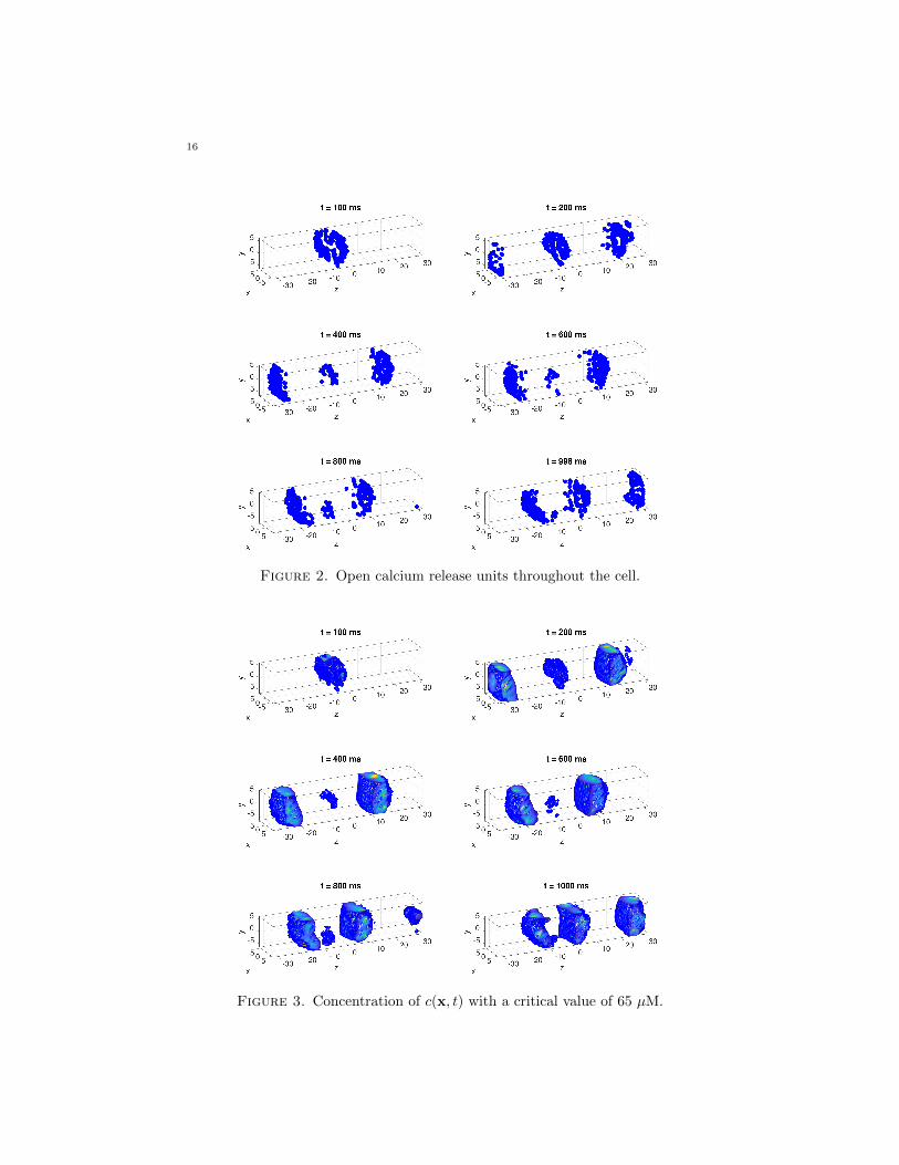
The first set of plots, in Figure 2, display the locations of open calcium releaseunits by a dot. The more dark dots are visible, the more CRUs are open at thatspecific time. More specifically, since one open CRU tends to promote neighboringCRUs to open through the diffusion of calcium, a clustering of dots indicates aregion of several open CRUs. Note that we start with initial conditions in Table 5for which there are no open CRUs and the right-hand sides of all equations in (1)–(7) are zero. Thus, these simulations represent a study in spontaneous sparking,in which some CRUs happen to open according to the probabilistic model in (15)–(17). This model embodies the effect of a higher concentration of cytosol calciumincreasing the probability for a CRU to open in (17). The result of this spontaneousself-initiation is seen in the first sub-plot in Figure 2, where a number of CRUs inone region of the cell have opened by t = 100 ms. The study of self-initiation wasthe original purpose of this model of calcium induced calcium releases [IMBW01,IWB01] and only required modest final times. The extension of the simulations tolarger final times allows to study if the opening and closing of CRUs self-organizesinto a sustained wave. This is seen in the following sub-plots in Figure 2. Themodel requires CRUs to close for 100 ms after opening for 5 ms; thus the sub-plotsindicate that the original cluster of open CRUs travels in both directions throughthe elongated direction of the cell and roughly repeats every 100 ms. Movies of thefull results including intervening times confirm this behavior.

Figure 3 shows a collection of isosurface plots for calcium concentration in thecytosol. An isosurface plot displays the surface in the three-dimensional cell, wherethe species concentration is equal to a critical value, stated in the caption of thefigure, here 65 µM for the concentration of cytosol calcium c(x, t). Blue representswhen the species’ concentration equals 65 µM. For densities lower than 65 µM, thereare no markings. More extreme concentrations of each species are indicated withthe spectrum from yellow to red, where darker hues are more intense in density. Aswe can see from the sub-plots in Figure 2, we have an original cluster in the middleat t = 100 ms that diffuses towards the ends of the cell and repeats on a 100 mscycle. Due to the connection of the calcium in the cytosol with open CRUs throughthe effect of calcium induced calcium release, calcium concentrations in the cytosolcorresponds to locations of open CRUs.

This physiological concept is shown with each sub-plot in Figure 3 where thespecies’ concentration colors are in agreement with the amount of open CRUs inFigure 2 at that time.

15

The concentrations of b(c)1 (x, t) and b

(c)2 (x, t) have the same charactersitics as

the calcium levels in the cytosol since they are all influenced in the same way,therefore, we do not show them. The remaining isosurface plots for the base case arenot included because each of the additional species concentration remain constant.Resultantly, each subplot would remain uneventful. As the CICR components areadded to the base case in the following subsections, the respective isosurface plotswill also be included.

16

Figure 2. Open calcium release units throughout the cell.

Figure 3. Concentration of c(x, t) with a critical value of 65 µM.

17

4.2. Adding the Calcium Store in the Sarcoplasmic Reticulum (SR). Toadd the calcium store in the Sarcoplasmic Reticulum (SR), (5) must provide non-constant concentrations of calcium. We can set γ = 14 to remove the previousreduction of this equation in Subsection 4.1. These values for γ and Ds are fromTable 5.

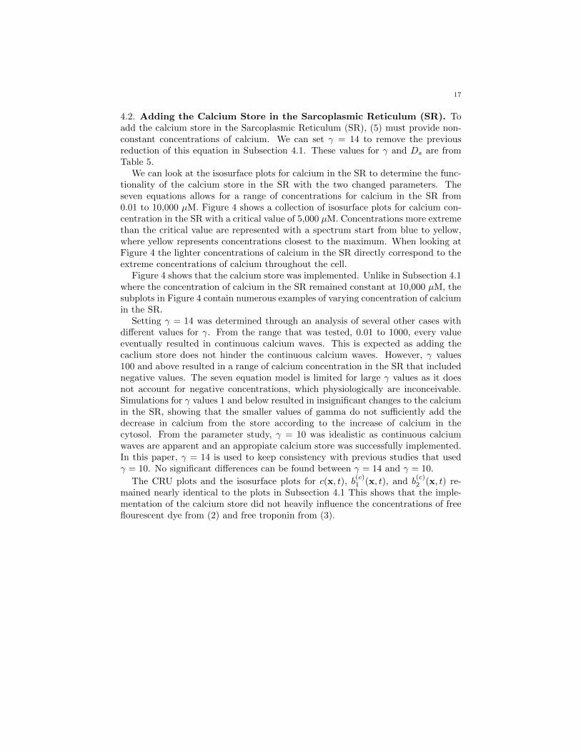
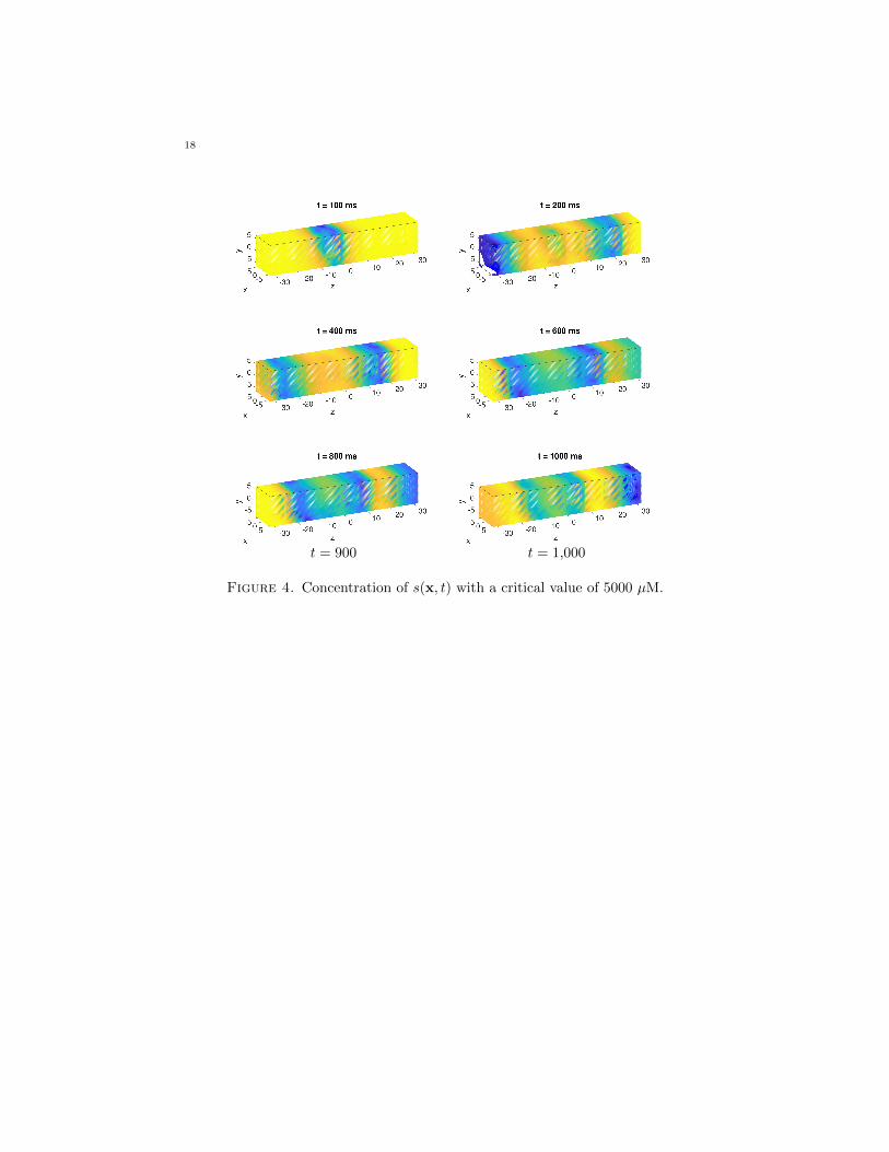
We can look at the isosurface plots for calcium in the SR to determine the func-tionality of the calcium store in the SR with the two changed parameters. Theseven equations allows for a range of concentrations for calcium in the SR from0.01 to 10,000 µM. Figure 4 shows a collection of isosurface plots for calcium con-centration in the SR with a critical value of 5,000 µM. Concentrations more extremethan the critical value are represented with a spectrum start from blue to yellow,where yellow represents concentrations closest to the maximum. When looking atFigure 4 the lighter concentrations of calcium in the SR directly correspond to theextreme concentrations of calcium throughout the cell.

Figure 4 shows that the calcium store was implemented. Unlike in Subsection 4.1where the concentration of calcium in the SR remained constant at 10,000 µM, thesubplots in Figure 4 contain numerous examples of varying concentration of calciumin the SR.

Setting γ = 14 was determined through an analysis of several other cases withdifferent values for γ. From the range that was tested, 0.01 to 1000, every valueeventually resulted in continuous calcium waves. This is expected as adding thecaclium store does not hinder the continuous calcium waves. However, γ values100 and above resulted in a range of calcium concentration in the SR that includednegative values. The seven equation model is limited for large γ values as it doesnot account for negative concentrations, which physiologically are inconceivable.Simulations for γ values 1 and below resulted in insignificant changes to the calciumin the SR, showing that the smaller values of gamma do not sufficiently add thedecrease in calcium from the store according to the increase of calcium in thecytosol. From the parameter study, γ = 10 was idealistic as continuous calciumwaves are apparent and an appropiate calcium store was successfully implemented.In this paper, γ = 14 is used to keep consistency with previous studies that usedγ = 10. No significant differences can be found between γ = 14 and γ = 10.

The CRU plots and the isosurface plots for c(x, t), b(c)1 (x, t), and b

(c)2 (x, t) re-

mained nearly identical to the plots in Subsection 4.1 This shows that the imple-mentation of the calcium store did not heavily influence the concentrations of freeflourescent dye from (2) and free troponin from (3).

18

t = 900 t = 1,000

Figure 4. Concentration of s(x, t) with a critical value of 5000 µM.

19

4.3. Adding the Effect of Electrical Excitation. Implementing the effect ofelectrical excitation on top of the calcium store in the SR is achieved throughactivating (6) and (7). From the reduced version of the seven variable model,setting τv = 0.1µM µm3/ms, Vmpump

= 0.3µM /ms, ω = 100, and κ = 0.1 resultsin functional equations for electrical excitation. We can make several other caseswith various values of each varied parameter to see how different extremes for eachvariable changes the resulting calcium wave.

From Subsection 4.2, we performed three separate one-dimensional studies inorder to find values for Vmpump

, ω, and κ that fully add the voltage system withoutsignificant changes to the various species concentrations in Subsection 4.2.

The first one-dimensional study varied Vmpumpfrom 0.001 to 1. Changing this

parameter a non-zero value allows for the functionality of the function (21) andconsequently (22). Both Vmpump and Vmleak

have an influence on equations (1) and(6). From this study, the largest value that retains the continous calcium wavesdescribed in Subsection 4.1 was Vmpump

= 0.3µM /ms.With this fixed value for Vmpump

, we can perform a one dimensional study of

ω, the feedback strength for Ca2+ efflux, and following an additonal study of κ.When varying ω, we noted that from ω = 0.1 to 1000, the CRU plots are almostidentical to our CRU plots from Subsection 4.2. We this as such, can set ω = 100.0,a fixed value, as all tested cases of ω simulated similar results to the plots shownin Subsection 4.2.

To fully implement the voltage system, we need to test values of κ to find whatnonzero value of κ would allow for continous calcium waves with a fully implementedvoltage system and calcium in the SR. When varying κ from 0.001 to 10, we notedthat κ = 0.1 was the largest value in which the calcium waves were comprable tothe previous subsections.

Setting κ = 0.1, ω = 100, τv = 0.1µM µm3/ms, and Vmpump= 0.3µM /ms

in addition to the predetermined values for the parameters in Table 5 allows forthe full implementation of the voltage system without fundamentally changing theoutflow of calcium.

The CRU plots and the isosurface plots for c(x, t), b(c)1 (x, t), and b

(c)2 (x, t) did

not significantly change with the implementation of the voltage system. However,there are more notable differences when comparing the calcium concentrations ofthe stores shwon in Figure 5 and Figure 4. In Figure 5, the latter plots havecolorless space between each clump of calcium. As these spaces are representativeof lower calcium concentrations, these plots show that the store in the SR haslower concentrations of calcium. Larger time studies may indicate that the calciumconcentration in the store continues to lower past t = 100 ms.

The voltage plot in Figure 6 shows that the electrical system was implemented.The voltage plots from the previous subsections remained constant at −50 mV .In Figure 6, there is a clear repetition of the voltage rising up to approximately 26mV back down to approximately -23 mV. This figure confirms that external voltageis present. Based on these comparisions, these plots maintain the same behaviorsfrom Subsection 4.2 with the addition of the voltage system.

20

Figure 5. Concentration of s(x, t) with a critical value of 5000 µM.

Figure 6. Voltage levels throughout the cell over period of 1000 ms

21

4.4. Adding the Effect of Mechanical Contraction. In the seven variablemodel, mechanical contraction is described through (3) and (4). From the parame-ters added in Subsection 4.3 shown in Table 5, a parameter study was performed onthe values for Fmax. By changing this parameter to nonzero values, we can studythe effects of mechanical contraction on top of the previously included calcium storeand electrical excitation. In additon to these set values, we created other cases withvarious values for Fmax to note the physiological changes with various values of (3)and (4).

For this parameter study, we tested a range from Fmax = 0.001 to Fmax = 100.For Fmax values less than 1, there shortening factor remained the same, where afterabout 125 ms ε began to cycle between a small range and remained this way up to1000 ms. For Fmax = 100, the shortening factor loses its period, where the valuedoes not cycle. Rather, the shortening factor spikes up two times throughout the1,000 ms. While Fmax = 10 maintains the cyling value of the shortening factor,there is an apparent delay for the cycle to begin. Unlike the start time of 125 msfor the lower values of Fmax, for Fmax = 10, the start time is 250 ms. Since thesimulations are only 1,000 ms in length the desired value for Fmax is 1.

As in the previous subsections, the CRU plots and the isosurface plots for c(x, t),

b(c)1 (x, t), and b

(c)2 (x, t) appear to be extremely similar if not identical to plots from

the previous subsections. Additionally, the concentrations shown in Figures 5 and6 remain the same with the addition of Fmax This shows that the implementationof the mechanical contraction did not heavily influence the other components tothe extent of changing the system.

With Fmax set to a nonzero value, the shortening factor, described in (11),is able to vary based on inactive actin-myosin cross-bridges described in (4). Inthe previous subsections, the lack of the variance in the shortening factor led toinability for the continuous contractions of the cross-bridges to take place. Unlikethe previous subsections, this shortening factor is able to vary in severity allowingfor the repetition of inactive cross-bridges switching to active ones. This repetitivecycle is displayed in Figure 7. In previous subsections, the plots for inactive actin-myosin cross-bridges remained constant throughout the 1,000 ms.

As in the previous subsections, the CRU plots and the isosurface plots for c(x, t),

b(c)1 (x, t), and b

(c)2 (x, t) appear to be extremely similar to plots from the previous

subsections. Additionally, the concentrations shown in Figures 5 and 6 remainthe same with the addition of Fmax This shows that the implementation of themechanical contraction with the so-far chosen parameters did not heavily influencethe other components to the extent of changing the system.

22

Figure 7. Concentration of b(c)3 (x, t) with a critical value of 50 µM.

23

4.5. Influence of Fmax on the Entire System. With these set parameters de-scribed in Subsection 4.1, we are able to test questions retaining to the entiremodel. One example of this is the study of Fmax for the much longer final timetfin = 5,000 ms rather than 1,000 ms on the seven variable model. From thetested values for Fmax from 0.001 to 100, values 1 and 100 are shown in the plotsbelow. These values were determined through the parameter study of Fmax fromSubsection 4.4.

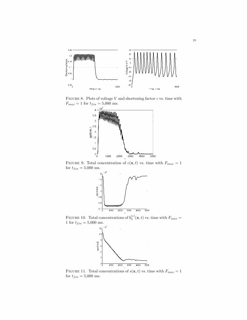
Figures 8 and 12 show plots of both the voltage V and shortening factor ε vs. timefor the model. While the content is different, the structure of the voltage plots isidentical to the voltage plots described in Subsection 4.3. The shortening factor εvs. time plots track the value of the shortening factor, ε, used in (3).

There are several differences between how each Fmax value affects the system.Figures 8–11 are representative of the same simulations as in Subsection 4.4, exceptthe duration of time was extended from tf in = 1,000 ms to 5,000 ms. As previouslydescribed, around 125 ms the calcium concentration in the cytosol shown in Figure 9jumps from 0 to slightly less than 4 × 105 and slowly decreases as the calciumconcentration in the store depletes. In Figure 11, the calcium concentration in thestore drops at the same time. The calcium concentration in the store continues to

drop until about 2,500 ms, where it then levels out. The concentration of b(c)3 (x, t)

in Figure 10 drop at the same time as the calcium change in the cytosol. Once the

calcium in the cytosol depletes, the concentration of b(c)3 (x, t) returns to its initial

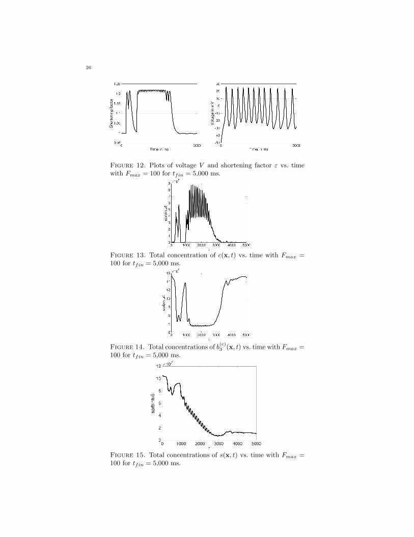
state.When comparing Figures 8–11 using Fmax = 1 and Figures 12–15 using Fmax =

100, there are clear differences. In Figure 13, the calcium concentration jumpsfrom its initial state similarly to the calcium concentration of Figure 9. However, itshortly returns to its initial state and remains so for several hundred millisecondsbefore jumping back up. This spike back downards is not characterized in Figures 8–11. The concentration around 1,000 ms jumps up to nearly 9×105, more than doublethe peak concentration of calcium in the cytosol for Fmax = 1. Furthermore, therange of concentration levels in 100 ms is much larger than in Figure 9. The calciumin the store, shown in Figure 11, overall has a downard trend until around 3,000 ms,where the calcium concentration in the store levels out. The calcium concentrationin the cytosol in Figure 9 correspondingly drops down to nearly 0. Similar to the

first spike of calcium in Figure 9, in Figure 10, the concentration of b(c)3 (x, t) drops

with the spike and almost returns to its initial state before dropping a second timearound 1,000 ms. The concentration remains relatively constant until the calcium

in the cytosol drops. At this point the concentration of b(c)3 (x, t) rises back up to

the same concentration as its initial state and remains around that level until thefinal time tfin = 5,000 ms.

There are also notable differences between the plots of the shortening factor εvs. time in Figures 8 and 12. Both plots generally have the same characteristics as

the plots of b(c)3 . Where the value for ε is greater, the concentration of b

(c)3 is lower.

Between the plots in Figures 8 and 12, the range of oscillation is much smaller inFigure 12 than in Figure 8 during the period where the value of ε oscillates.

Unlike the other plots, the plots of voltage V vs. time in Figures 8 and 12 retainconsistency throughout the entire 5,000 ms. The voltage level in both plots oscilatesfrom a negative value to a positive value. It appears that the range of one oscillationof voltage shrinks slightly as the calcium levels in the cytosol increase. Other than

24

this, it appears that the change in Fmax does not have such a drastic impact on thecharacteristics of voltage compared to the concentrations of each species of the cell.As such, it appears that the influence of the mechanical system is directed towardscalcium signaling and therefore has an indirect influence on voltage. This might beexpected as there are no direct links between the mechanical system and electricalexcitation.

25

Figure 8. Plots of voltage V and shortening factor ε vs. time withFmax = 1 for tfin = 5,000 ms.

Figure 9. Total concentration of c(x, t) vs. time with Fmax = 1for tfin = 5,000 ms.

Figure 10. Total concentrations of b(c)3 (x, t) vs. time with Fmax =

1 for tfin = 5,000 ms.

Figure 11. Total concentrations of s(x, t) vs. time with Fmax = 1for tfin = 5,000 ms.

26

Figure 12. Plots of voltage V and shortening factor ε vs. timewith Fmax = 100 for tfin = 5,000 ms.

Figure 13. Total concentration of c(x, t) vs. time with Fmax =100 for tfin = 5,000 ms.

Figure 14. Total concentrations of b(c)3 (x, t) vs. time with Fmax =

100 for tfin = 5,000 ms.

Figure 15. Total concentrations of s(x, t) vs. time with Fmax =100 for tfin = 5,000 ms.

27

5. Conclusions and Outlook

We successfully created a table of parameters in Section 4 that allow for a com-plete functioning model. This model includes the calcium store, electrical excita-tion, and mechanical contraction of the cardiac muscle cell. Unlike before, thistable allows for the cohesion of all components of the model. With this, we areable to study the model in its entirety. As an example, we showed some influencesof Fmax, a constant of the shortening factor, on the entire system over a period of5,000 ms. When comparing a small and large value for Fmax, we noticed that theinfluence of Fmax was much less extreme on the electrical excitation compared tothe calcium signaling. When comparing the plots of the relevant species of the sys-tem, this conclusion becomes apparent. This is important as it allows us to graspa better understanding of the linkage between the mechanical system and calciumsignaling, shown by Link 1© in Figure 1.

Future research on this could look more in depth at different values of otherparameters with a final time of 5,000 ms. This would allow for studies on thesystem for longer periods of time. Studying multiple cases for each parametervalue with randomized locations for calcium sparking would allow for more concreteconclusions with a stronger representation of the physiological processes of the cell.While this is one further area of study, this complete set of parameters opens manyareas to study the model in its entirety.

Acknowledgements

The hardware in the UMBC High Performance Computing Facility (HPCF) issupported by the U.S. National Science Foundation through the MRI program(grant nos. CNS–0821258, CNS–1228778, and OAC–1726023) and the SCREMSprogram (grant no. DMS–0821311), with additional substantial support from theUniversity of Maryland, Baltimore County (UMBC). See hpcf.umbc.edu for moreinformation on HPCF and the projects using its resources. Co-author Carlos Bara-jas was supported by UMBC as HPCF RA.

28

References

[ABM+16] Kallista Angeloff, Carlos A. Barajas, Alexander Middleton, Uchenna Osia,Jonathan S. Graf, Matthias K. Gobbert, and Zana Coulibaly. Examining the effect of

introducing a link from electrical excitation to calcium dynamics in a cardiomyocyte.

Spora: A Journal of Biomathematics, 2:49–73, 2016.[ADFI+15] Amanda M. Alexander, Erin K. DeNardo, Eric Frazier III, Michael McCauley,

Nicholas Rojina, Zana Coulibaly, Bradford E. Peercy, and Leighton T. Izu. Spon-

taneous calcium release in cardiac myocytes: Store overload and electrical dynamics.Spora: A Journal of Biomathematics, 1:36–48, 2015.

[BHJ+12] Tamas Banyasz, Balazs Horvath, Zhong Jian, Leighton T Izu, and Ye Chen-Izu.Profile of L-type Ca 2+ current and Na+/Ca 2+ exchange current during cardiac

action potential in ventricular myocytes. Heart Rhythm, 9(1):134–142, 2012.

[DFL+17a] Kristen Deetz, Nygel Foster, Darius Leftwich, Chad Meyer, Shalin Patel, CarlosBarajas, Matthias K. Gobbert, and Zana Coulibaly. Developing the coupling of the

mechanical to the electrical and calcium systems in a heart cell. Technical Report

HPCF–2017–15, UMBC High Performance Computing Facility, University of Mary-land, Baltimore County, 2017.

[DFL+17b] Kristen Deetz, Nygel Foster, Darius Leftwich, Chad Meyer, Shalin Patel, Carlos Bara-

jas, Matthias K. Gobbert, and Zana Coulibaly. Examining the electrical excitation,calcium signaling, and mechanical contraction cycle in a heart cell. Spora: A Journal

of Biomathematics, 3:66–85, 2017.

[Gob08] Matthias K. Gobbert. Long-time simulations on high resolution meshes to modelcalcium waves in a heart cell. SIAM J. Sci. Comput., 30(6):2922–2947, 2008.

[HGI04] Alexander L. Hanhart, Matthias K. Gobbert, and Leighton T. Izu. A memory-efficient

finite element method for systems of reaction-diffusion equations with non-smoothforcing. J. Comput. Appl. Math., 169(2):431–458, 2004.

[IMBW01] Leighton T. Izu, Joseph R. H. Mauban, C. William Balke, and W. Gil Wier. Largecurrents generate cardiac Ca2+ sparks. Biophys. J., 80:88–102, 2001.

[IWB01] Leighton T. Izu, W. Gil Wier, and C. William Balke. Evolution of cardiac calcium

waves from stochastic calcium sparks. Biophys. J., 80:103–120, 2001.[M+14] Benjamin Mozaffarian et al. Heart disease and stroke statistics — 2015 update: A

report from the american heart association. Circulation, 131(4):e29, 2014.

[ML81] Catherine Morris and Harold Lecar. Voltage oscillations in the barnacle giant musclefiber. Biophys. J., 35(1):193, 1981.

[SGTK12] Thomas I. Seidman, Matthias K. Gobbert, David W. Trott, and Martin Kruzık. Fi-

nite element approximation for time-dependent diffusion with measure-valued source.Numer. Math., 122(4):709–723, 2012.

[SHK+15] Jonas Schafer, Xuan Huang, Stefan Kopecz, Philipp Birken, Matthias K. Gob-

bert, and Andreas Meister. A memory-efficient finite volume method for advection-diffusion-reaction systems with non-smooth sources. Numer. Methods Partial Differ-

ential Equations, 31(1):143–167, 2015.