Chloride-Induced Stress Corrosion Cracking in Used Nuclear ...

Chloride-Induced Stress Corrosion Cracking in Used Nuclear Fuel Welded Stainless

Steel Canisters

Dissertation

Presented in Partial Fulfillment of the Requirements for the Degree Doctor of Philosophy

in the Graduate School of The Ohio State University

By

Yi Xie, B.S.

Graduate Program in Nuclear Engineering

The Ohio State University

2016

Dissertation Committee:

Professor Jinsuo Zhang, Advisor

Professor Tunc Aldemir

Professor Marat Khafizov

Professor Andre F. Palmer

Copyright by

Yi Xie

2016

ii

Abstract

The used nuclear fuel (UNF) dry storage is one of the options for the interim storage of

UNF. Most of the dry storages are located in coastal and lake/river-side regions. They are

designed to serve for 60 years or even more. In most cases, the storage canister which is

in a welded austenitic stainless steel (SS) structure will be exposed to a salt-containing

environment for the entire storage period. Since the canister is a primary barrier to fission

product release, it has been determined to be robust with little degradation due to thermal,

mechanical or radiation effects. However, atmospheric and aqueous pitting corrosion, as

well as chloride induced stress corrosion cracking (CISCC) may occur because of the

aggressive species that form on or contact the canister surface and the residual tensile

stresses.

The objective of this dissertation is to develop an experimental integrated approach to

study the fundamentals of CISCC of Type 304L base metal (BM) and weld metal (WM)

and collect data to evaluate CISCC under relevant environmental conditions, and to

develop a model based on probabilistic analysis by parameterizing and validating using

the experimental studies to predict long-term pitting behaviors of the storage canister.

The efforts and findings documented in this dissertation consist of: (1) The

electrochemical techniques are used to identify the corrosion potential, passive current,

iii

pitting potential, passivation layer impedance of the BM and WM immersed in highly

concentrated chloride solutions at 40 and 70 °C. (2) The pitting corrosion resistance in

the chloride-containing aqueous and atmospheric environment is evaluated and compared

by the pit density and frequency distribution of depth. It is found that the welding process

depresses the corrosion resistance of a metal matrix under the investigated environments.

Metastable pitting is distinct especially for the early exposure times. The pitting corrosion

resistance is influenced by the chloride concentration and the temperature. The findings

of pitting corrosion in humid environments provide better forecasting on actual in-service

canisters. (3) CISCC experiments with in situ measurement of crack growth rates of the

BM and WM exposed to the salt deposit humid environment (15% RH at 70 °C) are

conducted in the SCC test system. The WM has much higher SCC growth rate than the

BM even with lower applied stress intensity, indicating the SCC resistance of the steel is

depressed by the welding process. (4) Micro-characteristics imaging and analytical

facilities are used to analyze the microstructure of pitting corrosion and CISCC. (5) The

experimental results are used to concurrently parameterize and validate the model based

on probabilistic analysis for pitting corrosion. The concept of Markov chain, as well as

the pitting corrosion mechanism, is involved in this model to predict the pitting corrosion

states, density and depth.

Since the safety performance of the storage is major concerned in the nuclear industry,

this study provides a technical basis for evaluating the technical issue and supports the

development of evaluating SCC occurrence, crack depth and growth rate on in-service

storage canisters.

iv

Dedication

Dedicated to my family.

v

Vita

2012....................................................B.S. Nuclear Engineering, University of Science

and Technology of China

2012-Present.......................................Graduate Research Associate, Nuclear Engineering

Program, Department of Mechanical and Aerospace

Engineering, The Ohio State University

Publications

[1] Y Xie, Y Wu, J Burns, and J Zhang. Characterization of stress corrosion cracks in Ni-

based weld alloys 52, 52M and 152 grown in high-temperature water. Materials

Characterization, 112, 87-97, 2016.

[2] Y Xie and J Zhang. Corrosion and deposition on the secondary circuit of steam

generators. Journal of Nuclear Science and Technology, 1-12. Online publication date:

Feb 26, 2016.

[3] Y Xie and J Zhang. Chloride-induced stress corrosion cracking of used nuclear fuel

welded SS canisters: A review. Journal of Nuclear Materials, 466, 85-93, 2015.

[4] Y Xie and J Zhang. High temperature and pressure stress corrosion cracking system.

Transactions of the American Nuclear Society, vol.109, pp.592-593, Washington, D.C.,

November 10-14, 2013.

Fields of Study

Major Field: Nuclear Engineering

vi

Table of Contents

Abstract ............................................................................................................................... ii

Dedication .......................................................................................................................... iv

Vita ...................................................................................................................................... v

Table of Contents ............................................................................................................... vi

List of Tables ...................................................................................................................... x

List of Figures ................................................................................................................... xii

Chapter 1: Introduction ....................................................................................................... 1

1. Background and significance ................................................................................... 1

2. Objective and scope ................................................................................................. 4

3. Overview of the studies of CISCC relevant to in-service canisters ......................... 5

3.1 Surface temperature variables ............................................................................... 5

3.2 Salt deposit composition ........................................................................................ 5

3.3 RH and salt deliquescence ..................................................................................... 7

3.4 Residual stress ....................................................................................................... 9

Chapter 2: Fundamentals of CISCC ................................................................................. 12

vii

1. Pitting corrosion mechanism .................................................................................. 12

2. Pitting corrosion of SSs in chloride ion environment ............................................ 16

3. Modeling of pitting corrosion ................................................................................ 20

3.1 Comparison of deterministic and probabilistic models ....................................... 20

3.2 Comparison of statistical and stochastic methods ............................................... 22

4. SCC mechanism ..................................................................................................... 26

Chapter 3: Pitting Corrosion of SSs in Brine Solutions .................................................... 29

1. Introduction ............................................................................................................ 29

2. Specimen preparation............................................................................................. 29

3. Solution preparation ............................................................................................... 31

4. Test procedures ...................................................................................................... 32

4.1 Electrochemical techniques ................................................................................. 32

4.2 Optical profiler .................................................................................................... 33

4.3 SEM/FIB and STEM/EDS analysis ..................................................................... 33

5. Results and analysis ............................................................................................... 34

5.1 WM properties ..................................................................................................... 34

5.2 The evolution of corrosion potential ................................................................... 36

5.4 The identification of passivation layer ................................................................ 42

5.5 Pit depth and density............................................................................................ 50

viii

5.6 The probability distribution of pit depth.............................................................. 56

5.7 Microstructure and microchemistry ..................................................................... 62

6. Summary ................................................................................................................ 66

Chapter 4: Pitting Corrosion of SSs in Humid Environments .......................................... 68

1. Introduction ............................................................................................................ 68

2. Specimen preparation and test procedure .............................................................. 69

3. Results and analysis ............................................................................................... 70

3.1 Pit depth and density............................................................................................ 70

3.2 The probability distribution of pit depth.............................................................. 77

3.3 Microstructure and microchemistry ..................................................................... 82

4. Summary ................................................................................................................ 86

Chapter 5: Markov model for pitting corrosion under relevant environmental conditions

........................................................................................................................................... 88

1. Concept .................................................................................................................. 88

2. Details of the model ............................................................................................... 90

2.1 Pitting corrosion states and sub-states ................................................................. 90

2.2 Transition rates .................................................................................................... 95

2.3 Pit density ............................................................................................................ 98

3. Case studies .......................................................................................................... 101

ix

4. Summary .............................................................................................................. 112

Chapter 6: Stress Corrosion Cracking of SSs in Humid Environments.......................... 114

1. Introduction .......................................................................................................... 114

2. Specimen preparation........................................................................................... 115

3. SCC crack growth test system ............................................................................. 117

4. Test procedure ...................................................................................................... 119

5. Results and analysis ............................................................................................. 123

6. Microstructure and microchemistry ..................................................................... 127

Chapter 7: Conclusions and Recommendations for Future Work .................................. 140

1. Conclusion and significance ................................................................................... 140

2. Technical challenges ............................................................................................... 143

3. Future work ............................................................................................................. 145

References ....................................................................................................................... 147

x

List of Tables

Table 1 The chemical compositions of ASTM D1141-98 sea water [23]. ......................... 7

Table 2 The chemical compositions of Type 304L BM circular disk specimen used in the

investigations (at %). ........................................................................................................ 30

Table 3 The chemical compositions of Type 304L BM coupon specimen used in the

investigations (at %). ........................................................................................................ 31

Table 4 Solution specifications. ........................................................................................ 31

Table 5 Atomic concentrations of spots shown in Figure 5b............................................ 36

Table 6 The starting and ending potentials in mV vs. SSE (average hourly). .................. 38

Table 7 Electrochemical polarization parameters at (a) the 1st hour and (b) the 43rd hour

of immersion testing. ........................................................................................................ 42

Table 8 Values obtained from the analysis of the EIS spectra in (a) BM-A, (b) WM-A, (c)

BM-C, (d) WM-C. ............................................................................................................ 47

Table 9 Values obtained from the analysis of the EIS spectra in (a) BM-B, (b) WM-B. . 50

Table 10 EDS concentration profiles obtained from the spectrum scan shown in Figure 16.

........................................................................................................................................... 65

Table 11 Preparation of the salt solution for pasting. ....................................................... 70

Table 12 Compositions of O, Cr, Fe and Ni in the detected areas shown in Figure 28. ... 84

Table 13 Summary of the variables and parameters derived within section 2. .............. 100

xi

Table 14 Measured data of exposure times with pit density and diameter for the data set.

......................................................................................................................................... 103

Table 15 Input parameters for case 1. ............................................................................. 104

Table 16 Exposure times with mean maximum pit depth and standard deviation for the

data set (some data come from the reference [106]). ...................................................... 109

Table 17 Input parameters for case 2. ............................................................................. 109

Table 18 The pre-cracking and crack-transitioning procedure for SCC crack growth

testing of BM at 9 MPa√m exposed to 15 % RH at 70 °C. The specimen was immersed in

the saturated sea-salt solution at room temperature (RT) and dried in air. ..................... 124


testing of WM at 7 MPa√m exposed to 15 % RH air at 70 °C. The specimen was

immersed in the saturated sea-salt solution at room temperature (RT) and dried in air. 125

xii

List of Figures

Figure 1 Relationship between RH, surface temperature, and conditions of deliquescence

for potentially relevant salt assemblages [21]. .................................................................... 9

Figure 2 Schematic of anodic and cathodic electrochemical reactions in an initiated pit. 15

Figure 3 Representative polarization curve with Epit and Ecorr indicated. Additionally,

metastable pits prior to Epit are shown. ............................................................................. 17

Figure 4 Representative cyclic polarization curve with Epit and Erep indicated. ............... 18

Figure 5 SEM images of the surface of (a) BM, and (b) WM before testing. .................. 35

Figure 6 Plots of OCP in 43 hours. A, B and C represent the solutions shown in Table 4.

........................................................................................................................................... 38

Figure 7 Plots of potentiodynamic polarization curves at (a) the 1st hour, and (b) the 43rd

hour of testing. .................................................................................................................. 41

Figure 8 EIS spectra and the equivalent circuit. (a) BM-A, (b) WM-A, (c) BM-C, (d)

WM-C, (e) equivalent circuit used to fit the EIS spectra. ................................................. 46

Figure 9 EIS spectra and the equivalent circuit. (a) BM-B, (b) WM-B, (c) equivalent

circuit used to fit the spectra. ............................................................................................ 49

Figure 10 The 3D morphology profile of pits by optical profiler. .................................... 51

Figure 11 Relationships of pit depth and density. (a) BM-A, (b) WM-A, (c) BM-B, (d)

WM-B, (e) BM-C, (f) WM-C. .......................................................................................... 53

xiii

Figure 12 Pit density evolution with time. (a) BM-A, (b) WM-A, (c) BM-B, (d) WM-B,

(e) BM-C, (f) WM-C......................................................................................................... 55

Figure 13 CDF of the pit depth with exposure times: (a) BM-A, (b) WM-A, (c) BM-B, (d)

WM-B, (e) BM-C, and (f) WM-C. ................................................................................... 59

Figure 14 Data from Figure 13a plotted on (a) exponential paper, and (b) normal paper.

The straight lines indicate fits to the distribution. For clarity not all data from Figure 13

are shown. ......................................................................................................................... 62

Figure 15 (a) SEM image: titled view of the pit in the BM specimen exposed to the 1.5 M

chloride sea-salt solution at 70 °C. (b) STEM dark field image: TEM foil with the pit

cross-section. ..................................................................................................................... 64

Figure 16 STEM image of the cross-section of the pit with an EDS spectrum scan

indicated with a red spot. .................................................................................................. 64

Figure 17 (a) STEM image of the bottom of the pit with an EDS line scan indicated with

a red line. (b) Corresponding EDS concentration profiles of Ni, Cr, Fe and O measured at

the line. .............................................................................................................................. 65

Figure 18 (a) STEM dark field image of the matrix near to the pit with an EDS line scan

indicated with a red line. (b) Corresponding EDS concentration profiles of Ni, Cr, Fe and

O measured at the line....................................................................................................... 66

Figure 19 The frequency distribution of pit depth: (a) BM with 1 g/m2 NaCl in 60 % RH

at 40 °C, (b) WM with 1 g/m2 NaCl in 60 % RH at 40 °C, (c) BM with 10 g/m

2 NaCl in

60 % RH at 40 °C, (d) WM with 10 g/m2 NaCl in 60 % RH at 40 °C. ............................ 73

xiv

Figure 20 The frequency distribution of pit depth: (a) BM with 1 g/m2 sea-salt in 15 %

RH at 70 °C, (b) WM with 1 g/m2 sea-salt in 15 % RH at 70 °C, (c) BM with 10 g/m

2

sea-salt in 15 % RH at 70 °C, (d) WM with 10 g/m2 sea-salt in 15 % RH at 70 °C. ........ 74

Figure 21 Pit density evolution with time: (a) BM with 1 g/m2 NaCl in 60 % RH at 40 °C,

(b) WM with 1 g/m2 NaCl in 60 % RH at 40 °C, (c) BM with 10 g/m

2 NaCl in 60 % RH

at 40 °C, (d) WM with 10 g/m2 NaCl in 60 % RH at 40 °C. ............................................ 75

Figure 22 Pit density evolution with time: (a) BM with 1 g/m2 sea-salt in 15 % RH at

70 °C, (b) WM with 1 g/m2 sea-salt in 15 % RH at 70 °C, (c) BM with 10 g/m

2 sea-

salt15 % RH at 70 °C, (d) WM with 10 g/m2 sea-salt15 % RH at 70 °C. ........................ 76

Figure 23 CDF of the pit depth with exposure times: (a) BM with 1 g/m2 NaCl in 60 %

RH at 40 °C, (b) WM with 1 g/m2 NaCl in 60 % RH at 40 °C, (c) BM with 10 g/m

2 NaCl

in 60 % RH at 40 °C, (d) WM with 10 g/m2 NaCl in 60 % RH at 40 °C. ........................ 78

Figure 24 CDF of the pit depth with exposure times: (a) BM with 1 g/m2 sea-salt in 15 %

RH at 70 °C, (b) WM with 1 g/m2 sea-salt in 15 % RH, at 70 °C, (c) BM with 10 g/m

2

sea-salt15 % RH at 70 °C, (d) WM with 10 g/m2 sea-salt15 % RH at 70 °C. .................. 80

Figure 25 SEM images of the pit geometry of the BM specimen exposed to 15 % RH at

70 ºC. ................................................................................................................................. 83

Figure 26 STEM image of the cross-section of the pit. .................................................... 83

Figure 27 (a) STEM image of the pit interface with an EDS line scan indicated with an

orange arrow. (b) Corresponding EDS concentration profiles of Ni, Cr, Fe and O

measured at the line. ......................................................................................................... 84

xv

Figure 28 STEM dark field images of the pit with EDS mapping areas indicated with the

red boxes: (a) area A, (b) area B, and (c) comparison of element profiles of Ni, Fe, Cr and

O between the two areas. .................................................................................................. 85

Figure 29 A physics based multi-state transition model diagram. S: initial state. G:

growth state, D: declining state, R: repassivation state, C: critical state. ......................... 91

Figure 30 A physics based multi-state transition model diagram with sub-states Gi and Dj.

........................................................................................................................................... 94

Figure 31 A diagram illustrates the pit depth states in a material matrix. ........................ 95

Figure 32 Comparison of optimized result and measured data of pit density in (a) short

term, and (b) long term. .................................................................................................. 104

Figure 33 Modeling results of the pitting corrosion states with time. ............................ 105

Figure 34 Comparison of the frequency distribution of pit depth (a) laboratory measured

data, (b) simulation. ........................................................................................................ 106

Figure 35 Simulation results of frequency distribution of pit depth. .............................. 107

Figure 36 Pit density with depth of SS316L specimens at various exposure times exposed

to 1.12 M chloride sea-salt solution at 72 °C [106]. ....................................................... 108

Figure 37 Comparison of optimized result and measured data of pit density. ............... 110

Figure 38 Modeling results of the pitting corrosion states with time. ............................ 110


data (b) simulation. ......................................................................................................... 111

Figure 40 Standard 0.5 inch thickness CT specimen: (a) schematic view, (b) solid view.

......................................................................................................................................... 116

xvi

Figure 41 Picture of the SCC test system (located in W396 Scott Lab, OSU). .............. 118

Figure 42 Schematic diagram of autoclave inner structure setup (not scaled). .............. 119

Figure 43 Schematic diagram of DCPD test system setup. ............................................ 119

Figure 44 Crack length with time of the SCC propagation testing of the BM specimen at

the stress intensity factor of 9 MPa√m exposed to 15 % RH air at 70 °C. ..................... 126

Figure 45 Crack length with time of the SCC propagation testing of the WM specimen at

the stress intensity factor of 8 MPa√m exposed to 15 % RH air at 70 °C. ..................... 126

Figure 46 Comparison of crack growth rate of the BM and the WM specimens. .......... 127

Figure 47 TEM foil preparation of the WM-made CT specimen exposed to 15 % RH air

at 70 °C. (a) Overview of the cracking from notch (bottom) to the tip (top), (b) the tip of

cracking with a Pt layer (mark), (c) foil has been etched, and (d) the TEM foil is attached

to a TEM grid. ................................................................................................................. 130

Figure 48 STEM dark field image of the cross-section of the crack with an STEM-EDS

mapping area indicated by a red box. ............................................................................. 131

Figure 49 (a) STEM dark field image. Elemental maps of (b) Pt, (c) C, (d) Cr, (e) Fe, (f)

Ni, and (g) O. .................................................................................................................. 132

Figure 50 STEM-EDS elemental maps of (a) Mg, and (b) Cl. ....................................... 133

Figure 51 STEM-EDS concentration profiles (atomic normalized) measured at the spots

in Figure 49a. .................................................................................................................. 134

Figure 52 Corresponding STEM-EDS concentration profiles of C, Cr, Fe, Ni and O

measured at the line in Figure 49a. ................................................................................. 135

xvii

Figure 53 (a) STEM dark field image with an STEM-EDS line scan indicated with a red

line. EDS elemental maps of (b) O, (c) Fe, and (d) Ga................................................... 137

Figure 54 Corresponding EDS concentration profiles of O, Cr, Fe, Ni and Ga measured at

the line of Figure 53a. ..................................................................................................... 138

Figure 55 STEM dark field image of the cross-section of the tip of crack with a STEM-

EDS mapping area indicated with a red box. .................................................................. 138

Figure 56 EDS elemental maps of the area in Figure 55. (a) STEM dark field image, (b)

O, (c) Fe, (d) Ga. ............................................................................................................. 139

1

Chapter 1: Introduction

1. Background and significance

More than 1,500 dry storage facilities which are loaded at 63 independent used nuclear

fuel (UNF) storage installations in the United States coastal and lake/river-side regions [1]

have been licensed for operating periods of up to 60 years since the 1980’s. The fuel in

these systems and those that will be discharged in the foreseeable future may need to

remain in storage for up to 100 years [2]. In a host of cases, a salty air environment exists.

Accordingly, the storage facility will be exposed to a salty environment for the entire

storage period.

One type of dry storage facilities is the thin-walled stainless steel (SS) welded canister

within an overpack (concrete or hollow SS filled with concrete). The overpack both

protects the canister from weather and provides radiation shielding from the high

radiation fluxes. Type 304/304L SS and Type 316/316L SS are the standard body

materials for canisters [3]. Type 308/SS308L SS and Type 316/316L SS are commonly

used as weld filler metals.

Recent evaluations by the Nuclear Regulatory Commission (NRC) [1], the U.S.

Department of Energy Office of Nuclear Energy Used Fuel Disposition Program [4], the

Electric Power Research Institute Extended Storage Collaboration Program [5] and the

2

Nuclear Waste Technical Review Board (NWTRB) [6] claimed that the welded canisters

are robust due to low levels of degradation caused by thermal, mechanical and radiation

effects. However, they are susceptible to chloride-induced stress corrosion cracking

(CISCC) as a continuous deliquescent-salt moisture film can form and remain on the

surface. CISCC is one of the major technical gaps for extended dry storage facilities and

listed as the highest priority of concern in the NRC and NWTRB reports.

CISCC is influenced by the combination of aggressive environment (chloride ions and

oxidized species in our case) and tensile stresses (residual tensile stresses in our case) on

susceptible materials (austenitic SSs in our case). Note that SSs are useful only due to the

nanometer scale oxide layer or the passive film formed on the metal surface. The oxide

layer naturally forms on the SS surface and significantly reduces the rate of corrosion in

aggressive environments. However, such oxide layer is often susceptible to be localized

breakdown by the attack of aggressive ions (e.g. chloride ions), resulting in the

accelerated dissolution of the underlying metal. In the case of canisters, the attack

initiates on an open surface called pitting corrosion. Pitting corrosion can lead to

accelerated failure of structural components by perforation or acting as an initiation site

for cracking [7].

CISCC causes the potential for significant impacts on safety as it will lead to partial or

through-wall corrosion and cracking of canisters. The integrity of canisters is of

paramount importance as the systems not only prevent the release of radionuclides but

also provides an inert atmosphere (helium backfilled) for the irradiated fuel. Helium

3

backfilled inside the welded canisters provides improved heat transfer and minimizes the

potential for fuel degradation during subsequent storage. If helium leaks, and the air is

allowed to enter together with the moisture in the air, oxidation of the fuels and claddings

will occur.

Methods of mitigating or reducing CISCC on canister body and welds are available. The

industry is developing advanced canisters which are made of CISCC resistant materials

(e.g. SUS329J4L and S31254 [8]) and employing modifying welding process (e.g. low

heat input, high speed, and narrow weld zone) to reduce the thermal damage. However, in

the past 20 years, the welded canisters were fabricated without such mitigations.

Available studies suggested that the primary factors affecting the potential CISCC of the

welded canisters include: the presence of surface temperature variables, the surface

relative humidity (RH), the deliquescent sea-salt concentration, and tensile stresses

caused by the welding process [9-12]. The canister surface temperature is very high at the

initial due to the UNF and then becomes lower with the time increasing due to the decay

heat. The maximum temperature at the initial can be around 140 ºC. The surface

temperature is not homogeneous due to the divergent flowing air. Sea-salt and other

impurities are carried in by the air and deposit on the canister surface. The deliquescence

of sea-salt will start once the surface temperature reduced to the temperature for limiting

relative humidity (RHL). The deliquescent sea-salt will form a corrosive aqueous

moisture layer on the canister surface, leading to pitting corrosion. Pitting corrosion is the

trigger of SCC according to a multitude of studies (e.g. [13-15]). Canisters are fabricated

4

by cold rolling and welding processes. The fabrication processes make hundreds of MPa

tensile residual stresses remain [16], which are known to be sufficient to promote SCC

[17].

2. Objective and scope

The goal of the study is to develop a robust method for evaluating CISCC of in-service

storage canisters. The study will perform experimental work assessing the effect of

environmental conditions and canister materials (variations in weld-induced tensile

stresses) on pitting and SCC initiation and growth rates. This work will be used to

parameterize a Markov model for anticipating canister failure.

Experimental of canister pitting and SCC initiation will be undertaken to evaluate

conditions under which corrosion pits occur, grow and ultimately provide a locus for

SCC initiation. This work will not only assess conditions and timing of corrosion

initiation but also evaluate the pitting corrosion resistance in variations of environmental

terms and materials. The work will also provide assistance in the evaluation of the

incubation time for SCC following the start of localized corrosion.

SCC experiments under typical canister surface conditions will be conducted to evaluate

crack growth rates and crack characteristics. This part of work will provide data for

parameterization and validation of models about SCC corrosion model.

The probabilistic corrosion model will be developed based on the Markov chain concept

and corrosion growth law to simulate the pitting corrosion states, as well as density and

5

depth. The model will be parameterized and validated using the experimental studies of

canister pitting, and can provide a mechanistic basis for the predictive model of SCC

crack initiation and growth, assessing corrosion for different storage facilities and

environmental conditions.

3. Overview of the studies of CISCC relevant to in-service canisters

3.1 Surface temperature variables

Canister bottom has the lowest temperature due to the entrance of cooling air. A study of

the single point on the bottom of a mockup canister supports that the surface temperature

decreases over time [18]. The canister surface temperature could significantly vary,

which depends on the decay heat, locations, and temporal weather variations. Within the

overpack, passive airflow cools the canister but results in significant temperature

gradients due to the flow direction. Recent modeling [19, 20] as well as actual

measurements on the surface of an in-service horizontal storage canister [21, 22] shows

that the canister surface temperature greatly varies across the surface, being cooler at the

bottom where the air flowing in the inlets of the overpack first contacts the canister and

progressively hotter going up the canister side. The modeling and the measurement both

show the maximum temperature difference on the surface more than 50 ºC.

3.2 Salt deposit composition

The compositions of the salt deposit on the container surface determine the temperature

for salt deliquescence. Many dry storage facilities are in near-marine settings so that the

6

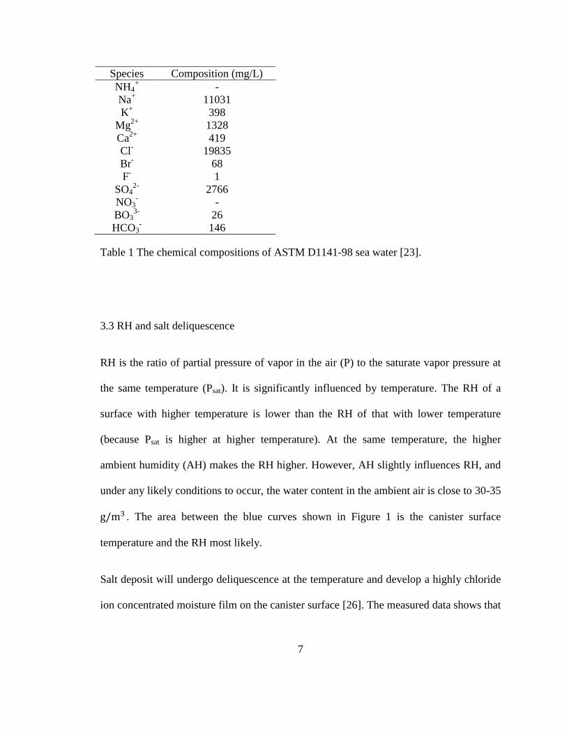
salts in dust and aerosols are expected to be dominated by sea-salt. Table 1 lists the

compositions of ASTM D1141-98 synthetic sea water [23] which is dominated by

sodium-magnesium chloride sulfates, being widely used in corrosion experiments for sea

spray.

While sea water may represent the primary source of salts in near marine environments, it

is not the only one. Rainwater and fog in near marine environments are not pure sea-salt,

contain variable but significant amounts of ammonium and nitrate, and are enriched in

sulfate relative to sea-salt. For marine aerosols, reactions with atmospheric volatiles may

substantially modify the composition of sea-salt particulates. Reactions with nitric acid

and acidic sulfur compound in the atmosphere act to convert sea-salt to nitrate and sulfate

compounds, accounting for the enrichment of these species in atmospheric aerosols

adjacent marine areas and even above the oceans. Sea-salt chloride in sea breezes on the

west shore of the Iberian Peninsula is depleted by 67% and 24% of fine and coarse

particles respectively, by the time the air mass reaches the coast [24]. What’s further,

inland atmospheric salts are dominantly ammonium-calcium-nitrate-sulfates, with only

minor chloride, according to Bryan and Enos [25]. However, chloride ion salt represents

the atmospheric salt load because of it is the aggressive factor to pitting corrosion of SSs,

instead of others such as dust and aerosols. Study of sea-salt deposit on SSs at the

temperature for deliquescence will closely simulate the corrosion behavior of canisters in

service.

7

Species Composition (mg/L)

NH4+ -

Na+ 11031

K+ 398

Mg2+

1328

Ca2+

419

Cl- 19835

Br- 68

F- 1

SO42-

2766

NO3- -

BO33-

26

HCO3- 146

Table 1 The chemical compositions of ASTM D1141-98 sea water [23].

3.3 RH and salt deliquescence

RH is the ratio of partial pressure of vapor in the air (P) to the saturate vapor pressure at

the same temperature (Psat). It is significantly influenced by temperature. The RH of a

surface with higher temperature is lower than the RH of that with lower temperature

(because Psat is higher at higher temperature). At the same temperature, the higher

ambient humidity (AH) makes the RH higher. However, AH slightly influences RH, and

under any likely conditions to occur, the water content in the ambient air is close to 30-35

g/m3 . The area between the blue curves shown in Figure 1 is the canister surface

temperature and the RH most likely.

Salt deposit will undergo deliquescence at the temperature and develop a highly chloride

ion concentrated moisture film on the canister surface [26]. The measured data shows that

8

the salt deposit on the canister surface after 19 years’ service was 1 g/m2 (which is

extremely small), but there was highly chloride ion concentrated moisture film formed by

deliquescence (> 6 M chloride).

Figure 1 shows the deliquescence RH values for NaCl, MgCl2, and sea-salt. The single

salt deliquescence RH values are beyond 20%. While for sea-salt (a mixture of NaCl,

MgCl2 and others), many studies have shown that the corrosion occurs well below the

deliquescence RH value of any single salt [6, 27]. This value is referred to limiting

relative humidity (RHL). Shirai et. al [28] measured the deliquescence RHL of sea-salt

for canister corrosion is 15% (the red line in Figure 1), which is a universal RH value

used to evaluate canister corrosion.

RHL is a significant value to refer when estimating the start of deliquescence of mixed

salts, considering the decline of surface temperature due to the air cooling and decay heat.

Once the surface temperature dropped to the temperature for deliquescence, the pitting

corrosion will start to occur. At 15% RHL with 30-35 g/m3 ambient air, it is estimated

that the corrosion will initiate when the canister surface temperature decreases to 70 °C.

Previous studies demonstrated that both Type 304L BM and WM are susceptible to crack

initiation at all salt concentrations from 0.1 to 10 g/m2 and the temperatures between 35

and 80 °C [29].

9

Figure 1 Relationship between RH, surface temperature, and conditions of deliquescence

for potentially relevant salt assemblages [21].

3.4 Residual stress

The applied stress caused by the inner pressure on the canister body is not considered as

the extremely low value, especially compared with the residual stress. The worst case

calculation indicates that the maximum value of internal pressurization is 0.35 MPa

hydrated uranium oxides (assuming 1 kg of UO2·2H2O which yields 112 g of water)

heated to 250°C by decay heat after sealing [30]. Accordingly, this maximum value of

inner pressure should not be high enough to cause any significant problems.

10

The high tensile residual stress caused by welding is the primary contributor of CISCC.

Sufficiently high tensile residual stresses exist in the canister welds and their associated

heat affected zones (HAZs) to allow for SCC initiation and potential through-wall growth

if exposed to a corrosive environment [16, 31]. There are limited stress reliefs on the

body longitudinal or circumferential welds or the lid closure welds. When the welds are

rapidly cooled to room temperature rather than being thermally or mechanically annealed

to relieve the stresses, highly tensile or compressive residual stresses may develop around

the welding area.

Welding process has two major effects on corrosion. Firstly, it induces residual stresses

in the weld and the adjacent HAZ, which weaken the corrosion resistance of the metal,

increasing pitting and general corrosion rates. Residual stresses, if sufficiently high, can

also support SCC of the metal. Secondly, the welding heat sensitizes the metal at HAZ.

Sensitization occurs when carbon and chromium in the steel diffuse to the grain boundary

(GB) and combines to form chrome rich carbides, resulting in a Cr-depleted selvage on

the grains along the GBs and therefore much more readily than the BM. GB corrosion

also helps to support SCC. Note that the WM itself is cooled from a molten state and

annealed such that avoids being sensitized.

A finite element analysis presented the residual stress distribution on a canister [31]. The

circumferential storage canister weld resulted in high tensile hoop stresses in the weld

and HAZ, remaining near or above yield strength throughout the thickness of the canister.

The longitudinal weld induced high tensile residual stresses in the axial direction, also

11

remaining near or above yield strength throughout the thickness of the canister. Both the

longitudinal and circumferential results suggest that a potential CISCC indication would

have a tendency to grow perpendicular to the weld direction, but would reach a region of

compressive stress approximately 40 mm from the weld centerline.

The residual stress measurement on a full-scale mockup container by Enos and Bryan [16]

verified that there are sufficient through-wall tensile stresses to support SCC crack

propagation. Far from the welds, the residual stresses are tensile on the outer diameter,

then compressive on the inner diameter. Circumferential welds are actively tensile

through the thickness, with the largest stress (up to 340 MPa) being parallel to the weld

direction. Longitudinal welds are also strongly tensile through the thickness, with the

largest stresses (up to 450 MPa) parallel to the weld direction.

Both the calculation and measurement of residual stresses in the canister indicate

deleterious effects on potential crack growth since no compressive regions exist to slow

or arrest through-wall growth.

12

Chapter 2: Fundamentals of CISCC

1. Pitting corrosion mechanism

Localized corrosion frequently forms at the locations of inhomogeneous steel matrix

(typically at welded joints), discontinuous surface films, differential aeration and

different pH, as where usually form the macro-galvanic cells [32]. Pits almost always

initiate due to chemical or physical heterogeneity at the surface such as inclusions,

second phase particles, solute-segregated GBs, mechanical damage, or dislocations [33].

Most engineering alloys have many or all such defects, and a pit tends to form at the most

responsive sites first. For example, pits in SSs often associate with manganese sulfide

(MnS) inclusions. The role of MnS inclusions in promoting the breakdown and localized

corrosion of SSs has been broadly recognized [7, 33, 34].

SSs are resistant to electrochemical corrosion due to the chromium oxide passive layer

(1-3 nm) [35]. However, aggressive anionic species, especially chloride ions, can locally

damage the passive layer, and the damage was reported in [36-38]. Where the steel loses

passivity above a critical potential, is called Epit, Eb, or film breakdown potential; the

phenomenon is responsible for pitting corrosion. Because of deliquescent salts, the

canister surface moisture film is strongly acidic and makes the steel electrical potential

above Epit.

13

The pitting corrosion resistance tends to be varied with the concentrations of chloride

ions. The reason for the aggressiveness of chloride ions has been considered, and a

number of investigations and examinations were carried out in marine and offshore

installations [7]. Chloride is an anion of a strong acid, and many metal cations exhibit

considerable solubility in chloride solutions. Pitting phenomenon can be summarized as

the local pit environment depleted in the cathodic reactant, such as dissolved oxygen, and

enriched in metal cation including anionic species [39]. Hence, the presence of the

oxidizing agent (oxide) in a chloride-containing environment is extremely damaging as to

enhance localized corrosion.

Previous studies commonly agreed that there are two stages of pitting progress:

metastable pitting and stable pitting. Pitting decline is a mid-state between propagation

and repassivation. It is difficult to distinguish that whether a pit is at the declined state

through observing, but its existence is considerable.

Pits are in nucleation state when the aggressive species rapidly penetrate the protective

oxide film. They start to grow after the nucleation. Figure 2 shows that the anodic and

cathodic electrochemical reactions that comprise corrosion spatially separate during

pitting. The metal, M, is being pitted by an aerated NaCl solution. Rapid dissolution of M

releases more Mn+

in the pit, while oxygen reduction takes place on the adjacent metal

surfaces. More Cl- ions are attracted in the pit to neutralize, since the total charge of a

solution must be zero. Oxygen is consumed in the pit and shifts most of the cathodic

reaction outside of the pit. The cathodic reaction is

14

O2 + 2H2O + 4e− → 4OH−

The acidic chloride environment is aggressive to most metals and tends to prevent

repassivation, thereby promoting the propagation.

The alloy compositions and microstructure have strong effects on the pitting corrosion

resistance. An existing pit can also be repassivated if the material contains a sufficient

amount of alloying elements such as Cr, Mo, Ti and so forth. Epit was correspondingly

found to increase dramatically as the Cr content increased above 13 %, which is a critical

value to create SSs [40]. Increasing concentration of Ni, which stabilizes the austenitic

phase, moderately improves the pitting resistance of Fe-Cr balanced alloy [40]. Small

increases in certain minor alloy elements include Mo and N can greatly reduce pitting

susceptibility [33]. Mo is practically effective but only in the presence of Cr through

enhancing the enrichment of Cr in the oxide film.

The majority of the researchers seem to favor the notion that removal of oxidizing agents,

e.g. removal of dissolved oxygen, is one powerful approach for reducing susceptibility to

localized corrosion. However, it is also supported that sufficient oxygen to the reaction

may enhance the formation of an oxide layer and thus repassivate or heal the damage to

the passive film, especially the increase in potential associated with oxidizing agents

would improve pitting potential, Epit [33].

The solid salt film which forms on the pit surface would enhance stability by providing a

buffer of ionic species that can dissolve into the pit to re-concentrate the environment in

15

the event of a catastrophic event, such as the sudden loss of a protective pit cover [7].

Under mass-transport-limited growth of solid salt film formed on the pit surface, pits can

be hemispherical with polished surfaces; while in the absence of a salt film, pits can be

crystallographically etched or irregularly shaped [7].

Figure 2 Schematic of anodic and cathodic electrochemical reactions in an initiated pit.

16

2. Pitting corrosion of SSs in chloride ion environment

Previous studies used various techniques to understand the pitting corrosion of materials

occurred in brine solutions. These methods include analyzing the local chemistries, the

potentiostatic characterization, potentiodynamic characterization, etc.

The local chemistries were in considerable interest and investigated by a range of

techniques. Wong et al. [41] described a way to isolate the pit solution by the rapid

freezing of the electrode in liquid nitrogen, removing the surface excess and subsequent

thawing. This approach is mainly used to study the pH in aluminum pits and the chloride

ion concentration in pits for SSs, allowing a considerable volume of pit solution to be

analyzed. Likewise, Frankel [7] suggested the way to isolate the pit solution by using

artificial pit electrode methods. This is also known as one-dimensional pit, or lead–in-

pencil electrode, which is a wire embedded in an insulator such as epoxy. Another way to

isolate the pit solution is by inserting microelectrodes into pits, cracks and crevices. With

this technique, once the local solution composition is fully characterized, it is possible to

reassemble the local environment by reconstituting it in bulk form from reagent grade

chemicals, and then determining the electrochemical behavior of a normal-sized sample

extracted from a local environment [7].

The electrochemical characteristic inside the cavity was also in interest as it would reveal

the different aspects of potentials existing within pitting corrosion. Figure 3 is a typical

polarization curve displaying the relationship of Ecorr and Epit, and the region of

metastable pits. Epit is principally treated as a standard to compare the pitting resistance

17

among all the metals and as a criterion whether the initiated cavity becomes stably

propagated. For instance, metals with low experimentally determined Epit have a higher

tendency to form pits naturally at open circuits [42]. The metastable pit, which initiates

for a limited period before repassivating, is found that it occurs below Epit, being not an

initiation point of pitting.

Figure 3 Representative polarization curve with Epit and Ecorr indicated. Additionally,

metastable pits prior to Epit are shown.

Repassivation potential (Erep) is the other criteria to interpret the pitting resistance. With

the effects of Epit and Erep, cyclic polarization experiments are used to measure the pitting

resistance of metals. The values could be used to determine under what conditions pitting

18

corrosion occurs. Figure 4 illustrates the typical repassivating polarization curve to

estimate the susceptibility of the metal alloy to pitting corrosion. The curve is used to find

Epit and repassivation potential (Erep). Higher Epit for material in a given environment

indicates greater resistance to pitting. Similarly, if the potential reduces below Epit, the

surface may repassivate and pit growth can stop. However, if the potential is between Epit

and Erep, pitting can be expected. Related studies have been undertaken by Szklarska-

Smialowska [33], Caines [43], Melchers [44] and Abood [45].

Figure 4 Representative cyclic polarization curve with Epit and Erep indicated.

However, using the electrochemical method to compare the pitting corrosion resistance is

not absolutely valid. The potentiodynamically determined Epit of most metals exhibits a

19

broad experimental scatter, of the other of hundreds of millivolts. Epit is insufficient for

the development of a fundamental understanding of the mechanism of pitting corrosion.

The other study interest of pitting corrosion is the influence of pit chemistry on pit

growth and stability, which has been provided by Galvele et al. [46]. The concentrations

of various ionic species at the bottom of modeled one-dimensional pit geometry were

also studied [7, 46]. The concentration of various ionic species is determined as a

function of current density based on a material balance that considered generation of

cations by dissolution, outward diffusion, and thermodynamic equilibrium of various

reactions such as cation hydrolysis [7]. Galvele et al. [46] found that a critical value of

the factor x.i, (where x is pit depth and i is current density), correspond to a critical pit

acidification for sustained pit growth. Current density in a pit is a measure of the

corrosion rate within the pit and thus a measure of the pit penetration rate. x.i can be used

to determine the current density required to initiate pitting at a defect of a given size.

Increasing the pit density increases the ionic concentration in the pit solution, often

reaching supersaturation conditions.

The aggressive ions, take significant effect on the rate of pitting corrosion. It is revealed

that Ecorr and Epit decreased, and current density in the passive region increased with the

increase of chloride ion concentrations [47]. A linear relationship between Epit and the

chloride ion concentration was found [47]. The previous anodic potentiodynamic tests of

Type 304L SS suggested that for the NaCl solution (pH 2) under 4.5 % concentration,

passivation region had a significant range between the Ecorr and Epit, and passivation

20

break-down potential Epit shifted towards more positive potentials with the decrease of

chloride concentration [47]. A steady increase of current with potential in 4.5% NaCl

which indicated active corrosion was observed [47].

3. Modeling of pitting corrosion

3.1 Comparison of deterministic and probabilistic models

A wide range of diverse pitting corrosion models that have been proposed can be

characterized as either deterministic or probabilistic (include statistical and stochastic

methods) [48-53].

A deterministic model is often formulated using partial differential equations based on a

set of variables and environmental parameters [49, 50]. Different deterministic models do

not use the same set of variables because they consider various aspects of the corrosion

mechanism. The partial differential equations could come from the kinetics or

electrochemistry [54]. Numerical solution of these partial differential equations is used to

make the prediction from the models.

The probabilistic models use probabilities to interpret certain factors of the dynamics of

pitting corrosion [51-53]. One example of the probabilistic model divides the metal

surface into a 2D array of hypothetical cells, then assigns the probabilities for the

transition between pitting states to each cell. Nucleation or destruction of a pit embryo is

controlled by comparing random numbers to an environment-dependent probability.

After a pit embryo grows to a certain stage, it becomes a stable pit and follows the

21

probabilistic rules for pitting growth. The environmental parameters come into the model

through the probabilities, and the computation is based on the theoretical formulation as

well as the empirical observation.

Models which are already constructed to be probabilistic in nature are more favorable for

the initial modeling effort since deterministic models must be adapted to probabilistic

forms if they are selected. Although deterministic models are easy to approach and

interpret regarding actual physical and chemical parameters, they cannot explain the

stochastic behavior of an actual corrosion process. Thereafter, deterministic models

cannot determine the realistic results through simulating. Probabilistic models, on the

other hand, only involve simple computations but are likely to generate more realistic

results than deterministic models. However, none of the probabilities in these models can

be related to the physical or chemical parameters; also, the probabilistic models are

localized and do not show global interactions.

Mears and Evans stated in 1934 [55] that “from the practical standpoint … it may be

more important to know whether … corrosion is likely to occur at all than to know how

quickly it will develop.” Yet, deterministic approaches have so far prevailed in corrosion

science, even though the stochastic theory was successfully used to explain pitting

corrosion characteristics such as the probability distribution of both Epit and the induction

time [56]. The work by Henshall et al. [57] showed that a computing model based on

stochastic theory could describe the pit initiation and growth on SSs and include some

deterministic elements.

22

It is recognized that the probabilistic model is an effective and persuasive simulation

method to predict the complex corrosion process. While, two approaches: statistical and

stochastic methods are commonly used on probabilistic models, leading to two directions

on the way to the eventuality. The following section will in further discovery the

probabilistic models through comparing its two methods.

3.2 Comparison of statistical and stochastic methods

The majority of researchers seem to agree on the notion that it is impossible to depend on

a single distribution of the statistic approach to simulate the complicated pitting corrosion

process. A combination of several probabilistic distributions is prone to be more factual.

Valor [58] modeled the pitting corrosion as the combination of two independent

nonhomogeneous in time physical process, one for pit initiation and one for pit growth.

Extreme value distribution was applied to produce a unified stochastic model of pitting

corrosion.

For instance, Valor, et al. [59] treated the pit generation process as a nonhomogeneous

Poisson process, in which induction time for pit initiation was simulated as the realization

of a Weibull process; it also combined the pit growth process as a nonhomogeneous

Markov process through using extreme value statistics. The model was able to display the

whole process of pitting corrosion from an embryo to stable growth, and it was

demonstrated to be valid on the specific conditions through experimental methods.

23

However, if further applications are intended under a variety of conditions, some

problems will arise: (1) It was static and thus limited in analysis of the time-dependent

probabilistic aspects of pitting corrosion; (2) It was weak in involving the changes of

environment and the model parameters must be derived from the experimental results at

the specific environments; (3) It is difficult to get sample data for the objective, and thus

decide how many samples to apply. Summarily, the limitations of the statistical approach

include the assumption of nominal “homogeneity” in the system (e.g. random distribution

of material microstructure, and solution flow rate), and inflexibility in dealing with

changes in operating conditions, environment or pit shapes [60].

Environment determines the severity of pitting damage [61], thereafter, to improve

corrosion models, it is necessary to not only account for the time but also include

contributing variables [62]. However, there is no accomplished model attempted to

include all the significant factors for naturally induced pitting corrosion of metals.

Among the validated models, compared with the statistic method, the stochastic method

is better for probabilistic events depending upon time, and a birth and death stochastic

parameter is more suitable to describe the whole process of pit initiation and

repassivation. In addition, previous developed stochastic models have demonstrated the

ability to involve with environmental factors.

A stochastic approach has been developed for probabilistic events depending upon time

and found to apply to pit generation events that change with time. The approach first was

introduced to explain the relation between the distribution of Epit and induction time for

24

pit generation [63, 64]. Williams, et al., described a random generation of pit and current

noise by assuming a stochastic process [65, 66]. Gabrielli, et al., reviewed the

probabilistic aspects of localized corrosion and discussed a general approach to the

stochastic process, including a counting process and noise generation [67].

There existed a substantial interest in the environmental parameters, but little quantitative

work has been done on corrosion damage generation and growth simulation models.

Baroux applied the stochastic theory to pitting corrosion of SS and analyzed the effect of

inclusions and inhibitors [68]. Macdonald, et al., combined the deterministic approach

with the stochastic model [69]. The elegant point-defect model for pit generation of a

passive film was used to explain the distribution of the induction time and Epit by

introducing the distribution function for the diffusion constant in the deterministic model.

Doelling, et al. reported that analysis of the distribution for pit generation time at a

potentiostatic condition for iron led to the same conclusion obtained by the deterministic

approach [70]. Hashimoto, et al., reported that the noise spectrum for iron in chloride

chromate solution could be explained by assuming pit generation and repassivation [71].

Murer and Buchheit [72] developed a Monte Carlo model for aluminum alloys, which

was based on Henshall’s [57]. The design collected experimental input parameters of

birth rate and death rate through multichannel microelectrode analysis, which was

statistically significant. However, the assumption that death rate was equal to the birth

rate remained to be questioned, and the equations of stable pit growth rate were

deterministic rather than stochastic. In addition, it is well known that aluminum alloys

25

have an exponential dependence on electrochemical potential, a logarithmic dependence

on chloride ion concentration, and an exponential dependence on temperature, while the

model did not consider them.

The Monte Carlo model [53] developed by Henshall started to involve environmental

parameters quantitatively into the "birth and death" stochastic theory of pitting for SSs. It

included three critical environmental parameters: applied potential, chloride ion

concentration, and absolute temperature. The model explained the development process

which was based on the work of Janik-Czachor [73], Broli et al. [74] Herbsleb and Engell

[75], and Szklarska-Smialowska and Janik-Czachor [76]. It only directly combined the

separate proportionalities of variables, rather than considering synergistic reactions

between variables. The initiation of corrosion pits followed a statistical distribution of

induction time. The growth of corrosion pits was based on stochastic parameters derived

from a variety of experimental data. The model was based on Monte Carlo method such

that provided a microscopic and mechanistic view, as well as to qualitatively simulated

the effects of environment on pit generation and growth. However, the sensitivity

analysis was not adequately performed; according to the results, the model would largely

depend on the input parameters, remaining to be studied.

Among the numerous stochastic models, it is difficult to decide a definite model as a

general model to explain all the pit formation processes observed, but the experimental

data obtained in various cases could be fitted to a particular model by numerical or

graphic analysis using the formulated equations. The estimation of pitting generation and

26

growth places high demands in estimating the lifetime of materials in the specific

environments. A valid model with the ability to solve the significantly related factors for

naturally induced pitting corrosion is in high priority of interest.

4. SCC mechanism

In 1969, Staehle [77] concluded that “there presently is no reliable fundamental theory of

SCC in any alloy-environment system that can be used to predict the performance of

equipment even in environments where conditions are readily defined. There was an

almost uniform conclusion that no unifying mechanisms of SCC exist.” This conclusion

is still applicable today. Although the SCC mechanism is difficult to conclude, an amount

of studies has been undertaken to reveal the fundamentals of SCC and suggest the

tendency of structure failure for each SS at its application environment. It has been

concluded that susceptibility to chloride cracking in SSs is a function not of the crystal

structure of ferrite or austenite but of the compositions of these phases and the presence

of Cr-depleted zones around precipitations in ferritic alloys [78].

In many applications, pitting is the precursor to SCC because it provides the combination

of local aggressive solution chemistry and a stress concentrating feature [79]. The

fundamental steps in the overall process of crack development involve pit initiation, pit

growth, the transition from a pit to a crack, short crack growth and long crack growth. In

predictive schemes [80-82], the pit-to-crack transition is based on the phenomenological

requirements that the pit depth must be greater than a threshold depth, corresponding to a

threshold stress intensity factor, and that the crack growth rate should exceed the pit

27

growth rate. Except for the continuum-based models, the detail of how SCC actually

emerges from a pitting corrosion precursor has been clarified through unique 3-D images

which show the early stages of cracks evolving from pits in 3NiCrMoV steam turbine

disc steel [83]. It is demonstrated that SCC invariably originates from corrosion pits [84]

and cracks that have nucleated on pit walls can grow around the pit and coalesce to form

a complete through-crack [83].

With the materials used on the welded canister, CISCC occurs from the combined effect

of pitting corrosion under residual stress [27]. The process is a composite of the initiation

stage dominated by electrochemical mechanism and the propagation stage dominated by

both electrochemistry and metal separation. The initiation of CISCC by pitting corrosion

is widely accepted [85-90]. It is considered corrosion with local slip at the crack tip and is

often found to initiate where pitting corrosion has occurred. Kosaki [91], Nakahara and

Takahashi [92], Kawamoto [93] and Mayuzumi [94] found SCC initiation starts from the

bottom of the pitting corrosion area.

The origin of the crack is located on a stress concentration region, but its nucleation is a

result of high corrosive conditions [95]. Once the crack is initiated at the corrosion area,

it will propagate at a fast rate under the conditions of metal dissolution and residual stress.

The study of pitting and crack nucleation at the early stages of SCC under ultra-low

elastic load suggests that SCC emanates from the defect on the sample surface, and the

preferential SCC initiation sites are at the shoulders rather than at the bottoms of the

surface defect [96]. The likelihood of SCC propagation from an area of pitting corrosion

28

should increase with time as the depth of metal loss increases [97]. Metal separation is

faster than electrochemical dissolution during the process of propagation.

Note that crack propagation conditions must all be satisfied otherwise the propagation

will not occur. One study [27] found that below the RHL that pitting corrosion probably

did not occur, no SCC propagated in Type 304 SS after 125 days with simulated residual

stress. Moreover, according to the competing theory [97], even if the applied stress

intensity factor (K) exceeds the threshold stress intensity factor for SCC (i.e., K > K1SCC),

a crack will only initiate in a pit if the crack growth rate is more rapid than the rate of pit

growth. It is reasonable to expect that pitting corrosion will slow down with time as a

corroded area deepens and the diffusion distance increases. Overall, the SCC propagation

demands the satisfaction of all threshold conditions.

29

Chapter 3: Pitting Corrosion of SSs in Brine Solutions

1. Introduction

Motivated by the need to explore and compare the corrosion behaviors of BM and WM

exposed to highly concentrated chloride solutions as well as to supply laboratory

measured data to the expected pitting corrosion model, this study focused on observing

the pitting corrosion characteristics of Type 304L BM and the WM in the highly

concentrated NaCl solution and ASTM D1141-98 standard sea-salt solution at

temperatures of 40 and 70 °C. Extensive experimental data have been achieved by the

techniques include (1) microscope characterizations: focused ion beam/ scanning electric

microscope (FIB/SEM), scanning transmission electron microscope (STEM) equipped

with an electron energy dispersive spectroscope (EDS); (2) electrochemical techniques:

open circuit potential (OCP), electrochemical impedance spectroscopy (EIS), and

potentiodynamic polarization; and (3) optical profiler.

2. Specimen preparation

The Type 304L BM and WM were prepared based on the focus of research. The WM

was machined from the welding zone of a butt weld. The outer surface of the weld was

exposed to the investigated environments. The specimens were fabricated in the shapes of

circular disk and coupon, for electrochemical testing and immersion testing, respectively.

30

The copper deposit caused by electric discharge machining (EDM) was cleaned by DI

water, acetone and sandpaper polishing.

Each circular disk specimen was in 5 mm diameter and 4 mm thick, installed on a

polytetrafluoroethylene (PTFE) electrode head used on the electrochemical testing. The

edges of specimens were protected by washers from crevice corrosion, and the spherical

surface was 0.196 cm2

and exposed to the test environment. The exposed surface was

successively mechanically polished up to an 800-grit finish using sandpapers.

Each coupon specimen was machined to 4 cm2 square and 5 mm thick, mechanically

abraded and SiC diamond polished to 1 μm.

After polishing, the specimens were ultrasonically cleaned in acetone of analytical grade

for about 3 minutes, rinsed with ultrapure water (resistivity > 18 MΩ cm) and dried by

ethanol of analytical grade. They were kept in a desiccator for 3 days to form stable oxide

layers before testing. The chemical compositions of the specimens are displayed in Table

2 and Table 3.

Fe Cr Ni C P Si Cu N Cb+Ta Mn

Bal. 18.470 8.190 0.025 0.037 0.260 0.620 0.069 0.013 1.800

S Mo Ti Co Al B V W Ta Sn

0.025 0.400 0.003 0.123 0.006 0.001 0.060 0.029 0.001 0.008

Table 2 The chemical compositions of Type 304L BM circular disk specimen used in the

investigations (at %).

31

Fe Cr Ni C P Si Cu N Mn S Mo Co

Bal. 18.21 8.06 0.021 0.031 0.44 0.46 0.082 1.65 0.024 0.65 0.11

Table 3 The chemical compositions of Type 304L BM coupon specimen used in the

investigations (at %).

3. Solution preparation

The base solution was made up by dissolving an appropriate amount of analytical grade

and chemically pure NaCl or ASTM D1141-98 sea-salt1 in distilled water (18.2 MΩ∙cm).

Table 4 shows solution specifications.

Series Solute

Weight

Concentration

(wt %)

Chloride

Molarity

(M)

Temperature

(°C) pH

A 99.99 % pure NaCl 26.7 6.25 40 7.00

B ASTM D1141-98 sea-salt 10.5 1.5 40 7.32

C ASTM D1141-98 sea-salt 10.5 1.5 70 7.00

Table 4 Solution specifications.

1 Chemical compositions (g/L): NaCl 24.53, MgCl2 5.20, Na2SO4 4.09, CaCl2 1.16, KCl 0.695,

NaHCO3 0.201, KBr 0.101, H3BO3 0.027, SrCl2 0.025, NaF 0.003 and traces of nitrate compounds.

32

4. Test procedures

4.1 Electrochemical techniques

The experiments were conducted in a typical three-electrode electrochemical system in a

glass cell. The glass cell was filled with 1 L of test solution. The circular disk specimen

was installed on the working electrode (WE). A graphite rod seated inside a fritted glass

tube was used as the counter electrode (CE). An Ag/AgCl (4M KCl) reference electrode

(RE) was connected to the cell externally via a Luggin tube. The solution temperature

was maintained within ± 1 °C by using a thermocouple and a controllable hot plate. The

solution was exposed to the atmosphere via a condenser, which was also used to avoid

the evaporation of water. The solution was heated up to boiling and cooled down to the

desired temperatures (40 °C and 70 °C), then maintained at the desired test temperatures

for 3 hours for the equilibration with air. All electrochemical measurements were

performed using a Gamry Interface 1000 potentiostat controlled by the Gamry

Framework software.

After preparing the solution, the specimen was immersed in the solution. A

potentiodynamic polarization measurement at the 1st hour of immersion was conducted.

The potentiodynamic measurement was carried out at a scan rate of 0.5mV/s ranging

from -0.2V to 0.8V vs. OCP. After the test, the specimen was released from the WE,

rinsed with DI water and analytical grade acetone, and stored in the desiccator.

33

The other solution, as well as a new specimen, was prepared to take a 43-hour testing.

OCP measurement throughout the test was undertaken on the specimen with a sample

period of 1 second. EIS measurements at times of 1, 4, 9, 17, 25, 34 and 43 hours were

carried out at the OCP over a frequency range from 100 kHz to 10 mHz amplitude

sinusoidal voltage applied as the disturbance signal. After 43 hours, a potentiodynamic

polarization measurement was conducted at a scan rate of 0.5mV/s ranging from -0.2V to

0.8V vs. OCP. Replicate tests were conducted, and results were essentially the same.

4.2 Optical profiler

The coupon specimens were immersed in the solutions as shown in Table 4 at the time

intervals of 2, 5, 10, 20 and 30 days. After testing, they were ultrasonically cleaned in

acetone of analytical grade for 2 minutes, rinsed with DI water (18.2 MΩ∙cm) and dried

by ethanol of analytical grade. The 3D surface morphology of the specimen after the test

was observed using the non-contact ContourGT-I 3D optical profiler; the depth and

radius, as well as density of pits, were analyzed by the Vision64TM

software.

4.3 SEM/FIB and STEM/EDS analysis

The FEI Nova NanoLabTM

600 Dual-Beam (FIB/SEM) was used to observe the

microstructure of the specimen surface, as well as to prepare a thin cross-section slice

(typically 100-200 nm thick foil). Microchemistry analysis was also conducted by FEI

Tecnai F20 S/TEM equipped with an efficient collection of X-rays for elemental analysis

down to the sub-nanometer level.

34

5. Results and analysis

5.1 WM properties

Before testing, the specimen surface was examined by SEM. The differences between the

BM and the WM are compared in Figure 5. The BM is homogenous (Figure 5a), and the

WM has two phases shown as two contrasts in Figure 5b. Table 5 displays the

compositions of the lighter gray phase (e.g. spot 1) and the darker gray phase (e.g. spot 2).

The second phase is susceptible to Cr-C precipitations due to the higher content of Cr and

C, and extremely low content of Ni compared with the BM.

To maintain high resistance to localized corrosion, it is commonly agreed that alloying

elements must be homogeneously distributed. The balance of alloying elements can be

changed by the precipitation of various secondary phases, due to welding process and

applied conditions. The most common precipitates are secondary austenite (γ2), nitrides,

M23C6 carbide and Fe-Cr-Mo intermetallic phases such as σ phase, χ phase, and R phase.

Their presence can cause degradation of the metal, particularly its corrosion properties.

The severity of corrosion attack depends on the nature and a number of undesirable

phases, the chemical compositions of the metal as well as the production conditions [98,

99]. In the steel welded joint, coarsening of the M23C6 precipitate by weld thermal cycle

renders the creep rupture strength of the welded joint significantly lower than the BM

[100].

Besides Cr-C precipitations, it is observed that intergranular crack (IGC) occurring in the

stabilized SS is also caused by Cr depletion due to the segregation of the solute Cr atoms

35

in the grain boundary (GB) [101], contrasting with the conventionally favored

mechanism that IGC occurs due to the formation of Cr-C precipitations in the GB. This

discovery illustrated that the stabilizer elements (e.g. Ti, Nb) precipitated with carbon in

the GB, and Cr diffused out from the precipitate and formed a depletion zone between the

GB and the matrix. Combined with the Cr-C distribution examined at the welding zone, it

is predictable that partial of Cr will diffuse out from the Cr-C precipitations and form a

depletion zone around the GB, and weaken the corrosion resistance.

Figure 5 SEM images of the surface of (a) BM, and (b) WM before testing.

36

Spot 1 Spot 2

Atomic % Uncertainty % Atomic % Uncertainty %

Fe 70.43 2.76 60.1 3.01

Cr 19.7 4.02 21.47 4.07

Ni 9.87 7.56 0 0

C 0 0 18.43 18.84

Table 5 Atomic concentrations of spots shown in Figure 5b.

5.2 The evolution of corrosion potential

The corrosion potential is when the corrosion rate of oxidation equals to the corrosion

rate of reduction. In general, the material with a more positive corrosion potential is

expected to be more corrosion resistant in that particular solution than one with a more

negative corrosion potential. The results of materials in differently concentrated chloride

solutions usually can be ranked according to the resistance to corrosion based on

potentials.

Figure 6 shows the OCP results of the specimens exposed to the investigated

environments. Table 6 summarizes their starting and ending potentials (average hourly).

A, B and C represent the solutions shown in Table 4.The OCP value fluctuated in the

testing, not showing a steady increasing or decreasing. The OCP value of the WM

specimen had more significant fluctuations than the one of the BM specimen. Breakdown

of oxide layer and repassivation of oxide layer alternatively occurred on the metal surface.

For the duplicate tests of one metal in one environment, the starting potentials were not

37

always the same, and the fluctuation of potential did not follow an order; however, the

potential always reached the same value after 35 hours and became relatively stable.

The WM typically had much lower OCP values than the BM in the same environment,

indicating the less corrosion resistance. To the localized corrosion at welded joints, when

the WM is less noble than the parent metal, the former corrodes selectively. Since both

are ferrous metals, the difference in the OCP between the anode and the cathode would

not be significant. As shown in Table 6, in the same test condition, the difference in the

OCP of WM and BM is about 30- 90 mV. However, the penetration rate could be high

because a small shift of the potential of the anode in the noble direction causes a large

increase in the dissolution rate [102]. The WM at the welded joint will be selectively

attacked in the aggressive environment.

The chloride ion concentration significantly affected potentials. The specimens exposed

to 6.25 M chloride NaCl solution had significantly lower corrosion potentials than those

to 1.5 M chloride sea-salt solution. Temperature has a small effect on the potential

changes when compared the values of 1.5 M chloride sea-salt solution at 40 °C and 70 °C.

38

Figure 6 Plots of OCP in 43 hours. A, B and C represent the solutions shown in Table 4.

Time BM-A WM-A BM-B WM-B BM-C WM-C

The first hour -238.3 -40.1 -73.6 -130.5 -101.9 -112.7

The last hour -251.6 -286.5 -51.8 -139.7 -65.1 -126.9

Table 6 The starting and ending potentials in mV vs. SSE (average hourly).

5.3 The identification of pitting potential

The evolution of pitting on SSs in chloride-containing solutions occurs in three stages: (1)

pit nucleation, (2) metastable growth of pit, and (3) stable pit growth [7]. For the stable

pit growth which is characterized by the pitting potential, Epit, several critical conditions

39

should be met. When the critical conditions are not satisfied, pits will repassivate without

further growth, which is called metastable pit growth.

In the early hours, the oxide layer formed in the aggressive solution was unstable.

Breakdown and repassivation of the layer alternatively occurred. The potentiodynamic

testing at the 1st hour was conducted, and the result is shown in Table 7a. Significant

current density spikes are in the passivation zone, i.e. below Epit. These spikes are due to

the occurrence of metastable pits and are explained by the consecutive formation and

repassivation of micro-size pits. The pit nucleation and metastable pit growth appeared as

current spikes on polarization curves.

Note that the passivation layer became relatively stable after 35 hours, which is illustrated

by the OCP values in Figure 6. The potentiodynamic testing at the 43rd

hour was also

conducted to compare with the results of 1st hour, shown in Figure 7b. The current

density spikes are not manifest in the passivation zone. Besides, the passivation zones

become wider than the curves obtained at the 1st hour (Figure 7a).

The WM typically has larger anodic passive current density and lower cathodic current

density than the BM. Larger anodic passive current density is the representative of faster

dissolution rate of metals, thereafter the corrosion resistance is depressed by welding. The

anodic passive current density of specimens exposed to 6.25 M chloride NaCl solution

was much larger than that of 1.5 M chloride.

40

Table 7 summarizes the electrochemical parameters, including Epit, Ecorr, βa (anodic Tafel

constant), βc (cathodic Tafel constant) and icorr (corrosion current density). The consistent

pattern on the effect of chloride ion concentration on Ecorr and Epit was observed. The

potential range of the passive region is displaced toward more negative potentials and

becomes progressively narrower with increased chloride ion concentration and

temperature. Larger icorr and more negative Epit are caused by the adsorption of chloride

ions.

A negative linear relationship of Epit and temperature has been derived, and the

coefficients are influenced by the type of metal and corrosive medium. The relation

Epit (mV vs. SHE) = 174 – 5.32 T (°C)

was suggested by Ezuber [103] to SS316 in NaCl system at 1M. In our case, a negative

relationship was also found, though it would need more replicate tests as well as at

different temperatures to parameterize the relationship.

Cyclic polarization scans were also applied at the investigated environments; however no

pronounced hysteresis loops were achieved. The hysteresis loops typically intersect with

the cathodic curves were far below the corrosion potentials. Metals have little

repassivation ability in the investigated solutions.

41

Figure 7 Plots of potentiodynamic polarization curves at (a) the 1st hour, and (b) the 43rd

hour of testing.

42

(a)

Test Epit

(mV vs. SSE)

Ecorr

(mV vs. SSE)

βa

(mV/decade)

βc

(mV/decade)

icorr

(mA/cm2)

BM-A -94 -230 105 122 5.46E-04

WM-A -150 -274 107 346 8.57E-04

BM-B 118 -118 354 126 1.02E-04

WM-B 156 -185 274 74 7.45E-05

BM-C 49 -116 281 79 2.46E-04

WM-C 72 -150 328 78 2.32E-04

(b)

Test Epit

(mV vs. SSE)

Ecorr

(mV vs. SSE)

βa

(mV/decade)

βc

(mV/decade)

icorr

(mA/cm2)

BM-A 40 -228 114 172 3.50E-07

WM-A -3 -300 245 373 1.24E-06

BM-B 224 -131 598 68 4.56E-05

WM-B 161 -156 350 132 3.81E-04

BM-C 149 -114 450 58 3.63E-05

WM-C 247 -159 375 113 7.70E-05

Table 7 Electrochemical polarization parameters at (a) the 1st hour and (b) the 43rd hour

of immersion testing.

5.4 The identification of passivation layer

To the EIS spectra corresponding to the specimens exposed to 6.25 M chloride NaCl

solution at 40 °C (Figure 8a & 8b), and to the 1.5 M chloride sea-salt solution at 70 °C

(Figure 8c & 8d), an equivalent circuit shown in Figure 8e consisting of a double- parallel

R-constant phase element (CPE) arrangement in series with the solution resistance is used

to simulate the elements deriving from the spectra, and a good fitting quality is obtained.

43

The passive layer formed on the SS surface can be considered to be a parallel circuit of a

resistor due to the conductivity of the film, and a capacitor due to its dielectric properties

[104, 105]. On the equivalent circuit, Re represents the solution resistance; CPEf1

represents the capacitance of the outer layer, Rf1 is the resistance of the outer layer; CPEf2

represents the capacitance of the inner layer, and Rf2 is the resistance of the inner layer.

Table 8 is a summary of the fitting data to the EIS spectra.

A CPE is utilized instead of a capacitance because often the measured capacitance is not

ideal, i.e. the element is not a pure capacitance. The impedance representation of a CPE is

given as

Z(CPE) =1

Q0(jω)n

where Q0 is a fit parameter. In the ideal case when the exponential factor n = 1, the CPE

acts as a capacitor with Q0 equal to the capacitance C. In practice, n is less than 1. The

CPE behavior arises because microscopic material properties can exhibit a distribution,

and the n-value provides the information on the nature of the surface or the passive layer.

Accordingly, the impedance of the equivalent circuit is given by

Z = Re +1

Qf1(jω)nf1 +1

Rf1 +1

Rf2 +1

Qf2(jω)nf2

44

In Figure 8a- 8d, two time constants can be identified during the exposure: an incomplete

capacitive time constant at high-frequency zone (>104 Hz) and a capacitive time constant

at medium-frequency zone. Normally, the impedance of the inner layer (passive layer) is

negligible at high-frequency zone and the inner layer responses as a resistor giving a

phase angle of zero. In Figure 8a- 8d, the non-zero (negative) phase angle at 105 Hz

indicates the impedance of the capacitor at 105 Hz is considerable, illustrated by the

values of Qf2. Meanwhile, the resistance of inner layer (Rf2) is large, representing the

compact structure. Besides, the capacitance response (Qf1) of the outer layer is from the

lower frequency zone. The outer layer is passive as well. While compared with the

resistance of the inner layer (Rf2), this resistance of outer layer (Rf1) is much smaller,

indicating the outer layer is porous.

Polarization resistance, Rp, is the sum of Rf1 and Rf2 for a bi-layer structure. According to

the data shown in Table 8a & 8b, Rp values become smaller with the increasing time. The

decline of Rp represents that the transportation of metal ions became faster, and the

passive layer was slowly dissolved. Note that the OCP values of the specimens exposed

to this investigated environment kept declining (with fluctuations) during the OCP

measurement (Figure 6). The slowly dissolved passive layer explains the reason for the

potential decline.

On the contrary, Rp values in Table 8c & 8d become larger with the increasing time,

representing that the transportation of metal ions became slower, and the passive layer

became firmer. This is also coherent with the OCP values shown in Figure 6.

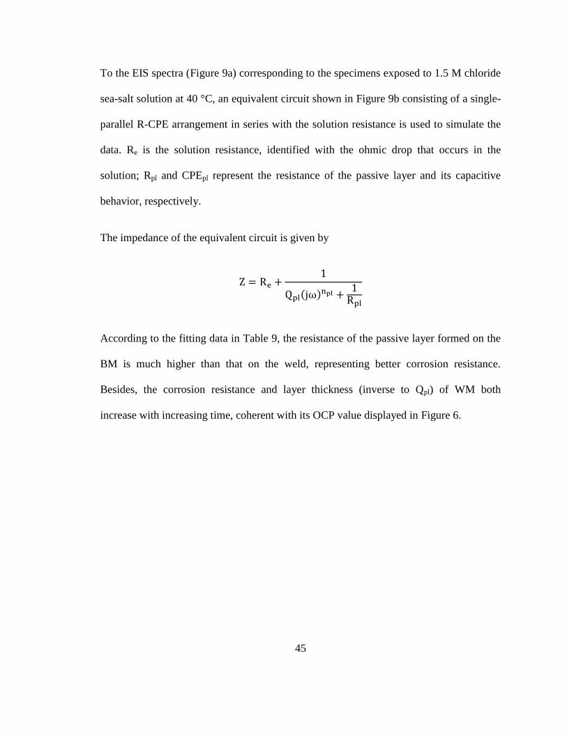
45

To the EIS spectra (Figure 9a) corresponding to the specimens exposed to 1.5 M chloride

sea-salt solution at 40 °C, an equivalent circuit shown in Figure 9b consisting of a single-

parallel R-CPE arrangement in series with the solution resistance is used to simulate the

data. Re is the solution resistance, identified with the ohmic drop that occurs in the

solution; Rpl and CPEpl represent the resistance of the passive layer and its capacitive

behavior, respectively.

The impedance of the equivalent circuit is given by

Z = Re +1

Qpl(jω)npl +

1Rpl

According to the fitting data in Table 9, the resistance of the passive layer formed on the

BM is much higher than that on the weld, representing better corrosion resistance.

Besides, the corrosion resistance and layer thickness (inverse to Qpl) of WM both

increase with increasing time, coherent with its OCP value displayed in Figure 6.

46

Continued

Figure 8 EIS spectra and the equivalent circuit. (a) BM-A, (b) WM-A, (c) BM-C, (d)

WM-C, (e) equivalent circuit used to fit the EIS spectra.

47

Figure 8 continued

(a) Test BM-A

Time

(hour)

Re

(kΩcm2)

Rf1

(kΩcm2)

Qf1

(μSsncm

-2)

nf1 Rf2

(kΩcm2)

Qf2

(μSsncm

-2)

nf2

1 0.001 0.037 74.949 0.736 11.117 132.551 0.617

4 0.001 0.079 77.347 0.721 11.748 85.969 0.670

9 0.001 0.056 106.327 0.697 9.590 86.429 0.666

17 0.001 0.098 239.592 0.641 6.456 6.117 0.987

25 0.001 0.055 269.235 0.646 5.116 9.541 0.931

34 0.001 0.038 297.296 0.664 3.540 9.791 0.907

43 0.001 0.001 289.694 0.608 3.665 124.745 0.740

(b) Test WM-A

Time

(hour)

Re

(kΩcm2)

Rf1

(kΩcm2)

Qf1

(μSsncm

-2)

nf1 Rf2

(kΩcm2)

Qf2

(μSsncm

-2)

nf2

1 0.001 0.074 41.612 0.696 121.677 49.474 0.762

4 0.001 0.050 47.827 0.692 93.139 67.347 0.736

9 0.001 0.028 55.510 0.697 47.138 79.643 0.743

17 0.001 0.018 174.745 0.649 10.216 37.026 0.858

25 0.001 0.018 211.429 0.639 10.737 25.357 0.899

34 0.001 0.014 335.051 0.606 7.189 28.429 0.873

43 0.001 0.012 369.031 0.604 7.264 27.704 0.879

Continued

Table 8 Values obtained from the analysis of the EIS spectra in (a) BM-A, (b) WM-A, (c)

BM-C, (d) WM-C.

48

Table 8 continued

(c) Test BM-C

Time

(hour)

Re

(kΩcm2)

Rf1

(kΩcm2)

Qf1

(μSsncm

-2)

nf1 Rf2

(kΩcm2)

Qf2

(μSsncm

-2)

nf2

1 0.003 0.778 60.714 0.810 240.688 15.230 0.866

4 0.003 1.834 51.990 0.824 461.384 12.740 0.852

9 0.003 1.761 43.362 0.840 916.300 13.923 0.813

17 0.003 1.634 40.138 0.848 1460.40 13.112 0.814

25 0.004 1.798 38.918 0.852 1913.35 11.005 0.816

34 0.004 1.962 37.995 0.856 2402.96 9.679 0.820

43 0.004 1.974 36.765 0.857 3087.00 9.327 0.808

(d) Test WM-C

Time

(hour)

Re

(kΩcm2)

Rf1

(kΩcm2)

Qf1

(μSsncm

-2)

nf1 Rf2

(kΩcm2)

Qf2

(μSsncm

-2)

nf2

1 0.001 2.060 5.995 0.835 163.542 57.041 0.704

4 0.001 2.283 4.490 0.853 459.228 50.418 0.721

9 0.001 1.924 3.966 0.861 1103.28 47.173 0.748

17 0.001 1.512 3.811 0.866 2434.32 45.383 0.763

25 0.001 1.307 3.908 0.865 3706.36 44.168 0.772

34 0.004 1.200 4.211 0.858 6134.80 43.122 0.778

43 0.004 1.103 4.348 0.856 10050.9 42.735 0.783

49

Figure 9 EIS spectra and the equivalent circuit. (a) BM-B, (b) WM-B, (c) equivalent

circuit used to fit the spectra.

50

(a) BM-B

Exposure time

(hour) Re(kΩcm

2) Rpl(kΩcm

2) Qpl(μSs

ncm

-2) nf1

1 0.020 529.396 46.128 0.855

4 0.020 511.168 45.561 0.858

9 0.021 534.688 45.969 0.861

17 0.021 553.896 45.903 0.864

25 0.021 566.048 45.490 0.867

34 0.021 568.204 45.184 0.868

43 0.010 562.128 45.061 0.869

(b) WM-B

Exposure time

(hour) Re(kΩcm

2) Rpl(kΩcm

2) Qpl(μSs

ncm

-2) nf1

1 0.003 15.796 130.459 0.829

4 0.003 17.028 133.827 0.835

9 0.003 27.793 106.224 0.848

17 0.003 62.132 84.847 0.862

25 0.003 86.083 78.418 0.868

34 0.003 85.280 74.286 0.869

43 0.004 83.339 75.459 0.865

Table 9 Values obtained from the analysis of the EIS spectra in (a) BM-B, (b) WM-B.

5.5 Pit depth and density

Figure 10 is the 3D morphology profile, showing the pit distribution and geometry on the

specimen surface. The images like the 3D morphology profile illustrated in Figure 10

were used to count the pit depth and diameter, as well as pit density. The max depth of

each pit was counted as the pit depth for each pit, and the pit diameter appeared in the

surface was counted as the pit diameter for each pit.

51

Figure 10 The 3D morphology profile of pits by optical profiler.

Figure 11 shows the frequency distribution of pit depth in the investigated solutions. In

most cases, the WM has a higher frequency of pit depth than the BM. In the 30-day

exposure, most pits are concentrated at the depth of less than 1 μm.

Figure 12 displays the pit density with time in the investigated solutions. During the

exposure, the BM had increased pit density in the first 10 days while declined after 10

days. The phenomenon represents the repassivation process of the metastable pit growth.

While the WM had declined pit density in the first 10 days, while increased one after 10

days. The metastable pits support for the fluctuations of OCP evolution shown in Figure

6. The pit density after 1 month is determined to be 200-400 per cm2 in the investigated

solutions.

52

These results suggested that the chloride ion concentration and temperature influenced

the pitting corrosion resistance. Considering the potentiodynamic polarization curves of

different environments shown in Figure 7, it can be concluded that the more negative Epit,

the less pitting corrosion resistance.

The chloride ion concentration affected pitting corrosion resistance in these metals,

compared with that, the temperature had a relatively small effect on the damage

accumulation.

Higher pit depth and density of the specimens exposed to 6.25 M chloride NaCl solution

(A) were observed, compared with those exposed to 1.5 M chloride sea-salt solution (B &

C). Over the range investigated, chloride ion concentration mainly affected the severity of

attack rather than morphology. Besides, the chloride ion concentration should be

significant in the initiation of pitting, but has small effect on the propagation, through the

range of tested. The chloride ion concentration was more important in disrupting the film

than promoting the propagation of pits. The change of behavior was attributed to the

varying response of the matrix and intermetallic with chloride ions, but even these

variations are yet to be understood. Further work in this area needs to be performed to

elucidate the influence of chloride ion concentration upon corrosion mode determination

and also the extent to which that corrosion manifests.

A higher temperature solution is expected to produce more damage according to its

electrochemical testing, shown in Figure 6 and Figure 7. However, the influence of

temperature was difficult to conclude, since in some cases, the damage increased with the

53

increasing temperature, coinciding with the accepted understanding, i.e. higher

temperature leads to more pitting susceptibility (referring to the BM exposed to B & C,

Figure 11c & 11e). However, the higher pitting density also occurred at the lower

temperature (referring to the WM exposed to B & C, Figure 11d & 11f).

°

Continued

Figure 11 Relationships of pit depth and density. (a) BM-A, (b) WM-A, (c) BM-B, (d)

WM-B, (e) BM-C, (f) WM-C.

54

Figure 11: Continued

55

Continued

Figure 12 Pit density evolution with time. (a) BM-A, (b) WM-A, (c) BM-B, (d) WM-B,

(e) BM-C, (f) WM-C.

56


5.6 The probability distribution of pit depth

The probability that either a pit is initiated or a metastable pit evolves as a stable pit

should be in consideration of the pit characterization distribution (i.e. pit depth in this

study) with increased time. The model is to incorporate the complete process of pit

evolution, including the metastable pitting and stable pitting. For the particular case of

SSs in chloride ion environment, pits are considered to initiate early in life from MnS

inclusions so that the primary issue is the growth of these pits and their stable promotion.

Experimental observation at relatively long exposure times indicated that once the pit

grew to as deep as above 5 μm it can be considered effectively as stable pits [106]. For pit

depths reach a range of depth, about more than 10 μm deep, the pit density overall does

not significantly change with exposure time; on the whole, the pits simply appear to

become deeper. For instance, the pitting corrosion of SSs in this study expected that the

57

pit density after 1 month is determined to be 200-400 per cm2 in all the investigated

solutions. Pits of this dimension are stable and propagating, albeit with very slow and

stable growth rates in some cases. Accordingly, it is critical to distinguish the difference

and discover the probability distribution that fit in the evolution of pitting corrosion for

the developing of a stochastic model.

In applied corrosion mechanics, it is conventional to represent pit depth distribution by an

extreme value distribution, usually Gumbel distribution, as can be found in the

publications [58, 59, 107-109]. Extreme value distribution is reliable for the constitute

appearance of extreme values during the statistics; the maximum pits, accordingly, must

be in the appearance of the specimens for statistic purpose. Besides, the modern

understanding of the existence of a maximum pit for statistics is that some pits undergo

stable pitting behavior immediately after the initiation process upon exposure. However,

the limiting of the statistic area caused by the limited specimens leads to the failure of

obtaining the maximum pit for the investigated conditions, making the extreme value

distribution for stable pits unreliable. Furthermore, pits that undergo metastable pitting

which have few regulations to follow are unlikely to be the extreme value, leading to a

different statistical population. Both factors cast doubt on the conventional use of

extreme value theory in representing the uncertainty associated with maximum pit depth.

The previous investigations of the distribution of depth of pitting as a function of

exposure time commonly agreed that the pit depth may be represented by the negative

exponential distribution in a short-term (e.g. two weeks), and the bi-modal form which

58

mixes a negative exponential distribution and a normal distribution at a long-term

develop [110, 111]. A detailed examination of the field data for maximum pit depth of

mild steel under marine conditions shows that it can be fitted as well or better to a bi-

model probability distribution [111].

In our investigation, a bi-model distribution also fits for most of the cases. Figure 13

show the cumulative distribution function (CDF) of pit depth plotted on the distribution

papers. The exponential distribution fits well for the shallower pits, and the normal

distribution fits for the deeper pits. An instance illustrating the fits of different

distribution for pit depth is shown in Figure 14. As demonstrated by the high correlation

factor R, reasonably good linear fit is now obtained for the shallower pit depth region for

the data set. This supports that the normal distribution is a good fit for the deeper pit

depths for each data set and is consistent with the limit of applicability of the exponential

distribution for shallower pit depths.

59

Continued

Figure 13 CDF of the pit depth with exposure times: (a) BM-A, (b) WM-A, (c) BM-B, (d)

WM-B, (e) BM-C, and (f) WM-C.

60


Continued

61


62

Figure 14 Data from Figure 13a plotted on (a) exponential paper, and (b) normal paper.

The straight lines indicate fits to the distribution. For clarity not all data from Figure 13

are shown.

5.7 Microstructure and microchemistry

One pit in the BM specimen exposed to the 1.5 M chloride sea-salt solution at 70 °C was

analyzed under FIB/SEM and STEM-EDS. The pit is elongated, about 30 μm long and 5

μm wide, and of which the depth is about 3 μm (Figure 15).

The spectrum scan inside the pit is shown in Figure 16, and the EDS concentration

profiles are displayed in Table 10. There is a little metal element, including Fe, Ni and Cr,

and 80 at % is O. The significant content of O is caused by the passive layer breakdown.

63

Besides, the sea-salt elements, Mg and Ca, are found in the pit, being an evidence of the

deliquescence of the salt deposit.

A further STEM-EDS line scan which compared the element profiles of the pit interface

is shown in Figure 17. The line scan captured 32 spots on a 3 μm line, crossing the pit

and the matrix. At the interface, i.e. distance 0.8-1.0 μm, the composition of elements

seriously changes: O drops from about 98 at % to 12 at %; Fe, Ni and Cr abundantly

incline.

The other EDS line scan was undertaken near to the pit, shown in Figure 18. The line is

2.5 μm long, outside of the pit and very close to its edge. The content of O is relatively

stable and enriched throughout the line, indicating the diffusion of oxygen during the

exposure test.

64

Figure 15 (a) SEM image: titled view of the pit in the BM specimen exposed to the 1.5 M

chloride sea-salt solution at 70 °C. (b) STEM dark field image: TEM foil with the pit

cross-section.

Figure 16 STEM image of the cross-section of the pit with an EDS spectrum scan

indicated with a red spot.

65

Element Weight % Atomic % Uncertainty %

O 89.64 94.01 8.57

Mg 6.09 4.20 2.08

Ca 4.27 1.79 0.96

Table 10 EDS concentration profiles obtained from the spectrum scan shown in Figure 16.

Figure 17 (a) STEM image of the bottom of the pit with an EDS line scan indicated with

a red line. (b) Corresponding EDS concentration profiles of Ni, Cr, Fe and O measured at

the line.

66

Figure 18 (a) STEM dark field image of the matrix near to the pit with an EDS line scan

indicated with a red line. (b) Corresponding EDS concentration profiles of Ni, Cr, Fe and

O measured at the line.

6. Summary

Chapter 3 described the methodology and results for the pitting corrosion studies of SS in

the highly concentrated chloride ion solutions. The studies include the electrochemical

testing, immersion testing, and microstructure analysis, comprehensively understanding

the characteristics of pitting corrosion of SSs in the solution environment.

The welding process depressed the corrosion resistance, which was confirmed by the

microstructure analysis, potential measurement, and potentiodynamic polarization scan.

The elements of WM were heterogeneously distributed, and the secondary phase was

67

susceptible to the Cr-C precipitations. The corrosion potential of the WM was lower than

that of the BM, and the anodic passive current densities of which were higher.

In the electrochemical testing, the sudden drop and recovery of the corrosion potential

were observed, supporting the metastable pitting. Meanwhile, the optical profiler

morphology found that the pit density fluctuated with increasing time (in 30 days),

indicating some pits were repassivated while some others were nucleated and stably

grown.

The more negative Epit, the less pitting corrosion resistance. The pitting potential

depended on the chloride ion concentration and the temperature: increased chloride ion

concentration significantly decreased the pitting potential and narrowed the passive

region; furthermore, the higher temperature declined the pitting potential in an eligible

level. The chloride ion concentration affected the pitting corrosion resistance of these

metals, compared with that, the temperature (from 40 °C to 70 °C) had a relatively small

effect on the damage accumulation.

The pit had little metal elements inside, while the salt species (e.g. Mg and Ca) existed.

Oxygen significantly diffused in the matrix around the edge of pit, diffusion layer of

which being above 2.5 μm.

The next chapter, Chapter 4, describes the coupon tests in the humid environment with

salt particles deposit. The test results of the coupon specimens immersed in solutions and

exposed to humid environments is compared.

68

Chapter 4: Pitting Corrosion of SSs in Humid Environments

1. Introduction

To further examine the pitting corrosion resistance of canister materials under the coastal

region, the laboratory tests under the humid environments are undertaken. Considering

the representative environment where canisters are located, it is determined to make a

humid environment of 60 % RH at 40 °C for the deliquescence of NaCl, and 15 % RH at

70 °C for the deliquescence of sea-salt.

In previous studies, several salt particle deposition methods have been employed to

prepare the NaCl particle loaded specimens before exposure to the high humidity. One

commonly used approach involves spraying ethanol or methanol/water mixture saturated

with salts onto metal surfaces and followed by drying in air at room temperature [112-

119]. The other way of salt particle deposition is by manually depositing grounded NaCl

particles on metal surfaces with the assistance of optical microscope [120-123].

The type of salt particles is important since different types of salts have different RHL for

deliquescence, affecting the wetting of the sample surface. For example, regions with

mixed sea-salt can be wet at RH levels as low as 15% due to the RHL of sea-salt while

those with Na-rich salts require RH levels near the RHL of NaCl or approximately 60%

for deliquescence.

69

It is suggested that the metallic corrosion rate increases the fastest concerning chloride

deposition between 0.1 and 0.4 g/m2 per day, and slower when the chloride deposition is

less than 0.1 g/m2 per day or more than 0.4 g/m

2 per day. Specifically, for salinity values

of less than 0.1 g/m2 per day, there is a slight increase in steel atmospheric corrosion,

which subsequently increases faster with salinity values up to 0.4 g/m2 per day. After this

point the growth in corrosion with salinity again becomes slight, and then corrosion

seems to stabilize as the atmospheric salinity increases. The tests last from 2 days to 60

days, separately. Considering the test time and deposit rate, the deposit densities of 1

g/m2 and 10 g/m

2 are selected for the testing. Pitting corrosion is expected to occur in

both situations, and will be more severe for the one of 10g/m2.

2. Specimen preparation and test procedure

The test specimens are in the dimension of 20 mm × 20 mm × 5 mm as described in

Chapter 3 section 2, made of BM and WM. Two values of concentrations of salt deposit

on the coupon surface were applied: 1 g/m2 and 10 g/m

2. The following procedure makes

salt particles deposit for the laboratory exposure tests. 10 μL salt solution was evenly

pasted on the top side of the coupon surface using a transfer pipette. The salt solution is

displayed in Table 11. The coupon samples were stored in a desiccator for about 24 hours

before exposing to the humid environment to make ethanol and water volatilize and salt

particles firmly deposit. After the drying process, the coupon specimens were transferred

to the humidity chamber at the expected humidity and temperature. The RH value of each

test environment was the same as the RHL for each type of salt, and therefore, the

70

exposure surface had a moisture film of highly concentrated chloride ions. These series of

tests were undertaken: BM/WM with 1 g/m2 or 10 g/m

2 NaCl exposed to 40 ºC 60 % RH

environment, and BM/WM with 1 g/m2 or 10 g/m

2 sea-salt exposed to 70 ºC 15 % RH

environment. The test times for each series of tests were at 2, 5, 10, 20 and 30 days, and

for the specimens exposed to 70 ºC 15 % RH environment lasted to 60 days. After the

test, the specimen was rinsed with DI water, cleaned by ultrasonic with analytical acetone

and then rinsed with DI water and ethanol. The clean process thoroughly dissolved and

removed the salt deposit.

Solvent Solid Salt Concentration

(wt %) T

Mixture of

50 %

Ethanol and

50 % DI

water

NaCl 0.40775 %

Room

temperature

NaCl 4.0775 %

Sea-salt 0.40775 %

Sea-salt 4.0775 %

Table 11 Preparation of the salt solution for pasting.


3.1 Pit depth and density

Like section 5.5 in Chapter 3, Figure 19 and Figure 20 display the frequency distribution

of pit depth for the environments of 40 ºC 60 % RH and 70 ºC 15 % RH, separately;

71

Figure 21 and Figure 22 display the pit density evolution with exposure time for the

environments of 40 ºC 60 % RH and 70 ºC 15 % RH, separately.

As the results of specimens immersed in the investigated solutions (Chapter 3), the results

here show that the WM has the higher frequency of pit depth than the BM, that is the

growth rate of WM is greater than that of BM. The repassivation also occurred in these

tests as the pit density rapidly increased in the first days while mostly dropped to a

relatively stable value after reaching the maximum pit density. Some of the pits that were

nucleated became passivated, while others became stable for growing. Note that the

density result of the 60-day test (shown in Figure 22) is very close to the density result of

the 30-day test. The pit density gradually becomes stable after the early-term exposure.

The pitting corrosion resistance once again is evident to be affected by the chloride ion

concentration and temperature. Higher salt concentration (10 g/m2) deposit specimens

have larger pit density as well as pit depth than the lower salt concentration deposit

specimens (1 g/m2). Higher temperature (70 ºC) makes pit density higher than lower

temperature (40 ºC), though the effect is less significant than the chloride ion

concentration.

Unlike the results are shown in Chapter 3, the results here present that the specimens had

less pit density while deeper pit depth than the specimens immersed in the investigated

solutions. Note that the investigated solutions are highly concentrated, close to saturating.

The chloride ions in the solution are homogenously distributed, being evenly contact with

the specimen surface. The nucleation of a pit is caused by the inhomogeneous steel

72

matrix or the chemical or physical heterogeneity at the surface. The homogeneously

distributed chloride ion makes pitting corrosion uniform rather than electrochemically

reacted at a single spot. So a number of microscale sizes on the specimen surface are

nucleated, and an eligible number of them are in the metastable states of shallow depth.

However, the humid environment which makes the specimen surface deposit with a thin

moisture film with highly concentrated chloride ions is different than the solution

environment. Deliquescent salt is not as homogenous as the salt dissolved in the solution.

It is unavoidable that part of the specimen has more salt particles concentrated while the

other part has less. This distribution of salt particles is on a scale of micrometers.

Corrosion cells with anodic and cathodic electrodes were formed by this condition.

Therefore, the potential for pit nucleation and grow at each micro-scale size is different.

Higher chloride ion concentrated size becomes easier to be nucleated, and the chloride

ions in the cavity are enriched and make the potential in the cavity much lower than the

outside, therefore keep reacting with the matrix. Thereafter, at the same temperature and

similar chloride ion concentration environment, the specimens exposed to the humid

environment have less pit density and deeper pit depth.

73

Figure 19 The frequency distribution of pit depth: (a) BM with 1 g/m2 NaCl in 60 % RH

at 40 °C, (b) WM with 1 g/m2 NaCl in 60 % RH at 40 °C, (c) BM with 10 g/m

2 NaCl in

60 % RH at 40 °C, (d) WM with 10 g/m2 NaCl in 60 % RH at 40 °C.

74

Figure 20 The frequency distribution of pit depth: (a) BM with 1 g/m2 sea-salt in 15 %

RH at 70 °C, (b) WM with 1 g/m2 sea-salt in 15 % RH at 70 °C, (c) BM with 10 g/m

2

sea-salt in 15 % RH at 70 °C, (d) WM with 10 g/m2 sea-salt in 15 % RH at 70 °C.

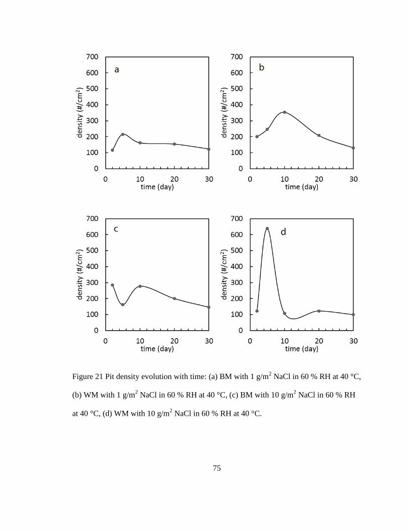
75

Figure 21 Pit density evolution with time: (a) BM with 1 g/m2 NaCl in 60 % RH at 40 °C,

(b) WM with 1 g/m2 NaCl in 60 % RH at 40 °C, (c) BM with 10 g/m

2 NaCl in 60 % RH

at 40 °C, (d) WM with 10 g/m2 NaCl in 60 % RH at 40 °C.

76

Figure 22 Pit density evolution with time: (a) BM with 1 g/m2 sea-salt in 15 % RH at

70 °C, (b) WM with 1 g/m2 sea-salt in 15 % RH at 70 °C, (c) BM with 10 g/m

2 sea-

salt15 % RH at 70 °C, (d) WM with 10 g/m2 sea-salt15 % RH at 70 °C.

77

3.2 The probability distribution of pit depth

Like section 5.6 in Chapter 3, Figure 23 displays the probability distribution of pit depth.

The figures support that the probability distribution follows the bi-model distribution, i.e.

an exponential distribution for shallower pits and a normal distribution for deeper pits.

78

Continued

Figure 23 CDF of the pit depth with exposure times: (a) BM with 1 g/m2 NaCl in 60 %

RH at 40 °C, (b) WM with 1 g/m2 NaCl in 60 % RH at 40 °C, (c) BM with 10 g/m

2 NaCl

in 60 % RH at 40 °C, (d) WM with 10 g/m2 NaCl in 60 % RH at 40 °C.

79


80

Continued

Figure 24 CDF of the pit depth with exposure times: (a) BM with 1 g/m2 sea-salt in 15 %

RH at 70 °C, (b) WM with 1 g/m2 sea-salt in 15 % RH, at 70 °C, (c) BM with 10 g/m

2

sea-salt15 % RH at 70 °C, (d) WM with 10 g/m2 sea-salt15 % RH at 70 °C.

81


82

3.3 Microstructure and microchemistry

Figure 25 is the pit geometry of the BM specimen exposed to 15 % RH at 70 ºC. Small

and concentrated pores are accumulated around the pit edge, which can be explained by

the cathodic reaction discussed in section 1 in Chapter 2, as well as the electrochemical

reactions shown in Figure 2. It is predictable that the size of the pit will outspread with

time throughout the electrochemical reaction.

Figure 26 is a STEM image of the TEM foil fabricated from the pit shown in Figure 25.

The pit cross-section, Pt coating, thinned matrix and the original matrix are marked to

distinguish the details of the foil.

Figure 27 and Figure 28 are the STEM images with the EDS line scan and area scan, as

well as the concentration profiles. In Figure 27b, at the pit interface the content of O

increases and the metal elements, including Fe, Ni and Cr, slightly decline. In Figure 28,

the area of the bottom of the pit (A) and the area of the matrix were measured, the

concentration profiles of which are displayed in Figure 28c. The content of O is high

inside of the pit and low in the matrix. Note that there is a considerable content of O at

area B, which is susceptible to be the oxygen diffusion after the breakdown of the passive

layer. Table 12 summarizes the compositions of area A and area B, as well as the matrix

before testing. The ratios of Fe to Ni of area A and B are smaller than that of the matrix

before testing, indicating that Fe diffused out of the material in the test. The ratios of Cr

to Ni of area A and B are larger than that of the matrix before testing, caused by the

decrease of Fe.

83

Figure 25 SEM images of the pit geometry of the BM specimen exposed to 15 % RH at

70 ºC.

Figure 26 STEM image of the cross-section of the pit.

84

Figure 27 (a) STEM image of the pit interface with an EDS line scan indicated with an

orange arrow. (b) Corresponding EDS concentration profiles of Ni, Cr, Fe and O

measured at the line.

Area A Area B The matrix

Atomic

percentage

(%)

Ratio

(/Ni)

Atomic

percentage

(%)

Ratio

(/Ni)

Atomic

percentage

(%)

Ratio

(/Ni)

O 23.10 - 15.21 - - -

Cr 16.12 2.53 17.74 2.47 18.86 2.26

Fe 54.41 8.54 59.87 8.34 72.79 8.72

Ni 6.37 1.00 7.18 1.00 8.35 1.00

Table 12 Compositions of O, Cr, Fe and Ni in the detected areas shown in Figure 28.

85

Figure 28 STEM dark field images of the pit with EDS mapping areas indicated with the

red boxes: (a) area A, (b) area B, and (c) comparison of element profiles of Ni, Fe, Cr and

O between the two areas.

86

4. Summary

To evaluate the pitting corrosion resistance of the investigated materials in humid

environments, a series of pitting corrosion tests specifically aimed at obtaining a measure

of the variability of the pits as a function of time, to complement the growth in the mean,

was undertaken. This test strictly simulates the actual environment (include temperature

and relative humidity) of a welded canister exposed to the marine coastal circumstance

with appropriate salt deposit, and therefore provides valid and reliable laboratory data for

evaluating the actual severity of pitting corrosion for canisters and characterizing the

metal surface in micro- and nano-scales.

Similar results as the tests in the chloride solutions have been obtained by testing in the

humid environment with salt particles deposit. A saturate salt particle moisture film was

made on the surface to electrochemically react with the metal matrix. WM once again is

evident to be less corrosion resistant than BM through observing larger pit density and pit

depth. Comparing the data obtained from these tests, it is concluded that the pitting

corrosion resistance is mainly affected by the chloride ion, and partially affected by

temperature. The results of the humid environment tests presented deeper pit depth.

Considering about the deliquescence of salt particles deposit, this phenomenon is

ascribed to the inhomogeneous distribution of deliquescent salt particles on the deposit

surface. For the long-term service canisters exposed to the marine coastal circumstance,

salt deposit on the canister surface is in the level of grams per meter square, making the

deliquescent salt moisture film saturated as well as inhomogeneous with chloride ions.

87

The pitting corrosion resistance in this condition generally will be less than that in

saturating solutions.

The next chapter, Chapter 5, predicts the evolution of pitting corrosion over time in the

methodology of Markov chain. The modeling provides the method to predict the pitting

corrosion states, density and depth based on the Markov chain corrosion model and

corrosion growth law. The simulating is fit with the laboratory measured data to verify its

reliability and flexibility.

88

Chapter 5: Markov model for pitting corrosion under relevant environmental conditions

1. Concept

This work applies the Markov chain method to simulate the evolution of pitting corrosion

with time, providing the simulating results of pitting corrosion states, pit density and the

frequency distribution of pit depth. According to Valor, et al. [124], the Markov model is

the best for predicting the future pit depth distributions. The statement is verified by the

reliability assessment based on different corrosion rate models through comparing the

different corrosion rate distribution applied to the modeling, including a single-value

corrosion rate based on the NACE recommendations for buried pipelines [125], a

distribution derived from the linear growth model, time-dependent and time-independent

distributions predicted from a soil corrosion model developed by Caleyo, et al. [126], and

a distribution derived from a Markov chain corrosion model [127]. The Markov model

has the best reliability assessment among all the available methods.

A Markov process is a stochastic process with no memory that would allow it to use past

information to modify the probabilities that follow. The process is founded on the views

of set theory, measure theory, the axiomatic definitions of probability and conditional

probability, random variables, and distribution functions. f is denoted as the conditional

density, Dt represents the state at time t. For any sequence of instants t1 < t2 < … < tn-1 <

89

tn ∈ T (n = 4, 5, …) and any possible observed values x1, x2, …, xn ∈ Ω (n = 3, 4, …), f

satisfies:

f(Dtn|Dtn−1Dtn−2…Dt1)(xn| xn−1xn−2…x1) = f(Dtn|Dtn−1)

(xn|xn−1)

In words, above equation signifies that the present state of the process makes its future

independent of the past.

If a sufficiently large area of the material used to manufacture the specimen was exposed

to the test environment for a particular exposure time, there would be a sufficient number

of pits such that the distribution of flaw sizes could be well characterized. This could be

inferred to be the “characteristic” distribution for those conditions at that time.

In practice, measurements are primarily based on laboratory tests which supply the

results of pit distribution in a relatively small total area. The pit distribution of specimens

exposed to brine solution and in the humid environment which have been discussed in

Chapter 3 and Chapter 4 can therefore be used as measured data to parameterize and

validate this model.

In essence, although the characteristic distribution can be sampled, the relatively small

area leads to inherent uncertainty in the extent to which the characteristic distribution is

adequately represented. This uncertainty can even be magnified when the population of

pits is sparse, which is likely for normal operating conditions with good control of water

chemistry or humid environment. For this reason, the approach adopted in this work will

90

undertake a simulation of the pit growth process, i.e. model experiments, and use the

measured data only to derive the unknown variables.

With preliminary fitting at one exposure time, the model reflects the tendency in the

experimental measurement and simulates the expected distribution of pit characteristics

for a particular area exposed to different test environments. The condition based on

deterministic equations with statistically distributed input parameters is also considered

for simulating the evolution of the frequency distribution of pit depth at different

exposure times.

2. Details of the model

This section describes the formulation of the model combined with the mechanism of

pitting corrosion. The Markov model includes the modeling of pitting corrosion state

transition that estimates the pit density for each state and pit depth state transition that

predicts the frequency distribution of pit depth with time. The model is implemented for

the SS exposed to chloride ion contained aggressive environment, for the cases of pitting

corrosion scenario.

2.1 Pitting corrosion states and sub-states

The modeling of pitting corrosion state transition involves ordinary differential equations

(ODEs) which are solved by a Markov chain approach to account for corrosion history

and environment dependent transition rates. Figure 29 shows the pitting corrosion state

91

transition diagram, states of which include the initial state (S), growth state (G), declining

state (D), repassivation state (R) and critical state (C).

Figure 29 A physics based multi-state transition model diagram. S: initial state. G:

growth state, D: declining state, R: repassivation state, C: critical state.

Initial state represents that the pit is not observable, and oxide layer well protects the

specimen from corrosion; growth state means that the pit is nucleated and metastable, the

size of which being above the level of detectability; declining state indicates that the pit

depth reduces over time because of the repassivation property of pitting corrosion;

repassivation state is when a metastable pit becomes sufficiently passivated; critical state

is that the pit reaches the stable size and keeps growing at a growth rate without declining

or repassivation.

Markov chain system is used to simulate the pitting corrosion states with time and further

obtain the estimated pit density at each state. The frequency distribution of pit depth

which illustrates the relation of pit depth and pit density can be simulated through the

92

known pit density at each state and the corresponding pit growth rates. Similar studies

have been undertaken by Valor, et al. [58, 59] and Caleyo [127].

This model considers the distribution of pit depth into sub-states. The pit growth state

represents the metastable pitting corrosion which has pit depth less than the critical depth.

A well-known characteristic of the pitting corrosion rates in addition to its time

dependence is that it also depends on the defect depth [128] and has a marked stochastic

character. This means that the mean value and variance of the corrosion rate distribution

undergo changes with the exposure time increasing [126, 129]. The frequency

distribution of pit depth of metastable pitting corrosion that is smaller than the critical

depth therefore is significant to consider.

The Markov chain process outlined in this work is based on the discretization of the

critical depth into N states of equal thickness, Th

Th =Critical Depth

N (E. 1)

The growth state of the physics based multi-state transition diagram can be discretized in

N sub-states Gi (i = 1, 2, …, N) and Dj (j = 1, 2, …, N-1) as shown in Figure 30. Figure

31 further illustrates this discretization in a material matrix.

A pit advances through the states as it grows. Gi(t) is the probability of a pit that is in

state i at global time t. G1 represents the nucleation; state GN represents the pit depth

exceeds the critical depth and becomes stable pitting corrosion. λi(t) is the state transition

rate for a pit advancing from state i to state (i+1). The metastable pit has a possibility to

93

be in the state of decline, which is each sub-state Gi has a transition rate m1i to be in state

D. To simplify, it is assumed that any m1i is equal to m1.

Similarly, a pit advances through the states Dj (j = 1, 2, …, N-1) as it declines. Dj(t) is

the probability of a pit that is in state j at global time t. γj(t) is the probabilistic transition

rate for a pit advancing from state j to state (j+1). D1 represents the decline pit at depth

Th(N-1), DN-1 represents the decline pit at depth Th.

Accordingly, state evolutions are described through the equations

dS(t)

dt= −f1(t)S(t),

dGi(t)

dt= −[λi(t) + m1(t)]Gi(t) + f1(t)S(t), i = 1

dGi(t)

dt= −[λi(t)+m1(t)]Gi(t) + λi−1(t)Gi−1(t), i = 2, 3, … , N

dDj(t)

dt= −γj(t)Dj(t) + m1(t)GN(t), j = 1

dDj(t)

dt= −γj(t)Dj(t) + γj−1(t)Dj−1(t) + m1(t)GN+1−j(t), j = 2, 3, … , N − 1

dR(t)

dt= m1(t)G1(t) + γN−1(t)DN−1 (t),

dC(t)

dt= λN(t)GN(t).

(E. 2)

The equations should be satisfied as:

S(t) +∑Gi(t)

N

i=1

+∑Dj(t)

N−1

j=1

+ R(t) + C(t) = 1

94

At start, S(t=0) = 1.

Figure 30 A physics based multi-state transition model diagram with sub-states Gi and Dj.

95

Figure 31 A diagram illustrates the pit depth states in a material matrix.

2.2 Transition rates

Note that the Markov chain architecture has been established, the method for parameter

determination, which is the expression of the state transition rates applied to the Markov

chain modeling, needs to be discussed.

Weibull distribution can be used to characterize the density function for transitioning

from the initial state without observable pits to the growth state with macroscopic pits.

The second Weibull distribution involves the characteristic time for a macroscopic pit to

become sufficiently passivated to start to decline. It can be used to characterize the

transition rate from the growth state with macroscopic pits to the declining state. The

transition rates f1(t) and m1(t) are accordingly defined as

96

f1(t) = (b1

τ1) (

u(t)

τ1)b1−1

(E. 3)

m1(t) = (b2

τ2) (

v(t)

τ2)b2−1

(E. 4)

where bi (i = 1, 2) is a Weibull shape parameter, and τi (i = 1, 2) is a Weibull scale

parameter, which has been observed to have both a chloride concentration and

temperature dependence. u(t) and v(t) separately represent the time for metastable pitting

corrosion, and the time for declining.

In essence, the time for metastable pitting corrosion and the time for declining are not

equal to global time. To simplify the simulating process, this model ignores the start time

for metastable pitting corrosion or declining. In words, the model unifies them to the

global time, that is u(t) = t and v(t) = t.

The transition rate λi(t) (i =1, 2, … N) is the expression of the general pit growth rate

through the pit growth law. The expression of a general pit growth rate governs the

accuracy of the prediction. The simplest case of pit growth rate is suggested by the

National Association of Corrosion Engineers (NACE) that empirical values for the

average corrosion rate according to the corrosiveness of the media [130]. When no data

for the pit growth rate is available, NACE recommends using a unique value for

corrosion rate of 0.4 mm/yr [125]. However, pit growth rates have little doubt to change

with the particular environment and time. It is widely accepted that the time dependence

of the characteristic dimension of a corrosion defect (depth) follows a power function in

the form

97

Grow(t) = α(t − tini)ν

where α and υ are empirical parameters and tini is the time at which the corrosion process

begins [128, 129, 131]. Power-type time dependence of defect growth leads to a different

corrosion rate distribution than that of the linear growth rate, being more reliable and

convincing. The pit growth law used on this work is

Grow(t) = a(t)(t − u)b(t) (E. 5)

where a(t) and b(t) are time-dependent parameters account for dynamic environmental

changes and pitting corrosion states, u is the initiation time.

(E.2) yields that λi is in the unit of state

time, then it can be deduced λi =

dG

dt

G i. Bringing (E. 5)

into this expression yields

λi(t; u) = [b(t)

t−u+a′(t)

a(t)+ b′(t) ln(t − u)] i (E. 6)

When state thickness N is large enough, Th will be small enough to justify the

approximation G(t; u) ≈ iTh. Substituting the approximation into (E. 6) yields

λi(t) = [b(t) (a(t)

iTh)

1

b(t)+a′(t)

a(t)+b′(t)

b(t)ln (

iTh

a(t))] i (E. 7)

The substitution differentiates local pit time (t-u) from global time t by emphasizing the

time that the pit belongs to the state through the variable for state i instead of through the

variable for time t.

98

Effectively, if a metastable pit can avoid becoming sufficiently passivated such that its

size begins to decline before it reaches the stable size, it transitions to stable. If we look at

the final stage of growth before becoming stable, the characteristic rate of transition to

stable is the growth rate over the delta depth and the transition rate to a declining state is

λN.

Similar to λi, the transition rates γj (j = 1, 2,…, N-1) can be expressed by

γj(t) = [d(t) (c(t)

jTh)

1

d(t)+c′(t)

c(t)+d′(t)

d(t)ln (

jTh

c(t))] j (E. 8)

where c(t) and d(t) are also time-dependent parameters account for dynamic

environmental changes and pitting corrosion states. γN−1 is a rate of decline to get from

the declining state (D) back to a size below the level of detectability (R).

Note that the pits in the critical state also follow the pit growth law.

2.3 Pit density

States Gi (i = 1, 2, …, N), Dj (j = 1, 2, …, N-1) and C represent the probability when pits

are detectable. The sum of the states multiplies the number of potential maximum pitting

locations (M) of a specimen will obtain the pit density (PD). The equation is

∑ Gi(t)Ni=1 + ∑ Dj(t)

N−1j=1 + C(t) × M = PD(t) (E. 9)

The potential maximum pitting locations M of a specimen depend on the specimen’s

compositions and corrosion-resistance. For SSs, the locations usually occur on the MnS

99

inclusions, and M does not exceed the number of MnS inclusions. According to Schmuki,

et al. [132], the MnS inclusion density is about 500-600 per 100 μm2, therefore, the max

pit number should not be above 6 × 106 per cm2. For more specific situations, like the

tests on Chapter 3 and Chapter 4, which obtained the results of pit diameter, M can be

estimated as the consequence of the unit area to the averaged pit area, making the

estimation of M more close to the actual.

By fitting with the measured pit density at test times, PD(t) can be optimized through

optimizing the results of G(t), D(t) and C(t) which is to optimize the parameters for state

transition rates.

100

Variable Equation usage Description

t various Global time

Th (E. 1) Depth per state

S(t), Gi(t), Di(t), R(t), C(t) (E. 2) The probability of being in the

states of pitting corrosion

fi(t) (i = 1, 2), mi(t) (i = 1, 2) (E. 3)(E. 4)

Transition rates of the Markov

system representing the transition

of one pitting corrosion state to

the next

bi (i = 1, 2) (E. 3)(E. 4) Weibull shape parameters for the

transition rates

τi (i = 1, 2) (E. 3)(E. 4) Weibull scale parameters for the

transition rates

Grow(t;u) (E. 5) Pit growth law; depth at time t of

a pit initiated at time u

λi (E. 6)(E. 7) Probabilistic growth rate from Gi

to Gi+1

γj (E. 8) Probabilistic declining rate from

Di to Di+1

N Constant The number of states of depth

M Constant

The potential pit density of the

specimen in the exposed

environment

PD(t) (E. 8) Pit density at time t

Table 13 Summary of the variables and parameters derived within section 2.

101

3. Case studies

In this section, two cases were studied to demonstrate the reliability and flexibility of the

proposed model.

Case 1: BM in 6.25 M Chloride ion NaCl solution at 40 °C

The laboratory test of BM exposed to 6.25 M chloride NaCl solution at 40 °C has been

discussed in Chapter 3, the results of which are displayed in section 3.5. Table 14

presents the primary results used on this modeling, including the measured pit density

and pit diameter with exposure times. The estimated number of maximum pit occurrence

locations is 3.10 × 105 per cm2 as

108μm2/cm2

π(25.43 + 29.84 + 26.78 + 20.96 + 31/53)2

4 (μm2/pit)= 1.76 × 105 pits/cm2

Other input parameters for this modeling are shown in Table 15. Note that the parameters

a, b, c and d are assumed to be the time constants, that is to take on a constant transition

value for each pit depth level. The comparison of the measured pit density in 30 days and

simulated pit density in 3 years is shown in Figure 32, indicating a proper optimization.

The result illustrated in Figure 33 displays the simulated behavior for the general body of

knowledge about pitting corrosion states. Figure 34 compares the simulated frequency

distribution of pit depth with the laboratory measured data, which are well consistent.

Figure 35 shows the results of the frequency distribution of pit depth in the long-term (3

years). The number of metastable pits reduces while stable pits keep growing over time.

102

Specifically, the pit density instantly increases to a significant value in the early days

while drops to an extremely low value in three months; after that, the pit density slowly

increases to a relatively stable value (Figure 32b). SSs are expected to have a number of

metastable pits at the start of the investigated corrosive environment, while part of them

transfer to stable pits over time, and part of them repassivate. Several authors have

attempted to characterize pit initiation and also establish the requirements necessary for

the transition from metastable to stable pitting in SSs. Important work was done by

Williams et al. [133, 134], who evaluated the rate of stable pitting Λ by the following

equation:

Λ = aλ exp(−μτc)

where a is the electrode area (cm2), λ is the nucleation frequency (s

-1cm

-2), μ is the

repassivation probability (s-1

), and τc is the induction time for stable propagation (s). This

relationship asserts that the rate of stable pit generation directly depends on the

metastable pitting rate and the probability that the metastable pits survive to become

stable. Because of this relation, it is therefore reasonable to study metastable pits, which

are more frequent and easier to observe than stable pits, and necessary to determine when

they transfer to stable pits. The authors also proposed that, from these parameters, the

expected number of pits, n, and the probability of having no stable pits, P(0), can be

determined as a function of time (t > τc) by

n = λa(t − τc) exp(−μτc) = Λ(t − τc)

and

103

ln[P(0)] = −λa(t − τc) exp(−μτc) = −Λ(t − τc)

Therefore, the expectation that the pit density will decrease and stays at a relatively stable

number is logically based on the previous studies. The next case, case 2, which has

laboratory measured data both in the early one month and much longer times, also

supports this prediction.

Time (day) Pit density (#/cm2) Pit diameter (μm)

2 476.9 25.43

5 761.54 29.84

10 692.31 26.78

20 384.62 20.96

30 361.54 31.53

Table 14 Measured data of exposure times with pit density and diameter for the data set.

104

Model input

parameter Value

M 1.76 × 105

b1 0.23

τ1 1 × 109

b2 0.7

τ2 5

a 1.2

b 0.3

c 0.5

d 0.3

Critical depth 5

N 10

Th 0.5

Table 15 Input parameters for case 1.

Figure 32 Comparison of optimized result and measured data of pit density in (a) short

term, and (b) long term.

105

Figure 33 Modeling results of the pitting corrosion states with time.

106


data, (b) simulation.

107

Figure 35 Simulation results of frequency distribution of pit depth.

Case 2: SS316L exposed to 1.12 M chloride sea-salt solution at 72 °C

To demonstrate the flexibility of the proposed model, it applies the data set of Type 316L

SS specimens exposed to 1.12 M chloride sea-salt solution at 72 °C provided by Xin, et

al. [106]. The measured data is displayed in Figure 9 in the publication; re-displayed here

in Figure 36. We also conducted the same tests as Xin’s at times of 2, 10, 20 and 30 days,

which is to obtain the measured data of pit characteristics in the early exposure time.

Both of ours and Xin’s results are summarized in Table 16. The input parameters for

simulating are shown in Table 17.

108

The simulating results (Figure 37- Figure 39) are well fit with the measured data,

verifying the flexibility of this model. The laboratory test results suggest that the pit

density largely increases up to 1700 per cm2 in the early exposure time and then drop to

about 200 per cm2 at a relatively stable level in the long term. This data demonstrates the

prediction in the case 1 that the number of pits will be relatively flat over time.

Figure 36 Pit density with depth of SS316L specimens at various exposure times exposed

to 1.12 M chloride sea-salt solution at 72 °C [106].

109

Time (day) Pit density (/cm2)

2 1761.5

10 1700.0

20 1046.2

30 961.5

133 90.5 [106]

223 177.3 [106]

282 117.5 [106]

366 164.8 [106]

Table 16 Exposure times with mean maximum pit depth and standard deviation for the

data set (some data come from the reference [106]).

Model input

parameter Value

M 1.20 × 105

b1 0.15

τ1 1 × 109

b2 0.8

τ2 7

a 2.5

b 0.4

c 0.5

d 0.3

Critical depth 10

N 10

Th 1

Table 17 Input parameters for case 2.

110

Figure 37 Comparison of optimized result and measured data of pit density.

Figure 38 Modeling results of the pitting corrosion states with time.

111


data (b) simulation.

112

4. Summary

In this chapter, a Markov chain model for predicting the pitting corrosion evolution has

been developed and validated by experimental pitting corrosion data.

Based on the reliability assessment by Valor, et al. [124], Markov model is the most

reliable model for predicting the long-term pitting behaviors. The concept of Markov

chain, as well as the pitting corrosion mechanism, was involved in this model to predict

the pitting corrosion states, density and depth. ODEs with state transition rates were

mathematically solved for the corrosion states. Through ascribing the pit depth in sub-

states and applying the corrosion growth law, the frequency distribution of pit depth was

achieved. Weibull distribution was used to characterize the density function for

transitioning from one state to the other. The general pit growth rate was also used to

characterize the density function for transitioning from one depth to the other in the sub-

states.

The experimental pitting corrosion data was well fit in the model for input parameters.

The model further estimated the pitting corrosion in the long-term exposure, through

comparing with the known long-term exposure laboratory corrosion data. With

preliminary fitting at one exposure time, the model reflects the tendency in the

experimental measurement and predicts the expected distribution of pit characteristics for

a particular area exposed to different test environments.

113

The next chapter, Chapter 6, describes the methodology and results of CISCC of SSs

exposed in the humid environment. It compares the CISCC rates of BM and WM and

characterizes the microstructure.

114

Chapter 6: Stress Corrosion Cracking of SSs in Humid Environments

1. Introduction

The objective of this test is to evaluate the CISCC susceptibility of Type 304L BM and

its WM, establish quantitative measurements of crack growth rates and determine

relationships among cracking susceptibility, environmental conditions, and metallurgical

characteristics. SCC crack growth rates have been identified for a BM specimen and a

WM specimen in the simulated marine coastal environment. In both cases, the crack

extension was monitored in situ by direct current potential drop (DCPD) with length

resolution of about ± 1 μm making it possible to measure extremely low growth rates

approaching 10-11

m/s. Extensive characterizations have been performed on material

microstructures and stress-corrosion cracks by micro-characteristics imaging and

analytical facilities and linked to crack growth test results to help define physical and

environmental parameters controlling SCC susceptibility.

Establishing the necessary conditions for a pit to transfer to a fatigue crack is essential for

lifetime prediction. The recognized criteria for this transition consist of two parts, both of

which are considered to be necessary for the onset of cracking. First, the pit must grow to

a critical size, causing the stress intensity factor to equal the threshold value. This critical

size varies depending on the loading, i.e. a smaller pit leads to cracking under higher

115

stress levels. Second, the crack growth rate must exceed the pit growth rate. When the

requirements are met, a fracture mechanics approach can be utilized for determining the

time to failure.

All levels of damage may result in a significant reduction in SCC life: pit depths as

shallow as 20 um can initiate cracks; however, the deepest pits do not always instigate the

cracks. In addition to depth, pit surface area, size, shape, and proximity to other pits are

also determined to be critical factors in when and where a crack develops.

2. Specimen preparation

The tests used standard 0.5-inch thickness compact tension (CT) specimens with side

grooves. The composition of elements of the CT specimens is shown in Table 2b, the

same as the coupon specimens. The dimensional tolerances and the surface finishes

shown in Figure 40 were followed in the specimen preparation. Care was taken in

machining to prevent contamination of specimen and notch surfaces that were difficult or

impossible to clean. The copper deposit left by electric discharge machining (EDM) with

a copper electrode was cleaned with DI water, acetone, and sandpaper polishing.

According to the material certification of the BM, the yield strength (σγs) is 207 MPa,

and the ultimate tensile stress (σTS) is 517 MPa.

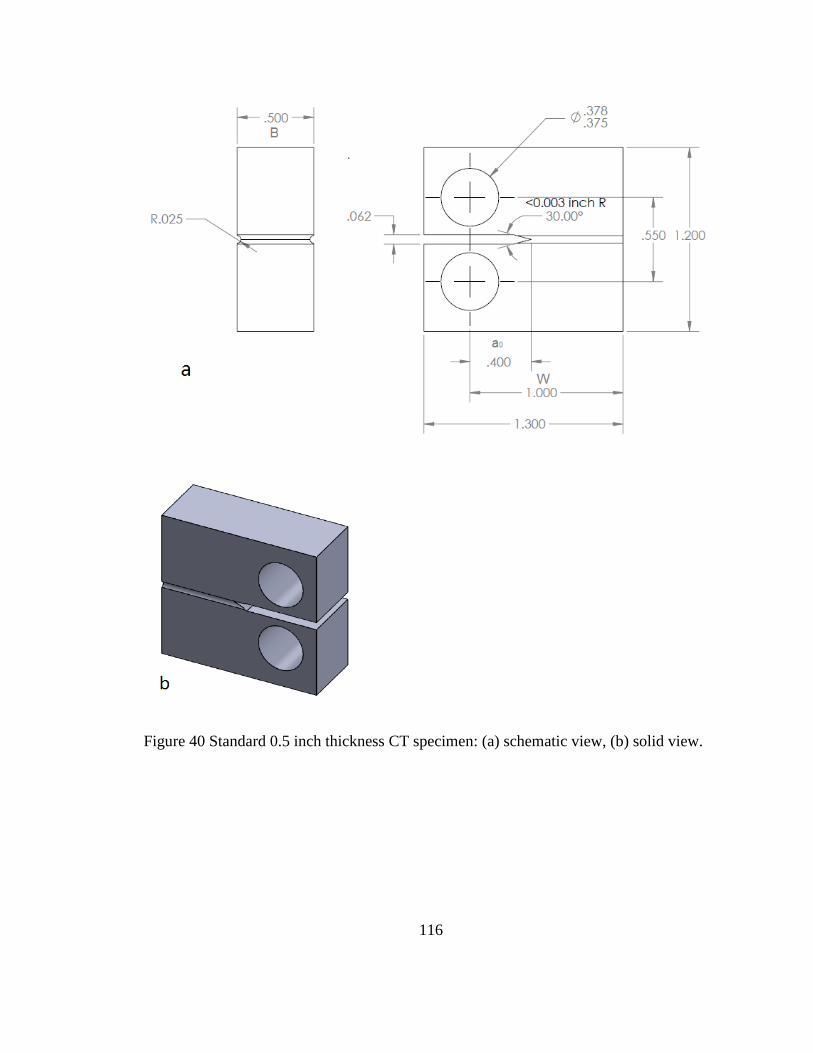
116

Figure 40 Standard 0.5 inch thickness CT specimen: (a) schematic view, (b) solid view.

117

3. SCC crack growth test system

During my Ph.D. study, a SCC crack growth test system working at high temperature (up

to 360 ºC) and high pressure (up to 2200 psi or 15.2 MPa) with the function of flow

chemistry controlling and in situ crack growth rate measurement has been fabricated.

Figure 41 illustrates the components and structures of the system. The details of the

system can be found in the transaction [135]. Features expected in a good crack growth

system include active constant K load control, active temperature control, a sensitive

crack length measurement apparatus, a recirculating high-temperature water system,

control over all aspects of water chemistry, and continuous monitoring of all pertinent

test parameters [136]. Understanding the expected features, this crack growth system is

purposely developed to control and measure stress corrosion cracks under the well-

defined material and environmental conditions, and ensure that the SCC growth rate

response is reproducible in the test conditions.

The SCC tests of the specimens exposed to humid environments were undertaken in the

autoclave of this system. To better conduct the tests in humid conditions rather than fluid

flow, the SCC test system was modified and fabricated to supply a humid environment

with the functions of real-time monitoring and controlling the applied loading, crack

growth rate of specimens and test temperatures. The digital control workstation has full

computer interface capabilities.

The specimen was tested in the 4-liter Type 316 austenitic SS-made autoclave using the

5000 lb.-loading frame with 0-5 Hz controllable frequency which accelerates the cracking

118

propagation. The inner structure of the autoclave is shown in Figure 42. The specimens

crack growth rate (CGR) can be measured through direct current potential drop (DCPD)

technique at 10-11

m accuracy (see DCPD setup at Figure 43). The wrapping heating

mantle heated the autoclave, and the high precision proportional-integral-derivative (PID)

temperature controller controls the temperature.

Figure 41 Picture of the SCC test system (located in W396 Scott Lab, OSU).

119

Figure 42 Schematic diagram of autoclave inner structure setup (not scaled).

Figure 43 Schematic diagram of DCPD test system setup.

4. Test procedure

120

The test procedures strictly followed the standard test method ASTM E1681-03 (2013)

[137], which is for determining threshold stress intensity factor for environment-assisted

cracking of metallic materials, and the standard test method ASTM E647 -13a (2014)

[138], which is for measurement of crack growth rates.

Before loading a specimen in the autoclave, the sample thickness B, notch depth a0, and

the distance from the center of holes to the back side of the specimen W (see Figure 40a)

are all measured and recorded into the data record. Using the sample dimension and the

strength of the specimen at the test temperature, in accordance with ASTM E-1681 [137],

an upper limit on stress intensity factor threshold for environmental assisted cracking

(KEAC) value was calculated using the formula

minB,W − a, a ≥4

π(KEAC

σγ)2

(E. 9)

where σγ is the effective yield strength at the test temperature, and a represents the length

of crack (include the notch depth a0),

σγ =σγs+σTS

2 (E. 10)

σγs is the yield strength, σTS is the ultimate tensile strength. minB,W − a, a is the

smaller of the specimen thickness, the remaining uncracked specimen width, and the

crack length. After the specimen dimensions were measured and spot-weld locations

were marked on the sample, it was cleaned and installed on the inner structure of the

autoclave.

121

The specimen was fixed on the loading frame of the system for fatigue pre-cracking in

the room environment before testing in the humid environment. The importance of pre-

cracking is to provide a sharpened fatigue crack of adequate size and straightness which

ensures that 1) the effect of the machined starter notch is removed from the specimen K-

calibration, and 2) the effects on subsequent crack growth rate data caused by changing

crack front shape or pre-crack load history are eliminated. The fatigue pre-crack is

allowed to extend to a depth of from 1.3 mm to 3.8 mm.

The first step in pre-cracking was to cycle the specimen at a relatively high frequency

(1.5-2 Hz in the test) with a small load ratio (R = 0.3 in the test) and maximum stress

intensity factor (Kmax) less than the K level chosen for constant K. As the crack began to

grow from the notch, the frequency was reduced while the load ratio R and applied

maximum stress intensity factor Kmax were increased. By pre-cracking in this way, each

pre-crack segment can grow beyond the plastic zone created by the previous segment.

The increment of the final 1 mm fatigue pre-crack was conducted at a Kmax value of not

more than 60% of the expected KEAC. The direction of cracking was parallel to the groove,

within the angle of ± 10°.

After pre-cracking, the specimen was un-installed on the loading frame of the system and

immersed in the saturated sea-salt solution at room temperature for 10-15 hours. Then the

specimen was dried in compressed air to make the sea-salt deposit on the specimen

surface as well as thoroughly cover the crack-tip region.

122

The specimen was re-installed on the loading frame of the system. A small beaker with

DI water of measured weight was placed in the autoclave. The autoclave was closed with

eight hex screws to prevent from leaking. It was heated to the expected temperature. Note

that with some environment-material combinations, preconditioning of the specimen in

the investigated environment prior to force or displacement application will greatly

influence the resulting KEAC values. Considering the effects of preconditioning, the

specimen was immediately exposed to the test environment (i.e. humid environment at

the expected temperature) for 8 hours before applying loading. The test ensured that

proper humidity was in the autoclave, and the crack-tip region of the specimen stayed in

the corrosive environment at all times. Seals between the autoclave and the specimen

were regularly inspected for leakage.

Crack transitioning steps were carefully selected to grow the crack in the humid

environment using the following stages: (1) fatigue, (2) corrosion fatigue and (3) SCC.

This means producing cracks of about 1 mm by cycling in-situ before transitioning to

slow cyclic loading plus hold times to promote SCC. Cyclic loading steps at frequencies

of 0.1 Hz down to 0.001 Hz were performed in the humid environment. The final phase

involved crack transitioning by very slow cycling. This grew the crack beyond the pre-

cracking plastic zone and allowed the crack to transition from transgranular (TG) fatigue

to the crack growth mechanism that occurs for that material under constant K conditions.

Details about the test steps are shown in the tables of the next section.

123

After the SCC test, the specimens were rinsed with ultrapure water, cleaned by ultrasonic

with analytical acetone, and then dried by ethanol of analytical grade. The crack surface

of each specimen was mechanically abraded and SiC diamond polished to 1 μm. The

polished surface was further examined under SEM/FIB, and the TEM foil with the cross-

section of the crack was prepared by FIB.


Table 18 and Table 19 separately display the test steps for BM and WM exposed to 15 %

RH at 70 ºC. The BM was applied the stress intensity factor of 9 MPa√m for crack

propagation, while the WM was applied the lower stress intensity factor of 7 MPa√m,

due to the yield strength was reduced after welding. The determination of the K values

was according to (E. 9)(E. 10). Though the WM was applied lower stress, its crack

growth rate was much higher than the BM at the same test phase, which can be obtained

through comparing Figure 44 and Figure 45. This indicates that the welding process

largely depressed the resistance to SCC.

124


testing of BM at 9 MPa√m exposed to 15 % RH at 70 °C. The specimen was immersed in

the saturated sea-salt solution at room temperature (RT) and dried in air.

Test

phase

Duration

(hour)R

Frequency

(Hz)Hold (hour) Humidity

Temperatu

re (°C)

Kmax

(MPa√m)CGR (m/s)

Crack

increment

(mm)1 1 0.3 2 0 air RT 7 7.06E-08 0.254

2 0.38 0.3 2 0 air RT 9 7.37E-07 1.016

3 0.18 0.5 2 0 air RT 9 1.66E-06 1.0922

4 22.5 0.7 0.1 0 15% 70 9 3.45E-09 0.2794

5 81.83 0.7 0.01 0 15% 70 9 9.48E-10 0.2794

6 86.5 0.7 0.001 0 15% 70 9 1.63E-10 0.0508

7 148.28 0.7 0.001 0 15% 70 9 4.76E-11 0.0254

8 170.72 0.7 0.001 0 15% 70 9 - -

9 24.83 0.7 0.001 0 15% 70 9.5 2.84E-10 0.0254

10 73.5 NA NA NA 15% 70 9 9.60E-11 0.0254

11 70.5 NA NA NA 15% 70 9 2.00E-10 0.0508

125


testing of WM at 7 MPa√m exposed to 15 % RH air at 70 °C. The specimen was

immersed in the saturated sea-salt solution at room temperature (RT) and dried in air.

Test phaseDuration

(hour)R

Frequency

(Hz)Hold (hour) Humidity

Temperatu

re (°C)

Kmax

(MPa√m)CGR (m/s)

Crack

increment

(mm)1 2.33 0.3 1.5 0 air RT 5 2.12E-08 0.1778

2 1.17 0.3 2 0 air RT 5 1.21E-07 0.508

3 0.42 0.3 2 0 air RT 7 6.77E-07 1.016

4 0.33 0.5 2 0 air RT 7 3.60E-07 0.4318

5 1.33 0.7 0.1 0 15% 70 7 5.29E-08 0.254

6 87.5 0.7 0.01 0 15% 70 7 2.42E-10 0.0762

7 107 0.7 0.001 0 15% 70 7 6.59E-11 0.0254

8 62 0.7 0.001 0 15% 70 7 - -

9 5.17 0.7 0.001 0 15% 70 7.5 1.37E-09 0.0254

10 66.5 0.7 0.001 0 15% 70 7 2.12E-10 0.0508

11 48 NA NA NA 15% 70 7 2.94E-10 0.0508

126

Figure 44 Crack length with time of the SCC propagation testing of the BM specimen at

the stress intensity factor of 9 MPa√m exposed to 15 % RH air at 70 °C.

Figure 45 Crack length with time of the SCC propagation testing of the WM specimen at

the stress intensity factor of 8 MPa√m exposed to 15 % RH air at 70 °C.

127

Figure 46 Comparison of crack growth rate of the BM and the WM specimens.

6. Microstructure and microchemistry

The micro-characteristics of the CT specimens were analyzed under SEM/FIB and

STEM-EDS. This section shows the results of the WM-made CT specimen (section 6.1)

and the BM-made CT specimen (section 6.2) exposed to 15 % RH air at 70 °C.

6.1 WM-made CT specimen

Figure 47 displays the main steps of making a TEM foil. Figure 47a is a SEM image,

showing the overview of the cracking from notch (bottom) to the tip (top). Figure 47b is a

zoom-in image indicating the tip of the crack. A mark is made by the Pt deposit to

128

illustrate the location of making a TEM foil. Figure 47c shows an etched foil ready to be

picked up. Figure 47d is a complete TEM foil attached to a TEM grid.

Figure 48 shows a STEM image in dark field mode of the cross-section of the crack. A

red box is marked to present the location of EDS mapping. The crack interface is distinct;

however, the crack is contaminated by redeposition. When making a TEM foil in the FIB

chamber, while most of the sputtered material is rapidly pumped away into the vacuum

system, some sputtered atoms may redeposit onto the freshly milled walls of the

specimen. The atoms from the specimen matrix and the Pt deposit, as well as the Ga+ ion

beam (Ga+ ion beam is used to hit the sample surface and sputter a small amount of

material), may therefore be deposited onto an adjacent region. Although redeposition is

impossible to be eliminated, it has been significantly reduced by using low accelerating

voltages in our case. Redeposition does not significantly affect the integrity of chemical

analysis since the metal elements, such as Fe and Cr, do not redeposit in the crack.

Figure 49 shows a STEM image of the specimen in dark field mode (Figure 49a) and the

elemental maps (Figure 49b- 49g). The redeposition of Pt layer caused by ion beam

trenching is in the crack (Figure 49b). Slight of C and O are in the crack. Oxide particles

are formed in the branch of the crack, and an oxygen diffusion layer is distinct (Figure

49g).

The sea-salt elements, Mg and Cl, are detected in the crack (Figure 50), being an

evidence of the deliquescence of the salt deposit. Similar to the micro-characteristics of

129

the pit (in Chapter 3 & 4), there is a little metal element in the crack and a manifest

amount of salt species.

Figure 51 is the EDS concentration profiles of elements (Pt, C, Si, Cu, Ni, Fe, Cr and O)

measured at the six spots (Spot 1, 2, … 6) shown in Figure 49a. Spot 1 and 2 are in the

matrix. Since the content of Cr and C of spot 2 is higher, and the content of Fe and Ni is

lower than spot 1, spot 2 is susceptible to be the secondary phase, Cr-C precipitations

(note that the specimen is made of WM). The region of the secondary phase is

distinguished in Figure 49d and Figure 49f by the dashed lines.

Spot 3 and 4 are in the crack. There is an extremely low content of metal elements, and

an amount of redeposition, including Pt.

Spot 5 and 6 are also in the crack. Both of them have an acknowledgeable amount of O

and Si. Spot 5 also has significant C. The content of Si and C in the material is trivial. Si

and C are susceptible to be the contamination caused by the SiC diamond polishing. The

polishing was made before preparing the TEM foil, as described in section 4.

Figure 52 is the concentration profiles of C, Fe, Cr, Ni and O measured by the EDS line

scan at the crack interface. The content of O is relatively stable throughout the line,

indicating the oxygen diffusion layer at the interface.

130

Figure 47 TEM foil preparation of the WM-made CT specimen exposed to 15 % RH air

at 70 °C. (a) Overview of the cracking from notch (bottom) to the tip (top), (b) the tip of

cracking with a Pt layer (mark), (c) foil has been etched, and (d) the TEM foil is attached

to a TEM grid.

131

Figure 48 STEM dark field image of the cross-section of the crack with an STEM-EDS

mapping area indicated by a red box.

132

Continued

Figure 49 (a) STEM dark field image. Elemental maps of (b) Pt, (c) C, (d) Cr, (e) Fe, (f)

Ni, and (g) O.

133

Figure 49 continued

Figure 50 STEM-EDS elemental maps of (a) Mg, and (b) Cl.

134

Continued

Figure 51 STEM-EDS concentration profiles (atomic normalized) measured at the spots

in Figure 49a.

135

Figure 51 continued

Figure 52 Corresponding STEM-EDS concentration profiles of C, Cr, Fe, Ni and O

measured at the line in Figure 49a.

136

6.2 BM-made CT specimen

The steps of making a TEM foil is the same as described in section 6.1. The TEM foil is

also made at the tip of the crack.

Figure 53 is a STEM image in dark field mode of the crack interface between the matrix

and the crack. Note that a 200 nm-thick redeposition layer was made by the ion beam

trenching process and accumulated on the edge of the crack. Ga (Figure 53d) represents

the region of redeposition. Besides, a 40 nm-thick oxygen diffusion layer is measured

(Figure 53b).

To better illustrate the element profiles at the crack interface, the STEM-EDS line scan

was conducted on the line in Figure 53a. Accordingly, Figure 54 is the EDS

concentration profiles of O, Cr, Fe, Ni and Ga. Between the distance 200 nm and 240 nm,

a peak of O is distinct. The content of Fe, Ni and Cr drops.

Besides, the other location with a little redeposition on the TEM foil was also analyzed,

shown in Figure 55. At this location, the redeposition does not affect the integrity of

chemical analysis. The EDS mapping was measured at the crack interface.

Figure 56 displays the EDS elemental maps of O, Fe and Ga. There is a little Ga (Figure

56d). Similar to Figure 53b, the oxygen diffusion layer is also found at the interface, and

the thickness is about 50 nm.

137

Figure 53 (a) STEM dark field image with an STEM-EDS line scan indicated with a red

line. EDS elemental maps of (b) O, (c) Fe, and (d) Ga.

138

Figure 54 Corresponding EDS concentration profiles of O, Cr, Fe, Ni and Ga measured at

the line of Figure 53a.

Figure 55 STEM dark field image of the cross-section of the tip of crack with a STEM-

EDS mapping area indicated with a red box.

139

Figure 56 EDS elemental maps of the area in Figure 55. (a) STEM dark field image, (b)

O, (c) Fe, (d) Ga.

140

Chapter 7: Conclusions and Recommendations for Future Work

Chapter 7 contains the summary of the entire study and results, conclusions drawn from

the studies, the overview of the contribution of the research to the state-of-the-art, the

discussion of limitations of the study and the suggestion about areas research that could

be extended beyond those described in this dissertation.

1. Conclusion and significance

The study has developed tools for evaluating the potential occurrence of SCC on UNF

storage welded SS canisters and evaluating pitting corrosion and SCC penetration rates

through the wall of the canister. This has been done using the integrated approach:

identified the corrosion potential, passive current, pitting potential range, passivation

layer impedance; evaluated the pit density and depth in the highly concentrated chloride

ion solutions; parallel evaluated the pit density and depth in the salt particles deposit

humid environment; measured SCC growth under relevant environmental conditions;

concurrently parameterized and validated a Markov model for pitting corrosion.

The welding process depresses the corrosion resistance of metal matrix under the

investigated environments, evident by the heterogeneously distributed elements, the

declined corrosion potential, the increased anodic passive current density and the

narrowed passive zone. The WM is detected to be less pitting corrosion resistant than the

141

BM when exposed to the same aggressive environment, including the highly concentrated

chloride ion solutions and salt particles deposit humid environment. The SCC

propagation rate of WM is also much higher than the BM even when applied by lower

stress intensity factor, indicating the welding process depresses the SCC resistance.

The phenomenon of metastable pitting is manifested for the tests undertaken, in particular

for the early exposure times. After metastable pitting, some of the metastable pits are

sufficiently large to be stable in growth; some of them re-passivate and become non-

visible.

Both the chloride ion concentration and the temperature influence the pitting corrosion

resistance. Under the investigated environment, the chloride ion concentration of 6.25 M

makes the higher pit density and the deeper pit depth on the specimens compared with the

one of 1.5 M. Temperatures of 40 °C and 70 °C show small differences in the pitting

corrosion resistance.

For the near-saturate chloride ion environment, the specimens exposed to the

deliquescent moisture film are less corrosion resistant than those immersed in the solution.

Deliquescent salt is not as homogenous as the salt dissolved in the solution; it is

unavoidable that in the microscale, part of the exposure surface has more salt ions

concentrated when deliquescent while the other part has less. A microscale galvanic

corrosion cell could be formed between the anode (higher salt concentration) and the

cathode (lower salt concentration), resulting in the higher pitting corrosion rate and larger

pit in the anode. Considering the environment of coastal and lake/river-side region, the

142

findings of the pitting corrosion in humid environments provide better forecasting on

actual in-service canisters.

Both the pits and crack tips of SCC are void of metal elements, while salt elements, such

as Mg and Cl, are susceptible to form a non-dissolvable compound. Oxygen is

concentrated around the region of pits and crack tips, and oxide diffusion layer is in

micro-scale.

A Markov model for predicting the pitting corrosion evolution has been developed and

validated using experimental pitting corrosion data. The simulating results are well fit

with the measured data of different conditions, verifying the flexibility of this model. The

use of a continuous-time linear growth Markov process is particularly attractive. This

supports the idea that the transition rates in the Markov process are closely related to the

pitting damage rate. Simplifications are made to improve computation speeds. The

predictive model can be further developed based on this Markov model and used to serve

for defining timelines of concern for SCC and guide inspection intervals during service.

One of the advantages of the Markov chain approach over deterministic and other

stochastic models for pitting corrosion is that the Markov chain model can capture the

dependence of the pitting rate on the pit depth and lifetime. It allows for an estimation of

not only the probability distribution of the pitting rate associated with the entire pit

population but also such a distribution for a subpopulation within specific lifetime and

depth ranges, in other works, it obtains not only the expected pit depth with time as a

function of environment but also the frequency distribution of pit depth and pit density.

143

Based on the preceding discussion, a successful methodology for assessing the likelihood

of SCC on simulated UNF canister materials has been developed well to understand the

problem of SCC on UNF canisters. It includes a coordinated approach of laboratory-scale

data collection, field deployable testing and measurement systems, and Markov modeling.

Since the safety performance of long-term interim storage is major concerned in the

nuclear industry, this work provides a technical basis for evaluating a technical issue

facing the industry.

2. Technical challenges

The shortage of observations on in-service canisters is apparent by reviewing the

available studies of SCC of UNF canisters. Existing experimental data do not

comprehensively consider the in-service canister temperatures or RH, or the salts and

other contaminants on the canister surface. The residual stress data obtained thus far is

only one indicator but not the consideration of the difference between assumed and actual

conditions. The measurements of residual tensile stress in the in-service canisters are not

available because of the difficulties in installing measurement tools and limit installation

space. The un-replicate welding process is another issue that makes the residual tensile

stress different for each canister.

The problem of SCC in SSs has been researched for many years, and there is massive

amount data about material characteristics. However, the applicable data for in-service

canister conditions is very scarce, and uncertainty-quantified data on environmental

conditions is even less. Although our study has explored a new direction to understanding

144

the mechanism of SCC of canister materials combined with coastal environments, it has

limited influence for evaluating a critical regulatory and technical issue facing the nuclear

industry. This is due to the amount of test specimens, the specimen area, and the variance

of canister materials in residual stresses. The results are not comprehensively

representative for the in-service canisters.

Our experiment system is not perfect for simulating the actual coastal environment

referring to the temperature, RH and salt deposit. These parameters are flexible and

varied over time, instead of fixed values. In spite of the difficulties associated with

obtaining near real-time data, modifying the experiment system and adjusting the

parameters to the actual environment will make the results closer to the actual.

The modeling analysis does not involve the in-service conditions of coastal environment

vary or the residual stresses. Uncertainties in data coupled with conservative assumptions

limit the usefulness of the model. In spite of the supplied laboratory data, obtaining near

real-time data will make extremely generous benefits.

Some simplifications for the model are offered. To ensure the accuracy of the

simplifications, the results of simulating have been compared with the experimentally

measured data. However, data is scarce, and the uncertainty is not analyzed. Data outside

the laboratory over long-term experiments and for metastable pitting corrosion is even

less. A call for thorough experimentations is made to aid the continued research in this

area.

145

Transition rates consider the pit growth rate once the pit is born and visible. While the

modeling of pitting corrosion state transition ignores the start time of birth of pits for

simplification purpose. Although the modeling results fit well with the measured data, it

is worthy to further study the effect of involving the start time into the modeling

procedures. The methodology to solve this issue can be Sojourn time approach.

3. Future work

The future work of both experiments and models may focus on the in-service canister and

observe the corresponding factors of temperature, RH, salt deposit and tensile stress.

Both the follow-up studies and replication studies are suggested to be undertaken. A list

of future work is given in the following, which can make the problem on CISCC of

canisters be more comprehensively understood.

1) Characteristics on pitting corrosion that strongly depend on the changes of

conditions.

2) Environments necessary for localized corrosion initiation for long-term storage.

3) Long-term behavior of pitting corrosion and SCC as a function of environmental

changes (for example, seasonal changes in temperature and RH).

4) Initiation time for SCC on SS weldment and the effects of pre-existing

imperfections on SCC initiation and propagation.

5) Deposition rates for marine salts, dust, and atmospheric deposits on canister

surfaces and the changes of environment conditions with time.

146

6) Predictive model development to assess the factors of environmental conditions,

residual stress and salt deposit over time.

7) Residual stress contour measurements and the relation of residual stress with the

un-replicate welding process.

8) The residual tensile stress and compressive stress concerning the SCC growth rate.

9) Thermal analysis of the canister surface for a variety of dry canister storage

facilities and the thermal mapping over time.

10) Development of diagnostic tools for detection of cracks and assessment of crack

initiation and growth.

147

References

[1] USNRC, "Identification and prioritization of the technical information needs

affecting potential regulation of extended storage and transportation of spent

nuclear fuel," United States Nuclear Regulatory Commission, 2012.

[2] J. D. Werner, "U.S. Spent Nuclear Fuel Storage," Congressional Research Service,

2012.

[3] M. Hasegawa, Sutenresuko Binran (Stainless Steel Handbook), Tokyo: Nikkan

Kogyo Shinbun, 1975, pp. 1-50.

[4] B. Hanson, H. Alsaed, C. Stockman, D. Enos, R. Meyer and K. Sorenson, "Gap

analysis to support extended storage of used nuclear fuel rev. 0," United States

Department of Energy, 2012.

[5] EPRI, "Extended storage collaboration program (ESCP) progress report and review

of gap analyses," Electric Power Research Institute, Palo Alto, CA, 2011.

[6] USNWTRB, "Evaluation of the technical basis for extended dry storage and

transportation of used nuclear fuel," United States Nuclear Waste Technical

Review Board, 2010.

[7] G. Frankel, "Pitting corrosion of metals a review of the critical factors," Journal of

The Electrochemical Society, vol. 145, pp. 2186-2198, 1998.

[8] T. Saegusa, G. Yagawa and M. Aritomi, Nuclear Engineering and Design, vol.

238, pp. 1168-1174, 2008.

[9] EPRI, "Effects of marine environments on stress corrosion cracking of austenitic

stainless steels," Electric Power Research Institute, Palo Alto, California, 2005.

148

[10] R. M. Meyer, A. F. Pardini, J. M. Cuta, H. E. Adkins, A. M. Casella, A. Qiao, M.

Larche, A. A. Diaz and S. R. Doctor, "NDE to manage atmospheric SCC in

canisters for dry storage of spent fuel: an assessment," Pacific Northwest National

Laboratory, Richland, Washington, 2013.

[11] J. Tani, M. Mayuzumi and N. Hara, Journal of Nuclear Material, vol. 379, pp. 42-

47, 2008.

[12] USNWTRB, "Evaluation of the technical basis for extended dry storage and

transportation of used nuclear fuel," United States Nuclear Waste Technical

Review Board, 2010.

[13] M. Mayuzumi, J. Tani and T. Arai, Nuclear Engineering and Design, vol. 238, pp.

1227-1232, 2008.

[14] R. Parrott and H. Pitts, "Chloride stress corrosion cracking in austenitic stainless

steel- recommendations for assessing risk, structural integrity and NDE based on

practical cases and a review of literature," Health& Safety Laboratory, 2010.

[15] X. He, L. Tipton, Y. Pan, H. Jung, J. Tait, R. Einziger and H. Gonzalez,

"Development and evaluation of cask demonstration programs," United States

Nuclear Regulatory Commission, Washington, DC, 2011.

[16] D. G. Enos and C. R. Bryan, "Understanding the risk of chloride induced stress

corrosion cracking of interim storage containers for the dry storage of spent nuclear

fuel: residual stress in typical welded containers," in NACE International

Corrosion 2016, Vancouver, BC, Canada, 2016.

[17] B. P. Black, "Effect of residual stress on the life prediction of dry storage canisters

for used nuclear fuel (thesis)," Massachusetts Institute of Technology, Cambridge,

MA, 2013.

[18] M. Wataru, K. Saegusa and H. Shirai, "Demonstration Tests on the Full-Scale

Concrete Casks," 2003.

[19] M. Wataru, H. Takeda, K. Shirai and T. Saegusa, "Thermal hydraulic analysis

compared with tests of full-scale concrete casks," Nuclear Engineering and Design,

vol. 238, no. 5, pp. 1213-1219, 2008.

149

[20] S. R. Suffield, J. M. Cuta, J. A. Fort, B. A. Collins, H. E. Adkins and E. R.

Siciliano, "Thermal modeling of NUHOMS HSM-15 and HSM-1 storage modules

at Calvert Cliffs nuclear power station ISFSI," Pacific Northwest National

Laboratories (PNNL), Richland, WA, 2012.

[21] "Calvert Cliffs stainless steel dry storage canister inspection," Electric Power

Research Institute, Palo Alto, CA, 2014.

[22] C. Bryan and D. Enos, "Analysis of dust samples collected from spent nuclear fuel

interim storage containers at Hope Creek, Delaware, and Diablo Canyon,

California," Sandia National Laboratories, Albuquerque, NM, 2014.

[23] ASTM, "Standard practice for the preparation of substitute ocean water," ASTM

International, West Conshohocken, PA, 2013.

[24] C. A. Pio and D. A. Lopes, "Chlorine loss from marine aerosol in a coastal

atmosphere," Journal of Geophysical Research, vol. 103, no. D19, pp. 25263-

25272, 1998.

[25] C. R. Bryan and D. G. Enos, "Understanding the environment on the surface of

spent nuclear fuel interim storage containers," in Probabilistic Safety Assessment

and Management, Honolulu, Hawaii, 2014.

[26] S. E. Ferry, B. P. Black, S. Teysseyre and R. G. Ballinger, "The effect of weld

residual stress on life of used nuclear fuel dry storage canisters," in 16th

International Conference on Environmental Degradation of Materials in Nuclear

Power System-Water Reactors, 2013.

[27] M. Mayuzumi, J. Tani and T. Arai, "Chloride induced stress corrosion cracking of

candidate canister mateirals for dry storage of spent fuel," Nuclear Engineering and

Design, vol. 238, pp. 1227-1232, 2008.

[28] K. Shirai, J. Tani, T. Arai, M. Wataru, H. Takeda and T. Saegusa, "SCC evaluation

test of multi-purpose canister," in 13th International High-level Radioactive Waste

Management Conference (ANS), 2011.

[29] T. S. Mintz, L. Caseres, D. S. Dunn and M. Bayssie, "Atmospheric salt fog testing

to evaluate chloride induced stress corrosion cracking of type 304, 304L, and 316L

stainless steel," in Corrosion, San Antonio, Texas, 2010.

150

[30] A. C. 1553, "Standard guide for drying behavior of spent nuclear fuel," ASTM

International, 2008.

[31] J. Kusnick, M. Benson and S. Lyons, "Finite element analysis of weld residual

stresses in austenitic stainless steel dry cask storage system canisters technical letter

report," United States Nuclear Regulatory Commission, 2013.

[32] I. Matsushima, "Localized corrosion of iron and steel," in Uhlig's Corrosion

Handbook, Hoboken, NJ, John Wiley & Sons, Inc., 2011, pp. 615-619.

[33] Z. Szklarska-Smialowska, Pitting corrosion of metals, National Association of

Corrosion Engineers, 1986.

[34] A. Sidharth, "Effect of pitting corrosion on ultimate strength and buckling strength

of plate - a review," Digest Journal of Nanomaterials and Biostructures, vol. 4, pp.

783-788, 2009.

[35] R. C. Newman and W. R. Whitney, "Understanding the corrosion of stainless

steel," Corrosion, vol. 57, no. 12, pp. 1030-104, December 2001.

[36] S. Feliu, M. Morcillo and S. Feliu, Corrosion Science, vol. 34, pp. 403-414, 1993.

[37] F. Corvo and I. Leon, Revista Iberoamericana de Corrosión y Protección, vol. 5,

no. 19, 1988.

[38] C. Arroyave, F. A. Lopez and M. Morcillo, Corrosion Science, vol. 37, no. 1751,

1995.

[39] J. Bhandari, F. Khan, R. Abbassi, V. Garaniya and R. Ojeda, "Modelling of pitting

corrosion in marine and offshore steel structures - a technical review," Journal of

Loss Prevention in the Process Industries, vol. 37, pp. 39-62, 2015.

[40] J. Horvath and H. H. Uhlig, Journal of The Electrochemical Society, vol. 115,

1968.

[41] K. P. Wong and R. C. Alkire, "Local chemistry and growth of single corrosion pits

in aluminum," Journal of The Electrochemical Society, vol. 137, pp. 3010-3015,

1990.

151

[42] H. P. Leckie and H. H. Uhlig, Journal of The Electrochemical Society, vol. 113, pp.

1262-1267, 1966.

[43] S. Caines, F. Khan and J. Shirokoff, "Analysis of pitting corrosion on steel under

insulation in marine environments," Journal of Loss Prevention in the Process

Industries, vol. 26, pp. 1466-1483, 2013.

[44] R. Melchers and R. Jeffrey, "The critical involvement of anaerobic bacterial

activity in modelling the corrosion behaviour of mild steel in marine

environments," Electrochimica Acta, vol. 54, pp. 80-85, 2008.

[45] T. H. Abood, "The influence of various parameters on pitting corrosion of 316L

and 202 stainless steel," Department of Chemical Engineering of the University of

Technology, 2008.

[46] J. Galvele, "Tafel's law in pitting corrosion and crevice corrosion susceptibility,"

Corrosion Science, vol. 47, pp. 3053-3067, 2005.

[47] M. D. Asaduzzaman, C. M. Mustafa and M. Islam, CI&CEQ, vol. 17, no. 4, pp.

477-483, 2011.

[48] R. M. Pidaparti, L. Fang and M. J. Palakal, "Computational simulation of multi-pit

corrosion process in materials," Computational Materials Science, vol. 41, pp. 255-

265, 2008.

[49] J. C. Walton, Corrosion Science, vol. 30, pp. 915-928, 1990.

[50] J. C. Walton, G. Cragnolino and S. K. Kalandros, Corrosion Science, vol. 38, no. 1,

pp. 1-18, 1996.

[51] D. G. Harlow and R. P. Wei, Fatigue and Fracture Engineering of Materials and

Structures, vol. 22, no. 6, pp. 427-436, 1999.

[52] D. G. Harlow and R. P. Wei, Engineering Fracture Mechanics, vol. 59, no. 3, pp.

305-325, 1998.

[53] G. A. Henshall, Journal of Nuclear Material, vol. 195, pp. 109-125, 1992.

[54] P. Marcus and J. Oudar, Corrosion mechanisms in theory and practice, New York:

152

Marcel Dekker, Inc., 1995.

[55] U. R. Evans and R. B. Mears, "Corrosion velocity and corrosion probability,"

Engineering, vol. 136, pp. 689-690, 1933.

[56] T. Shibata and M. Sudo, "Stochastic process of pit generation of aluminum," Denki

Kagaku, vol. 53, no. 8, pp. 227-231, 1990.

[57] G. A. Henshall, W. G. Hasley, W. L. Clarke and R. D. McCright, "Modeling pitting

corrosion damage of high level radioactive waste containers, with emphasis on the

stochastic approach," Lawrence Livermore National Laboratory, 1993.

[58] A. Valor, F. Caleyo, L. Alfonso, J. C. Velázquez and J. M. Hallen, "Markov chain

models for the stochastic modeling of pitting corrosion," Mathematical Problems in

Engineering, vol. 2013, p. Article ID 108386, 2013.

[59] A. Valor, F. Caleyo, L. Alfonso, D. Rivas and J. M. Hallen, "Stochastic modeling

of pitting corrosion: A new model for initiation and growth of multiple corrosion

pits," Corrosion Science, vol. 49, pp. 559-579, 2007.

[60] A. Turnbull, "Mathematical modeling of localized corrosion," in Modelling

aqueous corrosion from individual pits to system management, Manadon,

Plymouth, U.K., Springer Science+Business Media, Dordrecht, 1993.

[61] M. K. Cavanaugh, "Modeling the environmental dependence of localized corrosion

evolution in AA7075-T651 (Dissertation)," Ohio State University, Columbus, OH,

2009.

[62] R. Melchers, Corrosion, vol. 61, pp. 895-906, 2005.

[63] T. Shibata, T. Takeyama and Nature, Nature, vol. 260, p. 315, 1976.

[64] T. Shibata and T. Takeyama, Corrosion, vol. 33, p. 243, 1977.

[65] D. E. Williams, C. Westcott and M. Fleischmann, Journal of The Electrochemical

Society, vol. 37, p. 1703, 1988.


Society, vol. 132, p. 1804, 1985.

153

[67] C. Gabrielli, F. Huet, M. Keddam and R. Oltra, Corrosion, vol. 46, no. 4, p. 266,

1990.

[68] B. Baroux, Corrosion Science, vol. 28, no. 10, p. 969, 1988.

[69] D. D. Macdonald and M. Urquidi-Macdonald, Journal of The Electrochemical

Society, vol. 136, p. 961, 1989.

[70] R. Doelling, K. E. Heusler and Z. Physik, Chem, vol. 139, p. 39, 1984.

[71] M. Hashimoto, S. Miyajima and T. Murata, Corrosion Science, vol. 33, no. 6,

1992.

[72] N. Murer and R. G. Buchheit, Corrosion Science, vol. 69, pp. 139-148, 2013.

[73] M. Janik-Czachor, British Corrosion Journal, vol. 6, p. 57, 1971.

[74] A. Broli, H. Holtan and T. B. Andreassen, Werkstoffe Und Korrosion-Materials

and Corrosion, vol. 27, p. 497, 1976.

[75] G. Herbsleb and H. J. Engell, Werkstoffe Und Korrosion-Materials and Corrosion,

vol. 17, p. 365, 1966.

[76] Z. Szklarska-Smialowska and M. Janik-Czachor, British Corrosion Journal, vol. 4,

p. 138, 1969.

[77] R. W. Staehle, in Conference on fundamental aspects of stress corrosion cracking,

NACE, Houston, TX, 1969.

[78] M. A. Streicher, "Austenitic and Ferritic Stainless Steels," in Uhlig's Corrosion

Handbook (3rd edition), Hoboken, NJ, John Wiley & Sons, Inc., 2011, pp. 657-

693.

[79] A. Turnbull, S. Zhou, L. Orkney and N. McCormick, "Visualization of stress

corrosion cracks emerging from pits," Corrosion, vol. 62, no. 7, pp. 555-558, 2006.

[80] Y. Kondo, Corrosion, vol. 45, p. 7, 1989.

[81] G. Engelhardt, D. D. Macdonald, Y. Zhang and B. Dooley, Power Plant Chemistry,

vol. 6, p. 647, 2004.

154

[82] G. Engelhardt and D. D. Macdonald, Corrosion Science, vol. 46, p. 2755, 2004.

[83] D. A. Horner, B. J. Connolly, S. Zhou, L. Crocker and A. Turnbull, "Novel images

of the evolution of stress corrosion cracks from corrosion pits," Corrosion Science,

vol. 53, pp. 3466-3485, 2011.

[84] A. Turnbull and Zhou S, Corrosion Science, vol. 46, p. 1239, 2004.

[85] J.-i. Tani, M. Mayuzumi and N. Hara, "Stress corrosion cracking of stainless-steel

canister for concrete cask storage of spent fuel," Journal of Nuclear Materials , vol.

379, pp. 42-47, 2008.

[86] A. Sjong and L. Eiselstein, "Marine atmospheric SCC of Unsensitized stainless

steel rock climbing protection," Journal of Failure Analysis and Prevention, vol. 8,

pp. 410-418, 2008.

[87] A. Kosaki, "Evaluation method of ccorion lifetime of conventional stainless steel

canister under oceanic air environment," Nuclear Engineering and Design, vol.

238, pp. 1233-1240, 2008.

[88] A. J. Sedriks, Corrosion of stainless steels, New York, NY: J. Wiley and Sons,

1979.

[89] S. M. Bruemmer, R. N. Jones, J. R. Divine and A. B. Johnson, "Evaluating the

intergranular SCC resistance of sensitized type 304 stainless steel in low-

temperature water environments," ASTM Special Technical Testing Publication

821, Philadelphia, PA, 1984.

[90] R. A. Cottis and R. C. Newman, Stress corrosion cracking resistance of duplex

stainless steels, vol. 94, H. a. S. O. T. Report, Ed., London: HSE, 1995.

[91] A. Kosaki, "An example of corrosion estimation of metal cask," in The 2002

meeting for Weathering Technology, Japan Weathering Test Center, 2002.

[92] M. Nakahara and K. Takahashi, "Field experiences of ESCC in chemical plants. In:

Proceedings of the JSCE Materials and Environments," Japan, Tokyo, 1985.

[93] T. Kawamoto, "An investigation into the actual condition of external stress

corrosion cracking (ESCC) of austenitic stainless steels," Boshoku-Gijutsu, vol. 37,

155

pp. 30-33, 1988.

[94] M. Mayuzumi, T. Arai and K. Hide, "Chloride induced stress corrosion cracking of

type 304 and 304 L stainless steels in air," Zairyo-to-Kankyo/ Corrosion

Engineering, vol. 52, pp. 166-170, 2003.

[95] J. A. Escobar, A. F. Romero and J. Lobo-Guerrero, "Failure analysis of

submersible pump system collapse caused by assembly bolt crack propagation by

stress corrosion cracking," Engineering Failure Analysis, vol. 60, pp. 1-8, 2016.

[96] L. K. Zhu, Y. Yan, L. J. Qiao and A. A. Volinsky, "Stainless steel pitting and early-

stage stress corrosion cracking under ultra-low elastic load," Corrosion Science,

vol. 77, pp. 360-368, 2013.

[97] P. C.-s. Chen, T. Shinohara and S. Tsujikawa, "Applicability of the competition

concept in determining the stress corrosion cracking behavior of austenitic stainless

steels in chloride solutions," Zairyo-to-Kankyo/ Corrosion Engineering, vol. 46, pp.

313-320, 1997.

[98] Y. S. Sato and H. Kokawa, Scripta Materialia, vol. 24, pp. 659-663, 1999.

[99] M. B. Cortie and E. Jackson, Metallurgical and Materials Transactions A, vol. 28,

pp. 247-2484, 1997.

[100] K. Laha, K. S. Chandravathi, P. Parameswaran, K. Bhanu Sankara Rao and S. L.

Mannan, "Characterization of microstructures across the heat-affected zone of the

modified 9Cr-1Mo weld joint to understand its role in promoting type IV

cracking," Metallurgical and Materials Transactions A, vol. 38A, pp. 58-68, 2007.

[101] J. H. Park, J. K. Kim, B. H. Lee, S. S. Kim and K. Y. Kim, "Three-dimensional

atom probe analysis of intergranular segregation and precipitation behavior in Ti–

Nb-stabilized low-Cr ferritic stainless steel," Scripta Materialia, vol. 68, pp. 237-

240, 2013.

[102] I. Matsushima, "Localized corrosion of iron and steel," in Uhlig's Corrosion

Handbook (3rd edition), Hoboken, NJ, John Wiley & Sons, Inc., 2011, pp. 615-

619.

[103] H. M. Ezuber, "Influence of temperature on the pitting corrosion behavior of AISI

316L in chloride–CO2 (sat.) solutions," Materials and Design, vol. 59, pp. 339-

156

343, 2014.

[104] C. Exartier, S. Maximovitch and B. Baroux, "Streaming potential measurements on

stainless steels surfaces: evidence of a gel-like layer at the steel/electrolyte

interface," Corrosion Science, vol. 46, no. 7, pp. 1777-1800, 2004.

[105] C. M. Abreu, M. J. Cristóbal, R. Losada, X. R. Nóvoa, G. Pena and M. C. Pérez,

"High frequency impedance spectroscopy study of passive films formed on AISI

316 stainless steel in alkaline medium," Journal of Electroanalytical Chemistry,

vol. 572, no. 2, pp. 335-345, 2004.

[106] S. S. Xin and M. C. Li, "Electrochemical corrosion characteristics of type 316L

stainless steel in hot concentrated seawater," Corrosion Science, vol. 81, pp. 96-

101, 2014.

[107] T. Shibata, "Statistical and stochastic approaches to localized corrosion,"

Corrosion, vol. 52, no. 11, pp. 813-830, 1996.

[108] A. Turnbull, L. N. McCartney and S. Zhou, "A model to predict the evolution of

pitting corrosion and the pit-to-crack transition incorporating statistically

distributed input parameters," Corrosion Science, vol. 48, pp. 2084-2105, 2006.

[109] T. Zhang, Y. Yang, Y. Shao, G. Meng and F. Wang, "A stochastic analysis of the

effect of hydrostatic pressure on the pit corrosion of Fe–20Cr alloy,"

Electrochimica Acta, vol. 54, pp. 3915-3922, 2009.

[110] R. E. Melchers, "Extreme value statistics and long-term marine pitting corrosion of

steel," Probabilistic Engineering Mechanics, vol. 23, pp. 482-488, 2008.

[111] R. E. Melchers, "Statistical characterization of pitting corrosion - Part 1: data

analysis," Corrosion, vol. 61, no. 7, pp. 655-664, 2005.

[112] H. Strandberg and L. G. Johansson, Journal of The Electrochemical Society, vol.

145, 1998.

[113] R. Lindstrom, J. E. Svensson and L. G. Jahansson, Journal of The Electrochemical

Society, vol. 147, 2000.

[114] D. B. Blucher, R. Lindstrom, J. E. Svensson and L. G. Johansson, Journal of The

157

Electrochemical Society, vol. 148, 2001.

[115] R. Lindstrom, J. E. Svensson and L. G. Johansson, Journal of The Electrochemical


[116] J. Weissenrieder and C. Leygraf, Journal of The Electrochemical Society, 2004.

[117] D. B. Blucher, J. E. Svensson and L. G. Johansson, Journal of The Electrochemical


[118] Z. Y. Chen, D. Persson, F. Samie, S. Zakipour and C. Leygraf, Journal of The

Electrochemical Society, vol. 152, p. 2005.

[119] X. Zhang, C. Leygraf and I. O. Wallinder, Corrosion Science, vol. 73, 2013.

[120] A. K. Neufeld, I. S. Cole, A. M. Bond and S. A. Furman, Corrosion Science, vol.

44, 2002.

[121] J. Zhang, J. Wang and Y. Wang, Electrochemistry Communications, vol. 7, 2005.

[122] Z. Y. Chen, D. Persson, A. Nazarov, S. Zakipour, D. Thierry and C. Leygraf, J.

Electrochem. Soc., vol. 152, 2005.

[123] Z. Y. Chen, D. Persson and C. Leygraf, Corrosion Science, vol. 50, 2008.

[124] A. Valor, F. Caleyo, J. M. Hallen and J. C. Velázquez, "Reliability assessment of

buried pipelines based on different corrosion rate models," Corrosion Science, vol.

66, pp. 78-87, 2013.

[125] "Standard Recommended Practice TG041: Pipeline External Corrosion Direct

Assessment Methodology," NACE, 2002.

[126] F. Caleyo, J. C. Velázquez, A. Valor and J. M. Hallen, "Probability distribution of

pitting corrosion depth and rate in underground pipelines: a Monte Carlo study,"

Corrosion Science, vol. 51, pp. 1925-1934, 2009.

[127] F. Caleyo, J. C. Velázquez, A. Valor and J. M. Hallen, "Markov chain modelling of

pitting corrosion in underground pipelines," Corrosion Science, vol. 51, pp. 2197-

2207, 2009.

158

[128] D. Rivas, F. Caleyo, A. Valor and J. M. Hallen, "Extreme value analysis applied to

pitting corrosion experiments in low carbon steel: comparison of block maxima and

peak over threshold approaches," Corrosion Science, vol. 50, pp. 3193-3204, 2008.

[129] D. D. Macdonald, "Critical issues in understanding corrosion and electrochemical

phenomena in super critical aqueous media," in Corrosion 04, New Orleans, LA,

2004.

[130] "Standard Recommended Practice RP 0169–92: Control of External Corrosion on

Underground or Submerged Metallic Piping Systems," NACE, 1992.

[131] J. C. Velazquez, F. Caleyo, A. Valor and J. M. Hallen, "Predictive model for pitting

corrosion in buried oil and gas pipelines," Corrosion, vol. 65, pp. 332-342, 2009.

[132] P. Schmuki, H. Hildebrand, A. Friedrich and S. Virtanen, "The composition of the

boundary region of MnS inclusions in stainless steel and its relevance in triggering

pitting corrosion," Corrosion Science, vol. 47, pp. 1239-1250, 2005.

[133] D. E. Williams, J. Stewart and P. H. Balkwill, Corrosion Science, vol. 36, 1994.



[135] Y. Xie and J. Zhang, "High temperature and pressure stress corrosion cracking

system," Transactions of the American Nuclear Society, vol. 109, pp. 592-593,

2013.

[136] S. M. Bruemmer, M. B. Toloczko and M. J. Olszta, "Pacific Northwest National

Laboratory investigation of stress corrosion cracking in nickel-base alloys, volume

2 (NUREG/CR-7103)," U.S. Nuclear Regulatory Commission, Washington, DC,

2012.

[137] A. E1681-03(2013), "Standard test method for determining threshold stress

intensity factor for environment-assisted cracking of metallic materials," ASTM

International, West Conshohocken, PA, 2013.

[138] ASTM E647-13a(2014), "Standard test method for measurement of fatigue crack

growth rates," ASTM International, West Conshohocken, PA, 2014.

Chloride-Induced Stress Corrosion Cracking in Used Nuclear ...

Documents

Transcript of Chloride-Induced Stress Corrosion Cracking in Used Nuclear ...